Embed Size (px)
Citation preview
004: Macroeconomic TheoryIntroduction to Macroeconomics (Static Macro Models)
Mausumi Das
Lecture Notes, DSE
Jan 2-9, 2018
Das (Lecture Notes, DSE) Macro Jan 2-9, 2018 1 / 115

What is Macroeconomics?
Macroeconomics is one particular field of Economics that relates tothe aggregate economy.
Macroeconomics essentially deals with a general equilibrium set upwhere we simultaneously analyze the equilibrium scenarios in variousmarkets, as determined by the behaviour of three sets of economicagents:
Households;Firms;Government.
The functioning of these different set of agents are often interlinkedand these interlinked actions generate certain outcomes for theaggregate economy.
In Macroeconomics, we are concerned with these aggregativeoutcomes for the entire economy.
Das (Lecture Notes, DSE) Macro Jan 2-9, 2018 2 / 115
Modern Macroeconomics - The Central Issue:
Macroeconomics is one field in Economics which carries utmostimportance in the arena of policy making.Two central issues that motivate this field are as follows:
What causes aggregate output and employment levels in an economyto fluctuate/change over time?How effective are various government policies in stabilizing theeconomy/generating steady growth?
Despite its tremendous importance from the policy perspective,macroeconomics is one field which is fraught with controversies anddebates.The focal point of all the major debates in macroeconomics over theyears has been an ideological issue: should government intervene inthe functioning of a private market economy or should it not?Or, to put it differently, does government intervention inmacroeconomic matters improve welfare or does governmentintervention create more problems than it solves?
Das (Lecture Notes, DSE) Macro Jan 2-9, 2018 3 / 115
Macroeconomics: Various Schools of Thought
There are various schools of thoughts - starting with Keynes and hispredecessors (the Classics), and their modern reincarnations(Neo-classicals, New Keynesians, New Classicals) - each trying tomake a case for its respective position using specific theoreticalconstructs (macro models).
These models differ in terms of the underlying assumptions about thefunctioning of the aggregate economy and about individual behaviour.
The primary objective of the course is to expose the students to thesevarious schools of thoughts in terms of rigorous macro models andanalyse the associated policy implications.
Das (Lecture Notes, DSE) Macro Jan 2-9, 2018 4 / 115
Modern Macroeconomics: Dynamic Analysis
The secondary objective of the course is to familiarize the studentswith the major mathematical tools used in modern macro analysesacross the world.
The core issues underlying these debates have remained unchanged,but the techniques used in expositing alternative schools of thoughtshave undergone a dramatic change over the last two decades.
While the earlier theoretical expositions were based on ‘static’models(involving a single time period), all the recent expositions use dynamicsettings (involving tracing the economy/agents over a period of time)to analyse issues which also have dynamic implications (e.g. growthand inflation rather than commenting on just the current status ofoutput, prices and employment).
Das (Lecture Notes, DSE) Macro Jan 2-9, 2018 5 / 115
Modern Macroeconomics: From Statics to Dynamics
Analysing macro issues in a dynamic setting is a key element ofModern Macroeconomics.
A part of this course would therefore entail some discussion of thebasic dynamic tools (e.g, difference and differential equations) anddynamic optimization techniques (Dynamic Programming and/orOptimal Control)).
These tools will then be applied to analyse the macro issues at hand.
Das (Lecture Notes, DSE) Macro Jan 2-9, 2018 6 / 115
Course Content:
The course has two modules. The first module will be taught byMausumi Das and the second module will be taught by Pami Dua.
The first module begins with a brief discussion of the static macromodels that are used to analyse short run issues.
These static models, being static in nature, take various timedependent variables (e.g, capital stock, population) as exogenous andanalyse the effectiveness of various policies under alternativeassumptions but essentially in a static one-period framework. Thesestatic models are also aggregative in nature —often without anyobvious micro-foundations.
The first module then goes on to provide a micro-foundedunderpinning to these aggregative macro models and in the processalso introduces a dynamic framework to analyse various medium andlong run macroeconomic issues at hand.
Das (Lecture Notes, DSE) Macro Jan 2-9, 2018 7 / 115

Course Content: (Contd.)
The first module focuses explicitly on output dynamics, i.e., issuesrelated to economic growth (assuming prices to be constant). It usesdynamic techniques to analyse how the aggregate as well as percapita GDP growth rates respond to policy changes under alternativeschools of thoughts.
The second module also moves away from the static models but itexplicitly looks at the price dynamics, i.e., issues related to inflation .This module uses dynamic techniques to analyse how the pricedynamics (inflation) responds to policy changes under alternativeschools of thoughts.
Das (Lecture Notes, DSE) Macro Jan 2-9, 2018 8 / 115

Preliminary Reading:
Any student of macroeconomics must start by reading the followingarticle by Mankiw to get a broad perspective about the field:"The Macroeconomist as Scientist and Engineer": N. GregoryMankiw, The Journal of Economic Perspectives, Vol. 20, No. 4(Oct., 2006), pp. 29-46.Other (more specific) readings will be provided as we move from topicto topic.
Exact chapters of various books and other supplementary readingswill be specified during the course.
Lecture Notes on selected topics will be put up in the course folder atthe department website and the department server.
Problem sets will be circulated upon completion of various broadtopics to help students apply the concepts taught in the class.
Das (Lecture Notes, DSE) Macro Jan 2-9, 2018 9 / 115

Mode of Evaluation:
2 midterms (of 15 marks each) be held during the semester.
A final examination (of 70 marks) will be held at the end of thesemester.
Das (Lecture Notes, DSE) Macro Jan 2-9, 2018 10 / 115

Help Outside the Class Room:
Regular tutorials will be held by 2 tutors to facilitate understating ofthe concepts and techniques taught in the class and also to assistwith the problem sets.
I am available for clarification outside the class during the followingcontact hours:
Tuesdays: 3-4 pmFridays: 3-4 pm
I can also be reached by e-mail at: [email protected]
Das (Lecture Notes, DSE) Macro Jan 2-9, 2018 11 / 115
Static Macro Models: Short Run
In the next couple of lectures, we shall briefly discuss the static,one-period macro models.
These models were very much in vogue in the decade of 1950s and60s and majorly contributed to the academic and policy debates until1970s.
Subsequently these theories were challenged on several grounds - boththeoretical and empirical. We shall provide a critique of these staticframeworks and then move on to more modern macro frameworkswhich are essentially dynamic in nature.
Das (Lecture Notes, DSE) Macro Jan 2-9, 2018 12 / 115
Mr. Keynes & the Classics Revisited:
There are two main variants of the static macro models: (a) TheKeynesian Framework; (b) The Classical/Neoclassical Framework.
We shall start by re-visiting these two basic static macro frameworks.
Both frameworks summarise the aggregate economy in terms of threemarkets:
The Goods MarketThe Labour MarketThe Money (or alternatively, the Bond) Market
Each market is represented by a pair of equations that capture thedemand and the supply side respectively. These equations representaggregative behaviour that are not necessarily derived from anyexplicit micro-founded analysis.
The major difference between the frameworks arises from thedescription of the labour market.
Das (Lecture Notes, DSE) Macro Jan 2-9, 2018 13 / 115

Role of various agents in the macroeconomy:
Recall that there are three sets of agents in this economy: households;firms and the government. Their respective roles are as follows:
Households:All factors of production (capital, labour) are owned and supplied bythe households. They also are the share holders of the firms (implyingif the firms earn any positive profit then that profit would bedistributed back to the households in the form of dividends). Thus theentire flow of output (unless taxed) goes back to the households in theform of income.The households also decide how much to consume and how much tosave out of their total income.
Firms:Firms are engaged in actual production. They employ the factorsowned by the households to produce the final commodity and pay thehouseholds in the form of wages and rents. If the firms earn anypositive profit, that also eventually goes back to the households asdividends. However, to begin with, we shall assume a perfectlycompetitive market structure and CRS technology (which means firmsearn zero profit).
Das (Lecture Notes, DSE) Macro Jan 2-9, 2018 14 / 115

Role of various agents in the Macroeconomy: (Contd).
Government:
We consider a decentralized market economy, not a socially planned (orcommand) economy. So the government is not actively engaged in theproduction process. But it can intervene into the goods market byimposing taxes and/or contributing to the demand (governmentconsumption).It also directly operates in the money market, either by controlling themoney supply or by setting the interest rate. However, to begin with„we shall assume that it controls the money supply and allows theinterest rate to be determined by the market.
Das (Lecture Notes, DSE) Macro Jan 2-9, 2018 15 / 115
Demand & Supply in the three markets:
In the goods market:
demand comes from the households (consumption demand), firms(investment demand) and the government (government consumption);supply comes from the firms.
In the labour market:
demand comes from the firms;supply comes from the household.
In the money market:
demand comes from the households;supply comes from the government.
Das (Lecture Notes, DSE) Macro Jan 2-9, 2018 16 / 115

The Classical/Neoclassical System (in equations):
The Goods Market:Supply Equation:
Y = F (N, K );FN ,FK > 0;FNN ,FKK < 0 (1)
Demand Equation:
Y = C (Y ) + I (r) + G ; 0 < C ′(Y ) < 1; I ′(r) < 0 (2)
The Labour Market:Supply Equation:
W = Pg(N); g ′(N) > 0 (3)
Demand Equation:
W = Pf (N); f ′(N) < 0 (4)
The Money Market:Supply Equation:
M = M (5)
Demand Equation:
M = PL(Y , r); LY > 0; Lr < 0 (6)
Das (Lecture Notes, DSE) Macro Jan 2-9, 2018 17 / 115

The Classical System: Solution
We have 6 equations in 6 variables (P,Y ,W ,N, r ,M) which definethe classical macroeconomic system.
Solution consists of
Equilibrium values of the Price & Quantity in the Goods Market:P∗,Y ∗
Equilibrium values of the Price & Quantity in the Labour Market:W ∗,N∗
Equilibrium values of the Price & Quantity in the Money Market:r∗,M∗
The equations being interdependent, we cannot solve for theequilibrium values of quantities & prices in each market separately. Sowe follow a more roundabout method.
Das (Lecture Notes, DSE) Macro Jan 2-9, 2018 18 / 115
The Classical System: Solution (contd.)
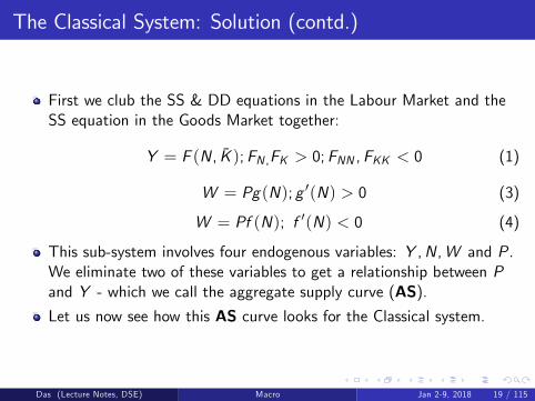
First we club the SS & DD equations in the Labour Market and theSS equation in the Goods Market together:
Y = F (N, K );FN ,FK > 0;FNN ,FKK < 0 (1)
W = Pg(N); g ′(N) > 0 (3)
W = Pf (N); f ′(N) < 0 (4)
This sub-system involves four endogenous variables: Y ,N,W and P.We eliminate two of these variables to get a relationship between Pand Y - which we call the aggregate supply curve (AS).Let us now see how this AS curve looks for the Classical system.
Das (Lecture Notes, DSE) Macro Jan 2-9, 2018 19 / 115

Derivation of the AS Schedule under the Classical System:Graphical Method
In deriving the AS curve, we first focus on the two labour marketequations.Plot (3) and (4) in the N-W plane (assuming some arbitrarily givenvalue of P):
Das (Lecture Notes, DSE) Macro Jan 2-9, 2018 20 / 115
Derivation of the AS Schedule under the Classical System:Graphical Method (Contd.)
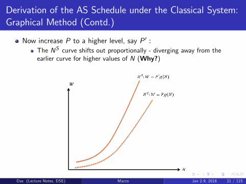
Now increase P to a higher level, say P ′ :The NS curve shifts out proportionally - diverging away from theearlier curve for higher values of N (Why?)
Das (Lecture Notes, DSE) Macro Jan 2-9, 2018 21 / 115

Derivation of the AS Schedule under the Classical System:Graphical Method (Contd.)
Likewise as P increases to a higher level, say P ′ :The ND curve also shifts out proportionally - but it converges closer tothe earlier curve for higher values of N (Why?)
Das (Lecture Notes, DSE) Macro Jan 2-9, 2018 22 / 115
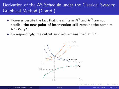
Derivation of the AS Schedule under the Classical System:Graphical Method (Contd.)
However despite the fact that the shifts in NS and ND are notparallel, the new point of intersection still remains the same atN∗ (Why?)Correspondingly, the output supplied remains fixed at Y ∗ :
Das (Lecture Notes, DSE) Macro Jan 2-9, 2018 23 / 115
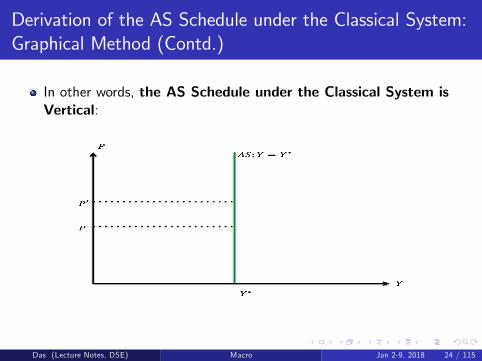
Derivation of the AS Schedule under the Classical System:Graphical Method (Contd.)
In other words, the AS Schedule under the Classical System isVertical:
Das (Lecture Notes, DSE) Macro Jan 2-9, 2018 24 / 115

The Classical System: Solution (contd.)
Let us now go back to the rest of the equations in the classicalsystem.
Let us club the SS & DD equations in the Money Market and the DDequation in the Goods Market together:
Y = C (Y ) + I (r) + G ; 0 < C ′(Y ) < 1; I ′(r) < 0 (2)
M = M (5)
M = PL(Y , r); LY > 0; Lr < 0 (6)
This sub-system involves four endogenous variables: Y , r ,M and P.We eliminate two of these variables to get another relationshipbetween P and Y - which we call the aggregate demand curve (AD).How does the AD look under the Classical system? We discuss thatbelow.
Das (Lecture Notes, DSE) Macro Jan 2-9, 2018 25 / 115
Derivation of the AD Schedule under the Classical System:Graphical Method
In deriving the AD Schedule, first notice that the Money SupplyFunction is constant. This allows us to write the Money MarketEquilibrium condition as:
M = PL(Y , r); LY > 0; Lr < 0 (7)
This is the so-called LM curve, which represents a relationshipbetween Y , r and P.
On the other hand the Demand Equation for the Goods marketrepresents another relationship between Y and r :
Y = C (Y ) + I (r) + G ; 0 < C ′(Y ) < 1; I ′(r) < 0 (2)
This is the so-called IS curve.
Das (Lecture Notes, DSE) Macro Jan 2-9, 2018 26 / 115

Derivation of the AD Schedule under the Classical System:Graphical Method (Contd.)
Plot the IS and the LM curve in the Y -r plane (assuming somearbitrarily given value of P):
Das (Lecture Notes, DSE) Macro Jan 2-9, 2018 27 / 115
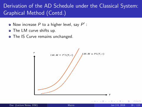
Derivation of the AD Schedule under the Classical System:Graphical Method (Contd.)
Now increase P to a higher level, say P ′ :The LM curve shifts up.The IS Curve remains unchanged.
Das (Lecture Notes, DSE) Macro Jan 2-9, 2018 28 / 115
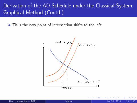
Derivation of the AD Schedule under the Classical System:Graphical Method (Contd.)
Thus the new point of intersection shifts to the left:
Das (Lecture Notes, DSE) Macro Jan 2-9, 2018 29 / 115

Derivation of the AD Schedule under the Classical System:Graphical Method (Contd.)
In other words, the AD Schedule under the Classical System isDownward Sloping:
Das (Lecture Notes, DSE) Macro Jan 2-9, 2018 30 / 115

The Classical System: Solution (contd.)
We then simultaneously plot the the AS and AD schedule in the Y -Pplane to determine the equilibrium price level P∗ and equilibriumoutput Y ∗ in the Goods Market.Once these two values are determined, other equilibrium values canbe found by substituting these back in the other equations.Equilibrium price and quantity in the Goods Market - P∗ and Y ∗ - asdetermined simultaneously by the intersection of the AS and the ADschedule - are shown below:
Das (Lecture Notes, DSE) Macro Jan 2-9, 2018 31 / 115

Digression: A Heuristic Justification of the ClassicalSystem
Although we have specified all the equations here as ad hocbehavioural relationships without any explicit micro-foundations, theyare not devoid of any economic logic. There are heuristicjustifications for each of these equations - although these logics justappeal to common sense; they are not explicitly derived from agents’optimization exercise.
We now examine these heuristic arguments one by one. In the processwe also point out the limitations of these arguments.
Let us first start with the labour market story underlying the classicalsystem.
Das (Lecture Notes, DSE) Macro Jan 2-9, 2018 32 / 115
A Heuristic Justification of the Classical System (Contd.)
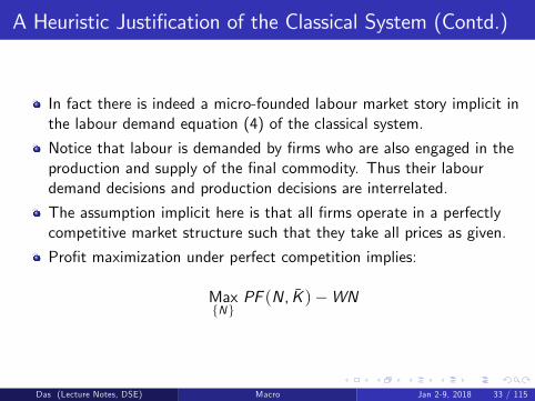
In fact there is indeed a micro-founded labour market story implicit inthe labour demand equation (4) of the classical system.
Notice that labour is demanded by firms who are also engaged in theproduction and supply of the final commodity. Thus their labourdemand decisions and production decisions are interrelated.
The assumption implicit here is that all firms operate in a perfectlycompetitive market structure such that they take all prices as given.
Profit maximization under perfect competition implies:
Max{N}
PF (N, K )−WN
Das (Lecture Notes, DSE) Macro Jan 2-9, 2018 33 / 115

Heuristic Justification of the Classical System (Contd.)
From the FONC, we get
FN (N, K ) =WP
which can be re-written as the labour demand function specified in(4):
W = Pf (N); f ′(N) < 0 .
Notice however that this profit-maximizing exercise is based on theaggregate production function. This begs the following question: whooperates this aggregate production function?In a decentralized market economy obviously nobody actually operateswith the aggregate production technology. So this outcome mustcome from aggregation of individual firms’optimization exercises.Is such aggregation always feasible? More importantly, willaggregation of firms’behaviour necessarily generate a labour demandfunction that looks as above? These are questions that we shall comeback to when we discuss the micro-foundations explicitly.
Das (Lecture Notes, DSE) Macro Jan 2-9, 2018 34 / 115
Heuristic Justification of the Classical System (Contd.)
Next, consider the labour supply equation in the Classical system(equation (3)):
W = Pg(N); g ′(N) > 0 (3)
Inverting, we get:
NS : N = g(WP
); g ≡ g−1.
The underlying logic here is that workers look at the real wage ratewhen they decide how much labour to supply. If the real wage rategoes up, then they are willing to supply more labour.
Needless to say, this story presupposes an implicit labour-leisurechoice of a household which positively responds to income. Does thisnecessarily hold? Again, without precise microfoundations we cannotsay. (Remember the backward bending labour supply curve?)
Das (Lecture Notes, DSE) Macro Jan 2-9, 2018 35 / 115
Heuristic Justification of the Classical System (Contd.)
The classical labour market story also presupposes that workers knowthe real wage rate when they decide about their labour supply,although prices are determined in the goods market.
This implies some role of expectations (since goods prices wouldpresumably not be known when wages were set in the labour market)which would influence the optimal labour supply decisions of thehouseholds. Once again without a precise theory of expectationformation, we do not know whether this assumption is justified or not.
Das (Lecture Notes, DSE) Macro Jan 2-9, 2018 36 / 115
Heuristic Justification of the Classical System (Contd.)
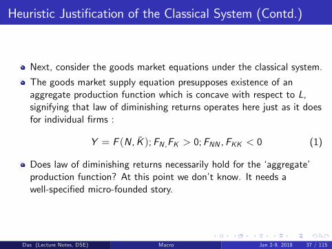
Next, consider the goods market equations under the classical system.
The goods market supply equation presupposes existence of anaggregate production function which is concave with respect to L,signifying that law of diminishing returns operates here just as it doesfor individual firms :
Y = F (N, K );FN ,FK > 0;FNN ,FKK < 0 (1)
Does law of diminishing returns necessarily hold for the ‘aggregate’production function? At this point we don’t know. It needs awell-specified micro-founded story.
Das (Lecture Notes, DSE) Macro Jan 2-9, 2018 37 / 115
Heuristic Justification of the Classical System (Contd.)
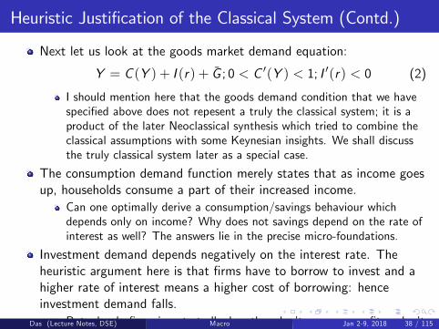
Next let us look at the goods market demand equation:
Y = C (Y ) + I (r) + G ; 0 < C ′(Y ) < 1; I ′(r) < 0 (2)
I should mention here that the goods demand condition that we havespecified above does not repesent a truly the classical system; it is aproduct of the later Neoclassical synthesis which tried to combine theclassical assumptions with some Keynesian insights. We shall discussthe truly classical system later as a special case.
The consumption demand function merely states that as income goesup, households consume a part of their increased income.
Can one optimally derive a consumption/savings behaviour whichdepends only on income? Why does not savings depend on the rate ofinterest as well? The answers lie in the precise micro-foundations.
Investment demand depends negatively on the interest rate. Theheuristic argument here is that firms have to borrow to invest and ahigher rate of interest means a higher cost of borrowing: henceinvestment demand falls.
But why do firms invest at all when they don’t eran any profit or don’tget to keep it (everything goes back to the households as dividends)?Again we need precise micro-foundations to answer these questions.
Das (Lecture Notes, DSE) Macro Jan 2-9, 2018 38 / 115
Heuristic Justification of the Classical System (Contd.)
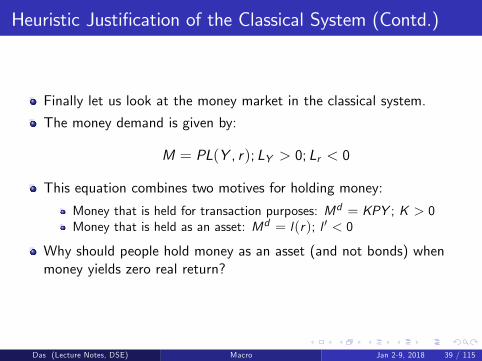
Finally let us look at the money market in the classical system.
The money demand is given by:
M = PL(Y , r); LY > 0; Lr < 0
This equation combines two motives for holding money:
Money that is held for transaction purposes: Md = KPY ; K > 0Money that is held as an asset: Md = l(r); l ′ < 0
Why should people hold money as an asset (and not bonds) whenmoney yields zero real return?
Das (Lecture Notes, DSE) Macro Jan 2-9, 2018 39 / 115

Heuristic Justification of the Classical System (Contd.)
The answer provided by Keynes was that people will hold money(vis-a-vis bond) if they expect bond prices to fall in future so thatthey can buy it cheap. Thus they can make some speculative gain outof it.But if bond prices are already very low (which means the interest rateis already very high) then people believe that it is unlikely to fall anyfurther; hence they will be less willing to hold money.This would generate a negative relationship between demand formoney (held as an asset) and the rate of interest. (Question: Whichinterest rate - nominal or real? Why?)
What kind of optimizing behaviour under risk/unceratinty andexpectation would generate this outcome for the households? Only amicro-founded story can answer that question.Also note once again that the money demand condition that we havespecified above is not truly the classical money demand equation; it isa product of the latter Neoclassical synsthesis which tried to combinethe classical assumptions with some Keynesian insights.
Das (Lecture Notes, DSE) Macro Jan 2-9, 2018 40 / 115
Equilibrium in the Classical System:
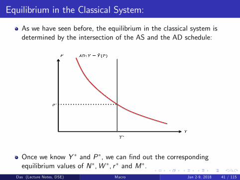
As we have seen before, the equilibrium in the classical system isdetermined by the intersection of the AS and the AD schedule:
Once we know Y ∗ and P∗, we can find out the correspondingequilibrium values of N∗,W ∗, r ∗ and M∗.
Das (Lecture Notes, DSE) Macro Jan 2-9, 2018 41 / 115
Equilibrium vis-a-vis Full Employment
Recall that the equilibrium level of employment in this model isdefined by the point of intersection between the NS and ND curvesdrawn for the equilibrium price level P∗. The equilibrium nominalwage rate (W ∗) is also simultaneously determined.This equilibrium level of employment represents the market clearinglevel of employment. It implies that given the equilibrium real wagerate
(W ∗P ∗
), everybody who is willing to supply labour indeed finds
employment.In other words, there is no ‘involuntary’unemployment.But to call it ‘full employment’could be misleading!What is full employment?
Suppose there exists a maximum limit on the labour supply - say N,such that it is not feasible to increase the labour supply beyond thislevel.This maximum feasible level is some times referred to as thefull-employment level of labour supply.
Das (Lecture Notes, DSE) Macro Jan 2-9, 2018 42 / 115
Equilibrium vis-a-vis Full Employment (Contd.)
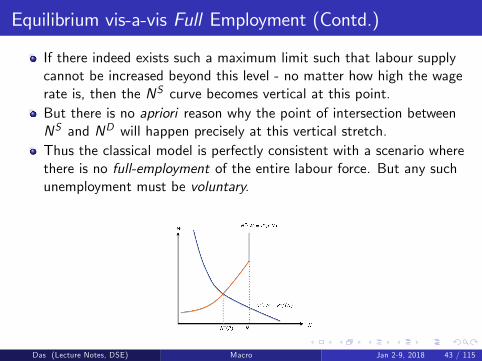
If there indeed exists such a maximum limit such that labour supplycannot be increased beyond this level - no matter how high the wagerate is, then the NS curve becomes vertical at this point.But there is no apriori reason why the point of intersection betweenNS and ND will happen precisely at this vertical stretch.Thus the classical model is perfectly consistent with a scenario wherethere is no full-employment of the entire labour force. But any suchunemployment must be voluntary.
Das (Lecture Notes, DSE) Macro Jan 2-9, 2018 43 / 115
Equilibrium vis-a-vis Full Employment (Contd.)
Question: Let us begin with an AS-AD configuration such that atthe corresponding equilibrium N∗ < N. In that case, will theequilibrium price level (P∗) re-adjust so that in equilibrium you alwaysend up with N∗ = N ?
The answer is "no"! So the complete price flexibility in the Classicalsystem does not necessarily lead to ‘full employment’; it onlyeliminates ‘involuntary unemployment’.
Das (Lecture Notes, DSE) Macro Jan 2-9, 2018 44 / 115

Effectiveness of Government Policies under the ClassicalSystem:
We shall primarily focus on two kinds of government policies:
Fiscal Policy - which usually changes the amount of governmentexpenditure (G )Monetary Policy - which usually changes the amount of money supply(M)
There could be other forms of government policies - e.g. taxes;government borrowing; government directly influencing the wage rateor price level in the goods/labour market or the interest rate in themoney market. We shall talk about some of these latter policies asspecial cases.
Das (Lecture Notes, DSE) Macro Jan 2-9, 2018 45 / 115
Effectiveness of Government Policies under the ClassicalSystem (contd.):
Notice that G enters only in the IS equation, while M enters only inthe LM equation.
In particular, an increase in G shifts the IS curve up while an increasein M shifts the LM curve down.
Both policies lead to a rightward shift of the AD curve but leave theAS curve unchanged.
Therefore the equilibrium output does not change.
Das (Lecture Notes, DSE) Macro Jan 2-9, 2018 46 / 115
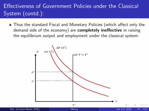
Effectiveness of Government Policies under the ClassicalSystem (contd.):
Thus the standard Fiscal and Monetary Policies (which affect only thedemand side of the economy) are completely ineffective in raisingthe equilibrium output and employment under the classical system:
Das (Lecture Notes, DSE) Macro Jan 2-9, 2018 47 / 115

Proportional Income Tax - A Possible Exception?
So far we had not introduced taxes in our model. Let us nowintroduce a proportional income tax (t) which is imposed at thehousehold level.This changes the disposable income -available to the household forconsumption:
C d = C (Y − tY ) = C (Y d ); 0 < C ′(Y d ) < 1
Thus the demand equation in the Goods Market now becomes:
Y = C (Y d ) + I (r) + G ; 0 < C ′(Y d ) < 1; I ′(r) < 0
The corresponding IS curve (representing the demand condition in theGoods Market in the Y -r plane) still looks the similar.
But a change in a tax rate will now shift the IS curve, but not the LMcurve. Thus the AD schedule gets affected.
Das (Lecture Notes, DSE) Macro Jan 2-9, 2018 48 / 115
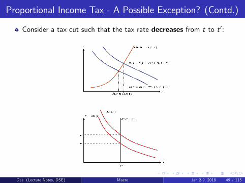
Proportional Income Tax - A Possible Exception? (Contd.)
Consider a tax cut such that the tax rate decreases from t to t ′:
Das (Lecture Notes, DSE) Macro Jan 2-9, 2018 49 / 115
Proportional Income Tax - A Possible Exception? (Contd.)
As before the AD shifts to the right (because the IS curve has shiftedup due to the tax cut).
But this is not the end of the story!!Recall that the labour is supplied by the households.
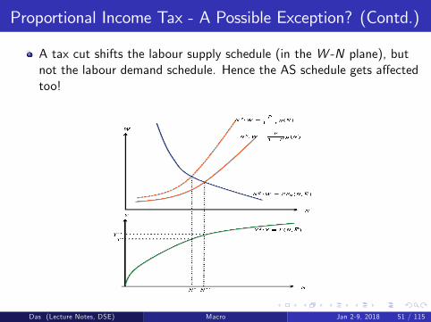
If household incomes are taxed then so would be wage income!So theeffective wage rate - relevant for the households (and only for thehouseholds) is now (1− t)W - not W !In other words, the supply equation in the labour market nowbecomes:
W =P
(1− t)g(N); g′(N) > 0
The demand equation in the labour market however remainsunchanged (Why?).
Das (Lecture Notes, DSE) Macro Jan 2-9, 2018 50 / 115
Proportional Income Tax - A Possible Exception? (Contd.)
A tax cut shifts the labour supply schedule (in the W -N plane), butnot the labour demand schedule. Hence the AS schedule gets affectedtoo!
Das (Lecture Notes, DSE) Macro Jan 2-9, 2018 51 / 115
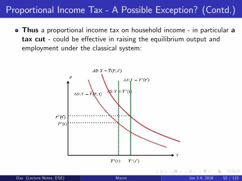
Proportional Income Tax - A Possible Exception? (Contd.)
Thus a proportional income tax on household income - in particular atax cut - could be effective in raising the equilibrium output andemployment under the classical system:
Das (Lecture Notes, DSE) Macro Jan 2-9, 2018 52 / 115
Emergence of the Keynesian System: The GreatDepression (1929-1941)
The western capitalist economies (US,UK) were running more or lessin line with the Classical/Neo-classical system till the 1920s - with alaissez faire government allowing private initiatives to dominate.
Then came the Great Depression which created havoc - especially inthe US economy.
Das (Lecture Notes, DSE) Macro Jan 2-9, 2018 53 / 115
The Great Depression (1929-1941): (Contd.)
“The Great Depression of 1929 devastated the U.S. economy. Half of allbanks failed. Unemployment rose to 25 percent and homelessness increased.Housing prices plummeted 30 percent, global trade collapsed by 60 percentand prices fell 10 percent. ....The economy shrank 50 percent in the first fiveyears of the Depression. In 1929, economic output was $105 billion, asmeasured by gross domestic product. By 1933, the country had suffered fiveyears of losses. It only produced $57 billion, half what it produced in 1929.New Deal spending boosted GDP growth 10.8 percent in 1934. It grewanother 8.9 percent in 1935, a whopping 12.9 percent in 1936 and 5.1percent in 1937. Unfortunately, the government cut back on New Dealspending in 1938, and the depression returned.” (K. Amadeo (2017)).
Shift in ideology: The dominant economic belief shifted from a pure freemarket economy to a mixed economy with much more emphasis ongovernment spending for its success. This new school of thought owed itsorigin to Keynes’General Theory (1936).
Das (Lecture Notes, DSE) Macro Jan 2-9, 2018 54 / 115
The Keynesian System:
The benchmark Keynesian system that we shall consider here will bealmost analogous to the Classical system characterized above, exceptfor the labour supply equation.
The Keynesian model assumes that the labour market is unionizedand the supply of labour is therefore determined by the rules/normsset by the labour union.
The union sets the nominal wage rate at some level W by collectivebargaining and once the wage is set, all workers supply their entirelabour stock at this wage rate. (Why all workers would comply tosuch a rule is a different story and would require precise modelling ofthe union’s and the workers’optimization problem(s). We shall comeback to this point when we discuss the microfoundations of theseassumptions).
Thus the labour supply schedule now becomes perfectly elastic (a flatline) at the union-determined wage rate: W .
Das (Lecture Notes, DSE) Macro Jan 2-9, 2018 55 / 115

The Keynesian System (in equations):
The Goods Market:Supply Equation:
Y = F (N, K );FN ,FK > 0;FNN ,FKK < 0 (8)
Demand Equation:
Y = C (Y ) + I (r) + G ; 0 < C ′(Y ) < 1; I ′(r) < 0 (9)
The Labour Market:Supply Equation:
W = W (10)
Demand Equation:W = Pf (N) (11)
The Money Market:Supply Equation:
M = M (12)
Demand Equation:
M = PL(Y , r); LY > 0; Lr < 0 (13)
Das (Lecture Notes, DSE) Macro Jan 2-9, 2018 56 / 115

The Keynesian Labour Market
As we have explained before, the only equation that differs betweenthe two systems is the labour supply equation.
The Keyenesian System assumes that labour supply is perfectly elasticat a given wage rate W .
The Labour Market:
Supply Equation:W = W (14)
Demand Equation:W = Pf (N) (15)
Das (Lecture Notes, DSE) Macro Jan 2-9, 2018 57 / 115
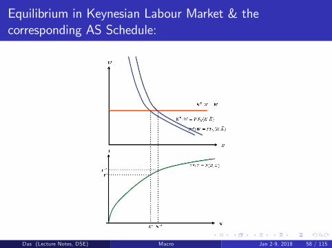
Equilibrium in Keynesian Labour Market & thecorresponding AS Schedule:
Das (Lecture Notes, DSE) Macro Jan 2-9, 2018 58 / 115
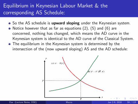
Equilibrium in Keynesian Labour Market & thecorresponding AS Schedule:
So the AS schedule is upward sloping under the Keynesian system.Notice however that as far as equations (2), (5) and (6) areconcerned, nothing has changed, which means the AD curve in theKeynesian system is identical to the AD curve of the Classical System.The equilibrium in the Keynesian system is determined by theintersection of the (now upward sloping) AS and the AD schedule:
Once we know Y and P, we can find out the correspondingequilibrium values of N, r and M.(Recall that value of W is nowexogenously given at W ).
Das (Lecture Notes, DSE) Macro Jan 2-9, 2018 59 / 115

Effectiveness of Government Policies under the KeynesianSystem:
Question: What does this tell you about the effectiveness of thestandard monetary and fiscal policies (↑ in G or M)?
Das (Lecture Notes, DSE) Macro Jan 2-9, 2018 60 / 115
Equilibrium Employment: Comparing Keynes with Classics
How does N (equilibrium level of employment under the KeynesianSystem) compare with N∗(equilibrium level of employment under theClassical system)?
Or equivalently: how does Y (equilibrium output under the KeynesianSystem) compare with Y ∗(equilibrium output under the Classicalsystem)?
To answer this question, we shall consider two cases:(a) W > W ∗
(b) W < W ∗
Das (Lecture Notes, DSE) Macro Jan 2-9, 2018 61 / 115

Equilibrium Employment: Keynes vis-a-vis Classics(Contd.)
Let us start with case when W > W ∗.Let us first diagrammatically depict the Classical Equilibrium(P∗,Y ∗,N∗,W ∗) and then see whether this can still be an equilibriumwhen the nominal wage rate is arbitrarily fixed at some W > W ∗ :
Das (Lecture Notes, DSE) Macro Jan 2-9, 2018 62 / 115
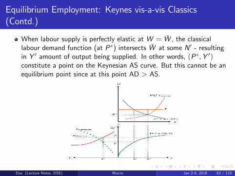
Equilibrium Employment: Keynes vis-a-vis Classics(Contd.)
When labour supply is perfectly elastic at W = W , the classicallabour demand function (at P∗) intersects W at some N ′ - resultingin Y ′ amount of output being supplied. In other words, (P∗,Y ′)constitute a point on the Keynesian AS curve. But this cannot be anequilibrium point since at this point AD > AS.
Das (Lecture Notes, DSE) Macro Jan 2-9, 2018 63 / 115
Equilibrium Employment: Keynes vis-a-vis Classics(Contd.)
This tells us that when W > W ∗ :
The Keynesian equilibrium price (P) must be higher than the Classicalequilibrium price level (P∗).But since higher P means lower demand (along a downward slopingAD curve), this implies that the Keynesian equilibrium output (Y )must be less than the Classical equilibrium output level (Y ∗).Consequently, equilibrium employment level under the Keynesiansystem (N) must be lower that the equilibrium employment level underthe Classical system (N∗)
Das (Lecture Notes, DSE) Macro Jan 2-9, 2018 64 / 115
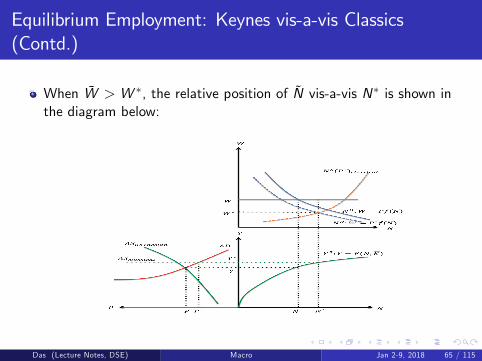
Equilibrium Employment: Keynes vis-a-vis Classics(Contd.)
When W > W ∗, the relative position of N vis-a-vis N∗ is shown inthe diagram below:
Das (Lecture Notes, DSE) Macro Jan 2-9, 2018 65 / 115
Keynesian System: Involuntary Unemployment?
Is the reduction in employment from N∗ to N involuntary orinvoluntary?
A flat Keynesian labour supply schedule at W = W does not allow usto properly identify the extent of voluntary vis-a-vis involuntaryunemployement.
To differentiate between voluntary and involuntary unemployment, wehave to draw the classical labour supply schedule (that captureshousehold’willingnes to work) for the given W and P.
Das (Lecture Notes, DSE) Macro Jan 2-9, 2018 66 / 115
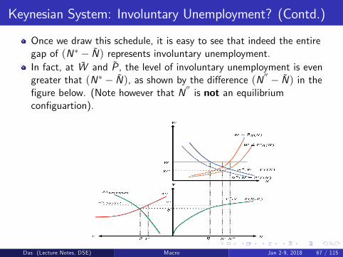
Keynesian System: Involuntary Unemployment? (Contd.)
Once we draw this schedule, it is easy to see that indeed the entiregap of (N∗ − N) represents involuntary unemployment.In fact, at W and P, the level of involuntary unemployment is evengreater that (N∗ − N), as shown by the difference (N ′′ − N) in thefigure below. (Note however that N
′′is not an equilibrium
configuartion).
Das (Lecture Notes, DSE) Macro Jan 2-9, 2018 67 / 115

Keynesian System: Involuntary Unemployment? (Contd.)
What happens is the Keynesian System if trade union fixes thenominal wage rate at a level such that W < W ∗?We can anlyse as before and show that now N > N∗.But notice thatnow part of this labour supply is ‘forced labour’!!
If is not clear why a worker would be part of trade union if the unionforces him to work beyond his optimal choice. So from now on weshall focus only on the case where W > W ∗.
Das (Lecture Notes, DSE) Macro Jan 2-9, 2018 68 / 115
Keynesian System: An Increase in Nominal Wage Rate
Suppose now the labour union becomes stronger and is able tonegotiate a higher nominal wage W ′.
What happens to equilibrium output in the Keynesian System if thenominal wage rate changes (increases) from W to W ′?
In particular, would the households be better off in terms of income?
Das (Lecture Notes, DSE) Macro Jan 2-9, 2018 69 / 115
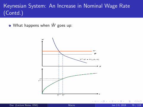
Keynesian System: An Increase in Nominal Wage Rate(Contd.)
What happens when W goes up:
Das (Lecture Notes, DSE) Macro Jan 2-9, 2018 70 / 115
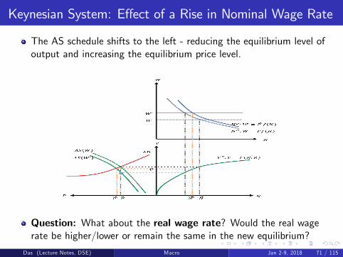
Keynesian System: Effect of a Rise in Nominal Wage Rate
The AS schedule shifts to the left - reducing the equilibrium level ofoutput and increasing the equilibrium price level.
Question: What about the real wage rate? Would the real wagerate be higher/lower or remain the same in the new equilibrium?
Das (Lecture Notes, DSE) Macro Jan 2-9, 2018 71 / 115
Keynesian System: Effect of a Rise in Nominal Wage Rate(Contd.)
As it turns out, in the new equilibrium the real wage rate actuallyincreases. (In other words, although the price level in the newequilibrium will be higher, it will not be high enough to completelyoutweigh the increase in the nominal wage rate). (Why?)Are the households better off? The answer is not clear! While realwage rate is indeed higher than before, total income has actually gonedown. So the households for whom wage component is high will bebetter off but at the expense of others.
Das (Lecture Notes, DSE) Macro Jan 2-9, 2018 72 / 115
Keynesian System: Effect of a Rise in Aggregate Demand
What happens to the real wage rate when G or M increases?
This leads to a shift in the AD curve (with unchanged AS curve).
So the price level rises in the new equilibrium, and with a constantW , the real wage rate surely falls.
Notice that the real wage rate in this model behaves in acounter-cyclical fashion: In periods of boom (high demand) we havehigher equilibrium output (and employment) but it is associated withlower real wages. And opposite happens in periods of slump (lowdemand).
In other words, in this version of the Keynesian model real wage rateand aggregate output (and employment) are negatively correlated.
This feature of the model is not supported by the empirical facts. Ithas been observed that real wage rate typically moves in pro-cyclicalmanner. In periods of boom, employment, output and real wage rate- all move in the upward direction; opposite happens during recessions.
Das (Lecture Notes, DSE) Macro Jan 2-9, 2018 73 / 115
Extension of the Keynesian System: The Neo-Keynesians& Sticky Prices
An extension of the general Keynesian structure was later proposed,which was able to address this issue, while retaining the other basicKeynesian features. This is the Neo-Keynesian extension.
This extension assumes that not only that nominal wage is rigid, butso is the nominal price level.
Sticky prices mean that the aggregate supply curve is horizontal atsome P = P.
Notice that a horizontal AS schedule means that this system iscompletely demand-determined. At P whatever output demanded isalways supplied. (Thus this set up is diametrically opposite to thesupply-determined Classical System discussed earlier).
Das (Lecture Notes, DSE) Macro Jan 2-9, 2018 74 / 115
The Neo-Keynesians & Sticky Prices: (Contd.)
The underlying assumption is that there is imperfect competition inthe final goods market; firms can set their own prices. Typicallyfacing a constant nominal wage cost they set a price which is a markup (λ) over the nominal cost such that P = (1+ λ)W .
But often firms do not adjust the price level immediately in responseto an increase in W .
This could be because of a variety of reasons:
There could be adjustment costs associated with price change (menucost) due to which it may not be optimal for the firms to change theirprices immediately;The firms might have limited bargaining power vis-a-vis the unions sothat the union is able to extract a higher real wage (in which case λadjusts keeping P unchanged).
Das (Lecture Notes, DSE) Macro Jan 2-9, 2018 75 / 115
The Neo-Keynesians & Sticky Prices: (Contd.)
In what follows, we shall assume that P does not respond to achange in the wage rate for whatever reason (or at least notimmediately).
Das (Lecture Notes, DSE) Macro Jan 2-9, 2018 76 / 115
The Neo-Keynesians & Sticky Prices: (Contd.)
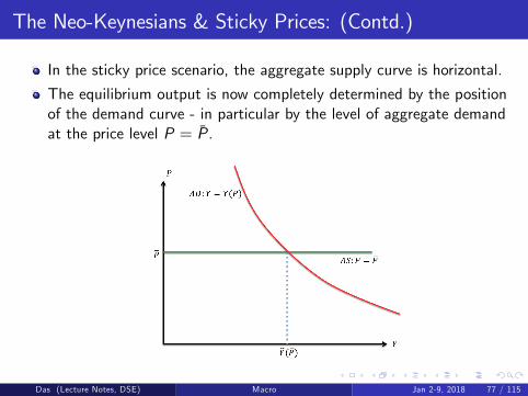
In the sticky price scenario, the aggregate supply curve is horizontal.
The equilibrium output is now completely determined by the positionof the demand curve - in particular by the level of aggregate demandat the price level P = P.
Das (Lecture Notes, DSE) Macro Jan 2-9, 2018 77 / 115
The Neo-Keynesians & Sticky Prices: (Contd.)
The crucial question is: At what level would the firms set their prices?
Notice that we can plot the Keynesian (upward-sloping) AS schedulein the backdrop and identify two regions with reference to theKeynesian equilibrium price level (P):
The region above P (above the intersection point of the Keynesian AS& AD schedules) which is demand-constrained;The region below P (below the intersection point of the Keynesian AS& AD schedules) which is supply-constrained.
Can we ever have a Neo-Keynesian scenario where the P is set belowP?
Das (Lecture Notes, DSE) Macro Jan 2-9, 2018 78 / 115
The Neo-Keynesians & Sticky Prices: (Contd.)
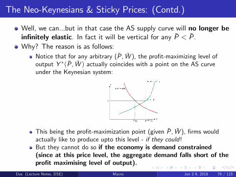
Well, we can...but in that case the AS supply curve will no longer beinfinitely elastic. In fact it will be vertical for any P < P.Why? The reason is as follows:
Notice that for any arbitrary (P, W ), the profit-maximizing level ofoutput Y ∗(P, W ) actually coincides with a point on the AS curveunder the Keynesian system:
This being the profit-maximization point (given P, W ), firms wouldactually like to produce upto this level - if they could!But they cannot do so if the economy is demand constrained(since at this price level, the aggregate demand falls short of theprofit maximising level of output).
Das (Lecture Notes, DSE) Macro Jan 2-9, 2018 79 / 115

The Neo-Keynesians & Sticky Prices: (Contd.)
But this argument does not hold if at this price level, the economy isactually supply constrained!
When the economy is supply-constrained, the producers can chooseoutput level that maximizes their profit (given P, W ).
That is, they can actually pick a point on the Keynesian AS curve(given P, W ).
Indeed facing a wage-price combination of (P, W ), a firm wouldnever have any incentive to produce beyond Y ∗(P, W ).This implies that we have to draw the Neo-Keynesian AS schedule(with sticky prices and sticky wages) a little differently that we didbefore:
At the given P, It is no longer horizontal for all Y ; it becomes verticalprecisely at the point Y ∗(P, W ).
Das (Lecture Notes, DSE) Macro Jan 2-9, 2018 80 / 115
Labour Market under Sticky Prices:
Let us now assume that P is such that the economy is indeeddemand-constrained.
We have seen that in this case, stickiness of the price level impliesquantity adjustment by the firms: they produce exactly as muchoutput as is demanded.
This quantity adjustment will have implications for the labourdemand function as well.
When prices are sticky and the economy is demand-constrained, thelabour demand function is given by:
ND = N(P) : F (N, K ) = Y (P).
Since the labour supply is horizontal at W , N(P) also represents theequilibrium employment level under the Neo-Keynesian system.
Das (Lecture Notes, DSE) Macro Jan 2-9, 2018 81 / 115

The Neo-Keynesians & Sticky Prices: (Contd.)
It is important to recognise here that due to the stickiness of the pricethat is set at a region where there is excess supply, the producers arenot operating on their AS schedule.This implies that they are not supplying their profit-maximising levelof output, which in turn means they are unable to operate on theiroptimal labour demand curve (which presupposes profit maximisingbehaviour). Thus the labour demand schedule now becomes irrelevantin determining equilibrium level of employment.
Das (Lecture Notes, DSE) Macro Jan 2-9, 2018 82 / 115

The Neo-Keynesians & Sticky Prices: (Contd.)
The following diagram characterizes the equilibrium in theNeo-Keynesian system:
Das (Lecture Notes, DSE) Macro Jan 2-9, 2018 83 / 115
The Neo-Keynesians & Sticky Prices: (Contd.)
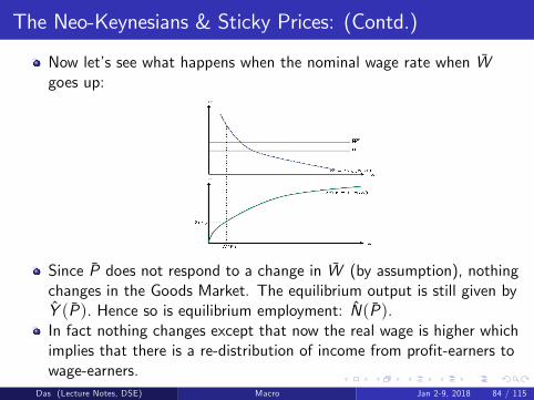
Now let’s see what happens when the nominal wage rate when Wgoes up:
Since P does not respond to a change in W (by assumption), nothingchanges in the Goods Market. The equilibrium output is still given byY (P). Hence so is equilibrium employment: N(P).In fact nothing changes except that now the real wage is higher whichimplies that there is a re-distribution of income from profit-earners towage-earners.
Das (Lecture Notes, DSE) Macro Jan 2-9, 2018 84 / 115

The Neo-Keynesians & Sticky Prices: (Contd.)
Now consider a positive demand shock: suppose for some reason theaggregate demand schedule shifts to the right. This couldpolicy-induced (e.g., a change in G or M) or could be due to anindependent shift in parameters. However let us assume that theeconomy is still demand-constrained.
Notice that with sticky prices and rigid nominal wages, real wage rateremains that same, while output and employment goes up in the newequilibrium.
So even though real wage now is not exactly pro-cyclical, at least itdoes not move in the opposite direction to output and employment!(In fact the total wage bill would actually go up.)
Das (Lecture Notes, DSE) Macro Jan 2-9, 2018 85 / 115

The Neo-Keynesians & Sticky Prices: (Contd.)
There are other variants of the Neo-Keynesian framework that assumethat union’s bargaining power increases as level of employment goesup.
In such a case, a positive aggregate demand shock (with sticky prices)would increase the real wage rate as well. (Aggreagte profit wouldalso rise, although the mark up/profit margin would go down).
Thus real wage and output (as well as employment) would now movein the same direction, making the real wage rate pro-cyclical- as isconsistent with the empirical evidence.
We shall come back to this case when we discuss the precise microfoundations of the Neo-Keynesian model.
Das (Lecture Notes, DSE) Macro Jan 2-9, 2018 86 / 115
Other Extensions of Keynes & the Classics:
Quantity Theory of Money (A Special Case of the ClassicalSystem):
Money Demand Equation now becomes:
M = PkY ;
where k is a positive constant (related to the velocity of circulation ofmoney)Notice that this still generates a downward sloping AD schedule(why?), while the AS schedule remains vertical as before.Nothing much changes in this special case of the Classical System interms of equilibrium output/employment.
Question: What is the role of the IS curve here?
Das (Lecture Notes, DSE) Macro Jan 2-9, 2018 87 / 115
Other Extensions of Keynes & the Classics: (Contd.)
Liquidity Trap/Interest Rate Targeting (A Special Case of theKeynesian System)
Equation of the LM curve now becomes:
r = r
(At this interest rate money supply is perfectly elastic.)The aggregate demand schedule in the Y -P plane is now vertical.In this special Keynesian System, output is completely demanddetermined. Since the level of demand is now independent of the pricelevel, there is only quantity adjustment - even though prices are fullyflexible.
Question: What happens if we import this assumption of liquiditytrap/interest rate targeting to an otherwise Classical System?
Das (Lecture Notes, DSE) Macro Jan 2-9, 2018 88 / 115
Other Extensions of Keynes & the Classics: (Contd.)
Autonomous Investment (Another Special Case of the KeynesianSystem):
Equation of the IS curve now becomes:
Y = C (Y ) + I + G
The aggregate demand schedule in the Y -P plane is once againvertical.In this special Keynesian System once again output is completelydemand-determined. Again, there is only quantity adjustment - eventhough prices are fully flexible.
Question: What happens if we import this assumption ofautonomous investment to an otherwise Classical System?
Das (Lecture Notes, DSE) Macro Jan 2-9, 2018 89 / 115

Keynes & the Classics: What have we learnt so far?
We have now seen different variants of the Keynesian and theClassical System.No matter which specific set of assumptions one takes, the starkestdifference between these two categories of models (in terms ofcharacterization of the equilibrium) is as follows:
In the Keynesian system, demand plays a crucial role in determiningthe equilibrium output.In the Classical model, demand plays no role in determining theequilibrium output; it is completely supply driven.
To the extent that government policies affect the demand side (andonly the demand side) of the economy, such policies would work inthe Keynesian system but would not work in the Classical System.
Notice however that any policy that affects the supply side of theeconomy will work in the Classical system as well as in the Keynesiansystem (but may not work in the two special cases of the Keynesiansystem).
Das (Lecture Notes, DSE) Macro Jan 2-9, 2018 90 / 115
Keynes & the Classics: Incomplete Information
So far we have assumed that workers (households) as well as firmshave complete information about the prices and wages that wouldprevail in the actual economy.In fact, the classical system that we have discussed represents theideal scenario - there is no market imperfection or rigidity in anymarket, nor is there any incomplete information.We could treat this as our benchmark case - the best possiblescenario (what would have happened is everything was perfect!)This ideal scenario - the benchmark case - is also somewhatunrealistic. The real world is characterized by various kinds of marketimperfections or rigidities as well as incomplete information.We have already seen what happens if there are various kinds ofrigidities.But even in the absence of market imperfections, things could be farfrom perfect simply because agents have incomplete information.We now turn to one such case.
Das (Lecture Notes, DSE) Macro Jan 2-9, 2018 91 / 115
Incomplete Information and Role of Expectations:
Let us consider a modified version of the classical system, where thefirms have full information about the wages and prices, but workersdo not have complete information.
In particular, let us assume that workers do not have completeinformation about the price level.(This is the Lucas model ofincomplete information.)
The underlying logic is that since prices are determined in the goodsmarket while nominal wages are set in the labour market, workers oftendo not have perfect knowledge about the price behaviour.
If the workers do not have perfect knowledge about the price levelthat prevails, then they would make their calculations on the basis oftheir expectations about the price level.
In other words, in this model with incomplete information, workersdetermine their labour supply on the basis of the ‘expected’realwage.
Das (Lecture Notes, DSE) Macro Jan 2-9, 2018 92 / 115
Incomplete Information and Role of Expectations: (Contd.)
Notice that till now we have deliberately kept expectations out of thepicture.
But the moment we bring in incomplete information, expectationsstart playing a major role.
In this modified Classical System, workers’labour supply schedulenow depends on the expected real wage rate.
If we incorporate this in our standard Classical system, then the ASschedule under the classical system may change its character - as wewill see in a moment.
Das (Lecture Notes, DSE) Macro Jan 2-9, 2018 93 / 115

AS Schedule in the Classical System when Labour Supplydepends on Expected Real Wage:
When the workers determine their labour supply on the basis of the‘expected’real wage, the labour supply equation is given by:
NS : W = Peg(N); g ′ > 0
The labour demand equation remains unchanged (because producers’are assumed to have complete information about the price of theproduct that they themselves would be selling):
W = PFN (N, K )
The labour market equilibrium now depends crucially on how priceexpectations are formed.If workers can perfectly anticipate the actual price level, then Pe = Pand we are back to the good old Classical world with a vertical AScurve.
Das (Lecture Notes, DSE) Macro Jan 2-9, 2018 94 / 115
AS Schedule in the Classical System when Labour Supplydepends on Expected Real Wage (Contd.):
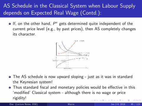
If, on the other hand, Pe gets determined quite independent of thecurrent price level (e.g., by past prices), then AS completely changesits character.
The AS schedule is now upward sloping - just as it was in standardthe Keynesian system!Thus standard fiscal and monetary policies would be effective in this‘modified’Classical system - although there is no wage or pricerigidity!
Das (Lecture Notes, DSE) Macro Jan 2-9, 2018 95 / 115
How are Expected Prices Determined?
It seems a little unrealistic to assume that the agent’s expectationswould be completely independent of the actual value of the variable.
But to see exactly how they are related we have to look for sometheories of expectation formation, which we shall discuss now.
Das (Lecture Notes, DSE) Macro Jan 2-9, 2018 96 / 115
Various Theories of Expectation Formation:
Static Expectations:Today’s expected value of the variable (x) depends on previousperiod’s actual value. In particular:
xet = xt−1
Adaptive Expectations:Today’s expected value of the variable (x) depends on previousperiod’s actual value and previous period’s expected value. Inparticular:
xet = xet−1 + λ [xt−1 − xet−1] ; 0 < λ < 1
Notice that Static Expectations is a special case of AdaptiveExpectations (when λ = 1)
Das (Lecture Notes, DSE) Macro Jan 2-9, 2018 97 / 115

Various Theories of Expectation Formation (Contd.):
Perfect Foresight:Agent’s make a guess about the value of the variable and (by somedevine power) the guess exactly matches its actual value. Inparticular:
xet = xt
Notice that guessing is NOT knowing!Rational Expectations:Agent applies mathematical tools of expectation formation, using theavailable information set, to come up with the expected value of thevariable. In particular:
xet = E [xt | It−1]Notice that under complete information and complete certainty,Perfect Foresight and Rational Expectations are equivalent.
Das (Lecture Notes, DSE) Macro Jan 2-9, 2018 98 / 115

Various Theories of Expectation Formation: (Contd.)
We have now specified 4 different expectation formation rules.
There are more sophisticated rules of expectation formation thatexplicitly incorporate a learning process (e.g, Bayesian Inference).However in this course we shall limit ourselves to the 4 simple rulesspecified above.
We shall now apply these rule one by one to a particularmacroeconomic system.
A natural choice is Lucas’Incomplete Information model which bringsin a role of expectations in the labour market.
Das (Lecture Notes, DSE) Macro Jan 2-9, 2018 99 / 115

Various Expectation Formation Rules: An Application(Classical Labour Market)
Recall that in the Classical system, when both workers and producers
base their supply/demand decisions on the actual real wage(Wt
Pt
),
then the labour market equilibrium is given by:
N∗ : g(N) = FN (N, K )
This N∗ - which we shall call the ‘Natural Level of Employment’-is independent of the current price level (Pt).
Das (Lecture Notes, DSE) Macro Jan 2-9, 2018 100 / 115
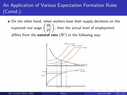
An Application of Various Expectation Formation Rules(Contd.):
On the other hand, when workers base their supply decisions on the
expected real wage(Wt
Pet
), then the actual level of employment
differs from the natural rate (N∗) in the following way:
Das (Lecture Notes, DSE) Macro Jan 2-9, 2018 101 / 115

An Application of Various Expectation Formation Rules(Contd.):
In other words,
Nt T N∗ according as Pet S Pt .
Define Y ∗ as the ‘natural level of output’such that
Y ∗ = F (N∗, K ).
When workers base their supply decisions on the expected real wage,then the actual output supplied differs from the natural level (Y ∗) inthe following way:
Y st T Y ∗ according as Pet S Pt .
This allows us to write the Aggregate Supply schedule in the followingway:
Y st : Yt = Y ∗ + f (Pt − Pet ); f (0) = 0; f ′ > 0.Das (Lecture Notes, DSE) Macro Jan 2-9, 2018 102 / 115
An Application of Various Expectation Formation Rules(Contd.):
This representation of the aggregate supply schedule is called theLucas Supply Function (after Robert Lucas, who postulated that (inthe short run) workers’may not have complete information about theprice behaviour and hence their expectations may differ from theactual.)
Without any loss of generality, let us assume that the Lucas SupplyFunction (i.e., the AS schedule under incomplete information) islinear:
Y st : Yt = Y ∗ + α [Pt − Pet ] ; α > 0. (I)
The equilibrium price level will of course depend on aggregatedemand function, which we now turn to.
Das (Lecture Notes, DSE) Macro Jan 2-9, 2018 103 / 115
An Application of Various Expectation Formation Rules(Contd.):
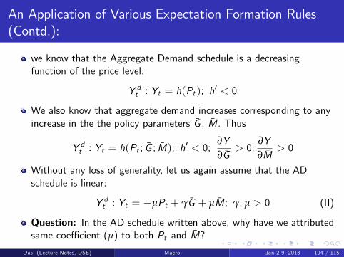
we know that the Aggregate Demand schedule is a decreasingfunction of the price level:
Y dt : Yt = h(Pt ); h′ < 0
We also know that aggregate demand increases corresponding to anyincrease in the the policy parameters G , M. Thus
Y dt : Yt = h(Pt ; G ; M); h′ < 0;∂Y∂G
> 0;∂Y∂M
> 0
Without any loss of generality, let us again assume that the ADschedule is linear:
Y dt : Yt = −µPt + γG + µM; γ, µ > 0 (II)
Question: In the AD schedule written above, why have we attributedsame coeffi cient (µ) to both Pt and M?
Das (Lecture Notes, DSE) Macro Jan 2-9, 2018 104 / 115

An Application of Various Expectation Formation Rules(Contd.):
From the AS and the AD schedule (given by (I) and (II) respectively,we can solve for the equilibrium price level at time t as:
Pt : Y ∗ + α [Pt − Pet ] = −µPt + γG + µM
⇒ Pt =1
α+ µ[γG + µM − Y ∗ + αPet ] (III)
Equation (III) gives us the precise relationship between actual pricelevel and expected price level in this economy at every point of time.
Let us now apply the different theories of expectation formation toequation (III) and see how the behaviour of the aggregate economychanges (if at all) over time.
Das (Lecture Notes, DSE) Macro Jan 2-9, 2018 105 / 115
An Application of Various Expectation Formation Rules(Contd.):
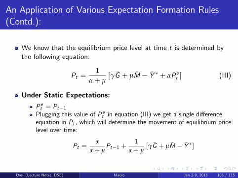
We know that the equilibrium price level at time t is determined bythe following equation:
Pt =1
α+ µ[γG + µM − Y ∗ + αPet ] (III)
Under Static Expectations:
Pet = Pt−1Plugging this value of Pet in equation (III) we get a single differenceequation in Pt , which will determine the movement of equilibrium pricelevel over time:
Pt =α
α+ µPt−1 +
1α+ µ
[γG + µM − Y ∗]
Das (Lecture Notes, DSE) Macro Jan 2-9, 2018 106 / 115
An Application of Various Expectation Formation Rules(Contd.):
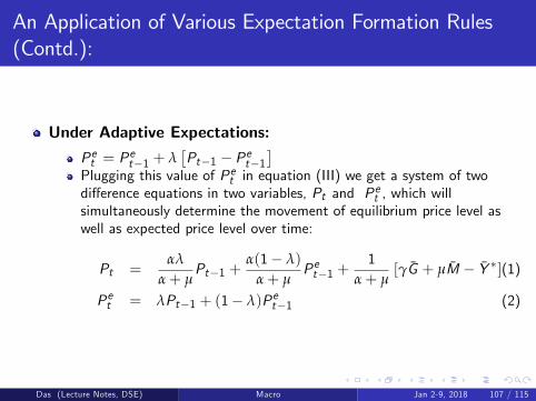
Under Adaptive Expectations:
Pet = Pet−1 + λ
[Pt−1 − Pet−1
]Plugging this value of Pet in equation (III) we get a system of twodifference equations in two variables, Pt and Pet , which willsimultaneously determine the movement of equilibrium price level aswell as expected price level over time:
Pt =αλ
α+ µPt−1 +
α(1− λ)
α+ µPet−1 +
1α+ µ
[γG + µM − Y ∗](1)
Pet = λPt−1 + (1− λ)Pet−1 (2)
Das (Lecture Notes, DSE) Macro Jan 2-9, 2018 107 / 115
An Application of Various Expectation Formation Rules(Contd.):
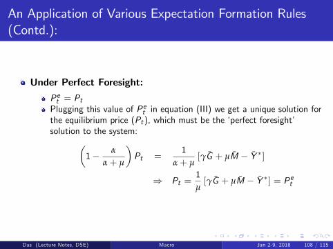
Under Perfect Foresight:
Pet = PtPlugging this value of Pet in equation (III) we get a unique solution forthe equilibrium price (Pt ), which must be the ‘perfect foresight’solution to the system:(
1− α
α+ µ
)Pt =
1α+ µ
[γG + µM − Y ∗]
⇒ Pt =1µ[γG + µM − Y ∗] = Pet
Das (Lecture Notes, DSE) Macro Jan 2-9, 2018 108 / 115
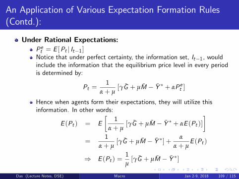
An Application of Various Expectation Formation Rules(Contd.):
Under Rational Expectations:Pet = E [Pt | It−1 ]Notice that under perfect certainty, the information set, It−1, wouldinclude the information that the equilibrium price level in every periodis determined by:
Pt =1
α+ µ[γG + µM − Y ∗ + αPet ]
Hence when agents form their expectations, they will utilize thisinformation. In other words:
E (Pt ) = E[
1α+ µ
[γG + µM − Y ∗ + αE (Pt )]]
=1
α+ µ[γG + µM − Y ∗] + α
α+ µE (Pt )
⇒ E (Pt ) =1µ[γG + µM − Y ∗]
Das (Lecture Notes, DSE) Macro Jan 2-9, 2018 109 / 115

An Application of Various Expectation Formation Rules(Contd.):
Notice that once we replace this value of E (Pt ) in the equilibriumprice determination equation (III), we get
Pt =1µ[γG + µM − Y ∗] = E (Pt )
Point to note: The rational expectation solution and the perfectforesight solution are identical, although the underlying mechanismsof arriving at the two solutions are different!
Das (Lecture Notes, DSE) Macro Jan 2-9, 2018 110 / 115

Difference between Perfect Foresight and RationalExpectation Solutions Under Uncertainty:
Let us now introduce some uncertainty in the system such that theprice determination equation is given by:
Pt =1
α+ µ[γG + µM − Y ∗ + αPet ] + εt (IIIa)
where εt is a random variable with an expected value of ε.In this case the perfect foresight solution is given by:
Pt =1µ[γG + µM − Y ∗] + α+ µ
µεt = Pet .
On the other hand the Rational Expectation solutions for expectedprice and actual price are given by:
E (Pt ) =1µ[γG + µM − Y ∗] + α+ µ
µε
Pt =1µ[γG + µM − Y ∗] + α+ µ
µεt
Das (Lecture Notes, DSE) Macro Jan 2-9, 2018 111 / 115
Perfect Foresight and Rational Expectation SolutionsUnder Uncertainty (Contd.):
Notice that since the realized value of the random term εt may notbe equal to its expected value ε,
the solution for expected price level under perfect foresight and underrational expectation now differ.In fact, under perfect foresight, the expected price level still coincideswith its actual value.However, under rational expectations, the expected price level nowdiffers from the actual price level due to the existence of a randomsurprise term (εt − ε).
Das (Lecture Notes, DSE) Macro Jan 2-9, 2018 112 / 115
Existence of Multiple Perfect Foresight/RationalExpectation Solutions:
Food for Thought:
In this model (because the functional forms are assumed to be linear)we end up with ‘unique’perfect foresight/rational expectationsolutions.It is conceivable that these equations are not linear. Then there mayexist multiple solutions to the same equation.In such a scenario, would agents’expectations be necessarily met evenunder the assumption of perfect foresight/rational expectation (withcomplete certainty and perfect information)?The answer is "no" - unless all agents coordinate and everybodypicks the same value among these multiple solutions! This in fact isone of the problematic areas of the perfect foresight/rationalexpectation hypothesis, which we shall come back to later in the course(in module 3).
Das (Lecture Notes, DSE) Macro Jan 2-9, 2018 113 / 115

Keynes & the Classics: A Critique
As we have mentioned at the beginning of the class, these static (oneperiod) macro models have two major short-comings:
They are all based on ‘ad-hoc’assumptions. Prima facie it is notobvious that all these assumptions can be substantiated by explicitoptimizing behaviour of agents;They ignore all intertemporal (dynamic) issues, even when we knowthat savings, investment etc. will necessarily have implications forfuture and therefore completely ignoring the future in current decisionmaking process does not seem right.
In the next few sections, we shall try to address each of thesecriticisms one by one.
Das (Lecture Notes, DSE) Macro Jan 2-9, 2018 114 / 115
Keynes & the Classics: References
A word of caution: I do not follow any particular textbook adverbatim. Thus the refereneces are only suggestive; they are meant tobe read as a supplementary reading and not as a substitute for thelecture notes.
Das (Lecture Notes, DSE) Macro Jan 2-9, 2018 115 / 115