Embed Size (px)
Citation preview
© 2006 McGraw-Hill Ryerson Limited. All rights reserved.
1
Chapter 8:The Goods Market and the Aggregate Expenditures ModelPrepared by:Kevin Richter, Douglas CollegeCharlene Richter, British Columbia Institute of Technology
© 2006 McGraw-Hill Ryerson Limited. All rights reserved.
2
The Historical Development of Modern Macroeconomics
The Great Depression of the 1930s led to the development of macroeconomics and aggregate demand tools to deal with recessions.
During the Depression, output fell by 30 percent and unemployment rose to 25 percent.
© 2006 McGraw-Hill Ryerson Limited. All rights reserved.
3
Keynes is the author of The General Theory of Employment, Interest and Money, which provided the new framework for macroeconomic policy.
Keynes is pronounced “canes”
The Historical Development of Modern Macroeconomics
© 2006 McGraw-Hill Ryerson Limited. All rights reserved.
4
Classical Economists
The Classical economists' approach was laissez-faire (leave the market alone).
They believed the market was self-adjusting.
They concentrated on the long run and largely ignored the short run.
© 2006 McGraw-Hill Ryerson Limited. All rights reserved.
5
Classical Economics
They used microeconomic supply and demand arguments to explain the Great Depression.
Their solution to the high unemployment was to eliminate labour unions and government policies that kept wages too high.
© 2006 McGraw-Hill Ryerson Limited. All rights reserved.
6
The Historical Development of Modern Macroeconomics
Before the Depression, the prominent ideology was laissez-faire -- keep the government out of the economy.
After the Depression, most people believed government should have a role in regulating the economy.
© 2006 McGraw-Hill Ryerson Limited. All rights reserved.
7
The Layperson's Explanation for Unemployment
Laypeople believed that the depression was caused by an oversupply of goods that glutted the market.
They wanted the government to hire the unemployed even if the work was not needed.
© 2006 McGraw-Hill Ryerson Limited. All rights reserved.
8
The Layperson's Explanation for Unemployment
Classical economists opposed deficit spending, arguing that the money to create jobs had to be borrowed.
This money would have financed private economic activity and jobs, so everything would cancel out.
© 2006 McGraw-Hill Ryerson Limited. All rights reserved.
9
The Essence of Keynesian Economics Keynes thought that the economy could get
stuck in a rut as wages and price level adjusted to sudden decreases in expenditures.
© 2006 McGraw-Hill Ryerson Limited. All rights reserved.
10
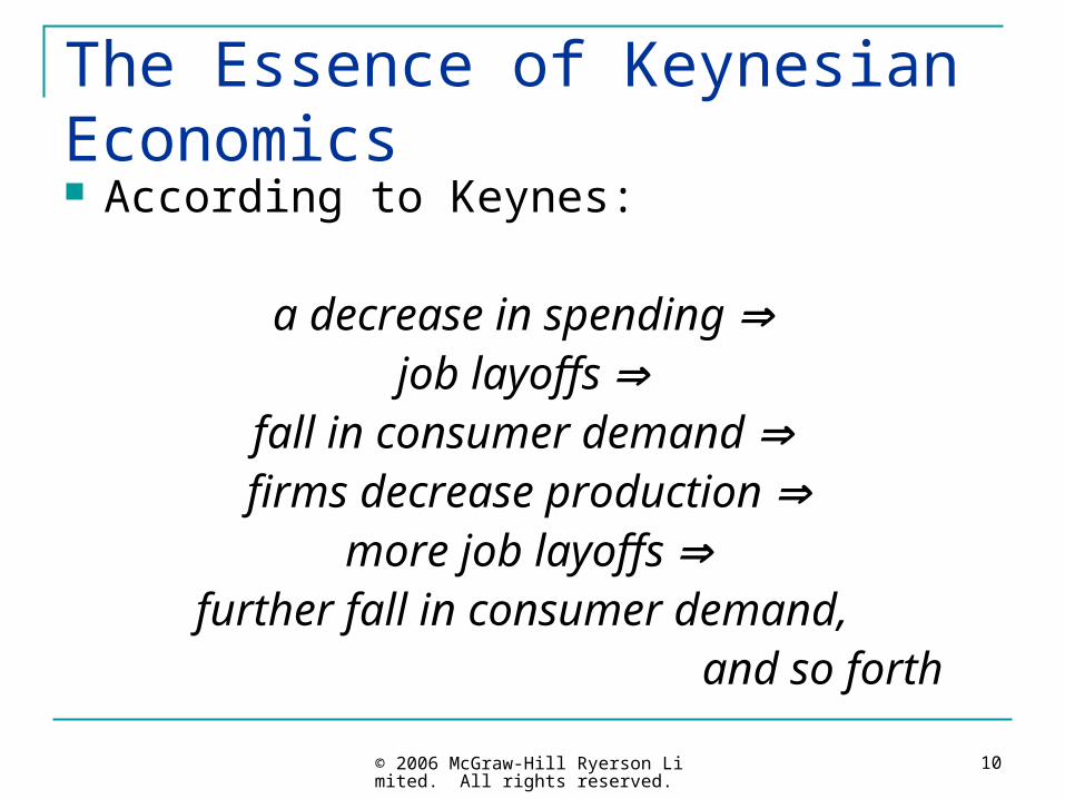
The Essence of Keynesian Economics According to Keynes:
a decrease in spending job layoffs
fall in consumer demand firms decrease production
more job layoffs further fall in consumer demand,
and so forth

© 2006 McGraw-Hill Ryerson Limited. All rights reserved.
11
Equilibrium Income Fluctuates Income is not fixed at the economy's long-run
potential income – it fluctuates.
For Keynes there was a difference between equilibrium income and potential income.
© 2006 McGraw-Hill Ryerson Limited. All rights reserved.
12
Equilibrium Income Fluctuates Equilibrium income – the level toward which
the economy gravitates in the short run because of the cumulative cycles of declining or increasing production.
© 2006 McGraw-Hill Ryerson Limited. All rights reserved.
13
Equilibrium Income Fluctuates Potential income – the level of income that
the economy technically is capable of producing without generating accelerating inflation.
© 2006 McGraw-Hill Ryerson Limited. All rights reserved.
14
Equilibrium Income Fluctuates Keynes felt that at certain times the economy
needed help to reach its potential income.
He believed that market forces would not work fast enough and would not be strong enough to get the economy out of a recession
© 2006 McGraw-Hill Ryerson Limited. All rights reserved.
15
Equilibrium Income Fluctuates Because short-run aggregate production
decisions and expenditure decisions were interdependent, the downward spiral could start at any time.
© 2006 McGraw-Hill Ryerson Limited. All rights reserved.
16
The Paradox of Thrift
Incomes would fall as people lost their jobs causing both consumption and saving to fall as well.
The economy would reach a new equilibrium which could be at an almost permanent recession.
© 2006 McGraw-Hill Ryerson Limited. All rights reserved.
17
The Paradox of Thrift
Paradox of thrift – an increase in savings can lead to a decrease in expenditures, decreasing output and causing a recession.
© 2006 McGraw-Hill Ryerson Limited. All rights reserved.
18
The Aggregate Expenditures Model Using a few simplifying assumptions,
economists can construct a model of the economy.
The Aggregate Expenditures (AE) Model looks at how real income is determined in an economy.
© 2006 McGraw-Hill Ryerson Limited. All rights reserved.
19
The Aggregate Expenditures Model The AE model assumes that the price level is
fixed, and explores how an initial shift in expenditures changes equilibrium output.
The AE model quantifies the effect of changes in aggregate expenditures on aggregate output.
© 2006 McGraw-Hill Ryerson Limited. All rights reserved.
20
Aggregate Production
Aggregate production –the total amount of goods and services produced in every industry in an economy.
Production creates an equal amount of income.
Thus, actual production and actual income are always equal.
© 2006 McGraw-Hill Ryerson Limited. All rights reserved.
21
Aggregate Production
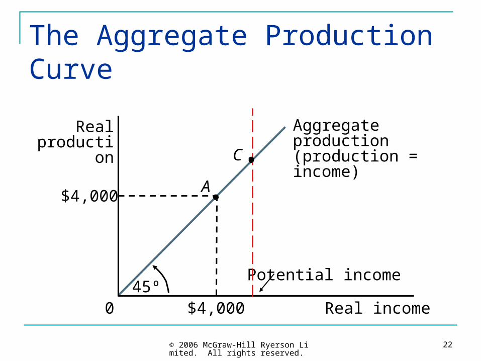
Graphically, aggregate production in the AE model is represented by a 45° line through the origin
At all points on this Aggregate Production Curve, income equals production.
© 2006 McGraw-Hill Ryerson Limited. All rights reserved.
22
The Aggregate Production Curve
Aggregate production(production = income)
A
45º$4,0000
Real production
Real income
$4,000
Potential income
C
© 2006 McGraw-Hill Ryerson Limited. All rights reserved.
23
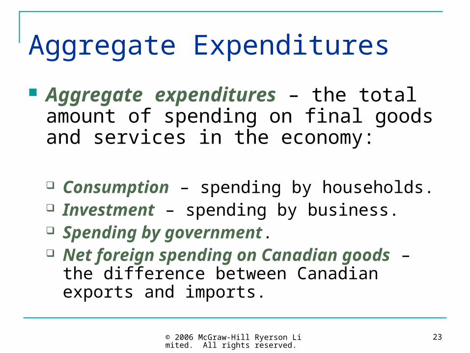
Aggregate Expenditures
Aggregate expenditures – the total amount of spending on final goods and services in the economy:
Consumption – spending by households. Investment – spending by business. Spending by government. Net foreign spending on Canadian goods – the
difference between Canadian exports and imports.
© 2006 McGraw-Hill Ryerson Limited. All rights reserved.
24
Autonomous and Induced Expenditures
Autonomous expenditures are expenditures that are independent of income. Autonomous expenditures change because
something other than income changes.
Induced expenditures – expenditures that change as income changes.
© 2006 McGraw-Hill Ryerson Limited. All rights reserved.
25
Autonomous and Induced Expenditures
Autonomous expenditures is the level of expenditures that would exist at zero income.
They remain constant at all levels of income.
© 2006 McGraw-Hill Ryerson Limited. All rights reserved.
26
Autonomous and Induced Expenditures
Induced expenditures are those that change as income changes.
When income rises, induced expenditures rise by less than the change in income.
© 2006 McGraw-Hill Ryerson Limited. All rights reserved.
27
Expenditures Function
The relationship between expenditures and income can be expressed more concisely as an expenditures function.
An expenditures function is a representation of the relationship between aggregate expenditures and income.
© 2006 McGraw-Hill Ryerson Limited. All rights reserved.
28
The Expenditures Function The relationship between aggregate
expenditures and income can be expressed mathematically:
AE = AEo + mpcY
AE = aggregate expenditures
AEo = autonomous expenditures mpc = marginal propensity to consume Y = income
© 2006 McGraw-Hill Ryerson Limited. All rights reserved.
29
The Marginal Propensity to Consume Marginal propensity to consume (mpc) –
the change in consumption that occurs with a change in income.
The mpc is between 0 and 1 because individuals tend to save a portion of an increase in income.
© 2006 McGraw-Hill Ryerson Limited. All rights reserved.
30
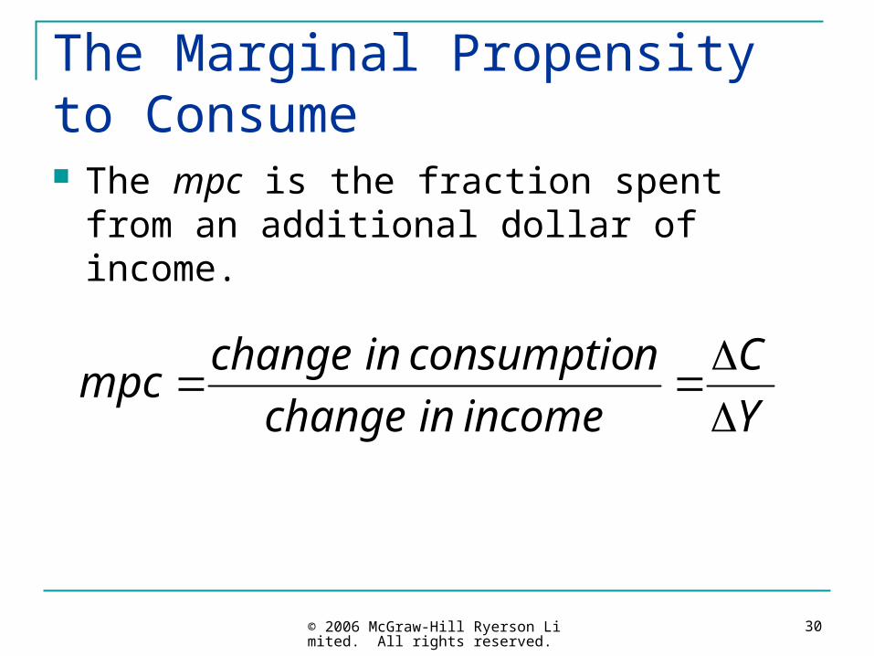
The Marginal Propensity to Consume The mpc is the fraction spent from an
additional dollar of income.
Y
C
income in change
nconsumptio in changempc
© 2006 McGraw-Hill Ryerson Limited. All rights reserved.
31
The Marginal Propensity to Consume The marginal propensity to consume
(mpc) is the ratio of a change in consumption (C) to a change in income (Y).
© 2006 McGraw-Hill Ryerson Limited. All rights reserved.
32
Expenditures Function
Autonomous expenditures is the sum of the autonomous components of expenditures:
AE = C + I + G + X – IM
© 2006 McGraw-Hill Ryerson Limited. All rights reserved.
33
Graphing the Expenditures Function The graphical representation of the
expenditures function is called the aggregate expenditures curve.
The slope of the expenditures function tells us how much expenditures change with a particular change in income.
© 2006 McGraw-Hill Ryerson Limited. All rights reserved.
34
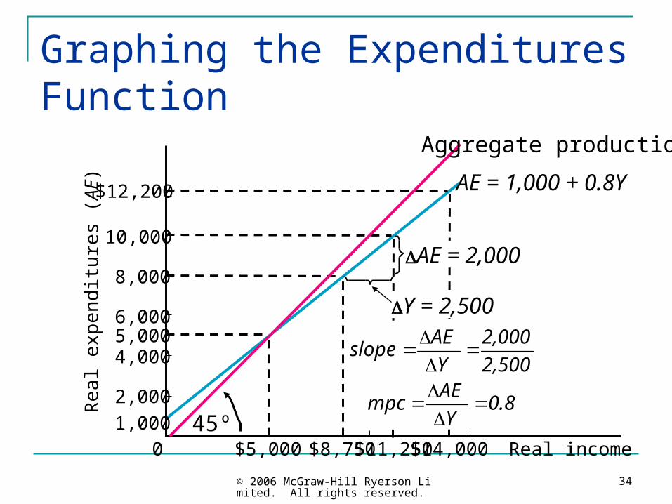
Graphing the Expenditures Function
045º
AE = 1,000 + 0.8Y
Real
exp
endi
ture
s (A
E)
$12,200
10,000
8,000
6,000
4,000
2,000
5,000
1,000$5,000 $11,250$14,000$8,750 Real income
AE = 2,000
Y = 2,500
Aggregate production
2,500
2,000
Y
AE slope
0.8 Y
AE mpc
© 2006 McGraw-Hill Ryerson Limited. All rights reserved.
35
Shifts in the Expenditures Function The aggregate expenditure curve shifts when
autonomous C, I, G, or (X – IM) change.
Autonomous Consumption expenditures respond to changes in:
interest rates household wealth expectations of future conditions
© 2006 McGraw-Hill Ryerson Limited. All rights reserved.
36
Shifts in the Expenditures Function Autonomous Investment is the most volatile
component of GDP.
It responds to changes in: interest rates capital goods prices consumer demand conditions expectations regarding future economic conditions
© 2006 McGraw-Hill Ryerson Limited. All rights reserved.
37
Autonomous exports and imports depend on foreign and domestic incomes and relative prices.
Autonomous Government expenditures may also change as policies change.
Shifts in the Expenditures Function
© 2006 McGraw-Hill Ryerson Limited. All rights reserved.
38
Determining the Equilibrium Level of Aggregate Income
At equilibrium, planned expenditures must equal production.
Graphically, it is the income level at which AE equals AP.
© 2006 McGraw-Hill Ryerson Limited. All rights reserved.
39
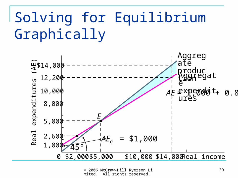
Solving for Equilibrium Graphically
45°
Aggregate expenditures AE = 1,000 + 0.8Y
Aggregate production
12,200
0
Real
exp
endi
ture
s (A
E)
5,000
1,000
$5,000 $14,000
$14,000
10,000
8,000
Real income$2,000 $10,000
2,600 AE0 = $1,000
E
© 2006 McGraw-Hill Ryerson Limited. All rights reserved.
40
In equilibrium, Y = AE.
Substituting in for aggregate expenditures, we have
Y = AE0 + mpcY
Solving for Equilibrium Algebraically
© 2006 McGraw-Hill Ryerson Limited. All rights reserved.
41
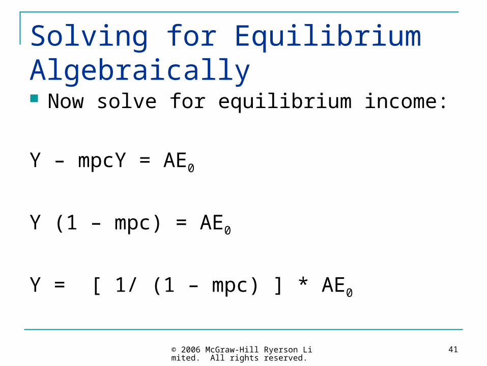
Now solve for equilibrium income:
Y – mpcY = AE0
Y (1 – mpc) = AE0
Y = [ 1/ (1 – mpc) ] * AE0
Solving for Equilibrium Algebraically
© 2006 McGraw-Hill Ryerson Limited. All rights reserved.
42
The Multiplier Equation
The multiplier equation tells us that income equals the multiplier times autonomous expenditures.
Y = Multiplier X Autonomous expenditures
© 2006 McGraw-Hill Ryerson Limited. All rights reserved.
43
The Multiplier Equation
The multiplier process amplifies changes in autonomous expenditures.
What forces are operating to ensure that the income level we determined is actually the equilibrium income level?
© 2006 McGraw-Hill Ryerson Limited. All rights reserved.
44
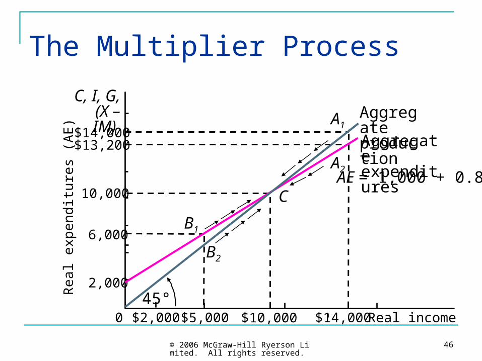
The Multiplier Process
When aggregate production do not equal aggregate expenditures:
Businesses change production levels,
which changes income,
which changes expenditures,
which changes production,
which changes income, which changes . . . etc.
© 2006 McGraw-Hill Ryerson Limited. All rights reserved.
45
The Multiplier Process
The process ends when aggregate production equals aggregate expenditures.
Firms are selling all they produce, so they have no reason to change their production levels.
© 2006 McGraw-Hill Ryerson Limited. All rights reserved.
46
The Multiplier Process
C, I, G, (X – IM)
A2
A1
C
B1
B2
0
Real
exp
endi
ture
s (A
E)
6,000
2,000
$5,000 $14,000
$14,000
10,000
Real income$2,000 $10,000
Aggregate expenditures
45°
Aggregate production
$13,200
AE = 1,000 + 0.8Y
© 2006 McGraw-Hill Ryerson Limited. All rights reserved.
47
The Circular Flow Model and the Multiplier Process
The circular flow model provides the intuition behind the multiplier process.
The flow of expenditures equals the flow of income.
© 2006 McGraw-Hill Ryerson Limited. All rights reserved.
48
The Circular Flow Model and the Multiplier Process
Expenditures are injections into the circular flow.
The mpc measures the percentage of expenditures that get injected back into the economy each round of the circular flow.
But there are withdrawals.
© 2006 McGraw-Hill Ryerson Limited. All rights reserved.
49
The Circular Flow Model and the Multiplier Process
Economists use the term the marginal propensity of save (mps) to represent the percentage of income flow that is withdrawn from the economy for each round of the circular flow.
© 2006 McGraw-Hill Ryerson Limited. All rights reserved.
50
The Circular Flow Model and the Multiplier Process
By definition:
mpc + mps = 1
Alternatively expressed:
mps = 1 - mpc
multiplier = 1/mps
© 2006 McGraw-Hill Ryerson Limited. All rights reserved.
51
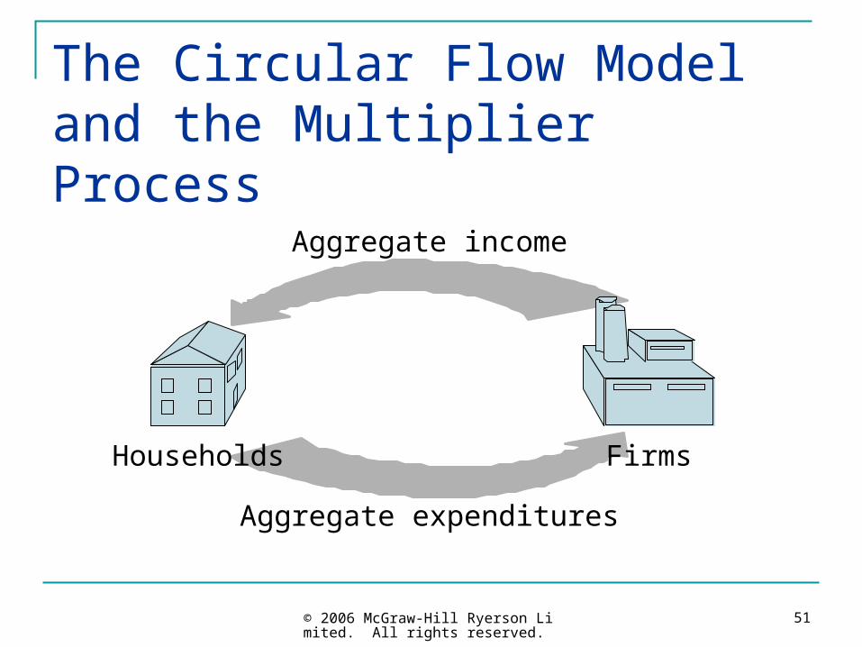
The Circular Flow Model and the Multiplier Process
Aggregate income
Aggregate expenditures
Households Firms
© 2006 McGraw-Hill Ryerson Limited. All rights reserved.
52
The AE Model in Action
The AE model illustrates how a change in autonomous expenditures changes the equilibrium level of income.
© 2006 McGraw-Hill Ryerson Limited. All rights reserved.
53
The Multiplier Model in Action Autonomous expenditures are determined
outside the model and are not affected by changes in income.
When autonomous expenditures shift, the multiplier process is called into play.
© 2006 McGraw-Hill Ryerson Limited. All rights reserved.
54
The Steps of the Multiplier Process The income adjustment process is directly
related to the multiplier.
Any initial shock (a change in autonomous AE) is multiplied in the adjustment process.

© 2006 McGraw-Hill Ryerson Limited. All rights reserved.
55
The Steps of the Multiplier Process The multiplier process repeats and repeats
until a new equilibrium level is finally reached.
© 2006 McGraw-Hill Ryerson Limited. All rights reserved.
56
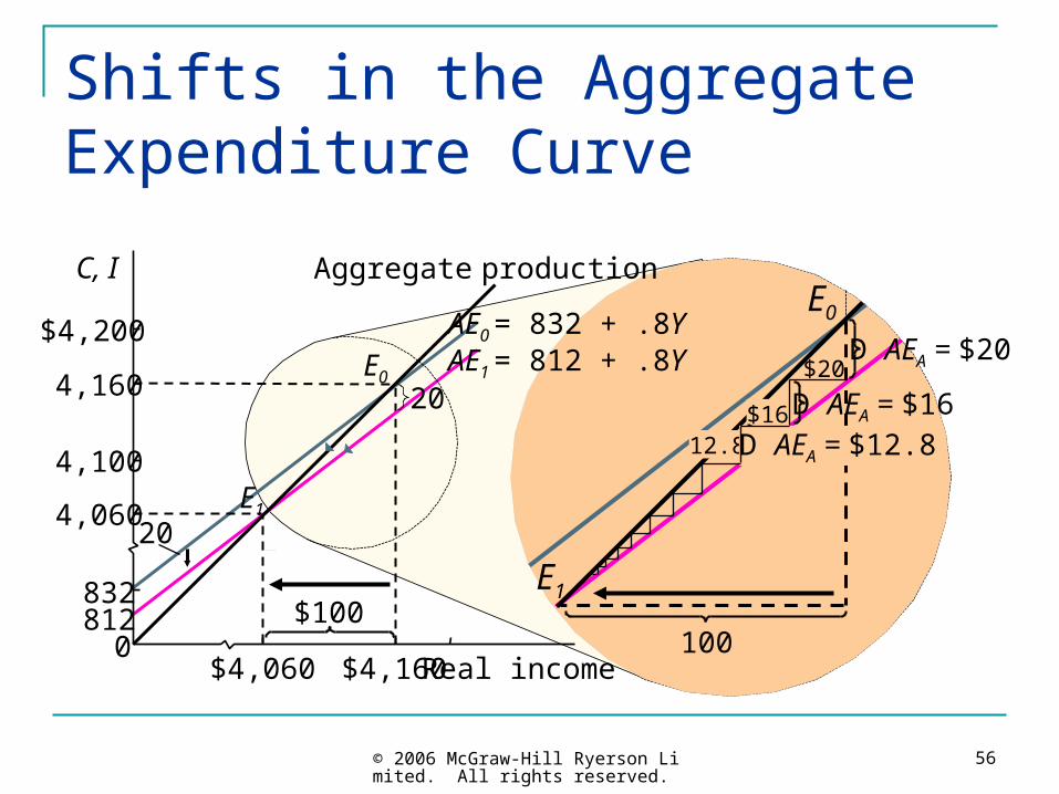
Shifts in the Aggregate Expenditure Curve
C, I
$4,200
4,100
832
4,160
4,060
8120
Real income$4,060 $4,160
$100
20E1
E0
20
Aggregate production
AE0 = 832 + .8YAE1 = 812 + .8Y
E1
100
E0
D AEA = $20$20
$1612.8
D AEA = $16D AEA = $12.8
© 2006 McGraw-Hill Ryerson Limited. All rights reserved.
57
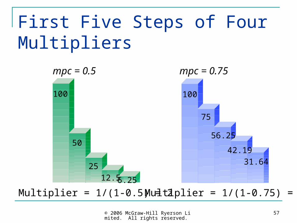
mpc = 0.5
Multiplier = 1/(1-0.5) = 2
100
50
2512.5 6.25
First Five Steps of Four Multipliers
100
75
56.25
42.1931.64
Multiplier = 1/(1-0.75) = 4
mpc = 0.75

© 2006 McGraw-Hill Ryerson Limited. All rights reserved.
58
First Five Steps of Four Multipliers
100
80
64
51.240.96
mpc = 0.8
Multiplier = 1/(1-0.8) = 5
10090
8172.9
65.61
Multiplier = 1/(1-0.9) = 10
mpc = 0.9
© 2006 McGraw-Hill Ryerson Limited. All rights reserved.
59
Examples of the Effect of Shifts in Aggregate Expenditures There are many reasons for shifts in
autonomous expenditures:
Natural disasters. Changes in investment caused by technological
developments. Shifts in government expenditures. Large changes in the exchange rate.
© 2006 McGraw-Hill Ryerson Limited. All rights reserved.
60
The Effect of Shifts in Aggregate Expenditures
An understanding of these shifts can be enhanced by tying them to the formula:
AE = C + I + G + X - IM
© 2006 McGraw-Hill Ryerson Limited. All rights reserved.
61
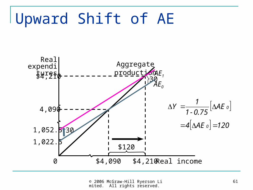
Upward Shift of AE
Aggregate production
1,052.5
AE1
30
30
4,090
$4,090
$4,210
$4,210
$120
Real expenditures
0 Real income
1,022.5
AE0
120 AE4
AE0.75-1
1 Y
0
0
© 2006 McGraw-Hill Ryerson Limited. All rights reserved.
62
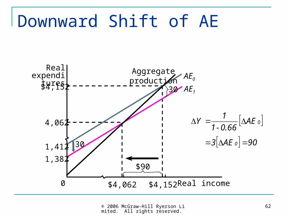
$90
$4,152
$4,152
$4,062
4,062
AE0
1,412
AE1
1,382
Downward Shift of AE
Real expenditures
30
30
0 Real income
Aggregate production
90 AE3
AE0.66-1
1 Y
0
0
© 2006 McGraw-Hill Ryerson Limited. All rights reserved.
63
Real World Examples
Canada in 2000.
Japan in the 1990s.
The 1930s depression.
© 2006 McGraw-Hill Ryerson Limited. All rights reserved.
64
Canada in 2000
Consumer confidence rose substantially causing autonomous consumption expenditures to increase more than economists had predicted.
While economists had expected the economy to grow slowly, it boomed.
© 2006 McGraw-Hill Ryerson Limited. All rights reserved.
65
Japan in the 1990s
Aggregate income and production fell during the 1990s.
A dramatic rise in the yen cut Japanese exports. Autonomous consumption decreased as
consumers’ confidence fell Suppliers responded by laying off workers and
cutting production.
© 2006 McGraw-Hill Ryerson Limited. All rights reserved.
66
The 1930s Depression
The 1929 stock market crash, which continued into 1930, threw the financial markets into chaos.
This resulted in a downward shift of the AE curve.
© 2006 McGraw-Hill Ryerson Limited. All rights reserved.
67
The 1930s Depression Frightened business people decreased
investment and laid off workers.
Frightened consumers decreased autonomous consumption and increased savings, thereby increasing withdrawals from the system.
Governments cut spending to balance their budgets, as tax revenue declined.
© 2006 McGraw-Hill Ryerson Limited. All rights reserved.
68
The 1930s Depression
Business people responded by decreasing output, which decreased income, starting a downward cycle, thereby confirming the fears of the businesspeople.
The process continued until the economy settled at a low-level equilibrium, far below the potential level of income.
© 2006 McGraw-Hill Ryerson Limited. All rights reserved.
69
The 1930s Depression
The process caused the paradox of thrift, whereby individuals attempting to save more, spent less, and caused income to decrease.
They ended up saving not more, but less.
© 2006 McGraw-Hill Ryerson Limited. All rights reserved.
70
AE Model Is Not a Complete Model The AE model determines income given
autonomous expenditures.
These autonomous expenditures, however, are determined by economic variables which are not in our simple model.
© 2006 McGraw-Hill Ryerson Limited. All rights reserved.
71
The AE model uses aggregate expenditures to determine equilibrium income.
It does not explain production.
It assumes firms can supply the output demanded.
AE Model Is Not a Complete Model
© 2006 McGraw-Hill Ryerson Limited. All rights reserved.
72
Model of Aggregate Demand
Shifts may be simultaneous shifts in supply and demand that do not necessarily reflect suppliers responding to changes in demand.
Expansion of this line of thought has led to the real business cycle theory of the economy.
© 2006 McGraw-Hill Ryerson Limited. All rights reserved.
73
Real business cycle theory of the economy – changes in aggregate supply are the principle way for real income to change.
Model of Aggregate Demand
© 2006 McGraw-Hill Ryerson Limited. All rights reserved.
74
Prices are Fixed
The multiplier model assumes that the price level is fixed.
The price level can change in response to changes in aggregate demand.
© 2006 McGraw-Hill Ryerson Limited. All rights reserved.
75
Does Not Include Expectations People's forward-looking expectations make
the adjustment process much more complicated.
Most people, however, act upon their expectations of the future.
Business people may not automatically cut back production and lay-off workers if they think a fall in sales is temporary.

© 2006 McGraw-Hill Ryerson Limited. All rights reserved.
76
Forward-Looking Expectations Complicate the Adjustment Process Rational expectations model – captures the
effect expectations have on individuals’ behaviour.
Expectations can be self-fulfilling.
© 2006 McGraw-Hill Ryerson Limited. All rights reserved.
77
Consumption Behaviour
People may base their spending on lifetime income, not yearly income.
Permanent income hypothesis -- the hypothesis that expenditures are determined by permanent or lifetime income.
© 2006 McGraw-Hill Ryerson Limited. All rights reserved.
78
We can increase the power of our AE model by adding more detail.
For example, adding taxes to the model Changes consumption expenditures. Introduces government budget deficits and
surpluses. Changes the multiplier.
Expanded AE Model
© 2006 McGraw-Hill Ryerson Limited. All rights reserved.
79
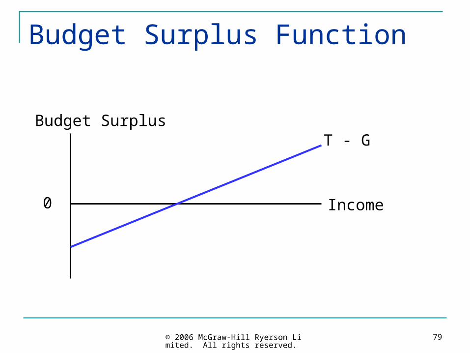
Budget Surplus Function
Budget Surplus
Income0
T - G
© 2006 McGraw-Hill Ryerson Limited. All rights reserved.
80
Expanded AE Model
Adding income-induced imports
Changes import spending.
Changes net exports, and introduces trade surpluses and deficits.
Changes the multiplier.
© 2006 McGraw-Hill Ryerson Limited. All rights reserved.
81
The marginal propensity to import (mpi) gives the increase in import spending from an additional $1 of disposable income. Disposable = after-tax
Mpi lies between 0 and 1
Expanded AE Model
© 2006 McGraw-Hill Ryerson Limited. All rights reserved.
82
The Goods Market and the Aggregate Expenditures Model
End of Chapter 8