Weighted least squares support vector machines: robustness and sparse approximation

Neurocomputing 48 (2002) 85–105www.elsevier.com/locate/neucom

Weighted least squares support vector machines: robustnessand sparse approximation�

J.A.K. Suykens∗, J. De Brabanter, L. Lukas, J. VandewalleDepartment of Electrical Engineering, Katholieke Universiteit Leuven, ESAT-SISTA Kasteelpark

Arenberg 10, B-3001 Leuven (Heverlee), Belgium

Received 3 November 2000; accepted 6 June 2001

Abstract

Least squares support vector machines (LS-SVM) is an SVM version which involvesequality instead of inequality constraints and works with a least squares cost function.In this way, the solution follows from a linear Karush–Kuhn–Tucker system instead ofa quadratic programming problem. However, sparseness is lost in the LS-SVM case andthe estimation of the support values is only optimal in the case of a Gaussian distributionof the error variables. In this paper, we discuss a method which can overcome these twodrawbacks. We show how to obtain robust estimates for regression by applying a weightedversion of LS-SVM. We also discuss a sparse approximation procedure for weighted andunweighted LS-SVM. It is basically a pruning method which is able to do pruning basedupon the physical meaning of the sorted support values, while pruning procedures forclassical multilayer perceptrons require the computation of a Hessian matrix or its inverse.The methods of this paper are illustrated for RBF kernels and demonstrate how to obtainrobust estimates with selection of an appropriate number of hidden units, in the case ofoutliers or non-Gaussian error distributions with heavy tails. c© 2002 Elsevier Science B.V.All rights reserved.

Keywords: Support vector machines; (Weighted) least squares; Ridge regression; Sparseapproximation; Robust estimation

� This research work was carried out at the ESAT laboratory and the Interdisciplinary Center ofNeural Networks ICNN of the Katholieke Universiteit Leuven, in the framework of the FWO projectLearning and Optimization: an Interdisciplinary Approach, the Belgian Program on InteruniversityPoles of Attraction, initiated by the Belgian State, Prime Minister’s OCce for Science, Technologyand Culture (IUAP P4-02 & IUAP P4-24) and the Concerted Action Project MEFISTO of the FlemishCommunity. Johan Suykens is a postdoctoral researcher with the National Fund for ScientiEc ResearchFWO - Flanders.

∗ Corresponding author. Tel.:+32-16-32-18-02; fax:+32-16-32-19-70.E-mail address: [email protected] (J.A.K. Suykens).

0925-2312/02/$ - see front matter c© 2002 Elsevier Science B.V. All rights reserved.PII: S0925-2312(01)00644-0

86 J.A.K. Suykens et al. / Neurocomputing 48 (2002) 85–105

1. Introduction

Support vector machines (SVM) for classiEcation and nonlinear function esti-mation, as introduced by Vapnik [35,36] and further investigated by many others[4,21–25], is an important new methodology in the area of neural networks andnonlinear modelling [27]. While classical neural networks approaches, such as mul-tilayer perceptrons (MLP) and radial basis function (RBF) networks [2,17], suMerfrom problems like the existence of many local minima and the choice of the num-ber of hidden units [2,13], SVM solutions are characterized by convex optimizationproblems, up to the determination of a few additional tuning parameters. Moreover,model complexity follows from this convex optimization problem. Typically, onesolves a convex quadratic programming (QP) problem in dual space in order todetermine the SVM model. The formulation of the optimization problem in theprimal space associated with this QP problem involves inequality constraints. Inthe case of function estimation it is related to Vapnik’s epsilon-insensitive lossfunction. An interesting property of the SVM solution is that one obtains a sparseapproximation, in the sense that many elements in the QP solution vector are equalto zero. The additional hyperparameters of the SVM model are often determinedby model selection based upon generalization bounds, which have been derivedwithin the area of statistical learning theory. SVM is a kernel based approach,which allows the use of linear, polynomial and RBF kernels and others that satisfyMercer’s condition.Recently, least squares (LS) versions of SVM’s have been investigated for clas-

siEcation [28] and function estimation [20]. In these LS-SVM formulations oneworks with equality instead of inequality constraints and a sum squared error (SSE)cost function as it is frequently used in training of classical neural networks. Thisreformulation greatly simpliEes the problem in such a way that the solution ischaracterized by a linear system, more precisely a KKT (Karush–Kuhn–Tucker)system [8], which takes a similar form as the linear system that one solves inevery iteration step by interior point methods for standard SVM’s [26]. This linearsystem can be eCciently solved by iterative methods such as conjugate gradient[29]. However, despite these computationally attractive features, LS-SVM solutionsalso have some potential drawbacks. The Erst drawback is that sparseness is lostin the LS-SVM solution. In this case every data point is contributing to the modeland the relative importance of a data point is given by its support value. The sec-ond drawback is that it is well known that the use of a SSE cost function withoutregularization might lead to estimates which are less robust, e.g. with respect tooutliers on the data or when the underlying assumption of a Gaussian distributionfor the error variables is not realistic.The aim of this paper is to show that one can overcome these drawbacks con-

cerning sparseness and robustness within the present LS-SVM framework. Firstof all one should note that only the output weights of the SVM model followas solution to the linear system. Only these parameters are related to the SSE

J.A.K. Suykens et al. / Neurocomputing 48 (2002) 85–105 87

cost function which means that (up to a certain extent) one can still correct forwrong assumptions by an appropriate choice of the hyperparameters. These canbe determined in several possible ways such as crossvalidation, bootstrapping, VCbounds, Bayesian inference etc. [4,34]. We show in this paper how one can applyweighted least squares in order to produce a more robust estimate. This is doneby Erst applying an (unweighted) LS-SVM and, in the second stage, associateweighting values to the error variables based upon the resulting error variablesfrom the Erst stage. Techniques of weighted least squares are well known e.g. instatistics, identiEcation and control theory and signal processing. For LS-SVM’s itcan be employed as a cheap and eCcient way to make the solution robust. In thisway it can be used as an alternative to other methods in robust estimation [14] asL1 estimators and M -estimators with Huber loss function. Robust estimation is alsopossible within the standard SVM context [36]. In standard SVM methodology, onechooses a given cost function (any convex cost function can be taken in principle asshown in [26]). Instead of this top–down approach the weighted LS-SVM approachaims at working bottom–up by solving a sequence of weighted LS-SVM’s startingfrom the unweighted version. In this way one implicitly tries to End an optimalunderlying cost function, instead of imposing the cost function beforehand. In thissense there is also a close link between solving the SVM problem for a givenconvex cost function by interior point methods and iterative weighting of LS-SVMsolutions.Furthermore, in this paper we illustrate how sparseness can be imposed to the

weighted LS-SVM solution by gradually pruning the sorted support value spec-trum. While in pruning methods for MLP’s [2] (like optimal brain damage [16]and optimal brain surgeon [12]) the procedure involves a Hessian matrix or itsinverse, the pruning in LS-SVM’s can be done based upon the solution vectoritself (note that this implicitly requires inverting the system). Less meaningfuldata points as indicated by their support values, are removed and the LS-SVM isre-computed on the basis of the remaining points while validating on the com-plete training data set. In this paper we focus on a cheap and simple pruningmethod. Other methods for obtaining a sparse approximation with LS-SVM’s arepossible [6]. The advantage of the method shown in this paper is that the de-termination of the hyperparameters can be kept localized, while in the other ap-proaches one needs to solve the convex optimization problem (which implicitlycorresponds to solving a sequence of linear systems) for a given set of hyper-parameters.In general, parametric models like MLP’s or RBF networks are applicable within

a broad range of applications of either static problems (classiEcation, regression,density estimation) or dynamic problems (recurrent networks, optimal control).Standard SVM’s on the other hand have only been applied to static problems. How-ever, the use of equality constrained and SSE based formulations within LS-SVMgreatly simpliEes the formulations and allows us to extend the method to recurrentnetworks [31] and control applications [32]. In the latter case convexity is lost,


but some of the other interesting SVM properties remain applicable. The results ofthis paper on weighted LS-SVM’s for robust estimation and sparse approximationfurther motivates the LS-SVM approach towards its use as a new and generalneural network methodology.This paper is organized as follows. In Section 2 we review some basic notions of

LS-SVM’s for function estimation. In Section 3 we discuss the weighted LS-SVMformulation. The sparse approximation procedure is discussed in Section 4. Finally,illustrative examples are given in Section 5.

2. LS-SVM for nonlinear function estimation

Given a training data set of N points {xk ; yk}Nk=1 with input data xk ∈Rn andoutput data yk ∈R; one considers the following optimization problem in primalweight space:

minw;b;eJ (w; e)=

12wTw +

12 N∑k=1

e2k (1)

such that

yk =wT’(xk) + b+ ek ; k=1; : : : ; N

with ’(·) :Rn → Rnh a function which maps the input space into a so-called higherdimensional (possibly inEnite dimensional) feature space, weight vector w∈Rnh inprimal weight space, error variables ek ∈R and bias term b. Note that the costfunction J consists of a SSE Etting error and a regularization term, which is also astandard procedure for the training of MLP’s and is related to ridge regression [10].The relative importance of these terms is determined by the positive real constant . In the case of noisy data one avoids overEtting by taking a smaller value.SVM problem formulations of this form have been investigated independently in[20] (without bias term) and [28].In primal weight space one has the model

y(x)=wT’(x) + b: (2)

The weight vector w can be inEnite dimensional, which makes a calculation ofw from (1) impossible in general. Therefore, one computes the model in the dualspace instead of the primal space. One deEnes the Lagrangian

L(w; b; e; �)= J (w; e)−N∑k=1

�k{wT’(xk) + b+ ek − yk} (3)


with Lagrange multipliers �k ∈R (called support values). The conditions for opti-mality are given by

@L@w

=0 → w=N∑k=1

�k’(xk);

@L@b

=0 →N∑k=1

�k =0;

@L@ek

=0 → �k = ek ; k=1; : : : ; N;

@L@�k

=0 → wT’(xk) + b+ ek − yk =0; k=1; : : : ; N:

(4)

These conditions are similar to standard SVM optimality conditions, except forthe condition �k = ek . At this point one loses the sparseness property inLS-SVM’s [9].After elimination of w; e one obtains the solution

0 1Tv

1v �+ 1 I

[b�

]=

[0y

](5)

with y=[y1; : : : ;yN ]; 1v=[1; : : : ; 1]; �=[�1; : : : ; �N ] and �kl=’(xk)T’(x1) fork; l=1; : : : ; N . According to Mercer’s condition, there exists a mapping ’ and anexpansion

K(x; y)=∑i

’i(x)’i(y); x; y∈Rn; (6)

if and only if, for any g(x) such that∫g(x)2dx is Enite, one has

∫K(x; y)g(x)g(y) dx dy¿ 0: (7)

As a result, one can choose a kernel K(·; ·) such that

K(xk ; xl)=’(xk)T’(xl); k; l=1; : : : ; N: (8)

The resulting LS-SVM model for function estimation becomes

y(x)=N∑k=1

�kK(x; xk) + b (9)

where �; b are the solution to (5). We focus on the choice of an RBF kernelK(xk ; xl)= exp{−‖xk − xl‖22=�2} for the sequel.


When solving large linear systems, it is necessary to apply iterative methods[10] to (5). However, the matrix in (5) is not positive deEnite. According to [29]one can transform the system into a positive deEnite system such that iterativemethods (conjugate gradient, successive overrelaxation or others) can be appliedto it. Note that the computational complexity of the conjugate gradient method forsolving a linear system Ax=B is O(Nr2) where rank(C)= r with A= I +C andA∈RN×N . It converges in at most r+1 steps. The speed of convergence dependson the condition number of the matrix. In the case of LS-SVM this is inPuencedby the choice of ( ; �) when using an RBF kernel.

3. Robust estimation by weighted LS-SVM

In order to obtain a robust estimate based upon the previous LS-SVM solution,in a subsequent step, one can weight the error variables ek = �k= by weightingfactors vk . This leads to the optimization problem:

minw?;b?;e?

J (w?; e?)=12w?Tw? +

12 N∑k=1

vke?2k (10)

such that

yk =w?T’(xk) + b? + e?k ; k=1; : : : ; N:

The Lagrangian becomes

L(w?; b?; e?; �?)= J (w?; e?)−N∑k=1

�?k {w?T’(xk) + b? + e?k − yk}: (11)

The unknown variables for this weighted LS-SVM problem are denoted by the ?symbol. From the conditions for optimality and elimination of w?; e? one obtainsthe KKT system

0 1Tv

1v �+ V

[b?

�?

]=

[0y

]; (12)

where the diagonal matrix V is given by

V =diag{

1 v1; : : : ;

1 vN

}: (13)

The choice of the weights vk is determined based upon the error variables ek = �k= from the (unweighted) LS-SVM case (5). Robust estimates are obtained then (see


[5,18]) e.g. by taking

vk =

1 if |ek=s|6 c1;c2 − |ek=s|c2 − c1 if c16 |ek=s|6 c2;

10−4 otherwise;

(14)

where s is a robust estimate of the standard deviation of the LS-SVM errorvariables ek :

s=IQR

2× 0:6745: (15)

The interquartile range IQR is the diMerence between the 75th percentile and 25thpercentile. In the estimate s one takes into account how much the estimated er-ror distribution deviates from a Gaussian distribution. Another robust estimate ofthe standard deviation is s=1:483 MAD(xi) where MAD stands for the medianabsolute deviation [11]. The SSE cost function in the unweighted LS-SVM for-mulation is optimal under the assumption of a normal Gaussian distribution forek . The procedure (14) corrects for this assumption in order to obtain a robustestimate when this distribution is not normal. Eventually, the procedure (10) (14)can be repeated iteratively, but in practice one single additional weighted LS-SVMstep will often be suCcient. One assumes that ek has a symmetric distributionwhich is usually the case when ( ; �) are well-determined by an appropriate modelselection method. The constants c1; c2 are typically chosen as c1 = 2:5 and c2 = 3[18]. This is a reasonable choice taking into account the fact that for a Gaussiandistribution, there will be very few residuals larger than 2:5s. Another possibilityis to determine c1; c2 from a density estimation of the ek distribution. Using theseweightings one can correct for y-outliers or for a non-Gaussian instead of Gaussianerror distributions.This leads us to the following algorithm:

Algorithm 1---weighted LS-SVM

1. Given training data {xk ; yk}Nk=1; End an optimal ( ; �) combination (e.g. by10-fold cross-validation or generalization bounds) by solving linear systems (5).For the optimal ( ; �) combination one computes ek = �k= from (5).

2. Compute s from the ek distribution.3. Determine the weights vk based upon ek ; s.4. Solve the Weighted LS-SVM (12), giving the model y(x)=

∑Nk=1 �

?k K(x; xk)+

b?.

An important notion in robust estimation is the breakdown point of an estima-tor [1,6,19]. Loosely speaking, it is the smallest fraction of contamination of agiven data set that can result in an estimate which is arbitrarily far away from the


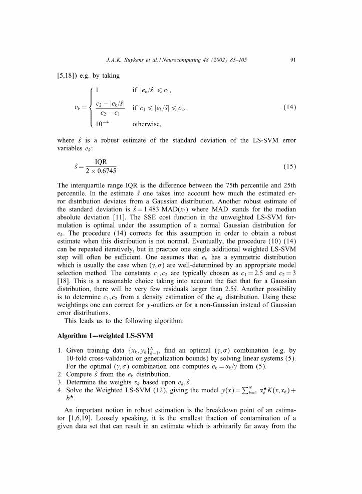
Fig. 1. Estimation of a sinc function by LS-SVM with RBF kernel, given 300 training data point,corrupted by zero mean Gaussian noise and three outliers (denoted by ‘+’). (Top-Left) Trainingdata set; (Top-Right) resulting LS-SVM model evaluated on an independent test set: (solid line) truefunction, (dashed line) LS-SVM estimate; (Bottom-Left) ek = �k = values; (Bottom-Right) histogramfor distribution of ek values, which is non-Gaussian due to the three outliers.

estimated parameter vector obtained from the uncontaminated data set. It is wellknown that the least squares estimate in linear regression (parametric) withoutregularization has a low breakdown point. At this point the unweighted LS-SVMhas already better properties due to the fact that least squares is only applied forEnding � (which corresponds to estimating the output layer and not ( ; �)). Itis still possible then to correct with ( ; �) when using an RBF kernel. Althoughunweighted LS-SVM already has rather desirable properties, the breakdown pointis further improved by applying the weighted LS-SVM afterwards.In standard SVM approaches one usually chooses a certain cost function (any

convex cost function can be taken according to [26]). However, in such a top–down approach one assumes in fact that the noise distribution is known because oneknows which cost function is optimal for a given noise distribution. The weighted


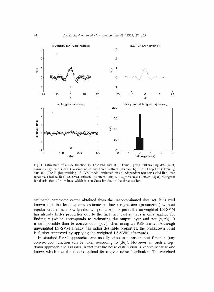
Fig. 2. (Continued) Weighted LS-SVM applied to the results of Fig. 1. The ek distribution becomesGaussian and the generalization performance on the test data improves.

LS-SVM procedure tries to work bottom–up and aims at Ending the optimal un-derlying cost function for the given noisy data. The methods can be conceptuallylinked by the fact that when one applies an interior point method for solving astandard SVM problem, at every iteration step a KKT system is solved which issimilar to solving one single LS-SVM. Hence, solving a standard SVM with arbi-trary convex cost function implicitly corresponds, in fact, to solving a sequence ofLS-SVMs.

4. Imposing sparseness

While standard SVM’s possess a sparseness property in the sense that many �kvalues are equal to zero, this is not the case for LS-SVM’s due to the fact that�k = ek from the conditions for optimality. An equivalence has also been provenbetween sparse approximation and SVM’s [3,9]. Here we discuss a simple proce-dure that shows how a sparse approximation for LS-SVM’s can be obtained. This


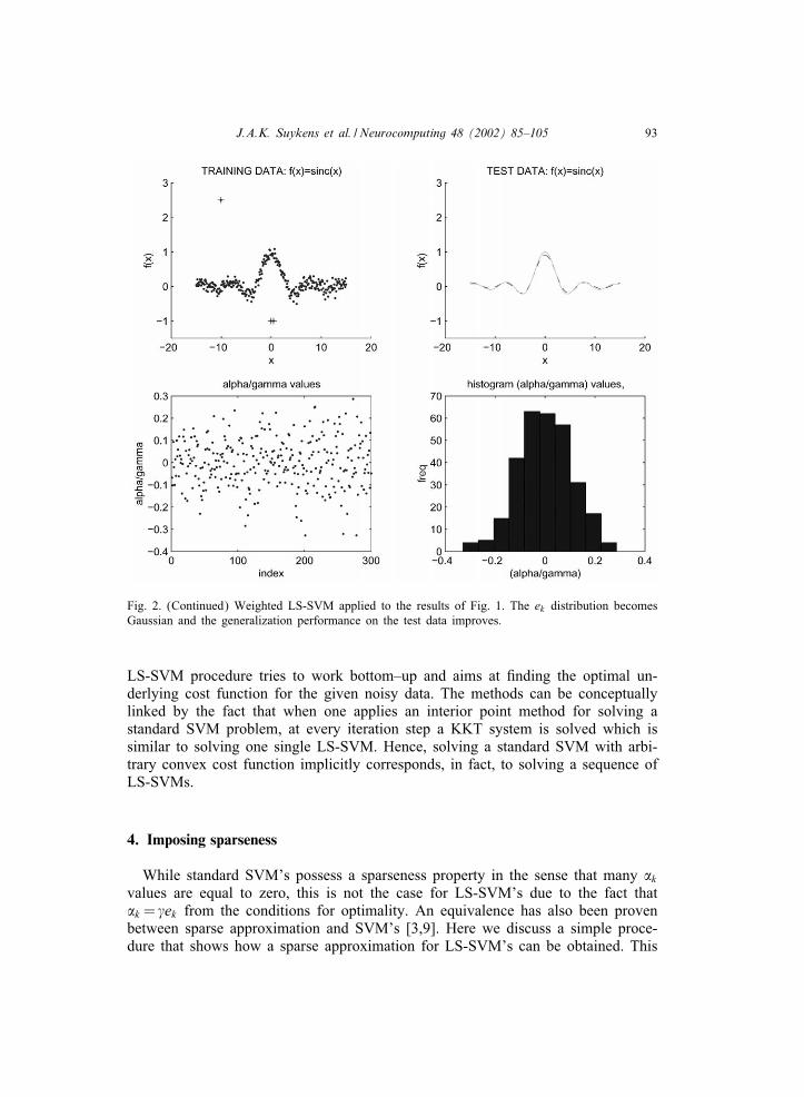
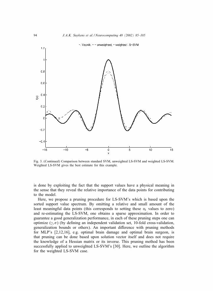
Fig. 3. (Continued) Comparison between standard SVM, unweighted LS-SVM and weighted LS-SVM.Weighted LS-SVM gives the best estimate for this example.

is done by exploiting the fact that the support values have a physical meaning inthe sense that they reveal the relative importance of the data points for contributingto the model.Here, we propose a pruning procedure for LS-SVM’s which is based upon the

sorted support value spectrum. By omitting a relative and small amount of theleast meaningful data points (this corresponds to setting these �k values to zero)and re-estimating the LS-SVM, one obtains a sparse approximation. In order toguarantee a good generalization performance, in each of these pruning steps one canoptimize ( ; �) (by deEning an independent validation set, 10-fold cross-validation,generalization bounds or others). An important diMerence with pruning methodsfor MLP’s [2,12,16], e.g. optimal brain damage and optimal brain surgeon, isthat pruning can be done based upon solution vector itself and does not requirethe knowledge of a Hessian matrix or its inverse. This pruning method has beensuccessfully applied to unweighted LS-SVM’s [30]. Here, we outline the algorithmfor the weighted LS-SVM case.


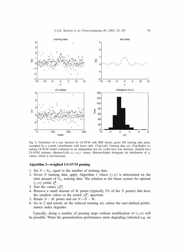
Fig. 4. Estimation of a sinc function by LS-SVM with RBF kernel, given 300 training data point,corrupted by a central t-distribution with heavy tails. (Top-Left) Training data set; (Top-Right) re-sulting LS-SVM model evaluated on an independent test set: (solid line) true function, (dashed line)LS-SVM estimate; (Bottom-Left) ek = �k = values; (Bottom-Right) histogram for distribution of ekvalues, which is non-Gaussian.

Algorithm 2---weighted LS-SVM pruning

1. Set N =Ntot equal to the number of training data.2. Given N training data, apply Algorithm 1 where ( ; �) is determined on the

total amount of Ntot training data. The solution to the linear system for optimal( ; �) yields �?k .

3. Sort the values |�?k |.4. Remove a small amount of M points (typically 5% of the N points) that have

the smallest values in the sorted |�?k | spectrum.5. Retain N −M points and set N :=N −M .6. Go to 2 and retrain on the reduced training set, unless the user-deEned perfor-

mance index degrades.

Typically, doing a number of pruning steps without modiEcation of ( ; �) willbe possible. When the generalization performance starts degrading (checked e.g. on


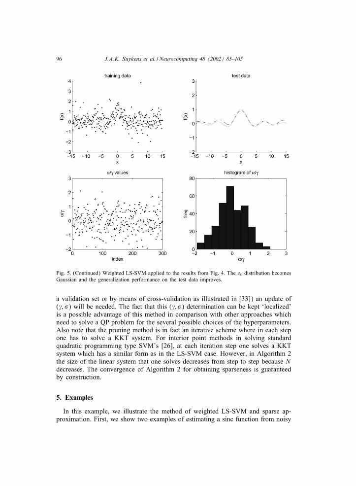
Fig. 5. (Continued) Weighted LS-SVM applied to the results from Fig. 4. The ek distribution becomesGaussian and the generalization performance on the test data improves.

a validation set or by means of cross-validation as illustrated in [33]) an update of( ; �) will be needed. The fact that this ( ; �) determination can be kept ‘localized’is a possible advantage of this method in comparison with other approaches whichneed to solve a QP problem for the several possible choices of the hyperparameters.Also note that the pruning method is in fact an iterative scheme where in each stepone has to solve a KKT system. For interior point methods in solving standardquadratic programming type SVM’s [26], at each iteration step one solves a KKTsystem which has a similar form as in the LS-SVM case. However, in Algorithm 2the size of the linear system that one solves decreases from step to step because Ndecreases. The convergence of Algorithm 2 for obtaining sparseness is guaranteedby construction.

5. Examples

In this example, we illustrate the method of weighted LS-SVM and sparse ap-proximation. First, we show two examples of estimating a sinc function from noisy


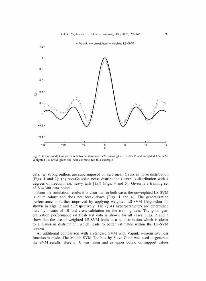
Fig. 6. (Continued) Comparison between standard SVM, unweighted LS-SVM and weighted LS-SVM.Weighted LS-SVM gives the best estimate for this example.

data: (a) strong outliers are superimposed on zero mean Gaussian noise distribution(Figs. 1 and 2); (b) non-Gaussian noise distribution (central t-distribution with 4degrees of freedom, i.e. heavy tails [15]) (Figs. 4 and 5). Given is a training setof N =300 data points.From the simulation results it is clear that in both cases the unweighted LS-SVM

is quite robust and does not break down (Figs. 1 and 4). The generalizationperformance is further improved by applying weighted LS-SVM (Algorithm 1),shown in Figs. 2 and 5, respectively. The ( ; �) hyperparameters are determinedhere by means of 10-fold cross-validation on the training data. The good gen-eralization performance on fresh test data is shown for all cases. Figs. 2 and 5show that the use of weighted LS-SVM leads to a ek distribution which is closerto a Gaussian distribution, which leads to better estimates within the LS-SVMcontext.An additional comparison with a standard SVM with Vapnik &-insensitive loss

function is made. The Matlab SVM Toolbox by Steve Gunn was used to generatethe SVM results. Here &=0 was taken and as upper bound on support values


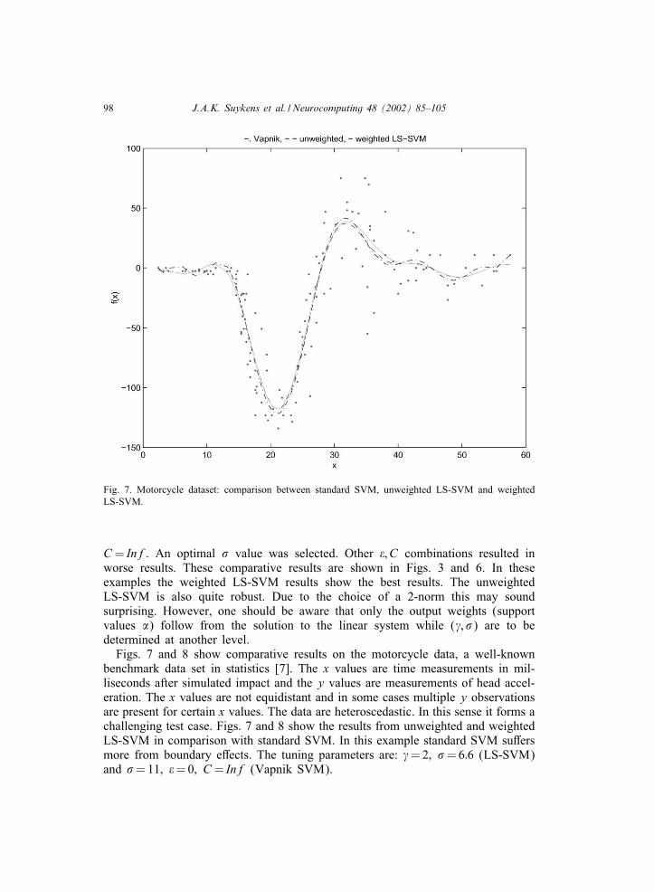
Fig. 7. Motorcycle dataset: comparison between standard SVM, unweighted LS-SVM and weightedLS-SVM.

C= Inf. An optimal � value was selected. Other &; C combinations resulted inworse results. These comparative results are shown in Figs. 3 and 6. In theseexamples the weighted LS-SVM results show the best results. The unweightedLS-SVM is also quite robust. Due to the choice of a 2-norm this may soundsurprising. However, one should be aware that only the output weights (supportvalues �) follow from the solution to the linear system while ( ; �) are to bedetermined at another level.Figs. 7 and 8 show comparative results on the motorcycle data, a well-known

benchmark data set in statistics [7]. The x values are time measurements in mil-liseconds after simulated impact and the y values are measurements of head accel-eration. The x values are not equidistant and in some cases multiple y observationsare present for certain x values. The data are heteroscedastic. In this sense it forms achallenging test case. Figs. 7 and 8 show the results from unweighted and weightedLS-SVM in comparison with standard SVM. In this example standard SVM suMersmore from boundary eMects. The tuning parameters are: =2; �=6:6 (LS-SVM)and �=11; &=0; C= Inf (Vapnik SVM).


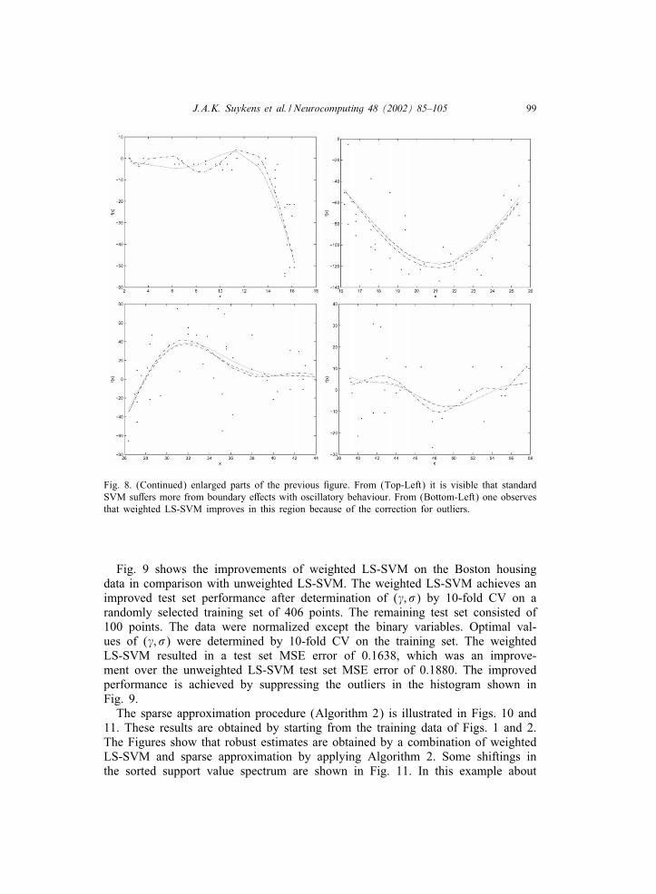
Fig. 8. (Continued) enlarged parts of the previous Egure. From (Top-Left) it is visible that standardSVM suMers more from boundary eMects with oscillatory behaviour. From (Bottom-Left) one observesthat weighted LS-SVM improves in this region because of the correction for outliers.

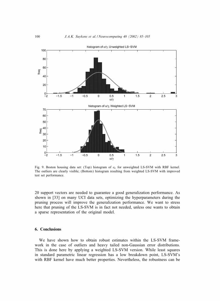
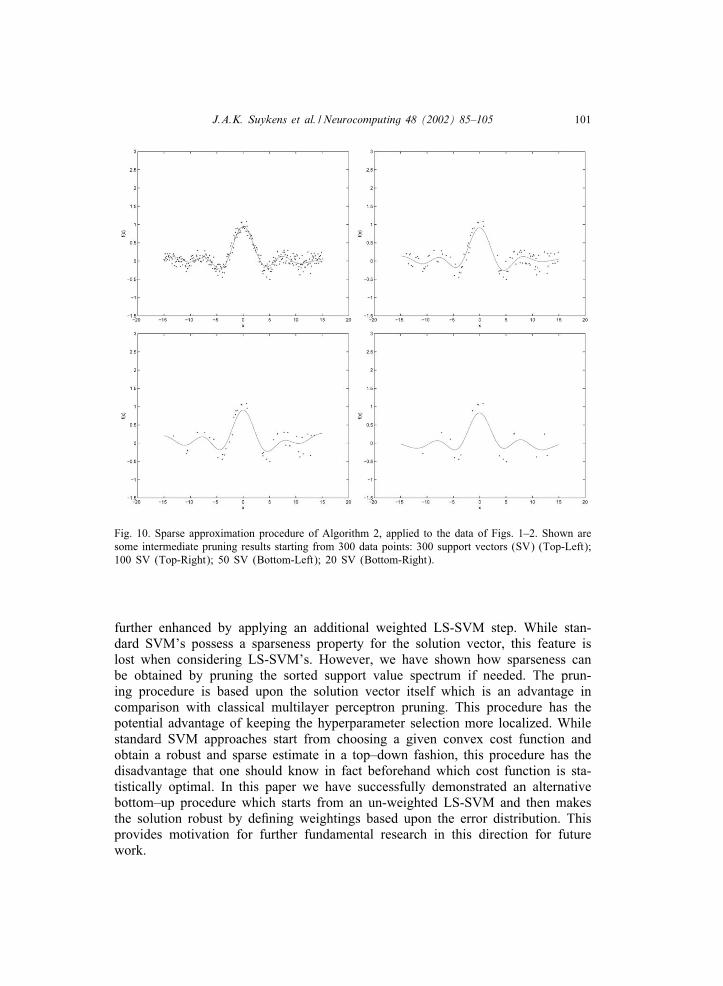
Fig. 9 shows the improvements of weighted LS-SVM on the Boston housingdata in comparison with unweighted LS-SVM. The weighted LS-SVM achieves animproved test set performance after determination of ( ; �) by 10-fold CV on arandomly selected training set of 406 points. The remaining test set consisted of100 points. The data were normalized except the binary variables. Optimal val-ues of ( ; �) were determined by 10-fold CV on the training set. The weightedLS-SVM resulted in a test set MSE error of 0.1638, which was an improve-ment over the unweighted LS-SVM test set MSE error of 0.1880. The improvedperformance is achieved by suppressing the outliers in the histogram shown inFig. 9.The sparse approximation procedure (Algorithm 2) is illustrated in Figs. 10 and

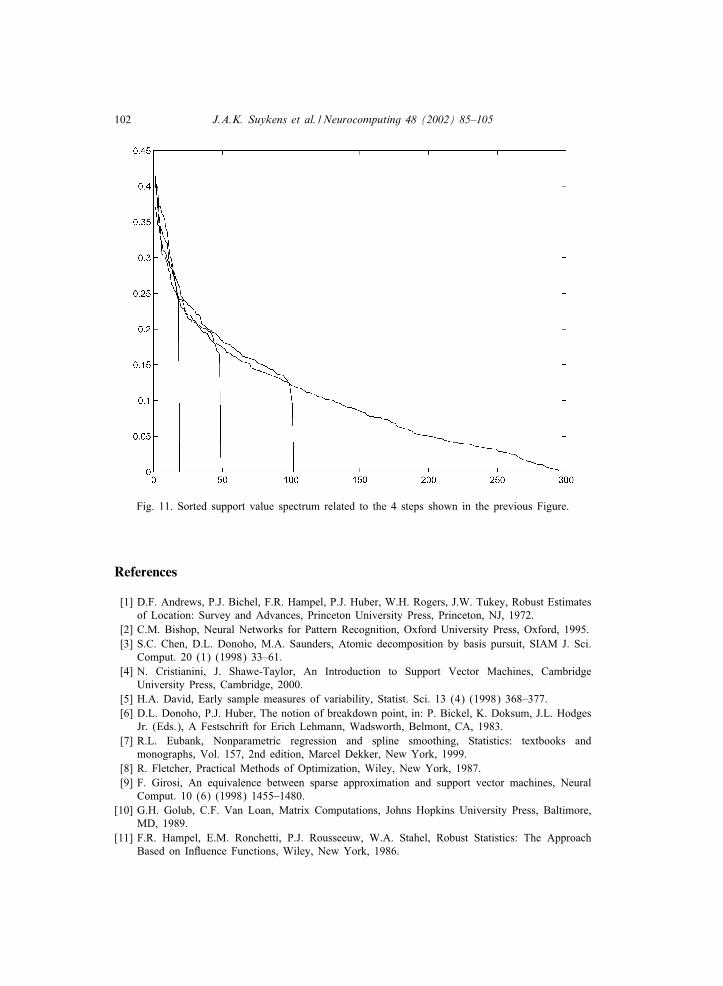
11. These results are obtained by starting from the training data of Figs. 1 and 2.The Figures show that robust estimates are obtained by a combination of weightedLS-SVM and sparse approximation by applying Algorithm 2. Some shiftings inthe sorted support value spectrum are shown in Fig. 11. In this example about


Fig. 9. Boston housing data set: (Top) histogram of ek for unweighted LS-SVM with RBF kernel.The outliers are clearly visible; (Bottom) histogram resulting from weighted LS-SVM with improvedtest set performance.

20 support vectors are needed to guarantee a good generalization performance. Asshown in [33] on many UCI data sets, optimizing the hyperparameters during thepruning process will improve the generalization performance. We want to stresshere that pruning of the LS-SVM is in fact not needed, unless one wants to obtaina sparse representation of the original model.

6. Conclusions

We have shown how to obtain robust estimates within the LS-SVM frame-work in the case of outliers and heavy tailed non-Gaussian error distributions.This is done here by applying a weighted LS-SVM version. While least squaresin standard parametric linear regression has a low breakdown point, LS-SVM’swith RBF kernel have much better properties. Nevertheless, the robustness can be


Fig. 10. Sparse approximation procedure of Algorithm 2, applied to the data of Figs. 1–2. Shown aresome intermediate pruning results starting from 300 data points: 300 support vectors (SV) (Top-Left);100 SV (Top-Right); 50 SV (Bottom-Left); 20 SV (Bottom-Right).

further enhanced by applying an additional weighted LS-SVM step. While stan-dard SVM’s possess a sparseness property for the solution vector, this feature islost when considering LS-SVM’s. However, we have shown how sparseness canbe obtained by pruning the sorted support value spectrum if needed. The prun-ing procedure is based upon the solution vector itself which is an advantage incomparison with classical multilayer perceptron pruning. This procedure has thepotential advantage of keeping the hyperparameter selection more localized. Whilestandard SVM approaches start from choosing a given convex cost function andobtain a robust and sparse estimate in a top–down fashion, this procedure has thedisadvantage that one should know in fact beforehand which cost function is sta-tistically optimal. In this paper we have successfully demonstrated an alternativebottom–up procedure which starts from an un-weighted LS-SVM and then makesthe solution robust by deEning weightings based upon the error distribution. Thisprovides motivation for further fundamental research in this direction for futurework.


Fig. 11. Sorted support value spectrum related to the 4 steps shown in the previous Figure.

References

[1] D.F. Andrews, P.J. Bichel, F.R. Hampel, P.J. Huber, W.H. Rogers, J.W. Tukey, Robust Estimatesof Location: Survey and Advances, Princeton University Press, Princeton, NJ, 1972.

[2] C.M. Bishop, Neural Networks for Pattern Recognition, Oxford University Press, Oxford, 1995.[3] S.C. Chen, D.L. Donoho, M.A. Saunders, Atomic decomposition by basis pursuit, SIAM J. Sci.

Comput. 20 (1) (1998) 33–61.[4] N. Cristianini, J. Shawe-Taylor, An Introduction to Support Vector Machines, Cambridge

University Press, Cambridge, 2000.[5] H.A. David, Early sample measures of variability, Statist. Sci. 13 (4) (1998) 368–377.[6] D.L. Donoho, P.J. Huber, The notion of breakdown point, in: P. Bickel, K. Doksum, J.L. Hodges

Jr. (Eds.), A Festschrift for Erich Lehmann, Wadsworth, Belmont, CA, 1983.[7] R.L. Eubank, Nonparametric regression and spline smoothing, Statistics: textbooks and

monographs, Vol. 157, 2nd edition, Marcel Dekker, New York, 1999.[8] R. Fletcher, Practical Methods of Optimization, Wiley, New York, 1987.[9] F. Girosi, An equivalence between sparse approximation and support vector machines, Neural

Comput. 10 (6) (1998) 1455–1480.[10] G.H. Golub, C.F. Van Loan, Matrix Computations, Johns Hopkins University Press, Baltimore,

MD, 1989.[11] F.R. Hampel, E.M. Ronchetti, P.J. Rousseeuw, W.A. Stahel, Robust Statistics: The Approach

Based on InPuence Functions, Wiley, New York, 1986.


[12] B. Hassibi, D.G. Stork, Second order derivatives for network pruning: optimal brain surgeon,in: S. Hanson, J. Cowan, L. Giles (Eds.), Advances in Neural Information Processing Systems,Vol. 5, Morgan Kaufmann, San Mateo, CA, 1993, pp. 164–171.

[13] K. Hornik, M. Stinchcombe, H. White, Multilayer feedforward networks are universalapproximators, Neural Networks 2 (1989) 359–366.

[14] P.J. Huber, Robust Statistics, Wiley, New York, 1981.[15] N.L. Johnson, S. Kotz, Distributions in Statistics: Continuous Univariate Distributions, Vol. 1–2,

Wiley, New York, 1970.[16] Y. Le Cun, J.S. Denker, S.A. Solla, Optimal brain damage, in: Touretzky (Ed.), Advances

in Neural Information Processing Systems, Vol. 2, Morgan Kaufmann, San Mateo, CA, 1990,pp. 598–605.

[17] T. Poggio, F. Girosi, Networks for approximation and learning, Proc. IEEE 78 (9) (1990)1481–1497.

[18] P.J. Rousseeuw, A. Leroy, Robust Regression and Outlier Detection, Wiley, New York, 1987.[19] P.J. Rousseeuw, B.C. van Zomeren, Unmasking multivariate outliers and leverage points, J. Am.

Statist. Assoc. 85 (1990) 633–639.[20] C. Saunders, A. Gammerman. V. Vovk, Ridge regression learning algorithm in dual variables,

Proceedings of the 15th International Conference on Machine Learning (ICML’98), MorganKaufmann, 1998, pp. 515–521.

[21] B. SchVolkopf, K.-K. Sung, C. Burges, F. Girosi, P. Niyogi, T. Poggio, V. Vapnik, Comparingsupport vector machines with Gaussian kernels to radial basis function classiEers, IEEE Trans.Signal Process. 45 (11) (1997) 2758–2765.

[22] B. SchVolkopf, C. Burges, A. Smola (Eds.), Advances in Kernel Methods—Support VectorLearning, MIT Press, Cambridge, MA, 1998.

[23] B. SchVolkopf, S. Mika, C. Burges, P. Knirsch, K.-R. MVuller, G. RVatsch, A. Smola, Input space vs.feature space in kernel-based methods, IEEE Trans. Neural Networks 10 (5) (1999) 1000–1017.

[24] A. Smola, B. SchVolkopf, K.-R. MVuller, The connection between regularization operators andsupport vector kernels, Neural Networks 11 (1998) 637–649.

[25] A. Smola, B. SchVolkopf, On a kernel-based method for pattern recognition, regression,approximation and operator inversion, Algorithmica 22 (1998) 211–231.

[26] A. Smola, Learning with Kernels, Ph.D. Thesis, GMD, Birlinghoven, 1999.[27] J.A.K. Suykens, J. Vandewalle (Eds.), Nonlinear Modeling: Advanced Black-box Techniques,

Kluwer Academic Publishers, Boston, 1998.[28] J.A.K. Suykens, J. Vandewalle, Least squares support vector machine classiEers, Neural Process.

Lett. 9 (3) (1999) 293–300.[29] J.A.K. Suykens, L. Lukas, P. Van Dooren, B. De Moor, J. Vandewalle, Least squares support

vector machine classiEers: a large scale algorithm, European Conference on Circuit Theory andDesign, (ECCTD’99), PP. 839–842, Stresa Italy, August 1999.

[30] J.A.K. Suykens, L. Lukas, J. Vandewalle, Sparse least squares support vector machine classiEers,European Symposium on ArtiEcial Neural Networks (ESANN 2000), Bruges Belgium, April 2000,pp. 37–42.

[31] J.A.K. Suykens, J. Vandewalle, Recurrent least squares support vector machines, IEEE Trans.Circuits Systems-I 47 (7) (2000) 1109–1114.

[32] J.A.K. Suykens, J. Vandewalle, B. De Moor, Optimal Control by Least Squares Support VectorMachines, Neural Networks 14 (1) (2001) 23–35.

[33] T. Van Gestel, J.A.K. Suykens, B. Baesens, S. Viaene, J. Vanthienen, G. Dedene, B. De Moor,J. Vandewalle, Benchmarking least squares support vector machine classiEers, Internal Report00-37, ESAT-SISTA, K.U.Leuven.

[34] T. Van Gestel, J.A.K. Suykens, D. Baestaens, A. Lambrechts, G. Lanckriet, B. Vandaele, B. DeMoor, J. Vandewalle, Financial time series prediction using least squares support vector machineswithin the evidence framework, IEEE Trans. Neural Networks (special issue on Neural Networksin Financial Engineering) 12 (4) (2001) 809–821.

[35] V. Vapnik, The Nature of Statistical Learning Theory, Springer, New York, 1995.[36] V. Vapnik, Statistical Learning Theory, Wiley, New York, 1998.


Johan A.K. Suykens was born in Willebroek Belgium, May 18,1966. He re-ceived the degree in Electro-Mechanical Engineering and the Ph.D. degree inApplied Sciences from the Katholieke Universiteit Leuven, in 1989 and 1995,respectively. In 1996 he was a Visiting Postdoctoral Researcher at the Uni-versity of California, Berkeley. At present, he is a Postdoctoral Researcherwith the Fund for ScientiEc Research FWO Flanders. His research interestsare mainly in the areas of the theory and application of nonlinear systems andneural networks. He is author of the book “ArtiEcial Neural Networks for Mod-elling and Control of Non-linear Systems” and editor of the book “NonlinearModeling: Advanced Black-Box Techniques”, published by Kluwer AcademicPublishers. The latter resulted from an International Workshop on Nonlinear

Modelling with Time-series Prediction Competition that he organized in 1998. He has served asassociate editor for the IEEE Transactions on Circuits and Systems-I (1997–1999) and since 1998 heis serving as associate editor for the IEEE Transactions on Neural Networks. He received a Best PaperAward as Winner for Best Theoretical Developments in Computational Intelligence at ANNIE’99 andan IEEE Signal Processing Society 1999 Best Paper Award, for his contributions on NLq Theory. Heis a recipient of the International Neural Networks Society INNS 2000 Young Investigator Award forsigniEcant contributions in the Eeld of neural networks.

Jos De Brabanter received the diploma of Ind. Ing. (Brussels, Belgium) in1990, the Master degree in ArtiEcial Intelligence in 1996 and the Masterdegree of Statistics in 1997, both from the K.U. Leuven (Belgium). He iscurrently pursuing the Doctoral degree in Applied Sciences at the Departmentof Electrical Engineering of the K.U. Leuven. His scientiEc research interestsare in the area of statistics and its application to neural networks and supportvector learning.

Lukas received the B.Eng. degree in Computer Engineering in 1995 from theInstitute of Technology, Bandung (ITB), Indonesia, and the Master degree inArtiEcial Intelligence from the K.U. Leuven, Belgium in 1998. He is currentlypursuing the Doctoral degree at the Department of Electrical Engineering at theK.U. Leuven. His research interests are in the area of support vector machines,biomedical engineering and artiEcial intelligence.

Joos Vandewalle was born in Kortrijk, Belgium, in August 1948. He obtainedthe electrical engineering degree and doctoral degree in applied sciences, bothfrom the Katholieke Universiteit Leuven, Belgium in 1971 and 1976, respec-tively. From 1976 to 1978 he was Research Associate and from July 1978to July 1979, he was Visiting Assistant Professor both at the University ofCalifornia, Berkeley. Since July 1979 he is back at the ESAT Laboratory ofthe Katholieke Universiteit Leuven, Belgium, where he is Full Professor since1986. He is an Academic Consultant since 1984 at the VSDM group of IMEC(Interuniversity Microelectronics Center, Leuven). From August 1996 to Au-gust 1999 he was Chairman of the Department of Electrical Engineering atthe Katholieke Universiteit Leuven. Since August 1999 he is the vice-deanof the Department of Engineering. He teaches courses in linear algebra, linear


and nonlinear systems and circuit theory, signal processing and neural networks. His research interestsare mainly in mathematical system theory and its applications in circuit theory, control, signal pro-cessing, cryptography and neural networks. He has authored and co-authored more than 200 papersin these areas. He is co-author with S. Van HuMel of the book “The Total Least Squares Problem”and co-editor with T. Roska of the book “Cellular Neural Networks”. He is a member of the editorialboard of “Journal A”, a Quarterly Journal of Automatic Control and of the International Journal ofCircuit Theory and its Applications, Neurocomputing and the Journal of Circuit Systems and Comput-ers. From 1989 till 1991, he was associate editor at the IEEE Transactions on Circuits and Systems inthe area of nonlinear and neural networks. He was elected fellow of IEEE in 1992 for contributionsto nonlinear circuits and systems. During 1991-1992 he held the Francqui chair of ArtiEcial NeuralNetworks at the University of LiZege, Belgium. He is one of the three coordinators of the Interdisci-plinary Center for Neural Networks ICNN that was set up in 1993 in order to stimulate the interactionand cooperation among the 50 researchers on neural networks at the Katholieke Universiteit Leuven.

Documents

Weighted least squares support vector machines: robustness and sparse approximation