A parallel algorithm to approximate inverse factors of a matrix via sparse–sparse iterations

Applied Mathematics and Computation 181 (2006) 782–792

www.elsevier.com/locate/amc

A parallel algorithm to approximate inverse factorsof a matrix via sparse–sparse iterations

Davod Khojasteh Salkuyeh a,*, Saeed Karimi b, Faezeh Toutounian c

a Department of Mathematics, Mohaghegh Ardabili University, P.O. Box 56199-11367, Ardabil, Iranb Department of Mathematics, Persian Gulf University, Boushehr, Iran

c School of Mathematical Sciences, Ferdowsi University of Mashhad, P.O. Box 1159-91775, Mashhad, Iran

Abstract

In [D.K. Salkuyeh, F. Toutounian, A block version algorithm to approximate inverse factors, Appl. Math. Comput.,162 (2005) 1499–1509], the authors proposed the BAIB algorithm to approximate inverse factors of a matrix. In this papera parallel version of the BAIB algorithm is presented. In this method the BAIB algorithm is combined with computing thesparse approximate solution of a sparse linear system by sparse–sparse iterations. The new method does not require thatthe sparsity pattern be known in advance. Some numerical experiments on test matrices from Harwell–Boeing collectionare presented to show the efficiency of the new method and comparing to the AIB algorithm.� 2006 Elsevier Inc. All rights reserved.

Keywords: Inverse factors; Preconditioning; Krylov subspace methods; Sparse matrices; AIB algorithm; BAIB algorithm; Parallel

1. Introduction

The problem of finding the solution vector x of a linear system of equations

0096-3

doi:10

* CoE-m

Ax ¼ b; ð1Þ
where A 2 Rn�n is large, sparse and x, b 2 Rn, arises in many application areas. Iterative methods which com-bine preconditioning techniques are among the most efficient techniques for solving (1). More precisely, iter-ative methods usually involve a second matrix that transforms the coefficient matrix into one with a morefavorable spectrum. The transformation matrix is called a preconditioner. Without a preconditioner, an iter-ative method may have a poor convergence or even fail to converge. Approximate inverse techniques can bemainly divided into two categories. In the first category, a nonsingular matrix M is computed such thatM � A�1 in some sense. In this case the transformed linear system
AMy ¼ b; x ¼ My; or MAx ¼ Mb ð2Þ

003/$ - see front matter � 2006 Elsevier Inc. All rights reserved.

.1016/j.amc.2006.02.006

rresponding author.ail addresses: [email protected] (D.K. Salkuyeh), [email protected] (S. Karimi), [email protected] (F. Toutounian).

mailto:[email protected]



D.K. Salkuyeh et al. / Applied Mathematics and Computation 181 (2006) 782–792 783

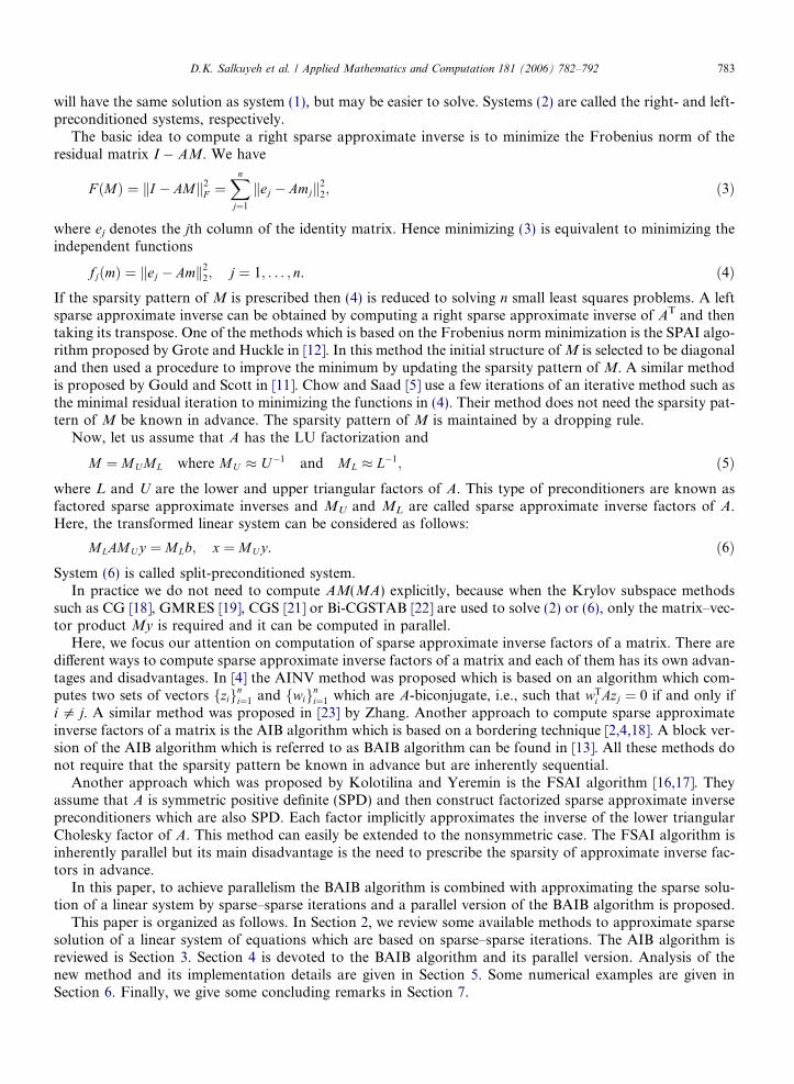
will have the same solution as system (1), but may be easier to solve. Systems (2) are called the right- and left-preconditioned systems, respectively.

The basic idea to compute a right sparse approximate inverse is to minimize the Frobenius norm of theresidual matrix I � AM. We have

F ðMÞ ¼ kI � AMk2F ¼

Xn

j¼1

kej � Amjk22; ð3Þ

where ej denotes the jth column of the identity matrix. Hence minimizing (3) is equivalent to minimizing theindependent functions

fjðmÞ ¼ kej � Amk22; j ¼ 1; . . . ; n. ð4Þ

If the sparsity pattern of M is prescribed then (4) is reduced to solving n small least squares problems. A leftsparse approximate inverse can be obtained by computing a right sparse approximate inverse of AT and thentaking its transpose. One of the methods which is based on the Frobenius norm minimization is the SPAI algo-rithm proposed by Grote and Huckle in [12]. In this method the initial structure of M is selected to be diagonaland then used a procedure to improve the minimum by updating the sparsity pattern of M. A similar methodis proposed by Gould and Scott in [11]. Chow and Saad [5] use a few iterations of an iterative method such asthe minimal residual iteration to minimizing the functions in (4). Their method does not need the sparsity pat-tern of M be known in advance. The sparsity pattern of M is maintained by a dropping rule.

Now, let us assume that A has the LU factorization and

M ¼ MU ML where MU � U�1 and ML � L�1; ð5Þ
where L and U are the lower and upper triangular factors of A. This type of preconditioners are known asfactored sparse approximate inverses and MU and ML are called sparse approximate inverse factors of A.Here, the transformed linear system can be considered as follows:
MLAMU y ¼ MLb; x ¼ MU y. ð6Þ
System (6) is called split-preconditioned system.
In practice we do not need to compute AM(MA) explicitly, because when the Krylov subspace methodssuch as CG [18], GMRES [19], CGS [21] or Bi-CGSTAB [22] are used to solve (2) or (6), only the matrix–vec-tor product My is required and it can be computed in parallel.

Here, we focus our attention on computation of sparse approximate inverse factors of a matrix. There aredifferent ways to compute sparse approximate inverse factors of a matrix and each of them has its own advan-tages and disadvantages. In [4] the AINV method was proposed which is based on an algorithm which com-putes two sets of vectors fzign

i¼1 and fwigni¼1 which are A-biconjugate, i.e., such that wT

i Azj ¼ 0 if and only ifi 5 j. A similar method was proposed in [23] by Zhang. Another approach to compute sparse approximateinverse factors of a matrix is the AIB algorithm which is based on a bordering technique [2,4,18]. A block ver-sion of the AIB algorithm which is referred to as BAIB algorithm can be found in [13]. All these methods donot require that the sparsity pattern be known in advance but are inherently sequential.

Another approach which was proposed by Kolotilina and Yeremin is the FSAI algorithm [16,17]. Theyassume that A is symmetric positive definite (SPD) and then construct factorized sparse approximate inversepreconditioners which are also SPD. Each factor implicitly approximates the inverse of the lower triangularCholesky factor of A. This method can easily be extended to the nonsymmetric case. The FSAI algorithm isinherently parallel but its main disadvantage is the need to prescribe the sparsity of approximate inverse fac-tors in advance.

In this paper, to achieve parallelism the BAIB algorithm is combined with approximating the sparse solu-tion of a linear system by sparse–sparse iterations and a parallel version of the BAIB algorithm is proposed.

This paper is organized as follows. In Section 2, we review some available methods to approximate sparsesolution of a linear system of equations which are based on sparse–sparse iterations. The AIB algorithm isreviewed is Section 3. Section 4 is devoted to the BAIB algorithm and its parallel version. Analysis of thenew method and its implementation details are given in Section 5. Some numerical examples are given inSection 6. Finally, we give some concluding remarks in Section 7.

784 D.K. Salkuyeh et al. / Applied Mathematics and Computation 181 (2006) 782–792

2. Sparse approximate solution to Ax = b

In this section, we review some available techniques to compute sparse approximate solution to Ax = b.When the nonzero pattern of x is fixed in advance, the computation of x can be accomplished as follows.The nonzero pattern of x is a subset J � fij1 6 i 6 ng such that xi = 0 if i 62 J. Now a sparse vector m iscomputed as the solution of the following constrained minimization problem:

minm2Skb� Amk2; ð7Þ

where S is the set of vectors with nonzero pattern J. The vector m can be considered as an sparse approx-imation of the vector x. Let bA ¼ AðJÞ be the submatrix of A with column indices in J and m̂ ¼ mðJÞ. Thenthe nonzero entries of m can be computed by solving the unconstrained least squares problem

minm̂kb� bAm̂k2. ð8Þ

In our context vector b is also very sparse. Hence many rows of this least squares problem are zero and can bedeleted. Therefore the least squares problem (8) is extremely small and can be solved by means of the QR fac-torization of bA. For more details see [12].

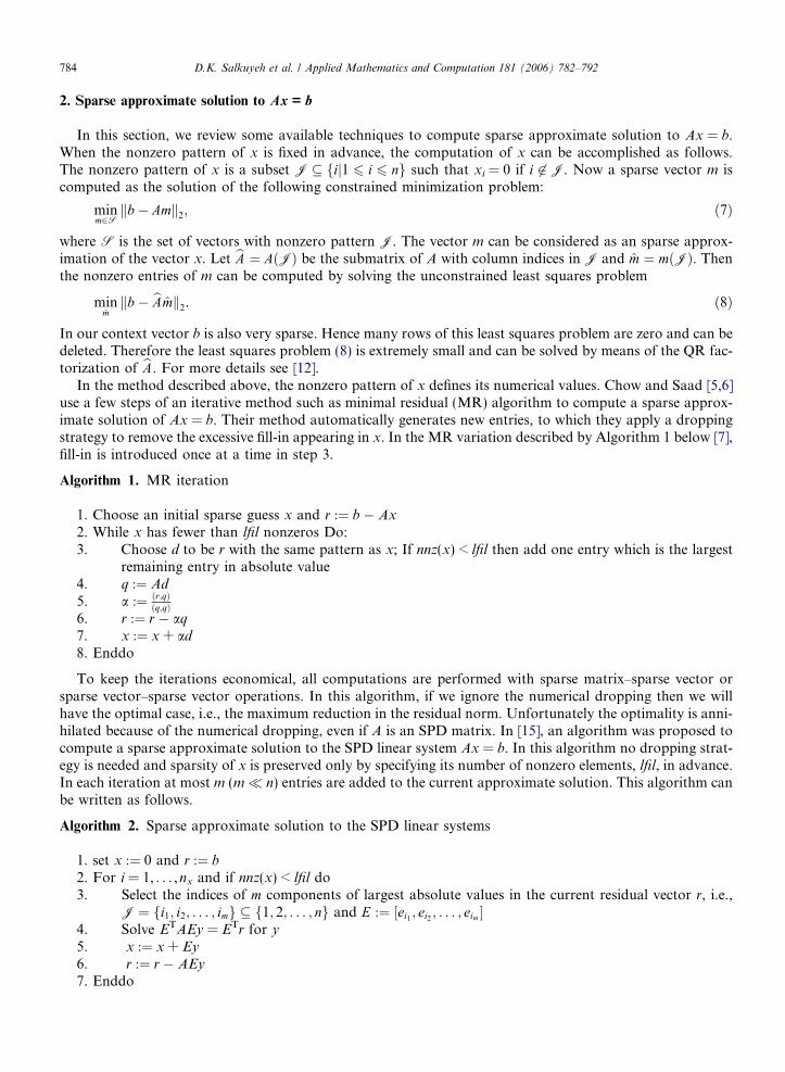
In the method described above, the nonzero pattern of x defines its numerical values. Chow and Saad [5,6]use a few steps of an iterative method such as minimal residual (MR) algorithm to compute a sparse approx-imate solution of Ax = b. Their method automatically generates new entries, to which they apply a droppingstrategy to remove the excessive fill-in appearing in x. In the MR variation described by Algorithm 1 below [7],fill-in is introduced once at a time in step 3.

Algorithm 1. MR iteration

1. Choose an initial sparse guess x and r :¼ b � Ax

2. While x has fewer than lfil nonzeros Do:3. Choose d to be r with the same pattern as x; If nnz(x) < lfil then add one entry which is the largest

remaining entry in absolute value4. q :¼ Ad

5. a :¼ ðr;qÞðq;qÞ

6. r :¼ r � aq

7. x :¼ x + ad

8. Enddo

To keep the iterations economical, all computations are performed with sparse matrix–sparse vector orsparse vector–sparse vector operations. In this algorithm, if we ignore the numerical dropping then we willhave the optimal case, i.e., the maximum reduction in the residual norm. Unfortunately the optimality is anni-hilated because of the numerical dropping, even if A is an SPD matrix. In [15], an algorithm was proposed tocompute a sparse approximate solution to the SPD linear system Ax = b. In this algorithm no dropping strat-egy is needed and sparsity of x is preserved only by specifying its number of nonzero elements, lfil, in advance.In each iteration at most m (m� n) entries are added to the current approximate solution. This algorithm canbe written as follows.

Algorithm 2. Sparse approximate solution to the SPD linear systems

1. set x :¼ 0 and r :¼ b

2. For i = 1, . . . ,nx and if nnz(x) < lfil do3. Select the indices of m components of largest absolute values in the current residual vector r, i.e.,

J ¼ fi1; i2; . . . ; img � f1; 2; . . . ; ng and E :¼ ½ei1 ; ei2 ; . . . ; eim �4. Solve ETAEy = ETr for y

5. x :¼ x + Ey

6. r :¼ r � AEy7. Enddo


In step 3 of this algorithm eij denotes the ij column of the identity matrix. Here we note that the matrixS = ETAE is an SPD matrix of dimension m and is the principal submatrix of matrix A consisting of the rowsand columns of A with indices in J. Vector x computed by this algorithm has at most lfil nonzero entries. Inpractical implementation of the algorithm the number m is usually chosen to be very small, for example m = 1,2 or 3. The number nx is taken somewhat greater than lfil because it is possible an entry of x improves severaltimes and may contain very few nonzero elements. It has been shown that [15] this algorithm is more effectivethan Algorithm 1 in the case that matrix A is SPD. In the case that m = 1 the algorithm was investigated in[14].

3. The AIB algorithm

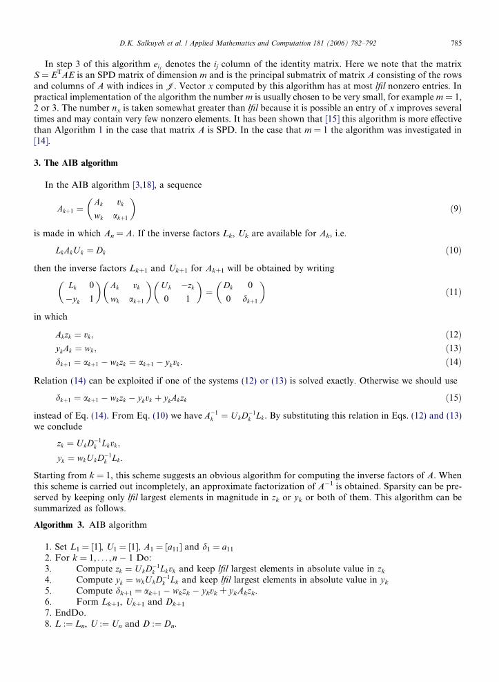
In the AIB algorithm [3,18], a sequence

Akþ1 ¼Ak vk

wk akþ1

� �ð9Þ

is made in which An = A. If the inverse factors Lk, Uk are available for Ak, i.e.

LkAkUk ¼ Dk ð10Þ

then the inverse factors Lk+1 and Uk+1 for Ak+1 will be obtained by writing

Lk 0

�yk 1

� �Ak vk

wk akþ1

� �Uk �zk

0 1

� �¼

Dk 0

0 dkþ1

� �ð11Þ

in which

Akzk ¼ vk; ð12ÞykAk ¼ wk; ð13Þdkþ1 ¼ akþ1 � wkzk ¼ akþ1 � ykvk. ð14Þ

Relation (14) can be exploited if one of the systems (12) or (13) is solved exactly. Otherwise we should use

dkþ1 ¼ akþ1 � wkzk � ykvk þ ykAkzk ð15Þ

instead of Eq. (14). From Eq. (10) we have A�1k ¼ UkD�1

k Lk. By substituting this relation in Eqs. (12) and (13)we conclude

zk ¼ UkD�1k Lkvk;

yk ¼ wkU kD�1k Lk.

Starting from k = 1, this scheme suggests an obvious algorithm for computing the inverse factors of A. Whenthis scheme is carried out incompletely, an approximate factorization of A�1 is obtained. Sparsity can be pre-served by keeping only lfil largest elements in magnitude in zk or yk or both of them. This algorithm can besummarized as follows.

Algorithm 3. AIB algorithm

1. Set L1 = [1], U1 = [1], A1 = [a11] and d1 = a11

2. For k = 1, . . . ,n � 1 Do:3. Compute zk ¼ U kD�1

k Lkvk and keep lfil largest elements in absolute value in zk

4. Compute yk ¼ wkU kD�1k Lk and keep lfil largest elements in absolute value in yk

5. Compute dk+1 = ak+1 � wkzk � ykvk + ykAkzk.6. Form Lk+1, Uk+1 and Dk+1

7. EndDo.8. L :¼ Ln, U :¼ Un and D :¼ Dn.


This algorithm returns L and U and we have LAU � D. If A is symmetric, L = UT and work is halved. Fur-thermore, if A is SPD, then it can be shown that [11], in exact arithmetic, dk > 0 for all k. Therefore, AIB algo-rithm will not breakdown.

4. A parallel implementation of the BAIB algorithm

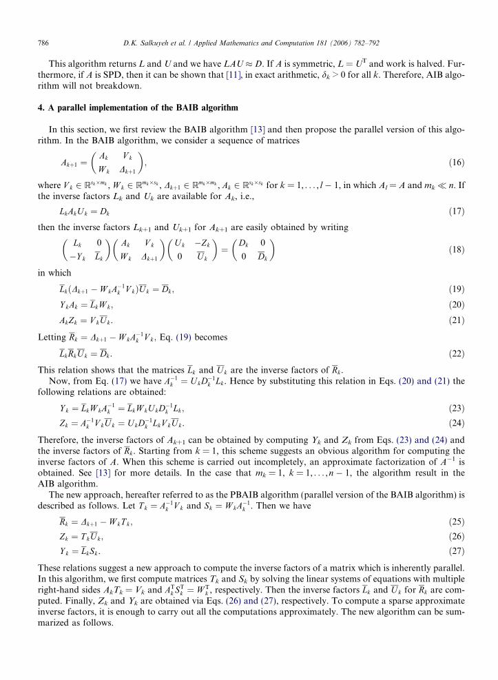
In this section, we first review the BAIB algorithm [13] and then propose the parallel version of this algo-rithm. In the BAIB algorithm, we consider a sequence of matrices

Akþ1 ¼Ak V k

W k Dkþ1

� �; ð16Þ

where V k 2 Rsk�mk , W k 2 Rmk�sk , Dkþ1 2 Rmk�mk , Ak 2 Rsk�sk for k = 1, . . . , l � 1, in which Al = A and mk� n. Ifthe inverse factors Lk and Uk are available for Ak, i.e.,

LkAkU k ¼ Dk ð17Þ
then the inverse factors Lk+1 and Uk+1 for Ak+1 are easily obtained by writing
Lk 0

�Y k Lk

� �Ak V k

W k Dkþ1

� �U k �Zk

0 Uk

� �¼

Dk 0

0 Dk

� �ð18Þ

in which

LkðDkþ1 � W kA�1k V kÞUk ¼ Dk; ð19Þ

Y kAk ¼ LkW k; ð20ÞAkZk ¼ V kUk. ð21Þ

Letting Rk ¼ Dkþ1 � W kA�1k V k; Eq. (19) becomes

LkRkU k ¼ Dk. ð22Þ

This relation shows that the matrices Lk and U k are the inverse factors of Rk.Now, from Eq. (17) we have A�1

k ¼ U kD�1k Lk. Hence by substituting this relation in Eqs. (20) and (21) the

following relations are obtained:

Y k ¼ LkW kA�1k ¼ LkW kU kD�1

k Lk; ð23ÞZk ¼ A�1

k V kU k ¼ U kD�1k LkV kUk. ð24Þ

Therefore, the inverse factors of Ak+1 can be obtained by computing Yk and Zk from Eqs. (23) and (24) andthe inverse factors of Rk. Starting from k = 1, this scheme suggests an obvious algorithm for computing theinverse factors of A. When this scheme is carried out incompletely, an approximate factorization of A�1 isobtained. See [13] for more details. In the case that mk = 1, k = 1, . . . ,n � 1, the algorithm result in theAIB algorithm.

The new approach, hereafter referred to as the PBAIB algorithm (parallel version of the BAIB algorithm) isdescribed as follows. Let T k ¼ A�1

k V k and Sk ¼ W kA�1k . Then we have

Rk ¼ Dkþ1 � W kT k; ð25ÞZk ¼ T kU k; ð26ÞY k ¼ LkSk. ð27Þ

These relations suggest a new approach to compute the inverse factors of a matrix which is inherently parallel.In this algorithm, we first compute matrices Tk and Sk by solving the linear systems of equations with multipleright-hand sides AkTk = Vk and AT

k STk ¼ W T

k , respectively. Then the inverse factors Lk and U k for Rk are com-puted. Finally, Zk and Yk are obtained via Eqs. (26) and (27), respectively. To compute a sparse approximateinverse factors, it is enough to carry out all the computations approximately. The new algorithm can be sum-marized as follows.


Algorithm 4. PBAIB algorithm

1. Let A1 be the m1th leading principal submatrix of A. Compute L1, U1 and D1 such that L1A1U1 � D1

2. For k = 1, . . . , l � 1 Do (in parallel)3. Solve AkTk = Vk for Tk approximately4. Rk :¼ Dkþ1 � W kT k

5. Compute Lk and U k and Dk such that LkRkUk � Dk

6. Zk :¼ T kUk and apply numerical dropping to Zk

7. Solve ATk ST

k ¼ W Tk for ST

k approximately8. Y k :¼ LkSk and apply numerical dropping to Yk

9. EndDo

Some considerations can be posed for this algorithm. It is obvious that if A is symmetric then the work ishalved. In steps 1 and 5 of this algorithm, the computation of the inverse factors of A1 and Rk can be computedapproximately by the AIB algorithm. Here we note that in steps 3 and 7, two linear systems with multipleright-hand sides should be solved approximately and it can be carried out in parallel. Another point whichis mentioned here is the computation of matrix Tk. In fact, we do not need to store this matrix. After com-puting the ith column of Tk, the ith column of Rk is computed. Hence, it is enough to store the matrix Rk whichis of small size and use a temporary vector for computing the ith column of Tk.

5. Analysis and implementation details

In steps 3 and 7 of Algorithm 3 two linear systems with coefficient matrices Ai and ATi should be solved

approximately. Hence, we need the nonsingularity of all the leading principal submatrices of A. We first intro-duce the concept of an M-matrix. A = (aij) is called an M-matrix if aij 6 0 for all i 5 j, A is nonsingular andA�1 P 0. Let A be an M-matrix that is partitioned in block matrix form A = (Aij), where Aii’s are squarematrices. Then the matrices Aii on the diagonal of A are M-matrices [1]. Also, let A be an M-matrix that ispartitioned in two-by-two block form, i.e.

A ¼B E

F C

!; ð28Þ

where B is square matrix. Then the Schur complement

S ¼ C � FB�1E ð29Þ

exists and, itself is an M-matrix [1].Now, let A be an SPD matrix (M-matrix) and all steps of Algorithm 3 are done exactly. By definition Rk is

the Schur complement of Ak+1 and is an SPD matrix (M-matrix), since Ak+1 is a leading principal submatrix ofA and is an SPD (M-matrix). So Algorithm 2 will not break down.

In [13], for M-matrices, a strategy was proposed for approximating Rk that guarantees Algorithm 3 doesnot breakdown when it is done approximately.

In order to take advantage of the large number of zero entries of A, special schemes are required to storesparse matrices. The main goal is to preserve the nonzero elements. The common storage schemes are so-calledcompressed sparse row (CSR) or compressed sparse column (CSC) [20]. In the CSR format we create threearray: a real array A[nnz] and two integer arrays JA[nnz] and IA[n+1], where nnz is the number of non-zero entries in the matrix. Array A stores the nonzero entries of the matrix row by row from row 1 to n. ArrayJA stores the column indices of the entries in the array A. Finally, array IA stores the pointers to the beginningof each row in the arrays A, JA. The CSC format is identical with the CSR format except that the columns ofthe matrix are stored instead of the rows. In practical implementation of Algorithm 3 we must easily haveaccess to matrices Ai, i = 1, . . . ,n. This can be done if matrix A is stored in the skyline format described asfollows [20]. In this format, the following arrays are used: DIAG stores the diagonal of A, AL, JAL, IAL storethe strict lower part of matrix A in CSR format and AU, JAU, IAU store the strict upper part of matrix A in


CSC format. In the symmetric case we only need to store the lower triangular part of A. It can be easily seenthat if A is stored is the skyline format the matrices Ai can be extracted easily, moreover they are in they sky-line format.

To approximate the inverse factors of a matrix by using Algorithm 3 the following parameters are used:

• m: We let mk = m for k = 1, . . . ,k � 1.• lfil: We use lfil iterations of Algorithm 1 for solving the systems in steps 3 and 7.• innerlfil: In steps 1 and 5 of Algorithm 3 the inverse factors of A1 and Rk are computed by using AIB algo-

rithm (like PBAIB algorithm). Here we use the innerlfil iterations of Algorithm 1.

Table 1Test problems information and the number of iterations of unpreconditioned Bi-CGSTAB for convergence

Matrix n nnz Cond-Est Application Unp-Its

SHERMAN1 1000 3750 2.3e+04 Oil reservoir simulation 317SHERMAN3 5005 20,033 6.9e+16 Oil reservoir simulation �SHERMAN4 1104 3786 7.2e+03 Oil reservoir simulation 95SHERMAN5 3312 20,793 3.9e+05 Oil reservoir simulation 2014ADD20 2395 17,319 1.8e+04 Circuit modelling 244ADD32 4960 23,884 2.1e+02 Circuit modelling 43ORSIRR1 1030 6858 1.0e+02 Oil reservoir simulation 1293ORSIRR2 886 5970 1.7e+05 Oil reservoir simulation 1255HOR131 434 4710 1.3e+05 Flow network problem �JPWH991 991 6027 7.3e+02 Circuit physics modelling 33WATT1 1856 11,360 5.4e+09 Petroleum engineering 155WATT2 1856 11,550 1.4e+12 Petroleum engineering �STEAM2 600 13,760 3.5e+06 Enhanced oil recovery 82SAYLR1 238 1128 1.6e+09 Oil reservoir simulation �SAYLR3 1000 3750 1.0e+02 Oil reservoir simulation 283MEMPLUS 17,758 126,150 Not available Circuit modelling 979PDE900 900 4380 2.9e+02 Partial differential equation 76PDE2961 2961 14,585 9.5e+02 Partial differential equation 140

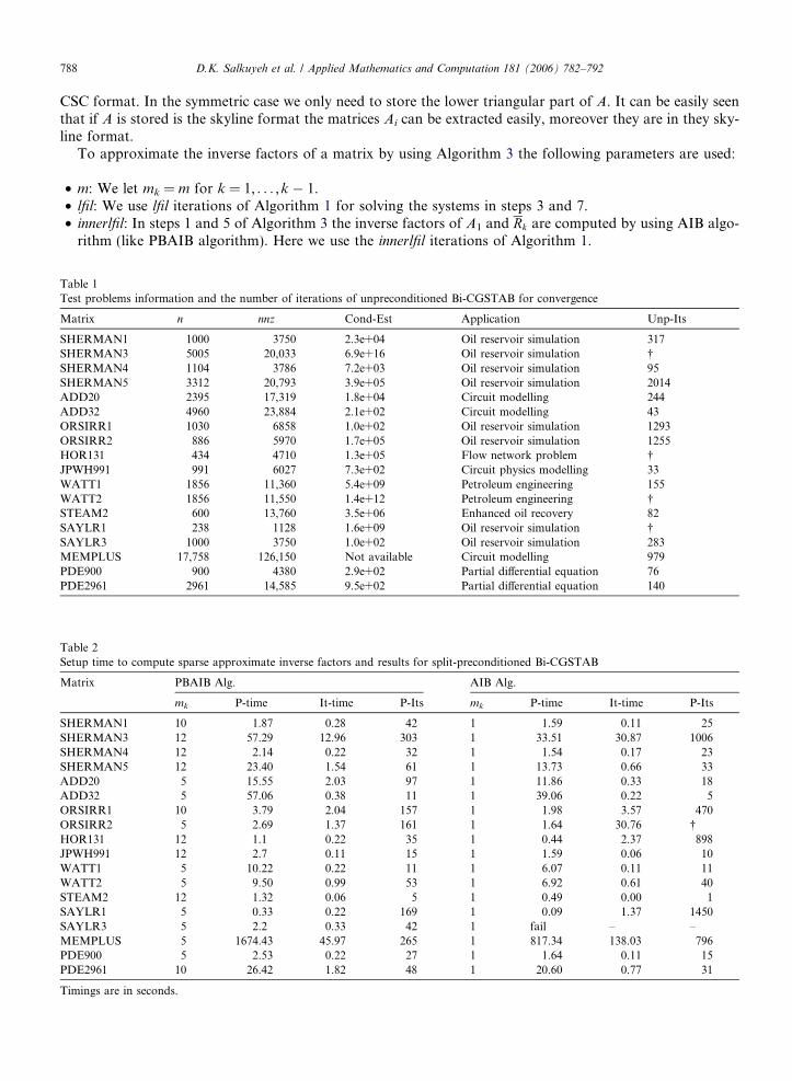
Table 2Setup time to compute sparse approximate inverse factors and results for split-preconditioned Bi-CGSTAB

Matrix PBAIB Alg. AIB Alg.

mk P-time It-time P-Its mk P-time It-time P-Its

SHERMAN1 10 1.87 0.28 42 1 1.59 0.11 25SHERMAN3 12 57.29 12.96 303 1 33.51 30.87 1006SHERMAN4 12 2.14 0.22 32 1 1.54 0.17 23SHERMAN5 12 23.40 1.54 61 1 13.73 0.66 33ADD20 5 15.55 2.03 97 1 11.86 0.33 18ADD32 5 57.06 0.38 11 1 39.06 0.22 5ORSIRR1 10 3.79 2.04 157 1 1.98 3.57 470ORSIRR2 5 2.69 1.37 161 1 1.64 30.76 �HOR131 12 1.1 0.22 35 1 0.44 2.37 898JPWH991 12 2.7 0.11 15 1 1.59 0.06 10WATT1 5 10.22 0.22 11 1 6.07 0.11 11WATT2 5 9.50 0.99 53 1 6.92 0.61 40STEAM2 12 1.32 0.06 5 1 0.49 0.00 1SAYLR1 5 0.33 0.22 169 1 0.09 1.37 1450SAYLR3 5 2.2 0.33 42 1 fail – –MEMPLUS 5 1674.43 45.97 265 1 817.34 138.03 796PDE900 5 2.53 0.22 27 1 1.64 0.11 15PDE2961 10 26.42 1.82 48 1 20.60 0.77 31

Timings are in seconds.


Matrices Zk and Yk computed in steps 6 and 8 are not necessarily sparse. To remedy this problem aftercomputing Zk and Yk, lfil largest elements in absolute value in each row of Zk and each column of Yk are kept.

Table 3Results for matrices SHERMAN1 with different values of lfil and innerlfil

lfil innerlfil P-time It-time P-Its

1 1 0.83 0.28 1112 2 1.10 0.22 673 3 1.32 0.27 584 4 1.59 0.22 465 5 1.87 0.28 426 6 2.09 0.33 417 7 2.42 0.38 388 8 2.64 0.33 339 9 2.85 0.33 3210 10 3.07 0.33 32

mk = 10.

Table 4Results for matrices SHERMAN5 and PDE900 with a different values of mk

mk SHERMAN5 PDE900

P-time It-time P-Its P-time It-time P-Its

6 19.11 1.54 71 1.75 0.22 327 19.39 1.54 69 1.81 0.27 318 19.66 1.59 68 1.86 0.27 319 20.38 1.53 64 1.87 0.28 2810 20.04 1.87 76 2.04 0.27 27

innerlfil = 6 and lfil = 4.

0 100 200 300 400 500 600 700 800 900 1000

0

100

200

300

400

500

600

700

800

900

1000

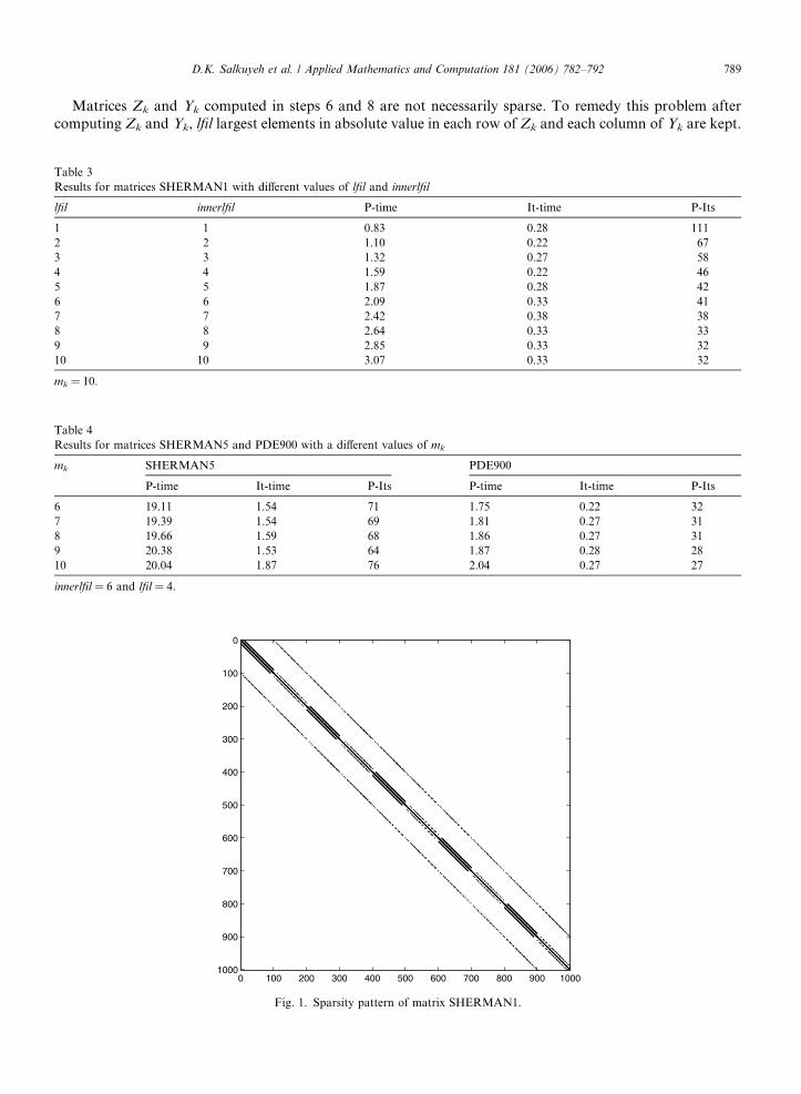
Fig. 1. Sparsity pattern of matrix SHERMAN1.

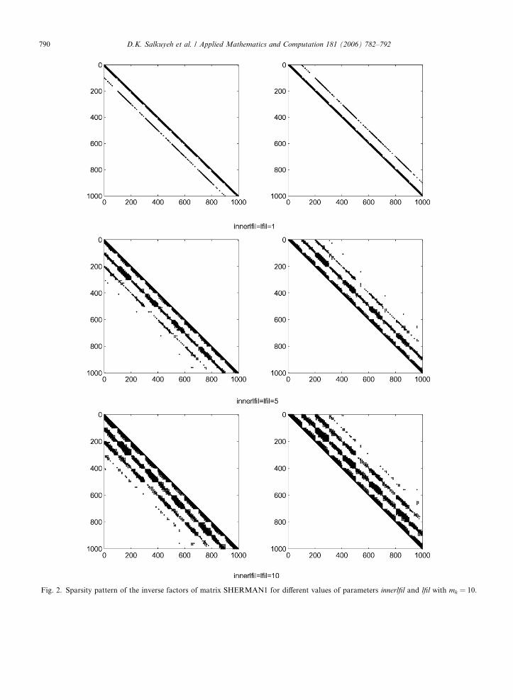
Fig. 2. Sparsity pattern of the inverse factors of matrix SHERMAN1 for different values of parameters innerlfil and lfil with mk = 10.



6. Numerical examples

All the numerical experiments presented in this section were computed in double precision with some FOR-TRAN 77 codes on a personal computer Pentium 3 – 800EB MHz. Some general matrices from Harwell–Boe-ing collection [8–10] were used for the numerical experiments. These matrices with their generic propertieswere shown in Table 1. This table gives, for each matrix, the order n and the number of nonzero entriesnnz, condition number estimation (Cond-Est) and their application. In the last column of this table the num-ber of iterations of the unpreconditioned Bi-CGSTAB (Unp-Its) [22] for convergence are given. Numericalresults of an experimental comparison between PBAIB and AIB algorithms are given in Table 2. In the PBAIBalgorithm we let lfil = innerlfil = 5 and in the AIB algorithm lfil = 10 was chosen. For all the examples, theright hand side of the system of equations were taken such that the exact solution is x = [1, . . . , 1]T. The stop-ping criterion

kb� Axik2

kbk2

< 10�7

was used and the initial guess was taken to be zero vector. For each preconditioner, we give the setup time forthe preconditioner (P-time), the number of iterations (P-Its) and time (It-time) for the split-preconditioned Bi-CGSTAB algorithm for convergence. The parameter mk for each linear system is also specified. In tables, adagger (�) indicates that there was no convergence in 5000 iterations.

Table 2 shows the effectiveness of the PBAIB algorithm. Numerical results in this table show that thismethod is very effective in improving the convergence of iterative solvers. From the point view of robustness,we see that the AIB algorithm fails on matrices ORSIRR2 and SAYLR3 and has poor convergence on matri-ces SHERMAN3, ORSIRR1, HOR131,SAYLR1 and MEMPLUS, but the PBAIB algorithm never fails andon this matrices have reasonable convergence. This is because of this fact that the AIB algorithm has a longrecursive relation for large matrices and the round off errors or errors which appear from approximating in theprimary stages may increase in large steps and an instability is detected. For the other examples the conver-gence results of these two algorithms are comparable. As Table 2 shows the setup time to compute sparseapproximate inverse factors of a matrix by the PBAIB algorithm for large matrices is usually greater than thatof the AIB algorithm. This is because of computing the sparse approximate solution of a system by algorithms1 or 2 is more expensive. Here we note the main advantage of the PBAIB algorithm over AIB algorithm is itsparallelism.

In Table 3, the numerical results for matrices SHERMAN1 with mk = 10 and different values of lfil andinnerlfil are given. This table shows the effect of increase in these parameters on the convergence results. Aswe expect with increasing these parameters the number of iterations for the split-preconditioned Bi-CGSTABalgorithm for convergence decreases.

In Table 4, the numerical results for matrices SHERMAN5 and PDE900 with different values of mk andinnelfil = 6 and lfil = 4 are given. This table shows the number of iterations for the split-preconditioned Bi-CGSTAB algorithm for convergence depends strongly on the value of parameter mk. An important part ofthe PBAIB algorithm is the choice of an appropriate block size. This is a problem for future works and isunder investigation.

In Fig. 1 the sparsity pattern of matrix SHERMAN1 is displayed and in Fig. 2 the sparsity pattern of theinverse factors of matrix SHERMAN1 computed by Algorithm 1 for different values of parameters innerlfil

and lfil with mk = 10 are shown.

7. Conclusion and future works

We have proposed an algorithm to compute the sparse approximate inverse factors of a matrix. In thismethod no sparsity pattern is needed in advance and the computations of inverse factors can be carriedout in parallel. Numerical results show that the new method is very effective to improve the convergence rateof the iterative methods. In this method, we have used the block size mk. Numerical results show that the num-ber of iterations to convergence for the preconditioned system depends on the value of this parameter. Here


the problem is to choose the best block size. Future work may focus on solving this problem. A comparisonbetween the new method and the AIB algorithm was also given.

References

[1] O. Axelsson, Iterative Solution Methods, Cambridge University Press, Cambridge, 1996.[2] M. Benzi, Preconditioning techniques for large linear systems: a survey, J. Comput. Phys. 182 (2002) 418–477.[3] M. Benzi, M. Tuma, A comparative study of sparse approximate inverse preconditioners, Appl. Numer. Math. 30 (1999) 305–340.[4] M. Benzi, M. Tuma, A sparse approximate inverse preconditioner for nonsymmetric linear systems, SIAM J. Sci. Comput. 19 (1998)

968–994.[5] E. Chow, Y. Saad, Approximate inverse preconditioners via sparse–sparse iterations, SIAM J. Sci. Comput. 19 (1998) 995–1023.[6] E. Chow, Y. Saad, Approximate inverse techniques for block-partitioned matrices, SIAM J. Sci. Comput. 18 (1997) 1657–1675.[7] E. Chow, Y. Saad, ILUS: an incomplete LU preconditioner in sparse skyline format, Int. J. Numer. Methods Fluids 25 (1997) 739–

748.[8] I.S. Duff, A survey of sparse matrix research, Proc IEEE 65 (1977) 500–535.[9] I.S. Duff, A.M. Erisman, J.K. Reid, Direct Methods for Sparse Matrices, Clarendon Press, Oxford, 1986.

[10] I.S. Duff, R.G. Grimes, J.G. Lewis, User’s guide for Harwell–Boeing sparse matrix test problems collection, Technical Rep. RAL-92-086, Rutherford Appleton Laboratory, 1992.

[11] N.I.M. Gould, J.A. Scott, Sparse approximate-inverse preconditioners using norm-minimization techniques, SIAM J. Sci. Comput.19 (1998) 605–625.

[12] M.J. Grote, T. Huckle, Parallel preconditioning with sparse approximate inverses, SIAM J. Sci. Comput. 18 (1997) 838–853.[13] D.K. Salkuyeh, F. Toutounian, A block version algorithm to approximate inverse factors, Appl. Math. Comput. 162 (2005) 1499–

1509.[14] D.K. Salkuyeh, F. Toutounian, A new approach to compute sparse approximate inverse of an SPD matrix, IUST – Int. J. Eng. Sci. 15

(2004).[15] D.K. Salkuyeh, F. Toutounian, A sparse–sparse iteration for computing a sparse incomplete factorization of the inverse of an SPD

matrix, in review.[16] L.Y. Kolotilina, A.Y. Yeremin, Factorized sparse approximate inverse preconditioning I. Theory, SIAM J. Matrix Anal. Appl. 14

(1993) 45–58.[17] L.Y. Kolotilina, A.Y. Yeremin, Factorized sparse approximate inverse preconditioning II: solution of 3D FE systems on massively

parallel computers, Int. J. High Speed Comput. 7 (1995) 191–215.[18] Y. Saad, Iterative Methods for Sparse Linear Systems, PWS press, New York, 1995.[19] Y. Saad, M.H. Schultz, GMRES: a generalized minimal residual algorithm for nonsymmetric linear systems, SIAM J. Sci. Stat.

Comput. 7 (1986) 856–869.[20] Y. Saad, SPARSKIT: a basic tool kit for sparse matrix computations, Technical Report CSRD TR 1029, CSRD, University of

Illinois, Urbana, IL, 1990.[21] P. Sonneveld, CGS, a fast Lanczos-type solver for nonsymmetric linear systems, SIAM J. Sci. Stat. Comput. 14 (1993) 461–469.[22] H.A. van der Vorst, Bi-CGSTAB: a fast and smoothly converging variant of Bi-CG for the solution of nonsymmetric linear systems,

SIAM J. Sci. Stat. Comput. 12 (1992) 631–644.[23] J. Zhang, A sparse approximate inverse technique for parallel preconditioning of general sparse matrices, Appl. Math. Comput. 130

(2002) 63–85.

Documents

A parallel algorithm to approximate inverse factors of a matrix via sparse–sparse iterations