Accuracy estimation in approximate query processing

Accuracy Estimation in Approximate Query Processing

Carlo DELL’AQUILA, Francesco DI TRIA, Ezio LEFONS, and Filippo TANGORRA Dipartimento di Informatica

Università degli Studi di Bari “Aldo Moro” Via Orabona 4, 70125 Bari

ITALY {dellaquila, lefons, tangorra, francescoditria}@di.uniba.it

Abstract: - The methodologies used in approximate query processing are able to provide fast responses to queries that require high computational time in the decision making process. However, the approximate answers are affected with a small quantity of error. For this reason, it is important to provide also an accuracy of the approximate value, that is, a confidence degree of the approximation. In this paper, we present a probabilistic model that can be used in order to provide the accuracy measure in a methodology based on polynomial approximation. This probabilistic model is a Bayesian network able to estimate the relative error of the approximate answers. Keywords: Query processing, Approximate query answer, Polynomials approximation, Accuracy estimation, Probabilistic model. 1 Introduction The traditional query processing engines have always focused on furnishing exact query answers provided that the response time is minimized. However, there are several environments where (minimized but) high answer time is unacceptable. As an example, On-Line Analytical Processing (OLAP) is devoted to execute complex queries using a data warehouse as a data source. Since these databases commonly store high volumes of data in tables having millions of tuples, even a single scanning for data aggregation requires answering times that may range from minutes to hours. Moreover, in case of a distributed system, the access to remote data can be sometimes im-practicable (due to the server and/or communica-tion line crash, for example).

These issues have led to define methodologies able to provide approximate query answers [1], such that the final users get fast responses, although affected with a small quantity of error. In fact, this research topic is based on the assumption that, if the query is very time-consuming and the error in the approximation is neglectable, then it is more suitable to have an approximate answer in a short time interval, rather than the exact answer after a long waiting time.

There are several scenarios where it is not mandatory to obtain exact query answers. As an example, in the drill-down task, the preliminary queries are used only to determine the most important facets to consider in decision making. In fact, analytical processing has always an unpredictable and exploratory nature. As a further

example, in numerical answers that require the computation of the average of a large set of data, the total precision is not needed and an approximate value will suffice. At last, in Database Management Systems, the optimizers must define a plan for the physical data access on the basis of the selectivity estimates [2].

What are approximate answers? As concerns queries that involve data aggregation, the answer is a scalar value and the relative approximate answer is an estimation of this value. The most popular methodologies that represent the theoretical basis for approximate query processing are based on sampling [3], histograms [4], wavelets [5], prob-abilistic models [6, 7, 8], distributed processing [9], clustering [10], orthonormal series approximation [11], genetic programming [12], and graph-based models [13]. Most of them need to perform a reduction of the data stored in database relations. In fact, these methodologies provide approximate an-swers using small and pre-computed data synopses, obtained by compressing the original data.

According to [14], the criteria for comparing the methodologies for approximate query processing are: (a) coverage, or the kind of queries for which it is possible to provide approximate answers; (b) response time, or the time needed for the computa-tion of the approximate value; (c) accuracy, or the confidence degree in the approximation; (d) update time, or the time to compute the data synopsis; and (e) footprint, or the space used to store the data synopses.

In this paper, we consider the well-known methodology based on polynomial approximation [15], and we extend it in order to provide the

LATEST TRENDS on COMPUTERS (Volume II)

ISSN: 1792-4251 452 ISBN: 978-960-474-213-4

accuracy along with the approximate answer. The accuracy is computed via a probabilistic inferential process based on a Bayesian network. This allows us to model the relationships among the main stochastic variables involved in the approximate query processing that determine the relative error.

The paper is organized as follows. Section 2 recalls the methodology for polynomial approxima-tion. Section 3 introduces the Bayesian networks. Section 4 presents our novel probabilistic model able to estimate the relative error in the approximate query processing. Section 5 reports our conclusions. 2 Analytic Methodology The analytic methodology consists of using orthonormal polynomial series to approximate the univariate data distribution function of an attribute X. The utilized approximation polynomial is the Legendre orthogonal polynomial series and its calculated coefficients carry synthetic information about the univariate data distribution of the attribute X. A complete discussion of this approach and the extension to the multivariate data distribution can be found in [15]. 2.1 Coefficients Computation Let R(Χ) be a relation of cardinality n on schema X, and let X∈X. We assume dom(X) = [a, b] be the numeric interval denoting the domain of the attribute X. Finally, let pdf (x) be the probability density function of R.X, where we use the dot notation to denote the attribute X of the relation R(X). We denote with g(x) its polynomial approximation up to degree d. Since the Legendre orthogonal polynomials are defined on the interval [-1, 1], each value x∈dom(X) is suitably mapped to the corresponding value x′∈[-1, 1]. Then, ∀x∈X, it results that

∑=

′+=≈d

iii xPcixgxpdf

0)()12(

21)()( , (1)

where, for i = 0, 1, …, d,

x → x′ is the opportune map from x∈X to x′∈ [-1, 1],

Pi(x′) is the Legendre polynomial up to degree i,

∑∈

′=X

)(1x

ii xPn

c is the mean value of Pi(x′) on

the n tuples of R.X.

Therefore, g(x) is the orthogonal polynomial approximation to pdf (x) up to degree d and the

coefficients {ci | i = 0, …, d} carry information about the univariate data distribution of the attribute X. These coefficients are the so-called Canonical Coefficients of X and they can be used in order to perform monodimensional analyses of X, by calculating aggregate functions, such as count, sum, and average (see, Sub-section 2.2).

Assuming that:

∫=x

a

dyypdfxcdf )()( , and (2)

∫′

−−+ ′≡′−′=+

x

iiii xQxPxPdyyPi1

11 )()()()()12( ,

(3) for i = 0, 1, …, d, and Q0(x′) = x′, it is possible to compute the cumulative density function cdf (x) of X in the following way:

=′≡≈ )()()( xGxGxcdf (4)

= ∑∫=

′

−

′=d

iii

x

xQcdyyg01

)(21)( ,

where, for all x∈X, G(x) is the polynomial approximation of the cdf of X. 2.2 Monodimensional Analysis The analytical process based on the set of pre-computed Canonical Coefficients provides an ap-proximation of typical aggregate functions, such as sum, average, and count. Let I = [x, y] ⊆ [a, b] be the generic query range used for the computation of the aggregate function and let I′ = [x′, y′] ⊆ [-1, 1] be the corresponding interval on the domain of the Legendre function. Given such an interval I, the main aggregate function, namely percent (or selec-tivity), is p(x ≤ X ≤ y) and it can be estimated by

∑=

′=′−′≈d

iii IQcxGyGIpercent

0

)(21)()()( , (5)

where Qi(I′) = Qi(y′) – Qi(x′), for i = 0, 1, …, d. Then, the count aggregate function on the query range I can be estimated as

count(I) ≈ n × percent(I), (6)

where n is the cardinality of the relation R. Moreover, the average and the sum functions can be estimated, respectively, by

average(I) = )(

)(Ipercent

IH, and (7)

sum(I) = average(I) × count(I), (8)

where ∫=I

dxxxgIH )()( .


ISSN: 1792-4251 453 ISBN: 978-960-474-213-4

3 Overview of Probability Concepts Let {V1, V2, …, Vk} be a set of k stochastic variables and let vi be the value assumed by the variable Vi, for i = 1, …, k. If variables indicate propositions, then possible values are true and false. If variables represent measures or physical entities (such as age, weight, or speed), then their values are numbers and they range in discrete or continuous domains. If variables represent categories, their values are cate-gorical and the variables are defined multinomial. As an example, the weather can be sunny, cloudy, snowfall, and rainy.

Let E be a stochastic variable, then p(E) denotes the a priori probability of E. As an instance, if E is the weather multinomial stochastic variable, then the probability function assigns a real value between 0 and 1 to each value of E in the following way: p(weather = sunny) = 0.7, p(weather = rainy) = 0.2, p(weather = cloudy) = 0.08, and p(weather = snowfall) = 0.02. Therefore, weather = ⟨sunny, rainy, cloudy, snowfall⟩ and p(weather) denotes the vector ⟨0.7, 0.2, 0.08, 0.02⟩, containing the values of the probability associated to corresponding category of the stochastic variable. This vector defines a probability distribution for the weather variable.

In general, a discrete probability function is such that:

∑=

==n

kkvVp

1

1)( , (9)

where V is a multinomial variable that assumes n distinct values.

There are several definitions to assign a priori probabilities to stochastic variables [16].

According to the classic definition, given an event E, p(E) is the ratio of the number of cases favourable to its occurrence to the total numbers of cases, all equally possible and mutually exclusive:

cases possible ofnumber cases positive ofnumber )( =Ep . (10)

As an example, in a coin launch, each face of the coin has 50% of probability to be verified.

According to the frequentist definition, when an experiment is repeated n times, if an event E happens sn times, then we say that the ratio of sn to n provides the relative frequency of E in reference to the given repetitions of the experiment. There-fore, p(E) is the limit of the relative frequency, when the number of the repetitions of the experiment increases indefinitely:

nsEp n

n ∞→= lim)( . (11)

At last, according to the subjective definition, given the event E, p(E) is the degree of confidence that a person assigns to the occurrence of E.

The axioms of the probability theory are: if E is a stochastic variable, then 0 ≤ p(E) ≤ 1, necessarily true propositions have 1 as probabil-

ity value, while the unsatisfiable ones have probability 0 (i.e., p(true) = 1 and p(false) = 0),

the probability of a disjunction is given by p(A ∨ B) = p(A) + p(B) – p(A ∧ B). (12) We denote the joint probability that the values

of V1, V2, …, Vk be equal to v1, v2, …, vk respective-ly, with the expression:

p(V1 = v1, V2 = v2, …, Vk = vk). (13) The function that assigns a number in [0, 1] to

the set of stochastic variables is called joint prob-ability function. The properties of this function are: 0 ≤ p(v1, v2, …, vk) ≤ 1, where p(v1, v2, …, vk)

stands for p(V1 = v1, V2 = v2, …, Vk = vk), and Σ p(v1, v2, …, vk) = 1, where (v1, v2, …, vk) ranges

over V1 × V2 ×…× Vk , and Vi denotes the set of the values of the variable Vi, for i = 1,..., k. If we know the joint probabilities of all the

values of a set of stochastic variables, then we can calculate the so-called marginal probability of each of these variables. As an example, the marginal probability of V1 is defined as

∑=

==11

),...,,()( 2111vV

kVVVpvVp , (14)

where p(V1, V2, …, Vk) is the vector of joint probabilities.

Example 1. Let A and B be two propositional variables. For simplicity, we write p(A) instead of p(A = true) and p(¬A) instead of p(A = false).

Then, given the following joint probabilities: p(A, B) = 0.2, p(A, ¬B) = 0.3, p(¬A, B) = 0.4, and p(¬A, ¬B) = 0.1, we can compute the marginaliza-tion of A as p(A) = p(A, B) + p(A, ¬B) = 0.2 + 0.3 = 0.5, and p(¬A) = p(¬A, B) + p(¬A, ¬B) = 0.4 + 0.1 = 0.5.

The probability that Vi = vi when Vj = vj is called conditional probability of Vi given Vj and it is computed as follows:

)(),(

)|(jj

jjiijjii vVp

vVvVpvVvVp

=

===== . (15)

It is possible to define the joint probability in reference of the conditional probability, using the following expression, known as product rule:

(Vi = vi, Vj = vj) = p(Vi = vi | Vj = vj) p(Vj = vj). (16)


ISSN: 1792-4251 454 ISBN: 978-960-474-213-4

The generalization of the product rule allows expressing the joint probability of a set of stochastic variables in terms of a set of conditional probabilities. The general form of the product rule is given by:

∏=

−=k

iiik vvvpvvvp

111,2,1 ),,|(),( KK . (17)

Let A and B be two stochastic variables. Then, in reference to the product rule, we obtain that p(A, B) = p(A | B) p(B), and p(B, A) = p(B | A) p(A).

Since

p(A, B) = p(B, A ) ⇒ p(A | B) p(B) = p(B | A) p(A),

then

)()()|()|(

ApBpBApABp = . (18)

Formula (18) is known as Bayes’ rule and it allows to perform a probabilistic reasoning [17, 18]. 3.1 Probabilistic Inference The general form of the probabilistic inference is based on a set V = {V1, V2, …, Vk} of k stochastic variables and the evidence e (i.e., the 100% of truthness) that the variables of a set E ⊆ V assume defined values. In this way, it is possible to compute the conditional probability p(Vi = vi | E = e) of V when E is known. This process is called probabilistic inference. As an example, if we know that the probability it rains is 80% when the weather is cloudy (i.e., there exists the conditional probability p(rainy = true | cloudy = true) = 0.8) and we have the evidence that today it is cloudy, then the probability that today it rains is 80%.

The application of the probabilistic inference from joint probabilities requires the explicit definition of full joint distribution. Therefore, in case of k propositional variables (that is, stochastic variables whose values can be true or false), we need a list of 2k values of the joint probability p(V1, V2, …, Vk). Indeed, for many problems of interest, we could never obtain such a distribution. On the basis of this kind of intractability, a more efficient probabilistic reasoning must be used. Such a method is based on the conditional independence existing among stochastic variables.

We say that a variable A is conditionally independent from a variable B, given C, if the fol-lowing expression holds:

p(A | B, C) = p(A | C). (19)

Intuitively, the conditional independence states that, if the previous expression holds, then B does not provide any information about A, for all the needed information is already given by C. The

conditional independences can be represented by graphs, or the so-called Bayesian Networks (or belief networks). In detail, these graphs allow modelling the cause-effect relationships existing among stochastic variables and, thus, they are very useful in the probabilistic inference, for they allow computing the conditional probabilities in a very fast way. 3.2 Bayesian Networks A Bayesian Network [19] is a Machine Learning technique used to perform probabilistic reasoning. The network is represented by an acyclic and oriented graph, whose nodes are labelled with the names of the stochastic variables and an edge repre-sents a cause-effect relationship between variables. On the basis of the conditional independence, such a network requires that each node is influenced only by its parents. In a Bayesian Network, the following properties hold: a set of stochastic variables form the nodes of

the graph, a set of oriented edges connect couples (parent,

descendant) of nodes, each node has the associated table of the

conditional probabilities that summarize the effects the parents have on the node itself,

the graph has not cycles. Therefore, the existence of an edge from the

node A to B states that A influences B directly. Let V1, V2, …,Vk be a set of k nodes of a Bayes-

ian Network. Under the assumption of conditional independence, we can compute the joint probabili-ties of each node of the network as:

p(V1,V2, …,Vk) = ∏=

k

i

ii VparentsVp1

))(|( , (20)

where parents(Vi) is the set of the parents of Vi. Notice that we must know the conditional

probabilities of each node respect its parents, in order to compute the joint probabilities. Nodes without parents are not conditioned by any other node and their a priori probabilities must be provided.

Example 2. Let us consider the network shown in Fig. 1. In this network, the B, S, I, and M nodes are 4 propositional variables. For B and S, the a priori probabilities are provided. For I and M, the conditional probabilities with respect to their own parents are provided. So, we can compute the joint probability p(I, B, M, S) in the following way:

p(I, B, M, S) = p(I | B) p(M | B, S) p(B) p(S), instead of using the more complex linkage expression p(I, B, M, S)=p(I | B, M, S) p(M | B, S) p(B | S) p(S).


ISSN: 1792-4251 455 ISBN: 978-960-474-213-4

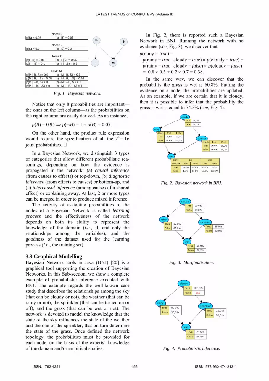
p(B) = 0.95 p(¬B) = 0.05

p(S) = 0.7 p(¬S) = 0.3

p(I | B) = 0.95 p(¬I | B) = 0.05p(I | ¬B) = 0.1 p(¬I | ¬B) = 0.9

p(M | B, S) = 0.9 p(¬M | B, S) = 0.1p(M | B, ¬S) = 0.05 p(¬M | B, ¬S) = 0.95p(M | ¬B, S) = 0 p(¬M | ¬B, S ) = 1p(M | ¬B, ¬S) = 0 p(¬M | ¬B, ¬S) = 1

Node B:

Node S:

Node I:

Node M:

Fig. 1. Bayesian network.

Notice that only 8 probabilities are important—the ones on the left column—as the probabilities on the right column are easily derived. As an instance,

p(B) = 0.95 ⇒ p(¬B) = 1 − p(B) = 0.05.

On the other hand, the product rule expression would require the specification of all the 24 = 16 joint probabilities.

In a Bayesian Network, we distinguish 3 types of categories that allow different probabilistic rea-sonings, depending on how the evidence is propagated in the network: (a) causal inference (from causes to effects) or top-down, (b) diagnostic inference (from effects to causes) or bottom-up, and (c) intercausal inference (among causes of a shared effect) or explaining away. At last, 2 or more types can be merged in order to produce mixed inference.

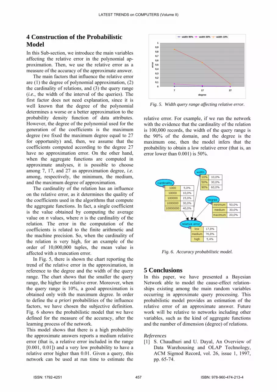
The activity of assigning probabilities to the nodes of a Bayesian Network is called learning process and the effectiveness of the network depends on both its ability to represent the knowledge of the domain (i.e., all and only the relationships among the variables), and the goodness of the dataset used for the learning process (i.e., the training set). 3.3 Graphical Modelling Bayesian Network tools in Java (BNJ) [20] is a graphical tool supporting the creation of Bayesian Networks. In this Sub-section, we show a complete example of probabilistic inference executed with BNJ. The example regards the well-known case study that describes the relationships among the sky (that can be cloudy or not), the weather (that can be rainy or not), the sprinkler (that can be turned on or off), and the grass (that can be wet or not). The network is devoted to model the knowledge that the state of the sky influences the state of the weather and the one of the sprinkler, that on turn determine the state of the grass. Once defined the network topology, the probabilities must be provided for each node, on the basis of the experts’ knowledge of the domain and/or empirical studies.

In Fig. 2, there is reported such a Bayesian Network in BNJ. Running the network with no evidence (see, Fig. 3), we discover that p(rainy = true) =

p(rainy = true | cloudy = true) × p(cloudy = true) + p(rainy = true | cloudy = false) × p(cloudy = false) = 0.8 × 0.3 + 0.2 × 0.7 = 0.38.

In the same way, we can discover that the probability the grass is wet is 60.8%. Putting the evidence on a node, the probabilities are updated. As an example, if we are certain that it is cloudy, then it is possible to infer that the probability the grass is wet is equal to 74.5% (see, Fig. 4).

Fig. 2. Bayesian network in BNJ.

Fig. 3. Marginalization.

Fig. 4. Probabilistic inference.


ISSN: 1792-4251 456 ISBN: 978-960-474-213-4

4 Construction of the Probabilistic Model In this Sub-section, we introduce the main variables affecting the relative error in the polynomial ap-proximation. Then, we use the relative error as a measure of the accuracy of the approximate answer.

The main factors that influence the relative error are (1) the degree of polynomial approximation, (2) the cardinality of relations, and (3) the query range (i.e., the width of the interval of the queries). The first factor does not need explanation, since it is well known that the degree of the polynomial determines a worse or a better approximation to the probability density function of data attributes. However, the degree of the polynomial used for the generation of the coefficients is the maximum degree (we fixed the maximum degree equal to 27 for opportunity) and, then, we assume that the coefficients computed according to the degree 27 have no approximation error. On the other hand, when the aggregate functions are computed in approximate analyses, it is possible to choose among 7, 17, and 27 as approximation degree, i.e. among, respectively, the minimum, the medium, and the maximum degree of approximation.

The cardinality of the relation has an influence on the relative error, as it determines the quality of the coefficients used in the algorithms that compute the aggregate functions. In fact, a single coefficient is the value obtained by computing the average value on n values, where n is the cardinality of the relation. The error in the computation of the coefficients is related to the finite arithmetic and the machine precision. So, when the cardinality of the relation is very high, for an example of the order of 10,000,000 tuples, the mean value is affected with a truncation error.

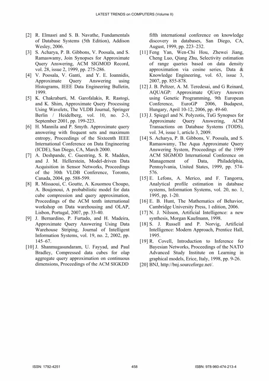
In Fig. 5, there is shown the chart reporting the trend of the relative error in the approximation, in reference to the degree and the width of the query range. The chart shows that the smaller the query range, the higher the relative error. Moreover, when the query range is 10%, a good approximation is obtained only with the maximum degree. In order to define the a priori probabilities of the influence factors, we have chosen the subjective definition. Fig. 6 shows the probabilistic model that we have defined for the measure of the accuracy, after the learning process of the network. This model shows that there is a high probability the approximate answers reports a medium relative error (that is, a relative error included in the range [0.001, 0.01]) and a very low probability to have a relative error higher than 0.01. Given a query, this network can be used at run time to estimate the

Fig. 5. Width query range affecting relative error.

relative error. For example, if we run the network with the evidence that the cardinality of the relation is 100,000 records, the width of the query range is the 90% of the domain, and the degree is the maximum one, then the model infers that the probability to obtain a low relative error (that is, an error lower than 0.001) is 50%.

Fig. 6. Accuracy probabilistic model.

5 Conclusions In this paper, we have presented a Bayesian Network able to model the cause-effect relation-ships existing among the main random variables occurring in approximate query processing. This probabilistic model provides an estimation of the relative error of an approximate answer. Future work will be relative to networks including other variables, such as the kind of aggregate functions and the number of dimension (degree) of relations. References [1] S. Chaudhuri and U. Dayal, An Overview of

Data Warehousing and OLAP Technology, ACM Sigmod Record, vol. 26, issue 1, 1997, pp. 65-74.

0

0,1

0,2

0,3

0,4

0,5

0,6

0,7

0,8

0,9

1

7 17 27

degree

erro

r

width 90% width 50% width 10%


ISSN: 1792-4251 457 ISBN: 978-960-474-213-4

[2] R. Elmasri and S. B. Navathe, Fundamentals of Database Systems (5th Edition), Addison Wesley, 2006.

[3] S. Acharya, P. B. Gibbons, V. Poosala, and S. Ramaswamy, Join Synopses for Approximate Query Answering, ACM SIGMOD Record, vol. 28, issue 2, 1999, pp. 275-286.

[4] V. Poosala, V. Ganti, and Y. E. Ioannidis, Approximate Query Answering using Histograms, IEEE Data Engineering Bulletin, 1999.

[5] K. Chakrabarti, M. Garofalakis, R. Rastogi, and K. Shim, Approximate Query Processing Using Wavelets, The VLDB Journal, Springer Berlin / Heidelberg, vol. 10, no. 2-3, September 2001, pp. 199-223.

[6] H. Mannila and P. Smyth. Approximate query answering with frequent sets and maximum entropy, Proceedings of the Sixteenth IEEE International Conference on Data Engineering (ICDE), San Diego, CA, March 2000.

[7] A. Deshpande, C. Guestring, S. R. Madden, and J. M. Hellerstein, Model-driven Data Acquisition in Sensor Networks, Proceedings of the 30th VLDB Conference, Toronto, Canada, 2004, pp. 588-599.

[8] R. Missaoui, C. Goutte, A. Kouomou Choupo, A. Boujenoui, A probabilistic model for data cube compression and query approximation, Proceedings of the ACM tenth international workshop on Data warehousing and OLAP, Lisbon, Portugal, 2007, pp. 33-40.

[9] J. Bernardino, P. Furtado, and H. Madeira, Approximate Query Answering Using Data Warehouse Striping, Journal of Intelligent Information Systems, vol. 19, no. 2, 2002, pp. 145–67.

[10] J. Shanmugasundaram, U. Fayyad, and Paul Bradley, Compressed data cubes for olap aggregate query approximation on continuous dimensions, Proceedings of the ACM SIGKDD

fifth international conference on knowledge discovery in databases, San Diego, CA, August, 1999, pp. 223–232.

[11] Feng Yan, Wen-Chi Hou, Zhewei Jiang, Cheng Luo, Qiang Zhu, Selectivity estimation of range queries based on data density approximation via cosine series, Data & Knowledge Engineering, vol. 63, issue 3, 2007, pp. 855-878.

[12] J. B. Peltzer, A. M. Teredesai, and G Reinard, AQUAGP: Approximate QUery Answers using Genetic Programming, 9th European Conference, EuroGP 2006, Budapest, Hungary, April 10-12, 2006, pp. 49-60.

[13] J. Spiegel and N. Polyzotis, TuG Synopses for Approximate Query Answering, ACM Transactions on Database Systems (TODS), vol. 34, issue 1, article 3, 2009.

[14] S. Acharya, P. B. Gibbons, V. Poosala, and S. Ramaswamy, The Aqua Approximate Query Answering System, Proceedings of the 1999 ACM SIGMOD International Conference on Management of Data, Philadelphia, Pennsylvania, United States, 1999, pp. 574-576.

[15] E. Lefons, A. Merico, and F. Tangorra, Analytical profile estimation in database systems, Information Systems, vol. 20, no. 1, 1995, pp. 1-20.

[16] E. B. Hunt, The Mathematics of Behavior, Cambridge University Press, 1 edition, 2006.

[17] N. J. Nilsson, Artificial Intelligence: a new synthesis, Morgan Kaufmann, 1998.

[18] S. J. Russell and P. Norvig, Artificial Intelligence: Modern Approach, Prentice Hall, 1995.

[19] R. Covell, Introduction to Inference for Bayesian Networks, Proceedings of the NATO Advanced Study Institute on Learning in graphical models, Erice, Italy, 1998, pp. 9-26.

[20] BNJ, http://bnj.sourceforge.net/.


ISSN: 1792-4251 458 ISBN: 978-960-474-213-4

Documents

Accuracy estimation in approximate query processing