Approximate Roots in Graded Rings

Johann Radon Institutefor Computational and Applied MathematicsAustrian Academy of Sciences (ÖAW)

RICAM-Report No. 2005-03

T. Beck, J. Schicho

Approximate Roots in Graded Rings

Powered by TCPDF (www.tcpdf.org)

http://www.tcpdf.org

Approximate Roots in Graded Rings∗

Tobias Beck, Josef Schicho

{Tobias.Beck, Josef.Schicho}@oeaw.ac.at

RICAM-Linz

- last updated March 1, 2005 -

Abstract

An approximate root of an univariate polynomial over a graded ring A isan element in A for which the evaluated polynomial vanishes up to a pre-scribed order. We give an algorithm for deciding existence of approximateroots and computing essentially all of them. Based on this algorithm wealso suggest a finite representation for multivariate algebraic power series.

Contents

1 Introduction 2

2 Graded rings and sliced rings 3

3 Induced slicings and Newton equations 6

4 Approximate and exact roots 10

∗This work was supported by the Austrian Science Fund (FWF) in the frame of the specialresearch area SFB 013, subproject 03.

1

1 Introduction

If A is a multivariate polynomial algebra over a field, and p is a univariate poly-nomial over A, then an approximate root is an element a ∈ A such that the orderof the residual p(a) is larger than a given integer. In this paper, we solve theproblem of deciding whether approximate roots exist and to compute essentiallyall of them (cf. Propositions 7 and 8).

We have approximate roots of any order if and only if there exists a root in theformal power series algebra, by Wavrik’s version [9] of the Artin ApproximationTheorem. Assuming formal solvability, we can use our algorithm for expandingsuch a power series solution up to any given order.

If the input polynomial is square-free then any approximate root of sufficientlyhigh order is a truncation of a power series solution, which is then uniquely de-termined. This observation provides a way to finitely represent algebraic powerseries, namely by minimal polynomial and suitable approximate root (cf. Corol-lary 10).

The idea is to increase the order of the residual iteratively, looking for a homo-geneous solution in each step. The algorithm is similar to the classical Newton-Puiseux algorithm for solving bivariate polynomials. That algorithm has beengeneralized to the multivariate case by McDonald [6] and Beringer, Richard-Jung[3]. In these generalizations, the constructed solutions are contained in a suitableextension of the power series ring. In contrast to these, we concentrate on solu-tions in the original power series ring (or approximate solutions in the originalpolynomial ring). The algorithm does not guarantee the existence of approximateroots of arbitrary order and therefore the existence of power series solutions. Onthe other hand, there are situations where formal solvability is guaranteed, e.g.Tougeron’s Implicit Function Theorem (cf. [7]) or the theorem of Jung-Abhyankarfor quasi-ordinary polynomials (cf. [5, 4]).

The theoretical results apply to integral domains graded over arbitrary well-ordered monoids. The algorithms work if the order is isomorphic to ω, in partic-ular for power series rings with an ordering based on total degree.

Our motivation for studying this problem originally was the intention to im-plement the algorithm of Alonso, Luengo and Raimondo [1] for solving quasi-ordinary polynomials. To do this, it would have been necessary to finitely rep-resent algebraic power series. Such a representation was suggested in [2]. Butthen we observed that exact representation of the intermediate results is not re-ally necessary, because for expansion up to a given order it suffices to work withapproximate roots throughout.

2

2 Graded rings and sliced rings

In this section we give some generalities about graded rings, we introduce notationand the concept of sliced rings which is important for the rest of the article.

Throughout this article M will denote an Abelian monoid that is endowed witha compatible well-ordering <, i.e. ∀r, s, t ∈ M : r < s ⇒ r + t < s + t. We writesucc(r) := min({s | s > r}) for the successor element of r ∈ M.

The fact that M is ordered in such a way has several implications. First, M hasthe cancellation property, i.e. r 7→ r+ t for any t ∈ M is an injective map. Indeedif r 6= s, say r < s, then r + t < s + t.

Second, 0 is the smallest element of M. For if r0 is the smallest element, thenr0 ≤ 0 and r0 + r0 ≤ r0 by compatibility. Hence r0 + r0 = r0 and r0 = 0 bythe cancellation property. This also means that for s + t = r we have s ≤ r andt ≤ r (because 0 ≤ t implies s ≤ s + t). All elements of M being positive or zeroimplies that M has no inverses.

Third, every element r ∈ M can be written as a sum in only finitely manyways, i.e. the set {(s, t) ∈ M

2 | s + t = r} is finite. Indeed assume it is infinitethen we can find a subset {(si, ti)}i∈N s.t. si < si+1 for all i. Together withr = si + ti = si+1 + ti+1 this implies ti > ti+1. So M would contain an infinitedescending chain, contradiction.

By A we will denote an M-graded integral domain. I.e. A can be decomposed as

A =⊕

r∈M

Ar

s.t. for a ∈ Ar and b ∈ As we have ab ∈ Ar+s. For a ∈ A we write degM(a) =max({r | ar 6= 0}). Most of the time we apply the degree to elements a ∈ Ar andsay that a is homogeneous of degree r.

Example Let A := Q[x1, x2] be the ring of bivariate polynomials over the field ofrational numbers. Then A may be considered a graded ring over M := N2: Thedirect summands are A(ν1,ν2) = {cxν1

1 xν22 | c ∈ Q} ∼= Q. Let N2 be ordered first by

total degree and second reverse lexicographically:

(ν1, ν2) < (µ1, µ2) :⇔ ν1 + ν2 < µ1 + µ2 or

ν1 + ν2 = µ1 + µ2 and ν2 < µ2

With this definition N2 is order-isomorphic to ω.

In our setting we can embed A into a larger ring A:

3

Definition 1 (Sliced rings)Let A be an M-graded integral domain. We first define the associated formalseries ring A as a product of modules

A :=∏

r∈M

Ar.

For a = (ar)r∈M ∈ A and b = (br)r∈M ∈ A we define multiplication as follows:

ab :=

(∑

s+t=r

asbt

)

r∈M

We call B an M-sliced ring if there is an M-graded ring A s.t. A ⊆ B ⊆ A.

Observe that multiplication is well-defined – meaning that the involved sums arefinite – because of the properties of M. It is not hard to deduce that an M-slicedring is integral because A was assumed integral in the definition.

Example (continued . . . ) If A = Q[x1, x2] as above then A is isomorphic tothe ring of formal power series Q[[x1, x2]] and every sub-ring of Q[[x1, x2]] con-taining all polynomials is an N2-sliced ring.

The definition of sliced rings allows a uniform treatment in particular of the ringsA and A. We will also write elements of a sliced ring as sums rather than astuples and speak of homogeneous and heterogeneous elements as in the gradedsituation.

Definition 2 (Support)Let B be an M-sliced ring. The support is defined as follows:

SuppM : B → 2M :∑

r∈M

ar 7→ {r ∈ M | ar 6= 0}

Definition 3 (Projections)Let B be an M-sliced ring. For an element a =

∑

r∈M ar ∈ A, s ∈ M and abinary relation ∗ ∈ {=,≤,≥, <, >} we write a∗s :=

∑

r∗s ar. For abbreviation(and in consistence with the notation for the sum decomposition) we also writeas := a=s.

Definition 4 (Order)Let B be an M-sliced ring. Then the order is defined as follows:

ordM : B \ {0} → M : a 7→ min(SuppM(a))

4

The usual rules for the order apply. E.g. for all a, b ∈ B\{0} we have ordM(ab) =ordM(a) + ordM(b). If a + b 6= 0 then ordM(a + b) ≥ min(ordM(a), ordM(b))and equality holds if ordM(a) 6= ordM(b). The fact that M has no inversesimplies that the only elements of sliced rings that have multiplicative inversesmust have order 0.

The ring Q[[x1, x2]] of our example can also be defined as the I-adic completionof Q[x1, x2] w.r.t. the maximal ideal I := 〈x1, x2〉. This can be generalized undercertain additional assumptions on A.

Proposition 1 (Isomorphic completions)Let A be an M-graded integral domain. Assume the ordering on M is isomorphicto ω and there is 0 < s ∈ M s.t. A is generated by all Ar with r ≤ s. Let A be theassociated formal series ring (as in definition 1), I := 〈Ar〉r>0 and C the I-adiccompletion of A. Then A ∼= C.

Proof: For every r ∈ M the set Jr := {a ∈ A | a = 0 or ordM(a) ≥ r} is ahomogeneous ideal and Jr ⊇ Js for r ≤ s. Since the ordering is isomorphic toω the system {Jr}r∈M induces a metric s.t. A becomes the completion of A. Inorder to prove that the two completions are isomorphic we have to show that

a) for all r ∈ M we can find n ∈ N s.t. In ⊆ Jr and

b) for all n ∈ N we can find r ∈ M s.t. Jr ⊆ In.

First we show a): Let 1 := succ(0). By definition we have I = J1 and thusIn = Jn

1. An element 0 6= a ∈ Jn

1is of the form

a =∑

1≤k≤u

(∏

1≤l≤n

ak,l

)

with all ak,l 6= 0 and ordM(ak,l) ≥ 1. Then ordM(a) ≥ n1 and hence a ∈ Jn1.This shows In ⊆ Jn1. Now for all r ∈ M we can find n ∈ N s.t. r ≤ n1 becauseof the order-isomorphism with ω. Then In ⊆ Jn1 ⊆ Jr.

For part b) we choose r = ns. The proof of Jr = Jns ⊆ In is by induction.The statement is clear for n = 0. Now let n > 0 and assume the statementholds for n − 1. Since Jns is a homogeneous ideal it is sufficient to show thatfor all homogeneous a 6= 0 s.t. degM(a) ≥ ns we have a ∈ In. Because of theassumption on A we can write

a =∑

1≤k≤u

akbk

with all ak, bk homogeneous and non-zero, 0 < degM(ak) ≤ s and degM(ak) +degM(bk) = degM(a). This implies degM(bk) ≥ (n−1)s and therefore bk ∈ In−1

by the induction hypothesis. Of course ak ∈ I and together a ∈ In. �

5

��

��

N

M

1

1

p

r1

r2

Πr1(p)

Πr2(p)

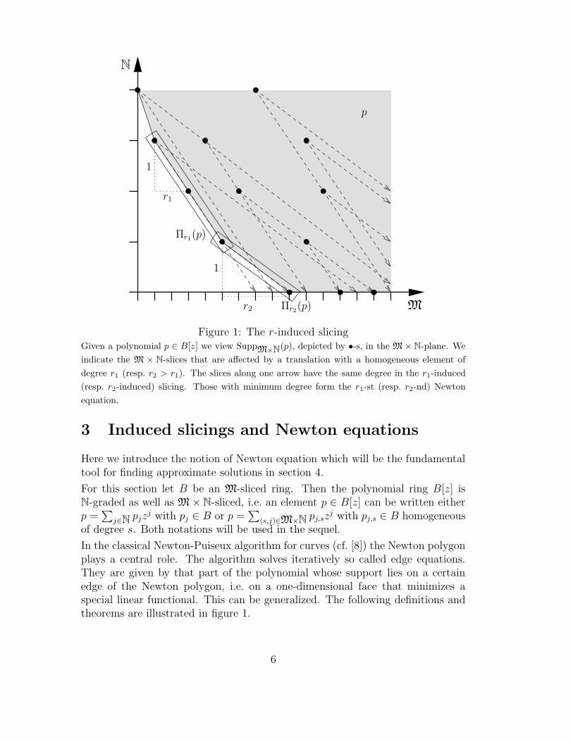
Figure 1: The r-induced slicingGiven a polynomial p ∈ B[z] we view SuppM×N(p), depicted by •-s, in the M × N-plane. We

indicate the M × N-slices that are affected by a translation with a homogeneous element of

degree r1 (resp. r2 > r1). The slices along one arrow have the same degree in the r1-induced

(resp. r2-induced) slicing. Those with minimum degree form the r1-st (resp. r2-nd) Newton

equation.

3 Induced slicings and Newton equations

Here we introduce the notion of Newton equation which will be the fundamentaltool for finding approximate solutions in section 4.

For this section let B be an M-sliced ring. Then the polynomial ring B[z] isN-graded as well as M × N-sliced, i.e. an element p ∈ B[z] can be written eitherp =

∑

j∈N pjzj with pj ∈ B or p =

∑

(s,j)∈M×N pj,szj with pj,s ∈ B homogeneous

of degree s. Both notations will be used in the sequel.

In the classical Newton-Puiseux algorithm for curves (cf. [8]) the Newton polygonplays a central role. The algorithm solves iteratively so called edge equations.They are given by that part of the polynomial whose support lies on a certainedge of the Newton polygon, i.e. on a one-dimensional face that minimizes aspecial linear functional. This can be generalized. The following definitions andtheorems are illustrated in figure 1.

6

Definition 5 (r-induced slicings)For r ∈ M we define the linear functional

hr : M × N → M : (s, j) 7→ s + jr.

Then B[z] may be viewed as a subset of∏

t∈M Pt with

Pt =

p ∈ B[z]

∣∣∣∣∣∣

p =∑

(s,j)∈M×N

pj,szj and hr(s, j) = t for all pj,s 6= 0

.

This way B[z] becomes an M-sliced ring. We call that slicing the r-induced

slicing on B[z] and we write SuppM,r, ordM,r

, degM,r.

Definition 6 (Newton equations)Given a polynomial 0 6= p ∈ B[z] and r ∈ M we define the r-th Newton

equation Πr(p) ∈ B[z] to be that part of p whose support minimizes the linearfunctional hr. More precisely:

Πr(p) := pordM,r

(p)

(Again in other words the r-th Newton equation is the initial form w.r.t. ther-induced slicing.)

Example (continued . . . ) From now on we consider a polynomial p as follows:

p1(z) := (x1 + x2)z − (x1 + x2)(x2 + x21 − 2x1x2 − x3

2) + x52

p2(z) := z3 + (1 − x1)(x1x2 − x22 + x3

1)z + x2(x1x2 − x22 + x3

1)2

p(z) := p1(z)p2(z)

= (x1 + . . . )z4 + (−x1x2 + . . . )z3 + (x21x2 + . . . )z2

+ (−x21x

22 + . . . )z − x3

1x42 + . . .

p would decompose as follows in the (0, 1)-induced slicing:

p = (−x21x

22z + x2

1x2z2)

︸︷︷︸

degN2

,(0,1)(... )=(2,3)

+ (−x1x2z3 + x1z

4)︸︷︷︸

degN2

,(0,1)(... )=(1,4)

+ (x42z − x3

2z2 − x2

2z3 + x2z

4)︸︷︷︸

degN2

,(0,1)(... )=(0,5)

+ (−2x41x2z + x4

1z2)

︸︷︷︸

degN2

,(0,1)(... )=(4,2)

+ (2x31x

22z − x3

1z3)

︸︷︷︸

degN2

,(0,1)(... )=(3,3)

+ (x21x

32z)

︸︷︷︸

degN2

,(0,1)(... )=(2,4)

+ . . .

I.e. ordN2,(0,1)

(p) = (2, 3) and the homogeneous part of that degree is Π(0,1)(p) =

−x21x

22z + x2

1x2z2.

7

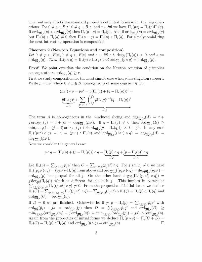
One routinely checks the standard properties of initial forms w.r.t. the ring oper-ations: For 0 6= p ∈ B[z], 0 6= q ∈ B[z] and r ∈ M we have Πr(pq) = Πr(p)Πr(q).If ordM,r

(p) < ordM,r(q) then Πr(p+q) = Πr(p). And if ordM,r

(p) = ordM,r(q)

but Πr(p) + Πr(q) 6= 0 then Πr(p + q) = Πr(p) + Πr(q). For a polynomial ringthe next interesting operation is composition.

Theorem 2 (Newton Equations and composition)Let 0 6= p ∈ B[z], 0 6= q ∈ B[z] and r ∈ M s.t. degN(Πr(q)) > 0 and s :=ordM,r

(q). Then Πr(p ◦ q) = Πs(p) ◦ Πr(q) and ordM,r(p ◦ q) = ordM,s

(p).

Proof: We point out that the condition on the Newton equation of q impliesamongst others ordM,r

(q) ≥ r.

First we study composition for the most simple case when p has singleton support.Write p = pzj where 0 6= p ∈ B homogeneous of some degree t ∈ M:

(pzj) ◦ q = pqj = p(Πr(q) + (q − Πr(q)))j =

pΠr(q)j

︸︷︷︸

=:A

+∑

1≤i≤j

(j

i

)

pΠr(q)j−i(q − Πr(q))

i

︸︷︷︸

=:B

The term A is homogeneous in the r-induced slicing and degM,r(A) = t +

j ordM,r(q) = t + js = degM,s

(pzj). If q − Πr(q) 6= 0 then ordM,r(B) ≥

min1≤i≤j(t + (j − i) ordM,r(q) + i ordM,r

(q − Πr(q))) > t + js. In any case

Πr((pzj) ◦ q) = A = (pzj) ◦ Πr(q) and ordM,r

((pzj) ◦ q) = degM,r(A) =

degM,s(pzj).

Now we consider the general case:

p ◦ q = (Πs(p) + (p − Πs(p))) ◦ q = Πs(p) ◦ q︸︷︷︸

=:C

+ (p − Πs(p)) ◦ q︸︷︷︸

=:D

Let Πs(p) =∑

0≤j≤d pjzj then C =

∑

0≤j≤d(pjzj) ◦ q. For j s.t. pj 6= 0 we have

Πr((pjzj)◦q) = (pjz

j)◦Πr(q) from above and ordM,s((pjz

j)◦q) = degM,s(pjz

j) =

ordM,s(p) being equal for all j. On the other hand degN(Πr((pjz

j) ◦ q)) =

j degN(Πr(q)) which is different for all such j. This implies in particular∑

0≤j≤d,pj 6=0 Πr((pjzj) ◦ q) 6= 0. From the properties of initial forms we deduce

Πr(C) =∑

0≤j≤d,pj 6=0 Πr((pjzj) ◦ q) =

∑

0≤j≤d(pjzj) ◦ Πr(q) = Πs(p) ◦ Πr(q) and

ordM,r(C) = ordM,s

(p).

If D = 0 we are finished. Otherwise let 0 6= p − Πs(p) =∑

0≤j≤d pjzj with

ordM(pj) + js > ordM,s(p) then D =

∑

0≤j≤d pjqj and ordM,r

(D) ≥

min0≤j≤d(ordM,r(pj) + j ordM,r

(q)) = min0≤j≤d(ordM(pj) + js) > ordM,s(p).

Again from the properties of initial forms we deduce Πr(p ◦ q) = Πr(C + D) =Πr(C) = Πs(p) ◦ Πr(q) and ordM,r

(p ◦ q) = ordM,s(p). �

8

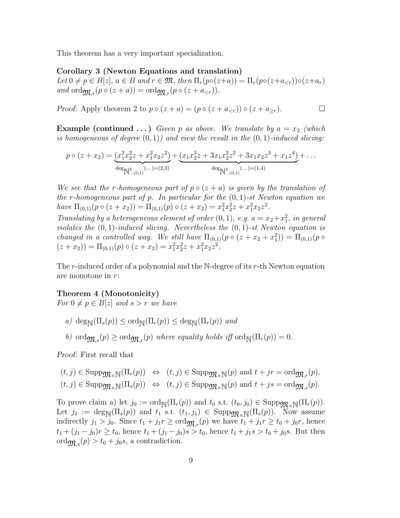
This theorem has a very important specialization.

Corollary 3 (Newton Equations and translation)Let 0 6= p ∈ B[z], a ∈ B and r ∈ M, then Πr(p◦(z+a)) = Πr(p◦(z+a<r))◦(z+ar)and ordM,r

(p ◦ (z + a)) = ordM,r(p ◦ (z + a<r)).

Proof: Apply theorem 2 to p ◦ (z + a) = (p ◦ (z + a<r)) ◦ (z + a≥r). �

Example (continued . . . ) Given p as above. We translate by a = x2 (whichis homogeneous of degree (0, 1)) and view the result in the (0, 1)-induced slicing:

p ◦ (z + x2) = (x21x

22z + x2

1x2z2)

︸︷︷︸

degN2

,(0,1)(... )=(2,3)

+ (x1x32z + 3x1x

22z

2 + 3x1x2z3 + x1z

4)︸︷︷︸

degN2

,(0,1)(... )=(1,4)

+ . . .

We see that the r-homogeneous part of p ◦ (z + a) is given by the translation ofthe r-homogeneous part of p. In particular for the (0, 1)-st Newton equation wehave Π(0,1)(p ◦ (z + x2)) = Π(0,1)(p) ◦ (z + x2) = x2

1x22z + x2

1x2z2.

Translating by a heterogeneous element of order (0, 1), e.g. a = x2+x21, in general

violates the (0, 1)-induced slicing. Nevertheless the (0, 1)-st Newton equation ischanged in a controlled way. We still have Π(0,1)(p ◦ (z + x2 + x2

1)) = Π(0,1)(p ◦(z + x2)) = Π(0,1)(p) ◦ (z + x2) = x2

1x22z + x2

1x2z2.

The r-induced order of a polynomial and the N-degree of its r-th Newton equationare monotone in r:

Theorem 4 (Monotonicity)For 0 6= p ∈ B[z] and s > r we have

a) degN(Πs(p)) ≤ ordN(Πr(p)) ≤ degN(Πr(p)) and

b) ordM,s(p) ≥ ordM,r

(p) where equality holds iff ordN(Πr(p)) = 0.

Proof: First recall that

(t, j) ∈ SuppM×N(Πr(p)) ⇔ (t, j) ∈ SuppM×N(p) and t + jr = ordM,r(p),

(t, j) ∈ SuppM×N(Πs(p)) ⇔ (t, j) ∈ SuppM×N(p) and t + js = ordM,s(p).

To prove claim a) let j0 := ordN(Πr(p)) and t0 s.t. (t0, j0) ∈ SuppM×N(Πr(p)).Let j1 := degN(Πs(p)) and t1 s.t. (t1, j1) ∈ SuppM×N(Πs(p)). Now assumeindirectly j1 > j0. Since t1 + j1r ≥ ordM,r

(p) we have t1 + j1r ≥ t0 + j0r, hence

t1 + (j1 − j0)r ≥ t0, hence t1 + (j1 − j0)s > t0, hence t1 + j1s > t0 + j0s. But thenordM,s

(p) > t0 + j0s, a contradiction.

9

Now we prove claim b): Choose arbitrary (t, j) ∈ SuppM×N(Πs(p)). Then im-mediately ordM,s

(p) = t + js ≥ t + jr ≥ ordM,r(p).

Let ordN(Πr(p)) = 0, then a) implies also ordN(Πs(p)) = 0. I.e. there is (t0, 0) ∈SuppM×N(Πs(p)) ∩ SuppM×N(Πr(p)) and ordM,s

(p) = t0 = ordM,r(p).

Let now ordM,s(p) = ordM,r

(p). Then there is (t0, j0) ∈ SuppM×N(Πs(p)) s.t.

t0 + j0s = ordM,s(p) = ordM,r

(p) ≤ t0 + j0r. This implies j0 = 0, (t0, 0) ∈

SuppM×N(Πr(p)) and hence ordN(Πr(p)) = 0. �

Example (continued . . . ) Now we compare p in the (0, 1)- and (1, 2)-inducedslicing. Observe that (1, 2) > (0, 1). We have ordN2

,(1,2)(p) = (3, 4) and

Π(1,2)(p) = −x21x

22z − x3

1x42. We see that ordN2

,(1,2)(p) > ordN2

,(0,1)(p) = (2, 3),

degN(Π(1,2)(p)) = 1 ≤ ordN(Π(0,1)(p)) = 1 and ordN(Π(1,2)(p)) = 0. For allr > (1, 2) we consequently get ordN2

,r(p) = (3, 4) and Πr(p) = −x3

1x42.

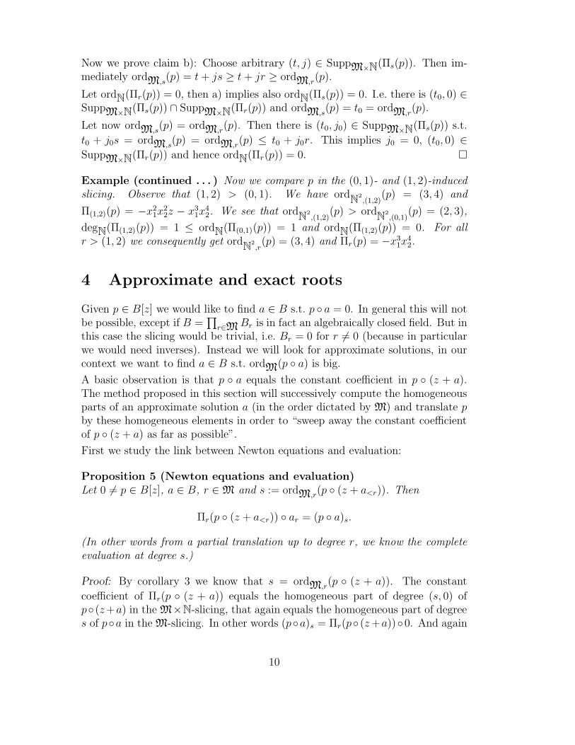
4 Approximate and exact roots

Given p ∈ B[z] we would like to find a ∈ B s.t. p ◦ a = 0. In general this will notbe possible, except if B =

∏

r∈M Br is in fact an algebraically closed field. But inthis case the slicing would be trivial, i.e. Br = 0 for r 6= 0 (because in particularwe would need inverses). Instead we will look for approximate solutions, in ourcontext we want to find a ∈ B s.t. ordM(p ◦ a) is big.

A basic observation is that p ◦ a equals the constant coefficient in p ◦ (z + a).The method proposed in this section will successively compute the homogeneousparts of an approximate solution a (in the order dictated by M) and translate pby these homogeneous elements in order to “sweep away the constant coefficientof p ◦ (z + a) as far as possible”.

First we study the link between Newton equations and evaluation:

Proposition 5 (Newton equations and evaluation)Let 0 6= p ∈ B[z], a ∈ B, r ∈ M and s := ordM,r

(p ◦ (z + a<r)). Then

Πr(p ◦ (z + a<r)) ◦ ar = (p ◦ a)s.

(In other words from a partial translation up to degree r, we know the completeevaluation at degree s.)

Proof: By corollary 3 we know that s = ordM,r(p ◦ (z + a)). The constant

coefficient of Πr(p ◦ (z + a)) equals the homogeneous part of degree (s, 0) ofp◦ (z+a) in the M×N-slicing, that again equals the homogeneous part of degrees of p◦a in the M-slicing. In other words (p◦a)s = Πr(p◦ (z +a))◦0. And again

10

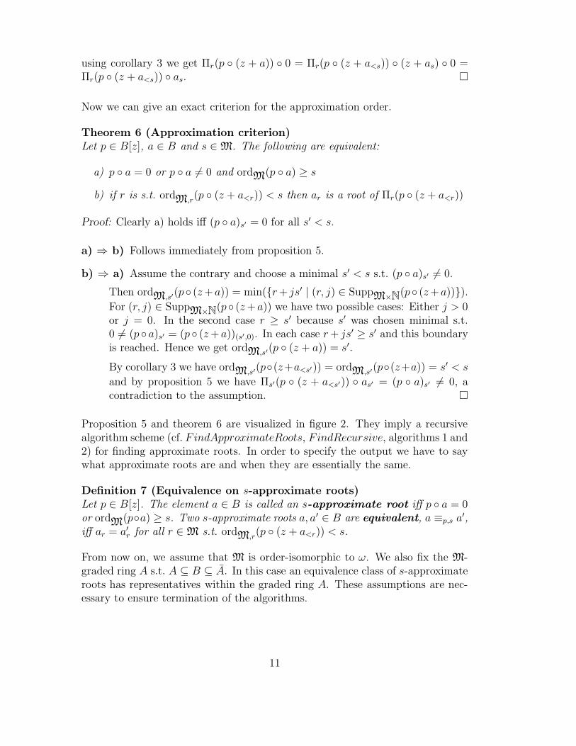
using corollary 3 we get Πr(p ◦ (z + a)) ◦ 0 = Πr(p ◦ (z + a<s)) ◦ (z + as) ◦ 0 =Πr(p ◦ (z + a<s)) ◦ as. �

Now we can give an exact criterion for the approximation order.

Theorem 6 (Approximation criterion)Let p ∈ B[z], a ∈ B and s ∈ M. The following are equivalent:

a) p ◦ a = 0 or p ◦ a 6= 0 and ordM(p ◦ a) ≥ s

b) if r is s.t. ordM,r(p ◦ (z + a<r)) < s then ar is a root of Πr(p ◦ (z + a<r))

Proof: Clearly a) holds iff (p ◦ a)s′ = 0 for all s′ < s.

a) ⇒ b) Follows immediately from proposition 5.

b) ⇒ a) Assume the contrary and choose a minimal s′ < s s.t. (p ◦ a)s′ 6= 0.

Then ordM,s′(p ◦ (z +a)) = min({r + js′ | (r, j) ∈ SuppM×N(p ◦ (z +a))}).

For (r, j) ∈ SuppM×N(p ◦ (z +a)) we have two possible cases: Either j > 0or j = 0. In the second case r ≥ s′ because s′ was chosen minimal s.t.0 6= (p ◦ a)s′ = (p ◦ (z + a))(s′,0). In each case r + js′ ≥ s′ and this boundaryis reached. Hence we get ordM,s′

(p ◦ (z + a)) = s′.

By corollary 3 we have ordM,s′(p◦(z+a<s′)) = ordM,s′

(p◦(z+a)) = s′ < s

and by proposition 5 we have Πs′(p ◦ (z + a<s′)) ◦ as′ = (p ◦ a)s′ 6= 0, acontradiction to the assumption. �

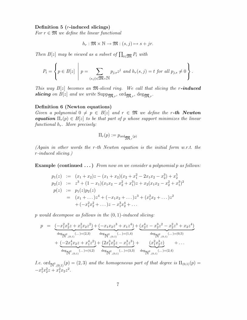
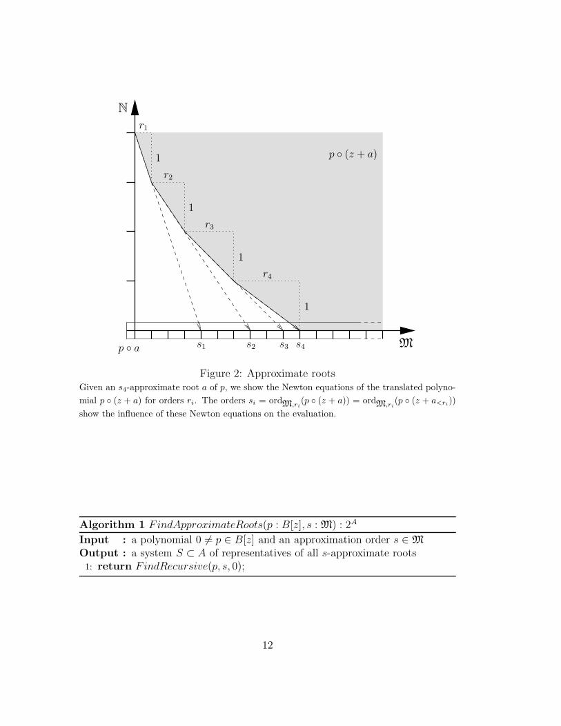
Proposition 5 and theorem 6 are visualized in figure 2. They imply a recursivealgorithm scheme (cf. FindApproximateRoots, FindRecursive, algorithms 1 and2) for finding approximate roots. In order to specify the output we have to saywhat approximate roots are and when they are essentially the same.

Definition 7 (Equivalence on s-approximate roots)Let p ∈ B[z]. The element a ∈ B is called an s-approximate root iff p ◦ a = 0or ordM(p◦a) ≥ s. Two s-approximate roots a, a′ ∈ B are equivalent, a ≡p,s a′,iff ar = a′

r for all r ∈ M s.t. ordM,r(p ◦ (z + a<r)) < s.

From now on, we assume that M is order-isomorphic to ω. We also fix the M-graded ring A s.t. A ⊆ B ⊆ A. In this case an equivalence class of s-approximateroots has representatives within the graded ring A. These assumptions are nec-essary to ensure termination of the algorithms.

11

N

M

1

1

1

1

r1

r2

r3

r4

s1 s2 s3 s4

p ◦ (z + a)

p ◦ a

Figure 2: Approximate rootsGiven an s4-approximate root a of p, we show the Newton equations of the translated polyno-

mial p ◦ (z + a) for orders ri. The orders si = ordM,ri

(p ◦ (z + a)) = ordM,ri

(p ◦ (z + a<ri))

show the influence of these Newton equations on the evaluation.

Algorithm 1 FindApproximateRoots(p : B[z], s : M) : 2A

Input : a polynomial 0 6= p ∈ B[z] and an approximation order s ∈ M

Output : a system S ⊂ A of representatives of all s-approximate roots1: return FindRecursive(p, s, 0);

12

Algorithm 2 FindRecursive(p : B[z], s : M, r : M) : 2A

Input : a polynomial 0 6= p ∈ B[z] , an approximation order s ∈ M and anorder r ∈ M s.t. for all r′ < r holds z|Πr′(p) and ordM,r′

(p) < sOutput : a system S ⊂ A of representatives of all s-approximate roots s.t.

ordM(a) ≥ r for all a ∈ S1: if ordM,r

(p) ≥ s then

2: return {0};3: S := ∅; S := HomogeneousRoots(Πr(p), r);4: for a ∈ S do5: q := p ◦ (z + a);6: R := FindRecursive(q, s, succ(r));7: S := S ∪ ({a} + R);8: return S;

Algorithm 3 HomogeneousRoots(p : A[z], r : M) : 2A

Input : a polynomial 0 6= p ∈ A[z] homogeneous in the r-induced slicingOutput : the set {a ∈ A | p ◦ a = 0, a = 0 or homogeneous of degree r}

Example (continued . . . ) Given p as above. Then a := x2 + x21 − 2x1x2 − x3

2

is a (1, 7)-approximate root, because ordN2(p ◦ a) = (1, 7) and one can check:

Π(1,0)(p) = x1z4,

Π(0,1)(p) = x21x2z

2 − x21x

22z with root x2,

Π(2,0)(p ◦ (z + x2)) = x21x

22z − x4

1x22 with root x2

1,Π(1,1)(p ◦ (z + x2 + x2

1)) = x21x

22z + 2x3

1x32 with root − 2x1x2,

Πr(p ◦ (z + x2 + x21 − 2x1x2)) = x2

1x22z for (0, 2) ≤ r ≤ (1, 2),

Π(0,3)(p ◦ (z + x2 + x21 − 2x1x2)) = x2

1x22z + x2

1x52 with root − x3

2,Πr(p ◦ (z + x2 + x2

1 − 2x1x2 − x32)) = x2

1x22z for (4, 0) ≤ r ≤ (0, 4) and

Πr(p ◦ (z + x2 + x21 − 2x1x2 − x3

2)) = x1x72 for r ≥ (5, 0) which is unsolvable.

Since Π(5,0)(p ◦ (z + a)) has no homogeneous root, a cannot be extended to ans-approximate root for any s > (1, 7). Also ordN2(p(a)) = (1, 7) for all a s.t.

a<(5,0) = a<(5,0). Such a is an (1, 7)-approximate root as well and a ≡p,(1,7) a.

If we call algorithm 1 with p and approximation order (1, 7) we get two roots

FindApproximateRoots(p, (1, 7)) = {−x1x22 + x3

2, x2 + x21 − 2x1x2 − x3

2}.

The first interesting Newton equation of p is Π(0,1)(p) = x21x2z

2 − x21x

22z. To

compute its homogeneous roots of degree (0, 1) we set z = cx2 and get Π(0,1)(p) ◦cx2 = c(c − 1)x2

1x32. This shows that for a fine grading like this we actually have

to solve polynomial equations in Q[c] only and we find c ∈ {0, 1}. Thus Π(0,1)(p)has the two roots 0 and x2. The algorithm branches according to these roots. The

13

two elements of the output correspond to the different choices. Looking for higherorder approximate roots results in a singleton set, for example

FindApproximateRoots(p, (4, 4)) = {−x1x22 + x3

2 − x31x2}.

Algorithm 1 is just a wrapper of algorithm 2, so it is sufficient to show correctnessand termination of that algorithm.

Proposition 7 (Correctness)If algorithm 2 terminates it is correct. More precisely:

a) If b ∈ B is an s-approximate root of p and ordM(b) ≥ r then there is b′ ∈ Ss.t. b ≡p,s b′.

b) If b′ ∈ S then b′ is an s-approximate root of p and ordM(b′) ≥ r.

c) For all b′, b′′ ∈ S we have b′ 6≡p,s b′′.

Proof: If ordM,r(p) ≥ s then we end up in line 2. In this case 0 is an s-

approximate root of p by theorem 6. Indeed it follows from theorem 4 that forr′ ∈ M the condition ordM,r′

(p◦(z+0<r′)) = ordM,r′(p) < s implies r′ < r. From

the input specification we know that in this case z|Πr′(p) = Πr′(p ◦ (z + 0<r′)),hence 0r′ = 0 is a root of that equation. Now let 0 6= b ∈ B be any s-approximateroot s.t. ordM(b) ≥ r then br′ = 0 for r′ < r hence b ≡p,s 0. This shows claimsa), b) and c) in case the recursion ends.

Next we show the claims when ordM,r(p) < s, i.e. when the algorithm might go

into recursion. It is not hard to show that the arguments to the recursive callsalways meet the input specification of the algorithm. Now we assume correctnessof the recursive call:

a) Let b ∈ B be an s-approximate root of p s.t. ordM(b) ≥ r. Then br mustbe a root of Πr(p ◦ (z + b<r)) by theorem 6. Hence br = a for some a ∈ S(cf. line 3 and the input specification of algorithm 3). Then b − a is ans-approximate root of q = p ◦ (z + a) s.t. ordM(b − a) ≥ succ(r). Thenthere must be c′ ∈ R (cf. line 6) s.t. c′ ≡q,s b − a. This implies a + c′ ≡p,s band a + c′ ∈ S after line 7.

b) If b′ ∈ S then there is a ∈ S and b′ = a + c′ where c′ is an s-approximateroot of q = p ◦ (z + a) s.t. ordM(c′) ≥ succ(r) if c′ 6= 0. Then of course b′

is an s-approximate root of p and ordM(b′) ≥ r if b′ 6= 0.

c) Let b′, b′′ ∈ S. If b′r 6= b′′r then for sure b′ 6≡p,s b′′ by the definition ofequivalence. Hence it is sufficient that b′, b′′ ∈ {a} ∪ R for a ∈ S and R asin line 6 are pairwise not equivalent. This follows from b′ = a+c′, b′′ = a+c′′

and c′ 6≡q,s c′′. �

14

Proposition 8 (Termination)Algorithm 2 terminates.

Proof: Assume algorithm 2 is called with p ∈ B[z] and r, s ∈ M. If ordM,r(p) ≥ s

in line 1 or S = ∅ in line 3 it terminates. Otherwise the algorithm will callitself recursively. If q is defined as in line 5 of the algorithm and a ∈ S, thenordN(Πr(q)) = ordN(Πr(p ◦ (z + a))) = ordN(Πr(p) ◦ (z + a)) > 0 because ais a root of Πr(p). It follows from theorem 4 that ordM,r′

(q) > ordM,r(p). So

the respective order is increasing with every recursive call and because of theorder-isomorphism with ω the case ordM,s

(p) < r cannot happen forever. �

Remark 1 (Effectivity)In order to turn this algorithm scheme effectively into an algorithm, we addition-ally have to provide an algorithm HomogeneousRoots (for its specification seealgorithm 3) that solves for homogeneous roots. In the case of power series overa field with a monomial slicing this boils down to univariate root solving over theground field (see example).

Algorithms 1 and 2 take as input elements of a sliced ring but produce elementsof a graded ring only (which are usually finite objects). So the algorithms areindependent of a representation for elements of the sliced ring as long as somevery elementary operations are possible.

Under certain assumptions there is essentially one approximate root of a fixedminimum order.

Proposition 9 (Uniqueness of approximate roots)Let 0 6= p ∈ B[z] and r, s ∈ M be s.t. degN(Πr(p)) = 1 and s ≥ ordM,r

(p).

If a, b ∈ B are s-approximate roots with ordM(a) ≥ r and ordM(b) ≥ r thena ≡p,s b.

Proof: We have to show that ar′ = br′ for all r′ s.t. ordM,r′(p ◦ (z + a<r′)) < s.

The proof is by induction on r′. ar′ = br′ = 0 for r′ < r by assumption. Now letr′ ≥ r and assume ordM,r′

(p ◦ (z + a<r′)) < s and a<r′ = b<r′. Then because of

theorem 6 both ar′ and br′ must be roots of Πr′(p◦(z+a<r′)) = Πr′(p◦(z+b<r′)).This implies that degN(Πr′(p ◦ (z + a<r′))) > 0. On the other hand degN(Πr′(p ◦(z + a<r′))) ≤ degN(Πr(p ◦ (z + a<r′))) = degN(Πr(p ◦ (z + a<r)) ◦ (z + ar)) =degN(Πr(p)) = 1 because of theorem 4 and corollary 3. Hence Πr′(p ◦ (z + a<r′))is a linear equation and has exactly one root ar′ = br′. �

Moreover if in this situation a is an exact root then it clearly is an s-approximateroot for any order s. Calling algorithm 2 with increasing approximation orders

15

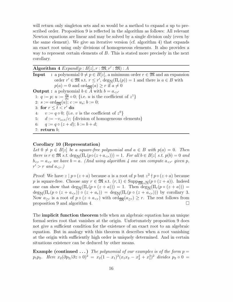
will return only singleton sets and so would be a method to expand a up to pre-scribed order. Proposition 9 is reflected in the algorithm as follows: All relevantNewton equations are linear and may be solved by a single division only (even bythe same element). We give an iterative version (cf. algorithm 4) that expandsan exact root using only divisions of homogeneous elements. It also provides away to represent certain elements of B. This is stated more precisely in the nextcorollary.

Algorithm 4 Expand(p : B[z], r : M, r′ : M) : A

Input : a polynomial 0 6= p ∈ B[z], a minimum order r ∈ M and an expansionorder r′ ∈ M s.t. r ≤ r′, degN(Πr(p)) = 1 and there is a ∈ B withp(a) = 0 and ordM(a) ≥ r if a 6= 0

Output : a polynomial b ∈ A with b = a<r′

1: q := p; u := ∂q∂z

◦ 0; {i.e. u is the coefficient of z1}2: s := ordM(u); c := us; b := 0;3: for r ≤ t < r′ do4: v := q ◦ 0; {i.e. v is the coefficient of z0}5: d := −vs+t/c; {division of homogeneous elements}6: q := q ◦ (z + d); b := b + d;7: return b;

Corollary 10 (Representation)Let 0 6= p ∈ B[z] be a square-free polynomial and a ∈ B with p(a) = 0. Thenthere is r ∈ M s.t. degN(Πr(p◦ (z +a<r))) = 1. For all b ∈ B[z] s.t. p(b) = 0 andb<r = a<r we have b = a. (And using algorithm 4 one can compute a<r′ given p,r′ > r and a<r.)

Proof: We have z | p ◦ (z + a) because a is a root of p but z2 - p ◦ (z + a) becausep is square-free. Choose any r ∈ M s.t. (r, 1) ∈ SuppM×N(p ◦ (z + a)). Indeedone can show that degN(Πr(p ◦ (z + a))) = 1. Then degN(Πr(p ◦ (z + a))) =degN(Πr(p ◦ (z + a<r)) ◦ (z + ar)) = degN(Πr(p ◦ (z + a<r))) by corollary 3.Now a≥r is a root of p ◦ (z + a<r) with ordM(a≥r) ≥ r. The rest follows fromproposition 9 and algorithm 4. �

The implicit function theorem tells when an algebraic equation has an uniqueformal series root that vanishes at the origin. Unfortunately proposition 9 doesnot give a sufficient condition for the existence of an exact root to an algebraicequation. But in analogy with this theorem it describes when a root vanishingat the origin with sufficiently high order is uniquely determined. And in certainsituations existence can be deduced by other means.

Example (continued . . . ) The polynomial of our examples is of the form p =p1p2. Here x2(∂p2/∂z ◦ 0)2 = x2(1 − x1)

2(x1x2 − x22 + x3

1)2 divides p2 ◦ 0 =

16

x2(x1x2 − x22 + x3

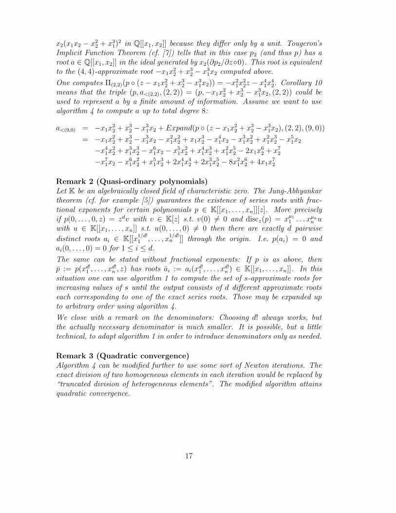
1)2 in Q[[x1, x2]] because they differ only by a unit. Tougeron’s

Implicit Function Theorem (cf. [7]) tells that in this case p2 (and thus p) has aroot a ∈ Q[[x1, x2]] in the ideal generated by x2(∂p2/∂z◦0). This root is equivalentto the (4, 4)-approximate root −x1x

22 + x3

2 − x31x2 computed above.

One computes Π(2,2)(p ◦ (z − x1x22 + x3

2 − x31x2)) = −x2

1x22z − x4

1x42. Corollary 10

means that the triple (p, a<(2,2), (2, 2)) = (p,−x1x22 + x3

2 − x31x2, (2, 2)) could be

used to represent a by a finite amount of information. Assume we want to usealgorithm 4 to compute a up to total degree 8:

a<(9,0) = −x1x22 + x3

2 − x31x2 + Expand(p ◦ (z − x1x

22 + x3

2 − x31x2), (2, 2), (9, 0))

= −x1x22 + x3

2 − x31x2 − x2

1x22 + x1x

32 − x4

1x2 − x31x

22 + x2

1x32 − x5

1x2

−x41x

22 + x3

1x32 − x6

1x2 − x51x

22 + x4

1x32 + x2

1x52 − 2x1x

62 + x7

2

−x71x2 − x6

1x22 + x5

1x32 + 2x4

1x42 + 2x3

1x52 − 8x2

1x62 + 4x1x

72

Remark 2 (Quasi-ordinary polynomials)Let K be an algebraically closed field of characteristic zero. The Jung-Abhyankartheorem (cf. for example [5]) guarantees the existence of series roots with frac-tional exponents for certain polynomials p ∈ K[[x1, . . . , xn]][z]. More preciselyif p(0, . . . , 0, z) = zdv with v ∈ K[z] s.t. v(0) 6= 0 and discz(p) = xµ1

1 . . . xµnn u

with u ∈ K[[x1, . . . , xn]] s.t. u(0, . . . , 0) 6= 0 then there are exactly d pairwise

distinct roots ai ∈ K[[x1/d!1 , . . . , x

1/d!n ]] through the origin. I.e. p(ai) = 0 and

ai(0, . . . , 0) = 0 for 1 ≤ i ≤ d.

The same can be stated without fractional exponents: If p is as above, thenp := p(xd!

1 , . . . , xd!n , z) has roots ai := ai(x

d!1 , . . . , xd!

n ) ∈ K[[x1, . . . , xn]]. In thissituation one can use algorithm 1 to compute the set of s-approximate roots forincreasing values of s until the output consists of d different approximate rootseach corresponding to one of the exact series roots. Those may be expanded upto arbitrary order using algorithm 4.

We close with a remark on the denominators: Choosing d! always works, butthe actually necessary denominator is much smaller. It is possible, but a littletechnical, to adapt algorithm 1 in order to introduce denominators only as needed.

Remark 3 (Quadratic convergence)Algorithm 4 can be modified further to use some sort of Newton iterations. Theexact division of two homogeneous elements in each iteration would be replaced by“truncated division of heterogeneous elements”. The modified algorithm attainsquadratic convergence.

17

References

[1] Alonso, M. E., Luengo, I., and Raimondo, M. An algorithm on quasi-ordinary polynomials. In Applied algebra, algebraic algorithms and error-correcting codes (Rome, 1988), vol. 357 of Lecture Notes in Comput. Sci.Springer, Berlin, 1989, pp. 59–73.

[2] Alonso, M. E., Mora, T., and Raimondo, M. A computational modelfor algebraic power series. J. Pure Appl. Algebra 77, 1 (1992), 1–38.

[3] Beringer, F., and Richard-Jung, F. Multi-variate polynomials andNewton-Puiseux expansions. In Symbolic and numerical scientific computa-tion (Hagenberg, 2001), vol. 2630 of Lecture Notes in Comput. Sci. Springer,Berlin, 2003, pp. 240–254.

[4] Gonzalez Perez, P. D. Singularites quasi-ordinaires toriques et polyedrede Newton du discriminant. Canad. J. Math. 52, 2 (2000), 348–368.

[5] Luengo, I. A new proof of the Jung-Abhyankar theorem. J. Algebra 85, 2(1983), 399–409.

[6] McDonald, J. Fiber polytopes and fractional power series. J. Pure Appl.Algebra 104, 2 (1995), 213–233.

[7] Ruiz, J. M. The basic theory of power series. Advanced Lectures in Mathe-matics. Friedr. Vieweg & Sohn, Braunschweig, 1993.

[8] Walker, R. J. Algebraic curves. Springer-Verlag, New York, 1978. Reprintof the 1950 edition.

[9] Wavrik, J. J. A theorem of completeness for families of compact analyticspaces. Trans. Amer. Math. Soc. 163 (1972), 147–155.

18

Documents

Approximate Roots in Graded Rings