Embed Size (px)
Citation preview

ApproximateAutomatedCampaign
Analysis withDensity BasedClustering
by
Federico Falconierisubmitted in partial fulfillment of therequirements to obtain the degree of
Master of Sciencein
Computer Scienceat the Delft University of Technology,
to be defended publicly onThursday October 11, 2018 at 10:00 AM.
This thesis is confidential and cannot be made public until December 31, 2019.
An electronic version of this thesis is available at http://repository.tudelft.nl/.

ii
Thesis committee:
Chair: Dr. ir. J. C. A. van der Lubbe, Faculty EEMCS, Cyber Security Group, TU DelftCommittee Member: Prof. dr. Alan Hanjalic, Faculty, EEMCS Multimedia Computing Group, TU DelftSupervisor: Dr. Christian Doerr, Faculty EEMCS, Cyber Security Group, TU Delft

Contents
1 Introduction 11.1 Contemporary Threat Landscape and Threat Intelligence . . . . . . . . . . . . . . . . . . 11.2 State of the art and gaps: Lockheed Martin kill chain model . . . . . . . . . . . . . . . . . 21.3 Research goal and vision . . . . . . . . . . . . . . . . . . . . . . . . . . . . . . . . . . . 4
2 Related Work 72.1 Multi Stage Threat Modelling: the kill chain . . . . . . . . . . . . . . . . . . . . . . . . . . 72.2 Lockheed Martin Intrusion Kill Chain . . . . . . . . . . . . . . . . . . . . . . . . . . . . . 9
2.2.1 Indicators . . . . . . . . . . . . . . . . . . . . . . . . . . . . . . . . . . . . . . . . 92.2.2 Course of Action . . . . . . . . . . . . . . . . . . . . . . . . . . . . . . . . . . . . 112.2.3 Kill chain analysis & synthesis . . . . . . . . . . . . . . . . . . . . . . . . . . . . . 112.2.4 Campaign analysis . . . . . . . . . . . . . . . . . . . . . . . . . . . . . . . . . . . 12
2.3 Kill Chain related work . . . . . . . . . . . . . . . . . . . . . . . . . . . . . . . . . . . . . 122.4 Research gaps . . . . . . . . . . . . . . . . . . . . . . . . . . . . . . . . . . . . . . . . . 20
3 Methodology 213.1 Hypotheses and research questions . . . . . . . . . . . . . . . . . . . . . . . . . . . . . 223.2 Automation: clustering . . . . . . . . . . . . . . . . . . . . . . . . . . . . . . . . . . . . . 23
3.2.1 Selecting a suitable clustering method . . . . . . . . . . . . . . . . . . . . . . . . 243.2.2 Density based clustering algorithms: DBSCAN and HDBSCAN . . . . . . . . . . . 24
3.3 Fuzziness: approximate string match . . . . . . . . . . . . . . . . . . . . . . . . . . . . . 253.4 Experimental data: Dutchsec Spamtrap. . . . . . . . . . . . . . . . . . . . . . . . . . . . 26
3.4.1 Emails and attachments in the kill chain. . . . . . . . . . . . . . . . . . . . . . . . 273.4.2 Dutchsec Spamtrap . . . . . . . . . . . . . . . . . . . . . . . . . . . . . . . . . . 283.4.3 Malignity blindess and data suitability . . . . . . . . . . . . . . . . . . . . . . . . . 293.4.4 Selection of features suitable for approximate match. . . . . . . . . . . . . . . . . 29
3.5 Approximate Automated Campaign Analysis with Density-Based Clustering . . . . . . . . 313.5.1 System overview . . . . . . . . . . . . . . . . . . . . . . . . . . . . . . . . . . . . 313.5.2 Phase 1: data enrichment . . . . . . . . . . . . . . . . . . . . . . . . . . . . . . . 323.5.3 Phase 2: preprocessing and feature selection . . . . . . . . . . . . . . . . . . . . 363.5.4 Phase 3-6: the automation engine. . . . . . . . . . . . . . . . . . . . . . . . . . . 363.5.5 Phase 3: indicator level similarity computation . . . . . . . . . . . . . . . . . . . . 373.5.6 Phase 4: indicator level clustering . . . . . . . . . . . . . . . . . . . . . . . . . . . 403.5.7 Phase 5: killchain level similarity computation . . . . . . . . . . . . . . . . . . . . 443.5.8 Phase 6: killchain level clustering (campaign labeling) . . . . . . . . . . . . . . . . 45
4 Results 494.1 Campaign Analysis, Research Gap and Research Goals of this project . . . . . . . . . . 494.2 Experimental results . . . . . . . . . . . . . . . . . . . . . . . . . . . . . . . . . . . . . . 49
4.2.1 Dataset . . . . . . . . . . . . . . . . . . . . . . . . . . . . . . . . . . . . . . . . . 504.2.2 Experimental Setup . . . . . . . . . . . . . . . . . . . . . . . . . . . . . . . . . . 504.2.3 False Negatives and Recall . . . . . . . . . . . . . . . . . . . . . . . . . . . . . . 514.2.4 False Positives and Precision . . . . . . . . . . . . . . . . . . . . . . . . . . . . . 52
4.3 Analysis . . . . . . . . . . . . . . . . . . . . . . . . . . . . . . . . . . . . . . . . . . . . . 534.4 Limitations . . . . . . . . . . . . . . . . . . . . . . . . . . . . . . . . . . . . . . . . . . . 534.5 Notable Findings . . . . . . . . . . . . . . . . . . . . . . . . . . . . . . . . . . . . . . . . 57
iii

iv Contents
5 Conclusion and Future Work 61
A Kill chain Features 65
B Synthetic campaigns 69
C Real Campaigns discovered manually 71
Bibliography 75
1Introduction
The modern cybersecurity landscape is characterised by the increasing number of actors capable ofperforming advanced and highly impactful hacking. The situation has worsened significantly in the lastdecade because more and more of the critical infrastructure is connected to the Internet, because thecapabilities of attackers have improved and because their numbers have increased.Threat Intelligence emerged as a valuable domain to enhance security defences by studying threatsmotives, techniques, tools and procedures. Campaign analysis is a process that belongs to this domainand deals with following attackers through time by linking several hack attempts that share a threatactor, a victim and that have a specific goal. Unfortunately, this process is rarely applied in practicebecause the campaign analysis models available in literature rely on manual investigation by securityprofessionals. This approach can become quickly too expensive, both regarding time and humanresources.
In this thesis project, we improve the state of the art by automating a popular campaign analysisframework introduced in 2011 by Lockheed Martin security researchers Hutchins et al. [10]. We donot only automate the process: we also improve its recall performance to provide security analyst withmore interesting and complete findings. Hopefully, this will empower all organisations, of any size ansecurity profile, to perform their threat intelligence. Lowering the adoption threshold is a fundamentalrequirement that is inescapable if we want security to improve horizontally throughout all industry sec-tors. Widespread adoption of campaign analysis would lead to a broader and quicker understandingof threat campaigns and goals, contributing to a safer society.
1.1. Contemporary Threat Landscape and Threat IntelligenceAdvance Persistent Threats, or APTs, are groups with enough time, resources and capabilities to con-tinuously attempt hacking towards a specific target. APTs started to become a severe problem at thebeginning of this decade. Not only they grew in numbers as nations scrambled to get their state-sponsored groups, but the impact of their operations started to be significant enough to fall under thedefinition of warfare (or better cyberwarfare). Indeed, NATO started considering cyberspace the fifthoperational domain for warfare after land, sea, air and space 1. The Pentagon started to do this as earlyas 2010 [14]. APTs are not all non-profit driven state-sponsored groups: some are large criminal groupsusing hacking as a source of income. In general, APTs activities range from acts of cyberwarfare (likethe Stuxnet hack 2) to both conventional and industrial espionage (like the Gemalto 3 4 and Petrobras5 cases). They are characterised by multi-staged, long-term intrusion attempts, persistence and useof highly sophisticated techniques. State-sponsored APTs techniques tend to be adopted by criminalgroups down the line. One excellent and recent example is the WannaCry ransomware campaign of
1https://www.militarytimes.com/2016/06/14/air-land-sea-cyber-nato-adds-cyber-to-operation-areas/2https://www.wired.com/2014/11/countdown-to-zero-day-stuxnet/3https://www.gemalto.com/press/pages/gemalto-presents-the-findings-of-its-investigations-into-the-alleged-hacking-of-sim-card-encryption-keys.aspx
4https://theintercept.com/2015/02/19/great-sim-heist/5https://www.theguardian.com/world/2013/sep/09/nsa-spying-brazil-oil-petrobras
1

2 1. Introduction
May 2017. The United States National Security Agency (NSA) discovered a flaw in Microsoft imple-mentation of an old but ubiquitous version of SMB (Server Message Block). Rather than responsiblydisclosing the flaw to Microsoft, the NSA developed an exploit, called EternalBlue, that abused the vul-nerability. On April 14th 2017 a group of hackers (the ShadowBrokers) leaked to the public several NSAdeveloped exploits, including EternalBlue. On May 12th 2017 the WannaCry ransomware campaignstarted and it infected over 230000 computers in more than 150 countries within a day 6. Wannacryused EternalBlue to infect other computers on the same local network over SMB. After ShadowBrokerspublication, the APT developed exploit was accessible to everyone, including criminal groups that thenstarted using it for their profit-driven purposes. The access to these sophisticated methods vastly en-larged the pool of threat actors capable of performing advanced hacking. As seen for Wannacry, toolsdeveloped by state-sponsored actors can quickly end up in criminal group hands.
This widespread adoption of APTs techniques when leaked (or sold on the black market to the bestofferer) have made the eggshell model of security increasingly insufficient. The eggshell security is thetraditional model where there is just one hard layer of defences at the border, around an organisation,and nothing more. Thus, if an attacker successfully breaches the perimeter, he then has instantlygained access to all valuable assets. To cope with the level of complexity and capability of APTs aswell as their modus operandi (which as seen can also spread to less skilled threat groups) the defensiveside of security has moved from the eggshell model to a layered model, where defensive technologiesare deployed both on the border of and within an organisation computer network. Furthermore, becauseacting only upon discovery of a compromise can be already too late, for example when the goal of thehack is the exfiltration of sensitive information, defensive effort has to focus on multiple aspects likeprevention, protection, detection and response.
Threat Intelligence has emerged as a valuable process to improve cybersecurity operations in or-ganisations by shifting the focus from sole defending to additionally understanding the threat landscape.The goal of threat intelligence is to study tactics, techniques and procedures of threats. Findings canbe leveraged and shared to select the most appropriate cybersecurity countermeasures, to performdata-driven cyber risk management and to predict & prevent their future moves.
The cyber-security research world has developed a plethora of multi-layered frameworks to performthreat intelligence in the past decade. Among them, one that stands out is Lockheed Martin kill chainmodel, which was released as a white paper in 2011 [10]. Lockheed Martin is the kind of organisa-tion that state-sponsored APTs target due to the highly sensitive nature of their intellectual property:the corporation operates in weapon manufacturing and aerospace development for the United Statesgovernment. The kill chain model was seminal in showing how data-driven threat intelligence can beperformed in practice and how it can be used to continuously improving defences by studying adver-saries over time. In the next section, we briefly present this model and why it stands out. Furthermore,we also show its limitation and how we aim to improve it.
1.2. State of the art and gaps: Lockheed Martin kill chain modelOne of the most relevant models developed to perform threat intelligence of APTs intrusion attempts isthe Lockheed Martin Intrusion Kill Chain [10], in which Hutchins et al. adapted the military concept ofkill chain to the cyber security domain. Intuitively, an attack (traditional or digital) is always composedof a series of steps like for example studying the victim, thinking of a strategy and selecting a weapon.The kill chain model is a framework that envisions a complex attack process as a series of atomicalsequential phases. To successfully achieve the attack objective it is required to complete every phaseof the chain successfully. Any disruption at any of the phases will lead to failure. The cyber intru-sion kill chain of Lockheed Martin has seven phases: reconnaissance (intelligence gathering on thevictim), weaponization (developing the computer virus), delivery of the virus to the victim (usually viaemail), exploitation (convincing the victim to open the virus or exploiting a program flaw likeWannaCry),installation of the virus on the victim computer, command and control (the installed virus enables the at-tacker to control the victim computer remotely) and finally actions on objective (for example exfiltratinginformation).
Among many other processes performed in Threat Intelligence, one is of particular interest: cam-paign analysis. The principal goal of campaign analysis is to determine the patterns and behaviours ofthe intruders, their tactics, techniques, and procedures (TTP), to detect “how” they operate rather than6http://www.bbc.com/news/world-europe-39907965

1.2. State of the art and gaps: Lockheed Martin kill chain model 3
specifically “what” they do [10]. Lockheed Martin defines a clear methodology to perform campaignanalysis in practice with email carried spear phishing attacks.
Related incidents can be grouped by looking for commonalities in the metadata of the vari-ous attempts after they have been mapped to kill chains. Campaign discovery allows to understandthe attacker motives, to track him through time and to understand his capabilities. All these findingscan be used to improve defences, leading ideally to a model where the defender iteratively adjusts hisdefensive posture to the attacker capabilities as the attacker evolve his campaign through time. Thisprocess can be particularly valuable because it allows for data-driven security spending. The budgetcan be allocated efficiently where it is needed based on the actual threats being faced, rather thanon a generic idea of the current threat landscape. Lockheed Martin intrusion kill chain and campaignanalysis are explained in depth in section 2.2.
Unfortunately, the kill chain model or any other multi-stage threat models are rarely usedin practice because frameworks found in literature, including Lockheed Martin’s, rely heavilyon manual aggregation performed by experienced security analysts. The cost of hiring dozens ofsecurity analysts to spend hundreds of hours to perform this manually is prohibitive for all companies butthose that are large enough and where threat intelligence is an absolute priority (like Lockheed Martin).Moreover, due to the absence of automation, it is necessary to hire a large number of experiencedanalyst, something not only expensive but also rare as the amount of professionals in cybersecurity isfar below the (increasing) demand of the market 7. These complexities are a deal breaker for a smallerorganisation but are also not ideal for large organisations, where the amount of data can quickly becomeoverwhelming.Furthermore, state of the art campaign analysis can be easily circumvented by adding a component ofrandomness when an attack is carried. Indeed, only exact match of kill chain features is performedin the original model. A spear phishing campaign is not going to be discovered by this methodologyif the attacker is wise enough to add a random sequence of numbers to his malicious attachmentfilenames. This kind of randomisation operation is easy to perform, but hard to do in a way that doesnot retain some form of structure (e.g. partial filename still the same or fixed number of digits). Weencountered many examples of this kind of obfuscation techniques in the dataset that we later usedto develop and test our automated framework. Figure 1.1 shows an example of “fuzzy” campaign thatwould effectively escape traditional exact-match-only campaign analysis.
According to a recent SANS survey 8 75% of the responders (representing organisations hetero-geneously distributed across many sectors) find cyber threat intelligence critical to security. Yet, only27% indicates that their teams have fully embraced the concept of CTI and integrated response policiesacross systems and staff. When asked what is holding their organisation back in achieving integratedCTI capabilities respectively 34.9% and 10.8% mentioned lack of budget and stuff to perform it andlack of management buy-in/understanding of its usefulness. We can not retrieve an exact figure onhow many companies perform Lockheed Martin version of campaign analysis, but the data availableseem to indicate that, together to other CTI processes, it is not performed very often.
Automation could undoubtedly help to lower the threshold (cost) in the adoption of this process. Amethodology that aids in automated campaign analysis would be very helpful for example in securityoperation centres to keep track of malicious actors over time and improving detection rules by conse-quence. The impact of such a methodology would be two-fold. On the one hand, organisations thatalready do perform campaign analysis could have their analysts use their time more efficiently becausethe manual grouping could be avoided. Instead, these analysts could focus on evaluation and data ex-ploration. On the other hand, organisations that do not perform any CTI and specifically campaignanalysis could finally perform it without the need for a large analyst team or a significant increase inbudget spending.A solution for automatic campaign analysis would significantly lower the adoption hassle for many or-ganisations. More organisations performing threat intelligence means more indicators collection andpossibly sharing, and indicator sharing leads to a more secure society.Bottom Line:
7https://www.forbes.com/sites/jeffkauflin/2017/03/16/the-fast-growing-job-with-a-huge-skills-gap-cyber-security/#20ed9c515163
8https://www.alienvault.com/docs/SANS-Cyber-Threat-Intelligence-Survey-2015.pdf

4 1. Introduction
• sophisticated techniques developed by APTs eventually leak/sold to less skilled groups...
• ...threat landscape increasingly larger and more capable of causing serious damage
• to cope with this: new defensive processes, including threat intelligence
• kill chain model and campaign analysis are effective forms of threat intelligence...
• ...but often too expensive because heavily manual and thus not performed in practice
• solution: automation
1.3. Research goal and visionThe problem we are trying to solve, automating campaign analysis, is a form of machine learning task.Specifically, in the absence of training data, we are dealing with unsupervised learning. We can think ofthis problem as a form of clustering because we are trying to aggregate similar items together. Indeed,we are trying to automatically infer a structure from the raw data, without any a priori knowledge. Thegoal of this thesis project is to produce and evaluate a methodology to automate campaign analysisemploying clustering. We obtained a large set of malicious emails from Dutchsec, an Utrecht-basedcybersecurity company; we use this data to design and evaluate our solution. We develop this solutionin practice with a pipeline of tools that:
• have as input non-labelled malicious emails
• extract valuable features from the emails
• extract further features by executing the malicious attachments and recording their activity
• cluster together related emails, allowing for different threat profiles to be selected for the clustering(e.g. APT targeted attacks or mass phishing scams campaigns)
• present the results back to the analyst
A diagram of our solution is shown in Figure 1.2, where the scientific contribution is highlighted in theblue area.
It is essential to understand to what degree we want to introduce automation in this domain. Thepresence of an analyst is fundamental to evaluate the results of the clustering. Our deliverable shouldbe seen as an aid to perform exploratory data analysis, rather than a perfect system that removes theneed for the human in the loop. The goal is to automate the process of aggregating kill chains, whichis the substantially mechanical portion of the job. This task can take hours or even be infeasible ifthe amount of data or its multidimensionality are large. We expect our system to produce some noisebecause no clustering can be perfect. We believe that the tradeoff between recall and precision will beworth it because if the linkage can take very long to be performed manually, whereas getting rid of noisecan be done quickly by an experienced analyst because of his domain knowledge. Furthermore, thebenefits of introducing automation would not be limited to the task of labelling campaigns. Indeed, afteranalyst evaluation, verified campaigns will have been found. These could then be used as a trainingset for further automatic detection and classification.
This thesis report is structured as follows.Section 2 contains a thorough explanation of the concept of kill chain, from its military origin to Lock-heed Martin cybersecurity adaptation and a survey of the state of the art in kill chain models for threatintelligence .Section 3 presents the research methodology together with the choices and implementing challengesthat characterised its development.Section 4 shows the final results.Section 5 finally describes the conclusion of this research project and the possible future work.

1.3. Research goal and vision 5
Figure 1.1: Example of a fuzzy spear phishing campaign encountered in the dataset at our disposal. All indicators seems toalmost always be randomized to a degree, but they also seem to maintain an overall logical structure.

6 1. Introduction
Figure 1.2: High level overview of the system envisioned for this thesis project. The orange area is implemented as a deliverable.The blue area represents the automation engine, which is the scientific contribution of this model.

2Related Work
This section contains a summary of the state of the art on multi-stage threat models for cybersecurity.The concept of kill chain is explained, as well as all the insight that can be derived from it, with a focuson threat intelligence and cyber risk management. We summarise here the related work and pointto the research gap. Section 2.1 explains the general theory and common military applications of killchain models. Section 2.2 describes in detail the paper that adapted the concept of kill chain to thecybersecurity domain: Lockheed Martin’s “Intelligence-Driven Computer Network Defense Informed byAnalysis of Adversary Campaigns and Intrusion Kill Chains”[10]. Section 2.3 is a broad summary ofthe most relevant literature inspired by Lockheed Martin intrusion kill chain.
2.1. Multi Stage Threat Modelling: the kill chainThe kill chain model is a framework that maps attacker behaviour to phases in an adversarial setting,for example conventional symmetric warfare or unconventional asymmetric warfare (like terrorism orguerrilla fighting). In a kill chain model, an attack is broken in atomic phases.
Figure 2.1 exemplarily shows a well known and used in practice model: the F2T2EA kill chain usedby the United States Air Force. F2T2EA stands for the 6 phases find, fix, track, target, engage, assess.
A short example of an attack mapped through this model is the following:
1. Find: a phone call by a person of high interest is detected in a heavily populated urban area of acity neighbouring a war zone.
2. Fix: GSM triangulation is used to establish the location of the subject
3. Track: a surveillance drone is deployed in the area to get visual confirmation of the target identity.Visual confirmation is establishedwhen the subject leaves the building. The drone keeps followinghim.
4. Target: the chain of command authorises a strike as soon as the subject leaves the urban areato minimise collateral damage.
5. Engage: an F16 jet takes off from the nearest airbase and reaches the target. Then strikes thetarget with a missile as he is moving in a car convoy out of town
6. Assess: the surveillance drone provides visual confirmation of the attack result, the subject carwas successfully hit and the subject is confirmed killed. The F16 jet can return to base
In a kill chain model, the attacker needs to go through each phase consecutively to reach his objec-tive. A disruption between any of the steps will stop the attack. In this example losing visual contact ofthe target at phase Track or a mechanical failure of the F16 jet at phase Engage would stop the attack.Aside from increasing chances of success in stopping/executing an attack, applying this model usuallycomes with further benefits:
• enhanced intelligence on adversary intent, capabilities and methods; this follows from the factthat the modus operandi of the studied actor is dissected in detail.
7

8 2. Related Work
Find
Fix
Track
Target
Engage
Assess
Locate and identify the target, for example by performing routine aerial orsatellite surveillance.
Making an accurate determination of location. The fix portion of what issometimes called the "kill chain" can be conducted in a number of ways.Items of interest can be imaged and the pictures compared with earlierimages, which include landmarks whose location is precisely known.
Monitor target movement.
Select an appropriate weapon or asset to use on the target to createdesired effects. Authorise the strike.
Apply the weapon to the target.
The use of men on the ground, satellites, UAVs, airplane imagery toestablish if the target was eliminated successfully.
F2T2EA Killchain Gen. John Jumper (U.S. Air Force), 1990
Figure 2.1: F2T2EA killchain model, used since 1990 by the U.S. Air Force.

2.2. Lockheed Martin Intrusion Kill Chain 9
• enhanced defence/offence by optimising resource allocation with the gathered intelligence.
General John Jumper, The Chief of Staff of the U.S. Air Force in the late 1990s is the father of themodern interpretation of the kill chain. He is the creator of the F2T2EA kill chain mentioned above,visible in Figure 2.1. The United States have been using this model in several conflicts since the firstGulf War, both with offensive and defensive goals.
An example of a defensive use of the model is to use it to disrupt IED 1 attacks from funding toattack execution.
2.2. Lockheed Martin Intrusion Kill ChainIn 2011 Hutchins, Cloppert and Amin adapted the concept to cybersecurity with the paper “Intelligence-Driven Computer Network Defense Informed by Analysis of Adversary Campaigns and Intrusion KillChains”[10] for LockheedMartin Corporation. The goal of the researchers was to establish a frameworkto enhance defensive capabilities against intrusions of Advanced Persistent Threats (APTs).
Hutchins et al. define a cyber intrusion as follows:
“The essence of an intrusion is that the aggressormust develop a payload to breach a trustedboundary, establish a presence inside a trusted environment, and from that presence, takeactions towards their objectives, be theymoving laterally inside the environment of violatingthe confidentiality, integrity, or availability of a system in the environment.”[10]
The phases of Lockheed Martin Intrusion Kill Chain are:
1. Reconnaissance: research, identify and select targets.
2. Weaponization: coupling of a remote access tool/backdoor with an exploit, often automaticallywith a tool called weaponizer, into a deliverable payload.
3. Delivery: transmission of the payload to the target.
4. Exploitation: triggering of the payload on the target environment through a software vulnerabilityor user action.
5. Installation: a remote access tool/backdoor is installed on the target environment to maintainpersistence and allow lateral movement.
6. Command and Control: the installed malware must establish a communication channel with theattacker to allow manual interaction.
7. Actions on Objectives: data exfiltration, lateral movement within the network, etc.
Figure 2.2 shows a diagram of the model with extensive phase explanation from the original paper.The authors developed this model to assess the disruptive rise of APTs in the threat landscape in theearly 2010s and the limits of traditional incident response, which mostly occurred only after a successfulbreach. Hutchins et al. publication was very impactful and introduced several concepts and processesthat are relevant for this thesis project: indicators, course of action, kill chain analysis & synthesis andcampaign analysis.
2.2.1. IndicatorsIndicators are any feature belonging to the data used or produced by the attacker. Examples of in-dicators in a spear phishing attack are the email headers, metadata of the payload, the vulnerabilityexploited, the hash of the payload, the files dropped by the malware, the IPs and domains that the mal-ware communicates to and many more. Indicators are essential for two reasons: they are traces thatthe attacker leaves, and as such, they can be used to fingerprint him and track him through campaignanalysis (more on this in a few paragraphs). Furthermore, they allow for practical risk managementbecause they show the capabilities of the threat agent. These capabilities can be mapped to counter-measures in what Hutchins et al. call a Course of Action matrix.1An improvised explosive device (IED) is a bomb constructed and deployed in ways other than in military action. It may be com-posed of conventional military explosives, such as an artillery shell, attached to a detonating mechanism. IEDs are commonlyused as roadside bombs, and they are generally seen in unconventional asymmetric warfare. In the second Iraq War, IEDswere used extensively against US-led invasion forces

10 2. Related Work
Reconnaissance
Weaponization
Delivery
Exploitation
Installation
Command &
Control
Actions on
Objective
Research, identification and selection of targets, often represented as crawling Internetwebsites such as conference proceedings and mailing lists for email addresses, socialrelationships, or information on specific technologies.
Coupling a remote access trojan with an exploit into a deliverable payload, typically bymeans of an automated tool (weaponizer). Increasingly, client application data files suchas Adobe Portable Document Format (PDF) or Microsoft Office documents serve as theweaponized deliverable.
Transmission of the weapon to the targeted environment. The three most prevalentdelivery vectors for weaponized payloads by APT actors, as observed by the LockheedMartin Computer Incident Response Team (LM-CIRT) for the years 2004-2010, are emailattachments, websites, and USB removable media.
After the weapon is delivered to victim host, exploitation triggers intruders’ code. Mostoften, exploitation targets an application or operating system vulnerability, but it could alsomore simply exploit the users themselves or leverage an operating system feature thatauto-executes code.
Installation of a remote access trojan or backdoor on the victim system allows theadversary to maintain persistence inside the environment.
Typically, compromised hosts must beacon outbound to an Internet controller server toestablish a C2 channel. APT malware especially requires manual interaction rather thanconduct activity automatically. Once the C2 channel establishes, intruders have “hands onthe keyboard” access inside the target environment.
Only now, after progressing through the first six phases, can intruders take actions toachieve their original objectives. Typically, this objective is data exfiltration which involvescollecting, encrypting and extracting information from the victim environment; violations ofdata integrity or availability are potential objectives as well. Alternatively, the intruders mayonly desire access to the initial victim box for use as a hop point to compromise additionalsystems and move laterally inside the network.
Lockheed Martin Intrusion Kill Chain, Hutchins et al., 2008
Figure 2.2: Lockheed Martin Intrusion Kill Chain Model [10]

2.2. Lockheed Martin Intrusion Kill Chain 11
Figure 2.3: Course of Action Matrix from Lockheed Martin “Intelligence-Driven Computer Network Defense Informed by Analysisof Adversary Campaigns and Intrusion Kill Chains”[10]. It maps the intrusion kill chain phases to the actions available to thedefender. At the intersections are the countermeasures available
2.2.2. Course of ActionThe Course of Action is a matrix that maps every phase of the kill chain to the six actions available toa defender. These actions come from the U.S. Department of Defense Information Operations Doc-trine and are: detect, deny, disrupt, degrade, deceive, destroy. Countermeasures are placed at theintersection between phase and action. For example, a firewall is a countermeasure to deny somereconnaissance activity (e.g. Nmap port scan). This matrix can be used to effectively map defensivecapabilities to attacker capabilities, leading to wiser investments in security. The Course of Actionmatrix from the paper can be seen in Figure 2.3
2.2.3. Kill chain analysis & synthesisKill chain analysis is a guide for analysts to understand what information is available for defensivecourses of action [10]. Upon detection of an intrusion attempt, a kill chain is created. Immediatelyit can be assumed that mitigations of phases before the one where detection happened failed. Forexample, if detection occurs at the Command and Control phase, this means that the attacker was ableto go through delivery, exploitation and installation successfully. Furthermore, the indicators belongingto these failed (from the defender perspective) phases can now be leveraged to improve the qualityof the countermeasures deployed. Studying failed mitigations is called Analysis, whereas the studyof post-detection phases is called Synthesis and is equally important. For example, if the email clientblocks the email with a malicious attachment upon delivery, indicators of the malicious attachmentcan be used to discover new techniques and capabilities on later phases (for example a new zero-day vulnerability) that perhaps would have been successful if not for early detection. In other words,analysis and synthesis allow to increase security from both failed and successful intrusions.
If detection happens at any given phase, not only the attack is stopped but allthe attacker techniques, intentions and to an extent identity are revealed, andthis information can be leveraged against him to mitigate against his futureattacks. This activedefensiveposturewill force the attacker to spenda lotmoretime and resources in recursively developing always new methods, as he can

12 2. Related Work
not recycle anything from his toolchain without being detected and linked toprevious attempts.
2.2.4. Campaign analysisKill chain analysis and synthesis over multiple intrusion attempts from an APT will likely reveal common-alities and overlapping indicators. Attackers tend to reuse parts of their toolchain when they persistentlyattack a target. It is merely natural and resource-wise to do so. If an attack is stopped at delivery, whyshould an attacker waste a perfectly working payload with a zero-day vulnerability that he purchasedon the black market for a high price? Overlapping indicators can be used for what Lockheed analystscall Campaign Analysis. Campaign Analysis allows tracking attackers through time by linking intrusionattempts (as kill chains) on overlapping indicators, getting a deep understanding not only of what theydo but of their patterns, behaviours, tactics, techniques and procedures as well as their intent. Thisprocess can also be used to attempt to establish attribution (mainly from time/geospatial indicators,victim and methods). Figure 2.4 shows an example of repeated spear phishing campaign observed byLockheed Martin.
Figure 2.4: Case study of three intrusion attempts experienced by LockheedMartin Computer Incident Response Team from [10].The attack vector of the intrusion was targeted malicious email. Some indicators are shown for each phase. One overlappingindicator links together the three attempts, leading the researchers to label this as a campaign.
2.3. Kill Chain related workAt the time of writing this section, Google Scholar counts 373 citations for Lockheed Martin’s whitepa-per [10]. Of those, over 50% are between 2016 and 2017, but the paper was published in 2011. Thiscitation trend shows that the article was probably quite ahead of its time. Since its publication, the workof Hutchins et al. has been broadly discussed, criticised and extended by the cybersecurity scientificcommunity. Figure 2.5 shows the distribution of citations over time according to Google Scholar.
Dan Guido’s “A case study of Intelligence-Driven Defense”[9] is the first work that used and mod-ified the concept of the kill chain for threat intelligence. It was published in 2011. Guido’s work is anengaging study because it uses the kill chain idea to gain knowledge on the economics of cybercrimeand it unveils the myth of complexity around mass malware campaigns. The author adapted Lockheed

2.3. Kill Chain related work 13
Figure 2.5: Google Scholar citation count for “Intelligence-driven computer network defense informed by analysis of adversarycampaigns and intrusion kill chains”[10] on June 20th 2018
Martin intrusion kill chain to the realm of mass malware; his modified chain has the steps: gain expo-sure, acquire capabilities, establish a delivery network, exploit the target, install malware, establish acommand and control, perform actions on objectives.
This kill chain is more abstract than Lockheed Martin’s, and thus less valuable if the goal is mappingthreat behaviour to countermeasures planning and deployment. Guido’s goal with this work is mainlyto do data-driven threat intelligence on mass malware cybercrime; improved defence is secondary.
Guido’s work is more interesting for his in-depth study of exploit kits than for the adapted kill chainthat he developed. He focused on the top 15 exploit kits of the first quarter of 2011 by popularity. Hisfindings are that the distribution of malicious URLs hosting these exploit kits is exponential: the top fourkits were responsible for 85% of the volume of malicious URLs. Furthermore, he collected the sourcecode of the exploits and mapped each kit to the vulnerabilities exploited. Guido found that the kitsdeveloped over the past two years implemented only 27 exploits and targeted only five applications:Microsoft Internet Explorer, Adobe Reader, Adobe Flash, Oracle Java, Apple QuickTime [9]. Thisfact is striking, as more than 8000 vulnerabilities were added at MITRE Common Vulnerability andExposure (CVE) project in 2010 alone. In other words, Guido found out that the most exploit kits targeta minimal set of vulnerabilities and focus on most commonly used applications. This finding makesperfect economic sense, as mass malware authors want to hit as many targets as possible minimisingcosts of development. The insight here from the defensive point of view is that by patching againstthose few vulnerabilities has a considerable impact on increasing resilience. The myth of complexitybehind mass malware is further unveiled when Guido shows the entirety of the 27 exploits code comesfrom two freely available sources:
• publicly disclosed targeted attacks by APTs, including vulnerabilities and possibly even imple-mented exploits;
• 0-days vulnerabilities responsibly disclosed by security researchers, possibly with implementedexploits;
The exploits that corrupted memory were developed predominantly by advanced persistent threats andused in targeted attacks. After this code became public, crime pack authors copied it verbatim and usedit for mass attacks [9]. The exploits that abused logic flaws originated entirely from security researcherdisclosures. A single researcher had disclosed three of the eight flaws [9].
In most cases, the attackers copied the exploit code verbatim. In other words, the authors of massmalware exploit kits rely almost entirely on others’ work. The most interesting conclusion of this workis that the kill chain model can be successfully extended from APT’s activity to untargeted mass mal-ware, as authors of exploit kits recycle partially/wholly APTs modus operandi and tools. A very recentexample of this is the WannaCry ransomware campaign of May 2017. The United States NationalSecurity Agency discovered a vulnerability of the SMBv1 protocol, CVE-2017-0144 2, that allowed forremote code execution. The NSA did not disclose the vulnerability and developed an exploit known as
2https://www.cve.mitre.org/cgi-bin/cvename.cgi?name=CVE-2017-0144
14 2. Related Work
Figure 2.6: Mandiant Attack Lifecycle model
EternalBlue 3. The exploit was leaked with others by the Shadow Brokers hacker group on April 14,2017 4. On May 12, 2017, the WannaCry ransomware campaign started, and it infected over 230000computers in more than 150 countries within a day 5. Wannacry used the EternalBlue exploit to infectother computers on the same local network over SMB. EternalBlue was also used for the NotPetyaransomware campaign that took place on June 27, 2017.
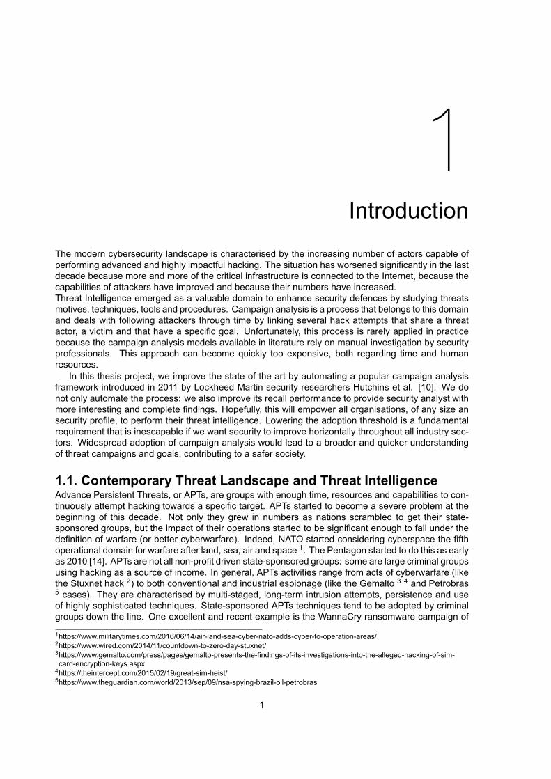
In 2013 the American cybersecurity firm Mandiant released a report on the activity of the advancedpersistent threat known as APT1 6. Mandiant did an impressive study of techniques, targets and mo-tives of the unit by observing the operations of APT1 since 2010. Researchers at the company likelyidentified the unit as the 2nd Bureau of the Chinese People’s Liberation Army General Staff Depart-ment’s 3rd Department also known as Unit 61398. Little information is officially available on Unit 61398and Mandiant makes the case that it is a cyber warfare division of the Chinese Army. In this work, Man-diant presents themulti-stage attackmodel that is used internally to study APTs like APT1: theMandiantAttack Lifecycle. Mandiant Attack Lifecycle has eight phases: initial recon, initial compromise, establisha foothold, escalate privileges, internal recon, move laterally, maintain presence, complete mission. Adiagram of the Mandiant Attack Lifecycle is showed at Figure 2.6. Escalate privileges, internal recon,move laterally and maintain presence are iterative and can be repeated until the mission is completed.The cyclic nature of Mandiant kill chain is a good representation of what happens in reality, whereattackers generally have to do quite some lateral movement from the first point of entry to find valu-able information on other machines. The attack lifecycle was developed with the mindset of the digitalforensics professional; unsurprisingly it is used by Mandiant only after successful exfiltration have beendiscovered.
Mandiant model may describe APTs behaviour better than Lockheed Martin original kill chain byadding a cyclic/iterative component, but it does not seem to be leveraged in practice for data science atleast in this report. Indeed, at least in this report, Mandiant does use their attack lifecycle as a reliabletool for mapping intrusions, comparing indicators, improving risk management and countermeasureswith analysis and synthesis but instead merely as a framework to describe APT activity more under-standable.
Bhatt et al. designed and implemented a “security event collection and analysis system”followingthe original kill chain model in “Towards a framework to detect multi-stage advanced persistent threatsattacks”[2]. The system is developed using Apache Hadoop technology and uses system logs as data.The process is described as semi-automatic because the detection and centralised logging is auto-matic, but the correlation process still requires the command of an experienced analyst. Furthermore,
3https://en.wikipedia.org/wiki/EternalBlue4https://arstechnica.com/information-technology/2017/04/nsa-leaking-shadow-brokers-just-dumped-its-most-damaging-release-yet/
5http://www.bbc.com/news/world-europe-399079656https://www.fireeye.com/content/dam/fireeye-www/services/pdfs/mandiant-apt1-report.pdf
2.3. Kill Chain related work 15
Bhatt et al. define the automatic event correlation to detect APTs as a research issue. The tool devel-oped has various modules, among which one of high interest for this research: the intelligence modulefor the log analysis process and the malware analysis module. The former uses a predefined tablecalled the Defense Plan. The table links intrusion kill chain phases to specific attack mechanism. Thelist of attack mechanism was extracted from CAPEC7 list from the non-profit MITRE corporation 8. Theresearchers tested an implementation without the malware analysis module and therefore were notable to test realistically kill chain phases after delivery. Furthermore, the intrusion synthesis module(for automatic correlation of kill chains into campaigns) is also missing and was replaced by manualwork by a security analyst. This short paper is a practical application of Lockheed Martin kill chainmodel and although the implementation lacks several critical elements the overall design is quite inter-esting. The main research issue, automatic correlation of kill chains in campaigns, remains open fouryears after publication.
In 2015 Mitre developed its framework for threat assessment: ATT&CK 9. The Cyber Attack Life-cycle, yet another revised kill chain, is one of the elements of ATT&CK and has the phases recon,weaponise, deliver, exploit, control, execute, maintain. ATT&CK is described as a threat data-informedadversary model, and it focuses on the post-exploit phases of the cyber attack lifecycle. Control, ex-ecute and maintain are decomposed in nine sub-phases: persistence, privilege escalation, defenseevasion, credential access, host enumeration, lateral movement, execution, c2, exfiltration. The de-construction is similar to what done in the Bryant kill chain [3] and has the same goal: to allow a practicalmapping of alerts and indicators to a multi-staged threat model. For each sub-phase, the techniquesavailable to adversaries are listed in a Tactics and Techniques table. Techniques may fall into one ormore sub-phases. Finally, each technique is labelled as detect, partially detect or no detect to showgaps in current cybersecurity countermeasures. Figure 2.7 shows an example of what is called theNotional Defense Gap table. This framework does not use the kill chain idea for enhanced threat in-telligence, but rather it is used for cyber risk management. Using a variation of the kill chain model forrisk management is not groundbreaking, as Hutchins et al. already did mention that the model couldbe used for that, but it is one of the few frameworks actually developed to do so.
Rutherford et al. [15] came up with an improved cybersecurity kill chain in “Using an ImprovedCybersecurity Kill Chain to develop an Improved Honey Community”with the following phases: re-connaissance, weapon selection, delivery, exploitation, intelligence gathering, objective execution andexfiltration of information. Interestingly, this kill chain features bidirectional attacker movement betweenthe last three steps. Whereas Lockheed work seems to give equal importance to each step, Ruther-ford’s work explicitly states the importance (for the defender) of the intelligence gathering phase (itreplaces the installation phase). This phase is here broader, and the rationale behind is similar to thatof Bryant kill chain [3].
The most significant change to the original kill chain introduced in this paper is the introduction ofbilateral arrows among the last phases. Non-linear kill chain navigation is not a new idea though, asseen in Mandiant Attack Lifecycle from 2013. Like in Mandiant case, Rutherford et al. do not show thepractical use of this kill chain, so the complications of introducing movement in the kill chain are ignored.
“A novel kill chain framework for remote security log analysis with SIEM software”by Bryant andSaiedian [3] is one of the latest (2017) and most inspirational interpretation at the kill chain concept.In this work, the authors develop a new kill chain framework centred on the use case of the internalsecurity analyst of an organisation. The new model leads to improved forensics and incident responsebut does not leverage the kill chain concept for improved threat intelligence and defences.
Security analysts often have to deal with incomplete or missing data when dealing with incidentinvestigation. Alerts are generated by a heterogeneous variety of sensors and countermeasures (IDS,firewalls, antiviruses, etc…), and even one single intrusion can trigger an overwhelming and disorgan-ised amount of alarms if proper automatic clustering is not in place.
7Common Attack Pattern Enumeration and Classification (CAPEC) is a list of software weaknesses curated by the non-profitMITRE Corporation
8https://capec.mitre.org/index.html9https://www.mitre.org/sites/default/files/publications/pr-15-1288-adversarial-tactics-techniques-common-knowledge-presentation.pdf

16 2. Related Work
Figure 2.7: Example of Notional Defense Gap table produced by MITRE’s ATT&CK framework

2.3. Kill Chain related work 17
Bryant and Saiedian explain that the state of the art in multi-staged attack modelling is not ad-dressing the issues of security analysts adequately: although a step in the right direction, actuallyimplementing and using established models is described as cumbersome and hardly successful if notin toy scenarios. The main issue with Lockheed Martin kill chain and Mandiant Attack Lifecycle is theirhigh level of abstraction. Phases are described vaguely, leading to subjective choices by the analyst inlabelling indicators. This vagueness, even if not critical in small investigations, points to potential incon-sistencies when more analysts work together on large cases or when organisations want to collaboratein cyber threat intelligence sharing.
Furthermore, the phases do not always align precisely with the countermeasures that generatealarms with additional confusion in labelling indicators. The first two phases of Lockheed Martin killchain (Reconnaissance and Weaponisation) extend beyond the scope of a single organisation networkand may require data unavailable to internal security teams. Vulnerabilities at these early phases maybe technical as well as non-technical (e.g. job posting on LinkedIn looking for professionals trained onspecific systems gives away information on the systems used internally). In general, vulnerabilities thatdon’t produce data in either way (out of scope or non-technical) are especially hard to use in a practical,easy to implement, way during an investigation. Concluding, the researchers agree that multi-stageattack modelling is the right idea but show that the state of the art models fail at implementation becausethey are too abstract and high level.
The authors present an improved multi-stage attack model called the Bryant kill chain. It is notjust another abstract tool to map APT’s intrusion activities but an entire methodology to systematicallyhandle complex incidents in an organisation with countermeasures deployed at multiple levels. TheBryant kill chain has four phases and seven sub-phases:
1. Network phase: Reconnaissance (Pre hack)
2. Network phase: Delivery (Pre hack)
3. Endpoint phase: Installation (Hack)
4. Endpoint phase: Privilege Escalation (Hack)
5. Domain phase: Lateral Movement (Compromise)
6. Domain phase: Actions on Objective (Compromise)
7. Egress phase: Exfiltration (Theft)
The seven sub-phases are further deconstructed in thirteen tasks that need to be executed progres-sively. The tasks are: (Reconnaissance) probing and enumeration, (Delivery) host access and networkdelivery, (Installation) host delivery and software modification, (Privilege Escalation) privilege esca-lation and privilege use, (Lateral Movement) internal reconnaissance and lateral movement, (Actionon Objective) data manipulation and obfuscation, (Exfiltration) external data transfer. The tasks aremapped to the following sensors: perimeter firewalls, network IDSs, domain controller logs, endpointmonitoring on the operating systems, host-based anti-malware programs, edge routers, network loadbalancers, remote access points. These sensors generate either logs (endpoint operating systems,firewall, etc…) or alerts (IDS, host-based anti-malware, etc…). Finally, tasks are mapped to indicators,features that can be extracted from the generated logs or alert. For example, in the case of probing theavailable indicators are port scans, default credential attempts, blacklisted traffic and the two specificWindows Event IDs 4625 and 5157 (respectively “Failed Logon”and “Firewall Deny”. A figure of thedeconstructed endpoint phase is provided in Figure 2.9 to have a better idea of how phases, tasks andindicators overlap.
The Bryant kill chain is designed to facilitate logical data aggregation. This is essential to link alertsfrom several sensors or phases into a single kill chain. Specifically, the model has a specific indicator asthe aggregate field for each sub-phase and then uses this aggregate field to link more phases together.For example, in Reconnaissance the aggregate field is the Source IP address. This source IP address ispresent also in the Delivery indicators, and therefore the two phases can be linked together. Continuingthrough the kill chain, the Destination IP indicator of the Delivery phase can be mapped to the ComputerName at Installation phase, and so on. This methodology is the same of Lockheed Martin’s kill chain.What is innovative is that this is the first time a practically deployable framework is described in detail

18 2. Related Work
Figure 2.8: Indicator relationship betwen phases in Bryant kill chain model [3]. Field used for data aggregation among phasesis in a red box.
for network intrusion. Whereas the original paper was an abstract description of a methodology, thispaper provides a working implementation. Figure 2.8 is provided for added clarity.
The authors deployed and tested the framework in conjunction with a SIEM10. The model provedeffective in reducing the number of false positives and negatives alerts, in reducing the overall numberof alerts by aggregating them and in providing a standard methodology for incident investigation. Thework of Bryant and Saiedian provides a remarkable evolution of the multi-stage attack model idea. Theproposed model is scalable, efficient and easy to use in practice. Less abstraction leads to less subjec-tivity when creating kill chains and therefore to improved consistency. The Bryant kill chain works wellregardless of the analyst and allows organisations to share data in the same format. Furthermore, thelinkage between phases by using aggregate indicator is a simple and very effective implementation.This approach is not exempt from shortcomings, because a less abstract framework comes at the costof reduced adaptability to unusual attack patterns. Furthermore, it is true that logs and sensor alarmscan easily provide attack data, but at the same time it is not addressed how indicators are extractedin vastly common scenarios like attacks that use emails as the attack vector. As we have previouslystated, the majority of attacks are The fundamental concepts of kill chain analysis and synthesis areignored, indicators of phases that are not triggering an alert are not leveraged during incident investiga-tion or afterwards to improve threat intelligence and defensive posture. Likewise, campaign analysis isalso not mentioned. The reason for this lies in the primary goal of the authors: improving the workflowof security analysts and forensics professionals with multi-stage attack models. Bryant and Saiedianachieved this goal by describing in detail a practical, non-abstract, methodology for these stakehold-ers, but sadly throughout the work there is no mention of threat intelligence or leveraging indicators forimproved defence and risk management. These were the main goals of Hutchins et al. for LockheedMartin.
10SIEM: security information and event management. Software to visualise and handle security incidents in an organisation ina centralised manner

2.3. Kill Chain related work 19
Figure 2.9: Deconstructed endpoint phase from Bryant kill chain [3]. This table shows clearly how sub phases, sensors, tasksand indicators overlap logically.
20 2. Related Work
2.4. Research gapsIn the previous sections, the original kill chain paper from Lockheed Martin[10] was presented togetherwith the most relevant related work that followed its publication in 2011. We want to highlight tworesearch gaps in the literature: the lack of automation and the increasingly anachronistic nature ofexclusively exact match of indicators in campaign analysis.Campaign analysis is a process rarely applied in practice, possibly due to the lack of a readily applicableand adaptable framework as well as for the lack of automation. Campaign analysis can be decomposedinto three sub-processes:
1. Detection of intrusion: automated with HIDS and NIDS technologies.
2. Killchain feature extraction from intrusion data: somewhat automated in the form of malwareanalysis tools and threat intelligence sources (e.g. Remnux, Virustotal, Cuckoo).
3. Correlation of kill chains in campaigns by looking for overlapping indicators: not automated.
Without automation, campaign analysis will remain an activity performed only by large organisationscapable of spending many resources in cybersecurity staff to manually look for overlapping indicators.
In all the kill chain models presented in section 2, campaign analysis was performed exclusivelyby searching for overlapping indicators that matched exactly. This approach is very simple, and itworks well enough in practice, especially with highly specific indicators like hashes, vulnerabilities CVEidentifiers or IP addresses. For other more “human oriented” indicators like email subjects or filenames,the exact match may not be the most optimal strategy. Changing one single character in an indicatorwill make exact match fail, and an attacker can easily automate the generation of always new subjectsand filenames, easily circumventing campaign analysis. Furthermore, this makes countermeasureslike static filtering based on databases of blacklisted indicators ineffective. What we see in practice, onthe other hand, is that often the automatic generation of new indicators tends to follow some form ofa pattern, possibly capturable by approximate matching. We believe approximate matching of someindicators could lead to not only more effective cyber defences but also to more exciting discoveries(at the inevitable price of a component of false positives).

3Methodology
In section 2.2 we thoroughly explained the concept of cyber kill chain and campaign analysis developedby Lockheed Martin in 2011. The kill chain is a model that maps an attack to phases in an adversarialsetting. In this model the attacker needs to go through each phase consecutively to reach his objec-tive: a disruption of the chain at any phase will cause the attack to fail. Aside from phases, the othercharacteristic atomic item of the kill chain model is the concept of indicator and its use. Indicators areany feature belonging to the data used or produced by the attacker. The usage of a specific exploit isan indicator, an IP address is an indicator, an email address is an indicator and so on.
A campaign is a repeated series of intrusion attempts, or in other words a collection of related killchains. Lockheed Martin researchers observed that in practice malicious actors, even sophisticatedones, tend to recycle to some extent at least a parts of their toolchain. In other words, separate intru-sion attempts can be linked together (in a campaign) if specific-enough indicators are found to occuracross them. When intrusions are targeted, frequent and persistent the volume of collectable indicatorsaugments, making it easier to spot patterns. The factors that lead attackers to recycle parts of their killchains are economical, threat-oriented and characteristic of the human nature.
Cybercriminals and APTs, no matter how large or advanced, have limited resources like any otherorganisation. These resources are money, time, workers at disposal. When a criminal group investsin an expensive vulnerability exploit acquired on the black market, they are incentivised to maximizethe return over the investiment by using it more often rather than less often. Similarly, when astate-sponsored APT spends months developing a highly advanced malware that exploits a zero-dayvulnerability, he will likely use it in more than one single attack.Like many other highly specific professions, APTs hackers tend to develop a particular style, or modusoperandi, in the way they perform their attacks. For example, the way they decide to move laterally ina network or to pick their targets and the techniques they use to socially engineer them are all influ-enced by their experiences, education, culture, upbringing. The modus operandi includes not only thetechniques and decision making but also the tools used. Some of these have to be developed inter-nally and are then shared by actors in the same collective but are not seen in other groups (similarly toconventional weapons for governments, state-sponsored APTs do not like to share their tools with theenemy).Moreover, these individuals and groups may actually not care about concealing their identity at all (forexample if they are protected by their country as long as they do hack organizations exclusively abroad,like Russia allegedly does 1 2) or value this less than reaching the objective of their campaign.Finally, hackers are humans, and humans make mistakes. Sloppiness, laziness and poor choice mak-ing can lead actors to recycle old indicators (e.g. usernames, passwords, emails).
Unfortunately, the models found in Literature to perform campaign analysis rely heavily on manualwork by an experienced security analyst, leading to prohibitive costs and complexity. Furthermore, wealso highlight the issue of the increasing inadequacy of exact-only match of indicators.The goal of this thesis project is to explore and implement a solution to significantly lower the cost ofperforming this process.1https://slate.com/technology/2018/02/why-the-russian-government-turns-a-blind-eye-to-cybercriminals.html2https://www.justice.gov/opa/pr/us-charges-russian-fsb-officers-and-their-criminal-conspirators-hacking-yahoo-and-millions
21

22 3. Methodology
In this chapter, we provide a detailed description of the methodology adopted. In section 3.1 wefirst explore two hypotheses on how to bridge the research gap mentioned and thus we formulate ourresearch questions and working items. Then, in sections 3.2 and 3.3 we study the hypotheses domainsin depth. In section 3.4 we describe the data used to build and test our solution. Finally, in section 3.5we present in detail our implemented solution.
3.1. Hypotheses and research questionsThe ultimate research goal of this thesis project is to improve the state of the art in campaign analysis.By studying the state of the art, we have highlighted two shortcomings of the models in the literature.The first research gap is the following:
Research Gap 1 Campaign labelling is a heavily manual, not automated, task and it is thusoften prohibitively expensive to perform in practice.
Campaign analysis is a process where separate incidents are grouped when relevant indicators overlapexactly. We can, therefore, say that campaign analysis is a task where unlabelled data (kill chains) areassigned a label (campaign). Performing this job manually becomes infeasible when the dataset orits dimensionality are large. We have therefore stated that we want to improve the state of the art byintroducing automation. Automating the process of labelling unlabelled categorical data is a very wellknown machine learning problem called classification. In this specific scenario, we do not know a priorithe number of categories (the number of campaigns). Furthermore, we want to develop a solutionthat does not require a training set of existing campaigns. We need to automate the discovery of newcampaigns together with the labelling of old campaigns. In machine learning performing classificationwithout a training set is called clustering or cluster analysis. Now that we understood that the problemat hand can be reduced to a form of well-known machine learning task, we formalise it as our firsthypothesis and thus come up with a related research question:
Hypothesis 1 Automating campaign analysis is a form of unsupervised classification(cluster analysis) task.
Research Question 1 Can campaign analysis be performed with an existent clustering tech-nique?
To perform unsupervised clustering analysis, it is necessary to use a measure of similarity to assess iftwo data points belong to the same cluster. In principle, more similar data points should be closer andthus more likely to end up in the same cluster whereas more different data points should be farther andthus less likely to cluster together. We will therefore also need to find a suitable measure of distance.In section 3.2 we will dive deeper into the domain of clustering in search of a suitable technique toperform it in our scenario.
The second research gap identified in the related work is the following:
Research Gap 2 Kill chains are grouped in campaigns only if indicators match exactly
In Lockheed Martin’s campaign analysis two intrusion attempts are grouped when one or more indica-tors belonging to their reciprocal list of indicators match exactly. Indicators are any feature belonging toan intrusion attempt, for example, the hash of the malicious payload, the CVE code of the vulnerabilityexploited, the email address of the sender of the malicious email, the IP that the malware contacts aftersuccessful installation. Although exact match of indicators surely performs well regarding precision,it can hardly keep up with the increasingly popular trend of obfuscation. To cope with increasinglyeffective forms of filtering, malware creators often add a component of randomness to indicators likefilenames, subjects and email addressed. This technique makes the exact match of indicators obso-lete, even though it was not developed for the precise reason of bypassing campaign analysis. We,therefore, formulate a second hypothesis and two related research question:
Hypothesis 2 Exact only indicator match likely does not perform optimally (in terms ofrecalla). A form of approximate match could improve the performance ofthe model for some indicators.ain this context, the recall is maximum when the number of false negatives is zero (items thatactually belong to a campaign but are not labelled as such by the system)

3.2. Automation: clustering 23
Research Question 2 Does approximate match of suitable indicators improve recall performanceof campaign analysis?
Research Question 3Can a methodology be developed to assess what indicators are most suit-able (and what are not) for approximate match?
In section 3.3 we explore the domain of similarity of information theory, looking for a suitable techniqueto perform approximate string matching and in section 3.4.4 we develop a methodology to understandwhat indicators are most suitable for this technique.
3.2. Automation: clusteringThe research problemwe are dealing with is to automate the process of linking relatedmalicious emails,by following the idea of Campaign Analysis introduced in LockheedMartin kill chain model[10]. As men-tioned in the previous section, this is a form of machine learning task called classification. Specifically,because we want to perform it without a training set, we are dealing with a clustering problem. Indeed,we want to build a system capable of performing unsupervised learning: we will feed it unlabelled killchains, and we want it to output their labels (the campaigns to which they belong).
In general, the goal of clustering is to separate an unlabeled data set into a finite and discrete setof “natural” hidden data structures [21]. Although many forms of clustering exist, the most prominentand related to the problem at hand are the following:
• Connectivity models: Hierachical Clustering
• Centroid based clustering
• Density based clustering
Hierarchical clustering (HC) algorithms organise data into a hierarchical structure according toa measure of proximity (also known as connectivity). The results of HC are usually depicted by abinary tree or dendrogram. The root node of the dendrogram represents the whole data set, and eachleaf node is regarded as a data object. The intermediate nodes, thus, describe the extent that theobjects are proximal to each other; and the height of the dendrogram usually expresses the distancebetween each pair of objects or clusters, or an object and a cluster. The ultimate clustering resultscan be obtained by cutting the dendrogram at different levels [21]. HC algorithms are mainly classifiedas agglomerative methods and divisive methods. Agglomerative clustering starts with clusters, andeach of them includes precisely one object. A series of merge operations are then followed out thatfinally lead all objects to the same group. Divisive clustering proceeds in an opposite way [21]. A clearadvantage of HC is that no a priori knowledge is required on the number of clusters, or categories. Thecommon criticism for classical HC algorithms is that they lack robustness and are, hence, sensitive tonoise and outliers [21]. A frequent phenomenon is chaining, or the production of a few large clusters,which are formed by virtue of nearness of points to be merged at different steps to opposite edges ofa cluster[20].
In contrast to hierarchical clustering, which yields a successive level of clusters by iterative fusionsor divisions, centroid based or partitional clustering assigns a set of objects into clusters with nohierarchical structure [21]. Here, clusters are represented by a central vector, whichmay not necessarilybe a member of the data set. When the number of clusters is fixed to k, k-means clustering gives aformal definition as an optimisation problem: find the k cluster centres and assign the objects to thenearest cluster centre, such that the squared distances from the cluster are minimised 3. Although it istheoretically possible to guess the number of k partitions in the data set, this can become increasinglyhard as the size of the dataset increases. In some cases not knowing a priori the exact number ofpartitions or even the order of magnitude makes using these techniques unfeasible.
Density based clustering (DBC) is an evolution of hierarchical clustering. The idea is to similarlyagglomerate or to divide the data points to find the final clusters, but instead of using a cut off valuebased on the distance of points, a more complex and granular measure is used: density.In DBC, a cluster is a set of data objects spread in the data space over a contiguous region of high3https://en.wikipedia.org/wiki/Cluster_analysis
24 3. Methodology
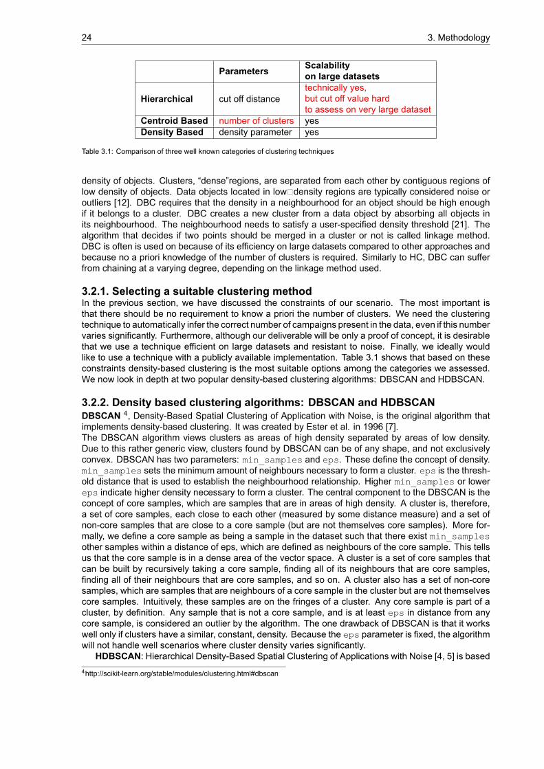
Parameters Scalabilityon large datasets
Hierarchical cut off distancetechnically yes,but cut off value hardto assess on very large dataset
Centroid Based number of clusters yesDensity Based density parameter yes
Table 3.1: Comparison of three well known categories of clustering techniques
density of objects. Clusters, “dense”regions, are separated from each other by contiguous regions oflow density of objects. Data objects located in low�density regions are typically considered noise oroutliers [12]. DBC requires that the density in a neighbourhood for an object should be high enoughif it belongs to a cluster. DBC creates a new cluster from a data object by absorbing all objects inits neighbourhood. The neighbourhood needs to satisfy a user-specified density threshold [21]. Thealgorithm that decides if two points should be merged in a cluster or not is called linkage method.DBC is often is used on because of its efficiency on large datasets compared to other approaches andbecause no a priori knowledge of the number of clusters is required. Similarly to HC, DBC can sufferfrom chaining at a varying degree, depending on the linkage method used.
3.2.1. Selecting a suitable clustering methodIn the previous section, we have discussed the constraints of our scenario. The most important isthat there should be no requirement to know a priori the number of clusters. We need the clusteringtechnique to automatically infer the correct number of campaigns present in the data, even if this numbervaries significantly. Furthermore, although our deliverable will be only a proof of concept, it is desirablethat we use a technique efficient on large datasets and resistant to noise. Finally, we ideally wouldlike to use a technique with a publicly available implementation. Table 3.1 shows that based on theseconstraints density-based clustering is the most suitable options among the categories we assessed.We now look in depth at two popular density-based clustering algorithms: DBSCAN and HDBSCAN.
3.2.2. Density based clustering algorithms: DBSCAN and HDBSCANDBSCAN 4, Density-Based Spatial Clustering of Application with Noise, is the original algorithm thatimplements density-based clustering. It was created by Ester et al. in 1996 [7].The DBSCAN algorithm views clusters as areas of high density separated by areas of low density.Due to this rather generic view, clusters found by DBSCAN can be of any shape, and not exclusivelyconvex. DBSCAN has two parameters: min_samples and eps. These define the concept of density.min_samples sets the minimum amount of neighbours necessary to form a cluster. eps is the thresh-old distance that is used to establish the neighbourhood relationship. Higher min_samples or lowereps indicate higher density necessary to form a cluster. The central component to the DBSCAN is theconcept of core samples, which are samples that are in areas of high density. A cluster is, therefore,a set of core samples, each close to each other (measured by some distance measure) and a set ofnon-core samples that are close to a core sample (but are not themselves core samples). More for-mally, we define a core sample as being a sample in the dataset such that there exist min_samplesother samples within a distance of eps, which are defined as neighbours of the core sample. This tellsus that the core sample is in a dense area of the vector space. A cluster is a set of core samples thatcan be built by recursively taking a core sample, finding all of its neighbours that are core samples,finding all of their neighbours that are core samples, and so on. A cluster also has a set of non-coresamples, which are samples that are neighbours of a core sample in the cluster but are not themselvescore samples. Intuitively, these samples are on the fringes of a cluster. Any core sample is part of acluster, by definition. Any sample that is not a core sample, and is at least eps in distance from anycore sample, is considered an outlier by the algorithm. The one drawback of DBSCAN is that it workswell only if clusters have a similar, constant, density. Because the eps parameter is fixed, the algorithmwill not handle well scenarios where cluster density varies significantly.
HDBSCAN: Hierarchical Density-Based Spatial Clustering of Applications with Noise [4, 5] is based4http://scikit-learn.org/stable/modules/clustering.html#dbscan

3.3. Fuzziness: approximate string match 25
Figure 3.1: Performance comparison of several clustering techniques. HDBSCAN performs better than DBSCAN. Taken fromHDBSCAN documentation.
on the aforementioned DBSCAN algorithm. HDBSCAN has just one very intuitive parameter: mincluster size. A cluster will be formed exclusively if this value is reached. This parameter is easyto set, whereas eps and min_samples are not very intuitive. The most significant advantage of HDB-SCAN over DBSCAN is that it performs well on a dataset with variable density clusters. HDBSCANrecursively performs DBSCANwith varying eps parameters, and then outputs themost optimal configu-ration automatically based on ametric of stability of the clusters found. This is a significant improvementover DBSCAN, because not only it is easier to configure (DBSCAN requires to try different values of epsextensively manually to find the best one, whereas HDBSCAN single parameter is the minimum clustersize), but also because it allows for different eps in different regions of the data space. For instance,HDBSCAN is capable of identifying a cluster within another cluster, whereas DBSCAN is not capableof doing so and it will label everything as the same one. Furthermore, HDBSCAN implementation isalso faster than DBSCAN, see Figure 3.1.
3.3. Fuzziness: approximate string matchIn section 2.4 we highlighted that one aspect missing from related work in campaign analysis literatureis fuzziness in indicator matching. To assess approximate matching, it is necessary to address first theconcepts of similarity.
The concept of similarity in Information Theory has been studied since the 1960s, mainly in thedomain of Probabilistic Record Linkage. It was based mainly on the seminal paper by Fellegi andSunter “A Theory for Record Linkage”[8] In the 1990s the topic was explored practically and not justtheoretically by a large number of researchers; most of today’s similarity algorithms and functions weredeveloped in this period [6]. Lin [13] gives a formal definition of Similarity in Information Theory:
The similarity between A and B ismeasured by the ratio between the amount of informationneeded to state the commonality of A and B and the information needed to describe fullywhat A and B are.
26 3. Methodology
Similarity is an especially important core element of processes that use features comparison forhigher level purposes, for example for Machine Learning.
As seen in the previous sections, features (or indicators) are the atomic element of existing kill chainmodels. No implementation seems to exist that uses systematic feature similarity methods with indica-tors in the related work on multi-stage threat modelling. This aspect is one of the novelties introducedin this thesis project. It was thus relevant to study the related literature on similarity methods to learnthe best techniques for our features.
String metrics are used mainly in search engines and in systems that check spelling or auto correctqueries. “A comparison of String Distance Metrics for Name-Matching Tasks”[6] by Cohen, Ravikumarand Fienberg provides an excellent reference point on the existing string metrics methods and howthey perform at different tasks. Four families of methods are presented:
• Edit-distance like functions: (Levenstein distance, Jaro distance and others) in which distancebetween two strings 𝑎 and 𝑏 is the cost of the best sequence of edit operations that convert 𝑎 into𝑏 (edit operations: character insertion, deletion, substitution etc…).
• Token-based distance function: two strings can be considered as multisets of substrings (or to-kens or n-grams). Jaccard similarity, TF-IDF or cosine similarity and other methods fall in thiscategory. The distance of two strings is computed as the difference between the two multisets.The tokens are also called n-gram based on the size 𝑛 of the tokens in characters (bi-gram andtri-gram if 𝑛 = 2 or 𝑛 = 3); this size is the most important parameters of token-based distancefunctions.
• Hybrid distance functions: they combine edit and token based distance functions in two or moresteps.
• “Blocking”or pruning methods: when matching large lists of strings it is often not computationallypractical or useful to measure the distance between all pairs. To solve this problem strings canbe grouped on some a priori variable and compare only groups that are interesting.
The Information Retrieval branch of Computer Science has produced countless methods for as-sessing document similarity (in this domain called relevance). The most pervasive application is in textsearch engines for the world wide web. These techniques usually involve creating a reverse index ofa text document [11], usually giving different weight to different words based on how often they occur(the idea is to make vastly common words like preposition less relevant). A reverse index is a tablethat tracks the number of occurrences and location of every word in the document.
One of the most common technique is called term frequency over inverse document frequency orTF-IDF. It is a numerical statistic that is intended to reflect how important a word is to a document ina collection or corpus. It is often used as a weighting factor in searches of information retrieval, textmining, and user modelling. The TF-IDF value increases proportionally to the number of times a wordappears in the document and is offset by the frequency of the word in the corpus, which helps to adjustfor the fact that some words appear more frequently in general. It can be applied to words as well asto token, for example in query completetion applications and keyboard auto-correction.
3.4. Experimental data: Dutchsec SpamtrapTo develop and test our improved campaign analysis system we need a dataset of kill chains. Lookingfor such a dataset, we started a collaboration with Dutchsec, a young cybersecurity company based inUtrecht that developed a spamtrap which collected almost half a million malicious emails. We found thedataset to be rich in features and mostly malicious, precisely what we needed. In this section we firstaddress the role of emails and attachment in Lockheed Martin kill chain model. Indeed, our dataset iscomposed of emails, not kill chains, so some form of data enrichment will be necessary for our systemto expand the former ones in the latter ones. Then we describe the dataset more in detail, and we alsodiscuss the problem of malignity blindness that will inevitably affect our system. Finally, we showcasea methodology to decide which features are suitable for approximate indicator match.

3.4. Experimental data: Dutchsec Spamtrap 27
3.4.1. Emails and attachments in the kill chainEmails are one of the most widespread methods of communication in the world. Private and publicorganisations use emails for communication, either internally or with the outside Internet or both. Ac-cording to the Email Statistics Report 2011-2015 released in 2011 by the Radicati Group “In 2016, thenumber of business and consumer emails sent and received per day totals over 215.3 billion, and isexpected to grow at an average annual rate of 4.6% over the next four years, reaching over 257.7 billionby the end of 2020”5. The report estimates 2.76 billion unique email users by the end of 2017, or 37%of the Earth population (although the 7.442 billion figure used to compute the percentage includes setsof the population not in the working age like children and elderly). Emails are also a prominent wayto share documents through attachments within companies as well as towards clients, partners andmore.
Email popularity makes it a very appealing attack vector in cybersecurity. Verizon’s 2015 DataBreach Investigation Report 6 indicates that 77.3% of cyber espionage attacks studied used emailsas the attack vector in malware installation. Respectively, 39.9% used email attachments and 37.4%used email links. 2016 version 7 of the same report states that “phishing remains a dominant cyberespionage attack vector”and that “the majority of phishing cases feature phishing as a means to installpersistent malware”. Unsurprisingly, examples and case studies presented in the kill chain modelsliterature often involve emails in the Delivery (or equivalent) phase [2, 3, 10]. Another reason to useemails is that indicators from almost the entirety of the kill chain phases can be extracted from just oneemail: recipient lists and email style for reconnaissance, email metadata for delivery, post exploitationphases from attached malware and many more. This is quite convenient as it is not necessary to dealwith data coming from a vast number of sensors, a very common burden in previous kill chain research[3].
Although no related work focuses exclusively and explicitly on emails within the kill chain model, alot of related work exists on email as attack vector and countermeasures for it. Most of the techniquesproposed involve some form of feature extraction which is quite relevant for this research, regardlessof the original motive (usually to train a classifier for anti-spam filters).
Broadly speaking, when dealing with malicious emails a somewhat clear separation can be donebetween low-quality mass spam and phishing campaigns and high-quality emails with a precise target.Although the line is blurring as the quality of phishing campaigns is improving to avoid current filteringmethods, the diversity in motive is still evident: the former usually has an economic motive (scams,phishing8 , advertisement) whereas the latter is more prominently used for espionage and data exfil-tration. Well crafted malicious emails are known in the literature as Target Malicious Emails or TMEs.TME is often explicitly tailored on a particular victim, uses social engineering to convince the victim ofits legitimacy and is used by APTs to carry spear phishing or reconnaissance activity.
Whereas mass spam can be considered an almost solved problem thanks to Machine Learningmethods developed in the first decade of the 2000s [18, 19], TMEs are still an open research issue,as it is tough to separate them from non-malicious email automatically and with an acceptable level offalse positives and negatives [1]. TMEs do not contain the usual giveaways of mass spam: spellingmistakes, bizarre content, recycled schemes that use specific keywords (sex improving drugs, Ponzischemes, Nigerian prince etc…). TMEs is usually the kind of email observed in APT’s activity.
Amin [1] has published several works on identifying TME. In “Detecting Targeted Malicious emailthrough classification of persistent threat and recipient-oriented features”[1] Amin developed a sys-tem to effectively identify TMEs out of a corpus composed of regular emails, mass spam and TMEs.Amin trained a supervised classifier using persistent threat features (threat actor locale, weaponisationtools…) and recipient-oriented features (victim email and other email header features). Specifically, a5http://www.radicati.com/wp/wp-content/uploads/2016/01/Email_Statistics_Report_2016-2020_Executive_Summary.pdf6http://www.isaca.org/chapters2/Luxembourg/Documents/201510%20Digital%20Forensics%20Master%20Class/5_DBIR%202015%20-%20CLUSIL-ISACA.pdf
7www.verizonenterprise.com/resources/reports/rp_DBIR_2016_Report_en_xg.pdf8The terms phishing, spear phishing and whaling are used quite often confusingly in the cybersecurity community. For claritysake, throughout this paper the following definitions are used. Phishing: a non-tailored attack that involves an attempt to obtainsensitive information such as usernames, passwords, and credit card details (and money), often for malicious reasons, bydisguising as a trustworthy entity in an electronic communication. It is typically carried out by email spoofing and it often directsusers to enter personal information at a fake website, the look and feel of which are identical to the legitimate one and the onlydifference is the URL of the website in concern [17]. Spear phishing: tailored attack where the attacker sends the victim anemail with malware attached or a link that leads to malware download. Whaling: spear phishing directed towards a very highprofile target.

28 3. Methodology
random forest classifier was used to separate TMEs from non-targeted malicious email (spam). Theperformance was measured regarding false negatives and compared to traditional email filtering tech-niques. Three are the main findings of this work:
• TME shows persistent threat features whereas mass spam does not (because the threat actorwill repeatedly try to perform the attack);
• TME shows persistent recipient-oriented features whereas mass spam does not (this is straight-forward as the former is targeted whereas the latter is non-targeted and on a mass scale);
• detection of TME through the combined use of persistent threat and recipient-oriented features re-sults in significantly lower false negatives than detection of TME using conventional email filteringtechniques (with an acceptable level of false positives).
Amin’s work is critical as it provides a scientific confirmation to the hypothesis of Hutchins et al. [10]that features (or indicators) of APT email activity can be found persistently in what can be called amalicious campaign. He foresaw future work in using more features from other elements of emails likeattachments and links, which is done in this thesis project.
In “Malicious PDF Detection using Metadata and Structural Features”[16] by Smutz and Stavroubuilt a random forest tree classifier to detect malicious PDF documents. This work further confirmsthat features extracted from metadata of malicious files can be used against their creators to performenhanced threat intelligence and map campaigns. Interestingly, the authors mainly performed kill chainand campaign analysis similarly to what is showed in Hutchins et al. [10] (although limited to theweaponisation phase) without any mention or reference to the original kill chain or any other multi-stage threat model.
3.4.2. Dutchsec SpamtrapAt the beginning of 2016, Dutchsec built a spam trap to collect and study spam emails directed towell-known spam infested mail domains. A spam trap is a honeypot dedicated to malicious emails.Dutchsec registered a large number of domains that have been active in the past but not anymore, andthen they changed the mail exchanger record (MX record) to point to their spamtrap. These domainsmostly belonged to organisations based in the Netherlands, and there was no specific methodology onhow they were selected. Dutchsec requested not to disclose the domains involved.
The dataset collected consists of 490649 emails (490649 MIME messages composed by 835075MIME parts) collected in the period from February 2016 to May 2017. The entirety of the emails seemsto be malicious, being either spam or a form of phishing. Of course, given the amount of data, it wasimpossible to check 100% emails for maliciousness. Aside from some test emails sent during the setup of the spam trap, no other was found to be non-malicious.
The dataset has several hundreds of features. The most substantial majority of these featuresis composed by information describing the emails themselves: all possibly imaginable email headerfields (e.g. body and subject), information on the email routing through the internet, geolocation data,email metadata (e.g. size and date). Furthermore, other features describe the content and metadataof attachments (e.g. size, filename, hash and links). Aside from the emails of the spamtrap, Dutchsecalso provided us with the raw attachments that we can execute in a malware lab to extract furtherindicators to fill our kill chains. The attachments collected are 79576 files, of which 38028 unique:
• 29834 javascript scripts (.js)
• 27860 zip archives (.zip)
• 14367 Microsoft Word documents (.doc, .docx)
• 4060 pdf documents (.pdf)
• 2840 Microsoft Excel documents (.xls, .xlsx)
• 79 Microsoft Windows executables (.exe)
• 17 Microsoft PowerPoint documents (.ppt, .pptx)
• 1520 others

3.4. Experimental data: Dutchsec Spamtrap 29
Eventually, we selected 68 features to be included in our system. Some of these belonged to thespamtrap whereas some others were extracted/created when testing the attachments in the malwarelab we later set up. These features can be seen in the Appendix at table A.1.
3.4.3. Malignity blindess and data suitabilityDutchSec spamtrap contains spam and phishing emails. Is this a suitable data set to perform campaignanalysis, a process developed by LockheedMartin against APT carried attacks? According to literature,mass malware and phishing campaigns are becoming increasingly similar to APTs in the techniquesemployed [9]. Therefore the answer seems to be yes, it makes sense to apply campaign analysis toDutchsec dataset of spam and phishing emails.
A more interesting problem is the following: does the campaign analysis methodology require ma-licious data to work? To answer this question, we need to understand precisely what it is performedin Lockheed Martin’s kill chain whitepaper. In the examples provided in the document, emails are firstflagged as malicious from the CERT team of Lockheed Martin, and only afterwards they are escalatedto the Threat Intelligence team where Hutchins et al. perform campaign analysis on them by lookingfor overlapping indicators. Thus, campaign analysis itself does not flag emails as malicious or benign,and it is performed only on malicious emails. What would happen if the initial filtering step was tobe skipped? The methodology of campaign analysis is quite data independent on its own. Emailsare grouped because some indicators overlap. This could be performed flawlessly on a set of benignemails too. The difference would be that the campaigns found would be benign, something distinctlyodd since campaigns are commonly intended to be malicious by definition.
The critical point here is that the methodology itself, the grouping by looking for overlapping meta-data, is independent of the data being malign, benign or mixed. We call this property malignity blin-dess, and our system will also be affected by it because we are not going to modify the manual processbut rather only automate it. Because the system will automatically infer campaigns from the input data,it will be up to the analyst to either make sure that only malicious emails are used or to ignore benigncampaigns after they are clustered. Once more we stress that the system we are developing mustkeep the human in the loop and it is designed as an auxiliary tool to the analyst: it is not intended toreplace the human but rather empower it.
3.4.4. Selection of features suitable for approximate matchHutchins et al.[10] approach when performing campaign analysis is to look for indicators overlappingexactly. Although exact match is most definitely a good choice, we believe that this can be improvedby additionally performing approximate match on a selection of indicators. In section 3.3 we presentedthe state of the art in string comparison and in section 3.1 we formulated research question 3: Cana methodology be developed to assess what indicators are most suitable (and what are not) for ap-proximate match? Because all the indicators we selected are strings, we will use techniques from thedomain of approximate string matching to assess the similarity of suitable indicators.
To select which indicators are suitable for approximate string matching we adopted an approachbased on statistical analysis and domain knowledge.For some indicators, this was not necessary, as it was entirely evident that they are not suitable forapproximate string matching. This is the case for example for highly specific indicators like hashes,payload sizes, IP addresses, location coordinates, YARA signature names, vulnerabilities exploitedand many more. Looking for overlap in these indicators makes sense exclusively when the match isexact: changing just one bit of a file leads to a hash function at least 50% different from the original dueto the Avalanche Effect. Similarly, changing one digit of a number can alter its meaning significantly.Likewise, a few indicators are suited for approximate string matching, for example, email subject, emailbody, email sender address, filename.
To further justify our decision we conducted a statistical analysis on the entropy of the indicatorsvalues. In section 3.5.5 we describe how we compute a distance matrix for every indicator. This dis-tance is the cosine distance (1− 𝑐𝑜𝑠𝑖𝑛𝑒𝑠𝑖𝑚𝑖𝑙𝑎𝑟𝑖𝑡𝑦) between all vector representations of the indicatorvalues.We then computed for each of these distance matrices the average and the standard deviation. Thestandard deviation is a measure that is used to quantify the amount of variation or dispersion of a set ofdata values. A low standard deviation indicates that the data points tend to be close to the mean (alsocalled the expected value) of the set, while a high standard deviation indicates that the data points are

30 3. Methodology
Figure 3.2: Distribution of entropy of cosine distance among indicators. Horizontal axis represents average distance, verticalaxis represents standard deviation
spread out over a broader range of values 9.The full table of average and standard deviation for the seventh week in the dataset, the 12th week
of 2016, is in the Appendix at A.2. These values were found to be similar among all weeks.Figure 3.2 shows the distribution of entropy in our indicators. The horizontal axis measures the averagevalue of the cosine distance; the vertical axis measures the standard deviation from the average value.
Very high values of average cosine distance are to be expected in indicators with high entropy likehashes or human-oriented strings (e.g. subject or filename). On the other hand, intuitively, lower valuesof the average cosine distance imply less entropy. A lower amount of possible values showing up ahigh number of times will lower the average distance between all items. In other words, the average ofthe pairwise cosine distance among all values of an indicator gives an idea of the entropy or variabilityof these values. Indicators with a low number of highly repeated values (low entropy) have low averagecosine distance, whereas indicators with a high number of rarely repeated values (high entropy) have ahigher average cosine distance. The standard deviation gives us another measure of entropy by tellingus how much of the distribution is close to the average.
Three areas can be observed in the figure. On the bottom right we can see a high number offeatures characterised by very high average cosine distance and very low standard deviation. Thisis the case for email body, subject, receiver address, sender address, filename, sha1, reverse DNS,dates, timestamps and other similar ones. This means that most values for these indicators are utterlydifferent from most other values. These indicators carry highly specific information (dates, hashes,other numbers) or human-oriented information (subject, email addresses). On the top left, we cansee another cluster of features characterised by low average cosine distance and medium standarddeviation (around 0.5). This is the case for all antiviruses’ result signatures and cuckoo signatures (e.g.if themalware is a dropper, trojan, ransomware or other). These can be highly specific strings containingdetailed information on the payload. These indicators are used for general information and repeat alot in the dataset. Finally, we observe a group of indicators between these two, with a relatively highaverage cosine distance (between 0.7 and 0.9) and a low standard deviation (around 0.25). Indicators inthis area are most notably the email content-type header and the maliciousness score of the antiviruses(a boolean True/False). A medium entropy characterises these indicators compared to the other twogroups. They tend to have a medium fixed set of possible values. It is sufficiently large to raise theaverage distance in this range, but not quite large enough to push it to the first group of highly specificand rare indicators. The content type of the email header is typically a string indicating the file formatof the following MIME part plus if present the filename attached. The presence of the filename helps9https://en.wikipedia.org/wiki/Standard_deviation

3.5. Approximate Automated Campaign Analysis with Density-Based Clustering 31
# Indicator Source Info15 exiftool.ZipFileName VirusTotal Name of zip archive, if present20 body SpamTrap MIME body of email
25 filename Cuckoo Name of extracted file if archive,otherwise name of attachment
27 file.name SpamTrap Name of attachment29 from SpamTrap MIME from header of email
36 headers.Return-Path SpamTrap MIME Return-Path, may differfrom ”from” header
52 reverse dns SpamTrap Retrieved by spamtrap64 subject SpamTrap MIME subject of email
Table 3.2: Features selected for approximate string matching
explaining why this indicator lays between the two predominant extreme groups in the figure.Our findings corroborate our domain knowledge and intuition.
Features characterised by low entropy are abstract specific labels (like antivirus signatures) or booleanvalues that are not suitable for approximate string matching. For example, we need the signatureLockyRansomware8963.11 to match exactly because PetyaRansomware896.1 is a similar stringbut an utterly different ransomware family.On the other hand, features characterised by high entropy are suitable for approximate string matchingbut only if they are human-oriented strings of text like the subject or the body of an email. Hashes anddates are also highly diverse, but we need them to match exactly because allowing the opposite wouldlead to severe false positives. The same reasoning holds for indicators in the middle group.With this methodology, eight features were deemed suitable for approximate string matching. They canbe seen in Table 3.2.
3.5. ApproximateAutomatedCampaignAnalysiswith Density-BasedClustering
In section 3.1 we have broken our research problem, automating campaign analysis, into workingitems, hypotheses and specific research questions. We, therefore, identified the two subdomains ofcomputer science that we identified as relevant to build a working solution: clustering (section 3.2) andapproximate string matching (section 3.3). In this analysis, we found some promising techniques andmethodologies: density based clustering to automate campaign labelling and TF/IDF for approximatestring match. Furthermore, we have obtained a dataset of malicious emails suitable to our needs,although it will be necessary to enrich it and preprocess it. Now that we have found all the necessarybuilding blocks for our system, in this section we can finally propose a complete framework to performautomated campaign analysis and bridge the research gap we have identified.
Section 3.5.1 first contains a high-level overview of the system. Then, sections 3.5.2 to 3.5.8 explainthe low level implementation details.
3.5.1. System overviewThe goal of our system is to aid a security analyst in performing campaign analysis. We have identifiedclustering and TF/IDF tokenisation + cosine distance as promising methods to perform this. We havealso found the necessity to expand our dataset, as it covers only a portion of the kill chain model. Wepropose to realise our system as a pipeline of scripts and modules. Most of the scripts are written inPython 3, with a minority being in Logstash to interface with the DutchSec SpamTrap (stored in anElasticSearch index).
This pipeline starts from unlabelled emails, enriches them by increasing the number of indicators(and kill chain phases covered) through a malware analysis module and then performs two steps ofclustering, ending with a campaign label for every email. We define six logically divided phases:
1. Data enrichment following the killchain model: malware analysis module: Cuckoo sandbox +VirusTotal.
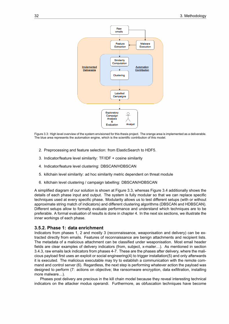
32 3. Methodology
Figure 3.3: High level overview of the system envisioned for this thesis project. The orange area is implemented as a deliverable.The blue area represents the automation engine, which is the scientific contribution of this model.
2. Preprocessing and feature selection: from ElasticSearch to HDF5.
3. Indicator/feature level similarity: TF/IDF + cosine similarity
4. Indicator/feature level clustering: DBSCAN/HDBSCAN
5. killchain level similarity: ad hoc similarity metric dependent on threat module
6. killchain level clustering / campaign labelling: DBSCAN/HDBSCAN
A simplified diagram of our solution is shown at Figure 3.3, whereas Figure 3.4 additionally shows thedetails of each phase input and output. The system is fully modular so that we can replace specifictechniques used at every specific phase. Modularity allows us to test different setups (with or withoutapproximate string match of indicators) and different clustering algorithms (DBSCAN and HDBSCAN).Different setups allow to formally evaluate performance and understand which techniques are to bepreferable. A formal evaluation of results is done in chapter 4. In the next six sections, we illustrate theinner workings of each phase.
3.5.2. Phase 1: data enrichmentIndicators from phases 1, 2 and mostly 3 (reconnaissance, weaponisation and delivery) can be ex-tracted directly from emails. Features of reconnaissance are benign attachments and recipient lists.The metadata of a malicious attachment can be classified under weaponisation. Most email headerfields are clear examples of delivery indicators (from, subject, x-mailer…). As mentioned in section3.4.3, raw emails lack indicators from phases 4-7. These are the phases after delivery, where the mali-cious payload first uses an exploit or social engineering(4) to trigger installation(5) and only afterwardsit is executed. The malicious executable may try to establish a communication with the remote com-mand and control server (6). Regardless, the next step is performing whatever action the payload wasdesigned to perform (7: actions on objective; like ransomware encryption, data exfiltration, installingmore malware…).
Phases post delivery are precious in the kill chain model because they reveal interesting technicalindicators on the attacker modus operandi. Furthermore, as obfuscation techniques have become
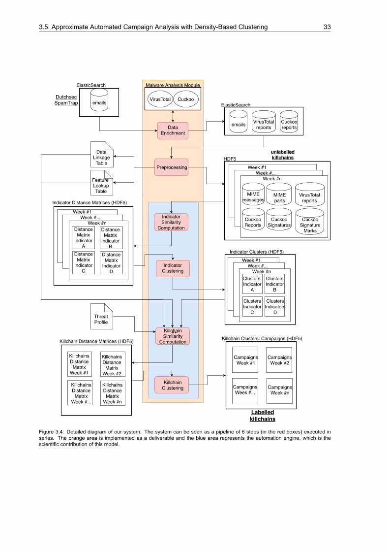
3.5. Approximate Automated Campaign Analysis with Density-Based Clustering 33
DataEnrichment
emails
ElasticSearch
VirusTotal Cuckoo
Malware Analysis Module
emails
ElasticSearch
VirusTotal reports
Cuckoo reports
PreprocessingHDF5
Week #1Week #...
Week #n
MIMEmessages
MIMEparts
VirusTotal reports
Cuckoo Reports
Cuckoo Signatures
Cuckoo Signature
Marks
Data Linkage
Table
Feature Lookup Table
Indicator Similarity
Computation
Indicator Distance Matrices (HDF5)
Week #1Week #...
Week #nDistance
Matrix Indicator
B Distance
Matrix Indicator
C
Distance Matrix
Indicator D
Distance Matrix
Indicator A
Indicator Clustering
Indicator Clusters (HDF5) Week #1
Week #...Week #n
Clusters Indicator
B
Clusters Indicator
C
Clusters Indicators
D
Clusters Indicator
A
Killchain Distance Matrices (HDF5)
Killchains Distance
Matrix Week #1
Killchain Clustering
Killchains Distance
Matrix Week #2
Killchains Distance
Matrix Week #...
Killchains Distance
Matrix Week #n
Killchain Clusters: Campaigns (HDF5)
Campaigns Week #1
Campaigns Week #2
Campaigns Week #...
Campaigns Week #n
Threat Profile
Labelled killchains
unlabelled killchains
Dutchsec SpamTrap
Killchain Similarity
Computation
Figure 3.4: Detailed diagram of our system. The system can be seen as a pipeline of 6 steps (in the red boxes) executed inseries. The orange area is implemented as a deliverable and the blue area represents the automation engine, which is thescientific contribution of this model.

34 3. Methodology
widespread, techniques that do not analyse in depth attachments properties and execution are notuseful anymore. The inclusion of a malware analysis module was then deemed critical for the qualityof this project. Malware analysis techniques can be broadly divided into two categories: static andbehavioural. Both can provide a vast deal of post-delivery indicators. The malware analysis moduleof our presented system is composed of the combined usage of VirusTotal APIs and a custom-builtCuckoo Sandbox malware lab. A diagram of this phase can be seen in Figure 3.5.
DataEnrichment
emails
ElasticSearch
VirusTotal Cuckoo
Malware Analysis Module
emails
ElasticSearch
VirusTotal reports
Cuckoo reports
Dutchsec SpamTrap
Figure 3.5: Phase 1 of our system. The attachments are extracted from the spamtrap, and then both are submitted to a custom-made cuckoo malware lab and VirusTotal for in-depth analysis. This greatly augments the number of indicators, filling for missingphases in the kill chain model (everything after delivery)
VirusTotal.com is an aggregator of antivirus products and online scan engines. The user uploads afile, a hash of the file, a link or an IP and the system returns a report. This report contains the result of 59antivirus programs, an overall score of malignity and many interesting additional pieces of informationlike the date of first submission, the ssdeep of the file and its metadata. VirusTotal comes with APIs,but the free tier does not allow to retrieve large volumes of reports in a short amount of time. LuckilyVirusTotal was interested in collaborating to this project and gave us free limited access to some of thepaid APIs for three months.
As mentioned in section 3.4.2, the dataset is composed of roughly 500000 emails spreading over16 months. The spamtrap itself labelled the attachments as malicious or not at collection time usingClamAV. According to this analysis, the dataset contains roughly 11000 malicious attachments, andof those only 6000 were unique. We found this figure suspiciously low, so we decided to perform ananalysis on our own. It is possible that because the analysis was done at collection time a large numberof false negatives would exist. Antiviruses perform in general worse on brand new malware comparedto old malware, as knowledge of malicious indicators becomes widely available and vendors updatetheir filters.
As a first thing, the malware analysis module hashes the attachments and then submits the hashesto VirusTotal through its APIs. VirusTotal returns a JSON report which we store in ElasticSearch. Onlyreports for files that had been analysed in the past can be retrieved, due to the limited access to thepaid APIs. No new report can be generated. Luckily, the attachments belonged to emails sent betweenFebruary 2016 and August 2017, so rather old concerning malware lifecycle. Indeed, we can retrievea report for 35078 out of the 38028 hashes.
Although the VirusTotal reports contained quite interesting information, they mostly strictly includedonly static analysis. The behavioural analysis had been performed on just 0.6% of our samples. Thislow percentage is quite logic, as the behavioural analysis is a feature available only to paid users.VirusTotal on its own is therefore insufficient to fill the kill chain model because we are missing allindicators of phases after exploitation. To obtain these, we decided to set up our own malware analysislaboratory to test all the attachments.
At this time, Cuckoo Sandbox is one of the most popular open source dynamic malware analysissystems. It is built in Python and requires minimum effort to set up (at least in its purest form). Cuckoohas a host-guest architecture. The main cuckoo process runs on the host, which then spawns a guestrunning the target environment in a virtual machine. The host then passes the file that needs to be testedto the guest, generates a report and then finally kills the guest. Everything that the malware does isrecorded (creation of files, internet connections, system calls etc…). This report contains both staticand behavioural analysis features. Of great interest and value are the YARA signatures that cuckoocan match over malware. YARA is a tool aimed at (but not limited to) helping malware researchersto identify and classify malware samples automatically. YARA signatures are, simply put, abstractionsof behaviours. To be more clear, they are a unique and understandable label for a behaviour that

3.5. Approximate Automated Campaign Analysis with Density-Based Clustering 35
Figure 3.6: Screenshot of Cuckoo Malware Analysis UI. Specifically this screenshot shows the YARA signatures found duringexecution of a malware sample.
can be composed of a multitude of simple atomic actions. Examples of YARA signatures are “HTTPconnection to blacklisted domain”, “connection to the TOR network”, etc. More can be seen in Figure3.6.
We set up a distributed cuckoo malware analysis system. The system itself is composed of twoAsus home servers and one Alienware gaming computer running Ubuntu 16.04 LTS. As suggestedby cuckoo in their setup guide, we used an official Windows 7 64 bit image. We also purchased alicence for Microsoft Office 2013 and installed Adobe Acrobat Reader for opening PDFs. Finally, alldefault security mechanism ofWindows are disabled andmacro execution is enabled on every programwhere it is an option (Microsoft Office, Adobe Acrobat Reader). The two home servers were capableof running ten virtual machines at the same time, whereas the Alienware pc could run up to four, for atotal of twenty-four hosts running on the three machines. The front end user interface of the malwarelab can be seen in Figure 3.6.
As usual, the malware landscape evolves in parallel with the countermeasures that the securityresearch community develops to stop it. Cuckoo, like any other behavioural analysis system that usesvirtual machines as a testing environment, also suffers from this dynamic. Malware has evolved todetect if it is running within a virtual machine and if so to stop execution altogether. This mechanismis also called sandbox evasion. Malware can perform it in a multitude of ways, for example by lookingat the MAC address of the network interface (by default VirtualBox and others have a unique MACaddress) or by looking at the size of the Hard Drive (e.g. nowadays a 10GB hard drive is not typical).Finally, we tested the “detectability”of our target system with the open source project Pafish 10. Some-what unintentionally following the idea of the kill chain, Pafish was developed by collecting indicatorson malware sandbox evasion techniques.
With the cuckoo distributed system successfully set up, we submitted the 38028 unique attachmentsto it for analysis. After eight days of continuous computation, we had a behavioural report for all of them.
10https://github.com/a0rtega/pafish

36 3. Methodology
emails
ElasticSearch
VirusTotal reports
Cuckoo reports
Preprocessing
HDF5Week #1
Week #...Week #n
MIMEmessages
MIMEparts
VirusTotal reports
Cuckoo Reports
Cuckoo Signatures
Cuckoo Signature
Marks
unlabelled killchains
Figure 3.7: Phase 2 of our proposed system. Data are unified and migrated from ElasticSearch to the more Python friendlyHDF5 format. The dataset is also divided in weeks.
The overwhelming majority of them was found to be malicious, with only roughly 3000 attachments nottriggering any signature. We can now say it was a good call to not trust the analysis performed byClamAV at collection time (it labelled only roughly 6000 as malicious). Indeed, the quality and amountof indicators obtained through our malware lab makes it an undeniably fundamental component of anyproper campaign analysis framework based on emails as the source data.
3.5.3. Phase 2: preprocessing and feature selectionIn phase 2, we tidy up our data, unifying the three databases (Dutchsec Spamtrap, VirusTotal analysesand Cuckoo reports) containing all the indicators discovered. Figure 3.7 shows a diagram of this phase.Wemigrate from three elastic search indices to one HDF5 data structure, where each item is a kill chainwith its plethora of indicators. HDF5 is a data model, library, and file format for storing and managingdata 11. It is used often in conjunction with Python to do data science.
Whereas ElasticSearch uses JSON as a data storage format, HDF5 uses numpy tables. JSONallows for a tree structure, but numpy tables are comparable to those of a database. Several fields in allof the indices, unfortunately, had a variable number of items. For example, one message is composedof multiple parts, one cuckoo report can have a variable amount of YARA signatures triggering, andthese signatures can trigger an arbitrary amount of time. In other words, to convert the data structurefrom JSON to HDF5 it was necessary to index a tree structure for every kill chain. This indexing provedto be quite challenging at first but was later solved using pandas DataFrames and their property ofstoring variable-size lists as items.
The final working item of this phase is to select a subset of the indicators. The reason why weinclude this aspect in the system is that it is dependent on the dataset. A widely different dataset willprobably come with a different indicator set.In our case, not all indicators present in the spamtrap or found later by the malware analysis module areof interest. Furthermore, some of these are often empty or unreliable, so we also have to exclude them.We select the remaining 68 indicators with the criterium of relevance (in cybersecurity maliciousnesssense) and by making sure we have some indicators for each Lockheed Martin’s kill chain phase. Thefull list of features is in the Appendix, at A.1.
3.5.4. Phase 3-6: the automation engineNow that our data is ready to perform campaign analysis we approach the first real scientific contributionof this thesis project: the automation engine. Since the problem seems suitable for it, we have decided
11https://www.hdfgroup.org/HDF5/

3.5. Approximate Automated Campaign Analysis with Density-Based Clustering 37
HDF5Week #1
Week #...Week #n
MIMEmessages
MIMEparts
VirusTotal reports
Cuckoo Reports
Cuckoo Signatures
Cuckoo Signature
Marks
Indicator Similarity
Computation
unlabelled killchains
Indicator Distance Matrices (HDF5)
Week #1Week #...
Week #nDistance
Matrix Indicator
B Distance
Matrix Indicator
C
Distance Matrix
Indicator D
Distance Matrix
Indicator A
Figure 3.8: Phase 3 of our proposed system. The input of this phase is the enriched dataset of killchains, the output is a similaritymatrix for each feature.
to try to implement automation through clustering. Our dataset is highly multidimensional (68 features,some of which with more than just one value) and non-categorical. Some features are numerical, butmostly are strings of arbitrary length and meaning. In order to use a clustering technique, we need totransform the values of our feature from unstructured strings to categorical/numerical. Furthermore, toperform clustering it is necessary to have some metric of either similarity or distance depending on thecontext, and not all distance metrics are good for all clustering techniques.We envision the following methodology to automate the process of campaign analysis:
• for each feature: using a measure of similarity, compute the pairwise similarity among all items.(Phase 3, this section). The output of this phase is a feature level 𝐹 × 𝐹 distance matrix
• for each feature: apply density-based clustering on the feature level distance matrix obtained atprevious phase. Phase 4, section 3.5.6.
• for each pair of kill chains: compare the result of the clustering at the previous phase. The morelabels two kill chains share, the more they are similar and vice versa: this can be used to builda similarity metric. Using this score to build a kill chain-level distance matrix 𝑁 × 𝑁. Phase 5,section 3.5.7.
• use the kill chain-level distance matrix for a second round of density-based clustering. Eachclustered label is a campaign. Phase 6, section 3.5.8.
3.5.5. Phase 3: indicator level similarity computationAs pointed out, the goal of this third phase is to, using a measure of similarity, compute the pairwisesimilarity among all items. Figure 3.8 shows a high level diagram of this phase.
The indicators considered are mostly strings, so we need to look for a similarity metric amongstrings. First, we try the most obvious option: edit based string metrics (e.g. Levenshtein, Hamming).This method is far too slow: computation of one row of the pairwise distance matrix (1 item comparedto all the others) took roughly 1 second on a 6th generation (Skylake) 2 GHz Intel Core i5. One averageweek of the dataset has roughly 10000 emails. The number of possible combination per week is thuson average (10000 )/2 = 50, 000, 000. 50 million seconds is roughly 580 days, for each feature. Wedecided to discard this method and look for better alternatives.
In section 3.3 we pointed at TF/IDF tokenisation of n-grams as an interesting approach to assessingthe similarity of strings. This approach is often used in practice, combined with cosine distance, to com-pute the pairwise similarity of a large set of strings. Looking for implemented examples, we encounteran open source project from ING 12 that uses n-grams and TF/IDF to perform approximate search ofstrings in a database. This ING library then computes the cosine distance (the measure of the angle12https://medium.com/wbaa/https-medium-com-ingwbaa-boosting-selection-of-the-most-similar-entities-in-large-scale-datasets-450b3242e618

38 3. Methodology
between two vectors) to return all the relevant items when querying a database afflicted by the inconsis-tent use of nomenclature/spelling mistakes. ING themselves resorted to this approach because theyfound edit distance techniques to be not scalable. The reason for the speedup is mostly due to theusage of efficient linear algebra techniques for the pairwise computation. In our testing, this proved tobe faster by a factor of x100 to x1000 when compared to the linear approach of going through all thepossible combinations of edit distance implementations. The computation time was reduced from 580days to hours. Due to bugs in the library, we ended up implementing the approach from scratch.
We nowwill present the pipeline of steps performed at this phase, but first, in Figure 3.9 we introducea simple example dataset that will recurrently be used through this chapter. In this simplified kill chainset, there are four kill chains with three indicators: sender, subject and the hash of an attachment.There are two spear phishing campaigns: (A, B) and (C, D).
Figure 3.9: Example dataset to showcase the similarity computation with TF/IDF and cosine distance computed at phase 3.Killchains A and B belong to one campaign, C and D to another.
Figure 3.10: Phase 3 TF/IDF + cosine distance for similarity computation of indicator “email sender”on example dataset

3.5. Approximate Automated Campaign Analysis with Density-Based Clustering 39
Phase 3 TF/IDF + cosine distance for feature level similarity computation:
1. for each feature corpus, the full token list is generated by an n-gram tokeniser from the pythonlibrary scikit-learn
2. a TF/IDF vectorizer from the python library scikit-learn generates one normalised token vector foreach document, computing each component (the value for each n-gram) using TF/IDF. In otherwords, each vector component measures the TF/IDF relevance score of a specific n-gram.The token vectors are normalised during computation to have all magnitude 1. The normalisationof the token vectors is necessary for two reasons. The first one is that this allows comparingall term vectors by exclusively looking at the cosine of the angle between them, which is easilycomputed by performing the dot product of the two. The second one is that TF/IDF is alreadytaking care of giving an appropriate weight for each token for each document. This value alreadytakes into account both the frequency within the document (TF) and the frequency within thedocument corpus (IDF). Indeed, normalisation of the magnitude of the token vector does notmean ignoring the different size of the documents, nor it means ignoring the amount of time atoken is present in a document. Not normalising the token vectors, in this case, would alterthe TF/IDF computation by redundantly accounting for the term frequency within each documentleading to an inconsistent value of tokens for each document.In a strictly positive vector space like ours, the cosine of the angle between all pair of possiblevectors is always between 0 and 1 because n-grams count can only be non-negative. Two vectorswith the same orientation have a cosine similarity of 1 and indicate identical documents, twovectors at 90∘ have a similarity of 0 and indicate completely different documents.
3. compute the cosine similarity between all pairs of vectorsThe cosine of two non zero vectors can be derived from the Euclidean dot product, which takesinto account the angle as well as the magnitude:
�⃗� ⋅ �⃗� = ||�⃗�| ⋅ ||�⃗�|| ⋅ cos(𝜃)
which is the same as:
cos(𝜃) = �⃗� ⋅ �⃗�||�⃗�|| ⋅ ||�⃗�||
Now, in the special case when magnitude is 1 for both vectors, it follows that:
cos(𝜃) = �⃗� ⋅ �⃗�1 ⋅ 1 = �⃗� ⋅ �⃗�
cos(𝜃) =∑𝑎 ⋅ 𝑏
To compute this measure for all possible combinations, it is sufficient to perform the dot productbetween the token vector matrix 𝑇 generated by the TF/IDF vectorizer by its transpose 𝑇 1.The resulting matrix contains at row 𝑥 and column 𝑦 the aforementioned normalised dot productwhich is simply the sum of the product of the components:
cos(𝜃) = �⃗� ⋅ �⃗� =∑𝑥 ⋅ 𝑦
This computes all pairwise cosine similarities and can be performed in python with the simpleone-liner.
𝑆𝐼𝑀 = 𝑛𝑝.𝑑𝑜𝑡(𝑇, 𝑇 1)

40 3. Methodology
Indicator Distance Matrices (HDF5)
Week #1Week #...
Week #nDistance
Matrix Indicator
B Distance
Matrix Indicator
C
Distance Matrix
Indicator D
Distance Matrix
Indicator A Indicator
Clustering
Indicator Clusters (HDF5) Week #1
Week #...Week #n
Clusters Indicator
B
Clusters Indicator
C
Clusters Indicators
D
Clusters Indicator
A
Figure 3.11: Phase 4: indicator level clustering. The input of this phase is the indicator similarity matrices obtained at phase 3,the output are the cluster labels.
4. Finally, as we care about distance and not similarity, and since our token vector space is nonnegative (TF/IDF scores are never negative, at most 0), we can compute the distance matrixfrom the similarity matrix by simply performing:
𝐷𝐼𝑆𝑇 = 𝑛𝑝.𝑠𝑢𝑏𝑡𝑟𝑎𝑐𝑡(1, 𝑆𝐼𝑀)
This methodology allows computing a similarity matrix for each of the 68 features in an amountof time on the order of hours (single core), although with burdensome memory requirements (up to60GBs for the weeks with more emails). Having solved the similarity assessment of features, in thenext section we perform a first round of clustering to group related items together under the same label(thus transforming raw uncategorical data in categorical data).
3.5.6. Phase 4: indicator level clusteringIn the previous section, we started working on the “automation engine”component of our system. Wedesigned a methodology to compute a similarity score between strings, and we then applied it to ourdataset, obtaining a similarity matrix for each indicator. We can now feed this similarity matrix (afterconverting it into a distance matrix) to a clustering algorithm. At the end of this step, we will have con-verted our raw, uncategorical dataset (strings) in a strictly categorical dataset (cluster labels, numbers).Figure 3.11 shows a high-level diagram of the input and output of this phase and Figure 3.12 illustratesthe effect of this phase in our example dataset.
This step allows us to do two things at once: to easily automate the process of exactly matching in-dicators (precisely like in Lockheed Martin’s methodology) and to eventually to implement approximateindicator match for the indicators we found to be suitable in section 3.4.4. We can do this as follows:
exact match we force the clustering algorithm to cluster together only elements with a perfect similarityscore (1)
approximate match we allow the clustering algorithm to cluster together elements with a similarityscore above a certain threshold.
As pointed out previously, clustering algorithms usually allow a distance matrix as input, not a sim-ilarity matrix. Distance makes more sense for clustering because when we plot the data points in ann-dimensional vector space, we want more similar elements to be represented closer and more dif-ferent elements to be represented far from each other. Converting a similarity matrix into a distancematrix is trivial for similarity metrics that have an upper bound. This is our case because our similaritymetric is bound to the interval [0, 1].
𝐷𝑖𝑠𝑡𝑀𝑎𝑡𝑟𝑖𝑥 = 1 − 𝑆𝑖𝑚𝑀𝑎𝑡𝑟𝑖𝑥In section 3.2 we have given a short survey on clustering techniques in the search for one suitable
for our needs and tailoring our constraints. We identified density-based clustering as a good candidate,

3.5. Approximate Automated Campaign Analysis with Density-Based Clustering 41
Figure 3.12: Abstract view of phase 4 on our example dataset
and we selected DBSCAN and HDBSCAN as the algorithm to use in our system. We described howthe two algorithms work in section 3.2.2. Again, our system is highly modular, and it thus allows to alterthe clustering technique or its parameters easily. We, therefore, test both DBSCAN and HDBSCAN tocompare the two. In this chapter we focus only on the implementation details, the results can be foundin chapter 4.
Fine tuning DBSCAN parametersThe DBSCAN algorithm can be found implemented in the python library scikit-learn. There are twoparameters to set: eps and min_samples. They both affect the measure of density that we desireto be captured. Lower values of eps and higher values of min_samples lead to denser and lessnoisy clusters, whereas high eps and low min_samples lead to less dense, more noisy clusters. Thesuggested approach to finding the best set up is to start with a min_samples values of 1, then playwith eps. If the clustering is too noisy increase min_samples and start over. This is repeated untilthe clustering quality is acceptable. However, how is the clustering evaluated? Unfortunately, in theabsence of a training set, there is no alternative than to manually evaluate the content of the foundclusters by counting false positives (how much noise in one cluster). In large datasets, like our case,this is far too time-consuming to perform for all the clusters found (in the order of thousands for a weekwith 10000 kill chains). Luckily, when the parameters are not ideal, the result is so weak that it isinstantly recognisable as such, leading to a faster than hoped cycle of evaluation¶meter-tuning. Afurther annoyance of DBSCAN is that different dataset will likely have different ideal parameters tuning;therefore it is necessary to perform the parameter discovery for each indicator. Luckily though:
1. parameters found for one period are good for other time periods too. Not only this saves us muchwork, but it also is an interesting find on its own as it tells us that the distribution of similarity scores(and therefore the patterns in the data) is somewhat coherent across different time series. It isimportant to note that if this is true for our dataset, it may not be for other datasets. This may bea problem.
2. parameters have to be found only for the indicators selected for approximate indicator match. Forindicators where exact match is necessary it is sufficient to set the eps parameter to 0, forcing

42 3. Methodology
the clustering to exclusively label together elements with similarity 1 (and therefore identical).
After extensive testing we eventually settled for min_samples = 1 and found the ideal value of epsfor all the indicators selected for approximate indicator match. They can be viewed at table 3.3.
Table 3.3: Features selected for approximate string matching with chosen eps parameter for DBSCAN
Indicator # Name DBSCAN eps15 additional_info.exiftool.ZipFileName 0.5520 body 0.3525 file.name 0.5527 filename 0.5529 from 0.4536 headers.Return-Path 0.4552 reverse 0.564 subject 0.475
HDBSCAN parameter tuningIn section 3.2 we have discussed how HDBSCAN allows for variable density clusters by automaticallyfinding an optimal eps parameter in different areas of data space. The only parameter that has to beset in HDBSCAN is the very obvious min cluster size. What should be the minimum cluster sizethat our clustering allows? If a cluster is below this threshold, it will be ignored, and its items will belabelled as noise at the end of the algorithm. To answer this question, we need to understand if wewant to allow for singleton campaigns. A singleton campaign is a campaign composed by just onekill chain, and we believe they should be allowed. The reason for this is two-fold. First of all, there is noadvantage in explicitly marking noise in our use case. Secondly, our methodology will eventually allowtracking campaigns through time by cross-checking the final cluster stage among contiguous weeks.Therefore, we should not discard the potential starting occurrence of a campaign only because thereis just one kill chain in a specific time interval. For example, imagine an APT that sends several emailsper week, starting Sunday the 26th of August. If campaign analysis is performed on a weekly basis withour system, the first kill chain will not end up in a campaign if singleton campaigns are not allowed, andit will be simply discarded as noise. Furthermore, there is no trade-off whatsoever in allowing singletoncampaign.Following this logic, we decide not only to allow singleton campaigns but also that they are a desirableproperty of our clustering. We thus set min cluster size to 1. No further tuning is required in HDB-SCAN. In section 4 we give a formal comparison of DBSCAN and HDBSCAN concerning performance,but so far we must state that HDBSCAN is far superior in ease of use. It took minutes to set and runHDBSCAN, whereas it took dozens of hours to set and evaluate DBSCAN parameters iteratively.
Campaign Analysis through looser clusteringDuring the process of fine-tuning DBSCAN parameters, we made an exciting discovery. We ideallydesire a value of eps that leads to zero false positives in our clusters. We found out that when thisparameter was set to be slightly underfitting so that a little amount of false positive is allowed, the resultsof the clustering are significantly more interesting. For example we show at Figure 3.13 the content ofa cluster of email subjects when eps is set to 0.45 compared to when it is set to 0.425.When the variable is set at 0.425 the clustering is more strict, the label contains 215 elements and theyall more or less related to the string “Laten we leren kennen?”. Furthermore, there are no blatant falsepositives in the cluster.When the variable is set at 0.45 the clustering is looser, and the label contains 911 elements. Not all theelements contain the string “Laten we leren kennen?”, however, they all seem to follow some similarlogical structure and meaning.What do we want from the clustering? Are these additional elements to be considered false positives?We have to make a decision here in what we want our system to do. The rationale behind a falsepositive assessment is that we have to have a definition of true positive. In our scenario, we want tocluster together things that are related to a campaign, following Lockheed Martin process of campaignanalysis. Although reasonably different, we can see that these subjects are related and most likely

3.5. Approximate Automated Campaign Analysis with Density-Based Clustering 43
Figure 3.13: Cluster content comparison of two runs of DBSCAN with different eps parameter on SpamTrap email subjects. Left:eps = 0.425, Right: eps= 0.45. The latter is looser but seems to actually capture well a real campaign. This is the effect of thephenomenon called cluster chaining.
were variation within a campaign. Not only the human-readable messages seem to relate, but thereis also a clear structure in the strings: some “machine oriented ”followed by three dots followed by amessage that hints at the opportunity of a date. Without really trying too much we have already foundthe combination of TF/IDF + cosine distance and density-based clustering to be able to spot campaignsin the data.If we further set the eps to 0.475 the cluster contains even more items: 1124. This time though, 13actual false positives, completely unrelated strings, are introduced. 13 out of 213 new items are thuswrongly labelled.We now have to make a decision. Allowing for these little false positives or getting rid of them at theexpense of some false negatives. The goal of our system is to automate the process of campaignanalysis to help a security analyst performing threat intelligence. The hard part of this process is themanual cross-reference of possibly thousands of multidimensional kill chains. We believe that a fullerbut less precise result is far more interesting for an analyst compared to a less complete but moreprecise result. Furthermore, an analyst can quickly, almost at a glance discard false positives whereasit would take hours to manually check all the other kill chains to manually find what the clustering missedout for the sake of precision.
Clustering Chaining: a desirable propertyThe “Laten we leren kennen”example also show us an interesting phenomenon of density based clus-tering: chaining. Wilks defines chaining as
the production of a few large clusters, which are formed by virtue of nearness of points tobe merged at different steps to opposite edges of a cluster[20].
Chaining is oftenmentioned as an undesirable property that makes density-based clustering less robust

44 3. Methodology
Indicator Clusters (HDF5) Week #1
Week #...Week #n
Clusters Indicator
B
Clusters Indicator
C
Clusters Indicators
D
Clusters Indicator
A
Killchain Distance Matrices (HDF5)
Killchains Distance
Matrix Week #1
Killchains Distance
Matrix Week #2
Killchains Distance
Matrix Week #...
Killchains Distance
Matrix Week #n
Threat Profile
Killchain Similarity
Computation
Figure 3.14: Phase 5 of the proposed automated campaign analysis system. In this phase, the similarity between killchains iscomputed with an ad hoc similarity metric that accounts for variable weight indicator and different threat profile (APT, spam etc).
compared to other clustering techniques[21]. As we will now illustrate, chaining is actually producing aquite desirable result in our scenario. Let’s look for example at the two following strings A and B:
A Ik wil u snel te zien
B Laten we leren kennen?
How do these two cluster together? When we look closely, we find that the following strings are alsopresent in the cluster:
C =?UTF-8?Q?=F3=BE=AC=8D_?= ... Ik wil u snel te zien ..
D =?UTF-8?Q?=F3=BE=AC=8D_?= ... Hello! Laten we leren kennen?
This is the famous chaining effect. String A is very similar to string C, string C is very similar to Dand string D is very similar to B. Generally speaking, chaining is an unwanted property that affectsdensity-based clustering, but in our scenario, it actually seems to allow for the perfect kind of campaignanalysis that we would expect a human, not a machine, to perform!
We have now performed clustering at the indicator level. Not only have we thus converted the rawdata in categorical labels, but we also found out that clustering can already allow a form of campaigndiscovery thanks to the surprisingly desirable phenomenon of chaining. In the next phase, we definean algorithm to compare two kill chains by cross-checking these categorical labels, producing anothersimilarity score (at the kill chain-level this time).
3.5.7. Phase 5: killchain level similarity computationIn phases 3 and 4 we transformed the raw data into categorical labels, for each indicator. Ultimately,though, campaign analysis should group incidents at the kill chain-level, not at the indicator level. Inthis phase, we develop a simple similarity metric to assess the similarity of two kill chains based onthe result of the clustering at the previous phase. Figure 3.14 gives an overview of the input and theoutputs of this process.
Intuitively, we have to compare every pair of kill chains by looking at the respective cluster labelsof all their indicators. If an indicator ended in the same cluster for both kill chains, then this shouldbe accounted as more similar. Once a kill chain-level similarity matrix is computed, it can be reversed

3.5. Approximate Automated Campaign Analysis with Density-Based Clustering 45
into a distance matrix, and clustering can be performed again. We develop a fairly simple algorithm toassess the similarity of two kill chains:
phase5(KC A, KC B, threat_module):similarity = 0LA = indicators_labels_ALB = indicators_labels_Bfor x in range 68:
if LA[x] == LB[x]:similarity += weight(threat_module, x)
return(similarity)
The most interesting component of the algorithm is the weight function. A weight function is neces-sary for two reasons. First of all, different indicators have different absolute importance. For example,the hash of a malicious payload is a far more important indicator than the language of the email. Theyboth matter and they both should be used for campaign analysis, but the former is a much strongerlink in forensic terms. Following this rationale, we assign an impact value to all the 68 features: low (1point), medium (5 points), high (20 points). Secondly, we derive from domain knowledge that differentkill chain components have different importance with different categories of threat actors. An exampleis useful to clarify. APTs and mass spam campaigns have some inherent differences to them, the mostimportant being that the former are targeted (if not to a single individual at least to a group), whereasthe latter generally are not. We should account for this in our system, allowing the analyst to selectwhat we call a threat profile that will alter the weight of specific indicators to give a more realistic andcoherent result. Finally, the weight function takes care of normalising the similarity score in the [0,1]interval. The 68 features were divided into four categories, trying to follow the original kill chain model:
• target: related to the victim (phase 1, 2 in LM kill chain)
• delivery: in this case all email metadata and headers (phase 2 in LM kill chain)
• static: metadata of the payload (phase 2, 4 in LM kill chain)
• dynamic: indicators collected by executing the payload (phases 4, 5, 6, 7 of LM kill chain)
An example of threat profile for APT would give much more weight to the victim and maybe less to thedelivery as the effort of varying delivery indicators is far less than in the case of mass spam. Little weightis given to static because of obfuscation techniques, and more is given to dynamic as core behaviourof malware and action on objectives will be likely similar in a campaign (also require much effort toalter. expensive) Figure 3.15 shows the threat profile weights used for our spam/phishing dataset anda suggested threat profile weights for APT targeted malicious emails.
3.5.8. Phase 6: killchain level clustering (campaign labeling)A similarity score is computed with the algorithm proposed at the previous phase. The scoring is donefor all couple of kill chains, resulting in a kill chain-level similarity matrix for each time interval considered.Similarly to what done previously, this one can too be converted into a distance matrix by performing(the similarity score was normalised in [0, 1]):
𝐷𝑖𝑠𝑡𝑀𝑎𝑡𝑟𝑖𝑥 = 1 − 𝑆𝑖𝑚𝑀𝑎𝑡𝑟𝑖𝑥
The final working item in this project is to feed the kill chain similarity matrices to a clustering algorithm.The clusters found are going to be the campaigns identified by the system and will be its final output.Figure 3.16 shows a high-level diagram of this process
We use density-based clustering for the same reasons we used it in 3.5.6. We test both DBSCANand HDBSCAN again. The same methodology of phase 4 was used to set DBSCAN parameters. Themin_samples variable was set to 1 again, for the same reasons mentioned in section 3.5.6. Theeps parameter was similarly fine-tuned by finding the optimal compromise between false positives andquality of results. The approach was again to minimise false positives and maximise utility, preferringa complete result at the price of some false positives. Again, fine-tuning DBSCAN parameters for

46 3. Methodology
Figure 3.15: On the left: threat profile used for campaign analysis of spam/phishing campaigns. On the right: a suggested threatprofile for APT targeted malicious emails. Notice how victim indicators weight is small in the case of spam/phishing campaigns(which usually are massive and untargeted) and higher in the case of advanced persistent threats’ targeted malicious emails.
one week of data took many hours, and it looks like it is necessary to retune it for every other weekmanually. On the other hand, HDBSCAN is again far easier to use. The only parameter of HDBSCAN,min_cluster_size, is set again to 1 and the algorithm will take care of optimising the eps value.
This phase completes our proposed system for automated campaign analysis. In the next chap-ter, we evaluate the results of our implementation, and we assess the performance of the variableconfigurations we can test (with or without approximate match, DBSCAN/HDBSCAN).

3.5. Approximate Automated Campaign Analysis with Density-Based Clustering 47
Killchain Distance Matrices (HDF5)
Killchains Distance
Matrix Week #1
Killchain Clustering
Killchains Distance
Matrix Week #2
Killchains Distance
Matrix Week #...
Killchains Distance
Matrix Week #n
Killchain Clusters: Campaigns (HDF5)
Campaigns Week #1
Campaigns Week #2
Campaigns Week #...
Campaigns Week #n
Labelled killchains
Figure 3.16: Sixth and last phase of our proposed automated campaign analysis system. Density based clustering is performedon the distance matrix computed at the previous phase. This process identifies the campaigns in the input dataset.


4Results
In this chapter, we present the results of this thesis project. First, we briefly reintroduce the domain, theresearch gap and our research goals. Then we show the performance of the developed framework withvarious settings, introduced in the previous chapter. The performance analysis allows us to understandif the designed system is a significant contribution to the body of knowledge. We quantify precision interms of false positives, and we quantify recall in terms of false negatives. We compare the performanceof various versions of our automatic framework, showing what setup performs best and why. Comparingthe performance enables us to quantify the benefit of automation in campaign analysis and also toassess the consequences of applying approximate string matching on some features. Next up, weaddress the limitation of our framework. Finally, in the last section, we showcase some notable findingsdiscovered by the system.
4.1. Campaign Analysis, Research Gap and Research Goals of thisproject
In 2011 researchers from Lockheed Martin Corporation released a whitepaper [10] that marked aparadigm shift in how cyber threat intelligence is performed. In this paper, Hutchins et al. intro-duced the concepts of cyber kill chain and campaign analysis. The kill chain is a concept adaptedfrom the military domain to the cyber domain. A kill chain is a multi-stage representation of an intrusionattempt. The stages are seven and allow to map an attack from its ideation to its completion. Indicatorsare atomical pieces of information belonging to the kill chains (e.g. the hash of malware, the senderemail, the IP that malware connects to). Cleary, enough indicators can be used to fingerprint attackers.
Campaign analysis is the process of linking together repeated attempts from a malicious entity bysearching for repeating indicators in the respective kill chains. The state of the art in campaign anal-ysis has two significant problems: lack of automation and strictness in indicator overlapping. Lack ofautomated implementations makes the task of looking for overlapping indicators manual, somethingunfeasible in most scenarios, and exact match of indicators may not be the ideal way to perform cam-paign analysis for all indicators.
In this project, we have set two research goals to overcome the gaps in the state of the art. We havedesigned a system to automatically extract features from malicious emails, enhancing the produced killchain with indicators from post-installation phases with a malware lab and established a methodology tocluster related kill chains in campaigns. Furthermore, we have introduced approximate string matchingfor some of the indicators.
4.2. Experimental resultsIn this section, we present a performance analysis of the system developed in section 3. First, webriefly discuss the spamtrap training data. Then we explain the experimental setup, and finally, weshow the actual results and their analysis.
49

50 4. Results
4.2.1. DatasetTo build and test our system we relied on a dataset of malicious emails generously provided by Dutch-sec, an Utrecht-based cybersecurity firm. In 2016 Dutchsec developed a spamtrap, a honeypot dedi-cated to collect malicious emails for threat intelligence purposes. The spamtrap has been running andcollecting emails since then. For our study we focused on a collection of emails spanning 16 months(February 2016 - May 2017), the spamtrap was modified afterwards, and we wanted our data to be asgapless and consistent as possible.
In this period, the spamtrap collected around half a million emails. From data exploration, we canstate with a certain degree of confidence that the dataset is entirely malicious, although a portion ofemails is “legitimate”commercial spam, which may not be considered malicious universally. Regard-less, the most substantial majority of these emails concern fraudulent spam (e.g. sex enhancing drugs)and spear phishing attacks.
Following the kill chain framework, we mapped the spamtrap features to kill chain indicators. Wefound the original data to lack indicators of phases post delivery (everything revolving around the instal-lation of malware and its execution). This lack is quite logic, as the spamtrap was developed to studyemail related metadata. To fill this gap in the kill chain model, we extracted roughly 38000 differentattachments, and we run them into a custom-made cuckoo malware lab, obtaining dozens of new indi-cators for phases exploitation, installation and command&control. We finally selected 68 indicators tobe used in our system; the full list can be found in Appendix A at Table A.1. We selected eight of these68 features for approximate indicator match. To do this, in Section 3.4.4 we developed a methodologybased on the entropy of the cosine distance in each indicator space.
Finally, to make the computation quicker (this is a proof of concept, after all), we split the dataset inweeks. We found the emails to be roughly equally distributed across the 16 months period (with someexceptions), with an average load of 10000 emails per week.
4.2.2. Experimental SetupIn the previous chapter, we have proposed and implemented a system to solve the research gapsidentified. To evaluate the system as well as some implementation options, we need to come up witha formal experimental setup.The primary goal of this project is to automate the process of campaign analysis, improving the stateof the art of manual exact match performed by a security analyst. Thus, we need to not only evaluateif our system is capable of performing campaign analysis (and thus if density-based clustering is asuitable choice for automation) but also if it does so better than the state of the art. Secondly, we wantto establish if approximate indicator match of suitable indicators is a valuable addition to the originalmodel. Finally, we want to assess if the density-based clustering is better when the density is assumedto be fixed (DBSCAN) or variable (HDBSCAN) in the dataset.
We design five different setups to test for all these conditions:
1. Manual exact (only) indicator match: performed manually. This is the state of the art in campaignanalysis as described by Lockheed Martin [10].
2. Automated exact (only) indicator match, clustering with DBSCAN
3. Automated exact (only) indicator match, clustering with HDBSCAN
4. Automated mixed indicator match (exact + approximate), clustering with DBSCAN
5. Automated mixed indicator match (exact + approximate), clustering with HDBSCAN
Comparing setup 1 with the others will let us understand if the automated setup is working andif it performs better or worse than the state of the art. Comparing setup 2 and 3 with 4 and 5 willlet us understand the consequences in terms of performance of introducing approximate match ofindicators. Finally, we can compare the result of DBSCAN and HDBSCAN. This last condition canmake us understand if our dataset is better suited by an algorithm that allows for variable densityregions or by one that requires a fixed density throughout the dataset.
Our approach to testing these five setups is to evaluate their performance. We have not yet dis-cussed precisely what we mean by performance. To do so, we first establish that the most criticalmetric at our disposal is the quality of the campaigns discovered. Therefore, our approach is two-fold.

4.2. Experimental results 51
First, we measure the false negatives over a dataset of synthetic campaigns: this allows to quantifythe recall of the system. Recall measures the percentage of relevant instances retrieved over the totalamount of relevant instances. This metric gives us an idea of how complete our campaign analysis is.We then measure the false positives: this gives us a measure of precision. Precision measures thepercentage of relevant instances over the total retrieved instances. This metric gives us an idea of howmany irrelevant items will be in the clusters of actual campaigns.
4.2.3. False Negatives and RecallRecall is defined as follows:
𝑟𝑒𝑐𝑎𝑙𝑙 = 𝑇𝑃𝑇𝑃 + 𝐹𝑁
To assess recall we need to know what is the true size of a campaign (the denominator, meaningall the relevant items). Obtaining knowledge is problematic when performing unsupervised learning asprelabelled data is missing. Furthermore, in this specific scenario, we are dealing with a dataset notonly large but also highly multidimensional. Moreover, the features are often non-categorical complexstrings.Themost appropriate way to assess recall is to search and label campaigns in the dataset indeedmanu-ally. Unfortunately, manual labelling is unfeasible in this case due to the multidimensionality mentionedabove and the limited amount of time and human resources.Therefore, we designed an alternative approach mixing synthetic data and highly distinguishable cam-paigns encountered in the data during its exploration.
We designed four synthetic spear phishing campaigns (𝑆1, 𝑆2, 𝑆3, 𝑆4), each composed by ten emails;they can be seen in detail in the Appendix, at Figures B.1, B.2, B.3, B.4. To evaluate the limits of oursystem we designed the four campaigns to be increasingly complex. We envisioned an increasinglyskilled attacker that, aware of the traditional campaign analysis methodology, tries to avoid repeatingindicators.In the first campaign S1, we imagine an attacker merely spamming the same kill chain ten times. In thesecond campaign S2, the attacker is more sophisticated. He tries to avoid campaign linkage by usingten different sender email addresses. Furthermore, he randomises a six digits number at the end of hissubject and filename. Finally, he uses obfuscation techniques to make sure his malware (hidden withina seemingly benign attachment) produces a different hash every time. To make his life easier, he craftsthe message in a way that any reply will always go to the same return address. He is not aware thathis x-mailer will remain the same if he uses the same email client. The third attacker is more proficientin avoiding campaign analysis. No indicator is ever repeated. He uses ten different email addressesregistered at the same domain to send the messages, making sure that the return addresses are alldifferent. The subjects he uses are always different, although the overall meaning remains the same.Finally, the x-mailer and the attachment name are partially randomised by appending a random sixdigits code at the end of the string. Finally, the fourth campaign is crafted by an attacker that is makingsure every single indicator is never identical. He uses entirely randomly generated email addressesand crafts the subjects by hand to resemble real ones. Only the filename and the x-mailer maintain astructure, with a word followed by a six digits random number.
Ideally, we would expect state of the art exact-only indicator matching to link the first two syntheticcampaign together. Indicators in campaigns 𝑆3 and 𝑆4 are never repeated. We crafted 𝑆4 especially tounderstand where and if our fuzzy system breaks. It is also important to note that to craft these syntheticcampaigns we took inspiration from the real campaigns we found in the dataset while exploring it.
We found several real campaigns while performing data exploration. Among them, three stoodout significantly from the rest. Because manual evaluation of every single message is required toestablish the campaign size formally, we were able to find all related message by looking at five highlyrelevant indicators that are easy to compare (in the case of spear phishing): hashes of parts andattachments, subjects, sender emails, payload sizes, filenames. We can then establish with a highdegree of confidence the size of these three campaigns. Thus we can use them for counting falsenegatives by counting the missing items. Excerpt of these three campaigns can also be found in theAppendix at figures C.1, C.2, C.3
Table 4.1 shows the percentage of false negatives found in the five setups mentioned above.More interestingly, figure 4.1 shows the average recall of the five setups over the seven campaignsanalysed.
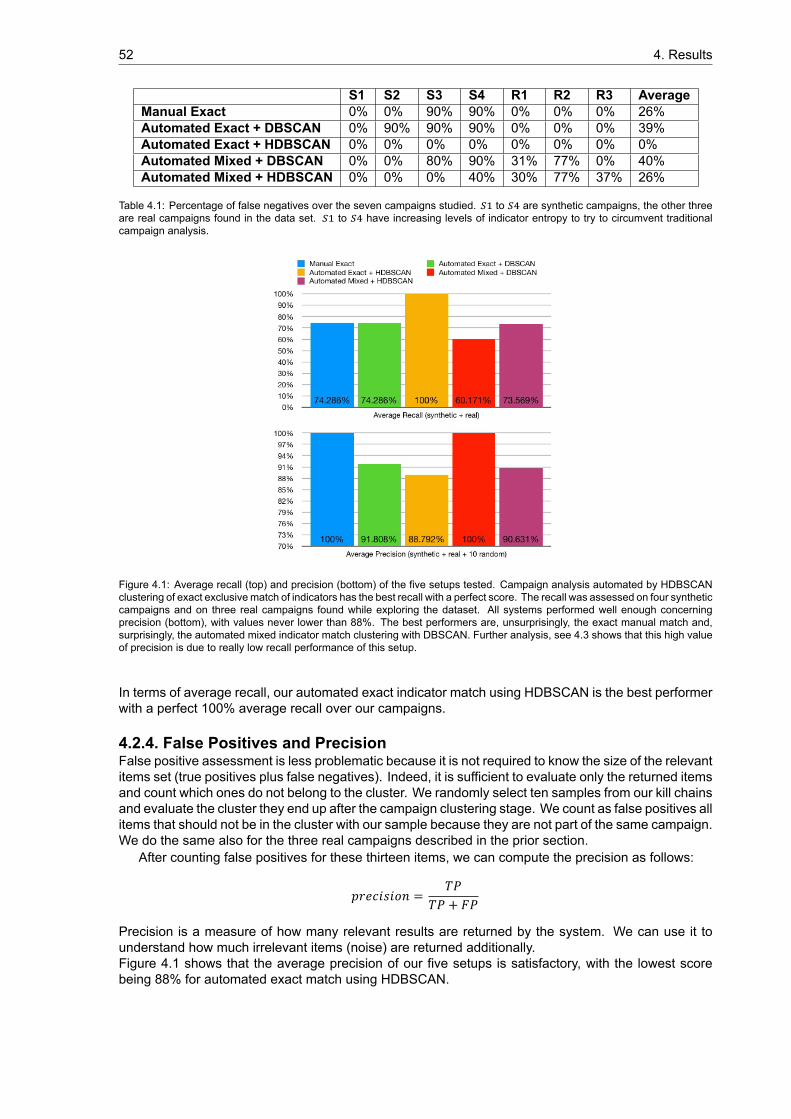
52 4. Results
S1 S2 S3 S4 R1 R2 R3 AverageManual Exact 0% 0% 90% 90% 0% 0% 0% 26%Automated Exact + DBSCAN 0% 90% 90% 90% 0% 0% 0% 39%Automated Exact + HDBSCAN 0% 0% 0% 0% 0% 0% 0% 0%Automated Mixed + DBSCAN 0% 0% 80% 90% 31% 77% 0% 40%Automated Mixed + HDBSCAN 0% 0% 0% 40% 30% 77% 37% 26%
Table 4.1: Percentage of false negatives over the seven campaigns studied. to are synthetic campaigns, the other threeare real campaigns found in the data set. to have increasing levels of indicator entropy to try to circumvent traditionalcampaign analysis.
Figure 4.1: Average recall (top) and precision (bottom) of the five setups tested. Campaign analysis automated by HDBSCANclustering of exact exclusivematch of indicators has the best recall with a perfect score. The recall was assessed on four syntheticcampaigns and on three real campaigns found while exploring the dataset. All systems performed well enough concerningprecision (bottom), with values never lower than 88%. The best performers are, unsurprisingly, the exact manual match and,surprisingly, the automated mixed indicator match clustering with DBSCAN. Further analysis, see 4.3 shows that this high valueof precision is due to really low recall performance of this setup.
In terms of average recall, our automated exact indicator match using HDBSCAN is the best performerwith a perfect 100% average recall over our campaigns.
4.2.4. False Positives and PrecisionFalse positive assessment is less problematic because it is not required to know the size of the relevantitems set (true positives plus false negatives). Indeed, it is sufficient to evaluate only the returned itemsand count which ones do not belong to the cluster. We randomly select ten samples from our kill chainsand evaluate the cluster they end up after the campaign clustering stage. We count as false positives allitems that should not be in the cluster with our sample because they are not part of the same campaign.We do the same also for the three real campaigns described in the prior section.
After counting false positives for these thirteen items, we can compute the precision as follows:
𝑝𝑟𝑒𝑐𝑖𝑠𝑖𝑜𝑛 = 𝑇𝑃𝑇𝑃 + 𝐹𝑃
Precision is a measure of how many relevant results are returned by the system. We can use it tounderstand how much irrelevant items (noise) are returned additionally.Figure 4.1 shows that the average precision of our five setups is satisfactory, with the lowest scorebeing 88% for automated exact match using HDBSCAN.

4.3. Analysis 53
4.3. AnalysisWe now proceed to analyse the results of our evaluation.The goal of our system is to aid a security analyst by correlating related intrusion attempts in campaigns.In this scenario, we believe that recall is more important than precision. The reason for this is that ifnoise is not overwhelming an analyst can easily ignore it, whereas making sure that all relevant itemsare clustered together is a much harder task without prior knowledge.
Our automated exact-only system that uses HDBSCAN for clustering is the best performer regard-ing recall. It is the only system that was capable of perfectly recalling all items from our synthetic andreal campaigns. Being recall our most crucial parameter for evaluation, and being precision not over-whelmingly bad (88%), we can confidently state that this is the best methodology for campaign analysisamong those that we tested. Figure 4.4 shows the visual result of HDBSCAN over the exact-only killchain distance matrix.
When comparing this solution to the state of the art manual exact-only campaign linkage, we can seethat unsurprisingly precision is worse: obviously, there are no false positives when manual campaignanalysis is performed. On the other hand, though, recall is significantly better (25% better on average).For an analyst exploring the data in search of a pattern, this has a critical impact.We can thus affirm that the system designed can not only perform automated campaign analysis, butit does it better (with higher recall but also higher noise) than the state of the art methodology.
Quite surprisingly, our automated mixed system using DBSCAN performs flawlessly concerningprecision. The recall is more than 10% better than the average of the three other automated setups.This anomaly is easily explained when looking at the average recall of this setup: it is by far the lowestat 60%. This system returned mostly singleton clusters, failing at clustering together related relevantitems. Singleton clusters have zero false positives, hence the high precision value.
Another interesting finding is that HDBSCAN is less precise than DBSCAN and has a higher recallfor both mixed and exact exclusive indicator matching. This most likely reason behind this difference isthat HDBSCAN allows for variable density clusters, whereas DBSCAN requires a fixed value of density.Furthermore, if extensive testing is necessary to find the optimal parameters of DBSCAN, HDBSCANautomatically select the best at runtime. With better performance and far easier usability, HDBSCANis a preferable choice to DBSCAN in this context.
Finally, we see that both of our mixed approaches perform worse in terms of recall than the equiv-alent exact-exclusive. In the mixed tests, we use exact string matching for most features and approx-imate string matching for eight suitable others. This means that we are contributing in adding morenoise in our dataset. Indeed the average distance between kill chains is 0.974 for exact exclusive in-dicator match is performed and 0.871 for mixed exact and approximate indicator match. This can beseen in figures 4.3 and 4.2. They show a tSNE projection of the two distance matrices produced by thesystem before clustering. The exact-only projection is noticeably less noisy than the mixed one. Thisulterior noise most likely is the culprit of the worse performance of both density-based clustering algo-rithm. Regardless, the conclusion is that when automating campaign analysis through density-basedclustering using approximate string matching of indicators worsen recall and is, therefore, less desir-able than exclusively exact indicator matching. We can say that density based clustering itself endsup performing a form of approximate campaign analysis, making approximate matching of indicatorsredundant and even excessive.
4.4. LimitationsAlthough promising, our methodology comes with four significant limitations.
Training In order to find new campaigns, the system needs to be retrained over the entire dataset.Retraining could be done every hour, day, week depending on the scenario.
Computational complexity Computing the kill chain level similarity (section 3.5.7) is resource intensebecause a recursive operation has to be performed on all combinations of kill chains. Combina-tions grow quadratically over the number of items considered. In this project, the computation wasspread among 64 cores and still required several days to finish. Code revision and implementa-tions on faster languages than python could help speed up the process (pypy, c). On the otherhand, campaign analysis should be performed only on emails that have already been flagged asmalicious. This should realistically be a rather small subset of the total emails within a company.

54 4. Results
Figure 4.2: t-SNE projection of the killchain distance matrix obtained when both exact and appriximate indicator matching isperformed. Every dot represents a killchain. This is noticeably noisier than when exact-only match is performed, see Figure 4.3

4.4. Limitations 55
Figure 4.3: t-SNE projection of the killchain distance matrix obtained when exact-only indicator matching is performed. Everydot represents a killchain.

56 4. Results
Figure 4.4: HDBSCAN clustering of the killchain distance matrix obtained when exact-only indicator matching is performed.Every dot represents a killchain.

4.5. Notable Findings 57
Privacy Applying this methodology organisation-wide means that all emails metadata and contentwould have to be accessible, which has a privacy problem. This is a common issue in networkmonitoring. A solution here could be to anonymise the most privacy-sensitive features (like emailbody, subject and sender) for example by hashing them. As hashes are non-deterministic, thiswould still allow for an exact match of indicators.
Malignity blindness System is blind to malignity, meaning it clusters related emails regardless of thembeing harmful or benign. The emails should be prefiltered based on malignity by some indicatorto perform valuable threat intelligence.
4.5. Notable FindingsThe system developed was capable of successfully discovering real campaigns in the dataset. In thissection, we present some notable findings to showcase the insight that can be obtained with campaignanalysis. We selected a random week of data and ran the best set up (exact match only + HDBSCAN).The system thus identified 581 campaigns (out of 4617 emails). After examining the content of thesecampaigns, we identified several aspects worthy of interest.
One of the most intriguing characteristics of the campaigns discovered is the different degree of ran-domisation of specific indicators. We hypothesise that there may be a correlation between the amountand kind of randomisation and the skill level of an attacker (or at least the amount of time that wentinto crafting the campaign). For example, almost all the campaigns discovered present randomisa-tion of subjects and attachment filenames, but only a minority has different attachment hashes andx-mailers. Whereas a less skilled attacker will randomise the filename, a more expert attacker, awareof hash-based filtering, will also modify the file itself. This alteration entails extra effort, but dramaticallyincreases the chances of a successful hack, as the most common antiviruses banally cross-check thehash of a file with a database of known malicious hashes. The most basic form of randomisation con-sists of the attacker appending a long random number to a string. An example of this is the classicfilename Factuur #xxxxxx used in spear phishing attacks to trick users into opening a seeminglyimportant file. Campaign 8, table 4.2 shows examples of this kind of randomisation in subject and file-names. A slightly more sophisticated form of randomisation can be seen in the sender email addresses,where typically a name is combined to a surname by a special character like dash, underscore or dot,and a number may or may not be added at the end. We observed this too in campaign 8. Names,surnames and domains are probably selected from a list and randomly put together. Campaign 158,table 4.3, shows an example of a campaign with seemingly randomly generated usernames. Lastly,we have observed the randomisation of whole sentences sharing a common meaning, see campaign188, table 4.4.
Another interesting discovery is the difference in tooling between more or less advanced threat ac-tors. Less sophisticated attackers seem to use general purpose email clients like Windows Outlook orApple Mail, whereas more sophisticated attackers are likely using a program to craft custom emails.Whereas stock email clients do not allow to modify fields like the x-mailer, custom tools allow all sortof changes to email header fields. We have discovered two example of campaigns were the x-mailerwas likely modified. In campaign 245, table 4.5, the attacker is using a plethora of seemingly regularx-mailers to send spam. The most likely explanation for this is that he is using an email crafting pro-gram always to vary the x-mailer (it seems quite unlikely each of this is sent from a different programor machine when automated solutions are available). Another example, even more peculiar, can beobserved in campaign 135, table 4.6. Here the x-mailer was by the attacker to avoid giving away anyinformation about his set up. What is interesting though, is that as usual randomisation is not exactlyperfect because a pattern, a structure, is maintained by the randomising function. What is interestinghere is we can now use the attacker highly specific hiding technique against him to identify and trackhim over time in his future attacks.
The campaigns discovered in the spamtrap seem to belong to two kinds of attack categories: mass(probably fraudulent) spam and mass spear phishing (seemingly not targeted). The majority of cam-paigns falls under mass spam, where the goal is to socially engineer the user into buying sex enhancingdrugs or dating related services. Although we did not investigate further, this kind of mass spam cam-
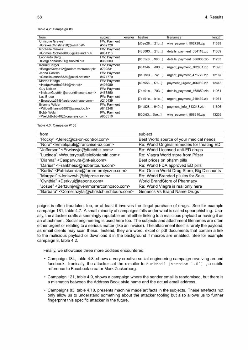
58 4. Results
Table 4.2: Campaign #8
from subject xmailer hashes filenames lengthChristine Graves<[email protected]>
FW: Payment#502728 [d0ee28..., 21c...] wire_payment_502728.zip 11339
Rochelle Grimes<[email protected]>
FW: Payment#034118 [488063..., 21c...] details_payment_034118.zip 11339
Leonardo Berg<[email protected]>
FW: Payment#386003 [8d65c8..., 996...] details_payment_386003.zip 11233
Kermit Berger<[email protected]>
FW: Payment#702831 [66134b..., d00...] urgent_payment_702831.zip 11695
Jenna Castillo<[email protected]>
FW: Payment#471779 [8a0be3..., 741...] urgent_payment_471779.zip 12167
Martha Hodge<[email protected]>
FW: Payment#406089 [a0c556..., f76...] payment_urgent_406089.zip 12446
Guy Nelson<[email protected]>
FW: Payment#468850 [7ed91e..., 703...] details_payment_468850.zip 11951
Luz Bruce<[email protected]>
FW: Payment#210439 [7ed91e..., b1e...] urgent_payment_210439.zip 11951
Brianna Wilder<[email protected]>
FW: Payment#813248 [04c828..., 940...] payment_info_813248.zip 11696
Bobbi Welch<[email protected]>
FW: Payment#858510 [600fd3.., 5be...] wire_payment_858510.zip 13233
Table 4.3: Campaign #158
from subject”Rocky” <[email protected]> Best World source of your medical needs”Nora” <[email protected]> Re: World Original remedies for treating ED”Jefferson” <[email protected]> Re: World Licensed anti-ED drugs”Lucinda” <[email protected]> Re: Viagra World store from Pfizer”Dianna” <[email protected]> Best prices on pharm pills”Darius” <[email protected]> Re: World FDA approved ED pills”Kurtis” <[email protected]> Re: Online World Drug Store, Big Discounts”Margret” <[email protected]> Re: World Branded pilules for Sale”Cynthia” <[email protected]> World BrandStore of Pharmacy”Josue” <[email protected]> Re: World Viagra is real only here”Barbara” <[email protected]> Generics Vs Brand Name Drugs
paigns is often fraudulent too, or at least it involves the illegal purchase of drugs. See for examplecampaign 181, table 4.7. A small minority of campaigns falls under what is called spear phishing. Usu-ally, the attacker crafts a seemingly reputable email either linking to a malicious payload or having it asan attachment. Social engineering is used here too. The subjects and attachment filenames are ofteneither urgent or relating to a serious matter (like an invoice). The attachment itself is rarely the payload,as email clients may scan these. Instead, they are word, excel or pdf documents that contain a linkto the malicious payload or download it in the background if macros are enabled. See for examplecampaign 8, table 4.2.
Finally, we showcase three more oddities encountered:
• Campaign 184, table 4.8, shows a very creative social engineering campaign revolving aroundfacebook. Ironically, the attacker set the x-mailer to ZuckMail [version 1.00] , a subtlereference to Facebook creator Mark Zuckerberg.
• Campaign 121, table 4.9, shows a campaign where the sender email is randomised, but there isa mismatch between the Address Book style name and the actual email address.
• Campaigns 83, table 4.10, presents machine made artifacts in the subjects. These artefacts notonly allow us to understand something about the attacker tooling but also allows us to furtherfingerprint this specific attacker in the future.

4.5. Notable Findings 59
Table 4.4: Campaign #188
from subject”Bruno Coley” <[email protected]> Want that position get the Degree”Maxwell Hoffman” <[email protected]> Look what you are up against...without a Degre...Latoya Rodgers <[email protected]> You have the on job experience now get the Deg...”Alberto Gibbons” <Plummer_Mercedes@sanibeland... Look what you are up against...without a Degre...”Troy Ramirez” <[email protected]> You have the trainning now get the Degree to m...Jon Vinson <[email protected]> Be the best...Get that Degree!”Nicholas Erwin” <[email protected]> Be the best out there with our Degree”Becky Newsome” <Aldridge_Audrey@restaurantdul... Everyone has a degree but not everyone has exp...”Haley Wooten” <Estrada_Tyree@chillhouseadrasa... Separate yourself from all the rest with a Degree
Table 4.5: Campaign #245
from subject xmailer hashes
”Jordyn”<[email protected]...
veel van dames uit badoo.comin uw Burgh wachten.
’Microsoft WindowsLiveMail 15.4.3550.950’
92fe6a...
”Jessie”<[email protected]...
Sometimes, life has a cruelsense of humor, gi...
’Microsoft Windows LiveMail 15.4.3543.943 610fea...
”Simone”<[email protected]...
The one you love and the onewho loves you are...
Microsoft Windows LiveMail 15.4.3500.900 e5deac...
”Geneva”<[email protected]...
her scent fades from the pillows,and even fro...
Microsoft Windows LiveMail 15.4.3579.979 29a65f...
”Katelin”<[email protected]...
veel van kutjes uit badoo.comin uw stad wachten.
Microsoft Windows LiveMail 15.4.3599.999 6163ee...
”Sasha”<[email protected]>
If you gave someone your heartand they died, ...
Microsoft Windows LiveMail 15.4.3596.996 54d990...
”Nina”<[email protected]...
zoveel van dames uit badoo.comin uw plek wach...
Microsoft Windows LiveMail 15.4.3571.971 9d1221...
Table 4.6: Campaign #135
from subject xmailer”zx”<[email protected]> MAKE YOUR SPACE SHINE: handmade oil painting ! ’Lbmk 6’
”fgc”<[email protected]> MAKE YOUR SPACE SHINE: handmade oil painting ! ’Vdryldnvhs 1’
Table 4.7: Campaign #181
from subject hashesWinston Heard <[email protected]> Superior Quality male pills 6b9059...Ellen Bledsoe <Estes_Katy@investmenttrustforum... Classic orgasm volumizer 178be0...Roderick Jimenez <[email protected]> Genuine erectile vitamins 4d3526...
Table 4.8: Campaign #184
from subject xmailer hashes”Facebook”<notification+zj4ozz926stc@facebook...
Ken je Jeanine Triezenberg,Fabienne Mok en 8 ... ZuckMail [version 1.00] [897c2b..., 85f...
”Facebook”<notification+zj4ozz926stc@facebook...
Peter V Beusekom, PaulMolenaar en 4 anderen w... ZuckMail [version 1.00] [535f16..., a5d...
”Facebook”<notification+zj4ozz926stc@facebook...
Je hebt meer vrienden opFacebook dan je denkt ZuckMail [version 1.00] [2b0a49..., ecd...

60 4. Results
Table 4.9: Campaign #121
from subject hashes”Rhoda Robles”<Whaley_Porfirio@erenkoysutesis... I’m ready for you baby and I know what you want. 3d8ed4...
”Rosemary Cruz”<[email protected]> Buy Male Sexual Enhancement Pills fc48b6...
”Salvador Dow”<[email protected]> Then our pilules are of great usefulness for you! ab67b2...
”Jeremy Root”<[email protected]> Special RX from Canada for men 74684f...
Table 4.10: Campaign #83
from subject hashesNat Calhoun<[email protected]>
=?UTF-8?Q?=F3=BE=AC=8D_?=... Ik wil u te ont... c9d90e..., d13...
Robyn<[email protected]>
=?UTF-8?Q?=F3=BE=AC=8D_?=... Niet bekend te ... e14fd0..., c9d...
Brant<[email protected]>
=?UTF-8?Q?=F3=BE=AC=8D_?=... Ik heb soms wil... c9d90e..., 97a...
Krista<[email protected]>
=?UTF-8?Q?=F3=BE=AC=8D_?=... Niet bekend te ... 2cd7ad..., c9d...
Vicky<[email protected]>
=?UTF-8?Q?=F3=BE=AC=8D_?=... Mijn favoriete ... 96e0ae..., c9d...
Ali<[email protected]>
=?UTF-8?Q?=F3=BE=AC=8D_?=... We houden met e... c9d90e..., e8e...

5Conclusion and Future Work
We now present our conclusions and suggests the possible future work, both concerning the improve-ment of our framework and the new research that can be performed with the output of our framework.
In this thesis project, we have addressed the task of performing campaign analysis. Campaign anal-ysis is the Threat Intelligence process of grouping together intrusion attempts that are orchestrated bythe same threat actors against the same victims with a specific goal. Lockheed Martin first introducedthis process in its 2011 seminal white paper “Intelligence-Driven Computer Network Defense Informedby Analysis of Adversary Campaigns and Intrusion Kill Chains”. The researchers of Lockheed Martincame up with campaign analysis to cope with Advanced Persistent Threats, highly motivated, resource-ful and skilled groups that started to become increasingly problematic at the beginning of the decade.
State-sponsored APTs typically engage in acts of cyberwarfare (like the Stuxnet hack) and espi-onage (both industrial and traditional). To do so, they develop bleeding edge tools and techniques.Unfortunately, these tend to eventually become available to less skilled groups, including traditionalcriminal groups, when they are disclosed irresponsibly to the public. Irresponsible disclosures vastlyincreased the number of entities capable of performing complex hacking: if before the rise of the APTsand their techniques, for most organisations the eggshell model of security (composed of a singlehardened layer of defences at its border) sufficed, now this is just not good enough. As the thresh-old for advanced hacking lowered, it became evident that a new model of security, multi-layered andpervasive, was necessary. Threat Intelligence emerged as a valuable process to improve defencesaccording to this new strategy. Threat Intelligence has the goal of studying threats techniques, tools,motives and by allowing to track them through time. Lockheed Martin campaign analysis is a process toperform data-driven threat intelligence by linking together related intrusion attempts (called kill chainsin the model) by looking for repeating elements. This methodology is similar to a police investigationdiscovering a serial killer by finding peculiarities that repeat across a multitude of seemingly unrelatedmurders.
Unfortunately, campaign analysis is a process rarely performed in practice. There are several rea-sons behind this, one of them is that there is a lack of automated framework to perform it. A medium-large organisation would likely need hundreds of security experts to establish connections between allincidents manually. Needless to say, this makes only large organisations where security is an absolutenecessity (like Lockheed Martin) capable and willing to perform it manually.
Having highlighted the research gap, lack of automation in campaign analysis, we established threeresearch questions:
1. Can campaign analysis be performed with an existent clustering technique?
2. Does approximate match of suitable indicators improve recall performance of campaign analysis?
3. Can a methodology be developed to assess what indicators are most suitable (and what are not)for approximate match?
We collaborated with Dutchsec, a cybersecurity company based in Utrecht that provided us with anextensive collection of malicious emails. We first extracted interesting features from these emails and
61

62 5. Conclusion and Future Work
further found more by setting up a malware lab where we executed all the malicious attachments of theemails, for a total of 68 features per kill chain.
We then designed a framework to perform automatic clustering of campaigns using two steps ofdensity-based clustering. We tried to select the best methodology by assessing the performance oftwo density-based clustering algorithms: DBSCAN and HDBSCAN. Furthermore, to answer our thirdresearch question, we tested the two algorithms on two versions of our framework: one allowing onlyexact match of features and one allowing approximate string matching for some features. Only exactmatch of features is performed in the state of the art. We selected the features more appropriate forapproximate string matching using both domain knowledge and by performing a statistical analysis oftheir entropy.
Finally, we obtained the following results:
• Campaign analysis can be automated and improved (concerning recall) by using density-basedclustering.
• Density-based clustering adds a layer of fuzziness that allows improving recall compared to thetraditional manual approach. In particular, it allows discovering campaigns even when they arecharacterised by randomisation of features to avoid classic campaign analysis.
• Density-based campaign analysis comes at the price of a loss in precision when compared to thetraditional manual approach.
• Approximate string matching does not help in automating campaign analysis when density-basedclustering is performed. Indeed, recall seems to worsen compared to when exact only stringmatching of features is performed.
• HDBSCAN performs better than DBSCAN for this task in terms of recall, which is more importantthan precision as finding complete campaigns is harder than dealing with noise. Furthermore,HDBSCAN is far superior in ease of use as the parameter tuning is minimal compared to DB-SCAN, which require extensive trials and error.
We stress the importance of understanding the scenario where we imagine this framework to be utilised.This framework does not replace a security analyst. A security analyst is necessary to evaluate thefound campaigns and eventually reject them. Our system should be seen as an aid in performingexploratory threat intelligence. We automated the expensive and tedious process of linking possiblyrelated incidents, allowing analysts to be able to perform campaign analysis even in a large organisationdealing with a lot of data. In other words, we believe that our framework can scale down significantlythe number of human resources needed to perform this process. Hopefully, lowering this thresholdwill allow small and medium organisations that do not have security as a critical requirement to finallyperform their own threat intelligence.
We believe this framework is only a good starting point, as there is room for improvement. First ofall, it would be interesting to understand if other clustering techniques could be used. Density-basedclustering seems to do a good job overall, but it is possible that other techniques perform even better,especially in terms of precision. Likewise, it would also be interesting to study the impact of using differ-ent similarity metrics than the ones we developed to assess the similarity of intrusion attempts beforethe final round of clustering. We fine-tuned our system to cluster spear phishing campaigns becausethis kind of campaign was often occurring in our dataset. It would be interesting to also work with realAPTs crafted emails. Unfortunately, these emails tend to be redacted when released to the public, sothe best way to do this would be to work with an organisation that experienced APT hacking directly.The malware found in our dataset is old, and for the most part, the command and control server withwhich the malware was designed to communicate with is not online anymore. This means that whenwe tested the malware in our malware lab, we were only able to retrieve static features (belonging to thecode itself) and behavioural (its actions), but not network communications. It would be very interestingto study the performance of our system on fresh malware. This has to be done in the first days, asthe malware lifecycle tends to be rather short. The malware lab component itself can be improved byswitching to spender-sandbox, a highly praised fork of the cuckoo sandbox we set up and used.

63
Moreover, we would like to highlight the future work that can be performed now that automaticcampaign analysis is possible. Our system performs unsupervised learning by assigning campaignlabels to malicious emails. Once an analyst evaluates these campaign labels, they could be usedfor a multitude of supervised learning tasks, for example, automatic classifications of emails in a livesystem.


AKill chain Features
indicator name h5 filename DBSCAN eps weight
1 additional_info.exiftool.AppVersion VirusTotal 0.02 MEDIUM2 additional_info.exiftool.Application VirusTotal 0.02 LOW3 additional_info.exiftool.CreateDate VirusTotal 0.02 LOW4 additional_info.exiftool.Creator VirusTotal 0.02 LOW5 additional_info.exiftool.DocSecurity VirusTotal 0.02 LOW6 additional_info.exiftool.FileType VirusTotal 0.02 LOW7 additional_info.exiftool.LastModifiedBy VirusTotal 0.02 LOW8 additional_info.exiftool.LinksUpToDate VirusTotal 0.02 LOW9 additional_info.exiftool.ModifyDate VirusTotal 0.02 LOW10 additional_info.exiftool.Pages VirusTotal 0.02 LOW11 additional_info.exiftool.Words VirusTotal 0.02 LOW12 additional_info.exiftool.ZipBitFlag VirusTotal 0.02 LOW13 additional_info.exiftool.ZipCRC VirusTotal 0.02 LOW14 additional_info.exiftool.ZipCompressedSize VirusTotal 0.02 LOW15 additional_info.exiftool.ZipFileName VirusTotal 0.55 HIGH16 additional_info.exiftool.ZipModifyDate VirusTotal 0.02 LOW17 additional_info.exiftool.ZipRequiredVersion VirusTotal 0.02 LOW18 additional_info.magic VirusTotal 0.02 LOW19 additional_info.openxmlchecker.ole.num_macros VirusTotal 0.02 LOW20 body Email 0.35 HIGH21 content_type Email 0.02 LOW22 date Email 0.02 LOW23 domain Email 0.02 LOW24 file.crc32 Cuckoo 0.02 LOW25 file.name Cuckoo 0.55 MEDIUM26 file.type Cuckoo 0.02 LOW27 filename Email 0.55 MEDIUM28 first seen VirusTotal 0.02 LOW29 from Email 0.45 HIGH30 geo.city Email 0.02 LOW31 geo.country.name Email 0.02 LOW32 hash.sha1 Email 0.02 2033 headers.Content-Type Email 0.02 LOW34 headers.Date Email 0.02 LOW35 headers.Priority Email 0.02 LOW36 headers.Return-Path Email 0.45 MEDIUM37 headers.X-Mailer Email 0.02 MEDIUM
65
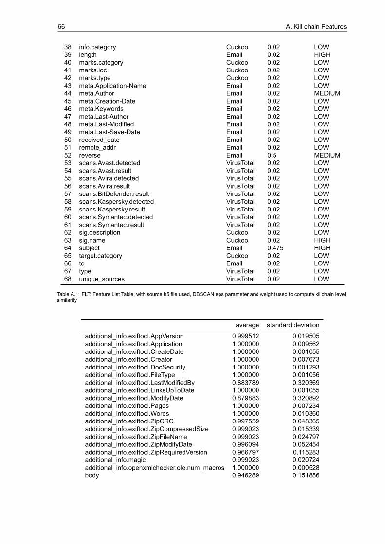
66 A. Kill chain Features
38 info.category Cuckoo 0.02 LOW39 length Email 0.02 HIGH40 marks.category Cuckoo 0.02 LOW41 marks.ioc Cuckoo 0.02 LOW42 marks.type Cuckoo 0.02 LOW43 meta.Application-Name Email 0.02 LOW44 meta.Author Email 0.02 MEDIUM45 meta.Creation-Date Email 0.02 LOW46 meta.Keywords Email 0.02 LOW47 meta.Last-Author Email 0.02 LOW48 meta.Last-Modified Email 0.02 LOW49 meta.Last-Save-Date Email 0.02 LOW50 received_date Email 0.02 LOW51 remote_addr Email 0.02 LOW52 reverse Email 0.5 MEDIUM53 scans.Avast.detected VirusTotal 0.02 LOW54 scans.Avast.result VirusTotal 0.02 LOW55 scans.Avira.detected VirusTotal 0.02 LOW56 scans.Avira.result VirusTotal 0.02 LOW57 scans.BitDefender.result VirusTotal 0.02 LOW58 scans.Kaspersky.detected VirusTotal 0.02 LOW59 scans.Kaspersky.result VirusTotal 0.02 LOW60 scans.Symantec.detected VirusTotal 0.02 LOW61 scans.Symantec.result VirusTotal 0.02 LOW62 sig.description Cuckoo 0.02 LOW63 sig.name Cuckoo 0.02 HIGH64 subject Email 0.475 HIGH65 target.category Cuckoo 0.02 LOW66 to Email 0.02 LOW67 type VirusTotal 0.02 LOW68 unique_sources VirusTotal 0.02 LOW
Table A.1: FLT: Feature List Table, with source h5 file used, DBSCAN eps parameter and weight used to compute killchain levelsimilarity
average standard deviation
additional_info.exiftool.AppVersion 0.999512 0.019505additional_info.exiftool.Application 1.000000 0.009562additional_info.exiftool.CreateDate 1.000000 0.001055additional_info.exiftool.Creator 1.000000 0.007673additional_info.exiftool.DocSecurity 1.000000 0.001293additional_info.exiftool.FileType 1.000000 0.001056additional_info.exiftool.LastModifiedBy 0.883789 0.320369additional_info.exiftool.LinksUpToDate 1.000000 0.001055additional_info.exiftool.ModifyDate 0.879883 0.320892additional_info.exiftool.Pages 1.000000 0.007234additional_info.exiftool.Words 1.000000 0.010360additional_info.exiftool.ZipCRC 0.997559 0.048365additional_info.exiftool.ZipCompressedSize 0.999023 0.015339additional_info.exiftool.ZipFileName 0.999023 0.024797additional_info.exiftool.ZipModifyDate 0.996094 0.052454additional_info.exiftool.ZipRequiredVersion 0.966797 0.115283additional_info.magic 0.999023 0.020724additional_info.openxmlchecker.ole.num_macros 1.000000 0.000528body 0.946289 0.151886

67
content_type 0.766113 0.274613date 0.921875 0.076555domain 0.989746 0.054091file.crc32 0.997559 0.036955file.name 0.974609 0.061529file.sha1 0.990234 0.037078file.type 0.413330 0.461046filename 0.999023 0.015367first seen 0.753906 0.339417from 0.987305 0.049153geo.city 0.968262 0.173706geo.country.name 0.932129 0.247122hash.sha1 0.980469 0.106910headers.Content-Type 0.881348 0.219213headers.Date 0.884277 0.102068headers.Priority 1.000000 0.000707headers.Return-Path 0.998047 0.011546headers.X-Mailer 0.999023 0.027572info.category 0.000000 0.000000length 0.995117 0.066848marks.category 0.126709 0.332604marks.ioc 0.915039 0.225819marks.type 0.000000 0.000000meta.Application-Name 1.000000 0.000421meta.Author 1.000000 0.000085meta.Creation-Date 1.000000 0.000397meta.Last-Author 1.000000 0.000060meta.Last-Modified 1.000000 0.000379meta.Last-Save-Date 1.000000 0.000379received_date 0.965820 0.039554remote_addr 0.982910 0.061133reverse 0.991699 0.058219scans.Avast.detected 0.875977 0.317107scans.Avast.result 0.264160 0.440917scans.Avira.detected 0.767578 0.278314scans.Avira.result 0.296875 0.456917scans.BitDefender.result 0.239014 0.426450scans.Kaspersky.detected 0.756836 0.331052scans.Kaspersky.result 0.275635 0.446763scans.Symantec.detected 0.826172 0.340801scans.Symantec.result 0.507812 0.499828sig.description 0.593262 0.453618sig.name 0.524902 0.426821ssdeep 0.994629 0.057752subject 0.967773 0.121797target.category 0.000000 0.000000to 0.961914 0.112798type 0.998535 0.023553unique_sources 0.582520 0.493161
Table A.2: Average and Standard Deviation of indicators cosine distance. Week 12 2016 (March 21st to March 27th)

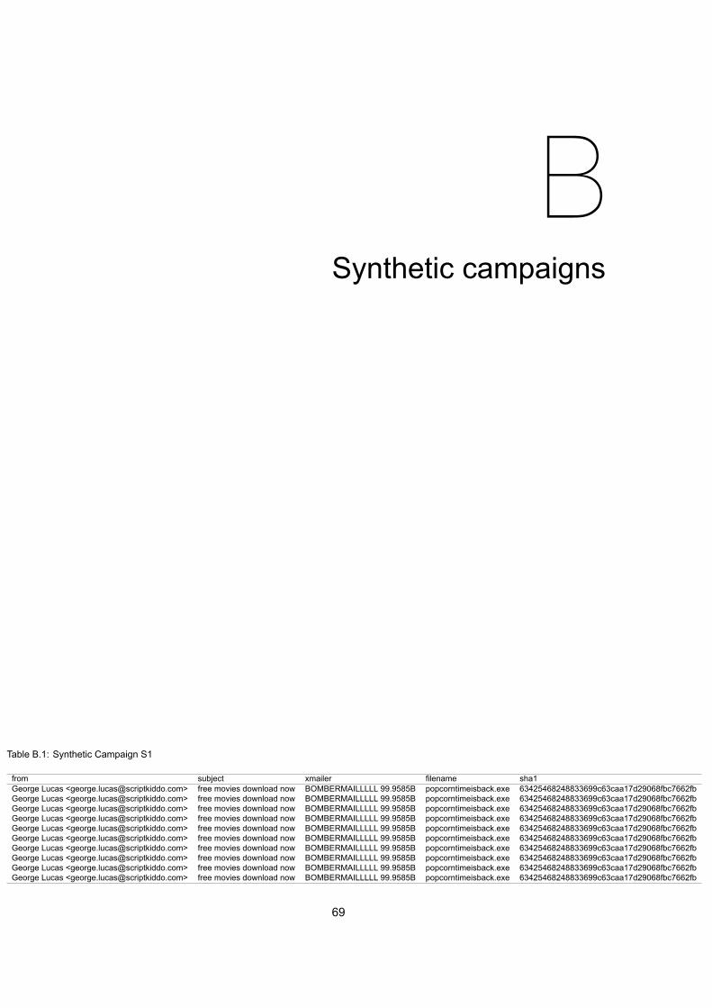
BSynthetic campaigns
Table B.1: Synthetic Campaign S1
from subject xmailer filename sha1George Lucas <[email protected]> free movies download now BOMBERMAILLLLL 99.9585B popcorntimeisback.exe 63425468248833699c63caa17d29068fbc7662fbGeorge Lucas <[email protected]> free movies download now BOMBERMAILLLLL 99.9585B popcorntimeisback.exe 63425468248833699c63caa17d29068fbc7662fbGeorge Lucas <[email protected]> free movies download now BOMBERMAILLLLL 99.9585B popcorntimeisback.exe 63425468248833699c63caa17d29068fbc7662fbGeorge Lucas <[email protected]> free movies download now BOMBERMAILLLLL 99.9585B popcorntimeisback.exe 63425468248833699c63caa17d29068fbc7662fbGeorge Lucas <[email protected]> free movies download now BOMBERMAILLLLL 99.9585B popcorntimeisback.exe 63425468248833699c63caa17d29068fbc7662fbGeorge Lucas <[email protected]> free movies download now BOMBERMAILLLLL 99.9585B popcorntimeisback.exe 63425468248833699c63caa17d29068fbc7662fbGeorge Lucas <[email protected]> free movies download now BOMBERMAILLLLL 99.9585B popcorntimeisback.exe 63425468248833699c63caa17d29068fbc7662fbGeorge Lucas <[email protected]> free movies download now BOMBERMAILLLLL 99.9585B popcorntimeisback.exe 63425468248833699c63caa17d29068fbc7662fbGeorge Lucas <[email protected]> free movies download now BOMBERMAILLLLL 99.9585B popcorntimeisback.exe 63425468248833699c63caa17d29068fbc7662fbGeorge Lucas <[email protected]> free movies download now BOMBERMAILLLLL 99.9585B popcorntimeisback.exe 63425468248833699c63caa17d29068fbc7662fb
69

70 B. Synthetic campaigns
Table B.2: Synthetic Campaign S2
from subject xmailer filename sha1Steve Steve <[email protected]> Your trip to Brussels invoice#384823 WONDERMAIL 7.777.6 INVOICE-688920.pdf 63425468343792699c63caa17d29068fbc7662fbSteven Lucas <[email protected]> Your trip to Brussels invoice#630571 WONDERMAIL 7.777.6 INVOICE-343792.pdf 63425468662073699c63caa17d29068fbc7662fbSteven Bolak <[email protected]> Your trip to Brussels invoice#790210 WONDERMAIL 7.777.6 INVOICE-662073.pdf 63425468747793699c63caa17d29068fbc7662fbMonster Luas <[email protected]> Your trip to Brussels invoice#837581 WONDERMAIL 7.777.6 INVOICE-747793.pdf 63425468948467699c63caa17d29068fbc7662fbRandy Bolak <[email protected]> Your trip to Brussels invoice#572893 WONDERMAIL 7.777.6 INVOICE-948467.pdf 63425468764343699c63caa17d29068fbc7662fbCptain Jordan <[email protected]> Your trip to Brussels invoice#894844 WONDERMAIL 7.777.6 INVOICE-764343.pdf 63425468203023699c63caa17d29068fbc7662fbRandy Jordan <[email protected]> Your trip to Brussels invoice#880807 WONDERMAIL 7.777.6 INVOICE-203023.pdf 63425468355612699c63caa17d29068fbc7662fbMonster Jordan <monster.jordan@banzaimail-camo... Your trip to Brussels invoice#327095 WONDERMAIL 7.777.6 INVOICE-355612.pdf 63425468311790699c63caa17d29068fbc7662fbEllie Luas <[email protected]> Your trip to Brussels invoice#765173 WONDERMAIL 7.777.6 INVOICE-311790.pdf 63425468283755699c63caa17d29068fbc7662fbSteven Jordan <[email protected]> Your trip to Brussels invoice#688920 WONDERMAIL 7.777.6 INVOICE-283755.pdf 63425468213588699c63caa17d29068fbc7662fb
Table B.3: Synthetic Campaign S3
from subject xmailer filename sha1George Lucas <[email protected]> You are 10 weeks late for your star wars merch... Force Mail client 117345 STARWARS-MERCH-DELAY-132337.pdf 63425468132337699c63caa17d29068fbc7662fbSteven Lucas <[email protected]> 10 weeks delay star wars merch Force Mail client 885020 STARWARS-MERCH-DELAY-178165.pdf 63425468178165699c63caa17d29068fbc7662fbSteven Bolak <[email protected]> You are 10 weeks late!!! Collect your merch! Force Mail client 378391 STARWARS-MERCH-DELAY-827478.pdf 63425468827478699c63caa17d29068fbc7662fbMonster Luas <[email protected]> Star wars: waiting for your payment 10 weeks Force Mail client 684614 STARWARS-MERCH-DELAY-799221.pdf 63425468799221699c63caa17d29068fbc7662fbRandy Bolak <[email protected]> 10 weeks delay star wars merch Force Mail client 983811 STARWARS-MERCH-DELAY-580233.pdf 63425468580233699c63caa17d29068fbc7662fbCptain Jordan <[email protected]> Star wars: waiting for your payment 10 weeks Force Mail client 610174 STARWARS-MERCH-DELAY-305531.pdf 63425468305531699c63caa17d29068fbc7662fbRandy Jordan <[email protected]> NEW MERCH Star Wars order, pay! Force Mail client 754355 STARWARS-MERCH-DELAY-896682.pdf 63425468896682699c63caa17d29068fbc7662fbMonster Jordan <[email protected]> You forgot to pay us for 10 weeks, star wars m... Force Mail client 605285 STARWARS-MERCH-DELAY-634752.pdf 63425468634752699c63caa17d29068fbc7662fbEllie Luas <[email protected]> 10 weeks delay in payment, star wars merch inv... Force Mail client 896582 STARWARS-MERCH-DELAY-434338.pdf 63425468434338699c63caa17d29068fbc7662fbSteven Jordan <[email protected]> fine for 10 weeks delay in collect... Force Mail client 937950 STARWARS-MERCH-DELAY-989545.pdf 63425468989545699c63caa17d29068fbc7662fb
Table B.4: Synthetic Campaign S4
from subject xmailer filename sha1Rebekah Fletcher : [email protected] AIAA 2018 Technical Committees invite callforpapers-806 callforpapers-6740217.pdf 634254686740217699c63caa17d29068fbc7662fbMaritza Schwartz : [email protected] IEEE 2018 Technical Conference callforpapers-922 callforpapers-5956651.pdf 634254685956651699c63caa17d29068fbc7662fbValerie Stephens : [email protected] Invite 2018 NIPS Conference invite callforpapers-459 callforpapers-1580009.pdf 634254681580009699c63caa17d29068fbc7662fbDeirdre Benjamin : [email protected] IEEE 2018 Technical Committee invite callforpapers-434 callforpapers-3293285.pdf 634254683293285699c63caa17d29068fbc7662fbBernard Petersen : [email protected] ACM 2018 conference call callforpapers-118 callforpapers-7937423.pdf 634254687937423699c63caa17d29068fbc7662fbStewart Mcknight : [email protected] ACM 2018 technical conference invite callforpapers-195 callforpapers-6468500.pdf 634254686468500699c63caa17d29068fbc7662fbMalinda Galloway , [email protected] ACM computing survey 2018 callforpapers-408 callforpapers-4742059.pdf 634254684742059699c63caa17d29068fbc7662fbNorbert Chambers : [email protected] AIAA 2018 call for papers invite callforpapers-611 callforpapers-6120838.pdf 634254686120838699c63caa17d29068fbc7662fbDomenic Caldwell : [email protected] IEEE 2018 conference call papers callforpapers-385 callforpapers-4702158.pdf 634254684702158699c63caa17d29068fbc7662fbStanton Roberson : [email protected] NIPS invite to conference 2018 callforpapers-901 callforpapers-3346929.pdf 634254683346929699c63caa17d29068fbc7662fb

CReal Campaigns discovered manually
71

72 C. Real Campaigns discovered manually
Figure C.1: Excerpt of real campaign R1 observed in the dataset
Figure C.2: Excerpt of real campaign R2 observed in the dataset

73
Figure C.3: Excerpt of real campaign R3 observed in the dataset

Bibliography[1] Rohan M. Amin, Julie J. C. H. Ryan, and Johan van Dorp. Detecting targeted malicious email.
IEEE Security & Privacy, 10(3):64–71, 2012. doi: 10.1109/MSP.2011.154. URL https://doi.org/10.1109/MSP.2011.154.
[2] Parth Bhatt, Edgar Toshiro Yano, and Per M. Gustavsson. Towards a framework to detect multi-stage advanced persistent threats attacks. In 8th IEEE International Symposium on Service Ori-ented System Engineering, SOSE 2014, Oxford, United Kingdom, April 7-11, 2014, pages 390–395, 2014. doi: 10.1109/SOSE.2014.53. URL https://doi.org/10.1109/SOSE.2014.53.
[3] Blake D. Bryant and Hossein Saiedian. A novel kill-chain framework for remote security log anal-ysis with SIEM software. Computers & Security, 67:198–210, 2017. doi: 10.1016/j.cose.2017.03.003. URL https://doi.org/10.1016/j.cose.2017.03.003.
[4] Ricardo J. G. B. Campello, Davoud Moulavi, and Joerg Sander. Density-based clustering basedon hierarchical density estimates. In Jian Pei, Vincent S. Tseng, Longbing Cao, Hiroshi Motoda,and Guandong Xu, editors, Advances in Knowledge Discovery and Data Mining, pages 160–172,Berlin, Heidelberg, 2013. Springer Berlin Heidelberg. ISBN 978-3-642-37456-2.
[5] Ricardo J. G. B. Campello, Davoud Moulavi, Arthur Zimek, and Jörg Sander. Hierarchical densityestimates for data clustering, visualization, and outlier detection. TKDD, 10(1):5:1–5:51, 2015.doi: 10.1145/2733381. URL http://doi.acm.org/10.1145/2733381.
[6] WilliamW. Cohen, Pradeep Ravikumar, and Stephen E. Fienberg. A comparison of string distancemetrics for name-matching tasks. In Proceedings of IJCAI-03Workshop on Information Integrationon the Web (IIWeb-03), August 9-10, 2003, Acapulco, Mexico, pages 73–78, 2003. URL http://www.isi.edu/info-agents/workshops/ijcai03/papers/Cohen-p.pdf.
[7] Martin Ester, Hans-Peter Kriegel, Jörg Sander, and Xiaowei Xu. A density-based algorithm fordiscovering clusters in large spatial databases with noise. pages 226–231. AAAI Press, 1996.
[8] Ivan P. Fellegi and Alan B. Sunter. A theory for record linkage. Journal of the American Statis-tical Association, 64(328):1183–1210, 1969. doi: 10.1080/01621459.1969.10501049. URLhttps://www.tandfonline.com/doi/abs/10.1080/01621459.1969.10501049.
[9] Dan Guido. A case study of intelligence-driven defense. IEEE Security & Privacy, 9(6):67–70,2011. doi: 10.1109/MSP.2011.158. URL https://doi.org/10.1109/MSP.2011.158.
[10] Eric M Hutchins, Michael J Cloppert, and Rohan M Amin. Intelligence-driven computer networkdefense informed by analysis of adversary campaigns and intrusion kill chains. Leading Issues inInformation Warfare & Security Research, 1(1):80, 2011.
[11] Karen Spärck Jones. IDF term weighting and IR research lessons. Journal of Documentation,60(5):521–523, 2004. doi: 10.1108/00220410410560591. URL https://doi.org/10.1108/00220410410560591.
[12] Hans-Peter Kriegel, Peer Kröger, Jörg Sander, and Arthur Zimek. Density-based clustering. WileyInterdisciplinary Reviews: Data Mining and Knowledge Discovery, 1(3):231–240. doi: 10.1002/widm.30. URL https://onlinelibrary.wiley.com/doi/abs/10.1002/widm.30.
[13] Dekang Lin. An information-theoretic definition of similarity. In Proceedings of the Fifteenth Inter-national Conference on Machine Learning (ICML 1998), Madison, Wisconsin, USA, July 24-27,1998, pages 296–304, 1998.
75
76 Bibliography
[14] William J Lynn III. Defending a new domain: The pentagon’s cyberstrategy. Cyberwar ResourcesGuide, (121), 2010.
[15] James Rutherford and Gregory B. White. Using an improved cybersecurity kill chain to develop animproved honey community. In 49th Hawaii International Conference on System Sciences, HICSS2016, Koloa, HI, USA, January 5-8, 2016, pages 2624–2632, 2016. doi: 10.1109/HICSS.2016.329. URL https://doi.org/10.1109/HICSS.2016.329.
[16] Charles Smutz and Angelos Stavrou. Malicious PDF detection using metadata and structuralfeatures. In 28th Annual Computer Security Applications Conference, ACSAC 2012, Orlando,FL, USA, 3-7 December 2012, pages 239–248, 2012. doi: 10.1145/2420950.2420987. URLhttp://doi.acm.org/10.1145/2420950.2420987.
[17] Peter P. Stavroulakis and Mark Stamp, editors. Handbook of Information and CommunicationSecurity. Springer, 2010. ISBN 978-3-642-04116-7. doi: 10.1007/978-3-642-04117-4. URLhttps://doi.org/10.1007/978-3-642-04117-4.
[18] Konstantin Tretyakov. Machine learning techniques in spam filtering. In Data Mining Problem-oriented Seminar, MTAT, volume 3, pages 60–79, 2004.
[19] Kiri Wagstaff. Machine learning that matters. In Proceedings of the 29th International Conferenceon Machine Learning, ICML 2012, Edinburgh, Scotland, UK, June 26 - July 1, 2012, 2012. URLhttp://icml.cc/2012/papers/298.pdf.
[20] Daniel S Wilks. Cluster analysis. In International geophysics, volume 100, pages 603–616. Else-vier, 2011.
[21] Rui Xu and Donald C. Wunsch II. Survey of clustering algorithms. IEEE Trans. Neural Networks,16(3):645–678, 2005. doi: 10.1109/TNN.2005.845141. URL https://doi.org/10.1109/TNN.2005.845141.


