Embed Size (px)
Citation preview
On imprecision in statistical theory
by
Marco Y. S. Shum
A thesispresented to the University of Waterloo
in fulfillment of thethesis requirement for the degree of
Doctor of Sciencein
Statistics
Waterloo, Ontario, Canada, 2021
c© Marco Y. S. Shum 2021

Examining Committee Membership
The following served on the Examining Committee for this thesis. The decision of theExamining Committee is by majority vote.
External Examiner: Name: Tahani Coolen-MaturiTitle: Professor
Supervisors: Name: Paul MarriottTitle: Professor
Name: Tony WirjantoTitle: Professor
Internal members: Name: Shoja’eddin ChenouriTitle: Professor
Name: Martin LysyTitle: Professor
Internal-external Member: Name: Thomas ParkerTitle: Professor
ii

Author’s declaration
I hereby declare that I am the sole author of this thesis. This is a true copy of the thesis,including any required final revisions, as accepted by my examiners.
I understand that my thesis may be made electronically available to the public.
iii
Abstract
This thesis provides an exploration of the interplay between imprecise probability and statis-tics. Mathematically, one may summarise this relationship as how (Bayesian) sensitivityanalysis involving a set of (prior) models can be done in relation to the notion of coherencein the sense of de Finetti [32], Williams [84] and, more recently, Walley [81]. This thesisexplores how imprecise probability can be applied to foundational statistical problems.
The contributions of this thesis are three folds. In Chapter 1, we illustrate and motivatethe need for imprecise models due to certain inherent limitations of elicitation of a sta-tistical model. In Chapter 2, we provide a primer of imprecise probability aimed at thestatistics audience along with illustrative statistical examples and results that highlightsalient behaviours of imprecise models from the the statistical perspective.
In the second part of the thesis (Chapters 3, 4, 5), we consider the statistical applicationof the imprecise Dirichlet model (IDM), an established model in imprecise probability. Inparticular, the posterior inference for log-odds statistics under sparse contingency tables,the development and use of imprecise interval estimates via quantile intervals over a set ofdistributions and the geometry of the optimisation problem over a set of distributions arestudied. Some of these applications require extensions of Walley’s existing framework, andare presented as part of our contribution.
The third part of the thesis (Chapters 6, 7) departs from the IDM parametric assumptionand instead focuses on posterior inference using imprecise models in a finite dimensionalsetting when the lower bound of the probability of the data over a set of elicited priorsis zero. This setting generalises the problem of zero marginal probability in Bayesiananalysis. In Chapter 6, we explore the methodology, behaviour and interpretability of theposterior inference under two established models in imprecise probability: the vacuous andregular extensions. In Chapter 7, we note that these extensions are in fact extremes inimprecision, the variability of an inference over the elicited set of probability distributions.Then we consider extensions which are of intermediate levels of imprecision, and discusstheir elicitation and assessment.
iv

Acknowledgements
Foremost, I am most indebted to my supervisors, Paul Marriott and Tony Wirjanto, fortaking this journey with me from the very beginning. Their wisdom has been invaluablefor me being able to put so many of the ideas of this thesis into perspective and makingthem communicable to the reader. They have been instrumental in making concrete myideas that usually start as a ‘stream of consciousness’, as Paul would put it. (They havebeen immensely patient with me regarding that habit.) Above all, their insights aboutstatistics and research have been very influential to me: with due modesty, I would like tothink that a modicum of it rubbed off on me, and made me a better statistician. Withoutdoubt, our discussions and interactions have been a joy. Thank you both, sincerely.
I would also like to thank my defence committee for having taken the time to read my thesisand raising inspiring questions. The engaging discussions with them was a pleasure for me.
I would like to thank the following people for their kind support, advice and friendshipthroughout these years: Joslin Goh, Jay Gweon, David Haskell, Celia Huang, MirabelleHuynh, Louise Kwan, Garcia (Jiaxi) Liang, Reza Ramezan, Reza Raoufi, Greg Rice, Vin-cent Russo, Basil Singer, Lu Xin. (I profusely apologise if I have missed anyone.)
I would like to thank the staff members of the Department of Statistics and Actuarial Sci-ences at UW for their friendly administration of the department. I would like to especiallythank Mary Lou Dufton, without whose help I would have otherwise stumbled into allsorts of administrative limbos.
v

Dedication
To my parents who, under vacuity, had faith in me during this journey.
vi

Table of Contents
List of Tables xii
List of Figures xiii
Notation xvii
1 Elicitation as a statistical motivation for imprecise models 1
1.1 A set of models as a more representative elicitation . . . . . . . . . . . . . 2
1.2 Sensitivity analysis and sets of distributions . . . . . . . . . . . . . . . . . 6
1.3 Imprecise methodology and sets of distributions . . . . . . . . . . . . . . . 10
2 Review of aspects of imprecise models 14
2.1 Avoiding sure losses and coherence . . . . . . . . . . . . . . . . . . . . . . 15
2.1.1 Probability distribution and expectation . . . . . . . . . . . . . . . 16
2.1.2 Sets of probability distributions and expectations . . . . . . . . . . 19
2.2 Aspects of the theory of imprecise probabilities . . . . . . . . . . . . . . . 23
2.2.1 Imprecise expectation . . . . . . . . . . . . . . . . . . . . . . . . . . 23
2.2.2 Imprecision and vacuity . . . . . . . . . . . . . . . . . . . . . . . . 26
2.2.3 The lower envelope theorem . . . . . . . . . . . . . . . . . . . . . . 27
2.2.4 Posterior lower/upper expectations . . . . . . . . . . . . . . . . . . 29
2.3 Imprecise Dirichlet Model (IDM) . . . . . . . . . . . . . . . . . . . . . . . 31
vii
2.4 A commentary for statisticians . . . . . . . . . . . . . . . . . . . . . . . . . 33
2.4.1 Properties of the IDM . . . . . . . . . . . . . . . . . . . . . . . . . 33
2.4.2 A synthesis of responses to IDM from statistical community . . . . 34
2.4.3 A brief review of statistics in imprecise probabilities . . . . . . . . . 35
2.4.4 Comments on imprecise models . . . . . . . . . . . . . . . . . . . . 37
3 Log-odds inference under IDM and sparse observations 39
3.1 Sensitivity of posterior inference to prior choice . . . . . . . . . . . . . . . 39
3.2 Literature: Affine geometry of IDM posterior updating under sparse obser-vations . . . . . . . . . . . . . . . . . . . . . . . . . . . . . . . . . . . . . . 43
3.2.1 Affine geometry of exponential family and Dirichlet-multinomial up-dating . . . . . . . . . . . . . . . . . . . . . . . . . . . . . . . . . . 43
3.2.2 Affine geometry of the IDM . . . . . . . . . . . . . . . . . . . . . . 45
3.3 Inference for log-odds under IDM . . . . . . . . . . . . . . . . . . . . . . . 48
3.3.1 Unboundedness of the log-odds and the theory of coherence . . . . 48
3.3.2 The divergence of coherence from sensitivity analysis under sparseobservations . . . . . . . . . . . . . . . . . . . . . . . . . . . . . . . 51
3.4 Inference for log-odds under IDM with sparse observations . . . . . . . . . 53
3.4.1 Behaviour of the posterior inference of the simple log odds under theIDM and sparse observations . . . . . . . . . . . . . . . . . . . . . . 53
3.4.2 Behaviour and solutions to optimisation problem of the posteriorinference of the general log odds under the IDM and sparse observations 56
3.4.3 Effects of cell counts on imprecision of posterior log-odds inferenceunder the IDM . . . . . . . . . . . . . . . . . . . . . . . . . . . . . 58
3.5 Illustrative numerical examples . . . . . . . . . . . . . . . . . . . . . . . . 60
3.5.1 Setting for numerical optimisation . . . . . . . . . . . . . . . . . . . 60
3.5.2 Dataset examples . . . . . . . . . . . . . . . . . . . . . . . . . . . . 60
3.6 Concluding remarks . . . . . . . . . . . . . . . . . . . . . . . . . . . . . . . 67
viii
4 Imprecise quantile functions and interval-valued statistics in the impre-cise setting 70
4.1 Quantiles and imprecision . . . . . . . . . . . . . . . . . . . . . . . . . . . 71
4.2 Literature: Imprecise Quantiles . . . . . . . . . . . . . . . . . . . . . . . . 72
4.3 Imprecise Quantile Functions . . . . . . . . . . . . . . . . . . . . . . . . . 73
4.4 Optimisation of imprecise quantile functions . . . . . . . . . . . . . . . . . 75
4.5 Properties of imprecise quantile functions . . . . . . . . . . . . . . . . . . . 78
4.5.1 Random variables need not be bounded . . . . . . . . . . . . . . . . 78
4.5.2 Relation to imprecise probabilities . . . . . . . . . . . . . . . . . . . 79
4.5.3 Lower coverage probability of quantile intervals . . . . . . . . . . . 82
4.6 Hypothesis testing using imprecise quantile intervals . . . . . . . . . . . . . 83
4.7 Dataset Examples . . . . . . . . . . . . . . . . . . . . . . . . . . . . . . . . 85
4.8 Concluding remarks . . . . . . . . . . . . . . . . . . . . . . . . . . . . . . . 94
5 On the optimisation problem for the log-odds inference with IDM 96
5.1 KKT solutions to common log-odds problems . . . . . . . . . . . . . . . . 96
5.1.1 An overview of the KKT conditions . . . . . . . . . . . . . . . . . . 97
5.1.2 The KKT conditions of posterior log-odds lower expectation underthe IDM . . . . . . . . . . . . . . . . . . . . . . . . . . . . . . . . . 98
5.1.3 Log probability ratios . . . . . . . . . . . . . . . . . . . . . . . . . . 101
5.1.4 Log odds ratios . . . . . . . . . . . . . . . . . . . . . . . . . . . . . 103
5.1.5 Independence test statistic . . . . . . . . . . . . . . . . . . . . . . . 106
5.2 Some properties of the objective function in mean-parameter space . . . . 109
5.2.1 A reparametrisation of the natural parameter space . . . . . . . . . 109
5.2.2 Geometry of the objective function . . . . . . . . . . . . . . . . . . 112
5.3 Concluding remarks . . . . . . . . . . . . . . . . . . . . . . . . . . . . . . . 116
ix
6 Imprecise posterior inference under zero lower marginal probability infinite dimensions 119
6.1 A running example . . . . . . . . . . . . . . . . . . . . . . . . . . . . . . . 120
6.2 Vacuous and regular extensions . . . . . . . . . . . . . . . . . . . . . . . . 122
6.3 Posterior imprecise inference for discrete parameter and observation spaces 126
6.3.1 Computing the regular extension . . . . . . . . . . . . . . . . . . . 127
6.3.2 Effects of likelihood on regular extension values . . . . . . . . . . . 127
6.3.3 Numerical behaviour of posterior inference . . . . . . . . . . . . . . 128
6.4 Concluding remarks . . . . . . . . . . . . . . . . . . . . . . . . . . . . . . . 136
7 Geometry of conditioning on events with zero lower probability in finitedimensions 138
7.1 The existence of imprecise models between the vacuous and regular extensions139
7.2 Sets of conditional assessments between the vacuous and regular extensions 139
7.2.1 Interpretation of N . . . . . . . . . . . . . . . . . . . . . . . . . . . 141
7.2.2 Intermediate extensions and joint coherence . . . . . . . . . . . . . 142
7.3 Elicitation and assessment of intermediate extensions . . . . . . . . . . . . 143
7.3.1 Range of the intermediate extension . . . . . . . . . . . . . . . . . . 144
7.3.2 Examples of assessments . . . . . . . . . . . . . . . . . . . . . . . . 145
7.3.3 Interpreting PM(B) = 0 . . . . . . . . . . . . . . . . . . . . . . . . 148
7.4 Concluding remarks . . . . . . . . . . . . . . . . . . . . . . . . . . . . . . . 150
8 Thesis summary 153
References 155
APPENDICES 162
A Appendix to Chapter 2 163
A.1 Geometrical interpretation of avoiding losses for probabilities . . . . . . . . 163
A.2 Results and proofs . . . . . . . . . . . . . . . . . . . . . . . . . . . . . . . 165
x
B Appendix to Chapter 3 170
B.1 The lower expectation of the general log-odds statistic under the IDM . . . 170
B.2 Unboundedness of the log-odds and the theory of coherence . . . . . . . . . 172
B.2.1 Extending Walley’s [81] coherence to the log-odds random variableunder the IDM under non-sparse observations . . . . . . . . . . . . 172
B.2.2 Convergence of lower and upper expectation of L1 approximation error174
B.2.3 Relation to coherence notions extended to unbounded random vari-ables[78] . . . . . . . . . . . . . . . . . . . . . . . . . . . . . . . . . 175
B.2.4 A note on behavioural interpretation of unbounded values of impre-cise expectations [78] . . . . . . . . . . . . . . . . . . . . . . . . . . 178
B.2.5 A simple counterexample in the sparse data case . . . . . . . . . . . 178
B.3 Proof of Theorem B.3.1 . . . . . . . . . . . . . . . . . . . . . . . . . . . . . 180
B.3.1 Some lemmas . . . . . . . . . . . . . . . . . . . . . . . . . . . . . . 180
B.3.2 L1 and pointwise convergence for general log-odds . . . . . . . . . . 182
B.3.3 Uniform L1 convergence for Dirichlet-Multinomial posterior expec-tations of general log-odds under non-sparse case . . . . . . . . . . 183
B.3.4 Auxiliary results . . . . . . . . . . . . . . . . . . . . . . . . . . . . 189
B.4 Results on IDM log-odds imprecision . . . . . . . . . . . . . . . . . . . . . 191
B.5 Indeterminate forms and their limiting processes . . . . . . . . . . . . . . . 194
B.6 Properties of Dirichlet-multinomial conjugate pair . . . . . . . . . . . . . . 196
C Appendix to Chapter 4 199
C.1 Optimisation algorithm used in Section 4.7 . . . . . . . . . . . . . . . . . . 199
D Appendix to Chapter 5 201
D.1 Results and proofs . . . . . . . . . . . . . . . . . . . . . . . . . . . . . . . 201
D.2 Some properties of the digamma function . . . . . . . . . . . . . . . . . . . 205
E Appendix to Chapter 7 206
E.1 Results and proofs . . . . . . . . . . . . . . . . . . . . . . . . . . . . . . . 206
Glossary 209
xi

List of Tables
3.1 Lower and upper expectations [E(g—ν,n), E(g|ν,n)] of the independencelog-odds statistic g under the modified hockey dataset. . . . . . . . . . . . 66
xii
List of Figures
1.1 Left: the Beta 25-th (red) and 75-th (blue) quantile functions level curvesas a function of its hyperparameters, a, b. Right: the same level curves, butrestricting the quantile levels to the 25-th quantile being in [0.2, 0.3] (red)and the 75-th quantile functions being in [0.7, 0.8] (blue). . . . . . . . . . . 6
1.2 Left: the Beta 25-th (red) and 75-th (blue) quantile functions level curves asa function of its natural parameters, a, b restricted to the quantile levels tothe 25-th quantile being in [0.2, 0.3] (red) and the 75-th quantile functionsbeing in [0.7, 0.8] (blue). Right: same level curves over mean parametrisation. 9
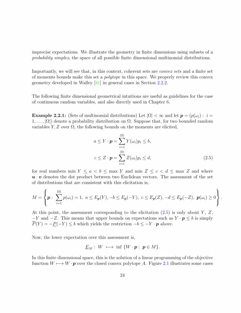
2.1 Cases for assessments of sets of distributions A of hyperplane boundariesa ≤ Y ·p ≤ b (in red) and c ≤ Z ·p ≤ d (orange). Top left: assessments aboutY do not intersect with those about Z such that A = AY ∩ AZ = ∅. TopRight: the assessment Y ·p ≤ b (top red line) is not used in constructing A,such that P (Y ) = b does not contribute to A, and is therefore an incoherentassessment. Bottom centre: a coherent assessment. . . . . . . . . . . . . . 25
3.1 Contour plots of the posterior density p((θ1, θ2, 1−θ1−θ2)|ν(α1, α2, 1−α1−α2)+(n1, n2, n3)) (Top) and the trinomial likelihood L((n1, n2, n3)|(θ1, θ2, 1−θ1−θ2)) (Bottom). Plots are in barycentric coordinates relative to the spaceof trinomial distributions Conv((0, 0, 1), (0, 1, 0), (1, 0, 0)) (left) and in log-odds space of all trinomial distributions (right). Posterior parameters areν = 2.0, (α1, α2) = (0.001, 0.998) and (n1, n2, n3) = (10, 0, 10). . . . . . . . 41
xiii
3.2 Contour plots of the posterior density p((θ1, θ2, 1−θ1−θ2)|ν(α1, α2, 1−α1−α2)+(n1, n2, n3)) (Top) and the trinomial likelihood L((n1, n2, n3)|(θ1, θ2, 1−θ1−θ2)) (Bottom). Plots are in barycentric coordinates relative to the spaceof trinomial distributions Conv((0, 0, 1), (0, 1, 0), (1, 0, 0)) (left) and in log-odds space of all trinomial distributions (right). Posterior parameters areν = 2.0, (α1, α2) = (0.001, 0.998) and (n1, n2, n3) = (10, 1, 10). . . . . . . . 42
3.3 A geometrical view of IDM update by translation. The larger simplex(dashed black) represents the set (3.3) of possible Dirichlet posteriors af-ter observing n observations with ν fixed apriori. The simplex of size ν(dashed blue) represents the natural parameters of the prior IDM set ofdistributions and the translation of this simplex by n = (n1, n2, n3) (solidblue) represents the natural parameters (3.2) of the posterior IDM set ofdistributions. . . . . . . . . . . . . . . . . . . . . . . . . . . . . . . . . . . 47
3.4 For ν = 2, each subplot is associated with updating with different obser-vation vectors totaling n = 6 observations. Left to right: (n1, n2, n3) =(1, 2, 3), (0, 3, 3), (0, 6, 0). The prior set of distributions with ν = 2 (dashedblue) is translated by (n1, n2) to obtain the posterior set of distributions ofDirichlet natural parameters (solid blue.) The possible posterior Dirichletnatural parameters is the scaled simplex (ν + n)N2 (dashed black.) . . . . 54
3.5 The ambient simplex (ν + n)N2 with (n1, n2, n3) = (0, n2, 0). The posteriorexpected log odds µ1 takes values +∞ and −∞ on the left and bottomedges, respectively, and does not have a continuous limit at the vertex ofthese two edges. . . . . . . . . . . . . . . . . . . . . . . . . . . . . . . . . 55
4.1 Four generating CDF’s, along with the lower and upper quantile functionsof this set at percentile p. The yellow and red CDF curves respectivelyrepresent the minimising and maximising CDF’s of the quantile function at p. 76
4.2 Graphical representation of the p-th symmetrical imprecise quantile intervalsgenerated by two distributions and its constituent imprecise quantiles. . . . 84
4.3 Sensitivity analysis from the example of Gelman et al. [41]. . . . . . . . . . 90
xiv
4.4 Left: Imprecise intervals, Q(α)(θ) := [Q(α)IDM(θ|ν,n), Q
(α)
IDM(θ|ν,n)] for various
values of ν. The imprecise expectations E(θ) := [EIDM(θ|ν,n), EIDM(θ|ν,n)]are also plotted. (Shorter lengths indicate lower ν values in 2,5,10,20,100).The left and right bounds of the precise Beta interval from Gelman et al.[41] are marked for the 2.5 and 97.5 percentiles. Right: Plot of the impre-
cise interval [Q(0.025)IDM ,Q
(0.975)
IDM ] and the precise Beta intervals [Q(0.025)Beta ,Q
(0.975)Beta ]
from Gelman et al. for different ν values. . . . . . . . . . . . . . . . . . . . 91
5.1 The difference function, α11 7−→ ψ′(να11 + n11 + n12) + ψ′(να11 + n11 +n21) − ψ′(να11 + n11), plotted over α11 ∈ [0, 1] for various datasets n =(n11, n12, n21, n22) that total to 10 and permute n1, n2, n3 over 1, 2, 5, andvarious ν values in 0.1, 0.5, 1, 2, 10. . . . . . . . . . . . . . . . . . . . . . 108
5.2 A visualisation of the parametrisation µ(t) = a(t)v0 + tv1 for two mean pa-rameters. The black curve is the set of points satisfying ψ−1(µ1)+ψ−1(µ2) =ν, the normalisation constraint of the natural parameters of the Dirichletdistribution. The red dashed lines are the asymptotes of the black curve.The cyan line is the hyperplane onto which µ(t) is projected bijectively. . . 111
5.3 Level curves of µi(t1, t2) = a(t1, t2)v0i+t1v1i+t2v2i over t1, t2 space for whenµ1, µ2 and µ3 being held constant (respectively, left, middle and right). . . 114
5.4 Contours of the objective function as a function of t1, t2 when n = 0. . . . 115
5.5 Various restrictions of the domain of optimisation with the objective func-tion’s contours being plotted only inside this domain. The left panel iswhen n1 = n2 = 0 such that only the points of the boundary satisfyingµ3(t) = ψ(n3) with n3 > 0 are finite, and the other two boundaries tend tothe infinities of the t1, t2 space. The middle panel is when n2 = 0 only andthe right panel is when n1, n2, n3 > 0. . . . . . . . . . . . . . . . . . . . . . 116
6.1 The linguist’s set of priors based on two constraints (blue hatched). Noticethat one of the constraints is redundant in defining the set. Notice also that(1, 0, 0), the prior assigning zero marginal probabilities to certain datasets,is included in the set of priors. . . . . . . . . . . . . . . . . . . . . . . . . . 124
6.2 Contour map of the posterior expectation as a function of the projected priordistribution (p2, p3) 7−→ E(θ|p = (1−p2−p3, p2, p3), n = (1, 9)). Note thatthe (1, 0, 0) is excluded from the polytope. Colours are normalised between0.1 (dark purple) to 0.25 (light yellow). . . . . . . . . . . . . . . . . . . . . 129
xv
6.3 Contour maps of the posterior expectation as a function of the projectedprior distribution (p2, p3) 7−→ E(θ|p = (1−p2−p3, p2, p3), n = (n1, n−n1))for various values of n1 and n. n is varied across the rows in 0, 4, 10, 20, 30and n1 computed as nθ where θ is varied across the columns in 0, 0.1, 0.25, 0.5.Colours are normalised between 0.1 (dark purple) to 0.25 (light yellow). . . 131
6.4 Contour map of the posterior expectation as a function of the projected priordistribution (p2, p3) 7−→ E(θ|p = (1− p2− p3, p2, p3), n = (1, 9)) with threeconstraints, one of which is redundant. Colours are normalised between 0.1(dark purple) to 0.25 (light yellow). . . . . . . . . . . . . . . . . . . . . . . 132
6.5 Contour map of the posterior expectation as a function of the projected priordistribution (p2, p3) 7−→ E(θ|p = (1 − p2 − p3, p2, p3), n = (0, 10)) with noconstraints on the prior set except that the prior (1, 0, 0) is excluded fromthe polytope. Colours are normalised between 0.1 (dark purple) to 0.25(light yellow). . . . . . . . . . . . . . . . . . . . . . . . . . . . . . . . . . . 134
7.1 A schematic of regular extension (RM(X|B), RM(X|B)) and vacuous exten-sion (V(X— B), V (X|B)) of X conditional on some event B. The valuesfor any lower and upper intermediate extensions jointly coherent with theunconditional model EM are hatched on the left and the right, respectively. 144
7.2 The optimisation domain of some posterior expectation as a function ofpriors over a Ω = ω1, ω2, ω3. The level curves of this function are drawnwith partial transparency. The right vertex (1, 0, 0) is excluded as the levelcurves meet there such that the function is not well-defined at that point.A sequence of planes (blue lines) converging to the singleton set (1, 0, 0)each with the same normal vector Y , a fixed random variable taking values(y1, y2, y3) over Ω. Each plane is of the form p : y1p1 + y2p2 + y3p3 = ciwith Y being its normal vector and where ci is a sequence of interceptsthat move the planes towards the limit as i→∞. The blue dots show onepossible path pi∞i=1 approaching (1, 0, 0) with each pi belonging to the i-thplane. . . . . . . . . . . . . . . . . . . . . . . . . . . . . . . . . . . . . . . 146
B.1 The digamma (left) and trigamma (right) functins over (0, 20]. . . . . . . . 171
xvi
Notation
a, (a1, . . . , am) – a vector in finite dimensional Euclidean space, Rm.
aC – for a vector a ∈ Rm, set of indices C ⊆ 1, . . . ,m, aC =∑
i∈C ai.
Ac – the complement of a set A
A – the (topological) closure of a set A
4m, 4m – the unit simplex (and its topological closure) in Rm.
L(Ω) – the linear space of bounded random variables from Ω to R
EP – an expectation operator with respect to a probability measure P .
E, EM – a lower expectation and a lower expectation with respect to a set of distributionsM , respectively.
P , PM – a lower probabilility and a lower probability with respect to a set of distributionsM , respectively.
ν – when used in the context of the imprecise Dirichlet model (IDM), ν is the apriorifixed concentration parameter of the prior set of Dirichlet distributions of the IDM,Dirichlet(να) : α ∈ 4p (for a fixed, finite p number of categories).
xvii
Chapter 1
Elicitation as a statistical motivationfor imprecise models
Throughout this thesis, we distinguish between the following.
• By a precise model, we refer to the usual Bayesian set up with a single prior anda single likelihood producing a single posterior distribution. Note that hierarchicaland mixture models with a single hyper-distribution at the top of the hierarchy areprecise.
• By an imprecise model, we mean a statistical model consisting of a set of Bayesianprior distributions and a single likelihood model that are used to obtain a corre-sponding set of posterior distributions, one for each prior.
A major theme in this thesis is that imprecise models can be a natural and intuitivestatistical tool due to the fact that (prior) elicitation does not always result in a singledistribution, but rather a collection that cannot be further whittled down with the infor-mation at hand.
1
1.1 A set of models as a more representative elicita-
tion
We illustrate the need for such models with the following examples.
Example 1.1.1: (Elicitation of a finite number of moments) During elicitation, typicallyonly a finite number of moments can be elicited from an expert (O’Hagan [62]). However,specifying these may not identify a single distribution. For example, Lindsay and Basak[54] observes that matching the first 2p moments of a distribution F to a standard nor-mal distribution results in large values of deviations |F (x) − Φ(x)| in the non-tail regionwhere |x| is small. For example, they report that when F is matched to the first 2p = 60moments, |F (0) − Φ(0)| ≤ 0.2233 meaning that moment matching does not guarantee atight fit between F and Φ at x = 0. Thus, a finite number of elicited moments cannot beguaranteed to specify a single distribution, and the elicited information would result in aset of distributions instead in these cases.
Example 1.1.2: (Elicitation of population parameters in an interval) Typically, mostparameters cannot be elicited to an arbitrary degree of precision. This may be due to thefollowing reasons.
• Limits of communication: The ability of the expert to articulate and communicate tothe statistician as well as the ability of the statistician to comprehend and ‘recover’the original meaning of the information communicated typically determine how ac-curate the expert information is translated into statistical quantities. This problemis explored in more detail in O’Hagan et al [63].
• Limits of the expert knowledge: communication issues aside, the expert may only beable to specify a statistical quantity up to an interval precision.
Due to the finite precision of the elicited parameters, multiple candidate distributions maybe identified as a result.
Example 1.1.3: (Combining experts’ opinion in isolation) It is sometimes desirable tosynthesise a single prior model from the opinions of two or more experts. Garthwaite,
2
Kadane and O’Hagan [39] provide a comprehensive account of eliciting a single prior prob-ability distribution in this case. We outline two considerations that present obstacles onthe path towards eliciting a single prior distribution.
Pooling methods: When individual priors are elicited from experts in isolation, two so-called opinion pools may be formed. The linear opinion pool is a convex mixture of theindividual elicited prior distributions and the logarithmic opinion pool is their weightedgeometric mean with weights summing to unity. Which pooling method should be used?Garthwaite, Kadane and O’Hagan, for example, states that the linear pooling satisfies aconsistency in marginalisation whereas the logarithmic pooling satisfies the Bayesian ex-ternality criteria, meaning that the pooling of the posterior distributions should coincidewith the posterior distribution computed from pooling the priors (Madansky [55]). Thepoint is that both properties are considered statistically desirable, and yet each of thesetwo common pooling methods satisfy only one of them [39]. It is not straightforward tochoose which pooling method to use unless one has further prior information.
Weights determination: With a choice of the pooling method, the weights to each expertneed to be assigned values. Two considerations come to mind: what definition or meaningdo the weights have, and how can one verify that the resulting criteria are satisfied?
Let us illustrate these issues with an example of such weight assignments. Garthwaite,Kadane and O’Hagan [39] remark that some experts may be less informed than others andthe prior should reflect the difference in credibilities. For example, O’Hagan [62] notes thatCooke [22] proposed to assign weights to each single prior distribution commensurate toeach expert’s credibility. This results in a prior that is a single mixture or convex com-bination of the priors with the weights being a hyper-prior distributions on the elicitedprior distributions. The weights themselves are determined by having each expert answerrelevant questions about the field, the answers to which the statistician knows but theexpert does not. In this way, the expert’s credibility is checked against a benchmark.
One major issue of this methodology is that the quality of the benchmark is dependenton the statistician’s competency with the expert domain. The statistician may err on theside of caution and use more elementary questions that can be easily verified by the statis-tician. The questions may be so simple that all the experts will pass the benchmark, suchthat it does not have much power to discriminate the experts’ competencies. On the otherhand, using more ambitious questions may result in the statistician’s inability to verify the
3
answers, thus invalidating the benchmark itself.
At the other extreme, the ideal benchmark will allow the statistician to exactly computeweights which are commensurate to the benchmark scoring and thus identify a single setof weights. It is likely that reality falls in between, resulting in a non-singleton subset ofweights that are candidates to reflecting the experts’ competencies.
Example 1.1.4: (Combining experts’ opinion in group) A second case of combining ex-perts’ opinions is when a prior is elicited when the experts act as a group, as opposed tocombining the priors elicited from each individual expert. Here, the experts are to reach,as a group that can directly interact with one another, a consensus to the questions posedduring elicitation. This is a behavioural aggregation method of group elicitation [39]. Thismethod naturally introduces biases due to the psychological effects of working in a group(such as the possibility of dominating personalities affecting and suppressing the views ofothers or that a final consensus is not possible for other reasons [39]). To partially mitigatethese effects, Garthwaite, Kadane and O’Hagan [39] considered also the Delphi methodwhereby each expert’s beliefs are separately elicited, aggregated and then shared to allother experts in individual isolation, and these steps are iterated.
Garthwaite, Kadane and O’Hagan [39] also propose two rational ways of reaching a con-sensus. The first is through a majority voting of ranking of all alternatives (such as thestochastic preference of indicator variables when eliciting probabilities). This is possibleonly in the most trivial of cases: Arrow’s theorem (Arrow [5]) implies that no single set ofsuch preferences can represent a group consensus (that satisfies some conditions for goodmathematical behaviour) when there are at least three alternatives to be considered withnon-dictatorial rational agents.
The second way discussed by Garthwaite, Kadane and O’Hagan [39] is to consider a singleBayes’ model representing the group belief that satisfies a so-called (weak) Pareto prin-ciple: that is, this group prior preserves all stochastic preferences agreed upon by theindividuals of the group. In only a few cases does a prior distribution representing sucha set of preferences exist (Garthwaite, Kadane and O’Hagan cite Seidenfeld, Kadane andSchervish [72] and Goodman [42] for such existence conditions).
4
In conclusion, as Garthwaite, Kadane and O’Hagan [39] have observed: group dynamicsprevent a definitive assertion and measurement of consensus. Without consensus, it isunclear what information from an interacting group of experts a single prior distributionactually represents. A set of prior distributions is a more natural representation in thissituation.
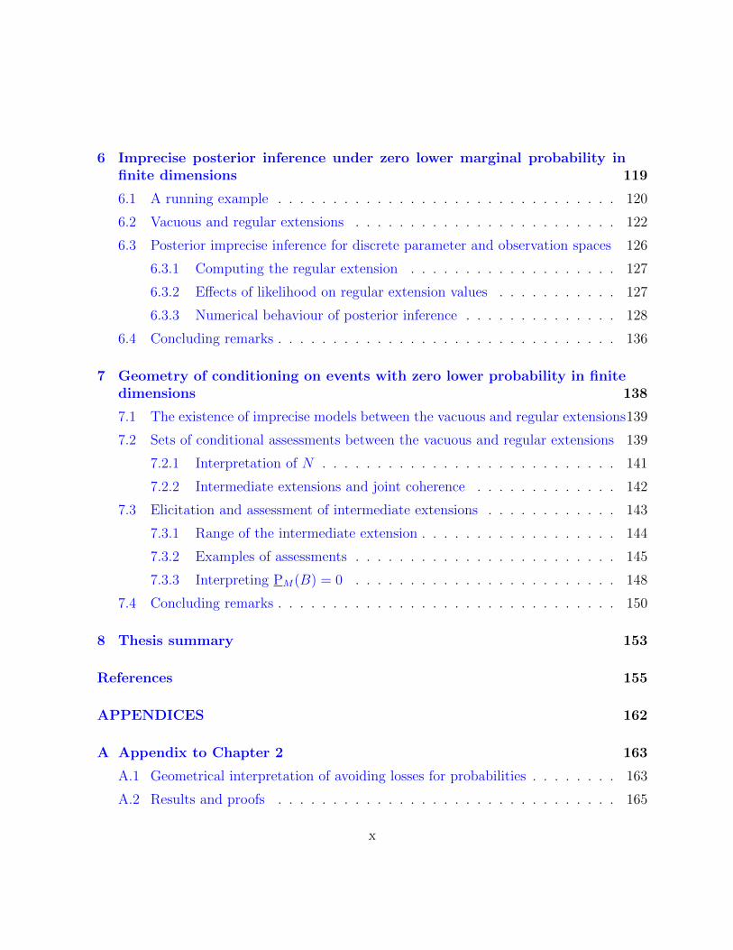
Example 1.1.5: (Bounds on quantiles specify a set of distribution from a Beta family)Quantiles are sometimes considered psychologically easier to elicit from an expert as theyare easier to comprehend than moments (O’Hagan [62]). However, we encounter the sameproblem as before, where a finite number of quantiles may only identify a set of distribu-tions.
Suppose that it has been elicited that a candidate prior for a Bernoulli probability θ shouldbe in the beta family of distributions,
Ba,b(p) =
∫ p
0
Γ(a)Γ(b)
Γ(a+ b)tα−1(1− t)b−1dt : a, b > 0
.
We are interested in the situation when lower and upper bounds of the 25-th and 75-thquantiles have also been elicited. The α-th quantile of a random variable θ following abeta distribution with parameters a, b is given by,
inf t : Ba,b(t) ≥ α.
In the left panel of Figure 1.1, the level curves of the 25-th and 75-th quantiles,
a, b 7−→ inf t : Ba,b(t) ≥ α,
for α = 0.25 and α = 0.75 are respectively plotted in red and blue over the set ofR+ × R+ 3 (a, b).
Now suppose that the elicited bounds are,
0.2 ≤ inf t : Ba,b(t) ≥ 0.25 ≤ 0.3,
and,0.7 ≤ inf t : Ba,b(t) ≥ 0.75 ≤ 0.8.
5
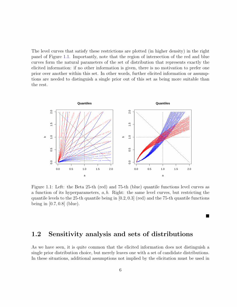
The level curves that satisfy these restrictions are plotted (in higher density) in the rightpanel of Figure 1.1. Importantly, note that the region of intersection of the red and bluecurves form the natural parameters of the set of distribution that represents exactly theelicited information: if no other information is given, there is no motivation to prefer oneprior over another within this set. In other words, further elicited information or assump-tions are needed to distinguish a single prior out of this set as being more suitable thanthe rest.
0.0 0.5 1.0 1.5 2.0
0.0
0.5
1.0
1.5
2.0
Quantiles
a
b
0.0 0.5 1.0 1.5 2.0
0.0
0.5
1.0
1.5
2.0
Quantiles
a
b
Figure 1.1: Left: the Beta 25-th (red) and 75-th (blue) quantile functions level curves asa function of its hyperparameters, a, b. Right: the same level curves, but restricting thequantile levels to the 25-th quantile being in [0.2, 0.3] (red) and the 75-th quantile functionsbeing in [0.7, 0.8] (blue).
1.2 Sensitivity analysis and sets of distributions
As we have seen, it is quite common that the elicited information does not distinguish asingle prior distribution choice, but merely leaves one with a set of candidate distributions.In these situations, additional assumptions not implied by the elicitation must be used in
6

order to pick out a single distribution. If one does choose a single prior out of this set andcomputes the posterior inference with it, then a sensitivity analysis is typically prescribedto check if the posterior inference is sensitive to the additional assumptions made to makethis choice. See section 4.7 of Berger [11] for an extensive review of this topic.
A complete sensitivity analysis seeks to understand how inference using the posterior dis-tribution,
P (θ ∈ ·|x) =
∫· L(x|θ)P (dθ)∫ΘL(x|θ)P (dθ)
,
can change when the components L, the likelihood model, P (·), the prior model and x,the observed data change. For example, the frameworks of Zhu and Ibrahim [88] andClarke and Gustafson [21] measure changes of posterior quantities on the left with respectto changes in all three components. However, a sensitivity analysis more commonly refersto the sensitivity towards the prior specification (for example, Berger [10], Gustafson [43],McCulloch [60], Ruggeri and Sivaganesan [68]). In this thesis, we follow the second ap-proach and make the prior model the main focus out of the three components.
1.2.1 Global sensitivity analysis: Prior sensitivity analysis can be categorised as globaland local sensitivity analyses, and this distinction will become relevant to motivating theimprecise methodology from a statistical perspective. ‘Global’ is meant in the sense thatthe change of posterior inference is taken over the entire prior model space. For example,if P denotes all the candidate models from which a single prior model on Θ 3 θ is to bechosen, Ruggeri and Sivaganesan [68] cite that the range (of the posterior expectation of astatistic T (θ)),
supP∈P
EP (T (θ)|x)− infP∈P
EP (T (θ)|x),
(where,
EP (T (θ)|x) =
∫T (θ)L(x|θ)P (dθ)∫L(x|θ)P (dθ)
,
for a fixed set of observations x), is a popular metric for sensitivity across all candidatemodels, whose properties are detailed by, for example, in the overview by Berger et al. [9].Importantly, for a fixed statistic of interest, the larger the range, the greater the variationof the posterior expectation over the prior model space. Importantly, this is not to beconfused with the variation due to the randomness inside of a single prior as measured,for example, by the posterior variance of T (although Ruggeri and Sivaganesan [68] makea case to scale the range with a variance to obtain a more comprehensive picture of the
7
variations due to both of these factors).
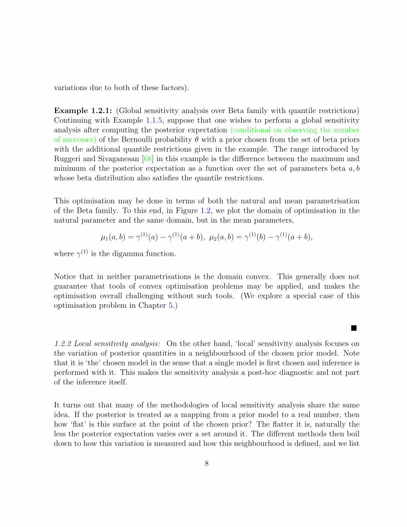
Example 1.2.1: (Global sensitivity analysis over Beta family with quantile restrictions)Continuing with Example 1.1.5, suppose that one wishes to perform a global sensitivityanalysis after computing the posterior expectation (conditional on observing the numberof successes) of the Bernoulli probability θ with a prior chosen from the set of beta priorswith the additional quantile restrictions given in the example. The range introduced byRuggeri and Sivaganesan [68] in this example is the difference between the maximum andminimum of the posterior expectation as a function over the set of parameters beta a, bwhose beta distribution also satisfies the quantile restrictions.
This optimisation may be done in terms of both the natural and mean parametrisationof the Beta family. To this end, in Figure 1.2, we plot the domain of optimisation in thenatural parameter and the same domain, but in the mean parameters,
µ1(a, b) = γ(1)(a)− γ(1)(a+ b), µ2(a, b) = γ(1)(b)− γ(1)(a+ b),
where γ(1) is the digamma function.
Notice that in neither parametrisations is the domain convex. This generally does notguarantee that tools of convex optimisation problems may be applied, and makes theoptimisation overall challenging without such tools. (We explore a special case of thisoptimisation problem in Chapter 5.)
1.2.2 Local sensitivity analysis: On the other hand, ‘local’ sensitivity analysis focuses onthe variation of posterior quantities in a neighbourhood of the chosen prior model. Notethat it is ‘the’ chosen model in the sense that a single model is first chosen and inference isperformed with it. This makes the sensitivity analysis a post-hoc diagnostic and not partof the inference itself.
It turns out that many of the methodologies of local sensitivity analysis share the sameidea. If the posterior is treated as a mapping from a prior model to a real number, thenhow ‘flat’ is this surface at the point of the chosen prior? The flatter it is, naturally theless the posterior expectation varies over a set around it. The different methods then boildown to how this variation is measured and how this neighbourhood is defined, and we list
8
0.0 0.5 1.0 1.5 2.0
0.0
0.5
1.0
1.5
2.0
Quantiles
a
b
−2.0 −1.5 −1.0 −0.5
−2.
0−
1.5
−1.
0−
0.5
Quantiles: mean parameters
m1
m2
Figure 1.2: Left: the Beta 25-th (red) and 75-th (blue) quantile functions level curves as afunction of its natural parameters, a, b restricted to the quantile levels to the 25-th quantilebeing in [0.2, 0.3] (red) and the 75-th quantile functions being in [0.7, 0.8] (blue). Right:same level curves over mean parametrisation.
9
a sample of such methods. McCulloch [60] measures sensitivity using the Kullback-Leiblerdivergences: if the second derivative of the divergence around the chosen prior model is lowbut the divergence around the resulting posterior model is high, then it means that smallchanges of prior is associated with large changes in the posterior. Diaconis and Freedman[35] and Ruggeri and Wasserman [69] define a Frechet derivative of the posterior expecta-tion of statistic as a function of the prior model and use the magnitude of the derivativeoperator evaluated at the chosen prior model as a measure of how sensitive the changeof the posterior expectation is to the prior model. Methods such as those due to Kurtekand Bharath [51] Zhu and Ibrahim [88] formulate similar calculations in a more explicitlygeometrical manner that leads to using the differential manifold structure to define theneighbourhood. Lastly, methods such as those due to Marriott and Maroufy [57] use theconcept of local mixing (for example Marriott [59]) to construct a neighbourhood that isconvex and linear, leading to more tractable computations.
1.2.3 Global or local?: We conclude this review of sensitivity analysis by contrasting globaland local analyses. If computationally tractable, a global analysis would by definition yieldmore information about sensitivity than local. However, one might prefer the local analysesover the global exactly because the latter is computationally too expensive or intractable.In particular, one may be only interested in certain types of perturbations (for example anε contamination neighborhood over a collection of distributions (for example, see Bergeret al. [12]). Finally, a local sensitivity implies global sensitivity, such that one might wishto check the former as a sufficient condition when it is straightforward to test first.
1.3 Imprecise methodology and sets of distributions
The imprecise methodology we study in this thesis is closely related to the global sensitiv-ity analysis. We will use our previous discussion about the latter to introduce the formerin the statistical context.
As we will see in the later chapters, the models in the imprecise methodology which we willbe exploring can be largely represented by a set of models, say M . Similar to the sensitivityanalysis methodology, we will be working with a set of priors that each produces a posteriordistribution, and we will be computing ranges of such sets of posterior expectations, as
10
well as the end points of the resulting intervals of the form[infP∈M
EP (T (θ)|x), supP∈M
EP (T (θ)|x)
].
In this methodology, the length of this interval is called imprecision.
1.3.1 Sensitivity analysis versus imprecise methodology: If the imprecise methodology isso similar to that of the global sensitivity analysis, why do we consider the former?
Firstly, the interpretations of the set of distributions in the imprecise setting and the globalsensitivity analysis setting are different. In the former, the set of priors is the object beingassessed as a model. For example, one might form a set of such prior distributions bytranslating elicited information into restrictions over a space of distributions.
Example 1.3.1: Consider Θ = θ1, θ2, θ3 to be the space of possible likelihood parametersin consideration. A prior on this space is specified by P (θi) = pi, for the triplet p =(p1, p2, p3) ∈ 43 in the unit simplex of R3. Let T (θ) be a statistic over the model space.One might elicit from an expert bounds on the expectation of a finite number of randomvariables f1(T ), . . . , fp(T ), each in the form of,
fi(T (θ1))p1 + fi(T (θ2))p2 + fi(T (θ3))p3 ≤ ci,
where ci is the elicited upper bound of the expectation of fi under p. In other words, theelicited information about the prior model is that the prior should satisfy,
Fp ≤ c,
where F = [fi(T (θj))] is a p × 3 matrix and c = [ci]T is a p × 1 vector of real numbers.
When feasible, this system represents a convex polytope in 43. That is to say, the distri-butions in this set of priors are all consistent with the elicited information, and no singleone is preferred over another in this set. Thus, at this apriori stage, this entire set shouldbe considered ‘a prior model’, as opposed to a single prior in this set. In the imprecisemethodology, the entire set is to be used in posterior inference and in the subsequent chap-ters of this thesis we will review how this is done in a coherent manner in the same waythat Bayesian probabilities are coherent (see Lindley [53], Jeffrey [49] or Definition 2.1.2,for example, for a definition of coherence for Bayesian probabilities).
11
In contrast, the set in a sensitivity analysis is not elicited in the same sense as the priordistribution of which it is a neighborhood. Rather, it is a post hoc construction specificallyfor testing the robustness of the inference, and is not part of the inference itself.
This leads to different interpretations between imprecision and range, even as they measurethe same quantity over the respective sets of distributions. However, because the set ispart of the model in the imprecise methodology, it is not to be interpreted as a measure ofrobustness in the usual sense of the range. Rather, the imprecision is to be taken directlyas one of the posterior statistics to be reported as part of the inference, at the same levelas say posterior means, quantiles and variances. In fact, we draw the following analogy:just as in Bayesian inference where the posterior distribution is considered to embody theinference itself (with a sensitivity analysis being post-hoc and considered separate), the setof posterior distributions resulting from the elicited set of prior distributions is also to beconsidered to embody the inference and not to be treated as a diagnostic tool.
One issue of working with a set of distributions as a model is that Bayesian inferencetypically works with coherent probabilities: the coherence of a set of probabilities is typ-ically not defined in common settings. (See Chapter 2.) Another reason why sensitivityanalysis is considered post-hoc and not part of the inference is that the sensitivity analysismethodology does not have a set of rules that defines it to be coherent, unlike (Bayesian)probabilities (again see Definition 2.1.2). This fact highlights a difference between a (global)sensitivity analysis and an imprecise methodology: there is a definition for coherence of aset of models in the latter, which is why it can be readily claimed to produce principledand coherent inference directly using a set of models as opposed to just one.
Example 1.3.2: We will see that a form of the generalised Bayes’ rule (GBR) (seeTheorem 2.2.4) in the imprecise methodology provides a coherent manner of constructingposterior inference from a set of prior distributions. To continue with our earlier example,if we let θ 7−→ L(x|θ) to be a fixed likelihood model, then a typical way to obtain animprecise posterior inference is to form a set of posterior expectations,
M|x =
U 7−→
∑3i=1 U(θi)L(x|θi)pi∑3
i=1 L(x|θi)pi: p ∈ 43 ∧ Fp ≤ c,
3∑i=1
L(x|θi)pi > 0
,
(where x is some observation from the likelihood model). A typical inference that might
12
be reported about T (θ) is,[inf
P∈M|xEP (T (θ)|x), sup
P∈M|xEP (T (θ)|x)
].
The real numbers in this interval are then interpreted as values which are consistent withthe data, the likelihood and the set of priors that generated the posterior inference.
Thus, we have another motivation to consider the imprecise methodology. Coherence al-lows for logical consistency when working with Bayesian probabilities (Lindley [53]), but itneeds to be defined for a set of prior distributions. Without such an extension, a Bayesianhas to perform inference with a single prior and essentially work with a candidate setthrough the external and post-hoc methodology of sensitivity analysis. From our earlierdiscussion, we have concluded that sometimes a single prior distribution might not be de-ducible from the elicited information alone. In this light, the imprecise methodology allowsone to work with a set of prior models apriori while maintaining coherence.
13
Chapter 2
Review of aspects of imprecisemodels
In this chapter, we critically review Walley’s [81] theory of imprecise probabilities, the the-ory upon which this thesis is based. In addition to being a literature review, we will alsoprovide our own pedagogical examples to illustrate the concepts in the theory for a statis-tical audience.
Throughout this thesis, we use imprecise probability as a tool to construct posterior infer-ence. By considering imprecision as part of the model as opposed to a separate indicatorof reliability of the model, posterior inference from imprecise models does not force thechoice of a single prior. This yields a model for statistical inference that is capable ofsimultaneously taking multiple prior models into consideration.
As we have alluded in Section 1.3, imprecise expectations, which are a procedure of takingthe minimum and maximum of expectations over a set of distributions, is methodologi-cally different from a sensitivity analysis over a set of distributions. Sensitivity analysisdoes not prescribe principled approaches to either picking a single distribution from a setof candidates or working with the whole set. Walley’s theory of imprecise probabilities,the theory behind imprecise expectations, in addition to its mathematical component, alsoprescribes how to construct reasonable models, in the form of the concepts of avoiding surelosses and coherence.
14
2.1 Avoiding sure losses and coherence
Let us first give a definition of assessment to pin down our usage of this term throughoutthis thesis.
Definition 2.1.1: An assessment is an assignment of (imprecise or precise) expectationvalues to a set of random variables.
Example 2.1.1: For sets A and B, there are at least two ways to provide an assessmentof the probability P (A ∪ B). One is use the inclusion-exclusion principle P (A) + P (B)−P (A∩B) if one already has these probabilities at hand. Another is to consider C = A∪Bdirectly: this can be done, for example, by eliciting information about P (C) from an ex-pert. (Notice that the expert need not know that C is in fact the union of A and B.)
Importantly, this example distinguishes an assessment which is derived from (and thereforeobeys) the laws of probability from one whose value may not do so. The latter maypotentially contradict other existing assessments of probabilities.
The two main principles driving the axioms of imprecise probabilities are avoiding surelosses (assessments of probabilities that incur such losses are called Dutch books) and co-herence. Importantly, sensitivity analysis does not implement these concepts, causing it todiverge from the methodology of imprecise probability models. We review how coherenceand avoiding losses are implemented in the imprecise probability theory, which will be theworkhorse of this thesis.
We begin with the following definition from Lindley [53].
Definition 2.1.2: (Section 5.4 of Lindley [53]) For a sample space Ω with subsets A,B ⊂Ω, an assessment P (·), P (·|·) over the subsets of this space is coherent iff it satisfies,
P (A), P (B) ∈ [0, 1],
P (Ω) = 1,
P (A ∪B) = P (A) + P (B), when A and B are disjoint,
P (A ∩B) = P (A)P (B|A).
15
Authors of foundational probability theory such as de Finetti [32], Savage [70], and Lind-ley [52], [53] have motivated this definition by a so-called subjective Bayesian viewpoint(Walley [81]). It provides qualitative requirements for consistency of the assessments viaa gambling analogy. A linear utility is established to measure a gambler’s gain or loss. Agambler engages in a gamble whose random reward is the realisation of a random variable.Elicitation and assessment of probabilities of events and expectations of random variablesare treated as assigning prices to such gambles which are acceptable for the gambler givencertain knowledge about the realisation of the generating process. In principle, the gamblershould not accept prices that lead to a systematic losses and prices should be internallyconsistent. Avoiding sure losses and coherence necessarily avoid two main types of suchinconsistencies in probability assessments.
2.1.1 Probability distribution and expectation
It is more useful to frame these inconsistencies in terms of expectations. In this context,let us understand first what avoiding sure losses precisely entails. First, we follow Walley[81] and make the following assumption.
Definition 2.1.3: For a sample space Ω, let L(Ω) be the linear space of bounded randomvariables over Ω. (The space is linear because finite sums of bounded random variables isagain a bounded random variable.)
Condition 2.1.1: Unless stated otherwise, all random variables are bounded and in L(Ω)1.
1This is in accordance with Walley [81] whom we follow closely. For discussions of imprecision involvingunbounded random variables, see Sections 3.3.1 in this thesis. For an in-depth treatment of extensions toextended-real-valued random variables of the theory of imprecise probabilities, see Troffaes and de Cooman[78].
16
The following is a special case of the more general definition stated in Walley [81], givenin Definition 2.1.7.
Definition 2.1.4: Given a sample space Ω, an assessment of expectation EP incurs surelosses (or is a Dutch book) iff it is an assessment over a set of random variables F ⊆ L(Ω),EP : F 7−→ R, such that there exists random variables X1, . . . , Xn ∈ F such that:
∀ω ∈ Ω :n∑i=1
(Xi(ω)− EP (Xi)) < 0. (2.1)
An assessment that does not incur sure losses is said to avoid sure losses.
An expectation that avoids sure losses ensures that we do not have any finite combinationof zero-expectation random variables being pointwise negative. Otherwise, it contradictsthe principle that such a sum should itself have a zero expectation. Expectations of asingle probability distribution typically avoid sure losses.
Lemma 2.1.1: (Lemma A.2.1) For any sample space Ω, and P a distribution over someσ-field of Ω, any expectation EP over all bounded random variables avoids sure losses. Inother words, for any X1, . . . , Xn that are bounded,
supω
n∑i=1
(Xi(ω)− EP (Xi)) ≥ 0.
Despite being seemingly trivial in the probabilistic setting, we will see in Example 2.1.2that avoiding sure losses is not at all trivial when attempting to ensure lack of losses overmultiple distributions, and we have seen from Chapter 1 that the latter could occur com-monly in statistical practice.
A less severe inconsistency amongst assessments is incoherence. The following is a specialcase of Definition 2.1.8, which represents a more general definition by Walley [81].
Definition 2.1.5: Given a sample space Ω, an assessment of expectation EP is incoherentif it is an assessment over a set of random variables F ⊆ L(Ω), EP : F 7−→ R, such that
17
there exists random variables X0, X1, . . . , Xn ∈ F and m ∈ N such that:
∀ω ∈ Ω :n∑i=1
(Xi(ω)− EP (Xi)) < m(X0(ω)− EP (X0)). (2.2)
An assessment that is not incoherent is coherent.
Let us qualitatively unwrap this definition. The random variables∑
i(Xi − EP (Xi)) andX0−EP (X0) both have an expectation of zero. What (2.2) means is that a sum of randomvariables with a zero expectations is strictly less than any other positively scaling of anyother random variable with a zero expectation, implying in contradiction that one of thesides does not have a zero expectation.
Importantly, this is less severe than avoiding sure losses as the assessments for the expecta-tion of a random variable can still be bounded between the latter’s infimum and supremum,so they are individually consistent with each other. Indeed, if the assessment EP (X0) isincoherent with the rest in (2.2), it is intuitively clear that EP (X0) can be corrected byincreasing it so as to bring the right side of the inequality closer to the left2.
Again, expectations of random variables from a single distribution are coherent.
Lemma 2.1.2: (Lemma A.2.2) For any sample space Ω, and P a distribution over Ω oversome σ-field of Ω, any expectation EP over all bounded random variables are coherent. Inother words, for any X0, X1, . . . , Xn that are bounded and m ∈ N,
supω
n∑i=1
((Xi(ω)− EP (Xi))−m(X0(ω)− EP (X0)) ≥ 0.
Like avoiding sure losses, we will see in Section 2.1.2 that coherence is not trivial whenconsidering multiple distributions simultaneously.
2The minimum value to which to increase the assessment is called a natural extension of EP (Z) (relativeto the rest of the assessments).
18
2.1.2 Sets of probability distributions and expectations
Despite the fact that probability assessments following Definition 2.1.2 avoids sure lossesand are coherent, such losses and incoherence may be unnoticeably present in practice whenconsidering sets of distributions. Throughout this thesis, we follow Walley [81] and focuson the lower and upper (or imprecise) expectations as a summary over a set of distributions.
Condition 2.1.2: Whenever given a set of distributions M over which we compute theexpectation of a random variable X ∈ L(Ω), we assume that it is measurable against anexisting σ-field shared by all distributions in M : we will simply say that X is suitablymeasurable in this case.
Definition 2.1.6: Let M be a set of distributions over some sample space Ω with asuitably chosen σ-field. Define the lower and upper expectations3 and similarly of a suitablymeasurable random variable X ∈ L(Ω), as,
EM(X) = inf EP (X) : P ∈M ,
andEM(X) = sup EP (X) : P ∈M ,
respectively. We will loosely refer to one or the pair of lower and upper expectations asimprecise expectations.
Notice that, EM(X) = −EM(−X) such that one can compute the upper expectation giventhe lower expectation4. As a result, where appropriate, we focus our analyses on the lowerexpectation.
Definition 2.1.7: (Walley [81], 2.4.1) Given a sample space Ω, an assessment of lowerexpectation EM from a set of probability distributions M incurs sure losses (or is a Dutch
3For reason of clarity, we forgo the typical use of E and E as natural extensions of lower and upperprevisions in the imprecise probabilities literature.
4EM and EM are said to be a conjugate pair of lower and upper previsions (Walley [81]).
19
book) iff it is an assessment over a set of random variables F ⊆ L(Ω), EM : F 7−→ R suchthat there exists random variables X1, . . . , Xn ∈ F such that:
∀ω ∈ Ω :n∑i=1
(Xi(ω)− EM(Xi)) < 0. (2.3)
An assessment that does not incur sure losses is said to avoid sure losses.
Definition 2.1.8: (Walley [81], 2.5.1) Given a sample space Ω, an assessment of lowerexpectation EM from a set of probability distributions M is incoherent if it is an assessmentover a set of random variables F ⊆ L(Ω), EM : F 7−→ R such that there exists randomvariables X0, X1, . . . , Xn ∈ F and m ∈ N such that:
∀ω ∈ Ω :n∑i=1
(Xi(ω)− EM(Xi)) < m(X0(ω)− EM(X0)). (2.4)
An assessment that is not incoherent is coherent.
We note here that these definitions are not new, even at the time Walley [81] was written.Indeed, Walley noted that these definitions were previously investigated by Huber [48],Smith [74] and Williams [86] [85]. For later chapters, we also define imprecise probabiltiesover a set of distribution.
Definition 2.1.9: For a set of distributions M , define the lower and upper probabilities ofa suitably measurable event A to be,
PM(A) := EM(IA), PM(A) := EM(IA) ,
where IA is the indicator function of the event A. We say that P and P are coherent iff Eand E are respectively coherent.
20
We illustrate sure losses by considering the following case involving two random variables,whose individual assessments on their expectations avoids sure losses but a sure loss canbe generated when they are considered jointly.
Example 2.1.2: Let the sample space consist of three categories, and
X1 = (−2, 0,−1), X2 = (0, 1, 2), Y1 = (−1, 0, 1), Y2 = (0, 1, 0),
be random variables on this sample space. Consider an assessment about these randomvariables by combining the elicitations from two different experts. The first expert hasmarginal information about X1 and X2 in the form of lower bounds for their expectationsthat reflect the elicited information. That is, a probability distribution P of this systemshould generate expectations EP satisfying,
EP (X1) ≥ −0.05, EP (X2) ≥ 1.75 .
The second expert has information about Y1 and Y2 in the form of upper and lower boundsfor their respective expectations, such that,
EP (Y1) ≤ 0, EP (Y2) ≥ 0.9 .
Consider that,
supω∈ω1,ω2,ω3
(X1(ω) +X2(ω)− Y1(ω) + Y2(ω))− (−0.05 + 1.75− 0 + 0.9) = 2− 2.6 = −0.6.
Why is this problematic? Write M to represent a subset of probability distributions overΩ that satisfies the elicited bounds, and,
EM(X1) = −0.05, EM(X2) = 1.75, EM(Y1) = 0, EM(Y2) = 0.9,
to represent the bounds. Then,
supω∈ω1,...,ω3
(X1(ω) +X2(ω)− Y1(ω) + Y2(ω))
< EM(X1) + EM(X2)− EM(Y1) + EM(Y2)
= infP∈M
EP (X1)+ infP∈M
EP (X2) − supP∈M
EP (Y1)+ infP∈M
EP (Y2)
= infP∈M
EP (X1)+ infP∈M
EP (X2)+ infP∈M
EP (−Y1)+ infP∈M
EP (Y2)
≤ infP∈M
EP (X1 +X2 − Y1 + Y2).
21

In other words, any expectation due to any probability distribution adhering to the assessedbounds results in the expectation of X1 + X2 − Y1 + Y2 being strictly greater than themaximum of this random variable, leading to a contradiction.
Let us provide an example where sure losses are avoided by a set of distributions (throughtheir expectations), but they are incoherent.
Example 2.1.3: Consider X = (−1/8, 1/4), Y = (2,−1) and Z = (3,−1/2), a distribu-tion P with the assessments,
EP (X) ≥ 0, EP (Y ) ≥ 0, EP (Z) ≥ 0 .
We write the set of distributions satisfying these constraints as,
M = p ∈ [0, 1] : Ep(X) ≥ 0 ∧ Ep(Y ) ≥ 0 ∧ Ep(Z) ≥ 0,
and the lower expectations,
EM(X) = 0, EM(Y ) = 0, EM(Z) = 0.
To simplify the algebra, we consider EP to be restricted to the domain F = X, Y, Z:this is shown to avoid sure losses over F in Proposition A.2.1. (For assessments over largersets of random variables, linear programming is typically used to check avoidance of surelosses. See Quaeghebeur [66] and Walley, Pelessoni and Vicig [82].)
However, consider the random variable (X − EM(X)) + (Y − EM(Y ))− (Z − EM(Z)) inthe criterion (2.4). By evaluating this point-wise over Ω,
ω = ω1 : −1
8+ 2− 3 < 0,
and
ω = ω2 :1
4− 1 +
1
2< 0,
such that this satisfies (2.4) so EP is incoherent.
22
Consider again the set of distributions that satisfy the assessed constraints:
M = p ∈ [0, 1] : Ep(X) ≥ 0 ∧ Ep(Y ) ≥ 0 ∧ Ep(Z) ≥ 0= p ∈ [0, 1] : −p/8 + (1− p)/4 ≥ 0 ∧ 2p− (1− p) ≥ 0 ∧ 3p− (1− p)/2 ≥ 0= p ∈ [0, 1] : 2/3 ≥ p ∧ p ≥ 1/3 ∧ p ≥ 1/7= p ∈ [0, 1] : 2/3 ≥ p ∧ p ≥ 1/3= p ∈ [0, 1] : 2/3 ≥ p ≥ 1/3.
Notice that the constraint Ep(Z) ≥ 0 is subsumed into Ep(Y ) ≥ 0. Incoherence, in thiscase, has to do with inconsistencies due to the assessment for Z: the lower bound of Ep(Z),under the constraints Ep(X) = 0 and Ep(Y ) = 0, is not zero. Indeed, if we consider Ep(Z),
Ep(Z) = −1
2+
7
2p.
Because the constraints Ep(X) ≥ 0 and Ep(Y ) ≥ 0 is equivalent to 2/3 ≥ p ≥ 1/3, thelower bound of Ep(Z) over this set of distributions is in fact,
−1
2+
7
2
1
3= −3
6+
7
6=
2
3> 0,
such that the original assessment Ep(Z) ≥ 0 is too loose and, therefore, redundant in lightof Ep(X), Ep(Y ) ≥ 0.
In Example 2.1.3, by removing redundant constraints on M , we have corrected the boundson Ep(Z) to better reflect the state of information represented by the assessed constraints.In other words, by reviewing a set of assessment that avoids sure losses, we can alter ourinitial assessments to make them consistent with one another5.
2.2 Aspects of the theory of imprecise probabilities
2.2.1 Imprecise expectation
We have already touched on this representation in the previous sections where the assess-ment is a set of distributions satisfying certain constraints over which we optimise to obtain
5This alteration is the natural extension of EM (Z). See 3.1 of Walley [81].
23
imprecise expectations. We illustrate the geometry in finite dimensions using subsets of aprobability simplex, the space of all possible finite dimensional multinomial distributions.
Importantly, we will see that, in this context, coherent sets are convex sets and a finite setof moments bounds make this set a polytope in this space. We properly review this convexgeometry developed in Walley [81] in general cases in Section 2.2.2.
The following finite dimensional geometrical intuitions are useful as guidelines for the caseof continuous random variables, and also directly used in Chapter 6.
Example 2.2.1: (Sets of multinomial distributions) Let |Ω| <∞ and let p = (p(ωi) : i =1, . . . , |Ω|) denote a probability distribution on Ω. Suppose that, for two bounded randomvariables Y, Z over Ω, the following bounds on the moments are elicited,
a ≤ Y · p =
|Ω|∑i=1
Y (ωi)pi ≤ b,
c ≤ Z · p =
|Ω|∑i=1
Z(ωi)pi ≤ d, (2.5)
for real numbers min Y ≤ a < b ≤ max Y and min Z ≤ c < d ≤ max Z and whereu · v denotes the dot product between two Euclidean vectors. The assessment of the setof distributions that are consistent with this elicitation is,
M =
p :
|Ω|∑i=1
p(ωi) = 1, a ≤ Ep(Y ),−b ≤ Ep(−Y ), c ≤ Ep(Z),−d ≤ Ep(−Z), p(ωi) ≥ 0
.
At this point, the assessment corresponding to the elicitation (2.5) is only about Y , Z,−Y and −Z. This means that upper bounds on expectations such as Y · p ≤ b is simplyP (Y ) = −P (−Y ) ≤ b which yields the restriction −b ≤ −Y · p above.
Now, the lower expectation over this assessment is,
EM : W 7−→ inf W · p : p ∈M.
In this finite dimensional space, this is the solution of a linear programming of the objectivefunction W 7−→ W ·p over the closed convex polytope A. Figure 2.1 illustrates some cases
24
of how this convex polytope may be assessed.
Figure 2.1: Cases for assessments of sets of distributions A of hyperplane boundariesa ≤ Y · p ≤ b (in red) and c ≤ Z · p ≤ d (orange). Top left: assessments about Y donot intersect with those about Z such that A = AY ∩ AZ = ∅. Top Right: the assessmentY · p ≤ b (top red line) is not used in constructing A, such that P (Y ) = b does notcontribute to A, and is therefore an incoherent assessment. Bottom centre: a coherentassessment.
The top left panel is a case where a, b, c, d are such that the moment conditions are in-compatible: that A is in fact empty. In other words, these constraints incur sure losses asbounds on expectations. From an optimisation perspective, the optimisation domain M
25
contains no feasible solutions. The top right panel is a case where A is in fact not empty,but is defined only by three of the four conditions (and the boundary of the simplex), suchthat the remaining condition Y ·p ≤ b is redundant. Thus, the four constraints avoid surelosses but are incoherent due to this redundancy. Finally, the bottom panel depicts anassessment of A where the information from all four assessments are in effect and coherent.
We have already covered much of the preliminary construction of lower and upper expec-tations in Section 2.1.2. Here, we will focus on the key results and concepts of Walley [81]about the imprecise expectations as a result of them being coherent assessments.
2.2.2 Imprecision and vacuity
In terms of imprecise expectations, the notion of imprecision represents the variation ofthe expectation over a set of distributions.
Definition 2.2.1: (Walley [81]) The imprecision of X over a set of distributions M is thequantity, EM(X) := EM(X)− EM(X).
When the imprecision is maximal for X, we say that the imprecise model is vacuous for X,as the set of distribution contains no information about the expectation of X to decreasethe imprecision.
Definition 2.2.2: (Walley [81]) A set of distributions M generates vacuous impreciseexpectations for X iff EM(X) = inf
ω∈ΩX(ω) and EM(X) = sup
ω∈ΩX(ω).
We emphasise here that X is in L(Ω), the linear space of bounded random variables. When,in addition, |Ω| <∞, vacuous imprecise expectations of any element X in L(Ω) are finiteand the imprecision is also finite.
26
It is interesting that imprecise expectations has a notation for representing noninformative-ness through vacuity. This is in contrast with probability models where noninformativenesstypically means the use of a uniform distribution as a single model of uncertainty. As Wal-ley argues in [80], a uniform distribution assumes that all states have the same probabilityof occurring: this itself is a piece of information, which contradicts its purpose of repre-senting noninformativeness.
Example 2.2.2: (Vacuous sets of multinomial models) Using the setting of Example 2.2.1,if instead of the moment conditions, suppose that only Ω has been elicited. Then, the setof distributions consistent with only knowing the finite number of categories of the samplespace is simply the set of all possible categorical distributions over Ω, i.e.
M =
p :
|Ω|∑i=1
p(ωi) = 1, p(ωi) ≥ 0
= 4Ω.
This is the closed unit simplex in R|Ω|. Notice that, for any bounded random variable X,
EM(X) = minω∈Ω
X(ω), EM(X) = maxω∈Ω
X(ω).
The optimisers of these solutions are simply the vertices of 4Ω where unit probabilitiesare assigned to the minimum and maximum of X, respectively.
2.2.3 The lower envelope theorem
Because EM is a functional that assigns values for the lower bound of expectations for acollection of random variables, we can consider the coherence of such an operator. Thefollowing result, called the lower envelope theorem, is the main driver of the results inWalley’s imprecise probability theory.
Definition 2.2.3: (Walley [81]) The lower envelope6 of a set of distributions M is thefunctional,
EM : X 7−→ inf EP (X) : P ∈M,
6In the main text of this thesis, we use the notation EM for both the lower envelope of M and lowerexpectation over M as they often coincide.
27

over the set of suitably measurable random variables in L(Ω).
Definition 2.2.4: (Walley [81]) For a functional E over L(Ω), define,
ME := P ∈ P : ∀X ∈ L(Ω), EP (X) ≥ E(X),
as its dominating set of distributions7. (P is the set of all distributions over Ω.)
Theorem 2.2.1: (Lower envelope theorem, Walley [81], 3.3.3) A functional E is coherentiff it is the lower envelope of the set ME.
Furthermore, the lower envelope of a set of distributions is an element of the set.
Theorem 2.2.2: (Extreme value theorem, Walley [81], 3.6.2 (c)) If E is coherent, then,for any bounded random variable X ∈ L(Ω), the minimisation,
inf EP (X) : P ∈ME,
is attainable by an element of ME.
We note that Theorems 2.2.1 and 2.2.2 are driven by the fact that, given a lower expec-tation E, its dominating set of expectations ME is a convex and compact set in the dualspace of L(Ω). (The convexity is clear from the definition of ME. See Appendix D ofWalley [81] for a discussion about the compactness of ME.)
7In Walley [81], this set is expressed as a set of expectation operators, and is more generally a set ofdominating linear previsions.
28
Finally, a coherent lower expectation is bijective to the set of distributions that dominatesit.
Theorem 2.2.3: (3.6.1 of Walley [81]) Let E be a coherent lower expectation and M beits dominating set such that E is the lower envelope of M . Then, the map E 7−→ME andM 7−→ EM are bijections that form the inverse of each other. In particular,
EME= E,
andMEM
= M.
2.2.4 Posterior lower/upper expectations
In this section, we introduce a version of the generalised Bayes’ rule that extends Bayesianposterior calculations to using lower and upper expectations developed in Walley [81].It guarantees a more general form of coherence called joint coherence than Definition2.1.8, amongst the imprecise prior model, the single likelihood and the resulting impreciseposterior model. To avoid detracting from the review, the relevant points to note are that,
• joint coherence (6.3.2 and 7.1 of Walley [81]) is again motivated to avoid Dutch books-like arbitrage amongst multiple conditional and unconditional imprecise models,
• the conditional lower and upper expectations induced by the lower and upper en-velopes of a collection of precise conditional distributions due to application of Bayes’rule on each of the unconditional distributions in the assessed set are also jointly co-herent with the prior imprecise expectations, and that
• under regularity conditions in Walley [81], any such posterior imprecise expectationsare also jointly coherent with the prior imprecise expectations as well as the preciselikelihood used.
The so-called generalised Bayes’ rule (GBR), Theorem 6.4.1 of Walley [81], is the followingequation as a direct consequence of joint coherence,
PM(IB(X − EM(X|B))) = 0. (2.6)
29
It defines the conditional lower expectation EM(·|B) as the solution to the equation that isjointly coherent with the unconditional model EM and generalises the probabilistic Bayes’rule. However, the following lower envelope version of the generalised Bayes’ rule is moreuseful and illustrative of how Bayes’ rule is generalised to the imprecise expectations setting.
Proposition 2.2.1: (Passage 6.4.2 of Walley[81]) when E is coherent and E(B) > 0, thenthe (coherent) conditional lower expectation E(·|B) that is the solution to the generalisedBaye’s rule equation (2.6) is the lower envelope of the pointwise application of the classicalBayes’ rule:
E(X|B) = min EP (XIB)/EP (IB) : EP ≥ E ,
over a domain of suitably measurable random variables.
Briefly, this result allows us to achieve joint coherence between our unconditional impre-cise model represented by the unconditional lower expectations E a set of conditional lowerexpectations E(·|B) : B ∈ B where B is a partition of Ω.
Given data D, for each prior P ∈M , we construct P (·|D) by applying Bayes’ rule to eachprior distribution paired with the likelihood function given. With this set of probabilitydistributions of prior distributions, coherent posterior lower and upper expectations of asuitably measurable random variable, say f(θ), may be had by appealing to Theorem 2.2.4.
Theorem 2.2.4: (Passage 8.4.8 of Walley [81]) Suppose that M is a set of (expectationoperators of) prior distributions on θ. When the likelihood of the data D, LD(θ), defined byP (D|θ), whenever the lower marginal probability E(LD) > 0 and f ∈ Dom(E) = K ⊆ F ,the posterior lower expectation,
E(f |D) = inf
EP (f(θ)LD(θ))
EP (LD(θ)): EP ∈M
,
is jointly coherent with all likelihoods LD(θ) = P (D|θ) indexed over θ ∈ Θ and E(·).
30
Let us summarise the material up to this point. In Chapter 1, we discuss the need formodels involving sets of distributions due to the nature of elicitation. At the beginningof this chapter, we discuss why avoiding losses and coherence is important when consid-ering such models and that Theorems 2.2.1 and 2.2.2 justify the coherence of optimisingexpectations over a set of distributions. Thus the notion of coherence has been extendedto include joint coherence between a set of conditional expectations and a set of uncondi-tional expectations, with the GBR being one way of generating a conditional model thatare jointly coherent with a given unconditional one. Finally, the GBR is applied to thecontext of prior/posterior inference. In all, we have the necessary tools to arrive at poste-rior imprecise models starting from elicitation of a set of prior distributions.
2.3 Imprecise Dirichlet Model (IDM)
The imprecise Dirichlet model (IDM) was first used by Walley [80] as an imprecise modelfor multinomial counts data. Mathematically, it is an application of Theorem 2.2.4 with Mbeing a set of precise Dirichlet priors and with the single likelihood being the multinomialdistribution. The imprecise Beta model in Examples 2.3.2 and 2.3.3 for binomial data wasalso introduced in Walley [81].
Fix the concentration parameter ν > 0, m ∈ N and consider the set of candidate Dirichletpriors for a random vector θ,
M := Dirichlet(να) : α ∈ 4m.
For a suitably measurable random variable, f(θ), a dataset of multinomial counts, n,Theorem 2.2.4 and the properties of the Dirichlet-Multinomial pairing yields the posteriorlower expectation
EM(f |n) = infEDirichlet(να+n)(f) : α ∈ 4m
,
Theorem 2.2.4 guarantees that this is coherent.
Example 2.3.1: (Posterior inference for first moment of a Bernoulli probability under aset of beta priors) Again, following the setting of Example 2.3.2, we can show, that when
31
P is Beta(να, ν(1−α)) for α ∈ (0, 1), after observing a total of n observations and n1 ≤ nnumber of ‘successes’, as the vector n = (n1, n− n1),
EP (θ|ν, α, n1, n) =να + n1
ν + n.
The posterior lower expectation of θ is therefore
E(θ|n) := inf EP (θ|ν, α, n, n1) : α ∈ (0, 1) = infα∈(0,1)
να + n1
ν + n=
n1
ν + n.
(Similarly, the upper expectation under this model is,
E(θ|n) := sup EP (θ|ν, α, n, n1) : α ∈ (0, 1) = supα∈(0,1)
να + n1
ν + n=ν + n1
ν + n.
Example 2.3.2: (The imprecise Beta model, Walley [81]) For an observation spaces1, s2, let θ ∈ [0, 1] be a distribution on this space (such that Pr(s1|θ) = θ andPr(s2|θ) = 1− θ). Walley [81] proposes to place a family of Beta priors on θ as follows.For a fixed concentration parameter ν > 0, consider the set of Beta distributions,
B(να, ν(1− α)) : α ∈ (0, 1).
Note that α ∈ (0, 1) ensures the integrability of the distributions in this set. However,the case with α ∈ [0, 1] is more appropriate in applications where one does not discountplacing a prior probability of one on θ = 0 and/or θ = 1. We will explore this case morein Chapter 3.
Example 2.3.3: (IBM is vacuous for its positive integer non-central moments) Followingthe setting of Example 2.3.2, we can show, that when P is Beta(να, ν(1−α)) for α ∈ (0, 1),
EP (θ|ν, α) = α.
Therefore,E(θ) := inf EP (θ|ν, α) : α ∈ (0, 1) = 0 = inf
θ∈[0,1]θ = 0.
(Similarly, the upper expectation under this model is 1.) The IBM is called a near ignorantmodel by Benavoli and Zaffalon [7]: for certain bounded random variables, their lower
32
and upper expectations are respectively their finite infimum and supremum. Becauseonly the set of all distributions over a measurable space yield vacuous lower and upperexpectations for all random variables in the measurable space [7], any restriction to thisset of distributions should in principle mean that the lower and upper expectations for somerandom variable in the measurable space is non-vacuous. However, many common statisticsare vacuous under these models. For example, for the Beta(να, ν(1 − α)) distribution,expectations that are monotonic functions with respect to α, such as the positive moments,
EP (θk) =k∏i=1
να + i− 1
ν + i− 1,
for k ≥ 1, are minimised at 0, by picking α = 0 and maximised at 1, by picking α = 1.
2.4 A commentary for statisticians
2.4.1 Properties of the IDM
Walley [80] notes that the inference of the IDM model carries forward the representationinvariance from the precise Dirichlet-Multinomial model. That is, if θ ∼ Dir(α), any aggre-gation of a subset of indices of θ gives rise to a Dirichlet distribution with the correspondingα’s summed, and this aggregation is done for every Dirichlet model in an IDM set. Walleyargues for this principle in both [81] and [80]: however, some practitioners cite exampleswhere this principle might not be required to hold in the discussions at the end of [80] (seethe synthesis of responses to the IDM in Section 2.4.2). When the prior parameter set istaken to be να : α ∈ 4K for a fixed concentration parameter ν > 0, then inference isalso invariant to permutations of categories (this is the symmetry principle [81]). Bernard[13] notes many proper priors subsumed by the precise Dirichlet model (for example [13]ν = K, ν = 1 and ν = K/2, respectively the Laplace uniform, Perks [64] and Jeffreys [50]priors) have posteriors whose probability of an event depends on on how the event is repre-sented with respect to the set of multinomial categories. Haldane’s prior [44], with ν → 0,satisfies these principles, but does not avoid sure loss. The IDM is therefore motivated asa model which satisfies all of these criteria.
33
2.4.2 A synthesis of responses to IDM from statistical commu-nity
We synthesise some comments from the statistical community regarding the principlesupon which the IDM is built, as well as some of its properties. We review some relevantcomments in the discussions at the end of Walley [80]. Except for explicit citations, allother author references in this section refer only to those appearing in Walley [80].
Throughout Walley [80], the IDM is applied to two examples. The first is of a conceptualbag of marbles representing inference of a multinomial sampling distribution, with the goalof inferring the prior probability of drawing a red marble (R) without knowing anythingabout the composition inside the bag. This example is used to demonstrate that no sin-gle (precise) Bayesian model can produce a coherent prior inference (without additionalassumptions.) The IDM is proposed as an alternative that generates reasonable prior in-ference (namely, P IDM[R] = 0 and P IDM[R] = 1), while producing non-trivial, reasonableand coherent posterior inference as data is accumulated. The IDM is then applied in ahypothesis test setting to the extracorporeal membrane oxygenation (ECMO) dataset todetermine whether or not the ECMO treatment is better than the conventional treatment.
ν as a tuning parameter: discussants observed that there is no principled way of choosingthe value ν, and therefore, as Good notes, makes the IDM more of a subjective thanobjective (extension of a) Bayesian model. Furthermore, Levi notes that “choosing a valuefor [ν] is one of several ways of exercising boldness in forming prior opinions”, and that”for [ν]= 1 and [ν]= 2, the inquirer is far from full probabilistic ignorance.” (This isinteresting as Walley proposes that these are suitable heuristics, but is sceptical that theycannot be justified in principle.) Hutton questions whether or not such an arbitrary choicerepresenting prior subjectivity should be represented merely by a one-dimensional object.Coolen gives an example of interest to us. If one was at a mall, and one encounters a personnamed John, then, according to the IDM, the lower probability of randomly encounteringanother John is P IDM = 1/(1 + ν), that, for ν = 1, 2 the probability of this happening is atleast 1/2 and 1/3, respectively. Coolen deems this to be too high for a single observation.
Representation invariance is not always valid: discussants were concerned that represen-tation invariance (that the inference of the IDM does not depend on the representationof the sample space, which was a criticism levelled at many precise Bayesian models byWalley in the body of the paper), should not always hold. For example, Dawid notes thatcoarsening of the multinomial bins typically discards information, and should thereforeresult in a different inference, and, if structural knowledge about the probabilities such asthe possibility that they vary continuously over a real variate that has been discretised
34
by binning (such as bins of heights of people), then a smoothed distribution should beexpected to produce more realistic and reasonable inference, which is not possible if themodel is representation invariant. Walley concedes to the idea that not all models should berepresentation invariant, but nevertheless notes that representation invariance is desirablewhen prior knowledge such as the ones discussed by Dawid are not available.
Over complexity of the IDM (and lower and upper probabilities in general): some dis-cussants have claimed that the IDM may be replaced by simpler, more familiar preciseBayesian paradigm. For example, O’Hagan and Lindley state that it is possible to elicit aproper prior under some reasonable assumptions about the bag of marbles example. Wal-ley’s rejoinder to this is that it is unnecessary (and unjustified given no prior knowledge)for coherent prior inference to assign a particular single set of probabilities which are con-ditional on the knowledge of a fixed sample space of colours to begin. (Note that this wasmade in reference to the use of imprecise probabilities in general.) Walker cited that thegeneralised Polya urn model provides the same lower and upper posterior expectations ofa cell probability as the IDM (although it is unclear if this holds for other functions of thecell probabilities.) Finally, Spiegelhalter and Best argue that a (local) sensitivity analysis ismore appropriate in the ECMO example. Walley’s rejoinder to these points is that (local)sensitivity analysis only makes sense when “some meaning can be given to the ‘correct’prior distribution and there is uncertainty about which distribution is correct”. Finally,Walley notes that, for the bag of marbles example, it would be even more complex to elicita single distribution that can take into account of any and all possible compositions in thebag.
Conservatism of imprecise probabilities and the need for precise decisions: some discussantspoint out that imprecise models sometimes provide inference that does not necessarilyprovide a definite conclusion. For example. Lindley questions how a medical decisionshould proceed when the (imprecise) model does not give a definite answer to distinguishbetween, say, two treatments. Walley replies that, in this case, the model indicates thatboth treatments are equally preferable, and therefore random allocation can be used toassign treatments.
2.4.3 A brief review of statistics in imprecise probabilities
We choose to work with Walley’s framework primarily as a gateway in our explorationof imprecise probabilities. Because Walley’s work generalises a vein of Bayesian statisticsin an apparent manner (i.e. through the lower envelope version of the generalised Bayes’rule, Proposition 2.2.1), our choice is meant merely to leverage this familiar grounding to
35
explore imprecision from the author’s “precise statistical” perspective. By no means is ourperspective closed off towards other approaches towards imprecision.
Research progress has been done by the imprecise probability community towards applyingimprecise probability towards statistical concerns. A select list of such work include thefollowing.
Weichselberger [83] introduced a generalisation of Kolmogorov’s measure theoretic proba-bilities, known as interval probability (or F-probability). Augustin and Coolen [6] combinedF-probabilities with Hill’s nonparametric inference (NPI) ([46] and [45]) to form an impre-cise probabilities model with frequentist properties. (In particular, Coolen and Augustin[23] compare this model with the IDM.) Recently, much work has been done on the appli-cation of this imprecise version of NPI towards statistical hypothesis testing and predictionproblems in various publications of T. Maturi-Coolen and her collaborators (such as [25],[58], [20], [4] and [24]). Benavoli, Magnili, Ruggeri and Zaffalon [8] introduced a gen-eralisation of the IDM to the imprecise Dirichlet process and applied it to a hypothesistest regarding a cell probability of the multinomial likelihood. Perolat, Couso, Loquinand Strauss [65] generalised the Mann-Whitney U test for random set data (so-called im-precise(ly observed) data by some researchers). Couso and Dubois [27] generalised themaximum likelihood procedure for imprecise data. Cattaneo and Wiencierz [19] introducea likelihood based approach to regression with imprecise data. Troffaes [76] explored severalcriteria towards loss minimisation during decision-making when using imprecise probabil-ities. Finally, Dempster’s rule of combination in the Dempster-Shafer theory (originallyproposed by Dempster [34] and later further developed in Shafer [73]) has been a longstanding methodology in the imprecise probabilities as well as the sensor fusion literature.
The contributions in this thesis seek to be complementary to the above work. We placefurther emphasis and attention towards the exploration of the following items.
• The incorporation of stochastic variation (such as credible and confidence intervalstatistics from a precise distribution) with variations due to imprecision (such as theposterior imprecise expectations produced by Theorem 2.2.4).
• The interplay between the occurrence of sparse data counts in multinomial observa-tions and a principled approach to sensitivity analysis (for example, under Walley’scoherence).
36
• The statistical interpretability of posterior inference in the above contexts, especiallyin light of Walley’s coherence.
• The computational tractability of the IDM when applied to statistics beyond themultinomial cell probability (particularly in this thesis, to log-odds statistics).
The first point is crucial for a complete generalisation and subsumption of the inferentialmethodology with a single precise distribution into the imprecise methodology. The thirdand fourth points highlight important obstacles against the mainstream statistical adoptionof imprecise probabilistic methodology. The lack of an established statistical interpretationsours the prospect of having to overcome the optimisation problem during the computationof imprecise expectations. A statistician committee member of this thesis summarised thisconcisely. The computation for Bayesian posterior expectations is difficult enough withouthaving to optimise it as a function of the prior. Prospective statisticians considering usingimprecise probabilities (in the form of Theorem 2.2.4) need to be given a very compellingreason to undertake this expensive operation. This thesis attempts to explore whether ornot such reasons exist in application.
2.4.4 Comments on imprecise models
We end this introductory chapter with a commentary on some key points, that we ourselvesfound helpful during the course of writing this document, for the reader to keep in mindwhile reading the rest of the document.
Imprecision versus uncertainty: It is important to distinguish between the concepts ofuncertainty and imprecision. Although they both induce variation in inference that statis-ticians will take into account, we should distinguish the sources. Uncertainty comes fromthe randomness that is modelled by a single precise distribution: variation of this kind isusually interpreted in ways such as the variation represented by frequentist confidence andBayesian credible intervals. On the other hand, this is distinct from imprecision wherethe variation is due not to the randomness of the system, but our inability to specify therandomness of the system.
Example 2.4.1: To illustrate this point, for a random variable θ ∈ [0, 1], consider a setof Dirac delta distributions over [0, 1] that it can take as law;
M = δa(·) : a ∈ [0, 1].
37
Then, it is clear that the variance of each distribution is 0, while, for example, the lowerand upper expectations are 0 and 1. We see that the former is ‘within’ variation of due tothe uncertainty represented by each distribution, while the latter is variation and property‘amongst’ the distributions of a set.
Imprecision versus sensitivity analysis: Recall that the distinction between the range in(global) sensitivity analysis reviewed in Chapter 1 and imprecision defined here as part ofthe imprecise methodology. While they both compute the difference between the maximumand minimum of expectations, they are interpreted very differently as sensitivity analysisis not defined to be coherent, while imprecise probabilities and expectations have such anotion. This means that the latter can be used as part of the inference in the same waycoherent probabilities can be without inducing logical inconsistencies such as Dutch bookassessments. This is in contrast to a sensitivity analysis being only treated as a post-hocmethodology separate from the inferential engine of coherent probabilities. Again, thepoint of this thesis is to study aspects of the consequence of using sets of distributions asa part of the inference through the imprecise methodology.
Boundedness of random variables and coherence: Because the notion of coherence for im-precise expectations follows Walley [81], it is motivated by betting procedures that aretroublesome to interpret when the random variable is unbounded. For an in-depth treat-ment of extensions to extended-real-valued (and, therefore, unbounded) random variablesin the theory of imprecise probabilities, see Troffaes and de Cooman [78]. Parts of thisthesis will involve only bounded random variables. In others, such a Chapter 3, part of ourcontributions is to justify certain limiting procedures as a sound methodology and exploretheir consequences.
38
Chapter 3
Log-odds inference under IDM andsparse observations
In this chapter, we apply the imprecise Dirichlet model (IDM, Walley [81] [80]) to theposterior inference of log-odds statistics of a multinomial system. We motivate the needfor imprecision by first showing that posterior inference can be sensitive to the choice ofprior when the likelihood does not dominate the prior in posterior expressions. This canoccur when the multinomial counts contain zero counts in certain categories, and we focuson inference when this kind of sparsity of observations occur. The set of distributions ofthe IDM captures this notion of prior sensitivity. Bickis [14] notes that the geometricalproperties in the natural parameter space of exponential families can be used to easilyconstruct imprecise posterior inference. However, under our sparse cases, we will see thatthe boundary of this space comes into effect and requires careful consideration.
A significant part of our work in this chapter deals with a modification of the IDM underWalley’s theory in order to apply it to the log-odds statistic. This is in order to over-come the fact that Walley’s imprecise probabilities are only defined for bounded randomvariable, whereas the log-odds statistic is unbounded. Walley’s [81] notion of coherenceintroduced in Chapter 2 breaks down in light of this: we will discuss the relation betweenour modifications and Walley’s notion of coherence.
3.1 Sensitivity of posterior inference to prior choice
Under the multinomial setting, the posterior inference is sensitive to prior choice when thelikelihood is almost or exactly flat in certain directions that extend to the boundary of the
39
parameter space. Particularly, distributional approximations such as Gaussian approxima-tions become increasingly poor close to the boundary. In these cases, sensitivity analysis isnecessary to analyse the effects of the prior on inference where the likelihood is relativelyuninformative.
Below we highlight these points in the Dirichlet-Multinomial setting.
Example 3.1.1: For a Dirichlet prior with hyperparameter ν(α1, α2, 1− α1 − α2), ν > 0,after observing the i.i.d.-trinomial data n = (n1, n2, n3), the posterior has the kernel,
(θ1, θ2) 7−→ θn1+να1−11 θn2+να2−1
2 (1− θ1 − θ2)n−n1−n2+ν(1−α1−α2)−1.
where (θ1, θ2, 1− θ1 − θ2) is a trinomial probability.
Let us consider using a single fixed Dirichlet prior with concentration ν = 2.0 and (α1, α2, 1−α1−α2) = (0.01, 0.98, 0.01), and consider the cases where we observe two different datasets(n1, n2, n3) = (10, 1, 10) and (10, 0, 10). Notice that the prior direction puts a lot of weightto the second category, whereas the dataset suggests otherwise in both cases.
Consider Figure 3.1, the case with the dataset (10, 0, 10) which has 0 samples in the secondcell. A prior Dirichlet concentration parameter of 2.0, when interpreted as the effectiveprior sample size, is weak relative to a dataset with 20 observations. Yet it is strong enoughto force the posterior contours to be unimodal, even if it is not well approximated by aGaussian. This is in contrast with the likelihood (lower panel of figure) which flats outto the bottom direction. This demonstrates the sensitivity of posterior inference to priorchoice in this setting. We note that this is despite the prior being relatively weak comparedto the total number of observations.
We see that sparsity (i.e. the observed 0 in the second cell of (n1, n2, n3) = (10, 0, 10)) isa significant contributor to this sensitivity. In Figure 3.2, we see the significant effect ofjust adding 1 observation to cell 2: the likelihood contours are mostly pulled back to thecentre, just like those of the posterior. So, sparsity in a cell category represents a majorcontributor to the sensitivity to the prior in Dirichlet-Multinomial systems.
40
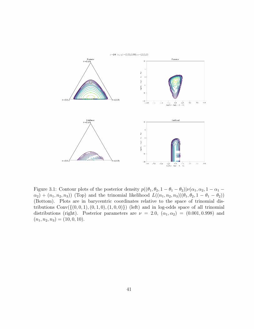
Figure 3.1: Contour plots of the posterior density p((θ1, θ2, 1− θ1 − θ2)|ν(α1, α2, 1− α1 −α2) + (n1, n2, n3)) (Top) and the trinomial likelihood L((n1, n2, n3)|(θ1, θ2, 1 − θ1 − θ2))(Bottom). Plots are in barycentric coordinates relative to the space of trinomial dis-tributions Conv((0, 0, 1), (0, 1, 0), (1, 0, 0)) (left) and in log-odds space of all trinomialdistributions (right). Posterior parameters are ν = 2.0, (α1, α2) = (0.001, 0.998) and(n1, n2, n3) = (10, 0, 10).
41
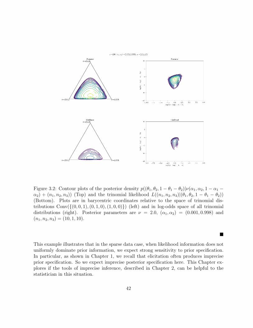
Figure 3.2: Contour plots of the posterior density p((θ1, θ2, 1− θ1 − θ2)|ν(α1, α2, 1− α1 −α2) + (n1, n2, n3)) (Top) and the trinomial likelihood L((n1, n2, n3)|(θ1, θ2, 1 − θ1 − θ2))(Bottom). Plots are in barycentric coordinates relative to the space of trinomial dis-tributions Conv((0, 0, 1), (0, 1, 0), (1, 0, 0)) (left) and in log-odds space of all trinomialdistributions (right). Posterior parameters are ν = 2.0, (α1, α2) = (0.001, 0.998) and(n1, n2, n3) = (10, 1, 10).
This example illustrates that in the sparse data case, when likelihood information does notuniformly dominate prior information, we expect strong sensitivity to prior specification.In particular, as shown in Chapter 1, we recall that elicitation often produces impreciseprior specification. So we expect imprecise posterior specification here. This Chapter ex-plores if the tools of imprecise inference, described in Chapter 2, can be helpful to thestatistician in this situation.
42
In our exploration we take inference about log-odds, in the IDM framework, as a practicaland statistically important test case for the applications of imprecise methods. Because thelog-odds is unbounded, we see that in Section 3.3.1 the boundedness condition on randomvariables used in Chapter 2 immediately creates a problem for application.
3.2 Literature: Affine geometry of IDM posterior up-
dating under sparse observations
We apply the work of Bickis [14] to establish that updating the posterior of the IDMamounts to the translation of a simplex in the prior Dirichlet natural parameter spaceby the observation vector which is a sufficient statistic of the likelihood. We see that inthe sparse case the translation does not move the posterior support entirely into the rela-tive interior and so the boundary still plays a role in understanding the sensitivity problem.
3.2.1 Affine geometry of exponential family and Dirichlet-multinomialupdating
Following Bickis [14], we review a familiar result of conjugate pairs of prior and observationmodels.
Definition 3.2.1: A random variable X follows a distribution in the exponential familyspanned by the sufficient statistic v(x) = (v1(x), . . . , vk(x)) (with respect to a base measureλ) if there exists a vector ξ = (ξ1, . . . , ξk) such that,
P (X ∈ A) =
∫A
exp(ξTv(x)− φ(ξ))λ(dx),
where,
φ(ξ) = log
(∫exp(ξTv(x))λ(dx)
).
The family is said to be finite dimensional when k <∞.
43
Definition 3.2.2: The natural parameter space of an exponential family spanned by v isthe set,
ΞNat = ξ : φ(ξ) <∞ .
Now, consider that a random variable X which follows a member of a finite dimensionalexponential family spanned by v = (v1(x), . . . , vk(x)) with natural parameters ξ. Place aprior on ξ with log-density of the exponential form,
ξ 7−→ ηTv∗(ξ)− ψ(η), (3.1)
spanned by,v∗(ξ) = (−φ(ξ), ξ1, . . . , ξk),
with natural parameters,η = (η0, η1, . . . , ηk),
For a fixed data point, x, of X,
ξTv(x)− φ(ξ) = v∗(ξ)Tηx,
where,ηx = (1, v1(x), . . . , vk(x)).
Now, consider the posterior measure after observing x with the aforementioned prior nat-ural parameters η. For every suitably measurable set B,
Π(ξ ∈ B|x) = k(x)
∫B
exp(ξTv(x)− φ(ξ))exp(ηTv∗(ξ)− ψ(η))dξ
=
∫B
exp((ηx + η)Tv∗(ξ)− ψ(η) + log k(x)dξ.
So, the posterior and prior are conjugate and the updating result in a translation in thenatural parameters. We record this in the theorem below.
Theorem 3.2.1: (Bickis [14]) For a likelihood of i.i.d. data x1, . . . , xn induced by anexponential family naturally parametrised by ξ ∈ ΞNat ⊆ Rk, k < ∞, spanned by the
44
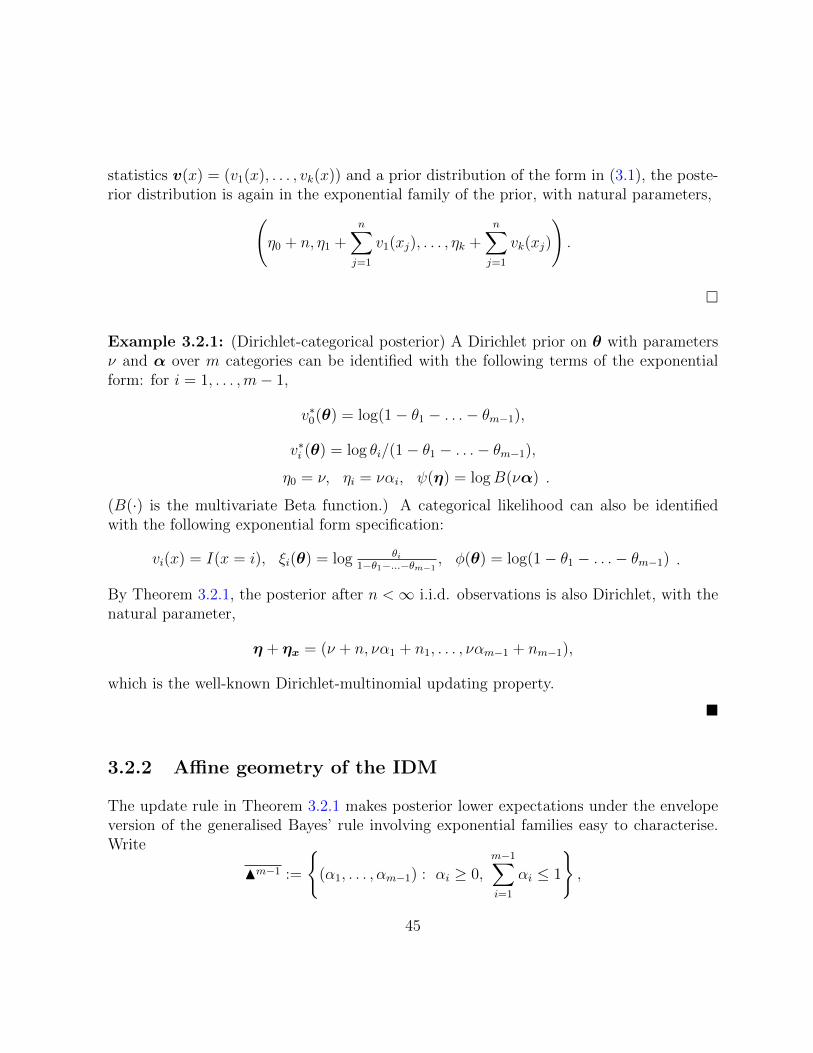
statistics v(x) = (v1(x), . . . , vk(x)) and a prior distribution of the form in (3.1), the poste-rior distribution is again in the exponential family of the prior, with natural parameters,(
η0 + n, η1 +n∑j=1
v1(xj), . . . , ηk +n∑j=1
vk(xj)
).
Example 3.2.1: (Dirichlet-categorical posterior) A Dirichlet prior on θ with parametersν and α over m categories can be identified with the following terms of the exponentialform: for i = 1, . . . ,m− 1,
v∗0(θ) = log(1− θ1 − . . .− θm−1),
v∗i (θ) = log θi/(1− θ1 − . . .− θm−1),
η0 = ν, ηi = ναi, ψ(η) = logB(να) .
(B(·) is the multivariate Beta function.) A categorical likelihood can also be identifiedwith the following exponential form specification:
vi(x) = I(x = i), ξi(θ) = log θi1−θ1−...−θm−1
, φ(θ) = log(1− θ1 − . . .− θm−1) .
By Theorem 3.2.1, the posterior after n <∞ i.i.d. observations is also Dirichlet, with thenatural parameter,
η + ηx = (ν + n, να1 + n1, . . . , ναm−1 + nm−1),
which is the well-known Dirichlet-multinomial updating property.
3.2.2 Affine geometry of the IDM
The update rule in Theorem 3.2.1 makes posterior lower expectations under the envelopeversion of the generalised Bayes’ rule involving exponential families easy to characterise.Write
Nm−1 :=
(α1, . . . , αm−1) : αi ≥ 0,
m−1∑i=1
αi ≤ 1
,
45
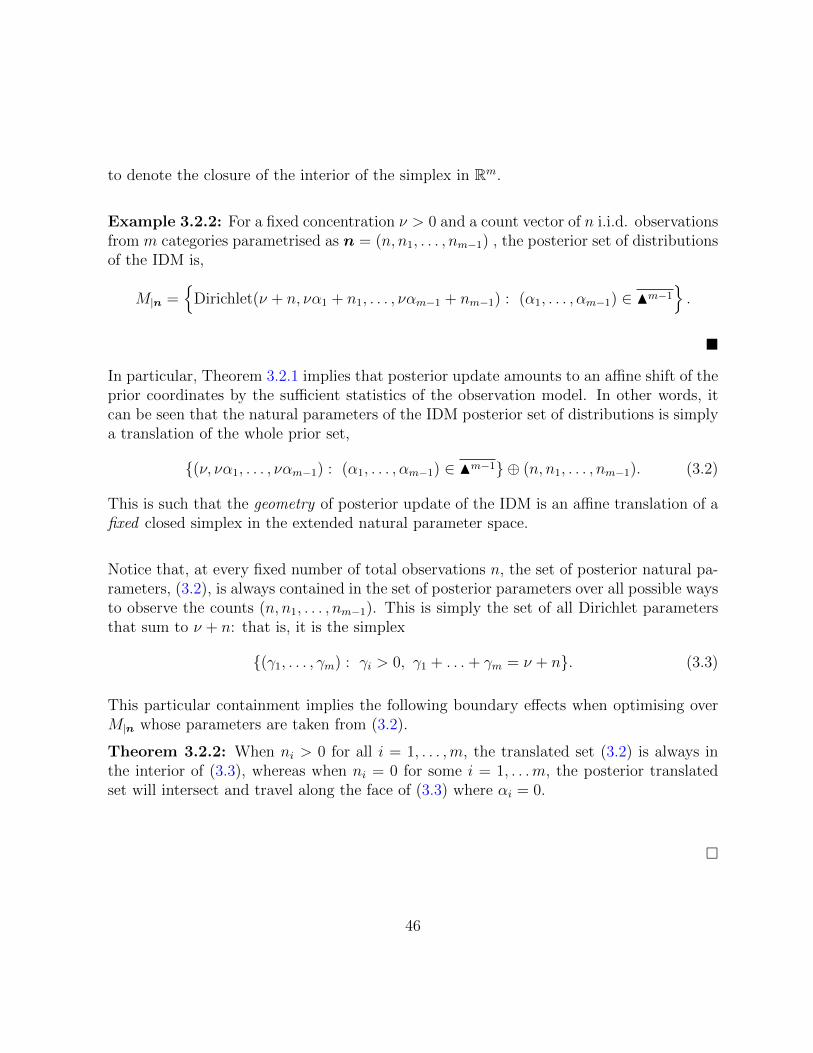
to denote the closure of the interior of the simplex in Rm.
Example 3.2.2: For a fixed concentration ν > 0 and a count vector of n i.i.d. observationsfrom m categories parametrised as n = (n, n1, . . . , nm−1) , the posterior set of distributionsof the IDM is,
M|n =
Dirichlet(ν + n, να1 + n1, . . . , ναm−1 + nm−1) : (α1, . . . , αm−1) ∈ Nm−1.
In particular, Theorem 3.2.1 implies that posterior update amounts to an affine shift of theprior coordinates by the sufficient statistics of the observation model. In other words, itcan be seen that the natural parameters of the IDM posterior set of distributions is simplya translation of the whole prior set,
(ν, να1, . . . , ναm−1) : (α1, . . . , αm−1) ∈ Nm−1 ⊕ (n, n1, . . . , nm−1). (3.2)
This is such that the geometry of posterior update of the IDM is an affine translation of afixed closed simplex in the extended natural parameter space.
Notice that, at every fixed number of total observations n, the set of posterior natural pa-rameters, (3.2), is always contained in the set of posterior parameters over all possible waysto observe the counts (n, n1, . . . , nm−1). This is simply the set of all Dirichlet parametersthat sum to ν + n: that is, it is the simplex
(γ1, . . . , γm) : γi > 0, γ1 + . . .+ γm = ν + n. (3.3)
This particular containment implies the following boundary effects when optimising overM|n whose parameters are taken from (3.2).
Theorem 3.2.2: When ni > 0 for all i = 1, . . . ,m, the translated set (3.2) is always inthe interior of (3.3), whereas when ni = 0 for some i = 1, . . .m, the posterior translatedset will intersect and travel along the face of (3.3) where αi = 0.
46
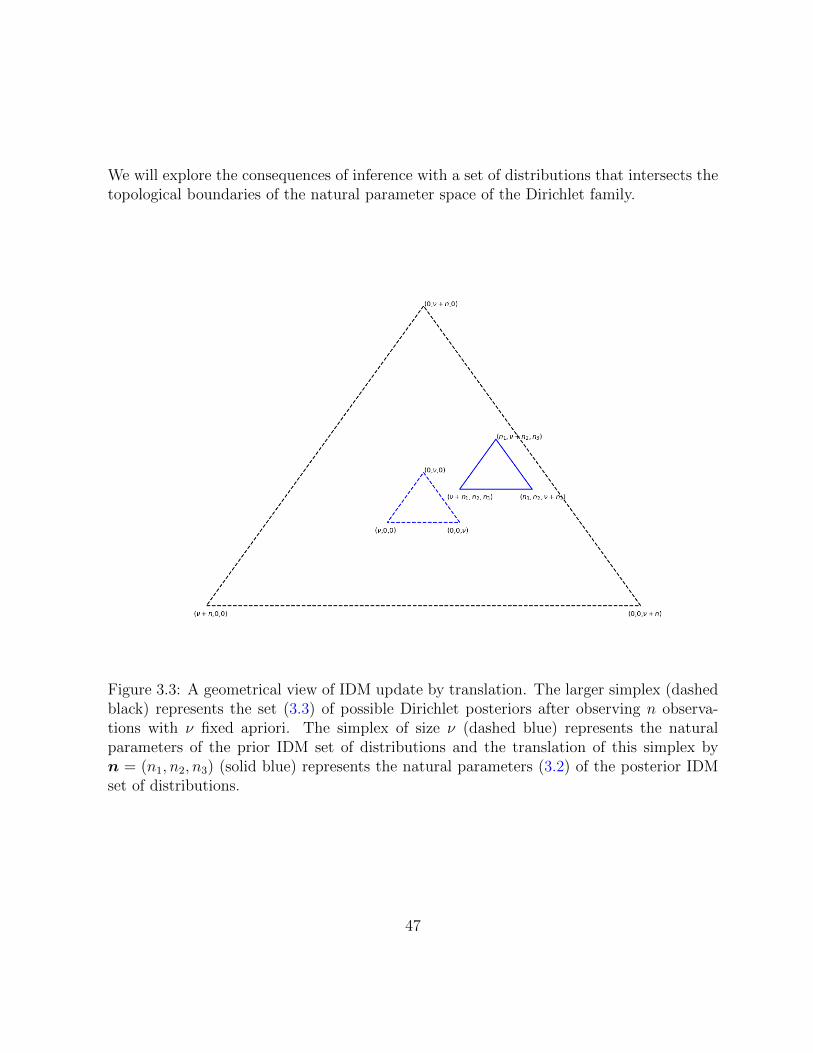
We will explore the consequences of inference with a set of distributions that intersects thetopological boundaries of the natural parameter space of the Dirichlet family.
Figure 3.3: A geometrical view of IDM update by translation. The larger simplex (dashedblack) represents the set (3.3) of possible Dirichlet posteriors after observing n observa-tions with ν fixed apriori. The simplex of size ν (dashed blue) represents the naturalparameters of the prior IDM set of distributions and the translation of this simplex byn = (n1, n2, n3) (solid blue) represents the natural parameters (3.2) of the posterior IDMset of distributions.
47
3.3 Inference for log-odds under IDM
We use categorical data analysis as a backdrop to investigate statistical inference using im-precise probabilities. We focus on the imprecise IDM version of the following log-odds in-ference. In the precise case with a single prior, under the Dirichlet(να+n) posterior distri-bution over m categories, for two collections of subsets of cell categories, A = A1, . . . , Arwith each Ai ⊆ 1, . . . ,m and B = B1, . . . , Bs with each Bj ⊆ 1, . . . ,m, the expec-tation of the general log-odds of the following form is a linear combination of digammafunctions,
E
(log
θA1 . . . θArθB1 . . . θBs
∣∣∣∣ να+ n
)=
r∑i=1
ψ(ναAi+nAi)−s∑j=1
ψ(ναBj +nBj)−(|A|−|B|)ψ(ν+n).
(3.4)where for a vector θ = (θ1, . . . , θm), and a subset of indices C ⊆ 1, . . . ,m,
θC :=∑i∈C
θi. (3.5)
(This follows from the fact that the log-probabilities log θi are sufficient statistics of theDirichlet distribution and the digamma functions result from differentiating the Beta func-tion of the normalising constant.) The IDM version of this involves computing the posteriorlower expectation,
EIDM
(log
θA1 . . . θArθB1 . . . θBs
∣∣∣∣ ν,n) = inf
E
(log
θA1 . . . θArθB1 . . . θBs
∣∣∣∣ να+ n
): α ∈ 4m
. (3.6)
From an optimisation perspective, we note that, when counts of some observation cells, ni’s,are zero, the objective function above contains terms of the form ψ(νa) which tends to −∞as the optimisation variable a tends to 0. We will examine this in more details in Chapter 5.
3.3.1 Unboundedness of the log-odds and the theory of coher-ence
We are interested in the cases where the log-odds statistic becomes unbounded when θcontain zeroes as prior sensitivity may be extreme. However, this case presents a problemfor directly applying the mathematical framework in Chapter 2 as Walley’s coherence oflower expectations [81] are defined only on sets of bounded random variables. There has
48
been relatively little work on extensions to unbounded random variables: we cite Troffaesand de Cooman [77], Troffaes [75], their culmination in the later book by Troffaes and deCooman [78] as well as the investigations by Crisma, Gigante, and Millossovich [31] andSchervish, Seidenfeld and Kadane [71].
We take an approach that is more in line with sensitivity analyses. We restrict our scopeof analysis to the IDM and justify our use of it with the log-odds with limiting arguments.Specifically, we consider a truncation of the log-odds that is bounded and finite.
Definition 3.3.1: For a coherent lower expectation, E, defined over the set of boundedrandom variable L(Ω)s, write E(ext) as its extension to the linear space,
span(L(Ω) ∪ g).
When the multinomial is non-sparse in the sense that each category has at least one ob-servation, we show that the approximation error between the posterior expectations of atruncated log-odds and the original one converges to zero in the L1 sense uniformly overthe posterior natural parameter space that is the optimisation domain of the IDM.
Theorem 3.3.1: (Theorem B.2.1) Consider the general log-odds statistic,
g(θ) = log
∏ri=1 P (Ai|θ)∏sj=1 P (Bj|θ)
,
and the following truncation of it,
Tc(θ) := g(θ)I(|g(θ)| ≤ c) + cI(|g(θ)| > c).
Under θ ∼ Dirichlet(να+ n) with sets A1, . . . , Ar, B1, . . . , Bs, such that nAi > 0, nBj > 0for all Ai, Bj,
supα∈4|Ω|
E(|Tc − g||να+ n)→ 0,
as c→∞.
49
The coherence of Troffaes and de Cooman [78] extends that of Walley [81] (introduced inChapter 2) to unbounded ones such as the general log-odds by using an approximationscheme. It can be shown that our construction is also coherent under their extended co-herence notions.
Theorem 3.3.2: (Theorem B.2.2) Under the conditions of Theorem 3.3.1, the extendedIDM whose value at the unbounded log-odds g is given by,
E(ext)IDM(g(θ)|ν,n) = lim
c→∞EIDM(Tc(θ)|να+ n),
is coherent under the Proposition B.2.1 of Troffaes and de Cooman [78].
Following their extension allows us to make the following interpretation of performing theoptimisation and treating its result as an extension of the IDM lower expectation to includeg in its domain.
Interpretation 3.3.1: For any general log-odds,
g(θ) = log
∏ri=1 P (Ai|θ)∏sj=1 P (Bj|θ)
,
whenever n contains at least one count in each category, we interpret, E(ext)IDM(g(θ)|ν,n) as
a double limit of the sequence of truncated Dirichlet expectations,
c,α 7−→ E(Tc|να+ n) = E
(g(θ)I(|g(θ)| ≤ c) + cI(|g(θ) > c|)
∣∣∣∣ να+ n
),
over the optimisation path of α contained in 4Ω and the limit of the truncation approxi-mation via c→∞.
As described in Chapter 2, we can interpret the imprecise theory as either a sensitivity anal-ysis of elicited priors or in terms of coherence of direct assessments about random variables.However, care must be taken when applying the interpretation of Section 2.1 motivating the
coherence definition 2.1.8 to E(ext)IDM(g|ν,n) = −∞ (and, by conjugacy, E
(ext)
IDM(g|ν,n) =∞).See 13.11 in Troffaes and de Cooman [78].
50
3.3.2 The divergence of coherence from sensitivity analysis undersparse observations
Despite the material in the previous section, the behavioural and mathematical extensionof Walley’s coherence [81] for the IDM encounters further obstacles when it is used to per-form posterior inference for the log odds-type statistics. In particular, we now demonstratethat the error of the previous approximation does not converge to zero if certain cells havezero samples.
Example 3.3.1: Consider θ ∼ Dirichlet(να + n) with α = (α1, α2, 1 − α1 − α2) ∈ 4|Ω|and,
g(θ) = log θ1/θ2,
for θ a vector of trinomial cell probabilities.
Consider the case when n = (0, 0, n3) such that n3 > 0:
limα1→0
E(|g − Tc||να+ n)
≥(
limα1→0
E(|g||να+ n)− E(|g|I(|g| ≤ c)|να+ n)− E(cI(|g| > c)|να+ n)
)= lim
α1→0(E(|g||να+ n)− E(|g|I(|g| ≤ c)|να+ n)− cP (|g| > c|να+ n))
> limα1→0
E(|g||να+ n)− 2c
≥ limα1→0
|E(g|να+ n)| − 2c
= limα1→0
|ψ(να1)− ψ(να2)| − 2c (ψ is the digamma function)
=∞,
Similarly,limα2→0
E(|g − Tc||να+ n) ≥ ∞.
This leads to,limc→∞ limα1→0E(|g − Tc||να+ n) =∞
limc→∞ limα2→0E(|g − Tc||να+ n) =∞. (3.7)
That is, the error of the truncation approximation does not converge to zero in this case.
51
Example 3.3.1 demonstrates that, in the case of interest where certain cells have zero ob-servations, there are issues with Walley’s coherence [81] on bounded random variables andwith its extension by Troffaes and de Cooman [78] to unbounded random variables viaapproximating random variables for posterior inference of log-odds.
Nevertheless, if we put coherence aside, the optimisation,
infα∈4|Ω|
EDir(g|να+ n),
itself can still yield well-defined solutions. This is because, for the general log-odds,
g(θ) = log
∏ri=1 P (Ai|θ)∏sj=1 P (Bj|θ)
,
its expectation under any posterior Dirichlet distribution in the set is a linear combinationof digamma functions,
EDir(g|να+ n) =r∑i=1
ψ(ναAi + nAi)−s∑j=1
ψ(ναBj + nBj)− (r − s)ψ(ν + n),
and is therefore a smooth function in the interior of the α simplex. (Recall that aC =∑i∈C ai for a vector a and a set of indices C, and n is the total number of observations.)
In the following sections, Theorem 3.4.1 show that this expectation may optimise to ±∞for when either all the sets of the numerator or all the sets of the denominator of g(θ) havestrictly positive cell counts. This yields an interpretable inference in the vein of a globalsensitivity analysis methodology.
Interpretation 3.3.2: When there exists no Ai ∈ A and Bj ∈ B such that nAi = 0 andnBj = 0 simultaneously, the general log-odds problem,
infα∈4|Ω|
EDir(g|να+ n),
where,
g(θ) = log
∏ri=1 P (Ai|θ)∏sj=1 P (Bj|θ)
,
52
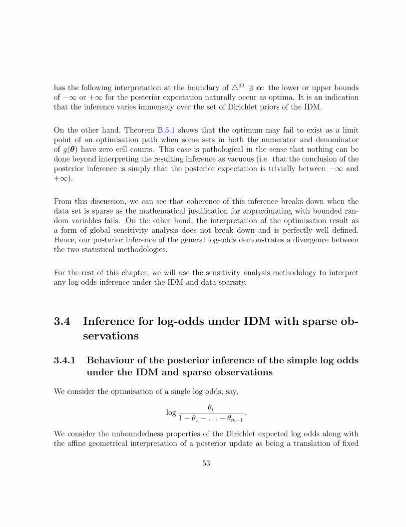
has the following interpretation at the boundary of 4|Ω| 3 α: the lower or upper boundsof −∞ or +∞ for the posterior expectation naturally occur as optima. It is an indicationthat the inference varies immensely over the set of Dirichlet priors of the IDM.
On the other hand, Theorem B.5.1 shows that the optimum may fail to exist as a limitpoint of an optimisation path when some sets in both the numerator and denominatorof g(θ) have zero cell counts. This case is pathological in the sense that nothing can bedone beyond interpreting the resulting inference as vacuous (i.e. that the conclusion of theposterior inference is simply that the posterior expectation is trivially between −∞ and+∞).
From this discussion, we can see that coherence of this inference breaks down when thedata set is sparse as the mathematical justification for approximating with bounded ran-dom variables fails. On the other hand, the interpretation of the optimisation result asa form of global sensitivity analysis does not break down and is perfectly well defined.Hence, our posterior inference of the general log-odds demonstrates a divergence betweenthe two statistical methodologies.
For the rest of this chapter, we will use the sensitivity analysis methodology to interpretany log-odds inference under the IDM and data sparsity.
3.4 Inference for log-odds under IDM with sparse ob-
servations
3.4.1 Behaviour of the posterior inference of the simple log oddsunder the IDM and sparse observations
We consider the optimisation of a single log odds, say,
logθi
1− θ1 − . . .− θm−1
.
We consider the unboundedness properties of the Dirichlet expected log odds along withthe affine geometrical interpretation of a posterior update as being a translation of fixed
53
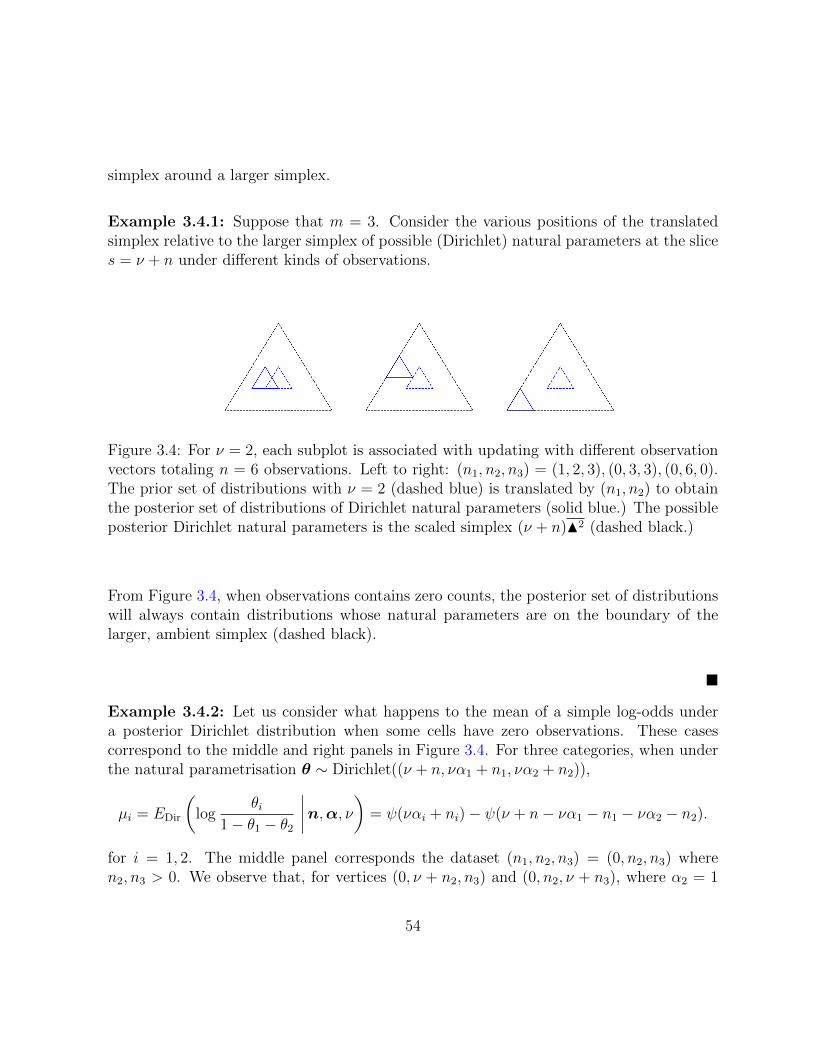
simplex around a larger simplex.
Example 3.4.1: Suppose that m = 3. Consider the various positions of the translatedsimplex relative to the larger simplex of possible (Dirichlet) natural parameters at the slices = ν + n under different kinds of observations.
Figure 3.4: For ν = 2, each subplot is associated with updating with different observationvectors totaling n = 6 observations. Left to right: (n1, n2, n3) = (1, 2, 3), (0, 3, 3), (0, 6, 0).The prior set of distributions with ν = 2 (dashed blue) is translated by (n1, n2) to obtainthe posterior set of distributions of Dirichlet natural parameters (solid blue.) The possibleposterior Dirichlet natural parameters is the scaled simplex (ν + n)N2 (dashed black.)
From Figure 3.4, when observations contains zero counts, the posterior set of distributionswill always contain distributions whose natural parameters are on the boundary of thelarger, ambient simplex (dashed black).
Example 3.4.2: Let us consider what happens to the mean of a simple log-odds undera posterior Dirichlet distribution when some cells have zero observations. These casescorrespond to the middle and right panels in Figure 3.4. For three categories, when underthe natural parametrisation θ ∼ Dirichlet((ν + n, να1 + n1, να2 + n2)),
µi = EDir
(log
θi1− θ1 − θ2
∣∣∣∣n,α, ν) = ψ(ναi + ni)− ψ(ν + n− να1 − n1 − να2 − n2).
for i = 1, 2. The middle panel corresponds the dataset (n1, n2, n3) = (0, n2, n3) wheren2, n3 > 0. We observe that, for vertices (0, ν + n2, n3) and (0, n2, ν + n3), where α2 = 1
54
and α3 = 1 respectively,
(µ1, µ2)(0, ν + n2, n3) = (ψ(0+)− ψ(n− n2), ψ(n2)− ψ(n− n2)),
(µ1, µ2)(0, n2, ν + n3) = (ψ(0+)− ψ(ν + n− n2), ψ(n2)− ψ(ν + n− n2)),
where the right limit at 0 of the digamma function ψ(0+) tends to infinity. Notice thatthese two vertices represent endpoints of the side of the blue solid simplex that coincideswith the boundary larger black simplex.
Similarly, the right panel corresponds to the dataset (0, n2, 0) for n2 = n > 0. For thevertex (0, ν + n2, 0),
(µ1, µ2)(0, ν + n2, 0) = (ψ(0+)− ψ(0+), ψ(ν + n2)− ψ(0+)).
The indeterminate form ψ(0+)− ψ(0+) in µ1 arises from (0, ν + n2, 0) coinciding with thevertex of the black simplex. This is qualitatively different from the terms that involve onlyone right limit of the digamma function at zero, which is merely unbounded.
Figure 3.5: The ambient simplex (ν + n)N2 with (n1, n2, n3) = (0, n2, 0). The posteriorexpected log odds µ1 takes values +∞ and −∞ on the left and bottom edges, respectively,and does not have a continuous limit at the vertex of these two edges.
The middle and right panels demonstrate qualitatively different boundary effects of theposterior natural parameter space upon log-odds inference depending on whether or not
55
the boundary contains vertices or not. This leads to the optimisation of the posteriorexpectation being also qualitatively very different amongst the three cases of boundariesin Figure 3.4.
3.4.2 Behaviour and solutions to optimisation problem of theposterior inference of the general log odds under the IDMand sparse observations
Let us now generalise the observations from the case with the simple log odds. Theobservations n can only affect the expected log-odds function only through the elementsthat appear explicitly in the linear combination of digamma functions,
α 7−→r∑i=1
ψ(ναAi + nAi)−s∑j=1
ψ(ναBj + nBj).
We can deduce the behaviour of this function through the behaviour of the difference be-tween two digamma functions as follows.
Lemma 3.4.1: When nj > 0,
α 7−→ ψ(ναi)− ψ(ναj + nj),
has a minimum of −∞ as αi tends to 0 on 4m 3 α. When ni, nj > 0, then the two termsin,
ψ(ναi + ni)− ψ(ναj + nj),
are bounded over α ∈ 4m.
Proof: the first result is due to the fact that ψ is an unbounded and increasing functionon R+. The last result is also clear as ψ(x) is finite when x is finite.
56
In particular, the appropriate categories having zero observations causes the entire poste-rior expected log odds to go to infinity in one or both directions.
We note that the optima of the expectation of the general log-odds remain infinite as longas at least one event has zero counts. In particular, we have the following.
Theorem 3.4.1:
• Suppose that nA1 = 0 and nAi , nBj > 0 for i 6= 1. Then, the lower expectation of thegeneral log-odds is −∞.
• Suppose that nB1 = 0 and nAi , nBj > 0 for j 6= 1. Then, the upper expectation ofthe general log-odds is +∞.
Proof: For the first case, the expectation to be minimised is,
α ∈ 4m 7−→ ψ(ναA1) +r∑i=2
ψ(ναAi + nAi)−s∑j=1
ψ(ναBj + nBj).
We need only demonstrate that −∞ is attainable and so must be the minimum. Indeed,
any solution on the faceα : αA1 = 0,
∧ri=2 αAi > 0
∧sj=1 αBj > 0
will suffice.
The case for nB1 = 0 is analogous, withα : αB1 = 0,
∧ri=1 αAi > 0
∧sj=2 αBj > 0
attain-
ing +∞.
Finally, we remark upon the indeterminate forms that appear in certain expressions forthe posterior expectation. For example, in Example 3.4.2, the expression for the posteriorexpectation of the log-odds was,
ψ(ναi + ni)− ψ(ν + n− να1 − n1 − να2 − n2).
for i = 1, 2, such that with i = 1, n1 = n2 = 0, the indeterminate form ψ(0+)−ψ(0+) occursas α1 and α2 approach 0. This is because the limit is not well-defined: the indeterminateform can take any real value depending on the path taken for α1, α2 to approach 0. This
57
simply means that the posterior expectation EDir
(log θi
1−θ1−θ2
∣∣n,α, ν) cannot be assigned
the value returned by this expression, and must be directly evaluated. Consequently, if thiscase occurs when computing this type of imprecise expectation, we minimise the Lebesgueintegral directly.
3.4.3 Effects of cell counts on imprecision of posterior log-oddsinference under the IDM
We have seen that zero sample counts in categories may cause the IDM’s lower and upperexpectations to be unbounded, and the inference to become noninformative. On the otherhand, as long as the categories involved in the log-odds contain at least one observation, theexpectation becomes finite. As next step, let us explore how observing a single observationin its event decreases the imprecision of the posterior inference. Suppose that nA = 1 suchthat,
E[log θA|n, ν,α] = ψ(ναA + 1)− ψ(ν + n).
Then the minimum is attained at,
ψ(1)− ψ(ν + n),
and the maximum is attained at,
ψ(ν + 1)− ψ(ν + n).
In terms of gain of precision, one observation in A causes the lower expectation to jumpfrom −∞ to the finite value ψ(1)−ψ(ν+n): thus ν and n also controls the location of thelower expectation when transitioning away from vacuity. The imprecision decreases from∞ to ψ(ν+1)−ψ(1) with a single observation nA = 1, and higher values of ν increases thisimprecision value. Interestingly, the total number of observations n does not contribute tothis phenomenon.
As expected, as more counts are accumulated by increasing ∆n, the imprecision of thelog-probability inference also decreases.
Proposition 3.4.1: for n and ∆n such that nA ≥ 1 and ∆nA = (∆n)A ≥ 0,
P [log θA|να+ n] ≥ P [log θA|να+ n+ ∆n].
Proof: See Proposition B.4.1.
58
Due to a triangular inequality of the imprecision of a sum (see Lemma B.4.1,) the impreci-sion of a general log-odds is bounded above by the imprecision of the sum of its componentsof log-probabilities.
Theorem 3.4.2: For finite r, s, the imprecision (induced by a coherent conjugate pair oflower and upper expectations) of the general log odds is bounded by the imprecisions ofits component log-probabilities:
P
[log
θA1 . . . θArθB1 . . . θBs
]≤
r∑i=1
P [log θAi ] +s∑j=1
P [log θBj ].
Proof: Apply Lemma B.4.1.
59
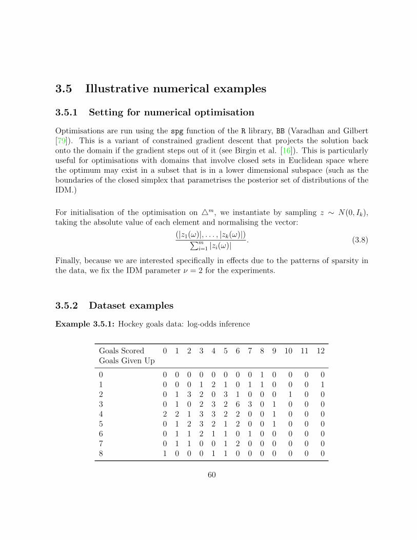
3.5 Illustrative numerical examples
3.5.1 Setting for numerical optimisation
Optimisations are run using the spg function of the R library, BB (Varadhan and Gilbert[79]). This is a variant of constrained gradient descent that projects the solution backonto the domain if the gradient steps out of it (see Birgin et al. [16]). This is particularlyuseful for optimisations with domains that involve closed sets in Euclidean space wherethe optimum may exist in a subset that is in a lower dimensional subspace (such as theboundaries of the closed simplex that parametrises the posterior set of distributions of theIDM.)
For initialisation of the optimisation on 4m, we instantiate by sampling z ∼ N(0, Ik),taking the absolute value of each element and normalising the vector:
(|z1(ω)|, . . . , |zk(ω)|)∑mi=1 |zi(ω)|
. (3.8)
Finally, because we are interested specifically in effects due to the patterns of sparsity inthe data, we fix the IDM parameter ν = 2 for the experiments.
3.5.2 Dataset examples
Example 3.5.1: Hockey goals data: log-odds inference
Goals Scored 0 1 2 3 4 5 6 7 8 9 10 11 12Goals Given Up
0 0 0 0 0 0 0 0 0 1 0 0 0 01 0 0 0 1 2 1 0 1 1 0 0 0 12 0 1 3 2 0 3 1 0 0 0 1 0 03 0 1 0 2 3 2 6 3 0 1 0 0 04 2 2 1 3 3 2 2 0 0 1 0 0 05 0 1 2 3 2 1 2 0 0 1 0 0 06 0 1 1 2 1 1 0 1 0 0 0 0 07 0 1 1 0 0 1 2 0 0 0 0 0 08 1 0 0 0 1 1 0 0 0 0 0 0 0
60
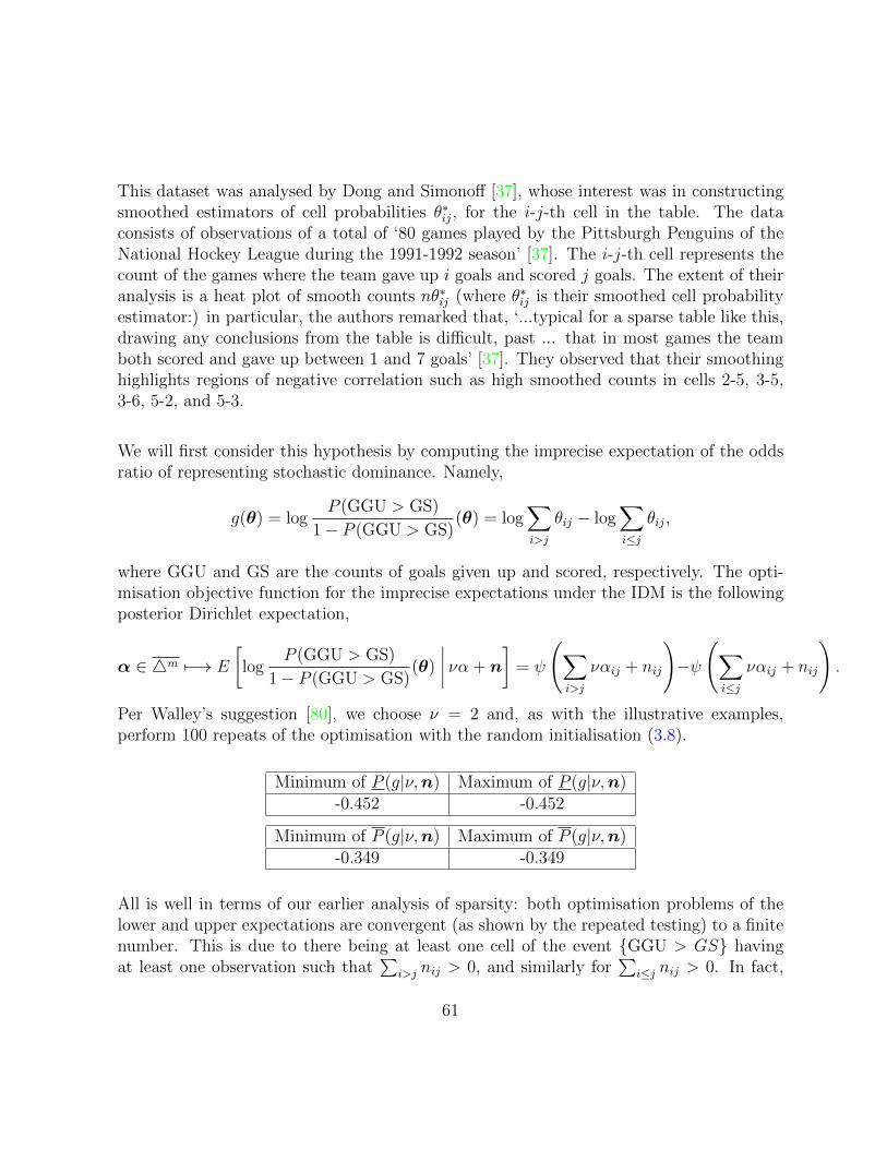
This dataset was analysed by Dong and Simonoff [37], whose interest was in constructingsmoothed estimators of cell probabilities θ∗ij, for the i-j-th cell in the table. The dataconsists of observations of a total of ‘80 games played by the Pittsburgh Penguins of theNational Hockey League during the 1991-1992 season’ [37]. The i-j-th cell represents thecount of the games where the team gave up i goals and scored j goals. The extent of theiranalysis is a heat plot of smooth counts nθ∗ij (where θ∗ij is their smoothed cell probabilityestimator:) in particular, the authors remarked that, ‘...typical for a sparse table like this,drawing any conclusions from the table is difficult, past ... that in most games the teamboth scored and gave up between 1 and 7 goals’ [37]. They observed that their smoothinghighlights regions of negative correlation such as high smoothed counts in cells 2-5, 3-5,3-6, 5-2, and 5-3.
We will first consider this hypothesis by computing the imprecise expectation of the oddsratio of representing stochastic dominance. Namely,
g(θ) = logP (GGU > GS)
1− P (GGU > GS)(θ) = log
∑i>j
θij − log∑i≤j
θij,
where GGU and GS are the counts of goals given up and scored, respectively. The opti-misation objective function for the imprecise expectations under the IDM is the followingposterior Dirichlet expectation,
α ∈ 4m 7−→ E
[log
P (GGU > GS)
1− P (GGU > GS)(θ)
∣∣∣∣ να + n
]= ψ
(∑i>j
ναij + nij
)−ψ
(∑i≤j
ναij + nij
).
Per Walley’s suggestion [80], we choose ν = 2 and, as with the illustrative examples,perform 100 repeats of the optimisation with the random initialisation (3.8).
Minimum of P (g|ν,n) Maximum of P (g|ν,n)-0.452 -0.452
Minimum of P (g|ν,n) Maximum of P (g|ν,n)-0.349 -0.349
All is well in terms of our earlier analysis of sparsity: both optimisation problems of thelower and upper expectations are convergent (as shown by the repeated testing) to a finitenumber. This is due to there being at least one cell of the event GGU > GS havingat least one observation such that
∑i>j nij > 0, and similarly for
∑i≤j nij > 0. In fact,
61
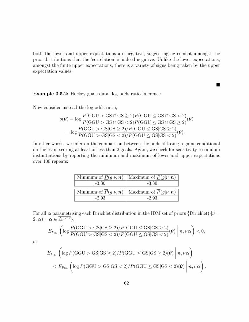
both the lower and upper expectations are negative, suggesting agreement amongst theprior distributions that the ‘correlation’ is indeed negative. Unlike the lower expectations,amongst the finite upper expectations, there is a variety of signs being taken by the upperexpectation values.
Example 3.5.2: Hockey goals data: log odds ratio inference
Now consider instead the log odds ratio,
g(θ) = logP (GGU > GS ∩GS ≥ 2)P (GGU ≤ GS ∩GS < 2)
P (GGU > GS ∩GS < 2)P (GGU ≤ GS ∩GS ≥ 2)(θ)
= logP (GGU > GS|GS ≥ 2)/P (GGU ≤ GS|GS ≥ 2)
P (GGU > GS|GS < 2)/P (GGU ≤ GS|GS < 2)(θ).
In other words, we infer on the comparison between the odds of losing a game conditionalon the team scoring at least or less than 2 goals. Again, we check for sensitivity to randominstantiations by reporting the minimum and maximum of lower and upper expectationsover 100 repeats:
Minimum of P (g|ν,n) Maximum of P (g|ν,n)-3.30 -3.30
Minimum of P (g|ν,n) Maximum of P (g|ν,n)-2.93 -2.93
For all α parametrising each Dirichlet distribution in the IDM set of priors Dirichlet(·|ν =2,α) : α ∈ 48×12,
EPDir
(log
P (GGU > GS|GS ≥ 2)/P (GGU ≤ GS|GS ≥ 2)
P (GGU > GS|GS < 2)/P (GGU ≤ GS|GS < 2)(θ)
∣∣∣∣n, να) < 0,
or,
EPDir
(logP (GGU > GS|GS ≥ 2)/P (GGU ≤ GS|GS ≥ 2)(θ)
∣∣∣∣n, να)< EPDir
(logP (GGU > GS|GS < 2)/P (GGU ≤ GS|GS < 2)(θ)
∣∣∣∣n, να) .62
In accordance with the observed data, the posterior distributions in the set of distributionsagree that the expected odds of them losing (goals given up (GGU) greater than goalsscored (GS)) conditional on them scoring at least 2 goals is less than the same odds con-ditional on scoring less than 2 goals, which is to be expected.
Example 3.5.3: Hockey goals data: log odds inference with finer conditioning on rareevents
Suppose that one was interested in comparing the odds of them losing under the regimeswhen the number of goals given up (GGU) and goals scored (GS) are low (that is, whenboth teams’ scores are low) and when both are high. This is also numerically interestingbecause these cases are also part of the sparse parts of the dataset (the upper-left andlower-right portions of it).
One way to model that is to split the values of the GGU and GS variables such that theconditioning is as follows. We condition on both GGU and GS being low, which we defineas when they are in 0, 1 and 0, 1 respectively, and when both are high, when theyare in 6, 7, 8 and 8, 9, 10, 11, 12 respectively. The conditioning events are sparse: theyare chosen such that the variable is ordinally smaller than the smallest value whose cellcount is greater than or equal to 3 occur (for example, GGU ∈ 0, 1 was chosen becauseGGU = 2 is the smallest ordinal value whose row starts containing cell counts of at least 3.)
The log-odds can be written as,
g(θ) = log P (GGU≥GS ∩ GGU∈0,1 ∩ GS∈0,1)P (GGU<GS ∩ GGU∈6,7,8 ∩ GS∈8,9,10,11,12)P (GGU≥GS ∩ GGU∈6,7,8 ∩ GS∈8,9,10,11,12)P (GGU<GS ∩ GGU∈0,1 ∩ GS∈0,1)(θ).
(3.9)In terms of conditional odds-ratios,
log P (GGU≥GS | GGU∈0,1 ∩ GS∈0,1)/P (GGU≥GS | GGU∈6,7,8 ∩ GS∈8,9,10,11,12)P (GGU<GS | GGU∈0,1 ∩ GS∈0,1)/P (GGU<GS | GGU∈6,7,8 ∩ GS∈8,9,10,11,12)(θ).
Labelling the log-odds in (3.9), log θAθB/θCθD, its posterior expectation with respect toone set of distributions element of the IDM is,
ψ(ναA) + ψ(ναB)− ψ(ναC)− ψ(ναD),
63
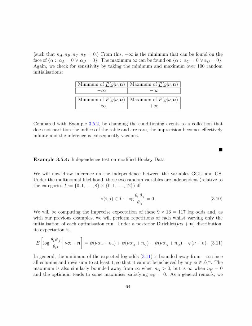
(such that nA, nB, nC , nD = 0.) From this, −∞ is the minimum that can be found on theface of α : αA = 0 ∨ αB = 0. The maximum∞ can be found on α : αC = 0 ∨αD = 0.Again, we check for sensitivity by taking the minimum and maximum over 100 randominitialisations:
Minimum of P (g|ν,n) Maximum of P (g|ν,n)−∞ −∞
Minimum of P (g|ν,n) Maximum of P (g|ν,n)+∞ +∞
Compared with Example 3.5.2, by changing the conditioning events to a collection thatdoes not partition the indices of the table and are rare, the imprecision becomes effectivelyinfinite and the inference is consequently vacuous.
Example 3.5.4: Independence test on modified Hockey Data
We will now draw inference on the independence between the variables GGU and GS.Under the multinomial likelihood, these two random variables are independent (relative tothe categories I := 0, 1, . . . , 8 × 0, 1, . . . , 12) iff
∀(i, j) ∈ I : logθi·θ·jθij
= 0. (3.10)
We will be computing the imprecise expectation of these 9 × 13 = 117 log odds and, aswith our previous examples, we will perform repetitions of each whilst varying only theinitialisation of each optimisation run. Under a posterior Dirichlet(να + n) distribution,its expectation is,
E
[log
θi·θ·jθij
∣∣∣∣ να+ n
]= ψ(ναi· + ni·) + ψ(να·j + n·j)− ψ(ναij + nij)− ψ(ν + n). (3.11)
In general, the minimum of the expected log-odds (3.11) is bounded away from −∞ sinceall columns and rows sum to at least 1, so that it cannot be achieved by any α ∈ 4m. Themaximum is also similarly bounded away from ∞ when nij > 0, but is ∞ when nij = 0and the optimum tends to some maximiser satisfying αij = 0. As a general remark, we
64

expect this as the statistic itself log θi·θ·j/θij for θ ∈ 4m is unbounded above (as θij tendsto 0) but bounded below away from −∞ as θi·, θ·j ≥ θij prevents the numerator of theratio from going to zero when θij > 0.
Notice that because the column GS = 11 has no counts, it can be seen that,
∀i ∈ 0, 1, . . . , 8 : E
[log
θi·θ·11
θi11
∣∣∣∣ να+ n
]= ψ(ναi·+ni·)+ψ(να·11)−ψ(ναi11)−ψ(ν+n),
which is minimised and maximised to −∞ and ∞ respectively, so it is not particularlyinteresting as far as satisfying (3.10) goes.
Instead, we will modify the hockey data slightly by adding a single unit count to the columnGS = 11. We add a single count to the cell (0,11). The modified table is as follows,
Goals Scored 0 1 2 3 4 5 6 7 8 9 10 11 12Goals Given Up
0 0 0 0 0 0 0 0 0 1 0 0 1 01 0 0 0 1 2 1 0 1 1 0 0 0 12 0 1 3 2 0 3 1 0 0 0 1 0 03 0 1 0 2 3 2 6 3 0 1 0 0 04 2 2 1 3 3 2 2 0 0 1 0 0 05 0 1 2 3 2 1 2 0 0 1 0 0 06 0 1 1 2 1 1 0 1 0 0 0 0 07 0 1 1 0 0 1 2 0 0 0 0 0 08 1 0 0 0 1 1 0 0 0 0 0 0 0
Notice that none of the rows and columns sums to zero now.
The lower and upper expectations of this problem is given in Table 3.1. (Based on 100random initialisations, we found that the results were not sensitive to the random initiali-sations. The output of these tests have been omitted for brevity.)
65
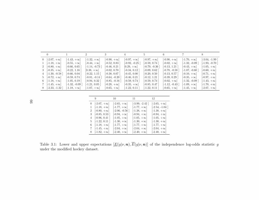
0 1 2 3 4 5 6 7 8
0 [-2.07, +∞] [-1.43, +∞] [-1.32, +∞] [-0.90, +∞] [-0.97, +∞] [-0.97, +∞] [-0.90, +∞] [-1.70, +∞] [-3.04, -1.99 ]1 [-1.18, +∞] [-0.55, +∞] [-0.44, +∞] [-0.52, 0.83 ] [-0.92, -0.25 ] [-0.59, 0.74 ] [-0.02, +∞] [-1.32, -0.09 ] [-1.93, -0.70 ]2 [-0.80, +∞] [-0.66, 0.65 ] [-1.14, -0.73 ] [-0.46, 0.21 ] [0.29, +∞] [-0.79, -0.36 ] [-0.13, 1.21 ] [-0.43, +∞] [-1.05, +∞]3 [-0.35, +∞] [-0.22, 1.16 ] [0.38, +∞] [-0.02, 0.70 ] [-0.34, 0.12 ] [-0.09, 0.62 ] [-0.78, -0.58 ] [-1.07, -0.60 ] [-0.60, +∞]4 [-1.30, -0.58 ] [-0.66, 0.04 ] [-0.22, 1.15 ] [-0.38, 0.07 ] [-0.45, 0.00 ] [-0.20, 0.50 ] [-0.13, 0.57 ] [-0.10, +∞] [-0.71, +∞]5 [-0.72, +∞] [-0.59, 0.74 ] [-0.81, -0.14 ] [-0.64, -0.20 ] [-0.46, 0.21 ] [-0.12, 1.21 ] [-0.39, 0.29 ] [-0.35, +∞] [-0.97, +∞]6 [-1.18, +∞] [-1.05, 0.19 ] [-0.94, 0.32 ] [-0.85, -0.16 ] [-0.59, 0.74 ] [-0.59, 0.74 ] [-0.02, +∞] [-1.32, -0.09 ] [-1.43, +∞]7 [-1.45, +∞] [-1.32, -0.09 ] [-1.21, 0.05 ] [-0.28, +∞] [-0.35, +∞] [-0.85, 0.47 ] [-1.12, -0.43 ] [-1.09, +∞] [-1.70, +∞]8 [-2.33, -1.32 ] [-1.18, +∞] [-1.07, +∞] [-0.65, +∞] [-1.22, 0.11 ] [-1.22, 0.11 ] [-0.65, +∞] [-1.45, +∞] [-2.07, +∞]
9 10 11 12
0 [-2.07, +∞] [-2.65, +∞] [-3.99, -2.42 ] [-2.65, +∞]1 [-1.18, +∞] [-1.77, +∞] [-1.77, +∞] [-2.54, -1.04 ]2 [-0.80, +∞] [-2.06, -0.56 ] [-1.38, +∞] [-1.38, +∞]3 [-0.85, 0.53 ] [-0.94, +∞] [-0.94, +∞] [-0.94, +∞]4 [-0.96, 0.41 ] [-1.05, +∞] [-1.05, +∞] [-1.05, +∞]5 [-1.22, 0.11 ] [-1.30, +∞] [-1.30, +∞] [-1.30, +∞]6 [-1.18, +∞] [-1.77, +∞] [-1.77, +∞] [-1.77, +∞]7 [-1.45, +∞] [-2.04, +∞] [-2.04, +∞] [-2.04, +∞]8 [-1.82, +∞] [-2.40, +∞] [-2.40, +∞] [-2.40, +∞]
Table 3.1: Lower and upper expectations [E(g|ν,n), E(g|ν,n)] of the independence log-odds statistic gunder the modified hockey dataset.
66
Because there are some cells whose imprecise intervals contain 0, while others do not, thereis no agreement amongst the elements about the independence statement (3.10). This leadsus to conclude that, under this modified hockey dataset, this particular inference is sensitiveto the choice of prior at which the posterior expectation is evaluated, to the point thatposterior inference from the different priors do not even agree on the sign of the posteriorexpectation of the log-odds in (3.10) for some cells. Indeed, the pair of lower and upperexpectations (E(g|ν,n), E(g|ν,n)) of each cell fall into one of the following cases in termsof their signs.
1. (−,−): all prior Dirichlet distributions produce posterior expectations of the inde-pendence statistic (3.11) which are negative. Conclusively, for such cells i − j, thepriors all agree on the statement EP [log θi·θ·j/θij] < 0.
2. (−,+) and (−,∞): some prior Dirichlet distributions produce posterior expectationsof the independence statistic (3.11) which are negative, while some produce positivevalues. Consequently, there is no consensus on the sign of EP [log θi·θ·j/θij]. Inparticular, the null value of interest 0, is in their imprecise interval.
3. (+,∞): all prior Dirichlet distributions produce posterior expectations of the inde-pendence statistic (3.11) which are positive. Conclusively, for such cells i − j, thepriors all agree on the statement EP [log θi·θ·j/θij] > 0.
For some cells, the upper expectation is unbounded. For the cells which are otherwise not,the upper expectation seemss to also be invariant against the random initialisations (3.8).In fact, the cells that correspond to upper expectations that are bounded are exactly theones with at least one observation.
3.6 Concluding remarks
Our contributions in this chapters can be summarised as follows. We construct Example3.1.1 to motivate the material presented in this chapter. Example 3.2.2 and Theorem 3.2.2demonstrate the geometry of IDM posterior update, pictorially demonstrated by Figure3.3. Theorem 3.3.1 yields the evaluation of the IDM coherent lower expectation of the un-bounded general log-odds. Example 3.3.1 demonstrates that this extension fails in certain
67

cases when the data is sparse. Subsequently, Corollary 3.3.2 argues that global sensitiv-ity analysis is a more suitable interpretation of the IDM log-odds problem in sparse datacases. Using Examples 3.4.1, 3.4.2, we demonstrate the behaviour of the posterior IDMoptimisation of the log-odds statistics at the boundary of the natural parameter space.We briefly explore the amount of precision gained for one unit of observations: Theorem3.4.2 provides a triangular inequality bound on its imprecision. Finally, inference on realdataset were demonstrated in Examples 3.5.1, 3.5.2, 3.5.3 and 3.5.4.
We observed that for some sparse multinomial observations, the likelihood can be flat insome directions and therefore Bayesian posterior inference will be to some extent dictatedby (and therefore sensitive to) the choice of prior distribution. Imprecise models such asthe IDM allow us to preserve a generalisation of the usual coherence that forms a pillar ofBayesian inference (see Chapter 2) and a global sensitivity analysis interpretation allowsus to consider the effect of sparsity and the use of multiple (Dirichlet) prior distributionson the inference by considering the so-called imprecise inference that consists of lower andupper bounds of posterior expectations.
Following Bickis [14], the posterior update can be geometrically represented by a transla-tion of the set of (natural parameters of) individual probabilistic models, and sparsity isreadily interpreted as a simplex being translated along the face of a larger simplex, mo-tivating the need to consider the extended Dirichlet family. We focused our analysis onthe properties of posterior imprecise expectation of a general form of log-odds and derivedits properties as an optimisation of sums and differences of digamma functions and thelatter’s asymptotic properties were heavily used in the analysis. Finally, synthetic anddata examples were used for numerical illustration for the model.
Like the Dirichlet-Multinomial model, the IDM also depends on the multinomial data onlythrough the cell counts. When the counts of interest are zero, because the IDM includessome degenerate Dirichlet distributions of lower dimensions, the posterior log-odds expec-tation value will gravitate towards ±∞ and our analysis and examples readily corroboratedthis.
When sparsity is not so severe, the IDM does provide a non-vacuous global sensitivity anal-ysis. For example, in the Hockey goals data examples 3.5.1 and 3.5.2, the counts involvedare all non-zero, and the IDM produces finite (but different) posterior lower and upperexpectations, yielding a meaningful inference by measuring the discrepancies amongst the
68
priors through the non-zero imprecision even though some of the component cells them-selves have zero count.
Aggregation plays the role of making inference less vacuous. For example, comparing Ex-amples 3.5.2 and 3.5.3, when in the former we condition on events which have non-zerocounts and on events which are finer and are of zero counts in the latter, the latter producesvacuous lower and upper expectations. In the modified Hockey data example, Example3.5.4, even when the rows and columns of the dataset have positive marginal counts, thefact that the independence statistic depend on each individual cell count in the denomina-tor that can still be zero means that, again, in this case the IDM can provide only (upper)vacuous inference.
More generally, the modified hockey example brings up some methodological problems inhypothesis testing and estimation using the imprecise framework. In the precise Bayesianand frequentist settings, a useful interpretive tool to account for variations of point esti-mates due to the randomness from the distribution is the construction of intervals such ascredible and confidence intervals (incoherence of the confidence interval not withstanding,see Chapter 7 of Walley [81]). As we have discussed in Section 2.4.4, the interval of apair of imprecise expectations, [E(f(θ)), E(f(θ))], does not have the same interpretationas the credible or confidence interval, as it is merely a collection of point estimates from adifferent prior.
To truly extend the usual statistical methodology of interval estimation to the impreciserealm, the variation of each prior must also somehow be aggregated to result in a summaryof, say, the imprecision of credible intervals over a set of priors, whichever form this sensi-tivity analysis may manifest. To our knowledge, this has not been explored in the literatureand, to our example of testing for the independence of the underlying data generating pro-cess of the modified hockey example, it seems inadequate to conclude anything about theindependence hypothesis by only computing a set of point estimates. An attempt to ad-dress this is made in Chapter 4 where we explore summarising posterior quantiles due to aset of prior distributions, and give interpretation to lower and upper quantiles at differentpercentiles as a type of ‘imprecise interval’ over a set of distributions.
69
Chapter 4
Imprecise quantile functions andinterval-valued statistics in theimprecise setting
In this chapter, we apply the imprecise probabilities methodology in the context of hypoth-esis testing and estimation of a univariate parameter. Work has been done on hypothesistesting using lower and upper probabilities (for example, Couso, Alvarez-Caballero andSanchez [26] and Perolat, Couso, Loquin and Strauss [65]) but estimation still remains tobe developed. One issue of estimation in the imprecise setting is that no generalisation ofinterval statistics such as confidence or posterior credible intervals have been proposed inthe same way that imprecise expectations coherently generalise the precise point estimateusing the expectation.
We are inspired by the work of Couso, Moral and Sanchez [30] to construct an imprecisequantile function over a set of distributions. Because the quantile operator is generallynonlinear, unlike the expectation operator, its optimisation is not guaranteed by the lowerenvelope theorem (Theorem 2.2.1) to be a tight bound over a convex set of distributions.To that issue, we show that, under certain regularity conditions, its optima over a convexset of distributions also occur over the extreme points of this set. We provide data examplesof how such imprecise quantiles can be used and, more importantly, interpreted in testingand estimation of a univariate parameter in the context of contingency tables under theimprecise Dirichlet model (IDM, Chapter 2, due to Walley [81, 80]).
70
4.1 Quantiles and imprecision
The notion of a quantile plays a major role in statistical theory and practice. In hypothesistesting, it may be used to define the acceptance region of some prescribed confidence orcredibility. In parameter estimation, one usually wishes to not only have a point estimate,but to also measure the variability of this estimate. This use of quantiles is important inBayesian analysis as the whole posterior distribution can be reported in order to preserveall the derived information (Gelman et al. [41]): in particular, the set of all quantiles,being the inverse of the distribution’s cumulative function, describes the whole posteriordistribution.
On the other hand, the imprecise expectations, introduced in Chapter 2, are lacking for thepurposes of statistical inference for the following reason. From the definition of impreci-sion, an imprecise expectation, [EM(X), EM(X)] is to be interpreted as all point estimatesof the mean coherent with your state of knowledge: it does not summarise the effects ofthe uncertainty or randomness of each distribution in M . Indeed, the typical tools toindicate this are intervals such as confidence and credible intervals, but, to the best of ourknowledge, there have been no development of their imprecise analogues used for statisticalinference.
There are some ways to try and reproduce interval statistics in the imprecise methodology.For example, Walley [81] justifies the lower and upper variances,
V M(X) := inf VarP (X) : P ∈M, V M(X) := sup VarP (X) : P ∈M,
in the same gamble-theoretic terms as the lower and upper expectations (see Chapter 2).Heuristically, one may combine them in a sensitivity analysis manner. For example, forsome constant c > 0, the following imprecise interval,[
EM(X)− c√V M(X), EM(X) + c
√V M(X)
],
will contain all the intervals of the form [EP (X) ± c√
VP (X)] over P ∈ M . However, itis unclear how to formally extend any concept of coherence to this. For example, we candemonstrate that this interval may exceed the domain of a bounded finite random variable.This raises the question of how avoidance of sure losses may be defined for such intervalsummaries.
71
Alternatively, we propose to compute lower and upper quantile functions directly over a setof distributions M . That is, for a fixed percentile p and random variable X, we compute
the minimum Q(p)
M(X) and maximum Q
(p)
M (X) of the quantile function as a function of theunderlying distribution,
P 7−→ Q(p)P (X) = inf u : P (X ≤ u) ≥ p.
Like the imprecise expectation, these will be lower and upper bounds, Q(p)
M(X),Q
(p)
M (X) ofthe p-th quantile over M .
For statistical inference, an imprecise interval statistic can be constructed by considering
α < β ∈ [0, 1], [Q(α)
M(X),Q
(β)
M (X)]. This construction has several advantages. Firstly,statements about bounds on imprecise quantiles can be shown to correspond to statementsabout bounds of the lower and upper CDFs (Theorem 4.5.1), which are coherent quantities.However, quantiles themselves do not readily fit into the coherence framework introducedin Chapter 2. Nevertheless, we show that just as the CDF and quantiles are monotonicallyconnected in the sense that,
P (X ≤ q) ≥ p ⇐⇒ Q(p)P (X) ≤ q,
we show in Theorem 4.5.2 that a similar relation occurs for the imprecise quantiles andits associate coherent lower and upper probabilities. Secondly, it has a sensitivity analysisinterpretation: it contains all the α-β intervals of every distribution in M . Third, conse-quently, 1−β−α is in fact a lower bound of the coverage probability of such α-β intervalsof each distribution in M (Theorem 4.5.3).
4.2 Literature: Imprecise Quantiles
Little research investigates the extension of the quantile to the imprecise realm. For ourpurposes, the most relevant one can be found in the work done by Couso, Moral andSanchez [30], who extend the analysis of a median set of a single distribution to a collec-tion of such sets over a set of distributions. Let us briefly go over their construction. Notethat they construct the median as a set of values.
Definition 4.2.1: (Couso, Moral and Sanchez [30]) For a distribution P and a random
72
variable X, the median of X under P is the set of values:
MeP (X) := x : P (X ≥ x) ≥ 0.5 ∧ P (X ≤ x) ≥ 0.5.
Definition 4.2.2: (Couso, Moral and Sanchez [30]) For M a set of distributions, definethe lower and upper median of X, respectively, as,
MeM(X) := infP∈M
inf MeP (X),
andMeM(X) := sup
P∈Msup MeP (X).
4.3 Imprecise Quantile Functions
Our goal is to combine the concept of quantile with imprecision in a way that is in linewith the frameworks already introduced in Chapter 2. In probability theory, a quantilecan be defined as a generalised inverse of the CDF. It is therefore reasonable to generalisethis to the imprecise case by taking the lower and upper cumulative distribution functionsto directly leverage the machinery presented in Chapter 2. However, as we have alludedalready, imprecise quantiles such as the imprecise median in Definition 4.2.2 by Couso,Moral and Sanchez may not be readily analysed using this machinery.
Consider that,
infP∈M
inf x : P (X ≤ x) ≥ 0.5 ≥ q
⇔ ∀P ∈M : inf x : P (X ≤ x) ≥ 0.5 ≥ q
⇔ ∀P ∈M : P (X ≤ q) ≤ 0.5
⇔ P (X ≤ q) ≤ 0.5.
73
However,
infP∈M
inf x : P (X ≤ x) ≥ 0.5 ≥ q
⇒ MeM(X) = infP∈M
inf x : P (X ≤ x) ≥ 0.5 ∧ P (X ≥ x) ≥ 0.5 ≥ q,
but the other direction is not immediately true. So, statements regarding bounds ontheir imprecise median over a set of distributions are not equivalent to imprecise CDFstatements. However, if we start by directly considering,
infP∈M
inf x : P (X ≤ x) ≥ 0.5,
instead of MeM , then the statements about the median quantile function over the set ofdistribution become equivalent to statements about the corresponding set of CDFs. In-stead of the formulation by Couso, Moral and Sanchez, we will consider optimising over thequantile function as opposed to the end points of the quantile set: this slight modificationwill result in the upper quantile being defined to maximise (over a set of distributions) theleft end point of a quantile set instead of the right.
Definition 4.3.1: For a set of distributions M and α ∈ [0, 1], we define the lower andupper imprecise quantile functions of the random variable X over M at level α as,
Q(α)
M(X) = inf
P∈MQ
(α)P (X),
Q(α)
M (X) = supP∈M
Q(α)P (X),
with,Q
(α)P (X) = inf x : P (X ≤ x) ≥ α
being the quantile function evaluated at the α-th percentile.
Henceforth, the word ‘quantile’ will refer to the solution of quantile function, which returnsthe infimum of the set of points where the CDF exceeds α, as oppose to the set itself.
74
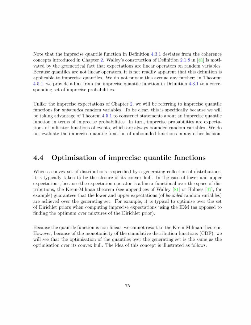
Note that the imprecise quantile function in Definition 4.3.1 deviates from the coherenceconcepts introduced in Chapter 2. Walley’s construction of Definition 2.1.8 in [81] is moti-vated by the geometrical fact that expectations are linear operators on random variables.Because quantiles are not linear operators, it is not readily apparent that this definition isapplicable to imprecise quantiles. We do not pursue this avenue any further: in Theorem4.5.1, we provide a link from the imprecise quantile function in Definition 4.3.1 to a corre-sponding set of imprecise probabilities.
Unlike the imprecise expectations of Chapter 2, we will be referring to imprecise quantilefunctions for unbounded random variables. To be clear, this is specifically because we willbe taking advantage of Theorem 4.5.1 to construct statements about an imprecise quantilefunction in terms of imprecise probabilities. In turn, imprecise probabilities are expecta-tions of indicator functions of events, which are always bounded random variables. We donot evaluate the imprecise quantile function of unbounded functions in any other fashion.
4.4 Optimisation of imprecise quantile functions
When a convex set of distributions is specified by a generating collection of distributions,it is typically taken to be the closure of its convex hull. In the case of lower and upperexpectations, because the expectation operator is a linear functional over the space of dis-tributions, the Krein-Milman theorem (see appendices of Walley [81] or Holmes [47], forexample) guarantees that the lower and upper expectations (of bounded random variables)are achieved over the generating set. For example, it is typical to optimise over the setof Dirichlet priors when computing imprecise expectations using the IDM (as opposed tofinding the optimum over mixtures of the Dirichlet prior).
Because the quantile function is non-linear, we cannot resort to the Krein-Milman theorem.However, because of the monotonicity of the cumulative distribution functions (CDF), wewill see that the optimisation of the quantiles over the generating set is the same as theoptimisation over its convex hull. The idea of this concept is illustrated as follows.
75
Figure 4.1: Four generating CDF’s, along with the lower and upper quantile functionsof this set at percentile p. The yellow and red CDF curves respectively represent theminimising and maximising CDF’s of the quantile function at p.
In Figure 4.1, a set of four CDF’s, M , whose mixture distributions are all the possibleCDF’s enclosed in the area by the four curves. For a fixed percentile p ∈ [0, 1] depictedby the horizontal dashed line, the lower quantile function Q(p) = Q(p)
Conv(M)(X) of some
random variable X is its range value at which any one of the mixtures (and thereforeof the four generating CDF’s) attain or exceed p. Similarly, the upper quantile function
Q(p)
= Q(p)
Conv(M)(X) is the range value at which all the mixtures CDF’s will have attained or
exceeded p. The point here is to see that Q(p) = Q(p)
Conv(M)(X) is in fact achieved by Q(p)
M(X),
the minimisation over the generating set instead of the set of mixtures, and similarly for
Q(p)
= Q(p)
Conv(M)(X) by Q(p)
M (X). That is, like imprecise expectations, we expect that theoptimisation of imprecise quantile functions over a convex set of mixtures is the same asthat of over the generating set, which greatly decreases the computational complexity andconfirms the intuition provided by the extreme value theorem of convex geometry.
We will now provide a rigourous argument of the above intuition.
76

Theorem 4.4.1: For a suitably measurable random variable X, let Fa : a ∈ A be a setof cumulative distribution functions of X indexed by A, a subset of a finite dimensionalEuclidean space equipped with the Lebesgue measure. Write the shorthand Q
(p)F as the
p-th quantile function of X under a cumulative distribution function F . Write
ΛA = λ ∈ RA :
∫λ(a)da = 1 ∧ (∀a : λ(a) ≥ 0),
as a set of mixing functions such that, for a fixed λ ∈ ΛA, a mixture over Fa : a ∈ A isrepresentable as,
Fλ : q 7−→∫λ(a)Fa(q)da.
(We allow λ to be a generalised function such as the Dirac delta function.) Then, for everyfixed p ∈ [0, 1],
Q(p)
ΛA= inf
λ∈ΛAQ
(p)Fλ
= infa∈A
Q(p)Fa
= Q(p)
A,
andQ
(p)
ΛA= sup
λ∈ΛA
Q(p)Fλ
= supa∈A
Q(p)Fa
= Q(p)
A ,
Proof: We will prove the infimum case only, as the supremum case can be analogouslyproven.
Because the minimisation over A is equivalent to minimising over the point mixture massesδa(·) : a ∈ A which is a subset of ΛA, the infimum over the latter larger set is smallerthan of that over the former smaller subset,
Q(p)
ΛA= inf
λ∈ΛAQ
(p)Fλ≤ inf
a∈AQ
(p)Fa
= Q(p)
A,
On the other hand, for any set of distritbutions M and real number q0, we have,
infF∈M
Q(p)F ≥ q0 ⇐⇒ ∀F ∈M : Q
(p)F ≥ q0 ⇐⇒ ∀F ∈M : F (q0) ≤ p ⇐⇒ sup
F∈MF (q0) ≤ p.
This is such that, setting q0 = Q(p)
A,
∀a ∈ A : Q(p)Fa≥ Q(p)
A
⇒ supa∈A
Fa(Q(p)
A) ≤ p,
⇒ PMA(X ≤ Q(p)
A) ≤ p.
77
Recall that an upper probability of an event is an upper expectation of the indicator variableof this event, which in turn is a bounded random variable. Then, the lower envelopetheorem 2.2.1 can be applied here, implying that the optimisation over a generated convexset of distributions is the optimisation over the generating set,
⇒ PMΛA(X ≤ Q(p)
A) ≤ p,
⇒ supλ∈ΛA
Fλ(Q(p)
A) ≤ p,
⇒ infλ∈ΛA
Q(p)Fλ≥ Q(p)
A,
which is the other side of the inequality, completing the proof.
The theorem implies that, for every p for which the quantiles are desired, the minimumand maximum quantiles over the convex set of mixtures over A may be computed by op-timising over A directly. Notice that the random variable does not need to be boundedin this result: we merely need the fact that imprecise CDF’s are imprecise expectations ofindicator functions of events about X are bounded functions.
4.5 Properties of imprecise quantile functions
Because the quantile function is not necessarily expressible through algebraic operationsusing expectations, its imprecise version is not necessarily expressible as an optimisationof expectations. Instead, we will rely on the relationship between the quantile and thecumulative distribution function, as follows.
4.5.1 Random variables need not be bounded
First and foremost, we do not require that the random variable for which we computeimprecise quantile function values be bounded. Again, this is because the imprecise quan-tile function is associated with imprecise probabilities: the boundedness requirements ofChapter 2 are automatically satisfied considering that the latter are imprecise expectationsof indicator variables that are bounded.
78
4.5.2 Relation to imprecise probabilities
We now show the connection between the lower and upper imprecise quantile functionsover a closed set of distributions M to the lower and upper probabilities over this sameset.
Lemma 4.5.1: Let PM and PM be coherent lower and upper probabilities over a closedset of distributions M . Then,
∀P ∈M : P (A) > α ⇐⇒ PM(A) > α,
∀P ∈M : P (A) < α ⇐⇒ PM(A) < α.
Proof: We prove the first statement only, since the other can be proven in an analogousmanner. It is clear that,
PM(A) > α⇒ ∀P ∈M : P (A) > α.
On the other hand,
∀P ∈M : P (A) > α ⇐⇒ PM(A) = infP∈M
P (A) > α.
The strictness of the right inequality is given by noting that, from Theorems 2.2.1 and2.2.2, the infimum on the right is a coherent lower probability and is therefore attainableby an element in M . Strictness follows since the inequality is strict for each element P inM by assumption.
Theorem 4.5.1: For α ∈ [0, 1], q ∈ R, M a closed set of distributions such that PM andPM are coherent, X a suitably measurable random variable,
Q(α)
M[X] > q ⇐⇒ α > PM [X ≤ q],
Q(α)
M[X] ≤ q ⇐⇒ α ≤ PM [X ≤ q],
Q(α)
M [X] > q ⇐⇒ α > PM [X ≤ q],
andQ
(α)
M [X] ≤ q ⇐⇒ α ≤ PM [X ≤ q].
79
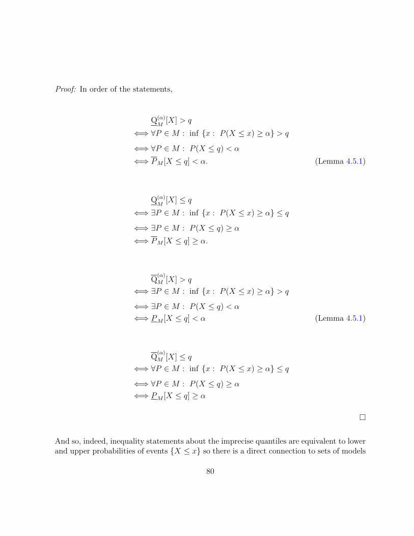
Proof: In order of the statements,
Q(α)
M[X] > q
⇐⇒ ∀P ∈M : inf x : P (X ≤ x) ≥ α > q
⇐⇒ ∀P ∈M : P (X ≤ q) < α
⇐⇒ PM [X ≤ q] < α. (Lemma 4.5.1)
Q(α)
M[X] ≤ q
⇐⇒ ∃P ∈M : inf x : P (X ≤ x) ≥ α ≤ q
⇐⇒ ∃P ∈M : P (X ≤ q) ≥ α
⇐⇒ PM [X ≤ q] ≥ α.
Q(α)
M [X] > q
⇐⇒ ∃P ∈M : inf x : P (X ≤ x) ≥ α > q
⇐⇒ ∃P ∈M : P (X ≤ q) < α
⇐⇒ PM [X ≤ q] < α (Lemma 4.5.1)
Q(α)
M [X] ≤ q
⇐⇒ ∀P ∈M : inf x : P (X ≤ x) ≥ α ≤ q
⇐⇒ ∀P ∈M : P (X ≤ q) ≥ α
⇐⇒ PM [X ≤ q] ≥ α
And so, indeed, inequality statements about the imprecise quantiles are equivalent to lowerand upper probabilities of events X ≤ x so there is a direct connection to sets of models
80
used in statistical applications.
However, they only provide bounds to lower and upper probabilities, thus they are notequivalent to equality statements about coherent values of lower and upper probabilities(recall that a coherent value for, say, a lower probability, is one which achieves the tightminimum over a set of distributions, as opposed to a possibly loose bound).
There are two properties of CDF’s that prevent such equality statements. First, CDF’smay be flat, such that the quantile function is not a unique inverse function of the CDF.This means that, in general, for any real number q, percentile p, CDF F ,
F (q) = p⇒ Q(p)F = q.
Secondly, vertical discontinuities in a CDF may prevent it from achieving all percentiles.That is, evaluating a CDF at its p-th quantile value may not result in p:
F (q) = p⇐ Q(p)F = q.
Conversely, a CDF that does is strictly increasing and continuous everywhere satisfies,
F (q) = p ⇐⇒ Q(p)F = q.
To generalise this to imprecise probabilities, suppose that, for some fixed q, the minimisa-tion of an imprecise CDF F (q) = P (X ≤ q) is achieved by some F0 in its set of distributionsM at p = F0(q). That is, by the lower envelope theorem, Theorem 2.2.1, and Theorem2.2.2 that the lower envelope over M is attainable by an element of M , we have,
∀F ∈M : F (q) ≥ p, ∃F0 ∈M : F0(q) = p.
If F0 is also continuous and strictly increasing at q, then,
∀F ∈M : Q(p)F ≤ p, ∃F0 ∈M : Q
(p)F0
= q,
is equivalent to the above statement. Finally, Theorem 4.4.1 implies that the above opti-misation of the quantile function coincides with the imprecise quantile function over M :that is,
Q(p)
M= q.
81
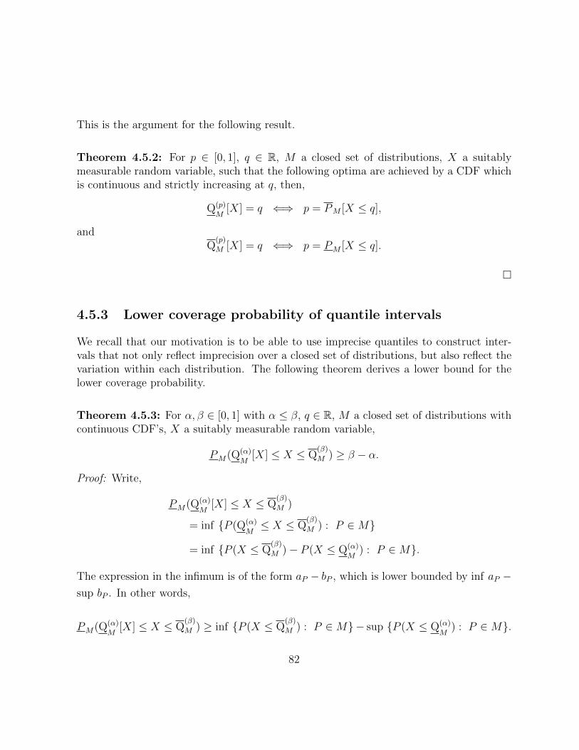
This is the argument for the following result.
Theorem 4.5.2: For p ∈ [0, 1], q ∈ R, M a closed set of distributions, X a suitablymeasurable random variable, such that the following optima are achieved by a CDF whichis continuous and strictly increasing at q, then,
Q(p)
M[X] = q ⇐⇒ p = PM [X ≤ q],
andQ
(p)
M [X] = q ⇐⇒ p = PM [X ≤ q].
4.5.3 Lower coverage probability of quantile intervals
We recall that our motivation is to be able to use imprecise quantiles to construct inter-vals that not only reflect imprecision over a closed set of distributions, but also reflect thevariation within each distribution. The following theorem derives a lower bound for thelower coverage probability.
Theorem 4.5.3: For α, β ∈ [0, 1] with α ≤ β, q ∈ R, M a closed set of distributions withcontinuous CDF’s, X a suitably measurable random variable,
PM(Q(α)
M[X] ≤ X ≤ Q
(β)
M ) ≥ β − α.
Proof: Write,
PM(Q(α)
M[X] ≤ X ≤ Q
(β)
M )
= inf P (Q(α)
M≤ X ≤ Q
(β)
M ) : P ∈M
= inf P (X ≤ Q(β)
M )− P (X ≤ Q(α)
M) : P ∈M.
The expression in the infimum is of the form aP − bP , which is lower bounded by inf aP −sup bP . In other words,
PM(Q(α)
M[X] ≤ X ≤ Q
(β)
M ) ≥ inf P (X ≤ Q(β)
M ) : P ∈M− sup P (X ≤ Q(α)
M) : P ∈M.
82
But, by definition,
Q(β)
M (X) = supP∈M
(Q
(β)P (X)
).
Q(β)
M(X) = inf
P∈MQ
(β)P (X).
Using Theorem 4.5.2 and that the CDF’s are continuous by assumption directly yields,
infP∈M
P (X ≤ Q(β)
M ) = β.
supP∈M
P (X ≤ Q(α)
M) = α.
This completes the proof.
From an inferential perspective, the coverage probability of the interval [Q(α)
M,Q
(β)
M ] mea-sured with each distributions in M is at least β − α. In terms of the Bayesian sensitivityanalysis methodology, this interval has credibility of at least β − α over each distributionin M .
4.6 Hypothesis testing using imprecise quantile inter-
vals
Care should be taken when interpreting inference about questions involving hypotheses ofBayesian probability of zero. A common Bayesian response is that a hypothesis of measurezero cannot be realised exactly, and so is not a valid hypothesis to test when the proce-dure involves its measure. For example, Gelman et al. [41] and Berger [11] interprets thissituation as it is ‘unlikely’ for a real parameter to be (known to be) precisely an exactreal number under continuous distributions. Nevertheless, this hypothesis may representan important question of study. For example, we may ask: ‘Are categorical variables Xand Y independent?’ Typically, this corresponds to the hypothesis that the their log oddsis zero, forming the hypothesis H = θ : log ρ(θ) = 0 for some θ that is multinomial:this hypothesis has measure zero whenever the prior is dominated by the Lebesgue measure.
83
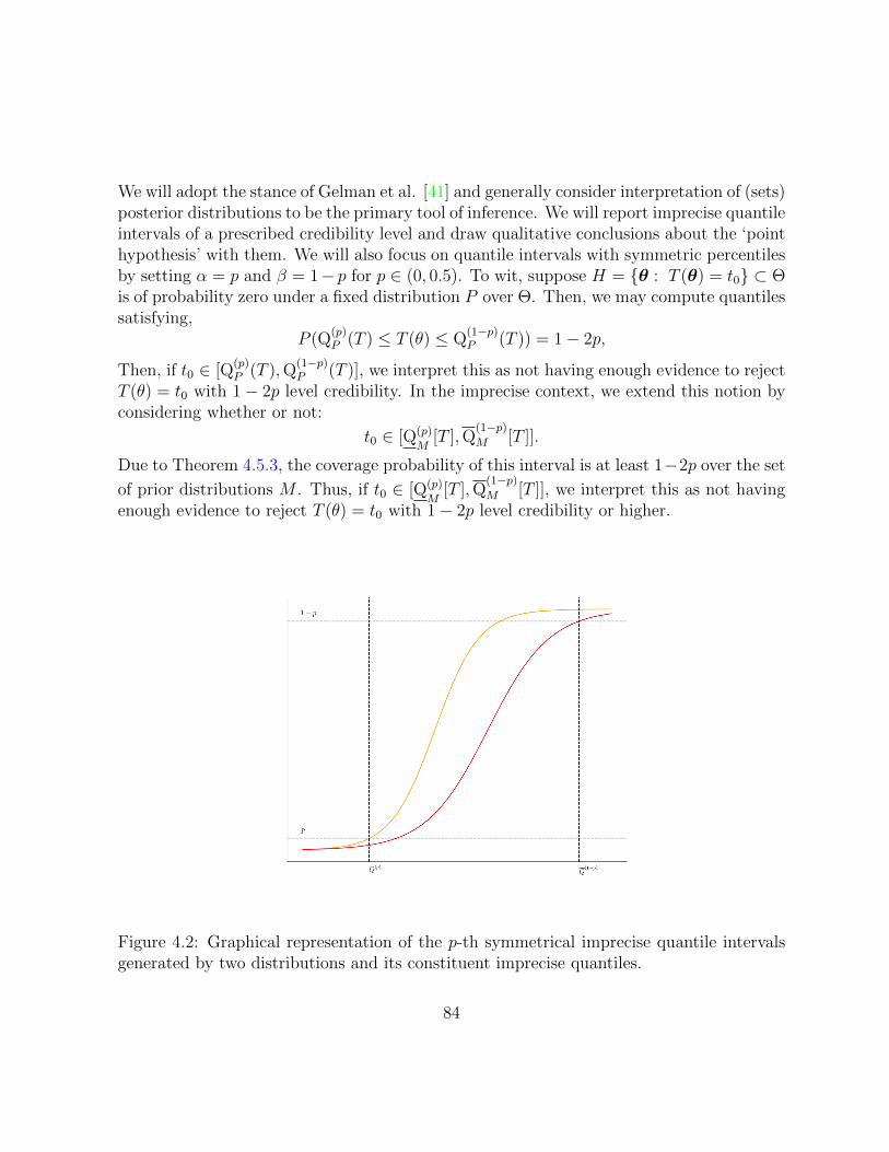
We will adopt the stance of Gelman et al. [41] and generally consider interpretation of (sets)posterior distributions to be the primary tool of inference. We will report imprecise quantileintervals of a prescribed credibility level and draw qualitative conclusions about the ‘pointhypothesis’ with them. We will also focus on quantile intervals with symmetric percentilesby setting α = p and β = 1− p for p ∈ (0, 0.5). To wit, suppose H = θ : T (θ) = t0 ⊂ Θis of probability zero under a fixed distribution P over Θ. Then, we may compute quantilessatisfying,
P (Q(p)P (T ) ≤ T (θ) ≤ Q
(1−p)P (T )) = 1− 2p,
Then, if t0 ∈ [Q(p)P (T ),Q
(1−p)P (T )], we interpret this as not having enough evidence to reject
T (θ) = t0 with 1− 2p level credibility. In the imprecise context, we extend this notion byconsidering whether or not:
t0 ∈ [Q(p)
M[T ],Q
(1−p)M [T ]].
Due to Theorem 4.5.3, the coverage probability of this interval is at least 1−2p over the set
of prior distributions M . Thus, if t0 ∈ [Q(p)
M[T ],Q
(1−p)M [T ]], we interpret this as not having
enough evidence to reject T (θ) = t0 with 1− 2p level credibility or higher.
Figure 4.2: Graphical representation of the p-th symmetrical imprecise quantile intervalsgenerated by two distributions and its constituent imprecise quantiles.
84
From a sensitivity analysis perspective, for p < 0.5, the imprecise interval [Q(p)
M(X),Q
(1−p)M (X)]
contains all the p-symmetrical intervals [Q(p)P (X),Q
(1−p)P (X)] for all P ∈M .
4.7 Dataset Examples
We now consider inference arising from using the imprecise quantiles with the IDM. Weapply the IDM to the same inferential problem and compare it with the conclusions drawnunder the methodology of its original author. To observe the effect of different levels ofprior imprecision, we perform inference with increasing values of ν.
Example 4.7.1: Lady Tea Tasting (Fisher [38])
We follow Agresti’s [3] of Fisher’s [38] classical example of contingency table analysis. Thisis a small sample table containing the data,
Guess Milk First Guess Tea First
Milk First 3 1Tea First 1 3
For indexing, let ij denote the i-th row and j-th column. The experiment is set up suchthat the marginal sums are known beforehand: the rows marginals are known becauseexactly four of cups of teas are poured with milk first and four with tea first, and thecolumns are known ahead because the lady was told this information before guessing. Theparameter of interest is,
ρ(θ) =θ11/θ12
θ21/θ22
=θ11θ22
θ12θ21
.
When all the margins are known, the contingency table follows a hypergeometric sampling.In this case, n11 exactly follows a hypergeometric distribution with the probability P (n11 =t) interpreted as ‘drawing without replacement’ from 8 cups of teas with 4 of them havingmilk first. Furthermore, n11 fully determines the table when the margins are given, and,under the null hypothesis of independent sampling ρ = 1 such that the hypergeometricdistribution is an exact distribution for n11, larger values of the test statistic n11 is evidencefor θ11 > 1 (Agresti [3]).
85
With this test statistic and null distribution, the one-sided test for,
H0 : ρ = 1, Ha : ρ > 1 ,
was performed and, for values n11 = 0, 1, 2, 3, 4 (the number of trials in which the ladyguesses correctly), the corresponding p-values are 1.0, 0.986, 0.757, 0.243 and 0.014 (Agresti[1]): the p-value for this particular table is 0.243 for n11 = 3.
We now focus on inference on the parameter log ρ(θ) using the IDM and infer about thenull hypothesis log ρ(θ) = 0 (which is equivalent to ρ(θ) = 1) at a credibility level of 95-%.
ν = 0.5 1.0 2.0 5.0 10.0
Q(0.025), Q(0.025)
(-1.457, 0.303) (-1.82, 0.484) (-2.232, 0.868) (-3.288, 1.662) (-4.274, 2.499)
Q(0.975), Q(0.975)
(5.329, 8.729) (4.515, 9.086) (3.371, 9.212) (1.549, 9.943) (0.1, 10.654)
For all tested values of ν, the intervals [Q(0.025)
M(log(ρ(θ)),Q
(0.975)
M (log(ρ(θ))] extend furtherto the right of 0 than to the left of it: this reflects the pattern in the data in which the di-agonals are larger than the off-diagonals. In terms of the credibility of H0, all the intervals
[Q(0.025)
M(log(ρ(θ)),Q
(0.975)
M (log(ρ(θ))] contain the null value θ0 = 0.
Interestingly, the imprecise 2.5-% quantiles, [Q(0.025)
M(log(ρ(θ)),Q
(0.025)
M (log(ρ(θ))], also allcontain the value of θ0 = 0. That is, some posterior distributions in the IDM are suchthat P (log ρ ≤ 0) ≤ 0.025. This suggests that, even at an imprecision level as small asν = 0.5, there is disagreement amongst the members of the posterior IDM set of distri-butions in terms of the left side threshold of 2.5-%. In relation to the sensitivity analysis,some priors in the IDM achieve one-sided posterior (Bayesian) p-values of less than 0.025but some do not. This points to the curious question of which distributions in M yieldQ
(0.025)P (log(ρ(θ))) that are to the left or to the right of zero: it may be useful to identify
similarities amongst prior Dirichlet distributions that induce values on each side of the nullhypothesis.
In the following examples, we examine what happens when we apply the imprecise quantilefunctions of the IDM to contingency tables with zero observations in the cells. Due to our
86
interpreting the imprecise quantile intervals via the coherent imprecise probabilities as inTheorems 4.5.1 and 4.5.2, the validity of computing posterior imprecise probabilities withthe IDM over such datasets are dealt with as per the development in Chapter 3, where wedetailed the construction of the posterior IDM imprecise expectation for such cases.
Example 4.7.2: Promotion/Racial Bias (Agresti [1], method from Birch [15])
This example illustrates that hypothesis testing with imprecise quantile intervals from theIDM can be highly sensitive to the hyperparameter ν. This is due to the IDM’s set ofDirichlet priors consisting of hyperparameter values να over all possible α ∈ 4m, causingit to include prior distributions with α being close to the extreme points of 4m. Numer-ically, we will see that the IDM produces some extreme values for imprecise quantiles forthe following log-odds statistic.
Consider the following dataset tabulating the promotion of each person in a group ofcomputer scientists (Gastwirth [40]) based on their race and stratified over three months:
Promotion Not Promoted PromotedRace Month
BlackJuly 7 0August 7 0September 8 0
WhiteJuly 16 4August 13 4September 13 2
For indexing, let ijk index over race (B,W), promotion (N,P) and the month (J,A, S),respectively. The goal of this example is to determine the conditional independence of raceand promotion variables given the month variable.
Agresti performed the inference under three assumptions. First, the sampling was doneindependently. (Agresti notes that the information about the overlapping of employeepromotion applications over the three months is not available.) Secondly, the test by Birch[15] requires the assumption that the odds ratios over the stratifying variable are equal:that is, for all k, k′ = J,A, S in the months variable,
ρk =θBNkθWPk
θBPkθWNk
=θBNk′θWPk′
θBPk′θWNk′= ρk′ .
87
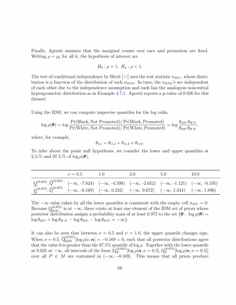
Finally, Agresti assumes that the marginal counts over race and promotion are fixed.Writing ρ = ρk for all k, the hypothesis of interest are
H0 : ρ = 1, Ha : ρ < 1.
The test of conditional independence by Birch [15] uses the test statistic nBN ·, whose distri-bution is a function of the distribution of each nBNk. In turn, the nBNk’s are independentof each other due to the independence assumption and each has the analogous noncentralhypergeometric distribution as in Example 4.7.1. Agresti reports a p-value of 0.026 for thisdataset.
Using the IDM, we can compute imprecise quantiles for the log odds,
log ρ(θ) = logPr(Black,Not Promoted)/Pr(Black,Promoted)
Pr(White,Not Promoted)/Pr(White,Promoted)= log
θBN ·θWP ·
θBP ·θWN ·,
where, for example,θ11· = θ11J + θ11A + θ11S.
To infer about the point null hypothesis, we consider the lower and upper quantiles at2.5-% and 97.5-% of log ρ(θ),
ν = 0.5 1.0 2.0 5.0 10.0
Q(0.025), Q(0.025)
(−∞, -7.824) (−∞, -4.599) (−∞, -2.652) (−∞, -1.121) (−∞, -0.195)
Q(0.975), Q(0.975)
(−∞, -0.169) (−∞, 0.232) (−∞, 0.672) (−∞, 1.344) (−∞, 1.896)
The −∞ value taken by all the lower quantiles is consistent with the empty cell nBN · = 0.Because Q(0.975)
IDMis at −∞, there exists at least one element of the IDM set of priors whose
posterior distribution assigns a probability mass of at least 0.975 to the set θ : log ρ(θ) =log θBP · + log θWN · − log θBN · − log θWP · = −∞.
It can also be seen that between ν = 0.5 and ν = 1.0, the upper quantile changes sign.
When ν = 0.5, Q(0.975)
IDM [log ρ|ν,n] = −0.169 < 0, such that all posterior distributions agreethat the value 0 is greater than the 97.5% quantile of log ρ. Together with the lower quantileat 0.025 at −∞, all intervals of the form [Q
(0.025)P [log ρ|n, ν = 0.5],Q
(0.975)P [log ρ|n, ν = 0.5]]
over all P ∈ M are contained in (−∞,−0.169]. This means that all priors produce
88
2.5% − 97.5% quantile intervals that do not contain zero, lending evidence at credibil-ity level 0.05 of rejecting the hypothesis log ρ ≥ 0.
On the other hand, for ν ≥ 1.0, the imprecise interval [Q(0.025)
M(log ρ|n, ν),Q
(0.975)
M (log ρ|n, ν)]
contain 0. Combined with the fact that Q(0.025)
M (log ρ|n, ν) < 0 for all tested values of ν, itmeans that there exists at least one P ∈M whose 2.5%− 97.5% quantile interval contains0. Unlike the case of ν = 0.5, there is no definite consensus amongst the priors for ν ≥ 1.0.In other words, at ν = 0.5, all priors lend credibility to the system being not independentat level 97.5%, roughly in agreement with the classical test. However, when ν ≥ 1.0, atleast one prior will not yield this conclusion. This demonstrates the sensitivity of the in-ference to the IDM hyperparameter ν, as discussed at the beginning of this example.
Example 4.7.3: (Probability of a girl birth given placenta previa [41])
This example illustrates the behaviour of the IDM imprecise quantiles when the samplesize is large and the number of observations in all categories are far from zero. It alsocompares the inference from an IDM model to the inference from a Bayesian treatmentusing a single Dirichlet prior. Because of this, the example also highlights the fact that theIDM inference includes a global analysis over the family of models considered, as opposedto the local analysis performed on a finite number of models post-hoc of Bayesian inference.
Placenta previa is a ‘condition of pregnancy in which the placenta is ... obstructing thefetus from normal vaginal delivery.’ Gelman et al. [41] cite a data set of placenta previabirths from Germany with 437 female births out of 980, and they are interested in the in-ference of the proportion of female births under this condition, and the odds ratio betweenthe births two genders under this condition. In particular, they wish to test the hypothesisthat the proportion is less than 0.485.
One of their precise Bayesian treatments is as follows. Let θ be the probability of a fe-male birth under the placenta previa condition. A Beta(1, 1) prior distribution was usedwith a binomial likelihood: using the Germany dataset, the posterior distribution for θ isBeta(438, 544). The statistics of interest are θ and (1 − θ)/θ. The authors report 95%posterior intervals of [0.415, 0.477] and [1.10, 1.41] for θ and (1− θ)/θ, respectively.
89
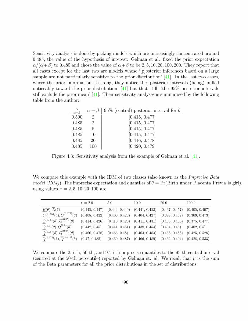
Sensitivity analysis is done by picking models which are increasingly concentrated around0.485, the value of the hypothesis of interest: Gelman et al. fixed the prior expectationα/(α+β) to 0.485 and chose the value of α+β to be 2, 5, 10, 20, 100, 200. They report thatall cases except for the last two are models whose ‘[p]osterior inferences based on a largesample are not particularly sensitive to the prior distribution’ [41]. In the last two cases,where the prior information is strong, they notice the ‘posterior intervals (being) pullednoticeably toward the prior distribution’ [41] but that still, ‘the 95% posterior intervalsstill exclude the prior mean’ [41]. Their sensitivity analyses is summarised by the followingtable from the author:
αα+β
α + β 95% (central) posterior interval for θ
0.500 2 [0.415, 0.477]0.485 2 [0.415, 0.477]0.485 5 [0.415, 0.477]0.485 10 [0.415, 0.477]0.485 20 [0.416, 0.478]0.485 100 [0.420, 0.479]
Figure 4.3: Sensitivity analysis from the example of Gelman et al. [41].
We compare this example with the IDM of two classes (also known as the Imprecise Betamodel (IBM)). The imprecise expectation and quantiles of θ = Pr(Birth under Placenta Previa is girl),using values ν = 2, 5, 10, 20, 100 are:
ν = 2.0 5.0 10.0 20.0 100.0
E(θ), E(θ) (0.445, 0.447) (0.444, 0.449) (0.441, 0.452) (0.437, 0.457) (0.405, 0.497)
Q(0.025)(θ), Q(0.025)
(θ) (0.408, 0.422) (0.406, 0.423) (0.404, 0.427) (0.399, 0.432) (0.369, 0.473)
Q(0.05)(θ), Q(0.05)
(θ) (0.414, 0.426) (0.413, 0.428) (0.411, 0.431) (0.406, 0.436) (0.375, 0.477)
Q(0.5)(θ), Q(0.5)
(θ) (0.442, 0.45) (0.441, 0.451) (0.438, 0.454) (0.434, 0.46) (0.402, 0.5)
Q(0.95)(θ), Q(0.95)
(θ) (0.466, 0.478) (0.465, 0.48) (0.463, 0.483) (0.458, 0.488) (0.425, 0.528)
Q(0.975)(θ), Q(0.975)
(θ) (0.47, 0.485) (0.469, 0.487) (0.466, 0.489) (0.462, 0.494) (0.428, 0.533)
We compare the 2.5-th, 50-th, and 97.5-th imprecise quantiles to the 95-th central interval(centred at the 50-th percentile) reported by Gelman et. al. We recall that ν is the sumof the Beta parameters for all the prior distributions in the set of distributions.
90
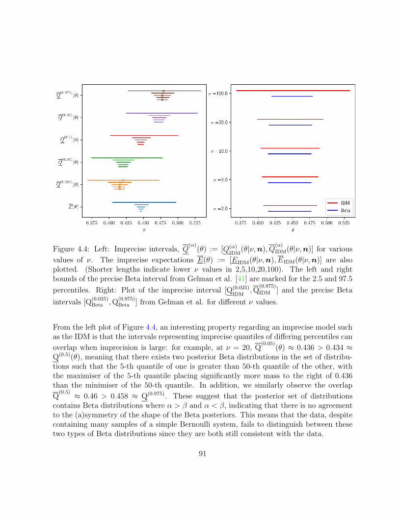
Figure 4.4: Left: Imprecise intervals, Q(α)
(θ) := [Q(α)
IDM(θ|ν,n), Q
(α)
IDM(θ|ν,n)] for various
values of ν. The imprecise expectations E(θ) := [EIDM(θ|ν,n), EIDM(θ|ν,n)] are alsoplotted. (Shorter lengths indicate lower ν values in 2,5,10,20,100). The left and rightbounds of the precise Beta interval from Gelman et al. [41] are marked for the 2.5 and 97.5
percentiles. Right: Plot of the imprecise interval [Q(0.025)
IDM,Q
(0.975)
IDM ] and the precise Beta
intervals [Q(0.025)Beta ,Q
(0.975)Beta ] from Gelman et al. for different ν values.
From the left plot of Figure 4.4, an interesting property regarding an imprecise model suchas the IDM is that the intervals representing imprecise quantiles of differing percentiles can
overlap when imprecision is large: for example, at ν = 20, Q(0.05)
(θ) ≈ 0.436 > 0.434 ≈Q(0.5)(θ), meaning that there exists two posterior Beta distributions in the set of distribu-tions such that the 5-th quantile of one is greater than 50-th quantile of the other, withthe maximiser of the 5-th quantile placing significantly more mass to the right of 0.436than the minimiser of the 50-th quantile. In addition, we similarly observe the overlap
Q(0.5) ≈ 0.46 > 0.458 ≈ Q(0.975). These suggest that the posterior set of distributions
contains Beta distributions where α > β and α < β, indicating that there is no agreementto the (a)symmetry of the shape of the Beta posteriors. This means that the data, despitecontaining many samples of a simple Bernoulli system, fails to distinguish between thesetwo types of Beta distributions since they are both still consistent with the data.
91

Example 4.7.4: Opinion on government spending on the arts (Agresti [2], Table 11.1,Section 11.2.5)
This example again compares the IDM to the Bayesian treatment with a single Dirchletprior. We examine the effect of imprecision on inference when the dataset is both small-sample, contains a zero observation one category and one observation in another. We willsee that IDM yields a range of posterior values which are consistent with the model’s set ofDirichlet priors: these values will turn out to be quite different than the values obtained byAgresti using a single prior. This reflects the sensitivity to prior specification for inferencein situations such as this.
The following dataset describes the opinions of 23 female survey takers of ages 18 to 21 ongovernment spending on culture and the arts.
Opinion Much More More Same Less Much Less
1 7 12 3 0
Note that not only is this a somewhat small sample, but also the data contains a cell withzero observations (the ‘Much Less’ category).
Agresti models the multinomial cell probabilities with a Dirichlet prior with equal relativeweights differing concentrations: the goal is to regularise the cell probabilities estimates inlight of the small sample size and having zero observation in some categories. Note thatthe prior implies that the modeller believes that, in expectation, all cell probabilities areequal. The Bayes’ point estimates are given as follows (Agresti [2]),
Much More More Same Less Much Lessν = 1 0.050 0.300 0.508 0.133 0.008ν = 5 0.071 0.286 0.464 0.143 0.036ν = 20 0.116 0.256 0.372 0.163 0.093
(Credible intervals were not provided by Agresti.) We run the IDM inference also usingν = 1, 5, 20 for the imprecise expectations of the cell probabilities:
92
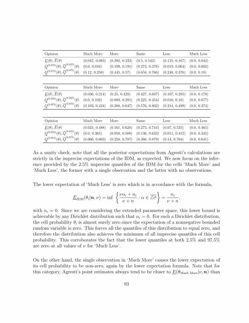
Opinion Much More More Same Less Much Less
E(θ), E(θ) (0.042, 0.083) (0.292, 0.333) (0.5, 0.542) (0.125, 0.167) (0.0, 0.042)
Q(0.025)(θ), Q(0.025)
(θ) (0.0, 0.016) (0.109, 0.191) (0.273, 0.378) (0.019, 0.064) (0.0, 0.002)
Q(0.975)(θ), Q(0.975)
(θ) (0.12, 0.258) (0.445, 0.57) (0.658, 0.766) (0.248, 0.376) (0.0, 0.18)
Opinion Much More More Same Less Much Less
E(θ), E(θ) (0.036, 0.214) (0.25, 0.429) (0.427, 0.607) (0.107, 0.285) (0.0, 0.178)
Q(0.025)(θ), Q(0.025)
(θ) (0.0, 0.102) (0.093, 0.281) (0.225, 0.454) (0.016, 0.16) (0.0, 0.077)
Q(0.975)(θ), Q(0.975)
(θ) (0.103, 0.424) (0.388, 0.647) (0.576, 0.802) (0.214, 0.499) (0.0, 0.374)
Opinion Much More More Same Less Much Less
E(θ), E(θ) (0.023, 0.488) (0.161, 0.628) (0.275, 0.744) (0.07, 0.535) (0.0, 0.465)
Q(0.025)(θ), Q(0.025)
(θ) (0.0, 0.365) (0.058, 0.508) (0.136, 0.633) (0.011, 0.412) (0.0, 0.345)
Q(0.975)(θ), Q(0.975)
(θ) (0.066, 0.663) (0.258, 0.787) (0.386, 0.879) (0.14, 0.704) (0.0, 0.641)
As a sanity check, note that all the posterior expectations from Agresti’s calculations arestrictly in the imprecise expectations of the IDM, as expected. We now focus on the infer-ence provided by the 2.5% imprecise quantiles of the IDM for the cells ‘Much More’ and‘Much Less’, the former with a single observation and the latter with no observations.
The lower expectation of ‘Much Less’ is zero which is in accordance with the formula,
EIDM(θi|n, ν) = inf
ναi + niν + n
: α ∈ 4p
=
niν + n
,
with ni = 0. Since we are considering the extended parameter space, this lower bound isachievable by any Dirichlet distribution such that αi = 0. For such a Dirichlet distribution,the cell probability θi is almost surely zero since the expectation of a nonnegative boundedrandom variable is zero. This forces all the quantiles of this distribution to equal zero, andtherefore the distribution also achieves the minimum of all imprecise quantiles of this cellprobability. This corroborates the fact that the lower quantiles at both 2.5% and 97.5%are zero at all values of ν for ‘Much Less’.
On the other hand, the single observation in ‘Much More’ causes the lower expectation ofits cell probability to be non-zero, again by the lower expectation formula. Note that forthis category, Agresti’s point estimates always tend to be closer to E(θMuch More|ν,n) than
93
to E(θMuch More|ν,n), the former of which being brought away from zero due to the singleobservation. This corroborates the possibility that, since Agresti started with a uniformDirichlet distribution, the low cell count in the data relative to other categories is reflectedhere. However, this also means that the fact that there are other posterior expectationsup to E(θ) is also consistent with the global sensitivity analysis it provides. The inferenceis therefore sensitive to the prior as there is only one count in the cell of interest, andthis is reflected by the imprecise expectation [EIDM(θMuch More|ν,n), EIDM(θMuch More|ν,n)]containing values which are very different from the single point estimate of using a singleuniform Dirichlet prior as in Agresti.
4.8 Concluding remarks
Our contributions in this chapters are as follows. We define the imprecise quantile function,the centerpiece of this chapter, in Definition 4.3.1. Theorems 4.4.1, 4.5.1 and 4.5.2 describesome of its imprecise-probabilistic properties. Theorem 4.5.3 guarantees a lower bound ofthe coverage probability of an interval using quantiles derived from the imprecise quan-tile function. Section 4.6 discusses the interpretation of the imprecise quantile function inprior/posterior inference settings, while Examples 4.7.1, 4.7.2, 4.7.3, 4.7.4 demonstrate itsapplication on real-life datasets.
We have defined the imprecise analogue of a quantile function and shown that, like theimprecise expectations, the optimisation of the lower and upper quantile functions over aset of mixtures induced by some set of distributions M can be achieved within M . Becausethe quantile function is a nonlinear functional and, in a dual manner, CDF’s of sums do notgenerally decompose into sums of CDF’s of the component random variables, the impre-cise quantile is not necessarily coherent. Nevertheless, we noted that they are valuable forinterpretation in two ways: they are properly a sensitivity analysis of the quantile functionover a set of distributions and that they have logically equivalent statements in terms ofbounds on the lower and upper CDF’s. In the case that the CDF’s are all continuous,these bounds are tight and statements about imprecise quantiles are exactly statementsabout lower and upper CDF’s, not just their bounds (Theorem 4.5.2).
Further, we used such imprecise quantiles to construct imprecise interval statistics that has
94
the sensitivity analysis interpretation of containing all the quantile intervals induced by themixture of the generating set of distributions. Unlike the imprecise expectation, which is aset of point estimates over the inducing set of distributions, imprecise interval formed usingquantiles also measures variations due to the randomness contributed by each distributionas well. Furthermore, despite the quantiles themselves not necessarily coherent, we haveshown that the lower coverage probability of our imprecise quantile interval using the α-thand β-th quantiles (α < β) is at least lower bounded by the nominal coverage probabilityβ − α of each model in the set of distributions. This provides an imprecise analogue tothe use of credible intervals in the precise Bayesian framework. We have compared ourmethodology to existing methodologies of other authors.
It is interesting to note that the construction of the imprecise quantile functions is anexample of coherence departing from sensitivity analysis. By this, we mean that, unlikethe imprecise expectation where the lower envelope theorem (Theorem 2.2.1) implies thatcoherence is equivalent to tight bounds of sensitivity analysis (that is, minimisation andmaximisation) of expectations over a set of distributions, our construction of imprecisequantiles demonstrates that this need not hold, at least for sensitivity analysis of nonlinearfunctionals.
This represents a divergence between the adherence to coherence in Bayesian analysis (inthe imprecise setting) and sensitivity analysis. In practice, one would like to do the lat-ter, and the imprecise framework allows one to perform such analysis globally on a set ofcandidate (prior) distributions (and such analysis is not post-hoc as it is part of the infer-ential process in the imprecise framework). On the other hand, in principle, the imprecisequantile functions themselves cannot be used as a coherent bounds on from a behaviouralperspective. (See Couso, Moral and Sanchez [30] and Couso and Dubois [28] that gener-alise the notion of gambling and desirability beyond bounds on expectations as coherentassessments.)
95
Chapter 5
On the optimisation problem for thelog-odds inference with IDM
An integral part of inference using imprecise expectations and probabilities is the opti-misation over the elicited set of priors. and it becomes important to characterise the setof optima as part of the qualitative understanding of one’s inference. In this chapter, westudy the specific optimisation problem for the lower expectation of log-odds statisticsunder the IDM model. Under the Dirichlet assumption, the expectation of log-odds is alinear combination of polygamma functions which are individually continuously differen-tiable and monotonic (see Appendix D.2). However, the difference of such functions ismore involved than expected from working with such nice functions individually. We willhighlight key properties of two aspects of the problem: the identification of a subset of thenatural parameters using the Karush-Kuhn-Tucker (KKT) conditions and the propertiesof the objective function over this subset.
5.1 KKT solutions to common log-odds problems
In this section, we study the Karush-Kuhn-Tucker (KKT) conditions of three classes oflog-odds that commonly appear in statistical applications. In particular, we study howknowing the specific structure of the log-odds may further reduce the set of candidate so-lutions to the optimisation problem.
96
5.1.1 An overview of the KKT conditions
The KKT conditions (for example, see [18]) characterise the necessary conditions of aconstrained optimisation problem,
minimise: I(α),
subjected to: g(α) ≤ 0,
h(α) = 0,
where I : Rm 7−→ R, g : Rm → Rl and h : Rm → R represent the objective function,l inequality constraints and a single equality constraint respectively. For the inequalityand equality constraints, a vector µ ∈ Rl and scalar λ ∈ R of multipliers are introducedrespectively. The KKT necessary conditions for (α∗,µ∗, λ∗) to be a constrained minimiserof this problem are,
∇I(α∗) +l∑
k=1
gk∇g(α∗) + λ∗∇h(α∗) = 0
∀i ∈ 1, . . . , l : µ∗i gi(α∗) = 0,
g(α∗) ≤ 0,
h(α∗) = 0,
µ∗ ≥ 0.
In particular, the constraints that α∗ is in the m-simplex is written as,
∀i ∈ 1, . . . ,m : µ∗iα∗i = 0,
∀i ∈ 1, . . . ,m : α∗i ≥ 0,
1−m∑i=1
α∗i = 0,
µ∗ ≥ 0.
The conditions µ∗iα∗i = 0 will be used extensively in what follows: a strategy for reducing
the solution space using the KKT condition is to identify α∗i = 0 by showing that µ∗i > 0using the properties of the stationariry conditions I(α∗)+
∑lk=1 gk∇g(α∗)+λ∗∇h(α∗) = 0.
97
5.1.2 The KKT conditions of posterior log-odds lower expecta-tion under the IDM
We will use two main facts to drive our analyses: the trigamma function ψ′ is strictlypositive over the positive real numbers (see Appendix D.2) and the optimal values of thecomplementary KKT multipliers µ are non-negative (see, for example, Boyd and Vanden-berghe [18]).
Let L be a finite number of categories of the observation multinomial model. The gen-eral form of the IDM posterior lower expectation of the log-odds ratio between two finitecollections A and B of subsets of L,
EIDM
(∑A∈A
log θA −∑B∈B
log θB
∣∣∣∣ ν,n)
= min
∑A∈A
ψ(ναA + nA)−∑B∈B
ψ(ναB + nB) : α ∈ 4L
,
where ψ is the digamma function and, for a vector a = (a1, . . . , am) and a subset C ⊆1, . . . ,m,
aC :=∑i∈C
ai.
We focus on cases where |A|, |B| are at most two, so that we are interested in minimisingthe function,
α 7−→ ψ(ναA1 + nA1) + ψ(ναA2 + nA2)− ψ(ναB1 + nB1)− ψ(ναB2 + nB2).
The Lagrangian equations of the KKT conditions for the minimisers of this problem are,
∇α∗(ψ′(να∗A1
+ nA1) + ψ(να∗A2+ nA2)
−ψ(να∗B1+ nB1)− ψ(να∗B2
+ nB2))
−µ∗ + λ∗1 = 0.
and ψ′ is the trigamma function. We will sometimes denote the digamma and trigammafunctions evaluated at a KKT solution as,
ψC := ψ(να∗C + nC),
98
andψ′C := ψ′(να∗C + nC),
respectively, when we do not need to appeal to the arguments within and wish to simplifynotation.
Notice that, because,∂
∂αiαC ,
is zero when i /∈ C, some trigamma function terms of the Lagrangian equations in someαi’s will become zero depending on whether or not that αi lies in A1, A2, B1, B2 or not. Inparticular, it is useful to distinguish the cases when a category k falls into the numeratoror denominator sets:
k ∈ A1 ∪ A2, k ∈ B1 ∪B2 : ψ′A1[k ∈ A1] + ψ′A2
[k ∈ A2]− ψ′B1[k ∈ B1]− ψ′B2
[k ∈ B2]− µk + λ = 0,
k′ ∈ A1 ∪ A2, k′ /∈ B1 ∪B2 : ψ′A1
[k′ ∈ A1] + ψ′A2[k′ ∈ A2]− µ′k + λ = 0,
k′′ /∈ A1 ∪ A2, k′′ ∈ B1 ∪B2 : − ψ′B1
[k′′ ∈ B1]− ψ′B2[k′′ ∈ B2]− µ′′k + λ = 0,
k′′′ /∈ A1 ∪ A2, k′′′ /∈ B1 ∪B2 : − µ′′′k + λ = 0,
where [k ∈ C] is the indicator function that k is in C. Depending on A1, A2, B1, B2, L,some of these forms may not be present. For example, if the log-odds involves all thecategories in question, such that A1 ∪A2 ∪B1 ∪B2 = L, then the Lagrangian equation ofthe form k′′′ will not be present. Similarly, if A1 ∪ A2 ⊂ B1 ∪ B2, then equations of theclass of k′ will not be present.
The significance of this decomposition is that, for some equations, the positivity of thetrigamma function that is uniform over 4L 3 α can be more readily exploited when theyare present. In particular, we will frequently make use of the following results.
Lemma 5.1.1: When there exists k′ ∈ L such that k′ ∈ A1 ∪ A2 and k′ /∈ B1 ∪B2,
λ < µk′ .
Proof: This follows from,
0 < ψ′A1[k ∈ A1] + ψ′A2
[k ∈ A2] = µk′ − λ.
99
Lemma 5.1.2: When there exists k′′ ∈ L such that k′′ /∈ A1 ∪ A2 and k′′ ∈ B1 ∪B2,
λ > 0.
Proof: This follows from,
0 < ψ′B1[k ∈ B1] + ψ′B2
[k ∈ B2] + µk′′ < λ.
Lemma 5.1.3: When there exists k′′′ ∈ L such that k′′′ /∈ A1 ∪ A2 and k′′′ /∈ B1 ∪B2,
µk′′′ = λ.
Consequently,λ ≥ 0.
Then, for example, if k′, k′′, k′′′ exist, then we can conclude that µk′ , µk′′′ > 0, leading tothe minimiser satisfying α∗k′ , α
∗k′′′ = 0 by the KKT complementary conditions.
As we have alluded at the beginning, we want to use the Lagrangian conditions,
µ∗ = λ∗1 +∇α∗(ψ′(να∗A1
+ nA1) + ψ(να∗A2+ nA2)
−ψ(να∗B1+ nB1)− ψ(να∗B2
+ nB2)).
by identifying which components µ∗k are strictly greater than zero to conclude that, corre-spondingly using the slackness condition µ∗kα
∗k = 0, α∗k = 0. To that end, define,
dk(α;n, ν) := ψ′A1(α;n, ν)[k ∈ A1]+ψ′A2
(α;n, ν)[k ∈ A2]−ψ′B1(α;n, ν)[k ∈ B1]−ψ′B2
, (α;n, ν)[k ∈ B2].
(We will write dk(α) when n and ν are notationally unambiguous.) This is such that thek-th Lagrangian equation can be written succinctly as,
µ∗k = λ∗ + dk(α∗;n, ν).
An equivalent sufficient condition for α∗k = 0 is that dk(α∗;n, ν) +λ∗. This is useful when,
say λ∗ ≥ 0 such that it is sufficient to show dk > 0 to conclude µ∗k > 0. In these cases, the
100
properties of the function dk(α|n, ν) over α parametrised by the data n and the hyperpa-rameter ν becomes of great interest to us.
Note that the sign of dk(α∗), a difference of sums of trigamma functions, is generally
dependent on α and n. For a fixed set of parameters n, ν and a particular k in question,suppose I∗ = i ∈ 1, . . . , L : α∗i = 0 has been identified by, for example, the KKTconditions. Then, our solution space is reduced to the face,
α ∈ 4L : ∀i ∈ I∗, αi = 0..
Now if dk > 0 over this face, then the Lagrangian equation of k can be exploited in asimilar manner to the others: setting αi = 0 for i ∈ I∗, we can write, for any α∗ that is aKKT solution in α ∈ 4L : ∀i ∈ I∗, αi = 0.,
0 < dk(α∗) = µ∗k − λ∗.
leading to,λ∗ < µ∗k.
Otherwise, the KKT complementary slackness condition is not used, and we resort to othermethods of analysis depending on the specifics of the problem. For example, we may iden-tify additional solutions to the constrained optimisation by noticing that dk is in fact thek-th element of the gradient of the objective function (scaled by 1/ν) and considering theproperties of this function over the face identified by I∗.
5.1.3 Log probability ratios
To illustrate the general approach, we look at the most important examples of odds ratiosstatistics.
Let L be a finite number of categories, A,B ⊆ L, ν > 0 be the predefined hyperparameterof the IDM, θ ∈ 4L be a multinomial probability vector over L, and n ∈ NL be a vectorof non-zero counts. We are interested in computing,
EIDM
(log
θAθB
∣∣∣∣ ν,n) = ψ(ναA + nA)− ψ(ναB + nB),
101
where θA =∑
l∈A θl is the sampling probability of the set A.
The possible KKT stationarity conditions for this problem are,
∀k ∈ A, k ∈ B : νψ′A − νψ′B − µk + λ = 0
∀k′ ∈ A, k′ /∈ B : νψ′A − µk′ + λ = 0,
∀k′′ /∈ A, k′′ ∈ B : − νψ′B − µk′′ + λ = 0,
∀k′′′ /∈ A, k′′′ /∈ B : − µk′′′ + λ = 0.
From Lemmas 5.1.1, 5.1.2 and 5.1.3, when the corresponding equations exist, we can de-duce the following algebraic consequences of each of the equations.
∀k′ ∈ A, k′ /∈ B : µk′ > λ.
∀k′′ /∈ A, k′′ ∈ B : λ > 0.
∀k′′′ /∈ A, k′′′ /∈ B : µk′′′ = λ.
More information is needed to analyse the µ’s of two classes k and k′′, and we will do soby a specific problem.
Example 5.1.1: Suppose L = 1, 2, 3, 4, A = 1, 2 and B = 2, 3 and fix a hyperpa-rameter ν and dataset n. Now,
k ∈ A∩B = 2, k′ ∈ A∩Bc = 1, k′′ ∈ Ac∩B = 3, k′′′ ∈ (A∪B)c = 1, 2, 3c = 4,
From k′′ = 3, we deduce,λ > 0.
This is such that µ1, µ4 > 0 and so,
α∗1, α∗4 = 0.
So, our solution space is now restricted to the face consisting of points (0, α2, α3, 0) ∈ 4L,such that α∗3 = 1− α∗2.
In this particularly simple problem, we can directly appeal to the objective function in thisreduced parametrisation,
α2 7−→ ψ(να2 + n1 + n2)− ψ(ν + n2 + n3),
102
and, by the increasing property of the digamma function ψ, the minimum must be α∗2 = 0,leading to α∗3 = 1.
Let us also point out a general pattern in the log-probability problem.
Theorem 5.1.1: Consider non-empty sets A 6= B ⊂ L such that the sets A ∩ Bc andAc ∩ B are nonempty. Then, all minimisers α∗ of the log-probability IDM problem lie onthe face of the simplex 4L satisfying
αAc∩B = 1.
Proof: Given non-empty sets A 6= B ⊂ L such that the sets A ∩ Bc and Ac ∩ B arenonempty, the equations of the type for k′, k′′ exist. So, k′′ yields λ > 0, which ultimatelyleads to µk′ > 0 and α∗k′ = 0. Similarly, µk′′′ > 0 leading to α∗k′′′ = 0. This means thatthe only categories over which to search are in B = (A ∩B) ∪ (Ac ∩B). Over this smallersimplex, the αi’s over B sum to one, and only the categories in A∩B are active variables.To wit, the objective function over B reduces to,
ψ(ναA∩B + nA∩B)− ψ(ν + nB).
Because ψ is monotonically increasing, this function achieves its minimum when α∗A∩B = 0,such that α∗Ac∩B = 1. In the general multivariate setting, any solution on the face ofαAc∩B = 1 can attain the minimum value, so consists of all the minimisers of the problem.Note that this result continues to hold even if A∩B = ∅, as the objective function over Bbecomes constant in this case,
−ψ(ν + nB).
5.1.4 Log odds ratios
Let us extend the analysis of the log-probability ratio to the log-odds case. Again, let Lbe a finite number of categories, A,B ⊆ L, ν > 0 be the predefined hyperparameter ofthe IDM, θ ∈ 4L be a multinomial probability vector over L, and n ∈ NL be a vector ofnon-zero counts. We are interested in computing the following quantity,
103
EIDM
(log
θA(1− θB)
(1− θA)θB
∣∣∣∣ ν,n)= ψ(ναA + nA) + ψ(ναBc + nBc)
− ψ(ναB + nB)− ψ(ναAc + nAc).
We can partition the possible KKT stationarity conditions for this problem as,
∀k ∈ A ∪Bc, k ∈ Ac ∪B : νψ′A[k ∈ A] + νψ′Bc [k ∈ Bc]− νψ′Ac [k ∈ Ac]− νψ′B[k ∈ B]− µk + λ = 0,
∀k′ ∈ A ∪Bc, k′ /∈ Ac ∪B : νψ′A[k′ ∈ A] + νψ′Bc [k′ ∈ Bc]− µk′ + λ = 0,
∀k′′ /∈ A ∪Bc, k′′ ∈ Ac ∪B : − νψ′Ac [k′′ ∈ Ac]− νψ′B[k′′ ∈ B]− µk′′ + λ = 0,
∀k′′′ /∈ A ∪Bc, k′′′ ∈ Ac ∪B : − µk′′′ + λ = 0.
Once again, when the corresponding equations exist, we can deduce the following algebraicconsequences of each of the equations.
∀k′ ∈ A ∪Bc, k′ /∈ Ac ∪B : µk′ > λ.
∀k′′ /∈ A ∪Bc, k′′ ∈ Ac ∪B : λ > 0.
∀k′′′ /∈ A ∪Bc, k′′′ /∈ Ac ∪B : µk′′′ = λ,
Let us again give the problem more structure and information to analyse the two classesk and k′′.
Example 5.1.2: Suppose A = 1, 2 and B = 2, 3 with L = 1, 2, 3, 4 and fix ahyperparameter ν and dataset n. Now,
k ∈ (A ∪Bc) ∩ (Ac ∪B) = 2, 4,
k′ ∈ (A ∪Bc) ∩ (Ac ∪B)c = 1,
k′′ ∈ (A ∪Bc)c ∩ (Ac ∪B) = 3,
k′′′ ∈ (A ∪Bc)c ∩ (Ac ∪B)c = ∅,
There exist no αk′′′ ’s in this problem. Because k′ and k′′ exist, we know that
λ > 0,
104
and,µk′ > λ > 0.
In this case, we obtainλ∗ > 0,
andα∗1 = 0.
To proceed with the equations of k, we consider the difference of trigamma functions thereinunder the condition that α2 + α3 + α4 = 1, a necessary condition for minimisation:
d2 : (α2, α3, α4) ∈ 43 7−→ ψ′(να2 + n1 + n2)− ψ′(ν(α2 + α3) + n2 + n3),
and,
d4 : (α2, α3, α4) ∈ 43 7−→ ψ′(να4 + n1 + n4)− ψ′(ν(α3 + α4) + n3 + n4).
Knowing λ∗ > 0, there are cases of the signs of d2 and d4 that allow us to identify morezeroes from the complementary conditions µiα
∗i = 0. For example, if n has been ob-
served such that d2(·|n, ν) and d4(·|n, ν) are nonnegative functions over α, then we canrespectively show that,
d2 ≥ 0 ⇒ 0 < λ ≤ µ2 ⇒ α∗2 = 0,
andd4 ≥ 0 ⇒ 0 < λ ≤ µ4 ⇒ α∗4 = 0.
We can solve for these conditions as inequalities by using the decreasing monotonicity ofψ′ over positive arguments:
d2 ≥ 0 ⇐⇒ α3 ≥1
ν(n1 − n3),
and,
d4 ≥ 0 ⇐⇒ α3 ≥1
ν(n1 − n3).
If optimisation problem is such that α∗3 ≥ (n1 − n3)/ν, then, knowing λ∗ > 0, we canconclude,
µ∗2 = λ∗ + d2(α∗) > 0 ⇒ α∗2 = 0,
and,µ∗4 = λ∗ + d4(α∗) > 0 ⇒ α∗4 = 0.
105
Because we have already identified α∗1 = 0 earlier, when this happens, we can directlyconclude that α∗3 = 1.
We briefly remark that this line of reasoning depends on the fact that (n1 − n3)/µ ≤ 1:there is no information on the positivity of d2 and d4 if this does not hold. From this wecan deduce the following effect of n and ν on this particular example: larger values of νand smaller (but nonnegative) differences of n1 − n3 causes the optima to localise to asmall region of the simplex (namely, the singleton (0, 0, 1, 0) = α ∈ 44 : α3 = 1).
5.1.5 Independence test statistic
Relative to the log-probability and log-odds ratios studied above, the independence teststatistic θA1 . . . θAr/θA1∩...∩Ar has a significant structure regarding the posterior distribu-tions of the IDM. Let us demonstrate these with the KKT conditions of inference for theindependence statistic of a cell in an I × J contingency table.
Consider L = uv : u = 1, . . . , I, v = 1, . . . , J with I, J < ∞. For a particular cell, ij,we are interested in computing the posterior lower expectation of,
EIDM
(log
θi·θ·jθij
∣∣∣∣n, ν) = ψ(ναi· + ni·) + ψ(να·j + n·j)− ψ(ναij + nij)− ψ(ν + n),
where, for example, αi· =∑
v=1,...J αiv.
Notice that, denominator categories, ij is nested in the numerator categories i·∪·j.This means that there is only one category that is in both the numerator and denominatorsets, and there are no categories that are only in the denominator but not the numerator.So, the possible KKT equations are,
k = ij : νψ′i· + νψ′·j − νψ′ij − µij + λ = 0,
k′ ∈ i· ∪ ·j, k′ 6= ij : νψ′i·[k′ ∈ i·] + νψ′·j[k
′ ∈ ·j]− µk′ + λ = 0,
k′′ /∈ i· ∪ ·j, k′′ = ij : (does not exist),
k′′′ /∈ i· ∪ ·j, k′′ 6= ij : µk′′′ − λ = 0.
106
Now, given a contingency table, the three classes of equations always exist since theypartition the table. Then, we have,
µk′ > λ,
andµk′′′ = λ.
Note that this implies,λ ≥ 0,
so that, µk′ > 0 and,α∗k′ = 0.
That is, all α∗u = 0, where its cell u is on either the i-th row or the j-th column, butnot equal to ij itself. Finally, note that there is only a single equation in the k class: itsdifference of trigamma functions is,
dij(α) = νψ′i·(α) + νψ′·j(α)− νψ′ij(α).
As we have observed in past examples, for some values of n and ν, it is possible for thedifferences of the first equation class can have a constant sign over 4IJ 3 α.
Example 5.1.3: Let us study the sign of dij with a 2 × 2 table. Suppose I, J = 2 andij = 11. Then
ψ′(ν(α11 + α12) + n11 + n12) + ψ′(ν(α11 + α21) + n11 + n21)− ψ′(να11 + n11),
over 0 ≤ α11 + α12 + α22 ≤ 1. But, we know that α∗12, α∗21 = 0, so the domain of interest
of the difference function simply becomes α11 ∈ [0, 1] (with α22 = 1 − α11, and so we areinterested in,
d11(α11) = ψ′(να11 + n11 + n12) + ψ′(να11 + n11 + n21)− ψ′(να11 + n11).
107
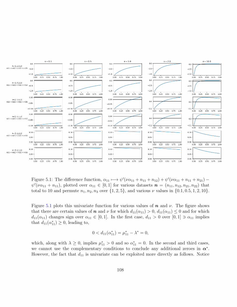
Figure 5.1: The difference function, α11 7−→ ψ′(να11 + n11 + n12) + ψ′(να11 + n11 + n21)−ψ′(να11 + n11), plotted over α11 ∈ [0, 1] for various datasets n = (n11, n12, n21, n22) thattotal to 10 and permute n1, n2, n3 over 1, 2, 5, and various ν values in 0.1, 0.5, 1, 2, 10.
Figure 5.1 plots this univariate function for various values of n and ν. The figure showsthat there are certain values of n and ν for which d11(α11) > 0, d11(α11) ≤ 0 and for whichd11(α11) changes sign over α11 ∈ [0, 1]. In the first case, d11 > 0 over [0, 1] 3 α11 impliesthat d11(α∗11) ≥ 0, leading to,
0 < d11(α∗11) = µ∗11 − λ∗ = 0,
which, along with λ ≥ 0, implies µ∗11 > 0 and so α∗11 = 0. In the second and third cases,we cannot use the complementary conditions to conclude any additional zeroes in α∗.However, the fact that d11 is univariate can be exploited more directly as follows. Notice
108
that d11 is in fact the derivative of the objective function restricted to α12, α21 = 0,
d11(a) =d
da(ψ(νa+ n11 + n12) + ψ(νa+ n11 + n21)− ψ(νa+ n11)).
This means that, if d11 is negative over [0, 1] as in the second case, then the restrictedobjective function is a non-increasing function over [0, 1], which must achieve its minimumat α∗11 = 1. In the third case where d11(α11) is continuous, monotonically non-decreasingon [0, 1] and has a root at, say a0 ∈ [0, 1], then it means that a0 is a stationary pointof the restricted objective function that is decreasing in [0, a0) and increasing in (a0, a].Because the restricted objective is continuous [0, 1], then a0 must be its minimum, suchthat α∗11 = a0. This characterises all the possible cases.
5.2 Some properties of the objective function in mean-
parameter space
It is expected that one would numerically optimise the objective function over the sub-space identified by the KKT conditions in the first step, and this subspace is another closedsimplex of lower dimension than that with which one started. Towards an analysis of thisoptimisation, it remains unclear that the objective function itself has any monotonic orconvexity properties.
We show that there exists a reparametrisation of the problem such that the convexity ofthe domain in the natural parameter space is preserved, the posterior log-odds expectationto be optimised is bounded in the interior of the space under the reparametrisation andthat there are some regions of the new space over which the objective function is locallymonotone. The latter is useful as we will show that some datasets and log-odds structuresrestrict the optimisation of the posterior expectation to this region, making the functionmonotone over this set.
5.2.1 A reparametrisation of the natural parameter space
For illustration, we graphically explore the salient ideas with a low dimensional problemsinstead of deriving the general finite dimensional case. Furthermore, the parametrisation
109
is simply a tool to transform the problem into one that is more amenable to a gradientdescent, and it is neither unique nor has any other significance. We will therefore focus onan illustration with an example for the rest of the section.
Example 5.2.1: Given a dataset of counts n over categories L = 1, 2 totaling to n anda hyperparameter choice ν > 0, the posterior IDM lower expectation of a log-odds statisticT , is the minimum of,
I : α ∈ 42 7−→ ψ(να1 + n1)− ψ(να2 + n2),
where we note that α2 = 1 − α1 and n2 = n − n1. Recall that the mean parameters aregiven by,
µi = ψ(ναi + ni),
for i = 1, 2, with the constraint that,
ψ−1(µ1) + ψ−1(µ2) = ν + n. (5.1)
We will study (5.1) in the subsequent set of examples via a convenient reparametrisation.The parametrisation allows us to derive some of the curve’s properties without resortingto direct manipulation (5.1), as well as reveals interesting geometrical properties of theoptimisation problem.
Definition 5.2.1: (Reparametrisation of µ curve) Define the parameter t ∈ R, and,
µ(t) = −a(t)v0 + tv1,
such that v0, v1 and a(t) are chosen to satisfy,
ψ−1(a(t)v01 + tv11) + ψ−1(a(t)v02 + tv12) = ν + n.
We can visualise this parametrisation in Figure 5.2.
110
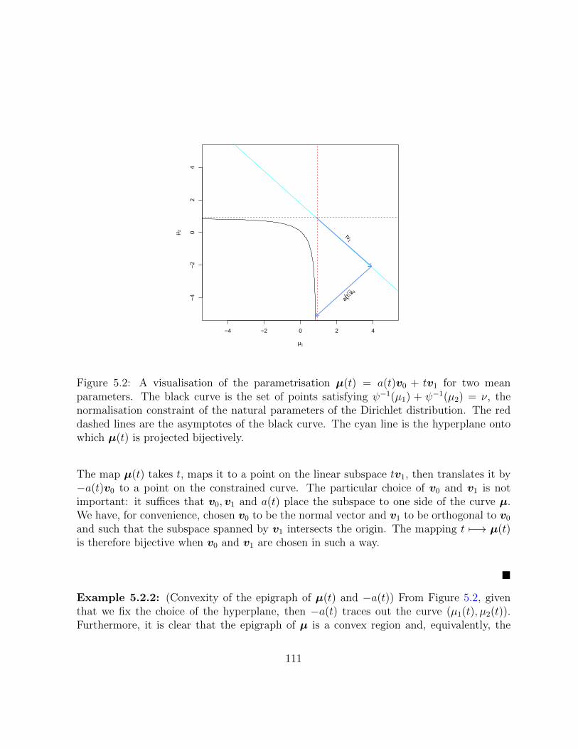
−4 −2 0 2 4
−4
−2
02
4
µ1
µ 2 tv1
a(t)v 0
Figure 5.2: A visualisation of the parametrisation µ(t) = a(t)v0 + tv1 for two meanparameters. The black curve is the set of points satisfying ψ−1(µ1) + ψ−1(µ2) = ν, thenormalisation constraint of the natural parameters of the Dirichlet distribution. The reddashed lines are the asymptotes of the black curve. The cyan line is the hyperplane ontowhich µ(t) is projected bijectively.
The map µ(t) takes t, maps it to a point on the linear subspace tv1, then translates it by−a(t)v0 to a point on the constrained curve. The particular choice of v0 and v1 is notimportant: it suffices that v0,v1 and a(t) place the subspace to one side of the curve µ.We have, for convenience, chosen v0 to be the normal vector and v1 to be orthogonal to v0
and such that the subspace spanned by v1 intersects the origin. The mapping t 7−→ µ(t)is therefore bijective when v0 and v1 are chosen in such a way.
Example 5.2.2: (Convexity of the epigraph of µ(t) and −a(t)) From Figure 5.2, giventhat we fix the choice of the hyperplane, then −a(t) traces out the curve (µ1(t), µ2(t)).Furthermore, it is clear that the epigraph of µ is a convex region and, equivalently, the
111
outline of this epigraph, −a(t), is a convex function.
Example 5.2.3: (Reparametrised images of faces) It is important to understand how thefaces of the simplex of the natural parameters map to the mean parameter space. Not onlydoes this give a complete picture of the transformed domain, but, as in examples like thelog-odds, the boundaries may contain optima.
Continuing with Example 5.2.1, the (singleton) faces αi = 0 map to µi = ψ(ni) in themean parameter space, for i = 1, 2. In particular, if ni = 0, then αi = 0 maps to an infinityin µ space. To put this in terms of t, the (singleton) face α1 = 0 is mapped to the set,
t : a(t)v0 + tv1 = (ψ(n1), ψ(ν + n2)).
It follows from the bijectivity we have established between t and µ(t) that this is a sin-gleton set that maps to a single vector (ψ(n1), ψ(ν + n2)). We can similarly establish theimage of the singleton face of α2 = 0 in terms of t.
We will see more nontrivial images of faces of 43 in subsequent examples.
5.2.2 Geometry of the objective function
Having established the necessary concepts in two-dimensions, we can explore the non-trivialgeometry that arises in the three-dimensional case that is also easily visualised.
Example 5.2.4: Suppose that we have a dataset of counts n over categories L = 1, 2, 3totaling to n and a hyperparameter choice ν > 0. Let us consider the log odds statistic,
logθ1 + θ2
θ2 + θ3
,
whose posterior IDM lower expectation is the minimum of,
I : α ∈ 43 7−→ ψ(ν(α1 + α2) + n1 + n2)− ψ(ν(α2 + α3) + n2 + n3).
112
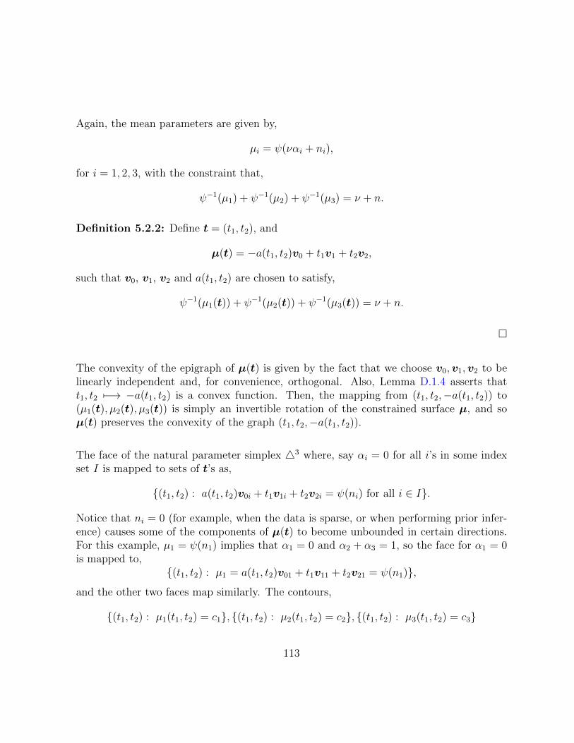
Again, the mean parameters are given by,
µi = ψ(ναi + ni),
for i = 1, 2, 3, with the constraint that,
ψ−1(µ1) + ψ−1(µ2) + ψ−1(µ3) = ν + n.
Definition 5.2.2: Define t = (t1, t2), and
µ(t) = −a(t1, t2)v0 + t1v1 + t2v2,
such that v0, v1, v2 and a(t1, t2) are chosen to satisfy,
ψ−1(µ1(t)) + ψ−1(µ2(t)) + ψ−1(µ3(t)) = ν + n.
The convexity of the epigraph of µ(t) is given by the fact that we choose v0,v1,v2 to belinearly independent and, for convenience, orthogonal. Also, Lemma D.1.4 asserts thatt1, t2 7−→ −a(t1, t2) is a convex function. Then, the mapping from (t1, t2,−a(t1, t2)) to(µ1(t), µ2(t), µ3(t)) is simply an invertible rotation of the constrained surface µ, and soµ(t) preserves the convexity of the graph (t1, t2,−a(t1, t2)).
The face of the natural parameter simplex 43 where, say αi = 0 for all i’s in some indexset I is mapped to sets of t’s as,
(t1, t2) : a(t1, t2)v0i + t1v1i + t2v2i = ψ(ni) for all i ∈ I.
Notice that ni = 0 (for example, when the data is sparse, or when performing prior infer-ence) causes some of the components of µ(t) to become unbounded in certain directions.For this example, µ1 = ψ(n1) implies that α1 = 0 and α2 + α3 = 1, so the face for α1 = 0is mapped to,
(t1, t2) : µ1 = a(t1, t2)v01 + t1v11 + t2v21 = ψ(n1),
and the other two faces map similarly. The contours,
(t1, t2) : µ1(t1, t2) = c1, (t1, t2) : µ2(t1, t2) = c2, (t1, t2) : µ3(t1, t2) = c3
113
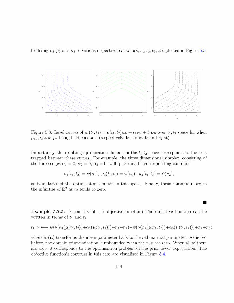
for fixing µ1, µ2 and µ3 to various respective real values, c1, c2, c3, are plotted in Figure 5.3.
−10 −5 0 5 10
−10
−5
05
t1
t 2
−18 −16
−14 −12
−10 −8 −6
−4
−2
0
−10 −5 0 5 10
−10
−5
05
t1
t 2
−14 −12 −12 −10 −10 −8
−6
−4
−2
0
−10 −5 0 5 10
−10
−5
05
t1
t 2
−20 −18
−16 −14
−12 −10 −8
−6
−4
−2
0
Figure 5.3: Level curves of µi(t1, t2) = a(t1, t2)v0i + t1v1i + t2v2i over t1, t2 space for whenµ1, µ2 and µ3 being held constant (respectively, left, middle and right).
Importantly, the resulting optimisation domain in the t1-t2-space corresponds to the areatrapped between these curves. For example, the three dimensional simplex, consisting ofthe three edges α1 = 0, α2 = 0, α3 = 0, will, pick out the corresponding contours,
µ1(t1, t2) = ψ(n1), µ2(t1, t2) = ψ(n2), µ3(t1, t2) = ψ(n3),
as boundaries of the optimisation domain in this space. Finally, these contours move tothe infinities of R2 as ni tends to zero.
Example 5.2.5: (Geometry of the objective function) The objective function can bewritten in terms of t1 and t2:
t1, t2 7−→ ψ(ν(α1(µ(t1, t2))+α2(µ(t1, t2)))+n1+n2)−ψ(ν(α2(µ(t1, t2))+α3(µ(t1, t2)))+n2+n3),
where αi(µ) transforms the mean parameter back to the i-th natural parameter. As notedbefore, the domain of optimisation is unbounded when the ni’s are zero. When all of themare zero, it corresponds to the optimisation problem of the prior lower expectation. Theobjective function’s contours in this case are visualised in Figure 5.4.
114
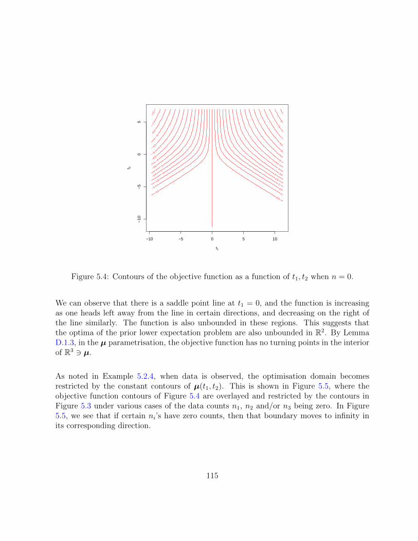
−10 −5 0 5 10
−10
−5
05
t1
t 2
−7.
5 −
7 −
6.5
−6
−5.
5 −5
−4.5
−4
−3.5 −3
−2.5 −2
−1.5
−1
−0.5
0.5
1
1.5
2
2.5
3 3.5
4
4.5
5
5.5
6
6.5 7
7.5 8
Figure 5.4: Contours of the objective function as a function of t1, t2 when n = 0.
We can observe that there is a saddle point line at t1 = 0, and the function is increasingas one heads left away from the line in certain directions, and decreasing on the right ofthe line similarly. The function is also unbounded in these regions. This suggests thatthe optima of the prior lower expectation problem are also unbounded in R2. By LemmaD.1.3, in the µ parametrisation, the objective function has no turning points in the interiorof R3 3 µ.
As noted in Example 5.2.4, when data is observed, the optimisation domain becomesrestricted by the constant contours of µ(t1, t2). This is shown in Figure 5.5, where theobjective function contours of Figure 5.4 are overlayed and restricted by the contours inFigure 5.3 under various cases of the data counts n1, n2 and/or n3 being zero. In Figure5.5, we see that if certain ni’s have zero counts, then that boundary moves to infinity inits corresponding direction.
115
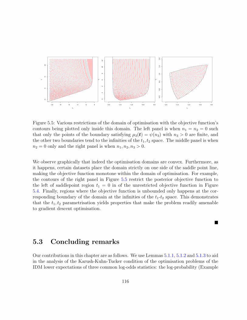
−10 −8 −6 −4 −2 0
−5
05
10
t1
t 2
−10
−
9.6 −
9.4
−9.
2 −9
−8.
8 −8.
6
−8.4
−8.
2
−8 −7.8
−7.6 −7.4
−7.2 −7
−6.8 −6.6
−6.4 −6.2
−6 −5.8 −5.6
−5.4 −5.2 −5
−4.8 −4.6 −4.4
−4.2 −4 −3.8
−3.6 −3.4 −3.2
−3 −2.8 −2.6 −2.4
−2.2 −2 −1.8
−1.6
−1.4
−1.2
−1.2
−1.2
−1
−0.
8
−2.0 −1.5 −1.0 −0.5 0.0
02
46
810
12
t1
t 2
−2.
45
−2.
4 −
2.35
−
2.3
−2.
25
−2.
2 −
2.15
−2.
1 −2.
05
−2 −1.
95
−1.9 −1.85 −1.
8
−1.
75
−1.7 −1.65 −1.6 −1.
55
−1.5 −1.45 −1.4 −1.35 −1.3
−1.25 −1.2 −1.15 −1.1 −1.05
−1 −0.95 −0.9 −0.85 −0.8 −0.75 −0.7 −0.
65
−0.6 −0.
55 −
0.5
−0.
45
−0.
4 −
0.35
−
0.3
−2.0 −1.5 −1.0 −0.5 0.0
−0.
50.
00.
51.
01.
52.
0
t1
t 2
−1.
65
−1.
55 −1.
5
−1.
45 −1.
4
−1.
35 −
1.3
−1.25 −
1.2
−1.15 −
1.1
−1.05 −1
−0.95 −0.9
−0.85 −0.8
−0.75
−0.7
−0.65
−0.6
−0.
55
−0.
5
−0.
45
−0.
4
−0.
35
−0.
3
−0.
25
Figure 5.5: Various restrictions of the domain of optimisation with the objective function’scontours being plotted only inside this domain. The left panel is when n1 = n2 = 0 suchthat only the points of the boundary satisfying µ3(t) = ψ(n3) with n3 > 0 are finite, andthe other two boundaries tend to the infinities of the t1, t2 space. The middle panel is whenn2 = 0 only and the right panel is when n1, n2, n3 > 0.
We observe graphically that indeed the optimisation domains are convex. Furthermore, asit happens, certain datasets place the domain strictly on one side of the saddle point line,making the objective function monotone within the domain of optimisation. For example,the contours of the right panel in Figure 5.5 restrict the posterior objective function tothe left of saddlepoint region t1 = 0 in of the unrestricted objective function in Figure5.4. Finally, regions where the objective function is unbounded only happens at the cor-responding boundary of the domain at the infinities of the t1-t2 space. This demonstratesthat the t1, t2 parametrisation yields properties that make the problem readily amenableto gradient descent optimisation.
5.3 Concluding remarks
Our contributions in this chapter are as follows. We use Lemmas 5.1.1, 5.1.2 and 5.1.3 to aidin the analysis of the Karush-Kuhn-Tucker condition of the optimisation problems of theIDM lower expectations of three common log-odds statistics: the log-probability (Example
116
5.1.1 and Theorem 5.1.1), the log-odds (Example 5.1.2) and the independence statistic(Example 5.1.3). These demonstrate how the KKT conditions can narrow down the loca-tion of the optimisers to certain faces of the natural parameters simplex. To geometricallystudy the objective function, we construct a reparametrisation of the optimisation problemexplore the geometry of the objective function in the mean parameter space: this is illus-trated conceptually in two dimensions in Definition 5.2.1, Examples 5.2.1, 5.2.2 and 5.2.3,and salient properties of higher dimensions are illustrated in three dimensions Examples5.2.4 and 5.2.5.
In this chapter the optimisation problem involved in computing the posterior lower expec-tation of log-odds statistics under the IDM was explored. For three commonly occurringlog-odds statistics, their KKT conditions were solved and used to identify the faces of thenatural parameter space containing the optimisers. Considerations were given to gradientbased methods typically used to search for the optimisers on these faces. In particu-lar, we have noted that these methods are problematic when searching for optimisers ofunbounded objective functions over a closed set such as those occurring with the IDMlog-odds problems. In this vein, we moved beyond the KKT condition to study the shapeof the objective function in the mean parameter space where the region over which theoptimiser is unbounded is at the infinities of the Euclidean space of mean parameters. Areparametrisation via a projection was developed to illustrate that domain of optimisa-tion is convex in both prior and posterior cases and, importantly, to provide a proof ofconcept that the objective function can be monotone for certain log-odds structure andparametrised by certain datasets.
The exploration done in this work suggests that, while the original optimisation problemof the IDM lower expectation problem is not a convex optimisation problem, it possessesproperties that nevertheless make it amenable to the usual tools used to analyse optimi-sation problems. From a statistical perspective, our study is pertinent regarding a globalsensitivity analysis over the closed simplex of the natural parameters of a Dirichlet fam-ily of priors with fixed concentration parameter. Our studies suggest that, at least forlog-odds statistics, such global analysis is amenable to optimisation techniques under theIDM due to the properties of the objective function and its domain. In fact, with log-oddsof certain structures, the observed dataset may parametrise the optimisation problem asto provide a sufficient amount of information and discrimination for the KKT conditionsto locate the set of optima by itself (for example when observations are predominantly oreven completely observed only in the sets involved in the numerator or only in those of thedenominator). Furthermore, as we have seen in Figures 5.4 and 5.5, the objective func-
117

tion, in both the mean parameter and its reparametrisation which we have constructed,may exhibit directions in which it is monotone, such that its optima always occur at theboundary of the domain of optimisation. This geometrical fact, which is not apparentfrom viewing the objective function in the natural parameters as a difference of digammafunctions, sheds light on the nature of the IDM log-odds problem and, equivalently, theglobal sensitivity analysis of Dirichlet prior families and its feasibility.
As gradient-based methods are a typical choice for such problems, we briefly remark onthe ramifications of our exploration upon its use. One may encounter two issues in ap-plying them to an IDM log-odds minimisation. First, because the objective function ispotentially an arbitrary sum and difference of digamma functions, it is unclear that ithas nice properties such as monotonicity and convexity which the optimiser algorithm canexploit. Second, as we have illustrated above, certain structures of sets in the log-oddsand datasets that parametrise the posterior problem yield vertex solutions whose objectivevalues are unbounded, ill-defined and cannot be smoothly extended to the boundary of theoptimisation domain. In this analysis, we have shown that there exists a reparametrisationof the problem such that the convexity of the domain is preserved, the posterior log-oddsexpectation to be optimised is bounded in the interior of the space under the reparametri-sation and that there are some regions of the new space over which the objective functionis locally monotone.
118
Chapter 6
Imprecise posterior inference underzero lower marginal probability infinite dimensions
In this chapter, we focus on an inferential issue that, in practice, does not occur whena single distribution is used. Recall that we are partially motivated by the case where aset of priors has been elicited from a set of experts, who may not hold consistent beliefs.The most extreme example of this would be when they differ in what they assess to havestrictly positive probability. Hence, some distributions in an elicited prior set assign zeromarginal probability to the possibly observed data. As a result, the lower probability (seeDefinition 2.1.9) of this particular dataset is zero, and the generalised Bayes’ rule of Wal-ley [81] (Theorem 2.2.4) does not necessarily hold. In these cases, extensions of the lowerexpectation may be used instead.
We explore whether or not coherence and imprecision might yield well-defined and sensibleinference when the lower probability of the conditioning set is zero. This is motivated bythe fact in, for example, Walley [81], Couso and Moral [29] and Quaeghbeur (Ch 1. ofAugustin et al. [6]), that the same unconditional lower expectation model may generatedifferent conditional imprecise models when the lower probability of the conditioning set iszero. Our finite discrete setting allows tractable and concrete exploration of the propertiesdirectly relevant to this issue.
We focus on two established imprecise methods that can be used in this situation. The
119
vacuous extension always yields vacuous inference. (Recall, from Definition 2.2.2, that im-precise expectations are vacuous for a random variable if the lower and upper expectationsare respectively the infimum and supremum of the random variable.) On the other hand,under certain conditions, the regular extension may yield non-vacuous inference even whenthe marginal lower probability is zero. In this chapter, we discuss in detail a very simpleexample to gain insight into the characteristics and problems of statistical inference arisingfrom these two extensions.
6.1 A running example
Let 1, . . . ,m index the known categories in consideration with m < ∞. We considerthe case when the sample size n is apriori fixed and each observation is i.i.d. followingsome multinomial distribution. Let n ∈ Nm be the counts of the categories summing to n.Let Θ = θ1, . . . ,θ|Θ| ⊂ 4m be a finite set of candidate multinomial probability vectors.
A prior p over Θ is therefore a point on the finite dimensional simplex 4Θ. When thedenominator is non-zero, the posterior expectation of a random variable f(θ) followingfrom Bayes’ rule is given by,
Ep(f) =
∑θ∈Θ f(θ)L(θ|n)p(θ)∑θ∈Θ L(θ|n)p(θ)
. (6.1)
Given a set M of priors, p’s, a posterior lower expectation can be formed by the optimisa-tion of the posterior expectation over the set M ,
E(f |n) = inf Ep(f(θ)|n) : p ∈M . (6.2)
Recall from Definition 2.1.9, the lower probability of an event A under E is P (A) = E(IA).As a shorthand notation, we will write the lower probability of observing n as P (n).
When P (n) > 0, (6.2) is a coherent lower expectation as a consequence of the generalisedBayes’ rule (Theorem 2.2.4). But, in this chapter, we are interested in the case when M issuch that this is not the case. To illustrate the context of the need for imprecision underthis finite setting, we furnish the following example.
Example 6.1.1: A linguist wishes to model the probability f(θ) = θ, θ ∈ [0, 1], of acertain phrase occurring in a corpus of documents all written in a single language. Thephrase is grammatically incorrect in the documents’ language: it is typical to assign a
120
structural zero to the occurrence of phrases which are syntactically not permissible (Mohriand Roark [61]). That is, θ1 = 0 is a candidate model. However, it is also possible thatsuch a document is written in a way that the phrase nevertheless occurs: for example,the phrase may be used as a colloquialism or written by somebody unfamiliar with thelanguage. To account for these cases, the linguist selects two other distributions, θ2, θ3 > 0.In all, the candidate distributions for the document are Θ = θ1, θ2, θ3.
The linguist wishes to construct a prior distribution over Θ. Because the linguist’s priorstate of knowledge does not favour any particular distribution, any prior distribution (as-signing any probability to θ1) is consistent with this state. In particular, this includesthe prior that assigns a prior probability of one to θ1 = 0 which will cause the marginalprobability of observing a document containing the phrase to be zero. That is, writing n1
to be the number of documents containing this phrase out of n observed documents,
P (n1 documents of n contain the phrase)
= P (n = (n1, n− n1))
= p(θ1)L(θ1|(n1, n− n1)) + p(θ2)L(θ2|(n1, n− n1)) + p(θ3)L(θ3|(n1, n− n1))
= 1 · 0 + 0 · L(θ2|(n1, n− n1)) + 0 · L(θ3|(n1, n− n1))
= 0.
This prevents any posterior inference involving conditional probabilities such as (6.1) tobe well-defined.
This example shows that M may happen to be elicited in a way such that the denominatorof (6.1) is zero for at least one potentially observable dataset. For such prior distributionsin the set, we highlight two practical concerns regarding this.
Firstly, the posterior expectation (6.1) is not defined when its denominator is zero. Inturn, this is so if and only if for every θ either its likelihood relative to the data or its priorprobability (or both) are zero. What should be done here methodologically? On the onehand, one should not alter the prior after observing the data. A satisfactorily elicited priorshould not be modified without any justification. On the other hand, one might aprioriassume a prior that assigns a positive probability to any potential datasets. However, thisprior may contradict any prior information that indicates that certain datasets in fact have
121
zero probability of occurring.
Secondly, when a dataset is observed such that its lower prior probability is zero, the gen-eralised Bayes’ rule does not guarantee a coherent posterior model. Moreover, under theglobal sensitivity analysis interpretation, the computation of the posterior lower expecta-tion found by minimising (6.1) over the prior space is not well-defined in the sense thatsome Bayes’ rules will not be defined with priors that produce a zero marginal probabilityfor the data. As such, one cannot readily depend on the generalised Bayes’ rule to generateposterior values that are coherent with the elicited set of priors.
From these observations, we do not expect that the lower and upper expectations of thegeneralised Bayes’ rule to be readily applicable here, as it is a function of all the preciseBayes’ rules over an elicited prior set. However, there are other more general ways ofconstructing imprecise posterior inferences beyond lower and upper bounds of conditionalexpectations.
6.2 Vacuous and regular extensions
Let us introduce some additional notations for this chapter. Consider a set of multinomialprobability vectors over m categories, Θ ⊂ 4m such that |Θ| < ∞, and M , set of priordistributions over Θ. Let n be a fixed dataset. For a prior,
p = (p(θ1), . . . , p(θ|Θ|)) ∈ 4|Θ|,
and likelihood,L(θ|n) = (L(θ1|n), . . . , L(θ|Θ||n)).
where,
L(θi|n) =
|Θ|∏j=1
θnjij .
Example 6.2.1: With only limited information about the source of the documents, thelinguist decides to construct a set of candidate prior distributions p = (p(θ1), p(θ2), p(θ3)) =(p1, p2, p3), M , that reflects the available but incomplete information. Suppose that thelinguist elicits Θ = 0, 1/10, 1/4 as the possible probabilities of the phrase occurring and
122
that there are 10 documents in the sampled corpus. Suppose also that from prior informa-tion of similar documents, the linguist assesses an upper bound on the prior expectationof odds of the phrase occurring, θ/(1− θ), to be less than 1/4,
0 · p1 +1
9p2 +
1
3p3 ≤
1
4,
as well an upper bound on the prior expectation of the number of occurrences of the phrasein a document of size 10, 10 · θ,
10 · 0 · p1 + 10 · 1
10p2 + 10 · 1
4p3 ≤ 2.
Now, M is to be constructed such that it reflects this known information. First, the linguistnotes the lack of information relevant to assessing probability of a document following therules of the language translates into including any p satisfying,
0 ≤ p1 ≤ 1,
as a candidate. After some manipulation, the linguist’s set of prior models is,(p1, p2, p3) : (p1, p2, p3) ∈ 43,
1
9p2 +
1
3p3 ≤
1
4, p2 +
5
2p3 ≤ 2
.
This set is a convex subset of the probability simplex in Figure 6.1, with vertices,
(1, 0, 0), (0, 1, 0), (0, 3/8, 5/8), (1/4, 0/3/4).
Importantly, note that p = (1, 0, 0), the prior assigning zero marginal probability to ob-serving any document containing the phrase of interest, is an extreme point of this convexset.
123

Figure 6.1: The linguist’s set of priors based on two constraints (blue hatched). Notice thatone of the constraints is redundant in defining the set. Notice also that (1, 0, 0), the priorassigning zero marginal probabilities to certain datasets, is included in the set of priors.
The following example demonstrates the effects of the prior assigning a zero lower proba-bility to a particular observed dataset under M when this dataset becomes observed.
Example 6.2.2: Consider a number of documents with the phrase is n1 ≥ 1 out of thesample of n <∞, so the binomial count vector is n = (n1, n− n1). The likelihood vectorbecomes,
L = (0, 0.1n1 · 0.9n−n1 , 0.25n1 · 0.75n−n1).
Of all the priors in M , only p = (1, 0, 0) assigns zero marginal probability to n = (n1, n−n1). Indeed,
L · p = (0, 0.1n1 · 0.9n−n1 , 0.25n1 · 0.75n−n1) · (1, 0, 0) = 0, (6.3)
124
and by the non-negativity of all the values involved, p = (1, 0, 0) is the only prior thatcauses this to happen. Nevertheless, this is sufficient for PM(n) = 0. Importantly, theminimisation of posterior expectations under this likelihood over the set of priors M is notwell-defined in the sense some priors cause the denominator in the Bayes’ rule to be zerocausing the objective function to be undefined at those points. On the other hand, theminimisation over M − (1, 0, 0), as an infimum, is well-defined in this example.
There are two ways to proceed with our analysis. On the one hand, one can make posteriorinference based on only the prior models that assign positive probability to the observeddata. This is provided by the so-called regular extension.
Definition 6.2.1: (Walley [81], Appendix J.) For a set of distributions M , a suitablymeasurable set B ⊆ Ω, the regular extension (of EM conditioning on B) is defined as,
X 7−→ inf
EP (IBX)
P (B): P ∈M ∧ P (B) > 0
.
On the other hand, one can abandon the use of the generalised Bayes’ rule and insteadconsider an alternative model. One established alternative method in this case is the so-called vacuous extension.
Definition 6.2.2: (Walley [81], 8.4.1) For a set of distributions M , a suitable measurableset B ⊆ Ω, the vacuous extension1 (of P to conditioning on B) is defined as,
X 7−→
infEP (IB ·)P (B)
: P ∈M
if PM(B) > 0,
infω∈Ω
X(ω) if PM(B) = 0
.
1In Walley [81], this is a natural extension of a conditional prevision due to the generalised Bayes’ rule,but, to avoid confusion, we will call this the vacuous extension.
125
Notice that the vacuous extension results in effectively throwing away the information pro-vided by M when the prior lower probability of the dataset is zero. Walley [81] notes that,under certain conditions, they are both jointly coherent with the prior lower expectationas discussed in Section 2.2.4. (In Section 6.3.3, we will see how certain assessments andelicitations may violate this.) As they stand, they are simply modelling choices one makesin anticipation of actually observing B whose lower probability is apriori zero.
Note that, when (the closure of) M contains at least one prior that assigns all of its massto the set of θ’s that assign zero likelihood to n1, the lower probability of observing thedata will always be zero. To identify these priors, write,
In = i ∈ 1, . . . , |Θ| : L(θi|n) > 0,
the indices of Θ whose likelihood values are strictly positive.
Proposition 6.2.1: If n is such that L(n|θi) = 0 for at least one i = 1, . . . , |Θ|, and thereexists p0 in the closure of M such that
∑i/∈In p0(θi) = 1, then PM(n) = 0.
Proof: Notice that,
PM(n) = inf
|Θ|∑i=1
p(θi)L(n|θi) : p ∈M
.
It is clear that the choice of the limit point p0 will minimise this quantity to zero.
6.3 Posterior imprecise inference for discrete param-
eter and observation spaces
From Definition 6.2.2, the vacuous extension takes values from the GBR when the lowerprobability of the conditioning event is strictly positive and takes the infimum of the ran-dom variable otherwise. On the other hand, the computation of the regular extension ismore involved, and we explore it under the discrete setting introduced in Section 6.1.
126
6.3.1 Computing the regular extension
Notice that the marginal probability,
L · p =∑θ∈Θ
L(θ|n)p(θ),
is zero iff every term in the sum is zero individually. In turn, this is equivalent to thestatement that for each θ ∈ Θ, at least one of L(θ|n) and/or p(θ) are zero, and so thevalid Bayes’ rules come from priors that avoid this.
For constructing the regular extension, we identify the set of priors that yield strictlypositive marginal probability for observing n:
p ∈M : ∃ i ∈ In, p(θi) > 0.
The (lower and upper) regular extension(s) for some random variable f(θ) are,
RM(f(θ)|n) = inf
∑i∈In fiLipi∑i∈In Lipi
∣∣∣∣ p ∈M : (∃ i ∈ In : pi > 0)
. (6.4)
RM(f(θ)|n) = sup
∑i∈In fiLipi∑i∈In Lipi
∣∣∣∣ p ∈M : (∃ i ∈ In : pi > 0)
. (6.5)
6.3.2 Effects of likelihood on regular extension values
From the above construction, the regular extension only considers the optimisation overthe posterior distributions normalised over only the prior probabilities of models θ ∈ Θwhich have a positive likelihood. In turn, the lower and upper regular extensions of, sayf(θ), are bounded below and above only by the minimum and maximum of f taken overthis active set of models. We can summarise this as follows.
Corollary 6.3.1: Consider the setting of Section 6.3.1. Recall that,
In = i ∈ 1, . . . , |Θ| : L(θi|n) > 0,
is the index set of observation models with a strictly positive likelihood value. Let M beany subset of the set of all prior distributions over Θ. For any bounded function f(θ) on
127
Θ, its regular extensions are bounded only by the values associated with strictly positivelikelihood,
mini∈In
f(θi) ≤ R(f(θ)|x) ≤ R(f(θ)|x) ≤ maxi∈In
f(θi).
Proof: This follows immediately from the form of the lower and upper regular extensionsin (6.4) and (6.5).
6.3.3 Numerical behaviour of posterior inference
Example 6.3.1: Continuing with Example 6.2.1, consider the case that out of n = 10documents, the phrase of interest occur in n1 = 1 of them. Let us plot the contours of theposterior expectations,
E(θ|p = (p1, p2, p3), n = (1, 9)) =0 · p1 + 0.1 · 0.1 · 0.99p2 + 0.25 · 0.25 · 0.759p3
0 · p1 + 0.1 · 0.99p2 + 0.25 · 0.759p3
,
as a function of p1, p2, p3. By (6.3), the prior (1, 0, 0) causes the marginal probability tobe zero. Because the Bayes’ rule of this prior is not defined under this dataset, the regularextension excludes this prior over M for n = (1, 9).
128
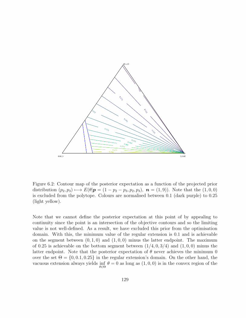
Figure 6.2: Contour map of the posterior expectation as a function of the projected priordistribution (p2, p3) 7−→ E(θ|p = (1 − p2 − p3, p2, p3), n = (1, 9)). Note that the (1, 0, 0)is excluded from the polytope. Colours are normalised between 0.1 (dark purple) to 0.25(light yellow).
Note that we cannot define the posterior expectation at this point of by appealing tocontinuity since the point is an intersection of the objective contours and so the limitingvalue is not well-defined. As a result, we have excluded this prior from the optimisationdomain. With this, the minimum value of the regular extension is 0.1 and is achievableon the segment between (0, 1, 0) and (1, 0, 0) minus the latter endpoint. The maximumof 0.25 is achievable on the bottom segment between (1/4, 0, 3/4) and (1, 0, 0) minus thelatter endpoint. Note that the posterior expectation of θ never achieves the minimum 0over the set Θ = 0, 0.1, 0.25 in the regular extension’s domain. On the other hand, thevacuous extension always yields inf
θ∈Θθ = 0 as long as (1, 0, 0) is in the convex region of the
129

optimisation.
The interpretation of whether or not 0.1 and 0.25 can be considered as posterior tightbounds reflecting the prior information depends on the role (1, 0, 0) plays: in the case ofthe regular extension, the question is whether or not it can be ignored.
Example 6.3.2: We consider how the contour map changes when the dataset n is varied.Figure 6.3 displays the contour maps of the posterior expectation for various values ofthe sample size n and the observed proportion of documents in this corpus containing thephrase, θ1 (such that n1 = nθ1), over values for p1.p2, p3.
130
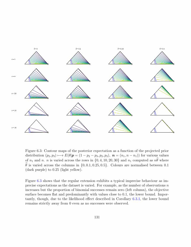
Figure 6.3: Contour maps of the posterior expectation as a function of the projected priordistribution (p2, p3) 7−→ E(θ|p = (1− p2 − p3, p2, p3), n = (n1, n− n1)) for various values
of n1 and n. n is varied across the rows in 0, 4, 10, 20, 30 and n1 computed as nθ where
θ is varied across the columns in 0, 0.1, 0.25, 0.5. Colours are normalised between 0.1(dark purple) to 0.25 (light yellow).
Figure 6.3 shows that the regular extension exhibits a typical imprecise behaviour as im-precise expectations as the dataset is varied. For example, as the number of observations nincreases but the proportion of binomial successes remain zero (left column), the objectivesurface becomes flat and predominantly with values close to 0.1, the lower bound. Impor-tantly, though, due to the likelihood effect described in Corollary 6.3.1, the lower boundremains strictly away from 0 even as no successes were observed.
131
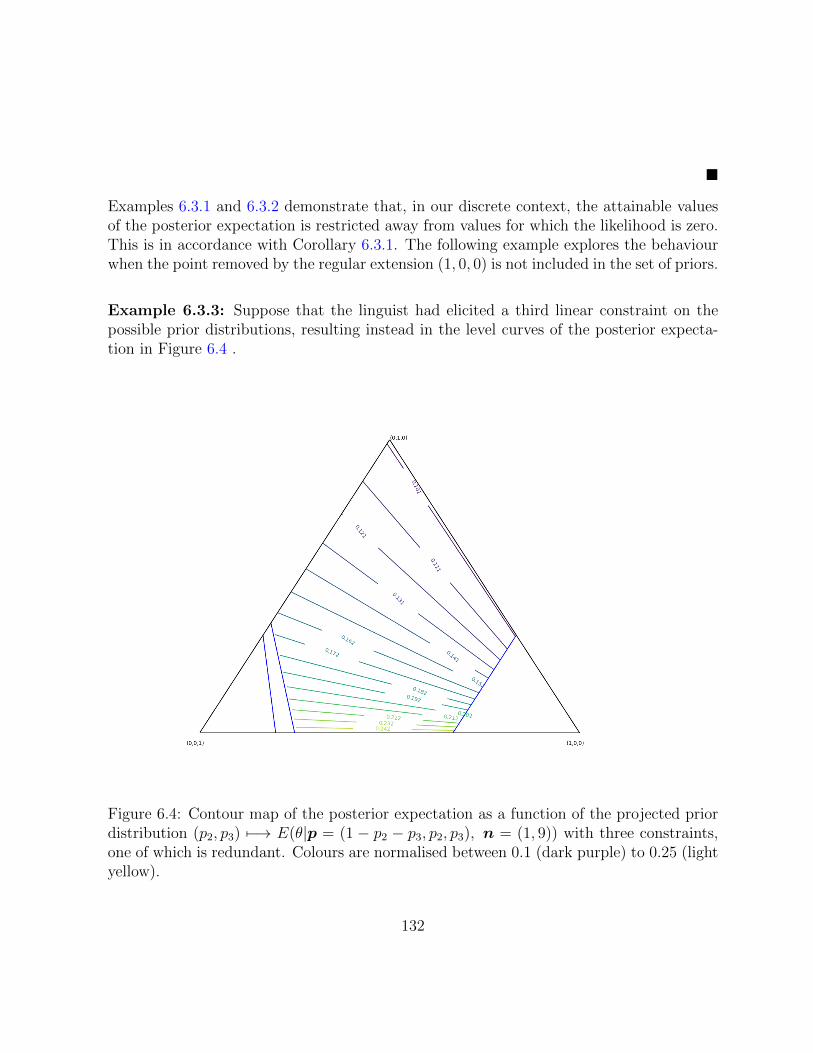
Examples 6.3.1 and 6.3.2 demonstrate that, in our discrete context, the attainable valuesof the posterior expectation is restricted away from values for which the likelihood is zero.This is in accordance with Corollary 6.3.1. The following example explores the behaviourwhen the point removed by the regular extension (1, 0, 0) is not included in the set of priors.
Example 6.3.3: Suppose that the linguist had elicited a third linear constraint on thepossible prior distributions, resulting instead in the level curves of the posterior expecta-tion in Figure 6.4 .
Figure 6.4: Contour map of the posterior expectation as a function of the projected priordistribution (p2, p3) 7−→ E(θ|p = (1 − p2 − p3, p2, p3), n = (1, 9)) with three constraints,one of which is redundant. Colours are normalised between 0.1 (dark purple) to 0.25 (lightyellow).
132
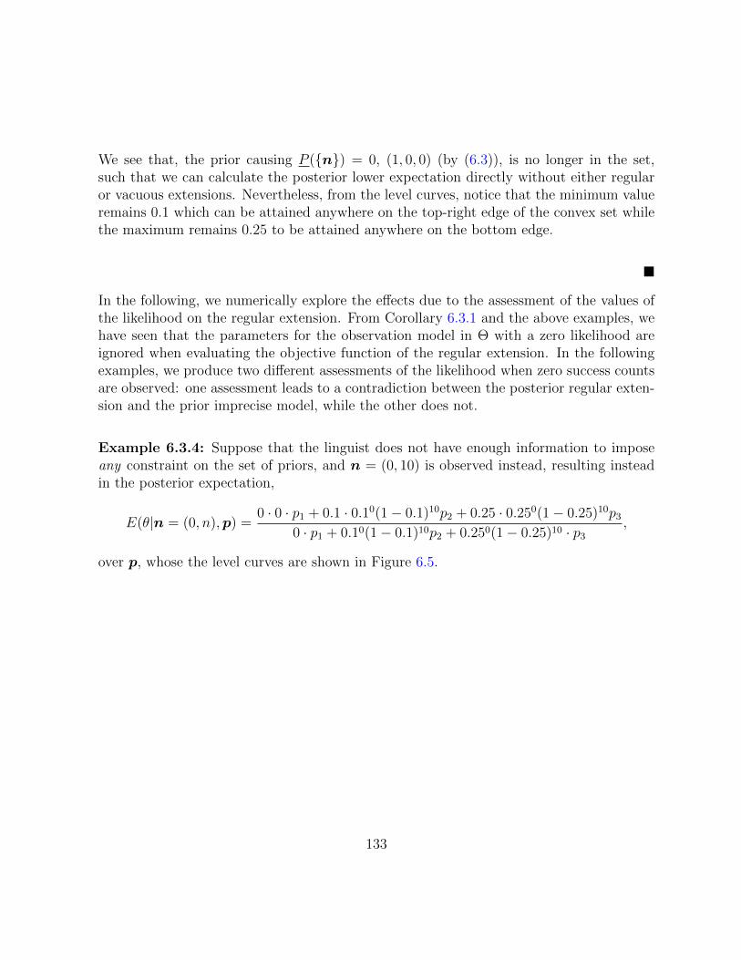
We see that, the prior causing P (n) = 0, (1, 0, 0) (by (6.3)), is no longer in the set,such that we can calculate the posterior lower expectation directly without either regularor vacuous extensions. Nevertheless, from the level curves, notice that the minimum valueremains 0.1 which can be attained anywhere on the top-right edge of the convex set whilethe maximum remains 0.25 to be attained anywhere on the bottom edge.
In the following, we numerically explore the effects due to the assessment of the values ofthe likelihood on the regular extension. From Corollary 6.3.1 and the above examples, wehave seen that the parameters for the observation model in Θ with a zero likelihood areignored when evaluating the objective function of the regular extension. In the followingexamples, we produce two different assessments of the likelihood when zero success countsare observed: one assessment leads to a contradiction between the posterior regular exten-sion and the prior imprecise model, while the other does not.
Example 6.3.4: Suppose that the linguist does not have enough information to imposeany constraint on the set of priors, and n = (0, 10) is observed instead, resulting insteadin the posterior expectation,
E(θ|n = (0, n),p) =0 · 0 · p1 + 0.1 · 0.10(1− 0.1)10p2 + 0.25 · 0.250(1− 0.25)10p3
0 · p1 + 0.10(1− 0.1)10p2 + 0.250(1− 0.25)10 · p3
,
over p, whose the level curves are shown in Figure 6.5.
133
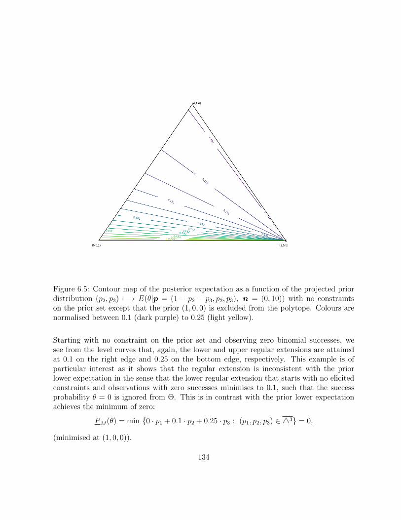
Figure 6.5: Contour map of the posterior expectation as a function of the projected priordistribution (p2, p3) 7−→ E(θ|p = (1 − p2 − p3, p2, p3), n = (0, 10)) with no constraintson the prior set except that the prior (1, 0, 0) is excluded from the polytope. Colours arenormalised between 0.1 (dark purple) to 0.25 (light yellow).
Starting with no constraint on the prior set and observing zero binomial successes, wesee from the level curves that, again, the lower and upper regular extensions are attainedat 0.1 on the right edge and 0.25 on the bottom edge, respectively. This example is ofparticular interest as it shows that the regular extension is inconsistent with the priorlower expectation in the sense that the lower regular extension that starts with no elicitedconstraints and observations with zero successes minimises to 0.1, such that the successprobability θ = 0 is ignored from Θ. This is in contrast with the prior lower expectationachieves the minimum of zero:
PM(θ) = min 0 · p1 + 0.1 · p2 + 0.25 · p3 : (p1, p2, p3) ∈ 43 = 0,
(minimised at (1, 0, 0)).
134
As in the examples in Section 6.3.3, this inconsistency between the regular extension andprior is due to the fact that, by Corollary 6.3.1, the value θ = 0 is being ignored becausethe likelihood at θ = 0 is zero under the dataset n = (0, 10). However, this also suggeststhat if the likelihood for θ = 0 was not zero, then θ = 0 can be exposed to the posteriorexpectation and this inconsistency can be avoided.
The issue in Example 6.3.4 pertains to the behaviour of the likelihood,
θn1(1− θ)n−n1
around θ = 0 and n1 = 0. One way to specify a limit value of the likelihood at this point isto use the conventional definition that 00 = 1 such that θn1(1−θ)n−n1 = 1·1n = 1. However,this limit is not unique: for example, 0 is also a limit if θ tends to 0 faster than n1. Unlikethe other examples where the dataset has at least one success (e.g. n = (1, 9)) and thelikelihood is well defined, we will be more explicit in assessing the value for L(n1 = 0|θ = 0)in the following.
Example 6.3.5: Continuing with Example 6.3.4, let us directly assess a value for L(n1 =0|θ = 0) instead of relying on the multinomial likelihood’s algebraic expression. Sinceθ = 0 was originally elicited, we can interpret L(n1 = 0|θ = 0) = P (n1 = 0|θ = 0) as theprobability of observing no successes under a data generating process whose probabilityof success is zero: a reasonable assessment is L(n1 = 0|θ = 0) = 1. Using the rules ofprobability, the resulting posterior expectation is well defined for n = (0, 10) because themarginal probability is strictly positive:
E(θ|n = (0, 10),p) =0 · 1 · p1 + 0.1 · 0.10(1− 0.1)10p2 + 0.25 · 0.250(1− 0.25)10p3
1 · p1 + 0.10(1− 0.1)10p2 + 0.250(1− 0.25)10 · p3
.
Notice that this conditional expectation is defined at p = (1, 0, 0) due to L(n1 = 0|θ = 0) =1. Further, unlike in Example 6.3.4, this prior achieves the minimum posterior expectationof 0 over the set of priors M and coincides with the vacuous extension.
Examples 6.3.4 and 6.3.5 highlight the importance of the assessment of the likelihood func-tion in contributing to the smooth operation of imprecise posterior inference in our cases.
135
In particular, the regular extension in posterior inferential settings is demonstrably sensi-tive to the definition (and any resulting pathologies) of the likelihood function.
6.4 Concluding remarks
Our contributions in this chapters are as follows. We demonstrated and compared theuse of the regular and vacuous extensions in a concrete, finite dimensional setting withExamples 6.1.1, 6.2.1, 6.2.2, 6.3.1, 6.3.2 and 6.3.3 and remarked upon some characteristicsof posterior inference when the set of priors is in conflict with data in the sense that thedata’s lower probability is zero. Corollary 6.3.1, Example 6.3.4 and Example 6.3.5 high-light the effect of the likelihood on the posterior regular extension and, importantly, how itmay induce incoherence between the prior model and posterior regular extension in certainpathological cases.
The regular and vacuous extensions each have their use cases. The regular extension canbe motivated as follows: if one observes a dataset, then its probability of being observedis, in hindsight, strictly positive such that it makes sense to perform posterior inference asif the assessed set of priors did not contain distributions assigning zero marginal proba-bility to the observed dataset. Note that this does not violate the principle that the datashould not influence the model choice because the choice of using the regular extension wasapriori decided. The vacuous extension, on the other hand, effectively ignores all elicitedprior information and produces vacuous bounds for the (conditional) expectations. It maysometimes be desirable to discard the entire prior elicitation. For example, if the set ofpriors were elicited using the same mechanism, then observing evidence against P (B) = 0for certain P in the set may indicate that the elicitation mechanism that produced allthe priors may be faulty, leading to the possibility that the elicitation for other P ′ withP ′(B) > 0 being faulty as well.
The vacuous extension can be an overly conservative choice to handle conflict betweenprior and data. In cases such as Example 6.3.1, the only offending prior is a single vertexout of a polytope, and the geometry of the problem suggests that there are other pointsaside from the removed one that would have achieved the global minimum anyway. Thevacuous extension would have missed the global minimum that effectively matches whatwe would have expected out of the sensitivity analysis over this polytope. Here, the vac-uous extension is overly conservative on two counts. First, it ignores the information of
136
an entire set of elicited priors due to a single pathological one. Secondly, since n1 = 1 inExample 6.3.1, it may be reasonable or even desirable to ignore the priors that assign azero marginal probability to the dataset.
On the other hand, the regular extension can be overly optimistic (or precise). In cor-ner cases such as Example 6.3.4, the behaviour of the posterior regular extension may beoverly precise. In particular, the effect of the likelihood on posterior imprecise inferenceis interesting in the context of zero-failure problems. When the observation model spaceΘ apriori includes the possibility of a zero success probability and zero successes are laterobserved, coherence between the regular extension and the prior is dependent on the directinterpretation and assessment of the likelihood values where the expression of the likeli-hood function is ill-defined, as demonstrated in Examples 6.3.4 and 6.3.5.
137
Chapter 7
Geometry of conditioning on eventswith zero lower probability in finitedimensions
In Chapter 6, we have explored the choice between the vacuous and regular extensionsfor posterior inference when the lower marginal probability of the conditioning set is zero.Under this sort of conflict between the set of priors and the posterior resulting from condi-tioning upon such a dataset, we have observed that, in contrast with the posterior impreciseexpectations over a set of prior distributions, the conditional vacuous extension effectivelycauses one to ignore one’s unconditional set of priors while the regular extension continuesby optimising only over the subset of priors that are not in conflict with the data. However,the principle of coherence by itself yields no compelling reason or definitive guideline onhow to choose between the two in practice. Moreover, the analysis in Chapter 6 also hassuggested that the regular and vacuous extensions may not be desirable as they are respec-tively overly precise or conservative in certain cases. This prompts us to consider possiblemodels of intermediate levels of imprecision between the two extensions. In this chapter,we will consider the mathematical construction as well as the assessment of such extensions.
138
7.1 The existence of imprecise models between the
vacuous and regular extensions
The existence of conditional assessments between the vacuous and regular extensions inthe case when PM(B) = 0 is corroborated by Theorem 10 in Couso and Moral [29] in theliterature of imprecise probabilities. We will not delve deeply into the result as it involvesa significant departure from our current set of notations. Instead, we will summarise thoseconcepts that are related to this chapter.
Couso and Moral investigate the conditioning problem using sets of desirable gambles,which are a set of random variables designated as a representation of a set of distributionsin the space of random variables. The possible conditional models associated with a set ofunconditional distributions are characterised by the choice of topological boundary pointsof the set of desirable gambles representing the unconditional model. In particular, thechoice to exclude all boundary points results in the vacuous extension and there exists amaximal set of boundary points associated with the regular extension beyond which thereis no gain in precision. Importantly, this suggests a class of extensions between this twoassociated with sets of boundary points which are non-empty strict subsets of the set as-sociated with the regular extension.
7.2 Sets of conditional assessments between the vac-
uous and regular extensions
Let us consider a closed set of distributions M . Given a non-empty, suitably measurablesubset B ⊆ Ω, one can decompose M into,
M = P ∈M : P (B) > 0 ∪ P ∈M : P (B) = 0.
If P ∈ M : P (B) = 0 is empty, the generalised Bayes’ rule (Proposition 2.2.1) yieldsa corresponding set of conditional distributions by applying Bayes’ rule to each elementof M . Otherwise, one way to form a conditional model is to use the regular extensionintroduced in Chapter 6, whose set of conditional distributions is,
MR|B :=
A 7−→ P (AB)
P (B): P ∈M ∧ P (B) > 0
.
139
The unconditional distributions in P ∈ M : P (B) = 0 do not provide any informationfor constructing conditional distributions (see 6.10 of Walley [81]) and so cannot be usedto construct probability assessments conditional on B. Recall that that the imprecision ofa lower expectation decreases as the set of distributions over which one optimises for thelower envelope becomes smaller. In particular, the regular extension increases the precisionof posterior inference by discarding distributions, and this may not accurately portray thedegree of lack of information. One way to better reflect the state of knowledge conditionalon B is to enlarge and append distributions to MR
|B.
Let us write PB as the set of all distributions over the set of sample points B and V B
to be the vacuous lower expectation of PB. When PM(B) = 0, the vacuous extensioncorresponds exactly to
V B(X) = infω∈B
X(ω),
where the vacuous extension on the right is achieved by a Dirac delta distribution in PB.Then,
MR|B ⊆ PB,
such that we recover the fact that the vacuous extension is more imprecise than the regularextension:
RM(X|B) = inf EPB(X) : PB ∈MR|B
≥ inf EPB(X) : PB ∈ PB
= infω∈B
X(ω)
= V B(X).
This construction is suggestive of sets of distribution over B in the middle:
MR|B ⊆MR
|B ∪N ⊆ PB,
where N is any set of distributions over the sample points B1. It is clear that,
RM(X|B) ≥ inf EPB(X) : PB ∈MR|B ∪N ≥ V B(X).
1We implicitly assume that MR|B ∪N is closed so its lower expectation is attainable in the set.
140
7.2.1 Interpretation of N
We are interested in sets of distributions on B, N , that have the following methodologicalinterpretation. Suppose that, for some fixed B, M was assessed such that PM(B) = 0.Then, B becomes observed, and this is in conflict with its lower probability being zero andrequires a further investigation. Revisiting the information available apriori, the analystscome up with a set of distributions N over the sample points B in addition to MR
|B. Wenote that, therefore, N contains information only about random variables defined on B,not Ω, in replacement of such information not provided by unconditional distributions inM assigning a zero probability to B.
Example 7.2.1: Recall that, in Example 6.3.5, the indeterminacy of the limit of a binomiallikelihood function θn1(1 − θ)n−n1 at θ = 0 and n1 = 0 caused the posterior expectationover M to be undefined at the prior p = (1, 0, 0) over the model space Θ = 0, 0.1, 0.25.As a result, the regular extension excludes this point from its domain of optimisation, MR.Recall also that we have produced a posterior model alternative to the regular extension,by directly assessing the likelihood value L(n1 = 0|θ = 0) = 1 so that one defines, outsideof the regular extension, the posterior distribution at p = (1, 0, 0) of θ as
p|n=(0,10),p=(1,0,0)
=1
1 · p1 + 0.10(1− 0.1)10p2 + 0.250(1− 0.25)10 · p3
1 · p1
0.10(1− 0.1)10p2
0.250(1− 0.25)10p3)
= (1, 0, 0).
In other words, we have set N = p|n=(0,10),p to be the posterior distribution in lieu ofthe ill-defined Bayes’ rule posterior and the resulting lower expectation in Example 6.3.5was in fact the optimisation over MR
|B ∪ p|n=(0,10),p.
Even though one should in principle avoid revisiting the model after observing (a partof) the data, this situation is not completely unrealistic. As we have seen in Chapter 1,real-life elicitation processes are not exact and it is unreasonable to expect the resultingassessments to be exact. In practice, when a model M apriori assigns PM(B) = 0 andthen B is observed, it is not unreasonable to revisit the elicitation process that has givenrise to this assessment.
141
7.2.2 Intermediate extensions and joint coherence
Because we are effectively optimising over a larger set of distributions from MR|B to MR
|B∪N ,we can see that this new extension can be written as the minimum of the lower expectationsof the components.
Definition 7.2.1: For B ⊆ Ω, and N a set of distributions on B, define the lowerexpectation over L(Ω),
E↑N(X|B) := EN(X|B),
where X|B is the restriction of X to B ⊆ Ω. For a partition B of Ω, write,
E↑N(X|B) =∑B∈B
IBE↑N(X|B).
Definition 7.2.2: For B ⊆ Ω, the intermediate extension of M by N conditional on B is,
EM ;N(X|B) := minEMR
|B(X), E↑N(X)
,
For a partition B of Ω, the intermediate extension of M by N conditional on B is,
EM ;N(X|B) :=∑B∈B
IBEM ;N(X|B).
Its conjugate upper extension conditional on a set B,
EM ;N(X|B) := −EM ;N(−X|B),
is given by the maximum of its components:
EM ;N(X|B) = −minEMR
|B(−X), EN(−X|B)
= −min
−EMR
|B(X),−EN(X|B)
= max
EMR
|B(X), EN(X|B)
.
142
Example 7.2.2: The vacuous extension is trivially recovered by setting N to be the spaceof all distributions over B, PB.
To preserve consistency between the unconditional and conditional assessments, they shouldbe jointly coherent with each other. (See Section 2.2.4.) For example. when PM(B) > 0,the lower expectation due to generalised Bayes’ rule in Proposition 2.2.1 is automaticallyjointly coherent with EM . The vacuous extension is jointly coherent with its prior model(8.4.1 of Walley [81]) and, under certain regularity conditions, the regular extension is alsojointly coherent with its prior model. (See Appendix J. of Walley [81].)
We can show that with some reasonable assumptions, EM ;N(·|B) is jointly coherent withEM .
Theorem 7.2.1: (Theorem E.1.1) Let B be a partition of Ω, and M be a closed set ofdistributions. Suppose that N is such that E↑N(·|B) is jointly coherent with EM . Supposealso that that such that its regular extension RM(·|B) is jointly coherent with EM . Then,EM ;N(·|B) is jointly coherent with EM .
7.3 Elicitation and assessment of intermediate exten-
sions
So far, we have defined the intermediate extensions in Definition 7.2.2. Furthermore, The-orem 7.2.1 establishes that the intermediate extension EM ;N(·|B) is jointly coherent withthe unconditional lower expectation EM . We now explore how the values of intermediateextensions can be assessed by incorporating certain types of additional information on howPM(B) = 0 can be further elicited.
143
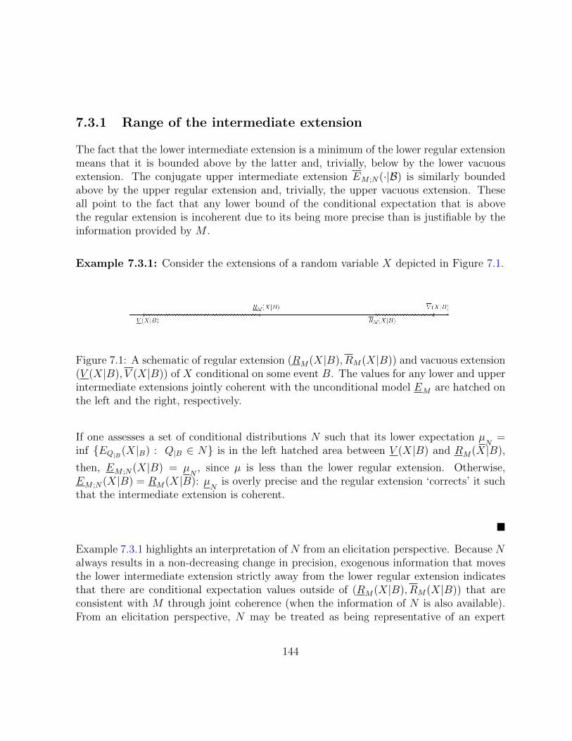
7.3.1 Range of the intermediate extension
The fact that the lower intermediate extension is a minimum of the lower regular extensionmeans that it is bounded above by the latter and, trivially, below by the lower vacuousextension. The conjugate upper intermediate extension EM ;N(·|B) is similarly boundedabove by the upper regular extension and, trivially, the upper vacuous extension. Theseall point to the fact that any lower bound of the conditional expectation that is abovethe regular extension is incoherent due to its being more precise than is justifiable by theinformation provided by M .
Example 7.3.1: Consider the extensions of a random variable X depicted in Figure 7.1.
Figure 7.1: A schematic of regular extension (RM(X|B), RM(X|B)) and vacuous extension(V (X|B), V (X|B)) of X conditional on some event B. The values for any lower and upperintermediate extensions jointly coherent with the unconditional model EM are hatched onthe left and the right, respectively.
If one assesses a set of conditional distributions N such that its lower expectation µN
=inf EQ|B(X|B) : Q|B ∈ N is in the left hatched area between V (X|B) and RM(X|B),
then, EM ;N(X|B) = µN
, since µ is less than the lower regular extension. Otherwise,EM ;N(X|B) = RM(X|B): µ
Nis overly precise and the regular extension ‘corrects’ it such
that the intermediate extension is coherent.
Example 7.3.1 highlights an interpretation of N from an elicitation perspective. Because Nalways results in a non-decreasing change in precision, exogenous information that movesthe lower intermediate extension strictly away from the lower regular extension indicatesthat there are conditional expectation values outside of (RM(X|B), RM(X|B)) that areconsistent with M through joint coherence (when the information of N is also available).From an elicitation perspective, N may be treated as being representative of an expert
144
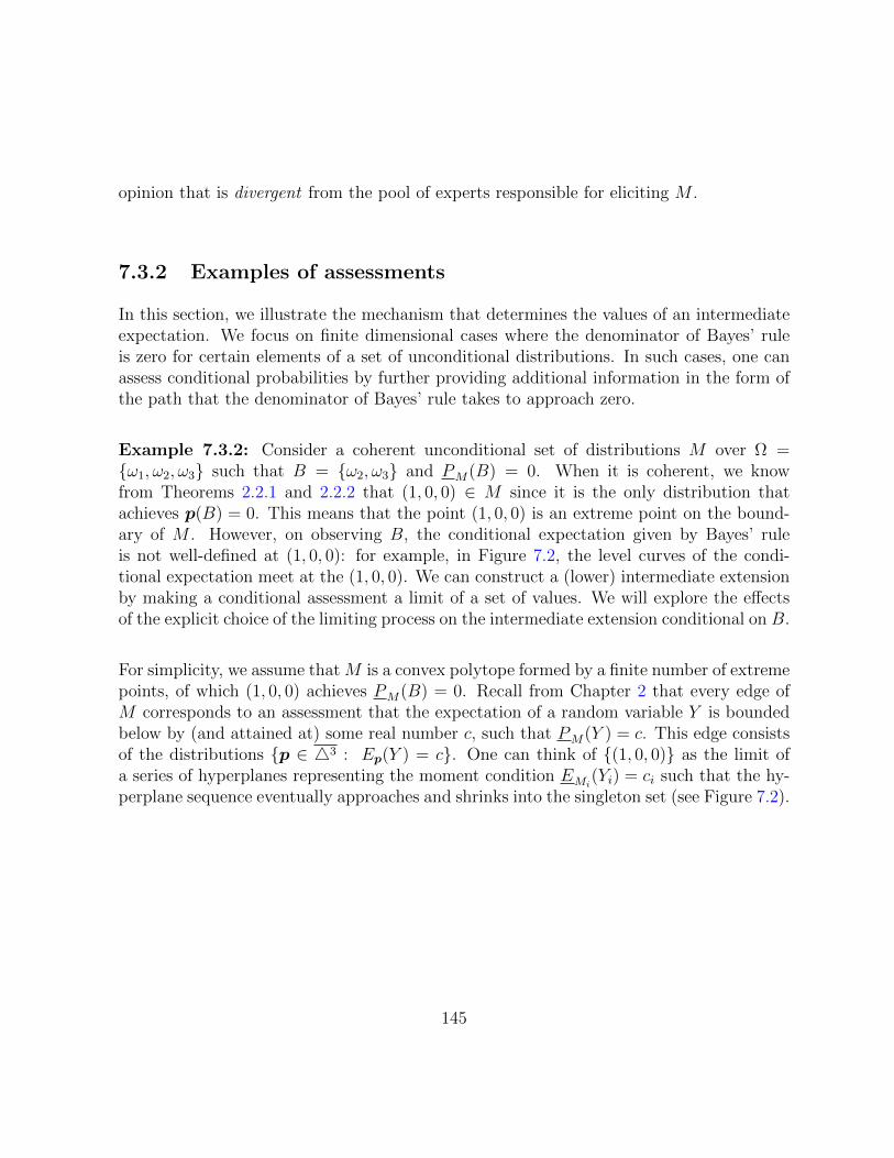
opinion that is divergent from the pool of experts responsible for eliciting M .
7.3.2 Examples of assessments
In this section, we illustrate the mechanism that determines the values of an intermediateexpectation. We focus on finite dimensional cases where the denominator of Bayes’ ruleis zero for certain elements of a set of unconditional distributions. In such cases, one canassess conditional probabilities by further providing additional information in the form ofthe path that the denominator of Bayes’ rule takes to approach zero.
Example 7.3.2: Consider a coherent unconditional set of distributions M over Ω =ω1, ω2, ω3 such that B = ω2, ω3 and PM(B) = 0. When it is coherent, we knowfrom Theorems 2.2.1 and 2.2.2 that (1, 0, 0) ∈ M since it is the only distribution thatachieves p(B) = 0. This means that the point (1, 0, 0) is an extreme point on the bound-ary of M . However, on observing B, the conditional expectation given by Bayes’ ruleis not well-defined at (1, 0, 0): for example, in Figure 7.2, the level curves of the condi-tional expectation meet at the (1, 0, 0). We can construct a (lower) intermediate extensionby making a conditional assessment a limit of a set of values. We will explore the effectsof the explicit choice of the limiting process on the intermediate extension conditional on B.
For simplicity, we assume that M is a convex polytope formed by a finite number of extremepoints, of which (1, 0, 0) achieves PM(B) = 0. Recall from Chapter 2 that every edge ofM corresponds to an assessment that the expectation of a random variable Y is boundedbelow by (and attained at) some real number c, such that PM(Y ) = c. This edge consistsof the distributions p ∈ 43 : Ep(Y ) = c. One can think of (1, 0, 0) as the limit ofa series of hyperplanes representing the moment condition EMi
(Yi) = ci such that the hy-perplane sequence eventually approaches and shrinks into the singleton set (see Figure 7.2).
145
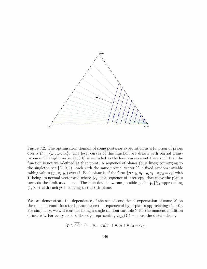
Figure 7.2: The optimisation domain of some posterior expectation as a function of priorsover a Ω = ω1, ω2, ω3. The level curves of this function are drawn with partial trans-parency. The right vertex (1, 0, 0) is excluded as the level curves meet there such that thefunction is not well-defined at that point. A sequence of planes (blue lines) converging tothe singleton set (1, 0, 0) each with the same normal vector Y , a fixed random variabletaking values (y1, y2, y3) over Ω. Each plane is of the form p : y1p1+y2p2+y3p3 = ci withY being its normal vector and where ci is a sequence of intercepts that move the planestowards the limit as i → ∞. The blue dots show one possible path pi∞i=1 approaching(1, 0, 0) with each pi belonging to the i-th plane.
We can demonstrate the dependence of the set of conditional expectation of some X onthe moment conditions that parametrise the sequence of hyperplanes approaching (1, 0, 0).For simplicity, we will consider fixing a single random variable Y for the moment conditionof interest. For every fixed i, the edge representing EMi
(Y ) = ci are the distributions,
p ∈ 43 : (1− p2 − p3)y1 + p2y2 + p3y3 = ci,
146
for a sequence of real numbers ci. Suppose further that min(Y ) = Y (ω1) = y1 and y3 > y1.As a result, because the distributions eventually converge to (1, 0, 0), the unconditionalmean will approach y1. (No convex combination of y2 and y3 can result in y1.) Therefore,it is reasonable to parametrise ci as y1 + εi where εi → 0.
We can study this convergence by analysing any arbitrary sequence of distributions pi∞i=1
such that each pi is in the i-th hyperplane. Then, we can parametrise pi = (1 − pi2 −pi3, pi2, pi3) by pi2, such that the moment condition can be written as,
y1(1− pi2 − pi3) + y2pi2 + y3pi3 = y1 + εi.
This leads to,
pi3 =εi
y3 − y1
− pi2y2 − y1
y3 − y1
.
Now, consider the conditional expectation of the random variable of interest, X, on B =ω2, ω3 under such a distribution on this edge:
x2pi2 + x3pi3pi2 + pi3
=x2pi2 + x3
(εi
y3−y1− pi2 y2−y1
y3−y1
)pi2 +
(εi
y3−y1− pi2 y2−y1
y3−y1
) .
For fixed choices of Y and X, this expression can take on various values depending onthe paths taken for pi2 → 0 and εi → 0. For example, suppose that εi = o(pi2) suchthat εi approaches zero faster than pi2. The expression will approach the following convexcombination of x2 and x3,
x2 + x3 · y2−y1
y3−y1
1 + y2−y1
y3−y1
.
If y2 = y1, then this expression becomes x2. On the other hand, if pi2 = o(εi), then theexpression approaches x3. If we set pi2 = εi, then, the expression approaches,
x2 + x3
(1
y3−y1− y2−y1
y3−y1
)1 +
(1
y3−y1− y2−y1
y3−y1
) =x2 + x3
(y3−y2
y3−y1
)1 +
(y3−y2
y3−y1
) .
In all, we have demonstrated that the posterior expectation can approach any value in theconvex combination of x2 and x3 as Mi approaches M depending the Y that parametrisesthe edge that approaches (1, 0, 0).
147
Example 7.3.3: Recall the running example of Chapter 6, Example 6.3.1. The linguisthas elicited the model space Θ = 0, 0.1, 0.25 for θ, the probability that a randomlychosen document in a corpus contains a certain phrase. Suppose that a set of priors Mcontaining the prior p = (1, 0, 0) was also elicited. Finally, suppose that it is observedthat one document out of a sample of ten contains the phrase, such that n = (1, 9). Theobservation probabilities L(θ|n) = θ1(1− θ)9 for each probability in Θ are,
L(n|θ = 0) = 0, L(n|θ = 0.1) = 0.1 · 0.99, and L(n|θ = 0.25) = 0.25 · 0.759.
For p such that the marginal probability of n is positive, the posterior expectation of θ isthen given by,
0 · p1 + 0.1 · 0.1 · 0.99p2 + 0.25 · 0.25 · 0.759p3
0 · p1 + 0.1 · 0.99p2 + 0.25 · 0.759p3
.
Once again, note that this expression is not defined for p = (1, 0, 0) as the denominatoris zero. This opens up the possibility of choosing either the vacuous extension or regularextension as we have done in Example 6.3.1, or constructing an intermediate extension byassessing the conditional expectation at p = (1, 0, 0) directly.
Let us consider an intermediate extension defined by the following limiting processes. Sup-pose that k2, k3 > 0 and a positive sequence ai > 0 such that 0 ≤ k2ai + k3ai ≤ 1 andai → 0. Set
pi2 = k2ai, and pi3 = k3ai.
Then, pi2 and pi3 converges to zero as i → ∞ and the expression for the posterior expec-tation approaches,
0.1 · 0.1 · 0.99k2 + 0.25 · 0.25 · 0.759k3
0.1 · 0.99k2 + 0.25 · 0.759p3k3
.
Because k2 and k3 represent information that is exogenous to the model, they can takeany values, such that the posterior expectation can take any value between 0.1 and 0.25depending on the values of k2 and k3.
7.3.3 Interpreting PM(B) = 0
It is important to note that the assessment PM(B) = 0 can result from an assessment ofanother random variable other than IB. As in Example 7.3.2, PM(B) = 0 can be thought
148
of as the result of a limiting process of expanding the boundary associated with the mo-ment condition on any random variable, e.g. P : EP (Y ) = c such that the limit set Mincludes at least one distribution P0 assigning P0(B) = 0. In turn, this random variablespecified a path for this limit at P0 upon which the conditional assessments with P0 alsodepend. Thus, the effect of the ill-definedness at P0 propagates into the imprecise modelM . From an elicitation perspective, if a limiting process provides a valid explanation forPM(B) = 0, it may be informative to understand from which part of the elicitation processthis stems.
Example 7.3.4: One scenario that results in PM(B) = 0 is the resolution of the assess-ment. For example, if B = ω2, ω3 with Ω = ω1, ω2, ω3 and Y is a random variable suchthat miny1, y2, y3 = y1, the assessment that,
EM(Y ) = y1, (7.1)
may result from approximating,
EMε(Y ) = y1 + ε, (7.2)
with ε being a measurement error during the assessment process. As discussed in Example7.3.2, no convex combination of y2 and y3 can result in y1, so p0 = (1, 0, 0) is the onlydistribution over all distributions over Ω that achieves Ep0(Y ) = y1 with p0 attaining thelower envelope of M when it is coherent.
However, as we have seen in Example 7.3.2, choosing a convergence rate for ε affects thelimiting values of the conditional assessments. Furthermore, eliciting information on a dif-ferent Y will also influence these limiting values. Methodologically, one should scrutinisehow one arrives at the elicitation (7.2) and the assessment (7.1). Perhaps the equipmentis not sensitive enough to measure ε at a sufficient resolution while measuring Y , so theexperts report (7.1) instead of (7.2) due to rounding errors. Furthermore, perhaps a dif-ferent Y ′ may be measured at a higher resolution and that EM ′(Y
′) = c may result inPM ′(B) > 0. In other words, in considering the limitation of one’s knowledge of Y , onemay opt to discard this information, possibly in favour of another piece of information Y ′
that has been more reliably measured (or otherwise, more reliably known).
When the assessment leading to PM(B) = 0 is about B itself, it may be informative tounderstand what kind of elicitation the assessment PM(B) = 0 is ideally meant to repre-sent in order to troubleshoot and correct the assessment that the lower probability of B
149
is zero. In particular, we briefly explore a hypothetical correction to weaken the strengthof the assessment PM(B) = 0 after observing B. (It is hypothetical in the sense that itcannot be modelled by imprecise probabilities.)
Example 7.3.5: When EM is coherent, the statement PM(B) = 0 is equivalent to theexistence of a distribution P0 ∈M that assigns a zero probability to the event B. That isto say,
min P (B) : P ∈M = 0.
Qualitatively, the analyst has effectively committed to the possibility that P0 is a validmodel. That is, the possibility that B is impossible is definitively consistent with M .
Contrast this with another possible (and much weaker) assessment that PM(B) > 0. Qual-itatively, this means that the lowest (attainable) probability of B over M is not zero, butdoes not specify exactly what this value is. This more accurately describes the state of themodeller having apriori assigned PM(B) = 0 and later observed B: the modeller knowsthat B is now possible, but no single non-zero lower bound can be elicited.
In terms of convex sets of distributions, no single hyperplane boundary can be specified.Therefore, it is unclear that this assessment (or any other strict inequality bounds aboutexpectations) can be explicitly expressed in the imprecise probability framework, and high-lights a statistical elicitation issue that imprecision has difficulty in addressing.
7.4 Concluding remarks
The contributions of this chapter are as follows. We were motivated by Couso and Moral[29] to consider extensions as in Definition 7.2.2 to capture conditional imprecise assess-ments of the form of lower envelopes of distributions on B in the case when PM(B) = 0.Theorem 7.2.1 guarantees the joint coherence of the intermediate extensions when the ex-ogenously appended set of distributions and regular extension from the original set aresimultaneously jointly coherent with the unconditional model. These extensions are point-wise bounded between the vacuous and regular extensions: Example 7.3.1 illustrates the
150
intuition that intermediate extensions in the form of Definition 7.2.2 always respect the co-herence of the two extremal extensions. Examples 7.3.2 and 7.3.3 illustrate the mechanismby which information exogenous to the information used to construct M can determinethe value of the intermediate extension. In particular, we focussed on information in theform of the specification of a limiting process by which a sequence of Mi with PMi
(B) > 0approaches M with PM(B) = 0. In Example 7.3.4 and Section 7.3.3, we touched uponsome possible ways to elicit intermediate extensions by revisiting and further scrutinisingthe elicitation that led to PM(B) = 0 after B was observed.
The main difficulty in using intermediate extensions lies in their elicitation. Example 7.3.4provides an example of an elicitation context which readily justifies the limiting processintroduced in Example 7.3.2. It remains an open question as to how other forms of ex-ogenous knowledge can be translated into similar assessments, or if there are other kindsof limiting process for Mi →M . From a mathematical perspective, in higher dimensionalspaces, the limit will generally be a face of the probability simplex and the limiting processwill be required to assign a value for a conditional assessment to each of the points on thisface. The mechanism in such cases remain to be explored, and the elicitation process tospecify this process remains also unclear. Even more generally, the possibility of represent-ing the exogenous information with a mathematical object other than limiting processes isan outstanding issue.
We also highlight the fact that, when the (lower) probability of the conditioning eventis zero, then the intermediate extension is able to more flexibly accommodate exogenousinformation than a precise model with a single distribution. When assessing the interme-diate extension, appending the exogenous information N to MR
|B either decreases or does
not change the precision of the posterior inference (as in Example 7.3.1). Because of thisproperty, if the intermediate extension happens to take values from the regular extension,then information from M is still preserved. In contrast, if one uses a precise model involv-ing a single prior distribution, one must necessarily discard the original model in favour ofa different set of assessments that incorporate the new information.
Within the imprecise methodology, the elicitation process for the vacuous and regularextensions is different from that used for the intermediate extensions. The vacuous andregular extensions produce posterior inference based on an automatic rule for including andexcluding models from the set of distributions M . The decision to use either the vacuousor regular extensions is simpler because it depends only on judgements upon the existingassessments M . In contrast, intermediate extensions are not automatic and require an
151

explicit intervention from the modeller to provide information N exogenous to the assess-ment process of M . One can always choose to use the vacuous and regular extensionsbut one cannot use (nontrivial) intermediate extensions if no additional information Nis available. However, as we have remarked following Example 7.3.1, N can usefully rep-resent new conditional beliefs which are divergent from those implied by M and Bayes’ rule.
152
Chapter 8
Thesis summary
In this thesis, we began our enquiry by motivating the need for imprecise models in statisticsthrough careful scrutiny of the elicitation process used to arrive at a probability model. Inparticular, we explored cases where a single probability distribution cannot represent theelicited information.
We focused on applying the imprecise probabilities framework developed in Walley [81] toproblems frequently encountered in Statistics. In particular, coherent sensitivity analysesusing imprecise probabilities were performed for inference regarding the posterior expec-tation and quantiles of log-odds statistics under the imprecise Dirichlet model (IDM) inChapters 3 and 4. Chapter 5 explored the optimization aspects of the posterior expectationproblem.
Chapters 6 and 7 explored the imprecise analogue of posterior inference when the marginalprobability of the conditioning observed data is zero: that is, when the lower probability iszero over a set of distributions. In particular, Chapter 6 explored the use of the regular andvacuous extensions in the existing literature to construct coherent conditional assessmentsin this situation. Chapter 7 noted that, due to a result by Couso and Moral [29] thesetwo extensions are respectively the least and most imprecise conditional models thay arejointly coherent with the prior imprecise model. This led to our construction of extensionsthat are of intermediate imprecision. These last two chapters represent our explorationinto how posterior inference can be constructed under the imprecise methodology whenthe conditioning event has a lower probability of zero.
These topics represent our earnest attempt at bridging between imprecise probabilitiesand everyday statistical practices. This bridge is important because, as we have seen inChapter 1, imprecise probabilities allows for a richer representation of elicited information
153

such that the statistical model can more naturally reflect the state of knowledge withoutunnecessarily restricting the model. For this reason, we hope that this thesis can bring theimprecise methodology to the needed attention of the statistical community at large.
154
References
[1] Agresti, Alan. “A survey of exact inference for contingency tables”. In: StatisticalScience 7.1 (1992), pp. 131–177.
[2] Agresti, Alan. Analysis of Ordinal Categorical Data. Second Edition. Wiley Series inProbability and Statistics. John Wiley & Sons, Hoboken, NJ, 2010.
[3] Agresti, Alan. Categorical Data Analysis. Third Edition. Wiley Series in Probabilityand Statistics. John Wiley & Sons, Hoboken, NJ, 2013.
[4] Alabdulhadi, Manal H, Coolen-Maturi, Tahani, and Coolen, Frank PA. “Nonpara-metric predictive inference for comparison of two diagnostic tests”. In: Communica-tions in Statistics-Theory and Methods (2020), pp. 1–17.
[5] Arrow, Kenneth J. Social Choice and Individual Values. Cowles Commission Mono-graph No. 12. John Wiley & Sons, New York; Chapman & Hall, London, 1951.
[6] Augustin, Thomas et al. Introduction to Imprecise Probabilities. Wiley Series in Prob-ability and Statistics. John Wiley & Sons, Chichester, 2014.
[7] Benavoli, Alessio and Zaffalon, Marco. “A model of prior ignorance for inferencesin the one-parameter exponential family”. In: Journal of Statistical Planning andInference 142.7 (2012), pp. 1960–1979.
[8] Benavoli, Alessio et al. “Imprecise Dirichlet process with application to the hypothesistest on the probability that X Y”. In: Journal of Statistical Theory and Practice 9.3(2015), pp. 658–684.
[9] Berger, James O. “An overview of robust Bayesian analysis”. In: TEST. An OfficialJournal of the Spanish Society of Statistics and Operations Research 3.1 (1994),pp. 5–124.
[10] Berger, James O. “Robust Bayesian analysis: sensitivity to the prior”. In: Journal ofStatistical Planning and Inference 25.3 (1990), pp. 303–328.
155
[11] Berger, James O. Statistical Decision Theory and Bayesian Analysis. Second Edition.Springer Series in Statistics. Springer-Verlag, New York, 1985.
[12] Berger, James O. and Berliner, Mark L. “Robust Bayes and empirical Bayes analysiswith ε-contaminated priors”. In: The Annals of Statistics 14.2 (1986), pp. 461–486.
[13] Bernard, Jean-Marc. “An introduction to the imprecise Dirichlet model for multino-mial data”. In: International Journal of Approximate Reasoning 39.2 (2005), pp. 123–150.
[14] Bickis, Mikelis. “Towards a geometry of imprecise inference”. In: International Jour-nal of Approximate Reasoning 83 (2017), pp. 281–297.
[15] Birch, M. W. “The detection of partial association. I. The 2 × 2 case”. In: Journalof the Royal Statistical Society. Series B. Methodological 26 (1964), pp. 313–324.
[16] Birgin, Ernesto G., Martınez, Jose Mario, and Raydan, Marcos. “Nonmonotone spec-tral projected gradient methods on convex sets”. In: SIAM Journal on Optimization10.4 (2000), pp. 1196–1211.
[17] Borkar, V. S., Konda, V. R., and Mitter, S. K. “On de Finetti coherence and Kol-mogorov probability”. In: Statistics & Probability Letters 66.4 (2004), pp. 417–421.
[18] Boyd, Stephen and Vandenberghe, Lieven. Convex Optimization. Cambridge univer-sity press, Cambridge, 2004.
[19] Cattaneo, Marco EGV and Wiencierz, Andrea. “Likelihood-based imprecise regres-sion”. In: International Journal of Approximate Reasoning 53.8 (2012), pp. 1137–1154.
[20] Chen, Junbin, Coolen, Frank PA, and Coolen-Maturi, Tahani. “On nonparamet-ric predictive inference for asset and European option trading in the binomial treemodel”. In: Journal of the Operational Research Society 70.10 (2019), pp. 1678–1691.
[21] Clarke, Bertrand and Gustafson, Paul. “On the overall sensitivity of the posteriordistribution to its inputs”. In: Journal of Statistical Planning and Inference 71.1-2(1998), pp. 137–150.
[22] Cooke, Roger M. Experts in Uncertainty. Opinion and Subjective Probability in Sci-ence. Environmental Ethics and Science Policy Series. The Clarendon Press, OxfordUniversity Press, New York, 1991.
[23] Coolen, Frank PA and Augustin, Thomas. “A nonparametric predictive alternativeto the Imprecise Dirichlet Model: the case of a known number of categories”. In:International Journal of Approximate Reasoning 50.2 (2009), pp. 217–230.
156
[24] Coolen-Maturi, Tahani, Coolen, Frank PA, and Alabdulhadi, Manal. “Nonparametricpredictive inference for diagnostic test thresholds”. In: Communications in Statistics-Theory and Methods 49.3 (2020), pp. 697–725.
[25] Coolen-Maturi, Tahani, Coolen, Frank PA, and Muhammad, Noryanti. “Predic-tive inference for bivariate data: Combining nonparametric predictive inference formarginals with an estimated copula”. In: Journal of Statistical Theory and Practice10.3 (2016), pp. 515–538.
[26] Couso, Ines, Alvarez-Caballero, Antonio, and Sanchez, Luciano. “Reconciling Bayesianand Frequentist Tests: the Imprecise Counterpart”. In: Proceedings of the Tenth In-ternational Symposium on Imprecise Probability: Theories and Applications. PMLR.2017, pp. 97–108.
[27] Couso, Ines and Dubois, Didier. “A general framework for maximizing likelihood un-der incomplete data”. In: International Journal of Approximate Reasoning 93 (2018),pp. 238–260.
[28] Couso, Ines and Dubois, Didier. “An imprecise probability approach to joint exten-sions of stochastic and interval orderings”. In: International Conference on Infor-mation Processing and Management of Uncertainty in Knowledge-Based Systems.Springer. 2012, pp. 388–399.
[29] Couso, Ines and Moral, Serafın. “Sets of desirable gambles: conditioning, representa-tion, and precise probabilities”. In: International Journal of Approximate Reasoning52.7 (2011), pp. 1034–1055.
[30] Couso, Ines, Moral, Serafın, and Sanchez, Luciano. “The behavioral meaning of themedian”. In: Information Sciences. An International Journal 294 (2015), pp. 127–138.
[31] Crisma, L, Gigante, P, and Millossovich, P. “A notion of coherent revision for ar-bitrary random quantities”. In: Journal of the Italian Statistical Society. StatisticalMethods and Applications 6.3 (1997), pp. 233–243.
[32] De Finetti, Bruno. “Foresight: Its logical laws, its subjective sources”. In: Break-throughs in Statistics. Springer, 1992, pp. 134–174.
[33] De Rainville, Francois-Michel et al. “DEAP: a python framework for evolutionaryalgorithms”. In: Proceedings of the 14th Annual Conference Companion on Geneticand Evolutionary Computation. GECCO ’12. ACM, 2012, pp. 85–92.
[34] Dempster, Arthur P. “Upper and lower probabilities induced by a multivalued map-ping”. In: The annals of mathematical statistics (1967), pp. 325–339.
157
[35] Diaconis, Persi and Freedman, David. “On the consistency of Bayes estimates”. In:The Annals of Statistics 14.1 (1986), pp. 1–26.
[36] Diaconis, Persi and Ylvisaker, Donald. “Conjugate priors for exponential families”.In: The Annals of Statistics 7.2 (1979), pp. 269–281.
[37] Dong, Jianping and Simonoff, Jeffrey S. “A geometric combination estimator ford-dimensional ordinal sparse contingency tables”. In: The Annals of Statistics 23.4(1995), pp. 1143–1159.
[38] Fisher, Ronald A. The Design of Experiments. Second Edition. Oliver & Boyd, Ed-inburgh & London., 1937.
[39] Garthwaite, Paul H, Kadane, Joseph B, and O’Hagan, Anthony. “Statistical meth-ods for eliciting probability distributions”. In: Journal of the American StatisticalAssociation 100.470 (2005), pp. 680–701.
[40] Gastwirth, Joseph L. Statistical Reasoning in Law and Public Policy: Tort Law, Ev-idence and Health. Vol. 2. Academic Press, Boston, MA, 1988.
[41] Gelman, Andrew et al. Bayesian Data Analysis. Third Edition. Texts in StatisticalScience Series. CRC Press, Boca Raton, FL, 2014.
[42] Goodman, Jay H. Existence of Compromises in Simple Group Decisions. PhD. The-sis. ProQuest LLC, Ann Arbor, MI, 1988.
[43] Gustafson, P., Srinivasan, C., and Wasserman, L. “Local sensitivity analysis”. In:Bayesian Statistics 5: Proceedings of the Fifth Valencia International Meeting, June5-9, 1994. Oxford University Press, New York, 1996, pp. 197–210.
[44] Haldane, JBS. “The precision of observed values of small frequencies”. In: Biometrika35.3/4 (1948), pp. 297–300.
[45] Hill, Bruce M. “Parametric models for An: splitting processes and mixtures”. In:Journal of the Royal Statistical Society: Series B (Methodological) 55.2 (1993), pp. 423–433.
[46] Hill, Bruce M. “Posterior distribution of percentiles: Bayes’ theorem for samplingfrom a population”. In: Journal of the American Statistical Association 63.322 (1968),pp. 677–691.
[47] Holmes, R. B. Geometric Functional Analysis and its Applications. Vol. 24. GraduateTexts in Mathematics. Springer, 2012.
[48] Huber, Peter J. Robust Statistics. Wiley Series in Probability and MathematicalStatistics. John Wiley & Sons, New York, 1981.
158

[49] Jeffrey, Richard. Subjective Probability: The Real Thing. Cambridge University Press,2004.
[50] Jeffreys, Harold. Theory of Probability. Third Edition. The International series ofmonographs on physics. Clarendon Press, Oxford, 1961.
[51] Kurtek, Sebastian and Bharath, Karthik. “Bayesian sensitivity analysis with theFisher-Rao metric”. In: Biometrika 102.3 (2015), pp. 601–616.
[52] Lindley, Dennis V. Introduction to probability and statistics from a Bayesian view-point. Part I: Probability. Cambridge University Press, New York, 1965.
[53] Lindley, Dennis V. Understanding Uncertainty. Revised Edition. Wiley Series inProbability and Statistics. John Wiley & Sons, Hoboken, NJ, 2014.
[54] Lindsay, Bruce G. and Basak, Prasanta. “Moments determine the tail of a distribution(but not much else)”. In: The American Statistician 54.4 (2000), pp. 248–251.
[55] Madansky, Albert. Externally Bayesian Groups. Tech. rep. RAND Corporation, SantaMonica, 1964.
[56] Magnus, Wilhelm, Oberhettinger, Fritz, and Soni, Raj Pal. Formulas and Theoremsfor the Special Functions of Mathematical Physics. Third Edition. Die Grundlehrender mathematischen Wissenschaften, Band 52. Springer-Verlag New York, New York,1966.
[57] Maroufy, Vahed and Marriott, Paul. “Local and global robustness with conjugateand sparsity priors”. In: Statistica Sinica 30 (2020), pp. 579–599.
[58] Marques, Filipe J, Coolen, Frank PA, and Coolen-Maturi, Tahani. “Introducing non-parametric predictive inference methods for reproducibility of likelihood ratio tests”.In: Journal of Statistical Theory and Practice 13.1 (2019), pp. 1–14.
[59] Marriott, Paul. “On the local geometry of mixture models”. In: Biometrika 89.1(2002), pp. 77–93.
[60] McCulloch, Robert E. “Local model influence”. In: Journal of the American Statis-tical Association 84.406 (1989), pp. 473–478.
[61] Mohri, Mehryar and Roark, Brian. Structural Zeros versus Sampling Zeros. Tech.rep. Oregon Health & Science University, Portland, OR, 2005.
[62] O’Hagan, Anthony. Research in Elicitation. 2005. url: http://www.tonyohagan.co.uk/academic/pdf/ElicRes.pdf.
[63] O’Hagan, Anthony et al. Uncertain Judgements: Eliciting Experts’ Probabilities. JohnWiley & Sons, 2006.
159

[64] Perks, Wilfred. “Some observations on inverse probability including a new indiffer-ence rule”. In: Journal of the Institute of Actuaries 73.2 (1947), pp. 285–334.
[65] Perolat, Julien et al. “Generalizing the Wilcoxon rank-sum test for interval data”.In: International Journal of Approximate Reasoning 56 (2015), pp. 108–121.
[66] Quaeghebeur, Erik. “The CONEstrip algorithm”. In: Synergies of Soft Computingand Statistics for Intelligent Data Analysis. Springer, 2013, pp. 45–54.
[67] Rudin, Walter. Principles of Mathematical Analysis. Second Edition. McGraw-HillBook Co., New York, 1964.
[68] Ruggeri, Fabrizio and Sivaganesan, Siva. “On a global sensitivity measure for Bayesianinference”. In: Sankhya, The Indian Journal of Statistics, Series A 62.1 (2000),pp. 110–127.
[69] Ruggeri, Fabrizio and Wasserman, Larry. “Infinitesimal sensitivity of posterior dis-tributions”. In: Canadian Journal of Statistics 21.2 (1993), pp. 195–203.
[70] Savage, Leonard J. The Foundations of Statistics. Revised Edition. Dover Publica-tions, New York, 1972.
[71] Schervish, Mark J., Seidenfeld, Teddy, and Kadane, Joseph B. “The fundamentaltheorems of prevision and asset pricing”. In: International Journal of approximateReasoning 49.1 (2008), pp. 148–158.
[72] Seidenfeld, Teddy, Kadane, Joseph B., and Schervish, Mark J. “On the shared pref-erences of two Bayesian decision makers”. In: The Journal of Philosophy 86.5 (1989),pp. 225–244.
[73] Shafer, Glenn et al. A mathematical theory of evidence. Vol. 1. Princeton universitypress Princeton, 1976.
[74] Smith, Cedric A. B. “Consistency in statistical inference and decision”. In: Journalof the Royal Statistical Society, Series B (Methodological) 23.1 (1961), pp. 1–25.
[75] Troffaes, Matthias C. M. “Conditional lower previsions for unbounded random quan-tities”. In: Soft Methods for Integrated Uncertainty Modelling. Springer, 2006, pp. 201–209.
[76] Troffaes, Matthias C. M. “Decision making under uncertainty using imprecise prob-abilities”. In: International Journal of Approximate Reasoning 45.1 (2007), pp. 17–29.
[77] Troffaes, Matthias C. M. and de Cooman, Gert. “Extension of coherent lower previ-sions to unbounded random variables”. In: Intelligent Systems for Information Pro-cessing. Elsevier, 2003, pp. 277–288.
160
[78] Troffaes, Matthias C. M. and de Cooman, Gert. Lower Previsions. John Wiley &Sons, 2014.
[79] Varadhan, Ravi and Gilbert, Paul. “BB: An R package for solving a large systemof nonlinear equations and for optimizing a high-dimensional nonlinear objectivefunction”. In: Journal of Statistical Software 32.4 (2009).
[80] Walley, Peter. “Inferences from multinomial data: learning about a bag of marbles”.In: Journal of the Royal Statistical Society, Series B (Methodological) 58.1 (1996),pp. 3–57.
[81] Walley, Peter. Statistical Reasoning with Imprecise Probabilities. Vol. 42. Monographson Statistics and Applied Probability. Chapman and Hall, London, 1991.
[82] Walley, Peter, Pelessoni, Renato, and Vicig, Paolo. “Direct algorithms for checkingconsistency and making inferences from conditional probability assessments”. In:Journal of Statistical Planning and Inference 126.1 (2004), pp. 119–151.
[83] Weichselberger, Kurt. “The theory of interval-probability as a unifying concept foruncertainty”. In: International Journal of Approximate Reasoning 24.2 (2000), pp. 149–170.
[84] Williams, Peter M. “Coherence, strict coherence and zero probabilities”. In: Proceed-ings of the Fifth International Congress on Logic, Methodology and Philosophy ofScience. Vol. 6. 1975, pp. 29–33.
[85] Williams, Peter M. “Indeterminate probabilities”. In: Formal Methods in the Method-ology of Empirical Sciences. Springer, 1976, pp. 229–246.
[86] Williams, Peter M. “Notes on conditional previsions”. In: International Journal ofApproximate Reasoning 44.3 (2007), pp. 366–383.
[87] Yeh, James. Real Analysis: Theory of Measure and Integration. Second Edition.World Scientific Publishing Company, 2006.
[88] Zhu, Hongtu, Ibrahim, Joseph G., and Tang, Niansheng. “Bayesian influence analysis:a geometric approach”. In: Biometrika 98.2 (2011), pp. 307–323.
161

APPENDICES
162
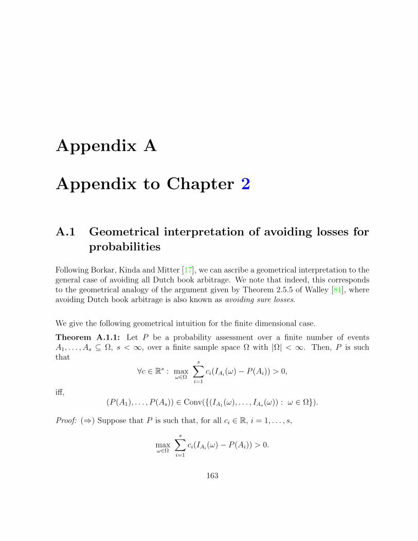
Appendix A
Appendix to Chapter 2
A.1 Geometrical interpretation of avoiding losses for
probabilities
Following Borkar, Kinda and Mitter [17], we can ascribe a geometrical interpretation to thegeneral case of avoiding all Dutch book arbitrage. We note that indeed, this correspondsto the geometrical analogy of the argument given by Theorem 2.5.5 of Walley [81], whereavoiding Dutch book arbitrage is also known as avoiding sure losses.
We give the following geometrical intuition for the finite dimensional case.
Theorem A.1.1: Let P be a probability assessment over a finite number of eventsA1, . . . , As ⊆ Ω, s < ∞, over a finite sample space Ω with |Ω| < ∞. Then, P is suchthat
∀c ∈ Rs : maxω∈Ω
s∑i=1
ci(IAi(ω)− P (Ai)) > 0,
iff,(P (A1), . . . , P (As)) ∈ Conv((IA1(ω), . . . , IAs(ω)) : ω ∈ Ω).
Proof: (⇒) Suppose that P is such that, for all ci ∈ R, i = 1, . . . , s,
maxω∈Ω
s∑i=1
ci(IAi(ω)− P (Ai)) > 0.
163
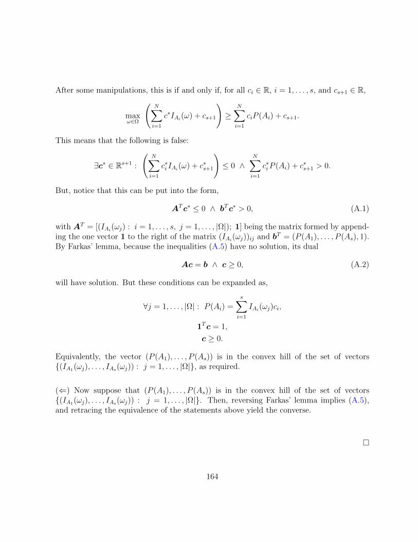
After some manipulations, this is if and only if, for all ci ∈ R, i = 1, . . . , s, and cs+1 ∈ R,
maxω∈Ω
(N∑i=1
c∗IAi(ω) + cs+1
)≥
N∑i=1
ciP (Ai) + cs+1.
This means that the following is false:
∃c∗ ∈ Rs+1 :
(N∑i=1
c∗i IAi(ω) + c∗s+1
)≤ 0 ∧
N∑i=1
c∗iP (Ai) + c∗s+1 > 0.
But, notice that this can be put into the form,
ATc∗ ≤ 0 ∧ bTc∗ > 0, (A.1)
with AT = [(IAi(ωj) : i = 1, . . . , s, j = 1, . . . , |Ω|); 1] being the matrix formed by append-ing the one vector 1 to the right of the matrix (IAi(ωj))ij and bT = (P (A1), . . . , P (As), 1).By Farkas’ lemma, because the inequalities (A.5) have no solution, its dual
Ac = b ∧ c ≥ 0, (A.2)
will have solution. But these conditions can be expanded as,
∀j = 1, . . . , |Ω| : P (Ai) =s∑i=1
IAi(ωj)ci,
1Tc = 1,
c ≥ 0.
Equivalently, the vector (P (A1), . . . , P (As)) is in the convex hill of the set of vectors(IA1(ωj), . . . , IAs(ωj)) : j = 1, . . . , |Ω|, as required.
(⇐) Now suppose that (P (A1), . . . , P (As)) is in the convex hill of the set of vectors(IA1(ωj), . . . , IAs(ωj)) : j = 1, . . . , |Ω|. Then, reversing Farkas’ lemma implies (A.5),and retracing the equivalence of the statements above yield the converse.
164
A.2 Results and proofs
Lemma A.2.1: For any sample space Ω, and P a distribution over some σ-field of Ω, anyexpectation EP over all bounded random variables avoids sure losses. In other words, forany X1, . . . , Xn that are bounded,
supω
n∑i=1
(Xi(ω)− EP (Xi)) ≥ 0.
Proof: Indeed, because EP is an expectation and Xi’s are bounded, the finite sum ofexpectations is the expectation of the sum, so that,
supω
n∑i=1
(Xi(ω)− EP (Xi)) = supω
n∑i=1
Xi − EP
(n∑i=1
Xi
).
Because expectations are convex combinations of its components, we can write,
supω
n∑i=1
Xi ≥ EP
(n∑i=1
Xi
),
yielding the result.
Lemma A.2.2: For any sample space Ω, and P a distribution over Ω over some σ-fieldof Ω, any expectation EP over all bounded random variables are coherent. In other words,for any X0, X1, . . . , Xn that are bounded and m ∈ N,
supω
n∑i=1
((Xi(ω)− EP (Xi))−m(X0 − EP (X0)) ≥ 0.
Proof: Indeed, because EP is an expectation and Xi’s are bounded, the finite sum ofexpectations is the expectation of the sum, so that,
supω
(n∑i=1
(Xi(ω)− EP (Xi))−m(X0 − EP (X0))
)= sup
ω
(n∑i=1
Xi −mX0
)−EP
(n∑i=1
Xi −mX0
).
165
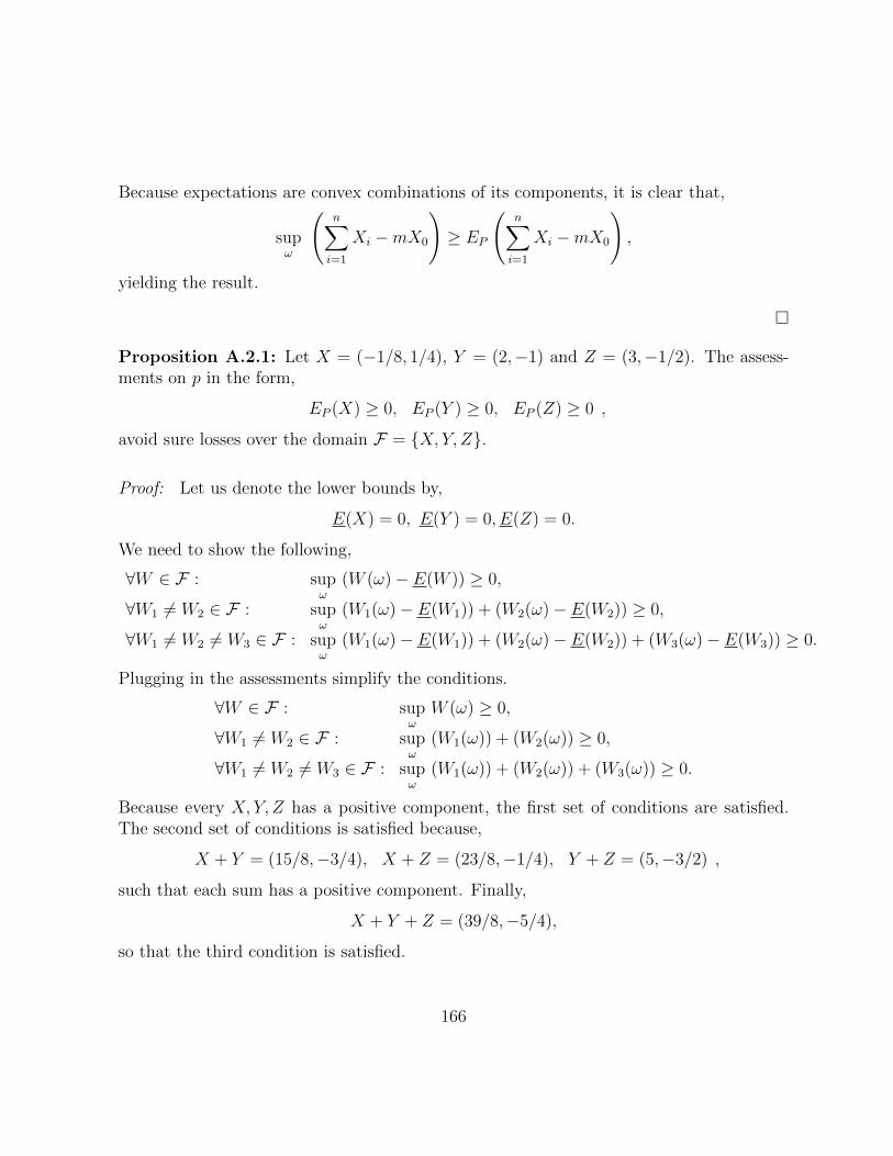
Because expectations are convex combinations of its components, it is clear that,
supω
(n∑i=1
Xi −mX0
)≥ EP
(n∑i=1
Xi −mX0
),
yielding the result.
Proposition A.2.1: Let X = (−1/8, 1/4), Y = (2,−1) and Z = (3,−1/2). The assess-ments on p in the form,
EP (X) ≥ 0, EP (Y ) ≥ 0, EP (Z) ≥ 0 ,
avoid sure losses over the domain F = X, Y, Z.
Proof: Let us denote the lower bounds by,
E(X) = 0, E(Y ) = 0, E(Z) = 0.
We need to show the following,
∀W ∈ F : supω
(W (ω)− E(W )) ≥ 0,
∀W1 6= W2 ∈ F : supω
(W1(ω)− E(W1)) + (W2(ω)− E(W2)) ≥ 0,
∀W1 6= W2 6= W3 ∈ F : supω
(W1(ω)− E(W1)) + (W2(ω)− E(W2)) + (W3(ω)− E(W3)) ≥ 0.
Plugging in the assessments simplify the conditions.
∀W ∈ F : supω
W (ω) ≥ 0,
∀W1 6= W2 ∈ F : supω
(W1(ω)) + (W2(ω)) ≥ 0,
∀W1 6= W2 6= W3 ∈ F : supω
(W1(ω)) + (W2(ω)) + (W3(ω)) ≥ 0.
Because every X, Y, Z has a positive component, the first set of conditions are satisfied.The second set of conditions is satisfied because,
X + Y = (15/8,−3/4), X + Z = (23/8,−1/4), Y + Z = (5,−3/2) ,
such that each sum has a positive component. Finally,
X + Y + Z = (39/8,−5/4),
so that the third condition is satisfied.
166
Theorem A.2.1: Let P be a probability assessment over a finite number of eventsA1, . . . , As ⊆ Ω, s < ∞, over the finite sample space Ω with |Ω| < ∞. Then, P issuch that
∀c ∈ Rs : maxω∈Ω
s∑i=1
ci(IAi(ω)− P (Ai)) > 0,
iff,(P (A1), . . . , P (As)) ∈ Conv((IA1(ω), . . . , IAs(ω)) : ω ∈ Ω).
Proof: (⇒) Suppose that P is such that, for all ci ∈ R, i = 1, . . . , s,
maxω∈Ω
s∑i=1
ci(IAi(ω)− P (Ai)) > 0.
After some manipulations, this is if and only if, for all ci ∈ R, i = 1, . . . , s, and cs+1 ∈ R,
maxω∈Ω
(N∑i=1
c∗IAi(ω) + cs+1
)≥
N∑i=1
ciP (Ai) + cs+1.
This means that the following is false:
∃c∗ ∈ Rs+1 :
(N∑i=1
c∗i IAi(ω) + c∗s+1
)≤ 0 ∧
N∑i=1
c∗iP (Ai) + c∗s+1 > 0.
But, notice that this can be put into the form,
ATc∗ ≤ 0 ∧ bTc∗ > 0, (A.3)
with AT = [(IAi(ωj) : i = 1, . . . , s, j = 1, . . . , |Ω|); 1] being the matrix formed by append-ing the one vector 1 to the right of the matrix (IAi(ωj))ij and bT = (P (A1), . . . , P (As), 1).By Farkas’ lemma, because the inequalities (A.5) have no solution, its dual
Ac = b ∧ c ≥ 0, (A.4)
will have solution. But these conditions can be expanded as,
∀j = 1, . . . , |Ω| : P (Ai) =s∑i=1
IAi(ωj)ci,
1Tc = 1,
c ≥ 0.
167
Equivalently, the vector (P (A1), . . . , P (As)) is in the convex hill of the set of vectors(IA1(ωj), . . . , IAs(ωj)) : j = 1, . . . , |Ω|, as required.
(⇐) Now suppose that (P (A1), . . . , P (As)) is in the convex hill of the set of vectors(IA1(ωj), . . . , IAs(ωj)) : j = 1, . . . , |Ω|. Then, reversing Farkas’ lemma implies (A.5),and retracing the equivalence of the statements above yield the converse.
Theorem A.2.2: Let P be a probability assessment over a finite number of eventsA1, . . . , As ⊆ Ω, s < ∞, over the finite sample space Ω with |Ω| < ∞. Then, P issuch that
∀c ∈ Rs : maxω∈Ω
s∑i=1
ci(IAi(ω)− P (Ai)) > 0,
iff,(P (A1), . . . , P (As)) ∈ Conv((IA1(ω), . . . , IAs(ω)) : ω ∈ Ω).
Proof: (⇒) Suppose that P is such that, for all ci ∈ R, i = 1, . . . , s,
maxω∈Ω
s∑i=1
ci(IAi(ω)− P (Ai)) > 0.
After some manipulations, this is if and only if, for all ci ∈ R, i = 1, . . . , s, and cs+1 ∈ R,
maxω∈Ω
(N∑i=1
c∗IAi(ω) + cs+1
)≥
N∑i=1
ciP (Ai) + cs+1.
This means that the following is false:
∃c∗ ∈ Rs+1 :
(N∑i=1
c∗i IAi(ω) + c∗s+1
)≤ 0 ∧
N∑i=1
c∗iP (Ai) + c∗s+1 > 0.
But, notice that this can be put into the form,
ATc∗ ≤ 0 ∧ bTc∗ > 0, (A.5)
168
with AT = [(IAi(ωj) : i = 1, . . . , s, j = 1, . . . , |Ω|); 1] being the matrix formed by append-ing the one vector 1 to the right of the matrix (IAi(ωj))ij and bT = (P (A1), . . . , P (As), 1).By Farkas’ lemma, because the inequalities (A.5) have no solution, its dual
Ac = b ∧ c ≥ 0, (A.6)
will have solution. But these conditions can be expanded as,
∀j = 1, . . . , |Ω| : P (Ai) =s∑i=1
IAi(ωj)ci,
1Tc = 1,
c ≥ 0.
Equivalently, the vector (P (A1), . . . , P (As)) is in the convex hill of the set of vectors(IA1(ωj), . . . , IAs(ωj)) : j = 1, . . . , |Ω|, as required.
(⇐) Now suppose that (P (A1), . . . , P (As)) is in the convex hill of the set of vectors(IA1(ωj), . . . , IAs(ωj)) : j = 1, . . . , |Ω|. Then, reversing Farkas’ lemma implies (A.5),and retracing the equivalence of the statements above yield the converse.
169
Appendix B
Appendix to Chapter 3
B.1 The lower expectation of the general log-odds
statistic under the IDM
We are interested in the posterior inference of the following general log odds statistic ofa categorical distribution θ over m < ∞ categories under the imprecise Dirichlet model(IDM),
T : θ 7−→ log
∏A∈A
∑i∈A θi∏
B∈B∑
j∈B θj=∑A∈A
log θA −∑B∈B
log θB,
whereA = A1, . . . , Ar and B = B1, . . . , Bq are finite collections of events with Aa, Bb ⊆1, . . . ,m. This statistic includes various ratios of probabilities of interest:
• A = A,B = B yields the log odds ratio log θA − log θB,
• For events C1, . . . , Cq, A = C1∩ . . .∩Cq,B = C1, . . . , Cq is a ratio that measuresthe validity of the independence statement,
θ∩C∈C1,...,CqC=
∏C∈C1,...,Cq
θC .
In this section, we assume that A and B are not non-empty, are not the set of all categories,and A 6= B for all A ∈ A and B ∈ B.
170
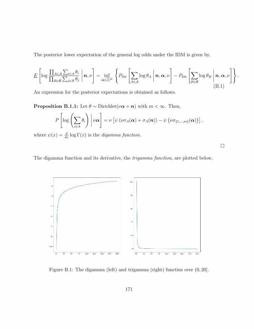
The posterior lower expectation of the general log odds under the IDM is given by,
E
[log
∏A∈A
∑i∈A θi∏
B∈B∑
j∈B θj
∣∣∣∣n, ν]
= infα∈4m
PDir
[∑A∈A
log θA
∣∣∣∣n,α, ν]− PDir
[∑B∈B
log θB
∣∣∣∣n,α, ν]
.
(B.1)An expression for the posterior expectations is obtained as follows.
Proposition B.1.1: Let θ ∼ Dirichlet(να+ n) with m <∞. Then,
P
[log
(∑i∈A
θi
) ∣∣∣∣ να]
= ν[ψ (νσA(α) + σA(n))− ψ
(νσ1,...,m(α)
)],
where ψ(x) = ddx
log Γ(x) is the digamma function.
The digamma function and its derivative, the trigamma function, are plotted below,
Figure B.1: The digamma (left) and trigamma (right) functins over (0, 20].
171
We will be frequently invoking the facts that the diagamma function, ψ is an increasingfunction over R, and that the trigamma function ψ′ is a decreasing, strictly positive func-tion.
Noting that the elements of α sum to one such that, ψ(νσ1,...,p(α)) = ψ(ν), the posteriorlower expectation of the general log-odds under the IDM is,
E
[log
∏A∈A
∑i∈A θi∏
B∈B∑
j∈B θj
∣∣∣∣n, ν]
= minα∈4m
ν
(∑A∈A
ψ(νσA(α))−∑B∈B
ψ(νσB(α))
)− (|A| − |B|)ψ(ν)
.
(B.2)
Because the last term is independent of α, the achievable minimum is a solution to,
minimise:r∑
a=1
ψ(νσAa(α) + σAa(n))−q∑b=1
ψ(νσBb(α) + σBb(n))
subjected to: α ∈ 4p. (B.3)
(It will be useful for what follows to index A by a ∈ 1, . . . , r and B by b ∈ 1, . . . , q.)
B.2 Unboundedness of the log-odds and the theory of
coherence
We detail the extension of Walley’s [81] theory of coherence from bounded random variablesfor the IDM to the case of the unbounded log-odds random variable.
B.2.1 Extending Walley’s [81] coherence to the log-odds randomvariable under the IDM under non-sparse observations
By a non-sparse observation, we mean that every category of the IDM system has at leastone count being observed. The main result that drives our construction of the extension
172
is the convergence of a bounded approximation of the log-odds statistic.
Theorem B.2.1: Consider the general log-odds statistic,
g(θ) = log
∏ri=1 P (Ai|θ)∏sj=1 P (Bj|θ)
,
and the following truncation of it,
Tc(θ) = g(θ)I(|g(θ)| ≤ c) + cI(|g(θ)| > c).
Under θ ∼ Dirichlet(να+ n) with sets A1, . . . , Ar, B1, . . . , Bs, such that nAi > 0, nBj > 0for all Ai, Bj,
supα∈4Ω
E(|Tc − g||να+ n)→ 0,
as c→∞.
Proof: see Theorem B.3.3.
Now, we define the IDM lower expectation of the unbounded log-odds statistic as a doublelimit of two limiting processes: the relaxation of the approximation of Theorem B.2.1 inthe variable of c and the limit in the optimisation variable α that may approach any pointin 4m (including the boundary).
We have, by the continuity of α 7−→ E(Tc|να+ n),
limc→∞
(limα→α0
E(Tc|να+ n)
)= lim
c→∞E(Tc|να0 + n) = E(g|να0 + n).
On the other hand, by Theorem B.2.1,
limα→α0
(limc→∞
E(Tc|να+ n))
= limα→α0
E(g|να0 + n) = E(g|να0 + n).
So, the double limits exist and are equal.
173
This justifies our plugging in of the log-odds into the IDM, despite it being unbounded, asfollows. Any path based optimisation (such as gradient descent) over 4Ω of the expecta-tion of the truncated log-odds Tc will yield converge to the limit point that is the infimumof the expectation of g, as the truncation c is relaxed. That is, we will make the followinginterpretation.
Definition B.2.1: For a coherent lower expectation, E, defined over set of bounded ran-dom variables, write E(ext) to be its natural extension to the linear space of unboundedrandom variables.
Interpretation 2.2.1: For any general log-odds,
g(θ) = log
∏ri=1 P (Ai|θ)∏sj=1 P (Bj|θ)
,
whenever n contains at least one count in each category, we interpret,
E(ext)IDM(g(θ)|ν,n) = inf
α∈4ΩE(g(θ)|να+ n),
as the double limit of the sequence of truncated Dirichlet expectations,
c,α 7−→ E(g(θ)I(|g(θ)| ≤ c) + cI(|g(θ) > c|)|να+ n),
over the optimisation path of α contained in 4Ω and the release of the truncation approx-imation via c→∞.
B.2.2 Convergence of lower and upper expectation of L1 approx-imation error
We note an immediate corollary of Theorem B.2.1.
Corollary B.2.1: Under the conditions of Theorem B.2.1,
infα∈4Ω
E(|Tc − g| |να+ n)→ 0,
as c→∞.
174
The uniform convergence in Corollary B.2.1 and Theorem B.2.1 are respectively equivalentto,
EIDM(|Tc − g| |ν,n) = infα∈4Ω
E(|Tc − g| |να+ n)→ 0,
EIDM(|Tc − g| |ν,n) = supα∈4Ω
E(|Tc − g| |να+ n)→ 0,
as c→∞.
B.2.3 Relation to coherence notions extended to unbounded ran-dom variables[78]
Theorem B.2.1 is closely related to the notion of previsible gambles introduced by Troffaesand de Cooman [78] defined in order to extend Walley’s coherence to unbounded randomvariables. Roughly, a previsible gamble is one whose lower prevision can be approximatedby a sequence of lower previsions of bounded gambles. We will show that any log-oddsis previsible with respect to the posterior IDM previsions, and subsequently show thatplugging in the general log-odds into the posterior IDM model is coherent in the sense ofthe extension of coherence to unbounded gambles by Troffaes and de Cooman.
Definition B.2.2: Throughout Section B.2.3 and nowhere else in this document, a gambleis a potentially unbounded random variable. This is in distinction to a bounded gamble.We will use these two terms explictly throughout Section B.2.3.
Definition B.2.3: (Troffaes and de Cooman [78], Definition 15.1, p.329) For a coherentlower prevision E, and gambles f, fn (which are not necessarily bounded), the net fcconverges in E-probability to f iff,
∀ε > 0 : E(|f − fc| > ε)→ 0,
(whereby we interpret 0 to be the Moore-Smith limit of E(|f − fc| > ε) as a net over c inan indexing directed set).
175
Definition B.2.4: (Troffaes and de Cooman [78], Definition 15.6, p.333) A gamble f isE-previsible if there is a sequence fn of bounded gambles such that,
1. fn converges in E-probability to f and,
2. limn,m→∞E(|fn − fm|) = 0.
If f is E-previsible, then the extended lower and upper previsions of f are defined by,
Ex(f) := limn→∞
E(fn),
andE
x(f) := lim
n→∞E(fn),
respectively.
Proposition B.2.1: (Troffaes and de Cooman [78], Proposition 15.11, p 335) The previ-sions, Ex and E
xin Definition B.2.4 are coherent previsions over the set of E-previsible
gambles.
With these preliminaries from Troffaes and de Cooman [78], we can now show that theextension of the IDM to the unbounded log-odds gamble g is coherent by showing that itsatisfies the conditions of Proposition B.2.1.
Theorem B.2.2: Under the conditions of Theorem B.2.1, the extended IDM whose valueat the unbounded log-odds g is given by,
E(ext)IDM(g(θ)|ν,n) = lim
c→∞EIDM(Tc(θ)|να+ n),
is coherent under the Proposition B.2.1 of Troffaes and de Cooman [78].
Proof: By Proposition B.2.1, we are done if we show that, under the conditions of The-orem B.2.1, g is EIDM(·|ν,n)-previsible by showing that the two conditions in DefinitionB.2.4 is satisfied. These two conditions are shown to be satisfied by g (with the sequenceof bounded gambles Tc) by Lemmas B.2.1 and B.2.2, respectively.
176
Lemma B.2.1: Under the conditions of Theorem B.2.1, the net Tc converges to g inEIDM(·|ν,n)-probability. That is,
∀ε > 0 : EIDM(|Tc − g| > ε|ν,n)→ 0,
as c→∞.
Proof: Recall, by Theorem B.2.1,
EIDM(|Tc − g| |ν,n) = supα∈4Ω
E(|Tc − g| |να+ n)→ 0.
On the other hand, by Markov’s inequality,
∀ε > 0 : P (|Tc − g| > ε|να+ n) <E(|Tc − g| |να+ n)
ε,
such that,
∀ε > 0 : EIDM(|Tc−g| > ε|ν,n) = supα∈4Ω
P (|Tc−g| > ε|να+n) <
supα∈4
E(|Tc − g| |να+ n)
ε→ 0,
as c→∞.
Lemma B.2.2: Under the conditions of Theorem B.2.1,
limc1,c2→∞
EIDM(|Tc1 − Tc2| |ν,n) = 0.
Proof:
EIDM(|Tc1 − Tc2| |ν,n)
= supα∈4Ω
E(|Tc1 − Tc2| |να+ n)
≤ supα∈4Ω
(E(|g − Tc1| |να+ n) + E(|g − Tc2 | |να+ n))
≤ supα∈4Ω
E(|g − Tc1| |να+ n) + supα∈4Ω
E(|g − Tc2| |να+ n)
→ 0. (Theorem B.2.1)
177
B.2.4 A note on behavioural interpretation of unbounded valuesof imprecise expectations [78]
Under the behavioural interpretation of Walley [81], EIDM(f |ν,n) is the highest price thatthe agent finds acceptable for the random reward f upon knowing only the IDM assump-tion, the fixed hyperparameter ν and the dataset n. Specifically, EIDM(f |ν,n), is the pricesuch that, for all ε > 0, an agent knowing only this information is behaviourally disposedto engage in the random reward f − EIDM(f |ν,n) + ε. (The meaning of ‘behaviourallydisposed’ is extensively treated in Walley [81].)
Then, EIDM(f |ν,n) = −∞ can be interpreted as: there is no finite buying price be-low which a gambler who has this information at hand should find desirable. (Similarly,EIDM(f |ν,n) = −∞ can be interpreted as: there is no finite selling price above which agambler who has this information at hand should find desirable.) This coincides exactlywith the interpretation given by Troffaes and de Cooman for E(X) = −∞: for example,‘... [E(X) = −∞] is taken to mean that ... our subject is not willing to buy the gamble [X]for any real price t ∈ R.’ and ’[E(X) = +∞] ... is taken to mean that ... the subject iswilling to buy the gamble [X] at any price.’ [78]. In fact, the following remark by Troffaesand de Cooman is interesting to keep in mind.
‘The rationality axioms [(that imply coherence)] are onlyan approximation of how agents really ought to behave...When utility becomes unbounded, we accept these rationalityaxioms as a matter of convenience in modelling... If thingsreally matter at the infinite end, as with the Saint Petersburgparadox, perhaps one should rethink one’s choice of utility.’ [78]
B.2.5 A simple counterexample in the sparse data case
We can use the following counterexample to show that the limit of the approximation errorfails to exist as we take both the relevant elements of the posterior hyperparameter, sayγ, to zero and the approximation parameter, c, tends to infinity.
Example B.2.1: Consider θ ∼ Dirichlet(να + n) with α = (α1, α2, 1 − α1 − α2) ∈ 4Ω
and n = (n1, n2, n3) and,g(θ) = log θ1/θ2,
178
for θ a vector of trinomial cell probabilities. From Theorem B.2.1 for every fixed α ∈ 4Ω,
limc→∞
E(|g − Tc||να+ n) = limc→∞
E(|g − gI(|g| ≤ c)||να+ n) = 0,
This leads to,limα1→0 limc→∞E(|g − Tc||να+ n) = 0
and limα2→0 limc→∞E(|g − Tc||να+ n) = 0.. (B.4)
However,
limα1→0
E(|g − Tc||να+ n)
≥(
limα1→0
E(|g||να+ n)− E(|g|I(|g| ≤ c)|να+ n)− E(cI(|g| > c)|να+ n)
)=
(limα1→0
E(|g||να+ n)− E(|g|I(|g| ≤ c)|να+ n)− cP (|g| > c|να+ n)
)> lim
α1→0E(|g||να+ n)− 2c
≥ limα1→0
|E(g|να+ n)| − 2c
= limα1→0
|ψ(1)(να1 + n1)− ψ(1)(να2 + n2)| − 2c (ψ(1) is the digamma function)
=∞,
and similarly, using the last two lines of the preceding inequalities,
limα2→0
E(|g − Tc||να+ n) >∞.
This leads to,limc→∞ limα1→0E(|g − Tc||να+ n) =∞
and limc→∞ limα2→0E(|g − Tc|να+ n) =∞. (B.5)
This demonstrates that there are at least two paths in the (c, α1, α2) space that lead todifferent double limits of E(|g − gI(|g| ≤ c)||να+ n), such that the double limits are notdefined.
179
B.3 Proof of Theorem B.3.1
For brevity, we will sometimes denote the general log odds by,
g(θ) = log
∏ri=1 P (Ai|θ)∏sj=1 P (Bj|θ)
. (B.6)
In this appendix section, we assume that, when dealing with log-odds involving any logprobability of the form logP (Ai|θ) where P (Ai|θ) =
∑ω∈A θω and θ ∼ Dirichlet(γ), that
γA =∑
ω∈A γω > 0. This is to ensure that the truncation is approximating somethingfinite, or else convergence in mean and in probability are ill-defined.
B.3.1 Some lemmas
Lemma B.3.1: For a probability space over a finite dimensional simplex (4Ω,Σ, µ) suchthat µ(4Ω) = 1 and µ assigns zero probability to any lower dimensional subsets, and fwhich is (Σ,BR∪±∞)-measurable and µ-integrable, and c a natural number,
E|fI(−c ≤ f ≤ c)− f | −→ 0,
as c→∞.
Proof: Consider,
fc : c ∈ N = |fI(−c ≤ f ≤ c)− f | : c ∈ N.
fc is a sequence of measurable functions in the index of c that decreases to zero in theinterior of 4Ω, which has measure one under µ. Therefore, this convergence is µ-almostsure. For every fixed c, we have that,
fc = |fI(−c ≤ f ≤ c)− f | = | − fI(|f | > c)| = |f |I(|f | > c) ≤ |f |.
Then, by Corollary B.3.1, the relaxation of the monotone convergence theorem of Yeh [87]to almost sure convergence requirements, yields,
E|fI(−c ≤ f ≤ c)− f | −→ 0.
180
Lemma B.3.2: Under a Dirichlet distribution with parameters γ > 0, the general logodds,
g(θ) = log
∏ri=1 P (Ai|θ)∏sj=1 P (Bj|θ)
,
is integrable.
Proof: This follows from the existence of the second moments of log θi’s and cross momentslog θi · log θj, and Holder’s inequality:
E(|g||γ) ≤ (E(g2|γ))1/2 <∞.
Lemma B.3.3: Under a Dirichlet distribution with parameters γ > 0,
E
∣∣∣∣(
log
∏ri=1 P (Ai|θ)∏sj=1 P (Bj|θ)
)I
(−c ≤
(log
∏ri=1 P (Ai|θ)∏sj=1 P (Bj|θ)
)≤ c
)−
(log
∏ri=1 P (Ai|θ)∏sj=1 P (Bj|θ)
) ∣∣∣∣ −→ 0.
Proof: follows from Lemma B.3.1 with f =(
log∏ri=1 P (Ai|θ)∏sj=1 P (Bj |θ)
)with the integrability of f
guaranteed by Lemma B.3.2.
We will also need the following convergence in probability result.
Lemma B.3.4: Let θ ∼ Dirichlet(γ) for some γ > 0. Then,
cP
(| log
∏ri=1 P (Ai|θ)∏sj=1 P (Bj|θ)
| > c|γ
)→ 0,
and,
c2P
(| log
∏ri=1 P (Ai|θ)∏sj=1 P (Bj|θ)
| > c|γ
)→ 0.
181
Proof: Write g for the general log odds as in (B.6). Consider that,
g2 =
(r∑i=1
log θAi −s∑j=1
log θBj
)2
,
is an order two polynomial involving terms of the form (log θA)2, (log θA)(log θB), andthe expectations of these terms all exist and are finite under the Dirichlet distribution.Importantly,
E(g2|γ
)<∞,
under the assumption that γ > 0. So, using Markov’s inequality,
cP (|g| > c|γ) ≤ cE (g2|γ)
c2→ 0,
Similarly, the following fourth moment exists for the Dirichlet distribution when γ > 0,
E(g4|γ
)<∞.
This yields,
c2P (|g| > c|γ) ≤ c2E (g4|γ)
c4→ 0,
B.3.2 L1 and pointwise convergence for general log-odds
Theorem B.3.1: (L1 convergence) Under θ ∼ Dirichlet(γ) with setsA1, . . . , Ar, B1, . . . , Bs,such that γAi > 0, γBj > 0 for all Ai, Bj,
E(|Tc − g||γ)→ 0.
as c→∞.
Proof: Lemma B.3.3 implies, as c→∞,
E(|g − gI(|g| ≤ c)| |γ)→ 0.
On the other hand, by Lemma B.3.4,
cP (|g| > c|γ)→ 0,
as c→∞. In all,
E(|Tc−g| γ) = E(|gI(|g| ≤ c)−g+cI(|g| > c)| |γ) ≤ E(|gI(|g| ≤ c)−g| |γ)+cP (|g| > c|γ)→ 0.
182
Theorem B.3.2: (Pointwise convergence) Under θ ∼ Dirichlet(γ) with setsA1, . . . , Ar, B1, . . . , Bs,such that γAi > 0, γBj > 0 for all Ai, Bj,
E(Tc|γ)→ E (g|γ) .
as c→∞.
Proof: this is a corollary of the L1 convergence in Theorem B.3.1.
B.3.3 Uniform L1 convergence for Dirichlet-Multinomial poste-rior expectations of general log-odds under non-sparse case
From the last section, we had the following pointwise convergence result,
E(|Tc − g||γ)→ 0,
as c → ∞, under the assumption that γ is such that γAi , γBj > 0 for all the sets Ai, Bj
involved in the general log odds.
We remark that it is generally impossible for this continuity to be uniform when certainelements of γ are zero. For example, for a fixed general log odds involving sets A1 andB1, if γA1 , γB1 = 0, then the expectation of the general log odds becomes undefined as thedifference of digamma functions ψ(γA1)−ψ(γB1) has ill-defined limiting behaviour. Rather,we will restrict ourselves to the special case of,
γ = να+ n,
such that n > 0 (elementwise), ν > 0 and α ∈ 4Ω. In this notation, the pointwiseconvergence is,
E(Tc|να+ n)− E (g|να+ n)→ 0.
Uniformity of convergence over the compact domain 4Ω 3 α is now much easier to obtainthan over the positive orthant containing γ whose elements can be zero. Specifically, we
183
will verify the conditions of Dini’s theorem, Theorem B.3.5, and apply it to obtain uniformconvergence. We first present the proof of the main results, followed by the major lemmasused in it.
Theorem B.3.3: (Uniform L1 convergence of posterior expectations) Under θ ∼ Dirichlet(να+n) with sets A1, . . . , Ar, B1, . . . , Bs, such that nAi > 0, nBj > 0 for all Ai, Bj,
supα∈4Ω
E(|Tc − g||να+ n)→ 0,
as c→∞.
Proof: First. consider that,
supα∈4Ω
E(|Tc − g| |να+ n)
≤ supα∈4Ω
E(|gI(|g| ≤ c)− g| |να+ n) + c supα∈4Ω
P (|g| ≥ c |να+ n)
≤ supα∈4Ω
E(|gI(|g| ≤ c)− g| |να+ n) +c
c2supα∈4Ω
E(g2 |να+ n). (Markov’s Inequality)
Because n > 0, the last quantity is finite and so tends to zero in the limit of c. So, if wecan show that the first supremum also tends to zero as c→∞, then we are finished.
We can use Dini’s theorem to do so as follows. Let us verify the conditions for Dini’stheorem. Over the compact domain 4Ω 3 α, let
fc(α) = E(|gI(|g| ≤ c)− g| |να+ n),
andf(α) = 0.
• By Lemma B.3.5, fc is continuous over 4Ω metrised by an Lp norm for every c ∈ N.
• For every fixed α ∈ 4Ω, fc → f , by the L1 convergence in Lemma B.3.3.
• Since |gI(|g| ≤ c)− g| ≥ |gI(|g| ≤ c+ 1)− g|, taking expectations on both sides forevery fixed α ∈ 4Ω, fc ≥ fc+1.
184
Then, by Dini’s theorem, the convergence,
E(|gI(|g| ≤ c)− g| |να+ n)→ 0,
is uniform over 4Ω 3 α.
Lemma B.3.5: For every fixed c ∈ N,
fc(α) = E(|gI(|g| ≤ c)− g| |να+ n),
is continuous at every point in 4Ω 3 α where 4Ω is metrised by an Lp norm.
Proof: For short in this proof, write,
pα(θ) := p(θ|να+ n).
Let us work in the projected parametrisation: write,
α′ = (α1, . . . , α|Ω|−1) ∈ N|Ω|−1,
where
N|Ω|−1 :=
p ∈ R|Ω|−1 : pi ≥ 0 ∧|Ω|−1∑i=1
pi ≤ 1
.
such that,α = [α′;α|Ω|].
Consider that, for any two points α′,α′0 ∈ N|Ω|−1,
fc(α′)− fc(α′0) =
∫4Ω
|gI(|g| ≤ c)− g|(θ)(pα′(θ)− pα′0(θ))dθ
=
∫4Ω
|g|I(|g| > c)(θ)(pα′(θ)− pα′0(θ))dθ.
It now suffices to prove continuity over N|Ω|−1 to obtain continuity over 4Ω.
185
Because n > 0, for every fixed θ ∈ 4Ω, the gradient of the map α′ 7−→ pα′(θ) hascomponents,
∂
∂αipα′(θ) =
∂
∂αi
1
B(να+ n)
|Ω|−1∏j=1
θναj+nj−1j θ
ν(1−α1−...−α|Ω|−1)+n|Ω|−1
|Ω|
=
1
B(να+ n)2
B(να+ n)
∂
∂αi
|Ω|−1∏j=1
θναj+nj−1j θ
ν(1−α1−...−α|Ω|−1)+n|Ω|−1
|Ω|
−|Ω|∏j=1
θναj+nj−1j
(∂
∂αiB(να+ n)
)=
1
B(να+ n)2
B(να+ n)
|Ω|−1∏j 6=i
θναj+nj−1j θ
ν(1−α1−...−αi−1+αi+1−...−α|Ω|−1)+n|Ω|−1
|Ω|
∂
∂αiθναi+ni−1i θ−ναi|Ω|
)−|Ω|∏j=1
θναj+nj−1j
(∂
∂αiB(να+ n)
)=
1
B(να′ + n)2
B(να′ + n)ν(log θi − log θ|Ω|)
|Ω|∏j=1
θναj+nj−1j
−|Ω|∏j=1
θναj+nj−1j
(∂
∂αiB(να′ + n)
)= ν(log θi − log θ|Ω|)pα′(θ)−
∂∂αiB(να′ + n)
B(να′ + n)pα′(θ).
This gradient is defined for each θ ∈ 4Ω where θ > 0 when n > 0. Then, for every such
186

fixed θ, we can apply the mean value theorem to find α′′ such that,
fc(α′)− fc(α′0)
=
∫4Ω
|g|I(|g| > c)(θ)(pα′(θ)− pα′0(θ))dθ
=
(∫4Ω
|g|I(|g| > c)(θ)∂
∂αipα′′(θ)dθ
)Ti
(α′ −α′0)
=
(∫4Ω
|g|I(|g| > c)(θ)
(ν(log θi − log θ|Ω|)pα′′(θ)−
∂∂αiB(να′′ + n)
B(να′′ + n)pα′′(θ)
)dθ
)T
i
(α′ −α′0).
By Lemma B.3.6, the upper bound of the left integral is finite over the relevant variables:
K = maxi=1,...,|Ω|
supα′′∈N|Ω|−1
ν
(∫4Ω
(|g(θ) log θi|+ |g log θ|Ω||)I(|g(θ)| > c)pα′′(θ)dθ
−∂∂αiB(να′′ + n)
B(να′′ + n)
∫4Ω
|g(θ)|I(|g(θ)| > c)pα′′(θ)dθ
)<∞.
Then, in all,|fc(α′)− fc(α′0)| ≤ |K| ||α′ −α′0||1,
where |α′ −α′0| = (|α1i − α2i : i = 1, . . . ,Ω). So, if the positive quantity ε is defined as,
|K| ||α′ −α′0||1 = ε,
then, the choice of δε,α′0 such that,
||α′ −α′0||1 ≤ δε,α′0 ,
implies,|fc(α′)− fc(α′0)| ≤ ε.
This is such that,
∀ε > 0, ∃ δε,α′0 : (||α′ −α′0||1 ≤ δε,α′0 ⇒ |fc(α′)− fc(α′0)| ≤ ε.
Finally, because continuity is preserved over all p-norms,
∀ε > 0, ∃ δε,α′0 : (||α′ −α′0||p ≤ δε,α′0 ⇒ |fc(α′)− fc(α′0)| ≤ ε.
187
Lemma B.3.6: When n > 0, the upper bound,
K = maxi=1,...,|Ω|
supα′′∈N|Ω|−1
ν
(∫4Ω
(|g(θ) log θi|+ |g log θ|Ω||)I(|g(θ)| > c)pα′′(θ)dθ
−∂∂αiB(να′′ + n)
B(να′′ + n)
∫4Ω
|g(θ)|I(|g(θ)| > c)pα′′(θ)dθ
).
is finite.
Proof: For every i = 1, . . . , |Ω|,∫4Ω
|g(θ)|I(|g(θ)| > c)
(ν(log θi − log θ|Ω|)pα′′(θ)−
∂∂αiB(να′′ + n)
B(να′′ + n)pα′′(θ)
)dθ
= ν
∫4Ω
|g(θ)|(log θi − log θ|Ω|)I(|g(θ)| > c)pα′′(θ)dθ
−∂∂αiB(να′′ + n)
B(να′′ + n)
∫4Ω
|g(θ)|I(|g(θ)| > c)pα′′(θ)dθ
≤ ν
∫4Ω
|g(θ)(log θi − log θ|Ω|)|I(|g(θ)| > c)pα′′(θ)dθ
−∂∂αiB(να′′ + n)
B(να′′ + n)
∫4Ω
|g(θ)|I(|g(θ)| > c)pα′′(θ)dθ
≤ ν
∫4Ω
(|g(θ) log θi|+ |g log θ|Ω||)I(|g(θ)| > c)pα′′(θ)dθ
−∂∂αiB(να′′ + n)
B(να′′ + n)
∫4Ω
|g(θ)|I(|g(θ)| > c)pα′′(θ)dθ.
Now, for any cell probability θk, by Holder’s inequality,∫|g log θk|pα′′dθ ≤
(∫g2pα′′dθ
)1/2(∫(log θk)
2pα′′dθ
)1/2
,
and the right quantities are finite because the second moments finitely exist for both g andlog θk under the Dirichlet distribution of pα′′ .
188
Also, the second term involving the derivative of the beta function is finite for everyα′′ ∈ N|Ω|−1, since, by Lemma B.3.2, the log odds g is integrable and the digamma andtrigamma function in the Beta function and its derivative are finite when n > 0 overα′′ ∈ 4Ω.
Then, any sequence of evaluations of this expression over α′′ in N|Ω|−1 must also have afinite limit, meaning that the supremum over the closed set N|Ω|−1 is finite. Let us denotethis finite upper bound by,
K = maxi=1,...,|Ω|
supα′′∈N|Ω|−1
ν
(∫4Ω
(|g(θ) log θi|+ |g log θ|Ω||)I(|g(θ)| > c)pα′′(θ)dθ
−∂∂αiB(να′′ + n)
B(να′′ + n)
∫4Ω
|g(θ)|I(|g(θ)| > c)pα′′(θ)dθ
).
B.3.4 Auxiliary results
In this appendix section, we make use of the following theorems from other authors.
Theorem B.3.4: (Yeh [87], Theorem 9.17, p.186) Let (X,F , µ) be an arbitrary measurespace. Let (fn : c ∈ N) be a monotone sequence of extended real-valued F -measurablefunctions on a set D ∈ F and let f = limc→∞ fn.
If (fc : c ∈ N) is a decreasing sequence, and there exists a µ-integrable extended real-valuedF -measurable function g such that fc ≤ g on D for every c ∈ N, then,
limc→∞
∫D
fcdµ =
∫D
fdµ.
Let us relax the sure convergence condition to almost sure.
Corollary B.3.1: Let (X,F , P ) be an arbitrary probability space. Let (fn : c ∈ N) bea monotone sequence of extended real-valued F -measurable functions on a set D ∈ F and
189
let P (f = limc→∞ fc) = 1.
If (fc : c ∈ N) is a decreasing sequence, and there exists a P -integrable extended real-valuedF -measurable function g such that fc ≤ g on D for every c ∈ N, then,
limc→∞
∫D
fcdµ =
∫D
fdP.
Proof: Let us denote by E the set of sample points over which fc converges to f almostsurely. Write
hc = fcIE, h = fIE.
We have that, for all c ∈ N,∫DhcdP =
∫DfcdP, and
∫DhdP =
∫DfdP. (B.7)
Also, by Theorem B.3.4, because hc ≤ g for the g that bounds fc, we also know that,
limc→∞
∫E
hcdP =
∫E
hdP.
Because E ⊆ D in order for the almost sure convergence to be defined, and P (E) = 1,∫DhcdP =
∫EhcdP,
∫DhdP =
∫EhdP,
such that,
limc→∞
∫D
hcdP =
∫D
hdP. (B.8)
Substituting (B.7) into (B.8) yields the required result.
Theorem B.3.5: (Rudin [67], Theorem 7.13, p. 150) Suppose K is compact and
(a) fc is a sequence of continuous functions on K,
(b) fc converges pointwise to a continuous function f on K,
(c) fc(x) ≥ fn+1(x) for all x ∈ K and n = 1, 2, 3, . . ..
Then fc → f uniformly on K.
190
B.4 Results on IDM log-odds imprecision
Proposition B.4.1: for n and ∆n such that nC ≥ 1 and ∆nC ≥ 0,
P IDM[log θC |να + n] ≥ P IDM[log θC |να + n+ ∆n].
Proof: recall that the imprecision of the log-probability is given by,
P IDM[log θC |να + n] = ψ(ν + nC)− ψ(nC).
The change in imprecision between having observations n and n+ ∆n is,
P IDM[log θC |να + n+ ∆n]− P IDM[log θC |να + n]
= ψ(ν + nC + ∆nC)− ψ(nC + ∆nC)− ψ(ν + nC) + ψ(nC).
We write this expression in terms of the derivative ψ′ by using the mean value theorem forwhen nC ≥ 1. In particular, when ν > ∆n, there exists u ∈ (ν + nC , ν + nC + ∆nC) andv ∈ (nC , nC + ∆nC),
(ψ(ν + nC + ∆nC)− ψ(nC + ν))− (ψ(∆nC + nC) + ψ(nC))
= ∆nC(ψ′(u)− ψ′(v))
< 0,
where the last inequality is because ψ′ is a strictly decreasing function and that u > v.This proves the desired result for ν > ∆n. The case ν ≤ ∆n results in the inequality,
ν(ψ′(a)− ψ′(b)) < 0,
with a ∈ (∆nC + nC , ν + nC + ∆nC) and b ∈ (nC , nC + ν), and this proves the desiredresult for ν ≤ ∆n.
Lemma B.4.1: For two random variables X and Y , and a conjugate pair of coherentexpectations E,E (not necessarily IDM,)
P [X + Y ] ≤ P [X] + P [Y ].
P [−X] = P [X].
191
By proof of induction, for finite collections X1, . . . , Xr and Y1, . . . , Ys,
P
[r∑i=1
Xi −s∑j=1
Yj
]≤
r∑i=1
P [X] +s∑j=1
P [Y ].
Proof: For the first statement, because sup p(x) + p(y) : p ∈ M ≤ sup p(x) : p ∈
M+sup p(y) : p ∈M, and inf p(x)+p(y) : p ∈M ≥ inf p(x) : p ∈M+inf p(y) :
p ∈M, imprecision satisfies the triangular inequality
P [X + Y ] = E[X + Y ]− E[X + Y ]
≤ E[X] + E[Y ]− E[X]− E[Y ]
≤ P [X] + P [Y ].
For the second statement, suppose E and E for envelopes for a set of expectations M ,
P [−X] = E[−X]− E[−X]
= sup p(−X) : p ∈M − inf p(−X) : p ∈M
= sup −p(X) : p ∈M − inf −p(X) : p ∈M
= −inf p(X) : p ∈M+ sup p(X) : p ∈M
= P [X].
We now prove that the decrease of imprecision of the log-probability inference is greaterwhen increasing the relevant event’s count from a small number: in particular, the jumpfrom no observation to a single observation is the greatest. Let us define the imprecisionas well as the change of imprecision of the inference of a log probability log θC (for someset C ⊂ 1, . . . ,m,
P (n) := ψ(ν + n)− ψ(n),
∆P (n; ∆n) := P (n+ ∆n)− P (n).
192
In particular, the last expression is the change of imprecision at n when an additional∆n > 0 counts are observed in the set C.
Proposition B.4.2: Let n1, n2,∆n, ν > 0 such that n2 > n1. Then,
0 ≥ ∆P (n2; ∆n) > ∆P (n1; ∆n).
Proof: From Lemma B.4.1, imprecision is a decreasing function so that the change of im-precision is a negative function.
For the next inequality, because sums of digamma functions is continuous and differentiableon the positive real line, we apply the mean value theorem to n ∈ R 7−→ ∆P (n; ∆n) ∈ Rby,
∆P (n2; ∆n)−∆P (n1; ∆n) = ∆P′(u; ∆n)(n2 − n1),
with u ∈ (n1, n2) and ,
∆P′(u; ∆n) = ψ′(ν + u+ ∆n)− ψ′(u+ ∆n)− ψ′(ν + u) + ψ′(u).
Our goal is to show that ∆P′(u; ∆n) is non-negative. Consider the case when ν > ∆n.
Then, because the trigamma function, ψ′, is again continuous and differentiable on thepositive real line, we can apply the mean value theorem again to obtain,
∆P′(u; ∆n) = (ψ′(ν+u+∆n)−ψ′(ν+u))− (ψ′(u+∆n)−ψ′(u)) = ∆nψ′′(w)−∆nψ′′(v),
with w ∈ (ν + u, ν + u+ ∆n) and v ∈ (u, u+ ∆n) such that v < w (for any u ∈ (n1, n2).)Because the tetragamma function, ψ′′, is strictly increasing, v < w implies ψ′′(v) < ψ′′(w).Thus, overall, we have, for u, v, w satisfying their respective bounds,
∆P′(u; ∆n) = ∆n(n2 − n1)(ψ′′(w)− nψ′′(v)) > 0.
On the other hand, if ν ≤ ∆n, one could instead use the difference,
∆P′(u; ∆n) = (ψ′(ν + u+ ∆n)− ψ′(u+ ∆n))− (ψ′(ν + u)− ψ′(u)) = νψ′′(a)− νψ′′(b),
with a ∈ (∆n + u, ν + u + ∆n) and b ∈ (u, ν + u) instead and apply the same procedureto obtain the same result. This completes the proof.
193
B.5 Indeterminate forms and their limiting processes
In the following, we demonstrate that when indeterminacy can happen in an expectation oflog-odds under a Dirichlet distribution, then the expectation can take on any value of theextended real line. We do so by constructing a limiting process for each value it can obtain.
Theorem B.5.1: Suppose that⋃ri=1Ai∪
⋃sj=1Bj ⊂ 1, . . . ,m (i.e. it does not cover the
whole set of indices.) For any mi,mj ∈ R+ ∪ 0, the finite collection of paths αi : i =1, . . . , r and αj : j = 1, . . . , s satisfying,(
r∑i=1
1
αi(t)
)= logmit,
(s∑j=1
1
αj(t)
)= logmjt,
and, as t→∞, αi(t), αj(t)→ 0, will yield,
r∑i=1
ψ(ναi(t))−s∑j=1
ψ(ναj(t))→1
νlog
mi
mj
.
Proof: The Laurent expansion of the digamma function around 0 implies that,
ψ(x) ≈ −1
x,
when x is in a sufficiently small neighbourhood of 0. Then,
r∑i=1
ψ(ναAi)−s∑j=1
ψ(ναBj) ≈ −1
ν
r∑i=1
1
αAi+
1
ν
s∑j=1
1
αBj.
This expression can be exponentiated to obtain,
1
νlog
exp(∑r
i=11αAi
)exp
(∑sj=1
1αBj
) .Then, substituting the construction,(
r∑i=1
1
αi(t)
)= logmit,
(s∑j=1
1
αj(t)
)= logmjt,
yields the desired result.
194
Notice that the possibility of mi = 0 and mj > 0 yields −∞ as a limit and mi > 0 andmj = 0 yields +∞.
Using this result as well as the consideration of aggregation of boundary Dirichlet distri-butions, one can characterise the degeneracy of the expected general log odds when theobservations are sparse in some cells involved in the general log odds. Indeed, consider,
E
[log
θA1 . . .θArθB1 . . .θBs
∣∣∣∣ να + n
]= Ψ(A,B; ν, α, n) +
r∑i=1
ψ(ναAi∩I)−s∑j=1
ψ(ναBj∩I),
where A = A1, . . . , Ar, B = B1, . . . , Bs and Ψ is the term to contain the sums overthe complements Ai − I and Bj − I (which are finite since their n’s are non-zero.) Theanalysis can then be boiled down to the expected value tending to +∞ on the face,
α :r∨i=1
αAi∩I = 0 ∧s∧j=1
αBj∩I > 0
,
to −∞ on the face, α :
r∧i=1
αAi∩I > 0 ∧s∨j=1
αBj∩I = 0
,
and indeterminate forms that take on any finite real values on,α :
r∨i=1
αAi∩I = 0 ∧s∨j=1
αBj∩I = 0
.
195
B.6 Properties of Dirichlet-multinomial conjugate pair
We briefly review the construction of a posterior distribution when the likelihood is inducedby an observation model of an exponential family. We follow Bickis [14], whose construc-tion generalises that of the usual interpretation put forth by Diaconis and Ylvisaker [36].
Let x ∈ X be i.i.d. data observed from an exponential family observation model spannedby finite number of sufficient statistics v = (v1(x), . . . , vk(x)) with natural parameters ξ.Then, the log-likelihood can be considered to be the logarithm of the Radon-Nikodymderivative of the posterior with respect to a prior measure Π0 when Bayes’ rule is applied:
logdΠx
dΠ0
(ξ) =m∑i=1
ξivi(x)− 1φ(ξ) =: ξTv(x),
φ(ξ) = log
∫eξT v(x)dx,
(where v(x) = (1, v1, . . . , vk) and dx denotes an ambient measure on X.) The naturalparameter space is the set Ξ = ξ : φ(ξ) ≤ ∞. Given this likelihood, one can define theexponential family on Ξ with sufficient statistics v∗(ξ) = (−φ(ξ), ξ1, . . . , ξk) and naturalparameters η = (η0, η1, . . . , ηk), such that,
logdΠη
dξ(ξ) = ηTv∗ − ψ(η),
ψ(η) = log
∫eη
T v∗(ξ)dξ,
(where dξ denotes an ambient measure on Ξ.) The natural parameter space is H = η :ψ(η) < ∞. When the prior belongs to this exponential family with coordinates η0, theposterior therefore has density with respect to dξ proportional to,
exp(ξTv(x) + η(0)Tv∗(ξ)) = exp((η(0) + v(x))Tv∗(ξ)).
Thus, the posterior is again in the family spanned by v∗ over Ξ. In particular, we arriveat the following result for posterior updating in this conjugate system.
Because the Dirichlet distribution is conjugate to the finite dimensional multinomial likeli-hood, the prior and posterior imprecise probabilities can be cast into the framework above.
196
In particular,
Theorem B.6.1: the posterior set of distributions of the IDM with m <∞ categories is,
M |x =
Πη(0)+v(x) : η(0) ∈ 4m.
A Dirichlet density on the multinomial probabilities θ ∈ 4m with natural parameters να,with α ∈ 4m, is proportional to the kernel,
m−1∏i=1
θναi−1i (1− θ1 − . . .− θm−1)ν(1−α1−...−αm−1)−1,
which is equivalent to,
exp
(m−1∑i=1
(ναi − 1)ξi − (ν −m) log
(1 +
m−1∑i=1
eξi
)),
under the following parametrisation,
ξi(θ) = logθi
1− θ1 − . . .− θm−1
.
Therefore, we have the following lemma.
Lemma B.6.1: a Dirichlet distribution with parameters να is identified with naturalcoordinates/parameters,
η = (ν, να1, . . . , ναm−1) + (−m,−1, . . . ,−1),
relative to the span,
v∗(ξ) =
(− log
(1 +
m−1∑i=1
eξ
), ξ1, . . . , ξm−1
).
197
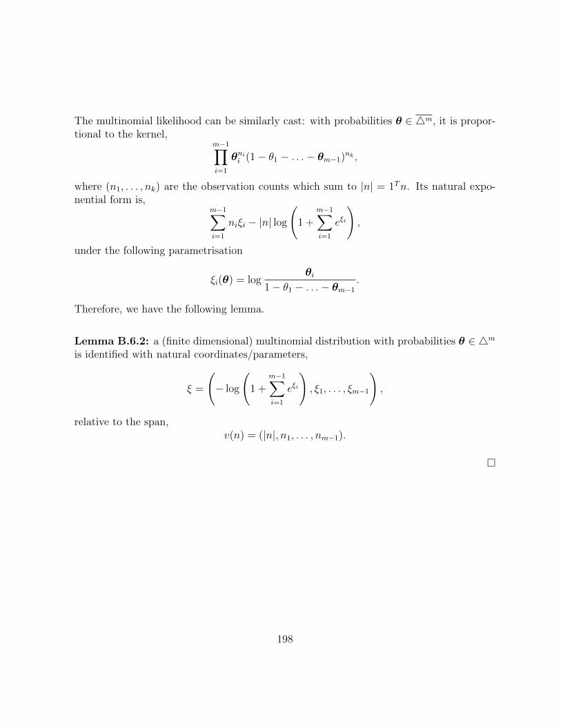
The multinomial likelihood can be similarly cast: with probabilities θ ∈ 4m, it is propor-tional to the kernel,
m−1∏i=1
θnii (1− θ1 − . . .− θm−1)nk ,
where (n1, . . . , nk) are the observation counts which sum to |n| = 1Tn. Its natural expo-nential form is,
m−1∑i=1
niξi − |n| log
(1 +
m−1∑i=1
eξi
),
under the following parametrisation
ξi(θ) = logθi
1− θ1 − . . .− θm−1
.
Therefore, we have the following lemma.
Lemma B.6.2: a (finite dimensional) multinomial distribution with probabilities θ ∈ 4m
is identified with natural coordinates/parameters,
ξ =
(− log
(1 +
m−1∑i=1
eξi
), ξ1, . . . , ξm−1
),
relative to the span,v(n) = (|n|, n1, . . . , nm−1).
198
Appendix C
Appendix to Chapter 4
C.1 Optimisation algorithm used in Section 4.7
All optimisations for lower and upper IDM expectations in Section 4.7 are done using agenetic algorithm built from the deap framework (De Raiville et al. [33]) under Python3.5.
199
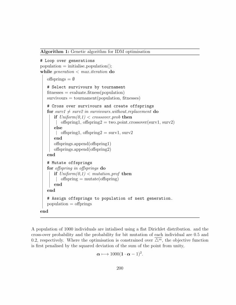
Algorithm 1: Genetic algorithm for IDM optimisation
# Loop over generations
population = initialise population();while generation < max iteration do
offsprings = ∅
# Select survivours by tournament
fitnesses = evaluate fitness(population)survivours = tournament(population, fitnesses)
# Cross over survivours and create offsprings
for surv1 6= surv2 in survivours without replacement doif Uniform(0,1) < crossover prob then
offspring1, offspring2 = two point crossover(surv1, surv2)else
offspring1, offspring2 = surv1, surv2endoffsprings.append(offspring1)offsprings.append(offspring2)
end
# Mutate offsprings
for offspring in offsprings doif Uniform(0,1) < mutation prof then
offspring = mutate(offspring)end
end
# Assign offsprings to population of next generation.
population = offprings
end
A population of 1000 individuals are intialised using a flat Dirichlet distribution. and thecross-over probability and the probability for bit mutation of each individual are 0.5 and0.2, respectively. Where the optimisation is constrained over 4m, the objective functionis first penalised by the squared deviation of the sum of the point from unity,
α 7−→ 1000(1 ·α− 1)2.
200
Appendix D
Appendix to Chapter 5
D.1 Results and proofs
Lemma D.1.1: Let ψ be the digamma function over the domain of positive arguments.Then,
ψ−1′(x) =1
ψ′(ψ−1(x)).
Proof: The inverse derivative of ψ is justified as it is bijective and continuously differen-tiable: taking the derivative on both sides of,
x = ψ(ψ−1(x)),
yields the result.
Lemma D.1.2: Let ψ be the digamma function over the domain of positive arguments.Then,
ψ−1′′(x) = − ψ′′(ψ−1(x))
(ψ′(ψ−1(x)))3.
201
Proof: The inverse derivative of ψ and ψ′ are justified as they are continuously differen-tiable. Then,
ψ−1′′(x) =d
dxψ−1′(x)
=d
dx
1
ψ′(ψ−1(x))(Lemma D.1.1)
= −(ψ′(ψ−1(x)))−2 · ψ′′(ψ−1(x)) · ddxψ−1(x)
= −(ψ′(ψ−1(x)))−2 · ψ′′(ψ−1(x)) · 1
ψ′(ψ−1(x))(Lemma D.1.1)
= − ψ′′(ψ−1(x))
ψ′(ψ−1(x))3.
Lemma D.1.3: Let ψ be the digamma function over the domain of positive arguments.Then, for the function,
I : µ 7−→ ψ(ψ−1(µ1) + ψ−1(µ2))− (ψ−1(µ2) + ψ−1(µ3)),
subject to the constraint,
ψ−1(µ1) + ψ−1(µ2) + ψ−1(µ3) = ν + n,
with ν + n > 0, we have,∇I > 0,
and I has no turning points over µ.
Proof: the gradient of I is given by,
∇I = ψ′(ψ−1(µ1) + ψ−1(µ2))
ψ−1(µ1)ψ−1(µ2)
0
− ψ′(ψ−1(µ2) + ψ−1(µ3))
0ψ−1(µ2)ψ−1(µ3)
.Also, taking the gradient of the constraint equation yields,
[∂µ1ψ−1′(µ1), ∂µ1ψ
−1′(µ2), ∂µ1ψ−1′(µ3)] = 0,
202
such that, substituting into the gradient of I,
∇I = ψ′(ψ−1(µ1) + ψ−1(µ2))
ψ−1(µ1)ψ−1(µ2)
0
+ ψ′(ψ−1(µ2) + ψ−1(µ3))
ψ−1(µ1)00
.Now, ψ′ is positive over positive arguments and ψ−1 maps any real number back to thepositive line, so ψ′(ψ′(µj)) is positive for j = 1, 2, 3. Furthermore, by Lemma D.1.1,
ψ−1′(x) =1
ψ′(ψ−1(x)),
for all x, such that it is again positive by similar arguments. So, all elements of ∇I arepositive. Because ∇I is continuous over µ and strictly positive, it never changes signs andso there is no turning point.
Lemma D.1.4: For t = (t1, t2), v0 = 1 and a choice of v1 and v2 with vi ∈ R3, thefunction a implicitly defined to satisfy,
µ(t) = a(t)v0 + t1v1 + t2v2,
and,ψ−1(µ1(t)) + ψ−1(µ2(t)) + ψ−1(µ3(t)) = ν + n,
is concave:[∂tk,tla(t)]k,l,
is negative definite.
Proof: For brevity, let us write,
xkj(t) := ∂tka(t) + δ1kv1j + δ2kv2j.
and similarly define xlj(t). Then, taking the partial derivative ∂tl of the second conditionand substituting the first condition for µ yield,
3∑j=1
ψ−1′(µj(t))xlj(t) = 0.
203
Applying a second partial derivative ∂tk yields,
3∑j=1
ψ−1′′(µj(t))xlj(t)xkj(t) + ψ−1′(µj(t))∂tk,tla(t) = 0.
This solves for,
∂tk,tla(t) = −∑3
j=1 ψ−1′′(µj(t))xlj(t)xkj(t)∑3j=1 ψ
−1′(µj(t)).
Notice that, by Lemma D.1.2,
ψ−1′′(µj) = − ψ′′(ψ−1(µj))
(ψ′(ψ−1(µj)))3,
such that, because ψ′′ is a negative function over positive arguments, ψ′ is a positive func-tion over positive arguments, and ψ−1)(µj) is always positive as ψ is bijective, continuousand restricted to the domain of positive real numbers,
ψ−1′′(µj) ≥ 0.
The negative definiteness can now be shown as follows. Since ψ−1′′(µj) ≥ 0, its square rootis again a non-negative number such that we can rewrite,
∂tk,tla(t) = −∑3
j=1(√ψ−1′′(µj(t))xlj(t))(
√ψ−1′′(µj(t))xkj(t))∑3
j=1 ψ−1′(µj(t))
.
Thus, the numerator is an element of a square product of a square matrix, which is positivedefinite. From Lemma D.1.1 and the fact that ψ′ is a positive function over its domain,the denominator is a positive scalar constant, so the matrix,
[∂tk,tla(t)]k,l = −
[∑3j=1(
√ψ−1′′(µj(t))xlj(t))(
√ψ−1′′(µj(t))xkj(t))∑3
j=1 ψ−1′(µj(t))
]k.l
,
is negative definite.
204
D.2 Some properties of the digamma function
The digamma function is defined as,
ψ(x) :=d
dxlog Γ(x).
In this document, the digamma function is usually evaluated in the form ψ(ν∑
i∈A αI)
where 0 ≤∑
i∈A αi ≤ 1. Indeed, it can be shown that (e.g. see [56]) over x > 0,
ψ(x) = −γ0 +∞∑n=0
(1
1 + n− 1
x+ n
),
where γ0 > 0 is the Euler-Mascheroni constant.
We note the following properties of ψ.
Corollary D.2.1: From this expansion, ψ is a monotonically increasing function in x overx > 0.
Corollary D.2.2: The unique root x0 of ψ(x0) = 0 is greater than one. Indeed, ψ(1) =−γ0 < 0 and so by increasing monotonicity, the root is unique and ψ must achieve zeroabove x = 1.
Corollary D.2.3: When x→∞, ψ(x)→∞. This happens as 11+n− 1
x+n≈ 1
1+n= O(1/n)
and the infinite sum of the latter diverges.
A loose approximation of the root of ψ(x) = 0: Using the scipy.special.digamma
(scipy==1.1.0) function in python3.5, we observe the loose bounds ψ(1.25) < 0 < ψ(1.5)containing the root.
205
Appendix E
Appendix to Chapter 7
E.1 Results and proofs
Lemma E.1.1: (6.5.3 of Walley [81]) Let B be a partition of Ω. Let E be a lowerexpectation. For each B ∈ B, let E(·|B) be a lower expectation conditional on B. Write,
E(X|B) =∑B∈B
IBE(X|B).
Finally, let E and E(·|B) for each B ∈ B be defined on L(Ω). Then, E and E(·|B) arejointly coherent iff,
• for all X ∈ L(Ω), E(X − E(X|B)) ≥ 0, and
• for all X ∈ L(Ω) and B ∈ B, E(IB(X − E(X|B))) = 0.
Lemma E.1.2: (2.6.1 of Walley [81]) Let E be a coherent lower expectation. Then, forX ≥ Y , E(X) ≥ E(Y ).
206
For every X ∈ L(Ω), write,
R(X|B) :=∑B∈B
IBR(X|B).
Theorem E.1.1:Let B be a partition of Ω, and M be a closed set of distributions. Supposethat N is such that E↑N(·|B) is jointly coherent with EM . Suppose also that the regular ex-tension RM(·|B) is jointly coherent with EM . Then, EM ;N(·|B) is jointly coherent with EM .
Proof: First, notice that,
EM ;N(X|B) =∑B∈B
IBminRM(X|B), E↑N(X|B)
≤∑B∈B
IBRM(X|B) = RM(X|B),
and,
EM ;N(X|B) =∑B∈B
IBminRM(X|B), E↑N(X|B)
≤∑B∈B
IBE↑N(X|B) = E↑N(X|B).
This leads to,
X − EM ;N(X|B) ≥ X −minRM(X|B), E↑N(X|B)
,
and, in turn, because
X −minRM(X|B), E↑N(X|B)
≥ X − E↑N(X|B), X −RM(X|B),
by Lemma E.1.2,
EM
(X − EM ;N(X|B)
)≥ EM(X − E↑N(X|B)), EM(X −RM(X|B)).
By Lemma E.1.1 and that both RM(·|B) and E↑N(·|B) are both jointly coherent with EM ,we have that, E(X −RM(X|B)) ≥ 0 and E(X − E↑N(X|B) ≥ 0. This implies that,
E(X − EM ;N(X|B)) ≥ minE(X −RM(X|B)), E(X − E↑N(X|B) ≥ 0. (E.1)
Second, consider a fixed B ∈ B and a fixed X ∈ L(Ω). Then,
EM ;N(X|B) = minRM(X|B), E↑N(X|B)
207
is a non-random constant whose value is either one of the real numbers in RM(X|B), EM ;N(X|B).Then, by Lemma E.1.1 and that RM(·|B) and E↑N(·|B) are both jointly coherent with E,that,
E(IB(X −RM(X|B))) = 0,
E(IB(X − E↑N(X|B))) = 0,
we have,E(IB(X − EM ;N(X|B))) = 0. (E.2)
By Lemma E.1.1, (E.1) and (E.2) imply that EM ;N(·|B) is jointly coherent with E.
208
Glossary
Bayes’ rule – The property of expectations that the right hand side of EP (X|B) =EP (IBX)/P (B) exists when P (B) > 0, and uniquely relates EP (·|B) and EP . (Itdoes not refer to the relationship between the two conditional measures, P (B|A) andP (A|B).)
Coherence – Qualitatively, a self-consistency amongst assessments over a set of randomvariables such that they do not contradict one another. See Chapter 2.
Generalised Bayes’ rule, GBR – the extension of Bayes’ rule (c.f. Bayes’ rule) to theimprecise case using expectations.
IDM – Abbreviation for ‘imprecise Dirichlet model’.
Imprecise model – A model that is not a precise model. E.g. a lower expectationinduced by a non-singleton set of distributions.
Imprecise probabilities/expectations – A special case of an imprecise model inducedby forming the lower and upper bounds of probabilities/expectations over a set ofdistributions. The term refers to the pair of lower and upper expectations used tomathematically represent them.
Precise model – A model that assigns a single fair price to every random variable in itsdomain. E.g. a single probability distribution assigning a single expectation value toall random variables when defined.
Vacuity, vacuous – The property that an imprecise model is non-informative regardingcertain statistics of interest. For example, a pair of lower and upper imprecise ex-pectations of a random variable X is considered vacuous (for X) if the lower and
209

upper bounds are trivially the infimum and the supremum of the random variable,respectively.
210