Embed Size (px)
Citation preview

Measurement and Visualisation of Slurry Flow Using
Electrical Resistance Tomography
By
Yousef Faraj
BEng, MSc, AFHEA
Submitted in accordance with the requirements for the degree of
Doctor of Philosophy
The University of Leeds
Institute of Particle Science and Engineering
School of Process, Environmental and Materials Engineering
March, 2013

- i -
The candidate confirms that the work submitted is his own, except where
work which has formed part of jointly authored publications has been
included. The contribution of the candidate and the other authors to this work
has been explicitly indicated below. The candidate confirms that appropriate
credit has been given within the thesis where reference has been made to
the work of others.
Chapter 4 and Chapter 5 of the thesis contain some materials from the five
jointly-authored publications given below;
1. Faraj, Y. and Wang, M. (2011). Slurry flow regime and velocity profile
visualisation in horizontal pipeline using Electrical Resistance
Tomography (ERT). PSFVIP-8, the 8th Pacific Symposium Flow
Visualisation and Image Processing, Moscow, Russia.
2. Faraj, Y. and Wang, M. (2011). Slurry flow measurement in pipeline via
Electrical Resistance Tomography (ERT). BAAF, Beihang Autumn
Academic Forum. Beijing, China.
3. Faraj, Y. and Wang, M. (2012). ERT investigation on horizontal and
counter-gravity slurry flow in pipelines. Journal of Procedia Engineering.
42, pp. 588-606
4. Faraj, Y., Wang, M. (2013). ERT based volumetric flow rate
measurement in vertical upward flow. ChemEngDayUk, Proceedings of
Chemical Engineering Day Uk, Imperial College London, London, UK.
5. Faraj, Y. and Wang, M. and Jia, J. (2013). Application of the ERT for
slurry flow regime characterisation. WCIPT7, 7th World Congress on
Industrial Process Tomography, Krakow, Poland. (Accepted in Journal of
Procedia Engineering)
All the experimental work presented in the above five publications was
carried out by the candidate (Yousef Faraj) under the supervision of Prof. M.
Wang (co-author, supervisor). The candidate is also the lead author of these
publications, however, advise was also given by Prof. M. Wang during the
experimental work for all the above publications, and some contribution by
Dr. J. Jia (co-author) during manuscript preparation of publication number 5.

- ii -
This copy has been supplied on the understanding that it is copyright
material and that no quotation from the thesis may be published without
proper acknowledgement.
The right of Yousef Faraj to be identified as Author of this work has been
asserted by him in accordance with the Copyright, Designs and Patents Act
1988.
© 2013 The University of Leeds and Yousef Faraj.

- iii -
The development of internal structure of a slurry pipeline can
accurately represent modern Western Societies. The reduction
of transport velocity, gives rise to three layers within the
pipeline, while unpredictable instabilities within the society
creates a pronounced social stratification, which are classified
as upper class, middle class and lower class...the less difference
is between the velocities of each layer in the pipeline, the safer
and more economical transport is achieved...
The concept of slurry transport has been employed long time
ago...it is undoubtedly considered as a dirty and murky
mixture... No matter how murky it can be, it is always seen as
a clear water in the eyes of the ERT, through which the
systematic movement of each particle can be visualised.
Y. F
araj
Y. F
araj
Turbulent Zone
Shear Layer
Granular Bed Lower Class
Middle Class
Upper Class

- iv -
This thesis is dedicated to my dear father, my beloved wife and my wonderful
children

- v -
Acknowledgements
Finally, the long episode of my PhD study has successfully reached the end.
My journey towards the PhD degree could not have had a better end. Now, it
is time to cordially appreciate the heart whelming support and
encouragement provided by many individuals, who made this journey more
thrilling, and consequential.
First and foremost, I would like to express my greatest appreciation to my
supervisor Prof. M. Wang, who has been the source of inspiration that made
me complete this project successfully. Prof. Wang, thank you for all the
monumental support you have provided to enable me reach the target. Your
simplicity and attitude of long life learning has always been a catalyst for my
motivation and encouragement to learn and explore different aspects of
science and technology. Words are inadequate in offering my thanks to
Miss. Judith Squires for her kind support, encouragement and inspiration in
every trial that came on my way during my PhD study. I wish to express my
deep sense of gratitude to Dr. Basit Munir, who has had a research project
with interest in slurry flows, for sharing his timely guidance and discussions
we have had to solve technical problems. I would also like to convey my
thanks to all the members of OLIL group for their assistance at all times. As
with any experimental PhD, a number of research technicians have rendered
their support and I wish to offer my thanks to all of them, especially Mr.
Robert Harris, Mr. John Cran & Mr. Peter Dawson for their valuable time and
help in building the flow system, Mr. R. Guest and Mr. Steve Caddick for the
loan of those bits and pieces whenever required. My thanks and
appreciations also go to many PhD students and post-doctoral fellows in
IPSE, who have abundantly shared their knowledge, their ideas and
numerous tips, all of which culminated in the completion of this project. I take
immense pleasure in thanking Mr. Geoff Oxtaby and his co-worker Tom from
O.G. Fabrication for conducting an excellent work in manufacturing and
building all the steel work required for the flow rig.
Finally, heartiest thanks to my wife; her support has been instrumental
throughout my PhD timeline, as without her love, understanding, endless
patience and encouragement this thesis could not have been completed. I
wish to express the sense of love to my wonderful children, Alain, Arman &
Anushik, whom in their own ways inspired me and subconsciously
contributed a tremendous amount of support in this degree.
- vi -
Abstract
Slurry transport has been a progressive technology for transporting a huge
amount of solid materials across the world in both, long distance and short
commodity pipelines. The occurrence of separation and slippage of the
constituent phases within the pipeline make these flows unpredictable and
time dependent. Therefore, it is paramount for the operator of slurry
pipelines to monitor and measure the flow continuously, particularly from the
local point of view. Undoubtedly, the measurement of local parameters
governing the flow, requires an instrument that provides high temporal
resolution. Besides, since each phase has different behaviour and flow
characteristics within the pipe, it is enormously difficult to measure the flow
parameters of each phase using only one conventional flow meter. Thus, a
second auxiliary sensor is required to develop a compact and multiphase
flow meter.
This project proposes a new automated online slurry measurement,
visualisation and characterization technique, in which a high performance
dual-plane Electrical Resistance Tomography (ERT) system is employed
with a capability of acquiring data at a rate of 1000 dual-frames per second.
It also proposes an ERT based technique, which combines the ERT and an
Electromagnetic Flow meter (EMF), to measure volumetric flow rate of each
phase, and thus the total slurry volumetric flow rate. The ERT is further
combined with the cross-correlation technique to estimate and image the
axial solid’s velocity distribution, through which the transient phenomena of
horizontal flow regimes can be visualised. The ERT is used for estimation of
several parameters of stratified flow. The development of a novel automated
technique for recognition of horizontal slurry flow regimes is also described.
A series of experiments were carried out on horizontal and upward vertical
sand-water flow through a pilot scale flow system with 50 mm ID pipeline.
Two sands, medium and coarse, were employed in two throughput
concentrations (2% and 10%) within the range of transport velocities 1.2-5.0
m/s. The solids volumetric concentration and velocity, along with slurry
volumetric flow rate are compared with the corresponding results obtained
from a sampling vessel.
- vii -
Table of Contents
Acknowledgements ..................................................................................... v
Abstract ....................................................................................................... vi
Table of Contents ...................................................................................... vii
List of Tables ............................................................................................ xiv
List of Figures ......................................................................................... xvii
Main Notations used ............................................................................... xxv
List of Abbreviations .............................................................................. xxix
Definitions of slurry flow characteristics ............................................ xxxii
Chapter 1 Introduction ................................................................................ 1
1.1 Hydraulic transport of solids in pipes ............................................. 1
1.2 Motivation of present work ............................................................ 5
1.3 Scope of present work .................................................................. 7
1.4 Research objectives ...................................................................... 8
1.5 Thesis layout ................................................................................. 8
Chapter 2 Hydraulic transport of solid particles in pipeline .................. 10
2.1 Introduction ................................................................................. 10
2.2 Slurry flow in pipelines ................................................................ 11
2.3 Horizontal flow ............................................................................. 12
2.3.1 Slurry flow regimes ............................................................ 13
2.3.1.1 Homogeneous flow regime ..................................... 15
2.3.1.2 Heterogeneous flow regime .................................... 16
2.3.1.3 Moving bed flow regime .......................................... 17
2.3.1.4 Stationary bed flow regime ...................................... 18
2.3.2 Transition velocities ........................................................... 18
2.3.3 Available models to determine transition velocities ........... 20
2.3.4 Pressure drop in slurry pipeline ......................................... 24
2.3.5 Physical mechanisms governing settling slurry flow .......... 26
2.3.6 Flow regime recognition .................................................... 27
2.4 Vertical slurry flow ....................................................................... 30
2.5 Inclined slurry flow ....................................................................... 32
2.6 Deposition velocity in horizontal and inclined flow ....................... 35
2.7 Conclusions ................................................................................. 37
- viii -
Chapter 3 Review of slurry flow measurement and visualisation techniques ......................................................................................... 38
3.1 Introduction ................................................................................. 38
3.2 A review of phase fraction and phase velocity measurement ...... 39
3.2.1 Differential pressure technique.......................................... 39
3.2.2 Probes ............................................................................... 41
3.2.3 Electromagnetic Flow Meter (EMF) ................................... 41
3.2.4 Cross-Correlation .............................................................. 46
3.3 Flow visualisation and imaging techniques ................................. 48
3.3.1 Ultrasonic technique .......................................................... 49
3.3.2 Magnetic Resonance Imaging ........................................... 55
3.3.3 Tomography techniques .................................................... 55
3.3.3.1 Electrical Resistance Tomography (ERT) ............... 56
3.3.3.2 Electrical Capacitance Tomography........................ 57
3.3.3.3 Electromagnetic Tomography (EMT) ...................... 58
3.3.3.4 Ultrasound Tomography .......................................... 58
3.3.3.5 Nucleonic Tomography ........................................... 59
3.3.3.5.1 X-ray and Gamma-ray Tomography .......... 59
3.3.3.5.2 Positron Emission Tomography (PET) ....... 60
3.4 Electrical Resistance Tomography system detail ........................ 60
3.4.1 Introduction ....................................................................... 60
3.4.2 Concept and working principle .......................................... 62
3.4.3 Voltage measurement strategy ......................................... 63
3.4.4 Fast Impedance Camera system (FICA) ........................... 64
3.4.5 ERT Sensor design ........................................................... 65
3.4.6 Image reconstruction analysis ........................................... 66
3.4.7 Application of the ERT ...................................................... 67
3.4.8 Conductivity conversion to solids concentration ................ 69
3.4.9 Limitation of the ERT ......................................................... 71
3.4.9.1 Spatial resolution .................................................... 71
3.4.9.2 Conductivity resolution ............................................ 71
3.4.9.3 Ability of distinguishing single particle ..................... 72
3.5 Conclusions ................................................................................. 72
Chapter 4 Horizontal and vertical flow experimental set up and calibration procedure........................................................................ 73
4.1 Introduction ................................................................................. 73
- ix -
4.2 Aims of the experimental work .................................................... 74
4.3 Horizontal and vertical slurry flow loop layout ............................. 75
4.3.1 Flow diversion technique ................................................... 79
4.3.2 High performance ERT system ......................................... 81
4.3.3 Visualisation and image reconstruction scheme ............... 81
4.3.3.1 Maxwell relationship and solids concentration ........ 82
4.3.4 The dual-plane ERT sensor .............................................. 82
4.3.5 Design of the photo-chamber (Light box) .......................... 83
4.4 Experimental procedure and operating conditions ...................... 85
4.4.1 Slurry component selection and characterisation .............. 85
4.4.1.1 Sand particle size analysis ...................................... 86
4.4.1.2 Density estimation of sand particles ........................ 88
4.4.2 Measured parameters and the measuring technique ........ 89
4.4.2.1 Mean slurry velocity measurement ......................... 89
4.4.2.2 Solids volumetric concentration measurement ........ 89
4.4.2.2.1 In-situ solids volumetric concentration
measurement .............................................................. 90
4.4.2.2.2 Delivered solids volumetric concentration
measurement .............................................................. 90
4.4.2.3 Local solids axial velocity measurement ................. 90
4.4.2.4 Temperature measurement ..................................... 91
4.4.2.5 Pressure measurement ........................................... 91
4.4.3 Operating procedure ......................................................... 92
4.5 Calibration procedure .................................................................. 94
4.5.1 Calibration of the thermocouple ........................................ 94
4.5.2 Calibration of pressure transducers .................................. 95
4.5.3 Calibration of the conductivity meter ................................. 96
4.5.4 Calibration of the measuring tank ...................................... 97
4.5.5 Calibration of the load cells ............................................... 98
4.5.6 Testing and calibration of the ERT sensor ........................ 99
4.6 Conclusions ............................................................................... 101
Chapter 5 Horizontal and vertical flow results, discussions and important findings ........................................................................... 102
5.1 Introduction ............................................................................... 102
5.2 Experimental strategy ............................................................... 103
5.3 Material and test conditions ....................................................... 105
- x -
5.4 Horizontal flow measurement and visualisation ........................ 106
5.4.1 Solid flow visualisation .................................................... 107
5.4.1.1 ERT tomograms .................................................... 107
5.4.2 ERT solids volume fraction distribution ........................... 111
5.4.3 ERT solids axial velocity distribution ............................... 115
5.4.4 Methods of solid flow velocity visualisation ..................... 118
5.4.5 Slurry flow regime visualisation and characterization ...... 122
5.4.5.1 Pseudo-homogeneous flow regime ....................... 123
5.4.5.2 Heterogeneous flow regime .................................. 124
5.4.5.3 Moving bed ........................................................... 124
5.4.5.4 Stationary bed ....................................................... 126
5.4.5.5 Pipe blockage ....................................................... 128
5.4.6 Formation of stratified flow .............................................. 131
5.4.6.1 Estimation of parameters relating to stratified flow ............................................................................ 134
5.4.7 Reducing entrained bubbles ........................................... 136
5.4.8 Estimation of delivered solids volume fraction ................ 138
5.4.9 Validation of the EMF velocity ......................................... 138
5.4.10 Validation of the ERT results ........................................... 143
5.4.10.1 Validation of mean solids volume fraction ........... 144
5.4.10.2 Validation of mean solids axial velocity ............... 147
5.5 Vertical upward flow measurement and visualisation ................ 154
5.5.1 ERT solids volume fraction and solids axial velocity measurement .................................................................. 155
5.5.2 ERT based slurry flow rate measurement ....................... 157
5.5.3 Validation of the vertical flow ERT results ....................... 164
5.5.3.1 Validation of mean solids volume fraction ............. 164
5.5.3.2 Validation of mean solids axial velocity ................. 168
5.5.3.3 Validation of mean solids flow rate ........................ 169
5.6 Conclusions ............................................................................... 175
Chapter 6 Design and construction of inclinable multiphase flow loop................................................................................................... 177
6.1 Introduction ............................................................................... 177
6.2 Design requirements ................................................................. 178
6.3 Design and construction project management .......................... 178
6.4 Types of slurry flow loop ........................................................... 182

- xi -
6.5 Overall structural design ........................................................... 183
6.6 Flow loop design and component selection............................... 183
6.6.1 Structural design of the pipe-rack.................................... 183
6.6.2 Selection of lifting method ............................................... 197
6.6.2.1 The winch system ................................................. 199
6.6.2.2 The telescopic table push-back system ................ 201
6.6.3 Piping design................................................................... 203
6.6.3.1 Piping construction material and diameter section ....................................................................... 203
6.6.3.2 Pipe sizing ............................................................. 205
6.6.3.3 Section mechanical joints ...................................... 206
6.6.3.4 Piping supports ..................................................... 207
6.6.3.5 Pipe jointing method.............................................. 208
6.6.3.6 Piping layout ......................................................... 210
6.6.3.7 Flexible pipe .......................................................... 215
6.6.3.8 Pipeline length and test section length .................. 220
6.6.4 Pump selection................................................................ 220
6.6.4.1 Pump performance................................................ 222
6.6.4.2 Suction limitations ................................................. 227
6.6.5 Equipment design ........................................................... 228
6.6.5.1 Mixing tank ............................................................ 229
6.6.5.2 Measuring tank ..................................................... 231
6.6.5.3 Flow diversion system ........................................... 233
6.6.5.4 Drainage system ................................................... 235
6.6.5.5 Slurry valves ......................................................... 236
6.6.5.6 Ultrasound probe holder ........................................ 236
6.6.6 Instrumentations used to measure the relevant parameters ...................................................................... 240
6.6.6.1 Mean velocity measuring device ........................... 240
6.6.6.2 Solids concentration and axial velocity measuring device ...................................................... 240
6.6.6.2.1 Design of 360 mm dual-plane ERT sensor
241
6.6.6.3 Mass flow rate measuring device .......................... 246
6.6.6.4 Additional local velocity measuring device ............ 249
6.6.6.5 Pressure measuring instrumentation .................... 250
- xii -
6.6.6.6 Temperature measuring device ............................ 251
6.6.6.7 Data Acquisition System (DAS) ............................ 253
6.6.7 Flow loop operation procedure ........................................ 255
6.6.8 Hydraulic and mechanical testing .................................... 259
6.7 Conclusions ............................................................................... 260
Chapter 7 Automated horizontal flow regime recognition using statistical signal analysis of the ERT data .................................... 261
7.1 Introduction ............................................................................... 261
7.2 Test strategy ............................................................................. 262
7.3 Automated flow regime recognition ........................................... 263
7.3.1 Experimental ERT measurement .................................... 263
7.3.2 Statistical signal analysis and flow feature extraction ...... 264
7.3.2.1 Signal analysis in the time domain ........................ 264
7.3.2.2 Signal analysis in the frequency domain ............... 268
7.3.3 Threshold indication of the signal .................................... 278
7.3.3.1 Threshold indication of the signal (Relative Conductivity) ............................................................. 278
7.3.3.2 Threshold indication of the signal (Average Power) ....................................................................... 280
7.3.4 Decision making .............................................................. 281
7.3.5 Program coding ............................................................... 284
7.3.6 Running the program ...................................................... 286
7.4 Evaluation of the method........................................................... 289
7.5 Conclusions ............................................................................... 291
Chapter 8 Contributions, conclusions and future work recommendations ........................................................................... 292
8.1 Author’s contributions to slurry flow measurement, visualisation and the design of particulate flow system ............. 292
8.1.1 Slurry flow measurement (Chapter 5) ............................. 293
8.1.1.1 Local solids volume fraction .................................. 293
8.1.1.2 Local solids axial velocity ...................................... 293
8.1.1.3 Slurry volumetric flow rate ..................................... 294
8.1.1.4 Phase slip velocity ................................................ 294
8.1.1.5 Parameters relevant to stratified flow .................... 294
8.1.1.6 Measurement of blocked horizontal line ................ 294
8.1.2 Slurry flow visualisation (Chapter 5) ................................ 295

- xiii -
8.1.2.1 Slurry flow regime visualisation and characterisation using ERT ....................................... 295
8.1.3 Design of slurry system (Chapter 6) ................................ 295
8.1.3.1 Design and construction of pilot scale inclinable slurry flow .................................................................. 295
8.1.4 Slurry flow regime recognition (Chapter 7) ...................... 296
8.1.4.1 Automated on-line flow regime recognition ........... 296
8.2 General conclusions .................................................................. 297
8.3 Future scope ............................................................................. 298
List of References and selected bibliography ...................................... 300
Appendix A Publications during the course of this study ................... 317
Appendix B Calibration Results ............................................................. 319
Appendix C Piping related charts .......................................................... 322
Appendix D MATLAB script for automated flow regime recognition . 323
Appendix E Horizontal & vertical flow loop sensor data ..................... 328
Appendix F Local solids volumetric concentration data ..................... 331
F.1 Local solids volumetric concentration in horizontal flow ............. 331
F.2 Local solids volumetric concentration in vertical flow ................. 334
Appendix G Local solids axial velocity data ......................................... 336
G.1 Local solids axial velocity in horizontal flow ............................... 336
G.2 Local solids axial velocity in vertical flow ................................... 339

- xiv -
List of Tables
Table 2.1 Flow regime classification by Govier and Aziz based on particle size. ........................................................................................ 14
Table 2.2 Performance of difference correlations for pressure drop (Lahiri, 2009) ....................................................................................... 25
Table 3.1 Advantages and limitations of EMF ............................................. 45
Table 3.2 Advantages and limitations of ultrasound Doppler ...................... 54
Table 4.1 Showing sieve analysis for coarse sand based on 500 g ............ 87
Table 4.2 Showing sieve analysis for medium sand based on 500 g .......... 87
Table 5.1 A summary of material and test conditions used in the experiments ....................................................................................... 105
Table 5.2 The data obtained from the EMF reading and discharge calculation along with the rate of deviation at each given velocity. .... 140
Table 5.3 The summary output of the statistical analysis of the two sands at 2% and 10% throughput concentration and 1.5-5 m/s velocity range .................................................................................... 141
Table 5.4 The comparison of solids concentration values for medium and coarse sand at 2% throughput concentration in the horizontal test section. The shaded area represents the values, only for which the comparison and error analysis have been carried out ....... 144
Table 5.5 The comparison of solids concentration values for medium and coarse sand at 10% throughput concentration in the horizontal test section. The shaded area represents the values, only for which the comparison and error analysis have been carried out ......................................................................................... 145
Table 5.6 The data obtained from the ERT measurement and flow diversion technique (discharge velocity) along with the rate of deviation at each flow condition for horizontal flow ........................... 148
Table 5.7 Showing the summary output of the statistical analysis of the two sands at 2% and 10% throughput concentration and 1.5-5 m/s velocity range .................................................................................... 150
Table 5.8 Solid and liquid volumetric flow rate obtained through combination of the ERT and EMF, along with the mixture velocity and flow rate in vertical flow .............................................................. 161
Table 5.9 Comparison of concentrations and occurring relative error for medium and coarse sand at 2% throughput concentration in vertical flow ....................................................................................... 165
Table 5.10 Showing the comparison of concentrations and occurring relative error for medium and coarse sand at 10% throughput concentration in vertical flow ............................................................. 165
- xv -
Table 5.11 Showing the data obtained from the ERT measurement and discharge calculation along with the rate of deviation at each given velocity for vertical flow ............................................................ 168
Table 5.12 Comparison of the volume flow rates obtained from the ERT and EMF with discharge corresponding values along with the rate of deviation at each condition in vertical flow .................................... 170
Table 6.1 List of items ordered for the flow loop ........................................ 180
Table 6.2 Schedule of work on the inclinable flow loop ............................. 181
Table 6.3 The weight of the U-shape pipeline on the inclinable table ....... 186
Table 6.4 Technical winch BETA II specification ....................................... 200
Table 6.5 Thermoplastic materials for piping system (US Army Corps Engineers) ......................................................................................... 204
Table 7.2 Showing the range of C value for every flow regime or transitional region .............................................................................. 279
Table 7.3 Showing the range of D value for every flow regime or transitional region .............................................................................. 281
Table 7.4 Summary of recognition results ................................................. 289
Table 7.5 Recognition results for different flow conditions ........................ 290
Table B.1 Thermocouple calibration results. ............................................. 319
Table B.2 Conductivity meter calibration results. ...................................... 319
Table B.3 Calibration results of two pressure transducers on horizontal line and two pressure transducers on vertical line against actual values. ............................................................................................... 320
Table B.4 Measuring tank & load cells calibration results. ........................ 321
Table B.5 ERT calibration results. ............................................................. 321
Table E.1 Flow loop sensor data for flowing medium sand at 2% throughput concentration. .................................................................. 328
Table E.2 Flow loop sensor data for flowing medium sand at 10% throughput concentration. .................................................................. 329
Table E.3 Flow loop sensor data for flowing coarse sand at 2% throughput concentration. .................................................................. 329
Table E.4 Flow loop sensor data for flowing coarse sand at 10% throughput concentration. .................................................................. 330
Table F.1.1 Local solids volumetric concentration for horizontal flow of medium sand at 2% throughput concentration. ................................. 331
Table F.1.2 Local solids volumetric concentration for horizontal flow of medium sand at 10% throughput concentration. ............................... 332
Table F.1.3 Local solids volumetric concentration for horizontal flow of coarse sand at 2% throughput concentration. ................................... 332

- xvi -
Table F.1.4 Local solids volumetric concentration for horizontal flow of coarse sand at 10% throughput concentration. ................................. 333
Table F.1.5 Local solids volumetric concentration for blocked horizontal line with coarse sand at 10% throughput concentration. ................... 333
Table F.2.1 Local solids volumetric concentration for vertical flow of medium sand at 2% throughput concentration. ................................. 334
Table F.2.2 Local solids volumetric concentration for vertical flow of medium sand at 10% throughput concentration. ............................... 334
Table F.2.3 Local solids volumetric concentration for vertical flow of coarse sand at 2% throughput concentration. ................................... 335
Table F.2.4 Local solids volumetric concentration for vertical flow of coarse sand at 10% throughput concentration. ................................. 335
Table G.1.1 Local solids axial velocity for horizontal flow of medium sand at 2% throughput concentration. ............................................... 336
Table G.1.2 Local solids axial velocity for horizontal flow of medium sand at 10% throughput concentration. ............................................. 337
Table G.1.3 Local solids axial velocity for horizontal flow of coarse sand at 2% throughput concentration. ............................................... 337
Table G.1.4 Local solids axial velocity for horizontal flow of coarse sand at 10% throughput concentration. ............................................. 338
Table G.1.5 Local solids axial velocity for blocked horizontal line with coarse sand at 10% throughput concentration. ................................. 338
Table G.2.1 Local solids axial velocity for vertical flow of medium sand at 2% throughput concentration. ....................................................... 339
Table G.2.2 Local solids axial velocity for vertical flow of medium sand at 10% throughput concentration. ..................................................... 339
Table G.2.3 Local solids axial velocity for vertical flow of coarse sand at 2% throughput concentration. ........................................................... 340
Table G.2.4 Local solids axial velocity for vertical flow of coarse sand at 10% throughput concentration. ......................................................... 340
- xvii -
List of Figures
Figure 2.1 Flow regimes in a horizontal pipe in terms of velocity versus concentration (Newitt et al., 1955) ....................................................... 14
Figure 2.2: Flow regimes in a horizontal pipe in terms of particle size versus mean velocity (Shen et al., 1970) ............................................ 15
Figure 2.3 Schematic presentation of fully suspended flow regime and solids concentration and velocity profile .............................................. 16
Figure 2.5 Schematic presentation of moving bed flow regime and solids concentration and velocity profile .............................................. 17
Figure 2.6 Schematic presentation of stationary bed flow regime and solids concentration and velocity profile .............................................. 18
Figure 2.7 Showing transitional velocities on a typical plot of the pressure gradient versus mean mixture velocity (Abulnaga, 2002) ..... 19
Figure 2.8 Superficial velocities flow pattern map (Taken from Doron and Barnea, 1996) .............................................................................. 29
Figure 2.9 Inverted U-tube device for slurry flow rate measurement ........... 31
Figure 2.10 Concentration profile of ascending and descending inclined sand water flow at 3.5 m/s, (Matousek, 1996) ..................................... 34
Figure 2.11 Concept of the two layer bipolar flow of slurry at an angle of inclination, (Abulnaga, 2002) ........................................................... 34
Figure 2.12 Assumed concentration profile in three layer model ................. 35
Figure 2.13 Effect of inclination angle on Durand deposition parameter, after Wilson & Tse (1984) .................................................................... 36
Figure 3.1 Showing components of a short-form of a venturi tube (taken from www.omega.co.uk) ........................................................... 40
Figure 3.2 Showing the arrangement of the electromagnets and pick-up electrodes (Modified from Baker, 2000) .............................................. 42
Figure 3.3 The principle of velocity measurement by cross correlation of ERT signals ..................................................................................... 46
Figure 3.4 Principle of point-by-point cross correlation method (Dai et al., 2004) ............................................................................................. 47
Figure 3.5 The cross correlation between X(n,m) and the vicinity of pixel Y(n,m), (Dai et al., 2004) ............................................................. 48
Figure 3.6 Showing working principle of UDVP ........................................... 51
Figure 3.8 Showing the Doppler Effect (Modified from Baker, 2000) .......... 53
Figure 3.9 Showing (a) The ERT sensor ring (b) The normal adjacent strategy (Taken from the ITS, 2005) ................................................... 57

- xviii -
Figure 3.10 Showing 8-electrode ECT sensor, (www.ect-instruments.com) ................................................................................. 58
Figure 3.11 Showing EMT sensor, (Ismail et al., 2005) .............................. 58
Figure 3.12 Showing the components of the ERT system........................... 62
Figure 3.13 Adjacent electrode pair strategy for 16 electrode ERT sensor ................................................................................................. 64
Figure 3.14 Actual photograph of FICA system ........................................... 65
Figure 4.1 Photographs of the flow loop with its associated instrumentations, showing (a) mixing tank with the flush line, (b) vertical test section, (c) horizontal test section, (d) centrifugal pump, (d) digi-drive frequency converter ............................................. 77
Figure 4.2 The schematic diagram of horizontal and vertical flow loop ....... 78
Figure 4.3 Photographs of the flow diversion system, (a) measuring tank with the switch system, (b) graded glass tube mounted on the measuring tank .................................................................................... 79
Figure 4.4 The actual photograph of the dual-plane ERT sensor within horizontal test section.......................................................................... 83
Figure 4.5 The actual photograph of the light box with the transparent pipe section ......................................................................................... 84
Figure 4.6 Showing the particle size distribution curve for the two sands ... 88
Figure 4.7 Electromagnetic Flow meter within vertical test section ............. 89
Figure 4.8 The thermocouple within vertical test section ............................. 91
Figure 4.9 The Pressure transducer within horizontal test section .............. 92
Figure 4.10 Measured temperature for the thermocouple and the thermometer ........................................................................................ 94
Figure 4.11 The transducers pressure readings against actual values before correction ................................................................................. 95
Figure 4.12 The transducers pressure readings against actual values after correction .................................................................................... 96
Figure 4.13 Comparison results of handheld and desktop conductivity meter ................................................................................................... 97
Figure 4.14 Showing the comparison between the weight of added water measured by the pre-calibrated scale and level based measured weight ................................................................................. 98
Figure 4.15 Showing the comparison between the weight of added water measured by the pre-calibrated scale and load cells readings .............................................................................................. 99
Figure 4.16 Changes in resistivity measured during the course of sensor testing .................................................................................... 100
Figure 4.17 Tomograms showing conductivity of the media: (a) prior to placing the stimulus (b) during placing the stimulus .......................... 100
- xix -
Figure 4.18 Comparison results of brine conductivity measured by the probe and the ERT ............................................................................ 101
Figure 5.1 Schematic briefing of the methodology used in this study ........ 104
Figure 5.2 Concentration tomograms from the ERT (AIMFLOW) for medium and coarse sand at the shown transport velocity and mean local solids concentration across the pipe cross-section, along with the real photographs of the flow within the pipeline .......... 109
Figure 5.3 Concentration tomograms from the ERT (AIMFLOW) for medium and coarse sand at the shown transport velocity and mean solids concentration along with the real photographs the flow within the pipeline ...................................................................... 110
Figure 5.4 Concentration tomograms from the ERT (AIMFLOW) for medium and coarse sand at the shown transport velocity and mean solids concentration along with the real photographs of the flow within the pipeline ...................................................................... 111
Figure 5.5 Concentration profile for flowing medium sand at 2% throughput concentration in the horizontal 50 NB pipe as a function of the transport velocity ........................................................ 112
Figure 5.6 Concentration profile for flowing medium sand at 10% throughput concentration in the horizontal 50 NB pipe as a function of the transport velocity ........................................................ 112
Figure 5.7 Concentration profile for flowing coarse sand at 2% throughput concentration in the horizontal 50 NB pipe as a function of the transport velocity ........................................................ 113
Figure 5.8 Concentration profile for flowing coarse sand at 10% throughput concentration in the horizontal 50 NB pipe as a function of the transport velocity. The red dashed arrow indicates the height of the bed at the bottom of the pipe .................................. 113
Figure 5.9 Solids axial velocity profile for flowing medium sand at 10% throughput concentration in the horizontal 50 NB pipe as a function of the transport velocity ........................................................ 117
Figure 5.10 Solids axial velocity profile for flowing coarse sand at 2% throughput concentration in the horizontal 50 NB pipe as a function of the transport velocity ........................................................ 117
Figure 5.11 Solids axial velocity profile for flowing coarse sand at 10% throughput concentration in the horizontal 50 NB pipe as a function of the transport velocity ........................................................ 118
Figure 5.12 Solids velocity profile across the pipe cross-section for medium sand at 10% throughput concentration and 2 m/s transport velocity ............................................................................... 119
Figure 5.13 Solids velocity profile across the pipe cross-section for medium sand at 10% throughput concentration and 1.5 m/s transport velocity ............................................................................... 119

- xx -
Figure 5.14 Solids velocity profile across the pipe cross-section for coarse sand at 2% throughput concentration and 4 m/s transport velocity .............................................................................................. 120
Figure 5.15 Solids velocity profile across the pipe cross-section for coarse sand at 2% throughput concentration and 3 m/s transport velocity .............................................................................................. 120
Figure 5.16 Solids velocity profile across the pipe cross-section for coarse sand at 10% throughput concentration and 3.5 m/s transport velocity ............................................................................... 120
Figure 5.17 Solids velocity profile across the pipe cross-section for coarse sand at 10% throughput concentration and 2.5 m/s transport velocity ............................................................................... 121
Figure 5.18 Solids velocity profile across the pipe cross-section for coarse sand at 10% throughput concentration and 1.5 m/s transport velocity ............................................................................... 121
Figure 5.19 Solids velocity profile across the pipe cross-section for coarse sand pipe blockage at 10% throughput concentration ........... 121
Figure 5.20 Pseudo-homogeneous flow regime for 10% throughput concentration of coarse sand at 4.5 m/s transport velocity shown on concentration profile (left) and solids velocity profile (right) .......... 123
Figure 5.21 Heterogeneous flow regime for 10% throughput concentration of coarse sand at 4 m/s transport velocity shown on concentration profile (left) and solids velocity profile (right) ............... 124
Figure 5.22 Moving bed flow regime for 10% throughput concentration of coarse sand at 2.5 m/s transport velocity shown on concentration profile (left) and solids velocity profile (right) ............... 126
Figure 5.23 Stationary bed flow regime for 10% throughput concentration of coarse sand at 1.5 m/s transport velocity shown on concentration profile (left) and solids velocity profile (right). The height of granular bed is indicated by a blue arrow and the boundary of the stationary bed is indicated by a red arrow ............... 127
Figure 5.24 Showing the blockage of the pipeline, (a) blocked horizontal section (b) coarser solid particles in the blocked transparent pipe section mounted at the bottom of the vertical
pipeline .............................................................................................. 129
Figure 5.25 Pipe blockage for 10% coarse sand occurred at approximately 1.2 m/s shown on concentration profile (left) and solids velocity profile (right) ............................................................... 131
Figure 5.26 Showing the three zones of the distorted profiles, concentration profile (left) and solids axial velocity profile (right), in stratified flow at 1.5 m/s transportation velocity ................................. 132
Figure 5.27 Showing sporadic movement of medium sand particles over the bed at 1.5 m/s transportation velocity and throughput concentration 2% (left) and 10% (right) ............................................. 133
- xxi -
Figure 5.28 Showing sporadic movement of coarse sand particles over the bed at 1.5 m/s transportation velocity and 2% throughput concentration ..................................................................................... 133
Figure 5.29 The vertical slurry discharge pipe into the mixing tank; (a) the Sanitary Tee connected to the outlet of the pipe; (b) the semicircle plates inserted into the pipe wall ...................................... 136
Figure 5.30 The baffle in the mixing tank; (a) the discharge zone with the Sanitary Tee, (b) the mixing zone ............................................... 137
Figure 5.32 The EMF velocity line fit (left) and the residuals about the predicted velocities (right) for (a) medium sand at 2% throughput concentration; (b) medium sand at 10% throughput concentration; (c) coarse sand at 2% throughput concentration; (d) coarse sand at 10% throughput concentration ...................................................... 142
Figure 5.33 Showing the comparison between the in-situ solids concentration obtained from the ERT and delivered solids concentration obtained from the flow diversion technique in horizontal flow for (a) medium sand at 2% throughput concentration, (b) medium sand at 10% throughput concentration; (c) coarse sand at 2% throughput concentration and (d) coarse sand at 10% throughput concentration .............................................. 146
Figure 5.34 Showing the ERT velocity line fit (left) and the residuals about the predicted velocities (right) for (a) medium sand at 2% throughput concentration, (b) medium sand at 10% throughput concentration, (c) coarse sand at 2% throughput concentration, (d) coarse sand at 10% throughput concentration ............................. 152
Figure 5.35 Concentration profile (left hand-side) and solids velocity profile (right hand-side) as a function of transport velocity in upward vertical flow for (a) medium sand at 2% throughput concentration, (b) medium sand at 10% throughput concentration, (c) coarse sand at 2% throughput concentration, (a) coarse sand at 10% throughput concentration ...................................................... 156
Figure 5.36 Schematic briefing of the methodology used in volumetric flow rate estimation ........................................................................... 159
Figure 5.37 The variation of solids volumetric flow rate against the carrier liquid volumetric flow rate for flowing medium and coarse sand at 2% throughput concentration in upward vertical flow. Each volumetric flow rate data point is labelled with the corresponding mean solids volume fraction and mean solids axial velocity.............. 162
Figure 5.38 The variation of solids volumetric flow rate against the carrier liquid volumetric flow rate for flowing medium sand at 10% throughput concentration in upward vertical flow. Each volumetric flow rate data point is labelled with the corresponding mean solids volume fraction and mean solids axial velocity .................................. 162
- xxii -
Figure 5.39 Comparison between in-situ (ERT) concentration and delivered solids concentration, through the line fit plot (left-hand side) and the residual plot (right-hand side), in vertical upward flow for (a) medium sand at 2% throughput concentration, (b) medium sand at 10% throughput concentration, (c) coarse sand at 2% throughput concentration, (d) coarse sand at 10% throughput concentration ..................................................................................... 167
Figure 5.40 Comparison of solids volumetric flow rate predicted by the ERT in vertical pipeline with that of flow diversion for medium and coarse sand at 2% throughput concentration .................................... 171
Figure 5.41 Comparison of solids volumetric flow rate predicted by the ERT in vertical pipeline with that of flow diversion for medium and coarse sand at 10% throughput concentration .................................. 171
Figure 5.42 Comparison of slurry flow rate measured by the combination of the ERT and EMF in vertical pipeline with that of flow diversion .................................................................................... 172
Figure 5.43 Comparison of the ERT solids flow rate in vertical pipeline with that of flow diversion for medium sand at 2% throughput concentration ..................................................................................... 173
Figure 5.44 Showing the comparison of the ERT solids flow rate in vertical pipeline with that of flow diversion for medium sand at 10% throughput concentration .......................................................... 173
Figure 5.45 Showing the comparison of the ERT solids flow rate in vertical pipeline with that of flow diversion for coarse sand at 2% throughput concentration ................................................................... 174
Figure 5.46 Showing the comparison of the ERT solids flow rate in vertical pipeline with that of flow diversion for coarse sand at 10% throughput concentration ................................................................... 174
Figure 6.1 Actual photo of both ends of the inclinable table, pivoted end (left) and D-shackle at anchored point (right) .................................... 190
Figure 6.2 Actual photo of the instrumentation fixture and hole matrices on the inclinable table........................................................................ 191
Figure 6.3 Schematic diagram of inclinable pipe rack (Top View-Ground Floor) .................................................................................... 192
Figure 6.4 Schematic diagram of inclinable table at horizontal and vertical level (East View) ................................................................... 193
Figure 6.5 Schematic diagram of inclinable section and rigid section (Top View-Ground Floor) ................................................................... 194
Figure 6.6 Schematic diagram of inclinable flow loop (Top View-Mezzanine Level) .............................................................................. 195
Figure 6.7 Schematic diagram of inclinable flow loop (East View) ............ 196
Figure 6.8 Actual photo of the electric wire rope winch ............................. 199
Figure 6.9 Showing the electric wire rope winch main dimensions ........... 200

- xxiii -
Figure 6.10 Winch remote control ............................................................. 201
Figure 6.11 Actual photo of the push-back system ................................... 202
Figure 6.12 Rubber-lined pipe clamp ........................................................ 208
Figure 6.13 Chamfering the pipe end cut, (a) before chamfering; (b) after chamfering; (c) chamfering the leading edge using Dremel ...... 209
Figure 6.14 Horizontal and inclinable U-shape piping layout, including suction and discharge sections ......................................................... 213
Figure 6.15 Vertical piping layout including returning limb ........................ 214
Figure 6.16 The suction and smoothly curved discharge section .............. 215
Figure 6.17 Minimum bending radius of a flexible pipe ............................. 218
Figure 6.18 Actual photo of the opening section on the rigid table ............ 218
Figure 6.19 Armorvin flexible pipe (Whitehouse flexible tubing) ................ 219
Figure 6.20 The flow loop as a fixed control volume ................................. 222
Figure 6.21 Ratio of viscosity of mixture versus viscosity of the carrier liquid in accordance with Thomas equation for settling slurries (Abulnaga, 2002) ............................................................................... 226
Figure 6.22 The schematic drawing of the holding tank ............................ 231
Figure 6.23 Schematic drawing of the measuring tank.............................. 232
Figure 6.24 Schematic drawing of the flow diversion system .................... 234
Figure 6.25 Actual photograph of the drainage system ............................. 235
Figure 6.26 Showing the UDVP probe fixture and 50 mm ID flanged spoolpiece ......................................................................................... 238
Figure 6.27 Schematic drawing of the dual-plane ERT sensor ................. 243
Figure 6.28 Schematic drawing of the 16-electrode ERT plane sensor .... 245
Figure 6.29 Schematic drawing of the Split Plummer Block ...................... 248
Figure 6.30 Showing the UDVP-DUO system from Met-Flow ................... 250
Figure 6.31 Pressure and temperature transmitter spoolpiece .................. 252
Figure 6.32 Showing the LabVIEW front panel ......................................... 253
Figure 6.33 Showing the LabVIEW programme ........................................ 254
Figure 6.34 Schematic diagram of the inclinable loop piping .................... 255
Figure 7.1 Mesh/21 cell zone scheme ....................................................... 264
Figure 7.2 Showing the time domain signal of the ERT measurement for coarse sand at 10% throughput concentration: (a) 4.5 m/s, (b) 4.0 m/s, (c) 3.5 m/s, (d) 3.0 m/s, (e) 2.5 m/s, (f) 2.0 m/s, (g) 1.5 m/s .................................................................................................... 266
Figure 7.3 Showing the frequency component of the signal in each zone for flowing coarse sand at 4 m/s. (a) Zone 1, (b) Zone 2, (c) Zone 3, (d) Zone 4 and (e) Zone 5 .................................................... 271
- xxiv -
Figure 7.4 Showing a zoomed frequency components of zones 1, 2 and 4 wave form, obtained from FFT, for flowing coarse sand at 4.0 m/s .............................................................................................. 272
Figure 7.5 Showing the periodogram Mean-Square Spectrum for each zone at 1.5 m/s .................................................................................. 274
Figure 7.6 Showing the periodogram Mean-Square Spectrum for each zone at 2 m/s ..................................................................................... 275
Figure 7.7 The average signal power against the 5 zones as a function of transport velocity ........................................................................... 278
Figure 7.8 Showing the threshold of the signal based on the relative difference in the conductivity of the top and bottom of the pip. (P) Pseudo-homogeneous, (HET) Heterogeneous, (MB) Moving Bed, (SB) Stationary Bed .......................................................................... 279
Figure 7.9 Showing the threshold of the signal based on the difference in the average power of the signal at the top and bottom of the pipe. (P) Pseudo-homogeneous, (HET) Heterogeneous, (MB) Moving Bed, (SB) Stationary Bed ...................................................... 280
Figure 7.10 Sequential flow chart of the recognition process .................... 283
Figure 7.11 Electrode configuration for flow regime recognition ................ 285
Figure 7.12 Initial running the program ...................................................... 286
Figure 7.13 Message box conveying the result of flow recognition computation ....................................................................................... 287
Figure 7.14 Wait-bar showing computation in progress ............................ 287
Figure 7.15 2D & 3D display of solids volumetric concentration distribution plot .................................................................................. 288
Figure 7.16 Display of solids local volume fraction distribution and data statistics ............................................................................................ 288
- xxv -
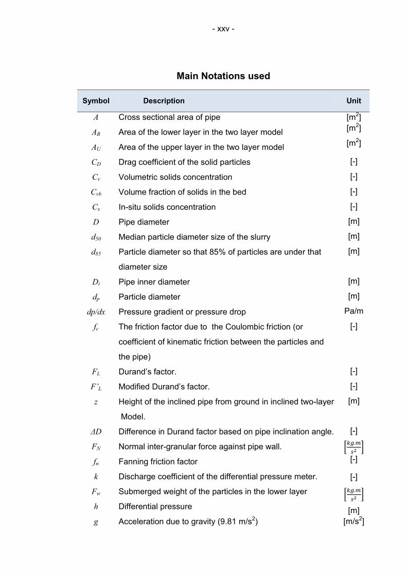
Main Notations used
Symbol Description Unit
A
AB
AU
CD
Cv
Cvb
Cx
D
d50
d85
Di
dp
dp/dx
fc
FL
F’L
z
ΔD
FN
fn
k
Fw
h
g
Cross sectional area of pipe
Area of the lower layer in the two layer model
Area of the upper layer in the two layer model
Drag coefficient of the solid particles
Volumetric solids concentration
Volume fraction of solids in the bed
In-situ solids concentration
Pipe diameter
Median particle diameter size of the slurry
Particle diameter so that 85% of particles are under that
diameter size
Pipe inner diameter
Particle diameter
Pressure gradient or pressure drop
The friction factor due to the Coulombic friction (or
coefficient of kinematic friction between the particles and
the pipe)
Durand’s factor.
Modified Durand’s factor.
Height of the inclined pipe from ground in inclined two-layer
Model.
Difference in Durand factor based on pipe inclination angle.
Normal inter-granular force against pipe wall.
Fanning friction factor
Discharge coefficient of the differential pressure meter.
Submerged weight of the particles in the lower layer
Differential pressure
Acceleration due to gravity (9.81 m/s2)
[m2]
[m2]
[m2]
[-]
[-]
[-]
[-]
[m]
[m]
[m]
[m]
[m]
Pa/m
[-]
[-]
[-]
[m]
[-]
[-]
[-]
[m]
[m/s2]
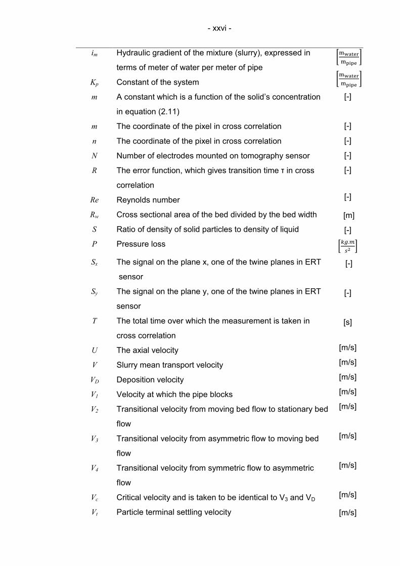
- xxvi -
im
Kp
m
m
n
N
R
Re
Rw
S
P
Sx
Sy
T
U
V
VD
V1
V2
V3
V4
Vc
Vt
Hydraulic gradient of the mixture (slurry), expressed in
terms of meter of water per meter of pipe
Constant of the system
A constant which is a function of the solid’s concentration
in equation (2.11)
The coordinate of the pixel in cross correlation
The coordinate of the pixel in cross correlation
Number of electrodes mounted on tomography sensor
The error function, which gives transition time τ in cross
correlation
Reynolds number
Cross sectional area of the bed divided by the bed width
Ratio of density of solid particles to density of liquid
Pressure loss
The signal on the plane x, one of the twine planes in ERT
sensor
The signal on the plane y, one of the twine planes in ERT
sensor
The total time over which the measurement is taken in
cross correlation
The axial velocity
Slurry mean transport velocity
Deposition velocity
Velocity at which the pipe blocks
Transitional velocity from moving bed flow to stationary bed
flow
Transitional velocity from asymmetric flow to moving bed
flow
Transitional velocity from symmetric flow to asymmetric
flow
Critical velocity and is taken to be identical to V3 and VD
Particle terminal settling velocity
[-]
[-]
[-]
[-]
[-]
[-]
[m]
[-]
[-]
[-]
[s]
[m/s]
[m/s]
[m/s]
[m/s]
[m/s]
[m/s]
[m/s]
[m/s]
[m/s]

- xxvii -
VX
VY
W
WPB
WPU
WPi
x
y
ΔP/L
ΣF
The value of the pixel (n,m) on plane X
The value of the pixel (n,m) on plane Y
Terminal settling velocity of the particles in three-layer
model
Perimeter of the lower layer of the pipe in the two layer
model
Perimeter of the upper layer of the pipe in the two layer
model
Perimeter at the interface between the two layers in two-
layer model
A constant which is a function of solid’s concentration
in equation (2.11)
The vertical coordinate, perpendicular to the pipe axis
Pressure gradient
The total force per unit forces exerted normal to the pipe in
the two layer
[-]
[-]
[m/s]
[m]
[m]
[m]
[-]
[m]
[pa/m]
Greek Letters
Symbol Description Unit
αc
γ
ε
θ
Φr
λs
μl
Volume fraction of the dispersed phase (solids
volume fraction).
Pipe inclination angle from horizontal
Roughness of the pipe
Half of the angle subtended at the pipe centre due to
the upper surface of the bed
Angle of repose of the solid particles
Coefficient of static friction of the solid particles
against the pipe wall
Liquid viscosity
[-]
[deg]
[-]
[deg]
[deg]
[-]
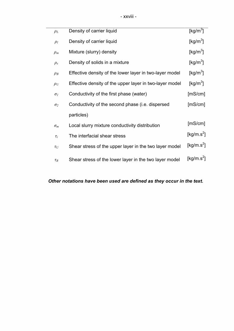
- xxviii -
ρL
ρl
ρm
ρs
ρB
ρU
σ1
σ2
σm
τi
τU
τB
Density of carrier liquid
Density of carrier liquid
Mixture (slurry) density
Density of solids in a mixture
Effective density of the lower layer in two-layer model
Effective density of the upper layer in two-layer model
Conductivity of the first phase (water)
Conductivity of the second phase (i.e. dispersed
particles)
Local slurry mixture conductivity distribution
The interfacial shear stress
Shear stress of the upper layer in the two layer model
Shear stress of the lower layer in the two layer model
[kg/m3]
[kg/m3]
[kg/m3]
[kg/m3]
[kg/m3]
[kg/m3]
[mS/cm]
[mS/cm]
[mS/cm]
[kg/m.s2]
[kg/m.s2]
[kg/m.s2]
Other notations have been used are defined as they occur in the text.

- xxix -
List of Abbreviations
AARE
ABS
ACF
AIMFLOW
ANN
BZP
CHS
CPVC
DAS
Dfps
DWV
ECT
ECTFE
EIT
EMF
EMR
EMT
ERT
ET
FFT
FICA
HET
ID
LBP
LDA
Average Absolute Relative Error
Acrylonitrile-Butadien-Styrene
Auto Correlation Functions
Advanced Imaging and Measurement for Flow, Multiphase
Flow and Complex Flow in the Industrial Plant
Artificial Neural Network
Bright Zinc Plated
Circular Hollow Section
Chlorinated Poly(Vinyle Chloride)
Data Acquisition System
Dual-Frames Per Second
Drain-Waste-Vent
Electrical Capacitance Tomography
Ethylene-Chlorotrifluoroethylene
Electrical Impedance Tomography
Electromagnetic Flow meter
Electron Magnetic Resonance
Electromagnetic Tomography
Electrical Resistance Tomography
Electrical Tomography
Fast Fourier Transform
Fast Impedance Camera System
Heterogeneous Flow Regime
Pipe Internal Diameter
Linear Back Projection
Laser Doppler Anemometry

- xxx -
LDV
MB
MRI
MSS
NMR
OD
OLIL
P
PE
PEPT
PET
PFA
PFC
PIV
PP
PSD
PSDF
PTFE
PVC
PVDC
PVDF
RF
SB
SBP
SCG
SHS
SNR
STDEV
Laser Doppler Velocimetry
Moving Bed Flow Regime
Magnetic Resonance Imaging
Mean Square Spectrum
Nuclear Magnetic Resonance
Pipe Outer Diameter
Online Instrumentation Laboratory(University of Leeds/UK)
Pseudo-homogeneous Flow Regime
Probability Density Functions
Polyethylene
Positron Emission Particle Tracking
Positron Emission Tomography
Perfluoro(Alkoxyalkane) Copolymer
Parallel Flange Channels
Particle Image Velocimetry
Polypropylene
Particle Size Distribution
Power Spectral Density Functions
Polytetrafluoroethylene
Poly Vinyl Chloride
Poly(Vinylidene Chlride)
Poly(Vinylidene Fluoride)
Radio Frequency
Stationary Bed
Sensitivity Back Projection
Sensitivity Conjugate Gradient
Square Hollow Section
Signal-to-Noise Ratio
Standard Deviation

- xxxi -
SVM
TEP
UB
UC
UDVP
uPVC
Support Vector Machine
Perfluoro (Ethylene-Proplylene) Copolymer
Universal Beam
Universal Column
Ultrasonic Doppler Velocity Profiler
Unplastisized Poly Vinyl Chloride
- xxxii -
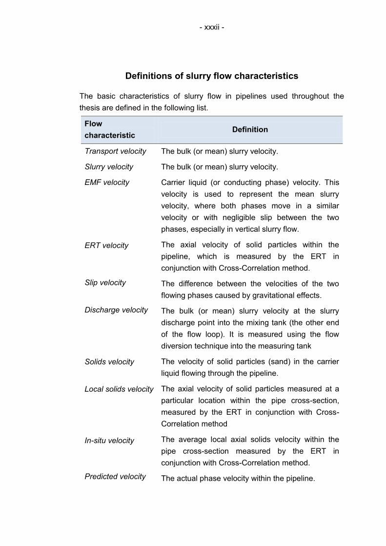
Definitions of slurry flow characteristics
The basic characteristics of slurry flow in pipelines used throughout the
thesis are defined in the following list.
Flow
characteristic Definition
Transport velocity
Slurry velocity
EMF velocity
ERT velocity
Slip velocity
Discharge velocity
Solids velocity
Local solids velocity
In-situ velocity
Predicted velocity
The bulk (or mean) slurry velocity.
The bulk (or mean) slurry velocity.
Carrier liquid (or conducting phase) velocity. This
velocity is used to represent the mean slurry
velocity, where both phases move in a similar
velocity or with negligible slip between the two
phases, especially in vertical slurry flow.
The axial velocity of solid particles within the
pipeline, which is measured by the ERT in
conjunction with Cross-Correlation method.
The difference between the velocities of the two
flowing phases caused by gravitational effects.
The bulk (or mean) slurry velocity at the slurry
discharge point into the mixing tank (the other end
of the flow loop). It is measured using the flow
diversion technique into the measuring tank
The velocity of solid particles (sand) in the carrier
liquid flowing through the pipeline.
The axial velocity of solid particles measured at a
particular location within the pipe cross-section,
measured by the ERT in conjunction with Cross-
Correlation method
The average local axial solids velocity within the
pipe cross-section measured by the ERT in
conjunction with Cross-Correlation method.
The actual phase velocity within the pipeline.
- xxxiii -
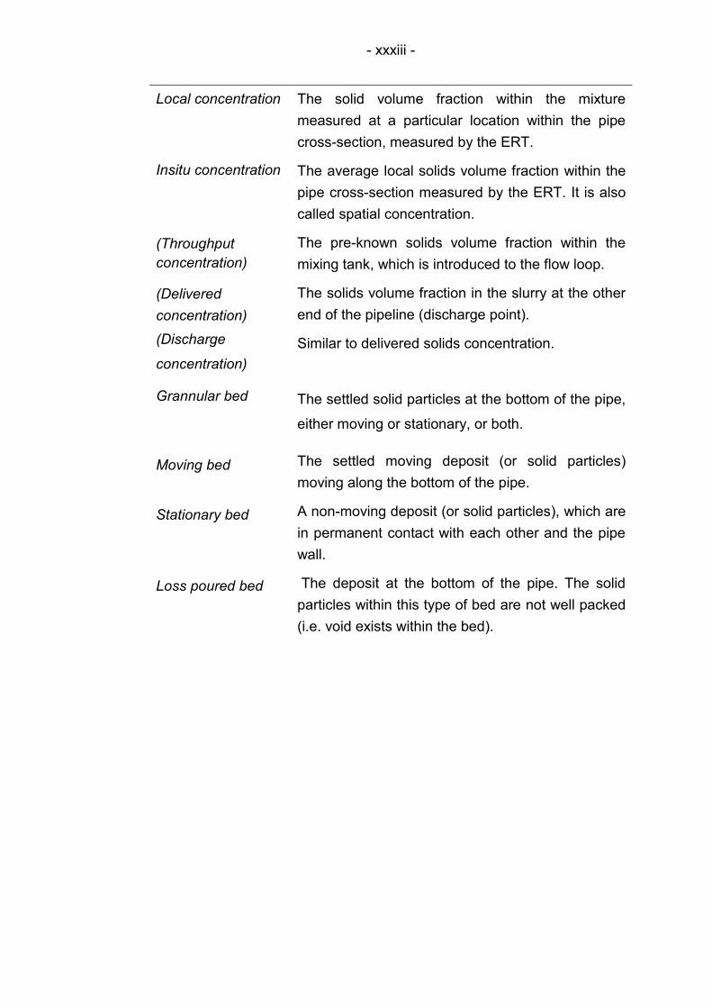
Local concentration
Insitu concentration
(Throughput
concentration)
(Delivered
concentration)
(Discharge
concentration)
Grannular bed
Moving bed
Stationary bed
Loss poured bed
The solid volume fraction within the mixture
measured at a particular location within the pipe
cross-section, measured by the ERT.
The average local solids volume fraction within the
pipe cross-section measured by the ERT. It is also
called spatial concentration.
The pre-known solids volume fraction within the
mixing tank, which is introduced to the flow loop.
The solids volume fraction in the slurry at the other
end of the pipeline (discharge point).
Similar to delivered solids concentration.
The settled solid particles at the bottom of the pipe,
either moving or stationary, or both.
The settled moving deposit (or solid particles)
moving along the bottom of the pipe.
A non-moving deposit (or solid particles), which are
in permanent contact with each other and the pipe
wall.
The deposit at the bottom of the pipe. The solid
particles within this type of bed are not well packed
(i.e. void exists within the bed).
- 1 -
Chapter 1
Introduction
1.1 Hydraulic transport of solids in pipes
The presence of solid particles in a carrier liquid form a mixture, which is
referred to as slurry. Slurry flows cover a wide spectrum of applications and
are the focus of considerable interest in engineering research. The concept
of slurry transport has been employed long time ago and it is widely utilised
in many industries such as minerals, chemical, coal, pharmaceutical, water,
dredging and other industries. It is worth mentioning that in some specific
applications, such as dredging, hydraulic transport is the only means of
transportation of solids through pipelines. In mid-nineteenth century slurry
transport was first used by mining industry, an example of which is the
transport of slurry used to reclaim gold from placers in California (Abulnaga,
2002). Pneumatic conveying is also another means of transporting solid
particles, in which gas (commonly air) is used instead of liquid. However, as
it is associated with some disadvantages such as high specific power
consumption, potential for particle breakage and degradation, high wear rate
on components and used for relatively short distance, some drawbacks are
seen to this technology (Dhodapkar et al., 2006). On the other hand, a great
interest and attention has been given to hydraulic transport due to its
advantages namely environmentally friendly, low operation and maintenance
costs, relative simplicity in its infrastructure etc. It has been a progressive
technology for transporting a vast amount of different solid materials through
various sizes of pipelines with different orientations, such as sands, iron
concentrates, copper concentrates, phosphate matrix, tailings, limestone
and sewage, in different densities, shapes, sizes up to 150 mm (6"), such as
those pumped from fields of phosphate matrix (Abulnaga, 2002). These are
the examples of long distance commodity pipelines. However, it has also
been transported through short in plant pipelines, such as that of nuclear,
chemical, pharmaceutical and food industry. The most commonly used
carrier fluid is water, which is referred to as “hydraulic transportation”.
Since these mixtures are encountered in a wide range of industries, their
classification is very important for describing their physical appearance and
flow behaviour. There are two broad classifications for hydraulic
transportation, which are referred to as settling (or heterogeneous) and non-
- 2 -
settling (or homogeneous) slurries. These classifications based on two
considerations, physical properties and flow behaviour (or rheological
behaviour). In other words, whether the solid particles in the slurry can settle
under the influence of gravity or are suspended within the carrier fluid. In
settling slurries the solid particles tend to separate from the carrier liquid and
segregate at the bottom of the pipe, either horizontal or inclined, under the
influence of gravity. This suggests that the settling slurries can be stratified
either fully or partially (Matousek, 2005). In contrast, non-settling or
homogeneous slurries composed of particles of colloidal dimensions, which
are characterised by primary particle diameters of typically less than 2 μm.
They are also highly concentrated and maintained in suspension by
molecular movement within the liquid, which is referred to as Brownian
motion (Peker et al., 2008). Their non-settling behaviour is probably due to
hindering settling, as do occur in most paints and emulsions (Brown and
Heywood, 1991). It is worth mentioning that non-settling slurries are beyond
the scope of this thesis, therefore, no further reference will be made to non-
settling slurries.
The behaviour of slurry flow through pipelines has been systematically
investigated since 1950s (Matousek, 1996). The focus was mainly based on
experimental investigations dealing with prediction of pressure drops and
demarcation of flow regimes with different velocities, using various particles
and pipe sizes, and then using the collected data to construct empirical
models. Then 1970s and 1980s marked the emergence of another
approach, by which the researchers were more focusing on the fundamental
principles or the rheological based continuum approach. This approach was
strictly applied to ultra fine non-colloidal particle slurries, such as the basics
of the macroscopic two-layer model by Wilson (1970) and microscopic slurry
flow by Shook and Roco (1991). Whereas the contemporary approach entail
the rapid development of measuring techniques and substantial
computational effort, which is still available approach to describe the
complex behaviour and nature of settling slurry flow through pipelines
(Matousek, 2005; Lahiri, 2009). Despite the excellent research work and
progress in the field our understanding of the fundamental and complex
nature of settling slurry flow is still not enough to satisfy the engineering
requirements. Since the slurry engineer requires a viable and reliable
methodology that suits all the conditions met in industry. Therefore, the
investigation of all the relevant variables is crucial.
- 3 -
A wide range of experimental results have been reported in the literature
including different operating conditions, material type and shape and
different flow orientations. In horizontal and inclined flow as the gravity acts
at right angle to the flow, the separation of phases occurs and gives rise to
several flow regimes, pseudo-homogeneous, heterogeneous, moving bed
and stationary bed. Whereas in vertical flow, especially upward flow, the
gravity acts counter to the dynamic forces, as a result the slippage of the
phases occurs (Parvareh et al., 2010). The occurrence of separation and
slippage of the constituent phases in settling solid-liquid flow in pipelines
makes the flow unpredictable and time dependent. Therefore it is paramount
for the operator of these pipelines to monitor and measure the flow
continuously, particularly from the local point of view (i.e. the knowledge of
internal structure of flow is necessary) so as to ensure safe transport and
maintaining acceptable control limits. In order to understand the internal
structure of such flows, solids volume fraction distribution and solids velocity
distribution are of great importance. Therefore, this study focuses mainly on
qualitative and quantitative measurement of these two parameters.
As noticed in the literature, there are many challenges that have to be
highlighted to boost our knowledge and tackle the limitations in
understanding and measuring settling slurry flows. In the past, several
intrusive methods, such as traditional probes, have been used to measure
solids volumetric concentration and velocity. The disadvantages of using
these probes have been reported, particularly for solid-liquid flow, Brown and
Heywood (1991). It is highly unlikely that these devices can survive the
harsh condition inside the pipelines due to abrasive nature of slurry. In many
cases solids may accumulate around them and cause pipe blockage. Also it
is well known that intrusive devices introduce an undesirable physical
disturbance and alter the internal structure of the flow (Heindel et al., 2008).
In order to overcome this limitation, researchers across the world developed
a variety of non-intrusive measurement techniques to highlight the internal
characteristics of two or multiphase flows, such as optical, ultrasound,
nuclear, conductance and electrostatic transducers. Nonetheless, each of
the above techniques suffers from serious limitations, especially for the
complex solid-liquid flows. For example, since slurries are opaque and flow
through opaque enclosures, then using optical techniques can be quite
difficult if not impossible. Although nuclear techniques provide an accurate
measurement, they are very expensive and suffer from low temporal
resolution and environmental issues (Thorn et al., 1997). Amongst all of the
above techniques Electrical Resistance Tomography (ERT), as one of the
- 4 -
family of non-intrusive sensors, has attracted the interest of many
researchers. This is due to the fact that the ERT offers many advantages,
such as non-intrusive, relatively low cost, no environmental restrictions,
providing quantitative and qualitative on-line measurement, fast etc. Within
the last two decades the ERT has seen a significant development and has
been applied to many industrial process involving two/multiphase systems.
Particularly the application of the ERT to solid-liquid flow has been reported
by many investigators (Razzak et al., 2009; Giguère et al., 2008; Lucas et
al., 1999; Wood and Jones, 2003; Wang et al., 2003; Pachowko et al.,
2004). All of the above studies have been carried out on vertical and/or
horizontal flows used the conventional ERT system, which acquires up to
200 images per second (Dyakowski et al., 2000). To the authors’ knowledge
no attempt has been made to measure solids volume fraction and solids
axial velocity using the combination of high performance ERT system in
conjunction with cross-correlation technique. It is evident that measurement
of the two parameters, especially velocity, in fast evolving processes
requires high frame rates (fast) of milliseconds. Therefore, this study uses a
high performance dual-plane electrical resistance tomography system, which
is called Fast Impedance Camera System (FICA) and is capable of acquiring
data at a rate of 1000 dual-frames per second (dfps). As horizontal and
vertical sections jointly make most of the pipelines, it is important to study
both orientations simultaneously with similar conditions, so as to reveal the
effect of one on another. However, at higher velocities (pseudo-
homogeneous) there may be higher degree of similarities in the internal
structure of the flow in the two orientations, but the differences could well be
noticed for the transport velocities below the deposition velocity, where the
homogeneity of vertical flow is still preserved, whereas a strata is formed in
the horizontal pipe invert.
Although it can be argued that most of pipelines in industry are horizontal
and vertical, inclined settling slurry flows are still play an important role,
despite that they have not been the subject of extensive studies. Unlike
horizontal and vertical flows, very limited work has been conducted in this
flow orientation. In fact since 1950s a very limited number of published body
work covers the characterisation and measurement of solid liquid flows in
inclined pipelines. Therefore, this project attempts to design and build a pilot
scale slurry flow loop, in the aim that it can be used as a tool for further
understanding and characterisation of inclined slurry flow and identifying flow
effects on its measurement scheme. The whole design strategies and
methodologies are described in Chapter 6, where the reader will be taken
- 5 -
through the whole journey from the preliminary design to the erection stage
and testing. However, no experimental work on inclined flow will be
mentioned throughout the present work. The reader is referred to several
previous works conducted on inclined pipeline: Worster and Denny (1955),
Brook (1962), Kao and Hwang (1979), Wilson et al. (1992), Shook et al.
(1974), Wilson and Tse (1984), Matousek (1997), Doron and Barnea (1997),
Lucas et al. (1999).
1.2 Motivation of present work
1. In order to understand the complex nature of slurry flow and optimising
the slurry flow systems a reliable method (or technique) is required to
continuously monitor and capture the internal images of the pipeline
through localised flow measurement, so that a safe transport is ensured
and acceptable control limits are maintained. It is quite apparent that an
automated and on-line internal measurement of pipe flow offers great
advantages, such as providing fast on-line measurements, reducing
labour resources and the requirement for additional sampling equipment.
However, the selection of which technique to use is strongly dependent
on several important issues, such as cost, simplicity in design, safety,
reliability, robustness, speed and non-intrusive. Due to the fact that the
ERT offers all the above advantages, then it is proposed to be the meter
of choice. Although the some previous works have made use of the ERT,
all of them used the conventional ERT system, which acquires 200
images per second (Dyakowski et al., 2000). Therefore, this thesis
employs a high performance Electrical Resistance Tomography system
(ERT) to explore its capability in localised measurements and
visualisation of horizontal and vertical slurry flow (i.e. solids concentration
distribution and solids axial velocity distribution within the carrier fluid),
with capability of acquiring data at a rate of 1000 dual frames per second.
2. In terms of industrial application the volumetric flow rate of the phases in
two/multiphase flows is very important flow parameter to the pipeline
operator. However, due to the complexity of multiphase/two phase flow,
particularly solid-liquid flow, it is enormously difficult to accurately
measure the flow parameters of each phase individually using only one
conventional flow meter. Thus, a secondary sensor is required to
determine the volumetric flow rate of each phase and so the total mixture
volumetric flow rate. A survey of the literature and commercially available
flow meters raised the alarm that currently there is almost no
- 6 -
multiphase/two phase flow meter practically available to majority of
industrial applications for measurement of volumetric flow rate of
constituent phases and total mixture (Li et al., 2005; Thorn et al., 1997).
Therefore, this research proposes an ERT based technique, which
combines the Electrical Resistance Tomography (ERT) and the
Electromagnetic Flow meter (EMF), to measure the volumetric flow rate of
each phase (continuous and dispersed) and producing the total slurry
volumetric flow rate.
3. Since settling slurries contain much coarser particles (up to few
millimetres), such as sand, coal-water, gravel, then these particles tend to
accumulate at the bottom of the pipe and produce several flow regimes.
As highlighted in the literature, these flow regimes affect one of the most
important parameter in settling slurry flow, which is pressure drop,
particularly in stratified flow. This may in itself cause partially or fully pipe
blockage, which reduces the efficiency. They also influence pipe erosion
and some other performance characteristics (Doron and Barnea, 1995).
Thus, the recognition of these flow regimes is very important.
Furthermore, the identification and evaluation of the information regarding
these flow regimes are usually performed by visual inspection through
graphic illustration, which sometimes difficult to interpret or identify, either
due to the system being opaque or with high velocity. Therefore, this work
explores the validity and applicability of the ERT as an automated online
flow regime recognition technique through statistical analysis of its signal.
4. Although it can be argued that in most of plants handling slurry flow, the
pipelines are either horizontal or vertical, inclined flows is still encountered
and essential in dredging ladder, pump-box feed systems and many long
overland pipelines, which have to go through dunes and hills. A survey
through the literature concluded that there is a lack of information
regarding the behaviour of inclined slurry flow, as very limited work has
been carried out in this type of pipeline orientation. It was also found that
to avoid the blockage of the line once the flow is shut down, a commonly
used design restriction of 10-16% (5.7°-9°) is often considered due to lack
of knowledge of the critical slope of the inclined pipe. As Kao and Hwang
(1979) criticised using the rule of thumb for the design of critical slope.
Their criticism was based on the fact that lack of properly designed critical
slope in an inclined pipe adds to construction costs and capital expenses.
Moreover, our present knowledge of the fundamentals, behaviour of
inclined slurry flow and the flow effects on its measurement is still in its
stage of infancy. This implies that almost no correlation has been
- 7 -
developed for inclined flow. Due to this reason, most of the designers do
not take the pipe inclination into account, but rather the whole transport
line as horizontal. Therefore, This work has attempted to design and build
a pilot scale inclinable multiphase flow loop, meeting all the design
requirements for slurry flow, so as to be used to gain insight of complex
inclined slurry flow and the potential effects on flow measurements.
However, This study attempts only the design and installation of the entire
flow loop and associated instrumentations and equipments, while
conducting experiments and performing measurements on inclined slurry
flow is beyond the scope of this research, due to the limited timeline of
this study. In other words, this thesis is limited to the measurement and
visualisation of horizontal and counter-gravity slurry flow.
5. A review in literature reveals that little work has been carried out within
the boundary of stationary bed flow regime in horizontal flows, this is
undoubtedly due to the fact that the risk of blockage is dominant in this
region. As a result of this, an investigation into the boundary of stationary
bed and pipeline blockage is conducted. Firstly, to gain further knowledge
regarding the minimum velocity within the frame of this flow regime,
secondly, to explore the functionality of the dual-plane ERT sensor
electrodes, while they are covered by a settled thick granular bed at the
bottom of the pipe.
6. Narrow Particle Size Distribution (PSD) has been used in most of the
investigations carried out in slurry flow, while the Particle Size Distribution
in industry is very broad. Therefore, this research deals with flow
characterisation and measurement of two broadly graded sands, medium
sand (d15 = 170 µm, d50 = 242 µm, d85 = 430 µm) and coarse sand (d15
= 270 µm, d50 = 480 µm, d85 = 2240 µm).
1.3 Scope of present work
The present work makes an extensive use of the Electrical Resistance
Tomography system and supporting instrumentation (EMF) for measurement
and characterisation of horizontal and vertical settling slurry flow. The local
flow characteristics of the above two flow orientations is determined. Non-
uniform shape and size and used as solid particles and tap water as a
carrier liquid. Only two sands are attempted, medium and coarse with PSD
(d15 = 170 µm, d50 = 242 µm, d85 = 430 µm) and (d15 = 270 µm, d50 =
480 µm, d85 = 2240 µm) respectively. The validation of each parameter,
obtained from the ERT and the EMF or the combination of both, is carried
- 8 -
out using a flow diversion technique, the results of which is presented within
the body of this thesis. Visualisation and recognition of each flow regime
encountered in settling slurry flow is attempted based on ERT localised
measurements. No work will be carried out on inclined flow, except the
design, erection and testing of an inclinable slurry flow loop.
1.4 Research objectives
The overall objective of this project is to explore the validity and applicability
of a new settling slurry flow measurement and visualisation technique, in
which the Electrical Resistance Tomography used as the main flow meter
and the EMF as a supporting auxiliary sensor. The ERT flow visualisation
scheme is also planned to characterise and reveal the mechanisms
occurring in horizontal and vertical solid-liquid flow. In order to achieve the
main aim of this study, the following specific objectives have to be fulfilled:
1. Localised measurement and visualisation of horizontal slurry flow.
2. Characterisation of stratified slurry flow, including the blockage
phenomena.
3. Localised measurement and visualisation of vertical slurry flow.
4. Characterisation of counter-gravity solid-liquid flow.
5. Slurry flow regime visualisation and characterisation in horizontal
slurry flow.
6. Estimation of phase volumetric flow rate through combination of the
ERT and the EMF.
7. Explore the validity of the results obtained from the measurement
scheme.
8. Develop an automated (on-line) horizontal flow regime recognition
technique.
9. Evaluation of the proposed measurement and recognition technique.
10. Design and erection of an inclinable settling slurry flow system.
1.5 Thesis layout
Chapter 2 presents the literature concerning the settling slurry flow in
various flow orientations, horizontal, vertical and inclined. This chapter
describes some of the previous work carried out on each orientation,
particularly in horizontal flow, with mentioning the common flow regimes and
governing physical mechanisms.
- 9 -
Chapter 3 critically reviews the current commercially available techniques
for measurement and visualisation of slurry flow and highlights the limitations
associated with each mentioned technique. The current status of the
Electrical Resistance Tomography is also discussed along with its
applications in various engineering field.
Chapter 4 describes the experimental methodology and the strategy used to
carry out each experiment. The test facility and the equipments used are
also highlighted in this chapter along with the instrumentations used for
measurement of the desired parameters. The calibration procedure of the
instrumentations are detailed and the results are illustrated quantitatively.
Chapter 5 contains a bulk of experimental findings and observations
concerning the measurement of horizontal and upward vertical slurry flow.
The measurement results cover various integral flow characteristics (slurry
velocity, pressure, special concentration, solids axial velocity, delivered
solids concentration and slurry volumetric flow rate) and local flow
characteristics (local solids concentration, solids concentration profile, mean
solids axial velocity, solids axial velocity distribution, liquid volumetric flow
rate, and solids volumetric flow rate). An analysis of horizontal stratified flow
is also reported in this chapter. An evaluation of each estimated parameter is
summarised.
Chapter 6 discusses the design and erection of a multiphase inclinable flow
system with focusing on main design requirement for settling slurry flow.
Various design procedures are described and the selection criteria for the
associated instrumentations are enclosed. The design of the inclinable table
and the most suitable lifting method is also detailed in this chapter.
Chapter 7 Develops a novel technique for recognition of common flow
regimes encountered in horizontal flow using statistical analysis of the ERT
signal. The evaluation of the proposed recognition scheme is presented with
summarising the overall success rate in recognising each flow regime.
Chapter 8 Draws the conclusions of each finding and observation with a
summary of the contribution from the present work. This chapter ends with
highlighting the future directions and recommendation for further studies in
slurry measurement, visualisation and characterisation.
- 10 -
Chapter 2
Hydraulic transport of solid particles in pipeline
In this chapter the literature and previous work on slurry flow is critically
reviewed, with considering different pipe configuration, horizontal, vertical
and inclined. The common four flow regimes are described, along with the
techniques used to recognise these regimes, by the previous investigators.
The boundary between the flow regimes are also detailed with the physical
mechanisms governing settling slurry flow.
2.1 Introduction
Settling slurry flow in pipeline is encountered in many industries such as
energy, chemical, pharmaceutical, petroleum, wastewater processing and
mining industry. It is worth mentioning that in some specific applications,
such as dredging, hydraulic transport is the only mean of transportation of
solids through pipelines. These mixtures are transported through different
pipeline orientations, mainly horizontal and vertical. Settling slurry flow is a
very complex and has attracted considerable attention of many investigators
across the world. A wide range of experimental results have been reported
in literature including different operating conditions, material type, shape and
different flow orientations (Newitt et al., 1955; Newitt et al., 1961; Wasp et
al., 1970; Roco and Shook, 1984; Bartosik, 1996; Gillies and Shook, 2000;
Hong et al., 2002; Barigoua et al., 2003; Pachowko et al., 2004; Pohlman et
al., 2006; Divoux and Geminard, 2007; Pougatch and Sacudean, 2008;
Matousek, 2009; Munir, 2011).
In horizontal flow as the gravity acts at right angle to the flow, the separation
of phases occurs and gives rise to several flow regimes, pseudo-
homogeneous, heterogeneous, moving bed and stationary bed. Similar flow
regimes are encountered in inclined flow with occurrence of backflow (Doron
et al., 1997; Matousek, 2002; Yamaguchi et al., 2011). Each flow regime is
described in the following sections and has been the subject of many studies
in literature such as (Wilson and Pugh, 1988; Gillies et al., 1991; Doron and
Barnea, 1993; Brown, 1991). Whereas in vertical flow, especially upward
flow, the gravity acts counter to the dynamic forces, as a result the slippage
of the phases occurs (Shook and Bartosik,1994; Parvareh et al., 2010). The
occurrence of separation and slippage of the constituent phases in settling
- 11 -
solid-liquid flow in pipeline configuration makes the flow unpredictable and
time dependent. Therefore it is paramount for the operator of these pipelines
to monitor and measure the flow continuously, particularly from the local
point of view, i.e. the knowledge of internal structure of flow is necessary, so
as to ensure safe transport and maintaining acceptable control limits.
This chapter highlights the previous work of others carried out within the past
years and critically review the knowledge gained from them. The
phenomenon of slurry flow in different pipe configurations (horizontal,
vertical and inclined) will be described, with particular attention to horizontal
and vertical flow. Since the distinction of flow regimes is very important for
flow measurement, design, maintaining control limits and economical
transport, then it will be covered along with transitional velocities. Also, in
order to understand the behaviour of settling slurry flow and evaluate the
accuracy and reliability of an instrument, especially those are used for
measurement of local flow parameters, this chapter covers the stratification
phenomenon, particle deposition velocity, pressure drop and physical
mechanisms governing settling slurry flow. One of the most important
parameters of slurry flow is the recognition of flow regimes, especially for the
purpose of metering (i.e. for flow regime dependent flow meters), therefore,
the last sections highlight the importance of flow regime recognition in
general and critically review the techniques proposed by previous
researchers in the field.
2.2 Slurry flow in pipelines
Slurry is a mixture of solid particles in a carrier liquid. The carrier liquid may
be water, Newtonian or non-Newtonian liquid. However, the carrier liquid
used in the vast majority of slurry flows is water. The hydraulic transport of
solid particles in pipes is widely used in many industrial applications, such as
chemical and mining industry. The aim of transporting these solids is either
for transporting of bulk solids or physical/chemical processes between the
carrier liquid and solids (Xia et al., 2004; Wilson et al., 2006). As previously
mentioned, slurries are classified into two categories, settling and non-
settling, however, this research deals only with settling slurries and no
reference will be made to non-settling slurries.
The large number and range of variables in slurry flow in pipelines influences
the behaviour of slurry flow and makes it very complex. These variables are
pipeline configuration (horizontal, vertical and inclined), solid particle size,
solids shape, solids density, liquids density, liquids viscosity, mean slurry
- 12 -
velocity, pipe diameter and flow direction (ascending or descending flow). It
is worth mentioning that the occurrence of such a large number of variables
can affect slurry metering and optimisation of slurry flow meters become
very difficult and variable dependent. For example, as the ERT is flow
regime dependent (Pachowko, 2004), then occurrence of these flow regimes
in horizontal slurry flow creates a challenge in measurement of dispersed
flow.
It is apparent that most of industrial applications employ horizontal pipe
configuration for transportation of solid materials. However, vertical pipe
configuration is also paramount for many industries such as mining, (Munir,
2011). Although it can be argued that most of pipe configurations are
horizontal and vertical, which are connected through elbows and fittings,
inclined flow can also play an important role for certain long distance
overland pipeline, thickener feed systems, pump box feed systems etc.
(Abulnaga, 2002). Therefore, this chapter gives a description over the
behaviour of slurry flow in each pie configuration. In horizontal and inclined
pipes, gravity tends to stratify the mixture and split it into two distinct layers,
the solid particles at the bottom of the pipe and the carrier liquid at the top.
On the other hand, in vertical pipes, the flow conditions are straight forward,
without deposition of solid particles on the pipe invert. Since horizontal flow
makes the majority of the pipelines and the gravity in this flow orientation
plays an important role for creation of several flow regimes, therefore, a
large portion of the chapter is devoted to horizontal flow rather than the other
two flow orientations.
2.3 Horizontal flow
Flow of settling slurry in horizontal pipeline is complex and has been the
subject of a vast number of studies from the early work of Blatch (1906),
Howard (1939), Durand (1952), Durand and Condolios (1953), Newitt et al.
(1955) and many others. The vast majority of literature devoted to pressure
drop, mixture velocity and critical velocity, friction characteristics,
visualisation and behaviour of solid particles within the carrier liquid,
determination of the internal structure of slurry flow via solids concentration
and solids velocity. The complexity of this type of flow is due to the influence
of gravity, which gives rise to different flow regimes from pseudo-
homogenous at high velocity to stationary bed and blockage at low slurry
velocity. The emergence of these flow regimes, which are sometimes called
flow patterns in literature, affects the pressure drop and influences pipe wear
- 13 -
and other performance characteristics. This suggests that settling slurry flow
suffers from flow discontinuity, due to the occurrence of these flow regimes,
thus affects the flow meters, which are flow regimes dependent. Therefore, a
description of each individual flow regime is presented in the following
sections, along with the effects of each flow regime on each flow parameter.
2.3.1 Slurry flow regimes
Flow regimes are normally described in terms of the distribution of solids
within the cross-section of the pipeline. In other words, they can be used to
describe the motion of the particles in horizontal or near horizontal slurry
flow, often based on visual observation and have been the subject of
numerous experimental studies, (Durand and Condolios, 1952; Matousek,
2009; Doron et al., 1997; Matousek, 2002; Parvareh et al., 2010; Brown,
1991; Giguère et al., 2008).
Since the settling slurry flow is very complex and the determination of a
certain flow regime relies mostly on visual inspection, the literature has
shown different names and definitions to certain regime. Durand (1952)
conducted the initial study on horizontal slurry flow regimes, in which he
classified the slurry flow in horizontal pipes into “non-deposit flow regime”
and a “regime with deposits” based on the specific gravity of the particles
used in the investigation. In (1963) the same classification was used by
Condolios and Chapus. However, this classification was refined, based on
the relationship between the particle size, concentration and deposition
velocity, by Newitt et al. (1955), Ellis and Round (1963), Thomas (1964),
Shen et al. (1970) and Wicks (1971). It is important to note that the term
“saltation”, referred to as a “moving bed”, was incorporated into the
classifications of flow regimes by Bain and Bonnington (1970). One of the
most common classification was done by Vocaldo and Charles (1972) and
Parzonka et al. (1981), who classified the slurry flow regimes into four main
categories, “homogeneous flow”, “heterogeneous flow”, heterogeneous and
sliding bed flow” and “ saltation and stationary bed flow” (Doron and Barnea,
1996). While some investigators have refined the classification into further
categories, such as Lazarus and Neilson (1978), who classified slurry flow
patterns into “homogeneous flow”, “pseudo-homogeneous flow”,
“heterogeneous flow”, “fully moving bed” and “stationary bed”. Then Ercolani
et al. (1979) attempted to show the form and outline of “pseudo-
homogeneous flow”, “heterogeneous flow”, “limit deposit condition”, “moving-
stationary bed”, “moving dunes” and “stationary bed”. Some other works
have been reported in the literature regarding slurry flow regimes in
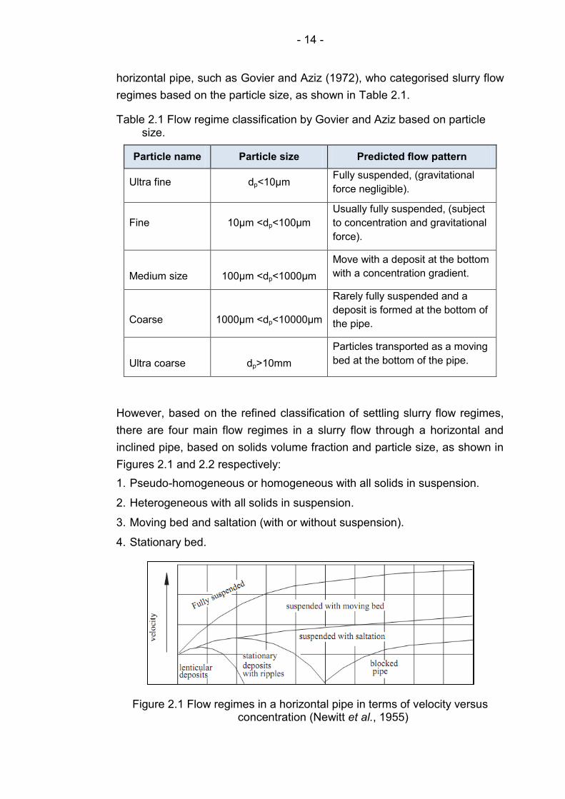
- 14 -
horizontal pipe, such as Govier and Aziz (1972), who categorised slurry flow
regimes based on the particle size, as shown in Table 2.1.
Table 2.1 Flow regime classification by Govier and Aziz based on particle size.
Particle name Particle size Predicted flow pattern
Ultra fine dp<10μm Fully suspended, (gravitational
force negligible).
Fine 10μm <dp<100μm
Usually fully suspended, (subject
to concentration and gravitational
force).
Medium size
100μm <dp<1000μm
Move with a deposit at the bottom
with a concentration gradient.
Coarse
1000μm <dp<10000μm
Rarely fully suspended and a
deposit is formed at the bottom of
the pipe.
Ultra coarse
dp>10mm
Particles transported as a moving
bed at the bottom of the pipe.
However, based on the refined classification of settling slurry flow regimes,
there are four main flow regimes in a slurry flow through a horizontal and
inclined pipe, based on solids volume fraction and particle size, as shown in
Figures 2.1 and 2.2 respectively:
1. Pseudo-homogeneous or homogeneous with all solids in suspension.
2. Heterogeneous with all solids in suspension.
3. Moving bed and saltation (with or without suspension).
4. Stationary bed.
Figure 2.1 Flow regimes in a horizontal pipe in terms of velocity versus concentration (Newitt et al., 1955)
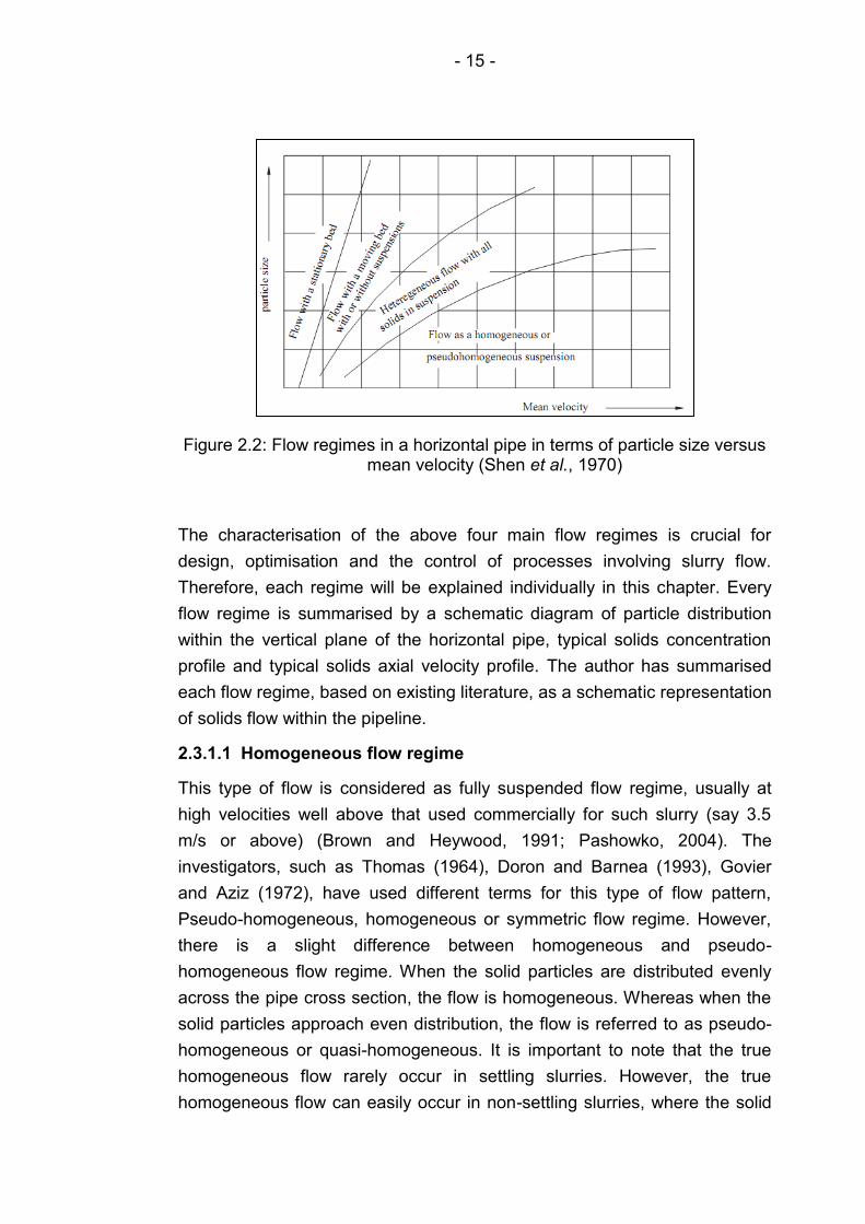
- 15 -
Figure 2.2: Flow regimes in a horizontal pipe in terms of particle size versus mean velocity (Shen et al., 1970)
The characterisation of the above four main flow regimes is crucial for
design, optimisation and the control of processes involving slurry flow.
Therefore, each regime will be explained individually in this chapter. Every
flow regime is summarised by a schematic diagram of particle distribution
within the vertical plane of the horizontal pipe, typical solids concentration
profile and typical solids axial velocity profile. The author has summarised
each flow regime, based on existing literature, as a schematic representation
of solids flow within the pipeline.
2.3.1.1 Homogeneous flow regime
This type of flow is considered as fully suspended flow regime, usually at
high velocities well above that used commercially for such slurry (say 3.5
m/s or above) (Brown and Heywood, 1991; Pashowko, 2004). The
investigators, such as Thomas (1964), Doron and Barnea (1993), Govier
and Aziz (1972), have used different terms for this type of flow pattern,
Pseudo-homogeneous, homogeneous or symmetric flow regime. However,
there is a slight difference between homogeneous and pseudo-
homogeneous flow regime. When the solid particles are distributed evenly
across the pipe cross section, the flow is homogeneous. Whereas when the
solid particles approach even distribution, the flow is referred to as pseudo-
homogeneous or quasi-homogeneous. It is important to note that the true
homogeneous flow rarely occur in settling slurries. However, the true
homogeneous flow can easily occur in non-settling slurries, where the solid

- 16 -
particles are equally distributed between the top and the bottom half of the
pipe. Ideally, in homogeneous (or pseudo-homogeneous) flow regime, solids
concentration gradient and solids velocity gradient across the pipe cross-
section is absent. As the flow is single phased and generally observed as a
vertical line. Therefore, Newitt et al. (1955) used the equivalent fluid model
for this type of flow. The schematic presentation of this type of flow regime,
along with typical solids volumetric concentration profile and solids axial
velocity profile is summarised as shown in Figure 2.3. This type of flow is
typical of the fine particles, which are all suspended in the carrier fluid and
the slurry property approaches that of a single fluid.
y/D
y/D
Solids
Concentration
Solids
Velocity
Flow Direction
Figure 2.3 Schematic presentation of fully suspended flow regime and solids concentration and velocity profile
2.3.1.2 Heterogeneous flow regime
This regime is the most complex flow regime, as the solid particles are not
evenly mixed in the horizontal plane and a gradient of solid concentration
and solids axial velocity exists in the vertical plane, as summarised in Figure
2.4. Some particles are suspended and supported by fluid turbulence at the
top half of the pipe, particularly the finer ones, and the coarser once either
suspended at the bottom half of the pipe, which is referred to as intermediate
flow regimes, or may be present in the form of a bed. This phenomenon is
due to occurrence of minimum hydraulic gradient, as the superficial velocity
of the settling velocity is reduced (Brown and Heywood, 1991). Wasp et al.
(1977) found through experiments that in heterogeneous flow the solids
have lower concentration and larger particle size compared to homogeneous
flow. Also, Shook and Roco (1991) noted in heterogeneous flow that the
deposition velocity depends on the particle size, particle density, solids
concentration and the pipe diameter. Heterogeneous flows require a
minimum carrier velocity, which casually referred to as the critical velocity.
Heterogeneous flows are encountered in many industries such as mining
and dredging applications (Wilson et al., 2006).
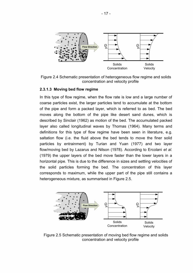
- 17 -
y/D
y/D
Solids
Concentration
Solids
Velocity
Flow Direction
Figure 2.4 Schematic presentation of heterogeneous flow regime and solids concentration and velocity profile
2.3.1.3 Moving bed flow regime
In this type of flow regime, when the flow rate is low and a large number of
coarse particles exist, the larger particles tend to accumulate at the bottom
of the pipe and form a packed layer, which is referred to as bed. The bed
moves along the bottom of the pipe like desert sand dunes, which is
described by Sinclair (1962) as motion of the bed. The accumulated packed
layer also called longitudinal waves by Thomas (1964). Many terms and
definitions for this type of flow regime have been seen in literature, e.g.
saltation flow (i.e. the fluid above the bed tends to move the finer solid
particles by entrainment) by Turian and Yuan (1977) and two layer
flow/moving bed by Lazarus and Nilson (1978). According to Ercolani et al.
(1979) the upper layers of the bed move faster than the lower layers in a
horizontal pipe. This is due to the difference in sizes and settling velocities of
the solid particles forming the bed. The concentration of this layer
corresponds to maximum, while the upper part of the pipe still contains a
heterogeneous mixture, as summarised in Figure 2.5.
y/D
y/D
Solids
ConcentrationSolids
Velocity
Flow Direction
Figure 2.5 Schematic presentation of moving bed flow regime and solids concentration and velocity profile
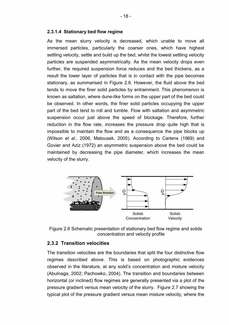
- 18 -
2.3.1.4 Stationary bed flow regime
As the mean slurry velocity is decreased, which unable to move all
immersed particles, particularly the coarser ones, which have highest
settling velocity, settle and build up the bed, whilst the lowest settling velocity
particles are suspended asymmetrically. As the mean velocity drops even
further, the required suspension force reduces and the bed thickens, as a
result the lower layer of particles that is in contact with the pipe becomes
stationary, as summarised in Figure 2.6. However, the fluid above the bed
tends to move the finer solid particles by entrainment. This phenomenon is
known as saltation, where dune-like forms on the upper part of the bed could
be observed. In other words, the finer solid particles occupying the upper
part of the bed tend to roll and tumble. Flow with saltation and asymmetric
suspension occur just above the speed of blockage. Therefore, further
reduction in the flow rate, increases the pressure drop quite high that is
impossible to maintain the flow and as a consequence the pipe blocks up
(Wilson et al., 2006, Matousek, 2005). According to Cartens (1969) and
Govier and Aziz (1972) an asymmetric suspension above the bed could be
maintained by decreasing the pipe diameter, which increases the mean
velocity of the slurry.
y/D
y/D
Solids
Concentration
Solids
Velocity
Flow Direction
Figure 2.6 Schematic presentation of stationary bed flow regime and solids concentration and velocity profile
2.3.2 Transition velocities
The transition velocities are the boundaries that split the four distinctive flow
regimes described above. This is based on photographic evidences
observed in the literature, at any solid’s concentration and mixture velocity
(Abulnaga, 2002; Pachowko, 2004). The transition and boundaries between
horizontal (or inclined) flow regimes are generally presented via a plot of the
pressure gradient versus mean velocity of the slurry. Figure 2.7 showing the
typical plot of the pressure gradient versus mean mixture velocity, where the

- 19 -
main four flow regimes can be presented. Normally, the definition of
transition velocities depends on the definition of the flow regime. Therefore,
the terminology for the transition velocities is quite confusing. According to
Abulnaga (2002) and Pachowko (2004) the transition velocities can be
defined as explained below:
1. V1: The velocity at or above which the bed at the lower half of the pipe is
stationary. However, at the upper half of the pipe, some solid particles
may move either by saltation or suspension. It is important to mention that
little work has been carried out within the boundary of this flow regime,
and that is due to the fact that the risk of blockage is dominant in this
region.
2. V2: The velocity at or above which the solid particles are transported by
suspension at the upper half of the pipe and the coarser particles forming
a moving bed.
3. V3: The velocity at or above which all solid particles are transported in
asymmetric suspended form.
4. V4: The velocity at or above which all solid particles are fully suspended
and transported as a symmetric suspension.
Figure 2.7 Showing transitional velocities on a typical plot of the pressure gradient versus mean mixture velocity (Abulnaga, 2002)
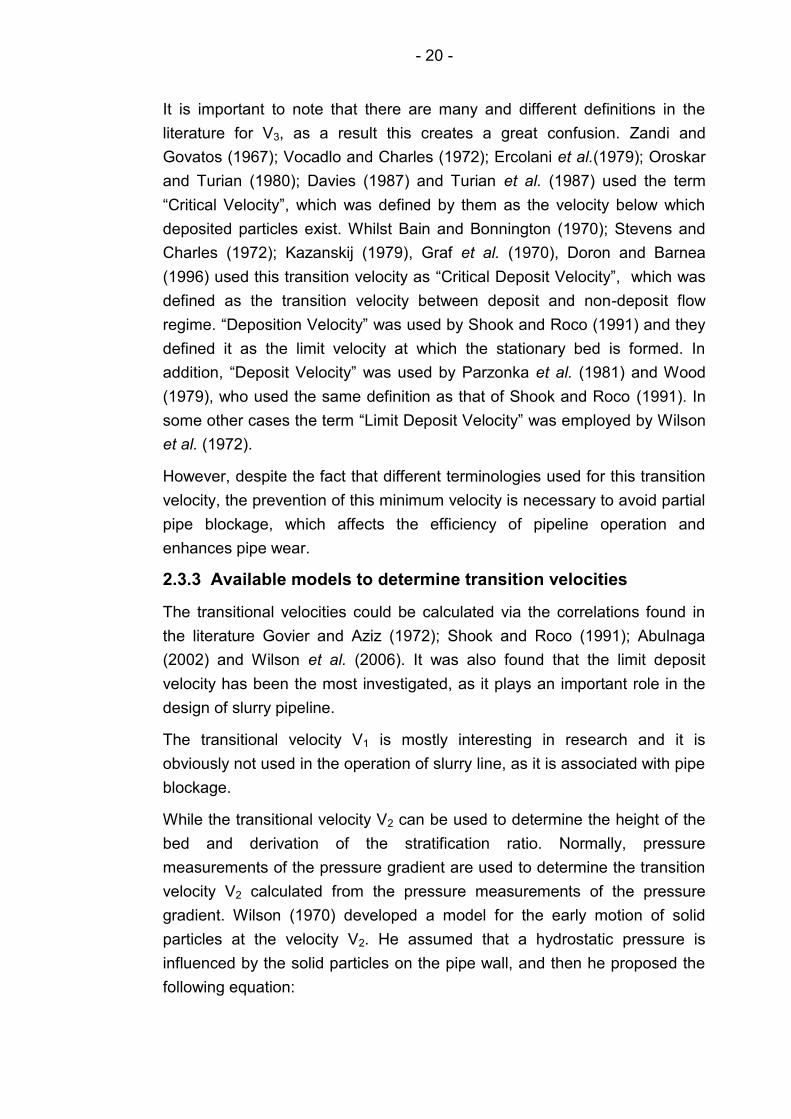
- 20 -
It is important to note that there are many and different definitions in the
literature for V3, as a result this creates a great confusion. Zandi and
Govatos (1967); Vocadlo and Charles (1972); Ercolani et al.(1979); Oroskar
and Turian (1980); Davies (1987) and Turian et al. (1987) used the term
“Critical Velocity”, which was defined by them as the velocity below which
deposited particles exist. Whilst Bain and Bonnington (1970); Stevens and
Charles (1972); Kazanskij (1979), Graf et al. (1970), Doron and Barnea
(1996) used this transition velocity as “Critical Deposit Velocity”, which was
defined as the transition velocity between deposit and non-deposit flow
regime. “Deposition Velocity” was used by Shook and Roco (1991) and they
defined it as the limit velocity at which the stationary bed is formed. In
addition, “Deposit Velocity” was used by Parzonka et al. (1981) and Wood
(1979), who used the same definition as that of Shook and Roco (1991). In
some other cases the term “Limit Deposit Velocity” was employed by Wilson
et al. (1972).
However, despite the fact that different terminologies used for this transition
velocity, the prevention of this minimum velocity is necessary to avoid partial
pipe blockage, which affects the efficiency of pipeline operation and
enhances pipe wear.
2.3.3 Available models to determine transition velocities
The transitional velocities could be calculated via the correlations found in
the literature Govier and Aziz (1972); Shook and Roco (1991); Abulnaga
(2002) and Wilson et al. (2006). It was also found that the limit deposit
velocity has been the most investigated, as it plays an important role in the
design of slurry pipeline.
The transitional velocity V1 is mostly interesting in research and it is
obviously not used in the operation of slurry line, as it is associated with pipe
blockage.
While the transitional velocity V2 can be used to determine the height of the
bed and derivation of the stratification ratio. Normally, pressure
measurements of the pressure gradient are used to determine the transition
velocity V2 calculated from the pressure measurements of the pressure
gradient. Wilson (1970) developed a model for the early motion of solid
particles at the velocity V2. He assumed that a hydrostatic pressure is
influenced by the solid particles on the pipe wall, and then he proposed the
following equation:
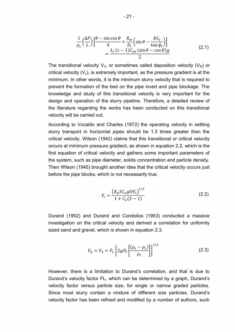
- 21 -
(2.1)
The transitional velocity V3, or sometimes called deposition velocity (VD) or
critical velocity (Vc), is extremely important, as the pressure gradient is at the
minimum. In other words, it is the minimum slurry velocity that is required to
prevent the formation of the bed on the pipe invert and pipe blockage. The
knowledge and study of this transitional velocity is very important for the
design and operation of the slurry pipeline. Therefore, a detailed review of
the literature regarding the works has been conducted on this transitional
velocity will be carried out.
According to Vocaldo and Charles (1972) the operating velocity in settling
slurry transport in horizontal pipes should be 1.3 times greater than the
critical velocity. Wilson (1942) claims that this transitional or critical velocity
occurs at minimum pressure gradient, as shown in equation 2.2, which is the
first equation of critical velocity and gathers some important parameters of
the system, such as pipe diameter, solids concentration and particle density.
Then Wilson (1945) brought another idea that the critical velocity occurs just
before the pipe blocks, which is not necessarily true.
(2.2)
Durand (1952) and Durand and Condolios (1953) conducted a massive
investigation on the critical velocity and derived a correlation for uniformly
sized sand and gravel, which is shown in equation 2.3.
(2.3)
However, there is a limitation to Durand’s correlation, and that is due to
Durand’s velocity factor FL, which can be determined by a graph, Durand’s
velocity factor versus particle size, for single or narrow graded particles.
Since most slurry contain a mixture of different size particles, Durand’s
velocity factor has been refined and modified by a number of authors, such
- 22 -
as Wasp et al. (1977), who represented the critical velocity in terms of
modified factor F'L including a ratio between the particle diameter and the
pipeline diameter , as shown in equation 2.4.
(2.4)
Moreover, Spells (1955) conducted a study, where he used fine particulate
slurry in horizontal pipe and developed a correlation to determine the critical
velocity, which he called minimum velocity, in terms of particle size, solid
and liquid density, slurry density and pipe diameter, as shown in equation
2.5. He also defined the critical velocity as the minimum velocity required to
prevent the deposition of the particles at the bottom of the pipe.
(2.5)
Spells equation 2.5 created a great confusion regarding the particle size,
which was presented as d85, as a result it was believed that the correlation
is only applicable to a narrow range of slurry Reynolds number, but d85
could represent colloidal range or coarse particles. Despite the fact that
Smith (1955) recommended that in pressure and critical velocity correlations
the particle size should be represented by weighted mean diameter.
Newitt et al. (1955) developed a correlation for the transitional velocity V3
between heterogeneous flow regime and moving bed (saltation), or critical
velocity, in terms of terminal velocity of particles, as shown in equation 2.6.
(2.6)
It can be noticed that Newitt’s equation is very simple, although it was used
as the basis for developing many models, such as that of Cairns et al.
(1960), as shown in equation 2.7, which is applicable to particle size
between 242 μm and 380 μm at low solids concentration, specific gravity up
to 2.6 and pipe diameter not more than 50 mm.
- 23 -
(2.7)
The transition velocity V4, which demarcates the boundary between the two
flow regimes Heterogeneous (asymmetric) and pseudo-homogeneous
(symmetric), has also been investigated by some investigators, such as
Newitt et al. (1955), Spells (1955), Govier and Aziz (1972). Newitt et al.
(1955) developed a correlation, in which the transitional velocity V4 is
determined in terms of terminal velocity, as shown in equation 2.8.
(2.8)
Whilst Govier and Aziz (1972) improved Newitt’s correlation by applying
Newton’s law and rewrote the equation in terms of drag coefficient (CD),
which is 0.44 according to Newton’s law, as shown in equation 2.9.
(2.9)
Goniewr and Aziz (1972) also derived equation 2.10 by analysing the work
of Spells (1955), which was done on solid particles with a diameter between
80 μm and 800 μm (mesh 180<dp<20).
(2.10)
It is important to take the notice that the above correlations for the
transitional velocities, between heterogeneous and pseudo-homogenous
flow patterns, ignore the influence of solid’s concentration, but rather provide
order of magnitude of V4.
The transitional velocities have not only been investigated in a horizontal
pipes, but also in pipe bends, such as the one of Giguère et al. (2009), who
studied the influence of pipe bend between the downward and horizontal
flows on the transitional velocities between slurry flow regimes and
introduced fantastic results. Their measurements indicated that flow is
homogeneous directly after the bend outlet and that the transition velocities

- 24 -
decreased after the bend outlet. This indicates that the slurry velocity
decreases after the bend, which in itself decreases the transition velocity
and the distance where these transition occur. They also concluded that the
solid’s concentration can influence these transitions, whilst there is little
effect of high concentration on the transitions on downward bend.
2.3.4 Pressure drop in slurry pipeline
Pressure drop, or sometimes known as pressure gradient or hydraulic
gradient, is the most important parameter for slurry transport in mineral and
many industries handling solid-liquid flows. Since the pressure drop
influences the power consumption and the whole economics of the slurry
transport, therefore the slurry pipeline design is based on optimisation of
pressure drop (Lahiri, 2009).
The first real equation, for calculating the pressure drop was first generated
by Howard (1939), who used his data in combination with that of Blatch
(1906) and Hazen and Hardy (1906). Equation 2.11 shows Howard’s
equation, which he used for calculating the head loss:
(2.11)
However, his equation was not taken as a universal equation that could
apply to other systems. Wilson (1942) came and divided the pressure drop
into two components, pressure drop due to fluid along and pressure drop
due existence of the solid particles.
In addition, numerous investigators, such as Wilson (1942); Durand and
Condolios (1952); Shook and Daniel (1969); Turian and Yuan (1977); Wasp
et al. (1977); Gillies et al. (1999); Kaushal and Tomita (2002) and Lahiri
(2009), have attempted and proposed many empirical, semi-theoretical and
theoretical correlations related to the pressure drop along with some other
flow parameters, such as solid’s density, liquid’s density, particle size, solid’s
concentration, solid’s velocity, pipe diameter and slurry viscosity. However,
these correlations are associated with some rate of error, as shown in Table
2.2 in terms of Average Absolute Relative Error (AARE). Nevertheless, a
considerable reduction in the prediction error can be noticed.
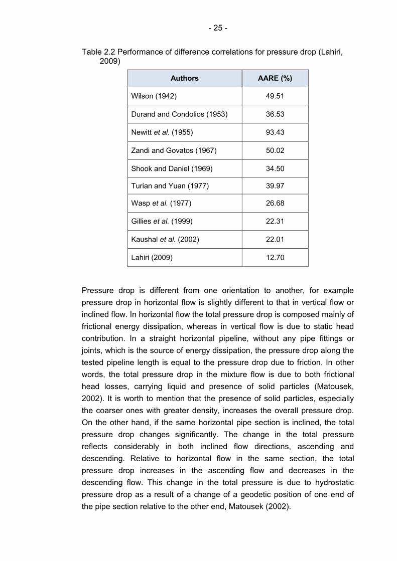
- 25 -
Table 2.2 Performance of difference correlations for pressure drop (Lahiri, 2009)
Authors AARE (%)
Wilson (1942) 49.51
Durand and Condolios (1953) 36.53
Newitt et al. (1955) 93.43
Zandi and Govatos (1967) 50.02
Shook and Daniel (1969) 34.50
Turian and Yuan (1977) 39.97
Wasp et al. (1977) 26.68
Gillies et al. (1999) 22.31
Kaushal et al. (2002) 22.01
Lahiri (2009) 12.70
Pressure drop is different from one orientation to another, for example
pressure drop in horizontal flow is slightly different to that in vertical flow or
inclined flow. In horizontal flow the total pressure drop is composed mainly of
frictional energy dissipation, whereas in vertical flow is due to static head
contribution. In a straight horizontal pipeline, without any pipe fittings or
joints, which is the source of energy dissipation, the pressure drop along the
tested pipeline length is equal to the pressure drop due to friction. In other
words, the total pressure drop in the mixture flow is due to both frictional
head losses, carrying liquid and presence of solid particles (Matousek,
2002). It is worth to mention that the presence of solid particles, especially
the coarser ones with greater density, increases the overall pressure drop.
On the other hand, if the same horizontal pipe section is inclined, the total
pressure drop changes significantly. The change in the total pressure
reflects considerably in both inclined flow directions, ascending and
descending. Relative to horizontal flow in the same section, the total
pressure drop increases in the ascending flow and decreases in the
descending flow. This change in the total pressure is due to hydrostatic
pressure drop as a result of a change of a geodetic position of one end of
the pipe section relative to the other end, Matousek (2002).
- 26 -
2.3.5 Physical mechanisms governing settling slurry flow
When solid particles in a carrier liquid is transported within a pipe, they are
acted upon by several forces, which are resulted from particle-particle
interaction, particle-liquid interaction and particle-pipe wall interaction. The
forces, which are resulted from particle-particle interaction, are transmitted
as an inter-particle stress. However, when a granular bed is formed (i.e. the
particles are in continuous contact), the Coulombic stress is created on the
particles, while Bagnold stress is created on the surface of the granular bed
as a result of sheared granular bed and the particles move in a sporadic
fashion. On the other hand, the forces, which are resulted from particle-liquid
interaction are buoyancy force, drag force and lift force, and if the carrier
liquid is turbulent, then the turbulent diffusive force is generated (Bagnold,
1954; Wilson, 2006).
A settling slurry flow, in a horizontal or inclined pipe, normally tends to
stratify. In other words, at the velocity used during the practical operations,
the particle distribution across a pipe cross section is non-uniform. Under
these circumstances the flow can be fully or partially stratified. If all solid
particles form the granular bed (stationary or sliding), then the flow is fully
stratified, and if a portion of the solid particles form the granular bed (where
particles are virtually in permanent contact with each other) and the
remaining particles are suspended within carrier fluid, then the flow is
partially stratified.
The previous description of particle motion was explained by Bagnold
(1956), who developed a concept that the solid particles are supported by
two major physical mechanisms: fluid suspension and inter-granular contact.
For the first mechanism, Wilson et al. (2002) observed that the particles are
suspended in the carrier fluid is due to turbulent diffusion.
Obviously, settling slurries composed of fine and coarse particles. The
friction behaviour of suspended coarse particles differs from that of fine
particles. The suspended coarse particles interact with each other and the
pipe wall. It is important to mention that the contact is not permanent, but
rather sporadic, which is due to turbulent dispersive action and collision
dispersive action. In other words, the solid particles are dispersed to all
directions by turbulent eddies and also the particles are collided with the
other particles of different velocities and impelled in the direction of the wall
(Matousek, 2005; Wilson, 2006). According to Brown and Heywood (1991)
the fluid suspension mechanism can come to play, when the velocity of
- 27 -
turbulent eddies is greater than the settling velocity and by further increasing
the mean velocity the more solid particles is suspended by the fluid force.
In the case of fully stratified flow, it can be noted that the settling velocity of
the solid particles is greater than the velocity of the turbulent eddies,
therefore the particles fall and are supported by granular contact rather than
fluid suspension. These particles are designated as contact load, in either
cases stationary or moving bed (Wilson, 2006). The motion of the particles
within the contact load can be analysed by applying the force balance, which
was first used by Wilson (1970) and Wilson et al. (1972), then it was latter
used to determine the limit deposition velocity for fully stratified flow.
2.3.6 Flow regime recognition
Since the settling slurry flow is a very complex flow and the coarser solid
particles tend to settle and form a bed at the pipe invert, various flow
regimes (or patterns) may occur, which depends on several parameters,
such as solid’s concentration, particle size, particle and liquid density,
mixture velocity and pipe diameter. It is worth pointing out that the common
four flow regimes, described in the previous sections, are mainly dependent
on mean slurry velocity. Therefore, the recognition of these flow regimes,
which would exist in the pipe, for any given set of operational condition, is
very important for design and operation of pipeline conveying settling
slurries. Also, since there are different pressure drop correlations for
different flow regimes, it is significantly important to apply an appropriate
pressure drop correlation for the given flow regime (Lahiri, 2009). Moreover,
the recognition of these flow regimes is similarly essential for optimisation
and correction of flow meters, which are flow regime dependent (such as
ERT).
Over the years, since 1953, researchers have attempted to establish various
methods to characterise and recognise the flow regimes encountered in the
pipeline. Pressure drop measurement has been one of the most common
methods that have been adopted to recognise flow regimes. Some of these
researchers are Newitt et al. (1955), Doron and Barnea (1993, 1996), Doron
et al. (1997), Gillies et al. (1999), Kaushal and Tomita (2002), Matousek
(2002), Kaushal et al. (2005).
Another method has been used by some researchers, based on signal
analysis, such as Albino et al. (2007). They have depended on different
output signals, such as passive acoustic signals, to identify the occurring
flow regimes.
- 28 -
A glance of the literature reveals that several correlations or techniques have
been reported regarding the recognition of settling slurry flow regimes.
However, it can be noticed that each of them more or less associated with
some degree of limitations and cannot predict the prevailing flow regime
over a wide of range of conditions, such as solids concentration, particle
size, slurry velocity, pipe diameter and configuration etc. Therefore a novel
technique is proposed in this study (Chapter 7), through which the prevailing
flow regime is identified regardless the condition, in which the flow operates,
such as physical properties, pipe diameter etc.
Usually the flow regimes are recognised by either subjective operator
judgements, which is done by visual inspections, although in some cases an
analysis of the spectral content is performed, where the desired information
cannot be extracted visually (Abulnaga, 2002), or by objective indication by
representing the boundaries between the flow regimes via flow regime
maps. Early investigators, such as Newitt et al. (1955) and Durand and
Condolios (1953) have carried out extensive studies to investigate the
detailed features of the flow. Their results are often displayed in the form of
flow regime maps. These flow regime maps represent the boundaries
between various flow regimes under different conditions, though these
boundaries are not distinctive lines, but rather poorly defined transition
zones. The transition from one flow regime normally occurs, as the flow
regime becomes unstable and causes transition (Brown and Heywood,
1991). However, there are limitations and problems with these flow regime
maps that they are often dimensional and cannot be applied on a different
operational condition. Despite the fact that some investigators have tried to
generalise these flow regime maps, so they can be applied to different fluids
and pipes of different sizes, but they could not achieve total generalisation,
as most flow regime maps represent several transitions.
Turian and Yuan (1977) also have represented some flow regime maps in
terms of mixture velocity and delivered concentration. Doron and Barnea
(1993, 1995 and 1996) carried out an analysis as an extension of Doron et
al. (1987) for the two layer model, where they employed three layer model
(stationary bed, moving bed and heterogeneous mixture) for the drawing of
flow regime maps, which is in term of slurry velocity versus solids velocity,
as shown in Figure 2.8. It can be seen on the map that the two regimes,
heterogeneous and pseudo-homogeneous, have not been distinguished, but
rather explained only in one term “Fully suspension”. Their flow regime maps
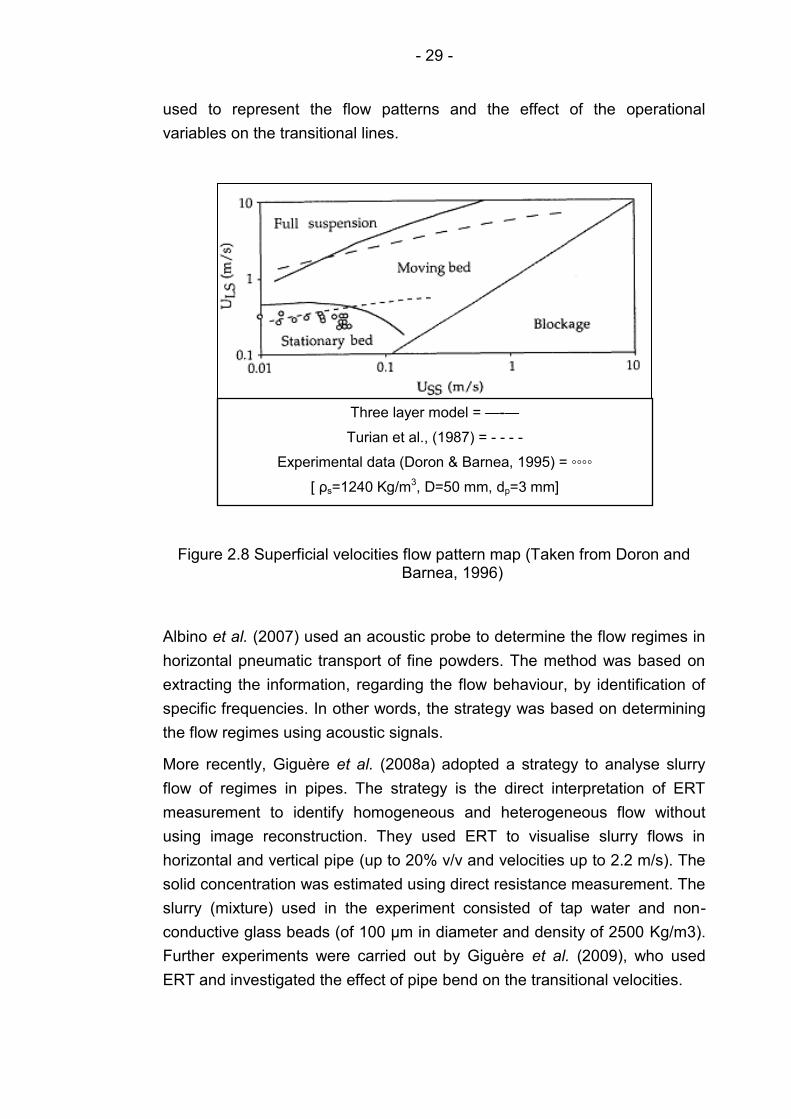
- 29 -
used to represent the flow patterns and the effect of the operational
variables on the transitional lines.
Figure 2.8 Superficial velocities flow pattern map (Taken from Doron and Barnea, 1996)
Albino et al. (2007) used an acoustic probe to determine the flow regimes in
horizontal pneumatic transport of fine powders. The method was based on
extracting the information, regarding the flow behaviour, by identification of
specific frequencies. In other words, the strategy was based on determining
the flow regimes using acoustic signals.
More recently, Giguère et al. (2008a) adopted a strategy to analyse slurry
flow of regimes in pipes. The strategy is the direct interpretation of ERT
measurement to identify homogeneous and heterogeneous flow without
using image reconstruction. They used ERT to visualise slurry flows in
horizontal and vertical pipe (up to 20% v/v and velocities up to 2.2 m/s). The
solid concentration was estimated using direct resistance measurement. The
slurry (mixture) used in the experiment consisted of tap water and non-
conductive glass beads (of 100 μm in diameter and density of 2500 Kg/m3).
Further experiments were carried out by Giguère et al. (2009), who used
ERT and investigated the effect of pipe bend on the transitional velocities.
Three layer model = —-—
Turian et al., (1987) = - - - -
Experimental data (Doron & Barnea, 1995) = ◦◦◦◦
[ ρs=1240 Kg/m3, D=50 mm, dp=3 mm]
- 30 -
Besides, Lahiri (2009) has successfully applied Artificial neural Network
(ANN), using Support Vector Machine (SVM) modelling to identify different
flow regimes in a horizontal pipe, based on a data bank of 800
measurements in the literature. Lahiri’s method has shown a great success
and advantages, as there is no need to calculate some parameters, such as
the drag co-efficient (CD) and some empirical co-efficient, settling velocity
and Froud number. The method is based on evaluating the flow regime
using some basic flow data, such as pipe diameter, solid’s concentration and
fluid velocity. Then after evaluation the correct flow regime, an appropriate
correlation can be used to determine the pressure drop. His method can
deliver only 1.5% error, unlike Turian and Yuan (1977) correlation, where the
delivered accuracy is 25% error.
2.4 Vertical slurry flow
As previously mentioned, in vertical slurry flow, no granular bed is formed
and no dunes can be observed and it is rather straight forward flow. The
solid particles are fully suspended with no component of the submerged
particle acting on the pipe wall and tend to have a symmetrical distribution
across the pipe cross-section, (Matousek, 2001; Clift & Clift, 1981, Munir,
2011, Wilson et at., 1979, Wilson, 2004). The force of the submerged
particle is acting downward and resists the flow of particles. As a result the
slip velocity occur between the solid particles and the carrier liquid.
Normally, the difference between the mixture velocity and the velocity of the
solid particles is smaller than hindered settling velocity of the solid particles.
If the particles are less than 150 µm, then the whole mixture behaves as a
liquid and The Equivalent Liquid Model can used for friction loss analysis
(i.e. the flow can be considered as pseudo-homogeneous). However, if the
particles are between (200 µm-2 mm), then these particles cannot directly
exhibit the liquid like friction, as the particles are large enough and cannot be
trapped within the laminar sub-layer. As a result, the particles migrate away
from the pipe wall towards the centre of the pipe (Barigoua, 2003; Wilson,
2006).
Shook and Bartosik (1994) carried out an investigation on vertical slurry flow
and claimed that the behaviour of solid particles to be due to Bagnold
dispersive stress, which acts against the pipe wall. In the meantime, they
concluded that, in vertical upward flow, the solids effect due to Bagnold
stress for flowing medium sand can be negligible. On the other hand, for
flowing coarse particle sand, the Bagnold stress on the pipe wall can be

- 31 -
generated as a result of mutual collision between the particles and the pipe
wall, where the carrier liquid acts on the particles and repels them from the
pipe wall due to liquid lift force. Also, Worster and Denny (1955) has
investigated the aspect of pressure loss in vertical slurry flow and concluded
that the solid particles does not affect the pressure loss due to hydraulic
friction.
An earlier analysis of vertical slurry flow was carried out by Hagler (1956),
who proposed a device (U-tube), which has been studied by several
researchers such as Brook (1962), Clift and Clift (1981). The schematic
drawing of the device is shown in Figure 2.9. It is worth mentioning that the
analysis carried out by Clift and Clift assumed to be more complete than the
others. The device is very simple and used for slurry flow rate measurement.
It consists of two vertical tubes, ascending and a descending, with four
elbows and a pair of pressure taps on each vertical line. The mean slurry
velocities of both branches (upward and downward) are equal, thus the wall
shear stress are also the same. Based on the analysis carried out by Clift
and Clift (1981), the In-situ solids concentration is approaching the delivered
solids concentration (i.e. their values are close, but not identical). However,
they concluded that as the difference between both values is subtle and can
be considered as negligible. Therefore, the delivered solids volume
concentration can represent the in-situ solids volume concentration within a
vertical pipe.
Slurry
Flow
2
1
3
4
ZA
ZB
Figure 2.9 Inverted U-tube device for slurry flow rate measurement
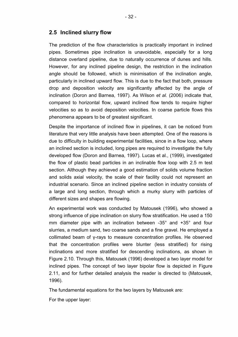
- 32 -
2.5 Inclined slurry flow
The prediction of the flow characteristics is practically important in inclined
pipes. Sometimes pipe inclination is unavoidable, especially for a long
distance overland pipeline, due to naturally occurrence of dunes and hills.
However, for any inclined pipeline design, the restriction in the inclination
angle should be followed, which is minimisation of the inclination angle,
particularly in inclined upward flow. This is due to the fact that both, pressure
drop and deposition velocity are significantly affected by the angle of
inclination (Doron and Barnea, 1997). As Wilson et al. (2006) indicate that,
compared to horizontal flow, upward inclined flow tends to require higher
velocities so as to avoid deposition velocities. In coarse particle flows this
phenomena appears to be of greatest significant.
Despite the importance of inclined flow in pipelines, it can be noticed from
literature that very little analysis have been attempted. One of the reasons is
due to difficulty in building experimental facilities, since in a flow loop, where
an inclined section is included, long pipes are required to investigate the fully
developed flow (Doron and Barnea, 1997). Lucas et al., (1999), investigated
the flow of plastic bead particles in an inclinable flow loop with 2.5 m test
section. Although they achieved a good estimation of solids volume fraction
and solids axial velocity, the scale of their facility could not represent an
industrial scenario. Since an inclined pipeline section in industry consists of
a large and long section, through which a murky slurry with particles of
different sizes and shapes are flowing.
An experimental work was conducted by Matousek (1996), who showed a
strong influence of pipe inclination on slurry flow stratification. He used a 150
mm diameter pipe with an inclination between -35° and +35° and four
slurries, a medium sand, two coarse sands and a fine gravel. He employed a
collimated beam of γ-rays to measure concentration profiles. He observed
that the concentration profiles were blunter (less stratified) for rising
inclinations and more stratified for descending inclinations, as shown in
Figure 2.10. Through this, Matousek (1996) developed a two layer model for
inclined pipes. The concept of two layer bipolar flow is depicted in Figure
2.11, and for further detailed analysis the reader is directed to (Matousek,
1996).
The fundamental equations for the two layers by Matousek are:
For the upper layer:
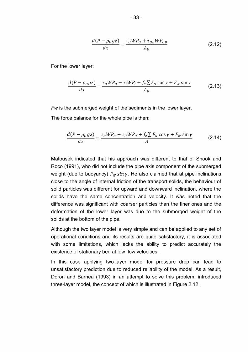
- 33 -
(2.12)
For the lower layer:
(2.13)
Fw is the submerged weight of the sediments in the lower layer.
The force balance for the whole pipe is then:
(2.14)
Matousek indicated that his approach was different to that of Shook and
Roco (1991), who did not include the pipe axis component of the submerged
weight (due to buoyancy) . He also claimed that at pipe inclinations
close to the angle of internal friction of the transport solids, the behaviour of
solid particles was different for upward and downward inclination, where the
solids have the same concentration and velocity. It was noted that the
difference was significant with coarser particles than the finer ones and the
deformation of the lower layer was due to the submerged weight of the
solids at the bottom of the pipe.
Although the two layer model is very simple and can be applied to any set of
operational conditions and its results are quite satisfactory, it is associated
with some limitations, which lacks the ability to predict accurately the
existence of stationary bed at low flow velocities.
In this case applying two-layer model for pressure drop can lead to
unsatisfactory prediction due to reduced reliability of the model. As a result,
Doron and Barnea (1993) in an attempt to solve this problem, introduced
three-layer model, the concept of which is illustrated in Figure 2.12.
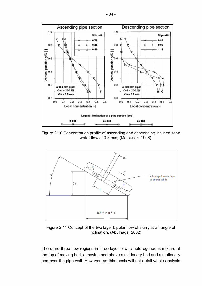
- 34 -
Figure 2.10 Concentration profile of ascending and descending inclined sand water flow at 3.5 m/s, (Matousek, 1996)
Figure 2.11 Concept of the two layer bipolar flow of slurry at an angle of inclination, (Abulnaga, 2002)
There are three flow regions in three-layer flow: a heterogeneous mixture at
the top of moving bed, a moving bed above a stationary bed and a stationary
bed over the pipe wall. However, as this thesis will not detail whole analysis
- 35 -
of three-layer model, therefore, for further detail of the model, the reader is
referred to Doron and Barnea (1993).
Solids Bed
Dispersed Layer
Suspended Layer
y/D
Solids Concentration
Figure 2.12 Assumed concentration profile in three layer model
Since both models assumes no slip velocity, , the author believes that both
models are associated with serious limitations. As the solid particles tend to
deposit at the bottom of the pipe and form a strata, then this suggests the
existence of slip velocity between the two phases.
2.6 Deposition velocity in horizontal and inclined flow
As previously mentioned, the critical transition velocity (V3) (or deposition
velocity) in either horizontal or inclined flow defines the lowered of the range
of desirable operating velocities. The great significance of coarse-particle
flow in upward inclined pipeline is that, compared to horizontal configuration,
it requires higher throughput velocities, so as to avoid deposition (Wilson,
2006).
Through an extensive literature survey, it was found that the approach of
Wilson and Tse (1984) is a useful tool to estimate the deposition velocity in
an inclined pipe. The concept of this method is based on estimating the
deposition velocity for horizontal flow first, then extending the analysis to
inclined pipes, based on the difference in Durand factor between the two
configurations (horizontal and inclined). The deposition velocity for horizontal
flow can be estimated from equation 2.4. Then if the analysis is extended for
inclined flow, it is appropriate to present the deposition velocity or Durand
factor FL (or ΔD) and neglecting the ratio between the particle diameter and
the pipeline diameter, as it is a very small value:
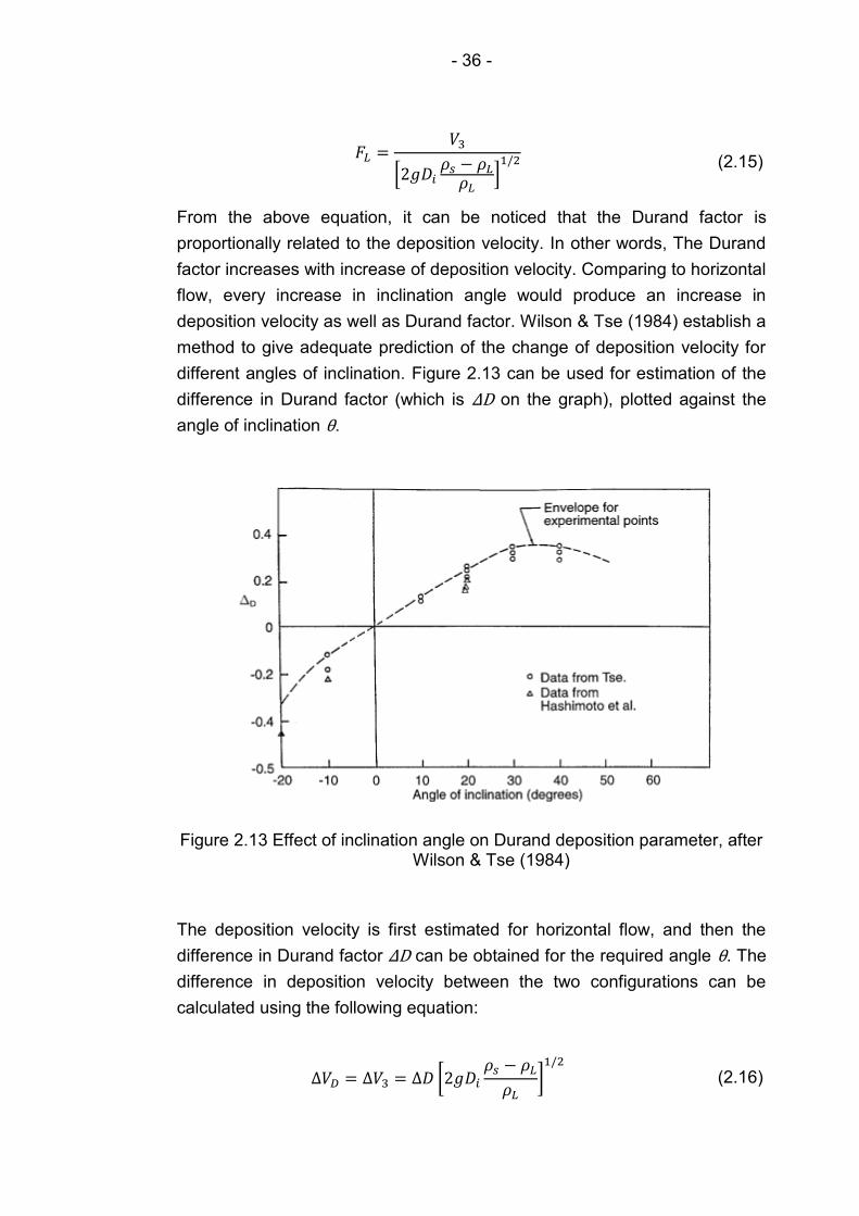
- 36 -
(2.15)
From the above equation, it can be noticed that the Durand factor is
proportionally related to the deposition velocity. In other words, The Durand
factor increases with increase of deposition velocity. Comparing to horizontal
flow, every increase in inclination angle would produce an increase in
deposition velocity as well as Durand factor. Wilson & Tse (1984) establish a
method to give adequate prediction of the change of deposition velocity for
different angles of inclination. Figure 2.13 can be used for estimation of the
difference in Durand factor (which is D on the graph), plotted against the
angle of inclination θ.
Figure 2.13 Effect of inclination angle on Durand deposition parameter, after Wilson & Tse (1984)
The deposition velocity is first estimated for horizontal flow, and then the
difference in Durand factor D can be obtained for the required angle θ. The
difference in deposition velocity between the two configurations can be
calculated using the following equation:
(2.16)

- 37 -
By adding the above quantity to the value found for the horizontal case, the
deposition velocity for the inclined case can be determined.
2.7 Conclusions
This chapter critically reviewed the literature concerning the settling slurry
flow in different flow orientations, horizontal, vertical and inclined. The
previous work regarding the flow regimes that occur as a result of particle
settling tendency and the recognition of each of them, pressure drop in slurry
pipelines, the physical mechanisms governing the flow and deposition
velocity have been extensively reviewed. It is concluded that, despite a
significant technical progress in the field, our knowledge concerning the
behaviour of solids and liquids is still limited. It is also concluded that all the
models and techniques that have been reported in the literature have their
own limitations, due to complexity and poor understanding of solid-liquid
flow. This clearly a major effect on the aspect of slurry flow metering.
Therefore, a good understanding of the underlying phenomena is crucial for
development and optimisation of slurry flow meters, which play an important
role in controlling the whole flow system.
- 38 -
Chapter 3
Review of slurry flow measurement and visualisation
techniques
This chapter presents a review of flow measurement and visualisation
techniques widely employed for slurry applications. It will broadly highlight
the techniques that are commercially available, while the main emphasis is
placed upon the Electrical Resistance Tomography technique.
3.1 Introduction
The measurement and visualisation of slurry flow in pipeline is a challenging
task due to complex nature of the flow, abrasive and viscous nature of the
material. There are some experimental techniques that have been
developed for measuring slurry flow, some of which are commercially
available and the others still at the stage of development and purely used for
research in laboratory tests (Brown and Heywood, 1991; Pachowko, 2004;
Mohinder and Nayyar, 2000). However, this work presents only the solutions
that are commercially available for measurement of slurry flow.
The choice of a correct instrument or method depends on a number of
factors, such as properties of the solid particles (size, shape and
abrasiveness), typical fluid characteristics (pressure, temperature, density,
viscosity and conductivity. Also depending on the application, in which the
metering is performed, further parameters have to be considered, such as
accuracy, repeatability, calibration, pipe geometry, ease of maintenance and
the effect of up and down stream pipeline on the meter.
This chapter is split into three main sections. Since phase volume fraction
and phase velocity inform about the internal structure of the flow, therefore,
the first section is devoted to a review of available techniques used for
measurement of phase fraction and phase velocity. Also the detailed
discussion will be confined to only the meters that are used in this study,
such as Electromagnetic Flow meter (EMF), Coriolis mass flow meter and
Ultrasonic Doppler Velocity Profiler (UDVP). It is important to note that no
reference regarding Coriolis is given in this chapter. A discussion over
Coriolis mass flow meter can be found in Chapter 6. The second section
highlights the widely used techniques for visualisation and imaging of flow.
The last major section covers the Electrical Resistance Tomography system
- 39 -
from working principle and sensing strategy to the limitations, along with
previous work carried out by the others.
3.2 A review of phase fraction and phase velocity
measurement
The mechanism of solid liquid transport in slurry pipelines is dependent on
several flow parameters, of which the most important are phase fraction and
phase velocity. These two parameters also determine the prevailing flow
regime within the pipeline. Therefore, it is vital that the operator continuously
monitor these two parameters, so as to prevent a potential line blockage at
an earlier stage. In other words, these two parameters are the governing
parameters, which can determine the internal structure of flow, and if the
internal structure of the flow is known to the operator, then control limits can
easily be maintained.
A number of commercially available techniques for measurement of these
two parameters are employed and mounted on slurry pipelines of many
industries such as chemical, food, mining, dredging etc. This section reviews
seven measurement techniques, which are commonly used for solid-liquid
flow. Besides, they are used in single and multiphase flow measurements.
3.2.1 Differential pressure technique
Calculation of fluid flow rate, based on pressure loss across a pipe
restriction, may be the most common flow measurement technique in
industrial applications. The pressure drop across a section can be generated
by a wide variety of geometrical restrictions, which have been characterised
over the years.
The theory of differential pressure devices is based on Bernoulli relationship.
Restrictions in cross sections increase in fluid acceleration, and the energy
of this acceleration is obtained from the fluid’s static pressure. As a result the
pressure drop occurs in the section. Once the pressure differential, created
by the device, is known, then the velocity of the flow can be obtained by the
following equation:
(3.1)
It is worth pointing out that only two types of pressure differential devices
can be applied for slurry flow, which are venturi, flow tube and segmental
wedge. Nevertheless, the most commonly used for slurry tend to be venturi,

- 40 -
due to the fact that most of pressure drop can be recovered in venturi flow
meters. As venturi is the most common pressure differential device for slurry
measurement, then no further detail will be given to the other types of
differential pressure elements.
The venturi meter consists of an approach section, which has the same
internal diameter as the system pipeline, and a conical nozzle section
followed by a short parallel throat and a conical diverging section, which
rejoin the venturi system to the system pipeline. The rejoin will be gradually
by returning the internal diameter up to that of the line system, as shown in
Figure 3.1.
Figure 3.1 Showing components of a short-form of a venturi tube (taken from www.omega.co.uk)
Although the initial cost of venturi meters are high, the total cost of
ownership can still be satisfactory, due to savings in installation, operating
and maintenance costs. Venturi has been used 100 years ago, and it design
and improvement still continues. There are many companies out there
producing a high accuracy venturi for a variety of applications, including
slurry, such as WYATT ENGINEERING (wyattflow.com), who produces
venturi tubes with accuracy flow measurement of ±0.50 for standard meters
(without calibration).
Experimental and theoretical studies have been carried out by many
researchers to assess the ability of venturi meter on various flow
measurements. For example, Shook and Masliyah (1974) and Shook (1982)
carried out experiments on stratified slurry flow using venturi meters. They
concluded that venturi meters can be reliably used, without any calibration
for measurement of non-stratified coarse particle slurry flows. They also
concluded that for the other flow regimes, the effect of pipeline conditions
must be well investigated. However, using venturi for stratified or partially
stratified slurry flow could be a potential for pipeline blockage.
- 41 -
3.2.2 Probes
Probe techniques are methods of making local measurements such as
phase volume fraction and phase velocity. Since the local concentration of
particles is reflected by the local resistively of the slurry, then conductivity
probes can be used to measure the local concentration and solids axial
velocity in slurries, as in the case of Nasr-El-Din et al. (1987), who used a
four-ring conductivity probe. Usually the resistively of the fluid is measured
by two pairs of electrodes contained along the body of the probe.
This technique has been used on a wide range of slurries and shown a
potentially useful tool to measure volume fraction and velocity (MacTaggart
et al.1993; Lucas et al., 1999 and Liu et al. 2007). However, the local
conductivity probes are considered as an intrusive and invasive technique,
therefore, it is not really favoured by many researchers.
3.2.3 Electromagnetic Flow Meter (EMF)
Electromagnetic flow meters have been used for several decades and based
on the principle of Faraday’s conduction (Wang et al., 2007). The industrial
interest in this type of flow meter grew in the 1950s, (Baker, 2000).
Nowadays, it is exclusively applied in industry to a variety of flows,
particularly multiphase flow, in which there is a high contrast between the
conductivity of the two phases (continuous and dispersed). The continuous
phase is often the high conducting material, such as water, whereas the
dispersed phase is often the low conducting material, or may even be totally
insulators, such as sand in slurry flow, oil, gas etc. (Brown and Heywood,
1991 and Baker, 2000). Electromagnetic flow meter is the most widely used
meter for slurry measurement, due to the advantage that it offers, which is
explained in the next sections.
Figure 3.2 showing the arrangement of an electromagnetic flow meter. The
electromagnets, two electrodes and electronic circuitry are mounted on a
flow tube. The electromagnets are positioned on the outside of the flow
element. However, the two electrodes are mounted opposite each other in
the wall of the flow tube and are in direct with the fluid. The fluid flows into
the circular cross-sectional and a uniform magnetic field is generated across
the pipe by the pair of electromagnetic. A voltage is induced into the fluid in
a direction at right angles to the magnetic field. The voltage signal picked-up
by the two electrodes, is conditioned and converted to a flow rate (or
velocity) (Baker, 2000 and Brown and Heywood, 1991).
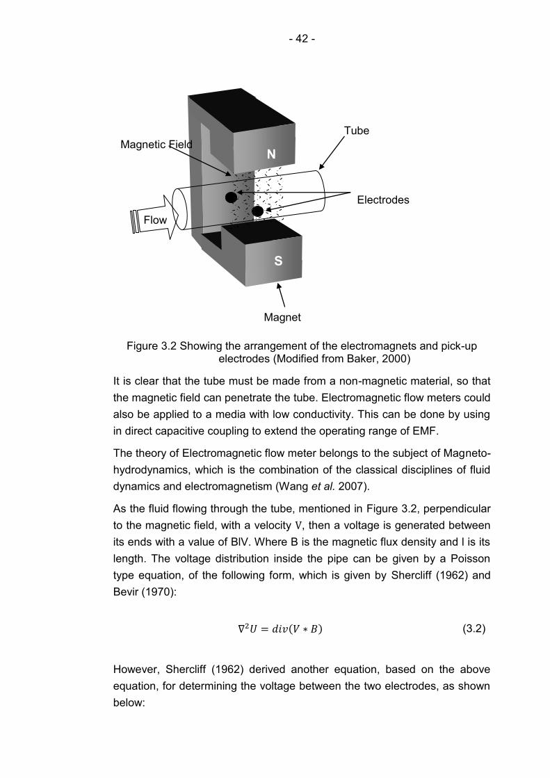
- 42 -
Figure 3.2 Showing the arrangement of the electromagnets and pick-up electrodes (Modified from Baker, 2000)
It is clear that the tube must be made from a non-magnetic material, so that
the magnetic field can penetrate the tube. Electromagnetic flow meters could
also be applied to a media with low conductivity. This can be done by using
in direct capacitive coupling to extend the operating range of EMF.
The theory of Electromagnetic flow meter belongs to the subject of Magneto-
hydrodynamics, which is the combination of the classical disciplines of fluid
dynamics and electromagnetism (Wang et al. 2007).
As the fluid flowing through the tube, mentioned in Figure 3.2, perpendicular
to the magnetic field, with a velocity V, then a voltage is generated between
its ends with a value of BlV. Where B is the magnetic flux density and l is its
length. The voltage distribution inside the pipe can be given by a Poisson
type equation, of the following form, which is given by Shercliff (1962) and
Bevir (1970):
(3.2)
However, Shercliff (1962) derived another equation, based on the above
equation, for determining the voltage between the two electrodes, as shown
below:
Tube
Electrodes
Magnet
Flow
Magnetic Field N
S
- 43 -
(3.3)
Where, B is the magnetic flux density (in tesla), D is the diameter of the tube
inside the EMF (in m) and Vm The fluid mean velocity in the tube (in m/s).
Shercliff’s equation is the basic equation for electromagnetic flow meter and
its validity is based on the two assumptions, the magnetic field is uniform
and the velocity profile is asymmetric. These two criteria will certainly impose
limitations in the theory. Shercliff (1962) then suggested a mean of
predicting the effected distorted profiles by using, as he called, a weight
function.
A weight function describes the combination of the velocity, in different parts
of the flow meter cross-section, to the total output signal (voltage). This
weight function shows that the flow near the electrodes have more influence
on the signal than at any point with increasing distance from the electrodes.
Furthermore, Bevir (1970) extended the weight function concept to three-
dimensional (or weight vector), as shown by the following equation:
(3.4)
Where, V is velocity at every point, τ is the flow meter volume, and the
integral is taken over τ, W is weight vector and can be given by:
(3.5)
Where, j is hypothetical current velocity, which is known as the virtual
current. In order to improve the theoretical performance, another approach
has been used, in which large electrodes are used to have an integral effect
on the signal (Baker, 2000).
According to some manufacturers the preferred installation of
electromagnetic flow meter is in vertical upward flow. Matousek (2005) also
claims that electromagnetic flow meters should be installed in the vertical
line of a slurry system. This is to ensure that the entrained air bubbles are
carried up with flow and solid particles are not settled on the electrodes.
Also, a vertical line, which is a common installation position in slurry flow
- 44 -
systems, it will be necessary to allow for any slip that may occur between the
carrier liquid and solid particles.
According to manufacturers valves should not be installed close upstream of
EMF, even if fully open, (www.icenta.co.uk and www.abb.co.uk ). They are
likely to have an effect of ±0.5% even if the distance is 15D upstream, (i.e.
the distance equivalent to 15 times the internal pipe diameter). However,
due to design differences between electromagnetic flow meters, it is not
possible to follow absolute guidelines that would be equally valid for all
designs.
Also, non-uniformity in conductivity in the flow meter can cause changes in
the EMF signal, due to the changes in the size of the shorting currents. For
certain conditions of turbulent flow, field shape and conductivity profile a
signal change of 3% may be expected. However, as Baker (2000) claims,
the value of uncertainty in the EMF reading may be given as a percentage or
a velocity. Manufacturers give uncertainty between ±0.3% -±1.5% rate for
flow range 2%-2.5% and 100%-50% respectively.
Application of EMF, for multiphase flows, where a marked difference in
velocity of the dispersed and continuous phase occur (such as slurry), has
been the centre of the debate as to what velocity is really measured. Despite
that, it is generally accepted that, for example in slurry flow, the EMF
measures the velocity of the mixture rather than that of the carrier liquid.
Cha et al. (2002) stated that “The electromagnetic flow meter has been
used successfully and accurately to measure the mean liquid velocity in
various industries...”. Also, it is obvious that electromagnetic flow meter
detects the potential difference, through the pair of electrodes, when a
conducting liquid is passing through the magnetic field. Therefore, this fact
can be used in favour of the argument that EMF measures the velocity of
conducting continuous phase rather than the dispersed phase or the
mixture, such as water in slurry flow.
Bernier and Brennen (1983) carried out an investigation regarding the use of
electromagnetic flow meter in measuring a multiphase flow. They concluded
that the EMF could well be used to measure the velocity of a multiphase
flow, in a condition that the continuous phase has a minimum conductivity.
However, Wyatt (1986) investigated the conclusion of Bernier and Brennen
(1983) and argued that this is only the case when the dispersed phase
consists of uniformly and randomly distributed particles.
- 45 -
Furthermore, Wang et al. (2007) investigated the relationship between the
induced voltage and the velocity distribution profile of the continuous phase,
in a two-phase flow to which electromagnetic field was applied. In their study
they modelled an AC current electromagnetic flow meter to investigate the
characteristics of an EMF in multiphase flow. They achieved the most
important findings that induced potential differences measured using an
array of boundary electrodes, could conceivably be used to infer the axial
velocity distribution of the flow.
Despite development and widely use of EMF on flow, like all flow meters, it
has advantages and limitations, which are shown in Table 3.1.
Table 3.1 Advantages and limitations of EMF
Advantages Limitations
Widely used.
The flow measurement is
independent of fluid rheology,
density, temperature and
pressure.
Compact design (no moving
parts).
Its flow tubes available in
standard inner diameter from
3-3000 mm.
Accuracy is much better that
1% of the range of the
instruments for flow rates in
excess of 10% of the range.
Restriction to conducting liquids.
The preferred vertical orientation may not
always be ideal, as even in clear fluids,
swirling flows experienced downstream
from bends are responsible for
systematic error.
The conducting fluid must have a
minimum conductivity of 2 µS/mm.
However special EMF with capacitive
signal pick-up are available that can be
used with conductivities as low as 0.005
µS/mm.
For application on settling slurries, such
as sand, the insulating deposits tend to
coat the exposed electrodes.
Entrained air bubbles adversely influence
measurements, if the flow tube is
installed horizontally, and such that the
electrodes are positioned at the top and
the bottom of the tube.
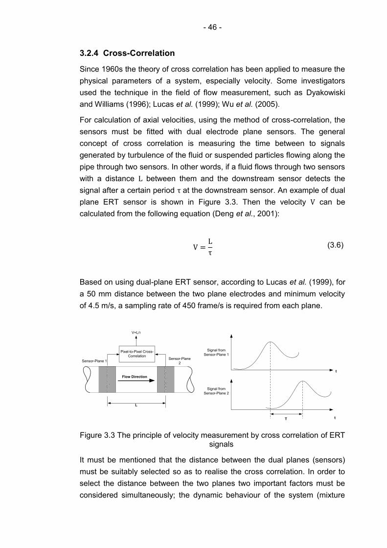
- 46 -
3.2.4 Cross-Correlation
Since 1960s the theory of cross correlation has been applied to measure the
physical parameters of a system, especially velocity. Some investigators
used the technique in the field of flow measurement, such as Dyakowiski
and Williams (1996); Lucas et al. (1999); Wu et al. (2005).
For calculation of axial velocities, using the method of cross-correlation, the
sensors must be fitted with dual electrode plane sensors. The general
concept of cross correlation is measuring the time between to signals
generated by turbulence of the fluid or suspended particles flowing along the
pipe through two sensors. In other words, if a fluid flows through two sensors
with a distance L between them and the downstream sensor detects the
signal after a certain period τ at the downstream sensor. An example of dual
plane ERT sensor is shown in Figure 3.3. Then the velocity V can be
calculated from the following equation (Deng et al., 2001):
τ (3.6)
Based on using dual-plane ERT sensor, according to Lucas et al. (1999), for
a 50 mm distance between the two plane electrodes and minimum velocity
of 4.5 m/s, a sampling rate of 450 frame/s is required from each plane.
Pixel-to-Pixel Cross-
Correlation
Flow Direction
Sensor-Plane
2Sensor-Plane 1
L
V=L/τ
Signal from
Sensor-Plane 1
tT
t
Signal from
Sensor-Plane 2
Figure 3.3 The principle of velocity measurement by cross correlation of ERT signals
It must be mentioned that the distance between the dual planes (sensors)
must be suitably selected so as to realise the cross correlation. In order to
select the distance between the two planes two important factors must be
considered simultaneously; the dynamic behaviour of the system (mixture

- 47 -
velocity) and the resolution of measurement of the transit time. In other
words, the smaller the distance the better similarity of the signals can be
obtained. However, the relatively slow speed of data acquisition and image
reconstruction requires longer distance. According to Deng et al. (2001) the
distance between the two planes could be 50, 75, 85 or 100mm. However,
they recommend that having L (the distance) adjustable, so as to coordinate
it with different cases and various flow velocities.
The signals can be correlated in different methods; point to point correlation
and best correlation pixels. Point to point correlation has been reviewed by
Dai et al. (2004), who suggests that the cross correlation measurement is
based on measuring the data obtained from two planes placed axially along
the flow stream. The basic concept of this method is to find similarities
between the two signals measured at each plane, as shown in Figure 3.4, in
which X denotes plane 1 and Y denotes plane 2.
Figure 3.4 Principle of point-by-point cross correlation method (Dai et al., 2004)
The basic function in which the time delay is calculated in terms of error
function (Rminimum), gives the time delay as:
(3.7)
While the point to point correlation is based on the assumption that the flow
trajectories are parallel to each other and perpendicular to the two planes.
As the nature of the flow is quite complex, then the basic of the assumption
can be a limitation in itself.
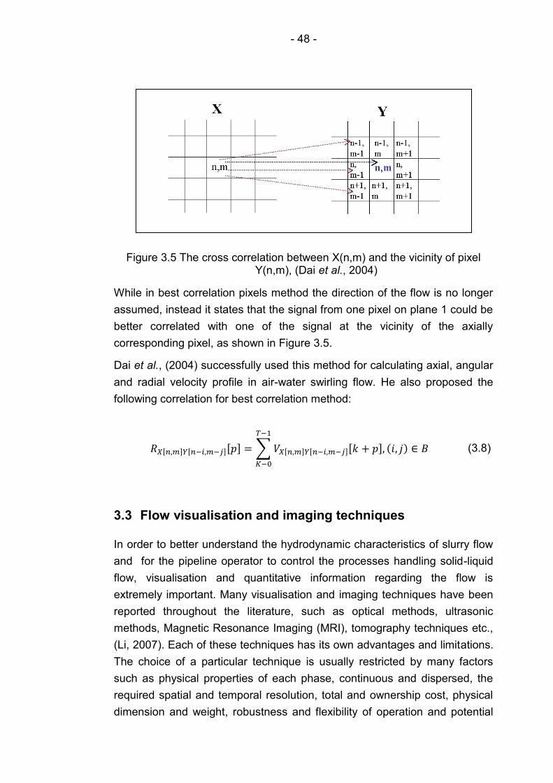
- 48 -
Figure 3.5 The cross correlation between X(n,m) and the vicinity of pixel Y(n,m), (Dai et al., 2004)
While in best correlation pixels method the direction of the flow is no longer
assumed, instead it states that the signal from one pixel on plane 1 could be
better correlated with one of the signal at the vicinity of the axially
corresponding pixel, as shown in Figure 3.5.
Dai et al., (2004) successfully used this method for calculating axial, angular
and radial velocity profile in air-water swirling flow. He also proposed the
following correlation for best correlation method:
(3.8)
3.3 Flow visualisation and imaging techniques
In order to better understand the hydrodynamic characteristics of slurry flow
and for the pipeline operator to control the processes handling solid-liquid
flow, visualisation and quantitative information regarding the flow is
extremely important. Many visualisation and imaging techniques have been
reported throughout the literature, such as optical methods, ultrasonic
methods, Magnetic Resonance Imaging (MRI), tomography techniques etc.,
(Li, 2007). Each of these techniques has its own advantages and limitations.
The choice of a particular technique is usually restricted by many factors
such as physical properties of each phase, continuous and dispersed, the
required spatial and temporal resolution, total and ownership cost, physical
dimension and weight, robustness and flexibility of operation and potential
- 49 -
hazards to the personnel (Gamma-ray is an example of potential health
hazard), (Munir, 2011).
This section reviews the widely used and commercially available techniques
for measurement and visualisation of constituent phases within two-phase
flow, particularly slurry flow. Since slurries are opaque and contained in
opaque enclosures , then optical visualisation of the flow is quite difficult, (
Heindel, 2008). Thus, optical techniques. such as laser Doppler Velocimetry
(LDV), Laser Doppler Anemometry (LDA) and Particle Image Velocimetry
(PIV) (Van Dinther et al., 2012), is excluded in this work. In the meantime, it
must be noted that the above three optical methods offer a great benefit for
measurement of micro-channels, non-slurry and diluted slurry applications.
However, their major drawback in settling slurry applications is that they are
less sensitive when coarse particles are used, besides their measurements
are affected by wall effects, (Van Dinther et al., 2012). The section will
mainly split into two categorised techniques, tomography techniques and
others. The tomography techniques will cover Electrical Resistance
Tomography (ERT), Electrical Capacitance Tomography (ECT),
Electromagnetic Tomography (EMT), Ultrasound Tomography and
Nucleonic Tomography techniques. Whereas, other techniques will be
confined only to Magnetic resonance Imaging and Ultrasonic techniques.
3.3.1 Ultrasonic technique
Application of ultrasonic flow meters has become really attractive in the past
50 years or so, after a significant development in the piezoelectric
transducers (Baker, 2000). This is due to the fact that ultrasonic techniques
can be used for fast and on-line characterisation of particularly dense and
opaque slurries and suspensions. Ultrasonic techniques offer potential of
measurement of changes in acoustic velocity, attenuation and frequency of
the propagating waves.
Through a journey into the literature, it was found that most of studies have
used attenuation methods. Nevertheless, studies of the variations in acoustic
velocity is also common, such as that of Shukla and Prakash (2006), who
used variations in acoustic velocity to determine changes in particle size and
concentration in two- and three-phase slurry and gas-liquid-solid
respectively.
One of the advantages of ultrasonic techniques is that it can offer a non-
intrusive measurement of the flow. Therefore, it has been attracted to many
- 50 -
researchers and industries such as food, oil and many others handling slurry
flows.
The main concept of ultrasonic flow meter is based on the fact that they use
acoustic energy (or acoustic waves) at frequencies above the limits of
human ability. These waves travel, in form of sound, with the speed of sound
relative to the medium and consist of pressure perturbation in gases and
liquids. However, in solid particles, the connecting wave can also move as a
shear, that is due to the elasticity of the solid shear.
There are three types of ultrasonic flow meters, which are listed below
(Brown and Heywood, 1991; Baker, 2000).
Transit Time (or time of flight).
Doppler.
Cross-correlation.
However, most of units that are available commercially based on one of two
principles, either frequency shift (Doppler) or time of flight (transit time).
The transit time flow meter is the most accurate type of acoustic flow meter
family, which is from a fraction of a percent to about 5% uncertainty. This
type of flow meter utilises the difference in transit time in an upstream and
downstream direction. In other words, the acoustic signal increased when
the direction of propagation is in the direction of flow, and decrease if it is in
the opposite direction. The difference between the two signals can be used
to calculate the velocity of the flow.
The Doppler flow meter is very different device. It requires particles in the
flow to reflect back the acoustic signal as shown in Figure 3.6, unlike transit
time, which transmits signal through the flow. The Doppler is widely used
and its measurement uncertainty is unlikely to be better than about ±2%. On
the other hand, installation affects significantly its performance.
The cross-correlation flow meter requires a distributed liquid or a multiphase
flow to operate properly. It is more expensive than the other two types of
ultrasonic flow meters.
Since this study uses the Ultrasound Velocity Profiler (UDVP) type, then the
focus will only be on Doppler, and the discussion in the following sections
will be confined to the Doppler technique.
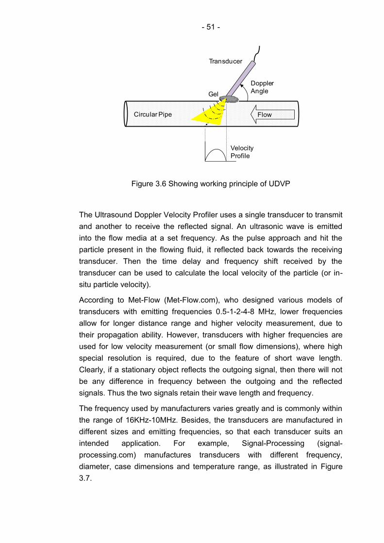
- 51 -
Figure 3.6 Showing working principle of UDVP
The Ultrasound Doppler Velocity Profiler uses a single transducer to transmit
and another to receive the reflected signal. An ultrasonic wave is emitted
into the flow media at a set frequency. As the pulse approach and hit the
particle present in the flowing fluid, it reflected back towards the receiving
transducer. Then the time delay and frequency shift received by the
transducer can be used to calculate the local velocity of the particle (or in-
situ particle velocity).
According to Met-Flow (Met-Flow.com), who designed various models of
transducers with emitting frequencies 0.5-1-2-4-8 MHz, lower frequencies
allow for longer distance range and higher velocity measurement, due to
their propagation ability. However, transducers with higher frequencies are
used for low velocity measurement (or small flow dimensions), where high
special resolution is required, due to the feature of short wave length.
Clearly, if a stationary object reflects the outgoing signal, then there will not
be any difference in frequency between the outgoing and the reflected
signals. Thus the two signals retain their wave length and frequency.
The frequency used by manufacturers varies greatly and is commonly within
the range of 16KHz-10MHz. Besides, the transducers are manufactured in
different sizes and emitting frequencies, so that each transducer suits an
intended application. For example, Signal-Processing (signal-
processing.com) manufactures transducers with different frequency,
diameter, case dimensions and temperature range, as illustrated in Figure
3.7.
Flow
Doppler
Angle
Transducer
Gel
Velocity
Profile
Circular Pipe
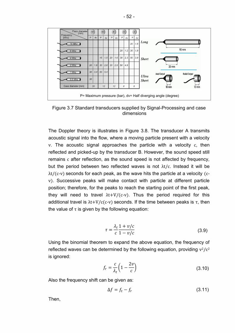
- 52 -
P= Maximum pressure (bar), dv= Half diverging angle (degree)
Figure 3.7 Standard transducers supplied by Signal-Processing and case dimensions
The Doppler theory is illustrates in Figure 3.8. The transducer A transmits
acoustic signal into the flow, where a moving particle present with a velocity
v. The acoustic signal approaches the particle with a velocity c, then
reflected and picked-up by the transducer B. However, the sound speed still
remains c after reflection, as the sound speed is not affected by frequency,
but the period between two reflected waves is not λ . Instead it will be
λ -v) seconds for each peak, as the wave hits the particle at a velocity (c-
v). Successive peaks will make contact with particle at different particle
position; therefore, for the peaks to reach the starting point of the first peak,
they will need to travel λ -v). Thus the period required for this
additional travel is λ -v) seconds. If the time between peaks is τ, then
the value of τ is given by the following equation:
(3.9)
Using the binomial theorem to expand the above equation, the frequency of
reflected waves can be determined by the following equation, providing v2/c2
is ignored:
(3.10)
Also the frequency shift can be given as:
(3.11)
Then,
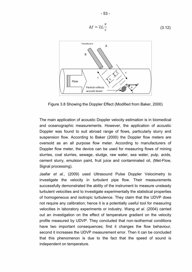
- 53 -
(3.12)
Figure 3.8 Showing the Doppler Effect (Modified from Baker, 2000)
The main application of acoustic Doppler velocity estimation is in biomedical
and oceanographic measurements. However, the application of acoustic
Doppler was found to suit abroad range of flows, particularly slurry and
suspension flow. According to Baker (2000) the Doppler flow meters are
oversold as an all purpose flow meter. According to manufacturers of
Doppler flow meter, the device can be used for measuring flows of mining
slurries, coal slurries, sewage, sludge, raw water, sea water, pulp, acids,
cement slurry, emulsion paint, fruit juice and contaminated oil, (Met-Flow,
Signal processing).
Jaafar et al., (2009) used Ultrasound Pulse Doppler Velocimetry to
investigate the velocity in turbulent pipe flow. Their measurements
successfully demonstrated the ability of the instrument to measure unsteady
turbulent velocities and to investigate experimentally the statistical properties
of homogeneous and isotropic turbulence. They claim that the UDVP does
not require any calibration; hence it is a potentially useful tool for measuring
velocities in laboratory experiments or industry. Wang et al. (2004) carried
out an investigation on the effect of temperature gradient on the velocity
profile measured by UDVP. They concluded that non-isothermal conditions
have two important consequences; first it changes the flow behaviour,
second it increases the UDVP measurement error. Then it can be concluded
that this phenomenon is due to the fact that the speed of sound is
independent on temperature.
λt
λr
Transducers
Flow
θ
v
V
Particle reflects
acoustic beam
c
c
A
B
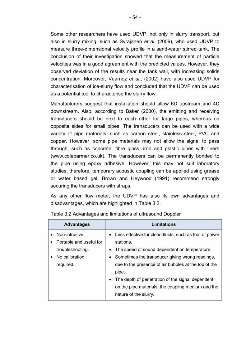
- 54 -
Some other researchers have used UDVP, not only in slurry transport, but
also in slurry mixing, such as Syrajänen et al. (2009), who used UDVP to
measure three-dimensional velocity profile in a sand-water stirred tank. The
conclusion of their investigation showed that the measurement of particle
velocities was in a good agreement with the predicted values. However, they
observed deviation of the results near the tank wall, with increasing solids
concentration. Moreover, Vuarnoz et al., (2002) have also used UDVP for
characterisation of ice-slurry flow and concluded that the UDVP can be used
as a potential tool to characterise the slurry flow.
Manufacturers suggest that installation should allow 6D upstream and 4D
downstream. Also, according to Baker (2000), the emitting and receiving
transducers should be next to each other for large pipes, whereas on
opposite sides for small pipes. The transducers can be used with a wide
variety of pipe materials, such as carbon steel, stainless steel, PVC and
copper. However, some pipe materials may not allow the signal to pass
through, such as concrete, fibre glass, iron and plastic pipes with liners
(www.coleparmer.co.uk). The transducers can be permanently bonded to
the pipe using epoxy adhesive. However, this may not suit laboratory
studies; therefore, temporary acoustic coupling can be applied using grease
or water based gel. Brown and Heywood (1991) recommend strongly
securing the transducers with straps.
As any other flow meter, the UDVP has also its own advantages and
disadvantages, which are highlighted in Table 3.2.
Table 3.2 Advantages and limitations of ultrasound Doppler
Advantages Limitations
Non-intrusive.
Portable and useful for
troubleshooting.
No calibration
required.
Less effective for clean fluids, such as that of power
stations.
The speed of sound dependent on temperature.
Sometimes the transducer giving wrong readings,
due to the presence of air bubbles at the top of the
pipe.
The depth of penetration of the signal dependent
on the pipe materials, the coupling medium and the
nature of the slurry.

- 55 -
3.3.2 Magnetic Resonance Imaging
Magnetic Resonance Imaging (MRI) is the most advanced and sophisticated
tool that generate almost real-time 3-D images of the material under
investigation. It allows the determination of phase volume fraction, physical
behaviour and properties, which are related to the state of the physical
system, (Van Dinther et al., 2012). The concept of MRI is that the object
subjected to a strong magnetic field and its hydrogen nuclei (or single
proton), which is spinning randomly is lined up in the direction of the
magnetic field. They are then hit by a burst of a Radio Frequency (RF) and
they flip round. Once they return to their original orientation they emit the
radio signal in the form of echo (Windt, 2007). This phenomenon is known
as Nuclear Magnetic Resonance (NMR). The Electron Magnetic Resonance
(EMR) is closely related to (NMR) and sense the free or unpaired electrons,
(Raguin et al., 2007). The spatial resolution of an MRI image can be 400 µm
and a temporal resolution of 1 m/s (Muller et al., 2008 and Kalaga et al.,
2009).
Despite the developments in the field, the MRI limitations have not been
overcome yet. Since MRI technique has limitations in maximum size of the
object, say in centimetres, as the object should be smaller than the magnetic
field. Also MRI cannot be applied for objects with any material, as the object
should contain either hydrogen or carbon atom. Therefore, this implies that
MRI is a relatively specialised technique and cannot be used for today’s
industry (Fukushima, 1999; Hoult et al., 1986).
3.3.3 Tomography techniques
The basic idea of tomography is to install a number of sensors at the
periphery of the pipe or vessel to be imaged. Then these images reveal
valuable information regarding the nature and distribution of the components
within the flow.
According to Williams and Beck (1995) there are many types of tomography
sensors such as ERT, ECT, PET, ultrasound tomography, nuclear etc. Each
of them has its own advantages and disadvantages. The choice is based on
the material under investigation, however some other considerations must
be made to safety issues, expenses and simplicity and applicability before
choosing the suitable type. For example, electrical tomography techniques
have been rated as the most attractive techniques, due to its safety issues,
unlike Gamma-ray and their moderate spatial resolution of the produced
image, unlike X-ray, electric field cannot be confined to a receiver.

- 56 -
Therefore, this study employs Electrical Tomography (ET) to visualise and
measure the parameters of slurry flow and the special attention will be paid
to electrical topography, particularly ERT. In the meantime some general
facts over the other types of electrical tomography (ECT, EIT, and EMT) will
be addressed briefly.
3.3.3.1 Electrical Resistance Tomography (ERT)
Electrical Resistance Tomography (ERT) has attracted a great interest from
researchers and engineers due to its safe application, relatively low price
(Windth, 2007; Cheney et al., 1999), design simplicity, despite that the
continuous phase must be conductive. Its application increases
progressively, not only in industrial processes but also in environmental
areas, such as monitoring of the hydraulic response of the rock mass in
Yucca Mountain, where thermo-mechanical and thermo-hydrological of this
horizon was studied (Deng et al., 2001).
The working principle of ERT system is to image mixtures, in pipes or
vessels, where the continuous phase is conductive and the dispersed phase
is insulating or less conductive, such as water and sand, as it is used in this
study.
Normally the ERT sensors composed of 16 equally spaced electrodes at the
periphery of the pipe or the vessel (mounted flush with inside surface of the
pipe), in a way that can be in direct contact with the fluid. The operating
principle is based on applying an alternating current and measuring the
potential differences across the cross section of the pipe or the vessel.
There are different strategies of measuring the voltage differences, as
discussed previously, however, the current study employs the adjacent
electrode strategy, which is injection of an electric current through a pair of
electrodes and measuring the voltage difference between the remaining of
electrode pairs and the procedure continues until the full rotation is
complete. The standard measurement protocol for measuring the
conductivity if N(N-3)/2 measurements, which is 104 measurements for 16
electrodes, as shown in Figure 3.9, (Williams and Beck, 1995; Wang et al.,
2002; Pashowko, 2004; Giguère et al., 2008b, 2009; Reinecke et al., 1998).
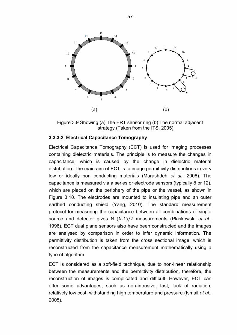
- 57 -
(a) (b)
Figure 3.9 Showing (a) The ERT sensor ring (b) The normal adjacent strategy (Taken from the ITS, 2005)
3.3.3.2 Electrical Capacitance Tomography
Electrical Capacitance Tomography (ECT) is used for imaging processes
containing dielectric materials. The principle is to measure the changes in
capacitance, which is caused by the change in dielectric material
distribution. The main aim of ECT is to image permittivity distributions in very
low or ideally non conducting materials (Marashdeh et al., 2008). The
capacitance is measured via a series or electrode sensors (typically 8 or 12),
which are placed on the periphery of the pipe or the vessel, as shown in
Figure 3.10. The electrodes are mounted to insulating pipe and an outer
earthed conducting shield (Yang, 2010). The standard measurement
protocol for measuring the capacitance between all combinations of single
source and detector gives N (N-1)/2 measurements (Plaskowski et al.,
1996). ECT dual plane sensors also have been constructed and the images
are analysed by comparison in order to infer dynamic information. The
permittivity distribution is taken from the cross sectional image, which is
reconstructed from the capacitance measurement mathematically using a
type of algorithm.
ECT is considered as a soft-field technique, due to non-linear relationship
between the measurements and the permittivity distribution, therefore, the
reconstruction of images is complicated and difficult. However, ECT can
offer some advantages, such as non-intrusive, fast, lack of radiation,
relatively low cost, withstanding high temperature and pressure (Ismail et al.,
2005).
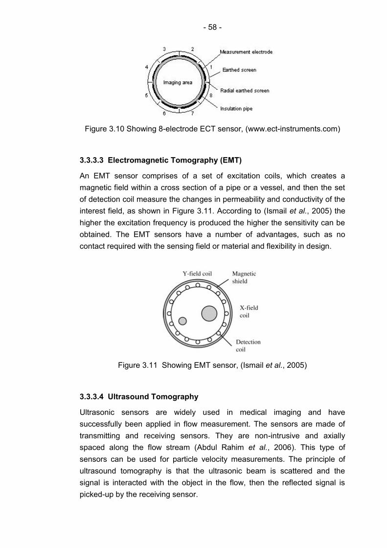
- 58 -
Figure 3.10 Showing 8-electrode ECT sensor, (www.ect-instruments.com)
3.3.3.3 Electromagnetic Tomography (EMT)
An EMT sensor comprises of a set of excitation coils, which creates a
magnetic field within a cross section of a pipe or a vessel, and then the set
of detection coil measure the changes in permeability and conductivity of the
interest field, as shown in Figure 3.11. According to (Ismail et al., 2005) the
higher the excitation frequency is produced the higher the sensitivity can be
obtained. The EMT sensors have a number of advantages, such as no
contact required with the sensing field or material and flexibility in design.
Figure 3.11 Showing EMT sensor, (Ismail et al., 2005)
3.3.3.4 Ultrasound Tomography
Ultrasonic sensors are widely used in medical imaging and have
successfully been applied in flow measurement. The sensors are made of
transmitting and receiving sensors. They are non-intrusive and axially
spaced along the flow stream (Abdul Rahim et al., 2006). This type of
sensors can be used for particle velocity measurements. The principle of
ultrasound tomography is that the ultrasonic beam is scattered and the
signal is interacted with the object in the flow, then the reflected signal is
picked-up by the receiving sensor.
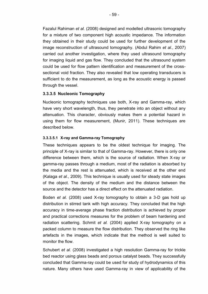
- 59 -
Fazalul Rahiman et al. (2008) designed and modelled ultrasonic tomography
for a mixture of two component high acoustic impedance. The information
they obtained in their study could be used for further development of the
image reconstruction of ultrasound tomography. (Abdul Rahim et al., 2007)
carried out another investigation, where they used ultrasound tomography
for imaging liquid and gas flow. They concluded that the ultrasound system
could be used for flow pattern identification and measurement of the cross-
sectional void fraction. They also revealed that low operating transducers is
sufficient to do the measurement, as long as the acoustic energy is passed
through the vessel.
3.3.3.5 Nucleonic Tomography
Nucleonic tomography techniques use both, X-ray and Gamma-ray, which
have very short wavelength, thus, they penetrate into an object without any
attenuation. This character, obviously makes them a potential hazard in
using them for flow measurement, (Munir, 2011). These techniques are
described below.
3.3.3.5.1 X-ray and Gamma-ray Tomography
These techniques appears to be the oldest technique for imaging. The
principle of X-ray is similar to that of Gamma-ray. However, there is only one
difference between them, which is the source of radiation. When X-ray or
gamma-ray passes through a medium, most of the radiation is absorbed by
the media and the rest is attenuated, which is received at the other end
(Kalaga et al., 2009). This technique is usually used for steady state images
of the object. The density of the medium and the distance between the
source and the detector has a direct effect on the attenuated radiation.
Boden et al. (2008) used X-ray tomography to obtain a 3-D gas hold up
distribution in stirred tank with high accuracy. They concluded that the high
accuracy in time-average phase fraction distribution is achieved by proper
and practical corrections measures for the problem of beam hardening and
radiation scattering. Schmit et al. (2004) applied X-ray tomography on a
packed column to measure the flow distribution. They observed the ring like
artefacts in the images, which indicate that the method is well suited to
monitor the flow.
Schubert et al. (2008) investigated a high resolution Gamma-ray for trickle
bed reactor using glass beads and porous catalyst beads. They successfully
concluded that Gamma-ray could be used for study of hydrodynamics of this
nature. Many others have used Gamma-ray in view of applicability of the
- 60 -
technique for industry, such as Wang and Yin (2001), Yin et al. (2002), Roy
et al. (2005), and Jin et al. (2005). Most interestingly Tortora et al. (2008)
used a multimodality tomography method, where they used Electrical
Impedance Tomography (EIT) in conjunction with Gamma-ray for circulating
fluidised bed, and they confirmed a good accuracy of using the two
technique.
3.3.3.5.2 Positron Emission Tomography (PET)
PET is a radioactive tracer that enables visualisation of real processes
taking place within the opaque boundaries. The principle of PET is based on
detecting the pairs of back-to-back gamma-rays produced when a positron
annihilates (or emitted in radioactive decay) with an electron. It is widely
used in medicine, however, in chemical engineering applications a extensive
use has been made of the alternative technique of Positron Emission
Particle Tracking (PEPT). In PEPT a single tracer particle is radioactively
labelled and can be accurately tracked at high speed (Seville et al., 2009).
PEPT has the capability of tracking tracer particles down to approximately
60 µm is size.
PEPT has successfully been used for monitoring and measuring particle
velocities in gas fluidised beds, mixers and other chemical applications
(Stein et al., 1997). Portillo et al. (2010) examined the movement of particles
within a continuous powder mixer, in which PEPT was employed. They
claimed that the particles along the vessel could be measured non-invasively
and the measurements were promising.
3.4 Electrical Resistance Tomography system detail
3.4.1 Introduction
Tomography is an imaging technique that is used to visualise the contents of
a closed system or body, such as a pipe or a vessel without physically
looking inside. Tomography originally is a Greek word, which is composed of
two words, “tomos” meaning “to slice” and “graph” meaning “image”
(Williams and Beck, 1995). In the late 1970s the technique was very popular
in medical fields, where tomography resistivity measurement was used by
biomedical engineers and considered as an alternative to the successful X-
ray scanner, due to its low cost and portability.
Since late 1980s tomography techniques have gone through a major
development and are used to provide a novel means of non-intrusively
- 61 -
visualising the internal behaviour of industrial processes, such as gas-liquid,
gas-oil-water in oil pipelines, gas-solid flows in pneumatic conveyers, solid-
liquid in slurry transfer system and mixing or separation processes in
vessels. Thus it is often called “industrial processes Tomography” or
“Process Tomography” (Williams and Beck, 1995). In process tomography
the signals are sent across the system through the electrodes that are
placed at the periphery of the pipe or the vessel, then depending on the
signals received, images of the cross sectional plane are constructed. Thus
the use of tomography can provide an image of the whole flow and can be
considered as a new type of multiphase flow meter. It is important to mention
that the current multiphase flow meters are non-linear, which are caused by
their flow regime dependency, while tomography can compensate their non-
linearity, therefore it is also a viable tool that can be used to determine the
flow regime (Ismail et al., 2005).
Many types of tomography systems can be found in the literature, such as
Electrical, ultrasonic or acoustic, radiation, Nuclear Magnetic Resonance
(NMR), microwave and optical, which are mainly based on different sensing
methods. However, this project employs Electrical Tomography (ET) due to
its advantages over the other tomography techniques for being cheap lack of
radiation and fast response. Based on the principle of electrical sensitivity,
electrical tomography is further classified into Electrical Impedance
Tomography (EIT), Electrical Capacitance Tomography (ECT), Electrical
Resistance Tomography and Electromagnetic Tomography (EMT) (Williams
and Beck, 1995). Amongst all the above electrical tomography forms, ERT
has been found to be the most attractive method, which is used in this
project to visualise the mechanisms of slurry flow systems and measure its
parameters. This attractiveness has come from its advantages, such as
simplicity, high speed capability and sufficiently robust to cope with the most
industrial environment, safe and cheap in comparison to nuclear techniques,
which makes them suitable for research as well as industry. It is therefore
widely used in different chemical engineering processes, such mixing
process (Wang and Yin, 2001); cyclonic separation (Williams et al., 1999)
and the mixing processes (Holden et al., 1999). However, the drawback of
ERT lays in its low spatial resolution, which has been reported to be
between 5 and 10% pipe diameter (Dyakowski et al., 2000).
Since ERT is still within development period, there are some challenges,
which need to be reported.

- 62 -
Increase of sensor spatial resolution.
Development of more accurate image reconstruction, as inaccurate
image will interpret inaccurate flow parameters, such as volume flow
rate.
Increase the efficiency of data processing.
Improve the design of the sensors mechanically and the electronic
hardware in order to increase the safety and reliability either in the
laboratory as well as the industry.
The structure of a typical ERT system composed of a hardware part, which
includes the sensor with electrode rings, the data acquisition system and the
image reconstruction system, which is the host computer, from which the
image are generated (Parvareh et al., 2010). Figure 3.12 showing the
components of a tomography system.
Figure 3.12 Showing the components of the ERT system
3.4.2 Concept and working principle
ERT can be used as a non-intrusive technique to measure and visualise a
multiphase flow, in which the continuous phase is an electrically conductive
fluid. The technique generates a 2D or 3D image (tomogram), by using
electrical resistance measurements and image reconstruction. A tomogram
shows the distribution of the conductivity within the flow system, and this is
determined by several colours. The basic idea of these colours is to interpret
the conductivity within the flow or a mixing system. In tomograms, usually,
Voltage signal measured
Data Acquisition
System
Image Reconstruction
System
Non-conducting object within the sensing region
15 mA current injected
Dual-plane ERT sensor
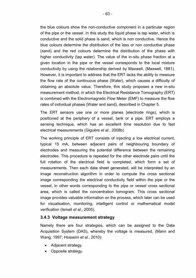
- 63 -
the blue colours show the non-conductive component in a particular region
of the pipe or the vessel. In this study the liquid phase is tap water, which is
conductive and the solid phase is sand, which is non conductive. Hence the
blue colours determine the distribution of the less or non conductive phase
(sand) and the red colours determine the distribution of the phase with
higher conductivity (tap water). The value of the in-situ phase fraction at a
given location in the pipe or the vessel corresponds to the local mixture
conductivity by using the relationship derived by Maxwell, (Maxwell, 1881).
However, it is important to address that the ERT lacks the ability to measure
the flow rate of the continuous phase (Water), which causes a difficulty of
obtaining an absolute value. Therefore, this study proposes a new in-situ
measurement method, in which the Electrical Resistance Tomography (ERT)
is combined with the Electromagnetic Flow Meter (EMF) to measure the flow
rates of individual phases (Water and sand), described in Chapter 5.
The ERT sensors use one or more planes (electrode rings), which is
positioned at the periphery of a vessel, tank or a pipe. ERT employs a
sensing technique, which has an excellent time resolution due to fast
electrical measurements (Giguère et al., 2008b)
The working principle of ERT consists of injecting a low electrical current,
typical 15 mA, between adjacent pairs of neighbouring boundary of
electrodes and measuring the potential difference between the remaining
electrodes. This procedure is repeated for the other electrode pairs until the
full rotation of the electrical field is completed, which form a set of
measurements. Then each data sheet generated, will be interpreted by an
image reconstruction algorithm in order to compute the cross sectional
image corresponding the electrical conductivity field within the pipe or the
vessel, in other words corresponding to the pipe or vessel cross sectional
area, which is called the concentration tomogram. This cross sectional
image provides valuable information on the process, which later can be used
for visualisation, monitoring, intelligent control or mathematical model
verification (Ismail et al., 2005).
3.4.3 Voltage measurement strategy
Namely there are four strategies, which can be assigned to the Data
Acquisition System (DAS), whereby the voltage is measured, (Mann and
Wang, 1997; Hosseini et al., 2010):
Adjacent strategy.
Opposite strategy.

- 64 -
Diagonal or cross strategy.
Conducting boundary strategy
This study will employs adjacent strategy, as it requires less hardware and
presents fast image reconstruction. Therefore, it will be the only strategy that
is discussed in detail here, and for the rest of strategies the reader will be
referred to the references given above.
In the adjacent strategy, an electrical current is applied through two adjacent
electrodes and the potential different is measured for the remaining adjacent
pairs of electrodes, then the injection and measurement procedure is
continued until the full independent combination is completed, as shown in
Figure 3.13. The standard measurement protocol for adjacent strategy gives
N(N-3)/2 measurements, where N is the number of electrodes. For example,
for a plane with 16 electrodes provides 104 individual voltage measurements
(Tapp et al., 2003). These measurements are communicated to the image
reconstruction computer by the Data Acquisition System (DAS), and then the
data are processed via a suitable image reconstruction algorithm.
Figure 3.13 Adjacent electrode pair strategy for 16 electrode ERT sensor
3.4.4 Fast Impedance Camera system (FICA)
The high performance ERT system (or a high performance electrical
impedance tomography system), is in house built (Online Instrumentation
Laboratory/University of Leeds/UK). With regard to the main ERT system
(Data Acquisition Hardware), the software and hardware of which have been
enhanced and consolidated by OLIL group (Online Instrumentation
V
I

- 65 -
Laboratory/University of Leeds). Figure 3.14 showing the actual photograph
of FICA system. It is worth pointing out that one of the advantages of this
system is the efficiency of the hardware and simplicity of the operation of the
control software. The principle of the hardware operating system and the
operation of the control software is described in detail in Schlagerg et al.
(2008).This development of the conventional EIT system could be
considered as a response to the requirement of many industrial processes
such as two/multiphase flow, where a higher (faster) frame rates is required
to measure and monitor the flow behavior. The Data Acquisition System
(DAS) is based on the phase sensitive demodulation and both the amplitude
and the phase of the measurement can be obtained. Once the system is
connected it allows the Data Acquisition System to operate in two modes,
continuous (on-line) and block mode.
Figure 3.14 Actual photograph of FICA system
In continuous mode, a single frame of data for one or two planes is acquired,
captured, transferred and displayed in the selected format. This mode can
capture data at a frame rate up to 50 dual-frames per second (dfps), which is
equivalent to 20 ms; whereas block mode can capture data up to 8000
frames at a rate up to 1000 dfps. At the end of acquisition of each data
block, it is then transferred and read by the PC, where it is processed and
can be visualised or saved on an external hard drive for later analysis. The
image reconstruction system can produce images for both amplitude and
phase of the domain, by using one of the versions of Linear Back Projection
(LBP) algorithm, which is called Sensitivity Back Projection (SBP) algorithm.
The reconstruction algorithm (SBP) can provide further option of displaying
images for real and imaginary part.
3.4.5 ERT Sensor design
The aim of ERT is to acquire the conductivity distribution in the domain of
concern. This is done by, as previously mentioned, injecting an electrical
- 66 -
current and measuring the voltage difference through the electrodes placed
on the boundary of the area of concern. Amongst the three components of
ERT system, the design of sensor (electrodes) is the most important part,
since the better design of electrodes the more efficient they can be to sense
the conductivity of the area of interest (Seagar et al., 1987). The electrode
material is normally fabricated from platinum, gold, silver, brass, stainless
steel or alloys, such as silver platinum. However, there are several factors
that can be considered prior to design the electrodes, such as the position of
the electrodes, the size of the electrodes and number of the electrodes
(Mann and Wang, 1997). As these factors are important for reconstruction
algorithm, measuring the conductivity field distribution, collecting the data
and reconstructing the image. Usually the electrodes are placed around the
boundary of the pipe or the vessel in order to make electrical contact with
the content of the pipe or vessel in a non-intrusive fashion or slightly
intrusive, as they are introduced to the field of interest through the wall of the
pipe or the vessel, which makes them invasive. The other ends of the
electrodes are connected to the Data Acquisition System (DAS) through co-
axial cables so as to avoid or reduce the electromagnetic noise or
interference (Williams and Beck, 1995). A dual plane ERT sensor was
designed to be used in this study, a geometry and dimensions of which is
shown in Chapter 6.
3.4.6 Image reconstruction analysis
The aim of image reconstruction in Electrical tomography is to compute a
tomogram, which is representing the electrical conductivity of the material
flowing through the pipe or the vessel (Giguère et al., 2008b).
Generally there are two types of algorithms that are used to process the data
for image reconstruction; non iterative algorithm as Linear Back Projection
(LBP) and iterative algorithm as Sensitivity Conjugate Gradient (SCG)
(Wang, 2002). The selection of the most suitable depends on accuracy,
speed and expense. Over the years many image reconstructions have been
proposed for electrical tomography, however, the most widely used
algorithm is still Linear Back Projection that is due to its advantages over the
iterative algorithms, which is computationally more time consuming and too
slow for real-time image reconstruction. Therefore, this study employs the
non-iterative algorithm (LBP). This algorithm is simple and fast, but it offers
qualitative images only. If the image needs to be enhanced, an iterative
image reconstruction algorithm can be employed (Ismail et al., 2005)
- 67 -
In order to obtain the conductivity distribution a grid of small equal squares is
applied on the area of interest. Each individual tomogram consists of a
20x20 pixel array, which gives 400 spatial elements. The circular image is
constructed using 316 pixels from 400 pixels squares grid. Some of these
pixels lay outside the pipe or the vessel circumference, but the image is
constructed from the pixels inside of the pipe or the vessel, as the sensors
are placed on the boundary of the body (Hosseini et al., 2010).
Electrical Tomography is considered as a soft-field technique, since the
image is based on measurements at the boundary of the sensor. The
sensitivity changes across the sensing zone and also the sensitivity of a
particular position within that zone depends on the spatial variation of the
physical parameter been imaged within the whole sensing zone. Therefore,
due to this linear behaviour the reconstructing of the image can be difficult.
Despite some development in image reconstruction, some concerns have
been raised, particularly ERT, regarding the performance, validation and
limitations of quantitative image reconstruction technique. Most of the efforts
made to improve the image reconstruction algorithm were made in Electrical
Capacitance Tomography (ECT). However, the image reconstruction
techniques used for ECT can be transposed to ERT, as there is a simple
mathematical analogy between them (Giguère et al., 2008b).
Most image analysis is based on the images produced by Linear Back
Projection (LBP). There are a number of approaches to analyse the images,
one of which is the generation of summary statistics (mean, maximum etc.),
which is the simplest. Statistics can be calculated either for the whole image
or for the smaller regions, such as concentric zones or course square tiles,
and this is done by dividing the image into zones. This method can be used
to define the heterogeneity parameters, as studied have been conducted on
flow regimes in bubble columns. Some other approaches are based on
comparison, such as comparing successive images (frames), multiple
planes. Cross correlation analysis can be used to obtain information on
particle velocities, mixing and diffusion. Here pixel correlations are computed
within frames, between successive frames or planes (Tapp et al., 2003)
3.4.7 Application of the ERT
The Electrical Resistance Tomography not only offers the opportunity to
visualise the two or multiphase flows, but also capable of measuring some
flow parameters, such as solid’s concentration and velocity (Parvareh et al.,
2010). In other words, the ERT can be sued to obtain qualitative and
quantitative data, representing the real life of what is really occurring inside

- 68 -
the process under investigation, and that is with the aid of one frame or
tomogram generated via image reconstruction system.
As solid and liquid used in this study, then the right choice must be made as
to which technique has to be used to visualise and measure the process.
The preferred method in the field of slurry transport is ERT, as it is safe
robust and more suitable to interpret the whole process fast and
continuously unlike Gamma-ray densitometry, which is only capable to
measure the local density value in one chord (vertical y-axis) in one plane
and not giving the full understanding of settling behaviour in slurry pipelines
(Brown and Heywood, 1991; Pugh, 1995; Matousek, 1997).
From a review of the literature in the last fifteen-twenty years, despite
appearing some new applications, it was found that the large scale
application has been in mixing process, particularly solid-liquid applications,
and two/multiphase flow. Tomography was used by McKee et al. (1995),
who studied the optimal agitation speed and its influence on the
concentration profile. It was also used by Williams (1995) for measuring a
mixing index. One year later Williams et al. (1996) used tomography again to
study the effect of impeller size, impeller type and particle distribution on the
mixing index. Wang et al. (1999) used ERT as a suitable technique for
identifying non-uniform density regions within foam, which suggests that
ERT can well be a viable method for process control in a foaming system.
Wang et al. (2000) studied gas liquid in a stirred vessel, where they used
ERT to investigate the effect liquid viscosity on the mixing behaviour. Kim et
al. (2006) investigated the mixing process and dispersion velocity of two
miscible liquids in a vessel with a rotating agitator. They used four-plane
ERT to calculate the mixing time from the temporal trend of cross sectional
conductivity distribution and concluded that data analysis method with ERT
to measure and analyse the mixing. In another study by Cho et al. (1999)
EIT used to visualise the bubble distribution in two phase flow, where they
decreased the image reconstruction time using an adaptive mesh grouping
method. Kim et al. (2001) designed an EIT system and employed to
visualise two phase flow system. When they obtained the image from the
image reconstruction, they found that the image quality was not very good.
However, they suggested that EIT could be used to visualise two phase flow
system. Giguère et al. (2008b) used ERT to visualise slurry flows in
horizontal and vertical pipe. They analysed slurry flow regimes using a
strategy based on the direct interpretation of ERT measurements.

- 69 -
Although ERT technique is a promising technique to visualise slurry flow,
there are limitations in terms of quantitative ERT images, which makes them
difficult to exploit the quantitative images, furthermore the validation of these
quantitative images are necessary. Giguère et al. (2008a) has described the
development of quantitative ERT image reconstruction software, in which the
validation of the results for the case of static solid particle bed, at the bottom
of the pipe sensor, has been carried out. He has also successfully shown
good agreement between a calibration curves, using ERT relating the size of
particle bed with experimental values using LBP.
3.4.8 Conductivity conversion to solids concentration
When the ERT is used to measure a mixture, for example slurry, it obviously
measures the conductivity distribution, or map the conductivity of phases,
and if the concentration of the dispersed phase (such as solid) is required,
then there must be a method or correlation to convert the measured
conductivity distribution to concentration of the dispersed phase or particles.
Within the last three centuries a number of correlations have been proposed
for conversion of conductivity to concentration of the non-conductive
dispersed phase. The most important of all are those of Maxwell (1881);
Brggeman (1935); Mridith and Tobias (1962); Prager (1963) and Weissberg
(1963).
Maxwell (1881) derived an equation for diluted mixture, as shown in
equation 3.13, in which relates conductivity distribution and particle
concentration distribution, which is expressed in terms of solids (or
dispersed phase) volume fraction, , (Maxwell, 1881; Lucas et al., 1999;
Pashowko, 2004).
(3.13)
If it is assumed that the dispersed particles are non-conductive, as sand is
used in this study, then the conductivity of sand is considered to be zero and
the above equation can be simplified to:
(3.14)

- 70 -
The above equation can well be used to calculate the particle volume
fraction, but only in case of isothermal condition, where the temperature of
the mixture remain constant or inevitably with slight change. Since any
change in temperature can affect its conductivity values.
Maxwell believed that his equation can only apply on diluted mixtures.
However, Turner (1976) confirmed that Maxwell’s equation can also be used
for high solids concentration, even with maximum packing concentration of
the slurry.
Bruggeman (1935) studied a mixture of non-conducting spherical particles in
a conducting media, and generated the following equation:
(3.15)
Meredith and Tobias (1962) also generated an equation relating the
conductivity and local solid’s concentration:
(3.16)
Another correlation proposed by Prager (1963), who derived a generalised
diffusion model for the suspension of irregular shaped particles, based on
random geometry:
(3.17)
Weissberg (1963) carried out further work and proposed another correlation,
in which he considered that the spherical particles were randomly distributed
in an idealised bed:
(3.18)
- 71 -
Now, as there are five correlations, by which the concentration of the
dispersed phase could be determined, then a question may raise here as to
which of the above correlations perform better. The answer could be given
by Holdich and Sinclair (1992), who found that the prediction of the
conductivity in all the above five correlations is similar, only if the solid or the
dispersed particles volume fraction is less that 30% (Pachowko, 2004).
Therefore this suggests that the prediction of all the above correlations differ
only when the solid bed is formed, since the solid bed is formed when the
solid’s volume fraction is more than 40%. Despite that, this study is still
employs Maxwell’s correlation, as it is well preferred by many researchers
and used in ERT system to convert the conductivity distribution to solid’s
concentration.
3.4.9 Limitation of the ERT
The previous sections have clearly highlighted the advantages of ERT over
the other measurement techniques. However, there is still scope for
improving some aspects of ERT, such as spatial resolution, conductivity
resolution and ability of distinguishing single particles. These limitations are
discussed below.
3.4.9.1 Spatial resolution
According to Seagar et al. (1987) this helps in identifying a minimum particle
size. Wang et al. (1999) found out that by varying the particle to vessel or
pipe diameter ratio and keeping the mixture conductivity constant and
measurement error less than 1%, a typical spatial resolution of 5% pipe
diameter can be achieved. As previously discussed, this study uses 50 mm
pipe diameter, and according to Wang et al. (1999) the ERT sensor can
identify sand particle size of 2.5 mm or greater.
3.4.9.2 Conductivity resolution
This parameter determines the minimum conductivity deviation in individual
pixels, which enable the image reconstruction algorithm to pick up the
change and demonstrate it in the images. Wang et al. (1999) carried out an
investigation regarding this aspect and found out that at least a deviation of
10% of conductivity is required for the object to be imaged, for fixed particle
to vessel diameter ratio and measurement error is less than 1%. This study
uses water and sand as the components of the slurry. The typical
conductivity of tap water is between 0.3 and 0.45 mS/cm, and the
conductivity of sand far less than this value, which makes more than 10%.

- 72 -
Therefore, the ERT could easily pick up the sand particles in the produced
images.
3.4.9.3 Ability of distinguishing single particle
This parameter determines the minimum distance between each single
particle so that the ERT would be able to distinguish each of them. Through
an investigation by Wang et al. (1999), the minimum value for this parameter
was found to be 20% of the vessel or pipe diameter, if the measurement
error is less than 1%. Since this study uses a 50 mm pipe diameter, then a
minimum distance of 10 mm is required between each sand particle, so that
they can clearly be seen in the tomograms, otherwise they will be seen as a
single particle. This suggests the impossibility of ERT to distinguish every
single particle in the slurry flow used in this study, unless a very low
concentration and very coarse sand are used in homogeneous flow regime.
However, this may not have an importance when the contact load of bed is
formed.
3.5 Conclusions
This chapter has reviewed the current techniques available for measurement
of solid-liquid flow. It was found that the abrasiveness, opacity and complex
nature of solid-liquid flow are considerable challenges to its measurement. It
was also concluded that amongst all commercially available techniques,
whether conventional or novel sensors, no technique measures face fraction
and face velocity without limitations. Functionality and applicability of current
flow meters over a wide range of conditions still remain unsolved. The
settling tendency of solid particles, which results in arising several flow
regimes within the pipelines, is still considered as a remarkable challenge to
slurry flow measurement. Particularly for measurement of stratified flow, as
the strata creates a coat over the sensors and affecting their functionality. A
light was also shed on the current status of electrical resistance tomography
technique, and it was gathered that the ERT, compared to the rest of novel
sensors, has a remarkable package of advantages, namely relatively low-
cost, having high temporal resolution, non-intrusive, providing qualitative
data as well as visual information about the flow, safe, robust and reliable.
However, despite a progressive work, it still suffers from low spatial
resolution, which requires to be overcome.

- 73 -
Chapter 4
Horizontal and vertical flow experimental set up and
calibration procedure
This chapter describes the laboratory experiments and the operating
procedure conducted on 50 mm horizontal and vertical pipeline. The
calibration procedure carried out on various instrumentations is also
presented along with the results of each calibration.
4.1 Introduction
In order to fulfil the objectives mentioned in Chapter 1, it is essential to
establish an effective and comprehensive methodology along with a flow
loop system that allows an easy measurement, visualisation and validation
of slurry flow parameters. The most important parameters that this study is
concerned are slurry velocity, solids velocity and its profile, in-situ and
delivered solids concentration. The flow loop used in the experiments and its
associated instrumentation are also discussed in the following sections.
The experiments were focused on the observations of both, the integral flow
characteristics and the local flow characteristics of settling slurry pipeline.
Since the measurement of the local flow characteristics is crucial for the
identification of the mechanisms governing the process of slurry flow, then
the ERT technique was employed to interrogate the internal structure of
slurry flow in the pipeline under various slurry flow conditions. Besides, the
ERT system was used to generate some of the integral flow characteristics,
such as mean solids concentration and mean solids velocity across
horizontal and vertical test section of the pipeline. Due to the dynamic and
rapid change of the internal structure of slurry flow, it was believed that a fast
measuring technique is required to provide continuous information about the
development of slurry flow inside pipelines. Therefore, the Fast Impedance
Camera system was used in these experiments with capability of acquiring
1000 dual frames per second.
The first approach is experimental measurement and visualisation of
horizontal and vertical flow. The experimental measurement and
visualisation involve intense utilisation of the ERT and the Electromagnetic
Flow meter (EMF). The ERT is used to determine solids concentration and
- 74 -
solids velocity distribution across the pipe cross section. EMF will be used to
measure mean slurry velocity. As settling slurry flow suffers from flow
discontinuity (or phase change), which adversely affects the measurement
scheme due to occurrence of various flow regimes in horizontal flow.
Therefore, a technique is proposed for recognition of the prevailing flow
regime, which is discussed in Chapter 7.
The following sections present the installation and measuring technique
together with the measured data for characteristics of the dispersed phase
(sand). The experimental data for slurry flow through the two orientations are
presented and discussed with an analysis of the measurement results in
Chapter 5.
4.2 Aims of the experimental work
The main aim of the experimental work was to evaluate the suitability and
applicability of the ERT (Fast Impedance Camera System-FICA) for
visualisation and measurement of settling slurry flow. This evaluation was
carried out by observing the behaviour of slurry flow in horizontal and vertical
pipeline and measuring the flow characteristics appropriate to the detection
and analysis of mechanisms governing the process of slurry flow
measurement. The measured characteristics had to be appropriate for the
verification of the components measured via the ERT system. In order to
achieve this, two types of flow parameters were measured:
a. The integral flow characteristics, which refers to the mean values of a
quantity in a pipeline cross-section (i.e. slurry velocity, pressure,
spatial solids concentration, solids axial velocity and delivered solids
concentration).
b. The local flow characteristics in horizontal and vertical pipeline, which
refers to the In-situ flow parameters (i.e. local concentration at
different positions in the vertical plane of the pipe cross-section and
local solids axial velocity at different positions in the vertical plane of
the pipe cross-section).
The fulfilment of the main objective required the execution of several specific
tasks, which are listed below:
1. Validation of slurry flow rate via flow diversion technique using
measuring tank.
2. Online visualisation of slurry flow through image reconstruction of
pipe cross-section.
- 75 -
3. Verification of 3-D solids velocity profile across the pipe cross-section
in horizontal flow.
4. Validation of solids volumetric distribution against the real flow
photographs captured at the very same flow conditions of the ERT
measurement.
5. Investigation of the effect of particle size on the measured
concentration and solids velocity profile using the FICA system and
identifying the reasons for the possible effects.
6. Exploring the effect of concentration on the measured concentration
and solids velocity profile using the FICA system. Also, identifying the
reasons for the possible effects.
7. Highlighting the effect of transport velocity on the measured
concentration and solids velocity profile using the FICA system and
mentioning the reasons for the possible effects.
8. Estimation of the parameters that define stratified settling slurry flow,
such as height of moving bed, height of stationary bed, height of
shear layer, height of turbulent zone at the upper part of the pipe,
identification of moving and stationary bed.
9. Comparison of In-situ and delivered solids concentration and
establishing the relationship between the two parameters.
10. Identification of blockage (total stationary) in horizontal pipeline and
estimation of mean solids concentration and mean solids velocity in
the blocked pipe section.
11. Visualisation of four main flow regimes in horizontal flow through
combination of concentration and solids velocity profile.
12. Automatic recognition of main flow regimes in horizontal flow through
combination of concentration and solids velocity profile.
13. Error analysis of mean concentration and mean solids velocity
obtained from the ERT system.
14. Investigation of the effect of Wave Velocity and any possible effect on
the mean solids velocity in stratified flow.
15. Highlighting the rate of deviation of the ERT measured concentration
at transport velocities up to 5 m/s.
4.3 Horizontal and vertical slurry flow loop layout
The experiments were carried out using a pilot scale re-circulating open flow
loop, the schematic layout of which is presented in Figure 4.2. The major
components are a mixing tank, slurry pump, horizontal and vertical pipeline
- 76 -
test sections, a switch or flow diversion system with a measuring tank
(sampling tank), dual-plane Electrical Resistance Tomography sensors
(ERT), an Electromagnetic Flow meter (EMF), pressure transducers and a
thermocouple. The flow loop is laid on two floors in G.56, Houldsworth
Building in the Institute of Particle Science and Engineering/ School of
Process, Environment and Materials Engineering in the University of Leeds.
The entire length of the loop is 22 m and has an internal diameter of 50 mm.
The connecting pipes (DN 50) are from uPVC material (class E 15 bar BS
EN1452) from Pipestock. The mixing tank has a capacity of 500 liter and is
coupled with a three-blade mixer so as to obtain a homogeneous mixture
before introducing it to the flow loop. Therefore, the main function of the
mixing tank is to mix and hold the returning slurry from the flow loop before
pumping it back to the flow loop. A bypass or a flush line is also connected
to the mixing tank for initial lubrication of the pipeline before introducing the
slurry of coarse particles, and also for draining purposes.
The loop is served by a 15 KW centrifugal pump (2/1/2 AH WARMAN
PUMP), which is connected to a Digi-drive Frequency Converter (LEROY
SOMER -15Kw) to control the mean slurry velocity. The two test sections of
the loop, horizontal and vertical test sections, are placed in the straight lines
so that the affect of bend and flow disturbances are avoided (Matousek,
1997). The length of both horizontal and vertical test sections is 2.40 m and
2.25 m respectively. The horizontal test section is equipped with two
pressure sensors and a dual plane ERT sensor. According to Gillies (1991)
and Pachowko (2004), the approach length must not be less than 50 pipe
diameter. Therefore, the dual plane ERT sensor is placed directly 3.40 m
away from the bend. Whereas the vertical test section is equipped with two
pressure sensors, an Electromagnetic Flow Meter, a thermocouple and a
dual plane ERT sensor. The dual plane ERT sensor, in the vertical section,
was placed 2.5 m away from the bend. The returning limb connected to the
top of the vertical section is 2.75 m and returns the slurry back into the
mixing tank or the measuring tank if the flow is diverted. A flow switch
mechanism is used for the flow diversion process. The measuring tank,
which has a capacity of 90.5 liter is placed on a set of three load cells for
measurement of weight and the level of diverted slurry into the measuring
tank. The level of each diverted amount of slurry is determined through a
graded glass tube, which is mounted on the measuring tank. A transparent
pipe section of 1 m long is included into the horizontal section directly after
the ERT sensor, which would enable visual observation of the flow and
capturing photographic images for visual observations and validation
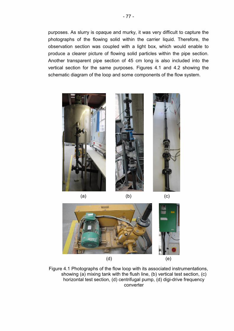
- 77 -
purposes. As slurry is opaque and murky, it was very difficult to capture the
photographs of the flowing solid within the carrier liquid. Therefore, the
observation section was coupled with a light box, which would enable to
produce a clearer picture of flowing solid particles within the pipe section.
Another transparent pipe section of 45 cm long is also included into the
vertical section for the same purposes. Figures 4.1 and 4.2 showing the
schematic diagram of the loop and some components of the flow system.
(a) (b) (c)
(d) (e)
Figure 4.1 Photographs of the flow loop with its associated instrumentations, showing (a) mixing tank with the flush line, (b) vertical test section, (c) horizontal test section, (d) centrifugal pump, (d) digi-drive frequency
converter
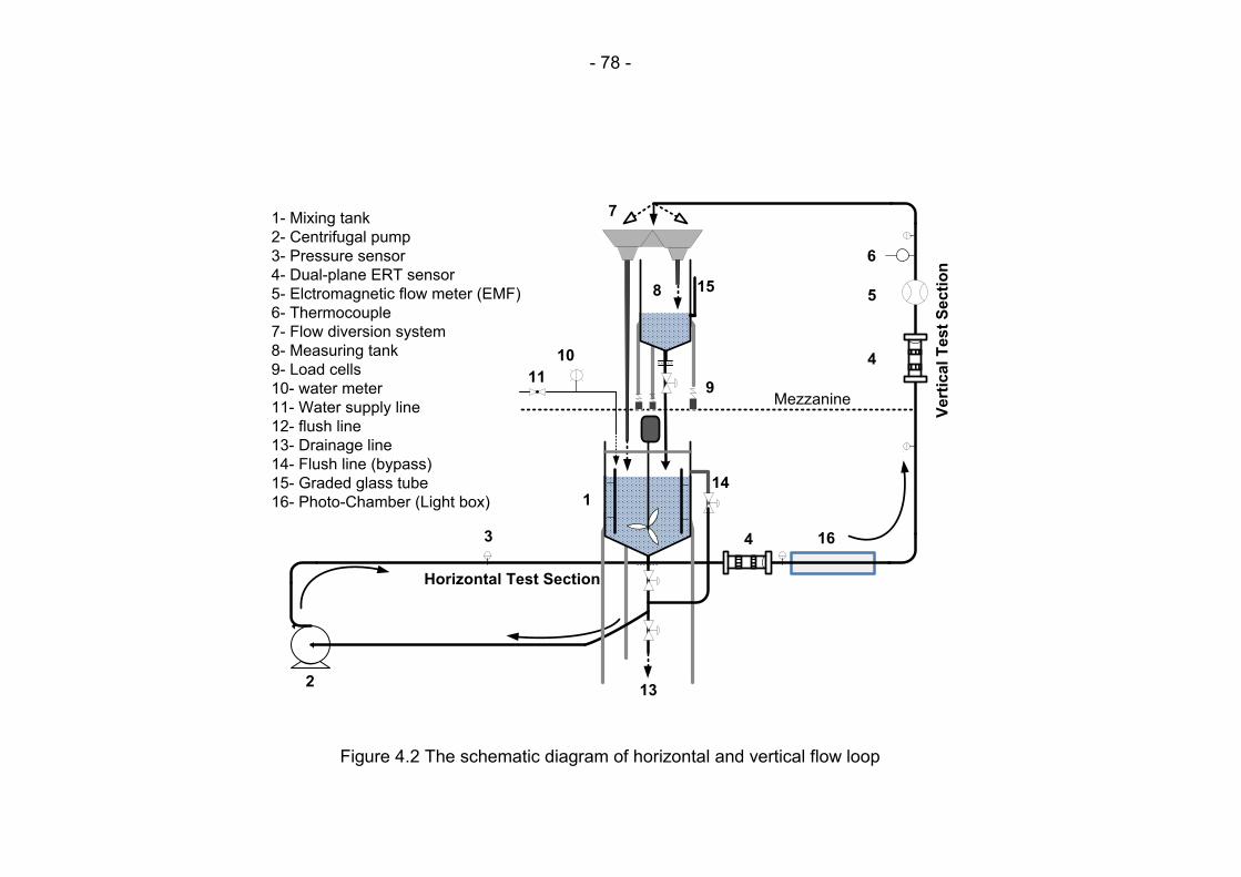
- 78 -
Figure 4.2 The schematic diagram of horizontal and vertical flow loop
213
4
9Mezzanine
11
10
5
4
6
3
7
8
1
1- Mixing tank
2- Centrifugal pump
3- Pressure sensor
4- Dual-plane ERT sensor
5- Elctromagnetic flow meter (EMF)
6- Thermocouple
7- Flow diversion system
8- Measuring tank
9- Load cells
10- water meter
11- Water supply line
12- flush line
13- Drainage line
14- Flush line (bypass)
15- Graded glass tube
16- Photo-Chamber (Light box)
Horizontal Test Section
Ve
rtic
al T
es
t S
ec
tio
n
14
15
16
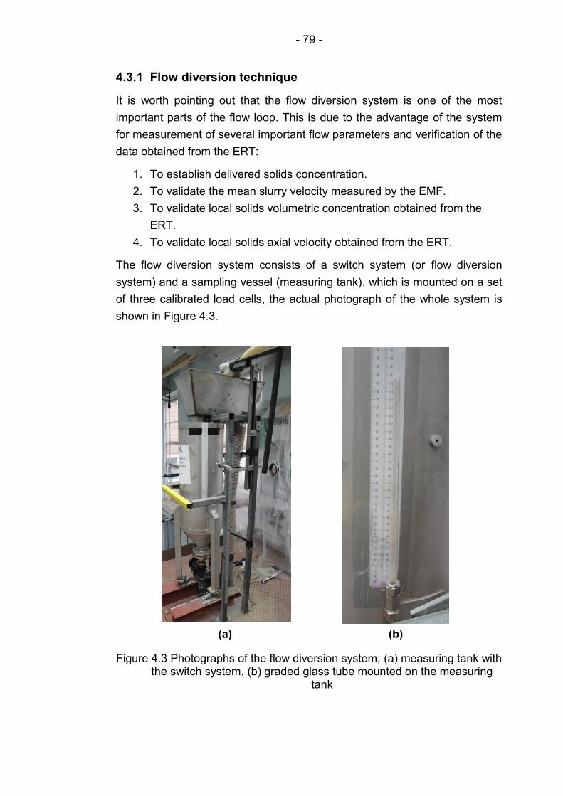
- 79 -
4.3.1 Flow diversion technique
It is worth pointing out that the flow diversion system is one of the most
important parts of the flow loop. This is due to the advantage of the system
for measurement of several important flow parameters and verification of the
data obtained from the ERT:
1. To establish delivered solids concentration.
2. To validate the mean slurry velocity measured by the EMF.
3. To validate local solids volumetric concentration obtained from the
ERT.
4. To validate local solids axial velocity obtained from the ERT.
The flow diversion system consists of a switch system (or flow diversion
system) and a sampling vessel (measuring tank), which is mounted on a set
of three calibrated load cells, the actual photograph of the whole system is
shown in Figure 4.3.
(a) (b)
Figure 4.3 Photographs of the flow diversion system, (a) measuring tank with the switch system, (b) graded glass tube mounted on the measuring
tank
- 80 -
The flow switch system is coupled to the sampling vessel at the exit of the
flow loop, through which the slurry would return to the mixing tank in a
routine fashion. The bottom of the vessel has a conical shape, so as to
facilitate the sliding of the solid particles at the bottom once the discharge
valve is opened for the slurry to be placed back into the mixing tank. The
flow diversion system was connected to the mixing tank through 100 mm
uPVC pipe. In order to measure mean slurry velocity or delivered solids
concentration, the flow is diverted to the sampling vessel for any given
length of time. Obviously, during the diversion process, the valve at the
outlet of the vessel has to be closed. A level graded glass tube was also
mounted on the measuring vessel, through which the diverted slurry level
could be monitored and measured. An electronic stop watch is used to
measure the duration for which the flow is diverted. However, a great effort
should be made to carry out the diversion process within a possible shortest
time. This is due to two reasons, firstly so as to avoid settling solid particles
at the bottom of the vessel, which could be a potential risk for blockage at
the discharge point of the sampling vessel. Secondly, removing a given
amount of slurry from the system would result in decreasing the suction
head of the pump, which precipitate the instability of the flow. The procedure
is to divert the slurry and allow a sufficient time for the slurry to reach a
certain level, somewhere 50% of the measuring tank. Then switch the flow
back to the mixing tank and record the slurry level and the duration of the
diversion. As the cross-section area of the measuring tank was known, then
the volume of the diverted slurry could be determined as well as the flow
rate. After several seconds of diverting the flow to the measuring tank, it was
noticed that the velocity shown on the Electromagnetic Flow meter (EMF)
was gradually dropping. Therefore, the reading of the Electromagnetic Flow
meter was recorded just before the slurry diversion. Although it was noticed
that the EMF readings were slightly fluctuating, the velocity shown of the
EMF just before the diversion was considered for the comparison process.
As slurry flow is quite complex by nature, then this fluctuation is well
expected. Both mean volumetric concentration and mean solids velocity
from the ERT and the flow diversion technique was then collected for the
comparison, as shown in the calibration section 4.5. It is worth mentioning
that the validation of the local concentration using this technique could not
be applied for all transport velocities, particularly low velocities, in horizontal
flow, due to phenomenon of particle deposition at lower velocities. As at
higher transport velocities the local concentration at any section of the flow
loop is more or less the same. Therefore, the local concentration in
- 81 -
horizontal flow was validated only for flow of high transport velocities (4 m/s
and above). On the other hand, as the slip velocity can totally be ignored for
the slurry flowing through the vertical test section, the validation of in-situ
solids volumetric concentration in the vertical line can be carried out using
flow diversion technique.
4.3.2 High performance ERT system
The full ERT system was in house built (Online Instrumentation
Laboratory/University of Leeds/UK). The main ERT system (Data Acquisition
Hardware), this study employs a Fast Impedance Camera system (FICA) (or
a high performance dual-plane electrical impedance tomography system),
the software and hardware of which have been enhanced and consolidated
by OLIL group (Online Instrumentation Laboratory/University of Leeds). It is
worth pointing out that one of the advantages of this system is the efficiency
of the hardware and simplicity of the operation of the control software. The
principle of the hardware operating system and the operation of the control
software is described in detail in Schlaberg et al. (2008).This development of
the conventional EIT system could be considered as a response to the
requirement of many industrial processes such as two/multiphase flow,
where a higher (faster) frame rates is required to measure and monitor the
flow behaviour. The Data Acquisition System (DAS) is based on the phase
sensitive demodulation and both the amplitude and the phase of the
measurement can be obtained. Once the system is connected it allows the
Data Acquisition System to operate in two modes, continuous (on-line) and
block mode.
In continuous mode, a single frame of data for one or two planes is acquired,
captured, transferred and displayed in the selected format. This mode can
capture data at a frame rate up to 50 dual-frames per second (dfps), which is
equivalent to 20 ms; whereas block mode can capture data up to 8000
frames at a rate up to 1000 dfps. At the end of acquisition of each data
block, it is then transferred and read by the PC, where it is processed and
can be visualised or saved on an external hard drive for later analysis.
4.3.3 Visualisation and image reconstruction scheme
The ERT technique can also provide a visual result from the tomograms
produced by the system. Each tomogram contains important information on
the cross sectional distribution of constituent phases. For example, the
conductivity of the domain or concentration of each phase (solid or liquid)
can easily be determined on the tomograms. The time taken to construct an
- 82 -
image (tomogram) and its resolution, depend primarily on the type of
algorithm used. The image reconstruction system can produce images for
both amplitude and phase of the domain, by using one of the versions of
Linear Back Projection (LBP) algorithm, which is called Sensitivity Back
Projection (SBP) algorithm. The reconstruction algorithm (SBP) can provide
further option of displaying images for real and imaginary part. In this study
an alternating current of 15 mA with a frequency of 9600 Hz was injected.
After mapping the conductivity of the media through each plane, the
conductivity data was converted into the local concentration distribution
using Maxwell relationship. Then the signals of the two planes were cross-
correlated, using pixel-to-pixel correlation, to estimate the solids axial
velocity profile. The principle of cross-correlation is described in section
3.2.4. The cross-correlation method, pixel-to-pixel, have been used in a
number of previous studies such as Etuke and Bonnecaze (1998), Lucas et
al. (1999), Mosorov et al. (2002), Wang et al. (2003), Henningsson et al.
(2006). Furthermore, clear PVC sections are included into both test sections,
in order to allow for visual observation of the flow, along with capturing
photographs via a digital camera.
4.3.3.1 Maxwell relationship and solids concentration
The averaged concentration profile can be used to determine the distribution
of the solid particles across the pipe cross section. The averaged
concentration profile is obtained via measuring the voltage at the sensor
location to determine the conductivity of the media. The conductivity is then
converted to concentration based on Maxwell relationship (1881). The local
conductivity value of each pixel can be converted to a solids concentration.
Conductivity conversion to solids concentration is described in section 3.4.8.
4.3.4 The dual-plane ERT sensor
The dual-plane ERT sensor was in house built (Online Instrumentation
Laboratory/University of Leeds/UK). The actual photograph of the dual plane
ERT sensor is illustrated in Figure 4.4.
The ERT sensor was conFigured as a dual plane sensor in order to apply
cross-correlation and measure the local axial velocity of the dispersed
phase. The distance between the electrodes of one plane to the other plane
was 70 mm. 16 stainless steel electrodes were mounted on the periphery of
each plane at equal interval, flush with the inner surface of the pipe, where
non-intrusively in contact with the media. The configuration of the electrodes
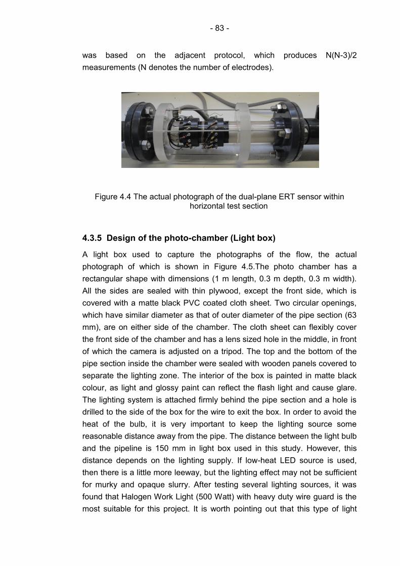
- 83 -
was based on the adjacent protocol, which produces N(N-3)/2
measurements (N denotes the number of electrodes).
Figure 4.4 The actual photograph of the dual-plane ERT sensor within horizontal test section
4.3.5 Design of the photo-chamber (Light box)
A light box used to capture the photographs of the flow, the actual
photograph of which is shown in Figure 4.5.The photo chamber has a
rectangular shape with dimensions (1 m length, 0.3 m depth, 0.3 m width).
All the sides are sealed with thin plywood, except the front side, which is
covered with a matte black PVC coated cloth sheet. Two circular openings,
which have similar diameter as that of outer diameter of the pipe section (63
mm), are on either side of the chamber. The cloth sheet can flexibly cover
the front side of the chamber and has a lens sized hole in the middle, in front
of which the camera is adjusted on a tripod. The top and the bottom of the
pipe section inside the chamber were sealed with wooden panels covered to
separate the lighting zone. The interior of the box is painted in matte black
colour, as light and glossy paint can reflect the flash light and cause glare.
The lighting system is attached firmly behind the pipe section and a hole is
drilled to the side of the box for the wire to exit the box. In order to avoid the
heat of the bulb, it is very important to keep the lighting source some
reasonable distance away from the pipe. The distance between the light bulb
and the pipeline is 150 mm in light box used in this study. However, this
distance depends on the lighting supply. If low-heat LED source is used,
then there is a little more leeway, but the lighting effect may not be sufficient
for murky and opaque slurry. After testing several lighting sources, it was
found that Halogen Work Light (500 Watt) with heavy duty wire guard is the
most suitable for this project. It is worth pointing out that this type of light
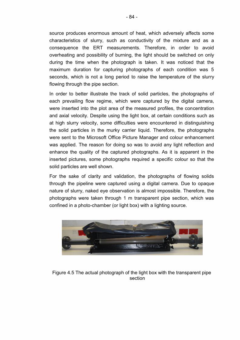
- 84 -
source produces enormous amount of heat, which adversely affects some
characteristics of slurry, such as conductivity of the mixture and as a
consequence the ERT measurements. Therefore, in order to avoid
overheating and possibility of burning, the light should be switched on only
during the time when the photograph is taken. It was noticed that the
maximum duration for capturing photographs of each condition was 5
seconds, which is not a long period to raise the temperature of the slurry
flowing through the pipe section.
In order to better illustrate the track of solid particles, the photographs of
each prevailing flow regime, which were captured by the digital camera,
were inserted into the plot area of the measured profiles, the concentration
and axial velocity. Despite using the light box, at certain conditions such as
at high slurry velocity, some difficulties were encountered in distinguishing
the solid particles in the murky carrier liquid. Therefore, the photographs
were sent to the Microsoft Office Picture Manager and colour enhancement
was applied. The reason for doing so was to avoid any light reflection and
enhance the quality of the captured photographs. As it is apparent in the
inserted pictures, some photographs required a specific colour so that the
solid particles are well shown.
For the sake of clarity and validation, the photographs of flowing solids
through the pipeline were captured using a digital camera. Due to opaque
nature of slurry, naked eye observation is almost impossible. Therefore, the
photographs were taken through 1 m transparent pipe section, which was
confined in a photo-chamber (or light box) with a lighting source.
Figure 4.5 The actual photograph of the light box with the transparent pipe section
- 85 -
4.4 Experimental procedure and operating conditions
In order to fulfil the objectives of this study, it is paramount to establish an
effective, comprehensive and flexible strategy for each measurement test
carried out on slurry flow. Since the aim is to investigate the applicability of
the ERT on slurry flow and the effects on measurement scheme, the effect
of different variables on slurry characteristics, thus the choice of slurry
components and the techniques used to measure each parameter
accurately merit special considerations.
4.4.1 Slurry component selection and characterisation
Prior to the selection of the components of the slurry that is be under
investigation, several characteristics of the solid particles have to be
considered. Also, a careful decision has to be made to satisfy the objectives
of this research. These could include particle density, particle size and
shape, solubility, electrical properties, cost, safety and availability.
Since settling slurries exist, in nature and industry, in different sizes and
shapes, therefore a uniform sized and shaped particle will be avoided in this
study. It was decided to select particles that approach the real industrial
scenario. Thoughts have been given to the mineral compounds, as they are
widely encountered in nature and industry. Based on the above
considerations, Glass sand (SiO2) was found to be the most suitable solid
component of the slurry in this study. This is due to the advantages listed
below:
1. Available in various sizes and shapes.
2. Cheap, (£60)/ton.
3. Non-harmful in case of exposure. Except the dust, for which the
protectors will be used, such as goggles and mask.
4. Insoluble in water.
5. Non-conductive that makes it suitable for the ERT measurements.
6. Suitable density (2650 kg/m3).
Since this study uses a system that handles a large amount of slurry, tap
water was decided to be used as carrier liquid. Besides some other
advantages, which are listed below, makes water the most suitable carrier
liquid.
1. Water is a safe compound.
2. Availability.
3. It can easily be drained without breaching any governmental policy.
- 86 -
4. Good conductivity that makes it a suitable carrier liquid for the ERT
measurements.
5. Suitable density and viscosity.
Thus the slurry used in this study consists of a mixture of water and a non-
uniform shape and size sand with density of 2650 kg/m³. However, based on
the objectives and the applicability of the methods used in this study, also in
order to determine the influence of particle size and solids concentration on
the measurement scheme, two sands were proposed, medium and coarse
sand. Furthermore, the settling characteristics are the most important
aspect of this study, which can easily be achieved with medium and coarse
sand. On the other hand, two throughput concentrations, 2% (v/v) and 10%
(v/v), were proposed for each of the sands to be used in the experiments.
4.4.1.1 Sand particle size analysis
The particle size distribution (PSD) for the two sands was obtained, by
taking the sample and oven-dried to achieve each 500 g of dried sand.
Sieving method was used, they were then sieved, using a laboratory test
sieve, through a series of sieves of standard mesh size (2360, 1180, 600,
300, 150 and 75 µm). The sample fraction obtained in each sieve was
weighted on a (Fisher brand, Model PF-6001) balance, ensuring that the
final mass measured for each sieve is within 100% of the total solids put
through. The fraction by mass was then recalculated to obtain a percentage
of oversized particles that cumulated in each sieve. The results of these
calculations are shown in Tables 1.1 and 1.2 for the both sands. The result
was then plotted against the sieve mesh size to generate a particle size
distribution curve, as shown in Figure 4.6.
Using the particle size distribution curve, various important statistics were
found. It was concluded that sand 1 has a particle size range with d85 = 430
µm, median particle size (d50) of 242 µm and d15 = 170 µm. Based on the
above analysis, sand 1 can be classified as medium quite broadly graded
sand. With regard to sand 2, it was found that d85 of which is 2240 µm, d50 is
480 µm and d15 is 270 µm. Therefore, sand 2 can be classified as coarse
broadly graded sand.
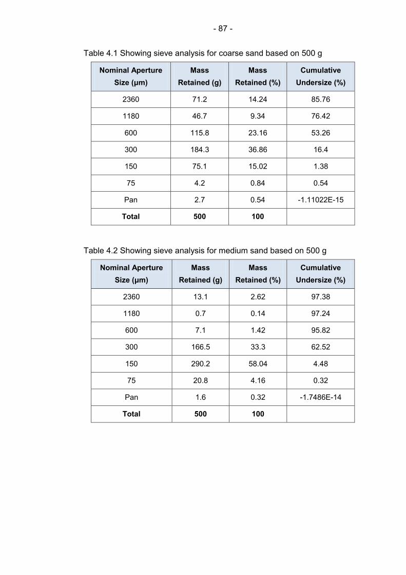
- 87 -
Table 4.1 Showing sieve analysis for coarse sand based on 500 g
Nominal Aperture
Size (μm)
Mass
Retained (g)
Mass
Retained (%)
Cumulative
Undersize (%)
2360 71.2 14.24 85.76
1180 46.7 9.34 76.42
600 115.8 23.16 53.26
300 184.3 36.86 16.4
150 75.1 15.02 1.38
75 4.2 0.84 0.54
Pan 2.7 0.54 -1.11022E-15
Total 500 100
Table 4.2 Showing sieve analysis for medium sand based on 500 g
Nominal Aperture
Size (μm)
Mass
Retained (g)
Mass
Retained (%)
Cumulative
Undersize (%)
2360 13.1 2.62 97.38
1180 0.7 0.14 97.24
600 7.1 1.42 95.82
300 166.5 33.3 62.52
150 290.2 58.04 4.48
75 20.8 4.16 0.32
Pan 1.6 0.32 -1.7486E-14
Total 500 100

- 88 -
Figure 4.6 Showing the particle size distribution curve for the two sands
4.4.1.2 Density estimation of sand particles
Since the density of solid particles flowing through a pipeline affects solids
settling characteristics and the pressure drop, therefore, the measurement of
particle density is very important.
A pycnometric method was employed to determine the density of each of the
sand used in the experiments. A pycnometer is a pre-calibrated glass bottle,
which is used to determine a volume of dry solid particles of known weight.
Initially the weight of empty and dry pycnometer was determined. The
pycnometer was then filled (by 1/3 volume) with the desired sand particles
and the total weight (Pycnometer and sand particles) was estimated. While
the pycnometer contained sand particles, it was filled with distilled water.
After completely emptying the pycnometer, it was then filled with only
distilled water and the weight was determined. As the total volume of the
pycnometer is known, then the volume of added water and full water in the
pycnometer can easily be calculated. The volume of added water can be
calculated theoretically (ratio of weight of added water and its known
density). On the other hand, the volume of sand particles is the difference
between the volume of water in the pycnometer, while containing sand
particles, and the volume of only water in the pycnometer. Finally, the
density of solid particles can be estimated through its known weight and
calculated volume. The density of sand 1 and sand 2 was found to be 2650
kg/m3.
0
10
20
30
40
50
60
70
80
90
100
0 400 800 1200 1600 2000 2400 2800
Cu
mu
lati
ve
Un
de
rsiz
e (
%)
Nominal Aperture Size (µm)
Coarse
Medium
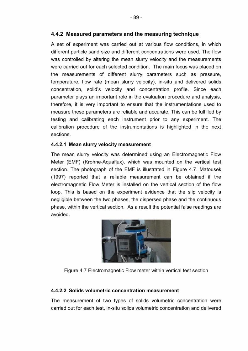
- 89 -
4.4.2 Measured parameters and the measuring technique
A set of experiment was carried out at various flow conditions, in which
different particle sand size and different concentrations were used. The flow
was controlled by altering the mean slurry velocity and the measurements
were carried out for each selected condition. The main focus was placed on
the measurements of different slurry parameters such as pressure,
temperature, flow rate (mean slurry velocity), in-situ and delivered solids
concentration, solid’s velocity and concentration profile. Since each
parameter plays an important role in the evaluation procedure and analysis,
therefore, it is very important to ensure that the instrumentations used to
measure these parameters are reliable and accurate. This can be fulfilled by
testing and calibrating each instrument prior to any experiment. The
calibration procedure of the instrumentations is highlighted in the next
sections.
4.4.2.1 Mean slurry velocity measurement
The mean slurry velocity was determined using an Electromagnetic Flow
Meter (EMF) (Krohne-Aquaflux), which was mounted on the vertical test
section. The photograph of the EMF is illustrated in Figure 4.7. Matousek
(1997) reported that a reliable measurement can be obtained if the
electromagnetic Flow Meter is installed on the vertical section of the flow
loop. This is based on the experiment evidence that the slip velocity is
negligible between the two phases, the dispersed phase and the continuous
phase, within the vertical section. As a result the potential false readings are
avoided.
Figure 4.7 Electromagnetic Flow meter within vertical test section
4.4.2.2 Solids volumetric concentration measurement
The measurement of two types of solids volumetric concentration were
carried out for each test, in-situ solids volumetric concentration and delivered
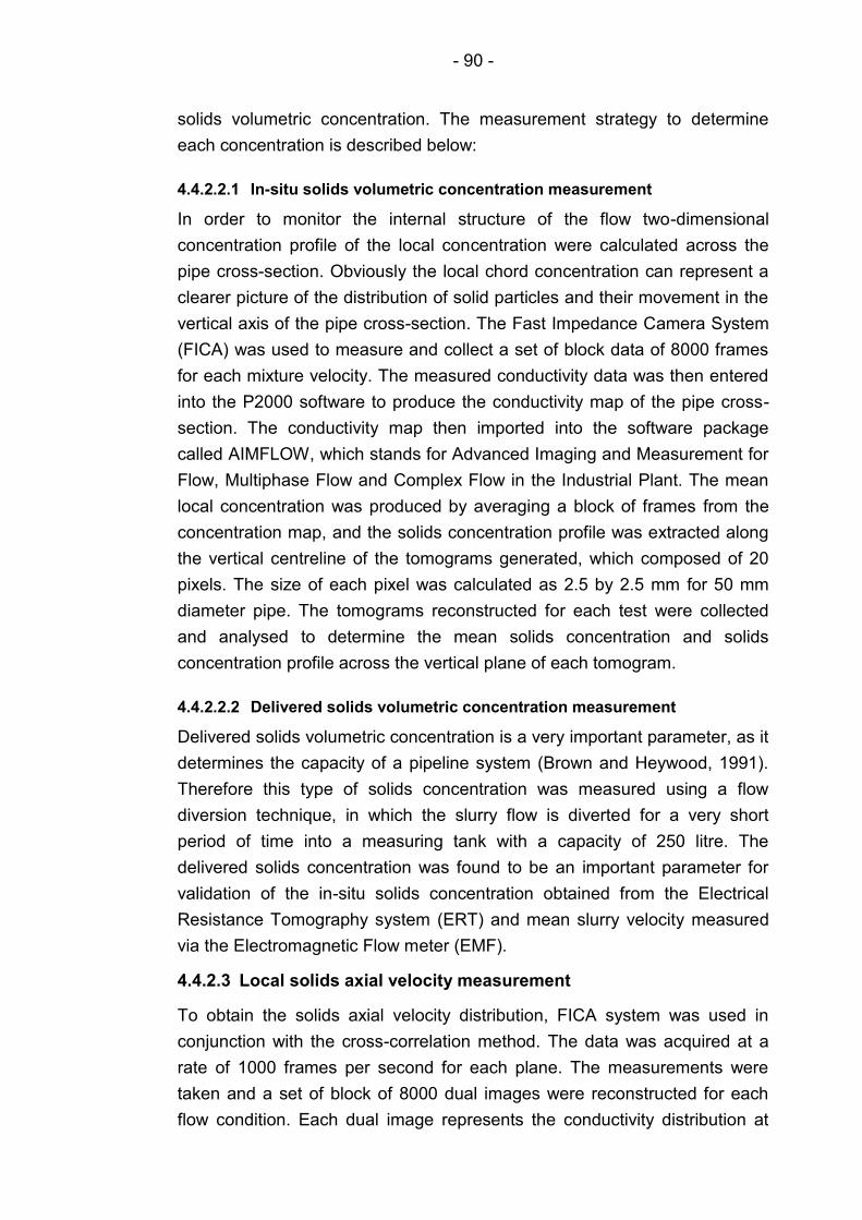
- 90 -
solids volumetric concentration. The measurement strategy to determine
each concentration is described below:
4.4.2.2.1 In-situ solids volumetric concentration measurement
In order to monitor the internal structure of the flow two-dimensional
concentration profile of the local concentration were calculated across the
pipe cross-section. Obviously the local chord concentration can represent a
clearer picture of the distribution of solid particles and their movement in the
vertical axis of the pipe cross-section. The Fast Impedance Camera System
(FICA) was used to measure and collect a set of block data of 8000 frames
for each mixture velocity. The measured conductivity data was then entered
into the P2000 software to produce the conductivity map of the pipe cross-
section. The conductivity map then imported into the software package
called AIMFLOW, which stands for Advanced Imaging and Measurement for
Flow, Multiphase Flow and Complex Flow in the Industrial Plant. The mean
local concentration was produced by averaging a block of frames from the
concentration map, and the solids concentration profile was extracted along
the vertical centreline of the tomograms generated, which composed of 20
pixels. The size of each pixel was calculated as 2.5 by 2.5 mm for 50 mm
diameter pipe. The tomograms reconstructed for each test were collected
and analysed to determine the mean solids concentration and solids
concentration profile across the vertical plane of each tomogram.
4.4.2.2.2 Delivered solids volumetric concentration measurement
Delivered solids volumetric concentration is a very important parameter, as it
determines the capacity of a pipeline system (Brown and Heywood, 1991).
Therefore this type of solids concentration was measured using a flow
diversion technique, in which the slurry flow is diverted for a very short
period of time into a measuring tank with a capacity of 250 litre. The
delivered solids concentration was found to be an important parameter for
validation of the in-situ solids concentration obtained from the Electrical
Resistance Tomography system (ERT) and mean slurry velocity measured
via the Electromagnetic Flow meter (EMF).
4.4.2.3 Local solids axial velocity measurement
To obtain the solids axial velocity distribution, FICA system was used in
conjunction with the cross-correlation method. The data was acquired at a
rate of 1000 frames per second for each plane. The measurements were
taken and a set of block of 8000 dual images were reconstructed for each
flow condition. Each dual image represents the conductivity distribution at
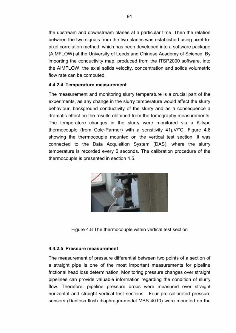
- 91 -
the upstream and downstream planes at a particular time. Then the relation
between the two signals from the two planes was established using pixel-to-
pixel correlation method, which has been developed into a software package
(AIMFLOW) at the University of Leeds and Chinese Academy of Science. By
importing the conductivity map, produced from the ITSP2000 software, into
the AIMFLOW, the axial solids velocity, concentration and solids volumetric
flow rate can be computed.
4.4.2.4 Temperature measurement
The measurement and monitoring slurry temperature is a crucial part of the
experiments, as any change in the slurry temperature would affect the slurry
behaviour, background conductivity of the slurry and as a consequence a
dramatic effect on the results obtained from the tomography measurements.
The temperature changes in the slurry were monitored via a K-type
thermocouple (from Cole-Parmer) with a sensitivity 41µV/°C. Figure 4.8
showing the thermocouple mounted on the vertical test section. It was
connected to the Data Acquisition System (DAS), where the slurry
temperature is recorded every 5 seconds. The calibration procedure of the
thermocouple is presented in section 4.5.
Figure 4.8 The thermocouple within vertical test section
4.4.2.5 Pressure measurement
The measurement of pressure differential between two points of a section of
a straight pipe is one of the most important measurements for pipeline
frictional head loss determination. Monitoring pressure changes over straight
pipelines can provide valuable information regarding the condition of slurry
flow. Therefore, pipeline pressure drops were measured over straight
horizontal and straight vertical test sections. Four pre-calibrated pressure
sensors (Danfoss flush diaphragm-model MBS 4010) were mounted on the
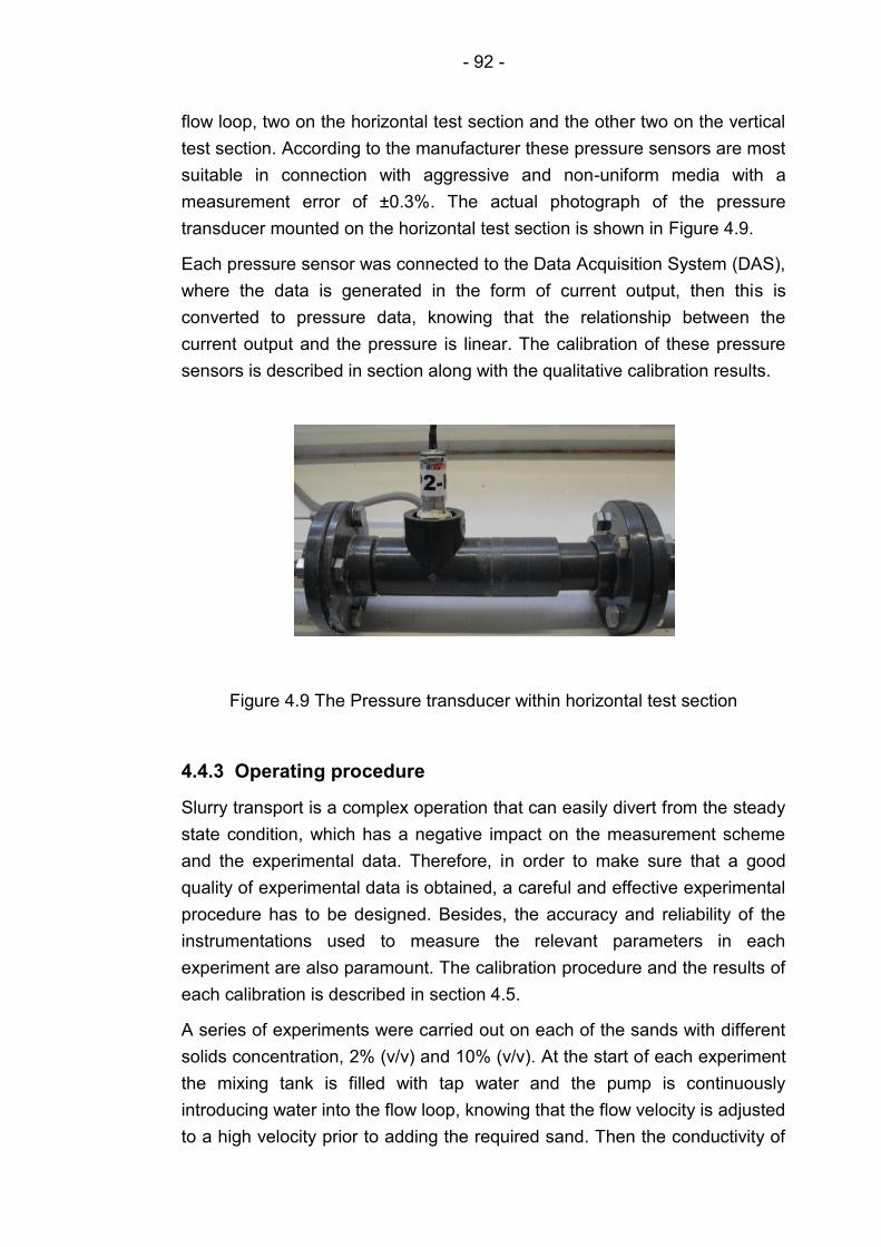
- 92 -
flow loop, two on the horizontal test section and the other two on the vertical
test section. According to the manufacturer these pressure sensors are most
suitable in connection with aggressive and non-uniform media with a
measurement error of ±0.3%. The actual photograph of the pressure
transducer mounted on the horizontal test section is shown in Figure 4.9.
Each pressure sensor was connected to the Data Acquisition System (DAS),
where the data is generated in the form of current output, then this is
converted to pressure data, knowing that the relationship between the
current output and the pressure is linear. The calibration of these pressure
sensors is described in section along with the qualitative calibration results.
Figure 4.9 The Pressure transducer within horizontal test section
4.4.3 Operating procedure
Slurry transport is a complex operation that can easily divert from the steady
state condition, which has a negative impact on the measurement scheme
and the experimental data. Therefore, in order to make sure that a good
quality of experimental data is obtained, a careful and effective experimental
procedure has to be designed. Besides, the accuracy and reliability of the
instrumentations used to measure the relevant parameters in each
experiment are also paramount. The calibration procedure and the results of
each calibration is described in section 4.5.
A series of experiments were carried out on each of the sands with different
solids concentration, 2% (v/v) and 10% (v/v). At the start of each experiment
the mixing tank is filled with tap water and the pump is continuously
introducing water into the flow loop, knowing that the flow velocity is adjusted
to a high velocity prior to adding the required sand. Then the conductivity of
- 93 -
water and its temperature is recorded, this will then be required for the ERT
reference measurement. The pre-weighed desired sand is added into the
mixing tank after switching on the mixer and adjusting the desired rotational
speed. It is worth mentioning that while the sand is added into the mixing
tank, the valve at the discharge point of the mixing tank is closed and the
valve on the flush line is opened. This procedure would ensure continuous
flow into the loop through the flush line. After adding the sand to the water,
the slurry was initially well agitated in the holding tank so as to achieve a
homogeneous mixture. The slurry was then introduced to the flow loop via
the centrifugal pump from the mixing tank. The average superficial velocities
were in the range of 1.5-5- m/s. The slurry flow was first established at the
highest velocity of the pump, which was controlled via the digi-drive
frequency converter, then reduced gradually from 5 m/s to 1.5 m/s. The
reason for that was to cover all the flow regimes. However, this aim could
not be attained for pseudo-homogeneous flow regime, particularly 10% (v/v)
coarse sand, due to the limitations imposed by the pump capacity. Particular
attention was paid to carry out every test at the steady state condition,
through observing the fluctuation of pressure data via pressure graphs on
the LabVIEW panel. For each condition and different sand with different
concentration the ERT measurements were carried out using the Fast
Impedance Camera System (FICA) by mapping the conductivity of the
media under investigation. A digital camera was used to capture the
photographs of the flow through the transparent pipe section confined in the
light box. Since the photographic images of the flow are used to validate the
flow regime visualisation, then it is very important to capture the photographs
at the same time of the ERT measurement. After each ERT measurement
and capturing photographs, the discharge measurements or flow diversion
technique was performed, by diverting the flow to the measuring tank for a
very short period of time, and then the level of the contents through the glass
tube and its weight using the load cells were recorded. As previously
mentioned, the diversion technique is a potential cause for flow instability,
therefore, after diverting the slurry and returning it into the flow loop, a short
period of time is required to ensure the steady state flow condition.
Thereafter the next measurement test can be carried out as per previous
procedure. Each test carried out for the horizontal flow was followed by the
vertical flow measurement. All the measured data then collected via the
LabVIEW and processed for future analysis.
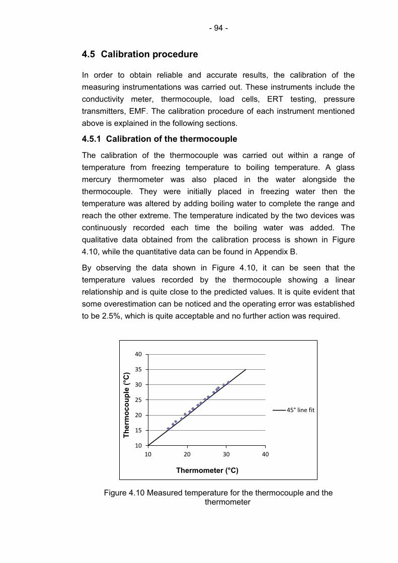
- 94 -
4.5 Calibration procedure
In order to obtain reliable and accurate results, the calibration of the
measuring instrumentations was carried out. These instruments include the
conductivity meter, thermocouple, load cells, ERT testing, pressure
transmitters, EMF. The calibration procedure of each instrument mentioned
above is explained in the following sections.
4.5.1 Calibration of the thermocouple
The calibration of the thermocouple was carried out within a range of
temperature from freezing temperature to boiling temperature. A glass
mercury thermometer was also placed in the water alongside the
thermocouple. They were initially placed in freezing water then the
temperature was altered by adding boiling water to complete the range and
reach the other extreme. The temperature indicated by the two devices was
continuously recorded each time the boiling water was added. The
qualitative data obtained from the calibration process is shown in Figure
4.10, while the quantitative data can be found in Appendix B.
By observing the data shown in Figure 4.10, it can be seen that the
temperature values recorded by the thermocouple showing a linear
relationship and is quite close to the predicted values. It is quite evident that
some overestimation can be noticed and the operating error was established
to be 2.5%, which is quite acceptable and no further action was required.
Figure 4.10 Measured temperature for the thermocouple and the thermometer
10
15
20
25
30
35
40
10 20 30 40
Th
erm
oco
up
le (
°C)
Thermometer (°C)
45° line fit

- 95 -
4.5.2 Calibration of pressure transducers
The calibration of the two pressure transducers mounted on the horizontal
line, H1 and H2, and the two pressure transducers mounted on the vertical
line, V1 and V2, were carried by recording static pressure against actual
values. A long vertical pipe (5 m) was used, on which each pressure
transducer could easily be mounted at the lower part of the pipe. The actual
pressure (ρgh) was calculated at different level of water in the pipe. For
each level the pressure was also recorded by the pressure transducers via
LabVIEW software. The calculated actual pressure and the response of
each pressure transducer, which was recorded via LabVIEW, are shown in
Figure 4.11. A linear relationship can be noticed for each sensor, which
confirms the functionality of the each pressure transducer. However, some
deviations from the line fit can be seen for each transducer. The amount by
which each transducer deviates was calculated and added to the reading of
each transducer in the LabVIEW software. After correcting each pressure
transducer, another calibration was then performed, the results of which is
shown in Figure 4.12. The corrected and uncorrected data obtained from the
calibration processes can be found in Appendix B. The observation of the
corrected data can reveal a good line fit between all pressure transducers
and actual values.
Figure 4.11 The transducers pressure readings against actual values before correction
0
5
10
15
20
25
30
35
40
45
0 20 40 60
Tra
nsd
uc
er
Re
ad
ing
(k
Pa
)
Actual value (kPa)
Before correction
45° line fit
H1
H2
V1
V2
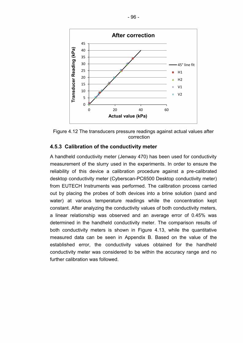
- 96 -
Figure 4.12 The transducers pressure readings against actual values after correction
4.5.3 Calibration of the conductivity meter
A handheld conductivity meter (Jenway 470) has been used for conductivity
measurement of the slurry used in the experiments. In order to ensure the
reliability of this device a calibration procedure against a pre-calibrated
desktop conductivity meter (Cyberscan-PC6500 Desktop conductivity meter)
from EUTECH Instruments was performed. The calibration process carried
out by placing the probes of both devices into a brine solution (sand and
water) at various temperature readings while the concentration kept
constant. After analyzing the conductivity values of both conductivity meters,
a linear relationship was observed and an average error of 0.45% was
determined in the handheld conductivity meter. The comparison results of
both conductivity meters is shown in Figure 4.13, while the quantitative
measured data can be seen in Appendix B. Based on the value of the
established error, the conductivity values obtained for the handheld
conductivity meter was considered to be within the accuracy range and no
further calibration was followed.
0
5
10
15
20
25
30
35
40
45
0 20 40 60
Tra
nsd
uc
er
Re
ad
ing
(k
Pa
)
Actual value (kPa)
After correction
45° line fit
H1
H2
V1
V2
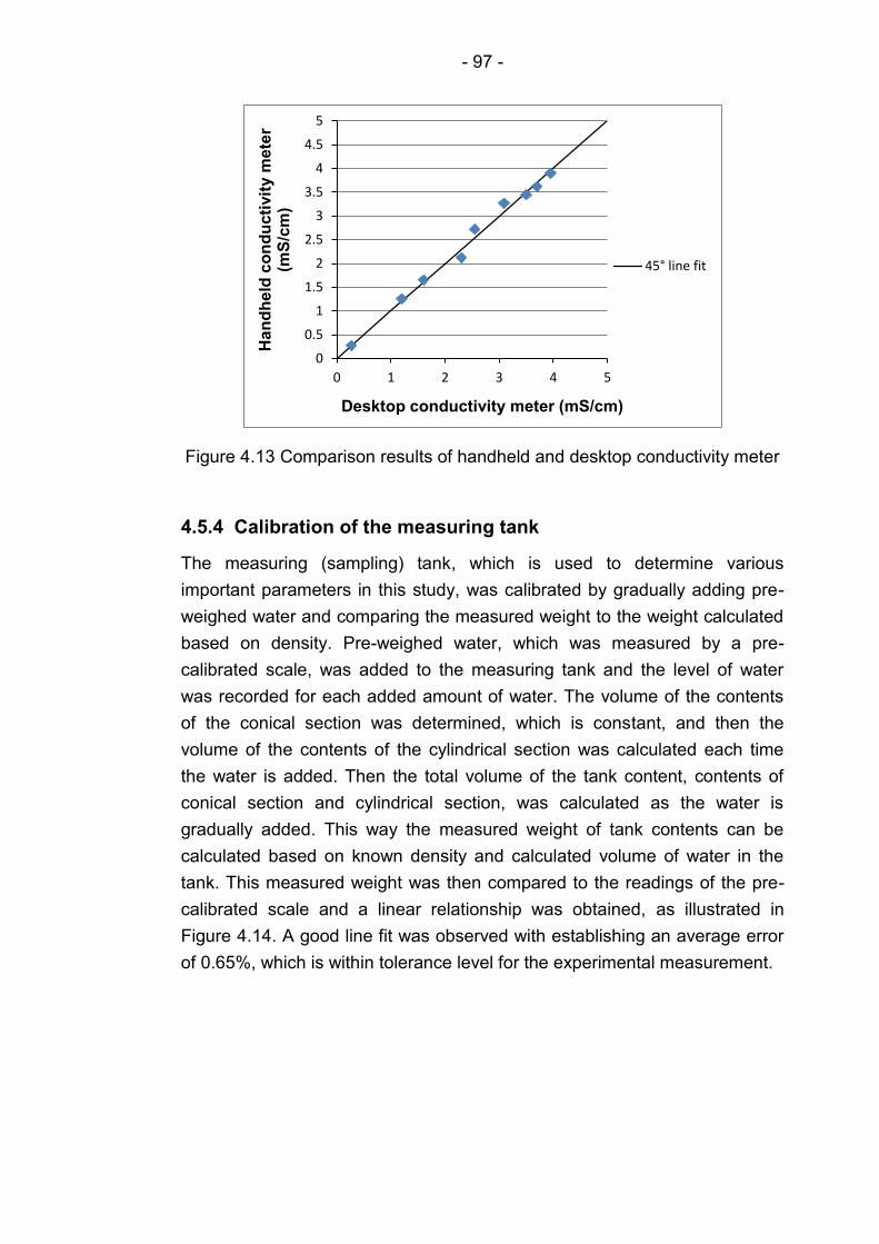
- 97 -
Figure 4.13 Comparison results of handheld and desktop conductivity meter
4.5.4 Calibration of the measuring tank
The measuring (sampling) tank, which is used to determine various
important parameters in this study, was calibrated by gradually adding pre-
weighed water and comparing the measured weight to the weight calculated
based on density. Pre-weighed water, which was measured by a pre-
calibrated scale, was added to the measuring tank and the level of water
was recorded for each added amount of water. The volume of the contents
of the conical section was determined, which is constant, and then the
volume of the contents of the cylindrical section was calculated each time
the water is added. Then the total volume of the tank content, contents of
conical section and cylindrical section, was calculated as the water is
gradually added. This way the measured weight of tank contents can be
calculated based on known density and calculated volume of water in the
tank. This measured weight was then compared to the readings of the pre-
calibrated scale and a linear relationship was obtained, as illustrated in
Figure 4.14. A good line fit was observed with establishing an average error
of 0.65%, which is within tolerance level for the experimental measurement.
0
0.5
1
1.5
2
2.5
3
3.5
4
4.5
5
0 1 2 3 4 5
Ha
nd
he
ld c
on
du
cti
vit
y m
ete
r (m
S/c
m)
Desktop conductivity meter (mS/cm)
45° line fit
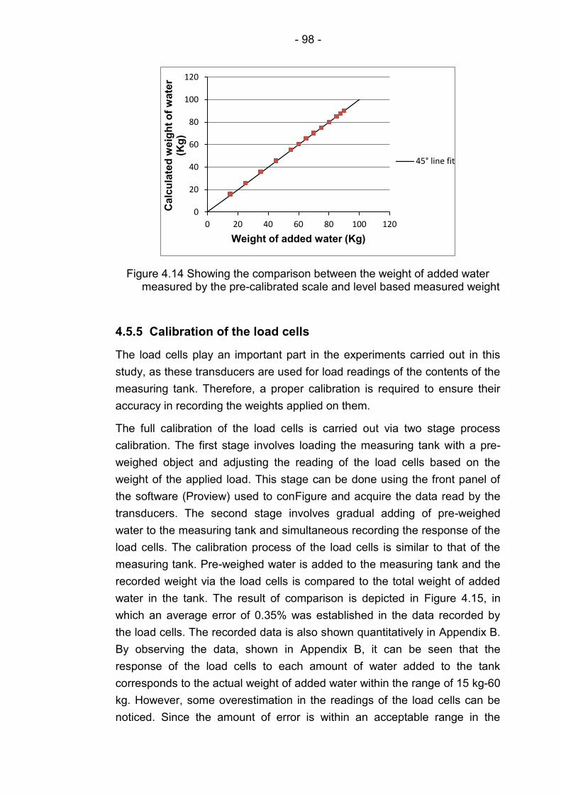
- 98 -
Figure 4.14 Showing the comparison between the weight of added water measured by the pre-calibrated scale and level based measured weight
4.5.5 Calibration of the load cells
The load cells play an important part in the experiments carried out in this
study, as these transducers are used for load readings of the contents of the
measuring tank. Therefore, a proper calibration is required to ensure their
accuracy in recording the weights applied on them.
The full calibration of the load cells is carried out via two stage process
calibration. The first stage involves loading the measuring tank with a pre-
weighed object and adjusting the reading of the load cells based on the
weight of the applied load. This stage can be done using the front panel of
the software (Proview) used to conFigure and acquire the data read by the
transducers. The second stage involves gradual adding of pre-weighed
water to the measuring tank and simultaneous recording the response of the
load cells. The calibration process of the load cells is similar to that of the
measuring tank. Pre-weighed water is added to the measuring tank and the
recorded weight via the load cells is compared to the total weight of added
water in the tank. The result of comparison is depicted in Figure 4.15, in
which an average error of 0.35% was established in the data recorded by
the load cells. The recorded data is also shown quantitatively in Appendix B.
By observing the data, shown in Appendix B, it can be seen that the
response of the load cells to each amount of water added to the tank
corresponds to the actual weight of added water within the range of 15 kg-60
kg. However, some overestimation in the readings of the load cells can be
noticed. Since the amount of error is within an acceptable range in the
0
20
40
60
80
100
120
0 20 40 60 80 100 120
Ca
lcu
late
d w
eig
ht
of
wa
ter
(Kg
)
Weight of added water (Kg)
45° line fit
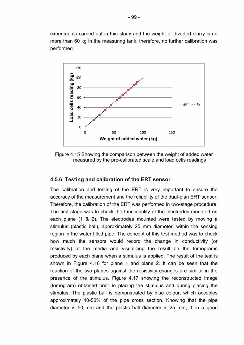
- 99 -
experiments carried out in this study and the weight of diverted slurry is no
more than 60 kg in the measuring tank, therefore, no further calibration was
performed.
Figure 4.15 Showing the comparison between the weight of added water measured by the pre-calibrated scale and load cells readings
4.5.6 Testing and calibration of the ERT sensor
The calibration and testing of the ERT is very important to ensure the
accuracy of the measurement and the reliability of the dual-plan ERT sensor.
Therefore, the calibration of the ERT was performed in two-stage procedure.
The first stage was to check the functionality of the electrodes mounted on
each plane (1 & 2). The electrodes mounted were tested by moving a
stimulus (plastic ball), approximately 25 mm diameter, within the sensing
region in the water filled pipe. The concept of this test method was to check
how much the sensors would record the change in conductivity (or
resistivity) of the media and visualizing the result on the tomograms
produced by each plane when a stimulus is applied. The result of the test is
shown in Figure 4.16 for plane 1 and plane 2. It can be seen that the
reaction of the two planes against the resistivity changes are similar in the
presence of the stimulus. Figure 4.17 showing the reconstructed image
(tomogram) obtained prior to placing the stimulus and during placing the
stimulus. The plastic ball is demonstrated by blue colour, which occupies
approximately 40-50% of the pipe cross section. Knowing that the pipe
diameter is 50 mm and the plastic ball diameter is 25 mm, then a good
0
20
40
60
80
100
120
0 50 100 150
Lo
ad
cell
s r
ea
din
g (
kg
)
Weight of added water (kg)
45° line fit
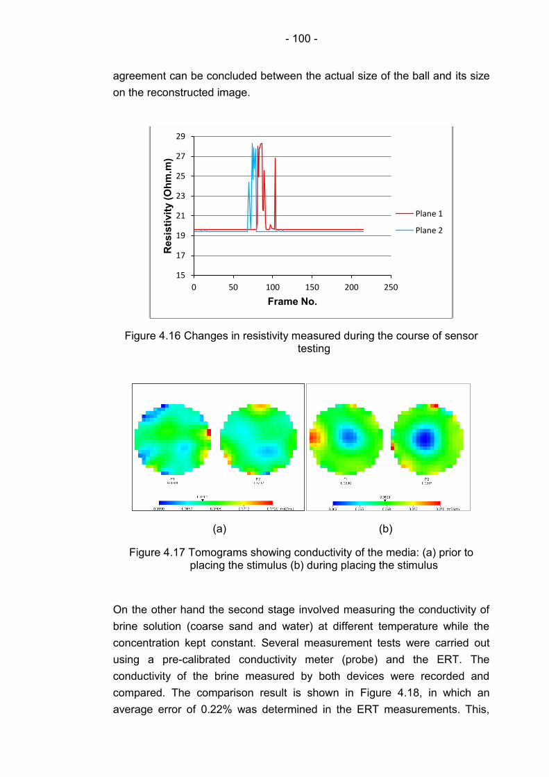
- 100 -
agreement can be concluded between the actual size of the ball and its size
on the reconstructed image.
Figure 4.16 Changes in resistivity measured during the course of sensor testing
(a) (b)
Figure 4.17 Tomograms showing conductivity of the media: (a) prior to placing the stimulus (b) during placing the stimulus
On the other hand the second stage involved measuring the conductivity of
brine solution (coarse sand and water) at different temperature while the
concentration kept constant. Several measurement tests were carried out
using a pre-calibrated conductivity meter (probe) and the ERT. The
conductivity of the brine measured by both devices were recorded and
compared. The comparison result is shown in Figure 4.18, in which an
average error of 0.22% was determined in the ERT measurements. This,
15
17
19
21
23
25
27
29
0 50 100 150 200 250
Re
sis
tivit
y (
Oh
m.m
)
Frame No.
Plane 1
Plane 2
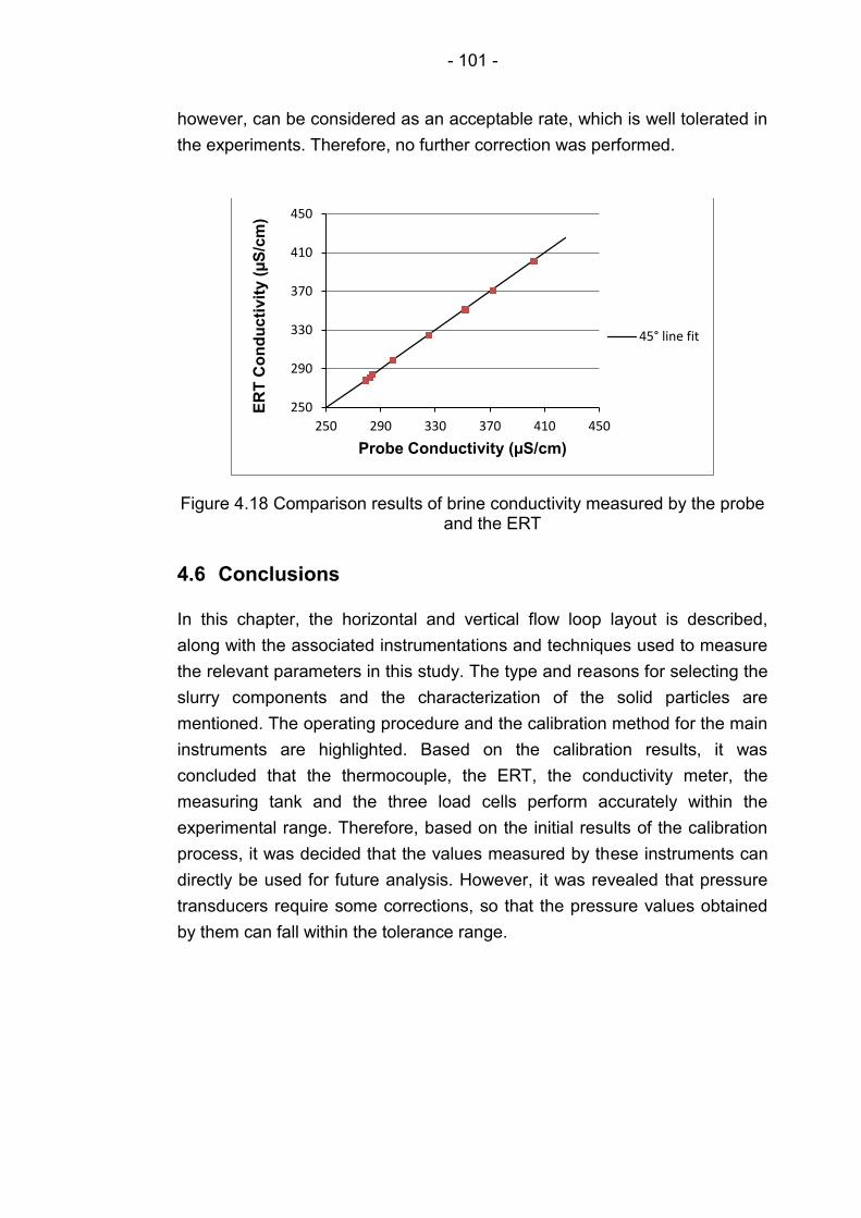
- 101 -
however, can be considered as an acceptable rate, which is well tolerated in
the experiments. Therefore, no further correction was performed.
Figure 4.18 Comparison results of brine conductivity measured by the probe and the ERT
4.6 Conclusions
In this chapter, the horizontal and vertical flow loop layout is described,
along with the associated instrumentations and techniques used to measure
the relevant parameters in this study. The type and reasons for selecting the
slurry components and the characterization of the solid particles are
mentioned. The operating procedure and the calibration method for the main
instruments are highlighted. Based on the calibration results, it was
concluded that the thermocouple, the ERT, the conductivity meter, the
measuring tank and the three load cells perform accurately within the
experimental range. Therefore, based on the initial results of the calibration
process, it was decided that the values measured by these instruments can
directly be used for future analysis. However, it was revealed that pressure
transducers require some corrections, so that the pressure values obtained
by them can fall within the tolerance range.
250
290
330
370
410
450
250 290 330 370 410 450
ER
T C
on
du
cti
vit
y (
µS
/cm
)
Probe Conductivity (µS/cm)
45° line fit
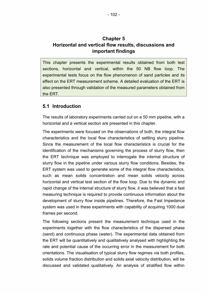
- 102 -
Chapter 5
Horizontal and vertical flow results, discussions and
important findings
This chapter presents the experimental results obtained from both test
sections, horizontal and vertical, within the 50 NB flow loop. The
experimental tests focus on the flow phenomenon of sand particles and its
effect on the ERT measurement scheme. A detailed evaluation of the ERT is
also presented through validation of the measured parameters obtained from
the ERT.
5.1 Introduction
The results of laboratory experiments carried out on a 50 mm pipeline, with a
horizontal and a vertical section are presented in this chapter.
The experiments were focused on the observations of both, the integral flow
characteristics and the local flow characteristics of settling slurry pipeline.
Since the measurement of the local flow characteristics is crucial for the
identification of the mechanisms governing the process of slurry flow, then
the ERT technique was employed to interrogate the internal structure of
slurry flow in the pipeline under various slurry flow conditions. Besides, the
ERT system was used to generate some of the integral flow characteristics,
such as mean solids concentration and mean solids velocity across
horizontal and vertical test section of the flow loop. Due to the dynamic and
rapid change of the internal structure of slurry flow, it was believed that a fast
measuring technique is required to provide continuous information about the
development of slurry flow inside pipelines. Therefore, the Fast Impedance
system was used in these experiments with capability of acquiring 1000 dual
frames per second.
The following sections present the measurement technique used in the
experiments together with the flow characteristics of the dispersed phase
(sand) and continuous phase (water). The experimental data obtained from
the ERT will be quantitatively and qualitatively analysed with highlighting the
rate and potential cause of the occurring error in the measurement for both
orientations. The visualisation of typical slurry flow regimes via both profiles,
solids volume fraction distribution and solids axial velocity distribution, will be
discussed and validated qualitatively. An analysis of stratified flow within
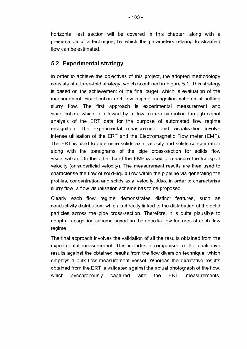
- 103 -
horizontal test section will be covered in this chapter, along with a
presentation of a technique, by which the parameters relating to stratified
flow can be estimated.
5.2 Experimental strategy
In order to achieve the objectives of this project, the adopted methodology
consists of a three-fold strategy, which is outlined in Figure 5.1. This strategy
is based on the achievement of the final target, which is evaluation of the
measurement, visualisation and flow regime recognition scheme of settling
slurry flow. The first approach is experimental measurement and
visualisation, which is followed by a flow feature extraction through signal
analysis of the ERT data for the purpose of automated flow regime
recognition. The experimental measurement and visualisation involve
intense utilisation of the ERT and the Electromagnetic Flow meter (EMF).
The ERT is used to determine solids axial velocity and solids concentration
along with the tomograms of the pipe cross-section for solids flow
visualisation. On the other hand the EMF is used to measure the transport
velocity (or superficial velocity). The measurement results are then used to
characterise the flow of solid-liquid flow within the pipeline via generating the
profiles, concentration and solids axial velocity. Also, in order to characterise
slurry flow, a flow visualisation scheme has to be proposed.
Clearly each flow regime demonstrates distinct features, such as
conductivity distribution, which is directly linked to the distribution of the solid
particles across the pipe cross-section. Therefore, it is quite plausible to
adopt a recognition scheme based on the specific flow features of each flow
regime.
The final approach involves the validation of all the results obtained from the
experimental measurement. This includes a comparison of the qualitative
results against the obtained results from the flow diversion technique, which
employs a bulk flow measurement vessel. Whereas the qualitative results
obtained from the ERT is validated against the actual photograph of the flow,
which synchronously captured with the ERT measurements.
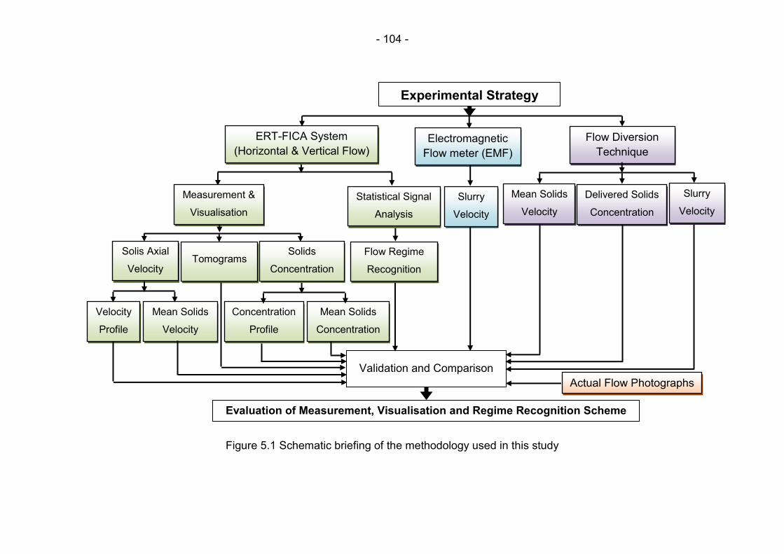
- 104 -
Figure 5.1 Schematic briefing of the methodology used in this study
Experimental Strategy
Electromagnetic
Flow meter (EMF)
ERT-FICA System
(Horizontal & Vertical Flow)
Flow Diversion
Technique
Validation and Comparison
Measurement &
Visualisation
Statistical Signal
Analysis
Slurry
Velocity
Slurry
Velocity
Mean Solids
Velocity
Delivered Solids
Concentration
Solis Axial
Velocity
Flow Regime
Recognition
Solids
Concentration
Concentration
Profile
Velocity
Profile
Evaluation of Measurement, Visualisation and Regime Recognition Scheme
Mean Solids
Velocity
Mean Solids
Concentration
Actual Flow Photographs
Tomograms

- 105 -
5.3 Material and test conditions
Slurry flow through horizontal and vertical test sections of the flow loop
shown in Figure 4.2 (Chapter 4) was studied. The loop consists of 50 mm
diameter uPVC pipeline, the details of which can be found in Chapter 4. The
material and test conditions are summarised in Table 5.1 shown below.
Table 5.1 A summary of material and test conditions used in the experiments
Slurry
Sand and tap water
ρwater= 998.2 kg/m3
ρsand= 2650 kg/m3
Particle size Medium sand (75-900 µm)
Coarse sand (150-2200 µm)
Throughput concentration 2%-10% (v/v)
Transport velocity 1.2-5.0 m/s
Pressure range 0.41-1.2 bar
Temperature range 20-28 °C
Pipeline uPVC, Class E 15 bar (50 mm ID)
The slurry consisted of a mixture of tap water and a non-uniform shape and
size sand with density of 2650 kg/m3. Two types of sand were used, medium
and coarse, with throughput concentration range 2%-10% (v/v) for each
type. The average superficial velocities were in the range of 1.2-5.0 m/s.
Transparent pipe sections were included into both, horizontal and vertical
test sections, as observation chambers, which would enable visual
observation of the motion of the solid particles within the pipeline and
capturing photographs. The slurry was first established at the highest
velocity, which was controlled via the Digi-drive frequency converter, then
reduced gradually from 5 m/s to 1.2 m/s, at which the pipeline blockage
occurred. The ERT measurements were carried out for each condition within
a temperature range of 20-28 °C. Each horizontal flow measurement
- 106 -
followed by a vertical flow measurement and flow diversion measurement.
Then the next measurement was carried out after allowing a sufficient time
for the flow to stabilise. Attempts were made to capture the photographs of
the flow at the same time of each ERT measurement. In order to reduce the
rate of error in the flow diversion measurement, three level measurements
were carried out, the average of which was then calculated against each
corresponding ERT measurement.
5.4 Horizontal flow measurement and visualisation
In order to visualise the internal structure of the flow, concentration profile of
the local concentration was calculated across the pipe cross section.
Obviously the local chord concentration can represent a clearer picture of
the distribution of solid particles and their movement in the vertical axis of
the pipe cross section. The Fast Impedance Camera System (FICA) was
used to measure and collect a set of block data of 8000 frames for each
mixture velocity. It was noticed that the FICA system can offer an excellent
speed in measuring the conductivity of the media and collecting the data.
The FICA system was developed by OLIL group at the University of Leeds
and is capable of measuring approximately 1000 dual frames per second,
which makes it one of the very fast instruments amongst others. This can be
considered as one of the primary advantage of the FICA system for
visualisation and measurement of slurry flow, due to dynamic and instability
of slurry flow over time. The measured conductivity data was then entered
into the P2000 software to produce the conductivity map of the pipe cross
section. The conductivity map then imported into the software package
called AIMFLOW, which stands for Advanced Imaging and Measurement for
Flow, Multiphase Flow and Complex Flow in the Industrial Plant. The mean
local concentration was produced by averaging a block of frames from the
concentration map, and the solids concentration profile was extracted along
the vertical centreline of the tomograms generated, which composed of 20
pixels. The size of each pixel was calculated as 2.5 by 2.5 mm for 50 mm
diameter pipe. The tomograms reconstructed for each test were collected
and analysed to determine the mean solids concentration and solids
concentration profile along with the mean solids axial velocity and solids
axial velocity distribution across the vertical plane of each tomogram.
- 107 -
5.4.1 Solid flow visualisation
Since the ERT provides an image reconstruction scheme, then it can be
used to monitor and visualise the internal structure of a pipe or a process.
The aim of the image reconstruction scheme is to compute a tomogram,
which is representing the electrical conductivity of the material flowing
through the pipe. In the case of slurry flow, in which the solid phase is
considered as dispersed phase, the value of in-situ solids volume fraction at
a given location in the pipe corresponds to the local mixture conductivity
using Maxwell relationship. It is worth mentioning that each measurement
data generated is interpreted by an image reconstruction algorithm, in order
to compute the cross-sectional image (tomogram) corresponding to the
electrical conductivity field within the pipe. The image reconstruction scheme
and the use of an appropriate algorithm are described in section 3.4.6. The
cross-sectional image or the tomogram provides valuable information, which
can readily be used for the purpose of visualisation. Flow visualisation using
tomograms may be beneficial to the operator in industry if certain flow
features are sought, such as bubbles, plug flow and formation of strata in
horizontal flow. However, for detailed qualitative evaluation, both profiles,
solids volumetric concentration and solids axial velocity, presented in the
following sections, may be the best tool. The tomograms reconstructed in
this study are used to monitor the distribution of sand particles across the
pipe cross-section, which is described in the following section. These
tomograms were generated using a non-iterative algorithm, Linear Back
Projection (LBP), which was found to be suitable for the purpose of this
study. The selection of this algorithm is based on its advantages, which are
simple and fast which make it most suitable for on-line monitoring of solids
flow within the pipeline.
5.4.1.1 ERT tomograms
Figures 5.2, 5.3 and 5.4 present the concentration tomogram obtained for
flowing of medium and coarse sand particles with 2% and 10% throughput
concentration at various transport velocities. The in-situ concentration
measured by the ERT is also mentioned for both sands at various flow
conditions. The cross-sectional area of the blocked horizontal pipeline is also
illustrated along with solids in-situ concentration and the height of the
stagnant bed. The in-situ concentration scale across the vertical line of the
pipe cross-section is also indicated by a vertical gradient coloured bar below
the tomograms for each sand and throughput concentration group. The
actual corresponding photographic evidence of the flow, which is used to
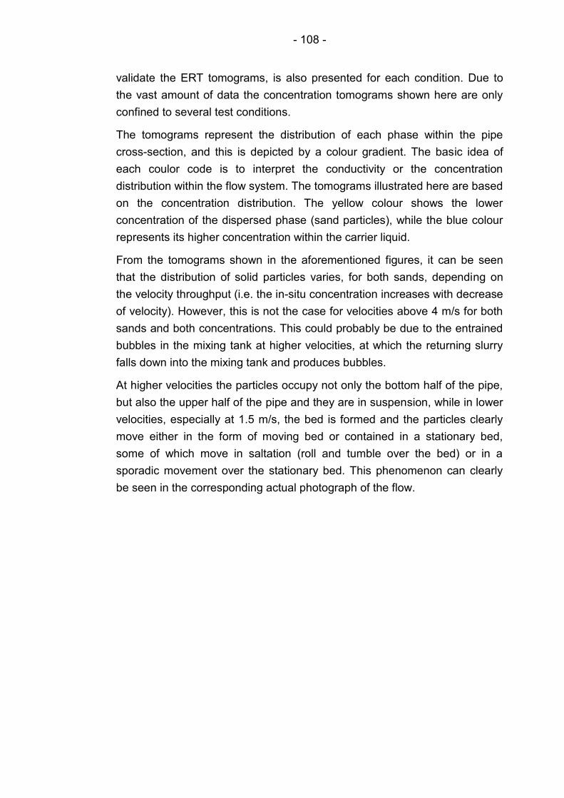
- 108 -
validate the ERT tomograms, is also presented for each condition. Due to
the vast amount of data the concentration tomograms shown here are only
confined to several test conditions.
The tomograms represent the distribution of each phase within the pipe
cross-section, and this is depicted by a colour gradient. The basic idea of
each coulor code is to interpret the conductivity or the concentration
distribution within the flow system. The tomograms illustrated here are based
on the concentration distribution. The yellow colour shows the lower
concentration of the dispersed phase (sand particles), while the blue colour
represents its higher concentration within the carrier liquid.
From the tomograms shown in the aforementioned figures, it can be seen
that the distribution of solid particles varies, for both sands, depending on
the velocity throughput (i.e. the in-situ concentration increases with decrease
of velocity). However, this is not the case for velocities above 4 m/s for both
sands and both concentrations. This could probably be due to the entrained
bubbles in the mixing tank at higher velocities, at which the returning slurry
falls down into the mixing tank and produces bubbles.
At higher velocities the particles occupy not only the bottom half of the pipe,
but also the upper half of the pipe and they are in suspension, while in lower
velocities, especially at 1.5 m/s, the bed is formed and the particles clearly
move either in the form of moving bed or contained in a stationary bed,
some of which move in saltation (roll and tumble over the bed) or in a
sporadic movement over the stationary bed. This phenomenon can clearly
be seen in the corresponding actual photograph of the flow.
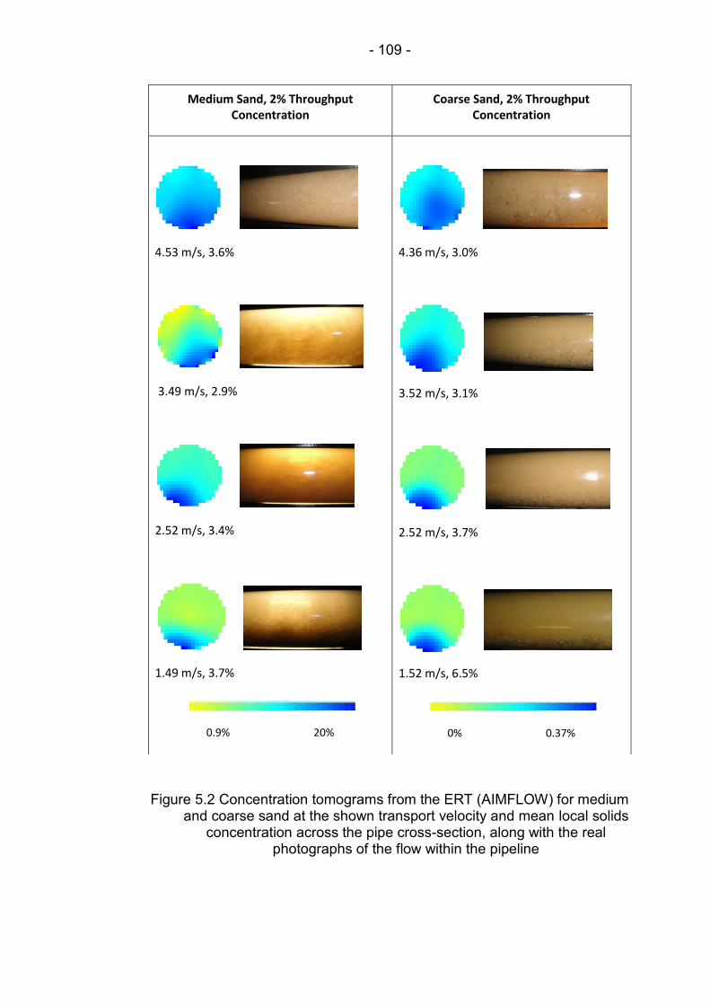
- 109 -
Figure 5.2 Concentration tomograms from the ERT (AIMFLOW) for medium and coarse sand at the shown transport velocity and mean local solids
concentration across the pipe cross-section, along with the real photographs of the flow within the pipeline
Medium Sand, 2% Throughput Concentration
Coarse Sand, 2% Throughput Concentration
4.53 m/s, 3.6%
3.49 m/s, 2.9%
2.52 m/s, 3.4%
1.49 m/s, 3.7%
0.9% 20%
4.36 m/s, 3.0%
3.52 m/s, 3.1%
2.52 m/s, 3.7%
1.52 m/s, 6.5%
0% 0.37%

- 110 -
Figure 5.3 Concentration tomograms from the ERT (AIMFLOW) for medium and coarse sand at the shown transport velocity and mean solids concentration along with the real photographs the flow within the
pipeline
Medium Sand, 10% Throughput
Concentration
Coarse Sand, 10% Throughput
Concentration
4.59 m/s, 10.2%
3.49 m/s, 9.7%
2.52 m/s, 10.5%
1.52 m/s, 12.0%
0.004% 38.6%
4.76 m/s, 16.5%
3.4 m/s, 12.8%
2.49 m/s, 13.3%
1.45 m/s, 21.0%
0% 54%

- 111 -
Figure 5.4 Concentration tomograms from the ERT (AIMFLOW) for medium and coarse sand at the shown transport velocity and mean solids
concentration along with the real photographs of the flow within the pipeline
5.4.2 ERT solids volume fraction distribution
Figures 5.5, 5.6, 5.7 and 5.8 showing the profile of solids concentration as a
function of transport velocity along the vertical axis of the 50 NB pipe cross-
section. In order to determine the effect of concentration along with the
particle size, two different sands, medium and coarse, were used at two
different throughput concentrations, 2% and 10%. The y-axis represents the
dimensionless vertical position (y/D) inside the pipe, while the x-axis
represents the local volumetric solids concentration.
The generated concentration profiles represent the typical concentration
profile of settling slurry flow. It can be noticed that, at velocities below 3.4
m/s, for the two sands the profiles composed of a concave (left-hand bend)
curve in the upper part of the pipe and convex (right-hand side) curve in the
lower part of the pipe. This behaviour can easily be noticed for all velocities
used in the experiment, except for 2% medium sand at transport velocity 5
m/s, for which the distribution of sand particles is rather quasi-homogeneous
with asymmetric distribution across the pipe cross-section.
The results for flowing medium sand with 2% throughput concentration,
which is shown in Figure 5.5, illustrates a gradual distortion in the profile and
changing its pattern from pseudo-homogeneous flow pattern to stratified flow
with decreasing the transport velocity.
Blockage of Coarse Sand, 10% Throughput Concentration
Blockage occurred at 1.2 m/s, 42%, bed thickness is 80%D
0% 62.1%
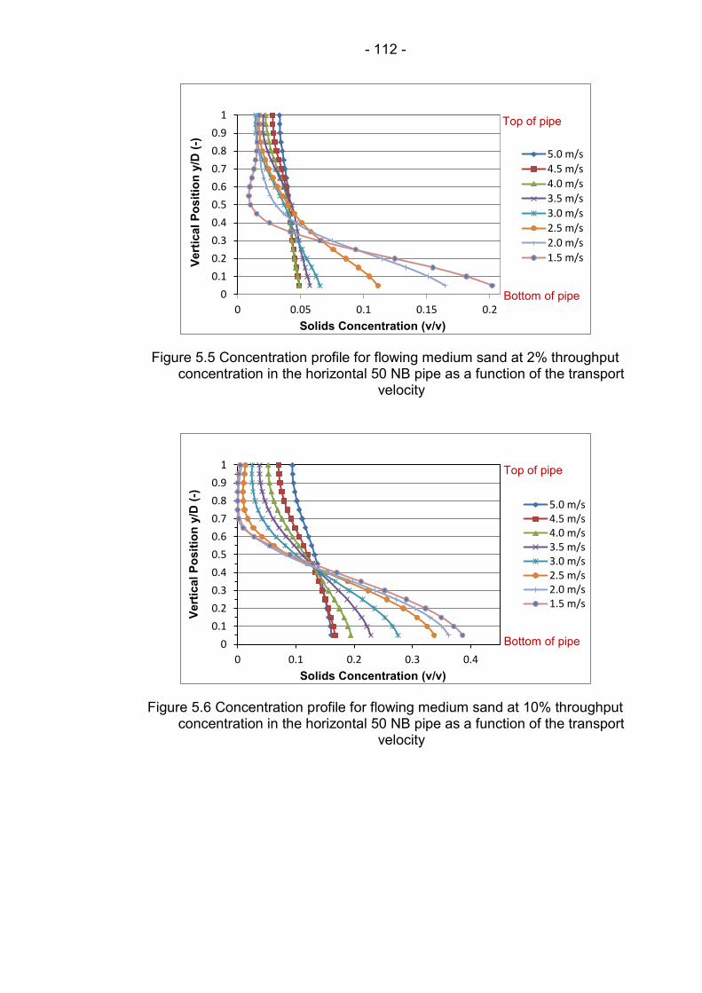
- 112 -
Figure 5.5 Concentration profile for flowing medium sand at 2% throughput concentration in the horizontal 50 NB pipe as a function of the transport
velocity
Figure 5.6 Concentration profile for flowing medium sand at 10% throughput concentration in the horizontal 50 NB pipe as a function of the transport
velocity
0
0.1
0.2
0.3
0.4
0.5
0.6
0.7
0.8
0.9
1
0 0.05 0.1 0.15 0.2
Vert
ical
Po
sit
ion
y/D
(-)
Solids Concentration (v/v)
5.0 m/s
4.5 m/s
4.0 m/s
3.5 m/s
3.0 m/s
2.5 m/s
2.0 m/s
1.5 m/s
0
0.1
0.2
0.3
0.4
0.5
0.6
0.7
0.8
0.9
1
0 0.1 0.2 0.3 0.4
Vert
ical
Po
sit
ion
y/D
(-)
Solids Concentration (v/v)
5.0 m/s 4.5 m/s 4.0 m/s 3.5 m/s 3.0 m/s 2.5 m/s 2.0 m/s 1.5 m/s
Top of pipe
Bottom of pipe
Top of pipe
Bottom of pipe
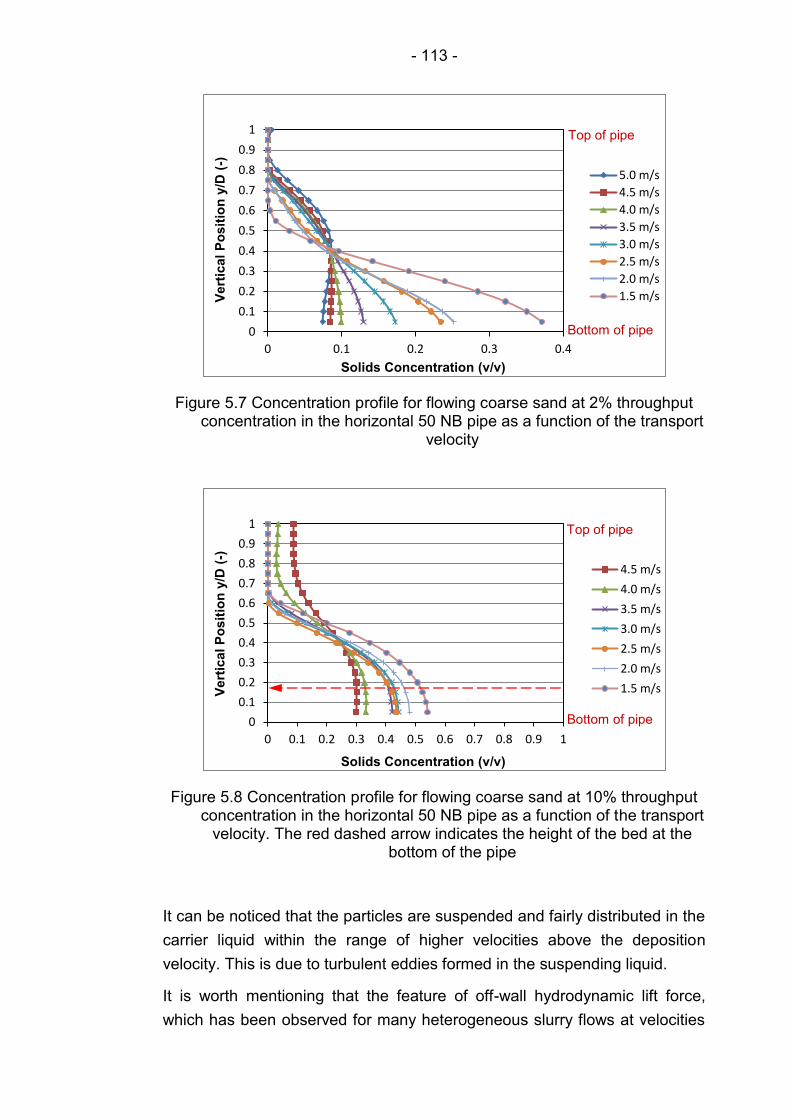
- 113 -
Figure 5.7 Concentration profile for flowing coarse sand at 2% throughput concentration in the horizontal 50 NB pipe as a function of the transport
velocity
Figure 5.8 Concentration profile for flowing coarse sand at 10% throughput concentration in the horizontal 50 NB pipe as a function of the transport
velocity. The red dashed arrow indicates the height of the bed at the bottom of the pipe
It can be noticed that the particles are suspended and fairly distributed in the
carrier liquid within the range of higher velocities above the deposition
velocity. This is due to turbulent eddies formed in the suspending liquid.
It is worth mentioning that the feature of off-wall hydrodynamic lift force,
which has been observed for many heterogeneous slurry flows at velocities
0
0.1
0.2
0.3
0.4
0.5
0.6
0.7
0.8
0.9
1
0 0.1 0.2 0.3 0.4
Vert
ical
Po
sit
ion
y/D
(-)
Solids Concentration (v/v)
5.0 m/s
4.5 m/s
4.0 m/s
3.5 m/s
3.0 m/s
2.5 m/s
2.0 m/s
1.5 m/s
0
0.1
0.2
0.3
0.4
0.5
0.6
0.7
0.8
0.9
1
0 0.1 0.2 0.3 0.4 0.5 0.6 0.7 0.8 0.9 1
Vert
ical
Po
sit
ion
y/D
(-)
Solids Concentration (v/v)
4.5 m/s
4.0 m/s
3.5 m/s
3.0 m/s
2.5 m/s
2.0 m/s
1.5 m/s
Top of pipe
Bottom of pipe
Top of pipe
Bottom of pipe
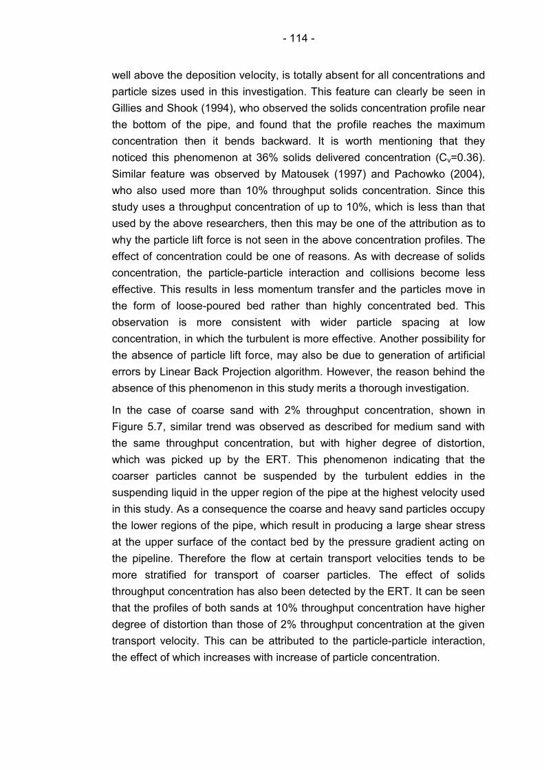
- 114 -
well above the deposition velocity, is totally absent for all concentrations and
particle sizes used in this investigation. This feature can clearly be seen in
Gillies and Shook (1994), who observed the solids concentration profile near
the bottom of the pipe, and found that the profile reaches the maximum
concentration then it bends backward. It is worth mentioning that they
noticed this phenomenon at 36% solids delivered concentration (Cv=0.36).
Similar feature was observed by Matousek (1997) and Pachowko (2004),
who also used more than 10% throughput solids concentration. Since this
study uses a throughput concentration of up to 10%, which is less than that
used by the above researchers, then this may be one of the attribution as to
why the particle lift force is not seen in the above concentration profiles. The
effect of concentration could be one of reasons. As with decrease of solids
concentration, the particle-particle interaction and collisions become less
effective. This results in less momentum transfer and the particles move in
the form of loose-poured bed rather than highly concentrated bed. This
observation is more consistent with wider particle spacing at low
concentration, in which the turbulent is more effective. Another possibility for
the absence of particle lift force, may also be due to generation of artificial
errors by Linear Back Projection algorithm. However, the reason behind the
absence of this phenomenon in this study merits a thorough investigation.
In the case of coarse sand with 2% throughput concentration, shown in
Figure 5.7, similar trend was observed as described for medium sand with
the same throughput concentration, but with higher degree of distortion,
which was picked up by the ERT. This phenomenon indicating that the
coarser particles cannot be suspended by the turbulent eddies in the
suspending liquid in the upper region of the pipe at the highest velocity used
in this study. As a consequence the coarse and heavy sand particles occupy
the lower regions of the pipe, which result in producing a large shear stress
at the upper surface of the contact bed by the pressure gradient acting on
the pipeline. Therefore the flow at certain transport velocities tends to be
more stratified for transport of coarser particles. The effect of solids
throughput concentration has also been detected by the ERT. It can be seen
that the profiles of both sands at 10% throughput concentration have higher
degree of distortion than those of 2% throughput concentration at the given
transport velocity. This can be attributed to the particle-particle interaction,
the effect of which increases with increase of particle concentration.
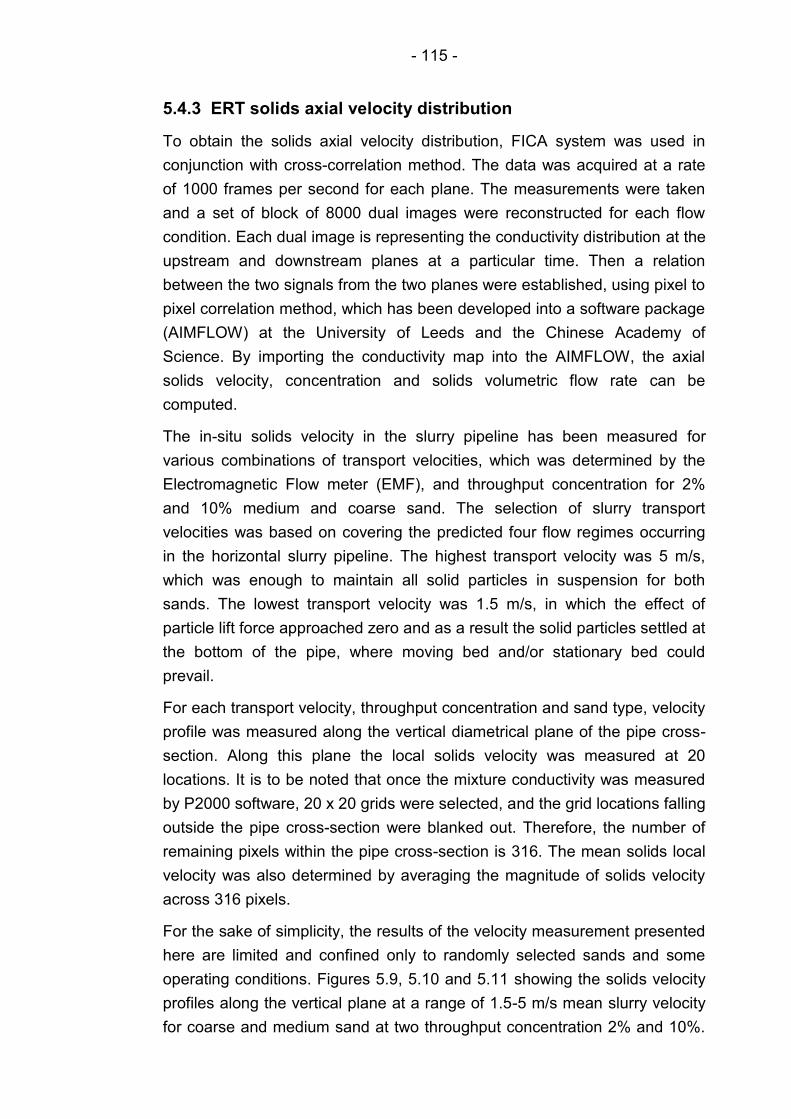
- 115 -
5.4.3 ERT solids axial velocity distribution
To obtain the solids axial velocity distribution, FICA system was used in
conjunction with cross-correlation method. The data was acquired at a rate
of 1000 frames per second for each plane. The measurements were taken
and a set of block of 8000 dual images were reconstructed for each flow
condition. Each dual image is representing the conductivity distribution at the
upstream and downstream planes at a particular time. Then a relation
between the two signals from the two planes were established, using pixel to
pixel correlation method, which has been developed into a software package
(AIMFLOW) at the University of Leeds and the Chinese Academy of
Science. By importing the conductivity map into the AIMFLOW, the axial
solids velocity, concentration and solids volumetric flow rate can be
computed.
The in-situ solids velocity in the slurry pipeline has been measured for
various combinations of transport velocities, which was determined by the
Electromagnetic Flow meter (EMF), and throughput concentration for 2%
and 10% medium and coarse sand. The selection of slurry transport
velocities was based on covering the predicted four flow regimes occurring
in the horizontal slurry pipeline. The highest transport velocity was 5 m/s,
which was enough to maintain all solid particles in suspension for both
sands. The lowest transport velocity was 1.5 m/s, in which the effect of
particle lift force approached zero and as a result the solid particles settled at
the bottom of the pipe, where moving bed and/or stationary bed could
prevail.
For each transport velocity, throughput concentration and sand type, velocity
profile was measured along the vertical diametrical plane of the pipe cross-
section. Along this plane the local solids velocity was measured at 20
locations. It is to be noted that once the mixture conductivity was measured
by P2000 software, 20 x 20 grids were selected, and the grid locations falling
outside the pipe cross-section were blanked out. Therefore, the number of
remaining pixels within the pipe cross-section is 316. The mean solids local
velocity was also determined by averaging the magnitude of solids velocity
across 316 pixels.
For the sake of simplicity, the results of the velocity measurement presented
here are limited and confined only to randomly selected sands and some
operating conditions. Figures 5.9, 5.10 and 5.11 showing the solids velocity
profiles along the vertical plane at a range of 1.5-5 m/s mean slurry velocity
for coarse and medium sand at two throughput concentration 2% and 10%.

- 116 -
In the profiles shown below, for both sands and the two throughput
concentrations, it can be seen that the shape of profile goes through
continuous distortion as the mean flow velocity is further decreased. This is
due to the fact that at low velocities the turbulent dispersing force decreases
and the carrier liquid is no longer able to maintain the coarser particles, as a
result the coarser particles migrate to the lower part of the pipe. This
phenomenon causes an increase of solids particle concentration at the lower
part of the pipe. In the case of medium sand at 10% throughput
concentration, the velocity profile of which is illustrated in Figure 5.9, it can
be noticed that with decrease in mean flow velocity the location of peak
solids velocity shifts towards the upper part of the pipe. Simultaneously, the
solid particles at the bottom of the pipe start to slow down. This slurry
feature, which is clearly highlighted by the ERT, has been the subject of
many previous studies (Kaushal et al., 2002; Matousek, 2002). As the
transport velocity decreases, the gravity force plays its role, in return the
solids concentration increases at the bottom of the pipe. This increase in
solids concentration causes a strong particle-particle interaction, which
diminishes the momentum of the flowing solids, as a result the particles at
the bottom of the pipe travel slower than those moving at the top of the pipe.
The same trend was observed for coarse sand, at both throughput
concentrations. However, an increase in the degree of asymmetry in the
solids velocity profile was noticed to be higher than that of medium sand at
the same throughput concentration and transport velocity. This behaviour
could well be attributed to the particle size effect. As the particle size
increases, the gravity effect dominate the turbulent eddies responsible for
suspending solid particles in the carrier liquid, as a result the coarser
particles are displaced to the bottom of the pipe. This effect enhances an
increase in the solids concentration at the bottom of the pipe, where the
particles face a strong interference between each other that cause them to
slow down. At a given throughput concentration and transport velocity the
degree of solids segregation at the bottom of the pipe is higher in coarse
sand rather than medium sand; hence the velocity profile for coarse sand
manifests a higher degree of asymmetry. Therefore, one can conclude that
the degree of asymmetry in solids velocity profile dependent on the particle
size.
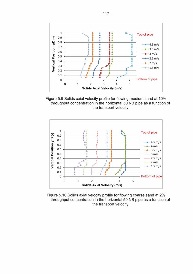
- 117 -
Figure 5.9 Solids axial velocity profile for flowing medium sand at 10% throughput concentration in the horizontal 50 NB pipe as a function of
the transport velocity
Figure 5.10 Solids axial velocity profile for flowing coarse sand at 2% throughput concentration in the horizontal 50 NB pipe as a function of
the transport velocity
0
0.1
0.2
0.3
0.4
0.5
0.6
0.7
0.8
0.9
1
0 1 2 3 4 5
Vert
ical
Po
sit
ion
y/D
(-)
Solids Axial Velocity (m/s)
4.5 m/s
3.5 m/s
3 m/s
2.5 m/s
2 m/s
1.5 m/s
0
0.1
0.2
0.3
0.4
0.5
0.6
0.7
0.8
0.9
1
0 1 2 3 4 5
Vert
ical
Po
sit
ion
y/D
(-)
Solids Axial Velocity (m/s)
4.5 m/s 4 m/s 3.5 m/s 3 m/s 2.5 m/s 2 m/s 1.5 m/s
Top of pipe
Bottom of pipe
Top of pipe
Bottom of pipe
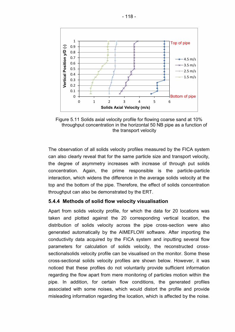
- 118 -
Figure 5.11 Solids axial velocity profile for flowing coarse sand at 10% throughput concentration in the horizontal 50 NB pipe as a function of
the transport velocity
The observation of all solids velocity profiles measured by the FICA system
can also clearly reveal that for the same particle size and transport velocity,
the degree of asymmetry increases with increase of through put solids
concentration. Again, the prime responsible is the particle-particle
interaction, which widens the difference in the average solids velocity at the
top and the bottom of the pipe. Therefore, the effect of solids concentration
throughput can also be demonstrated by the ERT.
5.4.4 Methods of solid flow velocity visualisation
Apart from solids velocity profile, for which the data for 20 locations was
taken and plotted against the 20 corresponding vertical location, the
distribution of solids velocity across the pipe cross-section were also
generated automatically by the AIMEFLOW software. After importing the
conductivity data acquired by the FICA system and inputting several flow
parameters for calculation of solids velocity, the reconstructed cross-
sectionalsolids velocity profile can be visualised on the monitor. Some these
cross-sectional solids velocity profiles are shown below. However, it was
noticed that these profiles do not voluntarily provide sufficient information
regarding the flow apart from mere monitoring of particles motion within the
pipe. In addition, for certain flow conditions, the generated profiles
associated with some noises, which would distort the profile and provide
misleading information regarding the location, which is affected by the noise.
0
0.1
0.2
0.3
0.4
0.5
0.6
0.7
0.8
0.9
1
0 1 2 3 4 5 6
Vert
ical
Po
sit
ion
y/D
(-)
Solids Axial Velocity (m/s)
4.5 m/s
3.5 m/s
2.5 m/s
1.5 m/s
Top of pipe
Bottom of pipe
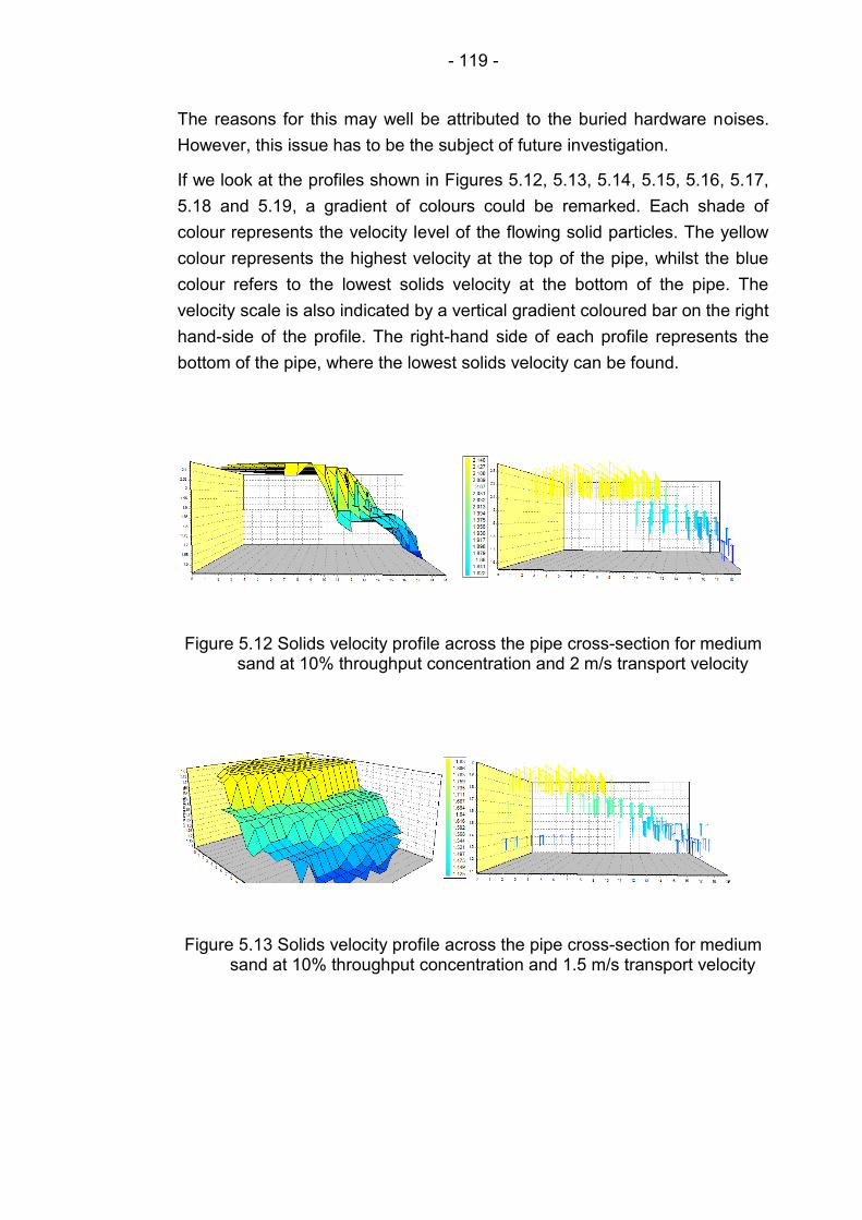
- 119 -
The reasons for this may well be attributed to the buried hardware noises.
However, this issue has to be the subject of future investigation.
If we look at the profiles shown in Figures 5.12, 5.13, 5.14, 5.15, 5.16, 5.17,
5.18 and 5.19, a gradient of colours could be remarked. Each shade of
colour represents the velocity level of the flowing solid particles. The yellow
colour represents the highest velocity at the top of the pipe, whilst the blue
colour refers to the lowest solids velocity at the bottom of the pipe. The
velocity scale is also indicated by a vertical gradient coloured bar on the right
hand-side of the profile. The right-hand side of each profile represents the
bottom of the pipe, where the lowest solids velocity can be found.
Figure 5.12 Solids velocity profile across the pipe cross-section for medium sand at 10% throughput concentration and 2 m/s transport velocity
Figure 5.13 Solids velocity profile across the pipe cross-section for medium sand at 10% throughput concentration and 1.5 m/s transport velocity

- 120 -
Figure 5.14 Solids velocity profile across the pipe cross-section for coarse sand at 2% throughput concentration and 4 m/s transport velocity
Figure 5.15 Solids velocity profile across the pipe cross-section for coarse sand at 2% throughput concentration and 3 m/s transport velocity
Figure 5.16 Solids velocity profile across the pipe cross-section for coarse sand at 10% throughput concentration and 3.5 m/s transport velocity
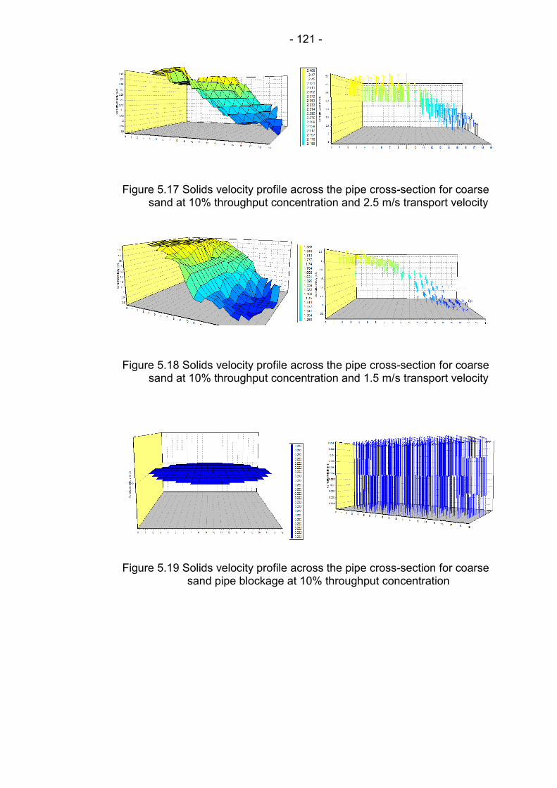
- 121 -
Figure 5.17 Solids velocity profile across the pipe cross-section for coarse sand at 10% throughput concentration and 2.5 m/s transport velocity
Figure 5.18 Solids velocity profile across the pipe cross-section for coarse sand at 10% throughput concentration and 1.5 m/s transport velocity
Figure 5.19 Solids velocity profile across the pipe cross-section for coarse sand pipe blockage at 10% throughput concentration
- 122 -
5.4.5 Slurry flow regime visualisation and characterization
Slurry flow regimes encountered in horizontal pipeline influence some
parameters of system such as pressure drop, system instability, pipe erosion
and some other performance characteristics. Therefore, monitoring
characterisation and of these flow regimes are important tools for design and
operation of pipelines conveying settling slurries.
This section presents a technique, by which the flow regimes in horizontal
pipeline can be visualised and characterised. The technique is based on the
analysis of solids concentration profile and axial velocity profile obtained
from a dual plane Electrical Resistance Tomography (ERT) sensor, which
was mounted in the middle of the horizontal test section of 50 NB flow loop.
Careful selection of the transport velocity range (1.2-5 m/s) allowed the
coverage of four main flow regimes along with pipe blockage. The flow
regimes predicted via ERT compared to the photographic images of actual
flow within the test section. An analysis of stratified slurry flow is also
discussed and it is proposed that the tomography technique can be used for
estimation of several parameters of stratified flow such as mean granular
bed concentration and velocity, height of bed etc. The estimation of these
parameters is based on the analysis of the grid of tomogram reconstructed
with Sensitivity Back Projection (SBP) algorithm.
For the sake of simplicity the flow regimes illustrated here are only for coarse
sand at 10% throughput concentration. However, due to the limitation in the
pump capacity, the homogeneous flow regime for flowing 10% coarse sand
could not be achieved; therefore, the pseudo-homogeneous regime of
flowing coarse sand at 10% concentration throughput was selected. The flow
regimes of flowing 10 % coarse sand shown here are pseudo-
homogeneous, heterogeneous flow regime, moving bed and stationary bed.
In addition, the concentration and velocity profile of the blocked horizontal
pipeline is also highlighted. In order to cover all flow regimes, for each sand
at a given throughput concentration, the transport velocity was decreased,
starting from 5 m/s and ending at 1.2 m/s, where the continuous formation of
stationary bed leads to pipeline blockage. For the sake of clarity and support
for both concentration and velocity profiles, the photographs of each
prevailing flow regime were captured by a digital camera and inserted into
the plot area of the measured profile. Due to the murky nature of slurry, it
was not easy to distinguish the solid particles in the murky carrier liquid.
Therefore, the photographs were sent to the Microsoft Office Picture
Manager, where colour enhancement was applied. As it is apparent in the

- 123 -
inserted pictures, some photographs required a specific colour for the solid
particles to be shown. The photographs were taken through 1 m transparent
pipe section, which was confined by a photo chamber details of which can
be found in Chapter 4.
5.4.5.1 Pseudo-homogeneous flow regime
Figure 5.20, showing a pseudo-homogeneous flow regime, in terms of
concentration and axial solids velocity profile, for 10% coarse sand at 4.5
m/s. On both profiles it can be seen that the particles occupying the pipe
cross-section are more or less distributed symmetrically. However, the
profile is slightly skewed at the centre of the pipe and changes its trajectory
indicating the presence of finer particles with lower concentration and higher
velocity. This distortion in profiles has been detected by tomography and it is
apparent from the background inserted photograph, where the entire
particles are suspended in the carrier liquid. Nevertheless, there is a
possibility of presence of some gravels (5 mm diameter), which cannot be
lifted, as gravitational attraction exceeds the fluid turbulence. These gravels
were detected within the coarse sand, which initially added to the mixing
tank.
Figure 5.20 Pseudo-homogeneous flow regime for 10% throughput concentration of coarse sand at 4.5 m/s transport velocity shown on
concentration profile (left) and solids velocity profile (right)
This is clearly seen in the velocity profile at the very bottom of the pipe,
despite its disappearance in the concentration profile. The existence of such
particles was very clear and could distinguishably felt during the experiment
while travelling through bends and elbows of the flow loop. The reason for
the distortion of both profiles could be attributed to the particle size and
0
0.2
0.4
0.6
0.8
1
0 0.2 0.4 0.6 0.8 1
Vert
ical
Po
sit
ion
y/D
(-)
Solids Concentration (v/v)
4.5 m/s
0 0.1 0.2 0.3 0.4 0.5 0.6 0.7 0.8 0.9
1
0 2.2 4.4 6.6 Vert
ical
Po
sit
ion
y/D
(-)
Solids Axial Velocity (m/s)
4.5 m/s
Flow Direction Flow Direction
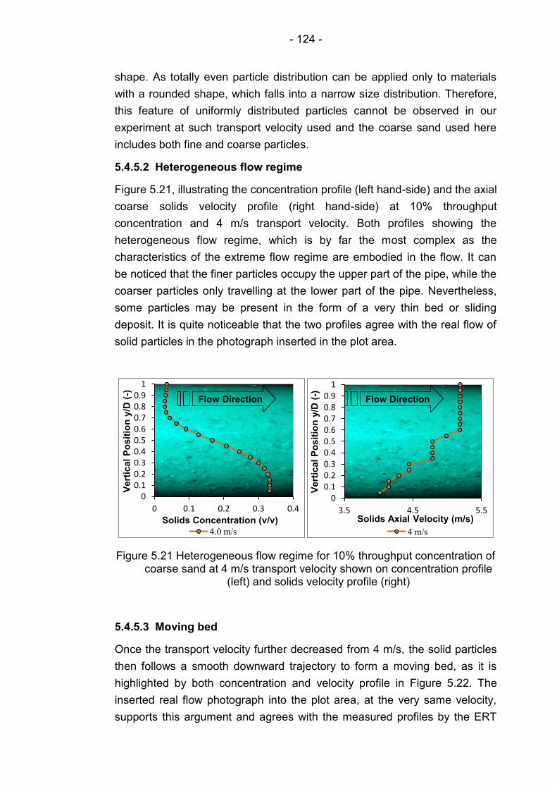
- 124 -
shape. As totally even particle distribution can be applied only to materials
with a rounded shape, which falls into a narrow size distribution. Therefore,
this feature of uniformly distributed particles cannot be observed in our
experiment at such transport velocity used and the coarse sand used here
includes both fine and coarse particles.
5.4.5.2 Heterogeneous flow regime
Figure 5.21, illustrating the concentration profile (left hand-side) and the axial
coarse solids velocity profile (right hand-side) at 10% throughput
concentration and 4 m/s transport velocity. Both profiles showing the
heterogeneous flow regime, which is by far the most complex as the
characteristics of the extreme flow regime are embodied in the flow. It can
be noticed that the finer particles occupy the upper part of the pipe, while the
coarser particles only travelling at the lower part of the pipe. Nevertheless,
some particles may be present in the form of a very thin bed or sliding
deposit. It is quite noticeable that the two profiles agree with the real flow of
solid particles in the photograph inserted in the plot area.
Figure 5.21 Heterogeneous flow regime for 10% throughput concentration of coarse sand at 4 m/s transport velocity shown on concentration profile
(left) and solids velocity profile (right)
5.4.5.3 Moving bed
Once the transport velocity further decreased from 4 m/s, the solid particles
then follows a smooth downward trajectory to form a moving bed, as it is
highlighted by both concentration and velocity profile in Figure 5.22. The
inserted real flow photograph into the plot area, at the very same velocity,
supports this argument and agrees with the measured profiles by the ERT
0 0.1 0.2 0.3 0.4 0.5 0.6 0.7 0.8 0.9
1
0 0.1 0.2 0.3 0.4
Vert
ical
Po
sit
ion
y/D
(-)
Solids Concentration (v/v)
4.0 m/s
0 0.1 0.2 0.3 0.4 0.5 0.6 0.7 0.8 0.9
1
3.5 4.5 5.5
Vert
ical
Po
sit
ion
y/D
(-)
Solids Axial Velocity (m/s)
4 m/s
Flow Direction Flow Direction
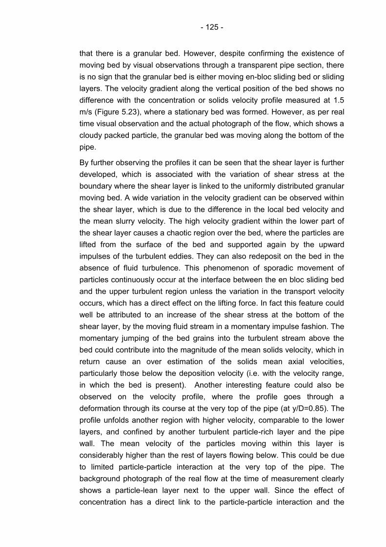
- 125 -
that there is a granular bed. However, despite confirming the existence of
moving bed by visual observations through a transparent pipe section, there
is no sign that the granular bed is either moving en-bloc sliding bed or sliding
layers. The velocity gradient along the vertical position of the bed shows no
difference with the concentration or solids velocity profile measured at 1.5
m/s (Figure 5.23), where a stationary bed was formed. However, as per real
time visual observation and the actual photograph of the flow, which shows a
cloudy packed particle, the granular bed was moving along the bottom of the
pipe.
By further observing the profiles it can be seen that the shear layer is further
developed, which is associated with the variation of shear stress at the
boundary where the shear layer is linked to the uniformly distributed granular
moving bed. A wide variation in the velocity gradient can be observed within
the shear layer, which is due to the difference in the local bed velocity and
the mean slurry velocity. The high velocity gradient within the lower part of
the shear layer causes a chaotic region over the bed, where the particles are
lifted from the surface of the bed and supported again by the upward
impulses of the turbulent eddies. They can also redeposit on the bed in the
absence of fluid turbulence. This phenomenon of sporadic movement of
particles continuously occur at the interface between the en bloc sliding bed
and the upper turbulent region unless the variation in the transport velocity
occurs, which has a direct effect on the lifting force. In fact this feature could
well be attributed to an increase of the shear stress at the bottom of the
shear layer, by the moving fluid stream in a momentary impulse fashion. The
momentary jumping of the bed grains into the turbulent stream above the
bed could contribute into the magnitude of the mean solids velocity, which in
return cause an over estimation of the solids mean axial velocities,
particularly those below the deposition velocity (i.e. with the velocity range,
in which the bed is present). Another interesting feature could also be
observed on the velocity profile, where the profile goes through a
deformation through its course at the very top of the pipe (at y/D=0.85). The
profile unfolds another region with higher velocity, comparable to the lower
layers, and confined by another turbulent particle-rich layer and the pipe
wall. The mean velocity of the particles moving within this layer is
considerably higher than the rest of layers flowing below. This could be due
to limited particle-particle interaction at the very top of the pipe. The
background photograph of the real flow at the time of measurement clearly
shows a particle-lean layer next to the upper wall. Since the effect of
concentration has a direct link to the particle-particle interaction and the

- 126 -
motion of solid particles within the carrier liquid, then it is remarkable that
this feature is absent in the solids concentration profile. However, this
discrepancy merits a future investigation.
Figure 5.22 Moving bed flow regime for 10% throughput concentration of coarse sand at 2.5 m/s transport velocity shown on concentration
profile (left) and solids velocity profile (right)
5.4.5.4 Stationary bed
During the experiment the flow was observed through the transparent pipe
section and found that a stationary granular packed bed had been formed,
on the surface of which a sliding thin layer was moving at the bottom of the
pipe. The thickness of this stationary layer within the bed was measured
using a ruler, and recorded as 7-8 mm from the bottom of the pipe. As the
flow was extremely murky and the surface of the bed was in an unsteady-
state condition, more precision could not be achieved in measuring the
thickness of the formed stationary layer. By observing the both profiles,
especially velocity profile, it is apparent that, for 10% throughput
concentration of coarse sand at 1.5 m/s, the height of inter-granular contact
bed is at y/D=2 at the vertical plane of pipe cross section, which makes 10
mm thickness and demarcated by a blue arrow, shown in Figure 5.23. Also,
by further observing the velocity profile, no variation or gradient can be seen
in the profile curve, where the minimum solids velocity occur. This
phenomenon is an indication that each pixel lies within the bed region, is
well saturated with solid particles and there is a mutual permanent contact
between them, in return a stationary bed is formed. On the concentration
profile it can be seen that within the bed height on the profile, the
concentration gradient is hardly noticeable; hence, this suggests that the
0
0.2
0.4
0.6
0.8
1
0 0.1 0.2 0.3 0.4 0.5
Vert
ical
Po
sit
ion
y/D
(-)
Solids Concentration (v/v)
2.5 m/s
0 0.1 0.2 0.3 0.4 0.5 0.6 0.7 0.8 0.9
1
1.9 2.1 2.3 2.5
Vert
ical
Po
sit
ion
y/D
(-)
Solids Axial Velocity (m/s)
2.5 m/s
Flow Direction Flow Direction

- 127 -
particles are well segregated and fully packed within the bed. Similarly, the
height of stationary bed can be indentified from the two profiles, particularly
the velocity profile, which is measured to be y/D=0.15 (y=7.5 mm) from the
bottom of the pipe and demarcated by a red line.
Figure 5.23 Stationary bed flow regime for 10% throughput concentration of coarse sand at 1.5 m/s transport velocity shown on concentration
profile (left) and solids velocity profile (right). The height of granular bed is indicated by a blue arrow and the boundary of the stationary bed is
indicated by a red arrow
If the height of the granular bed is 10 mm, and 7.5 mm out of which makes
the stationary bed, then the rest (2.5 mm) makes the saltating carpet or
rugged layer on the surface of the stationary bed. In other words, the
thickness of the sliding bed on the surface of the stationary bed is 2.5 mm.
However, as previously mentioned this moving layer on the surface of
stationary layer is not well pronounced on either concentration or the velocity
profile. Also, no or very little feature is provided by the profiles to indicate
whether the bed within 10 mm from the bottom of the pipe is moving or
stationary. As by observing the profiles in Figures 5.6 and 5.7, it is apparent
that the profiles show no difference within the granular bed, whilst visual
observation of flow through the transparent pipe section indicated a moving
bed with 7 mm thickness at 2.5 m/s mean slurry velocity and a stationary
bed with 10 mm thickness at 1.5 m/s. Therefore, it is still quite difficult to
identify the state of granular bed, whether it is moving or stationary.
However, the sporadic movement of particles above the granular bed may
be identifiable on the two profiles, concentration and solids axial velocity, but
0 0.1 0.2 0.3 0.4 0.5 0.6 0.7 0.8 0.9
1
0 0.1 0.2 0.3 0.4 0.5 0.6
Vert
ical
Po
sit
ion
y/D
(-)
Solids Concentration (v/v)
1.5 m/s
0 0.1 0.2 0.3 0.4 0.5 0.6 0.7 0.8 0.9
1
0.5 0.7 0.9 1.1 1.3 1.5 1.7 1.9
Vert
ical
Po
sit
ion
y/D
(-)
Solids Axial Velocity (m/s)
1.5 m/s
Height of stationary bed
Height of granular bed
Height of stationary bed
Height of granular bed
Flow Direction Flow Direction
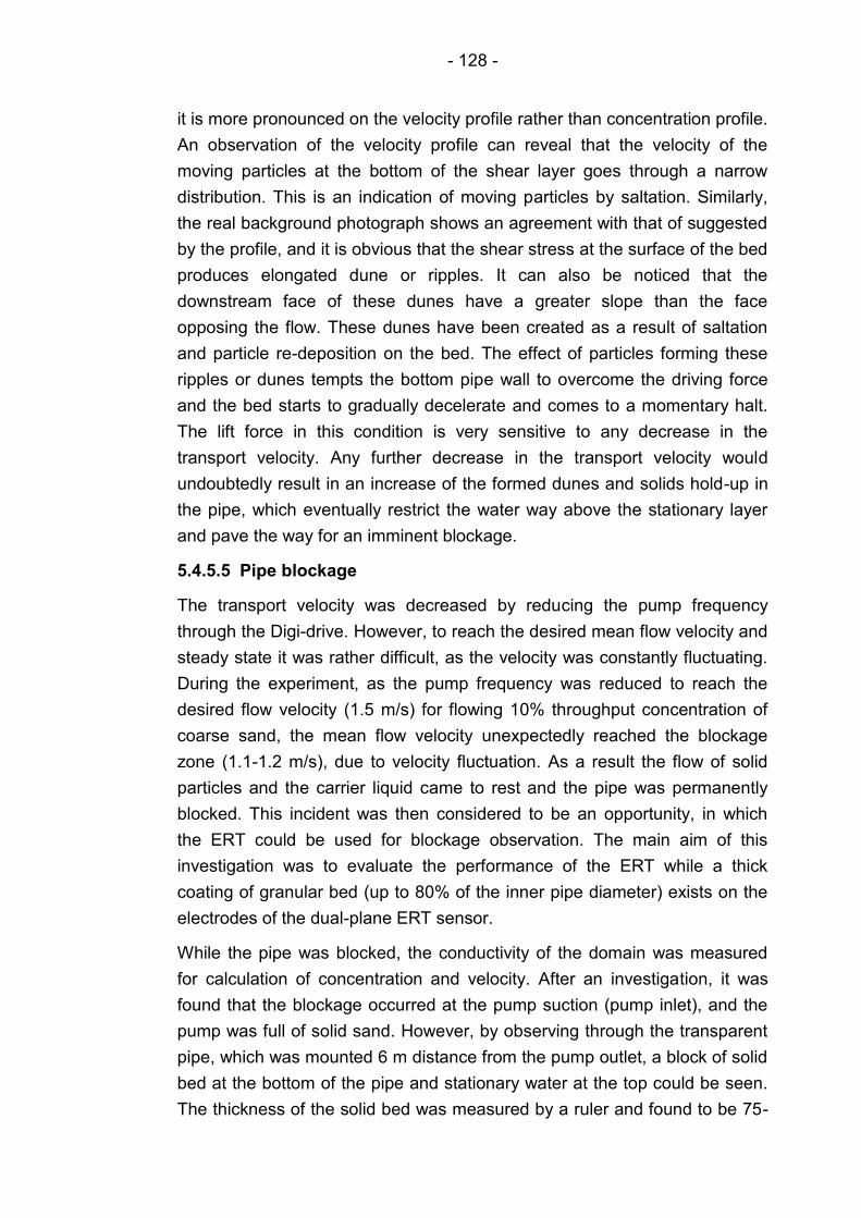
- 128 -
it is more pronounced on the velocity profile rather than concentration profile.
An observation of the velocity profile can reveal that the velocity of the
moving particles at the bottom of the shear layer goes through a narrow
distribution. This is an indication of moving particles by saltation. Similarly,
the real background photograph shows an agreement with that of suggested
by the profile, and it is obvious that the shear stress at the surface of the bed
produces elongated dune or ripples. It can also be noticed that the
downstream face of these dunes have a greater slope than the face
opposing the flow. These dunes have been created as a result of saltation
and particle re-deposition on the bed. The effect of particles forming these
ripples or dunes tempts the bottom pipe wall to overcome the driving force
and the bed starts to gradually decelerate and comes to a momentary halt.
The lift force in this condition is very sensitive to any decrease in the
transport velocity. Any further decrease in the transport velocity would
undoubtedly result in an increase of the formed dunes and solids hold-up in
the pipe, which eventually restrict the water way above the stationary layer
and pave the way for an imminent blockage.
5.4.5.5 Pipe blockage
The transport velocity was decreased by reducing the pump frequency
through the Digi-drive. However, to reach the desired mean flow velocity and
steady state it was rather difficult, as the velocity was constantly fluctuating.
During the experiment, as the pump frequency was reduced to reach the
desired flow velocity (1.5 m/s) for flowing 10% throughput concentration of
coarse sand, the mean flow velocity unexpectedly reached the blockage
zone (1.1-1.2 m/s), due to velocity fluctuation. As a result the flow of solid
particles and the carrier liquid came to rest and the pipe was permanently
blocked. This incident was then considered to be an opportunity, in which
the ERT could be used for blockage observation. The main aim of this
investigation was to evaluate the performance of the ERT while a thick
coating of granular bed (up to 80% of the inner pipe diameter) exists on the
electrodes of the dual-plane ERT sensor.
While the pipe was blocked, the conductivity of the domain was measured
for calculation of concentration and velocity. After an investigation, it was
found that the blockage occurred at the pump suction (pump inlet), and the
pump was full of solid sand. However, by observing through the transparent
pipe, which was mounted 6 m distance from the pump outlet, a block of solid
bed at the bottom of the pipe and stationary water at the top could be seen.
The thickness of the solid bed was measured by a ruler and found to be 75-

- 129 -
80% of the inner pipe diameter from the bottom of the pipe. The exact
estimation could not be achieved, as the surface of the granular stationary
bed was not totally flat, instead consisted of dunes and ripples, which had
been formed as a result of waves created by the upstream liquid. Once the
blockage occurred, there was no force to lift the slurry to the top of the
vertical line; as a result it falls down again to the bend, where it is connected
to the horizontal line. The coarser particles are expected to fall first, due to
the gravity effect. This phenomenon was captured by a digital camera,
through the transparent pipe section mounted at the bottom of the vertical
line, as shown in Figure 5.24 for both test sections, horizontal and vertical.
(a) (b)
Figure 5.24 Showing the blockage of the pipeline, (a) blocked horizontal section (b) coarser solid particles in the blocked transparent pipe
section mounted at the bottom of the vertical pipeline
Then the carrier liquid escapes through the gaps, formed between the
coarser particles, into the horizontal line, where pushes the existing water at
the top of the horizontal pipeline, until it reaches the other dead-end. Then it
reverses back and agitates the existing stationary bed, where some of
coarser particles are lifted and distributed into the surface of the downstream
stationary bed.
Another photograph of a blocked transparent section of the ERT sensor was
taken, so as to qualitatively compare to the profiles obtained by the ERT
measurement. Figure 5.25 showing the concentration and particle velocity
profile with a real photograph of the blocked pipe section inserted into the
plot area. It is apparent that the highest concentration can be seen within the
area occupied by well packed and granular stagnant bed particles, which is
0.62% at y/D=0.35 (y=17.5 from the bottom of the pipe). Consequently, the
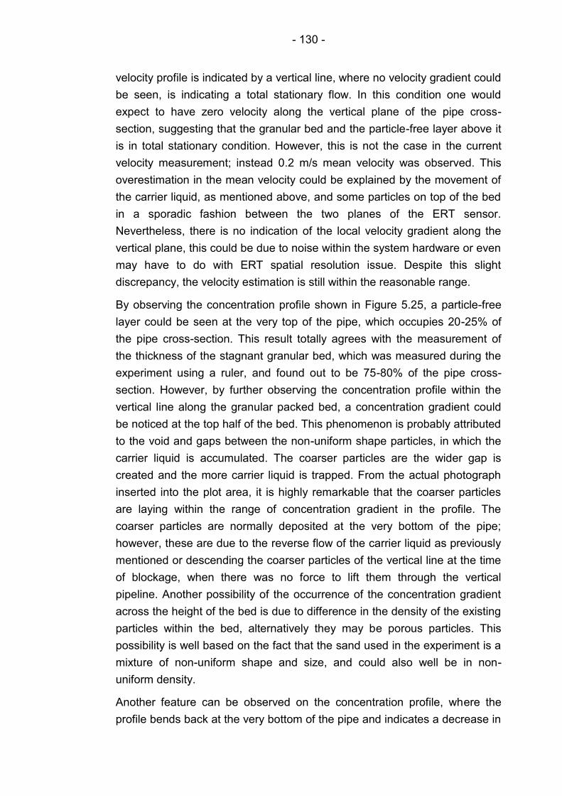
- 130 -
velocity profile is indicated by a vertical line, where no velocity gradient could
be seen, is indicating a total stationary flow. In this condition one would
expect to have zero velocity along the vertical plane of the pipe cross-
section, suggesting that the granular bed and the particle-free layer above it
is in total stationary condition. However, this is not the case in the current
velocity measurement; instead 0.2 m/s mean velocity was observed. This
overestimation in the mean velocity could be explained by the movement of
the carrier liquid, as mentioned above, and some particles on top of the bed
in a sporadic fashion between the two planes of the ERT sensor.
Nevertheless, there is no indication of the local velocity gradient along the
vertical plane, this could be due to noise within the system hardware or even
may have to do with ERT spatial resolution issue. Despite this slight
discrepancy, the velocity estimation is still within the reasonable range.
By observing the concentration profile shown in Figure 5.25, a particle-free
layer could be seen at the very top of the pipe, which occupies 20-25% of
the pipe cross-section. This result totally agrees with the measurement of
the thickness of the stagnant granular bed, which was measured during the
experiment using a ruler, and found out to be 75-80% of the pipe cross-
section. However, by further observing the concentration profile within the
vertical line along the granular packed bed, a concentration gradient could
be noticed at the top half of the bed. This phenomenon is probably attributed
to the void and gaps between the non-uniform shape particles, in which the
carrier liquid is accumulated. The coarser particles are the wider gap is
created and the more carrier liquid is trapped. From the actual photograph
inserted into the plot area, it is highly remarkable that the coarser particles
are laying within the range of concentration gradient in the profile. The
coarser particles are normally deposited at the very bottom of the pipe;
however, these are due to the reverse flow of the carrier liquid as previously
mentioned or descending the coarser particles of the vertical line at the time
of blockage, when there was no force to lift them through the vertical
pipeline. Another possibility of the occurrence of the concentration gradient
across the height of the bed is due to difference in the density of the existing
particles within the bed, alternatively they may be porous particles. This
possibility is well based on the fact that the sand used in the experiment is a
mixture of non-uniform shape and size, and could also well be in non-
uniform density.
Another feature can be observed on the concentration profile, where the
profile bends back at the very bottom of the pipe and indicates a decrease in
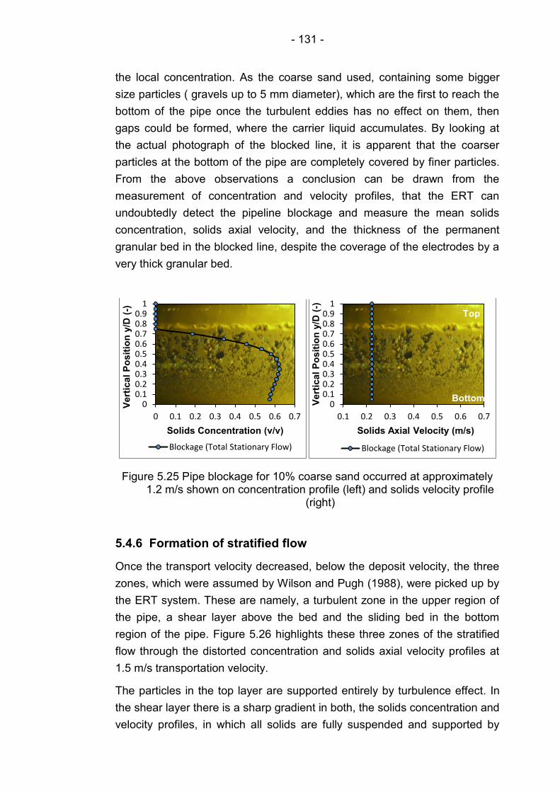
- 131 -
the local concentration. As the coarse sand used, containing some bigger
size particles ( gravels up to 5 mm diameter), which are the first to reach the
bottom of the pipe once the turbulent eddies has no effect on them, then
gaps could be formed, where the carrier liquid accumulates. By looking at
the actual photograph of the blocked line, it is apparent that the coarser
particles at the bottom of the pipe are completely covered by finer particles.
From the above observations a conclusion can be drawn from the
measurement of concentration and velocity profiles, that the ERT can
undoubtedly detect the pipeline blockage and measure the mean solids
concentration, solids axial velocity, and the thickness of the permanent
granular bed in the blocked line, despite the coverage of the electrodes by a
very thick granular bed.
Figure 5.25 Pipe blockage for 10% coarse sand occurred at approximately 1.2 m/s shown on concentration profile (left) and solids velocity profile
(right)
5.4.6 Formation of stratified flow
Once the transport velocity decreased, below the deposit velocity, the three
zones, which were assumed by Wilson and Pugh (1988), were picked up by
the ERT system. These are namely, a turbulent zone in the upper region of
the pipe, a shear layer above the bed and the sliding bed in the bottom
region of the pipe. Figure 5.26 highlights these three zones of the stratified
flow through the distorted concentration and solids axial velocity profiles at
1.5 m/s transportation velocity.
The particles in the top layer are supported entirely by turbulence effect. In
the shear layer there is a sharp gradient in both, the solids concentration and
velocity profiles, in which all solids are fully suspended and supported by
0 0.1 0.2 0.3 0.4 0.5 0.6 0.7 0.8 0.9
1
0 0.1 0.2 0.3 0.4 0.5 0.6 0.7
Vert
ical
Po
sit
ion
y/D
(-)
Solids Concentration (v/v)
Blockage (Total Stationary Flow)
0 0.1 0.2 0.3 0.4 0.5 0.6 0.7 0.8 0.9
1
0.1 0.2 0.3 0.4 0.5 0.6 0.7
Vert
ical
Po
sit
ion
y/D
(-)
Solids Axial Velocity (m/s)
Blockage (Total Stationary Flow)
Bottom
Top

- 132 -
turbulence and contact load effects. While in the bed there is no shear and
solid concentration is that of a porous packed bed.
Figure 5.26 Showing the three zones of the distorted profiles, concentration profile (left) and solids axial velocity profile (right), in stratified flow at
1.5 m/s transportation velocity
Another phenomenon could also be observed for the two sands with the
same condition, which is development of bed. The uniformly distributed bed
can only be seen in the case of coarse sand with 10% throughput
concentration, highlighted in Figure 5.26. This could be interpreted by the
fact that in medium sand (2% and 10% throughput concentration), shown in
Figure 5.27 and coarse sand (2% throughput concentration), shown in
Figure 5.28, the distribution of the particles in the bed approach a limiting
value in concentration (i.e. the concentration of the loose-poured bed has
not reached the maximum concentration of the occupying pixel at the bottom
of the pipe). Despite that, while observing the flow through the transparent
pipe section for medium sand (2% and 10% throughput concentration) and
coarse sand (2% throughput concentration) at low transport velocity (1.5
m/s), it was found that the loose-poured bed was moving in the form of en-
bloc sliding (in mass).
0 0.1 0.2 0.3 0.4 0.5 0.6 0.7 0.8 0.9
1
0 0.1 0.2 0.3 0.4 0.5 0.6
Vert
ical
Po
sit
ion
y/D
(-)
Solids Concentration (v/v)
1.5 m/s
0 0.1 0.2 0.3 0.4 0.5 0.6 0.7 0.8 0.9
1
0.5 0.7 0.9 1.1 1.3 1.5 1.7 1.9
Vert
ical
Po
sit
ion
y/D
(-)
Solids Axial Velocity (m/s)
1.5 m/s
Turbulent Zone
Shear Layer
Granular Bed
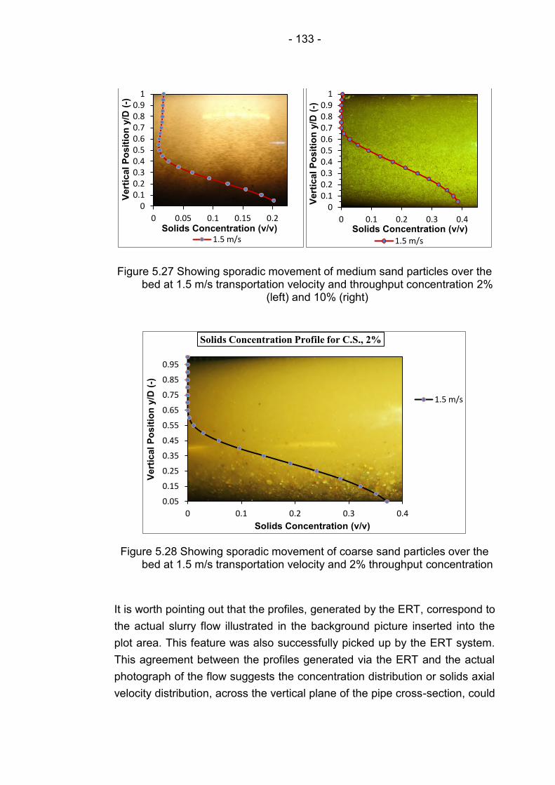
- 133 -
Figure 5.27 Showing sporadic movement of medium sand particles over the bed at 1.5 m/s transportation velocity and throughput concentration 2%
(left) and 10% (right)
Figure 5.28 Showing sporadic movement of coarse sand particles over the bed at 1.5 m/s transportation velocity and 2% throughput concentration
It is worth pointing out that the profiles, generated by the ERT, correspond to
the actual slurry flow illustrated in the background picture inserted into the
plot area. This feature was also successfully picked up by the ERT system.
This agreement between the profiles generated via the ERT and the actual
photograph of the flow suggests the concentration distribution or solids axial
velocity distribution, across the vertical plane of the pipe cross-section, could
0 0.1 0.2 0.3 0.4 0.5 0.6 0.7 0.8 0.9
1
0 0.05 0.1 0.15 0.2
Vert
ical
Po
sit
ion
y/D
(-)
Solids Concentration (v/v) 1.5 m/s
0 0.1 0.2 0.3 0.4 0.5 0.6 0.7 0.8 0.9
1
0 0.1 0.2 0.3 0.4
Vert
ical
Po
sit
ion
y/D
(-)
Solids Concentration (v/v)
1.5 m/s
0.05
0.15
0.25
0.35
0.45
0.55
0.65
0.75
0.85
0.95
0 0.1 0.2 0.3 0.4
Vert
ical
Po
sit
ion
y/D
(-)
Solids Concentration (v/v)
Solids Concentration Profile for C.S., 2%
1.5 m/s
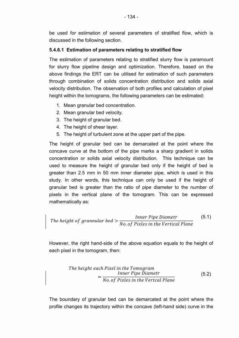
- 134 -
be used for estimation of several parameters of stratified flow, which is
discussed in the following section.
5.4.6.1 Estimation of parameters relating to stratified flow
The estimation of parameters relating to stratified slurry flow is paramount
for slurry flow pipeline design and optimization. Therefore, based on the
above findings the ERT can be utilised for estimation of such parameters
through combination of solids concentration distribution and solids axial
velocity distribution. The observation of both profiles and calculation of pixel
height within the tomograms, the following parameters can be estimated:
1. Mean granular bed concentration.
2. Mean granular bed velocity.
3. The height of granular bed.
4. The height of shear layer.
5. The height of turbulent zone at the upper part of the pipe.
The height of granular bed can be demarcated at the point where the
concave curve at the bottom of the pipe marks a sharp gradient in solids
concentration or solids axial velocity distribution. This technique can be
used to measure the height of granular bed only if the height of bed is
greater than 2.5 mm in 50 mm inner diameter pipe, which is used in this
study. In other words, this technique can only be used if the height of
granular bed is greater than the ratio of pipe diameter to the number of
pixels in the vertical plane of the tomogram. This can be expressed
mathematically as:
(5.1)
However, the right hand-side of the above equation equals to the height of
each pixel in the tomogram, then:
(5.2)
The boundary of granular bed can be demarcated at the point where the
profile changes its trajectory within the concave (left-hand side) curve in the
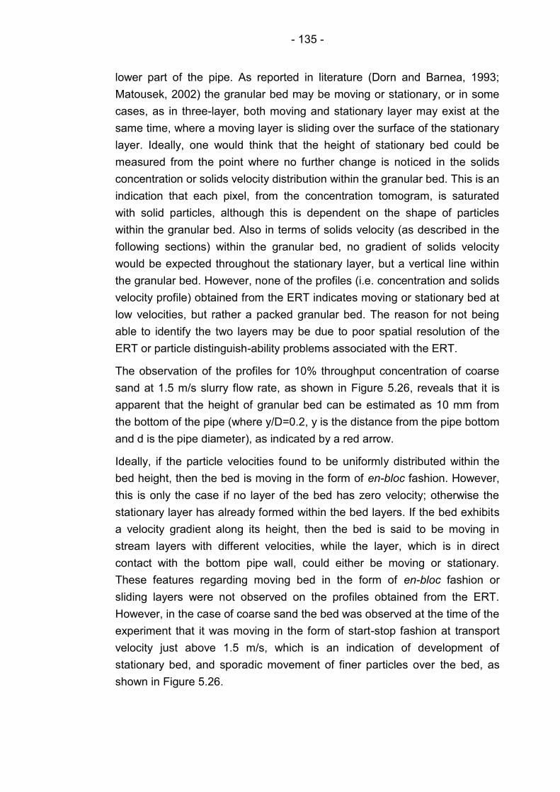
- 135 -
lower part of the pipe. As reported in literature (Dorn and Barnea, 1993;
Matousek, 2002) the granular bed may be moving or stationary, or in some
cases, as in three-layer, both moving and stationary layer may exist at the
same time, where a moving layer is sliding over the surface of the stationary
layer. Ideally, one would think that the height of stationary bed could be
measured from the point where no further change is noticed in the solids
concentration or solids velocity distribution within the granular bed. This is an
indication that each pixel, from the concentration tomogram, is saturated
with solid particles, although this is dependent on the shape of particles
within the granular bed. Also in terms of solids velocity (as described in the
following sections) within the granular bed, no gradient of solids velocity
would be expected throughout the stationary layer, but a vertical line within
the granular bed. However, none of the profiles (i.e. concentration and solids
velocity profile) obtained from the ERT indicates moving or stationary bed at
low velocities, but rather a packed granular bed. The reason for not being
able to identify the two layers may be due to poor spatial resolution of the
ERT or particle distinguish-ability problems associated with the ERT.
The observation of the profiles for 10% throughput concentration of coarse
sand at 1.5 m/s slurry flow rate, as shown in Figure 5.26, reveals that it is
apparent that the height of granular bed can be estimated as 10 mm from
the bottom of the pipe (where y/D=0.2, y is the distance from the pipe bottom
and d is the pipe diameter), as indicated by a red arrow.
Ideally, if the particle velocities found to be uniformly distributed within the
bed height, then the bed is moving in the form of en-bloc fashion. However,
this is only the case if no layer of the bed has zero velocity; otherwise the
stationary layer has already formed within the bed layers. If the bed exhibits
a velocity gradient along its height, then the bed is said to be moving in
stream layers with different velocities, while the layer, which is in direct
contact with the bottom pipe wall, could either be moving or stationary.
These features regarding moving bed in the form of en-bloc fashion or
sliding layers were not observed on the profiles obtained from the ERT.
However, in the case of coarse sand the bed was observed at the time of the
experiment that it was moving in the form of start-stop fashion at transport
velocity just above 1.5 m/s, which is an indication of development of
stationary bed, and sporadic movement of finer particles over the bed, as
shown in Figure 5.26.
- 136 -
5.4.7 Reducing entrained bubbles
In order to reduce the amount of bubbles in the flow loop two measures were
taken. The first was to reduce the acceleration of falling slurry at the
discharge point, by placing several semicircle trays (plates) into the pipe wall
of the vertical discharge pipe, in a way to occupy half of the pipe cross-
section. Figure 5.29 showing the vertical discharge pipe with inserted plates.
Since the flow does not cover the full bore of 100 mm discharge pipe, then
reducing the pipe bore does not add up into the flow pressure. The plate
spacing was arbitrary selected as 200 mm along the pipe section. The plates
were placed in the pipe in an opposite sequencing fashion to ensure that the
slurry flows down over the plates rather than through the passages
(openings). In this manner, the pressure of down-coming slurry is reduced.
In other words, the plates restrict the flow by approximately half and
eventually reduce the gravitational force and flow pressure into the mixing
tank.
(a) (b)
Figure 5.29 The vertical slurry discharge pipe into the mixing tank; (a) the Sanitary Tee connected to the outlet of the pipe; (b) the semicircle
plates inserted into the pipe wall
The second measure was to separate the mixing region within the tank from
the discharge zone, where the slurry returns to the mixing tank. The
discharge zone made up approximately 20% of the tank and separated by
welding a stainless-steel baffle to the tank wall. Figure 5.30 showing the
baffle in the mixing tank.
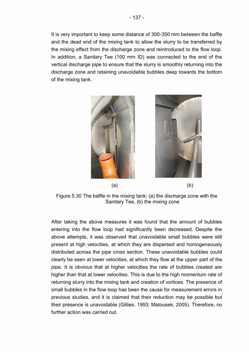
- 137 -
It is very important to keep some distance of 300-350 mm between the baffle
and the dead end of the mixing tank to allow the slurry to be transferred by
the mixing effect from the discharge zone and reintroduced to the flow loop.
In addition, a Sanitary Tee (100 mm ID) was connected to the end of the
vertical discharge pipe to ensure that the slurry is smoothly returning into the
discharge zone and retaining unavoidable bubbles deep towards the bottom
of the mixing tank.
(a) (b)
Figure 5.30 The baffle in the mixing tank; (a) the discharge zone with the Sanitary Tee, (b) the mixing zone
After taking the above measures it was found that the amount of bubbles
entering into the flow loop had significantly been decreased. Despite the
above attempts, it was observed that unavoidable small bubbles were still
present at high velocities, at which they are dispersed and homogeneously
distributed across the pipe cross section. These unavoidable bubbles could
clearly be seen at lower velocities, at which they flow at the upper part of the
pipe. It is obvious that at higher velocities the rate of bubbles created are
higher than that at lower velocities. This is due to the high momentum rate of
returning slurry into the mixing tank and creation of vortices. The presence of
small bubbles in the flow loop has been the cause for measurement errors in
previous studies, and it is claimed that their reduction may be possible but
their presence is unavoidable (Gillies, 1993; Matousek, 2005). Therefore, no
further action was carried out.

- 138 -
5.4.8 Estimation of delivered solids volume fraction
The delivered solids volume concentration (Cv) calculated using the
measuring tank, which is mounted on a set of three load cells, and the
diverter system described in Chapter 4. The diverter system (switch system)
was used to divert the slurry flowing out of the pipeline into the measuring
tank for a given length of time. This period of time was recorded by an
electronic stop watch. The volume of collected slurry in the measuring tank
was determined using the level of the slurry in the tank and calculating the
cross-sectional area of the measuring tank. Using the volume (v) and the
total weight of collected slurry (wt), which was recorded via the load cells,
the mixture density (ρm) can be determined, as shown in equation 5.4.
Finally, knowing the solids density (ρs) and the carrier liquid density (ρl), the
delivered solids concentration can be determined using equation 5.3.
(5.3)
(5.4)
5.4.9 Validation of the EMF velocity
The Electromagnetic Flow meter was installed in the vertical test section for
regularly monitoring and recording the transport slurry velocity. The method
used to validate the EMF consisted of using a switch system (or diverting
system) and a measuring tank, which was mounted on a set of three
calibrated load cells, the details of which is found in Chapter 4. After several
seconds of diverting the flow to the measuring tank, it was noticed that the
velocity on the Electromagnetic Flow meter was gradually dropping.
Therefore, in order to avoid any false reading, the Electromagnetic Flow
meter was recorded just before diversion of slurry. Both velocities from, the
Electromagnetic Flow meter and the discharge level was then collected for
the comparison, as shown in Table 5.2. The results of error analysis are
illustrated quantitatively and qualitatively. Table 5.2 illustrating the
comparison of velocity values obtained from the ERT and the discharge
measurement for flowing medium and coarse sand with two different
throughput concentrations (2% and 10%).
- 139 -
By observing the two data sets, it is apparent that the results, obtained within
the range of velocities considered in the experiments, are in total agreement
with each other. This conclusion was drawn from the results of error analysis
carried out on the two velocities, EMF and discharge, for each sand at 2%
and 10% throughput concentration and velocity range 1.5-5 m/s. The
absolute error was calculated as the difference between the magnitude of
the discharge velocity value and the observed EMF velocity value. However,
in order to compare how incorrect the EMF is from the discharge values
considered to be true, relative error was calculated between the discharge
and the EMF, which is shown in percentage relative error (%). This
calculation is shown in Equation 5.5, which is the product of absolute error,
divided by the discharge value. As it is often expressed in percentage, then it
is multiplied by 100:
(5.5)
Where:
V = Discharge Velocity (actual) (m/s)
Vo = Observed (EMF) Velocity (Measured) (m/s)
V-Vo = Absolute Error (m/s)
The results are summarised and illustrated in the following table in terms of
minimum deviation, maximum deviation and the average error within the
range of velocities mentioned above.
For further investigation of relationships between the EMF readings and the
calculated discharge, Regression Analysis was used as a statistical tool, for
which a linear relationship was assumed between the two set of values. The
results of this analysis are illustrated quantitatively in Figure 5.31, which in
the meantime assesses the statistical significance of the estimated
relationship between the two folds of data. The output results of the
regression provide a range of important statistical information, which can be
used for assessment of the relationship between the two variables, some of
which are listed under the regression statistics heading, as shown in Table
5.3. The most important value here is the value of R square, which
measures the degree of linear relationship between the velocity values
measured by the EMF and those calculated by the flow diversion technique.

- 140 -
By observing the R square values in Table 5.3 for all conditions used, it is
apparent that its values are not less than 0.99, which determines a well fit or
a very good degree of linear relationship between the two measured and
predicted velocity values. Nevertheless, the standard error shown in the
aforementioned table can also indicate a good fit between the two data.
Table 5.2 The data obtained from the EMF reading and discharge calculation along with the rate of deviation at each given velocity.
EMF
(m/s)
Discharge Velocity
(m/s)
Absolute Error (m/s)
Relative Error (%)
Remarks
Medium Sand 2%
4.97 4.97 0.00 0.01
4.53 4.49 0.04 -0.86
4.02 4.08 0.06 1.46 Min. Deviation = 0.01%
3.49 3.49 0.00 0.10 Max. Deviation = 3.13%
3.05 3.05 0.00 0.12 Average Error = 1.19%
2.52 2.55 0.02 0.97
2.06 2.12 0.06 2.84
1.49 1.54 0.05 3.13
Medium Sand 10%
4.96 5.59 0.63 11.27
4.59 4.47 0.12 -2.79
4.06 4.00 0.07 -1.69 Min. Deviation = 0.52%
3.49 3.47 0.02 -0.65 Max. Deviation = 11.27%
3.04 3.19 0.15 4.73 Average Error = 3.23%
2.52 2.54 0.02 0.67
2.01 2.02 0.01 0.52
1.52 1.58 0.05 3.49
Coarse Sand 2%
4.93 4.82 0.11 -2.29
4.36 4.53 0.17 3.79
4.11 4.29 0.18 4.14 Min. Deviation = 1.37%
3.52 3.66 0.14 3.90 Max. Deviation = 4.14%
3.11 3.18 0.08 2.48 Average Error = 2.81%
2.52 2.45 0.07 -3.00
2.00 2.03 0.03 1.50
1.52 1.50 0.02 -1.37
Coarse Sand 10%
4.76 5.24 0.48 9.18
4.14 4.61 0.48 10.30 Min. Deviation = 3.38%
3.40 3.62 0.22 6.11 Max. Deviation = 12.7%
2.94 3.36 0.43 12.75 Average Error = 17.17%
2.49 2.58 0.09 3.44
2.20 2.09 0.11 -5.05
1.45 1.40 0.05 -3.38
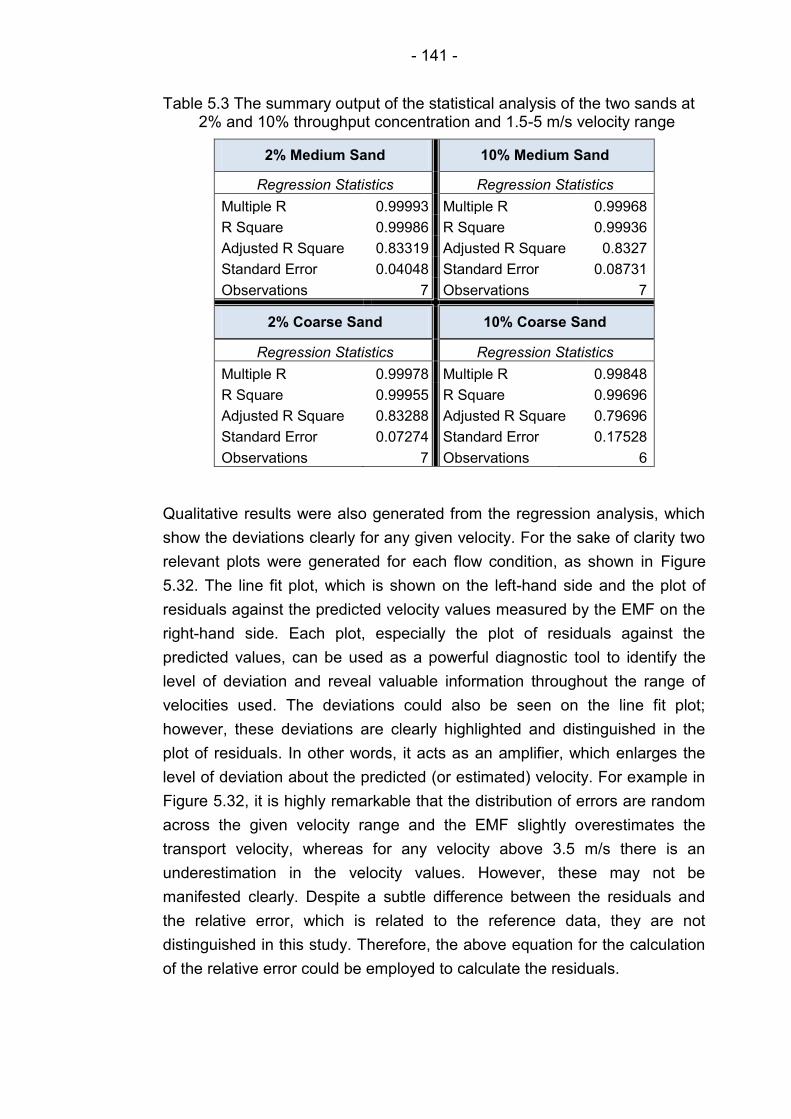
- 141 -
Table 5.3 The summary output of the statistical analysis of the two sands at 2% and 10% throughput concentration and 1.5-5 m/s velocity range
2% Medium Sand 10% Medium Sand
Regression Statistics Regression Statistics
Multiple R 0.99993 Multiple R 0.99968
R Square 0.99986 R Square 0.99936
Adjusted R Square 0.83319 Adjusted R Square 0.8327
Standard Error 0.04048 Standard Error 0.08731
Observations 7 Observations 7
2% Coarse Sand 10% Coarse Sand
Regression Statistics Regression Statistics
Multiple R 0.99978 Multiple R 0.99848
R Square 0.99955 R Square 0.99696
Adjusted R Square 0.83288 Adjusted R Square 0.79696
Standard Error 0.07274 Standard Error 0.17528
Observations 7 Observations 6
Qualitative results were also generated from the regression analysis, which
show the deviations clearly for any given velocity. For the sake of clarity two
relevant plots were generated for each flow condition, as shown in Figure
5.32. The line fit plot, which is shown on the left-hand side and the plot of
residuals against the predicted velocity values measured by the EMF on the
right-hand side. Each plot, especially the plot of residuals against the
predicted values, can be used as a powerful diagnostic tool to identify the
level of deviation and reveal valuable information throughout the range of
velocities used. The deviations could also be seen on the line fit plot;
however, these deviations are clearly highlighted and distinguished in the
plot of residuals. In other words, it acts as an amplifier, which enlarges the
level of deviation about the predicted (or estimated) velocity. For example in
Figure 5.32, it is highly remarkable that the distribution of errors are random
across the given velocity range and the EMF slightly overestimates the
transport velocity, whereas for any velocity above 3.5 m/s there is an
underestimation in the velocity values. However, these may not be
manifested clearly. Despite a subtle difference between the residuals and
the relative error, which is related to the reference data, they are not
distinguished in this study. Therefore, the above equation for the calculation
of the relative error could be employed to calculate the residuals.
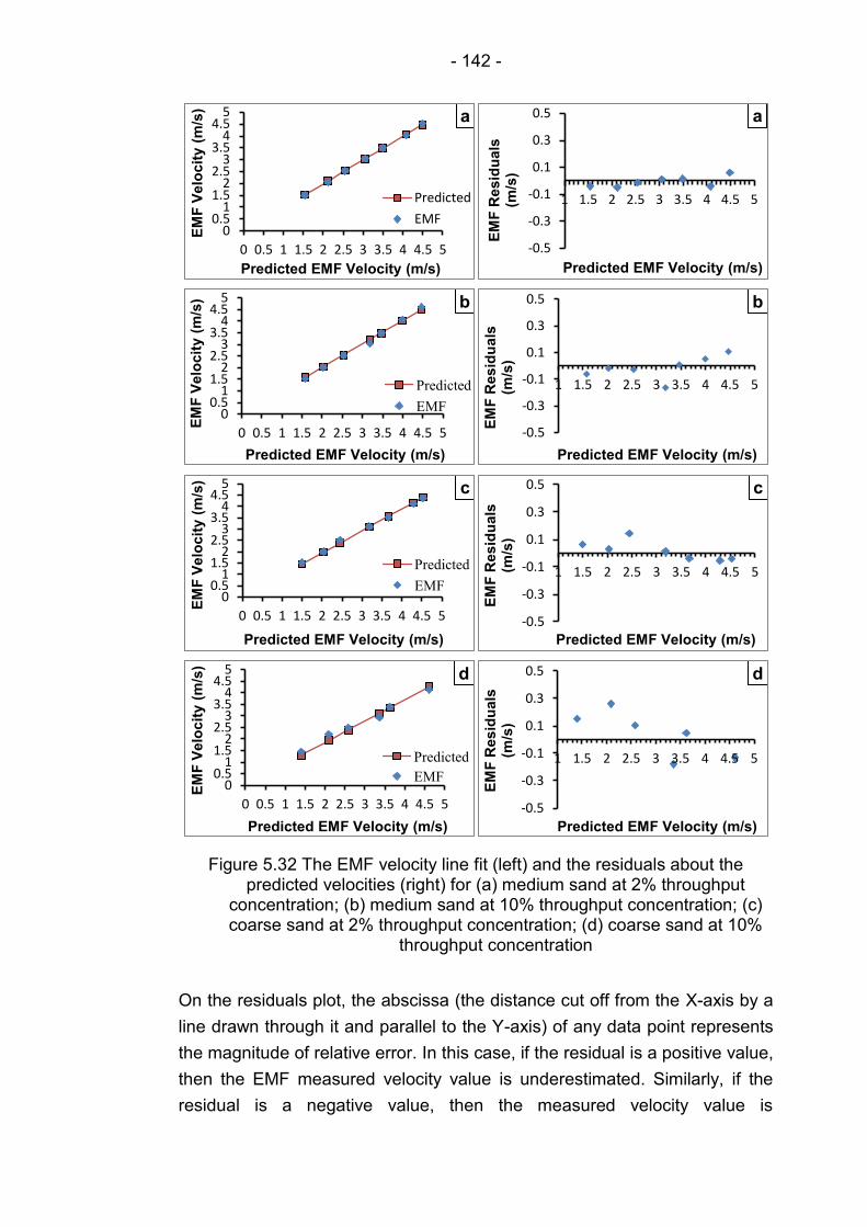
- 142 -
Figure 5.32 The EMF velocity line fit (left) and the residuals about the predicted velocities (right) for (a) medium sand at 2% throughput
concentration; (b) medium sand at 10% throughput concentration; (c) coarse sand at 2% throughput concentration; (d) coarse sand at 10%
throughput concentration
On the residuals plot, the abscissa (the distance cut off from the X-axis by a
line drawn through it and parallel to the Y-axis) of any data point represents
the magnitude of relative error. In this case, if the residual is a positive value,
then the EMF measured velocity value is underestimated. Similarly, if the
residual is a negative value, then the measured velocity value is
0 0.5
1 1.5
2 2.5
3 3.5
4 4.5
5
0 0.5 1 1.5 2 2.5 3 3.5 4 4.5 5
EM
F V
elo
cit
y (
m/s
)
Predicted EMF Velocity (m/s)
a
Predicted
EMF
-0.5
-0.3
-0.1
0.1
0.3
0.5
1 1.5 2 2.5 3 3.5 4 4.5 5
EM
F R
esid
uals
(m
/s)
Predicted EMF Velocity (m/s)
a
0 0.5
1 1.5
2 2.5
3 3.5
4 4.5
5
0 0.5 1 1.5 2 2.5 3 3.5 4 4.5 5
EM
F V
elo
cit
y (
m/s
)
Predicted EMF Velocity (m/s)
b
Predicted
EMF
-0.5
-0.3
-0.1
0.1
0.3
0.5
1 1.5 2 2.5 3 3.5 4 4.5 5
EM
F R
esid
uals
(m
/s)
Predicted EMF Velocity (m/s)
b
0 0.5
1 1.5
2 2.5
3 3.5
4 4.5
5
0 0.5 1 1.5 2 2.5 3 3.5 4 4.5 5
EM
F V
elo
cit
y (
m/s
)
Predicted EMF Velocity (m/s)
c
Predicted
EMF
-0.5
-0.3
-0.1
0.1
0.3
0.5
1 1.5 2 2.5 3 3.5 4 4.5 5
EM
F R
esid
uals
(m
/s)
Predicted EMF Velocity (m/s)
c
0 0.5
1 1.5
2 2.5
3 3.5
4 4.5
5
0 0.5 1 1.5 2 2.5 3 3.5 4 4.5 5
EM
F V
elo
cit
y (
m/s
)
Predicted EMF Velocity (m/s)
d
Predicted
EMF
-0.5
-0.3
-0.1
0.1
0.3
0.5
1 1.5 2 2.5 3 3.5 4 4.5 5
EM
F R
esid
uals
(m
/s)
Predicted EMF Velocity (m/s)
d
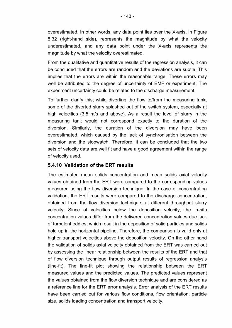
- 143 -
overestimated. In other words, any data point lies over the X-axis, in Figure
5.32 (right-hand side), represents the magnitude by what the velocity
underestimated, and any data point under the X-axis represents the
magnitude by what the velocity overestimated.
From the qualitative and quantitative results of the regression analysis, it can
be concluded that the errors are random and the deviations are subtle. This
implies that the errors are within the reasonable range. These errors may
well be attributed to the degree of uncertainty of EMF or experiment. The
experiment uncertainty could be related to the discharge measurement.
To further clarify this, while diverting the flow to/from the measuring tank,
some of the diverted slurry splashed out of the switch system, especially at
high velocities (3.5 m/s and above). As a result the level of slurry in the
measuring tank would not correspond exactly to the duration of the
diversion. Similarly, the duration of the diversion may have been
overestimated, which caused by the lack of synchronisation between the
diversion and the stopwatch. Therefore, it can be concluded that the two
sets of velocity data are well fit and have a good agreement within the range
of velocity used.
5.4.10 Validation of the ERT results
The estimated mean solids concentration and mean solids axial velocity
values obtained from the ERT were compared to the corresponding values
measured using the flow diversion technique. In the case of concentration
validation, the ERT results were compared to the discharge concentration,
obtained from the flow diversion technique, at different throughput slurry
velocity. Since at velocities below the deposition velocity, the in-situ
concentration values differ from the delivered concentration values due lack
of turbulent eddies, which result in the deposition of solid particles and solids
hold up in the horizontal pipeline. Therefore, the comparison is valid only at
higher transport velocities above the deposition velocity. On the other hand
the validation of solids axial velocity obtained from the ERT was carried out
by assessing the linear relationship between the results of the ERT and that
of flow diversion technique through output results of regression analysis
(line-fit). The line-fit plot showing the relationship between the ERT
measured values and the predicted values. The predicted values represent
the values obtained from the flow diversion technique and are considered as
a reference line for the ERT error analysis. Error analysis of the ERT results
have been carried out for various flow conditions, flow orientation, particle
size, solids loading concentration and transport velocity.

- 144 -
5.4.10.1 Validation of mean solids volume fraction
Tables 5.4 and 5.5 showing the comparison of in-situ concentration
measured by the ERT and delivered concentration measured via the flow
diversion technique, at different transport velocities. The comparison has
been carried out only for concentrations within the range of higher transport
velocities (3-5 m/s), shown within the shaded area within both tables. An
analysis of the error is also presented along with an estimation of average
error for each sand and throughput concentration. The average error was
determined only for the range of concentrations falling into the shaded area
in the either tables.
Through an observation of qualitative and quantitative results, it can be
revealed that the occurring errors are random and the values differ from one
condition to another. In other words, the rate of error is different from one
transport velocity to another as well as particles size and throughput
concentration.
Table 5.4 The comparison of solids concentration values for medium and coarse sand at 2% throughput concentration in the horizontal test section. The shaded area represents the values, only for which the comparison and error analysis have been carried out
Medium Sand, 2%
Throughput Concentration
Coarse Sand, 2%
Throughput Concentration
Velocity (m/s)
In-situ Conc. %(v/v)
Delivered Conc. %(v/v)
Relative Error (%)
In-situ Conc. %(v/v)
Delivered Conc. % (v/v)
Relative Error
%
5 2.9 2.4 20.8 3.9 3 30
4 3.2 2.4 33 2.7 2.9 6.9
3.5 2.9 2.7 7 3.1 3.2 3
3 2.4 2.5 4 3.4 3.2 6
2.5 3.4 2.5 - 3.7 3.4 -
2 3.7 2.5 - 3.8 3 -
1.5 3.7 2.4 - 6.5 2.8 -
Average Error=16.4% Average Error=12%
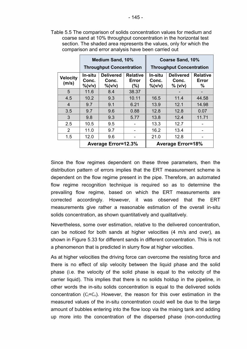
- 145 -
Table 5.5 The comparison of solids concentration values for medium and coarse sand at 10% throughput concentration in the horizontal test section. The shaded area represents the values, only for which the comparison and error analysis have been carried out
Medium Sand, 10%
Throughput Concentration
Coarse Sand, 10%
Throughput Concentration
Velocity (m/s)
In-situ Conc. %(v/v)
Delivered Conc. %(v/v)
Relative Error (%)
In-situ Conc. %(v/v)
Delivered Conc. % (v/v)
Relative Error
%
5 11.6 8.4 38.37 - -
4.5 10.2 9.3 10.11 16.5 11.4 44.58
4 9.7 9.1 6.21 13.9 12.1 14.98
3.5 9.7 9.6 0.88 12.8 12.8 0.07
3 9.8 9.3 5.77 13.8 12.4 11.71
2.5 10.5 9.5 - 13.3 12.7 -
2 11.0 9.7 - 16.2 13.4 -
1.5 12.0 9.6 - 21.0 12.8 -
Average Error=12.3% Average Error=18%
Since the flow regimes dependent on these three parameters, then the
distribution pattern of errors implies that the ERT measurement scheme is
dependent on the flow regime present in the pipe. Therefore, an automated
flow regime recognition technique is required so as to determine the
prevailing flow regime, based on which the ERT measurements are
corrected accordingly. However, it was observed that the ERT
measurements give rather a reasonable estimation of the overall in-situ
solids concentration, as shown quantitatively and qualitatively.
Nevertheless, some over estimation, relative to the delivered concentration,
can be noticed for both sands at higher velocities (4 m/s and over), as
shown in Figure 5.33 for different sands in different concentration. This is not
a phenomenon that is predicted in slurry flow at higher velocities.
As at higher velocities the driving force can overcome the resisting force and
there is no effect of slip velocity between the liquid phase and the solid
phase (i.e. the velocity of the solid phase is equal to the velocity of the
carrier liquid). This implies that there is no solids holdup in the pipeline, in
other words the in-situ solids concentration is equal to the delivered solids
concentration (Ci=Cv). However, the reason for this over estimation in the
measured values of the in-situ concentration could well be due to the large
amount of bubbles entering into the flow loop via the mixing tank and adding
up more into the concentration of the dispersed phase (non-conducting
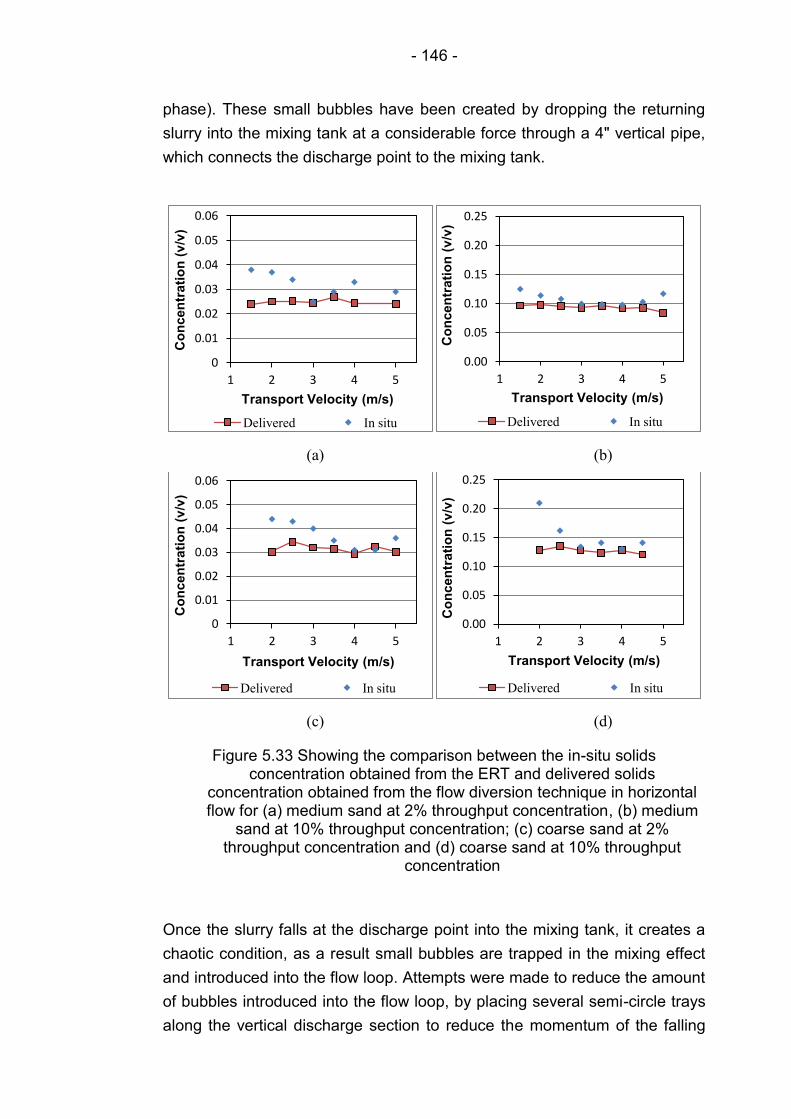
- 146 -
phase). These small bubbles have been created by dropping the returning
slurry into the mixing tank at a considerable force through a 4ʺ vertical pipe,
which connects the discharge point to the mixing tank.
(a) (b)
(c) (d)
Figure 5.33 Showing the comparison between the in-situ solids concentration obtained from the ERT and delivered solids
concentration obtained from the flow diversion technique in horizontal flow for (a) medium sand at 2% throughput concentration, (b) medium
sand at 10% throughput concentration; (c) coarse sand at 2% throughput concentration and (d) coarse sand at 10% throughput
concentration
Once the slurry falls at the discharge point into the mixing tank, it creates a
chaotic condition, as a result small bubbles are trapped in the mixing effect
and introduced into the flow loop. Attempts were made to reduce the amount
of bubbles introduced into the flow loop, by placing several semi-circle trays
along the vertical discharge section to reduce the momentum of the falling
0
0.01
0.02
0.03
0.04
0.05
0.06
1 2 3 4 5
Co
ncen
trati
on
(v
/v)
Transport Velocity (m/s)
Delivered In situ
0.00
0.05
0.10
0.15
0.20
0.25
1 2 3 4 5
Co
ncen
trati
on
(v
/v)
Transport Velocity (m/s)
Delivered In situ
0
0.01
0.02
0.03
0.04
0.05
0.06
1 2 3 4 5
Co
ncen
trati
on
(v
/v)
Transport Velocity (m/s)
Delivered In situ
0.00
0.05
0.10
0.15
0.20
0.25
1 2 3 4 5
Co
ncen
trati
on
(v
/v)
Transport Velocity (m/s)
Delivered In situ

- 147 -
slurry or reducing the vortex formed in the vertical pipe. In addition, a baffle
was placed in the mixing tank to separate the mixing zone from the region of
returning slurry. The methods used to reduce bubbles in the flow loop are
discussed in section 5.4.7. This possibility is based on the fact that at higher
velocities the slurry returning to the mixing tank through approximately 2 m
length uPVC vertical pipeline (100 mm ID), at the end of which the slurry
falling into the tank and creating a chaotic zone within the tank. As a result
bubbles are entrained into the tank, whereby they are trapped by the mixing
effect and introduced to the pipeline.
On the other hand, an increase in the In-situ concentration can be noticed at
lower velocities (3 m/s and below), this is totally predicted for slurry flow as
indicating the hold up of solids, which contribute into an increase in the local
concentration and as a result the delivered concentration is decreased.
5.4.10.2 Validation of mean solids axial velocity
The technique used to validate the solids velocity results of the ERT is
similar to that of the EMF, which is using the measuring tank and calculation
of the discharge velocity. Since at the discharge point, there is no slip
velocity, therefore, the solids velocity can be determined by the ratio of the
discharge slurry volume flow rate to the discharge pipe cross-sectional area.
Thereafter, comparing the two mean slurry velocity values (the discharge
with that of measured by the ERT). The procedure was to measure the
solids velocity by the ERT, then calculate the mean velocity across the
horizontal pipe cross-section. Consequently, measuring the discharge
velocity, considering all the implications that are associated with the slurry
diversion, which is the driving force for flow instability. This procedure was
repeated for both sands, each at 2% and 10% throughput concentration,
including the blockage of coarse sand at 10% throughput concentration. The
pre-calibrated EMF was used to monitor the mean slurry velocity within the
range of 1.2-5 m/s. The two data velocities, the ERT and the discharge,
were collected and compared against each other, as shown in Table 5.6.
Error analysis was carried out for each condition and the results are
highlighted quantitatively and qualitatively.
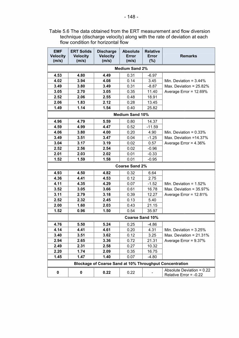
- 148 -
Table 5.6 The data obtained from the ERT measurement and flow diversion technique (discharge velocity) along with the rate of deviation at each flow condition for horizontal flow
EMF Velocity
(m/s)
ERT Solids Velocity
(m/s)
Discharge Velocity
(m/s)
Absolute Error (m/s)
Relative Error (%)
Remarks
Medium Sand 2%
4.53 4.80 4.49 0.31 -6.97
4.02 3.94 4.08 0.14 3.45 Min. Deviation = 3.44%
3.49 3.80 3.49 0.31 -8.87 Max. Deviation = 25.82%
3.05 2.70 3.05 0.35 11.40 Average Error = 12.69%
2.52 2.06 2.55 0.48 18.91
2.06 1.83 2.12 0.28 13.45
1.49 1.14 1.54 0.40 25.82
Medium Sand 10%
4.96 4.79 5.59 0.80 14.37
4.59 4.99 4.47 0.52 -11.59
4.06 3.80 4.00 0.20 4.90 Min. Deviation = 0.33%
3.49 3.51 3.47 0.04 -1.25 Max. Deviation =14.37%
3.04 3.17 3.19 0.02 0.57 Average Error = 4.36%
2.52 2.56 2.54 0.02 -0.96
2.01 2.03 2.02 0.01 -0.33
1.52 1.59 1.58 0.01 -0.95
Coarse Sand 2%
4.93 4.50 4.82 0.32 6.64
4.36 4.41 4.53 0.12 2.75
4.11 4.35 4.29 0.07 -1.52 Min. Deviation = 1.52%
3.52 3.05 3.66 0.61 16.78 Max. Deviation = 35.97%
3.11 2.79 3.18 0.39 12.27 Average Error = 12.81%
2.52 2.32 2.45 0.13 5.40
2.00 1.60 2.03 0.43 21.15
1.52 0.96 1.50 0.54 35.97
Coarse Sand 10%
4.76 5.50 5.24 0.25 -4.86
4.14 4.41 4.61 0.20 4.31 Min. Deviation = 3.25%
3.40 3.51 3.62 0.12 3.25 Max. Deviation = 21.31%
2.94 2.65 3.36 0.72 21.31 Average Error = 9.37%
2.49 2.31 2.58 0.27 10.32
2.20 1.74 2.09 0.35 16.75
1.45 1.47 1.40 0.07 -4.80
Blockage of Coarse Sand at 10% Throughput Concentration
0 0 0.22 0.22 - Absolute Deviation = 0.22 Relative Error = -0.22
- 149 -
The maximum, minimum and the average deviation are also highlighted for
both, coarse and medium sand, at different throughput concentrations and
velocity range mentioned above. Similarly, the error analysis was also
carried out for blockage of horizontal pipeline, which is also highlighted in the
aforementioned table.
The minimum deviation of (0.33%) between the discharge and the ERT
velocities was observed at (10%) medium sand throughput concentration,
whereas the maximum deviation of (35%) was noticed at (2%) coarse sand
throughput concentration and 1.5 m/s transport velocity. While the horizontal
pipeline was blocked, a transport velocity of 0 m/s was shown on the EMF.
In addition, there was 0 m/s flow at the discharge. However, the mean slurry
velocity measured by the ERT indicates 0.22 m/s, which makes -0.22 m/s
error relative to the true value indicated by the discharge. Since the
magnitude of the error is a negative value, then it is apparent that, based on
the equation for the relative error, the ERT overestimates the mean velocity
by 0.22 m/s.
However, if we look at the measured velocities it can be seen that the ERT
measured values of solids velocity are reasonably close to the values of
solids velocity measured by the measuring tank over the entire range of
throughput concentration and transport velocities. The linear relationship
between the ERT and the discharge velocities was also assessed through
quantitative and qualitative output results of regression analysis. The
quantitative results are shown in Table 5.7, in which it is apparent that the
degree of linear relationship between both measured and predicted ERT
velocity values are represented by R square. It is observed that the value of
R square in all conditions employed in the experiment is around 99%. This
value determines the suitability of using the predicted values of ERT to
highlight the deviations for each velocity data point.
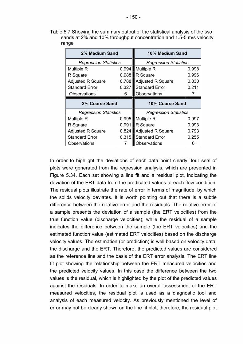
- 150 -
Table 5.7 Showing the summary output of the statistical analysis of the two sands at 2% and 10% throughput concentration and 1.5-5 m/s velocity range
2% Medium Sand 10% Medium Sand
Regression Statistics Regression Statistics
Multiple R 0.994 Multiple R 0.998
R Square 0.988 R Square 0.996
Adjusted R Square 0.788 Adjusted R Square 0.830
Standard Error 0.327 Standard Error 0.211
Observations 6 Observations 7
2% Coarse Sand 10% Coarse Sand
Regression Statistics Regression Statistics
Multiple R 0.995 Multiple R 0.997
R Square 0.991 R Square 0.993
Adjusted R Square 0.824 Adjusted R Square 0.793
Standard Error 0.315 Standard Error 0.255
Observations 7 Observations 6
In order to highlight the deviations of each data point clearly, four sets of
plots were generated from the regression analysis, which are presented in
Figure 5.34. Each set showing a line fit and a residual plot, indicating the
deviation of the ERT data from the predicated values at each flow condition.
The residual plots illustrate the rate of error in terms of magnitude, by which
the solids velocity deviates. It is worth pointing out that there is a subtle
difference between the relative error and the residuals. The relative error of
a sample presents the deviation of a sample (the ERT velocities) from the
true function value (discharge velocities); while the residual of a sample
indicates the difference between the sample (the ERT velocities) and the
estimated function value (estimated ERT velocities) based on the discharge
velocity values. The estimation (or prediction) is well based on velocity data,
the discharge and the ERT. Therefore, the predicted values are considered
as the reference line and the basis of the ERT error analysis. The ERT line
fit plot showing the relationship between the ERT measured velocities and
the predicted velocity values. In this case the difference between the two
values is the residual, which is highlighted by the plot of the predicted values
against the residuals. In order to make an overall assessment of the ERT
measured velocities, the residual plot is used as a diagnostic tool and
analysis of each measured velocity. As previously mentioned the level of
error may not be clearly shown on the line fit plot, therefore, the residual plot

- 151 -
is used, which clearly shows the deviation of each velocity data point about
the predicted values.
An overall observation of the line fit plot in Figure 5.34, suggests a rather
reasonable estimation of the ERT mean solids velocity values in all
conditions. However, from both, the line fit and the residual plots, three
observations can be remarked. Firstly, it is clear that the errors are quite
random throughout the velocity range used in the experiments. This
statement is valid for all conditions. Secondly, based on the discharge solids
velocity values, it is obvious that the ERT velocities are mostly
underestimated at low velocities (3 m/s and below), which is considered as
stratified velocity region, where the bed exists (either moving or stationary)
and the particles over it move in a sporadic fashion. Thirdly, an
overestimation of the ERT solids axial velocities is well pronounced at high
transport velocities (above 3 m/s). The occurrence of random errors can be
attributed to the complexity of solid flow within the carrier liquid and the
discontinuity of flow, whereby different flow regimes are manifested. Since
the flow regimes are dependent on particle size and solids concentration,
then the transitional velocities between flow regimes can differ for each
concentration and particle size used in this investigation. Therefore, it is
totally plausible for the errors to occur at different rate for each sand and
concentration at a given transport velocity. From this a conclusion can be
drawn that the ERT solids velocity measurement is dependent on the
prevailing flow regime within the pipe. Therefore, in order to make a rather
accurate ERT solids velocity measurement, automated flow regime
recognition has to be developed to identify the prevailing flow regime, after
which the ERT measurement correction will be applied based on the present
flow regime within the pipe. This can be confirmed by the general distribution
pattern of the errors on the line plots shown in Figure 5.34. At high velocities,
where the particles are suspended in the carrier liquid, the solids velocities
are overestimated by the ERT; whereas, at low velocities, within the range of
which fully or partially stratification occurs, the solids velocities are
underestimated. The change in the trajectory of the errors on the line fit is
highly likely to be due to the phenomenon of particle wave speed. This is
well related to the configuration of the dual plane ERT sensor (distance
between the sensor planes). The optimum distance between the two planes
is based on the transport velocities used in the pipeline. At low transport
velocities the interval distance between the two planes requires to be shorter
than that used for high velocities.
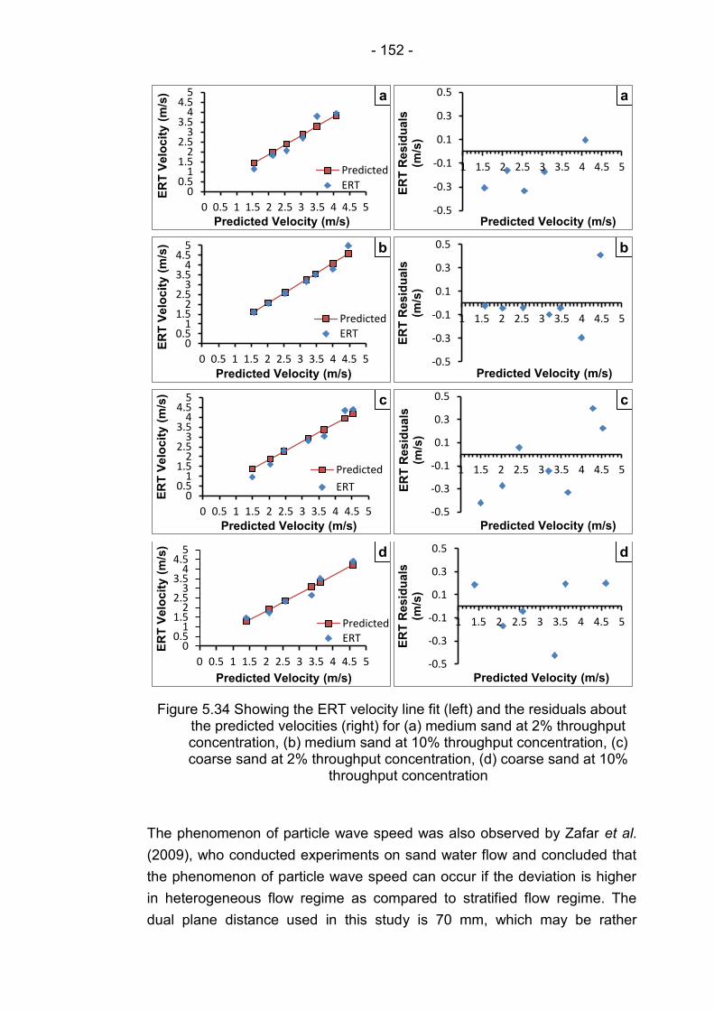
- 152 -
Figure 5.34 Showing the ERT velocity line fit (left) and the residuals about the predicted velocities (right) for (a) medium sand at 2% throughput concentration, (b) medium sand at 10% throughput concentration, (c) coarse sand at 2% throughput concentration, (d) coarse sand at 10%
throughput concentration
The phenomenon of particle wave speed was also observed by Zafar et al.
(2009), who conducted experiments on sand water flow and concluded that
the phenomenon of particle wave speed can occur if the deviation is higher
in heterogeneous flow regime as compared to stratified flow regime. The
dual plane distance used in this study is 70 mm, which may be rather
0 0.5
1 1.5
2 2.5
3 3.5
4 4.5
5
0 0.5 1 1.5 2 2.5 3 3.5 4 4.5 5
ER
T V
elo
cit
y (
m/s
)
Predicted Velocity (m/s)
a
Predicted
ERT
-0.5
-0.3
-0.1
0.1
0.3
0.5
1 1.5 2 2.5 3 3.5 4 4.5 5
ER
T R
esid
uals
(m
/s)
Predicted Velocity (m/s)
a
0 0.5
1 1.5
2 2.5
3 3.5
4 4.5
5
0 0.5 1 1.5 2 2.5 3 3.5 4 4.5 5
ER
T V
elo
cit
y (
m/s
)
Predicted Velocity (m/s)
b
Predicted
ERT
-0.5
-0.3
-0.1
0.1
0.3
0.5
1 1.5 2 2.5 3 3.5 4 4.5 5
ER
T R
esid
uals
(m
/s)
Predicted Velocity (m/s)
b
0 0.5
1 1.5
2 2.5
3 3.5
4 4.5
5
0 0.5 1 1.5 2 2.5 3 3.5 4 4.5 5
ER
T V
elo
cit
y (
m/s
)
Predicted Velocity (m/s)
c
Predicted
ERT
-0.5
-0.3
-0.1
0.1
0.3
0.5
1 1.5 2 2.5 3 3.5 4 4.5 5
ER
T R
esid
uals
(m
/s)
Predicted Velocity (m/s)
c
0 0.5
1 1.5
2 2.5
3 3.5
4 4.5
5
0 0.5 1 1.5 2 2.5 3 3.5 4 4.5 5
ER
T V
elo
cit
y (
m/s
)
Predicted Velocity (m/s)
d
Predicted ERT
-0.5
-0.3
-0.1
0.1
0.3
0.5
1 1.5 2 2.5 3 3.5 4 4.5 5
ER
T R
esid
uals
(m
/s)
Predicted Velocity (m/s)
d

- 153 -
suitable for high slurry velocity, but certainly not for lower velocities, where
partially of fully stratification is present. In other words, the sporadic
movement of the particles above the bed, as they are lifted from the top of
the bed by the wave velocity of the carrier liquid, can be detected by one
plane, however, due to long distance between the two planes, the second
plane is unable to detect, as a result the cross-correlation fails. In some
other cases, since the ERT suffers from particle distinguishability issues, the
particles move above the bed may not be well close to each other for the
ERT to detect them. Therefore, in this case the moving particle is not taken
into account, as a result an underestimation of solids velocity occurs.
It is accepted in literature (Gillies, 1993; Matousek, 2005), that the prevailing
mechanism of particle support, even within a short axial distance in the
horizontal pipeline, is due to the interaction with turbulent eddies of the
flowing stream. The same mechanism is applied for partially or fully stratified
flow, where a portion of particles are lifted again from the surface of the bed
by a lump of liquid and mixed with the stream flowing over the bed in a new
location. The transfer of momentum and mass occur within the mixing
length, the distance over which the lump of liquid transports its momentum
and the particles caught in this length are migrated into the stream layers
over the bed, (Perry et al.,1997). Once the particles are suspended in the
carrier liquid, due to turbulent wave (or sporadic movement), they transfer
their submerged weight to the carrier liquid above the bed. As a result a high
shear-stress occurs above the bed, which slightly accelerates the rate of
saltation (accelerates the rolling of particles over each other at the surface of
the bed). This phenomenon creates a conflict between the driving force (the
flowing stream) and the resisting force (the non-hydraulically smooth surface
of the bed). In reality the condition over the bed is highly unstable, which
imply that the conflict between the two forces, driving and resisting, is always
present, unless the transport velocity is varied to a level, in which the pulse
of liquid decrease or increase above the bed. In other words, while the
particles move in continuous sporadic motion, an increase of the transport
velocity would result in the increase of the turbulent eddies over the bed and
cause the top granular layers of the bed to suspend in the carrier liquid. In
this case the higher concentration of particles at the bottom of the shear
layer causes particle-particle interaction and fluid-particle interaction, which
both contribute into the mean solids axial velocity. Therefore, a conclusion
can be drawn that the unsteady-state condition over the bed, which causes
sporadic movement of a portion of particles at the surface of the bed, has
effect on the magnitude of the mean axial solids velocity. In addition, the
- 154 -
ERT underestimation in stratified flow may have to do with low spatial
resolution, due to which the moving particles at the surface of the bed
cannot be detected, as shown in the velocity profiles for coarse and medium
sand. In reality the particles of moving layer at the top of the bed roll over
each other along the surface of the bed and picked up by the turbulent
carrier liquid once they reach the bend, where they are taken upward
through the vertical pipeline to the discharge point. As the ERT also suffers
from particle distinguishability problem, then the particles moving within this
region may not be detected. As a result the mean solids velocity is
underestimated at stratified velocities.
It was observed that at high velocities (3.5-5 m/s) the ERT mostly
overestimate the mean dispersed velocity by as maximum as 11.59% at
4.50 m/s transport velocity for 10% medium sand throughput concentration.
Another reason for this overestimation could well be due to the presence of
bubbles in the flow loop. These small bubbles have been created by
dropping the returning slurry into the mixing tank at a considerable force
through a 4ʺ vertical pipe, which connects the discharge point to the mixing
tank, as previously discussed.
5.5 Vertical upward flow measurement and visualisation
The same flow loop used for horizontal was also used for vertical upward
flow measurement. The vertical test section was located directly after the
horizontal section and connected to each other via a 90° short radius bend.
The total length of the vertical section is approximately 4 m from the lower
bend. The dual plane ERT sensor was mounted on the vertical section at
approximately 3 m from the lower bend to ensure that the flow is fully
developed at the ERT dual-plane sensor location. The Electromagnetic Flow
meter (EMF) was mounted on the vertical line, 1 m above the ERT sensor,
to monitor the slurry flow rate through the vertical pipe line. Two pressure
sensors were also mounted on the same line, within the developed flow
region at 2.5 m interval, for pressure measurement and calculation of the
pressure difference across the test section.
The experiment procedure, for vertical flow measurement, was carried out
the same as that of horizontal flow measurement and in a consequent
fashion. In other words, after each horizontal measurement, consequently a
vertical measurement was conducted at the same flow condition. The aim of
carrying out the horizontal and vertical measurements approximately at the
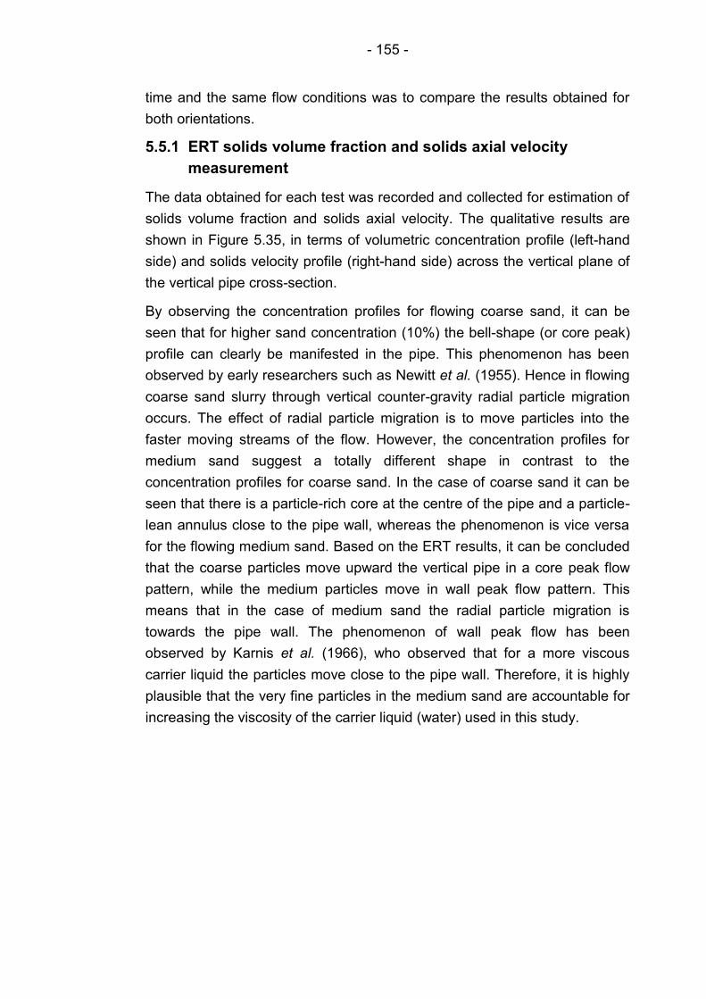
- 155 -
time and the same flow conditions was to compare the results obtained for
both orientations.
5.5.1 ERT solids volume fraction and solids axial velocity
measurement
The data obtained for each test was recorded and collected for estimation of
solids volume fraction and solids axial velocity. The qualitative results are
shown in Figure 5.35, in terms of volumetric concentration profile (left-hand
side) and solids velocity profile (right-hand side) across the vertical plane of
the vertical pipe cross-section.
By observing the concentration profiles for flowing coarse sand, it can be
seen that for higher sand concentration (10%) the bell-shape (or core peak)
profile can clearly be manifested in the pipe. This phenomenon has been
observed by early researchers such as Newitt et al. (1955). Hence in flowing
coarse sand slurry through vertical counter-gravity radial particle migration
occurs. The effect of radial particle migration is to move particles into the
faster moving streams of the flow. However, the concentration profiles for
medium sand suggest a totally different shape in contrast to the
concentration profiles for coarse sand. In the case of coarse sand it can be
seen that there is a particle-rich core at the centre of the pipe and a particle-
lean annulus close to the pipe wall, whereas the phenomenon is vice versa
for the flowing medium sand. Based on the ERT results, it can be concluded
that the coarse particles move upward the vertical pipe in a core peak flow
pattern, while the medium particles move in wall peak flow pattern. This
means that in the case of medium sand the radial particle migration is
towards the pipe wall. The phenomenon of wall peak flow has been
observed by Karnis et al. (1966), who observed that for a more viscous
carrier liquid the particles move close to the pipe wall. Therefore, it is highly
plausible that the very fine particles in the medium sand are accountable for
increasing the viscosity of the carrier liquid (water) used in this study.
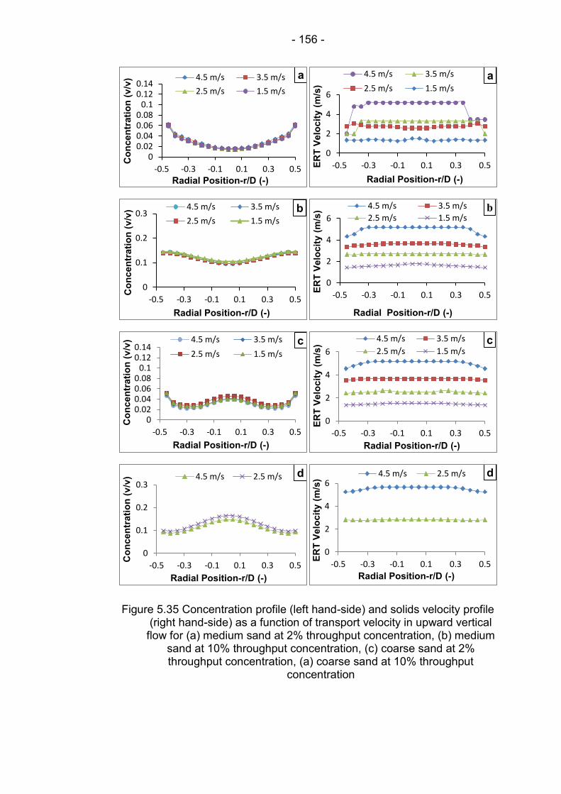
- 156 -
Figure 5.35 Concentration profile (left hand-side) and solids velocity profile (right hand-side) as a function of transport velocity in upward vertical
flow for (a) medium sand at 2% throughput concentration, (b) medium sand at 10% throughput concentration, (c) coarse sand at 2% throughput concentration, (a) coarse sand at 10% throughput
concentration
0 0.02 0.04 0.06 0.08
0.1 0.12 0.14
-0.5 -0.3 -0.1 0.1 0.3 0.5
Co
ncen
trati
on
(v
/v)
Radial Position-r/D (-)
a 4.5 m/s 3.5 m/s
2.5 m/s 1.5 m/s
0
2
4
6
-0.5 -0.3 -0.1 0.1 0.3 0.5 ER
T V
elo
cit
y (
m/s
)
Radial Position-r/D (-)
a 4.5 m/s 3.5 m/s
2.5 m/s 1.5 m/s
0
0.1
0.2
0.3
-0.5 -0.3 -0.1 0.1 0.3 0.5
Co
ncen
trati
on
(v
/v)
Radial Position-r/D (-)
b 4.5 m/s 3.5 m/s
2.5 m/s 1.5 m/s
0
2
4
6
-0.5 -0.3 -0.1 0.1 0.3 0.5
ER
T V
elo
cit
y (
m/s
) Radial Position-r/D (-)
b 4.5 m/s 3.5 m/s
2.5 m/s 1.5 m/s
0 0.02 0.04 0.06 0.08
0.1 0.12 0.14
-0.5 -0.3 -0.1 0.1 0.3 0.5
Co
ncen
trati
on
(v
/v)
Radial Position-r/D (-)
c 4.5 m/s 3.5 m/s
2.5 m/s 1.5 m/s
0
2
4
6
-0.5 -0.3 -0.1 0.1 0.3 0.5
ER
T V
elo
cit
y (
m/s
)
Radial Position-r/D (-)
c 4.5 m/s 3.5 m/s
2.5 m/s 1.5 m/s
0
0.1
0.2
0.3
-0.5 -0.3 -0.1 0.1 0.3 0.5
Co
ncen
trati
on
(v
/v)
Radial Position-r/D (-)
d 4.5 m/s 2.5 m/s
0
2
4
6
-0.5 -0.3 -0.1 0.1 0.3 0.5
ER
T V
elo
cit
y (
m/s
)
Radial Position-r/D (-)
d 4.5 m/s 2.5 m/s

- 157 -
It is also apparent that the phenomenon of radial particle migration for
coarse sand is not quite reflected in the solids velocity profile for all
conditions, instead showing a blunted shape rather than an inverse bell-
shape (or parabolic). The velocity of particles exhibits a uniform distribution
throughout the centre region of the pipe cross-section. It is quite expected
that the particles within the particle-rich core, for flowing coarse sand, move
slower relative to the surrounding layer due to gravity effect (density
difference) and particle-particle interaction. The flattened shape of velocity
profile has been observed by some researchers, for example Koh et al.
(1994), similar to the one obtained in this study using the ERT. They also
noticed that with increasing delivered solids concentration, the velocity
profile becomes increasingly blunted. This implies that at higher transport
velocities, the shape of solids velocity profile becomes further flattened, as it
can be observed in the solids velocity profiles shown in Figure 5.35. The
results of Koh et al. (1994) also revealed another phenomenon, which is with
increases in particle size the velocity profile become increasingly flattened.
This phenomenon was also picked up by the ERT used in this study.
It is also apparent that by increasing the concentration and particle size, the
particles move further towards the centre line region of the flow and the pick
takes more towards the centre of the pipe cross-section. It was found that
the results are in good agreement with those found by Lucas et al. (1999),
using an electrical probe. Also, similar results were found by Koh et al.
(1994), who measured the particle concentration and velocity profiles of
particle size 1-5 mm in a Newtonian fluid through a vertical rectangular
channel. Their results showed a non-uniform, bell-shaped concentration
profile, with a maximum particle concentration at the centre line and a
minimum particle concentration near the wall. Therefore, it can be concluded
that the local solids concentration profile and the solids velocity distribution
calculated using the ERT are a reasonably accurate representation of the
true flow profile for flowing slurry through a vertical counter-gravity pipe at
the particular conditions used in this investigation. However, there is only a
significant feature, which is overestimation of velocities at the centre of the
pipe, and this could well be attributed to the spatial resolution of the ERT
and sensitivity gradient across the pipe cross-section.
5.5.2 ERT based slurry flow rate measurement
Due to the complexity of multiphase/two phase flow, particularly solid-liquid
flow, it is enormously difficult to accurately measure the flow parameters of
each phase individually using only one conventional flow meter. Currently
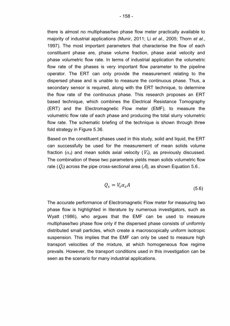
- 158 -
there is almost no multiphase/two phase flow meter practically available to
majority of industrial applications (Munir, 2011; Li et al., 2005; Thorn et al.,
1997). The most important parameters that characterise the flow of each
constituent phase are, phase volume fraction, phase axial velocity and
phase volumetric flow rate. In terms of industrial application the volumetric
flow rate of the phases is very important flow parameter to the pipeline
operator. The ERT can only provide the measurement relating to the
dispersed phase and is unable to measure the continuous phase. Thus, a
secondary sensor is required, along with the ERT technique, to determine
the flow rate of the continuous phase. This research proposes an ERT
based technique, which combines the Electrical Resistance Tomography
(ERT) and the Electromagnetic Flow meter (EMF), to measure the
volumetric flow rate of each phase and producing the total slurry volumetric
flow rate. The schematic briefing of the technique is shown through three
fold strategy in Figure 5.36.
Based on the constituent phases used in this study, solid and liquid, the ERT
can successfully be used for the measurement of mean solids volume
fraction (αs) and mean solids axial velocity (Vs), as previously discussed.
The combination of these two parameters yields mean solids volumetric flow
rate (Qs) across the pipe cross-sectional area (A), as shown Equation 5.6..
(5.6)
The accurate performance of Electromagnetic Flow meter for measuring two
phase flow is highlighted in literature by numerous investigators, such as
Wyatt (1986), who argues that the EMF can be used to measure
multiphase/two phase flow only if the dispersed phase consists of uniformly
distributed small particles, which create a macroscopically uniform isotropic
suspension. This implies that the EMF can only be used to measure high
transport velocities of the mixture, at which homogeneous flow regime
prevails. However, the transport conditions used in this investigation can be
seen as the scenario for many industrial applications.
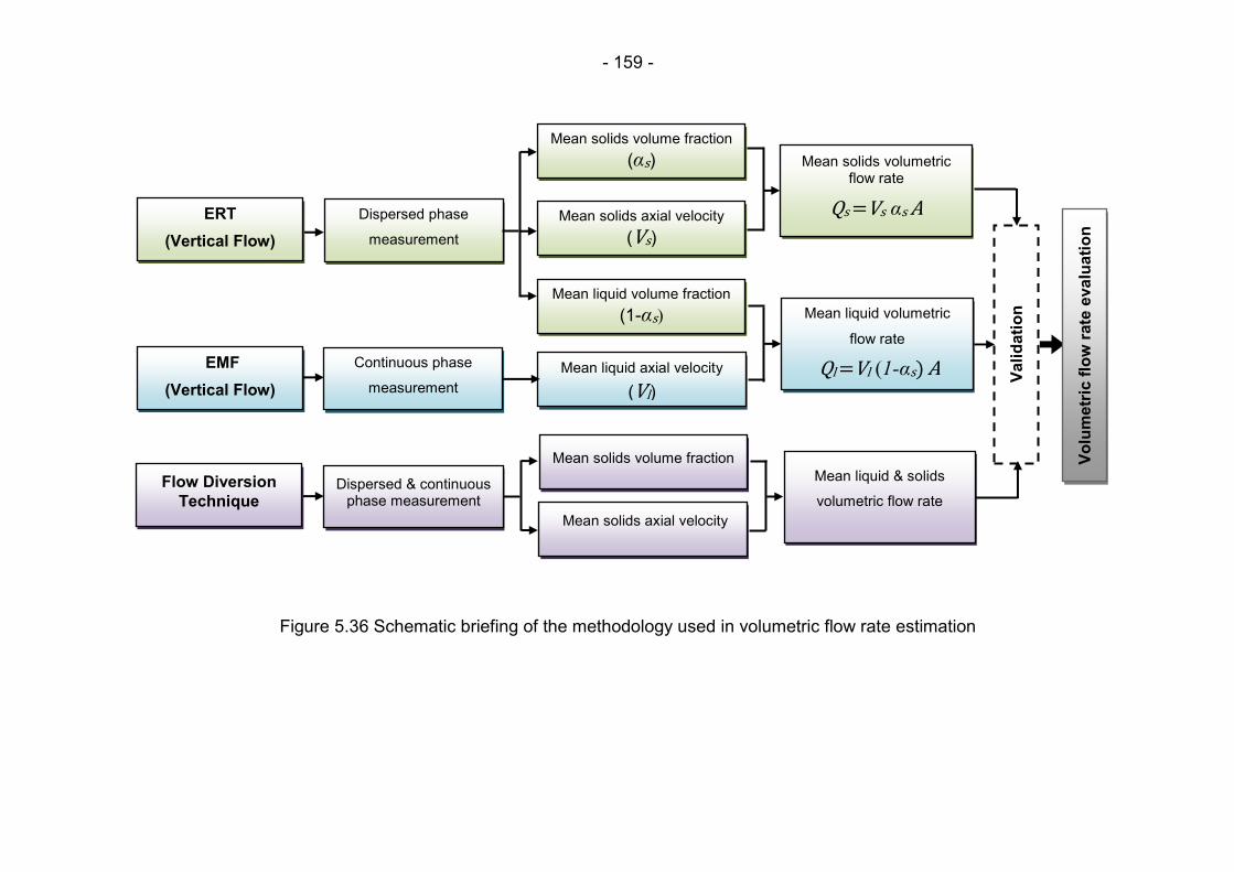
- 159 -
Figure 5.36 Schematic briefing of the methodology used in volumetric flow rate estimation
EMF
(Vertical Flow)
Mean liquid axial velocity
(Vl)
Flow Diversion
Technique
Mean liquid & solids
volumetric flow rate
Mean solids axial velocity
ERT
(Vertical Flow)
Mean solids axial velocity
(Vs)
Mean solids volume fraction
(αs)
Continuous phase
measurement
Dispersed phase
measurement
Mean liquid volume fraction
(1-αs)
Mean solids volumetric flow rate
Qs =Vs αs A
Dispersed & continuous phase measurement
Mean liquid volumetric
flow rate
Ql =Vl (1-αs) A
Va
lid
ati
on
Mean solids volume fraction Vo
lum
etr
ic f
low
rate
eva
lua
tio
n
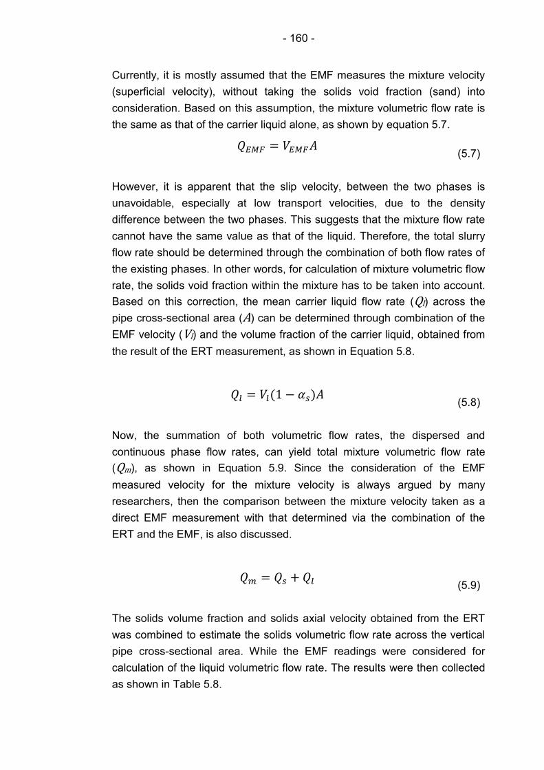
- 160 -
Currently, it is mostly assumed that the EMF measures the mixture velocity
(superficial velocity), without taking the solids void fraction (sand) into
consideration. Based on this assumption, the mixture volumetric flow rate is
the same as that of the carrier liquid alone, as shown by equation 5.7.
(5.7)
However, it is apparent that the slip velocity, between the two phases is
unavoidable, especially at low transport velocities, due to the density
difference between the two phases. This suggests that the mixture flow rate
cannot have the same value as that of the liquid. Therefore, the total slurry
flow rate should be determined through the combination of both flow rates of
the existing phases. In other words, for calculation of mixture volumetric flow
rate, the solids void fraction within the mixture has to be taken into account.
Based on this correction, the mean carrier liquid flow rate (Ql) across the
pipe cross-sectional area (A) can be determined through combination of the
EMF velocity (Vl) and the volume fraction of the carrier liquid, obtained from
the result of the ERT measurement, as shown in Equation 5.8.
(5.8)
Now, the summation of both volumetric flow rates, the dispersed and
continuous phase flow rates, can yield total mixture volumetric flow rate
(Qm), as shown in Equation 5.9. Since the consideration of the EMF
measured velocity for the mixture velocity is always argued by many
researchers, then the comparison between the mixture velocity taken as a
direct EMF measurement with that determined via the combination of the
ERT and the EMF, is also discussed.
(5.9)
The solids volume fraction and solids axial velocity obtained from the ERT
was combined to estimate the solids volumetric flow rate across the vertical
pipe cross-sectional area. While the EMF readings were considered for
calculation of the liquid volumetric flow rate. The results were then collected
as shown in Table 5.8.
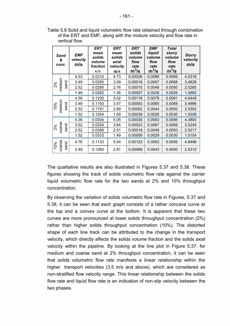
- 161 -
Table 5.8 Solid and liquid volumetric flow rate obtained through combination of the ERT and EMF, along with the mixture velocity and flow rate in vertical flow
Sand &
conc.
EMF velocity
m/s
ERT mean solids
volume fraction
v/v
ERT mean solids axial
velocity
m/s
ERT solids
volume flow rate
m3/s
EMF liquid
volume flow rate
m3/s
Total slurry
volume flow rate
m3/s
Slurry velocity
m/s
2%
med
ium
sand
4.53 0.0310 4.73 0.00028 0.0086 0.0089 4.5316
3.49 0.0285 3.09 0.00018 0.0067 0.0068 3.4828
2.52 0.0285 2.76 0.00015 0.0048 0.0050 2.5285
1.49 0.0282 1.36 0.00007 0.0028 0.0029 1.4882
10%
med
ium
sand
4.59 0.1200 5.02 0.00118 0.0079 0.0091 4.6448
3.49 0.1193 3.57 0.00083 0.0060 0.0069 3.4996
2.52 0.1191 2.69 0.00062 0.0044 0.0050 2.5392
1.52 0.1254 1.59 0.00039 0.0026 0.0030 1.5308
2%
coars
e
sand
4.36 0.0304 5.05 0.00030 0.0083 0.0086 4.3800
3.52 0.0324 3.64 0.00023 0.0067 0.0069 3.5245
2.52 0.0368 2.51 0.00018 0.0048 0.0050 2.5217
1.52 0.0333 1.49 0.00009 0.0029 0.0030 1.5154
10%
coars
e
sand
4.76 0.1133 5.54 0.00123 0.0083 0.0095 4.8496
2.49 0.1260 2.81 0.00069 0.0043 0.0050 2.5312
The qualitative results are also illustrated in Figures 5.37 and 5.38. These
figures showing the track of solids volumetric flow rate against the carrier
liquid volumetric flow rate for the two sands at 2% and 10% throughput
concentration.
By observing the variation of solids volumetric flow rate in Figures, 5.37 and
5.38, it can be seen that each graph consists of a rather concave curve at
the top and a convex curve at the bottom. It is apparent that these two
curves are more pronounced at lower solids throughput concentration (2%)
rather than higher solids throughput concentration (10%). The distorted
shape of each line track can be attributed to the change in the transport
velocity, which directly affects the solids volume fraction and the solids axial
velocity within the pipeline. By looking at the line plot in Figure 5.37, for
medium and coarse sand at 2% throughput concentration, it can be seen
that solids volumetric flow rate manifests a linear relationship within the
higher transport velocities (3.5 m/s and above), which are considered as
non-stratified flow velocity range. This linear relationship between the solids
flow rate and liquid flow rate is an indication of non-slip velocity between the
two phases.
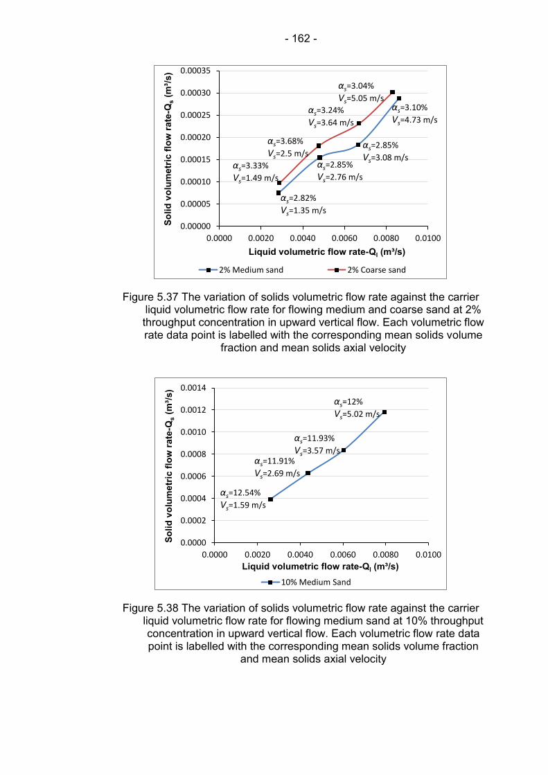
- 162 -
Figure 5.37 The variation of solids volumetric flow rate against the carrier liquid volumetric flow rate for flowing medium and coarse sand at 2% throughput concentration in upward vertical flow. Each volumetric flow rate data point is labelled with the corresponding mean solids volume
fraction and mean solids axial velocity
Figure 5.38 The variation of solids volumetric flow rate against the carrier liquid volumetric flow rate for flowing medium sand at 10% throughput concentration in upward vertical flow. Each volumetric flow rate data point is labelled with the corresponding mean solids volume fraction
and mean solids axial velocity
0.00000
0.00005
0.00010
0.00015
0.00020
0.00025
0.00030
0.00035
0.0000 0.0020 0.0040 0.0060 0.0080 0.0100
So
lid
vo
lum
etr
ic f
low
rate
-Qs (
m³/
s)
Liquid volumetric flow rate-Ql (m³/s)
2% Medium sand 2% Coarse sand
αs=3.68%
Vs=2.5 m/s
αs=3.24%
Vs=3.64 m/s
αs=3.04%
Vs=5.05 m/s
αs=3.33%
Vs=1.49 m/s
αs=2.82%
Vs=1.35 m/s
αs=2.85%
Vs=2.76 m/s
αs=2.85%
Vs=3.08 m/s
αs=3.10%
Vs=4.73 m/s
0.0000
0.0002
0.0004
0.0006
0.0008
0.0010
0.0012
0.0014
0.0000 0.0020 0.0040 0.0060 0.0080 0.0100
So
lid
vo
lum
etr
ic f
low
rate
-Qs (
m³/
s)
Liquid volumetric flow rate-Ql (m³/s)
10% Medium Sand
αs=12%
Vs=5.02 m/s
αs=11.93%
Vs=3.57 m/s αs=11.91%
Vs=2.69 m/s
αs=12.54%
Vs=1.59 m/s
- 163 -
In other words, within the range of velocities, at which all the solid particles
are suspended in the carrier liquid and they move more or less at the same
velocity as that of the carrier liquid, the track of solids volumetric flow rate
continuous on a straight line. However, by decreasing the transport velocity
the line changes its trajectory to produce a concave curve, then it bends
down to form a convex curve. This is due to the density difference between
the two phases. As the transport velocity decreases the solid particles slow
down, which leads to the reduction of their flow rate. After the convex curve,
further reduction of transport velocity leads to further reduction of solids axial
velocity and deposition of solid particles within the horizontal pipeline. As a
result the solids volumetric flow rate decreases in the vertical pipeline, which
is clearly highlighted in Figures 5.37 and 5.38. Continuous reduction of
transport velocity, towards pipe blockage condition, results in zero solids
flow rate and obviously the carrier liquid flow rate too, as the flow of each
phase comes to halt within the pipelines.
Another phenomenon can be noticed on each flow rate plot, on which the
track changes rather sharply its trajectory to form the concave curve and the
convex curve. The region between these two curves can be considered as a
transitional region between the stratified flow and non-stratified flow. This
argument is well based on the results of flow regime characterisation
discussed previously in this chapter. Based on visual observation and
photographic evidence, it was found that the stratified flow starts at around
3.5 m/s transport velocity. This region can be remarked between the two
points, starting at the first point where the track goes through a rather sharp
change to form the concave curve, and the second point where the curve
goes through another change in its trajectory to form the convex curve. As
previously mentioned this region is less pronounced for the flowing of sand
at 10% throughput concentration. Despite that the diversion point from the
linear track can be noticed.
Based on the above results and observations, it is apparent that the ERT
can detect the variations of solids volumetric flow rate within the range of
conditions used in this investigation. Also, based on the results obtained
from the combination of the ERT and the EMF, to measure the solids flow
rate and liquid flow rate respectively, the slip velocity between the two
phases, can successfully be estimated. The evaluation of the technique,
through highlighting the rate of associated error in each condition used in
this study, is also discussed later in this section.
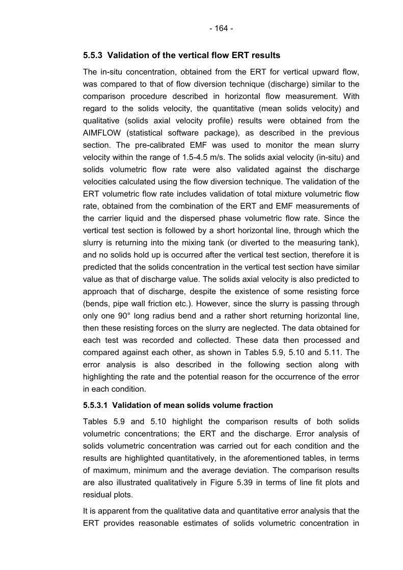
- 164 -
5.5.3 Validation of the vertical flow ERT results
The in-situ concentration, obtained from the ERT for vertical upward flow,
was compared to that of flow diversion technique (discharge) similar to the
comparison procedure described in horizontal flow measurement. With
regard to the solids velocity, the quantitative (mean solids velocity) and
qualitative (solids axial velocity profile) results were obtained from the
AIMFLOW (statistical software package), as described in the previous
section. The pre-calibrated EMF was used to monitor the mean slurry
velocity within the range of 1.5-4.5 m/s. The solids axial velocity (in-situ) and
solids volumetric flow rate were also validated against the discharge
velocities calculated using the flow diversion technique. The validation of the
ERT volumetric flow rate includes validation of total mixture volumetric flow
rate, obtained from the combination of the ERT and EMF measurements of
the carrier liquid and the dispersed phase volumetric flow rate. Since the
vertical test section is followed by a short horizontal line, through which the
slurry is returning into the mixing tank (or diverted to the measuring tank),
and no solids hold up is occurred after the vertical test section, therefore it is
predicted that the solids concentration in the vertical test section have similar
value as that of discharge value. The solids axial velocity is also predicted to
approach that of discharge, despite the existence of some resisting force
(bends, pipe wall friction etc.). However, since the slurry is passing through
only one 90° long radius bend and a rather short returning horizontal line,
then these resisting forces on the slurry are neglected. The data obtained for
each test was recorded and collected. These data then processed and
compared against each other, as shown in Tables 5.9, 5.10 and 5.11. The
error analysis is also described in the following section along with
highlighting the rate and the potential reason for the occurrence of the error
in each condition.
5.5.3.1 Validation of mean solids volume fraction
Tables 5.9 and 5.10 highlight the comparison results of both solids
volumetric concentrations; the ERT and the discharge. Error analysis of
solids volumetric concentration was carried out for each condition and the
results are highlighted quantitatively, in the aforementioned tables, in terms
of maximum, minimum and the average deviation. The comparison results
are also illustrated qualitatively in Figure 5.39 in terms of line fit plots and
residual plots.
It is apparent from the qualitative data and quantitative error analysis that the
ERT provides reasonable estimates of solids volumetric concentration in
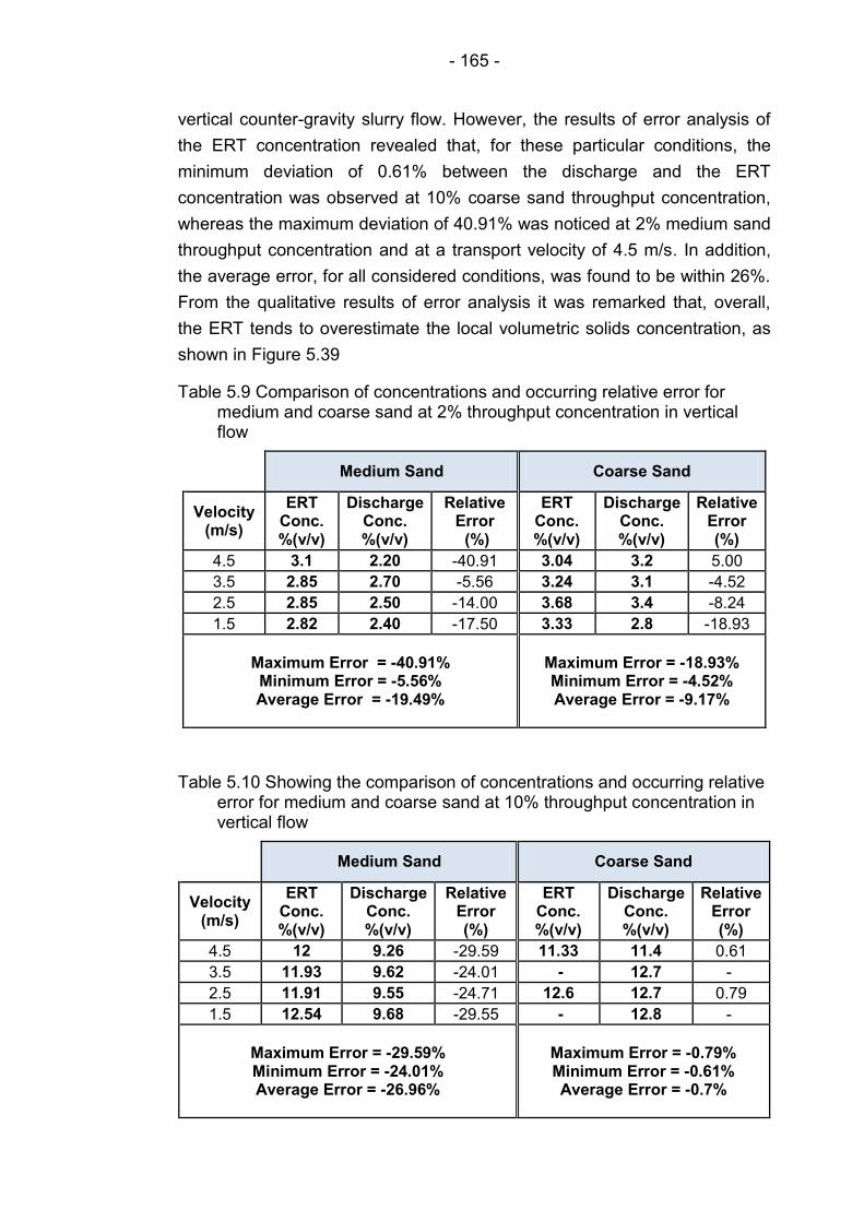
- 165 -
vertical counter-gravity slurry flow. However, the results of error analysis of
the ERT concentration revealed that, for these particular conditions, the
minimum deviation of 0.61% between the discharge and the ERT
concentration was observed at 10% coarse sand throughput concentration,
whereas the maximum deviation of 40.91% was noticed at 2% medium sand
throughput concentration and at a transport velocity of 4.5 m/s. In addition,
the average error, for all considered conditions, was found to be within 26%.
From the qualitative results of error analysis it was remarked that, overall,
the ERT tends to overestimate the local volumetric solids concentration, as
shown in Figure 5.39
Table 5.9 Comparison of concentrations and occurring relative error for medium and coarse sand at 2% throughput concentration in vertical flow
Medium Sand Coarse Sand
Velocity (m/s)
ERT Conc. %(v/v)
Discharge Conc. %(v/v)
Relative Error (%)
ERT Conc. %(v/v)
Discharge Conc. %(v/v)
Relative Error (%)
4.5 3.1 2.20 -40.91 3.04 3.2 5.00
3.5 2.85 2.70 -5.56 3.24 3.1 -4.52
2.5 2.85 2.50 -14.00 3.68 3.4 -8.24
1.5 2.82 2.40 -17.50 3.33 2.8 -18.93
Maximum Error = -40.91% Minimum Error = -5.56% Average Error = -19.49%
Maximum Error = -18.93% Minimum Error = -4.52% Average Error = -9.17%
Table 5.10 Showing the comparison of concentrations and occurring relative error for medium and coarse sand at 10% throughput concentration in vertical flow
Medium Sand Coarse Sand
Velocity (m/s)
ERT Conc. %(v/v)
Discharge Conc. %(v/v)
Relative Error (%)
ERT Conc. %(v/v)
Discharge Conc. %(v/v)
Relative Error (%)
4.5 12 9.26 -29.59 11.33 11.4 0.61
3.5 11.93 9.62 -24.01 - 12.7 -
2.5 11.91 9.55 -24.71 12.6 12.7 0.79
1.5 12.54 9.68 -29.55 - 12.8 -
Maximum Error = -29.59% Minimum Error = -24.01% Average Error = -26.96%
Maximum Error = -0.79% Minimum Error = -0.61% Average Error = -0.7%

- 166 -
This overestimation can clearly be seen on the line fit plot of the ERT
concentration vs. discharge concentration. The deviation of each data point
is more clearly highlighted for each transport velocity in the plot of ERT
deviation magnitude vs. discharge concentration. The reason for this
overestimation may have to do with mechanical installation of 32 electrodes
on the two electrode rings. In other words, one or more electrodes may not
have been well tightened and as a result the electrical connection is
affected, which affects the conductivity of the domain under investigation.
However, a future investigation is paramount to unveil the exact reason
behind this overestimation. Nevertheless, it can be seen that for the flowing
coarse sand, especially for 10% throughput concentration, an
underestimation can be observed. The cause could be due to the gradient in
sensitivity distribution across the radial plane on the sensitivity map (pipe
cross-section), as the higher sensitivity can be found near the pipe wall
rather than the centre of the pipe. This argument could well be supported by
the shape of concentration profile, where a particle-rich core of solids can
clearly be observed at the axis of the pipe surrounded by a particle-lean
annulus. In other words, non-uniform concentration profile, which exhibits a
maximum solids concentration at the centre line of the pipe, and minimum
solids concentration near the pipe-wall, can be noticed, as shown in Figure
5.35.
As the concentration increases the bell-shape (or or core flow) profile can
clearly be manifested in the centre of the pipe. Hence, in flowing coarse
sand slurry through vertical counter-gravity radial particle migration occurs.
Since most of the particles are segregated at the centre of the pipe, and the
centre of the pipe presents the lowest sensitivity relative to the regions near
the pipe wall, then it is reasonable to expect an underestimation of solids
concentration profile at the centre of the pipe, which in return gives an
overall underestimation of mean solids concentration across the pipe cross-
section.
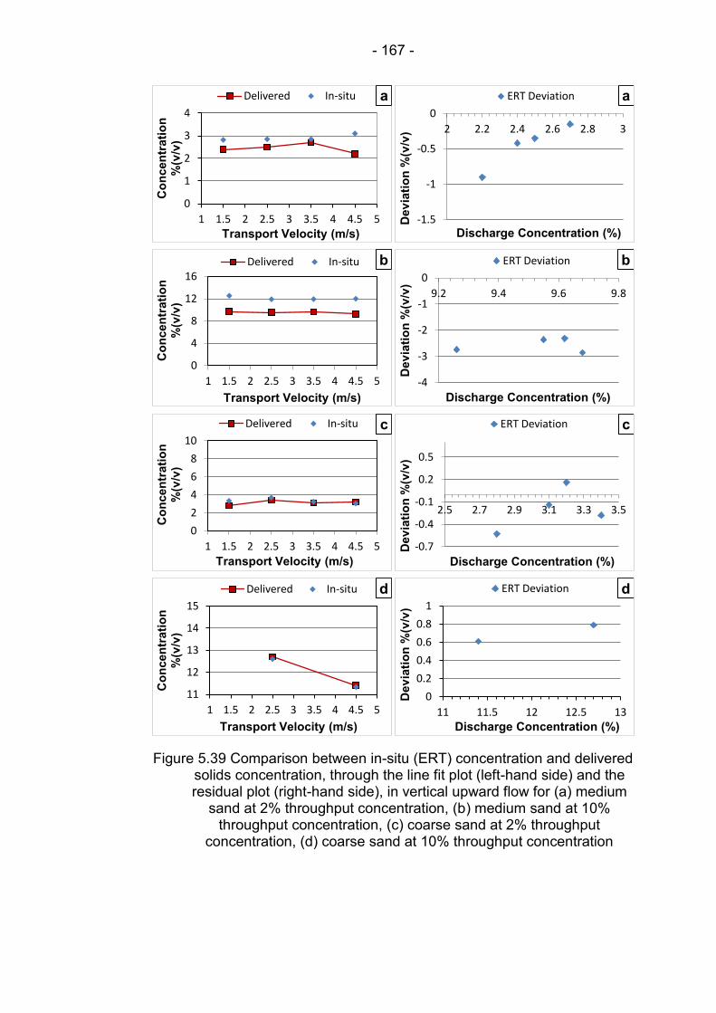
- 167 -
Figure 5.39 Comparison between in-situ (ERT) concentration and delivered solids concentration, through the line fit plot (left-hand side) and the residual plot (right-hand side), in vertical upward flow for (a) medium
sand at 2% throughput concentration, (b) medium sand at 10% throughput concentration, (c) coarse sand at 2% throughput
concentration, (d) coarse sand at 10% throughput concentration
0
1
2
3
4
1 1.5 2 2.5 3 3.5 4 4.5 5
Co
ncen
trati
on
%
(v/v
)
Transport Velocity (m/s)
a Delivered In-situ
-1.5
-1
-0.5
0
2 2.2 2.4 2.6 2.8 3
Dev
iati
on
%(v
/v)
Discharge Concentration (%)
a ERT Deviation
0
4
8
12
16
1 1.5 2 2.5 3 3.5 4 4.5 5
Co
ncen
trati
on
%
(v/v
)
Transport Velocity (m/s)
b Delivered In-situ
-4
-3
-2
-1
0
9.2 9.4 9.6 9.8
Dev
iati
on
%(v
/v)
Discharge Concentration (%)
b ERT Deviation
0
2
4
6
8
10
1 1.5 2 2.5 3 3.5 4 4.5 5
Co
ncen
trati
on
%
(v/v
)
Transport Velocity (m/s)
c Delivered In-situ
-0.7
-0.4
-0.1
0.2
0.5
2.5 2.7 2.9 3.1 3.3 3.5
Dev
iati
on
%(v
/v)
Discharge Concentration (%)
c ERT Deviation
11
12
13
14
15
1 1.5 2 2.5 3 3.5 4 4.5 5
Co
ncen
trati
on
%
(v/v
)
Transport Velocity (m/s)
d Delivered In-situ
0
0.2
0.4
0.6
0.8
1
11 11.5 12 12.5 13
Dev
iati
on
%(v
/v)
Discharge Concentration (%)
d ERT Deviation
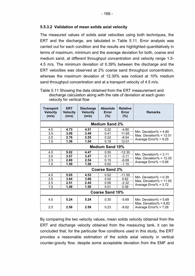
- 168 -
5.5.3.2 Validation of mean solids axial velocity
The measured values of solids axial velocities using both techniques, the
ERT and the discharge, are tabulated in Table 5.11. Error analysis was
carried out for each condition and the results are highlighted quantitatively in
terms of maximum, minimum and the average deviation for both, coarse and
medium sand, at different throughput concentration and velocity range 1.5-
4.5 m/s. The minimum deviation of 0.39% between the discharge and the
ERT velocities was observed at 2% coarse sand throughput concentration,
whereas the maximum deviation of 12.30% was noticed at 10% medium
sand throughput concentration and at a transport velocity of 4.5 m/s.
Table 5.11 Showing the data obtained from the ERT measurement and discharge calculation along with the rate of deviation at each given velocity for vertical flow
Transport Velocity
(m/s)
ERT Velocity
(m/s)
Discharge Velocity
(m/s)
Absolute Error (%)
Relative Error (%)
Remarks
Medium Sand 2%
4.5 4.73 4.51 0.22 -4.80 Min. Deviation% = 4.80 Max. Deviation% = 12.01 Average Error% = 9.25
3.5 3.09 3.49 0.41 11.65
2.5 2.76 2.55 0.22 -8.54
1.5 1.36 1.54 0.19 12.01
Medium Sand 10%
4.5 5.02 4.47 0.55 -12.30 Min. Deviation% = 3.11 Max. Deviation% = 12.30 Average Error% = 5.66
3.5 3.57 3.47 0.11 -3.11
2.5 2.69 2.54 0.15 -6.09
1.5 1.59 1.58 0.02 -1.15
Coarse Sand 2%
4.5 5.05 4.53 0.52 -11.55 Min. Deviation% = 0.39 Max. Deviation% = 11.55 Average Error% = 3.72
3.5 3.64 3.66 0.02 0.62
2.5 2.51 2.45 0.06 -2.32
1.5 1.49 1.50 0.01 0.39
Coarse Sand 10%
4.5 5.24 5.24 0.30 -5.69 Min. Deviation% = 5.69 Max. Deviation% = 8.82 Average Error% = 7.26 2.5 2.58 2.58 0.23 -8.82
By comparing the two velocity values, mean solids velocity obtained from the
ERT and discharge velocity obtained from the measuring tank, it can be
concluded that, for the particular flow conditions used in this study, the ERT
provides a reasonable estimation of the solids axial velocity in vertical
counter-gravity flow, despite some acceptable deviation from the EMF and
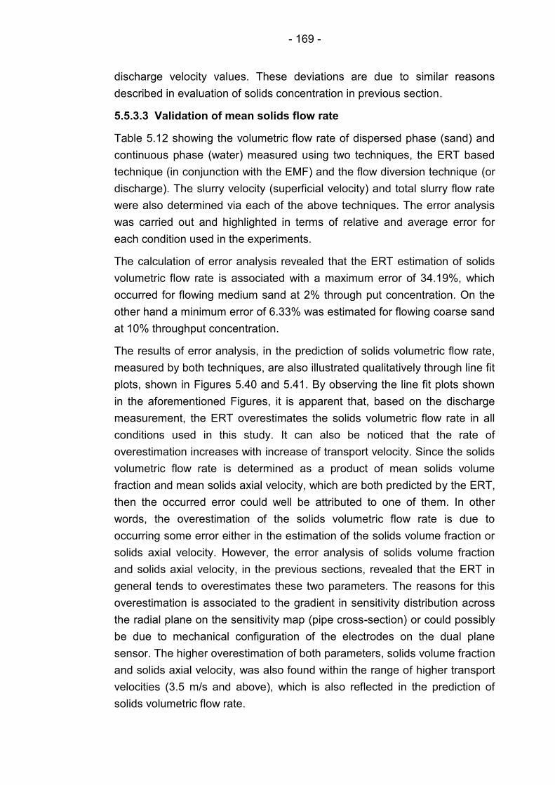
- 169 -
discharge velocity values. These deviations are due to similar reasons
described in evaluation of solids concentration in previous section.
5.5.3.3 Validation of mean solids flow rate
Table 5.12 showing the volumetric flow rate of dispersed phase (sand) and
continuous phase (water) measured using two techniques, the ERT based
technique (in conjunction with the EMF) and the flow diversion technique (or
discharge). The slurry velocity (superficial velocity) and total slurry flow rate
were also determined via each of the above techniques. The error analysis
was carried out and highlighted in terms of relative and average error for
each condition used in the experiments.
The calculation of error analysis revealed that the ERT estimation of solids
volumetric flow rate is associated with a maximum error of 34.19%, which
occurred for flowing medium sand at 2% through put concentration. On the
other hand a minimum error of 6.33% was estimated for flowing coarse sand
at 10% throughput concentration.
The results of error analysis, in the prediction of solids volumetric flow rate,
measured by both techniques, are also illustrated qualitatively through line fit
plots, shown in Figures 5.40 and 5.41. By observing the line fit plots shown
in the aforementioned Figures, it is apparent that, based on the discharge
measurement, the ERT overestimates the solids volumetric flow rate in all
conditions used in this study. It can also be noticed that the rate of
overestimation increases with increase of transport velocity. Since the solids
volumetric flow rate is determined as a product of mean solids volume
fraction and mean solids axial velocity, which are both predicted by the ERT,
then the occurred error could well be attributed to one of them. In other
words, the overestimation of the solids volumetric flow rate is due to
occurring some error either in the estimation of the solids volume fraction or
solids axial velocity. However, the error analysis of solids volume fraction
and solids axial velocity, in the previous sections, revealed that the ERT in
general tends to overestimates these two parameters. The reasons for this
overestimation is associated to the gradient in sensitivity distribution across
the radial plane on the sensitivity map (pipe cross-section) or could possibly
be due to mechanical configuration of the electrodes on the dual plane
sensor. The higher overestimation of both parameters, solids volume fraction
and solids axial velocity, was also found within the range of higher transport
velocities (3.5 m/s and above), which is also reflected in the prediction of
solids volumetric flow rate.
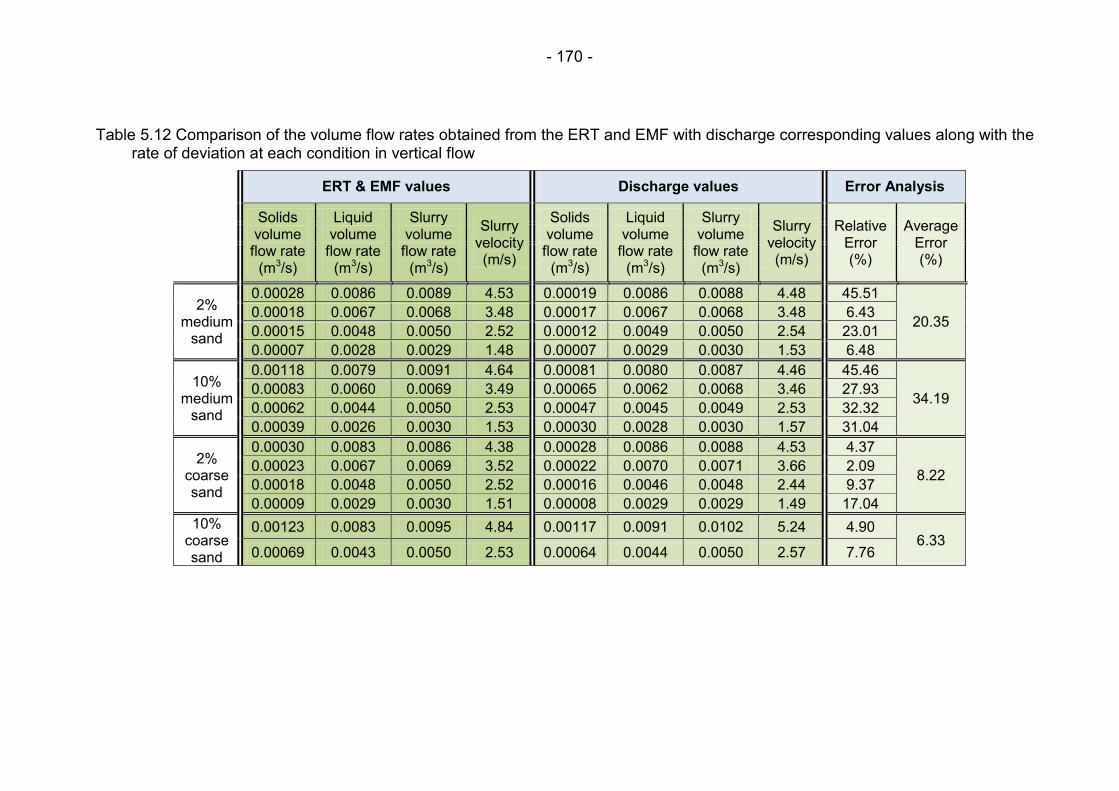
- 170 -
Table 5.12 Comparison of the volume flow rates obtained from the ERT and EMF with discharge corresponding values along with the rate of deviation at each condition in vertical flow
ERT & EMF values Discharge values Error Analysis
Solids volume
flow rate (m3/s)
Liquid volume
flow rate (m3/s)
Slurry volume
flow rate (m3/s)
Slurry velocity (m/s)
Solids volume
flow rate (m3/s)
Liquid volume
flow rate (m3/s)
Slurry volume
flow rate (m3/s)
Slurry velocity (m/s)
Relative Error (%)
Average Error (%)
2% medium
sand
0.00028 0.0086 0.0089 4.53 0.00019 0.0086 0.0088 4.48 45.51
20.35 0.00018 0.0067 0.0068 3.48 0.00017 0.0067 0.0068 3.48 6.43
0.00015 0.0048 0.0050 2.52 0.00012 0.0049 0.0050 2.54 23.01
0.00007 0.0028 0.0029 1.48 0.00007 0.0029 0.0030 1.53 6.48
10% medium
sand
0.00118 0.0079 0.0091 4.64 0.00081 0.0080 0.0087 4.46 45.46
34.19 0.00083 0.0060 0.0069 3.49 0.00065 0.0062 0.0068 3.46 27.93
0.00062 0.0044 0.0050 2.53 0.00047 0.0045 0.0049 2.53 32.32
0.00039 0.0026 0.0030 1.53 0.00030 0.0028 0.0030 1.57 31.04
2% coarse sand
0.00030 0.0083 0.0086 4.38 0.00028 0.0086 0.0088 4.53 4.37
8.22 0.00023 0.0067 0.0069 3.52 0.00022 0.0070 0.0071 3.66 2.09
0.00018 0.0048 0.0050 2.52 0.00016 0.0046 0.0048 2.44 9.37
0.00009 0.0029 0.0030 1.51 0.00008 0.0029 0.0029 1.49 17.04
10% coarse sand
0.00123 0.0083 0.0095 4.84 0.00117 0.0091 0.0102 5.24 4.90 6.33
0.00069 0.0043 0.0050 2.53 0.00064 0.0044 0.0050 2.57 7.76
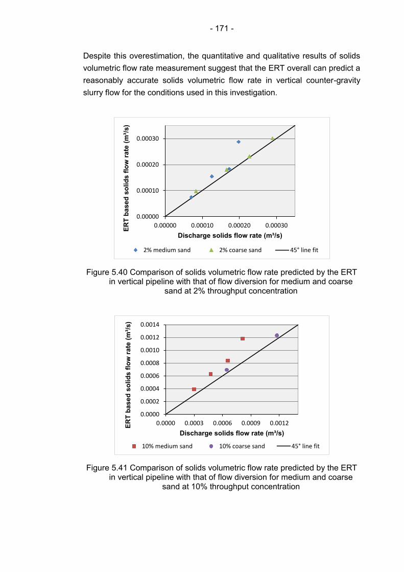
- 171 -
Despite this overestimation, the quantitative and qualitative results of solids
volumetric flow rate measurement suggest that the ERT overall can predict a
reasonably accurate solids volumetric flow rate in vertical counter-gravity
slurry flow for the conditions used in this investigation.
Figure 5.40 Comparison of solids volumetric flow rate predicted by the ERT in vertical pipeline with that of flow diversion for medium and coarse
sand at 2% throughput concentration
Figure 5.41 Comparison of solids volumetric flow rate predicted by the ERT in vertical pipeline with that of flow diversion for medium and coarse
sand at 10% throughput concentration
0.00000
0.00010
0.00020
0.00030
0.00000 0.00010 0.00020 0.00030
ER
T b
ased
so
lid
s f
low
rate
(m
³/s)
Discharge solids flow rate (m³/s)
2% medium sand 2% coarse sand 45° line fit
0.0000
0.0002
0.0004
0.0006
0.0008
0.0010
0.0012
0.0014
0.0000 0.0003 0.0006 0.0009 0.0012
ER
T b
ased
so
lid
s f
low
rate
(m
³/s)
Discharge solids flow rate (m³/s)
10% medium sand 10% coarse sand 45° line fit
- 172 -
The mixture flow rate was also determined, based on the flow rates of both
phases predicted by the ERT in conjunction with the EMF, in which the
solids void fraction was taken into account. The measured mixture flow rate
then compared to that of discharge, as shown in Figure 5.42. It can be seen
that error is quite random for the given conditions. However, a reasonable
agreement can be noticed between the slurry flow rate measured by the
ERT in conjunction with the EMF and the discharge.
Figure 5.42 Comparison of slurry flow rate measured by the combination of the ERT and EMF in vertical pipeline with that of flow diversion
In order to further evaluate the ERT based volumetric flow rate
measurement technique, in which the ERT is used in conjunction with the
EMF, further comparisons were carried out, as shown in Figures 5.43, 5.44,
5.45 and 5.56. In these comparisons, the solid and liquid volumetric flow rate
obtained from the ERT and EMF were compared to that measured by flow
diversion technique. It is quite apparent that, in the aforementioned figures,
the ERT can generate a reasonable qualitative track representation of solids
volume flow rate for the range of the transport velocities used in this
research. However, the overestimation again is quite pronounced for both
sands and all conditions, especially at higher velocities above stratified
velocity range ( 3.5 m/s).
0.000
0.002
0.004
0.006
0.008
0.010
0.012
0.000 0.002 0.004 0.006 0.008 0.010 0.012
ER
T b
ased
mix
ture
flo
w r
ate
(m
3/s
)
Discharge mixture flow rate (m3/s)
2% medium sand 10% medium sand 2% coarse sand
10% coarse sand 45° linefit

- 173 -
Figure 5.43 Comparison of the ERT solids flow rate in vertical pipeline with that of flow diversion for medium sand at 2% throughput concentration
Figure 5.44 Showing the comparison of the ERT solids flow rate in vertical pipeline with that of flow diversion for medium sand at 10% throughput
concentration
0.00000
0.00005
0.00010
0.00015
0.00020
0.00025
0.00030
0.00035
0.0020 0.0040 0.0060 0.0080 0.0100
So
lid
s F
low
Rate
(m
³/s)
Carrier Liquid Flow Rate (m³/s)
ERT Discharge
0.0000
0.0002
0.0004
0.0006
0.0008
0.0010
0.0012
0.0014
0.0020 0.0040 0.0060 0.0080 0.0100 0.0120
So
lid
s F
low
Rate
(m
³/s)
Carrier Liquid Flow Rate (m³/s)
ERT Discharge
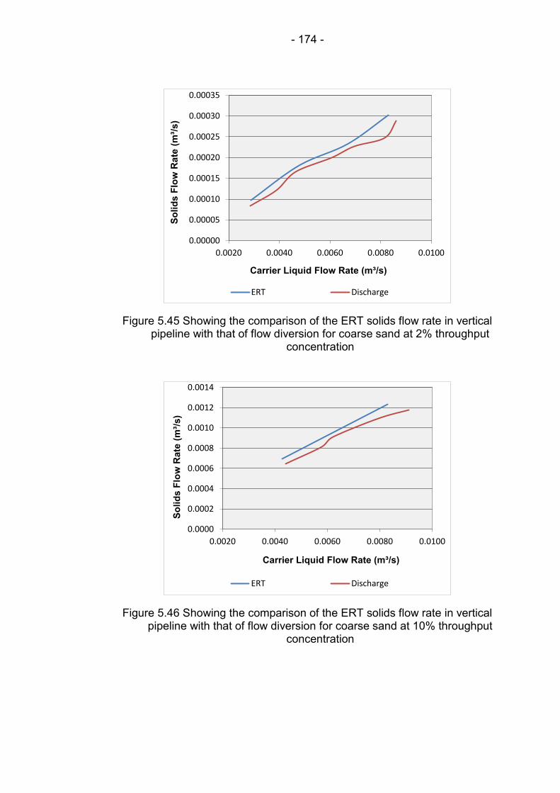
- 174 -
Figure 5.45 Showing the comparison of the ERT solids flow rate in vertical pipeline with that of flow diversion for coarse sand at 2% throughput
concentration
Figure 5.46 Showing the comparison of the ERT solids flow rate in vertical pipeline with that of flow diversion for coarse sand at 10% throughput
concentration
0.00000
0.00005
0.00010
0.00015
0.00020
0.00025
0.00030
0.00035
0.0020 0.0040 0.0060 0.0080 0.0100
So
lid
s F
low
Rate
(m
³/s)
Carrier Liquid Flow Rate (m³/s)
ERT Discharge
0.0000
0.0002
0.0004
0.0006
0.0008
0.0010
0.0012
0.0014
0.0020 0.0040 0.0060 0.0080 0.0100
So
lid
s F
low
Rate
(m
³/s)
Carrier Liquid Flow Rate (m³/s)
ERT Discharge
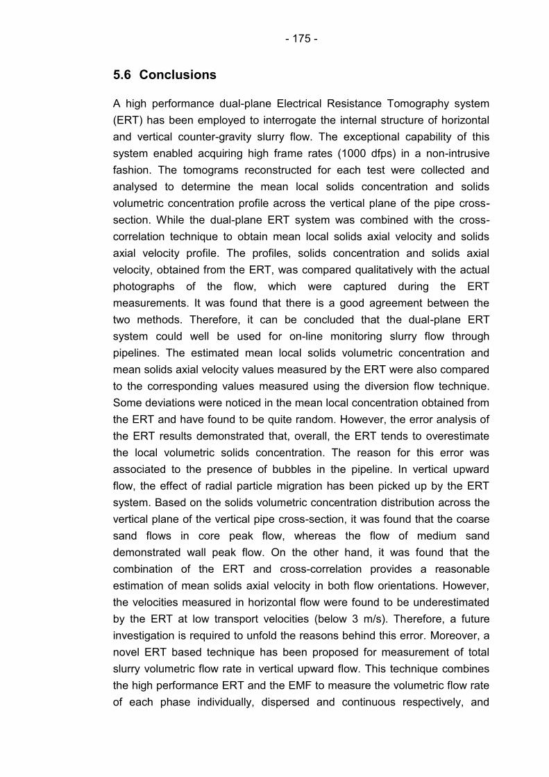
- 175 -
5.6 Conclusions
A high performance dual-plane Electrical Resistance Tomography system
(ERT) has been employed to interrogate the internal structure of horizontal
and vertical counter-gravity slurry flow. The exceptional capability of this
system enabled acquiring high frame rates (1000 dfps) in a non-intrusive
fashion. The tomograms reconstructed for each test were collected and
analysed to determine the mean local solids concentration and solids
volumetric concentration profile across the vertical plane of the pipe cross-
section. While the dual-plane ERT system was combined with the cross-
correlation technique to obtain mean local solids axial velocity and solids
axial velocity profile. The profiles, solids concentration and solids axial
velocity, obtained from the ERT, was compared qualitatively with the actual
photographs of the flow, which were captured during the ERT
measurements. It was found that there is a good agreement between the
two methods. Therefore, it can be concluded that the dual-plane ERT
system could well be used for on-line monitoring slurry flow through
pipelines. The estimated mean local solids volumetric concentration and
mean solids axial velocity values measured by the ERT were also compared
to the corresponding values measured using the diversion flow technique.
Some deviations were noticed in the mean local concentration obtained from
the ERT and have found to be quite random. However, the error analysis of
the ERT results demonstrated that, overall, the ERT tends to overestimate
the local volumetric solids concentration. The reason for this error was
associated to the presence of bubbles in the pipeline. In vertical upward
flow, the effect of radial particle migration has been picked up by the ERT
system. Based on the solids volumetric concentration distribution across the
vertical plane of the vertical pipe cross-section, it was found that the coarse
sand flows in core peak flow, whereas the flow of medium sand
demonstrated wall peak flow. On the other hand, it was found that the
combination of the ERT and cross-correlation provides a reasonable
estimation of mean solids axial velocity in both flow orientations. However,
the velocities measured in horizontal flow were found to be underestimated
by the ERT at low transport velocities (below 3 m/s). Therefore, a future
investigation is required to unfold the reasons behind this error. Moreover, a
novel ERT based technique has been proposed for measurement of total
slurry volumetric flow rate in vertical upward flow. This technique combines
the high performance ERT and the EMF to measure the volumetric flow rate
of each phase individually, dispersed and continuous respectively, and
- 176 -
producing the total volumetric slurry flow rate. Based on the results obtained
using this technique the slip velocity between the two phases can also be
successfully determined. The evaluation of the proposed technique for
volumetric flow rate measurement, through highlighting the rate of
associated error in each condition used in this study, suggests that a
reasonable qualitative track representation of volumetric flow rate of each
phase, along with the total slurry volume flow rate, can be generated.
Finally, this study revealed that the high performance dual-plane ERT
system can be used for monitoring slurry flow and estimation of volumetric
solids concentration and solids axial velocity in horizontal and volumetric
flow rate in vertical counter-gravity flow. However, particular attention should
be paid to quantitative results obtained at high transport velocities.

- 177 -
Chapter 6
Design and construction of inclinable multiphase flow loop
This chapter describes the design of an inclinable multiphase flow loop with
specific emphasis on slurry flow system. It attempts to provide a detailed
coverage of the design analysis and acceptance criteria for every
component of the system. The materials, fabrication, assembly, erection and
testing are also described.
6.1 Introduction
In order to investigate the effect of different variables on multiphase flow
characteristics and measurement scheme, a versatile, durable and accurate
pilot scale flow loop is required. Therefore, it was decided to design and
construct a pilot scale multiphase flow loop in the Engineering Building/G.56
in the university of Leeds. The aim was to build a durable and reliable flow
loop, which would include all orientations, horizontal, vertical and inclined. It
was also required to design the flow loop in such a way that could be used
not only for slurry flow, but also for multiphase flow, which includes
solid/liquid, gas/liquid, solid/gas/liquid, oil/liquid, oil/gas/liquid and
oil/solid/gas/liquid. It is worth mentioning that due to space limitations and
health and safety, the oil flow facility, such as storage vessel etc., has not
been included into the design. However, it is proposed that an oil simulant,
such as plastic beads with uniform shape and the same density of oil, could
be used. It is also important to mention that as the loop will mainly be used
for slurry flow and this type of flow is the most complex amongst the others,
then most of design considerations and attention have been given to slurry
flow rather than others.
The management of the design and construction, such as time and cost,
was also considered to be one of the most important aspect of the project. A
thorough examination was carried out for the selection and design of each
piece of equipment, based on cost, objectives of the research and flexibility,
along with producing a detailed working plan from conceptual design to the
construction and testing. The working plan was developed in such a way in
order for each task to be carried out efficiently and effectively.
This chapter details the methodology adopted to design and construct the
multiphase flow loop, along with the equipment and instrumentations used to

- 178 -
achieve the design requirements. The final design of the constructed flow
loop and each equipment is highlighted through schematic drawings and real
photographs. A detailed operating procedure, start up and shut down, of the
loop is also included in this chapter. The results of mechanical and
hydrodynamic testing are also described.
6.2 Design requirements
In order to investigate the effect of different flow parameters on multiphase
flow characteristics and flow measurement scheme, the flow loop must meet
the following requirements:
1. The flow loop must be usable within the range of inclination angles 0° to
90° from horizontal.
2. A safe and remotely controllable lifting method must be used.
3. The instrumentation and working area must be well and carefully
specified.
4. The piping material must be selected to suit the flow of solid particles and
abrasives.
5. It must accommodate up to 40% by weight of the dispersed phase.
6. Must allow the mean flow velocity up to 5.5 m/s.
7. It must include the upward and downward flow.
8. The test sections must be within the developed flow region.
9. It must be functional for stratified and non-stratified flow.
10. Must meet health and safety requirements.
11. Must be robust, accurate and durable.
12. Flexibility in removing and mounting any instrumentation or section.
13. Must allow for visual observation of flow within the pipeline.
14. Can easily be operated by one operator.
15. Cost must be well balanced against accuracy, durability and robustness.
16. Include a bulk flow measurement and validation system.
17. Space and access (work area, walk way storage area, maintenance of
equipment etc.) must be carefully considered.
18. Initial and later testing costs must be kept as low as possible, of course
after achieving a well balance between cost and quality.
6.3 Design and construction project management
In order to achieve the final goal efficiently and effectively, a very well
management of the entire project is paramount. Undoubtedly, a detailed

- 179 -
work plan is necessary to provide a framework for planning and controlling
the project. Also the large number of tasks, which had to be carried out by
different individuals and parties over a short period of time to reach the final
stage, was the driving force for the outputs to be achieved. Therefore, a
detailed work plan was introduced, amongst which the budget and schedule
of work were clearly outlined.
In order to have a clear knowledge of the total cost of the flow loop, the list of
material that had to be ordered was prepared, as shown in Table 6.1. Since
the cost was the driving force, then a comparison of price and quality of each
item, mentioned in the aforementioned table, was carried out between three
suppliers. After achieving a good balance between the price and quality, the
suitable supplier was chosen. Then of course every item had to be justified,
therefore, a meeting had to be arranged with the budget holder to produce
the documentations and justify the release of funds.
On the other hand, the schedule of the work plan, which was the most
important element of standard management tool, was found to be rather
more complicated. As previously mentioned, the number of tasks in the To
Do list and the involvement of different individuals made it rather difficult to
produce a rigid schedule of work. Therefore, the schedule produced for the
completion of the flow loop had to be updated from time to time, a version of
which is illustrated in Table 6.2. The scheduling strategy used for the
completion of the loop, was that the entire work was split into goals, each of
which had objectives for the goal to be achieved. It is apparent that the
completion of all the target goals would mean the completion of the loop. In
other words, a goal can never be achieved without achieving all the related
specific objectives. The scheduling was designed in such a way that for each
of stated objectives the completion date was listed in order with allotment of
a reasonable length of time, while some tasks were in progress in a parallel
fashion.

- 180 -
Table 6.1 List of items ordered for the flow loop
Item Imagemm/each of
Item
Net unit cost
£
Net item
total £Supplier
Product
no./CodeProduct name Comments
2" Clear Upvc Pipe
(Transparent)5 m 103.70/5m 103.7 http://www.pipestock.com/clear-pvcu-pipe/ PVCU.CLR5.0630
PVCu Clear Pipe 16 BAR 5m
Length 63mm
This is metric it can go with metric
fittings, but not with imperial
fittings (eg, 2" flange)
2" Upvc Pipe (Opaque/black) 12 m 23.33/6m 46.66 http://www.pipestock.com/pvcu/pipe/class-e-inch/ PVCU.CLE.0630 PVCu Pipe Class E 15 Bar 6m 2"
4" Upvc Pipe 6 m 80.48/6m 80.48 http://www.pipestock.com/pvcu/pipe/class-e-inch/ PVCU.CLE.1100 PVCu Pipe Class E 15 Bar 6m 4"
Flexible Pipe 10 m 23.95/m¹ 287.4Whitehouse Flexible Tubing Ltd. (quote will be
attached)See the quote
10 Mtrs X 63MM DIA,
ARMOURVIN TYPE FLEXIBLE
TUBING
Flexible Pipe Clamps (Heavy
Duty)8 piece 2.53/piece¹ 50.528
Whitehouse Flexible Tubing Ltd. (quote will be
attached)See the quote 8 X SUPER HEAVY DUTY CLAMPS
Flanges 30 piece 6.68/piece 200.4http://www.pipestock.com/pvcu/flanges-flange-
sets/flanges/full-face-pn1016-inch/PVCU.FNA.0630
PVCu Full Face Flange Drilled
BS EN1029-1 PN16 Plain 2"
EPDM Flat Gasket 15 piece 5.81 87.15http://www.pipestock.com/pvcu/flanges-flange-
sets/epdm-gaskets/full-face-bs-en1029-1/GFI.0630
EPDM Gasket For Full Face
Flange BS4504 NP10/16 2"
63mm
Nuts & bolts (M16 x 80)² 30 set 3.03/set 90.9http://www.pipestock.com/pvcu/flanges-flange-
sets/nuts-bolts/BBZP.M16.0750
Bolt Set BZP 4 Pack M16 X
75mm
Sockets (Plain) 6 1.73/piece 10.38http://www.pipestock.com/pvcu/pipe-fittings/plain-
inch/socket/PVCU.MAA.0630 PVCu Socket Plain 2"
Reducing Bushes (Plain:
OD63X32ID mm)2 1.21/ piece 2.42
http://www.pipestock.com/pvcu/pipe-fittings/plain-
inch/reducing-bush/PVCU.RCA.063D
PVCu Reducing Bush Plain 2" x
1"
Reducing Bushes (Plain:
OD32X25ID mm)2 0.58/ piece 1.16
http://www.pipestock.com/pvcu/pipe-fittings/plain-
inch/reducing-bush/PVCU.RCA.032C
PVCu Reducing Bush Plain 1" x
3/4"
Reducing Bushes (Threaded:
OD25X20ID mm)2 0.47/ piece 0.94
http://www.pipestock.com/pvcu/pipe-fittings/plain-
inch/reducing-bush/PVCU.RCA.025B
PVCu Reducing Bush Plain 3/4"
x 1/2"
Union 1 7.94/ piece 7.94http://www.pipestock.com/pvcu/pipe-fittings/plain-
inch/union/PVCU.BOA.0630 PVCu Union Plain 2"
Tee 90° 13 4.25/ piece 55.25http://www.pipestock.com/pvcu/pipe-fittings/plain-
inch/tee-90/PVCU.TIA.0630 PVCu Tee 90 Plain 2"
Tee 45° 2 10.65/ piece 21.3http://www.pipestock.com/pvcu/pipe-fittings/plain-
inch/tee-45/PVCU.TYA.0636 PVCu Tee 45 Plain 2"
Elbow 45° 1 3.73/ piece 3.73http://www.pipestock.com/pvcu/pipe-fittings/plain-
inch/elbow-45/PVCU.GYA.0630 PVCu Elbow 45 Plain 2"
Elbow 90° 1 3.32/ piece 3.32http://www.pipestock.com/pvcu/pipe-fittings/plain-
inch/elbow-90/PVCU.GOA.0630 PVCu Elbow 90 Plain 2"
Short Radius Bend 90° 8 9.53/ piece 76.24http://www.pipestock.com/pvcu/pipe-fittings/plain-
inch/short-radius-bend-90/PVCU.CUA.0630 PVCu Bend 90 Plain 2"
Solvent Cement³ 2 14.12/ tin 28.24http://www.pipestock.com/pvcu/accessories/pvcu-
solvent-cement/PVCU.RCO
Solvent Cement for PVC 500ml
Tin
Brushes 2 3.18/ piece 6.36http://www.pipestock.com/pvcu/accessories/pvcu-
solvent-cement/FAIPBSY34 Brush 3/4"
TFPE Tape 2 5.43/ pack 10.86http://www.pipestock.com/pvcu/accessories/ptfe-
tape/PTFE.B PTFE Tape 12m Roll Pack of 10
Latex Gloves (L) 1 (pack of 100) 13.48/ pack 13.48http://www.pipestock.com/pvcu/accessories/latex-
gloves/SCAGLOLATEXL
Latex Gloves Ambidextrous
100PK
Digital Caliper 1 11.98 (inc VAT) 11.98http://www.toolbox.co.uk/silverline-380244-digital-
16488-85361TBSL2911
Silverline 380244 Digital
Vernier Professional Caliper
Pipe Clamps⁴ 30 1.75/ pack 52.5http://www.thesitebox.com/britclips-girder-clips/pipe-
clamps/sound-insulated-standard-r-pipe-clips.aspxP/N: 1257060
59 - 62mm Sound Insulated
Standard Pipe Clip M8 & M10 (1
item per pack)
This can be adapted to M8 and
M10 threaded rod bar.
Threaded rod for pipe clamp
(M8 x 100 mm)10 2.25/ pack⁵ 22.5
http://www.thesitebox.com/nuts-and-bolts/metric-
studding/metric-high-tensile-steel-studding.aspxP/N: STHTM81SC
Metric High Tensile Steel
Studding 8mm x 1m (1 item per
pack)
U-Bolt clamp⁶ 1 17.10/ pack⁷ 17.1http://www.thesitebox.com/nuts-and-bolts/u-
bolts.aspxP/N: UB75M12
Standard 'U' Bolt with nuts.
75mm nominal bore. M12
thread....
Ratchet Strap (w:50mm,
L:4m, Load: 4000KG)⁹8 5.26/ piece 42.08
http://www.theratchetshop.com/ratchet-straps-lifting-
systems-ratchets-c-26_28.htmlLS02-04 (50mm) Ratchet Strap-Blue
Supply and Fit Tilted Table
and frame supports1 4500 4500 OG Fabrication
Supply and fit the table and
frame
Ultrasound Velocity Profiler
(UDVP)1 8500 8500
http://www.theratchetshop.com/ratchet-straps-lifting-
systems-ratchets-c-26_28.html
UDVP-DUO
(GAH100)UDVP-DUO
two standard transducers (TX line
model) with emitting frequencies
2 MHz and 4 MHz must be
Coriolis Mass Flow Meter 1 7432.79 7432.79http://www.theratchetshop.com/ratchet-straps-lifting-
systems-ratchets-c-26_28.htmlOPTIMASS 7300
Mass flow sensor OPTIMASS
7000-T 50 straight single tube
system (Titanium-Grade 9)
Wall mounting converter must be
ordered, along with transitional
pieces for leading edge protection
Coarse Sand ( Sand 1) 20 bags 1.81/bag⁹ 36.2http://www.theratchetshop.com/ratchet-straps-lifting-
systems-ratchets-c-26_28.htmlSMBQSHS40
B&Q Sharp Sand Natural Large
Bag
Medium Sand ( Sand 2) 20 bags 4.28/bag 85.6http://www.theratchetshop.com/ratchet-straps-lifting-
systems-ratchets-c-26_28.htmlSMBQKDS40 B&Q Kiln Dried Sand Natural
Total 21889.588¹VAT 20% + Carriage are included into the total price
²Each set consists of a threeaded bolt+2 washers+single nut.
⁸Break/load: 4000Kg, Colour: Blue, Width: 50mm, length: 4m
⁹If more than 10 bags ordered, the price comes to £1.18 per bag
All the above prices are of 9th February 2012
³Each tin contains 500 ml (500 ml can cover 60 joints of 2 inch pipeline)
⁴Rubber lined pipe clamp with one fixing M7 x 100mm or M8 x 100mm.
⁵Price per pack ex VAT ( Pack Size: 1x1m). This may not require ordering, checks have to ber made if there is any leftovers from the other
⁶Steel U-Bolt clamp for the flange to prevent the u-shape section from slipping down while the table is raised, especially at 90 degree.
⁷Price per pack ex VAT ( Pack Size: 10)
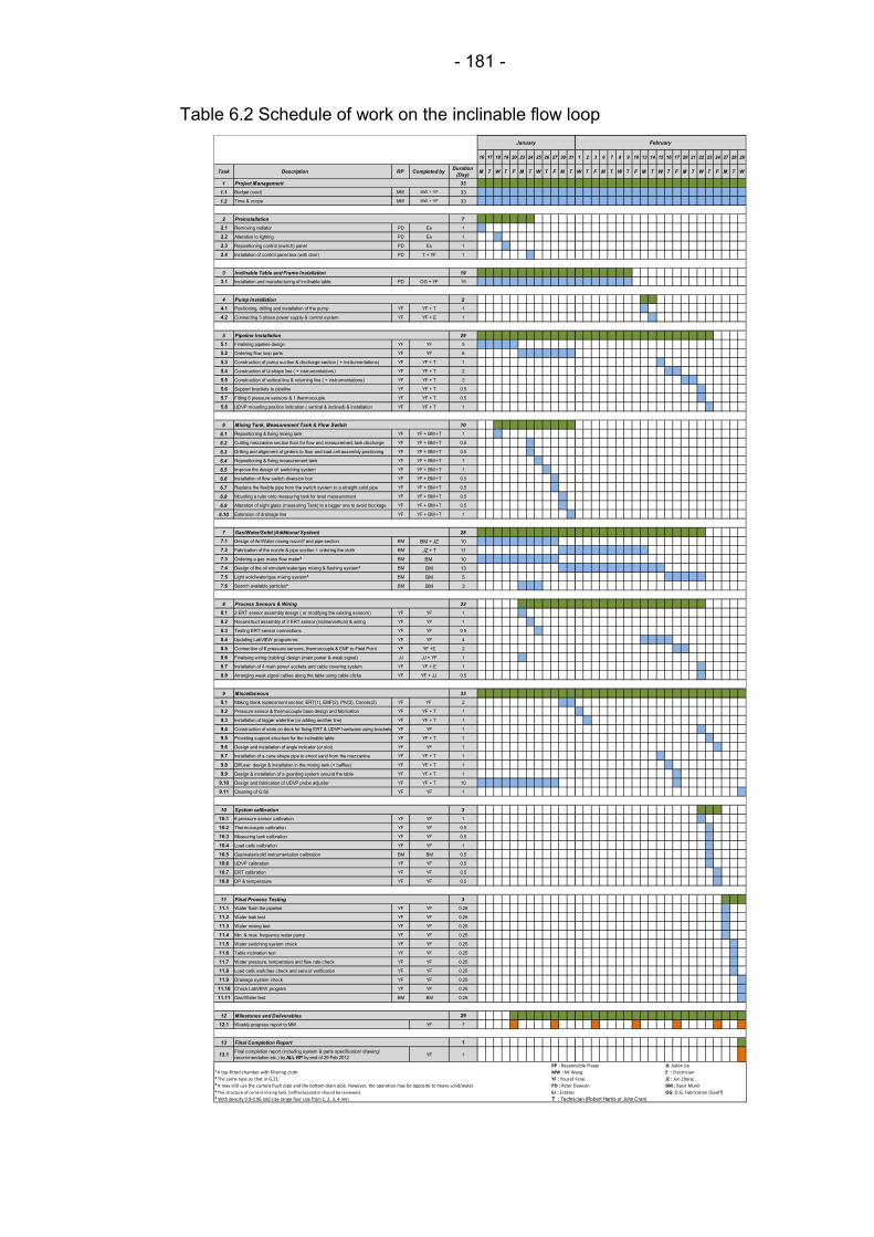
- 181 -
Table 6.2 Schedule of work on the inclinable flow loop
16 17 18 19 20 23 24 25 26 27 30 31 1 2 3 6 7 8 9 10 13 14 15 16 17 20 21 22 23 24 27 28 29
Task Description RP Completed byDuration
(Day)M T W T F M T W T F M T W T F M T W T F M T W T F M T W T F M T W
1 Project Management 33
1.1 Budget (cost) MW MW + YF 33
1.2 Time & scope MW MW + YF 33
2 Preinstallation 7
2.1 Removing radiator PD Es 1
2.2 Alteration to lighting PD Es 1
2.3 Repositioning control (switch) panel PD Es 1
2.4 Installation of control panel box (with door) PD T + YF 1
3 Inclinable Table and Frame Installation 19
3.1 Installation and manufacturing of inclinable table PD OG + YF 19
4 Pump Installation 2
4.1 Positioning, drilling and installation of the pump YF YF + T 1
4.2 Connecting 3 phase power supply & control system YF YF + E 1
5 Pipeline Installation 29
5.1 Finalising pipeline design YF YF 5
5.2 Ordering flow loop parts YF YF 6
5.3 Construction of pump suction & discharge section ( + instrumentations) YF YF + T 1
5.4 Construction of U-shape line ( + instrumentations) YF YF + T 2
5.5 Construction of vertical line & returning line ( + instrumentations) YF YF + T 2
5.6 Support brackets to pipeline YF YF + T 0.5
5.7 Fitting 6 pressure sensors & 1 thermocouple YF YF + T 0.5
5.8 UDVP mounting position indication ( vertical & inclined) & installation YF YF + T 1
6 Mixing Tank, Measurement Tank & Flow Switch 10
6.1 Repositioning & fixing mixing tank YF YF + BM +T 1
6.2 Cutting mezzanine section floor for flow and measurement tank discharge YF YF + BM +T 0.5
6.3 Drilling and alignment of girders to floor and load cell assembly positioning YF YF + BM +T 0.5
6.4 Repositioning & fixing measurement tank YF YF + BM +T 1
6.5 Improve the design of switching system YF YF + BM +T 1
6.6 Installation of flow switch diversion box YF YF + BM +T 0.5
6.7 Replace the flexible pipe from the switch system to a straight solid pipe YF YF + BM +T 0.5
6.8 Mounting a ruler onto measuring tank for level measurement YF YF + BM +T 0.5
6.9 Alteration of sight glass (measuring Tank) to a bigger one to avoid blockage YF YF + BM +T 0.5
6.10 Extension of drainage line YF YF + BM +T 1
7 Gas/Water/Solid (Additional System) 28
7.1 Design of Air/Water mixing nozzel¹ and pipe section BM BM + JZ 10
7.2 Fabrication of the nozzle & pipe section + ordering the cloth BM JZ + T 11
7.3 Ordering a gas mass flow meter² BM BM 10
7.4 Design of the oil simulant/water/gas mixing & flushing system³ BM BM 13
7.5 Light solid/water/gas mixing system⁴ BM BM 5
7.6 Search available particles⁵ BM BM 3
8 Process Sensors & Wiring 23
8.1 2 ERT sensor assembly design ( or modifying the existing sensors) YF YF 1
8.2 Reconstruct assembly of 2 ERT sensor (incline/vertical) & wiring YF YF 1
8.3 Testing ERT sensor connections YF YF 0.5
8.4 Updating LabVIEW programme YF YF 4
8.5 Connection of 6 pressure sensors, thermocouple & EMF to Field Point YF YF +E 2
8.6 Finalising wiring (cabling) design (main power & weak signal) JJ JJ + YF 1
8.7 Installation of 4 main power sockets and cable covering system YF YF + E 1
8.8 Arranging weak signal cables along the table using cable clicks YF YF + JJ 0.5
9 Miscellaneous 33
9.1 Making blank replacement section: ERT(1), EMF(2), PIV(2), Coriolis(2) YF YF 2
9.2 Pressure sensor & thermocouple base design and fabrication YF YF + T 1
9.3 Installation of bigger waterline (or adding another line) YF YF + T 1
9.4 Construction of slots on deck for fixing ERT & UDVP hardware using brackets YF YF 1
9.5 Providing support structure for the inclinable table YF YF + T 1
9.6 Design and installation of angle indicator (or slot) YF YF 1
9.7 Installation of a cone shape pipe to shoot sand from the mezzanine YF YF + T 1
9.8 Diffuser design & installation in the mixing tank (+ baffles) YF YF + T 1
9.9 Design & installation of a guarding system around the table YF YF + T 1
9.10 Design and fabrication of UDVP probe adjuster YF YF + T 10
9.11 Cleaning of G.56 YF YF 1
10 System calibration 3
10.1 6 pressure sensor calibration YF YF 1
10.2 Thermocouple calibration YF YF 0.5
10.3 Measuring tank calibration YF YF 0.5
10.4 Load cells calibration YF YF 1
10.5 Gas/water/solid instrumentation calibration BM BM 0.5
10.6 UDVP calibration YF YF 0.5
10.7 ERT calibration YF YF 0.5
10.8 DP & temperature YF YF 0.5
11 Final Process Testing 3
11.1 Water flush the pipeline YF YF 0.25
11.2 Water leak test YF YF 0.25
11.3 Water mixing test YF YF 0.25
11.4 Min. & max. frequency water pump YF YF 0.25
11.5 Water switching system check YF YF 0.25
11.6 Table inclination test YF YF 0.25
11.7 Water pressure, temperature and flow rate check YF YF 0.25
11.8 Load cells switches check and sensor verification YF YF 0.25
11.9 Drainage system check YF YF 0.25
11.10 Check LabVIEW program YF YF 0.25
11.11 Gas/Water test BM BM 0.25
12 Milestones and Deliverables 29
12.1 Weekly progress report to MW YF 7
13 Final Completion Report 1
13.1Final completion report (including system & parts specification/ drawing/
recommendation etc.) by ALL RP by end of 29 Feb 2012YF 1
RP : Responsible Player JJ: Jiabin Jia
¹ A top-fitted chamber with filtering cloth. MW : Mi Wang E : Electrician
² The same type as that in G.21. YF : Yousef Faraj JZ : Jun Zhang
³ It may still use the current flush pipe and the bottom drain pipe. However, the operation may be opposite to heavy solid/water. PD : Peter Dawson BM : Basit Munir
⁴ The structure of current mixing tank, baffle/separator should be reviewed. Es : Estates OG: O.G. Fabrication (Geoff)
⁵ With density 0.9-0.96 and size range four size from 1, 2, 3, 4 mm. T : Technician (Robert Harris or John Cran)
January February
- 182 -
6.4 Types of slurry flow loop
As slurry flow is a complex two phase flow, a properly designed flow loop
system is necessary, so that it offers a greater flexibility and capability of
generating data for wider range of conditions. Unfortunately, this wider range
of conditions is required; if a good understanding of slurry flow and the effect
of its behaviour is sought, especially in the case of flow measurement and
visualisation.
According to Brown and Heywood (1991), flow loops are commonly used to
determine and study and measure variety of slurry variables and their
influence on the flow. Some of which are listed below:
To determine the frictional pressure gradient for the flowing slurry.
To determine the higher concentration limit for practical handling of
slurry.
To determine the slurries deposition velocity, at which the solid
particles start to settle at the pipe invert.
To determine velocity and concentration profile of the solid particles
(radial and axial).
To test and calibrate the flow meters and concentration devices.
To assess pump characteristics and performance.
To determine particle degradation.
To determine the rate of pump and pipe erosion/corrosion of the
system.
To assess pipeline start/shutdown of a system, as in the case of
inclined flow.
Normally, there are two types of flow loop that can be used to obtain the
required data. These are the once-through and re-circulating flow loop. In
the once-through flow loop the slurry (solid and the carrier liquid) is
continuously fed to the flow loop during the course of the experiment. This
implies that a lot of slurry is required if a meaningful data is desired.
Therefore, this type of flow loop is ignored in this study and the other type
(re-circulating flow loop) is considered. In the re-circulating flow loop the
slurry is continuously returned to the pump, either directly or indirectly. In the
direct method, the slurry is returned directly through the pipeline to the pump
inlet, which forms a totally close flow loop. Whereas, in the indirect method
the contents of the pipeline flows into a mixing tank (or holding tank) and
continuously feeding the pump. Thus, the latter type can be considered as
an open flow loop. Since the open loop contributes into the increase in the

- 183 -
suction head, therefore, it was decided that the open loop will be used in this
study. In other words, the suction head increases with increase of slurry
level in the holding tank. Therefore, the holding tank must always be
monitored that the slurry level is sufficient, particularly when the flow is
diverted into the measuring tank. Also, the slurry level must be high enough
to avoid air entrainment in the mixture, which could enter into the pump and
result in damaging the pump. Another reason of choosing an open loop is
that samples can easily be collected, by diverting the flow via a switching
system into the measurement tank.
6.5 Overall structural design
A long table with a steel frame were designed and build, on which the
pipeline is laid. The table consists of two sections, the rigid section and the
inclinable section, which are coupled using a pivot point. The inclinable table
holding a U-shape pipeline, which consists of outgoing and returning limbs.
Since one of the flow loop design requirements is to provide the flexibility of
choosing any inclination angle between 0° to 90° from horizontal, then a
lifting method is required. An electric winch is used to lift the inclinable table
to a desired angle. The length of the U-shape pipeline (outgoing and
returning) is 4 m long, which is enough to include all the required
instrumentations within the developed flow region. Figures 6.5, 6.6 and 6.7
showing the schematic drawings of the inclinable flow loop system, which
was built in the Engineering Building.
6.6 Flow loop design and component selection
In an open flow loop the slurry is discharged from the pipeline into a conical
holding tank, which continuously feeding the pump through a connection at
the bottom of the holding tank. However, to achieve a versatile flow loop,
there are critical elements that must be carefully considered and selected.
These elements can include piping length, test section length, and slurry
instruments for measuring slurry parameters, such as velocity, concentration
etc. These components will be discussed in the following sections, including
the reasons behind the selection of each of them.
6.6.1 Structural design of the pipe-rack
A structural steel pipe rack is designed to support the pipeline, power cables,
some of instrumentation and instrument cables on ground floor in the
Engineering building/G.56. One of the design requirements is to include a

- 184 -
pivoted inclinable section within the structural steel framework, on which the
U-shape inclinable pipeline is laid.
In designing the structural steelwork, the main emphasis was placed upon
the stability, economics and practical aspects of the whole structure. The
pipe rack (or pipe support) work consists of 3-stage process: design,
fabrication and erection. The main considerations for the design aspect of
the pipeline support are given to strength and stability, static and dynamic
loads (pipeline, pipe costs and instrumentations) the intended function of the
steel frame structure, cost and maintenance. The fabrication process
involves cutting and preparation of each member to length, while the
erection process includes rigging of all prepared members to their intended
places in the pipeline support structure and making connections between all
structural members.
At the earlier stage of the design, steel pipe rack (approximately 7000 mm
long) was proposed to support the stationary horizontal lines and the
inclinable U-shape section. It was decided that the rigid pipe rack section to
be of a similar construction to the tilting section. Both sections are connected
through a pivoted pin, which allows the U-shape pipeline support to be tilted,
as shown in Figure 6.1. However, in order to complete the detailed design of
both sections of the pipe rack, several documentations and information have
to be reviewed and corrected. The following information is paramount for
development of the design and constructing an economical and successful
pipe rack.
1. Footprint plan and the pipeline layout (including the location of each
equipment).
2. Access and maintenance requirement for each part of the flow line.
3. Drawing of the electrical cabling, showing the routing and location of
electrical and instrumentation cables and/or support.
4. Information related to the concrete structure and foundations in the
area of the piping table.
5. The lifting method used to lift the inclinable table.
6. Intention of any future provisions for piping system or related loading.
Once the above preliminary information is obtained, it is well documented for
the next steps of the design. After collecting the required data for the
development of the design, the following stages are conducted in
chronological order:
- 185 -
1. Design load consideration.
2. Allowable deflection of the table.
3. Final framing of the pipe rack.
Normally, for pipe rack design, the loads considered are piping gravity load,
electrical conduits and cables, self weight of the pipe-rack, live load, snow
load, wind load, earthquake load, friction load (El-Reedy, 2011). Since the
multiphase flow loop is built indoor, then this fact automatically eliminates
snow load and wind load. Also, as the friction forces generated by hotlines
sliding across the pipe support, thus the friction loading is considered to be
negligible. The only loads that have to be considered are: piping gravity load,
with its contents, electrical conduits and instrumentations on the deck and
self weigh of the pipe rack.
The weight of all structural loads (except the support legging, on which the
tables stand on) was calculated. However, since the loading on the tilting
table is the most important to determine the capacity of winch used to lift it,
the loading calculation was performed only for this part. The weight of all
structural members of the tilting table was determined as approximately 200
kg. On the other hand, the piping gravity loads were determine by calculating
the weight of empty pipeline with equipment and instruments, along with the
weight of pipeline contents, for which slurry was considered. The weight of
empty pipeline (the U-shape section) was determined by considering every
individual component of the line, as shown in Table 6.3.
The result of weight calculation of inclinable table section with full pipeline is
summarised as follows:
Weight of the pipeline and instrumentation = 214 kg (based on 8.5 m
length).
Weight of slurry flowing through the inclinable section = 25 kg (this is
based on 0.017 m3 slurry flowing through 50 mm ID, 1350 kg/m3 slurry
density, 2650 kg/m3 sand density, 1000 kg/m3 water density and 40%
concentration by weight).
The total weight of inclinable U-shape pipeline with its contents = 214
+25 = 239 kg.
By considering 25% safety margin (59.75) for future provisional addition
to the pipeline, pipeline blockage etc, the total weight of the full U-shape
section = 298.75 kg.
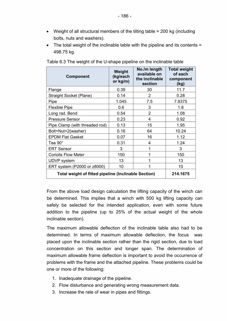
- 186 -
Weight of all structural members of the tilting table = 200 kg (including
bolts, nuts and washers).
The total weight of the inclinable table with the pipeline and its contents =
498.75 kg.
Table 6.3 The weight of the U-shape pipeline on the inclinable table
Component Weight
(kg/each or kg/m)
No./m length available on
the inclinable section
Total weight of each
component (kg)
Flange 0.39 30 11.7
Straight Socket (Plane) 0.14 2 0.28
Pipe 1.045 7.5 7.8375
Flexible Pipe 0.6 3 1.8
Long rad. Bend 0.54 2 1.08
Pressure Sensor 0.23 4 0.92
Pipe Clamp (with threaded rod) 0.13 15 1.95
Bolt+Nut+2(washer) 0.16 64 10.24
EPDM Flat Gasket 0.07 16 1.12
Tee 90° 0.31 4 1.24
ERT Sensor 3 1 3
Coriolis Flow Meter 150 1 150
UDVP system 13 1 13
ERT system (P2000 or z8000) 10 1 10
Total weight of fitted pipeline (Inclinable Section) 214.1675
From the above load design calculation the lifting capacity of the winch can
be determined. This implies that a winch with 500 kg lifting capacity can
safely be selected for the intended application, even with some future
addition to the pipeline (up to 25% of the actual weight of the whole
inclinable section).
The maximum allowable deflection of the inclinable table also had to be
determined. In terms of maximum allowable deflection, the focus was
placed upon the inclinable section rather than the rigid section, due to load
concentration on this section and longer span. The determination of
maximum allowable frame deflection is important to avoid the occurrence of
problems with the frame and the attached pipeline. These problems could be
one or more of the following:
1. Inadequate drainage of the pipeline.
2. Flow disturbance and generating wrong measurement data.
3. Increase the rate of wear in pipes and fittings.
- 187 -
4. Broken seals at the joint locations.
5. Strain on the pipeline or fixings.
6. Damage or excessive strain at the connection points.
7. Surface distortion of the table.
Normally, for most buildings and structures various guidelines have been
introduced based on the intended application to determine the maximum
allowable deflection values of a structural member. Therefore, in order to
find out the maximum allowable deflection value for the inclinable table, the
recommended allowable deflection limit for beams is considered, which is
L/360 of the span (El-Reedy, 2011). This means that based on the length of
the longitudinal beam member of the table, the beam’s maximum allowable
deflection for the inclinable table can be determined using the following
formulae.
(6.1)
da= Maximum allowable deflection.
L= The length of the span in mm.
360= Constant.
Thus, based on the above guideline a span of 4000 mm, which is the beam
length of the table, has a maximum allowable deflection of 11,11 mm. In
other words, the table beam subjected to the aforementioned load, bends
from its original horizontal position by 11.11 mm. However, since the two
beams are used and are connected by 5 transverse parallel flange channels,
then the deflection value for the whole table is expected to be far less than
11.11 mm. Therefore, this deflection value can be accepted.
The framing of the pipe rack decks (inclinable and rigid) based on the
pipeline layout, required safety and stability calculation and the intended
application of each deck, was one of the most important aspect of the flow
loop design and construction. As many factors had to be taken into account,
most of these factors were case and project specific and are listed below:
Some items had to be removed within the working area of the flow
loop, such as the radiator at ceiling level.
The heating pipeline running close to the ceiling had to be considered.

- 188 -
The design and construction of the table could not be separated from
the mezzanine, thus it was incorporated into the mezzanine redesign,
which would result in the omission of some structural member of the
mezzanine (column). Also at mezzanine level, there was a potential
problem with regard to the fact that a support beam fouls the line of
the inclinable table at 90%.
A buffer stop or pushback had to be included to ensure the 90° angle
is maintained and the table is lowered through some considerable
force.
The existing door at the end of the working area had to be kept
accessible, and this obviously would affect the dimensions and
installation of the table.
Consideration had to be given to the flexibility of the pipeline at the
pivot point.
The mezzanine floor construction had to be amended, so as to allow
the table to be raised to 90°.
Some steel work had to be carried out for adjustment of the winch
system, based on the level of the table at 90°.
Locating the lifting point on the tilting table using a steel wire.
Finalising the lifting method used to tilt the table and the associated
work to adjust the lifting system. For example, based on using a winch
system, some steel work had to be carried out to adjust it based on the
level of the table.
After careful considerations and detailed design of the frame system, the
following work had to be carried out to achieve an inclinable pipe rack, which
can be tilted from 0° to 90°:
1. Manufacture and installation of L-shape support legs.
2. Manufacture and installation of a Universal Beam (152 x 89 x 16 mm)
to support the mezzanine (2800 mm long).
3. Manufacture and installation of a tilting table (4000 mm long and 650
mm wide).
4. Manufacture and installation of a fixed table (3000 mm long and 650
mm wide).
5. Fixing 20 mm plywood to top surface of both tables.
6. Manufacture and installation of Universal Column (152 x 152 x 23 mm)
(6000 mm high) bolted to floor and restrained to wall with another
Universal Column (152 x 152 x 23 mm) (800 mm long).
7. Modification to the existing mezzanine to suit.
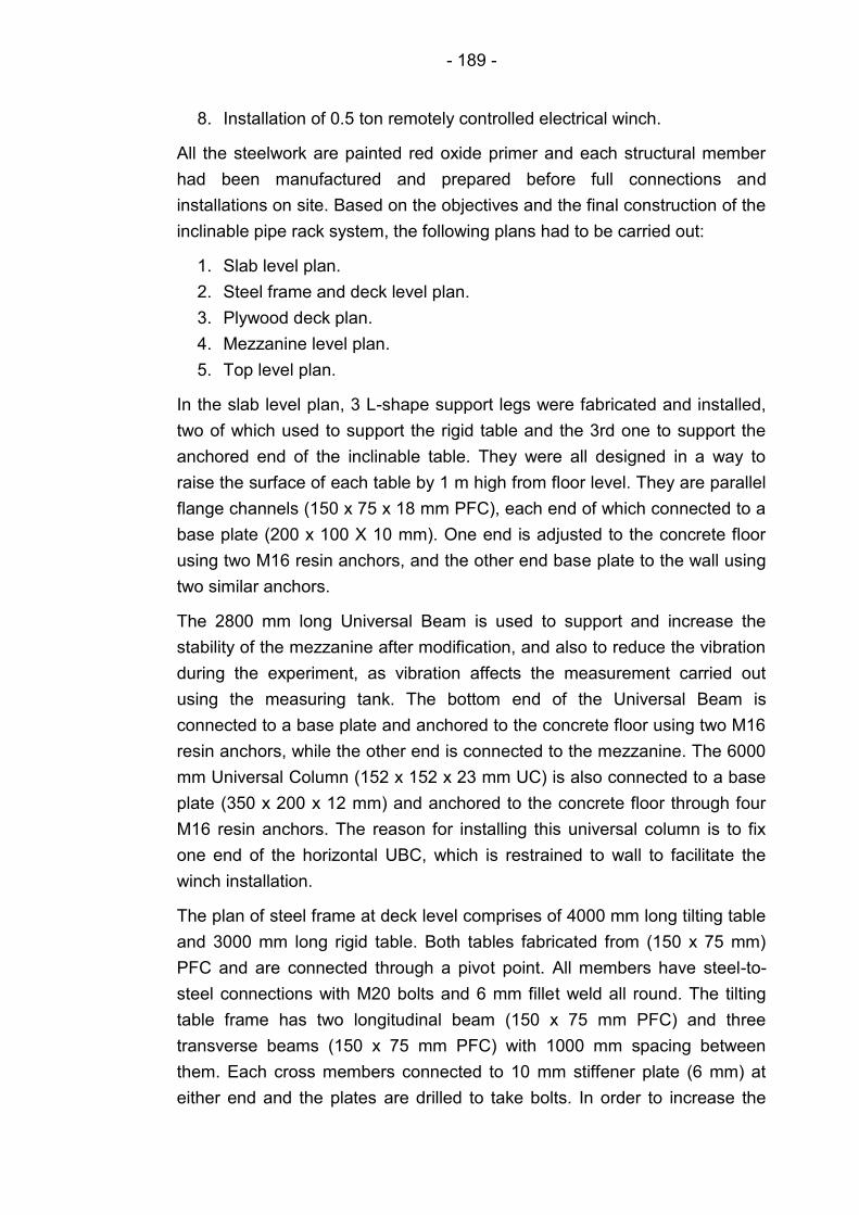
- 189 -
8. Installation of 0.5 ton remotely controlled electrical winch.
All the steelwork are painted red oxide primer and each structural member
had been manufactured and prepared before full connections and
installations on site. Based on the objectives and the final construction of the
inclinable pipe rack system, the following plans had to be carried out:
1. Slab level plan.
2. Steel frame and deck level plan.
3. Plywood deck plan.
4. Mezzanine level plan.
5. Top level plan.
In the slab level plan, 3 L-shape support legs were fabricated and installed,
two of which used to support the rigid table and the 3rd one to support the
anchored end of the inclinable table. They were all designed in a way to
raise the surface of each table by 1 m high from floor level. They are parallel
flange channels (150 x 75 x 18 mm PFC), each end of which connected to a
base plate (200 x 100 X 10 mm). One end is adjusted to the concrete floor
using two M16 resin anchors, and the other end base plate to the wall using
two similar anchors.
The 2800 mm long Universal Beam is used to support and increase the
stability of the mezzanine after modification, and also to reduce the vibration
during the experiment, as vibration affects the measurement carried out
using the measuring tank. The bottom end of the Universal Beam is
connected to a base plate and anchored to the concrete floor using two M16
resin anchors, while the other end is connected to the mezzanine. The 6000
mm Universal Column (152 x 152 x 23 mm UC) is also connected to a base
plate (350 x 200 x 12 mm) and anchored to the concrete floor through four
M16 resin anchors. The reason for installing this universal column is to fix
one end of the horizontal UBC, which is restrained to wall to facilitate the
winch installation.
The plan of steel frame at deck level comprises of 4000 mm long tilting table
and 3000 mm long rigid table. Both tables fabricated from (150 x 75 mm)
PFC and are connected through a pivot point. All members have steel-to-
steel connections with M20 bolts and 6 mm fillet weld all round. The tilting
table frame has two longitudinal beam (150 x 75 mm PFC) and three
transverse beams (150 x 75 mm PFC) with 1000 mm spacing between
them. Each cross members connected to 10 mm stiffener plate (6 mm) at
either end and the plates are drilled to take bolts. In order to increase the
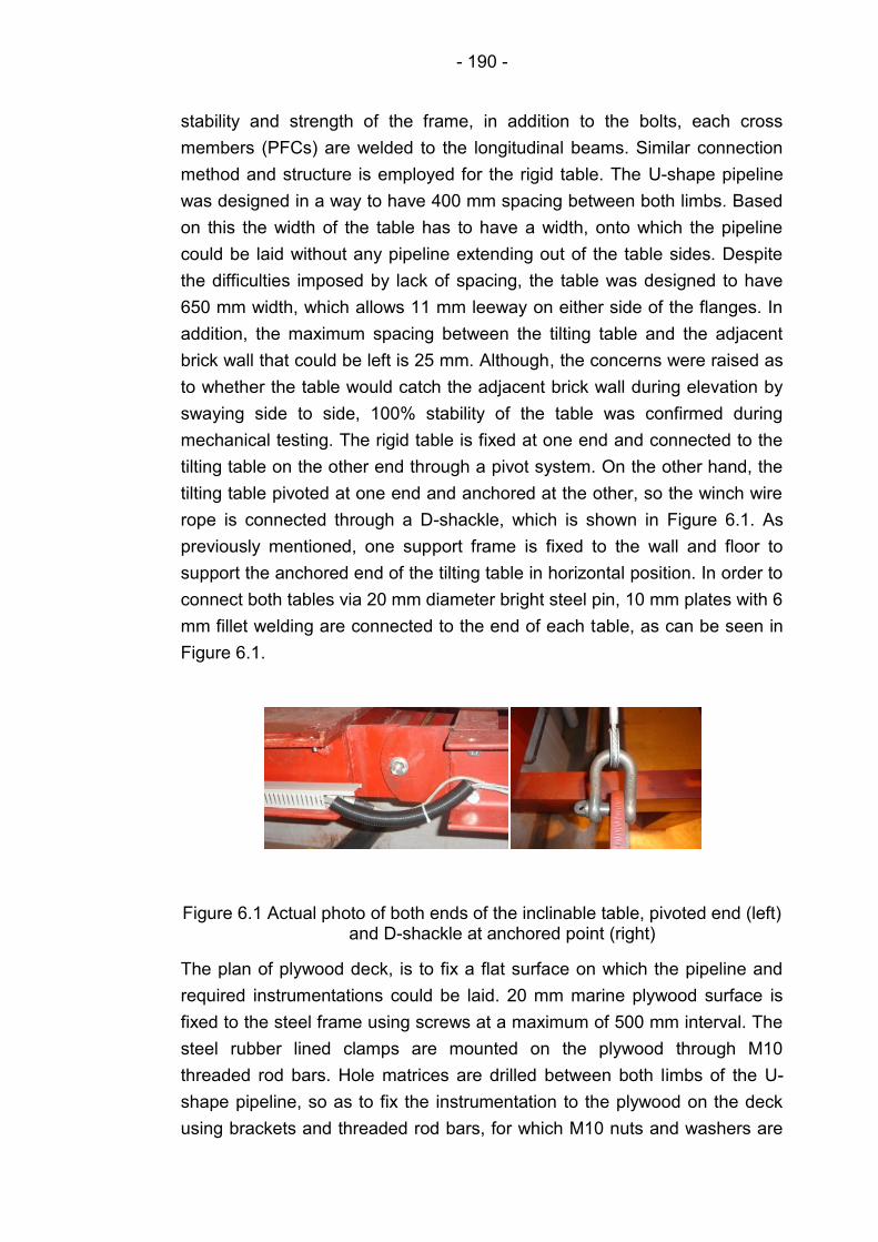
- 190 -
stability and strength of the frame, in addition to the bolts, each cross
members (PFCs) are welded to the longitudinal beams. Similar connection
method and structure is employed for the rigid table. The U-shape pipeline
was designed in a way to have 400 mm spacing between both limbs. Based
on this the width of the table has to have a width, onto which the pipeline
could be laid without any pipeline extending out of the table sides. Despite
the difficulties imposed by lack of spacing, the table was designed to have
650 mm width, which allows 11 mm leeway on either side of the flanges. In
addition, the maximum spacing between the tilting table and the adjacent
brick wall that could be left is 25 mm. Although, the concerns were raised as
to whether the table would catch the adjacent brick wall during elevation by
swaying side to side, 100% stability of the table was confirmed during
mechanical testing. The rigid table is fixed at one end and connected to the
tilting table on the other end through a pivot system. On the other hand, the
tilting table pivoted at one end and anchored at the other, so the winch wire
rope is connected through a D-shackle, which is shown in Figure 6.1. As
previously mentioned, one support frame is fixed to the wall and floor to
support the anchored end of the tilting table in horizontal position. In order to
connect both tables via 20 mm diameter bright steel pin, 10 mm plates with 6
mm fillet welding are connected to the end of each table, as can be seen in
Figure 6.1.
Figure 6.1 Actual photo of both ends of the inclinable table, pivoted end (left) and D-shackle at anchored point (right)
The plan of plywood deck, is to fix a flat surface on which the pipeline and
required instrumentations could be laid. 20 mm marine plywood surface is
fixed to the steel frame using screws at a maximum of 500 mm interval. The
steel rubber lined clamps are mounted on the plywood through M10
threaded rod bars. Hole matrices are drilled between both limbs of the U-
shape pipeline, so as to fix the instrumentation to the plywood on the deck
using brackets and threaded rod bars, for which M10 nuts and washers are
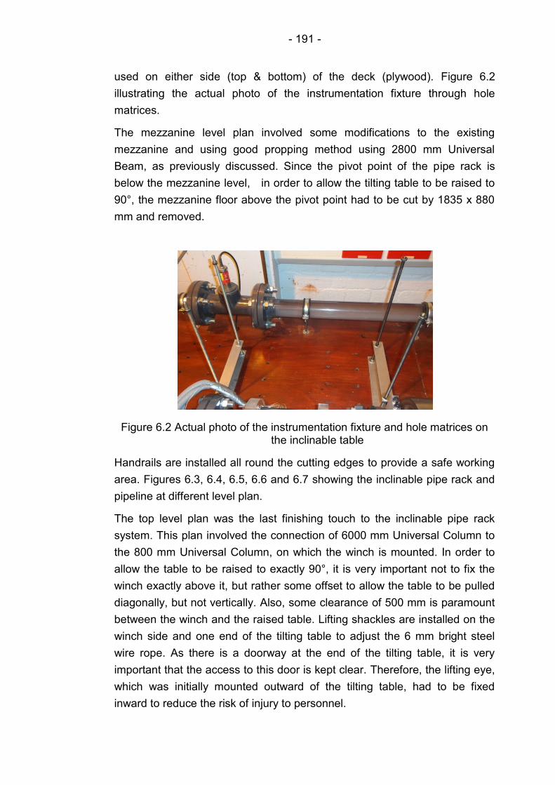
- 191 -
used on either side (top & bottom) of the deck (plywood). Figure 6.2
illustrating the actual photo of the instrumentation fixture through hole
matrices.
The mezzanine level plan involved some modifications to the existing
mezzanine and using good propping method using 2800 mm Universal
Beam, as previously discussed. Since the pivot point of the pipe rack is
below the mezzanine level, in order to allow the tilting table to be raised to
90°, the mezzanine floor above the pivot point had to be cut by 1835 x 880
mm and removed.
Figure 6.2 Actual photo of the instrumentation fixture and hole matrices on the inclinable table
Handrails are installed all round the cutting edges to provide a safe working
area. Figures 6.3, 6.4, 6.5, 6.6 and 6.7 showing the inclinable pipe rack and
pipeline at different level plan.
The top level plan was the last finishing touch to the inclinable pipe rack
system. This plan involved the connection of 6000 mm Universal Column to
the 800 mm Universal Column, on which the winch is mounted. In order to
allow the table to be raised to exactly 90°, it is very important not to fix the
winch exactly above it, but rather some offset to allow the table to be pulled
diagonally, but not vertically. Also, some clearance of 500 mm is paramount
between the winch and the raised table. Lifting shackles are installed on the
winch side and one end of the tilting table to adjust the 6 mm bright steel
wire rope. As there is a doorway at the end of the tilting table, it is very
important that the access to this door is kept clear. Therefore, the lifting eye,
which was initially mounted outward of the tilting table, had to be fixed
inward to reduce the risk of injury to personnel.
- 192 -
65
0
Mixing Tank
3900 2880200 200
120
12
00
94
0
25
0
10
5
7100
Door
18
0
Inclinable Piperack-Top View (Ground Floor)
DRAWN
BY:Y. Faraj
DATE:
Company TIME IN REQUEST: APPROVED BY: Prof. M. Wang DWG NO.
University
of Leeds/
OLIL
15th March 2012 SIGNATURE OF RT: 17
11th March 2012 SCALE 1:20 Material: Steel SHEET 1 of 3
Copyright
This drawing and the copyright, design rights and all other
intellectual property rights in it belong to the University of Leeds/
OLIL group. No licence or assignment of any such rights is granted
hereunder. This drawing is not to be copied or divulged to a third
party without written permission.
Dimensions are in mm
©
Figure 6.3 Schematic diagram of inclinable pipe rack (Top View-Ground Floor)
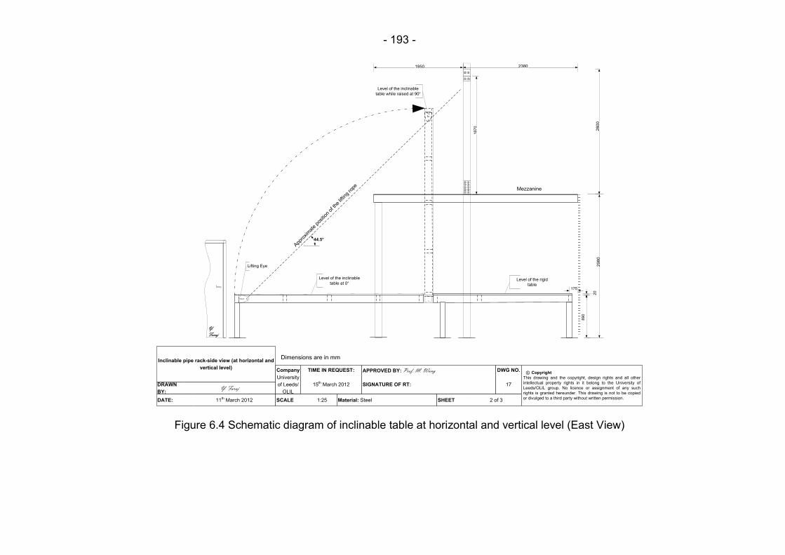
- 193 -
29
80
23801850
175
89
0
20
App
roxim
ate
positio
n of
the
liftin
g ro
pe
44.5°
Lifting Eye
Y.
Faraj
Inclinable pipe rack-side view (at horizontal and
vertical level)
DRAWN
BY:Y. Faraj
DATE:
Company TIME IN REQUEST: APPROVED BY: Prof. M. Wang DWG NO.
University
of Leeds/
OLIL
15th March 2012 SIGNATURE OF RT: 17
11th March 2012 SCALE 1:25 Material: Steel SHEET 2 of 3
Copyright
This drawing and the copyright, design rights and all other
intellectual property rights in it belong to the University of
Leeds/OLIL group. No licence or assignment of any such
rights is granted hereunder. This drawing is not to be copied
or divulged to a third party without written permission.
©
26
00
18
70
Level of the inclinable
table while raised at 90°
Level of the inclinable
table at 0°Level of the rigid
table
Mezzanine
Dimensions are in mm
Figure 6.4 Schematic diagram of inclinable table at horizontal and vertical level (East View)
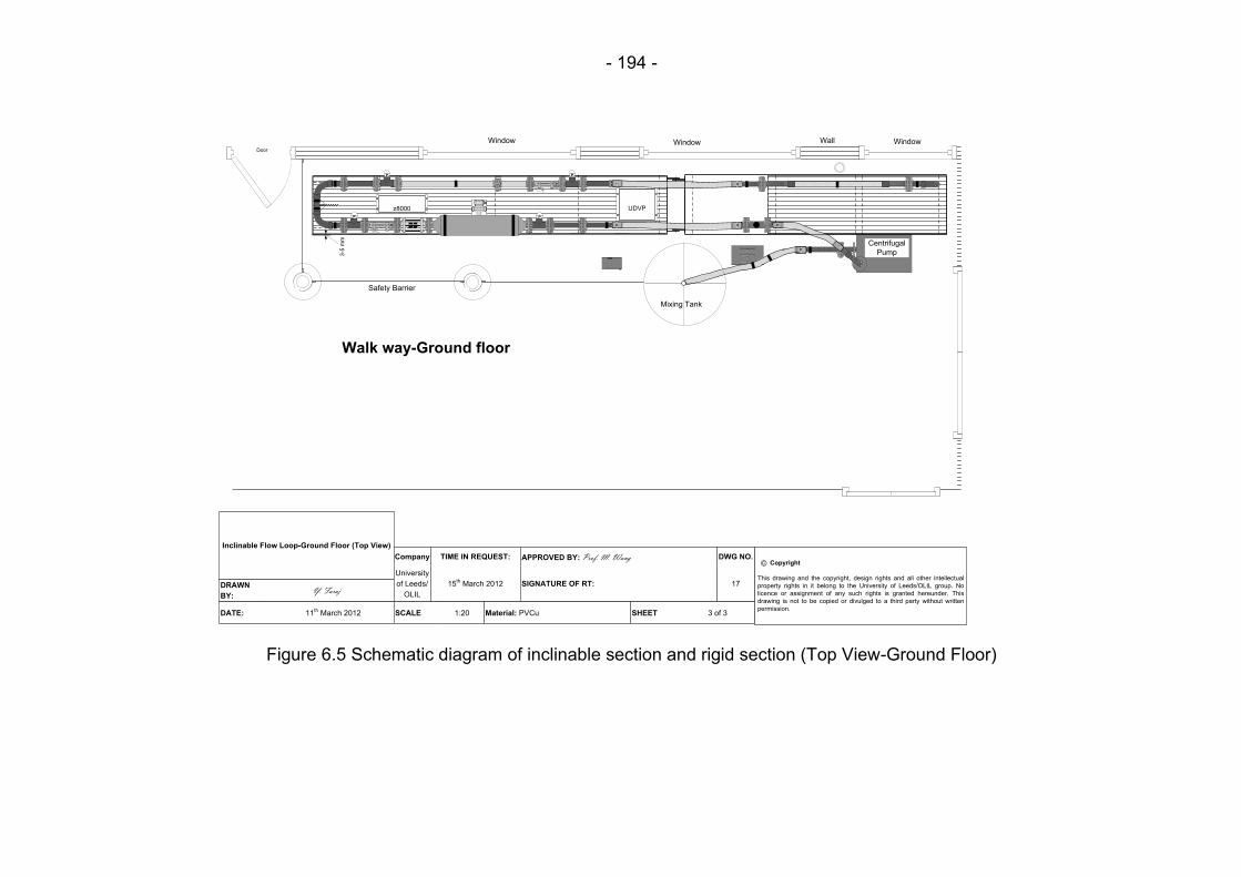
- 194 -
Centrifugal
Pump
Mixing Tank
PP
P
z8000
UDVP
P
Wall
Inclinable Flow Loop-Ground Floor (Top View)
DRAWN
BY:Y. Faraj
DATE:
Company TIME IN REQUEST: APPROVED BY: Prof. M. Wang DWG NO.
University
of Leeds/
OLIL
15th March 2012 SIGNATURE OF RT: 17
11th March 2012 SCALE 1:20 Material: PVCu SHEET 3 of 3
Copyright
This drawing and the copyright, design rights and all other intellectual
property rights in it belong to the University of Leeds/OLIL group. No
licence or assignment of any such rights is granted hereunder. This
drawing is not to be copied or divulged to a third party without written
permission.
©
3-5
mm
Walk way-Ground floor
Safety Barrier
Door
Window WindowWindow
Figure 6.5 Schematic diagram of inclinable section and rigid section (Top View-Ground Floor)
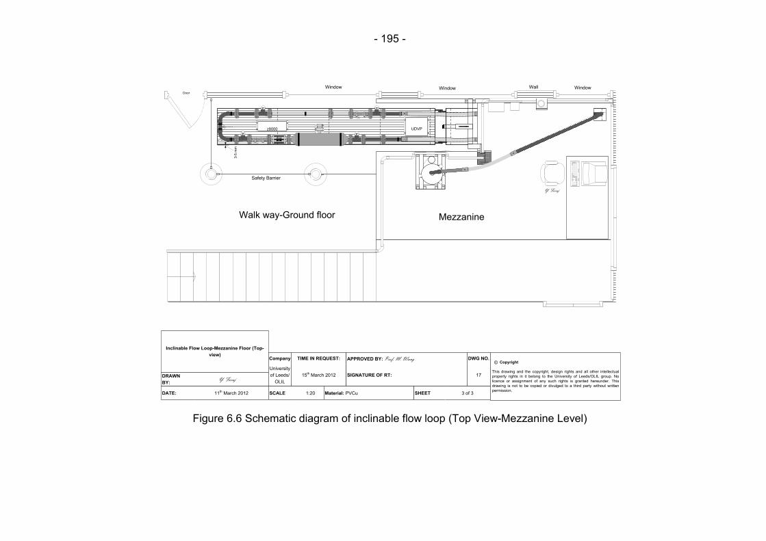
- 195 -
Centrifugal
Pump
Mixing Tank
PP
P
z8000
UDVP
P
Wall
Y. Faraj
Inclinable Flow Loop-Mezzanine Floor (Top-
view)
DRAWN
BY:Y. Faraj
DATE:
Company TIME IN REQUEST: APPROVED BY: Prof. M. Wang DWG NO.
University
of Leeds/
OLIL
15th March 2012 SIGNATURE OF RT: 17
11th March 2012 SCALE 1:20 Material: PVCu SHEET 3 of 3
Copyright
This drawing and the copyright, design rights and all other intellectual
property rights in it belong to the University of Leeds/OLIL group. No
licence or assignment of any such rights is granted hereunder. This
drawing is not to be copied or divulged to a third party without written
permission.
©
3-5
mm
Walk way-Ground floor
Safety Barrier
Mezzanine
Window Window WindowDoor
Figure 6.6 Schematic diagram of inclinable flow loop (Top View-Mezzanine Level)
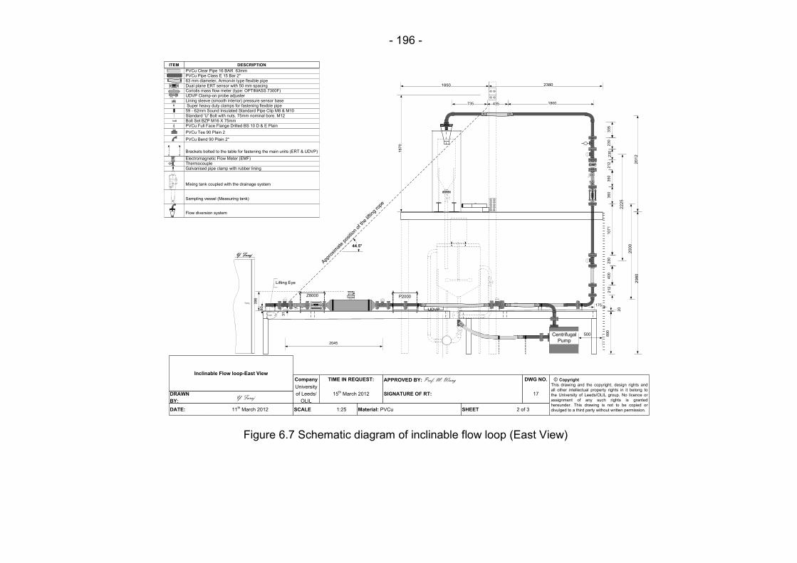
- 196 -
P2000Z8000
UDVP
Centrifugal
Pump
29
80
40
0
500
23
01
07
13
50
21
22
30
23
0
1800435735
23801850
EMF
175
21
28
90
20
39
6
36
0
80
App
roxim
ate
positio
n of
the
liftin
g ro
pe
44.5°
31
Lifting Eye
20
00
22
25
33
5
PVCu Clear Pipe 16 BAR 63mm
PVCu Pipe Class E 15 Bar 2"
63 mm diameter, Armorvin type flexible pipe
Dual plane ERT sensor with 50 mm spacing Coriolis mass flow meter (type: OPTIMASS 7300F)
UDVP Clamp-on probe adjuster
Lining sleeve (smooth interior) pressure sensor base
Super heavy duty clamps for fastening flexible pipe
59 - 62mm Sound Insulated Standard Pipe Clip M8 & M10
Standard 'U' Bolt with nuts. 75mm nominal bore. M12
Bolt Set BZP M16 X 75mm
PVCu Full Face Flange Drilled BS 10 D & E Plain
PVCu Tee 90 Plain 2
PVCu Bend 90 Plain 2"
Inclinable Flow loop-East View
DRAWN
BY:Y. Faraj
DATE:
Company TIME IN REQUEST: APPROVED BY: Prof. M. Wang DWG NO.
University
of Leeds/
OLIL
15th March 2012 SIGNATURE OF RT: 17
11th March 2012 SCALE 1:25 Material: PVCu SHEET 2 of 3
Copyright
This drawing and the copyright, design rights and
all other intellectual property rights in it belong to
the University of Leeds/OLIL group. No licence or
assignment of any such rights is granted
hereunder. This drawing is not to be copied or
divulged to a third party without written permission.
ITEM DESCRIPTION
©
Electromagnetic Flow Meter (EMF)
Thermocouple
Galvanised pipe clamp with rubber lining
EMF
Mixing tank coupled with the drainage system
Sampling vessel (Measuring tank)
20
12
18
70
Flow diversion system
2045
Brackets bolted to the table for fastening the main units (ERT & UDVP)
Y. Faraj
Figure 6.7 Schematic diagram of inclinable flow loop (East View)

- 197 -
6.6.2 Selection of lifting method
The selection of the lifting method to raise and to lower the inclinable table is
one of the most important part of the design process. The selection process
was based on four criteria: safety, efficiency, flexibility and economy. A
journey through lifting equipment suppliers revealed that there is wide range
of lifting equipments and methods available for almost any application, such
as (www.electricwinchshop.co.uk). The lifting methods that could be
considered in the selection process are hydraulic ram, hoists and winches.
Each of these methods has to be carefully assessed against the criteria
mentioned above.
The option of using hydraulic ram is totally eliminated in the selection list due
to the following implications:
1. The ram position have to be designed carefully, as any position may
not be mechanically acceptable due to space limitations.
2. Hydraulic ram housing was suggested, so that the ram direction would
be more towards vertical rather than horizontal. The method of
housing hydraulic ram was found to be an attractive one, as it would
not interfere with the pipeline on the deck. However, the housing
requires more steel work which increase the total cost and the total
load on the deck.
3. Since one of the design requirements is to raise the table up to 90°,
this suggests the requirement of a longer hydraulic ram, which
complicates positioning of the ram. In addition, using telescopic
cylinder can be another option, however, this type of cylinders are
found to be very expensive. The required telescopic cylinder that suits
the application in this project is very costly.
4. Since using hydraulic ram involves utilisation of 50 litre steel reservoir
filled with oil, further problems are to be faced with positioning of the
oil tank indoors due to lack of space in G.56-Engineering Building in
the University of Leeds. Also having oil around, would certainly
increase hazard in the working area and surrounding walkways
through spillage or fire hazard. Although, attempts were made to place
the oil tank outdoor, clearly this would increase the costs by adding
flexible pipes and to protect the whole facility against extreme weather
conditions.
Due to above implications using hydraulic ram as a lifting method was
completely removed from the selection list.
- 198 -
The possibility of using a crane-type hoist system was also considered. After
careful examination regarding the preliminary design of the hoist system, it
was proposed that a crane-type hoist can be used in lifting beam as part of
the whole system. This lifting beam is used as a mono-rail system along with
the inclination angle (0° to 90°) along which the hoist would roll. This system
would include a beam and a lifting block clamps over and it could move
forward and backward using wheels. This, however, would overcomplicate
the whole pipeline system by adding further steel work overhead. Also,
fabrication and installation of the steel would increase the total cost.
Therefore, this method was concluded as a costly and overcomplicated
method, which was also eliminated from the selection list.
The last considered lifting method was a winch system, which can come in
wide variety of styles and can be supplied from a choice of industrial and
commercial suppliers. A budget choices also can be found within the
supplied range that can deliver the job effectively.
As there are many different choices it can be very confusing to choose the
specific type, which makes a good balance between the costs and
effectiveness of the winch for the intended application. Therefore, the
assistance has to be sought from professionals to make the right choice.
In order to make the right choice a few important considerations have to be
taken into account, such as power and tension capabilities, size, reliability
and costs. After balancing all of these factors it was finally decided to select
an electrical wire steel rope winch (electric winch, BETA II, type Compact 1-
BGV D8). Based on the total weight of the inclinable section (pipeline with
contents and the steel frame) a 500 kg capacity was selected. In comparison
to hydraulic ram and crane type hoists system, a winch system can offer
several advantages: such as lower cost (unit and installation), simplicity of
installation, it also uses no fluid.
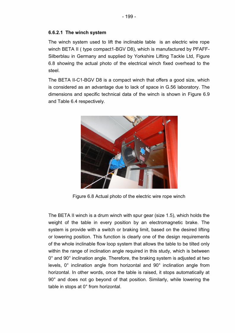
- 199 -
6.6.2.1 The winch system
The winch system used to lift the inclinable table is an electric wire rope
winch BETA II ( type compact1-BGV D8), which is manufactured by PFAFF-
Silberblau in Germany and supplied by Yorkshire Lifting Tackle Ltd, Figure
6.8 showing the actual photo of the electrical winch fixed overhead to the
steel.
The BETA II-C1-BGV D8 is a compact winch that offers a good size, which
is considered as an advantage due to lack of space in G.56 laboratory. The
dimensions and specific technical data of the winch is shown in Figure 6.9
and Table 6.4 respectively.
Figure 6.8 Actual photo of the electric wire rope winch
The BETA II winch is a drum winch with spur gear (size 1.5), which holds the
weight of the table in every position by an electromagnetic brake. The
system is provide with a switch or braking limit, based on the desired lifting
or lowering position. This function is clearly one of the design requirements
of the whole inclinable flow loop system that allows the table to be tilted only
within the range of inclination angle required in this study, which is between
0° and 90° inclination angle. Therefore, the braking system is adjusted at two
levels, 0° inclination angle from horizontal and 90° inclination angle from
horizontal. In other words, once the table is raised, it stops automatically at
90° and does not go beyond of that position. Similarly, while lowering the
table in stops at 0° from horizontal.

- 200 -
Size A (mm) B (mm) ØC (mm) D (mm) E (mm) G (mm)
1.5 215 300 13.5 6 325 340
Figure 6.9 Showing the electric wire rope winch main dimensions
Table 6.4 Technical winch BETA II specification
Drive group (DIN 15020) 1(Am)
Rope capacity (m) 8.4
Lifting capacity (kg) 500
Rope diameter (mm) 6
Minimum breaking force
(kN)
23.14
Rope speed (m/min) 3.7
Load protection Brake motor
Drive Three-phase motor with built-on brake
Duty cycle (%) 53-40
Circuits/hour 120
Weight (without rope) 63
Operation temperature -20 to 40 °C
The winch can be controlled by handheld remote control, which allows the
operator to lift or lower the table via push buttons, along with the emergency

- 201 -
stop button in case of emergency. The schematic diagram of the handheld
remote control is illustrated in Figure 6.10.
Figure 6.10 Winch remote control
In addition a main switch with external operating elements are also located
at the mezzanine level, where they can quickly and easily be accessed. It is
apparent that the remote control can provide more flexibility, and can be
used at the ground floor level as well as mezzanine level. Nevertheless, it is
recommended that while raising or lowering the table it is should be used in
a location where the entire inclinable table and surroundings are overlooked
from the operators position.
The winch is mounted on a steel structure (universal column-UC), and the
whole structure is designed considering the sustainability of maximum force
imposed by the winch, including consideration to the impact forces. In order
to carry a safe mounting of the winch system, a proper mechanical fixing to
be followed. After making sure that the mounting surface was flat, the winch
was positioned against overhead steel structure and fixed with four M12
bolts (8.8 material grade). The galvanised steel wire rope (6mm diameter) is
fixed to the left drum flange, within which the rope attachment is effectuated
with two screws. The other end of the rope is connected to the lifting eye of
the inclinable table via a D-shackle, which is pinned (threaded) so as to
allow easy removal.
6.6.2.2 The telescopic table push-back system
Once the table is raised to a vertical position (90°), it is at the equilibrium
position, based on Newton’s First Law (Fowles and Cassiday, 1999). The
only forces acting on the table are gravity force due to the load of the table
acting on the pivot system and the pivot system exerts an upward force on
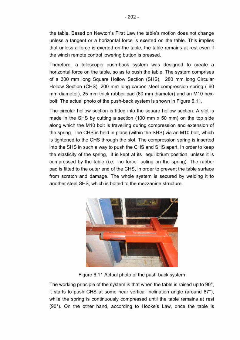
- 202 -
the table. Based on Newton’s First Law the table’s motion does not change
unless a tangent or a horizontal force is exerted on the table. This implies
that unless a force is exerted on the table, the table remains at rest even if
the winch remote control lowering button is pressed.
Therefore, a telescopic push-back system was designed to create a
horizontal force on the table, so as to push the table. The system comprises
of a 300 mm long Square Hollow Section (SHS), 280 mm long Circular
Hollow Section (CHS), 200 mm long carbon steel compression spring ( 60
mm diameter), 25 mm thick rubber pad (60 mm diameter) and an M10 hex-
bolt. The actual photo of the push-back system is shown in Figure 6.11.
The circular hollow section is fitted into the square hollow section. A slot is
made in the SHS by cutting a section (100 mm x 50 mm) on the top side
along which the M10 bolt is travelling during compression and extension of
the spring. The CHS is held in place (within the SHS) via an M10 bolt, which
is tightened to the CHS through the slot. The compression spring is inserted
into the SHS in such a way to push the CHS and SHS apart. In order to keep
the elasticity of the spring, it is kept at its equilibrium position, unless it is
compressed by the table (i.e. no force acting on the spring). The rubber
pad is fitted to the outer end of the CHS, in order to prevent the table surface
from scratch and damage. The whole system is secured by welding it to
another steel SHS, which is bolted to the mezzanine structure.
Figure 6.11 Actual photo of the push-back system
The working principle of the system is that when the table is raised up to 90°,
it starts to push CHS at some near vertical inclination angle (around 87°),
while the spring is continuously compressed until the table remains at rest
(90°). On the other hand, according to Hooke’s Law, once the table is
- 203 -
lowered, by lowering the winch rope, the restoring force acts to restore the
spring to its equilibrium state and the table is pushed back until one of the
force components is created (Blake, 1985). Once the gravity force
component (downward) is created, the table does not require the spring
expansion force to push it back.
6.6.3 Piping design
Piping consists of pipe, flanges, fittings, bolting, gaskets, valves and other
piping components, which are included into the pipeline for a specific
requirement. Moreover, it also includes pipe support and other necessary
elements to provide a safe, secure and effective pipeline. Therefore, piping
refers to the line, where pipe sections are joined with fittings, valves and
other items or mechanical equipment and are supported by supports.
In order to determine the most economical pipeline that responds to all the
design requirements of the multiphase flow loop, it is paramount to consider
several parameters of the pipeline, such as piping construction material,
sizing, jointing method, pipeline layout, length and others. It is apparent that
the economic viability of the pipeline can be defined through careful design
or selection of the above parameters. Therefore, so as to understand the
impact of each parameter and achieve a safe and economic pipeline design,
this section discusses the design and selection of each parameter along with
driving force for selecting some individual components or techniques used in
the design of the flow loop.
Since ignoring any parameters mentioned above can have an adverse
effect of the final design of the system, then careful selection and timely
preparation is crucial for achieving an economical and successful design and
installation of the flow loop piping. It is worth mentioning that throughout the
whole design and installation process it is necessary to make careful and
realistic compromises between the design features and costs, without
ignoring minimum safety standards.
6.6.3.1 Piping construction material and diameter section
The selection of materials of construction for multiphase piping system is
very important in designing a multiphase flow system. Since it is considered
as an optimisation process, then the material selected must be chosen for
the sum of its properties such as strength, ductile, corrosion resistance etc.
The selection of piping material is carried out in two stage process, in the
first stage consideration should only be given to those piping materials that:
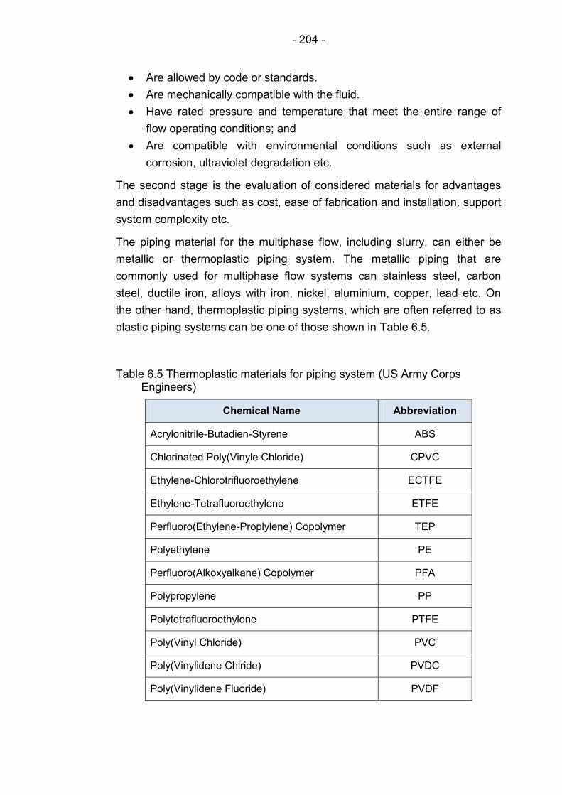
- 204 -
Are allowed by code or standards.
Are mechanically compatible with the fluid.
Have rated pressure and temperature that meet the entire range of
flow operating conditions; and
Are compatible with environmental conditions such as external
corrosion, ultraviolet degradation etc.
The second stage is the evaluation of considered materials for advantages
and disadvantages such as cost, ease of fabrication and installation, support
system complexity etc.
The piping material for the multiphase flow, including slurry, can either be
metallic or thermoplastic piping system. The metallic piping that are
commonly used for multiphase flow systems can stainless steel, carbon
steel, ductile iron, alloys with iron, nickel, aluminium, copper, lead etc. On
the other hand, thermoplastic piping systems, which are often referred to as
plastic piping systems can be one of those shown in Table 6.5.
Table 6.5 Thermoplastic materials for piping system (US Army Corps Engineers)
Chemical Name Abbreviation
Acrylonitrile-Butadien-Styrene ABS
Chlorinated Poly(Vinyle Chloride) CPVC
Ethylene-Chlorotrifluoroethylene ECTFE
Ethylene-Tetrafluoroethylene ETFE
Perfluoro(Ethylene-Proplylene) Copolymer TEP
Polyethylene PE
Perfluoro(Alkoxyalkane) Copolymer PFA
Polypropylene PP
Polytetrafluoroethylene PTFE
Poly(Vinyl Chloride) PVC
Poly(Vinylidene Chlride) PVDC
Poly(Vinylidene Fluoride) PVDF

- 205 -
Unlike metallic piping, plastic piping materials do not display corrosion rates
and are cheaper, easier for fabrication and installation. Since the cost is the
driving force and the technical criteria can easily be met with plastic piping
systems, therefore it was decided that thermoplastic material would be used.
Unplasticised Poly Vinyl (uPVC) Chloride was found to be the most attractive
piping material amongst all the others. The selection of uPVC was
influenced by its advantages and the required chemical criteria that is met
for the project. The most common advantages of uPVC are:
Environmentally sound.
Providing strength and durability, which ensure long service life.
Corrosion resistant.
Easy for fabrication and installation.
Light weight.
Cost effective.
Always recommended by manufacturers and widely accepted by
codes.
Available in different sizes.
According to manufacturers and contractors, the uPVC is a joy to work with
and it is used in may piping system processes, such as sewers, water
eservice line, Drain-Waste-Vent (DWV), irrigation, conduit and various
industrial installation. Therefore, the uPVC pipeline was found to be the most
suitable pipe for the multiphase flow loop.
6.6.3.2 Pipe sizing
The design criteria for sizing the uPVC piping system was to select the
minimum acceptable diameter of the piping necessary to transport the
mixture efficiently and the minimum pipe wall thickness to safely handle the
internal and external exerted pressure. In order to determine the minimum
acceptable diameter, the fluid flow design has to be carried out. The fluid
flow design is carried out by determining the flow rate and pressure drops.
However it is worth mentioning that before the determination of minimum
internal pipe diameter, a review of flow conditions must be made to
determine the operational conditions, such as transport velocity, or mean
velocity, viscosity, temperature, solids throughput concentration, solids
density and particle size analysis of the dispersed phase. Based on the
above information related to the above parameters, the minimum inside pipe
diameter can be determined. Due to tight cost controls, strict quality
standards and working space limitations 50 mm (2ʺ) pipe diameter was
selected.
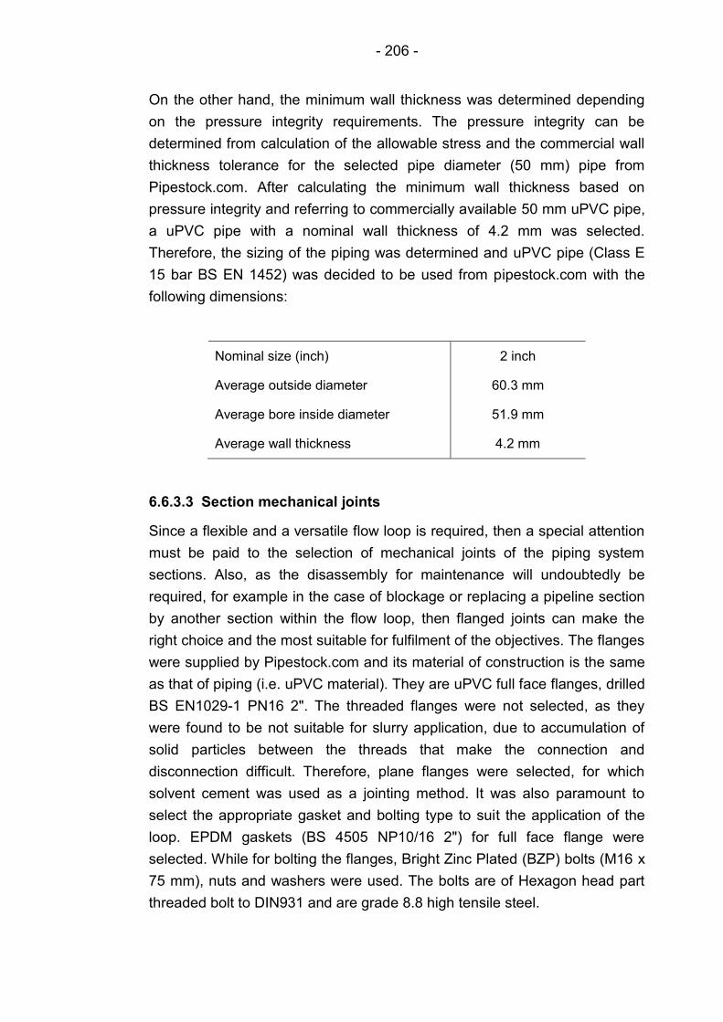
- 206 -
On the other hand, the minimum wall thickness was determined depending
on the pressure integrity requirements. The pressure integrity can be
determined from calculation of the allowable stress and the commercial wall
thickness tolerance for the selected pipe diameter (50 mm) pipe from
Pipestock.com. After calculating the minimum wall thickness based on
pressure integrity and referring to commercially available 50 mm uPVC pipe,
a uPVC pipe with a nominal wall thickness of 4.2 mm was selected.
Therefore, the sizing of the piping was determined and uPVC pipe (Class E
15 bar BS EN 1452) was decided to be used from pipestock.com with the
following dimensions:
Nominal size (inch) 2 inch
Average outside diameter 60.3 mm
Average bore inside diameter 51.9 mm
Average wall thickness 4.2 mm
6.6.3.3 Section mechanical joints
Since a flexible and a versatile flow loop is required, then a special attention
must be paid to the selection of mechanical joints of the piping system
sections. Also, as the disassembly for maintenance will undoubtedly be
required, for example in the case of blockage or replacing a pipeline section
by another section within the flow loop, then flanged joints can make the
right choice and the most suitable for fulfilment of the objectives. The flanges
were supplied by Pipestock.com and its material of construction is the same
as that of piping (i.e. uPVC material). They are uPVC full face flanges, drilled
BS EN1029-1 PN16 2ʺ. The threaded flanges were not selected, as they
were found to be not suitable for slurry application, due to accumulation of
solid particles between the threads that make the connection and
disconnection difficult. Therefore, plane flanges were selected, for which
solvent cement was used as a jointing method. It was also paramount to
select the appropriate gasket and bolting type to suit the application of the
loop. EPDM gaskets (BS 4505 NP10/16 2ʺ) for full face flange were
selected. While for bolting the flanges, Bright Zinc Plated (BZP) bolts (M16 x
75 mm), nuts and washers were used. The bolts are of Hexagon head part
threaded bolt to DIN931 and are grade 8.8 high tensile steel.
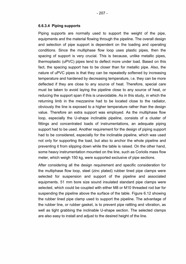
- 207 -
6.6.3.4 Piping supports
Piping supports are normally used to support the weight of the pipe,
equipments and the material flowing through the pipeline. The overall design
and selection of pipe support is dependent on the loading and operating
conditions. Since the multiphase flow loop uses plastic pipes, then the
spacing of support is very crucial. This is because, unlike metallic pipes,
thermoplastic (uPVC) pipes tend to deflect more under load. Based on this
fact, the spacing support has to be closer than for metallic pipe. Also, the
nature of uPVC pipes is that they can be repeatedly softened by increasing
temperature and hardened by decreasing temperature, i.e. they can be more
deflected if they are close to any source of heat. Therefore, special care
must be taken to avoid laying the pipeline close to any source of heat, or
reducing the support span if this is unavoidable. As in this study, in which the
returning limb in the mezzanine had to be located close to the radiator,
obviously the line is exposed to a higher temperature rather than the design
value. Therefore an extra support was employed. As the multiphase flow
loop, especially the U-shape inclinable pipeline, consists of a cluster of
fittings and concentrated loads of instrumentations, an adequate piping
support had to be used. Another requirement for the design of piping support
had to be considered, especially for the inclinable pipeline, which was used
not only for supporting the load, but also to anchor the whole pipeline and
preventing it from slipping down while the table is raised. On the other hand,
some heavy instrumentation mounted on the line, such as Coriolis mass flow
meter, which weigh 150 kg, were supported exclusive of pipe sections.
After considering all the design requirement and specific consideration for
the multiphase flow loop, steel (zinc plated) rubber lined pipe clamps were
selected for suspension and support of the pipeline and associated
equipments. 51 mm bore size sound insulated standard pipe clamps were
selected, which could be coupled with either M8 or M10 threaded rod bar for
suspending the pipeline above the surface of the table. Figure 6.12 showing
the rubber lined pipe clamp used to support the pipeline. The advantage of
the rubber line, or rubber gasket, is to prevent pipe rattling and vibration, as
well as tight grabbing the inclinable U-shape section. The selected clamps
are also easy to install and adjust to the desired height of the line.
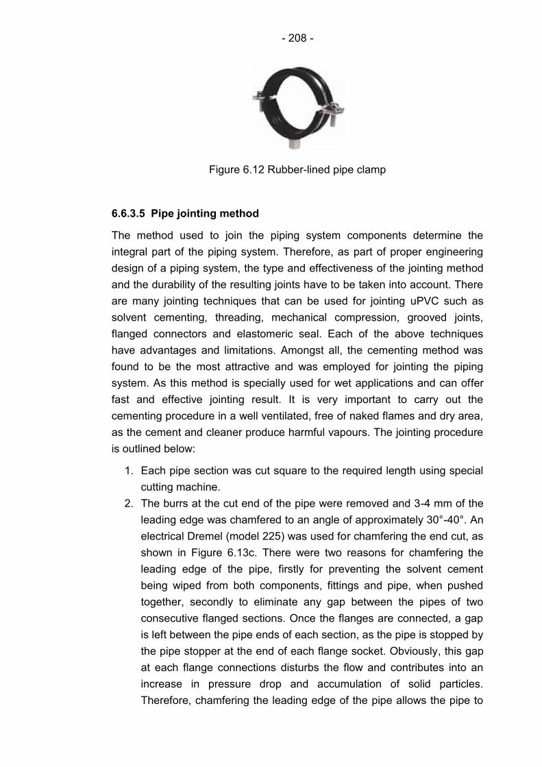
- 208 -
Figure 6.12 Rubber-lined pipe clamp
6.6.3.5 Pipe jointing method
The method used to join the piping system components determine the
integral part of the piping system. Therefore, as part of proper engineering
design of a piping system, the type and effectiveness of the jointing method
and the durability of the resulting joints have to be taken into account. There
are many jointing techniques that can be used for jointing uPVC such as
solvent cementing, threading, mechanical compression, grooved joints,
flanged connectors and elastomeric seal. Each of the above techniques
have advantages and limitations. Amongst all, the cementing method was
found to be the most attractive and was employed for jointing the piping
system. As this method is specially used for wet applications and can offer
fast and effective jointing result. It is very important to carry out the
cementing procedure in a well ventilated, free of naked flames and dry area,
as the cement and cleaner produce harmful vapours. The jointing procedure
is outlined below:
1. Each pipe section was cut square to the required length using special
cutting machine.
2. The burrs at the cut end of the pipe were removed and 3-4 mm of the
leading edge was chamfered to an angle of approximately 30°-40°. An
electrical Dremel (model 225) was used for chamfering the end cut, as
shown in Figure 6.13c. There were two reasons for chamfering the
leading edge of the pipe, firstly for preventing the solvent cement
being wiped from both components, fittings and pipe, when pushed
together, secondly to eliminate any gap between the pipes of two
consecutive flanged sections. Once the flanges are connected, a gap
is left between the pipe ends of each section, as the pipe is stopped by
the pipe stopper at the end of each flange socket. Obviously, this gap
at each flange connections disturbs the flow and contributes into an
increase in pressure drop and accumulation of solid particles.
Therefore, chamfering the leading edge of the pipe allows the pipe to
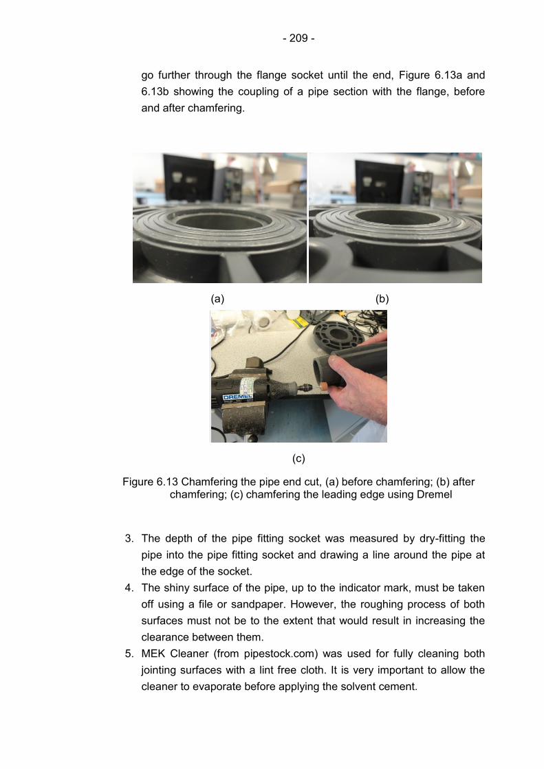
- 209 -
go further through the flange socket until the end, Figure 6.13a and
6.13b showing the coupling of a pipe section with the flange, before
and after chamfering.
(a) (b)
(c)
Figure 6.13 Chamfering the pipe end cut, (a) before chamfering; (b) after chamfering; (c) chamfering the leading edge using Dremel
3. The depth of the pipe fitting socket was measured by dry-fitting the
pipe into the pipe fitting socket and drawing a line around the pipe at
the edge of the socket.
4. The shiny surface of the pipe, up to the indicator mark, must be taken
off using a file or sandpaper. However, the roughing process of both
surfaces must not be to the extent that would result in increasing the
clearance between them.
5. MEK Cleaner (from pipestock.com) was used for fully cleaning both
jointing surfaces with a lint free cloth. It is very important to allow the
cleaner to evaporate before applying the solvent cement.
- 210 -
6. An appropriate sized brush (1ʺ flat brush for 50 mm nominal pipe bore
size) was used to apply the uPVC solvent cement directly from the tin.
First to the fitting socket and then to the pipe using longitudinal
strokes, then both, the pipe and fitting, must be pushed together while
the cement is wet, ensuring that the roughed area is completely
covered with an even layers of cement. It is very important to carry out
this step neatly and quickly, as the cement dries up very quickly.
7. After pushing the fitting and pipe together, both pieces must be held
for approximately 30-40 seconds (longer time for pipes larger than 2ʺ
bore size). It is crucial to wipe the bead and excess cement from the
outer join of the pipe, as this can weaken the wall. It is important not to
disturb the joint for 10-15 minutes. The cement within the join is dried
after 8 hours under normal conditions (temperatures above 10 °C).
However, the manufacturers recommendation is to leave the join for
the full period of 24 hours, after which the pipe system can be fully
pressure tested.
6.6.3.6 Piping layout
Since piping is a major expenditure and important in the design and
construction of flow loops, especially when one considers material costs,
fabrication and field costs. Therefore, proper planning and execution of the
design and routing of the pipeline have a major impact on controlling the
total cost. Piping design and its associated equipment arrangement are
interrelated and must both be taken into account in the pipeline design. Of
course both of them depend on a sound mechanical engineering as well as
chemical engineering background. The pipeline designer must well
understand the pipeline layout, equipment and instrumentation arrangement
and the functionality of the system. Moreover, the designer requires a good
knowledge and understanding of each element within the pipeline, such as
piping materials, valves, pumps, tanks, mixers and other equipments that
are included into the design.
In this project, proper planning was an important activity performed in the
early stages of the design. The whole system was evaluated in the
preliminary stages of the design, so as to achieve space conservation and a
symmetric piping arrangement. Piping layout was carried by designing
dimensioned routings from one point to another point, as shown in Figures
6.14 and 6.15. One of the most important considerations in the piping layout
process is to consider the cost of piping material, by keeping the lines as
- 211 -
short as possible, as well as maintaining proper piping flexibility and
engineering standards. In addition, some other factors have to be
considered in the process of piping layout, such as interference piping
flexibility, cost of material, pipe supports, operation, maintenance and safety
and construction requirements. One of the most challenging aspects of
piping layout was the avoidance of interferences with other facilities within
the working area in G.56 Engineering building, such as structural steel and
concrete (wall), heating systems (radiator) etc. This is obviously due to
space limitation in G.56 laboratory. The voidance of interferences was
tedious and time consuming. At the early stages of the design it was
necessary to search mentally and visually for interferences and find an
appropriate interference-free-rout.
Despite the avoidance of using too many valves in the pipeline, particular
attention was given to the placement of valves in the piping system. As
improper application and location valves can be detrimental to the flow loop
function. It was made sure that the valves are not installed upside down. As
a general guide a minimum of 100 mm clearance for all valve hand-wheels
and possible removal of the valve.
The routing of piping at the centrifugal pump was also carefully planned,
since the pipeline of the pump, particularly the suction section, can adversely
affect the operation and life expectancy of the pump. Poorly designed
suction line can cause cavitation, as a result of entrainment of air into the
pump. The cavitation obviously displaces liquid from within the pump casing,
which causes vibrations and the pump out-of-balance. The out-of-balance of
the pump causes a slight eccentric shaft rotation, which at the end wears out
the bearings and seals. It is worth mentioning that the cavitation results in
severe erosion of the impeller. On the other hand, the discharge line was
also carefully routed, depending on the efficiency of the pump and system
functionality.
The discharge point was designed in such a way so L-shape (or elbows)
would be avoided, which contributes an increase into the pressure drop.
Instead a heavy duty flexible pipe was connected to the discharge point, so
as to achieve a smoothly curved line to follow the rest of pipeline on the
table, as shown in Figure 6.16.
In addition, when the pipeline at the pump was designed, several
engineering rules, which are mostly recommended by the manufacturers,
had to be followed such as:

- 212 -
The suction and discharge sections were supported independently of
the pump, so as to decrease the amount of load transmitted to the
pump casing.
Since the suction section is in horizontal plane, then a minimum of 3-4
pipe diameter is provided between the pump suction point and the
bend below the mixing tank.
In order to avoid any loop or L-shape in the suction line a heavy duty
flexible pipe is connected to the discharge point of the mixing tank and
pump suction point.
The engineering of pipe supports was carefully considered in the piping
layout process. The pipelines are supported and located in close proximity of
the tables, the inclinable and rigid table. However, the pipeline was raised by
approximately 80 mm, which would allow the space of 31 mm between the
bottom of the flanges in the horizontal line and the table. Considering the
allowance of an adequate space between the pipeline and the table in the
design process was very crucial for installing and dismantling the flanged
sections, as well as facilitating the installation of equipments and
instrumentations, especially those that have bigger outer diameter than the
pipe diameter. In order to achieve this, the supports used are connected to
threaded steel rod with allowing an additional length to allow raising and
lowering the pipeline.

- 213 -
Wall
Centrifugal
Pump
Y. F
araj
12
00
94
0
500
25
0
2000 mm 490 mm1250 mm
PP
P
2000 mm 1280 mm
P
One end flanged
pipe section
(345.5 mm)
Flange to flange
pipe section
(1620 mm)
One end flanged
pipe section
(343 mm)One end flanged pipe
section (418 mm)
Flange to flange lining
sleeve pressure sensor
base (230 mm)
Flange to flange
transparent pipe
section (326 mm)
Flange to flange
transparent pipe
section (352 mm)
Flange to flange
transparent pipe
section (1092 mm)
Flange to flange lining
sleeve pressure
sensor base (230 mm)Flange to flange
pipe section
(352 mm)
One end
flanged pipe
section
(156 mm)
210
mm
One end
flanged
pipe
section
(156 mm)
Flange to flange lining sleeve
pressure sensor base (230 mm)
Flange to
flange UDVP
spool-piece
(326 mm)
Flange to
flange ERT
sensor (360
mm)
Coriolis mass flow
meter (1136 mm,
including transition
pieces)
Flange to flange lining sleeve
pressure sensor base (230 mm)
Flange to flange pipe
section (352 mm)
Flexible pipe
(1750 mm)
One end flanged pipe section 162 mm
Air injection nozzle (235 mm)
One end flanged
pipe section (175
mm)
Flexible pipe-suction
section (1500 mm)
Flexible pipe-discharge
section (650 mm)
Figure 6.14 Horizontal and inclinable U-shape piping layout, including suction and discharge sections
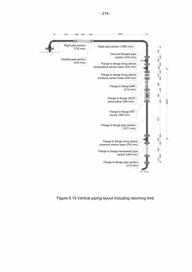
- 214 -
40
0
P
23
01
07
13
26
T
21
22
30
23
0
1800435735
EMF
Y. Faraj
21
23
60
P
22
25
33
5
Flange to flange pipe section
(212 mm)
Flange to flange transparent pipe
section (400 mm)
Flange to flange lining sleeve
pressure sensor base (230 mm)
Flange to flange pipe section
(1071 mm)
Flange to flange ERT
sensor (360 mm)
Flange to flange UDVP
spool-piece (326 mm)
Flange to flange EMF
(212 mm)
Flange to flange lining sleeve
pressure sensor base (230 mm)
Flange to flange lining sleeve
temperature sensor base (230 mm)
One end flanged pipe
section (335 mm)
Rigid pipe section (1800 mm)
Flexible pipe section
(435 mm)
Rigid pipe section
(735 mm)
Figure 6.15 Vertical piping layout including returning limb
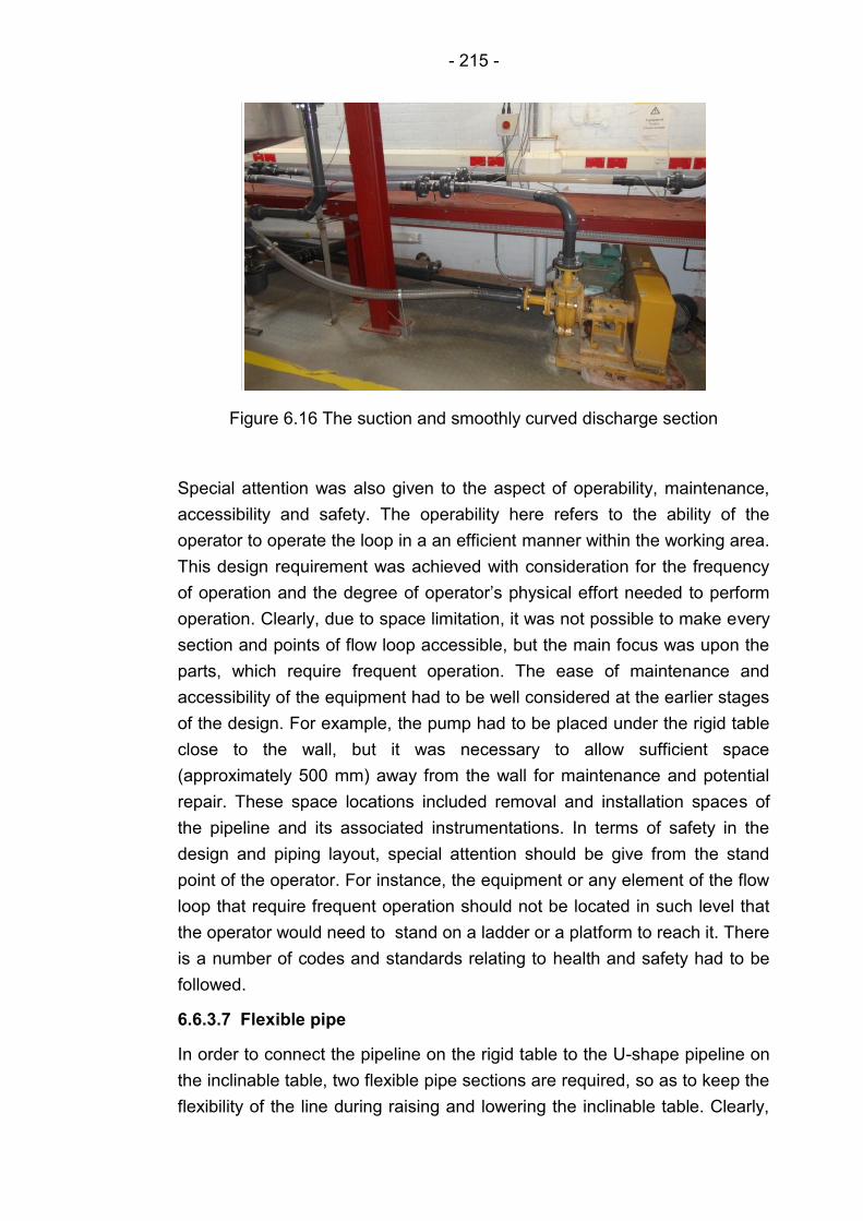
- 215 -
Figure 6.16 The suction and smoothly curved discharge section
Special attention was also given to the aspect of operability, maintenance,
accessibility and safety. The operability here refers to the ability of the
operator to operate the loop in a an efficient manner within the working area.
This design requirement was achieved with consideration for the frequency
of operation and the degree of operator’s physical effort needed to perform
operation. Clearly, due to space limitation, it was not possible to make every
section and points of flow loop accessible, but the main focus was upon the
parts, which require frequent operation. The ease of maintenance and
accessibility of the equipment had to be well considered at the earlier stages
of the design. For example, the pump had to be placed under the rigid table
close to the wall, but it was necessary to allow sufficient space
(approximately 500 mm) away from the wall for maintenance and potential
repair. These space locations included removal and installation spaces of
the pipeline and its associated instrumentations. In terms of safety in the
design and piping layout, special attention should be give from the stand
point of the operator. For instance, the equipment or any element of the flow
loop that require frequent operation should not be located in such level that
the operator would need to stand on a ladder or a platform to reach it. There
is a number of codes and standards relating to health and safety had to be
followed.
6.6.3.7 Flexible pipe
In order to connect the pipeline on the rigid table to the U-shape pipeline on
the inclinable table, two flexible pipe sections are required, so as to keep the
flexibility of the line during raising and lowering the inclinable table. Clearly,

- 216 -
these two sections of the pipeline are very important parts of the whole
pipeline, as connecting the inclinable U-shape section to the rest of flow loop
sections and the flexibility is required for handling the required situation, i.e.
some careful consideration in regards to the flexibility and motion expected
of the sections. Therefore, in order to select the most suitable type of flexible
pipe several important factors has to be considered, which are listed below:
Sizing.
Flow temperature and pressure.
Media.
Motion type and the amount of motion (bending radius).
Internal structure.
Length of the flexible pipe.
Connection.
The size of the flexible pipe was determined based on the existing piping on
either tables. Since the size of existing uPVC is 50 mm, then the size of
flexible pipe should fit the aforementioned pipe size. Therefore, the inside
diameter of the flexible pipe was selected as 63 mm.
The pressure rating for each type of flexible pipe depends on flow conditions
used. As rule of thumb, the maximum operating pressure should be 25% of
the nominal burst pressure. The nominal pressure here is referred to as the
pressure at which the pipe can be expected to burst. Based on the flow loop
specification, the design pressure that corresponds to the maximum pump
frequency is 2 bar. Accordingly, it was decided that the flexible pipe should
have a working pressure more than the flow loop design pressure, and
clearly the nominal pressure is quite above the working pressure. The
decision was made that a flexible pipe would be chosen with 4 bar working
pressure and not less than 10 bar nominal pressure. On the other hand, as
the slurry temperature is expected to correspond to ambient temperature,
considering cold weather in winter and hot in summer, and also elevation of
temperature as a result of heat generation from the pump. Since the flow
loop is build indoor, thus the slurry temperature range is expected to be 1°C
in cold weather and 30°C in hot weather. However, with some design
tolerance, it was decided to choose a flexible pipe with temperature range -
5-50°C.
In terms of the media, or material, since slurry is considered, then it is
associated with corrosion and abrasiveness. Therefore, the main
consideration in specifying a flexible pipe to select a material, which has a
high resistance to the media transported through the pipe. Based on the

- 217 -
nature of aqueous slurry, it was decided to select a flexible pipe with a
material that has a high corrosion resistance and abrasion resistance.
Normally, flexible pipes are used depending on the specified application and
requirements, such as to avoid excessive vibration, pipe alignment, flexibility
of motion and handling the situation etc. The selection of the proper pipe
requires careful consideration based on the intended application. In this
project, the main reason for using flexible pipe is flexibility of the pipeline
during raising or lowering the inclinable U-shape section. The most important
factor that determines high degree of pipe flexibility without affecting the
process or damaging the flexible pipe (kinking) is the minimum bending
radius. Minimum bending radius is the radius, which is measured to the
inside of curvature when bending the pipe without damaging or kinking the
pipe, as shown in Figure 6.17. Clearly, the minimum bending radius ensures
more flexibility of the flexible pipe. Since the range of flow loop inclination
angle between the inclinable section and the rigid section is designed to be
between 0°-90° from horizontal, then the selected flexible pipe must have a
minimum bending radius that allows the flexible pipe to connect the
inclinable section, while it is raised to 90° from horizontal to the rigid pipeline
section without kinking or damage to the flexible pipe or the connected rigid
pipeline. However, it is important not to choose such length that would
create a short radius bend, as previously mentioned, using or creating a
short radius bend can increase the rate of pipe wear and restrict the flow.
Thus it can be concluded that the flexibility factor and the pipe length are
interrelated. In order to select the optimum bending radius of the flexible pipe
for easy bending without damage and without putting any strain on the
connected rigid pipes, an optimum length must be designed. Therefore, a
journey through manufacturer’s websites revealed that the selected flexible
pipe must have a minimum radius between 140-145 mm, and the optimum
length was designed as between 1700-1800 mm, while the pipeline is in
horizontal orientation. Also, in order to avoid kinking, it was decided to select
a reinforced flexible pipe. However, once the table is raised the flexible pipe
is not bent to a straight angle, instead it is bent as a curve, which connects
the two pipeline sections. The further the table is raised the shorter the
distance along the curved pipe trajectory is required. This means that the
original connection point is extended by some length, which was found to be
20%-25% of the pipe length. Since both connection ends are not movable,
then the extra length must shape another bend to a specific direction.
Clearly, this extra bend is not desired and may put one of the connection
ends at enormous amount of strain. Therefore, in order to merge the
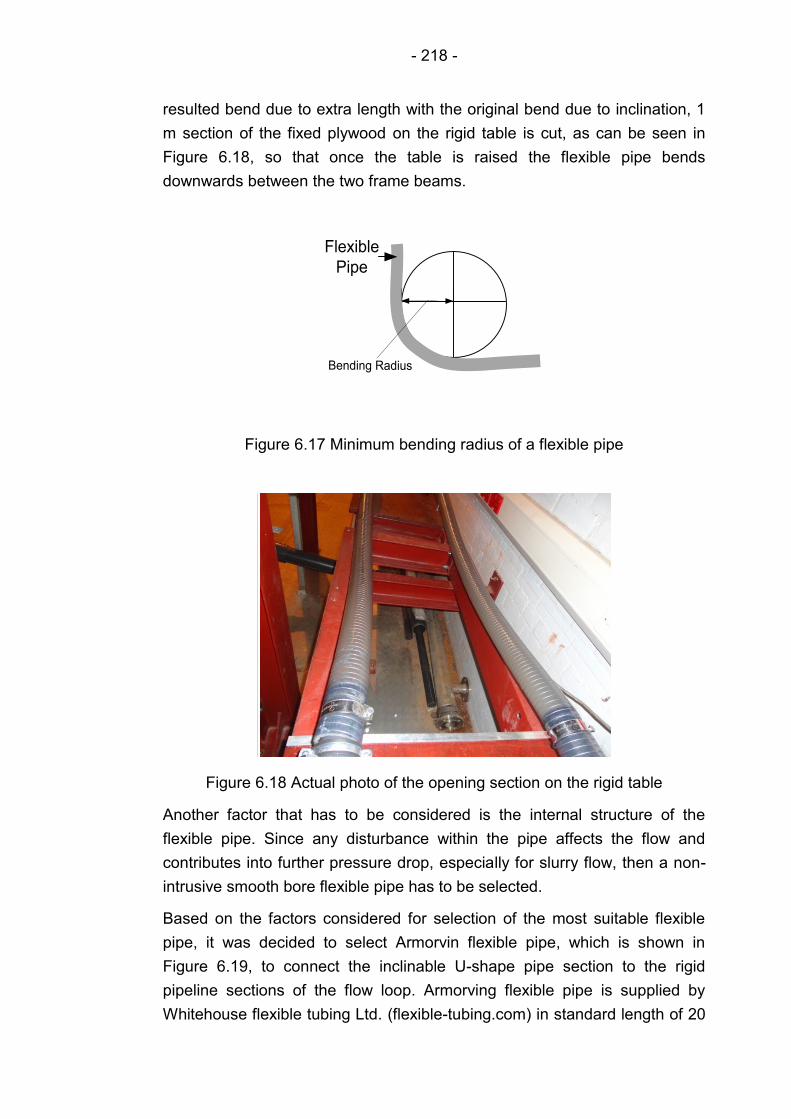
- 218 -
resulted bend due to extra length with the original bend due to inclination, 1
m section of the fixed plywood on the rigid table is cut, as can be seen in
Figure 6.18, so that once the table is raised the flexible pipe bends
downwards between the two frame beams.
Bending Radius
Flexible
Pipe
Figure 6.17 Minimum bending radius of a flexible pipe
Figure 6.18 Actual photo of the opening section on the rigid table
Another factor that has to be considered is the internal structure of the
flexible pipe. Since any disturbance within the pipe affects the flow and
contributes into further pressure drop, especially for slurry flow, then a non-
intrusive smooth bore flexible pipe has to be selected.
Based on the factors considered for selection of the most suitable flexible
pipe, it was decided to select Armorvin flexible pipe, which is shown in
Figure 6.19, to connect the inclinable U-shape pipe section to the rigid
pipeline sections of the flow loop. Armorving flexible pipe is supplied by
Whitehouse flexible tubing Ltd. (flexible-tubing.com) in standard length of 20
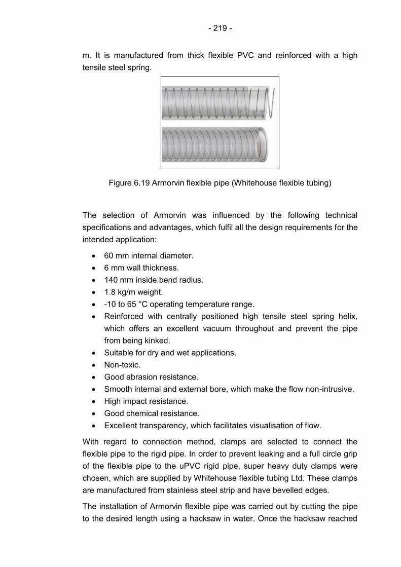
- 219 -
m. It is manufactured from thick flexible PVC and reinforced with a high
tensile steel spring.
Figure 6.19 Armorvin flexible pipe (Whitehouse flexible tubing)
The selection of Armorvin was influenced by the following technical
specifications and advantages, which fulfil all the design requirements for the
intended application:
60 mm internal diameter.
6 mm wall thickness.
140 mm inside bend radius.
1.8 kg/m weight.
-10 to 65 °C operating temperature range.
Reinforced with centrally positioned high tensile steel spring helix,
which offers an excellent vacuum throughout and prevent the pipe
from being kinked.
Suitable for dry and wet applications.
Non-toxic.
Good abrasion resistance.
Smooth internal and external bore, which make the flow non-intrusive.
High impact resistance.
Good chemical resistance.
Excellent transparency, which facilitates visualisation of flow.
With regard to connection method, clamps are selected to connect the
flexible pipe to the rigid pipe. In order to prevent leaking and a full circle grip
of the flexible pipe to the uPVC rigid pipe, super heavy duty clamps were
chosen, which are supplied by Whitehouse flexible tubing Ltd. These clamps
are manufactured from stainless steel strip and have bevelled edges.
The installation of Armorvin flexible pipe was carried out by cutting the pipe
to the desired length using a hacksaw in water. Once the hacksaw reached
- 220 -
the steel spiral wire, the wire bent out and cut with a bolt clipper. However,
as the wire protrudes after cutting, as a matter of safety and prevent injury, a
pair of pliers was used to bend the wire into the rubber.
6.6.3.8 Pipeline length and test section length
Selecting the piping length is an important aspect of the flow loop design.
Since too long flow loop will result in large sample requirement and costly
experiment, whereas too short flow loop will not be able to generate an
accurate data as a result of non-developed flow. Therefore, a careful
consideration has been given to the approach and the test section length.
According to Gillies (1991) and Pachowko (2004), the approach length must
not be less than 50 pipe diameter, and the test section can be any length
between 60-100 pipe diameter. Following the above recommendations, for
our 50 mm (2") pipe diameter, the flow loop used in this research must have
an approach length not less than 2.5 m and a test section between 3-5 m.
Therefore, outgoing limb of the inclinable U-shape section has an approach
length of approximately 2 m, while the table is raised and 3 m, while the
table is at rest horizontally, and the test section is approximately 3 m.
It is worth mentioning that the above recommendation is only applied to
horizontal and near-horizontal sections. For instance, the vertical section
does not necessarily have to have an approach length of 50 pipe diameter.
This is clearly due to the existing simpler flow patterns in vertical flow. The
approach length in the vertical section was chosen to be 20-25 pipe
diameter.
The length of the outgoing and returning limbs was designed to be 16 m in
total and vertical height of 5 m from the floor and 4 m from the top of the
table, which giving a total pipe length of approximately 21 m.
6.6.4 Pump selection
Slurry pump can be considered as the heart of any slurry transport system,
as an industry pumps main duty is to introduce to downstream pipeline and
unit operations. Also, in flow loop studies, such as the one used in this study,
the pump is the main element of the whole pipeline, to which the slurry is
pumped and introduced to the rest of pipe sections and equipments.
Slurry pumps are used to transport mixtures of solids and liquids in many
industries with the wide range of applications, such as dredging, mine
drainage, drilling mud etc. Slurry pumps are normally used for the purpose of
pumping a medium with abrasive particles, hydraulically transporting solids
or pumping the final product of a process.
- 221 -
There is a large number of pump types available for pumping slurries. All of
these types fall into the scope of two main categories, centrifugal pump and
positive displacement. However, by far the common type of slurry pumps
used are centrifugal pumps. The centrifugal pumps use the centrifugal force,
which is generated by the pump impeller to impart energy to the slurry being
transported.
In order to size a centrifugal slurry pump a number of factors have to be
taken in to account. In the mean time, it is very important to avoid an
overestimation of the system resistance (Warman Slurry Pumping
handbook), otherwise it will lead to the following consequences:
1. The pump provides a larger flow than it is required.
2. More power consumption.
3. Overloading the motor and causing damage.
4. Creating of cavitation due to poor suction conditions.
5. Increase of wear rate.
Therefore, for sizing the centrifugal pump in this study attempts were made
to make the best estimate of system head and the final required pump power
was calculated with an addition of safety margins. It was then decided that
for the multiphase flow loop, which is mainly used for slurry, a centrifugal
slurry pump to be used. The decision of using the centrifugal slurry pump
was based on the abilities of centrifugal pumps that are listed below:
1. The ability to handle larger flow rates.
2. The ability to handle larger solid particle size.
3. The ability to withstand high discharge pressure.
4. Smoother pressure characteristics.
5. Longer wear life.
6. Relatively lower cost than for positive displacement pumps.
7. Having heavy duty pump bearings.
On the other hand, one of the disadvantages of centrifugal slurry pumps is
the operation of the pump at a constant flow rate, i.e. it is very difficult to
alter the discharge flow rate of a centrifugal pump. Despite that, this
limitation can be overcome by either throttling the pump to the desired flow
rate or using variable speed drive, which allows variable speed output. In the
flow loop used in this study, the centrifugal pump is fitted with a variable
speed drive, which allows the total discharge pressure, and thus the flow
rate to be controlled and adjusted. The variable speed drive can also provide
the ability to maintain particular output to compensate of pump and pipeline
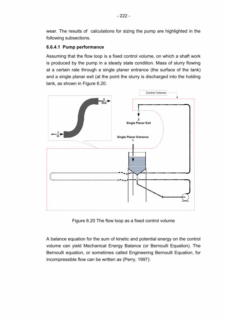
- 222 -
wear. The results of calculations for sizing the pump are highlighted in the
following subsections.
6.6.4.1 Pump performance
Assuming that the flow loop is a fixed control volume, on which a shaft work
is produced by the pump in a steady state condition. Mass of slurry flowing
at a certain rate through a single planer entrance (the surface of the tank)
and a single planar exit (at the point the slurry is discharged into the holding
tank, as shown in Figure 6.20.
2
Single Planar Exit
Single Planar Entrance
1
Control Volume
2
Out
1
In
Figure 6.20 The flow loop as a fixed control volume
A balance equation for the sum of kinetic and potential energy on the control
volume can yield Mechanical Energy Balance (or Bernoulli Equation). The
Bernoulli equation, or sometimes called Engineering Bernoulli Equation, for
incompressible flow can be written as (Perry, 1997):
- 223 -
(6.2)
Rewriting the equation in a customary form, as shown in Equation 6.3.
(6.3)
Where, P1, V1, Z1 denote the pressure, slurry velocity at inlet and the
elevation of inlet level respectively. Similarly, P2, V2, Z2 are related to the exit
planar. g is the gravitational acceleration (9.806 m2/s), ρ is the density of the
mixture. The factor α is the ratio of the cross-sectional area to the cube of
the average velocity. In turbulent flow α is usually equal unity and for a
circular pipe flow it is typically about (1.07). s is the summation of the
work done by moving solid boundaries. Here, in this project, the work is
done by the pump impellers and it is called shaft work. The last term, , is
the rate of viscous energy dissipation. In other words, the viscous or
frictional loss term that accounts for the pipeline and its associated fittings,
such as elbows and valves.
The slurry density (ρ ) can be calculated using the following equation from
Abulnaga (2002):
(6.4)
Where, Cw is the slurry concentration by weight that has already been
assumed as 40%. This amount has been assumed on the basis that the flow
loop may also be used for a high slurry concentration. ρm is the slurry
density, ρl is the liquid density, which is water, and equals to (1000 kg/m3). ρs
is the density of the solid phase (sand) and it was found to be (2650
kg/m3)(or the specific gravity of 2.65). Using the above data the slurry
density was calculated as 1331 kg/m3.
- 224 -
Since the volumetric flow rate Q is the product of average velocity and the
cross sectional area, then the slurry velocities, V1 and V2, at the entrance
and the exit of the system can be calculated using Equation 6.5:
(6.5)
For a flow rate of 35.28 m3/hr (0.0098 m3/s) through the tank cross-sectional
area (0.63 m2), the velocity V1 was calculated to be 0.015 m/s. As the same
amount discharging from the system through a pipe cross-sectional area of
0.00196 m2, then the velocity V2 was calculated to be 5 m/s.
Since the atmospheric pressure of inlet and discharge point (P1 and P2) of
the flow system are similar, then they will be eliminated at either sided of the
Engineering Bernoulli Equation.
Z1 and Z2 found to be 2.70 and 2.80 respectively.
The frictional loss term is the product of the summation of the total head loss
due to friction in pipes and the total head loss due to fittings. Therefore, it
can be written as Equation 6.6:
(6.6)
The total head loss due to friction for incompressible flow in sections of
straight pipe of constant diameter, using fanning friction factor, can be
determined by the Equation 6.7 (from Perry,1997):
(6.7)
Where, L is the length of the pipe, D is the pipe diameter, f is the fanning
friction factor, which can determined from the friction factor as a function of
pipe surface roughness and Reynolds Number ( (Perry, 1997).
However, in turbulent flow, the friction factor for rough pipe follows the
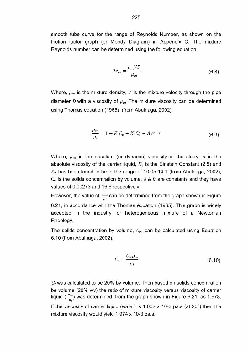
- 225 -
smooth tube curve for the range of Reynolds Number, as shown on the
friction factor graph (or Moody Diagram) in Appendix C. The mixture
Reynolds number can be determined using the following equation:
(6.8)
Where, is the mixture density, is the mixture velocity through the pipe
diameter with a viscosity of .The mixture viscosity can be determined
using Thomas equation (1965) (from Abulnaga, 2002):
(6.9)
Where, is the absolute (or dynamic) viscosity of the slurry, is the
absolute viscosity of the carrier liquid, is the Einstein Constant (2.5) and
has been found to be in the range of 10.05-14.1 (from Abulnaga, 2002),
is the solids concentration by volume, are constants and they have
values of 0.00273 and 16.6 respectively.
However, the value of
can be determined from the graph shown in Figure
6.21, in accordance with the Thomas equation (1965). This graph is widely
accepted in the industry for heterogeneous mixture of a Newtonian
Rheology.
The solids concentration by volume, , can be calculated using Equation
6.10 (from Abulnaga, 2002):
(6.10)
Cv was calculated to be 20% by volume. Then based on solids concentration
be volume (20% v/v) the ratio of mixture viscosity versus viscosity of carrier
liquid (
) was determined, from the graph shown in Figure 6.21, as 1.978.
If the viscosity of carrier liquid (water) is 1.002 x 10⁻³ pa.s (at 20°) then the
mixture viscosity would yield 1.974 x 10⁻³ pa.s.

- 226 -
Figure 6.21 Ratio of viscosity of mixture versus viscosity of the carrier liquid in accordance with Thomas equation for settling slurries (Abulnaga,
2002)
In order to take into account any design errors or uncertainties, then a high
viscosity value is to be chosen by an extra of 30%, which would make it
0.0025 pa.s. Therefore the mixture Reynolds Number would be
approximately 133100.
The surface roughness for uPVC pipe (category E class, Plastic and
Perspex) was found to be 0.0025 mm, then the relative roughness (
) was
calculated to be 0.05. Then, the friction factor was found, on the Moody
Diagram, as 0.001.
The total head loss due to friction in pipes for 20 m pipe length yields 1.4 m.
Similarly, the head loss due to fittings can be calculated using Equation 6.11
(from Perry, 1997).
(6.11)
Where, is the additional frictional loss (which is equivalent number of
velocity heads). There is one diaphragm valve and six 90° elbows (long
- 227 -
radius) in the flow system. The value was found from Perry (1997) for
diaphragm valves (assuming fully open) as 0.44. Also the value for the
elbows mentioned earlier was found to be 0.45. By adding up all values
and calculating the above equation, the total head loss due to fittings was
determined as 0.6 m.
Calculation of Equation 6.2 yields the shaft work per unit of mass (
) flowing the flow system, which was calculated to be 33 kw/unit mass.
Multiplying this value by the slurry mass flow rate would produce the power
required by the pump, which would be (13.2 kw). However, it is very
important to take any design uncertainties into account. Therefore, 10% was
added to the actual value and yielded the power requirement approximately
(15 kw).
6.6.4.2 Suction limitations
Every pump requires a minimum suction head to operate properly. This is
called the Required Net Positive Suction Head (NPSH)R, (Perry, 1997; Brown
and Heywood, 1991; Pachowko, 2004). This parameter is usually published
by the manufacturers and it should be equal or less than the Net Positive
Suction Head Available (NPSH)A, so that the cavitations are avoided.
Cavitations occur, when the absolute pressure of the pump is below the
vapour pressure of the liquid in the slurry at the operating temperature. As a
result the vapour bubbles appear and release the energy, which cause
damages to the pump components, such as keys, loosing of rotor and shaft
breakage.
Therefore, the (NPSH)A must be calculated at the design stage and has to be
equal or greater than (NPSH)R for the desired capacity. The (NPSH)A can be
calculated as:
(6.12)
Where ha is the atmospheric head and is equal to 10.34 m, as the holding
tank is vented to atmosphere. hs is the static head in (m), which was found to
be 2.35 m. hvp is the vapour pressure head of water at 20 °C and is 0.19 m.
hf is the frictional losses and was calculated from Darcy’s formula with the
help of equivalent length table for fittings and valves. hf was calculated to be
1.08 m. hi denotes the safety factor of 0.7 m as a compensation to the losses
- 228 -
after the fluid entering the pump. Finally, (NPSH)A was estimated as 10 m
with considering any design uncertainties.
According to Pachowko (2004) in order to avoid cavitation phenomenon, the
(NPSH)A is usually taken to be 0.5-1 m less than (NPSH)R.
The total dynamic head was also calculated using the following equation
from Perry (1997):
(6.13)
Where (hd)t is the total discharge head and is calculated from:
(6.14)
Where (hs)d is the discharge static head and (hf)d is the head loss in piping
and fittings, which was calculated from the Darcy’s Equation and estimated
as 12.6 m. The total discharge head was calculated as 30 m. Similarly, the
total suction head was estimated to be 9 m. By combining these two values
the total dynamic head was calculated as 21 m.
From the above calculations, it was concluded that a 15 kw pump would be
satisfactory to overcome the total head difference. As the cost is the main
point of consideration, therefore, it was decided to use the existing pump,
which is in G.56 laboratory/Engineering Building and used by the previous
researcher and meets the requirements. This decision was made based on
the fact that this pump meets the required pump capacity of our design and it
has been designed for heavy duty slurry pumping. It was also decide to use
the same (15 kw) Digi-drive frequency converter, in order to control slurry
flow rate.
6.6.5 Equipment design
A properly designed and arranged equipments of any pilot plant flow loop
will undoubtedly provide an excellent flexibility and capability of the loop to
generate a promising data over a wide range of conditions. Some of these
equipments may be used for different purposes, such as the measuring tank
and the flow diversion system, which are used for calibration purposes and
producing one of the important parameters delivered solids concentration.
Therefore, it is crucial to design a proper tank to fulfil the objectives and
cover the whole range of intended conditions. Another important piece of
- 229 -
equipment within the flow system is the holding or mixing tank, which can
have an adverse effect on the loop operation and the data generated from
the loop, if it is not carefully designed or located within the whole system. For
example, when designing the mixing tank it is very important to consider the
level of slurry within the tank. If the level of slurry in the mixing tank is not
kept high enough, it results in air entrainment in the mixture and introduced
to the pump. Also low slurry level within the tank have a negative impact on
the suction head. Therefore, the design functionality and layout of the main
equipments used within the multiphase flow system are described below.
These equipments are mixing tank, measuring tank, flow diversion system,
drainage system, slurry valves and the ultrasound probe holder.
6.6.5.1 Mixing tank
The holding tank has to be designed with a conical section rather than a flat
base. As this will prevent the accumulation of solid particles at the dead
ends of the tank and facilitate the drainage system at the end of each
experiment. To ensure that enough suction head is provided to the pump,
the volume and level of the slurry in the holding tank are very important to be
carefully designed. Pachowko (2004) successfully designed a holding tank
with a capacity 10 times the volume of the pipe work of his flow loop (24 m).
By following Pachowko’s design procedure we should have a holding tank
with a volume 10 times the volume of the 21 m pipeline length. If the volume
of 21 m pipeline length with 50 mm diameter is 0.04123 m3 (41.23 litre), then
10 times of the above value would make the volume of the holding tank,
which is 410.23 litres.
When the flow is diverted into the measurement tank, the slurry level would
decrease by the amount added to the measurement tank. This would have a
negative impact on the suction head. The holding tank volume has to be
designed with adding some extra volume to compensate the amount of
slurry added to the measuring tank. Therefore, the holding tank volume was
designed to be 500 litres, some of which replace the amount of slurry
diverted to the measuring tank.
The total height of the holding tank can be calculated, if assumed that the
diameter of the cylindrical part is the same as its diameter. Also, assuming a
slope of 20% (11°) at the base of the conical part, which can provide an easy
surface for the solid particles to slip down the tank, makes the height of the
conical part 0.1 of tank diameter. Figure 6.22 showing the schematic
drawing of the holding tank. The height of the tank can be determined using
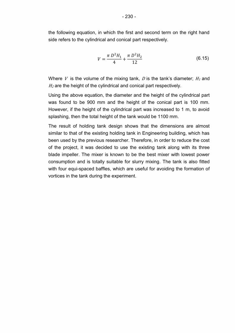
- 230 -
the following equation, in which the first and second term on the right hand
side refers to the cylindrical and conical part respectively.
(6.15)
Where V is the volume of the mixing tank, D is the tank’s diameter; H1 and
H2 are the height of the cylindrical and conical part respectively.
Using the above equation, the diameter and the height of the cylindrical part
was found to be 900 mm and the height of the conical part is 100 mm.
However, if the height of the cylindrical part was increased to 1 m, to avoid
splashing, then the total height of the tank would be 1100 mm.
The result of holding tank design shows that the dimensions are almost
similar to that of the existing holding tank in Engineering building, which has
been used by the previous researcher. Therefore, in order to reduce the cost
of the project, it was decided to use the existing tank along with its three
blade impeller. The mixer is known to be the best mixer with lowest power
consumption and is totally suitable for slurry mixing. The tank is also fitted
with four equi-spaced baffles, which are useful for avoiding the formation of
vortices in the tank during the experiment.
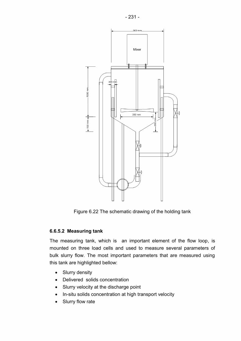
- 231 -
Figure 6.22 The schematic drawing of the holding tank
6.6.5.2 Measuring tank
The measuring tank, which is an important element of the flow loop, is
mounted on three load cells and used to measure several parameters of
bulk slurry flow. The most important parameters that are measured using
this tank are highlighted bellow:
Slurry density
Delivered solids concentration
Slurry velocity at the discharge point
In-situ solids concentration at high transport velocity
Slurry flow rate
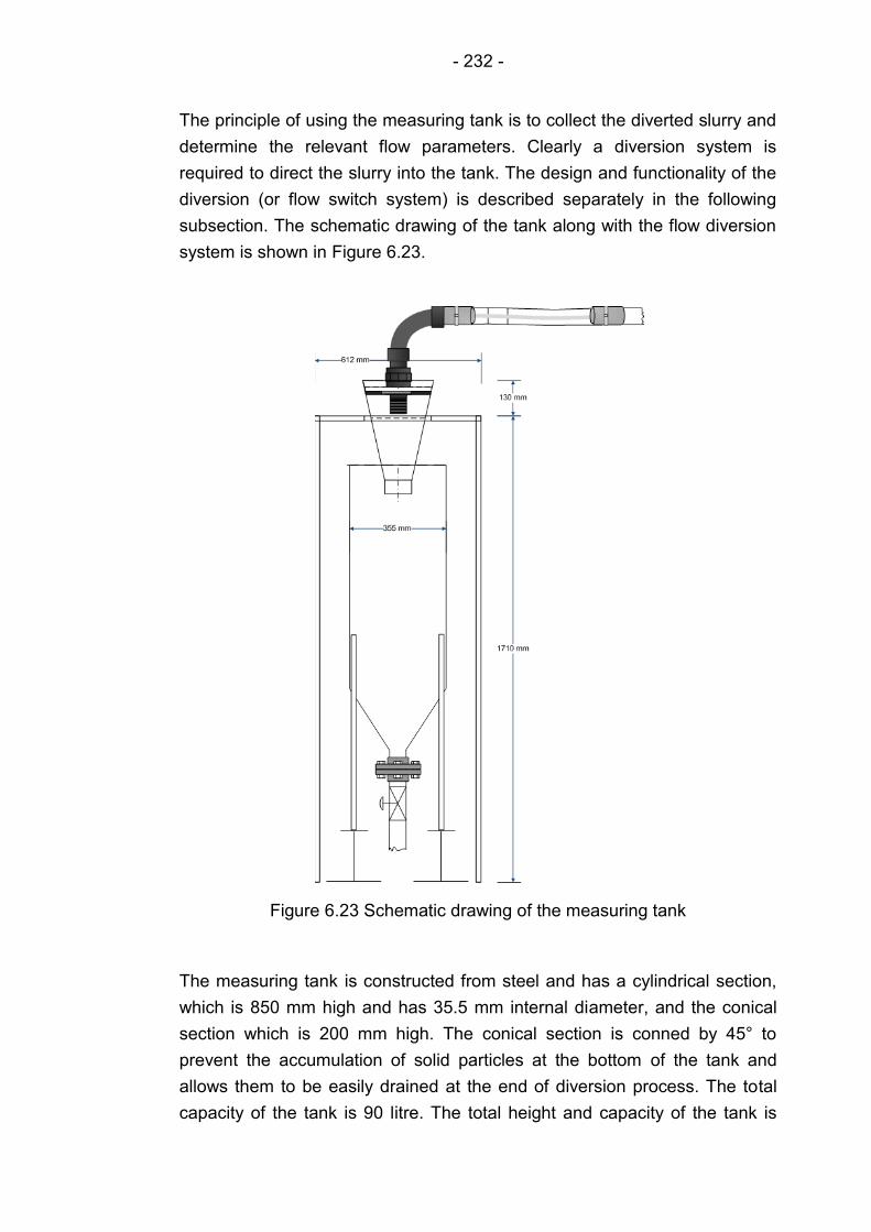
- 232 -
The principle of using the measuring tank is to collect the diverted slurry and
determine the relevant flow parameters. Clearly a diversion system is
required to direct the slurry into the tank. The design and functionality of the
diversion (or flow switch system) is described separately in the following
subsection. The schematic drawing of the tank along with the flow diversion
system is shown in Figure 6.23.
Figure 6.23 Schematic drawing of the measuring tank
The measuring tank is constructed from steel and has a cylindrical section,
which is 850 mm high and has 35.5 mm internal diameter, and the conical
section which is 200 mm high. The conical section is conned by 45° to
prevent the accumulation of solid particles at the bottom of the tank and
allows them to be easily drained at the end of diversion process. The total
capacity of the tank is 90 litre. The total height and capacity of the tank is
- 233 -
very important to be taken into account in the design process. Therefore,
some leeway was aloud for the tank to avoid splashing and overflow while
diverting the slurry. In order to determine the slurry level within the tank a
graded glass tube is mounted at the half point of the cylindrical section. A
diaphragm valve is also installed at the bottom of the tank ( at the discharge
point of the tank) for easy collection of diverted slurry during the diversion
process and drainage at the end. The measuring tank is located above the
mixing tank to avoid any extra bend in the pipeline and allow the slurry to be
drained through a straight part section into the mixing tank.
6.6.5.3 Flow diversion system
In order to facilitate the flow diversion process and obtain more accurate
data, a flow diversion system was designed, the geometry and dimension of
which is shown in Figure 6.24.
The main part of the system is a steel container which is split in to two port
circular sections with 99 mm outer diameter, each of which fits into 100 mm
(4 inch) PVC pipe. One of the sections directs the flow into the mixing tank
and the other one into the measuring tank. On either side of the steel
container two tracts are fixed, through which a 50 mm thick Perspex sheet
slides. Both tracks are extended on either side of the steel container by 160
mm, which accounts for the distance between the centre lines of the two
sections. In order to avoid accumulation of the solid particles and splashing,
the bottom of the steel container at the outlet of each section was designed
as a curved shape, on which the solid particles roll down. In other words,
any flat dead end within each section is avoided. 600 mm long flexible pipe
is used to connect the main pipeline to a pipeline fitting section, which is
going through the sliding Perspex sheet. A union system is used to fix the
line at the Perspex sheet point. The length of the Perspex sheet has
carefully been designed, so as to allow a flexible and easy switching of the
flow between the two sections. The length of the pipe section, which is
connected to the bottom of the sheet and through which the flow is
discharged into each section, must be long enough to avoid splashing.
However, some distance (0.15 mm) must be kept between the discharged
pipe section and the split plate inside the steel container, so that the pipe
does not catch the plate while sliding the Perspex sheet.
It is also very important to use some type of stoppers at the end of the two
tracks, to keep the Perspex sheet in place within the track. Therefore,
welded hinges (two wings and welded bush) are used in the switch system
in this study. The bush is welded to an L-shape metal bar (8 mm diameter),
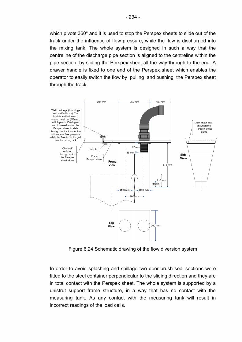
- 234 -
which pivots 360° and it is used to stop the Perspex sheets to slide out of the
track under the influence of flow pressure, while the flow is discharged into
the mixing tank. The whole system is designed in such a way that the
centreline of the discharge pipe section is aligned to the centreline within the
pipe section, by sliding the Perspex sheet all the way through to the end. A
drawer handle is fixed to one end of the Perspex sheet which enables the
operator to easily switch the flow by pulling and pushing the Perspex sheet
through the track.
Figure 6.24 Schematic drawing of the flow diversion system
In order to avoid splashing and spillage two door brush seal sections were
fitted to the steel container perpendicular to the sliding direction and they are
in total contact with the Perspex sheet. The whole system is supported by a
unistrut support frame structure, in a way that has no contact with the
measuring tank. As any contact with the measuring tank will result in
incorrect readings of the load cells.

- 235 -
The testing of the system concluded that diversion of the flow through sliding
of the Perspex sheet provides a convenient means of controlling the flow,
thus obtaining a good quality measuring data.
6.6.5.4 Drainage system
A drain-line is a necessary feature of the open loop. The drainage system
can be used for removing the slurry directly from the bottom of the holding
tank, at the end of each experiment.
The drainage system used, as a important element of the whole flow system,
consists of three tanks (large, medium and small), the actual photograph of
which is shown in Figure 6.25. The three tanks are connected to each other
via extended pipelines at the top and bottom level. The top connections are
permanently open, while the bottom connection lines can be controlled via
three diaphragm valves. This technique is based on settling characterisation
of solid particles. As the drainage line goes through the three tanks, the solid
particles settle at the bottom of the tanks successively, while the carrier
liquid (water) flows into the next tank and finally to the drain. During each
draining procedure, while the mixing tank is drained, all of the valves are
closed, so that the solid particles are trapped within the tank. This way, once
the slurry enters into the first tank, the solid particles settle at the bottom of
the tank due to gravity and the carrier liquid flows into the next tank and so
on. Based on previous experience, after each drainage procedure, a very
few coarse solid particle within (very fine particles in water) were noticed in
the third tank. This clearly confirms the efficiency of the system. The settled
solid particles then can easily be collected from the three tanks and
disposed off in accordance with health, safety and environmental standards.
Figure 6.25 Actual photograph of the drainage system
- 236 -
6.6.5.5 Slurry valves
According to Brown and Heywood (1991) the first rule on application of
valves in slurry systems is to avoid using them, if possible. This is due to
potential leakage and blockage.
The common valves used in slurry systems, based on the type of slurry, are
knife gate, diaphragm, pinch, plug, ball and butterfly valves. However, based
on the economical aspect and suitability, the diaphragm (straight through
type) is used throughout the flow loop in this research. Relative low cost and
ease of maintenance make the diaphragm an excellent choice in this project.
6.6.5.6 Ultrasound probe holder
The ultrasound transducers used in the multiphase flow loop are non-wetted
transducers, i.e. they are not in direct contact with the flowing slurry. This is
obviously due to abrasiveness of slurry and avoidance of the transducers to
be subjected to wear. Therefore they are used as clamp-on transducers.
This implies that they are clamped on to the pipe and send their ultrasonic
pulses through the PVC pipe wall. In order to avoid vibration of the
transducer and determine a good fixture on the pipe wall, along with
obtaining a good quality of data a robust and flexible clamp-on probe holder
has to be designed. This would also ensure an easy installation of the
transducer on any section of the flow loop.
The clamping transducer fixture consists of a solid PVC bar section (250 mm
x 55 mm x 15 mm), and the two pipe clamps are fixed on either end of the
PVC bar to suit 50 mm pipe, as shown in Figure 6.26.
In order to ensure a good coupling, robustness and versatility of the system,
it is split into two sections. One of the sections (variable angle region) is
used to fix the transducer non-intrusively, with a rotating variable angle
section. The transducer can be adjusted along the spoolpiece section, by
sliding another PVC bar (93 mm x 30 mm x 10 mm) variable angle section
(125 mm long). The sliding PVC bar can easily be tightened or loosened with
a BZP wing nut, which enables the operator to adjust it without using tools.
On the other hand, a solid circular PVC section (50 mm long and 20 mm
OD) is attached to the sliding PVC bar to slide along the variable angle
section. A hole is drilled across the circular PVC bar, so the transducer can
go through and reach the pipe wall, along with another hole perpendicular to
the transducer hole for a screw pin to tight fix the transducer. Since accurate
determination for the Doppler angle is a key issue for many UDVP
application (Geisler, 2001). Therefore a protractor is also fixed across the
- 237 -
circular PVC section in such a way when the circular PVC section is rotated,
so the protractor too to determine the Doppler angle. In order to provide a
more robust system which would facilitate the use of transducers with
different diameter, several circular PVC sections were fabricated and could
easily be replaced via the BZP wing nuts. On the other hand all the elements
of the second section (90° angle section) has similar structure as that of
variable angle section, except that the transducer, which is fixed on this
section can only provide 90° Doppler angle. It is believed that this section
can be used if an investigation regarding the solid bed in stationary and
sliding bed flow is sought. However, it will not render any sign of axial
velocity, as the axial velocity component is zero. In addition, two bubble
levels (spirit level or bulls eye level) are attached to the clamp-on fixture
system to determine whether the pipe surface test section is horizontally
levelled or not. Since the ultrasound measurements are intended to be
carried out non-intrusively on the multiphase flow loop, then the transducer
should be mounted on the pipe surface. However, it is very important that
the face of the transducer is totally in contact with the flat surface of the pipe
wall. Otherwise the sound signals are attenuated or side scattered due to
interaction of air and emitted ultrasonic waves, thus affecting the measuring
solids velocity (Wang et al., 2003).
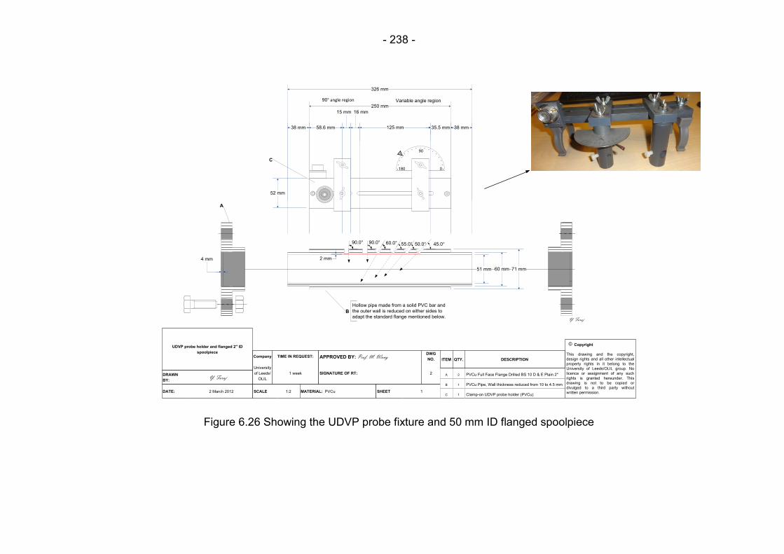
- 238 -
90.0° 90.0° 60.0° 55.0° 50.0°
Copyright
This drawing and the copyright,
design rights and all other intellectual
property rights in it belong to the
University of Leeds/OLIL group. No
licence or assignment of any such
rights is granted hereunder. This
drawing is not to be copied or
divulged to a third party without
written permission.
UDVP probe holder and flanged 2" ID
spoolpiece
DRAWN
BY:Y. Faraj
DATE:
Company TIME IN REQUEST: APPROVED BY: Prof. M. Wang DWG
NO.
University
of Leeds/
OLIL
1 week SIGNATURE OF RT: 2
2 March 2012 SCALE 1:2 MATERIAL: PVCu SHEET 1
326 mm
ITEM QTY. DESCRIPTION
A
B
C
2
1
1
PVCu Full Face Flange Drilled BS 10 D & E Plain 2"
PVCu Pipe, Wall thickness reduced from 10 to 4.5 mm
Clamp-on UDVP probe holder (PVCu)
A
B
38 mm
©
38 mm 125 mm
45.0°
60 mm51 mm
58.6 mm
250 mm
35.5 mm
16 mm15 mm
C
Hollow pipe made from a solid PVC bar and
the outer wall is reduced on either sides to
adapt the standard flange mentioned below.
71 mm
Y. Faraj
4 mm 2 mm
0
90
180
52 mm
90° angle region Variable angle region
Figure 6.26 Showing the UDVP probe fixture and 50 mm ID flanged spoolpiece
- 239 -
Based on this phenomenon, it was decided to drill two holes into the pipe
wall, where the transducers are placed. However, the Doppler angle (the
Doppler angle is the one over which the probe is tilting) plays a very
important role in the measurement of solids velocity, as it provides the
component of true solids flow velocity vector. Also, depending on the
application, an accurate determination of this angle is always a problem for
the ultrasound application. For example, the lower the angle is the higher
resolution can be achieved. However, with lower Doppler angle a very long
penetration is required until the best sound reaches the outer end of the pipe
wall. With higher solids concentration the sound burst may not reach the
other end (pipe wall) due to half way echoing, thus, a higher angle must be
used. Normally, a good quality of data can be obtained with the Doppler
angle between 45° and 60°. The selection of Doppler angle depend on
ultrasonic application (Camarasa et al., 1999).
Considering the facts shown above it was decided to drill the pipe wall test
section, to achieve four slots with Doppler angles 45°, 50°, 55° and 60° for
the transducer fixed on the variable angle section and a 90° hole for the
transducer fixed on the 90° angle section. However, due to thickness
limitation (4 mm) of the PVC pipe, the difficulty was recognised to drill holes
with the dead end of each of them 100% flat and enough deep for the
transducer to fit, especially for slots with lower angles such as 45°.
Therefore, it was decided to design and fabricate a flanged spoolpiece,
which is a hollow pipe made from a solid PVC bar with a larger outer
diameter than the rest of PVC pipeline in the flow loop. In order to adapt the
fabricated hollow pipe section of the spoolpiece, the outer wall was reduced
on either sides to suit the standard flanges used on the flow loop. The
flanged spoolpiece is shown in Figure 6.26. The length of the spoolpiece
(flange to flange) is 340 mm, on which the clamping transducer fixture can
easily be mounted. After making the hollow pipe section from the circular
solid PVC, the spoolpiece wall was found to be 20 mm, which was drilled to
obtain six slots with different Doppler angles. For example, one of the
transducers (4 MHz) has an outside diameter of 8 mm, and in order to
achieve the best fit, it was decided to make each slot with 8.1 mm diameter.
Also, after drilling each slot it was found that the thickness of the spool-pipe
wall, between the transducer face and the pipe contents, to be 2 mm, the
limit of which is shown by a red line in Figure 6.26. Since the spoolpiece is
flanged, thus it makes the whole system robust and versatile. In other words
the system can be mounted on any section within the flow loop via its
flanges. Nevertheless, an accurate ultrasonic velocity measurement and

- 240 -
performance depends on the location and alignment of the transducer.
Based on the engineering rules, the chosen location for the installation must
be at least 10 pipe diameter of straight line, undisturbed flow upstream and 5
pipe diameter of straight, undisturbed flow downstream from the
measurement point (GE sensing, 2007).
In general, non-wet transducers operate with coupling gel between the
transducer face and the pipe wall. This is to insure an acoustically
conductive path between the transducer face and the pipe wall surface. This
means that any air interface between the transducer face and the pipe wall
reflects all the ultrasonic energy, because air or gas has a very low acoustic
impedance. Therefore, the use of coupling gel is paramount.
6.6.6 Instrumentations used to measure the relevant parameters
The final selection of each instrumentation used to measure the relevant and
important parameters of flow within the multiphase flow loop was made after
a thorough examination and consideration of several factors such as
flexibility, cost, application and functionality. The following subsections detail
the selection and driving force for using each specific instrument mounted on
the flow loop.
6.6.6.1 Mean velocity measuring device
For determining slurry flow rate, several commercial instrumentations were
considered, kinetic energy meters (venturi meters, flow nozzles and wedge
meters), electromagnetic flow meters and acoustic velocimeters. Finally it
was decided to use an Electromagnetic Flow Meter (EMF Krohne Aqua-flux)
to measure the flow rate. This decision was influenced by the advantages
that the EMF can offer over the other flow meters. It is considered as a
reliable and relatively cheap flow meter. According to Brown and Heywood
(1991), Matousek (1997) and Pachowko (2004) the reliability of EMF is
without any doubt. However, Matousek (1997) has reported that to achieve a
reliable measurement, the EMF must be installed on the vertical section.
This is due to slip velocity between solid particles and the carrier liquid.
6.6.6.2 Solids concentration and axial velocity measuring device
There are two types of solids concentration, in-situ and delivered solids
concentration. In a definitive slurry flow loop, in order to extract productive
features, both in-situ and delivered solids concentration have to be
determined. In-situ solids concentration demonstrates the local conditions of
solid particles within the pipeline. This type of concentration is determined by
the dual-plane ERT sensor, which measures the conductivity of the pipe
- 241 -
contents, and the conductivity data is then converted to solids volume
fraction using Maxwell relationship. The dual-plane ERT sensor in
conjunction with cross-correlation method is also used to determine the
solids velocity profile in the carrier fluid. Two dual plane ERT sensors were
designed, the geometry and dimensions of which is shown in Figure 6.27.
They both are housed in the U-shape and vertical sections of the flow loop.
In-situ solid’s concentration can also be determined by sampling of slurry at
the discharge point, if no solids hold up occur in the pipeline. To ensure that
there is no hold up, the sampling must be carried out in very high velocity.
This high velocity is required to overcome the frictional loss, as a result the
whole slurry behaves as a single liquid.
Delivered solids concentration is a very important parameter, as it
determines the capacity of a pipeline system (Brown and Heywood, 1991).
This type of solids concentration is determined from the multiphase flow loop
using a pre-calibrated measuring tank, which is mounted on calibrated three
load cells that determine the weight of the slurry in the tank. In order to
perform this, the full pipe flow is diverted temporarily into the measuring tank
via a flow diversion system.
6.6.6.2.1 Design of 360 mm dual-plane ERT sensor
The dual plane ERT sensor, shown in Figure 6.27 consists of two 16-
electrodes planes, which are connected to three Perspex pipe sections (50
mm ID) in such a way to obtain a smooth internal section at the connection
points, to avoid any disturbance to the flow. The Perspex section A (140 mm
long) is connected to the left of plane 1 (P1), whereas the Perspex section C
(140 mm long) is connected to the right side of plane 2 (P2), while both
planes are separated by the third Perspex pipe section B (30 mm long). As
the length of each plane is 40 mm, then this gives the distance between the
centres of each electrode plane 50 mm. Considering the slot depth at the
end of each plane, in which the Perspex pipe section B placed, the apparent
separating the two electrode planes is 10 mm. In order to achieve a secure
section and good coupling, two Perspex flat flanges (D & E) are mounted at
the centre of both Perspex pipe sections (A & C) using PVC solvent cement.
The two flat flanges used as clamping fixtures via four M8 threaded rod bars,
which are going though the four pre-drilled holes in the flanges and pulling
the whole section together by tightening four M8 nuts at the end of each rod
bar. It is apparent that over-tightening the nuts can pull both flat flanges
together and separate them from the Perspex flat sections at the joint point.

- 242 -
Each end of the whole section is flanged, using the standard flanges used in
the loop (uPVC full face flange drilled Bs 16/10 PN plain 2 inch). Connecting
all the sections together gives a total length of the dual plane sensor 360
mm (flange to flange). This clearly makes the dual plane ERT censor a very
compacted and robust equipment, which can be coupled with any flanged
section within the flow loop.
The design of 16 electrodes at the periphery of each plane is one of the
most important aspect of the whole sensor design. The design of electrodes
followed the most common type of geometry and layout, in which the
equisized electrodes are arranged around the pipe’s inside diameter in an
equispaced fashion. In order to avoid impedance problems, the electrodes
have to be more conductive than the flowing fluid within the pipe. Since the
main carrier liquid used within the flow loop is mainly water and conductivity
difference between stainless steel and water is very high (GE Sencing 2007;
kayelaby.npl.co.uk, hypertextbook.com), therefore, stainless steel was
chosen as material of construction for the electrodes. In addition, some other
factors such as good ability to resist chemical attack, cost, protection
against fouling of the electrodes by solid particles make stainless steel the
prime material of construction amongst all.
Based on typical values of the number of nodes per electrodes (Nd), the
number of boundary nodes (NB), the number of electrodes in each plane (16
electrodes in this study), and the electrode angle 13.8°, the width of each
electrode was determined as 6 mm for 50 mm pipe diameter. On the other
hand the length of each electrode sized as 20 mm. This would make the
final electrode size mounted on each plane 20 mm x 6 mm. Each electrode
has been manufactured from M6 stainless steel rods, by cutting them in half
to give semi-cylindrical shape. 16 electrodes are mounted on a predrilled
circular PVC plane, in such a way to give an angle of 22.5° between centre
of an electrode to the centre of the next one.
Each electrode welded to 24 mm long stainless steel rod (M4), which is
inserted into the hole at the circumference of the uPVC plane. Each
electrode is placed in a slot within the PVC plane, which enables the
electrodes to be flush mounted in the interior without any disturbance to the
flow.
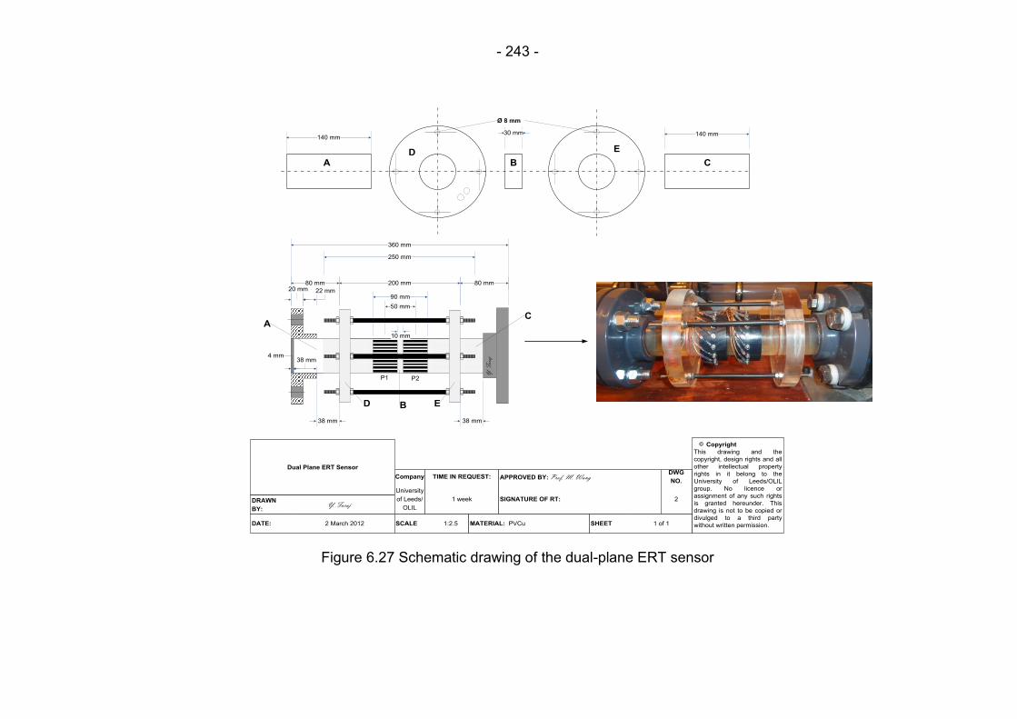
- 243 -
360 mm
250 mm
B
30 mm140 mm
140 mm
Ø 8 mm
ED
200 mm
38 mm 38 mm
Copyright
This drawing and the
copyright, design rights and all
other intellectual property
rights in it belong to the
University of Leeds/OLIL
group. No licence or
assignment of any such rights
is granted hereunder. This
drawing is not to be copied or
divulged to a third party
without written permission.
Dual Plane ERT Sensor
DRAWN
BY:Y. Faraj
DATE:
Company TIME IN REQUEST: APPROVED BY: Prof. M. Wang DWG
NO.
University
of Leeds/
OLIL
1 week SIGNATURE OF RT: 2
2 March 2012 SCALE 1:2.5 MATERIAL: PVCu SHEET 1 of 1
50 mm
©
Y. F
araj
80 mm 80 mm
A
20 mm 22 mm
4 mm
C
10 mm
90 mm
38 mm
P1 P2
C
EDBA
Figure 6.27 Schematic drawing of the dual-plane ERT sensor

- 244 -
The welded M4 rods extend out of the plane by 11.5 mm to allow the
connection of cables using solder tags. The cables are connected to the
electrodes using solder tags and fixed each of them with M4 nuts and
washers. Co-axial cables are used to connect the electrodes to the data
acquisition system (DAS) and are sheathed so as to reduce the
electromagnetic interference. The geometry and dimensions of the 16-
electrode plane is shown in Figure 6.28. In order to prevent leakage at the
coupling point of each plane with the Perspex pipe sections, slots of 3 mm
wide have been made on each plane, into which 2.63 mm (3/32 inch) O-ring
can be placed.
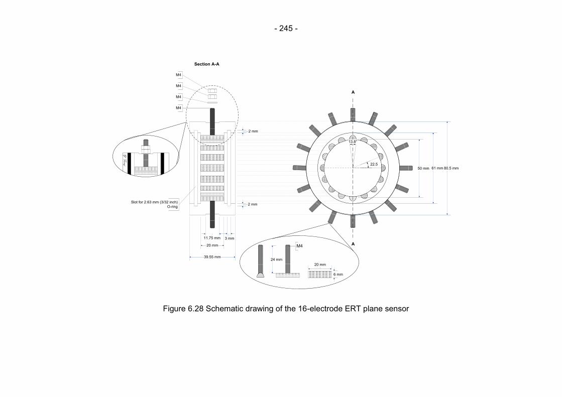
- 245 -
Y. F
araj
11.75 mm
M4
M4
M4
M4
22.5
39.55 mm
3 mm
20 mm
Slot for 2.63 mm (3/32 inch)
O-ring
A
A
Section A-A
80.5 mm61 mm50 mm
6 mm
20 mm
24 mm
M4
2 mm
2 mm
13.8°
Figure 6.28 Schematic drawing of the 16-electrode ERT plane sensor
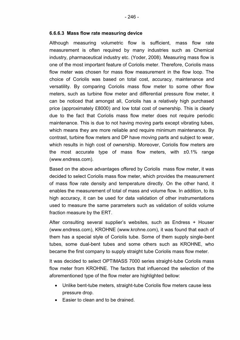
- 246 -
6.6.6.3 Mass flow rate measuring device
Although measuring volumetric flow is sufficient, mass flow rate
measurement is often required by many industries such as Chemical
industry, pharmaceutical industry etc. (Yoder, 2008). Measuring mass flow is
one of the most important feature of Coriolis meter. Therefore, Coriolis mass
flow meter was chosen for mass flow measurement in the flow loop. The
choice of Coriolis was based on total cost, accuracy, maintenance and
versatility. By comparing Coriolis mass flow meter to some other flow
meters, such as turbine flow meter and differential pressure flow meter, it
can be noticed that amongst all, Coriolis has a relatively high purchased
price (approximately £8000) and low total cost of ownership. This is clearly
due to the fact that Coriolis mass flow meter does not require periodic
maintenance. This is due to not having moving parts except vibrating tubes,
which means they are more reliable and require minimum maintenance. By
contrast, turbine flow meters and DP have moving parts and subject to wear,
which results in high cost of ownership. Moreover, Coriolis flow meters are
the most accurate type of mass flow meters, with ±0.1% range
(www.endress.com).
Based on the above advantages offered by Coriolis mass flow meter, it was
decided to select Coriolis mass flow meter, which provides the measurement
of mass flow rate density and temperature directly. On the other hand, it
enables the measurement of total of mass and volume flow. In addition, to its
high accuracy, it can be used for data validation of other instrumentations
used to measure the same parameters such as validation of solids volume
fraction measure by the ERT.
After consulting several supplier’s websites, such as Endress + Houser
(www.endress.com), KROHNE (www.krohne.com), it was found that each of
them has a special style of Coriolis tube. Some of them supply single-bent
tubes, some dual-bent tubes and some others such as KROHNE, who
became the first company to supply straight tube Coriolis mass flow meter.
It was decided to select OPTIMASS 7000 series straight-tube Coriolis mass
flow meter from KROHNE. The factors that influenced the selection of the
aforementioned type of the flow meter are highlighted bellow:
Unlike bent-tube meters, straight-tube Coriolis flow meters cause less
pressure drop.
Easier to clean and to be drained.

- 247 -
Can offer four tube materials of construction (Titanium, Stainless
Steel, Hastelloy or Tantalum).
Excellent zero stability.
Fast signal processing, even with changes in concentration or
temperature.
Can be used in many applications, such as non-homogeneous
mixtures, slurries, product with entrained solids or gas, products
requiring low flow velocities etc.
KROHNE OPTIMASS 7300F (field housing for wall mounting) is installed on
the U-shape outgoing pipe section just before the dual-plane ERT sensor.
The straight signal tube system made of Titanium (Grade 9) with mounting
length 1101 mm. The flow meter converter type is MFC300F (field housing
for wall mounting). It has an accuracy of ±0.15 of MV and uses PACTWARE
operating software. When installing the meter it was paramount to make
sure that the pipe work is supported behind the flanges, so as to avoid
placing any stress to the meter flanges. Also, as part of manufacturers
recommendations for slurry applications, transition pieces were used on the
inlet port and the outlet of the tube for leading edge protection.
It is worth pointing out that the heavy weight of the meter (approximately 150
kg) on the inclinable steel structure raised the concern that the whole
pipeline may slide down the table, while the table is raised, especially at
90°.It was essential to insure rigid and stable connection to the mounting
steel structure. Therefore, Split Plummer Blocks were designed and
fabricated for firm fixture of the heavy meter to the inclinable deck. Each
Plummer Block consists of two aluminium plates (12 mm thick), which are
welded to form an L-shape to support and clamp either flange parts of the
meter, as shown in Figure 6.29. Four M10 bolts were used to firmly fix the
meter to the steel beam and four M8 bolts were used to clamp and anchor
the meter.
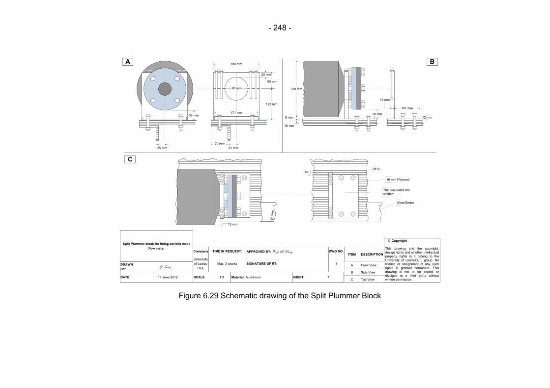
- 248 -
16 mm
25 mm
220 mm
38 mm38 mm
25 mm
Y. F
araj
90 mm
180 mm
65 mm
122 mm
65 mm
12 mm
101 mm
171 mm
8 mm
20 mm
M10M8
Steal Beam
16 mm Plywood
16 mm
Copyright
This drawing and the copyright,
design rights and all other intellectual
property rights in it belong to the
University of Leeds/OLIL group. No
licence or assignment of any such
rights is granted hereunder. This
drawing is not to be copied or
divulged to a third party without
written permission.
Split Plummer block for fixing coriolis mass
flow meter
DRAWN
BY:Y. Faraj
DATE:
Company TIME IN REQUEST: APPROVED BY: Prof. M. Wang DWG NO.
University
of Leeds/
OLIL
Max. 2 weeks SIGNATURE OF RT: 1
14 June 2012 SCALE 1:3 Material: Aluminium SHEET 1
ITEM DESCRIPTION
A
B
C
Front View
Side View
Top View
©
The two plates are
welded
12 mm
C
A B
Figure 6.29 Schematic drawing of the Split Plummer Block

- 249 -
6.6.6.4 Additional local velocity measuring device
The decision was made that another local velocity measuring device would
be used and mounted on the U-shape inclinable flow loop. The remarkable
advantage and driving force for the decision was to use this device for
measuring solids local velocity, mean solids velocity and solids velocity
profile, and thus validating solids local velocity obtained from the
combination of the ERT and cross-correlation. After a thorough research for
finding an instrument for Ultrasonic Doppler Velocity Profile measurement,
two versions were considered. The first instrument was the UDVP-DUO
(GAH100), which is manufactured by Met-Flow and supplied by Dantec
(www.dantec.com), while the other one was DOP velocimeter, which is
supplied by Signal-Processing (www.signal-processing.com). From an
objective prospective and measurement point of view, UDVP and DOP, offer
more or less the same functionality. However, the cost was the driving for
selecting UDVP-DUO from Met-Flow. Figure 6.30 showing the UDVP, which
is currently used in OLIL laboratories in the University of Leeds. The whole
system consists of three main parts:
1. Measuring unit, which performs signal processing and digitalisation.
2. Transducers, which transform electrical signals in ultrasonic acoustic
signals.
3. User interface, which provides data analysis and storage.
It is worth mentioning that all configurations are set via user interface, but
not from the main measuring unit. The main unit has a reasonable
dimensions (340x130x400 mm), which can be adjusted on the inclinable
table between the two limbs of the U-shape pipeline, and can easily be
handled due to its reasonable weight (9.3 kg). The main unit operates with a
set of TX-line transducers, each with five emitting frequencies (0.5, 1, 2, 4
and 8 MHz), which are connected to the main unit via an integrated
multiplexer. As recommended by the manufacturer (Met-Flow), 4 m long
cables are used for the transducers, so as to achieve reliable operation. In
other words, providing the best compromise between the installation of the
probe and attenuation of the signal.
For the detail description and technical specifications, relating to any part of
UDVP-DUO system, the author recommends a journey through
manufacturer’s website (www.met-flow.com).
- 250 -
Figure 6.30 Showing the UDVP-DUO system from Met-Flow
6.6.6.5 Pressure measuring instrumentation
The measurement of pressure differential between two points of a section of
a straight pipe is one of the most important measurements for pipeline
frictional head loss determination.
Monitoring the pressure changes over straight pipelines can provide
valuable information regarding the condition of flow. Therefore, it was
decided to mount six pre-calibrated pressure sensors on three sections of
the flow loop (vertical and ascending inclined section and descending
inclined section) at 2 m intervals between the two pressure sensors mounted
on each section. In order to avoid solid particles and entrained air entering
the sensors, six Danfoss flush diaphragm pressure transmitters ( type MBS
4010) were selected, which could measure the pressure within the range of
0-10 bar. These transmitters can perform an accurate measurement for all
conditions of testing and it is designed for use even under harsh
environmental conditions. Also according to the manufacturer (CSE
Industrial Electrical Distributers) the measurement error is ±0.3% and has an
excellent vibration stability and robust construction.
In order to make a robust pressure transmitter system, which can easily be
mounted in any section within the flow lop, a flanged lining sleeve was
designed an fabricated, as shown in Figure 6.31. The whole system consists
of a 50 mm ID pipe section, which is pressed into a 90° Tee to provide a
smooth internal surface and flanged at either ends using solvent PVC
cement. The Tee is machine treated for easy insertion of the pipe section. A
tapped cylindrical solid PVC bar is pressed into the vertical opening of the
Tee and sealed with PVC solvent cement to prevent leakage. The
remarkable advantages of this lining sleeve is that it allows easy connection
- 251 -
and disconnection of pressure transmitter by fitting it into the tapped solid
PVC bar and can be joined to any desired section within the flow loop via the
flanges. Similar lining sleeve is used for the connection of temperature
transmitter in the vertical test section.
Each pressure transmitter is connected to the Data Acquisition System
(DAS), which sense the deflection of each transmitter by the flowing slurry
and the data is generated in the form of current output. The data then can be
converted to pressure data due to linear relationship between the current
output and the pressure.
6.6.6.6 Temperature measuring device
Monitoring the operating temperature is an important task of any slurry flow.
As any change in slurry temperature can affect the slurry viscosity and as a
result this may have a dramatic effect on the slurry flow behaviour.
In this study, a K-type thermocouple is used and mounted on the vertical
section. It is also connected to the DAS, where the slurry temperature data is
recorded. The working principle of this type of thermocouple is based on
generating voltage, which is a function of temperature. The K-type
thermocouple is very common and widely used. They are cheap and can be
used to monitor the temperature range 0-100 °C (Pachowko, 2004).
However, controlling the temperature was found to be costly and needles, as
the time taking for each experiment was found to be rather short. Also the
heat, which is produced by the dissipation energy input to the pump, was
found to be very little and could not have a dramatic effect on the slurry’s
viscosity. Moreover, pumping a chilled heat transfer fluid through the
annulus of a double pipe heat exchanger can increase the cost of each
experiment and occupy a significant area. Therefore, based on the above
reasons, it was decided not use any heat exchanger in this study. However,
as a safety precaution, the slurry temperature will still be monitored via the
thermocouple.

- 252 -
45.0°
45.0°
3838
220144
230
PVC Pipe Class E 2"
PVC Full Face
Flange Drilled
BS Plain 2"
This part of pipe is taken out by cutting
the section From the inner edge of the vertical
bore of the tee to the pipe centre line With
an angle 45 degree
The part of pipe coming out of the tee
will have to be fit into the flange with no
gap between the tee and the flange
PVC Full Face Flange Drilled
BS Plain 2"
Pressure and temperature transmitter
spoolpiece
DRAWN
BY:Y. Faraj
DATE:
Company TIME IN REQUEST: APPROVED BY: Prof. M. Wang DWG NO.
University
of Leeds/
OLIL
1-2 weeks SIGNATURE OF RT: 1
28 March 2012 SCALE 1:2 Material: PVCu SHEET 1
The four steps (pipe stoppers) are removed
or shaved across the horizontal bore.
However the vertical bore remains.
The tee, pipe section
and two flanges are connected
with PVC solvent cement
ITEM QTY. DESCRIPTION
A
B
C
D
2
1
1
1
20 22
60.7 mm
60.17 mm
44.82 mm
19.2 mm6.5 mm
PVC Full Face Flange 2"
PVC Pipe Class E 2"
PVC Tee 90 Plain 2"
Tapped PVC solid bar
BA AC
D
Figure 6.31 Pressure and temperature transmitter spoolpiece

- 253 -
6.6.6.7 Data Acquisition System (DAS)
A Data Acquisition System is used to acquire the real time measurement of
the relevant parameters and quantities and presenting them on a personal
computer.
A National Instrument Field-Point (FP @ 129_11_241_2\FP-AI-111, 40-20
mA) is used, which is connected to the Electromagnetic Flow meter (EMF),
OPTIMASS Mass Coriolis Flow meter, six pressure transmitters and the
thermocouple. The current output is powered by the Field-Point (FP-1600),
10.100MPs Ethernet network interface power point, which collects the data
and present it in a Front Panel, a screen shot of the front panel is shown in
Figure 6.32.
Figure 6.32 Showing the LabVIEW front panel
In order to receive the current input from the above instrumentations and
convert to the desired measured parameters using scaling factor, a
LabVIEW programme was written, as shown in Figure 6.33. It is worth
mentioning that, for the conversion of the current input to the desired
variables, it is assumed that all the instrumentations have a linear response.
The current input of the EMF converted to slurry velocity (m/s), the current
input of mass flow meter to slurry mass flow rate (kg/min), pressure sensor
current input to slurry pressure (kPa) and the thermocouple current input to
slurry temperature (°C). In each experiment the data is collected every 5
seconds, they are then averaged at the end of each experiment. All the data
is recorded in a data file that can be reviewed later and used for the
analysis.
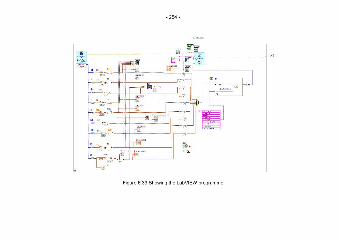
- 254 -
Figure 6.33 Showing the LabVIEW programme
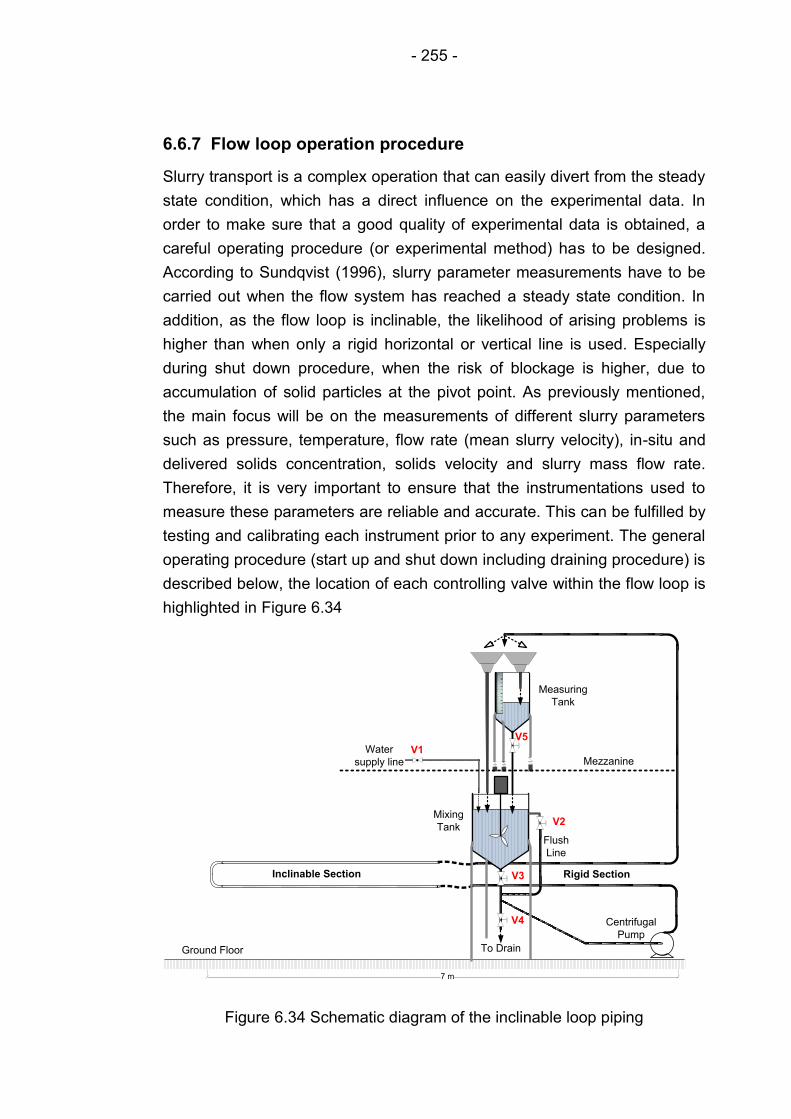
- 255 -
6.6.7 Flow loop operation procedure
Slurry transport is a complex operation that can easily divert from the steady
state condition, which has a direct influence on the experimental data. In
order to make sure that a good quality of experimental data is obtained, a
careful operating procedure (or experimental method) has to be designed.
According to Sundqvist (1996), slurry parameter measurements have to be
carried out when the flow system has reached a steady state condition. In
addition, as the flow loop is inclinable, the likelihood of arising problems is
higher than when only a rigid horizontal or vertical line is used. Especially
during shut down procedure, when the risk of blockage is higher, due to
accumulation of solid particles at the pivot point. As previously mentioned,
the main focus will be on the measurements of different slurry parameters
such as pressure, temperature, flow rate (mean slurry velocity), in-situ and
delivered solids concentration, solids velocity and slurry mass flow rate.
Therefore, it is very important to ensure that the instrumentations used to
measure these parameters are reliable and accurate. This can be fulfilled by
testing and calibrating each instrument prior to any experiment. The general
operating procedure (start up and shut down including draining procedure) is
described below, the location of each controlling valve within the flow loop is
highlighted in Figure 6.34
To Drain
MezzanineWater
supply line
7 m
Flush
Line
Inclinable Section
Ground Floor
V1
V2
V3
V4
V5
Mixing
Tank
Measuring
Tank
Rigid Section
Centrifugal
Pump
Figure 6.34 Schematic diagram of the inclinable loop piping
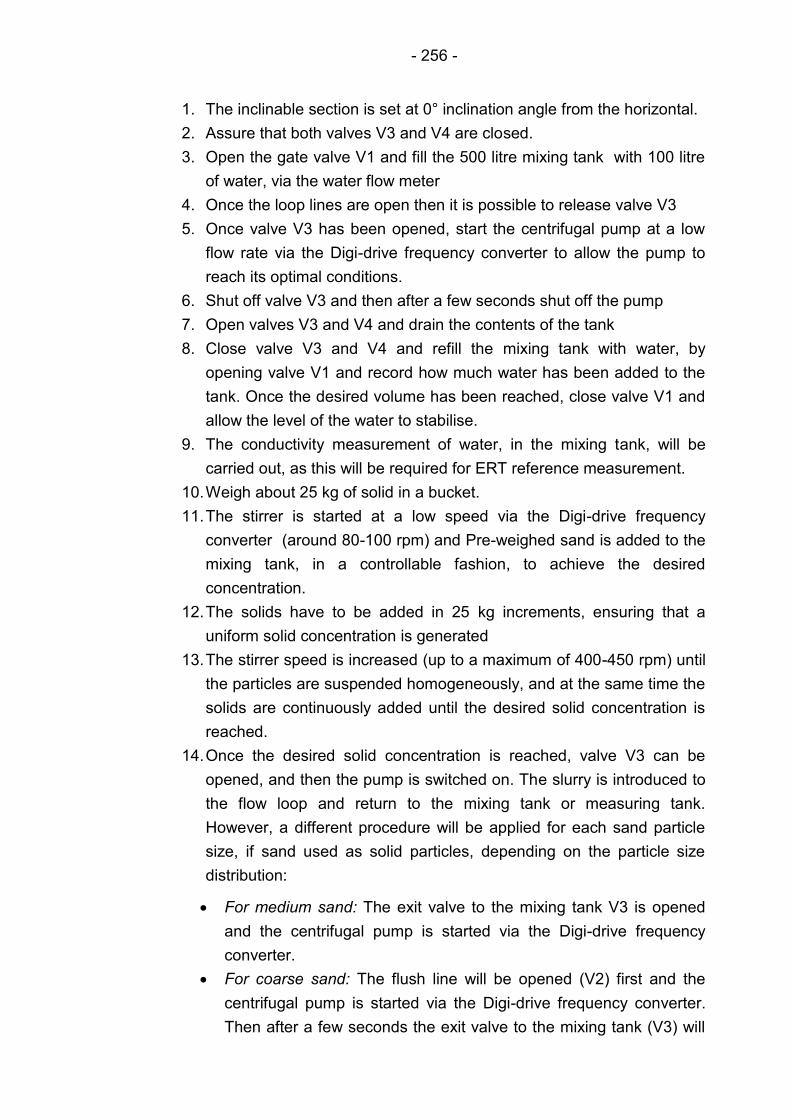
- 256 -
1. The inclinable section is set at 0° inclination angle from the horizontal.
2. Assure that both valves V3 and V4 are closed.
3. Open the gate valve V1 and fill the 500 litre mixing tank with 100 litre
of water, via the water flow meter
4. Once the loop lines are open then it is possible to release valve V3
5. Once valve V3 has been opened, start the centrifugal pump at a low
flow rate via the Digi-drive frequency converter to allow the pump to
reach its optimal conditions.
6. Shut off valve V3 and then after a few seconds shut off the pump
7. Open valves V3 and V4 and drain the contents of the tank
8. Close valve V3 and V4 and refill the mixing tank with water, by
opening valve V1 and record how much water has been added to the
tank. Once the desired volume has been reached, close valve V1 and
allow the level of the water to stabilise.
9. The conductivity measurement of water, in the mixing tank, will be
carried out, as this will be required for ERT reference measurement.
10. Weigh about 25 kg of solid in a bucket.
11. The stirrer is started at a low speed via the Digi-drive frequency
converter (around 80-100 rpm) and Pre-weighed sand is added to the
mixing tank, in a controllable fashion, to achieve the desired
concentration.
12. The solids have to be added in 25 kg increments, ensuring that a
uniform solid concentration is generated
13. The stirrer speed is increased (up to a maximum of 400-450 rpm) until
the particles are suspended homogeneously, and at the same time the
solids are continuously added until the desired solid concentration is
reached.
14. Once the desired solid concentration is reached, valve V3 can be
opened, and then the pump is switched on. The slurry is introduced to
the flow loop and return to the mixing tank or measuring tank.
However, a different procedure will be applied for each sand particle
size, if sand used as solid particles, depending on the particle size
distribution:
For medium sand: The exit valve to the mixing tank V3 is opened
and the centrifugal pump is started via the Digi-drive frequency
converter.
For coarse sand: The flush line will be opened (V2) first and the
centrifugal pump is started via the Digi-drive frequency converter.
Then after a few seconds the exit valve to the mixing tank (V3) will

- 257 -
be opened and the flush line valve (V2) will be closed. Carrying out
this procedure, for coarse sand, ensures that the blockage in the
suction line is avoided. As the finer particles flow through the flush
line and lubricate the line beforehand, then the coarser particles will
be following. In either case, when the centrifugal pump is started,
the electrical power supply to the pump must be adjusted to the
highest velocity mentioned in this study, so that a homogeneous
flow in the flow loop is achieved.
15. While the flow is circulating through the flow loop, the desired
inclination angle is set via the winch remote control.
16. Once the slurry reached the other end of the flow loop, it can either be
returned to the mixing tank or diverted to the measuring tank.
However, the flow must not be diverted to the measuring tank until the
steady state flow is reached, as the accuracy of the data, particularly
the delivered solids concentration and the flow rate may be in doubt.
17. For the purpose of calibrating the flow meter and determining solid
concentration, the measuring tank will be used; meaning the slurry is
diverted to the measuring tank at the discharge point using the flow
diversion system. Once the diversion process has finished and the
level measurement is complete the contents are allowed to flow into
the mixing tank via valve V5.
18. Slurry flow rate (mean velocity), Pressure, temperature, slurry mass
flow rate are recorded via the LabVIEW and the ERT measurements
are carried out.
19. It is important that initial tests are carried out at higher transport
velocities, then gradually reduced to the lowest. The procedure of
decreasing the mean slurry velocity is continued until the stationary
bed is totally formed. However, the last measurement must be carried
out as quickly as possible to avoid the blockage. Also, for each
measurement taken, the slurry flow must be visually inspected through
a transparent pipe section along with taking photographs if it is
desired. However, it is expected that visual inspection will be almost
impossible, as the media is totally murky.
20. If another solids concentration is due to be considered in the test
matrix, then more sand is added into the mixing tank, and the above
procedure is repeated. However, each set of measurements must be
carried out at different velocities, concentration and inclination angle,
so that the influence of each parameter is determined.
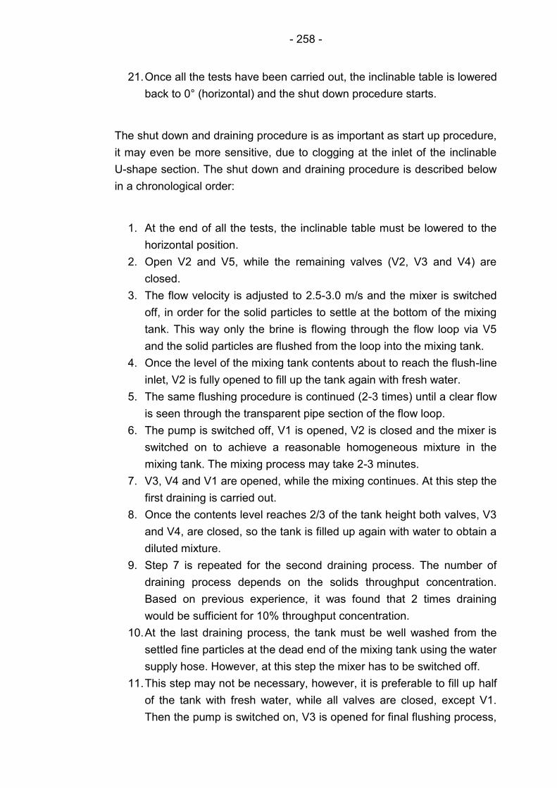
- 258 -
21. Once all the tests have been carried out, the inclinable table is lowered
back to 0° (horizontal) and the shut down procedure starts.
The shut down and draining procedure is as important as start up procedure,
it may even be more sensitive, due to clogging at the inlet of the inclinable
U-shape section. The shut down and draining procedure is described below
in a chronological order:
1. At the end of all the tests, the inclinable table must be lowered to the
horizontal position.
2. Open V2 and V5, while the remaining valves (V2, V3 and V4) are
closed.
3. The flow velocity is adjusted to 2.5-3.0 m/s and the mixer is switched
off, in order for the solid particles to settle at the bottom of the mixing
tank. This way only the brine is flowing through the flow loop via V5
and the solid particles are flushed from the loop into the mixing tank.
4. Once the level of the mixing tank contents about to reach the flush-line
inlet, V2 is fully opened to fill up the tank again with fresh water.
5. The same flushing procedure is continued (2-3 times) until a clear flow
is seen through the transparent pipe section of the flow loop.
6. The pump is switched off, V1 is opened, V2 is closed and the mixer is
switched on to achieve a reasonable homogeneous mixture in the
mixing tank. The mixing process may take 2-3 minutes.
7. V3, V4 and V1 are opened, while the mixing continues. At this step the
first draining is carried out.
8. Once the contents level reaches 2/3 of the tank height both valves, V3
and V4, are closed, so the tank is filled up again with water to obtain a
diluted mixture.
9. Step 7 is repeated for the second draining process. The number of
draining process depends on the solids throughput concentration.
Based on previous experience, it was found that 2 times draining
would be sufficient for 10% throughput concentration.
10. At the last draining process, the tank must be well washed from the
settled fine particles at the dead end of the mixing tank using the water
supply hose. However, at this step the mixer has to be switched off.
11. This step may not be necessary, however, it is preferable to fill up half
of the tank with fresh water, while all valves are closed, except V1.
Then the pump is switched on, V3 is opened for final flushing process,

- 259 -
including the measuring tank by diverting the flow for a couple of
seconds.
12. The pump is switched off, V1 is closed, V3 and V4 are opened to
empty the mixing tank and washing it.
13. All the electrical instrumentations and equipments are switched off and
secured.
14. The deposited sand within the drainage system must be disposed off
considering health and safety and environmental codes.
6.6.8 Hydraulic and mechanical testing
Before full operation of the whole flow loop, it is important to ensure that the
system is functional in accordance with the design requirement, and also
safe enough in accordance with the health and safety codes. Therefore, the
hydraulic and mechanical testing of the flow loop, particularly the mechanical
structure of the inclinable table and the flow through it, was performed. The
structural testing was carried out by raising and lowering the inclinable table
several times, considering the two extremes 0°, when the table is at
horizontal position and 90°, when the table is at vertical position. In addition,
several randomly chosen angles, within the aforementioned range, were
also included into the test.
However, it was very important to adhere to health and safety of everyone
working or walking in the vicinity of the working are. Therefore, 48 hours
before testing the whole system, the faculty staff and students were notified.
Moreover, guards and warning signs were used during the test process.
Each test involved the following checks and observations:
Visually checking the whole inclinable table, for swaying, deflection,
strain at the pivot point, the connection point of the wire rope and
general checking regarding the stability of the table in a raise and stop
and lower and stop fashion.
The winch position and controlling the lifting and lowering process had
to be well checked.
Examining the hooks for deformation and cracks.
Checking the telescopic push/stop system.
Visual inspection of the running rope.
The cables running along the table.
The flexible pipe and strain on the rigid pipes connected to it.
The bend in the flexible pipe and look for potential kinks throughout
the designed inclination angle range.
- 260 -
The stability of the pipeline on the table, especially at higher inclination
angles 45°-90°.
The hydraulic tests were initially carried out focusing mainly on leak test
throughout, while the table was in horizontal position. Then the hydraulic
testing was carried out at various inclination angles and various flow
velocities, including the highest velocity, at which the highest pump
frequency could be reached. All instrumentations, pressure transducers,
thermocouple, Electromagnetic Flow meter, Coriolis mass flow meter,
measuring tank and flow diversion system and the UDVP, were tested and
the randomly measured data was recorded. The flow measurement test
included the inspection and operation of the data acquisition system.
The whole results of the testing procedure was found to be promising and it
was finally concluded that the whole flow loop, including instrumentations
and equipments, is perfectly safe and functioning with meeting all the design
requirements and objectives for the intended application.
6.7 Conclusions
This chapter has highlighted the procedure and strategies used in the design
and construction of inclinable multiphase flow system, including the detailed
design of various equipments and instrumentations used to measure the
desired parameters of flow. The selection of each instrumentations and their
location within the flow loop have been based on slurry flow. The design and
layout of the whole piping system have been described with consideration to
the project design requirements and engineering rules. The structural
design, fabrication and erection of tables, rigid and inclinable, have been
presented in detail to generate a design procedure, along with associated
work to facilitate the process of inclination up to 90° (vertical). The design
and fabrication of pressure and temperature transmitter lining sleeve have
been detailed, along with the design and fabrication of the UDVP spoolpiece
to suit any potential future application. A general start up, shut down and
draining procedure, based on slurry flow, has also been discussed. Finally,
the mechanical and hydraulic testing of the whole system concluded that all
the design requirements for the intended application have been met
providing total functionality and safety for the future applications.
- 261 -
Chapter 7
Automated horizontal flow regime recognition using
statistical signal analysis of the ERT data
This chapter presents a new method of flow regime recognition based on
statistical signal analysis of the ERT data, along with writing a script using
MATLAB so as to facilitate an automated recognition. An evaluation of the
recognition scheme is also described with highlighting the success rate
based on different sands and different flow conditions.
7.1 Introduction
Flow regime recognition is not only useful for characterization of the flow, but
also for the purpose of modelling and for flow meters, as most of flow
meters, especially the ERT as discussed previously in Chapter 5, are flow
regime dependent. In order to develop a flow meter, it is paramount to
determine the flow regime present in the pipeline, which enables accurate
measurement and selection of the optimal method for flow measurement.
This investigation aimed at developing a method for recognition of slurry
(sand/water) flow regimes occurring in the pipeline and coding a program
based on the proposed method. Nevertheless, the modelling aspect to
correct the ERT measurement is not dealt with in this study.
Usually the flow regimes are recognised and distinguished using either direct
or indirect recognition method. The direct methods involve a visual
observation of the flow through a transparent pipe section and/or the
reconstructed images or real photographs of the flow within horizontal
pipeline. It is quite clear that as slurries are usually opaque and contained in
opaque enclosures, thus, the direct methods are very difficult if not
impossible. Also, even if the pipeline operator is able to visualise the flow
within the pipeline, the distinction between the flow regimes is dependent on
the operator bias. Therefore, the recognition of the prevailing flow regime
requires an indirect method, which moves away from the operator bias and
based upon a measurement scheme and flow feature extraction, which
related to the distribution of solid particles across the pipe cross-section
whether the pipe wall is transparent or opaque.
A new indirect method for recognition of the active flow regime using
statistical signal analysis of the ERT data (conductivity) has been proposed.
- 262 -
The zoned average conductivity of five zones, along the vertical centreline of
the tomogram is considered. Mesh (21 cells) of the regionisation scheme,
which is embedded in the p2000 software, described in Chapter 3, is
selected. The ERT data can undoubtedly reveal key flow features, which
would enable the recognition of the prevailing flow regime. The main
features are extracted from both, time domain signal and frequency domain
of the signal. Statistical spectrum analysis of the signal, such as Power
Spectral Density (PSD) of the signal, is rendering significant flow features.
Besides, a direct recognition method was attempt. The direct method
involved the observation of flow through a transparent pipe section, mounted
in the horizontal pipeline, along with the real photographs of flow captured
using a digital camera. It is worth mentioning that the direct method is used
as a mean of comparison for the proposed indirect method.
MATLAB has been used for coding the program to facilitate automatic
recognition of the active flow regime. The method has been evaluated and
the recognition rate has been determined at 90.32%. An automated
visualisation of the solids volumetric concentration has been included into
the main program, through which the local solids distribution can be
visualised and mean solids concentration is automatically calculated and
displayed.
7.2 Test strategy
A set of experiments were carried out using a pilot-scale slurry flow loop
shown in Chapter 4. The horizontal line of the flow loop made the test
section of the experiments, in which different flow regimes were generated
by altering the slurry velocity. In order to cover most of typical slurry flow
regimes, a relatively wide range of superficial velocity were selected to pump
two sands, medium and coarse, each with different throughput volumetric
concentration, 2% and 10%. At the beginning of each test the transport
velocity (mean slurry velocity) was nominally set to 5 m/s, then it was
incrementally decreased until the transport velocity reached 1.5 m/s. After a
steady state pressure gradient was observed on the LabVIEW front panel
the use of Fast Impedance Camera System (FICA) is attempted to measure
a cross-sectional pipe tomogram by collecting blocks of 8000 frames for
each flow condition. Since the data collection speed for FICA system is
around 1.15 ms/frame, then 9.2 seconds are required for collection of 8000
frames in real time. A 1.2 m transparent pipe section were included into the
test section, so as to visually inspect the active flow regime and note all the
- 263 -
phenomenon occurring in real time, such as type of flow regime seen,
measuring the height of the bed etc. Also for each measurement test
photographic images of the flow were captured for later comparison and
evaluation of the proposed method.
7.3 Automated flow regime recognition
In order to achieve automatic recognition of the prevailing flow regime in
horizontal slurry flow, two key stages had to be taken. First is developing a
recognition method, for which statistical signal analysis of the ERT data has
been proposed, second is coding a program; which would facilitate
automatic recognition of the prevailing flow regime.
The following typical slurry flow regimes were considered into the recognition
scheme:
1. Homogeneous.
2. Pseudo-homogeneous.
3. Heterogeneous.
4. Moving bed.
5. Stationary bed.
Statistical analysis of the conductivity data within each zone were carried out
to provide a quantitative comparison of the flow regimes, thus reducing the
subjectivity associated with recognising each flow regime. In order to
achieve this objective the following stages were adopted:
1. Experimental ERT measurement and generating 21 cell zoned
average scheme.
2. Statistical signal analysis and flow feature extraction.
3. Threshold indication for each flow regime.
4. Decision making.
5. Program coding.
6. Running and testing the new technique, and also determining the
recognition rate (error analysis).
7.3.1 Experimental ERT measurement
The ERT measurements were taken for each of the sand used in the
experiments at two different throughput concentration, 2% and 10%, and at
different slurry velocity so as to generate a range of flow regimes considered
in the investigation. Since each measurement block yields a huge amount of
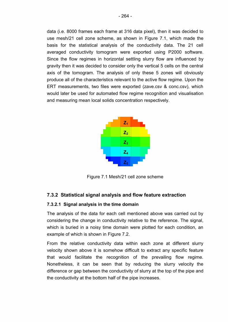
- 264 -
data (i.e. 8000 frames each frame at 316 data pixel), then it was decided to
use mesh/21 cell zone scheme, as shown in Figure 7.1, which made the
basis for the statistical analysis of the conductivity data. The 21 cell
averaged conductivity tomogram were exported using P2000 software.
Since the flow regimes in horizontal settling slurry flow are influenced by
gravity then it was decided to consider only the vertical 5 cells on the central
axis of the tomogram. The analysis of only these 5 zones will obviously
produce all of the characteristics relevant to the active flow regime. Upon the
ERT measurements, two files were exported (zave.csv & conc.csv), which
would later be used for automated flow regime recognition and visualisation
and measuring mean local solids concentration respectively.
Figure 7.1 Mesh/21 cell zone scheme
7.3.2 Statistical signal analysis and flow feature extraction
7.3.2.1 Signal analysis in the time domain
The analysis of the data for each cell mentioned above was carried out by
considering the change in conductivity relative to the reference. The signal,
which is buried in a noisy time domain were plotted for each condition, an
example of which is shown in Figure 7.2.
From the relative conductivity data within each zone at different slurry
velocity shown above it is somehow difficult to extract any specific feature
that would facilitate the recognition of the prevailing flow regime.
Nonetheless, it can be seen that by reducing the slurry velocity the
difference or gap between the conductivity of slurry at the top of the pipe and
the conductivity at the bottom half of the pipe increases.
Z1
Z2
Z3
Z4
Z5
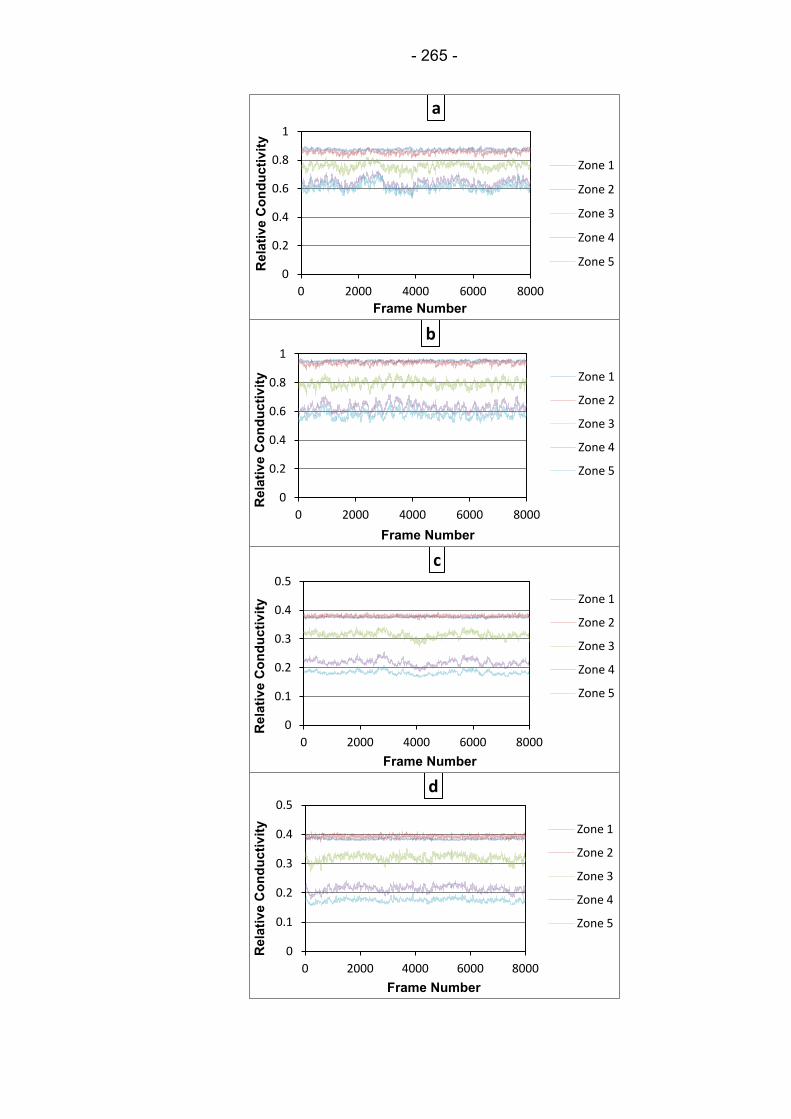
- 265 -
0
0.2
0.4
0.6
0.8
1
0 2000 4000 6000 8000
Rela
tiv
e C
on
du
cti
vit
y
Frame Number
a
Zone 1
Zone 2
Zone 3
Zone 4
Zone 5
0
0.2
0.4
0.6
0.8
1
0 2000 4000 6000 8000
Rela
tiv
e C
on
du
cti
vit
y
Frame Number
b
Zone 1
Zone 2
Zone 3
Zone 4
Zone 5
0
0.1
0.2
0.3
0.4
0.5
0 2000 4000 6000 8000
Rela
tiv
e C
on
du
cti
vit
y
Frame Number
c
Zone 1
Zone 2
Zone 3
Zone 4
Zone 5
0
0.1
0.2
0.3
0.4
0.5
0 2000 4000 6000 8000
Rela
tiv
e C
on
du
cti
vit
y
Frame Number
d
Zone 1
Zone 2
Zone 3
Zone 4
Zone 5
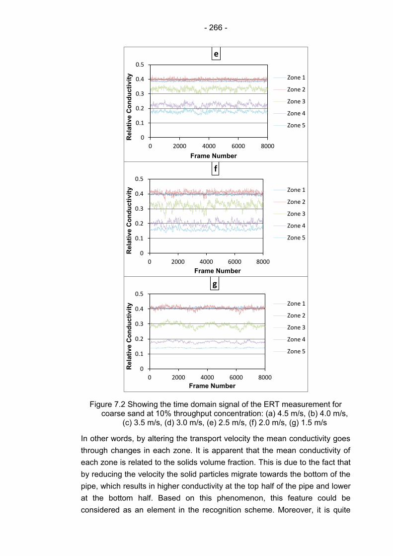
- 266 -
Figure 7.2 Showing the time domain signal of the ERT measurement for coarse sand at 10% throughput concentration: (a) 4.5 m/s, (b) 4.0 m/s,
(c) 3.5 m/s, (d) 3.0 m/s, (e) 2.5 m/s, (f) 2.0 m/s, (g) 1.5 m/s
In other words, by altering the transport velocity the mean conductivity goes
through changes in each zone. It is apparent that the mean conductivity of
each zone is related to the solids volume fraction. This is due to the fact that
by reducing the velocity the solid particles migrate towards the bottom of the
pipe, which results in higher conductivity at the top half of the pipe and lower
at the bottom half. Based on this phenomenon, this feature could be
considered as an element in the recognition scheme. Moreover, it is quite
0
0.1
0.2
0.3
0.4
0.5
0 2000 4000 6000 8000
Rela
tiv
e C
on
du
cti
vit
y
Frame Number
e
Zone 1
Zone 2
Zone 3
Zone 4
Zone 5
0
0.1
0.2
0.3
0.4
0.5
0 2000 4000 6000 8000
Rela
tiv
e C
on
du
cti
vit
y
Frame Number
f
Zone 1
Zone 2
Zone 3
Zone 4
Zone 5
0
0.1
0.2
0.3
0.4
0.5
0 2000 4000 6000 8000
Rela
tiv
e C
on
du
cti
vit
y
Frame Number
g
Zone 1
Zone 2
Zone 3
Zone 4
Zone 5
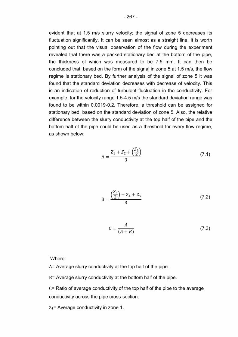
- 267 -
evident that at 1.5 m/s slurry velocity; the signal of zone 5 decreases its
fluctuation significantly. It can be seen almost as a straight line. It is worth
pointing out that the visual observation of the flow during the experiment
revealed that there was a packed stationary bed at the bottom of the pipe,
the thickness of which was measured to be 7.5 mm. It can then be
concluded that, based on the form of the signal in zone 5 at 1.5 m/s, the flow
regime is stationary bed. By further analysis of the signal of zone 5 it was
found that the standard deviation decreases with decrease of velocity. This
is an indication of reduction of turbulent fluctuation in the conductivity. For
example, for the velocity range 1.5-4.5 m/s the standard deviation range was
found to be within 0.0019-0.2. Therefore, a threshold can be assigned for
stationary bed, based on the standard deviation of zone 5. Also, the relative
difference between the slurry conductivity at the top half of the pipe and the
bottom half of the pipe could be used as a threshold for every flow regime,
as shown below:
(7.1)
(7.2)
(7.3)
Where:
A= Average slurry conductivity at the top half of the pipe.
B= Average slurry conductivity at the bottom half of the pipe.
C= Ratio of average conductivity of the top half of the pipe to the average
conductivity across the pipe cross-section.
Z1= Average conductivity in zone 1.
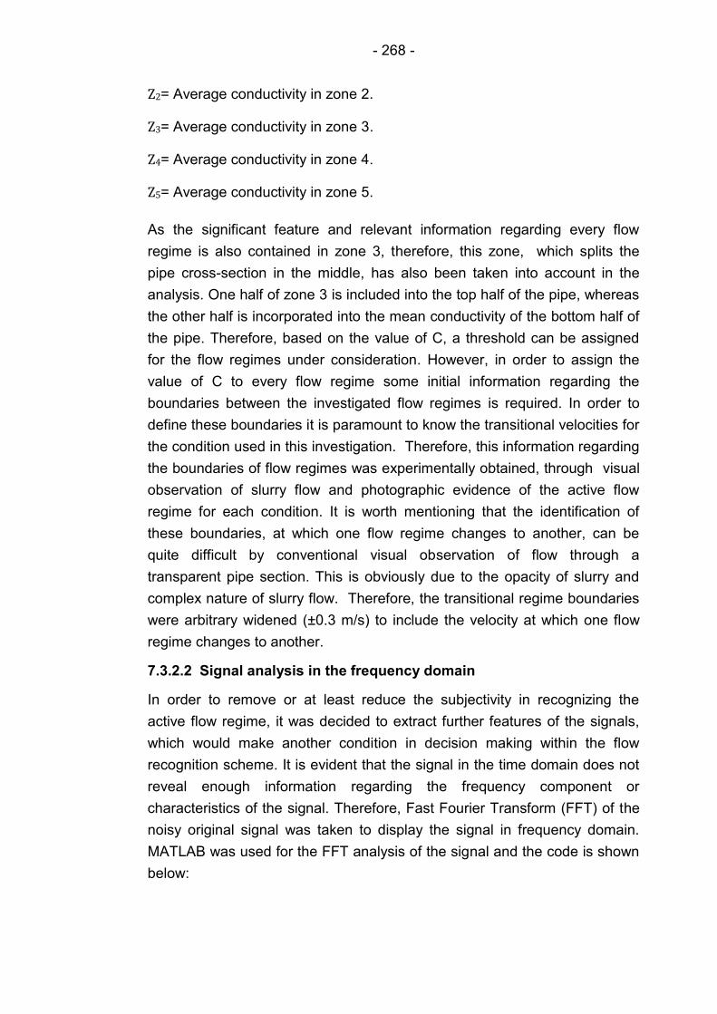
- 268 -
Z2= Average conductivity in zone 2.
Z3= Average conductivity in zone 3.
Z4= Average conductivity in zone 4.
Z5= Average conductivity in zone 5.
As the significant feature and relevant information regarding every flow
regime is also contained in zone 3, therefore, this zone, which splits the
pipe cross-section in the middle, has also been taken into account in the
analysis. One half of zone 3 is included into the top half of the pipe, whereas
the other half is incorporated into the mean conductivity of the bottom half of
the pipe. Therefore, based on the value of C, a threshold can be assigned
for the flow regimes under consideration. However, in order to assign the
value of C to every flow regime some initial information regarding the
boundaries between the investigated flow regimes is required. In order to
define these boundaries it is paramount to know the transitional velocities for
the condition used in this investigation. Therefore, this information regarding
the boundaries of flow regimes was experimentally obtained, through visual
observation of slurry flow and photographic evidence of the active flow
regime for each condition. It is worth mentioning that the identification of
these boundaries, at which one flow regime changes to another, can be
quite difficult by conventional visual observation of flow through a
transparent pipe section. This is obviously due to the opacity of slurry and
complex nature of slurry flow. Therefore, the transitional regime boundaries
were arbitrary widened (±0.3 m/s) to include the velocity at which one flow
regime changes to another.
7.3.2.2 Signal analysis in the frequency domain
In order to remove or at least reduce the subjectivity in recognizing the
active flow regime, it was decided to extract further features of the signals,
which would make another condition in decision making within the flow
recognition scheme. It is evident that the signal in the time domain does not
reveal enough information regarding the frequency component or
characteristics of the signal. Therefore, Fast Fourier Transform (FFT) of the
noisy original signal was taken to display the signal in frequency domain.
MATLAB was used for the FFT analysis of the signal and the code is shown
below:

- 269 -
T = 0.0015; % Sample Time Fs = 1/T; % Sampling Frequency L = 8000; % Length of Signal % Sum of a 50 Hz sinusoid and a 120 Hz sinusoid
NFFT = 2^nextpow2(L); % Next power of 2 from length of y
V = fft (Z1,NFFT)/L; % Zone 1 W = fft (Z2,NFFT)/L; % Zone 2 X = fft (Z3,NFFT)/L; % Zone 3 Y = fft (Z4,NFFT)/L; % Zone 4 Z = fft (Z5,NFFT)/L; % Zone 5
f = Fs/2*linspace(0,1,NFFT/2+1);
% Plot single sided amplitude spectrum plot(f,2*abs(V(1:NFFT/2+1)),f,2*abs(W(1:NFFT/2+1)),f,2*abs(X(1:NFFT/
2+1)),f,2*abs(Y(1:NFFT/2+1)),f,2*abs(Z(1:NFFT/2+1)))
plot(f,2*abs(V(1:NFFT/2+1))) plot(f,2*abs(W(1:NFFT/2+1))) plot(f,2*abs(X(1:NFFT/2+1))) plot(f,2*abs(Y(1:NFFT/2+1))) plot(f,2*abs(Z(1:NFFT/2+1))) title('Single-sided amplitude spectrum of noisy ERT signals-2.0
m/s') xlabel('Frequency (Hz)') ylabel('Amplitude') ylabel('|Y(f)|') axis([0 50 0 0.06])
legend('Zone 1','Zone 2','Zone 3','Zone 4','Zone 5');
legend('Zone 1') legend('Zone 2') legend('Zone 3') legend('Zone 4') legend('Zone 5') fprintf('%8.3f, %8.3f\n',f, 2*abs(V(1:NFFT/2+1)));
The frequency components of each zone for each condition were
determined, and an example of coarse sand at 10% throughput
concentration and 4.0 m/s is shown in Figure 7.3.
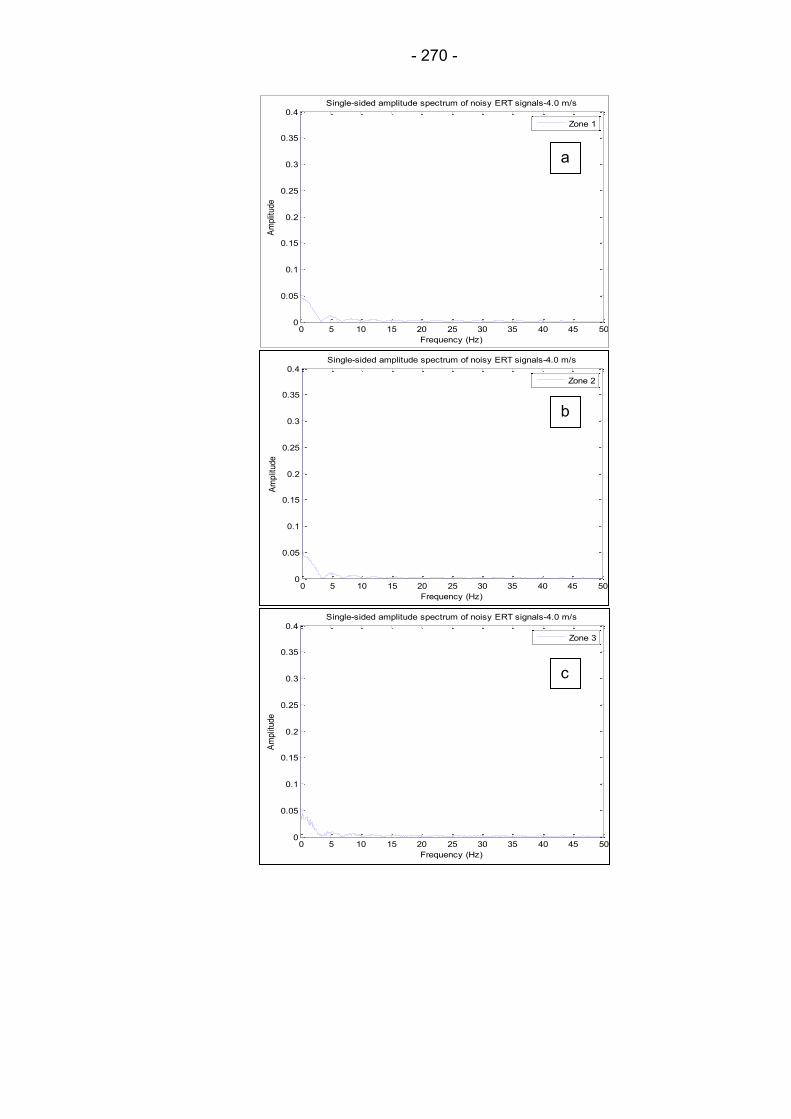
- 270 -
0 5 10 15 20 25 30 35 40 45 500
0.05
0.1
0.15
0.2
0.25
0.3
0.35
0.4Single-sided amplitude spectrum of noisy ERT signals-4.0 m/s
Frequency (Hz)
Am
plit
ude
Zone 1
0 5 10 15 20 25 30 35 40 45 500
0.05
0.1
0.15
0.2
0.25
0.3
0.35
0.4Single-sided amplitude spectrum of noisy ERT signals-4.0 m/s
Frequency (Hz)
Am
plit
ude
Zone 2
0 5 10 15 20 25 30 35 40 45 500
0.05
0.1
0.15
0.2
0.25
0.3
0.35
0.4Single-sided amplitude spectrum of noisy ERT signals-4.0 m/s
Frequency (Hz)
Am
plit
ude
Zone 3
a
b
c
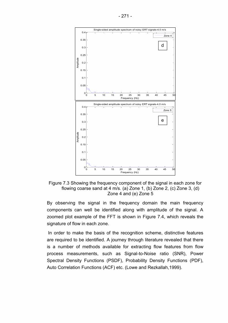
- 271 -
Figure 7.3 Showing the frequency component of the signal in each zone for flowing coarse sand at 4 m/s. (a) Zone 1, (b) Zone 2, (c) Zone 3, (d)
Zone 4 and (e) Zone 5
By observing the signal in the frequency domain the main frequency
components can well be identified along with amplitude of the signal. A
zoomed plot example of the FFT is shown in Figure 7.4, which reveals the
signature of flow in each zone.
In order to make the basis of the recognition scheme, distinctive features
are required to be identified. A journey through literature revealed that there
is a number of methods available for extracting flow features from flow
process measurements, such as Signal-to-Noise ratio (SNR), Power
Spectral Density Functions (PSDF), Probability Density Functions (PDF),
Auto Correlation Functions (ACF) etc. (Lowe and Rezkallah,1999).
0 5 10 15 20 25 30 35 40 45 500
0.05
0.1
0.15
0.2
0.25
0.3
0.35
0.4Single-sided amplitude spectrum of noisy ERT signals-4.0 m/s
Frequency (Hz)
Am
plit
ude
Zone 4
0 5 10 15 20 25 30 35 40 45 500
0.05
0.1
0.15
0.2
0.25
0.3
0.35
0.4Single-sided amplitude spectrum of noisy ERT signals-4.0 m/s
Frequency (Hz)
Am
plit
ude
Zone 5
d
e
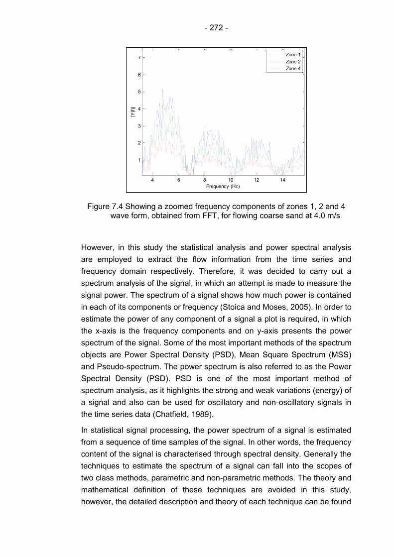
- 272 -
Figure 7.4 Showing a zoomed frequency components of zones 1, 2 and 4 wave form, obtained from FFT, for flowing coarse sand at 4.0 m/s
However, in this study the statistical analysis and power spectral analysis
are employed to extract the flow information from the time series and
frequency domain respectively. Therefore, it was decided to carry out a
spectrum analysis of the signal, in which an attempt is made to measure the
signal power. The spectrum of a signal shows how much power is contained
in each of its components or frequency (Stoica and Moses, 2005). In order to
estimate the power of any component of a signal a plot is required, in which
the x-axis is the frequency components and on y-axis presents the power
spectrum of the signal. Some of the most important methods of the spectrum
objects are Power Spectral Density (PSD), Mean Square Spectrum (MSS)
and Pseudo-spectrum. The power spectrum is also referred to as the Power
Spectral Density (PSD). PSD is one of the most important method of
spectrum analysis, as it highlights the strong and weak variations (energy) of
a signal and also can be used for oscillatory and non-oscillatory signals in
the time series data (Chatfield, 1989).
In statistical signal processing, the power spectrum of a signal is estimated
from a sequence of time samples of the signal. In other words, the frequency
content of the signal is characterised through spectral density. Generally the
techniques to estimate the spectrum of a signal can fall into the scopes of
two class methods, parametric and non-parametric methods. The theory and
mathematical definition of these techniques are avoided in this study,
however, the detailed description and theory of each technique can be found
4 6 8 10 12 14
1
2
3
4
5
6
7
x 10-3 Frequency components of zone 1 wave form
Frequency (Hz)
|Y(f
)|
Zone 1
Zone 2
Zone 4
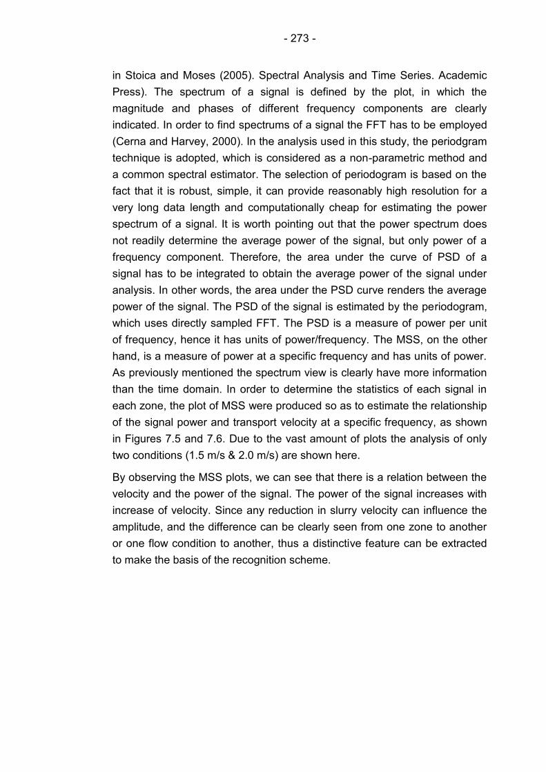
- 273 -
in Stoica and Moses (2005). Spectral Analysis and Time Series. Academic
Press). The spectrum of a signal is defined by the plot, in which the
magnitude and phases of different frequency components are clearly
indicated. In order to find spectrums of a signal the FFT has to be employed
(Cerna and Harvey, 2000). In the analysis used in this study, the periodgram
technique is adopted, which is considered as a non-parametric method and
a common spectral estimator. The selection of periodogram is based on the
fact that it is robust, simple, it can provide reasonably high resolution for a
very long data length and computationally cheap for estimating the power
spectrum of a signal. It is worth pointing out that the power spectrum does
not readily determine the average power of the signal, but only power of a
frequency component. Therefore, the area under the curve of PSD of a
signal has to be integrated to obtain the average power of the signal under
analysis. In other words, the area under the PSD curve renders the average
power of the signal. The PSD of the signal is estimated by the periodogram,
which uses directly sampled FFT. The PSD is a measure of power per unit
of frequency, hence it has units of power/frequency. The MSS, on the other
hand, is a measure of power at a specific frequency and has units of power.
As previously mentioned the spectrum view is clearly have more information
than the time domain. In order to determine the statistics of each signal in
each zone, the plot of MSS were produced so as to estimate the relationship
of the signal power and transport velocity at a specific frequency, as shown
in Figures 7.5 and 7.6. Due to the vast amount of plots the analysis of only
two conditions (1.5 m/s & 2.0 m/s) are shown here.
By observing the MSS plots, we can see that there is a relation between the
velocity and the power of the signal. The power of the signal increases with
increase of velocity. Since any reduction in slurry velocity can influence the
amplitude, and the difference can be clearly seen from one zone to another
or one flow condition to another, thus a distinctive feature can be extracted
to make the basis of the recognition scheme.
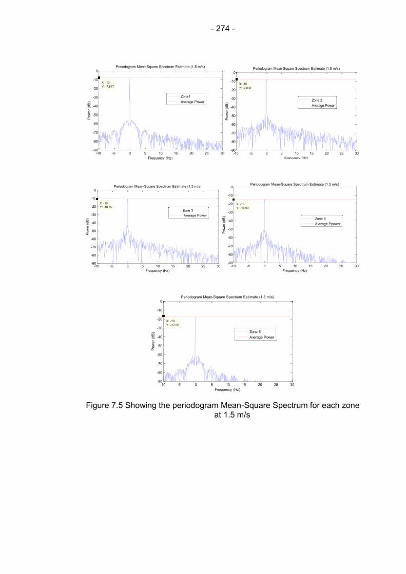
- 274 -
Figure 7.5 Showing the periodogram Mean-Square Spectrum for each zone at 1.5 m/s
-10 -5 0 5 10 15 20 25 30-90
-80
-70
-60
-50
-40
-30
-20
-10
0
X: -10
Y: -7.817
Periodogram Mean-Square Spectrum Estimate (1.5 m/s)
Frequency (Hz)
Pow
er
(dB
)
Zone1
Average Power
-10 -5 0 5 10 15 20 25 30-90
-80
-70
-60
-50
-40
-30
-20
-10
0
X: -10
Y: -7.833
Frequency (Hz)
Pow
er
(dB
)
Periodogram Mean-Square Spectrum Estimate (1.5 m/s)
Zone 2
Average Power
-10 -5 0 5 10 15 20 25 30-90
-80
-70
-60
-50
-40
-30
-20
-10
0
X: -10
Y: -10.75
Periodogram Mean-Square Spectrum Estimate (1.5 m/s)
Frequency (Hz)
Pow
er
(dB
)
Zone 3
Average Power
-10 -5 0 5 10 15 20 25 30-90
-80
-70
-60
-50
-40
-30
-20
-10
0
X: -10
Y: -14.93
Frequency (Hz)
Pow
er
(dB
)
Periodogram Mean-Square Spectrum Estimate (1.5 m/s)
Zone 4
Average Ppower
-10 -5 0 5 10 15 20 25 30-90
-80
-70
-60
-50
-40
-30
-20
-10
0
X: -10
Y: -17.08
Periodogram Mean-Square Spectrum Estimate (1.5 m/s)
Frequency (Hz)
Pow
er
(dB
) Zone 5
Average Power

- 275 -
Figure 7.6 Showing the periodogram Mean-Square Spectrum for each zone at 2 m/s
This feature can be used to relate the signal power at the top half of the pipe
to the signal power at the bottom half of the pipe. In other words, The
average signal power decreases with increase of solid particles in each
zone. Therefore, a threshold can be assigned, based on the relative
difference between the signal power at the top half of the pipe and the
bottom half of the pipe for each flow regime.
-10 -5 0 5 10 15 20 25 30-90
-80
-70
-60
-50
-40
-30
-20
-10
0
X: -10
Y: -8.054
Frequency (Hz)
Pow
er
(dB
)
Periodogram Mean-Square Spectrum Estimate (2.0 m/s)
Zone 1
Average Power
-10 -5 0 5 10 15 20 25 30-90
-80
-70
-60
-50
-40
-30
-20
-10
0
X: -10
Y: -7.77
Periodogram Mean-Square Spectrum Estimate (2.0 m/s)
Frequency (Hz)
Pow
er
(dB
) Zone 2
Average Power
-10 -5 0 5 10 15 20 25 30-90
-80
-70
-60
-50
-40
-30
-20
-10
0
X: -10
Y: -9.86
Frequency (Hz)
Pow
er
(dB
)
Periodogram Mean-Square Spectrum Estimate (2.0 m/s)
Zone 3
Average Power
-10 -5 0 5 10 15 20 25 30-90
-80
-70
-60
-50
-40
-30
-20
-10
0
X: -10
Y: -13.88
Periodogram Mean-Square Spectrum Estimate (2.0 m/s)
Frequency (Hz)
Pow
er
(dB
)Zone 4
Average Power
-10 -5 0 5 10 15 20 25 30-90
-80
-70
-60
-50
-40
-30
-20
-10
0
X: -10
Y: -15.93
Periodogram Mean-Square Spectrum Estimate (2.0 m/s)
Frequency (Hz)
Pow
er
(dB
) Zone 5
Average Power

- 276 -
However, in order to determine the threshold for each signal, the average
power of each signal is required. Since the methods of the PSD include a
plot and average power. Then the PSD is considered to return the average
power of each signal. The average power method uses a rectangle
approximation to the integral to calculate the signal’s average power using
the PSD data. Therefore, the following steps were followed to calculate the
average power of each signal:
1. Creating a periodogram spectrum with a Hamming window.
2. Create a power spectral density object.
3. Set the options for the periodogram.
4. Calculate the PSD.
5. Calculate the average power.
Once the average power of each zone is calculated, then the comparison is
made between the signal power at the top half of the pipe and the power at
the bottom half of the pipe. This can be done by calculating the ratio of the
average power at the top of the pipe (P1, P2 & P3/2) to the average power
across the five zones (or pipe cross-section); as shown below:
(7.4)
(7.5)
(7.6)
Where:
E= Average signal power at the top half of the pipe.
F= Average signal power at the bottom half of the pipe.
D= Ratio of average signal power of the top half of the pipe to the average
signal power across the pipe cross-section.
P1= Average signal power in zone 1.
P2= Average signal power in zone 2.
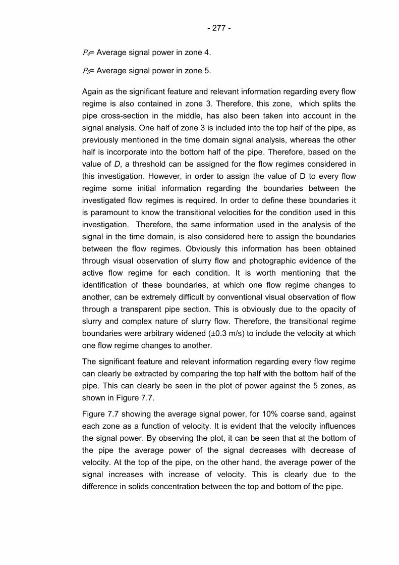
- 277 -
P4= Average signal power in zone 4.
P5= Average signal power in zone 5.
Again as the significant feature and relevant information regarding every flow
regime is also contained in zone 3. Therefore, this zone, which splits the
pipe cross-section in the middle, has also been taken into account in the
signal analysis. One half of zone 3 is included into the top half of the pipe, as
previously mentioned in the time domain signal analysis, whereas the other
half is incorporate into the bottom half of the pipe. Therefore, based on the
value of D, a threshold can be assigned for the flow regimes considered in
this investigation. However, in order to assign the value of D to every flow
regime some initial information regarding the boundaries between the
investigated flow regimes is required. In order to define these boundaries it
is paramount to know the transitional velocities for the condition used in this
investigation. Therefore, the same information used in the analysis of the
signal in the time domain, is also considered here to assign the boundaries
between the flow regimes. Obviously this information has been obtained
through visual observation of slurry flow and photographic evidence of the
active flow regime for each condition. It is worth mentioning that the
identification of these boundaries, at which one flow regime changes to
another, can be extremely difficult by conventional visual observation of flow
through a transparent pipe section. This is obviously due to the opacity of
slurry and complex nature of slurry flow. Therefore, the transitional regime
boundaries were arbitrary widened (±0.3 m/s) to include the velocity at which
one flow regime changes to another.
The significant feature and relevant information regarding every flow regime
can clearly be extracted by comparing the top half with the bottom half of the
pipe. This can clearly be seen in the plot of power against the 5 zones, as
shown in Figure 7.7.
Figure 7.7 showing the average signal power, for 10% coarse sand, against
each zone as a function of velocity. It is evident that the velocity influences
the signal power. By observing the plot, it can be seen that at the bottom of
the pipe the average power of the signal decreases with decrease of
velocity. At the top of the pipe, on the other hand, the average power of the
signal increases with increase of velocity. This is clearly due to the
difference in solids concentration between the top and bottom of the pipe.
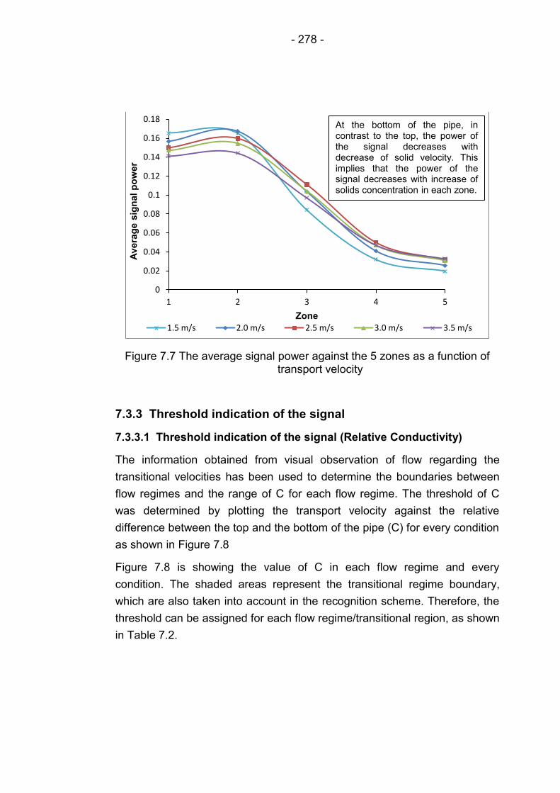
- 278 -
Figure 7.7 The average signal power against the 5 zones as a function of transport velocity
7.3.3 Threshold indication of the signal
7.3.3.1 Threshold indication of the signal (Relative Conductivity)
The information obtained from visual observation of flow regarding the
transitional velocities has been used to determine the boundaries between
flow regimes and the range of C for each flow regime. The threshold of C
was determined by plotting the transport velocity against the relative
difference between the top and the bottom of the pipe (C) for every condition
as shown in Figure 7.8
Figure 7.8 is showing the value of C in each flow regime and every
condition. The shaded areas represent the transitional regime boundary,
which are also taken into account in the recognition scheme. Therefore, the
threshold can be assigned for each flow regime/transitional region, as shown
in Table 7.2.
0
0.02
0.04
0.06
0.08
0.1
0.12
0.14
0.16
0.18
1 2 3 4 5
Av
era
ge s
ign
al
po
wer
Zone
1.5 m/s 2.0 m/s 2.5 m/s 3.0 m/s 3.5 m/s
At the bottom of the pipe, in contrast to the top, the power of the signal decreases with decrease of solid velocity. This implies that the power of the signal decreases with increase of solids concentration in each zone.
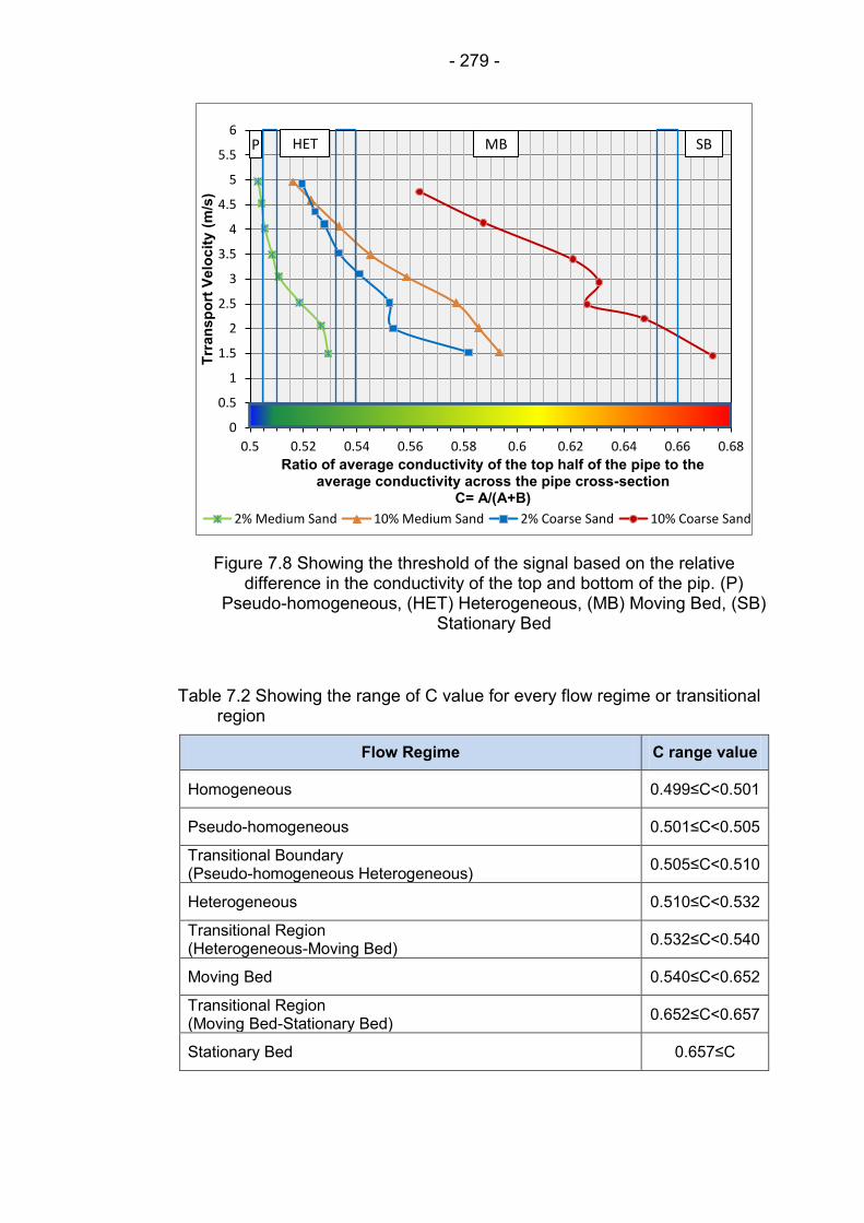
- 279 -
Figure 7.8 Showing the threshold of the signal based on the relative difference in the conductivity of the top and bottom of the pip. (P)
Pseudo-homogeneous, (HET) Heterogeneous, (MB) Moving Bed, (SB) Stationary Bed
Table 7.2 Showing the range of C value for every flow regime or transitional region
Flow Regime C range value
Homogeneous 0.499≤C<0.501
Pseudo-homogeneous 0.501≤C<0.505
Transitional Boundary (Pseudo-homogeneous Heterogeneous)
0.505≤C<0.510
Heterogeneous 0.510≤C<0.532
Transitional Region (Heterogeneous-Moving Bed)
0.532≤C<0.540
Moving Bed 0.540≤C<0.652
Transitional Region (Moving Bed-Stationary Bed)
0.652≤C<0.657
Stationary Bed 0.657≤C
0
0.5
1
1.5
2
2.5
3
3.5
4
4.5
5
5.5
6
0.5 0.52 0.54 0.56 0.58 0.6 0.62 0.64 0.66 0.68
Trr
an
sp
ort
Velo
cit
y (
m/s
)
Ratio of average conductivity of the top half of the pipe to the average conductivity across the pipe cross-section
C= A/(A+B)
2% Medium Sand 10% Medium Sand 2% Coarse Sand 10% Coarse Sand
SB MB HET P
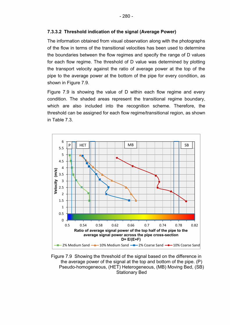
- 280 -
7.3.3.2 Threshold indication of the signal (Average Power)
The information obtained from visual observation along with the photographs
of the flow in terms of the transitional velocities has been used to determine
the boundaries between the flow regimes and specify the range of D values
for each flow regime. The threshold of D value was determined by plotting
the transport velocity against the ratio of average power at the top of the
pipe to the average power at the bottom of the pipe for every condition, as
shown in Figure 7.9.
Figure 7.9 is showing the value of D within each flow regime and every
condition. The shaded areas represent the transitional regime boundary,
which are also included into the recognition scheme. Therefore, the
threshold can be assigned for each flow regime/transitional region, as shown
in Table 7.3.
Figure 7.9 Showing the threshold of the signal based on the difference in the average power of the signal at the top and bottom of the pipe. (P)
Pseudo-homogeneous, (HET) Heterogeneous, (MB) Moving Bed, (SB) Stationary Bed
0
0.5
1
1.5
2
2.5
3
3.5
4
4.5
5
5.5
6
0.5 0.54 0.58 0.62 0.66 0.7 0.74 0.78 0.82
Velo
cit
y
(m/s
)
Ratio of average signal power of the top half of the pipe to the average signal power across the pipe cross-section
D= E/(E+F)
2% Medium Sand 10% Medium Sand 2% Coarse Sand 10% Coarse Sand
SB MB HET P
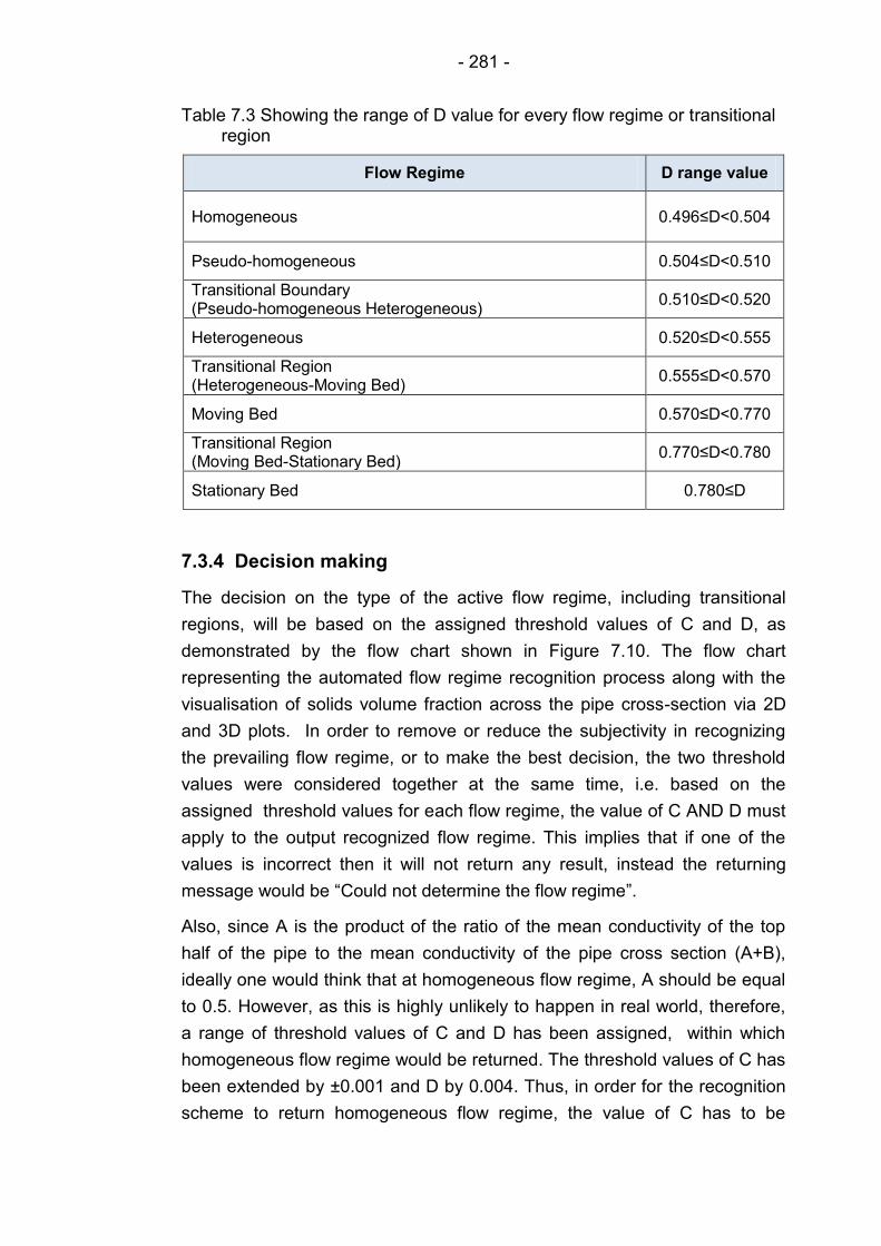
- 281 -
Table 7.3 Showing the range of D value for every flow regime or transitional region
Flow Regime D range value
Homogeneous 0.496≤D<0.504
Pseudo-homogeneous 0.504≤D<0.510
Transitional Boundary (Pseudo-homogeneous Heterogeneous)
0.510≤D<0.520
Heterogeneous 0.520≤D<0.555
Transitional Region (Heterogeneous-Moving Bed)
0.555≤D<0.570
Moving Bed 0.570≤D<0.770
Transitional Region (Moving Bed-Stationary Bed)
0.770≤D<0.780
Stationary Bed 0.780≤D
7.3.4 Decision making
The decision on the type of the active flow regime, including transitional
regions, will be based on the assigned threshold values of C and D, as
demonstrated by the flow chart shown in Figure 7.10. The flow chart
representing the automated flow regime recognition process along with the
visualisation of solids volume fraction across the pipe cross-section via 2D
and 3D plots. In order to remove or reduce the subjectivity in recognizing
the prevailing flow regime, or to make the best decision, the two threshold
values were considered together at the same time, i.e. based on the
assigned threshold values for each flow regime, the value of C AND D must
apply to the output recognized flow regime. This implies that if one of the
values is incorrect then it will not return any result, instead the returning
message would be “Could not determine the flow regime”.
Also, since A is the product of the ratio of the mean conductivity of the top
half of the pipe to the mean conductivity of the pipe cross section (A+B),
ideally one would think that at homogeneous flow regime, A should be equal
to 0.5. However, as this is highly unlikely to happen in real world, therefore,
a range of threshold values of C and D has been assigned, within which
homogeneous flow regime would be returned. The threshold values of C has
been extended by ±0.001 and D by 0.004. Thus, in order for the recognition
scheme to return homogeneous flow regime, the value of C has to be
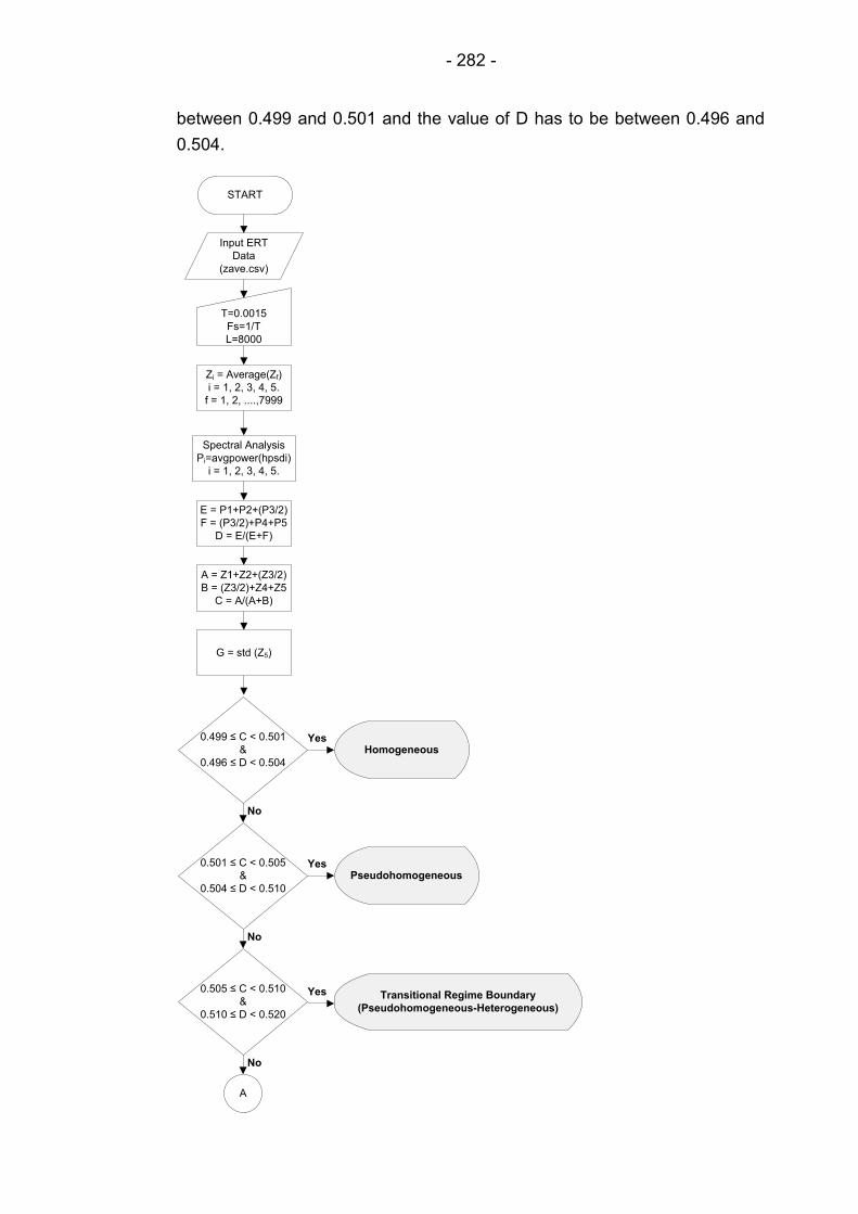
- 282 -
between 0.499 and 0.501 and the value of D has to be between 0.496 and
0.504.
START
Input ERT
Data
(zave.csv)
T=0.0015
Fs=1/T
L=8000
Zi = Average(Zf)
i = 1, 2, 3, 4, 5.
f = 1, 2, ....,7999
Spectral Analysis
Pi=avgpower(hpsdi)
i = 1, 2, 3, 4, 5.
E = P1+P2+(P3/2)
F = (P3/2)+P4+P5
D = E/(E+F)
0.499 ≤ C < 0.501
&
0.496 ≤ D < 0.504
A = Z1+Z2+(Z3/2)
B = (Z3/2)+Z4+Z5
C = A/(A+B)
0.501 ≤ C < 0.505
&
0.504 ≤ D < 0.510
Pseudohomogeneous
Homogeneous
0.505 ≤ C < 0.510
&
0.510 ≤ D < 0.520
Transitional Regime Boundary
(Pseudohomogeneous-Heterogeneous)
G = std (Z5)
Yes
No
Yes
No
Yes
No
A
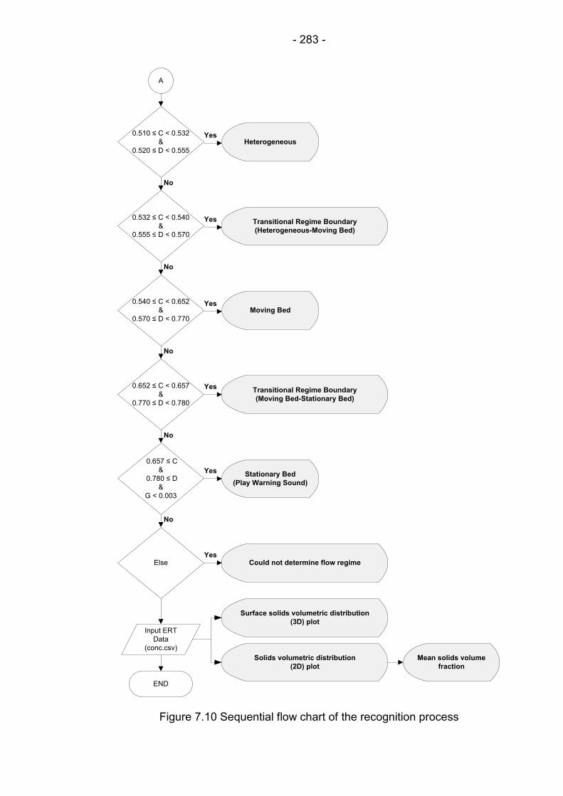
- 283 -
0.540 ≤ C < 0.652
&
0.570 ≤ D < 0.770
Moving Bed
0.657 ≤ C
&
0.780 ≤ D
&
G < 0.003
END
Stationary Bed
(Play Warning Sound)
0.510 ≤ C < 0.532
&
0.520 ≤ D < 0.555
Heterogeneous
0.532 ≤ C < 0.540
&
0.555 ≤ D < 0.570
Transitional Regime Boundary
(Heterogeneous-Moving Bed)
0.652 ≤ C < 0.657
&
0.770 ≤ D < 0.780
Transitional Regime Boundary
(Moving Bed-Stationary Bed)
Yes
No
Yes
No
Yes
No
Yes
No
Yes
Else Could not determine flow regime
No
Yes
A
Input ERT
Data
(conc.csv)
Surface solids volumetric distribution
(3D) plot
Solids volumetric distribution
(2D) plot
Mean solids volume
fraction
Figure 7.10 Sequential flow chart of the recognition process
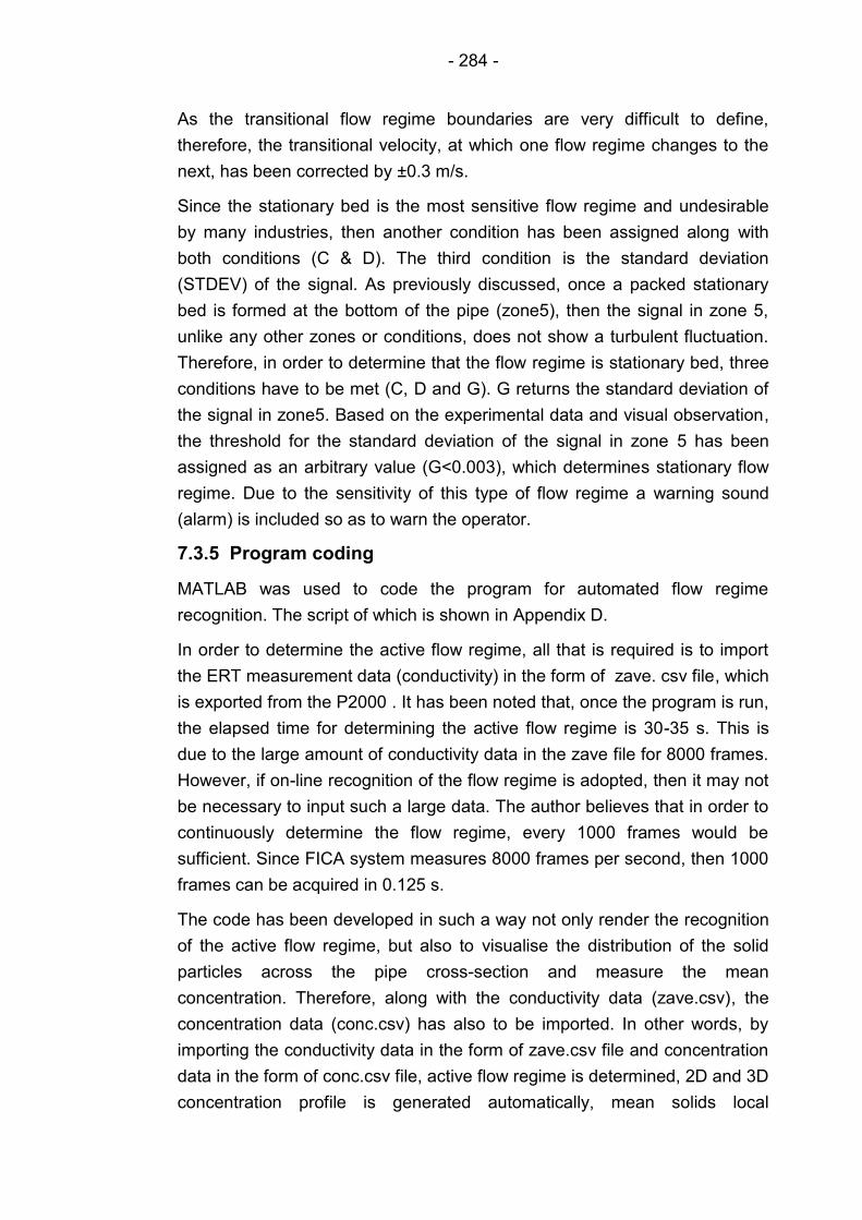
- 284 -
As the transitional flow regime boundaries are very difficult to define,
therefore, the transitional velocity, at which one flow regime changes to the
next, has been corrected by ±0.3 m/s.
Since the stationary bed is the most sensitive flow regime and undesirable
by many industries, then another condition has been assigned along with
both conditions (C & D). The third condition is the standard deviation
(STDEV) of the signal. As previously discussed, once a packed stationary
bed is formed at the bottom of the pipe (zone5), then the signal in zone 5,
unlike any other zones or conditions, does not show a turbulent fluctuation.
Therefore, in order to determine that the flow regime is stationary bed, three
conditions have to be met (C, D and G). G returns the standard deviation of
the signal in zone5. Based on the experimental data and visual observation,
the threshold for the standard deviation of the signal in zone 5 has been
assigned as an arbitrary value (G<0.003), which determines stationary flow
regime. Due to the sensitivity of this type of flow regime a warning sound
(alarm) is included so as to warn the operator.
7.3.5 Program coding
MATLAB was used to code the program for automated flow regime
recognition. The script of which is shown in Appendix D.
In order to determine the active flow regime, all that is required is to import
the ERT measurement data (conductivity) in the form of zave. csv file, which
is exported from the P2000 . It has been noted that, once the program is run,
the elapsed time for determining the active flow regime is 30-35 s. This is
due to the large amount of conductivity data in the zave file for 8000 frames.
However, if on-line recognition of the flow regime is adopted, then it may not
be necessary to input such a large data. The author believes that in order to
continuously determine the flow regime, every 1000 frames would be
sufficient. Since FICA system measures 8000 frames per second, then 1000
frames can be acquired in 0.125 s.
The code has been developed in such a way not only render the recognition
of the active flow regime, but also to visualise the distribution of the solid
particles across the pipe cross-section and measure the mean
concentration. Therefore, along with the conductivity data (zave.csv), the
concentration data (conc.csv) has also to be imported. In other words, by
importing the conductivity data in the form of zave.csv file and concentration
data in the form of conc.csv file, active flow regime is determined, 2D and 3D
concentration profile is generated automatically, mean solids local

- 285 -
concentration is automatically calculated and displayed on the screen along
with many other data statistics such as minimum solids local concentration,
maximum solids concentration etc.
It is worth mentioning that the script, mentioned in Appendix D, is applicable
for an electrode configuration, where the electrode number 1 positioned on
the top of the pipe and the numbering continues clockwise viewing the
direction of flow, as shown in Figure 7.11.
1
12
11
10
9
8
7
6
5
4
3
216
15
14
13The direction of flow
is into the paper
Top of the pipe
Bottom of the pipe
Figure 7.11 Electrode configuration for flow regime recognition
This configuration would obviously facilitate the importing concentration and
conductivity data. In other words, this type of electrode configuration
facilitate reading a range of consecutive columns in the conc.csv file rather
than taking random columns, which is highly likely to increase the elapsed
time of the computing. Since only the vertical centreline of the tomogram is
considered for the purpose of flow regime recognition and plotting and
measuring concentration, then it is not necessary to acquire all the data.
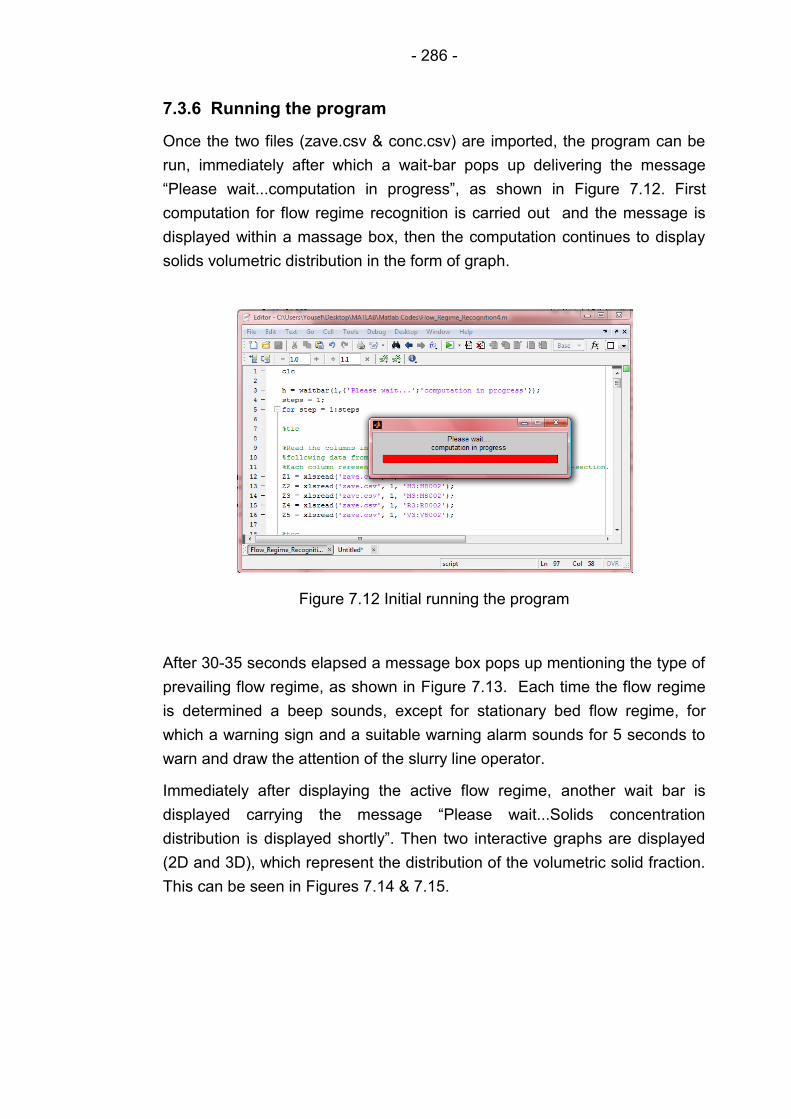
- 286 -
7.3.6 Running the program
Once the two files (zave.csv & conc.csv) are imported, the program can be
run, immediately after which a wait-bar pops up delivering the message
“Please wait...computation in progress”, as shown in Figure 7.12. First
computation for flow regime recognition is carried out and the message is
displayed within a massage box, then the computation continues to display
solids volumetric distribution in the form of graph.
Figure 7.12 Initial running the program
After 30-35 seconds elapsed a message box pops up mentioning the type of
prevailing flow regime, as shown in Figure 7.13. Each time the flow regime
is determined a beep sounds, except for stationary bed flow regime, for
which a warning sign and a suitable warning alarm sounds for 5 seconds to
warn and draw the attention of the slurry line operator.
Immediately after displaying the active flow regime, another wait bar is
displayed carrying the message “Please wait...Solids concentration
distribution is displayed shortly”. Then two interactive graphs are displayed
(2D and 3D), which represent the distribution of the volumetric solid fraction.
This can be seen in Figures 7.14 & 7.15.

- 287 -
Figure 7.13 Message box conveying the result of flow recognition computation
Figure 7.14 Wait-bar showing computation in progress
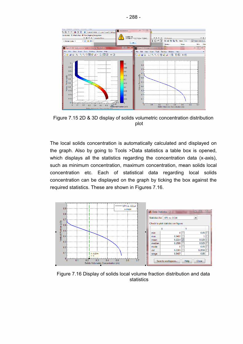
- 288 -
Figure 7.15 2D & 3D display of solids volumetric concentration distribution plot
The local solids concentration is automatically calculated and displayed on
the graph. Also by going to Tools >Data statistics a table box is opened,
which displays all the statistics regarding the concentration data (x-axis),
such as minimum concentration, maximum concentration, mean solids local
concentration etc. Each of statistical data regarding local solids
concentration can be displayed on the graph by ticking the box against the
required statistics. These are shown in Figures 7.16.
Figure 7.16 Display of solids local volume fraction distribution and data statistics

- 289 -
7.4 Evaluation of the method
In order to evaluate the recognition method, 31 test conditions were carried
out within the range of velocity 1.5-5 m/s, which would undoubtedly cover all
flow regimes considered in this recognition scheme. Different solid particle
size (coarse & medium) at two different throughput concentrations (2% &
10%) were also used to evaluate the effect of particle size and solids
concentration upon the recognition scheme. A summary of the evaluation
results is demonstrated in Table 7.4, while the recognition results for
different conditions are highlighted in Table 7.5.
Since the recognition decision is based on the analysis of the zones across
the vertical centreline of the pipe cross-section, therefore it is believed that it
can be applied on any pipe size conveying slurry. The results of the
recognition method have been compared to the photographs of the flow and
visual observation.
By observing the results in Table 7.5, it can be seen that out of 31 tests, the
flow regime could not be determined or correctly determined only for three
conditions. This error could be due to some systematic error in the original
conductivity data input to the test or the result of visual observation may
have been wrongly determined. The latter reason is more plausible due to
opaque and murky nature of slurry, especially sand/water flow. However, a
future investigation is recommended to determine the source of this error.
Table 7.4 Summary of recognition results
Total number of tests 31
Correct 28
Incorrect or unrecognised 3
Success rate 90.32%
Rate of error 9.68%
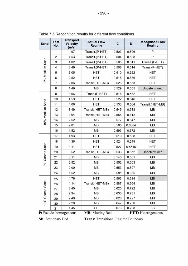
- 290 -
Table 7.5 Recognition results for different flow conditions
Sand Test No.
Transport Velocity
(m/s)
Actual Flow Regime
C D Recognised Flow
Regime 2%
Me
diu
m S
an
d
1 4.97 Transit.(P-HET) 0.503 0.506 P
2 4.53 Transit.(P-HET) 0.504 0.508 P
3 4.02 Transit.(P-HET) 0.505 0.511 Transit.(P-HET)
4 3.49 Transit.(P-HET) 0.508 0.514 Trans.(P-HET)
5 3.05 HET 0.510 0.522 HET
6 2.52 HET 0.518 0.536 HET
7 2.06 Transit.(HET-MB) 0.526 0.553 HET
8 1.49 MB 0.529 0.555 Undetermined
10%
Med
ium
Sa
nd
9 4.96 Trans.(P-HET) 0.516 0.532 HET
10 4.59 HET 0.522 0.546 HET
11 4.06 HET 0.533 0.564 Transit.(HET-MB)
12 3.49 Transit.(HET-MB) 0.545 0.588 MB
13 3.04 Transit.(HET-MB) 0.558 0.612 MB
14 2.52 MB 0.577 0.647 MB
15 2.01 MB 0.585 0.6604 MB
16 1.52 MB 0.593 0.672 MB
2%
Coars
e S
and
17 4.93 HET 0.519 0.538 HET
18 4.36 HET 0.524 0.549 HET
19 4.11 HET 0.527 0.5546 HET
20 3.52 Transit.(HET-MB) 0.533 0.572 Undetermined
21 3.11 MB 0.540 0.581 MB
22 2.52 MB 0.552 0.603 MB
23 2.00 MB 0.553 0.597 MB
24 1.52 MB 0.581 0.655 MB
10%
Co
ars
e S
and
25 4.76 HET 0.563 0.624 MB
26 4.14 Transit.(HET-MB) 0.587 0.664 MB
27 3.40 MB 0.620 0.722 MB
28 2.94 MB 0.630 0.731 MB
29 2.49 MB 0.626 0.727 MB
30 2.20 MB 0.647 0.760 MB
31 1.45 SB 0.673 0.798 SB
P: Pseudo-homogeneous MB: Moving Bed HET: Heterogeneous
SB: Stationary Bed Trans: Transitional Regime Boundary

- 291 -
7.5 Conclusions
A flow recognition method has been developed, which is based on the
statistical signal analysis of the ERT data in both time and frequency
domain. All common slurry flow regimes have been considered in the
recognition scheme, including the transitional regime boundaries. The
results of the evaluation suggest that the method is applicable to any particle
size, solids concentration. It is also believed that the pipe size should not
have any effect on the recognition scheme. However, application of the
recognition method is paramount on different pipe sizes. The rate of
recognition was determined to be 90.32% based on a sufficient number of
tests carried out on different particle size and different concentration. Since
the recognition decisions are based on the statistical ERT signal analysis, it
is believed that it removes the subjectivity associated with recognition of the
prevailing flow regime. This recognition method can be applied on any two
phase solid/liquid flow, as long as one of the phases is non- or less
conductive than the other one. It is believed that it can be useful for flow
metering, especially for flow regime dependent flow meters. It can also be
used in a non-invasive and on-line fashion for distinguishing the boundaries
between different typical settling slurry flow regimes so as to enable the
operator to take an appropriate control actions for other downstream
operations such as separation, mixing etc. In addition, the recognition code
has been developed in a way not only for recognition of the active flow
regime, but also to visualise the distribution of the solid particles across the
pipe cross-section and measure the mean concentration.
- 292 -
Chapter 8
Contributions, conclusions and future work
recommendations
This final chapter highlights the contribution of present work, which includes
the proposed ERT based measurement, flow visualisation and flow regime
recognition technique along with the design of a multiphase flow system. A
summary of the most important findings is presented. It also recommends
the future scope in different areas of slurry flow in pipelines and exploration
of further capabilities of the ERT system.
8.1 Author’s contributions to slurry flow measurement,
visualisation and the design of particulate flow system
Slurry transport has been a progressive technology for transporting a huge
amount of solid materials across the world in both long distance pipelines
and short commodity pipelines. Many slurry pipelines already exist and there
will be more to build including all pipeline orientations. In order to ensure
safe transport, optimised operation and reduction of financial costs by
avoiding blockage, the operational engineer requires a reliable technique
that suits all the conditions in industry. Clearly the complex nature of settling
slurry flow forces the operator to continuously measure the local parameters
governing the flow (solids concentration and solids velocity) and visualise
the internal structure of the flow within the pipeline. Undoubtedly the
measurement of these parameters and monitoring the flow within the pipe, in
fast evolving processes requires a fast responding instrument (i.e. high
frame rates of milliseconds). This study was performed in order to develop a
new automated online measurement technique, which is based on the
combination of a high performance ERT as the main sensor and the EMF as
an auxiliary sensor. This will prove advantageous, as it will allow the
operator to perform the measurement of each phase and to be able to see
the changes in solids concentration and solids movement within the pipe.
This work has also developed a new facility, which will act as a spring-board
for better understanding of slurry flow behaviour and the interaction of solid-
liquid inside pipeline, particularly inclined flow, which is complex and a very
limited information has been reported about it. This thesis can be considered
as a direct response to today’s slurry engineering requirements and a step

- 293 -
forward for better controlling the processes and reducing unnecessary
financial costs. The author’s findings and observations provide a novel
insight over the mechanisms of solid-liquid flow, along with a new ERT
based technique for local flow measurement, flow visualisation and
automated flow regime recognition. The results reveal the capabilities of the
ERT and pave the way to a reliable and robust technique, which helps to
further optimise the operation of settling slurry pipelines in industry. The
main contribution is described as below:
8.1.1 Slurry flow measurement (Chapter 5)
8.1.1.1 Local solids volume fraction
A high performance dual-plane Electrical Resistance Tomography system
has been employed to interrogate the internal structure of horizontal and
vertical counter-gravity slurry flow. The exceptional capability of this system
enabled acquiring high frame rates (1000 dfps) in a non-intrusive fashion.
The reconstructed tomograms obtained from the ERT were collected and
analysed to determine the in-situ solids concentration and solids
concentration profile across the vertical plane of the pipe cross-section. The
comparison of the results with that of flow diversion technique revealed that
the ERT measurements give a reasonable estimation of the in-situ solids
concentration in both orientations, horizontal and vertical. The description of
these results can be found in sections 5.4.10.1 for horizontal flow and
5.5.3.1 for vertical flow. The tracking of solids concentration changes as a
function of transport velocity was also generated, each of which represents
the typical concentration profile of settling slurry flow. For further detail
regarding the measured solids volumetric distribution, the reader is referred
to sections 5.4.2 for horizontal flow and 5.5.1 for vertical counter-gravity flow.
It seems that using a high performance ERT system for measurement of in-
situ solids concentration is completely novel.
8.1.1.2 Local solids axial velocity
The high performance ERT system in conjunction with the cross-correlation
technique can be used for local axial solids velocity and solids velocity
distribution across the vertical plane of the pipe cross-section. The detailed
description of solids velocity measurements can be found in sections 5.4.3
for horizontal flow and 5.5.1. To the author’s knowledge the measurement of
in-situ solids velocity and solids axial velocity distribution is rather novel for
the flow conditions used in this study.
- 294 -
8.1.1.3 Slurry volumetric flow rate
The present work proposes a novel ERT based technique, which combines
the Electrical Resistance Tomography and the Electromagnetic Flow Meter
for performance of volumetric flow rate measurement of each constituent
phase individually and measurement of mixture volumetric flow rate in
vertical pipeline. Sections 5.5.2 and 5.5.3.3 highlights the detailed
description of the measurement technique and final evaluation respectively.
8.1.1.4 Phase slip velocity
This project presents a new method of slip velocity estimation in vertical flow
using the combination of the ERT and the EMF. The slip velocity can be
determined through the track of volumetric flow rate of both phases (solid
and liquid). The reader is directed to section 5.5.2 for detailed explanation.
8.1.1.5 Parameters relevant to stratified flow
This present research reports a new method for estimation of several
parameters of stratified flow through an analysis of both profiles, solids
concentration and solids axial velocity. These parameters are mean granular
bed concentration, mean granular bed velocity, the height of granular bed,
the height of shear layer and the height of turbulent zone at the upper part of
horizontal pipeline. This technique can be used to measure the height of
granular bed only if the height of bed is greater than 2.5 mm in 50 mm inner
diameter pipe. In other words, this technique can only be used if the height
of granular bed is greater than the ratio of pipe diameter to the number of
pixels in the vertical plane of the tomogram. It is worth pointing out that the
estimation of these parameters is paramount for the design of slurry pipeline
and optimisation. The detailed discussion of this method is covered in
sections 5.4.6 and 5.4.6.1.
8.1.1.6 Measurement of blocked horizontal line
In some highly concentrated-solids transport systems the solid particles
travelling in horizontal flow in the form of contact load with transmitting the
submerged weight to the internal pipe surface, such as that of Alberta oil-
sand deposits (Schaan et al., 2007). This implies that the solids are
transported in sliding mass or sliding thick granular bed. This thick layer of
sliding granular bed may generate a potential error in slurry measurement.
This study reports an evaluation regarding the performance of the ERT while
a thick coating of granular bed (up to 80% of the inner pipe diameter) covers
the electrodes on the dual-plane ERT sensor. In other words, the ERT was
successfully performed for measurement of a horizontal pipeline. To the

- 295 -
author’s knowledge, the use of ERT for measurement of such high
concentrated slurry has never been reported in the literature. Therefore, this
can be considered as a novelty within the body of this thesis. The discussion
of this finding is presented in section 5.4.5.5. The observation of the results
revealed that the ERT can undoubtedly detect the pipeline blockage and
measure the mean solids concentration and thickness of the stagnant
granular bed. This finding can be useful for detection of blocked lines and for
measurement of highly concentrated slurries.
8.1.2 Slurry flow visualisation (Chapter 5)
8.1.2.1 Slurry flow regime visualisation and characterisation using ERT
Usually the common flow regimes in horizontal slurry flow is visualised
through solids concentration distribution across the vertical plane of the pipe
cross-section. This thesis presents a novel method, by which several flow
regimes, encountered in horizontal flow, can be visualised and characterised
using solids axial velocity distribution. It appears that the method of flow
regime visualisation via solids velocity distribution using the ERT technique
is completely new. The flow regimes that can be visualised using this
method are pseudo-homogeneous flow regime, heterogeneous flow regime,
granular bed flow regime and pipe blockage. The visualisation results were
compared qualitatively against the actual photograph of the flow and a good
agreement was noticed. The only limitation of this method is that, in stratified
flow, indicates only a packed granular bed. It is rather difficult to distinguish
between moving bed and stationary bed based on the velocity profile.
Besides, no feature can be observed to identify whether the bed is moving in
the form of en-bloc sliding (mass) or stream layers. Therefore, the term
“granular bed flow regime” is used for both flow regimes, moving bed and
stationary bed. The discussion and evaluation of this visualisation method
and characterisation is detailed in sections 5.4.5.1, 5.4.5.2, 5.4.5.3, 5.4.5.4
and 5.4.5.5.
8.1.3 Design of slurry system (Chapter 6)
8.1.3.1 Design and construction of pilot scale inclinable slurry flow
A review of the literature reveals that the behaviour of slurry flow has been
systematically investigated since 1950s, while the focus has mainly been
based on experimental investigations dealing with horizontal and vertical
flow. Very limited work on inclined flow can be noticed. As a response to this
issue, this study reports a novel design of a robust, versatile, durable and
functional inclinable flow loop, which paves the way to further understanding

- 296 -
the behaviour of solid-liquid particles within an inclined pipe. The flow
system can be used not only for two-phase flow such as slurry, but also for a
multiphase flow such as gas-water-solid flow. The flow system includes
various important and carefully selected instrumentations, which can be
used as tools for further understanding and characterisation of slurry flow
and identifying the potential effects on flow measurement scheme. The
versatility of the system allows investigations on any desired pipe
orientations (horizontal, vertical and inclined). The mechanical and hydraulic
testing of the flow loop confirmed total functionality and safety of the system.
The whole design and erection strategies are described in Chapter 6, where
the reader is taken through the whole journey from project management to
the final stage of testing.
8.1.4 Slurry flow regime recognition (Chapter 7)
8.1.4.1 Automated on-line flow regime recognition
This project has developed a novel automated technique for recognition of
horizontal slurry flow regimes based on the statistical analysis of the high
performance ERT signal in both, time and frequency domain. All common
slurry flow regimes are considered including the transitional regime
boundaries. The flow regimes that are recognised using this technique are:
Homogeneous, pseudo-homogeneous, heterogeneous, moving bed and
stationary bed. Since the stationary bed is the most undesirable flow regime,
as the risk of pipe blockage is dominant, a warning sound (alarm) is included
into the code, so as to warn the operator. The method has been evaluated
and a recognition success rate is confirmed as 90.32%. The recognition
decision is made based on the distribution of solid particles across five
zones along the vertical plane of the pipe cross-section. This implies that the
present technique is applicable to any settling slurry as long as one of the
phases is non- or less conductive than the other. Besides, it removes the
subjectivity associated with the recognition of the prevailing flow regime.
One of the main aim in developing of this method is that it can be used for
flow metering, especially for correction of flow regime dependent flow
meters, such as ERT. It can also be used to distinguish the boundaries
between common settling slurry flow regimes so as to enable the operator to
take appropriate control actions for other downstream operations, such as
separation, mixing etc. It also provides a visual distribution of the solid
particles across the pipe cross-section with displaying the average solids
volume fraction in the pipeline. Chapter 7 describes the whole technique.
- 297 -
8.2 General conclusions
1. A high performance dual-plane ERT system was used to interrogate the
internal structure of horizontal and vertical upward slurry flows. It was
found that the high temporal resolution of this system enabled a fast
measurement and online monitoring of slurry flow in both orientations.
2. The local solids volumetric concentration and solids volumetric distribution
across the pipe cross-section were determined for both flow orientations.
While the dual-plane ERT system was combined with the cross-
correlation technique and successfully measured the local solids axial
velocity and solids velocity distribution across the pipe cross-section. The
comparison of solids volumetric distribution and the solids velocity
distribution, with the actual photographs of the flow, revealed that there is
a good agreement between both methods.
3. The estimated local solids concentration was compared to that obtained
from flow diversion technique. The error analysis of the ERT local solids
concentration in horizontal flow, revealed that the error is random and a
maximum of 19% was observed throughout the conditions used in this
study. It was remarked that the ERT tends to overestimate the local solids
concentration. This overestimation was noticed for both sands, medium
and coarse.
4. The comparison of local solids axial velocity obtained from the ERT with
that of flow diversion technique revealed that a randomly distributed error
has been noticed with a maximum of 3.23% through horizontal test
section, whereas a maximum error of 9.25% was remarked through
vertical flow. It was also concluded that the ERT velocities are mostly
underestimated at low velocities (3 m/s and below), which is considered
as stratified velocity region. The reasons for this underestimation was
associated to the instability of the conditions over the formed granular
bed.
5. The observation of solids concentration profiles of both sands in vertical
counter-gravity flow concluded that the coarse sand particles move in
core peak flow pattern, while medium sand particles move in wall peak
flow pattern. This is clearly due to the phenomenon of radial particle
migration.
6. The solids velocity profiles obtained in vertical upward flow exhibits a
uniform distribution throughout the centre region of the pipe cross-section.
The flattened shape of velocity profiles were noticed for all conditions
used in this study.
- 298 -
7. The evaluation of the proposed technique for measurement of slurry
volumetric flow rate suggests a reasonably accurate estimation of the
volumetric flow rate obtained from the ERT and the EMF.
8. Despite occurrence of some deviations in solids concentration and solids
axial velocity and slurry volumetric flow rate, it can be concluded that for
the range of conditions used in this study, overall, the high performance
ERT system provides a reasonably accurate estimation of all parameters
measured in both flow orientations and enables visualisation of solids and
their motion within the pipelines.
8.3 Future scope
1. This research study has made contributions into the area of
two/multiphase flow measurement, visualisation and characterisation,
specifically slurry flows, which are clearly highlighted in Chapter 8
(Section 8.1) and can be found within the body of this thesis. Some of
them have already been exposed to a form of peer review and can now
be found in the public domain as published materials. Some others are
contained in the framework of this thesis and have a great potential for
future publications. The following papers are due to be published in the
nearest future:
i. An analysis of slurry flow within and around the boundary of
stationary bed and blockage in horizontal pipeline, the details of
which can be tracked in Chapter 5 (Sections 5.4.5.4 & 5.4.5.5). The
contribution is planned to be published under the title
“Measurement and characterisation of solid-liquid flow within
the boundary of stationary bed and blockage” in Chemical
Engineering Journal (Impact Factor = 3.461).
ii. Measurement, visualisation and characterisation of stratified slurry
flow in horizontal pipeline, which is detailed in Chapter 5 (Sections
5.4.6 & 4.5.6.1). The expected paper will be published under the
title “Measurement and analysis of stratified slurry flow in
pipeline using high performance Electrical Resistance
Tomography system” in Sensors and actuators B-Chemical
Journal (Impact Factor = 3.898).
iii. A novel automated recognition technique for common slurry flow
regimes in horizontal pipeline, which is described in Chapter 7. The
paper containing the proposed technique will be published under

- 299 -
the title “Flow regime recognition of horizontal slurry flow
using statistical analysis of the ERT signal” in Sensors and
actuators B-Chemical Journal (Impact Factor = 3.898).
iv. A proposed inclinable flow rig, which is discussed in detail in
Chapter 6. The paper will be published under the title “Design and
construction of a pilot scale inclinable particulate flow
system” in The International Journal of Multiphase Flow (Impact
Factor = 2.230).
v. Measurement of the two phases in two phase flows, which is
covered in Chapter 5 (Sections 5.5.2 & 5.5.3.3). The novel
technique will be reported in a paper with the title “A new
generation of dual-phase measurement and visualisation
system” in Sensors and actuators B-Chemical Journal (Impact
Factor= 3.898).
2. Further tests are required to investigate the overestimation of solids
concentration and solids axial velocity at higher velocities (above 3 m/s).
3. Development of a better reconstruction algorithm is paramount, so as to
take the ERT technique a couple of steps forward.
4. Since the ERT technique suffers from the effect of temperature and recipe
change, then its combination with a cheap secondary sensor, such as
differential pressure flow meter, can overcome this limitation. The role of
the secondary sensor is to compensate the temperature change and to be
used as a correction tool. This, undoubtedly, improvement will make the
ERT technique far more attractive in the view point of industry.
5. Further tests are required for investigation of off-wall particle lift
phenomenon. The use of additional technology for generating solids
concentration profile may be important for the purpose of comparison.
6. It is recommended that the proposed flow regime recognition technique to
be used on inclined flow. However, the threshold of the data may be
subject to a minor alteration.
7. A graphical user-friendly interface is recommended for automatic flow
regime recognition and reading the ERT data in a direct method.
8. In order to boost our knowledge and gain insight of complex inclined
slurry flow intense experiments are required, mainly over critical slope,
solids concentration, solids axial velocity, deposition velocity, flow
regimes, pressure drop etc.
THE END

- 300 -
List of References and selected bibliography
1. Abdul Rahim, R., Fazalul Rahiman, M.H., Chan, K.S., Nawawi, S.W.
(2007). Non-invasive imaging of liquid/gas flow using ultrasonic
transmission-mode tomography. Sensors and Actuators A: Physical,
135(2), pp. 337-345.
2. Abdul Rahim, R., Nayan, N.M., Rahiman, M.H. (2006). Ultrasonic
tomography system for liquid/gas flow: frame rate comparison between
visual basic and visual c++ programming. Journal Teknologi, 44(D), pp.
131-150.
3. Abulnaga, B. (2002). Slurry Systems Handbook. New York: McGraw-
Hill.
4. Albion, K., Briens. L., Briens, C. Berruti, F. (2007). Flow Regime
determination in horizontal pneumatic transport of fine powders using
non-intrusive acoustic probes. Powder Technology, 172(3), pp. 157-
166.
5. Bagnold, R.A. (1954). Gravity-free dispersion of large spheres in a
Newtonian fluid under shear. Proc. Royal Soc. A, 225, pp. 49-63.
6. Bagnold, R.A. (1956). The flow of Cohesionless Grains in Fluids.
Philosophy Transaction of the Royal Society, London, Series A, 249,
pp. 99235-297.
7. Bain, A.G. and Bonnington, S.T. (1970). The Hydraulic Transport of
Solids by Pipelines, 1st edition. Pergamon Press.
8. Baker, R.C. (2000). Flow Measurement Handbook. Cambridge:
Cambridge University Press.
9. Barigoua, M., Fairhurst, P.G., Fryer, P.J., Painc, J.P. (2003). Concentric
fow regime of solid–liquid food suspensions: theory and experiment.
Chemical Engineering Science, 58, pp. 1671-1686.
10. Bartosik, A.S. (1996). Modelling the Bagnold stress effects in vertical
slurry flow. J. Hydrol. Hydromech, 44(1), pp. 49-58.
11. Bernier, R.N., Brennen, C.E. (1983). Use of the electromagnetic flow
meter in a two-phase flow. International Journal of Multiphase Flow,
9(3), pp. 251-257.
12. Bevir, M.K. (1970). The theory of induced voltage electromagnetic flow
meters. Journal of Fluid Mechanics, 43(3), pp. 577-590.
13. Blake, A. (Ed.).(1985).Handbook of Mechanics, Materials, and
Structures. New York: J. Wiley & Sons.

- 301 -
14. Blatch, N.S. (1906). Discussion: Water Filtration at Washington D.C.
Transaction of the American Society of Civil Engineers, 57, pp. 400-
408.
15. Boden, S., Bieberle, M., Hampel, U. (2008). Quantitative measurement
of gas hold-up distribution in a stirred chemical reactor using X-ray
cone-beam computed tomography. Chemical Engineering Journal,
139(2), pp. 531-362.
16. Brook, N. (1962). Flow measurement of solid-liquid mixtures using
Venturi and other meters. Proc. Instit. Mech. Engrg., 176, pp. 127-140.
17. Brown, N.P. (1991). Flow regimes of settling slurries in pipes. In Brown,
N.P. Heywood, N.L. (eds). Slurry Handling Design of Solid–Liquid
Systems. London. pp. 41–52.
18. Brown, P.B. & Heywood, N.I. (1991). Slurry Handling: Design of solid-
liquid Systems. London: Elsevier Applied Science.
19. Bruggeman, D.A.G. (1935). Calculation of Various Physical Constants
of Heterogeneous Substances, Part 1, Constant and Conductivity of
Mixtures of Isotropic Substances, Annual Physics, Leipzig, 24, pp. 636.
20. Cairns, R.C., Lawther, K.R. Turner, K.S. (1960). Flow Characteristics of
Dilute Small Particle Suspensions, British Chemical Engineering, 5, pp.
849-856.
21. Camarasa, E., Vial, C., Poncin, S., Wild, G., Midoux, N., Bouillard, J.
(1999). Influence of coalescence behaviour of the liquid and of gas
sparging on hydrodynamics and bubble characteristics in a bubble
column. Chem. Eng. Process., 38, pp. 329-344.
22. Carstens, M.R. (1969). A Theory for Heterogeneous Flow of Solids in
Pipes, Proceedings of the Institution of Civil Engineers, Journal of the
Hydraulics Division, 95, pp. 275-286.
23. Cerna, M., Harvey, A. F. (2000). National Instruments Application, Note
041.
24. Cha, J.E., Ahn, Y.C., Kim, M.H. (2002). Flow measurement with an
electromagnetic flow meter in two-phase bubbly and slug flow regimes.
Flow Measurement and Instrumentation, 12(5-6), pp. 329-339.
25. Charles, M. E., and G. S. Stevens. (1972). The pipeline flow of
slurries—transitional velocities. Paper presented at the Second
International Conference on Hydraulic Transport of Solids and Pipes.
Second conference of the British Hydromechanic Research
Association. Cranfield, England.
26. Chatfield, C. (1989). The Analysis of Time Series-An Introduction (4th
ed.). Chapman and Hall: London.
- 302 -
27. Cheney, M., Isaacson, D., Newell, J.C. (1999). Electrical impedance
tomography. Siam Rev, 41, pp. 85-101.
28. Cho, K.H., Kim, S. Lee, Y.J. (1999). A fast EIT image reconstruction
method for the two-phase flow visualization. International
Communications in Heat and Mass Transfer, 26, pp. 637-646.
29. Clift, R. and Clift. D.H.M. (1981). Continuous measurement of the
density of flowing slurries. Int. J. Multiphase Flow, 75, pp. 555-561.
30. Condolios, E. and Chapus, E.E. (1963). Designing Solids Handling
Pipelines, Chemical Engineering, 70, pp. 131-138.
31. Dai.Y., Wang, M., Panayotopoulos, N., Lucas,G., Williams, A.R. (2004).
3-D Visualisation of a Swirling Flow Using Electrical Resistance
Tomography, 4th World Congress on Industrial Process Tomography,
Aizu, Japan, pp 362-369.
32. Davies, J.T. (1987). Calculation of Critical Velocities to Maintain Solids
in Suspension in Horizontal Pipes. Chemical Engineering Science,
42(7), pp. 1667-1670.
33. Deng, X., Dong, F. Xu, L.J., Liu, X.P., Xu, L.A. (2001). The design of a
dual-plane ERT system for cross correlation measurement of bubbly
gas/liquid pipe flow. Measurement Science and Technology, 12, pp.
1024-1031.
34. Dhodapkar, S. and Jacob, K. (2006). Multiphase flow handbook, edited
by Clayton T. Crowe. NW: Taylor & Francis Group.
35. Divoux, J., Géminard C. (2007). Friction and dilatancy in immersed
granular matter. Physical Review Letters, 99, pp. 258-301.
36. Doron, P. and Barnea, D. (1993). A three-layer model for solid–liquid
flow in horizontal pipes. Int. J. Multiphase Flow,19, pp. 1029-1043.
37. Doron, P. and Barnea, D. (1995). Pressure drop and limit deposit
velocity for solid–liquid flow in pipes. Chem. Eng. Sci., 50, pp. 1595-
1604.
38. Doron, P. and Barnea, D. (1996). Flow Pattern Maps for Solid-Liquid
Flow in Pipes. International Journal of Multiphase Flow, 22(2), pp. 273-
283.
39. Doron, P., Granica, D. and Barnea, D. (1987). Slurry Flow in Horizontal
Pipes-Experimental and Modeling, International Journal of Multiphase
Flow, 13(4), pp. 535-547.
40. Doron, P., Simkhis, M., Barnea, D. (1997). Flow of solid–liquid mixtures
in inclined pipes. International Journal of Multiphase Flow, 23, pp. 313-
323.

- 303 -
41. Durand R., Condolios, E. (1952). Compterendu des Deuxiemes
journees de L’Hydraulique, Paris, societe Hydrotechnique de France,
pp. 29-55.
42. Durand, R. (1952). Basic Relationship of the Transportation of Solids in
Pipes-Experimental Research, Proceedings of the Minnesota
International Hydraulics Convention, American Society of Civil
Engineers, Minneapolis, University of Minnesota, pp. 89-103.
43. Durand, R. and Condolios, E. (1953). The Hydraulic Transport of Coal
and Solid Materials in Pipes. Proceedings of Colloquium on the
Hydraulic Transport of Coal, National Coal Board, London, pp. 39-52.
44. Dyakowski, T. and Williams, R.A. (1996). Prediction of High Solids
Concentration Regions Within a Hydrocyclone. Powder Technology, 87,
pp. 43-47.
45. Dyakowski, T., Jeanmeure, L.F.C., Jaworski, A.J. (2000). Applications
of Electrical Resistance Tomography for Gas-Liquid and Liquid-Solids
Flows- A Review. Powder Technology, 112, pp. 174-192.
46. Ellis, H.S., and Round, G.F. (1963). Laboratory studies on the flow of
nickel–water suspensions. Canadian Mining and Metallurgical Bulletin,
56, pp. 773-781.
47. El-Reedy, A.M. (2011). Construction management and design of
industrial concrete and steel structures. N.Y: Taylor & Francis Group.
48. Ercolani, E., Ferrini, F., Arrigoni, V. (1979). Electric and Thermal Probe
for Measuring the Limit Deposit Velocity, Proceedings of the Sixth
International Conference on the Hydraulic Transport of Solids in Pipes,
BHRA, Canterbury, England, Paper A3, pp. 27-42.
49. Etuke, EO, Bonnecaze, RT. (1998). Measurement of angular velocities
using electrical impedance tomography. Flow Measurement and
Instrumentation, 9, pp. 159-169.
50. Fazalul Rahiman, M.H., Abdul Rahim, R., Zakaria, Z. (2008). Design
and modeling of ultrasonic tomography for two-component high-
acoustic impedance mixture. Sensors and Actuators A:Physical, 147,
pp. 409-414.
51. Fowles, G. R., Cassiday, G. L. (1999). Analytical Mechanics, (6th ed.).
Saunders College Publishing.
52. Fukushima, E. (1999). Nuclear magnetic resonance as a tool to study
flow. Annu Rev. Fluid Mech, 31, pp. 95-123.
53. GE Sensing. (2007). Panametrics Ultrasonic Flow Transducers for
Liquids. Installation Guide, Installation Guide 916-055B.
- 304 -
54. Geisler, T. (2001). Ultrasonic velocity profile measurements in
experimental hydraulics. Doctoral Thesis. Graz University of
Technology , Faculty of Civil Engineering , Austria.
55. Giguere, R., Fradette, L., Mignon, D. Tanguy, P. A. (2008b). ERT
algorithms for quantitative concentration measurement of multiphase
flows. Chemical Engineering Journal, 141, pp. 305-317.
56. Giguere, R., Fradette, L., Mignon, D. Tanguy, P. A. (2009). Analysis of
slurry flow regimes downstream of a pipe bend. Chemical Engineering
Research & Design, 87, pp. 943-950.
57. Giguere, R., Fradette, L., Mignon, D., Tanguy, P.A. (2008a).
Characterization of slurry flow regime transitions by ERT. Chemical
Engineering Research & Design, 86, pp. 989-996.
58. Gillies, R.G. (1991). Flow Loop Studies. In Brown, N. P. and
Heywood, N.I. (eds.). Slurry Handling: Design of Solid-liquid Systems.
Elsevier Applied Science.
59. Gillies, R.G. (1993). Pipeline Flow of Coarse Particle Slurries. Doctorial
Thesis. University of Saskatchewan, Department of Chemical
Engineering, Canada.
60. Gillies, R.G. and Shook, C.A. (1994). Concentration Distribution of
Sand Slurries in Horizontal Pipe Flow. Particulate Science and
Technology, 12, pp. 45-69.
61. Gillies, R.G., Hill, K.B., McKibben, Shook, C.A. (1999). Solids Transport
by Laminar Newtonian Flows. Powder Technology, 104, pp. 269-277.
62. Gillies, R.G., Shook, C.A. (2000). Modeling high concentration settling
slurry flows. The Canadian Journal of Chemical Engineering, 78, pp.
709-716
63. Gillies, R.G., Shook, C.A., Wilson, K.C. (1991). An improved two layer
model for horizontal slurry pipeline flow. The Canadian Journal of
Chemical Engineering, 69, pp. 173-178.
64. Govier, G.W. and Aziz, K. (1972). The Flow of Complex Mixtures in
Pipes. New York: van Nostrand Reinhold Company.
65. Graf, W.H., Robinson, M., Yucel, O. (1970). The Critical Deposit
Velocity for Solid-Liquid Mixtures. Proceedings of the First International
Conference on the Hydraulic Transport of Solids in Pipes, BHRA,
Coventry, England, Paper H5, pp. H5-77 to H5-88.
66. Hagler, T.W. Sr. (1956). Means for determining specific gravity of fluids
and slurries in motion. U. S. Pat. 2678529.
- 305 -
67. Hazen, A. and Hardy, H.D. (1906). Discussion of Work for the
Purification of the Water Supply of Washington, D.C., Transaction of the
American Society of Civil Engineers, 57, pp. 408-409.
68. Heindel, T.J, Grayb, J.N, Jensenb, T.C. (2008). An X-ray system for
visualizing fluid flows. Flow Measurement and Instrumentation, 19, pp.
67-78.
69. Henningsson, M, Ostergren, K, Dejmek, P. (2006). Plug flow of yoghurt
in piping as determined by cross-correlated dual-plane electrical
resistance tomography. Journal of Food Engineering, 76, pp. 163-168.
70. Holden, P.J., Wang, M., Mann, R., Dickin, F.J. Edwards, R.B. (1999).
On Detecting Mixing Pathologies Inside a Stirred Vessel Using
Electrical Resistance Tomography. Transactions of the Institution of
Chemical Engineers, 77, Part A, pp. 709-712.
71. Holdich, R.G. and Sinclair, I. (1992). Measurement of Slurry Solids
Content By Electrical Conductivity. Powder Technology, 72, pp. 77-87.
72. Hong , S., Choi, J., Yan, C.K. (2002). Experimental study on solid–
water slurry flow in vertical pipe by using ptv method. Proceedings of
the 12th International Offshore and Polar Engineering Conference, pp.
462–466.
73. Hosseini, S., Patel, D., Ein-Mozaffari, F., Mehrvar, M. (2010). Study of
solid-liquid mixing in agitated tanks through electrical resistance
tomography. Chemical Engineering Science, 65, pp. 1374-1384.
74. Hoult, D.I., Chen, C.N., Sank, V.J. (1986). The field-dependence of
NMR imaging: Arguments concerning an optimal field-strength. Magn
Reson Med, 3(2), pp. 730-46.
75. Howard, G.W. (1939). Transportation of Sand and Gravel in a Four-Inch
Pipe. Transaction of the American Society of Civil Engineers, 104, pp.
1334-1348.
76. Ismail, I., Gamio, J.C., Bukhari, S.F.A., Yang, W.Q. (2005).
Tomography for multi-phase flow measurement in the oil industry. Flow
Measurement and Instrumentation, 16, pp. 145-155.
77. ITS-Industrial Tomography Systems Ltd. (2005). P2000 Electrical
Resistance Tomography System, Operating Manual. Manchester: UK.
78. Jaafar, W., Fischer, S., Bekkour, K. (2009). Velocity and turbulence
measurements by ultrasound pulse Doppler velocimetry. Measurement,
42(2), pp. 175-182.
79. Jin, H., Yang, S., Guo, Z., He, G., Tong, Z. (2005). The axial distribution
of holdups in an industrial-scale bubble column with evaluated pressure
- 306 -
using γ-ray attenuation approach. Chemical Engineering Journal,
115(1-2), pp. 45-50.
80. Kalaga, D.V., Kulkarni, A.V., Acharya, R., Kumar, U., Singh, G., Joshi,
J.B. (2009). Some industrial applications of gamma-ray tomography.
Journal of the Taiwan Institute of Chemical Engineers, 40, pp. 602-612.
81. Kao, D.T.Y., Hwang, L.Y.(1979). Critical slope for slurry pipelines. P
Hydrotransport 6 Conference of the British Hydromechanical Research
Association, Cranfield, England.
82. Karnis, A, Goldsmith, H.L., Mason, S.G. (1966). The flow of
suspensions through tubes: V. Inertial effects. Canadian Journal of
Chemical Engineering, 44, pp. 181-193.
83. Kaushal, D.R. and Tomita, Y. (2002). Solids Concentration Profiles and
Pressure Drop in Pipeline Flow of Multisized Particulate Slurries.
International Journal of Multiphase Flow, 28, pp.1697-1717.
84. Kaushal, D.R., Sato, K., Toyota, T., Funatsu, K., Tomita. Y. (2005).
Effect of particle size distribution on pressure drop and concentration
profile in pipeline flow of highly concentrated slurry. International
Journal of Multiphase Flow, 31(7), pp. 809-823.
85. Kazanskij, I.B. (1979). Critical Velocity of Depositions for Fine Slurries-
New Results. Proceedings of the Sixth International Conference on the
Hydraulic Transport of Solids in Pipes, BHRA, Canterbury, England,
Paper A4, pp. 43-56.
86. Kim, S., Nkaya, A.N., Dyakowski, T. (2006). Measurement of mixing of
two miscible liquids in a stirred vessel with electrical resistance
tomography. International Communications in Heat and Mass
Tranasfer, 33(9), pp. 1088-1095.
87. Koh, C.J., Hookham, P., Leal, L.G. (1994). An Experimental
Investigation Of Concentrated Suspension Flows In A Rectangular
Channel. J. Fluid Mech, 266, pp. 1-32
88. Lahiri, S.K. (2009). Study of slurry flow modelling in pipeline. Doctoral
Thesis. National Institute of Technology, India.
89. Lazarus, J.H., Neilson, I.D. (1978). A generalized correlation for friction
head losses of settling mixtures in horizontal smooth pipelines.
Proceedings of the Fifth International Conference on the Hydraulic
Transport of Solids in Pipes, Hanover, Germany, Paper B1, pp. 1-32.
90. Li, H., Wang, M., Wu, Y., Ma, Y., Williams, R. (2005). Measurement of
oil volume fraction and velocity distributions in vertical oil-in-water flows
using Electrical Resistance Tomography and a local probe. J Zhejiang
Univ. Sci., 6A(12), pp. 1412-1415.
- 307 -
91. Li, L. (2007). Advanced flow visualization. Doctoral thesis. Graduate
School of The Ohio State University, The Ohio State University.
92. Liu, M., Wang, T., Yu, W., Wang, J. (2007). An electrical conductivity
probe method for measuring the local solid holdup in a slurry system.
Chemical Engineering Journal, 132(1-3), pp. 37-46.
93. Lowe, D.C., Rezkallah, K.S. (1999). Flow regime identification in
microgravity two-phase, flows using void fraction signals. International
Journal of Multiphase, 25(3), pp. 433-457.
94. Lucas, G.P., Cory, J., Waterfall, R.C., Loh, W.W., Dickin, F.J. (1999).
Measurement of the solids volume fraction and velocity distribution in
solids-liquid flows using dual-plane electrical resistance tomography.
Flow Meas. and Ins, 10(4), pp. 249-258.
95. MacTaggart, R.S., Nasr-El-Din, H. A., Masliyah, J.H. (1993). A
conductivity probe for measuring local solids concentration in a slurry
mixing tank. Separations Technology, 3(3), pp. 151-160.
96. Mann, R. and Wang, M. (1997). Electrical Process Tomography:
Simple and Inexpensive Techniques for Process Imaging.
Measurement and Control, 30, pp. 206-211.
97. Marashdeh, Q., Fan, L.S., Du, B., Warsito, W. (2008). Electrical
capacitance tomography - a perspective. Ind. Eng. Chem. Res., 47, pp.
3708-3719.
98. Matousek, V. (1996). Internal structure of slurry flow in inclined pipe.
Experiments and mechanistic modelling. 13th International Conference
on Slurry Handling and Pipeline Transport – Hydrotransport, 13, pp.
187-210.
99. Matousek, V. (1997). Flow Mechanism of Sand-Water Mixtures in
Pipelines. Doctoral Thesis. University of Delft, Holland.
100. Matousek, V. (2002). Pressure drops and flow patterns in sand–mixture
pipes, Experimental. Thermal and Fluid Science, 26, pp. 693-702.
101. Matousek, V. (2009). Predictive model for frictional pressure drop in
settling-slurry pipe with stationary deposit. Powder Technology, 192, pp.
367-374.
102. Matousek,V. (2005). Research developments in pipeline transport of
settling slurries. Poweder Technology, 156(1), pp. 43-51.
103. Maxwell, J.C. (1881). A Treatise on Electricity and Magnetism. Oxford:
Calendar Press.
104. McKee, S.L., Williams, R.A., Boxman, A. (1995). Development of Solid-
Liquid Mixing Models Using Tomographic Techniques. Chemical
Engineering Journal, 56, pp. 101-107.

- 308 -
105. Meredith, R.E. and Tobias, C.W. (1962). Advances in Electrochemistry
and Electrochemical Engineering, 2nd
edition. New York: Interscience.
106. Mohinder, L. & Nayyar, P.E. (2000). Piping handbook. New York:
Mcgrow-Hill.
107. Mosorov, V., Sankowski, D., Mazurkiewicz, L., Dyakowski, T. (2002).
The ‘‘best-correlated pixels’’ method for solid mass flow measurements
using electrical capacitance tomography. Measurement Science and
Technology, 13, pp. 1810-1814.
108. Muller, C.R., Holland, D.J., Sederman, A.J., Mantle, M.D., Gladden,
L.F., Davidson, J.F. (2008). Magnetic Resonance Imaging of fluidised
beds. Powder Technology, 183(1), pp. 53-62.
109. Munir, B. (2011). Visualisation & Quantitative Measurement of Vertical
Two-phase Mass Flows in Pipeline. Doctoral Thesis, University of
Leeds, UK.
110. Nasr-El-Din, H., Shook, C.A., Colwell, J. (1987). A conductivity probe
for measuring local concentrations in slurry systems. International
Journal of Multiphase Flow, 13(3), pp. 365-378.
111. Newitt, D.M., Richardson, J.F., Gliddon, B.J. (1961). Hydraulic
conveying of solids in vertical pipes. Transactions of the Institution of
Chemical Engineers, 39, pp. 93-100.
112. Newitt, D.M., Richardson, J.F., Abbott, M., Turtle, R.B. (1955).
Hydraulic conveying of solids in horizontal pipes. Transactions of the
Institution of Chemical Engineers, 33, pp. 93-110.
113. Oroskar, A.R. and Turian, R.M. (1980). The Critical Velocity in Pipeline
Flow of Slurries. American Institute of Chemical Engineers Journal,
26(4), pp. 550-558.
114. Pachowko, A.D. (2004). Design and modelling of a coarse particulate
slurry handling system. Doctoral thesis, University of Leeds, UK.
115. Pachowko, A.D., Poole, C., Wang, M. and Rhodes, D. (2004).
Measurement of slurry density profiles in horizontal pipes by using
electrical resistance tomography. Proceedings of the Hydrotransport
16th International Conference, Santiago, Chile.
116. Parvareh, A., Rahimi, M., Alizadehdakhel, A., Alsairafi, A.A. (2010).
CFD and ERT investigations on two-phase flow regimes in vertical and
horizontal tubes. International Communications in Heat and Mass
Transfer, 37, pp. 304-311.
117. Parzonka, W., Kenchington, J.M., Charles, M.E. (1981). Hydrotransport
of Solids in Horizontal Pipes: Effects of Solid Concentration and Particle
- 309 -
Size on Deposit Velocity. Canadian Journal of Chemical Engineering,
59, pp. 291-296.
118. Peker, S. M., Helvacı, Ş. Ş., Yener, H. B., İkizler, B., Alparslan, A.
(2008). Solid-Liquid Two Phase Flow. Oxford : Elsevier.
119. Perry, R.H., Green, D.W., Maloney, J.O. (1997). Perry’s Chemical
Engineers’ Handbook, 7th Edition. New York: McGraw Hill.
120. Plaskowski, A., Beck, M.S., Byars, M., Dyakowski, T., He, R., Wang,
S.J., Waterfall, R.C., Yang, W.Q. (1996). Industrial application of
electrical capacitance tomography. Pomiary Automatyka Kontrola, 42,
pp. 113-115.
121. Pohlman, N.A., Severson, B.L., Ottino, J.M., Lueptow, R.M. (2006).
Surface roughness effects in granular matter: influence on angle of
repose and the absence of segregation. Physical Review E, 73, pp.
031304.
122. Portillo, P.M., Vanarase, A.U., Ingram, A., Seville, J.K., Ierapetritou,
M.G., Muzzio, F.J. (2010). Investigation of the effect of impeller rotation
rate, powder flow rate and cohesion on powder flow behaviour in a
continuous blender using PEPT. Chemical Engineering Science, 65, pp.
5658.
123. Pougatch, K., Salcudean, M. (2008). Numerical modeling of deep sea
air-lift, Ocean Engineering, 35, pp. 1173.
124. Prager, S. (1963). Diffusion and Viscous Flow in Concentrated
Suspensions, Physica, 29, pp. 129-139.
125. Pugh, F.J. (1995). Bed Load Velocity and Concentration Profiles in High
Shear Stress Flows. Doctorial Thesis, Queen’s University, Canada.
126. Raguin, L.G., Ciobanu L. (2007). Multiple echo NMR velocimetry: fast
and localized measurements of steady and pulsatile flows in small
channels. J. Magn. Reson.,184, pp. 337-43.
127. Razzak, S.A., Barghi, S., Zhu, J.X. (2009). Application of electrical
resistance tomography on liquid–solid two-phase flow characterization
in an LSCFB riser. Chem. Eng. Sci, 64, pp. 2851-2858.
128. Reinecke, N., Petritsch, G., Boddem, M., Mewes, D. (1998).
Tomographic imaging of the phase distribution in two-phase slug flow.
Int. J. Multiphase Flow, 24, pp. 617-34.
129. Roco, M.C., Shook, C.A. (1984). Computational methods for coal slurry
pipeline with heterogeneous size distribution. Powder Technology, 39,
pp. 159-176.
130. Roy, S., Kemoun, A., Al-Dahhan, M., Dudukovic, M.P., Skourlis, T.B.,
Dautzenberg, F.M. (2005). Countercurrent flow distribution in structured

- 310 -
packing via computed tomography. Chemical Engineering and
Processing, 44(1), pp. 59-69.
131. Schaan, J., Cook, N., Sanders, R.S. (2007). On-line wear
measurements for commercial-scale, coarse-particle slurry pipelines.
The 17th International Conference on the Hydraulic Transport of Solids,
The South African Institute of Mining and Metallurgy and the BHR
Group.
132. Schlaberg, H.I., Jia, J., Qiu, C., Wang, M., Hua, L. (2008). Development
and application of the Fast Impedance Camera - a high performance
dual-plane electrical impedance tomography system. 5th International
Symposium on Process Tomography.
133. Schmit, C.E., Perkins, J., Eldridge, R.B. (2004). Investigation of X-ray
imaging of vapor-liquid contactors. 2. Experiments and simulations of
flows in an air-water contactors. Chemical Engineering Science, 59(6),
pp. 1267-1283.
134. Schubert, M., Hessel, G., Zippe, C., Lange, R., Hampel, U. (2008).
Liquid flow texture analysis in trickle bed reactors using high resolution
gamma ray tomography. Chemical Engineering Journal, 140(1-3), pp.
332-340.
135. Seager, A.D., Baber, D.C., Brown, B.H. (1987). Theoretical limits to
sensitivity and resolution in impedance imaging, Clinical Physiological
Measurements, 8 (Supplement A), pp. 13-31.
136. Seville, J.P.K., Ingram, A., Fan, X., Parker, D.J. (2009).
Characterization of Flow, Particles and Interfaces. Advances in
Chemical Engineering, 37, pp. iii.
137. Shen, H.W. and Wang J.S. (1970). Incipient Motion and Limiting
Deposit conditions of Solid Liquid Pipe Flow. Proceedings of the First
International Conference on the Hydraulic Transport of Solids in Pipes,
BHRA, Coventry, England, Paper H3, pp. H3-37 to H3-51.
138. Shercliff, J.A. (1962). The theory of electromagnetic flow-measurement.
Cambridge: Cambridge University Press.
139. Shook , C.A., Bartosik, A.S. (1994). Particle-wall stresses in vertical
slurry flows. J. Powder Tech., 81, pp. 119-134.
140. Shook, C. A. and Daniel, S. M. (1969). A Variable Density Model of the
Pipeline Flow of Suspensions. Canadian Journal of Chemical
Engineering, 47, pp. 196-200.
141. Shook, C.A. (1982). Flow of stratified slurries through horizontal venturi
meters. The Canadian Journal of Chemical engineering, 60(3), pp. 342-
345.

- 311 -
142. Shook, C.A. and Roco, M.C. (1991). Slurry Flow: Principles and
Practice. London: Butterworth-Heinemann.
143. Shook, C.A., Masliyah, J.H. (1974). Flow of slurry through a venturi
meter. The Canadian Journal of Chemical Engineering, 52(2), pp. 228-
233.
144. Shukla, A., Prakash, A. (2006). Ultrasonic technique to determine
particle size and concentration in slurry systems. Chemical Engineering
Science, 61, pp. 2468-2475.
145. Smith, R.A. (1955). Experiments on the Flow of Sand-Water Slurries in
Horizontal Pipes. Transactions of the Institution of Chemical Engineers,
33, pp. 85-92.
146. Spells, K.E. (1955). Correlations for Use in Transport of Aqueous
Suspensions of Fine Solids in Pipes. Transactions of the Institution of
Chemical Engineers, 33, pp. 79-84.
147. Stein, M., Martin, T.W., Seville, J.P.K., McNeil, P.A., parker, D.J.
(1997). Positron emission particle tracking: Particle velocities in gas
fluidised beds, mixers and other applications. Non-Invasive Monitoring
of Multiphase Flows, pp. 309-333, Editors: Chaouki, J., Larachi, F.,
Dudukovic, M.P, Elsevier Science.
148. Stoica, P., Moses, R. (2005). Spectra Analysis of Signal. New Jersey:
Prentice Hall.
149. Sundqvist, A. (1996). Hydraulic Transport of Mineral and Ore Products-
Friction Losses of Stratified Flows at High Solids Concentrations.
Doctoral Thesis, Lelea University of Technology.
150. Syrjänen, J., Haavisto, S., Koponen, A., Manninen, M. (2009). Particle
velocity and concentration profiles of sand-water slurry in stirred tank-
measurements and modelling. Seventh International Conference on
CFD in the minerals and process industries CSIRO, Milbourne,
Australia.
151. Tapp, H.S., Peyton, A.J., Kemsley, E.K., Wilson, R.H. (2003). Chemical
engineering applications of electrical process tomography. Sensors and
Actuators B: Chemical, 92, pp. 17-24.
152. Thomas, D.G. (1964). Transport Characteristics of Suspensions: Part
IX, Representation of Periodic Phenomena on a Flow Regime Diagram
for Dilute Suspension Transport. American Institute of Chemical
Engineers Journal, 10(3), pp. 303-308.
153. Thorn, R., Johansen, G.A., Hammer, E.A. (1997). Recent developments
in three- phase flow measurement. Meas. Sci. Technology,8, pp. 691-
701.
- 312 -
154. Tortora, P.R., Ceccio, S.L., Mychkovsky, A.G., O’Hern, T.J., Torczynski,
J.R. (2008). Radial profiles of solids loading and flux in a gas-solid
circulating fluidized bed. Powder Technology, 180(3), pp. 312-320.
155. Turian, R.M. and Yuan, T.Y. (1977). Flow of Slurries in Pipelines,
American Institute of Chemical Engineers Journal, 23(3), pp. 232-243.
156. Turian, R.M., Hsu, F.L., Ma, T.W. (1987). Estimation of the Critical
Velocity in Pipeline Flow of Slurries. Powder Technology, 51, pp. 35-47.
157. Turner, J.C.R. (1976). Electrical Conductivity of Liquid-Fluidized Bed of
Spheres. Chemical Engineering Science, 31, pp. 487-492.
158. US Army Corps Engineers. (1999). Engineering and Design: Liquid
Process Piping. Engineering Manual. Department of the Army,
Washington, DC 20314-1000.
159. Van Dinther, A.M.C., Schroën, C.G.P.H., Vergeldt, F.J., van der Sman,
R.G.M., Boom, R.M. (2012). Suspension flow in microfluidic devices —
A review of experimental techniques focusing on concentration and
velocity gradients. Advances in Colloid and Interface Science, 173, pp.
23-34.
160. Vocadlo, J.J. and Charles, M.E. (1972). Prediction of Pressure Gradient
for the Horizontal Turbulent Flow of Slurries. Proceedings of the Second
International Conference on the Hydraulic Transport of Solids in Pipes,
BHRA, Coventry, England, Paper C1, pp. C1-1 to C1-12.
161. Vuarnoz, D., Sari, O., Egolf, P.W., Liardon, H. (2002). Ultrasonic
velocity profiler uvp-xw for iceslurry flow characterisation. Third
International Symposium on Ultrasonic Doppler Methods for Fluid
Mechanics and Fluid Engineering, EPFL, Lausanne, Switzerland, 91.
162. Wang, J.Z., Tian, G.Y., Lucas, G.P. (2007). Relationship between
velocity profile and distribution of induced potential for an
electromagnetic flow meter. Flow Measurement and Instrumentation,
18(2), pp. 99-105.
163. Wang, L., McCarthy, K.L., McCarthy, M.J. (2004). Effect of temperature
gradient on ultrasonic Doppler velocimetry measurement during pipe
flow. Food Research International, 37(6), pp. 633-642.
164. Wang, M. and Yin, W. (2001). Measurement of the Concentration and
Velocity Distribution in Miscible Liquid Mixing using Electrical
Resistance Tomography. Transactions of the Institution of Chemical
Engineers, 79, part A, pp.883-886.
165. Wang, M., Dorward, A., Vlaev, D., Mann, R. (2000). Measurements of
Gas-Liquid Mixing in a Stirred Vessel Using Electrical Resistance
Tomography (ERT). Chemical Engineering Journal, 77, pp. 93-98.
- 313 -
166. Wang, M., Jones, T.F., Williams, R.A. (2003). Visualization of
asymmetric solids distribution in horizontal swirling flows using electrical
resistance tomography. Trans. IChemE, 81, Part A.
167. Wang, M., Jones, T.F., Yin, W., Ganeshalingam, J., Williams, R.A.,
Miles, N., Li, D., Lai, Y., Wu, Y. (2002). Measurement of Swirling Flow
in a Hydraulic Conveying Loop using Electrical Resistance
Tomography. 4th
World Congress on Particle Technology, Sydney,
Australia, pp. 21-25.
168. Wang, M., Mann, R., Dickin, F.J. (1999). Electrical Resistance
Tomographic Sensing System for Industrial Applications. Chemical
Engineering Communications, 175, pp.49-70
169. Wang, T., Wang, J., Ren, F., Jin, Y. (2003). Application of Doppler
ultrasound velocimetry in multiphase flow. Chemical Engineering
Journal, 92, pp. 111-122.
170. Warman Slurry Pumping Handbook. (2000). Warman International Ltd.
(Australasian Version).
171. Warman Centrifugal Slurry Pumps. (2009).Slurry Pump Handbook, (5th
edition). Weir Slurry Group.
172. Wasp, E.J., Aude, T.C., Kenny, J.P., Seiter, R.H., Jacques, R.B. (1970).
Deposition velocities transition velocities and spatial distribution of
solids in slurry pipelines. Proc. Hydro transport 1, BHRA Fluid
Engineering, Coventry, UK, paper H42, pp. 53-76.
173. Wasp, E.J., Kenny, J.P., Gandhi, R.L. (1977). Solid-Liquid Flow Slurry
Pipeline Transportation, 1st ed. 1, Series on Bulk Materials Handling,
Trans. Technical Publ., Clausthal-Zellerfield, F.R.G.
174. Weissberg, H.L. (1963). Effective Diffusion Coefficient in Porous
Media. Journal of Applied Physics, 34, pp. 2636-2639.
175. Wicks,M. (1971). Transportation of solids of low concentrations in
horizontal pipes. In Advances in Solid–Liquid Flow in Pipes and Its
application, edited by I. Zandi. New York: Pergamon Press.
176. Williams, R.A. (1995). A Journey Inside Mineral Separation Processes.
Minerals Engineering, 8(7), pp. 721-737.
177. Williams, R.A. and Beck, M.S. (1995). Process Tomography: Principles,
Techniques and Applications. Oxford: Butterworth-Heinemann.
178. Williams, R.A., Jia, X. and McKee, S.L. (1996). Development of Slurry
Mixing Models Using Resistance Tomography. Powder Technology, 87,
pp. 21-27.
179. Williams, R.A., Jia, X., West, R.M., Wang, M., Cullivan, J.C., Bond, J.,
Faulks, I., Dyakowski, T., Wang, S.J., Climpson, N., Kostuch, J.A.,
- 314 -
Payton, D. (1999). Industrial Monitoring of Hydrocyclones Operation
Using Electrical Resistance Tomography. Minerals Engineering,12(10),
pp. 1245-1252.
180. Wilson, K.C. (1970). Slip Point of Beds in Solid-Liquid Pipeline Flow.
Proceedings of the Institution of Civil Engineers, Journal of the
Hydraulics Division, 96, pp. 1-12.
181. Wilson, K.C. and Tse, J.K.P. (1984). Deposition limit for coarse-particle
transport in inclined pipes. Proc. Hydrotransport 9, BHR Fluid
Engineering Cranfield, UK, pp. 149-169.
182. Wilson, K.C., Addie, G.R, Clift, R. (1992). Slurry transportation using
centrifugal pumps. New York: Elsevier Applied Sciences.
183. Wilson, K.C., Addie, G.R., Sellgren, A., Clift, R. (2006). Slurry Transport
Using Centrifugal Pumps, (3rd ed.). NY: Springer.
184. Wilson, K.C., Clift, R., Sellgren, A. (2002). Operating Points of Pipelines
Carrying Concentrated Heterogeneous Slurries. Powder Technology,
123, pp. 19-24.
185. Wilson, K.C., Pugh, F.J. (1988). Dispersive-force modeling of turbulent
suspension in heterogeneous slurry flow. Can. J. Chem. Engg., 66, pp.
721-727.
186. Wilson, K.C., Streat, M., Bantin, R.A. (1972). Slip-Model Correlation of
Dense Two Phase Flow. Proceedings of the Second International
Conference on the Hydraulic Transport of Solids in Pipes, BHRA,
Coventry, England, Paper B1, pp. B1-1 to B1-10.
187. Wilson, W.E. (1942). Mechanics of Flow, with Non Colloidal Inert Solids.
Transactions of the American Society of Civil Engineers, 104, pp. 1576-
1586.
188. Wilson, W.E. (1945). Transportation of Suspended Solids in Pipe Lines.
Transactions of the American Society of Mining Engineers, 104, pp.
675-684.
189. Windt, C.W. (2007). Nuclear magnetic response imaging of sap flow in
plants. Doctoral Thesis, Wageningen University.
190. Wood, D.J. (1979). Pressure gradient requirements for re-establishment
of slurry flow. In Sixth International Conference on Hydraulic Transport
of Solids in Pipes. Cranfield, UK: BHRA Group, pp. 217.
191. Wood, R.J.K., Jones, T.F. (2003). Investigations of sand–water induced
erosive wear of AISI 304L stainless steel pipes by pilot-scale and
laboratory-scale testing. Wear; 255, pp. 206-218

- 315 -
192. Worster, R.C., Denny, D.E. (1955). Hydraulic transport of solid
materials in pipes. Proceedings of the Institute of Mechanical
Engineers, UK, 38, pp. 230-234.
193. Wu, Y., Li, H., Wang, M., Williams, A.R. (2005). Characterization of Air-
water Two-phase Vertical Flow by Using Electrical Resistance Imaging.
The Canadian Journal of Chemical Engineering, 83, pp.37-41.
194. www.abb.co.uk. Accessed on 5th of April 2012.
195. www.coleparmer.co.uk. Accessed on 24th of October 2012.
196. www.cse-distributors.co.uk. Accessed on 12th of May 2010.
197. www.ect-instruments.com. Accessed on 18th of December 2012.
198. www.electricwinchshop.co.uk/winches. Accessed on 1st of June 2011.
199. www.endress.com. Accessed on 20th of June 2011.
200. www.flexible-tubing.com. Accessed on 27th of February 2011.
201. www.hydromatic.com. Accessed on 24th of October 2010.
202. www.hypertextbook.com/fact. Accessed on 20th of March 2011.
203. www.icenta.co.uk. Accessed on 5th of April 2012.
204. www.kayelaby.npl.co.uk. Accessed on 20th of March 2011.
205. www.krohne.com. Accessed on 27th of July 2011.
206. www.met-flow.com. Accessed on 15th of March 2012.
207. www.omega.co.uk/literature. Accessed on 25th of September 2011.
208. www.pipestock.com. Accessed on 17th of February 2011.
209. www.signal-processing.com. Accessed on 7th of August 2010.
210. www.territorioscuola.com. Accessed on 23rd of October 2010.
211. www.wyattflow.com/venturi-tube/bvt. Accessed on 2nd of August 2012.
212. Wyatt, D.G. (1986). Electromagnetic flow meter sensitivity with two
phase flow. International Journal of Multiphase Flow, 12(6), pp. 1009-
1017.
213. Xia, J.X., Ni, J.R., Mendoza, C. (2004). Hydraulic lifting of manganese
nodules through a riser. Journal of Offshore Mechanics and Arctic
Engineering, 126(1), pp. 72-77.
214. Yamaguchi, H., Niu, X.D., Nagaoka, S., de Vuyst, F. (2011). Solid–
liquid two-phase flow measurement using an electromagnetically
induced signal measurement method. Journal of Fluids Engineering,
133, pp. 041302.

- 316 -
215. Yang, W. (2010). Design of electrical capacitance tomography sensors.
Meas. Sci. Technol., 21, pp. 042001.
216. Yin, F., Afacan, A., Nandakumar, K., Chuang, K.T. (2002). Liquid
holdup distribution in packed columns gamma ray tomography and CFD
simulation. Chemical Engineering and Processing, 41(5), pp. 473-483.
217. Yoder, J. (2008). The Changing Face of Coriolis, Technology Evolves to
Meet More Measurement Needs [online]. Available from:
www.flowreserach.com. [Accessed 22nd July 2012].
218. Zafar, U., Munir, B., Wang, B. (2009). Measurement and Visualisation
of slurry horizontal flow using electrical resistance tomography. 8th
International Conference On Measurement And Control Of Granular
Materials (MCGM 2009), Shenyang, CHINA .
219. Zandi, I. and Govatos, G. (1967). Heterogeneous Flow of Solids in
Pipelines, Proceedings of the Institution of Civil Engineers. Journal of
the Hydraulics Division, 93, pp. 145-159.

- 317 -
Appendix A
Publications during the course of this study
During the course of the timeline of this research study, the following papers
and presentations have been produced.
1. Faraj, Y. and Wang, M. (2011). Slurry flow regime and velocity profile
visualisation in horizontal pipeline using Electrical Resistance
Tomography (ERT). PSFVIP-8, the 8th Pacific Symposium Flow
Visualisation and Image Processing, Moscow, Russia.
2. Faraj, Y. and Wang, M. (2011). Slurry flow measurement in pipeline via
Electrical Resistance Tomography (ERT). BAAF, Beihang Autumn
Academic Forum. Beijing, China.
3. Faraj, Y. and Wang, M. (2012). ERT investigation on horizontal and
counter-gravity slurry flow in pipelines. Journal of Procedia Engineering.
42, pp. 588-606
4. Faraj, Y., Wang, M. (2013). ERT based volumetric flow rate
measurement in vertical upward flow. ChemEngDayUk, Proceedings of
Chemical Engineering Day Uk, Imperial College London, London, UK.
5. Faraj, Y. and Wang, M. and Jia, J. (2013). Application of the ERT for
slurry flow regime characterisation. WCIPT7, 7th World Congress on
Industrial Process Tomography, Krakow, Poland. (Accepted in Journal of
Procedia Engineering)
6. Jia, J., Wang, M., Faraj, Y., Zhang, J. and Yu, X. (2013).
Characterisation of Air-in-water Upward Flows with Electrical Impedance
Tomography and Wire Mesh Sensor. WCIPT7, 7th World Congress on
Industrial Process Tomography, Krakow, Poland. (Accepted in Journal of
Procedia Engineering)
7. Wang, M., Jia, J., Faraj, Y., Wang, Q., Xie, C., Oddie, G., Primrose, K.
and Qiu, C. (2013). A new visualisation and measurement technology for
multiphase flows. ISMTMF8, 8th International Symposium on
Measurement Techniques for Multiphase Flows, Guangzhou, China.
8. Jia, J., Faraj, Y. and Wang, M. (2013). Calibration methods of ERT
sensor for handling wide flow dynamic ranges. ISMTMF8, 8th
International Symposium on Measurement Techniques for Multiphase
Flows, Guangzhou, China.

- 318 -
9. Faraj, Y. and Wang, M. (2013). Flow regime recognition of horizontal
slurry flow using statistical analysis of the ERT signal. To be published in
Sensors and actuators B-Chemical.
10. Faraj, Y. and Wang, M. (2013). Measurement and analysis of stratified
slurry flow in pipeline using high performance Electrical Resistance
Tomography system. To be published in Chemical Engineering Journal.
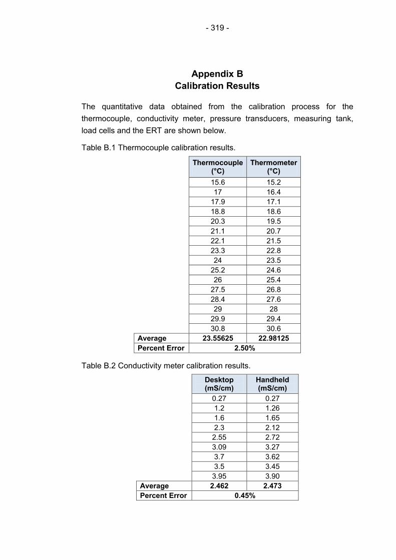
- 319 -
Appendix B
Calibration Results
The quantitative data obtained from the calibration process for the
thermocouple, conductivity meter, pressure transducers, measuring tank,
load cells and the ERT are shown below.
Table B.1 Thermocouple calibration results.
Thermocouple (°C)
Thermometer (°C)
15.6 15.2
17 16.4
17.9 17.1
18.8 18.6
20.3 19.5
21.1 20.7
22.1 21.5
23.3 22.8
24 23.5
25.2 24.6
26 25.4
27.5 26.8
28.4 27.6
29 28
29.9 29.4
30.8 30.6
Average 23.55625 22.98125
Percent Error 2.50%
Table B.2 Conductivity meter calibration results.
Desktop (mS/cm)
Handheld (mS/cm)
0.27 0.27
1.2 1.26
1.6 1.65
2.3 2.12
2.55 2.72
3.09 3.27
3.7 3.62
3.5 3.45
3.95 3.90
Average 2.462 2.473
Percent Error 0.45%
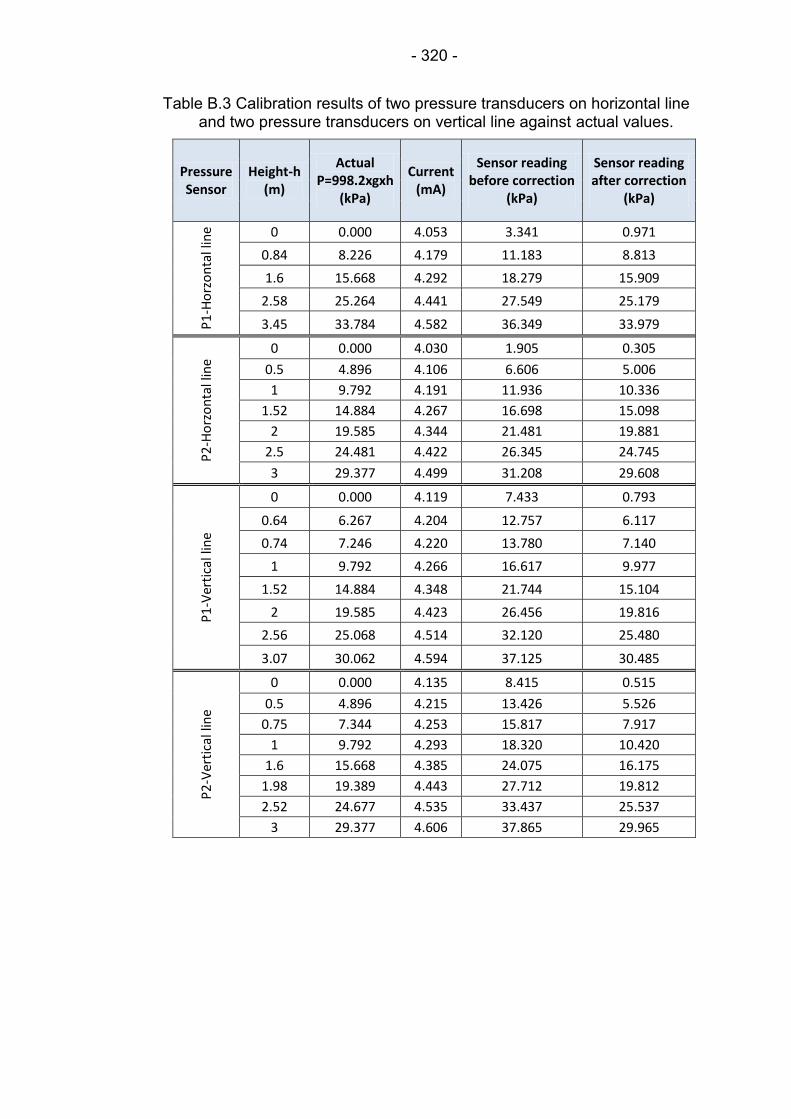
- 320 -
Table B.3 Calibration results of two pressure transducers on horizontal line and two pressure transducers on vertical line against actual values.
Pressure Sensor
Height-h (m)
Actual P=998.2xgxh
(kPa)
Current (mA)
Sensor reading before correction
(kPa)
Sensor reading after correction
(kPa) P
1-H
orz
on
tal l
ine 0 0.000 4.053 3.341 0.971
0.84 8.226 4.179 11.183 8.813
1.6 15.668 4.292 18.279 15.909
2.58 25.264 4.441 27.549 25.179
3.45 33.784 4.582 36.349 33.979
P2
-Ho
rzo
nta
l lin
e
0 0.000 4.030 1.905 0.305
0.5 4.896 4.106 6.606 5.006
1 9.792 4.191 11.936 10.336
1.52 14.884 4.267 16.698 15.098
2 19.585 4.344 21.481 19.881
2.5 24.481 4.422 26.345 24.745
3 29.377 4.499 31.208 29.608
P1
-Ver
tica
l lin
e
0 0.000 4.119 7.433 0.793
0.64 6.267 4.204 12.757 6.117
0.74 7.246 4.220 13.780 7.140
1 9.792 4.266 16.617 9.977
1.52 14.884 4.348 21.744 15.104
2 19.585 4.423 26.456 19.816
2.56 25.068 4.514 32.120 25.480
3.07 30.062 4.594 37.125 30.485
P2
-Ver
tica
l lin
e
0 0.000 4.135 8.415 0.515
0.5 4.896 4.215 13.426 5.526
0.75 7.344 4.253 15.817 7.917
1 9.792 4.293 18.320 10.420
1.6 15.668 4.385 24.075 16.175
1.98 19.389 4.443 27.712 19.812
2.52 24.677 4.535 33.437 25.537
3 29.377 4.606 37.865 29.965
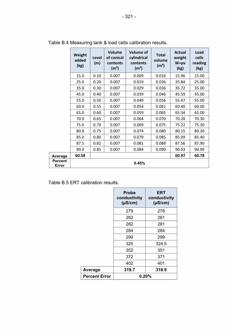
- 321 -
Table B.4 Measuring tank & load cells calibration results.
Weight added
(kg)
Level (m)
Volume of conical contents
(m³)
Volume of cylindrical contents
(m³)
Total volume
(m³)
Actual weight W=ρv (kg)
Load cells
reading (kg)
15.0 0.10 0.007 0.009 0.016 15.96 15.00
25.0 0.20 0.007 0.019 0.026 25.84 25.00
35.0 0.30 0.007 0.029 0.036 35.72 35.00
45.0 0.40 0.007 0.039 0.046 45.59 45.00
55.0 0.50 0.007 0.049 0.056 55.47 55.00
60.0 0.55 0.007 0.054 0.061 60.40 60.00
65.0 0.60 0.007 0.059 0.065 65.34 65.00
70.0 0.65 0.007 0.064 0.070 70.28 70.30
75.0 0.70 0.007 0.069 0.075 75.22 75.30
80.0 0.75 0.007 0.074 0.080 80.15 80.30
85.0 0.80 0.007 0.079 0.085 85.09 85.40
87.5 0.82 0.007 0.081 0.088 87.56 87.90
90.0 0.85 0.007 0.084 0.090 90.03 90.90
Average 60.58 60.97 60.78 Percent
Error 0.45%
Table B.5 ERT calibration results.
Probe
conductivity (µS/cm)
ERT conductivity
(µS/cm)
279 278
282 281
282 281
284 284
299 299
325 324.5
352 351
372 371
402 401
Average 319.7 318.9
Percent Error 0.20%
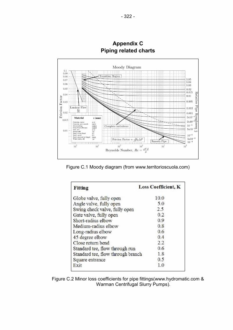
- 322 -
Appendix C
Piping related charts
Figure C.1 Moody diagram (from www.territorioscuola.com)
Figure C.2 Minor loss coefficients for pipe fittings(www.hydromatic.com & Warman Centrifugal Slurry Pumps).

- 323 -
Appendix D
MATLAB script for automated flow regime recognition
The full MATLAB script, which has been developed for automated flow
regime recognition, measurement of solids volume fraction and visualisation
of solids volumetric distribution across the horizontal pipe cross-section is
shown below:
clc
h = waitbar(1,{'Please wait...';'computation in progress'}); steps = 1; for step = 1:steps
%tic
%Read the columns in zave file (it takes 40 seconds to read all the %following data from zave.csv file). %Each column reresent a zone in the vertical line of the pipe cross-
section. Z1 = xlsread('zave.csv', 1, 'D3:D8002'); Z2 = xlsread('zave.csv', 1, 'H3:H8002'); Z3 = xlsread('zave.csv', 1, 'M3:M8002'); Z4 = xlsread('zave.csv', 1, 'R3:R8002'); Z5 = xlsread('zave.csv', 1, 'V3:V8002');
%toc
importfile('Warning.mat'); T = 0.0015; % Sample Time Fs = 1/T; % Sampling Frequency L = 8000; % Length of Signal % Sum of a 50 Hz sinusoid and a 120 Hz sinusoid
NFFT = 2^nextpow2(L); % Next power of 2 from length of y
V = fft (Z1,NFFT)/L; % Zone 1 W = fft (Z2,NFFT)/L; % Zone 2 X = fft (Z3,NFFT)/L; % Zone 3 Y = fft (Z4,NFFT)/L; % Zone 4 Z = fft (Z5,NFFT)/L; % Zone 5
f = Fs/2*linspace(0,1,NFFT/2+1);
Plot single sided amplitude spectrum plot(f,2*abs(V(1:NFFT/2+1)),f,2*abs(W(1:NFFT/2+1)),f,2*abs(X(1:NFFT/
2+1)),f,2*abs(Y(1:NFFT/2+1)),f,2*abs(Z(1:NFFT/2+1)))
plot(f,2*abs(V(1:NFFT/2+1))) plot(f,2*abs(W(1:NFFT/2+1))) plot(f,2*abs(X(1:NFFT/2+1))) plot(f,2*abs(Y(1:NFFT/2+1)))
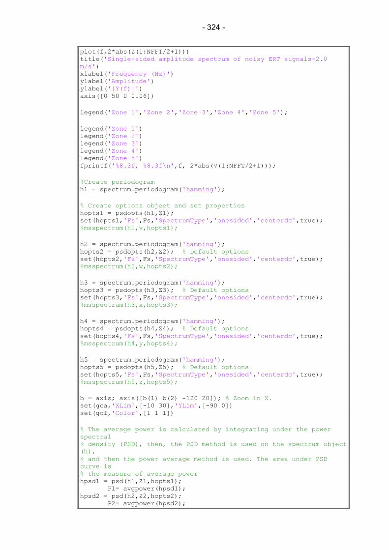
- 324 -
plot(f,2*abs(Z(1:NFFT/2+1))) title('Single-sided amplitude spectrum of noisy ERT signals-2.0
m/s') xlabel('Frequency (Hz)') ylabel('Amplitude') ylabel('|Y(f)|') axis([0 50 0 0.06])
legend('Zone 1','Zone 2','Zone 3','Zone 4','Zone 5');
legend('Zone 1') legend('Zone 2') legend('Zone 3') legend('Zone 4') legend('Zone 5') fprintf('%8.3f, %8.3f\n',f, 2*abs(V(1:NFFT/2+1)));
%Create periodogram h1 = spectrum.periodogram('hamming');
% Create options object and set properties hopts1 = psdopts(h1,Z1); set(hopts1,'Fs',Fs,'SpectrumType','onesided','centerdc',true); %msspectrum(h1,v,hopts1);
h2 = spectrum.periodogram('hamming'); hopts2 = psdopts(h2,Z2); % Default options set(hopts2,'Fs',Fs,'SpectrumType','onesided','centerdc',true); %msspectrum(h2,w,hopts2);
h3 = spectrum.periodogram('hamming'); hopts3 = psdopts(h3,Z3); % Default options set(hopts3,'Fs',Fs,'SpectrumType','onesided','centerdc',true); %msspectrum(h3,x,hopts3);
h4 = spectrum.periodogram('hamming'); hopts4 = psdopts(h4,Z4); % Default options set(hopts4,'Fs',Fs,'SpectrumType','onesided','centerdc',true); %msspectrum(h4,y,hopts4);
h5 = spectrum.periodogram('hamming'); hopts5 = psdopts(h5,Z5); % Default options set(hopts5,'Fs',Fs,'SpectrumType','onesided','centerdc',true); %msspectrum(h5,z,hopts5);
b = axis; axis([b(1) b(2) -120 20]); % Zoom in X. set(gca,'XLim',[-10 30],'YLim',[-90 0]) set(gcf,'Color',[1 1 1])
% The average power is calculated by integrating under the power
spectral % density (PSD), then, the PSD method is used on the spectrum object
(h), % and then the power average method is used. The area under PSD
curve is % the measure of average power hpsd1 = psd(h1,Z1,hopts1); P1= avgpower(hpsd1); hpsd2 = psd(h2,Z2,hopts2); P2= avgpower(hpsd2);

- 325 -
hpsd3 = psd(h3,Z3,hopts3); P3= avgpower(hpsd3); hpsd4 = psd(h4,Z4,hopts4); P4= avgpower(hpsd4); hpsd5 = psd(h5,Z5,hopts5); P5= avgpower(hpsd5);
meanZ1=mean(Z1); meanZ2=mean(Z2); meanZ3=mean(Z3); meanZ4=mean(Z4); meanZ5=mean(Z5);
E=P1+P2+(P3/2); F=(P3/2)+P4+P5;
D = E/(E+F);
A=meanZ1+meanZ2+(meanZ3/2); B=(meanZ3/2)+meanZ4+meanZ5; C=A/(A+B);
G=std(Z5);
if(C>=0.499 && C<0.501 && D>=0.496 && D<504) fprintf('HOMOGENEOUS FLOW REGIME\n'); msgbox('HOMOGENEOUS FLOW REGIME...','FLOW REGIME', 'replace') beep
elseif (C>=0.501 && C<0.505 && D>=0.504 && D<0.510)
fprintf('PSEUDO-HOMOGENEOUS FLOW REGIME\n'); msgbox('PSEUDO-HOMOGENEOUS FLOW REGIME...','FLOW REGIME',
'replace') beep
elseif (C>=0.505 && C<0.510 && D>=0.510 && D<0.520)
fprintf('TRANSITIONAL REGIME BOUNDARY(PSUDOHOMOGENEOUS-
HETEROGENEOUS)\n'); msgbox({'TRANSITIONAL REGIME BOUNDARY';'(PSUDOHOMOGENEOUS-
HETEROGENEOUS)...'},'FLOW REGIME', 'replace') beep
elseif (C>=0.510 && C<0.532 && D>=0.520 && D<0.555)
fprintf('HETEROGENEOUS FLOW REGIME\n'); msgbox('HETEROGENEOUS FLOW REGIME...','FLOW REGIME', 'replace') beep
elseif (C>=0.532 && C<0.540 && D>=0.555 && D<0.570)
fprintf('TRANSITIONAL REGIME BOUNDARY(HETEROGENEOUS-MOVING
BED)\n'); msgbox({'TRANSITIONAL REGIME BOUNDARY';'(HETEROGENEOUS-MOVING
BED)...'},'FLOW REGIME', 'replace') beep
elseif (C>=0.540 && C<0.652 && D>=0.570 && D<0.770)
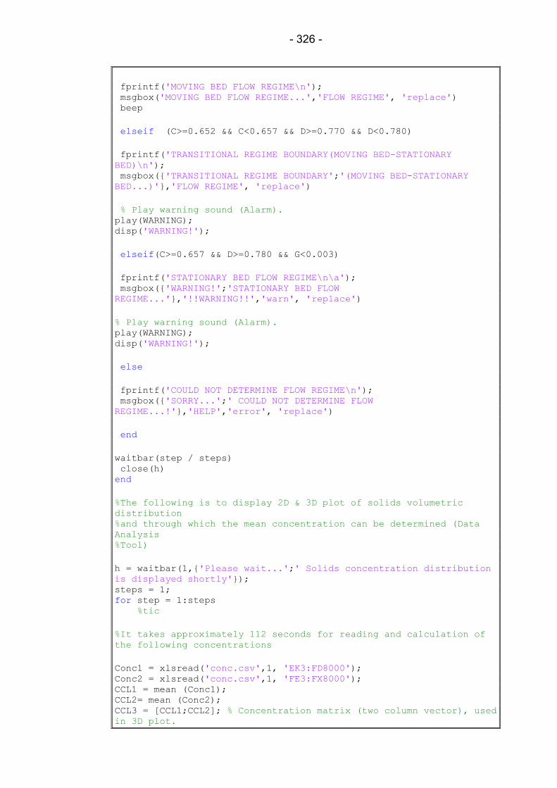
- 326 -
fprintf('MOVING BED FLOW REGIME\n'); msgbox('MOVING BED FLOW REGIME...','FLOW REGIME', 'replace') beep
elseif (C>=0.652 && C<0.657 && D>=0.770 && D<0.780)
fprintf('TRANSITIONAL REGIME BOUNDARY(MOVING BED-STATIONARY
BED)\n'); msgbox({'TRANSITIONAL REGIME BOUNDARY';'(MOVING BED-STATIONARY
BED...)'},'FLOW REGIME', 'replace')
% Play warning sound (Alarm). play(WARNING); disp('WARNING!');
elseif(C>=0.657 && D>=0.780 && G<0.003)
fprintf('STATIONARY BED FLOW REGIME\n\a'); msgbox({'WARNING!';'STATIONARY BED FLOW
REGIME...'},'!!WARNING!!','warn', 'replace')
% Play warning sound (Alarm). play(WARNING); disp('WARNING!');
else
fprintf('COULD NOT DETERMINE FLOW REGIME\n'); msgbox({'SORRY...';' COULD NOT DETERMINE FLOW
REGIME...!'},'HELP','error', 'replace')
end
waitbar(step / steps) close(h) end
%The following is to display 2D & 3D plot of solids volumetric
distribution %and through which the mean concentration can be determined (Data
Analysis %Tool)
h = waitbar(1,{'Please wait...';' Solids concentration distribution
is displayed shortly'}); steps = 1; for step = 1:steps %tic
%It takes approximately 112 seconds for reading and calculation of
the following concentrations
Conc1 = xlsread('conc.csv',1, 'EK3:FD8000'); Conc2 = xlsread('conc.csv',1, 'FE3:FX8000'); CCL1 = mean (Conc1); CCL2= mean (Conc2); CCL3 = [CCL1;CCL2]; % Concentration matrix (two column vector), used
in 3D plot.

- 327 -
CCL4 = mean(CCL3); % Mean concentration of the dual centreline, Used
for the x-axis of the 2D Plot.
%toc
VP1 = (1:-0.05:0.05); VP2 = (1:-0.05:0.05); VP = [VP1;VP2]; % Vertical Position of the pipe cross-section, used
in 2D &3D plot.
HP1(1:20)=0.5; HP2(1:20)=0.55; HP = [HP1;HP2]; % It is an array of 2 raws, indicating the
horizontal position of the pipe cross-section and used in 3D plot.
%Creating surface (3D)plot of the vertical dual centerline of the
concentration tomogram. Surface_Solids_Volumetric_Distribution(HP, CCL3, VP)
%Creating (2D)plot of the vertical centerline of the concentration
tomogram. Two_Dimenssional_Concentration_Distribution_Plot(CCL4, VP1)
waitbar(step / steps) end close(h)

- 328 -
Appendix E
Horizontal & vertical flow loop sensor data
The following tables showing the flow loop sensor data obtained from the EMF, the pressure transducers, the thermocouple and the
measuring tank (flow diversion technique), for each sand and different transport velocities.
Table E.1 Flow loop sensor data for flowing medium sand at 2% throughput concentration.
Solid Particle
EMF (m/s)
T (°C)
P1 Horizontal
(kPa)
P2 Horizontal
(kPa)
P1 Vertical
(kPa)
P2 Vertical
(kPa)
dp Horizontal
(kPa)
Discharge Velocity
(m/s)
Delivered Conc. (v/v)
μm/μl Slurry
Viscosity (pa.s)
Slurry Reynolds Number
(Rem)
2%
Med
ium
San
d
4.97 16.61 98.40 87.00 64.40 25.12 11.40 4.97 0.0242 1.06 0.00106 233595
4.53 18.48 86.17 76.91 57.32 20.48 9.27 4.49 0.0224 1.06 0.00106 211908
4.02 19.87 76.13 69.22 51.30 16.94 6.91 4.08 0.0243 1.06 0.00106 191872
3.49 20.91 66.30 60.93 45.10 13.06 5.38 3.49 0.0268 1.06 0.00106 164167
3.05 21.65 59.31 55.05 40.89 10.40 4.27 3.05 0.0245 1.06 0.00106 143458
2.52 22.25 51.90 48.97 36.90 7.60 2.93 2.55 0.0251 1.06 0.00106 119708
2.06 22.25 46.82 44.79 33.95 5.66 2.03 2.12 0.025 1.06 0.00106 99490
1.49 22.25 41.51 40.52 30.86 3.69 0.98 1.54 0.0239 1.05 0.00105 73096

- 329 -
Table E.2 Flow loop sensor data for flowing medium sand at 10% throughput concentration.
Solid Particle
EMF (m/s)
T (°C)
P1 Horizontal
(kPa)
P2 Horizontal
(kPa)
P1 Vertical
(kPa)
P2 Vertical
(kPa)
dp Horizontal
(kPa)
Discharge Velocity
(m/s)
Delivered Conc. (v/v)
μm/μl Slurry
Viscosity (pa.s)
Slurry Reynolds Number
(Rem)
10
% M
ediu
m S
and
4.96 26.00 106.9 95.43 70.32 29.18 11.42 5.59 0.0838 1.37 0.00137 204271
4.59 27.25 93.30 84.39 62.25 23.82 8.91 4.47 0.0926 1.37 0.00137 163334
4.06 27.84 83.47 76.20 56.68 19.51 7.26 4.00 0.0913 1.37 0.00137 146078
3.49 28.15 73.09 67.68 50.22 15.38 5.41 3.47 0.0962 1.37 0.00137 126714
3.04 28.36 65.79 61.42 45.74 12.30 4.37 3.19 0.0927 1.37 0.00137 116452
2.52 28.46 57.75 54.87 40.72 8.87 2.87 2.54 0.0955 1.37 0.00137 92683
2.01 28.48 52.29 50.18 37.35 6.63 2.10 2.02 0.0979 1.37 0.00137 73928
1.52 28.42 48.77 46.81 35.12 5.21 1.96 1.58 0.0968 1.37 0.00137 57626
Table E.3 Flow loop sensor data for flowing coarse sand at 2% throughput concentration.
Solid Particle
EMF (m/s)
T (°C)
P1 Horizontal
(kPa)
P2 Horizontal
(kPa)
P1 Vertical
(kPa)
P2 Vertical
(kPa)
dp Horizontal
(kPa)
Discharge Velocity
(m/s)
Delivered Conc. (v/v)
μm/μl Slurry
Viscosity (pa.s)
Slurry Reynolds Number
(Rem)
2%
Co
arse
San
d
4.93 17.17 105.6 94.37 68.49 29.45 11.27 4.82 0.0302 1.09 0.00109 220517
4.36 18.76 90.13 82.55 59.16 23.55 7.58 4.53 0.0325 1.09 0.00109 207337
4.11 19.67 79.39 73.40 52.29 19.50 6.00 4.29 0.0295 1.09 0.00109 196205
3.52 20.32 69.17 65.00 46.22 15.34 4.17 3.66 0.0315 1.09 0.00109 167651
3.11 20.73 61.45 58.52 41.98 12.27 2.93 3.18 0.032 1.09 0.00109 145717
2.52 21.02 53.17 51.60 37.09 8.81 1.57 2.45 0.0344 1.09 0.00109 112076
2.00 21.27 47.79 47.25 33.38 6.56 0.54 2.03 0.0302 1.09 0.00109 93116
1.52 21.47 43.97 43.88 31.10 5.17 0.10 1.50 0.0283 1.09 0.00109 68446
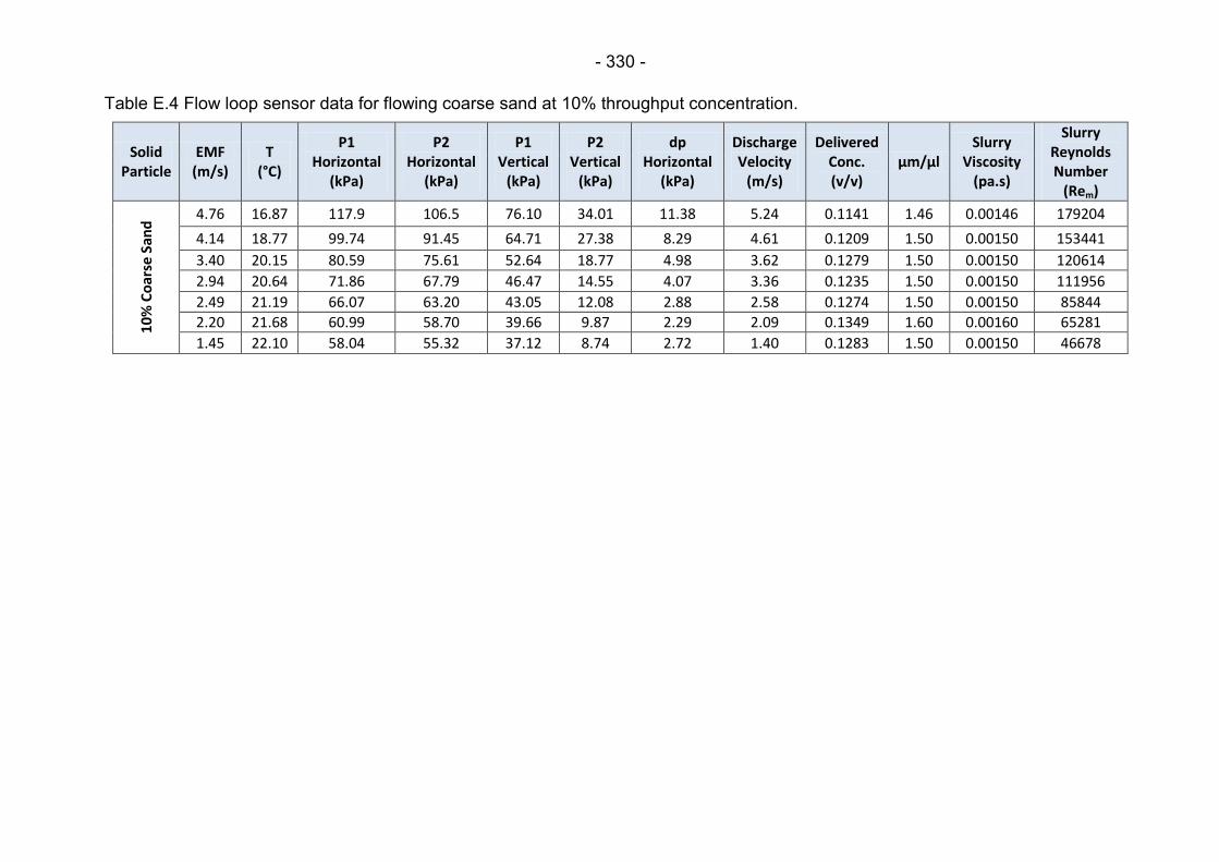
- 330 -
Table E.4 Flow loop sensor data for flowing coarse sand at 10% throughput concentration.
Solid Particle
EMF (m/s)
T (°C)
P1 Horizontal
(kPa)
P2 Horizontal
(kPa)
P1 Vertical
(kPa)
P2 Vertical
(kPa)
dp Horizontal
(kPa)
Discharge Velocity
(m/s)
Delivered Conc. (v/v)
μm/μl Slurry
Viscosity (pa.s)
Slurry Reynolds Number
(Rem)
10
% C
oar
se S
and
4.76 16.87 117.9 106.5 76.10 34.01 11.38 5.24 0.1141 1.46 0.00146 179204
4.14 18.77 99.74 91.45 64.71 27.38 8.29 4.61 0.1209 1.50 0.00150 153441
3.40 20.15 80.59 75.61 52.64 18.77 4.98 3.62 0.1279 1.50 0.00150 120614
2.94 20.64 71.86 67.79 46.47 14.55 4.07 3.36 0.1235 1.50 0.00150 111956
2.49 21.19 66.07 63.20 43.05 12.08 2.88 2.58 0.1274 1.50 0.00150 85844
2.20 21.68 60.99 58.70 39.66 9.87 2.29 2.09 0.1349 1.60 0.00160 65281
1.45 22.10 58.04 55.32 37.12 8.74 2.72 1.40 0.1283 1.50 0.00150 46678
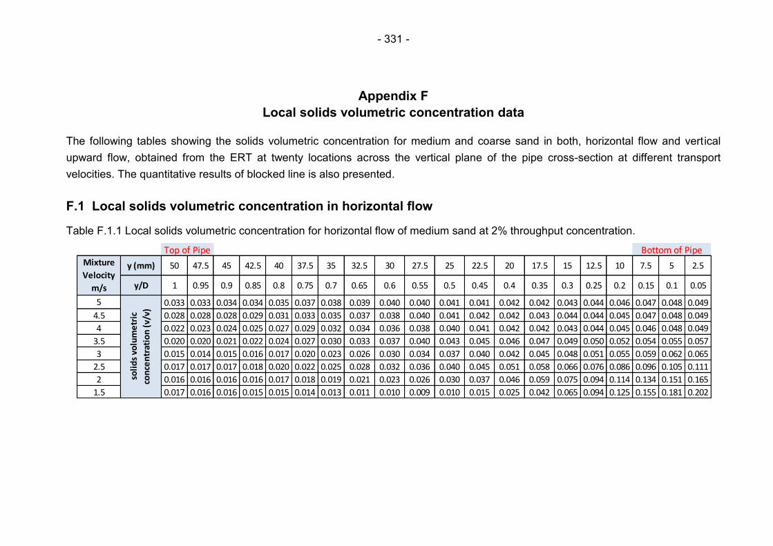
- 331 -
Appendix F
Local solids volumetric concentration data
The following tables showing the solids volumetric concentration for medium and coarse sand in both, horizontal flow and vertical
upward flow, obtained from the ERT at twenty locations across the vertical plane of the pipe cross-section at different transport
velocities. The quantitative results of blocked line is also presented.
F.1 Local solids volumetric concentration in horizontal flow
Table F.1.1 Local solids volumetric concentration for horizontal flow of medium sand at 2% throughput concentration.
y (mm) 50 47.5 45 42.5 40 37.5 35 32.5 30 27.5 25 22.5 20 17.5 15 12.5 10 7.5 5 2.5
y/D 1 0.95 0.9 0.85 0.8 0.75 0.7 0.65 0.6 0.55 0.5 0.45 0.4 0.35 0.3 0.25 0.2 0.15 0.1 0.05
5 0.033 0.033 0.034 0.034 0.035 0.037 0.038 0.039 0.040 0.040 0.041 0.041 0.042 0.042 0.043 0.044 0.046 0.047 0.048 0.049
4.5 0.028 0.028 0.028 0.029 0.031 0.033 0.035 0.037 0.038 0.040 0.041 0.042 0.042 0.043 0.044 0.044 0.045 0.047 0.048 0.049
4 0.022 0.023 0.024 0.025 0.027 0.029 0.032 0.034 0.036 0.038 0.040 0.041 0.042 0.042 0.043 0.044 0.045 0.046 0.048 0.049
3.5 0.020 0.020 0.021 0.022 0.024 0.027 0.030 0.033 0.037 0.040 0.043 0.045 0.046 0.047 0.049 0.050 0.052 0.054 0.055 0.057
3 0.015 0.014 0.015 0.016 0.017 0.020 0.023 0.026 0.030 0.034 0.037 0.040 0.042 0.045 0.048 0.051 0.055 0.059 0.062 0.065
2.5 0.017 0.017 0.017 0.018 0.020 0.022 0.025 0.028 0.032 0.036 0.040 0.045 0.051 0.058 0.066 0.076 0.086 0.096 0.105 0.111
2 0.016 0.016 0.016 0.016 0.017 0.018 0.019 0.021 0.023 0.026 0.030 0.037 0.046 0.059 0.075 0.094 0.114 0.134 0.151 0.165
1.5 0.017 0.016 0.016 0.015 0.015 0.014 0.013 0.011 0.010 0.009 0.010 0.015 0.025 0.042 0.065 0.094 0.125 0.155 0.181 0.202
Mixture
Velocity
m/s
soli
ds
volu
me
tric
con
cen
trat
ion
(v/
v)
Top of Pipe Bottom of Pipe
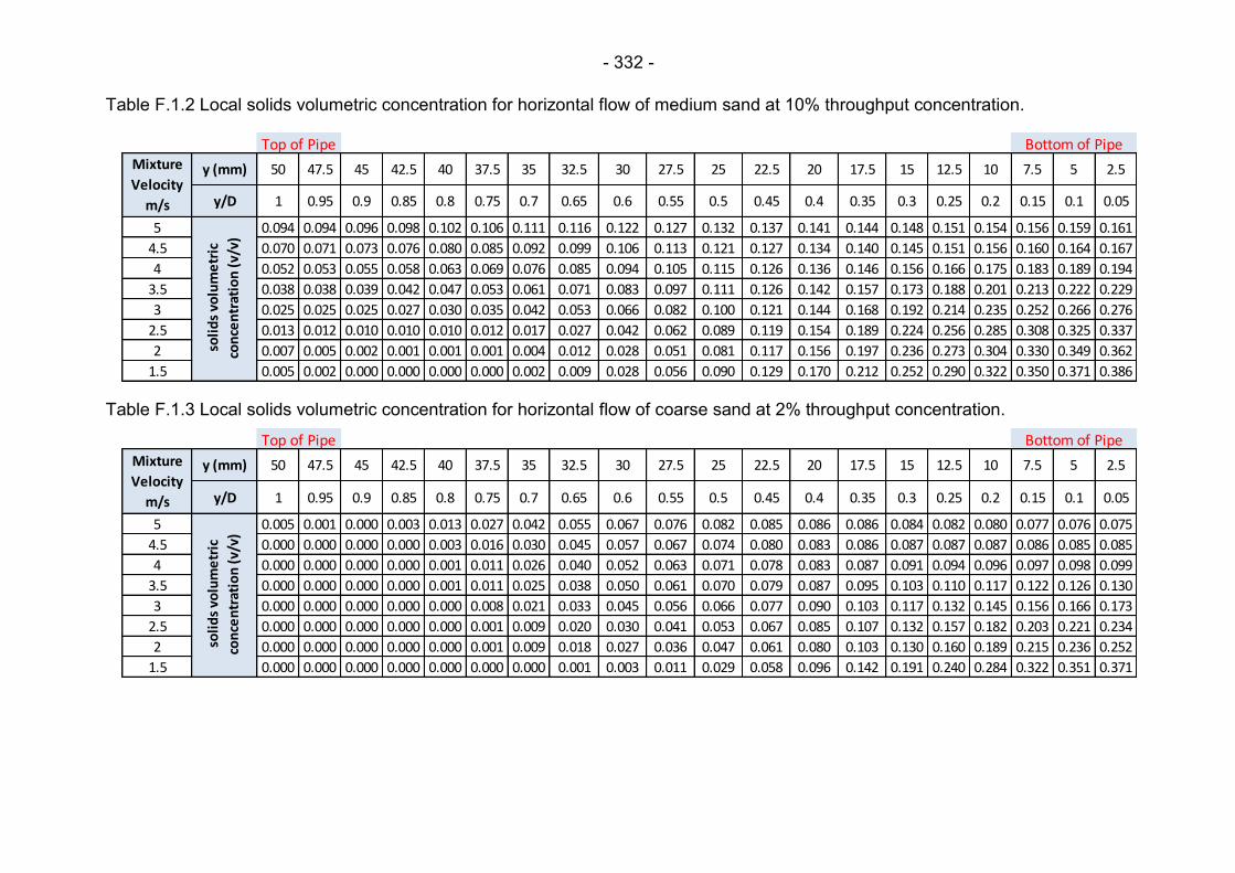
- 332 -
Table F.1.2 Local solids volumetric concentration for horizontal flow of medium sand at 10% throughput concentration.
Table F.1.3 Local solids volumetric concentration for horizontal flow of coarse sand at 2% throughput concentration.
y (mm) 50 47.5 45 42.5 40 37.5 35 32.5 30 27.5 25 22.5 20 17.5 15 12.5 10 7.5 5 2.5
y/D 1 0.95 0.9 0.85 0.8 0.75 0.7 0.65 0.6 0.55 0.5 0.45 0.4 0.35 0.3 0.25 0.2 0.15 0.1 0.05
5 0.094 0.094 0.096 0.098 0.102 0.106 0.111 0.116 0.122 0.127 0.132 0.137 0.141 0.144 0.148 0.151 0.154 0.156 0.159 0.161
4.5 0.070 0.071 0.073 0.076 0.080 0.085 0.092 0.099 0.106 0.113 0.121 0.127 0.134 0.140 0.145 0.151 0.156 0.160 0.164 0.167
4 0.052 0.053 0.055 0.058 0.063 0.069 0.076 0.085 0.094 0.105 0.115 0.126 0.136 0.146 0.156 0.166 0.175 0.183 0.189 0.194
3.5 0.038 0.038 0.039 0.042 0.047 0.053 0.061 0.071 0.083 0.097 0.111 0.126 0.142 0.157 0.173 0.188 0.201 0.213 0.222 0.229
3 0.025 0.025 0.025 0.027 0.030 0.035 0.042 0.053 0.066 0.082 0.100 0.121 0.144 0.168 0.192 0.214 0.235 0.252 0.266 0.276
2.5 0.013 0.012 0.010 0.010 0.010 0.012 0.017 0.027 0.042 0.062 0.089 0.119 0.154 0.189 0.224 0.256 0.285 0.308 0.325 0.337
2 0.007 0.005 0.002 0.001 0.001 0.001 0.004 0.012 0.028 0.051 0.081 0.117 0.156 0.197 0.236 0.273 0.304 0.330 0.349 0.362
1.5 0.005 0.002 0.000 0.000 0.000 0.000 0.002 0.009 0.028 0.056 0.090 0.129 0.170 0.212 0.252 0.290 0.322 0.350 0.371 0.386
Mixture
Velocity
m/sso
lid
s vo
lum
etr
ic
con
cen
trat
ion
(v/
v)
Top of Pipe Bottom of Pipe
y (mm) 50 47.5 45 42.5 40 37.5 35 32.5 30 27.5 25 22.5 20 17.5 15 12.5 10 7.5 5 2.5
y/D 1 0.95 0.9 0.85 0.8 0.75 0.7 0.65 0.6 0.55 0.5 0.45 0.4 0.35 0.3 0.25 0.2 0.15 0.1 0.05
5 0.005 0.001 0.000 0.003 0.013 0.027 0.042 0.055 0.067 0.076 0.082 0.085 0.086 0.086 0.084 0.082 0.080 0.077 0.076 0.075
4.5 0.000 0.000 0.000 0.000 0.003 0.016 0.030 0.045 0.057 0.067 0.074 0.080 0.083 0.086 0.087 0.087 0.087 0.086 0.085 0.085
4 0.000 0.000 0.000 0.000 0.001 0.011 0.026 0.040 0.052 0.063 0.071 0.078 0.083 0.087 0.091 0.094 0.096 0.097 0.098 0.099
3.5 0.000 0.000 0.000 0.000 0.001 0.011 0.025 0.038 0.050 0.061 0.070 0.079 0.087 0.095 0.103 0.110 0.117 0.122 0.126 0.130
3 0.000 0.000 0.000 0.000 0.000 0.008 0.021 0.033 0.045 0.056 0.066 0.077 0.090 0.103 0.117 0.132 0.145 0.156 0.166 0.173
2.5 0.000 0.000 0.000 0.000 0.000 0.001 0.009 0.020 0.030 0.041 0.053 0.067 0.085 0.107 0.132 0.157 0.182 0.203 0.221 0.234
2 0.000 0.000 0.000 0.000 0.000 0.001 0.009 0.018 0.027 0.036 0.047 0.061 0.080 0.103 0.130 0.160 0.189 0.215 0.236 0.252
1.5 0.000 0.000 0.000 0.000 0.000 0.000 0.000 0.001 0.003 0.011 0.029 0.058 0.096 0.142 0.191 0.240 0.284 0.322 0.351 0.371
Mixture
Velocity
m/s
soli
ds
volu
me
tric
con
cen
trat
ion
(v/
v)
Bottom of PipeTop of Pipe

- 333 -
Table F.1.4 Local solids volumetric concentration for horizontal flow of coarse sand at 10% throughput concentration.
Table F.1.5 Local solids volumetric concentration for blocked horizontal line with coarse sand at 10% throughput concentration.
y (mm) 50 47.5 45 42.5 40 37.5 35 32.5 30 27.5 25 22.5 20 17.5 15 12.5 10 7.5 5 2.5
y/D 1 0.95 0.9 0.85 0.8 0.75 0.7 0.65 0.6 0.55 0.5 0.45 0.4 0.35 0.3 0.25 0.2 0.15 0.1 0.05
4.5 0.088 0.087 0.087 0.088 0.09 0.095 0.104 0.1181 0.1383 0.1632 0.191 0.2191 0.2451 0.2669 0.284 0.295 0.301 0.302 0.301 0.3
4 0.036 0.034 0.032 0.03 0.03 0.034 0.044 0.0631 0.0912 0.127 0.1671 0.2075 0.2447 0.2761 0.3 0.317 0.327 0.332 0.333 0.332
3.5 0.002 4E-04 1E-05 2E-08 0 0 5E-05 0.0046 0.0342 0.082 0.1399 0.2012 0.2596 0.3103 0.351 0.381 0.401 0.413 0.419 0.421
3 4E-07 0 0 0 0 0 3E-06 0.0005 0.015 0.065 0.1288 0.1965 0.2608 0.3167 0.362 0.396 0.419 0.433 0.441 0.444
2.5 0 0 0 0 0 0 0 6E-05 0.0035 0.0382 0.0993 0.1667 0.2326 0.2913 0.34 0.377 0.403 0.421 0.431 0.436
2 0 0 0 0 0 6E-06 2E-04 0.0021 0.0122 0.0568 0.1305 0.2079 0.28 0.3415 0.39 0.427 0.452 0.468 0.477 0.481
1.5 0 0 0 0 0 0 1E-04 0.0044 0.044 0.1194 0.2004 0.2774 0.3453 0.4017 0.447 0.481 0.507 0.524 0.535 0.541
Mixture
Velocity
m/sso
lid
s vo
lum
etr
ic
con
cen
trat
ion
(v/
v)
Bottom of PipeTop of Pipe
y (mm) 50 47.5 45 42.5 40 37.5 35 32.5 30 27.5 25 22.5 20 17.5 15 12.5 10 7.5 5 2.5
y/D 1 0.95 0.9 0.85 0.8 0.75 0.7 0.65 0.6 0.55 0.5 0.45 0.4 0.35 0.3 0.25 0.2 0.15 0.1 0.05
0.0
so
lid
s vo
lum
etr
ic
con
cen
trat
ion
(v/
v)
0.0 0.0 0.0 0.0 0.0 0.0 0.2 0.3 0.5 0.5 0.6 0.6 0.6 0.6 0.6 0.6 0.6 0.6 0.6 0.6
Mixture
Velocity
m/s
Bottom of PipeTop of Pipe
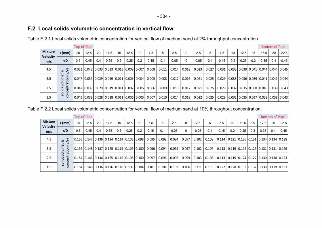
- 334 -
F.2 Local solids volumetric concentration in vertical flow
Table F.2.1 Local solids volumetric concentration for vertical flow of medium sand at 2% throughput concentration.
Table F.2.2 Local solids volumetric concentration for vertical flow of medium sand at 10% throughput concentration.
r (mm) 25 22.5 20 17.5 15 12.5 10 7.5 5 2.5 0 -2.5 -5 -7.5 -10 -12.5 -15 -17.5 -20 -22.5
r/D 0.5 0.45 0.4 0.35 0.3 0.25 0.2 0.15 0.1 0.05 0 -0.05 -0.1 -0.15 -0.2 -0.25 -0.3 -0.35 -0.4 -0.45
4.5 0.051 0.043 0.033 0.023 0.015 0.009 0.007 0.008 0.011 0.014 0.018 0.023 0.027 0.031 0.035 0.038 0.041 0.044 0.044 0.045
3.5 0.047 0.039 0.029 0.019 0.011 0.006 0.004 0.005 0.008 0.012 0.016 0.021 0.025 0.029 0.033 0.036 0.039 0.041 0.041 0.044
2.5 0.047 0.039 0.029 0.019 0.011 0.007 0.005 0.006 0.009 0.013 0.017 0.021 0.025 0.029 0.032 0.035 0.038 0.040 0.039 0.043
1.5 0.045 0.038 0.028 0.018 0.011 0.006 0.005 0.007 0.010 0.014 0.018 0.022 0.025 0.029 0.032 0.035 0.037 0.038 0.038 0.043
Mixture
Velocity
m/sso
lid
s vo
lum
etr
ic
con
cen
trat
ion
(v/
v)
Bottom of PipeTop of Pipe
r (mm) 25 22.5 20 17.5 15 12.5 10 7.5 5 2.5 0 -2.5 -5 -7.5 -10 -12.5 -15 -17.5 -20 -22.5
r/D 0.5 0.45 0.4 0.35 0.3 0.25 0.2 0.15 0.1 0.05 0 -0.05 -0.1 -0.15 -0.2 -0.25 -0.3 -0.35 -0.4 -0.45
4.5 0.155 0.147 0.136 0.124 0.114 0.105 0.098 0.095 0.093 0.094 0.097 0.102 0.108 0.114 0.121 0.126 0.131 0.134 0.134 0.128
3.5 0.156 0.148 0.137 0.125 0.115 0.106 0.100 0.096 0.094 0.095 0.097 0.102 0.107 0.113 0.119 0.124 0.129 0.131 0.131 0.126
2.5 0.154 0.146 0.136 0.125 0.115 0.106 0.100 0.097 0.096 0.096 0.099 0.103 0.108 0.113 0.119 0.124 0.127 0.130 0.130 0.123
1.5 0.154 0.146 0.136 0.126 0.116 0.109 0.104 0.101 0.101 0.103 0.106 0.111 0.116 0.122 0.128 0.133 0.137 0.139 0.139 0.133
soli
ds
volu
me
tric
con
cen
trat
ion
(v/
v)
Mixture
Velocity
m/s
Bottom of PipeTop of Pipe
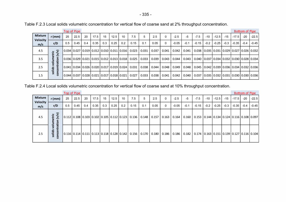
- 335 -
Table F.2.3 Local solids volumetric concentration for vertical flow of coarse sand at 2% throughput concentration.
Table F.2.4 Local solids volumetric concentration for vertical flow of coarse sand at 10% throughput concentration.
r (mm) 25 22.5 20 17.5 15 12.5 10 7.5 5 2.5 0 -2.5 -5 -7.5 -10 -12.5 -15 -17.5 -20 -22.5
r/D 0.5 0.45 0.4 0.35 0.3 0.25 0.2 0.15 0.1 0.05 0 -0.05 -0.1 -0.15 -0.2 -0.25 -0.3 -0.35 -0.4 -0.45
4.5 0.034 0.027 0.019 0.012 0.010 0.011 0.016 0.023 0.031 0.037 0.041 0.042 0.041 0.038 0.035 0.031 0.029 0.027 0.026 0.032
3.5 0.036 0.029 0.021 0.015 0.012 0.013 0.018 0.025 0.033 0.039 0.043 0.044 0.043 0.040 0.037 0.034 0.032 0.030 0.028 0.034
2.5 0.041 0.034 0.026 0.020 0.017 0.019 0.024 0.031 0.038 0.044 0.048 0.049 0.048 0.045 0.042 0.039 0.036 0.034 0.032 0.036
1.5 0.044 0.037 0.028 0.021 0.017 0.018 0.021 0.027 0.033 0.038 0.041 0.042 0.040 0.037 0.035 0.032 0.031 0.030 0.030 0.036
soli
ds
volu
me
tric
con
cen
trat
ion
(v/
v)
Mixture
Velocity
m/s
Top of Pipe Bottom of Pipe
r (mm) 25 22.5 20 17.5 15 12.5 10 7.5 5 2.5 0 -2.5 -5 -7.5 -10 -12.5 -15 -17.5 -20 -22.5
r/D 0.5 0.45 0.4 0.35 0.3 0.25 0.2 0.15 0.1 0.05 0 -0.05 -0.1 -0.15 -0.2 -0.25 -0.3 -0.35 -0.4 -0.45
4.5 0.112 0.108 0.103 0.102 0.105 0.112 0.123 0.136 0.148 0.157 0.163 0.164 0.160 0.153 0.144 0.134 0.124 0.116 0.108 0.097
2.5 0.116 0.114 0.111 0.113 0.118 0.128 0.142 0.156 0.170 0.180 0.186 0.186 0.182 0.174 0.163 0.151 0.139 0.127 0.116 0.104
soli
ds
volu
me
tric
con
cen
trat
ion
(v/
v)
Mixture
Velocity
m/s
Bottom of PipeTop of Pipe
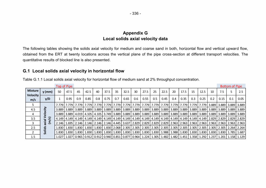
- 336 -
Appendix G
Local solids axial velocity data
The following tables showing the solids axial velocity for medium and coarse sand in both, horizontal flow and vertical upward flow,
obtained from the ERT at twenty locations across the vertical plane of the pipe cross-section at different transport velocities. The
quantitative results of blocked line is also presented.
G.1 Local solids axial velocity in horizontal flow
Table G.1.1 Local solids axial velocity for horizontal flow of medium sand at 2% throughput concentration.
y (mm) 50 47.5 45 42.5 40 37.5 35 32.5 30 27.5 25 22.5 20 17.5 15 12.5 10 7.5 5 2.5
y/D 1 0.95 0.9 0.85 0.8 0.75 0.7 0.65 0.6 0.55 0.5 0.45 0.4 0.35 0.3 0.25 0.2 0.15 0.1 0.05
5 7.779 7.779 7.779 7.779 7.779 7.779 7.779 7.779 7.779 7.779 7.779 7.779 7.779 7.779 7.779 7.779 3.889 3.889 3.889 3.889
4.5 3.889 3.889 3.889 3.889 3.889 3.889 3.889 3.889 3.889 3.889 3.889 3.889 3.889 3.889 3.889 3.889 3.889 3.889 3.889 3.889
4 3.889 3.889 4.019 4.105 4.105 3.749 3.889 3.889 3.889 3.889 3.889 3.889 3.889 3.889 3.889 3.889 3.889 3.889 3.889 3.889
3.5 4.149 4.149 4.149 4.149 4.149 4.149 4.149 4.149 4.149 4.149 4.149 4.149 4.149 4.149 4.149 4.149 2.829 2.829 2.829 2.829
3 2.146 1.695 2.146 2.146 2.146 2.146 4.445 3.637 2.829 2.829 2.829 2.829 2.963 2.963 2.963 2.963 2.963 2.963 2.963 2.963
2.5 1.830 1.830 1.830 1.830 1.830 1.830 2.068 2.305 2.305 2.305 2.305 2.305 2.305 2.305 2.305 2.305 2.305 2.305 2.264 2.264
2 1.830 1.830 1.830 1.830 1.830 1.830 1.830 1.830 1.830 1.830 1.830 1.988 1.988 1.830 1.830 1.830 1.830 1.830 1.785 1.687
1.5 1.027 1.027 0.965 0.912 0.912 0.940 0.851 0.877 0.964 1.224 1.305 1.482 1.482 1.451 1.358 1.292 1.237 1.201 1.158 1.129
Mixture
Velocity
m/s
Soli
ds
axia
l Ve
loci
ty
(m/s
)
Bottom of PipeTop of Pipe

- 337 -
Table G.1.2 Local solids axial velocity for horizontal flow of medium sand at 10% throughput concentration.
Table G.1.3 Local solids axial velocity for horizontal flow of coarse sand at 2% throughput concentration.
y (mm) 50 47.5 45 42.5 40 37.5 35 32.5 30 27.5 25 22.5 20 17.5 15 12.5 10 7.5 5 2.5
y/D 1 0.95 0.9 0.85 0.8 0.75 0.7 0.65 0.6 0.55 0.5 0.45 0.4 0.35 0.3 0.25 0.2 0.15 0.1 0.05
4.5 4.733 5.186 5.186 5.186 5.186 5.186 5.186 5.186 5.186 5.186 5.186 5.186 5.186 5.186 5.186 4.787 4.787 4.787 4.559 4.075
3.5 3.661 3.661 3.661 3.661 3.661 3.661 3.661 3.661 3.661 3.661 3.661 3.661 3.661 3.627 3.457 3.457 3.457 3.457 3.397 3.232
3 3.457 3.457 3.457 3.457 3.457 3.457 3.457 3.457 3.457 3.457 3.457 3.457 3.457 3.427 3.231 2.829 2.808 2.767 2.706 2.706
2.5 2.706 2.706 2.706 2.706 2.706 2.706 2.706 2.706 2.706 2.706 2.706 2.706 2.593 2.593 2.489 2.349 2.264 2.210 2.197 2.148
2 2.146 2.146 2.146 2.146 2.146 2.146 2.146 2.146 2.146 2.146 2.146 2.146 2.134 2.032 1.926 1.858 1.813 1.747 1.670 1.611
1.5 1.322 1.627 1.830 1.830 1.830 1.830 1.830 1.830 1.830 1.822 1.696 1.589 1.556 1.543 1.478 1.378 1.317 1.281 1.224 1.287
Soli
ds
axia
l
Ve
loci
ty (
m/s
)
Mixture
Velocity
m/s
Top of Pipe Bottom of Pipe
y (mm) 50 47.5 45 42.5 40 37.5 35 32.5 30 27.5 25 22.5 20 17.5 15 12.5 10 7.5 5 2.5
y/D 1 0.95 0.9 0.85 0.8 0.75 0.7 0.65 0.6 0.55 0.5 0.45 0.4 0.35 0.3 0.25 0.2 0.15 0.1 0.05
5 5.119 5.119 5.186 5.186 5.186 5.186 5.119 4.616 4.445 4.396 4.149 4.149 4.149 4.149 4.149 4.149 4.149 4.149 4.149 3.976
4.5 4.149 4.149 4.346 4.445 4.445 4.445 4.445 4.445 4.445 4.445 4.445 4.445 4.445 4.445 4.445 4.445 4.445 4.445 4.297 4.149
4 4.198 4.346 4.445 4.445 4.445 4.445 4.445 4.445 4.445 4.445 4.445 4.445 4.445 4.445 4.346 4.149 4.149 4.019 3.889 3.699
3.5 3.423 3.423 3.423 3.423 3.423 3.423 3.423 3.423 3.423 3.423 3.423 3.423 3.423 3.423 3.260 3.260 3.260 3.112 2.976 2.976
3 3.112 3.112 3.112 3.112 3.112 3.112 3.112 3.112 3.112 3.112 3.112 3.112 3.112 3.062 3.013 2.941 2.817 2.740 2.678 2.624
2.5 2.393 2.393 2.393 2.393 2.393 2.393 2.334 2.320 2.305 2.320 2.334 2.393 2.379 2.320 2.305 2.065 2.001 1.977 1.977 1.977
2 1.596 1.596 1.596 1.596 1.596 1.596 1.596 1.596 1.596 1.596 1.596 1.596 1.596 1.596 1.596 1.596 1.383 1.383 1.383 1.383
1.5 1.489 1.383 1.383 1.383 1.383 1.489 1.489 1.596 1.596 1.638 1.638 1.638 1.638 1.383 1.066 1.194 0.750 0.750 0.750 0.750
Soli
ds
axia
l Ve
loci
ty
(m/s
)
Top of Pipe
Mixture
Velocity
m/s
Bottom of Pipe
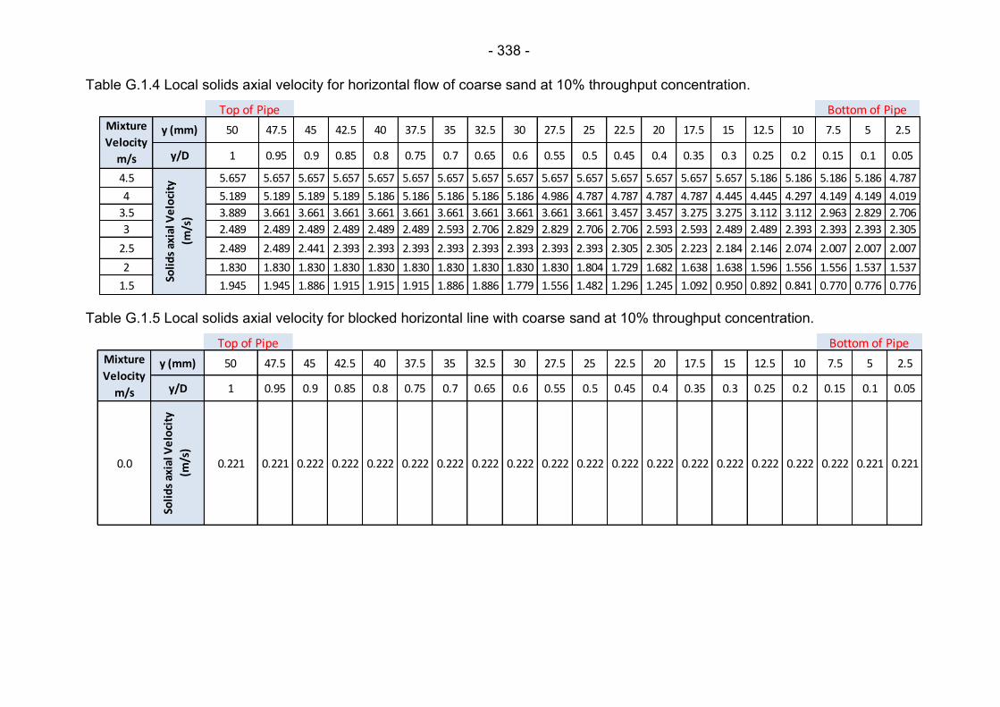
- 338 -
Table G.1.4 Local solids axial velocity for horizontal flow of coarse sand at 10% throughput concentration.
Table G.1.5 Local solids axial velocity for blocked horizontal line with coarse sand at 10% throughput concentration.
y (mm) 50 47.5 45 42.5 40 37.5 35 32.5 30 27.5 25 22.5 20 17.5 15 12.5 10 7.5 5 2.5
y/D 1 0.95 0.9 0.85 0.8 0.75 0.7 0.65 0.6 0.55 0.5 0.45 0.4 0.35 0.3 0.25 0.2 0.15 0.1 0.05
4.5 5.657 5.657 5.657 5.657 5.657 5.657 5.657 5.657 5.657 5.657 5.657 5.657 5.657 5.657 5.657 5.186 5.186 5.186 5.186 4.787
4 5.189 5.189 5.189 5.189 5.186 5.186 5.186 5.186 5.186 4.986 4.787 4.787 4.787 4.787 4.445 4.445 4.297 4.149 4.149 4.019
3.5 3.889 3.661 3.661 3.661 3.661 3.661 3.661 3.661 3.661 3.661 3.661 3.457 3.457 3.275 3.275 3.112 3.112 2.963 2.829 2.706
3 2.489 2.489 2.489 2.489 2.489 2.489 2.593 2.706 2.829 2.829 2.706 2.706 2.593 2.593 2.489 2.489 2.393 2.393 2.393 2.305
2.5 2.489 2.489 2.441 2.393 2.393 2.393 2.393 2.393 2.393 2.393 2.393 2.305 2.305 2.223 2.184 2.146 2.074 2.007 2.007 2.007
2 1.830 1.830 1.830 1.830 1.830 1.830 1.830 1.830 1.830 1.830 1.804 1.729 1.682 1.638 1.638 1.596 1.556 1.556 1.537 1.537
1.5 1.945 1.945 1.886 1.915 1.915 1.915 1.886 1.886 1.779 1.556 1.482 1.296 1.245 1.092 0.950 0.892 0.841 0.770 0.776 0.776
Top of PipeMixture
Velocity
m/sSo
lid
s ax
ial V
elo
city
(m/s
)
Bottom of Pipe
y (mm) 50 47.5 45 42.5 40 37.5 35 32.5 30 27.5 25 22.5 20 17.5 15 12.5 10 7.5 5 2.5
y/D 1 0.95 0.9 0.85 0.8 0.75 0.7 0.65 0.6 0.55 0.5 0.45 0.4 0.35 0.3 0.25 0.2 0.15 0.1 0.05
0.0
Soli
ds
axia
l Ve
loci
ty
(m/s
)
0.221 0.221 0.222 0.222 0.222 0.222 0.222 0.222 0.222 0.222 0.222 0.222 0.222 0.222 0.222 0.222 0.222 0.222 0.221 0.221
Mixture
Velocity
m/s
Bottom of PipeTop of Pipe

- 339 -
G.2 Local solids axial velocity in vertical flow
Table G.2.1 Local solids axial velocity for vertical flow of medium sand at 2% throughput concentration.
Table G.2.2 Local solids axial velocity for vertical flow of medium sand at 10% throughput concentration.
r (mm) 25 22.5 20 17.5 15 12.5 10 7.5 5 2.5 0 -2.5 -5 -7.5 -10 -12.5 -15 -17.5 -20 -22.5
r/D 0.5 0.45 0.4 0.35 0.3 0.25 0.2 0.15 0.1 0.05 0 -0.05 -0.1 -0.15 -0.2 -0.25 -0.3 -0.35 -0.4 -0.45
4.5 3.457 3.457 3.457 5.186 5.186 5.186 5.186 5.186 5.186 5.186 5.186 5.186 5.186 5.186 5.186 5.186 5.186 4.787 4.787 2.007
3.5 2.007 3.275 3.275 3.275 3.275 3.275 3.275 3.275 3.275 3.275 3.275 3.275 3.275 3.275 3.275 3.275 3.275 3.275 2.007 2.007
2.5 2.747 3.043 2.909 2.750 2.782 2.778 2.766 2.679 2.593 2.593 2.593 2.593 2.679 2.766 2.778 2.782 2.750 2.909 3.043 2.747
1.5 1.350 1.316 1.326 1.394 1.395 1.336 1.316 1.258 1.343 1.518 1.518 1.343 1.258 1.316 1.336 1.395 1.394 1.326 1.316 1.350
Mixture
Velocity
m/s
Top of Pipe
Soli
ds
axia
l Ve
loci
ty
(m/s
)
Bottom of Pipe
r (mm) 25 22.5 20 17.5 15 12.5 10 7.5 5 2.5 0 -2.5 -5 -7.5 -10 -12.5 -15 -17.5 -20 -22.5
r/D 0.5 0.45 0.4 0.35 0.3 0.25 0.2 0.15 0.1 0.05 0 -0.05 -0.1 -0.15 -0.2 -0.25 -0.3 -0.35 -0.4 -0.45
4.5 4.324 4.542 5.020 5.186 5.186 5.186 5.186 5.186 5.186 5.186 5.186 5.186 5.186 5.186 5.186 5.186 5.186 5.020 4.542 4.324
3.5 3.335 3.463 3.504 3.568 3.591 3.646 3.661 3.661 3.661 3.661 3.661 3.661 3.661 3.661 3.646 3.591 3.568 3.504 3.463 3.335
2.5 2.663 2.616 2.684 2.706 2.706 2.706 2.706 2.706 2.706 2.706 2.706 2.706 2.706 2.706 2.706 2.706 2.706 2.684 2.616 2.663
1.5 1.416 1.484 1.517 1.556 1.563 1.595 1.634 1.656 1.750 1.778 1.778 1.750 1.656 1.634 1.595 1.563 1.556 1.517 1.484 1.416
Mixture
Velocity
m/s
Top of Pipe
Soli
ds
axia
l Ve
loci
ty
(m/s
)
Bottom of Pipe

- 340 -
Table G.2.3 Local solids axial velocity for vertical flow of coarse sand at 2% throughput concentration.
Table G.2.4 Local solids axial velocity for vertical flow of coarse sand at 10% throughput concentration.
r (mm) 25 22.5 20 17.5 15 12.5 10 7.5 5 2.5 0 -2.5 -5 -7.5 -10 -12.5 -15 -17.5 -20 -22.5
r/D 0.5 0.45 0.4 0.35 0.3 0.25 0.2 0.15 0.1 0.05 0 -0.05 -0.1 -0.15 -0.2 -0.25 -0.3 -0.35 -0.4 -0.45
4.5 4.546 4.783 4.963 5.131 5.186 5.186 5.186 5.186 5.186 5.186 5.186 5.186 5.186 5.186 5.186 5.186 5.131 4.963 4.783 4.546
3.5 3.540 3.589 3.653 3.661 3.661 3.661 3.661 3.661 3.661 3.661 3.661 3.661 3.661 3.661 3.661 3.661 3.661 3.653 3.589 3.540
2.5 2.420 2.451 2.478 2.489 2.514 2.630 2.607 2.489 2.489 2.489 2.489 2.489 2.489 2.607 2.630 2.514 2.489 2.478 2.451 2.420
1.5 1.391 1.413 1.431 1.450 1.476 1.514 1.556 1.556 1.556 1.556 1.556 1.556 1.556 1.556 1.514 1.476 1.450 1.431 1.413 1.391
Top of Pipe
Soli
ds
axia
l Ve
loci
ty
(m/s
)
Mixture
Velocity
m/s
Bottom of Pipe
r (mm) 25 22.5 20 17.5 15 12.5 10 7.5 5 2.5 0 -2.5 -5 -7.5 -10 -12.5 -15 -17.5 -20 -22.5
r/D 0.5 0.45 0.4 0.35 0.3 0.25 0.2 0.15 0.1 0.05 0 -0.05 -0.1 -0.15 -0.2 -0.25 -0.3 -0.35 -0.4 -0.45
4.5 5.249 5.304 5.403 5.539 5.628 5.657 5.657 5.657 5.657 5.657 5.657 5.657 5.657 5.657 5.657 5.628 5.539 5.403 5.304 5.249
2.5 2.815 2.780 2.781 2.781 2.790 2.811 2.829 2.829 2.829 2.829 2.829 2.829 2.829 2.829 2.811 2.790 2.781 2.781 2.780 2.815
Soli
ds
axia
l Ve
loci
ty
(m/s
)
Mixture
Velocity
m/s
Bottom of PipeTop of Pipe

- 341 -
This page has been intentionally left blank


