Embed Size (px)
Citation preview
Utilization of extracellular information beforeligand-receptor binding reaches equilibrium expandsand shifts the input dynamic rangeAlejandra C. Venturaa,b, Alan Busha,b, Gustavo Vasena,b, Matías A. Goldína,b, Brianne Burkinshawa,b,Nirveek Bhattacharjeec, Albert Folchc, Roger Brentd, Ariel Chernomoretze,f,g, and Alejandro Colman-Lernera,b,1
aInstitute of Physiology, Molecular Biology, and Neuroscience (IFIBYNE), University of Buenos Aires (UBA)-National Scientific and Technical Research Council(CONICET), bDepartment of Physiology, Molecular, and Cell Biology, School of Exact and Natural Sciences (FCEN), ePhysics Institute of Buenos Aires (IFIBA),CONICET, and fDepartment of Physics, FCEN, UBA, C1428EGA Buenos Aires, Argentina; gFundación Instituto Leloir, C1405BWE Buenos Aires, Argentina;cDepartment of Bioengineering, University of Washington, Seattle, WA 98195; and dDivision of Basic Sciences, Fred Hutchinson Cancer Research Center,Seattle, WA 98109
Edited by Peter N. Devreotes, Johns Hopkins University School of Medicine, Baltimore, MD, and approved July 30, 2014 (received for review December 9, 2013)
Cell signaling systems sense and respond to ligands that bind cellsurface receptors. These systems often respond to changes in theconcentration of extracellular ligand more rapidly than the ligandequilibrates with its receptor. We demonstrate, by modeling andexperiment, a general “systems level” mechanism cells use to takeadvantage of the information present in the early signal, beforereceptor binding reaches a new steady state. This mechanism, pre-equilibrium sensing and signaling (PRESS), operates in signaling sys-tems inwhich the kinetics of ligand-receptor binding are slower thanthe downstream signaling steps, and it typically involves transientactivation of a downstream step. In the systems where it operates,PRESS expands and shifts the input dynamic range, allowing cells tomake different responses to ligand concentrations so high as to beotherwise indistinguishable. Specifically,we showthat PRESS appliesto the yeast directional polarization in response to pheromone gra-dients. Consideration of preexisting kinetic data for ligand-receptorinteractions suggests that PRESS operates in many cell signaling sys-tems throughout biology. The same mechanismmay also operate atother levels in signaling systems in which a slow activation step cou-ples to a faster downstream step.
cellular signaling | binding kinetics | dose–response
Detecting and responding to a chemical gradient is a centralfeature of a multitude of biological processes (1). For this
behavior, organisms use signaling systems that sense informationabout the extracellular world, transmit this information into thecell, and orchestrate a response. Measurements of the directionand proximity of the extracellular stimuli usually rely on thebinding of diffusing chemical particles (ligands) to specific cellsurface receptors. Different organisms have evolved differentstrategies to make use of this information. Small motile organ-isms, including certain bacteria, use a temporal sensing strategy,measuring and comparing concentration signals over time alongtheir swimming tracks (2). In contrast, some eukaryotic cells,including Saccharomyces cerevisiae, are sufficiently large to im-plement a spatial sensing mechanism, measuring concentrationdifferences across their cell bodies (3).The observation that some eukaryotes that use spatial sensing
exhibit remarkable precision in response to shallow gradients (1–2%differences in ligand concentration between front and rear) (4, 5)has led to several proposed models in which large amplification isachieved by positive feedback loops in the signaling pathwaystriggered by the ligand-receptor binding (6, 7). Here, we describea different mechanism, dependent on ligand-receptor bindingdynamics, which improves gradient sensing when the concentra-tion of external ligand is close to saturation. We use the buddingyeast S. cerevisiae to study the efficiency of this mechanism.Haploid yeast cells exist in two mating types, MATa and
MATα (also referred to as a and α cells). Mating occurs when
a and α cells sense each other’s secreted mating pheromones: a-factor and α-factor (αF) (8). The pheromone secreted by thenearby mating partner diffuses, forming a gradient surroundingthe sensing cell. Pheromone binds a membrane receptor, Ste2, inMATa yeast (9) that activates a pheromone response system(PRS), which cells use to decide whether to fuse with a matingpartner or not. At high enough αF concentrations, cells developa polarized chemotropic growth toward the pheromone source(4). To do that, the nonmotile yeast determines the direction ofthe potential mating partner measuring on which side there aremore bound pheromone receptors, which are initially distributedhomogeneously on the cell surface (10). However, this sensingmodality can only work when external pheromone is non-saturating: If all receptors are bound, cells should not be able todetermine the direction of the gradient. Surprisingly, even at highpheromone concentrations, yeast tend to polarize in the correctdirection (4, 11). Different amplification mechanisms have beenproposed to account for the conversion of small differences inligand concentration across the yeast cell, as is the case for densemating mixtures, into chemotropic growth (6).We previously studied induction of reporter gene output by
the PRS after step increases in the concentration of αF. Wefound large cell-to-cell variability, the bulk of which was due tolarge differences in the ability of individual cells to send signal
Significance
Many cell decisions depend on precise measurements of ex-ternal ligands reversibly bound to receptors. Yeast cells orientin gradients of sex pheromone detecting differences in theamount of ligand-receptor complex. However, yeast can orientin gradients with nearly all receptors occupied. We describea general systems-level mechanism, pre-equilibrium sensingand signaling (PRESS), which overcomes this saturation limit byshifting and expanding the input dynamic range to which cellscan respond. PRESS requires that events downstream of thereceptor be transient and faster than the time required for thereceptor to reach equilibrium binding. Experiments and simu-lations show that PRESS operates in yeast and may help cellsorient in gradients. Many ligand-receptor interactions are slow,suggesting that PRESS is widespread throughout eukaryotes.
Author contributions: A.C.V., A.B., and A.C.-L. designed research; A.C.V., A.B., G.V., M.A.G.,A.C., and A.C.-L. performed research; B.B., N.B., A.F., and R.B. contributed new reagents/analytic tools; A.C.V., A.B., G.V., A.C., and A.C.-L. analyzed data; and A.C.V., R.B., and A.C.-L.wrote the paper.
The authors declare no conflict of interest.
This article is a PNAS Direct Submission.1To whom correspondence should be addressed. Email: [email protected].
This article contains supporting information online at www.pnas.org/lookup/suppl/doi:10.1073/pnas.1322761111/-/DCSupplemental.
www.pnas.org/cgi/doi/10.1073/pnas.1322761111 PNAS Early Edition | 1 of 10
BIOPH
YSICSAND
COMPU
TATIONALBIOLO
GY
PNASPL
US
through the system and in their general capacity to expressproteins (12). The level of induced gene expression matches wellthe equilibrium binding curve of αF to receptor (13, 14), a phe-nomenon known as dose–response alignment (DoRA), commonto many other signaling systems (14). In the PRS, DoRA persistsfor several hours of stimulation.During these studies, we realized that the binding dynamics of
αF to its receptor is remarkably slow: At concentrations near thedissociation constant (Kd), binding takes about 20 min to reach90% of the equilibrium level (15, 16). This dynamics is slowrelative not only to the 90-min cell division cycle but also to thepheromone-dependent activation of the mitogen-activated pro-tein kinase (MAPK) Fus3, which takes 2 to 5 min to reachsteady-state levels (14). An unavoidable conclusion is that themachinery downstream of the αF receptor must be using pre-equilibrium binding information for its operation.This observation led us to study the consequences of fast and slow
ligand-receptor dynamics on the ability of cells to sense extracellularcues. In biology, the rates of ligand binding and unbinding to mem-brane receptors span a large range, including many cases with dy-namics similar to, or even slower than, that of mating pheromone(e.g., rates for EGF, insulin, glucagon, IFN-α1a, and IL-2 in Table 1).Our study revealed amode of sensing that can greatly increase the
ability of cells to discriminate doses at high ligand concentrations.
ResultsLigand-Receptor Binding Dose–Response Curve Changes Over Time.We consider the time evolution of occupied receptor at differentdoses of ligand for the simple case of one-step binding described by
L+R →k1
←k−
C;
where L is the ligand, R is the receptor, C is the ligand-receptorcomplex, and k+ and k− are the binding and unbinding rates,
respectively. Assuming free L is not significantly affected bythe reaction, binding over time may be described by
Cðt;LÞ =CeqðLÞ p�1− eð−t=τðLÞÞ�;
with
Ceq =RtotL
L+Kd;
and
τ=1
k− +L p k+:
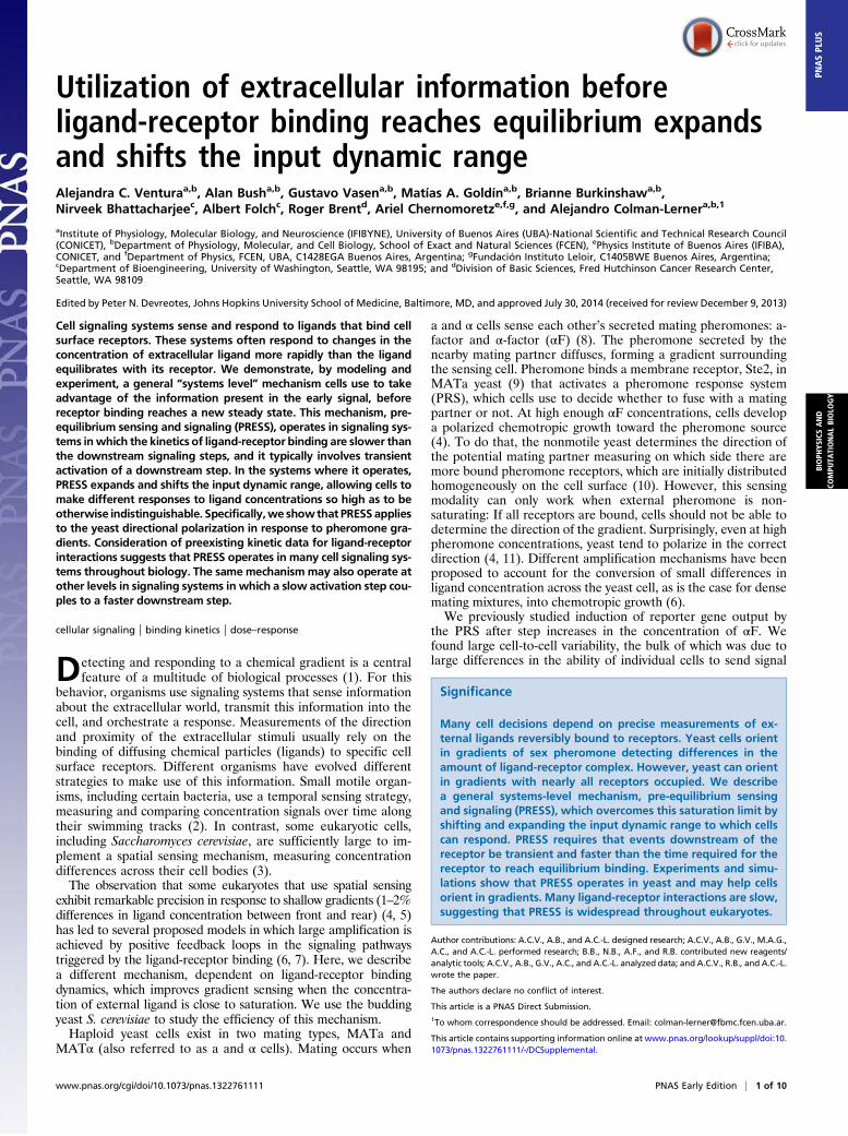
Ceq is the equilibrium value of C, Rtot is the total of amount ofreceptor, and τ is the exponential time constant (time at whichC reaches ∼63.2% of the steady-state value). Thus, the time evo-lution of C depends on ligand concentration: The higher the con-centration of ligand, the faster binding reaches equilibrium (Fig.1A). Similarly, plotting C vs. L at different times shows that theEC50 (concentration of the ligand that occupies 50% of the recep-tors) of the binding curve is high at early times but becomes pro-gressively lower as time passes (Fig. 1B). As a result, beforebinding reaches equilibrium (t∞), the receptor is sensitive in a re-gion of ligand concentrations that will later saturate the receptor(SI Appendix, section 1). For example, in the case of αF, two highconcentrations, L1 and L2 (55 Kd and 80 Kd), result in a 12.7%difference in occupied receptors at 10 s, and in only a 0.56%difference at equilibrium (Fig. 1B).To verify experimentally our theoretical analysis suggesting
a slow reduction over time in the EC50 of the dose–response curvefor receptor binding, we measured the binding dynamics of fluo-rescently tagged αF (37) to live yeast by fluorescence cytometry(Fig. 1C). To minimize ligand depletion at low concentrations, we
Table 1. Sample receptor/ligand binding parameters
Receptor Ligand Cell type k− (1/s) Kd (M) τ (at L = Kd), s Ref.
Fce IgE Human basophils 2.50E-05 4.80E-10 20,000.00 (17)Fcγ 2.4G2 monoclonal Fab Mouse macrophage 3.80E-05 7.70E-10 13,157.89 (18)Canabinoid receptor CP55,940 Rat brain 1.32E-04 2.10E-08 3,787.88 (19)IL-2 receptor IL-2 T cells 2.00E-04 7.40E-12 2,500.00 (20)α1-Adrenergic Prazosin BC3H1 3.00E-04 7.50E-11 1,666.67 (21)Glucagon receptor Glucagon Rat hepatocytes 4.30E-04 3.06E-10 1,162.79 (22)Formyl peptide receptor (FPR) fMLP Rat neutrophils 5.50E-04 3.45E-08 909.09 (23)Ste2 (αF receptor) αF S. cerevisiae 1.00E-03 5.50E-09 500.00 (15, 16)IFN Human IFN-α1a A549 1.20E-03 3.30E-10 416.67 (24)Transferrin Transferrin HepG2 1.70E-03 3.30E-08 294.12 (25)EGF receptor EGF Fetal rat lung 2.00E-03 6.70E-10 250.00 (26)TNF TNF A549 2.30E-03 1.50E-10 217.39 (24)Insulin receptor Insulin Rat fat cells 3.30E-03 2.10E-08 151.52 (27)FPR FNLLP Rabbit neutrophils 6.70E-03 2.00E-08 74.63 (28)Total fibronectin receptors Fibronectin Fibroblasts 1.00E-02 8.60E-07 50.00 (29)T-cell receptor Class II MHC-peptide 2B4 T-cells 5.70E-02 6.00E-05 8.77 (30)FPR N-formyl peptides Human neutrophils 1.70E-01 1.20E-07 2.94 (31)cAMP receptor cAMP D. discoideum 1.00E+00 3.30E-09 0.50 (32)IL-5 receptor IL-5 COS 1.47E+00 5.00E-09 0.34 (33)NMDA receptor Glutamate Hippocampal neurons 5.00E+00 1.00E-06 0.10 (34)Adenosine A2A Adenosine HEK 293 (human) 1.75E+01 5.20E-08 0.03 (35)AMPA receptor Glutamate HEK 293 (human) 2.00E+03 5.00E-04 2.50E-04 (36)
A549, human lung alveolar carcinoma; BC3H1, smooth muscle-like cell line; COS, fibroblast-like cell line derived from monkey kidney tissue; 2.4G2 Fab, Fabportion of 2.4G2 antibody against receptor; fMLP, N-formyl-methionyl-leucyl-phenylalanine; FNLLP, N-formylnorleucylleucylphenylalanine; HepG2, humanhepatoma cell line; τ, time it takes the binding reaction to reach 63% of its final (equilibrium) value. The value of τ depends on the concentration of the ligand(Fig. 1). Thus, we show the data for a concentration of ligand equal to the Kd of each reaction. Prazosin is an antagonist to the receptor.
2 of 10 | www.pnas.org/cgi/doi/10.1073/pnas.1322761111 Ventura et al.
used low numbers of yeast in a rather large volume. To blockreceptor turnover, we performed the experiment in the presenceof the translation inhibitor cycloheximide and used a strain ex-pressing a truncated receptor that is not endocytosed (T305) (38).As predicted, the dose–response curve for receptor binding exhibi-ted a highEC50 at early times (184±60 nM) that slowly decreased toits low equilibrium value (23 ± 3 nM).
Utilization of Pre-equilibrium Information Modulates the Input DynamicRange. This slow decrease in the EC50 of the response curve forreceptor binding suggested that cells that could activate signal-ing rapidly, before ligand-receptor binding reaches equilibrium,might be able to discriminate ligand doses that would be other-wise indistinguishable. This idea has not been previously exploredand itmay potentially be very important.We refer to such signaling
0.01 0.1 1 10 100 10000
0.2
0.4
0.6
0.8
1
L/Kd
Nor
m.
Bou
nd R
ecep
tor
(C)
0.1s
100s
10s1s
L1/Kd
L2/Kd
C1-10s
C2-10s
C2-eq
C1-eqB
0 5 10 15 200
0.2
0.4
0.6
0.8
1
Time (min)
Nor
m. B
ound
Rec
epto
r
0.1
L/Kd
1
10100
A
0
0.25
0.50
0.75
1
0.01 0.1 1 10 100Fluorescent αF/Kd
Mem
bran
e flu
ores
cenc
e(N
orm
. mea
n FL
/cel
l)
Time (min)153365180300
Time
C
Fig. 1. Time-dependent shift of the binding dose–response curve. (A) Time course of receptor/ligand complex formation for different ligand concentrations
(relative to the affinity dissociation constant, Kd), in the range 0.1–100 Kd. We computed values for the case of one-step binding using the reaction L+R →k1
←k−
C,
with the following αF binding reaction rates: k+ = 1.9 105 M−1·s−1 and k− = 0.001 s−1 (15, 16). We assumed that the concentration of free L over time isconstant. Norm., normalized. (B) Dose–response curves for the receptor/ligand reaction computed at different times, as indicated over the curves (and witha red arrow). Two concentrations, L1 and L2, result in well-separated levels of occupied receptor C1 and C2 at 10 s (0.4211 and 0.5483, respectively), but not atthe equilibrium values C1-eq and C2-eq (0.9821 and 0.9877, respectively). (C) Yeast cells of strain YAB3725 [Δbar1, PSTE2 STE2(T305)-CFP] were grown andstimulated with the indicated amounts of a fluorescent αF derivative (37), and the binding was determined by fluorescence microscopy as explained inMaterials and Methods. The mean and 95% confidence interval for the mean are shown for each concentration and time. A simple binding model wasglobally fitted to the data, resulting in Kd = 23 ± 3 nM and k− = 1.0 ± 0.2 10−4·s−1 (solid lines).
0 1 2 3 4 50
0.2
0.4
0.6
Time (min)
Dow
nstr
eam
Res
pons
e (X
*) 100
10
10.1
L+R C
X X*
X ^
A
0.01 1 100 100000
0.2
0.4
0.6
0.8
1
L/Kd
Nor
mal
ized
Res
pons
e
slow fast
fast fast
81
114343
Ceq
0.75%
8.5%
B
1000100.1
C(t)X*(peak)C(tmax)
C
0.01 0.1 1 10 100 10000
0.2
0.4
0.6
0.8
1
L/Kd
Nor
mal
ized
Res
pons
es
t = 3
3.5
sec
t = 4
.3 se
c
t = 1
15.4
sec
t = 1
1.3
sect =
359
.1 se
c
Ceq
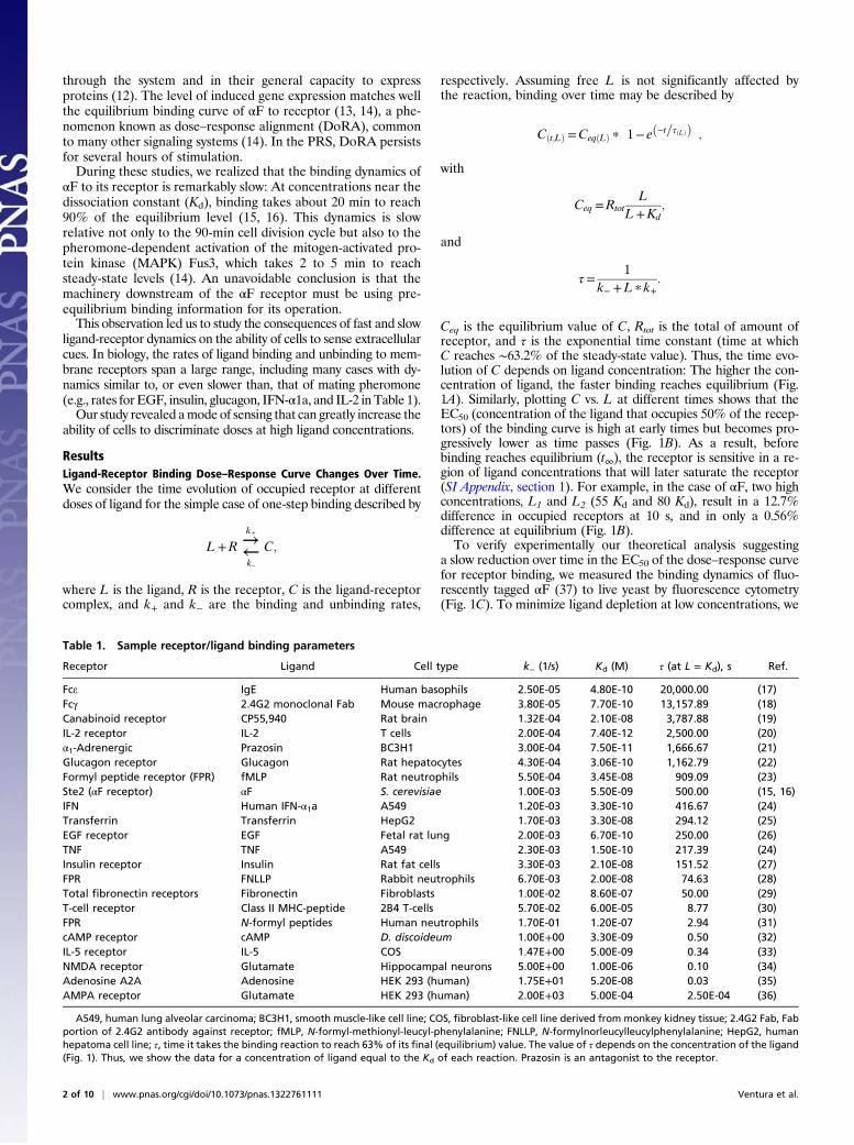
Fig. 2. PRESS. Coupling a slow binding reaction to a fast and transient response can expand the input dynamic range beyond equilibrium saturation. (A) Insetshows a toy model with a downstream response activated by the ligand-receptor complex computed in Fig. 1A. Occupied receptor activates effector X; then,X* converts into X^, which slowly converts back to X, closing the cycle (details are provided in SI Appendix, section 2). The plot shows X* vs. time for all of theconcentrations of L included in Fig. 1A. (B) Shift and expansion of the input dynamic range are due to PRESS. L-receptor complex at equilibrium (Ceq, solidblack line), as well as peak X* resulting from using slow (red dotted line) or fast (blue dashed line) binding/unbinding rates of L to R, vs. input L, are shown.The resulting input dynamic ranges (the fold change required in input to elicit a change from 10 to 90% of maximum output) are indicated. The two dosesindicated, L1 = 55 Kd and L2 = 80 Kd, result in an 8.5% difference in peak X* for slow-fast coupling, and only a 0.75% difference for fast-fast coupling. (C)Graphical description of the expansion of the input dynamic range in the toy model. The plot shows L-receptor complex at equilibrium (Ceq, solid black line),or at the indicated times before equilibrium (C(t), solid gray line), as well as peak X* (solid red line), all as a function of input L. Note, as shown in A, that peakX* occurs at different times for different concentrations of input L. Therefore, the values of C at the time when X* peaks (Ctmax, solid green line) correspondto different C(t) gray curves for each dose of L (green ○). The Ctmax curve is itself shifted to higher doses than Ceq, and it has a larger input dynamic range (lesssteep) than either Ceq or any C(t) curves [EC50 = 17.7 and sensitivity (nH) = 0.9]. In B and C, the x axis corresponds to L normalized by the Kd of the ligand-receptor reaction. All data correspond to simulations, done using the following parameters for the X cycle: r1 = 0.1, r2 = 0.08, r3 = 0.001, and Xtot = 10 (Xtot
being the total amount of X). Binding/unbinding rates were k− = 0.001 1/s, k+ = 0.00019 (nM · s)−1 for slow binding (A, red line in B and C) and 100-fold thosevalues for fast binding (blue line in B) (SI Appendix, Fig. S1).
Ventura et al. PNAS Early Edition | 3 of 10
BIOPH
YSICSAND
COMPU
TATIONALBIOLO
GY
PNASPL
US
as pre-equilibrium sensing and signaling (PRESS) and to the oper-ation of signaling systems before reaching equilibriumas operation inPRESS mode. In PRESS mode, such systems could determinedownstream responses using quantities different from equilibriumoccupancy levels, such as absolute receptor occupancy at a givenmoment or the time derivative of receptor occupancy, which, atshort times, is proportional to ligand concentration. We will showbelow that operation of signaling systems in PRESS mode can havetwo consequences. Operation in PRESS mode can shift the inputdynamic range (the range of input concentrations that elicit distin-guishable outputs, usually quantified by the EC90 and EC10) toa region of higher dose concentrations. Operation in PRESS modecan also expand the input dynamic range, permitting better dis-crimination at high concentrations, although still maintaining a goodresponse at low doses. Response curves with enlarged input dynamicranges are also called “subsensitive” (39) (SI Appendix, section 3).We reasoned that if the downstream signaling is transient, as well
as fast, the system should have the extra advantage of avoiding thetransmission of occupancy levels during equilibrium, which conveyno information useful to discriminate high doses. To introducePRESS and describe its effects, we considered the behavior ofa “toy model” system (Fig. 2A). Here, occupied receptor activateseffector X, then active X (X*) converts into an inactive refractorystate (X̂ ), which slowly converts back to the inactive form (X),closing the cycle. In this toy model, when X activation (X → X*)and inactivation (X* → X̂ ) reaction rates are fast relative to thereset reaction (X̂ → X), the value of X* peaks and declines; thatis, activation of X is transient [reactions that generate transientactivation are sometimes referred to as “pulse-generators” (40)].In addition, when activation and inactivation of X are fast rela-tive to the speed of the binding reaction of L, the output of thissystem (peak X*) depends on receptor occupancy before equi-librium. With the rates we used, the overall system exhibited alarge shift in the output EC50 to high doses relative to the EC50of the receptor binding reaction at equilibrium. In this case,there was also a large expansion of the input dynamic rangerelative to binding equilibrium (65-fold shift and 4.4-fold ex-pansion, with the rates used in Fig. 2B). Note that, as expected,the shift of the EC50 and the expansion of the input dynamicrange result from an increased ability of the system to discrimi-nate high doses (Fig. 2B).In this toy model, PRESS shifts the input dynamic range be-
cause the peak of X* occurs at a time when the dose–responsebinding curve has not yet reached the receptor binding equilib-rium curve; thus, it has a higher EC50 (Fig. 1B). To understandhow it is that PRESS may also expand the input dynamic range,consider that the peak of X* occurs at different times for dif-ferent concentrations of L (Fig. 2 A and C). In particular, whenL is large, the peak of X* occurs earlier than when L is small.Now, at the same time that the X cycle is taking place, the EC50 ofthe binding dose–response curve is decreasing over time (Fig. 1and Fig. 2D, gray curves). Thus, the effective ligand-receptorcurve at the time of the peak of X* is obtained by linking thevalues of the ligand-receptor complex at the time of the peak ofX* (Ctmax). This curve across times (green line in Fig. 2C) hasa larger input dynamic range than that of C at any given time. Itis for this reason that the overall system with PRESS has anexpanded dynamic range (SI Appendix, section 3).To test whether the observed expansion and displacement of
the input dynamic range required PRESS (i.e., to test if ligandbinding needed to be slower than downstream signaling), weincreased the binding reaction rates. This change largely elimi-nated the expansion of the input dynamic range and the shift ofthe EC50 (Fig. 2B, compare red and blue curves). We also testedthe requirement of PRESS by making the downstream responseless transient. We decreased the X* inactivation rate, making thetransient X* response peak later, and we obtained a smaller shiftof the output EC50 (SI Appendix, Fig. S1A).
A number of general signaling architectures can generatetransient responses, and thus would be expected to bring aboutPRESS when coupled to a relatively slow binding receptor (SIAppendix, section 2). In SI Appendix, Fig. S1 B and C, we testedtwo additional architectures, systems with incoherent feed-forward or negative feedback control. In models based on thesearchitectures, for the rates used, PRESS resulted in a large (up totwo orders) displacement in the output EC50, which was lost whenwe increased the ligand binding rates. Thus, we conclude that pre-equilibrium signaling can operate in at least the three signalingarchitectures we presented as toy models (Fig. 2 and SI Appendix,Fig. S1). These signaling topologies are found throughout pro-karyotes and eukaryotes (41–43).We wondered if the transient response from signaling systems
that operated in PRESS mode might amplify upstream noisedue, for example, to stochastic differences in the occupation ofthe receptor by ligand. A large effect of noise on the transientresponse might reduce the precision by which systems usingPRESS can distinguish between different input concentrations.To determine the effect of upstream noise on signaling in PRESSmode, we ran stochastic simulations of the toy model in Fig. 2A,using different number of receptors (SI Appendix, Fig. S2), andthen compared the coefficient of variation (CV; the SD divided bythe mean) of peak X* and of receptor occupancy at the time ofthat peak. Surprisingly, even in the case of a very small number ofreceptors (30 per cell), which introduced a significant noise at thelevel of the occupied receptor, peak X* had a smaller CV thanreceptor occupancy (SI Appendix, Fig. S2G). This result suggestedthat in the context of PRESS, a transient response downstream ofthe receptor does not amplify noise, and therefore the benefits ofenlarged and shifted input dynamic range are not lost or otherwisemasked (SI Appendix, section 4).
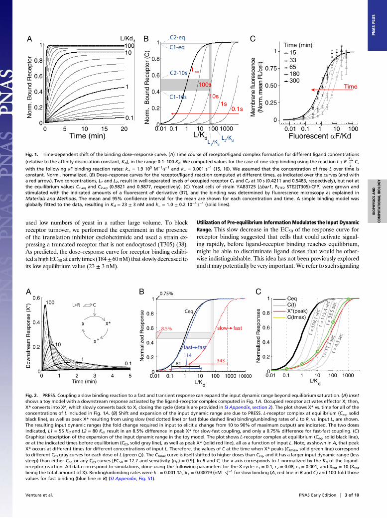
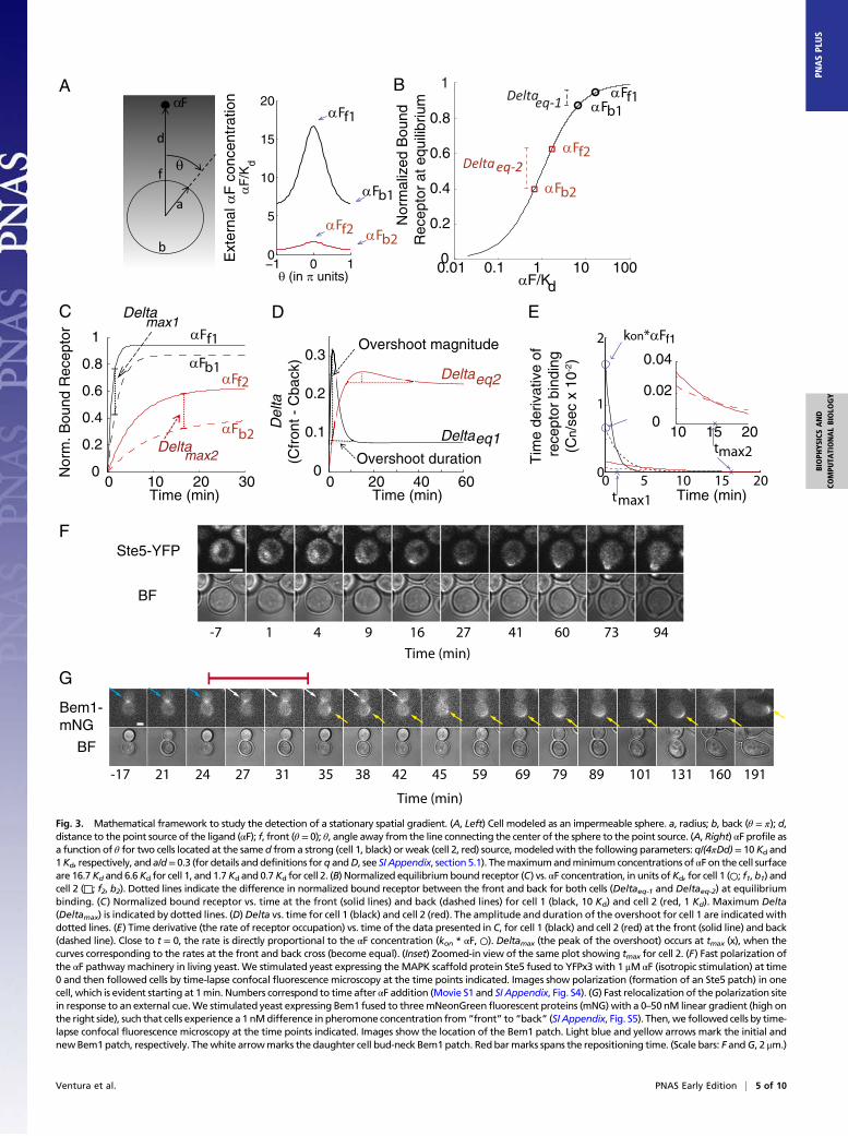
PRESS Can Operate During Yeast Polarization in a Chemical Gradient.We began this investigation with a system that causes yeast po-larization toward a mating pheromone source, whose architec-ture suggested that it could function in PRESS mode. We testedthis idea by modeling using experimentally based parameters. Todo so, we modeled yeast cells as impermeable spheres exposed toa steady-state αF gradient generated by a point source (Fig. 3Aand SI Appendix, section 5.1). We considered two cells located ingradients of different strengths at the same distance from thesource, where cell 1 received an average input of αF ∼10 Kdand cell 2 received an average input of αF ∼1 Kd (Fig. 3 A and B).Cells receive more αF on the side proximal to the source (front)than on the distal side (back). The difference in αF between thefront and back is the information cells have in order to determinegradient direction (8). Cells convert this information into a dif-ference in occupied receptor via the binding reaction. The maxi-mum difference in each cell occurs between points f and b, locatedat opposite sides of each cell. We call this difference, normalizedto total receptor, Delta. In principle, larger values of Delta shouldimprove the ability of the downstream machinery to detect thegradient. At equilibrium, cell 2 was in a location (∼1 Kd) with aDelta of ∼0.23. Cell 1 was closer to the saturating region of thebinding dose–response curve (∼10 Kd); therefore, Delta wassmaller, about 0.07. If gradient orientation were dependent on thevalue of Delta at equilibrium only, cell 1 would have just aboutno information to differentiate front from back (SI Appendix, Fig.S3A and section 5). However, analysis of the αF binding dynamicsrevealed an altogether different situation. Cell 1 reached 90% ofthe value of equilibrium binding in about 3.5 min, whereas cell 2reached it in about 19 min (Fig. 3C). Notably, in both cells, Deltaovershot: It peaked (Deltamax) and then declined to the equilib-rium value (Deltaeq) (Fig. 3D). For cell 1, Deltamax occurred atabout 1.7 min and was around 4.3-fold higher than Deltaeq. Cell 2had a similar but much smaller overshoot (Deltamax occurred atabout 17 min and was only 1.1-fold greater than Deltaeq).
4 of 10 | www.pnas.org/cgi/doi/10.1073/pnas.1322761111 Ventura et al.
−1 0 10
5
10
15
20
θ (in π units)
αF
/Kd
αF
d
a
f
b
θ
A
Ext
erna
l αF
con
cent
ratio
n
αFf1
αFf2
αFb1
αFb2
B αFf1
αFf2
αFb1
αFb2
0.01 0.1 1 10 1000
0.2
0.4
0.6
0.8
αF/Kd
Nor
mal
ized
Bou
nd
Rec
epto
r at
equ
ilibr
ium
C
0 10 20 300
0.2
0.4
0.6
0.8
1
Time (min)
Nor
m. B
ound
Rec
epto
r
Deltamax1
Deltamax2
αFf1
αFf2αFb1
αFb2
Deltaeq2
Overshoot magnitude
D
Deltaeq1
0 20 40 600
0.1
0.2
0.3
Time (min)
Del
ta(C
fron
t - C
back
)
Overshoot duration
0 5 10 15 200
1
2
Time (min)
10 15 200
0.02
0.04
tmax1
tmax2
E
Tim
e de
rivat
ive
of r
ecep
tor
bind
ing
(Cn/
sec
x 10
-2)
kon*αFf1
FSte5-YFP
BF
-7 1 4 9 16 27 41 60 73 94
G
Bem1-mNG
BF
Time (min)
-17 21 24 27 31 35 38 42 45 59 69 79 89 101 131 160 191
Time (min)
Deltaeq-2
Deltaeq-11
Fig. 3. Mathematical framework to study the detection of a stationary spatial gradient. (A, Left) Cell modeled as an impermeable sphere. a, radius; b, back (θ = π); d,distance to the point source of the ligand (αF); f, front (θ = 0); θ, angle away from the line connecting the center of the sphere to the point source. (A, Right) αF profile asa function of θ for two cells located at the same d from a strong (cell 1, black) or weak (cell 2, red) source, modeledwith the following parameters: q/(4πDd)= 10Kd and1Kd, respectively, and a/d= 0.3 (for details and definitions forq andD, see SI Appendix, section 5.1). Themaximumandminimumconcentrations of αF on the cell surfaceare 16.7Kd and 6.6Kd for cell 1, and 1.7Kd and 0.7Kd for cell 2. (B) Normalized equilibriumbound receptor (C) vs. αF concentration, in units ofKd, for cell 1 (○; f1, b1) andcell 2 (□; f2, b2). Dotted lines indicate the difference in normalized bound receptor between the front and back for both cells (Deltaeq-1 and Deltaeq-2) at equilibriumbinding. (C) Normalized bound receptor vs. time at the front (solid lines) and back (dashed lines) for cell 1 (black, 10 Kd) and cell 2 (red, 1 Kd). Maximum Delta(Deltamax) is indicated by dotted lines. (D)Delta vs. time for cell 1 (black) and cell 2 (red). The amplitude and duration of the overshoot for cell 1 are indicatedwithdotted lines. (E) Time derivative (the rate of receptor occupation) vs. time of the data presented in C, for cell 1 (black) and cell 2 (red) at the front (solid line) and back(dashed line). Close to t = 0, the rate is directly proportional to the αF concentration (kon * αF, ○). Deltamax (the peak of the overshoot) occurs at tmax (x), when thecurves corresponding to the rates at the front and back cross (become equal). (Inset) Zoomed-in view of the same plot showing tmax for cell 2. (F) Fast polarization ofthe αF pathwaymachinery in living yeast. We stimulated yeast expressing theMAPK scaffold protein Ste5 fused to YFPx3 with 1 μM αF (isotropic stimulation) at time0 and then followed cells by time-lapse confocal fluorescence microscopy at the time points indicated. Images show polarization (formation of an Ste5 patch) in onecell, which is evident starting at 1min. Numbers correspond to time after αF addition (Movie S1 and SI Appendix, Fig. S4). (G) Fast relocalization of the polarization sitein response to an external cue.We stimulated yeast expressing Bem1 fused to threemNeonGreen fluorescent proteins (mNG)with a 0–50nM linear gradient (high onthe right side), such that cells experience a 1 nMdifference in pheromone concentration from “front” to “back” (SI Appendix, Fig. S5). Then,we followed cells by time-lapse confocal fluorescence microscopy at the time points indicated. Images show the location of the Bem1 patch. Light blue and yellow arrows mark the initial andnewBem1patch, respectively. Thewhite arrowmarks the daughter cell bud-neck Bem1patch. Redbarmarks spans the repositioning time. (Scale bars: F andG, 2 μm.)
Ventura et al. PNAS Early Edition | 5 of 10
BIOPH
YSICSAND
COMPU
TATIONALBIOLO
GY
PNASPL
US
Fus3 P
cytosol
Ste5
cell membrane F
Ste2 GG
Ste7Ste11
Fus3FSte5
Ste20G
Far1
Cdc42Cdc24
GG
Far1
Bem1
A
DKon
kon( ,t) k ,t)B
5
20
(in units)
F/K
d
INPUT SENSING C( ,t)
Time (min)
00.20.40.60.8
-0.5
00.5
Time (min)
(in
un
its)
OUTPUT
-0.5
00.5
(in
un
its)
Time (min)
0
20
4050
C
D
0
20
40
Binding dynamics(k -
Out
puts
fron
t qu
adra
nt (
%)
wt
0 0.50
50
200
(in units)
Num
ber
of p
olar
izat
ions
(firs
t 5 m
in)
0 0.50
50
200
(in units)
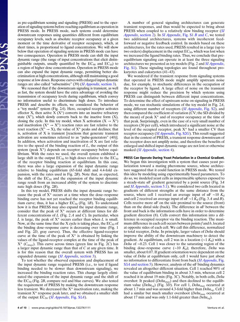
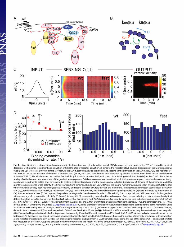
Fig. 4. Slow binding receptors efficiently convey gradient information to a cell polarization model. (A) Schema of the early events in the PRS (αF) related to gradientdetection. αF stimulates recruitment and activation of Cdc42 to sites of receptor activation. αF binds to the receptor (Ste2), causing dissociation of the G protein into Gα(Gpa1) and Gβγ (Ste4–Ste18) heterodimers. Gβγ recruits the MAPK scaffold (Ste5) to the membrane, leading to the activation of the MAPK Fus3. Gβγ also recruits Far1.Far1 recruits Cdc24, the activator of the small G protein Cdc42 (55, 56, 83). Cdc42 stimulates its own activation by binding to Bem1. Bem1 binds Cdc24, which furtheractivates Cdc42 (7, 49). αF stimulates this positive feedback loop further via recruited Ste5, which also binds Bem1 (green dotted line) (84). Active Cdc42 directs the as-sembly of actin filaments in a later phase of the gradient sensing process. Solid arrows correspond to activation, dotted arrows correspond tomoleculemovement (e.g.,membrane recruitment), dotted lines correspond to protein–protein interactions, and the double arrow indicates dissociation. (B) Schema of the Altschuler model forspontaneous emergence of cell polarity (54). It has four reactions: binding/unbinding of Cdc42 to/from the plasmamembrane, recruitment of cytoplasmic Cdc42 to siteswhere Cdc42 has already been recruited (positive feedback), and lateral diffusion of Cdc42 through themembrane. The associated parameters spontaneous associationrate (kon), random dissociation rate (koff), recruitment rate (kfb), lateral diffusion (D), and the total number of signalingmolecules (N) were estimated by Altschuler et al.(54) fromexperimental data. (C, Left) Input to thegradient sensingmodel: Steady-stateαF spatial profile, as in Fig. 3A, corresponds toa cell locatedatapoint inagradientwith an average αF concentration of 10 Kd. (C, Center) Sensing [C(θ,t)], representing normalized bound receptor. Plots correspond using a color scale on the right, atdifferent angles θ (as in Fig. 3A) vs. time, for slow [WT (wt), Left] or fast binding (fast, Right) receptors. For slow dynamics, we used published binding rates of αF to Ste2,k+=1.9×10⁵M−1·s−1andk−=0.001 s−1 (15). For fastdynamics,weusedk+andk−thatare100-foldgreater,maintaining thesameKd. Thus, theparametersare q
4πDd=10,a/d= 0.3, and k−= 0.001 (slow) or 0.1 (fast) (SI Appendix, section 5.1). (C, Right) Example of simulation output: Plot corresponds to particle density at themembrane usinga color scale, indicatedbyabaron the right, atdifferent angles θ (as in Fig. 3A) vs. time. (D, Left) Percentageofpolarizations in the frontquadrant as a functionofbindingdynamics (ratek−at constantKd) foracell locatedas inCafter5min (black●) or15min (red■) of simulation.Of the testedk−rates, only those rates lower thanorequal to0.001 1/s resulted in polarizations in the front quadrant thatwere significantly different from random (25%, black line), P< 0.05. Arrows indicate the results shown in thehistograms.At the slowest rate tested, therewerenopolarizations in the first 5min. (D,Right)Histograms showing thenumberof stochastic simulationswithpolarizationat the indicatedangles θ, using slow (Left) or fast (Right) ligand-receptor bindingdynamics (2,000 simulation runs each). The sizeof thebins is π/6.5. Thepolarization statewas measured at t = 5 min. Coupling between occupied receptor and this model was done through parameters kon and kfb as follows: konðθ,tÞ=Aon *Cðθ,tÞ andkfbðθ,tÞ=Afb *Cðθ,tÞ, where Aon and Afb are the coupling parameters. Aon = 0.0012, Afb = 23, koff = 9 min−1, D = 1.2 μm2, and N = 103 (SI Appendix, Fig. S6).
6 of 10 | www.pnas.org/cgi/doi/10.1073/pnas.1322761111 Ventura et al.
We noted that the transient behavior of Delta (the difference inreceptor occupancy on the front and back sides) is functionallyequivalent to the transient behavior of X* in our toy model (Fig.2A). In the case of gradient sensing,Delta overshot because the timederivative of the occupied receptor at the front was initially largerthan at the back (because the concentration at the front was largerthan at the back), but it reached zero (steady state) faster at thefront than at the back (Fig. 3E). Therefore, cells have greatersensitivity for differences between the front and back during a timewindow (Fig. 3D) before binding equilibrium, and PRESS operatingduring this time window provides an opportunity for the cell toextract more information from the gradient than after equilibrium isreached. The slower the binding dynamics of the receptor, thelonger is the time window for accurate gradient detection (SI Ap-pendix, Fig. S3C and section 5), potentially providing a selectiveadvantage over evolutionary time for cells carrying mutations thatresulted in slower binding αF receptors.
Yeast Can Polarize Fast, Within the Time Window Compatible withPRESS. The spatial differences in receptor occupation result indifferential recruitment of the polarization machinery to the re-gion of higher binding, thus initiating cell polarization at that site.We again considered cell 1 in the model. For cell 1, there are ∼6min (Fig. 3D) during which it would be possible to improve po-larization in the direction of an αF gradient using PRESS. Wetested experimentally whether the downstreammachinery coupledto bound receptor operated quickly enough to polarize during thistime. To do so, we performed two experiments. In the first, wemeasured the timing of polarization in yeast stimulated with 1 μMαF (∼200 Kd). We used such a high level of αF to saturate itsreceptors within a few seconds, thus allowing us to follow the dy-namics of the polarization process itself, independent of the dy-namics of receptor binding. We applied αF isotropically. Duringisotropic stimulation, cells use the same core machinery as they doin gradients but use the internal marks otherwise utilized forbudding to choose the site to polarize (44). To assay polarization,we used cells expressing the MAPK scaffold protein Ste5 fused tothree YFPs, which localizes to the active G protein βγ dimer (Ste4/Ste18) (14, 45, 46) (Fig. 4A). Although the timing of YFP accu-mulation to a single pole was somewhat variable (partly due todifferences among cells in their position in the cell cycle), cells withpolarized Ste5 were visible within 1 min (Fig. 3F, Movie S1, and SIAppendix, Fig. S4).Weobtained the same result when following thepolarization of a second marker protein Ste20-YFP (SI Appendix,Fig. S4). These experimental results argued that the recruitment ofpolarization machinery downstream of the αF receptor is suffi-ciently rapid to use binding information within the time window ofthe overshoot of Delta, and is thus compatible with PRESS.In the second experiment, we asked if polarization was also
fast when cells do not use their internal cues, such as when theyhave to use gradient information. To answer this question, weperformed measurements in a gradient device (47), which ex-posed cells to a linear gradient from 0 to 50 nM across a chamberof 200 μm (SI Appendix, Fig. S5). Yeast could determine thegradient vector in these gradients (in the central region of thechamber, 54.8% yeast polarized in the front quadrant vs. 24.3%in the corresponding region of a control nongradient chamber;SI Appendix, Fig. S5D). We monitored early events in polariza-tion by observing the localization of the polarization machineryusing cells expressing Bem1 fused to a tandem repeat of threemNeonGreen fluorescent proteins (SI Appendix, section 7) (48).Bem1 is a scaffold protein that activates and clusters Cdc42,leading to the formation of the “polarity patch,” both during thecell cycle and during the mating response (49–51). We looked incells that had finished budding but in which mother and daughterwere still connected, in which the polarization machinery wasinitially localized to the bud neck. Two things happened to suchcells in such gradients. Some cells relocalized their polarization
machinery to one of two internal marks, which lie on each polealong the major axis of the cell (52, 53). Other cells relocalizedthe Bem1 patch to a new site that did not correspond to eithermark (SI Appendix, Fig. S5). We scored cells as having relo-calized Bem1 to either internal mark or to a new site. This lattergroup represented yeast that had repositioned their “internalcompass.” We found that the average time to relocalize the bud-neck Bem1 patch to these new sites was fast (10.8 ± 8.1 min).The fastest times were less than 5 min, in the time window duringwhich PRESS could benefit the cell. These results support theidea that yeast should be able to take advantage of PRESS whenmaking the gradient direction determination.
Slow Binding Receptors Efficiently Convey Gradient Information toa Cell Polarization Model. To investigate further if PRESS couldguide the yeast polarization machinery to orient in pheromonegradients, we fed the level of bound receptor at every positionand at every time point generated by our model to a downstreammodel of cell polarization (Fig. 4). For this model, we chose thestochastic neutral drift model developed by Altschuler et al. (54)because (i) it models the polarization of the very molecule(Cdc42) that operates during yeast mating (55, 56) (Fig. 4A); (ii)the model is modular, making it easy to couple to our input; and(iii) there are only four parameters (that have been estimatedexperimentally) describing four reactions: binding/unbinding ofCdc42 to/from the plasma membrane, recruitment of cytoplasmicCdc42 to sites where Cdc42 has already been recruited (positivefeedback), and lateral diffusion of Cdc42 on the membrane. Thus,the simplicity of this model limited the number of decisions weneeded to make about how to couple information from the re-ceptor binding model to it. We decided to use linear coupling,the simplest, and arguably the most restrictive, method. For thecoupling coefficient, we chose the smallest value that resulted inpolarizations in 100% of the simulations run with an average αFconcentration of 1 Kd (Fig. 4, legend) because this output is whatis observed experimentally.Our model predicted that for the αF gradient detection system, in
which PRESS is favored over equilibrium signaling, faster thannormal binding dynamics [in which the overshoot has a shorterduration (details are provided in SI Appendix, Fig. S3 and section 5)]should result in fewer polarizations oriented correctly. Our modelalso predicted that the increased ability to discriminate between thefront and back of the cell provided by PRESS should be mostpronounced at concentrations of αF close to the receptor saturationregion. To test this prediction, we simulated a range of αF bindingrates, from slower to faster than the published rates (15), spanningtime windows for PRESS from ∼90 min to ∼6 s. In Fig. 4C, we showthe time course of binding for the published rates, in which PRESScan operate, and for 100-fold faster rates, in which PRESS cannotoperate. We then ran thousands of stochastic simulations of a celllocated in a gradient with an average αF concentration of 10 Kd foreach binding rate (Fig. 4D and SI Appendix, Fig. S6). In Fig. 4D, weshow the polarization states arising in the first 5 min of simulation(t ≤ 5 min) for the two conditions shown in Fig. 4C. After 5 min, forthe WT receptor the advantage gained by PRESS has nearly dis-appeared (Figs. 3C and 4C). As predicted, simulations that usedslow binding kinetics resulted in significantly better-orientedpolarizations than those simulations using fast kinetics (Fig. 4D andSI Appendix, Fig. S5A). Specifically, using WT receptor dynamics,34% of the simulated polarizations localized to the front quadrantof the cell. This value is similar to what has been observed experi-mentally (11). In contrast, using fast dynamics, only 25.3% of thepolarizations localized to the front quadrant (WT vs. fast; P < 10−6),which is the value expected if polarization quadrant choice wasrandom. Rates slower than WT rates further increased the per-centage of outputs in the front quadrant (SI Appendix, Fig. S6A).These results indicate that in conditions where cells with fastreceptors are unable to use the gradient information, cells with slow
Ventura et al. PNAS Early Edition | 7 of 10
BIOPH
YSICSAND
COMPU
TATIONALBIOLO
GY
PNASPL
US
receptors can polarize significantly better than expected by chance.These results also suggest that PRESS is helpful for gradient sensingat high concentrations of αF.
DiscussionIn some cell signaling systems, including the yeast PRS, ligandsbind and unbind receptors relatively slowly. Here, we asked whatmight be gained from this slowness. We showed by simplemathematical analysis that in cells exposed to a sudden increasein ligand, the EC50 of the dose–response curve for receptor oc-cupation becomes progressively smaller as binding approachesequilibrium over time (Fig. 1 B and C). When receptor binding/unbinding is slow, the EC50 changes correspondingly slowly. Werealized that signaling system architectures that coupled the slowshift in the dose–response curve to faster events could enable thecell to react to information about the extracellular environment,which would be obscured after equilibrium was achieved. We calledthis ability to extract information from the time-evolving dose–response curve PRESS. For many system architectures, PRESS canmodulate the input dynamic range, simply by the difference in timingbetween ligand-receptor binding equilibrium and faster actingevents. When it operates, PRESS can shift the input dynamic rangeto higher doses, and it can also expand the input dynamic range,allowing cells to discriminate between high concentrations of ex-tracellular ligand that would otherwise be indistinguishable. Weshowed by simulation, and supported by experimentation, thatPRESS improves the orientation of yeast cells in response to pher-omone gradients.
Downstream Systems That Couple to Slow Receptors to Enable PRESS.We simulated the operation of PRESS in three toy models (Fig.2 and SI Appendix, Fig. S1) to illustrate the idea that PRESSworks with different downstream signaling architectures thatproduce a transient response, which are ubiquitous in eukar-yotes. The toy model in Fig. 2 was inspired by the operation offast-inactivating ligand-gated ion channels, common in the ner-vous system (57). The other two toy models corresponded toincoherent feedforward and negative feedback loops, respec-tively, which are commonly found in cellular signaling pathways(42, 43). These toy models had in common that their outputs weretransient. None of the toy models reflected the transient behaviorduring gradient sensing that enables PRESS in the mating pher-omone pathway. In this last case, the role of the transientdownstream signaling is played by the difference in ligand con-centration at the front and at the back, which causes a transientdifference in receptor occupancy in different parts of the cell,enabling gradient direction detection.
PRESS Expands and Shifts the Input Dynamic Range. The transientresponse enables the exploitation of pre-equilibrium information. Itdoes so by bringing about a shift in input dynamic range, an ex-pansion of input dynamic range, or both. The shift occurs becausethe peak in the transient response in the toy models takes place ata time when the binding dose–response curve has itself a higherEC50 than at binding equilibrium (Fig. 1B). The earlier that thesepeaks occur, the larger is the shift in the output EC50. The expan-sion happens when the peak of X* occurs at different times fordifferent stimulus levels: earlier when the stimulus is big and laterwhen it is small. This time shift for the maximum response, con-volved with the slow shift in the binding dose–response curve,expands the input dynamic range, as illustrated in Fig. 2C.
Other Ways Systems Modulate Input Dynamic Range. The enlarge-ment of the dynamic range in PRESS mode comes at a cost: Theresponse becomes subsensitive; therefore, the difference in theoutput for two different stimuli is smaller than it would have beenotherwise (39).Cells use othermechanisms to regulate input dynamicrange. For example, during its life cycle, the amoeba Dictyostelium
discoideum detects gradients of cAMP in a broad range of cAMPconcentrations. Here, binding of cAMP to its receptors is very quick(32), precluding PRESS.Dictyostelium uses a different approach thatexpands the input dynamic range: It has four homologous cAMPreceptors with different Kd values for cAMP (58). This multiple re-ceptor solution has the advantage overPRESS that it does not reducethe system’s sensitivity.Another way of increasing the input dynamic range beyond
receptor saturation is to avoid saturation directly by modulatingreceptor affinity, as in the case of the Escherichia coli chemotaxissystem, where the affinity of receptors for the ligand diminishesas cells adapt to higher concentrations of attractants (59, 60), orby fast turnover of the receptors, such as in the case of theerythropoietin receptor (61). Alternatively, a broad input dynamicrange might be achieved if the concentration of a ligand is trans-formed into the duration of the signal. This transformationmay beachieved, for example, by depleting or degrading the ligand ata constant rate, resulting in longer signaling times for higher doses(62, 63). Signal duration may, in turn, be converted back intoamplitude by the signaling pathway. In more general terms, it hasbeen shown in theory and by experimentation (64, 65) that neg-ative feedback could help to expand the input dynamic range.
Stimulus Dynamics and PRESS. In this work, for simplicity (and tomatch to earlier experiments), we focused our analysis of PRESS oncaseswhere the ligand concentrationoutside the cell (or the gradient)increases suddenly and stays stable thereafter (i.e., a step increase).However, in many physiological conditions, ligand concentrations(and gradients) might change over time in the time scale of receptoractivation. In these cases, the advantage of the PRESS mechanism(namely, the modulation of the input dynamic range) is still present.
PRESS Enables Signaling Systems to Match Different Input DynamicRanges to Different Outputs.Other outputs of the yeast PRS, suchas αF-induced gene expression, exhibit DoRA (i.e., match wellthe equilibrium binding curve of pheromone to the receptor) forseveral hours of continued stimulation (13, 14). This result sug-gests that the pheromone response pathway, using a single typeof receptor, operates simultaneously in two modes to elicit dif-ferent outputs: PRESS for gradient sensing and equilibriumsignaling for determining the level of steady-state gene expres-sion. We suggest that yeast evolved a system with slow bindingdynamics that combines PRESS with equilibrium binding, thusenabling the PRS to cover a broad input dynamic range, from thehigh concentrations sensed during orientation in gradients to thelower concentrations affecting fate choices and gene expression.We speculate that a similar combination of PRESS with equilib-rium signaling operates in other signaling systems with multipleoutputs, providing the ability to shift the input dynamic rangeaccording to physiological function.
PRESS and Other Mechanisms.We note that PRESS, which we havedescribed in cells responding to a steady spatial gradient, is notthe same as a mechanism(s) that enables sensing slowly changingspatial ligand gradients. During Drosophila melanogaster embryodevelopment, before cellularization, the dividing nuclei decodethe concentration of the morphogen Bicoid (start to expressthe Bicoid target gene Hunchback) before the Bicoid ante-roposterior gradient reaches steady state. This process in knownas “pre–steady-state decoding” (66, 67).PRESS mode may combine with other mechanisms postulated
to improve gradient sensing. Previous modeling studies sug-gested that the secreted protease Bar1 might improve matingpheromone gradient sensing. This protease degrades pheromone(68), and by doing so, it changes the shape of the gradient, po-tentially facilitating discrimination between similar partners (69,70). However, gradient detection is not significantly affected instrains deleted for bar1 (11). In any case, PRESS provides an
8 of 10 | www.pnas.org/cgi/doi/10.1073/pnas.1322761111 Ventura et al.
independent mechanism by which cells might sense gradientsmore efficiently. In addition, positive feedback loops (6, 7), to-gether with negative feedbacks (71, 72), have been shown to helpyeast establish a single polarization site. These mechanismsoperate downstream of receptor binding, and therefore down-stream of PRESS. In fact, we have used a polarization model inour work that incorporates positive feedback (Fig. 4), and we haveshown that it interacts appropriately with PRESS. Thus, PRESSdoes not rule out other mechanisms that have been proposed.
PRESS Mechanism Might Be Widespread. Systems with PRESS maybe widespread, given that many cell signaling systems have slowbinding receptors (73) (Table 1) and that there are severaldownstream network topologies that can result in transient signalresponses (74). A number of candidates are in the central ner-vous system, where fast-inactivating, ligand-gated ion channelsare commonplace (41), enabling the pairing of neurotransmitterbinding to fast and transient responses. PRESS may also operatein signaling systems at points other than ligand-receptor binding.The key necessary requirement is, as explained above, that thedose–response at a given step shifts over time. For example,cycles of activation and inactivation of substrates by phosphor-ylation and dephosphorylation are ubiquitous in signaling sys-tems (75). Such cycles are similar to binding/unbinding reactionsin the sense that the time to reach state–state concentrations ofphosphorylated substrate after a step increase in the input (inthis case, the kinase) depends on the size of the increase. If theslowly increasing concentration of activated substrate, in turn,activates a faster transient response, the overall system is capableof PRESS.
Materials and MethodsMathematical Models. The toy model (Fig. 2) and the ligand-receptor modelformulation and analysis for the case of an αF gradient (Figs. 3 and 4) aregiven in SI Appendix, sections 2 and 5.
Numerical Simulations. Stochastic simulations (Fig. 4) were performed usingthe routines kindly provided by S. Altschuler (University of California, SanFrancisco) and modified by us to receive the ligand-receptor information, asdescribed. Simulations were done using custom MATLAB (MathWorks)software. The number of simulations needed for the histograms was de-termined by increasing the sample size until obtaining no changes in the overalloutput. Polarization in simulations was determined following the same criteriaas Altschuler et al. (54); the position of polarizations was computed at the timewhenpolarization first appeared, andhistograms contain the polarizations thatappeared in the first 5 min.
Experimental Procedures. S. cerevisiae strains were of the W303a geneticbackground, derived from ACL379 (12) (MATa, Δbar1) by standard nucleicacid and yeast manipulation procedures (76). More information on strainsused and their construction is provided in SI Appendix, section 6.1.
Binding Dose–Response Curve Measurement. Yeast [strain YAB3725, Δbar1PSTE2-STE2(T305)-CFP] was grown to exponential phase in synthetic completemedium and briefly sonicated, and cycloheximide was added to a final con-centration of 100 μg/mL to block protein translation. The carboxyl-terminaldomain of Ste2 was truncated to eliminate receptor endocytosis (38). At time 0,cells were imaged using the CFP filter cube to estimate total Ste2 abundance,immediately followed by the addition of various amounts of a Hilyte488-labeled αF (37). Images were then taken approximately every 15 min for up to5 h. To calculate αF binding dynamics, images were first analyzed using Cell-IDsoftware (77), which calculates the fluorescence density at the membrane for
each cell. Then, a simple binding model (αF + R ↔ C) was globally fitted to thedata, resulting in Kd = 23 ± 3 nM and k− = 1.0 ± 0.2 10−4·s−1.
Assay of Polarization. We used S. cerevisiae W303a strains MWY003 andESY3136 [relevant genotypes: STE5-YFP(3x) and STE20-YFP, respectively],which are derivatives of ACL379 expressing the fusions under the control oftheir respective native promoters. For image cytometry, we affixed expo-nentially growing cells to the bottom of wells in a glass-bottomed 96-wellplate, as described (12), and stimulated them with 1 μM αF. We performedimage acquisition essentially as described (78) and quantified the results asdescribed in SI Appendix, section 6.2.
Chemotropism Assay in Microfluidic Devices. We fabricated microfluidicdevices designed for the generation of stable gradients in open chambersusing standard protocols for polydimethylsiloxane (PDMS)microfluidic deviceconstruction (47). Briefly, we generated silicon molds by three-layer SU-8photolithography, which were then used for making PDMS replicas of thedevice, by excluding PDMS from the tallest features of the mold, therebyproducing open (roofless) chambers. After polymerization, we peeled offthe patterned PDMS structure and bonded it onto glass cover slides byplasma-oxygen treatment (660 mtorr, 60 W, 60 s).
To improve adherence of cells to the glass, we treated the bottom of thechambers with poly-D-lysine (1 mg/mL; Sigma) at room temperature for atleast 3 h and then incubated the chambers with Con A (1 mg/mL; Sigma)overnight at 4 °C. We then filled the device with 0.22 μm of sterile, filteredwater using a vacuum-assisted method (79). Subsequently, we connected thetwo ports of the device with tubing and syringes filled with filtered syntheticcomplete medium alone or with 50 nM αF and 0.1 mg/mL bromophenol blue(BPB) as tracking dye [DBPB = 4.4 10−6·cm2·s−1 (3), DαF = 3.2 10−6·cm2·s−1 (4)].All media contained 100 ppm PEG3000 (Sigma) to prevent nonspecific αFbinding to the container’s surfaces (80). Water hydrostatic pressure (H = 5 cm)drove all flow. We evaluated the formation of the gradients by monitoringBPB fluorescence. Finally, we stopped the flow, washed the chambers withmedia, and loaded a mildly sonicated yeast exponential culture on top of thedevice. We allowed cells to settle and bind to the bottom glass before re-suming the flow. We performed imaging using an Olympus IX-81 micro-scope, with an Olympus UplanSapo objective with a magnification of 63×(N.A. = 1.35) coupled with an HQ2 (Roper Scientific) cooled CCD camera.
Quantification of Repositioning Time. We loaded a yeast strain expressingBEM1-3×–mNeonGreen (48) fusion integrated at the endogenous locus(YGV5097, derived from ACL379) in the microfluidic device. We monitoredthe Bem1 polarization patch imaging approximately every 3 min. We thenquantified polarization times as explained for Ste5, with the additionalanalysis of the angle of the different polarizations. We considered patchesas using “internal marks” (proximal or distal), or “no internal cue” based onthe angle between the position of the polarization at the neck and the newsite. We measured repositioning time as the interval between the last framewith Bem1 at the bud-neck and the first frame where it appeared asa patch elsewhere.
Statistics. P values and SEs for the mean were calculated using bootstrapmethods (81, 82).
ACKNOWLEDGMENTS. We thank C. G. Pesce, P. Aguilar, Peter Pryciak, AlbertoKornblihtt, M. González Gaitán, and Andreas Constantinou for helpful discus-sions and comments on the manuscript; Peter Pryciak (University of Massachu-setts) and Eduard Serra (Institute of Predictive and Personalized Medicine ofCancer) for providing yeast strains YPP3662 and ESY3136; S. Altschuler (Universityof California, San Francisco) for providing the simulation code that was the basisfor our simulations; and D. G. Drubin (University of California, Berkeley) forkindly providing the fluorescent αF. Work was supported by Grant PICT2010-2248 from the Argentine Agency of Research and Technology (to A.C.-L.) andGrant 1R01GM097479-01 from the National Institute of General Medical Scien-ces, National Institutes of Health (to R.B. and A.C.-L.).
1. Li R, Bowerman B (2010) Symmetry breaking in biology. Cold Spring Harb PerspectBiol 2(3):a003475.
2. Macnab RM, Koshland DE, Jr (1972) The gradient-sensing mechanism in bacterialchemotaxis. Proc Natl Acad Sci USA 69(9):2509–2512.
3. Swaney KF, Huang CH, Devreotes PN (2010) Eukaryotic chemotaxis: A network ofsignaling pathways controls motility, directional sensing, and polarity. Annu Rev Bio-phys 39:265–289.
4. Segall JE (1993) Polarization of yeast cells in spatial gradients of alpha mating factor.Proc Natl Acad Sci USA 90(18):8332–8336.
5. Zigmond SH (1989) Chemotactic response of neutrophils. Am J Respir Cell Mol Biol1(6):451–453.
6. Arkowitz RA (2009) Chemical gradients and chemotropism in yeast. Cold Spring HarbPerspect Biol 1(2):a001958.
7. Slaughter BD, Smith SE, Li R (2009) Symmetry breaking in the life cycle of the buddingyeast. Cold Spring Harb Perspect Biol 1(3):a003384.
8. Jackson CL, Hartwell LH (1990) Courtship in S. cerevisiae: Both cell types choosemating partners by responding to the strongest pheromone signal. Cell 63(5):1039–1051.
Ventura et al. PNAS Early Edition | 9 of 10
BIOPH
YSICSAND
COMPU
TATIONALBIOLO
GY
PNASPL
US
9. Jenness DD, Burkholder AC, Hartwell LH (1983) Binding of alpha-factor pheromone to yeasta cells: Chemical and genetic evidence for an alpha-factor receptor. Cell 35(2 Pt 1):521–529.
10. Ayscough KR, Drubin DG (1998) A role for the yeast actin cytoskeleton in pheromonereceptor clustering and signalling. Curr Biol 8(16):927–930.
11. Moore TI, Chou CS, Nie Q, Jeon NL, Yi TM (2008) Robust spatial sensing of matingpheromone gradients by yeast cells. PLoS ONE 3(12):e3865.
12. Colman-Lerner A, et al. (2005) Regulated cell-to-cell variation in a cell-fate decisionsystem. Nature 437(7059):699–706.
13. Yi TM, Kitano H, Simon MI (2003) A quantitative characterization of the yeast het-erotrimeric G protein cycle. Proc Natl Acad Sci USA 100(19):10764–10769.
14. Yu RC, et al. (2008) Negative feedback that improves information transmission inyeast signalling. Nature 456(7223):755–761.
15. Jenness DD, Burkholder AC, Hartwell LH (1986) Binding of alpha-factor pheromone toSaccharomyces cerevisiae a cells: Dissociation constant and number of binding sites.Mol Cell Biol 6(1):318–320.
16. Bajaj A, et al. (2004) A fluorescent alpha-factor analogue exhibits multiple steps onbinding to its G protein coupled receptor in yeast. Biochemistry 43(42):13564–13578.
17. Pruzansky JJ, Patterson R (1986) Binding constants of IgE receptors on human bloodbasophils for IgE. Immunology 58(2):257–262.
18. Mellman IS, Unkeless JC (1980) Purification of a functional mouse Fc receptor throughthe use of a monoclonal antibody. J Exp Med 152(4):1048–1069.
19. HerkenhamM, et al. (1990) Cannabinoid receptor localization in brain. Proc Natl AcadSci USA 87(5):1932–1936.
20. Wang HM, Smith KA (1987) The interleukin 2 receptor. Functional consequences of itsbimolecular structure. J Exp Med 166(4):1055–1069.
21. Hughes RJ, Boyle MR, Brown RD, Taylor P, Insel PA (1982) Characterization of coex-isting alpha 1- and beta 2-adrenergic receptors on a cloned muscle cell line, BC3H-1.Mol Pharmacol 22(2):258–266.
22. Horwitz EM, Jenkins WT, Hoosein NM, Gurd RS (1985) Kinetic identification of a two-state glucagon receptor system in isolated hepatocytes. Interconversion of homoge-neous receptors. J Biol Chem 260(16):9307–9315.
23. Marasco WA, Feltner DE, Ward PA (1985) Formyl peptide chemotaxis receptors on the ratneutrophil: Experimental evidence for negative cooperativity. J Cell Biochem 27(4):359–375.
24. Bajzer Z, Myers AC, Vuk-Pavlovi�c S (1989) Binding, internalization, and intracellularprocessing of proteins interacting with recycling receptors. A kinetic analysis. J BiolChem 264(23):13623–13631.
25. Ciechanover A, Schwartz AL, Dautry-Varsat A, Lodish HF (1983) Kinetics of in-ternalization and recycling of transferrin and the transferrin receptor in a humanhepatoma cell line. Effect of lysosomotropic agents. J Biol Chem 258(16):9681–9689.
26. Waters CM, Oberg KC, Carpenter G, Overholser KA (1990) Rate constants for binding,dissociation, and internalization of EGF: Effect of receptor occupancy and ligandconcentration. Biochemistry 29(14):3563–3569.
27. Lipkin EW, Teller DC, de Haën C (1986) Kinetics of insulin binding to rat white fat cellsat 15 degrees C. J Biol Chem 261(4):1702–1711.
28. Zigmond SH, Sullivan SJ, Lauffenburger DA (1982) Kinetic analysis of chemotacticpeptide receptor modulation. J Cell Biol 92(1):34–43.
29. Akiyama SK, Yamada KM (1985) The interaction of plasma fibronectin with fibro-blastic cells in suspension. J Biol Chem 260(7):4492–4500.
30. Matsui K, Boniface JJ, Steffner P, Reay PA, Davis MM (1994) Kinetics of T-cell receptorbinding to peptide/I-Ek complexes: Correlation of the dissociation rate with T-cellresponsiveness. Proc Natl Acad Sci USA 91(26):12862–12866.
31. Sklar LA, Sayre J, McNeil VM, Finney DA (1985) Competitive binding kinetics in ligand-receptor-competitor systems. Rate parameters for unlabeled ligands for the formylpeptide receptor. Mol Pharmacol 28(4):323–330.
32. Ueda M, Sako Y, Tanaka T, Devreotes P, Yanagida T (2001) Single-molecule analysis ofchemotactic signaling in Dictyostelium cells. Science 294(5543):864–867.
33. Morton T, Li J, Cook R, Chaiken I (1995) Mutagenesis in the C-terminal region ofhuman interleukin 5 reveals a central patch for receptor alpha chain recognition. ProcNatl Acad Sci USA 92(24):10879–10883.
34. Clements JD, Lester RA, Tong G, Jahr CE, Westbrook GL (1992) The time course ofglutamate in the synaptic cleft. Science 258(5087):1498–1501.
35. Hoffmann C, et al. (2005) A FlAsH-based FRET approach to determine G protein-coupled receptor activation in living cells. Nat Methods 2(3):171–176.
36. Krampfl K, et al. (2002) Control of kinetic properties of GluR2 flop AMPA-typechannels: Impact of R/G nuclear editing. Eur J Neurosci 15(1):51–62.
37. Toshima JY, et al. (2006) Spatial dynamics of receptor-mediated endocytic traffickingin budding yeast revealed by using fluorescent alpha-factor derivatives. Proc NatlAcad Sci USA 103(15):5793–5798.
38. Konopka JB, Jenness DD, Hartwell LH (1988) The C-terminus of the S. cerevisiae alpha-pheromone receptor mediates an adaptive response to pheromone. Cell 54(5):609–620.
39. Koshland DE, Jr, Goldbeter A, Stock JB (1982) Amplification and adaptation in reg-ulatory and sensory systems. Science 217(4556):220–225.
40. Basu S, Mehreja R, Thiberge S, Chen M-TT, Weiss R (2004) Spatiotemporal control of geneexpression with pulse-generating networks. Proc Natl Acad Sci USA 101(17):6355–6360.
41. Jones MV, Westbrook GL (1996) The impact of receptor desensitization on fast syn-aptic transmission. Trends Neurosci 19(3):96–101.
42. Tyson JJ, Novák B (2010) Functional motifs in biochemical reaction networks. AnnuRev Phys Chem 61:219–240.
43. Alon U (2006) An Introduction to Systems Biology: Design Principles of BiologicalCircuits (Chapman & Hall, London).
44. Dorer R, Pryciak PM, Hartwell LH (1995) Saccharomyces cerevisiae cells execute a defaultpathway to select amate in the absence of pheromone gradients. J Cell Biol 131(4):845–861.
45. Whiteway MS, et al. (1995) Association of the yeast pheromone response G proteinbeta gamma subunits with the MAP kinase scaffold Ste5p. Science 269(5230):1572–1575.
46. Pryciak PM, Huntress FA (1998) Membrane recruitment of the kinase cascade scaffoldprotein Ste5 by the Gbetagamma complex underlies activation of the yeast phero-mone response pathway. Genes Dev 12(17):2684–2697.
47. Keenan TM, Hsu C-H, Folch A (2006) Microfluidic “jets” for generating steady-state gradients of soluble molecules on open surfaces. Appl Phys Lett 89(11):114103-1–114103-3.
48. Shaner NC, et al. (2013) A bright monomeric green fluorescent protein derived fromBranchiostoma lanceolatum. Nat Methods 10(5):407–409.
49. Butty AC, et al. (2002) A positive feedback loop stabilizes the guanine-nucleotideexchange factor Cdc24 at sites of polarization. EMBO J 21(7):1565–1576.
50. Irazoqui JE, Gladfelter AS, Lew DJ (2003) Scaffold-mediated symmetry breaking byCdc42p. Nat Cell Biol 5(12):1062–1070.
51. Chenevert J, Corrado K, Bender A, Pringle J, Herskowitz I (1992) A yeast gene (BEM1)necessary for cell polarization whose product contains two SH3 domains. Nature356(6364):77–79.
52. Casamayor A, Snyder M (2002) Bud-site selection and cell polarity in budding yeast.Curr Opin Microbiol 5(2):179–186.
53. Zahner JE, Harkins HA, Pringle JR (1996) Genetic analysis of the bipolar pattern of budsite selection in the yeast Saccharomyces cerevisiae. Mol Cell Biol 16(4):1857–1870.
54. Altschuler SJ, Angenent SB, Wang Y, Wu LF (2008) On the spontaneous emergence ofcell polarity. Nature 454(7206):886–889.
55. Nern A, Arkowitz RA (1998) A GTP-exchange factor required for cell orientation.Nature 391(6663):195–198.
56. Nern A, Arkowitz RA (1999) A Cdc24p-Far1p-Gbetagamma protein complex requiredfor yeast orientation during mating. J Cell Biol 144(6):1187–1202.
57. Lisman JE, Raghavachari S, Tsien RW (2007) The sequence of events that underlie quantaltransmission at central glutamatergic synapses. Nat Rev Neurosci 8(8):597–609.
58. Kim JY, Borleis JA, Devreotes PN (1998) Switching of chemoattractant receptors pro-grams development and morphogenesis in Dictyostelium: Receptor subtypes activatecommon responses at different agonist concentrations. Dev Biol 197(1):117–128.
59. Sourjik V, Wingreen NS (2012) Responding to chemical gradients: Bacterial chemo-taxis. Curr Opin Cell Biol 24(2):262–268.
60. Friedlander T, Brenne N (2011) Adaptive response and enlargement of dynamicrange. Math Biosci Eng 8(2):515–528.
61. Becker V, et al. (2010) Covering a broad dynamic range: Information processing at theerythropoietin receptor. Science 328(5984):1404–1408.
62. Behar M, Hao N, Dohlman HG, Elston TC (2008) Dose-to-duration encoding and signalingbeyond saturation in intracellular signaling networks. PLOS Comput Biol 4(10):e1000197.
63. Edelstein SJ, Stefan MI, Le Novère N (2010) Ligand depletion in vivo modulates thedynamic range and cooperativity of signal transduction. PLoS ONE 5(1):e8449.
64. Nevozhay D, Adams RM, Murphy KF, Josic K, Balázsi G (2009) Negative autoregulationlinearizes the dose-response and suppresses the heterogeneity of gene expression.Proc Natl Acad Sci USA 106(13):5123–5128.
65. Madar D, Dekel E, Bren A, Alon U (2011) Negative auto-regulation increases the inputdynamic-range of the arabinose system of Escherichia coli. BMC Syst Biol 5:111.
66. Bergmann S, et al. (2007) Pre-steady-state decoding of the Bicoid morphogen gra-dient. PLoS Biol 5(2):e46.
67. Tamari Z, Barkai N (2012) Improved readout precision of the Bicoid morphogengradient by early decoding. J Biol Phys 38(2):317–329.
68. MacKay VL, et al. (1988) The Saccharomyces cerevisiae BAR1 gene encodes an ex-ported protein with homology to pepsin. Proc Natl Acad Sci USA 85(1):55–59.
69. Andrews SS, Addy NJ, Brent R, Arkin AP (2010) Detailed simulations of cell biologywith Smoldyn 2.1. PLOS Comput Biol 6(3):e1000705.
70. Rappaport N, Barkai N (2012) Disentangling signaling gradients generated byequivalent sources. J Biol Phys 38(2):267–278.
71. Kuo C-CC, et al. (2014) Inhibitory GEF phosphorylation provides negative feedback inthe yeast polarity circuit. Curr Biol 24(7):753–759.
72. Wu C-FF, Lew DJ (2013) Beyond symmetry-breaking: Competition and negativefeedback in GTPase regulation. Trends Cell Biol 23(10):476–483.
73. Lauffenburger DA, Linderman JJ (1993) Receptors: Models for Binding, Trafficking,and Signaling (Oxford Univ Press, New York).
74. Ma W, Trusina A, El-Samad H, Lim WA, Tang C (2009) Defining network topologiesthat can achieve biochemical adaptation. Cell 138(4):760–773.
75. Kholodenko BN, Hancock JF, Kolch W (2010) Signalling ballet in space and time. NatRev Mol Cell Biol 11(6):414–426.
76. Guthrie C, Fink GR (1991) Methods in Enzymology, Guide to Yeast Genetics andMolecular Biology (Academic, San Diego).
77. Gordon, et al. (2007) Single-cell quantification of molecules and rates using open-source microscope-based cytometry. Nat Methods 4(2):175–181.
78. Bush A, Colman-Lerner A (2013) Quantitative measurement of protein relocalizationin live cells. Biophys J 104(3):727–736.
79. Monahan J, Gewirth AA, Nuzzo RG (2001) A method for filling complex polymericmicrofluidic devices and arrays. Anal Chem 73(13):3193–3197.
80. Liu B, et al. (2013) Parts-per-million of polyethylene glycol as a non-interferingblocking agent for homogeneous biosensor development. Anal Chem 85(21):10045–10050.
81. Efron B, Tibshirani R (1994) An Introduction to the Bootstrap (Chapman & Hall, New York).82. Cedersund G, Roll J (2009) Systems biology: Model based evaluation and comparison
of potential explanations for given biological data. FEBS J 276(4):903–922.83. Butty AC, Pryciak PM, Huang LS, Herskowitz I, Peter M (1998) The role of Far1p in
linking the heterotrimeric G protein to polarity establishment proteins during yeastmating. Science 282(5393):1511–1516.
84. Leeuw T, et al. (1995) Pheromone response in yeast: Association of Bem1p withproteins of the MAP kinase cascade and actin. Science 270(5239):1210–1213.
10 of 10 | www.pnas.org/cgi/doi/10.1073/pnas.1322761111 Ventura et al.
Ventura et al, SI Appendix
1
Figure Legends, Supplemental Computational/Experimental Procedures/Analysis
Utilization of extracellular information before ligand-‐receptor binding reaches equilibrium expands and shifts the input dynamic range.
Alejandra C Ventura, Alan Bush, Gustavo Vasen, Matías A Goldín, Brianne Burkinshaw, Nirveek
Bhattacharjee, Albert Folch, Roger Brent, Ariel Chernomoretz, and Alejandro Colman-‐Lerner
Ventura et al, SI Appendix
2
Table of contents.
Supplemental Figures directly called from the main text. ......................................................................... 3 Figure S1. Toy models with transient signaling modules perform PRESS, related to Figure 2. ............. 3 Figure S2. The effect of noise during PRESS, related to Figure 2. ......................................................... 4 Figure S3. Characterization of PRESS applied to gradient detection, related to Figure 3. ................... 5 Figure S4. Timing of yeast polarization, related to Figure 3. ................................................................. 6 Figure S5. Timing of polarization patch relocalization, related to Figure 3. .......................................... 7 Figure S6. The αF receptor binding dynamics might be optimal for PRESS, related to Figure 4. .......... 8
1. Characterization of the ligand-‐receptor time-‐dependent dose-‐response curve. ................................ 10 2. Toy models with transient signaling modules perform PRESS ............................................................. 12
Model 1: X with an inactive refractory state. ...................................................................................... 12 Model 2: X controlled by an incoherent feed-‐forward loop (IFFL); and Model 3: X controlled by a negative feed-‐back loop (NFBL). ......................................................................................................... 12
3. Models with transient signaling may be subsensitive, helping to expand the input dynamic range. . 14 Sensitivity in Model 1: X with an inactive refractory state. ................................................................ 14
Table S1. Model 1 sensitivity. ......................................................................................................... 15 Sensitivity in Model 3: X controlled by a negative feed-‐back loop (NFBL). ......................................... 16
Table S2. Model 3 sensitivity. ......................................................................................................... 16 General conclusions based on the above studies and the results in the main text: ........................... 16
4. The effect of noise during PRESS ......................................................................................................... 19 5. Mathematical model to study the sensing of a stationary spatial gradient ........................................ 21
5.1 An analytical expression for the αF gradient generated by a point source, and for the variable Delta (Description 1) ........................................................................................................................... 21 5.1.1 A simplified formula for the αF gradient generated by a point source, and the variable Delta 24 5.2 An analytical expression for the variable Delta (Description 2) ................................................... 26
Table S3. Strains. ............................................................................................................................ 29 6 Supplemental experimental procedures .............................................................................................. 29
6.1 Strains and plasmids. .................................................................................................................... 29 6.2 Quantification of Polarization Times ............................................................................................. 30
7. Triple monomeric NeonGreen DNA sequence. .................................................................................... 31 8. Supplemental References .................................................................................................................... 32
Ventura et al, SI Appendix
3
Supplemental Figures directly called from the main text.
Figure S1. Toy models with transient signaling modules perform PRESS, related to Figure 2. In the three models, left panels contain schemas of the corresponding model, middle panels show dose-‐responses and right panels show temporal dynamics. Parameters were selected so that X* has a transient behavior. Dose-‐responses are included for the equilibrium value of C (ligand-‐receptor complex) in solid black lines, and for the maximum of X* in dashed blue lines. The dose of the ligand is normalized by the Kd of the binding/unbinding reaction. Temporal profiles of C (solid lines) and of X* (dashed lines) are included at ligand concentrations indicated over the traces. A. X with an inactive refractory state (same as in Figure 2). Left. Occupied receptor activates effector X; after a while, active X (X*) converts into an inactive refractory state (X^), which slowly converts back to the inactive form (X), closing the cycle. Middle. Parameter values: k-‐=0.001 1/sec, r1=0.1, r2=0.06-‐0.8-‐1.6 (increasing from left to right in the middle panel), r3=0.001, Xtot=10 (k+ is not needed because of the dimensionless variables chosen, see section 1). EC50 for each response: 1 for C, and for X* is 9.3 for r2=0.06, 65.8 for r2=0.8, and 87 for r2=1.6. Right. Temporal profiles for the same parameters as in the middle panel, using r2=0.8. B. X controlled by an incoherent feed-‐forward loop (IFFL). Left. Occupied receptor activates both B and X into B* and X*, and B* increases X* inactivation. Middle. Parameter values: k-‐=0.001-‐0.1 1/sec (from right to left), kCB=0.5, KCB=0.01, kFBB=10, KFBB=10, FB=0.5, kCX=2, KCX=0.1, kBX=3, KBX=0.1 (see SI Appendix, Section 2 for details of the model, ki are catalytic rate constants and Ki are Michaelis-‐Menten constants, for example, kCB and KCB are the pair characterizing how C regulates B). Right. Temporal profiles for the same parameters as in the middle panel, using k-‐=0.001 1/sec. C. X controlled by a negative feed-‐back loop (NFBL). Left. Occupied receptor activates X into X*, X* activates B into B*, and B* increases X* inactivation. Middle. Parameter values: k-‐=0.001-‐0.1 1/sec (from right to left), kXB=1, KXB=0.01, kFBB=5, KFBB=100, FB=0.5, kCX=5, KCX=0.1, kBX=6, KBX=0.01 (see SI Appendix, Section 2 for details of the model). Right. Temporal profiles for the same parameters as in the middle panel, using k-‐=0.001 1/sec.
L+R C
X X*
X^
0.01 1 100 100000
0.2
0.4
0.6
0.8
1
L/Kd
Nor
mal
ized
Res
pons
e
A
r1
r2r3 increasing r2
Dose responses Dynamics
0 1 2 3 4 50
0.2
0.4
0.6
0.8
1
Time (min)
Nor
mal
ized
Res
pons
e
100
10
1X withrefractory state
CX*
k+
k-
0.001 0.1 10 10000
0.2
0.4
0.6
0.8
1
L/Kd
Nor
mal
ized
Res
pons
eL+R C
X X*B B*
B
0 0.1 0.2 0.3 0.40
0.2
0.4
0.6
0.8
1
Time (min)
Nor
mal
ized
Res
pons
e
1000
100
10increasingk+ and k-
Dose responses Dynamics
X controlled byincoherentfeed-forward loop(IFFL)
CX*k+
k-
L+R C
X X*B B*
0.01 1 100 100000
0.2
0.4
0.6
0.8
1
L/Kd
Nor
mal
ized
Res
pons
e
C
0 2 40
0.2
0.4
0.6
0.8
1
Time (sec)
Nor
mal
ized
Res
pons
e
500
1500
100increasingk+ and k-
k+
k-
Dose responses Dynamics
X controlled by ŶĞŐĂƟǀĞfeed-back loop(NFBL)
CX*
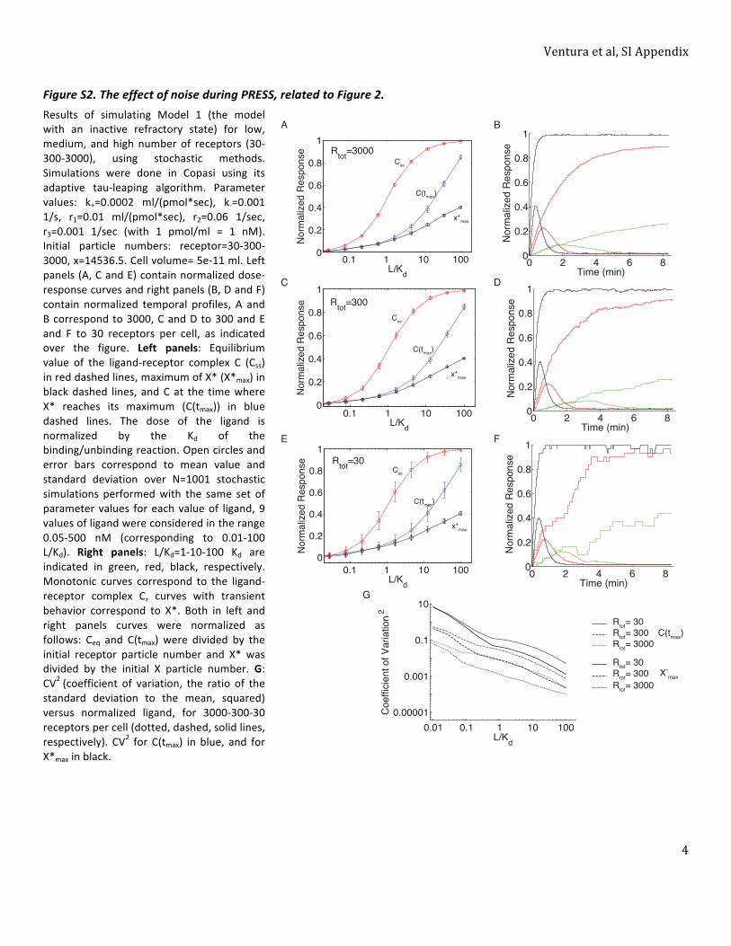
Ventura et al, SI Appendix
4
Figure S2. The effect of noise during PRESS, related to Figure 2. Results of simulating Model 1 (the model with an inactive refractory state) for low, medium, and high number of receptors (30-‐300-‐3000), using stochastic methods. Simulations were done in Copasi using its adaptive tau-‐leaping algorithm. Parameter values: k+=0.0002 ml/(pmol*sec), k-‐=0.001 1/s, r1=0.01 ml/(pmol*sec), r2=0.06 1/sec, r3=0.001 1/sec (with 1 pmol/ml = 1 nM). Initial particle numbers: receptor=30-‐300-‐3000, x=14536.5. Cell volume= 5e-‐11 ml. Left panels (A, C and E) contain normalized dose-‐response curves and right panels (B, D and F) contain normalized temporal profiles, A and B correspond to 3000, C and D to 300 and E and F to 30 receptors per cell, as indicated over the figure. Left panels: Equilibrium value of the ligand-‐receptor complex C (Css) in red dashed lines, maximum of X* (X*max) in black dashed lines, and C at the time where X* reaches its maximum (C(tmax)) in blue dashed lines. The dose of the ligand is normalized by the Kd of the binding/unbinding reaction. Open circles and error bars correspond to mean value and standard deviation over N=1001 stochastic simulations performed with the same set of parameter values for each value of ligand, 9 values of ligand were considered in the range 0.05-‐500 nM (corresponding to 0.01-‐100 L/Kd). Right panels: L/Kd=1-‐10-‐100 Kd are indicated in green, red, black, respectively. Monotonic curves correspond to the ligand-‐receptor complex C, curves with transient behavior correspond to X*. Both in left and right panels curves were normalized as follows: Ceq and C(tmax) were divided by the initial receptor particle number and X* was divided by the initial X particle number. G: CV2
(coefficient of variation, the ratio of the standard deviation to the mean, squared) versus normalized ligand, for 3000-‐300-‐30 receptors per cell (dotted, dashed, solid lines, respectively). CV2 for C(tmax) in blue, and for X*max in black.
0.1 1 10 1000
0.2
0.4
0.6
0.8
1
L/Kd
Nor
mal
ized
Res
pons
e Rtot=3000
C(tmax)
x*max
Css
A
0.1 1 10 1000
0.2
0.4
0.6
0.8
1
L/Kd
Nor
mal
ized
Res
pons
e Rtot=30
C(tmax)
x*max
Css
E
0.1 1 10 1000
0.2
0.4
0.6
0.8
1
L/Kd
Nor
mal
ized
Res
pons
e Rtot=300
C(tmax)
x*max
Css
C
C(tmax)
Rtot= 30Rtot= 300 X*
max
Rtot= 3000
Rtot= 30Rtot= 300Rtot= 3000
G
0.01 0.1 1 10 1000.00001
0.001
0.1
10
L/Kd
Coe
ffici
ent o
f Var
iatio
n 2
0 2 4 6 80
0.2
0.4
0.6
0.8
1
Time (min)
Nor
mal
ized
Res
pons
e
B
0 2 4 6 80
0.2
0.4
0.6
0.8
1
Time (min)
Nor
mal
ized
Res
pons
e
D
0 2 4 6 80
0.2
0.4
0.6
0.8
1
Time (min)
Nor
mal
ized
Res
pons
e
F
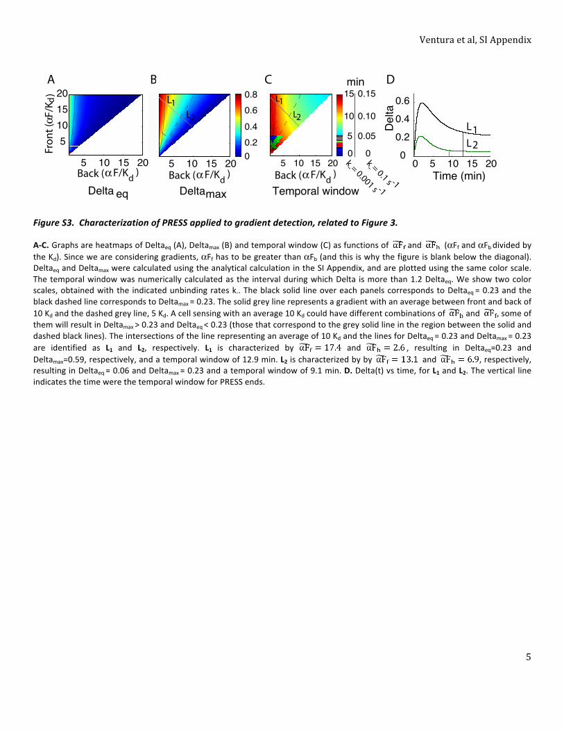
Ventura et al, SI Appendix
5
min
5
10
15
0
0.05
0.10
0.15
0
L1L2
k- = 0.1 s -1
k = 0.001 s -1
-5 10 15 20Back (FF/Kd )Temporal window
5 10 15 20
5101520 0.8
0.6
0.4
0.2
0Fron
t (FF
/Kd
)
A
Back (FF/Kd )
B0.80.6
0.4
0.2
L1L2
Back (FF/Kd )5 10 15 20
00 5 10 15 20
0
0.2
0.4
0.6
Time (min)
Del
ta
L1L2
DC
Delta eq Deltamax
Figure S3. Characterization of PRESS applied to gradient detection, related to Figure 3.
A-‐C. Graphs are heatmaps of Deltaeq (A), Deltamax (B) and temporal window (C) as functions of and (αFf and αFb divided by the Kd). Since we are considering gradients, αFf has to be greater than αFb (and this is why the figure is blank below the diagonal). Deltaeq and Deltamax were calculated using the analytical calculation in the SI Appendix, and are plotted using the same color scale. The temporal window was numerically calculated as the interval during which Delta is more than 1.2 Deltaeq. We show two color scales, obtained with the indicated unbinding rates k-‐. The black solid line over each panels corresponds to Deltaeq = 0.23 and the black dashed line corresponds to Deltamax = 0.23. The solid grey line represents a gradient with an average between front and back of 10 Kd and the dashed grey line, 5 Kd. A cell sensing with an average 10 Kd could have different combinations of and , some of them will result in Deltamax > 0.23 and Deltaeq < 0.23 (those that correspond to the grey solid line in the region between the solid and dashed black lines). The intersections of the line representing an average of 10 Kd and the lines for Deltaeq = 0.23 and Deltamax = 0.23 are identified as L1 and L2, respectively. L1 is characterized by and , resulting in Deltaeq=0.23 and Deltamax=0.59, respectively, and a temporal window of 12.9 min. L2 is characterized by by and , respectively, resulting in Deltaeq = 0.06 and Deltamax = 0.23 and a temporal window of 9.1 min. D. Delta(t) vs time, for L1 and L2. The vertical line indicates the time were the temporal window for PRESS ends.
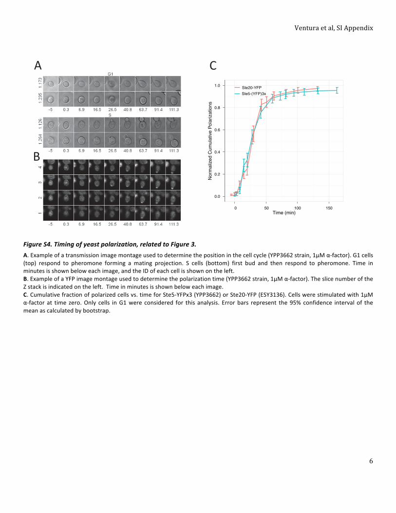
Ventura et al, SI Appendix
6
0.0
0.2
0.4
0.6
0.8
1.0
0 50 100 150Time (min)
Nor
mal
ized
Cum
ulat
ive
Pola
rizat
ions
Ste20-YFPSte5-(YFP)3x
A C
B
Figure S4, related to Figure 3
Figure S4. Timing of yeast polarization, related to Figure 3. A. Example of a transmission image montage used to determine the position in the cell cycle (YPP3662 strain, 1μM α-‐factor). G1 cells (top) respond to pheromone forming a mating projection. S cells (bottom) first bud and then respond to pheromone. Time in minutes is shown below each image, and the ID of each cell is shown on the left. B. Example of a YFP image montage used to determine the polarization time (YPP3662 strain, 1μM α-‐factor). The slice number of the Z stack is indicated on the left. Time in minutes is shown below each image. C. Cumulative fraction of polarized cells vs. time for Ste5-‐YFPx3 (YPP3662) or Ste20-‐YFP (ESY3136). Cells were stimulated with 1μM α-‐factor at time zero. Only cells in G1 were considered for this analysis. Error bars represent the 95% confidence interval of the mean as calculated by bootstrap.
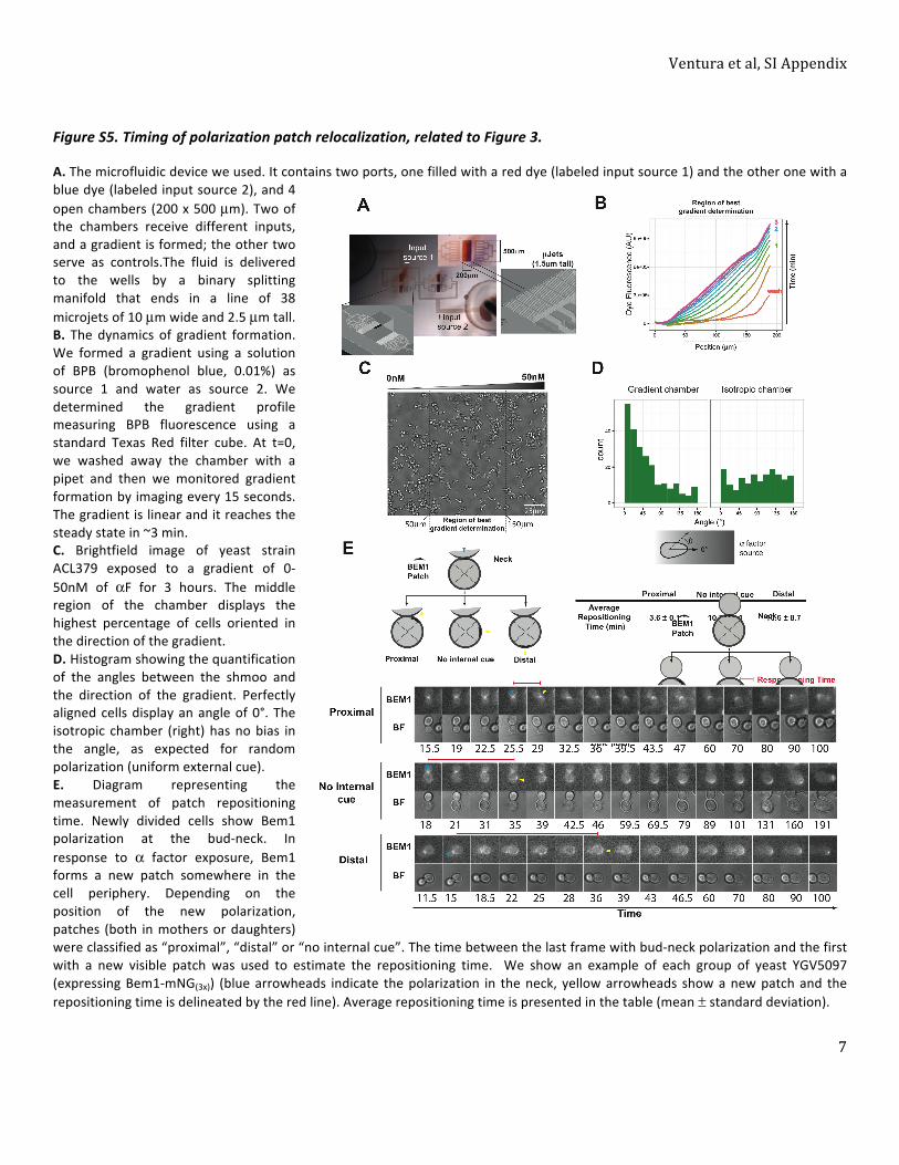
Ventura et al, SI Appendix
7
Figure S5. Timing of polarization patch relocalization, related to Figure 3.
A. The microfluidic device we used. It contains two ports, one filled with a red dye (labeled input source 1) and the other one with a blue dye (labeled input source 2), and 4 open chambers (200 x 500 µm). Two of the chambers receive different inputs, and a gradient is formed; the other two serve as controls.The fluid is delivered to the wells by a binary splitting manifold that ends in a line of 38 microjets of 10 µm wide and 2.5 µm tall. B. The dynamics of gradient formation. We formed a gradient using a solution of BPB (bromophenol blue, 0.01%) as source 1 and water as source 2. We determined the gradient profile measuring BPB fluorescence using a standard Texas Red filter cube. At t=0, we washed away the chamber with a pipet and then we monitored gradient formation by imaging every 15 seconds. The gradient is linear and it reaches the steady state in ~3 min. C. Brightfield image of yeast strain ACL379 exposed to a gradient of 0-‐50nM of αF for 3 hours. The middle region of the chamber displays the highest percentage of cells oriented in the direction of the gradient. D. Histogram showing the quantification of the angles between the shmoo and the direction of the gradient. Perfectly aligned cells display an angle of 0°. The isotropic chamber (right) has no bias in the angle, as expected for random polarization (uniform external cue). E. Diagram representing the measurement of patch repositioning time. Newly divided cells show Bem1 polarization at the bud-‐neck. In response to α factor exposure, Bem1 forms a new patch somewhere in the cell periphery. Depending on the position of the new polarization, patches (both in mothers or daughters) were classified as “proximal”, “distal” or “no internal cue”. The time between the last frame with bud-‐neck polarization and the first with a new visible patch was used to estimate the repositioning time. We show an example of each group of yeast YGV5097 (expressing Bem1-‐mNG(3x)) (blue arrowheads indicate the polarization in the neck, yellow arrowheads show a new patch and the repositioning time is delineated by the red line). Average repositioning time is presented in the table (mean ± standard deviation).
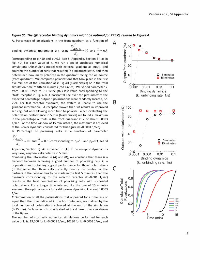
Ventura et al, SI Appendix
8
Figure S6. The αF receptor binding dynamics might be optimal for PRESS, related to Figure 4. A. Percentage of polarizations in the front quadrant as a function of
binding dynamics (parameter k-‐), using
q4πDdKd
= 10 and a
d= 0.3
(corresponding to p1=10 and p2=0.3, see SI Appendix, Section 5), as in Fig. 4D. For each value of k-‐, we run a set of stochastic numerical simulations (Altschuler’s model with external gradient as input), and counted the number of runs that resulted in a polarized state, and then determined how many polarized in the quadrant facing the αF source (front quadrant). We computed polarizations that took place in the first five minutes of the simulation as in Fig 4D (black circles) or in the total simulation time of fifteen minutes (red circles). We varied parameter k-‐ from 0.0001 1/sec to 0.1 1/sec (this last value corresponding to the “fast” receptor in Fig. 4D). A horizontal line over the plot indicates the expected percentage output if polarizations were randomly located, i.e. 25%. For fast receptor dynamics, the system is unable to use the gradient information. A receptor slower than wt results in improved sensing, but only allowing more time to polarize. When evaluating the polarization performance in 5 min (black circles) we found a maximum in the percentage outputs in the front quadrant at k-‐ of about 0.0003 1/sec. For the time window of 15 min instead, the maximum is achieved at the slower dynamics considered for this figure (k-‐=0.0001 1/sec). B. Percentage of polarizing cells as a function of parameter q4πDdKd
= 10 and a
d= 0.3 (corresponding to p1=10 and p2=0.3, see SI
Appendix, Section 5). As explained in (A), if the receptor dynamics is very slow, very few cells polarize in 5 min. Combining the information in (A) and (B), we conclude that there is a tradeoff between achieving a good number of polarizing cells in a population and obtaining a good performance for those polarizations (in the sense that those cells correctly identify the position of the partner). If the decision has to be made in the first 5 minutes, then the dynamics corresponding to the a-‐factor receptor (k-‐=0.001 1/sec) results in the best combination of polarizing cells with successful polarizations. For a longer time interval, like the one of 15 minutes analyzed, the optimal occurs for a still slower dynamics, k-‐ about 0.0003 1/sec. C. Summation of all the polarizations that appeared for a time less or equal than the time indicated in the horizontal axis, normalized by the total number of polarizations achieved at the end of the simulation (t=15 min). Each value of k-‐ is indicated with a different color as shown in the figure. The number of stochastic numerical simulations performed for each value of k-‐ is: 19,000 for k-‐=0.0001 1/sec, 10280 for k-‐=0.0003 1/sec, and
0.0001 0.001 0.01 0.10
10
20
30
40
Outp
uts
fro
nt quadra
nt (%
)
Binding dynamics
(k-, unbinding rate, 1/s)
15 minutes5 minutes
0.0001 0.001 0.01 0.10
20
40
60
80
100
Outp
uts
with p
ola
rization (
%)
Binding dynamics
(k-, unbinding rate, 1/s)
15 minutes5 minutes
0 5 10 150
0.2
0.4
0.6
0.8
1
Time (min)
Cu
mu
lative
/To
tal
Po
lariza
tio
ns
0.0001
0.0003
0.001
0.004
0.01
0.1
A
B
C
Figure S6, related to Figure 4

Ventura et al, SI Appendix
9
2000 for all the other values of k-‐. Comparing the outputs for each two successive values of k-‐ indicate that only the following pairs are significantly different (p < 0.05): 0.0003-‐0.001, and 0.001-‐0.004 at 5 min; 0.0001-‐0.0003, and 0.001-‐0.004 at 15 min.
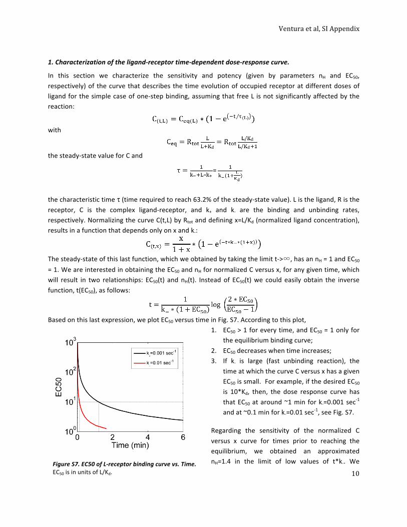
Ventura et al, SI Appendix
10
1. Characterization of the ligand-‐receptor time-‐dependent dose-‐response curve.
In this section we characterize the sensitivity and potency (given by parameters nH and EC50, respectively) of the curve that describes the time evolution of occupied receptor at different doses of ligand for the simple case of one-‐step binding, assuming that free L is not significantly affected by the reaction:
with
the steady-‐state value for C and
=
the characteristic time τ (time required to reach 63.2% of the steady-‐state value). L is the ligand, R is the receptor, C is the complex ligand-‐receptor, and k+ and k-‐ are the binding and unbinding rates, respectively. Normalizing the curve C(t,L) by Rtot and defining x=L/Kd (normalized ligand concentration), results in a function that depends only on x and k-‐:
The steady-‐state of this last function, which we obtained by taking the limit t-‐>∞, has an nH = 1 and EC50
= 1. We are interested in obtaining the EC50 and nH for normalized C versus x, for any given time, which will result in two relationships: EC50(t) and nH(t). Instead of EC50(t) we could easily obtain the inverse function, t(EC50), as follows:
Based on this last expression, we plot EC50 versus time in Fig. S7. According to this plot,
1. EC50 > 1 for every time, and EC50 = 1 only for the equilibrium binding curve;
2. EC50 decreases when time increases; 3. If k-‐ is large (fast unbinding reaction), the
time at which the curve C versus x has a given EC50 is small. For example, if the desired EC50 is 10*Kd, then, the dose response curve has that EC50 at around ~1 min for k-‐=0.001 sec-‐1 and at ~0.1 min for k-‐=0.01 sec-‐1, see Fig. S7.
Regarding the sensitivity of the normalized C versus x curve for times prior to reaching the equilibrium, we obtained an approximated nH=1.4 in the limit of low values of t*k-‐. We
Figure S7. EC50 of L-‐receptor binding curve vs. Time. EC50 is in units of L/Kd.
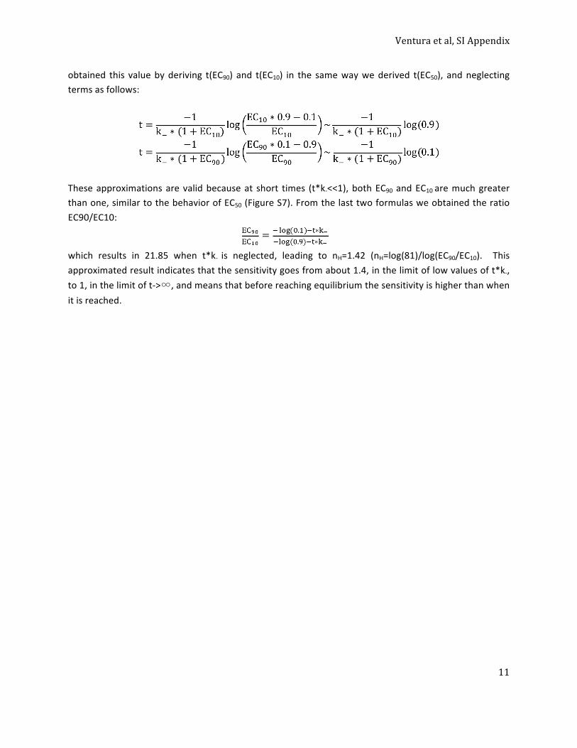
Ventura et al, SI Appendix
11
obtained this value by deriving t(EC90) and t(EC10) in the same way we derived t(EC50), and neglecting terms as follows:
These approximations are valid because at short times (t*k-‐<<1), both EC90 and EC10 are much greater than one, similar to the behavior of EC50 (Figure S7). From the last two formulas we obtained the ratio EC90/EC10:
which results in 21.85 when t*k-‐ is neglected, leading to nH=1.42 (nH=log(81)/log(EC90/EC10). This approximated result indicates that the sensitivity goes from about 1.4, in the limit of low values of t*k-‐, to 1, in the limit of t-‐>∞, and means that before reaching equilibrium the sensitivity is higher than when it is reached.
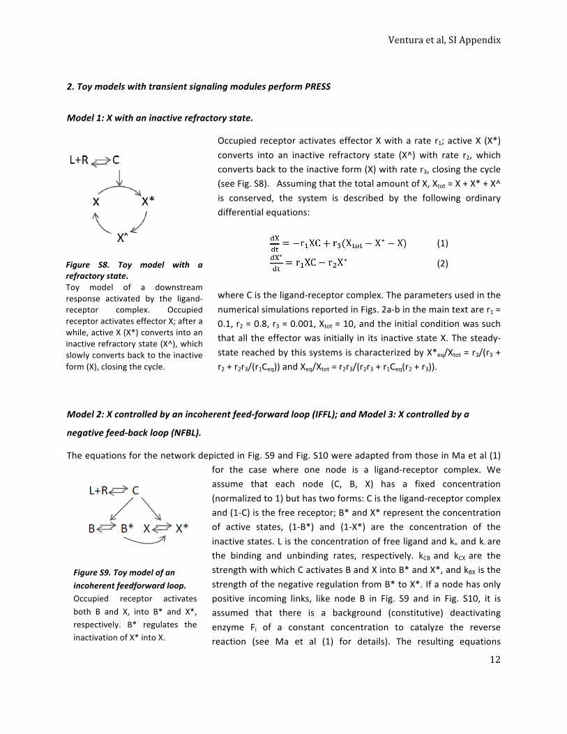
Ventura et al, SI Appendix
12
2. Toy models with transient signaling modules perform PRESS
Model 1: X with an inactive refractory state.
Occupied receptor activates effector X with a rate r1; active X (X*) converts into an inactive refractory state (X^) with rate r2, which converts back to the inactive form (X) with rate r3, closing the cycle (see Fig. S8). Assuming that the total amount of X, Xtot = X + X* + X^ is conserved, the system is described by the following ordinary differential equations:
(1)
(2)
where C is the ligand-‐receptor complex. The parameters used in the numerical simulations reported in Figs. 2a-‐b in the main text are r1 = 0.1, r2 = 0.8, r3 = 0.001, Xtot = 10, and the initial condition was such that all the effector was initially in its inactive state X. The steady-‐state reached by this systems is characterized by X*eq/Xtot = r3/(r3 + r2 + r2r3/(r1Ceq)) and Xeq/Xtot = r2r3/(r2r3 + r1Ceq(r2 + r3)).
Model 2: X controlled by an incoherent feed-‐forward loop (IFFL); and Model 3: X controlled by a
negative feed-‐back loop (NFBL).
The equations for the network depicted in Fig. S9 and Fig. S10 were adapted from those in Ma et al (1) for the case where one node is a ligand-‐receptor complex. We assume that each node (C, B, X) has a fixed concentration (normalized to 1) but has two forms: C is the ligand-‐receptor complex and (1-‐C) is the free receptor; B* and X* represent the concentration of active states, (1-‐B*) and (1-‐X*) are the concentration of the inactive states. L is the concentration of free ligand and k+ and k-‐ are the binding and unbinding rates, respectively. kCB and kCX are the strength with which C activates B and X into B* and X*, and kBX is the strength of the negative regulation from B* to X*. If a node has only positive incoming links, like node B in Fig. S9 and in Fig. S10, it is assumed that there is a background (constitutive) deactivating enzyme Fi of a constant concentration to catalyze the reverse reaction (see Ma et al (1) for details). The resulting equations
Figure S8. Toy model with a refractory state. Toy model of a downstream response activated by the ligand-‐receptor complex. Occupied receptor activates effector X; after a while, active X (X*) converts into an inactive refractory state (X^), which slowly converts back to the inactive form (X), closing the cycle.
Figure S9. Toy model of an incoherent feedforward loop. Occupied receptor activates both B and X, into B* and X*, respectively. B* regulates the inactivation of X* into X.
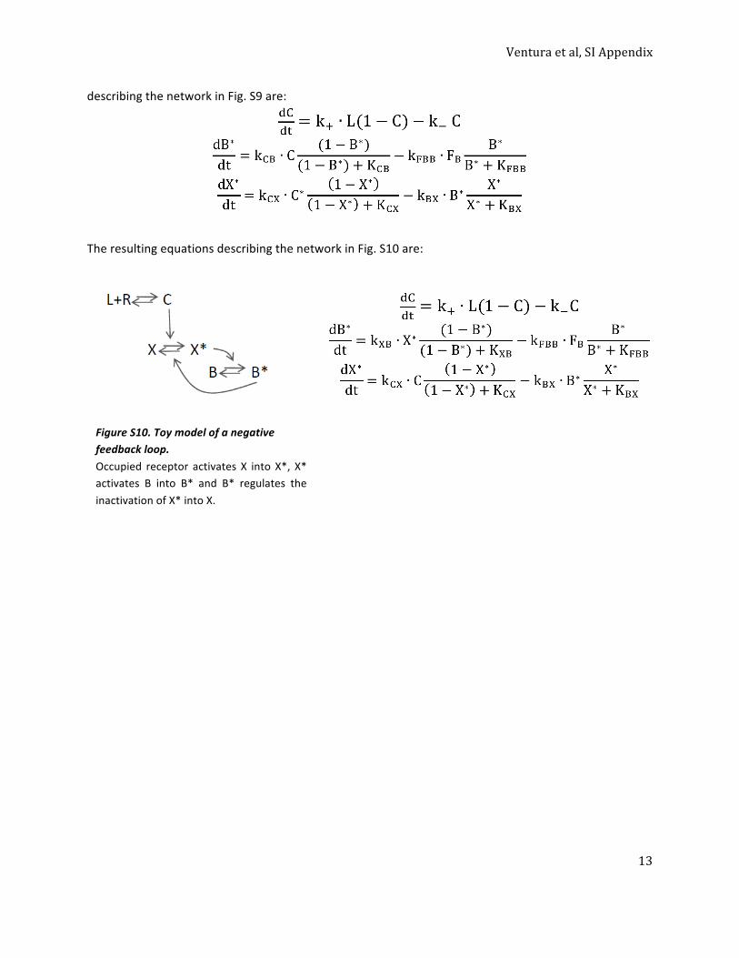
Ventura et al, SI Appendix
13
describing the network in Fig. S9 are:
The resulting equations describing the network in Fig. S10 are:
Figure S10. Toy model of a negative feedback loop. Occupied receptor activates X into X*, X* activates B into B* and B* regulates the inactivation of X* into X.
Ventura et al, SI Appendix
14
3. Models with transient signaling may be subsensitive, helping to expand the input dynamic range.
Modulation of the input dynamic range could imply its expansion/compression (i.e., an increase or decrease of the range of doses where the system produces dose-‐dependent responses), its displacement (i.e., the ratio EC90/EC10 is the same but it is centered around a different dose), or a combination of both. Expansion/compression of the dynamic range is determined by the sensitivity of the response, quantified by the change in the Hill coefficient nH (log(81)/log(EC90/EC10)) of the response: the higher the nH, the smaller the input dynamic range. Displacement of the dynamic range is usually quantified by the change in the EC50 of the response. A rightward displacement of the EC50 with constant nH enables dose-‐dependent responses in the high concentration range without compromising sensitivity, while a decrease in nH with constant EC50 results in an extended range of dose-‐dependent responses and a corresponding loss of sensitivity, meaning that the difference in the output you get for two different stimuli is smaller than otherwise would have been.
The common Michaelis-‐Menten relationship gives, by definition, an nH=1. Subsensitive responses (i.e., nH < 1) may arise, for example, from the presence of negative cooperativity (2) or negative feedback (3). Systems with transient responses, such as the one we implemented in our three toy models, also known as pulse-‐generators, can be subsensitive. Given that one of the effects of the PRESS signaling mode is to make the overall response subsensitive (expand the input dynamic range), we asked if the transient responses we implemented are intrinsically subsensitive (i.e., when studied uncoupled from a binding mechanism); and if so, how this subsensitivity contributes to the overall system behavior, when coupled to a slow or a fast binding reaction. With this in mind, in what follows we analyze in detail the model with an inactive refractory state and the model controlled by a negative feedback loop (Models 1 and 3).
Sensitivity in Model 1: X with an inactive refractory state.
In order to study the pulse generator of Model 1 in isolation, that is, independently of the ligand-‐receptor complex (C) formation, we first studied the peak response of X* as a function of a step increase in C (Fig. S11a). For the parameter values we selected, the system was subsensitive, with a Hill coefficient of 0.8, corresponding to a dynamic range (EC90/EC10) of 243 (colored lines in Fig. S11a), three times the dynamic range of a Michaelian response (81, black line). We tested three values of r2 (the rate of inactivation of X*, the key parameter controlling the duration of the pulse response), which had no significant impact on the nH, but had a strong effect on the EC50 of the response.
Next, we introduced a simple ligand-‐receptor binding reaction between the step input and the X cycle, using fast or slow ligand-‐receptor binding rates (Fig. S11b and c). The addition of the ligand-‐receptor binding reaction increased the sensitivity from 0.8 to 0.9 when we used fast ligand binding rates (reducing the dynamic range to ~132), and decreased it to 0.7 when we used slow binding rates (increasing the dynamic range to ~533) (Table S1). In both cases, parameter r2 had no significant impact on the nH, impacting strongly on the EC50 of the response.
These results indicate that the coupling of a ligand-‐receptor reaction interacts with the subsensitive pulse-‐generator, in a manner that depends on the speed of this reaction. When binding is fast, the
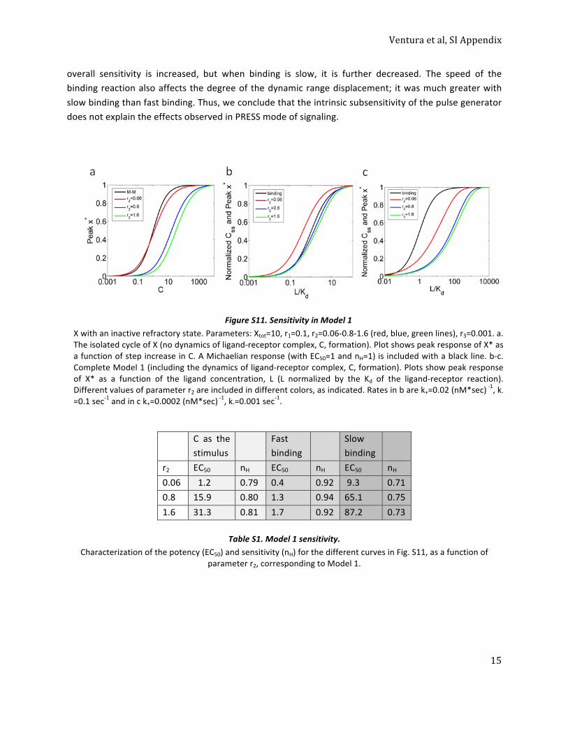
Ventura et al, SI Appendix
15
overall sensitivity is increased, but when binding is slow, it is further decreased. The speed of the binding reaction also affects the degree of the dynamic range displacement; it was much greater with slow binding than fast binding. Thus, we conclude that the intrinsic subsensitivity of the pulse generator does not explain the effects observed in PRESS mode of signaling.
C as the
stimulus Fast
binding Slow
binding
r2 EC50 nH EC50 nH EC50 nH 0.06 1.2 0.79 0.4 0.92 9.3 0.71 0.8 15.9 0.80 1.3 0.94 65.1 0.75 1.6 31.3 0.81 1.7 0.92 87.2 0.73
Table S1. Model 1 sensitivity. Characterization of the potency (EC50) and sensitivity (nH) for the different curves in Fig. S11, as a function of
parameter r2, corresponding to Model 1.
Figure S11. Sensitivity in Model 1 X with an inactive refractory state. Parameters: Xtot=10, r1=0.1, r2=0.06-‐0.8-‐1.6 (red, blue, green lines), r3=0.001. a. The isolated cycle of X (no dynamics of ligand-‐receptor complex, C, formation). Plot shows peak response of X* as a function of step increase in C. A Michaelian response (with EC50=1 and nH=1) is included with a black line. b-‐c. Complete Model 1 (including the dynamics of ligand-‐receptor complex, C, formation). Plots show peak response of X* as a function of the ligand concentration, L (L normalized by the Kd of the ligand-‐receptor reaction). Different values of parameter r2 are included in different colors, as indicated. Rates in b are k+=0.02 (nM*sec) -‐1, k-‐=0.1 sec-‐1 and in c k+=0.0002 (nM*sec) -‐1, k-‐=0.001 sec
-‐1.
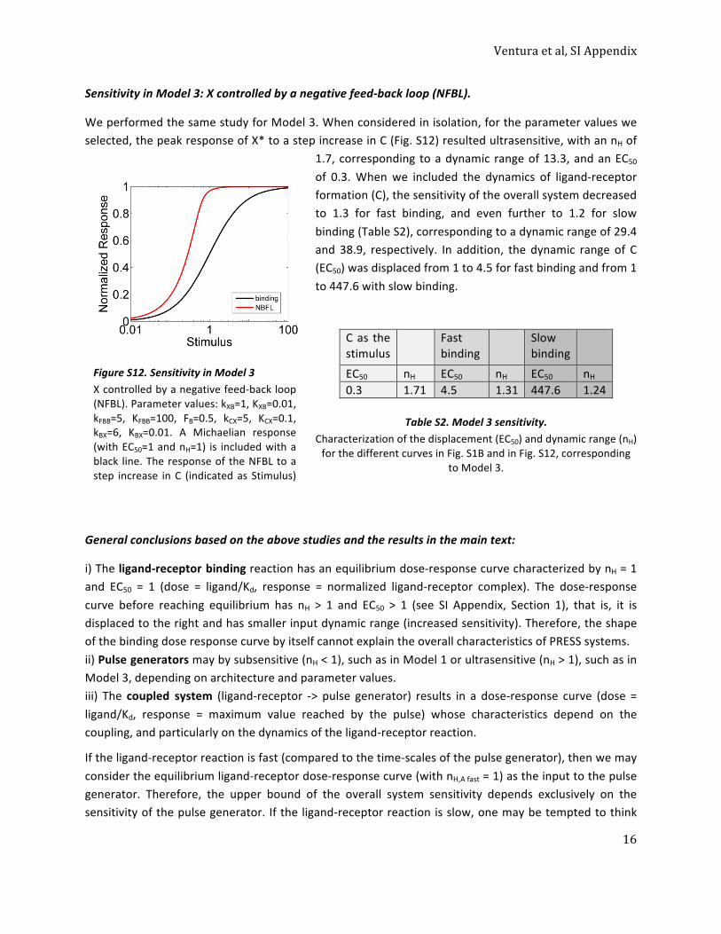
Ventura et al, SI Appendix
16
Sensitivity in Model 3: X controlled by a negative feed-‐back loop (NFBL).
We performed the same study for Model 3. When considered in isolation, for the parameter values we selected, the peak response of X* to a step increase in C (Fig. S12) resulted ultrasensitive, with an nH of
1.7, corresponding to a dynamic range of 13.3, and an EC50 of 0.3. When we included the dynamics of ligand-‐receptor formation (C), the sensitivity of the overall system decreased to 1.3 for fast binding, and even further to 1.2 for slow binding (Table S2), corresponding to a dynamic range of 29.4 and 38.9, respectively. In addition, the dynamic range of C (EC50) was displaced from 1 to 4.5 for fast binding and from 1 to 447.6 with slow binding.
C as the stimulus
Fast binding
Slow binding
EC50 nH EC50 nH EC50 nH 0.3 1.71 4.5 1.31 447.6 1.24
Table S2. Model 3 sensitivity. Characterization of the displacement (EC50) and dynamic range (nH) for the different curves in Fig. S1B and in Fig. S12, corresponding
to Model 3.
General conclusions based on the above studies and the results in the main text:
i) The ligand-‐receptor binding reaction has an equilibrium dose-‐response curve characterized by nH = 1 and EC50 = 1 (dose = ligand/Kd, response = normalized ligand-‐receptor complex). The dose-‐response curve before reaching equilibrium has nH > 1 and EC50 > 1 (see SI Appendix, Section 1), that is, it is displaced to the right and has smaller input dynamic range (increased sensitivity). Therefore, the shape of the binding dose response curve by itself cannot explain the overall characteristics of PRESS systems. ii) Pulse generators may by subsensitive (nH < 1), such as in Model 1 or ultrasensitive (nH > 1), such as in Model 3, depending on architecture and parameter values. iii) The coupled system (ligand-‐receptor -‐> pulse generator) results in a dose-‐response curve (dose = ligand/Kd, response = maximum value reached by the pulse) whose characteristics depend on the coupling, and particularly on the dynamics of the ligand-‐receptor reaction.
If the ligand-‐receptor reaction is fast (compared to the time-‐scales of the pulse generator), then we may consider the equilibrium ligand-‐receptor dose-‐response curve (with nH,A fast = 1) as the input to the pulse generator. Therefore, the upper bound of the overall system sensitivity depends exclusively on the sensitivity of the pulse generator. If the ligand-‐receptor reaction is slow, one may be tempted to think
Figure S12. Sensitivity in Model 3 X controlled by a negative feed-‐back loop (NFBL). Parameter values: kXB=1, KXB=0.01, kFBB=5, KFBB=100, FB=0.5, kCX=5, KCX=0.1, kBX=6, KBX=0.01. A Michaelian response (with EC50=1 and nH=1) is included with a black line. The response of the NFBL to a step increase in C (indicated as Stimulus)
is plotted in red.
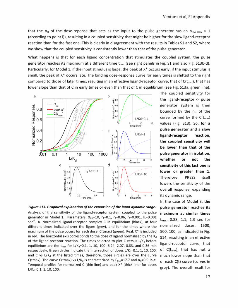
Ventura et al, SI Appendix
17
that the nH of the dose-‐reponse that acts as the input to the pulse generator has an nH,A slow > 1 (according to point i)), resulting in a coupled sensitivity that might be higher for the slow ligand-‐receptor reaction than for the fast one. This is clearly in disagreement with the results in Tables S1 and S2, where we show that the coupled sensitivity is consistently lower than that of the pulse generator.
What happens is that for each ligand concentration that stimulates the coupled system, the pulse generator reaches its maximum at a different time tmax (see right panels in Fig. S1 and also Fig. S13b-‐d). Particularly, for Model 1, if the input stimulus is large, the peak of X* occurs early; if the input stimulus is small, the peak of X* occurs late. The binding dose-‐response curve for early times is shifted to the right compared to those of later times, resulting in an effective ligand-‐receptor curve, that of C(tmax), that has lower slope than that of C in early times or even than that of C in equilibrium (see Fig. S13a, green line).
The coupled sensitivity for the ligand-‐receptor -‐> pulse generator system is then bounded by the nH of the curve formed by the C(tmax) values (Fig. S13). So, for a pulse generator and a slow ligand-‐receptor reaction, the coupled sensitivity will be lower than that of the pulse generator in isolation, whether or not the sensitivity of this last one is lower or greater than 1. Therefore, PRESS itself lowers the sensitivity of the overall response, expanding its dynamic range. In the case of Model 3, the pulse generator reaches its maximum at similar times tmax: 0.88, 1.1, 1.3 sec for normalized doses: 1500, 500, 100, as indicated in Fig. S14, resulting in an effective ligand-‐receptor curve, that of C(tmax), that has not a much lower slope than that of each C(t) curve (curves in grey). The overall result for
Figure S13. Graphical explanation of the expansion of the input dynamic range. Analysis of the sensitivity of the ligand-‐receptor system coupled to the pulse generator in Model 1. Parameters: Xtot=10, r1=0.1, r2=0.06, r3=0.001, k-‐=0.001 sec-‐1. a. Normalized ligand-‐receptor complex C in equilibrium (black), at four different times indicated over the figure (grey), and for the times where the maximum of the pulse occurs for each dose, C(tmax) (green). Peak X* is included in red. The horizontal axis corresponds to the dose of ligand normalized by the Kd of the ligand-‐receptor reaction. The times selected to plot C versus L/Kd before equilibrium are the tmax for L/Kd=0.1, 1, 10, 100: 6.24, 2.07, 0.83, and 0.36 min respectively. Green circles indicate the intersection of doses L/Kd=0.1, 1, 10, 100, and C vs L/Kd at the listed times, therefore, those circles are over the curve C(tmax). The curve C(tmax) vs L/Kd is characterized by EC50=17.7 and nH=0.9. b-‐e. Temporal profiles for normalized C (thin line) and peak X* (thick line) for doses L/Kd=0.1, 1, 10, 100.
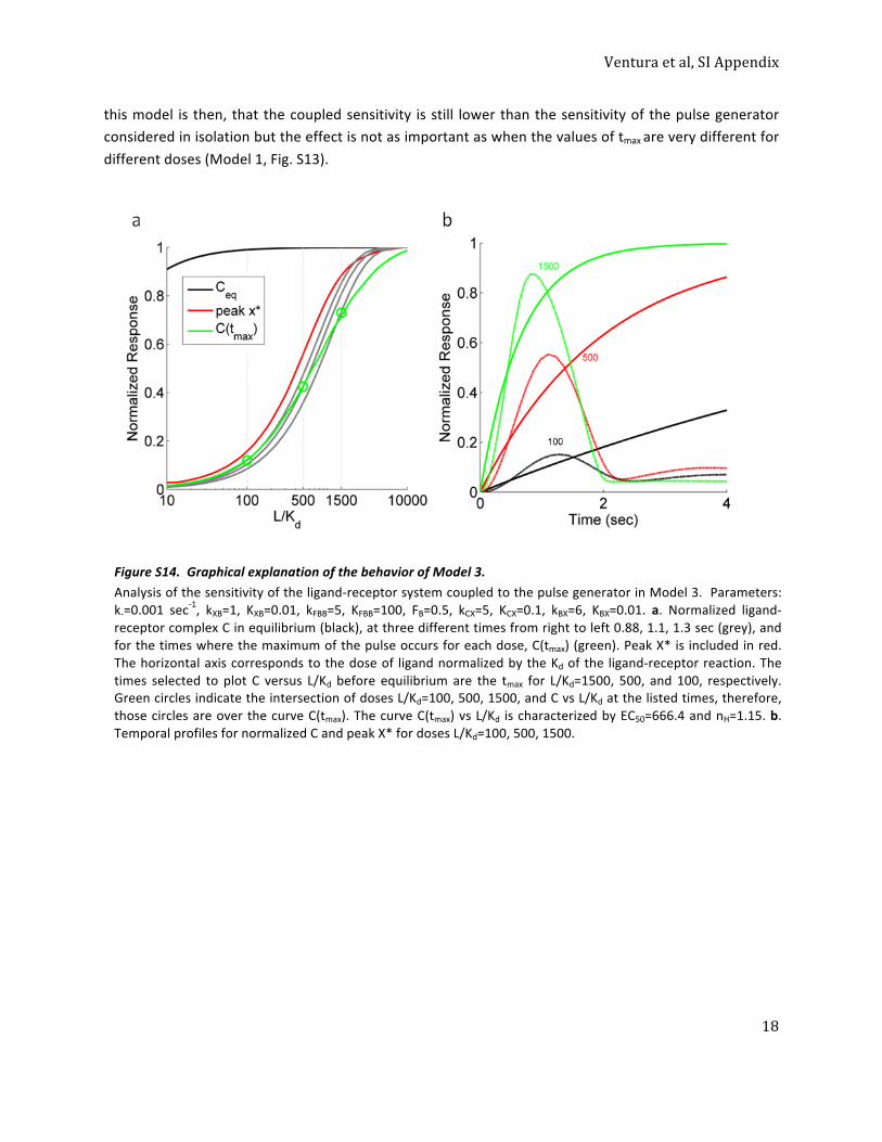
Ventura et al, SI Appendix
18
this model is then, that the coupled sensitivity is still lower than the sensitivity of the pulse generator considered in isolation but the effect is not as important as when the values of tmax are very different for different doses (Model 1, Fig. S13).
Figure S14. Graphical explanation of the behavior of Model 3. Analysis of the sensitivity of the ligand-‐receptor system coupled to the pulse generator in Model 3. Parameters: k-‐=0.001 sec
-‐1, kXB=1, KXB=0.01, kFBB=5, KFBB=100, FB=0.5, kCX=5, KCX=0.1, kBX=6, KBX=0.01. a. Normalized ligand-‐receptor complex C in equilibrium (black), at three different times from right to left 0.88, 1.1, 1.3 sec (grey), and for the times where the maximum of the pulse occurs for each dose, C(tmax) (green). Peak X* is included in red. The horizontal axis corresponds to the dose of ligand normalized by the Kd of the ligand-‐receptor reaction. The times selected to plot C versus L/Kd before equilibrium are the tmax for L/Kd=1500, 500, and 100, respectively. Green circles indicate the intersection of doses L/Kd=100, 500, 1500, and C vs L/Kd at the listed times, therefore, those circles are over the curve C(tmax). The curve C(tmax) vs L/Kd is characterized by EC50=666.4 and nH=1.15. b. Temporal profiles for normalized C and peak X* for doses L/Kd=100, 500, 1500.
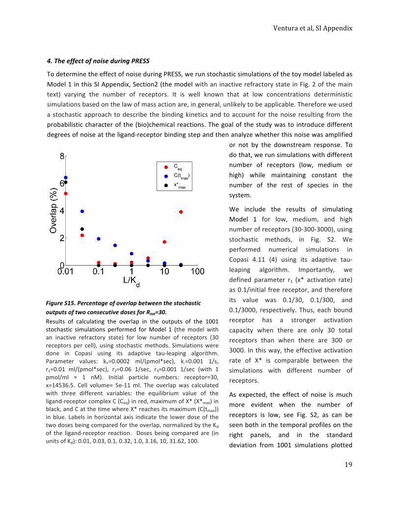
Ventura et al, SI Appendix
19
4. The effect of noise during PRESS
To determine the effect of noise during PRESS, we run stochastic simulations of the toy model labeled as Model 1 in this SI Appendix, Section2 (the model with an inactive refractory state in Fig. 2 of the main text) varying the number of receptors. It is well known that at low concentrations deterministic simulations based on the law of mass action are, in general, unlikely to be applicable. Therefore we used a stochastic approach to describe the binding kinetics and to account for the noise resulting from the probabilistic character of the (bio)chemical reactions. The goal of the study was to introduce different degrees of noise at the ligand-‐receptor binding step and then analyze whether this noise was amplified
or not by the downstream response. To do that, we run simulations with different number of receptors (low, medium or high) while maintaining constant the number of the rest of species in the system.
We include the results of simulating Model 1 for low, medium, and high number of receptors (30-‐300-‐3000), using stochastic methods, in Fig. S2. We performed numerical simulations in Copasi 4.11 (4) using its adaptive tau-‐leaping algorithm. Importantly, we defined parameter r1 (x* activation rate) as 0.1/initial free receptor, and therefore its value was 0.1/30, 0.1/300, and 0.1/3000, respectively. Thus, each bound receptor has a stronger activation capacity when there are only 30 total receptors than when there are 300 or 3000. In this way, the effective activation rate of X* is comparable between the simulations with different number of receptors.
As expected, the effect of noise is much more evident when the number of receptors is low, see Fig. S2, as can be seen both in the temporal profiles on the right panels, and in the standard deviation from 1001 simulations plotted
Figure S15. Percentage of overlap between the stochastic outputs of two consecutive doses for Rtot=30. Results of calculating the overlap in the outputs of the 1001 stochastic simulations performed for Model 1 (the model with an inactive refractory state) for low number of receptors (30 receptors per cell), using stochastic methods. Simulations were done in Copasi using its adaptive tau-‐leaping algorithm. Parameter values: k+=0.0002 ml/(pmol*sec), k-‐=0.001 1/s, r1=0.01 ml/(pmol*sec), r2=0.06 1/sec, r3=0.001 1/sec (with 1 pmol/ml = 1 nM). Initial particle numbers: receptor=30, x=14536.5. Cell volume= 5e-‐11 ml. The overlap was calculated with three different variables: the equilibrium value of the ligand-‐receptor complex C (Ceq) in red, maximum of X* (X*max) in black, and C at the time where X* reaches its maximum (C(tmax)) in blue. Labels in horizontal axis indicate the lower dose of the two doses being compared for the overlap, normalized by the Kd of the ligand-‐receptor reaction. Doses being compared are (in units of Kd): 0.01, 0.03, 0.1, 0.32, 1.0, 3.16, 10, 31.62, 100.
Ventura et al, SI Appendix
20
on the left panels. The square of the coefficient of variation plotted in the bottom panel indicates that for the three variables, Css (red curves), C(tmax) (blue curves), and peak X* (black curves), lower receptor number results in higher CV2 for the whole range of doses considered. Also, for the three amounts of receptors considered (30 in solid lines, 300 in dashed lines, and 3000 in dotted lines), the curve of Css is lower than that of peak X*, and peak X* is lower than the curve for C(tmax). This result suggests that even in the case of very low number of receptors (30 per cell), which introduce a significant noise at the level of occupied receptor (Fig. S2F), the pulse generator downstream of the receptor did not amplify it and therefore the improvement gained by PRESS is not lost or masked by the effects of noise. In Fig. S15, we show the percentage of overlap between the outputs of 1001 stochastic simulations for two consecutive doses, Li/Kd and Li+1/Kd, being Li+1/Kd~3* Li/Kd , evaluated for Ceq (red), C(tmax) (blue) and X*max (black), in the case of low number of receptors (30 receptors per cell). The aim of this figure is to evaluate if two doses can be identified as different doses based on the information given by each variable, Ceq, C(tmax), X*max, particularly in the region of high doses (L/Kd >1). The results in Fig. S15 indicate even in this case with significant noise at the level of occupied receptor, variable X*max has lower overlap than Ceq, supporting that the improvement gained by PRESS is not lost by the effects of noise.
Ventura et al, SI Appendix
21
5. Mathematical model to study the sensing of a stationary spatial gradient
In what follows we present two alternative mathematical descriptions for the variable Delta. In Description 1 we derived the steady-‐state concentration of αF as an approximate solution to the diffusion equation from a point source, with, and also without, reflecting boundary conditions on the sensing sphere. Combining this solution with the normalized bound receptor function we derived the variable Delta (difference of bound receptors at the front and at the back). In Description 1, Delta depends on three combinations of parameters related the average concentration sensed by the cell, the ratio between the radius of the cell and the distant to the source, and the ligand-‐receptor unbinding rate. In Description 2, we derived variable Delta in terms of the maximal and minimal ligand concentrations sensed by the cell, without relating them by any particular function (i.e. without specifying the profile of the gradient). In this case, Delta still depends on the ligand-‐receptor unbinding rate, and on the maximal and minimal ligand concentrations. Description 1 is based on a given source-‐sensing cell pair, while Description 2 is based on the local environment sensed by the cell. Both descriptions are easily related to one another.
5.1 An analytical expression for the αF gradient generated by a point source, and for the variable Delta (Description 1)
As in Segall (5), the cell is modeled as an impermeable sphere of radius a, with d the distance from the center of the sphere to the point source of αF. There is azimuthal symmetry with respect to the line between the center of the sphere and the point source. The concentration at any point on the sphere will vary with the angle, θ, between the line connecting the center of the sphere to the point source and the line connecting the center of the sphere to the point on the surface. The point over the sphere that is nearest the source is indicated with an f (front, θ = 0) and the point that has the greatest distance to the source is indicated with a b (back, θ = π). An approximate solution to the diffusion equation with a point source and given reflecting boundary conditions on the sphere (5) is:
(3)
where αF(θ) is the steady-‐state concentration of αF as a function of the position over the cell surface, q is the rate of release of alpha-‐factor from the point source, D is the αF diffusion coefficient, and Pj is the Legendre polynomial of order j (5). We model the ligand-‐receptor binding with the following reaction:
αF + R <-‐> C (4) where αF is the ligand (alpha-‐factor), R is the membrane receptor assumed to have a uniform density over the cell surface, C is the complex ligand-‐receptor, and k+ and k-‐ are the binding and unbinding rates, respectively. The dissociation constant Kd is defined as k-‐/k+ and represents the ligand concentration that produces a bound receptor level that is one-‐half of its maximum. The total concentrations of receptor and ligand in the system are assumed to be constant, Rtot = [R] + [C], αFtot = [αF] + [C]. Thus, only one concentration of the three ([R], [αF], and [C]) is independent; the other two may be determined from
Ventura et al, SI Appendix
22
Rtot, αFtot and the independent concentration. The kinetics of this system can be solved analytically. Choosing [C] as the independent concentration and representing the concentrations without the brackets for brevity (e.g. R = [R]), the kinetic rate equation can be written as:
(5)
where we have assumed that [αF] ~ αFtot, meaning that the consumption of ligand in the ligand-‐receptor reaction is negligible compared with αFtot. αFtot is then the function αF(θ) given by Eq. (3). The solution for Eq. (5) is:
, (6)
with
(7)
being the steady-‐state value for C and (8)
the time required for the bound receptor C to rise from zero to 1−1/e (that is, 63.2%) of its final steady-‐state value.
Combining Eqs. (3), (6), (7), and (8) we obtain that the normalized bound receptor, C/Rtot as a function of θ and t depends on the following combination of parameters:
(9)
Parameter p1 combines parameters related to the ligand source (q;D), the distance to the source (d), and Kd, and indicates the average concentration sensed by the cell in multiples of Kd, for instance, p1=1 means that the cell feels a concentration of about 1 × Kd. Parameter p2 is a geometrical parameter defined as the ratio between the radius of the spherical cell and the distance from the center of the cell to the point source. p1 and p2 are dimensionless parameters. Parameter p3 is the ligand-‐receptor unbinding rate and has units of 1/time. The three parameters are always positive, and p2 is such that 0 < p2 < 1.
For p1 = 10 and p2 = 0.3 (the values used in most of the paper), the total numbers of bound receptors in steady state, for the hemispheres facing and away from the point source, were calculated following (5) by integration over the angles 0 to π/2 radians (0 to 90 degrees) and π/2 to π radians (90 to 180 degrees), respectively. The total number of receptors was assumed to be 8000 (5). The hemisphere nearest the source has 3720 occupied receptors and the hemisphere away from the source has 3531 occupied receptors. The difference between the two sides, 189 receptors, is 2.6% of the total number of occupied receptors. The variable Delta is defined as Delta(t) = C(θ = 0, t) − C(θ=π, t) (difference of bound receptors at the front and at the back). The effectiveness of PRESS in the context of gradient sensing depends on how much (amplitude) and for how long (duration) lasts the overshoot of Delta(t). Delta depends on parameters p1, p2, and p3.
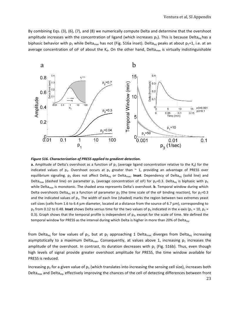
Ventura et al, SI Appendix
23
By combining Eqs. (3), (6), (7), and (8) we numerically compute Delta and determine that the overshoot amplitude increases with the concentration of ligand (which increases p1). This is because Deltaeq has a biphasic behavior with p1 while Deltamax has not (Fig. S16a inset). Deltaeq peaks at about p1=1, i.e. at an average concentration of αF of about the Kd. On the other hand, Deltamax is virtually indistinguishable
from Deltaeq for low values of p1, but at p1 approaching 1 Deltamax diverges from Deltaeq increasing asymptotically to a maximum Deltamax. Consequently, at values above 1, increasing p1 increases the amplitude of the overshoot. In contrast, its duration decreases with p1 (Fig. S16b). Thus, even though high levels of signal provide greater overshoot amplitude for PRESS, the time window available for PRESS is reduced.
Increasing p2 for a given value of p1 (which translates into increasing the sensing cell size), increases both Deltamax and Deltaeq, effectively improving the chances of the cell of detecting differences between front
! a b
Figure S16. Characterization of PRESS applied to gradient detection. a. Amplitude of Delta’s overshoot as a function of p1 (average ligand concentration relative to the Kd) for the indicated values of p2. Overshoot occurs at p1 greater than ~ 1, providing an advantage of PRESS over equilibrium signaling. p3 does not affect Deltaeq or Deltamax. Inset. Dependency of Deltaeq (solid line) and Deltamax (dashed line) on parameter p1 (average concentration of αF) for p2=0.3. Deltaeq is biphasic with p1 while Deltamax is monotonic. The shaded area represents Delta’s overshoot. b. Temporal window during which Delta overshoots Deltaeq as a function of parameter p3 (the time scale of the αF binding reaction), for p2=0.3 and the indicated values of p1. The width of each line (shaded) marks the region between two extremes yeast cell sizes (cells from 1.6 to 6.4 µm diameter, located at a distance from the source of 6.7 µm), corresponding to p2 from 0.12 to 0.48. Inset shows Delta versus time for the two values of p3 indicated in the x-‐axis (p1 = 10, p2 = 0.3). Graph shows that the temporal profile is independent of p3, except for the scale of time. We defined the temporal window for PRESS as the interval during which Delta is higher in more than 20% of Deltaeq.
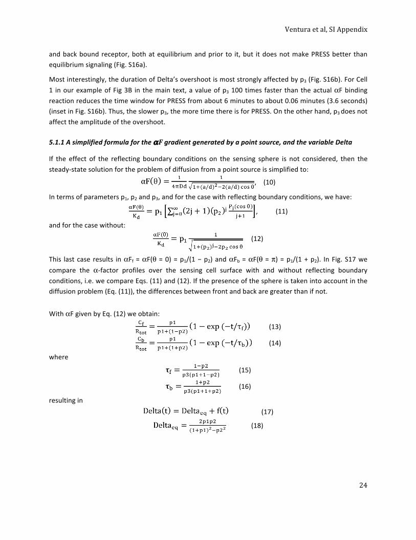
Ventura et al, SI Appendix
24
and back bound receptor, both at equilibrium and prior to it, but it does not make PRESS better than equilibrium signaling (Fig. S16a).
Most interestingly, the duration of Delta’s overshoot is most strongly affected by p3 (Fig. S16b). For Cell 1 in our example of Fig 3B in the main text, a value of p3 100 times faster than the actual αF binding reaction reduces the time window for PRESS from about 6 minutes to about 0.06 minutes (3.6 seconds) (inset in Fig. S16b). Thus, the slower p3, the more time there is for PRESS. On the other hand, p3 does not affect the amplitude of the overshoot.
5.1.1 A simplified formula for the αF gradient generated by a point source, and the variable Delta
If the effect of the reflecting boundary conditions on the sensing sphere is not considered, then the steady-‐state solution for the problem of diffusion from a point source is simplified to:
, (10)
In terms of parameters p1, p2 and p3, and for the case with reflecting boundary conditions, we have:
, (11)
and for the case without:
(12)
This last case results in αFf = αF(θ = 0) = p1/(1 − p2) and αFb = αF(θ = π) = p1/(1 + p2). In Fig. S17 we compare the α-‐factor profiles over the sensing cell surface with and without reflecting boundary conditions, i.e. we compare Eqs. (11) and (12). If the presence of the sphere is taken into account in the diffusion problem (Eq. (11)), the differences between front and back are greater than if not.
With αF given by Eq. (12) we obtain:
(13)
(14)
where
(15)
(16)
resulting in (17)
(18)
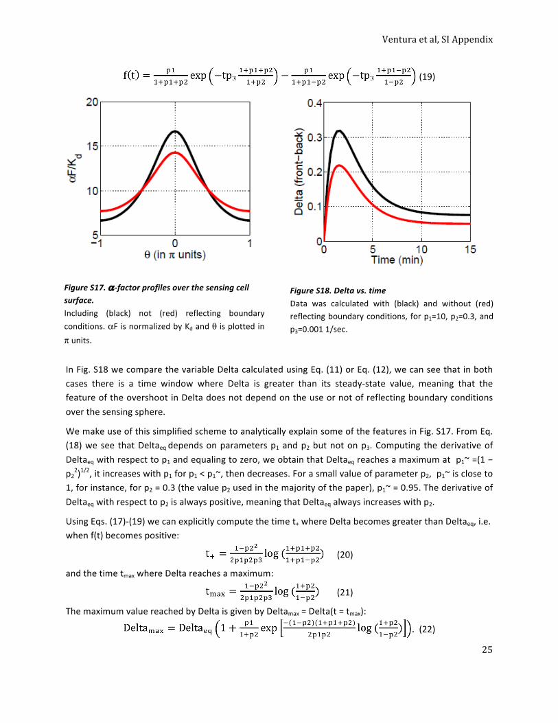
Ventura et al, SI Appendix
25
(19)
In Fig. S18 we compare the variable Delta calculated using Eq. (11) or Eq. (12), we can see that in both cases there is a time window where Delta is greater than its steady-‐state value, meaning that the feature of the overshoot in Delta does not depend on the use or not of reflecting boundary conditions over the sensing sphere.
We make use of this simplified scheme to analytically explain some of the features in Fig. S17. From Eq. (18) we see that Deltaeq depends on parameters p1 and p2 but not on p3. Computing the derivative of Deltaeq with respect to p1 and equaling to zero, we obtain that Deltaeq reaches a maximum at p1~ =(1 − p2
2)1/2, it increases with p1 for p1 < p1~, then decreases. For a small value of parameter p2, p1~ is close to 1, for instance, for p2 = 0.3 (the value p2 used in the majority of the paper), p1~ = 0.95. The derivative of Deltaeq with respect to p2 is always positive, meaning that Deltaeq always increases with p2.
Using Eqs. (17)-‐(19) we can explicitly compute the time t+ where Delta becomes greater than Deltaeq, i.e. when f(t) becomes positive:
(20)
and the time tmax where Delta reaches a maximum:
(21)
The maximum value reached by Delta is given by Deltamax = Delta(t = tmax):
. (22)
!
Figure S17. α -‐factor profiles over the sensing cell surface. Including (black) not (red) reflecting boundary conditions. αF is normalized by Kd and θ is plotted in π units.
!
Figure S18. Delta vs. time Data was calculated with (black) and without (red) reflecting boundary conditions, for p1=10, p2=0.3, and p3=0.001 1/sec.
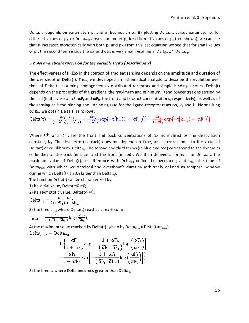
Ventura et al, SI Appendix
26
Deltamax depends on parameters p1 and p2 but not on p3. By plotting Deltamax versus parameter p1 for different values of p2, or Deltamax versus parameter p2 for different values of p1 (not shown), we can see that it increases monotonically with both p1 and p2. From this last equation we see that for small values of p1, the second term inside the parenthesis is very small resulting in Deltamax ~ Deltaeq.
5.2 An analytical expression for the variable Delta (Description 2)
The effectiveness of PRESS in the context of gradient sensing depends on the amplitude and duration of the overshoot of Delta(t). Thus, we developed a mathematical analysis to describe the evolution over time of Delta(t), assuming homogeneously distributed receptors and simple binding kinetics. Delta(t) depends on the properties of the gradient: the maximum and minimum ligand concentrations sensed by the cell (in the case of αF, αFf and αFb, the front and back αF concentrations, respectively), as well as of the sensing cell: the binding and unbinding rate for the ligand-‐receptor reaction, k+ and k-‐. Normalizing by Rtot we obtain Delta(t) as follows:
Where and are the front and back concentrations of αF normalized by the dissociation constant, Kd. The first term (in black) does not depend on time, and it corresponds to the value of Delta(t) at equilibrium, Deltaeq. The second and third terms (in blue and red) correspond to the dynamics of binding at the back (in blue) and the front (in red). We then derived a formula for Deltamax, the maximum value of Delta(t), its difference with Deltaeq define the overshoot; and tmax, the time of Deltamax, with which we obtained the overshoot’s duration (arbitrarily defined as temporal window during which Delta(t) is 20% larger than Deltaeq). The function Delta(t) can be characterized by: 1) its initial value, Delta(t=0)=0; 2) its asymptotic value, Delta(t-‐>∞):
;
3) the time tmax where Delta(t) reaches a maximum:
;
4) the maximum value reached by Delta(t) , given by Deltamax = Delta(t = tmax):
5) the time t+ where Delta becomes greater than Deltaeq:
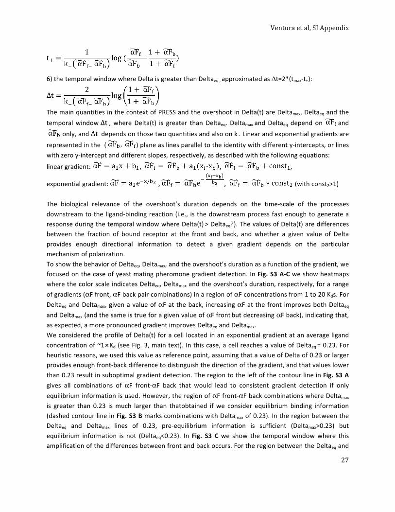
Ventura et al, SI Appendix
27
6) the temporal window where Delta is greater than Deltaeq , approximated as Δt=2*(tmax-‐t+):
The main quantities in the context of PRESS and the overshoot in Delta(t) are Deltamax, Deltaeq and the temporal window , where Delta(t) is greater than Deltaeq. Deltamax and Deltaeq depend on and
only, and depends on those two quantities and also on k-‐. Linear and exponential gradients are represented in the ( ) plane as lines parallel to the identity with different y-‐intercepts, or lines with zero y-‐intercept and different slopes, respectively, as described with the following equations:
linear gradient: , , ,
exponential gradient: , , (with const2>1) The biological relevance of the overshoot’s duration depends on the time-‐scale of the processes downstream to the ligand-‐binding reaction (i.e., is the downstream process fast enough to generate a response during the temporal window where Delta(t) > Deltaeq?). The values of Delta(t) are differences between the fraction of bound receptor at the front and back, and whether a given value of Delta provides enough directional information to detect a given gradient depends on the particular mechanism of polarization. To show the behavior of Deltaeq, Deltamax, and the overshoot’s duration as a function of the gradient, we focused on the case of yeast mating pheromone gradient detection. In Fig. S3 A-‐C we show heatmaps where the color scale indicates Deltaeq, Deltamax and the overshoot’s duration, respectively, for a range of gradients (αF front, αF back pair combinations) in a region of αF concentrations from 1 to 20 Kds. For Deltaeq and Deltamax, given a value of αF at the back, increasing αF at the front improves both Deltaeq and Deltamax (and the same is true for a given value of αF front but decreasing αF back), indicating that, as expected, a more pronounced gradient improves Deltaeq and Deltamax. We considered the profile of Delta(t) for a cell located in an exponential gradient at an average ligand concentration of ~1⨯Kd (see Fig. 3, main text). In this case, a cell reaches a value of Deltaeq = 0.23. For heuristic reasons, we used this value as reference point, assuming that a value of Delta of 0.23 or larger provides enough front-‐back difference to distinguish the direction of the gradient, and that values lower than 0.23 result in suboptimal gradient detection. The region to the left of the contour line in Fig. S3 A gives all combinations of αF front-‐αF back that would lead to consistent gradient detection if only equilibrium information is used. However, the region of αF front-‐αF back combinations where Deltamax is greater than 0.23 is much larger than thatobtained if we consider equilibrium binding information (dashed contour line in Fig. S3 B marks combinations with Deltamax of 0.23). In the region between the Deltaeq and Deltamax lines of 0.23, pre-‐equilibrium information is sufficient (Deltamax>0.23) but equilibrium information is not (Deltaeq<0.23). In Fig. S3 C we show the temporal window where this amplification of the differences between front and back occurs. For the region between the Deltaeq and
Ventura et al, SI Appendix
28
Deltamax lines, the temporal window is not smaller than 6.8 min. The duration of Delta’s overshoot is strongly affected by k-‐: a value of k-‐ 100 times faster than the reported αF binding reaction reduces it by a factor 100 (duration reaches a maximum of 15 min for k-‐=0.001 sec-‐1, but only of 0.15 min for k-‐=0.1 sec-‐1). Thus, the slower k-‐, the more time available for PRESS. On the other hand, k-‐ does not affect the amplitude of the overshoot (see formula for Deltamax above). With this analysis, we studied Delta(t) in different gradient situations. We show that the average concentration establishes a tradeoff between overshoot’s amplitude and duration. Deltamax is larger at higher average ligand concentrations, but the temporal windows are shorter (see grey lines in Fig. S3 B and C). The optimal condition depends on the downstream process time scale and sensitivity. Summarizing: -‐ Deltaeq and Deltamax depend only on and . A higher average αF concentration and a more pronounced gradient are conditions that favor Deltaeq and Deltamax. -‐ The temporal window for PRESS depends on and and also on the unbinding rate for the receptor-‐αF reaction, k-‐ (at a fixed Kd). It is shorter for higher averages of αF concentration and for faster unbinding rates.
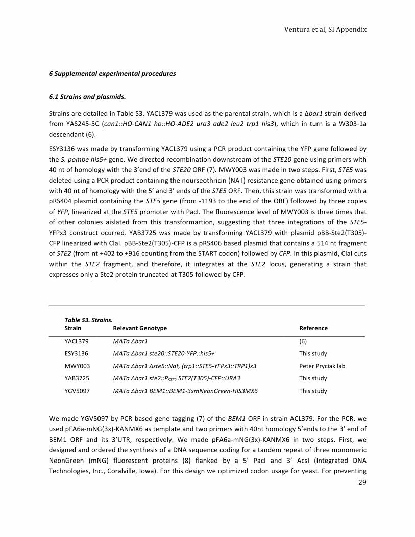
Ventura et al, SI Appendix
29
6 Supplemental experimental procedures
6.1 Strains and plasmids.
Strains are detailed in Table S3. YACL379 was used as the parental strain, which is a Δbar1 strain derived from YAS245-‐5C (can1::HO-‐CAN1 ho::HO-‐ADE2 ura3 ade2 leu2 trp1 his3), which in turn is a W303-‐1a descendant (6).
ESY3136 was made by transforming YACL379 using a PCR product containing the YFP gene followed by the S. pombe his5+ gene. We directed recombination downstream of the STE20 gene using primers with 40 nt of homology with the 3’end of the STE20 ORF (7). MWY003 was made in two steps. First, STE5 was deleted using a PCR product containing the nourseothricin (NAT) resistance gene obtained using primers with 40 nt of homology with the 5’ and 3’ ends of the STE5 ORF. Then, this strain was transformed with a pRS404 plasmid containing the STE5 gene (from -‐1193 to the end of the ORF) followed by three copies of YFP, linearized at the STE5 promoter with PacI. The fluorescence level of MWY003 is three times that of other colonies aislated from this transformartion, suggesting that three integrations of the STE5-‐YFPx3 construct ocurred. YAB3725 was made by transforming YACL379 with plasmid pBB-‐Ste2(T305)-‐CFP linearized with ClaI. pBB-‐Ste2(T305)-‐CFP is a pRS406 based plasmid that contains a 514 nt fragment of STE2 (from nt +402 to +916 counting from the START codon) followed by CFP. In this plasmid, ClaI cuts within the STE2 fragment, and therefore, it integrates at the STE2 locus, generating a strain that expresses only a Ste2 protein truncated at T305 followed by CFP.
We made YGV5097 by PCR-‐based gene tagging (7) of the BEM1 ORF in strain ACL379. For the PCR, we used pFA6a-‐mNG(3x)-‐KANMX6 as template and two primers with 40nt homology 5’ends to the 3’ end of BEM1 ORF and its 3’UTR, respectively. We made pFA6a-‐mNG(3x)-‐KANMX6 in two steps. First, we designed and ordered the synthesis of a DNA sequence coding for a tandem repeat of three monomeric NeonGreen (mNG) fluorescent proteins (8) flanked by a 5’ PacI and 3’ AcsI (Integrated DNA Technologies, Inc., Coralville, Iowa). For this design we optimized codon usage for yeast. For preventing
Table S3. Strains. Strain Relevant Genotype Reference
YACL379 MATa ∆bar1 (6)
ESY3136 MATa ∆bar1 ste20::STE20-‐YFP::his5+ This study
MWY003 MATa ∆bar1 ∆ste5::Nat, (trp1::STE5-‐YFPx3::TRP1)x3 Peter Pryciak lab
YAB3725 MATa ∆bar1 ste2::PSTE2 STE2(T305)-‐CFP::URA3 This study
YGV5097 MATa ∆bar1 BEM1::BEM1-‐3xmNeonGreen-‐HIS3MX6 This study
Ventura et al, SI Appendix
30
intra-‐repeat recombination, we designed each copy of mNG to use slightly different codons. The resulting plasmid is called pUCIDT-‐mNG(3x). In a second step, we subcloned a PacI and AscI cut fragment containing mNG-‐(3X) from pUCIDT-‐mNG(3x) into the pFA6-‐GFP-‐HIS3MX6 backbone also digested with PacI and AscI to release the GFP sequence. Finally, the PCR product was used for transformation of ACLY379.
6.2 Quantification of Polarization Times
Microscopy experiments were performed as described elsewhere (9, 10). Exponential growing cells were placed in 384-‐well glass-‐bottom plates pre-‐treated with 1mg/ml of concanavalin A (Sigma) to affix cells. Images were acquired using an Olympus FV1000 confocal module mounted on an Olympus IX-‐81 microscope, with an Olympus UplanSapo 63x objective (NA = 1.35).
Cells were stimulated with 1μM α-‐factor at time zero and the same field was followed for up to 2.5 hours. Transmission and YFP (excitation 515nm, emission 530-‐630nm) images were analyzed by our software Cell-‐ID (10), identifying individual cells. Using our package Rcell (http://cran.r-‐project.org/), we created transmission image montages as the ones showed in Fig 3F. Based on these montages, the position in the cell cycle for each cell was manually determined; pre-‐start cells (G1) responded to pheromone directly while post-‐start cells (S) budded and finished a round of replication before responding to pheromone (Fig S4A). Analogously image montage for YFP channel (as the one showed in Fig. S2B) were created with Rcell. To avoid missing out-‐of-‐focus polarizations, a Z stack was acquired at each time. Polarization time was determined as the first time in which a sustained polarization was observed, for example 16.5 minutes in Fig. S4B. To avoid any bias, the cell-‐cycle and polarization-‐time determinations were done independently, and the order in which the cells were presented was randomized.
Three independent repetitions of each strains were done, finding very good repeatability. To estimate the uncertainty in the cumulative polarization curves (Fig. S4C), repetitions were pooled and 95% confidence intervals were calculated from 1000 bootstrap samples (11).
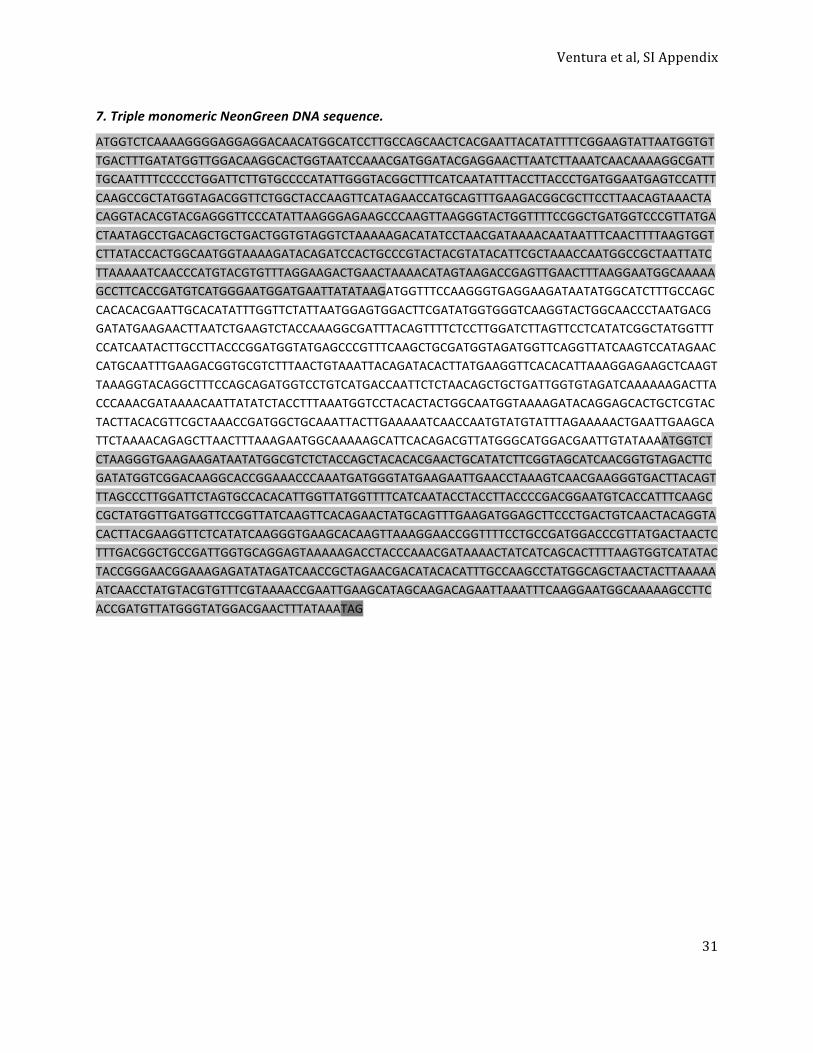
Ventura et al, SI Appendix
31
7. Triple monomeric NeonGreen DNA sequence.
ATGGTCTCAAAAGGGGAGGAGGACAACATGGCATCCTTGCCAGCAACTCACGAATTACATATTTTCGGAAGTATTAATGGTGTTGACTTTGATATGGTTGGACAAGGCACTGGTAATCCAAACGATGGATACGAGGAACTTAATCTTAAATCAACAAAAGGCGATTTGCAATTTTCCCCCTGGATTCTTGTGCCCCATATTGGGTACGGCTTTCATCAATATTTACCTTACCCTGATGGAATGAGTCCATTTCAAGCCGCTATGGTAGACGGTTCTGGCTACCAAGTTCATAGAACCATGCAGTTTGAAGACGGCGCTTCCTTAACAGTAAACTACAGGTACACGTACGAGGGTTCCCATATTAAGGGAGAAGCCCAAGTTAAGGGTACTGGTTTTCCGGCTGATGGTCCCGTTATGACTAATAGCCTGACAGCTGCTGACTGGTGTAGGTCTAAAAAGACATATCCTAACGATAAAACAATAATTTCAACTTTTAAGTGGTCTTATACCACTGGCAATGGTAAAAGATACAGATCCACTGCCCGTACTACGTATACATTCGCTAAACCAATGGCCGCTAATTATCTTAAAAATCAACCCATGTACGTGTTTAGGAAGACTGAACTAAAACATAGTAAGACCGAGTTGAACTTTAAGGAATGGCAAAAAGCCTTCACCGATGTCATGGGAATGGATGAATTATATAAGATGGTTTCCAAGGGTGAGGAAGATAATATGGCATCTTTGCCAGCCACACACGAATTGCACATATTTGGTTCTATTAATGGAGTGGACTTCGATATGGTGGGTCAAGGTACTGGCAACCCTAATGACGGATATGAAGAACTTAATCTGAAGTCTACCAAAGGCGATTTACAGTTTTCTCCTTGGATCTTAGTTCCTCATATCGGCTATGGTTTCCATCAATACTTGCCTTACCCGGATGGTATGAGCCCGTTTCAAGCTGCGATGGTAGATGGTTCAGGTTATCAAGTCCATAGAACCATGCAATTTGAAGACGGTGCGTCTTTAACTGTAAATTACAGATACACTTATGAAGGTTCACACATTAAAGGAGAAGCTCAAGTTAAAGGTACAGGCTTTCCAGCAGATGGTCCTGTCATGACCAATTCTCTAACAGCTGCTGATTGGTGTAGATCAAAAAAGACTTACCCAAACGATAAAACAATTATATCTACCTTTAAATGGTCCTACACTACTGGCAATGGTAAAAGATACAGGAGCACTGCTCGTACTACTTACACGTTCGCTAAACCGATGGCTGCAAATTACTTGAAAAATCAACCAATGTATGTATTTAGAAAAACTGAATTGAAGCATTCTAAAACAGAGCTTAACTTTAAAGAATGGCAAAAAGCATTCACAGACGTTATGGGCATGGACGAATTGTATAAAATGGTCTCTAAGGGTGAAGAAGATAATATGGCGTCTCTACCAGCTACACACGAACTGCATATCTTCGGTAGCATCAACGGTGTAGACTTCGATATGGTCGGACAAGGCACCGGAAACCCAAATGATGGGTATGAAGAATTGAACCTAAAGTCAACGAAGGGTGACTTACAGTTTAGCCCTTGGATTCTAGTGCCACACATTGGTTATGGTTTTCATCAATACCTACCTTACCCCGACGGAATGTCACCATTTCAAGCCGCTATGGTTGATGGTTCCGGTTATCAAGTTCACAGAACTATGCAGTTTGAAGATGGAGCTTCCCTGACTGTCAACTACAGGTACACTTACGAAGGTTCTCATATCAAGGGTGAAGCACAAGTTAAAGGAACCGGTTTTCCTGCCGATGGACCCGTTATGACTAACTCTTTGACGGCTGCCGATTGGTGCAGGAGTAAAAAGACCTACCCAAACGATAAAACTATCATCAGCACTTTTAAGTGGTCATATACTACCGGGAACGGAAAGAGATATAGATCAACCGCTAGAACGACATACACATTTGCCAAGCCTATGGCAGCTAACTACTTAAAAAATCAACCTATGTACGTGTTTCGTAAAACCGAATTGAAGCATAGCAAGACAGAATTAAATTTCAAGGAATGGCAAAAAGCCTTCACCGATGTTATGGGTATGGACGAACTTTATAAATAG
Ventura et al, SI Appendix
32
8. Supplemental References
1. Ma W, Trusina A, El-‐Samad H, Lim W, & Tang C (2009) Defining network topologies that can achieve biochemical adaptation. Cell 138(4):760-‐773.
2. Koshland DE, Jr., Goldbeter A, & Stock JB (1982) Amplification and adaptation in regulatory and sensory systems. Science 217(4556):220-‐225.
3. Ferrell JE (2001) Regulatory Cascades: Function and Properties. eLS, (John Wiley & Sons, Ltd).
4. Hoops S, et al. (2006) COPASI-‐-‐a COmplex PAthway SImulator. Bioinformatics 22(24):3067-‐3074.
5. Segall JE (1993) Polarization of yeast cells in spatial gradients of alpha mating factor. Proc Natl Acad Sci U S A 90(18):8332-‐8336.
6. Colman-‐Lerner A, et al. (2005) Regulated cell-‐to-‐cell variation in a cell-‐fate decision system. Nature 437(7059):699-‐706.
7. Longtine MS, et al. (1998) Additional modules for versatile and economical PCR-‐based gene deletion and modification in Saccharomyces cerevisiae. Yeast 14(10):953-‐961.
8. Shaner NC, et al. (2013) A bright monomeric green fluorescent protein derived from Branchiostoma lanceolatum. Nature methods 10(5):407-‐409.
9. Bush A, Chernomoretz A, Yu R, Gordon A, & Colman-‐Lerner A (2012) Using Cell-‐ID 1.4 with R for microscope-‐based cytometry. Current protocols in molecular biology / edited by Frederick M. Ausubel ... [et al Chapter 14:Unit 14 18.
10. Gordon A, et al. (2007) Single-‐cell quantification of molecules and rates using open-‐source microscope-‐based cytometry. Nat Methods 4(2):175-‐181.
11. Efron B & Tibshirani R (1994) An introduction to the bootstrap (Chapman & Hall, New York) pp xvi, 436 p.
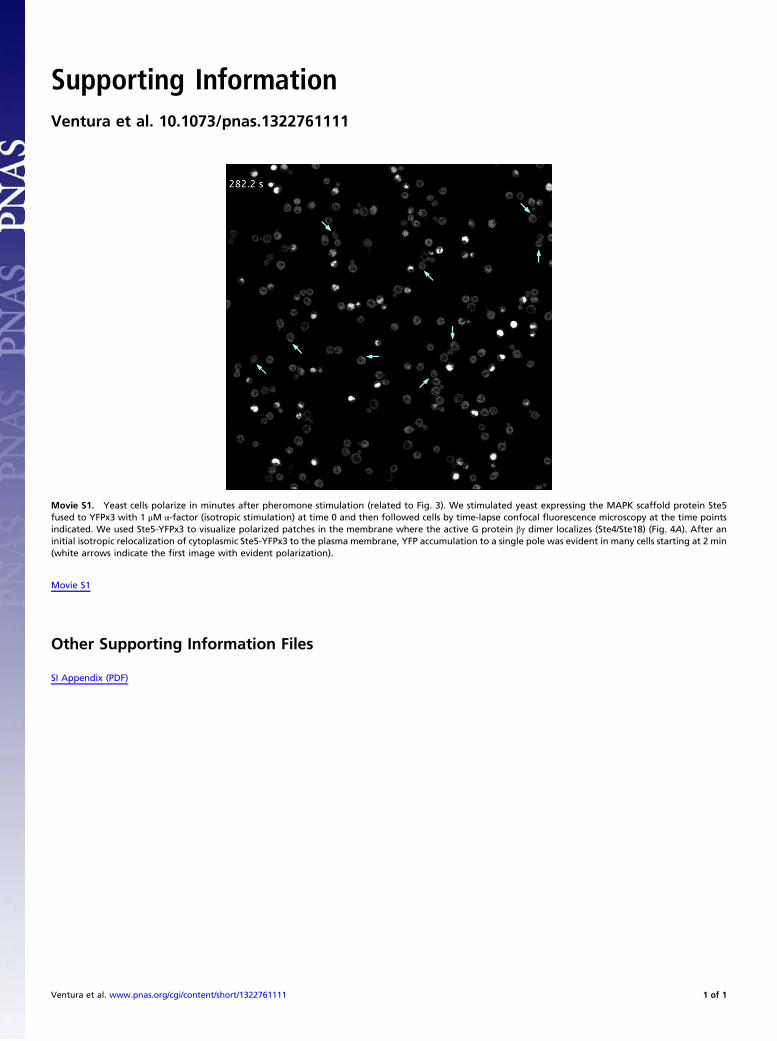
Supporting InformationVentura et al. 10.1073/pnas.1322761111
Movie S1. Yeast cells polarize in minutes after pheromone stimulation (related to Fig. 3). We stimulated yeast expressing the MAPK scaffold protein Ste5fused to YFPx3 with 1 μM α-factor (isotropic stimulation) at time 0 and then followed cells by time-lapse confocal fluorescence microscopy at the time pointsindicated. We used Ste5-YFPx3 to visualize polarized patches in the membrane where the active G protein βγ dimer localizes (Ste4/Ste18) (Fig. 4A). After aninitial isotropic relocalization of cytoplasmic Ste5-YFPx3 to the plasma membrane, YFP accumulation to a single pole was evident in many cells starting at 2 min(white arrows indicate the first image with evident polarization).
Movie S1
Other Supporting Information Files
SI Appendix (PDF)
Ventura et al. www.pnas.org/cgi/content/short/1322761111 1 of 1