ULTIMATE SENSITIVITY WITH ISOCAMB. ALTIERI, L. METCALFE, AND J. BLOMMAERTISO Science Centre,ESA Astrophysics Division, VILSPA, P.OBox 50727, E-28080 Madrid, SpainANDD. ELBAZ, J.-L. STARCK, AND H. AUSSELService d'Astrophysique, DSM/DAPNIA/CEA-Saclay, F91191Gif-sur-Yvette Cedex, FranceAbstract. We discuss the instrumental factors which constrain the sen-sitivity limits of the mid-infrared camera (ISOCAM) of ESA's InfraredSpace Observatory (ISO). The observing strategy judged to be best suitedto faint-source detection is described. A data analysis technique adaptedto the extraction of the faintest point-sources is discussed. We report theapplication of these techniques to an extremely deep mid-IR observation ofhigh redshift gravitationally lensed objects, in two �lters, looking througha lensing galaxy cluster.1. IntroductionTo take advantage of the unprecedented mid-IR sensitivity of the ISOCAMinstrument on-board the ISO satellite, several deep cosmological or galaxycluster observations have been performed with the Long Wavelength (LW)channel of ISOCAM. This paper describes the problems related to faint-source detection, the preferred observation strategy, and one of the bestadapted algorithms for their detection: PRETI developed at CEA/Saclay.The main di�culty in dealing with ISOCAM faint-source detection is thecombined e�ect of the cosmic ray impacts (glitches) and the signal tran-sient drift behaviour of the LW detector. Once these obstacles are overcomehowever, results at the fainter limits of the pre- ight expectations for ISO-CAM performance are obtained, and these strongly constrain cosmologicalmodels.

2 B. ALTIERI ET AL.2. Observations with ISOCAMThe ISOCAM instrument (Cesarsky et al., 1996) was one of the 4 instru-ments on board ESA's Infrared Space Observatory (ISO) satellite (Kessleret al., 1996). ISOCAM operated in the near- to mid-infrared 2.5-17 �mrange. Most of this wavelength range is inaccessible to ground-based in-struments due to atmospheric absorption and emission.The ISOCAM sensitivity was limited by 3 factors:� the fundamental photon Shot noise and the detector read noise ;� the signal drifts due to Transients (drifts which occur upon ux changesor following glitches) ;� the at-�eld noise (post- at-�elding residual variations in responsivityfrom pixel-to-pixel).2.1. THE PHOTON SHOT NOISE AND DETECTOR READ NOISEThese are the classical noise sources encountered with all array detectors,and for ISOCAM they both diminish with the square-root of the overallexposure time for any sky pixel. ISOCAM exposures are built up frommany detector readouts. Faint-source measurements were accomplished ina rastering (drizzled) mode. The duration of the on-chip integration timewas limited by the rate of cosmic ray particle impacts on the detector - theglitch rate. For faint source work the longest on-chip integration time whichcould be tolerated was used. Typically this was 5 to 10 seconds for the CAMLW detector. A deep faint-source measurement might then accumulate inthe region of 1000 to 2000 readouts (5000 to 10000 seconds) observationtime for the most deeply sampled sky pixels.2.2. TRANSIENTS AND GLITCHESTransient signal drifts occur whenever the detector is exposed to a change inillumination level. These transients a�ect to some degree all ISOCAM data.For LW, the pixel response to a positive ux change can be decomposedroughly into an initial step-response corresponding to about 60% of whatshould be the �nal signal change. This occurs within the 2 �rst readoutsafter the ux step - and is followed by a very slow signal increase, withvery long time constants when the ux change is small. For faint-sourcemeasurements, made typically in rastering mode with just 10 or 15 readoutsper raster position (see Section 3.), sources are usually measured close tothe initial rising edge of the transient. More on transient behaviour of thedetector can be found in Abergel et al. 1998.The e�ects of the cosmic ray particle impacts or glitches depend stronglyon the signal transient behaviour of the detector. The glitches, depending

Ultimate sensitivity with ISOCAM 3upon the type of triggering particle, can trigger strong upward or downwardexcursions of signal which can strongly increase the noise level in the data,and which can conceal or simulate true faint-source detections.The glitch rate is about 1 per second on the CAM LW detector. Itis so large because the detector is large compared to the standard arraystoday. This means that, for a typical 5 second on-chip integration, about�ve particle tracks will occur in the detector. On average each track a�ectsabout 8 pixels, so that very roughly about 5% of the detector pixels arecontaminated by glitches in each 5 second readout.Glitches can be divided into 3 families based upon their temporal pro�lefollowing the triggering particle impact;� the common glitches, that a�ect very few readouts and do not intro-duce signal variations.� the faders, strong glitches followed by a long decaying tail.� the dippers, glitches which suppress the signal by factors up to 20%or more in some cases, and leave long negative tails, in extreme caseslasting hundreds of readouts (and are attributed to heavy-ion impacts).The glitches are a major constraint on the sensitivity of the LW array.Wherever a glitch occurs at least a few readouts immediately following theimpact must be masked out.The size distribution of glitches does not obviously follow a gaussiandistribution. They certainly represent a non-gaussian contribution to theoverall noise in the data. This means that the rms of the signal from anygiven pixel over a period of time yields a value that cannot readily be usedto specify the 68% con�dence level for source detections on that pixel. I.e.1-� (one RMS) does not have the usual statistical signi�cance associatedwith a gaussian distribution. For more details and glitch characterisations,see Claret et al., 1998 and Dzitko H. et al. 1998Nevertheless, after appropriate steps have been taken to remove glitchspikes and to restore or suppress the values of distorted signals, the �nalraster mosaic image can be constructed, and the spatial noise over theimage is essentially gaussian. Then physically meaningful, conventional, 1-� sensitivity levels can be de�ned on the re-constructed image, when theredundancy in the deep raster is high enough. For the deepest rasters, thedeepest parts of the �eld will correspond to sky pixels which have beensampled by something of the order of 100 di�erent detector pixels.2.3. FLAT-FIELD NOISEThe detector " at-�eld" is the map of relative-responses of the detector pix-els to a source of uniform brightness-distribution within the �eld-of-view(FOV). The at-�eld can be determined in more than one way, adapted to

4 B. ALTIERI ET AL.some extent to the nature of the observation to be corrected. After at-�elding, the unavoidable residual pixel-to-pixel di�erences of response area classical source of additional noise. These pixel-to-pixel response varia-tions contribute a noise term proportional to the accumulated signal, andwhich therefore has the potential to saturate the S/N after only a few hun-dred readouts, especially for CAM �lters having wavelength ranges in thebrighter parts of the Zodiacal light spectrum.In practice, the e�ects of this residual at-�eld noise can be removed byappropriate �ltering of the data, e.g. a 'wide-window' median �lterering ofthe pixel time histories (Altieri et al. 1998a for the method description) or amulti-scale median �ltering (PRETI method, see x 4, and Starck et al. 1997for more details). This follows from the fact that, as stated earlier, CAMexposures are built from many individual readouts. Also, the observationis made in raster mode, so that source detections occur as step functions inthe time-history of detector pixels. These "steps" occur as a source comesto rest for a time on a pixel.If the smoothed time history of the signal from a pixel is �tted andsubtracted from the unsmoothed signal, then all background contributionalong with residual at-�eld induced uctuations, all long-term signal drifts,and many glitch remnants, are suppressed. What remains are the step-function source detections, plus some residual glitch spikes and dips, andthe shot and poisson noise. It must be stressed that this approach is onlysuitable for application to point-sources, because it attenuates extendedsource structure. It is also noted that the photometric calibration of point-source measurements must take account of any impacts of the smoothed-baseline subtraction. Careful studies have been, and are being, made of thise�ect, and an appropriate technical note, prepared by the CAM team atESA's ISO Science Operations Centre (SOC) in Madrid, is scheduled forplacement on the ESA ISO web pages in mid-1998.Notwithstanding this capacity to remove the e�ects of the at-�eld fromfaint point-source measurements, it is nonetheless important to at-�eldthe original data-cube before building the raster mosaic, so that the imagessu�er only from residual at-�elding problems. This is so because the at-�eld continues, even after �ltering of the data, to impact the photometricprecision for individual point-source detections.Flat-�elds may be extracted from the calibration libraries used for theISO O�ine Processing Pipeline standard processing. These at-�elds havebeen measured on the zodiacal light, during in- ight calibration of theinstrument, for those CAM �lters broad enough to yield su�cient signal.Then for all CAM LW �lters and optical con�gurations, library at-�eldshave been derived. These library at-�elds often give very good results andare supplied to all observers along with their data, for standard calibration

Ultimate sensitivity with ISOCAM 5purposes. But these at-�elds cannot match perfectly the conditions ofevery observation. One important limitation arises in the fact that, dueto some slight jitter in CAM lens wheel positioning, the optical vignettingpro�le seen by the detector may be slightly di�erent from one observationto the next - so that the at-�eld changes slightly, in a systematic way.Improved corrections for this e�ect are under study. For a description ofthe ISOCAM at-�eld calibration and noise introduced by library ats, werefer to Biviano et al., 1998a and 1998b.However, for long raster observations on homogeneous at backgrounds,an optimal at-�eld can be built directly from the data. During the faint-source raster, almost all sources remain below the noise level in any onereadout. The time history of each pixel is dominated by the constant illu-mination of the zodiacal background. By assigning a at-�eld value to eachpixel, equivalent to the median of its values throughout the duration of theraster measurement, one arrives at a at-�eld excellently adapted to theparticular con�guration and measurement in question. Of course, carefuljudgement must be employed to ensure that the accumulated backgroundsignal for the measurement is su�cient to generate a high signal-to-noise at-�eld. For the typical faint-source survey �lters LW2 and LW3 this isalmost always the case.The at-�eld generated in this way is called the auto at in CIA (CAMInteractive Analysis package), see Ott et al., 1996, and the CIA User'sManual for its use (Delaney et al., 1997). This method generally gives muchbetter results than can be obtained using library calibration at-�elds. How-ever, the auto- at may still be perturbed by the transient e�ects in the pixelhistories. A global transient usually occurs throughout an observation fol-lowing the initial illumination-change on the detector, and glitch inducedtransients also occur. Therefore a baseline �ltering technique such as thatdescribed above is extremely bene�cial in trying to reach the faintest levels.3. Observing StrategyThe parameters for a deep ISOCAM LW raster are as follows :� the central wavelength and width of the �lter� the on-chip integration time: Tint� the Pixel-�eld-of-view (PFOV) (1.5", 3" or 6" per pixel. 12" was rarelyused, and never for faint-source detection.)� the number of readouts used to build the full exposure: Nexp� the raster step size� the redundancy (in a single raster + in overlapping rasters) - the num-ber of times each sky pixel was sampled by some detector pixel.

6 B. ALTIERI ET AL.The central wavelength is driven by the scienti�c requirements of theobservation, balanced by considerations of sensitivity achievable in the var-ious con�gurations. For deep imaging observations, large band-width �lterswith the highest sensitivity are obviously desirable. Therefore the most used�lters for deep imaging (cosmological surveys for instance) were:� LW2 (5-8.5 �m, reference wavelength 6.7 �m)� LW3 (12-18 �m, reference wavelength 14.3 �m)� LW10 (8-15 �m, reference wavelength 12 �m; IRAS �lter)with the reference wavelengths taken from Blommaert et al.(1998),where they are justi�ed.The trade-o� between Tint and glitch rate was described in Section 2.1above, leading to the choice of the largest Tint compatible with keeping theglitch rate at an acceptable level. Data with Tint = 20 seconds would o�erextremely favourable read-noise performance, but are almost very di�cultto deglitch, so that it was advised early on in the mission not to use thison-chip integration time. However ultra-deep observations of the SSA13�eld (22 hours under the japaneese guaranteed time) were taken late in theISO mission with Tint = 20 sec., and lead apparently to good results. SeeBiviano et al. (1998b) for a more quantitative analysis.As also explained earlier, glitches are also better corrected with higherredundancy rasters.At 14.3�m, with appropriate �ltering of the data to remove the e�ects of at-�elding residuals, the dominant noise factor is still related to the highzodiacal background. Photon noise and read-noise levels are comparable,but the glitch induced responsive transients interacting with the relativelyhigh background signal, ensure that optimal performance is achieved byavoiding the Tint = 10 seconds setting, in favour of Tint = 5, for LW3.For LW2 at 6.7�m the Tint = 10.08 second option was sometimes pre-ferred because of the greater signi�cance of the readout noise at the corre-sponding lower Zodiacal background levels.TABLE 1. Noise characteristics�(�m) Integration Time Dominant noise6.7 �m 10 seconds READOUT noise14.3 �m 5 seconds PHOTON noiseThe choice of the pixel-�eld-of-view requires a trade-o� between thespatial resolution and the sensitivity. A big pixel-�eld-of-view will give more ux per pixel for a given point source. This implies, in principle, a better

Ultimate sensitivity with ISOCAM 7S/N per pixel once the baseline - including the residual at-�elding noise -has been removed. However, in relatively crowded �elds, such as the regionsnear the centres of galaxy clusters, the map may be a�ected by confusionof the numerous overlapping sources.Observers found qualitatively that the ultimate sensitivity in uncrowded�elds is reached when:� using the largest 600 PFOV� oversampling the pixels using non-integer raster steps.And in our observations in crowded �elds we found that the ultimatesensitivity may be enabled when:� using the smaller 300 PFOV� oversampling the pixels using non-integer raster steps.The �nal e�ective pixel size can be as small as 100 , when using the300 PFOV, but the minimal source separation stays close to the originalphysical pixel size (300 ). The spacecraft jitter (�0.500 ) is still small com-pared to this pixel size and only marginally extends point sources.The raster step size must be small enough to allow the largest redun-dancy within a raster. But the step size must be larger than the FWHMof the PSF, at least in one raster direction, so that the same source doesnot illuminate the same pixel for successive raster steps. If it does thenthe baseline removal along the time-axis will more strongly impact sourcephotometry. Dedicated ISO calibration measurements were made duringthe mission to quantify these e�ects and technical information notes are inpreparation at the ESA ISO Data Centre in Madrid, Spain, complementaryto the simulation studies already performed by CEA/Saclay. The numberof readouts per raster position need not be much higher than 10. This is sobecause, as explained in Section 2.2 above, after the initial ux step whena source arrives on a pixel, the signal stabilizes only very slowly. The initialsignal step is typically about 60% of the eventual stablized signal di�erence.During the mission, the practical wisdom was that the slow, asymptotic risein signal meant that the bene�ts of keeping the source on one pixel wereoutweighed by the glitch-rejection bene�ts derived from moving the sourceover the array. At the time of writing, after the end-of-mission, the discus-sion on the best compromise to chose between redundancy and stabilisationis still an open issue.So �nally the main free parameter is the redundancy, i.e. the numberof times a sky pixel will be seen by a detector pixel. A high redundancywill reduce the residual at-�elding noise, especially bene�cial if eventuallyany extended structure is to be examined, and it increases the reliability ofsource detection.

8 B. ALTIERI ET AL.TABLE 2. Optimum Observing Strategypoint source surveys - uncrowded �eldsPFOV 600Filter LW2 LW3 or LW10Nexp 12 20Tint 5 to 10 sec 5 secraster step � 1500TABLE 3. Optimum Observing Strategypoint source surveys - crowded �eldsPFOV 300Filter LW2 LW3 or LW10Nexp 12 20Tint 5 to 10 sec 5 secraster step � 1500This kind of observational strategy should also be best suited for deepobservation with SIRTF in the future, even if the detector technology isdi�erent. In other words, microscanning (making raster steps not corre-sponding to integer multiples of pixel dimensions) combined with a highredundancy should lead to the best results. Note that this kind of observa-tion strategy was used for the Hubble Deep Field observation with HST,so this technique is more general to deep CCD imaging (in the optical andthe IR). We should, of course, bear in mind that the exploration of the ISOdata has only really begun, so we must keep an open mind and expect laterre�nements and re�ned discussion of these conclusions.4. Data Reduction using PRETI4.1. METHODThe CEA/Saclay team has developed a dedicated technique for data re-duction of faint-source rasters: PRETI (Pattern REcognition Technique forISOCAM data). PRETI is based on the multi-resolution analysis of thecube of data generated by a deep-raster observation, and is described indetail in Starck et al., 1997. Note that this is not the only data reduction

Ultimate sensitivity with ISOCAM 9Figure 1. dipper glitch good correction by the PRETI method

Figure 2. Example of 2 spurious source detections after standard processingtechnique for detection of faint sources. Refer to Altieri et al. (1998a), for adescription of the other methods developed, or being developed or tested,in the ISOCAM consortium or at the ESA ISO data centre.PRETI allows the deglitching of the data, by separating the di�erent fre-quencies of the signal and extracting long glitches using a multi-resolutiontechnique based on the median transform in the temporal history of eachpixel.

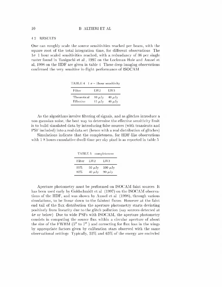
10 B. ALTIERI ET AL.4.2. RESULTSOne can roughly scale the source sensitivities reached per beam, with thesquare root of the total integration time, for di�erent observations. The1�{1 hour scaled sensitivities reached, with a redundancy of 36 per singleraster found in Taniguchi et al., 1997 on the Lockman Hole and Aussel etal, 1998 on the HDF are given in table 4. These deep imaging observationscon�rmed the very sensitive in- ight performance of ISOCAM.TABLE 4. 1 � { 1hour sensitivityFilter LW2 LW3Theoretical 10 �Jy 40 �JyE�ective 15 �Jy 40 �JyAs the algorithms involve �ltering of signals, and as glitches introduce anon-gaussian noise, the best way to determine the e�ective sensitivity limitis to build simulated data by introducing false sources (with transients andPSF included) into a real data set (hence with a real distribution of glitches)Simulations indicate that the completeness, for HDF-like observationswith 1.8 hours cumulative dwell-time per sky pixel is as reported in table 5.TABLE 5. completenessFilter LW2 LW395% 50 �Jy 100 �Jy80% 40 �Jy 90 �JyAperture photometry must be performed on ISOCAM faint sources. Ithas been used early by Goldschmidt et al. (1997) on the ISOCAM observa-tions of the HDF, and was shown by Aussel et al. (1998), through varioussimulations, to be linear down to the faintest uxes. However at the faintend tail of the ux distribution the aperture photometry starts deviatingpositively from linearity due to the glitch pollution (say sources detected at4� or below). Due to wide PSFs with ISOCAM, the aperture photometryconsists in computing the source ux within a circular aperture of aboutthe size of the FWHM (500 to 700 ) and correcting for ux loss in the wingsby appropriate factors given by calibration stars observed with the sameobservational settings. Typically, 55% and 65% of the energy are encircled

Ultimate sensitivity with ISOCAM 11in an aperture diameter of 700 in LW3 and LW2 respectively. Other typesof photometry such as Kron-like elliptical �tting, in SExtractor (Bertin &Arnouts, 1996) or `full object' wavelet photometry are non-linear at faint uxes.5. Ultimate CAM rasters: application to a deep crowded �eldIn order to push ISOCAM to the limits, both in terms of sensitivity andspatial resolution, we performed a series of observations which we refer toas the ultimate raster and which was targeted to obtain some of the deep-est ISOCAM images. This was implemented within ESA SOC guaranteedtime, as a follow-up to an ESA Guaranteed Time programme using grav-itational lensing clusters to probe the more distant background (Metcalfeet al., 1997 and 1999, Altieri et al., 1998b) and was allocated one full ISOrevolution, which amounts to 16 hours of science time. The target chosenwas Abell 2390, a very rich galaxy cluster where many mid-IR sources wereexpected to fall in a small area, with the source counts augmented by thegravitational lensing ampli�cation of this famous lensing cluster. (Mc Breen& Metcalfe, 1987, Paczynski B., 1986)Optimum spatial resolution being essential in this case, the 300 PFOVwas chosen. Emphasis was put on high redundancy by performing four10x10 rasters in each of the 2 �lter bands LW2 and LW3, leading to a re-dundancy factor of 400 in each �lter in the central part of the covered area.The 4 rasters were slightly o�set relative to each other to make the best useof the drizzling technique. Tint = 5 sec was chosen, to keep each individualraster to a reasonable time of 2 hours, for convenience in achieving opti-mum scheduling in the low-glitch-rate time near orbital apogee. Finally theminimum recommended step size (minimum for the data reduction �lteringstrategy preferred) of 700 was taken - this being very close to the FWHM ofthe LW3 PSF. This step-size allows an extremely high redundancy in eachindividual raster (100 in the central part).From the discussion in the sections above, it is seen that this representsthe optimum faint-source observing strategy interpreted for a relativelycrowded �eld and adapted to the scheduling constraints of these very, verylong cumulative exposures. Table 6 summarises the observation strategytaken for the ultimate CAM rasters.This approach yielded excellent scienti�c results very close to the limitsfound with surveys at 600 PFOV, reported in tables 4 and 5, but deeperwhen the gravitational magni�cation is taken into account. See �g. 3 forthe ultra-deep LW3 map through the cluster-lens Abell 2390, where almostall sources are lensed distant objects (Altieri et al., 1998c, 1988d).

12 B. ALTIERI ET AL.

Figure 3. Ultra deep map through the Abell 2390 cluster-lensTABLE 6. Ultimate CAM rastersPFOV 300Filter LW2 LW3Nexp 13 13Tint 5 sec 5 secraster step size � 700raster size 4 10x10 rastersmaximal redundancy 400

Ultimate sensitivity with ISOCAM 136. ConclusionDeep imaging observations with ISOCAM con�rmed the excellent in- ightperformance of the ISOCAM instrument, which matched the best pre- ighthopes. The faintest ISOCAM ux levels claimed are : in the 600 PFOV,around 50�Jy at 14.3�m on the ISOCAM observations of HDF (Rowan-Robinson et al., 1997; Aussel et al., 1998) and about 30�Jy at 6.7�m onthe Lockman Hole (Taniguchi et al, 1997), about 4 orders of magnitudesbelow IRAS, and, in the 300 PFOV about 30�Jy at 14.3�m on Abell 2390with the help of gravitational lensing.One of the best methods for data reduction, adapted to detect faintpoint-sources in deep raster observations with the ISOCAM LW detector,is the PRETI method, developed by Starck et al.AcknowledgementsThe ISOCAM data presented in this paper was analysed using "CIA", ajoint development by the ESA Astrophysics Division and the ISOCAMCon-sortium. The ISOCAM Consortium is led by the ISOCAM PI, C. Cesarsky,Direction des Sciences de la Matiere, C.E.A., France.ReferencesAbergel, A., et al., 1998, this volumeAltieri, B. et al., 1998a, `The ISOCAM Faint sources report', ESA/SSD, ISO WEBExplanatory library.Altieri, B., Metcalfe, L., et al., 1998b, in The Young Universe, Monteporzio conferenceproceedings, in press, astro-ph/9803155Altieri, B., Metcalfe, L., et al., 1988c, ESA SP-431 conf. proceedings, "NGST workshop:Science Drivers and Technological Challenges", astro-ph/9808131Altieri, B., Metcalfe, L., Kneib, J.-P., et al., 1998d, A&A letter, submitted, astro-ph/9810480.Aussel, H., Cesarsky, C., Elbaz, D., Starck J.-L., 1998, A&A in press, astro-ph/9810044Bertin, E. & Arnouts, S., 1996, A&A, 177, 393Biviano, A., et al., 1998a, `ISOCAM Flat-�eld calibration report', ESA/SSD, (ISO WEBexplanatory library)Biviano, A., 1998b, `The ISOCAM Calibration Error Budget Report', version 3.1, (ISOWEB explanatory library)Blommaert, J., Metcalfe, L., Altieri, B., et al., 1998, this volumeBoulade, O. & Gallais, P., 1998, ISOCAM Detectors: an Overview, this volumeCesarsky, C.J., et al. 1996, A&A 315, L32Claret, A., et al, 1998, this volumeDelaney, M. et al, `ISOCAM Interactive Analysis User's Manual, Version 2.0, referenceSAI-96-5226/DcDzitko, H., et al, 1998, this volumeGoldschmidt, P., Oliver, S., Serjeant, S., et al, 1997, MNRAS, 289, 465Kessler, M.F., et al. 1996, A&A 315, L27Ott, S., et al., 1997, "Design and implementation of CIA, the ISOCAM interactive anal-ysis system", ASP conference series vol.125

14 B. ALTIERI ET AL.Mc Breen, B., Metcalfe, L., 1987, Nature, Vol.330, p348Metcalfe, L., Altieri, B., et al., 1997, \ISO Mid-IR observations of Abell 370" in Extra-galactic Astronomy in the Infrared , Edt Frontieres, G. Mamon, astro-ph/9803174Metcalfe, L., Altieri, B., Kneib., J.-P. et al., 1999, under preparartion.Paczynski, B., 1986, Astrophys. J., 301, 503-516.Rowan-Robinson, M., Mann, R., Oliver, S., et al., 1997, MNRAS, 289, 490Starck, J.-L., Aussel, H., Elbaz, D., 1997, in Extragalactic Astronomy in the Infrared, Ed.Fronti�eres, Mamon G.A.Taniguchi, Y., Cowie, L., Sato, Y. et al., 1997, A&A, 329, L9