arX

iv:0

811.

1691

v2 [

gr-q

c] 1

0 Fe

b 20

09

Towards a gauge-polyvalent Numerical Relativity code

Daniela Alic, Carles Bona and Carles Bona-Casas

Departament de Fisica, Universitat de les Illes Balears, Palma de Mallorca, Spain.

Institute for Applied Computation with Community Code (IAC 3)

The gauge polyvalence of a new numerical code is tested, both in harmonic-coordinate

simulations (gauge-waves testbed) and in singularity-avoiding coordinates (simple Black-

Hole simulations, either with or without shift). The code is built upon an adjusted first-

order flux-conservative version of the Z4 formalism and a recently proposed family of robust

finite-difference high-resolution algorithms. An outstanding result is the long-term evolution

(up to 1000M ) of a Black-Hole in normal coordinates (zero shift) without excision.

PACS numbers: 04.25.Dm, 04.20.Cv

I. INTRODUCTION

In a recent paper [1], Kiuchi and Shinkai have analyzed numerically the behavior of many

’adjusted’ versions of the BSSN system. This is a follow-up of a former proposal [2] for using the

energy-momentum constraints to modify Numerical Relativity evolution formalisms. An important

point was to put the constraint propagation system (subsidiary system) in a strongly hyperbolic

form, so that constraint violations can propagate out of the computational domain. As a further

step, there is also the possibility of introducing damping terms, which would attract the numerical

solution towards the constrained subspace.

At the first sight, one could wonder why this idea is still deserving some interest today, when

the BSSN system is being successfully used in binary-black-holes simulations. Waveform templates

are currently being extracted for different mass and spin configurations, with an accuracy level

that depends just on the computational resources (including the use of mesh-refinement and/or

higher-order finite-difference algorithms). The same is true for neutron stars simulations, where the

BSSN formalism is currently used for evolving the spacetime geometry [3]-[6]. But these success

scenarios have a weak point: the BSSN simulations are based on the combination of the ’1+log’

and ’Gamma-driver’ gauge conditions, as proposed in Ref. [7] for the first long-term dynamical

simulation of a single Black Hole (BH) without excision.

Concerning BH simulations, we can understand that dealing numerically with collapse singulari-

ties requires the use of either excision, or time slicing prescriptions with strong singularity-avoidance

2

properties. In the ’1+log’ case, there is actually a ’limit hypersurface’, so that the numerical evolu-

tion gets safely bounded away from collapse singularities. But singularity-avoidance is a property

of the time coordinate, which should then be independent of the space coordinates prescription.

In the spirit of General Relativity, we should expect a gauge-polyvalent numerical code to work as

well in normal coordinates (zero shift), even if some specific type of time slicing condition (lapse

choice) is required for BH simulations. Moreover, this requirement should be extended to other

dynamical choices of the space coordinates. This means that a gauge-polyvalent numerical code

should also work with alternative shift prescriptions, provided that the proposed choices preserve

the regularity of the congruence of time lines. And this should be independent of the fact that a

freezing of the dynamics is obtained or not as a result. These considerations apply ’a fortriori’ to

neutron star simulations without any BH in the final stage, where no singularity is expected to

form.

The above proposed gauge-polyvalence requirements, which are in keeping with the spirit of

General Relativity, may seem too ambitious, allowing for the fact that they are not fulfilled by

current BH codes. But the need for improvement is even more manifest by looking at the results of

the gauge-waves test. This test consists in evolving Minkowsky spacetime in non-trivial harmonic

coordinates, and was devised for cross-comparing the numerical codes performance [8]. In Ref. [1],

the authors assay different adjustments in order to correct the poor performance of ’plain’ BSSN

codes, which was previously reported in Ref. [9]. They manage to get long-term evolutions for the

small amplitude case (A = 0.01) with a standard second-order-accurate numerical algorithm. The

same result was previously achieved by using a fourth-order accurate finite differences scheme [10].

Even in this case, however, the results for the medium amplitude case (A = 0.1) are disappointing.

More details can be found in a more recent cross-comparison paper [11], where actually a higher

benchmark (big amplitude, A = 0.5, devised for testing the non-linear regime) is proposed.

One could argue that the gauge-waves test is not relevant for real simulations, because periodic

boundary conditions do not allow constraint violations to propagate out of the computational

domain [9]. In BH simulations, however, constraint violations arising inside the horizon can not

get out, unless all the characteristic speeds of the subsidiary system are adjusted to be greater

than light speed. As far as this extreme adjustment is not implemented in the current evolution

formalisms, the gauge-waves test results can be indeed relevant, at least for non-excision BH

codes. As a result, in keeping with the view expressed in Ref. [1], we are convinced that either an

improvement of the current BSSN adjustments or any alternative formulation would be welcome,

as far as it could contribute to widen the gauge-polyvalence of numerical relativity codes.

3

In this paper we will consider an alternative numerical code consisting in two main ingredients.

The first one is the Z4 strongly-hyperbolic formulation of the field equations [12]. The original

(second order) version needs no adjustment for the energy and momentum constraints, as far as

constraint deviations propagate with light speed, although some convenient damping terms have

been also proposed [14]. We present in Section II a first-order version, which has been adjusted

for the ordering constraints which arise in the passage from the second-order to the first-order

formalism. Its flux-Conservative implementation is described in Appendix A. The second ingredient

is the recently developed FDOC algorithm [15], which is a (unlimited) finite-difference version

of the Osher-Chakrabarthy finite-volume algorithm [16], along the lines sketched in a previous

paper [17]. Although this algorithm, detailed in Appendix B, allows a much higher accuracy, we

will restrict ourselves here to the simple cases of third and fifth-order accuracy, which have shown

an outstanding robustness, confirmed by standard tests from Computational Fluid Dynamics,

including multidimensional shock interactions [15].

The results for the gauge-waves test are presented in section III, where just a small amount

of dissipation, without any visible dispersion error, shows up after 1000 crossing times, even for

the high amplitude (A = 0.5) case. Simulations of a 3D BH in normal coordinates are presented

in section IV, where we consider many variants of the ’Bona-Masso’ singularity-avoidant prescrip-

tion [18]. As expected, the best results for a given resolution are obtained for the choices with a

limit hypersurface far away from the singularity. For the f = 2/α choice, the BH evolves in normal

coordinates at least up to 1000M in a uniform grid with logarithmic space coordinates. This is

one order of magnitude greater than the normal-coordinates BSSN result, as reported in [7].

Concerning the shift conditions, we have tested in Section V many explicit first-order prescrip-

tions in single BH simulations. The idea is just to test the gauge-polyvalence of the code, so no

physically motivated condition has been imposed, apart from the three-covariance of the shift un-

der arbitrary time-independent coordinate transformations. Our results confirm that the proposed

code is not specially tuned for normal coordinates (zero shift).

II. ADJUSTING THE FIRST-ORDER Z4 FORMALISM

The Z4 formalism is a covariant extension of the Einstein field Equations, defined as [12]

Rµν + ∇µZν + ∇νZµ = 8 π (Tµν − 1

2T gµν). (1)

4

The four vector Zµ is an additional dynamical field, which evolution equations can be obtained

from (1). The solutions of the original Einstein´s equations can be recovered when Zµ is a Killing

vector. In the generic case, the Killing equation has only the trivial solution Zµ = 0, so that true

Einstein’s solutions can be easily recognized.

The manifestly covariant form (1) can be translated into the 3+1 language in the standard way.

The covariant four-vector Zµ will be decomposed into its space components Zi and the normal

time component

Θ ≡ nµ Zµ = α Z0 (2)

where nµ is the unit normal to the t = constant slices. The 3+1 decomposition of (1) is given then

by [12]

(∂t −Lβ) γij = −2 α Kij (3)

(∂t − Lβ) Kij = −∇iαj + α [Rij + ∇iZj + ∇jZi

− 2K2ij + (tr K − 2Θ) Kij − 8π{Sij −

1

2(tr S − τ) γij} ] (4)

(∂t − Lβ) Θ =α

2[R + 2 ∇kZ

k + (tr K − 2 Θ) tr K − tr (K2) − 2 Zkαk/α − 16πτ ] (5)

(∂t − Lβ) Zi = α [∇j (Kij − δi

j tr K) + ∂iΘ − 2 Kij Zj − Θ αi/α − 8πSi] . (6)

The evolution system can be completed by providing suitable evolution equations for the lapse

and shift components.

∂tα = −α2 Q , ∂tβi = − α Qi (7)

We will keep open at this point the choice of gauge conditions, so that the gauge-derived quantities

{Q, Qi} can be either a combination of the other dynamical fields or independent quantities with

their own evolution equation. We are assuming, however, that both lapse and shift are dynamical

quantities, so that terms involving derivatives of {Q, Qi} actually belong to the principal part of

the evolution system.

First-order formulation: ordering constraints

In order to translate the evolution system (3-7) into a fully first-order form, the space derivatives

of the metric components (including lapse and shift) must be introduced as new independent

quantities:

Ai ≡ ∂i ln α, Bki ≡ ∂kβ

i, Dkij ≡ 1

2∂kγij . (8)

5

Note that, as far as the new quantities will be computed now through their own evolution equa-

tions, the original definitions (8) must be considered rather as constraints (first-order constraints),

namely

Ak ≡ Ak − ∂k lnα = 0 (9)

Bki ≡ Bk

i − ∂k βi = 0 (10)

Dkij ≡ Dkij −1

2∂kγij = 0 . (11)

Note also that we can derive in this way the following set of constraints, related with the ordering

of second derivatives (ordering constraints):

Cij ≡ ∂i Aj − ∂j Ai = ∂i Aj − ∂j Ai = 0 , (12)

Crsi ≡ ∂r Bs

i − ∂s Bri = ∂r Bs

i − ∂s Bri = 0 , (13)

Crsij ≡ ∂r Dsij − ∂s Drij = ∂r Dsij − ∂s Drij = 0 . (14)

The evolution of the lapse and shift space derivatives could be obtained easily, just by taking

the time derivative of the definitions (8) and exchanging the order of time and space derivatives.

But then the characteristic lines for the transverse-derivative components in (8) would be the time

lines (zero characteristic speed). This can lead to a characteristic degeneracy problem, because

the characteristic cones of the second-order system (4-6) are basically the light cones [12], and the

time lines can actually cross the light cones, as it is the case in many black hole simulations. In

order to avoid this degeneracy problem, we can make use of the shift ordering constraint (13) for

obtaining the following evolution equations for the additional quantities (8):

∂tAk + ∂l[−βl Ak + δlk (α Q + βrAr)] = Bk

l Al − trB Ak (15)

∂tBki + ∂l[−βl Bk

i + δlk (α Qi + βrBr

i)] = Bkl Bl

i − trB Bki (16)

∂tDkij + ∂l[−βlDkij + δlk {α Kij − 1/2 (Bij + Bj i)} ] = Bk

l Dlij − trB Dkij . (17)

Note that the characteristic lines for the transverse-derivative components are now the normal

lines (instead of the time lines), so that characteristic crossing is actually avoided. This ordering

adjustment is crucial for long-term evolution in the dynamical shift case, as it has been yet realized

in the first-order version of the generalized harmonic formulation [13].

Damping terms adjustments

A further adjustment could be the introduction of some constraint-violation damping terms.

For the energy-momentum constraints, these terms can be added to the evolution equations (4-6),

6

as described in Ref. [14].

For the ordering constraints, we can also introduce simple constraint-violation damping terms

when required. For instance, equation (15) could be modified as follows:

∂tAi + ∂l[−βlAi + δli (α Q + βrAr)] = Bi

l Al − trB Ai − η Ai , (18)

with the damping parameter in the range 0 ≤ η ≪ 1/∆t. The same pattern could be applied to

equations (16, 17).

In order to justify this, let us analyze the resulting evolution equations for the first-order con-

straints (9). Allowing for (15), we would get

∂t Ak − βr (∂r Ak − ∂k Ar) = Bkr Ar − Br

r Ak . (19)

The hyperbolicity of the subsidiary evolution equation (19) can be analyzed by looking at the

normal and transverse components of the principal part along any space direction ~n, namely

∂t An − β⊥ (∂n A⊥) = 0 (20)

∂t A⊥ − βn (∂n A⊥) = 0 , (21)

with eigenvalues (0, −βn), which is just weakly hyperbolic in the fully degenerate case, that is for

any space direction orthogonal to the shift vector. Note that this is just the subsidiary system

governing constraint violations, not the evolution system itself. This means that the main concern

here is accuracy, rather than stability. But the resulting (linear) secular growth of first-order

constraint violations may become unacceptable in long-term simulations.

These considerations explain the importance of adding constraint-damping terms, so that (15)

is replaced by (18). The damping term −ηAk will appear as a result in the subsidiary system also.

The linearly growing constraint-violation modes arising from the degenerate coupling in (20) will

be kept then under control by these (exponential) damping terms. The same argument applies

mutatis mutandis to the remaining first-order constraints Bki, Dkij .

Secondary ordering ambiguities

The shift ordering constraints (13) can also be used for modifying the first-order version of the

evolution equation (6) in the following way

(∂t −Lβ) Zi = α [∇j (Kij − δi

j tr K) + ∂i Θ− 2Kij Zj −Θ Ai − 8πSi ]−µ (∂j Bi

j − ∂i trB) . (22)

7

Also, the ordering constraints (14) can be used for selecting a specific first-order form for the three-

dimensional Ricci tensor appearing in (4) [19]. This can be any combination of the standard Ricci

decomposition

Rij = ∂k Γkij − ∂ i Γ

kkj + Γr

rk Γkij − Γk

ri Γrkj (23)

with the De Donder decomposition

Rij = −∂k Dkij + ∂(i Γj )k

k − 2DrrkDkij

+ 4DrsiDrsj − ΓirsΓj

rs − Γrij Γrkk (24)

which is most commonly used in Numerical Relativity codes. Following Ref. [19], we will introduce

an ordering parameter ξ, so that ξ = 1 corresponds to the Ricci decomposition (23) and ξ = −1

to the De Donder one (24).

The choices of µ and ξ do not affect the characteristic speeds of the evolution system (see

Appendix A for details), nor the structure of the subsidiary system. In this sense, these are rather

secondary ordering ambiguities and we will keep these parameters free for the moment, although

there are some prescriptions that can be theoretically motivated:

• The choice µ = 1/2, ξ = −1 allows to recover at the first-order level the equivalence between

the generalized harmonic formulation and (the second-order version of) the Z4 formalism,

given by [14]

Zµ =1

2Γµ

ρσ gρσ (25)

(see Appendix A for more details). This can be important, because the harmonic system is

known to be symmetric hyperbolic.

• The choice µ = 1 is the only one that ensures the strong hyperbolicity of the Z3 system,

obtained from the Z4 one by setting θ = 0. This can be relevant if we are trying to keep

energy-constraint violations close to zero. Allowing for the quasi-equivalence between the Z3

and the BSSN systems [19], this adjustment will affect as well to the first-order version of

the BSSN system (NOR system [20]) in simulations using dynamical shift conditions. The

same comment applies to the old ’Bona-Masso’ system [21].

• The choice ξ = 0 ensures that the first-order version contains only symmetric combinations

of second derivatives of the space metric. This is a standard symmetrization procedure for

obtaining a first-order version of a generic second-order equation.

8

In the numerical simulations in this paper, we have taken µ = 1, ξ = −1, although we have also

tested other combinations, which also lead to long-term stability.

III. GAUGE WAVES TEST

We will begin with a test devised for harmonic coordinates. Let us consider the following line

element:

ds2 = H(x − t)(−dt2 + dx2) + dy2 + dz2 , (26)

where H is an arbitrary function of its argument. One could naively interpret this as the propa-

gation of an arbitrary wave profile with unit speed. But it is a pure gauge effect, because (26) is

nothing but the Minkowsky metric, written in some non-trivial harmonic coordinates system.

As proposed in Refs. [8], [11], we will consider the ’gauge waves’ line element (26), with the

following profile:

H = 1 − A Sin( 2π(x − t) ) , (27)

so that the resulting metric is periodic and we can identify for instance the points −0.5 and 0.5 on

the x axis. This allows to set up periodic boundary conditions in numerical simulations, so that

the initial profile keeps turning around along the x direction. One can in this way test the long

term effect of these gauge perturbations. The results show that the linear regime (small amplitude,

A = 0.01) poses no serious challenge to most Numerical Relativity codes (but see Ref. [1] for the

BSSN case). Following the recent suggestion in Ref. [11], we will then focus in the medium and

big amplitude cases (A = 0.1 and A = 0.5, respectively), in order to test the non-linear regime.

Concerning grid spacing, although ∆x = 0.01 would be enough for passing the test in the medium

amplitude case, the big amplitude one requires more resolution, so we have taken ∆x = 0.005 in

both cases.

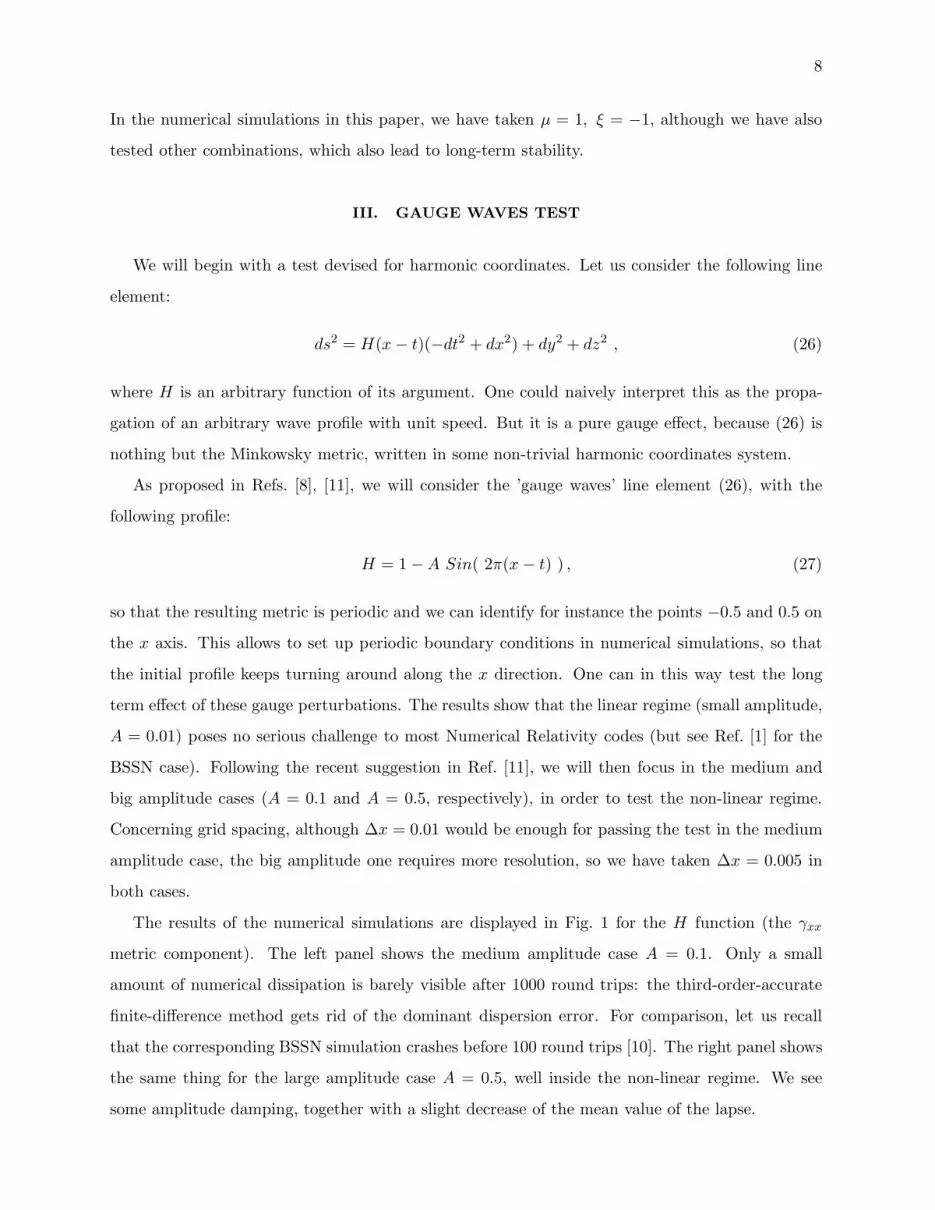
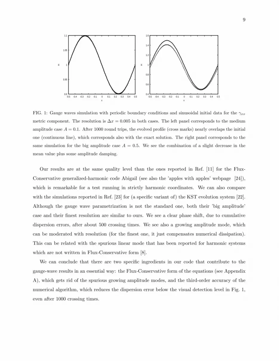
The results of the numerical simulations are displayed in Fig. 1 for the H function (the γxx

metric component). The left panel shows the medium amplitude case A = 0.1. Only a small

amount of numerical dissipation is barely visible after 1000 round trips: the third-order-accurate

finite-difference method gets rid of the dominant dispersion error. For comparison, let us recall

that the corresponding BSSN simulation crashes before 100 round trips [10]. The right panel shows

the same thing for the large amplitude case A = 0.5, well inside the non-linear regime. We see

some amplitude damping, together with a slight decrease of the mean value of the lapse.

9

0.9

0.95

1

1.05

1.1

-0.5 -0.4 -0.3 -0.2 -0.1 0 0.1 0.2 0.3 0.4 0.5

H

x

0.4

0.6

0.8

1

1.2

1.4

1.6

-0.5 -0.4 -0.3 -0.2 -0.1 0 0.1 0.2 0.3 0.4 0.5

H

x

FIG. 1: Gauge waves simulation with periodic boundary conditions and sinusoidal initial data for the γxx

metric component. The resolution is ∆x = 0.005 in both cases. The left panel corresponds to the medium

amplitude case A = 0.1. After 1000 round trips, the evolved profile (cross marks) nearly overlaps the initial

one (continuous line), which corresponds also with the exact solution. The right panel corresponds to the

same simulation for the big amplitude case A = 0.5. We see the combination of a slight decrease in the

mean value plus some amplitude damping.

Our results are at the same quality level than the ones reported in Ref. [11] for the Flux-

Conservative generalized-harmonic code Abigail (see also the ’apples with apples’ webpage [24]),

which is remarkable for a test running in strictly harmonic coordinates. We can also compare

with the simulations reported in Ref. [23] for (a specific variant of) the KST evolution system [22].

Although the gauge wave parametrization is not the standard one, both their ’big amplitude’

case and their finest resolution are similar to ours. We see a clear phase shift, due to cumulative

dispersion errors, after about 500 crossing times. We see also a growing amplitude mode, which

can be moderated with resolution (for the finest one, it just compensates numerical dissipation).

This can be related with the spurious linear mode that has been reported for harmonic systems

which are not written in Flux-Conservative form [8].

We can conclude that there are two specific ingredients in our code that contribute to the

gauge-wave results in an essential way: the Flux-Conservative form of the equations (see Appendix

A), which gets rid of the spurious growing amplitude modes, and the third-order accuracy of the

numerical algorithm, which reduces the dispersion error below the visual detection level in Fig. 1,

even after 1000 crossing times.

10

IV. SINGLE BLACK HOLE TEST: NORMAL COORDINATES

We will try next to test a Schwarzschild black-hole evolution in normal coordinates (zero shift).

Harmonic codes are not devised for this gauge choice, so we will compare with BSSN results

instead. Concerning the time coordinate condition, our choice will be limited by the singularity-

avoidance requirement, as far as we are not going to excise the black-hole interior. Allowing for

these considerations, we will determine the gauge evolution equations (7) as follows

Q = f (tr K − m Θ) , Qi = 0 (βi = 0) , (28)

where the second gauge parameter m is a feature of the Z4 formalism. We will choose here by

default m = 2, because the evolution equation for the combination trK−2Θ, as derived from (4, 5),

actually corresponds with the BSSN evolution equation for tr K (see Ref. [19] for the relationship

between BSSN and Z4 formalisms).

Concerning the first gauge parameter, we will consider first the ’1+log’ choice f = 2/α [25],

which is the one used in current binary BH simulations in the BSSN formalism. The name comes

from the resulting form of the lapse, after integrating the evolution equation (3, 7) with the

prescription (28) for true Einstein’s solutions (Θ = 0):

α = α0 + ln (γ/γ0) , (29)

where√

γ is the space volume element. It follows from (29) that the coordinate time evolution

stops at some limit hypersurface, before even getting close to the collapse singularity. This happens

when

√γ/γ0 = exp (−α0/2) , (30)

that is well before the vanishing of the space volume element: the initial lapse value is usually close

to one, so that the final volume element is still about a 60% of the initial one. This can explain

the robustness of the 1+log choice in current black-hole simulations.

We will consider as usual initial data on a time-symmetric time slice (Kij = 0) with the intrinsic

metric given in isotropic coordinates:

γij = (1 +m

2r)4 δij . (31)

This is the usual ’puncture’ metric, with the apparent horizon at r = m/2: the interior region is

isometric to the exterior one, so that the r = 0 singularity is actually the image of space infinity.

11

We prefer, however, to deal with non-singular initial data. We will then replace the constant mass

profile in interior region r < M/2 by a suitable profile m(r), so that the interior metric corresponds

to a scalar field matter content. Of course, the scalar field itself must be evolved consistently there

(see Appendix C for details). A previous implementation of the same idea, with dust interior

metrics, can be found in Ref. [26].

0

0.2

0.4

0.6

0.8

1

0 5 10 15 20

t=20M

t=40M

3rd h=0.1M3rd h=0.05M

5th h=0.1M

FIG. 2: Plots of the lapse profiles at t = 20M and t = 40 M . The results for the third-order accurate

algorithm (continuous lines) are compared with those for the fifth-order algorithm (dotted lines) for the

same resolution (h = 0.1M ). We have also included for comparison one extra line, corresponding to the

third-order results with h = 0.05 M , computed in a reduced mesh. Increasing resolution leads to a slope

steepening and a slower propagation of the collapse front. In this sense, as we can see for t = 20 M , switching

to the fifth-order algorithm while keeping h = 0.1 M amounts to doubling the resolution for the third-order

algorithm.

We have performed a numerical simulation for the f = 2/α case with a uniform grid with

resolution h = 0.1M , extending up to r = 20M (no mesh-refinement). We have used the third and

fifth-order FDOC algorithms, as described in Appendix B, with the optimal dissipation parameters

for each case. The results for the lapse profile are shown in Fig. 2 at t = 20M an t = 40M . We see

in both cases that the higher order algorithm leads to steeper profiles and a slower propagation of

the collapse front. Note that the differences in the front propagation speed keep growing in time,

although the third-order plot at t = 40M is clearly affected by the vicinity of the outer boundary.

12

This fact does not affect the code stability, as far as we can proceed with the simulations beyond

t = 50M , when the collapse front gets out of the computational domain (beyond t = 60M in

the higher-order simulations). Note that the corresponding BSSN simulations (f = 2/α in normal

coordinates) are reported to crash at about t = 40M [7].

We have added for comparison an extra plot in Fig. 2, with the results at t = 20M of a third-

order simulation with double resolution (h = 0.05M), obtained in a smaller computational domain

(extending up to 10M). Both the position and the slope of the collapse front coincide with those

of the fitfth-order algorithm with h = 0.1M . In this case, switching to the higher-order algorithm

amounts to doubling accuracy. Note, however, that higher-order algorithms are known to be less

robust [15]. Moreover, as the profiles steepen, the risk of under-resolution at the collapse front

increases. We have found that a fifth-order algorithm is a convenient trade-off for our h = 0.1M

resolution in isotropic coordinates.

We have also explored other slicing prescriptions with limit surfaces closer to the singularity,

as described in Table I. Note that in these cases the collapse front gets steeper than the one

shown in Fig. 2 for the standard f = 2/α case with the same resolution. This poses an extra

challenge to numerical algorithms, so we have switched to the third-order-accurate one for the sake

of robustness. In all cases, the simulations reached t = 50M without problem, meaning that the

collapse front has get out of the computational domain. It follows that the standard prescription

f = 2/α, although it leads actually to smoother profiles, is not crucial for code stability.

f 2/α 1+1/α 1/2+1/α 1/α√

γ/γ0 61% 50% 44% 37%

TABLE I: Different prescriptions for the gauge parameter f , with the corresponding values of the residual

volume element at the limit surface (normal coordinates), assuming a unit value of the initial lapse.

The results shown in Fig. 2 compare with the ones in Ref. [27], obtained with (a second-order

version of) the old Bona-Masso formalism. We see the same kind of steep profiles, produced by the

well known slice-stretching mechanism [28]. This poses a challenge to standard numerical methods:

in Ref. [27] Finite-Volume methods where used, including slope limiters. Our FDOC algorithm

(see Ref. [15] for details) can also be interpreted as an efficient Finite-Differences (unlimited)

version of the Osher-Chakrabarthy Finite-Volume algorithm [16]. Note however that in Ref. [27],

like in the BSSN case, a conformal decomposition of the space metric was considered, and an

spurious (numerical) trace mode arise in the trace-free part of the extrinsic curvature. An additional

mechanism for resetting this trace to zero was actually required for stability. In our (first-order)

13

Z4 simulations, both the plain space metric and extrinsic curvature can be used directly instead,

without requiring any such trace-cleaning mechanisms.

Let us take one further step. Note that the lifetime of our isotropic coordinates simulations

(with no shift) is clearly limited by the vicinity of the boundary (at r = 20M). At this point, we

can appeal to space coordinates freedom, switching to some logarithmic coordinates, as defined by

R = L sinh(r/L) , (32)

where R is the new radial coordinate and L some length scale factor. This configuration suggests

using the third-order algorithm because of its higher robustness. We have performed a long-term

numerical simulation for the f = 2/α case, with L = 1.5M , so that R = 20M in these logarithmic

coordinates corresponds to about r = 463.000M in the original isotropic coordinates. In this way,

as shown in Fig. 3, the collapse front is safely away from the boundary, even at very late times. We

stopped our code at t = 1000M , without any sign of instability. This provides a new benchmark

for Numerical Relativity codes: a long-term simulation of a single black-hole, without excision, in

normal coordinates (zero shift). Moreover, it shows that a non-trivial shift prescription is not a

requisite for code stability in BH simulations.

V. SINGLE BLACK HOLE TEST: FIRST-ORDER SHIFT CONDITIONS

Looking at the results of the previous Section, one can wonder wether our code is just tuned for

normal coordinates. This is why we will consider here again BH simulations, but this time with

some non-trivial shift prescriptions. The idea is just to test some simple cases in order to show

the gauge-polyvalence of the code. For the sake of simplicity, we will consider here just first order

shift prescriptions, meaning that the source terms (Q, Qi) in the gauge evolutions (7) are algebraic

combinations of the remaining dynamical fields. To be more specific, we shall keep considering

slicing conditions defined by

Q = −βk/α Ak + f (tr K − m Θ) , (33)

together with dynamical shift prescriptions, defined by different choices of Qi.

First-order shift prescriptions have been yet considered at the theoretical level [29]. We will

introduce here an additional requirement, which follows when realizing that, allowing for the 3+1

decomposition of the line element

ds2 = −α2 dt2 + γij (dxi + βidt) (dxj + βjdt) , (34)

14

laps

e

0

5

10

15

20

x

0 5

10 15

20

y

0 0.2 0.4 0.6 0.8

1 1.2

FIG. 3: Plot of the lapse function for a single BH at t = 1000 M in normal coordinates. Only one of every ten

points is shown along each direction. The third-order accurate algorithm has been used with β = 1/12 and

a space resolution h = 0.1 M . The profile is steep, but smooth: no sign of instability appears. Small riddles,

barely visible on the top of the collapse front, signal some lack of resolution because of the logarithmic

character of the grid. The dynamical zone is safely away from the boundaries.

the shift behaves as a vector under (time independent) transformations of the space coordinates.

We will impose then that its evolution equation, and then Qi, is also three-covariant.

This three-covariance requirement could seem a trivial one. But note that the harmonic shift

conditions, derived from

� xi = 0, (35)

are not three-covariant (the box here stands for the wave operator acting on scalars). In the 3+1

language, (35) can be translated as

∂t(√

γ/α βi) − ∂k(√

γ/α βkβi) + ∂k(α√

γ γik) = 0 , (36)

where the non-covariance comes from the space-derivatives terms.

Concerning the advection term, a three-covariant alternative would be provided either by the

Lie-derivative term

Lβ (√

γ βi/α ) = Lβ (√

γ/α ) βi , (37)

15

or by the three-covariant derivative term

βk ∇k(βi/α ) = 1/α [βk Bki − βiβkAk + Γi

j k βjβk ] . (38)

We have tested both cases in our numerical simulations.

Concerning the last term in (36), we can take any combination of Ai, Zi and the vectors obtained

form the space metric derivatives after subtracting their initial values, namely:

Di − Di |t=0 , Ei − Ei |t=0 . (39)

This is because the additional terms arising in the transformation of the non-covariant quantities

(Di, Ei) depend only on the space coordinates transformation, which is assumed to be time-

independent. Note that, for the conformal contracted-Gamma combination

Γi = 2Ei −2

3Di , (40)

the subtracted terms actually vanish in simulations starting from the isotropic initial metric (31).

Of course, the same remark applies to the BSSN Gamma quantity, namely [19]

Γi = Γi + 2Zi . (41)

We have considered the following combinations:

S1 : ∂t βi =α2

2Ai − α Qβi (42)

S2 : ∂t βi =α2

2Ai + βk Bk

i + Γij k βjβk − α Qβi (43)

S3 : ∂t βi =α2

4Γi + βk Bk

i + Γij k βjβk − αQβi , (44)

where S1 corresponds to the Lie-derivative term (37) and the remaining two choices to the covariant

advection term (38), with different combinations of the first-order vector fields.

We have obtained stable evolution in all cases, with the simulations lasting up to the point

when the collapse front crosses the outer boundary (about t = 50M). We can see in Fig. 4 the

lapse and shift profiles in the S1 and the S3 cases (S2 is very similar to S1). The shift profiles

are modulated by the lapse ones, so that the shift goes to zero in the collapsed regions. This is a

consequence of the term −αQβi in the shift evolution equation, devised for getting finite values

of the combination βi/α. In the non-collapsed region, S1 leads to a higher shift profile, which

spreads out with time, whereas S3 leads to a lower profile, which starts diminishing after the initial

growing. Allowing for (44), this indicates that the conformal gamma quantity Γi is driven to zero.

The lapse slopes are also slightly softened in the S3 case.

16

0

0.2

0.4

0.6

0.8

1

0 5 10 15 20 25 30

r/M

t=20M t=40M

0

0.2

0.4

0.6

0.8

1

0 5 10 15 20 25 30

r/M

t=20M t=40M

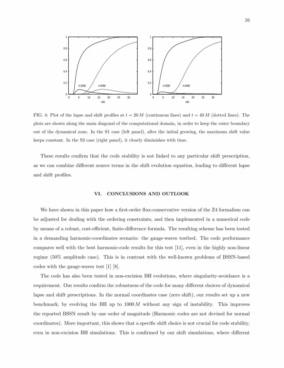
FIG. 4: Plot of the lapse and shift profiles at t = 20 M (continuous lines) and t = 40 M (dotted lines). The

plots are shown along the main diagonal of the computational domain, in order to keep the outer boundary

out of the dynamical zone. In the S1 case (left panel), after the initial growing, the maximum shift value

keeps constant. In the S3 case (right panel), it clearly diminishes with time.

These results confirm that the code stability is not linked to any particular shift prescription,

as we can combine different source terms in the shift evolution equation, leading to different lapse

and shift profiles.

VI. CONCLUSIONS AND OUTLOOK

We have shown in this paper how a first-order flux-conservative version of the Z4 formalism can

be adjusted for dealing with the ordering constraints, and then implemented in a numerical code

by means of a robust, cost-efficient, finite-difference formula. The resulting scheme has been tested

in a demanding harmonic-coordinates scenario: the gauge-waves testbed. The code performance

compares well with the best harmonic-code results for this test [11], even in the highly non-linear

regime (50% amplitude case). This is in contrast with the well-known problems of BSSN-based

codes with the gauge-waves test [1] [8].

The code has also been tested in non-excision BH evolutions, where singularity-avoidance is a

requirement. Our results confirm the robustness of the code for many different choices of dynamical

lapse and shift prescriptions. In the normal coordinates case (zero shift), our results set up a new

benchmark, by evolving the BH up to 1000M without any sign of instability. This improves

the reported BSSN result by one order of magnitude (Harmonic codes are not devised for normal

coordinates). More important, this shows that a specific shift choice is not crucial for code stability,

even in non-excision BH simulations. This is confirmed by our shift simulations, where different

17

covariant evolution equations for the shift lead also to stable numerical evolution.

In spite of the encouraging performance in these basic tests, we still are on the way towards

a gauge-polyvalent code, as pointed out by the title of this paper. More technical developments

on the numerical part are required: mesh refinement, improved boundary treatment, etc. On the

theoretical side, as far as the shift prescription is no longer determined by numerical stability, we

can explore shift choices from the physical point of view, adapting our space coordinates system

to the features of every particular problem. We are currently working in these directions.

Acknowledgments

This work has been jointly supported by European Union FEDER funds, the Spanish Ministry

of Science and Education (projects FPA2007-60220, CSD2007-00042 and ECI2007-29029-E) and by

the Balearic Conselleria d’Economia Hissenda i Innovacio (project PRDIB-2005GC2-06). D. Alic

and C. Bona-Casas acknowledge the support of the Spanish Ministry of Science, under the BES-

2005-10633 and FPU/2006-02226 fellowships, respectively

Appendix A: Flux-Conservative evolution equations

We will write the first-order evolution system in a balance-law form. For a generic quantity u,

this leads to

∂t u + ∂k F k(u) = S(u) , (A.1)

where the Flux F k(u) and Source terms S(u) can depend on the full set of dynamical fields in an

algebraic way. In the case of the space-derivatives fields, their evolution equations (15-17) are yet

in the balance-law form (A.1). Note however that any damping terms of the form described in (18)

will contribute both to the Flux and the Source terms in a simple way.

The metric evolution equation (3) will be written in the form

∂t γij = 2βkDkij + Bij + Bj i − 2 α Kij , (A.2)

so that it is free of any Flux terms. The remaining (non-trivial) evolution equations (4- 6) require

18

a more detailed development. We will expand first the Flux terms in the following way:

∂tKij + ∂k[−βk Kij + α λkij ] = S(Kij) (A.3)

∂tZi + ∂k[−βk Zi + α {−Kki + δk

i(trK − Θ)} (A.4)

+µ (Bik − δi

ktrB) ] = S(Zi)

∂tΘ + ∂k[−βk Θ + α (Dk − Ek − Zk) ] = S(Θ) (A.5)

where we have used the shortcuts Di ≡ Dikk and Ei ≡ Dk

ki , and

λkij = Dk

ij −1

2(1 + ξ) (Dij

k + Dj ik) +

1

2δk

i [Aj + Dj − (1 − ξ) Ej − 2 Zj ] (A.6)

+1

2δk

j [Ai + Di − (1 − ξ) Ei − 2 Zi ] .

The Source terms S(u) do not belong to the principal part and will be displayed later. Let us

focus for the moment in the hyperbolicity analysis, by selecting a specific space direction ~n, so that

the corresponding characteristic matrix is

An =∂ Fn

∂ u, (A.7)

where the symbol n replacing an index stands for the projection along the selected direction ~n. We

can get by inspection the following (partial) set of eigenfields, independently of the gauge choice:

• Transverse derivatives:

A⊥ , B⊥i , D⊥ij , (A.8)

propagating along the normal lines (characteristic speed −βn ). The symbol ⊥ replacing an

index means the projection orthogonal to ~n.

• Light-cone eigenfields, given by the pairs

Fn[Dn⊥⊥ ] ± Fn[K⊥⊥ ] (A.9)

−Fn[Z⊥ ] ± Fn[Kn⊥ ] (A.10)

Fn[Dn − En − Zn ] ± Fn[ Θ ] (A.11)

with characteristic speed −βn ± α , respectively.

Note that the eigenvector expressions given above, in terms of the Fluxes, are valid for any choice

of the ordering parameters µ and ξ. Only the detailed expression of the eigenvectors, obtained from

the Flux definitions, is affected by these parameter choices. For instance

Fn[Dn − En − Zn ] = −βn [Dn − En − Zn ] + α θ + (µ − 1) tr(B⊥⊥) . (A.12)

19

Any value µ 6= 1 implies that the characteristic matrix of the Z3 system, obtained by removing the

variable θ from our Z4 evolution system [19], can not be fully diagonalized in the dynamical shift

case. Of course, the hyperbolicity analysis can not be completed until we get suitable coordinate

conditions, amounting to some prescription for the lapse and shift sources Q and Qi, respectively.

But the subset of eigenvectors given here is gauge independent: non-diagonal blocs can not be

fixed a posteriori by the coordinates choice.

The detailed expressions for the eigenvectors can be relevant when trying to compare with

related formulations. For instance, a straightforward calculation shows that the eigenvectors (A.9-

A.11) can be matched to the corresponding ones in the harmonic formalism if and only if

ξ = −1 , µ = 1/2 . (A.13)

This shows that different requirements can point to different choices of these ordering parameters.

We prefer then to leave this choice open for future applications. Concerning the simulations in this

paper, we have taken ξ = −1 , µ = 1 .

Finally, we give for completeness the Source terms, namely:

S(Kij) = −Kij trB + Kik Bjk + Kjk Bi

k + α {1

2(1 + ξ) [−Ak Γk

ij +1

2(Ai Dj + Aj Di)]

+1

2(1 − ξ) [Ak Dk

ij −1

2{Aj (2 Ei − Di) + Ai (2 Ej − Dj)}

+ 2 (Dirm Dr

mj + Djrm Dr

mi) − 2 Ek (Dijk + Dji

k)]

+ (Dk + Ak − 2 Zk) Γkij − Γk

mj Γmki − (Ai Zj + Aj Zi) − 2 Kk

i Kkj

+ (trK − 2 Θ) Kij} − 8 π α [Sij −1

2(trS − τ) γij ] (A.14)

S(Zi) = −Zi trB + Zk Bik + α [Ai (trK − 2 Θ) − Ak Kk

i − Kkr Γr

ki + Kki (Dk − 2 Zk)]

−8 π α Si (A.15)

S(Θ) = −Θ trB +α

2[2 Ak (Dk − Ek − 2 Zk) + Dk

rs Γkrs − Dk(Dk − 2 Zk) − Kk

r Krk

+ trK (trK − 2 Θ)] − 8 π α τ . (A.16)

Appendix B: Finite-differences implementation

We follow the well-known method-of-lines (MoL [30]) in order to deal separately with the space

and the time discretization. Concerning the time discretization, we use the following third-order-

20

accurate Runge-Kutta algorithm

u∗ = un + ∆t rhs( un )

u∗∗ =3

4un +

1

4[u∗ + ∆t rhs( u∗ )] (B.1)

un+1 =1

3un +

2

3[u∗∗ + ∆t rhs( u∗∗ )] ,

which is strong-stability-preserving (SSP [31]), where we have used as a shorthand

rhs( u ) ≡ − ∂k F k(u) + S(u) . (B.2)

The Flux derivatives appearing in (B.2) will be discretized by using the finite-difference formula

proposed in Ref. [15] (FDOC algorithm). For instance the derivative of F x(u) will be represented

as

∂xF xj = C2mF x

j + (−1)mβ(∆x)2mDm+ Dm−1

−(λj−1/2 D−uj) , (B.3)

where C2m is the 2mth-order-accurate central difference operator and D± are the standard finite

difference operators. We have also noted

λj−1/2 = max(λj, λj−1) , (B.4)

where λj stands here for the local characteristic radius (the highest characteristic speed, typically

the gauge speed).

Note that the second term in the finite-difference formula (B.3) is actually a dissipation operator

of order 2m acting on (λu), so it could be regarded at the first sight as a mere generalization of the

standard Kreiss-Oliger artificial viscosity operators [32]. This is not the case: the formula (B.3)

can be instead derived in a finite-volume framework, when combining the local-Lax-Friedrichs flux

formula [33] with the (unlimited) Osher-Chakrabarthy flux interpolation [16] (see Ref. [15] for

details, including the optimal values of the β parameter).

Note that, contrary to the standard Kreiss-Oliger approach, the dissipation term is such that

the accuracy of the first (centered derivatives) term in (B.3) is reduced by one order: the resulting

FDOC algorithm accuracy is always of an odd order. This is important for code robustness. The

algorithms (B.3) can be shown to keep monotonicity even for remarkably high compression factors

(defined as the ratio between two neighbor slopes along a given direction) [15], which is what is

actually required in view of the steep profiles shown for instance in Fig. 2.

The space accuracy of the scheme (B.3) is 2m−1, with an stencil of 2m+1 points. We have used

in this paper both the third-order and fifth-order accurate methods, for which the optimal values

21

of the dissipation parameter are β = 1/12, β = 2/75, respectively [15]. In the fifth order case,

we have a seven-point stencil and the dissipation term corresponds to a sixth derivative, as in the

advanced finite-difference schemes used in Ref. [34]. The robustness of the proposed algorithms,

with compression factors of 5 and 3 respectively, makes them very convenient for steep-gradient

scenarios, such us the ones arising in black-hole simulations, where slice-stretching threatens the

stability of more standard finite-difference algorithms [28].

No sophisticated numerical tools (mesh refinement, algorithm-switching for the advection terms,

etc) have been incorporated to our code at this point, when we are facing just test simulations.

Concerning the boundary treatment, we simply choose at the points next to the boundary the most

accurate centered algorithm compatible with the available stencil there. When it comes to the last

point, we can either copy the neighbor value or propagate it out with the maximum propagation

speed (by means of a 1D advection equation). The idea is to keep the numerical code as simple as

possible in order to test here just the basic algorithm in a clean way.

Appendix C: Scalar field stuffing

Let us consider the stress-energy tensor

Tab = Φa Φb − 1/2 (gcdΦc Φd) gab , (C.1)

where we have noted Φa = ∂a Φ, corresponding to a scalar field matter content. The 3+1 decom-

position of (C.1) is given by

τ = 1/2 (Φn2 + γklΦk Φl) , Si = Φn Φi , Sij = Φi Φj + 1/2 (Φn

2 − γklΦk Φl) γij , (C.2)

where Φn stands for the normal time derivative:

(∂t − βk ∂k) Φ = −α Φn . (C.3)

The quantities (C.2) appear as source terms in the field equations (4-6).

The stress-energy conservation amounts to the evolution equation for the scalar field, which is

just the scalar wave equation. In the 3+1 language, it translates into the Flux-conservative form:

∂t [√

γ Φn ] + ∂k [√

γ (−βkΦn + αγkjΦj) ] = 0 . (C.4)

A fully first-order system may be obtained by considering the space derivatives Φi as independent

dynamical fields, as we did for the metric space derivatives.

22

Concerning the initial data, we must solve the energy-momentum constraints. They can be

obtained by setting both Θ and Zi to zero in (5, 6). In the time-symmetric case (Kij = 0), this

amounts to

R = 16π τ , Si = Φn Φi = 0 . (C.5)

The momentum constraint will be satisfied by taking Φ (and then Φi) to be zero everywhere on

the initial time slice. Concerning the energy constraint, we will consider the line element (31) with

m = m(r). We assume a constant mass value m = M for the black-hole exterior, so that the

energy constraint in (C.5) will be satisfied with τ = 0 there.

In the interior region, the energy constraint will translate instead into the equation

m′′ = −2πr (Φn)2 (1 +m

2r)5 , (C.6)

which can be interpreted as providing the initial Φn value for any convex (m′′ ≤ 0) mass profile.

Of course, some regularity conditions both at the center and at the matching point r0 must be

assumed. Allowing for (C.6), we have taken

m = m′′ = 0 (r = 0)

m = M, m′ = m′′ = 0 (r = r0) .

Note that, allowing for (C.6), these matching conditions ensure just the continuity of Φn , not

its smoothness. This can cause some numerical error, as we are currently evolving Φn through

the differential equation (C.4). If this is a problem, we can demand the vanishing of additional

derivatives of the mass function m(r), both at the origin and at the matching point (this is actually

the case in our shift simulations). This is not required in the standard case (f = 2/α, normal

coordinates), where we have used a simple profile, with the matching point at the apparent horizon

(r0 = M/2), given by

m(r) = 4r − 4/M [ r2 + (M/2π)2 sin2(2πr/M) ] . (C.7)

[1] K. Kiuchi and H-A. Shinkai, Phys. Rev. D77, 044010 (2008).

[2] G. Yoneda and H-A. Shinkai, Phys. Rev. D66, 124003 (2002).

[3] M. Shibata and Y.-I. Sekiguchi, Phys. Rev. D72, 044014 (2005).

[4] M. D. Duez, Y. T. Liu, S. L. Shapiro, and B. C. Stephens, Phys. Rev. D72, 024028 (2005).

23

[5] M. Anderson, E. W. Hirschmann, S. L. Liebling, and D. Neilsen, Class. Quantum Grav. 23, 6503

(2006).

[6] B. Giacomazzo and L. Rezzolla, Class. Quantum Grav. 24, 235 (2007).

[7] M. Alcubierre et al, Phys. Rev. D67, 084023 (2003).

[8] M. Alcubierre et al, Class. Quantum Grav. 21, 589 (2004).

[9] N. Jansen, B. Bruegmann and W. Tichy, Phys. Rev. D74, 084022 (2006).

[10] Y. Zlochower, J. G. Baker, M. Campanelli and C. O. Lousto, Phys. Rev. D72, 024021 (2005).

[11] M. Babiuc et al, Class. Quant. Grav. 25, 125012 (2008).

[12] C. Bona, T. Ledvinka, C. Palenzuela, M. Zacek, Phys. Rev. D 67, 104005 (2003).

[13] M. Holst, et al, Phys. Rev. D70 084017 (2004).

[14] C. Gundlach, G. Calabrese, I. Hinder and J.M. Martın-Garcıa, Class. Quantum Grav. 22, 3767 (2005).

[15] C. Bona, C. Bona-Casas and J. Terradas, J. Comp. Physics 228, 2266 (2009).

[16] S. Osher and S. Chakravarthy, ICASE Report 84–44,

ICASE NASA Langley Research Center, Hampton, VA (1984).

[17] D. Alic, C. Bona, C. Bona-Casas and J. Masso, Phys. Rev. D76, 104007 (2007)

[18] C. Bona, J. Masso, E. Seidel and J. Stela, Phys. Rev. Lett. 75 600 (1995).

[19] C. Bona, T. Ledvinka, C. Palenzuela and M. Zacek, Phys. Rev. D 69, 064036 (2004).

[20] G. Nagy, O. Ortiz and O. Reula, Phys. Rev. D70 044012 (2004).

[21] C. Bona and J. Masso, Phys. Rev. Lett. 68, 1097 (1992).

[22] L. E. Kidder, M. A. Scheel and S. A. Teukolsky, Phys. Rev. D64 064017 (2001).

[23] M. Tiglio, L. Lehner and D. Neilsen, Phys. Rev. D70 104018 (2004).

[24] www.appleswithapples.org/TestResults/Results/Abigel05/Abigel05.html

[25] D. Bernstein, Ph. D. Thesis, Dept. of Physics, Univ. of Illinois at Urbana-Champaign (1993).

[26] A. Arbona et al., Phys. Rev. D57 2397 (1998).

[27] A. Arbona, C. Bona, J. Masso and J. Stela, Phys. Rev. D60 104014 (1999).

[28] B. Reimann and B. Bruegmann, Phys. Rev. D69, 044006 (2004).

[29] C. Bona and C. Palenzuela, Phys. Rev. D69 104003 (2004).

[30] O. A. Liskovets, J. Differential Equations I, 1308-1323 (1965).

[31] C.-W. Shu and S. Osher, J. Comp. Physics, 77 (1988).

[32] B. Gustafsson, H. O. Kreiss and J. Oliger (1995), ”Time Dependent Problems and Difference Methods”.

Wiley-Interscience (New York).

[33] V. V. Rusanov (1961), J. Comput. Math. Phys. USSR 1: 267-279.

[34] S. Husa et al., Class. Quantum Grav. 25 105006 (2008).