Embed Size (px)
Citation preview
BAUMAN MOSCOW STATE TECHNICAL UNIVERSITY
British Society for the Philosophy of Science
S.C.&T., University of Sunderland, Great Britain
Liverpool University, Great Britain
Calcutta Mathematical Society
Physical Interpretations
of Relativity Theory
Proceedings
of International Scientific Meeting
PIRT-2008 London, 12-15 September, 2008
Edited by M.C. Duffy, V.O. Gladyshev, A.N. Morozov, P. Rowlands
Moscow, 2016
The conference is sponsored by the
British Society for Philosophy of Science, Bauman Moscow State Technical University,
The Calcutta Mathematical Society and is sponsored and organized with the assistance
and support of the School of Computing and Technology, University of Sunderland,
Great Britain.
Physical Interpretation of Relativity Theory: Proceedings of International Meeting.
Imperial College, London, 12-15 September, 2008. – Moscow: BMSTU, 2016. – 440 p.
ISSN 2309-7604
Physical Interpretations of Relativity Theory (PIRT) consortium arranges conferences
and publishes books to explore the chief characteristics – including the advantages and
disadvantages – of the various physical, geometrical, and mathematical interpretations of the
formal structure of Relativity Theory, and to examine the philosophical, geometrical, and
mathematical interpretations of the formal structure of Relativity Theory and to examine the
philosophical and other questions concerning the various interpretations of the accepted
mathematical expression of the Relativity Principle.
Support and assistance was provided particularly with respect to publicity, by the
Europhysical Society; the Foundation Louis de Broglie: the London Mathematical Society; the
Royal Astronomical Society; The Institute of Mathematics and its Applications; Institute of
Physics; British Journal for Philosophy of Science; Foundations of Physics; General Relativity
and Gravitation; International Journal of Theoretical Physics; American Institute of Physics;
Bauman Moscow State Technical University.
Editorial Board and Academic Committee of the London conferences includes:
Dr. M.R. Adhikari, Calcutta Mathematical Society, Calcutta, India.
Dr. G. Cavallei, Universita Cattolica, Brescia, Italy.
Dr. M.C. Duffy, University of Sunderland, Sunderland, United Kingdom.
Dr. V.O. Gladyshev, Moscow Bauman State Technical University, Russia.
Dr. T.M. Gladysheva, Moscow Bauman State Technical University, Russia.
Dr. Sankar Hajra, Calcutta Mathematical Society, Calcutta, India.
Dr. G.H. Keswani, New Delhi, India.
Dr. L. Kostro, University of Gdansk, Gdansk, Poland.
Dr. H.P. Maiumdar, Calcutta Mathematical Society, Calcutta, India.
Dr. K.K. Nandi, University of North Bengal, Raja Rammonhunpur, India.
Dr. Y. Pierseaux, Universite Libre de Bruxelles, Bruxelles, Belgium.
Dr. P. Rowlands, University of Liverpool, Liverpool, United Kingdom.
Dr. L. Szekely, Institute of Philosophy, Budapest, Hungary.
Dr. H.L. Szoecs, Kodolanyi University, Hungary.
Dr. E. Trell, University of Linkoping, Linkoping, Sweden.
Dr. M. Wegener, University of Arhus, Arhus, Denmark.
Professor Dr. F. Winterberg, Desert Research Institute, University of Nevada System, Reno,
U.S.A.
ISSN 2309-7604 © Bauman Moscow State Technical University, 2016

3
TIME(explanation of the meaning of cover design)
Meanwhile time races by, slipping away on fleet foot, nor can past time return to you.
The personification of time is an old man, bearded and winged, because time flies. He wears a drapery spangled with stars, because, in an age which still retained some faith in astrology, the stars were supposed to govern all earthly events. He wears on his head a wreath of roses, ears of grain, fruit, and dry branches, the products and symbols of the four seasons of the year. In one hand he holds a mirror, in which only the present instant is perceived. In the other hand he holds a snake biting its own tail, the ancient symbol of eternity, or the year which follows on from itself as long as time lasts. He stands on a great circular band of the Zodiac, because time is measured by the motion of the heavenly bodies. The two cherubs looking into a mirror represent the Past and the Future. The Past lives in the memory of the human race, while the Future lives in the hopes and fears for future times. The two other cherubs keep a record of what has happened, and they write history. The scales symbolize the fact that time equalizes everything and everybody by clacking all in impenetrable darkness. The ruins witness that time has iron teeth which gnaw away at everything, however permanent they seem.
The backgrounds shows a Ptolemaic sphere, probably of the celestial vault, with a huge crack in it. Through this aperture a boat is being steered by Charon, who has the job of ferrying the dead across the River Styx to Hades. On his head is an hourglass and he holds a scythe. The coffin in his boat is sign that death is the fate of all, with no exceptions.
Though time speeds on eternally, All men’s ends established be.
Michael DuffyUniversity of Sunderland

INTRODUCTIONThe papers included in this volume are those given at the twelfth London
conference on Physical Interpretations of Relativity Theory, held in the Lecture Theatre of the Civil Engineering Department, Imperial College, London, from 12 to 15 September 2008, and subsequently accepted for publication by the organizing commitee. The meeting was principally pre-organised by Dr. M.C. Duffy, with the support of the School of Computing Science and Technology, University of Sunderland, and principally carried through under the chairmanship of Dr. Peter Rowlands of the Physics Department, University of Liverpool. Dr. V.O. Gladyshev, of Bauman Moscow State Technical University, had the main role in overseeing the production of the final volume of Proceedings. We are grateful to all who played a significant part in this conference, either as organizers or participants, and to the institutions which generously supported them.
The conference, as the twelfth held in London, was significant milestone in the PIRT series. Now held during alternate years in London and Moscow, with additional annual meetings in Calcutta and approximately two-years ones in Budapest, the Conference has expanded massively since its foundation by Dr. Duffy in 1998. At that time there was no other significant conference dedicated to discussing the fundamental issues at the heart of physics in such an open and uninhibited manner. "Relativity Theory" was, from the first, taken as a very general term, covering the bulk of physics developed since 1900, and the idea was to examine, using all possible approaches, the position that physics found itself in following the revolutionary developments of relativity and quantum mechanics, in both theoretical and experimental terms. At the same time, it was considered important to maintain high standards of rigour and academic excellence. The result was the production of many outstanding but often thought-provoking papers. It is with the aim of stimulating new inquiries and discussion within the scientific community that we offer this volume of collected pappers from 2008 to our readers.
Peter RowlandsUniversity of Liverpool
4
Contents Arminjon Mayeul, Reifler Frank Quantum mechanics for three Dirac equations in a curved space-time ............................................................................................................. 7 Osmaston Miles F. Continuum theory: history of its conception, and outlines of its many current results: an informal account .......................................................................... 8 Pope Viv The pioneer anomaly, or a 'dissident ' perspective on modern physics ............. 39 Petit Jean-Pierre, d'Agostini Gilles A bimetric model of the Universe. Interpretation of the cosmic acceleration. In early time a symmetry breaking goes with a variable speed of light era, explaining the homogeneity of the early Universe. The c(R) law is derived from a generalized gauge process evolution ................................ 43 Gilson James G. Solutions of a Cosmological Schroedinger Equation for Exact Gravitational Waves based on a Friedman Dust Universe with Einstein’s Lambda ......... 59 Gladyshev V.O., Gladysheva T.M., Sharandin Ye.A., Tiunov P., Tereshin A.A., Portnov D. 3-Dimensional experiments for observing anisotropy of space ...................... 73 Rowlands P. What is vacuum?An algebraic investigation ................................................ 80 Almeida Jose B. Different algebras for one reality ........................................................ 102 Valentine John Pieces of eight: algebra of a three -fold symmetry for fundamental physics .............................................................................................................................. 111 Rauscher Elizabeth A. Relativistic physics in complex Minkowski space, nonlocality ether model and quantum physics ................................................................. 116 Brewis Roger Decoupling the metric .............................................................................. 117 Brewis Roger A hydrodynamic interpretation ................................................................ 118 Trell Erik Realization of elementary matter in self replicating regular solid rewrite ... 119 Guy Bernard Time is the other name of space. A philosophical, a physical and a mathematical space-time .................................................................................................. 145 Gladyshev Vladimir Time machine in space with dipole anisotropy ............................. 149 Kracklauer A.F. Can clocks tell time? ........................................................................... 163 Petry Walter Expanding or Non-Expanding Universe ................................................... 164 Giese Albrecht Taking Relativity back from principles to physical processes ............... 177 Carroll John Measuring a one - way light speed ............................................................ 178 Suntola Tuomo From local to global relativity .............................................................. 186 Kallio-Tamminen Tarja The dynamic universe and the concept of reality ................... 213 Beichler James E. Relativity, the surge and the Third Scientific Revolution .................. 214 Beichler James E. The fundamental nature of Relativity ................................................ 227 Mathe Francis Another theory of gravitation ................................................................. 243 Burde Georgy I. Conformal invariance and anisotropic propagation of light in Special Relativity .............................................................................................................. 255 Golovashkin A.I.,Izmaїlov G.N.,Ozolin V.V.,Tzhovrebov A.M.,Zherikhina L.N. The scheme of laboratory measurements of gravimagnetic effects with SHeQUID supplied by the rotation flux transformer ......................................................................... 256 Torres-Silva H. A new relativistic field theory of the electron ....................................... 265 Carroll John, Beals Joseph A relativistic wave - particle based on Maxwell's equations: part ii .............................................................................................................. 274
5
Kholmetskii A. L. Generalization of conception of measurement to space-time with arbitrary metrics and covariant ether theories ................................................................ 277 Kholmetskii A. L., Yarman T., Missevitch O.V. Mössbauer experiments in rotating systems reanalyzed .............................................................................................. 287 Smirnov-Rueda R., Kholmetskii A.L., Missevitch O.V. Manifest nonlocality of bound electro-magnetic fields in near zone of radiating sources: experimental observations ...................................................................................................................... 300 Spavieri G., Erazo J., Sanchez A., Gillies G. T. Momentum of electromagnetic fields and new tests of fundamental physics ..................................................................... 301 Bosi Leonardo, Cavalleri Giancarlo, Barbero Francesco, Bertazzi Gianfranco, Tonni Ernesto, Spavieri Gianfranco The origin of the famous, pure 1/f noise review of stochastic electrodynamics, with and without spin ........................................... 313 Bosi Leonardo, Cavalleri Giancarlo, Barbero Francesco, Bertazzi Gianfranco, Tonni Ernesto, Spavieri Gianfranco Review of Stochastic Electrodynamics, with and without spin ................................................................................................................ 319 Bosi Leonardo, Cavalleri Giancarlo, Barbero Francesco, Tonni Ernesto, Spavieri Gianfranco What is the phenomenon that keeps an in.nite memory for the uctuactions in the conduction current .............................................................................. 327 Szöcs H. L. Any Important Consequencies of the Classicall and Generalized Linear Transformations Between Inertial Systems ...................................................................... 333 Szöcs H. L. Submicroscopic black holes as magnetic monopoles and dyons in space time ................................................................................................................................... 340 Nassikas A.A. The electro-magnetic space -time ether under the claim for minimum contradictions ................................................................................................................... 347 Yarman Tolga The spatial behavior of Coulomb and Newton forces, yet reigning between exclusively static charges, is the same must, drawn by the special theory of relativity. Part I: under the given circumstances, coulomb force is a fundamental law of nature insuring a unique matter architecture .............................................................. 354 Yarman Tolga The spatial behavior of Coulomb and Newton forces, yet reigning between exclusively static charges, is the same must, drawn by the special theory of relativity. Part II: under the given circumstances, Newton force – just like Coulomb force - is a fundamental law of nature .............................................................................. 363 Carey Tony J.Which special relativity theory is correct – Einstein’s or Lorentz’s? ...... 369 Illert Christopher Nuclear Structure from Naive Meson Theory, part 1 ....................... 374 Petrov A.N. Perturbations and conservation laws for them on arbitrary vacuum backgrounds in metric theories of gravity ........................................................................ 399 Hajra Sankar Twin Paradox of Special Relativity .......................................................... 400 Székely László Relativity in Terms of Measurement and And Ether Lajos Jánosssy’s Ether-Based Reformulation Of Relativity Theory ........................................................... 406 Winterberg F. The Einstein myth and the crisis in modern physics ............................... 429
6
7
QUANTUM MECHANICS FOR THREE DIRAC EQUATIONS IN A CURVED SPACETIME
Mayeul Arminjon 1 and Frank Reifler 2 1 Laboratoire “Sols, Solides, Structures, Risques” (CNRS & Universités de Grenoble),
BP 53, F-38041 Grenoble cedex 9, France.
2 Lockheed Martin Corporation, MS2 137-205, 199 Borton Landing Road, Moorestown, New Jersey 08057, USA.
We consider three versions of the Dirac equation in a curved spacetime: the standard (Dirac-Fock-Weyl or DFW) equation, and two alternative versions. Both of these alternative versions are based on the recently proposed tensor representation of the Dirac field (TRD), that considers the Dirac wave function as a spacetime vector and the set of the Dirac matrices as a third-order tensor [1-3]. These three equations differ also in the covariant derivative Dµ. A common tool for the study is the Bargmann-Pauli hermitizing matrix A. Having the current conservation for any solution of the Dirac equation gives an equation to be satisfied by the fields (γ µ, A), with γ µ the Dirac matrices. This condition is always verified for DFW with its restricted choice for the field γ µ. It similarly restricts the choice of the field γ µ for TRD. However, this restriction can be achieved. A positive definite scalar product is defined and a hermiticity condition for the Dirac Hamiltonian is derived for a general coordinate system with minor restrictions, in a general curved spacetime. For DFW, the hermiticity of the Dirac Hamiltonian is not preserved under all admissible changes of the fields (γ μ, A).
Keywords: Dirac-Fock-Wey spacetimel, Bargmann-Pauli hermitizing matrix, Dirac matrices, Dirac wave function, Dirac field.
PACS number: 11.10.-z
REFERENCES [1] Arminjon, M.: Dirac equation from the Hamiltonian and the case with a gravitational field. Found. Phys. Lett. 19, 225–247 (2006). [arXiv:gr-qc/0512046] [2] Arminjon, M.: Two alternative Dirac equations with gravitation, arXiv:gr-qc/0702048. [3] Arminjon, M., Reifler, F.: Dirac equation: Representation independence and tensor transformation, to appear in the Braz. J. Phys. [arXiv:0707.1829, gr-qc]
8
CONTINUUM THEORY (CT): HISTORY OF ITS CONCEPTION, AND OUTLINES OF ITS MANY CURRENT RESULTS: AN INFORMAL ACCOUNT
Miles F. Osmaston
The White Cottage, Sendmarsh, Ripley, Woking, Surrey GU23 6JT [email protected]
APPENDICES A. Logic of the G-E field as a persistent associate of gravitation. B. Construction of the solar planetary system: a plethora of problems and a new
scenario. C. A Continuum Theory model for quasars. D. G-E field and the dynamical evolution of galaxies.
[To take the reader 'in at the deep end' you should first read the Appendix A]
This outlines the basis for my new recognition of the gravity-electric (G-E) field as a close associate of gravitation. This recognition represents the achievement of a hitherto unfulfilled desire, first expressed by Michael Faraday in March 1849, but subsequently by many others, to find a link between gravitation and the electromagnetic group of forces. Coincidentally, Faraday named his envisaged link ‘gravelectricity’ [James Hamilton 2002 A life of discovery: Michael Faraday, giant of the scientific revolution. New York, Random House. 465pp. See pp. 333-336].
Keywords: quasar, continuum theory, dynamical evolution of galaxies,G-E field, gravitation
PACS number: 95.30.Sf
I. INTRODUCTORY SUMMARY For more than a century, under the banner of Relativity, physicists, while
acknowledging the existence of transverse electromagnetic (TEM) waves conforming precisely in behaviour to Maxwell’s equations, have ignored or failed to satisfy the need to provide a physical implementation of the elastic aether upon which those equations hang. Yet the invoking of TEMwaves as perfect messengers between reference frames plays a central part in Relativity. The physical implementation of Maxwell’s aether faces the apparently paradoxical requirement of providing elasticity in shear - a property normally found exclusively in solids. CT is an ‘aether theory’ whose starting points are:- (a) achieving a physical implementation of the aether specified by Maxwell’s equations, and (b) a rejection of Relativity’s particle-aether dichotomy, particles in CT being ‘made’ out of aether, possibly as vortical phenomena, as Maxwell imagined. So the Universe contains nothing else and the aether, as are the particles within it, is inherently in random motion. This motion results in propagation effects upon TEMwaves, a possibility specifically excluded by Relativity’s use of them as perfect messengers and explicitly rejected by Einstein in 1920.
In Maxwell’s equations the velocity c of TEM waves within the local aether is determined by its charge density, which in CT is modified by gravitational action, so it is not an absolute, but is locally determined to a minor degree. Construction of fundamental particles out of aether yields dramatic new insight upon how they are endowed with the mass property and hence upon the mechanism of mutual gravitation.

9
This insight endows CT with an essential and major bearing upon the construction and evolutionary dynamics of planetary systems and galaxies and marks it out distinctively from the trivial implications wrought by Relativity in these cases. This is to be seen as a vital aspect of the scientific promotion of CT which, in the many other matters hitherto claimed to be the exclusive domain of Relativity, appears to be indistinguishable in its properties. For this reason, such observations which purport to underpin acceptance of GR, also support CT equally, so are, of themselves, not persuasive for a choice between them.
Outststanding among the CT results to be outlined here are the following. The cosmic redshift is one of the propagation effects upon TEMwaves, so the Universe is not expanding, and the appearance that it is accelerating is due to the erroneous treatment of the redshift as a velocity, requiring it to be subject to application of the Relativistic Doppler formula. This removes the need for ‘dark energy’; it abolishes the need for CDM to control expansion and the need for it is finally made negligible by the new insight on gravitational dynamics in galaxies and stellar clusters. This insight recognizes the presence, as a constant associate of gravitational force, of an electric field, the G-E field, which dominates the evolution of spiral galaxies, the formation of planetary systems and is responsible for the acceleration of cosmic rays, particularly from the surfaces of white dwarfs and neutron stars. Not only does this bring gravitation within the electromagnetic family, but it does so for the Strong Nuclear Force also.
If mass-bearing particles are rotational features in (and of) the aether, its random motion raises the expectation of ongoing particle creation and of the disintegration of those chance configurations that lack sufficient stability. The cosmogonical property of creating particles, and particle-antiparticle pairs in particular, out of aether, leads to a continuous-creation cosmology in which the mass of the Universe is still increasing, so is susceptible to current observation - far preferable to the hypothesis-ridden treatment of the BigBang. The cosmic microwave background (CMB) is no longer an exclusive attribute of the BigBang but is to be seen as radiation that results from the acceleration of electric charge associated with the random motion of the aether. Photons do not represent the right kind of aether motion to generate mass, so they possess energy but not mass; their deflection by gravity fields is due to the radial gradient of aether density associated with gravitation because Maxwell’s equations specify that c varies with aether charge density, so it is not an absolute ‘constant of physics’. Indeed, in a real aether-pervaded Universe, physical interactions, to a lesser or a major degree, must be inescapable, so it is doubtful if there is any justification for regarding any property as a ‘constant of physics’, except as a convenient approximation. Quantum mechanics only intrudes at the smallest of scales; this is precisely where the random motion of an all-pervasive aether can combine with classical electrodynamics to provide a substitute. Mass-bearing particles require finite space in which to exist, so black holes which compress mass without limit cannot exist. The relativistic mass increase with relative velocity is a fiction arising from a failure to recognize a classical electrodynamics effect foreseen in 1889, namely that electromagnetic acceleration/deceleration becomes progressively less efficient as the terminal velocity for interaction is approached.
Overall, CT appears to offer much mathematical simplification and exciting illumination of many problems in physics, but introduces new areas of great interest.
II. HISTORYHaving been an enthusiastic radio circuit designer and constructor, under the
original tutelage of a radio ham friend, ever since the age of 12 (1937), I was firmly
10
under the impression that transverse electromagnetic waves (TEM waves hereinafter) are, as the Admiralty Handbook of Wireless Telegraphy, Vols I & II (HMSO, 1938), plainly put it, propagated through and by ‘the aether'. Public school education and my subsequent degree in Engineering Science at Oxford did nothing to disabuse me of that view, Relativity not having the publicity in education that it has today.
Consequently, in the course of my first job (Vacuum Physics Division of Mullard Research Laboratories, Salfords, Redhill), where (1950) I took a close interest in the design and construction, in the adjacent laboratory, of the first(?) 4MeV linear accelerator for AWRE (Atomic Weapons Research Establishment) at Harwell, I realized that the mode of acceleration involved an interaction between the EM field of the electrons and that of the apparatus-rooted propagating TEMwave front. It was then that I heard of the slight adjustment in the spacing of the cavities along the axis responsible for providing an increasing propagation rate for that wave which was desirable, even at this low energy, to allow for 'the relativistic mass increase' of the particles. I was immediately struck by the thought that the accelerating action of even a constant-mass particle would inevitably fall off in efficiency as the terminal velocity (c) for the interaction between fields was approached, just like my pushing of my neighbour's car when its engine begins to start. So I was immediately suspicious of the 'mass-increase' idea, but that, at the time, was not my business.
To make more use of my engineering I subsequently switched to aircraft companies involved in development of airborne weaponry. In 1958, while in charge of the design of an inertial platform-based astronavigation telescope and sky-search system for high altitude airborne use, we encountered a problem with the daylight sky brightness distribution, which was not as expected from Rayleigh scattering theory and became more marked the higher the flight altitude. So, with the help of R.L. Nelson, a mathematician colleague, we demonstrated that scattering by a particle-associated randomly moving aether would do the job nicely.
It was only then that I discovered from my boss, a former first class physicist from Imperial College, that Einstein had thrown out the aether and indeed, as I subsequently have learnt, concluded his 1920 Leiden address with the statement that, if there is an aether, 'the idea of motion may not be applied to it' (see The collected papers of Albert Einstein <http://pup.princeton.edu/catalogs/series/cpe.html>). My boss, P.R.Wyke, who subsequently became Technical Director of Hawker Siddeley, was so excited at this evident and practically important contradiction of Relativity that in 1959 he got me board-level funding (in an aircraft manufacturer!) and librarian support to pursue this, and nothing else, for 9 months, until the project demanded my return to the job. This really got me started. My resulting 16-page report, in retrospect very superficial, entitled 'A medium theory of physical nature', was circulated to McCrae, Bondi, Hoyle and Finlay-Freundlich, but with little effect save that Hoyle was encouraging that I should clothe it with more mathematics. McCrae, indeed, sent it back unread.
Now convinced that I was really onto something, I wrote to Herbert Dingle (Prof at Imperial) in 1960 (but got no reply) to point out that, if the relativistic mass increase were indeed real, then the effect of the terminal velocity for the acceleration mechanism would perhaps double the effect: Was there any sign of this? I was unaware that he had lately done a volte face on GR by saying in the third(?) of his hitherto regular contributions on Relativity in Encyclopaedia Britanica that the clock paradox (of which more later) is 'absurd' and was for the rest of his life under intense ostracism from the

11
establishment for such wayward behaviour. See his 1972 book Science at the crossroads.
In 1965, fed up with repeated weapon cancellations and the need to change companies each time with no accumulated CV to present (secret work), I took a year off to invent and write up a form of plate tectonics - none then existed. Motivation to do this came from having studied the planets for additional use in our astronavigation system. This got me into Imperial's Geology Department, enabling me to switch careers into Earth and planetary science which I have assiduously pursued ever since, but with continuing work on CT in the background. Imagine my delight, therefore, when about 12 years ago these two apparently disparate lines of enquiry suddenly came together. I began to realize that CT, with little hope of acceptance in the light of establishment adherence to GR, has important things to say about forming our planetary system and, even more recently, those of other stars too. To this can now be added its major implications on the dynamical evolution of galaxies. So here at last was a platform of my own choosing for the 'launching' of CT; one upon which no fundamental and extra-Newtonian physical consideration, apart from the second order titivations of GR, has ever been thought to have a major bearing. My involvment in the series of PIRT conferences dates from this time.
To sum up, CT was not wittingly conceived as an attack upon Relativity but rather as the route which I, and any other scientist concerned with rigorously interconnected and constrained phenomenology might have pursued 110 years ago, building upon the foundations so firmly laid by Newton, Faraday, William Thompson and Maxwell, among others, had today's observational database been available. Its comparatively very barren actual state at that time made it almost inevitable that a person like Einstein should respond to the pressures of Poincaré-Lorentz (et al) with mathematical flights of fancy, seen as rationalization, in which 'all the rest is detail', as he put it. On the contrary, however, it will emerge as we proceed that actually ‘the devil is in the detail’. A notable example is that, having grasped the E = mc2 relation (it wasn’t even his own invention but, according to the late Paul Marmet, had arisen some 20 years earlier - see <http://www.newtonphysics.on.ca/faq/gamma-mass-13.html>), he chose to make it universally applicable in both directions, without saying how. By contrast we will show how it can be true, but that this limits its applicability. It appears that the event which really launched GR into the public consciousness, and therefore cast the die to a lasting atmosphere of scientific acceptance, was that which surrounded the attempt to measure the GR-predicted solar light deflection at the 1919 eclipse; not because that was achieved (which it was not until the Shapiro delay of pulsar pulses did so more than 50 years later) but because Eddington, as RAS President, gathered the press to an RAS meeting to 'announce a positive result' before the observations has been properly assessed.
A very remarkable, and thrilling, aspect of CT is that in certain cases (see below) its predictions are identical to those of GR, even it seems to the extent of formal identity, although (astonishingly) for radically different reasons. So in these cases the not infrequent publication of observations extolled as supporting GR are actually supporting CT to the same extent. The problem is that such an equal choice is no basis for a persuasive conversion to CT instead of GR. That is why the planetary system and galaxy morphological evolution aspects of CT, outlined here in Paras 5, 16, 26 and 28, but to be covered more fully elsewhere, are so uniquely important in that they bear fruitfully and in major degree upon these fundamental problems to which GR, by its nature, can make little or no contribution. [Some of the CT results (use Appendix A as a starting point)]
12
III. GROUP I. MASS, THE NATURE OF PARTICLES, NUCLEAR FORCES,GRAVITATION AND THE G-E FIELD
III. A. Michelson-MorleyIf fundamental particles are 'made out of aether' it follows that aether motion
around and in between them is mostly what the particles have endowed it with and it is not systematically independent. So the Michelson-Morley result is, in principle, automatically satisfied. (but see Para 1a below)
III. B. An irrotational aether?The ultrahigh charge density of the aether (Appendix A) probably gives it a
virtually irrotational property, because of being constrained by the ultrahigh magnetic field that would result from rotatating its charge around any centre. This, through the probable relationship between the aether, gravitation and inertia (see 14 below) offers a reason why the Foucault pendulum, gyroscopes and ring laser gyros all operate in a ‘fixed stars’/sidereal directional reference frame. The first two use inertia but the last operates in TEMwave propagation space, yet they have this common property. In GR, although rotation is not explicitly dealt with, all reference frames are, by definition, relative, so an absolute directional one doesn’t fit in. Reanalysis, by various people, of the MM results and of those more precisely obtained by Miller (1925-26), purporting to repeat the MM result, have shown the persistent presence of a small propagation inequality consistent with being due to the rotation of the Earth (0.47km/s at the equator), but which had been discarded as ‘error’ by those seeking to anchor the MM basis of SR and GR. In fact it seems clear that radio waves which travel around the Earth do so in a sidereal (broadly irrotational) reference frame, not one that rotates with the Earth. Failure to appreciate this has led to the idea that the wave is propagated at different speeds in the two directions. The internationally accepted (and experimentally proven) correction rate for transmitted time signals (± 207.4 ns for a complete equatorial circuit of the Earth) is precisely that which is attributable to the longitudinal movement of the receiver point with the Earth’s surface during the travel time of the wave. It has a positive or negative value according to the direction of propagation, so it cannot be a relativistic correction, as popularly claimed, because Relativity only produces second order effects, which are necessarily positive. Similarly, the Sagnac effect, which is the principle on which the ring laser gyro operates, has been shown experimentally to be in proportion to the path length (i.e. travel time) of the TEMwave around the circuit, not the area of it, as popularly reported in textbooks, although the former reduces to the latter if you do not alter the shape of the circuit.
III. C. Relativistic mass-increaseReasons for disbelieving the relativistic mass-increase were given in the
foregoing 'History' section, but it is worth adding that this velocity-limited interaction also applies in the other direction, to the retardation of high velocity particles (e.g. cosmic rays), so they likewise seem to have increased masses because they penetrate further into the retarding field structure. This realization meant that, instead of the mass being a 'will o' the wisp' quantity depending on how fast I was going relative that particle, I could now regard the mass of a particle as being a fixed quantity for that particle, regardless of what it, or I, am doing. It was this that freed my thinking to contemplate the 'design' of particles to generate that mass. I was not aware until about eight years ago that the famous classical electrodynamicist Oliver Heaviside (1889. On the electromagnetic effect due to the motion of electrification through a dielectric. Phil.
13
Mag. XXVII: 324-339) had demonstrated the expectation of just such a weakening of the effect, although he generalized it by assuming a non-unity refractive index. There has been some later work on this but I have not had the opportunity to consult these. It seems clear that when the effect was first observed in accelerators, the discoverer (who was it? and when?) was over-eager to claim discovery of yet another of Einstein's predictions, instead of looking at the literature (or thinking for himself). This has meant that the idea of relativistic mass increase has beeen applied indiscriminately to other situations as if it was proven by the electromagnetic acceleration observations.
III. D. Failures of E = mc2
If the fundamental property of mass is due to, and is measured by, the pumping action of a vortical phenomenon in the aether (Appendix A), a TEMwave is not the right kind of motion to generate the mass property. So in CT photons cannot have mass. Planck initially derived his black body distribution formula without resort to photons but Poincaré(?) jumped on the particulate alternative as suiting his line at the time, and Einstein followed, in cooperation with Planck. This is one of the two cases, in CT, in which the free interchangeability of mass and energy (E = mc2) is not available. The other is for neutrinos, regarded in CT as pure rotational (no sucking) entities, or eddies, of aether motion, with no excess or deficiency of aether content, which thereby possess energy but this is not mass.
III. E. Light deflectionThe radial aether density gradient established by a gravitationally coherent
assemblage is proportional to the gravitational potential at the point of interest. Maxwell's equations show that the velocity of light depends upon the charge density of the medium. Consequently the gravitational light deflection in CT is due to the slower value of c at the lower aether density nearer the Sun or any other gravitationally retained mass. This deflection seems to be formally identical to that of GR. The analogy with GR's 'distortion of space-time' is close.
III. F. Forming the solar planetary system, and othersThe widely accepted scenario for forming the solar system is the single
contracting solar nebula (SCSN). Yet a series of notable individuals (Jeans 1919, Lyttleton, Gold, Woolfson) have stressed, but virtually unavailingly, that the dynamics of the solar planetary system (notably the tilt of the planetary plane relative to the solar equator and the relatively extremely high specific angular momentum of planetary material) demand that the material from which the planets were made had a dynamically different origin from that from which the Sun was formed. See Appendix B for a full list of the dynamical problems at issue. The few attempts to resolve the problem within the frame of dragging material from a passing star, as originally suggested by Jeans, have been unable to fit more than a fraction of the growing body of observational constraints and are in direct conflict with the observation that meteorites incorporate material from a wide range of stellar types. The new scenario which I have explored is superficially similar, in that the Sun, an unmixed star, formed and achieved thermonuclear ignition in one dust cloud and, at some later time, ‘flew’ into another. From this (as it moved through it) the protoplanetary material was progressively acquired, together with a corresponding ‘contamination’ of the Sun’s composition above its tachocline at ~ 0.71 Rsun; no more than 2.5% of Msun resides there. This progressive acquisition removes canonical nebular collapse times from consideration. The crucial distinction, however, is that the acquisition and handling dynamics of this
14
second tranche of nebular material were dominated by the presence of my newly-recognized gravity-electric (G-E) field as outlined in Appendix A. This caused the acquisition inflow to be quasi-polar, with a quasi-equatorial outflow. The inflow column pressure was high and essentially gravitational plus a small ram-effect component, because its dust prevented its ionization and resultant response to the repulsion of the G-E field until very close to the Sun. The quasi-equatorial outflow, on the other hand, was assisted by a centrifugal component arising from its coupling to the solar sunspot-belt magnetic field. This coupling is why the Sun, with a rotation period of 26 days, is classified as a slow rotator, relative to many with periods of 5 days or less. I have been able to show that construction of the planetary system could not have been done, with its observed dynamical features, as listed in Appendix B, unless the protoplanetary material ('nebula') had been subject to this plasma-driven outwards push during their formation. Such a radial push on materials has the property of increasing the a.m. of the material in direct proportion to the increase in distance from the axis of the system. Although apparently not recognized, radiation pressure has the same property, but not the dependence upon ionization which endows the G-E field with its crucial dynamical behaviour in this case. By the same agency, individual planets were successively nucleated near to the Sun and pushed outward, a feature consistent with the close-in positions of many observed exoplanets, which would have evaporated had they been there long. Nucleation in such a position is made posssible by being screened from the star’s radiation by the opacity of the dust-laden nebular material; we must be seeing them shortly after nebular departure, i.e. after emergence from their second cloud. That departure means that these particular bodies are no longer being pushed outward to join their earlier-nucleated brethren but are likely eventually to die an evaporative death in situ.
In the construction of the solar planetary system the action of the G-E field on the now-much-ionized outflow produced an aerodynamic drive upon larger material, in which the smaller moved out past the larger, thus providing feedstock for the protoplanetary nuclei to grow from, probably by tidal capture. Such a mode of growth preserved their observed prograde rotation senses acquired by gravitational nucleation/condensation near the Sun. In a Keplerian orbital system, based on the sole action of Newtonian gravitation, the vorticity is retrograde, but it is prograde in the close-in zone of solar magnetic coupling and for rather further out in a G-E field-dominated outward flow. The asteroids are unlikely to be a ‘failed planet’ but, together with the satellites of Mars and of the gas-giant planets appear to be representatives of that feedstock that were passing outwards at the time the Sun flew out of the second cloud and the outward wind virtually ceased. The planetless gap between Mars and Jupiter marks an earlier drop in the cloud density along the solar path, so the asteroids are the feedstock bodies that had no planet to capture them.
Important things happened during this final G-E field-driven expulsion of the nebular material. In SCSN the source of the abundant solar system water has long been a problem. Accordingly, from 1960-1979, A.E.Ringwood favoured that the iron cores of the terrestrial planets (3 of the 4 Galilean satellites of Jupiter are now known to have them too) were built by the ‘subduction’ of iron produced by the nebular reduction of FeO erupted at the protoplanet’s surface, so the process was occurring during, and only during, the presence of the nebula. In that case the opacity of the nebular dust meant that solar radiation was excluded so the process would depend upon heating by accretion and radiogenic heating, not upon distance from the Sun. This explains the cores in the Galilean satellites. Ringwood argued - and this fits our new scenario well, with its nebula derived from a very cold (10-15K?) dust cloud - that a cool nebula (below 600K)
15
would yield iron in oxidized form for the planets to grow from, not the reduced form provided by a hot nebula. But he was forced to abandon his idea in face of criticism that there was no way of getting rid of the abundant water-laden atmosphere that would result. [If all the iron in the Earth’s core originated as FeO, over 400 ocean volumes of reaction water would be generated.] Recognition of the G-E field removes this problem. On emerging from the second cloud, the dusty nebular protoplanetary disk material would be progressively swept outward, exposing (for the first time) the water-laden envelopes of the terrestrial planets to solar heat and ionization, rendering theseresponsive to the G-E field. This swept the material outward, to be captured as the envelopes of the gas-giant planets, around their 8-18 Earth-mass silicate(?) ’core’ masses. This has the further benefit of escaping the much-discussed problem of building all of the Jovian mass during the planetary accretion phase. The gaseous and volatile content of these planets offers a measure of the nebular density present in the protoplanetary disk just before final clear-out began. This yields a density some forty times that in the canonical SCSN, and is consistent with observations of volatile and isotopic ratios retention in chondrules.
III. G. Solar windWe infer that the present solar wind is a diminutive relic of that plasma flow and
is primarily driven by the solar radial electric field (G-E field - Appendix A), enabling the ions to acquire the energy to ionize the corona to such high levels without it being in LTE. Strong magnetic fields are undoubtedly present but the assumption that they are primary to what is going on, without a secure theory of their primary origin should now be re-examined in the light of a primacy of electric currents driven by the G-E field. Charge separation is widespread, in the form of light-isotope enhancement, and is explicit in the high abundance of the negative H ion whose opacity forms the photospheric 'surface'. The temperature of the low chromosphere is too low to ionize hydrogen (13.6eV) so the extra electrons for this ion are those which were electrically separated in the chromosphere from the low-FIP (5-8 eV) ions that form most of the solar wind. CMEs appear to be due to the bursting of magnetic loops by the radial G-E field force upon the ions entrained and accumulated near the top of the loop. See also Para 6a (below).
III. H. The solar neutrino deficiency and stellar evolution theoryNotwithstanding all the horn-blowing claiming that the Sudbury Project had
resolved the problem of the roughly 50% deficiency of solar neutrinos, all that was actually achieved was to demonstrate that the neutrinos arriving at the Earth, including those that have passed through it, are not of the kinds predicted (but are mainly less energetic) from the Standard Solar Model of the kinds of reaction going on inside the Sun. The researchers’ offered suggestion that the neutrinos have changed their ‘colours’ on the way from the Sun could only relate to time, rather than to path character, because passage through the Earth seems to have had little effect, although a small diurnal variation was indeed observed. In fact, although confined to a short sentence in the final published report, the numerical deficiency remains unsolved. Stellar evolution theory is based upon a balance (or imbalance, in the case of stellar explosions) between the overburden load represented by the outer layers and the internal pressure generated by the nuclear reactions inside. Since the interior material is wholly ionized the action of the G-E field upon it will provide a substantial additional overburden support force. This, in turn, means that the balance can be achieved with a much lower rate of nuclear burning, and the lower central temperature means that the dominant reactions will be
16
different too. Since, in CT (Para 21c), there was no BigBang and the age of the Universe is indeterminately long, the implication is acceptable that the true age of the Sun’s interior may be up to twice what is currently supposed. On the same basis, the true age of every star in the Universe must be much older too, although by proportions that will vary with stellar class and mass. This greater age of the solar interior has a beneficial implication for our new scenario for forming the planets, in that a very much longer interval is available for the proto-Sun to find a second cloud to enter. The sparsity of suitable clouds is no longer a potential issue.
III. I. Cosmic raysExtrapolating the solar radial G-E field, with its observed production of 5-
10GeV solar cosmic rays (although only occasionally escaping through coronal holes in the muffling effect of the deep solar atmosphere), to what could be done by the far higher gravitational potentials at the surface of white dwarfs and of neutron stars suggests that this is the main mechanism of cosmic ray acceleration, with white dwarfs being responsible for energies up to the well-marked 'knee' in their abundance and neutron stars being responsible for those up to the observed limit of a few times 1019 eV. A corollary of this result is that ion flows (= electric currents) from relict patches of protonic material on the neutron star surface might be responsible for the pulsar phenomenon rather than the awkward oblique (magnetic field) rotator model. This might also explain the production of strange-shaped pulses. Just as in the particle-accelerator case, so also when cosmic ray particles are decelerated by entering the field structure of a recipient body, the interaction is velocity-limited, so they penetrate further and appear to have increased masses.
III. J. Strong nuclear forceIn CT the limited applicability of E = mc2 (see Para 3 above) means that the
term ‘mass of a particle’ can only mean its gravitational mass. So the mass of a particle or particle assemblage is measured by its external aether-pumping (Appendix A). Consequently a small assemblage, e.g. 3 quarks, is securely held together by the aether internal circuiting (which is the strong nuclear force) possible with a triangular arrangement and has an externally evident mass that is less than the sum of the 3 quarks. For the same reason 2 quarks, the essence of mesons, are less stable because aether circuiting is poorer. In Para 23, below, we refer to their evident susceptibility to the influence of aether random motion. (See also Para 8a below)
III. K. The mechanism of electrical superconductivityIt is generally accepted that superconductivity is due to the pairing of conduction
electrons, but the mechanism of that pairing is poorly understood. In Para 8 we suggested that the pairing of quarks to constitute mesons is attributable to antiparallel arrangement of the aether pumping flows, thus holding them together less efficiently with a weaker version of the strong nuclear force than when three quarks are present. Is the binding and pairing of electrons in superconductivity a similar phenomenon? This would have the effect of restricting the external aether-pumping flow of such a pair and, thereby, the electron-phonon interaction which is associated with resistivity. In this CT frame we might regard phonons as the influences residing in the currently terminological no-man’s-land between gravity force and the strong nuclear force and exhibiting all the modulation associated with the thermal motions of their sources. This form of electron bonding would fit the sudden loss of superconductivity at a particular temperature. A potentially diagnostic indicator, if it were possible to observe it, would
17
be the expectation that, at the onset of superconductivity, there would be a sudden drop in the masses (i.e. their external aether-pumping flows) of the electrons involved. This might be added to our list (later) of envisaged experimental checks of CT.
III. L. NucleosynthesisBecause of its extreme charge density the energy content of aether motion is
huge. The energy release and the mass reduction during nucleosynthesis may be due to the resulting simplification and internal confinement of some of the aether motion.
III. M. Effect of ionization on aether motionBecause the aether is made of electric charge, the motions of charged particles
have an enormously greater effect upon the aether around them than if they were neutral. This is measured by the ratio of electric to gravitational force between identical particles, a matter of 36 to 42 orders of magnitude.
III. N. Perihelion advanceSince gravitational interaction (Appendix A) is a communicated process, which
induces a physical response in both participants, treatment by a field theory is inappropriate. Communication is not by transverse waves but by density gradient, or longitudinal waves, so the velocity of communication is not the same. This appears to validate the theory of perihelion advance developed by Paul Gerber in 1898, but never acknowledged by Einstein when deriving or adopting the same formula for GR. In simple qualitative terms this advance can be understood as a communication response-time phenomenon; on the receding leg of the orbit the gravitional pull 'received' by Mercury from the Sun is out of date, so corresponds to its slightly earlier position and is stronger than the equilibrium value at that point. The reverse applies on the approaching leg. These actions advance the longitude of the orbit's axis.
III. O. Particle designThe idea that what aether motion is going on, dynamically, inside a mass-
bearing fundamental particle determines its nature raises the prospect of 'designing' that motion, in every case, to provide the masses and properties of all the particles in SU5, or whatever, but the table will need careful scrutiny to avoid mass interpretations that are purely based upon energy. In that the aether is envisaged as being an inherently massless superfluid means that such ‘design’ would be constrained not by considerations of its inertia, centrifugal force, or viscosity, but by its charge-laden character.
III. P. Particle construction, not 'finding'Conversely, since particles are made out of aether, we have the prospect that in
high-energy accelerators we are actually constructing the particles we think were there already, this being an application of E = mc2 that is valid in CT. I have little doubt on this basis that the Higgs boson, and perhaps even more massive constructs of aether motion, will eventually be 'made', but it may tell us little about what Nature can do on her own. For this reason, the lifetimes of such constructs may be expected to be increasingly brief.
III. Q. Black holes?Since particles are rotational entities they need a finite space in which to exist.
The finite size of electrons determined by scattering experiments with LEP at CERN
18
(pers comms from George Kalmus, incorporated into Appendix A) demonstrates this. Consequently black holes that compress mass without limit but do not eliminate the mass property are impossible. The mass would be annihilated, with huge energy release (GRBs?), long before that.
III. R. QuasarsAlthough the origin of inertia is still one of the outstanding problems of physics,
searches for formulations based upon Mach's Principle are still in favour and are encouraged by CT's communication-based mode of gravitational interaction. What has never been appreciated is that in this case inertia must be velocity-dependent; the velocity, that is to say, with respect to the 'rest of the Universe' that is conferring its inertia. Consider the contraction of a rotating body. Material at the surface moves inward only slowly, so experiences the full gravitational pull of the interior. But it is moving fast with respect to the Universe outside, so it experiences a centrifugal force (inertia) that is velocity-limited to some function of c.
Superluminal peripheral/tangential velocities thereby become possible and the radiation from such material will exhibit major A-R redshift (Para 18a, below), the CT equivalent of SR's ‘transverse Doppler effect’, which in CT is simply due to the hypotenuse of the velocity triangle being longer. On this basis I have developed a rather successful quasar model (Appendix C) in which a substantial proportion (up to z = 5) of the redshift is thereby potentially intrinsic and not a measure of distance. This copes with the awkward redshift differences within obvious spatial groups raised by the Burbidges, and previously by Arp. One of the nice features of the model is that successively outward shells of material, with lower peripheral velocities, will provide the Ly Alpha forest of absorption lines at successively lower redshifts - nothing to do with intervening clouds in the cosmos and therefore not a measure of its temperature (see later for the importance). The model explains nicely why the receivable luminosity of quasars falls off rapidly at high redshift, a phenomenon that was formerly thought might signify a real decrease in their abundance. Increased sensitivity has now yielded examples well beyond z = 6, but much care will be required to determine how much of this is intrinsic (A-R redshift, see Para 18a) and how much is cosmic (Para 21c).
III. S. Galaxies: the dynamical-morphological evolution of spiralsA firmly established and much-discussed feature of the internal dynamics of
spirals is that the tangential velocity profile, after a rise outwards in the central bulge region, then remains almost flat out to the limits of visibility. In our own galaxy, for example, it has long been known (see C.W.Allen, 1956 Astrophysical Quantities) that the velocity rises as far as 4 kPc from the centre but remains at 210-225km/s between there and the solar distance, 8.2 kpc. For a centrally condensed mass, Newtonian gravitation, as set out in Kepler’s laws, which incorporate conservation of angular momentum and is seen in the solar planetary system, the tangential velocity decreases outwards. Accordingly, under Newtonian gravitation with or without GR, this constancy can only be explained by the presence of large amounts of mass beyond that outer limit and has given rise to the hypothesis that this is Cold Dark Matter (CDM), see Para 26. In either case, such a velocity pattern will automatically result in a spiral structure, in that the angular velocity decreases with distance from the centre, so the outer parts lag progressively w.r.t. the inner, but more strongly in the Keplerian case. It seems to have escaped discussion, however, that, even within the luminous part, a flat velocity pattern raises an angular momentum problem very like that encountered in the solar planetary system (Para 5), namely that the specific angular momentum of the
19
material increases outwards, inconsistent with a.m. conservation in a centrally condensing assemblage, such as has been the supposed nature of galaxies. In the case of the CDM hypothesis, the source of its huge inferrable a.m. would appear to present an insoluble problem.
Recognition of the G-E field, and that the bulk of galactic materials are in an ionized condition, so are responsive to it, revolutionizes this picture. The flat part of the tangential velocity profile is precisely what is to be expected if the material is under the dominant influence, not of purely Newtonian gravitation, but of the purely radial push by the G-E field. In turn, just as in the solar planetary case, this means that the outward flow has to be fed from the centre as an axial infall. We can rule out that the outflow is derived from the central mass because there is no sign that the evolutionary course of galaxies runs in the direction of depleting a previously concentrated mass. In the galaxy case, the source of the infall material has to depend upon the cosmogonical-creative phenomenon implied by being able to make mass-bearing particles from the randomly moving aether, as illustrated in its simplest form (creation of electron-positron pairs) in Appendix A. This creation will be especially abundant in the high-energy environment of galaxy clusters. The presence of this real mass has been detected by gravitational lensing and assumed to be another ‘proof’ of CDM, but in our scenario it is not systematically orbiting so it has no dynamical relevance to the tangential velocity profiles of galaxies. We return to this aspect in Para 28.
The outflow pattern means that major amounts of ‘spent’ material are expected to have been driven outside the limits of visibility. To the extent that this ‘spent’ material is cool, non-ionized dust the outward force upon it must depend on its aerodynamic entrainment with outward-moving ionic material. So it will stop at a radius where the outward aerodynamic force is just in balance with the inward gravity force. Galaxies seen exactly edge-on show the presence, at the outer edge, of an opaque or dark shadow as dust that is evidently too low in density for star formation, in the dispersive presence of the outflow ‘wind’.
This radial filtering effect is nicely seen in the structure of spiral arms. The two main arms are ubiquitously defined by the presence of dust lanes lining their inner side, with hot, star-forming regions outside this within the main body of the arm. This shows that the arms themselves are being pushed outward, partly aerodynamically, by the galactic wind, i.e. they are unwrapping, contrary to popular supposition. A geometrical consequence of the tangential velocity being constant but the arm still covering the same angular arc is that the arm is being stretched longitudinally. This interrupts their (gravitational) longitudinal coherence, seen as transverse lower-temperature ruptures. Popularly these ruptures have been referred to as dust lanes, but colour images show that they differ importantly from the dust lanes that line the arms. The latter are very red, a feature of the emissivity of dust, whereas the cross-arm ‘lanes’ show no such colouration, confirming their rupture character. Further confirmation of this outwards drive is that, outboard of each such rupture, it is common (e.g. Appendix D(1)) to see an outward-directed ‘whisker’ or tongue of luminous, therefore ionized, material – clearly the effect of the radial G-E field. These tongues wrap around in the inter-arm spaces as the result of their unchanged tangential velocity as the radius from the centre increases. It is clear from Appendix D(1) that these processes, filling the inter-arm spaces and coalescing, will readily lead to multi-arm-type spirals. Where such arms become substantial enough by flow through gaps in the main arms, dust lanes will accumulate along their insides, just as when there are only two. Nevertheless, in a majority of spirals only two dust lanes can be traced into the nuclear region, which suggests the primacy of the two-arm arrangement, perhaps as a pair of oppositely-
20
directed G-E-driven flows from the nuclear bulge and not as a wave phenomenon, although the possible cause of such flows is currently obscure. It may be that uniformly divergent flow in a disk is unstable and that it will tend automatically to concentrate into two diametrally opposed ones. We conclude that our recognition of the G-E field offers an unparalleled illumination of the dynamical morphology of spiral galaxies. This, in turn, strongly secures the validity of that recognition, as set out in Appendix A.
III. T. Galaxies; the morphological transformation of spirals into barred galaxiesand thence into triaxial ellipticals
This discussion relies on the above demonstration that axial or quasi-axial infall is a prime feature of spiral galaxy evolutionary dynamics. The argument (see Appendix D(2)) is that when other galaxies are in the vicinity, as in a cluster, the infall streams will be deflected by their gravity and may not be oppositely-directed at the recipent galaxy. This will endow the opposed streams with a couple-generating capability, producing a bar whose axis does not rotate with the spiral but is fixed in relation to the constraints of neighbouring galaxies; consequently the spiral arms rotate past the ends of the bar and their dust lanes, insentive to the G-E field, are drawn gravitationally into the ends of the bar when involvement with the bar removes its a.m. with respect to the spiral’s axis. In several cases it is clear that the dust from the lanes which line the inner sides of the arms is bled off and forms a dust-defined pair of centre-directed flow lanes (Appendix D(2)). The straightness of these lanes would be hard to reconcile with rotation of the bar’s axis about the axis of the arm structure. On the other hand there is evidence that the convergence of these lane flows sometimes sets up a rotation within the very core of the galaxy at the centre point of the bar. Observations that have purported to detect rotation of the bar’s axis, on the basis of the Weinberg-Tremaine proposal for determining the ‘pattern speed’, have in fact observed that of the spiral arms, on the insecure assumption that these are parts of a single dynamical structure. We need observations of the bar itself.
When the infall streams cease, for any of a number of reasons, the bar will collapse axially under gravity, with the rotation about its own axis building the central bulge into a triaxial elliptical.
The foregoing discussion is further set in context by the important paper of Sheth et al (Sheth, K. & 15 others, 2008, Ap.J. 675, 1141-1155). They report that, in a sample of 2157 galaxies, the fraction of barred spirals increases greatly with decreasing redshift, from ~20% to ~65% in the range 0.84 > Z > 0.2, a feature to which the low-mass, blue (and therefore younger) spirals make the main contribution. Taken in combination with the observation that the abundance of irregulars in the galaxy population also seems to be much greater in the nearer/younger part of the Universe, this finding supports our proposal (Appendix D(2)) that the deflection of infall streams to form bars is due to the creational build-up of a sufficient abundance of other galactic masses in the near neighbourhood.
16b. Initiation of galaxies From what has been said above it seems that polar infall flows have the power to
systematise the structure of an Irregular galaxy, such as that currently displayed by the Large and Small Magellanic Clouds - our nearest neighbours. On the temperature-enhanced continuous creation cosmology outlined in Para 28, the environs of a cluster of galaxies increases the amount of cosmologically young material available for infall. So far so good, but what about the assembly of the masses within the Irregular in the first place? In the absence of cosmic expansion (Para 21c) there is no high-density
21
stage at which the Jeans-mass criterion could be applied to define ‘an epoch of galaxy formation’. So we must look for far smaller building blocks by appealing to the local enhancement of creation wherever the temperature is above the surrounding norm. The great age of some globular star clusters may bring them into this category. The huge star-burst H II region, 30 Doradus, in the LMC may represent a next stage along this route. In essence the route is one in which mass concentration by the local enhancement of particle creation plays the dominamt part, rather than drawing already-existing material together gravitationally.
IV. GROUP II RESULTS RELATING TO TEMWAVE PROPAGATION BYAND IN THE PRESENCE OF THE AETHER
IV. A. Lorentz transformations invalid in CTEinstein's rejection of an aether was fundamental to his adoption of TEMwaves
as perfect messengers between frames; any propagation effects would have spoiled that. His insistence from Poincaré that no object's velocity could exceed c relative to an observer meant that the composition of velocities - velocity of the propagating medium being one of them - was unacceptable because it could produce a resultant greater than c. However, a little known, and even less cited, paper by Ives and Stillwell (Ives, H. E.& Stillwell, G. R. 1941, Interference phenomena with a moving medium. J. Opt. Soc. Amer. 31, 14-24 - not the commonly cited one they published 9 months later) demonstrated both theoretically and experimentally, using gravity waves on mercury, that all three Lorentz transformations are entirely the product of denying the composition of velocities. In other words, if you accept an aether as the propagating medium (as we do in CT), those transformations, the happy hunting ground of so much mathematical fiddling, can be forgotten. That result is surely why it has been ignored.
IV. B. Stellar aberrationThe up to ~20.5arcsec correction to stellar apparent positions made necessary by
the Earth's orbital velocity transverse to the sightline ought, if relative velocity of source and observer were the only matters at issue, as Relativity maintains, to exhibit major modification when observing a binary with a transverse velocity often well over 30km/s. But they don't show any that has been reported, an awkward fact that rarely appears in textbooks. A notable example relates to the observation, based upon their proper motions, of stars possessing velocities of many hundred km/s around the supposed black hole at the galactic centre in Centaurus A. If an aberration correction had been applied this directional relationship would have virtually disappeared. If there is an aether, however, and the transverse velocity of the binary component is with respect to the 'local' aether of the interstellar medium, it is demonstrable graphically (Osmaston 2000, cited in Appendix A) that the resultant contribution to aberration is reduced in the ratio of the sightline distances between the binary and local aether and that between the latter and the observer. It appears that no general solution to this problem has ever been offered before, so is barely ever discussed.
IV. C. Abberration-related redshift - A-R redshiftBecause aberration produces a velocity triangle whose hypotenuse is greater
than c there is a related redshift. In the case of the Earth’s orbital velocity this is extremely small, to the point of being unobservable. In the binary and related cases, mentioned above, the A-R redshift should still be present in the light even though, for the above-mentioned geometrical reasons, the aberration itself is unobservably small.
22
Similarly, in the case of the new Quasar model (Para 15 and Appendix C), in which highly superluminal transverse velocities are possible, the A-R redshift can become very large and may become the main constituent of its redshift.
IV. D. Effects of aether random motionThe association of particles with the aether around them - no sharp boundary is
likely or envisaged - means that the aether through which TEMwaves are propagated is in random motion, because the particles are and they form part of the propagation path (albeit a small proportion). Spatial smoothing will mean that the amplitude of the aether motion is at a low level compared with that of individual particles. Nevertheless, this introduces four major effects, 3 being propagation effects which integrate with distance travelled and one being TEMwave-generative. Also, since aether is all-pervasive, the possibility of its random motion reaching atomic nuclei and disturbing their decay rates, generally thought to be immutable, needs to be considered. This pervasiveness means that nothing can be in a completely motionless state and seems likely to be the mechanism of ‘zero-point energy’. The essential feature of quantum mechanical treatments, the need for which intrudes when considering phenomena at very small scales, is the statistical overlay that it brings, so it has become widely recognized that in many cases the achievement can alternatively be regarded as a classical one with the addition of ‘the random energy of the absolute vacuum’. If we substitute ‘random motion of the aether’ for the latter expression, we may have an explanation of the need for quantum mechanics, and therefore of the entire concept that TEMwaves travel as packaged entities. In the case, for example, of the photo-emission of electrons, recognition that the aether motion causes the emitter atoms to be already in a randomly energized state means that actual emission of an electron does not require the input of a whole quantum of energy at that particular point, but only enough to tip the balance statistically.
The 3 propagation effects are scattering, redshift and line broadening. They are dealt with individually next.
IV. E. ScatteringIn the 'History' part of this document it is recorded that the original motivation
for my CT line of thinking in 1959 was the presence of an unexpected scattering phenomenon in the high flight-altitude daylight sky. In the context of our astronavigation project the presence of sky brightness gradients was an important constraint upon finding and locking onto the chosen navigation star within a prescribed time. In essence the phenomenon was the presence, measured by high-flying observations in USA nearly a decade earlier, of an area of enhanced brightness centred upon the antisolar point and seen increasingly as the solar altitude went below 40O. The enhancement became more marked at higher flight altitude, as the general sky brightness diminished, showing that it was not due to specular reflection from Earth-related dust. This suggested a correspondence with the night-time phenomenon known as the Gegenschein. The explanation we reached was based upon the idea of an aether in random motion related to the particles through which the sunlight had passed, as follows. The brightness at any point could then be described as the quotient of two functions, A and B. A would be a probability function to define the likelihood of sunlight being so deflected as to reach the observer from a direction Q away from the Sun line. B would define the area of an elemental circum-solar annulus, subtending 2Q at the observer, this being the area from which the light so deflected would reach him. Whereas A decreases progressively with increasing Q , B rises as far as 90 degrees, then
23
decreases to zero at 180 degrees, at which point all probabilities of arrival from there are concentrated, thus overtaking the attenuation wrought by function A and creating the antisolar enhancement. Much subsequent work on the gegenschein supports a similar origin, although most workers, lacking the CT explanation, continue to equate it to an offshoot from the zodiacal light, which is indeed due to solid interplanetary particles near the planetary plane. From the ground the gegenschein shows no sign of an Earth shadow. The gegenschein, although very faint, exhibits the solar spectrum without detectable alteration, suggesting that the phenomenon is independent of wavelength, as the CT hypothesis implies. It was observed by the Pioneer 10 spacecraft, both at 1.011 AU (but at 9.2 x 10⁶ km from Earth, so is not dependent upon the Earth’s presence) and from there out to 1.86 AU, and had the same rate of decrease in brightness from the antisolar point as when seen from the ground (Weinberg & Sparrow, 1978, in Cosmic Dust, ed. JAM McDonnell, Wiley). The fact that the antisolar point brightening was significant to us for star search in the high-flight-altitude daylight sky leaves no doubt that the brightness far exceeded that of the night-sky gegenschein. This difference is in principle clearly consistent, on a CT scattering basis, with the enhanced scattering to be expected of the Earth’s atmosphere, both because of its higher temperature (Maxwellian particle velocities) and higher density (greater number of scattering actions per unit path-length.
IV. F. RedshiftThis is a huge topic so it is dealt with in subsections below. The starting point is
that the aether motions transverse to the line of sight displace parts of the wave-train sideways, and in different directions, thus always stretching the wave along a hypotenuse and generating a redshift (there is no possibility that a sideways displacement could do the opposite) which is easily demonstrable to be proportional to the number and magnitude of those displacements, per unit path length. If it be argued that truly transverse displacement of a wave front cannot rotate its direction of propagation another, but theoretically less direct, option is available; the random aether motion inevitably implies the presence of transverse gradients of aether density and these (see Para 4 above) will deflect the propagation by the same mechanism as for the gravitational light deflection. In either case this is a redshift that grows in proportion to path length (i.e. the number of repetitions), but the constant of proportionality will vary with the (gas particle-tied) aether motion conditions along that path. The particle density alters the number of effectively distinct displacements per unit path length and the r.m.s. Maxwellian particle velocity the size of them, but spatial averaging is expected greatly to dilute the effect that one might attribute to individual particle motions. Nevertheless, this dependence makes the effect much more susceptible to observational proof (or otherwise). An important property of this redshifting process is that it does not alter the propagation time because the effective velocity along the hypotenuse is a composed velocity that is greater than c. Consequently the Shapiro pulse delays do not detect it (see Para 21d below).
IV. G. The solar redshiftIt is widely claimed that the solar spectrum exhibits the predicted GR
gravitational redshift but this does not withstand closer inspection. Finlay-Freundlich (1930) observed, and others have confirmed, that the redshift of absorption lines along various radii from the centre of the disc varies from appreciably below the GR prediction to about 1.5 times its value as the limb is approached. He offered a redshifting process similar in principle to, but much coarser than, the one offered here,
24
based on the longer chromospheric path length as the exit zenith angle increases at the limb. Crucially, precise observations in the post-World War II period, notably by M.G.Adam, showed that at the centre of the disc the redshift differed considerably between lines, depending upon the depth of the reversing level, and that the centroid of the wings (representing that stage) was redshifted relative to that of the main body of the line. Both of these observations show that the rate of redshift change with depth is far steeper than the change of gravitational potential upon which the GR theory depends. We argued already (see Para 3 above) that TEMwaves could possess no mass; this result confirms that gravitational force is not what causes the solar redshift. Interestingly, some observation suggests that the limb redshift continues to rise beyond the limb; this may be due to a refraction effect that enables one to see a little way round the back of the limb, but I haven't done any sums on this.
IV. H. Stellar intrinsic redshiftsIn continuation of Para 21a we note first that, seen from a distance, the solar
redshift would indeed appear to support GR. In fact, the much-vaunted observation that the redshift of the white dwarf Sirius B matches the GR value for its mass, turns out to be almost unique among WDs; most have mass-redshift relationships that differ in either direction from the GR prediction. Such variability of redshift is to be expected in CT, in view of the conflicting influences of their very thin atmospheres and very high temperatures. In the pre-WW II period a wealth of redshifts were noted which, for example, if regarded as Doppler, would imply systematic relative recession of the O-B stars in a long-lived cluster. A more direct example of this effect is that in WR-B binaries the WR star characteristically exhibits an apparent recession of >100km/s relative to the centroid of the system.
IV. I. Cosmic redshift and the Big BangIn 1968 a paper in Science (Sadeh, D., Knowles, S. & Au, B. 1968 The effect of
mass on frequency. Science 161, 567-569) reported redshift observations by the US Naval Laboratory using transmissions from stationary sets of intercompared caesium clocks over ground-level paths up to 1500km, indicating an approximately linear increase with distance. In 1969 my direct extrapolation of this result from atmospheric to supposedly extragalactic conditions (1029 g/cm3; 2.75 K) yielded a Hubble parameter of 59km/s/Mpc! However, the density that I used was the then supposed mean throughout the Universe (on Relativistic expanding (Einstein-de Sitter) Universe cosmology grounds, not observation) whereas the applicable density should be that of the vast intergalactic voids that form a major part of any path. Neverthless, for reasons given in Para 10, above, even a quite moderately greater ionization in space would enable the Hubble parameter to be matched for up to >8 orders lower density than I assumed. I therefore infer that the Universe is not expanding, there was no BigBang and the age of the Universe is indeterminate. The light element genesis problem is then (I hope) coped with both by the much longer timescale for production in stars and by ongoing production in the quasar model of Para 15 above. Recent statements that the 'expansion' rate is increasing are entirely due to application of the relativistic Doppler formula to the observations, which has the effect of scaling down the higher redshift-inferred velocities, to prevent them ever reaching the Relativity-limited value c relative to the observer. In velocity terms, a redshift z = dl/l = 1, is a doubling of the wavelength and would already imply recession at exactly the speed of light, so the relativistic correction wrought by the Doppler formula would be appropriate. This is invalid if the redshift is not a velocity; the actual redshift increase with apparent
25
distance is closely linear, as predicted by CT for the crude assumption of constant physical conditions along the path. The Sadeh et al experiments should be repeated with more awareness of the matter at issue. The redshifting rate appears to be only about 10-
13 of what the particle motions themselves, and their spacing, might lead one to expect; so is a measure of the spatial averaging/smoothing that was involved under the applicable path conditions.
What becomes of the ‘lost ticks? Linearity of the redshift-distance relation In the case of ordinary Doppler redshift, fewer waves per unit time reach the
observer because an increasing number are ‘paving’ the lengthening transmission path. When there is no relative motion of source and observer, as in the CT redshift case proposed here, how can fewer waves/unit time reach him? I discussed this in my main (2008) paper cited in Appendix A, but can now elaborate a little. In that case I concluded that because the TEMwaves are continually reconstituted by the aether motion they have generated, the energy of the lost waves is funnelled into the scattered waves, thus increasing the attenuation with distance over and above that of the inverse square rule.
On the other hand our redshifting process is a proportional incremental one, so the actual build-up of redshift with distance travelled must be exponential and we infer that the corresponding attenuation which results also increases exponentially.
The combined effect upon the redshift-distance relation is crucial. Let us consider the particular ratio of an observed redshift to the distance of the object (e.g. as determined by the supernova ‘standard candle’ method). Not knowing of the exponential redshift growth in CT, we will have inferred a Hubble ‘constant’ that is higher than that for lesser distances. Similarly, not knowing about the CT attenuation due to scattering, which will likewise build up exponentially with distance, since it is a corollary of the redshift mechanism, we will have inferred a distance that is bigger that it actually is. It follows that since redshift buildup and attenuation build-up proceed in step, the exponential behaviours are not seen and we should perceive a linear relation of redshift to apparent distance, as is observed.
But it does mean that at high redshift we have considerably over-estimated the true distance, but that the magnitude determinations are OK.
IV. J. Pioneer 6Superimposed upon a readily eliminated unidirectional drift rate throughout, its
carrier wave exhibited progressive redshift during approach to inferior conjunction and blueshift during its recession from it. This rose to a Doppler-equivalent of 11m/s for a reception path passing at 3 solar radii from the centre. We suspect it to be due to redshift within the corona and would increase further if reception were possible for paths passing even closer to the Sun. It compares with the GR (gravitational) prediction of 636m/s and about 800m/s Doppler-equivalent observed at the solar limb. It is about 200 times the Shapiro pulsar pulse delay associated with the solar light deflection, so has been regarded as erroneous. But the pulse delay actually measures the increase in transmission time, whereas we show in Para 21 above that the CT redshifting does not alter the transmission time. There is therefore no conflict between the two measurements. They are not measuring the same thing. The experiment should be repeated in confirmation. If it does so this would be strong support for CT.
26
IV. K. Broadening of spectral linesThis is due to the longitudinal component of random aether motions along the
transmission path and is an inescapable accompaniment of the redshift, the difference being that this is a symmetrical random effect and the linear increase with path length is of the variance, so the line width grows as the square root of the path length whereas the redshift grows linearly. This means that at large redshifts the redshift outstrips the broadening effect so the broadening has received less comment. In the CT model for quasars, however, (see Appendix C and Para 15 above) the great breadth of the main Ly Alpha line is due to rotational broadening (emission from both approaching and receding limbs).
Another consequence of this line broadening is that it will supply the increased opacity inside stars for which stellar evolution studies are busily seeking at the present time.
Almost certainly a further example of such broadening was the reason why, in the 1950s, two UK developments (ZETA and SCEPTRE III) aimed at nuclear fusion were thought on line-width grounds to have attained a 5MK temperature and this fact was loudly trumpeted in the journal Nature, only for it subsequently to be admitted on multiple evidence, including the non-isotropy of the neutron emission, that this was incorrect, only ~250kK having been achieved.
Another aspect of this phenomenon is that stellar line widths that are too wide for the observed colour temperature of the star, as is very commonly the case, are customarily attributed to stellar rotation of its atmosphere. But, as Struve noted more than 55 years ago, there would on this basis have to be a sudden drop in rotation as the star evolves from F4 to F6, raising the question of how all that angular momentum has been removed. At the other end of stellar evolution (Wolf-Rayet stars) there seems to be a similar disparity. W(He) stars are regarded as ordinary W(N or C) stars that have expelled all their more easily ionized gas, so have much thinner atmospheres but much the same temperatures. (He has the highest FIP known - 24.6 eV) However they do not exhibit the very marked line broadening which characterizes their brethren and it is unlikely that the effective diameter of the star could have been sufficiently reduced by the atmospheric loss to explain the difference in rotation terms. Clearly the proper interpretation of this sort of excess line broadening is that it is due to passage through deep hot atmospheres and not mainly to rotation.
The fact that in CT the broadening and the redshift are co-ordinated parts of a single process strengthens the CT interpretation when both features are present, as is very commonly the case astronomically.
IV. L. ‘Line broadening’ and measurements of the velocity of lightTo 1950, the many measurements of c, beginning with Michelson and latterly
using the Kerr cell as a shutter (but over much shorter - within-lab - distances), had obtained results mostly in the 299,770-776km/s range. All these determinations had, for well-known reasons of sensitivity, used the pulse extinction method, so that the timing of the shutter just excluded the tail of the returning light pulse. Then came Essen, L., 1950, (Velocity of light and of radio waves: Nature, v. 165, p. 582-583) using the superposing of a complete microwave to determine the transit time, obtaining a precise value close to 792km/s in the last 3 digits (the accepted figure now rests at 792.45km/s). I am not aware that the physics underlying this substantial jump in result, well outside the RMS scatter of most previous ones, has ever been discussed. A likely cause, which full-wave superposition would have almost eliminated, is that the trailing edge of the pulse had been spread during transmission. There are two potential sources of such a
27
spread: (a) Random variation of refractive index along the path during the travel time; (b) Random aether motion along the path during the pulse travel time. It is likely that the Kerr cell observations effectively eliminated (a), but they still yielded the low-velocity result. We suggest that serious consideration be given to (b).
IV. M. TEMwave generation by a randomly moving aether - the CMBAny random motion inevitably involves accelerations and an acceleration of
electric charge generates TEMwaves. We suggest, now that in CT the BigBang is unavailable to explain it (21c above), that this is the cause of the Cosmic Microwave Background (CMB) and, for this reason, its 2.73K temperature is a true indication of extragalactic cosmic temperature. This makes the above-mentioned restriction of quasar-related 104K 'clouds' to their immediate vicinity very important. Interestingly, the temperature of the CMB in the direction of the centre of the Virgo cluster, our nearest, has been found to be slightly higher than in other directions. This has been interpreted as indicating that we are approaching it, but we see it here as really indicating a higher aether motion temperature in that vicinity, as one might well expect. Similarly, the spatially biggest void of all has recently been discovered in the direction of the constellation Eridanus and this corresponds with a ‘dent’ in the CMB intensity. We have already noted the immense energy content represented by the randomly moving aether, so the energy loss associated with generating the CMB radiation is unlikely to be depleting that energy to any measurable degree.
IV. N. Effect of aether random motion upon nuclei: mu-meson decayIt seems reasonable to assume that, inside complete atoms, the electron shells
shield the nucleus to a great extent from being reached by the random aether motion. Consequently the apparent immutability of the nuclear decay property of each particular nucleus, in this regard, is understandable. But explanations of null effects are never secure on their own. Mu-mesons, however, deprived of such a shield, exhibit velocity-dependent decay lifetimes when in flight, lengthening with increasing velocity. This has widely been cited as evidence of relativistic time dilatation. In CT the explanation is that the decay rate is affected (increased) by the random motion of the aether (to which they are exposed when outside an atom) but, with increasing velocity of the particle, that access is a velocity-limited interaction between electomagnetic fields, so the particle is less affected, in just the same way as we explained in discounting the supposed relativistic mass increase (Para 2 above).
IV. O. Mössbauer observations of ‘gravitational redshift’Although nothing to do with aether motion, this item is conveniently included
here since it also involves the relationship between nucleus and electron shield. These experiments used the gamma ray decay emission of 57Fe and purported to show that upward emissions had lost quantum energy (seen as gravitational redshift) in reaching an absorber above it. No consideration was given to the inevitable fact that every nucleus must be gravitationally displaced relative to the electron shell - How else could it be supported? The observed fractional redshift being sought was many orders smaller than any that had ever had to be considered in ordinary spectroscopy, so the centering of nuclei, which never needed attention before, should have been considered. In simple terms for this outline, it is suggested that the gamma ray frequency emitted by each decay event is controlled by a resonance in the cavity between the nucleus and the effective electron shield, the wavelength being of the same order as that radial gap. Eccentricity of the nucleus in the Earth’s gravitational field means that the upper half-
28
cavity would be bigger and yield a longer emission wavelength, and conversely for the downward emissions or upward absorptions. Such resonance, related to the structure of this particular atom, would be a far preferable explanation of the extremely narrow bandwith of 57Fe emission (the feature that made this element peculiarly attractive for this purpose) to the ad hoc one of exceptionally small (but why?) ‘emission recoil’ of the nucleus, offered by the experimenters. Our proposed slight modification of the gamma ray emission frequency by this resonance is, in CT, probably not ruled out by the usual quantum theory inhibitions (see Para 19 above). It may, however, require the acceptance that, at this level of precision, even Planck’s Constant is not immutable (see footnote1). These experiments also spun the emitting 57Fe to determine the effect of centrifugal force. Finding the same effect they claimed to have confirmed the GR ‘Principle of Equivalence’. The nuclear displacement effect proposed here would also lead to expecting such a centrifugal effect .
V. GROUP III. IMAGINARY(?) SUBSTANCES V. A. Cold Dark Matter (CDM)
The supposed need for CDM has arisen on a variety of levels. Most, if not all, of this need is absent in CT. (a) Cosmic expansion. Something like >90% of the overall CDM requirement has
arisen in the context of an expanding, relativistic Universe. With no expansion and with GR invalidated in CT, this part of the CDM requirement vanishes.
(b) Galaxies - Constant tangential velocity structure of outer parts of spirals, to the limit of visibility. Significance of the G-E field. In CT, the evolution of galaxies, as in the formation of our planetary system, is dominated by disc outflows. The ‘flat’ plots of tangential velocity, outside the central region, are exactly what one expects if those flows are radially driven by the G-E field, which does not alter the tangential velocity. A Keplerian velocity pattern only develops when Newtonian gravitation is left in sole control by the departure of the G-E Field-propelled nebular material. That has already occurred in observable planetary systems but nebula-rich galactic forms, such as spirals, enable us to observe this effect directly. The outflowing material is supplied by quasi-vertically infalling material, whch may or may not be cosmogonically young (see Para 28 below), or it may be internally created (cosmogonically young). In any case, David Malin, (see his AAO website) by the use of heavily over-exposed photography on galaxies seen face-on, has shown the presence of very low light output, possibly reflective in origin, out to many times the normal optical fade-out radius. This is real matter, not CDM, because CDM is no longer needed to explain the ‘flat’ tangential velocity patterns. The amounts of mass may be substantial but nevertheless far less than the CDM argument has demanded.
(c) Long-term stability of clusters - galaxies and stellar.
Galaxy clusters Numerous analyses of the galactic redshift dispersion within clusters, without
regard to galaxy type, have been carried out on the assumption that it measures the velocity dispersion within the cluster. Many clusters, and particularly the centrally
1Footnote. In a fully interacting Universe there is no reason that the value of any parameter should be wholly independent of circumstance. The velocity c, as seen in CT, is an example. Rather than upon refining the value of a particular ‘constant’, physicists should now concentrate on determining its susceptibility to influences. That could be much more illuminating, fundamentally, than regarding discrepancies as ‘error’.
29
condensed Coma cluster, give the strong impression of having been a very stable grouping over the supposed life since the ‘galaxy-forming epoch’. These workers have applied the virial theorem to the data and have invariably inferred a need for much more mass within the cluster volume than is seen as galaxies, to ensure that the velocity dispersion does not result in disintegration of the cluster. So CDM has been inferred. But CT introduces three escapes from this. The first (1) is that the galaxy masses (as in (b) above), are indeed bigger than suggested by the optical magnitudes. The second (2) arises as the result of the intrinsic redshift arising as a propagation effect along hot-gas paths as the light leaves the stars within it, so it will vary according to the gassiness type and magnitude. My own analysis of the redshifts of the brighter galaxies in the Virgo cluster, published by G.De Vaucouleurs, yielded a clear redshift gradient from 1600km/s for Sc to only 950km/s for E0. Removal of this factor yeilds a much smaller velocity dispersion upon which to apply the virial theorem. The subsequent survey by J.Huchra, down to much fainter magnitudes (at which this gas-dependent effect would be expected to be smaller), seems merely to have swamped the earlier result but further analysis is required. The third (3) is that in CT (see Para 28 below), clusters of galaxies are the consquence, not primarily of gravitational action within a primordially-existing volume of material, but of having been created by mutual cosmogony, a reproduction-like process, involving the (exponential?) growth of mass over a long period of time. The time for which the cluster has existed at its present mass is therefore very limited and the spatial tightness of its layout is due more to the reproductive process than to gravitational retention. Overall, I suggest that these 3 considerations in CT will remove most or all of the related supposed CDM requirement.
Stellar clusters Just as in the case of galaxy clusters, virial theorem analysis of the redshift
dispersion in stellar clusters, assumed to represent the velocity dispersion, has consistently thrown doubt on the longevity of the cluster, often in the face of the members being from a common spectral population. So CDM has been invoked to hold it together. But in CT stellar intrinsic redshifts arise in major measure within their hot gaseous atmospheres. This effect has long been known as the K-term but not understood and increasingly ignored. Trumpler (1935 PASP) recorded an O-star-specific excess redshift within a star cluster. As noted in Para 21b, in WR-B binaries the WR component, with their typically extreme atmospheric temperatures, often exhibits a redshift of more than +100km/s (sometimes even +250km/s) relative to the centroid of the system. Clearly this matter requires the analysis of clusters, to see whether some combination of stellar class and magnitude yields a statistically valid redshift distinction in each case. If it does, then this component of the redshift dispersion must be subtracted before determining whether CDM would be needed. Even then, in CT we are left with a smaller-scale version of the cosmogonical escape No 3 that applied to galaxies. This is a matter of great importance for cosmology because, in the absence of a ‘galaxy-forming epoch’ in CT, it may be that the cosmogony of stellar globular clusters is an essential step along the way to galaxy formation. That route must necessarily take us via irregular galaxies, such as the Large Magellanic Cloud, whose intensely active 30 Doradus star-forming region may mark a step along that path to a sufficient mass to attract the infall streams that operate in the dynamics of spiral galaxies - see also Para 28.
30
V. B. Dark Energy The demand for this seems wholly to have arisen from the redshift interpretation
that the supposed expansion of the Universe is accelerating. As stated in Para 21c, this inference is wholly the result of applying the relativistic Doppler formula to the observation of a linear redshift-distance relation, on the assumption that the redshift is a velocity. In CT the cosmic redshift is not a velocity so the Doppler formula is inappropriate and the need for dark energy vanishes - in this context, at least.
VI. GROUP IV. ORIGIN OF THE UNIVERSEVI. A. A new continuous creation cosmology
Appendix A illustrates how in CT we can explain the observed readiness with which particle-antiparticle pairs may be created from the aether, simply by 'stirring it up' and converting on an E=mc2 basis. This encourages the view that Nature, given enough time, may have generated (and still be doing so) other fundamental particles, by trial and error, only the stable ones surviving. This means that the Universe may have begun an undefinably long time ago, simply as a randomly moving aether, the energy content of whose motion was great enough to have been the resource from which all the present mass in the Universe has since been 'created'; a process that may be expected still to be going on. Since a concentration of aether motion intensity would clearly favour such creation, I suppose that this is how we now have clusters of galaxies, by a kind of reproductive process or positive feedback, with vast voids in between. The solar-corona-like X-ray auras observed to surround such clusters testifies to the presence of such material. The implied tendency for creation now to be increasingly concentrated in the vicinity of galaxy clusters opens the door for considering the effects upon galaxy morphological evolution of the ongoing infall of such material (see Para 26b above). A further important part played by such infall appears to be in the metamorphosis of young spirals into barred galaxies (Appendix D(2)). These do not seem to occur on their own and offer an evolutionary route from flat spirals to 3-dimensional ellipsoids. On this basis there was no single 'galaxy forming epoch', so galaxy formation was and is an ongoing process. The full range of galactic morphologies seen already at large redshifts and long look-back times, though with a very different population mix, supports that for early-formed galaxies this evolutionary sequence could already have run its course within a relatively early part of the life of the Universe. The continuity of mass creation since then suggests that this sequence may now be running even faster. The problem of galaxy initiation needs therefore to be tackled afresh. In particular, the ‘reproductive’ property may apply not only to formation of clusters of galaxies but also, before that, to the formation of stellar globular clusters, long recognized as incorporating some of the oldest stars known, so therefore perhaps to be recognized as the building blocks for galaxy construction. This cosmology offers the supreme benefit, relative to that of the BigBang, of an ongoing process with a possibility of being much more comprehensively and directly observed and elucidated.
VI. B. How big is the Universe?The concept of an outer limit, or finite radius, is inherent in the idea of a
Relativistic BigBang Universe, being simply the product of age since the BigBang and the maximum velocity c. This, in turn, has encouraged discussions of the possible existence of more than one ‘universe’, although that usage is to degrade the true meaning of ‘universe’. In CT the situation is different. The high mean charge density of the aether implies a pressure of its self-repulsion, inviting the idea of containment of
31
the Universe by some sort of boundary. To escape this philosophical ‘castle in the air’ we note that ‘pressure’ is necessarily a relative term and is irrelevant on the grand scale if we infer that the Universe is indeed infinite, all with the same mean charge density. This in no way negates that very large (differential) pressure forces can arise wherever the means exists to generate differences in aether charge density. This emphasis upon differences, rather than upon absolutes, is a reflection of our similar approach (Appendix A) to the problem of particles with two kinds of charge but an aether with only one.
VII. EXPERIMENTAL CHECKSTo be persuasive of acceptance, the presentation of any new theory should do
either or both of two things. Firstly, it should offer an exclusive understanding of observations where success has been elusive. Secondly it should lead to predictions that are experimentally verifiable.
CT, in addition (as outlined above) to removing the exclusivity of GR interpretations, offers an apparently exclusive field of relevance of its own; that of gravitation, planetary system formation (see Para 5 above) and the internal dynamics of galaxies (Paras 16, 26 & 28), so the contact with observational detail is extremely comprehensive. As to experimentally verifiable predictions, the main CT document cited in Appendix A lists six possible experimental checks upon CT, of which three are shortlisted here. • Central to the whole basis of CT is the charge density and polarity of the aether
(Appendix A). A possible experimental method to determine the polarity andcharge density of the aether and at the same time to check the CT mechanism of thegravitational light deflection (Para 4), is as follows. The CT view of Maxwell'sdielectric displacement current (none is available in GR) is that the charging of acapacitor involves the displacement of aether away from one plate and towards theother. The resulting gradient of aether (charge) density set up in the aether betweenthe plates will, therefore, if a beam of light is passed transversely along the gapbetween them, progressively tilt the wave fronts and deflect the beam. If, asproposed, the aether is a continuum of negative charge the beam deflection will betowards the negative plate. The magnitude of the deflection would link theintensity of the G-E field to the gravitational field in observed light deflectionsituations, and thereby to the acceleration of cosmic rays (Para 7).
• The Sadeh et al (1968) experiment (Para 21c) using caesium clocks over a ground-level path should be repeated, with appropriate controls, to confirm the redshift-distance relation that they found. It would not be expensive. Attempts should bemade to discriminate the diagnostic effects of path temperature and ionization.
• The Pioneer 6 carrier-wave redshift observation during superior conjunction, asdiscussed in Para 21d, should be repeated on the carrier wave from another spacevehicle to confirm it and secure it as an example of coronal random transverseaether velocity redshift. With so many vehicles currently orbiting the Sun thisshould be quite easy to arrange.
VIII. FINAL COMMENT ON MAXWELL'S AETHERTo accept and use Maxwell's equations for the nature of TEM waves while
neglecting to implement, and even rejecting, the aether upon which they are based was a completely sterile idea, like (in a modern context) being in favour of plate tectonics but taking away the Earth. The absurdity of endowing absolute nothingness with finite and well-determined physical properties (permeability and permittivity), as required for the
32
implementation of Maxwell’s equations, should have been recognized as such right from the start. The failure to do so may indeed have encouraged the current acceptance of two other apparent absurdities - CDM and dark energy. CT seeks to redress that. The resulting Universe is devoid of singularities of any kind, hence the name Continuum Theory. Did we just see an obstructive bird called 'Renormalization' fly out of the window?
IX. POSTSCRIPT: THE CLOCK PARADOX OF GRIn the foregoing list I have, for brevity, not included all of the supposedly GR-
supportive observations that seem to fit fairly successfully within the CT frame - indeed I may have missed some - but one, the clock paradox, deserves to be singled out for special final attention. In 1972 Hafele & Keating published in Science what purported to be the results of a test of the clock paradox by flying a set of caesium clocks around the world, first one way, then the other, claiming that they had demonstrated the verity of the GR proposition, the experiment being done under the auspices of the US Naval Office. This fact, and the US freedom of information legislation, have made it possible to get hold of an USNO internal report written by Hafele four months before submission of the Science paper, and cited in that paper. Analytical comparison of this with the published paper shows, inter alia, that no fewer than 14 'corrections' were made to the original in-flight observations, one of these being 5.5 times the size of the result eventually sought. The clock to which this correction was applied was then, in their paper, regarded as the master clock. My friend who did this analysis submitted it to Science for publication but got an abruptly negative response with an insinuation that if he proceeded to publish elsewhere, legal proceedings for defamation would be likely. In fact he has published, both in a paper (Kelly, A.G. 2000 Hafele and Keating tests: did they prove anything? Physics Essays 13 (4) 616-621) and, more comprehensively, in a book (Kelly, A. 2005, Challenging modern physics: questioning Einstein’s Relativity Theories. Brown-Walker Press, Boca Raton, 307 pp) but he has since died, so escaped any litigation consequences. The motive for such evident falsification appears to have been that Herbert Dingle had just published (1972) his book 'Science at the crossroads' in which he elaborated upon his continuing view that the paradox is 'absurd'. The continuing success of this travesty of the scientific method is demonstrated by the continued reference to the success of the experiment on Google and elsewhere. For obvious reasons, any further attempt to test the clock paradox, still a desirable enterprise, would need to be conducted and analyzed under a joint or even a multiple supervision.
* * * * *
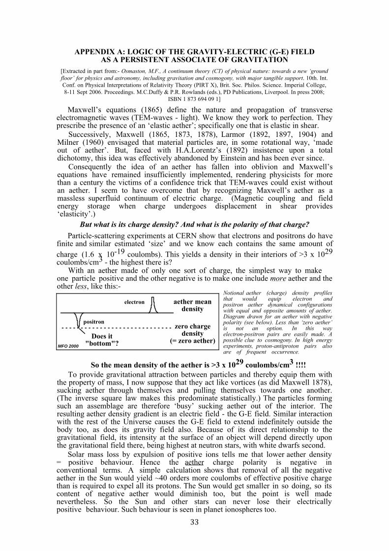
APPENDIX A: LOGIC OF THE GRAVITY-ELECTRIC (G-E) FIELDAS A PERSISTENT ASSOCIATE OF GRAVITATION
[Extracted in part from:- Osmaston, M.F., A continuum theory (CT) of physical nature: towards a new ‘ground floor’ for physics and astronomy, including gravitation and cosmogony, with major tangible support. 10th. Int. Conf. on Physical Interpretations of Relativity Theory (PIRT X), Brit. Soc. Philos. Science. Imperial College, 8-11 Sept 2006. Proceedings. M.C.Duffy & P.R. Rowlands (eds.), PD Publications, Liverpool. In press 2008;
ISBN 1 873 694 09 1]
Maxwell’s equations (1865) define the nature and propagation of transverse electromagnetic waves (TEM-waves - light). We know they work to perfection. They prescribe the presence of an ‘elastic aether’; specifically one that is elastic in shear.
Successively, Maxwell (1865, 1873, 1878), Larmor (1892, 1897, 1904) and Milner (1960) envisaged that material particles are, in some rotational way, ‘made out of aether’. But, faced with H.A.Lorentz’s (1892) insistence upon a total dichotomy, this idea was effectively abandoned by Einstein and has been ever since.
Consequently the idea of an aether has fallen into oblivion and Maxwell’s equations have remained insufficiently implemented, rendering physicists for more than a century the victims of a confidence trick that TEM-waves could exist without an aether. I seem to have overcome that by recognizing Maxwell’s aether as a massless superfluid continuum of electric charge. (Magnetic coupling and field energy storage when charge undergoes displacement in shear provides ‘elasticity’.)
But what is its charge density? And what is the polarity of that charge?Particle-scattering experiments at CERN show that electrons and positrons do have
finite and similar estimated ‘size’ and we know each contains the same amount of charge (1.6 x 10⁻¹⁹ coulombs). This yields a density in their interiors of >3 x 1029coulombs/cm3 - the highest there is?
With an aether made of only one sort of charge, the simplest way to make one particle positive and the other negative is to make one include more aether and the other less, like this:-
Notional aether (charge) density profiles that would equip electron and positron aether dynamical configurations with equal and opposite amounts of aether. Diagram drawn for an aether with negative polarity (see below). Less than ‘zero aether’ is not an option. In this way electron-positron pairs are easily made. A possible clue to cosmogony. In high energy experiments, proton-antiproton pairs also are of frequent occurrence.
So the mean density of the aether is >3 x 1029 coulombs/cm3 !!!!To provide gravitational attraction between particles and thereby equip them with
the property of mass, I now suppose that they act like vortices (as did Maxwell 1878), sucking aether through themselves and pulling themselves towards one another. (The inverse square law makes this predominate statistically.) The particles forming such an assemblage are therefore ‘busy’ sucking aether out of the interior. The resulting aether density gradient is an electric field - the G-E field. Similar interaction with the rest of the Universe causes the G-E field to extend indefinitely outside the body too, as does its gravity field also. Because of its direct relationship to the gravitational field, its intensity at the surface of an object will depend directly upon the gravitational field there, being highest at neutron stars, with white dwarfs second.
Solar mass loss by expulsion of positive ions tells me that lower aether density = positive behaviour. Hence the aether charge polarity is negative in conventional terms. A simple calculation shows that removal of all the negative aether in the Sun would yield ~40 orders more coulombs of effective positive charge than is required to expel all its protons. The Sun would get smaller in so doing, so its content of negative aether would diminish too, but the point is well made nevertheless. So the Sun and other stars can never lose their electrically positive behaviour. Such behaviour is seen in planet ionospheres too.
- - - - - - - - - - - - - - - - - - - - - - - - - - - - -positron
electron
Does it "bottom"?
aether mean density
MFO 2000
zero chargedensity
(= zero aether)
33
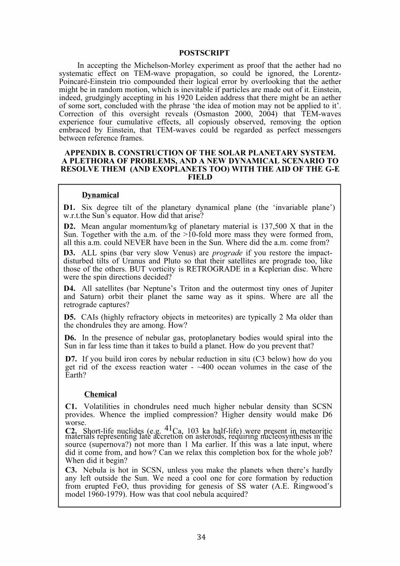
POSTSCRIPTIn accepting the Michelson-Morley experiment as proof that the aether had no
systematic effect on TEM-wave propagation, so could be ignored, the Lorentz-Poincaré-Einstein trio compounded their logical error by overlooking that the aether might be in random motion, which is inevitable if particles are made out of it. Einstein, indeed, grudgingly accepting in his 1920 Leiden address that there might be an aether of some sort, concluded with the phrase ‘the idea of motion may not be applied to it’. Correction of this oversight reveals (Osmaston 2000, 2004) that TEM-waves experience four cumulative effects, all copiously observed, removing the option embraced by Einstein, that TEM-waves could be regarded as perfect messengers between reference frames.
APPENDIX B. CONSTRUCTION OF THE SOLAR PLANETARY SYSTEM.A PLETHORA OF PROBLEMS, AND A NEW DYNAMICAL SCENARIO TO RESOLVE THEM (AND EXOPLANETS TOO) WITH THE AID OF THE G-E
FIELD
DynamicalD1. Six degree tilt of the planetary dynamical plane (the ‘invariable plane’) w.r.t.the Sun’s equator. How did that arise?D2. Mean angular momentum/kg of planetary material is 137,500 X that in the Sun. Together with the a.m. of the >10-fold more mass they were formed from, all this a.m. could NEVER have been in the Sun. Where did the a.m. come from?D3. ALL spins (bar very slow Venus) are prograde if you restore the impact-disturbed tilts of Uranus and Pluto so that their satellites are prograde too, like those of the others. BUT vorticity is RETROGRADE in a Keplerian disc. Where were the spin directions decided?D4. All satellites (bar Neptune’s Triton and the outermost tiny ones of Jupiter and Saturn) orbit their planet the same way as it spins. Where are all the retrograde captures?D5. CAIs (highly refractory objects in meteorites) are typically 2 Ma older than the chondrules they are among. How?D6. In the presence of nebular gas, protoplanetary bodies would spiral into the Sun in far less time than it takes to build a planet. How do you prevent that?D7. If you build iron cores by nebular reduction in situ (C3 below) how do you get rid of the excess reaction water - ~400 ocean volumes in the case of the Earth?
ChemicalC1. Volatilities in chondrules need much higher nebular density than SCSN provides. Whence the implied compression? Higher density would make D6 worse.C2. Short-life nuclides (e.g. 41Ca, 103 ka half-life) were present in meteoriticmaterials representing late accretion on asteroids, requiring nucleosynthesis in thesource (supernova?) not more than 1 Ma earlier. If this was a late input, where did it come from, and how? Can we relax this completion box for the whole job? When did it begin?C3. Nebula is hot in SCSN, unless you make the planets when there’s hardly any left outside the Sun. We need a cool one for core formation by reduction from erupted FeO, thus providing for genesis of SS water (A.E. Ringwood’s model 1960-1979). How was that cool nebula acquired?
34
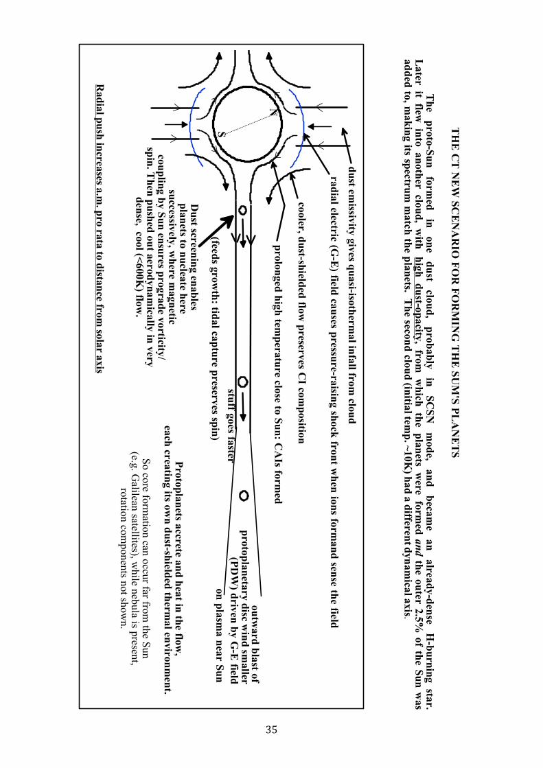
TH
E C
T N
EW
SCE
NA
RIO
FOR
FOR
MIN
G T
HE
SUM
'S PLA
NE
TS
The
proto-Sun form
ed in
one dust
cloud, probably
in SC
SN
mode,
and becam
e an
already-dense H
-burning star. L
ater it flew into another cloud, w
ith high dust-opacity, from
which the planets w
ere formed and the outer 2.5%
of the Sun was
added to, making its spectrum
match the planets. T
he second cloud (initial temp. ~10K
) had a different dynamical axis.
dust emissivity gives quasi-isotherm
al infall from cloud
N
S
radial electric (G-E
) field causes pressure-raising shock front when ions form
and sense the field
cooler, dust-shielded flow preserves C
I composition
outward blast of
(feeds growth: tidal capture preserves spin)
prolonged high temperature close to Sun: C
AIs form
ed
protoplanetary disc wind sm
aller stuff goes faster
(PDW
) driven by G-E
fieldon plasm
a near Sun
Protoplanets accrete and heat in the flow,
each creating its own dust-shielded therm
al environment.
So core formation can occur far from
the Sun (e.g. G
alilean satellites), while nebula is present,
rotation components not show
n.
Radial push increases a.m
. pro rata to distance from solar axis
Dust screening enables
planets to nucleate heresuccessively, w
here magnetic
coupling by Sun ensures prograde vorticity/spin. T
hen pushed out aerodynamically in very
dense, cool (<600K) flow
.
35
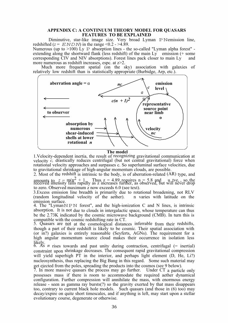
APPENDIX C: A CONTINUUM THEORY MODEL FOR QUASARS FEATURES TO BE EXPLAINED
Diminutive, star-like image size. Very broad Lyman PNemission line, redshifted (z = ENDN) in the range <0.2 - >4.89.Numerous (up to >100) Ly P absorption lines - the so-called "Lyman alpha forest" - extending along the shortward flank (less redshift) of the main Ly emission (+ some corresponding CIV and NIV absorptions). Forest lines pack closer to main Ly and more numerous as redshift increases, espc. at z>2.
Much more frequent spatial (on the sky) association with galaxies of relatively low redshift than is statistically appropriate (Burbidge, Arp, etc.).
The model1.Velocity-dependent inertia, the result of recognizing gravitational communication atvelocity c, drastically reduces centrifugal (but not central gravitational) force when rotational velocity approaches and surpasses c. So superluminal surface velocities, due to gravitational shrinkage of high-angular momentum clouds, are possible.2. Most of the redshift is intrinsic to the body, is of aberration-related (AR) type, andamounts to z = m(n2 + 1. Thus z = 4.89 requires n = 5.8 and u tve, , so thereceived intensity falls rapidly as z increases further, as observed, but will never dropto zero. Observed maximum z now exceeds 6.0 (see text).3.Excess emission line breadth is primarily due to rotational broadening, not RLV(random longitudinal velocity of the aether). n varies with latitude on the emission surface.4. The "LymanNPN forest", and the high-ionization C and N lines, is intrinsicabsorption. It is not due to clouds in intergalactic space, whose temperature can thus be the 2.73K indicated by the cosmic microwave background (CMB). In turn this is compatible with the cosmic redshifting rate in CT.5. Quasars are not at the cosmological distances inferrable from their redshifts,though a part of their redshift is likely to be cosmic. Their spatial association with (or in?) galaxies is entirely reasonable (Seyferts, AGNs). The requirement for a high angular momentum source cloud makes their occurrence in isolation less likely.
to observero
representative
velocity nc
nc cα
source pointnear limb
c(n + 1)2 ½
emission level
numerous shear-induced shells at lower rotational n
absorption by
aberration angle = α
6. As n rises towards and past unity during contraction, centrifugal (= inertial)constraint upon shrinkage decreases. The consequent rapid gravitational compression will yield superhigh PT in the interior, and perhaps light element (D, He, Li?) nucleosynthesis, thus replacing the Big Bang in this regard. Some such material may get ejected from the poles, spreading the products into the cosmos (see 9 below).7. In more massive quasars the process may go further. Under CT a particle onlypossesses mass if there is room to accommodate the required aether dynamical configuration. Further compression will annihilate the mass, with enormous energy release - seen as gamma ray bursts(?) so the gravity exerted by that mass disappears too, contrary to current black hole models. Such quasars (and those in (6) too) may decay/expire on quite short timescales, and if anything is left, may start upon a stellar evolutionary course, degenerate or otherwise.
36
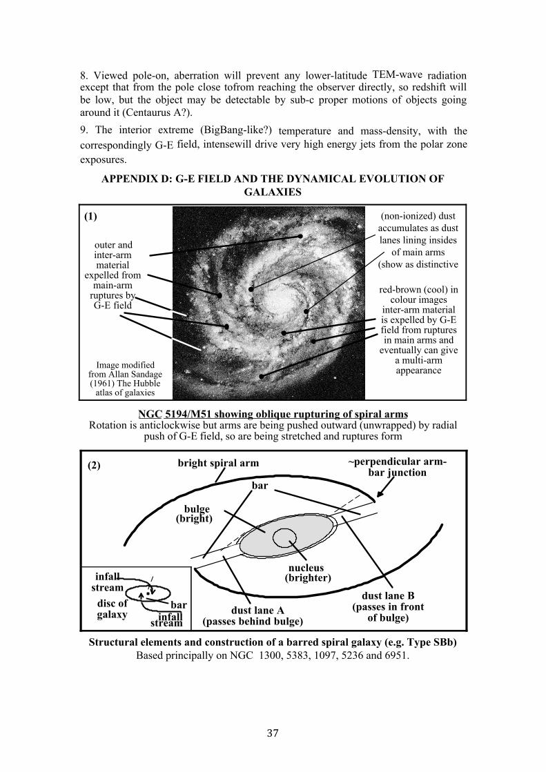
APPENDIX D: G-E FIELD AND THE DYNAMICAL EVOLUTION OF GALAXIES
NGC 5194/M51 showing oblique rupturing of spiral armsRotation is anticlockwise but arms are being pushed outward (unwrapped) by radial
push of G-E field, so are being stretched and ruptures form
(1) (non-ionized) dustaccumulates as dust lanes lining insides
of main arms(show as distinctive
outer andinter-arm material
expelled from main-arm
ruptures byG-E field
Image modified from Allan Sandage (1961) The Hubble
atlas of galaxies
red-brown (cool) in colour images
inter-arm materialis expelled by G-Efield from rupturesin main arms and
eventually can give a multi-armappearance
8. Viewed pole-on, aberration will prevent any lower-latitude TEM-wave radiationexcept that from the pole close tofrom reaching the observer directly, so redshift will be low, but the object may be detectable by sub-c proper motions of objects going around it (Centaurus A?). 9. The interior extreme (BigBang-like?) temperature and mass-density, with thecorrespondingly G-E field, intensewill drive very high energy jets from the polar zone exposures.
_ _ _ _
_ _ _ _
bulge
bar
bright spiral arm
dust lane A(passes behind bulge)
dust lane B(passes in front
of bulge)
~perpendicular arm-bar junction
(bright)
nucleus(brighter)
_ _
infalldisc ofgalaxy
bar
infallstream
stream
(2)
Structural elements and construction of a barred spiral galaxy (e.g. Type SBb)Based principally on NGC 1300, 5383, 1097, 5236 and 6951.
37
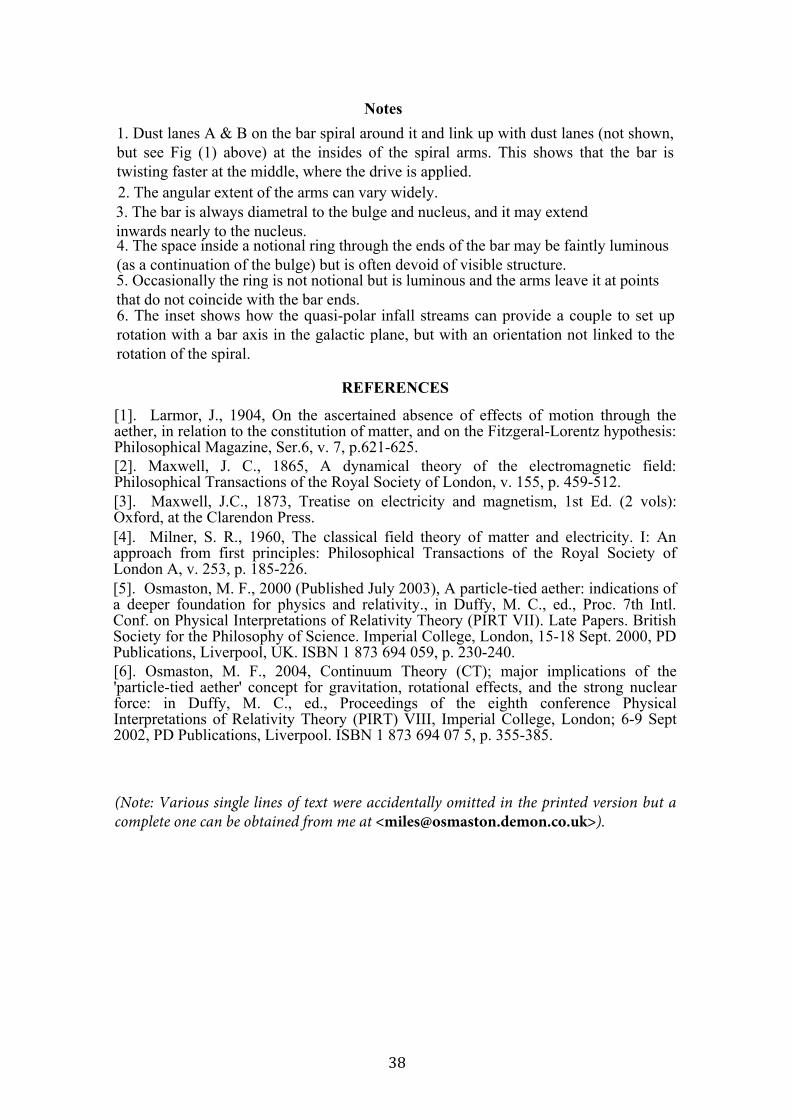
[1]. Larmor, J., 1904, On the ascertained absence of effects of motion through the aether, in relation to the constitution of matter, and on the Fitzgeral-Lorentz hypothesis: Philosophical Magazine, Ser.6, v. 7, p.621-625.[2]. Maxwell, J. C., 1865, A dynamical theory of the electromagnetic field: Philosophical Transactions of the Royal Society of London, v. 155, p. 459-512.[3]. Maxwell, J.C., 1873, Treatise on electricity and magnetism, 1st Ed. (2 vols): Oxford, at the Clarendon Press.[4]. Milner, S. R., 1960, The classical field theory of matter and electricity. I: An approach from first principles: Philosophical Transactions of the Royal Society of London A, v. 253, p. 185-226.[5]. Osmaston, M. F., 2000 (Published July 2003), A particle-tied aether: indications of a deeper foundation for physics and relativity., in Duffy, M. C., ed., Proc. 7th Intl. Conf. on Physical Interpretations of Relativity Theory (PIRT VII). Late Papers. British Society for the Philosophy of Science. Imperial College, London, 15-18 Sept. 2000, PD Publications, Liverpool, UK. ISBN 1 873 694 059, p. 230-240.[6]. Osmaston, M. F., 2004, Continuum Theory (CT); major implications of the 'particle-tied aether' concept for gravitation, rotational effects, and the strong nuclear force: in Duffy, M. C., ed., Proceedings of the eighth conference Physical Interpretations of Relativity Theory (PIRT) VIII, Imperial College, London; 6-9 Sept 2002, PD Publications, Liverpool. ISBN 1 873 694 07 5, p. 355-385.
Notes1. Dust lanes A & B on the bar spiral around it and link up with dust lanes (not shown,but see Fig (1) above) at the insides of the spiral arms. This shows that the bar is twisting faster at the middle, where the drive is applied.2. The angular extent of the arms can vary widely.3. The bar is always diametral to the bulge and nucleus, and it may extendinwards nearly to the nucleus.4. The space inside a notional ring through the ends of the bar may be faintly luminous(as a continuation of the bulge) but is often devoid of visible structure.5. Occasionally the ring is not notional but is luminous and the arms leave it at pointsthat do not coincide with the bar ends.6. The inset shows how the quasi-polar infall streams can provide a couple to set uprotation with a bar axis in the galactic plane, but with an orientation not linked to the rotation of the spiral.
REFERENCES
(Note: Various single lines of text were accidentally omitted in the printed version but a complete one can be obtained from me at <[email protected]>).
38
39
THE PIONEER ANOMALY, OR
A ‘DISSIDENT’ PERSPECTIVE ON MODERN PHYSICS
Neville Vivian Pope1
1Llys Alaw, West End, Penclawdd, Swansea, South Wales SA4 3YX, United Kingdom
This paper is a critique of the present state of Theoretical Physics and its flagrant departure from the constraints of commonsense logic. As a contrast to this, an example is provided of a simple, unified, solution of two allegedly separate physical anomalies which have so far defeated every attempt at explanation in terms of standard orthodox Physics. This is to the extent that a NASA spokesman has said that in order to explain these anomalies, a whole ‘new physics’ might have to be contemplated.
These anomalies are the well-documented ‘Pioneer anomaly’ and the ‘Missing Mass anomaly’. This paper counters conventional attempts at explanation in terms of intellectually elevated theories such as, for instance, those of ‘cosmological expansion’, ‘dark matter’, ‘deviations from Einsteinian gravity’ and so on. It also questions the Newtonian concept of an in vacuo ‘gravitational force’.
Keywords: Pioneer anomaly, Missing Mass anomaly, cosmological expansion, dark matter, deviations from Einsteinian gravity
PACS number: 04.50.-h
INTRODUCTION On the Internet, I, Viv Pope, am referred to as a ‘Dissident’. Now why is that? It
is because I am convinced that Modern Physics has become much – much - too clever for its own good.
Let me speak plainly. As I see it, Theoretical Physics has become far too big for its own boots with its elevated ideas of the ‘Big Bang’, ‘wormholes’ in the vacuum and so on, ad nauseam. In my view, the trouble lies in a strange, lofty compulsion towards theorising. What encourages this, unfortunately, is the public appetite for novelty and the media’s commercial interests in pandering to it. This puts a premium on the selection of the most wacky ideas and the virtual suppression of the more sensible ones.
Let’s face it, then, nothing is more boring than a simple solution to a captivating mystery. This makes some physicists vie with one another to produce more and more bizarre theories about physical phenomena instead of using plain commonsense logic to interpret observational and experimental data in a search for natural truth.
What disturbs me most, however, is talking to people who profess to being scientists but can scarcely add two and two together without going into the depths of things like integral calculus, general relativity, quantum chromodynamics and God knows what. Indeed, I have met some people who, surely, if they were asked to count horses, would have to count their legs and tails and divide by five, or if asked to count a dozen eggs would have to express the result as the square root of a hundred and forty four. These people remind me of the Greek philosopher who, it is reported, while contemplating the Universe fell down a pit shaft.
Here is just one of many examples I could cite of how much more simple and effective our modern approach to Physics could be with the application of a bit of critical commonsense logic.
40
For instance, what I find very strange is that so many generations of Physics students have failed to see something which should be entirely obvious.
Newton was, undoubtedly a genius. However, his theories of motion were based essentially on experiments with bodies moving on flat surfaces, such as bench-tops, inclined planes and so on. In this way he conceived the idea of the motion of a body with no forces acting upon it as taking place in an ideally Euclidean vacuum called ‘inertial space’. Basic to his ideas of mechanics, therefore, was that of straight-line motion as the product of mass and velocity, called momentum. All moving bodies he declared, travel in straight-lines under their own momentum, i.e., ‘inertially’, unless acted upon by an external force.
Logically, then, it follows from this assumption that any body moving in space other than in a straight line, such as a cannon ball in its curved trajectory or a planet orbiting the sun, must have some kind of ‘force’ acting upon it. In this way was created the notion of ‘gravitational force’ as an invisible agency acting in the vacuum, dragging all bodies towards one another instead of following their straight lines in the way Newton had previously decreed.
So Newton’s ‘gravitational force’ was an ad-hoc, conceptual afterthought, a conjectural add-on to his original mechanics. What is so obvious, however, is that all Newton had to do, in order to deal with orbital motion, was to include, together with the parameters of mass and velocity, the further parameter of orbital radius. His definition of momentum as the product of mass and velocity, mv then becomes angular momentum, which is the product of mass, velocity and radius, mvr. Straight-line momentum then becomes orbital momentum, and the invisible, in vacuo ‘gravitational force’ disappears like ‘Scotch mist’.
Now angular momentum is an automatically paired relation, so the simple formula for angular momentum, L, is
L = mvr = GMm/ v, (1)
Here, m is the mass of the orbiting body, v is its velocity, M is the mass of the central body and G is an empirical factor, or constant. This formula proves to be sufficient in itself, with no need of Newton’s hypothetical ‘gravitational force’, to compute simple circular motion, as of the moon orbiting the earth, or the earth orbiting the sun.
But, of course, planetary motion is not circular, but elliptical, as Kepler described it. Nevertheless, this basic formula remains at the root of all spatial motion no matter how complex and convoluted. This means that all talk of ‘gravitational force’, ‘gravitational field’, ‘gravity waves’, ‘gravitons’, etc,. etc., is logically redundant. Speaking as a taxpayer, this should save us billions of pounds and dollars in closing down those laboratories which are so heavily funded to chase theoretical rainbows.
The advantages for true Natural Philosophy that are offered by this change in conception from ‘gravity’ to angular momentum as the agency of orbital motion, apart from its commercial advantages, are as follows.
Newton’s hypotheses of ‘gravitational force’ presents a fundamental anomaly. This is that it is logically at odds with the law of the conservation of angular momentum. According to that law, the total angular momentum of an orbiting, spinning body has to be the sum of its orbital and spin angular momenta. However, Newtonian ‘gravitational force’ takes no account of spin. It is a purely hypothetical ‘force’ which is defined in terms of mass and distance only, hence is the same for an orbiting body, whether or not that body is spinning.
41
But in nature, practically all orbiting bodies spin, from NASA’s space-probes to the spiral galaxies. Computing the trajectories of these spinning bodies without taking account of the spin therefore presents serious anomalies. Two of these have recently become evident. One is the so-called Pioneer Anomaly, in which NASA’s space-probes in solar obit veer inexplicably towards the sun; and the other is the so-called ‘Missing Mass Anomaly’ according to which the total mass of the spinning galaxies is found to be far greater than expected according to the ‘gravitational’ calculations.
In the Pioneer case, the reason why the spinning space-probes veer towards the sun is plain. It is because according to the law of angular momentum conservation, for the total angular momentum of the probe, the larger the spin angular momentum the smaller is the orbital angular momentum; and the smaller the orbital angular momentum the smaller is the orbit radius. So a spinning probe orbits nearer to the sun than if it were not spinning – which is, predictably, what NASA have discovered.
In the case of the ‘Missing Mass Anomaly’, the reason is that the computations of that measure are based on the assumption that the so-called ‘gravitational’ factor, G is a constant. However, for spinning bodies, such as the spiral galaxies and just about everything else in the universe, that factor G has to be a variable. For instance, in our above equation (1) we have:
L = mvr = GMm/ v, (1)
From this we have:
G = v2r/M. (2)
Now v2 is kinetic energy, K/m, according to the formula K = ½mv2, whence (2) becomes
G = 2Kr/mM. (3)
So now let the orbital kinetic energy be signified by KO and the spin kinetic energy by KS. The formula for G thus becomes:
G = 2(KO + KS)r/mM. (4)
Plainly, with the same values for m and M in this formula as in (3), the value of G in this formula (4) is greater than in that previous formula, and the greater the value of G, the more closely the body orbits the centre of mass.
From this it follows that for the spinning galaxies, the value of G must be greater than the standard value, so that these galaxies are crowded more closely together than if they were not spinning. This explains why these galaxies, plus all other spinning objects, appear to have more mass than they should have according to the traditional ‘gravitational’ account. What is the reason for this ‘extra mass’? Not ‘dark matter’, surely, but ‘dark spin’ – for ‘dark, here, read ‘neglected’.
So there is no anomaly of this sort in nature, to be explained by theories of any tortuously intellectual kind. The only anomaly lies in the failure of Newton’s ‘gravitational’ account to include spin in the total angular momentum of an orbiting body. Extending Newton’s ingenious formalism to include spin brings Newton out of the age of falling apples and steam technology up to speed with our second-millennium space-age.
42
Newton famously stated ‘hypotheses non fingo’ (I make no assumptions). Little did he know that his biggest and most misleading assumption was that of his fictitious ‘in vacuo gravitational force’. In view of what Newton achieved, he might be forgiven for that. But what beats me is why, nowadays, we keep making such a Big Production out of what is no more that a conceptual fabrication that is long past it’s sell-by’ date. May I remind you that this is no purely academic matter. In pursuit of ‘gravitation’ and all that the mystique entails, billions and billions of pounds and dollars altogether, are continually wasted. That mystery is, no doubt, intriguing and entertaining but, seriously, I ask you, in the interests of true science and a struggling economy, is it worth it?
REFERENCES [1]. The Eye of the Beholder: the Role of the Observer in Modern Physics, by Viv Pope,
phi Philosophical Enterprises, Swansea, UK (2004), page 30. [2]. Light-Speed, Gravitation and Quantum Instantaneity, by A. D. Osborne and N. V.
Pope, phi Philosophical Enterprises, Swansea, UK (2007).

43
A BIMETRIC MODEL OF THE UNIVERSE. INTERPRETATION OF THE COSMIC ACCELERATION. IN EARLY TIME A
SYMMETRY BREAKING GOES WITH A VARIABLE SPEED OF LIGHT ERA, EXPLAINING THE HOMOGENEITY OF THE EARLY UNIVERSE. THE
C(R) LAW IS DERIVED FROM A GENERALIZED GAUGE PROCESS EVOLUTION.
1Jean-Pierre Petit and 1Gilles d'Agostini
1Lambda Laboratory, F.Buisson Blvd 17, Rochefort 17200, France [email protected]
The universe, far from being homogenous, expands in large empty bubbles of large-scale structure, but not in mass concentrations like galaxies, so that the Robertson-Walker solution does not fit. We suggest that a symmetry breaking occurred in a distant past, during the radiation-dominated era. Before, the three-dimensional hypersurface was invariant under the action of O(3) and the Robertson-Walker solution could be used. But this obliges the so called constants of physics, length and time scale factors, to be involved through a generalized gauge process, which is thus built. The subsequent variation of the speed of light solves the horizon problem, while the Planck barrier disappears.
The present work is fairly different from other attempts published on the now so-called VSL, variable speed of light. The reader will find these other papers mentioned in the references at the end of this paper.
Keywords: Robertson-Walker solution, variable speed of light, Planck, gauge process.
PACS number: 04.20.-q
I. INTRODUCTION Let's present the general idea. The classical cosmological model was built from
the Robertson-Walker solution of the Einstein field equations. This solution is based on the cosmological principle assuming the Universe is homogeneous and isotropic. Initially the model-makers believed that they could consider the Universe as a gas whose molecules would be the galaxies. In clusters these galaxies have a random velocity which may be compared to the thermal velocity of the kinetic theory of gases. The order of magnitude of the random galaxy velocities, with respect to the galaxy clusters, is around 1000 km/s, which is small if compared to the speed of light. So that theoreticians thought that this velocity could be neglected, this cosmic fluid being compared to dust ("dust Universe"). This was widely confirmed by observations.
Oppositely the observation of the large-scale structure gave evidence that matter was arranged around big voids, 100 light-years across in the mean, to be compared to joined soap bubbles". That was frankly non-homogeneous. As a consequence the curvature field is non-uniform.
A puzzling problem arises. Astronomers measure redshifts and conclude that the Universe is expanding, according to Hubble's law. But where does this expansion occur? Does the solar system expand? No. If it were expanding, it would be unstable. Do the galaxies expand? No, for the same reason.
To explain the measured redshifts we must admit some regions expand in the Universe and some others do not. Basically, the Robertson-Walker metric cannot take
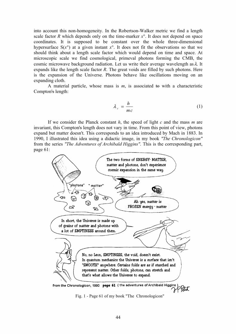
44
into account this non-homogeneity. In the Robertson-Walker metric we find a length scale factor R which depends only on the time-marker x°. It does not depend on space coordinates. It is supposed to be constant over the whole three-dimensional hypersurface S(x°) at a given instant x°. It does not fit the observations so that we should think about a length scale factor which would depend on time and space. At microscopic scale we find cosmological, primeval photons forming the CMB, the cosmic microwave background radiation. Let us write their average wavelength as λ. It expands like the length scale factor R. The great voids are filled by such photons. Here is the expansion of the Universe. Photons behave like oscillations moving on an expanding cloth.
A material particle, whose mass is m, is associated to with a characteristic Compton's length:
cmh
c =λ (1)
If we consider the Planck constant h, the speed of light c and the mass m are invariant, this Compton's length does not vary in time. From this point of view, photons expand but matter doesn't. This corresponds to an idea introduced by Mach in 1883. In 1990, I illustrated this idea using a didactic image, in my book "The Chronologicon" from the series "The Adventures of Archibald Higgins". This is the corresponding part, page 61:
Fig. 1 - Page 61 of my book "The Chronologicon"
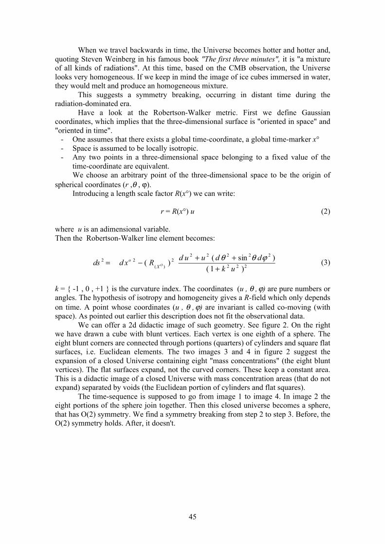
45
When we travel backwards in time, the Universe becomes hotter and hotter and, quoting Steven Weinberg in his famous book "The first three minutes", it is "a mixture of all kinds of radiations". At this time, based on the CMB observation, the Universe looks very homogeneous. If we keep in mind the image of ice cubes immersed in water, they would melt and produce an homogeneous mixture.
This suggests a symmetry breaking, occurring in distant time during the radiation-dominated era.
Have a look at the Robertson-Walker metric. First we define Gaussian coordinates, which implies that the three-dimensional surface is "oriented in space" and "oriented in time".
- One assumes that there exists a global time-coordinate, a global time-marker x° - Space is assumed to be locally isotropic. - Any two points in a three-dimensional space belonging to a fixed value of the
time-coordinate are equivalent. We choose an arbitrary point of the three-dimensional space to be the origin of
spherical coordinates (r ,θ , ϕ). Introducing a length scale factor R(x°) we can write:
r = R(x°) u (2)
where u is an adimensional variable. Then the Robertson-Walker line element becomes:
222
222222
)(22
)1()sin()(
ukdduudRxdds OX
o
+++−= ϕθθ (3)
k = -1 , 0 , +1 is the curvature index. The coordinates (u , θ , ϕ) are pure numbers or angles. The hypothesis of isotropy and homogeneity gives a R-field which only depends on time. A point whose coordinates (u , θ , ϕ) are invariant is called co-moving (with space). As pointed out earlier this description does not fit the observational data.
We can offer a 2d didactic image of such geometry. See figure 2. On the right we have drawn a cube with blunt vertices. Each vertex is one eighth of a sphere. The eight blunt corners are connected through portions (quarters) of cylinders and square flat surfaces, i.e. Euclidean elements. The two images 3 and 4 in figure 2 suggest the expansion of a closed Universe containing eight "mass concentrations" (the eight blunt vertices). The flat surfaces expand, not the curved corners. These keep a constant area. This is a didactic image of a closed Universe with mass concentration areas (that do not expand) separated by voids (the Euclidean portion of cylinders and flat squares).
The time-sequence is supposed to go from image 1 to image 4. In image 2 the eight portions of the sphere join together. Then this closed universe becomes a sphere, that has O(2) symmetry. We find a symmetry breaking from step 2 to step 3. Before, the O(2) symmetry holds. After, it doesn't.

46
Fig. 2 - Two-dimensional didactic image of an expanding, closed Universe experiencing a symmetry breaking in step 2.
Geometers can immediately extend this for a three-dimensional closed surface, illustrated as a set of flat volumes joined to constant curvature portions of space. In the two-dimensional model we have shown eight "mass concentrations", but we could put as many as we want, thus forming a diamond-like object, with blunt vertices (rounded summits). Similarly, a 3-sphere could be transformed into a many-3d-faces 3d-diamond whose curved volumes would be smoothed (constant curvature and constant volume object) linked by Euclidean elements.
Similarly we could imagine a symmetry breaking. Before the objects is a 3-sphere, having an O(3) symmetry. After, this symmetry is broken or lost. The object becomes a three-dimensional polyhedron where each constant curvature (and volume) portion represents a galaxy or some mass concentration that does not expand. .
This is the general idea. We suppose the Robertson-Walker metric is suitable to describe the (homogeneous) early Universe. Then a symmetry breaking occurs, very early in the radiation-dominated era. Matter concentrations begin to form. We suggest that this corresponds to two different evolution processes.
When we want to build a model of cosmic evolution we have to deal with: - Pure geometric features, governed by Einstein's field equations - Features linked to special relativity (invariance through Lorentz rotations) - Electromagnetic features (the particles are linked by electromagnetic forces, ruled
by Maxwell's equations) - Quantification is present, which is governed by, for example, the (non relativistic)
Schrödinger equation. All these features come from local observations and experiments, which satisfy a
certain set of physical equations, containing the following quantities: G: gravitational constant c: speed of light m: masses h: Planck constant e: elementary charge µo: magnetic constant (vacuum permeability)
47
From this set of equations we can build measuring instruments. They extend our senses. But finally the last measuring instrument is ourselves, with our body as a length scale and our average life, a "shelf time", as a time scale. We may compare this duration to astronomical phenomena, like the year, the day (a complete rotation of the Earth). We can build mechanical systems, like a torsion pendulum, and discover that they can be used as clocks. Comparing this object to our body, our hand, we can build rules. We can divide it, and so on.
We replace the fully human measurement by mechanical measurements, based on the equations of physics. It works. We can perform measurements of constants and we don't find any change, so we think they should be absolute constants. Quantum mechanics works too and brings a new insight into the nature of matter. From the constant of today's physics we can build two characteristic quantities The Planck length:
3cGhL P = (4)
The Planck time:
5cGht P = (5)
Quantum mechanics generates its own limits in space and time. It becomes impossible, through QM formalism, to analyze or even to conceive processes occurring on lengths and durations shorter than these characteristic values.
As the scientist believes the constants found are absolute constants that do not vary alongside cosmic evolution, he thinks of some hypothetical "quantum era" and asks how things could have been in the extremely early conditions.
II. EXISTENCE OF A FUNDAMENTAL GAUGE RELATIONAll physicists know the power of dimensional analysis. Considering a given set
of physical equations they can introduce characteristic length and time and introduce adimensional space and time variables. Then they can weight, measure the relative importance of different terms in an equation in which the constants of physics appear.
This could be extended, considering that we can use today's values of the constants, considering they may vary, and introduce their adimensional form. As an example, let us consider the constant of gravitation. Call Go today's measured value. If we admit that G may vary, we can write:
G = Γ Go (6)
Γ being an adimensional quantity. We can do similar operations for all constants, as we do for length and time. Now, ask the question: - Can we find what we will call a generalized gauge transform, linking the length and time scale factors, and the adimensional variables, which takes into account the variation of the physical constants, and which would keep all the equations invariant?
The answer is yes. There is a single one, see reference [4]. Note that we cannot obtain evidence of such variations using our measuring instruments. The reason is very
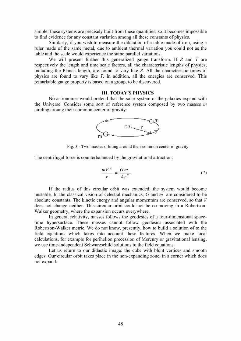
48
simple: these systems are precisely built from these quantities, so it becomes impossible to find evidence for any constant variation among all these constants of physics.
Similarly, if you wish to measure the dilatation of a table made of iron, using a ruler made of the same metal, due to ambient thermal variation you could not as the table and the scale would experience the same parallel variations.
We will present further this generalized gauge transform. If R and T are respectively the length and time scale factors, all the characteristic lengths of physics, including the Planck length, are found to vary like R. All the characteristic times of physics are found to vary like T. In addition, all the energies are conserved. This remarkable gauge property is based on a group, to be discovered.
III. TODAY'S PHYSICSNo astronomer would pretend that the solar system or the galaxies expand with
the Universe. Consider some sort of reference system composed by two masses m circling aroung their common center of gravity:
Fig. 3 - Two masses orbiting around their common center of gravity
The centrifugal force is counterbalanced by the gravitational attraction:
2
2
4 rmG
rVm = (7)
If the radius of this circular orbit was extended, the system would become unstable. In the classical vision of celestial mechanics, G and m are considered to be absolute constants. The kinetic energy and angular momentum are conserved, so that V does not change neither. This circular orbit could not be co-moving in a Robertson-Walker geometry, where the expansion occurs everywhere.
In general relativity, masses follows the geodesics of a four-dimensional space-time hypersurface. These masses cannot follow geodesics associated with the Robertson-Walker metric. We do not know, presently, how to build a solution of to the field equations which takes into account these features. When we make local calculations, for example for perihelion precession of Mercury or gravitational lensing, we use time-independent Schwarzschild solutions to the field equations.
Let us return to our didactic image: the cube with blunt vertices and smooth edges. Our circular orbit takes place in the non-expanding zone, in a corner which does not expand.

49
Fig. 4 - Reference circular orbit location
This is a composite geometry since curved and flat elements form the object. To be closer to reality, this circular orbit should be inscribed in a non-expanding volume, part of a three-dimensional hypersurface. There, it would be part of a region of space-time that would behave like a quasi steady-state element of the geometric solution, while the area between the mass concentrations space-time would be close to a Friedman non-steady solution. Currently we do not know how to manage that.
IV. THE EARLY EVOLUTION AS A GENERALIZED GAUGE PROCESSIf we go further backwards into the past, we meet the symmetry breaking event.
Then the Robertson-Walker solution holds and the Universe obeys an O(3) symmetry. If we want to inscribe the circular orbit corresponding to our two masses linked by gravitational force, the span of this co-moving orbit must vary like R(x°). See the small circle:
Fig. 5 - 2d didactic image of the symmetry breaking
We will assume the Universe undergoes a generalized gauge process, keeping the equations invariant. At the end of this study the benefit will be the justification of the homogeneity of the early Universe with no need to call for the inflation theory. Let
50
us build the gauge laws. As shown in [1] this gauge process make all the characteristic lengths of physics to follow the variation of the length scale factor R. The energies are conserved. Look at the invariance of the field equation, in which we take a cosmological constant equal to zero, while it does not refer to early Universe and short range gravitational interaction.
S = χ T (8)
It is divergenceless, which implies that the constant χ must be an absolute constant. This last is classically determined through an expansion into a series of the metric, the zero-order term being the time-independent Lorentz metric. We add a perturbation term which is also time-independent:
g = η + ε γ( (9)
We perform a Newtonian approximation (weak field, low velocities with respect to the speed of light). The constant is determined, identifying the linearized field equation to Poisson's equation. The expression depends on how we decide to write the tensor T. Let us follow [20], section 10.5:
T oo = ρ (10)
Then the identification gives:
2
8c
Gπχ −= (11)
The Einstein equation is invariant if
2cG ≈ (12)
Notice that, when we determine the expression of Einstein's constant combining G an c in (11), this does not imply that these two should be absolute constants, for the perturbation method is based on time-independent terms in the expansion into a series of the metric.
Writing that the Schwarzschild length varies like R, we get:
Rc
mG ≈2 , Rm ≈ (13)
The conservation of the energy brings immediately:
Cstcm ≈2 , R
c 1≈ , R
G 1≈ (14)
If we write the Planck length varies like R we get:
51
RcGh ≈3
, 2Rch ≈ , 2
3Rh ≈ (15)
The invariance of the kinetic energy (or the fact that the Jeans length varies like R) gives:
cR
V ≈≈ 1 (16)
If we write that the radius of the circular orbit of the two masses orbiting around their common center of gravity varies like R, we get:
23
RT ≈ (17)
Remark that:
R = c T (18)
Writing that the energy h ν = h / τ is conserved we obtain:
TRh ≈≈≈ 23
τ (19)
Notice this looks like a first link between quantum and gravitational worlds. Let us look now to electromagnetism. Write the Bohr radius varying like R:
Rem
hre
b ≈= 2
2
, Re ≈ (20)
We can complete that, assuming that the fine-structure constant α does not vary in this gauge evolution process:
che
oεα
2
= , εo = Constant, Ro ≈µ (21)
This would be a consequence of the invariance of Maxwell's equations, coupled to the hypothesis of electromagnetic energy conservation [26]. Of course we would find that all the characteristic lengths of electromagnetism (like the Debye length) vary like R, while the coulomb cross section varies like R2. Similarly all the characteristic times of physics are found to vary like the time scale factor T. This gives one gauge variation law keeping all equations invariant.
As we said, our goal is to justify the observed homogeneity of the early Universe without calling on inflation theory to rescue the model. At this level we must start from the results of our bimetric model, presented in an earlier paper [18]. We recall that the motivation then was to clarify the nature of so-called "dark energy", producing the late acceleration of the expansion process. This "component" of the Universe was identified
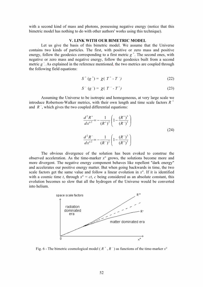
52
with a second kind of mass and photons, possessing negative energy (notice that this bimetric model has nothing to do with other authors' works using this technique).
V. LINK WITH OUR BIMETRIC MODEL Let us give the basis of this bimetric model. We assume that the Universe
contains two kinds of particles. The first, with positive or zero mass and positive energy, follow the geodesics corresponding to a first metric g +. The second ones, with negative or zero mass and negative energy, follow the geodesics built from a second metric g -. As explained in the reference mentioned, the two metrics are coupled through the following field equations:
S + (g +) = χ ( T + - T –) (22)
S – (g –) = χ ( T – - T +) (23)
Assuming the Universe to be isotropic and homogeneous, at very large scale we introduce Robertson-Walker metrics, with their own length and time scale factors R + and R –, which gives the two coupled differential equations:
⎟⎟⎠
⎞⎜⎜⎝
⎛−−=
°
⎟⎟⎠
⎞⎜⎜⎝
⎛−−=
°
+
−
−
−
−
+
+
+
3
3
22
2
3
3
22
2
)()(1
)(1
)()(1
)(1
RR
RxdRd
RR
RxdRd
(24)
The obvious divergence of the solution has been evoked to construe the observed acceleration. As the time-marker x° grows, the solutions become more and more divergent. The negative energy component behaves like repellent "dark energy" and accelerates our positive energy matter. But when going backwards in time, the two scale factors get the same value and follow a linear evolution in x°. If it is identified with a cosmic time t, through x° = ct, c being considered as an absolute constant, this evolution becomes so slow that all the hydrogen of the Universe would be converted into helium.
Fig. 6 - The bimetric cosmological model ( R + , R – ) as functions of the time-marker x°
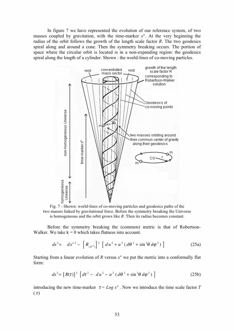
53
In figure 7 we have represented the evolution of our reference system, of two masses coupled by gravitation, with the time-marker x°. At the very beginning the radius of the orbit follows the growth of the length scale factor R. The two geodesics spiral along and around a cone. Then the symmetry breaking occurs. The portion of space where the circular orbit is located is in a non-expanding region: the geodesics spiral along the length of a cylinder. Shown : the world-lines of co-moving particles.
Fig. 7 - Shown: world-lines of co-moving particles and geodesics paths of the two masses linked by gravitational force. Before the symmetry breaking the Universe
is homogeneous and the orbit grows like R. Then its radius becomes constant.
Before the symmetry breaking the (common) metric is that of Robertson-Walker. We take k = 0 which takes flatness into account.
ds 2= dxo 2 − R(X O )[ ] 2 d u 2 + u 2 ( dθ 2 + sin 2θ dϕ 2 )[ ] (25a)
Starting from a linear evolution of R versus x° we put the metric into a conformally flat form:
ds 2= R(τ )[ ] 2 dτ 2 − d u 2 − u 2 ( dθ 2 + sin 2θ dϕ 2 )[ ] (25b)
introducing the new time-marker τ = Log x° . Now we introduce the time scale factor T ( τ )
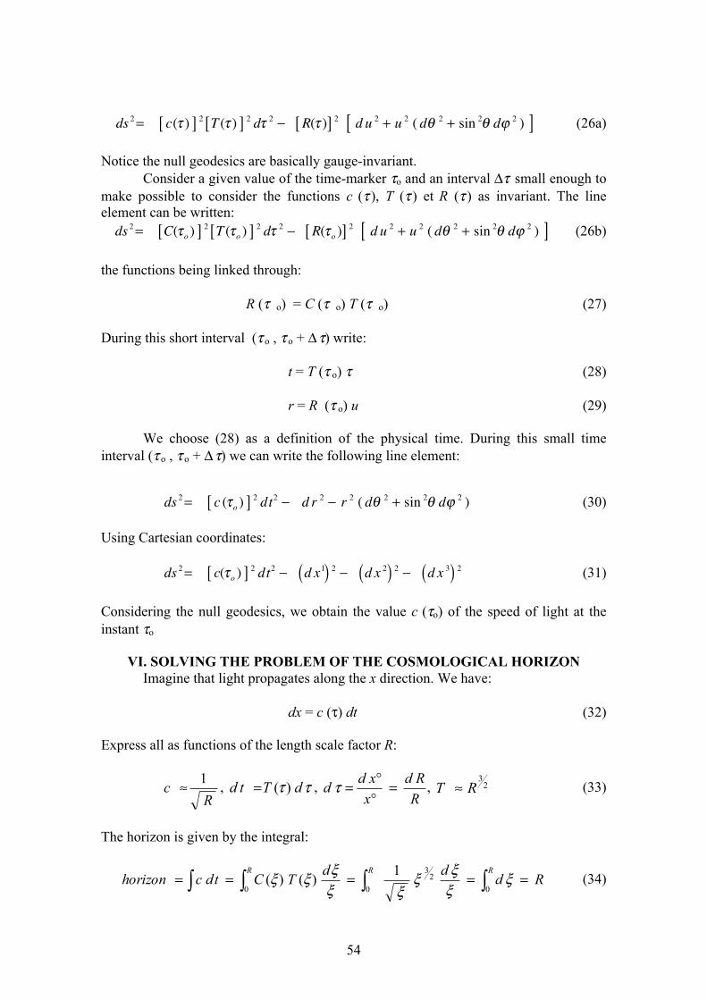
54
ds 2= c(τ )[ ] 2 T (τ )[ ] 2 dτ 2 − R(τ )[ ] 2 d u 2 + u 2 ( dθ 2 + sin 2θ dϕ 2 )[ ] (26a)
Notice the null geodesics are basically gauge-invariant. Consider a given value of the time-marker τo and an interval Δτ small enough to
make possible to consider the functions c (τ ), T (τ ) et R (τ ) as invariant. The line element can be written:
ds 2= C(τo )[ ] 2 T (τo )[ ] 2 dτ 2 − R(τo )[ ] 2 d u 2 + u 2 ( dθ 2 + sin 2θ dϕ 2 )[ ] (26b)
the functions being linked through:
R (τ o) = C (τ o) T (τ o) (27)
During this short interval (τ o , τ o + Δ τ) write:
t = T (τ o) τ (28)
r = R (τ o) u (29)
We choose (28) as a definition of the physical time. During this small time interval (τ o , τ o + Δ τ) we can write the following line element:
ds 2= c (τo )[ ] 2 dt2 − d r 2 − r 2 ( dθ 2 + sin 2θ dϕ 2 ) (30)
Using Cartesian coordinates:
ds 2= c(τo )[ ] 2 dt2 − d x1( ) 2 − d x 2( ) 2 − d x 3( ) 2 (31)
Considering the null geodesics, we obtain the value c (τo) of the speed of light at the instant τo
VI. SOLVING THE PROBLEM OF THE COSMOLOGICAL HORIZONImagine that light propagates along the x direction. We have:
dx = c (τ) dt (32)
Express all as functions of the length scale factor R:
Rc 1≈ , ττ dTtd )(= ,
RRd
xxdd =°°=τ , 2
3RT ≈ (33)
The horizon is given by the integral:
RdddTCtdchorizonRRR
===== ∫∫∫∫ 02
3
00
1)()( ξξξξ
ξξξξξ (34)
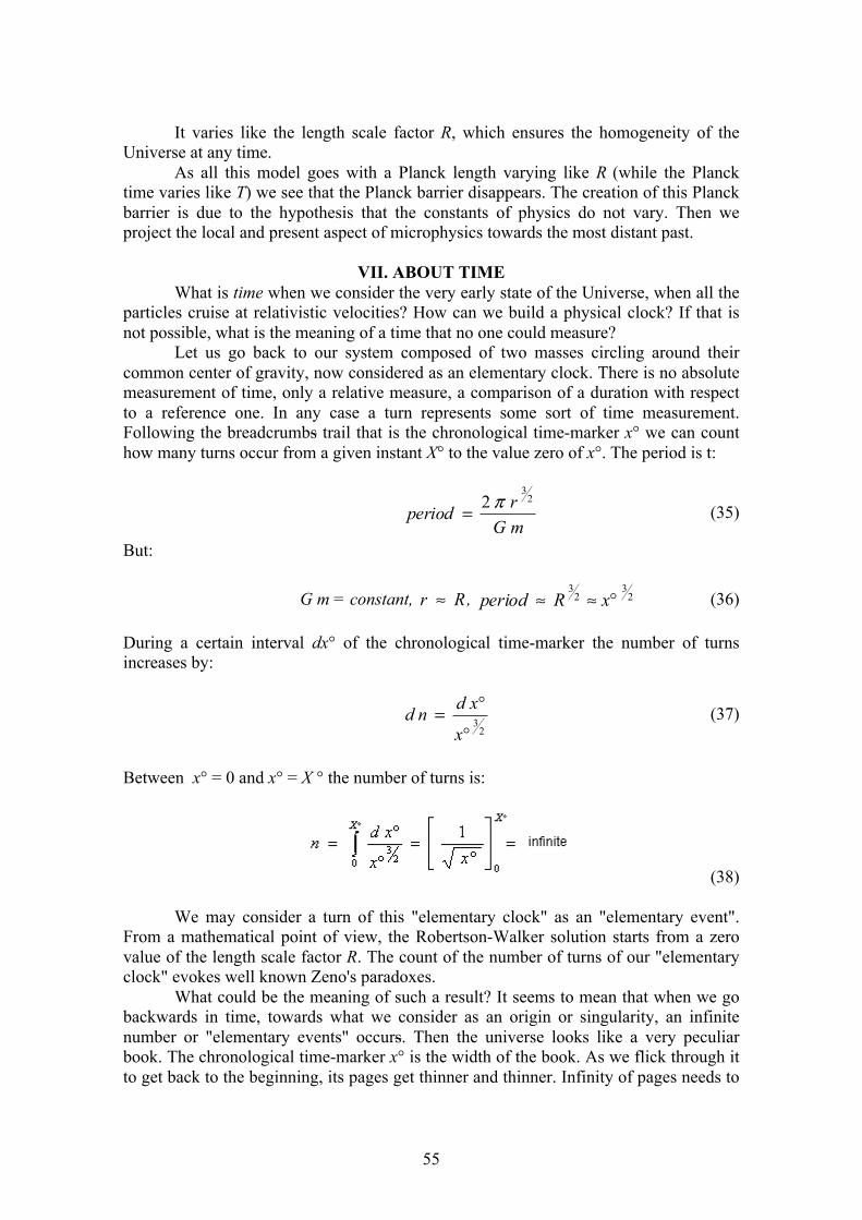
55
It varies like the length scale factor R, which ensures the homogeneity of the Universe at any time.
As all this model goes with a Planck length varying like R (while the Planck time varies like T) we see that the Planck barrier disappears. The creation of this Planck barrier is due to the hypothesis that the constants of physics do not vary. Then we project the local and present aspect of microphysics towards the most distant past.
VII. ABOUT TIMEWhat is time when we consider the very early state of the Universe, when all the
particles cruise at relativistic velocities? How can we build a physical clock? If that is not possible, what is the meaning of a time that no one could measure?
Let us go back to our system composed of two masses circling around their common center of gravity, now considered as an elementary clock. There is no absolute measurement of time, only a relative measure, a comparison of a duration with respect to a reference one. In any case a turn represents some sort of time measurement. Following the breadcrumbs trail that is the chronological time-marker x° we can count how many turns occur from a given instant X° to the value zero of x°. The period is t:
mGrperiod
23
2 π= (35)
But:
G m = constant, Rr ≈ , 23
23
°≈≈ xRperiod (36)
During a certain interval dx° of the chronological time-marker the number of turns increases by:
23
°
°=x
xdnd (37)
Between x° = 0 and x° = X ° the number of turns is:
(38)
We may consider a turn of this "elementary clock" as an "elementary event". From a mathematical point of view, the Robertson-Walker solution starts from a zero value of the length scale factor R. The count of the number of turns of our "elementary clock" evokes well known Zeno's paradoxes.
What could be the meaning of such a result? It seems to mean that when we go backwards in time, towards what we consider as an origin or singularity, an infinite number or "elementary events" occurs. Then the universe looks like a very peculiar book. The chronological time-marker x° is the width of the book. As we flick through it to get back to the beginning, its pages get thinner and thinner. Infinity of pages needs to
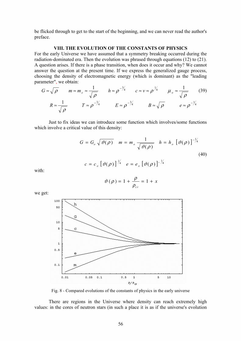
56
be flicked through to get to the start of the beginning, and we can never read the author's preface.
VIII. THE EVOLUTION OF THE CONSTANTS OF PHYSICSFor the early Universe we have assumed that a symmetry breaking occurred during the radiation-dominated era. Then the evolution was phrased through equations (12) to (21). A question arises. If there is a phase transition, when does it occur and why? We cannot answer the question at the present time. If we express the generalized gauge process, choosing the density of electromagnetic energy (which is dominant) as the "leading parameter", we obtain:
ρµρρ
ρρ 11 4
14
3≈≈≈≈≈≈≈ −
oe vchmmG (39)
41
43
431 −−− ≈≈≈≈≈ ρρρρ
ρeBETR
Just to fix ideas we can introduce some function which involves/some functions which involve a critical value of this density:
[ ]
[ ] [ ] 41
41
43
)()(
)()(
1)(
−
−
==
===
ρϑρϑ
ρϑρϑ
ρϑ
oo
ooo
eecc
hhmmGG
(40)
with:
we get:
Fig. 8 - Compared evolutions of the constants of physics in the early universe
There are regions in the Universe where density can reach extremely high values: in the cores of neutron stars (in such a place it is as if the universe's evolution
ϑ ( ρ ) = 1 + ρρc r
= 1 + x
57
was going backward in time). The state of the matter in the core of the star is similar to that of the very early Universe). It could be interesting to consider the evolution of this star core beyond a certain density value, as accompanying an alteration of local physical constants, as local length and time scale factors. We speculate that this could modify the topology inside the core, bearing a hypertoric space bridge suitable for transferring excess matter to another Universe. Another paper will discuss this possibility, giving insights into the first work undertaken on this idea.
IX. CONCLUSIONWe started from the remark that the Robertson-Walker solution, assuming the
cosmos is isotropic and homogeneous, does not describe the observed universe since it is clearly non-homogeneous, and that expansion is supposed not to occur within the vast regions occupied by galaxies. We suggested this non-homogeneity was born from a symmetry breaking that happened in a distant past, where the three dimensional hypersurface lost its symmetry O(3).
We proposed the hypothesis that masses, and in particular a couple of masses m linked by gravitational force and orbiting around their common center of gravity, follow the geodesics of the four-dimensional space-time hypersurface. We have shown that this is possible, if the equations of physics are to keep their validity, only if the physical constants undergo joint variations.
We established the gauge variation laws linking them, as well as the length and time scale factors. We obtained a description of cosmic evolution where the cosmological horizon varies like the length scale factor, which guarantees the homogeneity of the early Universe without calling on the inflation theory.
In this generalized gauge process, before the symmetry breaking occurs, all characteristic lengths of physics vary like the length scale factor R, while all characteristic times vary like the time scale factor T. In this way the Plank barrier disappears.
Focusing on our two mass system linked by gravitational force, we assimilated it to an elementary clock where time would be measured by each turn count. After the symmetry breaking, the number of turns evolves like classical cosmic time, following from x° = ct with c being an absolute constant. We have shown that in the previous era, before this symmetry breaking, the elementary clock makes an infinite number of turns which brings up the problem of the definitions of "time" and of the "origin".
Acknowledgments: The authors thank Dr B. Kolev for useful advices and comments, J. Geffray and J. Murphy for the translation of the paper into English.
58
REFERENCES [1] J.P.Petit : An interpretation of cosmological model with variable light velocity. Modern Physics Letters A, Vol. 3, n°16, nov 1988, p.1527 http://www.jp-petit.org/science/f300/modern_physics_letters_a1.pdf [2] J.P.Petit : Cosmological model with variable light velocity: the interpretation of red shifts. Modern Physics Letters A, Vol.3 , n° 18, dec. 1988, p.1733 http://www.jp-petit.org/science/f300/modern_physics_letters_a2.pdf [3] J.P.Petit & Maurice Viton : Gauge cosmological model with variable light velocity. Comparizon with QSO observational data. Modern Physics Letters A Vol.4 , n°23 (1989) pp. 2201-2210 http://www.jp-petit.org/science/f300/modern_physics_letters_a3.pdf [4] J.P.Petit Twin Universe Cosmology : Astronomy and Space Science 226 : 273-307, 1995 [5]Andreas Albrecht and João Magueijo (1999). "A time varying speed of light as a solution to cosmological puzzles". Phys. Rev. D59. arXiv:astro-ph/9811018 [6] João Magueijo, Faster Than the Speed of Light: The Story of a Scientific Speculation, Perseus Books Group , Massachusetts , 2003, ISBN 0-7382-0525-7. [7] J.W.Moffat, Int. J. Mod. Phys. D 2 , 351, 1993 [8] J.Barrow, New Scientist, 2196-21 July, pp 28, 1999 [9] C.B.Netterfield et al., Astrophys. J. 571 : 604-614, 2002 [10] C.L.Bennet et al, astro-ph/0302207 [11] G. Amelino-Camelia ; Int. J. of Mod. Phys. D11, 1643, 2002 [12] J.D.Barrow & J. Magueijo , Astrophys. J. Lett. 532 , L 87-90, (2000) [13] M.A.Clayton, J.W.Moffat, Phys. Lett. B 460 (1999), 263-270 [14] S.Alexander , JHEP , 0011 ( 2000 ) 017, hep-th/9912037 [15] J. Magueijo, Phys. Rev. D63, 043502, 2001 [16] J.Magueijo & L.Smolin Lorentz invariance with an invariant energy scale, arXiv : hep-the/0112090v2, 18 dec 2001 [17] B.a.Basset, S. Liberati, C.Molina-Paris and M. Visser : Geometrodynamics of Variable_Speed—f_light Cosmologies. ArXiv : astro-ph/00011441v2 17 july 2000 [18] J.P.Petit & G. D'Agostini : Bigravity as an interpretation of cosmic acceleration. Colloque international sur le Techniques Variationnelles, le Mont Dore, août 2007. http://arxiv.org/abs/0712.0067 2007/12/2 [19] R.Adler, M. Bazin & M. Schifer : Introduction to General Relativity, Mac Graw Hill Books Cie, 1975 [20] A.Guth, Phys. Rev. D 23 347 ( 1981 ) ; A. Linde, Phys. Lett. B108, 1220 ( 1982 ) ; A. Albreicht and P.Steinhardt, Phys. Rev. Lett. 48 1220 ( 1982) ; A. Linde, Phys. Lett. B 129, 177 ( 1983) [21] J.P.Petit : The missing mass problem. Il Nuovo Cimento B Vol. 109 July 1994, pp. 697-710 [22] J.P. Petit, P.Midy & F.Landsheat : Twin matter against dark matter. International. Meeting. on Astrophys. and Cosm. "Where is the matter ? ", Marseille 2001 june 25-29.

SOLUTIONS OF A COSMOLOGICAL SCHRODINGER EQUATION FOR EXACT GRAVITATIONAL WAVES BASED ON
A FRIEDMAN DUST UNIVERSE WITH EINSTEIN’S LAMBDAJames G. Gilson
School of Mathematical Sciences Queen Mary University of London Mile End Road London E14NS
In an earlier paper, it was shown that the cosmological model that was introduced in a sequence of three earlier papers under the title A Dust Universe Solution to the Dark Energy Problem, originally described by the Friedman equations, can be expressed as a solution to a non-linear Schrodinger equation. In this paper, a large collection of solutions to this Schrodinger equation are found and discussed in the context of relaxing the uniform mass density condition usually employed in cosmology theory. The surprising result is obtained that this non-linear equation can have its many solutions linearly superposed to obtain solution of the cosmology theory problem of great generality and applicability.
Keywords: cosmological Schrodinger equation, gravitational waves, Friedman dust universe, cosmology theory.
PACS number: 04.30.-w
I. INTRODUCTIONThe work to be described in this paper is an application of the cosmologi-cal
model introduced in the papers A Dust Universe Solution to the Dark Energy Problem [23], Existence of Negative Gravity Material. Identification of Dark Energy [24] and Thermodynamics of a Dust Universe [32] together with applications of those papers to the cosmological constant problem, the cosmological coincidence problem and other subsidiary cosmological prob-lems.
The conclusions arrived at in those papers was that the dark energy sub-stance is physical material with a positive density, as is usual, but with a negative gravity, -G, characteristic and is twice as abundant as has usually been considered to be the case. References to equations in those papers will be prefaced with the letter A, B and C respectively. The work in A, B and C, and the application here have origins in the studies of Einstein’s general relativity in the Friedman equations context to be found in ref-erences ([16],[22],[21],[20],[19],[18],[4],[23]) and similarly motivated work in references ([10],[9],[8],[7],[5]) and ([12],[13],[14],[15],[7],[25],[3]). Other useful sources of information are ([17],[3],[30],[27],[29],[28]) with the measurement essentials coming from references ([1],[2],[11],[37]). Further references will be mentioned as necessary. The application of the cosmological model in-troduced in the papers A [23], B,[24] and C [32], in paper E, ([36]), is to the extensively discussed and analysed Cosmological Coincidence Problem. In the paper D, [34], it was shown that the quantum vacuum polarisation idea can be seen to play a central role in the Friedman dust universe model in-troduced by the author. In the paper, [40], it was
59
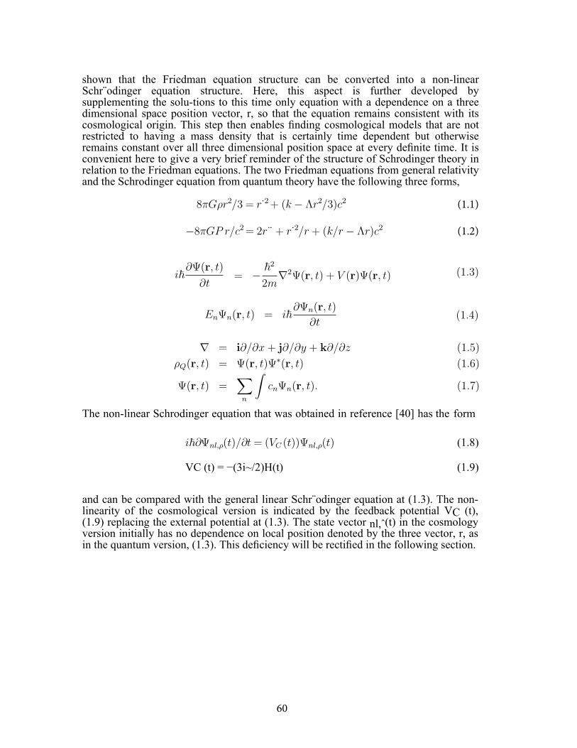
shown that the Friedman equation structure can be converted into a non-linear Schr¨odinger equation structure. Here, this aspect is further developed by supplementing the solu-tions to this time only equation with a dependence on a three dimensional space position vector, r, so that the equation remains consistent with its cosmological origin. This step then enables finding cosmological models that are not restricted to having a mass density that is certainly time dependent but otherwise remains constant over all three dimensional position space at every definite time. It is convenient here to give a very brief reminder of the structure of Schrodinger theory in relation to the Friedman equations. The two Friedman equations from general relativity and the Schrodinger equation from quantum theory have the following three forms,
8πGρr2/3 = r˙2 + (k − Λr2/3)c2 (1.1)
−8πGP r/c2 = 2r¨ + r˙2/r + (k/r − Λr)c2 (1.2)
i~∂Ψ(r, t)
∂t= −
~2
2m∇2Ψ(r, t) + V (r)Ψ(r, t) (1.3)
EnΨn(r, t) = i~∂Ψn(r, t)
∂t(1.4)
(1.5)∇ = i∂/∂x + j∂/∂y + k∂/∂z
ρQ(r, t) = Ψ(r,∫t)Ψ∗(r, t) (1.6)
Ψ(r, t) =∑
cnΨn(r, t). (1.7)n
The non-linear Schrodinger equation that was obtained in reference [40] has the form
i~∂Ψnl,ρ(t)/∂t = (VC (t))Ψnl,ρ(t) (1.8)
VC (t) = −(3i~/2)H(t) (1.9)
and can be compared with the general linear Schr¨odinger equation at (1.3). The non-linearity of the cosmological version is indicated by the feedback potential VC (t), (1.9) replacing the external potential at (1.3). The state vector nl,ˆ(t) in the cosmology version initially has no dependence on local position denoted by the three vector, r, as in the quantum version, (1.3). This deficiency will be rectified in the following section.
60
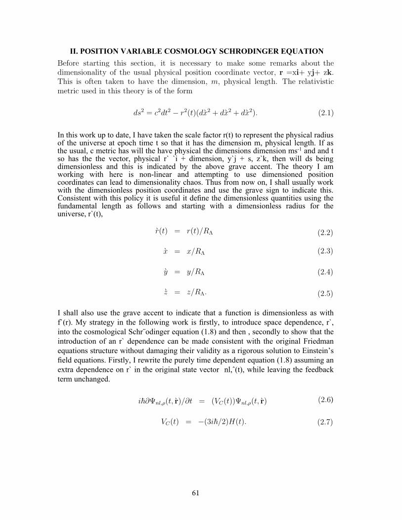
II. POSITION VARIABLE COSMOLOGY SCHRODINGER EQUATIONBefore starting this section, it is necessary to make some remarks about thedimensionality of the usual physical position coordinate vector, r =xi+ yj+ zk.This is often taken to have the dimension, m, physical length. The relativisticmetric used in this theory is of the form
ds2 = c2dt2 − r2(t)(dx2 + dx2 + dx2). (2.1)
In this work up to date, I have taken the scale factor r(t) to represent the physical radius of the universe at epoch time t so that it has the dimension m, physical length. If as the usual, c metric has will the have physical the dimensions dimension ms-1 and and t so has the the vector, physical r` `i + dimension, y`j + s, z`k, then will ds being dimensionless and this is indicated by the above grave accent. The theory I am working with here is non-linear and attempting to use dimensioned position coordinates can lead to dimensionality chaos. Thus from now on, I shall usually work with the dimensionless position coordinates and use the grave sign to indicate this. Consistent with this policy it is useful it define the dimensionless quantities using the fundamental length as follows and starting with a dimensionless radius for the universe, r`(t),
r(t) = r(t)/RΛ (2.2)
x = x/RΛ (2.3)
y = y/RΛ (2.4)
z = z/RΛ. (2.5)
I shall also use the grave accent to indicate that a function is dimensionless as with f`(r). My strategy in the following work is firstly, to introduce space dependence, r`, into the cosmological Schr¨odinger equation (1.8) and then , secondly to show that the introduction of an r` dependence can be made consistent with the original Friedman equations structure without damaging their validity as a rigorous solution to Einstein’s field equations. Firstly, I rewrite the purely time dependent equation (1.8) assuming an extra dependence on r` in the original state vector nl,ˆ(t), while leaving the feedback term unchanged.
i~∂Ψnl,ρ(t, r)/∂t = (VC(t))Ψnl,ρ(t, r) (2.6)
VC(t) = −(3i~/2)H(t). (2.7)
61
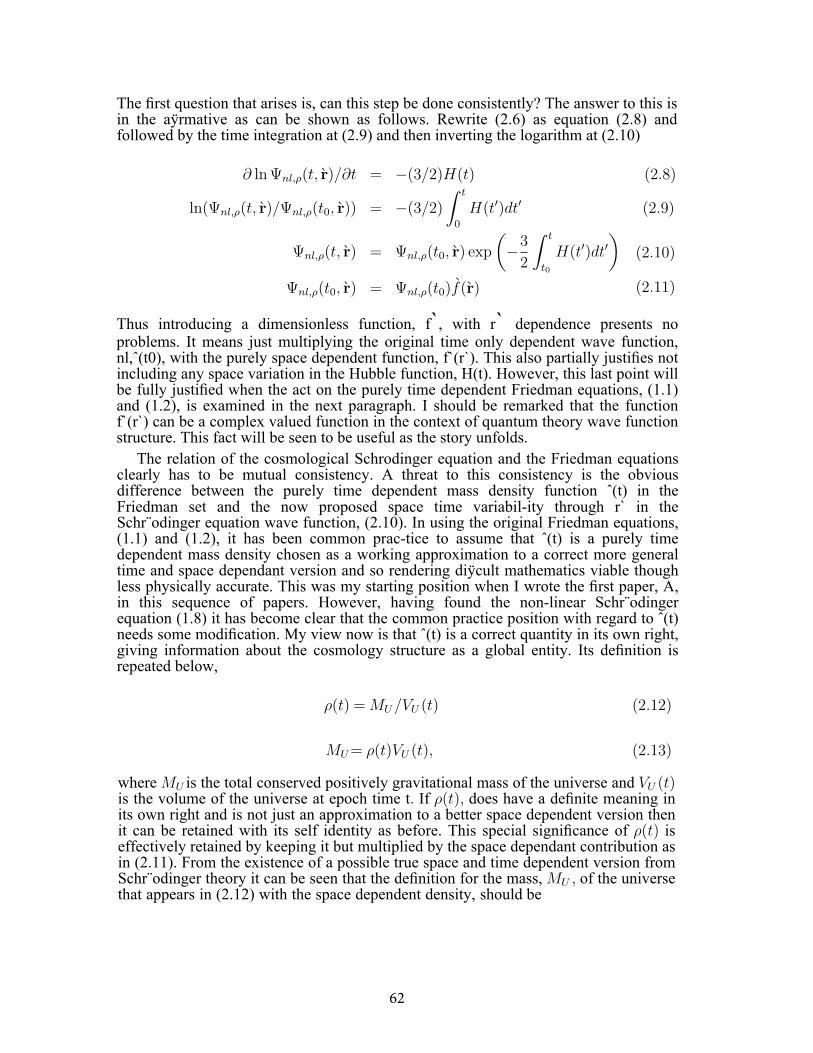
The first question that arises is, can this step be done consistently? The answer to this is in the aÿrmative as can be shown as follows. Rewrite (2.6) as equation (2.8) and followed by the time integration at (2.9) and then inverting the logarithm at (2.10)
∂ ln Ψnl,ρ(t, r)/∂t = −(3/2)H(t) (2.8)
ln(Ψnl,ρ(t, r)/Ψnl,ρ(t0, r)) = −(3/2)
∫ t
0
H(t′)dt′ (2.9)(−3
2
∫ t
t0
H(t′)dt′)
(2.10)Ψnl,ρ(t, r) = Ψnl,ρ(t0, r) exp
Ψnl,ρ(t0, r) = Ψnl,ρ(t0)f(r) (2.11)
Thus introducing a dimensionless function, f`, with r` dependence presents noproblems. It means just multiplying the original time only dependent wave function, nl,ˆ(t0), with the purely space dependent function, f`(r`). This also partially justifies not including any space variation in the Hubble function, H(t). However, this last point will be fully justified when the act on the purely time dependent Friedman equations, (1.1) and (1.2), is examined in the next paragraph. I should be remarked that the function f`(r`) can be a complex valued function in the context of quantum theory wave function structure. This fact will be seen to be useful as the story unfolds.
The relation of the cosmological Schrodinger equation and the Friedman equations clearly has to be mutual consistency. A threat to this consistency is the obvious difference between the purely time dependent mass density function ˆ(t) in the Friedman set and the now proposed space time variabil-ity through r` in the Schr¨odinger equation wave function, (2.10). In using the original Friedman equations, (1.1) and (1.2), it has been common prac-tice to assume that ˆ(t) is a purely time dependent mass density chosen as a working approximation to a correct more general time and space dependant version and so rendering diÿcult mathematics viable though less physically accurate. This was my starting position when I wrote the first paper, A, in this sequence of papers. However, having found the non-linear Schr¨odinger equation (1.8) it has become clear that the common practice position with regard to ˆ(t) needs some modification. My view now is that ˆ(t) is a correct quantity in its own right, giving information about the cosmology structure as a global entity. Its definition is repeated below,
ρ(t) = MU /VU (t) (2.12)
MU = ρ(t)VU (t), (2.13)
where MU is the total conserved positively gravitational mass of the universe and VU (t) is the volume of the universe at epoch time t. If ρ(t), does have a definite meaning in its own right and is not just an approximation to a better space dependent version then it can be retained with its self identity as before. This special significance of ρ(t) is effectively retained by keeping it but multiplied by the space dependant contribution as in (2.11). From the existence of a possible true space and time dependent version from Schr¨odinger theory it can be seen that the definition for the mass, MU , of the universe that appears in (2.12) with the space dependent density, should be
62
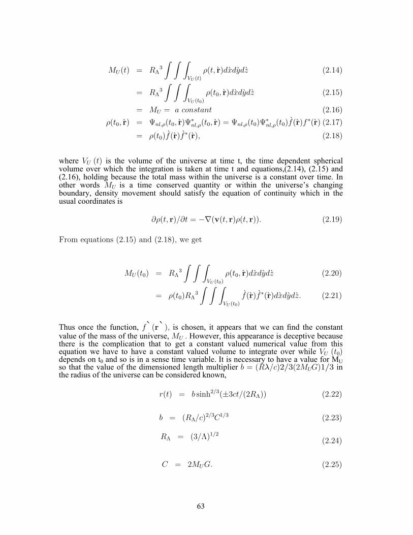
MU(t) = RΛ3
∫ ∫ ∫VU (t)
ρ(t, r)dxdydz (2.14)
= RΛ3
∫ ∫ ∫VU (t0)
ρ(t0, r)dxdydz (2.15)
= MU = a constant (2.16)
ρ(t0, r) = Ψnl,ρ(t0, r)Ψ∗nl,ρ(t0, r) = Ψnl,ρ(t0)Ψ
∗nl,ρ(t0)f(r)f ∗(r) (2.17)
= ρ(t0)f(r)f ∗(r), (2.18)
where VU (t) is the volume of the universe at time t, the time dependent spherical volume over which the integration is taken at time t and equations,(2.14), (2.15) and (2.16), holding because the total mass within the universe is a constant over time. In other words MU is a time conserved quantity or within the universe’s changing boundary, density movement should satisfy the equation of continuity which in the usual coordinates is
∂ρ(t, r)/∂t = −∇(v(t, r)ρ(t, r)). (2.19)
From equations (2.15) and (2.18), we get
MU(t0) = RΛ3
∫ ∫ ∫∫ V∫U (t0∫) ρ(t0, r)dxdydz (2.20)
= ρ(t0)RΛ3
VU (t0)
f(r)f ∗(r)dxdydz. (2.21)
Thus once the function, f`(r`), is chosen, it appears that we can find the constant value of the mass of the universe, MU . However, this appearance is deceptive because there is the complication that to get a constant valued numerical value from this equation we have to have a constant valued volume to integrate over while VU (t0) depends on t0 and so is in a sense time variable. It is necessary to have a value for MU so that the value of the dimensioned length multiplier b = (Rλ/c)2/3(2MUG)1/3 in the radius of the universe can be considered known,
r(t) = b sinh2/3(±3ct/(2RΛ)) (2.22)
(2.23)b = (RΛ/c)2/3C1/3
RΛ = (3/Λ)1/2
(2.24)
C = 2MUG. (2.25)
63
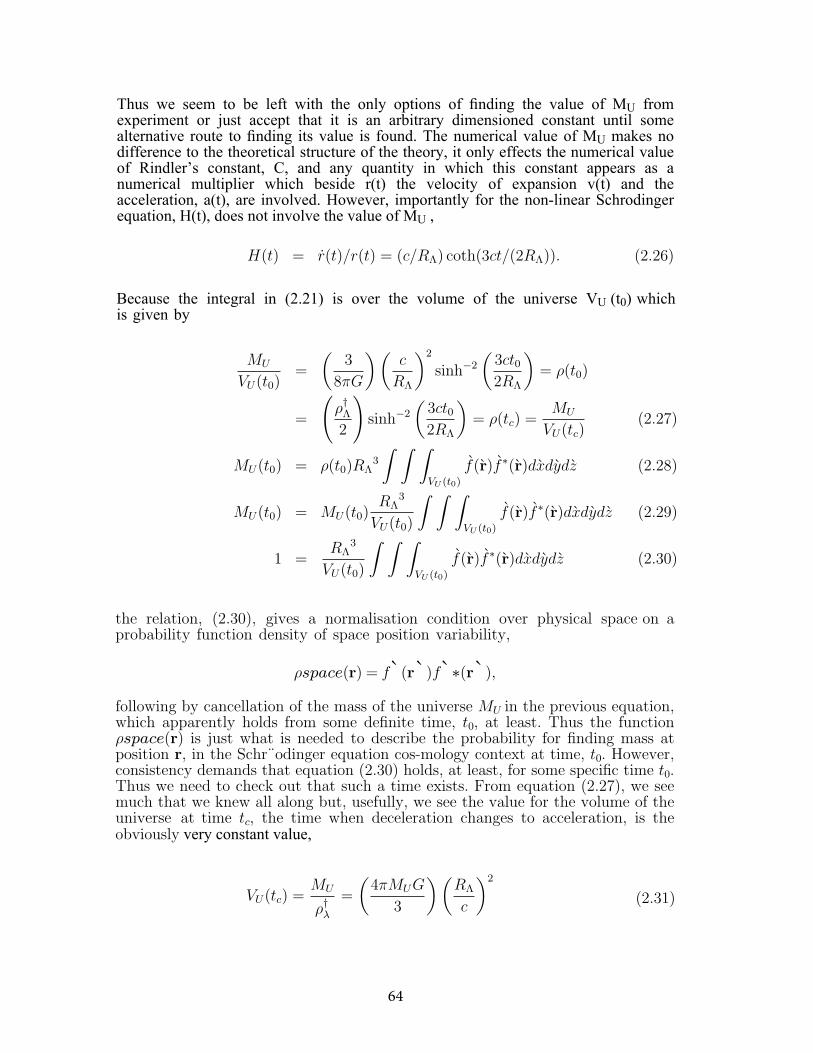
Thus we seem to be left with the only options of finding the value of MU from experiment or just accept that it is an arbitrary dimensioned constant until some alternative route to finding its value is found. The numerical value of MU makes no difference to the theoretical structure of the theory, it only effects the numerical value of Rindler’s constant, C, and any quantity in which this constant appears as a numerical multiplier which beside r(t) the velocity of expansion v(t) and the acceleration, a(t), are involved. However, importantly for the non-linear Schrodinger equation, H(t), does not involve the value of MU ,
H(t) = r(t)/r(t) = (c/RΛ) coth(3ct/(2RΛ)). (2.26)
Because the integral in (2.21) is over the volume of the universe VU (t0) which is given by
MU
VU(t0)=
(3
8π
)(c
RΛ
)2
sinh−2
(3ct02RΛ
)= ρ(t0)
=
(ρ†Λ
G)sinh−2
(3ct02RΛ
)= ρ(tc) =
MU(2.27)
2
MU(t0) = ρ(t0)RΛ3
∫ ∫ ∫VU (t0)
VU(tc)
f(r)f ∗(r)dxdydz (2.28)
MU(t0) = MU(t0)RΛ
3 ∫ ∫ ∫f(r)f∗(r)dxdydz (2.29)
1 =RΛ
3
VU(t0)
VU(t0)∫ ∫ ∫VU (t0)
VU (t0)
f(r)f∗(r)dxdydz (2.30)
the relation, (2.30), gives a normalisation condition over physical space on aprobability function density of space position variability,
ρspace(r) = f`(r`)f`∗(r`),
following by cancellation of the mass of the universe MU in the previous equation,which apparently holds from some definite time, t0, at least. Thus the functionρspace(r) is just what is needed to describe the probability for finding mass atposition r, in the Schr¨odinger equation cos-mology context at time, t0. However,consistency demands that equation (2.30) holds, at least, for some specific time t0.Thus we need to check out that such a time exists. From equation (2.27), we seemuch that we knew all along but, usefully, we see the value for the volume of theuniverse at time tc, the time when deceleration changes to acceleration, is theobviously very constant value,
VU(tc) =MU
ρ†λ=
(4πMUG
3
)(RΛ
c
)2
(2.31)
64
that we need to evaluate the apparently time dependent multiples integrals such as
1 =RΛ
3
VU(tc)
∫ ∫ ∫VU (tc)
f(r)f ∗(r)dxdydz. (2.32)
Thus we seem very near a prescription for a usable cosmological Schr¨odingerequation. However, given a space dependent solution like (2.10) it is likely that the
part − ~2 ∇2Ψ(`r, t) of the quantum version at (1.3) would occur and this might render the cosmological quantum version not consistent with cosmology. It is by no means certain that such a complication would neces-sarily occur and not be handleable but certainly it can be avoided by playing safe and imposing the condition on this term as being zero as follows,
~2
∇2Ψ(t, r) = 0. (2.33)
This implies that the function f`(r`) from equation (2.11) also satifies the Laplaceequation,
∇2f(r) = 0. (2.34)
The Laplace equation has a very large number of solutions. Thus there are many possible space dependent versions for the wave function,Ψ(t, r`). Furthermore, I shall show that in spite of the cosmological Schrodinger being non-linear, the many solutions of the Laplace equation can be linearly superposed to produce yet more solutions. Thus although the condition (2.33) reduces the number of possibilities that might be considered for the space dependent wave function it leaves us more than enough solutions to think about for a very long time. It does have another advantage that could turn out to be important concerning a possible quantum conjugate momentum, pˆC , for the space variable r. This can be defined as
pC =~∂
∂r= ~∇. (2.35)
2m
2m
and this momentum exists as a result of the Laplace equation (2.33) and automatically takes the form after operating on the wave function as follows
pCΨ(t, r) = ~∇∧ g(t, r), (2.36)
where g(t, r`) is some definite vector function of t and r`.The wave motion followed by the dark mass dark energy time relation process
can help to identify the effect that introducing position dependence has on the hyperspace vacuum. Space dependence implies the need to see this process as also space dependent. The density functions for the dark mass, dark energy and the ratio, r',DM (t), of dark energy to dark mass as functions of the time only global process are respectively represented by
65
ρ(t) = (3/(8πG))(c/RΛ)2 sinh−2(3ct/(2RΛ)) (2.37)
ρ†Λ = (3/(4πG))(c/RΛ)2 (2.38)
rΛ,DM(t) = ρ†Λ/ρ(t) = 2 sinh2(3ct/(2RΛ)) (2.39)
rΛ,DM(±tc) = 2 sinh2(±3ctc/(2RΛ)) = 1. (2.40)
The space time dependent version for (2.37) is given simply by multiplying both sides of this equation by the space dependant contribution f`(r`)f` (r`) giving
ρ(t, r) = (3/(8πG))(c/RΛ)2f(r)f ∗(r) sinh−2(3ct/(2RΛ)) (2.41)
= (Λc2/(8πG))f(r)f ∗(r) sinh−2(3ct/(2RΛ)). (2.42)
From equation (2.42), it follows that the cosmological constant Λ and the space dependence function can be taken together to define a local space dependent cosmological function, Λ (r), associated with any specific solution of the Laplace equation as follows
Λ(r) = Λf(r)f∗(r) (2.43)
= Λf(r/RΛ)f ∗(r/RΛ). (2.44)
It follows from this definition, that the mean value of the cosmological func-tion is equal to Λ for all solutions of the Laplace equation. In other words, the cosmological function is centred on Einstein’s cosmological constant.
The linearity superposition of the various solutions of the Cosmological Schrodinger equation (1.8) to produce more solutions follows from (2.10) as in the following. Suppose we have two arbitrarily chosen spatially different solutions of this equation labelled with subscripts 1 and 2 as in
Ψnl,ρ,1(t, r) = Ψnl,ρ,1(t0, r) exp(−3
2
∫ t
t0
H(t′)dt′)
(2.45)
Ψnl,ρ,2(t, r) = Ψnl,ρ,2(t0, r) exp
(−3
2
∫ t
t0
H(t′)dt′)
(2.46)
Ψspp(t, r) = c1Ψnl,ρ,1(t, r) + c2Ψn 2(t, r)
= Ψspp(t0, r) exp
(−3
2
l∫,ρ,
t
t0
H(t′)dt′)
, (2.47)
66
where c1 and c2 are arbitrary constants and the subscript spp means super-posed. It follows from (2.47) that any number of solutions of the cosmolog-ical Schr¨odiner equation can be linearly superposed to produce yet further solutions. Thus, altogether, there is vast scope to produce solutions with almost any space form whatsoever. The common feature of all the solutions is that that they all related to the common cosmological platform defined by and with the same time variation structure of the space constant density function of the Friedman equations. The final prescription for finding solu-tions to the cosmological Schrodinger equation involve the following three steps. Find any solution, f, to the three dimensional Laplace equation and involve in this solution one initially multiplicative arbitrary constant, A0. Form the space-time wave function for this solution,Ψ(t, r). Find the value of A0 by using the probability normalisation condition and integration over the Hermitian square of f over the volume of the universe at time, tc. The wave function will then be completely determined. The probability density is also now fully determined via the definition ρC (t, r) =Ψ(t, r)Ψ∗
(t, r). The result will be a probability density function over space and time which is compatible with the Friedman equations from general relativity. The steps will be demonstrated in the next subsection for one typical case.
I shall finish this paper with the simplest nontrivial example giving auniverse that involves a varying space and time density. One of the simplest solutions, f(r`), to the Laplace equation (2.34) is the sum of three variable complex numbers and just one arbitrary dimensionless constant, A0,
II.A. A Simple Example
f(r) = A0((x + iy) + (y + iz) + (z + ix))
= A0(x + y + z)(1 + i). (2.48)
f ∗(r) = A0(x + y + z)(1− i) (2.49)
f(r)f ∗(r) = 2A20(x + y + z)2 (2.50)
= 2(A0/RΛ)2(x + y + z)2 = F (r), say. (2.51)
The definition (2.51) displays the formula in terms of the physical space coordinates, x, y, z. The normalisation condition on the probability density,(2.30), at time tc requires the following two results
1 =1
VU(tc)
∫ ∫ ∫VU (tc)
f(r)f ∗(r)dxdydz (2.52)
VU(tc) =
(4πMUG
3
)(RΛ
c
)2
. (2.53)
67
We need to evaluate the triple integral over the physical coordinates to find the value of the arbitrary constant A0. This will be done in spherical polar coordinates with some condensations of notation used for the sin and cos functions,
(2.54)
(2.55)
x = r sin(θ) cos(φ) = rSθCφ
y = r sin(θ) sin(φ) = rSθSφ
z = r cos(θ) = rCθ(2.56)
dxdydz = r2drSθdθdφ (2.57)
(2.58)0 < θ ≤ π, 0 < φ ≤ 2π, 0 < r ≤ r(tc)
r(tc) = (MUG(RΛ/c)2)1/3 (2.59)
Thus the function, F (r) = f`(r`)f`∗(r`), in the triple integral becomes
F (r) = 2(A0/RΛ)2(x + y + z)2 (2.60)
= 2(A0r/RΛ)2(SθCφ + SθSφ + Cθ)2 (2.61)
= 2(A0r/RΛ)2((1 + 2(SθCφSθSφ + SθCφCθ + SθSφCθ)) (2.62)
= 2(A0r/RΛ)2((1 + 2(SθSθSφCφ + SθCθCφ + SθCθSφ)) (2.63)
Introducing the further notation
ir = r4dr Ir =
∫ r(tc)
0
ir = r5(tc)/5 (2.64)
iθ,1 = Sθ3dθ, I1 =
∫ π
0
iθ,1 =4
3(2.65)
iφ,1 = SφCφdφ, I2 =
∫ 2π
0
iφ,1 = 0 (2.66)
iθ,2 = Sθ2Cθdθ, I3 =
∫ π
0
iθ,2 = 0 (2.67)
iφ,2 = Cφdφ, I4 =
∫ 2π
0
iφ,2 = 0 (2.68)
iφ,3 = Sφdφ, I5 =
∫ 2π
iφ,3 = 0 (2.69)
0
68

the integral element and the integral can be expressed as
dI = 2(A0r/RΛ)2((1 + 2(SθSθSφCφ + SθCθCφ + SθCθSφ))r2drSθdθdφ
= 2(A0/RΛ)2ir(dθdφ + 2(iθ,1iφ,1 + iθ,2iφ,2 + iθ,2iφ,3)) (2.70)
I(tc) = (4/5)
(A0π
RΛ
)2
r5(tc). (2.71)
The last expression for I(tc) is all that is left after integration. The nor-malisation condition at time tc using (2.31) can now be used to find the numerical value of A0 by
1 = I/VU(tc) = (4/5)
(A0π
R2Λ
)2
r5(tc)
(3c2
4πMUG
)(2.72)
3A20π=
5
(MUG
c2RΛ
)2/3(2.73)
A0 =
(5
3π
)1/2(c2RΛ
MUG
)1/3(2.74)
Thus the full solution for the wave function, the probability density and all theconstants involved is as follows:
Ψnl,ρ(t, r) = Ψnl,ρ(tc, r) exp
(−3
2
∫ t
tc
H(t′)dt′)
(2.75)
Ψnl,ρ(tc, r) = Ψnl,ρ(tc)f(r) (2.76)
Ψnl,ρ(tc) = (ρ†Λ)1/2 (2.77)
f(r) = (A0/RΛ)(x + y + z)(1 + i) (2.78)
ρ(t, r) = 2(A0/RΛ)2ρ†Λ(x + y + z)2 exp
(−3
∫ t
tc
H(t′)dt′)
(2.79)
ρ†Λ =Λc2
4πG(2.80)
A0 =
(5
3π
)1/2(c2RΛ
MUG
)1/3
. (2.81)
69
III. CONCLUSIONSIn an earlier paper, it was shown that a non-linear Shr¨odinger equation can
be obtained from the Friedman cosmology equations which is entirely con-sistentwith those equations. Here, the time evolution of this Schr¨odinger equation isexamined in relation to conservation of the universe’s total pos-itive gravitationalmass. This leads to the identification of a wave function for cosmology states with adefinite time evolution and consequently also to a probability density forcosmology. This cosmological probability density can depend on spatial variabilityin addition to just the time variability of the Friedman equation structure.Consistency of the new Schr¨odinger equation with its originating Friedman set isachieved by restricting solu-tions to the condition that they satisfy the Laplaceequation in hyperspace. It becomes clear that, even with this restriction, a multipleinfinity of so-lutions remain available and applicable. The structure of this theoryseems to confirm the view often expressed about the quantum vacuum that it is abubbling cauldron of activity in the form of random quantum transitions, such aspair production and annihilation, between short lived virtual states of fundamentalparticles. The expansion of the universe can be explained in such terms as aspherical advancing and evolving wave of quantum before and after measurementtype conditions in reverse through the expanding oundary. Just outside the expanding boundary, the vacuum chaotic states as described by the wave function, resourced by the multiplicity of solutions of the Laplace equation, are progressively converted from chaos to a definite gravitational form suÿcient to describe the mass density that has taken up residence within the expanded boundary. The universe expansion colonises surrounding hyperspace so as to accommodate within its boundary its con-served positive gravitational mass with more territory and in a quantum form that can hold non-transient positive gravitational mass. Outside the universe the solution holds but remains a linear superposition of many var-ied chaotic transient states with mass density value centred on the value of twice Einstein’s dark energy mass density ρ†Λ.
Acknowledgements: I am greatly indebted to Professors Clive Kilmister and Wolfgang Rindler for help, encouragement and inspiration.
70
REFERENCES[1]. R. A. Knop et al. arxiv.org/abs/astro-ph/0309368 New Constraints on and w from an independent Set (Hubble) of Eleven High-Redshift Supernovae, Observed with HST.
ΩM, ΩΛ
[2]. Adam G. Riess et al xxx.lanl.gov/abs/astro-ph/0402512 Type 1a Supernovae Discoveries at z > 1. From The Hubble Space Telescope: Evidence for Past Deceleration and constraints on Dark energy Evolution.[3]. Berry 1978, Principles of cosmology and gravitation, CUP.[4]. Gilson, J.G. 1991, Oscillations of a Polarizable Vacuum, Journal of Applied Mathematics and Stochastic Analysis, 4, 11, 95–110.[5]. Gilson, J.G. 1994, Vacuum Polarisation and The Fine Structure Constant, Speculations in Science and Technology , 17, 3 , 201-204.[6]. Gilson, J.G. 1996, Calculating the fine structure constant, Physics Essays, 9 , 2 June, 342-353.[7]. Eddington, A.S. 1946, Fundamental Theory, Cambridge University Press.[8]. Kilmister, C.W. 1992, Philosophica, 50, 55.
[9]. Bastin, T., Kilmister, C. W. 1995, Combinatorial Physics World Scientific Ltd.[10]. Kilmister, C. W. 1994 , Eddington’s search for a Fundamental Theory, CUP.[11]. Peter, J. Mohr, Barry, N. Taylor, 1998, Recommended Values of the fundamental Physical Constants, Journal of Physical and Chemical Reference Data, AIP.[12]. Gilson, J. G. 1997, Relativistic Wave Packing and Quantization, Speculations in Science and Technology, 20 Number 1, March, 21-31.[13]. Dirac, P. A. M. 1931, Proc. R. Soc. London, A133, 60.
[14]. Gilson, J.G. 2007, www.fine-structure-constant.org The fine structure constant.[15]. McPherson R., Stoney Scale and Large Number Coincidences, Apeiron, Vol. 14, No. 3, July, 2007.[16]. Rindler, W. 2006, Relativity: Special, General and Cosmological, Second Edition, Oxford University Press.[17]. Misner, C. W.; Thorne, K. S.; and Wheeler, J. A. 1973, Gravitation, Boston, San Francisco, CA: W. H. Freeman.[18]. J. G. Gilson, 2004, Physical Interpretations of Relativity Theory Conference IX London, Imperial College, September, 2004 Mach’s Principle II.[19]. J. G. Gilson, A Sketch for a Quantum Theory of Gravity: Rest Mass Induced by Graviton Motion, May/June 2006, Vol. 17, No. 3, Galilean Electrodynamics.[20]. J. G. Gilson, arxiv.org/PS cache/physics/pdf/0411/0411085v2.pdf A Sketch for a Quantum Theory of Gravity: Rest Mass Induced by Graviton Motion.[21]. J. G. Gilson, arxiv.org/PS cache/physics/pdf/0504/0504106v1.pdf Dirac’s Large Number Hypothesis and Quantized Friedman Cosmologies.[22]. Narlikar, J. V., 1993, Introduction to Cosmology, CUP
[23]. Gilson, J.G. 2005, A Dust Universe Solution to the Dark Energy Problem, Vol. 1, Aether, Spacetime and Cosmology, PIRT publications, 2007, arxiv.org/PS cache/physics/pdf/0512/0512166v2.pdf
71
[24]. Gilson, PIRT Conference 2006, Existence of Negative Gravity Material, Identification of Dark Energy, arxiv.org/abs/physics/0603226.[25]. G. Lemaˆıtre, Ann. Soc. Sci. de Bruxelles, Vol. A47, 49, 1927.[26]. Ronald J. Adler, James D. Bjorken and James M. Overduin 2005, Finite cosmology and a CMB cold spot, SLAC-PUB-11778.[27]. Mandl, F., 1980, Statistical Physics, John Wiley
[28]. Rizvi 2005, Lecture 25, PHY-302, http://hepwww.ph.qmw.ac.uk/˘rizvi/npa/NPA-25.pdf[29]. Nicolay J. Hammer, 2006 www.mpa-garching.mpg.de/lectures/ADSEM/SS06 Hammer.pdf[30]. E. M. Purcell, R. V. Pound, 1951, Phys. Rev.,81, 279.[31]. Gilson J. G., 2006, www.maths.qmul.ac.uk/∼ jgg/darkenergy.pdf Presentation to PIRT Conference 2006.[32]. Gilson J. G., 2007, Thermodynamics of a Dust Universe,Energy density, Temperature, Pressure and Entropy for Cosmic Microwave Background http://arxiv.org/abs/0704.2998[33]. Beck, C., Mackey, M. C. http://xxx.arxiv.org/abs/astro-ph/0406504.[34]. Gilson J. G., 2007, Reconciliation of Zero-Point and Dark Energies in a Friedman Dust Universe with Einstein’s Lambda, http://arxiv.org/abs/0704.2998[35]. Rudnick L. et al, 2007, WMP Cold Spot, Apj in press.[36]. Gilson J. G., 2007, Cosmological Coincidence Problem in an Einstein Universe and in a Friedman Dust Universe with Einstein’s Lambda, Vol. 2, Aether, Spacetime and Cosmology, PIRT publications, 2008.[37]. Freedman W. L. and Turner N. S., 2008, Observatories of the Carnegie Institute Washington, Measuring and Understanding the Universe.[38]. Gilson J. G., 2007, Expanding Boundary Pressure Process. All pervading Dark Energy Aether in a Friedman Dust Universe with Einstein’s Lambda, Vol. 2, Aether, Spacetime and Cosmology, PIRT publications, 2008.[39] Gilson J. G., 2007, Fundamental Dark Mass, Dark Energy Time Relation in a Friedman Dust Universe and in a Newtonian Universe with Einstein’s Lambda, Vol. 2, Aether, Spacetime and Cosmology, PIRT publications, 2008.[40] Gilson J. G., 2008, . A quantum Theory Friendly Cosmology Exact Gravitational Waves in a Friedman Dust Universe with Einstein’s Lambda, PIRT Conference, 2008.
72
73
3-DIMENTIONAL EXPERIMENTS FOR OBSERVING ANISOTROPY OF SPACE
V.O. Gladyshev, T.M. Gladysheva, Ye.A. Sharandin, P. Tiunov, D. Portnov, A.A. Tereshin
Laboratory of Moving Media Electrodynamics, Department of Physics, Bauman Moscow State Technical University
E-mail: [email protected]
Results of interferometric experiment of observating space anisotropy are presented in this work. A rotated optical disc was used in construction of the interferometer on base of which experiments were making. The interferometer was continuously rotated in horizontal plane during a day and a night. A light beam from a He-Ne laser propagated through the rotating optical disc in opposite directions. The frequency of optical disk rotation is 250Hz.
The obtained results of measurement of interference pattern shift have a view of dipole anisotropy, and direction of a dipole coincides with the direction of dipole anisotropy of the relict radiation. In the report the signal spectrum and noise sources are discussed.
Keywords: relict radiation, dipole anisotropy, interferometer, space-time anisotropy, optics of the movable media.
PACS number: 95.75.Kk
I. INTRODUCTION Experimental works are conducted jointly with the Laboratory of
electrodynamics of moving media of the BMSTU Physics Department and, where experimental works for the laboratory detection of the anisotropy of the velocity space of the electromagnetic radiation in moving media are carried out.
The interest in experimental attempts of detection of anisotropy space-time are connected with known results in the measuring of the anisotropy of relict microwave radiation [1].
However earlier attempts of detecting space anisotropy were made not in radio astronomy, but in optics. Such attempts are: the classical experiments of Hoek [2], the Michelson- Morley experiments [3] and the more recent experiments of Brillet and Hall [4]. An analysis of measurement procedures performed in these experiments allows to explain the lack of anisotropy occurrence by means of methods of the actual optics of moving media and to propose more sensitive interferometric circuits.
In these works it is studied the anisotropy arising in moving optical transparent media with 3-dimensional velocity fields. In these media, the velocity of light propagation nonlinearly depends on the vector field of the motion of the medium. As a result, optical anisotropy can depend on the orientation of the orientation of the velocity field of the moving medium relative to the velocity of motion of the interferometer in the space of independent physical variables. All numerical calculations are based on the coordinate solution of the dispersion equation.
The amplitude of the variations of the position of the interference pattern is proportional to the speed of the interferometer, but the angular dependence effect is an effect of higher-order smallness in comparison to the classical effect of light deflection.
74
The nature of the optical anisotropy in moving media is related to the anisotropic properties of forces linking media lattice atoms and has local character. In the case when the geometry of space-time is different from the Minkowski one, nonlinear processes of interaction between electromagnetic radiation and the moving medium will depend on spatial orientation. As a result, there must appear additional angular variations in the observed optical anisotropy.
II. SPACE-TIME ANISOTROPY PROPPERTIESLets consider the case of ISF1 and ISF2 (inertial system of frame) parallel
movement relative to some initial ISF. Transformation of coordinates in this case are:
!!xα = gβi
α xiβ , i =1,2 , !α ,β =1,2,3,4 (1)
where
!!
gβiα =
γ i 0 0 γ iVi0 1 0 00 0 1 0
γ i
Vic2
0 0 γ i
⎛
⎝
⎜⎜⎜⎜⎜⎜
⎞
⎠
⎟⎟⎟⎟⎟⎟
, !!γ i = 1−βi2( )− 12 , !!βi =Vi /c (2)
We want to compare its eigen time intervals, which are reckoned by clocks in two arbitrary ISFi, so we take the differential of (1)
!dxα = gβi
α dxiβ , (5)
and considering !!dxiβ =0 at a value of !β =1,2,3 , tacking onto account that fact that
clocks !Ti are at rest in ISFi. Then we could obtain two relations
!!dx4 = γ idxi
4 , (6)
and excluding !!dx4 , we could set the following relationship
!!dx14 = γ 0 1+β0β1( )dx24 , (7)
where !γ 0 = 1−β02( )− 12 , !!β0 =V0 /c , !!V0 – the relative speed of movement for ISFi.
The result of the analysis depends on what ISF can be considered as the original one with respect to which coordinate transformations associated physically independent quantities.
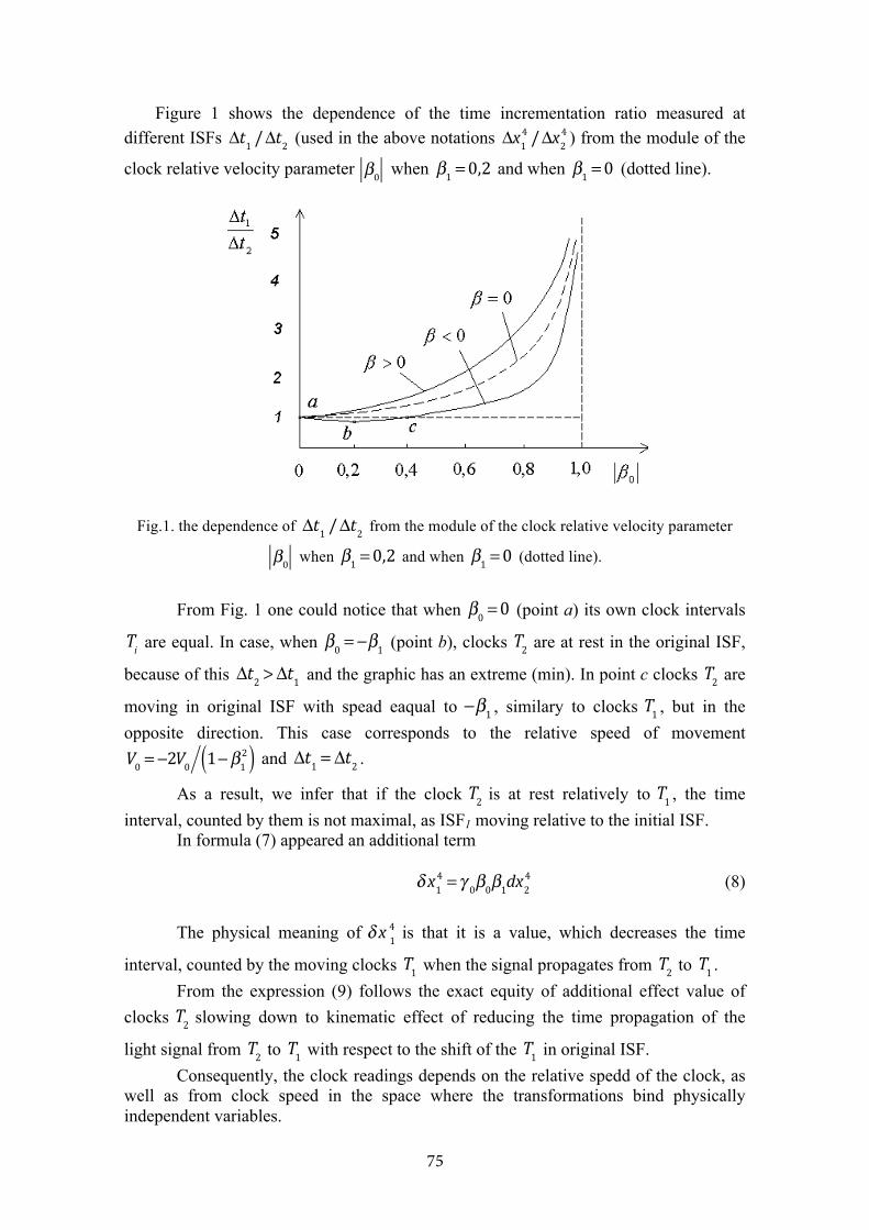
75
Figure 1 shows the dependence of the time incrementation ratio measured at different ISFs !!Δt1 /Δt2 (used in the above notations !!Δx1
4 /Δx24 ) from the module of the
clock relative velocity parameter !β0 when !β1 =0,2 and when !β1 =0 (dotted line).
Fig.1. the dependence of !!Δt1 /Δt2 from the module of the clock relative velocity parameter
!β0 when !β1 =0,2 and when !β1 =0 (dotted line).
From Fig. 1 one could notice that when !β0 =0 (point a) its own clock intervals
!Ti are equal. In case, when !β0 = −β1 (point b), clocks !!T2 are at rest in the original ISF,
because of this !!Δt2 > Δt1 and the graphic has an extreme (min). In point c clocks !!T2 are
moving in original ISF with spead eaqual to !−β1 , similary to clocks !!T1 , but in theopposite direction. This case corresponds to the relative speed of movement
!!V0 = −2V0 1−β12( ) and !!Δt1 = Δt2 .
As a result, we infer that if the clock !!T2 is at rest relatively to !!T1 , the timeinterval, counted by them is not maximal, as ISF1 moving relative to the initial ISF.
In formula (7) appeared an additional term
!!δ x14 = γ 0β0β1dx2
4 (8)
The physical meaning of !!δ x 14 is that it is a value, which decreases the time
interval, counted by the moving clocks !!T1 when the signal propagates from !!T2 to !!T1 .From the expression (9) follows the exact equity of additional effect value of
clocks !!T2 slowing down to kinematic effect of reducing the time propagation of the
light signal from !!T2 to !!T1 with respect to the shift of the !!T1 in original ISF.Consequently, the clock readings depends on the relative spedd of the clock, as
well as from clock speed in the space where the transformations bind physically independent variables.
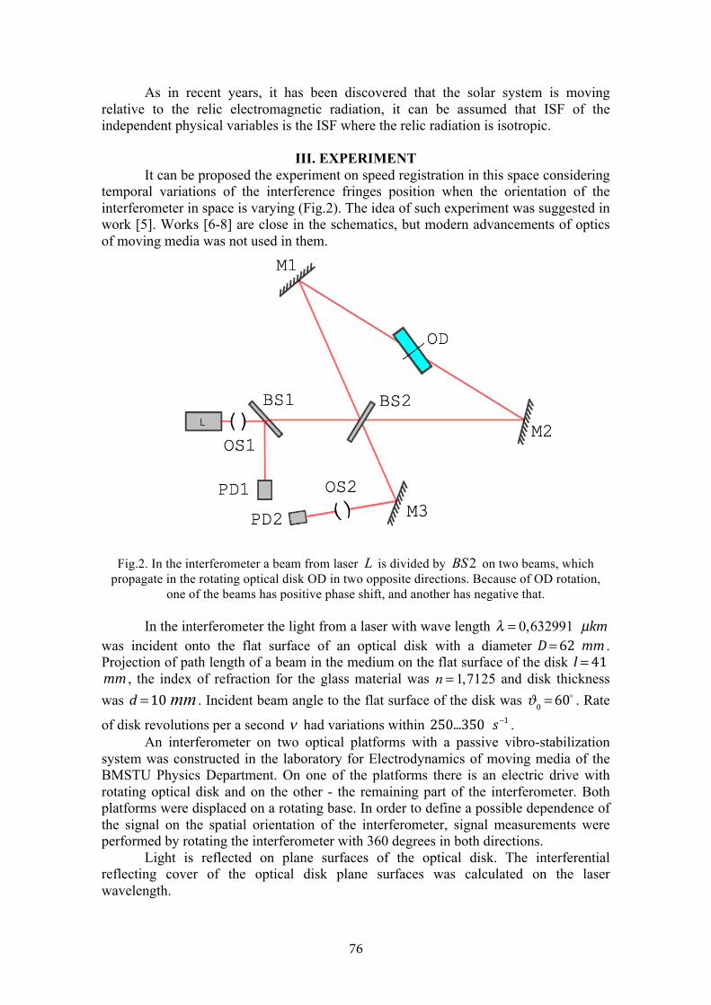
76
As in recent years, it has been discovered that the solar system is moving relative to the relic electromagnetic radiation, it can be assumed that ISF of the independent physical variables is the ISF where the relic radiation is isotropic.
III. EXPERIMENTIt can be proposed the experiment on speed registration in this space considering
temporal variations of the interference fringes position when the orientation of the interferometer in space is varying (Fig.2). The idea of such experiment was suggested in work [5]. Works [6-8] are close in the schematics, but modern advancements of optics of moving media was not used in them.
Fig.2. In the interferometer a beam from laser L is divided by BS2 on two beams, which propagate in the rotating optical disk OD in two opposite directions. Because of OD rotation,
one of the beams has positive phase shift, and another has negative that.
In the interferometer the light from a laser with wave length λ = 0,632991 !µkmwas incident onto the flat surface of an optical disk with a diameter !!D=62 !mm . Projection of path length of a beam in the medium on the flat surface of the disk !!l = 41!mm , the index of refraction for the glass material was n = 1,7125 and disk thickness was !!d =10 mm . Incident beam angle to the flat surface of the disk was ! ϑ0 =60! . Rate
of disk revolutions per a second ν had variations within !250...350 !!s−1 . An interferometer on two optical platforms with a passive vibro-stabilization
system was constructed in the laboratory for Electrodynamics of moving media of the BMSTU Physics Department. On one of the platforms there is an electric drive with rotating optical disk and on the other - the remaining part of the interferometer. Both platforms were displaced on a rotating base. In order to define a possible dependence of the signal on the spatial orientation of the interferometer, signal measurements were performed by rotating the interferometer with 360 degrees in both directions.
Light is reflected on plane surfaces of the optical disk. The interferential reflecting cover of the optical disk plane surfaces was calculated on the laser wavelength.
77
The mixing of the interference picture is defined by the change of the time of observation.
The initial transformation of signals was performed by a National Instruments analog-digital converter, and then the numerical sequence of signals order was introduced in the personal computer and further processed.
The interferometer was located into a casing with an active thermo-stabilization system. Temperature was controlled inside and outside the interferometer by three independent channels. The rotation of the interferometer was produced by a step engine and was computer-controlled. As a measuring photo detector it was chosen a high-speed Hamamatsu phototransistor.
It was estimated the variation of position of interference fringes, depending on the anisotropy parameter β.Theoretical base for this was introduced in [9].
Difference in interferometer readings when β = 0 and β ≠ 0 will be equal to
δΔ ≈ βΔ0 , (9)
where
Δ0 =cλ
(t2 − t1) = lcλω0
(k2n,2 − k2n,1) = 4lλ
β2n(n22 −1)
1− n22β2n
2 . (10)
Thus, maximal variations for the IF shift in the interferometer moving relative to the Sun with β ≅ 10−4 and with different orientations of the interferometer to velocity vector would have order of a value δΔ = ±βΔ0 = ±1,7 ×10⁻⁵ (of fringe).
Estimation for fringes shift variations in the interferometer when it rotates in space with !β ≅2,3×10⁻³ gives the magnitude order !!dΔ =2βΔΣ
− = (0,78...1,10)×10−4 (ofa fringe).
The obtained results of measurement of interference pattern shift have a view of dipole anisotropy, and direction of a dipole coincides with the direction of dipole anisotropy of the relict radiation (We mean, that Sun moves with respect background radiation in direction constellation Lion, to point with equatorial coordinates alpha = 11h 12m и delta = –7,1° (epoch J2000); Galactical coordinates l = 264,26° и b = 48,22°).
Hence, we can see from the figure that variation of position of interference
fringes in time region corresponds to !!d Δt
T⎛⎝⎜
⎞⎠⎟=2...4×10−2 . This gives estimation for β
which is more on two orders then it expects proceeding from comparison with results of measurement of relict radiation anisotropy.
Thus we can conclude that it is necessary to increase signal-noise relation and gather statistics in different seasons of a year.
So, numerical estimations shown that the reached sensibility of the interferometer in the best experiments is on the level which is needed for detecting anisotropy with the parameter !β ≅2,3×10⁻³ .
78
We introduced previous results of the experiment in which pattern shift have a view of dipole anisotropy, and direction of a dipole coincides with the direction of dipole anisotropy of the relict radiation.
REFERENCES [1]. M.V. Sazhin, “Anisotropy and polarization of cosmic microwave background: state
of the art”, UFN, 174:2 (2004), 197–205). [2]. (Hoek M. Arch. Neerl., 1868), [3]. Michelson A., Morley E.W. Influence of motion of the medium on the velocity of
light. // Am. J. Phys. 1886. V.31. 185. pp.377-386. [4]. Brillet A., Hall J.L. Improved Laser Test of the Isotropy of Space. // Phys. Rev.
Lett. 1979. V.42. 9. pp. 549 – 552. [5]. Gladyshev V.O., Gladysheva T.M., Zubarev V.Ye., Podguzov G.V. On possibility
of a new 3D experimental test of moving media electrodynamics// Physical Interpretation of Relativity Theory: Proceedings of International Meeting. – Moscow: BMSTU, 2005. – pp.202-207.
[6]. Bilger H.R. & Stowell W.K. Light drag in a ring laser: An improved determination of the drag coefficient. // Phys. Rev. A. 1977. 16 (No1), pp.313-319.
[7]. Ring laser for precision measurement of nonreciprocal phenomena / H.R.Bilger, G.E.Stedman, W.Screiber, M.Scneider // IEEE Trans. - 1995. - V. 44 IM, 2. - P. 468-470.
[8]. Sanders G.A., Ezekiel S. Mesurement of Fresnel drag in moving media using a ring resonator technique // J. Opt. Soc. Am. – 1988. – V. B5. – P. 674-678.
[9]. Gladyshev V., Gladysheva T., Zubarev V. Propagation of electromagnetic waves in complex motion media//Journal of Engineering Mathematics. 2006. V.55. No.1-4, pp.239-254.
79
WHAT IS VACUUM? AN ALGEBRAIC INVESTIGATION
Peter Rowlands
Department of Physics, University of Liverpool, Oliver Lodge Laboratory, Oxford Street, Liverpool, L69 7ZE, UK. e-mail [email protected]
Vacuum is the state which remains when a fermion, with all its special characteristics, is created out of absolutely nothing. Defining it in this way leads to a special form of relativistic quantum mechanics, which only requires the construction of a creation operator. This form of quantum mechanics is especially powerful for analytic calculation, at the same time as explaining, from first principles, many aspects of the Standard Model of particle physics. The characteristics of the weak, strong and electric interactions, in particular, can be derived from the structure of the creation operator itself.
Keywords: vacuum; nilpotent; fermion; zero totality; creation operator; Standard Model.
PACS number: 02.10.De
I. THE NILPOTENT DIRAC EQUATION
Vacuum is the state of minimum (but seemingly nonzero) energy in quantum mechanics, it is also an active component in quantum field theory, and it is the main objective of such projected unifying theories as string theory to find the particular vacuum which makes their particle structures possible. Nevertheless, vacuum is not a well-defined concept, and the reason why nature requires it at all has never been made clear. However, it is possible to show that vacuum has an exact, mathematically precise and logically satisfying meaning, and that the discovery of that meaning is a very significant step in understanding the Standard Model of particle physics. Although this understanding requires a very particular formulation of relativistic quantum mechanics, it turns out that this is the most compact and powerful formulation available and the one that leads most readily into a quantum field representation and a rich field of interpretation in particle physics.
Physics at its most fundamental level is entirely concerned with fermions and their interactions, gauge bosons being generated by such interactions. A quantum mechanical equation for the fermionic state might therefore be expected to give us a great deal of information about these interactions and related matters. The Dirac equation, in its usual form, certainly tells us how to handle the interactions in terms of calculation, but it tells us very little about their origins and distinctive characteristics. This may be partly due to the specific mathematical form of the equation, as normally used, and it may be that a greater depth of physical information may be revealed by using a mathematical structure which is more transparent and easier to manipulate. Conventionally, we write the equation in the form
0321 =⎟⎟⎠
⎞⎜⎜⎝
⎛+
∂∂+
∂∂+
∂∂+
∂∂=⎟
⎠⎞⎜
⎝⎛ +∇+
∂∂ 00 ψγγγγψγ im
zyxtim
tγ. (1)
80
where g0, g1, g2 and g3, are taken to be operators, which anticommute with each other, and with a fifth operator, g5 = ig0g1g2g3, and where
(g0)2 = (g5)2 = 1 (g1)2 = (g2)2 = (g3)2 = – 1. (2)
Usually, the g terms are taken to be 4 × 4 matrices, but this is an unnecessarily restrictive condition, and the only real requirements are that they are anticommuting operators with the multiplication properties defined in (2). In fact, since the g algebra is widely recognised as a Clifford algebra, it seems reasonable to use a more directly Cliffordian representation of the g operators, even though we could retain the g symbolism if required. The object here is not mathematical elegance but physical transparency, and so we construct an algebra which is closely related to the twistors of Penrose [1], and to Hestenes’ multivariate vectors [2]. To create a system of five anticommuting operators in an associative Clifford algebra, we need at least two commuting 3-dimensional systems of units. The simplest choice which will reflect the physical properties of the terms involved appears to be a combination of quaternions and multivariate 4-vectors. Effectively, this is equivalent to defining two vector spaces, one of which is ‘ordinary’ space; the other contains all other physical information at the fundamental and can be described as ‘vacuum’ space. The units of this algebra then become:
i j k quaternion units i j k multivariate vector units 1 scalar i pseudoscalar
The quaternions (represented by bold italic symbols) obey the usual multiplication rules i2 = j2 = k2 = ijk = –1, with a scalar term to complete the algebra, while the multivariate vectors (represented by bold symbols) are simply complexified quaternions, with the multiplication rules i2 = j2 = k2 = –iijk = 1, and a corresponding imaginary scalar (or pseudoscalar) to complete the algebra. In general, multivariate vectors a and b are distinguished from ordinary vectors by defining a full product:
ab = a.b + i a × b. (3)
The units i, j, k are isomorphic to Pauli matrices, and Hestenes and others have shown that the additional cross-product term which appears if we make the ∇ operator multivariate allows us to account for fermionic spin, even in the Schrödinger equation [1, 3]. In the Dirac equation, the same effect results from replacing g.∇ with g∇, where both g and ∇ are multivariate. Just as the complete g algebra, with all possible permutations, has 64 units (including + and – terms), and forms a group of that order, of which the five g matrices are generators, so the eight units i, j, k, 1, i, j, k, i create a group of 64 possible combinations, which can be generated by five terms which are isomorphic to the g matrices. The mappings can be done in many different ways, but all are equivalent in total structure. We will find it convenient to define two, so that we can effect a transformation:
go = -ii g1 = ik g2 = jk g3 = kk g5 = ij (4)
go = ik g1 = ii g2 = ji g3 = ki g5 = ij (5)
81
Substituting the first (4) into equation (1), we obtain
.imzyxt
i 0=⎟⎟⎠
⎞⎜⎜⎝
⎛+
∂∂+
∂∂+
∂∂+
∂∂− ψkji kkki (6)
A key move now is to multiply the equation from the left by j, at the same time altering the g representation to (5). After this transformation, the equation becomes:
.mizyxt
i 0=⎟⎟⎠
⎞⎜⎜⎝
⎛+
∂∂+
∂∂+
∂∂+
∂∂ ψjiiik kji (7)
The remarkable thing about this equation is that it is fully symmetric. For the first time, all the g terms are incorporated into the equation on the same footing. Though the 3-dimensionality of the anticommutative operators i, j, k and i, j, k makes their cyclic nature explicit, equation (7) does not depend on the algebraic representation. If we had been prepared to make the same change of representation which allows the transition from (6) to (7), we could have obtained the same result using the g notation.
03215 =⎟⎟⎠
⎞⎜⎜⎝
⎛+
∂∂+
∂∂+
∂∂+
∂∂− 0 ψγγγγγ im
zyxti
05321 =⎟⎟⎠
⎞⎜⎜⎝
⎛+
∂∂+
∂∂+
∂∂+
∂∂0 ψγγγγγ m
zyxt. (8)
Collecting the multivariate terms, for convenience, we can also write equations (7) and (8) in the form
.0=⎟⎠⎞⎜
⎝⎛ +∇+
∂∂ ψmit
i jik (9)
05 =⎟⎠⎞⎜
⎝⎛ +∇+
∂∂0 ψγγ mt
γ. (10)
Though these equations result only from algebraic transformations, they have a special physical significance. This becomes apparent when we apply a plane wave free particle solution to (9),
y = Ae–i(Et – p.r) . (11)
The result is an equation of the form
(kE + iip + ijm) Ae–i(Et – p.r) = 0.
This equation is only valid if A is either equal to (kE + iip + ijm) or a nonquaternionic multiple of it, because (kE + iip + ijm) is a nilpotent, a mathematical object that squares to zero, as in
(kE + iip + ijm) ikE + iip + ijm) = – E2 + p2 + m2 = 0. (12)
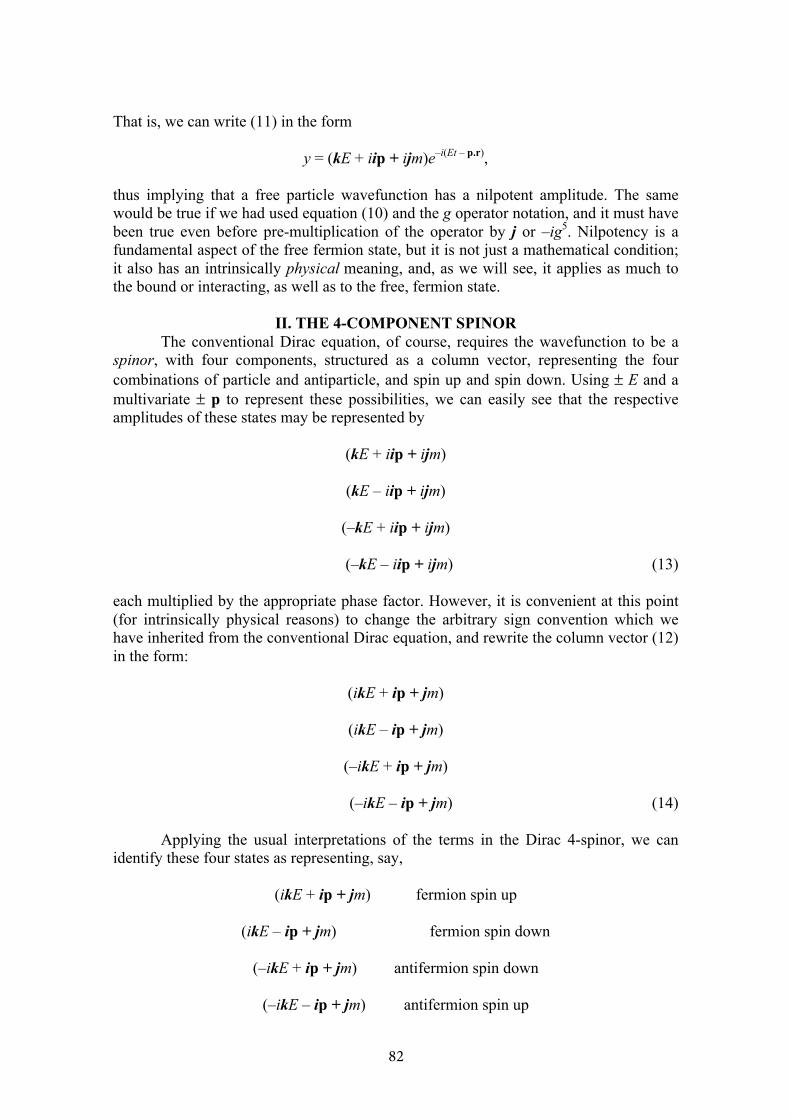
82
That is, we can write (11) in the form
y = (kE + iip + ijm)e–i(Et – p.r),
thus implying that a free particle wavefunction has a nilpotent amplitude. The same would be true if we had used equation (10) and the g operator notation, and it must have been true even before pre-multiplication of the operator by j or –ig5. Nilpotency is a fundamental aspect of the free fermion state, but it is not just a mathematical condition; it also has an intrinsically physical meaning, and, as we will see, it applies as much to the bound or interacting, as well as to the free, fermion state.
II. THE 4-COMPONENT SPINORThe conventional Dirac equation, of course, requires the wavefunction to be a
spinor, with four components, structured as a column vector, representing the four combinations of particle and antiparticle, and spin up and spin down. Using ± E and a multivariate ± p to represent these possibilities, we can easily see that the respective amplitudes of these states may be represented by
(kE + iip + ijm)
(kE – iip + ijm)
(–kE + iip + ijm)
(–kE – iip + ijm) (13)
each multiplied by the appropriate phase factor. However, it is convenient at this point (for intrinsically physical reasons) to change the arbitrary sign convention which we have inherited from the conventional Dirac equation, and rewrite the column vector (12) in the form:
(ikE + ip + jm)
(ikE – ip + jm)
(–ikE + ip + jm)
(–ikE – ip + jm) (14)
Applying the usual interpretations of the terms in the Dirac 4-spinor, we can identify these four states as representing, say,
(ikE + ip + jm) fermion spin up
(ikE – ip + jm) fermion spin down
(–ikE + ip + jm) antifermion spin down
(–ikE – ip + jm) antifermion spin up
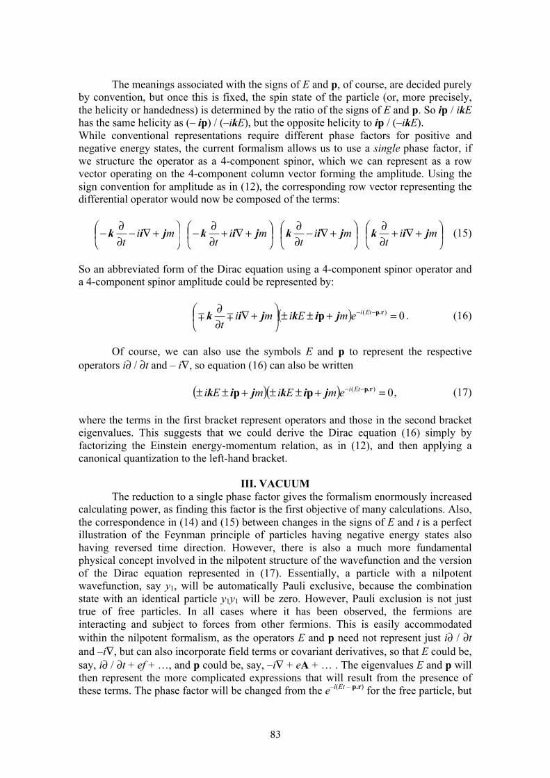
83
The meanings associated with the signs of E and p, of course, are decided purely by convention, but once this is fixed, the spin state of the particle (or, more precisely, the helicity or handedness) is determined by the ratio of the signs of E and p. So ip / ikE has the same helicity as (– ip) / (–ikE), but the opposite helicity to ip / (–ikE). While conventional representations require different phase factors for positive and negative energy states, the current formalism allows us to use a single phase factor, if we structure the operator as a 4-component spinor, which we can represent as a row vector operating on the 4-component column vector forming the amplitude. Using the sign convention for amplitude as in (12), the corresponding row vector representing the differential operator would now be composed of the terms:
⎟⎠⎞⎜
⎝⎛ +∇−
∂∂− mit
jik ⎟⎠⎞⎜
⎝⎛ +∇+
∂∂− mit
jik ⎟⎠⎞⎜
⎝⎛ +∇−
∂∂ mit
jik ⎟⎠⎞⎜
⎝⎛ +∇+
∂∂ mit
jik (15)
So an abbreviated form of the Dirac equation using a 4-component spinor operator and a 4-component spinor amplitude could be represented by:
( ) 0)( =+±±⎟⎠⎞⎜
⎝⎛ +∇
∂∂ −− p.rp EtiemEimit
jikjik ∓∓ . (16)
Of course, we can also use the symbols E and p to represent the respective operators i∂ / ∂t and – i∇, so equation (16) can also be written
( )( ) 0)( =+±±+±± −− p.rpp EtiemEimEi jikjik , (17)
where the terms in the first bracket represent operators and those in the second bracket eigenvalues. This suggests that we could derive the Dirac equation (16) simply by factorizing the Einstein energy-momentum relation, as in (12), and then applying a canonical quantization to the left-hand bracket.
III. VACUUMThe reduction to a single phase factor gives the formalism enormously increased
calculating power, as finding this factor is the first objective of many calculations. Also, the correspondence in (14) and (15) between changes in the signs of E and t is a perfect illustration of the Feynman principle of particles having negative energy states also having reversed time direction. However, there is also a much more fundamental physical concept involved in the nilpotent structure of the wavefunction and the version of the Dirac equation represented in (17). Essentially, a particle with a nilpotent wavefunction, say y1, will be automatically Pauli exclusive, because the combination state with an identical particle y1y1 will be zero. However, Pauli exclusion is not just true of free particles. In all cases where it has been observed, the fermions are interacting and subject to forces from other fermions. This is easily accommodated within the nilpotent formalism, as the operators E and p need not represent just i∂ / ∂t and –i∇, but can also incorporate field terms or covariant derivatives, so that E could be, say, i∂ / ∂t + ef + …, and p could be, say, –i∇ + eA + … . The eigenvalues E and p will then represent the more complicated expressions that will result from the presence of these terms. The phase factor will be changed from the e–i(Et – p.r) for the free particle, but
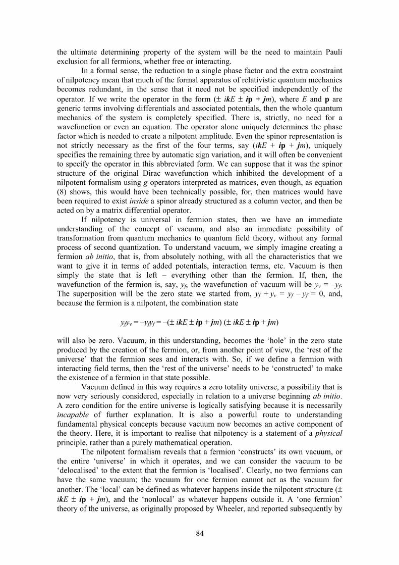
84
the ultimate determining property of the system will be the need to maintain Pauli exclusion for all fermions, whether free or interacting.
In a formal sense, the reduction to a single phase factor and the extra constraint of nilpotency mean that much of the formal apparatus of relativistic quantum mechanics becomes redundant, in the sense that it need not be specified independently of the operator. If we write the operator in the form (± ikE ± ip + jm), where E and p are generic terms involving differentials and associated potentials, then the whole quantum mechanics of the system is completely specified. There is, strictly, no need for a wavefunction or even an equation. The operator alone uniquely determines the phase factor which is needed to create a nilpotent amplitude. Even the spinor representation is not strictly necessary as the first of the four terms, say (ikE + ip + jm), uniquely specifies the remaining three by automatic sign variation, and it will often be convenient to specify the operator in this abbreviated form. We can suppose that it was the spinor structure of the original Dirac wavefunction which inhibited the development of a nilpotent formalism using g operators interpreted as matrices, even though, as equation (8) shows, this would have been technically possible, for, then matrices would have been required to exist inside a spinor already structured as a column vector, and then be acted on by a matrix differential operator.
If nilpotency is universal in fermion states, then we have an immediate understanding of the concept of vacuum, and also an immediate possibility of transformation from quantum mechanics to quantum field theory, without any formal process of second quantization. To understand vacuum, we simply imagine creating a fermion ab initio, that is, from absolutely nothing, with all the characteristics that we want to give it in terms of added potentials, interaction terms, etc. Vacuum is then simply the state that is left – everything other than the fermion. If, then, the wavefunction of the fermion is, say, yf, the wavefunction of vacuum will be yv = –yf. The superposition will be the zero state we started from, yf + yv = yf – yf = 0, and, because the fermion is a nilpotent, the combination state
yfyv = –yfyf = –(± ikE ± ip + jm) (± ikE ± ip + jm)
will also be zero. Vacuum, in this understanding, becomes the ‘hole’ in the zero state produced by the creation of the fermion, or, from another point of view, the ‘rest of the universe’ that the fermion sees and interacts with. So, if we define a fermion with interacting field terms, then the ‘rest of the universe’ needs to be ‘constructed’ to make the existence of a fermion in that state possible.
Vacuum defined in this way requires a zero totality universe, a possibility that is now very seriously considered, especially in relation to a universe beginning ab initio. A zero condition for the entire universe is logically satisfying because it is necessarily incapable of further explanation. It is also a powerful route to understanding fundamental physical concepts because vacuum now becomes an active component of the theory. Here, it is important to realise that nilpotency is a statement of a physical principle, rather than a purely mathematical operation.
The nilpotent formalism reveals that a fermion ‘constructs’ its own vacuum, or the entire ‘universe’ in which it operates, and we can consider the vacuum to be ‘delocalised’ to the extent that the fermion is ‘localised’. Clearly, no two fermions can have the same vacuum; the vacuum for one fermion cannot act as the vacuum for another. The ‘local’ can be defined as whatever happens inside the nilpotent structure (± ikE ± ip + jm), and the ‘nonlocal’ as whatever happens outside it. A ‘one fermion’ theory of the universe, as originally proposed by Wheeler, and reported subsequently by
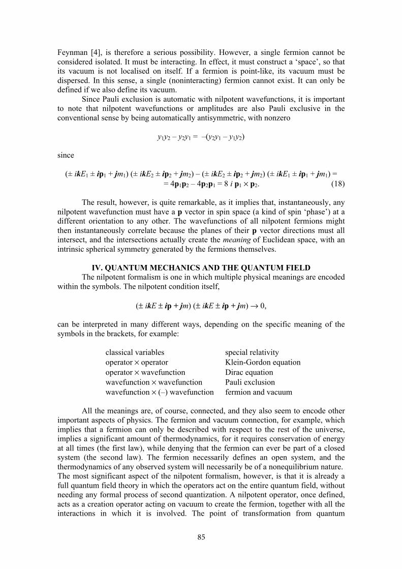
85
Feynman [4], is therefore a serious possibility. However, a single fermion cannot be considered isolated. It must be interacting. In effect, it must construct a ‘space’, so that its vacuum is not localised on itself. If a fermion is point-like, its vacuum must be dispersed. In this sense, a single (noninteracting) fermion cannot exist. It can only be defined if we also define its vacuum.
Since Pauli exclusion is automatic with nilpotent wavefunctions, it is important to note that nilpotent wavefunctions or amplitudes are also Pauli exclusive in the conventional sense by being automatically antisymmetric, with nonzero
y1y2 – y2y1 = –(y2y1 – y1y2)
since
(± ikE1 ± ip1 + jm1) (± ikE2 ± ip2 + jm2) – (± ikE2 ± ip2 + jm2) (± ikE1 ± ip1 + jm1) = = 4p1p2 – 4p2p1 = 8 i p1 × p2. (18)
The result, however, is quite remarkable, as it implies that, instantaneously, any nilpotent wavefunction must have a p vector in spin space (a kind of spin ‘phase’) at a different orientation to any other. The wavefunctions of all nilpotent fermions might then instantaneously correlate because the planes of their p vector directions must all intersect, and the intersections actually create the meaning of Euclidean space, with an intrinsic spherical symmetry generated by the fermions themselves.
IV. QUANTUM MECHANICS AND THE QUANTUM FIELDThe nilpotent formalism is one in which multiple physical meanings are encoded
within the symbols. The nilpotent condition itself,
(± ikE ± ip + jm) (± ikE ± ip + jm) → 0,
can be interpreted in many different ways, depending on the specific meaning of the symbols in the brackets, for example:
classical variables special relativity operator × operator Klein-Gordon equation operator × wavefunction Dirac equation wavefunction × wavefunction Pauli exclusion wavefunction × (–) wavefunction fermion and vacuum
All the meanings are, of course, connected, and they also seem to encode other important aspects of physics. The fermion and vacuum connection, for example, which implies that a fermion can only be described with respect to the rest of the universe, implies a significant amount of thermodynamics, for it requires conservation of energy at all times (the first law), while denying that the fermion can ever be part of a closed system (the second law). The fermion necessarily defines an open system, and the thermodynamics of any observed system will necessarily be of a nonequilibrium nature. The most significant aspect of the nilpotent formalism, however, is that it is already a full quantum field theory in which the operators act on the entire quantum field, without needing any formal process of second quantization. A nilpotent operator, once defined, acts as a creation operator acting on vacuum to create the fermion, together with all the interactions in which it is involved. The point of transformation from quantum

86
mechanics to quantum field theory is the point at which we choose to privilege the operator rather than the equation, and at which we assume that Pauli exclusion applies to all fermionic states, whether free or bound, and regardless of the number of interactions to which they are subject. No additional mathematical formalism is necessary. As we have seen, once we have taken this simple, but profound step, we no longer need an equation at all. We simply define a fermion creation operator in differential form and imagine creating it from nothing. The phase factor is simply an expression of all the possible variations in space and time which are encoded in the creation operator. This is uniquely defined once the operator is specified. A fermion is thus specified as a set of space and time variations. The mass term is purely passive, and is convenient, rather than necessary information.
The special advantage of the formalism is that it contains all the information required of a quantum field theory, while retaining the simpler structures of quantum mechanics in the conventional sense, and it is, of course, possible to use it to do quantum mechanics. Here, it is most convenient to define a probability density for a nilpotent wavefunction (± ikE ± ip + jm) by multiplication with its complex quaternion conjugate (± ikE ∓ ip – jm) (the extra ‘quaternion’ resulting from the fact that the nilpotent wavefunction differs from a conventional one through premultiplication by a quaternion operator). So the unit probability density can be defined by
( ) ( ) 122
=−±+±±E
mEiE
mEi jikjik pp ∓ ,
the 1/ E2 being a normalizing factor. If such factors are automatically assumed to apply in calculations, we can also define (± ikE ∓ ip – jm) as the ‘reciprocal’ of (± ikE ± ip + jm).
Individual calculations are also possible, in many cases using many fewer steps than by any conventional process, and sometimes also providing extra physical information. (The ease of calculation is clearly related to the fact that dual information, concerning both fermion and vacuum, is available.) We may, for example, using Dirac’s prescription [5], write down a non-time-varying nilpotent operator in polar coordinates:
( ) ⎟⎟⎠⎞
⎜⎜⎝⎛ +⎟
⎠⎞⎜
⎝⎛ +±+∂∂−→+∇− m
rji
rriEimiEi jikjik ½1 . (19)
Now, if the use of polar coordinates can be considered to represent spherical symmetry with respect to a point source, then (19) has no nilpotent solutions unless the E term also contains an expression proportional to 1 / r. In other words, simply defining a point source forces us to assume that a Coulomb interaction component is necessary for any nilpotent fermion defined with respect to it. In fact, all known forces have such components, together with an associated U(1) symmetry. For the gravitational and electric forces, it is the main or complete description; for the strong force it is the one-gluon exchange; for the weak field it is the hypercharge and the B0 gauge field. Its effect is connected purely with scale or magnitude and we can associate it with the coupling constant. The fact is, of course, well known, and the inverse square relation was connected with the 3-dimensionality of space by Kant as early as the eighteenth century, but it is not a deductive consequence of any other existing physical theory.
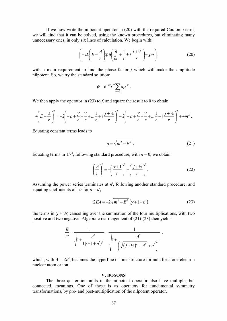
87
If we now write the nilpotent operator in (20) with the required Coulomb term, we will find that it can be solved, using the known procedures, but eliminating many unnecessary ones, in only six lines of calculation. We begin with:
.½1⎟⎟⎠⎞
⎜⎜⎝⎛ +⎟
⎠⎞⎜
⎝⎛ +±+∂∂
⎟⎠⎞⎜
⎝⎛ −± m
rji
rri
rAEi jik ∓ (20)
with a main requirement to find the phase factor f which will make the amplitude nilpotent. So, we try the standard solution:
∑=
−=0ν
νν
γφ rare ar .
We then apply the operator in (23) to f, and square the result to 0 to obtain:
.4½1...2½1...24 2222
mr
jirrr
ar
jirrr
arAE +⎟
⎠⎞⎜
⎝⎛ +−+++−−⎟
⎠⎞⎜
⎝⎛ +++++−−=⎟
⎠⎞⎜
⎝⎛ − νγνγ
Equating constant terms leads to
22 Ema −= . (21)
Equating terms in 1/r2, following standard procedure, with n = 0, we obtain:
222 ½1⎟⎠⎞⎜
⎝⎛ ++⎟
⎠⎞⎜
⎝⎛ +−=⎟
⎠⎞⎜
⎝⎛
rj
rrA γ . (22)
Assuming the power series terminates at n', following another standard procedure, and equating coefficients of 1/r for n = n',
( )nEmEA ′++−−= 122 22 γ , (23)
the terms in (j + ½) cancelling over the summation of the four multiplications, with two positive and two negative. Algebraic rearrangement of (21)-(23) then yields
( ) ( )2
22
2
2
2
½1
1
11
1
⎟⎠⎞⎜⎝
⎛ ′+−++
=
′+++
=
nAj
An
AmE
γ
,
which, with A = Ze2, becomes the hyperfine or fine structure formula for a one-electron nuclear atom or ion.
V. BOSONS The three quaternion units in the nilpotent operator also have multiple, but
connected, meanings. One of these is as operators for fundamental symmetry transformations, by pre- and post-multiplication of the nilpotent operator.
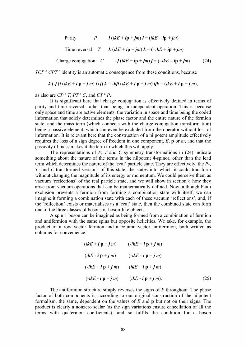
88
Parity P i (ikE + ip + jm) i = (ikE – ip + jm)
Time reversal T k (ikE + ip + jm) k = (–ikE + ip + jm)
Charge conjugation C –j (ikE + ip + jm) j = (–ikE – ip + jm) (24)
TCP º CPT º identity is an automatic consequence from these conditions, because
k (-j (i (ikE + i p + j m) i) j) k = -kji (ikE + i p + j m) ijk = (ikE + i p + j m),
as also are CP º T, PT º C, and CT º P. It is significant here that charge conjugation is effectively defined in terms of
parity and time reversal, rather than being an independent operation. This is because only space and time are active elements, the variation in space and time being the coded information that solely determines the phase factor and the entire nature of the fermion state, and the mass term (which connects with the charge conjugation transformation) being a passive element, which can even be excluded from the operator without loss of information. It is relevant here that the construction of a nilpotent amplitude effectively requires the loss of a sign degree of freedom in one component, E, p or m, and that the passivity of mass makes it the term to which this will apply.
The representations of P, T and C symmetry transformations in (24) indicate something about the nature of the terms in the nilpotent 4-spinor, other than the lead term which determines the nature of the ‘real’ particle state. They are effectively, the P-, T- and C-transformed versions of this state, the states into which it could transform without changing the magnitude of its energy or momentum. We could perceive them as vacuum ‘reflections’ of the real particle state, and we will show in section 8 how they arise from vacuum operations that can be mathematically defined. Now, although Pauli exclusion prevents a fermion from forming a combination state with itself, we can imagine it forming a combination state with each of these vacuum ‘reflections’, and, if the ‘reflection’ exists or materialises as a ‘real’ state, then the combined state can form one of the three classes of bosons or boson-like objects.
A spin 1 boson can be imagined as being formed from a combination of fermion and antifermion with the same spins but opposite helicities. We take, for example, the product of a row vector fermion and a column vector antifermion, both written as columns for convenience:
(ikE + i p + j m) (-ikE + i p + j m)
(ikE - i p + j m) (-ikE - i p + j m)
(-ikE + i p + j m) (ikE + i p + j m)
(-ikE - i p + j m) (ikE - i p + j m). (25)
The antifermion structure simply reverses the signs of E throughout. The phase factor of both components is, according to our original construction of the nilpotent formalism, the same, dependent on the values of E and p but not on their signs. The product is clearly a nonzero scalar (as the sign variations ensure cancellation of all the terms with quaternion coefficients), and so fulfils the condition for a boson
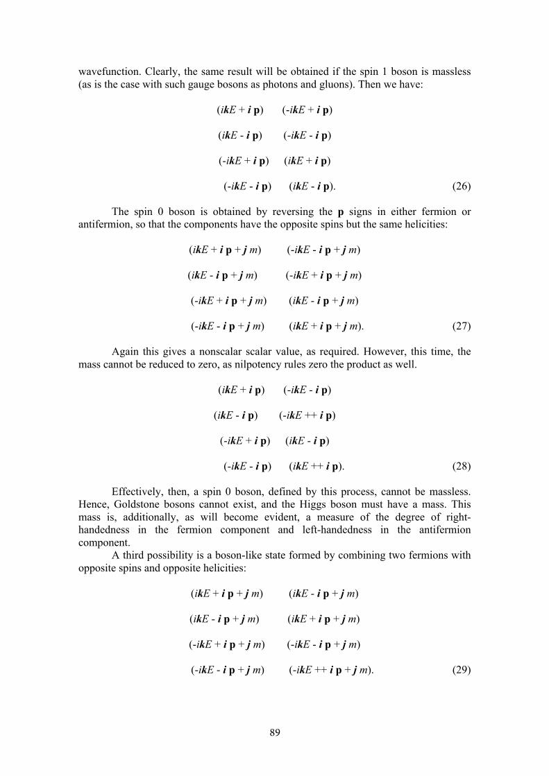
89
wavefunction. Clearly, the same result will be obtained if the spin 1 boson is massless (as is the case with such gauge bosons as photons and gluons). Then we have:
(ikE + i p) (-ikE + i p)
(ikE - i p) (-ikE - i p)
(-ikE + i p) (ikE + i p)
(-ikE - i p) (ikE - i p). (26)
The spin 0 boson is obtained by reversing the p signs in either fermion or antifermion, so that the components have the opposite spins but the same helicities:
(ikE + i p + j m) (-ikE - i p + j m)
(ikE - i p + j m) (-ikE + i p + j m)
(-ikE + i p + j m) (ikE - i p + j m)
(-ikE - i p + j m) (ikE + i p + j m). (27)
Again this gives a nonscalar scalar value, as required. However, this time, the mass cannot be reduced to zero, as nilpotency rules zero the product as well.
(ikE + i p) (-ikE - i p)
(ikE - i p) (-ikE ++ i p)
(-ikE + i p) (ikE - i p)
(-ikE - i p) (ikE ++ i p). (28)
Effectively, then, a spin 0 boson, defined by this process, cannot be massless. Hence, Goldstone bosons cannot exist, and the Higgs boson must have a mass. This mass is, additionally, as will become evident, a measure of the degree of right-handedness in the fermion component and left-handedness in the antifermion component.
A third possibility is a boson-like state formed by combining two fermions with opposite spins and opposite helicities:
(ikE + i p + j m) (ikE - i p + j m)
(ikE - i p + j m) (ikE + i p + j m)
(-ikE + i p + j m) (-ikE - i p + j m)
(-ikE - i p + j m) (-ikE ++ i p + j m). (29)
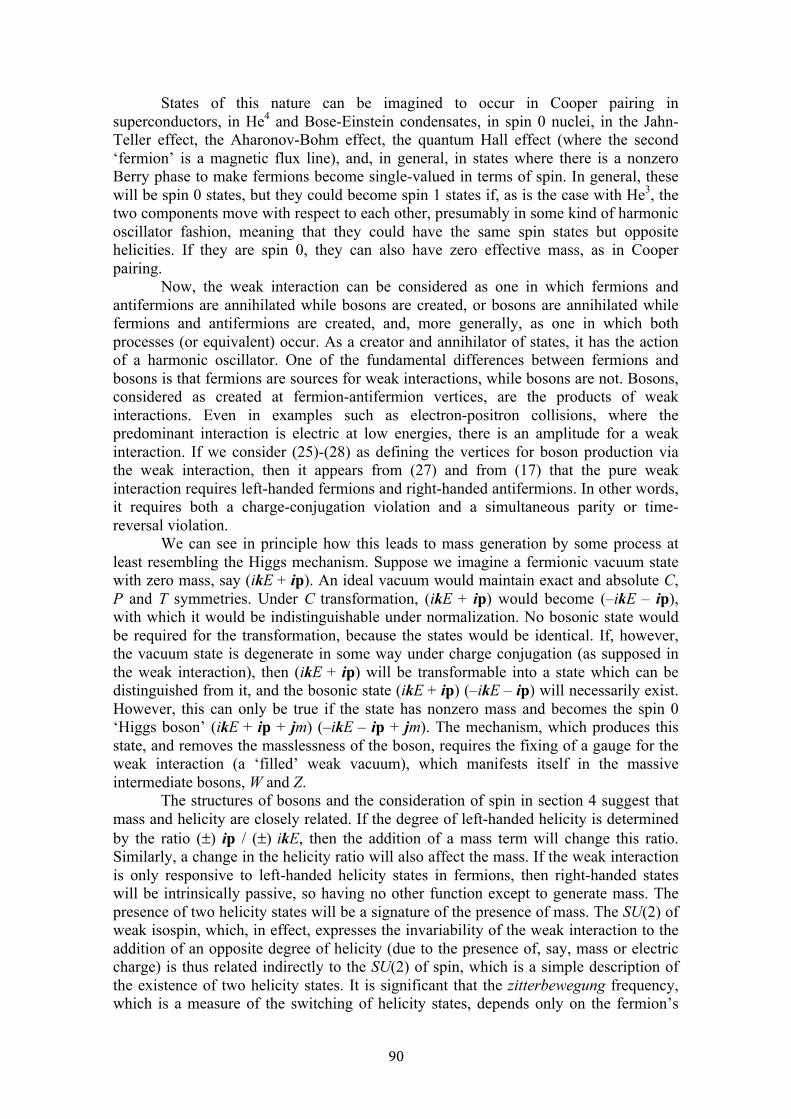
90
States of this nature can be imagined to occur in Cooper pairing in superconductors, in He4 and Bose-Einstein condensates, in spin 0 nuclei, in the Jahn-Teller effect, the Aharonov-Bohm effect, the quantum Hall effect (where the second ‘fermion’ is a magnetic flux line), and, in general, in states where there is a nonzero Berry phase to make fermions become single-valued in terms of spin. In general, these will be spin 0 states, but they could become spin 1 states if, as is the case with He3, the two components move with respect to each other, presumably in some kind of harmonic oscillator fashion, meaning that they could have the same spin states but opposite helicities. If they are spin 0, they can also have zero effective mass, as in Cooper pairing.
Now, the weak interaction can be considered as one in which fermions and antifermions are annihilated while bosons are created, or bosons are annihilated while fermions and antifermions are created, and, more generally, as one in which both processes (or equivalent) occur. As a creator and annihilator of states, it has the action of a harmonic oscillator. One of the fundamental differences between fermions and bosons is that fermions are sources for weak interactions, while bosons are not. Bosons, considered as created at fermion-antifermion vertices, are the products of weak interactions. Even in examples such as electron-positron collisions, where the predominant interaction is electric at low energies, there is an amplitude for a weak interaction. If we consider (25)-(28) as defining the vertices for boson production via the weak interaction, then it appears from (27) and from (17) that the pure weak interaction requires left-handed fermions and right-handed antifermions. In other words, it requires both a charge-conjugation violation and a simultaneous parity or time-reversal violation.
We can see in principle how this leads to mass generation by some process at least resembling the Higgs mechanism. Suppose we imagine a fermionic vacuum state with zero mass, say (ikE + ip). An ideal vacuum would maintain exact and absolute C, P and T symmetries. Under C transformation, (ikE + ip) would become (–ikE – ip), with which it would be indistinguishable under normalization. No bosonic state would be required for the transformation, because the states would be identical. If, however, the vacuum state is degenerate in some way under charge conjugation (as supposed in the weak interaction), then (ikE + ip) will be transformable into a state which can be distinguished from it, and the bosonic state (ikE + ip) (–ikE – ip) will necessarily exist. However, this can only be true if the state has nonzero mass and becomes the spin 0 ‘Higgs boson’ (ikE + ip + jm) (–ikE – ip + jm). The mechanism, which produces this state, and removes the masslessness of the boson, requires the fixing of a gauge for the weak interaction (a ‘filled’ weak vacuum), which manifests itself in the massive intermediate bosons, W and Z.
The structures of bosons and the consideration of spin in section 4 suggest that mass and helicity are closely related. If the degree of left-handed helicity is determined by the ratio (±) ip / (±) ikE, then the addition of a mass term will change this ratio. Similarly, a change in the helicity ratio will also affect the mass. If the weak interaction is only responsive to left-handed helicity states in fermions, then right-handed states will be intrinsically passive, so having no other function except to generate mass. The presence of two helicity states will be a signature of the presence of mass. The SU(2) of weak isospin, which, in effect, expresses the invariability of the weak interaction to the addition of an opposite degree of helicity (due to the presence of, say, mass or electric charge) is thus related indirectly to the SU(2) of spin, which is a simple description of the existence of two helicity states. It is significant that the zitterbewegung frequency, which is a measure of the switching of helicity states, depends only on the fermion’s
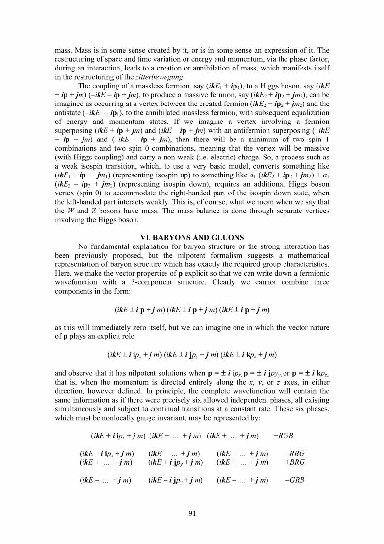
91
mass. Mass is in some sense created by it, or is in some sense an expression of it. The restructuring of space and time variation or energy and momentum, via the phase factor, during an interaction, leads to a creation or annihilation of mass, which manifests itself in the restructuring of the zitterbewegung.
The coupling of a massless fermion, say (ikE1 + ip1), to a Higgs boson, say (ikE + ip + jm) (–ikE – ip + jm), to produce a massive fermion, say (ikE2 + ip2 + jm2), can be imagined as occurring at a vertex between the created fermion (ikE2 + ip2 + jm2) and the antistate (–ikE1 – ip1), to the annihilated massless fermion, with subsequent equalization of energy and momentum states. If we imagine a vertex involving a fermion superposing (ikE + ip + jm) and (ikE – ip + jm) with an antifermion superposing (–ikE + ip + jm) and (–ikE – ip + jm), then there will be a minimum of two spin 1 combinations and two spin 0 combinations, meaning that the vertex will be massive (with Higgs coupling) and carry a non-weak (i.e. electric) charge. So, a process such as a weak isospin transition, which, to use a very basic model, converts something like (ikE1 + ip1 + jm1) (representing isospin up) to something like a1 (ikE2 + ip2 + jm2) + a1 (ikE2 – ip2 + jm2) (representing isospin down), requires an additional Higgs boson vertex (spin 0) to accommodate the right-handed part of the isospin down state, when the left-handed part interacts weakly. This is, of course, what we mean when we say that the W and Z bosons have mass. The mass balance is done through separate vertices involving the Higgs boson.
VI. BARYONS AND GLUONSNo fundamental explanation for baryon structure or the strong interaction has
been previously proposed, but the nilpotent formalism suggests a mathematical representation of baryon structure which has exactly the required group characteristics. Here, we make the vector properties of p explicit so that we can write down a fermionic wavefunction with a 3-component structure. Clearly we cannot combine three components in the form:
(ikE ± i p + j m) (ikE ± i p + j m) (ikE ± i p + j m)
as this will immediately zero itself, but we can imagine one in which the vector nature of p plays an explicit role
(ikE ± i ipx + j m) (ikE ± i jpy + j m) (ikE ± i kpz + j m)
and observe that it has nilpotent solutions when p = ± i ipx, p = ± i jpyy, or p = ± i kpz.,that is, when the momentum is directed entirely along the x, y, or z axes, in either direction, however defined. In principle, the complete wavefunction will contain the same information as if there were precisely six allowed independent phases, all existing simultaneously and subject to continual transitions at a constant rate. These six phases, which must be nonlocally gauge invariant, may be represented by:
(ikE + i ipx + j m) (ikE + ... + j m) (ikE + ... + j m) +RGB
(ikE – i ipx + j m) (ikE – ... + j m) (ikE – ... + j m) –RBG(ikE + ... + j m) (ikE + i jpy + j m) (ikE + ... + j m) +BRG
(ikE – ... + j m) (ikE – i jpy + j m) (ikE – ... + j m) –GRB
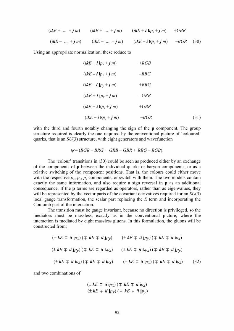
92
(ikE + ... + j m) (ikE + ... + j m) (ikE + i kpz + j m) +GBR
(ikE – ... + j m) (ikE – ... + j m) (ikE – i kpz + j m) –BGR (30)
Using an appropriate normalization, these reduce to
(ikE + i ipx + j m) +RGB
(ikE – i ipx + j m) –RBG
(ikE – i jpy + j m) +BRG
(ikE + i jpy + j m) –GRB
(ikE + i kpz + j m) +GBR
(ikE – i kpz + j m) –BGR (31)
with the third and fourth notably changing the sign of the p component. The group structure required is clearly the one required by the conventional picture of ‘coloured’ quarks, that is an SU(3) structure, with eight generators and wavefunction
ψ ~ (BGR – BRG + GRB – GBR + RBG – RGB).
The ‘colour’ transitions in (30) could be seen as produced either by an exchange of the components of p between the individual quarks or baryon components, or as a relative switching of the component positions. That is, the colours could either move with the respective px, py, pz components, or switch with them. The two models contain exactly the same information, and also require a sign reversal in p as an additional consequence. If the p terms are regarded as operators, rather than as eigenvalues, they will be represented by the vector parts of the covariant derivatives required for an SU(3) local gauge transformation, the scalar part replacing the E term and incorporating the Coulomb part of the interaction.
The transition must be gauge invariant, because no direction is privileged, so the mediators must be massless, exactly as in the conventional picture, where the interaction is mediated by eight massless gluons. In this formulation, the gluons will be constructed from:
(± kE ∓ ii ipx) (∓ kE ∓ ii jpy) (± kE ∓ ii jpy) (∓ kE ∓ ii ipx)
(± kE ∓ ii jpy) (∓ kE ∓ ii kpz) (± kE ∓ ii kpz) (∓ kE ∓ ii jpy)
(± kE ∓ ii ipz) (∓ kE ∓ ii ipx) (± kE ∓ ii ipx) (∓ kE ∓ ii ipz) (32)
and two combinations of
(± kE ∓ ii ipx) (∓ kE ∓ ii ipx) (± kE ∓ ii jpy) (∓ kE ∓ ii jpy)
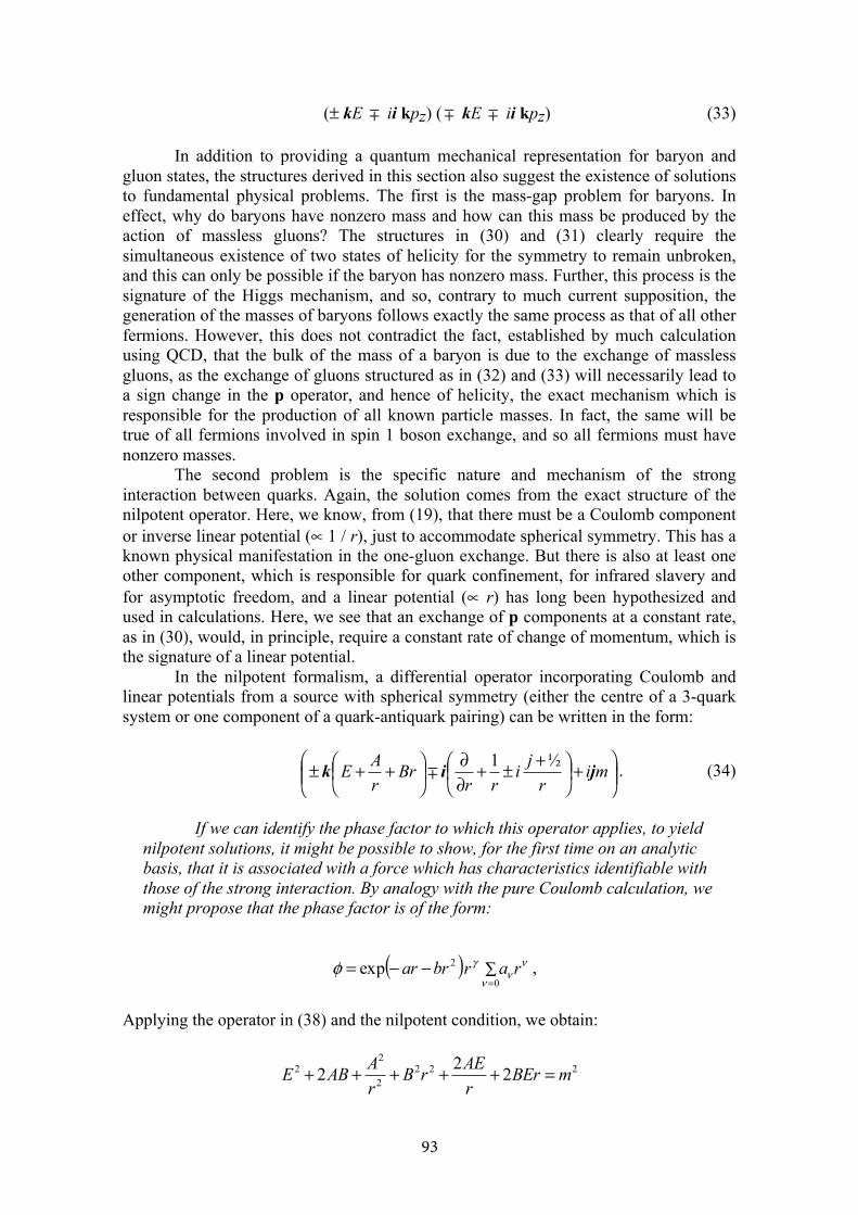
93
(± kE ∓ ii kpz) (∓ kE ∓ ii kpz) (33)
In addition to providing a quantum mechanical representation for baryon and gluon states, the structures derived in this section also suggest the existence of solutions to fundamental physical problems. The first is the mass-gap problem for baryons. In effect, why do baryons have nonzero mass and how can this mass be produced by the action of massless gluons? The structures in (30) and (31) clearly require the simultaneous existence of two states of helicity for the symmetry to remain unbroken, and this can only be possible if the baryon has nonzero mass. Further, this process is the signature of the Higgs mechanism, and so, contrary to much current supposition, the generation of the masses of baryons follows exactly the same process as that of all other fermions. However, this does not contradict the fact, established by much calculation using QCD, that the bulk of the mass of a baryon is due to the exchange of massless gluons, as the exchange of gluons structured as in (32) and (33) will necessarily lead to a sign change in the p operator, and hence of helicity, the exact mechanism which is responsible for the production of all known particle masses. In fact, the same will be true of all fermions involved in spin 1 boson exchange, and so all fermions must have nonzero masses.
The second problem is the specific nature and mechanism of the strong interaction between quarks. Again, the solution comes from the exact structure of the nilpotent operator. Here, we know, from (19), that there must be a Coulomb component or inverse linear potential (∝ 1 / r), just to accommodate spherical symmetry. This has a known physical manifestation in the one-gluon exchange. But there is also at least one other component, which is responsible for quark confinement, for infrared slavery and for asymptotic freedom, and a linear potential (∝ r) has long been hypothesized and used in calculations. Here, we see that an exchange of p components at a constant rate, as in (30), would, in principle, require a constant rate of change of momentum, which is the signature of a linear potential.
In the nilpotent formalism, a differential operator incorporating Coulomb and linear potentials from a source with spherical symmetry (either the centre of a 3-quark system or one component of a quark-antiquark pairing) can be written in the form:
⎟⎟⎠⎞
⎜⎜⎝⎛ +⎟
⎠⎞⎜
⎝⎛ +±+∂∂
⎟⎠⎞⎜
⎝⎛ ++± mi
rji
rrBr
rAE jik ½1
∓ . (34)
If we can identify the phase factor to which this operator applies, to yield nilpotent solutions, it might be possible to show, for the first time on an analytic basis, that it is associated with a force which has characteristics identifiable with those of the strong interaction. By analogy with the pure Coulomb calculation, we might propose that the phase factor is of the form:
( ) ∑=
−−=0
2expν
νν
γφ rarbrar ,
Applying the operator in (38) and the nilpotent condition, we obtain:
2222
22 222 mBEr
rAErB
rAABE =+++++
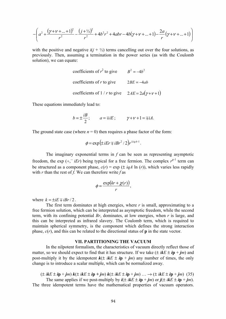
94
( ) ( ) ( ) ( )⎟⎟⎠⎞
⎜⎜⎝
⎛+++−+++−++++++− −+ 1...21...444½1... 22
2
2
2
22 νγνγνγ
rababrrb
rj
ra
with the positive and negative i(j + ½) terms cancelling out over the four solutions, as previously. Then, assuming a termination in the power series (as with the Coulomb solution), we can equate:
coefficients of r2 to give 22 4bB −=
coefficients of r to give abBE 42 −=
coefficients of 1 / r to give ( )122 ++= νγaAE
These equations immediately lead to:
2iBb ±= ; iEa ∓= ; iA∓=++ 1νγ .
The ground state case (where n = 0) then requires a phase factor of the form:
( ) 12 2exp / −±= iqAriBriEr ∓∓φ .
The imaginary exponential terms in f can be seen as representing asymptotic freedom, the exp (+,– iEr) being typical for a free fermion. The complex rg-1 term canbe structured as a component phase, c(r) = exp (± iqA ln (r)), which varies less rapidly with r than the rest of f. We can therefore write f as
( )r
rkr )(exp χφ += ,
where 2/iBriEk ∓±= . The first term dominates at high energies, where r is small, approximating to a
free fermion solution, which can be interpreted as asymptotic freedom, while the second term, with its confining potential Br, dominates, at low energies, when r is large, and this can be interpreted as infrared slavery. The Coulomb term, which is required to maintain spherical symmetry, is the component which defines the strong interaction phase, c(r), and this can be related to the directional status of p in the state vector.
VII. PARTITIONING THE VACUUMIn the nilpotent formalism, the characteristics of vacuum directly reflect those of
matter, so we should expect to find that it has structure. If we take (± ikE ± ip + jm) and post-multiply it by the idempotent k(± ikE ± ip + jm) any number of times, the only change is to introduce a scalar multiple, which can be normalized away.
(± ikE ± ip + jm) k(± ikE ± ip + jm) k(± ikE ± ip + jm) … → (± ikE ± ip + jm) (35) The same applies if we post-multiply by i(± ikE ± ip + jm) or j(± ikE ± ip + jm).
The three idempotent terms have the mathematical properties of vacuum operators.
95
However, another way of looking at (35) is to apply a time-reversal transformation to every even (± ikE ± ip + jm). Then we have
(± ikE ± ip + jm) (∓ ikE ± ip + jm) (± ikE ± ip + jm) … → (± ikE ± ip + jm) (36)
with every even bracket becoming an antifermion, or combining with the original fermion state to become a spin 1 boson (± ikE ± ip + jm) (∓ kE ± ip + jm).
The same process can be applied using i(± ikE ± ip + jm) and j(± ikE ± ip + jm), and the result is that, from an initial fermion state, we generate either three vacuum reflections, via respective T, P and C transformations, which represent antifermion with the same spin, fermion with opposite spin, and antifermion with opposite spin, or combined particle-vacuum states which have the respective structures of spin 1 bosons, spin 0 bosons, or boson-like paired fermion (PF) combinations of the same kind as constitute Cooper pairs and the elements of Bose-Einstein condensates. Using just the lead terms of the nilpotents, we could represent these as:
(ikE + ip + jm) k (ikE + ip + jm) k (ikE + ip + jm) k (ikE + ip + jm) … T (ikE + ip + jm) (–ikE + ip + jm) (ikE + ip + jm) (–ikE + ip + jm) … spin 1
(ikE + ip + jm) j (ikE + ip + jm) j (ikE + ip + jm) j (ikE + ip + jm) … P (ikE + ip + jm) (– ikE – ip + jm) (ikE + ip + jm) (– ikE – ip + jm) … spin 0
(ikE + ip + jm) i (ikE + ip + jm) i (ikE + ip + jm) i (ikE + ip + jm) … C (ikE + ip + jm) (ikE – ip + jm) (ikE + ip + jm) (ikE – ip + jm) … PF (37)
So, we can repeatedly post-multiply a fermion operator by any of the discrete idempotent vacuum operators, creating an alternate series of antifermion and fermion vacuum states, or, equivalently, an alternate series of boson and fermion states without changing the character of the real particle state. Essentially a fermion produces a boson state by combining with its own vacuum image, and the two states form a supersymmetric partnership. Nilpotent operators are thus intrinsically supersymmetric, with supersymmetry operators typically of the form:
Boson to fermion: Q = ( )mEi jik +±± p
Fermion to boson: Q† = ( )mEi jik +± p∓
A fermion converts to a boson by multiplication by an antifermionic operator; a boson converts to a fermion by multiplication by a fermionic operator, and we could represent the first sequence in (41) by the supersymmetric
Q Q† Q Q† Q Q† Q Q† Q …
We can choose to interpret this as the series of boson and fermion loops, of the same energy and momentum, required by the exact supersymmetry which would eliminate the need for renormalization, and remove the hierarchy problem altogether. Fermions and bosons (with the same values E, p and m) become their own supersymmetric partners through the creation of vacuum states, making the hypothesis

96
of a set of real supersymmetric particles to solve the hierarchy problem entirely superfluous.
The identification of i(ikE + ip + jm), k(ikE + ip + jm) and j(ikE + ip + jm) as vacuum operators and (ikE – ip + jm), (–ikE + ip + jm) and (–ikE – ip + jm) as their respective vacuum ‘reflections’ at interfaces provided by P, T and C transformations suggests a new insight into the meaning of the Dirac 4-spinor. With the extra knowledge we have now gained, we can interpret the three terms other than the lead term in the spinor as the vacuum ‘reflections’ that are created with the particle. We can regard the existence of three vacuum operators as a result of a partitioning of the vacuum as a result of quantization and as a consequence of the 3-part structure observed in the nilpotent fermionic state, while the zitterbewegung can be taken as an indication that the vacuum is active in defining the fermionic state.
Taken together, the four components of the spinor cancel exactly. The four components can be represented as creation operators for
fermion spin up (ikE + ip + jm)
fermion spin down (ikE – ip + jm)
antifermion spin down (–ikE + ip + jm)
antifermion spin up (–ikE – ip + jm)
or annihilation operators for
antifermion spin down (ikE + ip + jm)
antifermion spin up (ikE – ip + jm)
fermion spin up (–ikE + ip + jm)
fermion spin down (–ikE – ip + jm)
They could equally well be regarded as two operators for creation and two for annihilation, for example:
fermion spin up creation (ikE + ip + jm)
fermion spin down creation (ikE – ip + jm)
fermion spin up annihilation (–ikE + ip + jm)
fermion spin down annihilation (–ikE – ip + jm)
Either way, the cancellation is exact, both physically, and algebraically (when we use the discrete operators which leave out the passive mass component). It is interesting that the cancellation requires four components, rather than two, for, while the transitions:
(ikE + ip + jm) → (ikE – ip + jm) and (ikE + ip + jm) → (–ikE + ip + jm)
97
can occur through spin 1 boson and spin 0 paired fermion exchange, and the active space and time components, there is no process in nature for the direct transition:
(ikE + ip + jm) → (–ikE – ip + jm)
with no active component as agent. In this context, it might be worth noting that the spin 0 fermion-fermion state
(ikE + ip + jm) (ikE – ip + jm)
is such as would be required in a pure weak transition from –ikE to + ikE, or its inverse. Because the formation of the spin 0 state necessarily requires intrinsically massive components, even in those cases where it assumes nonzero effective mass through a Fermi velocity less than c, time reversal symmetry (the one applicable to the transition) must be broken in the weak formation or decay of such states. The most likely opportunity of observing such a process might be in one of the physical manifestations of the nonzero Berry phase, say the quantum Hall effect, in some special type of condensed matter such as graphene. Here, the conduction electrons have zero effective mass and a Hamiltonian that can be written in the form ± vFi(ipx + jpy), where vF is the Fermi velocity. We can imagine creating a boson-like state with single-valued spin by the quantum Hall effect, Aharonov-Bohm effect, or Bose-Einstein condensation, and then observing, perhaps through a change in the Fermi velocity during its decay, the violation of both P and CP = T symmetries.
VIII. WEAK INTERACTIONSSo far, we have been able to show that two fundamental interactions are intrinsic
to the definition of the fermionic state, and not something external imposed upon it. The Coulomb interaction, as we see from (20), is the direct product of spherical symmetry being applied at the same time as nilpotency. Since it is purely an expression of the magnitude of a scalar phase, all the terms in the nilpotent contribute, but only one, the passive (scalar) mass term, contributes to nothing else. An interaction with this precise property may therefore be defined, and it is the one we define as the electric interaction. At the same time, the strong interaction, with its characteristic linear potential, can be represented as we have seen, by the vector properties of the p term. However, yet another interaction seems to be required by the spinor structure of the nilpotent operator, and the associated phenomenon of zitterbewegung. While the co-existence of two spin states is, in some sense, real, and is accounted for by the presence of mass, the co-existence of two energy states is only meaningful in the context of the simultaneous existence of fermion and vacuum. While the transitions between the two energy states may be virtual, in this sense, the zitterbewegung would seem to require the production of an intermediate bosonic state at a vertex where one fermionic state is annihilated and another is created to replace by it. This behaviour is, of course, characteristic of the weak interaction, and, in this sense, we can say that the weak interaction, like the electric and strong interactions, is built into the structure of the nilpotent operator.
The weak interaction is clearly related to the nature of the pseudoscalar iE operator, whose sign uniquely determines the helicity of a weakly interacting particle, or more specifically its weakly interacting component. It also has a unique feature, in that its fermionic source cannot be separated from its vacuum partner. A fermion or antifermion cannot be created or annihilated, even with an antifermionic or fermionic partner, unless its vacuum is simultaneously annihilated or created. In this sense, the
98
weak source has a manifestly dipolar nature, whose immediate manifestation is the fermion’s ½-integral spin. This, then, leads to the question of whether we can derive an analytic expression from the nilpotent operator which will explain the special characteristics of this force. To answer this, it will be convenient to answer a more general question: what nilpotent solutions are available for an operator including a Coulomb potential together with any other potential which is a function of distance from a point source with spherical symmetry, other than the linear potential characteristic of the strong interaction?
We will assume that the nilpotent operator takes a form such as
⎟⎟⎠⎞
⎜⎜⎝⎛ +⎟
⎠⎞⎜
⎝⎛ +±+∂∂+⎟
⎠⎞⎜
⎝⎛ −− mi
rji
rrCr
rAE n jik ½1 . (38)
where n is an integer greater than 1 or less than –1, and, as usual, look for a phase factor which will make the amplitude nilpotent. Again, we will work from the basis of the Coulomb solution, with the additional information that polynomial potential terms which are multiples of rn require the incorporation into the exponential of terms which are multiples of rn+1. So, extending our work on the Coulomb solution, we may suppose that the phase factor is of the form:
( ) ∑−−==
+
0
1expν
νν
γφ rarbrar n
Applying the operator and squaring to zero, with a termination in the series, we obtain
( )22 ½1124 ⎟⎠⎞⎜
⎝⎛ +++++++−−=⎟
⎠⎞⎜
⎝⎛ −−
rji
rrrbrnaCr
rAE nn νγ
( )2½112 ⎟⎠⎞⎜
⎝⎛ +−+++++−−
rji
rrrbrna n νγ
Equating constant terms, we find
a = m2 – E2 (39)
Equating terms in r2n, with n = 0:
C2 = – (n + 1)2 b2
Equating coefficients of r, where n = 0:
AC = – (n + 1) b (1 + g) ,
(1 + g) = ± iA .
Equating coefficients of 1 / r2 and coefficients of 1 / r, for a power series terminating in n = n', we obtain
99
A2 = – (1 + g + n')2 + (j + ½)2 (40)
And
– EA = a (1 + g + n'). (41)
Combining (46), (47) and (48) produces:
( ) ( ) ( )2222
22
½11 ++′++−=′++⎟⎟⎠
⎞⎜⎜⎝
⎛ − jnnE
Em γγ
( )niAjmE ′+±+
−=½
. (42)
Equation (49) has the form of a harmonic oscillator, with evenly spaced energy levels deriving from integral values of n'. If we make the additional assumption that A, the phase term required for spherical symmetry, has some connection with the random directionality of the fermion spin, we might assign to it a half-unit value (± ½ i), and obtain the complete formula for the fermionic simple harmonic oscillator:
( )njmE ′++
−= ½½
. (43)
Whether or not this assumption is valid, equation (42) demonstrates that the additional potential of the form Crn, where n is an integer greater than 1 or less than –1, has the effect of creating a harmonic oscillator solution for the nilpotent operator, irrespective of the value of n, and, in fact, we can show that any polynomial sum of potentials of this form will produce the same result. Such potentials emerge from any system in which there is complexity, aggregation, or a multiplicity of sources, even if the individual sources have Coulomb or linear potentials. In the case of a dipolar weak sources, there will be a minimum extra term of the form Cr–3, and so we can say that (49) provides the correct characteristics for the weak interaction from the kind of potential that weak sources must necessarily produce. In addition, because this solution is exclusive for distance related potentials of the form Crn, except where r = 1 or –1, we have also, in effect, shown that a fermion interaction specified in relation to a spherically symmetric point source has only three physical manifestations, and that these are the ones associated with the electric (or other pure Coulomb), strong and weak interactions.
IX. VACUUM PARTITIONS AND SOURCESIn the previous section, we have seen that the nilpotent operator (± ikE ± ip +
jm), with its three components, iE, p and m, separated by three quaternion units k, i and j, is a source of interactions with the characteristics we describe as weak, strong and electric, through its own structure. We have also identified the origins of these interactions in the structures of the components. All the interactions contribute to the mass and dual spin state, and the magnitudes of all three terms, but only the weak interaction identifies the energy state or the sign attached to the pseudoscalar component iE, and the active direction of handedness, and only the strong interaction can respond to the vector or directional aspect of p. The electric interaction is distinguishable by
100
only responding to the magnitude scale in the same way as m. It may be significant here that the Kaluza-Klein theory, which effectively introduces a fifth dimension with a U(1) symmetry, which has a similar role to that played by mass in the nilpotent structure, is actually two separate theories with the respective aims of explaining the origins of mass and electric charge.
In principle, the association of the three quaternion units with objects with different mathematical properties, which are themselves connected with the physical parameters time, space and mass, suggests that the vacuum partitions responding to the operators k(± ikE ± ip + jm), i(± ikE ± ip + jm) and j(± ikE ± ip + jm) are to some extent those which create the physical effects connected with the respective weak, strong and electric interactions, and that the units k, i and j, to this extent, act as the sources. The object of these ‘sources’ is then to create the vacuum partitions that lead to the physical manifestations of the interactions in individual nilpotent structures. Of course, this picture takes no account of gravity, but it is yet to be established that gravity is a local force, like the others, or that it is determined by discrete sources. It is just as likely that it is a vacuum effect, ‘disguised’ as a local force by the inertial effect which it inevitably produces. The universal ubiquity, negative energy and positive norm of the coupling constant suggest fundamental differences with respect to the other interactions. In this case, the vacuum for gravity could be ±1(± ikE ± ip + jm), equivalent to the first term in the nilpotent. Clearly, there are significant aspects of gravity yet to be explained, in particular, dark matter and dark energy, and it is not yet established whether a quantum theory of gravity is actually possible. Further exploration of the vacuum can be expected to lead to a greater understanding of this difficult matter.
In addition to gravity, string theory has already been mentioned as an area where vacuum has a significantly active role. A perfect string theory is believed to be one in which self-duality in phase space determines vacuum selection. Interestingly, the nilpotent (± ikE ± ip + jm) is an object which has all these required characteristics. It also has a ‘10-dimensional’ structure in that the 5 ‘dimensions’ of E, p, m are paralleled by the 5 source terms, k, 3 × i terms, and j; and 6 of these (all but E and p) are conserved quantities, and, in that sense, ’compacted’. It may be that an exploration of vacuum in these terms might also produce significant results in particle structures.
X. CONCLUSION Vacuum is identified in this paper as the state that remains when a fermion is
created out of absolutely nothing. It is an existence condition, like conservation of energy, which must apply irrespective of our knowledge of how it is constructed, and it can be defined with exact mathematical precision. Like other existence conditions, the mathematical definition of the nilpotent vacuum provides a constraint upon the physical possibilities. This allows us to construct a version of quantum mechanics, which is more compact and powerful than any other formalism. It is already second quantized and intrinsically supersymmetric, and eliminates many currently perceived problems such as the infrared divergence, the mass gap and the hierarchy problem. Incorporating vacuum directly into the mathematics at the same time as the fermion effectively doubles the information available and halves the information to be discovered. It also gives us a way of seeing aspects of the Standard Model as automatic consequences of the nilpotent formalism. None of this actually gives the exact structure of the vacuum, in the sense of constructing the ‘rest of the universe’ that needs to exist to make a fermion in a particular state actually possible. However, it does suggest that the explanation of some things that are currently mysterious, such as dark matter, dark energy, and even gravity
101
itself, might respond, at some future date, to considerations based on the physical requirements that are needed to maintain the nilpotent vacuum existence condition.
REFERENCES [1]. Penrose, R., Twistor Quantization and the Curvature of Spacetime, Int. J. Theor.
Phys. 1, 61-99, 1968. [2]. Hestenes, D., Space-Time Algebra, Gordon and Breach, New York, 1966. [3]. Gough, W., Mixing scalars and vectors – an elegant view of physics, Eur. J. Phys.
11, 326-33, 1990. [4]. Feynman, R. P.: The development of the space-time view of quantum
electrodynamics, in Nobel Lectures: Physics 1963-70, Elsevier Publishing Company, Amsterdam, 1972.
[5]. Dirac, P. A. M., The Principles of Quantum Mechanics, fourth edition, Clarendon Press, Oxford, 1958.
DIFFERENT ALGEBRAS FOR ONE REALITY Jose´ B. Almeida
Universidade do Minho, Physics Department Braga, Portugal,email: [email protected]
The most familiar formalism for the description of geometry applicable to physics comprises operations among 4-component vectors and complex real numbers; few people realize that this formalism has indeed 32 degrees of freedom and can thus be called 32-dimensional. We will revise this formalism and we will briefly show that it is best accommodated in the Clifford or geometric algebra
G1,3 × C,
the algebra of 4-dimensional spacetime over the complex field.We will then explore other algebras isomorphic to that one, namely G2,3,
G4,1 and Q×Q×C, all of which have been used in the past by PIRT partici- pants to formulate their respective approaches to physics. G2,3 is the algebra of 3-space with two time dimensions, which John Carroll used implicitely in his formulation of electromagnetism in 3 + 3 spacetime, G4,1 was and it still is used by myself in a tentative to unify the formulation of physics and
Q × Q × C
is the choice of Peter Rowlands for his nilpotent formulation of quantum mechanics. We will show how the equations can be converted among isomorphic algebras and we also examine how the monogenic functions that I use are equivalent in many ways to Peter Rowlands nilpotent entities.
PACS numbers: 04.50.-h; 02.40.-k.
I. INTRODUCTIONWe call Physics to a discipline that creates mathematical models of
physical reality. In practice, we write mathematical equations whose solutions allow us to predict the outcome of experiments and observations. One physical model is just as good as the predictions it allows and the most successful models become known as physical theories.
Keywords: Clifford algebra, geometric algebra,complex field, electromagnetism.
Every model makes use of a limited set of independent variables, which can be oper- ated among themselves; we say that the model uses an underlying algebra. The model must also give physical meaning to the independent variables and algebraic operations performed among them, so that everybody can then translate into reality the results of operations performed within the model.
In view of what was said above, one sees that an algebra is an intrinsical component of any physical model, but it happens quite often that several algebras are only appar- ently different and can be shown to be isomorphic to each other. When this happens, models incorporating such algebras are frequently equivalent, although the insight one has over problems addressed with two equivalent models may be entirely different. In the following sections we will discuss the algebras associated with models proposed by various authors, showing that they are in many cases isomorphic. We will also show how to convert equations between isomorphic algebras. In the case of a model proposed by John Carroll [1], considering a space with 3 spatial and 3 temporal dimensions, the asso- ciated algebra is a superalgebra of several 5-dimensional algebras, so, the isomorphisms that can be found apply only to a subalgebra of the one proposed by the author.
102
II. ALGEBRAS MOST FREQUENTLY USED IN PHYSICSBoth Newtonian mechanics and Maxwell’s equations are models based on
4 independent variables, 3 space coordinates and 1 scalar time variable. The algebras used to operate with these variables are the algebras of real and complex numbers complemented with vector algebra, but it is easy to see that this system lacks consistency. For instance, two vectors a and determine a parallelogram with area given by
|a× | = | ×a|. We make use of an operation among two vectors and then define the area as a scalar quantity. It makes more sense to define a new product whose outcome is an oriented area, called out r product and denoted a . The outcome of the outer product is precisely the area of the parallelogram defined by the two vectors, with a sign defined by the direction of movement from one vector to the other.
Clifford algebras are based on the g om tric product or simply the product of vectors, incorporating both the inner and outer products. For any two vectors it is
ab = a·b + a∧b. (2.1)
The geometric product is associative and so it is possible to have products of 3 vectors, leading to a grade-3 element of the type a ∧ b ∧ c which, if not zero, represents an oriented volume. We can thus say that the algebra associated with the spatial part of Newtonian mechanics and Maxwell’s equations is Clifford algebra of dimension 3, also known as geometric algebra of dimension 3 and denoted G3 or G3,0. The volume elements of this algebra, as well as the highest grade elements of any Clifford algebra, are called pseudoscalars. For an extensive treatment of geometric algebras see [2, 3].
Further problems with the Newtonian and Maxwellian models reside in the fact that time is treated as scalar but it has to be differentiated from the scalar coefficients of vectors. This is solved in special relativity, because it proposes that time is to be treated as a dimension of spacetime, thus increasing the dimensionality of the associated geometric algebra to 4; the highest grade element is now a 4-dimensional hypervolume. There are two possible algebras, G1,3 and G3,1, associated with one positive and 3 negative norm frame vectors or one negative and 3 positive norm frame vectors, respectively. The former is the most common choice and it allows the formulation of most physics equations, including quantum mechanics [4]. In order to fully accommodate quantum mechanics one must, however, allow for complex coefficients, a possibility not considered in [4].
Starting with the work by Theodor Kaluza, who proposed a 5-dimensional unifi- cation of electromagnetism with general relativity [5], some authors have used higher dimensional spaces to try and unify the equations of physics. My own work makes use of 5-dimensional spacetime and bears a strong relation to Kaluza’s [6, 7]. The geometric algebra associated with 5-dimensional spacetime in this formulation is G4,1 but other authors have used the opposite signature G1,4 [8]. How different and how similar are all these approaches?
In order to answer the question we start by examining the overall dimensionality of the different algebras, starting with the algebra of physical space, 3,0. We realize that the elements of the algebra can be classified into 4 grades: scalars, vectors, areas and volumes, or better, grades ff, 1, 2 and 3. While both scalars and volumes have no associated orientation besides positive and negative, vectors and areas have 3 possible orientations, so, the total number of degrees of freedom is 8 and we say that total dimensionality is 8. In a similar way,
103
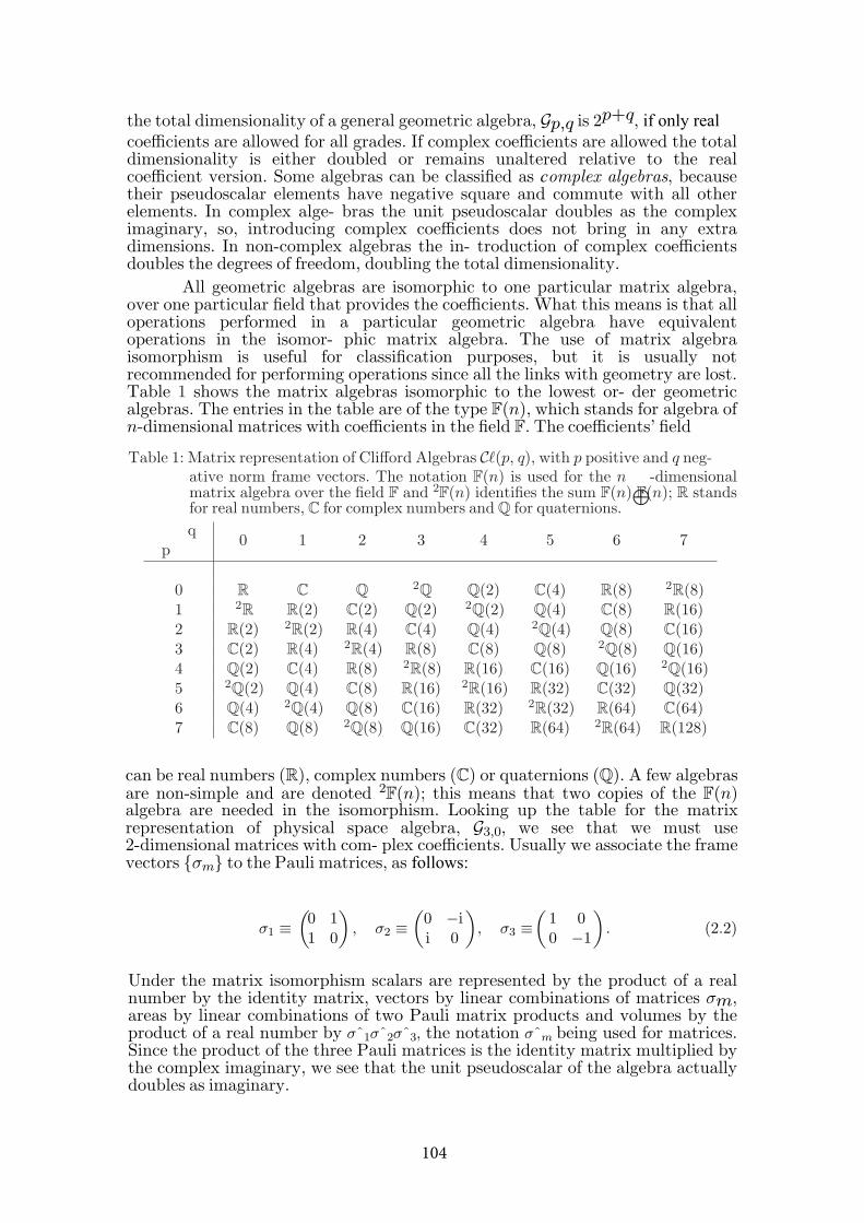
the total dimensionality of a general geometric algebra, Gp,q is 2p+q, if only real coefficients are allowed for all grades. If complex coefficients are allowed the total dimensionality is either doubled or remains unaltered relative to the real coefficient version. Some algebras can be classified as complex algebras, because their pseudoscalar elements have negative square and commute with all other elements. In complex alge- bras the unit pseudoscalar doubles as the complex imaginary, so, introducing complex coefficients does not bring in any extra dimensions. In non-complex algebras the in- troduction of complex coefficients doubles the degrees of freedom, doubling the total dimensionality.
All geometric algebras are isomorphic to one particular matrix algebra, over one particular field that provides the coefficients. What this means is that all operations performed in a particular geometric algebra have equivalent operations in the isomor- phic matrix algebra. The use of matrix algebra isomorphism is useful for classification purposes, but it is usually not recommended for performing operations since all the links with geometry are lost. Table 1 shows the matrix algebras isomorphic to the lowest or- der geometric algebras. The entries in the table are of the type F(n), which stands for algebra of n-dimensional matrices with coefficients in the field F. The coefficients’ field
Table 1: Matrix representation of Clifford Algebras C`(p, q), with p positive and q neg-ative norm frame vectors. The notation F(n) is used for the n ⊕-dimensionalmatrix algebra over the field F and 2F(n) identifies the sum F(n) F(n); R stands for real numbers, C for complex numbers and Q for quaternions.q
p0 1 2 3 4 5 6 7
0 CR Q 2Q Q(2) C(4) R(8) 2R(8)1 2R R(2) C(2) Q(2) 2Q(2) Q(4) C(8) R(16)2 R(2) 2R(2) R(4) C(4) Q(4) 2Q(4) Q(8) C(16)3 C(2) R(4) 2R(4) R(8) C(8) Q(8) 2Q(8) Q(16)4 Q(2) C(4) R(8) 2R(8) R(16) C(16) Q(16) 2Q(16)5 2Q(2) Q(4) C(8) R(16) 2R(16) R(32) C(32) Q(32)6 Q(4) 2Q(4) Q(8) C(16) R(32) 2R(32) R(64) C(64)7 C(8) Q(8) 2Q(8) Q(16) C(32) R(64) 2R(64) R(128)
can be real numbers (R), complex numbers (C) or quaternions (Q). A few algebras are non-simple and are denoted 2F(n); this means that two copies of the F(n) algebra are needed in the isomorphism. Looking up the table for the matrix representation of physical space algebra, G3,0, we see that we must use 2-dimensional matrices with com- plex coefficients. Usually we associate the frame vectors σm to the Pauli matrices, as follows:
σ1 ≡ 0 11 0
, σ2 ≡(
0 −ii 0
, σ3 ≡ 1 00 −1
( ) ) ( ). (2.2)
Under the matrix isomorphism scalars are represented by the product of a real number by the identity matrix, vectors by linear combinations of matrices σm, areas by linear combinations of two Pauli matrix products and volumes by the product of a real number by σˆ1σˆ2σˆ3, the notation σˆm being used for matrices. Since the product of the three Pauli matrices is the identity matrix multiplied by the complex imaginary, we see that the unit pseudoscalar of the algebra actually doubles as imaginary.
104
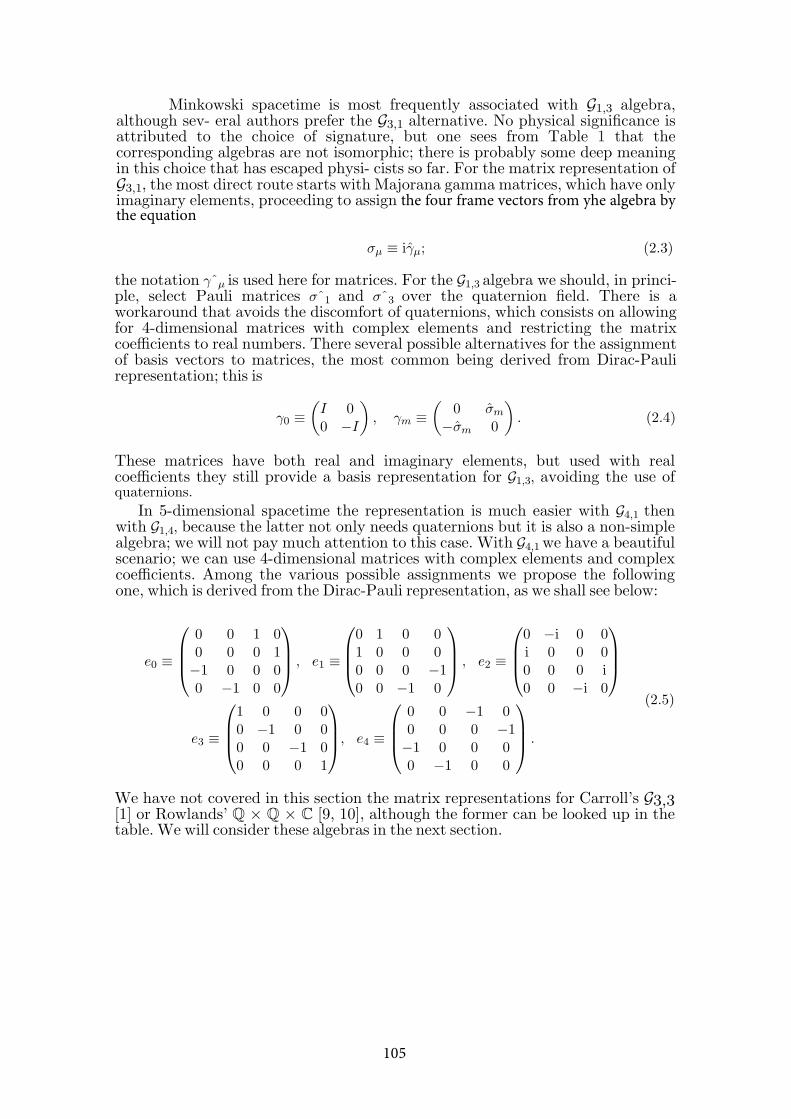
Minkowski spacetime is most frequently associated with G1,3 algebra, although sev- eral authors prefer the G3,1 alternative. No physical significance is attributed to the choice of signature, but one sees from Table 1 that the corresponding algebras are not isomorphic; there is probably some deep meaning in this choice that has escaped physi- cists so far. For the matrix representation of G3,1, the most direct route starts with Majorana gamma matrices, which have only imaginary elements, proceeding to assign the four frame vectors from yhe algebra by the equation
σµ ≡ iγµ; (2.3)
the notation γˆµ is used here for matrices. For the G1,3 algebra we should, in princi- ple, select Pauli matrices σˆ1 and σˆ3 over the quaternion field. There is a workaround that avoids the discomfort of quaternions, which consists on allowing for 4-dimensional matrices with complex elements and restricting the matrix coefficients to real numbers. There several possible alternatives for the assignment of basis vectors to matrices, the most common being derived from Dirac-Pauli representation; this is
(I 0 ≡ 0 σm
−σm 0
( ) )γ0 ≡ 0 −I
, γm . (2.4)
These matrices have both real and imaginary elements, but used with real coefficients they still provide a basis representation for G1,3, avoiding the use of quaternions.
In 5-dimensional spacetime the representation is much easier with G4,1 then with G1,4, because the latter not only needs quaternions but it is also a non-simple algebra; we will not pay much attention to this case. With G4,1 we have a beautiful scenario; we can use 4-dimensional matrices with complex elements and complex coefficients. Among the various possible assignments we propose the following one, which is derived from the Dirac-Pauli representation, as we shall see below:
e0 ≡
0 0 1 00 0 0 1−1 0 0 00 −1 0 0
, e1 ≡
0 1 0 01 0 0 00 0 0 −10 0 −1 0
, e2 ≡
0 −i 0 0i 0 0 00 0 0 i0 0 −i 0
e3 ≡
1 0 0 00 −1 0 00 0 −1 00 0 0 1
, e4 ≡
0 0 −1 00 0 0 −1−1 0 0 00 −1 0 0
.
(2.5)
We have not covered in this section the matrix representations for Carroll’s G3,3 [1] or Rowlands’ Q × Q × C [9, 10], although the former can be looked up in the table. We will consider these algebras in the next section.
105
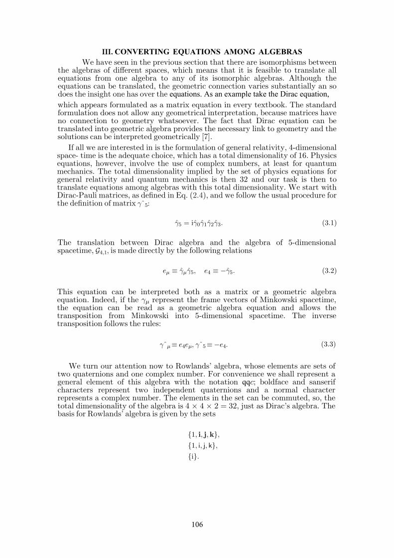
III. CONVERTING EQUATIONS AMONG ALGEBRASWe have seen in the previous section that there are isomorphisms between
the algebras of different spaces, which means that it is feasible to translate all equations from one algebra to any of its isomorphic algebras. Although the equations can be translated, the geometric connection varies substantially an so does the insight one has over the equations. As an example take the Dirac equation, which appears formulated as a matrix equation in every textbook. The standard formulation does not allow any geometrical interpretation, because matrices have no connection to geometry whatsoever. The fact that Dirac equation can be translated into geometric algebra provides the necessary link to geometry and the solutions can be interpreted geometrically [7].
If all we are interested in is the formulation of general relativity, 4-dimensional space- time is the adequate choice, which has a total dimensionality of 16. Physics equations, however, involve the use of complex numbers, at least for quantum mechanics. The total dimensionality implied by the set of physics equations for general relativity and quantum mechanics is then 32 and our task is then to translate equations among algebras with this total dimensionality. We start with Dirac-Pauli matrices, as defined in Eq. (2.4), and we follow the usual procedure for the definition of matrix γˆ5:
γ5 = iγ0γ1γ2γ3. (3.1)
The translation between Dirac algebra and the algebra of 5-dimensional spacetime, G4,1, is made directly by the following relations
eµ ≡ γµγ5, e4 ≡ −γ5. (3.2)
This equation can be interpreted both as a matrix or a geometric algebra equation. Indeed, if the γµ represent the frame vectors of Minkowski spacetime, the equation can be read as a geometric algebra equation and allows the transposition from Minkowski into 5-dimensional spacetime. The inverse transposition follows the rules:
γˆµ ≡ e4eµ, γˆ5 ≡ −e4. (3.3)
We turn our attention now to Rowlands’ algebra, whose elements are sets of two quaternions and one complex number. For convenience we shall represent a general element of this algebra with the notation qqc; boldface and sanserif characters represent two independent quaternions and a normal character represents a complex number. The elements in the set can be commuted, so, the total dimensionality of the algebra is 4 × 4 × 2 = 32, just as Dirac’s algebra. The basis for Rowlands’ algebra is given by the sets
1, i, j,k,1, i, j, k,i.
106
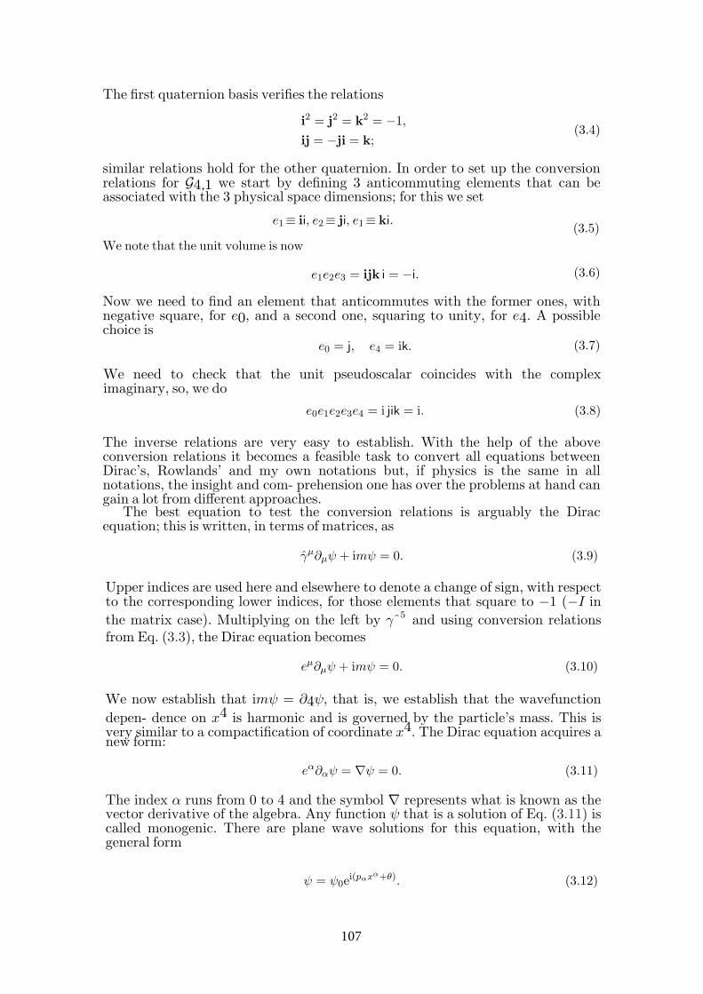
The first quaternion basis verifies the relations
i2 = j2 = k2 = −1,
ij = −ji = k;(3.4)
similar relations hold for the other quaternion. In order to set up the conversionrelations for G4,1 we start by defining 3 anticommuting elements that can be associated with the 3 physical space dimensions; for this we set
(3.5)e1 ≡ ii, e2 ≡ ji, e1 ≡ ki.
We note that the unit volume is now
e1e2e3 = ijk i = −i. (3.6)
Now we need to find an element that anticommutes with the former ones, with negative square, for e0, and a second one, squaring to unity, for e4. A possible choice is
e0 = j, e4 = ik. (3.7)
We need to check that the unit pseudoscalar coincides with the complex imaginary, so, we do
e0e1e2e3e4 = i jik = i. (3.8)
The inverse relations are very easy to establish. With the help of the above conversion relations it becomes a feasible task to convert all equations between Dirac’s, Rowlands’ and my own notations but, if physics is the same in all notations, the insight and com- prehension one has over the problems at hand can gain a lot from different approaches.
The best equation to test the conversion relations is arguably the Dirac equation; this is written, in terms of matrices, as
γµ∂µψ + imψ = 0. (3.9)
Upper indices are used here and elsewhere to denote a change of sign, with respect to the corresponding lower indices, for those elements that square to −1 (−I in the matrix case). Multiplying on the left by γˆ5 and using conversion relations from Eq. (3.3), the Dirac equation becomes
eµ∂µψ + imψ = 0. (3.10)
We now establish that imψ = ∂4ψ, that is, we establish that the wavefunction depen- dence on x4 is harmonic and is governed by the particle’s mass. This is very similar to a compactification of coordinate x4. The Dirac equation acquires a new form:
eα∂αψ = ∇ψ = 0. (3.11)
The index α runs from 0 to 4 and the symbol ∇ represents what is known as the vector derivative of the algebra. Any function ψ that is a solution of Eq. (3.11) is called monogenic. There are plane wave solutions for this equation, with the general form
ψ = ψ0ei(pαxα+θ). (3.12)
107
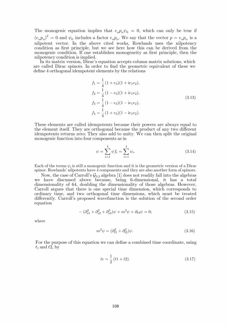
The monogenic equation implies that eαpαψ0 = 0, which can only be true if (eαpα)
2 = 0 and ψ0 includes a factor eαpα. We say that the vector p = eαpα is a nilpotent vector. In the above cited works, Rowlands uses the nilpotency condition as first principle, but we see here how this can be derived from the monogenic condition. If one establishes monogeneity as first principle, then the nilpotency condition is implied.
In its matrix version, Dirac’s equation accepts column matrix solutions, which are called Dirac spinors. In order to find the geometric equivalent of these we define 4 orthogonal idempotent elements by the relations
f1 =14
(1 + e3)(1 + ie1e2),
f2 =14
(1− e3)(1 + ie1e2),
f3 =14
(1− e3)(1− ie1e2),
f4 =14
(1 + e3)(1− ie1e2).
(3.13)
These elements are called idempotents because their powers are always equal to the element itself. They are orthogonal because the product of any two different idempotents returns zero; They also add to unity. We can then split the original monogenic function into four components as in
ψ =4∑
i=1
ψfi =4∑
i=1
ψi. (3.14)
Each of the terms ψi is still a monogenic function and it is the geometric version of a Dirac spinor. Rowlands’ nilpotents have 4 components and they are also another form of spinors.
Now, the case of Carroll’s G3,3 algebra [1] does not readily fall into the algebras we have discussed above because, being 6-dimensional, it has a total dimensionality of 64, doubling the dimensionality of those algebras. However, Carroll argues that there is one special time dimension, which corresponds to ordinary time, and two orthogonal time dimensions, which must be treated differently. Carroll’s proposed wavefunction is the solution of the second order equation
− (∂2s1 + ∂2
s2 + ∂2s3)ψ + m2ψ + ∂t3ψ = 0; (3.15)
where
m2ψ = (∂2t1 + ∂2
t2)ψ. (3.16)
For the purpose of this equation we can define a combined time coordinate, using t1 and t2, by
tc =12
(t1 + t2). (3.17)
108
Equation (3.16) is then a G2,3 algebra equation and we see from Table 1 that this algebra is isomorphic to G4,1. In order to convert between the two algebras we define the vectors for G2,3 by
esm = iem,
et3 = ie0,
etc = e4.
(3.18)
With this conversion it is easy to verify that Eq. (3.16) is indeed a second order version of Eq. (3.11). We don’t discuss here other implications of Carroll’s 6-dimensional approach, the purpose of this discussion being only to show that there is an implied 5-dimensional algebra isomorphic to the other ones presented above.
IV. CONCLUSION
Many authors resort to different algebras for the exposition of their own approaches to fundamental physical equations, such as Maxwell’s equations, Dirac’s equation and Einstein’s equations. Quite frequently authors propose their own versions of those equations, highlighting the virtues of their approaches. The task of comparing results is difficult because the form of both equations and their solutions is dependent on the particular algebra that the author has chosen. We have shown that the algebra used by Dirac has an overall dimensionality of 32, the same as several 5-dimensional algebras proposed by different authors. The tensor algebra that most people use for general relativity is indeed a 16-dimensional sub-algebra of the Dirac algebra, so, it does not need to be addressed specifically.
Particular examples of algebras isomorphic to the Dirac algebra are those used by Rowlands [9, 10] and the author himself [6, 7]. We have shown how to convert between those two algebras and the Dirac algebra. A slightly different case occurs with the algebra used by Carroll [1], because this has an overall dimensionality of 64. Here we have shown that some of the proposed equations can be set in analgebra isomorphic to the previous ones and we presented the means for converting equations between Carroll’s algebra and the remaining ones.
The choice of a particular algebra is irrelevant from the point of view of the mathe- matical validity of equations, but it may make a significant difference to the perception and comprehension of the physics behind the equations. Quite often, no single choice of an algebra offers the definitive approach to an equation. Looking at a particular problem from different angles usually broadens our perspective over that problem, so, it makes sense to have equivalent equations written in varied algebras. However, we need to be able to convert among algebras in order to unify the various approaches.
109
REFERENCES[1]. J. E. Carroll, Electromagnetic fields and charges in 3+1 spacetime derived from symmetry in 3+3 spacetime, 2004, arXiv: math-ph/0404033.[2]. C. Doran and A. Lasenby, Geometric Algebra for Physicists (CambridgeUniversityPress, Cambridge, U.K., 2003).[3]. D. Hestenes and G. Sobczyk, Clifford Algebras to Geometric Calculus. A Unified Language for Mathematics and Physics, Fundamental Theories of Physics (Reidel, Dordrecht, 1989).
[4]. D. Hestenes, Spacetime physics with geometric algebra, Am. J. Phys. 71, 691, 2003.[5]. T. Kaluza, On the problem of unity in physics, Sitzungsber. Preuss. Akad. Wiss. Berlin. (Math. Klasse) pp. 966–972, 1921.[6]. J. B. Almeida, The null subspace of G(4,1) as source of the main physical theo-ries, in Physical Interpretations of Relativity Theory – IX (London, 2004), arXiv: physics/0410035.[7]. J. B. Almeida, Hidden geometric character of relativistic quantum mechanics, J. Math. Phys. 49, 012301, 2007, arXiv: quant-ph/0606123.[8]. S. S. Seahra and P. S. Wesson, Null geodesics in five dimensional manifolds, Gen.Rel. Grav. 33, 1731, 2001, arXiv: gr-qc/0105041.[9]. P. Rowlands, The nilpotent Dirac equation and its applications in particle physics, 2003, arXiv: quant-ph/0301071.[10]. P. Rowlands, Zero to Infinity: The Foundations of Physics, vol. 41 of Series on Knots and Everything (World Scientific, Singapore, 2007).
110
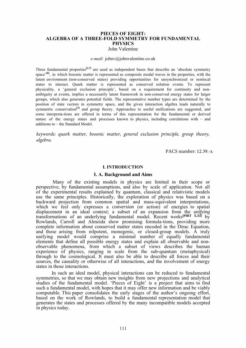
PIECES OF EIGHT: ALGEBRA OF A THREE-FOLD SYMMETRY FOR FUNDAMENTAL
PHYSICSJohn Valentine
e-mail: [email protected]
Three fundamental properties[2,7] are used as independent bases that describe an ‘absolute symmetry space’[6], in which bosonic matter is represented as composite modal waves in the properties, with the latent environment (non-conserved states) providing opportunities for unsynchronized or nonlocal states to interact. Quark matter is represented as conserved solution events. To represent physicality, a ‘general exclusion principle’, based on a requirement for continuity and non-ambiguity at events, implies a necessarily latent framework in non-conserved energy states for larger groups, which also generates potential fields. The representative number types are determined by the position of state vectors in symmetry space, and the given interaction algebra leads naturally to symmetric conservation[1] and group theory. Approaches to useful unifications are suggested, and some interpreta-tions are offered in terms of this representation for the fundamental or derived nature of the energy states and processes known to physics, including correlations with – and additions to – the Standard Model.
I. INTRODUCTION
I. A. Background and Aims Many of the existing models in physics are limited in their scope or
perspective, by fundamental assumptions, and also by scale of application. Not all of the experimental results explained by quantum, classical and relativistic models use the same principles. Historically, the exploration of physics was based on a backward projection from common spatial and mass-equivalent interpretations, which we feel only expresses a conversion (or action) of energies to spatial displacement in an ideal context; a subset of an expansion from the unifying transformations of an underlying fundamental model. Recent works[PIRT X,XI] by Rowlands, Carroll and Almeida show promising formula-tions, providing more complete information about conserved matter states encoded in the Dirac Equation, and those arising from nilpotent, monogenic, or closed-group models. A truly unifying model would comprise a minimal number of equally fundamental elements that define all possible energy states and explain all observable and non-observable phenomena, from which a subset of views describes the human experience of physics, ranging in scale from the sub-quantum (metaphysical) through to the cosmological. It must also be able to describe all forces and their sources, the causality or otherwise of all interactions, and the involvement of energy states in those interactions.
In such an ideal model, physical interactions can be reduced to fundamental symmetries, so that we may obtain new insights from new projections and analytical studies of the fundamental model. ‘Pieces of Eight’ is a project that aims to find such a fundamental model, with hopes that it may offer new information and be viably computable. This paper consolidates the early stages of the author’s ongoing effort, based on the work of Rowlands, to build a fundamental representation model that generates the states and processes offered by the many incompatible models accepted in physics today.
keywords: quark matter, bosonic matter, general exclusion principle, group theory, algebra.
PACS number: 12.39.-x
111
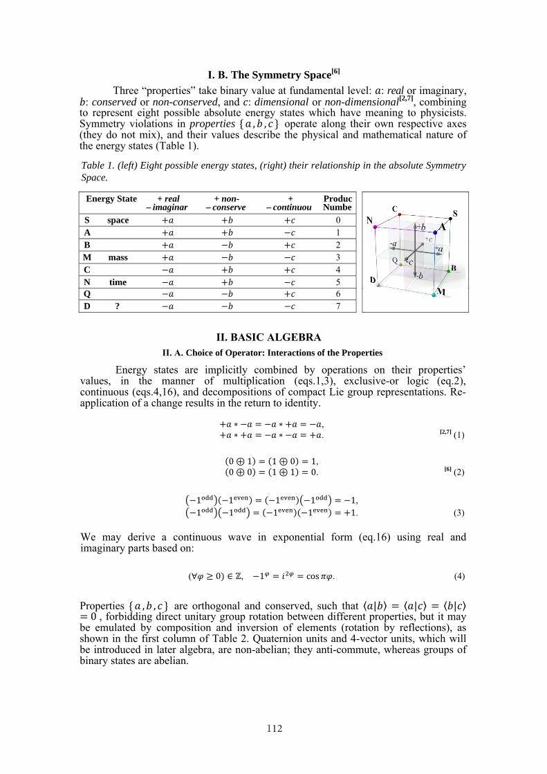
I. B. The Symmetry Space[6] Three “properties” take binary value at fundamental level: 𝑎: real or imaginary, 𝑏: conserved or non-conserved, and 𝑐: dimensional or non-dimensional[2,7], combining
to represent eight possible absolute energy states which have meaning to physicists. Symmetry violations in properties 𝑎 , 𝑏 , 𝑐 operate along their own respective axes (they do not mix), and their values describe the physical and mathematical nature of the energy states (Table 1).
Energy State + real – imaginar
y
+ non-conserved– conserve
d
+ dimensional – continuou
s
Product NumberS space +𝑎 +𝑏 +𝑐 0
A gravity
+𝑎 +𝑏 −𝑐 1 B momentum
+𝑎 −𝑏 +𝑐 2 M mass +𝑎 −𝑏 −𝑐 3 C magnetism?
−𝑎 +𝑏 +𝑐 4 N time −𝑎 +𝑏 −𝑐 5 Q charge
−𝑎 −𝑏 +𝑐 6 D ? −𝑎 −𝑏 −𝑐 7
Table 1. (left) Eight possible energy states, (right) their relationship in the absolute Symmetry Space.
II. BASIC ALGEBRAII. A. Choice of Operator: Interactions of the Properties
Energy states are implicitly combined by operations on their properties’ values, in the manner of multiplication (eqs.1,3), exclusive-or logic (eq.2), continuous (eqs.4,16), and decompositions of compact Lie group representations. Re-application of a change results in the return to identity. +𝑎 ∗ −𝑎 = −𝑎 ∗ +𝑎 = −𝑎,+𝑎 ∗ +𝑎 = −𝑎 ∗ −𝑎 = +𝑎. [2,7] (1)
(0 ⊕ 1) = (1 ⊕ 0) = 1,(0 ⊕ 0) = (1 ⊕ 1) = 0. [6] (2)
−1 (−1 ) = (−1 ) −1 = −1,−1 −1 = (−1 )(−1 ) = +1. (3)
We may derive a continuous wave in exponential form (eq.16) using real and imaginary parts based on:
∀𝜑 ≥ 0) ∈ ℤ, ( −1 = 𝑖 = cos 𝜋𝜑. (4)
Properties 𝑎 , 𝑏 , 𝑐 are orthogonal and conserved, such that ⟨𝑎|𝑏⟩ = ⟨𝑎|𝑐⟩ = ⟨𝑏|𝑐⟩ = 0 , forbidding direct unitary group rotation between different properties, but it may be emulated by composition and inversion of elements (rotation by reflections), as shown in the first column of Table 2. Quaternion units and 4-vector units, which will be introduced in later algebra, are non-abelian; they anti-commute, whereas groups of binary states are abelian.
112
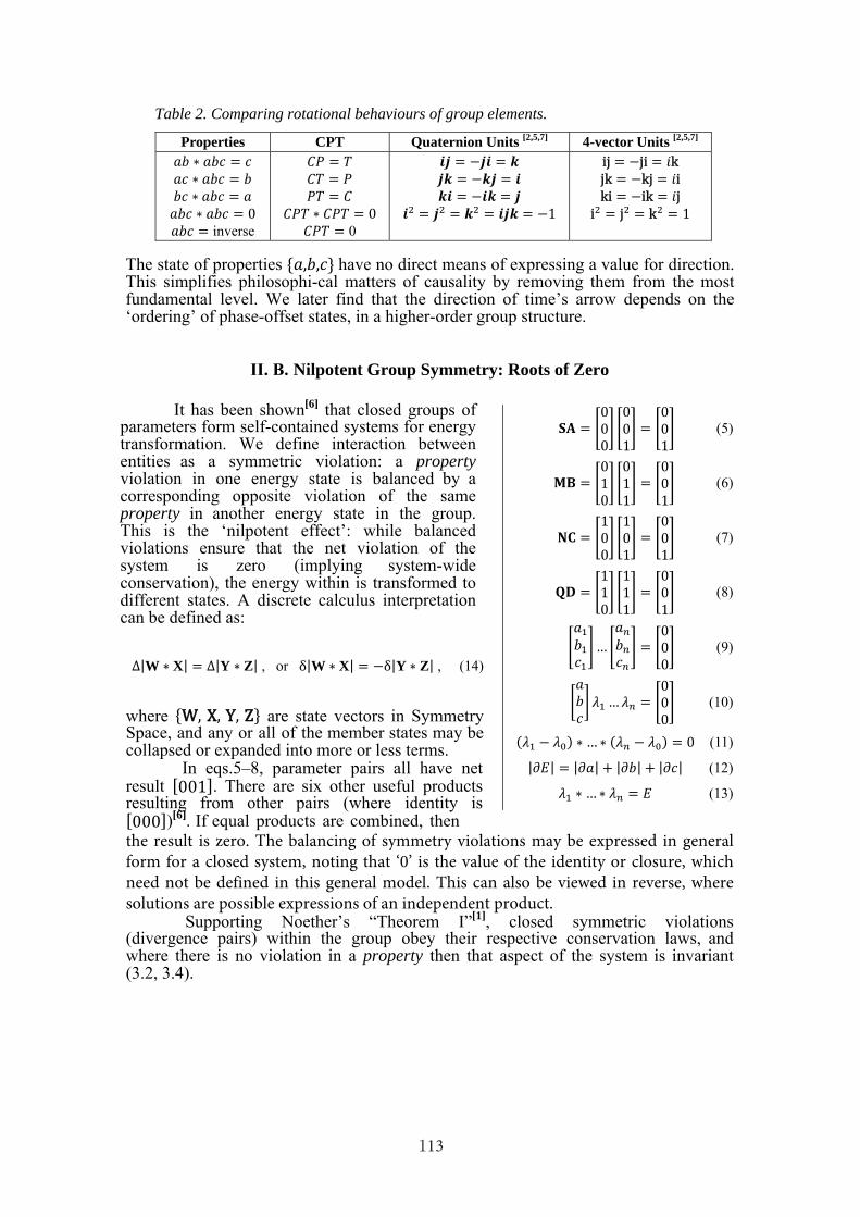
Properties CPT Quaternion Units [2,5,7] 4-vector Units [2,5,7] 𝑎𝑏 ∗ 𝑎𝑏𝑐 = 𝑐 𝑎𝑐 ∗ 𝑎𝑏𝑐 = 𝑏 𝑏𝑐 ∗ 𝑎𝑏𝑐 = 𝑎 𝑎𝑏𝑐 ∗ 𝑎𝑏𝑐 = 0 𝑎𝑏𝑐 = inverse
𝐶𝑃 = 𝑇 𝐶𝑇 = 𝑃 𝑃𝑇 = 𝐶 𝐶𝑃𝑇 ∗ 𝐶𝑃𝑇 = 0 𝐶𝑃𝑇 = 0
𝒊𝒋 = −𝒋𝒊 = 𝒌 𝒋𝒌 = −𝒌𝒋 = 𝒊 𝒌𝒊 = −𝒊𝒌 = 𝒋 𝒊 = 𝒋 = 𝒌 = 𝒊𝒋𝒌 = −1
ij = −ji = 𝑖k jk = −kj = 𝑖i ki = −ik = 𝑖j i = j = k = 1
Table 2. Comparing rotational behaviours of group elements.
The state of properties 𝑎,𝑏,𝑐 have no direct means of expressing a value for direction. This simplifies philosophi-cal matters of causality by removing them from the most fundamental level. We later find that the direction of time’s arrow depends on the ‘ordering’ of phase-offset states, in a higher-order group structure.
II. B. Nilpotent Group Symmetry: Roots of Zero
It has been shown[6] that closed groups of parameters form self-contained systems for energy transformation. We define interaction between entities as a symmetric violation: a property violation in one energy state is balanced by a corresponding opposite violation of the same property in another energy state in the group. This is the ‘nilpotent effect’: while balanced violations ensure that the net violation of the system is zero (implying system-wide conservation), the energy within is transformed to different states. A discrete calculus interpretation can be defined as:
Δ|W ∗ X| = Δ|Y ∗ Z| , or δ|W ∗ X| = −δ|Y ∗ Z| , (14)
where W, X, Y, Z are state vectors in Symmetry Space, and any or all of the member states may be collapsed or expanded into more or less terms.
In eqs.5–8, parameter pairs all have net result [001]. There are six other useful products resulting from other pairs (where identity is [000])[6]. If equal products are combined, then
Supporting Noether’s “Theorem I”[1], closed symmetric violations (divergence pairs) within the group obey their respective conservation laws, and where there is no violation in a property then that aspect of the system is invariant (3.2, 3.4).
𝐒𝐀 = 000 001 = 001 (5)
𝐌𝐁 = 010 011 = 001 (6)
𝐍𝐂 = 100 101 = 001 (7)
𝐐𝐃 = 110 111 = 001 (8) 𝑎𝑏𝑐 … 𝑎𝑏𝑐 = 000 (9) 𝑎𝑏𝑐 𝜆 … 𝜆 = 000 (10)
(𝜆 − 𝜆 ) ∗ … ∗ (𝜆 − 𝜆 ) = 0 (11) |∂𝐸| = |∂𝑎| + |∂𝑏| + |∂𝑐| (12) 𝜆 ∗ … ∗ 𝜆 = 𝐸 (13)
the result is zero. The balancing of symmetry violations may be expressed in general form for a closed system, noting that ‘0’ is the value of the identity or closure, which need not be defined in this general model. This can also be viewed in reverse, where solutions are possible expressions of an independent product.
113
II. C. Closed Groups and Approaches to UnificationsBecause the properties 𝑎,𝑏,𝑐 are rotation-asymmetric, they do not interact
upon each other; each of 𝑎,𝑏,𝑐 interacts on its own independent row (2.1). For this reason, the simplest quantitative expressions that successfully unify all energy states in the Symmetry Space are likely to comprise sums of three terms, corresponding to the three possible violations of fundamental properties (eqs.9,10,12), remembering that multiplication is generally for coupling interactions (both the inner and outer products), and addition separates anisomorphic terms. As with eqs.1,14, this applies also to differential versions, provided they describe fundamental interactions.
No practical system can be considered entirely closed; the representation of ‘free groups’ is unrealistically ideal, because a closed system is only an approximation, due to ambient conditions or nearby influences, such as residual charge interactions, and the accumulated gravitational interactions with the rest of the universe. Despite these shortcomings, the closed system presents a simple model from which we can learn.
In simple interactions and small groups, 𝜆 (eq.11), 𝐸 (eq.13), or ∂𝐸 (eq.15), may represent a unified quantum potential, satisfied by the solution in 𝑎, 𝑏, and 𝑐. Open systems have non-zero solutions (eq.13). They might be irreducible, or represent vacuum energy, so statistical representation of 𝐸 might suffice (2.4).
II. D. VacuumIn this model, vacuum is all 𝜆 (eqs.10,11) or 𝐸 (eqs.12,13); the set of potential
symmetry violations relative to any given energy state or group, with relevance to any system. It needn’t be physically manifest, nor local. It is not the empty volume between particulate matter, nor is it an aether-based field from which background energy may be tapped; nor is it a cloud of virtual particles surrounding matter.
There are eight super-symmetric binary groups[6] within the Symmetry Space. These are conjugate pairs of closed four-member sub-groups, whose four unit states may be connected by a plane or tetrahedron in ±𝑎, ±𝑏, ±𝑐. It is worth noting at this point that these super-symmetric groups do not imply a conjugate set of particles (‘super particles’) to mirror those of the Standard Model, because the physical meaning of energy states is absolute, rather than relative: the Symmetry Space conjugate (in all three properties) of a particle would not be a particle, but a field or potential.
II. E. State, Process, and Operator
We have used the ∗ operator to combine properties (eq.1) and to implicitly combine energy states (eq.14). This operator symbol is not strictly necessary, because instances of states are their own operators, interacting as change factors within the independent 𝑎,𝑏,𝑐 channels. This gives us a form that may be readily quantized in multiple orders, and the rich mathematical tools of group theory. Further, we are accustomed to modelling states and processes separately, but the combined approach used here avoids a significant obstacle to the completeness of any fundamental philosophy: the requirement for an agent of change that operates in parallel with the model. Here, such an external agent is not necessary. Instead, this model is inherently self-contained, with its own proper time.
II. F. Choice of Number TypesThe properties themselves determine the type and composition of
number representing the dimensional values of energy states, as shown in Table 3, along with the rotation symmetries implied by their position in the Symmetry Space. Imaginary units square to i (negative norm), and real units square to 1 (positive norm).
Rotation symmetry and translation symmetry apply only to non-conserved dimensional states [2]. It is important in group transformations, especially actions that are realised as spatial changes.
114
Composites of number types assume coupling, and these processes (of conjugation, complexification, and dimen-sionalization) will generate further number types: real, imaginary, complex, quaternion, multivariate vectors, and limited combinations thereof[4,7,8]. For example, Rowlands’ compactification of the dimensions of charge into those of energy, momentum, and mass[5,7] implicitly defines a unifying coupling, and privileges the inner products. As suggested in our earlier work[6], and by Almeida[8], similar treatment to other representations should provide useful insights.
State Value Representation
Rotation Symmetry Unit Basis Elements
space real 3-vector Yes x = sx, y = sy, z = sz A real scalar n/a x = g B real 3-vector No x = ρx, y = ρy, z = ρz
mass real scalar n/a x = m C imaginary 3-vector Yes i = Cx, j = Cy, k = Cz
time N imaginary scalar n/a i = τ charge imaginary 3-vector No i = Qe, j = Qw, k = Qs
D imaginary scalar n/a i = φ
Table 3. Number types and unit basis elements for absolute energy states
[Author’s note: Parts 3 to 10 (16pp total) will be presented at a later date]
REFERENCES[1]. E. Noether, Invariante Variationsprobleme, Nachr. v. d. Ges. d. Wiss. zu Göttingen 1918, pp235-257. English translation (1971), http://www.physics.ucla.edu/~cwp/articles/noether.trans/english/mort188.html
[2]. P. Rowlands, The Fundamental Parameters of Physics: an Approach towards a Unified Theory (PD Publications, Liverpool, 1991). [3]. J. S. Valentine, Pieces of Eight, a development of “The Fundamental Parameters of Physics”. ANPA 20, Cambridge,1998.
[4]. P. Rowlands and Bernard Diaz (2002) A universal alphabet and rewrite system. arXiv:cs/0209026v1.[5]. P. Rowlands, The Group Structure Bases of a Foundational Approach to Physics. arXiv:quant-ph/0110092.[6]. J. S. Valentine (2006) Pieces of Eight – Gravitation in Symmetrical Context of Space-Time, Conference on Physical Interpretation of Relativity Theory X, British Society for Philosophy of Science, London, 2006. [7]. P. Rowlands, Zero to Infinity, ISBN-13: 9789812709141, World Scientific Publishing, 2007.[8]. J. Almeida, Different Algebras for One Reality, Conference on Physical Interpretation of Relativity Theory XI, British Society for Philosophy of Science, London, 2008.
115
116
RELATIVISTIC PHYSICS IN COMPLEX MINKOWSKI SPACE, NONLOCALITY AETHER MODEL AND QUANTUM PHYSICS
Elizabeth A. Rauscher
Tecnic Research Laboratory 3500 S. Tomahawk Road, Bldg. 188 Apache Junction, AZ 85219 USA
Email: [email protected]
Many naturally occurring phenomena require theoretical treatment utilizing complex analysis by methods such as the Cauchy-Rieman relations. These methods use hypergeometrical spaces which treat inherently nonlinear, non-dispersive, collective nonlocal resonant states of a quantum system, so as to be consistent with the nonlinearity inherent in general relativity. Most typical approaches to the quantum theory form linear approximations, which limit the ability to formulate a quantum relativity theory. The fundamental nature of remote connectedness is exemplified by Young’s double slit experiment, Bell’s theorem nonlocality, Mach’s principle and the operation of a Foucault pendulum, which all appear to employ the existence of an aether.
We demonstrate that a geometric aether is not precluded by the structure of the relativity theory, although, in general, Einstein excluded the concept of an aether and a fixed reference frame. In fact, certain observable phenomena, such as Mack’s principle and also Bell’s theorem and the Young’s double slit experiment imply the existence of a fixed geometry spacetime aether. One of the basic tenants of this aether is the fundamental principle of nonlocality. In the quantum principle the nonlocality can be understood in terms of the Soliton – Solitary wave solutions of the Schrodinger equation solved in complex relativistic Minkowski space.
For the complex modified relativistic multidimensional aether will allow us to theoretically understand the fundamental nature and mechanism of nonlocality. This understanding will allow us to design experiments that further evaluate the properties of nonlocal coherent collective phenomena. The structure of quantum theory using the Schrodinger equation, covariant Dirac equation and sine-Gordon equation are solved in a complex hyper-eight dimensional relativistic geometric space. The symmetry of this space possesses relativistic Lorentz invariance for nonlinear hyper-dimensional geometry, nonlocality, and nonlinear coherent states which are expressed in terms of quantum soliton solutions.
Keywords: Modified Relativity, Complex Minkowski Spaces, Nonlocal Aether and Quantum Theory.
PACS number: 04.62.+v
117
DECOUPLING THE METRIC
Roger Brewis
BA, BSc, MSc.
The tensor calculus of general relativity provides a mathematical structure that is elegant, and permits a unified metric for both light and what has been called ‘ponderable matter’. The unification of light and matter in the gravitational mathematics mirrors the separate unification in quantum mechanics through the duality model.
The most accessible metric is that of Schwarzschild, which has been successful in a range of ‘key predictions’. It includes an anisotropy in that the radial component differs from the tangential components. An examination of the metric suggests that, at least in relation to the accepted key predictions of general relativity, a theoretical decoupling of the individual elements of the metric would still be in keeping with observation.
The abandonment of a unified mathematical structure for light and matter would be a serious step, but appears to open up the option of simple hydrodynamic interpretations for gravitational and other phenomena, and this will be considered in a companion paper.
There is some theoretical backing for such a move in the geometric algebra calculations of Doran at Cambridge, which suggest a revised black hole event horizon that is compatible with an isotropic metric.
Keywords: ponderable matter, Schwarzschild metric, general relativity, gravitation, geometric algebra calculations, hydrodynamic.
PACS number: 04.20.-q/04.20.GZ
118
A HYDRODYNAMIC INTERPRETATION
Roger Brewis
BA, BSc, MSc.
Hydrodynamic explanations for gravitational and other phenomena have a long history. Madelung and Korn are generally cited, but the approach is also seen in the extensive examination of magnetism by Maxwell in 1861.
In a companion paper I have suggested that it is possible to decouple the elements of the Schwarzschild metric, and thereby eliminate the anisotropy in general relativity that is otherwise problematic for hydrodynamic interpretations. That anisotropy is a complicating factor in many attempts at physical interpretation of relativity, and also in relation to the unification of physics theories.
The hydrodynamic interpretation now suggested invokes a vortex-ring particle, as popularised by Kelvin, that is in constant vibration. These vibrations provide a physical basis for the Bohr equation for emission frequency and the quantum well model. Work at DAMTP in Cambridge suggests that vortices can be self-organising.
The vibrations thereby transmitted obey the general requirement of the inverse square law, but require a non-linear element in order to create a motive force on other vortex ring particles. That non-linearity suggests explanations for a range of gravitational anomalies.
Additionally, there are clear parallels between the Schrödinger equation and the Navier-Stokes equation of hydrodynamics, permitting a physical interpretation of Schrödinger’s ψ. Geometric algebra, which has been shown to be so useful in quantum mechanics by Rowlands at Liverpool and in gravitational relativity by Doran and colleagues at Cambridge, and which was used in earlier forms in the nineteenth century for both hydrodynamics and electromagnetism, becomes a strong candidate for the mathematical unification of physics.
Keywords: hydrodynamic, Schwarzschild metric, physical interpretation of relativity, vortex-ring particle, Schrödinger equation, the Navier-Stokes equation.
PACS number: 04.20.-q/47.32.cf/47.32.C-
119
REALIZATION OF ELEMENTARY MATTER IN SELF-REPLICATING REGULAR SOLID REWRITE
Erik Trell
Professor Emeritus, University of Linköping, Strandviksvägen 47, SE-65590 Karlstad, Sweden
Tel +46 (0)705970727 email: [email protected], [email protected]
The Nilpotent Universal Computer Rewrite System (NUCRS) has operationalized the radical ontological dilemma of Nothing Whatsoever versus Anything at All down to the principal recursive syntax and primary mathematical realisation of this categorical dichotomy as such and so governing all its sui generis modalities, leading to fulfilment of their individual terms and compass when the respective choice sequence processing is brought to closure. In the distinct morphogenetical modality of structural Physics, NUCRS thus provides an algorithm for direct quantum holographic replication of the entire elementary particle spectroscopy with the perfect straight line as singular eigenvector unfolding along the NUCRS concatenations in the form of the classical regular solids and their differentials into maximally three-dimensional ordinary space and matter, where Lie algebra SO(3)×O(5) transformation dynamics is also immanent by adjoined Aristotelian phase transition between absolute Straight and Round. More specifically, the ground line element thereby spans a real three-dimensional eigenspace with cubical eigenunits, or ‘pixels’ (“cuBits”), where geometrically quark-skewed quantum-chromodynamical particle events self-generate in an exhaustive range of transition matrix elements and portions adapting to the spherical root vector symmetries and so reproducing all observed baryons, mesons and leptons and their exact channels, masses and electromagnetical and angular momentum quantum numbers, including a modular, truncated octahedron nano-distribution of the electrons which piecemeal enter into molecular structures or compressed to each other fuse into atomic honeycombs of periodic table signature. These honeycombs, in turn, template the ensuing self-similar super-positioning up to the complete orbital filling in the volumetric expansion of the separate Atoms, even including rare “designer atomic nuclei” isotopes like 11Li, delocalization processes such as K-shell hole ionization, and diatomic as well as larger inorganic molecules. The one-, two- or three-dimensional further geodetical iteration of the rendered motif determines its gaseous, fluid or firm state, over which the regular solids and their symmetries hence continue to prevail in corresponding hierarchical levels of exponentially volume-duplicating “self-assembly at all scales”.
Keywords: dilemma of Nothing Whatsoever versus Anything at All, quantum holographic replication, K-shell hole ionization, quantum information.
PACS number: 03.67.-a
I. INTRODUCTION Is there a difference between matter and mathematics? In these days when
“American particle physics stands at a crossroads” and its “decline has snowballed into a
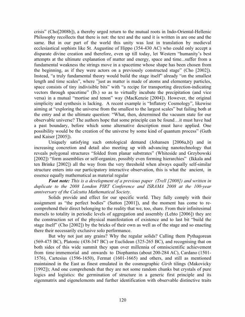
120
crisis” (Cho[2008b]), a thereby urged return to the mutual roots in Indo-Oriental-Hellenic Philosophy recollects that there is not: the text and the sand it is written in are one and the same. But in our part of the world this unity was lost in translation by medieval ecclesiastical sophists like St. Augustine of Hippo (354-430 AC) who could only accept a disparate divine creation and therefore, even up till today, let Western “humanity’s best attempts at the ultimate explanation of matter and energy, space and time...suffer from a fundamental weakness the strings move in a spacetime whose shape has been chosen from the beginning, as if they were actors on a previously constructed stage” (Cho [2002]). Instead, “a truly fundamental theory would build the stage itself” already “on the smallest length and time scales”, where ”just as matter is made of atoms and elementary particles, space consists of tiny indivisible bits” with “a recipe for transporting direction-indicating vectors through spacetime” (Ib.) so as to virtually incubate the precipitation (and vice versa) in a mutual “mortise and tenon” way (MacKenzie [2004]). However, the original simplicity and synthesis is lacking. A recent example is “Inflatory Cosmology”, likewise aiming at “exploring the universe from the smallest to the largest scales” but failing both at the entry and at the ultimate question: “What, then, determined the vacuum state for our observable universe? The authors hope that some principle can be found…it must have had a past boundary, before which some alternative description must have applied. One possibility would be the creation of the universe by some kind of quantum process” (Guth and Kaiser [2005]).
Uniquely satisfying such ontological demand (Johansen [2006a,b]) and in increasing concretion and detail also meeting up with advancing nanotechnology that reveals polygonal structures “folded from planar substrates” (Whiteside and Grzybowski [2002]) “form assemblies or self-organize, possibly even forming hierarchies” (Ikkala and ten Brinke [2002]) all the way from the very threshold when always equally self-similar structure enters into our participatory interactive observation, this is what the ancient, in essence equally mathematical as material regular
Foot note: This is a development of a previous paper (Trell [2008]) and written in duplicate to the 2008 London PIRT Conference and ISRAMA 2008 at the 100-year anniversary of the Calcutta Mathematical Society.
Solids provide and effect for our specific world. They fully comply with their assignment as “the perfect bodies” (Sutton [2001]), and the moment has come to re-comprehend their direct belonging to the reality that we, too, share. From their infinitesimal morsels to totality in periodic levels of aggregation and assembly (Lehto [2006]) they are the construction set of the physical manifestation of existence and to last bit “build the stage itself” (Cho [2002]) by the bricks of their own as well as of the stage and so enacting there their necessarily exclusive solo performance.
But why not just any grains? Why the regular solids? Calling them Pythagorean (569-475 BC), Platonic (438-347 BC) or Euclidean (325-265 BC), and recognising that on both sides of this wide summit they span over millennia of omniscientific achievement from time immemorial and onwards to Diophantus (about 200-284 AC), Cardano (1501-1576), Cartesius (1596-1650), Fermat (1601-1665) and others, and still as mentioned maintained in the East as finest emulated in the cosmographic Girih tilings (Makovicky [1992]); And one comprehends that they are not some random chunks but crystals of pure logics and logistics: the germination of structure in a generic first principle and its eigenmatrix and eigenelements and further identification with observable distinctive traits
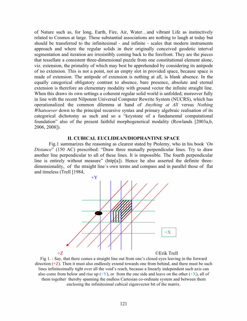
of Nature such as, for long, Earth, Fire, Air, Water…and vibrant Life as instinctively related to Cosmos at large. These substantial associations are nothing to laugh at today but should be transferred to the infinitesimal - and infinite - scales that modern instruments approach and where the regular solids in their originally conceived geodetic interval segmentation and iteration are irresistibly coming back to the forefront. They are the pieces that tessellate a consistent three-dimensional puzzle from one constitutional element alone, viz. extension, the primality of which may best be apprehended by considering its antipode of no extension. This is not a point, not an empty slot in provided space, because space is made of extension. The antipode of extension is nothing at all, is blank absence. In the equally categorical obligatory contrast to absence, bare presence, absolute and eternal extension is therefore an elementary modality with ground vector the infinite straight line. When this draws its own settings a coherent regular solid world is unfolded; moreover fully in line with the recent Nilpotent Universal Computer Rewrite System (NUCRS), which has operationalized the common dilemma at hand of Anything at All versus Nothing Whatsoever down to the principal recursive syntax and primary algebraic realisation of its categorical dichotomy as such and so a “keystone of a fundamental computational foundation” also of the present faithful morphogenetical modality (Rowlands [2003a,b, 2006, 2008]).
II. CUBICAL EUCLIDEAN/DIOPHANTINE SPACE Fig.1 summarizes the reasoning as clearest stated by Ptolemy, who in his book ‘On
Distance” (150 AC) prescribed: “Draw three mutually perpendicular lines. Try to draw another line perpendicular to all of these lines. It is impossible. The fourth perpendicular line is entirely without measure” (http[a]). Hence he also asserted the definite three-dimensionality, of the straight line´s own terms and compass and in parallel those of flat and timeless (Trell [1984, +Y
+Z ©Erik Trell
Fig 1. - Say, that there comes a straight line out from one’s closed eyes leaving in the forward direction (+Z). Then it must also endlessly extend towards one from behind, and there must be such
lines infinitesimally tight over all the void’s reach, because a linearly independent such axis can also come from below and rise up (+Y), or from the one side and leave on the other (+X), all of
them together thereby spanning the endless Cartesian co-ordinate system and between them enclosing the infinitesimal cubical eigenvector bit of the matrix.
+X
121
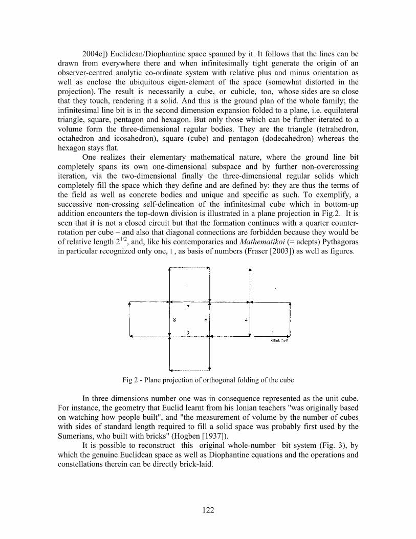
122
2004e]) Euclidean/Diophantine space spanned by it. It follows that the lines can be drawn from everywhere there and when infinitesimally tight generate the origin of an observer-centred analytic co-ordinate system with relative plus and minus orientation as well as enclose the ubiquitous eigen-element of the space (somewhat distorted in the projection). The result is necessarily a cube, or cubicle, too, whose sides are so close that they touch, rendering it a solid. And this is the ground plan of the whole family; the infinitesimal line bit is in the second dimension expansion folded to a plane, i.e. equilateral triangle, square, pentagon and hexagon. But only those which can be further iterated to a volume form the three-dimensional regular bodies. They are the triangle (tetrahedron, octahedron and icosahedron), square (cube) and pentagon (dodecahedron) whereas the hexagon stays flat.
One realizes their elementary mathematical nature, where the ground line bit completely spans its own one-dimensional subspace and by further non-overcrossing iteration, via the two-dimensional finally the three-dimensional regular solids which completely fill the space which they define and are defined by: they are thus the terms of the field as well as concrete bodies and unique and specific as such. To exemplify, a successive non-crossing self-delineation of the infinitesimal cube which in bottom-up addition encounters the top-down division is illustrated in a plane projection in Fig.2. It is seen that it is not a closed circuit but that the formation continues with a quarter counter-rotation per cube – and also that diagonal connections are forbidden because they would be of relative length 21/2, and, like his contemporaries and Mathematikoi (= adepts) Pythagoras in particular recognized only one, ׀ , as basis of numbers (Fraser [2003]) as well as figures.
Fig 2 - Plane projection of orthogonal folding of the cube
In three dimensions number one was in consequence represented as the unit cube. For instance, the geometry that Euclid learnt from his Ionian teachers "was originally based on watching how people built", and "the measurement of volume by the number of cubes with sides of standard length required to fill a solid space was probably first used by the Sumerians, who built with bricks" (Hogben [1937]).
It is possible to reconstruct this original whole-number bit system (Fig. 3), by which the genuine Euclidean space as well as Diophantine equations and the operations and constellations therein can be directly brick-laid.
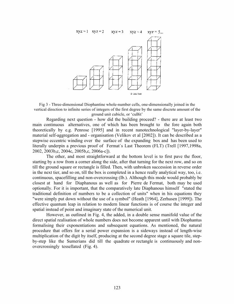
123
Fig 3 - Three-dimensional Diophantine whole-number cells, one-dimensionally joined in the vertical direction to infinite series of integers of the first degree by the same discrete amount of the
ground unit cubicle, or ‘cuBit’ Regarding next question - how did the building proceed? - there are at least two
main continuous alternatives, one of which has been brought to the fore again both theoretically by e.g. Penrose [1995] and in recent nanotechnological "layer-by-layer" material self-aggregation and - organisation (Velikov et al [2002]). It can be described as a stepwise eccentric winding over the surface of the expanding box and has been used to literally underpin a previous proof of Fermat´s Last Theorem (FLT) (Trell [1997,1998a, 2002, 2003b,c, 2004c, 2005b,c, 2006a-c]).
The other, and most straightforward at the bottom level is to first pave the floor, starting by a row from a corner along the side, after that turning for the next row, and so on till the ground square or rectangle is filled. Then, with unbroken succession in reverse order in the next tier, and so on, till the box is completed in a hence really analytical way, too, i.e. continuous, spacefilling and non-overcrossing (Ib.). Although this mode would probably be closest at hand for Diaphanous as well as for Pierre de Fermat, both may be used optionally. For it is important, that the comparatively late Diaphanous himself "stated the traditional definition of numbers to be a collection of units" when in his equations they "were simply put down without the use of a symbol" (Heath [1964], Zerhusen [1999]). The effective quantum leap in relation to modern linear functions is of course the integer and spatial instead of point and imaginary state of the numerical unit.
However, as outlined in Fig. 4, the added, in a double sense manifold value of the direct spatial realisation of whole numbers does not become apparent until with Diophantus formalising their exponentiations and subsequent equations. As mentioned, the natural procedure that offers for a serial power expansion is a sideways instead of length-wise multiplication of the digit by itself, producing at the second degree stage a square tile, step-by-step like the Sumerians did till the quadrate or rectangle is continuously and non-overcrossingly tessellated (Fig. 4).

124
XYZ 1 2 3 4…………
Fig 4 - Genuine Diophantine equation space
Then, in the same fashion, next layer is filled, and next, and next, till the resulting first-order third degree 'hypercube' is also analytically completed (Fig. 4). In turn, that ‘hypercube of the first order’ in same periodic progression re-multiplied by the base number yields a 4th power in the shape of a quasi-one-dimensional ‘hyper-rod of the second order’, which in forthcoming multiplications generates a 5th degree second order hypersquare, 6th degree hypercube etc. in an endless cyclical “self-assembly at all scales” (Whitesides and Grzybowski [2002]) that eventually contains all whole-number (and fractional) powers that there at all are (Fig. 4). The entire Diophantine equation Block Universe is thus generated by a recursive, perpendicularly revolving algorithm in a maximum of three dimensions, thereby reproducing the hierarchically retarded, non-overcrossing, i.e. analytical space-filling of consecutively larger constellations, imaginable up to the size and twist of galaxies, no matter if taking place during actual time or an instantaneous phase transition in the sufficient ordinary Cartesian co-ordinate frame.
In such geometrized mathematical iteration, a stepwise continuous “rod-coil-rod…self-assembly of phase-segregated crystal structures” (Kato [2002]) - which “in turn form assemblies or self-organize, possibly even forming hierarchies” (Ikkala and ten Brinke [2002]) - precipitates in a completely saturating, consecutively substrate-consuming way, displacing other stepwise cumulative syntheses (Fig. 4). This is of utmost relevance, since, with bearing to and like Fermat´s Last Theorem (FLT), “far from beingsome unimportant curiosity in number theory, it is in fact related to fundamental properties of space” (www [1996]) as well as of integers (www [1997]). And the uniformity, that all whole-number powers from n = 3 and onwards are realised in sufficiently three dimensions as saturated regular parallelepipeds enables the demonstrations ad modum Cardano to be exposed in the continuation as expressed by the simplest (but undeniable) ‘schoolboy mathematics’ formulas – by which yet Fermat’s Last
n=1 2
3
4
5
6
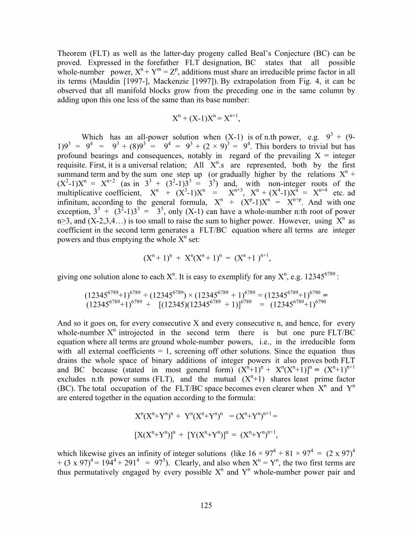
125
Theorem (FLT) as well as the latter-day progeny called Beal’s Conjecture (BC) can be proved. Expressed in the forefather FLT designation, BC states that all possible whole-number power, Xn + Ym = Zp, additions must share an irreducible prime factor in all its terms (Mauldin [1997-], Mackenzie [1997]). By extrapolation from Fig. 4, it can be observed that all manifold blocks grow from the preceding one in the same column by adding upon this one less of the same than its base number:
Xn + (X-1)Xn = Xn+1,
Which has an all-power solution when (X-1) is of n.th power, e.g. 93 + (9-1)93 = 94 = 93 + (8)93 = 94 = 93 + (2 × 9)3 = 94. This borders to trivial but hasprofound bearings and consequences, notably in regard of the prevailing X = integer requisite. First, it is a universal relation; All Xn.s are represented, both by the first summand term and by the sum one step up (or gradually higher by the relations Xn + (X2-1)Xn = Xn+2 (as in 33 + (32-1)33 = 35) and, with non-integer roots of the multiplicative coefficient, Xn + (X3-1)Xn = Xn+3, Xn + (X4-1)Xn = Xn+4 etc. ad infinitum, according to the general formula, Xn + (Xp-1)Xn = Xn+p. And with one exception, 33 + (32-1)33 = 35, only (X-1) can have a whole-number n:th root of power n>3, and (X-2,3,4…) is too small to raise the sum to higher power. However, using Xn as coefficient in the second term generates a FLT/BC equation where all terms are integer powers and thus emptying the whole Xn set:
(Xn + 1)n + Xn(Xn + 1)n = (Xn +1 )n+1,
giving one solution alone to each Xn. It is easy to exemplify for any Xn, e.g. 123456789 :
(123456789+1)6789 + (123456789) × (123456789 + 1)6789 = (123456789+1)6790 = (123456789+1)6789 + [(12345)(123456789 + 1)]6789 = (123456789+1)6790
And so it goes on, for every consecutive X and every consecutive n, and hence, for every whole-number Xn introjected in the second term there is but one pure FLT/BC equation where all terms are ground whole-number powers, i.e., in the irreducible form with all external coefficients = 1, screening off other solutions. Since the equation thus drains the whole space of binary additions of integer powers it also proves both FLT and BC because (stated in most general form) (Xn+1)n + Xn(Xn+1)]n = (Xn+1)n+1 excludes n.th power sums (FLT), and the mutual (Xn+1) shares least prime factor (BC). The total occupation of the FLT/BC space becomes even clearer when Xn and Yn are entered together in the equation according to the formula:
Xn(Xn+Yn)n + Yn(Xn+Yn)n = (Xn+Yn)n+1 =
[X(Xn+Yn)]n + [Y(Xn+Yn)]n = (Xn+Yn)n+1,
which likewise gives an infinity of integer solutions (like 16 × 974 + 81 × 974 = (2 x 97)4 + (3 x 97)4 = 1944 + 2914 = 975). Clearly, and also when Xn = Yn, the two first terms are thus permutatively engaged by every possible Xn and Yn whole-number power pair and
126
giving in the third term a sum whole-number power sharing prime factor but in a higher degree. Inserting each successively larger Xn and Yn thus proves both BC (by all X and Y permutations) and FLT (by all n powers) en bloc by the ascending differential “layer-by-layer…complete close-packed” (Velikov et al. [2002]) sequential iteration gradually sweeping over and so covering the overall Diophantine equation space.
III. ARISTOTELEAN PHASE TRANSITIONSince ancient time, a profound insight in relation to the straight and round forms is
that they are absolutely endless, yet distinct and irreconcilable over a gap of limes (the last decimal of) p. They are alternative versions of one principal realization, and this statutory dichotomy like two juxtaposed conduction plates generates a potential fall between their respective, maximally dilated versus maximally contracted infinite strands. One may here quote Aristotle (384 - 322 BC): “everything that comes to be comes into being from its contrary and in some substrate, and passes away likewise in a substrate by the action of the contrary into the contrary” and “if there is a contrary to circular. A straight line must be recognized as having the best claim to that name” (http [b]). The still valid corollary of the above is that structural rendering and dynamics (Santilli [2001]) differentially occur as an instantaneous geodetic phase transition “between the curved and the straight at the heart of Greek geometry and indeed of geometry in general” (Netz [2002]) as first mathematically described by Marius Sophus Lie in his Ph. D. thesis Over en Classe Geometriske Transformationer at Kristiania (as Oslo was then called) University in 1871.
Taking the nowadays mystics (Carmeli [1977]) out of these, their continuous transformation groups and algebras are quite concretely outlining the straight-to-round phase transition in Cartesian space (Fig. 5), whose natural endlessness is unproblematic since everywhere down to the ultimate quantum scale divided in infinitesimal neighbourhoods for the automatically co-ordinated discharge from the so relativistically connected interaction origins.
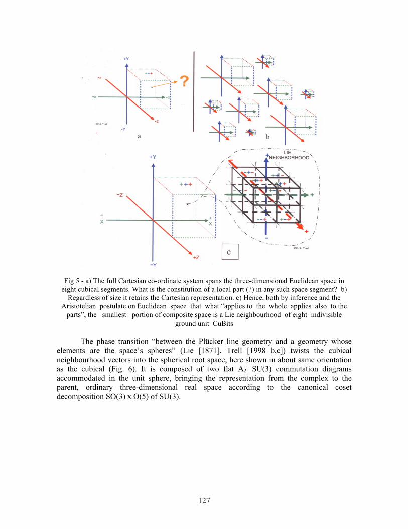
127
Fig 5 - a) The full Cartesian co-ordinate system spans the three-dimensional Euclidean space in eight cubical segments. What is the constitution of a local part (?) in any such space segment? b)
Regardless of size it retains the Cartesian representation. c) Hence, both by inference and the Aristotelian postulate on Euclidean space that what “applies to the whole applies also to the
parts”, the smallest portion of composite space is a Lie neighbourhood of eight indivisible ground unit CuBits
The phase transition “between the Plücker line geometry and a geometry whose elements are the space’s spheres” (Lie [1871], Trell [1998 b,c]) twists the cubical neighbourhood vectors into the spherical root space, here shown in about same orientation as the cubical (Fig. 6). It is composed of two flat A2 SU(3) commutation diagrams accommodated in the unit sphere, bringing the representation from the complex to the parent, ordinary three-dimensional real space according to the canonical coset decomposition SO(3) x O(5) of SU(3).
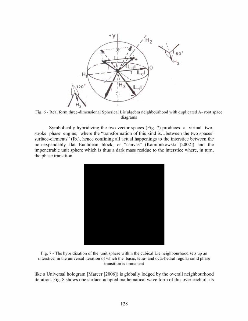
128
Fig. 6 - Real form three-dimensional Spherical Lie algebra neighbourhood with duplicated A2 root space diagrams
Symbolically hybridizing the two vector spaces (Fig. 7) produces a virtual two-stroke phase engine, where the “transformation of this kind is…between the two spaces’ surface-elements” (Ib.), hence confining all actual happenings to the interstice between the non-expandably flat Euclidean block, or “canvas” (Kamionkowski [2002]) and the impenetrable unit sphere which is thus a dark mass residue to the interstice where, in turn, the phase transition
Fig. 7 - The hybridization of the unit sphere within the cubical Lie neighbourhood sets up an interstice, in the universal iteration of which the basic, tetra- and octa-hedral regular solid phase
transition is immanent
like a Universal hologram [Marcer [2006]) is globally lodged by the overall neighbourhood iteration. Fig. 8 shows one surface-adapted mathematical wave form of this over each of its
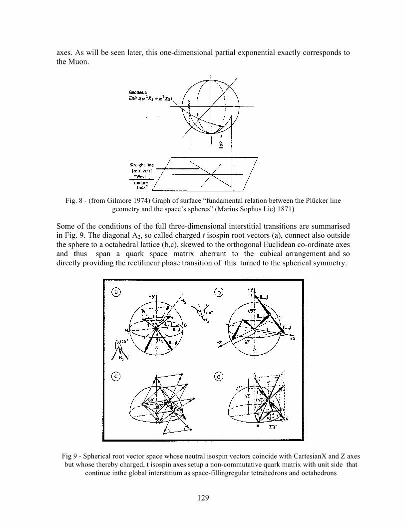
129
axes. As will be seen later, this one-dimensional partial exponential exactly corresponds to the Muon.
Fig. 8 - (from Gilmore 1974) Graph of surface “fundamental relation between the Plücker line geometry and the space’s spheres” (Marius Sophus Lie) 1871)
Some of the conditions of the full three-dimensional interstitial transitions are summarised in Fig. 9. The diagonal A2, so called charged t isospin root vectors (a), connect also outside the sphere to a octahedral lattice (b,c), skewed to the orthogonal Euclidean co-ordinate axes and thus span a quark space matrix aberrant to the cubical arrangement and so directly providing the rectilinear phase transition of this turned to the spherical symmetry.
Fig 9 - Spherical root vector space whose neutral isospin vectors coincide with CartesianX and Z axes but whose thereby charged, t isospin axes setup a non-commutative quark matrix with unit side that
continue inthe global interstitium as space-fillingregular tetrahedrons and octahedrons
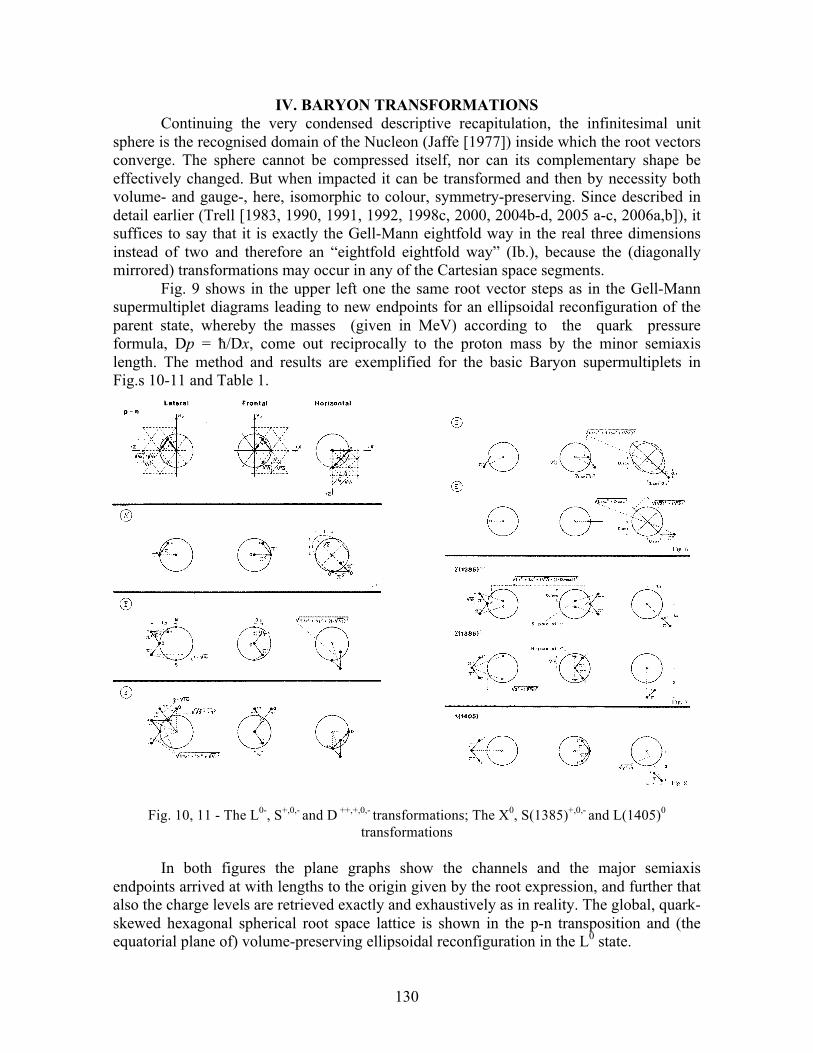
130
IV. BARYON TRANSFORMATIONSContinuing the very condensed descriptive recapitulation, the infinitesimal unit
sphere is the recognised domain of the Nucleon (Jaffe [1977]) inside which the root vectors converge. The sphere cannot be compressed itself, nor can its complementary shape be effectively changed. But when impacted it can be transformed and then by necessity both volume- and gauge-, here, isomorphic to colour, symmetry-preserving. Since described in detail earlier (Trell [1983, 1990, 1991, 1992, 1998c, 2000, 2004b-d, 2005 a-c, 2006a,b]), it suffices to say that it is exactly the Gell-Mann eightfold way in the real three dimensions instead of two and therefore an “eightfold eightfold way” (Ib.), because the (diagonally mirrored) transformations may occur in any of the Cartesian space segments.
Fig. 9 shows in the upper left one the same root vector steps as in the Gell-Mann supermultiplet diagrams leading to new endpoints for an ellipsoidal reconfiguration of the parent state, whereby the masses (given in MeV) according to the quark pressure formula, Dp = ħ/Dx, come out reciprocally to the proton mass by the minor semiaxis length. The method and results are exemplified for the basic Baryon supermultiplets in Fig.s 10-11 and Table 1.
Fig. 10, 11 - The L0-, S+,0,- and D ++,+,0,- transformations; The X0, S(1385)+,0,- and L(1405)0
transformations
In both figures the plane graphs show the channels and the major semiaxis endpoints arrived at with lengths to the origin given by the root expression, and further that also the charge levels are retrieved exactly and exhaustively as in reality. The global, quark-skewed hexagonal spherical root space lattice is shown in the p-n transposition and (the equatorial plane of) volume-preserving ellipsoidal reconfiguration in the L0 state.
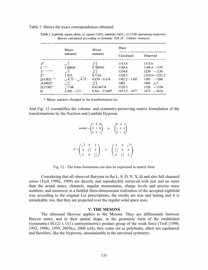
131
Table 1: Shows the exact correspondences obtained
And Fig. 12 exemplifies the volume- and symmetry-preserving matrix formulation of the transformations by the Nucleon and Lambda Hyperon. .
Fig. 12 - The trans-formations can also be expressed in matrix form
Considering that all observed Baryons in the L, S, D, N, X, Ω and also full charmed series (Trell 1998c, 1999) are directly and reproducibly retrieved with just and no more than the actual states, channels, angular momentums, charge levels and precise mass numbers, and moreover in a faithful three-dimensional realization of the accepted eightfold way according to the original Lie prescriptions, the results are true and lasting and it is remarkable, too, that they are projected over the regular solid space axes.
V. THE MESONS The aforesaid likewise applies to the Mesons. They are differentials between
Baryon states, and in their spatial shape, in the geometric form of the established (symmetric) SU(2) x U(1) (antisymmetric) product group of the weak force (Trell [1990, 1992, 1998c, 1999, 2005b,c, 2006 a,b]), they come out as polyhedra, albeit not equilateral and therefore, like the Hyperons, unsustainable in the universal symmetry.
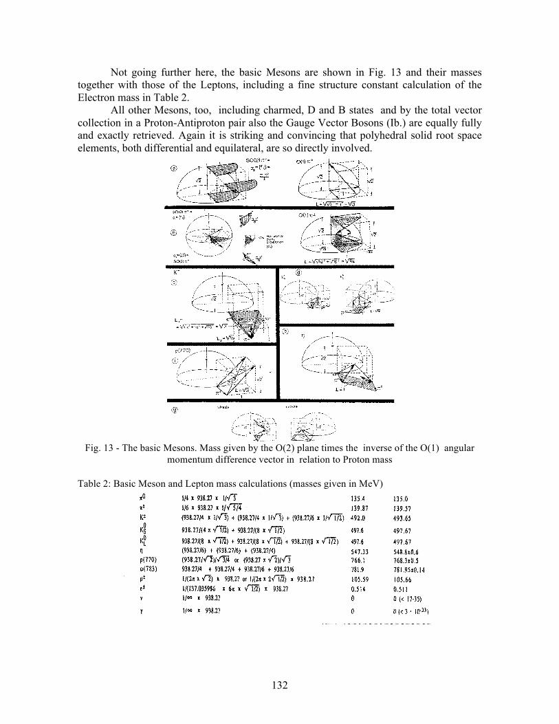
132
Not going further here, the basic Mesons are shown in Fig. 13 and their masses together with those of the Leptons, including a fine structure constant calculation of the Electron mass in Table 2.
All other Mesons, too, including charmed, D and B states and by the total vector collection in a Proton-Antiproton pair also the Gauge Vector Bosons (Ib.) are equally fully and exactly retrieved. Again it is striking and convincing that polyhedral solid root space elements, both differential and equilateral, are so directly involved.
Fig. 13 - The basic Mesons. Mass given by the O(2) plane times the inverse of the O(1) angular momentum difference vector in relation to Proton mass
Table 2: Basic Meson and Lepton mass calculations (masses given in MeV)

133
Fig. 14 shows the sequences obtained when the charged regular solid sides in the Nucleon root space are connected according to the geometrical automorphism of the antisymmetric U(1) Lie algebra of the Leptons. When the neutral, including the diagonal H2, vectors are joined, endless straight or zig-zag lines, corresponding to the Neutrinos and Photons, respectively, result with mass expression 1/∞ × Proton mass = 0 MeV. But when the charged unit vectors are linked, two types of plane, winged or helical orbits may occur over the Nucleon surface (Fig. 14), one by 90o angels (a-c) and giving a circumference in curved adaptation direct over the surface of length 2p × 21/2 or 2 × 2p × 1/21/2, and consequential mass number in relation to Proton mass and unit radius = 938.28/(2p × 21/2) MeV = 105.59 MeV, versus the actual 105.66 MeV of the Muon (Ib.).
Fig. 14 - (Cores of) charged Lepton geodesics over Nucleon/Cartesian segment surface (Compare Fig. 8)
The other, 60-120o sequence does not fit with the orthogonal Nucleon surface curvature but with the hexagonal root space alignment, connecting there to a three-pronged, electron/(positron) singlet circuit (d, e) and thus lifting into the next periodically expanded section of the regular solid warp, where in an assumed rounded distribution with the fine structure constant as radial proportionality factor, the mass comes out as 1/(137.036×3×2p×1/21/2 ) × 938.28 = 0.514 versus the actual 0.511 MeV of the Electron (Ib.)
However, outside the Nucleon the straight root vectors are direct polyhedral sides because, as shown in Fig. 15, their charge-preserving convolutions take the form of the (only) space-filling one-octa-/two-tetrahedron infinitesimal unit of the transition matrix. This double cast of the Electrons as “wave functions or transition matrix elements” are in line with recent Hydrogen ground state research (Martin et al. [2007]), and the instant material “modular building block” (de Weck et al. [2005]) nature of the Electron is pending in modern nanotechnology, molecular biology etc.
VI. THE LEPTONS
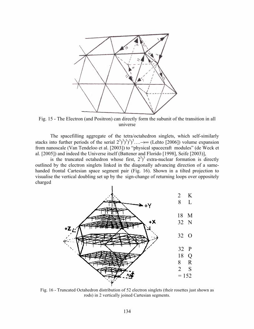
134
Fig. 15 - The Electron (and Positron) can directly form the subunit of the transition in all universe
The spacefilling aggregate of the tetra/octahedron singlets, which self-similarly stacks into further periods of the serial 23)3)3)3)3….→∞ (Lehto [2006]) volume expansion from nanoscale (Van Tendeloo et al. [2003]) to “physical spacecraft modules” (de Weck et al. [2005]) and indeed the Universe itself (Battener and Florido [1998], Seife [2003)],
is the truncated octahedron whose first, 23)3 extra-nuclear formation is directly outlined by the electron singlets linked in the diagonally advancing direction of a same-handed frontal Cartesian space segment pair (Fig. 16). Shown in a tilted projection to visualise the vertical doubling set up by the sign-change of returning loops over oppositely charged
Fig. 16 - Truncated Octahedron distribution of 52 electron singlets (their rosettes just shown as rods) in 2 vertically joined Cartesian segments.
2 K 8 L
18 M 32 N
32 O
32 P 18 Q 8 R 2 S = 152
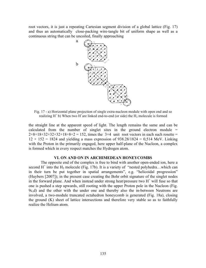
135
root vectors, it is just a repeating Cartesian segment division of a global lattice (Fig. 17) and thus an automatically close-packing wire-tangle bit of uniform shape as well as a continuous string that can be uncoiled, finally approaching
Fig. 17 - a) Horizontal plane projection of single extra-nucleon module with open end and so realizing H+ b) When two H+are linked end-to-end (or side) the H2 molecule is formed
the straight line at the apparent speed of light. The length remains the same and can be calculated from the number of singlet sites in the ground electron module = 2+8+18+32+32+32+18+8+2 = 152, times the 3×4 unit root vectors in each such rosette = 12 × 152 = 1824 and yielding a mass expression of 938.28/1824 = 0,514 MeV. Linking with the Proton in the primarily engaged, here upper half-plane of the Nucleon, a complex is formed which in every respect matches the Hydrogen atom.
VI. ON AND ON IN ARCHIMEDEAN HONEYCOMBSThe opposite end of the complex is free to bind with another open-ended ion, here a
second H+ into the H2 molecule (Fig. 17b). It is a variety of “nested polyhedra…which can in their turn be put together in spatial arrangements”, e.g. “helicoidal progression” (Huybers [2007]); in the present case creating the Bohr orbit signature of the singlet nodes in the forward plane. And when instead under strong heat/pressure two H+ will fuse so that one is pushed a step upwards, still rooting with the upper Proton pole in the Nucleon (Fig. 9c,d) and the other with the under one and thereby also the in-between Neutrons are involved, a two-module truncated octahedron honeycomb is generated (Fig. 18a), closing the ground (K) sheet of lattice intersections and therefore very stable so as to faithfully realize the Helium atom.
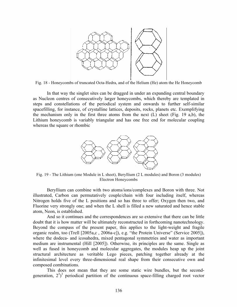
136
Fig. 18 - Honeycombs of truncated Octa-Hedra, and of the Helium (He) atom the He Honeycomb
In that way the singlet sites can be dragged in under an expanding central boundary as Nucleon centres of consecutively larger honeycombs, which thereby are templated in steps and constellations of the periodical system and onwards to further self-similar spacefilling, for instance, of crystalline lattices, deposits, rocks, planets etc. Exemplifying the mechanism only in the first three atoms from the next (L) sheet (Fig. 19 a,b), the Lithium honeycomb is variably triangular and has one free end for molecular coupling whereas the square or rhombic
Fig. 19 - The Lithium (one Module in L sheet), Beryllium (2 L modules) and Boron (3 modules) Electron Honeycombs
Beryllium can combine with two atoms/ions/complexes and Boron with three. Not illustrated, Carbon can permutatively couple/chain with four including itself, whereas Nitrogen holds five of the L positions and so has three to offer; Oxygen then two, and Fluorine very strongly one; and when the L shell is filled a new saturated and hence stable atom, Neon, is established.
And so it continues and the correspondences are so extensive that there can be little doubt that it is how matter will be ultimately reconstructed in forthcoming nanotechnology. Beyond the compass of the present paper, this applies to the light-weight and fragile organic realm, too (Trell [2005a,c , 2006a-c]), e.g. “the Protein Universe” (Service 2005]), where the dodeca- and icosahedra, mixed pentagonal symmetries and water as important medium are instrumental (Hill [2005]). Otherwise, its principles are the same. Single as well as fused in honeycomb and molecular aggregates, the modules heap up the joint structural architecture as veritable Lego pieces, patching together already at the infinitesimal level every three-dimensional real shape from their consecutive own and composed combinations.
This does not mean that they are some static wire bundles, but the second-generation, 23)3 periodical partition of the continuous space-filling charged root vector
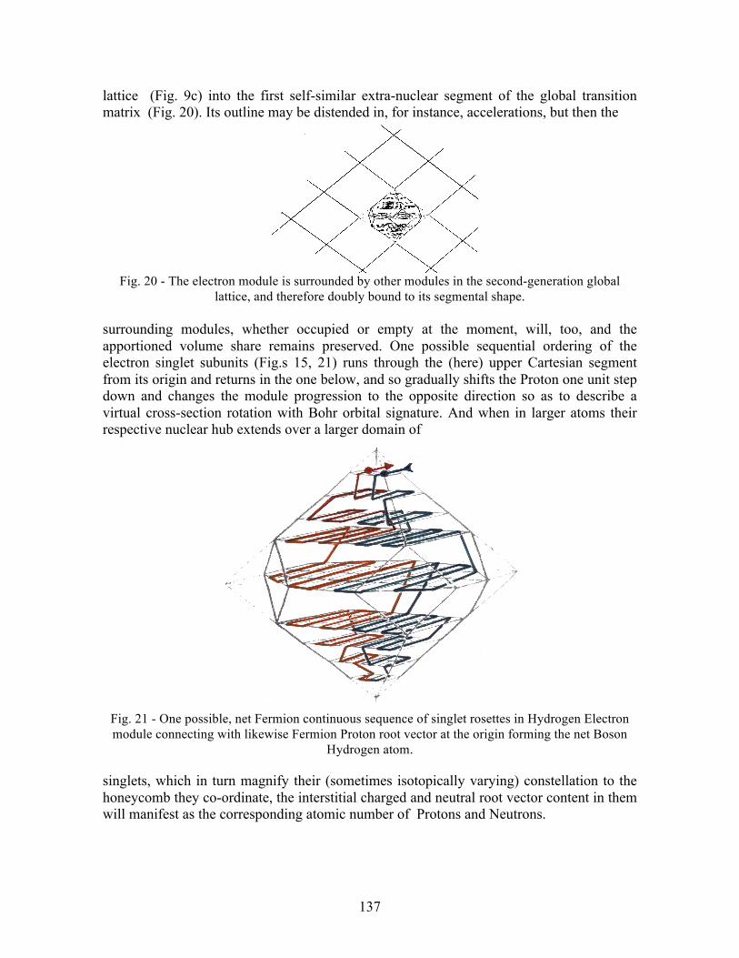
137
lattice (Fig. 9c) into the first self-similar extra-nuclear segment of the global transition matrix (Fig. 20). Its outline may be distended in, for instance, accelerations, but then the
Fig. 20 - The electron module is surrounded by other modules in the second-generation global lattice, and therefore doubly bound to its segmental shape.
surrounding modules, whether occupied or empty at the moment, will, too, and the apportioned volume share remains preserved. One possible sequential ordering of the electron singlet subunits (Fig.s 15, 21) runs through the (here) upper Cartesian segment from its origin and returns in the one below, and so gradually shifts the Proton one unit step down and changes the module progression to the opposite direction so as to describe a virtual cross-section rotation with Bohr orbital signature. And when in larger atoms their respective nuclear hub extends over a larger domain of
Fig. 21 - One possible, net Fermion continuous sequence of singlet rosettes in Hydrogen Electron module connecting with likewise Fermion Proton root vector at the origin forming the net Boson
Hydrogen atom.
singlets, which in turn magnify their (sometimes isotopically varying) constellation to the honeycomb they co-ordinate, the interstitial charged and neutral root vector content in them will manifest as the corresponding atomic number of Protons and Neutrons.
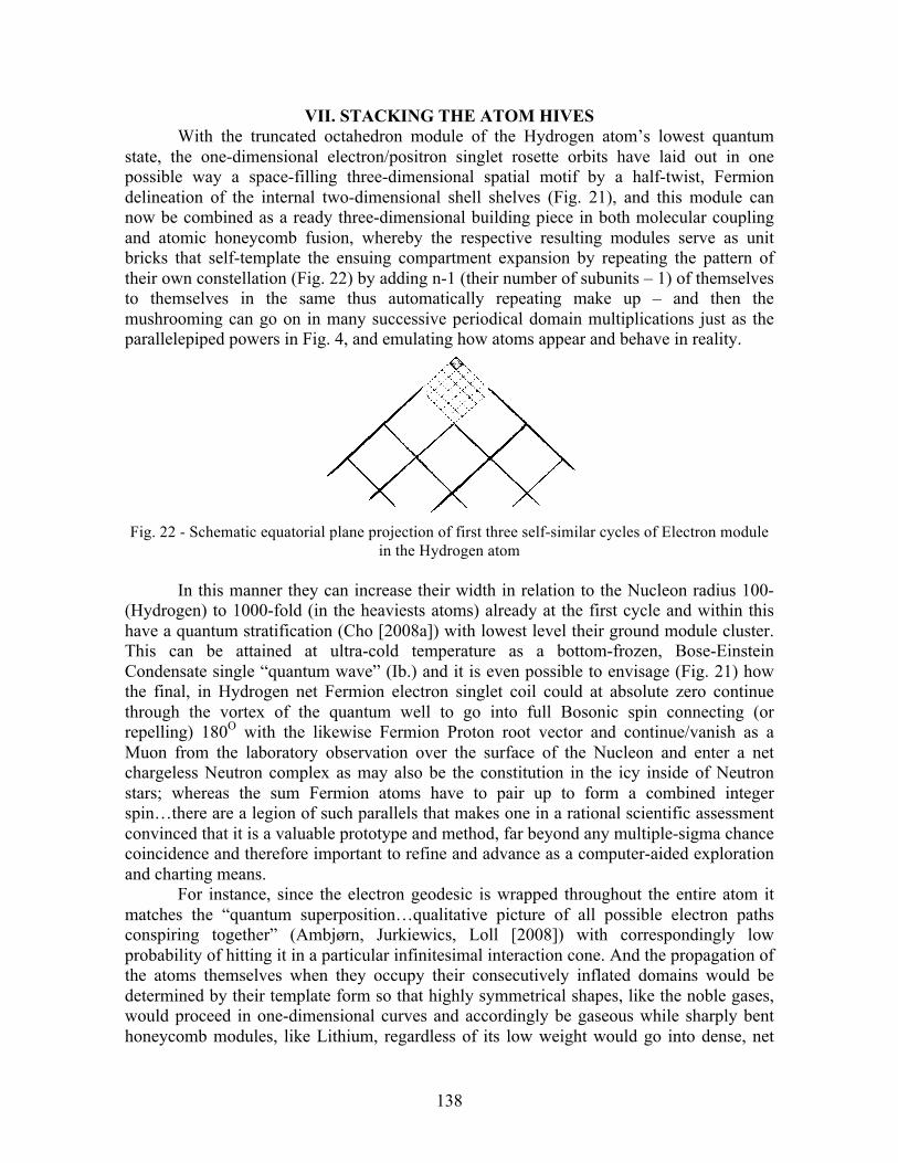
138
VII. STACKING THE ATOM HIVESWith the truncated octahedron module of the Hydrogen atom’s lowest quantum
state, the one-dimensional electron/positron singlet rosette orbits have laid out in one possible way a space-filling three-dimensional spatial motif by a half-twist, Fermion delineation of the internal two-dimensional shell shelves (Fig. 21), and this module can now be combined as a ready three-dimensional building piece in both molecular coupling and atomic honeycomb fusion, whereby the respective resulting modules serve as unit bricks that self-template the ensuing compartment expansion by repeating the pattern of their own constellation (Fig. 22) by adding n-1 (their number of subunits – 1) of themselves to themselves in the same thus automatically repeating make up – and then the mushrooming can go on in many successive periodical domain multiplications just as the parallelepiped powers in Fig. 4, and emulating how atoms appear and behave in reality.
Fig. 22 - Schematic equatorial plane projection of first three self-similar cycles of Electron module in the Hydrogen atom
In this manner they can increase their width in relation to the Nucleon radius 100- (Hydrogen) to 1000-fold (in the heaviests atoms) already at the first cycle and within this have a quantum stratification (Cho [2008a]) with lowest level their ground module cluster. This can be attained at ultra-cold temperature as a bottom-frozen, Bose-Einstein Condensate single “quantum wave” (Ib.) and it is even possible to envisage (Fig. 21) how the final, in Hydrogen net Fermion electron singlet coil could at absolute zero continue through the vortex of the quantum well to go into full Bosonic spin connecting (or repelling) 180O with the likewise Fermion Proton root vector and continue/vanish as a Muon from the laboratory observation over the surface of the Nucleon and enter a net chargeless Neutron complex as may also be the constitution in the icy inside of Neutron stars; whereas the sum Fermion atoms have to pair up to form a combined integer spin…there are a legion of such parallels that makes one in a rational scientific assessment convinced that it is a valuable prototype and method, far beyond any multiple-sigma chance coincidence and therefore important to refine and advance as a computer-aided exploration and charting means.
For instance, since the electron geodesic is wrapped throughout the entire atom it matches the “quantum superposition…qualitative picture of all possible electron paths conspiring together” (Ambjørn, Jurkiewics, Loll [2008]) with correspondingly low probability of hitting it in a particular infinitesimal interaction cone. And the propagation of the atoms themselves when they occupy their consecutively inflated domains would be determined by their template form so that highly symmetrical shapes, like the noble gases, would proceed in one-dimensional curves and accordingly be gaseous while sharply bent honeycomb modules, like Lithium, regardless of its low weight would go into dense, net
139
two- or three-dimensional convolutions so as to be solid (until heated/excited so that it starts to boil into orbit). And since the offset ‘caps’ that the honeycombs’ collective truncation leaves at the top contain the abandoned central root vectors there will be a reciprocal nucleus, always with as many charged, Proton ones as the atomic number, while the Neutrons can be more numerous reflecting the lateral displacements possible, e.g. in 11Li (Sherril [2008]). Illustrated here is only Hydrogen but it is a general procedure from which the full inorganic realm and its likewise polygonal macroscopic minerals and crystals can be reconstructed in the real three dimensions.
VIII. DISCUSSIONAccompanying the initially mentioned experimental elementary particle crisis there
is also a theoretical one, as highlighted in a prominent recent Scientific American article (Ambjørn, Jurkiewics, Loll [2008]). Its “new approach to the decades-old problem of quantum gravity goes back to basics and shows how the building blocks of space and time pull themselves together”. In comparison, “superstring theory has not yet produced an answer…leading to a bewildering variety of possible outcomes”, and prior “Euclidean quantum gravity…using tiny building blocks…gluing four-simplices along their faces (which are actually three-dimensional tetrahedra)” by their “quantum fluctuations on short scale…makes the entire space crumple up into a tiny ball with an infinite number of dimensions”.
As posed in the article: “what could the trouble be? In our search for loopholes and loose ends in the Euclidean approach, we finally hit on the crucial idea, the one ingredient absolutely necessary to make the stir fry come out right: the universe must encode what physicists call causality. Causality means that empty space has a structure that allows us to distinguish unambiguously between cause and effect” by assigning “each simplex an arrow of time pointing from the past to the future. And then we enforced causal gluing rules: two simplices must be glued together to keep their arrows pointing in the same direction” and so enabling an iterated “dynamic triangulation”, however, “without regard to any symmetry or preferred geometrical structure” so that at the “limit, nothing depends on whether the blocks were triangular, cubic, pentagonal or any mixture thereof to start with”. In addition “for our model to work we needed to include from the outset a so-called cosmological constant, an invisible and immaterial substance that space contains even in the absence of other forms of matter”. So calibrated, the computer “calculations of a large causal superposition of four-simplices” gave the result that “the number of dimensions came out as four (more precisely as 4.02 ±0)” (Ib.). This is a great advance of Quantum Gravity, but also restricted to that field so that the statement that “it is difficult to imagine how physicists could get away with fewer ingredients and technical tools than we have used to create a quantum universe with realistic properties” (Ib.) is arguable. For instance, “the holy grail…the prediction of observable consequences derived from the microscopic quantum structure” is lacking, the regular solids are not considered, and it is not in general true that it is a faithful “Euclidean approach” that really “goes back to the basics” in that sense.
The common denominator of the shortcomings would seem to be that even at the threshold already composed objects like triangles are employed which don’t reach the truly elemental ground quantum of Euclidean space where form does matter (in double meaning) from the start and is conveyed throughout. This truly ground quantum is by necessity of the straight line because at the infinite descent limit the singular, simplest and further
140
irreducible shape that remains can only be one-dimensional and rectilinear as the infinitesimal interval bit in its own bare instep while round or other bends can not exist at this smallest ‘last decimal of p‘ scale as shown already by Archimedes (287-212 BC) when he approximated said decimal by repeated halvings of the sides of the polygon inscribed in a circle. Perfect round is then, as Plato put it, an Idea, an attractor to be drawn at, and is hence the phase transition motor of dynamics and transformations and self-aggregations in genuine Euclidean space, enacted there – and here – by infinitesimal straight eigenvectors and eigenoperations, whose minute features are transferred in eigentemplates of exponentially enlarged compartments and compounds all the way up to the “octahedron structure” of “the distribution of superclusters in the Local Supercluster neighbourhood” which “presents such a remarkable periodicity that some kind of network must fit” (Battaner and Florido [1998]).
Another, more antrophic argument for Straight is that we and our perceptions are directly parts of and resonating with actual reality all from the quantum level. In other words, we should pay much attention to testimonies like the following (cited from Tate Modern): “Piet Mondrian (1872-1944) believed that all complex forms could be reduced to a ‘plurality of straight lines in rectangular opposition’…his paintings…also represent a physiological reality about the brain…the cells of the visual brain are responsive to straight lines of specific orientation and the field of view to which they respond is rectangular in shape”. And this applies to our binary branching thought processes as well, i.e. intelligence and logic (Marcer [2008]), where the straight line bit and its Platonic concatenations and expansions constitute a faithful morphogenetic ground modality of NUCRS (Rowlands [2003a,b, 2006, 2008]) and likewise are engaged in the three-dimensional orthogonal twist “processes of Encryption/Decryption” utilized in “Quantum Holography, defined by means of the Heisenberg nilpotent Lie Group” and “applied at Bletchley Park in World War Two using various machines including the Turing Bombes and Colossus” (Marcer [2008]) as well as more recently in Magnetic Resonance Imaging (Schempp [1997]).
But the strongest argument is the reproducible outcome. It is obtained by genuine first principles and in many instances comprises a first itself. And the results are what counts and persists; Some day, some model will prevail, and the simpler and more akin to the world at large the better and more plausible and workable. At the elementary particle/atomic stage the direct structural reproductions cover the inorganic realm with unprecedented resolution and completeness. Organic matter, however, predominantly rises from much more composite, molecular building blocks but still applies the regular bodies in enlarged form-specific – and nota bene and to every recruited bit principally form-specific – casts, including the pentagonal and mixed symmetrical dodecahedra and icosahedra. Fundamental morphological work is here under way above all by Hill and Rowlands [2008].
The present paper is but a brief summary in need of further clarification, e.g. of crowding and overlapping properties in atoms rooted from central parts of larger cores. However, the findings are true and lasting, and open the way for a definite bottom-up reconstruction of rendered matter. To sum up; It is time to abandon the latter-day Western misconception of the regular solids as mere pastimes of ancient symposia. They are the conceived elements of a world built by itself and its deep philosophical and logical imperative, and it is the one and only structural world that we are equal parts of. And it is essential that they are so distinct already at the ground because precise constructions need
141
precise elements; still vastly larger than the ‘not even wrong’ superstrings currently in vogue. It is at last fascinating to consider that all real line forms and constellations are conveyed in the span between their engendering straight and round extremities.
REFERENCES [1]. Adhikari, M.R., Adhikari, A. Groups, Rings and Modules With Applications, 2nd Edition. Hyderabad: Universities Press, 2003. [2]. Ambjørn, J., Jurkiewics, J., Loll, R. ‘The self-organizing Quantum Universe’, Scientific American, July 2008, pp. 42-49. [3]. Battener, E. and Florido, E. ‘The egg-carton Universe’, arXiv: astro-ph/9802009v1, 1998, pp. 1-7. [4]. Carmeli, M. Group Theory and General Relativity. New York, St. Louis, San Francisco, Toronto: McGraw-Hill International, 1977. [5]. Cho, A. ‘Constructing Spacetime - No Strings Attached’, Science, 298, 2002, pp. 1166-1167. [6]. Cho, A. ‘Insights Flow From Uktracold Atoms That Mimic Superconductors’, Science, 319, 2008, pp. 1180-1181. [7]. Cho, A. ‘Does Fermilab Have a Future?’, Science, 320, 2008, pp. 1148-1151. [8]. De Weck O.L., Nadir, W.D., Wong, J.G., Bounova, G., Coffee, T.M. ‘Modular Structures for Manned Space Exploration: The Truncated Octahedron as a Building Block’, AIAA, 2005-2764, 2005, pp. 1-26. [9]. Fraser, J.T. ‘Mathematics and Time’, Kronoscope Journal for the Study of Time, 3, 2003, pp. 153-67. [10]. Guth, A.H. and Kaiser, D.I. ‘Inflatory Cosmology: Exploring the Universe from the Smallest to the Largest Scales’, Science, 307, 2005, pp. 884-890. [11]. Hill, V. Polyhedral rendering of DNA structure. The joint NTNU/BCSCMsG Symposium‘Science and Philosophy Engaged’ 31stMarch-2nd April, Sage Skysstasjon Trollheimer conference center, 2006. [12]. Hill, V. and Rowlands, P. ‘Nature’s Code’, To be published in AIP Conference Proceedings, 2008. [13]. Hogben, L. Mathematics for the Million. London: Georg Allen&Unwin, 1937. [14]. http://scholar.uwinnipeg.ca/courses/38/4500.6001/Cosmology/dimensionality.htm (a) [15]. http://academic.udayton.edu/BradHume/hst340/aristotle.htm (b) [16]. Huybers, P. ‘Nested Polyhedra, IASS Newsletter, 14, 2007, pp. 31-40. [17]. Ikkala, O. and ten Brinke, G. ‘Functional Materials Based on Self-Assembly of Polymeric Supramolecules’, Science, 295, 2002, pp. 2407-2409. [18]. Jaffe, R. ‘Quark confinement’, Nature, 268, 1997,pp. 201-208. [19]. Johansen, S. ‘Initiation of 'Hadronic Philosophy', the Philosophy Underlying Hadronic Mechanics and Chemistry’, Hadronic Journal, 29, 2006, pp. 111-135. [20]. Johansen, S. ‘Outline of a Differential Epistemology’. The joint NTNU/BCSCMsG Symposium ‘Science and Philosophy Engaged’ 31stMarch-2nd April, 2006, Sage Skysstasjon Trollheimer conference center. [21]. Kamionkowski, M. ‘A Hawking-eye View of the Universe’, Science, 296, 2002, p
142
[22]. Kato, T. ‘Self-Assembly of Phase-Segregated Liquid Crystal Structures’, Science, 295, 2002, pp. 2414-2418. [23]. Lehto, A. ‘On the structure of space-time and matter as obtained from the Planck scale by period doubling in three and four dimensions’. Physical Interpretations of Relativity Theory X, 8-11 September 2006, Imperial College, London. [24]. Lie, M. S. Ph.D. thesis: Over en Classe Geometriske Transformationer, Kristiania (now Oslo): Kristiania University, 1871. [25]. Mackenzie, D. ‘Number Theorists Embark on a New Treasure Hunt’, Science, 279, 1997, p 139. [26]. Mackenzie, D. ‘Taming the Hyperbolic Jungle by Pruning its Unruly Edges’, Science, 306, 2004, pp. 2182-2183. [27]. Makovicky, E. ‘800 Year Old Pentagonal Tiling from Maragha, Iran, and the New Varieties of Aperiodic Tiling it Inspired’. In: I. Hargittai, Ed. Fivefold Symmetry. Singapore: World Scientific, 1992, pp. 67-86. [28]. Marcer, P. ‘Notes on 3-D quantum holography Universe’. The joint NTNU/BCSCMsG Symposium ‘Science and Philosophy Engaged’ 31stMarch-2nd April, 2006, Sage Skysstasjon Trollheimer conference center. [29]. Marcer, P. ‘A Mathematical Definition of Intelligence. Back to the Future: the Machines of Bletchley Park’. Manuscript, 2008. [30]. Mauldin, R. D. ‘The Beal Conjecture and Prize’, www.math.unt. edu/mauldin/ beal.html, 1997. [31]. Netz, R. ‘Proof, Amazement, and the Unexpected’, Science, 298, 2002, pp. 967-968. [32]. Penn, R.L. ‘Resolving an Elusive Structure’, Science, 316, 2007, pp. 1704-1705. [33]. Penrose, R. Shadows of the Mind. Oxford: Oxford University Press, 1995. [34]. Rowlands, P. ‘From Zero to the Dirac Equation’. In: (Ed.s) Duffy MC, Gladyshev VO, Morozov AN. Proceedings of Inter-national Scientific Meeting PIRT -2003, Moscow 30/6–3/7 2003, Bauman State University, Moscow, Liverpool, Sunderland, 2003,pp.13-34. [35]. Rowlands, P. and Diaz, B. ‘A Computational Path to the Nilpotent Dirac Equation’, Symposium 10, International Conference for Computing Anticipatory Systems, HEC Liege, Belgium, August 11-16, 2003, International Journal of Computing Anticipatory Systems, editor Daniel Dubois, 203-218. Also at arXiv.cs.OH/0209026 [36]. Rowlands, P. ‘How close are we to a fundamental theory?’ The joint NTNU/BCSCMsG Symposium ‘Science and Philosophy Engaged’ 31stMarch-2nd April, 2006, Sage Skysstasjon Trollheimer conference center. [37]. Rowlands, P. ‘Nilpotent theory & vacuum’. Physical Interpretations of Relativity Theory X, 8-11 September 2006, Imperial College, London. [38]. Santilli, R.M. Foundations of hadronic chemistry with applications to new clean energies and fuels. Boston, Dordrecht, London: Kluwer Academic Publishers, 2001. [39]. Schempp, W. Magnetic Resonance Imaging: Mathematical Foundations and Applications. New York: John Wiley and sons, 1997. [40]. Seife, C., ‘Polyhedral Model Gives the Universe An Unexpected Twist’, Science, 302, 2003, p 209. [41]. Service, R.F. ‘A Dearth of New Folds’, Science, 307, 2005, p 1555. [42]. Sherrill, B.M., ‘Designer Atomic Nuclei’, Science, 320, 2008, pp. 751-752.
143
[43]. Sutton, D. Platonic and Archimedean Solids. Walkmill, Cascob, Presteigne, Powys, Wales: Wooden books, 2001. [44]. Trell, E. ‘A calculation of the electron circular orbital radius, Speculations in Science and Technology, 5, 1982, pp. 533-535. [45]. Trell, E. ‘Representation of particle masses in Hadronic SU(3) diagram, Acta Physica Austriaca, 55, 1983, pp. 97-110. [46]. Trell, E. ‘Scheme for a time antenna in three-dimensional Hausdorff space', Speculations in Science and Technology, 7, 1984, pp 269-277. [47]. Trell, E. ‘Geometrical Reproduction of (u,d,s) Baryon, Meson, and Lepton Transformation Symmetries, Masses, and Channels’, Hadronic Journal, 13, 1990, pp 277-297. [48]. Trell, E. ‘On Rotational Symmetry and Real Geometrical Representations of the Elementary Particles With Special Reference to the N and D Series’, Physics Essays, 4, 1991, pp. 272-283. [49]. Trell, E. ‘Real Forms of the Elementary Particles with A Report of the S Resonances’, Physics Essays, 5, 1992, pp. 362-373. [50]. Trell, E. ‘An alternative solution to Fermat´s Last Theorem: Infinite ascent in isotopic geometry’, Hadronic Journal Supplement, 12, 1997, pp. 217-240. [51]. Trell, E. ‘Isotopic proof and reproof of Fermat’s Last Theorem verifying Beal’s Conjecture’, Algebras Groups and Geometries, 15, 1998, pp. 299-318. [52]. Trell, E. and Santilli, R.M. ‘Marius Sophus Lie's Doctoral Thesis Over en Classe Geometriske Transformationer’, Algebras Groups and Geometries, 15, 1998, pp. 395-445. [53]. Trell, E. ‘The Eightfold Eightfold Way: Application of Lie's True Geometriske Transformationer to Elementary Particles’, Algebras Groups and Geometries, 15, 1998, pp. 447-471. [54]. Trell, E. ‘Real Charm of Form - Real Form of Charm. In: (Gill, T., Liu, K., Trell, E., Ed.s), Fundamental Open Problems in Science at the End of the Millenium, 1999,pp. 1-29, Palm Springs: Hadronic Press. [55]. Trell, E. ‘The Eightfold Eightfold Way. A Lateral View on the Standard Model’. Physical Interpretations of Relativity Theory (11-14 September 1998), Late Papers, London: British Society for the Philosophy of Science, 2000, pp. 263-284. [56]. Trell, E. ‘Book Review: Foundations of Hadronic Chemistry with Applications to New Clean Energies and Fuels’, International Journal of Hydrogen Energy, 28, 2003, pp. 251-253. [57]. Trell, E. ‘String and Loop Quantum Gravity Theories Unified in Platonic Ether. With Proof of Fermat´s Last Theorem and Beal´s Conjecture’. In: (Ed.s) Duffy MC, Gladyshev VO, Morozov AN. Proceedings of International Scientific Meeting PIRT - 2003, Moscow 30 June – 03 July, 2003, Bauman State University, Moscow, Liverpool, Sunderland, pp. 134-149. [58]. Trell, E. ‘Original Diophantine equations lodge BC without ABC’ International Symposium on Recent Advances in Mathematics and its Applications 2003, Proceedings, Calcutta: Calcutta Mathematical Society. [59]. Trell, E. ‘Original Diophantine equations lodge BC without ABC’, Rev. Bull. Cal. Math. Soc., 12, 2004, pp. 29-54. [60]. Trell, E. ‘Cubit Isounits 'Tread a Daunting Path to Reality' While Proving Fermat's Last Theorem and Beal's Conjecture’, Hadronic Journal, 26, 2004, pp. 237-271.
144
[61]. Trell, E. ‘Tessellation of Diophantine Equation Block Universe’. Physical Interpretations of Relativity Theory VIII (6-9 September 2002), Proceedings, London: British Society for the Philosophy of Science, 2004, pp. 585-601. [62]. Trell, E. ‘Classical 3-d. Geometrical ‘Sponge World-Ether Provides Natural Quantum Cavity Elementary Particle Standing Wave Incubation and Original Diophantine Equation Encapsulation’. Physical Interpretations of Relativity Theory IX (3-6/9 2004), Proceedings, London: British Society for the Philosophy of Science, 2004, pp. 503-530. [63]. Trell, E. ‘Temporospatial transition – Back to go’. Physical Interpretations of Relativity Theory (15-18 September 2000), Late Papers, London: British Society for the Philosophy of Science, 2004,pp. 305-11. [64]. Trell, E. ‘Invariant Aristotelian Cosmology: Binary Phase Transition of the Universe from the smallest to the largest scales’, Hadronic Journal, 28, 2005, pp. 1-42. [65]. Trell, E. ‘An excursion in curvature I. Diophantine equations get real again in re-established flat Euclidean space’, Bull. Cal. Math. Soc., 97, 2005, pp. 509-530. [66]. Trell, E. ‘An excursion in and between curvature II. From classical Lie algebra neighbourhood to QED and QCD of real elementary particles’, Bull. Cal Math. Soc., 97, 2005, pp. 509-530. [67]. Trell, E. ‘Regular Solid Universal Morphogenesis’. The joint NTNU/BCSCMsG Symposium‘Science and Philosophy Engaged’ 31stMarch-2nd April, Sage Skysstasjon Trollheimer conference center, 2006. [68]. Trell, E. ‘Filling a Gap in Nilpotent Vacuum: How Close Are We to a Fundamental Reality?’, Physical Interpretations of Relativity Theory X (8-11 September 2006), Proceedings, London: British Society for the Philosophy of Science, 2006, pp. 503-530. [69]. Trell, E. ‘Space-filling electron module is a truncated octaeder’ International Symposium on Recent Advances in Mathematics and its Applications (ISRAMA 2006), Proceedings, Calcutta: Calcutta Mathematical Society, 2006. [70]. Trell, E. ‘Elementary Particle Spectroscopy in Regular Sold Rewrite’, To be published in AIP Conference Proceedings, 2008. [71]. Van Tendeloo, G., Lebedev, O.I., Collart, O., Cool, P., Vansant, E.F. [2003]: ‘Structure of nanoscale mesophorous silica spheres?’, J. Phys. Condens. Matter, 15, pp. 3037-3046. [72]. Velikov, K. P., Christova, C. G., Dullens, R. A. and van Blaaderen, A ‘Layer-by-Layer Growth of Binary Colloid Crystals’, Science, 296, 2002, pp. 106-109. [73]. Whitesides, G. M. and Grzybowski, B. ‘Self-Assembly at all Scales’, Science, 295, 2002, pp. 2418-2421. [74]. wwwgroups.dcs.stand.ac.uk/~history/HistTopics/Fermat'slast_theorem.html, 1996. [75]. www.coe.uncc.edu/cas/flt.html ‘History of Fermat´s Last Theorem’, 1997. [76]. Zerhusen, A. Diophantine Equations’ www.ms.uky.edu/~carl/ma330/projects/diophantin1.html, 1999.
145
TIME IS THE OTHER NAME OF SPACE A PHILOSOPHICAL, A PHYSICAL AND A MATHEMATICAL SPACE-TIME
Bernard GUY
Ecole nationale supérieure des mines de Saint-Etienne, France [email protected]
June 2008
Time does not exist: there is no mysterious substance that would flow everywhere but that one would never see. Time does not flow. Time does not exist alone, time is relation. But space that matters is also relation. It is thus necessary to think time as a non separable way to think space, as relativity theory already implicitly invites us to say. Some consequences of this approach are outlined on a general standpoint and on the point of view of the equations. The difficulty in seizing this point of view puts the mind in front of an epistemological circle, the (provisional) stop of which requires a renouncement of thought: thought is not founded on itself; we cannot avoid sometime to show something of the reality external to thought, and to allot to it some qualities that we are not “sure” of (cf. the postulate of the constancy of light speed). One retrieves the concepts of uncompleteness, uncertainty, undecidable propositions, withdrawal of foundations etc. which are a general characteristic of the contemporary scientific and philosophical thought. Pascal already said in his “Pensées”: “whatever the end at which we were aiming in order to stop and rest, it escapes, slips from our grasp and flees for an eternal run ". But does one think time better today?
Keywords: time, relativity theory, space.
PACS number: 04.20.-q
I. Introduction Various authors find many problems in physics today, even if they do not necessary
agree on their nature [1]. Some physicists in particular see problems in the theory of relativity. We think that the first problem which arises is not a technical problem, nor such or such particular problem. The first problem which arises is the fundamental problem of the understanding of time in physics, and more generally in thinking. After more than two thousand years of history since the Greeks, the concept of time is always full of mystery, it always raises many questions. Basically, we think that time does not correspond to a separate substance of the world, it is not merely observed nor measured. On the contrary it results from a construction from the tangible world, which goes together with the construction of space. When the physicists wish to compute the relations between the parameters x, y, z and t, it is too late, they already separated the two concepts of time and space, even if they connect the corresponding measurements as in the theory of relativity. We think that the understanding of the construction of time is the key to all the other problems, or, in any case, the compulsory route to take again the other problems.
146
In this paper, we give a short summary of the various steps of this construction and its main consequences in physics. The reader is invited to refer to various papers written by the author for more details [2].
II. First step: construction of a philosophical space-time: time and space are the samething.
Basically, time does not flow, nowhere: time is relation, time is change of relation. Similarly, the position of a point in space is not a property of this point, but of a relation to other points. In short, we will say that time and space are two ways, always associated, to speak about the world, i.e. to speak about the relations of the material points the ones with the others. There is no clock independent of the world to define and measure time, there is no ruler independent of the world to define and measure space; there are only choices among the phenomena, we can only compare phenomena to other phenomena.
We need words to name this fundamental association of time and space. We can speak of movement, which we attach to any amplitude of tangible reality. The particular portion of space which is attached to this portion of reality corresponds to the amplitude of the movement, while the particular portion of time corresponds to the process of the movement, either that of the mind which travels along this amplitude, or that of the physical phenomenon which connects the points as a portion of space (what would be the meaning of space for points that would be juxtaposed the ones besides the others without any link?). Standard space and time (we could say global, or synchronized, space and time) are simply built by comparing the various movements of the material points the ones to the others: the constant relations allow to build space, compared to the variable relations from which we build time. We dissociate the concept of velocity from that of movement. The velocity is given by the ratio of a given movement to a reference movement.
In short, to any time interval corresponds a space interval, and reciprocally. Such is the crucial point of our approach, which we do not justify completely here, but which will be consolidated by its consequences.
III. Stop: a renouncement of reason to found itselfIt is capital to understand that, by saying that time and space are “the same thing”,
we are facing an epistemological circle. Indeed, in order to think the first movement, in order to think these various particular movements that we compare the ones with the others, it seems to us that we already need separate concepts of time and space. It is capital to understand how we manage with this circle, how we cope with it, how we stop it.
The stop of this circle requires a renouncement of reason: we cannot define all the concepts, nor all the words, by way of other concepts nor other words, within an approach which remains above and beyond the real world. At a given moment, we must refer to the world, exterior to the words. We cannot but show something, and give it a name, without being completely sure of the good adequacy between the word and the thing, with respect to the relation of the word with the other words. We must then assume this choice in its consequences on the relations of the words with the things, and of the words between them; we may want to take again this construction by making other choices. We say for example today: a) these points have invariable relations, this is a first phenomenon, for example a metallic ruler; b) this other phenomenon (the light) defines a propagating signal at a constant speed as compared to the points of the ruler, it defines a clock. One thus
147
pronounces these two (interrelated) decrees, even if one is not sure of the ultimate meaning of the words immobility or constant mobility for them, as if these words were defined independently from the world. This approach leads us to the very structure of the theory of relativity (which is not strictly related to the properties of light).
We are in a situation that we meet today in many fields of philosophy and physics. To speak about it, we can use various qualifiers we do not discuss the respective nuances nor the relations. We speak of uncompleteness (as required by a formal system to refer to an outside of it, or to depend on choices external to it), of uncertainty (we are not strictly “sure” of the numerical values allotted to such physical parameter), of an assumption of the constancy of a signal speed, of coherence-truth (as opposed to correspondence-truth), of complementarity, of going beyond contradictions, of the third included assumption, of the foundation withdrawal, of undecidable propositions etc.
IV. Second step: construction of a physical space-timeLet us admit, at least as a new receipt, or a new game, the association of a space
interval to any time interval. The working of a clock at a given place always amounts establishing a correspondence between the “flow” of time and a travel in space. It is also to say that we can never speak of time at a given point, by reducing the space interval to zero (there would be nothing any more). It is also to say that we must always specify the orientation in space of the movement that defines the clock. Today we must wonder which is the direction of the photon movement of the photon clock. Measurements of the time and space parameters associated with various points in a reference frame are always equivalent in a final analysis to compare some movements to other movements, or, which is the same, some traveled distances to other distances: those of the photons in boxes (or clocks) with those traveled by other photons outside the box. By comparisons of these movements from one place to another, we build a physical space time where space and time co-ordinates are defined everywhere. The common time of a reference frame finally results from agreeing on the position of a photon somewhere.
V. Third step: construction of a mathematical space-time As a consequence of the preceding step, we are led to give at least temporarily, a
vectorial character to time. That is needed in order to locate in space the reference mobile (the photon) used to measure time. For the good coherence of the construction, any velocity of any mobile must be defined in the same direction as that of the time mobile which is used to quantify it. The mathematical assumption subjacent with the transformations between moving reference frames is then the constancy of the velocity of the photon in the direction of the relative movement between the various reference frames, whatever this direction (which can be oblique compared to the co-ordinate axes). We then obtain Lorentz relations that are different from the usual relations, because of the three time co-ordinates. One will find their mathematical expression for example in Franco [3] (who did not give a physical interpretation like the one here).
VI. Consequences of the point of view presented hereThe two new angles of attack that we propose are: 1) the conventional character of
the choice of the physical phenomenon with “decided” constant characteristics to define time and space (we could build space and time on another phenomenon than light
148
propagation); 2) the temporarily three-dimensional character of the time parameter associated with the reference movement [4]. The consequences are very numerous.
At the conceptual level, we can discuss within this framework a whole series of questions such as the Langevin twins problem (the difference in age corresponds to a different point of view to a mobile), the problem of time irreversibility (the first problem of time is not its irreversibility but its construction; it cannot avoid an uncertainty where an ontological irreversibility comes into play; the second law is not a universal law of nature, it is valid at a probabilistic level for systems of a certain size i.e. containing a certain number of particles [5]), philosophical problems associated to the time aporia (the distinction between future past and present) etc.
At the mathematical level, it is necessary to re-examine the problems concerning the space-time metrics, the Lorentz relations and a certain number of their consequences; etc. In particular all that relate to Thomas rotations for the composition of several Lorentz transformations with different orientations. The solution is to restrict oneself to transformations where the velocity directions of the reference frames and that of the photons are the same. Certain difficulties arise on the level of the relations between quantum mechanics and relativity, where it is said that time may not exist at microscopic level: the solution is to say that time does not exist at any level, it is a simple position parameter. The existence of supraluminal displacements is not prohibited by principle. One can also establish a link with certain formulations of string theory where a three-dimensional temporal parameter appears to be useful etc.
Let us stop there. This is to say that the point of view presented offers directions for research from which it is necessary to take again a certain number of the foundations of physics [6]. [
REFERENCES [1]. NPA works (National Philosophy Alliance), the PIRT conferences (Physical
interpretations of relativity theory); also see, among many other books, that recent by Lee Smolin: “The trouble with physics, the rise of string theory, the fall of science and what comes next”, Dunod, 2007, p. 488.
[2]. Guy B. (2004) On lightning and thunder, a stroll between space and time (about the theory of relativity), Editions EPU, Paris, p. 224, www.emse.fr/~guy
[3]. Franco J.A. (2006) Vectorial Lorentz transformations, Electronic Journal of Theoretical Physics, 9, 35-64.
[4]. Only scalar time is useful for us to order the events of the world; it is the curvilinear coordinate of the movement of time point, or the modulus of the time vector. Many works in literature show the use in the formalism of a three-dimensional time, in the absence of a true physical interpretation.
[5]. Guy B. (2008) Particles, scale, time construction and the second law of thermodynamics, Meeting the entropy challenge, an international thermodynamics conference in honor and memory of J.H. Keenan, the MIT, Cambridge, USA, Oct. 2007, Proceedings. Videos of presentations on MIT website.
[6]. Our conviction in particular is that we can reconcile criticisms on the theory of relativity with the structure of this theory, which must certainly be taken again.
149
TIME MACHINE IN SPACE WITH DIPOLE ANISOTROPY
Vladimir O. Gladyshev
Laboratory of Moving Media Electrodynamics, Department of Physics, Bauman Moscow State Technical University
http://www.bmstu.ru/~nilfn4/ E-mail: [email protected]
Considering the last discovery of relict radiation anisotropy, there appeared the problem of existing a device which can change the course of physical processes.
At present there are two principals of time control which are known. First of them has been well known since creating the Special Relativity and it concludes in controlled slowing down of a moving process course. Traveling with very large velocity allows for an astronaut to be in future time when he comes back on the Earth. Slowing down of time of moving clocks was tested in experiments [1]. The second that is based on assumption that there are topological peculiarities – “mole burrows”, which identify different space-time fields [2, 3]. Hence, in order to the “mole burrow” doesn’t collapse before the astronaut can pass through it, it is needed that negative energy density exists, that justifies skeptical attitude to similar constructions [4].
In this work shown that accelerated course of cyclically moving physical processes are possible in space-time continuum with anisotropy. In the simplest case the idea of the method concludes in equivalence of a space with dipole anisotropy and a space of an observer moving with constant velocity in an isotropic physical space (PS). Application of a metrical tensor with other anisotropic features will change the expected magnitude of the effect of time acceleration or slowing-down.
We will get the metric with dipole anisotropy which is equivalent to translational movement in plane space, if we follow the method presented in [5]. We will consider that variables ,r tr are corresponding to inertial reference (IR) which is resting in PS, but ir
r
and it are corresponding to arbitrary moving IRs.
Keywords: anisotropy of relict radiation, isotropic physical space, dipole anisotropy, relativity theory, space-time.
PACS number: 03.30.+p
Accordingly the Moller’s method we can write inverse transformations for time
( )2
,i ii i i
r Vt t
cγ γ= +
rr, (1)
where
1i iα γ= − , 2 21i iγ β− = − , /i iV cβ = , 1, 2i = .

150
Here irr
assigns location of clock iT in i -th IR. The vector iVr
is velocity of a
moving i -th IR, which was measured in initial IR, therefore scalar products ( ), 0i ir V >rr if i
-th IR moves in the direction irr
. The values t and it , ir are provided with synchronization procedure, therefore (1) connect observable values.
Let us compare eigen-observations of clocks 1T and 2T , resting in two moving IRs. Accounting that space coordinates ir
r are invariable, we can write for partial coordinates for i=1,2
1 1 2 2dt dtγ γ= . (2)
We can notice that as the synchronization procedure is not broken, so relations for intervals of eigen-time will correspond to observable values.
By using the formula of velocity transformation
2 0 1a bβ β β= +r r r
, (3)
( )( )( )
( )2
2 1 0 11
1 0 1 0
, 1 1 11 ,1 , 1 ,
a bβ β ββ
β β β β
− − +−= =
+ +
r r
r r r r ,
from (2) we will get
( )0 11 22
0
1 ,
1dt dt
β β
β
+=
−
r r
. (4)
Here 0βr
is velocity of the second IR relative to the first IR. The given relation has a form which differs from the form i idt dtγ= , it follows from
(1). To find transformations of a time coordinate, we will write unknown transformations in the view
( )( ) ( )01 0 0 1 2 2 01 , ,dt dt dr
cγγ β β λ β= + +
r r rr% , (5)
Where λ% is a coefficient, which is compensating contribution of time coordinate in the given transformation.
In order to the result of transformations coincides with the result of invariant form transformations, the condition should be satisfied
( )( ) ( ) ( )0 1 2 2 0 2 2 01 11 , , ,dt dr dt drc c
β β λ β β+ + = +r r r rr r% . (6)
151
Solving relatively λ%, we will get
( )( )0 1 2
2 0
,1
,
cdt
dr
β βλ
β= −
r r% rr . (7)
Let us take into account that 2 2cdt dr= r and 22
2
ndr drdr
=r rr and substitute (7) into (5).
( )( ) ( )( ) ( )0 10
1 0 0 1 2 2 02 0
,1 , 1 ,
,ndt dt dr
c dr
β βγγ β β ββ
⎛ ⎞⎜ ⎟= + + +⎜ ⎟⎝ ⎠
r rr r rrrr , (8)
Analogically we can get transformations for radius-vectors [6]. After this we can get
( )( ) ( )0 11 0 0 1 2 0 1 2
1
11 , ,dt dt drcγ βγ β β β β
β+= + +
r r r r, (9)
It can be noticed, if 1T and 2T move along OX , so ( )0 1 0 1,β β β β=r r
, and tensor of
coordinate transformations will have a view
( ) ( )
( ) ( )
0 1 0 0 0 1
00 1 0 1 02
1 0 0 10 1 0 00 0 1 0
1 0 0 1
V
g
Vc
νµ
γ β β γ β
γ β γ β β
+ −
=
− +
. (10)
Using (10) and expression for squared interval
2 2 2 2 2 21 1 1 1 1dS dx dy dz c dt= + + − ,
We can find that even in special case, when motion is along OX , the given expression is not form-invariant
2 2 2 2 2 21 0 2 2 2 0 2dS dx dy dz c dtα α= + + − ,
where
( ) ( )2 220 0 1 0 0 11 1α γ β β β β⎡ ⎤= + − −⎣ ⎦ .
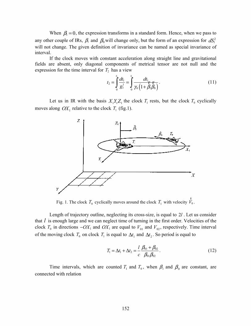
152
When 1 0β = , the expression transforms in a standard form. Hence, when we pass to any other couple of IRs, 1β and 0β will change only, but the form of an expression for 2
1dS will not change. The given definition of invariance can be named as special invariance of interval.
If the clock moves with constant acceleration along straight line and gravitational fields are absent, only diagonal components of metrical tensor are not null and the expression for the time interval for 2T has a view
( )1 1
1 12 1
1 0 1 00 01
t tdt dttg γ β β
= =+∫ ∫ r r . (11)
Let us in IR with the basis 111 ZYX the clock 1T rests, but the clock 0T cyclically moves along 1OX relative to the clock 1T (fig.1).
Fig. 1. The clock 0T cyclically moves around the clock 1T with velocity 0Vr
.
Length of trajectory outline, neglecting its cross-size, is equal to l2 . Let us consider that l is enough large and we can neglect time of turning in the first order. Velocities of the clock 0T in directions 1OX− and 1OX are equal to 01V and 02V , respectively. Time interval of the moving clock 0T on clock 1T is equal to 1tΔ and 2tΔ . So period is equal to
01 021 1 2
01 02
lT t tcβ ββ β+= Δ +Δ = . (12)
Time intervals, which are counted 1T and 0T , when 1β and 0β are constant, are connected with relation

153
ii
i tt 020
011
1
cos1Δ
−
+=Δ
βαββ , 2,1=i (13)
When 1=i the clock 0T moves in the direction 1OX− , therefore 1α π= , when 2=i , motion is in opposite direction and 2 0α = . Let us compare difference between
readings of the clock 0T , which is cyclically alter direction of its motion in two parts of a trajectory, and the clock 1T .
Difference of the clock readings for one period is equal to
12021101 ttttt Δ−Δ+Δ−Δ=δ . (14) Let us substitute (13) into (14):
⎟⎟
⎠
⎞⎜⎜
⎝
⎛
−
+−Δ+⎟
⎟
⎠
⎞⎜⎜
⎝
⎛
−
−−Δ=
202
021022
01
01101
1
11
1
11
βββ
βββδ ttt . (15)
We take into account that c
ltc
lt02
1201
11 ,ββ
=Δ=Δ , then from (13) we have
011
201
0101 1
11βββ
β −−
=Δc
t , 021
202
0202 1
11βββ
β +−
=Δc
t . (16)
Then from (15) we have
⎪⎭
⎪⎬⎫
⎪⎩
⎪⎨⎧
⎟⎟
⎠
⎞⎜⎜
⎝
⎛−
+−
+⎟⎟
⎠
⎞⎜⎜
⎝
⎛−
−−
= 11
1111
11
021
202
02011
201
01 βββ
ββββ
βδ
clt . (17)
For maximal velocity of the clock 0T it is needed that for period 1T the relation 1Ttδ would
be maximal. Divided (17) by (12) we will get
( ) ( )( )( )( )
2 201 1 01 02 02 1 02 01
1 01 02 1 01 1 02
1 1 1 11
1 1t
Tβ β β β β β β βδ
β β β β β β− − + + −
= −+ − +
. (18)
In the fig.2 the dependence ( )02011
,ββδT
t is presented for 1 0,9β = . From (17) and fig.2 it
follows that the magnitude tδ can be positive and negative. As 01 >T always and 0>tδ ,
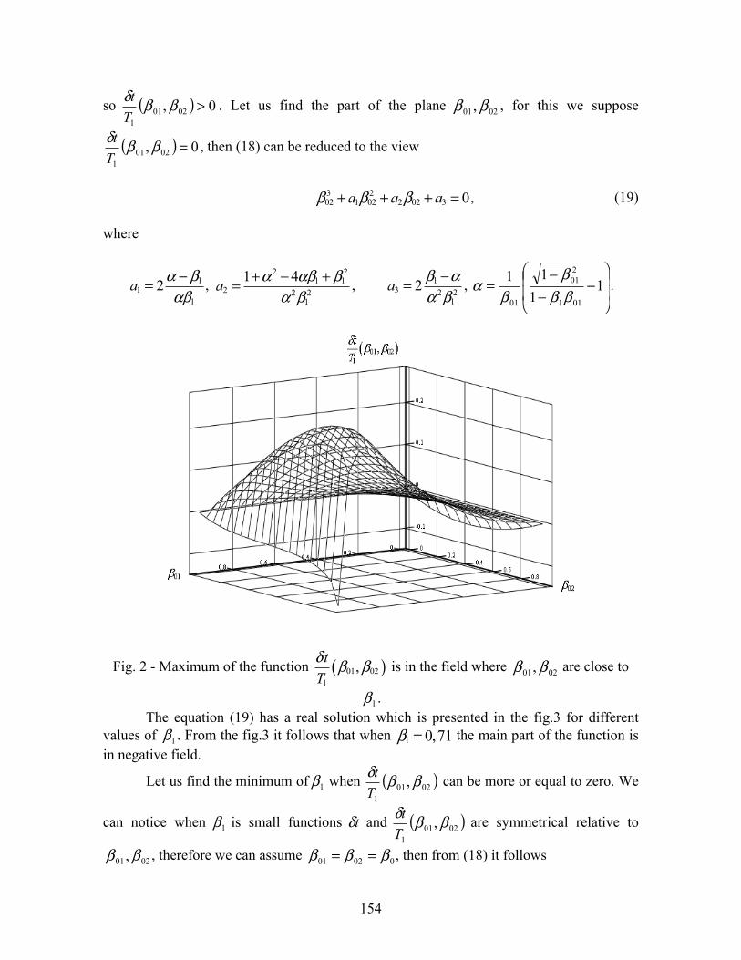
154
so ( ) 0, 02011
>ββδT
t . Let us find the part of the plane 0201,ββ , for this we suppose
( ) 0, 02011
=ββδT
t , then (18) can be reduced to the view
3 202 1 02 2 02 3 0a a aβ β β+ + + = , (19)
where
11
12a α β
αβ−= ,
2 21 1
2 2 21
1 4a α αβ βα β
+ − += , 13 2 2
12a β αα β−= , ⎟
⎟
⎠
⎞⎜⎜
⎝
⎛−
−−
= 11
11
011
201
01 βββ
βα .
Fig. 2 - Maximum of the function ( )01 021
,tTδ β β is in the field where 0201,ββ are close to
1β . The equation (19) has a real solution which is presented in the fig.3 for different
values of 1β . From the fig.3 it follows that when 1 0,71β = the main part of the function is in negative field.
Let us find the minimum of 1β when ( )02011
,ββδT
t can be more or equal to zero. We
can notice when 1β is small functions tδ and ( )02011
,ββδT
t are symmetrical relative to
0201,ββ , therefore we can assume 00201 βββ == , then from (18) it follows
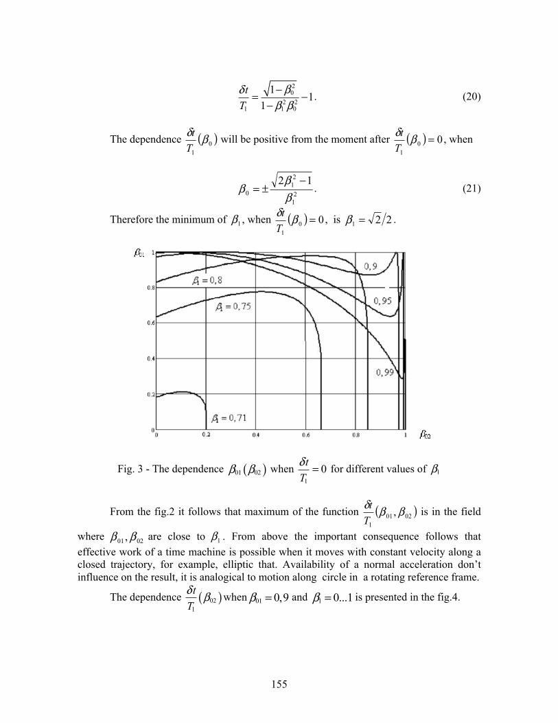
155
20
2 21 1 0
1 11
tT
βδβ β−
= −−
. (20)
The dependence ( )01
βδT
t will be positive from the moment after ( ) 001
=βδT
t , when
21
21
0
12ββ
β−
±= . (21)
Therefore the minimum of 1β , when ( ) 001
=βδT
t , is 221 =β .
Fig. 3 - The dependence ( )01 02β β when1
0tTδ = for different values of 1β
From the fig.2 it follows that maximum of the function ( )02011
,ββδT
t is in the field
where 0201,ββ are close to 1β . From above the important consequence follows that effective work of a time machine is possible when it moves with constant velocity along a closed trajectory, for example, elliptic that. Availability of a normal acceleration don’t influence on the result, it is analogical to motion along circle in a rotating reference frame.
The dependence ( )021
tTδ β when 01 0,9β = and 1 0...1β = is presented in the fig.4.
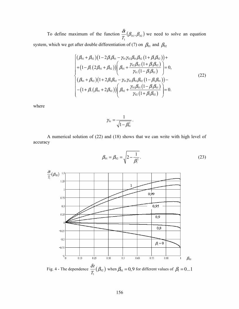
156
To define maximum of the function ( )02011
,ββδT
t we need to solve an equation
system, which we get after double differentiation of (7) on 01β and 02β
( ) ( )( )( )( ) ( )
( )( ) ( )( )
( )( ) ( )( )
01 02 1 01 01 02 01 02 1 02
02 02 1 021 01 02 01
01 1 01
01 02 1 02 01 02 01 02 1 01
01 01 1 011 01 02 02
02 1 02
1 2 11
1 2 0,1
1 2 11
1 2 0.1
β β β β γ γ β β β βγ β β β
β β β βγ β β
β β β β γ γ β β β βγ β β β
β β β βγ β β
⎧ + − − + +⎪ ⎛ ⎞+⎪+ − + + =⎜ ⎟⎜ ⎟⎪ −⎪ ⎝ ⎠⎨
+ + − − −⎪⎪ ⎛ ⎞−− + + + =⎪ ⎜ ⎟⎜ ⎟+⎪ ⎝ ⎠⎩
(22)
where
0 20
11
i
i
γβ
=−
.
A numerical solution of (22) and (18) shows that we can write with high level of accuracy
01 02 21
12β ββ
= = − . (23)
Fig. 4 - The dependence ( )021
tTδ β when 01 0,9β = for different values of 1 0...1β =
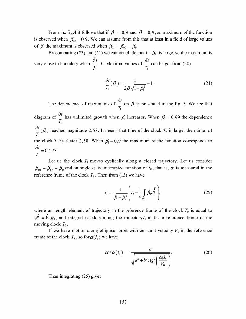
157
From the fig.4 it follows that if 01 0,9β = and 1 0,9β = , so maximum of the function is observed when 02 0,9β = . We can assume from this that at least in a field of large values of β the maximum is observed when 01 02 1β β β= = .
By comparing (23) and (21) we can conclude that if 1β is large, so the maximum is
very close to boundary when 1
tTδ
=0. Maximal values of1
tTδ can be got from (20)
( )1 21 1 1
1 12 1
tTδ β
β β= −
−. (24)
The dependence of maximums of 1
tTδ on 1β is presented in the fig. 5. We see that
diagram of 1
tTδ has unlimited growth when 1β increases. When 1 0,99β = the dependence
11
( )tTδ β reaches magnitude 2,58. It means that time of the clock 0T is larger then time of
the clock 1T by factor 2,58. When 1 0,9β = the maximum of the function corresponds to
10,275t
Tδ = .
Let us the clock 0T moves cyclically along a closed trajectory. Let us consider
00201 βββ == and an angle α is interrupted function of 0t , that is, α is measured in the reference frame of the clock 0T . Then from (13) we have
( )0
1 0 120
1 11 l
t t dlc
ββ
⎛ ⎞⎜ ⎟= −⎜ ⎟− ⎝ ⎠
∫rr
, (25)
where an length element of trajectory in the reference frame of the clock 0T is equal to
0 0 0dl V dt=r r
, and integral is taken along the trajectory 0l in the в reference frame of the moving clock 0T .
If we have motion along elliptical orbit with constant velocity 0V in the reference frame of the clock 0T , so for 0( )lα we have
( )0
0 02 2 2
0
cosctg
alla b
V
αω
= ±⎛ ⎞+ ⎜ ⎟⎝ ⎠
, (26)
Than integrating (25) gives
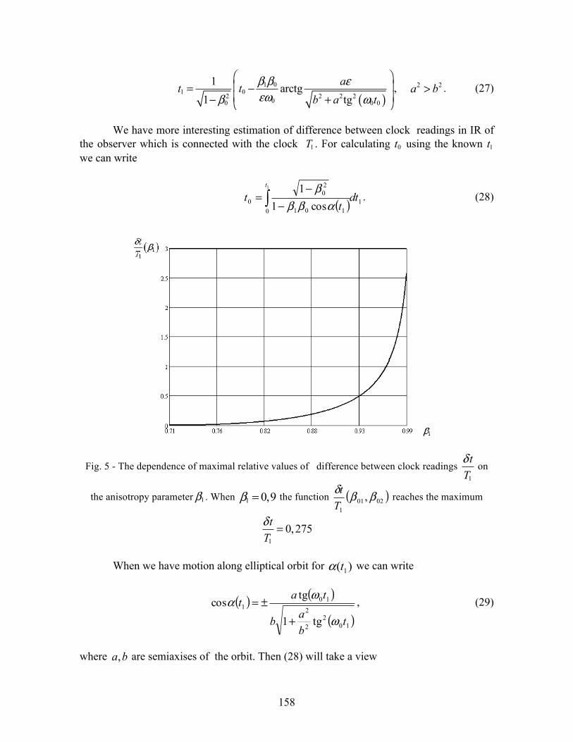
158
( )1 0
1 02 2 2 200 0 0
1 arctg1 tg
at tb a t
β β εεωβ ω
⎛ ⎞⎜ ⎟= −⎜ ⎟− +⎝ ⎠
, 2 2a b> . (27)
We have more interesting estimation of difference between clock readings in IR of the observer which is connected with the clock 1T . For calculating 0t using the known 1t we can write
( ) 10 101
20
0
1
cos11
dtt
tt
∫ −−
=αββ
β. (28)
Fig. 5 - The dependence of maximal relative values of difference between clock readings 1
tTδ
on
the anisotropy parameter 1β . When 1 0,9β = the function ( )02011
,ββδT
t reaches the maximum
10,275t
Tδ =
When we have motion along elliptical orbit for )( 1tα we can write
( ) ( )
( )102
2
2
101
tg1
tgcos
tbab
tat
ω
ωα+
±= , (29)
where ba, are semiaxises of the orbit. Then (28) will take a view
159
( )( ) 1
0 10011022
1022
200
1
1
11 dt
ttgttg
ttgt
t
∫ −+−
+−−=
ωββωε
ωεβ . (30)
Here 222 /1 ab−=ε is eccentricity.
Integrating (30) when 2 0γ > and using the substitution )(ch)cos( 10 tt =ω we have
( )
( ) ( ) ( )
2 2 2 20 1 0 1 02
0 1 0 12 21 0 0 0
0 1 1
1 arctg tg( t )1
arsh cos( t ) arsh
t t
I t
β β β ε β βε γ ωβ β ω γ ω
ε ω ε λ
⎧−= − − ×⎨− ⎩
× − −⎡ ⎤⎣ ⎦(31)
where
1 0
2 2 2 21 02
β βλγ ε β β
=−
, 2
20
212
11
εββγ
−−
= ,
( )
2 2 2 20 1
2 20 1 1 0
2 2 2 20 1
1 2 20 1 1 0
2 20 1
0 1
cos ( ) 11 1 1 1arctg arctg , 1cos( t )
cos ( ) 11 1 1 1= arth arth , 0 1cos( t )
cos ( ) 11 1arcctg arcctgcos( t )
t
tI t
t
ε ω ε γλ ε ω λ ε β β
ε ω ε γλ ε ω λ ε β β
ε ω ελ ε ω λ
⎛ ⎞ ⎛ ⎞− − −⎜ ⎟ − >⎜ ⎟⎜ ⎟⎜ ⎟ ⎝ ⎠⎝ ⎠⎛ ⎞ ⎛ ⎞− − −⎜ ⎟ − < <⎜ ⎟⎜ ⎟⎜ ⎟ ⎝ ⎠⎝ ⎠
⎛ ⎞−⎜ ⎟ −⎜ ⎟⎝ ⎠
2 2
2 21 0
1 1, 0γε β β
⎧⎪⎪⎪⎪⎪⎨⎪⎪
⎛ ⎞⎪ − − <⎜ ⎟⎪ ⎜ ⎟⎪ ⎝ ⎠⎩
A solution is presented in the view 1 0 1 1( ) ( )t t t t tδ = − in the fig.6 for the next parameters: 10a b = , 8
0 3 10ω = × рад/с, 1 0,9β = , 0 0,9β = . From the fig.6 it follows, when the clock 0T moves in direction 1OX− it overtakes
the clock 1T on 81,2 10tδ −≈ × с. In opposite direction 1OX the clock 0T lags on 80,9 10tδ −≈ × . During a period 8
10
2 2,09 10T πω
−= = × с the clock 0T overtakes the clock 1T
on 91( ) 3 10t Tδ −= × с. In the solution (31) frequency 0ω enter as a product 0 1tω , therefore, if frequency 0ω
decreases, so the period 1T will increase, and with the fixed relation 11
( 0,9) 0,3tTδ β = = (see
the fig.5), the magnitude tδ will increase proportionally the period 1T . In other words, if
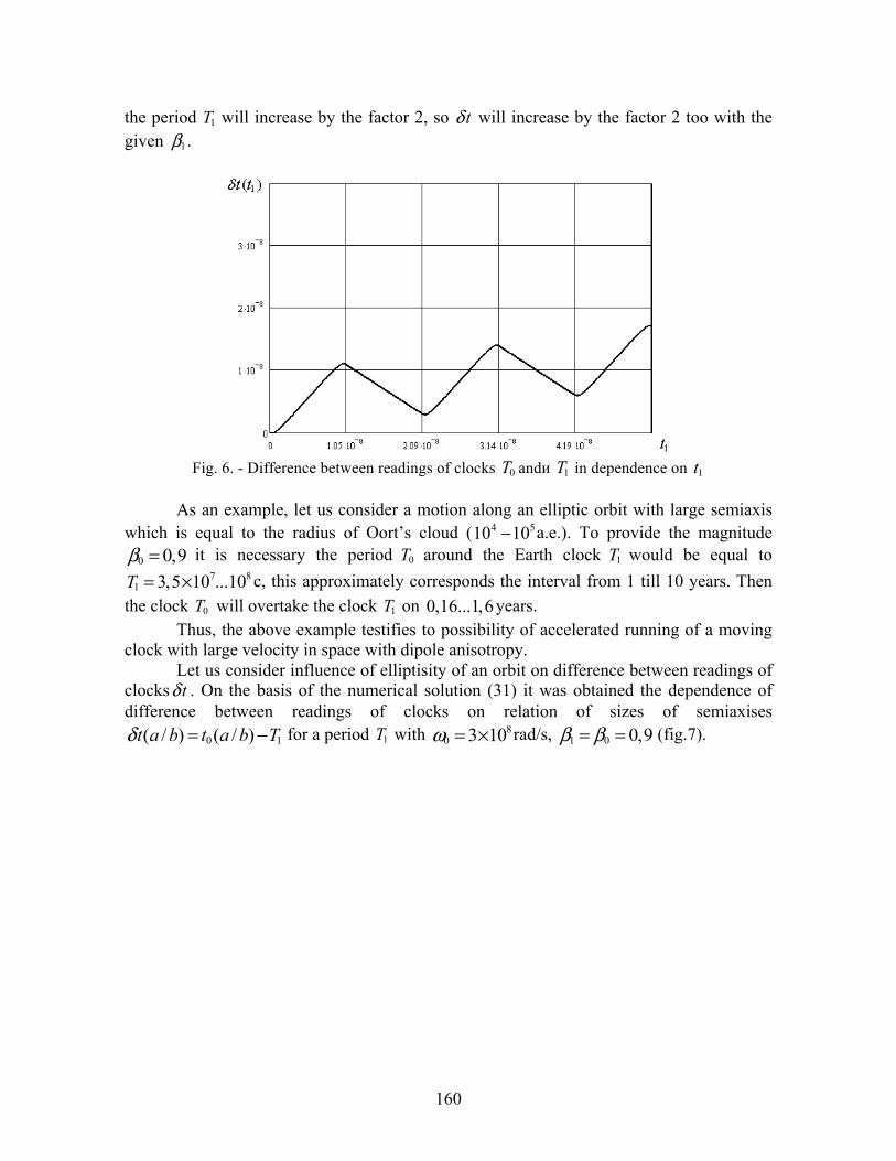
160
the period 1T will increase by the factor 2, so tδ will increase by the factor 2 too with the given 1β .
Fig. 6. - Difference between readings of clocks 0T andи 1T in dependence on 1t
As an example, let us consider a motion along an elliptic orbit with large semiaxis which is equal to the radius of Oort’s cloud ( 4 510 10− а.е.). To provide the magnitude
0 0,9β = it is necessary the period 0T around the Earth clock 1T would be equal to 7 8
1 3,5 10 ...10T = × с, this approximately corresponds the interval from 1 till 10 years. Then the clock 0T will overtake the clock 1T on 0,16...1,6years.
Thus, the above example testifies to possibility of accelerated running of a moving clock with large velocity in space with dipole anisotropy.
Let us consider influence of elliptisity of an orbit on difference between readings of clocks tδ . On the basis of the numerical solution (31) it was obtained the dependence of difference between readings of clocks on relation of sizes of semiaxises
0 1( / ) ( / )t a b t a b Tδ = − for a period 1T with 80 3 10ω = × rad/s, 1 0 0,9β β= = (fig.7).
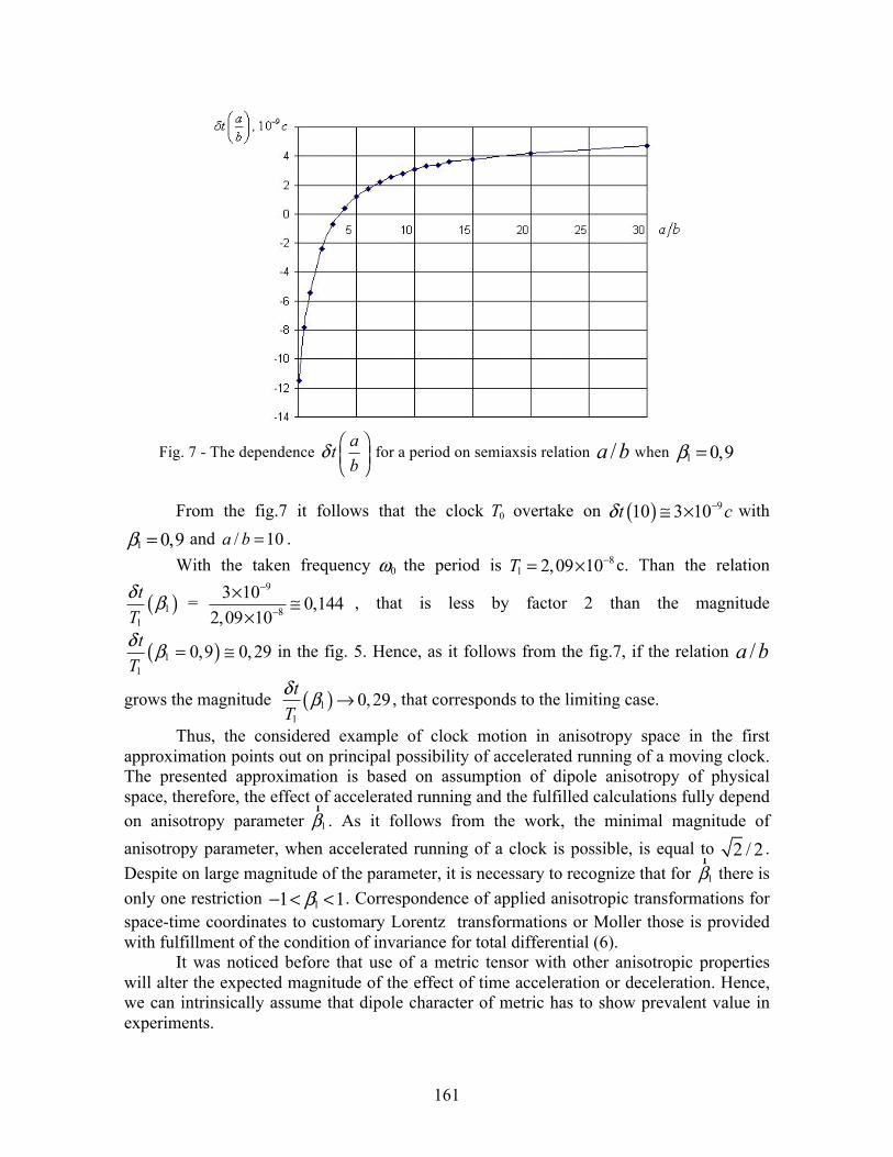
161
Fig. 7 - The dependence atb
δ ⎛ ⎞⎜ ⎟⎝ ⎠
for a period on semiaxsis relation ba / when 1 0,9β =
From the fig.7 it follows that the clock 0T overtake on ( ) 910 3 10t сδ −≅ × with
1 0,9β = and / 10a b = . With the taken frequency 0ω the period is 8
1 2,09 10T −= × с. Than the relation
( )11
tTδ β =
9
8
3 10 0,1442,09 10
−
−
× ≅×
, that is less by factor 2 than the magnitude
( )11
0,9 0,29tTδ β = ≅ in the fig. 5. Hence, as it follows from the fig.7, if the relation ba /
grows the magnitude ( )11
0,29tTδ β → , that corresponds to the limiting case.
Thus, the considered example of clock motion in anisotropy space in the first approximation points out on principal possibility of accelerated running of a moving clock. The presented approximation is based on assumption of dipole anisotropy of physical space, therefore, the effect of accelerated running and the fulfilled calculations fully depend on anisotropy parameter 1β
r. As it follows from the work, the minimal magnitude of
anisotropy parameter, when accelerated running of a clock is possible, is equal to 2 / 2 . Despite on large magnitude of the parameter, it is necessary to recognize that for 1β
r there is
only one restriction 11 1β− < < . Correspondence of applied anisotropic transformations for space-time coordinates to customary Lorentz transformations or Moller those is provided with fulfillment of the condition of invariance for total differential (6).
It was noticed before that use of a metric tensor with other anisotropic properties will alter the expected magnitude of the effect of time acceleration or deceleration. Hence, we can intrinsically assume that dipole character of metric has to show prevalent value in experiments.
162
In conclusion we can notice, that if 1βr
is small, the accelerated running is impossible, hence, availability of weak dipole anisotropy leads to appearance of corrections to difference between readings of moving clocks with any nonzero value of anisotropy parameter. The given effect can be found in experiments on measurement of variations of life time for elementary particles, which move in accumulating rings [7]. We can assume that a phenomenon of dependence of clock running velocity on a vector field 1β
r can have
essential value for long-time space flights.
REFERENCES [1]. Hafele J.C., Keating R.E. //Science. 1972. V.177. P.166. [2]. Novikov I.D. Analyze of time machine. // JETP, 1989. V.95. .3, pp.769-776. [3]. Thorne K.S. Black Holes and Time Warps: Einstein's Outrageous Legacy (W.W.
Norton & Company, New York, 1994). [4]. Penrose Roger. The Road to Reality: A Complete Guide to the Laws of the Universe.
Knopf Publishing Group. 2007. 1099pp. [5]. Gladyshev V.O. A possible explanation for the delay in detecting an astrophysical
signal by using ground-based detectors // J. Moscow Phys. Soc. -1999. -V.9, N1, pp.23-29.
[6]. Gladyshev V.O. Irreversible electromagnetic processes in problems of astrophysics. –Moscow: Bauman University, 2000. – 276pp. (In Russian).
[7]. Bailey J., Borer K. e.a.// Nature. 1977. V.268, pp.301-310.
163
CAN CLOCKS TELL TIME?
A. F. Kracklauer
At past PIRT conferences, and elsewhere, I have asserted, that the usual arguments for time dilation, i.e., the twin paradox contain an oversight that annihilates their conclusion. Inevitably, this has provoked the question: 'how then is the extension of the decay time of moving muons to be understood?'
My response, that this effect can be understood as an effect of space-time perspective, was heard only with skepticism? And, indeed, my own researches into just how this effect can be understood better has led me to a more inclusive viewpoint, namely: while there is no such thing as kinematical time-dilation, there are obviously dynamical effects that objectively slow individual physical processes, e.g., pendulums depend on altitude, biological decay depends on temperature (e.g., in refrigerators). Perspective alone cannot account for everything.
These local modifications of the tempo1 of processes, conned within a sub-unit of the universe, however, cannot be designated time dilation, anymore that can use of a refrigerator be considered to dilate time for the universe. 'Tempo' must be distinguished from an unalterable 'time,' in that the latter is given by the variable conjugate to the Hamiltonian of the universe and, therefore, unalterable from within the universe; whereas, the ow of sub-processes, or the rate of changes of state (tempo), in sub-volumes of the universe, can be altered at the expense of other portions of the universe. To say that time itself is dilated, would be to say that the ow of all processes in the whole universe has been slowed. Obviously, in this light, clocks tell tempo only of their own inner workings, i.e., for localized processes, affected by local conditions (potentials) and cannot take into account of the whole universe; they do not, therefore, tell 'time' per second.
Muons, however, are thought to be decoupled from all external interaction; thus, they are said to spontaneously decay, without external trigger in gin put. However, it is a common insight from Quantum Electrodynamics, that so called 'spontaneous decay' can be seen actually as decay stimulated by a vacuum mode.
From this viewpoint, then, acceleration through the vacuum can be taken as a dynamical under taking doing work on the inner processes of muons, which alters their tempo, analogous to extending biological decay in refrigerators.
This fact, then, in addition to determination of an anisotropy of the cosmic microwave background, provides a physical and operationally practical means of distinguishing a privileged frame, namely that one in which muons have the shortest decay time. As such, it provides additional support for a Lorentzian viewpoint on Special Relativity. This term is taken from music, where it is instinctively recognized that the rapidity of the ow of a piece of music is gauged in terms of an unalterable, external and universal time ow.
Keywords: muons, quantum electrodynamics, vacuum mode, cosmic microwave background, special relativity.
PACS number:03.30.+p/12.20.-m
EXPANDING OR NON-EXPANDING UNIVERSE
Walter Petry
Mathematisches Institut der Universitaet Duesseldorf, D-40225 Duesseldorf E-mail: [email protected]; [email protected]
The observed redshift of galaxies in the universe is generally interpreted as expansion of space. In a previous paper the author has given an other interpretation. It has been proved that the proper time is not absolute but the so called observer’s time corresponding to the proper time at present is absolute. This gives the observed redshift of galaxies. In this preprint several results of an expanding and a non-expanding universe are compared with one another. There exists no definite answer whether the universe expands or not. Einstein’s theory suggests an expanding space and flat space-time theory of gravitation suggests a non-expanding space.
Keywords: redshift of galaxies, general theory of relativity, gravitational field, theory of gravitaion.
PACS number: 04.20.-q/04.20.Cv
II. INTRODUCTIONThe redshift of distant galaxies in the universe is generally interpreted as
expansion of space. Homogeneous, isotropic, cosmological models of Einstein’s general theory of relativity suggest this interpretation. Hubble had doubts about the reality of the expansion but Sandage and collaborators believe that the space is really expanding. For a discussion of these two interpretations of the redshift of distant galaxies compare the paper of Soares [1] where further references can be found. The interpretation of the redshift as expansion of space is generally accepted but some problems with this interpretation exist (see, e.g. [2-4] ).
In addition to Einstein’s general theory of relativity a covariant theory of gravitation in flat space-time will be considered (see Petry [5] ). This gravitational theory is based on a flat space-time metric and gravitation is described by a field in analogy to Maxwell’s theory. It gives the same results as Einstein’s general theory of relativity to the experimentally needed accuracy for the following effects: gravitational redshift, light deflection, perihelion precession, radar time-delay, post-Newtonian approximation, gravitational radiation and the precession of the spin axis of a gyroscope in the orbit of a rotating body. The theory of gravitation in flat space-time gives non-singular, homogeneous, isotropic, cosmological models in contrast to Einstein’s theory (see, e.g. Petry [6-11] ). The space of the universe in flat space-time theory of gravitation is flat for all cosmological models as recent observations also suggest. In addition to the proper time (atomic time) in the universe the observer’s time is introduced (see Petry [12] ) which corresponds to the proper time at present. The observer’s time interval and the proper time interval are different and they agree only at present. This result has been used to give an explanation of the anomalous Doppler frequency shift of the Pioneers [12] and an explanation of the redshift of galaxies without the assumption of an expanding space ( see [13] ). It is proved that the observer’s time interval is absolute [13] suggesting that the time interval of proper time is changeable in the universe. An Euclidean space and different times such as observer’s time resp. proper time are used to study non-expanding cosmological models. Cosmological models with an expanding space and the use of the proper time are also considered. The light velocity in the universe depends on the used time. It is equal to the vacuum light velocity for all times only by the use of observer’s time. It is using an other time interval only at the observer equal to the vacuum light velocity whereas at distant objects it is different from it and it depends in an expanding space also on the expansion of space as well for flat space-time theory of gravitation as for Einstein’s general theory of relativity. Therefore, superluminal velocities in an
164
expanding space are real and not contradicting to special relativity. The energy of an emitted photon moving in the universe is in general time-depenent and only by the use of the observer’s time it is always constant because the observer’s time is absolute. The total energy of the universe is conserved and positive for all cosmological models (including an expanding space) by flat space-time theory of gravitation. This follows from the fact that the total energy-momentum in flat space-time theory of gravitation is a tensor. For a non-expanding flat space of Einstein’s theory the total energy of the universe is equal to zero (see [14] ). It is worth mentioning that a total energy of the universe being equal to zero in flat space-time theory of gravitation would also give singular cosmological models like Einstein’s theory. In flat space-time theory of gravitation a bound system in the universe is calculated to post-Newtonian approximation [15]. The result to Newtonian accuracy is identical with that of general relativity. The simple case of a solid, spherically symmetric body and a test particle moving around it is studied. The results of an expanding or a non-expanding space mathematically agree but the interpretation of an expanding universe yields that the space of the bound system does not expand [16] whereas the interpretation of a non-expanding space implies that the test body moves spirally towards the solid body.
It is worth mentioning that the two considered theories of gravitation allow the interpretation of an expanding and a non-expanding space for all the studied results but the interpretation of expanding space is suggested by Einstein’s theory whereas flat space-time theory of gravitation suggests a non-expanding space. This follows from the fact that Einstein’s theory defines the proper time and the metric of space and time by the same line element whereas flat space-time theory of gravitation defines proper time indepenently of the background metric of space and time.
The theory of gravitation in flat space-time [5] has been studied in several papers. A summary of the theory with applications can be found in paper [6] where references to detailed studies are stated.Subsequently, some results of the papers [5-11] are summarized which are used in the following. Flat space-time theory of gravitation uses a flat space-time background metric
(ds)2ij= −η dxidx j . (2.1)
The gravitational field is described by a symmetric tensor gij satisfying covariant (with regard to the flat spacetime metric (2.1)) differential equations of order two. The source of the gravitational field is the total energy-momentum tensor inclusive that of the gravitational field. The proper time (atomic time) is defined by
2 (dτ )2ij= −g dxidx c j . (2.2)
The equations of motion of a test particle with the four-velocity ⎟⎠
⎜⎛ dxi
⎟⎞
⎜⎝ dτ
in the
dττττdx
ddx
xg
dd
kj
ijkd ⎜
⎛g dx j
ij ∂
∂=⎟⎟
⎠
⎞⎜⎝ 2
1 (i =1− 4.) (2.3)
gravitational field are given by
The total energy-momentum tensor is conserved. The derivation of these results can be found in the paper of Petry [5] . The application of the theory of gravitation in flat space-time to homogeneous, isotropic, cosmological models is studied in several papers (see, e.g. Petry [6-10] ). The background metric uses the pseudo-Euclidean geometry
165
( ) ( )1,1,1,1 −= diagijη (2.4)
with the Cartesian coordinates x1, x2 , x3 and x4 = ct . The four-velocity of the universe is
0==τd
dxui
i )3,2,1( =i , .4
τddtcu = (2.5)
Then, the potentials gij are given by
( ) ( ) ( ) ( ) ( ))/1,,,( 222 thtatatadiaggij −= (2.6)
where a(t) and h(t) satisfy two coupled nonlinear differential equations of order two resulting from the field equations of the gravitational theory. Here, the source of the gravitational field consists of the densities of matter (dust) (t), of radiationmρ
rρ (t), and of the cosmological constant ) Λρ (t) with
( ) ( ),/0 tht mm ρρ = ( ) ( ) ( )( ),/0 thtat rr ρρ = ( ) ( ) ( )./8
32
thtak
ctπ
ρ Λ=Λ (2.7)
The parameters ρ m0 and rρ 0 are the densities at present , Λ is the cosmological constant and k is the gravitational constant. The initial conditions of the differential equations are the values at present time t = 0, i.e.
( ) ( ) ,100 == ha ( ) ,0 0Ha =& ( ) 00 hh && = (2.8)
. where the dot denotes the t − derivative. Here, H0 denotes the Hubble constant and h0 is a further constant of integration which is zero for Einstein’s theory because h(t) ≡1 which is not possible in flat space-time theory of gravitation. Under natural conditions on the universe the cosmological models are nonsingular, i.e. all the densities are finite for all times. The functions a(t) and h(t) are defined for all t∈R. The function h(t) goesto infinity as t → −∞, then for increasing time it decreases to a small positive minimum and then increases to infinity as t → ∞. The function a(t) starts from a small positive value as t → −∞, then for increasing time it decreases to a positive minimum and then increases for all t ∈R. The functions a(t) and h (t) have their minimum in the very earlyuniverse. The energy density of the gravitational field in the universe is
2166
641
223 ⎟
⎟⎠
⎞⎜⎜⎝
⎛⎟⎠
⎜⎛ h& ⎟⎞⎜⎝
+⎞ +⎟⎠
⎜⎝
− ⎛=hhaa
aa hπkG
a& h&& ρ . (2.9)
The space of the universe is flat which is suggested by recent observations.The energy-momentum tensor of the total universe is given by
166
2223
32
21
1
31 cccTTT Gr ρρρ +−=== Λ
( ) 2224
4 cccT Grm ρρρρ −−+−= Λ
(2.10)
where the non-diagonal elements are equal to zero. The total energy of the universe is conserved, i.e.
( ) ( ) ( ) ( )( ) 22 cctttt Grm λρρρρ =+++ Λ (2.11)
with a constant λ >0. Einstein’s theory gives for a flat space that the total energy is zero (see, e.g.Berman [14] ).
In addition to the time t the proper time t of the observer at rest is~
dt~ = dt / h(t) (2.12a)
with
(t)) = ∫−∞
t
dt / ht~(t (2.12b)
implying the potentials
(g t~( ))= diag(a2 (t),a2 (t),a2 (t),−1)ij (2.13)
and the background metric
diag(1,1,1,−h(t)).ij(η (t~))= (2.14)
In the relations (2.13) and (2.14) the time t must be replaced by t by the use ofinverse relation of (2.12b). Furthermore, let us define the observer’s time t' by
dt '= dt /
(a(t) h(t )) (2.15a)
~
with
) = ∫ )( )−∞
t
dt / a t( ) h(t t '(t (2.15b)
implying the potentials
(g (t diag(a (t) a (t ) a (t ) a (t ))ij2222 ,, ,−'))= (2.16)
167

and the flat background metric
( ) diag(1,1,1,−a2 (t)h(t))ij(η t ' )= (2.17)
where relation (2.15b) must be used to replace t by t'. The absolute values of thelight velocity vl with regard to the three different times t, t and t' in the universe are
v t( ) c /(a t( ) h(t)),l = v~ (t ) = c / a(t ),l v'(t ) = c. (2.18)
Hence, the light velocity is only with regard to the observer’s time equal to c for all times whereas for t and t the light velocity is time dependent and it is only equal to c at present by virtue of the initial conditions (2.8). It follows by the initial conditions (2.8) and the use of (2.12a) and (2.15a) at present time t = 0 :
dt = dt~ = dt'. (2.19)
Therefore, the frequency of a photon emitted at present by an atom at rest is by(2.19) independent of the used time t, t or t'. Relation (2.1) together with the background metric (2.4) or (2.14) or (2.17) suggests that (x1, x2 , x3 ) are the Cartesian coordinates of an Euclidean non-expanding space.
Let us now consider the time t' with the relations (2.16) and (2.17). It follows from (2.2) by the use of (2.16) under the assumption that a light ray is emitted at distance r and at time t'e resp. t'e+dt'e and received by theobserver at time t'= 0 resp. 0 + dt' then it holds
~
~
~
r = c dt = c∫ ∫ dt = c dt∫ + c −(dt ' dt ' .)'
0 0+dt '
'
0
'e
t te e+t ' dte e
Hence,we have
edt '= dt '
i.e. dt' is independent of the distance r and of the time t'. Therefore, dt' is the absolute time interval and the proper time dt is not absolute in contradiction to the general assumption. At present the time interval dt' agrees with the present atomic time interval dt by vitue of (2.19).Let us now introduce an expanding space by the new coordinates
(2.20) x~ i = a t( )xi (i =1,2,3) , dx~4 = dx4 / h(t).Elementary calculations give the potentials (see, e.g. [10] )
~
~
168
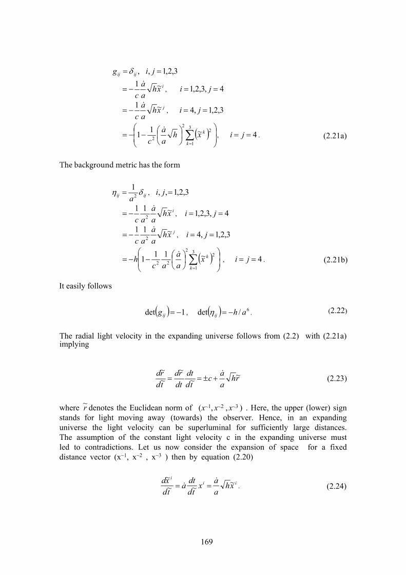
ijij aδη 2
1= , 3,2,1,, =ji
ixhaa
ac~11
2
&−= , 4,3,2,1 == ji
jxhaa
ac~11
2
&−= , 3,2,1,4 == ji
( ) ⎟⎟⎠
⎞⎜⎜⎝
⎛⎟⎠⎞
⎜⎝⎛−−= ∑
=
3
1
22
22~111
k
kxaa
ach
&, 4== ji . (2.21b)
It easily follows
( ) 1det −=ijg , ( ) 6/det ahij −=η . (2.22)
The radial light velocity in the expanding universe follows from (2.2) with (2.21a) implying
rhaac
tddt
dtrd
tdrd ~
~~
~~ &
+±== (2.23)
where r denotes the Euclidean norm of (x~1, x~2 , x~3 ) . Here, the upper (lower) sign stands for light moving away (towards) the observer. Hence, in an expanding universe the light velocity can be superluminal for sufficiently large distances. The assumption of the constant light velocity c in the expanding universe must led to contradictions. Let us now consider the expansion of space for a fixed distance vector (x~1, x~2 , x~3 ) then by equation (2.20)
iii
xhaax
tddta
tdxd ~
~~~ &
& == . (2.24)
ij ijg = δ , i, j =1,2,3
i
ac1 a& hx~ = − , i =1,2,3, j = 4
hx~ j
ac1 a&
= − , i = 4, j =1,2,3
x~( k ) ⎟⎟⎠
⎞⎜⎜⎛
⎟⎠⎞
⎜⎝
= − − ⎛ ∑=
3
1
22
211
kh
aca&
, i = j = 4 . (2.21a) ⎝
The background metric has the form
~
169
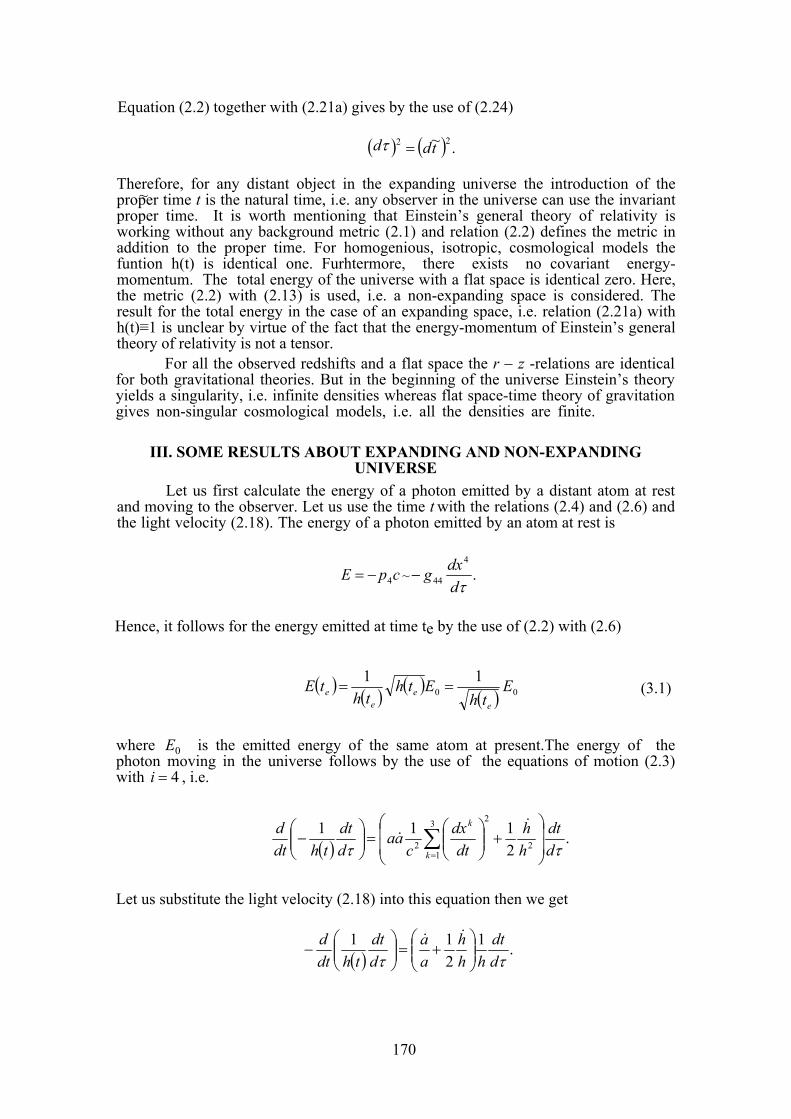
Equation (2.2) together with (2.21a) gives by the use of (2.24)
( )2 = (dt~)2 .dτ
~Therefore, for any distant object in the expanding universe the introduction of the proper time t is the natural time, i.e. any observer in the universe can use the invariant proper time. It is worth mentioning that Einstein’s general theory of relativity is working without any background metric (2.1) and relation (2.2) defines the metric in addition to the proper time. For homogenious, isotropic, cosmological models the funtion h(t) is identical one. Furhtermore, there exists no covariant energy-momentum. The total energy of the universe with a flat space is identical zero. Here, the metric (2.2) with (2.13) is used, i.e. a non-expanding space is considered. The result for the total energy in the case of an expanding space, i.e. relation (2.21a) with h(t)≡1 is unclear by virtue of the fact that the energy-momentum of Einstein’s general theory of relativity is not a tensor.
For all the observed redshifts and a flat space the r − z -relations are identical for both gravitational theories. But in the beginning of the universe Einstein’s theory yields a singularity, i.e. infinite densities whereas flat space-time theory of gravitation gives non-singular cosmological models, i.e. all the densities are finite.
III. SOME RESULTS ABOUT EXPANDING AND NON-EXPANDINGUNIVERSE
Let us first calculate the energy of a photon emitted by a distant atom at rest and moving to the observer. Let us use the time t with the relations (2.4) and (2.6) and the light velocity (2.18). The energy of a photon emitted by an atom at rest is
E = − p c4 ~4
44 dτ− g dx .
Hence, it follows for the energy emitted at time te by the use of (2.2) with (2.6)
h t( ) 0h t( ) 01 1 Eh t( )E
ee
e
=E te( ) = (3.1)
where E0 is the emitted energy of the same atom at present.The energy of the photon moving in the universe follows by the use of the equations of motion (2.3) with i = 4 , i.e.
t( ) 2111 3
12
2
2 dττdt
hdtcddt
dt ⎜⎝ hd
k
⎟⎟⎠
⎞⎜⎜⎝
⎛+⎟
⎠⎜⎛ dxk
⎟⎞
⎜⎝
=⎟⎟⎠
⎞⎜⎛− ∑
=
h&aa& .
Let us substitute the light velocity (2.18) into this equation then we get
t( )1 dt .
211
dττ h ⎟⎠ haa
ddt
dt ⎜⎝ h⎟⎞
⎝
⎛= ⎜⎜
&+⎟⎟
⎠
⎞d⎜⎛
−h&
170
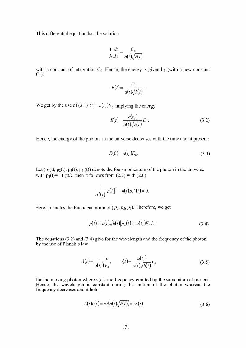
( ) ( )thtaC
ddt
h01
=τ
with a constant of integration C0. Hence, the energy is given by (with a new constant С1):
( )( ) ( )thta
CtE 1= .
We get by the use of (3.1) ( ) 01 EtaC e= implying the energy
( ) ( )( ) ( )
.0Ethta
tatE e= (3.2)
Hence, the energy of the photon in the universe decreases with the time and at present:
( ) ( ) .0 0EtaE e= (3.3)
Let (p1(t), p2(t), p3(t), p4 (t)) denote the four-momentum of the photon in the universe with p4(t)= −E(t)/c then it follows from (2.2) with (2.6)
( ) ( ) ( ) ( ) .01 24
22 =− tpthtp
ta
Here, ⋅ denotes the Euclidean norm of ( p1, p2, p3). Therefore, we get
( ) ( ) ( ) ( ) ( ) ./04 cEtatpthtatp e== (3.4)
The equations (3.2) and (3.4) give for the wavelength and the frequency of the photon by the use of Planck’s law
( ) ( ) ,10ν
λ cta
te
= ( ) ( )( ) ( ) 0νν
thtatat e= (3.5)
This differential equation has the solution
for the moving photon where ν0 is the frequency emitted by the same atom at present. Hence, the wavelength is constant during the motion of the photon whereas the frequency decreases and it holds:
c /(a(t) h(t))= v (t).lλ t( )ν (t) = (3.6)
171

At present time the observer measures for the arriving photon
( ) ( ) ,100ν
λ cta e
= ( ) ( ) ,0 0νν eta= ( ) ( ) .00 c=νλ
Let us now introduce the times t resp. t'. It follows by the use of (2.12a) or (2.15a) and the transformation formulas
,~~
i
k
ki xxpp∂∂
='
' i
k
ki xxpp∂∂
= ( )41−=i
the result
iii ppp == '~ ( ),3,2,1=i ,~44 hpp = .' 44 happ =
Hence, the relations (3.4) and (3.2) yield:
( ) ( ) ( ) ,/'~0 cEtatptp e==
( ) ( )( ) ,~
0EtatatE e= ( ) ( ) .' 0EtatE e=
The wavelength and the frequency of the photon in the universe are therefore
~
a t((t) = )ν 0
1λ~ t( ) = λ ' c
e
,ν~ t( ) = a(te
))ν ,0a(t (t) = a(t )ν .ν ' 0e (3.7)
The relations (3.7) yield by the use of (2.18)
( ),( ) ( ) c / a t( ) = v~ tlλ~ t ν~ t = ) ) v '(t).lλ '(t ν '(t = c = (3.8)
Hence, the wavelength of the photon is constant during its motion through the universe independently of the used time whereas the frequency is in general changeing and it is constant only by the use of the observer’s time. These considerations of a non-expanding space are already contained in the paper [12]. In the paper [13] generalizations to a moving body in the universe are considered implying an explanation of the anomalous Doppler frequency shift of the Pioneers. An unpleasent result of cosmological models by Einstein’s theory is the non-conservation of the energy of the photon moving in the universe (see [17]).
Let us now consider the expanding universe with the transformations (2.20) and the corresponding transformation fomulas for the four-momentum. This gives the relations
172
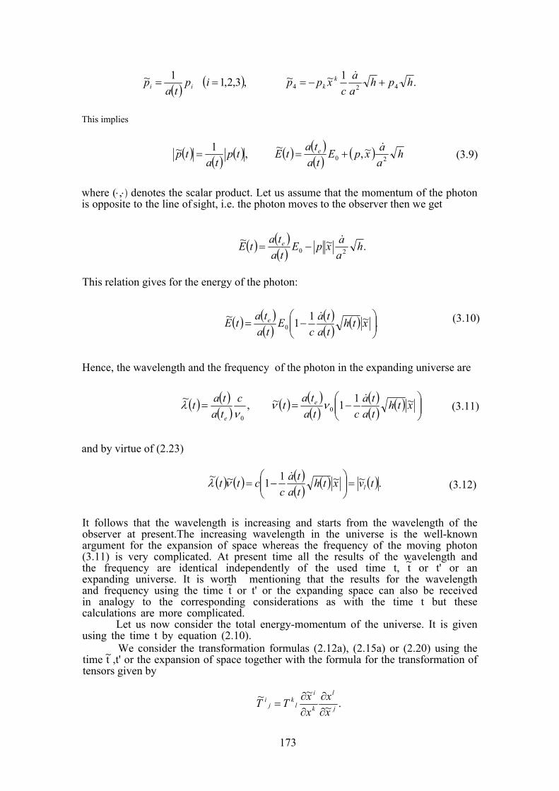
1) pii a(t
~p = i =( 1,2,3 ,) x~ k 1424 h + p h
acp~p k= −
a& .
This implies
a t),1
( ) p(t~p t( ) = ))
ah
a tE~ t( ) = a(t
(e
20E + p, x~( ) a& (3.9)
where (⋅,⋅) denotes the scalar product. Let us assume that the momentum of the photon is opposite to the line of sight, i.e. the photon moves to the observer then we get
( )t =a(te )
t( )E~ 20 haa
E − p x~ a& .
This relation gives for the energy of the photon:
t( )(t)( ) )E ⎛
−a&( ) h t( ) x~ .11E~ 0 ⎟⎟
⎠
⎞⎜
a ⎜⎝ c a t
t =a(te (3.10)
Hence, the wavelength and the frequency of the photon in the expanding universe are
λ~(t) = a t( ))a t( ν
,0
c
e
)⎟⎟⎠) h t( ) x~ ⎞
⎜⎜⎝ a(t
a&(tca t
t( ) = a(te
( ))ν ⎛1− 1ν~ 0 (3.11)
and by virtue of (2.23)
(t) )) h t( ) x~ = v~ t( ).11~ t( )~
a(ta&(t
c= c l⎟⎟
⎠
⎞
⎝
⎛⎜⎜ − λ ν (3.12)
It follows that the wavelength is increasing and starts from the wavelength of the observer at present.The increasing wavelength in the universe is the well-known argument for the expansion of space whereas the frequency of the moving photon (3.11) is very complicated. At present time all the results of the wavelength and the frequency are identical independently of the used time t, t or t' or an expanding universe. It is worth mentioning that the results for the wavelength and frequency using the time t or t' or the expanding space can also be received in analogy to the corresponding considerations as with the time t but these calculations are more complicated.
Let us now consider the total energy-momentum of the universe. It is given using the time t by equation (2.10).
We consider the transformation formulas (2.12a), (2.15a) or (2.20) using the time t ,t' or the expansion of space together with the formula for the transformation of tensors given by
j .∂xk ∂x~∂x~T~
li
j =T li k x∂
~
~
~
173
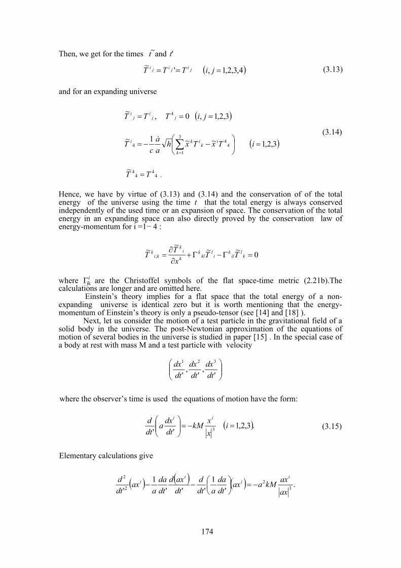
Then, we get for the times t and t'
jijiji TTT == '~ ( )4,3,2,1, =ji (3.13)
and for an expanding universe
,~j
ij
i TT = 04 =jT ( )3,2,1, =ji
⎟⎠
⎞⎜⎝
⎛−−= ∑
=
3
14
44
~~1~k
ik
iki TxTxhaa
cT
& ( )3,2,1=i
44
44~ TT = .
(3.14)
Hence, we have by virtue of (3.13) and (3.14) and the conservation of of the total energy of the universe using the time t that the total energy is always conserved independently of the used time or an expansion of space. The conservation of the total energy in an expanding space can also directly proved by the conservation law of energy-momentum for i =1− 4 :
0~~~~; =Γ−Γ+
∂∂
= kl
ilk
il
klk
ki
k
kik TT
xTT
where Γi are the Christoffel symbols of the flat space-time metric (2.21b).The calculations are longer and are omitted here.
Einstein’s theory implies for a flat space that the total energy of a non-expanding universe is identical zero but it is worth mentioning that the energy-momentum of Einstein’s theory is only a pseudo-tensor (see [14] and [18] ).
Next, let us consider the motion of a test particle in the gravitational field of a solid body in the universe. The post-Newtonian approximation of the equations of motion of several bodies in the universe is studied in paper [15] . In the special case of a body at rest with mass M and a test particle with velocity
⎟⎟⎠
⎞⎜⎜⎝
⎛'
,'
,'
321
dtdx
dtdx
dtdx
where the observer’s time is used the equations of motion have the form:
3'' xxkM
dtdxa
dtd ii
−=⎟⎟⎠
⎞⎜⎜⎝
⎛ ( ).3,2,1=i (3.15)
Elementary calculations give
( ) ( ) ( ) .'
1'''
1' 3
22
2
axaxkMaax
dtda
adtd
dtaxd
dtda
aax
dtd i
ii
i −=⎟⎠⎞
⎜⎝⎛−−
~
jk
174
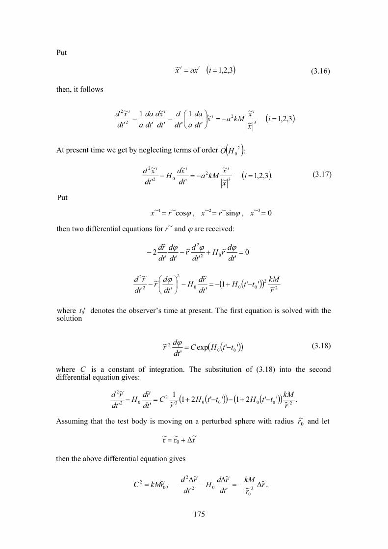
Put
x~ i = axi (i =1,2,3) (3.16)
then, it follows
32
2
2
x~x~
'1
''x~
'1
'd x~ a kM
dtda
dt ⎝ ad
dtd
dtda
dt a
iii ⎞x~ i = −⎟⎠
⎜− ⎛− (i =1,2,3).
At present time we get by neglecting terms of order ):20O(H
32
02
2
x~a kM
~
'x~
'x
dtH d
dt
iid x~ i
= −− (i =1,2,3). (3.17)
Put
x~1 = r~cosϕ , x~2 = r~sinϕ , x~3 = 0
then two differential equations for r~ and ϕ are received:
dt ''' dt '2 02
2
=+− − H r~ ddt
r~ ddt
ϕϕdr~ dϕ 0
'−t ' k))= − 1+( 22
000
2
2
2
r~'r~
'dt 'd r~ H t( M
dtH d
dtr~⎛ d
−⎟⎠⎞
⎜⎝
−ϕ
where t0' denotes the observer’s time at present. The first equation is solved with the solution
'))'
r~ 002 C exp H t( '−( t
dtd
=ϕ (3.18)
where C is a constant of integration. The substitution of (3.18) into the second differential equation gives:
=C 1+( H t '−t ' kM)( )2H t '−t '( ) − 1+ 2) ( .r~r~
1'
r~
'r~
2000032
02
2
dtH d
dtd
−
~Assuming that the test body is moving on a perturbed sphere with radius r0 and let
then the above differential equation gives
,C 2 = kMr~0 r~.'r~
'd ∆r~
30
02
2
rdtdt= − ~
kM∆H d∆
−
r = r0 + ∆r ~ ~ ~
175
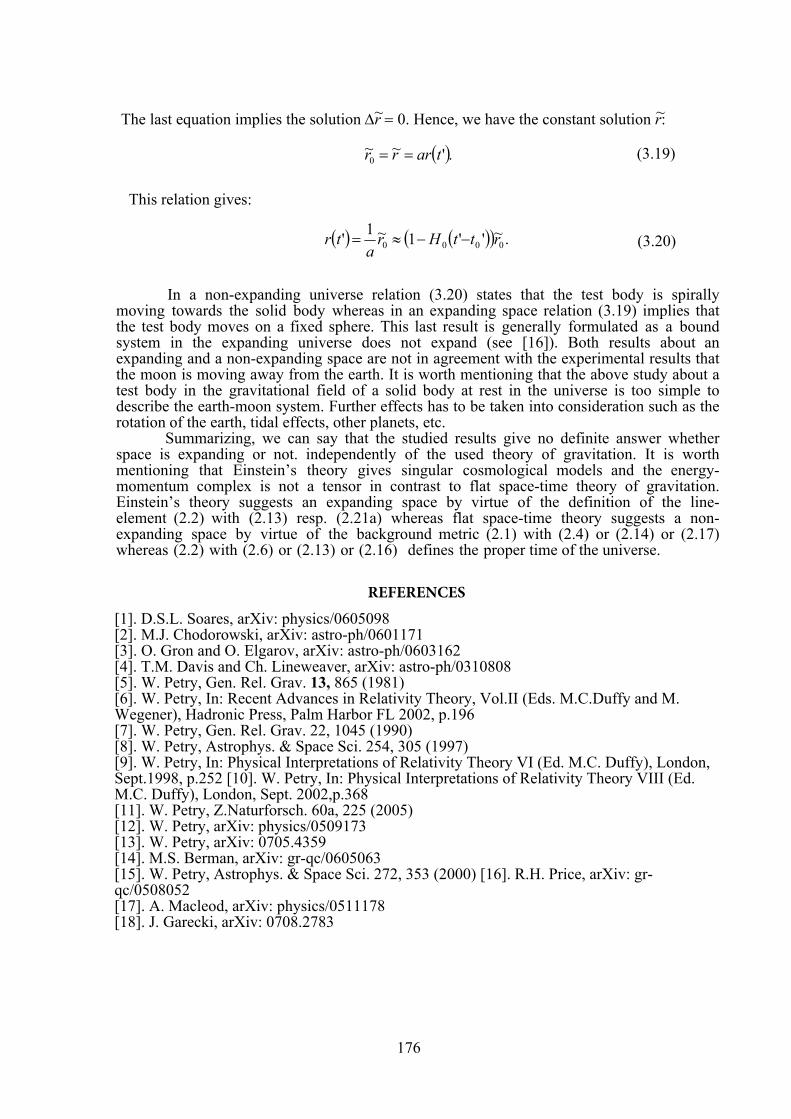
The last equation implies the solution ∆r = 0. Hence, we have the constant solution r:
( ).'~~0 tarrr == (3.19)
This relation gives:
( ) ( )( ) .~''1~1' 0000 rttHra
tr −−≈= (3.20)
In a non-expanding universe relation (3.20) states that the test body is spirally moving towards the solid body whereas in an expanding space relation (3.19) implies that the test body moves on a fixed sphere. This last result is generally formulated as a bound system in the expanding universe does not expand (see [16]). Both results about an expanding and a non-expanding space are not in agreement with the experimental results that the moon is moving away from the earth. It is worth mentioning that the above study about a test body in the gravitational field of a solid body at rest in the universe is too simple to describe the earth-moon system. Further effects has to be taken into consideration such as the rotation of the earth, tidal effects, other planets, etc.
Summarizing, we can say that the studied results give no definite answer whether space is expanding or not. independently of the used theory of gravitation. It is worth mentioning that Einstein’s theory gives singular cosmological models and the energy-momentum complex is not a tensor in contrast to flat space-time theory of gravitation. Einstein’s theory suggests an expanding space by virtue of the definition of the line-element (2.2) with (2.13) resp. (2.21a) whereas flat space-time theory suggests a non-expanding space by virtue of the background metric (2.1) with (2.4) or (2.14) or (2.17) whereas (2.2) with (2.6) or (2.13) or (2.16) defines the proper time of the universe.
[1]. D.S.L. Soares, arXiv: physics/0605098 [2]. M.J. Chodorowski, arXiv: astro-ph/0601171 [3]. O. Gron and O. Elgarov, arXiv: astro-ph/0603162 [4]. T.M. Davis and Ch. Lineweaver, arXiv: astro-ph/0310808 [5]. W. Petry, Gen. Rel. Grav. 13, 865 (1981) [6]. W. Petry, In: Recent Advances in Relativity Theory, Vol.II (Eds. M.C.Duffy and M. Wegener), Hadronic Press, Palm Harbor FL 2002, p.196 [7]. W. Petry, Gen. Rel. Grav. 22, 1045 (1990) [8]. W. Petry, Astrophys. & Space Sci. 254, 305 (1997) [9]. W. Petry, In: Physical Interpretations of Relativity Theory VI (Ed. M.C. Duffy), London, Sept.1998, p.252 [10]. W. Petry, In: Physical Interpretations of Relativity Theory VIII (Ed. M.C. Duffy), London, Sept. 2002,p.368 [11]. W. Petry, Z.Naturforsch. 60a, 225 (2005) [12]. W. Petry, arXiv: physics/0509173 [13]. W. Petry, arXiv: 0705.4359 [14]. M.S. Berman, arXiv: gr-qc/0605063 [15]. W. Petry, Astrophys. & Space Sci. 272, 353 (2000) [16]. R.H. Price, arXiv: gr-qc/0508052 [17]. A. Macleod, arXiv: physics/0511178 [18]. J. Garecki, arXiv: 0708.2783
~ ~
REFERENCES
176
177
TAKING RELATIVITY BACK FROM PRINCIPLES TO PHYSICAL PROCESSES
Dr. Albrecht Giese
Taxusweg 15, D-22605 Hamburg
Abstract The “new” understanding of physics in the 20th century was based on principles,
symmetries, and abstractions, rather than referring to physical processes. Einstein initiated this way by replacing Lorentz’ physical understanding of the
contraction of fields (causing the contraction of objects) by the abstract contraction of ‘space’, adding to it the dilation of ‘time’ in order to fulfil the Relativity Principle, which became the basis for his understanding of the physical world. Many physicists look upon Einstein’s way to geometrize physics as an outcome of his genius. But more likely, this was just the path into a dead end in physics.
For quantum mechanics something similar was done. QM can, according to the (still dominating) Copenhagen interpretation, not be visualized but only mathematically treated in a formal way referring also to certain principles and symmetries. Heisenberg made the acceptance of this view to a precondition for a successful physicist.
The fact that the physical world since 40 years faces the conflict between relativity (here GR) and quantum mechanics, under the heading Quantum Gravity, without any cognizable first sign of a solution, may be a consequence of these settings.
If we take relativity back to the physical path, using the approach of Lorentz for contraction and the detection of the Zitterbewegung by Dirac and Schrödinger to understand time dilation, then we not only find an easier understanding of special relativity, but also learn a lot about particle physics.
As further consequences, we understand the origin of mass (no need for a Higgs, which will not be detected) and learn, that gravity is not the force no. 4, but a side effect of other forces causing reflection processes to basic particles. And this also abolishes the problem of Quantum Gravity.
I want to point out that the results listed above are not merely philosophical ideas but provide correct quantitative results regarding special relativity, gravity, and particle mass.
Further information is available at the website: www.ag-physics.org
Keywords: physical processes, relativity, quantum mechanics, quantum gravity.
PACS number: 03.65.-w/04.60.-m
178
MEASURING A ONE WAY LIGHT SPEED
John Carroll
University of Cambridge, Centre for Advanced Photonics and Electronics, 9 J J Thomson Avenue, Cambridge, CB3 0FA, UK,
A novel method of measuring a one way light speed (OWLS) is proposed using standard equipment of frequency generators, laser pulse generators and oscilloscopes with periodic pulses going from A to B and also from B to A. The method can then inform B how long it has taken light pulses to reach B’s laboratory from A and similarly A can establish how long the pulses have taken to come from B. The method is based on experimental work that actually used a very similar method to measure the relative speeds of photons and classical pulses. It is expected that with classical optical pulses, the method could measure the one way velocity to an accuracy better than 1 part in 106.
Keywords: one way light speed, Michelson Morley experiment, classical pulses, photons, oscilloscope.
PACS number: 07.07.Hj/07.60.Ly
I. INTRODUCTION It is generally accepted that the result of the Michelson Morley experiment relies
on the two way speed of light being invariant. In current forms of this experiment the constancy can be measured with remarkable accuracy[1]. There are also sophisticated measurements of the one way light speed (OWLS) again with a remarkable accuracy and constancy [1,2]. Never the less, there is still no universal agreement that the one way light speed is actually a fixed value of c because there are both theories and experiments that suggest that c can vary or appear to vary depending on the velocity of the frame of reference [1,2,3,4,5,6]. There are also varying views about the measurement of OWLS [1,2,3,4]. Indeed the references here are but a small sample and it is not the intention to give a review in this short contribution. Here, the paper is limited to describing a novel way of measuring OWLS with relatively straightforward apparatus of stable frequency sources, oscilloscopes and pulse generators. A slightly different version of this system was used to measure the relative speed of photons and classical pulses propagating along optical fibres [1], but the system was not invented with any initial intention that it would measure OWLS. The experiment, described below, is a proposal but is based closely on these previous experiments that worked well
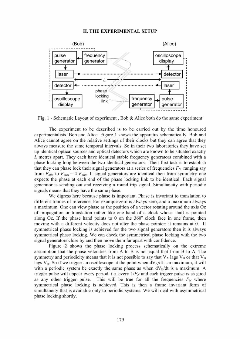
179
II. THE EXPERIMENTAL SETUP
detector
oscilloscopedisplay
(Bob)
pulsegenerator
laser
frequencygenerator
detector
oscilloscopedisplay
pulsegenerator
laser
(Alice)
phase locking
link frequencygenerator
L
Fig. 1 - Schematic Layout of experiment . Bob & Alice both do the same experiment
The experiment to be described is to be carried out by the time honoured experimentalists, Bob and Alice. Figure 1 shows the apparatus schematically. Bob and Alice cannot agree on the relative settings of their clocks but they can agree that they always measure the same temporal intervals. So in their two laboratories they have set up identical optical sources and optical detectors which are known to be situated exactly L metres apart. They each have identical stable frequency generators combined with a phase locking loop between the two identical generators. Their first task is to establish that they can phase lock their signal generators at a series of frequencies FN ranging say from Fmin to Fmax
~ 4 Fmin. If signal generators are identical then from symmetry one expects the phase at each end of the phase locking link to be identical. Each signal generator is sending out and receiving a round trip signal. Simultaneity with periodic signals means that they have the same phase.
We digress here because phase is important. Phase is invariant to translation to different frames of reference. For example zero is always zero, and a maximum always a maximum. One can view phase as the position of a vector rotating around the axis Oz of propagation or translation rather like one hand of a clock whose shaft is pointed along Oz. If the phase hand points to 0 on the 360o clock face in one frame, then moving with a different velocity does not alter the phase pointer: it remains at 0. If symmetrical phase locking is achieved for the two signal generators then it is always symmetrical phase locking. We can check the symmetrical phase locking with the two signal generators close by and then move them far apart with confidence.
Figure 2 shows the phase locking process schematically on the extreme assumption that the phase velocities from A to B is not equal that from B to A. The symmetry and periodicity means that it is not possible to say that VA lags VB or that VB lags VA. So if we trigger an oscilloscope at the point when dVA/dt is a maximum, it will with a periodic system be exactly the same phase as when dVB/dt is a maximum. A trigger pulse will appear every period, i.e. every 1/FN and each trigger pulse is as good as any other trigger pulse. This will be true for all the frequencies FN where symmetrical phase locking is achieved. This is then a frame invariant form of simultaneity that is available only to periodic systems. We will deal with asymmetrical phase locking shortly.
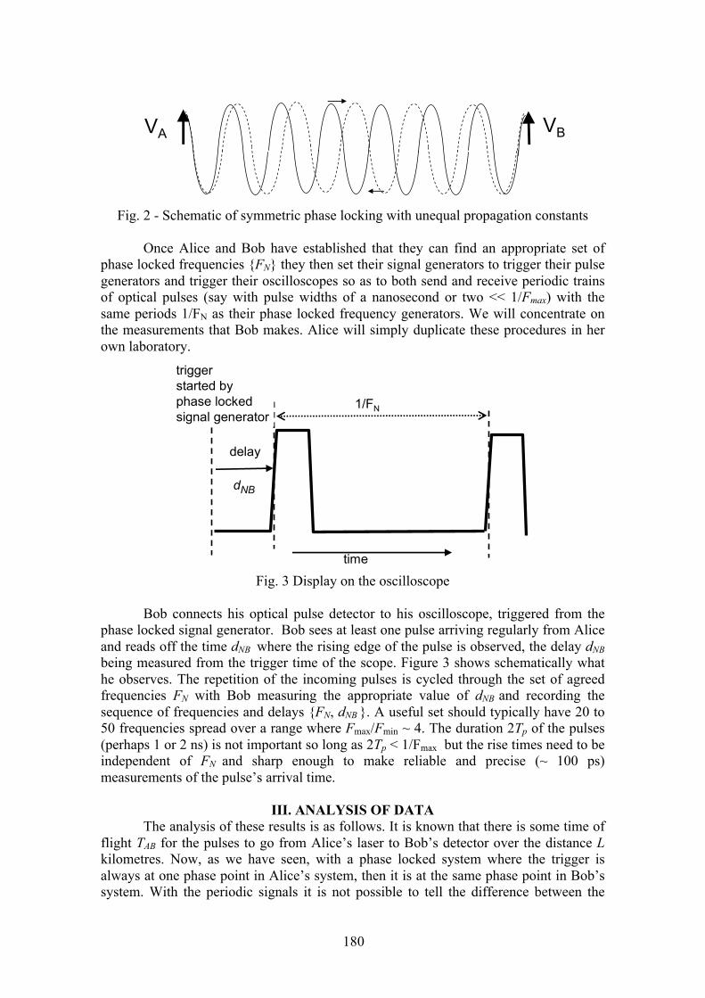
180
VA VB
Fig. 2 - Schematic of symmetric phase locking with unequal propagation constants
Once Alice and Bob have established that they can find an appropriate set of phase locked frequencies FN they then set their signal generators to trigger their pulse generators and trigger their oscilloscopes so as to both send and receive periodic trains of optical pulses (say with pulse widths of a nanosecond or two << 1/Fmax) with the same periods 1/FN as their phase locked frequency generators. We will concentrate on the measurements that Bob makes. Alice will simply duplicate these procedures in her own laboratory.
delay
dNB
time
1/FN
triggerstarted by phase lockedsignal generator
Fig. 3 Display on the oscilloscope
Bob connects his optical pulse detector to his oscilloscope, triggered from the phase locked signal generator. Bob sees at least one pulse arriving regularly from Alice and reads off the time dNB where the rising edge of the pulse is observed, the delay dNB being measured from the trigger time of the scope. Figure 3 shows schematically what he observes. The repetition of the incoming pulses is cycled through the set of agreed frequencies FN with Bob measuring the appropriate value of dNB and recording the sequence of frequencies and delays FN, dNB . A useful set should typically have 20 to 50 frequencies spread over a range where Fmax/Fmin ~ 4. The duration 2Tp of the pulses (perhaps 1 or 2 ns) is not important so long as 2Tp < 1/Fmax but the rise times need to be independent of FN and sharp enough to make reliable and precise (~ 100 ps) measurements of the pulse’s arrival time.
III. ANALYSIS OF DATAThe analysis of these results is as follows. It is known that there is some time of
flight TAB for the pulses to go from Alice’s laser to Bob’s detector over the distance L kilometres. Now, as we have seen, with a phase locked system where the trigger is always at one phase point in Alice’s system, then it is at the same phase point in Bob’s system. With the periodic signals it is not possible to tell the difference between the
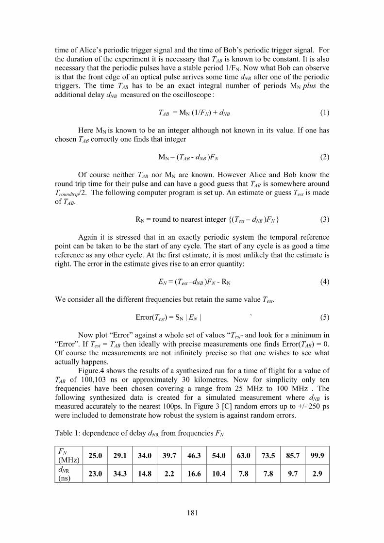
181
time of Alice’s periodic trigger signal and the time of Bob’s periodic trigger signal. For the duration of the experiment it is necessary that TAB is known to be constant. It is also necessary that the periodic pulses have a stable period 1/FN. Now what Bob can observe is that the front edge of an optical pulse arrives some time dNB after one of the periodic triggers. The time TAB has to be an exact integral number of periods MN plus the additional delay dNB measured on the oscilloscope :
TAB = MN (1/FN) + dNB (1)
Here MN is known to be an integer although not known in its value. If one has chosen TAB correctly one finds that integer
MN = (TAB - dNB )FN (2)
Of course neither TAB nor MN are known. However Alice and Bob know the round trip time for their pulse and can have a good guess that TAB is somewhere around Troundtrip/2. The following computer program is set up. An estimate or guess Test is made of TAB.
RN = round to nearest integer (Test – dNB )FN (3)
Again it is stressed that in an exactly periodic system the temporal reference point can be taken to be the start of any cycle. The start of any cycle is as good a time reference as any other cycle. At the first estimate, it is most unlikely that the estimate is right. The error in the estimate gives rise to an error quantity:
EN = (Test –dNB )FN - RN (4)
We consider all the different frequencies but retain the same value Test.
Error(Test) = SN | EN | ` (5)
Now plot “Error” against a whole set of values “Test” and look for a minimum in “Error”. If Test = TAB then ideally with precise measurements one finds Error(TAB) = 0. Of course the measurements are not infinitely precise so that one wishes to see what actually happens.
Figure.4 shows the results of a synthesized run for a time of flight for a value of TAB of 100,103 ns or approximately 30 kilometres. Now for simplicity only ten frequencies have been chosen covering a range from 25 MHz to 100 MHz . The following synthesized data is created for a simulated measurement where dNB is measured accurately to the nearest 100ps. In Figure 3 [C] random errors up to +/- 250 ps were included to demonstrate how robust the system is against random errors.
Table 1: dependence of delay dNR from frequencies FN
FN (MHz) 25.0 29.1 34.0 39.7 46.3 54.0 63.0 73.5 85.7 99.9
dNR(ns) 23.0 34.3 14.8 2.2 16.6 10.4 7.8 7.8 9.7 2.9
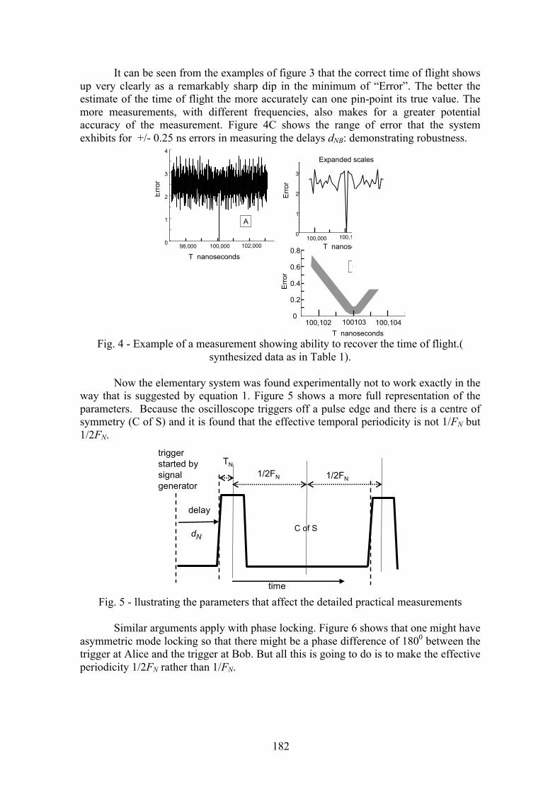
182
It can be seen from the examples of figure 3 that the correct time of flight shows up very clearly as a remarkably sharp dip in the minimum of “Error”. The better the estimate of the time of flight the more accurately can one pin-point its true value. The more measurements, with different frequencies, also makes for a greater potential accuracy of the measurement. Figure 4C shows the range of error that the system exhibits for +/- 0.25 ns errors in measuring the delays dNB: demonstrating robustness.
98,000 100,000 102,0000
1
2
3
4
100,000 100,100 100,2000
1
2
3
100,102 100103 100,1040
0.2
0.4
0.6
0.8 T nanoseconds
Expanded scales
T nanoseconds
T nanoseconds
Erro
r
Erro
r
Erro
r
AB
C
Fig. 4 - Example of a measurement showing ability to recover the time of flight.( synthesized data as in Table 1).
Now the elementary system was found experimentally not to work exactly in the way that is suggested by equation 1. Figure 5 shows a more full representation of the parameters. Because the oscilloscope triggers off a pulse edge and there is a centre of symmetry (C of S) and it is found that the effective temporal periodicity is not 1/FN but 1/2FN.
delay
dN
1/2FN
time
1/2FN
TN
C of S
triggerstarted by signal generator
Fig. 5 - llustrating the parameters that affect the detailed practical measurements
Similar arguments apply with phase locking. Figure 6 shows that one might have asymmetric mode locking so that there might be a phase difference of 1800 between the trigger at Alice and the trigger at Bob. But all this is going to do is to make the effective periodicity 1/2FN rather than 1/FN.
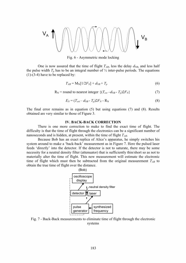
183
VA VB
Fig. 6 - Asymmetric mode locking
One is now assured that the time of flight TAB, less the delay dNB, and less half the pulse width Tp has to be an integral number of ½ inter-pulse periods. The equations (1)-(3-4) have to be replaced by:
TAB = MN[1/2FN] + dNB + Tp (6)
RN = round to nearest integer (Test –dNB - Tp)2FN (7)
EN = (Test – dNB - Tp)2FN - RN (8)
The final error remains as in equation (5) but using equations (7) and (8). Results obtained are very similar to those of Figure 3.
IV. BACK-BACK CORRECTIONThere is one more correction to make to find the exact time of flight. The
difficulty is that the time of flight through the electronics can be a significant number of nanoseconds and is hidden, at present, within the time of flight TAB.
Because Bob has an exact replica of Alice’s apparatus, he simply switches his system around to make a ‘back-back’ measurement as in Figure 7. Here the pulsed laser feeds ‘directly’ into the detector. If the detector is not to saturate, there may be some necessity for a neutral density filter (attenuator) that is sufficiently thin/short so as not to materially alter the time of flight. This new measurement will estimate the electronic time of flight which must then be subtracted from the original measurement TAB to obtain the true time of flight over the distance.
detector
oscilloscopedisplay
pulsegenerator
laser
synthesizedfrequency
(Bob)
neutral density filter
Fig. 7 - Back-Back measurements to eliminate time of flight through the electronic systems
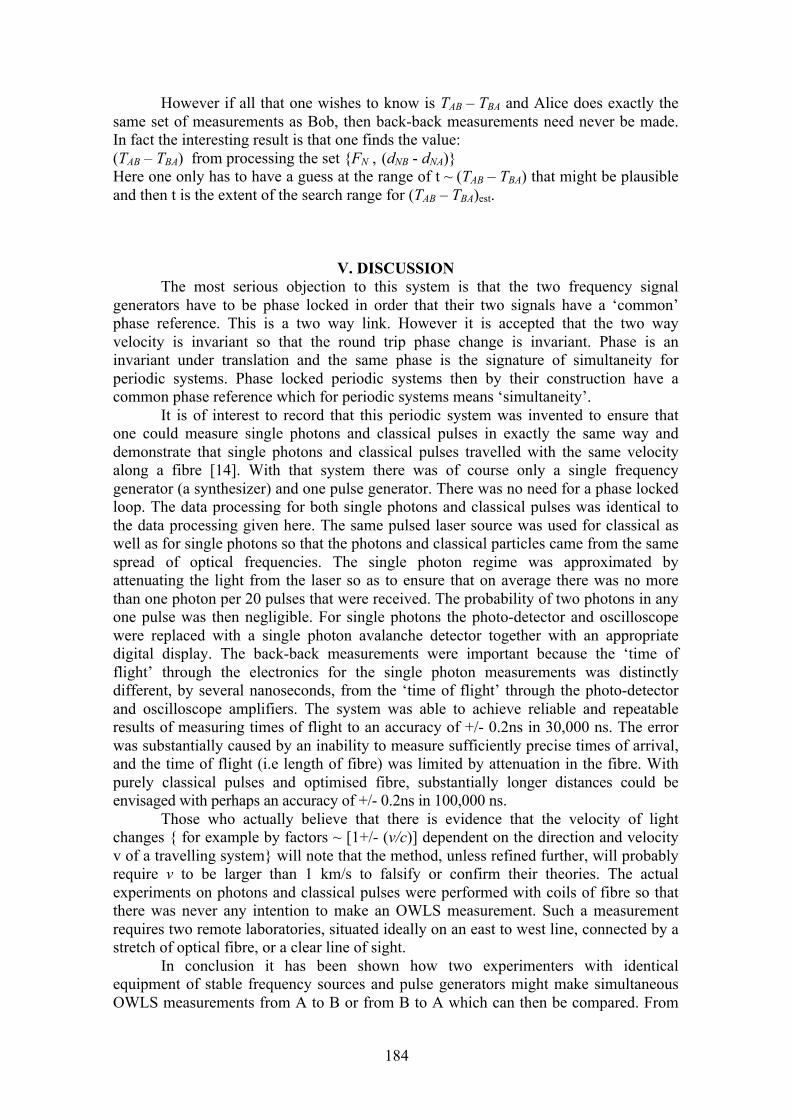
184
However if all that one wishes to know is TAB – TBA and Alice does exactly the same set of measurements as Bob, then back-back measurements need never be made. In fact the interesting result is that one finds the value: (TAB – TBA) from processing the set FN , (dNB - dNA) Here one only has to have a guess at the range of t ~ (TAB – TBA) that might be plausible and then t is the extent of the search range for (TAB – TBA)est.
V. DISCUSSION The most serious objection to this system is that the two frequency signal
generators have to be phase locked in order that their two signals have a ‘common’ phase reference. This is a two way link. However it is accepted that the two way velocity is invariant so that the round trip phase change is invariant. Phase is an invariant under translation and the same phase is the signature of simultaneity for periodic systems. Phase locked periodic systems then by their construction have a common phase reference which for periodic systems means ‘simultaneity’.
It is of interest to record that this periodic system was invented to ensure that one could measure single photons and classical pulses in exactly the same way and demonstrate that single photons and classical pulses travelled with the same velocity along a fibre [14]. With that system there was of course only a single frequency generator (a synthesizer) and one pulse generator. There was no need for a phase locked loop. The data processing for both single photons and classical pulses was identical to the data processing given here. The same pulsed laser source was used for classical as well as for single photons so that the photons and classical particles came from the same spread of optical frequencies. The single photon regime was approximated by attenuating the light from the laser so as to ensure that on average there was no more than one photon per 20 pulses that were received. The probability of two photons in any one pulse was then negligible. For single photons the photo-detector and oscilloscope were replaced with a single photon avalanche detector together with an appropriate digital display. The back-back measurements were important because the ‘time of flight’ through the electronics for the single photon measurements was distinctly different, by several nanoseconds, from the ‘time of flight’ through the photo-detector and oscilloscope amplifiers. The system was able to achieve reliable and repeatable results of measuring times of flight to an accuracy of +/- 0.2ns in 30,000 ns. The error was substantially caused by an inability to measure sufficiently precise times of arrival, and the time of flight (i.e length of fibre) was limited by attenuation in the fibre. With purely classical pulses and optimised fibre, substantially longer distances could be envisaged with perhaps an accuracy of +/- 0.2ns in 100,000 ns.
Those who actually believe that there is evidence that the velocity of light changes for example by factors ~ [1+/- (v/c)] dependent on the direction and velocity v of a travelling system will note that the method, unless refined further, will probably require v to be larger than 1 km/s to falsify or confirm their theories. The actual experiments on photons and classical pulses were performed with coils of fibre so that there was never any intention to make an OWLS measurement. Such a measurement requires two remote laboratories, situated ideally on an east to west line, connected by a stretch of optical fibre, or a clear line of sight.
In conclusion it has been shown how two experimenters with identical equipment of stable frequency sources and pulse generators might make simultaneous OWLS measurements from A to B or from B to A which can then be compared. From
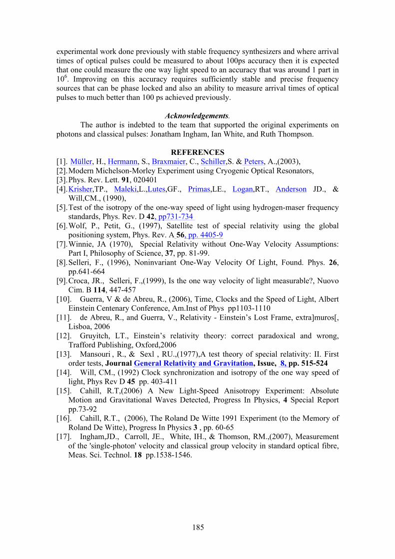
185
experimental work done previously with stable frequency synthesizers and where arrival times of optical pulses could be measured to about 100ps accuracy then it is expected that one could measure the one way light speed to an accuracy that was around 1 part in 106. Improving on this accuracy requires sufficiently stable and precise frequency sources that can be phase locked and also an ability to measure arrival times of optical pulses to much better than 100 ps achieved previously.
Acknowledgements. The author is indebted to the team that supported the original experiments on
photons and classical pulses: Jonatham Ingham, Ian White, and Ruth Thompson.
REFERENCES [1]. Müller, H., Hermann, S., Braxmaier, C., Schiller,S. & Peters, A.,(2003), [2]. Modern Michelson-Morley Experiment using Cryogenic Optical Resonators, [3]. Phys. Rev. Lett. 91, 020401 [4]. Krisher,TP., Maleki,L.,Lutes,GF., Primas,LE., Logan,RT., Anderson JD., &
Will,CM., (1990), [5]. Test of the isotropy of the one-way speed of light using hydrogen-maser frequency
standards, Phys. Rev. D 42, pp731-734 [6]. Wolf, P., Petit, G., (1997), Satellite test of special relativity using the global
positioning system, Phys. Rev. A 56, pp. 4405-9 [7]. Winnie, JA (1970), Special Relativity without One-Way Velocity Assumptions:
Part I, Philosophy of Science, 37, pp. 81-99. [8]. Selleri, F., (1996), Noninvariant One-Way Velocity Of Light, Found. Phys. 26,
pp.641-664 [9]. Croca, JR., Selleri, F.,(1999), Is the one way velocity of light measurable?, Nuovo
Cim. B 114, 447-457 [10]. Guerra, V & de Abreu, R., (2006), Time, Clocks and the Speed of Light, Albert
Einstein Centenary Conference, Am.Inst of Phys pp1103-1110 [11]. de Abreu, R., and Guerra, V., Relativity - Einstein’s Lost Frame, extra]muros[,
Lisboa, 2006 [12]. Gruyitch, LT., Einstein’s relativity theory: correct paradoxical and wrong,
Trafford Publishing, Oxford,2006 [13]. Mansouri , R., & Sexl , RU.,(1977),A test theory of special relativity: II. First
order tests, Journal General Relativity and Gravitation, Issue, 8, pp. 515-524 [14]. Will, CM., (1992) Clock synchronization and isotropy of the one way speed of
light, Phys Rev D 45 pp. 403-411 [15]. Cahill, R.T,(2006) A New Light-Speed Anisotropy Experiment: Absolute
Motion and Gravitational Waves Detected, Progress In Physics, 4 Special Report pp.73-92
[16]. Cahill, R.T., (2006), The Roland De Witte 1991 Experiment (to the Memory of Roland De Witte), Progress In Physics 3 , pp. 60-65
[17]. Ingham,JD., Carroll, JE., White, IH., & Thomson, RM.,(2007), Measurement of the 'single-photon' velocity and classical group velocity in standard optical fibre, Meas. Sci. Technol. 18 pp.1538-1546.
FROM LOCAL TO GLOBAL RELATIVITY
Tuomo Suntola, www.sci.fi/~suntola
Newtonian physics is local by its nature. No local frame is in a special position in space. There are no overall limits to space or to physical quantities. Newtonian space is Euclidean until infinity, and velocities in space grow linearly as long as there is a constant force acting on an object. Finiteness of physical quantities was observed for about 100 years ago – first as finiteness of velocities.
The theory of relativity introduces a mathematical structure for the description of the finiteness of velocities by modifying the coordinate quantities, time and distance for making the velocity of light appear as the maximum velocity in space and an invariant for the observer. Like in Newtonian physics, no local frame, or inertial observer, is in a special position in space. Friedman-Lemaître-Robertson-Walker (FLRW) metrics derived from the general theory of relativity predicts finiteness of space if a critical mass density in space is reached or exceeded.
In the Dynamic Universe approach space is described as the three-dimensional surface of a four-dimensional sphere. Finiteness of physical quantities in DU space comes from the finiteness of total energy in space — finiteness of velocities is a consequence of the zero-energy balance, which does not allow velocities higher than the velocity of space in the fourth dimension. The velocity of space in the fourth dimension is determined by the zero-energy balance of motion and gravitation of whole space and it serves as the reference for all velocities in space. Relativity in DU space means relativity of local to the whole — relativity is a measure of locally available share of the primary rest energy, the rest energy of the object in hypothetical homogeneous space. Atomic clocks in fast motion or in high gravitational field do not lose time because of slower flow of time but because part of their energy is bound into interactions in space. There is no space-time linkage in the Dynamic Universe; time is universal and the fourth dimension is metric by its nature. Local state of rest in DU space is the zero-momentum state in a local energy frame which is linked to hypothetical homogeneous space via a chain of nested energy frames.
Predictions for local phenomena in DU space are essentially the same as the corresponding predictions given by special and general theories of relativity. At extremes, at cosmological distances and in the vicinity of local singularities differences in the predictions become meaningful. Reasons for the differences can be traced back to the differences in the basic assumptions and in the structures of the two approaches.
Keywords: Friedman-Lemaître-Robertson-Walker, general relativity, atomic clocks, dynamic universe, local energy frame.
PACS number: 04.20.-q
186
Newtonian physics is local by its nature. No local frame is in a special position in space. There are no overall limits to space or to physical quantities. Newtonian space is Euclidean until infinity, time is absolute without start or end, and velocities grow linearly as long as there is a constant force acting on an object. Velocities in Newtonian space summed up linearly without limitations.
The success of Newtonian physics led to a well-ordered mechanistic picture of physical reality. The nice Newtonian picture dominated until observations on the velocity of light in late 19th century when it turned out that the observer’s velocity did not add the velocity of light which looked like an upper limit to all velocities.
In the theory of relativity the finiteness of velocities was solved by postulating the velocity of light as an invariant and the maximum velocity for any observer. In the theory of relativity, finiteness of velocities is described by linking time to space to form four-dimensional spacetime, which defines spacetime interval ds = c⋅ dτ as an invariant equal to the product of the velocity of light and the differential of proper timeτ. The invariance of the proper time relies on relativity principle which requires nature laws to look the same for any observer independent of his state of motion or gravitation. In the framework of relativity theory, clocks in a high gravitational field and in fast motion conserve the local proper time but lose coordinate time related to time measured by a clock at rest in zero gravitational field. Like in Newtonian space, gravitation and motion in relativistic space are linked by equivalence principle equalizing inertial acceleration and gravitational acceleration. General appearance of relativistic space is derived assuming uniform distribution of mass at cosmological distances. Due to the local nature of the relativity theory, relativistic space conserves the gravitational energy and dimensions of local gravitational systems. The expansion of relativistic space occurs as “Hubble flow” in empty space between the local systems – probably speeded up by dark energy with gravitational push.
I. IntroductionIn its basic approach modern physics relies on Galilean and Newtonian
tradition of connecting observer, observation and a mathematical description of the observation. Orientation to observations required the definition of observer’s position and the state of rest. Newton’s great breakthrough was the equation of motion, which linked acceleration to the mass of the accelerated object and thus defined the concept of force. The linkage of force to acceleration allowed the definition of gravitation as a force resulting in the acceleration of a falling object which allowed a physical interpretation of Kepler’s laws of the motion of celestial bodies.
The need for relativity theory came from the observed finiteness of velocities and the unique property of the velocity of light as being insensitive to the velocity of the observer. The solution of modifying time and distance limit velocities in the spirit of relativity principle, but it does not account for the physical basis of such limitation. In specific areas of physics like in thermodynamics and quantum mechanics the system studied is specified by boundary conditions, the total energy of the system and a possible energy exchange from and to the system. Energy has been generally accepted as a primary conservable in closed systems.
Is there a way of studying whole space as a closed energy system and derive interactions and local limitations from the conservation of total energy in space? In his lectures on gravitation in early 1960’s Richard Feynman [1] stated:
“If now we compare this number (total gravitational energy MΣ2G/R) to the total
rest energy of the universe, MΣ c2, lo and behold, we get the amazing result that GMΣ
2/R = MΣ c2, so that the total energy of the universe is zero. — It is exciting to think that it costs nothing to create a new particle, since we can create it at the center of the universe where it will have a negative gravitational energy equal to MΣc2. — Why this should be so is one of the great mysteries—and therefore one of the important questions of physics. After all, what would be the use of studying physics if the mysteries were not the most important things to investigate”.
187
and further [2] “...One intriguing suggestion is that the universe has a structure analogous to
that of a spherical surface. If we move in any direction on such a surface, we never meet a boundary or end, yet the surface is bounded and finite. It might be that our three-dimensional space is such a thing, a tridimensional surface of a four sphere. The arrangement and distribution of galaxies in the world that we see would then be something analogous to a distribution of spots on a spherical ball.”
Once we adopt the idea of the fourth dimension with metric nature, Feynman’s findings open up the possibility of a dynamic balance of space: the rest energy of matter is the energy of motion mass in space possesses due to the motion of space in the direction of the radius of the 4-sphere. Such a motion is driven by the shrinkage force resulting from the gravitation of mass in the structure. Like in a spherical pendulum in the fourth dimension, contraction building up the motion towards the center is followed by expansion releasing the energy of motion gained in the contraction.
The Dynamic Universe approach [3–9] is just a detailed analysis of combining Feynman’s “great mystery” of zero-energy space to the “intriguing suggestion of spherically closed space” by the dynamics of a four-sphere. The Dynamic Universe is a holistic model of physical reality starting from whole space as a spherically closed zero-energy system of motion and gravitation. Instead of extrapolating the cosmological appearance of space from locally defined field equations, locally observed phenomena are derived from the conservation of the zero-energy balance of motion and gravitation in whole space. The energy structure of space is described in terms of nested energy frames starting from hypothetical homogeneous space as the universal frame of reference and proceeding down to local frames in space. Time is decoupled from space – the fourth dimension has a geometrical meaning as the radius of the sphere closing the three-dimensional space.
In the Dynamic Universe, finiteness comes from the finiteness of the total energy in space — finiteness of velocities in space is a consequence of the zero-energy balance, which does not allow velocities higher than the velocity of space in the fourth dimension. The velocity of space in the fourth dimension is determined by the zero-energy balance of motion and gravitation of whole space and it serves as the reference for all velocities in space.
The total energy is conserved in all interactions in space. Motion and gravitation in space reduce the energy available for internal processes within an object. Atomic clocks in fast motion or in high gravitational field in DU space do not lose time because of slower flow of time but because they use part of their total energy for kinetic energy and local gravitation in space.
Relativity in Dynamic Universe does not need relativity principle, equivalence principle, Lorentz transformation, or postulation of the velocity of light. By equating the integrated gravitational energy in the spherical structure with the energy of motion created by momentum in the direction of the 4-radius we enter into zero-energy space with motion and gravitation in balance. Total energy of gravitation in spherically closed space is conserved in mass center buildup via local tilting of space which converts part of the gravitational interaction in the fourth dimension to gravitational interaction in a space direction and part of the velocity of space into velocity of free fall towards the local mass center created.
Relativity in Dynamic Universe means relativity of local to whole. Local energy is related to the total energy in space. As consequences, local velocities become related to the velocity of space in the fourth dimension and local gravitation becomes related to the total gravitational energy in space. Expansion of space occurs in a zero-energy balance of motion and gravitation. Local gravitational systems expand in direct proportion to the expansion of whole space.
188

The Dynamic Universe model allows a unified expression of energies and shows mass as wavelike substance for the expression of energies both in localized mass objects, in electromagnetic radiation, and Coulomb systems. The late 1800’s great mystery of the invariance of the velocity of light in moving frames disappears as soon as we observe the momentum of radiation, not only the velocity. The momentum of radiation caught to a moving frame is changed due to the Doppler shift of frequency, not due to a change in velocity as observed in the case of catching mass objects to a moving frame. Equal Doppler change of wavelength and cycle time in detected radiation conserves the phase velocity but at a changed momentum.
II. GLOBAL APPROACH TO FINITENESS AND RELATIVITYII. A. Space as spherically closed energy structure
In the Dynamic Universe model a global approach to finiteness relies on the description of space as a closed energy system with potential energy and the energy of motion in balance. The structure closing the three dimensional space with minimum potential (gravitational) energy is the “surface” of a four dimensional sphere. Zero-energy balance in spherically closed space is obtained via interplay of the energies of motion and gravitation in the structure — in a contraction phase the energy of gravitation is converted into the energy of motion — in an expansion phase the energy of motion gained in the contraction is released back to the energy of gravitation, Fig. 2.1-1. In the contraction, space as a four-dimensional sphere releases volume and gains velocity. In the expansion, space releases velocity and gains volume.
Mathematically, the zero-energy dynamics of spherically closed space is expressed as
( ) ( )20
0
" 0rest tot global totGME E M c M
RΣ+ = − Σ = (2.1:1)
where G is the gravitational constant, MΣ is the total mass in space, M" = 0.776⋅MΣ is the mass equivalence of the total mass (when concentrated into the center of the 4-sphere), R0 is the radius of the 4-sphere, and c0 is the velocity of contraction or expansion
2 30
0 00 0
0.776 2" 1.246G RGMcR R
ρ π R Gπ ρ⋅
= ± = ± = ± ⋅ (2.1:2)
where ρ is the mass density in space. The contraction and expansion of spherically closed space is the primary
energy buildup process creating the rest energy of matter as the complementary counterpart to the global gravitational energy.
189
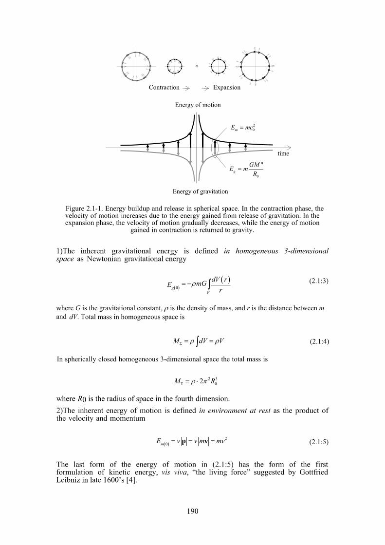
Figure 2.1-1. Energy buildup and release in spherical space. In the contraction phase, the velocity of motion increases due to the energy gained from release of gravitation. In the expansion phase, the velocity of motion gradually decreases, while the energy of motion
gained in contraction is returned to gravity.
1)The inherent gravitational energy is defined in homogeneous 3-dimensionalspace as Newtonian gravitational energy
( )( )
0gV
dV rE mG
rρ= − ∫ (2.1:3)
where G is the gravitational constant, ρ is the density of mass, and r is the distance between m and dV. Total mass in homogeneous space is
M dV Vρ ρΣ = =∫ (2.1:4)
20mE mc=
0
"g
GME mR
=
Energy of motion
Energy of gravitation
Expansion
time
Contraction
2 30M = ⋅ 2ρ π RΣ
where R0 is the radius of space in the fourth dimension.
In spherically closed homogeneous 3-dimensional space the total mass is
2)The inherent energy of motion is defined in environment at rest as the product ofthe velocity and momentum
0( )2
mE = =v vp vm = mv (2.1:5)
The last form of the energy of motion in (2.1:5) has the form of the first formulation of kinetic energy, vis viva, “the living force” suggested by Gottfried Leibniz in late 1600’s [4].
190
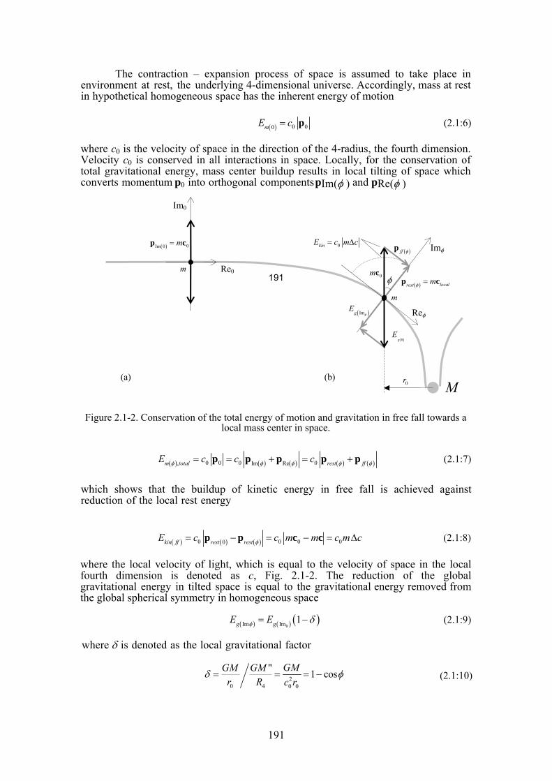
The contraction – expansion process of space is assumed to take place in environment at rest, the underlying 4-dimensional universe. Accordingly, mass at rest in hypothetical homogeneous space has the inherent energy of motion
m 0( ) 0 0=E c p (2.1:6)
where c0 is the velocity of space in the direction of the 4-radius, the fourth dimension. Velocity c0 is conserved in all interactions in space. Locally, for the conservation of total gravitational energy, mass center buildup results in local tilting of space which converts momentum p0 into orthogonal components pIm(φ ) and pRe(φ )
Re0
Im0
Figure 2.1-2. Conservation of the total energy of motion and gravitation in free fall towards a local mass center in space.
rest φ( ) local= mcp
g 0( )E
0mc
p ff φ( )
M(a)
m
0Im 0( ) = mp c Imφ
φ
Reφ
0kin =E c Δm c
Eg Im( )φ
0r
m
(b)
0 rest( ) ff ( )0 0 0 φI ( )m ( )φRem( ) totalE c, = =p pc cφ + = +p p pφ φ (2.1:7)
which shows that the buildup of kinetic energy in free fall is achieved against reduction of the local rest energy
kin ff( ) rest 00 ( ) rest(φ ) 0 0 0E p= c cc −m m=− p c = Δc m c (2.1:8)
where the local velocity of light, which is equal to the velocity of space in the local fourth dimension is denoted as c, Fig. 2.1-2. The reduction of the global gravitational energy in tilted space is equal to the gravitational energy removed from the global spherical symmetry in homogeneous space
Im( φ ) Im( 0 ) 1g gEE = ( δ )− (2.1:9)
where δ is denoted as the local gravitational factor
20 4 0 0r R c r
δ =GM GM " GM
= 1 c= osφ− (2.1:10)
191
191
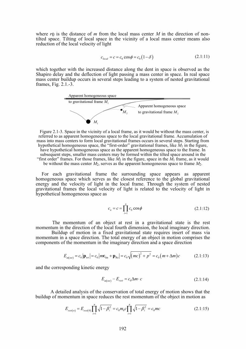
where r0 is the distance of m from the local mass center M in the direction of non-tilted space. Tilting of local space in the vicinity of a local mass center means also reduction of the local velocity of light
(0 0cos 1localc c c c )φ δ= = = − (2.1:11)
which together with the increased distance along the dent in space is observed as the Shapiro delay and the deflection of light passing a mass center in space. In real space mass center buildup occurs in several steps leading to a system of nested gravitational frames, Fig. 2.1.-3.
Figure 2.1-3. Space in the vicinity of a local frame, as it would be without the mass center, is referred to as apparent homogeneous space to the local gravitational frame. Accumulation of
mass into mass centers to form local gravitational frames occurs in several steps. Starting from hypothetical homogeneous space, the “first-order” gravitational frames, like M1 in the figure, have hypothetical homogeneous space as the apparent homogeneous space to the frame. In subsequent steps, smaller mass centers may be formed within the tilted space around in the
“first order” frames. For those frames, like M2 in the figure, space in the M1 frame, as it would be without the mass center M2, serves as the apparent homogeneous space to frame M2.
1M
2M
1
Apparent homogeneous spaceto gravitational frame M
2
Apparent homogeneous spaceto gravitational frame M
For each gravitational frame the surrounding space appears as apparent homogeneous space which serves as the closest reference to the global gravitational energy and the velocity of light in the local frame. Through the system of nested gravitational frames the local velocity of light is related to the velocity of light in hypothetical homogeneous space as
01
n
ni
=c c=
= ∏c cosφ (2.1:12)
The momentum of an object at rest in a gravitational state is the rest momentum in the direction of the local fourth dimension, the local imaginary direction.
Buildup of motion in a fixed gravitational state requires insert of mass via momentum in a space direction. The total energy of an object in motion comprises the components of the momentum in the imaginary direction and a space direction
t( ot )2
0tot0 Im Re 0 0mE = =c cp cm + p = c ( )2mc + p = c (m + Δm)c (2.1:13)
and the corresponding kinetic energy
m tot( ) 0restE − =E c Δm ⋅ c (2.1:14)
A detailed analysis of the conservation of total energy of motion shows that the buildup of momentum in space reduces the rest momentum of the object in motion as
n( ) (0)22
00 011
11nn
i irest restii
E E= =
∏ −= β = c m c −∏ β = c mc (2.1:15)
192
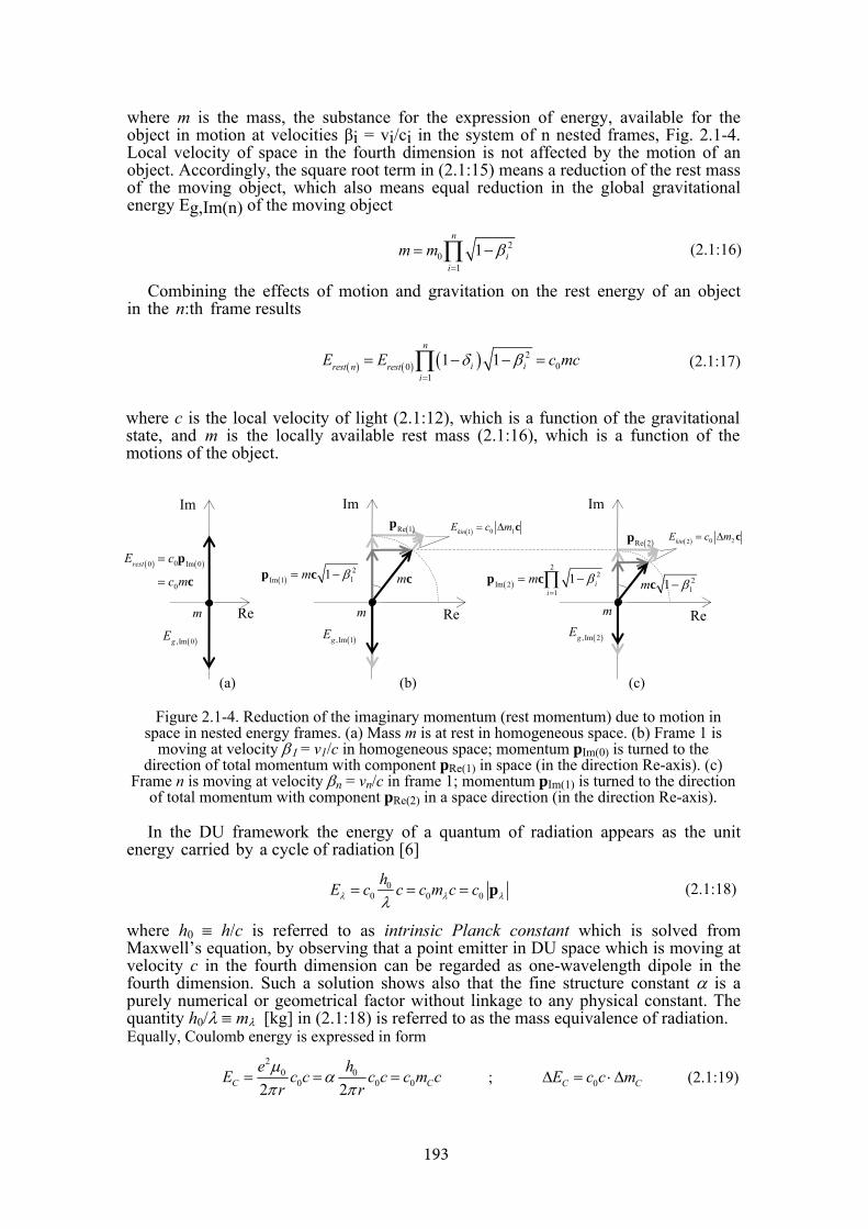
where m is the mass, the substance for the expression of energy, available for the object in motion at velocities βi = vi/ci in the system of n nested frames, Fig. 2.1-4. Local velocity of space in the fourth dimension is not affected by the motion of an object. Accordingly, the square root term in (2.1:15) means a reduction of the rest mass of the moving object, which also means equal reduction in the global gravitational energy Eg,Im(n) of the moving object
20
1
1n
ii
m m β=
= −∏ (2.1:16)
Combining the effects of motion and gravitation on the rest energy of an object in the n:th frame results
( ) ( ) ( ) 200
1
1 1n
i irest n resti
E E δ β=
= − − =∏ c mc
( )
(2.1:17)
where c is the local velocity of light (2.1:12), which is a function of the gravitational state, and m is the locally available rest mass (2.1:16), which is a function of the motions of the object.
Figure 2.1-4. Reduction of the imaginary momentum (rest momentum) due to motion in space in nested energy frames. (a) Mass m is at rest in homogeneous space. (b) Frame 1 is
moving at velocity β1 = v1/c in homogeneous space; momentum pIm(0) is turned to the direction of total momentum with component pRe(1) in space (in the direction Re-axis). (c)
Frame n is moving at velocity βn = vn/c in frame 1; momentum pIm(1) is turned to the direction of total momentum with component pRe(2) in a space direction (in the direction Re-axis).
0 11kinE c m= Δ c
Re
Im
Re
Im ( )Re 1p
Re
Im
( )Re 2p
mc
(a) (b) (c)
m m m
( ) ( )00 Im 0
0
restE c
c m
=
=
p
c ( )2
1Im 1 1m β= −p c( )
22
Im 21
1 ii
m β=
= −∏p c 211m β−c
( ) 0 22kinE c m= Δ c
( ),Im 0gE ( ),Im 1gE ( ),Im 2gE
In the DU framework the energy of a quantum of radiation appears as the unit energy carried by a cycle of radiation [6]
00 0 0E c h c c= m cλ λ λλ
= c= p (2.1:18)
where h0 ≡ h/c is referred to as intrinsic Planck constant which is solved from Maxwell’s equation, by observing that a point emitter in DU space which is moving at velocity c in the fourth dimension can be regarded as one-wavelength dipole in the fourth dimension. Such a solution shows also that the fine structure constant α is a purely numerical or geometrical factor without linkage to any physical constant. The quantity h0/λ ≡ mλ [kg] in (2.1:18) is referred to as the mass equivalence of radiation. Equally, Coulomb energy is expressed in form
20 0
0 022C Che
0E c cπ rπ r
μα== c c c m= c ; 0C CΔE c c= ⋅ Δm (2.1:19)
193
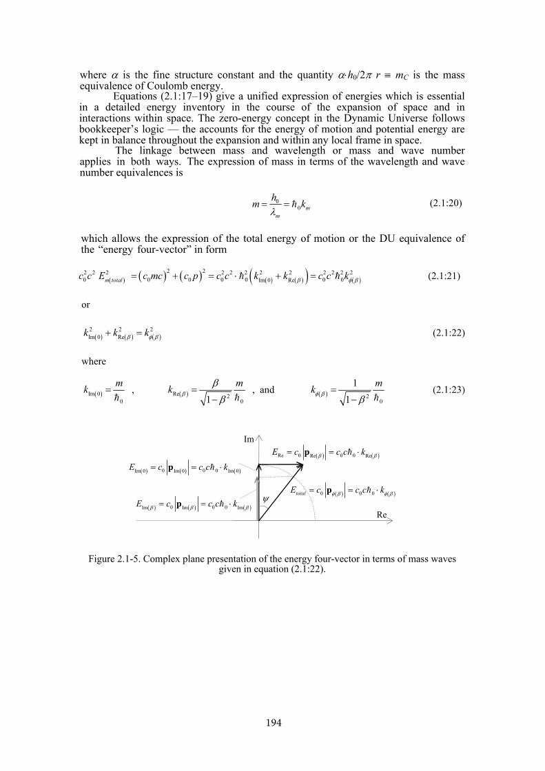
where α is the fine structure constant and the quantity α⋅h0/2π r ≡ mC is the mass equivalence of Coulomb energy.
Equations (2.1:17–19) give a unified expression of energies which is essential in a detailed energy inventory in the course of the expansion of space and in interactions within space. The zero-energy concept in the Dynamic Universe follows bookkeeper’s logic — the accounts for the energy of motion and potential energy are kept in balance throughout the expansion and within any local frame in space.
The linkage between mass and wavelength or mass and wave number applies in both ways. The expression of mass in terms of the wavelength and wave number equivalences is
00 m
m
hmλ
= = k (2.1:20)
which allows the expression of the total energy of motion or the DU equivalence of the “energy four-vector” in form
2 20c c ( ) ( ) ( ) ( ) ( )( ) ( )
2 22 2 2 2 2 20 0 0 0 0 0Im 0 Rem total
2 2 2 2E c mc c p c c k k c c kβ φ β= + = ⋅ + = (2.1:21)
or
( ) ( ) ( )2 2 2Im 0 Rek k kβ φ β+ = (2.1:22)
where
( )Im 00
mk = , ( )Re 201
mk ββ
β=
− , and ( ) 2
0
11
mkφ ββ
=−
(2.1:23)
Re
Im
( ) ( )Re 0 0 0Re ReE c c c kβ β= = ⋅p
( )
Figure 2.1-5. Complex plane presentation of the energy four-vector in terms of mass waves given in equation (2.1:22).
ψ ( )0 0 0totalE c c c kφ β φ β= = ⋅p
( ) ( ) ( )0 0 0Im 0 Im 0 Im 0E c c c k= = ⋅p
( ) ( ) ( )0 0 0Im Im ImE c c c kβ β= = ⋅pβ
194
II.B. Relativity as the measure of locally available energyRelativity in Dynamic Universe is observed as relativity of locally available rest
energy to the rest energy the object has at rest in hypothetical homogeneous space. Relativity in Dynamic Universe is a direct consequence of the conservation of the total energy in interactions in space. It does not rely on relativity principle, spacetime, the equivalence principle, Lorentz covariance, or the invariance of the velocity of light — but just on the zero-energy balance of space.
The linkage of local and global is a characteristic feature of the Dynamic Universe. There are no independent objects in space — all local objects are linked to the rest of space.
The whole in the Dynamic Universe is not composed as the sum of elementary units — the multiplicity of elementary units is a result of diversification of the whole.
The rest energy that mass m possesses in the n:th energy frame is
( )20 0 0 0
1
1 1n
rest i ii
E c c mc m c 2δ β=
= = = − −∏p (2.2:1)
where c0 is the velocity of light in hypothetical homogeneous space, which is equal to the velocity of space in the direction of the 4-radius R0. Momentum p in (2.2:1) is referred to as the rest momentum which appears in the local fourth dimension. The factors δi = GMi/c2 and βi = vi/ci are the gravitational factor and the velocity factor relevant to the local frame, respectively. On the Earth, for example, the gravitational factors define the gravitational state of an object on the Earth, the gravitational state of the Earth in the solar frame, the gravitational state of the solar frame in the Milky Way frame, etc. The velocity factors related to an object on Earth comprise the rotational velocity of the Earth and the orbital velocities of each sub-frame in each one’s parent frame.
An important message of equation (2.2:1) is that the effects of motion and gravitation on the rest energy of an object are different: motion at constant gravitational potential in a local frame releases part of the rest mass into the buildup of momentum in space – free fall in local gravitational field reduces the local rest momentum by reducing the velocity of space in the local fourth dimension via tilting of space.
Also, the buildup of kinetic energy (see equations 2.1:8 and 2.1:14) is different in inertial acceleration and in gravitational acceleration. Kinetic energy can be generally expressed as
( )0 0kinE = Δpc c= Δc m + m Δc (2.2:2)
where the first term shows the insert of mass in inertial acceleration and the second term shows the reduction of the velocity in space in the local fourth dimension. The first term is essentially equal to the kinetic energy in special relativity, the second term does not have direct counterpart in relativity theory which equalizes the effects of gravitational acceleration and inertial acceleration by the equivalence principle.
Equation (2.2:2) shows that the locally available rest energy is a function of the gravitational state, and the velocity of the object studied. Substituting (2.2:1) for the rest energy of electron in Balmer’s equation the characteristic frequency related to an energy transition in atoms obtains the form
∏f= −( ) ( )20 1
1
11 1 1n
local i i n n ni
f δ − β 2δ −=
− β = f − (2.2:3)
where frequency fn–1 is the characteristic frequency of the atom at rest in apparent homogeneous space of the local the local frame. The last form of equation (2.2:3) is essentially equal to the expression of coordinate time frequency on Earth, or Earth satellite clocks in the GR framework. The physical message of (2.2:3) is that “the greater is the energy used for motions and gravitational interactions in space the less energy is left for running internal processes”.
195
The Dynamic Universe links the energy of any localized object to the energy of whole space. Relativity in Dynamic Universe means relativity of local to the whole. At the cosmological scale an important consequence of the linkage between local space and whole space is that local gravitational systems grow in direct proportion to the expansion of space, thus, together with the spherical symmetry explaining the observed Euclidean appearance and surface brightnesses of galaxies in space. The magnitude versus redshift relation of a standard candle in the DU framework is in an accurate agreement with observations without assumptions of dark energy or any free parameter. Moreover, the zero-energy balance in the DU leads to stable orbits down to the critical radius in the vicinity of local singularities in space.
III. COMPARISON OF LOCAL AND GLOBAL RELATIVITYIII.A. Definitions and basic quantities
Table 3.1-I gives a comparison of some fundamental quantities of relativity as described by special and general relativity and in the Dynamic Universe. The primary conservable in the DU framework is mass as wavelike substance for the expression of energy. Basic physical quantities are momentum and the energies of motion and gravitation, which are primarily defined in hypothetical homogeneous space. Force in the DU is a derived quantity as the negative of the gradient of energy. Electromagnetic energy is linked to mass via the mass equivalence of Coulomb energy and a cycle of radiation.
Differences between the two approaches result from the basic choice: - In the framework of relativity theory finiteness in space is described in terms of modified coordinate quantities, which makes time and distance functions of velocity and the gravitational environment. The effect of gravitation relies on equivalence principle which links the acceleration in gravitational field to the inertial acceleration in the absence of gravitational field. Local rest energy is independent of the motion and gravitational environment of an objects. - In the framework of Dynamic Universe finiteness in space is described as finiteness of total energy, which makes the locally available rest energy a function of energy reserved by motion and gravitation in space – via the velocity and gravitational potential of the local frame in its parent frames. Time and distance are universal in the DU.
In the SR&GR framework the velocity of light is constant by definition and the buildup of kinetic energy is described in terms of increase of effective mass – equally in the case of inertial acceleration in the absence of gravitational field and the case of free fall in gravitational field.
In the DU framework the buildup of kinetic energy is different in the case of acceleration via mass insert at constant gravitational potential and in acceleration via free fall in gravitational field. The physical meaning of the mass insert is demonstrated by the concept of mass equivalence, e.g. acceleration of a charged mass object in Coulomb field releases Coulomb energy in terms of a reduction of the mass equivalence as shown in equation (2.1:19). In the case of free fall in local gravitational field the buildup of kinetic energy occurs via tilting of local space against reduction of the local rest energy via a reduction of the velocity of space in the local fourth dimension, Table 3.1-I(4).
In the DU framework a point source of electromagnetic radiation can be studied as one-wavelength dipole in the fourth dimension. Solving the energy emitted by a dipole in an oscillation cycle results
0( )
22 2 2 4 432 200 0
016 2
12N e z μ π fE =
z⎛ ⎞N A ⋅ π μe f⋅cfλ ⎜ ⎟λP
= =cπ f ⎝ ⎠
(3.1:1)
196
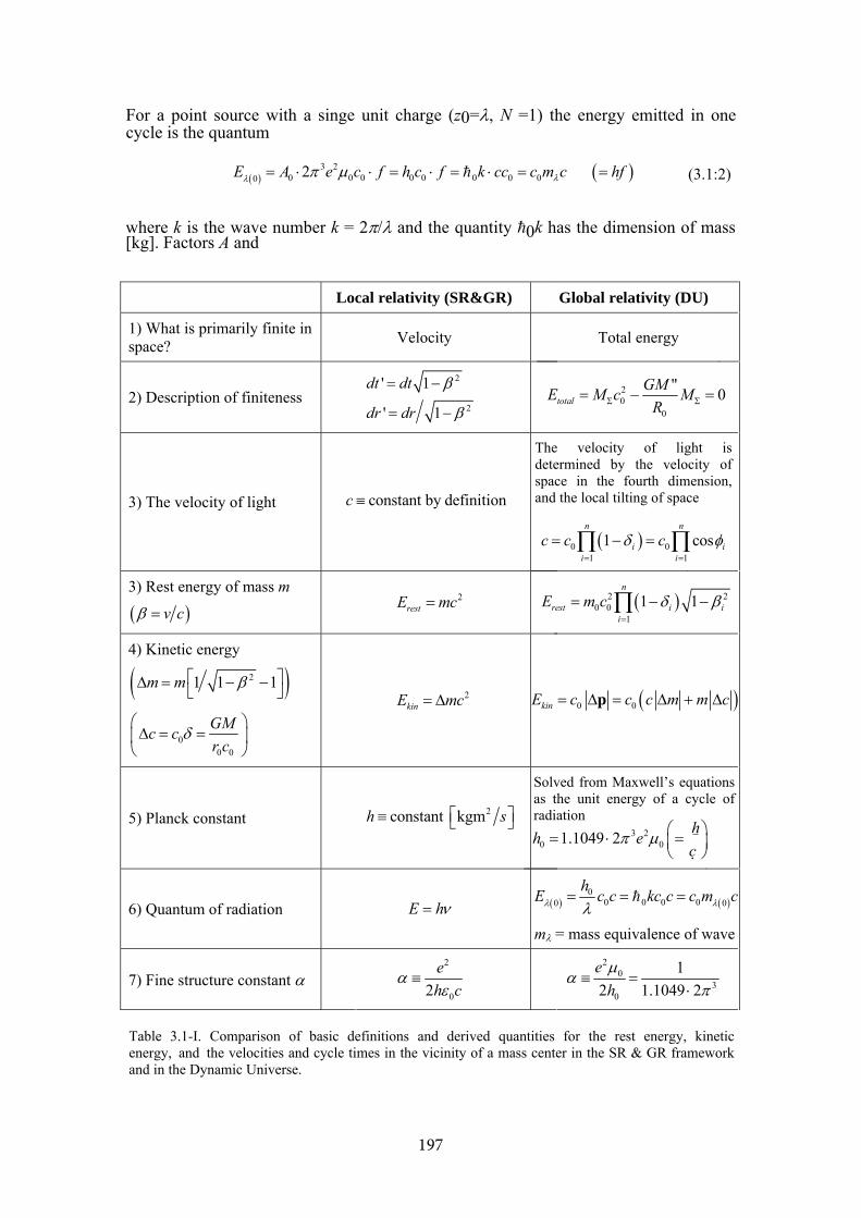
Local relativity (SR&GR) Global relativity (DU)
1) What is primarily finite inspace? Velocity Total energy
2) Description of finiteness2
2
1'
' 1dr = dr
β
β
−dt dt=
−
20
0totalE M c GM
−" M
RΣ Σ= = 0
3) The velocity of light c ≡ constant by definition
The velocity of light is determined by the velocity of space in the fourth dimension, and the local tilting of space
001 1
1 cnn
iiii
=c c φ os= =
δ c=( )−∏ ∏
3) Rest energy of mass m
β = v c( ) 2
restE = mc )2 20 0
1
1 1n
rest i ii
=E m c δ β=
∏( − −
4) Kinetic energy
( ⎦⎤)Δ =m m 1 1⎡
⎣ − β 2 −1
000
GMr c
⎞⎛Δ =c c⎜ δ = ⎟
⎝ ⎠
2kinE = Δmc 0 0kinE = pΔ =c c Δc +m Δm( )c
≡ constant ⎡⎣kgm2h s⎤⎦
Solved from Maxwell’s equations as the unit energy of a cycle of radiation
2300 =1.1049 ⋅ 2πh e μ ⎛ =
c⎜ ⎟⎝ ⎠
5) Planck constant h⎞
⋅
6) Quantum of radiation E = hν ( )0
00 0 00 0E ( ) λc cλ = kc c c= mh cλ=
mλ = mass equivalence of wave
7) Fine structure constant α 2
02eεh c
α ≡2
03
0
12 1.1049 ⋅ 2e
hμ
απ
=≡
Table 3.1-I. Comparison of basic definitions and derived quantities for the rest energy, kinetic energy, and the velocities and cycle times in the vicinity of a mass center in the SR & GR framework and in the Dynamic Universe.
For a point source with a singe unit charge (z0=λ, N =1) the energy emitted in one cycle is the quantum
0( ) (= hf )3 20 0 0 0 0 0 0 0E c m cλλ = ⋅2A eπ μ c f⋅ = h c f⋅ = k c⋅ c = (3.1:2)
where k is the wave number k = 2π/λ and the quantity 0k has the dimension of mass [kg]. Factors A and
197
A0 are geometrical constants characteristic to the antenna. For an ordinary one wavelength dipole in space A= 2/3, for a point source as dipole in the fourth dimension A0 =1.1049. Equation (3.1:2) breaks down the Planck constant into primary electrical constants; the unit charge (e), and the vacuum permeability (μ0). In the intrinsic Planck constant (h0) used in the DU framework the velocity of light (as a non-constant quantity) is removed. As a result the unit of the intrinsic Planck constant is [kg m] instead of [kg m2/s] like the traditional Planck constant, Table 3.1-I(5,6). The removal of the velocity of light from the Planck constant links the concept of quantum to mass rather than to momentum. The breakdown of the Planck constant into primary constants shows the fundamental nature of the fine structure constant as number independent of any physical constant, Table 3.1-I(7).
Localized mass object is described as a closed standing (mass)wave structure as illustrated with a one-dimensional resonator in Figure 3.1-1. The external momentum of a mass object moving in space at velocity β can be expressed as the sum of momentums of the Doppler shifted front wave and back wave
( ) ( ) ( )0 00 0 0Re 2
½ 1 ½ 11 1
DeBrogliek k kβ
ββ ββ β
= ⎡ + − − ⎤ = =⎣ ⎦− −
p c2
c c (3.1:3)
or a wave front with wave number kβ propagating in parallel with the object at velocity v = β c
( )0
0Re 21k kββ β
β= =
−p c 0 v (3.1:4)
where the wave number kβ is equal to the wave number of the effective mass (relativistic mass), Fig. 3.1-1
02
01effmkkβ
β= =
−(3.1:5)
A physical interpretation of equation (3.1:4) is that a mass object moving in space is associated with a parallel wave front carrying the external momentum the object in the parent frame.
This is exceedingly important as a physical explanation to the double-slit experiment. An energy object carries the rest energy as a standing wave in a localized energy structure. The external momentum appears as wave front kβ propagating at velocity β in parallel with the localized object. The wave front is subject to buildup of interference patterns on the screen when passing through the slits. The deflection angle of a singe object is determined by the phase difference between the wave fronts from the slits, Fig. 3.1-1(b).
198
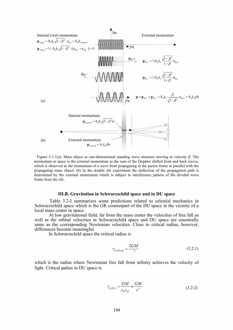
Figure 3.1-1(a). Mass object as one-dimensional standing wave structure moving at velocity β. The momentum in space is the external momentum as the sum of the Doppler shifted front and back waves, which is observed as the momentum of a wave front propagating in the parent frame in parallel with the propagating mass object. (b) In the double slit experiment the deflection of the propagation path is determined by the external momentum which is subject to interference pattern of the divided wave fronts from the slit.
III.B. Gravitation in Schwarzschild space and in DU spaceTable 3.2-I summarizes some predictions related to celestial mechanics in
Schwarzschild space which is the GR counterpart of the DU space in the vicinity of a local mass center in space.
At low gravitational field, far from the mass center the velocities of free fall as well as the orbital velocities in Schwarzschild space and DU space are essentially same as the corresponding Newtonian velocities. Close to critical radius, however, differences become meaningful.
In Schwarzschild space the critical radius is
( ) 2
2c Schwd
GMr
c
= (3.2:1)
which is the radius where Newtonian free fall from infinity achieves the velocity of light. Critical radius in DU space is
( ) 20 0
c DUGM GMrc c cδ
= ≈ (3.2:2)
( )2
0 0 Im 0Im 1 ComptonI k kβ= − ⋅ =p c
2
Re 0 0 Re1½1
k ββ+ +
−=
−p c
Im
( ) ( )20 0 Re ReRe ½ 1 0I k β + −= ⋅ − ⋅ + =p c c
2
Re 0 0 Re1½1
k ββ− −
−=
+p c
Internal (rest) momentum External momentum
Re –
Re +
β c
Re Re 0 0 Re 021k kβ
β ββ
+ − += + = =−
p p p c cβ c(a)
(b)0external kβ β=p c
20 0 1internal k β= −p c
Internal momentum:
External momentum:
199
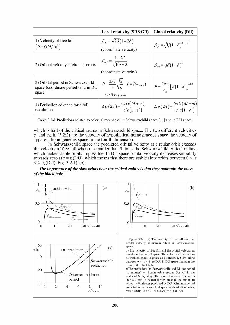
Local relativity (SR&GR) Global relativity (DU)
1) Velocity of free fall( )2GM rcδ =
( )2 1 2ffβ δ δ= −
(coordinate velocity) ( )21 1 1ffβ δ= − −
2) Orbital velocity at circular orbits1 21 3orb
δβδ
−=
−
(coordinate velocity) ( )31orbβ δ δ= −
2 rPcπ3) Orbital period in Schwarzschild
space (coordinate period) and in DU space
2δ
= ( = PNewton )
r > 3⋅rc(Schwd)
( ) 3 2
0
2 1crPc δ
πδ δ
−= ⎡ − ⎤⎣ ⎦
4) Perihelion advance for a fullrevolution
( ) ( )( )2 2
62
1G M m
c a eπ
ψ π+
Δ =−
( ) ( )( )2 2
62
1G M m
c a eπ
ψ π+
Δ =−
Table 3.2-I. Predictions related to celestial mechanics in Schwarzschild space [11] and in DU space.
which is half of the critical radius in Schwarzschild space. The two different velocities c0 and c0δ in (3.2:2) are the velocity of hypothetical homogeneous space the velocity of apparent homogeneous space in the fourth dimension.
In Schwarzschild space the predicted orbital velocity at circular orbit exceeds the velocity of free fall when r is smaller than 3 times the Schwarzschild critical radius, which makes stable orbits impossible. In DU space orbital velocity decreases smoothly towards zero at r = rc(DU), which means that there are stable slow orbits between 0 < r < 4 rc(DU), Fig. 3.2-1(a,b).
The importance of the slow orbits near the critical radius is that they maintain the mass of the black hole.
Figure 3.2-1. a) The velocity of free fall and the orbital velocity at circular orbits in Schwarzschild space, b) The velocity of free fall and the orbital velocity atcircular orbits in DU space. The velocity of free fall in Newtonian space is given as a reference. Slow orbits between 0 < r < 4 rc(DU) in DU space maintain the mass of the black hole. с)The predictions by Schwarzschild and DU for period (in minutes) at circular orbits around Sgr A* in the center of Milky Way. The shortest observed period is 16.8 ± 2 min [8] which is very close to the minimum period 14.8 minutes predicted by DU. Minimum period predicted in Schwarzschild space is about 28 minutes, which occurs at r = 3 rc(Schwd) = 6 r c(DU).
fβ f Newto( )n
β f Schwa( rzsch )ildf βorb Schwarzschild( )
r rc DU( )
0δβ
0
0.5
1
0 10 20 30 40
stable orbits (a)
r rc DU( )
f ,f DUβ
orb,DUβ
fβ f Newto( )n
(b)
0
0.5
1
0 10 20 30 40
0δβ
Schwarzschild prediction
Observed minimum period
0
20
40
60
0 4 8 1062r /rc(DU)
min. DU prediction (c)
200
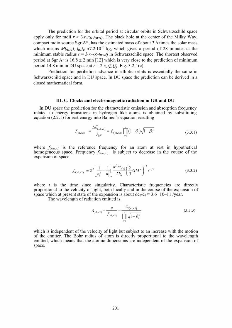
The prediction for the orbital period at circular orbits in Schwarzschild space apply only for radii r > 3⋅rc(Schwd). The black hole at the center of the Milky Way, compact radio source Sgr A*, has the estimated mass of about 3.6 times the solar mass which means Mblack hole ≈7.2⋅1036 kg, which gives a period of 28 minutes at the minimum stable radius r = 3⋅rc(Schwd) in Schwarzschild space. The shortest observed period at Sgr A* is 16.8 ± 2 min [12] which is very close to the prediction of minimum period 14.8 min in DU space at r = 2⋅rc(DU), Fig. 3.2-1(c).
Prediction for perihelion advance in elliptic orbits is essentially the same in Schwarzschild space and in DU space. In DU space the prediction can be derived in a closed mathematical form.
III. C. Clocks and electromagnetic radiation in GR and DUIn DU space the prediction for the characteristic emission and absorption frequency
related to energy transitions in hydrogen like atoms is obtained by substituting equation (2.2:1) for rest energy into Balmer’s equation resulting
( )( )
( ) ( )1, 2 21, 2 0 1, 2
10
1 1n
n nin n n n
i
Ef f
h c iδ β=
Δ= = − −∏ (3.3:1)
where f0(n1,n2) is the reference frequency for an atom at rest in hypothetical homogeneous space. Frequency f0(n1,n2) is subject to decrease in the course of the expansion of space
0( )2 1/ 3
20 1n n,( )2 22
21 0
1 1 2 "32
em1 3f = −⎢ ⎥Z G
n n h
α−⎤⎡ ⎛ ⎞
⎟⎜⎠⎝⎣ ⎦
M t (3.3:2)
where t is the time since singularity. Characteristic frequencies are directly proportional to the velocity of light, both locally and in the course of the expansion of space which at present state of the expansion is about dc0/c0 ≈ 3.6 10–11 /year.
The wavelength of radiation emitted is
λ( 1,n2)( 2)
0 1n n,( )2
2
1
1n n
1,n ni
i
cf
λ
β=
==
∏ −(3.3:3)
which is independent of the velocity of light but subject to an increase with the motion of the emitter. The Bohr radius of atom is directly proportional to the wavelength emitted, which means that the atomic dimensions are independent of the expansion of space.
201

Local relativity (SR&GR) Global relativity (DU) 1) Flow of time (proper
time) in Schwarzschild space and the
frequency of a clock DU space
τd dt= −1 2δ β− 2 20,0f f= −δ( )1 1 β−
2) Gravitational red/blue shift.
Frequency of electromagnetic
radiation transmitted from higher to lower altitude (gravitation
potential)
Frequency increases, velocity of light is
conserved, wavelength decreases
(= gravitational blueshift)
Frequency is conserved, the velocity of light decreases,
wavelength decreases (=gravitational blueshift)
(the observed frequency looks increased when compared to the
frequency of a reference oscillator at receiver’s gravitational state)
3) Shapiro delay
(D1,D2 >> d ) 21
1, 2 3 2
42 lnD DD DGMt
c d⎡ ⎤=Δ ⎢⎣ ⎥⎦
211, 2 23
42 ⎡⎧ln 1D DD DGMtdc
⎤ −⎫
Δ = ⎬⎦⎥ ⎭⎢⎣
⎨⎩
4) Shapiro delay ofradar signal (in radial
direction to and from a mass center)
( −A B) 3
2 B
A
GM ln rtc r
Δ = ( −A B) 3
2 B
A
GM ln rtrc
=Δ
5) Bending of lightpath 2
4GMc d
φ = 2
4GMc d
φ =
6) Doppler effect B( )r( )( )r( )( )
2
2
11
11
β − βBA ABA
B B A
f fβ − β
δ− −=
δ− − )A B(
( − ) r( )−δ β − β( )( r( )( )
2
1
2
1
1 1 1
1 1 1
n
Bj Bj jB=j k
B m
Ai Ai iA=i k
f f)δ β− − β
+
+
=−
∏
∏
Table 3.3-I. summarizes some predictions related to the characteristic frequency of atomic oscillators (or proper time) and the propagation of electromagnetic radiation in space.
202
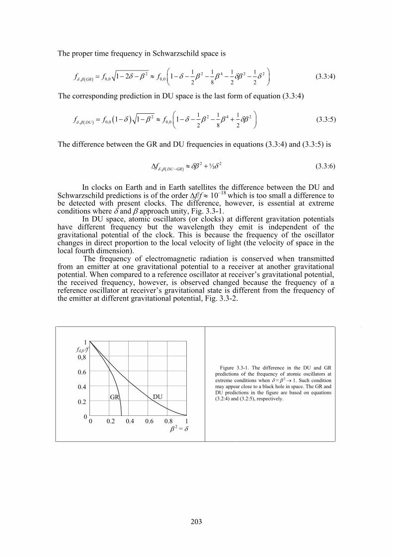
The proper time frequency in Schwarzschild space is
( )2 2 4 2
0,0 0,0,1 1 1 1
2 8 2 21 2 1GRf f fδ β
2δ β δ β β δβ⎛= − − ≈ − − − − −⎜⎝ ⎠
δ ⎞⎟ (3.3:4)
The corresponding prediction in DU space is the last form of equation (3.3:4)
( ) ( ) 2 2 40,0 0,0,
1 1 1
2 8 21 1 1DUf f fδ β
2δ β δ β β⎛= − − ≈ − − − +⎜⎝ ⎠
δβ ⎞⎟
2
(3.3:5)
The difference between the GR and DU frequencies in equations (3.3:4) and (3.3:5) is
( )2
, ½DU GRfδ β δβ−Δ ≈ + δ (3.3:6)
In clocks on Earth and in Earth satellites the difference between the DU and Schwarzschild predictions is of the order Δf/f ≈ 10–18
which is too small a difference to be detected with present clocks. The difference, however, is essential at extreme conditions where δ and β approach unity, Fig. 3.3-1.
In DU space, atomic oscillators (or clocks) at different gravitation potentials have different frequency but the wavelength they emit is independent of the gravitational potential of the clock. This is because the frequency of the oscillator changes in direct proportion to the local velocity of light (the velocity of space in the local fourth dimension).
The frequency of electromagnetic radiation is conserved when transmitted from an emitter at one gravitational potential to a receiver at another gravitational potential. When compared to a reference oscillator at receiver’s gravitational potential, the received frequency, however, is observed changed because the frequency of a reference oscillator at receiver’s gravitational state is different from the frequency of the emitter at different gravitational potential, Fig. 3.3-2.
Figure 3.3-1. The difference in the DU and GR predictions of the frequency of atomic oscillators at extreme conditions when δ = β 2 → 1. Such condition may appear close to a black hole in space. The GR and DU predictions in the figure are based on equations (3.2:4) and (3.2:5), respectively.
0
0.2
0.4
0.6
0,8
1
0 0.2 0.4 0.6 0.8
GR DU
β 2 = δ1
fδ,β /f
203
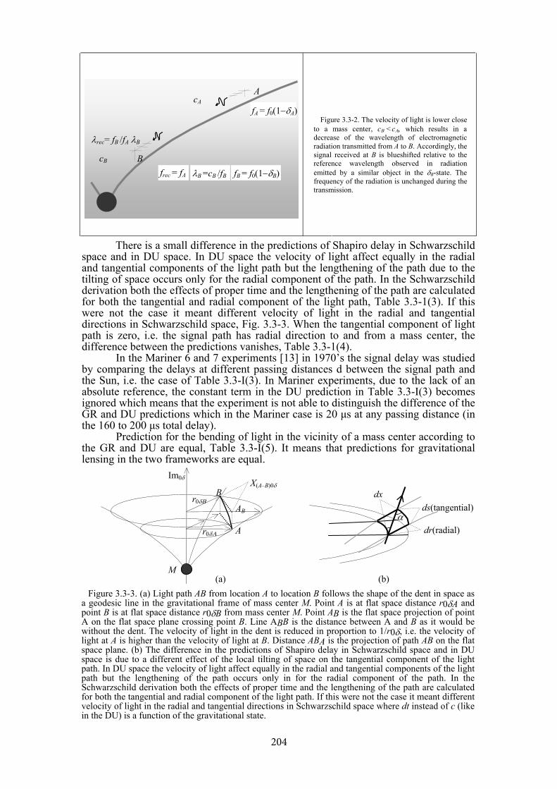
Figure 3.3-2. The velocity of light is lower close to a mass center, cΒ < cΑ, which results in a decrease of the wavelength of electromagnetic radiation transmitted from A to B. Accordingly, the signal received at B is blueshifted relative to the reference wavelength observed in radiation emitted by a similar object in the δB-state. The frequency of the radiation is unchanged during the transmission.
There is a small difference in the predictions of Shapiro delay in Schwarzschild space and in DU space. In DU space the velocity of light affect equally in the radial and tangential components of the light path but the lengthening of the path due to the tilting of space occurs only for the radial component of the path. In the Schwarzschild derivation both the effects of proper time and the lengthening of the path are calculated for both the tangential and radial component of the light path, Table 3.3-1(3). If this were not the case it meant different velocity of light in the radial and tangential directions in Schwarzschild space, Fig. 3.3-3. When the tangential component of light path is zero, i.e. the signal path has radial direction to and from a mass center, the difference between the predictions vanishes, Table 3.3-1(4).
In the Mariner 6 and 7 experiments [13] in 1970’s the signal delay was studied by comparing the delays at different passing distances d between the signal path and the Sun, i.e. the case of Table 3.3-I(3). In Mariner experiments, due to the lack of an absolute reference, the constant term in the DU prediction in Table 3.3-I(3) becomes ignored which means that the experiment is not able to distinguish the difference of the GR and DU predictions which in the Mariner case is 20 μs at any passing distance (in the 160 to 200 μs total delay).
Prediction for the bending of light in the vicinity of a mass center according to the GR and DU are equal, Table 3.3-I(5). It means that predictions for gravitational lensing in the two frameworks are equal.
Figure 3.3-3. (a) Light path AB from location A to location B follows the shape of the dent in space as a geodesic line in the gravitational frame of mass center M. Point A is at flat space distance r0δA and point B is at flat space distance r0δB from mass center M. Point AB is the flat space projection of point A on the flat space plane crossing point B. Line ABB is the distance between A and B as it would be without the dent. The velocity of light in the dent is reduced in proportion to 1/r0δ, i.e. the velocity of light at A is higher than the velocity of light at B. Distance ABA is the projection of path AB on the flat space plane. (b) The difference in the predictions of Shapiro delay in Schwarzschild space and in DU space is due to a different effect of the local tilting of space on the tangential component of the light path. In DU space the velocity of light affect equally in the radial and tangential components of the light path but the lengthening of the path occurs only in for the radial component of the path. In the Schwarzschild derivation both the effects of proper time and the lengthening of the path are calculated for both the tangential and radial component of the light path. If this were not the case it meant different velocity of light in the radial and tangential directions in Schwarzschild space where dt instead of c (like in the DU) is a function of the gravitational state.
M
Im0δ
r0δΒ
A
B
r0δΑ
AB
X(A–B)0δ
dx
(b)
α
dr(radial)
(a)
ds(tangential)
A
λrec= fB /fA λB
cA
frec = fA fB = f0(1−δB) λB =cB /fB
cB
fA = f0(1−δA)
B
204
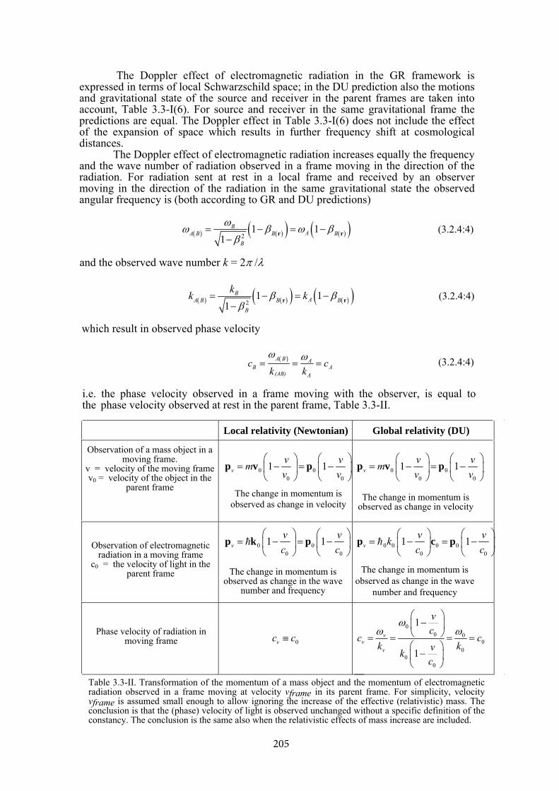
The Doppler effect of electromagnetic radiation in the GR framework is expressed in terms of local Schwarzschild space; in the DU prediction also the motions and gravitational state of the source and receiver in the parent frames are taken into account, Table 3.3-I(6). For source and receiver in the same gravitational frame the predictions are equal. The Doppler effect in Table 3.3-I(6) does not include the effect of the expansion of space which results in further frequency shift at cosmological distances.
The Doppler effect of electromagnetic radiation increases equally the frequency and the wave number of radiation observed in a frame moving in the direction of the radiation. For radiation sent at rest in a local frame and received by an observer moving in the direction of the radiation in the same gravitational state the observed angular frequency is (both according to GR and DU predictions)
( ) ( )( ) ( )( )21 1
1B
AA B B BB
ωω β ωβ
= − = −−
r β r (3.2.4:4)
and the observed wave number k = 2π /λ
( ) ( )( ) ( )( )21 1
1B
AA B B BB
kk ββ
= − = −−
r k β r (3.2.4:4)
which result in observed phase velocity
( )A B AB A
A
ck k
ω ω= = = c (3.2.4:4)
(AB)
i.e. the phase velocity observed in a frame moving with the observer, is equal to the phase velocity observed at rest in the parent frame, Table 3.3-II.
Local relativity (Newtonian) Global relativity (DU)
Observation of a mass object in a moving frame.
v = velocity of the moving frame v0 = velocity of the object in the
parent frame
000 0
1 1vv
v v⎜ −⎛ ⎞v
= p⎛ ⎞
⎟ −⎜ ⎟⎠⎝ ⎝ ⎠
p m= v
The change in momentum is observed as change in velocity
0 00 0
1 1vvm
v v⎛
−⎞v
= p⎛ ⎞
= ⎜ ⎟ −⎜ ⎟⎠⎝ ⎠⎝
vp
The change in momentum is observed as change in velocity
Observation of electromagnetic radiation in a moving frame
c0 = the velocity of light in the parent frame
0 000
1 1c c
⎞vp k= ⎜ −
⎛ v ⎞= p
⎛−
v
⎝ ⎠ ⎝ ⎠⎟ ⎟⎜
The change in momentum is observed as change in the wave
number and frequency
00 0 00 0
k ⎜1 ⎟ =c p ⎜ ⎟− 1 vcc
⎞v ⎛ ⎞v =p
⎝ ⎠ ⎠⎝
⎛−
The change in momentum isobserved as change in the wave
number and frequency
Phase velocity of radiation in moving frame 0v ≡c c
00 0
00
00
1
1v
v
vc
cckk
k
ω ⎝ ⎠ =ω
⎛ ⎞ω −⎜ ⎟
= v =⎞⎛
−cv
⎟⎜⎠⎝
=
Table 3.3-II. Transformation of the momentum of a mass object and the momentum of electromagnetic radiation observed in a frame moving at velocity vframe in its parent frame. For simplicity, velocity vframe is assumed small enough to allow ignoring the increase of the effective (relativistic) mass. The conclusion is that the (phase) velocity of light is observed unchanged without a specific definition of the constancy. The conclusion is the same also when the relativistic effects of mass increase are included.
205
The late 1800’s great confusion of the conservation of the observed velocity of light in moving frames obtains a trivial solution once we study the moving frames as momentum frames instead of velocity frames:
The constancy of the observed (phase) velocity of light in moving frames is a consequence of the change of momentum via the Doppler shift of frequency (and mass equivalence) instead of change in the velocity as we observe the change of the momentum of mass objects.
Studying of the Michelson – Morley interferometer as a momentum frame moving in its parent frames guarantees a zero result.
III. D. Cosmological appearance of space derived from general relativity and theDU
At the cosmological scale, like the DU space, GR space is assumed to be isotropic and homogeneous; i.e., it looks the same from any point in space [14]. As a major difference to the Friedman-Lemaître-Robertson-Walker (FLRW) cosmology or ΛCDM cosmology (Lambda Cold Dark Matter cosmology), local gravitational systems in DU space are subject to expansion in direct proportion to the expansion of the 4-radius R0. Accordingly, e.g., the radii of galaxies are not observed as standard rods but as expanding objects which makes the sizes of galaxies appear in Euclidean geometry to the observer.
As shown by an analysis of the Bohr radius, material objects built of atoms and molecules are not subject to expansion with space. Like the Bohr radius, the characteristic emission wavelengths of atomic objects are unchanged in the course of the expansion of space. When propagating in space, the wavelength of electromagnetic radiation is increased in direct proportion to the expansion. Accordingly, when detected after propagation in space, characteristic radiation is observed redshifted relative to the wavelength emitted by the corresponding transition in situ at the time of observation.
Major difference between FLRW space and DU space comes from the general cosmological appearance and the picture of reality. The expression of energy and the evolution of DU space is a continuous process from infinity in the past to infinity in the future under unchanged laws of nature. In the DU mass is not a form of energy but the substance for the expression of energy via excitation of motion against release of potential energy. Any local expression of energy in DU space is linked to the rest of space. Anti-energy for the rest energy of a mass object in space is the gravitational energy due to the rest of mass in space as indicated by zero-energy balance of the rest energy and the global gravitational energy. Relativity in DU space means relativity of local to the whole.
Table 3.4-I summarizes some general features of the FLRW space and the DU space. The difference between the local approach of the GR based FLRW space and the global approach of the DU space is well demonstrated by the scope of expansion: For conserving the gravitational energy in local systems expansion in FLRW space is assumed to occur between galaxies or galaxy groups only. In the DU local gravitation is a share of the total gravitational energy; dilution of the total gravitational energy in the expansion dilutes equally the gravitational energy of local systems, which is seen as the expansion of gravitationally bound local systems with the expansion of whole space.
Another important difference between the FLRW and DU models is the conservation of the energy of radiation propagating in space. In both models the wavelength of radiation is supposed to increase in direct proportion to the expansion of space. In the FLRW interpretation of the effect of redshift on the power density of radiation is based on the fundamental work of Hubble, Tolman, Humason, deSitter, and Robertson, in the 1930’s [15–20]. After an active debate the conclusion was that the dilution of the power density of redshifted radiation comes from two factors: The reduced rate of quanta received, and the dilution of the energy of a quantum due to the reduced frequency as suggested by a direct interpretation of the Planck’s equation. Combining these two effects the dilution of power density due to the expansion of FLRW space obtains the form
206
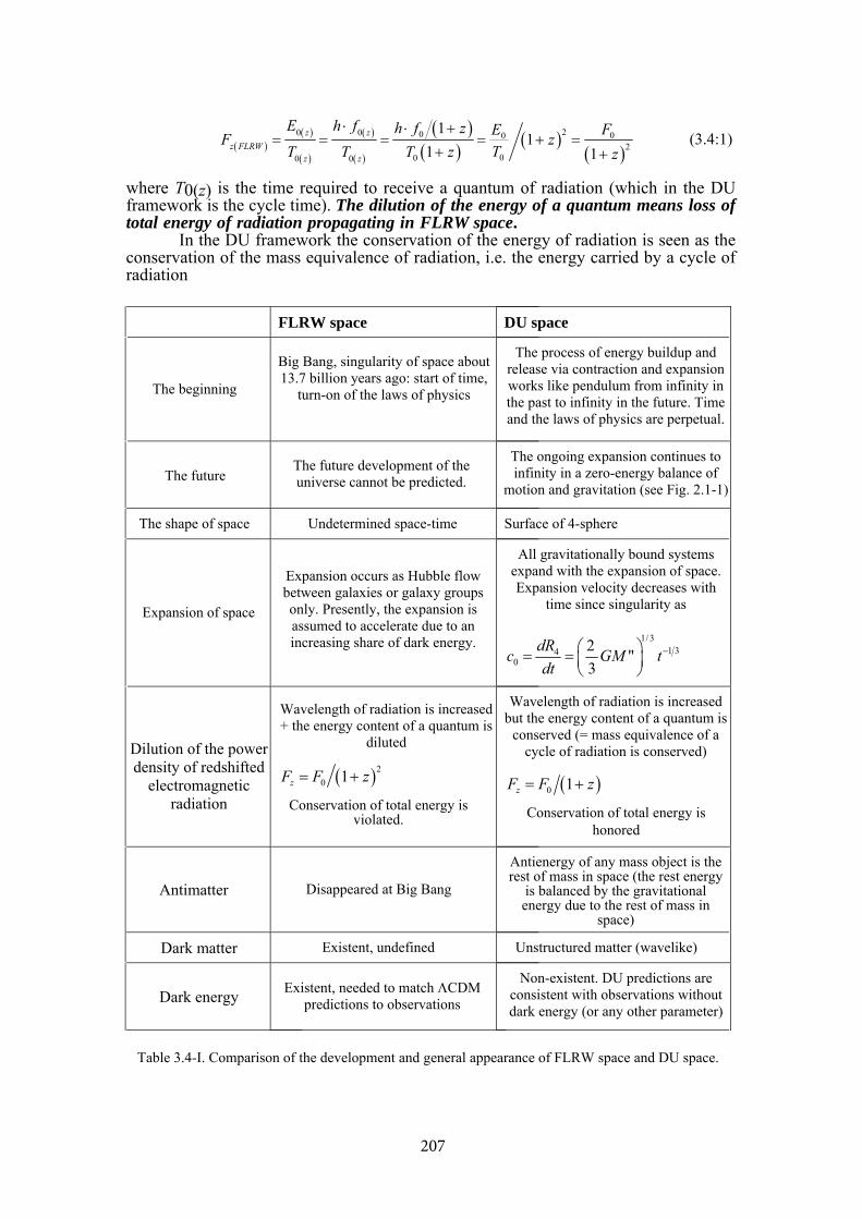
z FLRW( )z( )
z( ) ( + z )20 0 0 00
20000
11
1 1( )z
( )z
E ⋅h f ⋅h f FFTTT T ( + )z
( z )+== =
E= + =( )z (3.4:1)
where T0(z) is the time required to receive a quantum of radiation (which in the DU framework is the cycle time). The dilution of the energy of a quantum means loss of total energy of radiation propagating in FLRW space.
In the DU framework the conservation of the energy of radiation is seen as the conservation of the mass equivalence of radiation, i.e. the energy carried by a cycle of radiation
FLRW space DU space
The beginning
Big Bang, singularity of space about 13.7 billion years ago: start of time,
turn-on of the laws of physics
The process of energy buildup and release via contraction and expansion works like pendulum from infinity in the past to infinity in the future. Time and the laws of physics are perpetual.
The future The future development of the universe cannot be predicted.
The ongoing expansion continues to infinity in a zero-energy balance of
motion and gravitation (see Fig. 2.1-1)
The shape of space Undetermined space-time Surface of 4-sphere
Expansion of space
Expansion occurs as Hubble flow between galaxies or galaxy groups only. Presently, the expansion is assumed to accelerate due to an increasing share of dark energy.
All gravitationally bound systems expand with the expansion of space.Expansion velocity decreases with
time since singularity as
1/31 34
02 "3
=dRc GMdt
−⎜= ⎛ ⎞
⎟⎠⎝
t
Dilution of the power density of redshifted
electromagnetic radiation
Wavelength of radiation is increased + the energy content of a quantum is
diluted
( z 2)0 1zF F= +
Conservation of total energy is violated.
Wavelength of radiation is increased but the energy content of a quantum is
conserved (= mass equivalence of a cycle of radiation is conserved)
( z)0 1zF = F +
Conservation of total energy is honored
Antimatter Disappeared at Big Bang
Antienergy of any mass object is the rest of mass in space (the rest energy
is balanced by the gravitational energy due to the rest of mass in
space)
Dark matter Existent, undefined Unstructured matter (wavelike)
Dark energy Existent, needed to match ΛCDM predictions to observations
Non-existent. DU predictions are consistent with observations without dark energy (or any other parameter)
Table 3.4-I. Comparison of the development and general appearance of FLRW space and DU space.
207
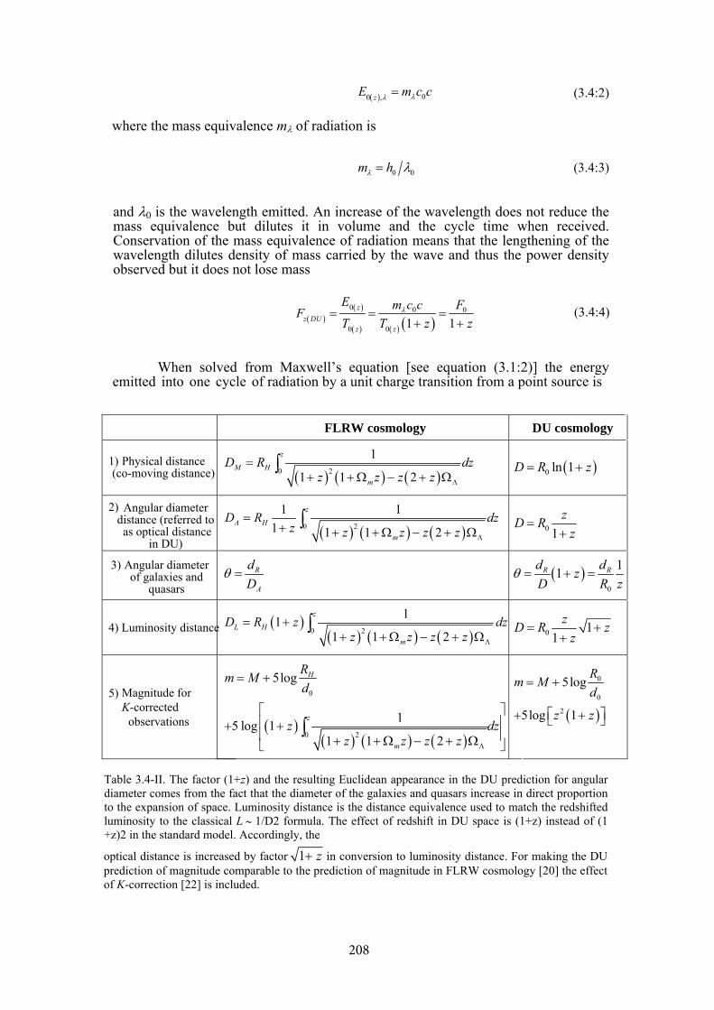
( ) 00 ,zE m c cλλ = (3.4:2)
where the mass equivalence mλ of radiation is
0 0m hλ λ= (3.4:3)
and λ0 is the wavelength emitted. An increase of the wavelength does not reduce the mass equivalence but dilutes it in volume and the cycle time when received. Conservation of the mass equivalence of radiation means that the lengthening of the wavelength dilutes density of mass carried by the wave and thus the power density observed but it does not lose mass
( )( )
( ) ( ) ( )0 0
0 0 1 1z
z DUz z
E m c c FFT T z
λ= = =+ +
0
z(3.4:4)
When solved from Maxwell’s equation [see equation (3.1:2)] the energy emitted into one cycle of radiation by a unit charge transition from a point source is
FLRW cosmology DU cosmology
1) Physical distance(co-moving distance) ( + z ) (20
1
11
z
HM
m
D = R dz)z − z (2 )z Λ+ Ω + Ω
∫ )0D R ln (1= + z
2) Angular diameterdistance (referred toas optical distance
in DU) ( + z ) (0 2
111 11
z
HA
m
dD = Rz )z − z (2 )z Λ
+ + Ω + Ω∫ z
0 1=D R z
z+
3) Angular diameterof galaxies and
quasars
R
A
dD
θ = z)0
11(R Rd dRD
θ = + =z
4) Luminosity distance ( + ∫z0
)( + z ) (2
1111
z
HL
m
D = R)z − z (2 )z Λ+ Ω + Ω
dz0 11
D R=z z
z+
+
5) Magnitude forK-corrected
observations +⎢ 1( z )( + z ) (
0
20
5log
15 log1 1
H
z
m
R=m M
d
dz)z − z (2 )z Λ
+
⎡ ⎤⎥+⎥⎢ + Ω Ω+ ⎦⎣
∫+ z )5log ⎣⎡z 1(
0
0
2
5log R=m M
d+
+ ⎤⎦
Table 3.4-II. The factor (1+z) and the resulting Euclidean appearance in the DU prediction for angular diameter comes from the fact that the diameter of the galaxies and quasars increase in direct proportion to the expansion of space. Luminosity distance is the distance equivalence used to match the redshifted luminosity to the classical L 1/D2 formula. The effect of redshift in DU space is (1+z) instead of (1+z)2 in the standard model. Accordingly, the
∼
optical distance is increased by factor 1+ z in conversion to luminosity distance. For making the DU prediction of magnitude comparable to the prediction of magnitude in FLRW cosmology [20] the effect of K-correction [22] is included.
208
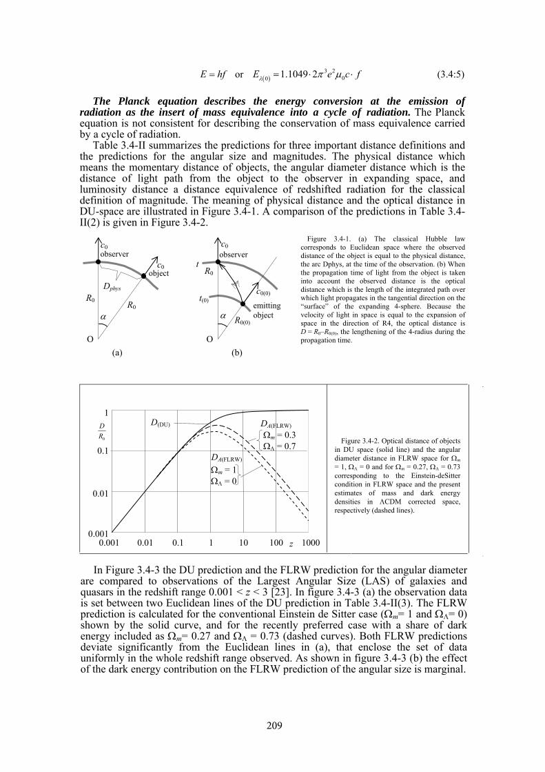
E hf= or ( )3 2
00 1.1049 2E e c fλ π μ= ⋅ ⋅ (3.4:5)
The Planck equation describes the energy conversion at the emission of radiation as the insert of mass equivalence into a cycle of radiation. The Planck equation is not consistent for describing the conservation of mass equivalence carried by a cycle of radiation.
Table 3.4-II summarizes the predictions for three important distance definitions and the predictions for the angular size and magnitudes. The physical distance which means the momentary distance of objects, the angular diameter distance which is the distance of light path from the object to the observer in expanding space, and luminosity distance a distance equivalence of redshifted radiation for the classical definition of magnitude. The meaning of physical distance and the optical distance in DU-space are illustrated in Figure 3.4-1. A comparison of the predictions in Table 3.4-II(2) is given in Figure 3.4-2.
Figure 3.4-1. (a) The classical Hubble law corresponds to Euclidean space where the observed distance of the object is equal to the physical distance, the arc Dphys, at the time of the observation. (b) When the propagation time of light from the object is taken into account the observed distance is the optical distance which is the length of the integrated path over which light propagates in the tangential direction on the “surface” of the expanding 4-sphere. Because the velocity of light in space is equal to the expansion of space in the direction of R4, the optical distance is D = R0–R0(0), the lengthening of the 4-radius during the propagation time.
(b)
c0 c0
R0(0)
observer
emitting object
R0 R0
observer
objectDphys
α
O
c0(0)
R0 t
t(0)
α
O
c0
(a)
Figure 3.4-2. Optical distance of objects in DU space (solid line) and the angular diameter distance in FLRW space for Ωm = 1, ΩΛ = 0 and for Ωm = 0.27, ΩΛ = 0.73 corresponding to the Einstein-deSitter condition in FLRW space and the present estimates of mass and dark energy densities in ΛCDM corrected space, respectively (dashed lines).
0.001
0.01
1000
Ωm = 0.3 ΩΛ = 0.7
D(DU)
0.1
1
0.01 0.1 1 10 0.001 100 z
Ωm = 1ΩΛ = 0
DA(FLRW)
DA(FLRW) 0
DR
In Figure 3.4-3 the DU prediction and the FLRW prediction for the angular diameter are compared to observations of the Largest Angular Size (LAS) of galaxies and quasars in the redshift range 0.001 < z < 3 [23]. In figure 3.4-3 (a) the observation data is set between two Euclidean lines of the DU prediction in Table 3.4-II(3). The FLRW prediction is calculated for the conventional Einstein de Sitter case (Ωm= 1 and ΩΛ= 0) shown by the solid curve, and for the recently preferred case with a share of dark energy included as Ωm= 0.27 and ΩΛ = 0.73 (dashed curves). Both FLRW predictions deviate significantly from the Euclidean lines in (a), that enclose the set of data uniformly in the whole redshift range observed. As shown in figure 3.4-3 (b) the effect of the dark energy contribution on the FLRW prediction of the angular size is marginal.
209
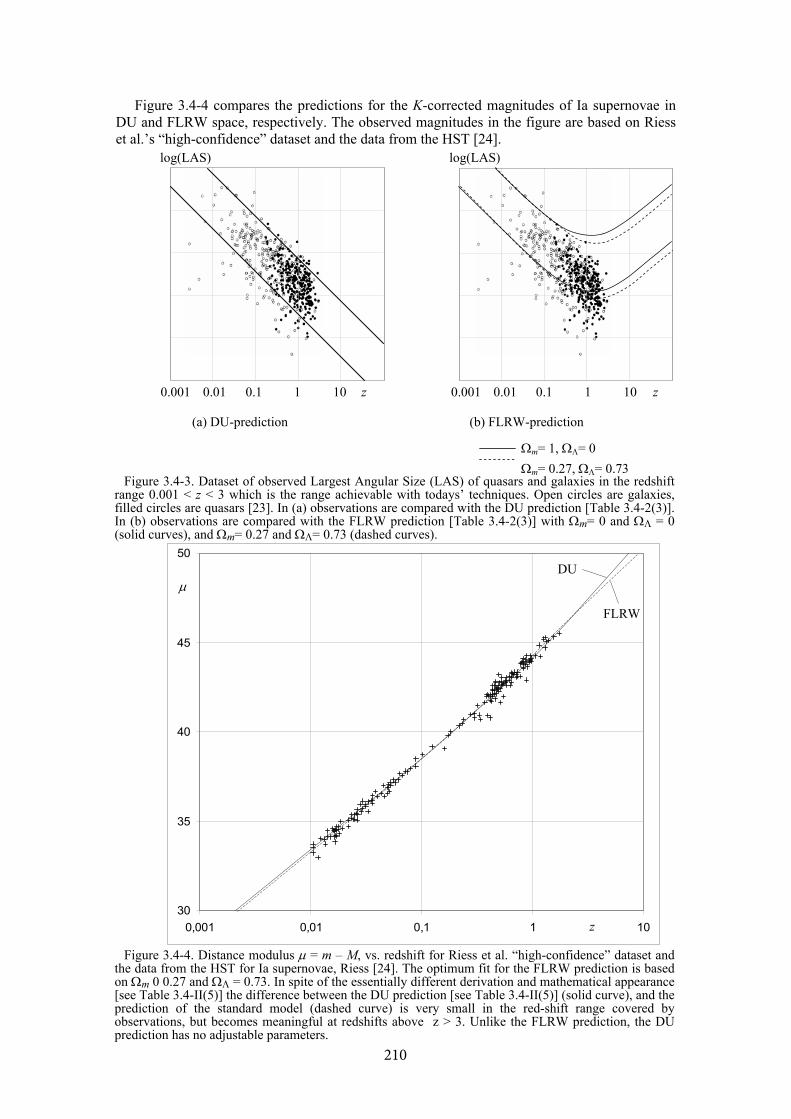
Figure 3.4-4 compares the predictions for the K-corrected magnitudes of Ia supernovae in DU and FLRW space, respectively. The observed magnitudes in the figure are based on Riess et al.’s “high-confidence” dataset and the data from the HST [24].
Figure 3.4-3. Dataset of observed Largest Angular Size (LAS) of quasars and galaxies in the redshift range 0.001 < z < 3 which is the range achievable with todays’ techniques. Open circles are galaxies, filled circles are quasars [23]. In (a) observations are compared with the DU prediction [Table 3.4-2(3)]. In (b) observations are compared with the FLRW prediction [Table 3.4-2(3)] with Ωm= 0 and ΩΛ = 0 (solid curves), and Ωm= 0.27 and ΩΛ= 0.73 (dashed curves).
(a) DU-prediction (b) FLRW-prediction
0.001 0.01 0.1 1 10 z
log(LAS)
Ωm= 1, ΩΛ= 0 Ωm= 0.27, ΩΛ= 0.73
0.001 0.01 0.1 1 10 z
log(LAS)
Figure 3.4-4. Distance modulus μ = m – M, vs. redshift for Riess et al. “high-confidence” dataset and the data from the HST for Ia supernovae, Riess [24]. The optimum fit for the FLRW prediction is based on Ωm 0 0.27 and ΩΛ = 0.73. In spite of the essentially different derivation and mathematical appearance [see Table 3.4-II(5)] the difference between the DU prediction [see Table 3.4-II(5)] (solid curve), and the prediction of the standard model (dashed curve) is very small in the red-shift range covered by observations, but becomes meaningful at redshifts above z > 3. Unlike the FLRW prediction, the DU prediction has no adjustable parameters.
30
35
40
45
50
0,001 0,01 0,1 1 10
FLRW
DU μ
z
210
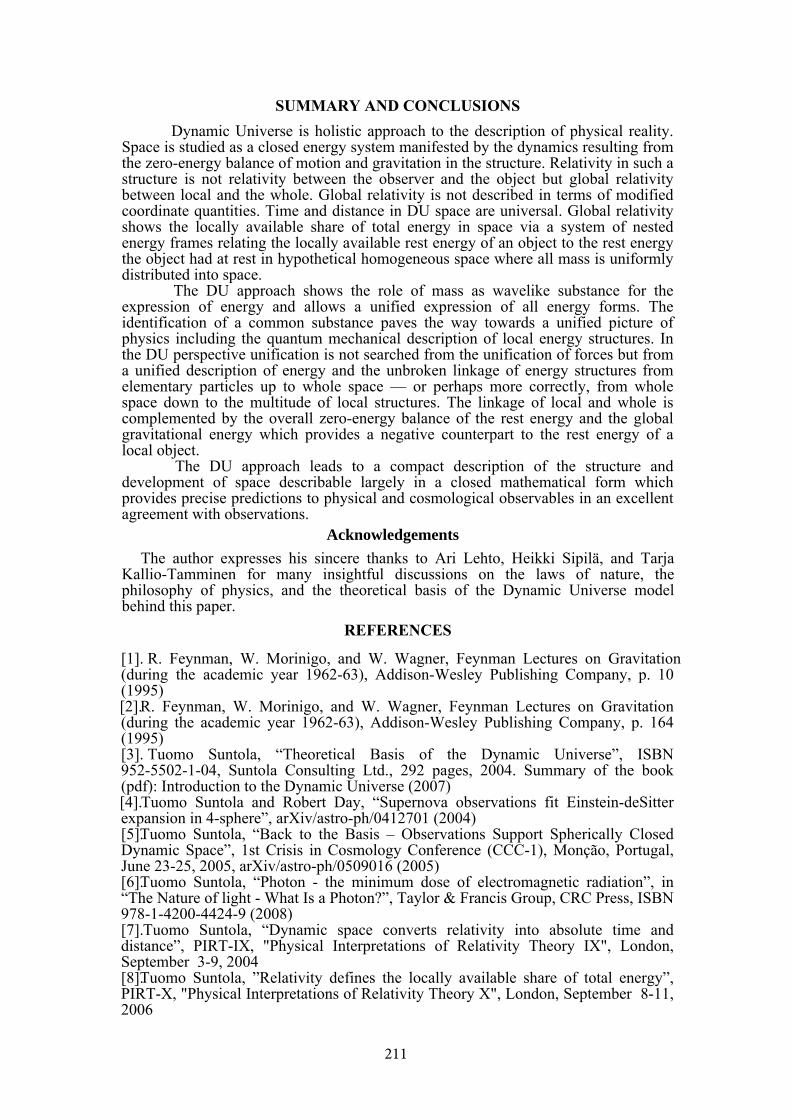
SUMMARY AND CONCLUSIONS Dynamic Universe is holistic approach to the description of physical reality.
Space is studied as a closed energy system manifested by the dynamics resulting from the zero-energy balance of motion and gravitation in the structure. Relativity in such a structure is not relativity between the observer and the object but global relativity between local and the whole. Global relativity is not described in terms of modified coordinate quantities. Time and distance in DU space are universal. Global relativity shows the locally available share of total energy in space via a system of nested energy frames relating the locally available rest energy of an object to the rest energy the object had at rest in hypothetical homogeneous space where all mass is uniformly distributed into space.
The DU approach shows the role of mass as wavelike substance for the expression of energy and allows a unified expression of all energy forms. The identification of a common substance paves the way towards a unified picture of physics including the quantum mechanical description of local energy structures. In the DU perspective unification is not searched from the unification of forces but from a unified description of energy and the unbroken linkage of energy structures from elementary particles up to whole space — or perhaps more correctly, from whole space down to the multitude of local structures. The linkage of local and whole is complemented by the overall zero-energy balance of the rest energy and the global gravitational energy which provides a negative counterpart to the rest energy of a local object.
The DU approach leads to a compact description of the structure and development of space describable largely in a closed mathematical form which provides precise predictions to physical and cosmological observables in an excellent agreement with observations.
Acknowledgements The author expresses his sincere thanks to Ari Lehto, Heikki Sipilä, and Tarja
Kallio-Tamminen for many insightful discussions on the laws of nature, the philosophy of physics, and the theoretical basis of the Dynamic Universe model behind this paper.
REFERENCES
[1]. R. Feynman, W. Morinigo, and W. Wagner, Feynman Lectures on Gravitation(during the academic year 1962-63), Addison-Wesley Publishing Company, p. 10 (1995)[2].R. Feynman, W. Morinigo, and W. Wagner, Feynman Lectures on Gravitation(during the academic year 1962-63), Addison-Wesley Publishing Company, p. 164 (1995)[3]. Tuomo Suntola, “Theoretical Basis of the Dynamic Universe”, ISBN952-5502-1-04, Suntola Consulting Ltd., 292 pages, 2004. Summary of the book (pdf): Introduction to the Dynamic Universe (2007)[4].Tuomo Suntola and Robert Day, “Supernova observations fit Einstein-deSitterexpansion in 4-sphere”, arXiv/astro-ph/0412701 (2004)[5].Tuomo Suntola, “Back to the Basis – Observations Support Spherically ClosedDynamic Space”, 1st Crisis in Cosmology Conference (CCC-1), Monção, Portugal, June 23-25, 2005, arXiv/astro-ph/0509016 (2005)[6].Tuomo Suntola, “Photon - the minimum dose of electromagnetic radiation”, in“The Nature of light - What Is a Photon?”, Taylor & Francis Group, CRC Press, ISBN 978-1-4200-4424-9 (2008)[7].Tuomo Suntola, “Dynamic space converts relativity into absolute time anddistance”, PIRT-IX, "Physical Interpretations of Relativity Theory IX", London, September 3-9, 2004[8].Tuomo Suntola, ”Relativity defines the locally available share of total energy”,PIRT-X, "Physical Interpretations of Relativity Theory X", London, September 8-11, 2006
211
[9].Tuomo Suntola, “Zero-energy space cancels the need for dark energy",Proceedings of PIRT Budapest 7-9.9.2007[10]. G. W. Leibniz, Matematischer Naturwissenschaflicher und TechnischerBriefwechsel, Sechster band (1694)[11].J. Foster, J.D. Nightingale, A Short Course in General Relativity, 2nd edition,Springer-Verlag, ISBN 0-387-94295-5 (2001)[12]. R. Genzel, et al., Nature 425, 934 (2003)[13].The Mariner Mars missions, NASA http://nssdc.gsfc.nasa.gov/planetary/mars/mariner.html[14].Misner C. W., Thorne K. S. & Wheeler J. A., “Gravitation”, W. H. Freeman &Co., New York (1973)[15]. Tolman, PNAS 16, 511-520 (1930)[16]. E. Hubble, M. L. Humason, Astrophys.J., 74, 43 (1931)[17].W. de Sitter, B.A..N., 7, No 261, 205 (1934)[18]. E. Hubble and R. C. Tolman, ApJ, 82, 302 (1935)[19]. E. Hubble, Astrophys. J., 84, 517 (1936)[20]. Robertson, H.P., Zs.f.Ap., 15, 69 (1938)[21]. S. M. Carroll, W. H. Press, and E. L. Turner, ARA&A, 30, 499 (1992)[22]. Kim, A., Goobar, A., & Perlmutter, S. 1996, PASP, 190–201[23]. K. Nilsson et al., Astrophys. J., 413, 453, 1993[24]. A. G. Riess, et al., Astrophys. J., 607, 665 (2004)
212
213
DYNAMIC UNIVERSE AND THE CONCEPTION OF REALITY
Tarja Kallio-Tamminen
From ancient times both philosophy and science have aimed to understand the nature of reality. The conception of reality has evolved by undergoing deep changes whenever natural science has found new invariances and interconnections in nature, which enabled the handling of a wider variety of phenomena under one and same mathematical formalism. The historical process has characteristically focused on the examination of the interrelations between substance, motion, space and time but the final hierarchy of these perennial concepts has not been decided yet.
Extended debate on natural philosophy started in antiquity with the general outcome that reality was comparable to an organism. The outlook was overturned at the times of Kepler, Galilei and Newton when rapid development took place in natural research. The world was seen as a huge clockwork until the beginning of 20th century when quantum physics and relativity theory were born. Modern physics challenged the previous metaphysical presuppositions and obscured the common world view. Time became connected to space and the idea of reducing everything to solid material particles was implausible because of their non-local properties.
There is a demand for a new conception of reality but very few vote for a profound paradigm change to take place. The trials to unify quantum mechanics and relativity theory lead to complicated and highly abstract mathematics which is impossible to conceive in common terms. Tuomo Suntola’s Dynamic universe –theory, however, is a good candidate for a new theoretical framework. Suntola gives a plausible model of reality whose scope and profound simplicity surpasses the capacity of present theories. Moreover the theory is pregnant with fundamental metaphysical implications.
In Suntola’s theory the totality of mass is a fundamental invariant which links everything together. Through energy excitation mass determines the motion, size and time development of space, and regulates all local structures in space. The new arrangement of the basic concepts allows a revealing perspective to history. Why Newton had to equal inertial mass and gravitational mass and what Einstein’s famous formula of equality between mass and energy actually means? This paper focuses on the relation between mass and energy in the DU theory and clarifies how it provides a natural basis for the human conception of irreversible absolute time, which is excluded in present theory structures.
Keywords: quantum mechanics, relativity theory, Tuomo Suntola’s Dynamic universe, dynamic universe theory.
PACS number: 03.65.-w/03.30.+p
214
RELATIVITY, THE SURGE AND A THIRD SCIENTIFIC REVOLUTION
James E. Beichler, Ph.D.
P.O. Box 624, Belpre, Ohio 45714, USA [email protected]
Quantum theory emerged the victor of the last Scientific Revolution even though relativity theory had a more progressive view of reality to offer science. As a result, the physical aspects and properties of the gravitational field were never fully explored or exploited and science went through several decades of denial concerning the relevance of general relativity and its physical implications. The only small victory that relativity theory could claim before the 1960s was in cosmology with the expanding universe. The victory was small because the expanding universe was far from the everyday needs of a science more concerned with the atom and the nucleus. Under these circumstances, the theory of relativity had no practical applications in the everyday real world, so its theoretical implications were largely ignored. However, the 1970s brought something of a resurgence of good fortunes and everyday relevance for relativity theory and quantum theorists finally accepted the possibility that unification was the primary goal of physics, albeit a unification based upon the quantum concept of discrete particles rather than the Einsteinian concept of field continuity: According to quantum field theory, the gravity field could be reduced to an exchange of gravitons. But what at first seemed a resurgence of general relativity under the quantum paradigm in the 1970s has slowly evolved into a surge of physical relevance resulting in the emergence of general relativity as a dominating field of research in physics. And the story does not end there. The recent discoveries of Dark Matter and Dark Energy are about to push physics and relativity theory into a Third Scientific Revolution in which a unification with the quantum will be made on relativity’s terms. The quantum will not emerge out of the mathematics as a constraint on the continuous field as Einstein had hoped, but it will emerge as a field constant that limits the continuous field as described by general relativity.
Keywords: Second Scientific Revolution, Third Scientific Revolution, Mach, positivism, Mind, Matter, consciousness, motion of mater, crises, quantum relativity, curvature, higher dimensions, Einstein, history, paradigm, Standard Model, cosmology, surge, Dark Matter, Dark Energy.
PACS number: 04.62.+v
I. INTRODUCTION A scientific revolution occurred between the years 1900 and 1927. No one
would dare disagree with this fact. But that revolution was never completed, a fact with which very few, if any, would agree, but a fact all the same. This Second Scientific Revolution was an unfinished symphony of science. In fact, this incompleteness led to a well-known series of philosophical debates after the 1920s, but they never resulted in any direct physical challenges to the quantum theory. Any problems that were foreseen with quantum theory were problems of interpretation rather than problems of a physical nature. That fact has been the strength of the quantum philosophy as well as its major flaw. The very fact that the revolution started in 1900 when Max Planck published his seminal paper on blackbody radiation and ended in 1927 with the Solvay Conference
215
settling the primary issues and questions regarding quantum mechanics readily demonstrates that the revolution has been completely dominated by the quantum theory. Yet two different crises seemed to have caused the revolution, the blackbody radiation paradox and the failure to detect the luminiferous aether, while only the blackbody problem led to quantum theory. The accepted solution to the aether problem came in the form of relativity theory.
The story of relativity theory and the important dates of 1905, 1912 and 1915 in the development of relativity seem to have been overwhelmed by the story of the quantum, as if they were not as important unless they were somehow related to the quantum story, even though relativity forms the second leg upon which the revolution stood. To further complicate this mess, Newtonian theory was at the height of its success at the outset of the revolution, which implies that a paradox of history exists, while relativity theory is generally grouped with Newtonian theory as a form of ‘classical’ physics, i.e., old physics before the second revolution that is philosophically contaminated. These historical inequities need to be identified and understood before science can come to terms with the next scientific revolution because the seeds of the next revolution can be found in the failures and misconceptions that arose during the Second Scientific Revolution. To understand the past revolution more completely is to understand how science has evolved since the past revolution and where the future is taking science.
First of all, the standard view that scientific revolutions (Kuhnian view) result from crises does not offer all that accurate and complete a picture of the historical events. It does not take into account the fact that the crises themselves resulted from the successes of previous theories and the subsequent attempts to expand the previous paradigms. Those successes represent the constant ongoing evolution of science, which is just as important as the revolutions in science as well as intimately related to the emergence of revolutions. Newtonianism was completely progressive and it never failed, not even during the revolution that supposedly overthrew it. It had come so far that its successes forced science to consider phenomena and natural processes that were previously off-limits to science, i.e., the ultimate nature of life, mind, consciousness and even matter itself. In fact, Newtonian physics had solved both of the crises before the revolution. Lorentz-Fitzgerald contraction had already been offered as the solution to the aether problem before it was derived by Albert Einstein in 1905 from first principles, without resorting to the hypothetical aether. That is why it is still called Lorentz-Fitzgerald contraction today, in spite of its more modern relativistic interpretation. Furthermore, Planck considered his solution to the blackbody problem a completely statistical and thermodynamical solution, well within the context of Newtonian science, rather than a revolutionary new solution. Quantum theory really began in 1905 with Einstein’s solution to the photoelectric effect.
Secondly, the purely philosophical issues leading to the Second Scientific Revolution have been completely subverted, ignored and lost to history by the shift of emphasis to a philosophical rivalry between determinism (classical and Newtonian) and indeterminism (quantum mechanical), which in turn was heavily influenced by the positivism adopted by scientists during the revolution. From a far broader historical and philosophical perspective, the real (unknown and unsuspected) revolution resulted from a shift in the boundaries between the realms of Mind (spirit) and Matter (the mechanical universe) that had originated with René Descartes during the Scientific Revolution of the seventeenth century before they were institutionalized by Isaac Newton in the Principia. Physics has always been about matter and the ‘motion of matter’, as it still is, but the fundamental nature of matter has never been discovered, nor has the
216
fundamental nature of the mind that perceives and conceives matter. Yet these facts have gone completely unmentioned and unexplored by scientists, scholars and academics alike.
Given this broader philosophical perspective, relativity theory actually forms a more realistic basis for the revolution than the quantum because relativity sought to completely change the scientific concept of matter by equating matter to space-time curvature. But that change never occurred, at least not yet. Relativity theory also took a positivistic turn early in its history, succumbing to the strong positivistic influences that dominated science during the era. Under the growing influence of positivism, science interpreted space-time curvature as an intrinsic property of the four-dimensional space-time continuum instead of attaching any real physical meaning to the concept of curvature. General relativity was thus reduced to a secondary role in physics behind quantum physics. It became no more than a mathematical artifice and was given little or no physical meaning. Edwin Hubble’s observation of an expanding universe was the only real physical success of any note that relativity could claim before the 1960s and it had very little to do with the common everyday physical phenomena that scientists investigate. Relativity had no practical uses in science and the everyday world, so it was relegated to an esoteric existence within theoretical physics.
The end product of this story is that physics is still dominated by the quantum paradigm today and the physical interpretation of relativity theory is given very little credence, at least nowhere near the fundamental influence in science that it has earned or deserves. Quantum theory is still considered the most accurate theory ever produced by the human mind, even though general relativity passed the quantum theory in accuracy of prediction more than a decade ago. The accuracy of general relativity continues to increase with each passing day: A satellite is currently testing frame dragging near the earth as well as microgravity and new tests of general relativity in the upper and lower extremes of its applicable range are being conducted in cosmology. Yet quantum theory and its underlying assumption of the discrete nature of reality still seem to dominate physics and science.
So, where and how did science, especially physics, go astray? The answer is not that hard to find. The revolution actually went astray before it started in 1900, primarily through the philosophical work and later influence of Ernst Mach and especially his followers. However, this interpretation of history should not be construed as implying that Mach’s work was wrong, nor that it was bad or even unnecessary for the continuing progress of science. In all respects, Mach’s work was in strict keeping with his era, extremely important to the history of science, completely necessary for his time and quite necessary for the continued advance of physics. Unfortunately, science has held on to Machian positivism for too long to benefit the latest and newest advances in physics. Science has outlived the strict Machian positivism to which it has adhered for the past century and needs to move on before nature forces the issue.
II. MACHING MODERN PHYSICSBy the 1840s, Newtonian Natural Philosophy (physics) had become so
successful that science achieved the status of a profession and Natural Philosophy split into the different branches of science that we know science by today. Within the next decade Newtonian successes continued with the development of thermodynamics and electromagnetic theory in physics and evolution within the sciences in general. Darwinian evolution was clearly a Newtonian mechanism. The Newtonian system of science was so successful that it began to consider problems that had been passed over in science’s rapid rush forward as well as older problems that had been relegated to
217
religion and metaphysics by Descartes’ division of Mind and Matter. Science began to think seriously about the origin and nature of life, mind and consciousness as well as matter. In some cases, the scientific speculations on these subjects went too far and too fast, so a scientific backlash developed. Science had also matured enough to sit back on its laurels and take a good look at itself as well as openly criticize its excesses. Not only were the most extreme scientific speculations on physical matters an open sore for conservative science, but the educated public seemed to go their own way with the changing standards be establishing movements like Modern Spiritualism. Under these circumstances, criticism of science and critical analysis of its development and procedures began to emerge. Within this context, the work of Ernst Mach seemed to capture the conservativism of science better than the work of any other scholar. Mach was not the only scientist or scholar to question the scientific and philosophical excesses of the era, but he was fairly outspoken and emerged as the chief spokesperson for the backlash.
Mach’s system of logical empiricism quickly evolved into a logical or empirical positivism that denied the possibility that humans could ever directly know or experience either mind or material reality. Newtonian science had long been the ideal of objectivity, but science could no longer dissociate the observer and the observed material reality. Newtonian objectivity had been corrupted by the excesses of scientific speculation. In other words, science discovered that mind was just as important in physics as matter, but this fact was hidden by the adoption of Mach’s positivism. The distinction between the mind that perceives matter and interprets the matter that it perceives had become blurred at the same time as the ‘crises’ in physics emerged and new discoveries were made (x-rays, the electron and radioactivity) that stretched the limits of physics. The boundaries between Cartesian/Newtonian Mind and Matter began to shift all the more erratically.
Mach himself advocated a middle-of-the-road approach to the Mind/Matter dichotomy without even acknowledging its existence, let alone its importance. Instead, Mach concentrated on ‘sensations’. He declared that science (and thinking humans) can never know either mind or matter directly, because we only know of them through our sensations of the outside world (the physical environment). Science was therefore reduced to discovering efficient and economical systems of Natural Laws that reflected our sensations of reality rather than reality itself. The positivistic school of philosophy adopted Mach’s views, or perhaps it was the other way around, but what developed in the following decades was the philosophical denial that science could ever know, understand or reduce either mind or consciousness on the one hand and matter or material reality on the other hand. Mach’s positivism implied that if mind and matter were beyond direct knowledge and experience, then it was nonsense to consider them as subjects for direct investigation in science.
Others in the scientific community reacted to the same successes of Newtonian science and recognized the need for a new science of mind in the late 1800s. The philosophical subject of psychology was no longer about the philosophy of mind alone and the new science of psychology began to emerge. The birth of psychology resulted from the work of several scientists reflecting the importance, relevance and widespread nature of the issue of mind to science at that time. Wilhelm Wundt developed experimental psychology, Sigmund Freud developed medical psychology or psychiatry, Gustav Fechner developed psychophysics and William James developed the philosophical and paranormal basis of the new science. The new science was supposed to be about mind and consciousness, but it took a positivistic turn and was developed as a science of behaviorism after the 1913 work of John Watson. Behaviorism is no more
218
than Machian sensations applied to psychology, just as indeterminism is no more than Machian sensations and their limits applied to the quantum theory. Psychology lost consciousness and probably its mind in 1913, while ht rest of science silently acquiesced and thus seemed to agree that it did not ‘matter’.
The revolution in physics was actually about the ‘motion of matter’, not about matter itself. Both of the crises, blackbody radiation and luminiferous aether, addressed physical interactions between matter and electromagnetic waves, while the new discoveries of x-rays, radioactivity and the electron also pointed toward a new understanding of matter and how matter interacted with waves. So it would seem that the second revolution should have been about matter directly, just as the new science of mind should have dealt directly with mind, but that was not the case. Instead the revolution in physics after 1900 addressed only the ‘motion of matter’. In fact, the revolution redefined the ‘motion of matter’ in three different extremes. Motion was redefined at extremely high speeds near the speed of light in 1905 by special relativity, near extremely large gravitating masses by general relativity in 1915 and at the sub-microscopic extremes (levels) of reality by Planck in 1900, Einstein in 1905, in orbits around atomic nuclei by Nils Bohr in 1913, as matter waves by Louis deBroglie in 1923, as probabilities by Werner Heisenberg in 1926 and finally as waves by Erwin Schrödinger in 1926.
While the motion of matter was redefined in the revolution, no definition of matter was ever attempted. The closest that scientists ever came to defining matter came in Einstein’s general theory which equated matter to space-time curvature, but the positivistic philosophies rendered that curvature intrinsic to four-dimensional space-time and therefore just a mathematical gimmick rather than a physical existence. The whole question of the ultimate nature of matter was left sorely open. In fact, the issue was completely sidestepped by changing the philosophical basis of the revolution to a rivalry between the forces of determinism and indeterminism and rendered irrelevant to the continued progress of physics under the guise of the quantum. Quantum theory had won the revolution at the expense of relativity theory and a direct interpretation of matter, but it brought with it the baggage of the discrete nature of matter as opposed to the continuous nature of matter. Yet the seed of the coming revolution was sown in quantum’s incomplete view of nature.
III. THE UNFINISHED REVOLUTIONIn general, when human logic is applied to nature, it will eventually lead to a
logical impasse because human logic does not perfectly duplicate the logic of nature. Furthermore, the ability of advancing technology to measure nature at its extremes eventually surpasses the ability of human logic to explain nature with any one given theory, so discrepancies between human explanations and nature tend to grow as time passes. In other words, nature rules over and hopefully guides the theories and hypotheses of science or, rather, the theories and hypotheses of mankind do not rule over nor do they guide nature. Nor is there anything in nature that guarantees that any specific human made theory will last forever and quantum theory makes a good example for this principle. Quantum theory is a very logical system, but as science and technology measure (and observe) nature ever more carefully and accurately the human logic of quantum theory has digressed further from the true logic of nature. Quantum theory does not have the innate ability to decide if it is a complete system, nature decides if quantum theory best represents her. While quantum theory claims to be complete, it needs to invoke both consciousness and entanglement (neither of which it can explain) from outside of its logical framework to make the theory work. Quantum
219
theory also needs to invent an ever increasing number of particles to support its discrete view of reality, a practice which is grossly ad hoc at best.
In the past few decades, the most advanced theory in the quantum catalogue of theories, the Standard Model, has been making mistake after mistake. Gravitons and super-symmetry particles have never been detected. Nor have magnetic monopoles or the purported decay of protons been detected. Neutrinos have been found to have mass even though the Standard Model predicted that neutrinos should be massless. And finally, the Standard Model could not do away with mass so it is now looking for the Higgs particle (or field) to explain mass. At what point do scientists throw up their hands and consider the possibility that the Standard Model is pathological and moribund?
The Standard Model will eventually fail because the positivistic quantum hypothesis upon which it is ultimately based masks the central problem of science and reality, the Cartesian/Newtonian distinction between Mind and Matter (which only exists now in the difference between subjective and objective) by convincing everyone that determinism and indeterminism are the central and most fundamental issue in science. Quantum theory refuses to consider the ultimate nature of matter as an issue, so it keeps inventing new particles to account for the fundamental physical properties of real material particles. Properties of material particles are not themselves particles. Yet quantum theory still considers itself complete and assumes that any future unification with general relativity (gravity theory), which most scientists have only admitted is a worthy goal for physics in the past three decades, will be based on the quantum hypothesis. Quantum theory thus renders itself progressive in its own eyes as opposed to relativity, which it classifies as classical, as if classical is old fashioned and bad. While the results and predictions of quantum theory are valid within a specific range of phenomena, it is incomplete and limited to that range of phenomena alone. Otherwise, science may have reached the limits of the quantum hypothesis and alternatives may have become necessary. Pushing the quantum theory forward under these circumstances is just creating new paradoxes such as the ever growing number of ‘elementary’ particles.
Although quantum theory is incomplete in its most fundamental assumptions and aspects, stating so still remains heretical, at the very least, against the overwhelming popularity of the quantum paradigm. The fact that quantum theory is incomplete has been suspected since the development and takeover of quantum theory by quantum mechanics at the 1927 Solvay Conference. It is widely known that Einstein and Bohr debated this very issue and that Einstein ‘lost’ the debate, or that is how the story is told by the quantum historians who have written their own history. But other scientists also objected to the strict takeover of the quantum concept by quantum mechanics. Schrödinger never completely bought into the statistical (quantum mechanical) interpretation of his wave mechanics. Oskar Klein was talked out of his five-dimensional model of the quantum that was based upon Theodore Kaluza‘s unification of general relativity and electromagnetism. Louis deBroglie was also convinced that his theory of the ‘double solution’ was useless and he was converted to the quantum camp. Yet both Klein and deBroglie later returned to their original views and theories. Even Einstein later returned to criticize the quantum theory in what has become possibly the most misunderstood philosophical argument of all time, the 1935 EPR paper. And finally, Schrödinger developed his cat paradox and the concept of ‘entanglement’ in the 1930s to demonstrate how ridiculous quantum theory had become. But these were only seen as minor irritants and the Copenhagen Interpretation of the quantum prevailed.
220
The point is that these and other criticisms regarding the incomplete nature of the quantum theory were never really taken seriously because they did not take into account the real nature of that incompleteness: The failure to properly identify the root cause of the problem in the shifting boundaries between Mind and Matter. And this problem renders the Second Scientific Revolution incomplete, not just the quantum theory that emerged during the revolution. So the positivist takeover during of the second revolution doomed the revolution to only a partial completion, at best, and in so doing it also planted the seeds for the next revolution. The whole rise and takeover of the quantum concept by statistics and indeterminism, as institutionalized within the Copenhagen Interpretation, was pure positivism and thus incomplete by definition. Yet the effects of positivism went further and adversely influenced relativity, the alternative point-of-view. The possible physical reality of space-time curvature in a higher dimension implied a new fundamental way of conceptualizing the ultimate nature of matter, but Einstein and the relativists surrendered to positivism and reduced curvature to an ‘intrinsic’, purely mathematical (non-physical) property of the space-time continuum. Their surrender, coupled with the fact that relativity was totally impractical for nearly all scientific purposes for the next several decades, sealed the coffin for relativity as a competing theory to explain the most fundamental aspects of physical reality.
A higher-dimensional space would be necessary to the physical reality of space-time or spatial curvature, but higher-dimensional spaces had never been sensed, perceived or observed in any manner, so they could not possibly exist according to the positivist doctrine. However, higher-dimensional space-times have become popular in the last three decades as the only way out of the quantum impasse. Yet even here the positivist doctrine has triumphed, because these higher dimensions of space-time have become unnecessarily ‘compactified’ to explain why they cannot be sensed, perceived or directly observed. The final acceptance and advocacy of higher dimensions, even in their ‘compactified’ form, is an integral part of the recent failure of quantum theory to progress independent of relativity as well as a quantum’s answer to the recent surge of relativity theory.
IV. THE SURGESince the 1960s, relativity theory has experienced rising fortunes. A new attitude
about relativity has emerged. It is clearly evident that both general and special relativity were impractical before the 1960s. When Einstein died in 1955, only two universities in the United States offered courses on general relativity. Time dilation had only been confirmed in the late 1940s when mesons created in the upper atmosphere were detected at the surface of the earth. The concept of the expanding universe was well accepted, but an alternate explanation was also popular. What is now called the Big Bang theory was not a foregone conclusion as it is today since it was being challenged by the steady state theory. So the popularity and acceptance of general relativity was anything but overwhelming within the scientific community.
When Einstein developed general relativity he made three predictions. The first, the advance of the perihelion of Mercury was already known, so it readily confirmed Einstein’s theory. The second prediction, that light rays would bend around massive objects such as the sun, was verified in 1919 by Sir Arthur Eddington. Yet the third prediction, that light coming out of a gravitational well would be shifted toward the red end of the light spectrum, had not yet been verified. The third prediction was only verified in 1959 with the Pound-Rebka experiment at Harvard. Technology had finally advanced to the point where R.V. Pound and G.A. Rebka could measure the red shift of
221
light between the bottom and top of the tower of a building at Harvard University. This experiment ushered in a new era of precision tests of general relativity. When these new precision tests are combined with the space exploration program and new and more accurate methods of observation in astronomy, a surge in the scientific knowledge and acceptance of relativity theory developed. Relativity had finally come of age. Quite simply, relativity theory had finally become practical in everyday science. Even the successes of general relativity in cosmology in the 1920s and 30s were not enough for relativity to challenge the priority and fundamental status of the quantum paradigm, but now the playing field was beginning to level out. Cosmology had always been far away from everyday life and thus impractical, but the space program brought cosmology and astronomy into everyone’s homes.
On the other hand, quantum theory had always been closer to the world of experience and useful for understanding the atom. Quantum theory was also progressive during the period. Quantum field theory was developed in the late 1940s and quantum chromodynamics emerged in the 1960s. The weak nuclear field and electromagnetism were unified as the electroweak force, followed by unification with the strong nuclear force in the 1970s. Hope grew that the quantum theory would become the basis for a total unification of physics, i.e., lead to a single theory to explain all four natural forces (or interactions). So quantum scientists adopted Einstein’s concept of unification, but differed from Einstein’s continuous approach to the field by basing unification on the fundamental principle of discrete particles. In the late 1970s, the ‘supergravity’ theory was developed to unify physics, but this theory failed. However, the ‘supergravity’ theory adopted an eleven-dimensional Kaluza-Klein model for space-time, legitimizing the concept of higher dimensions of space and space-time in physics. In the 1980s, the superstring theorists adopted the notion of ‘compactified’ higher dimensions using the same Kaluza-Klein theory as their basis, further legitimizing the concept of higher dimensions of space and space-time, but these theories, along with their ‘brane’ theory progeny, have also failed. So it would seem that quantum approaches to unification have come up short handed, but mysteriously very few scientists have turned to the alternate view of approaching unification from the relativity (continuity) point-of-view.
Relativity had barely begun to challenge the quantum dominance of physics in the 1970s when unification became a popular subject and goal for the quantum theorists. Quantum theorists realized that they could not do without relativity, but nor could they do with it, so they adopted Einstein’s goal of unification. The scientists proposing quantum unification surely saw this as the next step in the progress of quantum theory and have laid claim to be Einstein’s heirs in the attempt to unify the quantum and the relativistic gravity field, but they are not approaching unification from the same direction or path that Einstein intended. They are not legitimate heirs to Einstein’s ideas. The quantum paradigm still remained so strongly entrenched that very few scientists have dared to seek unification from the point-of-view of a strict physical interpretation of relativity theory. Relativity theory still has to breach the barrier of physicality that was established by the positivistic notion of intrinsic curvature decades earlier. Real curvature is extrinsic and requires a higher dimension of space or space-time. However, nature began to intervene on behalf of relativity theory at this point in time when scientists discovered Dark Matter (DM).
In the 1970s, Vera Rubin and Kent Ford observed that stars in the rims of spiral galaxies moved at roughly constant speeds as if large quantities of invisible matter surrounded the galaxies in ‘halos’, but no corresponding matter had ever been observed. Their ‘discovery’ was not new because the phenomenon had first been noted by Fritz Zwicky and Sinclair Smith in the 1930s (Zwicky, 1933; 1937a; 1937b; Smith, 1936).
222
Zwicky had predicted the existence of some type of dark matter that affected the motion of stars in the arms of spiral galaxies. The existence of these halos was further confirmed when clusters of galaxies were observed to exhibit motions that could require as much as ten times the material content of the visible portions of the galaxies that makeup the clusters (Oort, 1940). However, this fact was not confirmed until the 1970s by Rubin and Ford. This anomaly was confirmed by further observations and the concept of galactic ‘halos’ and DM was born (Rubin and Ford, 1970; Rubin, et.al., 1985). Scientists assume that the halos are made of Cold Dark Matter (CDM) since no apparent source of these gravitational attractions is visible. The ‘matter’ in the halo is assumed cold because it has no discernible (or very low) kinetic energy, i.e., it is devoid of motion, whatever it is. It is dark because it neither emits nor reflects visible light nor other electromagnetic waves. The gravitational source is assumed to be material simply because science knows of nothing other than matter that can act gravitationally, so there is little reason to believe that CDM is the same as normal baryonic matter.
The mystery was further complicated by the discovery of what has been described as Dark Energy (DE) characterized by a negative pressure just a decade ago. This latest twist occurred in 1998 when teams headed by Saul Perlmutter and Adam Riess detected an increase in the expansion rate of the universe (Perlmutter, et al, 1999; Riess, et al, 1998). Both groups were investigating redshifts exhibited by Type Ia supernovae and noticed that these redshifts were dimmer by a small amount from that expected. The values thus obtained could only be explained by assuming that the expansion rate of the universe is increasing. The discovery was completely unexpected since the standard model of cosmology posits that the expansion should be slowly decreasing due to gravitational attraction. The only thing that could counteract gravitational attraction would be a small negative pressure and the concept of DE was born. The discoveries of both the CDM halos and DE have been at complete odds with general relativity since their discovery. They indicate two possibilities, something is wrong with general relativity or it is incomplete, yet general relativity seems perfectly valid in all other respects.
On the one hand, the discoveries of DM and DE have given particle physicists cause to rejoice in that they demonstrate problems with general relativity that quantum theorist hope to solve from their own quantum perspective. They also give quantum theorists a new reason to invent new particles to add to their particle zoo (such as WIMPS and accelerons), if not find new uses for previously suspected hypothetical particles whose existence and properties have not yet been verified (such as axions). On the other hand, there is no reason to believe that the DM and DE anomalies have anything to do with particle physics. Both problems seem to be more amenable to relativistic solutions. In fact, particle physicists have had to apologize for their inability to predict or explain the phenomena and are at a true loss to explain either anomaly. Yet the problems of DM and DE must be solved because they have been detected in nature and nearly everyone agrees that solving either of these problems, or both, will cause a scientific revolution.
From a strictly historical point-of-view, it is curious why no one questioned the fact and straightforward observation that galaxies have stable spiral arms in all the years that they have been observed. The fact that spiral arms even exist should have indicated that something was wrong with the rotation speeds of the stars and star systems that constitute the arms. Yet this simple fact went unnoticed for five decades before Rubin and Ford made their observations. Until the 1970s, science seemed blind to the modified speeds of stars that form galactic arms and imply the existence of the DM halo. These phenomena illustrate the dark side of science; the existence and nature of biased
223
observations that must be made to fit the accepted paradigm or go unrecognized (even when they are made subconsciously). In this case, science has only become mature enough to accept the existence of these obvious anomalies in the past few decades as the positivistic influence over science has weakened.
The stage has been prepared for a new revolution in science with the discoveries of DM and DE. The ‘crises’ for modern science have thus been identified and they have been recognized as revolutionary, such that either radical modification of old theories or a new theory needs to be developed to explain them. In any case, people now realize that a revolution will come in the form of a new theory of matter because nature has forced the ultimate nature of matter into the forefront of science with DM and DE. Yet experience has taught us that a theory of matter can be neither had nor complete without considering the role of the consciousness that perceives matter and material reality, so the next revolution will encompass both matter and consciousness.
V. THE THIRD REVOLUTION IS ENGAGED Scientists and academics alike missed the boat during the Second Scientific
Revolution, although that assessment may be too harsh. Perhaps it would be more accurate to say that they just were not ready or prepared to take the ride that nature and the circumstances of their own successes offered them. Whichever the case may be, they did not directly address any scientific questions directly related to either mind (consciousness) or matter. They skirted the issues. The desire to bypass these thorny issues is so strong that some scientists still try to circumvent nature and the clues nature provides them that they are willing to claim that ‘mathematics is the reality rather than the physical world’ or that ‘physics is really about information or processes’, not about ‘things’. These philosophies may look tempting and they may even work for a while, like quantum mechanics has worked for the past several decades, but nature would ultimately bring science back to the old standards of mind and matter if such philosophies were ever accepted by science. Such esoteric opinions are just not good physics, if they can be considered physics at all. Solving a problem by denying its existence is not solving the problem at all, it is just delaying the real solution. These mentalizations of physical science are not about answers, but about excuses for not finding answers. Yet some scientists still try to propose these tactics to obfuscate physics and press their own agendas. From the historical point-of-view, such proposals are indicative of the frustration and consternation that scientists are presently feeling for the lack of progress toward the scientific goal of unification, The search for unification seems stymied at present and will remain stymied as long as unification goes forward on the basis of the quantum hypothesis.
According to the prevailing attitude in the physics and general scientific communities today, physics as it is, in the form of quantum field theories and the Standard Model, are highly successful. In fact, most scientists believe that quantum theory is the most accurate theory ever developed, accurate to twelve decimal places. Furthermore, many scientists believe that quantum theory will eventually solve all the problems that nature presents it with. They also believe in the eventual development of a ‘theory of everything’ (TOE) based on the quantum theory and the discrete nature of reality that forms the basis of the quantum hypothesis. DM and DE can and will eventually be explained by WIMPs, MACHOs, neutrinos or some other quantum particles. These hopes are commonly and openly expressed within the physics community today and stories about these new wonders of physics are common fodder in the popular scientific media (magazines, journals and television documentaries about science). Fortunately, getting good press does not constitute scientific verification.
224
Within the more general scientific community, it is also commonly understood that the study of consciousness is rapidly growing as a new branch of science, but it is not limited to psychology. Consciousness studies, as it is called, is instead a multidisciplinary field. The human genome project and other advances are also changing biology and related fields. Under these circumstances, many scientists, scholars and academics have predicted that a revolution in science is coming, but they do not take their claims as seriously as they should.
To illustrate the point, numerous historical parallels between the situation in science today and the situation in science just prior to the Second Scientific revolution have become apparent in recent years. These parallels are not just coincidences, but rather historical markers that would normally precede scientific revolutions. If physics in the form of quantum field theories and the Standard Model are highly successful, so was Newtonianism in 1900. Most scientists believe that the quantum theory is the most accurate theory ever developed, accurate to twelve decimal places, but then so was Newtonianism in 1900. It does not matter that many scientists believe that quantum theory will eventually will solve all the problems that nature presents it with, the scientists of 1900 also thought that Newtonianism would solve all possible problems in nature just prior to the last revolution. Modern scientists also believe in the eventual development of a ‘theory of everything’ (TOE) based on the quantum theory and the discrete nature of reality that forms the basis of the quantum hypothesis, but then Newtonianism was thought to be universal in 1900. Newtonian physics was in essence a TOE in the minds of scientists a century ago. Nor does it matter that particle physicists believe that DM and DE can and will eventually be explained by WIMPs, MACHOs, neutrinos or some other quantum particles. Planck was just doing thermodynamics when he solved the blackbody paradox in 1900, while Lorentz and Fitzgerald solved the aether problem of their day within the Newtonian paradigm. The older solutions do not forestall a scientific revolution and the subsequent changes in paradigms. The new paradigm will re-solve the old problems according to its own tenets. While the study of consciousness is rapidly growing multidisciplinary branch of science today, it strictly parallels the early multidisciplinary development that established psychology as a science in the late 1900s. And finally, academics in the late nineteenth century had to deal with the ramifications of human evolution and Darwinism, while scientists today are dealing with the ramifications of mapping the human genome and related advances in the life sciences. It is déjà vu all over again. If these indicators are to be believed, science is clearly on the verge of a Third Scientific Revolution, if that revolution has not already begun. The parallels and the historical signs and trends are just too great to ignore.
VI. CONCLUSIONIf we follow the recent historical trends within science to their logical
conclusion, some notable features of the coming revolution begin to emerge: The last scientific revolution was left incomplete due to an overzealous positivistic response to new theoretical work in describing nature. Thus seeds were sown for a new revolution in the future and the new revolution is presently at hand. Whether the new revolution began yesterday, will begin today or will begin tomorrow is an unanswered question. But it is quite possible and quite reasonable that the Third Scientific Revolution has already begun. Recent historical trends indicate that the quantum paradigm’s fundamental hypothesis is failing while the relativistic point-of-view is gaining an ever larger and more serious scientific audience.
225
The Standard Model of quantum theory has been shooting blanks with its predictions for the past several years and seems to have reached a plateau of accuracy some time ago, while general relativity is just becoming more and more accurate with recent experiments. All attempts to quantize gravity have utterly failed and compromise approaches such as quantum loops, superstrings and brane theories that attempt to retain or explain the continuity of relativity while saving the phenomena and particle structure of quantum theory have gone nowhere in spite of their phenomenal popularity. They are incapable of rendering testable predictions. So it would seem that the quantum point-of-view of physical reality is slipping while the relativistic point-of-view is surging. In this picture of an emerging Third Scientific Revolution, the Standard Model is the ‘aether vortex’ theory of this era and quantum loops, superstrings and branes are the idle speculations resulting from a paradigm in trouble and grasping at straws. They are all competing theories and thus the hallmark of a pre-revolutionary period, but the real competition is between the quantum hypothesis of the discrete nature of reality and the relativity hypothesis of the continuous nature of reality. So the real competing theories are the quantum theory and relativity, which offer mutually exclusive views of nature. And, of course, we have the modern ‘crises’ that precede the revolution in the form of DM (the modern parallel with the luminiferous aether problem) and DE (the modern parallel with the blackbody paradox). From these comparisons it should become evident that a revolution is indeed in the making if not already in progress.
The advantage of studying recent historical trends in physics is that they point the way toward the new theory and paradigm, whether it has already been proposed, or not. The trends indicate that the new theory (paradigm) will be based upon continuity and the relativistic concept of field, although it will be a completely physical concept of field, i.e., the field will be characterized by physical constants such as permittivity, permeability and Planck’s constant. The field will be hyper-dimensional and non-Euclidean. Curvature will be an extrinsic property of the four-dimensional space-time continuum, thus requiring a physical interpretation of relativity theory and curvature. And finally, this revolution will be as much about consciousness and mind as it is about matter, realizing the aspirations of the minority of scientists who studied mind before the last revolution. DM and DE will be defined and explained, but so will the mind and consciousness that observes and perceives them, rendering this the most significant revolution of all.
REFERENCES [1]. Beichler, James E. (1980, 1999) A five-dimensional continuum approach to a
unified field theory. Master’s Thesis, San Francisco State University; Published in Yggdrasil: The Journal of Paraphysics, 2, 2: 101-203. Online. WWW. Available at <http://members.aol.com/Mysphyt1/yggdrasil-2/kal1x.htm>
[2]. Beichler, James E. (2007) “Three Logical Proofs: The five-dimensional reality of space-time.” Journal of Scientific Exploration 21.
[3]. Beichler, James E. (2008) To Die For: The physical reality of conscious survival. Victoria, B.C.: Trafford. William Kingdon Clifford. (1870) “On the space-theory of matter”. Read 21 February. Transactions of the Cambridge Philosophical Societ 2 (1866/1876); Reprinted in Mathematical Papers, edited by Robert Tucker with a preface by H.J. Stephen Smith. (1882): 21-22.
[4]. Theodor Kaluza. (1921) "Zur Unitätsproblem der Physik". Sitzungsberichte der Preussischen Akademie der Wissenschaften 54: 966-972.
[5]. Oskar Klein. (1926a) "Quantentheorie und fünfdimensionale Relativitätstheorie". Zeitschrift fur Physik 37: 895-906.
226
[6]. Oskar Klein. (1926b) "The Atomicity of Electricity as a Quantum Theory Law". Nature 118: 516.
[7]. Oskar Klein. (1927) "Zur fünfdimensionale Darstellung der Relativitätstheories". Zeitschrift fur Physik 46: 188-208.
[8]. Mach, Ernst. (1883; Reprint 1897) Die Mechanik in ihrer Entwicklung: Historisch-Kritisch Dargestellt.
[9]. Leipzig: Brockhaus; (1974) The Science of Mechanics. Translated by Thomas J. [10]. McCormack. LaSalle: Open Court; Reprint of the sixth American edition. [11]. Mach, Ernst. (1906) Analysis of Sensations, 5th edition. Reprint translated by
C.M. Williams and revised by Sydney Waterlow. New York: Dover. [12]. Charles Misner, Kip Thorne and John A. Wheeler. (1973) Gravitation. San
Francisco: Freeman: 417-428. [13]. Newton, Isaac. (1687) Philosophiae Naturalis Principia Mathematica (The
Principia). Translated by [14]. Florian Cajori. Berkeley: University of California Press, 1934. [15]. Jan Hendrik Oort. (1940) “Some Problems Concerning the Structure and
Dynamics of the Galactic System and the Elliptical Nebulae NGC 3115 and 4944”. Astrophysical Journal 91: 273-306.
[16]. Henri Poincaré. (1892) "Non-Euclidean Geometry", Translated by W.J.L. Nature 45: 407.
[17]. Saul Perlmutter, et.al. (1999) “Measurements of Omega and Lambda from 42 High Redshift Supernovae”. The Astrophysical Journal 517: 565-586. Eprint at arXiv: astro-ph/9812133.
[18]. Adam G. Riess, et.al. (1998) “Observational Evidence from Supernovae for an Accelerating Universe and a Cosmological Constant”. The Astronomical Journal 116: 1009-1038. Eprint at arXiv: astro-ph/9805201v1.
[19]. Vera Rubin and W. Kent Ford. (1970) "Rotation of the Andromeda Nebula from a Spectroscopic Survey of Emission Regions". Astrophysical Journal 159: 379.
[20]. Vera Rubin, W. Kent Ford, D. Burstein and N. Thonnard. (1985) "Rotation Velocities of 16 Sa Galaxies and a Comparison of Sa, Sb, and Sc Rotation Properties". Astrophysical Journal 289: 81.
[21]. Erhard Scholz. (2005) “Curved spaces: Mathematics and Empirical evidence, ca. 1830-1923". Preprint at Wuppertal. At <www.mathg.uni-wuppertal.de/~scholz/preprints/ES_OW2005.pdf>. Shorter version to appear at Oberwalfach Reports.
[22]. Sinclair Smith. (1936) “The Mass of the Virgo Cluster”. Astrophysical Journal 83: 23.
[23]. Fritz Zwicky. (1933) “Die Rotverscheibung von extragalaktischen Nebeln”. Helvetica Physica Acta 6: 110-127.
[24]. Fritz Zwicky. (1937a) “Nebulae as Gravitational Lenses”. Physical Review 51: 290.
[25]. Fritz Zwicky. (1937b) “On the Masses of Nebulae and of Clusters of Nebulae”. Astrophysical Journal 86: 217-246.
227
THE FUNDAMENTAL NATURE OF RELATIVITY
James E. Beichler, Ph.D.
P.O. Box 624, Belpre, Ohio 45714, USA [email protected]
While the confirmed existence of Dark Matter (DM) and Dark Energy (DE) forms a serious and indeed revolutionary problem for physics, they are actually easy to explain if the reality of a fourth macroscopically extended spatial dimension is assumed. The four-dimensionality of space is best portrayed in the case of galactic formation in the early universe, where the DM halo that surrounds spiral galaxies can be modeled. DM is nothing more than spatial curvature in the higher fourth dimension that is not associated with local matter (matter inside the spiral galaxy itself), but is instead the result of an interaction between local matter and the overall curvature of the universe. This model yields a definition of DE that also depends on curvature in the fourth dimension in that it predicts the increasing expansion rate of the universe. The model is strictly geometrical and it does not readily reduce to a simple algebraic formula. Yet the geometry does lead to testable predictions rendering the model falsifiable and a classical algebraic formula that adequately describes the gravitational source of the DM in the geometry of the fourth dimension does emerge upon further consideration of how galaxies evolve by the accretion of material bodies gravitating toward the central core. This formula can also be quantized and relativized and thus leads to a complete unification of physics that once again establish the fundamental nature of relativity.
Keywords: galactic rotation problem, halo, Dark Matter, CDM, HDM, Dark Energy, General Relativity, Kaluza, Klein, five-dimensional, fourth dimension, space-time, Einstein, positive curvature, extrinsic curvature.
PACS number: 04.50.Cd/04.62.+v/95.35.+d
I. INTRODUCTION The scientific community is presently faced with two serious anomalies that are
rapidly evolving into crises: DM and DE. Neither comprehensive nor accurate solutions to either of these anomalies have been advanced although dozens of suggestions and hypotheses have been proposed. It has become common practice to solve these problems independently, even though it is commonly believed that they must eventually have a single solution. However, it is actually simpler to find a geometrical solution to the CDM problem first and then use geometry to demonstrate the presence of DE. In this case, the solution to both anomalies is rather straight forward and proceeds from a simple hypothesis that space actually has a fourth macroscopically extended dimension.
The problems of DM and DE must be solved because these quantities have been detected in nature. Stars in the rims of spiral galaxies have been observed to move at constant speeds as if large quantities of invisible matter surround the galaxies in ‘halos’, but no corresponding matter has ever been observed. Vera Rubin and Kent Ford discovered this phenomenon more than three decades ago (Rubin and Ford, 1970; Rubin, et.al., 1985), although Fritz Zwicky and Sinclair Smith had originally predicted DM during the 1930s (Zwicky, 1933; 1937a; 1937b; Smith, 1936). The existence of these halos was further confirmed when clusters of galaxies were observed to exhibit motions that could require as much as ten times the material content of the visible
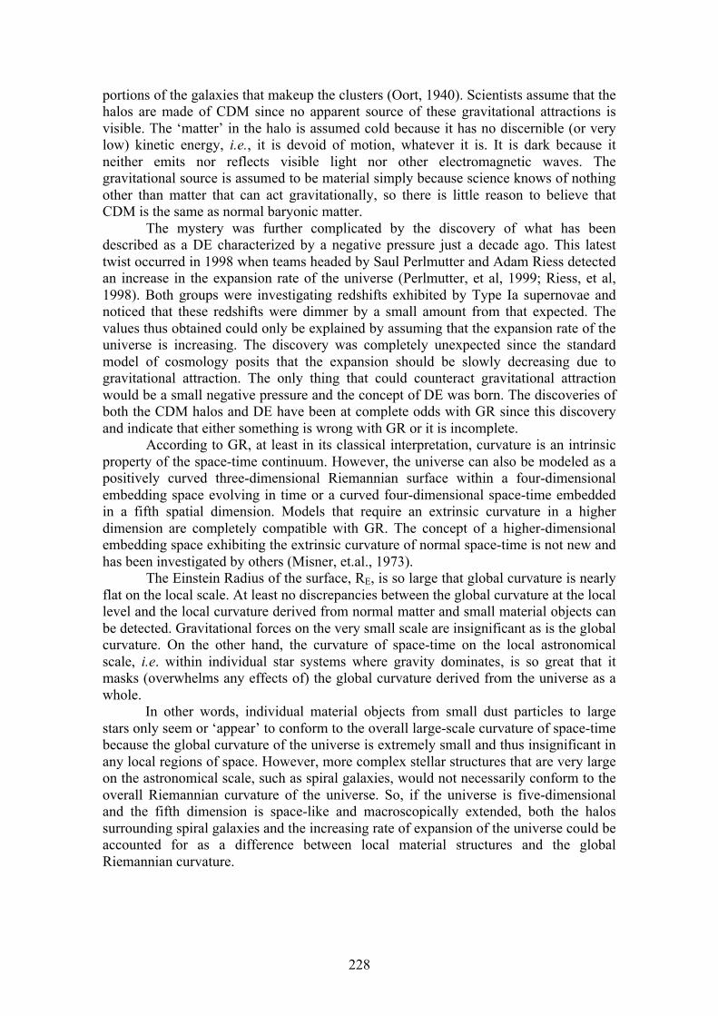
228
portions of the galaxies that makeup the clusters (Oort, 1940). Scientists assume that the halos are made of CDM since no apparent source of these gravitational attractions is visible. The ‘matter’ in the halo is assumed cold because it has no discernible (or very low) kinetic energy, i.e., it is devoid of motion, whatever it is. It is dark because it neither emits nor reflects visible light nor other electromagnetic waves. The gravitational source is assumed to be material simply because science knows of nothing other than matter that can act gravitationally, so there is little reason to believe that CDM is the same as normal baryonic matter.
The mystery was further complicated by the discovery of what has been described as a DE characterized by a negative pressure just a decade ago. This latest twist occurred in 1998 when teams headed by Saul Perlmutter and Adam Riess detected an increase in the expansion rate of the universe (Perlmutter, et al, 1999; Riess, et al, 1998). Both groups were investigating redshifts exhibited by Type Ia supernovae and noticed that these redshifts were dimmer by a small amount from that expected. The values thus obtained could only be explained by assuming that the expansion rate of the universe is increasing. The discovery was completely unexpected since the standard model of cosmology posits that the expansion should be slowly decreasing due to gravitational attraction. The only thing that could counteract gravitational attraction would be a small negative pressure and the concept of DE was born. The discoveries of both the CDM halos and DE have been at complete odds with GR since this discovery and indicate that either something is wrong with GR or it is incomplete.
According to GR, at least in its classical interpretation, curvature is an intrinsic property of the space-time continuum. However, the universe can also be modeled as a positively curved three-dimensional Riemannian surface within a four-dimensional embedding space evolving in time or a curved four-dimensional space-time embedded in a fifth spatial dimension. Models that require an extrinsic curvature in a higher dimension are completely compatible with GR. The concept of a higher-dimensional embedding space exhibiting the extrinsic curvature of normal space-time is not new and has been investigated by others (Misner, et.al., 1973).
The Einstein Radius of the surface, RE, is so large that global curvature is nearly flat on the local scale. At least no discrepancies between the global curvature at the local level and the local curvature derived from normal matter and small material objects can be detected. Gravitational forces on the very small scale are insignificant as is the global curvature. On the other hand, the curvature of space-time on the local astronomical scale, i.e. within individual star systems where gravity dominates, is so great that it masks (overwhelms any effects of) the global curvature derived from the universe as a whole.
In other words, individual material objects from small dust particles to large stars only seem or ‘appear’ to conform to the overall large-scale curvature of space-time because the global curvature of the universe is extremely small and thus insignificant in any local regions of space. However, more complex stellar structures that are very large on the astronomical scale, such as spiral galaxies, would not necessarily conform to the overall Riemannian curvature of the universe. So, if the universe is five-dimensional and the fifth dimension is space-like and macroscopically extended, both the halos surrounding spiral galaxies and the increasing rate of expansion of the universe could be accounted for as a difference between local material structures and the global Riemannian curvature.
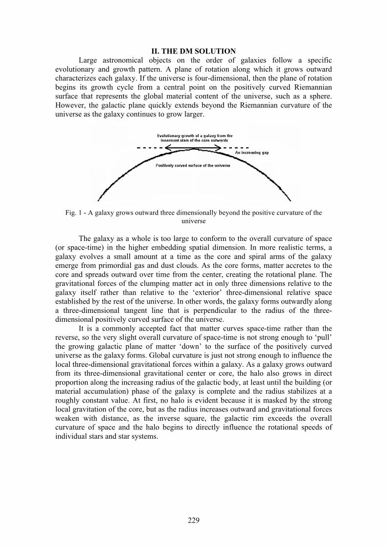
229
II. THE DM SOLUTIONLarge astronomical objects on the order of galaxies follow a specific
evolutionary and growth pattern. A plane of rotation along which it grows outward characterizes each galaxy. If the universe is four-dimensional, then the plane of rotation begins its growth cycle from a central point on the positively curved Riemannian surface that represents the global material content of the universe, such as a sphere. However, the galactic plane quickly extends beyond the Riemannian curvature of the universe as the galaxy continues to grow larger.
Fig. 1 - A galaxy grows outward three dimensionally beyond the positive curvature of the universe
The galaxy as a whole is too large to conform to the overall curvature of space (or space-time) in the higher embedding spatial dimension. In more realistic terms, a galaxy evolves a small amount at a time as the core and spiral arms of the galaxy emerge from primordial gas and dust clouds. As the core forms, matter accretes to the core and spreads outward over time from the center, creating the rotational plane. The gravitational forces of the clumping matter act in only three dimensions relative to the galaxy itself rather than relative to the ‘exterior’ three-dimensional relative space established by the rest of the universe. In other words, the galaxy forms outwardly along a three-dimensional tangent line that is perpendicular to the radius of the three-dimensional positively curved surface of the universe.
It is a commonly accepted fact that matter curves space-time rather than the reverse, so the very slight overall curvature of space-time is not strong enough to ‘pull’ the growing galactic plane of matter ‘down’ to the surface of the positively curved universe as the galaxy forms. Global curvature is just not strong enough to influence the local three-dimensional gravitational forces within a galaxy. As a galaxy grows outward from its three-dimensional gravitational center or core, the halo also grows in direct proportion along the increasing radius of the galactic body, at least until the building (or material accumulation) phase of the galaxy is complete and the radius stabilizes at a roughly constant value. At first, no halo is evident because it is masked by the strong local gravitation of the core, but as the radius increases outward and gravitational forces weaken with distance, as the inverse square, the galactic rim exceeds the overall curvature of space and the halo begins to directly influence the rotational speeds of individual stars and star systems.
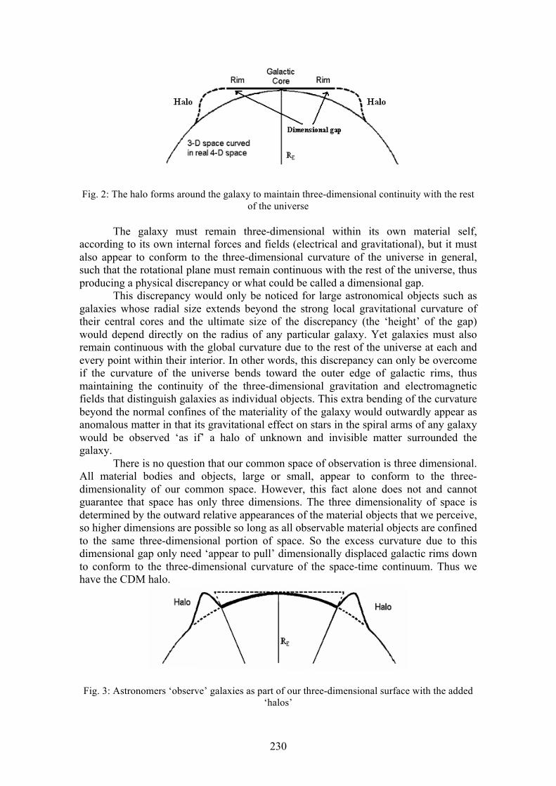
230
Fig. 2: The halo forms around the galaxy to maintain three-dimensional continuity with the rest of the universe
The galaxy must remain three-dimensional within its own material self, according to its own internal forces and fields (electrical and gravitational), but it must also appear to conform to the three-dimensional curvature of the universe in general, such that the rotational plane must remain continuous with the rest of the universe, thus producing a physical discrepancy or what could be called a dimensional gap.
This discrepancy would only be noticed for large astronomical objects such as galaxies whose radial size extends beyond the strong local gravitational curvature of their central cores and the ultimate size of the discrepancy (the ‘height’ of the gap) would depend directly on the radius of any particular galaxy. Yet galaxies must also remain continuous with the global curvature due to the rest of the universe at each and every point within their interior. In other words, this discrepancy can only be overcome if the curvature of the universe bends toward the outer edge of galactic rims, thus maintaining the continuity of the three-dimensional gravitation and electromagnetic fields that distinguish galaxies as individual objects. This extra bending of the curvature beyond the normal confines of the materiality of the galaxy would outwardly appear as anomalous matter in that its gravitational effect on stars in the spiral arms of any galaxy would be observed ‘as if’ a halo of unknown and invisible matter surrounded the galaxy.
There is no question that our common space of observation is three dimensional. All material bodies and objects, large or small, appear to conform to the three-dimensionality of our common space. However, this fact alone does not and cannot guarantee that space has only three dimensions. The three dimensionality of space is determined by the outward relative appearances of the material objects that we perceive, so higher dimensions are possible so long as all observable material objects are confined to the same three-dimensional portion of space. So the excess curvature due to this dimensional gap only need ‘appear to pull’ dimensionally displaced galactic rims down to conform to the three-dimensional curvature of the space-time continuum. Thus we have the CDM halo.
Fig. 3: Astronomers ‘observe’ galaxies as part of our three-dimensional surface with the added ‘halos’
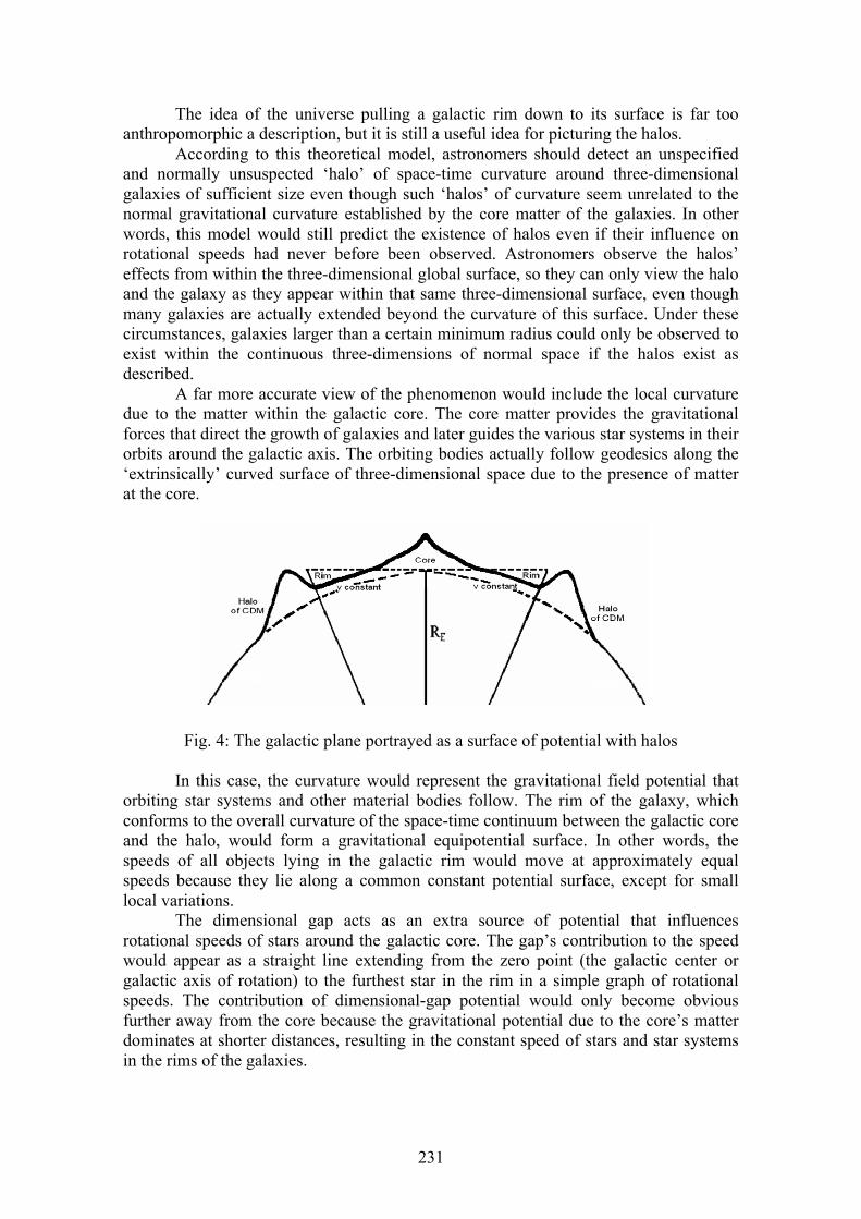
231
The idea of the universe pulling a galactic rim down to its surface is far too anthropomorphic a description, but it is still a useful idea for picturing the halos.
According to this theoretical model, astronomers should detect an unspecified and normally unsuspected ‘halo’ of space-time curvature around three-dimensional galaxies of sufficient size even though such ‘halos’ of curvature seem unrelated to the normal gravitational curvature established by the core matter of the galaxies. In other words, this model would still predict the existence of halos even if their influence on rotational speeds had never before been observed. Astronomers observe the halos’ effects from within the three-dimensional global surface, so they can only view the halo and the galaxy as they appear within that same three-dimensional surface, even though many galaxies are actually extended beyond the curvature of this surface. Under these circumstances, galaxies larger than a certain minimum radius could only be observed to exist within the continuous three-dimensions of normal space if the halos exist as described.
A far more accurate view of the phenomenon would include the local curvature due to the matter within the galactic core. The core matter provides the gravitational forces that direct the growth of galaxies and later guides the various star systems in their orbits around the galactic axis. The orbiting bodies actually follow geodesics along the ‘extrinsically’ curved surface of three-dimensional space due to the presence of matter at the core.
Fig. 4: The galactic plane portrayed as a surface of potential with halos
In this case, the curvature would represent the gravitational field potential that orbiting star systems and other material bodies follow. The rim of the galaxy, which conforms to the overall curvature of the space-time continuum between the galactic core and the halo, would form a gravitational equipotential surface. In other words, the speeds of all objects lying in the galactic rim would move at approximately equal speeds because they lie along a common constant potential surface, except for small local variations.
The dimensional gap acts as an extra source of potential that influences rotational speeds of stars around the galactic core. The gap’s contribution to the speed would appear as a straight line extending from the zero point (the galactic center or galactic axis of rotation) to the furthest star in the rim in a simple graph of rotational speeds. The contribution of dimensional-gap potential would only become obvious further away from the core because the gravitational potential due to the core’s matter dominates at shorter distances, resulting in the constant speed of stars and star systems in the rims of the galaxies.
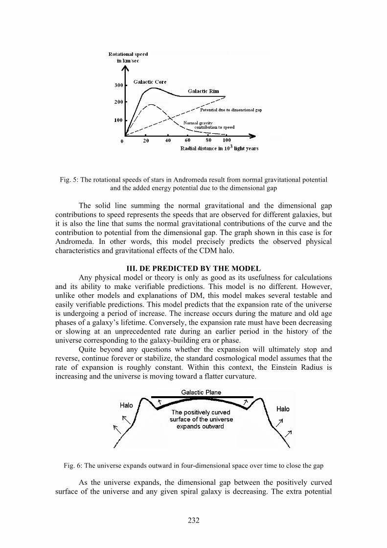
232
Fig. 5: The rotational speeds of stars in Andromeda result from normal gravitational potential and the added energy potential due to the dimensional gap
The solid line summing the normal gravitational and the dimensional gap contributions to speed represents the speeds that are observed for different galaxies, but it is also the line that sums the normal gravitational contributions of the curve and the contribution to potential from the dimensional gap. The graph shown in this case is for Andromeda. In other words, this model precisely predicts the observed physical characteristics and gravitational effects of the CDM halo.
III. DE PREDICTED BY THE MODELAny physical model or theory is only as good as its usefulness for calculations
and its ability to make verifiable predictions. This model is no different. However, unlike other models and explanations of DM, this model makes several testable and easily verifiable predictions. This model predicts that the expansion rate of the universe is undergoing a period of increase. The increase occurs during the mature and old age phases of a galaxy’s lifetime. Conversely, the expansion rate must have been decreasing or slowing at an unprecedented rate during an earlier period in the history of the universe corresponding to the galaxy-building era or phase.
Quite beyond any questions whether the expansion will ultimately stop and reverse, continue forever or stabilize, the standard cosmological model assumes that the rate of expansion is roughly constant. Within this context, the Einstein Radius is increasing and the universe is moving toward a flatter curvature.
Fig. 6: The universe expands outward in four-dimensional space over time to close the gap
As the universe expands, the dimensional gap between the positively curved surface of the universe and any given spiral galaxy is decreasing. The extra potential
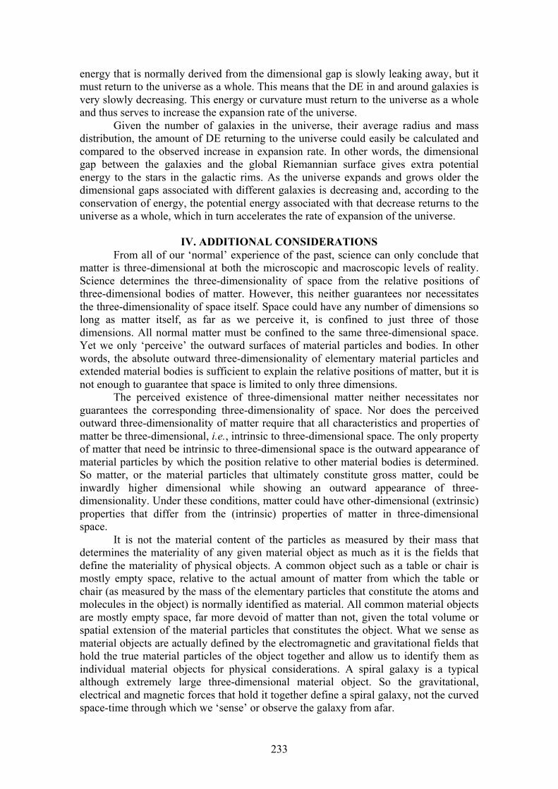
233
energy that is normally derived from the dimensional gap is slowly leaking away, but it must return to the universe as a whole. This means that the DE in and around galaxies is very slowly decreasing. This energy or curvature must return to the universe as a whole and thus serves to increase the expansion rate of the universe.
Given the number of galaxies in the universe, their average radius and mass distribution, the amount of DE returning to the universe could easily be calculated and compared to the observed increase in expansion rate. In other words, the dimensional gap between the galaxies and the global Riemannian surface gives extra potential energy to the stars in the galactic rims. As the universe expands and grows older the dimensional gaps associated with different galaxies is decreasing and, according to the conservation of energy, the potential energy associated with that decrease returns to the universe as a whole, which in turn accelerates the rate of expansion of the universe.
IV. ADDITIONAL CONSIDERATIONSFrom all of our ‘normal’ experience of the past, science can only conclude that
matter is three-dimensional at both the microscopic and macroscopic levels of reality. Science determines the three-dimensionality of space from the relative positions of three-dimensional bodies of matter. However, this neither guarantees nor necessitates the three-dimensionality of space itself. Space could have any number of dimensions so long as matter itself, as far as we perceive it, is confined to just three of those dimensions. All normal matter must be confined to the same three-dimensional space. Yet we only ‘perceive’ the outward surfaces of material particles and bodies. In other words, the absolute outward three-dimensionality of elementary material particles and extended material bodies is sufficient to explain the relative positions of matter, but it is not enough to guarantee that space is limited to only three dimensions.
The perceived existence of three-dimensional matter neither necessitates nor guarantees the corresponding three-dimensionality of space. Nor does the perceived outward three-dimensionality of matter require that all characteristics and properties of matter be three-dimensional, i.e., intrinsic to three-dimensional space. The only property of matter that need be intrinsic to three-dimensional space is the outward appearance of material particles by which the position relative to other material bodies is determined. So matter, or the material particles that ultimately constitute gross matter, could be inwardly higher dimensional while showing an outward appearance of three-dimensionality. Under these conditions, matter could have other-dimensional (extrinsic) properties that differ from the (intrinsic) properties of matter in three-dimensional space.
It is not the material content of the particles as measured by their mass that determines the materiality of any given material object as much as it is the fields that define the materiality of physical objects. A common object such as a table or chair is mostly empty space, relative to the actual amount of matter from which the table or chair (as measured by the mass of the elementary particles that constitute the atoms and molecules in the object) is normally identified as material. All common material objects are mostly empty space, far more devoid of matter than not, given the total volume or spatial extension of the material particles that constitutes the object. What we sense as material objects are actually defined by the electromagnetic and gravitational fields that hold the true material particles of the object together and allow us to identify them as individual material objects for physical considerations. A spiral galaxy is a typical although extremely large three-dimensional material object. So the gravitational, electrical and magnetic forces that hold it together define a spiral galaxy, not the curved space-time through which we ‘sense’ or observe the galaxy from afar.
234
The three-dimensionality of a galaxy is not defined by the three-dimensionality of the universe, as represented by the surface curvature of space-time. Nor is it defined by the actual material mass of the galaxy. Three-dimensionality is a property of the object as a whole, not external to the object and thus not determined by the three-dimensionality of external relative space-time. So a three-dimensional object, if it is large enough, need not follow nor be restricted by the three-dimensional surface of the universe as it curves in the higher fourth spatial dimension. This logical argument further confirms the notion that a three-dimensional galaxy is independent of the three-dimensionality of the external spatial curvature of the global space-time that surrounds it. Thus it forms a halo of curvature as described above.
Since the fourth dimension of space is real and curvature is an extrinsic property of four-dimensional space-time in the higher dimension, rather than an intrinsic property of space-time as commonly believed, the overall or global curvature of space-time also becomes the source of the observed Hot Dark Matter (HDM). The global curvature of space-time in a three-dimensional Riemannian sphere embedded in a four-dimensional space results from the total material content of the universe. This curvature extends throughout the normally empty space (at least empty of normal matter) that exists between all material bodies in the universe in roughly equal proportions, just as HDM is believed to fill all of space between material bodies. Therefore, HDM is just the average and normal space-time curvature of the universe in a Riemannian surface in the higher dimension. DM itself is nothing but space-time curvature that is not normally associated with local matter, but is instead either associated with, or the product of, the total (global) material content of the universe.
V. THE THEORETICAL STRUCTURE Rather conveniently, a theoretical structure for a five-dimensional space-time
already exists. Theodor Kaluza added a fifth dimension to GR to further expand the theory (Kaluza, 1921), but he gave no physical meaning to his fifth dimension. It was merely a mathematical device that he used to derive both Maxwell and Einstein’s equations from a ‘single field’ model of the universe. Kaluza obtained the proper mathematical formulations for gravity and electromagnetism in spite of his purely mathematical interpretation of the higher dimension, but this restriction left his model with no predictive capabilities. His mathematical model merely duplicated the formulas and equations that were already known, so Kaluza’s theory was not well received by a scientific community that was far more concerned with quantum theory than with relativity theory. Simply put, Kaluza’s five-dimensional model was not falsifiable as it was originally conceived.
However, endowing Kaluza’s fifth dimension with a physical reality guarantees the falsifiability and explanatory power of the five-dimensional model while retaining the unification of general relativity and electromagnetism that Kaluza obtained. All that is necessary is to determine the physical properties of the fifth physical dimension, which could be difficult because it is generally assumed that any higher embedding dimension has no direct sensible or measurable effect on physical phenomena. This belief, albeit false, renders the simple solution of a fourth dimension of space quite radical because it requires such an assumption to explain ‘why’ the fourth dimension does not influence normal phenomena. In fact, the influence of the embedding higher dimension is quite common across the spectrum of phenomena investigated by science, if one knows what to look for. That influence is, precisely, the observed effects of DM and DE.
235
The fifth dimension of the space-time continuum is space-like rather than temporal, but differs radically from the ordinary three dimensions of space. Matter is clearly three dimensional as are the electric field and electric potential, yet the magnetic field strength varies over normal three-dimensional space while the magnetic vector potential that the mathematical formulas describing the magnetic field indicate is perpendicular to the three dimensions of normal space. According to Maxwell’s electromagnetic theory, the magnetic field B is associated with a vector or magnetic potential A such that
Curl A = B and Div B = 0 .
Accordingly, the magnetic field strength B is a three-dimensional quantity, but the vector potential varies along a line that is perpendicular to three-dimensional space at each point in three-dimensional space. The quantity A is not subject to physical measure under normal circumstances, as has been the case, but it still must exist. Variations in A cannot be measured because they occur in the fourth dimension of space, along lines extended through all points in three-dimensional space in a fourth direction perpendicular to the three-dimensional space. This model of the Maxwell field theory is completely compatible with the Kaluza five-dimensional model of space-time. William K. Clifford first suggested a four-dimensional electromagnetic model of space of this type well over a century ago (Clifford, 1870; 1885).
So a fourth dimension of space is implied by Maxwell’s electromagnetic theory, although this spatial dimension would be unique in its differences with the other three dimensions of space. The physical space constituting our universe could therefore be considered a four-dimensional space for the purposes of scientific analysis under proper time-independent physical conditions (Beichler, 2007). A single field that is the precursor to the known normal physical fields as well as matter itself, all of which are specific field-density structures within the single field, occupies the five-dimensional space-time indicated by Kaluza’s mathematical model. Einstein attempted to develop a mathematical model of this single field, which he called “unified field theory”, during the last decades of his life. Although this fourth dimension of space is macroscopically extended, it remains closed with respect to the three normal dimensions of space, such that it does not alter Kaluza’s unification in any manner (Einstein and Bergmann, 1938; Einstein, Bergmann and Bargmann, 1941; Beichler, 2007). Within this context, the four-dimensional spatial model reduces CDM and the galactic halo to a simple geometric problem.
This simple fact poses a serious problem, at the very least, for any theory that depends on the compactification of higher dimensions. Under these circumstances, compactification is neither justified nor required from either the theoretical or a purely philosophical perspective. Kaluza’s original five-dimensional model depended upon two stated mathematical conditions, plus another assumed condition and one suggestion. Kaluza required that (1) the higher dimension be closed with respect to four-dimensional space-time and (2) the A-lines that connected points in the normal four-dimensional space-time continuum through the higher dimension are of equal length. Kaluza assumed continuity in the higher dimension, just as continuity exists in the normal dimensions. Otherwise, he only suggested that any extension in the fifth direction must be very small because we cannot sense or detect that higher dimension.
Oskar Klein took advantage of Kaluza’s suggestion and related the periodicity in the higher dimension, what has been called the ‘cylindrical condition’, to the quantum (1926a; 1926b; 1927; 1939; 1947). Yet Klein did not go beyond Kaluza’s mathematical
236
conditions, nor did he contradict them in any way. Klein only followed one of the possible legitimate paths that could be used to extend Kaluza’s theory. Klein was trying to unify relativity and the quantum, but his efforts failed, by his own admission. In the 1980s, the string theorists were in a quandary on how to develop their own quantum model further when they rediscovered and then adopted Klein’s extension of Kaluza’s model, but they expanded Klein’s extension of Kaluza’s model to include several more dimensions without considering how doing so might affect the original unification that was accomplished using only a five-dimensional model.
Kaluza placed no physical conditions on his higher dimension, so varying the field density neither affects nor harms his unification. So instead of using Klein’s approach, the density of space in the fifth direction could be varied such that our material world only inhabits a thin three-dimensional ‘sheet’ of extremely high single field density, extending through a slice of the four-dimensional space (or five-dimensional space-time), while the overall extension in the fourth direction of space remains macroscopic. The width of the three-dimensional ‘sheet’ would be extremely small, but not infinitesimally small, and still define the quantum. The width of the ‘sheet’ also defines our material world of senses and perceptions as far as they correspond to Newtonian and classical physics. Einstein and his colleagues followed this second path of application in the late 1930s, but applied it unsuccessfully because they never completely understood the versatility and finer geometrical points of the five-dimensional approach, such that they did not consider the possibility that space had physical properties such as a varying density.
If the extension of our three-dimensional space in the fourth direction is macroscopic, then a small but finite ‘minimum’ width of three-dimensional space must exist. This minimum ‘width’ in the higher dimension is necessary to create the three-dimensionality of matter as observed. On the other hand, there is absolutely no reason to assume that this minimum width is as small as the Planck length. Describing the three-dimensional ‘thickness’ or ‘effective width’ of the ‘sheet’ as a ‘minimum’ value better conforms to the quantum interpretation of material reality and is, in fact, proportional to the quantum. The discrete quantum enters the continuous field model through the concept of this ‘minimum’ or ‘effective width’ of our three-dimensional space in the fourth direction, such that the ‘effective width’ is proportional to the fine-structure constant.
In fact, the ‘effective width’ defines the common quantum of action as expressed in the quantum theory. The ‘effective width’ equals the product of the fine structure constant and the proton width, or about 1/137 x 10 –15 meters, leaving the ‘sheet’ continuous along its macroscopic extension in the fourth direction. To further maintain continuity in the fourth direction, we could picture successive layers of three-dimensional space, each having the same ‘effective width’, stacked on top of each other in the fourth direction of space like the pages of a book or onion skins. Each successive layer, defined by equal ‘effective widths’, would correspond to the principle quantum numbers used in quantum mechanics, while the density of the single field would fall off by a factor of 1/r4 as distance from the center of the three-dimensional ‘sheet’ increases in the fifth dimension of space-time.
VI. THE ALGEBRAIC FORMAlthough the above geometrical description of DM and DE is simple and
straightforward, converting the geometry into an equivalent algebraic form is not so simple. However, an algebraic description of the process and phenomenon can be derived from another direction. Particle physicists claim that the CDM that constitutes
237
the galactic halos must be composed of particles, usually referred to as WIMPs (weakly interacting massive particles). Yet the CDM that seems to constitute the halo could not possibly be particulate. CDM is only known by its gravitational effect on star systems in the galactic arms and gravity is always attractive and only attractive. So, if CDM in the halo were particulate, exhibiting normal gravity, it would have been attracted to the center of the galactic core during the accretion era of galaxy formation and would not have accumulated to form a halo around the galaxy. Therefore, CDM cannot be particulate by any standards that science now accepts.
On the other hand, CDM might still be particulate without exhibiting normal gravity. For instance, if CDM were particulate, but characterized by anti-gravity or gravitational repulsion, then it would have been repelled outward during the accumulation era of the galactic building process toward the halo. However, the CDM particles would then have dissipated into the emptiness of space between galaxies rather than accumulate and form galactic halos. So, if particulate, CDM could not exhibit ‘levity’ or ‘anti-gravity’ either. The only possibility left would be that CDM only ‘seems’ to be repelled during the accretion phase, but also acts like normal gravity, attractive, to form the galactic halo, which does not completely make sense given science’s present understanding of gravity. The only way for this set of circumstances to occur would be if gravity acted centripetally rather than radially such that CDM could accumulate to make the halo.
Take for example a round rod rotating about a central point along its length. Two sliding ring weights are placed on either side of the central axis of rotation. As the rod rotates the rings would be forced outward to the ends of the rod by their inertia according to Newton’s first law of motion, but still be held to the center axis of rotation. This is the same commonly known action that holds the moon in orbit about the earth. CDM mimics this motion in that it moves to the outer expanses of galaxies like sliding weights on rotating poles. This process would only be possible if CDM was the result of a tangential component of gravitational attraction coupled to the normal radial component of gravity, which does not require separate and distinct particles of CDM. Normal gravity has an unsuspected tangential component, so the normally gravitating particles which constitute the galaxy also form the CDM halo.
In essence, the present scientific view of gravity is incomplete in both its Newtonian and Einsteinian forms, but then that incompleteness has already been suggested by the observed presence of DM and DE. In other words, the total force on matter due to gravity has not yet been established or accounted for by science. In fact, the formula for the gravitational force should include a new tangential component and the tangential component would indicate the existence of a fourth spatial dimension in addition to the normal three. In this case, a gravitational analogy could be made to the relationship between electricity and magnetism. Like electricity and magnetism, we could have a form of gravity and ‘gravnetism’. In electromagnetic theory, science accepts a specific relationship between the vector potential (A) and the magnetic field (B), such that Curl A = B and Div A = 0. So a similar relationship would exist between a gravitational vector potential and the external gravity field such that Curl W = Γ and Div W = 0, where W represents the gravity vector potential and Γ the ‘gravnetic’ field strength. It could then be argued that both B and Γ are four-dimensional fields because the ‘del’ function represents three-dimensional space and the Curl (del cross product) is thus a direction orthogonal to normal three-dimensional space.
The total gravitational force could then take a form something like the Lorentzian force for electromagnetism, or
238
F = qE + qv x B .
So for gravity, the total force would be
FG = mg + mv x Γ ,
where g represents the normal radial component of gravity and Γ represents the new tangential portion of gravity or the ‘gravnetic’ field. The quantity mv would be limited by boundary conditions of the physical model such that the CDM component of curvature in the fourth direction goes to zero at the galactic center and reaches a maximum value at the extreme radius of the galaxy, yielding a geometric picture that duplicates the one explained above. Thus, the higher the gravitational induced v of material bodies near the core, the higher the four-dimensional spatial component according to Special Relativity, i.e., more apparent inertia at higher speeds, so the interaction is less with the four-dimensional component of Γ.
The quantity Γ represents the external ‘gravnetic’ field due to the rest of the universe and mv represents the ‘gravnetic’ field due to the individual material objects that constitute a galaxy. However, in an even broader sense, the quantity mv can represent any individual material body and the formulation becomes valid for all material bodies. In the case of a spiral galaxy, the four-dimensional components of gravity for both quantities would add together since gravity is only attractive and thereby create the halo of CDM. Since mv represents the inertia of moving bodies relative to Γ, the rest of the universe, the quantity ‘mv x Γ’ can be interpreted as a mathematical formulation of Mach’s Principle.
Like the vector potential in electromagnetic theory, the gravitational vector potential could not be directly measured. Its existence is only apparent by its physical side-effects and the mathematical formulation. Potential, both the scalar and vector varieties, exists in each and every point of space occupied by fields, but only the potential difference is measurable. In the case of scalar potential, the electric potential difference is measured as volts, but there is no measurable magnetic equivalent in the form of the vector potential because the vector potential difference only exists between two points that are separated along the fourth direction of space. In general, vector potentials are non-measurable because they vary in the fourth direction of our four-dimensional space, or rather along the fifth direction of a five-dimensional space-time. Nor are the direct effects of the gravitational vector potential normally observed. For individual objects, the mass is so small and thus the ‘gravnetic’ effect so extremely weak that the gravitational vector potential is masked by ordinary gravity. This masking effect would hold for objects up to the size of individual star systems. The ‘gravnetic’ effect is only observable for objects the size of galaxies because the radial distances are so great that normal gravity does not mask the effect.
The units for Γ would be 1/sec, rendering Γ a frequency. Waves have frequencies, material bodies do not, yet a frequency could be associated with every material body that is moving since moving material bodies are associated with deBroglie waves. Gravity waves predicted by GR would also exhibit a frequency so the quantity ‘mv x Γ’ would indicate that the inertia of moving bodies in a galaxy (mv) would interact with the gravity field of the rest of the universe (Γ) via gravitational waves. Since the quantity ‘mv x Γ’ is a new mathematical representation of Mach’s Principle, the local mv (or inertia) interacts with the rest of the universe represented by Γ, allowing science to understand and define the inertia of a material body relative to the whole universe as a four-dimensional property of matter. By interpreting inertia in
239
this way, relativity is related back to Newton’s first law of motion, which, of course, accounts for the tangential component of gravity appearing to migrate (being just more pronounced) to the outer edge of a galaxy from our three-dimensional perspective.
A frequency associated with CDM indicates periodicity and thus ‘closure’ in the fourth direction of space or the fifth dimension of space-time. Closure in the fifth dimension is a fundamental requirement of Kaluza’s original five-dimensional unification of general relativity and electromagnetism. To develop his five-dimensional model, Kaluza set two mathematical conditions or restrictions. Each point in normal space-time has a component in the fifth dimension defined as an A-line that is orthogonal to the four-dimensional space-time continuum, such that (1) The fifth dimension is closed along the A-lines with respect to the ordinary four dimensions of space-time and (2) all A-lines are of equal length. These conditions were necessary for Kaluza to mathematically derive the electromagnetic equations from his five-dimensional model. However, the closure condition introduces a periodicity into the fifth dimension of space-time that could be associated with the frequency of the ‘gravnetic’ field Γ. In other words, the five-dimensional interpretation of this model leads directly to a complete unification of general relativity and the electromagnetic theory as suggested in the parallels between the Lorentz force and the new gravity equation as stated above. This implies that both Einstein and Friedman’s tensor equations could be altered to account for CDM using this model.
Furthermore, a quantum equivalent to this formulation, using deBroglie’s concept of a matter wave, could possibly account for the structure of electronic orbits in atoms, or at least show that gravity considerations correspond to whole number waves along orbital paths. On a still larger scale, this mathematical model might also account for the Titus-Bode structure in star systems as well as planetary rings. But a more direct relationship to the quantum can be easily seen. Using the deBroglie matter wave of λmatter = h/mv we can restate the new gravitational formula in quantum terms. From deBroglie’s equation we get mv = h/λ, but also v = fλ so that mv = hf/v. Therefore,
F = mg + (hf/v) x Γ ,
which constitutes a quantum approximation of gravity. The quantity (hf/v) represents a material wave moving outward along the radius r while Γ represents the frequency of the incoming universal gravity wave, thus creating a standing wave interference pattern that could act to guide electrons in their orbits around atomic nuclei. Otherwise, a similar although large-scale standing material wave pattern would be created around the galaxy, i.e., the halo. The standing wave pattern would actually amount to a real curvature in the fourth dimension of space. So, from a three-dimensional perspective, the halo of real curvature (the resonant wave) would appear to be material, but not particulate. Individual material bodies and extended objects (star systems and etc.) would just be complexes of resonant wave patterns in four-dimensional space while we perceive or sense real curvature in four-dimensional space as matter and material bodies in our commonly sensed three-dimensional space, given the relativistic perspective. Otherwise, material objects could be considered complex superposition patterns from the quantum perspective.
VII. CONCLUSIONThe confirmed existence of DM in both the galactic halo and more generally
throughout the emptiness of space between material bodies offers clear observational evidence of the existence of a macroscopically extended fourth dimension of space.
240
Although a macroscopically extended fourth dimension of space was first used as a hypothesis by which the CDM halo could be explained, the fact that the concept of a fourth dimension so fully explains the observations leads to the conclusion that the fourth dimension is not a hypothesis, but rather a physical reality. This evidence is irrefutable, although alternative hypotheses to explain DM will surely persist far into the future because the implications of a real fourth dimension of space are extremely radical compared to the present worldview of science and culture.
As an added bonus, this model also explains DE and unifies the quantum and relativity within a single theory. Although only a new Newtonian formula for gravity has been developed, the tensor equivalents to this formulation are implied. DM is nothing more than the real extrinsic curvature of the four-dimensional space-time continuum that is not directly associated with local matter, but is a consequence of the non-local material content of the universe that determines the global curvature of the universe. DE is just the field ‘thickness’ of three-dimensional space in the fourth spatial dimension. This explanation of DM and DE is extremely simple, but it will be difficult for many scientists and scholars to accept. Simple ideas are quite often the hardest to accept and the easiest to overlook when proposed as solutions to the most difficult and pernicious problems in science. And yet the reality of a fourth dimension is actually an old question in science.
Scientists have sought evidence of a higher dimension of space, as exhibited by curvature, since the days of Friedrich Gauss (Scholz, 2005), but the search has never before been a priority because there has never been more than an esoteric need to discover the next higher dimension of space. In the late nineteenth century, when a few forward thinking scientists were actually using parallax measurements of stars to look for a suspected space curvature, the French mathematician Henri Poincaré stated that he would rather change the basic laws of optics than accept the possibility that space might be curved (Poincaré, 1892). Poincaré’s statement clearly reflected the existence of a three-dimensional bias in science and that bias is still prevalent today.
The scientific and cultural bias against the possibility of a higher dimension is symptomatic of a deeply rooted positivistic attitude in science that has held sway over science since the late 1900s and poses a real problem for solving the DM and DE crises even today. However, a need for using higher-dimensional spaces in physics has developed in the past few decades and hyper-dimensional theories have become commonplace in theoretical physics to explain some of the stranger and more exotic phenomena observed in nature. Unfortunately, hyper-dimensionality has only been accepted because of the supposed compactification of the higher dimensions that ‘saves the phenomena’ described within the present paradigms of physics: Compactification is no more than a positivistic compromise that circumvents any possible reality of a physical fourth dimension of space.
Scientists who are presently attempting to develop hyper-dimensional theories in physics seem never to have studied the mathematical properties and consequences of a single higher dimension or they would have realized that only a single higher dimension is necessary to unify physics and account for the observed physical properties of reality. Instead, they have adopted as many as six or seven extra dimensions, if not more, to account for the extra degrees of freedom that they need to unify different physical theories, which is a bad practice. They are merely offering a compromise between physical reality and the quantum paradigm that could account for the discrete nature of the quantum. The fourth dimension alone has a rich enough group of properties to render still higher dimensions of space unnecessary at this time.
241
The fourth dimension of space differs from the ordinary three by far more than just another degree of freedom for physicists to play with. It has unique physical properties and special characteristics that will further impact science and physics, so ordinary physics will eventually need to be rewritten to cope with this new higher-dimensional reality. Unfortunately, many scientists and scholars will not easily give up their hyper-dimensional compromises or the alternative theories that they have constructed on that hypothesis and accept the simplicity of a single continuous higher dimension. Too many scientists are too enamored with the purported fundamental nature of the quantum and their own mathematical prowess and dexterity to seriously consider the simpler physics and mathematics of continuity in the next higher dimension. They are just following Poincaré’s solution of fitting an incorrect theory to reality rather than accept the reality that nature shows them. Accepting the reality of a fourth dimension will be neither simple nor easy for science, but science will eventually be forced toward acceptance by the evidence provided by nature.
REFERENCES [1]. James E. Beichler. (2007) “Three Logical Proofs: The five-dimensional reality of
space-time”. Journal of Scientific Exploration, to be published. [2]. William Kingdon Clifford. (1870) “On the space-theory of matter”. Read 21
February. Transactions of the Cambridge Philosophical Societ 2 (1866/1876); Reprinted in Mathematical Papers, edited by Robert Tucker with a preface by H.J. Stephen Smith. (1882): 21-22.
[3]. William Kingdom Clifford. (1885) The Common Sense of the Exact Sciences, edited by Karl Pearson. London: Macmillan.
[4]. Albert Einstein and Peter Bergmann (1938). "On a Generalization of Kaluza's Theory of Electricity". Annals of Mathematics 39 (3): 693-701.
[5]. Albert Einstein, Peter G. Bergmann and Valentine Bargmann (1941). "On the Five-Dimensional Representation of Gravitation and Electricity". Theodor von Karman Anniversary Volume. Pasadena: California Institute of Technology: 212-225.
[6]. Theodor Kaluza. (1921) "Zur Unitätsproblem der Physik". Sitzungsberichte der Preussischen Akademie der Wissenschaften 54: 966-972.
[7]. Oskar Klein. (1926a) "Quantentheorie und fünfdimensionale Relativitätstheorie". Zeitschrift fur Physik 37: 895-906.
[8]. Oskar Klein. (1926b) "The Atomicity of Electricity as a Quantum Theory Law". Nature 118: 516.
[9]. Oskar Klein. (1927) "Zur fünfdimensionale Darstellung der Relativitätstheories". Zeitschrift fur Physik 46: 188-208.
[10]. Oskar Klein. (1939) “On the Theory of Charged Fields”. New Theories in Physics. Paris: International Institute of Intellectual Cooperation: 77-93.
[11]. Oskar Klein. (1947) “Meson Fields and Nuclear Interaction”. Arkiv for Mathematik, Astronomi och Fysik 34A: 1-19.
[12]. Charles Misner, Kip Thorne and John A. Wheeler. (1973) Gravitation. San Francisco: Freeman: 417-428.
[13]. Jan Hendrik Oort. (1940) “Some Problems Concerning the Structure and Dynamics of the Galactic System and the Elliptical Nebulae NGC 3115 and 4944”. Astrophysical Journal 91: 273-306.
[14]. Henri Poincaré. (1892) "Non-Euclidean Geometry", Translated by W.J.L. Nature 45: 407.
[15]. Saul Perlmutter, et.al. (1999) “Measurements of Omega and Lambda from 42 High Redshift Supernovae”. The Astrophysical Journal 517: 565-586. Eprint at
242
arXiv: astro-ph/9812133. [16]. Adam G. Riess, et.al. (1998) “Observational Evidence from Supernovae for an
Accelerating Universe and a Cosmological Constant”. The Astronomical Journal 116: 1009-1038. Eprint at arXiv: astro-ph/9805201v1.
[17]. Vera Rubin and W. Kent Ford. (1970) "Rotation of the Andromeda Nebula from a Spectroscopic Survey of Emission Regions". Astrophysical Journal 159: 379.
[18]. Vera Rubin, W. Kent Ford, D. Burstein and N. Thonnard. (1985) "Rotation Velocities of 16 Sa Galaxies and a Comparison of Sa, Sb, and Sc Rotation Properties". Astrophysical Journal 289: 81.
[19]. Erhard Scholz. (2005) “Curved spaces: Mathematics and Empirical evidence, ca. 1830-1923". Preprint at Wuppertal. At <www.mathg.uni-wuppertal.de/~scholz/preprints/ES_OW2005.pdf>. Shorter version to appear at Oberwalfach Reports.
[20]. Sinclair Smith. (1936) “The Mass of the Virgo Cluster”. Astrophysical Journal 83: 23.
[21]. Fritz Zwicky. (1933) “Die Rotverscheibung von extragalaktischen Nebeln”. Helvetica Physica Acta 6: 110-127.
[22]. Fritz Zwicky. (1937a) “Nebulae as Gravitational Lenses”. Physical Review 51: 290.
[23]. Fritz Zwicky. (1937b) “On the Masses of Nebulae and of Clusters of Nebulae”. Astrophysical Journal 86: 217-246.
243
ANOTHER THEORY OF GRAVITATION
Francis MATHE 44 La Clairière, 78830 BULLION, France
E-MAIL: [email protected]
I. CONVENTIONS AND ABBREVIATIONS The sign conventions for the metric and curvature tensors are (-, +, +) in the
terminology of Mismer, Thorne & Wheeler [1]. That is, the metric signature is (+,-,-,-). For this paper we use geometric units in which c = G =1. (Except the § 4.22).
The following symbols and abbreviations are used throughout: ∂µ or ,µ partial derivative Dµ or ;µ covariant derivative ln natural logarithm i, j, k,…. Latin indices equal to 1, 2 & 3 λ, µ, ν,… Greek indices equal to 0, 1, 2, & 3 cst constant quantity laplacian on a four dimensional manifold [ , ]L Lie’s brackets ≈ Asymptotically equal to # Approximately equal to
II. INTRODUCTION AND HYPOTHESIS [5]The study of the movement of the non charged matter lead to consider that the
space-time is a four dimensional differentiable Riemannian manifold U whose the metric tensor g has the signature (+,-,-,-).
ds² = gλµ dxλ dxµ (1.1)
For example the space-time of the rotating disk is not flat. On the other hand we reject, with J. L. Synge, the weak equivalence principle.
We utilise, for describe the non charged matter, three fields on the manifold U: • The inertial field who is a field of symmetric connection Γ.• The matter field who is a field q taking its values in a three dimensional
manifold.• The gravitational field who is a real scalar field Φ.From now we suppose that the matter is a perfect fluid with an equation of state
ρ = ϕ(p)
where ρ is the density and p the pressure of the fluid, the habitual hypothesis of approximation lead to the lagrangians :
Linert = gλµRλµ √(-g)
Lgrav = - 2Φ, λ Φ, λ √(-g)
Lmat = - 16πρ √(-g)
Keywords: non charged matter, Riemannian manifold U, gravitational field, general relativity theory.
PACS number:02.40.Ky/04.20.-q
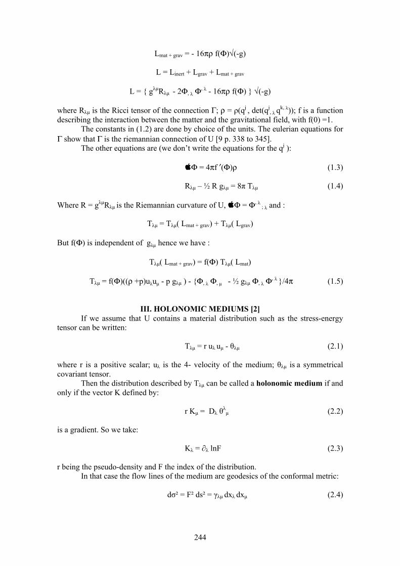
244
Lmat + grav = - 16πρ f(Φ)√(-g)
L = Linert + Lgrav + Lmat + grav
L = gλµRλµ - 2Φ, λ Φ, λ - 16πρ f(Φ) √(-g)
where Rλµ is the Ricci tensor of the connection Γ; ρ = ρ(qj , det(qj
, λ qk, λ)); f is a function describing the interaction between the matter and the gravitational field, with f(0) =1.
The constants in (1.2) are done by choice of the units. The eulerian equations for Γ show that Γ is the riemannian connection of U [9 p. 338 to 345].
The other equations are (we don’t write the equations for the qj ):
Φ = 4πf ′(Φ)ρ (1.3)
Rλµ – ½ R gλµ = 8π Tλµ (1.4)
Where R = gλµRλµ is the Riemannian curvature of U, Φ = Φ, λ ; λ and :
Tλµ = Tλµ( Lmat + grav) + Tλµ( Lgrav)
But f(Φ) is independent of gλµ hence we have :
Tλµ( Lmat + grav) = f(Φ) Tλµ( Lmat)
Tλµ = f(Φ)((ρ +p)uλuµ - p gλµ ) - Φ, λ Φ, µ - ½ gλµ Φ, λ Φ, λ /4π (1.5)
III. HOLONOMIC MEDIUMS [2]If we assume that U contains a material distribution such as the stress-energy
tensor can be written:
Tλµ = r uλ uµ - θλµ (2.1)
where r is a positive scalar; uλ is the 4- velocity of the medium; θλµ is a symmetrical covariant tensor.
Then the distribution described by Tλµ can be called a holonomic medium if and only if the vector K defined by:
r Kµ = Dλ θλµ (2.2)
is a gradient. So we take:
Kλ = ∂λ lnF (2.3)
r being the pseudo-density and F the index of the distribution. In that case the flow lines of the medium are geodesics of the conformal metric:
dσ² = F² ds² = γλµ dxλ dxµ (2.4)
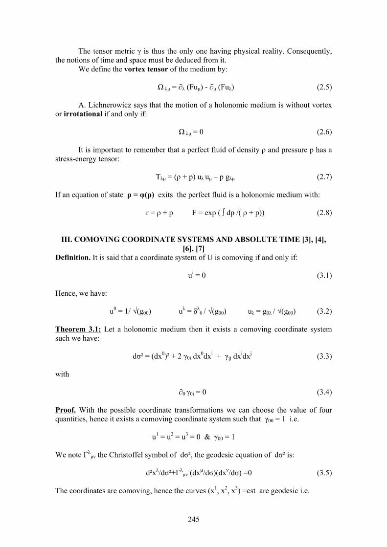
245
The tensor metric γ is thus the only one having physical reality. Consequently, the notions of time and space must be deduced from it.
We define the vortex tensor of the medium by:
Ω λµ = ∂λ (Fuµ) - ∂µ (Fuλ) (2.5)
A. Lichnerowicz says that the motion of a holonomic medium is without vortex or irrotational if and only if:
Ω λµ = 0 (2.6)
It is important to remember that a perfect fluid of density ρ and pressure p has a stress-energy tensor:
Tλµ = (ρ + p) uλ uµ – p gλµ (2.7)
If an equation of state ρ = φ(p) exits the perfect fluid is a holonomic medium with:
r = ρ + p F = exp ( ∫ dp /( ρ + p)) (2.8)
III. COMOVING COORDINATE SYSTEMS AND ABSOLUTE TIME [3], [4],[6], [7]
Definition. It is said that a coordinate system of U is comoving if and only if:
ui = 0 (3.1)
Hence, we have:
u0 = 1/ √(g00) uλ = δλ0 / √(g00) uλ = g0λ / √(g00) (3.2)
Theorem 3.1: Let a holonomic medium then it exists a comoving coordinate system such we have:
dσ² = (dx0)² + 2 γ0i dx0dxi + γij dxidxj (3.3)
with
∂0 γ0i = 0 (3.4)
Proof. With the possible coordinate transformations we can choose the value of four quantities, hence it exists a comoving coordinate system such that γ00 = 1 i.e.
u1 = u2 = u3 = 0 & γ00 = 1
We note Γλµν the Christoffel symbol of dσ², the geodesic equation of dσ² is:
d²xλ/dσ²+Γλµν (dxµ/dσ)(dxν/dσ) =0 (3.5)
The coordinates are comoving, hence the curves (x1, x2, x3) =cst are geodesic i.e.
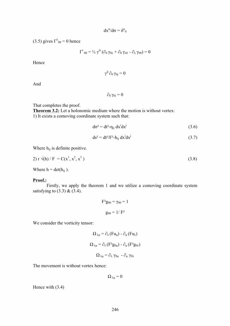
246
dxµ/dσ = δµ0
(3.5) gives Γλ00 = 0 hence
Γi 00 = ½ γiλ (∂0 γ0λ + ∂0 γλ0 - ∂λ γ00) = 0
Hence
γij ∂0 γ0j = 0
And
∂0 γ0i = 0
That completes the proof. Theorem 3.2: Let a holonomic medium where the motion is without vortex: 1) It exists a comoving coordinate system such that:
dσ² = dt²-ηij dxidxj (3.6)
ds² = dt²/F²-hij dxidxj (3.7)
Where hij is definite positive.
2) r √(h) / F = C(x1, x2, x3 ) (3.8)
Where h = det(hij ).
Proof.: Firstly, we apply the theorem 1 and we utilize a comoving coordinate system
satisfying to (3.3) & (3.4).
F²g00 = γ00 = 1
g00 = 1/ F²
We consider the vorticity tensor:
Ω λµ = ∂λ (Fuµ) - ∂µ (Fuλ)
Ω λµ = ∂λ (F²g0µ) - ∂µ (F²g0λ)
Ω λµ = ∂λ γ0µ - ∂µ γ0λ
The movement is without vortex hence:
Ω λµ = 0
Hence with (3.4)
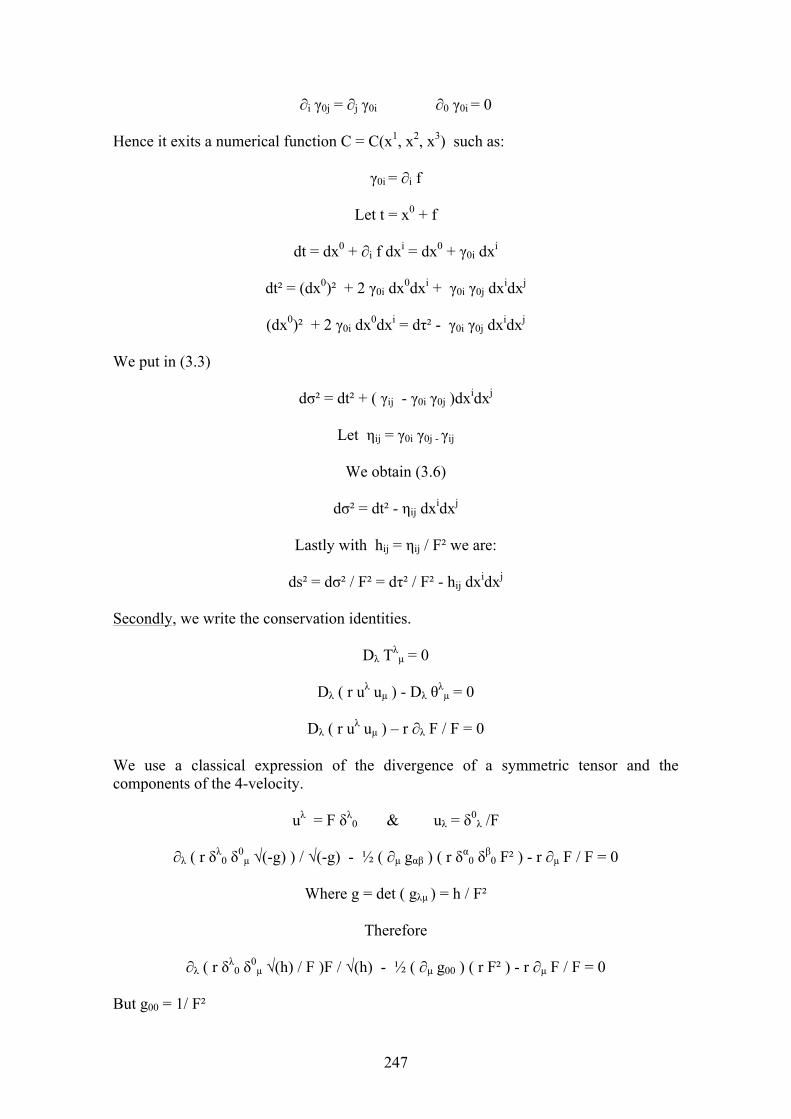
247
∂i γ0j = ∂j γ0i ∂0 γ0i = 0
Hence it exits a numerical function C = C(x1, x2, x3) such as:
γ0i = ∂i f
Let t = x0 + f
dt = dx0 + ∂i f dxi = dx0 + γ0i dxi
dt² = (dx0)² + 2 γ0i dx0dxi + γ0i γ0j dxidxj
(dx0)² + 2 γ0i dx0dxi = dτ² - γ0i γ0j dxidxj
We put in (3.3)
dσ² = dt² + ( γij - γ0i γ0j )dxidxj
Let ηij = γ0i γ0j - γij
We obtain (3.6)
dσ² = dt² - ηij dxidxj
Lastly with hij = ηij / F² we are:
ds² = dσ² / F² = dτ² / F² - hij dxidxj
Secondly, we write the conservation identities.
Dλ Tλµ = 0
Dλ ( r uλ uµ ) - Dλ θλµ = 0
Dλ ( r uλ uµ ) – r ∂λ F / F = 0
We use a classical expression of the divergence of a symmetric tensor and the components of the 4-velocity.
uλ = F δλ0 & uλ = δ0
λ /F
∂λ ( r δλ0 δ0
µ √(-g) ) / √(-g) - ½ ( ∂µ gαβ ) ( r δα0 δβ
0 F² ) - r ∂µ F / F = 0
Where g = det ( gλµ ) = h / F²
Therefore
∂λ ( r δλ0 δ0
µ √(h) / F )F / √(h) - ½ ( ∂µ g00 ) ( r F² ) - r ∂µ F / F = 0
But g00 = 1/ F²
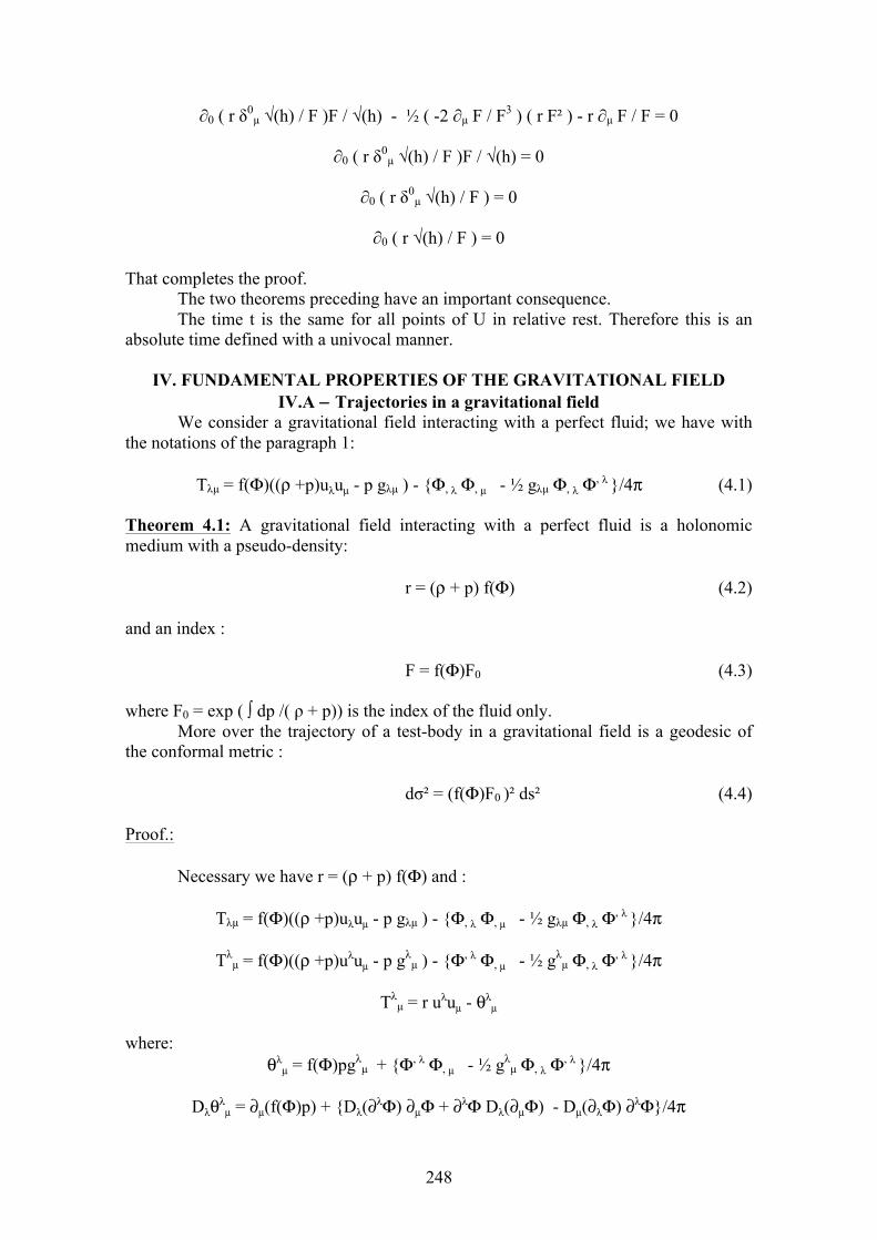
248
∂0 ( r δ0µ √(h) / F )F / √(h) - ½ ( -2 ∂µ F / F3 ) ( r F² ) - r ∂µ F / F = 0
∂0 ( r δ0µ √(h) / F )F / √(h) = 0
∂0 ( r δ0µ √(h) / F ) = 0
∂0 ( r √(h) / F ) = 0
That completes the proof. The two theorems preceding have an important consequence. The time t is the same for all points of U in relative rest. Therefore this is an
absolute time defined with a univocal manner.
IV. FUNDAMENTAL PROPERTIES OF THE GRAVITATIONAL FIELDIV.A − Trajectories in a gravitational field
We consider a gravitational field interacting with a perfect fluid; we have withthe notations of the paragraph 1:
Tλµ = f(Φ)((ρ +p)uλuµ - p gλµ ) - Φ, λ Φ, µ - ½ gλµ Φ, λ Φ, λ /4π (4.1)
Theorem 4.1: A gravitational field interacting with a perfect fluid is a holonomic medium with a pseudo-density:
r = (ρ + p) f(Φ) (4.2)
and an index :
F = f(Φ)F0 (4.3)
where F0 = exp ( ∫ dp /( ρ + p)) is the index of the fluid only. More over the trajectory of a test-body in a gravitational field is a geodesic of
the conformal metric :
dσ² = (f(Φ)F0 )² ds² (4.4)
Proof.:
Necessary we have r = (ρ + p) f(Φ) and :
Tλµ = f(Φ)((ρ +p)uλuµ - p gλµ ) - Φ, λ Φ, µ - ½ gλµ Φ, λ Φ, λ /4π
Tλµ = f(Φ)((ρ +p)uλuµ - p gλ
µ ) - Φ, λ Φ, µ - ½ gλµ Φ, λ Φ, λ
/4π
Tλµ = r uλuµ - θλ
µ
where: θλ
µ = f(Φ)pgλµ + Φ, λ Φ, µ - ½ gλ
µ Φ, λ Φ, λ /4π
Dλθλµ = ∂µ(f(Φ)p) + Dλ(∂λΦ) ∂µΦ + ∂λΦ Dλ(∂µΦ) - Dµ(∂λΦ) ∂λΦ/4π
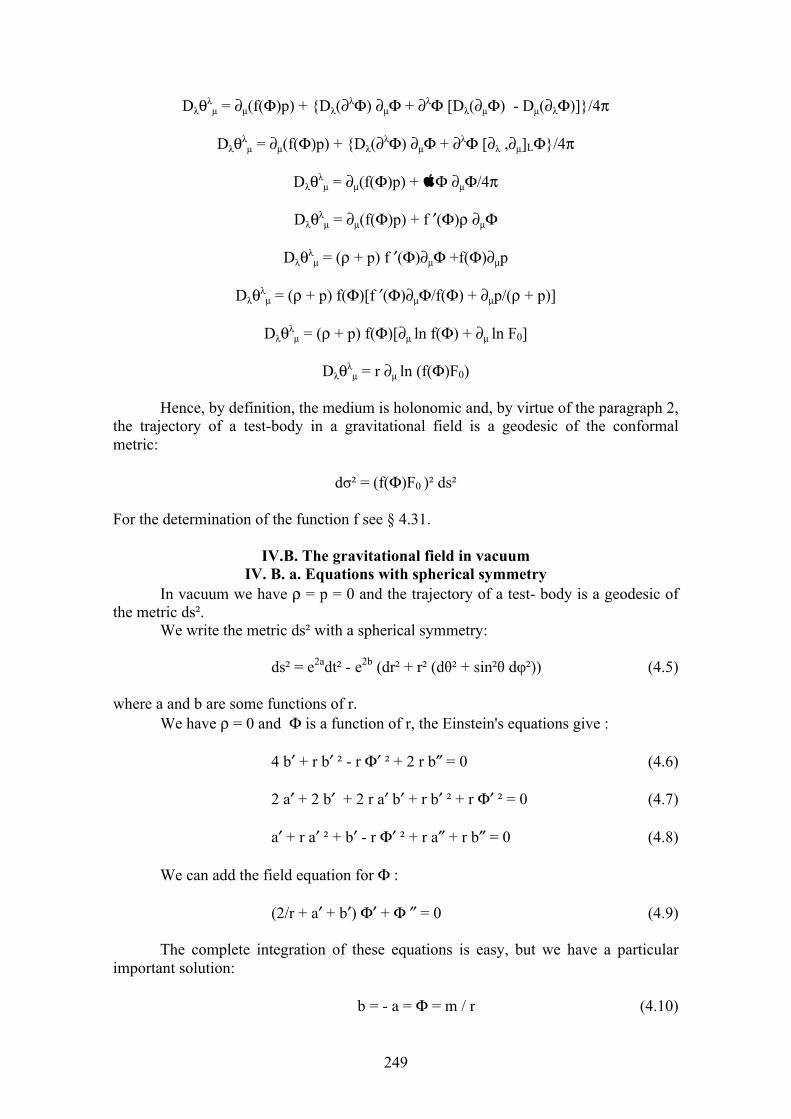
249
Dλθλµ = ∂µ(f(Φ)p) + Dλ(∂λΦ) ∂µΦ + ∂λΦ [Dλ(∂µΦ) - Dµ(∂λΦ)]/4π
Dλθλµ = ∂µ(f(Φ)p) + Dλ(∂λΦ) ∂µΦ + ∂λΦ [∂λ ,∂µ]LΦ/4π
Dλθλµ = ∂µ(f(Φ)p) + Φ ∂µΦ/4π
Dλθλµ = ∂µ(f(Φ)p) + f ′(Φ)ρ ∂µΦ
Dλθλµ = (ρ + p) f ′(Φ)∂µΦ +f(Φ)∂µp
Dλθλµ = (ρ + p) f(Φ)[f ′(Φ)∂µΦ/f(Φ) + ∂µp/(ρ + p)]
Dλθλµ = (ρ + p) f(Φ)[∂µ ln f(Φ) + ∂µ ln F0]
Dλθλµ = r ∂µ ln (f(Φ)F0)
Hence, by definition, the medium is holonomic and, by virtue of the paragraph 2, the trajectory of a test-body in a gravitational field is a geodesic of the conformal metric:
dσ² = (f(Φ)F0 )² ds²
For the determination of the function f see § 4.31.
IV.B. The gravitational field in vacuumIV. B. a. Equations with spherical symmetry
In vacuum we have ρ = p = 0 and the trajectory of a test- body is a geodesic of the metric ds².
We write the metric ds² with a spherical symmetry:
ds² = e2adt² - e2b (dr² + r² (dθ² + sin²θ dφ²)) (4.5)
where a and b are some functions of r. We have ρ = 0 and Φ is a function of r, the Einstein's equations give :
4 b′ + r b′ ² - r Φ′ ² + 2 r b″ = 0 (4.6)
2 a′ + 2 b′ + 2 r a′ b′ + r b′ ² + r Φ′ ² = 0 (4.7)
a′ + r a′ ² + b′ - r Φ′ ² + r a″ + r b″ = 0 (4.8)
We can add the field equation for Φ :
(2/r + a′ + b′) Φ′ + Φ ″ = 0 (4.9)
The complete integration of these equations is easy, but we have a particular important solution:
b = - a = Φ = m / r (4.10)
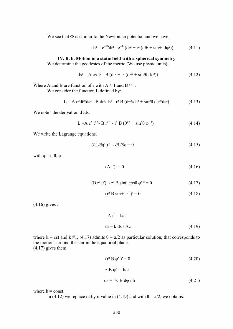
250
We see that Φ is similar to the Newtonian potential and we have:
ds² = e-2Φdt² - e2Φ (dr² + r² (dθ² + sin²θ dφ²)) (4.11)
IV. B. b. Motion in a static field with a spherical symmetryWe determine the geodesics of the metric (We use physic units):
ds² = A c²dt² - B (dr² + r² (dθ² + sin²θ dφ²)) (4.12)
Where A and B are function of r with A ≈ 1 and B ≈ 1. We consider the function L defined by:
L = A c²dt²/ds² - B dr²/ds² - r² B (dθ²/ds² + sin²θ dφ²/ds²) (4.13)
We note ′ the derivation d /ds.
L =A c² t′ ²- B r′ ² - r² B (θ′ ² + sin²θ φ′ ²) (4.14)
We write the Lagrange equations.
(∂L/∂q′ ) ′ - ∂L/∂q = 0 (4.15)
with q = t, θ, φ.
(A t′)′ = 0 (4.16)
(B r² θ′)′ - r² B sinθ cosθ φ′ ² = 0 (4.17)
(r² B sin²θ φ′ )′ = 0 (4.18)
(4.16) gives :
A t′ = k/c
dt = k ds / Ac (4.19)
where k = cst and k #1, (4.17) admits θ = π/2 as particular solution, that corresponds to the motions around the star in the equatorial plane. (4.17) gives then:
(r² B φ′ )′ = 0 (4.20)
r² B φ′ = h/c
ds = r²c B dφ / h (4.21)
where h = const. In (4.12) we replace dt by it value in (4.19) and with θ = π/2, we obtains:
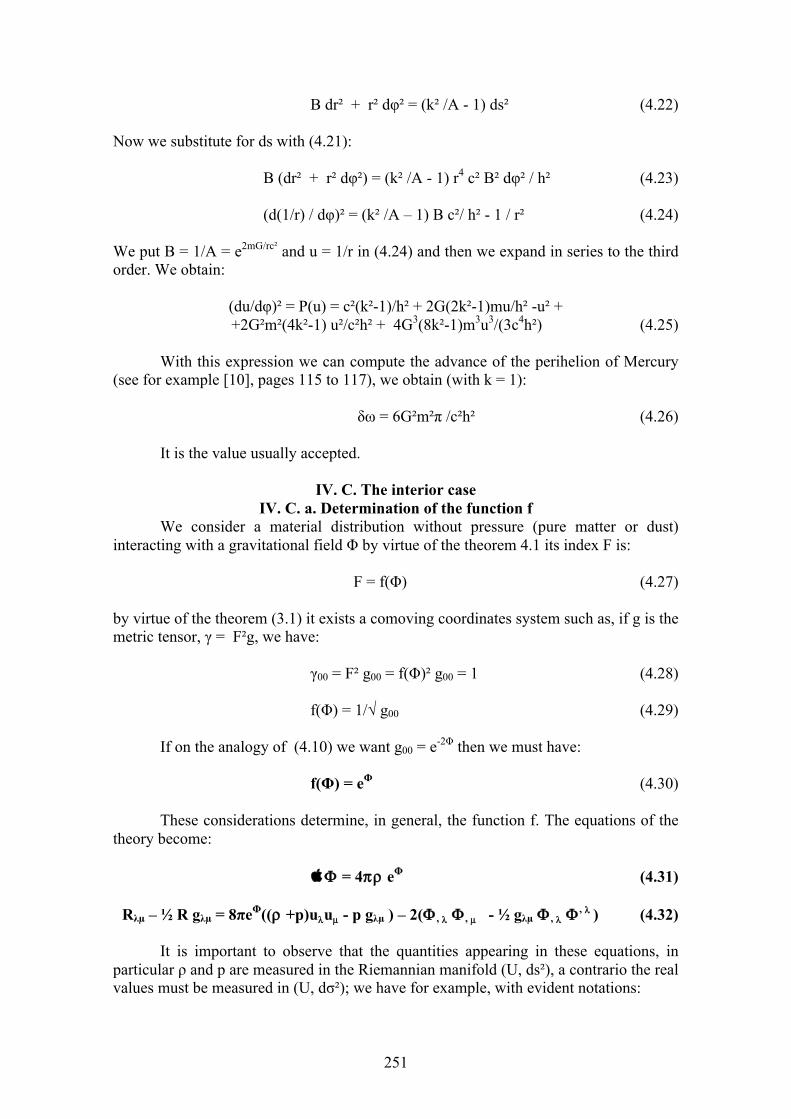
251
B dr² + r² dφ² = (k² /A - 1) ds² (4.22)
Now we substitute for ds with (4.21):
B (dr² + r² dφ²) = (k² /A - 1) r4 c² B² dφ² / h² (4.23)
(d(1/r) / dφ)² = (k² /A – 1) B c²/ h² - 1 / r² (4.24)
We put B = 1/A = e2mG/rc² and u = 1/r in (4.24) and then we expand in series to the third order. We obtain:
(du/dφ)² = P(u) = c²(k²-1)/h² + 2G(2k²-1)mu/h² -u² + +2G²m²(4k²-1) u²/c²h² + 4G3(8k²-1)m3u3/(3c4h²) (4.25)
With this expression we can compute the advance of the perihelion of Mercury (see for example [10], pages 115 to 117), we obtain (with k = 1):
δω = 6G²m²π /c²h² (4.26)
It is the value usually accepted.
IV. C. The interior caseIV. C. a. Determination of the function f
We consider a material distribution without pressure (pure matter or dust) interacting with a gravitational field Φ by virtue of the theorem 4.1 its index F is:
F = f(Φ) (4.27)
by virtue of the theorem (3.1) it exists a comoving coordinates system such as, if g is the metric tensor, γ = F²g, we have:
γ00 = F² g00 = f(Φ)² g00 = 1 (4.28)
f(Φ) = 1/√ g00 (4.29)
If on the analogy of (4.10) we want g00 = e-2Φ then we must have:
f(Φ) = eΦ (4.30)
These considerations determine, in general, the function f. The equations of the theory become:
Φ = 4πρ eΦ (4.31)
Rλµ – ½ R gλµ = 8πeΦ((ρ +p)uλuµ - p gλµ ) – 2(Φ , λ Φ , µ - ½ gλµ Φ , λ Φ , λ ) (4.32)
It is important to observe that the quantities appearing in these equations, in particular ρ and p are measured in the Riemannian manifold (U, ds²), a contrario the real values must be measured in (U, dσ²); we have for example, with evident notations:
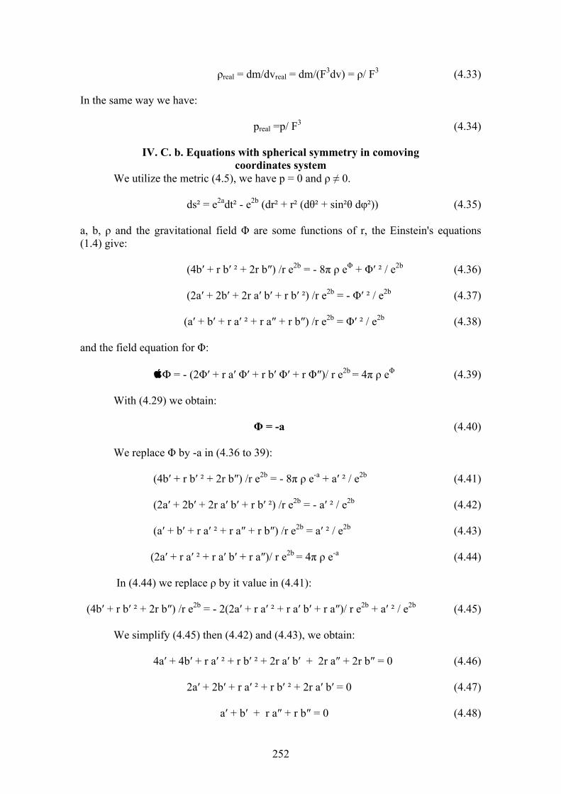
252
ρreal = dm/dvreal = dm/(F3dv) = ρ/ F3 (4.33)
In the same way we have:
preal =p/ F3 (4.34)
IV. C. b. Equations with spherical symmetry in comovingcoordinates system
We utilize the metric (4.5), we have p = 0 and ρ ≠ 0.
ds² = e2adt² - e2b (dr² + r² (dθ² + sin²θ dφ²)) (4.35)
a, b, ρ and the gravitational field Φ are some functions of r, the Einstein's equations (1.4) give:
(4b′ + r b′ ² + 2r b″) /r e2b = - 8π ρ eΦ + Φ′ ² / e2b (4.36)
(2a′ + 2b′ + 2r a′ b′ + r b′ ²) /r e2b = - Φ′ ² / e2b (4.37)
(a′ + b′ + r a′ ² + r a″ + r b″) /r e2b = Φ′ ² / e2b (4.38)
and the field equation for Φ:
Φ = - (2Φ′ + r a′ Φ′ + r b′ Φ′ + r Φ″)/ r e2b = 4π ρ eΦ (4.39)
With (4.29) we obtain:
Φ = -a (4.40)
We replace Φ by -a in (4.36 to 39):
(4b′ + r b′ ² + 2r b″) /r e2b = - 8π ρ e-a + a′ ² / e2b (4.41)
(2a′ + 2b′ + 2r a′ b′ + r b′ ²) /r e2b = - a′ ² / e2b (4.42)
(a′ + b′ + r a′ ² + r a″ + r b″) /r e2b = a′ ² / e2b (4.43)
(2a′ + r a′ ² + r a′ b′ + r a″)/ r e2b = 4π ρ e-a (4.44)
In (4.44) we replace ρ by it value in (4.41):
(4b′ + r b′ ² + 2r b″) /r e2b = - 2(2a′ + r a′ ² + r a′ b′ + r a″)/ r e2b + a′ ² / e2b (4.45)
We simplify (4.45) then (4.42) and (4.43), we obtain:
4a′ + 4b′ + r a′ ² + r b′ ² + 2r a′ b′ + 2r a″ + 2r b″ = 0 (4.46)
2a′ + 2b′ + r a′ ² + r b′ ² + 2r a′ b′ = 0 (4.47)
a′ + b′ + r a″ + r b″ = 0 (4.48)
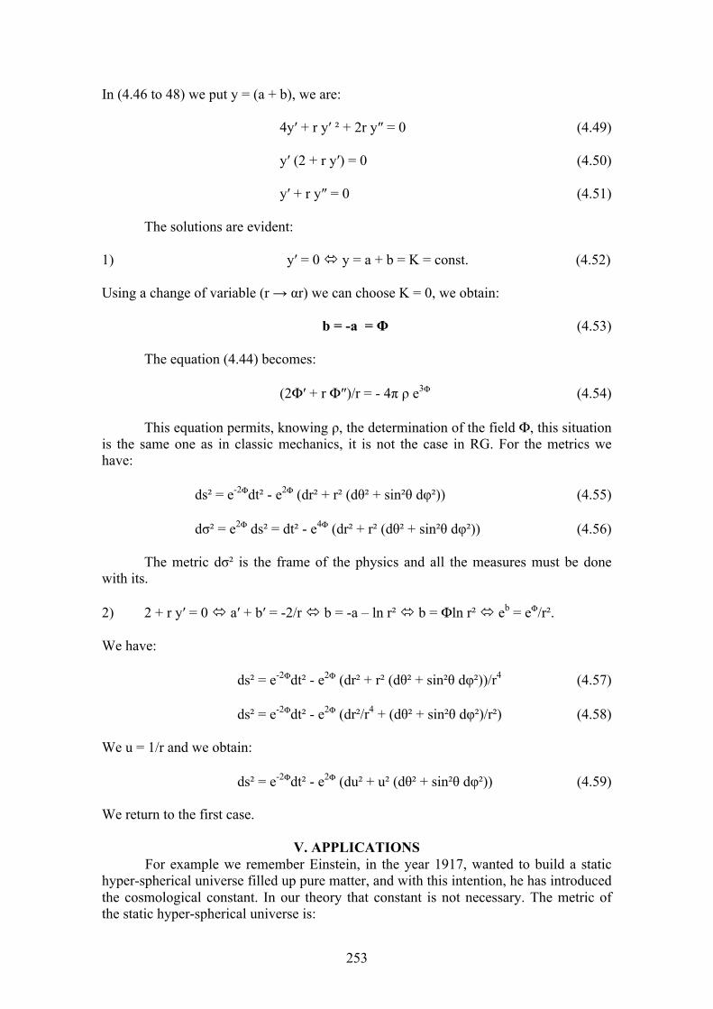
253
In (4.46 to 48) we put y = (a + b), we are:
4y′ + r y′ ² + 2r y″ = 0 (4.49)
y′ (2 + r y′) = 0 (4.50)
y′ + r y″ = 0 (4.51)
The solutions are evident:
1) y′ = 0 ó y = a + b = K = const. (4.52)
Using a change of variable (r → αr) we can choose K = 0, we obtain:
b = -a = Φ (4.53)
The equation (4.44) becomes:
(2Φ′ + r Φ″)/r = - 4π ρ e3Φ (4.54)
This equation permits, knowing ρ, the determination of the field Φ, this situation is the same one as in classic mechanics, it is not the case in RG. For the metrics we have:
ds² = e-2Φdt² - e2Φ (dr² + r² (dθ² + sin²θ dφ²)) (4.55)
dσ² = e2Φ ds² = dt² - e4Φ (dr² + r² (dθ² + sin²θ dφ²)) (4.56)
The metric dσ² is the frame of the physics and all the measures must be done with its.
2) 2 + r y′ = 0 ó a′ + b′ = -2/r ó b = -a – ln r² ó b = Φln r² ó eb = eΦ/r².
We have:
ds² = e-2Φdt² - e2Φ (dr² + r² (dθ² + sin²θ dφ²))/r4 (4.57)
ds² = e-2Φdt² - e2Φ (dr²/r4 + (dθ² + sin²θ dφ²)/r²) (4.58)
We u = 1/r and we obtain:
ds² = e-2Φdt² - e2Φ (du² + u² (dθ² + sin²θ dφ²)) (4.59)
We return to the first case.
V. APPLICATIONS For example we remember Einstein, in the year 1917, wanted to build a static
hyper-spherical universe filled up pure matter, and with this intention, he has introduced the cosmological constant. In our theory that constant is not necessary. The metric of the static hyper-spherical universe is:
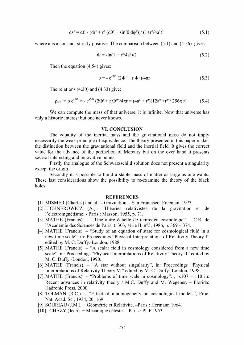
254
ds² = dt² - (dr² + r² (dθ² + sin²θ dφ²))/ (1+r²/4a²)² (5.1)
where a is a constant strictly positive. The comparison between (5.1) and (4.56) gives:
Φ = -ln(1 + r²/4a²)/2 (5.2)
Then the equation (4.54) gives:
ρ = - e-3Φ (2Φ′ + r Φ″)/4πr (5.3)
The relations (4.30) and (4.33) give:
ρreal = ρ e-3Φ = - e-6Φ (2Φ′ + r Φ″)/4πr = (4a² + r²)(12a² +r²)/ 256π a6 (5.4)
We can compute the mass of that universe, it is infinite. Now that universe has only a historic interest but one never knows.
VI. CONCLUSIONThe equality of the inertial mass and the gravitational mass do not imply
necessarily the weak principle of equivalence. The theory presented in this paper makes the distinction between the gravitational field and the inertial field. It gives the correct value for the advance of the perihelion of Mercury but on the over hand it presents several interesting and innovative points.
Firstly the analogue of the Schwarzschild solution does not present a singularity except the origin.
Secondly it is possible to build a stable mass of matter as large as one wants. These last considerations show the possibility to re-examine the theory of the black holes.
REFERENCES [1]. MISMER (Charles) and all. - Gravitation. - San Francisco: Freeman, 1973. [2]. LICHNEROWICZ (A.).– Théories relativistes de la gravitation et de
l’electromgnétisme. - Paris : Masson, 1955, p. 71. [3]. MATHE (Francis). – “ Une autre échelle de temps en cosmologie”. – C.R. de
l’Académie des Sciences de Paris, t. 303, série II, n°5, 1986, p. 369 – 374. [4]. MATHE (Francis). – “Study of an equation of state for cosmological fluid in a
new time scale”, in: Proceedings “Physical Interpretations of Relativity Theory I” edited by M. C. Duffy.-London, 1988.
[5]. MATHE (Francis). – “A scalar field in cosmology considered from a new time scale”, in: Proceedings “Physical Interpretations of Relativity Theory II” edited by M. C. Duffy.-London, 1990.
[6]. MATHE (Francis). – “A star without singularity”, in: Proceedings “Physical Interpretations of Relativity Theory VI” edited by M. C. Duffy.-London, 1998.
[7]. MATHE (Francis). – “Problems of time scale in cosmology”. , p.107 – 110 in: Recent advances in relativity theory / M.C. Duffy and M. Wegener. – Florida: Hadronic Press, 2000.
[8]. TOLMAN (R.C.). – “Effect of inhomogeneity on cosmological models”, Proc. Nat. Acad. Sc., 1934, 20, 169
[9]. SOURIAU (J.M.). − Géométrie et Relativité. –Paris : Hermann 1964. [10]. CHAZY (Jean). − Mécanique céleste. – Paris : PUF 1953.
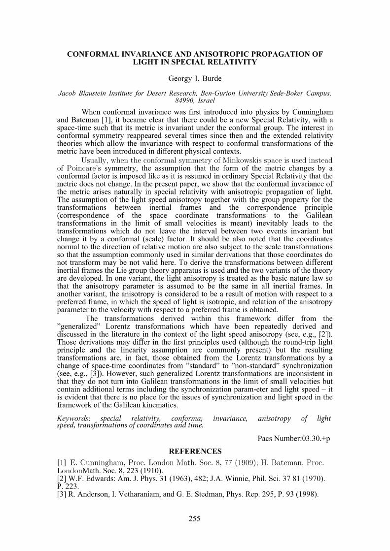
CONFORMAL INVARIANCE AND ANISOTROPIC PROPAGATION OF LIGHT IN SPECIAL RELATIVITY
Georgy I. Burde
Jacob Blaustein Institute for Desert Research, Ben-Gurion University Sede-Boker Campus, 84990, Israel
When conformal invariance was first introduced into physics by Cunningham and Bateman [1], it became clear that there could be a new Special Relativity, with a space-time such that its metric is invariant under the conformal group. The interest in conformal symmetry reappeared several times since then and the extended relativity theories which allow the invariance with respect to conformal transformations of the metric have been introduced in different physical contexts.
Usually, when the conformal symmetry of Minkowskis space is used insteadof Poincare’s symmetry, the assumption that the form of the metric changes by a conformal factor is imposed like as it is assumed in ordinary Special Relativity that the metric does not change. In the present paper, we show that the conformal invariance of the metric arises naturally in special relativity with anisotropic propagation of light. The assumption of the light speed anisotropy together with the group property for the transformations between inertial frames and the correspondence principle (correspondence of the space coordinate transformations to the Galilean transformations in the limit of small velocities is meant) inevitably leads to the transformations which do not leave the interval between two events invariant but change it by a conformal (scale) factor. It should be also noted that the coordinates normal to the direction of relative motion are also subject to the scale transformations so that the assumption commonly used in similar derivations that those coordinates do not transform may be not valid here. To derive the transformations between differentinertial frames the Lie group theory apparatus is used and the two variants of the theory are developed. In one variant, the light anisotropy is treated as the basic nature law so that the anisotropy parameter is assumed to be the same in all inertial frames. In another variant, the anisotropy is considered to be a result of motion with respect to a preferred frame, in which the speed of light is isotropic, and relation of the anisotropy parameter to the velocity with respect to a preferred frame is obtained.
The transformations derived within this framework differ from the ”generalized” Lorentz transformations which have been repeatedly derived and discussed in the literature in the context of the light speed anisotropy (see, e.g., [2]). Those derivations may differ in the first principles used (although the round-trip lightprinciple and the linearity assumption are commonly present) but the resulting transformations are, in fact, those obtained from the Lorentz transformations by a change of space-time coordinates from ”standard” to ”non-standard” synchronization (see, e.g., [3]). However, such generalized Lorentz transformations are inconsistent in that they do not turn into Galilean transformations in the limit of small velocities but contain additional terms including the synchronization param-eter and light speed – it is evident that there is no place for the issues of synchronization and light speed in the framework of the Galilean kinematics.
REFERENCES[1] E. Cunningham, Proc. London Math. Soc. 8, 77 (1909); H. Bateman, Proc. LondonMath. Soc. 8, 223 (1910).[2] W.F. Edwards: Am. J. Phys. 31 (1963), 482; J.A. Winnie, Phil. Sci. 37 81 (1970). P. 223.[3] R. Anderson, I. Vetharaniam, and G. E. Stedman, Phys. Rep. 295, P. 93 (1998).
Keywords: special relativity, conforma; invariance, anisotropy of light speed, transformations of coordinates and time.
Pacs Number:03.30.+p
255
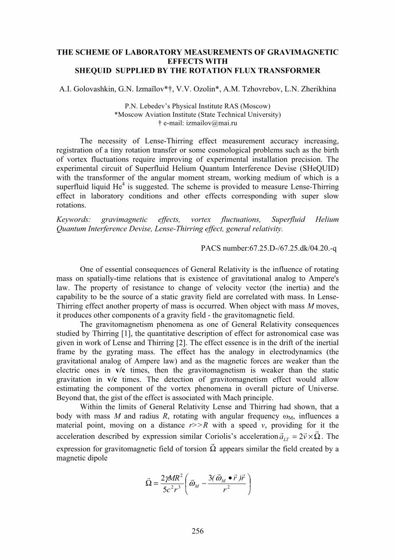
256
THE SCHEME OF LABORATORY MEASUREMENTS OF GRAVIMAGNETIC EFFECTS WITH
SHEQUID SUPPLIED BY THE ROTATION FLUX TRANSFORMER
A.I. Golovashkin, G.N. Izmaїlov*†, V.V. Ozolin*, A.M. Tzhovrebov, L.N. Zherikhina
P.N. Lebedev’s Physical Institute RAS (Moscow) *Moscow Aviation Institute (State Technical University)
† e-mail: [email protected]
The necessity of Lense-Thirring effect measurement accuracy increasing, registration of a tiny rotation transfer or some cosmological problems such as the birth of vortex fluctuations require improving of experimental installation precision. The experimental circuit of Superfluid Helium Quantum Interference Devise (SHeQUID) with the transformer of the angular moment stream, working medium of which is a superfluid liquid He4 is suggested. The scheme is provided to measure Lense-Thirring effect in laboratory conditions and other effects corresponding with super slow rotations.
Keywords: gravimagnetic effects, vortex fluctuations, Superfluid Helium Quantum Interference Devise, Lense-Thirring effect, general relativity.
PACS number:67.25.D-/67.25.dk/04.20.-q
One of essential consequences of General Relativity is the influence of rotating mass on spatially-time relations that is existence of gravitational analog to Ampere's law. The property of resistance to change of velocity vector (the inertia) and the capability to be the source of a static gravity field are correlated with mass. In Lense-Thirring effect another property of mass is occurred. When object with mass M moves, it produces other components of a gravity field - the gravitomagnetic field.
The gravitomagnetism phenomena as one of General Relativity consequences studied by Thirring [1], the quantitative description of effect for astronomical case was given in work of Lense and Thirring [2]. The effect essence is in the drift of the inertial frame by the gyrating mass. The effect has the analogy in electrodynamics (the gravitational analog of Ampere law) and as the magnetic forces are weaker than the electric ones in v/c times, then the gravitomagnetism is weaker than the static gravitation in v/c times. The detection of gravitomagnetism effect would allow estimating the component of the vortex phenomena in overall picture of Universe. Beyond that, the gist of the effect is associated with Mach principle.
Within the limits of General Relativity Lense and Thirring had shown, that a body with mass M and radius R, rotating with angular frequency ωM, influences a material point, moving on a distance r>>R with a speed ν, providing for it the acceleration described by expression similar Coriolis’s acceleration Ω×=
!!! vaLT 2 . The expression for gravitomagnetic field of torsion Ω
! appears similar the field created by a
magnetic dipole
⎟⎠⎞⎜
⎝⎛ •
−=Ω 232
2 352
rr)r(
rcMR M
M
!!!!! ωωγ

257
and it is justified the term gravitomagnetism. If the axis of rotation of a body M lies in the plane of an orbit of the material
point then the last experiences an influence of gravitomagnetic forces when the point moves near to the poles - crossing points of the axis of rotation and the orbit. Being gyroscopic, these forces cause precession, i.e. turn of its plane around of an axis of rotation M. For example, rotation of the Earth leads to slow turn of a plane of an orbit of the artificial satellite around of a terrestrial axis with a speed approximately equal to
⊕−
⊕
⊕⊕⊕Ω ωωγ 10
2 10~Rc
M~ .
The formula for Lenze-Tirring effect, produced by a rotating body at the distance r much more then its own size R, gives the right order of magnitude of the effect in the vicinity of the body (i.e. in case of r≈R) and was used for the above evaluation of Ω.
Schiff suggestion [3], developed by Everitt [4], was based on the mechanical proof of an effect existence. It was also suggested to check this effect in electrodynamics experiments. In particular, to check precisely the dependence of a light frequency deviation as a function of an angular velocity of the ring interferometers, because of Lense-Thirring effect. It resembles with Sagnac effect (but the effect is fewer by ten orders of when angle measurements on rotary Earth are carried out) [5]. There are the performing variants of processing of experimental result on gravitational lensing taking into account Lense-Thirring effect [6].
Recently the successful checking of Lense-Thirring effect in a space experiment has been held [7]. Over next eleven years during LAGEOS program, the drift of the gyroscope located on a satellite was observed. The satellite orbited (there were two satellites really) at an altitude of about 12200 km. The rotary Earth mass causes the turning of the coordinate system, connected with the satellite. The angular rotation resulted in the drift of a gyroscope axis relative to a suspension system, which was joined with satellite housing. Let us mention that the subtle magnitude of the effect (~10-10
⊕ω ) makes the particular demands for high precision of the gyroscope itself and to noises of an installation.
In fact, it is needed to provide new precise and another way of looking, so, we discuss new experiments with the promising sensitivity reserve here. The experimental circuit of quantum interferometer, supplied by the transformer of the angular moment stream, using the superfluid state of He4 (or He3) is offered. We expect that the application of modern technology will provide the adequate experimental accuracy.
Several experiments of registration of small angular speeds are known [8, 9]. As the part of a plant the gyroscope is under construction on the basis of «superfluid analogue» sensitive ring DC-SQUID. The nano-throttles or nano-apertures or their arrays play the role of Josephson tunnel junctions in such interferometers. However, the area of a registering ring appears is limited by the micron sizes, that essentially limits sensitivity interferometer at measurements of angular speeds of turns. This annoying restriction occurs due to the lack of analogue of the superconducting transformer of the stream entering as a necessary functional element in any efficient SQUID magnetometer in such scheme,.
As it known [10] Не4 transfers into the superfluid state at temperatures T<Tλ=2.17К (below λ-point) and in these conditions the macroscopic coherent effects occur in helium. Such effects are good for the dissipationless processes, i.e. the
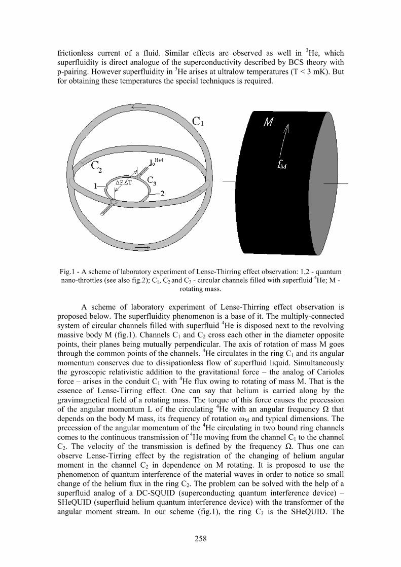
258
frictionless current of a fluid. Similar effects are observed as well in 3He, which superfluidity is direct analogue of the superconductivity described by BCS theory with p-pairing. However superfluidity in 3He arises at ultralow temperatures (T < 3 mK). But for obtaining these temperatures the special techniques is required.
Fig.1 - A scheme of laboratory experiment of Lense-Thirring effect observation: 1,2 - quantum nano-throttles (see also fig.2); C1, C2 and C3 - circular channels filled with superfluid 4He; M -
rotating mass.
A scheme of laboratory experiment of Lense-Thirring effect observation is proposed below. The superfluidity phenomenon is a base of it. The multiply-connected system of circular channels filled with superfluid 4He is disposed next to the revolving massive body M (fig.1). Channels C1 and C2 cross each other in the diameter opposite points, their planes being mutually perpendicular. The axis of rotation of mass M goes through the common points of the channels. 4He circulates in the ring C1 and its angular momentum conserves due to dissipationless flow of superfluid liquid. Simultaneously the gyroscopic relativistic addition to the gravitational force – the analog of Carioles force – arises in the conduit C1 with 4He flux owing to rotating of mass M. That is the essence of Lense-Tirring effect. One can say that helium is carried along by the gravimagnetical field of a rotating mass. The torque of this force causes the precession of the angular momentum L of the circulating 4He with an angular frequency Ω that depends on the body M mass, its frequency of rotation ωM and typical dimensions. The precession of the angular momentum of the 4He circulating in two bound ring channels comes to the continuous transmission of 4He moving from the channel C1 to the channel C2. The velocity of the transmission is defined by the frequency Ω. Thus one can observe Lense-Tirring effect by the registration of the changing of helium angular moment in the channel C2 in dependence on M rotating. It is proposed to use the phenomenon of quantum interference of the material waves in order to notice so small change of the helium flux in the ring C2. The problem can be solved with the help of a superfluid analog of a DC-SQUID (superconducting quantum interference device) – SHeQUID (superfluid helium quantum interference device) with the transformer of the angular moment stream. In our scheme (fig.1), the ring C3 is the SHeQUID. The
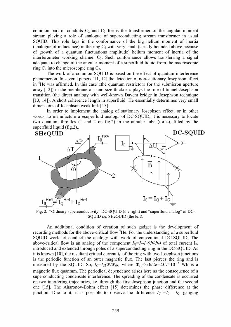
259
common part of conduits C2 and C3 forms the transformer of the angular moment stream playing a role of analogue of superconducting stream transformer in usual SQUID. This role lays in the conformance of the big helium moment of inertia (analogue of inductance) in the ring C2 with very small (strictly bounded above because of growth of a quantum fluctuations amplitude) helium moment of inertia of the interferometer working channel C3. Such conformance allows transferring a signal adequate to change of the angular moment of a superfluid liquid from the macroscopic ring C2 into the microscopic ring C3.
The work of a common SQUID is based on the effect of quantum interference phenomenon. In several papers [11, 12] the detection of non-stationary Josephson effect in 4Не was affirmed. In this case «the quantum restrictor» (or the submicron aperture array [12]) in the membrane of nano-size thickness plays the role of tunnel Josephson transition (the direct analogy with well-known Dayem bridge in Josephson technique [13, 14]). A short coherence length in superfluid 4Не essentially determines very small dimensions of Josephson weak link [15].
In order to implement the analog of stationary Josephson effect, or in other words, to manufacture a «superfluid analog» of DC-SQUID, it is necessary to locate two quantum throttles (1 and 2 on fig.2) in the annular tube (torus), filled by the superfluid liquid (fig.2),.
Fig. 2. “Ordinary superconductivity” DC-SQUID (the right) and “superfluid analog” of DC-SQUID i.e. SHeQUID (the left).
An additional condition of creation of such gadget is the development of recording methods for the above-critical flow 4Не. For the understanding of a superfluid SQUID work let conduct the analogy with work of conventional DC-SQUID. The above-critical flow is an analog of the component IQ=I0-IC(Ф/Ф0) of total current I0, introduced and extended through poles of a superconducting ring in the DC-SQUID. As it is known [10], the resultant critical current IC of the ring with two Josephson junctions is the periodic function of an outer magnetic flux. The last pierces the ring and is measured by the SQUID. So, IC=IC(Ф/Ф0), where Фo=2πħ/2е=2.07×10-15 Wb is amagnetic flux quantum. The periodical dependence arises here as the consequence of a superconducting condensate interference. The spreading of the condensate is occurred on two interfering trajectories, i.e. through the first Josephson junction and the second one [15]. The Aharonov-Bohm effect [15] determines the phase difference at the junction. Due to it, it is possible to observe the difference IC =I0 - IQ, gauging
260
component IQ when fixed I0. Then the value of magnetic flux Ф to accuracy of integer quantum Ф0 [15] is determined also.
The registration of a component IQHe4 when fixed total flow of helium I0
He4 (on fig.2 components are labeled by «large» arrows) will allow us to determine superfluid component of helium flow IC
He4 and its phase. The phase implies the information on parameters, measured by SHeQUID. The process of IQ
He4 registration can be based either on the detection of pressure differential, arising when helium flows through a weak link, or on the detection of heat transfer by excitations of above-critical component (there is no entropy of superfluid component) (see fig.2). In the first process, the pressure difference ΔP between inlet and outlet of the ring can be measured. If one applies the pressure differential to the third weak link, then because of non-stationary Josephson effect the acoustic vibrations must be generated. The Josephson frequency Ω is proportional to ΔP. It should be emphasized that according to elementary theory of non-stationary Josephson effect [10] amplitude of these oscillations P0 has to be much less than ΔP. The realistic estimations of P0 point on need for developing of a high-sensitive microphone, which is able to pick up the acoustic vibrations with amplitude at the level of fraction of pikoPascals [16]. In the second, it is possible to measure the entropy growth, transferred by above-critical current component IQ
He4 at the exit from the ring of the superfluid interferometer thermally connected with the working medium of magnetocalorimeter [17, 18].
What parameters and signals SHeQUID can measure? In conditions of super fluidity, it is difficult to find the direct analog of magnetic field [19, 20]; however, it is possible to examine the difference of quantum phases, describing the coherent states, in both devices. The phase difference, determining the resultant critical current IC=IC(φ) in conventional SQUID, is identified as
rdAqprd !!!"
!!"
)(110 ∫∫ −=Ρ=−ϕϕ .
The conventional superconducting SQUID responds to the second term in contour integral (q=2e is the charge of Cooper pair). If the magnetic field is threading the SQUID ring, then with the help of Stokes theorem, it is possible to pass from vector potential A
! to flux density B
!. Next, relate it to a magnetic flux quantum:
0
22ΦΦ== ∫∫∫
πSdBerdAq !!
"!!
".
At the same time, the contribution of the first term to integral can be excluded as the result of the gauge transformation. In super fluidity of 4He case the integrand appears to be a single, because q=0. Under the condition of 4He a rotation (real or imaginary with angular frequency ω) along the toroidal pipe with radius r the angular momentum of helium with mass m will amount to p=mωr, but
θrdrd =! ,
where0<θ<2π. At that, the circulation can be correlated to Planck constant ħ through the momentum of superfluid He Λ
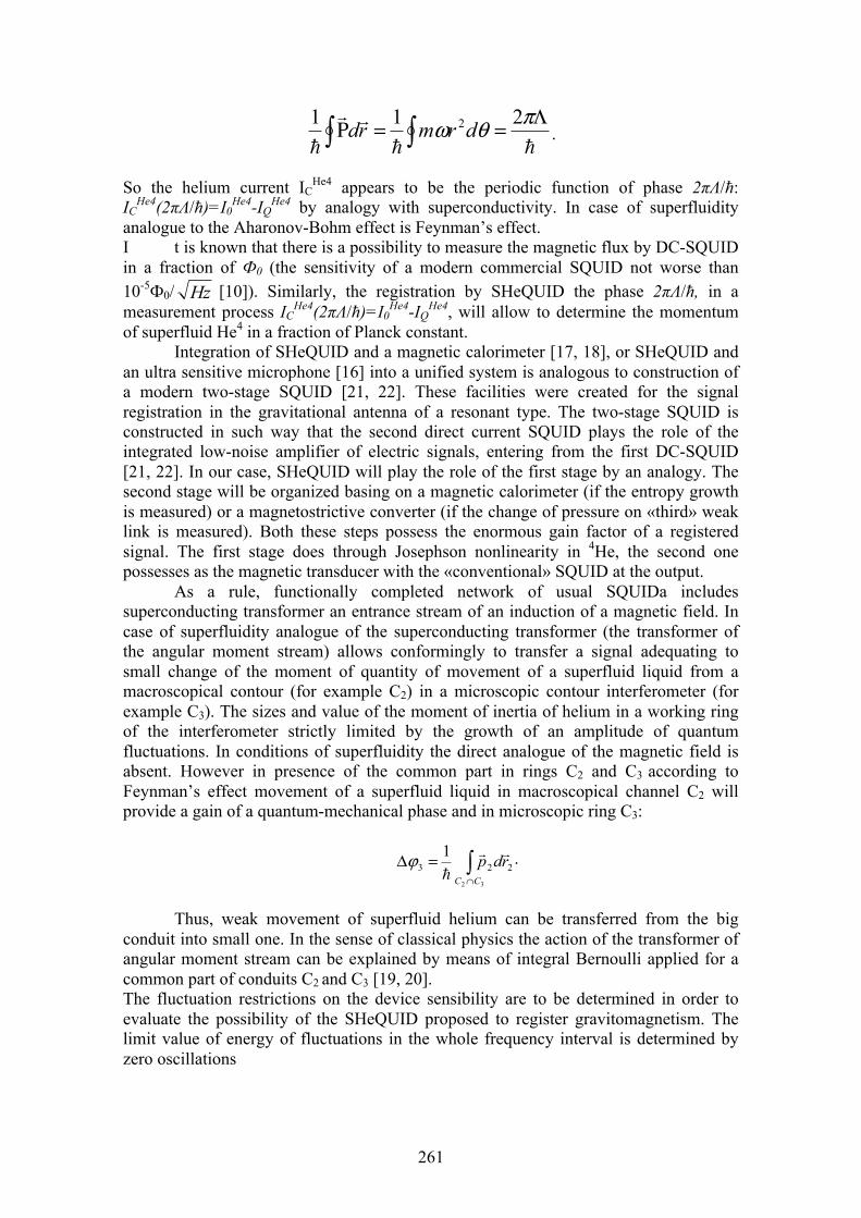
261
!!""
!Λ==Ρ ∫∫
πθω 211 2drmrd .
So the helium current IСHe4 appears to be the periodic function of phase 2πΛ/ħ:
IСHe4(2πΛ/ħ)=I0
He4-IQHe4 by analogy with superconductivity. In case of superfluidity
analogue to the Aharonov-Bohm effect is Feynman’s effect. I t is known that there is a possibility to measure the magnetic flux by DC-SQUID in a fraction of Ф0 (the sensitivity of a modern commercial SQUID not worse than10-5Ф0/ Hz [10]). Similarly, the registration by SHeQUID the phase 2πΛ/ħ, in a measurement process IС
He4(2πΛ/ħ)=I0He4-IQ
He4, will allow to determine the momentum of superfluid He4 in a fraction of Planck constant.
Integration of SHeQUID and a magnetic calorimeter [17, 18], or SHeQUID and an ultra sensitive microphone [16] into a unified system is analogous to construction of a modern two-stage SQUID [21, 22]. These facilities were created for the signal registration in the gravitational antenna of a resonant type. The two-stage SQUID is constructed in such way that the second direct current SQUID plays the role of the integrated low-noise amplifier of electric signals, entering from the first DC-SQUID [21, 22]. In our case, SHeQUID will play the role of the first stage by an analogy. The second stage will be organized basing on a magnetic calorimeter (if the entropy growth is measured) or a magnetostrictive converter (if the change of pressure on «third» weak link is measured). Both these steps possess the enormous gain factor of a registered signal. The first stage does through Josephson nonlinearity in 4He, the second one possesses as the magnetic transducer with the «conventional» SQUID at the output.
As a rule, functionally completed network of usual SQUIDа includes superconducting transformer an entrance stream of an induction of a magnetic field. In case of superfluidity analogue of the superconducting transformer (the transformer of the angular moment stream) allows conformingly to transfer a signal adequating to small change of the moment of quantity of movement of a superfluid liquid from a macroscopical contour (for example C2) in a microscopic contour interferometer (for example C3). The sizes and value of the moment of inertia of helium in a working ring of the interferometer strictly limited by the growth of an amplitude of quantum fluctuations. In conditions of superfluidity the direct analogue of the magnetic field is absent. However in presence of the common part in rings C2 and C3 according to Feynman’s effect movement of a superfluid liquid in macroscopical channel C2 will provide a gain of a quantum-mechanical phase and in microscopic ring C3:
223
32
1 rdpCC
!!" ∫
∩
=Δϕ .
Thus, weak movement of superfluid helium can be transferred from the big conduit into small one. In the sense of classical physics the action of the transformer of angular moment stream can be explained by means of integral Bernoulli applied for a common part of conduits C2 and C3 [19, 20]. The fluctuation restrictions on the device sensibility are to be determined in order to evaluate the possibility of the SHeQUID proposed to register gravitomagnetism. The limit value of energy of fluctuations in the whole frequency interval is determined by zero oscillations
262
∫∫∀∀
=ωω
ω dndE2! ,
where the normalization of quantum filling, characterizing the system excitation,
1=∫∀ω
dn .
The fluctuation spectral density looks like the following way
2
21
2⎟⎠⎞⎜
⎝⎛ ><==
δωδ
δωδω
δωδ l
JnE ! ,
where <δl> is the mean square amplitude of angular momentum fluctuations, and J is the moment of inertia of superfluid helium in the working ring of SHeQUID C3. In the case of “white” quantum noise the fluctuation energy is uniformly distributed over the whole frequency interval and
ωω
δωδ
ωω
1== ∫∫∀∀
ddnn .
Then the fluctuation restriction of the angular momentum measurements accuracy would occur at the level
Jl!=><
δωδ .
However, if the spectrum of the fluctuation excitations is a single mode of frequency ω0 and a characteristic quality factor Q, then far from ω0, ω<<ω0, i.e. on “the resonance tail” another relationship would be valid
20
1Q
nωδω
δ = .
Using the later we get the spectral density
2
2 211
2⎟⎠⎞⎜
⎝⎛ ><=⋅=
δωδ
δωδ l
JQE !
and hence the fluctuation restriction of the angular momentum measurements accuracy on the level
QJl !=><
δωδ .
It means that the limit accuracy of the angular momentum measurements
263
Hzl !=><δωδ ,
when Q=100, could be achieved with the moment of inertia J of superfluid helium in the ring C3 of the order of J≈10-30 m2kg. Due to the definite construction conditions and above evaluations of J the ring C3 (fig.1) should have the ellipse shape with axis lengths 4 and 1 µm correspondingly and the channel diameter 0.1 µm. The creation of a closed channel with such dimensions, containing two weak links is achievable on the modern level of nanotechnology. The estimations of parameters of the scheme based on SHeQUID (fig.1) for laboratory observations of Lense-Thirring effect are given below. The stored angular momentum L of superfluid 4He circulating in the ring channel C1 is equal to L=1031ћ, when the ring diameter D=1 m, helium mass m=10 g and helium velocity v=30 cm/s. Channel C1 is crossed in the diameter opposite points by another ring channel C2. Cross sections of channels C2 and C3 are of the same order of magnitude. Channels C2 and C3 have common length s about 0.3 µm. The phase difference on this length, appeared due to the helium flowing in C2, determines the result interference of the matter waves in the microscopic channel C3 of the interferometer. Hence, the signal could appear in the SHeQUID the possibility of which registration were considered above. The massive body (M=100 kg, characteristic size R=1 m) rotating with frequency fM generates in the channel C1 the relativistic gyroscope force, that corresponds to Lense-Thirring effect. The torque of this force causes the turn of helium plane of circulation with angular velocity
232 1052 −⋅≈=Ω
RcMfMπγ rad/s,
when fм≈100 Hz. In the geometry of the installation the turn of the helium circulation plane means the redistribution of angular moment between channels C1 and C2: the rotation will be transmitted from the first ring into the second one with the velocity determined by Ω. The angular momentum, arising in the ring C2, acts through the common length of the channels C2 and C3 upon the phase in the SHeQUID ring and causes the stationary phase drift, that corresponds to the enhancement of the angular momentum l in the ring C3 with the velocity approximately
sLR
sdtdl
!302
≈Ω=π
.
This drift can be registered by the SHeQUID with noise restriction on the level
Hzl !=><δωδ
(the possibility of creation of such interferometer was shown above). Thus one can observe Lense-Thirring effect in the laboratory conditions by the registration of the SHeQUID output signal appearing when a massive body is set in rotation and disappearing when it stops.

264
REFERENCES [1]. Thirring H. Phys. Ztschr. 19, 33 (1918); ibid. 22, 29 (1921). [2]. Thirring H., Lense J. Phys. Ztschr. 19, 156 (1918). [3]. Schiff L.I. Proc. Natl. Acad. Sci. U.S.A. 46, 871 (1960); Phys.Rev.Lettr. 4, 215
(1960). [4]. Everitt C.W.R. In: Experimental Gravitation Proc. of Course 56 of the Intern.
School of Physics “E.Fermi”, ed. B.Bertotti, p. 331. Academic, N.Y. (1974). [5]. Scully M.O., Zubary M.S., Haugan M.P. Phys. Rev. A24, 2009 (1981). [6]. Ciufolini I., Ricci F. http://www.arXiv: gr-qc/0301030 v1. [7]. Neil Ashby Nature 431 918 (2004); Ciufolini I., Pavlis E. C. Nature 431, 958
(2004). [8]. Y. Sato, E. Hoskinson, and R. E. Packard. Phys. Rev. B 74, 144502 (2006) [9]. Y. Sato, A. Joshi, and R. Packard, Appl. Phys. Lett. 91, 074107 (2007) [10]. Tilley D.R., Tilley J. Superfluidity and Superconductivity (New York,
Cincinnati, Toronto, London, Melbourne: Van Nostrand Reinhold Company, 1974). [11]. Richards P.L., Anderson .W. Phys. Rev. Lett., 14, 540 (1965). [12]. Hoskinson E., Packard R.E., Haard Th.M. Nature, 433, 376, (2005). [13]. Superconductor Applications: SQUIDs and Machines. Eds. Br. B. Schwartzand [14]. Likharev K.K., Ulrikh B.T. Systems with Josephson contacts. Moscow Univ.
Press (1978). [15]. Feynman R.P. Statistical mechanics. W.A.Benjamin Inc., Advanced Book
Program Reading, Massachusetts, (1972). [16]. Golovashkin A.I., Gudenko A.V., Tskhovrebov A.M., Zherikhina L.N. et al.
JETP Lett. 60, 8, 612 (1994). [17]. Golovashkin A.I., Mishachev V.M., Troitskii V.F., Tskhovrebov A.M.,
Zherikhina L.N., Izmailov G.N. J. of Appl. Phys. 6, 27-34, (2003) (in Russian). [18]. Golovashkin A.I., Izmaïlov G.N., Kuleshova G.V, Khánh T.Q., Tskhovrebov
A.M., Zherikhina L.N. «Magnetic calorimeter for registration of small energy release» Europe Physics Journal B, Volume 58, Number 3, 243-249 (2007).
[19]. Golovashkin A.I., Mishachev V.M., Tskhovrebov A.M., Berlov I.V., Izmailov G.N. Bulletin of the Lebedev Physics Institute 6, с.21-30 (2006)
[20]. Golovashkin A.I., Izmailov G.N., Kuleshova G.V., Tskhovrebov A.M., Zherikhina L.N. Quantum Electronics, Volume 36 Number 12, 1168-1175 (2006).
[21]. Falferi P. Class. Quantum Grav. 21, S973-S976 (2004). [22]. Gottardi L. et.al. Class. Quantum Grav. 21, S1191-S1196 (2004).
265
A NEW RELATIVISTIC FIELD THEORY OF THE ELECTRON
H. Torres-Silva
1 Instituto de Alta Investigación. Universidad de Tarapacá. Antofagasta Nº 1520. Arica, Chile. Email:[email protected]
In this paper, we present a new General Relativistic Field Theory for the electron, obtaining the Dirac equation from electromagnetic fields with the electric field parallel to the magnetic field. Within of general relativity the main hypothesis is that the chiral electromagnetic tensor embrace the Dirac theory and the Maxwell-Lorentz theory as of two special cases respectively. We concern ourselves with the consistency and compatibility among those conditions under which the fundamental equations are reduced to the Dirac equation and the Maxwell-Lorentz equations. We expect that the present investigation will shed some light on those perplexing difficulties which we encounter in comprehending the behavior of an electron solely according to the Dirac equation and the Maxwell-Lorentz equations. Beyond this, we have a goal to investigate the possibility that other elementary particles are governed by the same fundamental equations under varied restrictive conditions.
Keywords: Dirac equation, matter tensor, Einstein-Maxwell system, general relativity.
PACS number: 04.20.-q/04.40.Nr
I. INTRODUCTION Albert Einstein spent several years of his life trying to develop a theory which
would relate electromagnetism and gravity to a common “unified field”. Hence the name unified field theory.
After Einstein finished his first article on the unified field theory in 1922, despite criticism he spent much of the second half of his life pursuing the development of the unified field theory besides the discussion of completeness of quantum mechanics. Most physicists thought Einstein’s quest was hopeless, and in fact he never succeeded. Einstein did manage to develop a theory which “wrapped” electromagnetism and gravitation into a common metric tensor. In one of his formulations of a unified field theory (called Einstein-Schrodinger Theory), gravitation was wrapped into the symmetric part of the metric tensor, while electromagnetism was wrapped into the antisymmetric part of the metric tensor. This wrapping is possible because electromagnetism and gravity share some mathematical similarities. They both have a stress-energy tensor. The electric charge is analogous to the gravitational mass. The magnetic moment is analogous to the angular momentum moment. The electric potential and electric field are analogous to the gravitational potential and gravitational field, respectively. Finally, the magnetic field is analogous to the magneto-gravitic field.
The mathematical wrapper which Einstein developed exploits this analogy. However, the analogy between electromagnetism and gravity breaks down at higher field strengths when nonlinear field effects set in. As a result, Einstein-Schrödinger theory correctly describes electromagnetism and gravity at low field strengths where they are not coupled to each other. However, it does not describe the interactions between electromagnetism and gravitation which occur at higher field strengths. Thus, Einstein-Schrödinger theory achieved an approximate mathematical unification, but no
266
real physical unification of electromagnetism and gravity. In this sense, it did not really achieve its objective.
Kaluza and Klein developed an alternative wrapper for electromagnetism and gravitation. Instead of wrapping electromagnetism into the antisymmetric part of the metric tensor, they retained a symmetric metric tensor but added a fifth dimension. They were able to show that Maxwell’s Laws and General Relativity can be expressed in terms of their five-dimensional metric tensor. Again, this exploits the analogies between electromagnetism and gravity.
The problem with Einstein’s unified field theory and Kaluza-Klein’s unified field theory is that they don't address the fundamental issue. They still treat gravitation and electromagnetism as two completely separate interactions. Neither theory can tell you how a gravitational field is fundamentally produced by a charged particle (electron). Within of the unified program a fundamental question was if gravitational fields did play an essential part in the structure of the elementary particles of matter (electron). The first unimodular theory was developed by Einstein in 1919, assuming as source the Maxwell tensor, max well
ij ijT T= where the quantum electron theory was not reproduced [6]. We see the same failure in Dirac’s interpretation of the Dirac equation for the electron if we not considerer that the Dirac equation is derived from chiral electromagnetic fields with PE B [14-16].
Following [9], in the beginning of this century, Lorentz, Poincaré, Abraham, Mie and others attempted to show that the constitution of an electron be explained as a field of electromagnetic nature, however, did not explain quantum-mechanical phenomena To overcome these difficulties appeared to have completely been resolved with the Dirac equation for the electron discovered in 1928. It has conventionally been believed that the information of an electron near its core is fully provided by the Dirac equation. The notion of the electron formed by the conventional interpretation of the Dirac equation is hardly acceptable as rational and feasible. Here, we think that an electron is a localized field of which some part remote from its center may well be regarded as normal electromagnetic, and some other part near its center is governed by the Dirac equation derived from parallel fields. The connection between the two parts must be continuous and gradual, and there is no clear-cut border between them. A real electron, as a whole, must be a unified field governed by a common set of partial differential equations. It is important to anticipate the possibility that those fundamental equations governing the field be reduced to the Maxwell-Lorentz equations under a restrictive condition and to the Dirac equation under another restrictive condition [6-7]. The electronic mass has its representation in the Dirac equation, but not in the Maxwell-Lorentz equations. On the other hand, the electronic charge is seen in the Maxwell-Lorentz equations, but not in the Dirac equation for a free electron. We infer from these observations that the electronic mass and charge are approximate substitutes of field variables that are functions of time and space in the fundamental equations. Only because the variables are comparatively less variants, they may be replaced with constants as depending on conditions of observation [8-9].
These difficulties are overcomes with our Maxwell’s equations, [14-16], where the close relation between the Maxwell system and the Dirac equation with PE B is shown in [15].
267
II. THE NATURE OF THE INVESTIGATIONAgain, following [9], if one accepts as valid the principle of relativity, i.e., the
principle of covariance of the laws under coordinate transformations, the choice of a proper scheme of geometry is an essential part of the task of constructing the fundamental equations concerned. In this respect, it is significant to recall that the Dirac equation is not completely covariant under the Lorentz transformation. It appears that the range of the meaning implied by the Dirac equation can no longer be confined in the Euclid space. This situation suggests first that the scheme of geometry be properly generalized and then that the Dirac equation be modified accordingly. We expect, in this way, that the fundamental equations thus found will be able to embrace the Dirac equation and the Maxwell-Lorentz equations as of two special cases respectively.
In a geometrical scheme more general than the Euclidean, each component of the metric tensor ijg is a function of space-time coordinates. Therefore, it seems to be sensible to expect that any matter field, with no exception, is accompanied by a gravity field. The fundamental equations govern simultaneously the matter field and the metric field is the equation 1
2ij ij ijR g R kT− = − proposed earlier by Einstein [10-11]. The left hand
side of the equation is called the Einstein tensor ijG . One might surmise that a matter field determines uniquely the Einstein tensor of the space where the matter field is located. Thus it appears that the Einstein tensor can be the representation or the image of the matter field..
Here we can say that the field equations of general relativity are rarely used without simplifying assumptions. The most common application treats of a mass, sufficiently distant from other masses, so as to move uniformly in a straight line. All applications of special relativity are of this type, in order to stay in Minkowski space-time. A body that moves inertially (or at rest) is thus assumed to have four-dimensionally straight world lines from which they deviate only under acceleration or rotation. The well-known Minkowski diagram of special relativity is a graphical representation of this assumption and therefore refers to a highly idealized situation, only realized in isolated free fall or improbable regions of deep intergalactic space.
In the real world the stress tensor never vanishes and so requires a non- vanishing curvature tensor under all circumstances. Alternatively, the concept of mass is strictly undefined in Minkowski space-time. Any mass point in Minkowski space disperses spontaneously, which means that it has a space-like rather than a time-like world line. In perfect analogy a mass point can be viewed as a local distortion of space-time. In euclidean space it can be smoothed away without leaving any trace, but not on a curved manifold. Mass generation therefore resembles distortion of a euclidean cover when spread across a non-euclidean surface. A given degree of curvature then corresponds to creation of a constant quantity of matter, or a constant measure of misfit between cover and surface, that cannot be smoothed away.
Here, a strain field appears in the curved surface. At any point on the curved manifold the gradient of the strain field is perpendicular to the tangent vector and coincides with the axis of the local light cone. To relieve the stress, the natural response of the mass point is displacement along the stress gradient and hence it traces out a time-like world line at constant spatial coordinates. This displacement, along the time coordinate only, is the arrow of time, which appears as a direct consequence of the curvature of space. There is no time in euclidean space.
268
The primary cause of mass generation by space curvature is elimination of the strict orthogonality between time and space coordinates which allows the strain field (mass point) to acquire complementary time-like and space-like attributes. This is the mechanism envisaged by Corben [4] as a model for creating mass through relativistically invariant self-trapping of a free bradyon and a free tachyon, (time-like and space-like waves).
The essence of the argument advanced here is that real world-space is not euclidean and that space is generally curved into the time dimension, consistent with the theory of general relativity. The curvature may not be sufficient to become obvious in a local context. However, it is sufficient to break the time-reversal symmetry that seems to characterize the laws of physics. Not only does it cause perpetual time with respect to all mass, but actually identifies a fixed direction for this It creates an arrow of time and thereby eliminates an inconsistency in the logic of physics: how reversible microscopic laws can underpin an irreversible macroscopic world. General curvature of space breaks the time-reversal symmetry and produces chiral space, manifest in the right-hand force rule of electromagnetism. The fact that most other fundamental laws of physics do not refer the chirality of space, nor the arrow of time, confirms that the curvature on a local scale is barely detectable. Here to overcome the electron problem we considerer the chiral electrodynamic [14]
In connection with quantum phenomena, Einstein emphasized often that the field in question must be free of singularities. His reasoning seems to be based on the following two observations: Conventional wave functions in quantum mechanics are free of singularities. On the other hand, in his general theory of relativity completed in 1916, the differential equations of the metric space completely replace the Newton theory of the motion of celestial bodies, if the masses are substituted with singularities of the field; those equations contain the law of force as well as the law of motion while eliminating inertial systems.
Einstein had a conjecture that a satisfactory theory be obtained by modifying the general theory of relativity so that the singularities do not arise in a field determined by the differential equations of the metric space. He assumed that the desirable modification be made by eliminating the symmetry condition of the metric tensor from the general theory of relativity completed in 1916.
In 1948, near the end of his life, Einstein thought that he had success in formulating a satisfactory scheme of geometry in which the metric tensor is no longer symmetric. He hoped that this geometry could provide the framework in which the new theory of physics be established. Unfortunately, however, the result was disappointing; a stationary field free from singularities could never represent a mass different from zero. We thus recognize that Einstein’s view of conventional quantum mechanics is partially right, and a causal and determinative law is underlying conventional quantum-mechanical phenomena of the electron.
Now, we can say that the general solution of a partial differential equation contains a set of functions whose forms are not determined by the equation but by initial and boundary conditions. A physically significant solution is a particular solution that satisfies proper initial and boundary conditions. It is a significant event in the history of physics that Einstein had persistently failed to recognize the significance of initial and boundary conditions in interpreting physical laws. His theory with max well
ij ijT T= however, does not explain quantum-mechanical phenomena, and is not satisfactory if we considerer the unimodular theory. We see the same failure in Dirac’s interpretation of the Dirac equation for the electron if we not considerer that the Dirac equation is derived from chiral electromagnetic fields with PE B [14-16].

269
III. FUNDAMENTAL EQUATIONSIn the following investigation, the variables are in general defined as tensors in a
four-dimensional Riemannian space. The mathematical treatment of them follows the ordinary rule of tensor calculus. For the convenience of reference, the mathematical symbols employed are mostly similar to those in (Koga, Møller, [9-11]), unless otherwise specified.
Those equations are mutually coupled, and the strong tendency of the electron to be a localized and stable field must be effected by the characteristics of those equations and proper boundary and initial conditions.
For formulating the fundamental equations, it is customary to rely on Hamilton’s principle of variation of deriving covariant equations from a Lagrangian function. But the choice of the Lagrangian function is arbitrary, and so is of variation methods. There is no assurance of uniqueness of the result. As Eddington remarked earlier [12], the physical significance of the method is unknown and doubtful, particularly when we have no means of evaluating those resulting equations immediately and directly in comparison with empirical information. Our experience in this field of physics is yet naive; instead of taking any axiomatic approach, it seems to be desirable to continue an effort of reflecting on the physical reality via equations known thus far. The guiding principle is that of general relativity, and the main hypothesis is that the fundamental equations embrace the Dirac equation and the Maxwell-Lorentz equations as of two special cases respectively. Although we do not intend to compare solutions of the fundamental equations directly with empirical information, we concern ourselves with the consistency and compatibility among those conditions under which the fundamental equations are reduced to the Dirac equation and the Maxwell-Lorentz equations. We expect that the present investigation will shed some light on those perplexing difficulties which we encounter in comprehending the behavior of an electron solely according to the Dirac equation and the Maxwell-Lorentz equations. Beyond this, we have an ambition to investigate the possibility that other elementary particles are governed by the same fundamental equations under varied restrictive conditions”.
IV. THE MATTER FIELD AND THE METRIC TENSOR FIELDThe equations for the matter field and those for the metric tensor field are
intimately coupled together. In a conventional sense, however, we may call the following the equations for the matter field [9]:
( )1 0ij
ijj j
g Fg
x xgη∂ − ∂− =
∂ ∂−, (1)
( )*1 0ij
ijj j
gFg
x xgξ∂ − ∂− =
∂ ∂−. (2)
In these equations, g is the determinant of the metric tensor ijg ; ijF is an antisymmetric tensor and *ijF is conjugate to ijF ; ξ and η are scalars. One might ask why these equations are fundamental. The answer is simple: Firstly, these equations are covariant in the Riemannian sense; secondly, these equations can be as the Riemannian generalization of the Maxwell-Lorentz equations. However, we do not immediately relate these equations to the Maxwell-Lorentz equations; a physical consideration is needed prior to doing so.
270
We expect that those equations in the above will eventually be reduced to the Dirac equation and also to the Maxwell-Lorentz equations, and write for ijF
00
00
z y x
z x yij
y x z
x y z
B B EB B E
FB B EE E E
− −⎛ ⎞⎜ ⎟− −⎜ ⎟= ⎜ ⎟− −⎜ ⎟⎜ ⎟⎝ ⎠
. (3)
Considering
* *ij ik jmkmF g g F=
12
ik jm stkmstgg g Fδ= − (4)
where kmstδ is the Levi-Civita symbol, we have
00
*0
0
z y x
z x yij
y x z
x y z
E E BE E B
F gE E BB B B
−⎛ ⎞⎜ ⎟−⎜ ⎟= × −⎜ ⎟−⎜ ⎟⎜ ⎟− − −⎝ ⎠
,
00
*0
0
z y x
z x yij
y x z
x y z
P P QP P Q
FP P Q
Q Q Q
′ ′ ′− −⎛ ⎞⎜ ⎟′ ′ ′− −⎜ ⎟= ⎜ ⎟′ ′ ′− −⎜ ⎟⎜ ⎟′ ′ ′⎝ ⎠
. (5)
From here on, we shall often write Eur
for ( , ,x y zE E E ) and Bur
for ( , ,x y zB B B ) simply for the sake of convenience, although they are not three-vectors. We note that in general.
´E E≠ur ur
, ´B B≠ur ur
(6)
However, if
E E , ´B B= =ur ur ur ur
(7)
Are permissible to a good approximation. We expect the equivalence between the two sets of equations will be established, if the metric tensor field be properly evaluated in the following.
As is well known, Einstein in 1916 proposed an equation for the metric tensor [6].
12ij ij ijR g R kT− = − (8)
where ijR is the contracted curvature tensor, R is the curvature scalar, and ijT is the energy-momentum tensor of the matter field. Einstein gave this equation by
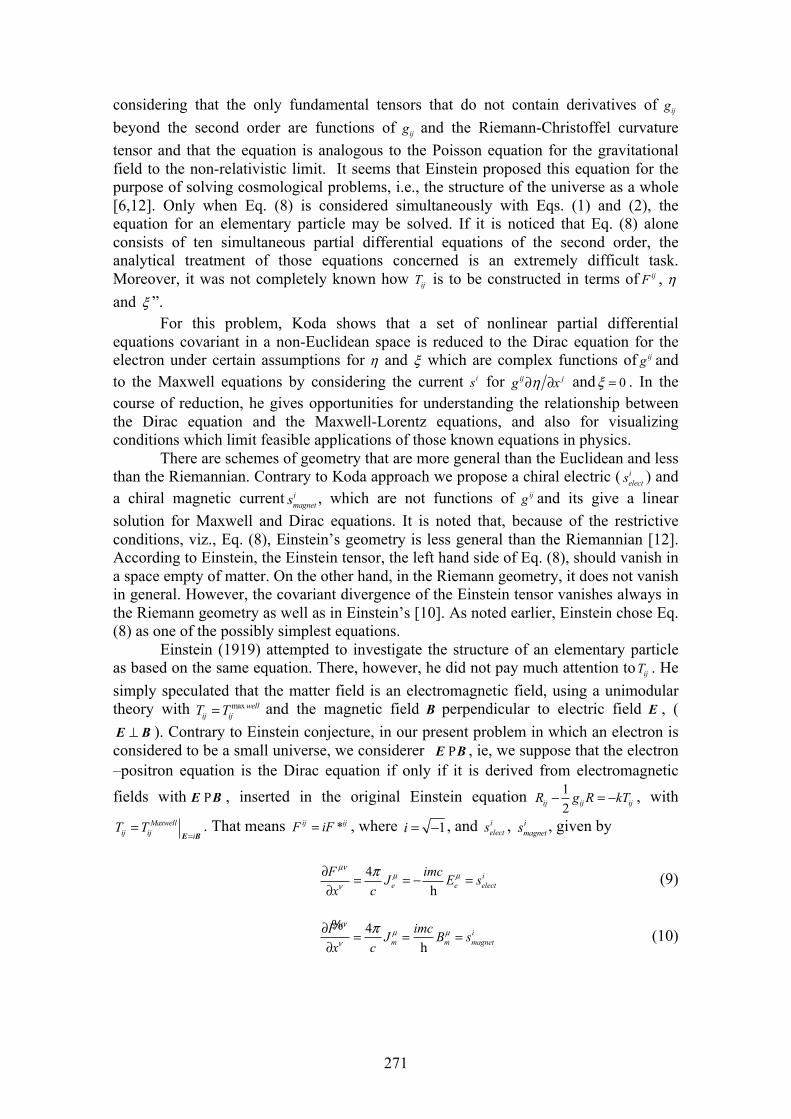
271
considering that the only fundamental tensors that do not contain derivatives of ijg
beyond the second order are functions of ijg and the Riemann-Christoffel curvature tensor and that the equation is analogous to the Poisson equation for the gravitational field to the non-relativistic limit. It seems that Einstein proposed this equation for the purpose of solving cosmological problems, i.e., the structure of the universe as a whole [6,12]. Only when Eq. (8) is considered simultaneously with Eqs. (1) and (2), the equation for an elementary particle may be solved. If it is noticed that Eq. (8) alone consists of ten simultaneous partial differential equations of the second order, the analytical treatment of those equations concerned is an extremely difficult task. Moreover, it was not completely known how ijT is to be constructed in terms of ijF , η and ξ ”.
For this problem, Koda shows that a set of nonlinear partial differential equations covariant in a non-Euclidean space is reduced to the Dirac equation for the electron under certain assumptions for η and ξ which are complex functions of ijg and to the Maxwell equations by considering the current is for ij jg xη∂ ∂ and 0ξ = . In the course of reduction, he gives opportunities for understanding the relationship between the Dirac equation and the Maxwell-Lorentz equations, and also for visualizing conditions which limit feasible applications of those known equations in physics.
There are schemes of geometry that are more general than the Euclidean and less than the Riemannian. Contrary to Koda approach we propose a chiral electric ( i
elects ) and a chiral magnetic current i
magnets , which are not functions of ijg and its give a linear solution for Maxwell and Dirac equations. It is noted that, because of the restrictive conditions, viz., Eq. (8), Einstein’s geometry is less general than the Riemannian [12]. According to Einstein, the Einstein tensor, the left hand side of Eq. (8), should vanish in a space empty of matter. On the other hand, in the Riemann geometry, it does not vanish in general. However, the covariant divergence of the Einstein tensor vanishes always in the Riemann geometry as well as in Einstein’s [10]. As noted earlier, Einstein chose Eq. (8) as one of the possibly simplest equations.
Einstein (1919) attempted to investigate the structure of an elementary particle as based on the same equation. There, however, he did not pay much attention to ijT . He simply speculated that the matter field is an electromagnetic field, using a unimodular theory with max well
ij ijT T= and the magnetic field B perpendicular to electric field E , (⊥E B ). Contrary to Einstein conjecture, in our present problem in which an electron is
considered to be a small universe, we considerer PE B , ie, we suppose that the electron –positron equation is the Dirac equation if only if it is derived from electromagneticfields with PE B , inserted in the original Einstein equation 1
2ij ij ijR g R kT− = − , with Maxwell
ij ij iT T
==
E B. That means *ij ijF iF= , where 1i = − , and i
elects , imagnets , given by
4 ie e elect
F imcJ E scx
µνµ µ
νπ∂ = = − =
∂ h (9)
4 im m magnet
F imcJ B scx
µνµ µ
νπ∂ = = =
∂
%
h (10)
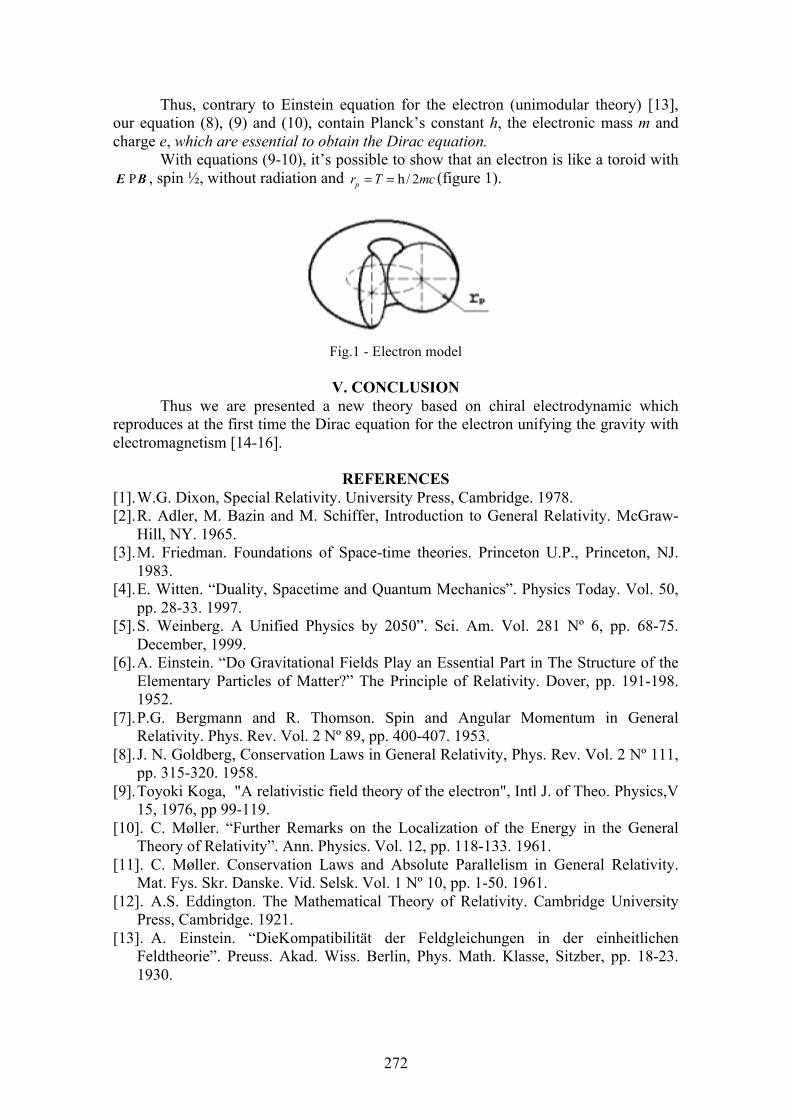
272
Thus, contrary to Einstein equation for the electron (unimodular theory) [13], our equation (8), (9) and (10), contain Planck’s constant h, the electronic mass m and charge e, which are essential to obtain the Dirac equation.
With equations (9-10), it’s possible to show that an electron is like a toroid with PE B , spin ½, without radiation and / 2pr T mc= = h (figure 1).
Fig.1 - Electron model
V. CONCLUSION Thus we are presented a new theory based on chiral electrodynamic which
reproduces at the first time the Dirac equation for the electron unifying the gravity with electromagnetism [14-16].
REFERENCES [1]. W.G. Dixon, Special Relativity. University Press, Cambridge. 1978. [2]. R. Adler, M. Bazin and M. Schiffer, Introduction to General Relativity. McGraw-
Hill, NY. 1965. [3]. M. Friedman. Foundations of Space-time theories. Princeton U.P., Princeton, NJ.
1983. [4]. E. Witten. “Duality, Spacetime and Quantum Mechanics”. Physics Today. Vol. 50,
pp. 28-33. 1997. [5]. S. Weinberg. A Unified Physics by 2050”. Sci. Am. Vol. 281 Nº 6, pp. 68-75.
December, 1999. [6]. A. Einstein. “Do Gravitational Fields Play an Essential Part in The Structure of the
Elementary Particles of Matter?” The Principle of Relativity. Dover, pp. 191-198. 1952.
[7]. P.G. Bergmann and R. Thomson. Spin and Angular Momentum in General Relativity. Phys. Rev. Vol. 2 Nº 89, pp. 400-407. 1953.
[8]. J. N. Goldberg, Conservation Laws in General Relativity, Phys. Rev. Vol. 2 Nº 111, pp. 315-320. 1958.
[9]. Toyoki Koga, "A relativistic field theory of the electron", Intl J. of Theo. Physics,V 15, 1976, pp 99-119.
[10]. C. Møller. “Further Remarks on the Localization of the Energy in the General Theory of Relativity”. Ann. Physics. Vol. 12, pp. 118-133. 1961.
[11]. C. Møller. Conservation Laws and Absolute Parallelism in General Relativity. Mat. Fys. Skr. Danske. Vid. Selsk. Vol. 1 Nº 10, pp. 1-50. 1961.
[12]. A.S. Eddington. The Mathematical Theory of Relativity. Cambridge University Press, Cambridge. 1921.
[13]. A. Einstein. “DieKompatibilität der Feldgleichungen in der einheitlichen Feldtheorie”. Preuss. Akad. Wiss. Berlin, Phys. Math. Klasse, Sitzber, pp. 18-23. 1930.

273
[14]. H. Torres-Silva. “Electrodinámica quiral: eslabón para la unificación del electromagnetismo y la gravitación”. Ingeniare. Rev. chil. ing. Vol. 16 Nº 1, pp. 6-23. 2008
[15]. H. Torres-Silva. “The close relation between the maxwell system and the dirac equation when E
r is parallel to
!H ”. Ingeniare. Rev. chil. ing. Vol. 16 Nº 1, pp. 43-
47. 2008.[16]. H. Torres-Silva. “Chiral field ideas toward a theory of matter”. Ingeniare. Rev.
chil. ing. Vol. 16 Nº 1, pp. 36-42. 2008.
274
A RELATIVISTIC WAVE-PARTICLE BASED ON MAXWELL’S EQUATIONS: PART II
John Carroll, Joseph Beals University of Cambridge, Engineering Department, Centre for Advanced Photonic and
Electronics, 9 J J Thomson Avenue, Cambridge, CB3 0FA UK .
Keywords: solution to Maxwell’s classical equations, Transverse Electric fields, Transverse Magnetic fields, Lorents invariant.
PACS number: 03.50.De/03.30.+p
At PIRT 2006, a speculative concept of a photon-like solution to Maxwell’s classical equations was presented [1] in which helically rotating solutions appeared to have properties that are typically associated with photons. Since that time, our understanding of these solutions has increased and the previous work has to be modified. This paper will present a digest of the latest results that enables us to clarify past work and review new experimental evidence for the theory.
There is already sufficient experimental evidence to show that single photons can have a measurable group velocity [2], measurable phase velocity [3] and can be localised [4]. Various Maxwellian models that provide a confined packet of classical energy have been discussed theoretically by several researchers [5,6] but these packets all rely on specific field profiles. Here the task is to find a packet that applies to all classical modes, is invariant to Lorentz transformations, and has a property that is recognisable as spin that increments in energy in appropriate units. At present the work is confined to beams in free space.
As a starting point, general solutions of Maxwell’s equations are conveniently labelled as TE (Transverse Electric fields) or TM (Transverse Magnetic fields) solutions (Figure 1). Here E, B and the direction of propagation form a right handed set of vectors [7]. TE and TM modes have a group velocity vg < c with a phase velocity = c2/vg > c. It is therefore always possible to travel in a frame of reference moving with the group velocity of these electromagnetic waves. In such a frame of reference, and using light cone coordinates [8] , there are wave vectors kf and kr (associated with light on the forward and reverse branches of the light cone) which are equal and opposite : kf = - kr as is found in most resonators.
With these concepts it is found possible to invent a Lorentz invariant wave-packet with a definite frequency, definite duration, definite phase velocity vp> c and definite group velocity vg< c:
Fz = Ez + i cBz = Fzo exp[i(ko z - wot)] cos[(wo/c)(z - vgt) d].
Here d is an arbitrary Lorentz invariant number that defines the phase-length of the packet and also defines the relative spread of the frequencies composing the wave-packet. This packet produces a Lorentz invariant envelope for the axial fields but fails to envelope properly the transverse fields FT = ET + i cBT .
Different mechanisms are used to ensure that the transverse fields are localised. These mechanisms are called here distributed spin-rotations. They are localised rotations of the transverse fields of any mode and can be observed mathematically only in the vector formulation of Maxwell’s equations. They provide helical modulation moving at the group velocity and form an enveloping packet for the transverse fields. Spin-rotations should not be confused with the helical phase fronts observed by other

275
workers [9]. In principle distributed spin-rotations can have arbitrary frequencies. However to ensure that the packet enveloping the transverse fields has the same duration as the packet enveloping the axial fields, two fields with equal and oppposite spin rotations are required with magnitudes that are quantised to be proportional to (2N+1)(wo/c) where N is integer. Figure 1 shows the idea schematically (N = 1). The lateral extent of the packet can be controlled, not just by the classical field profile, but by additional imaginary distributed spin rotations. Thus distributed spin rotations in principle allow for a flexible range of packets that might either emerge from confined sources or be detected by compact detectors. The duration of this photon-like packet is also flexible (determined by the value 1/d) but, when this duration is taken into account, the helical distributed spin rotations appear to contribute to a classical energy proportionally to (2N+1) (w/c) H where N is some Lorentz invariant integer. At present the theory is unable to evaluate H.
The paper will end with a brief review of experiments that could support this theory as a model for a photon
Transverse Electric/Magnetic electromagnetic waves
ET || c BT × nFor both TE and TM
n
ET
cBT
cBz
TE
n
ET
cBT
Ez
TM
|ET|/ |cBT|=(ω/c)/kz > 1
|ET|/ |cBT|= kz /(ω/c) < 1
Fig. 1 - TE and TM waves (TE waves are ‘driven’ by cBz TM waves are ‘driven’ by cEz). Phase velocity = w/k = vp > c; Group velocity vg = c2/vp < c. Can therefore always find a real frame of
reference moving with the velocity of the electromagnetic waves.
Fz ∝ 2 cos[ δ (ωο/c)(z – vg t )] Fzo
π
FT ∝ 2 cos[M δ(ωο/c)(z − vg t)] FTo
πFT enveloped by counter spinning rotations
Fz enveloped by two frequencies
Fig. 2 - Lorentz Invariant Envelopes. Every modal field with axial fields Fz = Ez + icBz and transverse fields FT = ET + icBT can be enveloped about a central frequency wo with a Lorentz invariant parameter d controlling the phase duration of the envelope. The transverse fields are enveloped by counter rotating spins. M=2N+1 is always an odd integer to ensure the axial and transverse fields to have the same duration of packet. The classical energy added by this spin is
proportional to M (w/c) H where H is some Lorentz invariant number.
276
REFERENCES [1]. Carroll, J.E. “A relativistic wave-particle based on Maxwell’s equations: model for
a classical photon” PIRT 2006, London [2]. Ingham,J.D., J.E., White,I.H. and R.M.Thompson “Measurement of the 'single-‐
photon' velocity and classical group velocity in standard optical fibre” Meas. Sci. Technol. 18 1538-‐1546
[3]. Branning D, Migdail A L and Sergienko AV 2000 Simultaneous measurement of group and phase delay between two photons Phys. Rev A 62 063808/1-12
[4]. Hong C K and Mandel L 1986 “Experimental realization of a localized one-photon state” Phys. Rev. Lett 56 58–60
[5]. Sezginer A. 1985 “A general formulation of focus wave modes” J. Appl. Phys 57 678-683
[6]. Nienhuis, G, Allen, L., “Paraxial wave optics and harmonic oscillators” paper 2.3 pp48-57 in Optical Angular Momentum editors L Allen SM Barnett MJ Padgett Inst of Physics Bristol 2003 ISBN 07503 0901 6
[7]. Sander K. F. and Reed G. A. L. 1986 Transmission and propagation of electromagnetic waves (Cambridge CUP)
[8]. Kim Y S and Wigner E P 1987 “Covariant phase-space representation for localized light waves” Phys. Rev. A 36 1293-1297
[9]. Leach J., Yao E. and Padgett M.J. 2004 Observation of the vortex structure of a non-integer vortex beam New Jnl. Phys 6 1-8
277
GENERALIZATION OF CONCEPTION OF MEASUREMENT TO SPACE-TIME WITH ARBITRARY METRICS AND COVARIANT ETHER THEORIES
Alexander L. Kholmetskii
Department of Physics, Belarus State University
Analyzing a conception of measurement in space-time, we derive some general properties of ether theories, which adopt the Minkowskian metrics for an absolute space.
Keywords: space-time, covariant ether theories, Minkowskian metrics, Einstein’s postulates.
PACS number: 03.30.+p
I. INTRODUCTION It is known that a conception of measurement and corresponding measuring
procedures has been first introduced in macrophysics by Einstein under physical interpretation of the Lorentz transformations and their implications. Later the conception of “measurement” acquired further development in quantum mechanics, but its specifics obviously lied outside of classical phenomena. Due to this reason we will not consider below any quantum measurements and restrict our analysis by the classical approach only.
So, Einstein was the first who said that the spatial and time intervals, entering into the Lorentz transformations, should be measured experimentally, and he defined methods for measurement of these intervals. Namely, he suggested applying unit scales for measurement of length and standard clocks for measurement of time. Such standard clocks are based on any stationary periodic process, and, besides, being placed at different spatial points, they should be synchronized to each other. For this purpose Einstein suggested a familiar procedure, which involves the exchange by short light pulses between distant clocks. On the basis of such a model of an inertial reference frame, which includes three spatial coordinates and an infinite set of synchronized clocks filled the entire space, Einstein was successful to explain all principal implications of the Lorentz transformations.
However, a number of physicists of the beginning of 20th century were not completely satisfied by Einstein’s explanation of relativistic effects, suspecting an artificial point in the involving of a concrete (Einstein) model of the inertial reference frame in a general physical analysis. There aroused a question: do the same relativistic effects take place, if we determine the inertial reference frame in some other way, with another set of adopted measuring procedures? It has been understood later that the measuring procedures in macrophysics could be indeed defined at a more general level, than the suggested by Einstein. Namely, one can introduce any measuring procedure belonging to a type of “admissible”. This type of procedures must satisfy three requirements [1]:
1. Unambiguity: i.e., the results of measurement should be reproducible for thefixed physical conditions.
2. Reversibility: for example, the distance measured from A to B should be equal tothe distance measured from B to A.Transitivity: for example, the sum ofmeasured lengths AB and BC should be equal to the length AC, when AB, BC
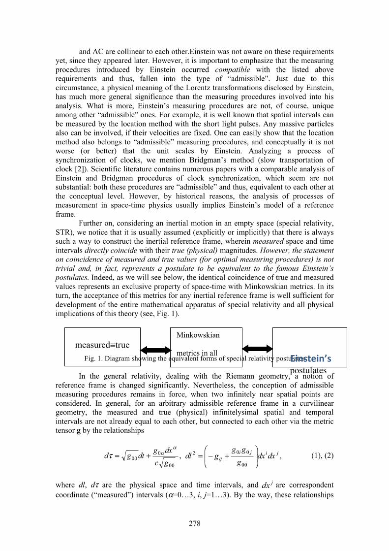
278
and AC are collinear to each other.Einstein was not aware on these requirements yet, since they appeared later. However, it is important to emphasize that the measuring procedures introduced by Einstein occurred compatible with the listed above requirements and thus, fallen into the type of “admissible”. Just due to this circumstance, a physical meaning of the Lorentz transformations disclosed by Einstein, has much more general significance than the measuring procedures involved into his analysis. What is more, Einstein’s measuring procedures are not, of course, unique among other “admissible” ones. For example, it is well known that spatial intervals can be measured by the location method with the short light pulses. Any massive particles also can be involved, if their velocities are fixed. One can easily show that the location method also belongs to “admissible” measuring procedures, and conceptually it is not worse (or better) that the unit scales by Einstein. Analyzing a process of synchronization of clocks, we mention Bridgman’s method (slow transportation of clock [2]). Scientific literature contains numerous papers with a comparable analysis of Einstein and Bridgman procedures of clock synchronization, which seem are not substantial: both these procedures are “admissible” and thus, equivalent to each other at the conceptual level. However, by historical reasons, the analysis of processes of measurement in space-time physics usually implies Einstein’s model of a reference frame.
Further on, considering an inertial motion in an empty space (special relativity, STR), we notice that it is usually assumed (explicitly or implicitly) that there is always such a way to construct the inertial reference frame, wherein measured space and time intervals directly coincide with their true (physical) magnitudes. However, the statement on coincidence of measured and true values (for optimal measuring procedures) is not trivial and, in fact, represents a postulate to be equivalent to the famous Einstein’s postulates. Indeed, as we will see below, the identical coincidence of true and measured values represents an exclusive property of space-time with Minkowskian metrics. In its turn, the acceptance of this metrics for any inertial reference frame is well sufficient for development of the entire mathematical apparatus of special relativity and all physical implications of this theory (see, Fig. 1).
Fig. 1. Diagram showing the equivalent forms of special relativity postulates
In the general relativity, dealing with the Riemann geometry, a notion of reference frame is changed significantly. Nevertheless, the conception of admissible measuring procedures remains in force, when two infinitely near spatial points are considered. In general, for an arbitrary admissible reference frame in a curvilinear geometry, the measured and true (physical) infinitelysimal spatial and temporal intervals are not already equal to each other, but connected to each other via the metric tensor g by the relationships
,00
000 gc
dxgdtgd
αατ += ,
00
002 jijiij dxdx
ggg
gdl ⎟⎟⎠
⎞⎜⎜⎝
⎛+−= (1), (2)
where dl, dτ are the physical space and time intervals, and jdx are correspondent coordinate (“measured”) intervals (α=0…3, i, j=1…3). By the way, these relationships
measured≡true Minkowskian
metrics in all
inertial frames
Einstein’s postulates
279
show that physical and measured infinitelysimal intervals coincide with each other only for the metric tensor (1 -1 -1 -1), i.e., for Minkowskian space-time.There is a known mathematical theorem, according to which any symmetric tensor with the constant coefficients can be transformed to a diagonal form by means of an appropriate transformation. Such is the metric tensor at any fixed point of space-time, and hence in the neighborhood of such a point, this tensor can be presented in the diagonal form. This statement constitutes one of the cornerstones in mathematical substantiation of the equivalence principle, although the latter is wider (in particular, it also requires a simultaneous vanishing of the Christoffel symbols). Physically it means that any gravitational field at any space-time point can be excluded by suitable acceleration motion. In this case we locally get a diagonal metric tensor and the equality of physical and measured (coordinate) values. At the same time, in the analysis of conception of measurement it is worth to distinguish a special kind of transformations
x0, xi→x’0(xi), x’i(xi), (i=1…3), (3) when an observer does not leave his own frame of references with the given instantaneous velocity and acceleration. Then one can show that it is impossible to diagonalize the metric tensor by means of the transformations (3) alone. This result seems to be obvious from a physical viewpoint: in the considered frame of references, we cannot exclude the gravitation field at any fixed spatial point by means of coordinate transformations solely. In its turn, this signifies that the coordinate (measured) spatial and time intervals, obtained by an experimenter in his own reference frame, do not, in general, coincide with corresponding physical values. In other words, physical space-time becomes not observable directly by this experimenter. It does not create any problems, if this experimenter knows the metric tensor. Then he can apply eqs. (1), (2) to the available coordinate values and obtain corresponding physical spatial and temporal intervals. However, when we conceive to analyze the foundations of space-time physics, then, in general, we cannot know the metric tensor a priori, even for an empty space-time. Thus, a determination of physical space-time coordinates from the available measured spatial and temporal intervals becomes a non-trivial problem, which, in author’s opinion, is often underestimated. As the simplest example on this subject we refer to the known ether theories alternative to special relativity. Almost all such theories, beginning with a primitive hypothesis on the “classical ether” and finishing by modern covariant constructions, adopt (often tacitly) an “obvious” statement that physical values for this or that inertial observer can be directly measured in experiment. However, it has been shown above that such a statement represents, in fact, a principal postulate of special relativity. Therefore, the adoption of this postulate and simultaneous negation of the equivalence of all inertial reference frames is a highly inconsistent step, which often explains a failure to construct a reasonable space-time theory to be alternative to special relativity. This example shows that the problem of interpretation of the results of measurements in various geometries is very important. The experimental data in space-time can be conditionally divided into two classes: astrophysical and laboratory. In astrophysical observations the problem to distinguish “physical” and “measured” values usually does not emerge. However, in the realization of laboratory scale experiments and their interpretation, a possible difference between physical and measured values should be obligatory taken into account. Besides, the distinguishing of such values, in general, should be included into a structure of any space-time theory.
Below we demonstrate an efficiency of such an approach with the simplest case: inertial reference frames in an empty space-time.
280
It is well known that within special relativity all inertial frames in an empty space-time are equivalent to each other. Mathematically it means that all fundamental physical equations are form-invariant with respect to the Lorentz transformations. Numerous ether theories (for their review see, e.g. [3]) admit a breakage of equivalence of the inertial frames, suggesting various physical interpretations to the world ether.
We intend to show below that all ether theories, which adopt the homogeneity and isotropy of physical space-time in the privileged (absolute) inertial frame, should have some essential common features at the phenomenological level, regardless of the postulated concrete physical properties of ether. A disclosure of such phenomenological similarity of various ether theories will be based on the presented above approach to the analysis of measuring procedure in space-time.
The homogeneity and isotropy of physical space-time in the absolute inertial reference frame simply signifies that it has pseudo-Euclidean geometry with the Minkowskian metrics. Further on we notice that any possible physical model of the world ether, from a mathematical viewpoint, signifies a dependence of metric coefficients gαβ on the absolute velocity v of a reference frame in question, or in a symbolic notation,
( )vgg = . (4)
Simultaneously we demand that the dependence (4) should be “admissible”, that is, it does not destroy the known requirements
,000 >g ,0<βααβ dxdxg (5)
which mean that the given inertial reference frame can be realized in nature. It is worth to emphasize that eqs. (4), (5), which restrict a form of possible
dependences (4), immediately signify that the developed ether theory complies with the general relativity principle.
Further on we notice that any motion of a reference frame cannot influence a type of geometry of empty space-time and thus, it remains pseudo-Euclidean. One follows from there that any four-vector in physical space-time xph within an arbitrary inertial reference frame should be a linear function of the corresponding Minkowskian four-vector xL of the same frame:
( ) ( ) jiji
xBx Lph = , (6)
where the coefficients of the matrix B depend only the absolute v of the inertial frame under consideration (if we exclude trivial rotations and translations of space), and the Minkowskian four-vectors xL obey the Lorentz transformation:
βαβα LL 'xLx = (7)
(hereinafter the primed four-vectors belong to the absolute frame). Pseudo-Euclidean space with the four-vector xph defined by eq. (6) has the so-called oblique-angled metrics. In this space the physical xph and measured xm (co-ordinate) four-vectors differ from each other, and we actually work under negation of the STR postulates and thus develop logically non-contradictory ether theory.
Further we need to determine the transformation rules separately for physical xph and measured xm four-vectors. We take into account that in the absolute frame, due to its
(4)
II. EMPTY SPACE-TIME AND COVARIANT ETHER THEORIES
281
Minkowskian metrics, both kinds of four-vectors do coincide with each other and equal to the Minkowskian four-vectors xL:
( ) ( ) ( )ααα Lmph ''' xxx == !! (8)
(hereinafter the primed four-vectors belong to the absolute frame K0). Thus, in contrast to the standard approach, now we need to determine two different, in general, laws of transformation for physical and measured four-vectors under the implementation of eq. (8). It is wonder that a pure set of requirements (6)-(8) occur, nevertheless, sufficient to find the transformation rules for measured space-time four-vectors. Omitting particular calculations (which can be found in [4, 5]), we present a final result: a transformation between the absolute frame and arbitrary inertial frame, moving at the constant absolute velocity v, has the Lorentz form: ( ) ( ) .')( β
αβα mm v xLx = (9)Further, a transformation between two arbitrary inertial frames K1 and K2 also has the Lorentz form, but it is implemented via the absolute frame K0:
( ) ( ) ,")]()[( 21
1 γβγ
αβα mm vv xLLx −= (10)
where v1, v2 are the absolute velocities of the frames K1 and K2, correspondingly. Of course, a direct Lorentz transformation between the frames K1 and K2 with the velocity
21 vvu ⊕= is also possible, but it will be not rotation-free [6]. Now it is worth to recall that within special relativity, a transformation between
two arbitrary inertial frames is completely determined by their relative velocity u. However
( )uvv LLL ≠− )]()[( 21
1 , (11)
in a general case (when v1, v2 are not collinear to each other), even if .21 vvu ⊕= The inequality (11) reflects a known property of non-commutativity of the Lorentz transforms for non-collinear velocities v1 and v2. In its turn, this inequality indicates that, in general, the developed ether theory can be distinguished from STR at the level of experimentally measured quantities. Hence there is a possibility, at least in principle, to choose experimentally either STR, or the developed general ether theory, named by us as covariant ether theory (CET) due to its compatibility with the general relativity principle. Moreover, we can immediately formulate two necessary requirements for realization of a crucial experiment for verification of CET:
1. Eq. (11) shows that we have to deal with transformation between two inertialframes at least, which move at the different velocities v1 and v2 in the absolute space, and both velocities should be not collinear to each other. (We remind that for v1 // v2,
( )uvv LLL =− )]()[( 21
1 (where 21 vvu ⊕= ), and the absolute velocity is not observable). Since any laboratory scale experiments are carried out on Earth, the latter represents the first natural reference frame, moving in the absolute space at the velocity vE. In order to get the second inertial frame, different from the first one (which is attached to the Earth), we need to have a moving inertial element in our experimental setup, which has the absolute velocity v≠vE. Then the maximum value of a “non-relativistic” effect will be observed in the case, where v and vE are orthogonal to each other. By the way, one
282
immediately follows from there that all the interference experiments of Michelson-like type cannot distinguish STR and covariant ether theories.
2. In order to derive the second requirement for the crucial experiment, we recallthat successive Lorentz transforms with non-collinear relative velocities entail the Thomas-Wigner rotation of co-ordinate axes of the inertial frames involved, eq. (12)
,2
sin2c
uvE α≈Ω (12)
where Evvu ⊕= is the velocity of moving inertial element in the laboratory frame, and α is the angle between vectors u and vE.
The same effect (12) takes place in covariant ether theories for measured four-vectors xm. At the same time, in contrast to STR, we may be flexible in the physical interpretation of the Thomas-Wigner rotation. Namely, within STR this rotation is always a real effect, even if we cannot indicate a dynamic origin of this rotation. In the covariant ether theories the Thomas-Wigner rotation happens for the measured four-vectors xm, which, in general, do not coincide with the physical space-time xph. Hence we get a right to interpret this rotation as a purely apparent phenomenon, whose origin is completely kinematical and reflects the properties of physical space-time (for illustrative explanation of this statement see below, the problem in Fig. 2). Nevertheless, in spite of the appreciable difference in physical interpretation of the Thomas-Wigner rotation within both theories, it should be detected by an appropriate experimental setup. And here it is important that the angle Ω within CET is proportional to the absolute velocity of Earth vE (eq. (12). Hence we have to observe oscillations of measured values of Ω due to daily and annual rotation of Earth: the effect, which is impossible for STR. Thus, an experimental setup for the crucial test of special relativity and covariant ether theories should be aimed to the measurement of Thomas-Wigner angle. From there we derive the second requirement to such crucial experiment: a long enough moving inertial element of an experimental setup in order to measure its spatial turn due to the Thomas-Wigner rotation.
Now it is worth to emphasize that both listed above requirements to the crucial experiment have been obtained at a phenomenological level, and hence they are relevant for any ether theory, regardless of a particular model of the world ether, if we adopt that such an ether is homogeneous and isotropic.
Another side of such crucial experiment is its consistent physical interpretation, especially in the case, where an oscillative character of Ω(v) dependence will be found. Let us show that such an interpretation can be given at the phenomenological level, too, without looking for physical properties of hypothetical ether. For this purpose one needs to determine some general properties of transformations in physical space-time.
Let us adopt that a transformation A between the absolute frame K0 and arbitrary inertial frame K in physical space-time
( ) ( )βαβα phph 'xAx = (13)
belongs to a kind of admissible, i.e., it does not violate the inequalities (5), and it constitutes a ten-parametric group of Lie. Excluding again trivial rotations and translations, we obtain the transformation between two arbitrary inertial reference frames in physical space-time in the form:
283
( ) ( )γ
βγαβα phph ")]()[( xvAvAx 2
11
!! −= (14)
Further on we find a relationship between the matrix A and introduced above matrix B (see, eq. (6)):
0000 AB γ= ,
)]1()11([ 2200
20000 −−+×+= γγα
vv
Acv
AAB iii ,
)11(20 γ−+=
v
vAAB j
iijij ,
where
221 cv−=γ . (15)
In fact, this is all, what we can say about the transformation A in physical space-time, when we proceed from the adopted properties of its symmetry. Further on we may only advance these or that hypotheses on the form of matrix A and determine corresponding properties of physical space-time.
It is interesting to consider the simplest case, where A=G (admissible Galilean transformation). Notice that this case does not mean a return to the classical Newton mechanics, because the admissible Galilean transformations keep the inequalities (5), which demand, for example, a finiteness of the light velocity in vacuum. Substituting the matrix G into the obtained above Eqs. (15), one gets
γ=00B , 00 =iB , γ20 сv
B ii = , )11(2 γ
δ −=v
vvB ji
ijij . (16)
One can show (see, [4, 5]) that eqs. (16) are equivalent to the adoption of the Lorentz ether postulates in physical space-time
1. Galilean law of speed composition2. Absolute contraction of scale along the vector v3. Absolute dilation of time.It is interesting to notice that the successive Galilean transformations are rotation-
free. Hence, no Thomas-Wigner rotation takes place in physical space-time. Therefore, such a rotation is an illusive effect and is observed only in measured space-time coordinates.
Let us demonstrate this general conclusion with a particular problem depicted in Fig. 2, where we assume the admissible Galilean transformation in physical space-time.
Let two clocks Cl1 and Cl2 be placed upon the x-axis of some inertial reference frame K at rest in the absolute frame K0. The distance between Cl1 and Cl2 is equal to L. Let some rod with a proper length L moves along the y-axis at a constant velocity u. The axis of the rod is parallel to the x-axis, and the coordinates of its opposite ends upon the x-axis coincide with corresponding coordinates of Cl1 and Cl2. So, at the instant when the rod is intersecting the axis x, it is simultaneously touching the Cl1 and Cl2. We
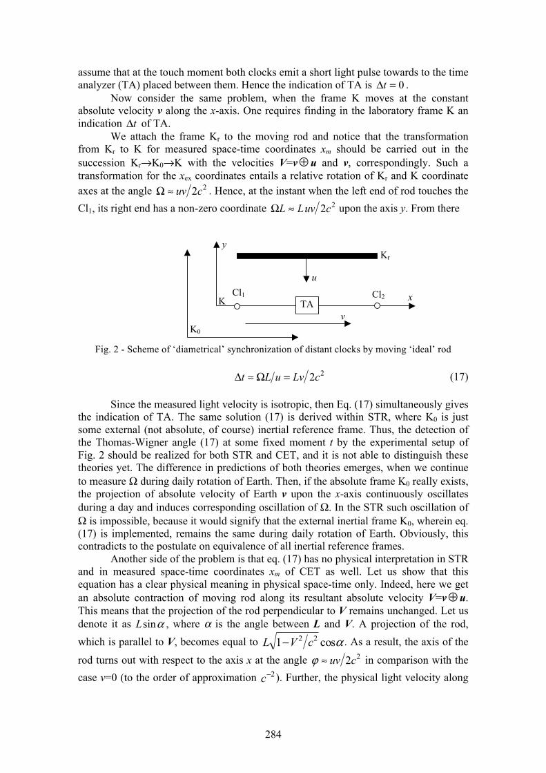
284
assume that at the touch moment both clocks emit a short light pulse towards to the time analyzer (TA) placed between them. Hence the indication of TA is 0=Δt .
Now consider the same problem, when the frame K moves at the constant absolute velocity v along the x-axis. One requires finding in the laboratory frame K an indication tΔ of TA.
We attach the frame Kr to the moving rod and notice that the transformation from Kr to K for measured space-time coordinates xm should be carried out in the succession Kr→K0→K with the velocities V=v⊕u and v, correspondingly. Such a transformation for the xex coordinates entails a relative rotation of Kr and K coordinate axes at the angle 22cuv≈Ω . Hence, at the instant when the left end of rod touches the Cl1, its right end has a non-zero coordinate 22cuvLL ≈Ω upon the axis y. From there
Fig. 2 - Scheme of ‘diametrical’ synchronization of distant clocks by moving ‘ideal’ rod
22cLvuLt =Ω≈Δ (17)
Since the measured light velocity is isotropic, then Eq. (17) simultaneously gives the indication of TA. The same solution (17) is derived within STR, where K0 is just some external (not absolute, of course) inertial reference frame. Thus, the detection of the Thomas-Wigner angle (17) at some fixed moment t by the experimental setup of Fig. 2 should be realized for both STR and CET, and it is not able to distinguish these theories yet. The difference in predictions of both theories emerges, when we continue to measure Ω during daily rotation of Earth. Then, if the absolute frame K0 really exists, the projection of absolute velocity of Earth v upon the x-axis continuously oscillates during a day and induces corresponding oscillation of Ω. In the STR such oscillation of Ω is impossible, because it would signify that the external inertial frame K0, wherein eq. (17) is implemented, remains the same during daily rotation of Earth. Obviously, this contradicts to the postulate on equivalence of all inertial reference frames.
Another side of the problem is that eq. (17) has no physical interpretation in STR and in measured space-time coordinates xm of CET as well. Let us show that this equation has a clear physical meaning in physical space-time only. Indeed, here we get an absolute contraction of moving rod along its resultant absolute velocity V=v⊕u. This means that the projection of the rod perpendicular to V remains unchanged. Let us denote it as αsinL , where α is the angle between L and V. A projection of the rod, which is parallel to V, becomes equal to αcos1 22 cVL − . As a result, the axis of the
rod turns out with respect to the axis x at the angle 22cuv≈ϕ in comparison with the case v=0 (to the order of approximation 2−c ). Further, the physical light velocity along
TA
uCl1 Cl2 x
yKr
K
K0
v
285
the-x axis of the laboratory frame K is equal to vcc −=+ , and in the opposite direction vcc +=− . Hence, the indication of TA is
( ) ( ) 2222 cLv
vcL
vcL
uLt ≈
−−
++≈Δ ϕ .
This coincides with Eq. (17). Thus Eq. (17) can be interpreted as the real appearance of the properties of physical space-time, in spite of the impossibility to directly measure phx . In particular, the calculations presented allow one to consider Eq. (17) as the inference of an absolute contraction of rod as well as anisotropy of the physical light speed phc in the moving laboratory frame K. From a formal viewpoint, such a result follows from the dependence of Ω on v in experimentally measured coordinates exx caused by the general transformation rule (10).
Thus, we find that a formal application of the transformation (10) for Minkowskian four-vectors Lx (leading to the measurable dependence of Ω on v) acquires a physical interpretation only in the phx coordinates, despite of the impossibility of observing the phx four-vectors experimentally.
Unfortunately, the experiment in Fig. 2 is practically impossible for the realization. Indeed, assuming the absolute velocity of Earth v=10-3c, choosing u=1 m (typical value for a laboratory scale experiment), we obtain 122 1051c2uv −⋅≈≈Ω . . For L=1m, a corresponding difference in the y-coordinates of the left and right ends of the rod is about 10-12 m. Obviously, the smallest vibrations in the moving rod have much larger magnitude.
That is why we paid our attention to electromagnetic phenomena, related to the Thomas-Wigner rotation and dealing with non-commutativity of the electric and magnetic field transformation. Among such possible effects, the Faraday induction law is especially attractive due to the reasons as follows: - for an appropriate experimental scheme, possible mechanical vibrations in moving
elements of an experimental setup, which are crucial for any direct measurement of Ω, now are not important;
- there is a possibility to multiply the eventual non-relativistic effect by n times due to application of multi-turned closed circuits with n>>1 turns.
A possible scheme of Faraday experiment for a search of the absolute velocity of Earth is described, for example, in [7].
III. CONCLUSIONSOn the basis of conception of measurement in space-time we explore ether
theories, which adopt the Minkowskian metrics for an absolute space. Without looking for physical properties of any particular physical model of ether, we only demanded the compatibility of space-time transformations with the general relativity principle, and obtained common phenomenological properties of covariant ether theories: - for an arbitrary inertial reference frame, the measured spatial and temporal intervals
do not coincide with corresponding physical magnitudes; - the measured space-time four-vectors always obey the Lorentz transformations; - any possible “non-relativistic effect” (depending on the absolute velocity v of the
frame of observation), results from the dependence of Thomas-Wigner angle Ω on v;
286
- the dependence Ω(v) has the same form for any admissible choice of physical space-time transformation A. The latter influences only on a particular kinematical interpretation of the Thomas-Wigner rotation, which represents an illusive effect in physical space-time;
- Faraday’s law is a promised tool for revealing the dependence of Ω on v. If such dependence will be actually detected, it will prove the existence of a privileged inertial reference frame.
REFERENCES [1]. L.I. Mandelstam. Lectures on Optics, Theory of relativity and Quantum
Mechanics. (Moscow, Nauka, 1972). [2]. P.W. Bridgman. Sophysticate’s Primer of Relativity. (Middletown: Wesleyan
Univ. Press, 1962). [3]. M.C. Duffy. The ether concept in Modern Physics. In: Einstein and Poincaré: the
physical vacuum (Ed. V. Dvoeglazov) (Montreal, Apeiron, 2006). P. 11-34. [4]. A.L. Kholmetskii. Covariant ether theories and special relativity. Physica Scripta,
67 (2003) 381-387. [5]. A.L. Kholmetskii. Empty space-time and the general relativity principle. In:
Einstein and Poincaré: physical vacuum (Ed. by V. Dvoeglazov) (Monreal, Apeiron, 2006), P. 55-73.
[6]. C. Møller. The Theory of Relativity (Clarendon Press, Oxford 1972). [7]. A.L. Kholmetskii. Faraday induction law, Einstein relativity principle and
Thomas-Wigner rotation. In: Has the last word been said in classical electrodynamics? (Ed. A. Chubykalo, V. Onoochin, A. Espinoza and R. Smirnov-Rueda), (Pinton Press, 2004). p. 177-199.
287
MÖSSBAUER EXPERIMENTS IN ROTATING SYSTEMS REANALYZED
1A. L. Kholmetskii, 2T. Yarman, 3O. V. Missevitch
1Department of Physics, Belarusian State University, 4, Nezavisimosti Avenue, 220050 Minsk Belarus
2Department of Engineering, Okan University Istanbul, Turkey & Savronik, Eskisehir, Turkey 3Institute for Nuclear Problems, Belarus State University, 220030, Minsk, Belarus
In this paper we re-analyze the known Mossbauer experiments in rotating systems, and first of all, the experiment by Kündig (Phys. Rev. 129 (1963) 2371). We show that a correct processing of experimental data obtained by Kündig gives a relative energy shift EEΔ of the absorption line different from the value of classically assumed relativistic time dilation for rotating resonant absorber. Namely, instead of the relative energy shift ( ) 22 2011.00065.1 cvEE ±−=Δ reported by Kündig (v being the linearvelocity of absorber, and c is the light velocity in vacuum), we derive from his results
( ) 22 2011.0192.1 cvEE ±−=Δ . We incline to think that the revealed deviation ofEEΔ from relativistic prediction cannot be explained by any instrumental error and
thus represents a physical effect. In particular, we assume that the energy shift of absorption resonant line is induced not only by the standard time dilation effect, but some additional effect missed to the moment. Perhaps, such an effect appears, if we adopt that not only relativistic change of mass, but also its change due to a variation of binding energy of system, is accompanied by corresponding change of the time rate. The idea of a new experiment on this subject, which is now under preparation, is described.
Keywords: Mossbauer experiments, Kündig experiment, theory of relativity, Doppler shift.
PACS number: 29.30.Kv
I. INTRODUCTION Nowadays, the basic physics of the relativistic time dilation has been verified to
a high degree of accuracy. Historically, the dilation of time for moving objects was first verified experimentally in [1]. The quantitative measurements of time dilation effect have been carried out in a series of Mössbauer experiments in rotating systems [2-7]. Later much more precise experiments with ion beams confirmed this relativistic effect with the accuracy of about 10-9 ([8, 9] and references therein) and left no room for any doubts in its validity. At the same time, one should emphasize that in the mentioned above experiments the effect of time dilation was verified, in fact, for essentially different physical conditions: charged particles in ion beam can be considered as moving freely, whereas resonant nuclei in Mössbauer experiments are bound in solid body and constitute a macroscopic quantum system. Thus, despite of huge difference in measuring precision: 10-9 for ion beam measurements and 10-2 for Mössbauer measurements - the latter have their own independent significance for verification of unified character of dilation of time both for free and bound atoms. Among known Mössbauer experiments, mentioned above, the experiment by Kündig implemented 45 years ago [2], remains the most precise, because Kündig was a sole, who successfully applied a modulation of energy of resonant radiation in a rotating system. This method
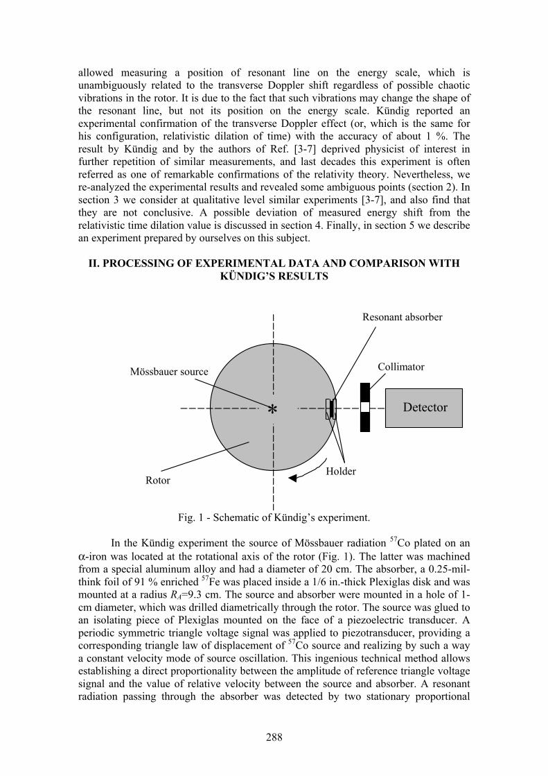
288
allowed measuring a position of resonant line on the energy scale, which is unambiguously related to the transverse Doppler shift regardless of possible chaotic vibrations in the rotor. It is due to the fact that such vibrations may change the shape of the resonant line, but not its position on the energy scale. Kündig reported an experimental confirmation of the transverse Doppler effect (or, which is the same for his configuration, relativistic dilation of time) with the accuracy of about 1 %. The result by Kündig and by the authors of Ref. [3-7] deprived physicist of interest in further repetition of similar measurements, and last decades this experiment is often referred as one of remarkable confirmations of the relativity theory. Nevertheless, we re-analyzed the experimental results and revealed some ambiguous points (section 2). In section 3 we consider at qualitative level similar experiments [3-7], and also find that they are not conclusive. A possible deviation of measured energy shift from the relativistic time dilation value is discussed in section 4. Finally, in section 5 we describe an experiment prepared by ourselves on this subject.
II. PROCESSING OF EXPERIMENTAL DATA AND COMPARISON WITHKÜNDIG’S RESULTS
Detector
Mössbauer source
Resonant absorber
Rotor
*
Holder
Collimator
Fig. 1 - Schematic of Kündig’s experiment.
In the Kündig experiment the source of Mössbauer radiation 57Co plated on an α-iron was located at the rotational axis of the rotor (Fig. 1). The latter was machined from a special aluminum alloy and had a diameter of 20 cm. The absorber, a 0.25-mil-think foil of 91 % enriched 57Fe was placed inside a 1/6 in.-thick Plexiglas disk and was mounted at a radius RA=9.3 cm. The source and absorber were mounted in a hole of 1-cm diameter, which was drilled diametrically through the rotor. The source was glued to an isolating piece of Plexiglas mounted on the face of a piezoelectric transducer. A periodic symmetric triangle voltage signal was applied to piezotransducer, providing a corresponding triangle law of displacement of 57Co source and realizing by such a way a constant velocity mode of source oscillation. This ingenious technical method allows establishing a direct proportionality between the amplitude of reference triangle voltage signal and the value of relative velocity between the source and absorber. A resonant radiation passing through the absorber was detected by two stationary proportional
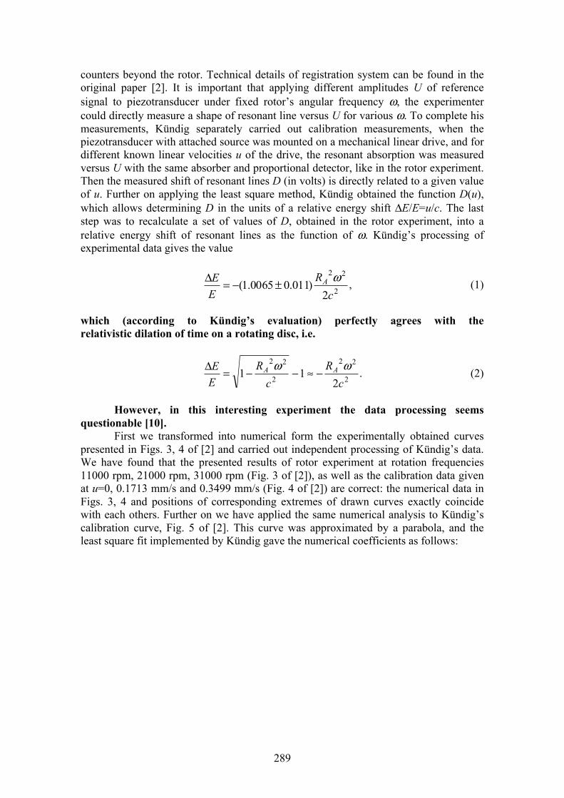
289
counters beyond the rotor. Technical details of registration system can be found in the original paper [2]. It is important that applying different amplitudes U of reference signal to piezotransducer under fixed rotor’s angular frequency ω, the experimenter could directly measure a shape of resonant line versus U for various ω. To complete his measurements, Kündig separately carried out calibration measurements, when the piezotransducer with attached source was mounted on a mechanical linear drive, and for different known linear velocities u of the drive, the resonant absorption was measured versus U with the same absorber and proportional detector, like in the rotor experiment. Then the measured shift of resonant lines D (in volts) is directly related to a given value of u. Further on applying the least square method, Kündig obtained the function D(u), which allows determining D in the units of a relative energy shift ΔE/E=u/c. The last step was to recalculate a set of values of D, obtained in the rotor experiment, into a relative energy shift of resonant lines as the function of ω. Kündig’s processing of experimental data gives the value
2
22
2)011.00065.1(
cR
EE A ω
±−=Δ , (1)
which (according to Kündig’s evaluation) perfectly agrees with the relativistic dilation of time on a rotating disc, i.e.
2
22
2
22
211
cR
cR
EE AA ωω
−≈−−=Δ . (2)
However, in this interesting experiment the data processing seems questionable [10].
First we transformed into numerical form the experimentally obtained curves presented in Figs. 3, 4 of [2] and carried out independent processing of Kündig’s data. We have found that the presented results of rotor experiment at rotation frequencies 11000 rpm, 21000 rpm, 31000 rpm (Fig. 3 of [2]), as well as the calibration data given at u=0, 0.1713 mm/s and 0.3499 mm/s (Fig. 4 of [2]) are correct: the numerical data in Figs. 3, 4 and positions of corresponding extremes of drawn curves exactly coincide with each others. Further on we have applied the same numerical analysis to Kündig’s calibration curve, Fig. 5 of [2]. This curve was approximated by a parabola, and the least square fit implemented by Kündig gave the numerical coefficients as follows:
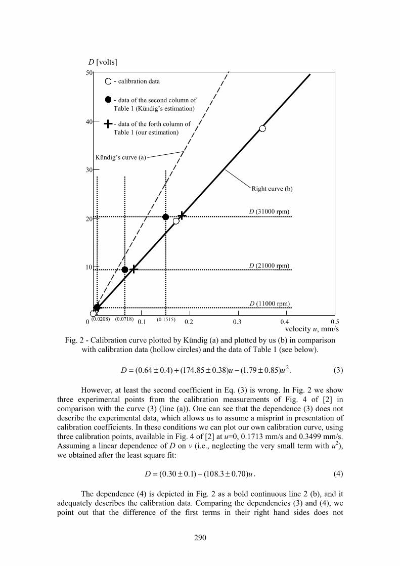
290
10
20
30
40
50
0.1 0 0.2 0.3 0.4 0.5
D (31000 rpm)
D (21000 rpm)
D (11000 rpm)
(0.1515) (0.0718) (0.0208)
Right curve (b)
Kündig’s curve (a)
- calibration data
- data of the second column of Table 1 (Kündig’s estimation)
- data of the forth column of Table 1 (our estimation)
D [volts]
velocity u, mm/s Fig. 2 - Calibration curve plotted by Kündig (a) and plotted by us (b) in comparison
with calibration data (hollow circles) and the data of Table 1 (see below).
2)85.079.1()38.085.174()4.064.0( uuD ±−±+±= . (3)
However, at least the second coefficient in Eq. (3) is wrong. In Fig. 2 we show three experimental points from the calibration measurements of Fig. 4 of [2] in comparison with the curve (3) (line (a)). One can see that the dependence (3) does not describe the experimental data, which allows us to assume a misprint in presentation of calibration coefficients. In these conditions we can plot our own calibration curve, using three calibration points, available in Fig. 4 of [2] at u=0, 0.1713 mm/s and 0.3499 mm/s. Assuming a linear dependence of D on v (i.e., neglecting the very small term with u2), we obtained after the least square fit:
uD )70.03.108()1.030.0( ±+±= . (4)
The dependence (4) is depicted in Fig. 2 as a bold continuous line 2 (b), and it adequately describes the calibration data. Comparing the dependencies (3) and (4), we point out that the difference of the first terms in their right hand sides does not

291
essentially influence D, but the second coefficients (which are the most crucial) differ by ∼70%.
Thus, due to Kündig’s misprint, we cannot evaluate the details of his further calculations summarized in the table of [2]. The three left columns of the table 1 reproduce the results by
Table 1. The results of Kündig’s experiment (1-3 columns) in comparison with author’s estimations (4 column)
Speed of rotor (rpm)
Shift D (10-6 m/s)
(Kündig)
( ) 222 ωsA RRD − ,(10-9 s/m) (Kündig)
( ) 222 ωsA RRD − ,(10-9 s/m)
(our estimation) 3 000 -1.5±1.8 -1.7±2.1 - 11 000 20.8±1.5 1.803±0.127 1.965±0.11 21 000 71.8±1.2 1.705±0.029 1.955±0.025 25 000 101.4±1.5 1.703±0.026 - 31 000 151.5±2.3 1.653±0.025 2.037±0.020 35 000 195.0±2.3 1.666±0.020 -
Weighted average
1.679±0.013 1.986±0.01
Expected result =1/2c
1.668 ?
Kündig: the second column presents the values of shift D obtained in the rotor experiment for different ω, recalculated with the calibration curve into velocity units; the third column shows the computed ratio ( ) 222 ωsA RRD − (Rs<<RA being an averageradial co-ordinate of the source). One sees that the weighted average of this ratio is well matched to the expected value 1/2c=1.668⋅10-9 s/m given by relativistic Eq. (2) We marked in bold the lines of Table 1, corresponding to rotation frequencies 11000 rpm, 22000 rpm and 31000 rpm, for which the original experimental data were presented by Kündig in [2], and hence which can be evaluated independently. The marked in bold data of the second column of Table 1 are shown in Fig. 2 as black cycles. One can see that they are compatible neither with Kündig’s calibration curve (a), nor with our own calibration curve (b). Thus the origin of these data remains unclear. Our own estimation of the shift D (in velocity units) with the calibration curve (b) of Fig. 2 gives the values to be shown in the forth column of Table 1 and depicted in Fig. 2 by daggers.
Thus we reveal a valuable discrepancy with the results reported by Kündig. In particular, the weighted average of ( ) 222 ωsA RRD − comes to be equal to(1.986±0.01)⋅ 10-9 s/m, and approximately 20 % higher than Kündig’s result (1.679±0.013)⋅10-9 s/m. Correspondingly, instead of the relative energy shift (1) estimated by Kündig, we obtain
( ) 2
22
2011.0192.1
cR
EE A ω
±−=Δ . (5)
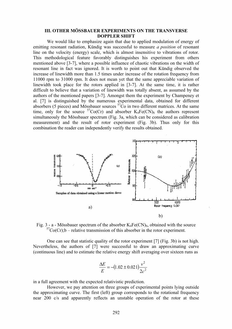
292
III. OTHER MÖSSBAUER EXPERIMENTS ON THE TRANSVERSEDOPPLER SHIFT
We would like to emphasize again that due to applied modulation of energy of emitting resonant radiation, Kündig was successful to measure a position of resonant line on the velocity (energy) scale, which is almost insensitive to vibrations of rotor. This methodological feature favorably distinguishes his experiment from others mentioned above [3-7], where a possible influence of chaotic vibrations on the width of resonant line in fact was ignored. It is worth to point out that Kündig observed the increase of linewidth more than 1.5 times under increase of the rotation frequency from 11000 rpm to 31000 rpm. It does not mean yet that the same appreciable variation of linewidth took place for the rotors applied in [3-7]. At the same time, it is rather difficult to believe that a variation of linewidth was totally absent, as assumed by the authors of the mentioned papers [3-7]. Amongst them the experiment by Champeney et al. [7] is distinguished by the numerous experimental data, obtained for different absorbers (5 pieces) and Mössbauer sources 57Co in two different matrices. At the same time, only for the source 57Co(Cr) and absorber K4Fe(CN)6 the authors represent simultaneouly the Mössbauer spectrum (Fig. 3a, which can be considered as calibration measurement) and the result of rotor experiment (Fig. 3b). Thus only for this combination the reader can independently verify the results obtained.
Fig. 3 - a - Mössbauer spectrum of the absorber K4Fe(CN)6, obtained with the source 57Co(Cr);b – relative transmission of this absorber in the rotor experiment.
One can see that statistic quality of the rotor experiment [7] (Fig. 3b) is not high. Nevertheless, the authors of [7] were successful to draw an approximating curve (continuous line) and to estimate the relative energy shift averaging over sixteen runs as
( ) 2
2
2021.002.1
cv
EE ±−=Δ
in a full agreement with the expected relativistic prediction. However, we pay attention on three groups of experimental points lying outside
the approximating curve. The first (left) group corresponds to the rotational frequency near 200 c/s and apparently reflects an unstable operation of the rotor at these
a)
b)
293
comparably low frequencies, which is accompanied by a variable level of vibration. It is more interesting to explain the deviation of central (near 800 c/s) and right (1300…1400 c/s) groups of experimental points. We assume that the right group of points obtained at extremely high frequencies >1300 c/s reflects a known effect of reducing of chaotic vibrations in a rotor, when a centripetal acceleration approaches to the strengthen limit of rotor’s material. If so, the experimental points at frequency range ∼ 900...1300 c/s should also lie higher than the approximating continuous curve in the absence of vibrations. For the assumed uncertainty it seems especially important to determine an exact position of a minimum of approximating curve for data in Fig. 3b, which is essentially less sensitive to rotor vibration than the shape of this curve. The approximating line drawing by Champeney et al. gives a minimum at the frequency about 950 c/s. Now we pay attention on the central group of experimental points, which lie below the approximating curve and allow us to suppose that the actual extreme is located at the frequency 800…830 c/s. Using the calibration curve in Fig. 3a and drawing an approximating curve 22 2cvEE λ−=Δ (λ being the variable parameter) with the minimum at ∼ 800 c/s, we found that this curve also passes through the experimental data points of ν=1300…1400 c/s. As a result, we get the estimation
( ) 2
2
2050.021.1
cv
EE ±−=Δ , (6)
which agrees with our result (5) derived from Kündig’s experimental data. We do not insist that the estimation (6) exactly follows from the Champeney et al. experiment. Rather we wanted to demonstrate that this experiment, like other mentioned above rotor experiments without energy modulation of resonant gamma-quanta, bears an ambiguous interpretation. In these conditions we may consider the Kündig experiment (were the related data appropriately treated) as the most reliable one for the measurement of a relative energy shift between resting resonant source and rotating resonant absorber.
IV. DISCUSSIONNow we ask the crucial question on the origin of the deviation of Kündig’s result
from relativistic prediction on the time dilation effect. We trust in the validity of the usual relativistic dilation of time due to the motion, which, as we mentioned above, has numerous confirmations in the experiments dealing with atomic beams and free muons (Refs. [8, 9] and references therein). Rather we conjecture that in the Kündig experiment, the energy shift of absorption resonant line is induced not only by the standard time dilation effect solely, but some additional effect missed to the moment. Eq. (5) shows that this additional relative energy shift has the order of magnitude
2
2
2
21.0
22.0
cv
cv
EE −=−≈Δ (7)
and for the rotation frequency 31000 rpm it reaches the value of
Γ=−≈Δ − 15.010 13EE , (8)
Γ being the natural linewidth of 57Fe resonance.
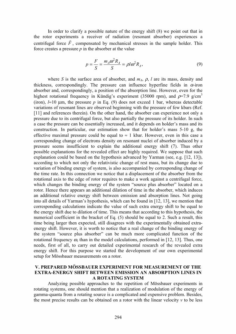
294
In order to clarify a possible nature of the energy shift (8) we point out that in the rotor experiments a receiver of radiation (resonant absorber) experiences a centrifugal force F
!, compensated by mechanical stresses in the sample holder. This
force creates a pressure p in the absorber at the value
AAA Rl
SRm
SFp 2
2ωρω === , (9)
where S is the surface area of absorber, and mA, ρ, l are its mass, density and thickness, correspondingly. The pressure can influence hyperfine fields in α-iron absorber and, correspondingly, a position of the absorption line. However, even for the highest rotational frequency in Kündig’s experiment (35000 rpm), and ρ=7.9 g/cm3 (iron), l≈10 µm, the pressure p in Eq. (9) does not exceed 1 bar, whereas detectable variations of resonant lines are observed beginning with the pressure of few kbars (Ref. [11] and references therein). On the other hand, the absorber can experience not only a pressure due to its centrifugal force, but also partially the pressure of its holder. In such a case the pressure can be essentially increased, and it depends on holder’s mass and its construction. In particular, our estimation show that for holder’s mass 5-10 g, the effective maximal pressure could be equal to ≈ 1 kbar. However, even in this case a corresponding change of electrons density on resonant nuclei of absorber induced by a pressure seems insufficient to explain the additional energy shift (7). Thus other possible explanations for the revealed effect are highly required. We suppose that such explanation could be based on the hypothesis advanced by Yarman (see, e.g. [12, 13]), according to which not only the relativistic change of rest mass, but its change due to variation of binding energy of system, is also accompanied by corresponding change of the time rate. In this connection we notice that a displacement of the absorber from the rotational axis to the edge of rotor requires to make a work against a centrifugal force, which changes the binding energy of the system “source plus absorber” located on a rotor. Hence there appears an additional dilation of time in the absorber, which induces an additional relative energy shift between emission and absorption lines. Not going into all details of Yarman’s hypothesis, which can be found in [12, 13], we mention that corresponding calculations indicate the value of such extra energy shift to be equal to the energy shift due to dilation of time. This means that according to this hypothesis, the numerical coefficient in the bracket of Eq. (5) should be equal to 2. Such a result, this time being larger then expected, still disagrees with the experimentally obtained extra-energy shift. However, it is worth to notice that a real change of the binding energy of the system “source plus absorber” can be much more complicated function of the rotational frequency ω, than in the model calculations, performed in [12, 13]. Thus, one needs, first of all, to carry out detailed experimental research of the revealed extra energy shift. For this purpose we started the development of our own experimental setup for Mössbauer measurements on a rotor.
V. PREPARED MÖSSBAUER EXPERIMENT FOR MEASUREMENT OF THE EXTRA-ENERGY SHIFT BETWEEN EMISSION AN ABSORPTION LINES IN
A ROTATING SYSTEM Analyzing possible approaches to the repetition of Mössbauer experiments in
rotating systems, one should mention that a realization of modulation of the energy of gamma-quanta from a rotating source is a complicated and expensive problem. Besides, the most precise results can be obtained on a rotor with the linear velocity v to be less
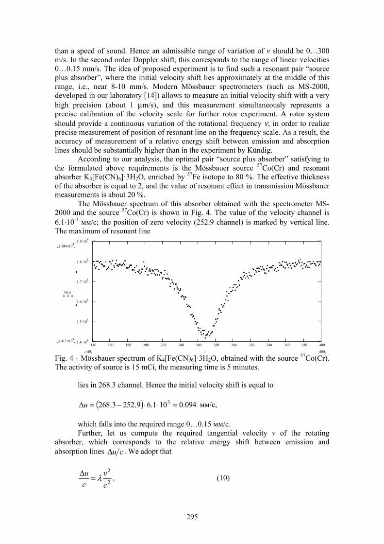
295
than a speed of sound. Hence an admissible range of variation of v should be 0…300 m/s. In the second order Doppler shift, this corresponds to the range of linear velocities 0…0.15 mm/s. The idea of proposed experiment is to find such a resonant pair “source plus absorber”, where the initial velocity shift lies approximately at the middle of this range, i.e., near 8-10 mm/s. Modern Mössbauer spectrometers (such as MS-2000, developed in our laboratory [14]) allows to measure an initial velocity shift with a very high precision (about 1 µm/s), and this measurement simultaneously represents a precise calibration of the velocity scale for further rotor experiment. A rotor system should provide a continuous variation of the rotational frequency ν, in order to realize precise measurement of position of resonant line on the frequency scale. As a result, the accuracy of measurement of a relative energy shift between emission and absorption lines should be substantially higher than in the experiment by Kündig.
According to our analysis, the optimal pair “source plus absorber” satisfying to the formulated above requirements is the Mössbauer source 57Co(Cr) and resonant absorber K4[Fe(CN)6]·3H2O, enriched by 57Fe isotope to 80 %. The effective thickness of the absorber is equal to 2, and the value of resonant effect in transmission Mössbauer measurements is about 20 %.
The Mössbauer spectrum of this absorber obtained with the spectrometer MS-2000 and the source 57Co(Cr) is shown in Fig. 4. The value of the velocity channel is 6.1⋅10-3 мм/c; the position of zero velocity (252.9 channel) is marked by vertical line. The maximum of resonant line
140 160 180 200 220 240 260 280 300 320 340 360 380 4001.4 .104
1.5 .104
1.6 .104
1.7 .104
1.8 .104
1.9 .104
1.809 104×
1.417 104×
N i( )
400140 i
Fig. 4 - Mössbauer spectrum of K4[Fe(CN)6]·3H2O, obtained with the source 57Со(Cr). The activity of source is 15 mCi, the measuring time is 5 minutes.
lies in 268.3 channel. Hence the initial velocity shift is equal to
( ) 094.0101.69.2523.268 3 =⋅⋅−=Δu мм/c,
which falls into the required range 0…0.15 мм/с. Further, let us compute the required tangential velocity v of the rotating
absorber, which corresponds to the relative energy shift between emission and absorption lines cuΔ . We adopt that
2
2
cv
cu λ=Δ , (10)
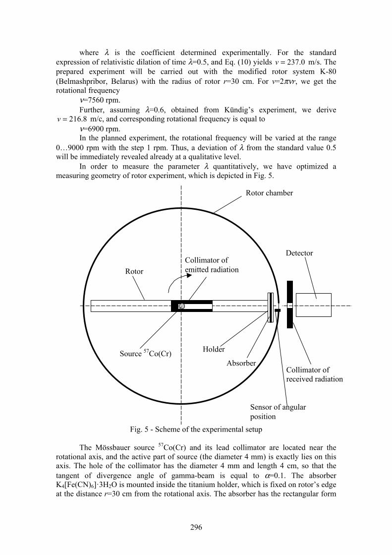
296
where λ is the coefficient determined experimentally. For the standard expression of relativistic dilation of time λ=0.5, and Eq. (10) yields 0.237=v m/s. The prepared experiment will be carried out with the modified rotor system K-80 (Belmashpribor, Belarus) with the radius of rotor r=30 cm. For v=2πνr, we get the rotational frequency
ν=7560 rpm. Further, assuming λ=0.6, obtained from Kündig’s experiment, we derive 8.216=v m/c, and corresponding rotational frequency is equal to ν=6900 rpm. In the planned experiment, the rotational frequency will be varied at the range
0…9000 rpm with the step 1 rpm. Thus, a deviation of λ from the standard value 0.5 will be immediately revealed already at a qualitative level.
In order to measure the parameter λ quantitatively, we have optimized a measuring geometry of rotor experiment, which is depicted in Fig. 5.
Rotor chamber
Rotor
Source 57Co(Cr)
Collimator of emitted radiation
Collimator of received radiation детектора
Detector
Absorber
Holder
Sensor of angular position
Fig. 5 - Scheme of the experimental setup
The Mössbauer source 57Co(Cr) and its lead collimator are located near the rotational axis, and the active part of source (the diameter 4 mm) is exactly lies on this axis. The hole of the collimator has the diameter 4 mm and length 4 cm, so that the tangent of divergence angle of gamma-beam is equal to α=0.1. The absorber K4[Fe(CN)6]·3H2O is mounted inside the titanium holder, which is fixed on rotor’s edge at the distance r=30 cm from the rotational axis. The absorber has the rectangular form
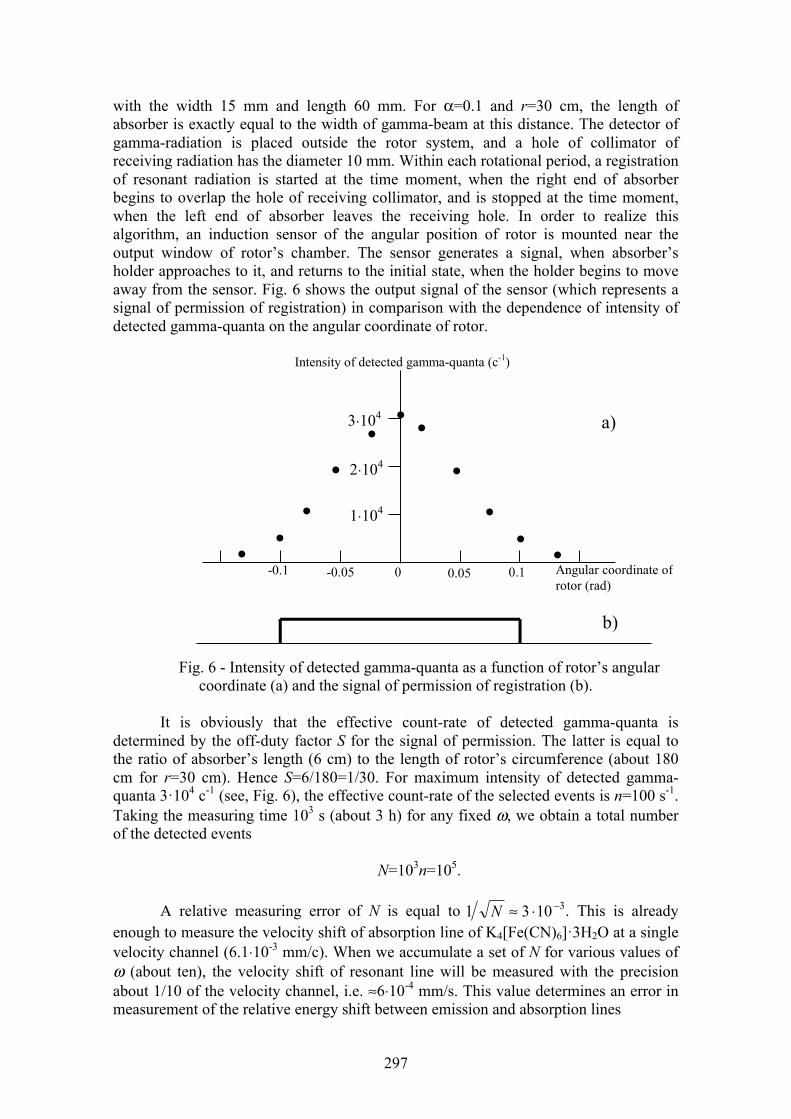
297
with the width 15 mm and length 60 mm. For α=0.1 and r=30 cm, the length of absorber is exactly equal to the width of gamma-beam at this distance. The detector of gamma-radiation is placed outside the rotor system, and a hole of collimator of receiving radiation has the diameter 10 mm. Within each rotational period, a registration of resonant radiation is started at the time moment, when the right end of absorber begins to overlap the hole of receiving collimator, and is stopped at the time moment, when the left end of absorber leaves the receiving hole. In order to realize this algorithm, an induction sensor of the angular position of rotor is mounted near the output window of rotor’s chamber. The sensor generates a signal, when absorber’s holder approaches to it, and returns to the initial state, when the holder begins to move away from the sensor. Fig. 6 shows the output signal of the sensor (which represents a signal of permission of registration) in comparison with the dependence of intensity of detected gamma-quanta on the angular coordinate of rotor.
. 3⋅104
. . .
. . .
2⋅104
1⋅104
. . . .
а)
b)
Intensity of detected gamma-quanta (c-1)
0 0.05 0.1 -0.05 -0.1 Angular coordinate of rotor (rad)
Fig. 6 - Intensity of detected gamma-quanta as a function of rotor’s angular coordinate (a) and the signal of permission of registration (b).
It is obviously that the effective count-rate of detected gamma-quanta is determined by the off-duty factor S for the signal of permission. The latter is equal to the ratio of absorber’s length (6 cm) to the length of rotor’s circumference (about 180 cm for r=30 cm). Hence S=6/180=1/30. For maximum intensity of detected gamma-quanta 3·104 с-1 (see, Fig. 6), the effective count-rate of the selected events is n=100 s-1. Taking the measuring time 103 s (about 3 h) for any fixed ω, we obtain a total number of the detected events
N=103n=105.
A relative measuring error of N is equal to 31031 −⋅≈N . This is already enough to measure the velocity shift of absorption line of K4[Fe(CN)6]·3H2O at a single velocity channel (6.1⋅10-3 mm/c). When we accumulate a set of N for various values of ω (about ten), the velocity shift of resonant line will be measured with the precision about 1/10 of the velocity channel, i.e. ≈6⋅10-4 mm/s. This value determines an error in measurement of the relative energy shift between emission and absorption lines
298
[ ]15
4102106 −
−⋅=⋅=Δ
мм/ccEE . (11)
Since we adopt that 2
2
cv
EE
2λ=Δ (λ being the parameter, determined
experimentally), then the error of its measurement is
2
215 2102
vcδλ −⋅= . (13)
For maximum value v=300 m/s, 3104 −⋅=δλ =0,4 %. The estimated measuring error of λ is few times smaller than in the experiment
by Kündig (1.1 %), and much more less than the expected relative extra energy shift between emission and absorption lines (about 20 %). Thus, a performance of the described experiment will allow us to get unambiguous information on the presence of this extra energy shift.
V. CONCLUSION We emphasize a principle result of our analysis: to the moment there is a sole
reliable Mössbauer experiment for the measurement of time dilation effect in a rotating frame (Kündig’s experiment), and it certainly indicates a deviation from the standard relativistic prediction. We incline to think that the revealed deviation (of about 20 %) cannot be explained by any instrumental error. Rather we assume that the origin of this extra energy shift is closely related to Yarman’s hypothesis on unified relationship between dilation of time and change of mass of a system (including the change caused by variation of the binding energy). Thus we hope to stimulate further theoretical and experimental activity, in order to understand the origin of the revealed effect.
We were sad to know that Walter Kündig died more than two years ago. We give him due for realization of the ingenious experiment, representing one of the first fundamental applications of then recently discovered Mössbauer effect, when a methodology of Mössbauer spectroscopy was in its infancy. We seem not to be able to know the required technical details of this experiment with respect to absorber’s holding and some others. Thus we decided to repeat Kündig’s experiment with application of recent methodological achievements of Mössbauer spectroscopy, which will allow us to get unambiguous information on the origin of the revealed extra energy shift between emission and absorption lines.
REFERENCES [1]. H.E. Ives and G.R. Stilwell. J. Opt. Soc. Am. 28 (1938) 215. [2]. W. Kündig. Phys. Rev. 129 (1963) 2371. [3]. H.J. Hay, et al. Phys. Rev. Lett. 4 (1960) 165. [4]. H.J. Hay. In: Proceedings of the Second Conference on the Mössbauer
effect (ed. A. Schoen and D.M.T. Compton) (New York, Wiley, 1962), p. 225. [5]. T.E. Granshaw and H.J. Hay. In: Proceedings Int. School of Physics,
“Enrico Fermi” (New York, Academic Press, 1963), p. 220. [6]. D.C. Champeney and P.B. Moon. Proc. Phys. Soc. 77 (1961) 350.

299
[7]. D.C. Champeney, G.R. Isaak and A.M. Khan. Proc. Phys. Soc. 85 (1965) 583.
[8]. R.W. McGowan, D.M. Giltner, S.J. Sternberg and Sui Au Lee. Phys. Rev. Lett. 70 (1993) 251.
[9]. I. Bailey et al. Nature 268 (1977) 301. [10]. A.L. Kholmetskii, T. Yarman, and O.V. Missevitch. Kündig’s
experiment on the transverse Doppler shift re-analyzed. Physica Scripta 54 (2008) 255. [11]. M.P. Pasternak and R.D. Taylor. In: Mössbauer Spectroscopy in Material
Science (ed. M. Miglierini and D. Petridis) (Netherlands, Kluwer Academic Publisher, 1999). P. 349-358.
[12]. T. Yarman. In: Proceedings of International Meeting “Physical Interpretation of Relativity Theory”, Moscow, 4 - 7 July 2005 / Edited by M.C. Duffy, et al. - Moscow: BMSTU PH, 2005.
[13]. T. Yarman, V.B. Rozanov, M.Arik. In: Proceedings of International Meeting “Physical Interpretation of Relativity Theory”, Moscow, 4 - 7 July 2005 / Edited by M.C. Duffy, et al. - Moscow: 2007.
[14]. A.L. Kholmetskii, V.A. Evdokimov, M. Mashlan and O.V. Missevitch. Hyperfine Interactions 156/157 (2004) 3.

300
MANIFEST NON-LOCALITY OF BOUND ELECTROMAGNETIC FIELDS IN NEAR ZONE OF RADIATING SOURCES: EXPERIMENTAL
OBSERVATION
A.L. Kholmetskii1, O.V. Missevitch2, R. Smirnov-Rueda*3 1Department of Physics, Belarus State University, 220030, Minsk, Belarus
2Institute of Nuclear Problems, 220030, Minsk, Belarus *corresponding author: [email protected]
3Faculty of Mathematics, Complutense University, 28040 Madrid, Spain
As the central concept of genuine relativistic field theories, locality is referred as impossibility of superluminal causal propagation. The creation of Quantum Mechanics (QM) and its further development led to Bell’s theorem which in the most general form sorted out QM predictions of strong correlations between space-like separated systems from probabilities of measurement outcomes calculated on the basis of local realism admitted by EPR.
Various versions of EPR-type experiments gave overwhelming support to orthodox QM predictions in detriment of local realism, casting doubts on the relativistic locality as universal physical concept. Since then common view has it that the quantum realm involves some type of misterious non-locality because it has no analogy in the classical worldview. Additionally, recent QED-based studies of so-called evanescent modes (identified with virtual photons) gave clear indications on quantum non-locality as a tunneling effect which seems to be at odds with relativistic causality.
As response to the above-mentioned controversy on non-locality we propose a novel approach which concerns only classical relativistic field theory. We found that the actual experimental verification of the standard locality (causality) within domains of classical electromagnetism is essentially incomplete since it does not take into account the internal structure of EM field as a superposition of bound and radiation components. In fact, it does not provide any explicit information on propagation properties of bound EM fields that are dominant in the near zone of radiating EM sources.
Any ideally rigorous test of causal behavior of the whole EM field within the framework of classical electromagnetism must be based on individual (separate) test for bound and radiation components so that we made a clear distinction between the near and the far zones (where bound and radiation fields are prevailing, respectively). As a consequence, we proposed and implemented direct experimental procedure for correct identification of propagation characteristics of bound EM fields of radiating sources (antennas etc). Measurements1,2 were carried out in two different configurations between emitting and receiving antenna at UHF 125 MHz (2.5 m EM radiation wave-length) clearly showing that the propagation rate of classical bound EM fields highly exceeds the velocity of light in the near zone (up to 60 cm). Interestingly, their propagation speed tends to c in far zone. This fact might indicate on a possible limit of applicability of the standard locality concept on semi-classical level, i.e. within transition from QM to classical phenomena.
Keywords: electromagnetic fields, quantum mechanics, virtual photons, relativistic field theory.
PACS number: 03.65.-w/03.50.-z REFERENCES
[1] A.L. Kholmetskii, O.V. Missevitch, R. Smirnov-Rueda, R. Ivanov and A.E. Chubykalo, J. Appl. Phys. 101, 023532 (2007) [2] A.L. Kholmetskii, O.V. Missevitch and R. Smirnov-Rueda, J. Appl. Phys. 102, 0
1G. Spavieri, 1J. Erazo, 1A. Sanchez, 2G. T. Gillies1Centro de Física Fundamental, Facultad de Ciencias, Universidad de Los Andes,
Mérida, 5101-Venezuela2Department of Physics, University of Virginia Charlottesville, VA 22901-4714 USA
The momentum of the electromagnetic (em) fields Pe appears in several areas of modern physics. In both the equations for matter and light wavepropagation
Pe represents the relevant em interaction. As an application of wave
propagation properties, a first order optical experiment which tests the speed of light in moving rareed gases is presented. We recall that Pe is a lso t he l ink to t he unitary vision of the quantum e¤ects of the Aharonov-Bohm ( AB) type and that, besides the traditional classical approaches to the limit of the photon mass mph, e¤ects of the AB type provide a powerful quantum approach for the limit o f mph. Table-top experiments based on a new e¤ect of the AB type, together with the scalar AB e¤ect, yield the limit
mph = 9 ; 4 1 052g, a value
that improves upon the results achieved with o ther approaches.
PACS number: 0 3.30.+p, 0 3.65.Ta, 0 1.55.+b, 42.15.-i
MOMENTUM OF ELECTROMAGNETIC FIELDS AND NEW TESTS OF FUNDAMENTAL PHYSICS
I. INTRODUCTIONThe interaction em momentum Pe has attracted physicistsattention as it
arises in di¤erent scenarios of modern physics involving em interactions. One of these scenarios is that of light propagation in slowly moving media [1], [2]. Another is that of a unitary view of quantum nonlocal e¤ects of the Aharonov-Bohm (AB) type [3], [4]. More commonly, the interaction em momentum Pe appears as a nonvanishing quantity in em experiments involving "open" or convection currents, while Pe vanishes in the common em experi- ments or interactions with closed currents or circuits [2], [5].
The main purpose of this article is to review the recent advances of physics involving the em momentum Pe and its role in the proposal of new tests or in making other advances, such as setting a new limit on the photon mass.
In the eld of electromagnetism, a growing number of articles questioning the standard interpretation of special relativity have appeared [6]-[8]. Some of the authors of Refs. [6] and [7] adhere to a point of view close to the historical works of Lorentz and Poincaré, who maintained the existence of a preferred frame. It has been argued that these di¤erent formulations of Special Relativity are truly compatible only in vacuum, as di¤erences may appear when light propagates in transparent moving media. Thus, Consoli and Costanzo [8], Cahill and Kitto [9], and Guerra and de Abreu [7], point out that, for the experiments of the MichelsonMorley type, which are often said to have given a null-result, this is not the case and cite the famous work by Miller [10]. The claim of these authors is that the available data point towards a consistency of non-null results when the interferometer is operated in the gas-mode, corresponding to light propagating through a gas [8] (as in the case of air or helium, for instance, even in modern maser versions of optical tests).
Keywords: electromagnetic fields, Aharonov-Bohm quantum effects, quantum mechanics.
301

Moreover, tests that involve em interactions in open currents or circuits have been reconsidered by Indorato and Masotto [11] who points out that these experiments are not completely reliable and may be inconclusive [2]. Because of all this, physicists have recently proposed experiments about those predictions of the theory that have not been fully tested, or they have for- mulated untested assumptions that di¤er from the standard interpretation of Special Relativity [2], [5], [7], [8].
The interesting point is that all the above-mentioned scenarios and polemical hypotheses are linked to the interaction em momentum. Therefore, throughout this article we highlight the role of Pe in each one of these scenarios.
II. WAVE EQUATIONS FOR MATTER AND LIGHT WAVES
To elucidate the role of em momentum in modern physics, we start by con-sidering the wave equations for matter and light waves and show how the interaction term Q of these equations is related to Pe [12]. In general, with theT MikMaxwell stress-tensor, the covariant description of the em momentum leads to thefour-vector em momentum P e expressed as
Pei c = (cg + Tik
Mi)d3 cPe0 =
Z Z(uem v g)d3 (1)
where = v=c, and the em energy and momentum are evaluated in a special frame K(0) moving with velocity v with respect to the laboratory frame. Here, uem is the energy density and S = gc is the energy fluxor flow.
The analogy between the wave equation for light in moving media and that for charged matter waves has been pointed out by Hannay [1] and later addressed by Cook, Fearn, and Milonni [1] who have suggested that light propagation at a uid vortex is analogous to the Aharonov-Bohm (AB) e¤ect, where charged matter waves (electrons) encircle a localized magnetic ux [3]. Generally, in quantum e¤ects of the AB type [3]-[4] matter waves undergo an em interaction as if they were propagating in a ow of em origin that acts as a moving medium [4] and modies the wave velocity. This analogy has led to the formulation of the so-called magnetic model of light propagation [1],[2].
According to Fresnel [13], light waves propagating in a transparent, incompressible moving medium with uniform refraction index n, are dragged by the medium and develop an interference structure that depends on the velocity u of the uid (u << c). At the time of Fresnel the preferred inertial frame was that at rest with the so-called ether, which here may be taken to coincide with the laboratory frame. The speed achieved in the ether frame is
c
nv = + (1
n
12)u (2)
as later corroborated by Fizeau [13]. Because of the formal analogy between the wave equation for light in slowly moving media and the Schrödinger equation for charged matter waves in the presence of the external vector potential
302
A (i.e., the magnetic Aharonov-Bohm e¤ect), both equations contain a term that is generically referred to as the interaction momentum Q. Thus, the Schrödinger equation for quantum e¤ects of the AB type (with h = 1) [4] and the wave equation for light in moving media can be written [1], [2] as
(irQ)2 = p2: (3)
Eq.(3) describes matter waves if the momentum p is that of a material particle, while, if p is taken to be the momentum hk of light (in units of h = 1), Eq.(3) describes light waves.
a)All the e¤ects of the AB type discussed in the literature [3]-[4] can bedescribed by Eq.(3), provided that the interaction momentum Q is related[4], [12] to Pe, the momentum of the em elds. The AB term Q = (e=c)Aof the magnetic AB e¤ect is obtained by taking Q = Pe = 1
R(EB)d3x0
4c
where E is the electric eld of the charge and B the magnetic eld of the solenoid. A general proof that this result holds in the natural Coulomb gauge, has been given by several authors [14]. For these quantum e¤ects, the solution to Eq. (3) is given by the matter wave function
= ei0 = eiRQdx0 = e
iRQdx ei(pxEt)A (4)
where 0 solves the Schrödinger equation with Q = 0.b)Calculations of the quantity Q = Pe (1) for light in slowly moving
media show [12] that the interaction term yields the Fresnel-Fizeau momentum [2]
Q = !c2(n21)u; (5)
and that a solution of the type described in (4) may assume the forms
= ei0 = eiRQdxei
R(kdx! dt)A; = ei
R(K(x)dx! dt)A (6)
where k and K(x) are wave vectors, ! = k c=n the angular frequency, and n the index of refraction, while 0 solves Eq.(3) with Q = u = 0.The fact that the interaction momentum Q is related to Pe [4], [12] for
both matter waves of e¤ects of the AB type [4] and light waves in moving media [12], denitely reinforces the existing analogy between the two wave equations. Two theoretical possibilities arise [2R]:
- By incorporating the phase in the term K(x)dx, the last expressionon the rhs of Eq.(6) keeps the usual invariant form of the solution as required
303
by special relativity and one nds [12] for the speed of light the result v=(c=n)cb + (1 1=n2)u = (c=n)cb Q(c2=n2!) in agreement with Eq.(2) andSpecial Relativity.- Maintaining instead the analogy with the AB e¤ect, the solution can be
chosen to be represented by the rst term of Eq.(6), = ei0. In this case, the phase velocity changes but the speed of light (the particle, or photon) may not change [2]. This result is in total agreement with the analogous result for the AB e¤ect where Q = (e=c)A and the particle speed is left unchanged by the interaction with the vector potential A.
The established relation (5) will be used in the next sections to tenta- tively express in a quantitative way the hypothesis of Consoli and Costanzo [8] referring to v, the speed of light in a moving rareed media. With a quantitative expression for v it is then possible to formulate a dedicated experiment that tests Consoli and Costanzos hypothesis.
II. A. PROPAGATION OF EM WAVES IN RAREFIED MOVING MEDIADu¤y [15] has noted that the concept of an ether-like preferred frame has
always incited controversy, even in modern scientic investigations aimed at exploring the less understood aspects of relativity theory. Within this sce- nario, Consoli and Costanzo [8], Cahill and Kitto [9], and Guerra and de Abreu [7], after a re-analysis of the optical experiments of the Michelson Morley type, claim that the available data point towards a consistency of non-null results when light in the arms of the interferometer propagates in a rareed gas, like the cases of air at normal pressure and temperature. The possibility of maintaining the existence of a preferred frame, and parallel interests in the Michelson-Morley, Trouton-Noble and related e¤ects, arises because the coordinate transformation used, the Tangherlini transformations [16] foresee the same length contraction and time dilation of the Lorentz transformations. However, they contain an arbitrariness in the determina- tion of the time synchronization parameter, with the consequence that there are quantities which eventually cannot be measured, such as the one-way speed of light, its measured value depending on the synchronization proce- dure adopted [16]. Di¤erent synchronization procedures are possible [6]-[8], fully compatible with Einsteins relativity in practice, but with very di¤erent assertions in fundamental and philosophical terms.
The original important assumption made by Consoli et al. to corroborate their claims of a non-null result and open a window for the possible existence of a preferred frame, is that light in a moving rareed gas of refractive index n very close to 1 propagates with speed c=n , isotropically, in the preferred frame, as if the medium were not moving. Obviously, this hypothesis is in contrast with special relativity that foresees the speed (2), but it is not ruled out by the known optical tests. Thus, this assumption needs justication and experimental corroboration.
304
In the following, we explore possible modications of the form of the present Fresnel-Fizeau momentum when the moving medium is composed of rareed gas. It is not unconceivable that the e¤ectiveness of the light delay mechanism in a compact moving medium di¤ers, and perhaps even substantially so, from that of a non-compact moving medium, such as a rareed gas, even if they have the same index n. As an ad hoc hypothesis or a tentative model of a light delay mechanism, it has been supposed [17] that its e¤ectiveness ef arises from the relative spatial extension Vi of the interaction em momentum Q(u) with respect to the extension V of the total em momentum. Introducing then the ratio ef = Vi=V , the e¤ective em interaction momentum, to be used in determining the speed of light in a moving media, will be assumed to be given by the e¤ective Fresnel-Fizeau term ef Q = (Vi=V ) Q, while the resulting velocity of light in moving rareed media is
v =c
nbc c2
n2!ef Q =
c
nbc+ ef (1 1
n2)u: (7)
The hypothesis of Consoli et al. of the speed c=n in the preferred frame formoving rareed gases, will be justied by our model if ef = Vi=V turns out to be very small and, in this case, negligible. Calculations leading to a rough estimate ofVi=V for air at room temperature yield [17] ef = Na(a3=R3) 22:9 = 6:1 103, whichindeed can be neglected. Thus, our model foresees that the speed of light in moving media is actually not c=n but, quantitatively, the changes found do not alter signicantly the basic hypothesis and resulting analysis by Consoli et al. [8], [9] and Guerra et al. [7].
III. OPTICAL TEST IN THE FIRST ORDER IN v=cThe main consequence is that, with the present hypothesis of negligible
drag- like e¤ect for moving rareed gases, ether drift experiments of the order v=c become meaningful again. Let us consider for example the following experiment which is a variant of the Mascart and Jamin experiment of 1874 [18].
A ray of light travels from point A to point B of a segment A===B representing an optical interferometer. The original ray is split into two rays at A, which propagate separately through the two arms (1 and 2) of the in- terferometer. The rays recombine then at B where the interference pattern is observed. The arms 1 and 2 are made of a transparent rareed gases or ma- terials with indices of refraction n1 and n2 and wherein the speeds are c=n1 and c=n2 in the preferred frame, respectively, in agreement with Consolis et al. hypothesis [8] of the velocity expression (7) with ef = 0. The labora- tory frame with the interferometer and the rareed gas is moving with speed u with respect to the preferred frame. We could be using the expressions for the speed in the moving laboratory frame resulting from the Tangherlini transformation, which can be found in [16], [7]. The calculation can also be done using the standard velocity addition from the Lorentz transformation, i.e., using the denition of Einstein speed as detailed in [7]. Both approaches yield the same result. The speed of light in arm 1 in the frame of the in- terferometer, moving with speed u with respect to the preferred frame, is respectively
305
w1 =c=n1 u1 u2=c2 or w1 =
c=n1 u1 u=(c n1)
; (8)
and analogously for w2. If L is the length of the arms, the time delay, or optical path di¤erence, for the two rays yields, in the rst order in u=c,
t(0o) = L(1
w1 1
w2) ' L
c(n1 n2)[1 +
u
c(n1 + n2)]: (9)
In order to observe a fringe shift, the interferometer needs to be rotated, typically by 90 or 180 degrees. The time delay for 180 degrees is the same of Eq.(9) with u replaced by u. The observable fringe shift upon rotation of the interferometerdoes not vanish in the rst order in u=c and is related to the time delay variation
t = t(0o)t(180o) ' 2uc(n21 n22)
L
c: (10)
Choosing two media with di¤erent refractive index such that n21 n22 isnot too small (> 103), the resulting fringe shift should be easily observable if the preferred frame exists and its speed u is not too small. Knowing the sensitivity of the apparatus, one could set the lower limit of the observable preferred speed u. Interferometers, used in advanced Michelson-Morleys type of experiments, could detect a speed u as small as 1km=s (a few m=s for He-Ne maser tests). Thus, this optical experiment, in passing from second order (u2=c2) to rst order tests, should be able to improve the range of detectability of u by a factor
(c=u)(n21 n22) ' 3 105 103 = 3 102,
i.e., detect with the same interferometer speeds 3 102 smaller. New, more rened versions of the Michelson-Morley type of experiment (incleding the tests using He-Ne masers.) are not suitable to test the hypothesis of Consoli et al. [8] because of the relatively low sensitivity of these experimental approaches for rareed gases. However, as shown above, an optical test in the rst order in v=c becomes meaningful in this case and can provide important advantages over the second order experiments of the Michelson-Morley type.
IV. EFFECTS OF THE AHARONOV-BOHM TYPE AND THE PHOTON MASSWe have shown in the previous sections that all the e¤ects of the AB type
can be described in a unied way by the wave equation (3) where, for each one of the e¤ects, the quantity Q represents the em interaction momentum (1). Both the interaction energy and momentum appear in the expression of the phase of the quantum wave function. Through the phenomenon of interference, phase variations can be measured and the observable quantity can be related to variations of the interaction em momentum or energy. In the following sections we show how the photon mass can be determined by measuring its e¤ect on the observable phase variation via the related changes of em momentum or energy.
306
The possibility that the photon possesses a nite mass and i ts physical implications have b een d iscussed theoretically and i nvestigated e xperimen- tally b y several researchers [19], [20]. Originally, the nite photon mass m (measured i n c entimeters 1) has b een related to the range o f validity o f Coulomb l aw [19]. I f m 6 = 0 this l aw i s modied b y the Yukawa potential U(r)= em r =r, with
m 1 = -h=mph c = C = 2 where mph is expressed in grams and
C is the Compton wavelength of the photon.There are direct and indirect tests for the photon mass, most of them based
on classical approaches. Recalling some of the classical tests, we men- tion the results o f Williams, Faller a nd Hill [ 19] y ielding t he range o f t he photon rest mass m
1
> 1:
>
66
3 1010
9
13
cm
cm
, aa
nn
dd
ofco
Lrr
ue
os
,p
To
un
,di
Hn
ug
,p
ah
no
dto
Ln
uam
na
[s
2s
0]m
yield<
ing the range m 1
ph 2:1 1051g.Several conjectures related to the Aharonov-Bohm (AB) e¤ect have been
developed assuming electromagnetic interaction of elds of innite range, i.e., zero photon mass. The possibility that any associated e¤ects become mani- fest within the context of nite-range electrodynamics has been discussed by Boulware and Deser (BD) [21]. In their approach, BD consider the coupling of the photon mass m , as predicted by the Proca equation @F +m2
A = J, and calculate the resulting
magnetic eld B = B0 +kb m2 (), that might be used in a test of the AB e¤ect.
Because of the extra mass-dependent term, BD obtained a nontrivial limit on the range of the transverse photon from a table-top experiment yielding m
1 > 1:4 107cm.
After the AB e¤ect, other quantum e¤ects of this type have been devel- oped, such as those associated with neutral particles that have an intrinsic magnetic [22] or electric dipole moment [4], and those with particles possess- ing opposite electromagnetic properties, such as opposite dipole moments or charges [4], [23]-[25]. The impact of some of these new e¤ects on the photon mass has been studied by Spavieri and Rodriguez (SR) [26].Based on theoretical arguments of gauge invariance, SR point out that, in
analogy with the AC e¤ect for a coherent superposition of beams of magnetic dipoles of opposite magnetic moments [24] and the e¤ect for electric dipoles ofopposite moments d [25], the Spavieri e¤ect [23] of the AB type for a coherentsuperposition of beams of charged particles with opposite charge state q feasible. Using
/
this e¤ect, SR evaluate its relevance in eventually determining a bound for the photon mass mph. SR consider a coherent superposition of beams of charged particles with opposite
+-
charge state q passing near a huge superconductingcyclotron. The charges feel the e¤ect of the vector potential A created by theintense mag- netic eld of the cyclotron and the phases of the associated wave function are shifted, leading to an observable phase shift [26]. For a cyclotron of standard size, SR show that the limit
m 1 = 106m1
BD ' 2 1013cm
is achievable. With their table-top experiment, BD obtained the value m1 BD
'140Km that is equivalent to mphBD = 2:5 1045g. With SR approach, the
307
new limit of the photon mass is mph ' 2 1051g which is of the same order ofmagnitude of that found by Luo et al. [20]. Of course, by increasing the size of the cyclotron a better limit could be obtained. With the standard technology available, we expect that the limit mph ' 2 1052g is not out of reach.
IV. A. THE SCALAR AHARANOV-BOHM EFFECT AND THE PHOTON MASSHaving exploited the magnetic AB e¤ect in the previous section, we
consider now the scalar AB e¤ect. In this e¤ect charged particles interact with an
l
external scalar potentia V . The standard phase 's acquired during the time of interaction is
h
R 's = 1 eV (t) dt.
In the actual test of the scalar AB e¤ect, a conducting cylinder of radius R is set at the potential V during a time while electrons travel inside it. Since no forces act on the charges it is a eld-free quantum e¤ect. If the photon mass does not vanish the potential is modied according to Proca equation. Gauss law is modied and the potential obeys the equation
r2 m2 = 0,
with the boundary condition that the potential on the cylinder be V. In cylindrical coordinates the solutions are the modied Bessel functions of zero order, I0 (m ) and K0 (m ) which are regular at the origin and innite, respectively. It follows that the acceptable solution is
() ' V1 +
m2
2
2 R2
(11)
where the rst two terms of the expansion of I0 (m ) have been considered [27].For two interfering beams of charges passing through separate cylinders,
the relative phase shift is
's =1
h
Ze [V1 (t) V2 (t)] dt (12)
where V1 (t) and V2 (t) are the potentials applied to cylinder 1 and 2, respectively. Consequently, according to (11), the contribution of the photon mass to the relative phase shift is
' = 's +' = 's +m2
4
2 R2
's: (13)
308

Obviously, this additional phase shift term vanishes if m vanishes and the standard result is recovered. The last term of (13) is useful for determining the photon mass in a table-top experiment. We consider the simple case of one beam travelling inside cylinder 1 and the other travelling outside it (V2 (t) = 0) for a short time interval . It follows that ' = ' 's reads
' = em2
4
2 R2
V
h(14)
where V = V1 (t) V2 (t). This is our main result for determining the photon masslimit. Interferometric experiments may be performed with a precision of up to 104; therefore, following the approaches of BD and SR we set ' = ", " = 104. Also, we suppose that the beam 1 travels nearly at the centre of the cylinder ( R) sothat
m
1
=R
2
sV "(h=2e)
(15)
The following values may be used to estimate m1: V = 107V , h=2e = 2:067 1015Tm2, = 5 102s and R = 27cm. The corresponding range of thephoton mass is
m1 = 3; 4 1013cm (16)
which yields the improved photon mass limit mph = 9; 4 1052g, but we are left tojustify the values used above for and R, which are both quite high. It is interesting to compare the strength of the AB phase of the scalar AB e¤ect with that of the magnetic AB e¤ect. The scalar AB phase may be expressed as eV =h, while the magnetic AB phase is eAL=(ch), and the link between the particle's classical path is L = v with v its speed assumed to be uniform. According to special relativity, magnetism is a second order e¤ect of electricity, therefore in normal conditions the strength of the coupling eA=c is smaller than the coupling eV . As a consequence of this, the phase variation due to the nite photon mass should be smaller in the magnetic than in the scalar AB e¤ect. In other words, the scalar AB e¤ect should be yielding a better limit for the photon mass than the magnetic AB e¤ect. However, the above consideration is valid if in the actual experiments we have comparable path lengths, i.e., if ' L=v. In the table-top experiment by SR[26] L is of the order of several meters. Choosing as charged particles heavy ions, for example 133Cs+; their speed could be 27m=s [28]. With this speed and L = 1:35m for the cylinder length, we get = 5 102s for the time of ight inside thecylinder. Since ' L=v, the improved result (16) obtained by exploiting the scalarAB e¤ect is justified.
309
However, the high values chosen for R and L imply that the charged particle beams will have to keep their state of coherence through an extended region of space L = 1:35m during the interferometric measurement process, while in standard interferometry the path separations are of the order of at most a few cm. Thus, technological advances are needed in this respect, as also mentioned in the article by SR [26] and the references cited therein.
Nevertheless, the feasibility of testing the photon mass with the scalar AB e¤ect has been conrmed by the recent work of Neyenhuis, Christensen, and Durfee [27], lending support to the quantum approach. Actually, it is conceivable the possibility of extending to the case of the scalar AB e¤ect the techniques of Refs. [24] and [25] for a coherent superposition of beams of charged particles with oppposite charge state q, as suggested by SR in Ref. [26]. This may lead to achieveeven better limits for the photon mass. This and other technical aspects of our table-top experimental approach will be elaborated elsewwhere.
V. CONCLUSIONSWe have recalled that the interaction momenta Q of the e¤ects of the AB
type and of light in moving media have the same physical origin, i.e., are given by the variation of the momentum of the interaction em elds Pe. Expecting that the e¤ectiveness of the light delay mechanism in a rareed gas di¤ers from that of a compact transparent uid or solid, we consider a tentative model of light propagation that validates the analysis made by Consoli et al. [8] and Guerra et al. [7]. As a test of the speed of light in moving rareed media and of the preferred frame velocity, we propose an improved rst order optical experiment that is a variant of the historical Mascart-Jamine experiment.Finally, we have considered the table-top approach of Boulware and Deser to
the photon mass and veried its applicability to other e¤ects of the AB type, concluding that the new e¤ect using beams of charged particles with opposite charge state q for the magnetic AB e¤ect, and the scalar AB e¤ect are a goodcandidates for determining the limit of the photon mass. Using a quantum approach to evaluate the limit of mph with these e¤ects, we perform realistic table-top experiments that yield the limit mph = 9; 4 1052g, an important result thateither matches or improves the limits achieved with recent classical and quantum approaches. In conclusion, advances in this area indicate that quantum approaches the photon mass limit are feasible and may compete with and even surpass the traditional classical methods.
Acknowledgments. This work was supported in part by the CDCHT (Project C-1413-06-05-A), ULA, Mérida, Venezuela.
310
REFERENCES[1] J. H. Hannay, unpubl., Cambridge Univ. Hamilton prize essay (1976);
R. J. Cook, H. Fearn, and P. W. Milonni, Am. J. Phys. 63 (1995) 705.[2] G. Spavieri and G. T. Gillies, Chin. J. Phys., 45 (2007) 12; G. Spavieri,
G. T. Gillies et al., in Ether, Spacetime & Cosmology, (2008) in press.[3] Y. Aharonov and D. Bohm, Phys. Rev. 115 (1959) 485; Y. Aharonov
and A. Casher, Phys. Rev. Lett. 53 (1984) 319; G. Spavieri, Phys. Rev.Lett. 81 (1998) 1533, Phys. Rev. A 59 (1999) 3194; V. M. Tkachuk,Phys. Rev. A 62 (2000) 052112-1.
[4] G. Spavieri, Phys. Rev. Lett. 82, 3932 (1999); Phys. Lett. A, 310, 13(2003); Eur. J. Phys. D, 37 (2006) 327.
[5] G. Spavieri and G. T. Gillies, Nuovo Cimento, 118 B (2003) 205; G.Spavieri, L. Nieves, M. Rodriguez, and G. T. Gillies. Has the last wordbeen said on Classical Electrodynamics?-New Horizons, Rinton Press,USA (2004) 255.
[6] J. S. Bell, Speakable and Unspeakable in Quantum Mechanics, Cam-bridge Univ. Press, Cambridge, 1988; C. Leubner, K. Aunger, P.Krumm, Eur. J. Phys. 13 (1992) 170. F. Selleri, Found. Phys. 26 (1996)641; Found. Phys. Lett. 18 (2005) 325.
[7] R. de Abreu, V. Guerra, RelativityEinsteins Lost Frame, 1st ed., Ex-tra]muros[, Lisboa, 2005. V. Guerra and R. de Abreu, Found. Phys. 36(200691826; V. Guerra and R. de Abreu, Phys. Lett. A 333 (2004) 355.
[8] M. Consoli, E. Costanzo, Phys. Lett. A 333 (2004) 355; astro-ph/0311576; M. Consoli, A. Pagano and L. Pappalardo, Phys. Lett.A 318 (2003) 292; M. Consoli, Phys. Rev. D 65 (2002) 105017; Phys.Lett. B 541 (2002) 307; M. Consoli and E. Costanzo, Phys. Lett. A 361(2007) 513.
[9] R.T. Cahill, K. Kitto, physics/0205070; Apeiron 10 (2003) 104; R.T.Cahill, Apeiron 11 (2004) 53.
[10] D.C. Miller, Rev. Mod. Phys. 5, 203 (1933) .[11] L. Indorato and G. Masotto, Annals of Science, 46, 117-163 (1989).[12] G. Spavieri, Eur. Phys. J. D, 39, 157 (2006).[13] A. J. Fresnel, Ann. Chim. (Phys.) 9, 57 (1818). H. Fizeau, C. R. Acad.
Sci. (Paris) 33, 349 (1851).[14] See: T. H. Boyer, Phys. Rev. D 8 (1973) 1667; X. Zhu and W. C.
Henneberger, J. Phys. A 23 (1990) 3983; G. Spavieri, in Refs. [4].[15] M. Du¤y, private comm., Int. Conf. Physical Interpretation of Relativity
Theory 2006.
311

[16] F. R. Tangherlini, Supp. Nuovo Cimento 20 (1961) 1; T. Sjodin, NuovoCimento, B 51 (1979) 299; T. Sjodin and M. F. Podlaha, Lett. NuovoCimento, 31 (1982) 433; R. Mansouri and R. V. Sexl, Gen. Rel. Grav.,8, (1977) 497, 515, 809.
[17] G. Spavieri, G. T. Gillies, V. Guerra, and R. De Abreu, EPJD in press(2008).
[18] E. Mascart and J. Jamine, Ann. Éc. norm. 3 (1874) 336.
[19] E. R. Williams, J. E. Faller and H. A. Hill, Phys. Rev. Lett., 26, 721(1971); L. Davis, A.S. Goldhaber and M. M. Nieto, Phys. Rev. Lett.,35, 1402 (1975); P. A. Franken and G. W. Ampulski, Phys. Rev. Lett,26, 115 (1971); J. J. Ryan, F. Accetta, and R. H. Austin, Phys. Rev.D, 32, 802 (1985); R. Lakes, Phys. Rev. Lett. 80, 1826 (1998).
[20] J. Luo, L.-C. Tu, Z. K. Hu, and E.-J. Luan, Phys. Rev. Lett., 90, 081801-1 (2003); L.-C. Tu, J. Luo, and G. T. Gillies, Rep. Prog. Phys. 68, 77(2005).
[21] D. G. Boulware and S. Deser, Phys. Rev. Lett., 63, 2319 (1989).[22] G. Spavieri, Phys. Lett. A, 310, 13 (2003).[23] G. Spavieri, Eur. J. Phys. D, 37, 327 (2006).[24] K. Sangster, E.A. Hinds, S.M. Barnett, E. Riis, Phys. Rev. Lett. 71,
3641 (1993); K. Sangster, E.A. Hinds, S. M. Barnett, E. Riis, A.G.Sinclair, Phys. Rev. A 51, 1776 (1995); see also R.C. Casella, Phys.Rev. Lett. 65, 2217 (1990).
[25] J.P. Dowling, C.P. Williams, J.D. Franson, Phys. Rev. Lett. 83, 2486(1999).
[26] G. Spavieri and M. Rodriguez, Phys. Rev. A 75, 052113 (2007).[27] B. Neyenhuis, D. Christensen, D. S. Durfee, Phys. Rev. Lett. 99, 200401
(2007).[28] Z. T. Lu, K. L. Corwin, M. J. Renn, M. H. Anderson, E. A. Cornell,
and C. E. Wieman, Phys. Rev. Lett. 77, 3331 (1996).
312
THE ORIGIN OF THE FAMOUS, PURE 1/f NOISE IS EXPLAINED AS AN EFFECT OF THE ZERO-POINT FIELD ACTING ON THE FREE ELECTRONS OF
THE CONDUCTION CURRENTLeonardo Bosi∗
Politecnico di Milano (Polo Regionale di Lecco),CNR/INFM and Dipartimento di Fisica, piazza L. da Vinci 32, 20133 Milano, Italy
Giancarlo
Cavalleri,† Francesco
Barbero,
and
Ernesto
TonniDipartimento
di
Matematica
e
Fisica,
Universit`a
Cattolica
del
Sacro
Cuore,
via
Musei
41,
25121
Brescia,
ItalyGianfranco Spavieri‡
Centro de F´ ısic a F undamental, Facultad de Ciencias, Universidad de Los Andes, M´erida, 5101Venezuela
The
introduction
of
the
ZPF
leads
to
a
probability
density
p0(v)
(where
v
is
the
electron
speed)
similar
tothe
Fermi-Dirac
distribution, and to a correlation function CG(τ ) of the conductance G, which, in a small,unique v interval δv (where the electrons are at the threshold of runaways) decays as τ −εwith 0.003 ≤ ε ≤0.007. The
corresponding
power
spectral density turns out
to
be
SG(f)
=
G2αεN
−1(2πτm)εfε−1,
where
f
is
the frequency, N the total number of electrons in the considered
sample,
τm
the
information
transmission
time, and αε
a dimensionless quantity depending on
electron
number
density
N.
For
the
purest
semiconductors,
αε that
turns
out
to
be
in
excellent
agreement
with
the
experimental
data
vs
N.
The
above
result
also
holds
for
a
finite
sample
because
the
electron diffusion
in
the
small
δv
is
much
more
rapid
than
the
drift
velocity.
I. INTRODUCTION
The noise whose power spectral density S(f) is roughlyinversely to the frequency f , usually in a limited f range,is denoted as 1/f noise. Starting from Weissman review[1], the 1/f in semiconductors was considered as due totrapping-detrapping of electrons. Actually, the curvesreported by Weissman [1], regarding the spectral slopeof Fig. 8, the fS(f) of Fig. 9, and the logS(f), all vs f(which are the only plots vs f), are very far from being areal 1/f noise. This behaviour has also been predicted ina recent theory [2] strictly dedicated to semiconductors.A flattening of S(f) for f < f0 is found, in some caseswith f0 ' 10
−3÷10−2 Hz much larger than the observedf0 ' 2× 10
−7 Hz.
Since in many cases the traps, and their τ0s, can bedetected, it was the merit of Hooge’s team of research [3,4] to have subtracted their, usually main, contribution,and also the thermal noise, from the total 1/f similarnoise, and having shown that the remaining noise is anexact (or real, or pure) 1/f noise. The residual, pure 1/fnoise is equal to the one for the quietest semiconductors,as found in the samples prepared by the Hooge group[3–6].
A pure 1/f noise requires a fundamental theory. Suchtheory seemed to be the one developed by Handel [7, 8]who claimed that the 1/f noise was due to low frequencyphoton emission by part of electrons. The current mod-
∗Electronic address: [email protected]†Electronic address: [email protected]‡Electronic address: [email protected]
ulation seemed to be a “beating” term. But Kiss andHeszler [9] proved by rigorous QM that the beating termis zero. Moreover, the screening (cage effect) due to theconsidered sample, and the set-ups surrounding it, elimi-nate the soft photons at extremely small frequencies (upto 1/month) necessary to produce the scattering with theconduction current. Finally, the scattering with the lat-tice prevents the long coherence time between electronsand soft photons [1, 3, 10]. The two last criticisms applyto a recent variant of Handel’s theory [11]. An inter-esting recent theory [12] of coupled harmonic oscillatorsimplies, to within an approximation, an S(f) ∝ 1/f forlow f values. However, free electrons are evidently notharmonic oscillators. Even the electrons in atoms have adistribution function in r, for instance exponential in 1Sstate. Consequently, their periods of revolutions aroundtheir nuclei have wide spreadings.The hope to have a fundamental theory for the pure
1/f noise also decreased with the cumulation of exper-imental results. Actually, the data turned out to bewidely scattered, up to four orders of magnitude, evenif the results are limited to the purest semiconductors atthe same absolute temperature T , as appears from Fig. 1,where for T ' 300 K there is the majority of the data.It is clear that it is impossible to summarize the resultsof Fig. 1 by the Hooge’s formula [3]
S(f)/G2 = α(T )/(N f) , (1)
(where S(f) is the power spectral density of the conduc-tance G, and N the total number of charge carriers), ifα(T ) is taken as a function of the only absolute tem-perature T . Nevertheless, as shown in the companionpaper [13], in any conductor, and in any semiconductor,the zero-point field (ZPF) of QED but not renormalized
313
Keywords: pure noise, zero-point field, Fermi-Dirac distribution, correlation function, conductance.PACS number:03.50.-z

FIG. 1: Hooge’s coefficient α vs 103/T . The values withN = 7× 10²⁰; 8× 10²¹; 8× 10²² are taken from Ref. 5. Theother four values, at only T = 300 K, have been given usby Vandamme, and are the experimental results whence αlatt
has been derived in Ref. 6.
[i.e., the ZPF of stochastic electrodynamics (SED)] bringsabout a small interval δv, starting from a speed v1, wherethe two collision frequencies ν1 and ν2 appearing in theFokker-Planck equation accounting for electron-electron(e − e) interactions [denoted as e − e FP and given byEqs. (16) and (17) of Ref. 13] are both proportional to1/v [as given by Eq. (6) of Ref. 13], which correspondsto the threshold of runaways. The conditional (or tran-sition) probability density in the mentioned δv intervalturns out to be given by Eq. (30) of Ref. 13, showing anextremely slow time decay, such that the memory of afluctuation is practically infinite. It is just starting fromEq. (30) of Ref. 13 that, in Sec. II, we derive the con-sequent power spectral density Sε(f) which turns out tobe
Sε(f)G−2 = αε(T = 0, N)(2πτm)
εN−1fε−1 , (2)
where τm denotes the information transmission timegiven by Eq. (27) of Ref. 13. Now αε shows a nevernoticed dependence on the number density N , and inter-polates the experimental data of Fig. 1 (we repeate: forthe purest, quitest semiconductors). Another advantage
of Eq. (2) is that the total noise power, i.e.,∫ +∞
0dfSε(f),
does not diverge for f → 0 because ε > 0 (although it isvery small). On the contrary, an exact 1/f noise as ex-pressed by Eq. (1) presents such unphysical divergence.The other unphysical divergence for f →∞ is eliminatedfor both Eqs. (1) and (2) because the high speed electronsundergo inelastic scatterings with the lattice.What we find in Sec. II (in particular, that the αε ap-
pearing in Eq. (2) interpolates all the known experimen-tal data for the purest semiconductors) regards an indef-inite medium. Taking into account that our mechanismis not due to electron-lattice scatterings but to electron-electron interactions, it would seem at first glance thatthe finite transit time τtr in a finite sample would imply
a lower cut-off at fmin ' 1/τtr. However, it will be shownin Sec. III that the diffusion in the configuration space(for the only electrons in the small effective δv range) be-comes ballistic, hence much larger than the drift velocityfor the electrons in the same δv range. Consequently,the back diffusion, much larger than the drift, transmitsand preserves the information of a fluctuaction betweenthe electrodes of a finite sample. That is possible alsobecause the transmission of information is mainly dueto e− e interactions and, in the effective δv interval, thee−e collision frequency is much larger than that betweenelectrons and lattice.We conclude in Sec. IV underscoring why this long-
standing problem for the purest, quitest semiconductors,has required such a long time for its solution.
II. 1/f IN AN INDEFINITE SEMICONDUCTOR
The adjective “indefinite” means that here we do nottake into account the finite transient time between theelectrodes. Actually, we consider a semiconductor samplehaving length L between the two electrodes connected tothe measuring instrument, in which a uniform currentdensity j flows through a constant cross-section S underthe action of a uniform electric field E. The total currentI flowing in the considered sample may be expressed as
I = jS = eNwS =e
LNµmE = GEL , (3)
where e is the electron charge, N the number density ofthe free electrons, N = NSL their total number in theconsidered sample, w = µmE the drift velocity, G theconductance, and µm the mobility given by [14, 15]
µm =e
m∗
〈µ(v)〉p0=
e
m∗
⟨
1
ν2(v)−
v
3ν22(v)
dν2
dv
⟩
p0
,
(4)v being the electron speed, m∗ the electron effective massin the considered semiconductor, and ν2(v) the electroncollision frequency. The conductance, in terms of micro-scopic quantities, is easily derived from Eqs. (3) and (4)
G(t) =e
L2Nµm =
e2
m∗L2N〈µ(v)〉p0
, (5)
and fluctuates in time t because the distribution functionp0(v, t) (contained in the average over v) fluctuates in t.If we average over t or, since the process is ergodic, wetake the ensemble average, we have 〈G(t)〉 = G. Thecorrelation function CG(τ) of G(t) is the same of g(t) =G(t)−G, having zero mean value. It is
CG(τ) = 〈g(t)g(t+ τ)〉 =⟨
G(t)G(t+ τ)−G2⟩
= N
(
e2
m∗L2
)2 ∫ ∞
0
dv04πv20p0(v0)µ(v0)
×
∫ ∞
0
dv4πv2 [p0(v, τ |v0)− p0(v)]µ(v) ,(6)
314
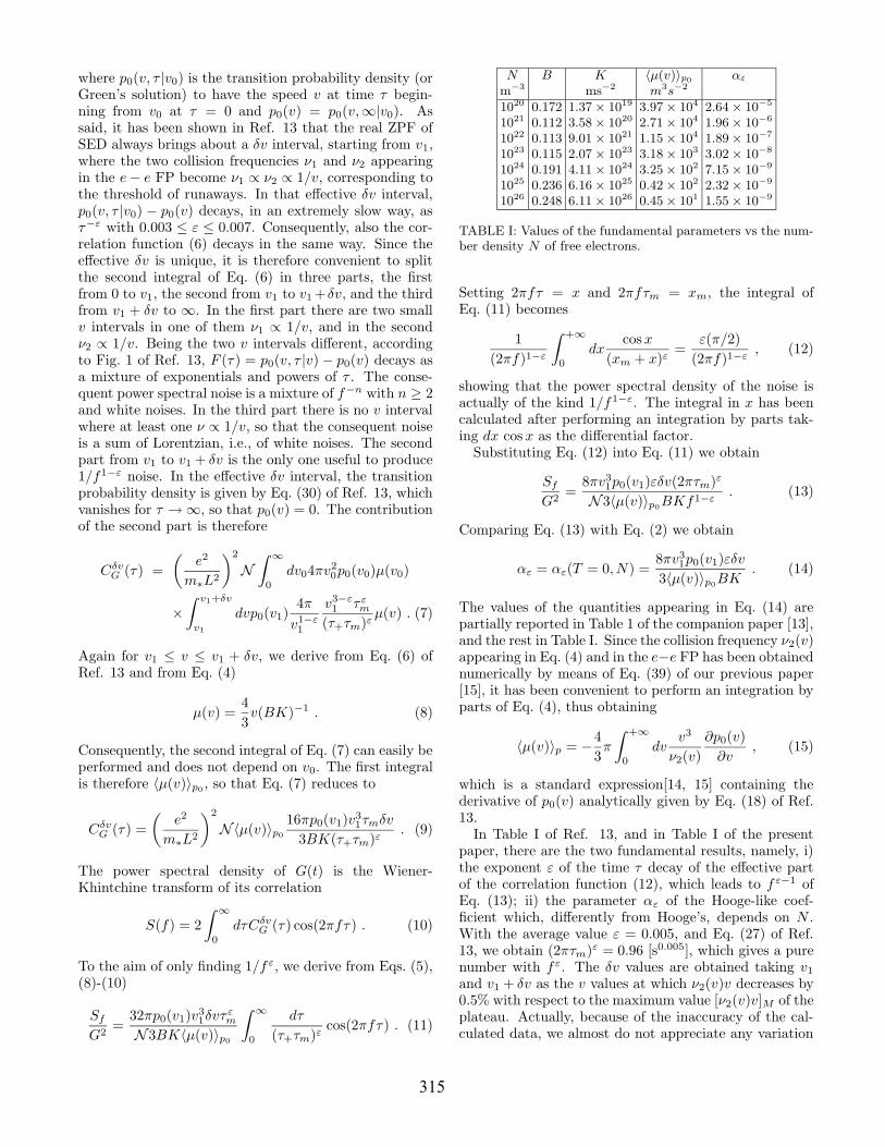
where p0(v, τ |v0) is the transition probability density (orGreen’s solution) to have the speed v at time τ begin-ning from v0 at τ = 0 and p0(v) = p0(v,∞|v0). Assaid, it has been shown in Ref. 13 that the real ZPF ofSED always brings about a δv interval, starting from v1,where the two collision frequencies ν1 and ν2 appearingin the e− e FP become ν1 ∝ ν2 ∝ 1/v, corresponding tothe threshold of runaways. In that effective δv interval,p0(v, τ |v0) − p0(v) decays, in an extremely slow way, asτ−ε with 0.003 ≤ ε ≤ 0.007. Consequently, also the cor-relation function (6) decays in the same way. Since theeffective δv is unique, it is therefore convenient to splitthe second integral of Eq. (6) in three parts, the firstfrom 0 to v1, the second from v1 to v1+δv, and the thirdfrom v1 + δv to ∞. In the first part there are two smallv intervals in one of them ν1 ∝ 1/v, and in the secondν2 ∝ 1/v. Being the two v intervals different, accordingto Fig. 1 of Ref. 13, F (τ) = p0(v, τ |v)− p0(v) decays asa mixture of exponentials and powers of τ . The conse-quent power spectral noise is a mixture of f−n with n ≥ 2and white noises. In the third part there is no v intervalwhere at least one ν ∝ 1/v, so that the consequent noiseis a sum of Lorentzian, i.e., of white noises. The secondpart from v1 to v1 + δv is the only one useful to produce1/f1−ε noise. In the effective δv interval, the transitionprobability density is given by Eq. (30) of Ref. 13, whichvanishes for τ →∞, so that p0(v) = 0. The contributionof the second part is therefore
CδvG (τ) =
(
e2
m∗L2
)2
N
∫ ∞
0
dv04πv20p0(v0)µ(v0)
×
∫ v1+δv
v1
dvp0(v1)4π
v1−ε1
v3−ε1 τεm(τ+τm)ε
µ(v) . (7)
Again for v1 ≤ v ≤ v1 + δv, we derive from Eq. (6) ofRef. 13 and from Eq. (4)
µ(v) =4
3v(BK)−1 . (8)
Consequently, the second integral of Eq. (7) can easily beperformed and does not depend on v0. The first integralis therefore 〈µ(v)〉p0
, so that Eq. (7) reduces to
CδvG (τ) =
(
e2
m∗L2
)2
N〈µ(v)〉p0
16πp0(v1)v31τmδv
3BK(τ+τm)ε. (9)
The power spectral density of G(t) is the Wiener-Khintchine transform of its correlation
S(f) = 2
∫ ∞
0
dτCδvG (τ) cos(2πfτ) . (10)
To the aim of only finding 1/f ε, we derive from Eqs. (5),(8)-(10)
Sf
G2=32πp0(v1)v
31δvτ
εm
N3BK〈µ(v)〉p0
∫ ∞
0
dτ
(τ+τm)εcos(2πfτ) . (11)
N B K 〈µ(v)〉p0αε
m−3 ms−2 m3s−2
1020 0.172 1.37× 10¹⁹ 3.97× 10⁴ 2.64× 10⁻⁵
1021 0.112 3.58× 10²⁰ 2.71× 10⁴ 1.96× 10⁻⁶
1022 0.113 9.01× 10²¹ 1.15× 10⁴ 1.89× 10⁻⁷
1023 0.115 2.07× 10²³ 3.18× 10³ 3.02× 10⁻⁸
1024 0.191 4.11× 1024 3.25× 10² 7.15× 10⁻⁹
1025 0.236 6.16× 1025 0.42× 10² 2.32× 10⁻⁹
1026 0.248 6.11× 1026 0.45× 101 1.55× 10⁻⁹
TABLE I: Values of the fundamental parameters vs the num-ber density N of free electrons.
Setting 2πfτ = x and 2πfτm = xm, the integral ofEq. (11) becomes
1
(2πf)1−ε
∫ +∞
0
dxcosx
(xm + x)ε=
ε(π/2)
(2πf)1−ε, (12)
showing that the power spectral density of the noise isactually of the kind 1/f1−ε. The integral in x has beencalculated after performing an integration by parts tak-ing dx cosx as the differential factor.Substituting Eq. (12) into Eq. (11) we obtain
Sf
G2=8πv3
1p0(v1)εδv(2πτm)ε
N3〈µ(v)〉p0BKf1−ε
. (13)
Comparing Eq. (13) with Eq. (2) we obtain
αε = αε(T = 0, N) =8πv3
1p0(v1)εδv
3〈µ(v)〉p0BK
. (14)
The values of the quantities appearing in Eq. (14) arepartially reported in Table 1 of the companion paper [13],and the rest in Table I. Since the collision frequency ν2(v)appearing in Eq. (4) and in the e−e FP has been obtainednumerically by means of Eq. (39) of our previous paper[15], it has been convenient to perform an integration byparts of Eq. (4), thus obtaining
〈µ(v)〉p = −4
3π
∫ +∞
0
dvv3
ν2(v)
∂p0(v)
∂v, (15)
which is a standard expression[14, 15] containing thederivative of p0(v) analytically given by Eq. (18) of Ref.13.In Table I of Ref. 13, and in Table I of the present
paper, there are the two fundamental results, namely, i)the exponent ε of the time τ decay of the effective partof the correlation function (12), which leads to f ε−1 ofEq. (13); ii) the parameter αε of the Hooge-like coef-ficient which, differently from Hooge’s, depends on N .With the average value ε = 0.005, and Eq. (27) of Ref.13, we obtain (2πτm)
ε = 0.96 [s0.005], which gives a purenumber with f ε. The δv values are obtained taking v1
and v1 + δv as the v values at which ν2(v)v decreases by0.5% with respect to the maximum value [ν2(v)v]M of theplateau. Actually, because of the inaccuracy of the cal-culated data, we almost do not appreciate any variation
315
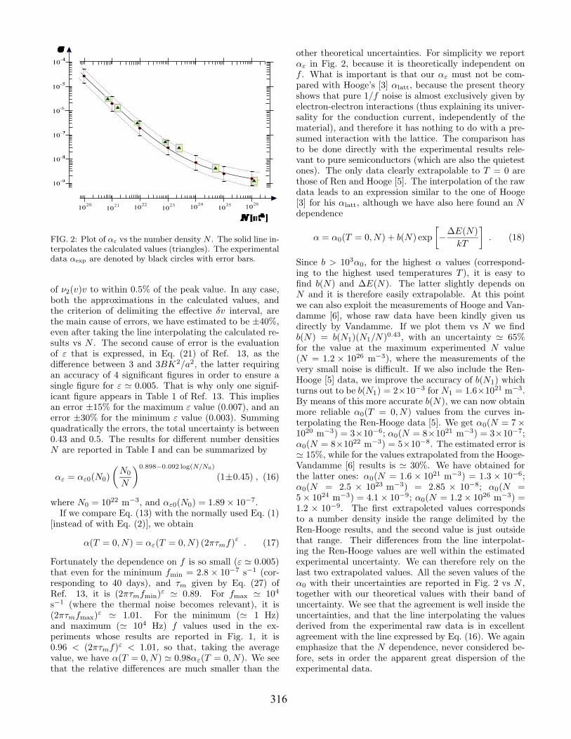
FIG. 2: Plot of αε vs the number density N . The solid line in-terpolates the calculated values (triangles). The experimentaldata αexp are denoted by black circles with error bars.
of ν2(v)v to within 0.5% of the peak value. In any case,both the approximations in the calculated values, andthe criterion of delimiting the effective δv interval, arethe main cause of errors, we have estimated to be ±40%,even after taking the line interpolating the calculated re-sults vs N . The second cause of error is the evaluationof ε that is expressed, in Eq. (21) of Ref. 13, as thedifference between 3 and 3BK2/a2, the latter requiringan accuracy of 4 significant figures in order to ensure asingle figure for ε ' 0.005. That is why only one signif-icant figure appears in Table 1 of Ref. 13. This impliesan error ±15% for the maximum ε value (0.007), and anerror ±30% for the minimum ε value (0.003). Summingquadratically the errors, the total uncertainty is between0.43 and 0.5. The results for different number densitiesN are reported in Table I and can be summarized by
αε = αε0(N0)
(
N0
N
)0.898−0.092 log(N/N0)
(1±0.45) , (16)
where N0 = 1022 m−3, and αε0(N0) = 1.89× 10
−7.If we compare Eq. (13) with the normally used Eq. (1)
[instead of with Eq. (2)], we obtain
α(T = 0, N) = αε(T = 0, N) (2πτmf)ε
. (17)
Fortunately the dependence on f is so small (ε ' 0.005)that even for the minimum fmin = 2.8 × 10
−7 s−1 (cor-responding to 40 days), and τm given by Eq. (27) ofRef. 13, it is (2πτmfmin)
ε ' 0.89. For fmax ' 104
s−1 (where the thermal noise becomes relevant), it is(2πτmfmax)
ε ' 1.01. For the minimum (' 1 Hz)and maximum (' 104 Hz) f values used in the ex-periments whose results are reported in Fig. 1, it is0.96 < (2πτmf)ε < 1.01, so that, taking the averagevalue, we have α(T = 0, N) ' 0.98αε(T = 0, N). We seethat the relative differences are much smaller than the
other theoretical uncertainties. For simplicity we reportαε in Fig. 2, because it is theoretically independent onf . What is important is that our αε must not be com-pared with Hooge’s [3] αlatt, because the present theoryshows that pure 1/f noise is almost exclusively given byelectron-electron interactions (thus explaining its univer-sality for the conduction current, independently of thematerial), and therefore it has nothing to do with a pre-sumed interaction with the lattice. The comparison hasto be done directly with the experimental results rele-vant to pure semiconductors (which are also the quietestones). The only data clearly extrapolable to T = 0 arethose of Ren and Hooge [5]. The interpolation of the rawdata leads to an expression similar to the one of Hooge[3] for his αlatt, although we have also here found an Ndependence
α = α0(T = 0, N) + b(N) exp
[
−∆E(N)
kT
]
. (18)
Since b > 103α0, for the highest α values (correspond-ing to the highest used temperatures T ), it is easy tofind b(N) and ∆E(N). The latter slightly depends onN and it is therefore easily extrapolable. At this pointwe can also exploit the measurements of Hooge and Van-damme [6], whose raw data have been kindly given usdirectly by Vandamme. If we plot them vs N we findb(N) = b(N1)(N1/N)
0.43, with an uncertainty ' 65%for the value at the maximum experimented N value(N = 1.2 × 1026 m−3), where the measurements of thevery small noise is difficult. If we also include the Ren-Hooge [5] data, we improve the accuracy of b(N1) whichturns out to be b(N1) = 2×10
−3 for N1 = 1.6×10²¹ m−3.
By means of this more accurate b(N), we can now obtainmore reliable α0(T = 0, N) values from the curves in-terpolating the Ren-Hooge data [5]. We get α0(N = 7×10²⁰ m−3) = 3×10⁻⁶; α0(N = 8×10²¹ m−3) = 3×10⁻⁷;α0(N = 8×10²² m−3) = 5×10⁻⁸. The estimated error is' 15%, while for the values extrapolated from the Hooge-Vandamme [6] results is ' 30%. We have obtained forthe latter ones: α0(N = 1.6 × 10²¹ m−3) = 1.3 × 10⁻⁶;α0(N = 2.5 × 10²³ m−3) = 2.85 × 10⁻⁸; α0(N =5× 1024 m−3) = 4.1× 10⁻⁹; α0(N = 1.2× 1026 m−3) =1.2 × 10⁻⁹. The first extrapoleted values correspondsto a number density inside the range delimited by theRen-Hooge results, and the second value is just outsidethat range. Their differences from the line interpolat-ing the Ren-Hooge values are well within the estimatedexperimental uncertainty. We can therefore rely on thelast two extrapolated values. All the seven values of theα0 with their uncertainties are reported in Fig. 2 vs N ,together with our theoretical values with their band ofuncertainty. We see that the agreement is well inside theuncertainties, and that the line interpolating the valuesderived from the experimental raw data is in excellentagreement with the line expressed by Eq. (16). We againemphasize that the N dependence, never considered be-fore, sets in order the apparent great dispersion of theexperimental data.
316
III. S(f) ∝ 1/f0.995 IN A FINITE SAMPLE
The preceding ideas and results are sufficient to explainin a satisfactory way the 1/f 0.995 noise in an indefinitemedium. The point is that the electrons between thetwo electrodes (where a fluctuating voltage is measured)L apart from each other, take a time interval L/w (wherew is the drift velocity, only due to aD.C.) to traverse L.But there is no evidence of a tiny change in the decayafter L/w. The solution is due to the rapid back diffusionfor the fraction of the electrons whose speed is inside thesmall, effective time interval δv. The diffusion velocity(for only that small fraction) turns out to be much largerthan the drift velocity. More in detail, the explanationis based on the following two results: i) The electron-electron (e− e) scattering is dominant for the generationof 1/f1−ε noise. ii) The e − e scattering also preservesthe memory of a fluctuaction much beyond the averagetransit-time L/w. In fact, free electrons are subjectedto the drift velocity due to aD.C., but also to diffusiondue to aZPF. Now, during the time τm of informationtransmission given by Eq. (27) of Ref. 13, the averagedisplacement due to the drift velocity is
δx = wτm = µmED.C.τm . (19)
The most probable displacement in the same time inter-val, due to the longitudinal diffusion coefficient DL forthe electrons in the useful δv range, is [15, 16]
δr = [4DL(v1)τm]1/2 , (20)
where v1 is the smallest velocity of the useful δv range.Now, as shown by Parker and Lowke [16], when ν ∝ v−1,i.e., at the threshold of runaways, DL diverges. In fact,the expression of ν considered after Eq. (13) of Ref. 16(p.293), is ν = ν0(ε/ε0)
(l+1)/2 = ν0(v/v0)l+1 (since ε =
mv2/2) and they found
DL/DT = (l + 3)/[2(l + 2)] , (21)
where DT is the transversal diffusion coefficient. We seeclearly that this ratio diverges for l→ −2, correspondingto ν ∝ v−1. Parker and Lowke [16] obtained it by a semi-quantitative model (their Sec. III), and their quantitativetheory implies a still stronger divergence, as can be seencomparing this ratio with Table I of Ref. 16. Since DL
is defined as limt→∞〈(x− x0)2/t〉, the divergence means
that (x − x0)2 ∝ t2, i.e., the diffusion becomes ballis-
tic and δr ' v1τm. The ratio between δr and the δxgiven by Eq. (19), i.e., δr/δx = v1/(µmED.C.), is verylarge [17], and independent of τm. Consequently, the ve-locity of back diffusion, responsible for the transmissionof information to the new electrons entering the L sec-tion of the sample (between the two electrodes L apartfrom each other), is much larger than the drift velocityw. That is why the memory of a fluctuaction is preservedindependently of the transit-time L/w. It was just thedivergence of DL when ν ∝ v−1 that suggested to one
of us (G. Cavalleri) the idea of the possible origin of 1/fnoise when ν2 ∝ v−1, because of the connection betweennoise power spectral densities and generalized diffusioncoefficients [18]. The pure 1/f noise is therefore valid forboth an indefinite medium and a small sample.
IV. CONCLUSIONS
When a fluctuation produces a pimple in the distri-bution function of the electron speeds, the pimple tendsto diffuse and drift in the speed space because of colli-sions. However, at the threshold of runaways there is akind of counter-diffusion and counter-drift in the speedspace, so that the pimple appears as almost crystallized,decaying as τ−0.005. Moreover, this result is independentof the transit time L/w of the electrons. What is more,our theoretical expression (16) fits the experimental datamuch better than Hooge’s empirical formula, because wefind a dependence on the electron concentration N be-sides the total number N of electrons in the consideredsample. No previous paper has ever predicted the Ndependence that is peculiar for the pure 1/f noise, andnot for the 1/f like component due to electron trapping-detrappings. The data fittings hold only for the pure1/f noise, i.e., the one present in the purest and quietestsemiconductors. The pure 1/f noise can also be obtainedas the residue of the usual much larger 1/f like noise af-ter subtracting the usually much larger contribution dueto trapping-detrappings.Finally, the 1/f1−ε noise only depends on the electron-
electron (e − e) scattering in a small δv range, and it istherefore independent of the electron-lattice (e−lattice)scattering. The coefficient of proportionality αε dependson the material only via the mobility 〈µ(v)〉p0
appearingat the denominator of Eq. (14). In turn, 〈µ(v)〉p0
, aver-aged over 0 < v <∞, is due to both e− e and e−latticescatterings (e−e scattering is much larger than e−latticescattering only in the neighborhoods of the effective δvinterval).The pure 1/f noise is therefore fully explained from
both the experimental and theoretical points of view.The reason why this long standing problem challenged allthe previous attempts is that it required a catena of suc-cessive achievements, we summarize below: 1) The reduc-tion of the nonlinear Boltzmann equation with electron-electron (e−e) interaction to a Fokker-Planck (FP) equa-tion; 2) The steady-state solution p0(v) of e−e FP equa-tion, which depends on the square of acceleration a; 3)p0(v) becomes similar to the Fermi-Dirac distributionfunction if a2 is caused by the zero-point field (ZPF) ofQED. It is just because of a2
ZPF that there is a small in-terval δv for the electron speed v where runaways occur;4) In this δv range, the time-dependent Green’s solutionof the e − e FP decreases as τ−ε with ε ≤ 0.007. Then,S(f) ∝ 1/f1−ε and also depends on the electron con-centration, thus closely fitting the experimental data; 5)In a finite sample, fluctuactions are remembered because
317
back diffusion is much more rapid than drift velocity.Indirectly, the qualitative and quantitative explanation
of the universal pure 1/f noise is a new proof of the
existence of the real (i.e., unrenormalized) zero-point field(ZPF) of SED.
[1] M. B. Weissman, Rev. Mod. Phys. 60, 357-371 (1988).[2] S. V. Melkonyan, V. M. Aroutiounian, F. V. Gasparyan,and H. V. Asriyan, Physica B 382, 65-70 (2006).
[3] F. N. Hooge, IEEE Trans. Electron Devices 41, 1926-1935 (1994).
[4] X. Y. Chen, F. N. Hooge, and M. R. Leys, Solid-St. Elec-tron. 41, 1269-1275 (1997).
[5] L. Ren, and F. N. Hooge, Physica B 176, 209-212 (1992).[6] F. N. Hooge and L. K. J. Vandamme, Physics Letters A
66, 315-316 (1978)[7] P. H. Handel, Phys. Rev. Lett. 34, 1492-1495 (1975).[8] P. H. Handel, Phys. Rev. Lett. 34, 1495-1498 (1975).[9] L. B. Kiss and P. Heszler, J. Phys. C 19, L631-L634(1986).
[10] Th. M. Nieuwenhuizen, D. Frenkel, and N. G. van Kam-pen, Phys. Rev. A 35, 2750-2753 (1987).
[11] K. A. Kazakov, Int. J. Mod. Phys. B 20, 233-248 (2006).[12] T. Musha and M. Tacano, Physica A 346, 339-346
(2005).[13] G. Cavalleri, E. Tonni, and G. Spavieri, Physica A, com-
panion paper (2008).[14] L. J. H. Huxley and R. W. Crompton, “The Diffusion and
Drift of Electrons in Gases” (Wiley, New York 1974).[15] G. Cavalleri, E. Tonni, L. Bosi, and G. Spavieri, Nuovo
Cimento B 116, 1-30 (2001).[16] J. H. Parker and J. J. Lowke, Phys. Rev. 181, 290-301
(1969).[17] Notice that the rapid diffusion is practically not de-
tectable experimentally, because it is relevant to a num-ber δN ' 10−3N of electrons in the small speed intervalδv ' 2× 10⁻³〈v2〉1/2. Moreover, the diffusion coefficient(for only the electrons in δv) tends to diverge in the con-figuration space, while tends to vanish in the speed space.
[18] G. Cavalleri and G. Mauri, Phys. Rev. B 37, 6868-6881(1988).
318
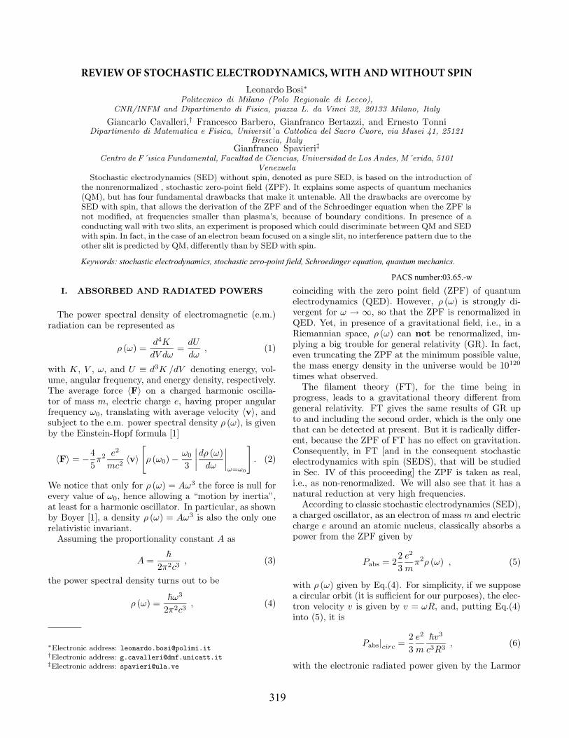
REVIEW OF STOCHASTIC ELECTRODYNAMICS, WITH AND WITHOUT SPINLeonardo Bosi∗
Politecnico di Milano (Polo Regionale di Lecco),CNR/INFM and Dipartimento di Fisica, piazza L. da Vinci 32, 20133 Milano, Italy
Giancarlo Cavalleri,† Francesco Barbero, Gianfranco Bertazzi, and Ernesto Tonni Dipartimento di Matematica e Fisica, Universit`a Cattolica del Sacro Cuore, via Musei 41, 25121
Brescia, ItalyGianfranco Spavieri‡
Centro de F´ısica Fundamental, Facultad de Ciencias, Universidad de Los Andes, M´erida, 5101Venezuela
Stochastic
electrodynamics
(SED)
without
spin,
denoted
as
pure SED, is based on the introduction ofthe nonrenormalized , stochastic zero-point field (ZPF). It explains some aspects of quantum mechanics(QM), but has four fundamental drawbacks that make it untenable. All the drawbacks are overcome bySED
with
spin,
that
allows
the
derivation
of
the
ZPF and
of
the
Schroedinger
equation
when
the
ZPF
is
not modified, at frequencies smaller than plasma’s, because
of
boundary
conditions.
In
presence
of
a
conducting
wall
with
two
slits,
an
experiment
is
proposed
which
could
discriminate
between
QM
and
SED
with
spin.
In
fact,
in
the
case
of an electron beam focused
on
a
single
slit,
no
interference
pattern
due
to
the
other slit is predicted by QM, differently than by SED with
spin.
I. ABSORBED AND RADIATED POWERS
The power spectral density of electromagnetic (e.m.)radiation can be represented as
ρ (ω) =d4K
dV dω=
dU
dω, (1)
with K, V , ω, and U ≡ d3K /dV denoting energy, vol-ume, angular frequency, and energy density, respectively.The average force 〈F〉 on a charged harmonic oscilla-tor of mass m, electric charge e, having proper angularfrequency ω0, translating with average velocity 〈v〉, andsubject to the e.m. power spectral density ρ (ω), is givenby the Einstein-Hopf formula [1]
〈F〉 = −4
5π2 e2
mc2〈v〉
[
ρ (ω0)−ω0
3
∣
∣
∣
∣
dρ (ω)
dω
∣
∣
∣
∣
ω=ω0
]
. (2)
We notice that only for ρ (ω) = Aω3 the force is null forevery value of ω0, hence allowing a “motion by inertia”,at least for a harmonic oscillator. In particular, as shownby Boyer [1], a density ρ (ω) = Aω3 is also the only onerelativistic invariant.Assuming the proportionality constant A as
A =~
2π2c3, (3)
the power spectral density turns out to be
ρ (ω) =~ω3
2π2c3, (4)
∗Electronic address: [email protected]†Electronic address: [email protected]‡Electronic address: [email protected]
coinciding with the zero point field (ZPF) of quantumelectrodynamics (QED). However, ρ (ω) is strongly di-vergent for ω → ∞, so that the ZPF is renormalized inQED. Yet, in presence of a gravitational field, i.e., in aRiemannian space, ρ (ω) can not be renormalized, im-plying a big trouble for general relativity (GR). In fact,even truncating the ZPF at the minimum possible value,the mass energy density in the universe would be 10120
times what observed.The filament theory (FT), for the time being in
progress, leads to a gravitational theory different fromgeneral relativity. FT gives the same results of GR upto and including the second order, which is the only onethat can be detected at present. But it is radically differ-ent, because the ZPF of FT has no effect on gravitation.Consequently, in FT [and in the consequent stochasticelectrodynamics with spin (SEDS), that will be studiedin Sec. IV of this proceeding] the ZPF is taken as real,i.e., as non-renormalized. We will also see that it has anatural reduction at very high frequencies.According to classic stochastic electrodynamics (SED),
a charged oscillator, as an electron of massm and electriccharge e around an atomic nucleus, classically absorbs apower from the ZPF given by
Pabs = 22
3
e2
mπ2ρ (ω) , (5)
with ρ (ω) given by Eq.(4). For simplicity, if we supposea circular orbit (it is sufficient for our purposes), the elec-tron velocity v is given by v = ωR, and, putting Eq.(4)into (5), it is
Pabs|circ =2
3
e2
m
~v3
c3R3, (6)
with the electronic radiated power given by the Larmor
Keywords: stochastic electrodynamics, stochastic zero-point field, Schroedinger equation, quantum mechanics.
PACS number:03.65.-w
319
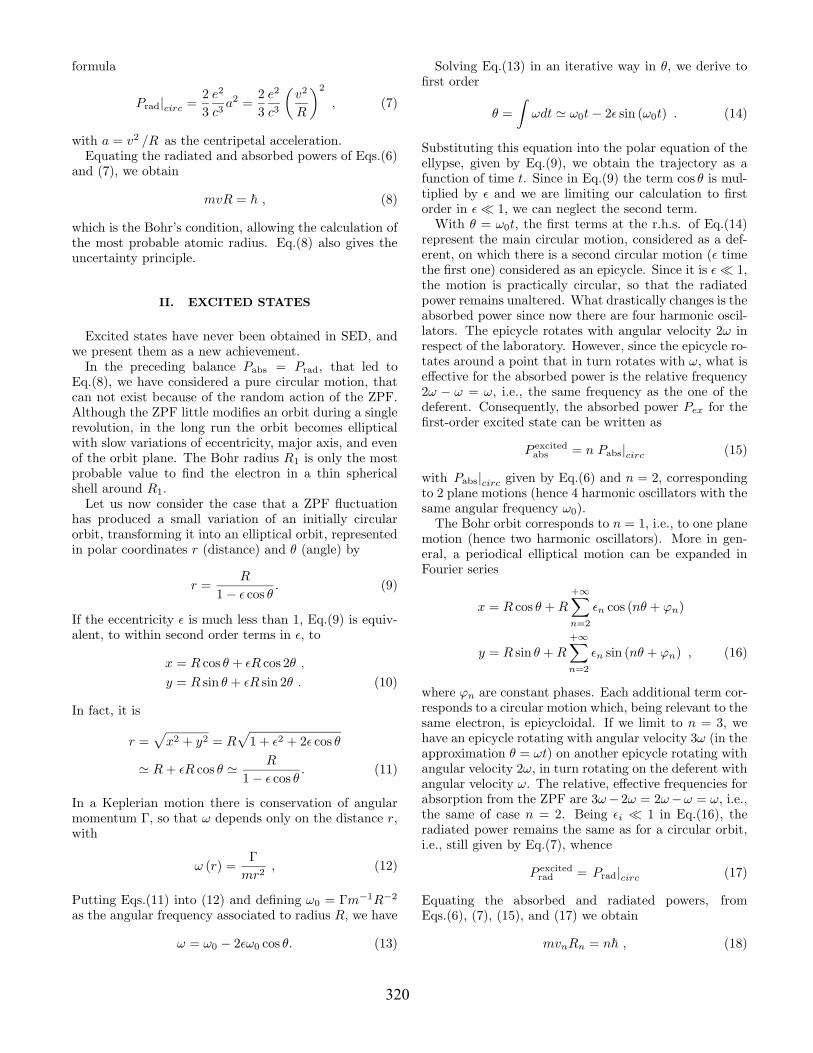
formula
Prad|circ =2
3
e2
c3a2 =
2
3
e2
c3
(
v2
R
)2
, (7)
with a = v2 /R as the centripetal acceleration.Equating the radiated and absorbed powers of Eqs.(6)
and (7), we obtain
mvR = ~ , (8)
which is the Bohr’s condition, allowing the calculation ofthe most probable atomic radius. Eq.(8) also gives theuncertainty principle.
II. EXCITED STATES
Excited states have never been obtained in SED, andwe present them as a new achievement.In the preceding balance Pabs = Prad, that led to
Eq.(8), we have considered a pure circular motion, thatcan not exist because of the random action of the ZPF.Although the ZPF little modifies an orbit during a singlerevolution, in the long run the orbit becomes ellipticalwith slow variations of eccentricity, major axis, and evenof the orbit plane. The Bohr radius R1 is only the mostprobable value to find the electron in a thin sphericalshell around R1.Let us now consider the case that a ZPF fluctuation
has produced a small variation of an initially circularorbit, transforming it into an elliptical orbit, representedin polar coordinates r (distance) and θ (angle) by
r =R
1− ε cos θ. (9)
If the eccentricity ε is much less than 1, Eq.(9) is equiv-alent, to within second order terms in ε, to
x = R cos θ + εR cos 2θ ,
y = R sin θ + εR sin 2θ . (10)
In fact, it is
r =√
x2 + y2 = R√
1 + ε2 + 2ε cos θ
' R+ εR cos θ 'R
1− ε cos θ. (11)
In a Keplerian motion there is conservation of angularmomentum Γ, so that ω depends only on the distance r,with
ω (r) =Γ
mr2, (12)
Putting Eqs.(11) into (12) and defining ω0 = Γm−1R−2
as the angular frequency associated to radius R, we have
ω = ω0 − 2εω0 cos θ. (13)
Solving Eq.(13) in an iterative way in θ, we derive tofirst order
θ =
∫
ωdt ' ω0t− 2ε sin (ω0t) . (14)
Substituting this equation into the polar equation of theellypse, given by Eq.(9), we obtain the trajectory as afunction of time t. Since in Eq.(9) the term cos θ is mul-tiplied by ε and we are limiting our calculation to firstorder in ε¿ 1, we can neglect the second term.With θ = ω0t, the first terms at the r.h.s. of Eq.(14)
represent the main circular motion, considered as a def-erent, on which there is a second circular motion (ε timethe first one) considered as an epicycle. Since it is ε¿ 1,the motion is practically circular, so that the radiatedpower remains unaltered. What drastically changes is theabsorbed power since now there are four harmonic oscil-lators. The epicycle rotates with angular velocity 2ω inrespect of the laboratory. However, since the epicycle ro-tates around a point that in turn rotates with ω, what iseffective for the absorbed power is the relative frequency2ω − ω = ω, i.e., the same frequency as the one of thedeferent. Consequently, the absorbed power Pex for thefirst-order excited state can be written as
P excitedabs = n Pabs|circ (15)
with Pabs|circ given by Eq.(6) and n = 2, correspondingto 2 plane motions (hence 4 harmonic oscillators with thesame angular frequency ω0).The Bohr orbit corresponds to n = 1, i.e., to one plane
motion (hence two harmonic oscillators). More in gen-eral, a periodical elliptical motion can be expanded inFourier series
x = R cos θ +R
+∞∑
n=2
εn cos (nθ + ϕn)
y = R sin θ +R
+∞∑
n=2
εn sin (nθ + ϕn) , (16)
where ϕn are constant phases. Each additional term cor-responds to a circular motion which, being relevant to thesame electron, is epicycloidal. If we limit to n = 3, wehave an epicycle rotating with angular velocity 3ω (in theapproximation θ = ωt) on another epicycle rotating withangular velocity 2ω, in turn rotating on the deferent withangular velocity ω. The relative, effective frequencies forabsorption from the ZPF are 3ω− 2ω = 2ω−ω = ω, i.e.,the same of case n = 2. Being εi ¿ 1 in Eq.(16), theradiated power remains the same as for a circular orbit,i.e., still given by Eq.(7), whence
P excitedrad = Prad|circ (17)
Equating the absorbed and radiated powers, fromEqs.(6), (7), (15), and (17) we obtain
mvnRn = n~ , (18)
320
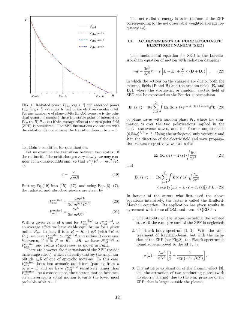
FIG. 1: Radiated power Prad [erg s−1] and absorbed power
Pabs [erg s−1] vs radius R [cm] of the electron circular orbit.
For any number n of plane orbits (in QM terms, n is the prin-cipal quantum number) there is a stable point of intersectionPabs (n,R)Prad (n) if the average effect of the zero-point field(ZPF) is considered. The ZPF fluctuations concordant withthe radiation damping cause the transition from n to n− 1.
i.e., Bohr’s condition for quantization.Let us examine the transition between two states. If
the radius R of the orbit changes very slowly, we may con-sider it in quasi-equilibrium, so that e2
/
R2 = mv2 /R ,i.e.
v =e
√mR
(19)
Putting Eq.(19) into (15), (17), and using Eqs.(6), (7),the radiated and absorbed powers are given by
P excitedabs =
2ne5~3c3m5/2R9/2
(20)
P excitedrad =
2e6
3c3m2R4. (21)
With a given value of n and for P excitedabs ' P excited
rad , asan average effect we have stable equilibrium for a givenradius Rn. In fact, if it is R = Rn + δR (with δR ¿Rn), we have P excited
rad > P excitedabs and radius R decreases.
Viceversa, if it is R = Rn − δR, we have P excitedrad <
P excitedabs and radius R increases, as shown in Fig.1.There are however the fluctuations of the ZPF (beside
its average effect), which can easily destroy the small am-plitude εnR of one of epicyclic motions. In this case,P excited
abs loses two armonic oscillators (passing from nto n − 1) and we have P excited
rad sensitively larger thanP excited
abs . As a consequence, the electron motion becomes,on an average, a spiral motion towards the lower mostprobable orbit n− 1.
The net radiated energy is twice the one of the ZPFcorresponding to the net observable weighted average fre-quency 〈ω〉.
III. ACHIEVEMENTS OF PURE STOCHASTIC
ELECTRODYNAMICS (SED)
The fundamental equation for SED is the Lorentz-Abraham equation of motion with radiation damping
mr−2e2
3c3...r = e
[
E+Er +v
c× (B+Br)
]
, (22)
in which the actions on the charge e are due to both theexternal fields (E and B) and the random fields (Er andBr), where the stochastic, or random, electric field ofSED can be expressed as the Fourier superposition
Er (r, t) = Re
2∑
s=1
∫
Ek (k, s, t) ei[ωkt−k·r+θk(s)]d3
k (23)
of plane waves with random phase θk, where the sum-mation is over the two polarizations implied in thee.m. transverse waves, and the Fourier amplitude is
(0.5~ω)1/2 π−1. Using the orthogonal unit vectors ε and
k in the direction of the electric field and wave propaga-tion vectors respectively, we can write
Ek (k, s, t) = ε (s)
√
~ω2π2
(24)
and
Br (r, t) = Re2∑
s=1
∫
k× ε (s)
√
~ω2π2
× exp i [ωkt− k · r+ θk (s)] d3k . (25)
In honour of the autors who first used the aboveequations intensively, the latter is called the Brafford-Marshall equation. Its application has given results inagreement with those of QM, and even of QED for:
1. The stability of the atoms including the excitedstates if the e.m. pressure of the ZPF is neglected;
2. The black body spectrum [1, 2]. With the sametreatment of Rayleigh-Jeans, but with the inclu-sion of the ZPF (see Fig.2), the Planck spectrum isfound superimposed to the ZPF, i.e.
ρ (ω) =~ω3
π2c3
[
1
2+
1
exp (−~ω /kT )
]
;
3. The intuitive explanation of the Casimir effect [3],i.e., the attraction of two conducting plates (withno electric charge), due to the e.m. pressure of theZPF, that is larger outside the plates;
321
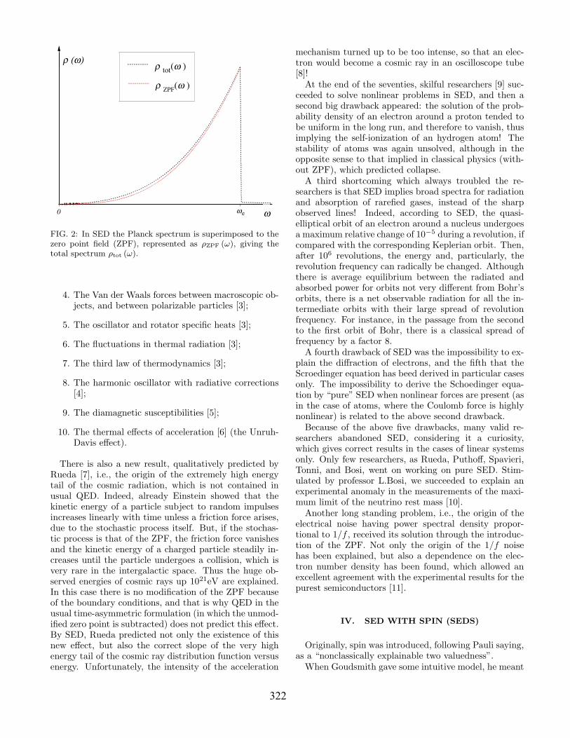
FIG. 2: In SED the Planck spectrum is superimposed to thezero point field (ZPF), represented as ρZPF (ω), giving thetotal spectrum ρtot (ω).
4. The Van der Waals forces between macroscopic ob-jects, and between polarizable particles [3];
5. The oscillator and rotator specific heats [3];
6. The fluctuations in thermal radiation [3];
7. The third law of thermodynamics [3];
8. The harmonic oscillator with radiative corrections[4];
9. The diamagnetic susceptibilities [5];
10. The thermal effects of acceleration [6] (the Unruh-Davis effect).
There is also a new result, qualitatively predicted byRueda [7], i.e., the origin of the extremely high energytail of the cosmic radiation, which is not contained inusual QED. Indeed, already Einstein showed that thekinetic energy of a particle subject to random impulsesincreases linearly with time unless a friction force arises,due to the stochastic process itself. But, if the stochas-tic process is that of the ZPF, the friction force vanishesand the kinetic energy of a charged particle steadily in-creases until the particle undergoes a collision, which isvery rare in the intergalactic space. Thus the huge ob-served energies of cosmic rays up 1021eV are explained.In this case there is no modification of the ZPF becauseof the boundary conditions, and that is why QED in theusual time-asymmetric formulation (in which the unmod-ified zero point is subtracted) does not predict this effect.By SED, Rueda predicted not only the existence of thisnew effect, but also the correct slope of the very highenergy tail of the cosmic ray distribution function versusenergy. Unfortunately, the intensity of the acceleration
mechanism turned up to be too intense, so that an elec-tron would become a cosmic ray in an oscilloscope tube[8]!At the end of the seventies, skilful researchers [9] suc-
ceeded to solve nonlinear problems in SED, and then asecond big drawback appeared: the solution of the prob-ability density of an electron around a proton tended tobe uniform in the long run, and therefore to vanish, thusimplying the self-ionization of an hydrogen atom! Thestability of atoms was again unsolved, although in theopposite sense to that implied in classical physics (with-out ZPF), which predicted collapse.A third shortcoming which always troubled the re-
searchers is that SED implies broad spectra for radiationand absorption of rarefied gases, instead of the sharpobserved lines! Indeed, according to SED, the quasi-elliptical orbit of an electron around a nucleus undergoesa maximum relative change of 10−5 during a revolution, ifcompared with the corresponding Keplerian orbit. Then,after 106 revolutions, the energy and, particularly, therevolution frequency can radically be changed. Althoughthere is average equilibrium between the radiated andabsorbed power for orbits not very different from Bohr’sorbits, there is a net observable radiation for all the in-termediate orbits with their large spread of revolutionfrequency. For instance, in the passage from the secondto the first orbit of Bohr, there is a classical spread offrequency by a factor 8.A fourth drawback of SED was the impossibility to ex-
plain the diffraction of electrons, and the fifth that theScroedinger equation has beed derived in particular casesonly. The impossibility to derive the Schoedinger equa-tion by “pure” SED when nonlinear forces are present (asin the case of atoms, where the Coulomb force is highlynonlinear) is related to the above second drawback.Because of the above five drawbacks, many valid re-
searchers abandoned SED, considering it a curiosity,which gives correct results in the cases of linear systemsonly. Only few researchers, as Rueda, Puthoff, Spavieri,Tonni, and Bosi, went on working on pure SED. Stim-ulated by professor L.Bosi, we succeeded to explain anexperimental anomaly in the measurements of the maxi-mum limit of the neutrino rest mass [10].Another long standing problem, i.e., the origin of the
electrical noise having power spectral density propor-tional to 1/f , received its solution through the introduc-tion of the ZPF. Not only the origin of the 1/f noisehas been explained, but also a dependence on the elec-tron number density has been found, which allowed anexcellent agreement with the experimental results for thepurest semiconductors [11].
IV. SED WITH SPIN (SEDS)
Originally, spin was introduced, following Pauli saying,as a “nonclassically explainable two valuedness”.When Goudsmith gave some intuitive model, he meant
322
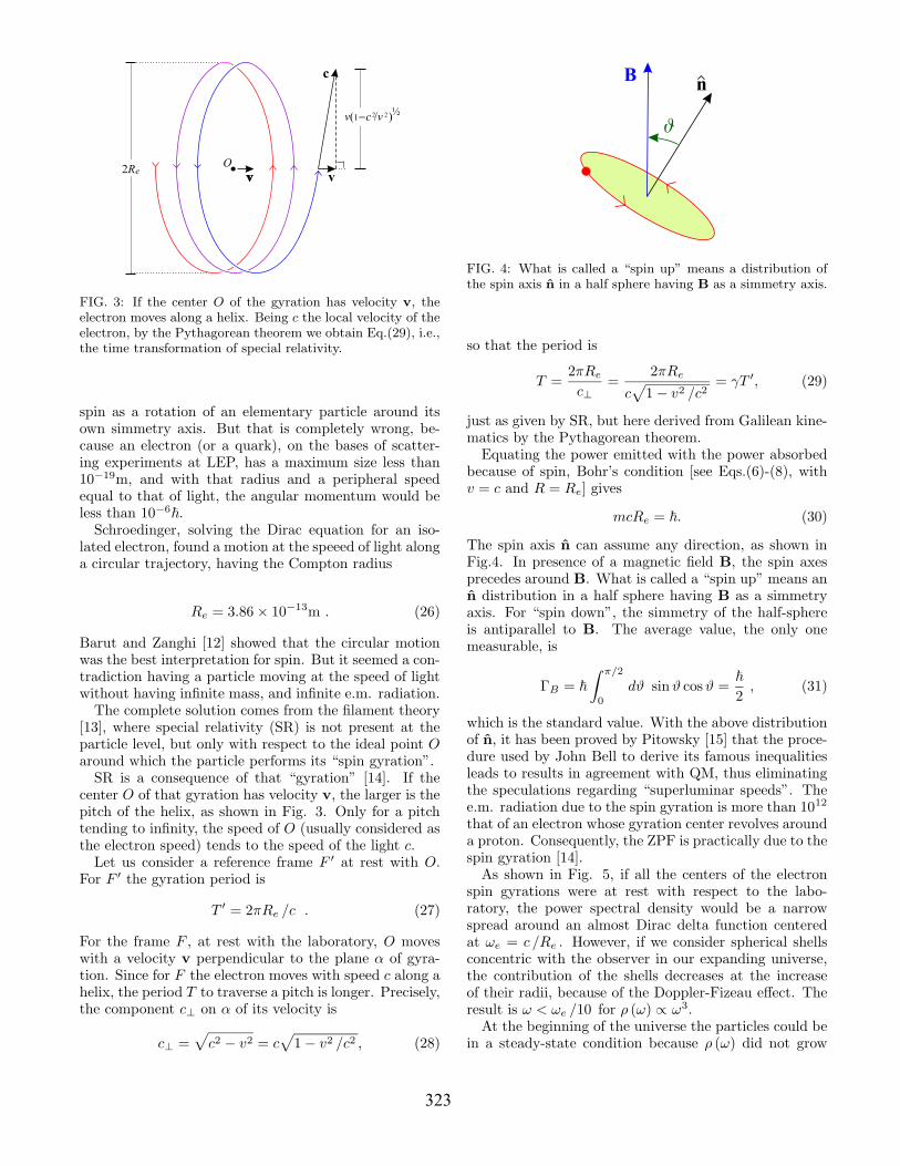
FIG. 3: If the center O of the gyration has velocity v, theelectron moves along a helix. Being c the local velocity of theelectron, by the Pythagorean theorem we obtain Eq.(29), i.e.,the time transformation of special relativity.
spin as a rotation of an elementary particle around itsown simmetry axis. But that is completely wrong, be-cause an electron (or a quark), on the bases of scatter-ing experiments at LEP, has a maximum size less than10−19m, and with that radius and a peripheral speedequal to that of light, the angular momentum would beless than 10−6~.Schroedinger, solving the Dirac equation for an iso-
lated electron, found a motion at the speeed of light alonga circular trajectory, having the Compton radius
Re = 3.86× 10⁻¹³m . (26)
Barut and Zanghi [12] showed that the circular motionwas the best interpretation for spin. But it seemed a con-tradiction having a particle moving at the speed of lightwithout having infinite mass, and infinite e.m. radiation.The complete solution comes from the filament theory
[13], where special relativity (SR) is not present at theparticle level, but only with respect to the ideal point Oaround which the particle performs its “spin gyration”.SR is a consequence of that “gyration” [14]. If the
center O of that gyration has velocity v, the larger is thepitch of the helix, as shown in Fig. 3. Only for a pitchtending to infinity, the speed of O (usually considered asthe electron speed) tends to the speed of the light c.Let us consider a reference frame F ′ at rest with O.
For F ′ the gyration period is
T ′ = 2πRe /c . (27)
For the frame F , at rest with the laboratory, O moveswith a velocity v perpendicular to the plane α of gyra-tion. Since for F the electron moves with speed c along ahelix, the period T to traverse a pitch is longer. Precisely,the component c⊥ on α of its velocity is
c⊥ =√
c2 − v2 = c√
1− v2 /c2 , (28)
FIG. 4: What is called a “spin up” means a distribution ofthe spin axis n in a half sphere having B as a simmetry axis.
so that the period is
T =2πRe
c⊥=
2πRe
c√
1− v2 /c2= γT ′, (29)
just as given by SR, but here derived from Galilean kine-matics by the Pythagorean theorem.Equating the power emitted with the power absorbed
because of spin, Bohr’s condition [see Eqs.(6)-(8), withv = c and R = Re] gives
mcRe = ~. (30)
The spin axis n can assume any direction, as shown inFig.4. In presence of a magnetic field B, the spin axesprecedes around B. What is called a “spin up” means ann distribution in a half sphere having B as a simmetryaxis. For “spin down”, the simmetry of the half-sphereis antiparallel to B. The average value, the only onemeasurable, is
ΓB = ~∫ π/2
0
dϑ sinϑ cosϑ =~2, (31)
which is the standard value. With the above distributionof n, it has been proved by Pitowsky [15] that the proce-dure used by John Bell to derive its famous inequalitiesleads to results in agreement with QM, thus eliminatingthe speculations regarding “superluminar speeds”. Thee.m. radiation due to the spin gyration is more than 1012
that of an electron whose gyration center revolves arounda proton. Consequently, the ZPF is practically due to thespin gyration [14].As shown in Fig. 5, if all the centers of the electron
spin gyrations were at rest with respect to the labo-ratory, the power spectral density would be a narrowspread around an almost Dirac delta function centeredat ωe = c /Re . However, if we consider spherical shellsconcentric with the observer in our expanding universe,the contribution of the shells decreases at the increaseof their radii, because of the Doppler-Fizeau effect. Theresult is ω < ωe /10 for ρ (ω) ∝ ω3.At the beginning of the universe the particles could be
in a steady-state condition because ρ (ω) did not grow
323
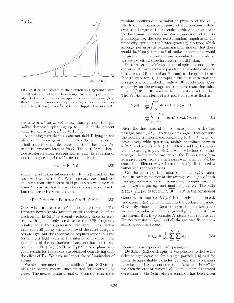
FIG. 5: If all the centers of the electron spin gyrations wereat rest with respect to the laboratory, the power spectral den-sity ρ (ω) would be a narrow spread centered at ωe = c /Re .However, ours is an expanding universe, whence, at least forω < 0.1ωe, it is ρ (ω) ∝ ω3 due to the Doppler-Fizeau effect.
versus ω as ω3 for ωe /10 < ∞. Consequently, the spinradius decreased spiralling up to ∼ 10−16 the presentvalue Re and ρ (ω) ∝ ω3 up to 1016ωe.A spinning particle in a constant field E lying in the
plane of the spin gyration increases the spin radius ina half trajectory and decreases it in the other half. Theresult is a zero acceleration for O. The particle can there-fore accelerate along its spin axis n, and the equation ofmotion, neglecting the self-reaction, is [10, 14]
m∗a = F · n n , (32)
wherem∗ is the inertial mass when F = n (indeed, in thiscase, we have m∗a = F). When an e.m. wave impingeson an electron, the electric field produces a velocity vari-ation δv ∝ n, so that the additional acceleration due toLorentz force δFL vanishes since
δFL · n = e δv ×B · n ∝ e n×B · n = 0. (33)
Only when n precesses δFL is no longer zero. TheEinstein-Boyer-Rueda mechanism of acceleration of anelectron in the ZPF is strongly reduced, since an elec-tron with spin is only sensitive to the ZPF frequencyroughly equal to its precession frequency. This mecha-nism can still justify the existence of the most energeticcosmic rays, but the acceleration requires some thousand(or million) light years in the intergalactic space. Thequenching of the mechanism of acceleration due to thecomponent Er+(v /c )×Br in Eq.(22) also explains whygood results for the atoms are obtained considering onlythe effect of Er. We have no longer the self-ionization ofatoms.We also overcome the impossibility of pure SED to ex-
plain the narrow spectral lines emitted (or absorbed) bygases. The new equation of motion strongly reduces the
random impulses due to radiation pressure of the ZPF,which would vanish in absence of n precession. How-ever, the torque of the extended orbit of spin and dueto the atomic nucleus produces a precession of n. Asa consequence, the ZPF exerts random impulses on theprecessing spinning (or better gyrating) electron, whichstrongly perturbs the regular spiraling motion that therewould be if only the classical radiation damping wouldbe present. The actual motion is similar to a spiral-liketrajectory with a superimposed rapid diffusion.In other terms, while the classical spiraling motion re-
quires ∼ 106 revolutions to pass from an excited state (forinstance the 2P state of an H atom) to the ground state(the 1S state for H), the rapid diffusion is such that thepassage is accomplished in only ∼ 102 revolutions. Con-sequently, on the average, the complete transition takesn ∼ 106
/
102 = 104 passages from one state to the other.The Fourier transform of net radiated electric field is
E (ω) =1
2π
∫ +∞
−∞
dt E (t) exp (−iωt)
=1
2π
n−1∑
s=1
∫ ts+1
ts
dt E (t) exp (−iωt) , (34)
where the time interval t2 − t1 corresponds to the firstpassage, and tn− tn−1 to the last passage. If we considerthe Fourier transform corresponding to t2 − t1 only, wehave a very wide spectrum, mainly contained betweenω (2P ) and ω (1S) = 8ω (2P ). This would be the spec-trum according to pure SED. If we now include the otherpassages, between the two states, the Fourier transformat a given intermediate ω increases with a factor
√n, be-
cause the different waves have differently distributed ωvalues and random phases.On the contrary, the radiated field E (〈ω〉), calcu-
lated in correspondence of the average value 〈ω〉 of eachpassage, increases as n, because 〈ω〉 changes very lit-tle between a passage and another passage. The ratio
E (〈ω〉)/
E (ω) is roughly√104 = 102 in the considered
example. In practice, E (〈ω〉) is the only one observed,the others E (ω) being included in the background noise.Obviously, there is a Gaussian spread about 〈ω〉, sincethe average value of each passage is slighly different fromthe others. But, if we consider N atoms that radiate, theFourier transform Etot (ω) of all the radiated fields has astill sharper line around
〈ω〉tot =1
Nn
N∑
s=1
n∑
i=1
ωis , (35)
because it corresponds to Nn passages.By SEDS (SED with spin) it was possible to derive the
Schroedinger equation for a single particle [16] and formany distinguishable particles [17], and the two papershave been positively commented in “News and Views” bythe then director of Nature [18]. Then, a more elaboratedderivation of the Schroedinger equation has been given
324
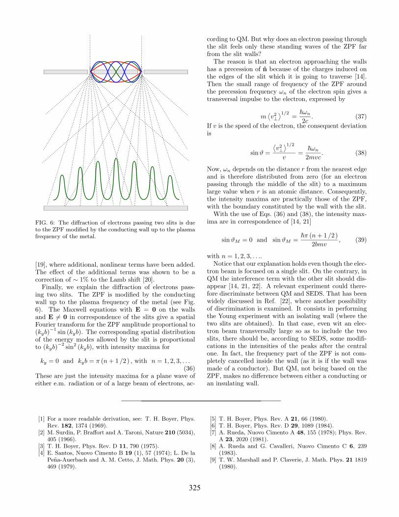
FIG. 6: The diffraction of electrons passing two slits is dueto the ZPF modified by the conducting wall up to the plasmafrequency of the metal.
[19], where additional, nonlinear terms have been added.The effect of the additional terms was shown to be acorrection of ∼ 1% to the Lamb shift [20].Finally, we explain the diffraction of electrons pass-
ing two slits. The ZPF is modified by the conductingwall up to the plasma frequency of the metal (see Fig.6). The Maxwell equations with E = 0 on the wallsand E 6= 0 in correspondence of the slits give a spatialFourier transform for the ZPF amplitude proportional to(kyb)
−1sin (kyb). The corresponding spatial distribution
of the energy modes allowed by the slit is proportionalto (kyb)
−2sin2 (kyb), with intensity maxima for
ky = 0 and kyb = π (n+ 1/2) , with n = 1, 2, 3, . . .(36)
These are just the intensity maxima for a plane wave ofeither e.m. radiation or of a large beam of electrons, ac-
cording to QM. But why does an electron passing throughthe slit feels only these standing waves of the ZPF farfrom the slit walls?The reason is that an electron approaching the walls
has a precession of n because of the charges induced onthe edges of the slit which it is going to traverse [14].Then the small range of frequency of the ZPF aroundthe precession frequency ωn of the electron spin gives atransversal impulse to the electron, expressed by
m⟨
v2⊥
⟩1/2=
~ωn
2c. (37)
If v is the speed of the electron, the consequent deviationis
sinϑ =
⟨
v2⊥
⟩1/2
v=
~ωn
2mvc. (38)
Now, ωn depends on the distance r from the nearest edgeand is therefore distributed from zero (for an electronpassing through the middle of the slit) to a maximumlarge value when r is an atomic distance. Consequently,the intensity maxima are practically those of the ZPF,with the boundary constituted by the wall with the slit.With the use of Eqs. (36) and (38), the intensity max-
ima are in correspondence of [14, 21]
sinϑM = 0 and sinϑM =~π (n+ 1/2)
2bmv, (39)
with n = 1, 2, 3, . . ..Notice that our explanation holds even though the elec-
tron beam is focused on a single slit. On the contrary, inQM the interference term with the other slit should dis-appear [14, 21, 22]. A relevant experiment could there-fore discriminate between QM and SEDS. That has beenwidely discussed in Ref. [22], where another possibilityof discrimination is examined. It consists in performingthe Young experiment with an isolating wall (where thetwo slits are obtained). In that case, even wit an elec-tron beam transversally large so as to include the twoslits, there should be, according to SEDS, some modifi-cations in the intensities of the peaks after the centralone. In fact, the frequency part of the ZPF is not com-pletely cancelled inside the wall (as it is if the wall wasmade of a conductor). But QM, not being based on theZPF, makes no difference between either a conducting oran insulating wall.
[1] For a more readable derivation, see: T. H. Boyer, Phys.Rev. 182, 1374 (1969).
[2] M. Surdin, P. Braffort and A. Taroni, Nature 210 (5034),405 (1966).
[3] T. H. Boyer, Phys. Rev. D 11, 790 (1975).[4] E. Santos, Nuovo Cimento B 19 (1), 57 (1974); L. De laPena-Auerbach and A. M. Cetto, J. Math. Phys. 20 (3),469 (1979).
[5] T. H. Boyer, Phys. Rev. A 21, 66 (1980).[6] T. H. Boyer, Phys. Rev. D 29, 1089 (1984).[7] A. Rueda, Nuovo Cimento A 48, 155 (1978); Phys. Rev.A 23, 2020 (1981).
[8] A. Rueda and G. Cavalleri, Nuovo Cimento C 6, 239(1983).
[9] T. W. Marshall and P. Claverie, J. Math. Phys. 21 1819(1980).
325
[10] L. Bosi and G. Cavalleri, Nuovo Cimento B 117, 243(2002).
[11] G. Cavalleri and L. Bosi, Phys. Stat. Sol. (c) 4, 1230(2007); G. Cavalleri, E. Tonni, L. Bosi, and G. Spavieri,Fluct. Noise Lett. 7, L193-L207 (2007).
[12] A. O. Barut and N. Zanghi, Phys. Rev. Lett. 52, 2009(1984).
[13] G. Cavalleri, F. Barbero, E. Tonni, D. Molteni, G. Bot-toni, and S. Lacchin, in Proc. of X Int. Conf. “Physi-cal Interpretations of Relativity Theory” (London, 8-11September, 2006), edited by M. C. Duffy, University ofSunderland (PD Publications, Liverpool, Great Britain),Vol. I (2008), in press.
[14] G. Cavalleri, Nuovo Cimento B 112, 1193 (1997).
[15] I. Pitowsky, Phys. Rev. Lett. 48 1299 (1982).[16] G. Cavalleri, Lett. Nuovo Cimento 43, 285 (1985).[17] G. Cavalleri and G. Spavieri, Nuovo Cimento B 95, 194
(1986).[18] J. Maddox, Nature (London) 325, 385 (1987).[19] G. Cavalleri and G. Mauri, Phys. Rev. B 41, 6751 (1990).[20] G. Cavalleri and A. Zecca, Phys. Rev. B 43, 3223 (1991).[21] A. Zecca and G. Cavalleri, Nuovo Cimento B 112, 1
(1997).[22] G. Cavalleri and E. Tonni, in “The Foundation of Quan-
tum Mechanics – Historical Analysis and Open Questions– Lecce 1998”, edited by C. Garola and A. Rossi (WorldScientific Publ. 2000), p. 111.
326

WHAT IS THE PHENOMENON THAT KEEPS AN IFINITE MEMORY FOR THE FLUCTUACTIONS IN THE CONDUCTION CURRENT
Leonardo Bosi∗
Politecnico di Milano (Polo Regionale di Lecco),CNR/INFM and Dipartimento di Fisica, piazza L. da Vinci 32, 20133 Milano, Italy
Giancarlo Cavalleri,† Francesco Barbero, and Ernesto TonniDipartimento di Matematica e Fisica, Universit`a Cattolica del Sacro Cuore, via Musei 41, 25121
Brescia, Italy
Gianfranco Spavieri‡
Centro de Fısica Fundamental, Facultad de Ciencias,Universidad de Los Andes, Merida, 5101 Venezuela
I. INTRODUCTION
The decay time of the direction v = v/v of the elec-tron velocity v in the conduction current is of the orderof the mean free flight, i.e., td ' 10−13 s. The aver-age decay of v = |v|, is given by the preceding resulttimes 2M/m∗, whereM andm∗ are the atomic mass andthe electron effective mass, respectively. For instance,in Si such decay time is td(v) ' 10−8 s. More pre-cisely, let us consider free electrons in a uniform mediumand denote p = p(v, t + τ |t) the transition (or condi-tional) probability density in time for an electron to havethe velocity v at time t + τ starting from the initialcondition p = p(v, t) at time t. In a steady-state, er-godic stochastic process, the ensemble (or time) average〈p(v, t + τ |t)〉 = p(v, τ) no longer depends on t. In thepresence of an acceleration a = eE/m∗ (where E is anexternal electric field, e and m∗ the charge and the effec-tive mass, respectively, of an electron), p is usually ex-panded in Legendre polinomials Pl truncated after twoterms p(v, τ) = p0(v, τ) + v · ap1(v, τ). Substituting thisp1 approximation into the Boltzmann equation whereelectron-electron (e − e) interactions are neglected oneobtains [1] the standard Fokker-Planck equation (FP)
∂p0
∂τ=
m∗
Mv2
∂
∂v
[
v3p0ν(v)]
+a2
3 v2
∂
∂v
[
v2
ν(v)
∂p0
∂v
]
,(1)
∗Electronic address: [email protected]†Electronic address: [email protected]‡Electronic address: [email protected]
where ν(v) the electron collision frequency with the lat-tice, and
p0 = p0 +kT
m∗v
∂p0
∂v, (2)
the so called “Davidov approximation” (k denotes theBoltzmann constant, T the absolute temperature). Oncefound the isotropic component p0, the anisotropic com-ponent p1 is given by p1 = −[a/ν(v)]∂p0/∂v, and all thetransport quantities (like drift velocity, diffusion, relax-ation, etc.) can be calculated. Some authors, and moreextensively Stenflo [1], solved Eq. (1) when T = 0 and
ν(v) = Kvn , (3)
so that Eq. (1) becomes
∂p0
∂τ=
m∗
Mv2
∂
∂v
(
Kv3+n p0
)
+a2
3v2
∂
∂v
(
v2−n
K
∂p0
∂v
)
. (4)
Transition probability density solutions for Eq. (4) canthen be derived from Stenflo’s results [1]. Such time-dependent Green’s solution p(v, τ |v0) means that if, atthe initial time, all the electron speeds have the value v0,the delta function drifts from v0 towards the equilibriummost probable value, at the same time diffusing in thespeed space, until it becomes the steady-state distribu-tion p0(v) = p0(v, τ → ∞), which is independent of v0.The same behavior is common to a “pimple”, due to anoise fluctuaction on p0(v). For n > −1, the differenceF (v, τ) = p0(v, τ |v0)−p0(v) turns out to be expressed bya series
∑
i fi exp(−τ/τi). If we retain only the first term,which is the most important because it has the longest de-cay, we may write F (τ) ∝ exp[−τ/τ0(n)], meaning that
If the electron acceleration a ZPF due to the nonrenormalized zero-point field (ZPF) of stochastic electrodynamics (SED) is introduced in the Fokker-Planck equation accounting for electron-electron acceleration (e − e FP), there is always a small interval δv of speed v starting from v1 where the two collision frequencies ν1(v) and ν2(v) appearing in the e − e FP are both proportional to 1/v, corresponding to the threshold of runaways. Both diffusion and drift in the v space almost vanish in the small δv where ν2(v) = Bν1(v) = BK/v. The Green’s solution p0(v, τ |v1) [or a pimple on p0(v, τ → ∞)] is almost crystallized, being ∝ τ −ε with 0.003 ≤ ε ≤ 0.007. There is therefore a process of reconstruction of a fluctuaction occurring in δv, and that fluctuaction decays with a power law with such a small exponent that its memory is practically infinite.Keywords: zero-point field, stochastic electrodynamics, Focker-Planck equation, conduction current, electron-electron acceleration. PACS number 05.60.Cd/05.30.-d
327
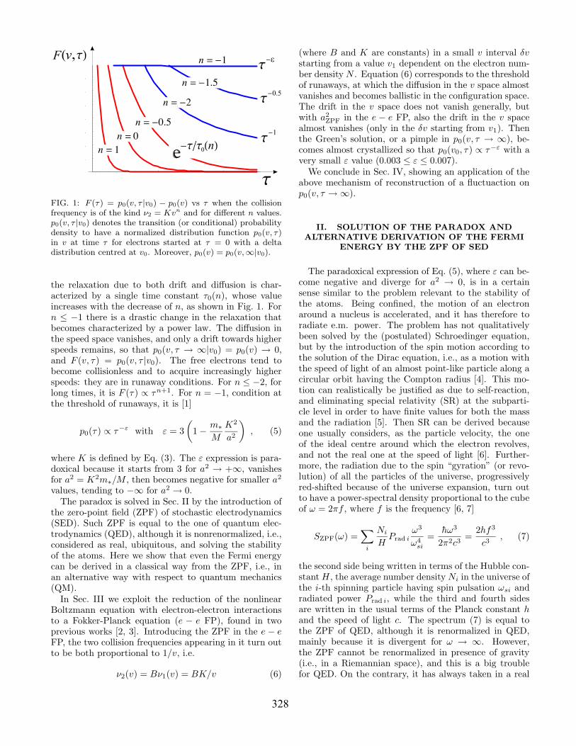
FIG. 1: F (τ) = p0(v, τ |v0) − p0(v) vs τ when the collisionfrequency is of the kind ν2 = Kvn and for different n values.p0(v, τ |v0) denotes the transition (or conditional) probabilitydensity to have a normalized distribution function p0(v, τ)in v at time τ for electrons started at τ = 0 with a deltadistribution centred at v0. Moreover, p0(v) = p0(v,∞|v0).
the relaxation due to both drift and diffusion is char-acterized by a single time constant τ0(n), whose valueincreases with the decrease of n, as shown in Fig. 1. Forn ≤ −1 there is a drastic change in the relaxation thatbecomes characterized by a power law. The diffusion inthe speed space vanishes, and only a drift towards higherspeeds remains, so that p0(v, τ → ∞|v0) = p0(v) → 0,and F (v, τ) = p0(v, τ |v0). The free electrons tend tobecome collisionless and to acquire increasingly higherspeeds: they are in runaway conditions. For n ≤ −2, forlong times, it is F (τ) ∝ τn+1. For n = −1, condition atthe threshold of runaways, it is [1]
p0(τ) ∝ τ−ε with ε = 3
(
1−m∗
M
K2
a2
)
, (5)
where K is defined by Eq. (3). The ε expression is para-doxical because it starts from 3 for a2 → +∞, vanishesfor a2 = K2m∗/M , then becomes negative for smaller a
2
values, tending to −∞ for a2 → 0.The paradox is solved in Sec. II by the introduction of
the zero-point field (ZPF) of stochastic electrodynamics(SED). Such ZPF is equal to the one of quantum elec-trodynamics (QED), although it is nonrenormalized, i.e.,considered as real, ubiquitous, and solving the stabilityof the atoms. Here we show that even the Fermi energycan be derived in a classical way from the ZPF, i.e., inan alternative way with respect to quantum mechanics(QM).In Sec. III we exploit the reduction of the nonlinear
Boltzmann equation with electron-electron interactionsto a Fokker-Planck equation (e − e FP), found in twoprevious works [2, 3]. Introducing the ZPF in the e − eFP, the two collision frequencies appearing in it turn outto be both proportional to 1/v, i.e.
ν2(v) = Bν1(v) = BK/v (6)
(where B and K are constants) in a small v interval δvstarting from a value v1 dependent on the electron num-ber density N . Equation (6) corresponds to the thresholdof runaways, at which the diffusion in the v space almostvanishes and becomes ballistic in the configuration space.The drift in the v space does not vanish generally, butwith a2
ZPF in the e − e FP, also the drift in the v spacealmost vanishes (only in the δv starting from v1). Thenthe Green’s solution, or a pimple in p0(v, τ → ∞), be-comes almost crystallized so that p0(v0, τ) ∝ τ−ε with avery small ε value (0.003 ≤ ε ≤ 0.007).We conclude in Sec. IV, showing an application of the
above mechanism of reconstruction of a fluctuaction onp0(v, τ →∞).
II. SOLUTION OF THE PARADOX AND
ALTERNATIVE DERIVATION OF THE FERMI
ENERGY BY THE ZPF OF SED
The paradoxical expression of Eq. (5), where ε can be-come negative and diverge for a2 → 0, is in a certainsense similar to the problem relevant to the stability ofthe atoms. Being confined, the motion of an electronaround a nucleus is accelerated, and it has therefore toradiate e.m. power. The problem has not qualitativelybeen solved by the (postulated) Schroedinger equation,but by the introduction of the spin motion according tothe solution of the Dirac equation, i.e., as a motion withthe speed of light of an almost point-like particle along acircular orbit having the Compton radius [4]. This mo-tion can realistically be justified as due to self-reaction,and eliminating special relativity (SR) at the subparti-cle level in order to have finite values for both the massand the radiation [5]. Then SR can be derived becauseone usually considers, as the particle velocity, the oneof the ideal centre around which the electron revolves,and not the real one at the speed of light [6]. Further-more, the radiation due to the spin “gyration” (or revo-lution) of all the particles of the universe, progressivelyred-shifted because of the universe expansion, turn outto have a power-spectral density proportional to the cubeof ω = 2πf , where f is the frequency [6, 7]
SZPF(ω) =∑
i
Ni
HPrad i
ω3
ω4si
=hω3
2π2c3=2hf3
c3, (7)
the second side being written in terms of the Hubble con-stantH, the average number densityNi in the universe ofthe i-th spinning particle having spin pulsation ωsi andradiated power Prad i, while the third and fourth sidesare written in the usual terms of the Planck constant hand the speed of light c. The spectrum (7) is equal tothe ZPF of QED, although it is renormalized in QED,mainly because it is divergent for ω → ∞. However,the ZPF cannot be renormalized in presence of gravity(i.e., in a Riemannian space), and this is a big troublefor QED. On the contrary, it has always taken in a real
328
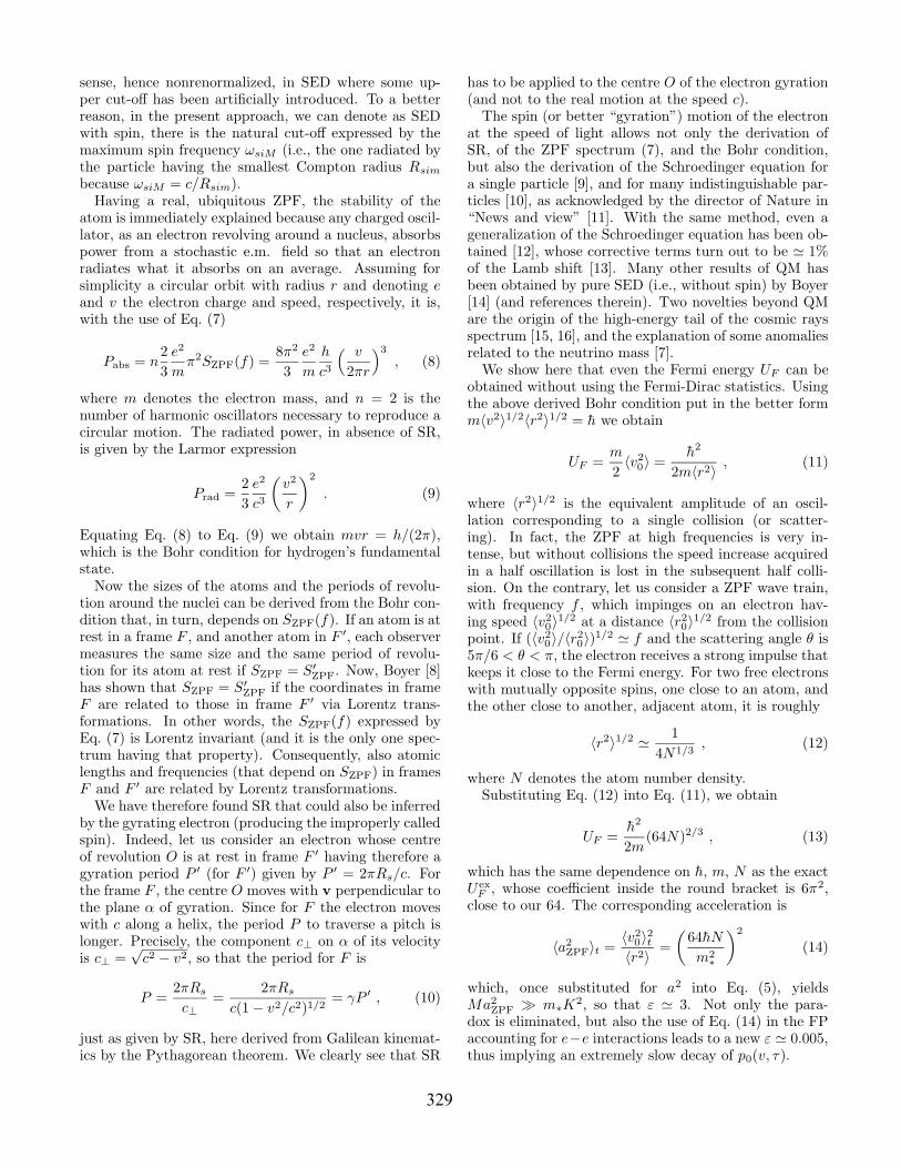
sense, hence nonrenormalized, in SED where some up-per cut-off has been artificially introduced. To a betterreason, in the present approach, we can denote as SEDwith spin, there is the natural cut-off expressed by themaximum spin frequency ωsiM (i.e., the one radiated bythe particle having the smallest Compton radius Rsim
because ωsiM = c/Rsim).Having a real, ubiquitous ZPF, the stability of the
atom is immediately explained because any charged oscil-lator, as an electron revolving around a nucleus, absorbspower from a stochastic e.m. field so that an electronradiates what it absorbs on an average. Assuming forsimplicity a circular orbit with radius r and denoting eand v the electron charge and speed, respectively, it is,with the use of Eq. (7)
Pabs = n2
3
e2
mπ2SZPF(f) =
8π2
3
e2
m
h
c3
( v
2πr
)3
, (8)
where m denotes the electron mass, and n = 2 is thenumber of harmonic oscillators necessary to reproduce acircular motion. The radiated power, in absence of SR,is given by the Larmor expression
Prad =2
3
e2
c3
(
v2
r
)2
. (9)
Equating Eq. (8) to Eq. (9) we obtain mvr = h/(2π),which is the Bohr condition for hydrogen’s fundamentalstate.Now the sizes of the atoms and the periods of revolu-
tion around the nuclei can be derived from the Bohr con-dition that, in turn, depends on SZPF(f). If an atom is atrest in a frame F , and another atom in F ′, each observermeasures the same size and the same period of revolu-tion for its atom at rest if SZPF = S′
ZPF. Now, Boyer [8]has shown that SZPF = S′
ZPF if the coordinates in frameF are related to those in frame F ′ via Lorentz trans-formations. In other words, the SZPF(f) expressed byEq. (7) is Lorentz invariant (and it is the only one spec-trum having that property). Consequently, also atomiclengths and frequencies (that depend on SZPF) in framesF and F ′ are related by Lorentz transformations.We have therefore found SR that could also be inferred
by the gyrating electron (producing the improperly calledspin). Indeed, let us consider an electron whose centreof revolution O is at rest in frame F ′ having therefore agyration period P ′ (for F ′) given by P ′ = 2πRs/c. Forthe frame F , the centre O moves with v perpendicular tothe plane α of gyration. Since for F the electron moveswith c along a helix, the period P to traverse a pitch islonger. Precisely, the component c⊥ on α of its velocityis c⊥ =
√c2 − v2, so that the period for F is
P =2πRs
c⊥=
2πRs
c(1− v2/c2)1/2= γP ′ , (10)
just as given by SR, here derived from Galilean kinemat-ics by the Pythagorean theorem. We clearly see that SR
has to be applied to the centre O of the electron gyration(and not to the real motion at the speed c).The spin (or better “gyration”) motion of the electron
at the speed of light allows not only the derivation ofSR, of the ZPF spectrum (7), and the Bohr condition,but also the derivation of the Schroedinger equation fora single particle [9], and for many indistinguishable par-ticles [10], as acknowledged by the director of Nature in“News and view” [11]. With the same method, even ageneralization of the Schroedinger equation has been ob-tained [12], whose corrective terms turn out to be ' 1%of the Lamb shift [13]. Many other results of QM hasbeen obtained by pure SED (i.e., without spin) by Boyer[14] (and references therein). Two novelties beyond QMare the origin of the high-energy tail of the cosmic raysspectrum [15, 16], and the explanation of some anomaliesrelated to the neutrino mass [7].We show here that even the Fermi energy UF can be
obtained without using the Fermi-Dirac statistics. Usingthe above derived Bohr condition put in the better formm〈v2〉1/2〈r2〉1/2 = h we obtain
UF =m
2〈v2
0〉 =h2
2m〈r2〉, (11)
where 〈r2〉1/2 is the equivalent amplitude of an oscil-lation corresponding to a single collision (or scatter-ing). In fact, the ZPF at high frequencies is very in-tense, but without collisions the speed increase acquiredin a half oscillation is lost in the subsequent half colli-sion. On the contrary, let us consider a ZPF wave train,with frequency f , which impinges on an electron hav-ing speed 〈v2
0〉1/2 at a distance 〈r2
0〉1/2 from the collision
point. If (〈v20〉/〈r
20〉)
1/2 ' f and the scattering angle θ is5π/6 < θ < π, the electron receives a strong impulse thatkeeps it close to the Fermi energy. For two free electronswith mutually opposite spins, one close to an atom, andthe other close to another, adjacent atom, it is roughly
〈r2〉1/2 '1
4N1/3, (12)
where N denotes the atom number density.Substituting Eq. (12) into Eq. (11), we obtain
UF =h2
2m(64N)2/3 , (13)
which has the same dependence on h, m, N as the exactU exF , whose coefficient inside the round bracket is 6π
2,close to our 64. The corresponding acceleration is
〈a2ZPF〉t =
〈v20〉
2t
〈r2〉=
(
64hN
m2∗
)2
(14)
which, once substituted for a2 into Eq. (5), yieldsMa2
ZPF À m∗K2, so that ε ' 3. Not only the para-
dox is eliminated, but also the use of Eq. (14) in the FPaccounting for e−e interactions leads to a new ε ' 0.005,thus implying an extremely slow decay of p0(v, τ).
329
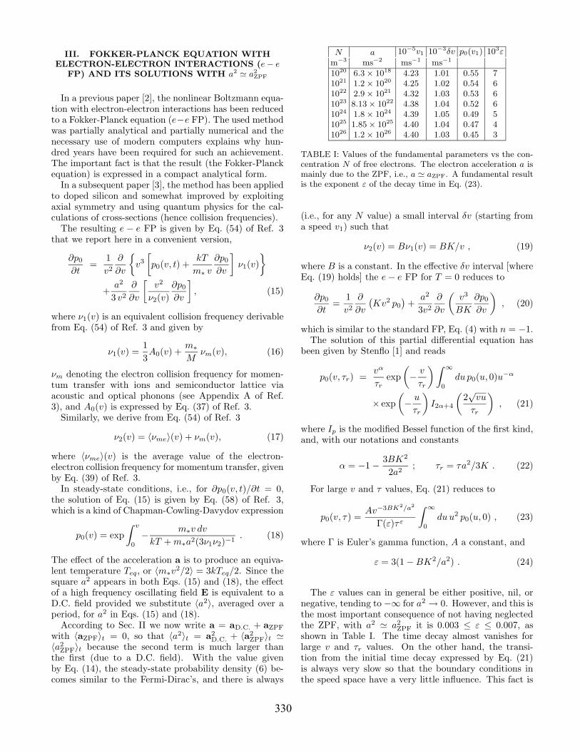
III. FOKKER-PLANCK EQUATION WITH
ELECTRON-ELECTRON INTERACTIONS (e− eFP) AND ITS SOLUTIONS WITH a2 ' a2
ZPF
In a previous paper [2], the nonlinear Boltzmann equa-tion with electron-electron interactions has been reducedto a Fokker-Planck equation (e−e FP). The used methodwas partially analytical and partially numerical and thenecessary use of modern computers explains why hun-dred years have been required for such an achievement.The important fact is that the result (the Fokker-Planckequation) is expressed in a compact analytical form.In a subsequent paper [3], the method has been applied
to doped silicon and somewhat improved by exploitingaxial symmetry and using quantum physics for the cal-culations of cross-sections (hence collision frequencies).The resulting e − e FP is given by Eq. (54) of Ref. 3
that we report here in a convenient version,
∂p0
∂t=
1
v2
∂
∂v
v3
[
p0(v, t) +kT
m∗ v
∂p0
∂v
]
ν1(v)
+a2
3 v2
∂
∂v
[
v2
ν2(v)
∂p0
∂v
]
, (15)
where ν1(v) is an equivalent collision frequency derivablefrom Eq. (54) of Ref. 3 and given by
ν1(v) =1
3A0(v) +
m∗
Mνm(v), (16)
νm denoting the electron collision frequency for momen-tum transfer with ions and semiconductor lattice viaacoustic and optical phonons (see Appendix A of Ref.3), and A0(v) is expressed by Eq. (37) of Ref. 3.Similarly, we derive from Eq. (54) of Ref. 3
ν2(v) = 〈νme〉(v) + νm(v), (17)
where 〈νme〉(v) is the average value of the electron-electron collision frequency for momentum transfer, givenby Eq. (39) of Ref. 3.In steady-state conditions, i.e., for ∂p0(v, t)/∂t = 0,
the solution of Eq. (15) is given by Eq. (58) of Ref. 3,which is a kind of Chapman-Cowling-Davydov expression
p0(v) = exp
∫ v
0
−m∗v dv
kT +m∗a2(3ν1ν2)−1. (18)
The effect of the acceleration a is to produce an equiva-lent temperature Teq, or 〈m∗v
2/2〉 = 3kTeq/2. Since thesquare a2 appears in both Eqs. (15) and (18), the effectof a high frequency oscillating field E is equivalent to aD.C. field provided we substitute 〈a2〉, averaged over aperiod, for a2 in Eqs. (15) and (18).According to Sec. II we now write a = aD.C. + aZPF
with 〈aZPF〉t = 0, so that 〈a2〉t = a2D.C. + 〈a
2ZPF〉t '
〈a2ZPF〉t because the second term is much larger than
the first (due to a D.C. field). With the value givenby Eq. (14), the steady-state probability density (6) be-comes similar to the Fermi-Dirac’s, and there is always
N a 10−5v1 10−3δv p0(v1) 10
3ε
m−3 ms−2 ms−1 ms−1
1020 6.3× 10¹⁸ 4.23 1.01 0.55 71021 1.2× 10²⁰ 4.25 1.02 0.54 61022 2.9× 10²¹ 4.32 1.03 0.53 61023 8.13× 10²² 4.38 1.04 0.52 61024 1.8× 1024 4.39 1.05 0.49 51025 1.85× 1025 4.40 1.04 0.47 41026 1.2× 1026 4.40 1.03 0.45 3
TABLE I: Values of the fundamental parameters vs the con-centration N of free electrons. The electron acceleration a ismainly due to the ZPF, i.e., a ' aZPF. A fundamental resultis the exponent ε of the decay time in Eq. (23).
(i.e., for any N value) a small interval δv (starting froma speed v1) such that
ν2(v) = Bν1(v) = BK/v , (19)
where B is a constant. In the effective δv interval [whereEq. (19) holds] the e− e FP for T = 0 reduces to
∂p0
∂t=1
v2
∂
∂v
(
Kv2 p0
)
+a2
3v2
∂
∂v
(
v3
BK
∂p0
∂v
)
, (20)
which is similar to the standard FP, Eq. (4) with n = −1.The solution of this partial differential equation has
been given by Stenflo [1] and reads
p0(v, τr) =vα
τrexp
(
−v
τr
)∫ ∞
0
du p0(u, 0)u−α
× exp
(
−u
τr
)
I2α+4
(
2√vu
τr
)
, (21)
where Ip is the modified Bessel function of the first kind,and, with our notations and constants
α = −1−3BK2
2a2; τr = τa2/3K . (22)
For large v and τ values, Eq. (21) reduces to
p0(v, τ) =Av−3BK2/a2
Γ(ε)τ ε
∫ ∞
0
duu2 p0(u, 0) , (23)
where Γ is Euler’s gamma function, A a constant, and
ε = 3(1−BK2/a2) . (24)
The ε values can in general be either positive, nil, ornegative, tending to −∞ for a2 → 0. However, and this isthe most important consequence of not having neglectedthe ZPF, with a2 ' a2
ZPF it is 0.003 ≤ ε ≤ 0.007, asshown in Table I. The time decay almost vanishes forlarge v and τr values. On the other hand, the transi-tion from the initial time decay expressed by Eq. (21)is always very slow so that the boundary conditions inthe speed space have a very little influence. This fact is
330

very important because Stenflo solved Eq. (20) consider-ing Eq. (9) as valid in all the interval 0 ≤ v ≤ ∞, whilein our case it is satisfied in δv only and the boundaryconditions in v space are different. Nevertheless, for verysmall ε values p0(v, τ) depends on τ so weakly in δv thatwe have a crystallization of a fluctuation and we can haveany boundary conditions because there is practically notime evolution.In order to turn Eq. (23) into a transition probabil-
ity p0(v, τ |v0) the initial probability density p0(u, 0) ap-pearing in Eq. (23) has to be concentrated at a sin-gle v0 value. Moreover, in order to be normalized 1 =∫∞
0du 4πu2p0(u, 0) it must take the expression
p0(u, 0) = (4πv02)−1 δ(u− v0) , (25)
where δ denotes the Dirac’s delta function. SubstitutingEq. (25) into Eq. (23), and using Eq. (22) with τ for τr,we obtain
p0(v, τ |v0) =Avε−3(3K/a2)ε
4πΓ(ε)τ ε, (26)
which is independent of v0. As said, Eq. (23), henceEq. (26), is valid for sufficiently large v and τ , i.e., forv > 〈v2〉1/2 and τ À tf , where tf ' ν−1
2 (v) is a free flight
time. Looking at Fig. 2, we see that v1 ' 2.02〈v2〉1/2 =
4.32 × 10⁵ ms−1 is larger than twice the square root ofthe mean square value. Moreover, the relaxation timeτm of the high energy tail just in correspondence of v1
turns out to be dominated by triple collisions and is ofthe order[17]
τm ' 8.6× 10⁻⁵s , (27)
much greater than the average time of free flight tf 'ν−12 (v) ' 8.6 × 10⁻¹⁷ s. The two conditions v > 〈v2〉1/2
and τ À tf are therefore well satisfied. In runaway condi-tions there is a process that turns the exponential decayinto a power law, but τm remains the time of the trans-mission of information, and also the time necessary forthe relaxation of Eq. (21) to Eq. (23).Having found that Eq. (26) is valid for τ ≥ τm À tf ,
and that Eq. (21) is “crystallized” for 0 < τ < τm, wemay take τm as the initial, starting time for τ , and extendEq. (26) to τ → 0, provided we use τm + τ for τ , thusobtaining
p0(v, τ |v0) =Avε−3(3K/a2)ε
4πΓ(ε)(τm + τ)ε. (28)
We can find the constant A, appearing in Eq. (28), byequating p0(v, 0|v0) to the equilibrium value p0(v) [givenby Eq. (18)] with v = v1 which is the beginning of the vinterval δv where Eq. (9) holds. We obtain
p0(v = v1, 0|v0) = p0(v1) =A(3Kv1/a
2)ε
4πv31Γ(ε)τ
εm
. (29)
0 1 2 3 4 5vr
0
50
100
150
200
250
ν1(v) vrν2(v) vr
δv
vr1
FIG. 2: Plot of the functions ν1(vr) vr and ν2(vr) vr (in
1014 s−1) vs vr, defined as vr = v〈v2〉−1/2. In the interval2.0215 < vr < 2.0263, the two functions are constant, so thatthe collision frequencies ν1(v) and ν2(v) go as 1/v satisfyingEq. (19).
Finally, deriving A from Eq. (29) and substituting it intoEq. (28), we obtain
p0(v, τ |v0) = p0(v1)(v1/v)
3−ετεm(τ + τm)ε
, (30)
which is the desired conditional probability density (orGreen function), showing the very slow time decay be-cause ε, as appears from Table I, is very small.
IV. CONCLUSIONS
The final result (30) shows that there is a small v inter-val δv where the conditional (or transition) probabilityp0(v, τ |v0) remains almost crystallized. In our calcula-tions, performed for silicon, both δv, and its initial pointv1, are given in Table I for different values of the numberdensity N . The result (30) is always valid because it ispractically due to electron-electron (e − e) interaction,so that it is independent of the lattice scattering, i.e., ofthe different materials. Moreover, the existence of a δvwhere the two collision frequencies are both proportionalto v−1 (condition at the threshold of runaways) is dueto the zero-point field (ZPF) that is universal and ubiq-uitous. This new phenomenon balances both the driftand the diffusion of p0(v, τ |v0) in the velocity space. Thepoint is: does this new result, interesting in itself, lead tosome observable consequence? The answer is positive, asshown in the companion paper, but not for drift and dif-fusion in the configuration space, because the fraction ofelectrons in δv is ' 10−3. Its observation is possible onlyfor the generalized diffusion coefficients [18] and for thenoise power spectral density. In fact, in the companionpaper, it is shown that the result (30) leads straightfor-wardly to the pure (or real, or exact) 1/f noise, i.e., to
331
the one obtainable after subtracting the usually larger ef-fect due to the material defects. In semiconductors, theresidual, or pure, 1/f noise is equal to the one measured
in the purest and quietest semiconductors. A new, nevernoticed N dependence is predicted, in excellent agree-ment with the experimental results.
[1] L. Stenflo, Plasma Phys. 8, 665-673 (1966).[2] G. Cavalleri and G. Mauri, Phys. Rev. B 49, 9993-9996(1994).
[3] G. Cavalleri, E. Tonni, L. Bosi, and G. Spavieri, NuovoCimento B 116, 1-30 (2001).
[4] A. O. Barut and N. Zanghi, Phys. Rev. Lett. 52, 2009-2012 (1984).
[5] G. Cavalleri et al., New progress of the filament theoryProceedings on Physical Interpretation of Relativity The-ory (PIRT) (London, 8-11 September, 2006), in press(2008).
[6] G. Cavalleri, Nuovo Cimento B 112, 1193-1206 (1997).[7] L. Bosi and G. Cavalleri, Nuovo Cimento B 117, 243-249(2002).
[8] T. H. Boyer, Phys. Rev. D 11, 790-808 (1975).[9] G. Cavalleri, Lett. Nuovo Cimento 43, 285-291 (1985).
[10] G. Cavalleri and G. Spavieri, Nuovo Cimento B 95, 194-204 (1986).
[11] J. Maddox, Nature (London) 325, 385 (1987).[12] G. Cavalleri and G. Mauri, Phys. Rev. B 41, 6751-6758
(1990).[13] G. Cavalleri and A. Zecca, Phys. Rev. B 43, 3223-3227
(1991).[14] T. H. Boyer, Phys. Rev. D 29, 1089-1095 (1984).[15] A. Rueda, Phys. Rev. A 23, 2020-2040 (1981).[16] A. Rueda and G. Cavalleri, Nuovo Cimento C 6, 239-260
(1983).[17] G. Cavalleri, E. Cesaroni, E. Tonni, and G. Spavieri, Eur.
Phys. J. D, 42, 407-424 (2007).[18] G. Cavalleri and G. Mauri, Phys. Rev. B 37, 6868-6881
(1988).
332
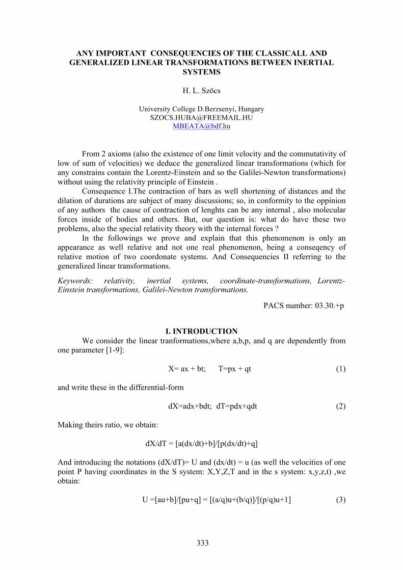
333
ANY IMPORTANT CONSEQUENCIES OF THE CLASSICALL AND GENERALIZED LINEAR TRANSFORMATIONS BETWEEN INERTIAL
SYSTEMS
H. L. Szöcs
University College D.Berzsenyi, Hungary [email protected]
From 2 axioms (also the existence of one limit velocity and the commutativity of low of sum of velocities) we deduce the generalized linear transformations (which for any constrains contain the Lorentz-Einstein and so the Galilei-Newton transformations) without using the relativity principle of Einstein .
Consequence I.The contraction of bars as well shortening of distances and the dilation of durations are subject of many discussions; so, in conformity to the oppinion of any authors the cause of contraction of lenghts can be any internal , also molecular forces inside of bodies and others. But, our question is: what do have these two problems, also the special relativity theory with the internal forces ?
In the followings we prove and explain that this phenomenon is only an appearance as well relative and not one real phenomenon, being a conseqency of relative motion of two coordonate systems. And Consequencies II referring to the generalized linear transformations.
Keywords: relativity, inertial systems, coordinate-transformations, Lorentz-Einstein transformations, Galilei-Newton transformations.
PACS number: 03.30.+p
I. INTRODUCTION We consider the linear tranformations,where a,b,p, and q are dependently from
one parameter [1-9]:
X= ax + bt; T=px + qt (1)
and write these in the differential-form
dX=adx+bdt; dT=pdx+qdt (2)
Making theirs ratio, we obtain:
dX/dT = [a(dx/dt)+b]/[p(dx/dt)+q]
And introducing the notations (dX/dT)= U and (dx/dt) = u (as well the velocities of one point P having coordinates in the S system: X,Y,Z,T and in the s system: x,y,z,t) ,we obtain:
U =[au+b]/[pu+q] = [(a/q)u+(b/q)]/[(p/q)u+1] (3)
334
In the case if u = 0,the ratio (b/q) must be a velocity,too,also we notate (b/q) = v (the velocity of the origine of s system reffering to the S system).Also we obtain from (3):
U = [(a/q)u+v]/[(p/q)u + 1] (3a)
This it is the (most) general low of addition (sum) of velocities u and v. But relation (3a) must satisfay to following axioms:
A1: Exists one so called limit-velocity of the system A2:The low of sum of velocities must commuts. Also for A1 we introduce the notations (a/q) = k and (p/b) = l, where k and l are
dependently from parameter v: k=k(v) and l=l(v),and after any elementary computations we have:
(p/q)=(p/b).(b/q) = (p/b).v (3a-a)
and also
U = [(a/q)u+v]/[(p/b)u.v+1] (3b)
From which in conformity to the (3a-a) we obtaine:
U = [ku+v]/[l.u.v+1] (3c)
After differentiating by v we give:
(dU/dv) = [-l′uv2+(k′l-kl′)u2.v+k′u-klu2+1]/[l.u.v+1] 2
but,because U= constant,it follows that U′ = (dU/dv) = 0 and so we have
[-l′uv2+(k′l-kl′)u2.v+k′u-klu2+1] = 0 (4)
and for roots of equation (4) U has one or two extremum.But this is not compatible with the physical realty,as wel it is a paradox.It follows that the expression (3b) must be a monotonicaly function of v.As well we must have k′ = l′ = 0.
In this case from (4) it follows
k.l. u2 = 1 (5)
(a/q).(p/b) . u2 = 1 (5a)
and moreover
u = ((bq)/(ap))^0.5 = u ∗ (6)
is the so called limit velocity of the system.It Follows that U ≤ u ∗ for all u ≤ u ∗ and also for all v ≤ u ∗.
335
II. OBSERVATIONVery important it is here that the limit velocity u ∗ can be :
u ∗ > c or u ∗ = c or u ∗ < c ,
where c it is the velocity of light in the vacuum. And we have the first conclusion: the additional low of velocities has
NOTHING with the velocity of light,but also only with the limit-velocity of the system u ∗. And now applying the A2 axiom (commutativity-axiom) we give:
[(a/q)u+v]/[(p/b)u.v+1] = [(a/q)v+u]/[(p/b)v.u+1]
from which it follows
(a/q)u+v = (a/q)v+u
also [(a/q) = 1 and finaly :
a = q (7)
And,so we have
U = [u+v]/[(uv)/ u ∗2 + 1] (8)
Note: after before we can write (1) in the form:
X=ax+bt=ax+avt=a(x+vt) = a[x+vt]; T=[(av)/ (u ∗2)]+at]= a[(v/ u ∗2)x+t] (9)
Because of:
(p/q)=(p/a)=(p/b).(b/q)=(p/b).(b/a) = (p/b).v = (1/ u ∗∧2).v; b = aq = av.
In the (9) “a” it is a free parameter. If we want to be a = β∗ where
β∗=(1)/√ [1-(v/ u ∗)2)].
as well for obtaine the generalised Lorentz-Einstein transformations, “a” must be so that:
a2 = 1/[1-(v/ u ∗)2)] (10)
also:
u ∗2 = (v2). (a2)/( a2 – 1)
(where a > 1),and we go to:
X = β∗ (x+vt); T = β∗ [(v/ u ∗2).t +x]

336
The generalised Lorentz-Einstein transformations. If a → 1, also u ∗→ ∞ (and NOT c !),we obtain
X = x + vt; T =t (12)
Also the common Galilei-Newton transformations. Note: for (10) we obtain the inverse L-E tranformations if we get:
X →x, x→X, T→t, t→T and v → - v
Also:
x=a(X-vT) ; t=a[(-vX/ u ∗2) + T] (13)
which, in conformity to F.Selleri oppinion is equivalent to the Einstein-relativity principle.
The Inverses of generalized linear transformations are the followings :
x = [1/(a(1-(v/ u ∗)2))].[X-vT] ; t = [1/(a(1-(v/ u ∗)2))].[(-vX/ u ∗2) + T] (14)
also the inverses of the (9).
III. CONSEQUENCE IOn relativity of phenomenon of contraction of lenghts and the dilatation of durations in
Special Relativity Theory
Really, that if we transform not only the lenght L 0 , but we transform the measure as well the measuring meter-bare, then the unit of lenght is transormed as folows:
1'=10.[(1-(v/c)1/2] (15)
where the 1 0 is the unit of lenght in the 0xyz system, the 1' is the transformed lenght-unit also the lenght-unit in the o'x'y'z't' system, the v is the relativelly velocity of the systems and c is the ( exemple) the velocity of light in the vacua.
And, now, "measure" the lenght of our bare in the system with "comma": also lat me see that how many times does go the lenght-unit into it:, also we obtain:
(L'/1')=L0.[(1-(v/c 2]1/2/10.[(1-(v/c)2]1/2=L0/10=L0 (16)
also the lenght of our bare in the oxyz system !, because in the system with "comma" we must measure with the meter-bare with comma !
Refferring to the time-transformation, similarly, are valid the followings and we obtain that :
(T'/1's)=T0/[1-(v/c)2]1/2/1s0/[1-(v/c)2]1/2=T0/1s0=T0, (17)
where T0 is one duration, 1s0 is the "second" in the oxyzt system and also, T' the duration and , respectivelly 1's the "second" in the 0'x'y'z't' system:
337
1's=1s0/[-(v/c)2]1/2 (18)
And, the conclusion we leave to the Honourable Reader.
IV. CONSEQUENCE IIConsequencies using the generalised linear transformation (9)
X = a[x+vt]; T=a[(v/u∗2)x+t]
We obtain for any distance between two points:
X2 and X1
X2-X1=ΔX=a[Δx+vΔt] (19)
If Δ t = 0 , we obtain
ΔX=a.Δx (20)
Now if a=1 so ΔX=Δx
a>1 so ΔX>Δx
a<1 so ΔX<Δx
understanding with out of transforming the distance measure. And similarly for time-variance (for Δ x = 0):
ΔT=a.Δt (21)
Also a=1 so ΔT=Δt
a>1 so ΔT>Δt
a<1 so ΔT<Δt
Regarding the generalised inverse transformations (14)
x = [1/(a(1-(v/ u ∗)2))].[X-vT]; t = [1/(a(1-(v/ u ∗)2))].[(-vX/ u ∗2) + T]
the inverses of the (9), we obtain
Δx=γ[ΔX–vΔT]
and now if ΔT=0, it results
Δx=γΔX (22)
338
1 γ = ----------------------- II
v2 a [ 1 – ----- ] u ∗ 2
u ∗ being the limit velocity. For
v<u∗
we have
1 ----------------- > 1
v2 1 – -----
u ∗ 2
and we obtain for
a = 1 γ > 1
a > 1 γ<1 or γ>1
a<1 γ>1
Acknowledgements: my expression of gratitude for my invitation for PIRT 2008, for Organizing Committee of PIRT 2008 London , especially for Professor.Dr.M.C. DUFFY and for T.Warwasovsky Major of Municipality Szekesfehervar (Alba Regia) Hungary
REFERENCES [1]. Szőcs Huba László: Egy elfelejtett magyar tudós: Gaál Sándor tudományos
életművéről (Of scientific work of forgotten Hungarian scientist: Alexander von Gaal),1999,Electronic Journal "Szabadpart",University College J.Kodolányi,Hungary,www.kodolanyi.hu
[2]. Huba-László Szőcs: On Physics Work In Relativity Of Alexander Von Gaál,Proceedings of International Conference On Educational Technologies For The Third Millenium “Medacta 95”,Nitra,1995,Volume-Zbornik 4.pp.176-180.
[3]. Huba-László Szőcs: “On Physics Work In Relativity Of Alexander Von Gaál”.Part.II.,
[4]. Proceedings Of International 7th Biennial Conference On History And Philosophy Of Physics In Education,HPPE ’96,Bratislava-Pozsony ,August 21-24 1996,pp.253-258 and 3.2.Proceedings Of International Conference On Non-Euclidian Geometry In Modern Physics,Uzghorod-Ungvár,13-16 August,1997,pp.210-216.
[5]. Huba-László Szőcs: “On Physics Work In Relativity Of Alexander Von Gaál”.Part.III..The Clock Paradox As Consequence Of Doppler’s Antinomy,Proceedings of International Conference on Non – Euclidian
339
Geometry in Modern Physics,Uzghorod-Ungvár (Kiev) ,13-16August,1997,pp.217-220.
[6]. Huba-László Szőcs: Essays Upon Special Relativity.Part IV.On Basic System Of Lorentz Group,
[7]. Volume of Abstracts Of International Workshop On Superluminal Velocities,Universities Cologne-Bielefeld,Germany,Koeln,June 6-10 ,1998,p.37 and 5.2.Volume Of Abstracts Of International Conference on Differential Geometry and Applications DGA ’98,Satellite Conference of International Congress of Mathematicians ICM 1998,Brno,August 10-18,1998, pp.44-45;
[8]. Proceedings of International Workshop on “Lorentz-Group,CPT and Neutrinos” Universidad Autonoma de Zacatecas,Mexico,June 23-26,1999;
[9]. Proceedings (Journal “Heavy Ion Physics “ 11 (2000) Publishing House of the Hungarian Academy of Sciences),of 2-nd Biannual (BGL) International Conference on “Non-Euklidian Geometry In Modern Physics”,Nyiregyháza,Hungary,7-10 July 1999.
[10]. Huba-László Szőcs: Essays Upon Special Relativity Part V.The Rectification Of Rotating Experiments And The Possibility Of Existence Of One Basic System,
[11]. Volume of Abstracts Of International Workshop On Superluminal Velocities,Universities Cologne-Bielefeld,Germany,Koeln,June 6-10 ,1998,p.38
[12]. Volume of Abstracts Of International Conference On Differential Geometry And Applications DGA’98 ,Satellite Conference of International Congress Of Mathematicians ICM 1998,Brno,August 10-18,1998,pp.45;
[13]. Proceedings of International Workshop on “Lorentz-Group,CPT and Neutrinos” Universidad Autonoma de Zacatecas,Mexico,June 23-26,1999;
[14]. Heavy Ion Physics 11 (2000) Publishing House of the Hungarian Academy of Sciences), Proceedings of 2-nd Biannual (BGL) International Conference on “Non-Euklidian Geometry In Modern Physics”,Nyiregyháza,Hungary,7-10 July 1999
[15]. HUBA L. SZŐCS : A forgotten Hungarian scientist: Sándor Gaál (Alexander von Gaál) WEB Proceedings of International Conference " Volta and the History of Electricity" ,Como-Italy,11-15 SEPT 1999;web site: http://opus.cilea.it/cgi-bin/fisicasite/webdriver?MIval=qp_comom&pg=CO
[16]. HUBA L. SZŐCS : Essays Upon Electromagnetism And Special Relativity WEB Proceedings of International Conference " Volta and the History of Electricity" ,Como-Italy,11-15 SEPT 1999;web site: http://opus.cilea.it/cgi-bin/fisicasite/webdriver?MIval=qp_comom&pg=CO
[17]. HUBA L. SZÖCS: The Basic Sytem and the Lorentz-group, Journal of New Energy,US,Vol.5.N.3.2001
[18]. Huba L.SZÖCS :.On relativity of phenomenon of contraction of lenghts and the dilatation of durations in Special Relativity Theory.PIRT 2006 London, published in Proceedings of the Conference 2006.
[19]. Huba L.SZÖCS : Any Consequencies of classical and generalized linear transformations between inertial systems, published in the Proceedings of PIRT Budapest 2007

340
SUBMICROSCOPIC BLACK HOLES AS MAGNETIC MONOPOLES AND DYONS IN SPACE-TIME
Huba L.Szõcs West Hungarian University Savaria University Centrum, Hungary
[email protected] [email protected], The paper presents the main results of the investigation of the author of different
physical characteristics of the particlelike magnetic charge: the magnetic monopole. Considering monopoles as submicroscopic black-holes and using the curved space-time metric type Reissner-Nordström and the generalised Reissner-Nordström-Weyl metric,the radius,the mean density of Dirac's magnetic monopole and dyon and the ratio of radii of electron and monopole is evaluated and also the stability is studyied.
Keywords: magnetic monopole, Reissner-Nordström-Weyl curved space-time metric, Dirac's magnetic monopole, dyon, submicroscopic black holes.
PACS number:04.62.+v/31.30.J-
I. INTRODUCTION The particlelike magnetic monopole presents interest again of later years
(Rújula1,1994.,et all).Among his different properties and characteristics physics especially the mass was investigated with regard to GUT,to gauge field theory,to early univers scenario and to stability of this particle (Bais and Russel2 1975,Cho and Freund3 1975,Nieuwenhuizen,Wilkinson and Perry4 1976,Bartnik and Mc.Kinnon5 1988,Künzle and Masood6 1990,Bloore and Horváthy7 1992,Breitenlohner,Forgács and Maison8 1992,Liu and Wesson9 1992,Wali10 1993,Horváth11,Palla et al.1976-1989).Other physical characteristics of particlelike magnetic monopole has been investigated since 1989 (Szõcs12,13,14,15,16,1989-1994, Szőcs 25 2000). Today , it appears that become possibly to produce submicroscopic blask-holes via future giant colliders (at TeV energy order) (Carr and Giddings 26 , Dimopoulos and Landsberg 27 , Giddings and Thomas 28 , and/or can be produce via high-energy cosmic rays by collision of high-energy neutrinos in the terrestrial atmosphere (Carr 29 , Anchordoqui et al. 30 ), which justified our prevision regarding monopoles as subminiaturized and charged black-holes (Szöcs 12,13,31,32 ).
II. THE RADIUS OF MAGNETIC MONOPOLEIn this part of the paper we shall calculeite the charge and deduce the expression
of radius of the magnetic monopole (Sass17 1986,Szõcs13 1989,Szõcs and Sass12 1989,Szõcs14 1991,Szõcs15 1993,Szõcs15 1994) in function of different metrics. Let us denote: e = charge of the electron (antiparticle,respectively), g = charge of the magnetic monopole (antiparticle,respectively), h = 6.6260755(40).10-27 cm2g/s,the Planck's constant, h* = h/2π (Relative uncertaintly ppm: 0.60). G = 6.67259(85).10-8 cm3/(s2g) the gravitational constant (Relative incertaintly ppm: 128),
341
c = 299792458.1010 cm/s,the velocity of light in vacuum (exact)(Cohen and Taylor 17,18) and the same time,the transformation factor between the IS system,in which the previous three values are given,and Gauss system.With this,we have:
eCGS = eIS.c/10 and gCGS = gIS.108/c (1)
One passes from geometrized to physical units (indexed by "geom" and "ph",respectively) and conversely,by the formulae:
egeom = eph.G1/2/c2 and ggeom = gph.G/c2 (2)
So,using Dirac's quantization relation 9,19
e.g = n.(h / 2) (3)
we obtain for n = 1:
e = 1.602177335.10-19 As = 4.803206814.10-10 (cm3g/s2)1/2
g = 2.067834616.10-15 Vs = 6.89755382.10-18 (cm.g)1/2 (4)
The radii of the electron and the magnetic monopole have been obtained using the REISSNER-NORDSTRÖM metric13,20,21,22,23:
ds2 = (1 − 2m/r + Q2/r2)dt2+ (1 − 2m/r + Q2/r2)-1/2 dr2 −r2 (dθ2 + sin2θ .dΦ2) (5)
where r,θ ,Φ are the spherical coordinates. The components of the acceleration will be 17,22,23:
ar = 2(m/r2 − Q2/r3) (6)
aθ = 0
aΦ = 0
and the module of acceleration is :
a = ⎜2(m/r2 − Q2/r3)⎜(1 − 2m/r + Q2/r2)-1/2 (7)
where in our case 20,23,24:
Q2 = Q2e + Q2m (8)
Qe being the electric,and Qm the magnetic charge,respectively. The (elementary) quasi-force (the "accretion") at surface is:
342
dF = ar.dm (9)
where dm is an elementary mass. This mass is in equilibrium (stable on the surface of spherical body) if dF = 0,
namely ar = 0,resulting
r = Q2/m (10)
in geometrized units. From (2) and (10) we deduce the radius:
re = (e2ph/mph)/c2 = 2.81794091.10-13 cm (11)
for electron; (the numerical value being very well into conformity with specific literature value17,18 ),resulting for magnetic monopole:
rg,CGS = (gph)2 / mph (12)
where "e" and "g" refer to electron and magnetic monopole,respectively.
III. THE NUMERICAL VALUES OF RADIUS OF (PARTICLELIKE)MAGNETIC MONOPOLE
In the following we calculeite and compare the radius,the mean density and the ratio of radii of electron and of monopole (re/rg) in function of appreciated masses1,3et al.(see Table 1.):
We have in case of de Rújula-type of mass of monopole1 :
mg < 8.7.n.h PeV (106 GeV) (13)
(between lower limit = 200 mproton and mGUT) the radius is the order 10-19 cm.
We mark that the Planck-lenght: l PLANCK = 1.61605(10).10-33 cm is smallerthan the radius of Planck-mass monopole (only with three orders,at the same time the mean-density of this monopole is smalller than the Planck-density with ten orders (the Planck-density is 5.5174(57).1093 g/cm3).
IV. THE RADIUS IN BASIS OF GENERALIZED REISSNER-NORDSTRÖM-WEYL METRIC (RNW-METRIC)
The RNW-metric we wrote in the following form15,16,22:
ds2=(1-2mG/r+Q2G/r2+βGr2/3)dt2+(1-2mG/r+Q2G/r2+βGr2/3)-1dr2- -r2(dθ2+sin2θdΦ2) (14)
where β is one constant proportional with the cosmological constant.In this case results for radius of monopole the following equation:
343
βr4 + 3mr − 3 Q2 = 0 (15)
where βph = 10-29 gcm-3 = 10-47 GeV and β=βph((G/c2)3.h./c)1/2=7.42466.10-58
cm-2 in geometrized units. In this case we have estimated the relative error as compared to solution in basis
of Reissner-Nordström metric,also the relative error is: 3.089375.10-115.%.In conclusion the contribution of cosmological extent of Reissner-Nordström metric with cosmological constant,is negligible 15,16.
V.THE BLACK-HOLE RADIUS OF MAGNETIC MONOPOLE Finaily we analyse tha black-hole radius of magnetic monopole.The
Schwartzschild-radius is respectively:
rSCHW. = rgrav.= 2mgeom.= 2mph(G/c2) (16)
referring to chargeless body.In this case results the following
rSCHW.elec. = 1.352610851.10-56 cm me = 5.1099906(15).10-4 GeV
rSCHW.mon.=9.302235224.10-45 cm mmonRú.= 3.602348.107 GeV
rSCHW.mon.=2.647014400.10-36 cm mmon.= 1016 GeV
rSCHW.mon.=2.647014400.10-35 cm mmon.= 1017 GeV
rSCHW.mon.=3.23209680.10-33 cm mmonPl.= 1.2210345.1019 GeV
We can establish that in all preceding cases the Schwartzschild-radius are smaller than the radius of the particle,consequently the collaps it is possible when we leave the charge out of consideration.
But considering the electric and/or magnetic charged particle,we obtain for black hole radius in case of Reissner-Nordström metric the following formula:
rblack-hole = mgeom+ (m2geom − Q2geom)1/2 < rSchwartzschild (17)
If we consider that the maximum mass of magnetic monopole it is the Planck-mass,we have:
m2Planck = 2.611611138.10-66< 3.532187774.10-64 = Q2
and the black-hole radius becomes imaginary and the black-hole-type collaps is impossible; follows that the electric and/or magnetic charge impedes the black-hole-type collapse of particle.In this case the black-hole solution of problem does not exist.
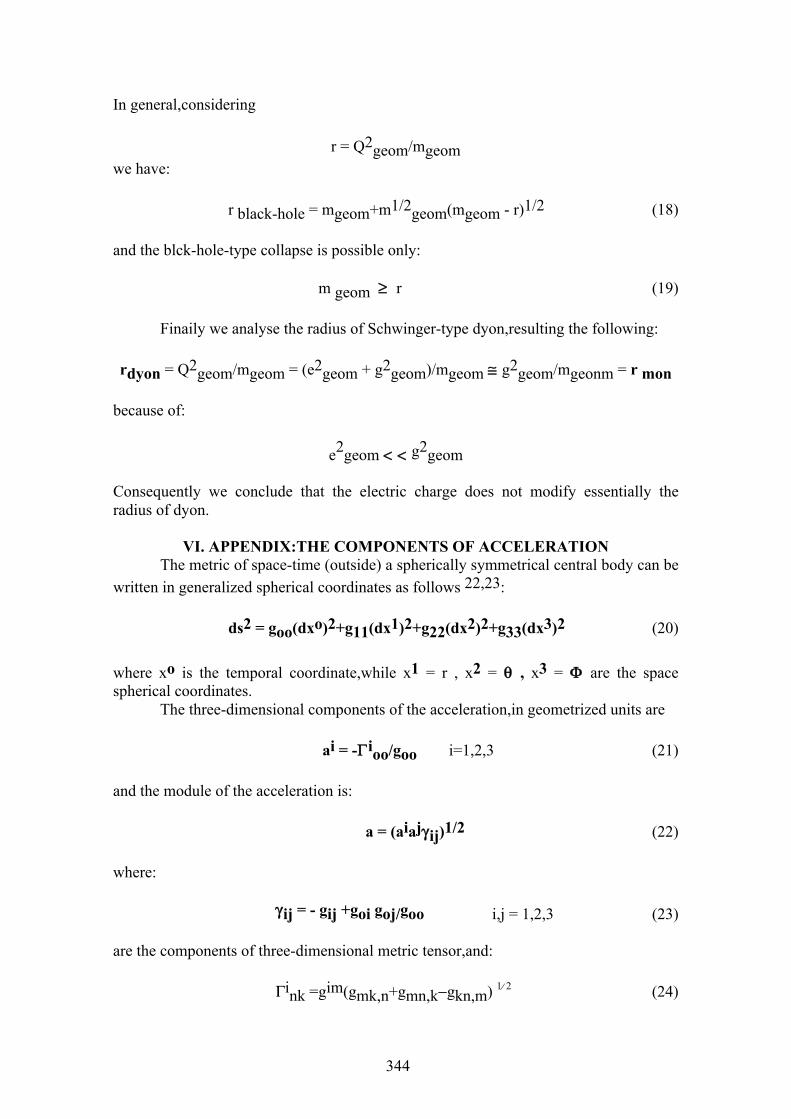
344
In general,considering
r = Q2geom/mgeomwe have:
r black-hole = mgeom+m1/2geom(mgeom - r)1/2 (18)
and the blck-hole-type collapse is possible only:
m geom ≥ r (19)
Finaily we analyse the radius of Schwinger-type dyon,resulting the following:
rdyon = Q2geom/mgeom = (e2geom + g2geom)/mgeom ≅ g2geom/mgeonm = r mon
because of:
e2geom < < g2geom
Consequently we conclude that the electric charge does not modify essentially the radius of dyon.
VI. APPENDIX:THE COMPONENTS OF ACCELERATIONThe metric of space-time (outside) a spherically symmetrical central body can be
written in generalized spherical coordinates as follows 22,23:
ds2 = goo(dxo)2+g11(dx1)2+g22(dx2)2+g33(dx3)2 (20)
where xo is the temporal coordinate,while x1 = r , x2 = θ , x3 = Φ are the space spherical coordinates.
The three-dimensional components of the acceleration,in geometrized units are
ai = -Γ ioo/goo i=1,2,3 (21)
and the module of the acceleration is:
a = (aiajγ ij)1/2 (22)
where:
γ ij = - gij +goi goj/goo i,j = 1,2,3 (23)
are the components of three-dimensional metric tensor,and:
Γink =gim(gmk,n+gmn,k−gkn,m) 1⁄ 2 (24)

345
are Cristoffel's symbols the second kind 24.In our case only the components: γ11=− g11 , γ22 = − g22 , γ33 = − g33 (25)
are nonzero,hence:
Γ ioo = − goo,1/(2g11) (26)
In our case results the module of acceleration
a = (ararγ11)1/2 = (- g11) - 1/2goo,1/goo1/ 2 (27)
and from (21) and (25) it results:
ai = - (goo,1) /2 = - (∂ goo/∂ r) 1/ 2 (28)
and,finaily
a = a1(goo) -1/2 (29)
Ackowledgement: I thanks very much to Professor Dr.Michael C.Duffy and Professor Dr.Peter Rowlands for kind invitation and sponzoring, to Tihamer Warvasovszky, Major of Municipality Szekesfehervar Hungary, for Sponzoring my travell and attendance to PIRT 2008 LONDON:
REFERENCES [1]. A.De.Rújula,Preprint CERN-TH.7273/94 May (1994) [2]. F.A.Bais and R.J.Russel,Phys.Rev.D 11,2692-2695 (1975) [3]. Y.M.Cho and P.G.Freund,Phys.Rev.D 12,1588-1589 (1975) [4]. P.van Nieuwenhuizen,D.Wilkinson and M.J.Perry,Phys.Rev.D 13,7780784 (1976) [5]. R.Bartnik and J.Mc Kinnon,Phys.Rev.Letters 61 141-144 (1988) [6]. H.P.Künzle and A.K.M.Masood,J.Math.Phys.31,926-935 (1990) [7]. F.Bloore and F.P.Horváthy,J.Math.Phys.33 ,1870-1877 (1992) [8]. F.Breitenlohner,P.Forgács and D.Maison,Preprint MPI-Ph/91-91,March (1992) [9]. H.Liu and S.Wesson,J.Math.Phys.33 ,3888-3891 (1992) [10].K.C.Wali,Monopoles in curved space-time,J.Hopkins Workshop,EL Univ.Bpest
(1993) [11].Z.Horváth,Doctoral thesis,Eotvös Loránd University (1989( [12].H.L.Szõcs and H.I.A.Sass,Scient.Seminar on Stellar Structurs,Univ.Napocensis
(1989) [13].H.L.Szõcs,Univ.Napocensis,Fac.Math.Phys.,Res.Sem.Preprint 5 ,275-278
(1989) [14].H.L.Szõcs,Proc.of XVIII..Scient.Meeting,Kandó K.Techn.Coll.Bpest, 3 , 81
(1991) [15].H.L.Szõcs,On determination of phys.properties of elementary particles in basis of metric of curved space-time,K.Lánczos Centenary-Meeting,Székesfehérvár,Hungary (1993) [16].H.L.Szõcs,One determination of physical characteristics of magnetic
monopole,International Workshop on Chiral Perturbation Theory,Comenius Univ.Bratislava (1994)
346
[17].17.E.R.Cohen and B.N.Taylor,Physics Today Bg9-Bg12 August (1992) [18].B.N.Taylor and E.R.Cohen,J.Res.National.Inst.Standards Technol. 95 497(1990) [19].P.A.M.Dirac,Proc.Roy.Soc.London A 133 (1931) [20].D.Kramer,H.Stephani,E.Herlt and M.Callum,Exact Solutions of Einstein's Field
Equations (Univ.Press Cambridge,1979),pp.209. [21].L.D.Landau and E.M.Lifschitz,The Classical Theory of Fields
(Pergamon,Oxford,1971). [22].H.I..A.Sass,Univ.Napocensis,Fac.Math.Phys.,Res.Sem.Preprint 3 ,49-73 (1987) [23].H.I.A.Sass,Univ.Napocensis,Fac.Math.Phys.,Res.Sem.Preprint 3 ,143 (1990) [24].B.I.Zeldovich and I.D.Novikov,Stars and Relativity (Univ.Chicago Press ,1971) [25].H.L.Szöcs,A Determination of Any Physical Characteristics of Magnetic
Monopole in Basis of Metrics of Curved Space-Time, Recent Developments in GeneralRelativity Genoa 2000, R.Cianci, R.Collina, M.Francaviglia, P.Fré (Eds), Springer-Verlag, Italia, Milano 2002, pp. 377-382.
[26].B.J.Carr and S.B.Giddings, Quantum Black Holes, Scientific American, May 2005
[27].S.Dimopoulos and G.Landsberg,Black Holes at the LHC, arXiv; hep-ph/0106295 vl 27 Jun 2001.
[28].S.B.Giddings and S.Thomas ,High Energy Colliders as Black Holes Factories: The End of Short Distance Physics, arXiv; hep-ph/0106219 v4 Jun 2002
[29].B.J.Carr, Primordial Black Holes as a Probe of cosmology and High Energy Physics, arXiv?astro-ph/0310838 v1 29 Oct 2003
[30].L.H.Anchordoqui et al.,Black Holes from Cosmic Rays :Probes of Extra Dimensions and New Limits on TeV-Scale Gravity, arXiv; hep-ph/0112247 v3 Apr 2002
[31].H.L.Szöcs, On Any Physical Properties of Possible Cosmic Ray Originating Rare Particles as Magnetic Monopoles, Proceedings of X. ICRC, South Africa, 1996
[32].H.L.Szöcs, A Determination of any Physical Characteristics of Magnetic Monopoles in Basis of Metrics of Curved Space Time, talk on NATO ASI Cascais, Portrugal ,26 JUN-07 JUL International Conference on Recent Developments on Particle Physics and Cosmology
347
THE ELECTROMAGNETIC SPACE-TIME-AETHER UNDER THE CLAIM FOR MINIMUM CONTRADICTIONS
A.A. Nassikas
Technological Education Institute of Larissa 10, Ethnikis Antistasseos Str., 41335 Larissa, GREECE
e-mail [email protected]
Purpose of this paper is to describe the electromagnetic dimension of Ether through an (em) Hypothetical Measuring Field- emHMF)( . The (em) space-time together with the gravitational (g) one can describe the Ether as a whole under a minimum contradictions point of view. Keywords: electromagnetic space-time-aether, Hypothetical Measuring Field, gravitational field, coulomb law, electromagnetic space-time particle filed.
PACS number:04.20.-q/03.30.+p/03.50.De
I. INTRODUCTION According to minimum contradictions point of view, space-time is stochastic
and it can be regarded as matter –ether [1]. However, matter can be either mass or charge. Thus, there exist both mass-gravitational (g) and charge-electromagnetic (em) space-time. The (em) space-time behaves as a (g) one, since both are space-time and obey the same principles but it is not. Thus, any time interval in the (em) space-time is incomprehensible with respect to a coexisting (g) one and it can be regarded as an imaginary number which is incomprehensible too. According to [1] the energy of an infinitesimal (em) space-time can be regarded as imaginary since it is equivalent to an (em) time interval. Therefore, in general, the electromagnetic energy and in extension (em) magnitudes can be regarded as imaginary. The electromagnetic space-time can be regarded as a four dimensional space-time which coexists with the gravitational one. Taking into account the existence of negative physical and geometrical magnitudes [2] we may assume that there exists also an anti-em space-time that corresponds to antimatter. Thus, space-time as a whole is described through sixteen dimensions, i.e. four dimensions for each of the following space-times: (g), (anti-g), (em) and (anti-em). This does not mean that space-time has 16 dimensions, simply it is described through 16 dimensions. In reality space-time is fractal described through four dimensions. It is noted that there is a coexistence scale between (g) and (em) space-time and that the probability density function, according to the spirit to this work, can take either positive or negative values. The epistemological basis of this can be found in previous works[1,2].
II. ELECTROMAGNETIC HYPOTHETICAL MEASURING FIELD (HMF)em
The electromagnetic Space Time should be studied through an Electromagnetic Hypothetical Measuring Field emHMF)( . Since the emHMF)( coexists with the gravitational one gHMF)( we should find the scale of their interconnection. By definition both )(em and )(g reference space-time are continua and flat. According to Lorentz transformations for a continuum space-time, we have :
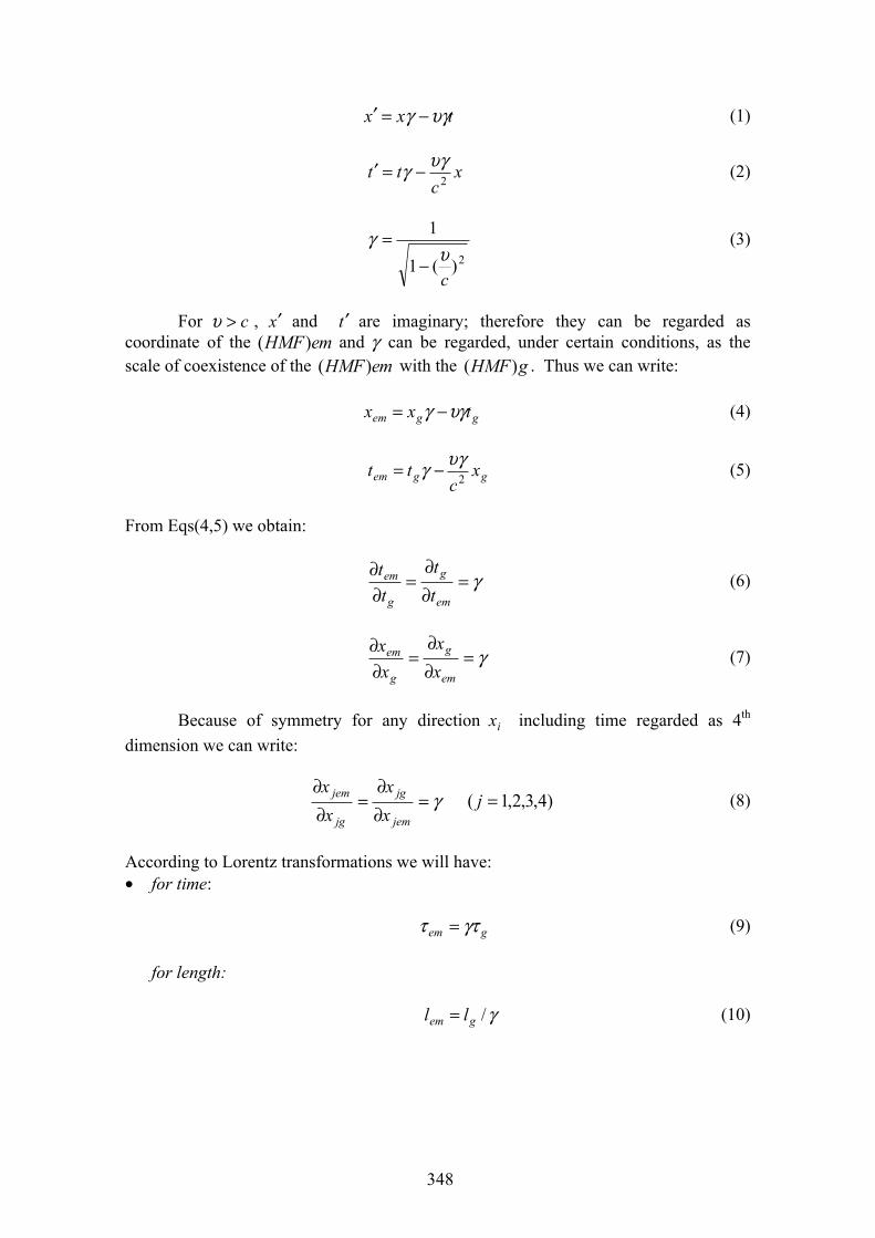
348
txx υγγ −=′ (1)
xc
tt 2υγγ −=′ (2)
2)(1
1
cυ
γ−
= (3)
For c>υ , x′ and t ′ are imaginary; therefore they can be regarded as coordinate of the emHMF)( and γ can be regarded, under certain conditions, as the scale of coexistence of the emHMF)( with the gHMF)( . Thus we can write:
ggem txx υγγ −= (4)
ggem xc
tt 2υγγ −= (5)
From Eqs(4,5) we obtain:
γ=∂∂
=∂∂
em
g
g
em
tt
tt (6)
γ=∂∂
=∂∂
em
g
g
em
xx
xx (7)
Because of symmetry for any direction ix including time regarded as 4th dimension we can write:
γ=∂∂
=∂∂
jem
jg
jg
jem
xx
xx
)4,3,2,1( =j (8)
According to Lorentz transformations we will have: • for time:
gem γττ = (9)
for length:
γ/gem ll = (10)
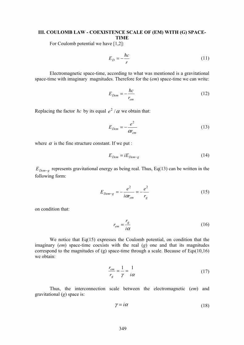
349
III. COULOMB LAW - COEXISTENCE SCALE OF (EM) WITH (G) SPACE-TIME
For Coulomb potential we have [1,2]:
rcED!−= (11)
Electromagnetic space-time, according to what was mentioned is a gravitational space-time with imaginary magnitudes. Therefore for the (em) space-time we can write:
emDem r
cE !−= (12)
Replacing the factor c! by its equal α/2e we obtain that:
emDem r
eEα
2−= (13)
where α is the fine structure constant. If we put :
gDemDem iEE −= (14)
gDemE − represents gravitational energy as being real. Thus, Eq(13) can be written in the following form:
gemgDem r
eri
eE22
−=−=− α(15)
on condition that:
αir
r gem = (16)
We notice that Eq(15) expresses the Coulomb potential, on condition that the imaginary (em) space-time coexists with the real (g) one and that its magnitudes correspond to the magnitudes of (g) space-time through a scale. Because of Eqs(10,16) we obtain:
αγ irr
g
em 11 == (17)
Thus, the interconnection scale between the electromagnetic (em) and gravitational (g) space is:
αγ i= (18)
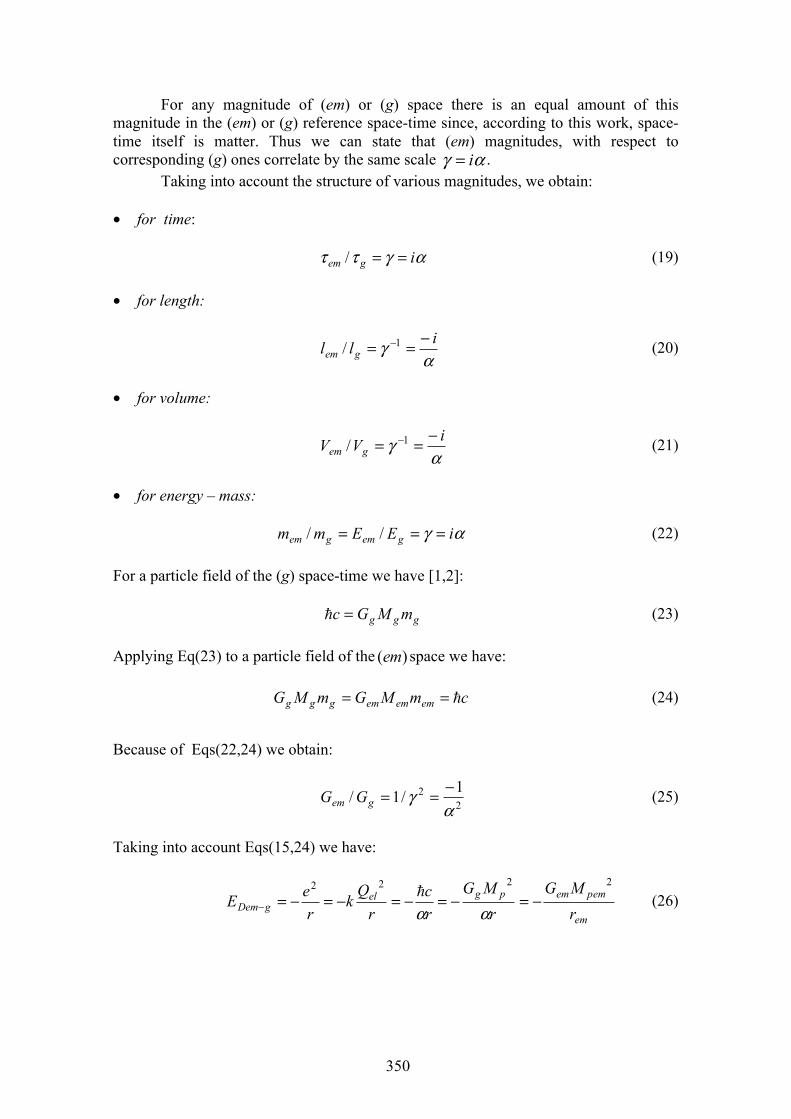
350
For any magnitude of (em) or (g) space there is an equal amount of this magnitude in the (em) or (g) reference space-time since, according to this work, space-time itself is matter. Thus we can state that (em) magnitudes, with respect to corresponding (g) ones correlate by the same scale αγ i= .
Taking into account the structure of various magnitudes, we obtain:
• for time:
αγττ igem ==/ (19)
• for length:
αγ ill gem
−== −1/ (20)
• for volume:
αγ iVV gem
−== −1/ (21)
• for energy – mass:
αγ iEEmm gemgem === // (22)
For a particle field of the (g) space-time we have [1,2]:
ggg mMGc =! (23)
Applying Eq(23) to a particle field of the )(em space we have:
cmMGmMG emememggg !== (24)
Because of Eqs(22,24) we obtain:
22 1/1/
αγ −==gem GG (25)
Taking into account Eqs(15,24) we have:
em
pemempgelgDem r
MGr
MGrc
rQ
kr
eE2222
−=−=−=−=−=− αα! (26)
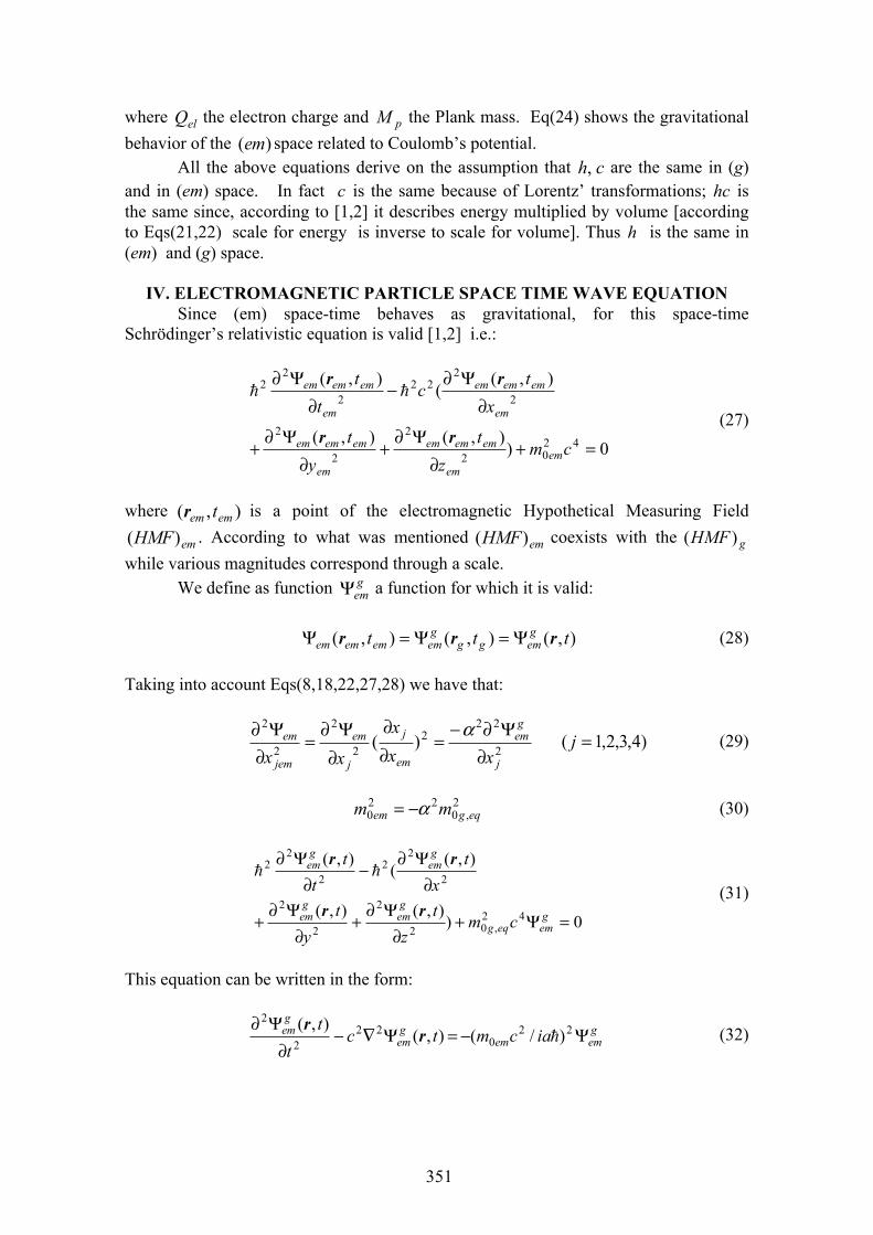
351
where elQ the electron charge and pM the Plank mass. Eq(24) shows the gravitational behavior of the )(em space related to Coulomb’s potential.
All the above equations derive on the assumption that ch, are the same in (g) and in (em) space. In fact c is the same because of Lorentz’ transformations; hc is the same since, according to [1,2] it describes energy multiplied by volume [according to Eqs(21,22) scale for energy is inverse to scale for volume]. Thus h is the same in (em) and (g) space.
IV. ELECTROMAGNETIC PARTICLE SPACE TIME WAVE EQUATIONSince (em) space-time behaves as gravitational, for this space-time
Schrödinger’s relativistic equation is valid [1,2] i.e.:
0)),(),(
),((
),(
4202
2
2
2
2
222
2
22
=+∂
Ψ∂+
∂Ψ∂
+
∂Ψ∂
−∂
Ψ∂
cmz
ty
t
xt
ct
t
emem
ememem
em
ememem
em
ememem
em
ememem
rr
rr!!
(27)
where ),( emem tr is a point of the electromagnetic Hypothetical Measuring Field
emHMF)( . According to what was mentioned emHMF)( coexists with the gHMF )( while various magnitudes correspond through a scale.
We define as function gemΨ a function for which it is valid:
),(),(),( ttt gemgg
gemememem rrr Ψ=Ψ=Ψ (28)
Taking into account Eqs(8,18,22,27,28) we have that:
2
222
2
2
2
2
)(j
gem
em
j
j
em
jem
em
xxx
xx ∂Ψ∂−
=∂∂
∂Ψ∂
=∂Ψ∂ α )4,3,2,1( =j (29)
2,0
220 eqgem mm α−= (30)
0)),(),(
),((
),(
42,02
2
2
2
2
22
2
22
=Ψ+∂
Ψ∂+
∂Ψ∂
+
∂Ψ∂
−∂
Ψ∂
gemeqg
gem
gem
gem
gem
cmz
ty
tx
tt
t
rr
rr!!
(31)
This equation can be written in the form:
gemem
gem
gem iacmtct
tΨ−=Ψ∇−
∂Ψ∂ 22
022
2
2
)/(),(),(
!rr (32)
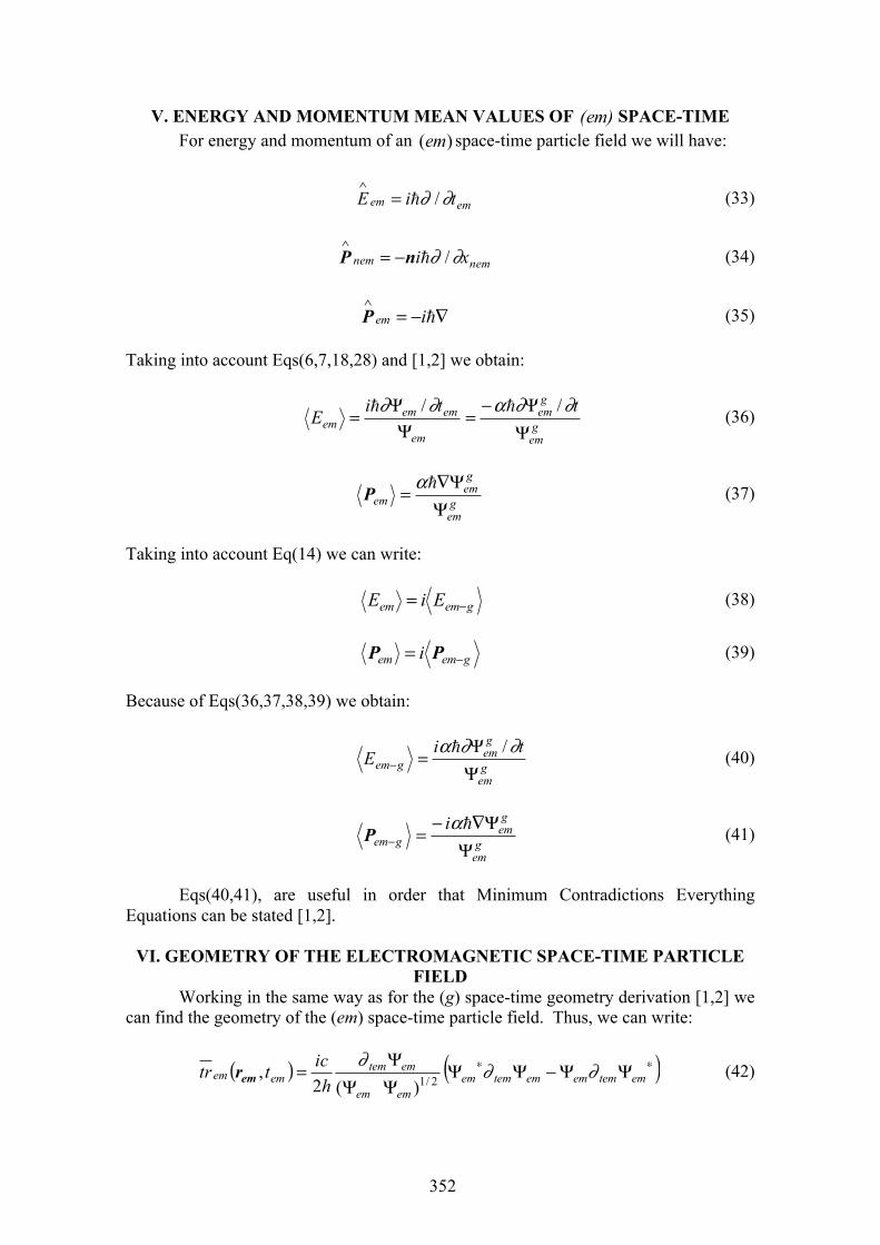
352
V. ENERGY AND MOMENTUM MEAN VALUES OF (em) SPACE-TIME For energy and momentum of an )(em space-time particle field we will have:
emem tiE ∂∂ /!=∧
(33)
nemnem xi ∂∂ /!nP −=∧
(34)
∇−=∧
!iemP (35)
Taking into account Eqs(6,7,18,28) and [1,2] we obtain:
gem
gem
em
ememem
ttiE
ΨΨ−
=Ψ
Ψ=
∂∂α∂∂ // !! (36)
gem
gem
em ΨΨ∇
=!α
P (37)
Taking into account Eq(14) we can write:
gemem EiE −= (38)
gemem i −= PP (39)
Because of Eqs(36,37,38,39) we obtain:
gem
gem
gemti
EΨΨ
=−∂∂α /! (40)
gem
gem
gemiΨ
Ψ∇−=−
!αP (41)
Eqs(40,41), are useful in order that Minimum Contradictions Everything Equations can be stated [1,2].
VI. GEOMETRY OF THE ELECTROMAGNETIC SPACE-TIME PARTICLEFIELD
Working in the same way as for the (g) space-time geometry derivation [1,2] we can find the geometry of the (em) space-time particle field. Thus, we can write:
( ) ( )∗∗ ΨΨ−ΨΨΨΨΨ
= emtemememtemememem
emtememem
hicttr ∂∂∂
2/1)(2,emr (42)
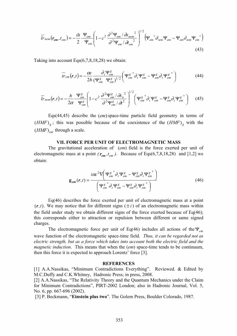
353
( ) ( )∗∗ ΨΨ−ΨΨ⎟⎟⎠
⎞⎜⎜⎝
⎛
ΨΨ
−ΨΨ
−= emtemememtemememem
nemem
em
ememnem
tx
cihtlr ∂∂∂∂∂∂
2/1
22
222
//
12
,emr
(43)
Taking into account Eqs(6,7,8,18,28) we obtain:
( ) ⎟⎠⎞⎜⎝
⎛ ΨΨ−ΨΨΨΨΨ
−=∗∗ g
emtgem
gemt
gemg
emgem
gemt
emhcttr ∂∂∂α
2/1)(2,r (44)
( ) ⎟⎠⎞⎜⎝
⎛ ΨΨ−ΨΨ⎟⎟⎠
⎞⎜⎜⎝
⎛
ΨΨ
−ΨΨ
−=∗∗ g
emtgem
gemt
gemg
em
ngem
gem
gem
nemtx
chtlr ∂∂∂∂∂∂
α
2/1
22
222
//
12
,r (45)
Eqs(44,45) describe the )(em space-time particle field geometry in terms of
gHMF )( ; this was possible because of the coexistence of the gHMF )( with the
emHMF)( through a scale.
VII. FORCE PER UNIT OF ELECTROMAGNETIC MASSThe gravitational acceleration of (em) field is the force exerted per unit of
electromagnetic mass at a point )t,( ememr . Because of Eqs(6,7,8,18,28) and [1,2] we obtain:
⎟⎠⎞⎜⎝
⎛ ΨΨ−ΨΨ
⎟⎠⎞⎜⎝
⎛ ΨΨ−ΨΨ∇=
∗∗
∗∗
gemt
gem
gemt
gem
gemt
gem
gemt
gemci
t∂∂
∂∂α 2
),(remg (46)
Eq(46) describes the force exerted per unit of electromagnetic mass at a point )( t,r . We may notice that for different signs ( i± ) of an electromagnetic mass within
the field under study we obtain different signs of the force exerted because of Eq(46); this corresponds either to attraction or repulsion between different or same signed charges.
The electromagnetic force per unit of Eq(46) includes all actions of the emΨ wave function of the electromagnetic space-time field. Thus, it can be regarded not as electric strength, but as a force which takes into account both the electric field and the magnetic induction. This means that when the (em) space-time tends to be continuum, then this force it is expected to approach Lorentz’ force [3].
REFERENCES [1] A.A.Nassikas, “Minimum Contradictions Everything”. Reviewed. & Edited by M.C.Duffy and C.K.Whitney, Hadronic Press; in press, 2008. [2] A.A.Nassikas, “The Relativity Theory and the Quantum Mechanics under the Claim for Minimum Contradictions”, PIRT-2002 London; also in Hadronic Journal, Vol. 5, No. 6, pp. 667-696 (2002). [3] P. Beckmann, “Einstein plus two”. The Golem Press, Boulder Colorado, 1987.
354
THE SPATIAL BEHAVIOR OF COULOMB AND NEWTON FORCES, YET REIGNING BETWEEN EXCLUSIVELY STATIC CHARGES, IS THE SAME
MUST, DRAWN BY THE SPECIAL THEORY OF RELATIVITY
PART I: UNDER THE GIVEN CIRCUMSTANCES, COULOMB FORCE IS A FUNDAMENTAL LAW OF NATURE INSURING A UNIQUE MATTER
ARCHITECTURE
Tolga Yarman
Okan University, Akfirat, Istanbul, Turkey ([email protected])
The compatibility of Coulomb Force with the special theory of relativity (STR), is a well know fact. But, any compatibility is not a must. Thus, the following question arises: Would there a more fundamental level, shaping the known structure of Coulomb Force, perhaps based on the foundations of the STR? Yes, indeed: It is that electric charges are Lorentz invariant, just like the speed of light, is. What seems so far ignored is the following. Not only that the constancy of the speed of light is, an empirical evidence, but the Lorentz invariance of electric charges, is too. These two facts do not seem to imply each other. Thus, both of them (as well as, perhaps the Lorenz invariance of similar entities, such as nuclear charges), must be considered concomitantly, in order to insure the Galilean principle of relativity with respect to all inertial frames of reference, which is in effect, the underlying postulate of the STR. Actually the constancy of the speed of light, does not appear to insure all alone, the validity of this principle, and this is why, exactly, Einstein cared to state the second postulate of the STR (regarding the sameness of the laws of nature with regards to all inertial frames of reference), although he did not make any use of it, throughout. Once we have the two evidences of concern (i.e. the Lorentz invariance of electric charges and that of the speed of light), then we can right away, mathematically derive the known Coulomb Force, though reigning between two static charges, exclusively. By the same token, the spatial dependency of Newton Force too, regarding two static masses, becomes a mathematical requirement based on the STR, which seems to be something totally overlooked. So, both forces (still reigning between static, respectively, electric and gravitational charges only), are fundamental laws of nature, essentially imposed by the Galilean principle of relativity. In a subsequent article, however, we will show that, quite on the contrary to the general wisdom, neither Coulomb Force, nor Newton Force holds, if the – electric or gravitational – test charge in consideration, is in motion (the source charge being as usual, considered at rest, throughout). We show that, assuming the opposite (i.e. asserting that Coulomb Force, or Newton Force holds if the test charge, is in motion), constitutes a clear violation of the law of conservation of energy. Our approach removes the blockade toward a unification of fields, and the quantization of the gravitational field (hindered by the general theory of relativity).
Keywords: general theory of relativity, Coulomb force, Newton force,special theory of relativity, matter, gravitational field.
PACS number: 03.30.+p/04.20.-q
355
I. INTRODUCTION The classical Coulomb Force1 is assumed to act, between a “source charge” at
rest, and a “test charge”, either at rest, or in motion [1]. The denominations of “source charge” and “test charge” are arbitrary, but useful
in simplifying the presentation. Let us then define the following quantities. Q : intensity of the source charge, assumed at rest, throughout q : intensity of the test charge interacting with Q r : distance between the test charge and the source charge, assumed to be at the center of the coordinate system
CCF : strength of the Classical Coulomb Force reigning between Q (at rest) and q (either at rest, or in motion) k : proportionality constant, being unity in the CGS unit system. Thus, as usual,
2CC rQqkF = , (1)
(Classical Coulomb Force reigning between the two charges, no matter q is at rest, or in motion)
For convenience, we will work in the CGS unit system (where k is unity). Herein, we propose to show that, Eq.(1) is anyway correct, for a “test charge at
rest”, and this result, is a “must”, directly imposed by the special theory of relativity (STR).
The compatibility of Coulomb Force, with the STR, is a well known fact; but “compatibility”, is not a “must”. Thus, we should ask the following question: Would there be a more fundamental level, shaping the known structure of Coulomb Force based on the STR? The answer is “Yes”; it is that, electric charges are Lorentz invariant, just like the speed of light is.
So what? What seems so far ignored is, “not only that the constancy of the speed of light, is an empirical evidence”, but (from the present stand point) “the Lorentz invariance of electric charges is too”. These two facts do not seem to imply each other. Thus, both facts must be considered concomitantly, in order to insure the Galilean principle of relativity, with respect to all inertial frames of reference, which is the underlying postulate of the STR. Indeed the constancy of the speed of light, all alone, does not seem to suffice to insure the validity of this principle, and this is why, exactly, Einstein cared to state the second postulate of the STR (regarding the sameness of the laws of nature with regards to all inertial frames of reference), although he did not make any use of it, throughout.2 1 Charles Augustine de Coulomb: 1736 – 1806
2 Note that what is most essential is the Galilean principle of relativity. Because historically the empirical evidences about the constancy of the speed of light and the principle of relativity (due to the Galilean addition rule of velocities), appeared to be contradictory, the two evidences in question, were classified as separate laws of nature, and ultimately (due to the null result of efforts aiming to discard the latter), constituted the two postulates of the special theory of relativity. One has to recall though that, Einstein did not make use of his second postulate (i.e. the Lorentz invariance of the laws of nature, through a uniform translational motion, which is basically, the Galilean principle of relativity) in the derivation of the special theory of relativity; this postulate is there just for the sake of completeness. And, in fact, the principle of relativity, necessarily induces the constancy of the speed of light, along with the relativity
356
Once we have the two evidences of concern (i.e. the Lorentz invariance of electric charges, and that of the speed of light), we can right away derive the known Coulomb Force, though reigning between two static charges, exclusively.
The conclusion we will arrive at is that, Eq.(1) is incorrect, if q is in motion. And this is implied by the law of conservation of energy. In other words, assuming that Eq.(1) is valid, were q is in motion, as controversial as this may be, constitutes a clear violation of the law of conservation of energy.
II. POSTULATESIn order to proceed, we will forget how we actually define and use the historical
Coulomb Force, and will introduce two postulates. Here is the first one.
Postulate: The Coulomb Force, reigning between two electric charges Q and q, both strictly at rest, is proportional to the product of the intensities of these charges, and is inversely proportional to the nth power of the distance separating, Q and q.
Thus beforehand, we assume that Coulomb Force reigning between two charges Q and q, both at rest, separated by a distance 0r behaves, in CGS unit system, as
n0
0C rQqF = ; (2)
(present assumption about Coulomb Force reigning, between just two static charges)
the exponent n, is a priori, not known. Though, empirically we know that n is very close to 2, a priori, we still do not
know the exact value of it. The system made of Q and q, can be a dipole, such as a water molecule.
In water molecule, the oxygen atom (O) attracts, respectively the two binding electrons of the hydrogen (H) atoms, delineating an angle HOH of about 105º. This makes that, the hydrogen atoms get charged positively, and the oxygen atom, negatively. Thus, water molecule can indeed be described by a dipole, made of -2e situated nearby the oxygen atom, and +2e situated on the median of the triangle HOH, in between the hydrogen atoms; e is the electron’s charge intensity. We call 0r the distance between the two representative charges +2e and -2e. We further call 0m , the mass of the water molecule, at rest. Thus the above postulate says that, the force acting between the charges +2e and -2e in a water molecule obeys Eq.(2).
The second postulates we will introduce, consists in the Lorentz invariance of electric charges.
If the electric charges were not Lorentz invariant, say, in an excited atom, an energetic electron (moving with a velocity different than the velocity it would bear at the ground level), would exhibit an electric charge intensity, different than the electric charge intensity, it would display at the ground level; this would amongst other things
of space and time. (In other words, if the speed of light were not constant with respect to all inertial frames, still along with the relativity of space and time, then the principle of relativity would be broken.) Thus, from he point of view in question, one can classify the Galilean principle of relativity, as the imperative law of nature. (Note further that if the laws of nature did not remain the same through a uniform translational motion, then the principle of relativity would still be broken; thence the second postulate of the special theory of relativity, is nothing else but the Galilean principle of relativity).
357
alter even the neutrality of atoms, which is not the case. Thus, we state our next postulate.
Postulate: Electric charges are Lorentz invariant.
Recall that the Lorentz invariance of electr5ic charges, does not seem to be implied by the Lorentz invariance of the speed of light. Thus, at the stage where we are, both of the evidences (perhaps others, such as the Lorentz invariance of nuclear charges) must be considered concomitantly, in order to insure the “Galilean principle of relativity” (which happens to be the underlying postulate of the STR). We will elaborate on this, in the conclusion of this article, in the light of a derivation of a quantum mechanical theorem we provide in a subsequent article, where we show that the Lorentz invariance of electric charges represents more than the content of a postulate. It is indeed a requirement imposed by a unique matter architecture, which is in return a necessity to insure the Galilean principle of relativity, as well as the end results of the general theory of relativity. It should be emphasized that, nowhere we had access to, the Lorentz invariance of electric charges is considered as a postulate or a primordial ingredient of a fundamental theory. Note that, the above postulate naturally implies the Lorentz invariance of the product of any two charges, as well.
III. DERIVATION OF COULOMB FORCE BASED ON THE STR AND THELORENTZ INVARIANCE OF ELECTRIC CHARGES
Now we are ready to show the following theorem.
Theorem: Were Coulomb Force reigning, between two static charges, assumed to act as 2
0r1/ , 0r being the distance separating the two charges, and n being a priori unknown, then based on the STR, n must exclusively assume the value of 2.
This theorem can be proven by noting that the quantity H,
H = force x mass x length3 , (3)
is Lorentz invariant. Proof of the Fact that, the Quantity H = force x mass x length3 is Lorentz
Invariant In fact, dimensionally speaking, H amounts to the square of Planck Constant,
which in return is Lorentz invariant. Note indeed that Planck Constant’s dimension [P] is
[P]= [mass] x [length]2 x [period of time]-1 [ ]H= . (4)
Here, as customary, the quantities in between brackets represent respectively, the dimensions of the quantities coming into play.
We can quickly check the Lorentz invariance of Planck Constant in the following way. Suppose that a quantity bearing the dimension of P, is brought to a uniform translational motion, for simplicity (but without any loss of generality), along the direction of the length in consideration.
358
The speed of light is Lorentz invariant; thus, as usual, the quantity of dimension
[C] = [length] x [period of time]-1 , (5) is Lorentz invariant. Yet, while mass is increased, length is contracted. Therefore, the quantity of dimension
[I] = [mass] x [length] , (6)
remains invariant.
Hence, any quantity bearing the dimension [P], with respect to a uniform translational motion, remains Lorentz invariant. Accordingly the square of [P], i.e. [H] or the quantity H, itself of Eq.(3), is Lorentz invariant too (c.q.f.d.). Proof of the Above Theorem, Based on the Lorentz Invariance of
H = force x mass x length3
Suppose now, we bring the dipole representing the water molecule’s electric charge structure, to a uniform translational motion of velocity u, along the direction of the line connecting the electric poles. Through the motion, the quantity [cf. Eq. (6)],
⎟⎟⎠
⎞⎜⎜⎝
⎛γ
γ== 0000
rmrm )(I , (7)
remains invariant; γ is the Lorentz dilation factor, i.e.
2
2
cu1
1
−
=γ ; (8)
c is the speed of light in empty space. Thence (owing to the fact that the electric charges are Lorentz invariant), it
becomes evident that, the Lorentz invariance (in CGS unit system) of the quantity
H = (force) x (mass) x (distance)3
= Constant=γ== −−
220
300n
0
rxqqrxmxrQq Ix
γrQrxIx
rQ
nn0
20n
0
, (9)
holds, if and only if n=2, i.e. if Coulomb Force, behaves as
20
0C rQqF = (c.q.f.d.) . (10)
(Coulomb Force setup, for two static charges, as imposed by the STR)
359
We have come to demonstrate that, if Coulomb Force between two static charges behaved as n
0rQq / , then owing to the Lorentz invariance of electric charges, the STR, imposes that n must strictly be 2. This ends the proof of the above theorem.
The fact that the 20r1/ dependency of Coulomb Force, for two static charges, is
imposed by the STR, is certainly correlated with the fact that, this dependency is, well furnished as a result of the Klein Gordon Equation, erected via replacing the energy and momentum quantities in the relativistic equation
2420
22 Ecmcp =+ ∞ , (11)
by the corresponding quantum mechanical symbolism; here p is the momentum of a moving particle of rest mass ∞0m , and E its total energy. With regards to Coulomb Force, the rest mass ∞0m is taken to be zero.
Note yet that, the derivation in question does not tell us anything about the Lorentz invariance of the electric charges. Furthermore, note that it does not tell us anything in regards to whether Coulomb Force would hold or not, if the test charge were in motion with regards to the source charge.
IV. CONCLUSION: THE SPATIAL DEPENDENCY OF COULOMB FORCEACTING BETWEEN STRICTLY STATIC CHARGES, IS IMPOSED BY THE STR, INSURING A UNIQUE MATTER ARCHITECTURE, WHILE
LEAVING THE ELECTRIC CHARGES LORENTZ INVARIANT It is useful to condense our derivation leading to Eq.(10), into a new theorem.
Theorem: Given that electric charges are Lorentz invariant, the known structure of Coulomb Force, reigning, between two static charges exclusively, is imposed by the STR.
In a subsequent paper, we show that, the Lorentz invariance of electric charges is more than the content of a postulate. We will further elaborate on this below.
Thus the previous theorem can be reformulated as follows.
Theorem: “The constancy of the speed of light in empty space with regards to all Galilean frames of reference”, and “the spatial behavior of Coulomb Force between two static charges”, are interrelated occurrences. This behavior, is consequently, a validation ground of the STR, or the same, the STR imposes the spatial behavior in question.
This is deep. The structure of Coulomb Force constitutes, already at rest, a check of the validity of the STR. In order to pass such a test, the way we have proven, Coulomb Force must indeed be built as delineated by Eq.(10). Conversely, amongst other things, because Coulomb Force is built that way, the known results of the STR hold. Let us explain this, a bit more.
Consider a given weight and a stick meter brought side by side to a uniform translational motion, for simplicity, along the direction the latter lies on. Both are subject to Lorentz transformations. The mass of the weight, as referred to an outside fixed observer dilates as much as the Lorentz factor coming into play, and the stick meter contracts just as much.
360
However, the stick meter too, has a mass which should dilate just as much, and the weight evidently has dimensions; thus, its size along the direction of motion should contract, still as much.
The mass of the stick meter with respect to its length is in general arbitrary. Likewise, the size of the weight with respect to the mass of this latter is also, in general, arbitrary.
Not all weights and their respective sizes, though, are arbitrary. Similarly not all lengths and masses of the objects respectively bearing the lengths in question, are altogether arbitrary.
Indeed the mass of an object and its size may somehow be interrelated. The size of the hydrogen atom for instance, is not independent of its mass, and in order to cope with the end results of the STR, they should, already at rest, be structured as inversely proportional to each other, so that when the hydrogen atom is brought to a uniform translational motion; as its mass dilates, its size along the direction of motion contracts, just as much.
The proportionality constant in consideration, must then be a Lorentz invariant constant. As we refer to an atomic entity, the proportionality constant must as well be a universal constant; thence, this must be a universal Lorentz invariant constant.
A simple analysis on the basis of even the Bohr Atom Model in effect, shows that, owing to the Bohr Postulate, as well as Coulomb Force reigning between the proton and the electron, the size of the hydrogen atom, and its reduced mass, turn out to be inversely proportional to each other, the proportionality constant being )/( 222 e4h π ,3 where h is the Planck Constant and e is the electron’s, or the proton’s charge intensity. (Note that, were the hydrogen atom brought to a uniform translational motion, once both the electron mass and the proton mass dilate, their reduced mass too, dilates as much.)
Thus, the proportionality constant of the relationship relating the size of the hydrogen atom to the reduced mass of the atom becomes )/( 222 e4h π ; it is indeed a Lorentz invariant universal constant, given that both e and h are.
Recall that we have postulated e’s Lorentz invariance based on an empirical evidence. At this point it is worth to notice that, unless e (next to h) is Lorentz invariant, the coefficient )/( 222 e4h π would not be Lorentz invariant and the Galilean principle of relativity would fail.
Thus the relativistic invariance of the electron charge can essentially be considered as a requirement drawn by the Galilean principle of relativity. This point will be elaborated in a subsequent article, and is worth to be stated as a separate theorem.
3 The Bohr relationship in question, with respect to the ground level of hydrogen atom, is as customary, 2
0022 hre4 =µπ ;
here 0µ is the reduced mass of the atom, and
0r the Bohr Radius. This relationship, were it appropriate, would (amongst other relationships, one could derive in relation to the reduced mass, radius, and period of rotational time of the electron around the proton, or along the same line, the total energy of the atom), constitutes a test of the special theory of relativity, on the basis of the hydrogen atom already at rest. In other words, the above relationship (or any similar relationship) is Lorentz invariant; Planck Constant is (dimension-wise) Lorentz invariant; e is, as discussed in the text, empirically found to be Lorentz invariant.
361
Theorem: The Lorentz invariance of electric charges is a requirement imposed by a unique matter architecture, which is in return a necessity to insure the Galilean principle of relativity, as well as the end results of the general theory of relativity.
Anyway, what we come to say is that, as a general rule, mass and size delineated by any wave-like entity, already at rest, ought to be structured, as inversely proportional to each other, so that, if the object is brought to a uniform translational motion, while mass, as expected, dilates by the Lorentz factor, the size contracts, concurrently, as much. This occurrence once again, can only be achieved, if the mass and the size in consideration are structured as inversely proportional to each other, and this, as mentioned, already at rest. The proportionality constant, must on the other hand, be a Lorentz invariant constant. For atomistic and molecular object, for instance, it is made of electric charges and the Planck constant (which are furthermore, universal Lorentz invariant constants).
The disclosure we just made about the pair of [mass and size], can be right away extended to the pairs of [mass and period of time], and [size and period of time], to be associated with the internal mechanism of a wave-like object. Thus, the quantities taking place within these latter two pairs too, already at rest, ought to be installed two by two, in such a manner that, the end results of the STR hold, were the object brought to a uniform translational motion.
The relationships we reveal indeed, delineate a Lorentz invariant cast. This finding can further be derived as the solution of the “appropriate quantum mechanical description” [2,3], as will be elaborated in a subsequent article. At this point, it is important to recall a remark made by R. Feynman [4]: - Strangely enough, it turns out (for reasons we do not at all understand) that the combination of relativity and quantum mechanics as we know them, seems to forbid the invention of an equation fundamentally different than Gauss Law (i.e. essentially Coulomb’s Law), and which does not at the same time leads to some kind of contradiction. Not simply a disagreement with experiment, but an internal contradiction. As, for example, the prediction that the sum of the probabilities of all possible occurrences is not equal to unity, or that energies may sometimes come out as complex numbers, or some other such idiocy. No one has yet made up a theory of electricity for which Gauss Law is understood as a smoothed-out approximation to a mechanism underneath, and which does not lead ultimately to some kind of an absurdity.
Well, we believe, we have brought an explanation to Feynman’s worries and queries. It is that the spatial behavior of Coulomb Force (reigning between two static charges), is implied by the STR. It is this force, in all atomic and molecular structures, which, along with the cast imposed by the Planck Constant (i.e. essentially de Broglie relationship), insures a given architecture between masses, lengths and energies, coming into play. This is how one can test the validity of the STR, already at rest. (Along this line, note that, as shown in a subsequent article, even the outcome of a non-relativistic quantum mechanical description, but based on Coulomb Force, happens to be Lorentz invariant.)
If Coulomb Force were not built the way it is, then the STR, more fundamentally the Galilean principle of relativity, would be broken. This latter principle (and not the constancy of the speed of light), furthermore imposes that the electric charge is Lorentz invariant. Thus the invariance of the electric charge is not only an empirical evidence, but is, fundamentally required by the Galilean principle of relativity.
362
In any case, so far we still do not know, whether Eq.(10) is valid, if q is in motion (assuming that Q is anyway at rest). Though we now, know that, Eq.(10) is a universal law of nature, if both Q and q are at rest.
But, as stated, this occurrence does not offer to us any knowledge, in view of whether Coulomb Force’s expression remains the same, or how Coulomb Force will be transformed, if q (with regards to Q), is in motion. Thus apparently, we have no reason to assume that Eq.(10) is still valid, if the test charge q is in motion.
Nonetheless at this stage, again, we have every reason to believe that Eq.(10) is a fundamental law of nature (reigning between two static charges), imposed by the STR (given the Lorentz invariance of electric charges, which in return is fundamentally required by the Galilean principle of relativity).
REFERENCES [1]. Coulomb's Law Committee, Amer. J. Phys., 18, 6-11, 1950. [2]. T. Yarman, An Essential Approach to the Architecture of Diatomic Molecules. Part I. Basic Theory, Optics and Spectroscopy, Volume 97 (5), 2004 (683). [3]. T. Yarman, An Essential Approach To The Architecture of Diatomic Molecules, Part II: How Size, Vibrational Period of Time And Mass Are Interrelated?, Optics and Spectroscopy, Volume 97 (5), 2004 (691). [4]. R. P. Feynman, R. B. Leighton, M. Sands, The Feynman Lectures on Physics, Conclusion of Chapter 12, Volume 2, Addison-Wesley Publishing Company, 1966.
363
THE SPATIAL BEHAVIOR OF COULOMB AND NEWTON FORCES, YET REIGNING BETWEEN EXCLUSIVELY STATIC CHARGES, IS THE SAME
MUST, DRAWN BY THE SPECIAL THEORY OF RELATIVITY
PART II: UNDER THE GIVEN CIRCUMSTANCES, NEWTON FORCE – JUST LIKE COULOMB FORCE - IS A FUNDAMENTAL LAW OF NATURE
Tolga Yarman
Okan University, Akfirat, Istanbul, Turkey ([email protected])
In the previous article, we have shown that the spatial behavior of Coulomb Force reigning between two static charges, exclusively, is (not only compatible with, but is also) imposed by the special theory of relativity, more profoundly, the underlying Galilean principle of relativity.
Herein we do the same for Newton Force reigning between two static masses, exclusively.
In a subsequent article, we will show that, quite on the contrary to the general wisdom, neither Coulomb Force, nor Newton Force holds if the – electric or gravitational – test charge in consideration, is in motion (the source charge being as usual, considered at rest, throughout). Assuming the opposite (i.e. asserting that Coulomb Force, or Newton Force holds if the test charge is in motion), constitutes a violation of the law of conservation of energy.
Our approach removes the blockade toward a unification of fields, and the quantization of the gravitational field (hindered by the general theory of relativity).
Keywords: Newton Force, Coulomb force, gravitational field, static charges, theory of relativity.
PACS number: 03.30.+p/04.20.-q
I. INTRODUCTION The classical Newton Force4 is assumed to act, between a “source mass” at rest,
and a “test mass”, either at rest or in motion. The denominations of “source mass” and “test mass” are arbitrary, but useful in simplifying the presentation. Let us then define the following quantities. M : mass of the gravitational source, such as the Sun, assumed at rest, throughout m : mass of the test object, such as a planet, interacting with M r : distance between the test object and the gravitational source, assumed to be at the center of the coordinate system
CF : strength of the Classical Newton Force reigning between M (at rest) and m (either at rest or in motion) G : universal gravitational constant (6.67 x 10⁻¹¹ SI) Thus, as usual
4 Isaac Newton (1642 -1727)
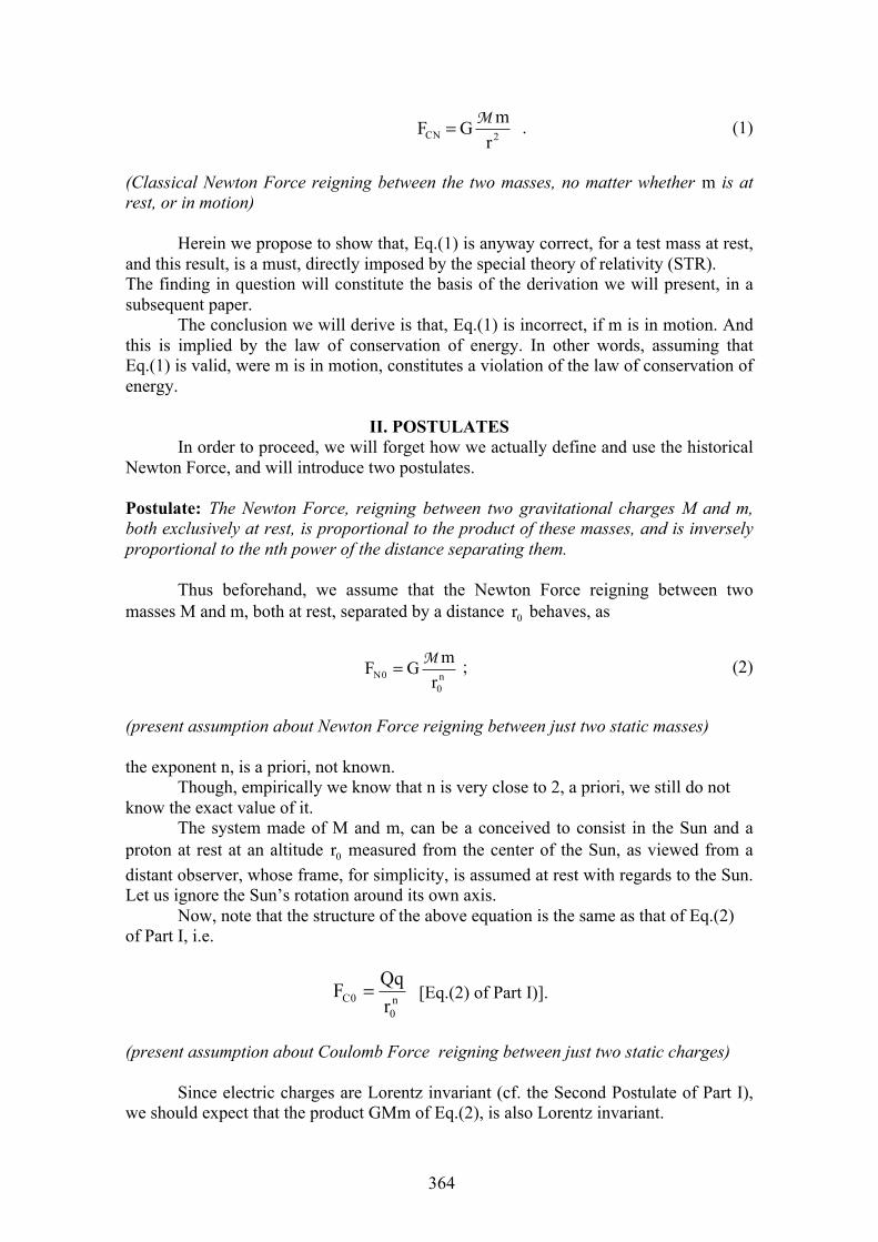
364
2CN rmGF M= . (1)
(Classical Newton Force reigning between the two masses, no matter whether m is at rest, or in motion)
Herein we propose to show that, Eq.(1) is anyway correct, for a test mass at rest, and this result, is a must, directly imposed by the special theory of relativity (STR). The finding in question will constitute the basis of the derivation we will present, in a subsequent paper.
The conclusion we will derive is that, Eq.(1) is incorrect, if m is in motion. And this is implied by the law of conservation of energy. In other words, assuming that Eq.(1) is valid, were m is in motion, constitutes a violation of the law of conservation of energy.
II. POSTULATESIn order to proceed, we will forget how we actually define and use the historical
Newton Force, and will introduce two postulates.
Postulate: The Newton Force, reigning between two gravitational charges M and m, both exclusively at rest, is proportional to the product of these masses, and is inversely proportional to the nth power of the distance separating them.
Thus beforehand, we assume that the Newton Force reigning between two masses M and m, both at rest, separated by a distance 0r behaves, as
n0
0N rmGF M= ; (2)
(present assumption about Newton Force reigning between just two static masses)
the exponent n, is a priori, not known. Though, empirically we know that n is very close to 2, a priori, we still do not
know the exact value of it. The system made of M and m, can be a conceived to consist in the Sun and a
proton at rest at an altitude 0r measured from the center of the Sun, as viewed from a distant observer, whose frame, for simplicity, is assumed at rest with regards to the Sun. Let us ignore the Sun’s rotation around its own axis.
Now, note that the structure of the above equation is the same as that of Eq.(2) of Part I, i.e.
n0
0C rQqF = [Eq.(2) of Part I)].
(present assumption about Coulomb Force reigning between just two static charges)
Since electric charges are Lorentz invariant (cf. the Second Postulate of Part I), we should expect that the product GMm of Eq.(2), is also Lorentz invariant.
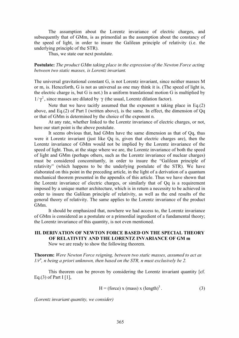
365
The assumption about the Lorentz invariance of electric charges, and subsequently that of GMm, is as primordial as the assumption about the constancy of the speed of light, in order to insure the Galilean principle of relativity (i.e. the underlying principle of the STR).
Thus, we state our next postulate.
Postulate: The product GMm taking place in the expression of the Newton Force acting between two static masses, is Lorentz invariant.
The universal gravitational constant G, is not Lorentz invariant, since neither masses M or m, is. Henceforth, G is not as universal as one may think it is. (The speed of light is, the electric charge is, but G is not.) In a uniform translational motion G is multiplied by
21 γ/ , since masses are dilated by γ (the usual, Lorentz dilation factor). Note that we have tacitly assumed that the exponent n taking place in Eq.(2)
above, and Eq.(2) of Part I (written above), is the same. In effect, the dimension of Qq or that of GMm is determined by the choice of the exponent n.
At any rate, whether linked to the Lorentz invariance of electric charges, or not, here our start point is the above postulate.
It seems obvious that, had GMm have the same dimension as that of Qq, thus were it Lorentz invariant (just like Qq is, given that electric charges are), then the Lorentz invariance of GMm would not be implied by the Lorentz invariance of the speed of light. Thus, at the stage where we are, the Lorentz invariance of both the speed of light and GMm (perhaps others, such as the Lorentz invariance of nuclear charges) must be considered concomitantly, in order to insure the “Galilean principle of relativity” (which happens to be the underlying postulate of the STR). We have elaborated on this point in the preceding article, in the light of a derivation of a quantum mechanical theorem presented in the appendix of this article. Thus we have shown that the Lorentz invariance of electric charges, or similarly that of Qq is a requirement imposed by a unique matter architecture, which is in return a necessity to be achieved in order to insure the Galilean principle of relativity, as well as the end results of the general theory of relativity. The same applies to the Lorentz invariance of the product GMm.
It should be emphasized that, nowhere we had access to, the Lorentz invariance of GMm is considered as a postulate or a primordial ingredient of a fundamental theory; the Lorentz invariance of this quantity, is not even mentioned.
III. DERIVATION OF NEWTON FORCE BASED ON THE SPECIAL THEORYOF RELATIVITY AND THE LORENTZ INVARIANCE OF GM m Now we are ready to show the following theorem.
Theorem: Were Newton Force reigning, between two static masses, assumed to act as 1/rn, n being a priori unknown, then based on the STR, n must exclusively be 2.
This theorem can be proven by considering the Lorentz invariant quantity [cf. Eq.(3) of Part I [1],
H = (force) x (mass) x (length)3 . (3)
(Lorentz invariant quantity, we consider)
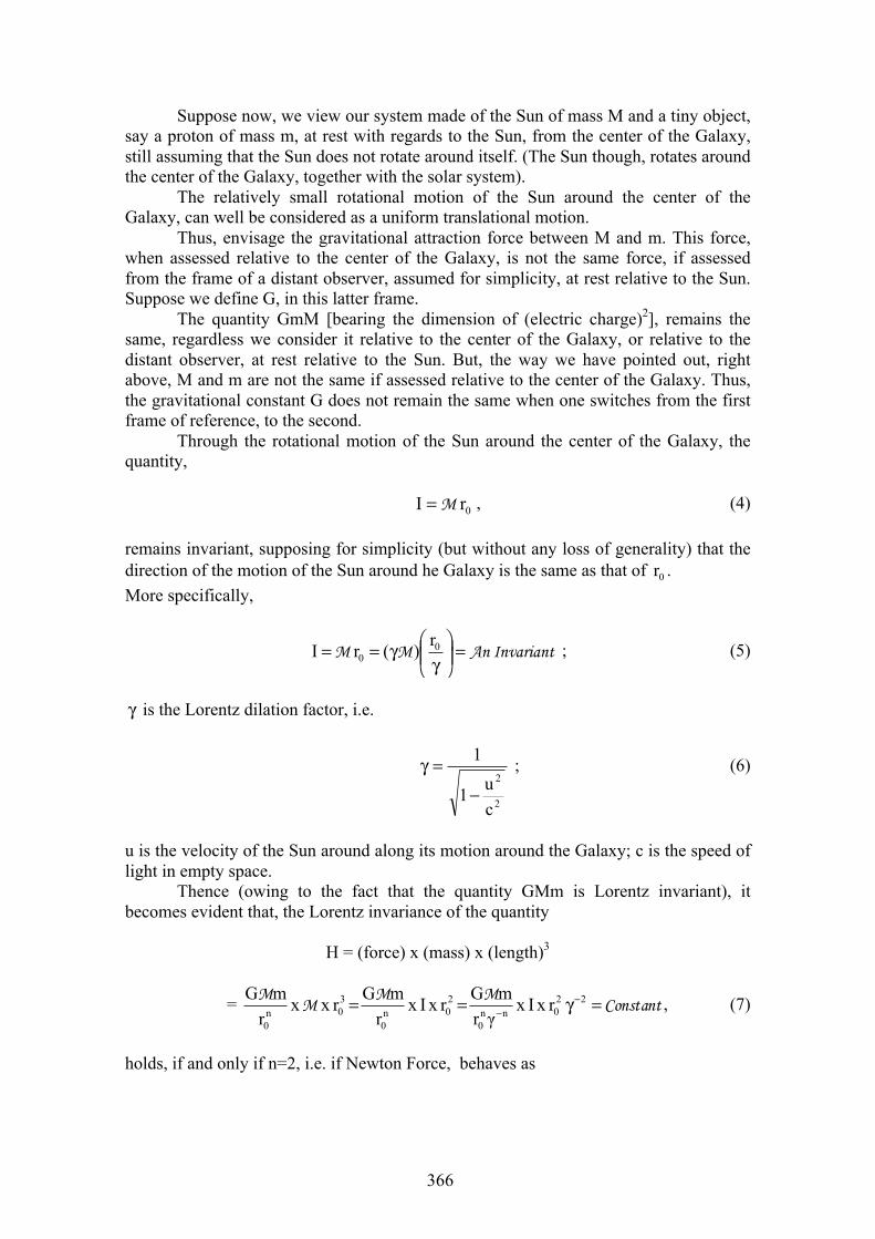
366
Suppose now, we view our system made of the Sun of mass M and a tiny object, say a proton of mass m, at rest with regards to the Sun, from the center of the Galaxy, still assuming that the Sun does not rotate around itself. (The Sun though, rotates around the center of the Galaxy, together with the solar system).
The relatively small rotational motion of the Sun around the center of the Galaxy, can well be considered as a uniform translational motion.
Thus, envisage the gravitational attraction force between M and m. This force, when assessed relative to the center of the Galaxy, is not the same force, if assessed from the frame of a distant observer, assumed for simplicity, at rest relative to the Sun. Suppose we define G, in this latter frame.
The quantity GmM [bearing the dimension of (electric charge)2], remains the same, regardless we consider it relative to the center of the Galaxy, or relative to the distant observer, at rest relative to the Sun. But, the way we have pointed out, right above, M and m are not the same if assessed relative to the center of the Galaxy. Thus, the gravitational constant G does not remain the same when one switches from the first frame of reference, to the second.
Through the rotational motion of the Sun around the center of the Galaxy, the quantity,
0rM=I , (4)
remains invariant, supposing for simplicity (but without any loss of generality) that the direction of the motion of the Sun around he Galaxy is the same as that of 0r . More specifically,
InvariantAnMM =⎟⎟⎠
⎞⎜⎜⎝
⎛γ
γ== 00
rr )(I ; (5)
γ is the Lorentz dilation factor, i.e.
2
2
cu1
1
−
=γ ; (6)
u is the velocity of the Sun around along its motion around the Galaxy; c is the speed of light in empty space.
Thence (owing to the fact that the quantity GMm is Lorentz invariant), it becomes evident that, the Lorentz invariance of the quantity
H = (force) x (mass) x (length)3
= ConstantMM
MM =γ== −
−22
030n
0
rxmGmGrxxr
mG Ixγr
rxIxr nn
0
20n
0
, (7)
holds, if and only if n=2, i.e. if Newton Force, behaves as
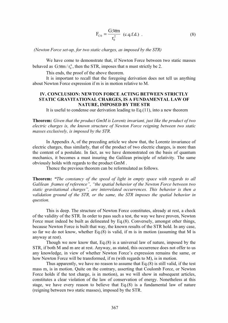
367
20
0C rmGF M= (c.q.f.d.) . (8)
(Newton Force set-up, for two static charges, as imposed by the STR)
We have come to demonstrate that, if Newton Force between two static masses behaved as n
0rmG /M , then the STR, imposes that n must strictly be 2. This ends, the proof of the above theorem. It is important to recall that the foregoing derivation does not tell us anything
about Newton Force expression if m is in motion relative to M.
IV. CONCLUSION: NEWTON FORCE ACTING BETWEEN STRICTLYSTATIC GRAVITATIONAL CHARGES, IS A FUNDAMENTAL LAW OF
NATURE, IMPOSED BY THE STR It is useful to condense our derivation leading to Eq.(11), into a new theorem
Theorem: Given that the product GmM is Lorentz invariant, just like the product of two electric charges is, the known structure of Newton Force reigning between two static masses exclusively, is imposed by the STR.
In Appendix A, of the preceding article we show that, the Lorentz invariance of electric charges, thus similarly, that of the product of two electric charges, is more than the content of a postulate. In fact, as we have demonstrated on the basis of quantum mechanics, it becomes a must insuring the Galilean principle of relativity. The same obviously holds with regards to the product GmM .
Thence the previous theorem can be reformulated as follows.
Theorem: “The constancy of the speed of light in empty space with regards to all Galilean frames of reference”, “the spatial behavior of the Newton Force between two static gravitational charges”, are interrelated occurrences. This behavior is then a validation ground of the STR, or the same, the STR imposes the spatial behavior in question.
This is deep. The structure of Newton Force constitutes, already at rest, a check of the validity of the STR. In order to pass such a test, the way we have proven, Newton Force must indeed be built as delineated by Eq.(8). Conversely, amongst other things, because Newton Force is built that way, the known results of the STR hold. In any case, so far we do not know, whether Eq.(8) is valid, if m is in motion (assuming that M is anyway at rest).
Though we now know that, Eq.(8) is a universal law of nature, imposed by the STR, if both M and m are at rest. Anyway, as stated, this occurrence does not offer to us any knowledge, in view of whether Newton Force’s expression remains the same, or how Newton Force will be transformed, if m (with regards to M), is in motion.
Thus apparently, we have no reason to assume that Eq.(8) is still valid, if the test mass m, is in motion. Quite on the contrary, asserting that Coulomb Force, or Newton Force holds if the test charge, is in motion), as we will show in subsequent articles, constitutes a clear violation of the law of conservation of energy. Nonetheless at this stage, we have every reason to believe that Eq.(8) is a fundamental law of nature (reigning between two static masses), imposed by the STR.

368
Our approach removes the blockade toward a unification of fields, and the quantization of the gravitational field hindered by the General Theory of Relativity [2,3]
REFERENCES [1]. T. Yarman, The Spatial Behavior of Coulomb And Newton Forces, Yet Reigning
Between Exclusively Static – Respectively, Electric And Gravitational – Charges, Is The Same Must, Drawn By The Special Theory of Relativity. Part I: Under These Circumstances, Coulomb Force is a Fundamental Law of Nature, Preceding Article.
[2]. T. Yarman, The General Equation of Motion Via the Special Theory of Relativity and Quantum Mechanics, AFBL, Volume 29, Numéro 3, 2004.
[3]. T. Yarman, The End Results of the General Relativity Theory Via Just Energy Conservation and Quantum Mechanics, Foundations of Physics Letters, December 2006.
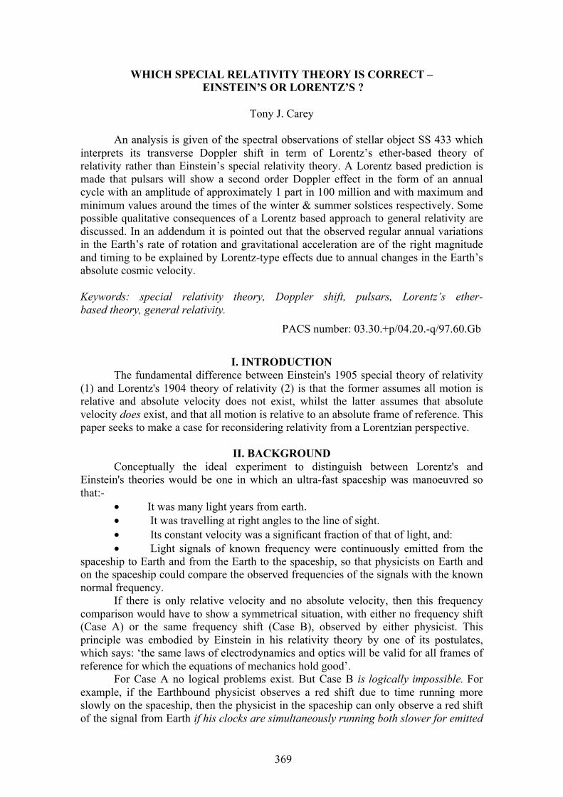
369
WHICH SPECIAL RELATIVITY THEORY IS CORRECT – EINSTEIN’S OR LORENTZ’S ?
Tony J. Carey
An analysis is given of the spectral observations of stellar object SS 433 which interprets its transverse Doppler shift in term of Lorentz’s ether-based theory of relativity rather than Einstein’s special relativity theory. A Lorentz based prediction is made that pulsars will show a second order Doppler effect in the form of an annual cycle with an amplitude of approximately 1 part in 100 million and with maximum and minimum values around the times of the winter & summer solstices respectively. Some possible qualitative consequences of a Lorentz based approach to general relativity are discussed. In an addendum it is pointed out that the observed regular annual variations in the Earth’s rate of rotation and gravitational acceleration are of the right magnitude and timing to be explained by Lorentz-type effects due to annual changes in the Earth’s absolute cosmic velocity.
Keywords: special relativity theory, Doppler shift, pulsars, Lorentz’s ether-based theory, general relativity.
PACS number: 03.30.+p/04.20.-q/97.60.Gb
I. INTRODUCTION The fundamental difference between Einstein's 1905 special theory of relativity
(1) and Lorentz's 1904 theory of relativity (2) is that the former assumes all motion is relative and absolute velocity does not exist, whilst the latter assumes that absolute velocity does exist, and that all motion is relative to an absolute frame of reference. This paper seeks to make a case for reconsidering relativity from a Lorentzian perspective.
II. BACKGROUNDConceptually the ideal experiment to distinguish between Lorentz's and
Einstein's theories would be one in which an ultra-fast spaceship was manoeuvred so that:-
• It was many light years from earth.• It was travelling at right angles to the line of sight.• Its constant velocity was a significant fraction of that of light, and:• Light signals of known frequency were continuously emitted from the
spaceship to Earth and from the Earth to the spaceship, so that physicists on Earth and on the spaceship could compare the observed frequencies of the signals with the known normal frequency.
If there is only relative velocity and no absolute velocity, then this frequency comparison would have to show a symmetrical situation, with either no frequency shift (Case A) or the same frequency shift (Case B), observed by either physicist. This principle was embodied by Einstein in his relativity theory by one of its postulates, which says: ‘the same laws of electrodynamics and optics will be valid for all frames of reference for which the equations of mechanics hold good’.
For Case A no logical problems exist. But Case B is logically impossible. For example, if the Earthbound physicist observes a red shift due to time running more slowly on the spaceship, then the physicist in the spaceship can only observe a red shift of the signal from Earth if his clocks are simultaneously running both slower for emitted
370
signals and faster for received signals. This is due to the fact that an observer near the spaceship, and stationary with respect to Earth, will receive unshifted signals from Earth, and therefore the only possible cause of a frequency shift for the physicist in the spaceship is if his clocks are actually running at a different rate to those on Earth. So the observation of a red (or blue) shift on Earth is only logically possible if absolute velocity exists. Then, in the case of a redshift observed on Earth, the spaceship physicist would observe the signal from Earth to be blue shifted because his clocks are actually running more slowly than the Earthbound clocks.
Thus Lorentz's theory, with its assumption of absolute velocity, predicts an actual slowing of time on the spaceship which will slow down the emitted frequency, leading to a red shift being observed on Earth -this is usually called the transverse Doppler effect.
III. THE EVIDENCEThe remarkable stellar object SS 433 provides us with the almost exact
equivalent of the above experiment - lacking only the physicist on the spaceship. It is some 12,000 light years distant and is emitting jets at 26% of the velocity of light and the orientation of the jets goes through a cycle so that every 164 days the jets are travelling exactly at right angles to the line of sight. At these times the jets show a transverse Doppler red shift corresponding to that expected on the Lorentz theory for a velocity of 0.26 c. Full details of SS 433 are given by Margon (3).
IV. DISCUSSIONSo now we appear to have evidence that absolute motion exists with respect to
some universal frame of reference in which atomic clocks go fastest -it will be assumed in this paper that this frame of reference is coincident with that of the cosmic microwave background radiation at 2.7 K. Therefore it is Lorentz's theory which seems to be correct. However, the paradigm shift needed to switch over to this perspective can apparently be avoided because the same prediction, of a transverse red shift, is implied by the clock prediction in Einstein's 1905 paper.
How is it that Einstein's theory can make the same prediction as Lorentz's theory about time slowing down, when such a prediction appears to be in conflict with one of its own postulates? The answer was provided by Essen (4) in a letter to Nature in which he pointed out 'The Error in the (Einstein's) Special Theory of Relativity'. He concludes his letter by saying that at that time there was no evidence concerning this aspect of the special theory, because no experimental work had been done at high velocities without accelerations. In view of this error it is not surprising that Synge (5) said that the concepts of Einstein's special relativity were incompatible with the concept of clocks that run regularly. Also, no satisfactory answer has emerged to a question by Dingle (6) as to what entitled Einstein to conclude from his theory that, as stated in the 1905 paper, 'a balance-clock at the equator must go more slowly, by a very small amount, than a precisely similar clock, situated at the poles under otherwise identical conditions.'
What is needed is an experimental test to decide between the two theories. Such a test may be possible because the vector of the Earth's net motion with respect to the cosmic microwave background lies approximately in the same plane as its orbit round the sun (7). This means that the Earth's absolute velocity oscillates by 30 km. per second with an annual cycle. From this oscillation in absolute velocity, Lorentzian relativity predicts that pulsars will show a second order, relativistic effect in their rates, in the form of an annual cycle with an amplitude of approximately 1 part in 100 million, and with maximum and minimum values around the times of the winter and summer
371
solstices respectively. This effect, if confirmed, would be in conflict with the relativity postulate of Einstein's special theory and is therefore a decisive test of Lorentz's theory, together with the assumption that the absolute inertial frame of reference is coincident with the frame in which the 2.7K° microwave radiation shows zero Doppler shift in any direction.
So what could actually be happening to cause high absolute velocities to change the frequency of emitted light? Lorentz assumed that the effect was due to interaction with the ether, and Vigier (8) concludes that moving clocks must interact with the local Dirac "aether". A more explicit hypothesis, linking relativity with quantum theory, is that atoms moving at high velocity pick up mass from the quantum vacuum, possibly via the hypothetical Higgs particles. This extra inertial mass then causes the vibrations of the atoms, including their electrons, to slow down. If inertial and gravitational mass do actually change as absolute velocity changes, this clearly would have major cosmological and astronomical implications. One consequence, which seems to be intuitively possible within this framework, is that very rapidly spinning astronomical objects of solar mass or greater could form hollow stable structures, like a doughnut or hollow cylinder, with much of the mass concentrated near a perimeter having a peripheral velocity close to that of light. Furthermore, there does not appear to be any intrinsic reason, from a Lorentzian perspective of such objects, as to why there could not be sufficient acceleration to matter from internal mechanisms for it to escape at a velocity less than light from within a free-fall event horizon. So matter could emerge even if light could not escape, thus enabling an object to be both a 'black hole' to light and a 'white hole' to matter. Such an object might therefore be able to recycle light into matter. It would also be able to store energy as real relativistic mass. The significance of these possibilities is that they could help with the understanding, not only of the jets of SS 433, but also of jets from quasars and the very massive objects at the centres of galaxies.
V. CONCLUSION In the context of the unsatisfactory aspects of Einstein's special relativity, as
described by Essen (4) and Synge (5) in 1968, and as further outlined above for the particular case of an astronomically based transverse Doppler effect, the observations of SS 433 may be considered to represent a prima facie case for reconsidering relativity from a Lorentzian perspective of absolute velocity, particularly as at least one absolute frame of reference, the cosmic microwave one, has been established. A test of the Lorentzian hypothesis, combined with the assumption that the absolute inertial frame of reference is coincident with this frame, is that it predicts that pulsars will show a second order, relativistic effect in their rates, in the form of an annual cycle with an amplitude of approximately 1 part in 100 million, and with maximum and minimum values around the times of the winter and summer solstices respectively. It is suggested that a Lorentzian based general relativity, with the consequent postulate of real increases in inertial and gravitational mass with velocity, might lead to improved understanding of the ultra high velocity jets emerging from astronomical objects such as SS 433, quasars and galactic nuclei.
VI. 2008 ADDENDUMWhat might be the effect on the Earth itself of this seasonal variation in its
absolute velocity? A modified version of the Lorentz approach to special relativity yields predictions that are in basic agreement with present observations. This modified ‘Lorentzian’ approach is based on the following three postulates:
372
1. That mass, due to an interaction with the quantum vacuum (Higgsparticles ??), varies with absolute velocity in relation to the framework of the cosmic black body background radiation
2. That the angular momentum of a rotating body, such as the Earth,remains constant even when its total mass is varying through changes in its absolute velocity.
3. That relativistic changes in the rate of working of atomic clocks are dueto their increase in mass and that, as in standard oscillator theory, their frequency varies with the square root of their mass.
For the seasonal period of maximum absolute velocity of the Earth, which just happens to coincide with the time around the winter solstice, mass is predicted to be at a maximum, compared to the time of minimum mass, by a relativity factor of one part in 100 million5. Now if the angular momentum (ref. Postulate 2) approximately remains constant, the Earth’s rate of rotation will slow by this factor. At the same time atomic clocks will also be slowed by a factor of approximately half this due to the oscillator dependence on the square root of the mass (ref Postulate 3). Thus this modified Lorentzian theory predicts a nett observed slowing at the winter solstice of the rate of rotation of the Earth, in relation to the standard astronomical framework of very distant galaxies, of the order of one part in 200 million and a corresponding speeding up at the summer solstice.
In addition, the predicted increase in mass would cause a seasonal fluctuation in the observed acceleration due to gravity, g, by a factor of about one part in 100 million.
Observations of seasonality of day length (See note 1) and gravity (see note 2) are of the predicted direction and order of magnitude. Current hypotheses to explain these seasonal variations are all terrestrially linked. Such hypotheses would be consistent with considerable year-to-year variability in the timing of the cycles. In contrast, the cosmological hypothesis above predicts that, within experimental error, there would be constancy in the year-to-year timing of the cycles. Further observations and data analysis are needed to be able to say whether the terrestrial or cosmological approach best fits the facts.
Note 1: Go to: www.jpl.nasa.gov/earth/features/longdays.html for details of paper by Dr Richard Gross. Note 2: Ref: Seasonal Gravity Variation, by Sato et al., Geophysical Research Abstracts, Vol. 5, 14120, 2003
ACKNOWLEDGEMENTS The advice, comments and information from Professors: J.P. Vigier, L. O'C.
Drury, P. A. Wayman, and Subhash Kak and Dr. H. Hopkins are gratefully acknowledged. The challenging contribution of the late Professor H. Dingle (6) was also most helpful.
5 Although other experimental work suggests this factor is probably of the right magnitude, the exact
factor may not be as calculated by traditional relativity theory which, apart from the velocity of light, does
not include properties of the quantum vacuum.
373
REFERENCES [1]. Einstein. Ann. d. Phys. 17 (1905) 891. Also as English translation in: Einstein
and others, The Principle of Relativity (Methuen. London, 1923). [2]. H.A. Lorentz, Proc. Acad. Sci. Amst. 6 (1904) 809. [3]. B.Margon, Sc. Am. 243 No.4 (1980) 44. [4]. Margon et a1. , Astrophys. Jrn1. Lett. 230 No.l Pt. 2 ( 1979) L41. [5]. Margon et al., Astrophys. Jrnl. Lett. 233 No.2 Pt.2 (1979) L63. [6]. B. Margon and G.O. Abell, 279 No.5715 (1979) 701 [7]. L. Essen, Nature 217 (1968) 19. [8]. J.L. Synge, Nature 219 (1968) 790. [9]. H. Dingle, Science at the Crossroads (Martin Brian & O'Keefe, London, 1972)
pp. 45-46. [10].R.A. Muller, Sc. Am. 238 No.5( 1978) 64. [11].J.P. Vigier, Phys. Lett. A 234 (1997) 79. [12].Background Bibliography. [13].L. Marder, Time and the Space Traveller (George Allen & Unwin,
London, 1971).
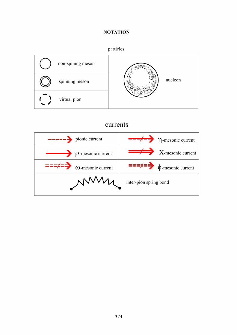
NOTATION
particles
non-spining meson
spinning meson
virtual pion
nucleon
currents
pionic current η-mesonic current
ρ-mesonic current X-mesonic current
ω-mesonic current φ-mesonic current
inter-pion spring bond
374
NUCLEAR STRUCTURE FROM NAÏVE MESON THEORY, PART 1
Christopher Illert
University of Western Sydney, CCR, 2/3 Birch Crescent, East Corrimal, NSW 2518, AUSTRALIA
I. INTRODUCTIONIn 1958 R.B. Leighton lamented “… on the one hand, no one seriously
doubts that the meson theory is at least qualitatively correct, but on the other hand, not a single quantity has yet been calculated and measured with sufficient accuracy to constitute a convincing confirmation of its quantitative correctness”. The 50th anniversary of this statement is an appropriate occasion to review progress in understanding meson theory and nuclear structure – a topic that epitomizes Relativistic concepts by encompassing the quickest and most energetic of all processes, with mass and energy being routinely inter-convertible, and nuclear binding-energies directly calculated from “missing mass” by means of Einstein’s famous formula E = mc2.
On a philosophical level, Relativity can be about viewing the world from different frames of reference – what would the world look like if we could ride a beam of light? In like vein we could ask what nuclear processes and structures would look like from the relativistic frame of reference of, say, a meson? Processes that take say 10-22 seconds in our macro-worldview, would represent an eternity for some highly accelerated and short-lived elementary particles. Mesonic currents flowing between nucleons would seem steady and eternal, instead of so brief that we in the big world can only think of them in terms of probability and uncertainty.
This paper argues that nuclear processes, and nuclear structure itself, becomes almost trivially Newtonian from the frame of reference of mesonic currents, providing an unexpectedly simple “ball and stick” type general solution to the N-body problem in nuclear physics (similar to molecular structures in chemistry), universally enabling nuclear binding energies to be calculated to a few significant figures using little more than mental arithmetic based upon intuitive circuit diagrams. This is in stark contrast to the horrendously complex supercomputer computations, based on wave mechanics, which basically don’t work and are still struggling with the mere Three Body (“Borromeo”) problem that may be insoluble in principle.
This paper offers the first real (albeit approximate) general solution to the N-body problem in nuclear physics, accounting for exotic halo and super-deformed nuclear states as well as nuclear shells, in terms of a new system of mesonic circuit diagrams that are to nuclear physics what the Feynman diagrams are to quantum electrodynamics. Doing nuclear binding energy calculations from a relativistic meson’s frame of reference is no more mysterious than using logarithms to turn multiplications into additions.
Keywords: Naive meson theory, antimatter, nuclear, structure, nucleon, relativity, pion,3He,4He.
Pacs number: 25.40.Ve/25.55.-e/25.40.Qa
375
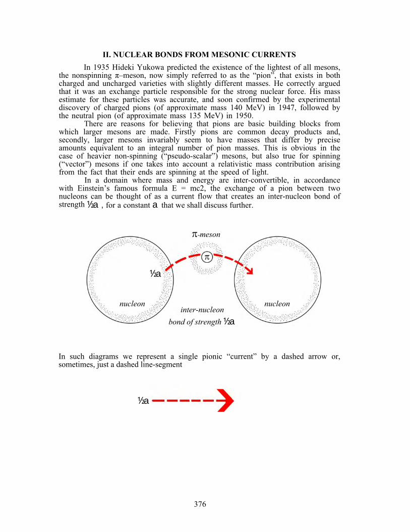
II. NUCLEAR BONDS FROM MESONIC CURRENTSIn 1935 Hideki Yukowa predicted the existence of the lightest of all mesons,
the nonspinning π–meson, now simply referred to as the “pion”, that exists in both charged and uncharged varieties with slightly different masses. He correctly argued that it was an exchange particle responsible for the strong nuclear force. His mass estimate for these particles was accurate, and soon confirmed by the experimental discovery of charged pions (of approximate mass 140 MeV) in 1947, followed by the neutral pion (of approximate mass 135 MeV) in 1950.
There are reasons for believing that pions are basic building blocks from which larger mesons are made. Firstly pions are common decay products and, secondly, larger mesons invariably seem to have masses that differ by precise amounts equivalent to an integral number of pion masses. This is obvious in the case of heavier non-spinning (“pseudo-scalar”) mesons, but also true for spinning (“vector”) mesons if one takes into account a relativistic mass contribution arising from the fact that their ends are spinning at the speed of light.
In a domain where mass and energy are inter-convertible, in accordance with Einstein’s famous formula E = mc2, the exchange of a pion between two nucleons can be thought of as a current flow that creates an inter-nucleon bond of strength ½a , for a constant a that we shall discuss further.
In such diagrams we represent a single pionic “current” by a dashed arrow or, sometimes, just a dashed line-segment
½a
inter-nucleon bond of strength ½a
nucleon nucleon
π-meson
½a
376
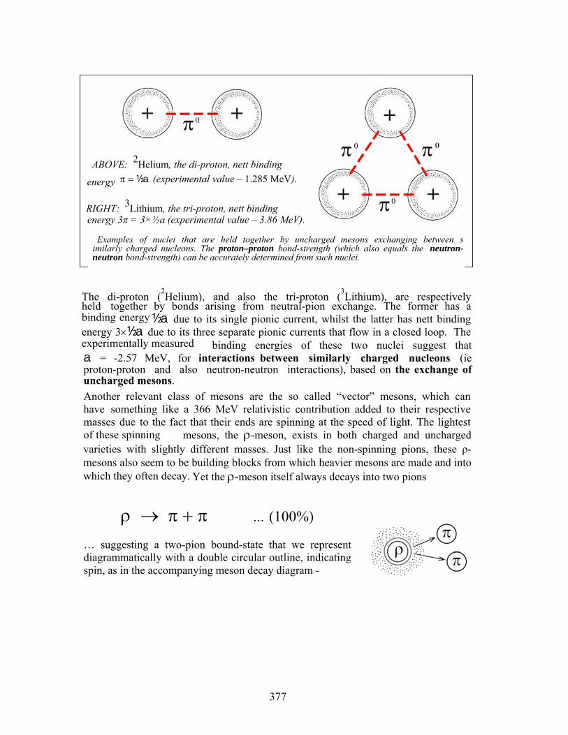
The di-proton (2Helium), and also the tri-proton (3Lithium), are respectively held together by bonds arising from neutral-pion exchange. The former has a binding energy ½a due to its single pionic current, whilst the latter has nett bindingenergy 3×½a due to its three separate pionic currents that flow in a closed loop. Theexperimentally measured binding energies of these two nuclei suggest that a = -2.57 MeV, for interactions between similarly charged nucleons (ie proton-proton and also neutron-neutron interactions), based on the exchange of uncharged mesons. Another relevant class of mesons are the so called “vector” mesons, which can have something like a 366 MeV relativistic contribution added to their respective masses due to the fact that their ends are spinning at the speed of light. The lightest of these spinning mesons, the ρ-meson, exists in both charged and uncharged varieties with slightly different masses. Just like the non-spinning pions, these ρ-mesons also seem to be building blocks from which heavier mesons are made and into which they often decay. Yet the ρ-meson itself always decays into two pions
ρ → π + π ... (100%)
… suggesting a two-pion bound-state that we representdiagrammatically with a double circular outline, indicating spin, as in the accompanying meson decay diagram -
ABOVE: 2Helium, the di-proton, nett binding
energy π = ½a (experimental value – 1.285 MeV).
RIGHT: 3Lithium, the tri-proton, nett bindingenergy 3π = 3×½a (experimental value – 3.86 MeV).
Examples of nuclei that are held together by uncharged mesons exchanging between s imilarly charged nucleons. The proton–proton bond-strength (which also equals the neutron-neutron bond-strength) can be accurately determined from such nuclei.
377
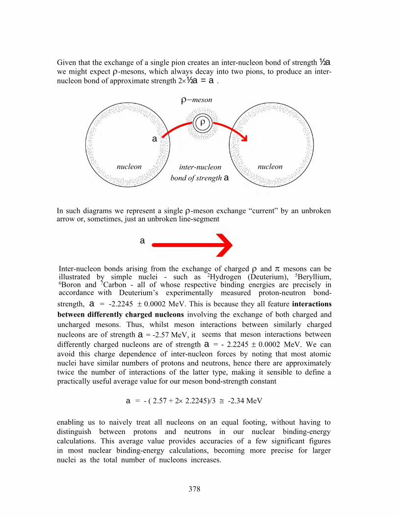
Given that the exchange of a single pion creates an inter-nucleon bond of strength ½a we might expect ρ-mesons, which always decay into two pions, to produce an inter-nucleon bond of approximate strength 2×½a = a .
In such diagrams we represent a single ρ-meson exchange “current” by an unbroken arrow or, sometimes, just an unbroken line-segment
Inter-nucleon bonds arising from the exchange of charged ρ and π mesons can be illustrated by simple nuclei - such as 2Hydrogen (Deuterium), 5Beryllium, 6Boron and 7Carbon - all of whose respective binding energies are precisely in accordance with Deuterium’s experimentally measured proton-neutron bond-strength, a = -2.2245 ± 0.0002 MeV. This is because they all feature interactions between differently charged nucleons involving the exchange of both charged and uncharged mesons. Thus, whilst meson interactions between similarly charged nucleons are of strength a = -2.57 MeV, it seems that meson interactions between differently charged nucleons are of strength a = - 2.2245 ± 0.0002 MeV. We can avoid this charge dependence of inter-nucleon forces by noting that most atomic nuclei have similar numbers of protons and neutrons, hence there are approximately twice the number of interactions of the latter type, making it sensible to define a practically useful average value for our meson bond-strength constant
a = - ( 2.57 + 2× 2.2245)/3 ≅ -2.34 MeV
enabling us to naively treat all nucleons on an equal footing, without having to distinguish between protons and neutrons in our nuclear binding-energy calculations. This average value provides accuracies of a few significant figures in most nuclear binding-energy calculations, becoming more precise for larger nuclei as the total number of nucleons increases.
a
ρ−meson
inter-nucleon bond of strength a
a
nucleon nucleon
378

2Hydrogen, the Deuteron, with nettbinding energy ρ = a(experimental value – 2.2245 MeV)
5Beryllium, a Deuteron with a small halo ofmutually repelling protons that arrange them-selves (probably tetrahedrally), about the central neutron, a ma ximum distance apart. Nett binding energy
3π + ρ = 3×(½a) + a = 5×(½a)
(experimental value – 5.53 MeV)
6Boron, a Deuteron with a halo of mutually repelling protons that arrange themselves (probably hexahed- rally) , about the central neutron, a maximum distance apart. Nett binding energy
4π + ρ = 4×(½a) + a = 3a (experimental value - 6.6735 MeV)
7 Carbon, a Deuteron with a halo of mutually repel- ling protons that arrange themselves (probably octahedrally), about the central neutron, a maximum distance apart. Nett binding energy
5π + ρ = 5×(½a) + a = 7×(½a) (experimental value – 7.79 MeV)
Various nuclei held together by mesons exchanging between differently charged nucleons. The proton-neutron bond strength can be accurately
determined from such examples. However the overall shape of these nuclei is not due to meson bonds but,
rather, elastic-sphere packing about the central neutron … forces of the “contact” kind.
379
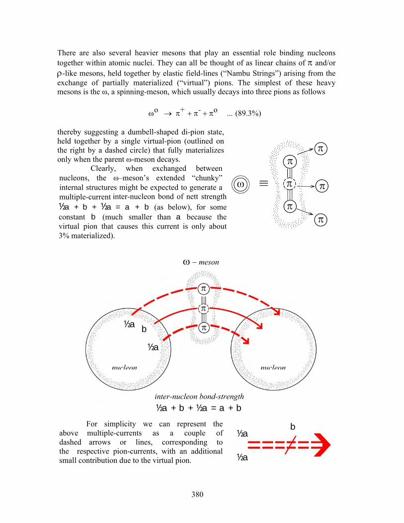
There are also several heavier mesons that play an essential role binding nucleons together within atomic nuclei. They can all be thought of as linear chains of π and/or ρ-like mesons, held together by elastic field-lines (“Nambu Strings”) arising from the exchange of partially materialized (“virtual”) pions. The simplest of these heavy mesons is the ω, a spinning-meson, which usually decays into three pions as follows
ωo → π+ + π- + πo ... (89.3%)
thereby suggesting a dumbell-shaped di-pion state, held together by a single virtual-pion (outlined on the right by a dashed circle) that fully materializes only when the parent ω-meson decays.
Clearly, when exchanged between nucleons, the ω–meson’s extended “chunky” internal structures might be expected to generate a multiple-current inter-nucleon bond of nett strength ½a + b + ½a = a + b (as below), for some constant b (much smaller than a because the virtual pion that causes this current is only about 3% materialized).
For simplicity we can represent the above multiple-currents as a couple of dashed arrows or lines, corresponding to the respective pion-currents, with an additional small contribution due to the virtual pion.
ω − meson
inter-nucleon bond-strength ½a + b + ½a = a + b
½a
½a
b
nucleon nucleon
½a
½a
b
380
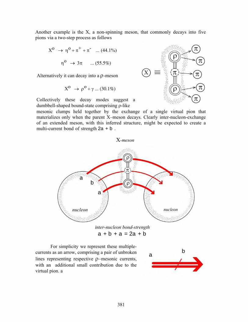
Another example is the X, a non-spinning meson, that commonly decays into five pions via a two-step process as follows
Xo → ηo + π+ + π- ... (44.1%)
ηo → 3π ... (55.5%)
Alternatively it can decay into a ρ-meson
Xo → ρo + γ ... (30.1%)
Collectively these decay modes suggest adumbbell-shaped bound-state comprising ρ-like mesonic clumps held together by the exchange of a single virtual pion that materializes only when the parent X–meson decays. Clearly inter-nucleon-exchange of an extended meson, with this inferred structure, might be expected to create a multi-current bond of strength 2a + b .
For simplicity we represent these multiple-currents as an arrow, comprising a pair of unbroken lines representing respective ρ–mesonic currents, with an additional small contribution due to the virtual pion. a
a b
X-meson
inter-nucleon bond-strength a + b + a = 2a + b
a b
nucleon
a
nucleon
381
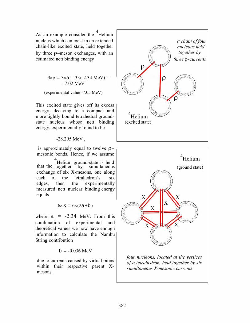
As an example consider the 4Helium
nucleus which can exist in an extended chain-like excited state, held together by three ρ–meson exchanges, with an estimated nett binding energy
3×ρ = 3×a = 3×(-2.34 MeV) = -7.02 MeV
(experimental value -7.05 MeV).
This excited state gives off its excess energy, decaying to a compact and more tightly bound tetrahedral ground-state nucleus whose nett binding energy, experimentally found to be
-28.295 MeV ,
is approximately equal to twelve ρ–mesonic bonds. Hence, if we assume
that the 4Helium ground-state is held
together by simultaneous exchange of six X-mesons, one along each of the tetrahedron’s six edges, then the experimentally measured nett nuclear binding energy equals
6×X = 6×(2a+b)
where a = -2.34 MeV. From this combination of experimental and theoretical values we now have enough information to calculate the Nambu String contribution
b = -0.036 MeV
due to currents caused by virtual pions within their respective parent X-mesons.
4Helium(excited state)
4Helium(ground state)
a chain of four nucleons held together by three ρ-currents
four nucleons, located at the vertices of a tetrahedron, held together by six simultaneous X-mesonic currents
382
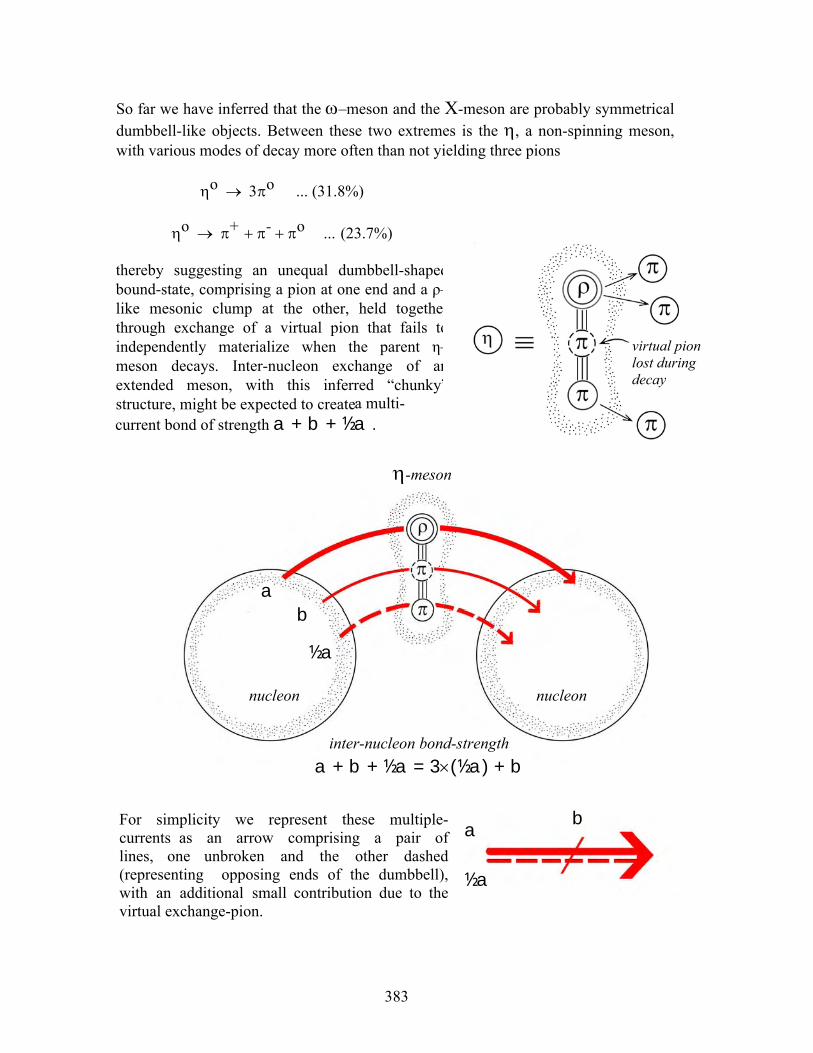
So far we have inferred that the ω–meson and the X-meson are probably symmetrical dumbbell-like objects. Between these two extremes is the η, a non-spinning meson, with various modes of decay more often than not yielding three pions
ηo → 3πo ... (31.8%)
ηo → π+ + π- + πo ... (23.7%)
thereby suggesting an unequal dumbbell-shaped bound-state, comprising a pion at one end and a ρ–like mesonic clump at the other, held together through exchange of a virtual pion that fails to independently materialize when the parent η–meson decays. Inter-nucleon exchange of an extended meson, with this inferred “chunky” structure, might be expected to create a multi-current bond of strength a + b + ½a .
For simplicity we represent these multiple-currents as an arrow comprising a pair of lines, one unbroken and the other dashed (representing opposing ends of the dumbbell), with an additional small contribution due to the virtual exchange-pion.
a
½a
b
nucleon nucleon
inter-nucleon bond-strength a + b + ½a = 3×(½a) + b
η-meson
a b
½a
virtual pion lost during decay
383
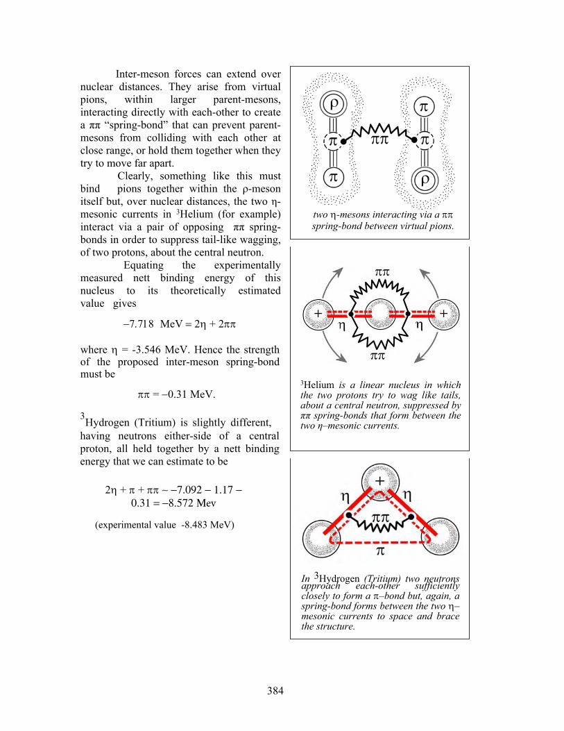
Inter-meson forces can extend over nuclear distances. They arise from virtual pions, within larger parent-mesons, interacting directly with each-other to create a ππ “spring-bond” that can prevent parent-mesons from colliding with each other at close range, or hold them together when they try to move far apart.
Clearly, something like this must bind pions together within the ρ-meson itself but, over nuclear distances, the two η-mesonic currents in 3Helium (for example) interact via a pair of opposing ππ spring-bonds in order to suppress tail-like wagging, of two protons, about the central neutron.
Equating the experimentally measured nett binding energy of this nucleus to its theoretically estimated value gives
−7.718 MeV = 2η + 2ππ
where η = -3.546 MeV. Hence the strength of the proposed inter-meson spring-bond must be
ππ = −0.31 MeV.
3Hydrogen (Tritium) is slightly different,having neutrons either-side of a central proton, all held together by a nett binding energy that we can estimate to be
2η + π + ππ ∼ −7.092 − 1.17 − 0.31 = −8.572 Μev
(experimental value -8.483 MeV)
two η-mesons interacting via a ππ spring-bond between virtual pions.
3Helium is a linear nucleus in which the two protons try to wag like tails, about a central neutron, suppressed by ππ spring-bonds that form between the two η–mesonic currents.
In 3Hydrogen (Tritium) two neutrons approach each-other sufficiently closely to form a π–bond but, again, a spring-bond forms between the two η–mesonic currents to space and brace the structure.
384
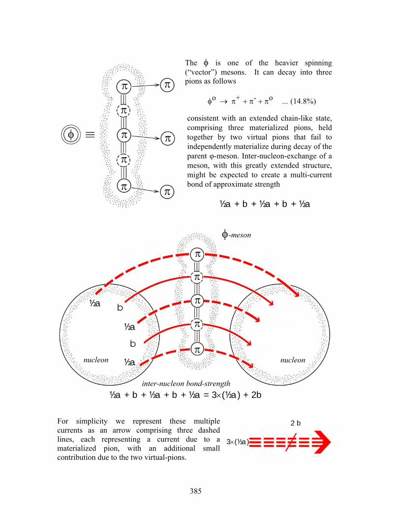
The φ is one of the heavier spinning (“vector”) mesons. It can decay into three pions as follows
φo → π+ + π- + πo ... (14.8%)
consistent with an extended chain-like state, comprising three materialized pions, held together by two virtual pions that fail to independently materialize during decay of the parent φ-meson. Inter-nucleon-exchange of a meson, with this greatly extended structure, might be expected to create a multi-current bond of approximate strength
½a + b + ½a + b + ½a
For simplicity we represent these multiple currents as an arrow comprising three dashed lines, each representing a current due to a materialized pion, with an additional small contribution due to the two virtual-pions.
inter-nucleon bond-strength ½a + b + ½a + b + ½a = 3×(½a) + 2b
½a
b
½a
½a
φ-meson
nucleon nucleon
2 b
3×(½a)
b
385
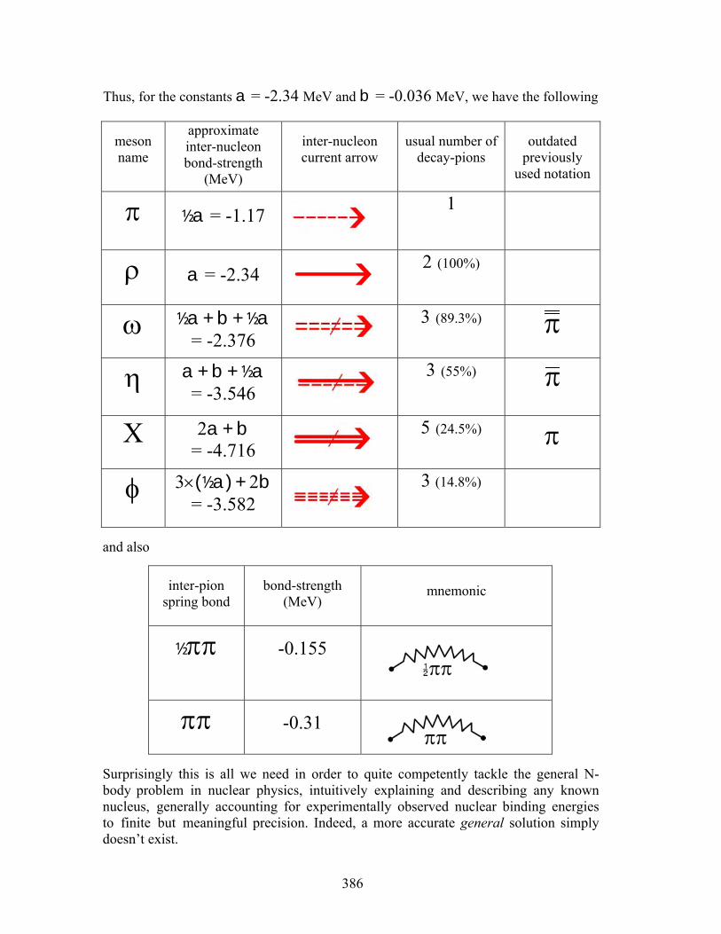
Thus, for the constants a = -2.34 MeV and b = -0.036 MeV, we have the following
meson name
approximate inter-nucleon bond-strength
(MeV)
inter-nucleon current arrow
usual number of decay-pions
outdated previously
used notation
π ½a = -1.17 1
ρ a = -2.34 2 (100%)
ω ½a + b + ½a = -2.376
3 (89.3%) π
η a + b + ½a = -3.546
3 (55%) π
X 2a + b = -4.716
5 (24.5%) π
φ 3×(½a) + 2b = -3.582
3 (14.8%)
and also
inter-pion spring bond
bond-strength (MeV)
mnemonic
½ππ -0.155
ππ -0.31
Surprisingly this is all we need in order to quite competently tackle the general N-body problem in nuclear physics, intuitively explaining and describing any known nucleus, generally accounting for experimentally observed nuclear binding energies to finite but meaningful precision. Indeed, a more accurate general solution simply doesn’t exist.
386
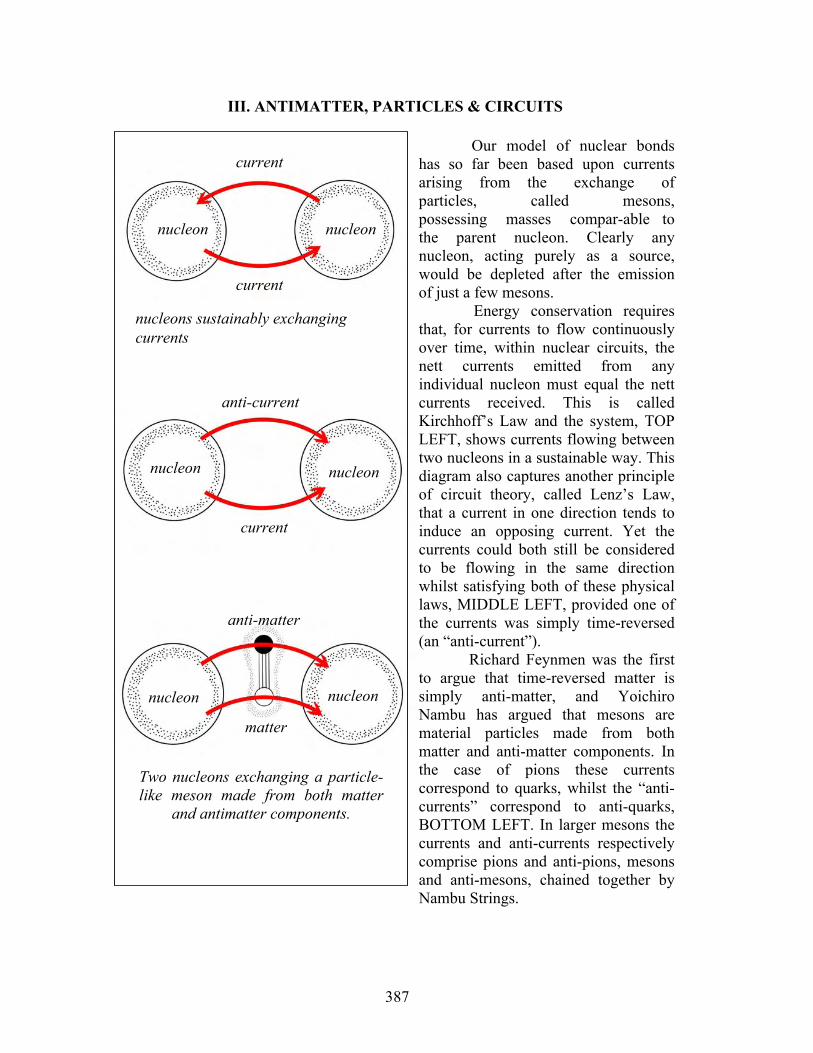
III. ANTIMATTER, PARTICLES & CIRCUITS
Our model of nuclear bonds has so far been based upon currents arising from the exchange of particles, called mesons, possessing masses compar-able to the parent nucleon. Clearly any nucleon, acting purely as a source, would be depleted after the emission of just a few mesons.
Energy conservation requires that, for currents to flow continuously over time, within nuclear circuits, the nett currents emitted from any individual nucleon must equal the nett currents received. This is called Kirchhoff’s Law and the system, TOP LEFT, shows currents flowing between two nucleons in a sustainable way. This diagram also captures another principle of circuit theory, called Lenz’s Law, that a current in one direction tends to induce an opposing current. Yet the currents could both still be considered to be flowing in the same direction whilst satisfying both of these physical laws, MIDDLE LEFT, provided one of the currents was simply time-reversed (an “anti-current”).
Richard Feynmen was the first to argue that time-reversed matter is simply anti-matter, and Yoichiro Nambu has argued that mesons are material particles made from both matter and anti-matter components. In the case of pions these currents correspond to quarks, whilst the “anti-currents” correspond to anti-quarks, BOTTOM LEFT. In larger mesons the currents and anti-currents respectively comprise pions and anti-pions, mesons and anti-mesons, chained together by Nambu Strings.
Two nucleons exchanging a particle-like meson made from both matter
and antimatter components.
nucleon
nucleon
anti-matter
matter
current
anti-current
current
current
nucleon
nucleon nucleon
nucleon
nucleons sustainably exchanging currents
387
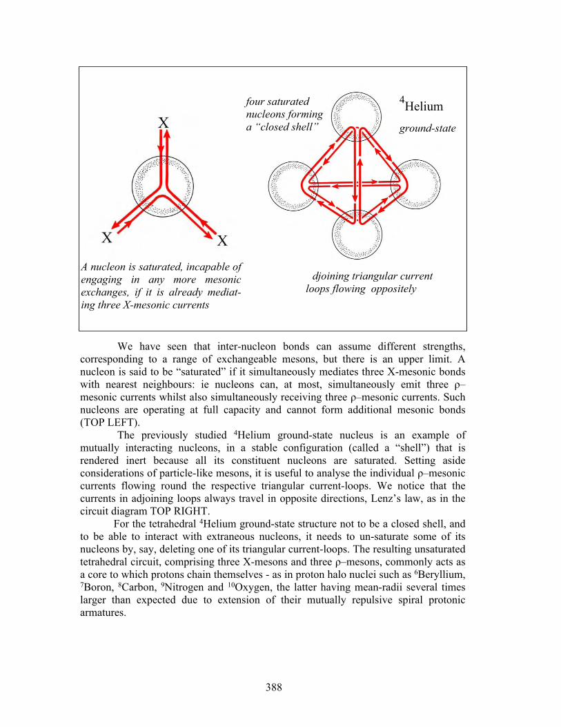
We have seen that inter-nucleon bonds can assume different strengths, corresponding to a range of exchangeable mesons, but there is an upper limit. A nucleon is said to be “saturated” if it simultaneously mediates three X-mesonic bonds with nearest neighbours: ie nucleons can, at most, simultaneously emit three ρ–mesonic currents whilst also simultaneously receiving three ρ–mesonic currents. Such nucleons are operating at full capacity and cannot form additional mesonic bonds (TOP LEFT).
The previously studied 4Helium ground-state nucleus is an example of mutually interacting nucleons, in a stable configuration (called a “shell”) that is rendered inert because all its constituent nucleons are saturated. Setting aside considerations of particle-like mesons, it is useful to analyse the individual ρ–mesonic currents flowing round the respective triangular current-loops. We notice that the currents in adjoining loops always travel in opposite directions, Lenz’s law, as in the circuit diagram TOP RIGHT.
For the tetrahedral 4Helium ground-state structure not to be a closed shell, and to be able to interact with extraneous nucleons, it needs to un-saturate some of its nucleons by, say, deleting one of its triangular current-loops. The resulting unsaturated tetrahedral circuit, comprising three X-mesons and three ρ–mesons, commonly acts as a core to which protons chain themselves - as in proton halo nuclei such as 6Beryllium, 7Boron, 8Carbon, 9Nitrogen and 10Oxygen, the latter having mean-radii several times larger than expected due to extension of their mutually repulsive spiral protonic armatures.
four saturated nucleons forming a “closed shell”
Adjoining triangular current loops flowing oppositely
4Heliumground-state
A nucleon is saturated, incapable ofengaging in any more mesonicexchanges, if it is already mediat-ing three X-mesonic currents
388
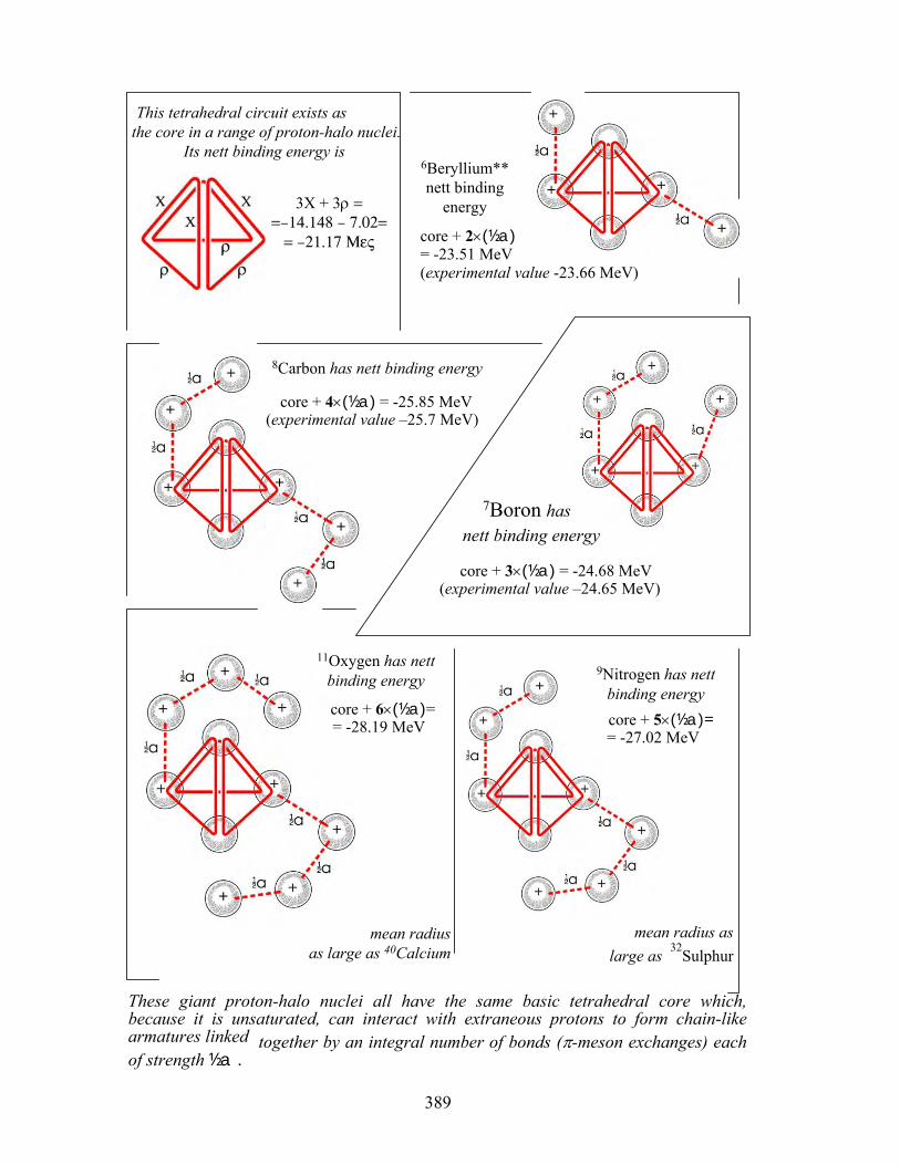
This tetrahedral circuit exists as the core in a range of proton-halo nuclei.
Its nett binding energy is
3X + 3ρ = =–14.148 – 7.02=
= –21.17 Μες
7Boron has nett binding energy
core + 3×(½a) = -24.68 MeV (experimental value –24.65 MeV)
9Nitrogen has nett binding energy
core + 5×(½a)= = -27.02 MeV
6Beryllium** nett binding
energy
core + 2×(½a) = -23.51 MeV (experimental value -23.66 MeV)
8Carbon has nett binding energy
core + 4×(½a) = -25.85 MeV (experimental value –25.7 MeV)
11Oxygen has nett binding energy
core + 6×(½a)= = -28.19 MeV
These giant proton-halo nuclei all have the same basic tetrahedral core which, because it is unsaturated, can interact with extraneous protons to form chain-like armatures linked together by an integral number of bonds (π-meson exchanges) each of strength ½a .
mean radius as large as 32Sulphur
mean radiusas large as 40Calcium
389
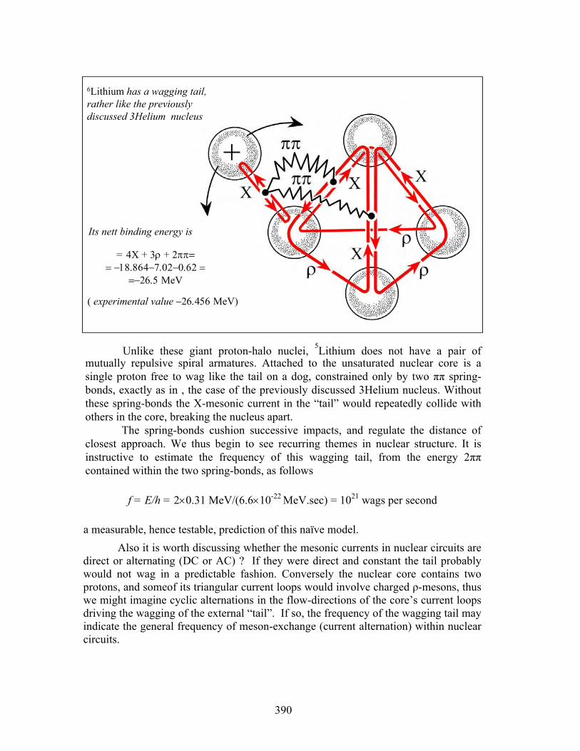
Unlike these giant proton-halo nuclei, 5Lithium does not have a pair of mutually repulsive spiral armatures. Attached to the unsaturated nuclear core is a single proton free to wag like the tail on a dog, constrained only by two ππ spring-bonds, exactly as in , the case of the previously discussed 3Helium nucleus. Without these spring-bonds the X-mesonic current in the “tail” would repeatedly collide with others in the core, breaking the nucleus apart.
The spring-bonds cushion successive impacts, and regulate the distance of closest approach. We thus begin to see recurring themes in nuclear structure. It is instructive to estimate the frequency of this wagging tail, from the energy 2ππ contained within the two spring-bonds, as follows
f = E/h = 2×0.31 MeV/(6.6×10-22 MeV.sec) = 1021 wags per second
a measurable, hence testable, prediction of this naïve model.Also it is worth discussing whether the mesonic currents in nuclear circuits are
direct or alternating (DC or AC) ? If they were direct and constant the tail probably would not wag in a predictable fashion. Conversely the nuclear core contains two protons, and someof its triangular current loops would involve charged ρ-mesons, thus we might imagine cyclic alternations in the flow-directions of the core’s current loops driving the wagging of the external “tail”. If so, the frequency of the wagging tail may indicate the general frequency of meson-exchange (current alternation) within nuclear circuits.
6Lithium has a wagging tail, rather like the previously discussed 3Helium nucleus
Its nett binding energy is
= 4X + 3ρ + 2ππ== −18.864−7.02−0.62 =
=−26.5 MeV
( experimental value −26.456 MeV)
390

In its ground-state the 9Lithium nucleus has two chain-like tails of (mostly) neutrons -attached to an un-saturated tetrahedral core and prevented from colliding by a single ππ spring-bond – rather like the neutron armatures of the previously discussed Tritium nucleus. This ground-state can be excited, to a truly giant dipole, by simultaneously collapsing the external triangular current loop to an X-meson and breaking the spring-bond. The difference in energy between these states is thus
ΔE = a + ππ = 2.34 + 0.31 MeV = 2.65 MeV
(experimental value 2.691 MeV) .
a lovely confirmation of naïve meson theory. It is unlikely that the giant dipole can befurther excited as the breakup reaction, to 8Lithium plus neutron, occurs at –41.3 MeV.
This triangular current-loop collapses to an X-meson This spring-bond is lost
9Lithium, ground-state,with nett binding energy
= 8X + 4ρ + ππ = = −37.728−9.36−0.31 =
=−47.4 MeV
Giant di-pole state with a mean radiu as large as
32Sulphur and nett binding energy s
= 8X + 3ρ= = −37.728−7.02 = −44.75 ΜeV
ππ
391
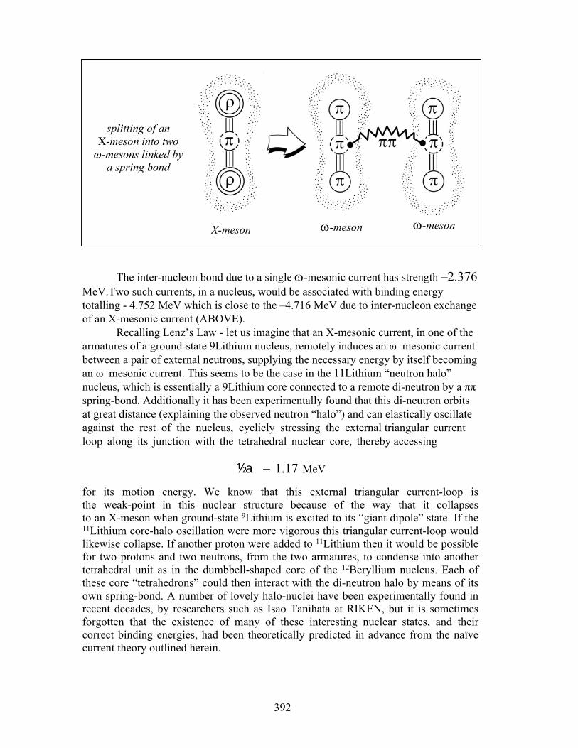
The inter-nucleon bond due to a single ω-mesonic current has strength –2.376 MeV.Two such currents, in a nucleus, would be associated with binding energy totalling - 4.752 MeV which is close to the –4.716 MeV due to inter-nucleon exchange of an X-mesonic current (ABOVE).
Recalling Lenz’s Law - let us imagine that an X-mesonic current, in one of the armatures of a ground-state 9Lithium nucleus, remotely induces an ω–mesonic current between a pair of external neutrons, supplying the necessary energy by itself becoming an ω–mesonic current. This seems to be the case in the 11Lithium “neutron halo” nucleus, which is essentially a 9Lithium core connected to a remote di-neutron by a ππ spring-bond. Additionally it has been experimentally found that this di-neutron orbits at great distance (explaining the observed neutron “halo”) and can elastically oscillate against the rest of the nucleus, cyclicly stressing the external triangular current loop along its junction with the tetrahedral nuclear core, thereby accessing
½a = 1.17 MeV
for its motion energy. We know that this external triangular current-loop is the weak-point in this nuclear structure because of the way that it collapses to an X-meson when ground-state 9Lithium is excited to its “giant dipole” state. If the 11Lithium core-halo oscillation were more vigorous this triangular current-loop would likewise collapse. If another proton were added to 11Lithium then it would be possible for two protons and two neutrons, from the two armatures, to condense into another tetrahedral unit as in the dumbbell-shaped core of the 12Beryllium nucleus. Each of these core “tetrahedrons” could then interact with the di-neutron halo by means of its own spring-bond. A number of lovely halo-nuclei have been experimentally found in recent decades, by researchers such as Isao Tanihata at RIKEN, but it is sometimes forgotten that the existence of many of these interesting nuclear states, and their correct binding energies, had been theoretically predicted in advance from the naïve current theory outlined herein.
X-meson ω-meson ω-meson
splitting of an X-meson into two
ω-mesons linked by a spring bond
392
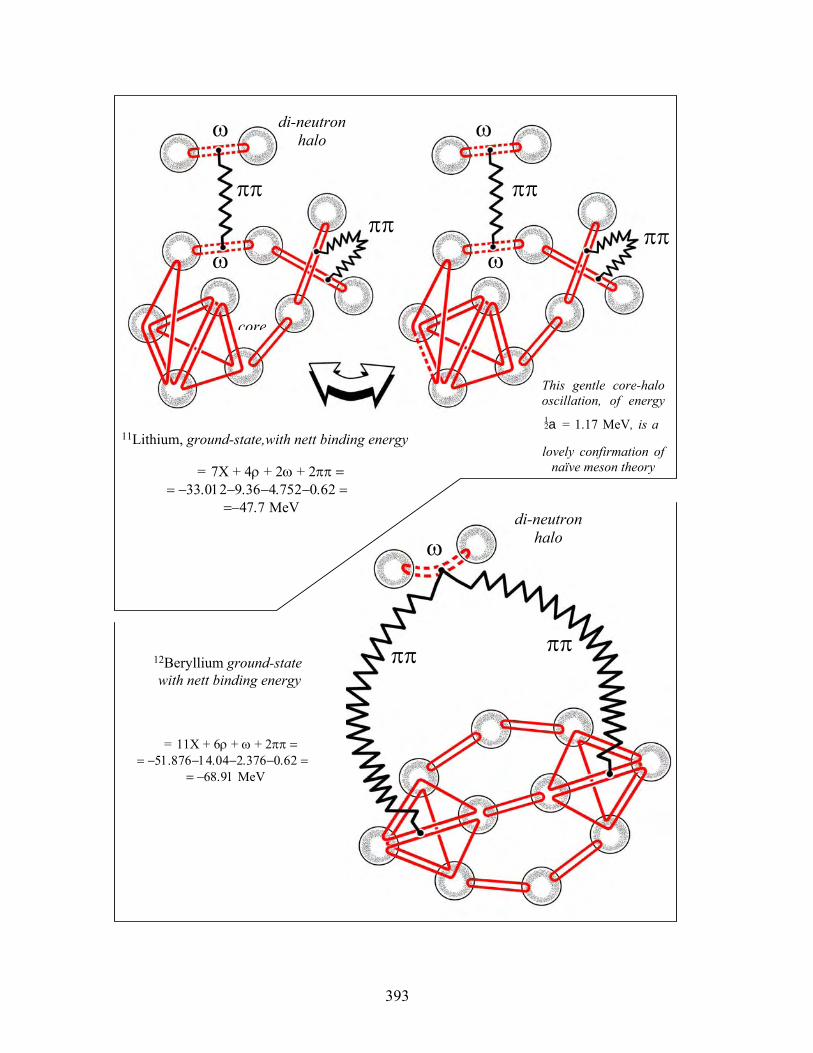
11Lithium, ground-state,with nett binding energy
= 7X + 4ρ + 2ω + 2ππ = = −33.012−9.36−4.752−0.62 =
=−47.7 MeV
This gentle core-halo oscillation, of energy
@a = 1.17 MeV, is a
lovely confirmation of naïve meson theory
12Beryllium ground-state with nett binding energy
= 11X + 6ρ + ω + 2ππ = = −51.876−14.04−2.376−0.62 =
= −68.91 MeV
di-neutron halo
core
di-neutron halo
ππ ππ
ππ
ππ
ω
ω
ω
ω
ππ ππ
ω
393
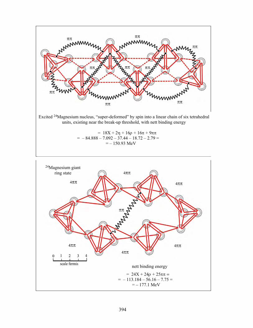
Excited
24 Magnesium nucleus, “super-deformed” by spin into a linear
chain of six tetrahedral units, existing near the break-up threshold, with nett binding energy
nett binding energy
= 24X + 24ρ + 25ππ = = – 113.184 – 56.16 – 7.75 =
= – 177.1 MeV
24Magnesium giant ring state
Excited 24Magnesium nucleus, “super-deformed” by spin into a linear chain of six tetrahedral units, existing near the break-up threshold, with nett binding energy
= 18X + 2η + 16ρ + 16π + 9ππ = – 84.888 – 7.092 – 37.44 – 18.72 – 2.79 =
= – 150.93 MeV
394
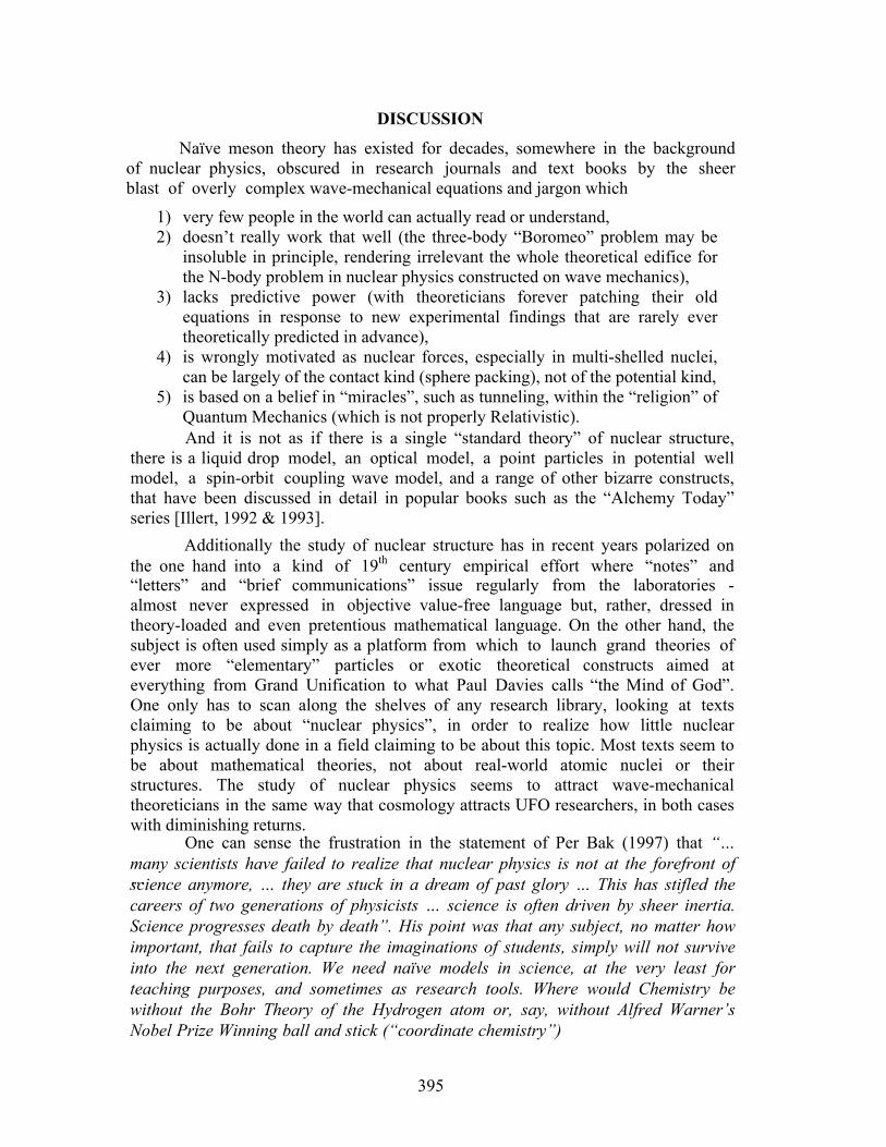
DISCUSSION
Naïve meson theory has existed for decades, somewhere in the background of nuclear physics, obscured in research journals and text books by the sheer blast of overly complex wave-mechanical equations and jargon which
1) very few people in the world can actually read or understand,2) doesn’t really work that well (the three-body “Boromeo” problem may be
insoluble in principle, rendering irrelevant the whole theoretical edifice forthe N-body problem in nuclear physics constructed on wave mechanics),
3) lacks predictive power (with theoreticians forever patching their oldequations in response to new experimental findings that are rarely evertheoretically predicted in advance),
4) is wrongly motivated as nuclear forces, especially in multi-shelled nuclei,can be largely of the contact kind (sphere packing), not of the potential kind,
5) is based on a belief in “miracles”, such as tunneling, within the “religion” ofQuantum Mechanics (which is not properly Relativistic).And it is not as if there is a single “standard theory” of nuclear structure,
there is a liquid drop model, an optical model, a point particles in potential well model, a spin-orbit coupling wave model, and a range of other bizarre constructs, that have been discussed in detail in popular books such as the “Alchemy Today” series [Illert, 1992 & 1993].
Additionally the study of nuclear structure has in recent years polarized on the one hand into a kind of 19th century empirical effort where “notes” and “letters” and “brief communications” issue regularly from the laboratories - almost never expressed in objective value-free language but, rather, dressed in theory-loaded and even pretentious mathematical language. On the other hand, the subject is often used simply as a platform from which to launch grand theories of ever more “elementary” particles or exotic theoretical constructs aimed at everything from Grand Unification to what Paul Davies calls “the Mind of God”. One only has to scan along the shelves of any research library, looking at texts claiming to be about “nuclear physics”, in order to realize how little nuclear physics is actually done in a field claiming to be about this topic. Most texts seem to be about mathematical theories, not about real-world atomic nuclei or their structures. The study of nuclear physics seems to attract wave-mechanical theoreticians in the same way that cosmology attracts UFO researchers, in both cases with diminishing returns.
One can sense the frustration in the statement of Per Bak (1997) that “… many scientists have failed to realize that nuclear physics is not at the forefront of science anymore, … they are stuck in a dream of past glory … This has stifled the careers of two generations of physicists … science is often driven by sheer inertia. Science progresses death by death”. His point was that any subject, no matter how important, that fails to capture the imaginations of students, simply will not survive into the next generation. We need naïve models in science, at the very least for teaching purposes, and sometimes as research tools. Where would Chemistry be without the Bohr Theory of the Hydrogen atom or, say, without Alfred Warner’s Nobel Prize Winning ball and stick (“coordinate chemistry”)
…
395
models of molecular structures (from a man who never published a single mathematical equation) ?
Naïve meson theory needs to be taken seriously and more broadly supported by theoreticians. It is, in fact, the only general theory capable of describing real-world nuclear states comprising N-bodies. And, in any case, it is important to resist the temptation to use overly complicated mathematical models when simple ones will suffice. This first paper has outlined the basics of nuclear bonding and structure, for halo and super-deformed states, explaining all that we need to initially know. And a second paper will follow in the next volume of Conference proceedings dealing with multi-shelled nuclei. However the basic theory needs to be polished, and a couple of immediate problems have been appended to this paper for the attention of Conference attendees. Perhaps there are other problems/solutions, associated with naïve meson theory, that you might think of and also like to comment about in the second volume of Conference Proceedings.
ACKNOWLEDGEMENTS
This paper is dedicated to HRH Prince Leonard 1, Principality of Hutt River, and has arisen out of a perceived need to teach nuclear physics to a new generation of students - any one of whom may solve the problem of worthwhile energy generation, from sustainable nuclear fusion, in the laboratory. As fossil fuels dwindle, and greenhouse pollution increases on a planetary scale, it may ultimately happen that the only hope for sustainably meeting humanity’s future energy requirements lies with the next generation of nuclear fusion scientists. I have been assisted in this task by Daniela Reverberi whose expertise with computers and software has been essential in the production of the many lovely current diagrams in this present paper, and the spectacular Bucky Balls in the following installment.
396
REFERENCES
[1] BAK, P. (1997), How Nature Works, the science of self-organised criticality, Oxford University Press, England. pp. 132-133. [2] BERTSCH, B.F., et al (March 1989), high-energy reaction cross sections of light nuclei,Physical Review C, vol. 39(3). pp. 1154-1157. [3] BROWN, B.A., et al (1984), Systematics of Nuclear RMS charge radii, J. Physics G (Nucl. Phys.), vol. 10: pp. 1683-1701. [4] COUGHLAN G.D., & DODD, J.E. (1984/1991), the Ideas of Particle Physics, Cambridge University Press, England. [5] EMSLEY, J., (1989), the Elements, Clarendon Press, Oxford, England. [6] FUKUDA, M., et al (1991), Neutron Halo in Beryllium 11 …, Phys. Lett. B, vol. 268: pp. 339-344. [7] ILLERT, C., (Luglio 1987), formulation and solution …, il Nuovo Cimento (series D), vol. 9(7): pp. 791-814. [8] ILLERT, C., (1992), Alchemy Today, volume 1, Platonic geometries in nuclear physics,Science Art Library, Wollongong, Australia. [9] ILLERT, C., (1993), Alchemy Today, volume 2, a beginners guide to hadronic circuit diagrams, Science Art Library, Wollongong, Australia. [10] ILLERT, C., (2003), Essays on the Structure of Atomic Nuclei, from a Newtonian perspective, Wollongong, Australia. [11] LAURENT, J., (Oct 1994), review of Alchemy Today vol. 1, Chemeda (Aust. J. Chem. Ed. RACI), vol. 41, p. 32. [12] LAPUSZYNSKI, V., (1995), review of Alchemy Today vol 2, Cold Fusion, vol. 8, pp. 1-4. [13] LEIGHTON, R.B., (1958), Principles of Modern Physics, McGraw Hill Publishing Co., USA. Data Tables in Appendix G, pp. 736-783. [14] NAMBU, Y., (1981), Quarks, frontiers in Elementary Particle Physics, World Scientific Publishing Co., Singapore. [15] REVERBERI, D., (Sept 1985), clockspring model …, Zeitschrift fur angewandte Mathematik und Physik (ZAMP), vol. 36(5): pp. 743-756. [16] TANIHATA, I., (1991), structure of Neutron-rich Nuclei studied by radioactive beams, Nuclear Physics A, vol. 522: pp. 275c-292c. [17] TANIHATA, I., (Oct 1985), Measurements of … radii of He isotopes, Physics Letters B, vol. 160(6): pp. 380-384. [18] WAPSTRA, A.H., & BOS, K., (May/June 1976), a 1975 midstream atomic mass evaluation, Atomic data and Nuclear Data Tables, vol. 17(5/6): pp. 474-490.
397
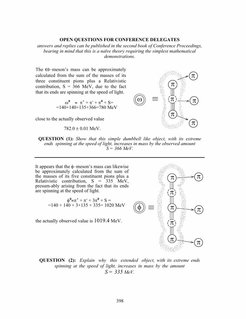
OPEN QUESTIONS FOR CONFERENCE DELEGATESanswers and replies can be published in the second book of Conference Proceedings,
bearing in mind that this is a naïve theory requiring the simplest mathematical demonstrations.
The ω–meson’s mass can be approximatelycalculated from the sum of the masses of its three constituent pions plus a Relativistic contribution, S = 366 MeV, due to the fact that its ends are spinning at the speed of light.
ω0 ≈ π+ + π- + π0 + S==140+140+135+366=780 MeV
close to the actually observed value
782.0 ± 0.01 MeV.
QUESTION (1): Show that this simple dumbbell like object, with its extreme ends spinning at the speed of light, increases in mass by the observed amount
S = 366 MeV.
It appears that the φ–meson’s mass can likewise be approximately calculated from the sum of the masses of its five constituent pions plus a Relativistic contribution, S = 335 MeV, presum-ably arising from the fact that its ends are spinning at the speed of light.
φ0≈π+ + π- + 3π0 + S = =140 + 140 + 3×135 + 335= 1020 MeV
the actually observed value is 1019.4 MeV.
QUESTION (2): Explain why this extended object, with its extreme ends spinning at the speed of light, increases in mass by the amount
S = 335 MeV.
398
399
PERTURBATIONS AND CONSERVATION LAWS FOR THEM ON ARBITRARY VACUUM BACKGROUNDS IN METRIC THEORIES OF
GRAVITY
A.N.Petrov
Sternberg Astronomical instiyute, Universitetskii pr., 13, 119992 Moscow, Russia; [email protected]
In two last decades, numerous multidimensional generalizations of general relativity (GR) are developed very intensively. Definitions and interpretation of conserved quantities for perturbations in such theories acquire an important significance. In the framework of the
D-dimensional metric theories (D > 4), including Lovelock and Einstein-Gauss-Bonnet (EGB) gravity we construct covariant conserved quantities for perturbations on a background of arbitrary curved vacuum solutions of this theory. The construction is carried out in three independent directions, which have been well developed in the framework of the usual
4-dimensional GR. The first one has an origin in the Weinberg construction generalized by Abbott and Deser [1]; Grishchuk, Petrov and Popova [2]; Deser and Dekin [3]; Petrov [4]. The second takes the beginning from the Einstein and von Freud canonical approach generalized by Katz, Bicak and Lynden-Bell [5]. The third develops the Belinfante method adopted by Papapetrou to GR and generalized later by Petrov and Katz [6]. The formulae obtained by an each of the three above methods are tested to calculate the mass of the Schwarzschild-anti-de Sitter (S-AdS) black hole solution in the EGB gravity in two cases as follows. The first case is when a background is chosen as a non-degenerated AdS solution for D > 4; the second one corresponds to a vacuum background chosen as “mass gap”, which is a basic (null mass) state for the 5-dimensional S-AdS black hole in EGB gravity and which (unlike AdS) is not a spacetime of the maximum symmetry. All the three approaches give the same results in an each of these two cases, which are also in a convenience with known results other authors. Degenerated AdS backgrounds in EGB gravity are discussed.
Keywords: gravity, d-dimensional metric theories, general relativity, Weinberg construction, Einstein and von Freud canonical approach, the Belinfante method.
PACS number: 04.20.-q/04.20.Gz
REFERENCES [1] Abbott L F and Deser S, Nucl. Phys. B, 195, 76 (1982) [2] Grishchuk L P, Petrov A N and Popova A D, Commun. Math. Phys., 94, 379 (1984) [3] Deser S and Tekin B, Phys. Rev. D, 67, 084009 (2003); hep-th/0212292 [4] Petrov A N, Class. Quantum Grav., 22, L83 (2005); gr-qc/0504058 [5] Katz J, Bicak J and Lynden-Bell D, Phys. Rev. D, 55, 5957 (1997); gr-qc/0504041 [6] Petrov A N and Katz J, Proc. R. Soc. A, 458, 319 (2002); gr-qc/9911025
400
TWIN PARADOX OF SPECIAL RELATIVITY
Sankar Hajra
Calcutta Philosophical Forum Salt Lake, AC-54, Sector-1, Flat No.A1, Kolkata-700064, India
E-mail: [email protected]
Lorentz Transformation Equations (LTE) predict that if an electric dipole stationary in the free space oscillates n times/sec, then the same dipole must oscillate
22 /1 cun −× times/sec when it moves with a velocity u in that space. Curiously, the same equations also predict that even if the dipole is at rest in the free space and the measuring apparatus moves with the same opposite velocity, then too, the apparatus will record that the dipole is oscillating 22 /1 cun −× times/sec. Classical physics does not accept it. In fact, LTE themselves are not at all acceptable from the consideration of classical physics (as real physical equations).
Keywords: special relativity, Lorentz Transformation Equations, dipoles, Doppler’s effect.
PACS number: 03.30.+p
Albert Einstein has accepted LTE and, thereby, has tried to justify the reality of the LTE by his well known principles (assumptions) which constitute the Special Theory of Relativity (STR). Instead of classical time independent of co-ordinates, it uses relative time as a function of co-ordinates and imports equivalent observers to make the frequency-shift phenomenon (derived from LTE in both ways) intelligible from its novel setting.
Abolition of both the preferential observer in free space and classical absolute time makes much difficulty to settle the real time in the clock of each equivalent observer. The constancy of the speed of light to all equivalent observers further complicates the situation.
Though overlooked, relative time, in spite of its supposed good health, struggles hard, just from its birth, to breath at the cruel noose of many an alien unintelligible concepts in spite of palliative measure (of symmetry) adopted by its originator. This is evident in twin paradox. The difficulty arises not from the management of time artificially by its originator; it originates from the absurd assumption of Einstein that all four Lorentz transformation Equations are real.
The paradox centers on the problem of time in case when a man and his twin have a steady relative motion. From the consideration of STR, each twin would claim that the other’s clock runs slow compared to the synchronized clock in his own frame. Such a decision of relativity arouses suspicion. Now, when relativists try hard with sheer pedagogy to justify such a decision and, when the originator of STR makes another theory to resolute the paradox to his own satisfaction, the suspicion grows strong.
Some people [1] suggest that the resolution of twin paradox as presented by the relativists is devoid of any rationality. They are in favor of the rejection of STR
Some relativists [2] has countered the above consideration from the consideration of STR. But, unfortunately, they have evaded the central question relating to the problem.
401
However, we may clarify here the central question of twin paradox in the following simple examples:
(a) The theory of relativity predicts that the life-span of radioactive particles increases with velocity which has been verified by experiments when the observer with his measuring apparatus is at rest on the surface of the earth and the radioactive particles moves with respect to it. To establish the validity of the theory of relativity, it is the burden of the relativists to show that similar results are confirmed by experiments when the radioactive particles are stationary on earth while the observer with his measuring apparatus steadily moves in the opposite direction on it. In the absence of such a clear-cut experiment, relativists’ analysis is meaningless.
(b) Similarly, STR predicts transverse Doppler Effect (time dilation effect) for steadily moving radiating dipoles which has been verified by experiments when the observer with his measuring apparatus is at rest on the surface of the earth and the radiating dipoles move transversely to the observer. To establish the validity of STR, similar results should be confirmed by experiments when the radiating dipoles are at rest on earth while the observer with his measuring apparatus moves steadily in the opposite direction on this planet. Relativists should agree with us that any experiment with latest techniques will
not detect any of the phenomena (like time-dilation / transverse Doppler’s effect) when the radiating dipoles are at rest on earth while the observer with his measuring apparatus moves steadily in the opposite direction, as our classical theory predicts. And they should admit that physics should be based on available experimental data and not on data which could never be verified, nor on data which are expected to be verified later. Unfortunately, relativists are innocently oblivious of these situations. Their ‘consistent’ phantom world has in no way been proved to be the real world. Therefore, their discussion is a matter of philosophy, but not of physics.
Moreover, it is really shocking that relativists are not at all aware and do not like to be aware that their favorite ‘time –dilation’ could easily be explained from classical electrodynamics. However, in that case, the confusing time-dilation of the relativists has been replaced by the natural increment of the period of an electromagnetic event due to motion, time remaining the same to all observers as per classical physics. The gist of this explanation is given below:
When a radiating electric dipole moves steadily on earth, the electric and the induced magnetic fields inside the dipole change as per the classical electrodynamics of Heaviside, and, thereby, all electrodynamic phenomena inside the steadily moving dipole, too, change, which at once destroys relativistic time-dilation concept. The classical treatment in brief is as follows:-
Heaviside [3] deduced classically the electric field (E) and the induced magnetic field (B*) of a steadily moving point charge (Q ) with a velocity u in the free space at a point P ),,( φθr in spherical polar coordinate where r is the distance from the origin as under.
( )[ ] 2/322230
2
sin/14 θπε curQk
−= rE , ( 22 /1 cuk −= ) (1)
!!!B* =u!× !E/c2 (2)
where 0ε and 0µ are the permittivity and permeability of free space, and 00/1 εµ=c .
402
Relativists should note that the vital Equations (1) and (2) were deduced first not by Albert Einstein from relativity as often tacitly claimed, but by Heaviside from the consideration of classical physics in 1888. The Magnitude of Electromagnetic momentum of a steadily moving point charge could be written from Searle (1897) [4] from the consideration of classical electrodynamics as
uTP /2= )6/( 20
2 RkcuQ δπε= [5] (3)
(T is the magnetic energy, Rδ is the radius of the point charge, the direction of momentum being the direction of the velocity of the charge.)
Electromagnetic force acting on a point charge moving steadily in free space at a direction perpendicular to the direction of the uniform electric field operating in free space.
⊥⊥⊥ == akmauPF )/()||/||( 0 ⊥= am0γ [ 02
02 )6/( mRcQ =δπε , k/1=γ ]= m ⊥a
(4)
( ⊥a , being the acceleration of the point charge in the direction perpendicular tou ) which implies from the consideration of classical electrodynamics that transverse electromagnetic mass of charges vary with velocity.
However, all those deductions were based on the experiments made on the surface of the earth and extended to free space which may induce some confusion at this stage of discussion. To avoid any confusion, we may say that in true sense, these deductions are applicable on the surface of the moving earth and the high translational motion of this planet with respect to the sun has no effect on those formulations.
Now, using the above four equations, we shall prove the velocity-dependence of frequency and period of oscillations of an electric dipole classically, for which relativists have burdened their theory with complicated ideas unnecessarily. Let an electric force (originating from a small charge) drive a point charge back and forth from one end to the other end of a radiating dipole stationary on the surface of the earth . Then from classical electrodynamics,
SF 2000 ωm−= (5)
when the velocity of oscillation is small ( 0m is the electromagnetic mass of the charge in the stationary dipole, 0ω is the radian frequency of oscillation of the charge, is the separating distance of the dipole).
Now, if the dipole moves with a velocity u on earth in any direction perpendicular to its direction of oscillations, the electric force and the magnetic force acting on the charge will be respectively from Eqs. (1) and (2), (when 900) and - . Therefore, total electromagnetic force acting on the moving charge is
!!!F = γ F0 !−(u2 /c2)γ F0 = F0k (6)
Now, under the circumstance that the dipole moves on earth and radiates, we have from the consideration of classical electrodynamics,
403
SF 2ωm−= (7)
where m ( mkm =/0 ) is the electromagnetic mass of the charge in the moving dipole, ω is the frequency of oscillation of the charge which is moving with a velocity u on earth with the dipole, and is the electromagnetic force acting on the moving charge.
From Eqs. (4), (5), (6) and (7) for the dipole moving with an uniform velocity on earth in any direction perpendicular to its direction of oscillation we have,
k0ωω = (8)
This explains transverse Doppler’s effect from classical physics. For a dipole stationary on earth,
00 /2 ωπ=t (9)
where 0t is the period of oscillation and 0ω is the radian frequency. If the same radiating dipole moves with a velocity u on earth, then for the moving dipole, the period of oscillation t and radian frequency ω satisfy
ωπ /2=t (10)
Comparing Eqs. (9) and (10) with the Eq. (8) we have,
0tt γ= (11)
The equations (8) shows frequency of oscillation of the moving dipole decreases and the equation (11) shows that the period of oscillation of a moving electric dipole increases with its velocity on earth.
This at once destroys ‘here is one time’, ‘there is another time’-concept as well as the twin paradox of relativity.
However, in this classical approach, there will be no transverse Doppler’s effect when the radiating dipole is at rest on earth while the observer with his measuring apparatus moves transversely to the dipole in the opposite direction.
Now, if transverse Doppler’s effect is proved in the case cited in the previous paragraph, relativists with their confusing time-dilation concept may insist on continuing such unending metaphysical discussions on the resolution of the paradox. Otherwise, such an analysis as in [2] seems to be some pedagogical relativistic nonsense.
( )∫ ×=spaceall
dv*BDP and dvBc
Tspaceall
22
0 *2 ∫=
ε
where *BD,P, are electromagnetic momentum, electric induction vector and induced magnetic field vector respectively, T = magnetic energy of a steadily moving system of charges and dv is the infinitesimal volume element in the free space.
Using 2/ cE)(uB* ×= we have,
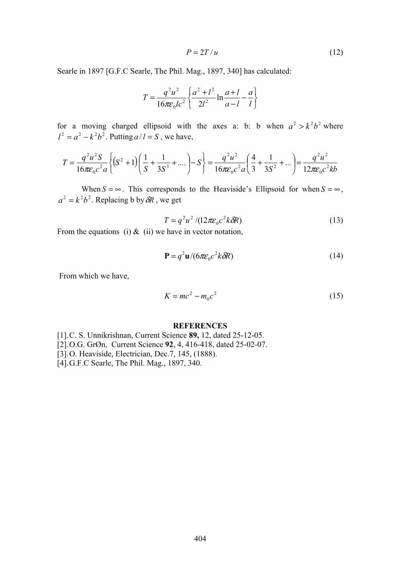
404
uTP /2= (12)
Searle in 1897 [G.F.C Searle, The Phil. Mag., 1897, 340] has calculated:
⎭⎬⎫
⎩⎨⎧
−−++=
la
lala
lla
lcuqT ln
216 2
22
20
22
πε
for a moving charged ellipsoid with the axes a: b: b when 222 bka > where 2222 bkal −= . Putting Sla =/ , we have,
( )⎭⎬⎫
⎩⎨⎧ −⎟
⎠⎞⎜
⎝⎛ +++= S
SSS
acSuqT ....
3111
16 32
20
22
πε kbcuq
Sacuq
20
22
220
22
12...
31
34
16 πεπε=⎟
⎠⎞⎜
⎝⎛ ++=
When ∞=S . This corresponds to the Heaviside’s Ellipsoid for when ∞=S , 222 bka = . Replacing b by Rδ , we get
)12/( 20
22 RkcuqT δπε= (13)
From the equations (i) & (ii) we have in vector notation,
)6/( 20
2 Rkcq δπεuP = (14)
From which we have,
20
2 cmmcK −= (15)
REFERENCES [1]. C. S. Unnikrishnan, Current Science 89, 12, dated 25-12-05. [2]. O.G. GrØn, Current Science 92, 4, 416-418, dated 25-02-07. [3]. O. Heaviside, Electrician, Dec.7, 145, (1888). [4]. G.F.C Searle, The Phil. Mag., 1897, 340.
405
RELATIVITY IN TERMS OF MEASUREMENT AND ETHER LAJOS JÁNOSSSY’S ETHER-BASED REFORMULATION OF
RELATIVITY THEORY
László Székely
Institute for Philosophical Research of the Hungarian Academy of Sciences
Postal address: HU-1398 Budapest, Post Box: 594 [email protected]
In his monograph Theory of Relativity Based on Physical Reality, Hungarian physicist Lajos Jánossy develops the complete Einsteinian formalism of relativity theory by analysing the process of measurement, the systems of measures created in this process and experimental data expressed in terms of measures. He demonstrates that based on a simple principle (which he calls the Lorentz principle) and its generalization the whole formalism of the original theory may be developed in conformity with the notions of common sense without mathematizing physical reality, so that the new way of development is of the same heuristic power as the original one. His analysis makes it clear that the allegedly revolutionary new notions of space and time follows not from physical experiences but from Einstein’s positivist philosophical commitments. Having established the place and role of a privileged (but not absolute) reference system, at the second level of his theory Jánossy connects this system to the carrier of electromagnetic phenomena which he also assumes to be the carrier of the gravitational and other physical fields. Although he uses the term ‘ether’, he explicitly rejects the old theories of this entity and attributes to it dynamic properties. In the last section of the paper Einstein’s and Jánossy’s ether concepts are compared and it is argued that despite the parallelism between the two concepts, from Jánossy’s point of view Einstein’s ether is too mathematical to cure the inverted relation between mathematics and physics characteristic for Einstein’s relativity.
Keywords: relativity, ether, propagation of light, privileged reference system, space-time, measurement, ideal solid rod, ideal clock, common sense in physics, mathematics in physics, physical reality, Einstein, Lorentz, Jánossy.
PACS number: 03.30.+p
I. INTRODUCTION In Physical Relativity, a monograph published by Clarendon Press in 2005,
Harvey Brown criticizes the received view of Einstein’s theory and argues for a physical interpretation of relativistic phenomena. [Brown 2005] Both Brown’s book and the regular conferences on the interpretations of relativity theory organized by Michel Duffy [Duffy 1988, 1990 ….2006] clearly indicate that the long tradition of considering the original, Einsteinian-Minkowskian notion of relativity theory too mathematical and claiming that it blurs (or even turns into its opposite) the epistemological relation between mathematics and physics is alive even today, more then 100 years after Einstein’s famous paper.
In the introduction to his book Brown mentions the Hungarian physicist Lajos Jánossy as one of his forerunners inspiring his ideas. [Brown 2005, vii.] Jánossy was an important figure in the tradition of alternative interpretations of Einstein’s theory, who
406
(following Lorentz’s ideas) elaborated a comprehensive alternative (“physical”) relativity. He, along with American Herbert Ives (who belonged to a former generation of physicists) and Prokhovnik (a contemporary of Jánossy) may be considered as one of the classics of the field. However, while on the basis of personal communications it seems that his work on relativity theory was well known by those who did research in the topic in the last decades, he (in contrast with Ives and Prokhovnik) is only rarely cited in the literature. (M. Duffy mentions Jánossy’s work in his recent paper [Duffy 2008] and Bell in his famous study How Teach Relativity? also expresses his appreciation for Jánossy’s contribution to the topic [Bell 1976].)
The aim of this paper is to give a brief review of Jánossy’s reformulation of relativity theory, which deserves more recognition than it has received until now.
II. LAJOS JÁNOSSY’S CAREERLajos Jánossy was born in Mátyásföld (then a village near Budapest, now part of
the Hungarian capital) in 1912. His father Imre Jánossy was an astronomer who died relatively young in 1920. After the death of her husband, his mother, Gertrud Borstrieber (a mathematician belonging to the first generation of Hungarian women with a university degree) married the Hungarian philosopher George Lukács, who was considered by the French philosopher Lucian Goldman the first representative of the existentialist philosophy, but who later gave up his youthful enthusiasm for Kierkegaard and became a famous and highly controversial Marxist philosopher of the 20th century, oscillating permanently between communist movement discipline and sovereign philosophical thought and causing many a disturbance for the party leadership. After the fall of the Hungarian Soviet Republic in 1919 Lajos Jánossy’s family moved to Austria and later to Berlin. Instead of following his stepfather in politics or philosophy, Jánossy became a physicist. He studies physics at the Humbold University in Berlin where he was a student of Edwin Schrödinger whose metatheoretical considerations on physics had a determinative influence on him. In the 1930s Jánossy became also a university professor and read physics (and especially relativity theory) at Manchester University (while his stepfather left Hitler’s Berlin for Stalin’s Moscow and lived there with his political and moral compromises). His main research field being cosmic radiations, he became an internationally respected scientist in the field, and his monograph on the topic belongs to the basic literature on the subject [Jánossy 1948, 1950].
After Word War Two George Lukács returned to Hungary and in 1950 Lajos Jánossy (then a professor at the Institute for Advanced Studies in Dublin and a colleague of his former professor, Schrödinger) followed him. While his stepfather was never a “pet” (or with the good German word a “Liebling”) of the communist party, party leaders needed his international respect, as well as Lajos Jánossy’s scientific knowledge. So the latter became head of the Central Institute for Physical Research, a grand new research institute established on a Soviet model.
It is generally held that Einstein’s theory of relativity was deemed by the official Soviet ideologists as a bourgeois theory, so Jánossy’s criticism of the Einsteinian notion of relativity may appear in this context as a version of the Soviet criticism of the theory, but it is not the case.
On the one hand, although several attempts were made in the Soviet Union to discredit relativity theory as a prototype of false, idealistic physics, and at the turn of the forties to the fifties of the last century a fierce campaign was waged against the theory, the attempts never resulted in its official denunciation. On the contrary, after the death of Stalin, Einstein‘s Soviet followers won the debate and Einstein’s theory came to be
407
glorified as a true dialectical theory, which as such fully corresponds to Marxism-Leninism. [See e.g. Graham 1972, 111-138; Székely 1987]
On the other hand, and quite importantly, Lajos Jánossy had never taken part in the antirelativistic campaign. The greater part of his critical considerations on relativity theory was published in a period when official Soviet ideology endorsed Einstein. Hence, beside the criticism his concept received from orthodox Einsteinian physicists, Jánossy’s notion of the relativity theory also became a target of official philosophers of the Soviet block. Although the Hungarian Academy Press undertook the publication of his comprehensive work „Theory of Relativity Based on Physical Reality” [Jánossy 1971], in his last years he was considered by the orthodox Einsteinian physicists who were then dominating the Hungarian physics scene as an anti-relativist dinosaur and (while formally preserving his university position) he was gradually displaced from Hungarian scientific life. He died in 1978.
Whereas the ideological, political and sociological contexts of Lajos Jánossy’s scientific work would also offer interesting topics, this contribution will be restricted to reviewing his concept of the theory of relativity only from the point of view of physics and the philosophy of science.
III. THE METATHEORETICAL FOUNDATIONIII. A. The relation between mathematics and physics and the norm of
common sense As indicated in the title of his monograph, Lajos Jánossy characterizes his notion
of relativity theory as a theory based on physical reality. This title expresses both a critical and a confirmative aspect. On the one hand, Jánossy argues that the Einsteinian theory is not based on physical reality: while it is an effective mathematical tool for handling the results of measurements and for making predictions, it does not provide an appropriate theory of physical reality. On the other hand, he affirms that the mathematical formulas of Einstein’s theory are correct in the sense that they are in correspondence with observation and empirical data and are able to give correct predictions about the behaviour of physical reality.
Of course, Jánossy sees clearly that what Einstein offers us is not only mere mathematics but a definite physical theory. He insists, however, that Einstein turns the relation between mathematics and physics into its opposite: in his view the German physicist projects mathematical formulae into the physical world and in this way constructs physical reality by hypostatisation of mathematical ideas. Consequently in the context of his criticism the so called “spatialization of physics” which is often praised as a great achievement of relativity theory appears as a result of hypostatisation and Jánossy focuses his criticism on this element of the theory:
“The theory of relativity in its original formulation is certainly not a mere attempt to describe phenomena by suitable mathematical expressions – the theory is a far reaching attempt to give a theory of space and time. Our criticism of the theory is just connected with this latter feature. We think that the theory reflects correctly certain general physical laws, but these laws – in our opinion – have nothing to do with the “general structure of space and time”. Therefore our attempt is to give a physical interpretation of relativistic formulae, which is different from old one.” [Jánossy 1971, 13]
But how do we know that the view Einstein offers of the physical world is inappropriate? An incorrect methodology does not necessarily imply the incorrectness of the theory. Does the theory have any independent, non-methodological features which might make it problematic?
408
In answering this question, Lajos Jánossy represents a view which is typical in the criticism of Einstein’s relativity and which can be characterized as “common sense criticism”.
“I got acquainted with the theory of relativity at a comparatively early age – I read the famous popular book written by Einstein. Reading the latter I had difficulties with some of Einstein’s concepts: however, having been young and enthusiastic, I convinced myself in the end that I could understand those concepts – to prove this I tried to explain the theory to everybody who was interested. In the course of such attempts I learned the ‘language of relativity’ and I gradually ‘got used’ to the theory.
…. Many years later I read several years in succession a course of physics at the university of Manchester. My course contained also the special theory of relativity. As the years went on I developed a technique of presenting the subject so that in the end I could convince my students that they really understood the theory. However, as my technique presenting the theory improved, my own belief in the adequateness of the concepts vanished. In the end I became convinced that from the philosophical point of view the concepts had to be changed. Since about 1950 I have struggled with the problem of the reformulation of the theory and the results of my deliberations are found in this volume.” [Jánossy 1971, 14]
As Descartes’s narrative about his schools and education in his Discours de la Methode (Discourse on the Method) expresses a radical criticism of the philosophical views of the epoch and his personal style functions as endorsement and authentication of the criticism, here, in Jánossy’s reminiscence we also encounter a radical philosophical criticism. Jánossy challenges the generally received view that relativity theory requires us to give up our common sense terms. We should not be mislead, he argues, but recognize that there is really something disturbing in Einstein’s theory and the correct attitude is not to suppress this disturbing factor by blaming our common sense for incapacity to grasp physical reality but to face and eliminate it by reformulating the theory.
In other writings he is more sanguine and characterizes the received attitude of modern physics to common sense as a cult of irrationality, in the context of which contradiction with common sense becomes a virtue and the scientific character of a theoretical claim is measured by the extent of its absurdity. Rejecting this approach, he insists that “[a] scientific way of thinking cannot be but the refinement, deepening and further development of everyday thought” and that “the whole complex of the theory of relativity can be built up by means of natural methods in conformity with everyday thought”. [Jánossy and Elek 1963, 9, the original is in Hungarian] (Jánossy, influenced by the philosophy of his stepfather, prefers the term “everyday thought” to “common sense” but in his argument the former functionally corresponds to the latter.)
To summarize, the metatheoretical foundation of the criticism and reformulation of relativity theory by Jánossy consists of two interlaced moments, namely, the priority of physics regarding the mathematical formalism and the conscious acceptance of the terms of common sense as a norm for theory construction. Whereas these moments are common to criticisms of Einstein’s theory, the metatheoretical foundation of the criticism is only seldom formulated so explicitly and definitely as in his case, and this is especially true regarding the role of common sense. The requirement of conformity with the basic notions of common sense as a norm for theory construction emphasized so resolutely by Jánossy may be regarded as Jánossy’s thesis and considered as one of the most important metatheoretical theses concerning modern physics. [Székely 1987; Székely 1988]
409
III. B. Measures, measurement and relativity theoryMetatheoretical norms and principles, however excellent, cannot have any
significance if one cannot find the way of their correct application in concrete theories. Jánossy’s main achievement regarding relativity theory is not simply the formulation of the metatheoretical foundation of the criticism but a complete and consistent reformulation of the theory in physical and mathematical terms.
In the following parts of our paper Jánossy’s version of relativity theory will be often contrasted with the Einsteinian one. To avoid misunderstandings, it is important to emphasize that in doing so we will always use the terms „Einstein’s theory” or “Einsteinian relativity” in the sense of the version of the theory as it was presented in Einstein’s original (physical) papers and as it is generally taught at universities and presented in textbooks. That is, in our usage the term „Einstein’s theory” will not include any of the metatheoretical and physical reflections made by the German physicist after the publication of the theory. The relation of Jánossy’s notion of relativity theory to Einstein’s subsequent, out-of-theory reflections (which cast a new light on his original formulation of the theory and leave room for a reading which might suggest its reformulation in the direction represented by Jánossy) will be considered at the end of this paper.
As a consequence of the heated ideological debates, late in his scientific career Jánossy abandoned philosophical categories regarding relativity theory. Thus in his comprehensive monograph “Theory of Relativity Based on Physical Relativity” published in 1971 we cannot find even such ideologically neutral categories as “common sense” or “everyday thought”. Instead of using philosophical categories he identifies the indicated disturbing aspect of Einstein’s theory in terms of measurement theory. According to him,
“ [i]n our approach of physics in general and the theory of relativity in particular we think it very important always to remember that we are dealing with objective physical quantities and that we attempt to describe the latter in terms of measures.” [Jánossy 1971, 15]
Furthermore, “ [a]n objective physical process develops according to its own laws and it can
be described in arbitrary measures.” [Jánossy 1971, 14] Distinguishing measures from things measured, Jánossy definitely commits
himself to the traditional concept of physical reality, according to which there exists something „out there” with its own laws and thus he rejects the positivist approach. But emphasizing the arbitrariness of the measures used by physics, he also opposes naive, metaphysical realism which maintains that the investigated objects and the theoretical entities directly correspond to each other (or – in a weaker version – considers the latter the approximations or conceptual pictures of the formers). In his concept physical quantities as characteristics of physical entities are outside of physical theories, while measures (and theoretical construction, so coordinate systems built up of these measures) are the representations of these quantities which physicists can chose arbitrarily. [Jánossy 1971, 72]
Consequently, in Jánossy’s interpretation space and time coordinates, as well as their transformations lose the mystical character conferred them by relativity theory:
“We may write x=r,t for a four-coordinate of an event. Changing from one system of reference to another we can introduce transformed coordinates x’=f(x) (1) where f(x) is some reversible four-function of its variable x. If the coordinates x are suitable to describe events, then the transformed coordinates are also suitable. Introducing particular measures x or x’ for events we give some kind of names to the
410
events with the help of which we recognize them. … The fact that a transformation type (1) mixes the measures of time and space coordinates does not seem to be of particular importance and it does not imply any properties of space and time.” [Jánossy 1971, 14]
This view of physical quantities and their measures is open to contention. However, it is based on acceptable and justified metatheoretical postulates well established in the history of physics which may serve as a foundation for physical theories. Furthermore, it is clear that these postulates contradict the Machian-positivist philosophical background of Einstein’s notion of relativity and thus their definite formulation by Jánossy makes it evident that that notion is not neutral from the point of view of physics: it does not follow from the nature of the physical world but rather is a consequence of Einstein’s metatheoretical commitments.
But if measures are only names or signs arbitrarily chosen by physicists, how is it possible to know anything about physical reality that is supposed to exist outside physics, a system of human theories?
Lajos Jánossy answers this problem by introducing the concept of distinguished measures. While a physical quantity can be described by an infinite number of systems of measures, the majority of the possible descriptions do not contain any information about the quantity in question. Distinguished measures are particular classes of measures which “reflect clearly certain properties of quantities” [Jánossy 1971, 72]. Therefore, one of the most important tasks of theoretical research is to find distinguished measures for the quantities under scrutiny, that is, to attempt to find for the description of particular quantities numbers which reflect adequately certain physical properties. [ibid.]
To elucidate the concept in more detail, in Chapter III of his monograph Jánossy analyses the measurement of electric charges and then (taking into account that relativity theory is strongly connected to the so called space and time coordinates) in Chapter IV he works out distinguished measures for space and time. According to his analysis distinguished measures are characterized by the fact that in general both their sum and product (or in certain special cases at least their sum) express significant physical quantities, that is, their sum and product also appear in our measurements and/or in the established physical laws. For example, the sum of the usual measures of two electric charges E1 and E2 (say measures e1 and e2) will be equal to the measure we receive measuring the joint charge, while the product of e1 and e2 appears in Columb’s Law. (In fact, Jánossy designates physical quantities with Gothic letters while their measures with Roman letters, so he designates a physical charge with a Gothic e while its measures with a Roman e. For technical reasons we do not follow his notation here.) A physicist used to the usual notation and language of physics may find this terminology rather curious, since physical texts do not usually distinguish the charge and its measure but designate both by the same symbol (say e). However, in the metatheoretical context established by Jánossy it is clear that the charges as objective physical entities do not determine directly the measures to be constructed in the process of measurement and hence it is not at all evident that the measure of joint charges should be the sum of the measures of the two original ones. In Jánossy’s words,
“[i]n practice there seems to be no point in introducing non-additive scales for quantities if there is a possibility of introducing also additive representations. It must be emphasized, however, that it is not trivial that for certain quantities additive measures can be introduced. Whether or not such measures can be introduced in a particular case is a question which can be decided experimentally….” [Jánossy 1971, 78]
Of course, the question of measurement is a very complex topic and in his monograph on relativity theory Jánossy could only briefly outline his respective ideas.
411
A more detailed presentation can be found in his earlier monograph Theory and Practice of Evaluation of Measurements which contains a comprehensive presentation of his theory of measurement. That book should be consulted by those interested in this aspect of Jánossy’s theory. [Jánossy 1965]
What follows is a brief sketch of Jánossy’s reformulation of relativity theory based on the metatheoretical commitments outlined above. We will attempt to reproduce the logic and the conceptual structure of his theory and will set aside the technical-mathematical details that are essentially the same as the well known textbook formulation of Maxwellian electrodynamics, the formulae of Lorentz transformation and the Einsteinian formalism of the special and general theory of relativity.
III. B. Measures and relativityIII. B. a. Measures of space and time based on rigid rods and physical laws.
The definition of ideal clocks. While in his famous paper Einstein firstly introduces a scale of length with the
help of rigid rods and then “defines time” (ie, in Jánossy’s terms, “introduces distinguished temporal measures“) with the help of clocks and light signals and so he establishes a “hybrid” scale of space and time, Jánossy separates the rigid rod method from the light signal method and introduces two independent systems of measures: one based on rigid rods, another on light signals.
As we have seen, for Jánossy it is not at all trivial that additive length measures can be introduced. The use of additive length scales in everyday practice is based on the fact that with the help of rods considered in every day life as “solid” additive length measures can be obtained. According to Jánossy, science can introduce the term of ideal solid rods only because we are given this experience and he defines a rod to be an ideal solid rod if with its help an additive scale of length can be obtained. [Jánossy 1971, 79]
On the other hand, Jánossy emphasizes that with the help of periodical processes (such as mechanical clocks, planetary motions etc) we can complete our system of length measures to set up a combined system of length and temporal measures in terms of which physical phenomena obey certain rules. As measures in general, temporal measures in particular can be obtained in several ways and there is no a priori guarantee that these ways will all result in the same measures (or that measures arrived at in different ways will coincide). However, considering that the aim of physics is to discover rules in the behaviour of the physical world and formulate them as physical laws, from the point of view of science it is rational to attempt to complete our length scale with a temporal scale in such a way that certain fundamental and in the practice well confirmed laws, for example, Newton’s first law be fulfilled.
At first sight, perhaps, this approach may seem to be logically circular, since physical rules may appear only if we have already a joint scale of length and time, while Jánossy want to complete the length scale with a temporal scale with the help of already known laws. Is this not a vicious circle?
Taking a closer look at the issue reveals that the approach is correct. In the history of physics we are given physical rules (for example, Newton’s first law) which seem to work if we use our everyday length and time measures or measures established in the history of physics. These rules appear in terms of measures, which are intuitive and without reflection (or are based on metaphysical commitments as for example in Newton’s case) and therefore it cannot be excluded that they are to a certain extent consequences of our choice of measures. To enlighten the nature of these rules we need an a priory analysis of the applied measures and in this analysis (while suspending the
412
validity of the concerned rules regarding physical reality) we may introduce a hypothetical world in which these rules are assumed to be fulfilled, and Jánossy follows this methodology.
Thus we may assume a region where Newton’s first law is valid in terms of a given (but yet unknown) system of measures. Provided that we already have a length scale, in such a region we no longer need Einstein’s radar method to synchronize clocks: it will suffice to observe the motion of free particles and to adjust the local measures of time showed on the local clocks in such a way that Newton’s first law be fulfilled. (To observe the path of a particle we need not use light signals: every observer can measure with the help of his own clock and make a note of the time when his own position is crossed by a moving particle and then the notes can be collected and analysed in order to synchronize the clocks.) Exploiting this a priory possibility, Jánossy introduces the term of „ideal clock”. According to his definition a clock is ideal when it gives immediately (without correction) the distinguished temporal measures based on Newton’s first law. [Jánossy 1971, 95-96] The rate of an ideal clock is by definition constant and our physical practice definitely shows that there are regions in the real world which allow us to introduce good approximations of a system of measures based on ideal solids and ideal clocks. (Otherwise Newton’s first law would not be applicable in practice.)
Similarly, we may introduce temporal measures using planetary motions or the rotation of the Earth around its axis and assuming the validity of the law of gravitation and it is also possible to use atoms as clocks and taking into account the physical theories of atoms. Of course, it is not evident that all these scales will correspond to the first, mechanical or ‘ideal’ temporal scale; neither is it evident that the non-mechanical (planetary, sideric or atomic) scales will be adjustable to each other. In this respect Jánossy’s definition of ideal clocks is a metatheoretical norm requesting a physical explanation in any case when an applied time scale deviates from the ideal one. (Incidentally, since Newton’s first law is deducible from Leibnitz’s principle of sufficient reason, Jánossy’s definition of ideal clocks may be deduced from this fundamental Leibnitzian thesis. On the other hand, it can be also shown that the Einsteinian version of special relativity does not fulfil the Leibnitzian principle. Thus Jánossy’s version of relativity theory - despite its empirical orientation - can be seen as a reformulation of the original Einsteinian theory, with the aim of satisfying Leibnitz’s principle. Furthermore, Jánossy’s method of definitions of ideal solid rods and ideal clocks, a beautiful example of the application of everyday experiences in physics, follows – unconsciously – the logic of the so called “hermeneutic circle” emphasized by Heideggers’ philosophy and indicates how promising a possible Heideggerian metatheory of physics may be.)
III. B. b. Measures by radar method without rodsJánossy also shows that it is possible to attempt to introduce length and time
scales using only light signals, provided that we assume that light is propagated isotropically and with a constant velocity relative to a given reference system, say K. It is clear that similarly to the rigid rod scale, we do not have any a priory guarantee of success in this case either. It is a matter of practice whether a coherent system of space and time coordinates can be constructed in such a way and if we succeed and a system of coordinates introduced by this method passes the test of coherence, then this fact „can be taken to support the hypothesis about the mode of propagation of light in K”. [Jánossy 1971, 99] The introduction of such a scale follows the same logic as the rod scale without the radar method: first an ideal region is assumed where light is
413
propagated isotropically and the measures are defined for this ideal region, then, as the second step, experience will show whether these measures can or cannot be applied in the real world.
IV. LORENTZ TRANSFORMATIONS AND JÁNOSSY’S THEOREMIV. A. Lorentz trasformations as transformations of measures
Applying the conceptual basis introduced above, Jánossy demonstrates that: if there is a system of coherent measures M of length and time in terms of which
light appears to be propagated isotropically and with the velocity c relative to a reference system S,
then there exists a group of mathematical transformations of that system of measures with the following characteristic:
- each members of the group transforms the system of measures M into another system of measures M’ in whose terms light appears to be propagated isotropically and with the velocity c relative to another reference system S’ which is in rectilinear and even motion relative to the original reference system S;
- vice versa, for any reference system S’ in rectilinear and even motion relative to the original reference system S there exist a member of the group of transformation above, which transforms the system of measures M into a system of measures M’ so that in the reference system S’ light will appear to be propagated isotropically in terms of M’. [Jánossy 1971, 100-105]
Anyone familiar with relativity theory will see that the group of transformations which Jánossy found is the well known group of the Lorentz transformations. That is, he did not discover transformation of a new kind but deduced the famous ones in a new way different from both the Einsteinian and the Lorentzian deductions. However, what is important for us is not simply the new deduction but the new meaning of the transformations. Whereas in Einstein Lorentz transformations are deduced as transformations which connects inertial reference systems so that Einstein’s two axioms be satisfied, in Jánossy they emerge in an investigation of the propagation of light in terms of various systems of measures without referring to the concept of inertia and their existence are stated in the form of an a piori, mathematical theorem.
We will refer to this theorem as “Jánossy’s theorem” and (following his terminology) call the reference systems relative to which light appears to be propagated isotropically in terms of a particular system of measures “Lorentz systems”. Notice, that Jánossy’s theorem is not about inertial systems: it is valid independently of whether Lorentz systems are inertial or not.
IV. B. The analysis of Jánossy’s theoremJánossy’s theorem imposes two a priory constraints upon physical reality. A) On the one hand, if rods and clocks are never deformed when in motion with
respect to any Lorentz system (that is they preserve their shape and pace), then 1. (on simple geometrical grounds) there will be only one Lorentz system in
which the system’s own Lorentz measures (that is, the measures in terms of which light appears to be propagated isotropically relative to the system) and measures based on rods and clocks without light signals will coincide; consequently
2. the relative velocity of any other Lorentz system with respect to thisspecial system will be determinable with the help of rods and clocks and light signals, since in terms of measures established with the help of these rods and clocks light will not appear to be propagated isotropically relative to these systems. (This simply follows from the fact that Lorentz measures are connected with Lorentz transformations which
414
change the measures of length and time, while the unchanged rods and clocks will establish the same system of measures independently of their motion relative to any Lorentz system.)
3. B) On the other hand, if we observe that Lorentz measures and measures based on rods and clocks co-moving with the systems will always coincide, then this observation will indicate that
4. there is a definite Lorentz system in physical reality which may be calledas the basic system, and
5. rods and clocks moving relatively to this basic system suffer deformationaccording to the formulae of the Lorentz transformations.
The observed relativistic effects (that is, the relativistic contraction of lengths and the slowing down of physical processes according to Lorentz’s formulae) show that in physical reality the second possibility is the case, thus on the basis of Jánossy’s theorem as an a priory theorem these effects necessarily imply the existence of a basic physical system in which rods and clocks at rest are not deformed, while in motion relative to this system they suffer deformation according to Lorentz’s formulae.
IV. C. The hidden epistemological and logical background of Einstein’sspecial theory
The a priory analysis of Jánossy’s theorem makes clear that Einstein’s special theory of relativity is based on two mathematical “boundary-conditions”. On the one hand, special relativity is only possible because Jánossy’s theorem is valid, that is, Lorentz transformations exist and they transform a system of measures in term of which light appears to be propagated isotropically into another system of measures with the same characteristic. On the other hand, the Einsteinian version of the theory, that is, the version in which – in contrast to the implication of Jánossy’s theorem –, the existence of any privileged systems is rejected, can only escape logical contradiction because Einstein implicitly rejects that the spatial relations of the physical entities of a given region form a definite, consistent spatial configuration.
To enlighten the latter moment of Einstein’s theory, let us recall that the claim about the isotropic propagation of light in any inertial system is perhaps the most paradoxical ingredient of the Einsteinian theory of special relativity. Namely, if a physical effect is propagated in a given reference system isotropically, then it cannot (on geometrical grounds) be propagated in a similar way in other systems moving rectilinearly and evenly with respect to the former. How is it possible that Einstein succeeded in working out a consistent theory incorporating this geometrically impossible characteristic of the propagation of light?
Jánossy’s theorem helps to explore the hidden conceptual background which makes possible for Einstein to avoid the contradiction.
Namely, geometry excludes the simultaneous isotropic propagation of light relative two different (physical) reference systems in motion at a constant velocity relative to each other only if the following two premises are fulfilled:
1. the space and time relations of the physical entities of the concernedregion define a common, definite space in which the investigated systems move
and 2. length and time are measured in both systems with the same measures.Consequently, we can construct a consistent physical theory in which light
appears to be propagated isotropocilly with respect to two different reference systems in motion relative to each other only if we reject at least one of these premises.
415
Now, Jánossy explains relativistic phenomena with the help of the assumption that rods and clocks in motion relative to the basic system are deformed according to Lorentz’s formulae. Consequently, in the case of two Lorentz systems in motion at different rate relative to the basic system these measuring tools will suffer different deformations and so the systems of measures introduced with their help will be also different. Thus in Jánossy’s conceptual framework it is premise ii) that is not fulfilled, and the function of the assumed deformations of rods and clocks are exactly to give an explanation of the change of measures that takes place despite the use of the same rods and clocks when we change the systems. Of course this explanation – as any Lorentzian kind approach – breaks the ontological symmetry of the relativistic effects: in its context the contraction of rods observed from a system moving faster relative to the basic system than the observed rods is only an apparent phenomenon since the latter suffer smaller contraction than the measuring rod of the observer and hence in reality they are longer than the observer’s rod.
Since Einstein’s theory excludes the existence of any basic system and assumes relativistic effects to be symmetric that does not allow to speak about real, physical deformations of measuring tools, his theory can be consistent only if the first premise is rejected. However, if we assume that physical entities are definite entities with definite spatial relations, then these relations will form a definite physical space in which these entities exist and move. So the rejection of premise i) amounts to rejecting that physical entities have definite spatial relations independently of the applied measures and in Einstein’s special relativity this really is the case. Due to Einstein’s neopositivist attitude, in his theory physical entities exist and move not in a common physical space but inside relative co-ordinate spaces, that is, (using Jánossy’s term) inside spaces of different systems of measures and it can’t be introduced any common system of spatial relations that could be independent of our measures. Put differently, Einstein’s axiom of special relativity by exclusion of the existence of any privileged reference system also excludes the possibility of any definite physical configuration formed by the spatial relations of the physical entities, and so, in the words of Hungarian philosopher Melchior Palágyi, it fragments physical reality into an infinite number of reference systems. [Palágyi 1914, 59-60; see also: Székely 1996]
V. ETHER AND LORENTZ PRINCIPLE V. A. Ether and Lorentz deformations
Jánossy calls the deformations of clocks and rods in motion relative to the basic system “Lorentz deformations”. Taking into account that these deformations emerge when rods and clocks are in motion with respect to the basic system, it is natural to assume that the basic system is connected to some physical entity (such as a background physical field) and the deformation is somehow caused by this entity. Furthermore, considering that the classical concepts of the ether have a function similar to that of this entity, the latter can be called “ether” without any commitment to the notions of the classical ether theories. However, it is not necessary to use this term. What is important is only that if one distinguishes measures as representations from the measured things as parts of physical reality, then the observed relativistic phenomena discussed in the special theory of relativity will imply the existence of such a background entity as well as the Lorentz deformations of clocks and rods in motion relative to it.
Now Jánossy identifies this background entity with the electromagnetic ether which he introduces on common sense grounds. According to him
“From Maxwell’s theory it follows that light in particular and all electromagnetic action in general is propagated with a velocity c= c’, where c’ is the
416
critical velocity. …. The question cannot be avoided relative to what are electromagnetic waves propagated with velocity c?…. A simple answer to this question could be obtained claiming that light is propagated with the velocity c relative to its source. The latter assumption contradicts, however, the well established theory of Maxwell and seems also to be contradicted directly by experiments…. Electromagnetic perturbation once it has left its source is propagated thus with a velocity c independently of how the perturbation comes about. The only reasonable interpretation of this is to assume that the perturbation moves with a velocity c relative to its carrier. The carries may be denoted using Maxwell’s terminology, ether. We shall in accord with the ideas of Maxwell also assume that light is propagated with a velocity c relative to the ether.” [Jánossy 1971, 48]
That is, for him the existence of a basic system is granted in advance, independently of the Lorentz transformation and an analysis of relativistic phenomena, on the basis of Maxwell’s theory. So the logic of his presentation does not follow strictly our a priori analysis above. We have made a small change in the presentation of his ideas and deduced the existence of a basic system from the observed relativistic phenomena with the help of his theorem just to indicate the heuristic power of his approach.
V.B. The Lorentz principle Relying on the null results of the experiments aiming to determine the
translation velocity of the Earth relative to the ether (such as the Michelson-Morley and the Kennedy-Thorndike experiments) and on the observation of the perpendicular Doppler effect, Jánossy finds it reasonable to introduce the following general principle which he calls “the Lorentz principle”:
“The law of nature is such that provided S is a real physical system, then the Lorentz deformed systems S* are possible systems obeying the same laws as S.” [Jánossy 1971, 120]
It is evident that this is a reformulation of Einstein’s principle of special relativity in physical terms, implying the same observational predictions and the same modifications of classical physics as Einstein’s principle does. It is a frequently repeated argument against Lorentzian-type interpretations that they are ad hoc in contrast to Einstein’s beautiful axiomatic theory. Now Jánossy has definitely showed that this is not the case. On the one hand, the Lorentz transformation can be deduced in a train of thought of simple considerations about measurements and measures. On the other hand, the Lorentz principle as a simple idea based on observational data completely substitutes Einstein’s axiom of the equivalence of inertial systems and predicts the relativistic phenomena in a similarly simple and coherent way as Einstein’s axiom does. Furthermore, if we want to compare the two approaches using the term “ad hoc”, we must conclude that it is Einstein’s theory and not Jánossy’s reformulation that is ad hoc in the particular sense that it states the equivalence of inertial systems as an unexplainable and non-deducible axiom, while Jánossy’s Lorentz principle and the concept of Lorentz deformations are based on an analysis of physical measurement and measures, a problem that Einstein’s positivist attitude prevents even to address.
VI. JÁNOSSY’S GENERAL RELATIVITYJánossy does not stop at the reformulation of the special theory of relativity, but
also reconsiders the general one. His notion of general relativity is based on two ideas:
417
1. the concept of measures applied in the reformulation of the special theoryand the term of rigid bodies defined with the help of these measures;
2. the generalization of the Lorentz principle originally introduced by himin the context of the special theory.
VI. A. Ideal solid rods and the exclusion of the space-time metaphysics ofgeneral relativity
As we have seen, Jánossy defines ideal solid rods as rods with the help of which a consistent additive length scale may be obtained. In a further step Jánossy introduces a system of space co-ordinate vectors (that is, the usual space coordinate system) with the help of measures determined by rigid measuring rods and defines the distance of two points in this co-ordinate space by the formula (Ri-Rk)G(Ri-Rk)=Rik
2 (formula F) where Ri and Rk are the coordinate vectors of points Pi and Pk, G is a positive definite symmetric matrix, and Rik is the distance. It is clear that according to this definition for any N+1 points P0, P1 ….. P(N+1) we are given N(N+1)/2 equations for the 3xN components of the co-ordinate vectors, thus we will have an overdetermined system of equations which does not have necessary solutions. Jánossy applies this fact to an extended definition of ideal solid rods: if in a system of space co-ordinates which has been established by measuring rods the distance formula above will work for any number of points (that is, the system of equations defined by the formula F for any points P0, P1…Pk …..Pn will have solutions), then we may consider our rods to behave as ideal solid rods. [Jánossy 1971, 81] Consequently, if we observe that the system of equations according to the formula F does not have a solution at any set of points, then this fact will indicate that the rods we have used in the construction of our co-ordinate system have been deformed in the process of measurement (that is, they are not ideal solid rods).
It is clear that this extended notion of ideal solid rods introduced by Jánossy aims to exclude any word usage about non-Euclidean physical spaces and is in full agreement with Poincare’s idea of the relation of physics to geometry. Our hypothesis is neither on geometry nor on physics in itself but on geometry and physics together, Poincaré emphasizes, and Jánossy commits himself to a connection of physics and geometry in which the structure of space (at least in the Einstenian sense) loses its meaning. If formula F does not work consistently (that is, our co-ordinate space is not Euclidean), that will only inform us about the behaviour of measuring rods but will have nothing to do with the “structure of physical space”:
“The above statements can also be formulated in another way. If the measured distances rik between the points of a set can be expressed by a quadratic form (F), then one might conclude the space in which the points are situated is ‘Euclidean’. Or if no consistent co-ordinate measures can be obtained one might conclude that the space is ‘non- Euclidean‘.
We do not think, however, that such a conclusion has any meaning. The fact that the overdetermined system (F) poses solutions Rk k=0,1, 2 …… n seems to us to reflect upon the method of measurement of the distances rik and in particular upon the measuring rods used. Roughly speaking one may conclude from the consistency of measures that the measuring rods made use of are behaving like rigid bodies, i.e. if the measuring rods are turned or shifted they do not change their length.” [Jánossy 1971, 86. Italics mine: Sz. L.]
It is to be noted that this conceptual scheme (whereas it radically opposes Einstein’s view of the relation between geometry and experience presented in his paper of 1921 [Einstein, 1921]) is more than a clever trick to prevent any talk about non-
418
Euclidean physical spaces. On the contrary, it is based on a correct epistemological presentation of the practice of physics and the relations among measures, the measured characteristics of physical entities and measuring tools. Jánossy’s concept of the ideal solid rod makes it once again clear that non-Euclidean spaces in Einstein’s theory are only implications of Einstein’s positivist philosophical commitment which neglects that measures and theoretical spaces built up of them are only human constructs which do not correspond directly to physical entities or their characteristics.
On the other hand, this positivist washing away of the difference between physical reality and human representations may turn into its opposite and result in a metaphysics of space-time if (as is the general case in the university teaching of relativity theory) we assume that the metric of space-time appearing in the general theory is the cause of the gravitational phenomena. Namely, in this interpretation the structures and characteristics of co-ordinate spaces will appear as objective properties of the physical world and thus Einstein’s positivist starting point will results in a theory of “objective” curvature of space-time which determines the behaviour of physical phenomena. If we have a feeling that in Einstein the cart is put before the horses [see: Balashov and Jansen 2003, 340; Brown 2005,133-134]), then Jánossy’s analysis will explain the reason for this feeling. Measures as human constructions are numbers, so co-ordinate systems, coordinate spaces etc. constructed with their help are necessarily of a mathematical-geometrical nature. Washing away the difference between these human constructions and physical reality necessarily transforms physical reality into mathematics.
VI. B. The extension of the Lorentz principle from homogeneous regions toinhomogeneous ones
On the face of it Jánossy’s notion of general relativity may seem disturbing. While Einstein introduces the principle of special relativity as the equivalence of inertial systems and arrives at the general theory by extending that principle to arbitrary systems, in Jánossy’s reformulation the special theory deals with the propagation of light and not with inertial systems. However, this apparent difference can be easily resolved, since (as Jánossy shows) the Lorentz principle implies that Lorentz systems are inertial systems and vice versa. This implication is eventually equivalent to the claim that the two independent systems of measures introduced by Jánossy (that is, the system of measures based on rods without light signals and that established with the help of light signals by means of the radar method) are equivalent. So Jánossy would also be able to introduce the general theory as the extension of the special theory from inertial to arbitrary systems.
Nevertheless, he does not follow this path, but continues to investigate the problem in terms of measures and the propagation of light. While he demonstrates that Lorentz systems and inertial systems coincide and thus a Lorentz system can be identified with the help of inertial phenomena, in his approach inertia remains only a secondary characteristic of these systems. The primer characteristic of a Lorentz system is for him the existence of a special system of measures in whose terms light appears to be propagated isotropically and with constant velocity relative to the system itself. Since such systems can only exist in physical regions where light appears to be propagated homogeneously, Lorentz systems are connected to such regions and Jánossy formulates the problems of general relativity with the help of this fact:
“In the special theory of relativity only such regions are considered in which light is propagated homogeneously. The laws governing the motion of physical systems inside such regions obey symmetries which can be expressed by the Lorentz principle.
419
In reality light can nowhere be assumed to be propagated strictly homogeneously, as we have reason to believe that the propagation of light is affected by gravitation and regions entirely free of gravitation do not exist. The Lorentz principle can be therefore taken to be valid only to such an approximation as gravitational effects can be neglected. The question arises, how the Lorentz principle should be generalized so as to apply to regions containing not negligible gravitational fields.” [Jánossy 1971, 214]
Although his terminology considerably differs from that of Einstein’s, Jánossy’s train of thought is mathematically parallel to the consideration of the German physicist. So he shows that the sufficient and necessary condition of the homogeneous propagation of light in a given physical region is the existence of a straight (that is Euclidean) representation of the region established with the help of light signals, a criterion which is mathematically equivalent to the criterion that the Riemann-Christoffel tensor formed of the propagation tensor of light expressed in any measures of coordinate is equal to zero. [Jánossy 1971, 218-220]
“We see thus that using signals of light only we are in a position to examine whether or not light is propagated homogeneously in the region we are investigating, and if the propagation of light proves to be homogeneous, we are in a position to construct a straight system of reference with the help of the signals of light.” [Jánossy 1971, 222]
The Lorentz principle implies that homogeneous regions obey the same physical laws even if a system is Lorentz deformed, so physical laws of homogeneous regions are Lorentz invariant. Jánossy generalizes this fact along the following train of thoughts:
[1]. From a mathematical point of view the laws valid for homogeneous regions may have several generalizations for inhomogeneous regions even if
a) we restrict the possibilities of generalizations by requiring that the Lorentzprinciple originally valid for homogenous regions should also be valid for sufficiently small inhomogeneous regions [Jánossy 1971, 230], and
b) we prescribe that the laws of homogenous regions should be contained aslimiting cases by the generalized laws. [Ibid 264]
[2]. Since i) allows an unlimited number of possibilities for generalization, we ought to seek further restrictions and it seems that the most rational and heuristically most fruitful restriction is to seek only generalizations that can be expressed in tensors and covariant operators.
Jánossy introduces the latter requirement as the extended (that is, generalized) Lorentz principle. [Ibid.] Thus in contrast to Einstein’s general principle of relativity which forms a definite claim on the nature of physical reality, his general theory of relativity is based on a methodological principle involving only a vague ontological element: namely the conjecture, that physical reality is such that this principle can be successfully applied to it.
There is no place and perhaps it is not even necessary to give a more detailed presentation of Jánossy’s development of the general theory, since it is easy to see that it mathematically corresponds to Einstein’s considerations. What is important for us is the physical meaning of his presentation which considerably differs from Einstein’s.
a. Firstly, in Jánossy’s notion general relativity primarily is about thepropagation of light. As a consequence, in his presentation the metric tensor of the general theory primarily appears as the propagation tensor of light. It emerges only in a later phase of the development of the theory that this tensor coincides with the metric tensor of the gravitation field [Jánossy 1971, 242-256, 266] (a coincidence which requires an explanation since the extended Lorentz principle as a heuristic principle cannot explain anything). Similarly, the equivalence of the gravitational and inertial
420
masses (on which Einstein’s theory is based) loses its fundamental role and appears only as a secondary implication of the theory [241, 263].
b. Secondly, since the generalized Lorentz principle is for Jánossy only aheuristic principle, it is not at all granted that laws constructed with its help really are natural laws:
“Sometimes suggestions are made to the effect as if the generalizations of the laws of nature which lead to the forms of the laws in gravitational fields could be obtained in a priori considerations. According to this view the laws thus obtained are logically more or less the only possible ones …. Such considerations are at fault; we shall show in the following that relativistic laws are based on well-defined physical hypotheses concerning the structure of matter and gravitation. It is a question of fact as to what extent these hypotheses give a correct description of real nature. ” [Jánossy 1971, 213-214]
“So as to find the form of various physical laws in inhomogeneous regions it is useful to see how the mathematical form of such laws, valid in homogeneous regions, can be generalized. It is a question of experiment to find out whether or not the generalizations which suggest themselves are in accord with experiment.” [Jánossy 1971, 235]
In any particular case it remains thus to be decided by experiment which of the generalized form of the physical law describes correctly the observed phenomenon. However, we have to go further: it is also a question to be decided by experiment whether or not the law describing a particular phenomenon correctly is an invariant one?” [Jánossy 1971, 264]
(Notice that in Jánossy’s terminology a law is characterized as ‘invariant’ if it can be expressed in terms of tensors and covariant operators.)
c. Thirdly, while non-Euclidean spaces appear in both Einstein’s andJánossy’s theory, Jánossy argues that they are only spaces of measures, that is, theoretical spaces constructed by human beings to represent physical reality. The primary physical terms for Jánossy are homogeneous and inhomogeneous regions of the propagation of light, of which the first can but the second cannot be represented with straight coordinates. As a consequence, with Jánossy straight coordinates always indicate homogeneous regions and so regarding such regions they should be considered as privileged representations which directly characterize the regions, while in Einstein there are no privileged representations.
d. Lastly, in Jánossy the four dimensional space-time is only a constructionbuilt up of measures, that is of representations constructed by human beings. So the interpretation that real physical bodies move on their geodetic paths in the four dimensional space-time is meaningless.
“… it seems to us that it is a play with words if we suppose the geodetic line to be a ‘straight line in four dimensions’. ….. the solutions [of Einstein’s field equations]…. include among others Kepler’s ellipses along which planets move. – If we call those orbits ‘straight‘ then we lose completely the meaning of what is usually called straight.” [Jánossy 1971, 241]
VII. THE NATURE OF JÁNOSSY’S ETHER.VII. A. The antenna problem. The erroneous claim on the simplicity of
Einstein’s theory
Jánossy’s reformulation of relativity theory in terms of measurement arrives at a mathematical formalism equivalent to that of Einstein’s theory. Jánossy might as well
421
stop at this point since his version of the theory does everything that the original version does. However, as he considers the term „structure of space-time” devoid of physical meaning, he is firmly opposed to using it to explain relativistic phenomena. In his interpretation it is not the metric of space-time that determines the behaviour of other physical entities but the latter imply the former: the relations and rules of the physical world are such as to permit theoretical representation with the help of this term. As a consequence, in Jánossy‘s conceptual framework the original version of relativity theory appears as a merely phenomenological theory, while the ether-based interpretation of its mathematical formalism serves as its completion with a second, explanatory level.
And at this point we arrive at the heart of any ether-based issue: what is the nature of the ether and what is the mechanism by which it impacts physical phenomena?
It is often argued in favour of Einstein that his theory needs no such mechanism and so it is incomparably simpler and more elegant as any ether-based approach. A common counterargument (present also in Jánossy) is that simplicity and elegance are no criteria of truth since nature does not have to respect these human qualifications.
As a matter of fact, even this counterargument is unnecessary since Einstein does not give us any explanation of how the assumed mathematical properties of space-time can influence physical phenomena or, put differently, how it is possible that physical entities follow geodetic lines. Is there an influence, a constraint exercised by the space-time (or the ether) on physical entities determining their behaviour or do the latter have an innate inclination to follow geodesics? Here we face the so called “antenna problem” well known in the literature. [Nerlich 1976, 264; DiSalle 1994; Brown 2005, 24-25] The main point is not, however, the problem, but the fact that the classical formulation of Einstein’s theory does not even attempt to answer the problem. Now, a theory that ignores and fails to address a crucial point of its subject and is, in this respect, incomplete, is highly likely to be simpler than another theory, which not only deals with the issues addressed by the first theory but also confronts problems ignored by the other one. The claim that Einstein’s theory is simpler and more elegant than the ether-based approaches is mere tautology. (Put ironically, the null theory is the simplest theory as it sees no problem and thus only declares that there is nothing to be solved.) Consequently, the ether-based explanation of relativistic phenomena is not an unnecessary and clumsy alternative to the original, Einsteinian explanation but, on the contrary, is a completion of the latter proposing a physical-causal explanation of the phenomena described mathematically by the original one.
VII. B. The nature of Jánossy’s ether and Jánossy’s hypothesis on themechanism of the Lorentz deformation
Turning to Jánossy’s views on the physical nature of the ether, it should be emphasized that the main objective of Jánossy’s monograph on relativity theory is to reformulate Einstein’s theory on correct epistemological and physical grounds and to elucidate the logical and physical place of a privileged physical system in the context of a theory of relativistic phenomena. As such, the work does not aim at a complete theory of the ether. It lays down only the basic principles and outlines a few provisional hypotheses in order to assist and orientate further work on the topic.
So the Hungarian physicist emphasizes that using the term “ether” he does not want to commit himself to any traditional theory:
422
“ [...] as to avoid misconceptions we wish to emphasize that we regard the ether merely as the carrier of electromagnetic waves and possibly the waves associated with other fields and of elementary particles.” [Jánossy 1971, 48]
He also rejects the macroscopic-mechanical models of the ether and its notion as a reference frame at absolute rest:
“Einstein’s polemic against the ether concerned mainly the assumption that the ether is at ‘absolute rest’. Thus Einstein denied the existence of a system K0 which is at ‘absolute rest’. ” [Jánossy 1971, 49]
“We think that the assumption that electromagnetic waves possess a carrier has nothing to do with the question of absolute rest. The concept of ‘absolute rest’ is a metaphysical concept which must be rejected. However, the concept of the ether as the carrier of electromagnetic and other phenomena is quite a different one….. Whether or not the ether, i.e. the carrier of electromagnetic waves, is at rest or at ‘absolute rest’ is a question which does not arise here and certainly has no significance in relation to our problems…. For our consideration it is also immaterial whether or not various parts of the ether move relative to each other. It seems quite plausible that considered on a cosmic scale distant parts of the ether are streaming with various velocities ….” [Jánossy 1971, 49-50]
On the other hand, as an affirmative feature of his concept, besides being primarily the carrier of electromagnetic interactions, the ether also appears as an entity causing the Lorentz deformations. Jánossy assumes that the deformation emerge when physical entities accelerate relative to the ether. If the acceleration is slow enough and proceeds step by step, then the accelerated physical system will have time after all consecutive phases to settle down into newer and newer configurations. However, if the acceleration is continuous, the system will lag behind the configuration corresponding to the achieved velocity, and it will settle down into the latter only after a certain small temporal interval following the acceleration. So in the latter case the process of the deformation is (at least theoretically) observable, since there is a minor temporal interval during which the deformation has not yet taken place and thus the states of measuring tools do not coincide with the states expected according to the Lorentz transformation. [Jánossy, 127-128]
Jánossy illustrates this hypothesis with the help of a practically solid rod. A rod is a configuration of its atoms and these latter are in a state of dynamic equilibrium. The forces causing the acceleration disturb this state, but after the acceleration has ceased, the atoms - now moving relatively to the ether - will establish a new equilibrium [Ibid, 127]. (Of course, in the case of deceleration inverse processes occur.)
These hypothetical processes also constitute a physical explanation for the Lorentz principle. Whereas the principle declares the form of possible physical systems, the mechanism of deformations caused by the acceleration relative to the ether explains how and when such systems come to exist. To express the connection between these processes and the Lorentz principle, Jánossy formulates a dynamic version of the principle, which he considers to be one “compatible with the originally formulated Lorentz principle and […] an addition to it” [Jánossy 1971, 126]:
“If a connected physical system is carefully accelerated [with respect to the ether] then, as a result of the acceleration, it suffers a Lorentz deformation.” [Ibid.]
In contrast with Jánossy, Harvey Brown opines that this principle is only a simple implication of the original formulation of the Lorentz principle [Brown 123-124]. However, the original formulation leaves open the question about the concrete physical cause of the Lorentz deformations, since from an a priori point of view it is not necessary to connect these deformations to the acceleration. So one may assume that the
423
deformations are caused by permanent pressure of the ether during the rectilinear and even motion. By connecting the Lorentz deformations to the process of acceleration the dynamic principle excludes the alternative explanations and hence it really contains an additional element with respect to the original formulation.
In the context of the general theory Jánossy assigns other characteristics to the ether. So it may have different physical states, it contains inhomogeneous structures, strains, etc. and functions as the seat of different physical fields (such as the field of gravitation). While Einstein explains the phenomena of the general theory with the help of the metric of space-time, for Jánossy the clue is the state of the ether which is represented with the metric tensor:
“G (the metric tensor) represents some physical field which appears when observing very different physical phenomena – the propagation of light is only one of many such phenomena. The usually accepted interpretation of G is that it represents the ‘metric of the space-time continuum’. We do not think the latter interpretation to be a fortunate one. We would rather suggest that G represents the state of the ether which is the carrier of all physical fields.” [Jánossy 1971, 266]
Before closing this section, we would like to make two brief remarks. The first concerns the above citation which shows some ambiguity. Namely,
Jánossy speaks here about the tensor G as a representation but uses a Gothic G rather than a Roman G to denote it, which seems to run contrary to the convention introduced earlier in his book, according to which representations are notated by Roman Gs. However, from the context it is clear, that the word “representation” here does not mean the representation in our theories but a characterization of the state of the ether by physical quantities as, for example, the quantities of volume, temperature, pressure etc. “represent” – that is characterize – the state of a gas cloud. Jánossy’s refers here with the term „metric tensor” to a complex of physical quantities (or briefly to a “tensor quantity”) which is not a mathematical entity and, therefore, does not consist of numerical values or mathematical functions but may be considered as a “tensor” only in the sense that we need mathematical tensors to represent it. Consequently, its notation by a Gothic G is correct and the ambiguity of Jánossy’s text follows not from the notation but from the fact that he uses the word “represent” in two different senses.
Our second remark is about a critical reflection by Harvey Brown on the relation between Jánossy’s Lorentz principle and the Lorentz covariance of the laws of physics.
“[The] ambiguity in the formulation of the principle would be removed if Jánossy just equated it with the Lorentz covariance of the fundamental laws of physics, and it is hard to see why he didn’t. It is almost as if Jánossy intends the Lorentz principle to stand over Lorentz covariance. At the start of the mentioned discussion of Maxwell’s equations, he announces that ‘Physically new statements are obtained if we apply the Lorentz principle to Maxwell’s equations’. But of course what emerges in the discussion is simply the Lorentz covariance of these equations.” [Brown 2005, 123]
Brown is formally right. Lorentz covariance really may substitute Jánossy’s Lorentz principle. However, the requirement of Lorentz covariance in itself is only a formal requirement which allows different physical interpretations. Whereas in the original Einsteinian theory Lorentz convariance relates to our representations depending of the chosen reference system and later is connected to the‘structure of space-time’, in Jánossy the term ‘structure of space-time’ is without physical meaning and Lorentz covariance is rather connected to physical deformations emerging independent of our representations. The function of Jánossy’s Lorentz principle is to exclude the Einsteinian interpretation and to give a physical interpretation to the relativistic phenomena; a function that cannot be served by the formal requirement of the Lorentz
424
covariance of physical laws. (May be I am wrong but it seems to me that Brown overlooks this important moment of Jánossy’s notion of relativity theory since he ignores the measurement theory aspect of Jánossy’s investigations.)
VII. C. The emergence of gravitation forcesJánossy closes his reformulation of general relativity with an interesting
hypothesis on the emergence of gravitational forces. According to his hypothesis closed physical systems are kept together by internal forces which are propagated with the velocity of light in the ether. When a gravitation field is present, it disturbs the homogeneous propagation of these forces (as it also disturbs the propagation of light). Due to this disturbance a new force emerges which tends to accelerate the system just like the Newtonian gravitational force is expected to do. Consequently,
“[t]he gravitational force observed phenomenologically is equal to the self force with which a closed system acts upon itself, if the propagation of the internal forces is made inhomogeneous by the gravitational field.” [Jánossy 1971, 263]
In this context we also receive an physical explanation of the equivalence of inertial and free gravitational motion, which forms a basis pillar of Einstein’s general relativity:
“in a free falling particle the propagation of inner forces is nearly homogeneous relative to the particle itself, therefore in the free fall no resultant self force is present.” [Ibid.]
Jánossy illustrates the applicability of his hypothesis on the example of an electric charge, but he unfortunately does not proceed further in this direction. However, the author of the present paper think that his hypothesis is of heuristic value and worth for further consideration even in this preliminary form and even if one agrees with Brown that several aspects of Jánossy’s idea of the ether are too traditional. If one feels similar to Brown then one must be aware of that we face a problem here characteristic for any ether-based approach. Namely, it is not so easy to find how to satisfy all the requirements we expect from a modern theory of the ether without turning it into a ‘mathematical ghost’ as Walter Ritz had characterized yet not the Einsteinian but the Lorentzian ether 100 years ago [Ritz 1908], which, in turn, was considered by Einstein several years later as still too mechanical.
VII. D. Einstein’s and Jánossy’s etherIt is well known that after publishing his general theory of relativity, Einstein
made several metatheoretical assertions which shed new light on the problem of relativity. So he reintroduced the concept of the ether in the interpretation of the metric field of the general theory, and (as a more far reaching change with respect to his early ideas) he also indicated that his special theory needed a completion concerning the dynamical mechanism of the deformation of rods and clocks. These assertions clearly indicated that after the publication of his theory Einstein had a feeling that it was not sufficiently complete but needed a second, physical level. That is, in contrast to many current representatives of Einstein’s theory at universities and research institutes (who are more Einsteinian in this respect than the German physicists himself was) Einstein did not consider the published version of his theory to be necessarily final and did not exclude an ether-based interpretation of relativistic phenomena and a physical-dynamical theory of the deformation of rods and clocks. [See e.g. Einstein 1920; 1921, 127; 1924; 1949, 22-23; Kostro 2000; 2008; Brown 2005, 113-114]
So it is not at all an unfounded reference to Einstein’s authority when at the beginning of Chapter II of his discussed book Jánossy cites an important fragment of
425
Einstein on the ether and insists that his reformulation of the relativity theory is based on similar ideas as the ideas expressed there by the German physicist. The key assertion of the citation runs as follows:
“Dass es in der allgemeinen Relativitaetstheorie keine bevorzugten, mit der Metrik eindeutig verknüpften raumzeitlichen Koordinaten gibt, ist mehr für die matematischen Form dieser Theorie als für ihren physikalishen Gehalt charakteristisch.” [Jánossy 1971, 49; the original: Einstein 1924, 90-91]
In Jánossy’s translation: “The fact, that in the framework of the general theory of relativity, there are no
distinguished space-time representations connected in an unambiguous manner with metric - is rather a characteristic of the mathematical methods of the theory than a characteristic of its physical contents.” [Ibid.]
Although this study deals with Jánossy and not with Einstein, it seems necessary to emphasize that this is a very serious statement, which seems to withdraw the principle of general relativity, or more adequately, to degrade it to a mere consequence of the applied methodology. If taken seriously, the assertion will imply that there is a definite, privileged (bevorzugt) metric structure of physical reality (the structure carried by the ether) while the metric structures of a given system of “raumzeitlichen Koordinaten” (and so the “relativity” of the possible systems of co-ordinates) are only an implication of the “matematischen Form” of the theory. Now it is easy to see that Jánossy translates Einstein’s German terms into his own English terminology (so “bevorzugten … Koordinaten” into “distinguished .. representations”) but even in the absence of his tendentious translation the German original allows us to perceive a definite parallelism between Einstein’s view expressed here and Jánossy’s ether based notion of relativity. If both the original Einsteinian formulation and the received view of the relativity theory may be characterized by a washing away of the difference between the theoretical-mathematical representation as a human product and the represented physical reality, then here, in this discussion of the problem of the ether Einstein recaptures this difference and represents a view similar to that of Jánossy. So despite the contrast between the original formulation of relativity theory and Jánossy’s reformulation, Einstein’s out-of-theory reflections seem to be near to Jánossy’s view.
However, at a closer look it will be also clear that the parallelism between Einstein and Jánossy is limited.
Firstly, whereas Jánossy’s ether is the carrier both of the electromagnetic waves and the gravitational field, for Einstein the ether is only the “gravitational ether”. [See for example: Kostro 2008. 52-53]
Secondly, for Jánossy the united space-time or the space-time continuum is only a human construction, a human representation of physical reality. Consequently, he opposes the view according to which the difference between space and time is a mere appearance due to the shortcomings of our senses, as it is claimed in Minkowski’s paper introducing the concept of the four dimensional space-time [Minkowsky 1909] and then many times endorsed by Einstein. Whereas Einstein claims that the separation of space and time is without ‘objective meaning’ [i.e. Einstein 1949, 22; 1949a, 99-100; Kostro 2008, 57] for Jánossy it is an evident and “objective” physical fact appearing in the radical difference between the measuring tools of length and time. As a consequence, Jánossy’s ether is definitely a three dimensional spatial entity, while in the case of Einstein it is hard to see how his ether could be imagined otherwise than a mystical four dimensional space-time continuum.
It also can be easily seen that the problem of four dimensional space-time is closely connected to Jánossy’s thesis on the importance of common sense regarding
426
physical theories. Taking seriously the ontological priority of the Einsteinian-Minkowskian space-time, a temporal interval, for example, that between the birth and the death of a person will appear of the same nature as the spatial distance between, say, Budapest and London, and the difference between translational motion and aging will disappear. Considering these consequences we may see that Jánossy’s thesis on the role of common sense is considerably more than a naive insistence on our accustomed everyday habits and judgments; it concerns our most ultimate ontological experiences, such as our experience of life and death. But these consequences also show that Einstein’s claim on the ontological, “objective” priority of the four dimensional space-time has significant metaphysical implications and transforms Einstein’s positivist starting point into a metaphysics of a four dimensional space time.
Lastly, whereas Einstein verbally acknowledges that the ether has physical properties and speaks only about its deprivation of “mechanical” characteristics, it is clear that with the term “mechanical” he refers to all traditional physical properties including pressure, strain, density etc. In contrast with Einstein, Jánossy characterizes the state of the ether with the help of these terms. Of course, in doing so he is using the latter only in a metaphorical sense and he does not mean to claim that the ether has exactly the same properties as macroscopic entities. However, the application of these terms definitely indicates that in his view the ontological nature of the ether is basically similar to the macroscopic physical entities. The difference between Einstein’s and Jánossy’s notions of the ether cannot be reduced even if we assume that in the context of physics Einstein also uses the term “geometry of space-time” metaphorically. The metaphorical use does not change the fact that Jánossy’s terms come from physics and they attribute to the ether physical characteristics even if they are used metaphorically, while Einstein’s term is transferred into physics from mathematics and hence its application necessarily results in a mathematization of physical reality. Therefore the conversion of the German physicist to the concept of the ether does not cure the epistemologically inverted relation between mathematics and physics characterizing his theory.
In this respect it is often argued that the Einsteinian turn of physics brought about not only a theory change but also transformed the conceptual framework of physics and, as part of this transformation, it gave a new meaning to the word “physical”. The properties of Einstein’s ether are not “physical” if we use the old meaning of the word but in the new conceptual framework they become definitely physical. However, this argument is invalid since the point is exactly whether one accepts or refuses the conceptual change. The new meaning of “physical” is a consequence of the mathematization of physics by the Einsteinian version of relativity theory, the main target of Jánossy’s reformulation of the theory. Dubbing mathematical terms and properties as physical will not change their real nature. On the contrary, physical reality should first be attributed a mathematical nature in order to characterize such properties as physical. And conversely, if we really think that the latter are truly “physical”, then this will amount to transforming the nature of physical reality from physical to mathematical.
Or is it possible that the mathematization of physical reality, criticized so vehemently by Lajos Jánossy (and more recently by H. Brown) regarding the theory of relativity, but also present in quantum mechanics, is more than a pure consequence of a methodological mistake? Is it possible that in its ultimate ontology the world around us is not of a physical but a mathematical nature? Maybe the cart is put before the horses not only by the received interpretation of relativity theory but also in physical reality? These are far reaching metaphysical questions that surely do not belong to relativity
427
theory, and especially not to the topic of the present review of Jánossy’s interpretation of relativity theory, but still concern so intensively the whole interpretational problem of the theory that they must be raised at the close of this paper.
VIII. SUMMARYWe have seen that Jánossy’s theory of relativity consists of two levels. At the
first level he reformulates Einstein’s theory in terms of measurement, while at the second level he outlines an ether-based explanation of relativistic effects. His reformulation of the relativity theory not only elucidates the relation between the mathematical formalism of the theory and physical reality and establishes an ether-based interpretation of relativistic phenomena, but also gives a deep insight into the hidden conceptual background of the Einsteinian version of the theory. In our days when the relation between physics and mathematics in relativity theory has become a topical issue again, Jánossy’s analysis of the relativistic phenomena and his deduction of the formalism of the theory in terms of measurement are especially significant both from a physical and a philosophical point of view. We have seen furthermore that his consideration about the role of the ether in the explanation of relativistic phenomena as well as his hypotheses about the nature of this entity are of high heuristic value and may give significant stimulation for further research in the direction of a dynamical theory of the ether.
Acknowledgement The author expresses his gratefulness to the Hungarian Scientific Research Fund
(OTKA) for the support granted to his research (Project Number T 046261)
REFERENCES [1]. Balashov, Y. and Janssen M. 2003, “Critical Notices: Presentism and Relativity”, British Journal for the Philosophy of Science, 54. 327-346. [2]. J. S. Bell 2001, The Foundation of Quantum Mechanics, M. Bell, K. Gottfried and M. Veltman (eds.) World Scientific. [3]. J. S. Bell 1987, Speakable and Unspeakable in Quanten Mechanics. (1. Edition) Cambridge University Press, Cambridge. [4]. J. S. Bell 1976, How to Teach Special Relativity, Progress in Scientific Culture, Vol. 1, No. 2, reprinted in [Bell 1987] and [Bell 2001] [5]. H. Brown 2005, Physical Relativity. Clarendon Press, Oxford. [6]. DiSalle, R. 1995, “On Dynamics, Indiscernibility and Space-Time Ontology”, British Journal for the Philosophy of Science, 45, No 1 (Mart 1994) 265-287 [7]. Duffy, M.C. 2008, “Ether as an Disclosing Model.” In: Duffy M. C. and Levy J. 2008. [8]. Duffy M. C. and Levy J. (eds.) 2008, Ether, Space-Time and Cosmology. Volume 1. Liverpool. [9]. Duffy, M. C. (ed.) 1988-2006, Physical Interpretations of Relativity Theory I-XIV. Proceedings of the Conferences 1988, 1990, 1992, 1994,1996, 1998, 2000, 2002,2004, 2006. The British Society for the Philosophy of Science, London. [10]. Einstein, A. 1920, Äther und Relativitätstheorie. Verlag von J. Springer, Berlin. [11]. Einstein, A. 1921, „Geometrie und Erfahrung.” Sitzungsberichte der königlichen Preussische Akademie der Wissenschaften. 123-130. o. [12]. Einstein, A. 1924, „Über den Äther.” Verhandlungen der Schweizerischen Naturforschenden Gesellschaft. 105. Teil 2. 85-93. [13]. Einstein, A.1949, „Autobiographisches“. In: Schilpp 1949, 1-35.
428
[14]. Einstein, A. – Infeld L. 1949a, Die Physik als Abenteur der Erkenntnis. Sijthofs Witgeversmaatschappij, Leiden. [15]. Graham, L. R. 1972, Science and Philosophy in the Soviet Union. Knopf, New York. [16]. Jánossy L. 1948, 1950, Cosmic Rays. Clarendon Press, Oxford. [17]. Jánossy L. 1963, „Foreword 1.” In: Jánossy, L. and Elek, T, A relativitáselmélet filozófiai problémái. (The Philosophical Problems of Relativity Theory.) Budapest: Akadémiai Kiadó. 9-11. (In Hungarian) [18]. Jánossy L. 1965, Theory and Practice of the Evaluation of Measurements. Clarendon Press, Oxford. [19]. Jánossy, L. 1971, Theory of Relativity Based on Physical Reality. Akadémiai Kiadó, Budapest. [20]. Kostro, L. 2000, Einstein and Ether. Aperion, Montreal. [21]. Kostro, L. 2008, „Einstein’s New Ether 1916 – 1955.” In: Duffy M. C. and Levy J. 2008. [22]. Minkowski, H. 1909, „Raum und Zeit“, Physicalishce Zeitschrift 10. 104-111. [23]. Nerlich G. 1976, The Shape of Space. Cambridge University Press, Cambridge. [24]. Palágyi, M. 1914, Die Relativitaetstheorie in der modernen Physik. Berlin: 1914. (Also in Palágyi 1925. pp 34-83.) [25]. Palágyi, M. 1925, Ausgewaehlte Werke, Band III. Zur Weltmechanik (Beitraege zur Metaphysik der Physik). Leipzig: Johann Ambrosius Barth. [26]. Ritz, W. 1908, „Du rôle de l'éther en physique“ Scientia 1908, Vol 3. Nr. VI. 260-274. Republished in Karl Dürr’s German translation as „Über die Rolle des Aethers in Physik” in Ritz 1963. [27]. Ritz, W. Theorien Über Aether, Gravitation, Relativitaet und Elektrodynamik.” Bern und Badisch-Reihnfelden: Schritt Verlag 1963. [28]. Schilpp P. A. (ed.) 1949, Albert Einstein als Philosoph und Naturforscher. Kohlhammer Verlag, Stuggart. [29]. Székely, L. 1987, „Physical Theory and Philosophical Values.” Doxa 9. (Published by The Institute for Philosophy of the Hungarian Academy of Sciences.) 159-181. [30]. Székely, L. 1988, „A Hungarian Interpretation of Relativity Theory.” In: Duffy (ed.) 1988. [31]. Székely, L. 1996, "Melchior Palágyi's Space-Time” Ultimate Reality and Meaning. (Interdisciplinary Studies in the Philosophy of Understanding.) Vol. 19. No. 1. 3-15.
429
THE EINSTEIN MYTH & THE CRISIS IN MODERN PHYSICS F. Winterberg
University of Nevada, Reno, Nevada, USA.
I. INTRODUCTION The failure to quantize Einstein’s gravitational field equations formulated in a
Riemannian curved space-time has led to a profound crisis in modern physics, no less profound than was the crisis of physics at the turn of the 20th century, resolved by the special theory of relativity and quantum mechanics. But how can quantum mechanics with its strange, over 10 meters experimentally verified superluminal quantum correlations be reconciled with Einstein’s postulate that nothing can go faster than the velocity of light?
It was Einstein’s obsession that geometry is marble and matter is wood, and that all attempts to find the fundamental law of nature should be directed by the quest to turn wood into marble. In the context of the general theory of relativity marble means the non-Euclidean structure of space-time, while in the context of quantum mechanics matter means atoms. It was Einstein who believed that the fundamental law can be found in geometry, while Heisenberg believed that it should be found in quantum mechanics, that is in an atomic structure. It is the same ancient schism between Plato and Democrit, with Plato believing in geometry as the fundamental truth and Democrit believing that everything can be explained by atoms embedded in empty space.
The Aristotelean myth was the Ptolomaic system of a geometric universe, ruled by the laws of Euclidean geometry, with the earth in its center ruled by the axiom of circular motions. The Einsteinian myth is a non-Euclidean universe with three axioms: 1. The velocity of light is constant and equal to c in all inertial references systems.2. The principle of relativity.3. The equivalence principle.
The Ptolemaic system was overcome by a simplifying principle placing the sun in the center. To overcome the present crisis, several leading theoretical physicists have entered into a maze of speculations from which there is no escape, like the existence of higher dimensions, not supported by a single piece of physical evidence, with all physics laboratories still three-dimensional. When Heisenberg unsuccessfully tried to formulate a unified theory of elementary particles he changed the postulates of quantum mechanics, but did not question the special theory of relativity. Therefore, could it be that either quantum mechanics or the theory of relativity, or perhaps both are “wrong”, in the same sense “wrong” as Newton’s mechanics was found to be “wrong” in the face of quantum mechanics? There are reasons why the special theory of relativity, and by implication the general theory of relativity, might not be the ultimate truth to describe the physical universe, and the same might be true for quantum mechanics. We only can
Modern physics consists of two paradigms and one myth: The theory of relativity, quantum theory and the Einstein myth. While both, the special theory of relativity and quantum mechanics, are confirmed by a very large body of experimental facts, this cannot be said about the general theory of relativity. But it is the general theory of relativity and gravitation which has created the Einstein myth through the fascination of the non-Euclidean geometry adopted by Albert Einstein from his German landsman Bernhard Riemann. A possible alternative described, by a non-Archimedean geometry can instead be contemplated. Keywords: special theory of relativity, quantum mechanics, general theroy of relativity, gravitation, non-Euclidean geometry,non-Archimedean geometry.
PACS number: 03.30.+p/04.20.-q/02.40.-k
430
say with some certainty that physics has its roots at the Planck energy of ≈ 1019 GeV, a view also taken by the advocates of the string- and M-theories. Even though this energy is inaccessible to particle accelerators, a theory formulated at the Planck energy must be capable to reproduce all the known facts of low energy physics, all the masses of all elementary particles and all the coupling constants, like the fine structure constant. In opposition to the string- and M-theorists, who got stuck in their higher dimensional speculations, a growing number of physicists, are, in what is called “Analog Models of General Relativity,” trying to understand gravity, not by a curved space-time, but in a more conventional way by analogs taken from condensed matter physics. In elaborating this idea, one may likewise look for condensed matter physics analogs even of quantum mechanics.
II. EINSTEIN’S PROGRAM-THE MARCH OF THE GEOMETRIES ORMAKING MARBLE OUT OF WOOD
The Ptolemaic system was cast in the assumption of circular motions, permitting to add an arbitrary number epicycles. In a likewise way Einstein’s universe is cast in the non-Euclidean of geometry, permitting to add an arbitrary number of (higher) dimensions. In the gravitational field equations
!!Rik −
12 gikR =
8πGc 4
Tik (1)
geometry is expressed by the curvature tensor on the left hand side, and matter by the energy momentum tensor on the right hand side, with Newton’s constant G a measure of the strength matter curves space-time. The trajectory of a test particle in the gravitational field obtained as a solution of (1) is a geodesic given by
0=∫dsδ (2)
where ds is the four dimensional line element of the Riemannian non-Euclidean metric in effect eliminating all together a force. In quantum theory the force is explained by the exchange of “virtual” particles, borrowing energy from the vacuum with Heisenberg’s uncertainty principle, very different in comparison.
Einstein’s program is to bring the r.h.s. of (1) onto the l.h.s., by giving the r.h.s a geometric meaning. For this to be done, it has first to be recognized that the r.h.s. contains two very different parts, one from bosonic and the other from fermionic fields, making up the so-called standard model. The bosonic part consists of the electromagnetic field, the strong and weak interaction fields; The fermionic part of the quark and lepton fields. The bosonic fields have the character of true force fields, whereas the fermionic fields described by the Dirac equation have the character of particles. At first, and that is what Einstein tried to do, is to bring the bosonic part to the l.h.s. of eq. (1), describing the trajectory of a charged particle in an electromagnetic field for example, by a geodesic equation of motion in a curved space-time, as for an uncharged particles in a gravitational field. This is relatively easy. It is more difficult to bring the fermionic fields to the l.h.s. of (1) as well.
Ignoring quantum mechanics three steps were taken: 1. By adding a fifth space dimension (Kaluza-Klein), Maxwell’s equation could be
incorporated into the space-time curvature tensor on the l.h.s., whereby the

431
trajectory of an electrically charged particle could be described by a geodesic in 5-dimensioanl space-time.
2. By further increasing the number of dimensions, Yang-Mills theories, describingthe weak and strong nuclear interactions, could likewise be brought to the l.h.sof (1).
3. By doubling the four space-time dimensions of the curved Riemannian space,(where the coordinates are ordinary commuting numbers like 3× 4= 4× 3,respectively ab = ba) with four space-time dimensions where the coordinates areanticommuting Grassmann numbers, ab = -ba (numbers which can be expressedby matrices). In this way both bosonic (corresponding to ordinary numbers), andfermonic (corresponding to Grassmann numbers) fields could be given ageometric meaning. The third, all encompassing step led to the theory ofsupergravity.
Symbolically one may write:
Riemann + Einstein = Gravity
Riemann + Grassmann + Einstein = Supergravity.
This actually completes Einstein’s program of a unified classical field theory for all fields in physics, or the conversion of all “wood” into “marble”. But because it leaves out quantum mechanics it cannot be complete. It is here where supergravity fails. Therefore, supergravity was not the end of physics as media-celebrity physicist Steven Hawking once claimed it was.
Finally, an irony: It was Marcel Grossmann who brought the work of Einstein’s landsman Riemann to the attention of Einstein, giving Einstein the decisive clue to solve the problem of gravity. If someone else had brought the work of Einstein’s other German landsman Hermann Grassmann, to Einstein’s attention, Einstein could have discovered the theory of supergravity a long time ago, and fulfilled his lifelong dream for a unified field theory.
III. THE PROBLEM OF THE INFINITIES “Let me say something that people who worry about mathematical proofs and
inconsistencies seem not to know. There is no way of showing mathematically that a physical conclusion is wrong or inconsistent. All that can be shown is that the mathematical assumptions are wrong. If we find that certain mathematical assumptions lead to a logically inconsistent description of Nature, we change the assumptions, not Nature.”(Richard Feynman) [1]
The reason why quantum theory prevents supergravity to be the final theory is because its quantization leads to infinite results. It is often claimed that the problem of infinites already occurs in classical electrodynamics in computing the energy, and hence mass, of a point charge. This claim is quite incorrect, because Maxwell’s equations have no point charge solutions. Rather, the following is true:
1. A mechanism with a finite number of degrees of freedom, for example an atom,if quantized leads to quantized energy levels. A field, for example Maxwell’selectromagnetic field, with an infinite number of degrees of freedom, ifquantized leads to particles as the quanta of this field. Similarly, Dirac’sequation can be viewed as a classified field equation, which if quantized leads toelectrons as the quanta of this field.
432
2. The theory of relativity requires that the particles of the quantized field must bepointlike, because the time sequence of cause and effect can otherwise bechanged by a Lorentz transformation.
An extended particle, to be called elementary, would have to be rigid, where the velocity a signal passing through the particle is infinite, i.e. superluminal, which according to the theory of relativity would violate causality in the sense that in any reference system an effect must always follow the cause. Therefore, extended particles are always composed of some smaller particles, or what is the same, held together by fields which if quantized would have pointlike particles as the quanta of this field. A good example for an extended particle is a proton which is composed of three pointlike quarks held together by the field of gluons. The infinities then simply follow from the application of Heisenberg’s uncertainty principle, which says that for a vanishing length, i.e. point, the energy fluctuation diverges inversely proportional to the length.
In the two most important field theories of matter: 1) Quantum electrodynamics, describing the force between electrons by the electromagnetic force, and 2) quantum chromodynamics, describing the force between quarks by the chromodynamic force, the electrons, respectively the quarks, are surrounded by virtual electron-positron, respectively quark-antiquark pairs, screening the electric charge of an electron, respectively anti-screening the chromodynamic charge of a quark. In both cases this makes the infinite selfenergy diverge only logarithmically. Primarily because of this weak divergence, one can, with the so-called renormalization procedure, isolate the divergence in a relativistically invariant way. It roughly works as follows: The experimentally known particle mass (respectively energy) is assumed to be the difference of two infinite quantities, the infinite unrenormalized mass of the particle, and the infinite energy stored in the field surrounding the pointlike particle. In these renormalizable theories, virtual particle pairs borrow their energy for a short time out of the vacuum with the help of Heisenberg’s uncertainty principle. With no comparable virtual pair production in a theory of quantum gravity, Einstein’s general theory of relativity and gravitation, but also supergravity cannot be renormalized and quantized. According to Feynman this simply means that the mathematical assumptions are wrong. These assumptions are here Einstein’s gravitational field equations and quantum mechanics. Therefore, either one of them or both cannot be completely correct. It is here where string theory claims to provide an answer. Quantitatively one can say this: In classical electrodynamics the selfenergy of an electrically charged sphere is inversely proportional to the diameter of the sphere, and the selfenergy of a string proportional to the logarithm of the thickness of the string diameter. With the selfenergy of a charged sphere reduced by electron positron pair production to a logatithmic dependence, it seems plausible that for a charged string the selfenergy is finite. However, this is really not true because the divergent selfenergy is there compensated by the infinite stress in the zero diameter string.
IV. UNPHYSICAL PROPERTIES OF EINSTEIN’S MARBLEIn the special theory of relativity any object is described by a world line in the
four dimensional Minkowski space-time, encompassing the past, present and future. With the velocity of light the highest possible velocity, a world line must be positioned inside the light cone, and there can be no closed world lines because such a world lines would have to pass through forbidden regions outside the light cone, only possible with superluminal velocities. But as it was shown by Goedel, what is not possible in the flat space-time of special relativity is possible in the curved space-time of general relativity. Solutions with closed world lines make possible travel back in time, obviously not
433
possible in physical reality. Other solutions of general relativity discovered by Newman, Unti and Tamburino, are multivalued, which too have to be excluded from physical reality.
As beautiful as Einstein’s theory is (as was the Ptolomaic theory of the planetary system), it cannot be a completely correct description of physical reality. As a model it must not be totally wrong, because it can describe the perihelion motion of Mercury, for example, which Newton’s theory was unable to explain.
V. EINSTEIN – PARMENIDES AND THE ONTOLOGICAL PROOF FOR THE NON-EXISTENCE OF GOD
Einstein’s special theory of relativity, explained by MInkowski as a four-dimensional space-time continuum, implies a kind of superdeterminism with the future completely determined down to the smallest detail. This was the reason why Einstein believed time is an illusion and why Karl Popper told Einstein “You are Parmenides,” the Greek philosopher (515-445) who believed that being is not becoming and time (becoming) an illusion. With everything exactly predetermined there can be no free will, not even for a hypothetical God, and a God without free will is an ontological impossibility.
One therefore can say: If Einstein is right then there can be no God. The opposite though, is not true. True rather is, if God exists then Einstein must be wrong.
VI. THE TWO FACES OF QUANTUM MECHANICSA deeper insight is gained if one realizes that quantum mechanics has two faces:
1. The deterministic evolution of the wave function describing a particle movingwith subliminal velocities inside the light cone.
2. The indeterministic collapse of the wave function going with superluminalvelocity outside the light cone.Whereas for the deterministic evolution of the wave function there exists a well
developed theory (Schrödinger and Dirac equation), no such theory exists for the superluminal wave function collapse.
Because the superluminal collapse occurs in the course of making a measurement, this is wrongly called the measurement problem, with the claim that the Copenhagen interpretation of quantum mechanics provides the missing link, a position also taken by the string theorists. Assuming instead, that the wave function is an object of physical reality, not just an expression of our limited knowledge of reality as the Copenhagen interpretation claims, the occurrence of the superluminal wave function collapse (with certainty observed over at least 10 meters in the experiment by Aspect) is in gross violation of Einstein’s light velocity postulate, and it is only through the stochastic nature of the wave function collapse that a peaceful coexistence of quantum mechanics with the special theory of relativity seems possible. A deterministic theory of this collapse, required if the wave function is real, would destroy this coexistence and with it special theory of relativity and it would also bring down string theory and its latest successor, the M-theory.
VII. ON MACH’S PRINCIPLE AND MINKOWSKI SPACE-TIMEMach’s principle is the conjecture that inertia has its cause in the accelerated
motion relative to all masses in the universe. According to this conjecture the Coriolis and centrifugal forces observed on a rotating platform would be the same if all the masses of the universe are brought into a rotational motion around the platform. Support for this conjecture seemed to be provided when Thirring [2] showed that Einstein’s
434
gravitational field equations, applied to the space inside a hollow sphere of mass M and radius R set into uniform rotation around its axis with the angular velocity ω, predict in the center of the sphere a force (per unit mass)
f ( )RcGM 28π= [2v×ω+ω(ω×r)] (3)
Setting R equal the world radius 28 cGMR π= , with M the mass of the universe, this force becomes the same as the Coriolis and centrifugal force observed on a rotating platform. But it would take the time cR after the cosmic sphere is set into rotation, that is billions of years, before the force f is felt in the center of the sphere of radius R . Thirring’s solution therefore is not a derivation of Mach’s principle from general relativity. In fact, inertial forces occur even in Minkowski space-time void of any matter, making Newton’s absolute space true as ever. Overlooked here is the zero point energy of the vacuum. With inertia “present”, not transmitted by a long time delay as in Thirring’s solution, it can only be the vacuum energy that is responsible for the phenomenon of inertia. As quantum mechanics tells us this vacuum energy has a divergent 3ω frequency spectrum. If cut off at the Planck length, it gives the vacuum a mass density of 1095 g/cm3. It is this huge mass density which can explain why inertia is highly isotropic. At Mach’s time the vacuum energy was not known. With the vacuum energy, complete kinematic equivalence is achieved, if the vacuum energy, overwhelming all other masses, is brought into a rotational motion around a stationary platform. Since the 3ω frequency dependence of the zero point vacuum energy is the only one which is Lorentz invariant, it must be the vacuum energy which sets up the Minkowki space-time. With the vacuum energy cut off at the Planck length, Lorentz invariance is broken, establishing a privileged reference system at rest with the vacuum energy, the Minkowski space-time can only be an approximate model of physical reality. As Selleri [3] has demonstrated, the slightest violation of Lorentz invariance, no matter how small, will ultimately bring down the Minkowski space-time and by implication the general theory of relativity.
The conclusion that the zero point vacuum energy explains why Minkowski space-time is an approximate description of physical reality is also supported by the Scharnhorst effect [4]. It predicts a small increase in the velocity of light by a reduction of the zero point vacuum energy in between conducting plates, in the same configuration which leads to the Casimir effect.
Now we can understand why Heisenberg failed in his attempt to reduce all marble to wood. In Einstein’s program the Minkowski space-time is the most elementary form of marble, with general relativity giving the marble of space-time only a different shape. If Heisenberg’s goal was to reduce all marble to wood, he should have done the same with space-time, or what is the same, reduced space-time to atoms. “Atoms” of course, means finitistic, as opposed to continuous.
VIII. NON-EUCLIDEAN IS MARBLE – NON-ARCHIMEDEAN IS WOOD“I consider it quite possible that physics cannot be based on the field concept,
i.e., on continuous structures. In that case, nothing remains of my entire castle in the air,gravitational theory included, [and of] the rest of modern physics.” A. Einstein (1954) in a letter to his friend M. Besso.
In his marble versus wood analogy, Einstein understood marble as a metaphor for non-Euclidean geometry, but it seems that he never asked himself the question what
435
would be the metaphor of wood. I claim it is what mathematicians call non-Archimedian geometry.
Archimedes believed he could determine the value of π through a limiting process, by drawing inside a circle a sequence of polygons with an ever increasing number of sides. This “exhaustion” method though must fail if there is a smallest length. It was Planck who in 1899 had shown that the fundamental constants of physics, h, G and c, give us such a smallest length, the Planck length 333 10−≅= chGlo cm, in
addition to a fundamental mass Ghcmo = and fundamental time 5chGto = . These three quantities are sufficient for the architecture of a non-Archimedean geometry, and thus for a finitistic formulation of physics. The square root in the expression for mo gives us still the freedom to have two possible signs for mo, permitting negative besides positive masses, but nothing more.
In such a finitistic formulation one can, (in an arbitrary number of space dimensions), replace differentiation operators by finite difference operators [5], (see Mathematical Appendix).
IX. PLANCK MASS PLASMAWith Planck’s finite size elements of space, time and mass, the simplest
configuration one can think of is what one may call a Planck mass plasma. It makes the following three assumptions:
1. Space is densely filled with an equal number of positive and negative Planckmasses, with each Planck length volume element occupied by one Planck mass.
2. The Planck masses interact over a Planck length with the Planck force c4/G, withmasses of equal sign repelling, and those of opposite sign attracting each other.
3. The interaction obeys the laws of Newtonian mechanics, except for lex tertia,which under the assumed force law is violated during the collision between apositive and a negative Planck mass.
The violation of the lex tertia means that during the mutually attractive collision between a positive and a negative Planck mass, the momentum, not the energy, fluctuates. This establishes Heisenberg’s uncertainty principle at the most fundamental level, explaining why quantum mechanics can be derived from the Planck mass plasma.
In addition to quantum mechanics, the Planck mass plasma leads to Lorentz invariance as a dynamic symmetry, with a spectrum of quasiparticles greatly resembling the particles of the standard model. It also gives a novel perspective on Einstein’s quest to unify gravity with electromagnetism, with gravity and electromagnetic waves interpreted as the symmetric and antisymmetric vortex lattice waves of the superfluid Planck mass plasma. And because of the fluid dynamic analogy, it also leads the principle of equivalence.
Furthermore, Dirac spinors can be explained as excitonic quasiparticles made up from the positive and negative mass component of the Planck mass plasma, with the compensating effect of the negative masses explaining the smallness of the typical fermion mass in terms of the Planck mass. Finally, the Planck mass plasma may conceively be able to explain the superluminal wave function collapse as a gravitational collapse enhanced by the presence of negative masses.
X. ON QUANTUM GRAVITY One of the major outstanding problems of modern physics is quantum gravity.
Because it leads to nonrenormalizable infinites, Einstein’s gravitational field equations cannot be quantized. This is possible with string (M) theory, but the price to be paid is
436
high: It is the need to assume the existence of the higher dimensions, in particular 10 space-time dimensions. But with physical reality taking place in 4 space-time dimensions, the superfluous 6 dimensions have to be compactified, and it is suggested that they have to be compactified down to the Planck length of 10-33 cm. Since this can be done in a very large number of different ways, each leading to a different universe, the uniqueness of the theory is lost.
In the Planck mass plasma, where gravity is associated with a transverse vortex lattice wave, which for small amplitudes has the same property as Einstein’s gravitational waves in the weak field limit of general relativity, the situation is quite different. In this theory, special relativity, and by implication general relativity, is a dynamic symmetry as in the pre-Einstein theory of relativity by Lorentz and Poincare. It assumed the existence of an aether, taken here up by the Planck mass plasma. With the Planck mass plasma made up of discrete elements for which the laws of Newtonian mechanics apply, there can be no infinities, as there are no infinites in the many body problems of nonrelativistic quantum mechanics. It appears to the author that assuming such a finitistic description of physical reality is more plausible than the assumption of higher dimensions.
A comparison of the string and Planck mass plasma model is also instructive. In the Planck mass plasma, a zero diameter string in 9 space and one time dimension is replaced by a vortex in 3 space and one time dimension, with a diameter of the vortex core equal one to Planck length. And the closed strings with a ring radius equal to the Planck length are replaced by vortex rings, with a ring radius about thousand times larger than the Planck length. In both models, gravitational waves are described by the same kind of elliptic deformations of the closed strings respectively vortex rings.
XI. MATHEMATICAL APPENDIXNon-Archimedean is here meant in the sense of Archimedes’ belief that the
number π can be obtained by an unlimited progression of polygons inscribed inside a circle, impossible if there is a smallest length.
For the finitistic non-Archimedean analysis we proceed as follows: the finite difference quotient in one dimension is
( ) ( )o
oo
llxflxf
xy 22 −−+=
ΔΔ (1)
where 0>ol is the finite difference. We can write [6]
( ) ( )xfehxf dxhd=+ (2)
( ) ( ) ( ) ...!2 2
222
+++=dx
xfdhhdx
xdfhxf
and thus for (1) ( )[ ] ( )xfl
dxdlxy
o
o
22sinh=
ΔΔ (3)
We also introduce the average
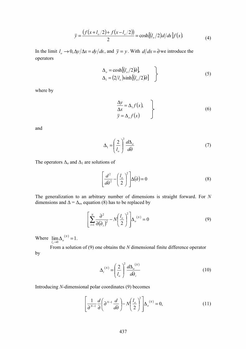
437
( ) ( )( )2
22 oo lxflxfy −++= ( )[ ] ( ).2cosh xfdxdlo= (4)
In the limit dxdyxylo =ΔΔ→ ,0 , and yy = . With ∂=dxd we introduce the operators
( )[ ]( ) ( )[ ]∂=Δ
∂=Δ2sinh2
,2cosh
1 oo
oo
lll
(5)
where by
( )( )xfy
xfxy
oΔ=
Δ=ΔΔ ,1 (6)
and
∂Δ
⎟⎟⎠
⎞⎜⎜⎝
⎛=Δ
dd
lo
o
2
12 (7)
The operators Δo and Δ1 are solutions of
( ) 02
2
2
2
=∂Δ⎥⎥⎦
⎤
⎢⎢⎣
⎡⎟⎠⎞⎜
⎝⎛−
∂ol
dd (8)
The generalization to an arbitrary number of dimensions is straight forward. For N dimensions and Δ = Δo, equation (8) has to be replaced by
( )( ) 0
21
2
2
2
=Δ⎥⎥⎦
⎤
⎢⎢⎣
⎡⎟⎠⎞⎜
⎝⎛−
∂∂∂∑
=
No
N
i
o
i
lN (9)
Where ( ) .1lim0
=Δ→
Nolo
From a solution of (9) one obtains the N dimensional finite difference operator by
( )( )
i
No
o
Ni d
dl ∂
Δ⎟⎟⎠
⎞⎜⎜⎝
⎛=Δ
22 (10)
Introducing N-dimensional polar coordinates (9) becomes
( ) ,02
1 21
1 =Δ⎥⎥⎦
⎤
⎢⎢⎣
⎡⎟⎠⎞⎜
⎝⎛−⎟
⎠⎞⎜
⎝⎛
∂∂
∂∂−
−N
ooN
N
lNddd (11)
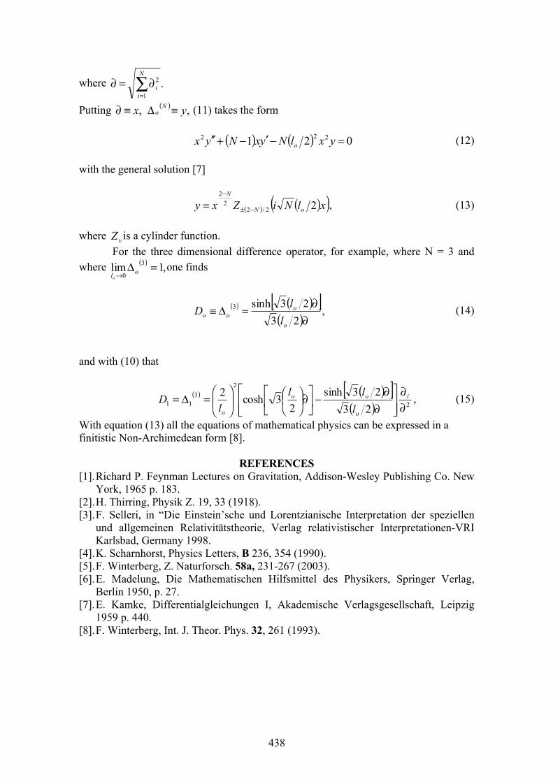
438
where .1
2∑=
∂=∂N
ii
Putting ,x≡∂ ( ) ,yNo ≡Δ (11) takes the form
( ) ( ) 021 222 =−′−+′′ yxlNyxNyx o (12)
with the general solution [7]
( ) ( )( )xlNiZxy oN
N
22/22
2
−±
−
= , (13)
where vZ is a cylinder function. For the three dimensional difference operator, for example, where N = 3 and
where ( ) ,1lim 3
0=Δ
→ oloone finds
( ) ( )[ ]( ) ,
2323sinh3
∂∂
=Δ≡o
ooo l
lD (14)
and with (10) that
( ) ( )[ ]( ) 2
23
11 2323sinh
23cosh2
∂∂
⎥⎥⎦
⎤
⎢⎢⎣
⎡
∂∂−⎥
⎦
⎤⎢⎣
⎡∂⎟⎠⎞⎜
⎝⎛
⎟⎟⎠
⎞⎜⎜⎝
⎛=Δ= i
o
oo
o lll
lD , (15)
With equation (13) all the equations of mathematical physics can be expressed in a finitistic Non-Archimedean form [8].
REFERENCES [1]. Richard P. Feynman Lectures on Gravitation, Addison-Wesley Publishing Co. New
York, 1965 p. 183. [2]. H. Thirring, Physik Z. 19, 33 (1918). [3]. F. Selleri, in “Die Einstein’sche und Lorentzianische Interpretation der speziellen
und allgemeinen Relativitätstheorie, Verlag relativistischer Interpretationen-VRI Karlsbad, Germany 1998.
[4]. K. Scharnhorst, Physics Letters, B 236, 354 (1990). [5]. F. Winterberg, Z. Naturforsch. 58a, 231-267 (2003). [6]. E. Madelung, Die Mathematischen Hilfsmittel des Physikers, Springer Verlag,
Berlin 1950, p. 27. [7]. E. Kamke, Differentialgleichungen I, Akademische Verlagsgesellschaft, Leipzig
1959 p. 440. [8]. F. Winterberg, Int. J. Theor. Phys. 32, 261 (1993).
Physical Interpretetions of Relativity Theory
Proceedings of International Scientific Meeting PIRT-2008, 12 - 15 September 2008
Bauman Moscow State Technical University 5, 2-nd Baumanskaya street, 105005, Moscow
Тираж 300 экземпляров. Заказ


