arX

iv:g

r-qc

/970

3061

v1 2

1 M

ar 1

997

ULB-TH-97/04PAR-LPTHE-97-08

A note on the gauge symmetries of pure Chern-Simonstheories with p-form gauge fields

M. Banados1,2, M. Henneaux1,3, C. Iannuzzo3 and C.M. Viallet4

1Centro de Estudios Cientıficos de Santiago, Casilla 16443, Santiago, Chile2Departamento de Fısica, Universidad de Santiago, Casilla 307, Correo 2,

Santiago, Chile3Faculte des Sciences, Universite Libre de Bruxelles, Campus Plaine,

C.P. 231, B-1050, Bruxelles, Belgium4Centre National de la Recherche Scientifique

Laboratoire de Physique Theorique et Hautes Energies,

Universites Paris VI et Paris VII, Bte 126, 4, Place Jussieu,

75252 Paris Cedex 05, France

Abstract

The gauge symmetries of pure Chern-Simons theories with p-form

gauge fields are analyzed. It is shown that the number of independent

gauge symmetries depends crucially on the parity of p. The case where

p is odd appears to be a direct generalization of the p = 1 case and

presents the remarkable feature that the timelike diffeomorphisms can

be expressed in terms of the spatial diffeomorphisms and the internal

gauge symmetries. By constrast, the timelike diffeomorphisms may be

an independent gauge symmetry when p is even. This happens when

the number of fields and the spacetime dimension fulfills an algebraic

condition which is explicitely written.

1

1 Introduction

Pure Chern-Simons theory in 3 dimensions is one of the most studied exam-ples of a topological field theory. It is a model which does not involve thespacetime metric but is yet generally covariant. Furthermore, as noted bymany authors [1], the spacetime diffeomorphisms

δξAaµ = £ξA

a

µ = ξρF a

ρµ + Dµ(ξρAa

ρ), (1.1)

are not independent from the internal gauge symmetries

δξAaµ = Dµǫ

a (1.2)

since (1.1) reduces to (1.2) with ǫa = ξρAaρ when the equations of motion hold

(F aρµ = 0). In (1.1) and (1.2), the Aa

µ are the components of the connection,while the F a

ρµ are those of the curvature 2-form, respectively.Due to the non-independence of the spacetime diffeomorphisms, the only

first class-constraints in the Hamiltonian formulation are the constraints as-sociated with the internal gauge symmetry (1.2). There is no independentfirst class constraint associated with (1.1). Thus, by finding the most generalstate invariant under (1.2), one may automatically produce states which areinvariant under (1.1). Implementing diffeomorphism invariance is then amere byproduct of implementing invariance under internal gauge symme-tries.

It was shown in recent publications [2] that this crucial property of three-dimensional Chern-Simons theory does not survive in the higher dimensionalgeneralizations. In those models, described by the Lagrangian (2k+ 1)-form

L(2k+1)C.S. = ga1...ak+1

F a1 ∧ . . . ∧ F ak ∧ Aak+1 + “more”(k ≥ 2) (1.3)

where ga1...ak+1is an invariant tensor and where “more” completes (1.3) so

as to make it invariant under (1.2) up to an exact term. It is genericallyno longer true that the diffeomorphisms (1.1), which are still symmetries of(1.3), can be expressed in terms of the internal gauge transformations (1.2).The reason is that the equations of motion no longer imply the vanishing ofthe curvature two-form F a

µν . At the same time, the theory described by (1.3)does possess degrees of freedom for k > 1 while it does not for k = 1.

2

However, the higher-dimensional Chern-Simons models still possess a re-markable feature. Namely, not all the spacetime diffeomorphisms are in-dependent gauge transformations, but only those defined by spatial repa-rameterizations. As established in [2], the timelike diffeomorphisms can beexpressed in terms of the internal gauge symmetries and the spacelike diffeo-morphisms. This implies that, in the Hamiltonian formalism, there are firstclass constraints Ga ≈ 0 generating the internal gauge symmetries (1.2) andfirst class constraints Hi ≈ 0 generating the spatial diffeomorphisms, butthere are no independent first class constraints associated with the timelikediffeomorphisms. In order to find the most general gauge invariant state, itsuffices to solve the conditions Hi|ψ >= 0 and Ga|ψ >= 0. Since these condi-tions are purely kinematical, they are in principle more easily amenable to anexact resolution (using e.g. the loop representation [3] ). From this point ofview, Chern-Simons theories in higher dimensions are of great interest to rel-ativists since they provide non trivial models (models with a finite number oflocal degrees of freedom per space point) in which the problem of implement-ing quantum-mechanically invariance under the full diffeomorphism group isreduced to the kinematical problem of finding quantum states invariant un-der spatial diffeomorphisms. They are in that respect comparable to the toymodels analyzed in [4].

In the search for other generally covariant theories with the same property,we have analyzed the dynamics of pure Chern-Simons theories with forms ofhigher degree. These are described by the Lagrangian n-form

L = ga1...ak+1Ba1 ∧Ha2 ∧ . . . ∧Hak+1 (1.4)

where Ba(a = 1, . . . , N) are p-forms and Ha are the corresponding (Abelian)curvatures,

Ha = dBa. (1.5)

The spacetime dimension n is equal to p + k(p + 1). We shall call k theorder of the Chern-Simons theory. The (p + 1)-forms Ha are commutingwhen p is odd and anticommuting when p is even. If p is odd, the nottotally symmetric parts of ga1...ak+1

contribute a total derivative to L, andone may then assume that ga1...ak+1

is totally symmetric. Similarly, if p iseven, we will assume that ga1...ak+1

is totally antisymmetric. The Chern-Simons Lagrangian is such that in (n+1) dimensions,

∫

dL is the topologicalinvariant

∫

ga1...ak+1Ha1 ∧ . . . ∧ Hak+1. The Lagrangian L is invariant under

3

the usual p-form Abelian gauge transformations

δΛBa = dΛa (1.6)

where Λa are N (p− 1)-forms, as well as under spacetime diffeomorphisms

δξBa = £ξB

a . (1.7)

The first gauge symmetry (1.6) is reducible since if one takes Λa = dµa,one gets δΛB

a = 0 (identically). The second gauge symmetry (1.7) can berewritten equivalently as

δ′ξBa = iξH

a (1.8)

since £ξ = iξd + diξ.The equations of motion following from (1.4) are explicitly

ga1a2...ak+1Ha2 ∧ . . . ∧Hak+1 = 0 (1.9)

and do not imply that the curvatures Ha vanish, unless the order k is equalto one.

P -form gauge fields appear systematically in supergravity theories inhigher dimensions [5]. A Chern-Simons-like term appears in the Lagrangianof n = 11 supergravity [6], besides the kinetic term proportional toHµνλρHµνλρ.

We have found that the pure Chern-Simons theories with Lagrangiandensity (1.4) generically have local degrees of freedom when k ≥ 2. This isnot surprising in view of the analysis of [2]. The new result, however, is thatthe timelike diffeomorphisms may now be independent gauge symmetries.

This will occur only when p is even, and the number κ defined by

κ ≡ N

(

n− 1p

)

− (n− 1) (1.10)

is an odd integer.The number κ is the difference between the total number of spatial com-

ponents of the set of p-forms, and the number of spatial dimensions in thetheory.

The above condition can be fulfilled by choosing appropriately N and k(for a given even p). There is thus a striking difference between pure Chern-Simons theories with p-forms of even degree and pure Chern-Simons theories

4

with p-forms of odd degree. This difference could not have been anticipatedby a mere look at the gauge symmetries (1.6),(1.7),(1.8) - which take the sameform in all cases - and requires a more detailed investigation of the dynamics.Our results imply that the dependence of the timelike diffeomorphisms onthe other gauge symmetries found for p = 1 in [2] is not a remnant of thetopological construction leading to these models. Indeed this construction isidentical for all values of p, N or k. The phenomenon has a different originwhich is yet to be uncovered.

2 The case p = 2, k = 2

2.1 Constraints

We begin the discussion with p = 2. The condition κ= odd integer becomes,using n = k(p+ 1) + p:

(3k + 1)[3kN

2− 1] = odd integer (2.1)

and cannot be realized for k = 1 for which the theory has actually no degreesof freedom. We thus take the simplest case, namely k = 2, which yields

7[3N − 1] = odd integer, (2.2)

a condition that is fulfilled if and only if N is an even integer.The goal of this section is to show that indeed, the timelike diffeomor-

phisms can be expressed in terms of the internal gauge transformations andthe spatial diffeomorphisms for odd values of N , while they are independentgauge symmetries for even values of N (except for low values of N (N < 8)where there are accidental degeneracies1). The proof of this property turnsout to be of mathematical interest in its own right since it involves the dis-crete projective plane with 7 points related to the octonion algebra.

1For N = 1 and N = 2, the Lagrangian vanishes identically and those theories are then

trivial. For N = 4, one field identically drops out because any antisymmetric tensor gabc

admits a “zero vector” λa 6= 0, solution of the equation gabcλc = 0. So, one is effectively

reduced to the N = 3 case plus one field with zero Lagrangian. Finally, the case N = 6

appears to be equivalent to two independent N = 3 theories and thus has twice the number

of gauge symmetries as the N = 3 case.

5

In order to analyze the gauge symmetries, we rewrite the Lagrangian(1.4) in Hamiltonian form. It is well appreciated by now that the conceptof gauge symmetry cannot be thought of independently from the dynamics.This appears quite strikingly when discussing the (in)dependence of a givenset of a gauge transformations, since the form of the “on-shell trivial” gaugesymmetries explicitly involves the dynamics. It is for this reason that theHamiltonian formulation, where the dynamics takes a transparent form, isconvenient in the analysis of the gauge symmetries - see for instance [7]. Withp = 2 and k = 2, the Lagrangian (1.4) reads

L = gabcBa ∧Hb ∧Hc (2.3)

where Hb is the 3-form dBa, and where gabc is completely antisymmetric.When split into space and time, the action (2.3) is up to a boundary term

equal to

S =∫

dx0d7x[lija Baij − Ba

0iKia] (2.4)

withlija = ǫijk1...k5gabcB

bk1k2

Hck3k4k5

(2.5)

andKi

a = ǫij1j2j3j4j5j6gabcHbj1j2j3

Hcj4j5j6

(2.6)

It follows from (2.4) that the temporal components Ba0i are not true dy-

namical degrees of freedom but rather are Lagrange multipliers for the con-straints

Kia ≈ 0. (2.7)

These are reducible since

Kia,i = 0 identically (2.8)

Although (2.4) is linear in the time derivatives, it is not yet in canonicalform because the exterior derivative (in field space) of the one-form lija δB

aij is

degenerate and thus does not define a symplectic structure. To deal with this,we follow the standard Dirac procedure and define the conjugate momentathrough

pija =

∂L

∂Baij

= lija (2.9)

6

These momenta are subject to 21N primary constraints

Φija ≡ pij

a − lija ≈ 0 i, j = 1, . . . , 7; a = 1, . . . , N (2.10)

(Φija = −Φji

a ). It turns out to be more convenient to replace the constraintsKi

a ≈ 0 by the equivalent constraints

Gia = Ki

a − ∂jΦija ≈ 0 (2.11)

because the new constraints generate the internal gauge transformations (1.6)in the Poisson brackets,

[Baij ,∫

Σd7xΛb

kGkb ] = (dΛ)ij (2.12)

The constraints (2.11) are also clearly reducible since ∂iGia = 0 (identically).

The Hamiltonian action takes the form

IH =∫

dx0∫

d7x[pija B

aij − Ba

0iGia − ua

ijΦija ] (2.13)

The Poisson brackets among the constraints are given by[

Φija (x),Φkl

b (x′)]

= Ωijklab δ(x, x

′) (2.14)[

Φija (x), Gl

b

]

= 0 (2.15)[

Gia, G

jb

]

= 0 (2.16)

where Ωijklab is an antisymmetric matrix given by

Ωij kla b = gabcǫ

ijklm1m2m3Hcm1m2m3

(2.17)

Ωij kla b = −Ωkl ij

b a (2.18)

It follows from the constraint algebra that there are no further constraints.It is also clear that the constraints Gi

a ≈ 0 are first class, as they should sincethey generate the internal gauge transformations (1.6).

7

2.2 Rank of Ωijklab and projective plane Π7

2.2.1 Strategy for computing the rank of Ωijklab

To complete the canonical analysis, it is necessary to determine the natureof the constraints Φij

a ≈ 0. To that end, one must determine the number ofzero eigenvectors possessed by the matrix Ωijkl

ab of the brackets [Φija ,Φ

klb ]. This

number turns out to depend on the number N of fields, on the antisymmetrictensor gabc defining the theory and, for a given choice ofN and gabc, it dependsalso on the phase space location of the dynamical system. Indeed, the matrixΩijkl

ab involves both gabc and Haijk (the latter being constrained by Ki

a ≈ 0).

To determine all the possible ranks that the matrix Ωijklab can achieve is

a rather complicated algebraic task and we shall not attempt to pursue ithere. We will describe what happens in the generic situation in which Ωijkl

ab

has the maximum possible rank compatible with the constraints Kia ≈ 0. We

call it generic because maximum rank conditions define open regions in thespace of theories (space of the g’s) and of allowed configurations (space ofthe H ’s) and are thus stable under small deformations. This is not true forlower ranks, which are associated with equations rather than inequalities.

It is easy to see that the matrix Ωijklab has at least seven zero eigenvectors

Hbkl m (m = 1, 2, . . . , 7), since Ωijkl

ab Hbklm ≈ 0. These zero eigenvectors are

associated with the spatial diffeomorphisms in the sense that the first classconstraints

Hi ≡ HaiklΦ

kla ≈ 0 (2.19)

are the generators of the spatial diffeomorphisms in the “improved” form(1.8). In the generic case, the zero eigenvectors Hb

klm are independent becausethe equations

Haiklξ

i = 0 (2.20)

imply ξi = 0 (more on this in subsection 2.4 below).The study parallels so far quite closely the discussion of pure Chern-

Simons theories with 1-form gauge fields. New features arise when one ad-dresses the question as to whether there are further independent first classconstraints among the Φ ’s. These first class constraints (if any) would cor-respond to additional independent gauge symmetries.

The total number of constraints is the size of Ω, that is to say 21N . Thereare as many second class constraints as there are non-vanishing eigenvalues

8

of Ω. Therefore, there has to be an even number of second class constraints.This means that the number of first class constraints among the Φ’s is oddfor odd N and even for even N . We already know from (2.19) seven of thefirst class constraints. If N is even, there must be at least one additional firstclass constraint still to be identified. This does not need to be the case forN odd.

By computer-assisted investigation of the first values of N (≤ 20), wehave reached the following conclusions. If N is odd (and greater than orequal to three), then there is generically no further first class constraintamong the Φ’s; while if N is even (and greater than or equal to eight in orderto avoid the accidental degeneracies), then there is generically one and onlyone additional first class constraint among the Φ’s.

We have come to this conclusion by constructing examples in which theantisymmetric matrix Ωij kl

a b has exactly rank κ = 21N − 7 for N odd, andexactly rank κ− 1 = 21N − 8 for N even. Since these values of the rank cor-respond to the maximum rank that Ω can achieve (the first class constraints(2.19) are always present), they are stable under small deformations and thusgeneric.

In order to analyse the equations, we proceed as follows:

i. First, we pick at random an arbitrary set of completely antisymmetrictensors gabc;

ii. Second, we construct the general solution of the constraints K la ≡

gabcHbijkH

cmnpǫ

lijkmnp = 0 for these given gabc;

iii. Knowing the curvatures Haijk (which are subject to the sole condition

K la ≈ 0 ), we compute the matrix Ωijkl

ab = ǫijklmnpgabcHcmnp and deter-

mine its rank.

Of these three steps, the first one and the last one are direct. Onlythe second one needs further discussion because the equations K l

a = 0 arequadratic in the unknown Hb

ijk. It is here that we shall use the properties ofthe finite projective plane Π7.

2.2.2 Projective plane Π7

The projective plane Π7 has seven points and seven lines containing threepoints each, with the properties that any pair of points determines one and

9

only one line, while any pair of lines intersects in one and only one point.The points and lines of Π7 are drawn in figure 2.1, with an arbitrary choiceof indices (1, 2, . . . , N).

1 2 3

4

5

6

7

Figure 2.1

Caption: The projective plane Π7 has seven points (1,2,3,4,5,6,7) and sevenlines containing three points each. The set of these lines is the set of tripletsT = 1, 2, 3, 1, 4, 5, 1, 6, 7, 2, 4, 7, 2, 5, 6, 3, 4, 6, 3, 5, 7.

To the line (i, j, k) ∈ T , one associates the three-form dxi ∧ dxj ∧ dxk.Because Π7 arises in the description of the octonion algebra (the “product”of two points is the third point on the same line, with a sign fixed by theorientation), we shall call these seven 3-forms the “octonionic 3-forms” andshall denote them by ωα

(3)(α = 1, 2, . . . , 7). The rest of the basis 3-forms,

formed with triplets not in T , shall be denoted by ϕA(3)(A = 1, . . . , 28).

The main property of the octonionic 3-forms is

ωα(3) ∧ ω

β(3) = 0 (2.21)

for any α, β = (1, 2, ..., 7). Indeed, any pair of lines of Π7 have one (and onlyone if the lines are distinct) point in common, so that ωα

(3) and ωβ(3) have one

dxi in common, which implies (2.21).

10

In what follows we shall use differential form notation in the spatial man-ifold. The constraint equations

Kia = gabcǫ

ijklmnpHbjklH

cmnp = 0 (2.22)

are rewritten asKa = gabcH

b ∧Hc = 0 (2.23)

where the Ha are regarded as three forms in seven dimensions. The rank ofΩ is determined by the number of solutions of the equation

gabcHb ∧ V c = 0 (2.24)

where the 3-form curvature H satisfies the constraint equation (2.23) and V a

is a 2-form. The zero eigenvectors Haklmξ

m described above are simply iξHa.

2.2.3 The N = 3 case

We begin with the N = 3 case (the smallest number of fields for which theantisymmetric tensor gabc is non-zero) because it is particularly straightfor-ward. A simple solution for the constraint is given by a linear combinationof the octonionic monomials Ha = λa

αωα(3) because ωα ∧ ωβ = 0.

This solution has maximum rank when none of the coefficient λaα is zero.

Indeed, since Ha is a 3-form, its dual in seven dimensions can be viewed asthe symmetric 21 × 21 matrix ∗H(a) ij kl = ǫijklmnpHa

mnp, for each value ofa = 1, 2, 3. We can thus write Eq. (2.24) in matrix form

∗H1V 2 = ∗H2V 1, ∗H1V 3 = ∗H3V 1, ∗H2V 3 = ∗H3V 2. (2.25)

The determinant of the matrix ∗Ha, for a given a, is easily expressed in termsof the expansion Ha = λa

αωα(3). Let ∗H3 be equal to

∗H3 = a1∗ω1 + a2

∗ω2 + · · · + a7∗ω7 (2.26)

where ∗ωα represents the dual of ωα. The determinant of ∗H3 (as a 21×21matrix) is equal to 27 a1a2 · · ·a7. Thus, if all the monomials wα are presentin (2.26), ∗H3 is invertible. In that case, one can solve V 1 and V 2 in termsof V 3 from the last two equations in (2.25). Replacing V 1 and V 2 back inthe first equation we find an equation for V 3

(∗H1J ∗H2 − ∗H2J ∗H1)V 3 = 0 (2.27)

11

where J is the inverse of ∗H3. Equation (2.27) can be investigated numeri-cally and one finds that it has (generically) only 7 solutions for V 3. Since V 1

and V 2 are completely determined in terms of V 3, this implies that the matrixΩijkl

ab for the N = 3 case has no other zero eigenvalues besides those associatedwith spatial diffeomorphisms and has thus maximum rank 21 × 3 − 7 = 56.

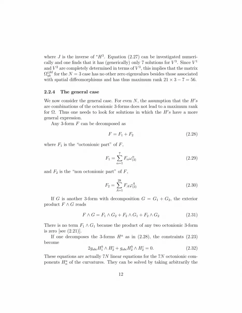
2.2.4 The general case

We now consider the general case. For even N , the assumption that the H ′sare combinations of the octonionic 3-forms does not lead to a maximum rankfor Ω. Thus one needs to look for solutions in which the H ′s have a moregeneral expression.

Any 3-form F can be decomposed as

F = F1 + F2 (2.28)

where F1 is the “octonionic part” of F ,

F1 =7∑

α=1

Fαωα(3) (2.29)

and F2 is the “non octonionic part” of F ,

F2 =28∑

A=1

FAϕA(3) (2.30)

If G is another 3-form with decomposition G = G1 + G2, the exteriorproduct F ∧G reads

F ∧G = F1 ∧G2 + F2 ∧G1 + F2 ∧G2 (2.31)

There is no term F1 ∧G1 because the product of any two octonionic 3-formis zero [see (2.21)].

If one decomposes the 3-forms Ha as in (2.28), the constraints (2.23)become

2gabcHb1 ∧H

c2 + gabcH

b2 ∧H

c2 = 0. (2.32)

These equations are actually 7N linear equations for the 7N octonionic com-ponents Ha

α of the curvatures. They can be solved by taking arbitrarily the

12

non octonionic components HaA of the curvatures and determining then the

octonionic components Haα through (2.32). [The linear, inhomogeneous sys-

tem (2.32) is easily verified to have one and only one solution for generic HaA

’s]. Consequently, even though the constraints are quadratic in Ha one canproduce an explicit rational solution by using the octonionic decomposition.

We have carried out the task of solving the constraint along the lines justdescribed for random choices of the constants gabc and of the componentsHa

A. We have then computed numerically the dimension of the kernel ofΩijkl

ab and found in each case that the zero eigenvalue was degenerate exactlyeight times for N even(≥ 8) and seven times for N odd. What we got fromthese calculations for the first values of N is thus that the rank of Ωijkl

ab isgenerically equal to 21N − 8 for N even(≥ 8) and 21N − 7 for N odd. Wehave established this result for N ≤ 20 and shall take it for granted for highervalues of N .

2.3 Geometrical interpretation of the eighth first classconstraint

For N odd (and N ≥ 3), the first class constraints Gia ≈ 0 and Hi ≈ 0 are the

only (independent) first class constraints. The other constraints are secondclass. This implies that the internal gauge symmetries (1.6), generated byGi

a, and the spatial diffeomorphisms, generated by Hi, form a complete setof gauge symmetries. Any gauge symmetry of the system, including thetimelike diffeomorphisms, can be expressed in terms of them.

For N even (and ≥ 8) there is, by contrast, an eighth first class constraintamong the Φij

a given by µaijΦ

ija where µa

ij is a zero eigenvector of Ωijklab ,

Ωijklab µ

bkl = 0, (2.33)

independent of the seven eigenvectors Haijm associated with the spatial dif-

feomorphisms. One may relate the transformation generated by Φija µ

aij ≡ H

δρBaij(~x) = [Ba

ij(~x),∫

ρ(~x′)H(~x′)dx′] (2.34)

= ρµaij(~x) (2.35)

to the timelike diffeomorphisms as follows.In the improved form (1.8), the timelike diffeomorphisms read

13

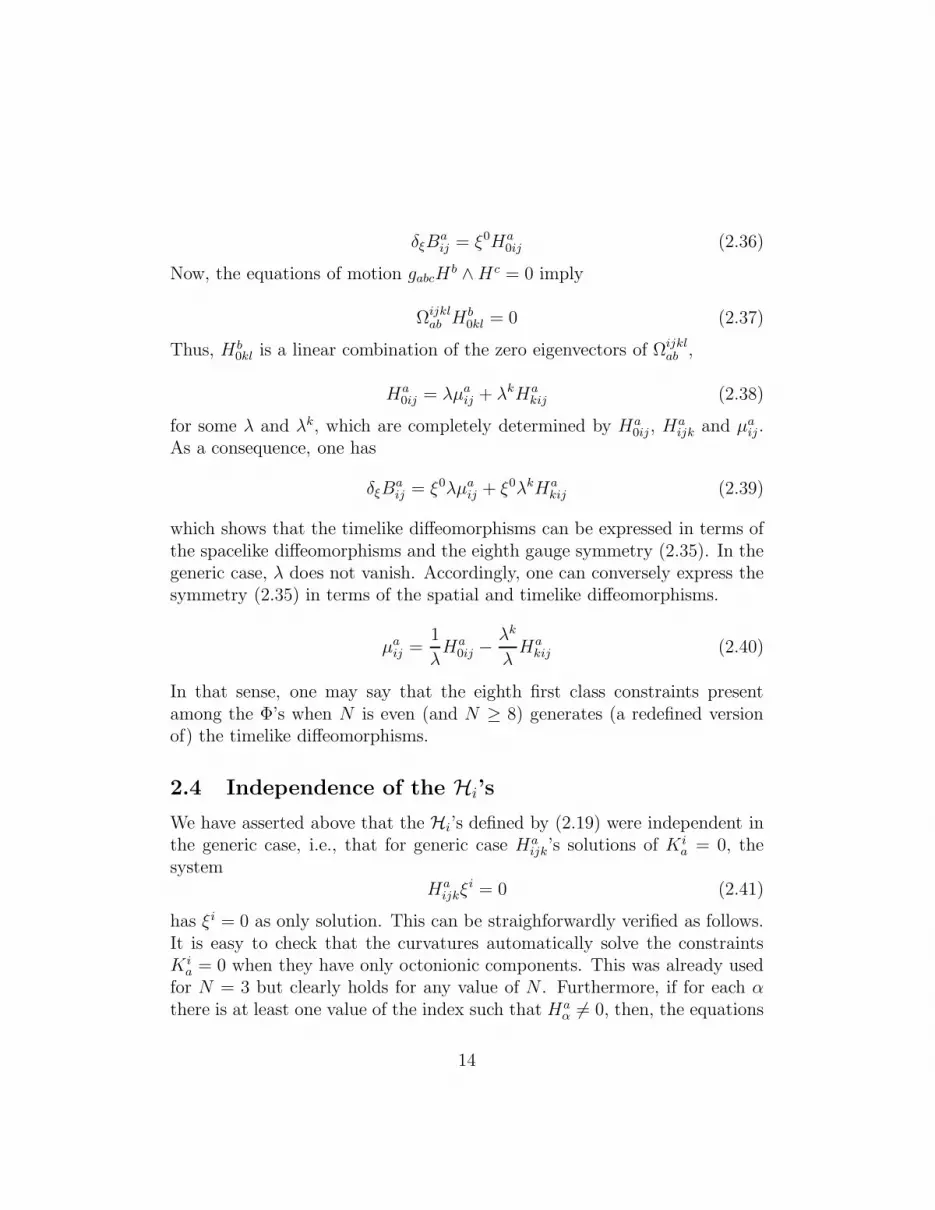
δξBaij = ξ0Ha

0ij (2.36)

Now, the equations of motion gabcHb ∧Hc = 0 imply

Ωijklab H

b0kl = 0 (2.37)

Thus, Hb0kl is a linear combination of the zero eigenvectors of Ωijkl

ab ,

Ha0ij = λµa

ij + λkHakij (2.38)

for some λ and λk, which are completely determined by Ha0ij , H

aijk and µa

ij .As a consequence, one has

δξBaij = ξ0λµa

ij + ξ0λkHakij (2.39)

which shows that the timelike diffeomorphisms can be expressed in terms ofthe spacelike diffeomorphisms and the eighth gauge symmetry (2.35). In thegeneric case, λ does not vanish. Accordingly, one can conversely express thesymmetry (2.35) in terms of the spatial and timelike diffeomorphisms.

µaij =

1

λHa

0ij −λk

λHa

kij (2.40)

In that sense, one may say that the eighth first class constraints presentamong the Φ’s when N is even (and N ≥ 8) generates (a redefined versionof) the timelike diffeomorphisms.

2.4 Independence of the Hi’s

We have asserted above that the Hi’s defined by (2.19) were independent inthe generic case, i.e., that for generic case Ha

ijk’s solutions of Kia = 0, the

systemHa

ijkξi = 0 (2.41)

has ξi = 0 as only solution. This can be straighforwardly verified as follows.It is easy to check that the curvatures automatically solve the constraintsKi

a = 0 when they have only octonionic components. This was already usedfor N = 3 but clearly holds for any value of N . Furthermore, if for each αthere is at least one value of the index such that Ha

α 6= 0, then, the equations

14

(2.41) imply ξi = 0. In other words, for such curvatures, the 21N × 7 matrixH(a

ij)k has maximum rank 7. Using again the argument that maximum rankconditions are stable against small deformations, one infers that the systemHa

ijkξi = 0 implies generically that ξi is zero.

2.5 Number of degrees of freedom

We conclude the discussion of the 2-form case by counting the number ofdegrees of freedom. There are 21N conjugate pairs (Ba

ij , pija ). These pairs are

constrained by the 6N first class constraints Gia = 0 (there are actually 7N

such constraints, but they are subject to the differential identity Gia,i = 0),

as well as by the 21N constraints Φija = 0. Of these, 7 are first class and

21N − 7 are second class for N odd (and N ≥ 3); while 8 are first class and21N − 8 are second class for N even (and N ≥ 8). According to the generalrule for counting the degrees of freedom (= number M of physical conjugatepairs), one finds

M =1

2[2 × 21N − 2 × 6N − 2 × 7 − (21N − 7)]

=1

2[9N − 7] (N odd, N ≥ 3)

and

M =1

2[2 × 21N − 2 × 6N − 2 × 8 − (21N − 8)]

=1

2[9N − 8] (N even, N ≥ 8)

For N = 4, one has the same number of degrees of freedom as for N = 3,i.e., 10, while for N = 6, one has twice as many degrees of freedom as forN = 3, i.e., 20. [For N = 1 and 2, the theory is pure gauge and M = 0]. Inall cases but N = 1 or 2, the theory has local degrees of freedom (M > 0),as for 1-forms [2]. This concludes the analysis of the case p = 2, k = 2.

3 Discussion of the general case (p ≥ 2, k ≥ 2)

15

3.1 Constraints

We now turn to the general case p ≥ 2. If k = 1, the Lagrangian is quadratic,L = gabB

a ∧Hb, and the equations of motion are just equivalent to Hb = 0(assuming gab to be invertible). The theory has no local degrees of freedomand one sees from (1.8) that the diffeomorphisms (both temporal and spatial)are not independent gauge symmetries. The case k ≥ 2 is, however, muchricher. Its analysis proceeds as that of the case p = 2, k = 2. We shall usethroughout differential form notations. The number of spatial dimensions isequal to n− 1 = k(p+ 1) + p− 1.

By following the same method as above, one finds that the spatial fieldstrengths Ha are subject to the algebraic constraints

Ki1...ip−1

a = gab1...bk[∗(Hb1 ∧ . . . ∧Hbk)]i1...ip−1 ≈ 0, (3.1)

which can be written as

Ka = gaa1...akHa1 ∧Ha2 ∧ ... ∧Hak ≈ 0. (3.2)

The 2N

(

n− 1p

)

phase space variables Bai1...ip

and pi1...ipa are restricted not

only by (3.1), but also by the primary constraints.

Φi1...ipa = pi1...ip

a − li1...ipa (B) ≈ 0 (3.3)

analogous to (2.10), where li1...ipa is given by

li1...ipa = gabc1...ck−1

[∗(Bb ∧Hc1 ∧ . . . ∧Hck−1)]i1...ip . (3.4)

There are no further constraints. One can replace (3.1) by Gi1...ip−1 ≈ 0,where

Gi1...ip−1

a = Ki1...ip−1

a − ∂iΦii1...ip−1

a ≈ 0. (3.5)

These constraints generate the internal gauge symmetry (1.6) and are firstclass. The constraints (3.3) have brackets given by

[Φi1...ipa (~x),Φ

j1...jp

b (~x′)] = Ωi1...ipj1...jp

ab δ(~x, ~x′) (3.6)

where the antisymmetric matrix Ω is

Ωi1...ipj1...jp

ab = gabc1...ck−1[∗(Hc1 ∧ . . . ∧Hck−1)]i1...ipj1...jp (3.7)

16

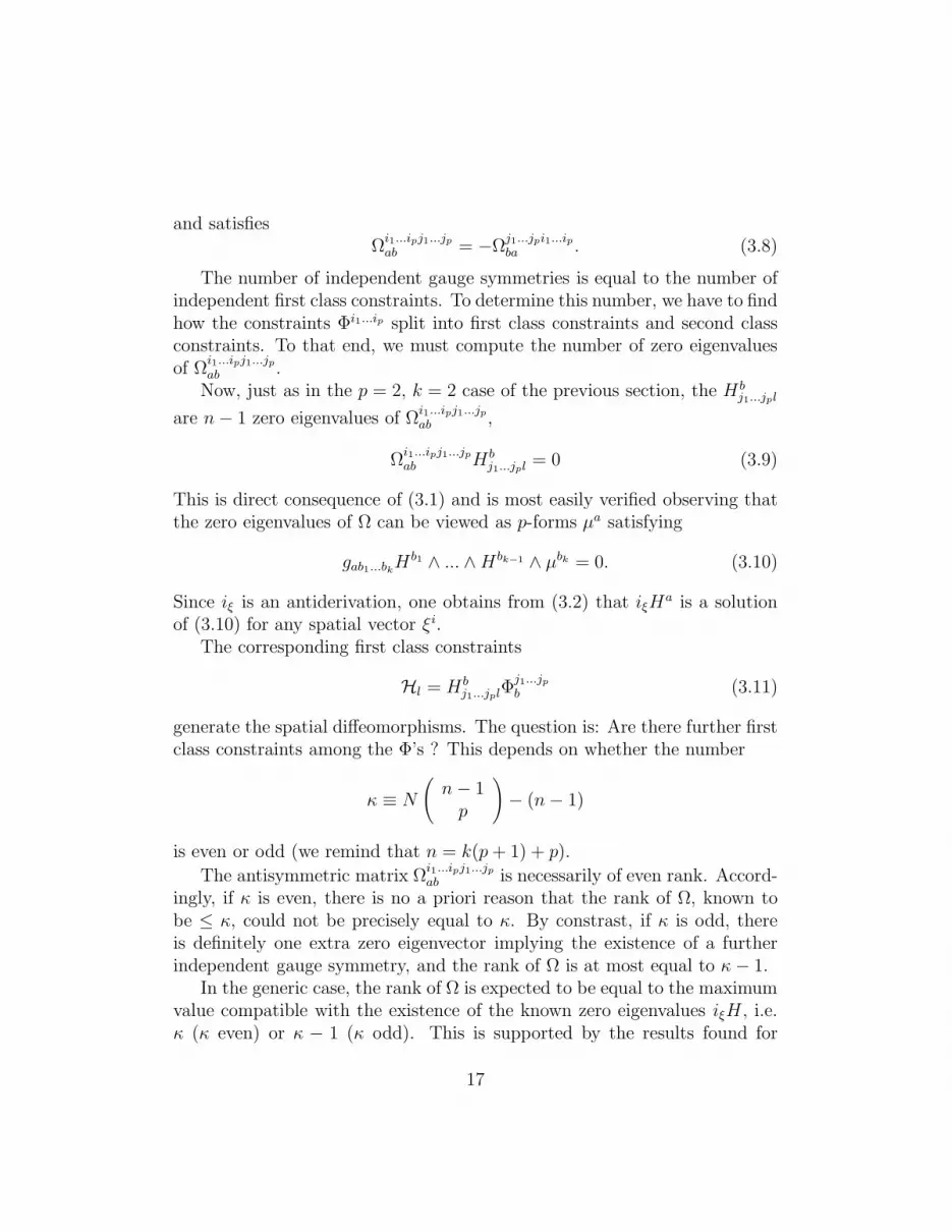
and satisfiesΩ

i1...ipj1...jp

ab = −Ωj1...jpi1...ipba . (3.8)

The number of independent gauge symmetries is equal to the number ofindependent first class constraints. To determine this number, we have to findhow the constraints Φi1...ip split into first class constraints and second classconstraints. To that end, we must compute the number of zero eigenvaluesof Ω

i1...ipj1...jp

ab .Now, just as in the p = 2, k = 2 case of the previous section, the Hb

j1...jpl

are n− 1 zero eigenvalues of Ωi1...ipj1...jp

ab ,

Ωi1...ipj1...jp

ab Hbj1...jpl = 0 (3.9)

This is direct consequence of (3.1) and is most easily verified observing thatthe zero eigenvalues of Ω can be viewed as p-forms µa satisfying

gab1...bkHb1 ∧ ... ∧Hbk−1 ∧ µbk = 0. (3.10)

Since iξ is an antiderivation, one obtains from (3.2) that iξHa is a solution

of (3.10) for any spatial vector ξi.The corresponding first class constraints

Hl = Hbj1...jplΦ

j1...jp

b (3.11)

generate the spatial diffeomorphisms. The question is: Are there further firstclass constraints among the Φ’s ? This depends on whether the number

κ ≡ N

(

n− 1p

)

− (n− 1)

is even or odd (we remind that n = k(p+ 1) + p).

The antisymmetric matrix Ωi1...ipj1...jp

ab is necessarily of even rank. Accord-ingly, if κ is even, there is no a priori reason that the rank of Ω, known tobe ≤ κ, could not be precisely equal to κ. By constrast, if κ is odd, thereis definitely one extra zero eigenvector implying the existence of a furtherindependent gauge symmetry, and the rank of Ω is at most equal to κ− 1.

In the generic case, the rank of Ω is expected to be equal to the maximumvalue compatible with the existence of the known zero eigenvalues iξH , i.e.κ (κ even) or κ − 1 (κ odd). This is supported by the results found for

17

p = 1 [2], p = 2, n = 8 (see above) and p = 3, n = 11, N = 1 (section3.3. below). Thus, there will be no further independent gauge symmetriesbesides the internal gauge symmetries and the spatial diffeomorphisms (κeven), or the internal gauge symmetries, the spatial diffeomorphisms andthe timelike diffeomorphisms (κ odd). Other independent gauge symmetriescould arise for particular choices of field configurations or tensor ga1...ak+1

,but these should be thought of as accidental.

Of course, the above comments would be somewhat empty if κ was alwayseven. But we have seen that at least for p = 2, one may have an odd κ. Thisis not the only case. The number κ may be odd whenever p is even. Toprove this statement, we must investigate the parity of κ as a function of theform-degree p, the number N of fields and the order k of the Chern-Simonstheory.

3.2 Case p odd

If the form degree p is odd, the spatial dimension n − 1 = k(p + 1) + p − 1is even since both p+ 1 and p− 1 are even. It is straightforward to see thatin a space with an even number of dimensions, a form of odd degree has aneven number of components,

(

up

)

= even number ( u even, p odd) (3.12)

(u = n− 1). More precisely,

(

up

)

=u(u− 1)(u− 2) . . . (u− p+ 1)

1.2.3 . . . p (3.13)

= u Kp (3.14)

where K is the integer

K =

(

u− 1p− 1

)

=(u− 1)(u− 2) . . . (u− p+ 1)

1.2.3 . . . (p− 1).

Since the left-hand side of (3.14) is an integer, uK is a multiple of p. Since uis even, the product uK is even. Consequently, uK is a multiple of 2p sincep is odd. Hence u.K/p is even.

18

It follows that the integer κ, given by the difference between two evenintegers, is also an even integer. Thus, whenever p is odd, the rank of Ωshould be exactly equal to κ (barring accidental degeneracies) and the tem-poral diffeomorphisms should not be independent gauge symmetries. This isexactly as in the p = 1 case studied in [2].

3.3 The eleven dimensional H ∧H ∧B theory

Another interesting illustration of the results just stated is given by the caseN = 1, p = 3 and k = 2 (implying n = 11) for which the Chern-Simonsaction reads

I =∫

H ∧H ∧B (3.15)

This term arises in supergravity in eleven dimensions [6] which has recentlyreceived much attention in the context of M− theory.

To show that Ω has generically maximum rank 120 (number of primaryconstraints) - 10 (number of spatial diffeomorphisms) = 110, it is enough toexhibit one 4-form H , solution of the constraint equation

H ∧H = 0, (3.16)

for which this property is fulfilled.A solution for (3.16) with maximum rank can be constructed as follows.

We consider the following 4-form,

H = f dx1 ∧ dx3 ∧ dx5 ∧ dx7 + 2dx2 ∧ dx4 ∧ dx6 ∧ dx8

− α dx1 ∧ dx2 ∧ dx3 ∧ dx4 − β dx1 ∧ dx2 ∧ dx5 ∧ dx6

+ a dx1 ∧ dx2 ∧ dx7 ∧ dx8 + b dx1 ∧ dx2 ∧ dx9 ∧ dx10

− γ dx3 ∧ dx4 ∧ dx5 ∧ dx6 + c dx3 ∧ dx4 ∧ dx7 ∧ dx8

+ d dx3 ∧ dx4 ∧ dx9 ∧ dx10 + A dx5 ∧ dx6 ∧ dx7 ∧ dx8

+ B dx5 ∧ dx6 ∧ dx9 ∧ dx10 + dx7 ∧ dx8 ∧ dx9 ∧ dx10

where a, b, c, d, α, β, γ, A,B, f are constants. This form of H has been foundby trial and error, by successive complications of the initial attempt thatinvolved only products of the binomials dx1 ∧ dx2, dx3 ∧ dx4, dx5 ∧ dx6, dx7 ∧dx8, dx9 ∧ dx10.

19

The equation H ∧ H = 0 imposes the following restrictions among thecoefficients

αA+ βc+ γa = 2f (3.17)

αB + βd+ γb = 0 (3.18)

and

α = ad+ bc

β = aB + bA (3.19)

γ = cB + dA

Replacing (3.19) in (3.17) and (3.18) we obtain a system of equations for Aand B whose solution is

A = −(ad+ bc)f

acbd − (ad+ bc)2, B =

bdf

acbd− (ad+ bc)2(3.20)

Therefore, α, β, γ and A,B are determined in terms of the parameters a, b, c, dand f , which are left arbitrary in the solution.

We have computed the rank of Ω for generic values of the coefficientsa, b, c, d and f and found that the maximum rank is achieved. The 120×120matrix Ω has only 10 zero eigenvalues which correspond to the 10 independentdiffeomorphisms of the spatial surface. Note that this theory has 19 localdegrees of freedom, as easily checked by using the rule for counting degreesof freedom recalled above.

3.4 Case p even

If the form degree p is even, κ can be even or odd. As a function of thenumber of fields N for fixed p and k, various possibilities may actually arise:

i) κ is even no matter N is;

ii) κ is even for odd N and odd for even N ;

iii) κ is even for odd N and odd for odd N ;

iv) κ is odd no matter what N is.

20

We have found an instance of (ii) in the previous case p = 2, k = 2.To illustrate the other possibilities, we just consider other values of k whilekeeping p fixed and equal to two.

i) k = 5: the number of spatial dimensions is equal to 5 × 3 + 1 = 16.

A 2-form has

(

162

)

= 16×152

= 120 spatial components. Thus κ =

120N − 16 is even no matter what the integer N is.

iii) k = 3: n− 1 = 10 and

(

n− 12

)

= 45. Thus κ = 45N − 10 is even for

N even and odd for N odd.

iv) k = 4: n− 1 = 13 and

(

n− 12

)

= 78. Thus κ = 78N − 13 is odd no

matter what the integer N is.

4 Conclusions

We have established that the nature of the independent gauge symmetriesof pure Chern-Simons theory based on p-form gauge fields crucially dependson the parity of p. While the spacelike diffeomorphisms and the internalgauge symmetries are the only independent gauge symmetries for odd p (inthe absence of, non-generic, extra gauge symmetries), the timelike diffeomor-phisms are independent gauge symmetries when p is even, if, in addition, the

number κ ≡ N

(

n− 1p

)

− (n−1) is an odd integer. The difference between

odd p and even p persists even in the presence of accidental gauge symme-tries, which must necessarily come in pairs since the rank of Ω is necessarilyeven. For odd values of p, the timelike diffeomorphisms can be expressed interms of the spacelike diffeomorphisms, the internal gauge symmetries andthe (even number of) accidental gauge symmetries. This is not true for evenp (and odd κ).

This result is somehow unexpected since the construction of the Chern-Simons Lagrangian is identical in all cases. Furthermore, for fixed (even)p and fixed spacetime dimension n, the parity of κ may depend - againsomewhat surprisingly - on the number N of p-forms involved. We have

21

not provided a deep explanation of why the distinction between the casesof even or odd p arises, but we have provided explicit examples illustratingboth situations. Perhaps an investigation of Chern-Simons theories involvingsimultaneously forms of different degrees could shed further light on thequestion.

5 Acknowledgements

MB was partially supported by grants # 1960065 and # 1970150 fromFONDECYT (Chile), and institutional support by a group of Chilean com-panies (EMPRESAS CMPC, CGE, COPEC, CODELCO, MINERA LA ES-CONDIDA, NOVAGAS, ENERSIS, BUSINESS DESIGN ASS. and XEROXChile).

References

[1] See for instance R. Jackiw, Phys. Rev. Lett. 41 (1978) 1635.

[2] M.Banados, L.J.Garay and M.Henneaux, Phys. Rev. D53, R593 (1996);Nucl. Phys. B476, 611 (1996)

[3] R. Gambini and A. Trias, Nucl.Phys. B278, 436 (1986). C. Rovelli andL. Smolin, Phys.Rev.Lett. 61, 115 (1988); Nucl.Phys B331, 80 (1990)

[4] V. Hussain and K. Kuchar, Phys. Rev. D42, (1990), 4070. G. Barnichand V. Hussain, gr-qc/9611030

[5] See e.g., P. van Nieuwenhuizen, in Relativity, Groups and Topology II,Les Houches lectures 1983, pp 823-932.

[6] E. Cremmer, B. Julia and J. Scherk, Phys.Lett. B76, 409 (1978)

[7] M. Henneaux and C. Teitelboim, Quantization of gauge systems,(Princeton University Press, Princeton, 1992).

22