Embed Size (px)
Citation preview
arX
iv:1
303.
6853
v2 [
hep-
th]
1 O
ct 2
013
On the Chern-Simons terms in Lifshitz like quantum
electrodynamics
Van Sergio Alves,1, ∗ B. Charneski,2, † M. Gomes,2, ‡
Leonardo Nascimento,1, § and Francisco Pena3, ¶
1Faculdade de Fısica, Universidade Federal do Para, 66075-110, Belem, Para, Brazil
2Instituto de Fısica, Universidade de Sao Paulo
Caixa Postal 66318, 05315-970, Sao Paulo, SP, Brazil
3Departamento de Ciencias Fısicas, Facultad de Ingenierıa,
Ciencias y Administracion, Universidad de La Frontera,
Avda. Francisco Salazar 01145, Casilla 54-D, Temuco, Chile
(Dated: October 3, 2013)
Abstract
In this work the generation of generalized Chern-Simons terms in three dimensional quantum
electrodynamics with high spatial derivatives is studied. We analyze the self-energy corrections
to the gauge field propagator by considering an expansion of the corresponding amplitudes up to
third order in the external momenta. The divergences of the corrections are determined and explicit
forms for the Chern-Simons terms with high derivatives are obtained. Some unusual aspects of the
calculation are stressed and the existence of a smooth isotropic limit is proved. The transversality
of the anisotropic gauge propagator is also discussed.
PACS numbers: 11.10.Gh, 11.10.Hi, 11.10.-z
∗Electronic address: [email protected]†Electronic address: [email protected]‡Electronic address: [email protected]§Electronic address: [email protected]¶Electronic address: [email protected]
1
I. INTRODUCTION
A great deal of attention has been devoted to the analysis of possible effects of the space-
time anisotropy [1–3]. In the context of quantum field theory (QFT), this possibility appears
as a tool to study nonrenormalizable theories since it improves the ultraviolet behavior of
the perturbative series, in spite of violating the Lorentz symmetry which in its turn has been
considered in several situations [4–7].
The different behavior between space and time coordinates xi → bxi, t→ bzt [8], amelio-
rates the ultraviolet behavior and it has been argued that four-dimensional gravity becomes
renormalizable when z = 3 [9]. However, the implementation of this kind of anisotropy intro-
duces unusual aspects and therefore it is important to carefully investigate the consequences
of this new approach [10, 11].
One special situation concerns the Chern-Simons (CS) term [12, 13]: when it is added
to quantum electrodynamics (QED) Lagrangian, the generation of mass for the gauge field
happens without gauge symmetry breaking and it naturally emerges from quantum correc-
tions to the gauge field propagator [14]. Beyond that, applications have been devised into
diverse areas [6, 15–18]. Therefore, the study of the spacetime anisotropy on the theories
involving the CS term is certainly relevant.
In this work we will analyze the new contributions to the self-energy of the gauge field in
the z = 2 case up to one loop order in the small momenta regime. In particular, corrections
to the CS term will be studied. On general grounds we expect that the leading CS corrections
have following form:
LCS = aǫµρνAµ∂ρAν + bǫµρν∆Aµ∂ρAν + c ǫµρν∂20Aµ∂ρAν , (1)
where ∆ denotes the Laplacian. In an interesting work [19] where the isotropic spacetime
was considered, a CS term with structure similar to (1) was employed. There, the Laplacian
was replaced by a D’Alambertian and c = 0, so that the gauge propagator shows two massive
excitations, one of them being a ghost like.
By starting from (1) with c = 0, so that there is at most one time derivative, and adding
the Maxwell term,
LA = −1
4FµνF
µν −λ
2(∂µA
µ)2, (2)
2
we obtain the propagator
Dµν(k) =−i
[k2 − (a− b~k2)2]
(
gµν −kµkν
k2−i(a− b~k2)ǫµρνkρ
k2
)
+
−ikµkν
λk2[k2 − (a− b~k2)2]+
i(a− b~k2)2kµkν
λk2[k2 − (a− b~k2)2], (3)
which does not contain particle like poles and, for small momenta, indicates disturbances
propagating with squared velocity (1 − 2ab). In this work we will also check the consis-
tency with respect to the gauge symmetry of these corrections through the verification of
the transversality of the self-energy contributions to the gauge field propagator. Our cal-
culations show that, analogously to the relativistic situation, although finite the coefficient
a is regularization dependent. Actually, if dimensional reduction (see appendix A) is em-
ployed, the constant a turns out to be equal to zero whereas in the relativistic situation it
is nonvanishing.
This work is organized as follows. In Sec. II we introduce high derivative terms in the
Dirac and Maxwell Lagrangians and analyze the CS generation and the characteristics of
the self-energy of the gauge field. For simplicity, our calculations will be restricted to small
momenta regime. In Sec. III we discuss the transversality of the corrections to the gauge
field propagator. Sec. IV presents some concluding remarks. Two appendices are dedicated
to detail some aspects of the calculations.
II. GENERATION OF CHERN-SIMONS TERMS IN THE ANISOTROPIC QED
The modified Dirac Lagrangian, containing a high spatial derivative of second order is
L = ψ(iγ0D0)ψ + b1ψ(iγiDi)ψ + b2ψ(iγ
iDi)2ψ −mψψ, (4)
where i = 1, 2 and Dµ = ∂µ − ieAµ (µ = 0, 1, 2) is the covariant derivative and γµ indicates
a 2×2 representation of the Dirac gamma matrices. To obtain the QED Lagrangian we add
to (4) the Maxwell term with high derivatives:
LM =1
4(Fij∆Fij + 2F0iF0i) =
1
4Fij∆Fij +
1
2∂iA0∂iA0 − ∂0Ai∂iA0 +
1
2∂0Ai∂0Ai, (5)
in which Fij = ∂iAj − ∂jAi. The above contribution exhibits a mixture among space and
time components, which may cause complications on the calculations involving the gauge
3
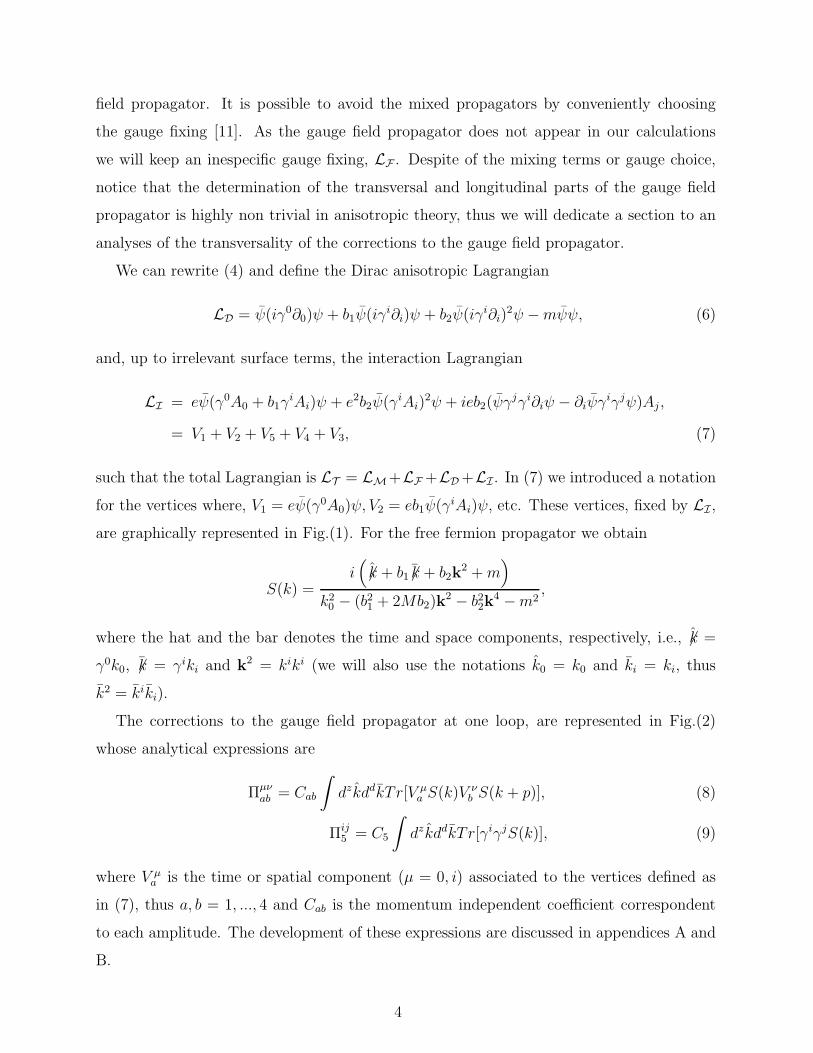
field propagator. It is possible to avoid the mixed propagators by conveniently choosing
the gauge fixing [11]. As the gauge field propagator does not appear in our calculations
we will keep an inespecific gauge fixing, LF . Despite of the mixing terms or gauge choice,
notice that the determination of the transversal and longitudinal parts of the gauge field
propagator is highly non trivial in anisotropic theory, thus we will dedicate a section to an
analyses of the transversality of the corrections to the gauge field propagator.
We can rewrite (4) and define the Dirac anisotropic Lagrangian
LD = ψ(iγ0∂0)ψ + b1ψ(iγi∂i)ψ + b2ψ(iγ
i∂i)2ψ −mψψ, (6)
and, up to irrelevant surface terms, the interaction Lagrangian
LI = eψ(γ0A0 + b1γiAi)ψ + e2b2ψ(γ
iAi)2ψ + ieb2(ψγ
jγi∂iψ − ∂iψγiγjψ)Aj ,
= V1 + V2 + V5 + V4 + V3, (7)
such that the total Lagrangian is LT = LM+LF+LD+LI . In (7) we introduced a notation
for the vertices where, V1 = eψ(γ0A0)ψ, V2 = eb1ψ(γiAi)ψ, etc. These vertices, fixed by LI ,
are graphically represented in Fig.(1). For the free fermion propagator we obtain
S(k) =i(
ˆ6k + b1¯6k + b2k2 +m
)
k20 − (b21 + 2Mb2)k2 − b22k
4 −m2,
where the hat and the bar denotes the time and space components, respectively, i.e., ˆ6k =
γ0k0, ¯6k = γiki and k2 = kiki (we will also use the notations k0 = k0 and ki = ki, thus
k2 = kiki).
The corrections to the gauge field propagator at one loop, are represented in Fig.(2)
whose analytical expressions are
Πµνab = Cab
∫
dzkddkT r[V µa S(k)V
νb S(k + p)], (8)
Πij5 = C5
∫
dzkddkT r[γiγjS(k)], (9)
where V µa is the time or spatial component (µ = 0, i) associated to the vertices defined as
in (7), thus a, b = 1, ..., 4 and Cab is the momentum independent coefficient correspondent
to each amplitude. The development of these expressions are discussed in appendices A and
B.
4
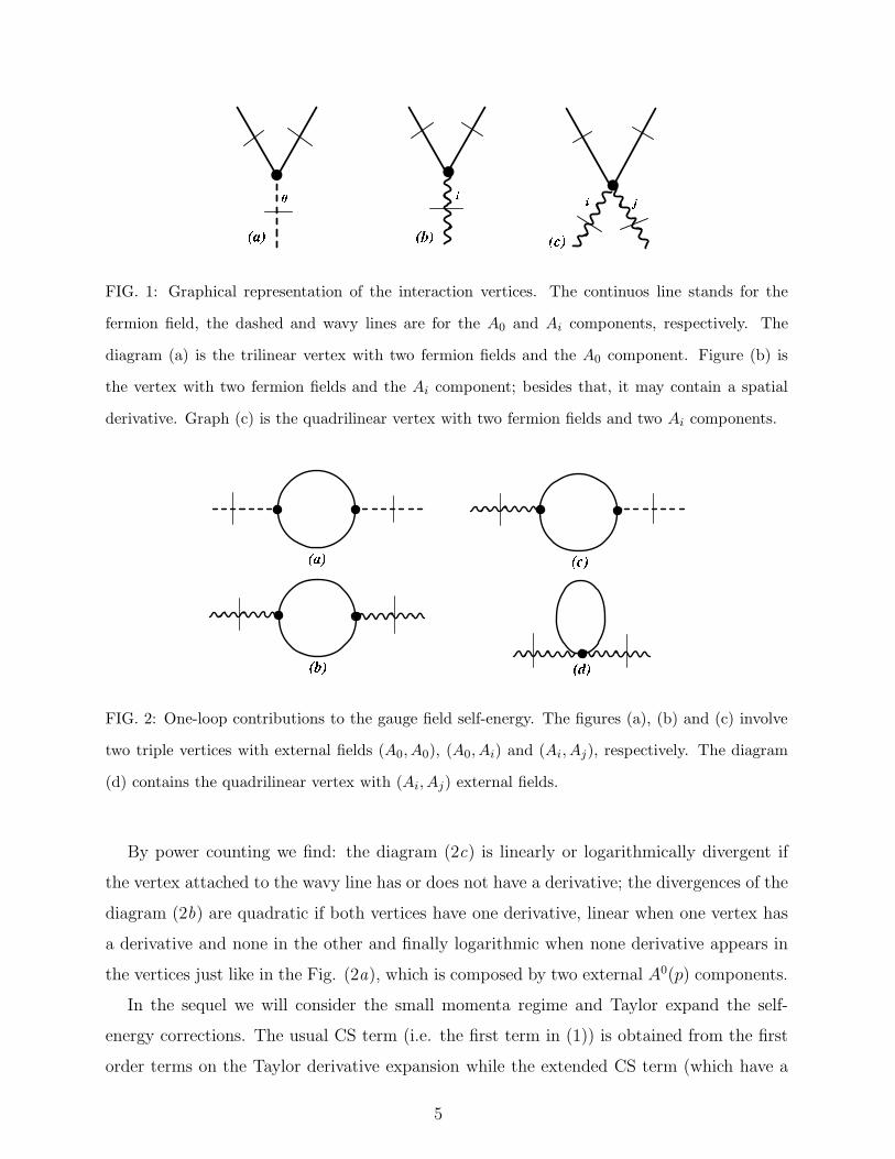
FIG. 1: Graphical representation of the interaction vertices. The continuos line stands for the
fermion field, the dashed and wavy lines are for the A0 and Ai components, respectively. The
diagram (a) is the trilinear vertex with two fermion fields and the A0 component. Figure (b) is
the vertex with two fermion fields and the Ai component; besides that, it may contain a spatial
derivative. Graph (c) is the quadrilinear vertex with two fermion fields and two Ai components.
FIG. 2: One-loop contributions to the gauge field self-energy. The figures (a), (b) and (c) involve
two triple vertices with external fields (A0, A0), (A0, Ai) and (Ai, Aj), respectively. The diagram
(d) contains the quadrilinear vertex with (Ai, Aj) external fields.
By power counting we find: the diagram (2c) is linearly or logarithmically divergent if
the vertex attached to the wavy line has or does not have a derivative; the divergences of the
diagram (2b) are quadratic if both vertices have one derivative, linear when one vertex has
a derivative and none in the other and finally logarithmic when none derivative appears in
the vertices just like in the Fig. (2a), which is composed by two external A0(p) components.
In the sequel we will consider the small momenta regime and Taylor expand the self-
energy corrections. The usual CS term (i.e. the first term in (1)) is obtained from the first
order terms on the Taylor derivative expansion while the extended CS term (which have a
5
form like the second and third terms in (1)) is given by the third order terms. Considering
that the highest divergence is quadratic, the extended CS contributions, which are of third
order on Taylor expansion, are of course finite. Differently, for the usual CS terms, the
algebra reduces the degree of divergence of some diagrams only to logarithmic so that they
requires the introduction of a regularization scheme. Similarly to the relativistic theory, in
the sense that there is a regularization dependence, there is an ambiguity on the induced
CS term.
For the even terms in the momentum expansion, which do not contribute to the CS terms,
the integration on momenta furnishes hypergeometric functions, as indicated in the appendix
A. In this case, the divergences are characterized by the Schwinger parameter, x, which
receives contributions from the hypergeometric and from the coefficients associated to them
(see Eq. A2). To integrate on the x parameter, we will power expand the hypergeometric
for small x and d = 2, until its exponent becomes nonnegative. Observe that, here the
isotropic limit, b2 → 0, cannot be taken singly because it is inconsistent with the small x
expansion. However, although the divergent terms individually exhibit poles for d = 2, they
are canceled when summed to produce the total self-energy correction, allowing for a smooth
isotropic limit.
III. TRANSVERSALITY OF THE GAUGE SELF-ENERGY
The conservation of the Noether’s current
J0 = ψγ0ψ, (10)
Jk = b1ψγkψ − ib2
[
(∂iψ)γiγkψ − ψγkγi(∂iψ)
]
+ eb2[
ψγiγkψ + ψγkγiψ]
Ai .
allows us to prove the transversality of the self-energy corrections. Indeed, we may write
the LI in terms of the above current
LI =e
2
[
AµJµ(Aρ=0) + AµJ
µ]
, (11)
where in the first term, the argument of the current (Aρ) must be taken equal to zero.
Now, in computing of the self-energy contributions notice that it is equal to
〈TδSI
δAµ
δSI
δAν〉 ∝ 〈JµJν〉 , (12)
6
where SI =∫
LI is the interaction action; (12) must be transversal due to the conservation
of the current.
IV. CONCLUDING REMARKS
In this work we studied the effects of the anisotropy of the spacetime on the generation
of the CS term and on the self-energy correction to the gauge field propagator. We proved
that this correction is transversal by constructing the conserved Noether’s current which
interacts with the gauge field.
Some interesting aspects of the calculation are related to the structure of the divergences.
For the even part of the gauge field self-energy, there are seven amplitudes involving the
new vertices which are divergent and their pole terms break gauge invariance. Nevertheless,
a contribution coming from the usual vertices cancel these divergences.
There are two types of CS terms that may be induced by the radiative corrections, the
usual CS term which contains just one derivative and the extended CS term with three
derivatives. Whereas the second type of CS term is always finite, the usual one presents
results which are divergent but these divergences notabily cancel among themselves when
the total contribution is considered. Furthermore, the coefficient of the usual CS term is
regularization dependent and vanishes if dimensional reduction is adopted. In this situa-
tion, one is forced to consider the extended CS term which constitute then the dominant
contribution.
By referring to the usual CS terms, notice that the contributions coming from the usual
vertices are finite, therefore free from ambiguities caused by the regularization. On the
other hand, the contributions coming from the new vertices are regularization dependent.
Besides that, the explicit b2 factor from that vertices is canceled because it is multiplied
by amplitudes which diverge as b2 → 0, this furnishes non zero contributions when the
isotropic limit is considered. Consequently, the regularization dependence is restored and in
the isotropic limit unexpected results, as the just mentioned vanishing of the usual CS term
if dimensional reduction is employed, are obtained.
Considering the extended CS, all amplitudes associated to it are finite even if b2 → 0.
The isotropic limit for these terms is smooth remaining only the contributions coming from
the usual vertices.
7
By considering the Eqs. (B1) and (B2), the induced CS terms can be written as
ΠµνCS = −
[αµν + p2 + p2(b21 + 4mb2)] e2b21ǫ
µνρpρ
48πm2(b21 + 4mb2)(13)
in accord with our proposal (1). Notice that the breaking of the Lorentz invariance is a very
simple function of b1 and b2 and that in the isotropic limit with b1 = 1 the Lorenz symmetry
is restored.
Acknowledgments
This work was partially supported by Fundacao de Amparo a Pesquisa do Estado de Sao
Paulo (FAPESP), Conselho Nacional de Desenvolvimento Cientıfico e Tecnologico (CNPq)
and Coordenacao de Aperfeicoamento de Pessoal de Nıvel Superior (CAPES). (FP) ac-
knowledge the support to this research by Direccion de Investigacion y Desarrollo de la
Universidad de La Frontera and Facultad de Ingenierıa, Ciencias y Administracion, Univer-
sidad de La Frontera (Temuco-Chile) .
Appendix A: The calculation procedure
In this appendix we will describe the procedure employed to calculate the Feynman
diagrams. As an example, we will consider the amplitude given by the vertices (eb1ψγiψAi)
and (eb1ψγjψAj) which leads us to:
Πij(p) =(eb1)
2
(2π)3
∫
dkddk Tr[γiS(k)γjS(k − p)]. (A1)
To solve (A1) we adopt the dimensional reduction scheme, in which all the algebra of
the gamma matrices are done in d = 2 and afterwards the integral is promoted to d di-
mensions [20]. Therefore, the leading term in the Taylor expansion, i.e. the term with
(p = 0, p = 0) is
−(eb1)
2
(2π)3
∫
dkddk
[
2gij[m2 − k2 − b2k2(−k2b2 − 2M)]
(k2 − k2(b21 + 2Mb2)− k4b22 −m2)2
]
.
To perform the above integral, we use the Schwinger’s representation and integrate on the
momenta. The result is very extensive, therefore we will consider just one of the terms which
8
leads to a divergent result:
e−iM2xx−d/41F1
(
d+ 2
4;1
2;ix(b21 + 2Mb2)
2
4b22
)
, (A2)
where x is the Schwinger parameter and 1F1 denotes the hypergeometric function. Note
that this function is divergent in the limit x → 0, so we will Taylor expand it, up to a
nonnegative power of x for d = 2. Thus we obtain
x−d/41F1
(
d+ 2
4;1
2;ix(b21 + 2Mb2)
2
4b22
)
→ x−d/4
(
1 + 2d+ 2
4
ix(b21 + 2Mb2)2
4b22
)
(A3)
The final result is obtained by integrating on x and expanding the result around d = 2, such
that the general results for this amplitude is given by
ie2b21gij
2πb2(d− 2)+ finite. (A4)
Notice that this divergence is absent in the relativistic theory because it clearly comes from
modifications introduced by the anisotropy. Observe also that from the argument of the
hypergeometric function in (A2) that the isotropic limit, (b2 → 0), is incompatible with the
adopted expansion for x→ 0.
On the other hand, if we consider the subleading term in the Taylor expansion, responsible
for the usual CS term, i.e. ∂Πij
∂p
∣
∣
∣
p=p=0, the result is
(eb1)2
(2π)3
∫
dkddk
[
2iǫij0(m− b2k2)
(k2 − k2(b21 + 2Mb2)− k4b22 −m2)2
]
. (A5)
To compute the above integral, which is finite by power counting, we simply take d = 2 and
integrate on the momenta.
Appendix B: Interaction vertices
In this appendix we will present the one loop contributions, for small momenta, to the
self-energy of the gauge field. From the interaction Lagrangian we observe that we have a
total of 12 different amplitudes coming from the Wick’s contractions of the vertices. The
sum of all contributions gives (further details will be presented elsewhere):
ΠijCS = −
[αij + p2(b21 + 4mb2) + p2] e2b21ǫij0p0
48πm2(b21 + 4mb2)(B1)
9

and
Π0iCS = −
[α0i + p2(b21 + 4mb2) + p2] e2b21ǫ0iapa
48πm2(b21 + 4mb2)(B2)
where αij and α0i are constant parameters introduced in (B1) and (B2), respectively, to
denote the ambiguity coming from the regularization scheme. We may note that there is
a cancellation of the usual CS term, remaining only regularization dependent terms. This
occurs due to the contributions of the new vertices introduced by the anisotropy and by the
fact that their b2 vertex factor is eliminated after performing the momenta integrals.
In the isotropic limit b2 → 0 of (B1) and (B2) all the extended CS terms coming from
the new vertices contributions are cancelled and we get
ΠijCS = −
e2 (αij + b21p2 + p2) ǫij0p0
48πm2
and
Π0iCS = −
e2 (α0i + b21p2 + p2) ǫ0iapa
48πm2.
By taken b1 = 1 we obtain an expression similar to that one introduced in [19].
[1] R. A. Konoplya, Phys. Lett. B 679, 499 (2009); E. Kiritsis, G. Kofinas, Nucl. Phys. B 821,
467 (2009); G. Bertoldi, B. A. Burrington and A. W. Peet, Phys. Rev. D 82, 106013 (2010);
K. Goldstein, S. Kachru, S. Prakash, S. P. Trivedi, JHEP 1008, 078 (2010); F. S. Bemfica
and M. Gomes, Phys. Rev. D 84, 084022 (2011); E. Abdalla and A. M. da Silva, Phys. Lett.
B 707, 311 (2012); H. Lu, Y. Pang, C. N. Pope and J. F. Vazquez-Poritz, Phys. Rev. D 86,
044011 (2012); H. Liao, J. Chen and Y. Wang, Int. J. Mod. Phys. D 21, 1250045 (2012);
O. Obregon and J. A. Preciado, Phys. Rev. D 86, 063502 (2012).
[2] R. Gregory, S. L. Parameswaran, G. Tasinato and I. Zavala, JHEP 1012, 047 (2010); A.
Donos and J. P. Gauntlett, JHEP 1012, 002 (2010); K. Balasubramanian and K. Narayan,
JHEP 1008, 014 (2010); H. Singh, JHEP 1104, 118 (2011); W. Chemissany and J. Hartong,
Class. Quant. Grav. 28, 195011 (2011); D. Cassani and A. F. Faedo, JHEP 1105, 013 (2011);
K. Narayan, Phys. Rev. D 85, 106006 (2012); P. Dey and S. Roy, JHEP 1206, 129 (2012).
[3] D. T. Son, Nucl. Phys. Proc. Suppl. 195, 217 (2009); S. A. Hartnoll, Class. Quant. Grav. 26,
224002 (2009); R. G. Cai and H. Q. Zhang, Phys. Rev. D 81, 066003 (2010); E. J. Brynjolfsson,
10
U. H. Danielsson, L. Thorlacius and T. Zingg, J. Phys. A 43, 065401 (2010); D. Momeni,
M. R. Setare and N. Majd, JHEP 1105, 118 (2011); S. J. Sin, S. S. Xu and Y. Zhou, Int. J.
Mod. Phys. A 26, 4617 (2011).
[4] M. R. Douglas and N. A. Nekrasov, Rev. Mod. Phys. 73, 977 (2001); B. Charneski, A. F. Fer-
rari and M. Gomes, J. Phys. A 40, 3633 (2007); M. Gomes, V. G. Kupriyanov and A. J. da
Silva, Phys. Rev. D 81, 085024 (2010); M. Gomes, V. G. Kupriyanov and A. J. da Silva, J.
Phys. A 43, 285301 (2010).
[5] D. Colladay and V. A. Kostelecky, Phys. Rev. D 58, 116002 (1998).
[6] B. Charneski, M. Gomes, T. Mariz, J. R. Nascimento and A. J. da Silva, Phys. Rev. D 79,
065007 (2009).
[7] V. A. Kostelecky, N. Russell, Rev. Mod. Phys. 83, 11 (2011); B. Charneski, M. Gomes,
R. V. Maluf and A. J. da Silva, Phys. Rev. D 86, 045003 (2012).
[8] D. Anselmi and M. Halat, Phys. Rev. D 76, 125011 (2007); D. Anselmi, Ann. Phys. 324, 874
(2009); D. Anselmi Ann. Phys. 324, 1058 (2009); M. Visser, Phys. Rev. D 80, 025011 (2009).
[9] P. Horava, Phys. Rev. D 79, 084008 (2009); JHEP 0903, 020 (2009).
[10] R. Iengo, J. G. Russo and M. Serone, JHEP 0911, 020 (2009); R. Iengo and M. Serone, Phys.
Rev. D 81, 125005 (2010); P. R. S. Gomes and M. Gomes, Phys. Rev. D 85, 065010 (2012);
P. R. S. Gomes and M. Gomes, Phys. Rev. D 85, 085018 (2012); K. Farakos and D. Metaxas,
Phys. Lett. B 711, 76 (2012); J. Alexandre, J. Brister and N. Houston, Phys. Rev. D 86,
025030 (2012).
[11] C. F. Farias, M. Gomes, J. R. Nascimento, A. Yu. Petrov and A. J. da Silva, Phys. Rev. D
85, 127701 (2012).
[12] S. Deser, R. Jackiw and S. Templeton, Phys. Rev. Lett. 48, 975 (1982); S. Deser, R. Jackiw
and S. Templeton, Ann. Phys. 140, 372 (1982).
[13] J. S. Schonfeld, Nucl. Phys. B185, (1981); R. Jackiw, Phys. Rev. D29, 2375 (1984).
[14] A. J. Niemi and G. W. Semenoff, Phys. Rev. Lett. 51, 2077 (1983); A. N. Redlich, Phys. Rev.
Lett. 52, 18 (1984); Phys. Rev. D29, 2366 (1984).
[15] A. Foerster and H. O. Girotti, Nucl. Phys. B 342, 680 (1990).
[16] E. Witten, Prog. Math. 133, 637 (1995); M. Marino, Rev. Mod. Phys. 77, 675 (2005); K. Bal-
asubramanian and J. McGreevy, Class. Quant. Grav. 29, 194007 (2012).
[17] R. E. Prange and S. M. Girvin, The Quantum Hall Effect, Springer, Berlin, (1987); T.
11
Chkraborty and P. Pietilainen, The Fractional Quantum Hall Effect, Springer Verlag, (1988);
A. Lopez and E. Fradkin, Phys. Rev. B 44, 5246 (1991).
[18] R. B. Laughlin, Phys. Rev. B23, 5632 (1981); B. I. Halperin, Phys. Rev. B25, 2185 (1982);
F. Wilczek and A. Zee, Phys. Lett. 51, (1983) 2250; Y. Wu and A. Zee, Phys. Lett. 147B
(1984) 325; F. Wilczek, E. Witten and B. I. Halperin, Int. J. Mod. Phys. B3, 1001 (1989);
F. Wilczek, Fractional Statistics and Anyon Superconductivity, World Scientific, Singapore,
(1990); X. G. Wen and A. Zee, Phys. Rev. B41, 240 (1990); J. D. Lykken and J. Sonnenshein
and N. Weiss, Int. J. Mod. Phys. A6, 5155 (1991).
[19] S. Deser and R. Jackiw, Phys. Lett. B 451, 73 (1999).
[20] W. Siegel, Phys. Lett. B 84, 193 (1979).
12