1392 IEEE TRANSACTIONS ON BIOMEDICAL ENGINEERING, VOL. 47, NO. 10, OCTOBER 2000

Three-Dimensional Geometric Modeling of theCochlea Using Helico-Spiral Approximation

Sun K. Yoo*, Ge Wang, Senior Member, IEEE, Jay T. Rubinstein, Member, IEEE, andMichael W. Vannier, Member, IEEE

Abstract—In this paper, the three-dimensional geometry of thehuman cochlea is modeled by the helico-spiral seashell model.The 3-D helico-spiral model, the generalized representation of theArchimedian spiral model, provides a framework for measuringcochlear features based on consistent estimation of model param-eters. Nonlinear least square minimization based algorithms aredeveloped for the identification of rotation, center and intrinsicparameters of the helico-spiral representation. Two algorithmsare designed for the rotation axis aligned to the modiolar axis:one is more susceptible in the presence of noise, while the otherallows applicability to two-dimensional data sets. The estimatedcenter and intrinsic parameters allow the calculation of length,height and angular positions needed for frequency mapping ofmultichannel cochlear implant electrodes. Model performanceis evaluated with numerically synthesized curves with differentlevels of added random noise, histologic data and real humancochlear spiral computed tomography data.

Index Terms—Cochlear implantation, geometric model, helico-spiral approximation, nonlinear optimization.

I. INTRODUCTION

T HREE-DIMENSIONAL (3-D) geometric modeling of thehuman cochlea may be important for both preoperative

surgical planning and postoperative programming of multi-channel cochlear implants [1]–[6]. Cochlear implantation hasbecome a standard clinical intervention performed worldwidefor severe-profound deafness. The position of the implantedelectrode array within the cochlea has been postulated as oneof the important variables for speech recognition [1], [3], [5],[7] and provides critical parameters for an electro-anatomicalmodel of the implanted cochlea [8].

The cochlear dimensions including length and fractionallength have been measured from post-mortem temporal bonehistologic sections using computer-aided 3-D reconstruction[1], [2], [4]. Plain X-ray [5], [9] and spiral computed tomog-raphy (CT) [3], [6], [7], [10] have been used to define cochlearlength for individual patientsin vivo. Plain X-ray is the mostpopular in practice and offers high resolution for the implanted

Manuscript received November 19, 1999; revised June 5, 2000. This workwas supported in part by the Yonsei University Faculty Scholarship for foreignvisiting research and by the National Institutes of Health (NIH) under GrantDC03590.Asterisk indicates corresponding author..

*S. K. Yoo is with the Department of Radiology, The University of IowaSchool of Medicine, 200 Hawkins Dr., 3984 JPP, Iowa, USA and the Departmentof Medical Engineering, Yonsei University College of Medicine, Seoul, Korea(e-mail: sun-yoo@.uiowa.edu).

G. Wang and M. W. Vannier are with the Department of Radiology, The Uni-versity of Iowa School of Medicine, Iowa City, IA, 52242 USA.

J. T. Rubinstein is with the Department of Otolaryngology and Neck Surgery,The University of Iowa School of Medicine, Iowa City, IA, 52242 USA.

Publisher Item Identifier S 0018-9294(00)08529-3.

electrode array, but it is insufficient to obtain 3-D informationdue to the nature of two-dimensional (2-D) projection. SpiralCT provides high-resolution images for both the cochleaand the implanted electrode array, and sectional images forfacilitating 3-D visualization and measurement, but it can notdistinguish implanted electrodes due to metal artifact [3], [8],[10], [11].

Geometric modeling has been used to extract positional infor-mation from images acquired from either plain X-ray or spiralCT. Cohenet al. [5] modeled the implanted electrode array asa template spiral to measure each implanted electrode location.The inserted electrode array is visualized by plain X-ray andthen matched to the template spiral model. Particularly, anglerather than length is measured to specify the electrode position.Cohen’s model provides a relatively straightforward method forclinical assessment of electrode-frequency distribution. How-ever, the 2-D model limits application of the 3-D data set andcan not be applied to preoperative images because of the needto extract the implanted electrode array. Kettenet al. [3], [12]generated a 3-D model to measure the cochlear length. Parame-ters of the 3-D Archimedian spiral model are estimated by mea-suring the radius of each half turn and the height of the cochleaat some defined landmark points. Ketten’s model compensatesfor length compression induced by the 2-D projection [1], [2],is independent of the implanted electrode array and applicableto both preoperative and post-operative data. However, modelestimation might be sensitive to selected landmark points allo-cated manually from 3-D volumes.

All modeling methods require information on patient orien-tation: modified Stenver’s view [9] for plain X-ray, and modi-olar projection [3], [6] for spiral CT. However, cochlear tiltvaries among individuals and allocation of the anatomical fea-tures varies among observers. It is more difficult to determinelandmarks in some patients because of osteogenic changes orcapsular degeneration [3]. Therefore, there is a need for geo-metric modeling of the cochlea independent of the patient ori-entation. Such models should work with both preoperative andpost-operative images for cochlear implantation.

Many natural and man-made structures are well modeled bythe logarithmic spiral, particularly seashells. We have adoptedFowler’s helico-spiral seashell model [13] to geometrically rep-resent the human cochlea. Fowler’s model is the same as an ex-pansion of the 2-D Cohen’s logarithmic spiral into 3-D by incor-porating another logarithmic term to represent height displace-ment of the cochlea. Using the helico-spiral model, we devisetwo algorithms to automatically align a patient’s head orienta-tion: the first one is applicable only to a 3-D data set (spiral

0018–9294/00$10.00 © 2000 IEEE

YOO et al.: THREE-DIMENSIONAL GEOMETRIC MODELING OF THE COCHLEA USING HELICO-SPIRAL APPROXIMATION 1393

CT) and is more accurate than the second, but the second canalso be applied to the 2-D data set (plain X-ray). Least squareoptimization is used to fit measurements into the helico-spiralmodel. This provides an efficient way to analyze cochlear fea-tures including length, angle, and height from the spiral CTvolume obtained clinically prior to cochlear implantation. Wepresent the cochlear model, algorithms, and optimization in thenext section. The performance of our methods is evaluated viasimulations and experiments in Section III. The efficiency of ourmethods is discussed in Section IV.

II. M ATERIALS AND METHODS

A. 3-D Geometric Model

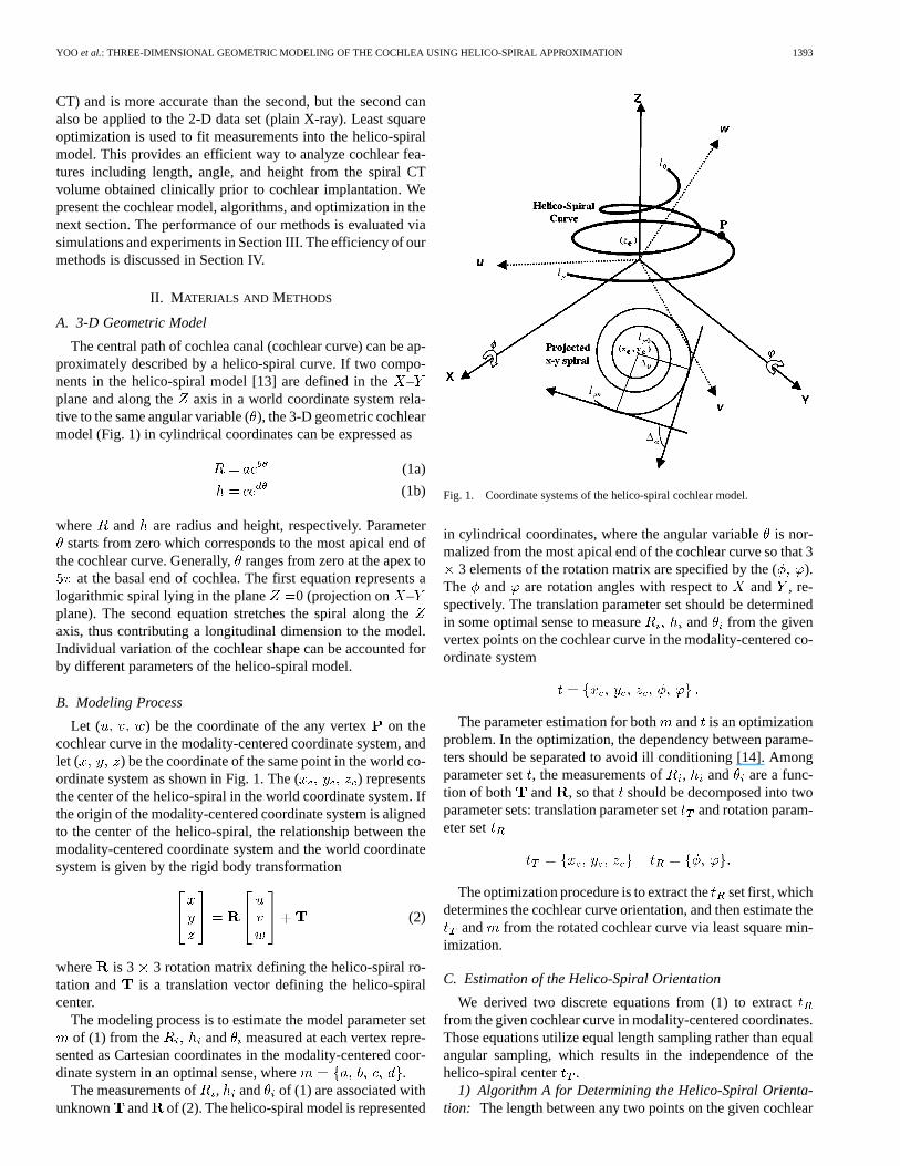
The central path of cochlea canal (cochlear curve) can be ap-proximately described by a helico-spiral curve. If two compo-nents in the helico-spiral model [13] are defined in the–plane and along the axis in a world coordinate system rela-tive to the same angular variable (), the 3-D geometric cochlearmodel (Fig. 1) in cylindrical coordinates can be expressed as

(1a)

(1b)

where and are radius and height, respectively. Parameterstarts from zero which corresponds to the most apical end of

the cochlear curve. Generally,ranges from zero at the apex toat the basal end of cochlea. The first equation represents a

logarithmic spiral lying in the plane 0 (projection on –plane). The second equation stretches the spiral along theaxis, thus contributing a longitudinal dimension to the model.Individual variation of the cochlear shape can be accounted forby different parameters of the helico-spiral model.

B. Modeling Process

Let ( ) be the coordinate of the any vertexon thecochlear curve in the modality-centered coordinate system, andlet ( ) be the coordinate of the same point in the world co-ordinate system as shown in Fig. 1. The ( ) representsthe center of the helico-spiral in the world coordinate system. Ifthe origin of the modality-centered coordinate system is alignedto the center of the helico-spiral, the relationship between themodality-centered coordinate system and the world coordinatesystem is given by the rigid body transformation

(2)

where is 3 3 rotation matrix defining the helico-spiral ro-tation and is a translation vector defining the helico-spiralcenter.

The modeling process is to estimate the model parameter setof (1) from the and measured at each vertex repre-

sented as Cartesian coordinates in the modality-centered coor-dinate system in an optimal sense, where .

The measurements of , and of (1) are associated withunknown and of (2). The helico-spiral model is represented

Fig. 1. Coordinate systems of the helico-spiral cochlear model.

in cylindrical coordinates, where the angular variableis nor-malized from the most apical end of the cochlear curve so that 3

3 elements of the rotation matrix are specified by the ().The and are rotation angles with respect to and , re-spectively. The translation parameter set should be determinedin some optimal sense to measure and from the givenvertex points on the cochlear curve in the modality-centered co-ordinate system

The parameter estimation for bothand is an optimizationproblem. In the optimization, the dependency between parame-ters should be separated to avoid ill conditioning [14]. Amongparameter set, the measurements of , and are a func-tion of both and , so that should be decomposed into twoparameter sets: translation parameter setand rotation param-eter set

The optimization procedure is to extract theset first, whichdetermines the cochlear curve orientation, and then estimate the

and from the rotated cochlear curve via least square min-imization.

C. Estimation of the Helico-Spiral Orientation

We derived two discrete equations from (1) to extractfrom the given cochlear curve in modality-centered coordinates.Those equations utilize equal length sampling rather than equalangular sampling, which results in the independence of thehelico-spiral center .

1) Algorithm A for Determining the Helico-Spiral Orienta-tion: The length between any two points on the given cochlear

1394 IEEE TRANSACTIONS ON BIOMEDICAL ENGINEERING, VOL. 47, NO. 10, OCTOBER 2000

curve in the modality-centered coordinates can be measured in-dependent of angular measurement, and the center and orien-tation of the helico-spiral. The cochlear curve can be uniformlysampled with an equal length increment, and the Cartesian co-ordinate ( ) in modality-centered coordinates for eachsampled point ( ) can be measured, wherecorresponds to the measured height of (1b) in the modality-cen-tered coordinate system. The measuredapproximately repre-sents (3) in the discrete domain. The mathematical derivation of(3) from (1) is in Appendix I. Let be the difference between

and in the modality-centered coordinate system.

(3)

where and are parameters. We denote

(4)

From (3), we can estimate from instead of the pa-rameter set in the helico-spiral model. No dependency on thespiral center exists in (4).

The mean square error (MSE) between estimatedandmeasured depends on the values of the rotation parameterset . The more the helico-spiral rotates, the more the shapeof helico-spiral will be distorted. The deviation of measuredin the modality-centered coordinate system compared to the trueheight of (1b) in the world coordinate system increases as the ro-tation angles increase. Since the measurement ofis affectedby acquisition and approximation noise [10], the orientation cor-rection problem for algorithm A is equivalent to a nonlinear op-timization, in which , and are determined by minimizingan objective function

(5)

The nonlinear optimization can be numerically solved by thesteepest-decent algorithm [14], in which is repeatedly up-dated until is less than a threshold ( ).This process can be formulated as follows:

(6)

(7)

(8)

where and are convergence factors, and and. are thresholds.

2) Algorithm B for Determining the Helico-Spiral Orienta-tion: While algorithm A utilizes the exponential variation inthe axis [equivalent to (1b)], algorithm B considers only thespiral-shape in the – plane [equivalent to (1a)]. Similar toalgorithm A, the helico-spiral projected onto the– plane(referred to as the projected- spiral) can be uniformly sam-pled with equal length if the projected vertices of the cochlearcurve are represented by a length parameterized description of

a spline curve [15] in the modality-centered coordinate system.The projected – spiral inherently has the equiangular prop-erty, in which the angle between the tangent and the radial lineat any sample point on the spiral curve is constant [15]. Hence,the angular variable of (1) is replaced by a summed tangentialangular difference ( ) between two consecutive sample pointsalong the projected – spiral. The derivation of (9) can befound in Appendix II

(9)

where is the relative length from the most apical end to thesample point. The tangential measurement at any point on thespiral curve is independent of the spiral center

(10)

From (9), parameter set instead of parameters ( ) of(1a) can be used to estimate the spiral shape from the measure-ments and length at each sample point in the modality-cen-tered coordinate system.

The shape distortion of the projected– spiral increases asthe rotation angle increases. Therefore, the variation ofisrelated to the angular rotation. Algorithm B is to determine fourunknown parameters in and by minimizing an objectivefunction

(11)

(12)

(13)

(14)

D. Estimation of Model Parameters and the Center of theHelico-Spiral

With , the given cochlear curve in the modality-centeredcoordinate system can be rotated to the correct orientation in thesense of maximally reflecting the spiral shape on the– planeand/or the axis. The remaining problem is to estimate two pa-rameter sets: for the spiral center and m for the helico-spiral.The optimum estimator in the least square sense for the param-eter set has the closed-form solution [14] if , , and( if the number of vertices is) at each vertexon the rotated cochlear curve are correctly measured. However,those measured values are associated with the unknown centerof the helico-spiral. Therefore, the estimation of parameter set

with unknown center is a nonlinear optimization problem.The amount of deviation of the measured values for, , and

is closely related to the discrepancy of the assumed centerrelative to the true center of the helico-spiral. The MSE be-tween estimated and measured values will be a function of thecenter location of the helico-spiral. Nonlinear optimizations for

YOO et al.: THREE-DIMENSIONAL GEOMETRIC MODELING OF THE COCHLEA USING HELICO-SPIRAL APPROXIMATION 1395

and are to minimize the objective functions:and .

(15a)

(15b)

where , and are estimated radius and height with re-spect to any fixed center, ( ). ( ) and ( ) inparameter set are independent of each other. The measured

and depend on ( ) and ( ) in , respectively.Therefore, ( ) and ( ) are separately estimatedby nonlinear optimization using the steepest-decent methodwith convergence factors ( ) and tolerance thresholds( )

(16a)

(16b)

where and are points defined on the– plane and theaxis in the world coordinate system. Those points are initially

assumed as the origin of the world coordinate system. In thisprocedure, the steepest-decent method as applied to (15a) and(15b) extracts ( ) and ( ) via iteration, while the optimumestimators for ( ) and ( ) have the closed form solutionsin the least square sense

(17a)

(17b)

(17c)

(17d)

E. Summary of the Modeling Procedures

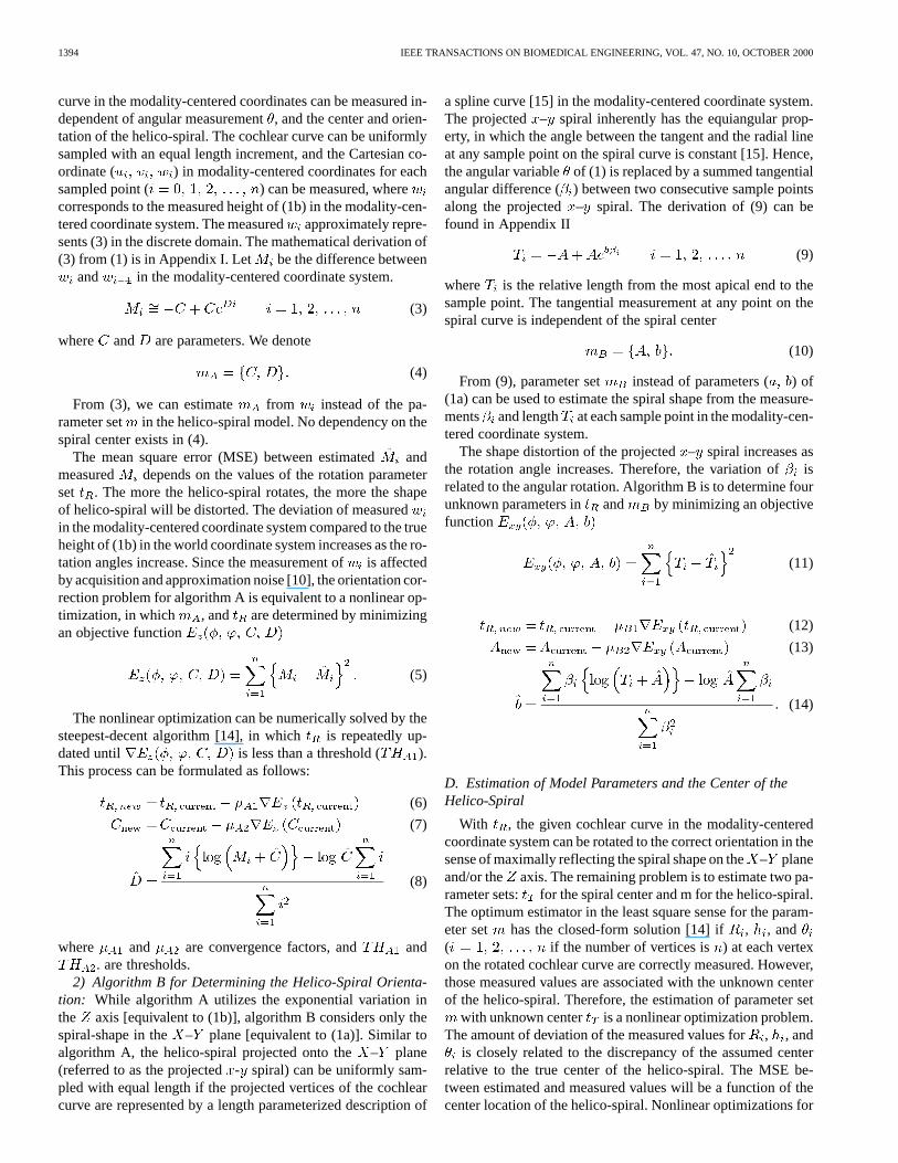
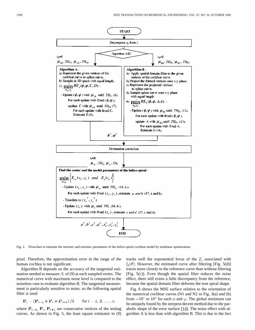
Initially, the cochlear curve can be extracted from the imagevolume acquired from an imaging modality, such as spiralCT. Fig. 2 shows the flowchart to fit the cochlea into a he-lico-spiral. It consists of two parts: rotation parameter estimationand combined estimation of both the model parameter andthe center of the helico-spiral model. The initial vector for

the steepest-decent loop starts from anduntil satisfying the threshold conditions, (

). The convergence factors, () control the converging speed. The

method estimates the optimum parameters, (), in which ( ) define the patient orien-

tation to the world coordinate system. ( ) specify thecenter of the helico-spiral. ( ) allow the estimationof the length, angle, and height.

III. RESULTS

A. Synthesis of Numerical Cochlear Central Curves

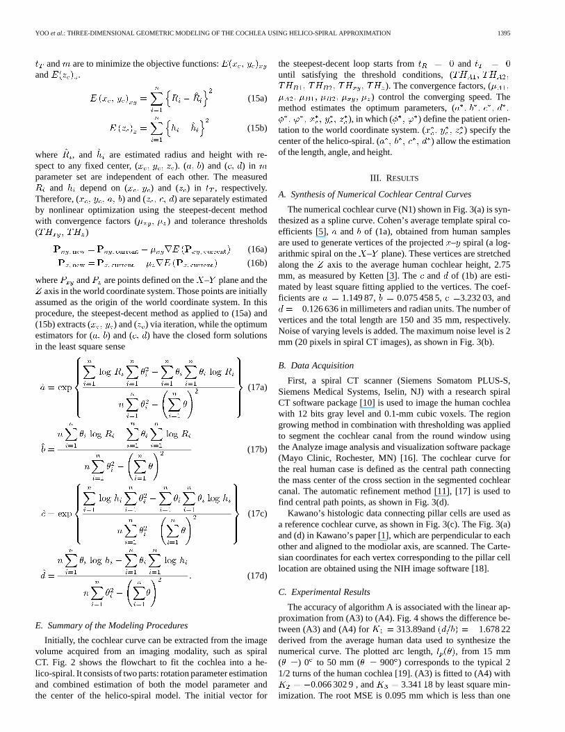
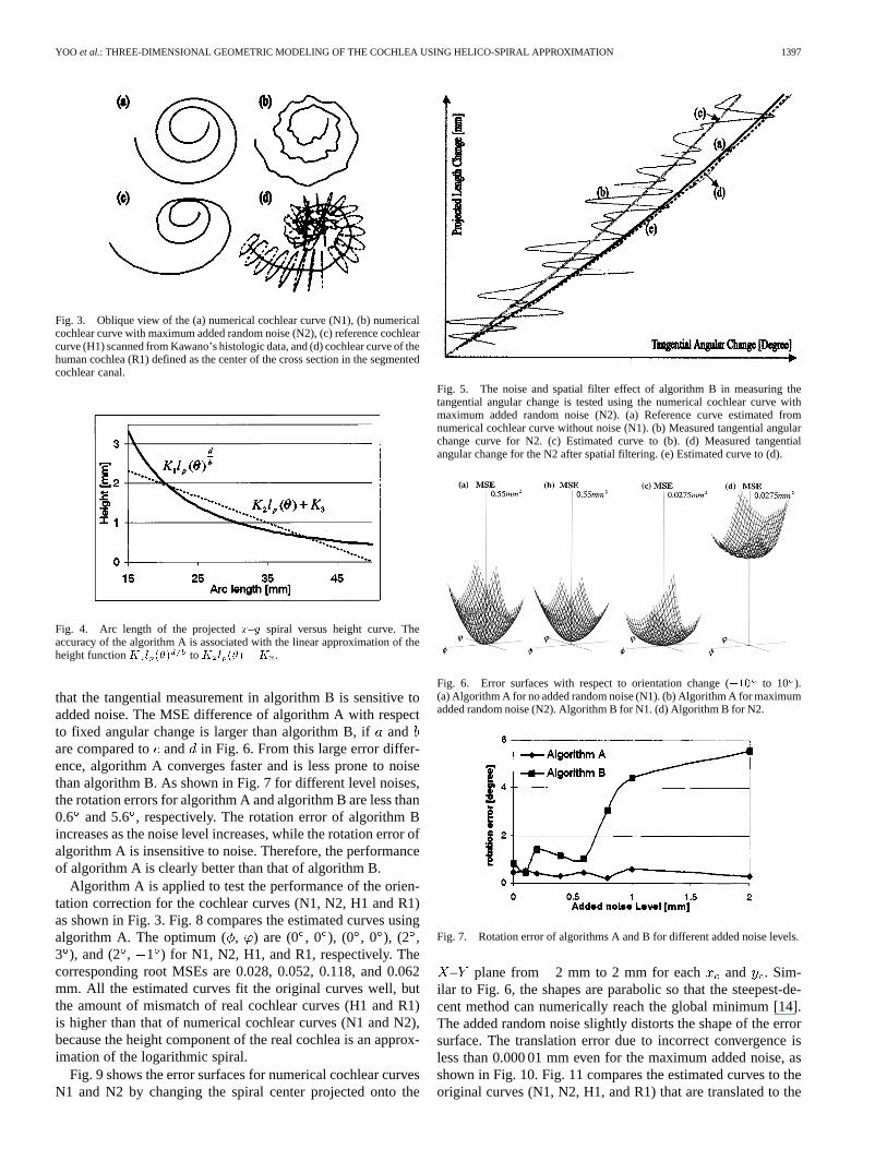
The numerical cochlear curve (N1) shown in Fig. 3(a) is syn-thesized as a spline curve. Cohen’s average template spiral co-efficients [5], and of (1a), obtained from human samplesare used to generate vertices of the projected– spiral (a log-arithmic spiral on the – plane). These vertices are stretchedalong the axis to the average human cochlear height, 2.75mm, as measured by Ketten [3]. Theand of (1b) are esti-mated by least square fitting applied to the vertices. The coef-ficients are 1.149 87, 0.075 458 5, 3.232 03, and

0.126 636 in millimeters and radian units. The number ofvertices and the total length are 150 and 35 mm, respectively.Noise of varying levels is added. The maximum noise level is 2mm (20 pixels in spiral CT images), as shown in Fig. 3(b).

B. Data Acquisition

First, a spiral CT scanner (Siemens Somatom PLUS-S,Siemens Medical Systems, Iselin, NJ) with a research spiralCT software package [10] is used to image the human cochleawith 12 bits gray level and 0.1-mm cubic voxels. The regiongrowing method in combination with thresholding was appliedto segment the cochlear canal from the round window usingthe Analyze image analysis and visualization software package(Mayo Clinic, Rochester, MN) [16]. The cochlear curve forthe real human case is defined as the central path connectingthe mass center of the cross section in the segmented cochlearcanal. The automatic refinement method [11], [17] is used tofind central path points, as shown in Fig. 3(d).

Kawano’s histologic data connecting pillar cells are used asa reference cochlear curve, as shown in Fig. 3(c). The Fig. 3(a)and (d) in Kawano’s paper [1], which are perpendicular to eachother and aligned to the modiolar axis, are scanned. The Carte-sian coordinates for each vertex corresponding to the pillar celllocation are obtained using the NIH image software [18].

C. Experimental Results

The accuracy of algorithm A is associated with the linear ap-proximation from (A3) to (A4). Fig. 4 shows the difference be-tween (A3) and (A4) for 313.89and 1.678 22derived from the average human data used to synthesize thenumerical curve. The plotted arc length, , from 15 mm( ) 0 to 50 mm ( 900 ) corresponds to the typical 21/2 turns of the human cochlea [19]. (A3) is fitted to (A4) with

0.066 302 9 , and 3.341 8 by least square min-imization. The root MSE is 0.095 mm which is less than one

1396 IEEE TRANSACTIONS ON BIOMEDICAL ENGINEERING, VOL. 47, NO. 10, OCTOBER 2000

Fig. 2. Flowchart to estimate the intrinsic and extrinsic parameters of the helico-spiral cochlear model by nonlinear optimization.

pixel. Therefore, the approximation error in the range of thehuman cochlea is not significant.

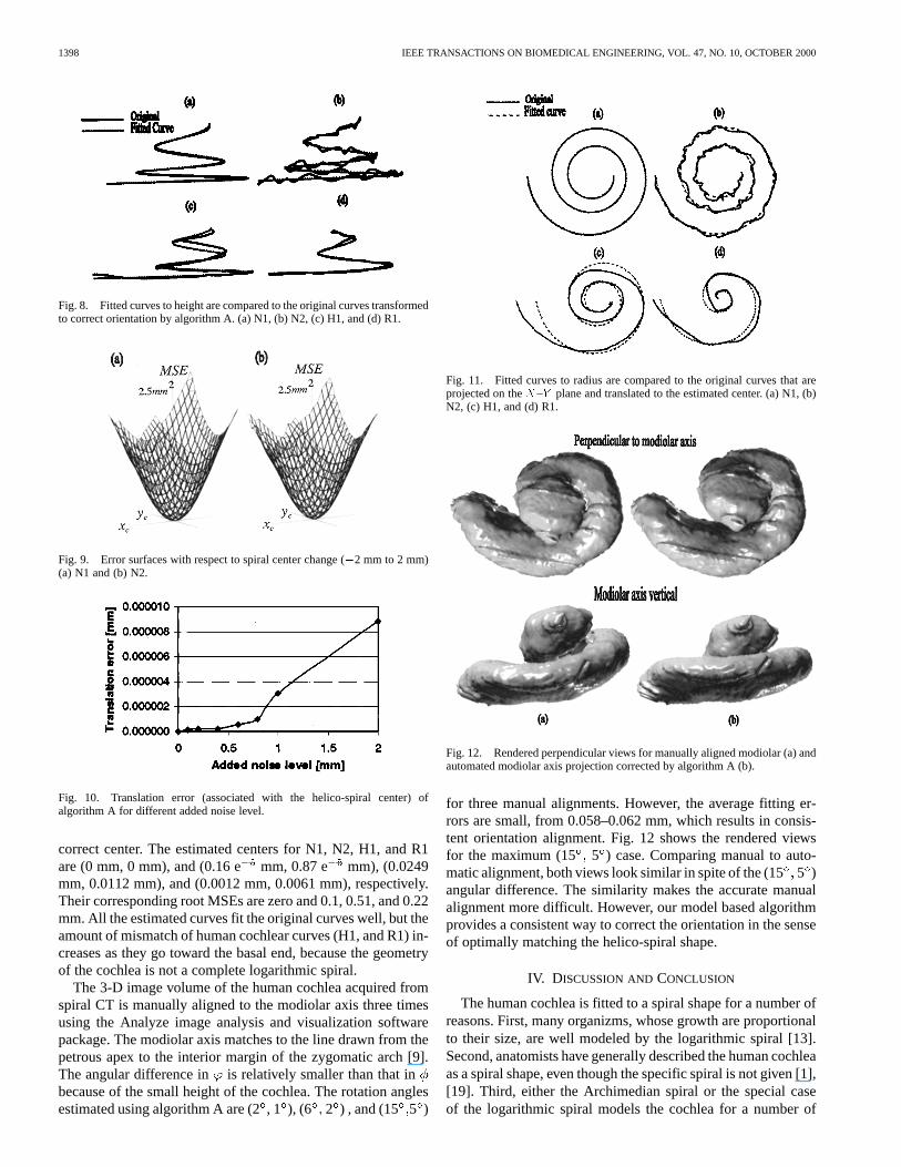
Algorithm B depends on the accuracy of the tangential esti-mation needed to measureof (9) at each sampled vertex. Thenumerical curve with maximum noise level is compared to thenoiseless case to evaluate algorithm B. The tangential measure-ment is particularly sensitive to noise, so the following spatialfilter is used

for

where are consecutive vertices of the testingcurves. As shown in Fig. 5, the least square estimator to (9)

tracks well the exponential locus of the associated with. However, the estimated curve after filtering [Fig. 5(d)]

traces more closely to the reference curve than without filtering[Fig. 5(c)]. Even though the spatial filter reduces the noiseeffect, there still exists a little discrepancy from the reference,because the spatial domain filter deforms the true spiral shape.

Fig. 6 shows the MSE surface relative to the orientation ofthe numerical cochlear curves (N1 and N2 in Fig. 3(a) and (b)from 10 to 10 for each and . The global minimum canbe uniquely found by the steepest-decent method due to the par-abolic shape of the error surface [14]. The noise effect with al-gorithm A is less than with algorithm B. This is due to the fact

YOO et al.: THREE-DIMENSIONAL GEOMETRIC MODELING OF THE COCHLEA USING HELICO-SPIRAL APPROXIMATION 1397

Fig. 3. Oblique view of the (a) numerical cochlear curve (N1), (b) numericalcochlear curve with maximum added random noise (N2), (c) reference cochlearcurve (H1) scanned from Kawano’s histologic data, and (d) cochlear curve of thehuman cochlea (R1) defined as the center of the cross section in the segmentedcochlear canal.

Fig. 4. Arc length of the projectedx–y spiral versus height curve. Theaccuracy of the algorithm A is associated with the linear approximation of theheight functionK l (�) to K l (�) +K .

that the tangential measurement in algorithm B is sensitive toadded noise. The MSE difference of algorithm A with respectto fixed angular change is larger than algorithm B, ifandare compared to and in Fig. 6. From this large error differ-ence, algorithm A converges faster and is less prone to noisethan algorithm B. As shown in Fig. 7 for different level noises,the rotation errors for algorithm A and algorithm B are less than0.6 and 5.6, respectively. The rotation error of algorithm Bincreases as the noise level increases, while the rotation error ofalgorithm A is insensitive to noise. Therefore, the performanceof algorithm A is clearly better than that of algorithm B.

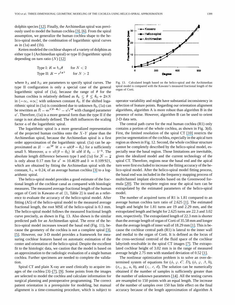
Algorithm A is applied to test the performance of the orien-tation correction for the cochlear curves (N1, N2, H1 and R1)as shown in Fig. 3. Fig. 8 compares the estimated curves usingalgorithm A. The optimum (, ) are (0 , 0 ), (0 , 0 ), (2 ,3 ), and (2 , 1 ) for N1, N2, H1, and R1, respectively. Thecorresponding root MSEs are 0.028, 0.052, 0.118, and 0.062mm. All the estimated curves fit the original curves well, butthe amount of mismatch of real cochlear curves (H1 and R1)is higher than that of numerical cochlear curves (N1 and N2),because the height component of the real cochlea is an approx-imation of the logarithmic spiral.

Fig. 9 shows the error surfaces for numerical cochlear curvesN1 and N2 by changing the spiral center projected onto the

Fig. 5. The noise and spatial filter effect of algorithm B in measuring thetangential angular change is tested using the numerical cochlear curve withmaximum added random noise (N2). (a) Reference curve estimated fromnumerical cochlear curve without noise (N1). (b) Measured tangential angularchange curve for N2. (c) Estimated curve to (b). (d) Measured tangentialangular change for the N2 after spatial filtering. (e) Estimated curve to (d).

Fig. 6. Error surfaces with respect to orientation change (�10 to 10 ).(a) Algorithm A for no added random noise (N1). (b) Algorithm A for maximumadded random noise (N2). Algorithm B for N1. (d) Algorithm B for N2.

Fig. 7. Rotation error of algorithms A and B for different added noise levels.

– plane from 2 mm to 2 mm for each and . Sim-ilar to Fig. 6, the shapes are parabolic so that the steepest-de-cent method can numerically reach the global minimum [14].The added random noise slightly distorts the shape of the errorsurface. The translation error due to incorrect convergence isless than 0.000 01 mm even for the maximum added noise, asshown in Fig. 10. Fig. 11 compares the estimated curves to theoriginal curves (N1, N2, H1, and R1) that are translated to the

1398 IEEE TRANSACTIONS ON BIOMEDICAL ENGINEERING, VOL. 47, NO. 10, OCTOBER 2000

Fig. 8. Fitted curves to height are compared to the original curves transformedto correct orientation by algorithm A. (a) N1, (b) N2, (c) H1, and (d) R1.

Fig. 9. Error surfaces with respect to spiral center change (�2 mm to 2 mm)(a) N1 and (b) N2.

Fig. 10. Translation error (associated with the helico-spiral center) ofalgorithm A for different added noise level.

correct center. The estimated centers for N1, N2, H1, and R1are (0 mm, 0 mm), and (0.16 e mm, 0.87 e mm), (0.0249mm, 0.0112 mm), and (0.0012 mm, 0.0061 mm), respectively.Their corresponding root MSEs are zero and 0.1, 0.51, and 0.22mm. All the estimated curves fit the original curves well, but theamount of mismatch of human cochlear curves (H1, and R1) in-creases as they go toward the basal end, because the geometryof the cochlea is not a complete logarithmic spiral.

The 3-D image volume of the human cochlea acquired fromspiral CT is manually aligned to the modiolar axis three timesusing the Analyze image analysis and visualization softwarepackage. The modiolar axis matches to the line drawn from thepetrous apex to the interior margin of the zygomatic arch [9].The angular difference in is relatively smaller than that inbecause of the small height of the cochlea. The rotation anglesestimated using algorithm A are (2, 1 ), (6 2 ) , and (15 5 )

Fig. 11. Fitted curves to radius are compared to the original curves that areprojected on theX–Y plane and translated to the estimated center. (a) N1, (b)N2, (c) H1, and (d) R1.

Fig. 12. Rendered perpendicular views for manually aligned modiolar (a) andautomated modiolar axis projection corrected by algorithm A (b).

for three manual alignments. However, the average fitting er-rors are small, from 0.058–0.062 mm, which results in consis-tent orientation alignment. Fig. 12 shows the rendered viewsfor the maximum (15 5 ) case. Comparing manual to auto-matic alignment, both views look similar in spite of the (155 )angular difference. The similarity makes the accurate manualalignment more difficult. However, our model based algorithmprovides a consistent way to correct the orientation in the senseof optimally matching the helico-spiral shape.

IV. DISCUSSION ANDCONCLUSION

The human cochlea is fitted to a spiral shape for a number ofreasons. First, many organizms, whose growth are proportionalto their size, are well modeled by the logarithmic spiral [13].Second, anatomists have generally described the human cochleaas a spiral shape, even though the specific spiral is not given [1],[19]. Third, either the Archimedian spiral or the special caseof the logarithmic spiral models the cochlea for a number of

YOO et al.: THREE-DIMENSIONAL GEOMETRIC MODELING OF THE COCHLEA USING HELICO-SPIRAL APPROXIMATION 1399

dolphin species [12]. Finally, the Archimedian spiral was previ-ously used to model the human cochlea [3], [6]. From the spiralassumption, we generalize the human cochlea shape to the he-lico-spiral model, the combination of logarithmic spiral curvesas in (1a) and (1b).

Ketten modeled the cochlear shapes of a variety of dolphins aseither type I (Archimedian spiral) or type II (logarithmic spiral)depending on turn ratio () [12]

Type I: for

Type II: for

where and are parameters to specify spiral curves. Thetype II configuration is only a special case of the generallogarithmic spiral of (1a), because the range offor thehuman cochlea is relatively defined asin with unknown constant . If the shifted loga-rithmic spiral in (1a) is considered due to unknown, (1a) canbe rewritten as with changed parameter

. Therefore, (1a) is a more general form than the type II if therange is not absolutely defined. The shift influences the scalingfactor of the logarithmic spiral.

The logarithmic spiral is a more generalized representationof the projected human cochlea onto the– plane than theArchimedian spiral, because the Archimedian spiral is a firstorder approximation of the logarithmic spiral. (1a) can be ap-proximated as for a sufficientlysmall . Moreover, if . Theabsolute length difference between type I and (1a) foris only about 0.17 mm for 10.4639 and 0.109 921,which are obtained by fitting the Archimedian spiral with theconstant, 0.24, of an average human cochlea [3] to a log-arithmic spiral.

The helico-spiral model provides a good estimate of the frac-tional length of the cochlear canal as compared with histologicmeasures. The measured average fractional length of the humanorgan of Corti in Kawanoet al. [1, Table 2] is used as a refer-ence to evaluate the accuracy of the helico-spiral model. Afterfitting (A5) of the helico-spiral model to the measured averagefractional length, the root MSE of the helico-spiral is 0.3 mm.The helico-spiral model follows the measured fractional lengthcurve precisely, as shown in Fig. 13. Also shown is the similarpredicted path for an Archimedian spiral. The error of the he-lico-spiral model increases toward the basal end (Fig. 11), be-cause the geometry of the cochlea is not a complete spiral [3],[5]. However, our 3-D model provides a framework for mea-suring cochlear features based on automatic estimation of thecenter and orientation of the helico-spiral. Despite the excellentfit to the histologic data, we caution that the model is based onan approximation to the radiologic evaluation of a single humancochlea. Further specimens are needed to complete the valida-tion.

Spiral CT and plain X-ray are used clinically to acquire im-ages of the cochlea [3]–[7], [9]. Some points from the imagesare selected to model the cochlea and calculate information forsurgical planning and postoperative programming. The correctpatient orientation is a prerequisite for modeling, but manualalignment is a time-consuming procedure, which is subject to

Fig. 13. Calculated length based on the helico-spiral and the Archimedianspiral model is compared with the Kawano’s measured fractional length of theorgan of Corti.

operator variability and might have substantial inconsistency inselection of feature points. Regarding our orientation alignmentalgorithms, algorithm A is more robust than algorithm B in thepresence of noise. However, algorithm B can be used to orient2-D data sets.

The central path curve for the real human cochlea (R1) onlycontains a portion of the whole cochlea, as shown in Fig. 3(d).First, the limited resolution of the spiral CT [10] restricts theprecise segmentation of the cochlea, especially in the apical turnregion as shown in Fig. 12. Second, the whole cochlear structurecannot be completely described by the helico-spiral model, es-pecially near the basal region. Those limitations are inevitable,given the idealized model and the current technology of thespiral CT. Therefore, regions near the basal end and the apicalturn were first excluded to increase the fitting accuracy of the he-lico-spiral model. After the helico-spiral model fitting process,the basal end was included in the frequency mapping process ofmultichannel implant electrodes based on the Greenwood for-mula [20]. The incomplete region near the apical turn can beextrapolated by the estimated parameters of the helico-spiralmodel.

The number of acquired turns of R1 is 1.81 compared to anaverage human cochlea turn ratio of 2.625 [1]. The estimatedlength and height for 1.81 turns are 19 and 2.29 mm, and theextrapolated length and height for 2.625 turns are 22.3 and 3.02mm, respectively. The extrapolated length of 22.3 mm is shorterthan the average length of organ of Corti of 35.58 mm and longerthan the average length of inner wall of 18.29 mm [1]. This is be-cause the cochlear central path (R1) is lateral to the inner walland medial to the organ of Corti. It is defined as the locus ofthe cross-sectional centroid of the fluid space of the cochlearlabyrinth resolvable in the spiral CT images [7]. The extrapo-lated cochlear height of 3.02 mm is in the range of measuredaverage height 2.75 mm with standard deviation of 0.52 [1].

The nonlinear optimization problem is to solve an over-de-termined system of equations for ( ), ( ),( ), and ( ). The solution can be numericallyobtained if the number of samples is sufficiently greater thanthe number of unknown parameters [14]. All the testing curvesare resampled to 150 points with an equal length. The increaseof the number of samples over 150 has little effect on the finalaccuracy because of the length approximation of algorithm A

1400 IEEE TRANSACTIONS ON BIOMEDICAL ENGINEERING, VOL. 47, NO. 10, OCTOBER 2000

and the noise sensitivity of algorithm B. The number of itera-tions to converge is proportional to the amount of deviation ofthe initial vector ( ) to the true value, but it changes a littledue to the gradient movement of the steepest-decent algorithm.The solutions for all the testing cases, except those obtainedusing algorithm B, converges within 25 iterations with a con-verging factor of 0.001 pixel and MSE termination thresholdof 0.000 001 pixel for ( ) and ( ), and withconverging factor 0.01and MSE termination threshold 0.0001pixel for ( ). Those converging factors and MSE ter-mination thresholds are insensitive to the settings because ofthe regularity of the error surfaces with respect to noise levelas shown in Figs. 6 and 8. However, the converging factor andMSE termination threshold of algorithm B is sensitive to thesetting, because the error surface of algorithm B is somewhatdistorted depending on the noise level, as shown in Fig. 6.

In conclusion, we have modeled the 3-D geometry of asingle human cochlea using spiral CT according to Fowler’shelico-spiral seashell model [13]. The separate nonlinearoptimization procedures with the steepest-decent methodconsistently estimate the rotation, center, and parameters of thehelico-spiral in the least square sense. We have derived twoalgorithms, which can align the patient orientation to a worldcoordinate system (modiolar axis) regardless of the patient’sorientation. Although the helico-spiral model is still an ap-proximation of the whole cochlear geometry, it can provide aframework for preoperative planning and postoperative evalu-ation for cochlear implants, as well as for medical educationand research on electro-anatomical cochlear models [8], [11]. Itcan predict characteristic frequency of an implanted electrodelocation along the basilar membrane based on percent totallength (Kettenet al. [3]) or based on insertion angle (Cohenetal. [5]). The model also permits adjustment for the more basallocation of Rosenthal’s canal (Blameyet al. [21]) based onhistologic measures (Kawanoet al. [1]).

APPENDIX ADERIVATION OF (3)

The arc length of the projected– spiral in – plane asshown in Fig. 1 is given by

(A1)

The arc length of helico-spiral in 3-D space is given by

(A2)

The height versus arc length in projected– plane can beobtained by taking the logarithm at both sides of (A1)

(A3)

where is constant.Let be arc length of the projected– spiral at the starting

point (arc length from to zero in – plane), andbe the arc length in projected– spiral at the end point

of the central path. If the is sufficiently small for, (A3) can be approximated to the 1st order

linear function with constant and

(A4)

Because the angle between the amount of height change() and its corresponding arc length of the projected– spiral

is constant, the arc length of the helico-spiral is proportional tothe arc length of projected– spiral

(A5)

where and are con-stant.

If the ( ) discrete samples ( ) are obtainedby uniformly sampling the helico-spiral with the equal lengthsampling interval in 3-D space, angle versus arc length ofthe helico-spiral in sampled space is derived from (A5)

for (A6)

Equation (1b) can be rearranged in the sampled space by sub-stituting by (A6), and taking the difference of each height tothe starting one

for (A7)

where , and are constants andis the function.

Apply Taylor series to about

(A8)

Equation (A8) can be rewritten by Taylor theorem for exponen-tial function

(A9)

The discrete equation in the sampled space can be derived byreplacing (A7) by (A9)

for (A10)

where and are constant.

YOO et al.: THREE-DIMENSIONAL GEOMETRIC MODELING OF THE COCHLEA USING HELICO-SPIRAL APPROXIMATION 1401

APPENDIX BDERIVATION OF (7)

Angle ( ) between two tangential vectors at each pointon the logarithmic spiral curve is the same as the angularchange( ) between two points from the spiral center as shownin Fig. 1

(A11)

If the ( ) discrete samples ( ) are ob-tained by uniformly sampling the projected– spiral in –plane from the most inward point ( ) with sampling length

, angles ( ) corresponding to samplepoint can be estimated by measuring the tangential changes( ) at each two consecutive sample points

(A12)

where .Equation (1b) can be rearranged in the sampled space by sub-

stituting by (A12), and taking the difference of each length to, because we know the relative length instead of actual length

for

(A13)

where is constant.

ACKNOWLEDGMENT

The authors would like to thank Dr. M. W. Skinner for her cri-tique of an earlier version of this paper as well as for providingthe reconstructed spiral CT images.

REFERENCES

[1] A. Kawano, H. L. Seldon, and G. M. Clark, “Computer-aided three-dimensional reconstruction in human cochlear maps: Measurement ofthe lengths of organ of Corti, outer wall, inner wall, and Rosenthal’scanal,”Ann. Otol. Rhinol. Laryngol., vol. 105, pp. 701–709, 1996.

[2] A. Takagi and I. Sando, “Computer-aided three-dimensional recon-struction: A method of measuring temporal bone structures includingthe length of the cochlea,”Ann. Otol. Rhinol. Laryngol., vol. 98, pp.515–522, 1989.

[3] D. R. Ketten, M. W. Skinner, G. Wang, M. W. Vannier, G. A. Gates, andJ. G. Neeley, “In vivo measures of cochlear length and insertion depth ofnucleus cochlear implant electrode array,”Ann. Otol., Rhinol. Laryngol.,vol. 107, no. 12, pp. 1–16, 1998.

[4] H. Takahashi and I. Sando, “Computer-aided 3-D temporal boneanatomy for cochlear implant surgery,”Laryngoscope, vol. 100, pp.417–421, 1990.

[5] L. T. Cohen, J. Xu, S. A. Xu, and G. M. Clark, “Improved and simplifiedmethods for specifiying positions of the electrode bands of a cochlearimplant array,”Amer. J. Otol., vol. 17, pp. 859–865, 1996.

[6] M. W. Skinner, D. R. Ketten, M. W. Vannier, G. A. Gates, R. L. Yoffie,and W. A. Kalender, “Determination of the position of Nucleus cochlearimplant electrodes in the inner ear,”Amer. J. Otol., vol. 15, no. 5, pp.644–651, 1994.

[7] G. Wang, M. W. Vannier, M. W. Skinner, W. A. Kalender, A. Polacin,and D. R. Ketten, “Unwrapping cochlear implants by spiral CT,”IEEETrans. Biomed. Eng., vol. 43, pp. 891–900, Sept. 1996.

[8] J. H. Frijns, “Cochlear Implants: A modeling approach,” Ph.D. disser-tation, Leiden University, Leiden, The Netherlands, 1995.

[9] M. A. Marsh, J. Xu, P. J. Blamey, L. A. Whitford, S. A. Xu, J. M. Sil-verman, and G. M. Clark, “Radiological evaluation of multiple-channelintracochlear implant insertion depth,”Amer J Otol, vol. 14, pp.386–391, 1993.

[10] G. Wang, M. W. Vannier, M. W. Skinner, M. G. P. Cavalcanti, and G. W.Harding, “Spiral CT image deblurring for cochlear implantation,”IEEETrans. Med. Imag., vol. 17, pp. 251–262, Apr. 1998.

[11] S. K. Yoo, G. Wang, J. T. Rubinstein, M. W. Skinner, and M. W. Vannier,“Three-dimensional modeling and visualization of the cochlea on theinternet,”IEEE Tran. Inform. Technol Biomed., pp. 144–151, June 2000.

[12] D. R. Ketten and D. Wartzok, “Three-dimensional reconstructions ofthe dolphin ear,” inSensory Abilities of Cetaceans, J. Thomas and R.Kastelein, Eds. New York: Plemum, 1990, pp. 81–105.

[13] D. R. Fowler, H. Meinhardt, and P. Prusinkiewicz, “Modeling seashells,”Comput. Graphics, vol. 26, no. 2, pp. 379–387, 1992.

[14] W. H. Press, B. P. Flannery, S. A. Teukolsky, and W. T. Vetterling,Nu-merical Recipes: The Art of Scientific Computing. New York: Cam-bridge Univ. Press, 1989.

[15] E. W. Weisstein,CRC Concise Encyclopedia of Mathematics. BocaRaton, FL: CRC, 1999.

[16] ANALYZE™ Reference Manual, Version 6.2, Biomedical Imaging Re-source, Mayo Foundation, Rochester, MN, 1993.

[17] S. K. Yoo, G. Wang, J. T. Rubinstein, M. W. Skinner, and M. W. Van-nier, “Cochlear modeling and visualization on the internet,” inProc.CARS’99, Computer Aided Radiology and Surgery, 1999, p. 1044.

[18] W. Rasband. NIH Image. [Online]. Available: HTTP:http://scrc.cit.nih.gov/imaging/

[19] J. D. Swartz and H. R. Harnsberger,Imaging of the Temporal Bone, 3rded. New York: Thieme, 1998.

[20] D. D. Greenwood, “A cochlear frequency-position function for severalspecies-29 years later,”J. Acoust. Soc. Amer., vol. 87, no. 6, pp.2592–2605, 1990.

[21] P. J. Blamey, G. J. Dooley, E. S. Parisi, and G. M. Clark, “Pitch com-parisons of acoustically and electrically evoked auditory sensations,”Hearing Res., vol. 99, pp. 139–150, 1996.

Sun K. Yoo received the B.S., M.S., and Ph.D. de-grees in electrical engineering from Yonsei Univer-sity, Seoul, Korea, in 1981, 1895, and 1989, respec-tively.

He was an Assistant Professor from 1990 to1994 in electrical engineering, SoonchunhyungUniversity, Asan, Korea. He is now an AssistantProfessor in medical engineering, Yonsei University,and a Visiting Associate at the Department ofRadiology, the University of Iowa, Iowa City. Hisinterests include 3-D visualization, telemedicine,

and real-time image processing.

Ge Wang (S’90–M’92–SM’00) is Associate Pro-fessor with Department of Radiology, Universityof Iowa, Iowa City. His interests are computedtomography (CT) and image analysis, with emphasison spiral/helical CT. He has written some 74 journalpapers and numerous other publications. He isAssociate Editor ofMedical Physicsand was GuestEditor for a special issue of IEEE TRANSACTIONS ON

MEDICAL IMAGING (devoted to multislice spiral CT).Dr. Wang received the 1996 Hounsfield Award

from the Society of Computed Body Tomographyand Magnetic Resonance, the 1997 Giovanni DiChiro Award for utstandingScientific Research from the Journal of Computer Assisted Tomography, andthe 1999 Medical Physics Travel Award from the American Association ofPhysicists in Medicine (AAPM) and the Institute of Physics and Engineeringin Medicine (IPEM).

1402 IEEE TRANSACTIONS ON BIOMEDICAL ENGINEERING, VOL. 47, NO. 10, OCTOBER 2000

Jay T. Rubinstein (S’80–M’82) received the Sc.B.and Sc.M. degrees in electrical engineering at BrownUniversity, Providence, RI, in 1981 and 1983. Hesubsequently attended the Medical Scientist TrainingProgram at the University of Washington, Seattle,where he received the M.D. and Ph.D. dgerees inbioengineering in 1988.

He completed the surgical internship at Beth IsraelHospital, and otolaryngology residency at the Massa-chusetts Eye and Ear Infirmary with postdoctoral re-search training in the in Harvard Medical School’s

Department of Otology & Laryngology, Cambridge, MA. In 1995, he completedthe clinical fellowship in otology/neurotology at The University of Iowa Hos-pitals & Clinics, Iowa City. Since then he has been an Assistant Professor ofOtolaryngology and Physiology and Biophysics at The University of Iowa. Hisclinical interests encompass disease of the ear and temporal bone. His researchinterests include physiological modeling of the electrically stimulated auditorysystem, and determinants of speech perception with cochlear implants.

Michael W. Vannier (S’67–M’71) received the M.D.degree from the University of Kentucky School ofMedicine, Lexington, and completed the diagnosticradiology residency at Mallinckrodt Institute of Ra-diology, Washington University School of Medicine,St. Louis, MO.

He is Professor and Chairman at the depart-ment of Radiology, University of Iowa School ofMedicine, Iowa, IA. His primary research interestsare morphometry and anthropometry based onvolumetric imaging modalities, especially CT, MR,

and PET/SPECT. He as authored more than 300 scientific publications.Dr. Vannier serves as Editor-in-Chief of the IEEE TRANSACTIONS ON

MEDICAL IMAGING. In 1994, he was inducted in the U.S. Space FoundationHall of Fame for work on digital medical imaging.

All in-text references underlined in blue are linked to publications on ResearchGate, letting you access and read them immediately.