The Geometric Mechanics of Undulatory Robotic Locomotion

683

The GeometricMechanics of

Undulatory RoboticLocomotion

Jim Ostrowski

School of Engineering and Applied Science

University of PennsylvaniaPhiladelphia, PA 19104-6315, USA

jpo @ grip. cis. upenn. edu

Joel Burdick

Division of Engineering and Applied ScienceCalifornia Institute of TechnologyPasadena, CA 91125, USA

jwb @ robby. caltech. edu

Abstract

This paper uses geometric methods to study basic problems in themechanics and control of locomotion. We consider in detail the caseof "undulatory locomotion" in which net motion is generated bycoupling internal shape changes with external nonholonomic con-straints. Such locomotion problems have a natural geometric inter-pretation as a connection on a principal fiber bundle. The propertiesof connections lead to simplified results for studying both dynamicsand issues of controllability for locomotion systems. We demonstratethe utility of this approach using a novel "snakeboard" and a mul-tisegmented serpentine robot that is modeled after Hirose’s activecord mechanism.

1. Introduction and Motivation

A large body of research has been developed in the area ofrobotic locomotion, since mobility is an important aspect ofautonomous systems. Most mobile robots are wheeled vehi-cles, since wheels provide the simplest means for mobility.The assumption that these wheels do not slip can be formu-lated as a nonholonomic kinematic constraint on a vehicle’smotion. Kinematic nonholonomic systems have been exten-

sively studied in the literature, with great success (Rouchon,Fliess, Levine, and Martin 1992; Murray and Sastry 1993;Laumond, Jacobs, Taix, and Murray 1994; M’Closkey andMurray 1995).

Naturally occurring biological examples of locomotionsuggest that there exist a large number of alternative forms ofmobility. Robotics researchers have considered legs and/ortracks to generate robot movement. Multilegged quasi-staticlocomotion has been the most extensively studied means of

The International Journal of Robotics Research,Vol. 17, No. 7, July 1998, pp. 683-701,01998 Sage Publications, Inc.

legged locomotion, and several quadrupedal and hexapodalrobots have been successfully developed and demonstrated(Hirose et al. 1985; Song and Waldron 1989). Beginningwith Raibert (1986), hopping robots have received consider-able attention (Koditschek and Biihler 1991; Vakakis, Bur-dick, and Caughey 1991; M’Closkey and Burdick 1993).Bipedal walking and running has also been an active area ofstudy (Miura and Shimoyama 1984; Furusho and Sano 1990;McGeer 1990; Kajita and Tani 1991). Other researchers haveinvestigated various forms of &dquo;snake-like&dquo; locomotion (Hi-rose and Umetani 1976; Burdick, Radford, and Chirikjian1995; Chirikjian and Burdick 1995), as snake-like robots canpotentially access environments such as tunnels and pipes thatare inaccessible to legged or wheeled vehicles.

In an attempt to derive strong results for specific examples,prior locomotion studies have focused either on a particular setof locomotion assumptions (such as the quasi-static assump-tion) or on a particular robot morphology (such as a bipedor quadruped). However, results derived for one morphol-ogy very often do not extend to other morphologies. Hence,there are no clearly defined paradigms for studying, design-ing, and controlling robotic locomotion systems at a high levelof generality. Our long-term goal is the development of a uni-fying methodology for studying and controlling locomotion.We believe that such a framework will help to take complexrobotic locomotion capability out of the realm of laboratoryexperiment and into the realm of robust application.

This paper introduces a unifying approach for the study ofundulatory locomotion:

DEFINITION 1. Undulatory locomotion is the process of gen-erating net displacements of a robotic mechanism via a cou-pling of internal deformations to a continuous interaction be-tween the robot and its environment.

by guest on April 7, 2016ijr.sagepub.comDownloaded from

http://ijr.sagepub.com/

684

Common biological examples of undulatory locomotioninclude worms, snakes, amoeba, and fish. In this paper, we

limit these interactions to those that can be modeled by non-holonomic kinematic constraints. This restriction allows usto model a rich class of systems while providing enough struc-ture to make the problem tractable. As discussed in Section6, we believe that this framework can ultimately be extendedto a very large class of locomotory systems.

In this paper, we first show that many locomotion problemscan naturally be formulated as a connection on a principalfiber bundle. Second, we introduce a specialized form of thedynamical equations of motion for mechanical systems withLagrangian symmetries and nonholonomic constraints. Thatis, we introduce a uniform normal form for the equations ofmotion that describe a large class of terrestrial locomotorysystems. Third, we show how these results lead to a simpleand appealing insight into undulatory locomotion. Finally,we show that the framework is a superset of prior work onthe mechanics of wheeled nonholonomic vehicles and free-

floating satellites. In this light, it makes sense to think of

problems such as satellite reorientation as undulatory loco-motion problems, where the net displacements are given byrotations. The ideas presented below are illustrated by two ex-amples : a &dquo;snakeboard&dquo; and a serpentine robot that is roughlymodeled on Hirose’s active cord mechanism. We hope toshow by these examples and the discussion in Section 6 thatour approach is useful for understanding complex undulatorylocomotion phenomena; leads to very efficient equations ofmotion; and lays the groundwork for exploring more complexissues in locomotion such as controllability (Ostrowski 1995)and trajectory generation.

The layout of this paper is as follows. In Section 2 we givea brief overview of the relevant locomotion literature. Themain thrust of the paper appears in Section 3. After develop-ing some of the basic mathematical tools and providing initialmotivating examples, we discuss in detail the construction ofa general formulation for the undulatory locomotion problem.Also included is some discussion of how this formulation re-duces to the limiting cases mentioned above. The examples ofthe snakeboard and the kinematic snake are developed withinthis framework. In Section 4 an explicit test for determiningcontrollability of locomotion systems is given, based on thegeometric structure formulated in Section 3. Closely relatedto this is the issue of locomotive gaits, for which some resultsare given in Section 5. This is followed by a brief discus-sion in Section 6 highlighting the significant features of thiswork, as well as topics of current and future research, andconcluding remarks in Section 7.

2. Relation to Previous Work

While there is vast literature on robotic locomotion, very fewworks have attempted to uncover the underlying mathematical

structure that is common to all locomotion systems. Here we

selectively consider those prior efforts that are relevant to themain themes of this paper.

One of the earliest relevant works is that of Shapere andWilczek (1989), who studied the movement of small organ-isms through a highly viscous fluid. Using gauge theory(which is the language used by physicists for a connectionon a principal bundle), they have shown how the organism’snet displacement results from cyclical changes in the shapeof the body. Using this same formalism, Montgomery (1990)analyzed the dynamics and (optimal) control of a falling cat,and investigated the geometric properties involved when a catdropped from an inverted position reorients itself in order toland on its feet. In this situation, there are no external con-straint forces. Instead, momentum conservation laws are usedto define a connection.

One of the earliest studies of snake-like robots (a form oflocomotion where constraints play an important role) was con-ducted by Hirose (Hirose and Umetani 1976; Hirose 1993).Hirose formulated a serpenoid curve-a curve representingthe path that a snake would trace out as it slithers forward. Heshowed that a snake-like vehicle could generate a net forwardforce by applying torques along the length of its body in themanner dictated by the serpenoid curve. To demonstrate theseresults, he built a snake-like robot capable of propelling itselfforward using only internal torques. In the ensuing sections,we revisit this problem using the framework developed belowfor understanding and controlling such systems. More re-

cently, Chirikjian and Burdick (1995) coined the term hyper-redundant to describe robots with a very large number of de-grees of freedom, such as snake-like robots. They consideredlocomotion schemes that were reminiscent of the sidewind-

ing (Burdick, Radford, and Chirikjian 1995) and creeping(Chirikjian and Burdick 1995) gaits of snakes. They alsoconsidered gaits that are analogous to those of inchwormsand earthworms.

Kelly and Murray (1995) have modeled a number of loco-motive systems, such as idealized inchworms and sidewind-ing snakes, using kinematic constraints. They show how thesesystems can be modeled using a principal kinematic connec-tion (which is described below). They also provide resultson controllability, as well as an interpretation of movement interms of geometric phases. In this paper, we generalize theirresults to a much broader class of locomotory systems.

Krishnaprasad and Tsakiris (1994) have investigated themovement of variable geometry truss (VGT) mechanisms thatemploy no-slip wheel constraints. They term these models G-snakes, because each mechanism segment must move withina subset of a Lie group, G. Hence, the mechanism’s config-uration space is a principal fiber bundle, and the kinematicconstraints define a principal kinematic connection. Theyshow that specified input patterns, or gaits, can be explicitlyintegrated by quadratures to give the overall trajectories ofthe G-snake motion. The methods of their work cannot be



685

applied to those systems whose movement is not uniquelyconstrained by kinematic constraints, such as the snakeboardexample reviewed in this paper.

Many locomoting mechanisms use wheels to provide non-holonomic kinematic constraints on the robot’s motion. Thesenonholonomic systems have largely been treated as purelykinematic systems, i.e., their dynamics are constrained in amanner such that only configuration velocities need be con-sidered. This assumption has led to some excellent progressin areas such as controllability (Bloch, Reyhanoglu, and Mc-Clamroch 1992), stabilization (Canudas de Wit and Sordalen1992), and trajectory generation (Murray and Sastry 1993).The framework outlined below includes all of these systemsas a special case.

It is clear, however, that dynamic effects are essential to themotion of some systems. For example, in the class of uncon-strained systems with symmetries, momentum conservationlaws can be treated as a type of internal nonholonomic con-straint. These problems primarily arise in rigid-body reorien-tation, such as the spinning satellite (Byrnes and Isidori 1991;Nakamura and Mukherjee 1993; Walsh and Sastry 1995) andthe falling cat (Montgomery 1990). Alternatively, there area number of systems, such as the snakeboard example con-sidered below (Lewis et al. 1994) where both kinematic con-straints and symmetry (dynamic) constraints come into play.These mixed nonholonomic systems have rarely been treatedin the literature. Notable exceptions include the work ofBloch, Reyhanoglu, and McClamroch (1992), where controlresults were established for the restrictive assumption thatthe unconstrained directions are fully actuated, and Bloch,Krishnaprasad, Marsden, and Murray (1996) on nonholo-nomic mechanical systems with symmetries, which has beena valuable foundation for many of the results presented here.

3. The Mechanics of Undulatory Locomotion

It is always possible to divide a locomoting robot’s configu-ration variables into two classes. The first set of variables de-scribes the position of the robot, which is the displacement ofa coordinate frame attached to the moving robot with respectto a fixed reference frame. The set of frame displacementsis SE(m), m < 3, or one of its subgroups, such as SE(2) orSO(3~-i.e., a Lie group. The second class of variables de-fines the internal configuration, or shape, of the mechanism.We only require that the set of all possible shapes (the &dquo;shapespace&dquo;) be described by a manifold, M. The total configura-tion space is Q = G x M. The shape and position variablesare coupled by the constraints acting on the robot. Hence, bymaking changes in the shape variables, it is possible to effectchanges in the position variables through the constraints. Therelationship between shape changes and position changes canbe described by a connection. The development of the con-nection in the case of locomotion systems and its use for for-

mulating the mechanics of locomotion will be a main focusof this paper.

3.1. Background

To motivate our subsequent developments, let us first considerthe conventional Lagrangian approach to studying the dynam-ics of locomotion systems with nonholonomic constraints.Since we are working with mechanical systems, we can as-sume the existence of a Lagrangian function, L(q, q), on TQ.We also assume that this system interacts with its environmentvia k constraints which are linear in velocities:

with q = (ql, ... , q’) E Q. (Throughout this paper wewill use the Einstein convention for summing over repeatedindices.) This class of constraints includes most commonlyinvestigated nonholonomic constraints. In conventional engi-neering mechanics, the constraints are incorporated into La-grange’s equations through the use of Lagrange multipliers, À:

where t is a forcing function. This defines a set of n equationsin n + k unknowns. To solve this system, we must add thek constraint equations, eq. (1). We will see in the next sec-tion that our formulation implicitly eliminates the Lagrangemultipliers from the problem, while also reparameterizing theequations of motion in a more intuitive and computationallysimpler form.

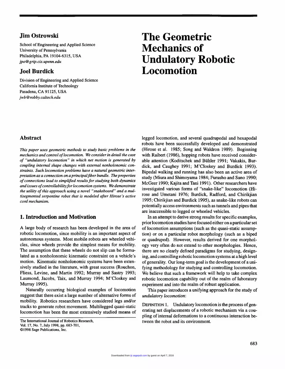
EXAMPLE 1: Consider the two-wheeled planar mobile robotshown in Figure 1. The robot’s position, (x, y, 0) E SE(2), ismeasured via a frame located at the center of the wheel base.The robot’s motion is affected by the movements of its twowheels, whose angles, (~1, cP2), are measured relative to ver-tical. Each wheel is assumed to rotate independently. Whilethis model does not look like an &dquo;undulatory&dquo; system, it pos-sesses the key property of generating net robot displacementby movements of its internal shape variables, (4ol, Ø2), that arecoupled to external nonholonomic constraints. In this case,the constraints arise from our assumption that the wheels rollwithout slipping.

The configuration space of this mechanism is Q = SE(2) x(~81 x .&1). The Lagrangian for this problem is

where m is the mass of the robot, J is its inertia, and Jw isthe inertia of each of the wheels.

The constraints defining the no-slip condition can be writ-ten as in eq. (1). However, we will rearrange the constraintsinto the more revealing form:



686

Fig. 1. Two-wheeled planar mobile robot.

The motion in the group variables, (x, y, 6) is strictly afunction of the motion in the internal shape variables, (~1, ~2),since there are three independent kinematic constraints onthe three-dimensional set of body displacements. If we as-sume that the variables (~1, ~2) are controllable, then giventhe time evolution of (951, cP2), we can completely solve forthe robot’s motion using eq. (3). That is, the kinematic con-straints completely determine the robot’s motion, and for thepurposes of motion planning, there is no need to determine therobot’s dynamic equations of motion. This characteristic de-fines the conventional nonholonomic vehicles that have been

actively studied in the robotics literature. For the purposesof implementation, it may be desirable to compute the equa-tions of motion, since the dynamic equations determine howmuch force or torque is required to actuate the internal shapevariables to follow a given trajectory. In fact, the dynamicequations for this example (and for more general locomotionproblems as well) have a form that structurally looks like amass/inertia matrix that is &dquo;shifted&dquo; by the constraints

A general formalism for the reduced shape dynamics can befound in Ostrowski and Burdick (forthcoming).

Equation (3) describes the relationship between the robot’s&dquo;internal&dquo; motions and its net movement. Thus, according tothe intuitive notions given in Section 1, it defines a connectionfor this problem (we will give a more formal definition ofthe connection below). However, the kinematics constraintsby themselves do not always define a connection. This isillustrated in the following example.

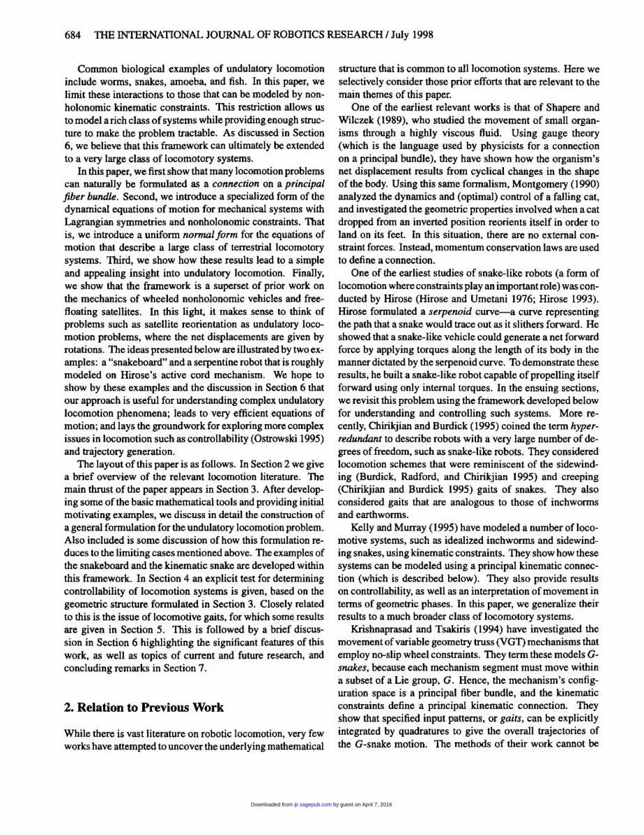
EXAMPLE 2. The snakeboard (Lewis et al. 1994; Ostrowski,Burdick, Lewis, and Murray 1995) is a variant of the skate-

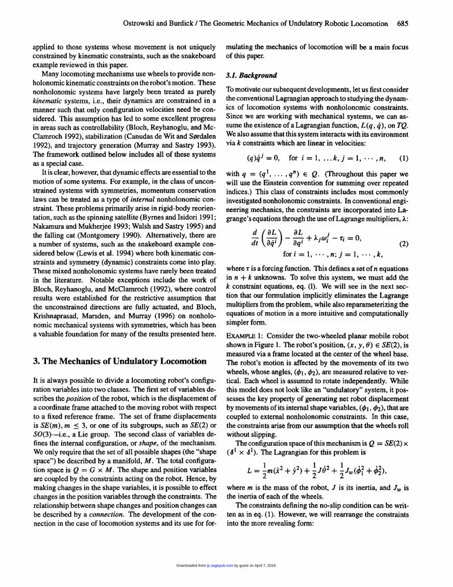
board in which the passive wheel assemblies can pivot freelyabout a vertical axis. By coupling a twisting of the humantorso with an appropriate turning of the wheels (where theturning is controlled by the rider’s foot movements), a ridercan generate a snake-like locomotion pattern without havingto kick off the ground. A simplified model that captures theessential behavior of the snakeboard operation at low speed isshown in Figure 2. It consists of a rigid body connecting thetwo sets of wheels. We assume for our problem that the front-and rear-wheel axles move through equal and opposite rota-tions, as shown in Figure 3. A momentum wheel rotates abouta vertical axis through the center of mass, simulating the mo-tion of a human torso. Figure 3 shows a robotic snakeboardprototype.

The snakeboard’s position variables, (x, y, 0) e SE(2), aredetermined by a frame affixed to its center of mass. The shapevariables are (1/1, cPb, cPt), and so Q = G x M = SE(2) x( .& x 4’ x .& 1). The Lagrangian is

where J is the snakeboard body inertia, Jr is the rotor iner-tia, and Jw is the inertia of the wheels about a vertical axis.

Fig. 2. The simplified model of the snakeboard.

Fig. 3. A prototype robotic snakeboard.



687

Control torques at the rotor and wheel axles are assumed, sot = (0, 0, 0, ’t’ýI, zb, t f). The assumption that the wheels donot slip in the direction of the wheel axles determines twoconstraints of the form of eq. ( 1 ):

Assuming full control of the shape variables, (1/1, -0b, Of ),there are not enough kinematic constraints to uniquely definethe snakeboard’s motion. The technique that was employedin Example 1 to use the kinematic constraints to solve for therobot’s motion as a function of shape changes is therefore nolonger viable. The snakeboard’s dynamics must come intoplay. To determine the robot’s dynamics, engineers have tra-ditionally been relegated to substituting the Lagrangian andthe constraints into eq. (2) and explicitly solving for the La-grange multipliers. There are many drawbacks to this ap-proach. First, the system is equivalent to 2n + k first-orderdifferential equations-i.e., 14 first-order coupled equationsin the case of the snakeboard. Second, when eliminating theLagrange multipliers, we do not have a relationship, suchas eq. (3), that readily shows the effect of mechanism shapechanges on robot motion, which is the key feature of undu-latory locomotion. We now present an alternate approachthat makes use of the inherent structure found in problems oflocomotion.

3.2. The Geometric Nature of the ProblemThe concept of conservation of linear and angular momen-tum is well known. In a geometric context, these conceptsare directly related to invariances, or symmetries, of the La-grangian. We revisit this theory in a geometric setting, asthese ideas will play a central role in formulating locomotionproblems as invariant systems with nonholonomic constraints.

If the robot’s initial body fixed-frame position is denotedby h (e.g., h is a homogeneous transformation matrix), andit is displaced by an amount g, then its final position is gh.This displacement can be thought of as a map Lg : G &horbar;~ G

given by Lg(h) = gh, and is termed a left translation. Theleft translation induces a left action of G on Q. In workingwith locomotion systems, it is immediately obvious that thebody fixed-frame displacement will either be an element ofSE(2) (for planar systems) or SE(3) (for spatially evolvingsystems), or one of their subgroups (such as SO(2) or SO(3) forpure rotations). Since SE(m) and all of its subgroups are Liegroups, we are naturally led to formulate the problem in termsof motion on Lie groups. A Lie group is basically a manifoldwith a group structure. In the context of locomotion, it is

perhaps most convenient to think in terms of homogeneousmatrix transformations, where the group product is simplymatrix multiplication.

DEFINITION 2. A left action of a Lie group G on a manifold

Q is a map (D : G x Q - Q such that

The left action can be viewed as a map from Q into Q,with the element g E G held fixed. Notationally, we willoften write (Dg : Q - Q where (Dg : (s, r) t--* (<I>(g, s), r).The lifted action, which describes the effect of O g on velocityvectors in TQ, is the linear map, Dq o g : Tq Q -~ Tq Q.

Recall the division of the configuration space, Q = G x M.Such a configuration space is termed a trivial principal fiberbundle.

DEFINITION 3. Let M be a manifold and G a Lie group. Atrivial principal fiber bundle with base space M and struc-ture group G consists of the manifold Q = G x M togetherwith the free left action of G on Q given by left translation:(Dg(s, r) = (gs, r) for r E M and g, s E G. Given a point(s, r) E G x M = Q, we define the natural projectionsTTi : 6 -~- G : (.y, r) h-~ .y and 7T2 : 6 &horbar;~ Af : (.y, r) )-~ r.

We say that Q is a fiber bundle with fibers G and base spaceM. Q is &dquo;trivial&dquo; because the product structure is global, andit is a &dquo;principal&dquo; bundle because the fiber is a Lie group.The additional structure arising from the Lie group compo-nent (which is common to all locomotion systems) is veryimportant for the ensuing developments.

Continuing with Example 2, the snakeboard’s configura-tion space is Q = SE(2) x (.&1 1 x S x .&1), and a configurationis denoted q = (x, y, 6, 1/1, ~b, ~ f). The action is the left ac-tion of SE(2) on itself. Given g = (al, a2, a) E SE(2), theaction and lifted action are

where vq = (vx, vy, VO, V1/!, vb, v f).The reader familiar with homogeneous matrix represen-

tations of rigid-body transformations should recognize theaction (Dg as a rigid-body planar translation and rotation act-ing on the first three coordinates, SE(2). Similarly, the liftedaction Dq(Dg, is simply the derivative of this map (which ina homogeneous representation is given by the same linearmatrix multiplication) applied to tangent vectors.



688

Associated with a Lie group, G, is its Lie algebra, denoted~. The Lie algebra can be identified with TeG, and locallygenerates G via the exponential mapping, ex- : 9 -+ G (seeAbraham and Marsden 1978; Murray, Li, and Sastry 1994).The exponential mapping also associates with each ~ e ~, avector field on G, and by extension on Q = G x M, calledthe infinitesimal generator, ~Q, given by:

Each infinitesimal generator is tangent to the fiber, and theset of all such vectors at q E Q forms the vertical subspaceof Tq Q,

That is, a vector uq E Vq Q represents a net velocity of thebody with respect to an inertial frame, such that vq = (vg, 0)with Vg E TgG.

Continuing further with Example 2, Lie algebra for SE(2)is denoted by se(2), and the relationship between an element,~ = (al, a2, a) E se(2), and the corresponding infinitesimalgenerator is

This calculation (based on eq. (9)) is somewhat involved,and so is not included in detail here. For the reader not famil-iar with the geometry of Lie groups, however, it is a useful

computation to perform. From eq. (10), the vertical subspaceis the set of all possible infinitesimal generators so defined.For the snakeboard, it is given trivially by TG x 0:

3.3. Mechanics with SymmetriesConservation laws naturally arise when a Lagrangian remainsfixed under the action of a Lie group. Such a function is said

to be invariant with respect to a symmetry group, G. More

formallyDEFINITION 4. A Lagrangian function, L : T Q - R, is saidto be G-invariant if it is invariant with respect to the lifted

action, DOg, i.e., if L(<I>g(q), Dq ogvq) = L(q, Vq), for allgeGand(~,~)€r6.We also refer below to invariant vector fields, which are

defined quite similarly:DEFINITION 5. A vector field, X E aG ( Q), is said to be

G-invariant if it satisfies the relationship DqOgX(q) =X(<I>g(q», for all g E G and q E Q.

In both these cases, invariance generally implies that thequantity in question varies in a manner compatible with thegroup action. For example, the kinetic energy of a planar

body moving on a frictionless surface does not depend onits initial position and orientation. Thus, the Lagrangian willbe invariant with respect to translations and rotations. In theabsence of external forces, the conservation laws for linearand angular momentum naturally arise due to invariances ofthe Lagrangian, as stated in Noether’s theorem (Abraham andMarsden 1978):THEOREM 1. Let L(q, q) be a Lagrangian that is invariant un-der the action of a Lie group, G, (i.e., L(<I>g(q), Dq<l>gvq) =L(q, vq)‘dg E G, for all Vq E Tq Q). Then, for all curvesc(t) : [a, b] -~ Q satisfying Lagrange’s equations:

for all ~ e g. Equivalently, if we define the generalizedmomentum, p, to be

then eq. (13) is equivalent to p = 0.The invariance of the Lagrangian with respect to a Lie

group is termed a symmetry. When G is SE(2) or SE(3),Noether’s theorem is equivalent to conservation of linear andangular momentum. However, undulatory locomotion reliesupon an interaction with the environment. Unfortunately,conservation laws may not be preserved in the presence ofconstraints. The next section describes a recent extensionto the classical theory that combines symmetries with con-straints.

3.4. Symmetries and ConstraintsLet the constraint distribution be the set of all velocities that

satisfy the kinematic constraints:

Let 4 denote the constrained fiber distribution, which is givenat each q by the intersection of the constraint distribution, Dq,with the vertical subspace, Vq Q :

If the constraints act vertically (i.e., if 4 is nonempty), thenwe have the following result (Bloch et al. 1996):PROPOSITION 1. Let L and lll define a constrained systemon Q = G x M whose Lagrangian is G-invariant. If c(t) isa curve that satisfies the Lagrange-d’Alembert equations (eq.(2)) for a system with nonholonomic constraints (eq. (1)), thenthe following generalized momentum equation holds for allvector fields, çQ E ~3:



689

where

is called the generalized momentum.

The generalized momentum equation can always be fac-tored into a form that is quadratic in the base and momentumvariables. The proof of this proposition is given in the ap-pendix. For more details, the reader is referred to Ostrowski(1995) and Bloch et al. (1996).

PROPOSITION 2. Given the invariance of the Lagrangian andthe constraints, the generalized momentum equation is inde-pendent of the group variables and can be written as

a quadratic function of p and i-.

Proposition 1 states that in the presence of constraints,momentum-like quantities exist, but may not be conserved.Equation (17) determines how these momentum-like quan-tities evolve, while Proposition 2 shows that the governingequations themselves reduce to a simpler form. The non-

conservation of these momentum-like quantities is the keyto dynamic undulatory locomotion (and many other forms oflocomotion). It describes why the snakeboard can build upmomentum, even though no external forces aside from theconstraints act on the system.

Continuing with Example 2, the snakeboard Lagrangian,eq. (6), is invariant with respect to an SE(2) group action.The wheel constraints of eq. (7) can be expressed as a four-dimensional constraint distribution:

where

The vertical distribution was defined in eq. (12), and theconstrained fiber distribution is

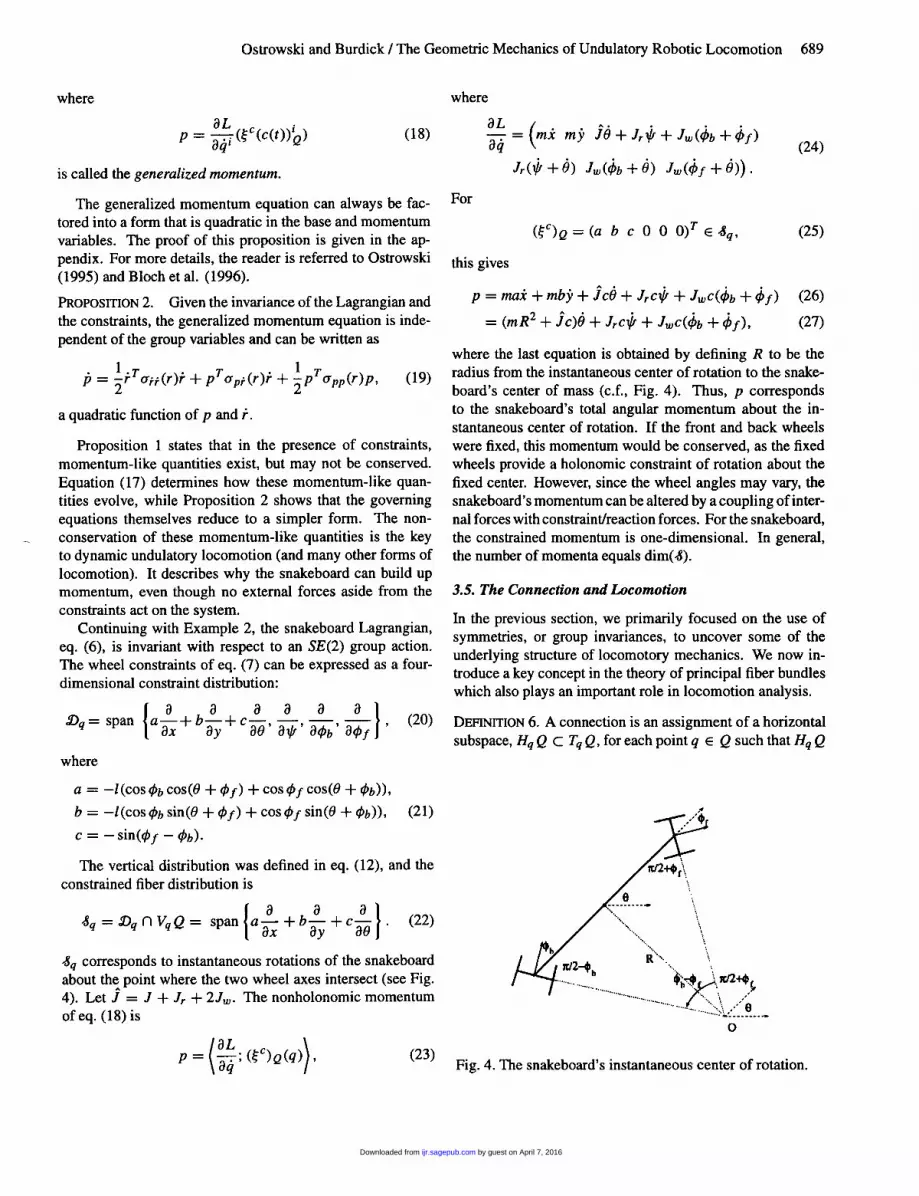
4q corresponds to instantaneous rotations of the snakeboardabout the point where the two wheel axes intersect (see Fig.4). Let 7 = J + Jr + 2Jw. The nonholonomic momentumof eq. (18) is

where

For

this gives

where the last equation is obtained by defining R to be theradius from the instantaneous center of rotation to the snake-board’s center of mass (c.f., Fig. 4). Thus, p correspondsto the snakeboard’s total angular momentum about the in-stantaneous center of rotation. If the front and back wheelswere fixed, this momentum would be conserved, as the fixedwheels provide a holonomic constraint of rotation about thefixed center. However, since the wheel angles may vary, thesnakeboard’s momentum can be altered by a coupling of inter-nal forces with constraint/reaction forces. For the snakeboard,the constrained momentum is one-dimensional. In general,the number of momenta equals dim(4).

3.5. The Connection and Locomotion

In the previous section, we primarily focused on the use ofsymmetries, or group invariances, to uncover some of theunderlying structure of locomotory mechanics. We now in-troduce a key concept in the theory of principal fiber bundleswhich also plays an important role in locomotion analysis.

DEFINITION 6. A connection is an assignment of a horizontalsubspace, Hq Q c Tq Q, for each point q E Q such that Hq Q

Fig. 4. The snakeboard’s instantaneous center of rotation.



690

depends smoothly on q and

Condition 1 implies that Tq Q can everywhere be dividedinto a vertical subspace, Vq Q, and a complementary (but notnecessarily orthogonal) subspace, Hq Q, which is termed thehorizontal subspace. Condition 2 states that vectors in thehorizontal subspace must transform under the lifted groupaction in an appropriate way.

Connections are extremely useful because of the follow-ing fact. The horizontal subspace defined by the connectionis everywhere isomorphic to the tangent space of the baseHqQ ^~ T7r2(q)M. That is, there must be a one-to-one rela-tionship between every vector in 77r2(~)~ (which represents a&dquo;shape-space velocity&dquo;) and every vector in Hq Q, which is asubspace of the configuration space velocities. The horizon-tal lift is the isomorphism that maps vectors in Tn2(q)M to thecorresponding lifted vectors in Hq Q C Tq Q. The horizon-tal lift determines the relationship between motion in the basespace (i.e., tangent vectors in T7r2(q)M) and motion in the totalspace, Q, where locomotion is effected. In the general theoryof principal fiber bundles, one can choose any connection, aslong as it satisfies the properties stated in Definition 6. How-ever, for locomotion analysis, we will choose the connection,Hq Q, to encode the action of the constraints. Hence, theconnection will determine how internal shape changes createnet robot motion. In other words, the connection is the for-malization of the intuitive procedure that lead to eq. (3) inExample 1.

For purposes of analysis and computation, a connectionon Q can alternatively be described by a Lie algebra-valuedone-form termed the connection form. That is, the connectionform is a mapping A (q) : Tq Q - g where g is the Lie algebraof G. The connection form has the properties

Condition 1 implies that A(q) takes infinitesimal gener-ators to their associated Lie algebra elements. The connec-tion form vanishes on horizontal vectors: A(q)4 = 0 for allq E Hq Q. Hence, Hq Q can alternatively be defined as the setof tangent vectors upon which the connection form vanishes.

The case of mechanics with symmetries, but no con-straints, has previously been studied in the geometric me-chanics literature. To encode the symmetry constraints intothe connection in this classical case, the connection is de-fined as the orthogonal complement to the vertical subspaceHqQ = {Vq E TqQI«vq, Wq)) = 0, VWq E VqQ}, wherez ) ) is the inner product with respect to the kinetic energymetrics. 1 That is, the horizontal subspace, or connection, is

composed of all vectors which are orthogonal to the groupdirection. In the geometric mechanics literature, this particu-lar connection is termed the mechanical connection (Marsdenand Ratiu 1994), and is a restatement of the law of conser-vation of linear/angular momentum. Let p denote the bodymomentum, along the lines of Noether’s theorem. It can beshown that the connection, or conservation law, takes the form

where A(r) is called the &dquo;local form&dquo; of the mechanical con-nection, and I (r) is the locked inertia tensor. I (r) describesthe total inertia of the system when all joints are frozen atconfiguration r. It is interesting to note that this connection,or conservation law, defines a nonholonomic constraint. Forp = 0 (a constant), eq. (28) defines the invariant horizontalsubspace as

Notice the surprisingly simple form of eq. (28), particu-larly the fact that all of the information of the connection isencoded in the term A (r), which is a function of the shape, r,only. An important result of this analysis is to show that thissimple relationship is characteristic of all modes of undula-tory locomotion.

The addition of nonholonomic constraints requires that aslightly different horizontal subspace be defined-one thatencodes the information of both the symmetries and the kine-matic constraints. To accommodate both of these require-ments, we define Hq Q using orthogonality with the con-strained fiber distribution as

If the constraints are G-invariant, i.e., if

then Hq Q defined in this way satisfies both conditions givenin Definition 6 of a connection. Thus, these horizontal vec-tors satisfy both the kinematic constraints and the symmetryconstraints. Using these two types of constraints allows usto write the connection in the mixed case in an analogousmanner to eq. (28) for the unconstrained case.

Notice that in the absence of constraints, the y = dim G de-grees of freedom in the group direction are exactly constrainedby the y momenta, which can be defined via Noether’s the-orem. In the mixed case, there already exist k constraintsgiven by the wi s. The remaining s = y - k constraints arethen synthesized using the s generalized momenta defined

1. If K(q) is the positive definite kinetic energy matrix of a mechanicalsystem at configuration q E Q, and v ∈ Tq Q, then in local coordinates thekinetic energy metric is ((vq , vq)) = vqT K(q)vq.



691

in Proposition 1. This again results in y constraints on they-dimensional symmetry group G, which take the form

The proof that the connection always takes this form can befound in Ostrowski (1995). The connection plays the mostcentral role in the mechanics of locomotion, since it deter-mines the robot’s motion (note that g-lg is the velocity ofthe robot’s reference frame, as seen in body coordinates) asthe combination of built-up momentum, p, and internal shapechanges, r.

In summary, we have reduced the equations of motion tothe following form:

In effect, we have reduced a system of n second-orderODEs with k first-order constraint (eqs. (1) and (2)) to a sys-tem of y = dim(G) first-order constraints (the connectionform), (y - k) first-order generalized momentum equations(which have a simple quadratic form), and dim(M) second-order equations on the base space (termed the reduced dynam-ics) ; that is, from 2n + k to 2n - k first-order ODEs (withoutexplicitly solving for Lagrange multipliers).

The reduced shape dynamics are not important for under-standing locomotion. It can generally be assumed that theshape variables can be controlled, and hence we can writei- = u, where u is a control input. They may be important inthe synthesis of a controller, however, as they describe the dy-namics of the mechanism’s internal shape deformations. Thecalculation of the reduced dynamical equations is the sub-ject of another paper Ostrowski and Burdick (forthcoming).Thus, the equations that are important for understanding lo-comotion are reduced to two sets of first-order equations thatmake explicit how shape changes lead to robot motion.

Continuing with Example 2, snakeboard’s connection andgeneralized momentum equation take the form of eq. (32),where

and

with

and the generalized momentum equation is

This approach leads to a very concise formulation of thedynamical relationships that govern the snakeboard’s move-ment. Important to understanding the reduction process is tonotice the way in which the generalized momentum equationreduces. The first step, marked above as eq. (37), is defined bythe generalized momentum equation (eq. ( 17)) given in Propo-sition 1. Notice that there are no second-derivative terms thatone would expect if we had simply taken the time derivativeof the generalized momentum. Furthermore, the second stepof this process involves eliminating the group variables fromthis equation (this step is marked as eq. (38), as described inProposition 2, eq. (19). These two propositions together guar-antee that the generalized momentum equation can always bereduced to terms involving only the shape and momentumvariables.

3.6. Special Cases

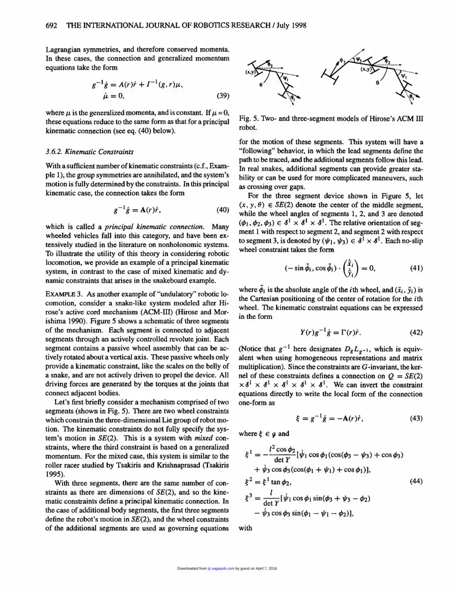
We now briefly consider special cases of these equations toshow that eq. (32) includes many previously studied problemsas a special case. To illustrate these ideas, we provide an ex-ample of a locomotion system involving principal kinematicconstraints based on Hirose’s ACM III snake robot.

3.6.1. Symmetry Constraints

There are no kinematic constraints in the cases of fallingcats or platform divers. Yet, these systems have inherent



692

Lagrangian symmetries, and therefore conserved momenta.In these cases, the connection and generalized momentumequations take the form

where g is the generalized momenta, and is constant. If/~=0,these equations reduce to the same form as that for a principalkinematic connection (see eq. (40) below).

3.6.2. Kinematic Constraints

With a sufficient number of kinematic constraints (c.f., Exam-ple 1), the group symmetries are annihilated, and the system’smotion is fully determined by the constraints. In this principalkinematic case, the connection takes the form

which is called a principal kinematic connection. Manywheeled vehicles fall into this category, and have been ex-

tensively studied in the literature on nonholonomic systems.To illustrate the utility of this theory in considering roboticlocomotion, we provide an example of a principal kinematicsystem, in contrast to the case of mixed kinematic and dy-namic constraints that arises in the snakeboard example.EXAMPLE 3. As another example of &dquo;undulatory&dquo; robotic lo-comotion, consider a snake-like system modeled after Hi-rose’s active cord mechanism (ACM-III) (Hirose and Mor-ishima 1990). Figure 5 shows a schematic of three segmentsof the mechanism. Each segment is connected to adjacentsegments through an actively controlled revolute joint. Eachsegment contains a passive wheel assembly that can be ac-tively rotated about a vertical axis. These passive wheels onlyprovide a kinematic constraint, like the scales on the belly ofa snake, and are not actively driven to propel the device. Alldriving forces are generated by the torques at the joints thatconnect adjacent bodies.

Let’s first briefly consider a mechanism comprised of twosegments (shown in Fig. 5). There are two wheel constraintswhich constrain the three-dimensional Lie group of robot mo-tion. The kinematic constraints do not fully specify the sys-tem’s motion in SE(2). This is a system with mixed con-straints, where the third constraint is based on a generalizedmomentum. For the mixed case, this system is similar to theroller racer studied by Tsakiris and Krishnaprasad (Tsakiris1995).

With three segments, there are the same number of con-straints as there are dimensions of SE(2), and so the kine-matic constraints define a principal kinematic connection. Inthe case of additional body segments, the first three segmentsdefine the robot’s motion in SE(2), and the wheel constraintsof the additional segments are used as governing equations

Fig. 5. Two- and three-segment models of Hirose’s ACM IIIrobot.

for the motion of these segments. This system will have a

&dquo;following&dquo; behavior, in which the lead segments define thepath to be traced, and the additional segments follow this lead.In real snakes, additional segments can provide greater sta-bility or can be used for more complicated maneuvers, suchas crossing over gaps.

For the three segment device shown in Figure 5, let

(x, y, 8) E SE(2) denote the center of the middle segment,while the wheel angles of segments 1, 2, and 3 are denoted(~ 1, 02, Ø3) e .&1 x .&1 x .&1. The relative orientation of seg-ment 1 with respect to segment 2, and segment 2 with respectto segment 3, is denoted by (1/11, *3) e 4 ~ x S 1. Each no-slipwheel constraint takes the form

where 4>i is the absolute angle of the ith wheel, and (Xi, Yi) isthe Cartesian positioning of the center of rotation for the i thwheel. The kinematic constraint equations can be expressedin the form

(Notice that g-1 here designates DgLg-l, which is equiv-alent when using homogeneous representations and matrixmultiplication). Since the constraints are G-invariant, the ker-nel of these constraints defines a connection on Q = SE(2)x4~ x .8’ 1 x .& 1 X .& x .& 1. We can invert the constraint

equations directly to write the local form of the connectionone-form as

where ~ E g and

with



693

Suppose that we add a fourth segment. Let cP4 and ~4denote the angles of the wheels and the body segment, re-spectively. Letting ~4 = cP4 + p3 + p4 + 0, the no-slipkinematic wheel constraint is:

We have added two degrees of freedom (~4 and ~4) and onekinematic constraint (eq. (46)). Both ~4 and ~4 are con-trolled, but we must also satisfy the constraint. This is doneby choosing to control the wheel angle, while inverting eq.(46) to establish a governing equation for ~4:

where <P4 = ~4 + p3 + ~4. i.e., $4 [ g=e = <P4Io=0. Noticethat ~4 depends upon a term with cos ~4 in the denominator(we assume that the wheels cannot pivot to an angle of::l::1-).Repeating this process, we can add additional segments so asto guarantee that each following segment satisfies all of theconstraints. It is always possible to arrange the additionalconstraint equations in the form

where k is the total number of body segments. The matrix Bis lower triangular, with determinant

and is always invertible.

4. Controllability

At a bare minimum, the examples presented above indicatethat this approach leads to equations of motion that have ahighly simplified and appealing form. However, there are

fundamentally more important reasons for using our methodto analyze undulatory locomotion systems. As an example ofthe utility of this theory, we briefly consider in this section thequestion of controllability of undulatory locomotion systems.The controllability question is not the focus of this paper-amore detailed discussion of controllability and the proof ofthe following proposition can be found in Ostrowski (1995).A locomotion mechanism is controllable if, given any ini-

tial configuration qi and final configuration qf, there existsan admissible control law that drives the system from qi to

qf. As we discuss below, controllability is an important issuefor several reasons. When designing a locomoting robot, wewould like to know if the robot can reach all possible posi-tions in its environment. To date, robotic engineers have beenrelegated to using their intuition or extensive numerical sim-ulation to determine if a given locomotion mechanism designcan completely access its environment. However, it shouldbe clear from the snakeboard example and the Hirose ACMmodel that intuition may not be a good guide for complicatedundulatory locomotion systems. To faithfully test a robot’scapabilities in simulation, it is first necessary to develop atrajectory planning scheme for the robot. The difficulty indeveloping trajectory generation schemes for undulatory sys-tems renders the heuristic simulation approach unappealing.Surprisingly, controllability can be directly determined viathe connection and the generalized momentum equation, viaa simple computational test that does not require the genera-tion of candidate trajectories. This result further illustrates theusefulness of these equations as tools for locomotion analysis.Additionally, we have found that the controllability calcula-tions can be used to give some heuristic intuition as to theappropriate choices of controls that should be used to gener-ate particular motions, or &dquo;gaits.&dquo; Section 5 will briefly dis-cuss this relationship between gaits and certain controllabilitycalculations.We now show that the connection and constrained momen-

tum equation can be put in the standard form for testing non-linear controllability, namely, one that is affine in the controlinputs, with an additional drift vector field:

To do so, we must dynamically extend the control inputsby redefining them as higher derivatives of the input vari-ables. Equivalently, in these generalized nonholonomic sys-tems where both symmetry and kinematic constraints are ineffect, the accelerations of the shape variables are the con-trol inputs. This is in contrast to the use of velocities as thecontrol inputs in the special kinematic case of conventionalnonholonomic wheeled vehicles. Letting v = 1i , and usingz = (g, p, r, r), the connection and generalized momentumequations can be put in the standard control form with



694

where ei is the m-vector (m = dim M) with a 1 in the ith rowand 0 otherwise.

There are two commonly used notions of control for non-linear systems-accessibility and controllability (see Hsidori(1989) for descriptions of these concepts). For nonlinear sys-tems with drift, small-time local controllability (STLC) isthe closest that we can come to our intuitive notion of con-

trollability. This type of controllability implies that the sys-tem can reach an open set of states containing the originalstate, in short periods of time and without leaving a boundedneighborhood of the original state. Accessibility is deter-mined by computing the accessibility distribution. Let Ao =span{ f, h 1, ... , hm }, and iteratively define the distributions

This nondecreasing sequence of distributions terminates atsome k f under certain regularity conditions. Ok f is the ac-cessibility distribution. A system is accessible if dim Ok f =dim Tz N for all z E N. Given the structure of the equations asin eqs. (51) and (52), the following proposition describes anexplicit controllability test for these types of systems, basedon the accessibility distribution and one of the terms in thegeneralized momentum equation.

PROPOSITION 3. (See Ostrowski 1995 and Ostrowski andBurdick 1997.) The system given by eqs. (51) and (52)is small-time locally controllable (STLC) from equilibriumpoints if

1. the accessibility distribution on the Lie algebra is fullrank (i.e., the system is ~-accessible);

2. Uff is surjective map; and

3. (a» ) ii = 0 for i = 1, ... , m (no summation).

Furthermore, it can be shown (Ostrowski 1995) that thecalculation of the accessibility distribution can be done solelybased on the connection and its (exterior) derivatives.

Note that in the above summary of the controllability anal-ysis that the reduced, or base, equations of motion are not in-cluded in the controllability calculations. In fact, these equa-tions can be treated separately, particularly in cases where theinitial and final internal configurations are not of importance,only the initial and final position of the body. This feature

of our approach is enhanced by the realization that the entiremotion of the vehicle can be reconstructed (Marsden 1992)from the connection and generalized momentum equations.Hence, it is not necessary to include the reduced, or base, dy-namics in the controllability calculations. This fact results insubstantial computational and theoretical advantages. For ex-ample, one could use the conventional Lagrangian approachof eq. (2) to derive the equations of motion for undulatory sys-tems, such as the snakeboard. One could then rearrange the

equations in the form of eq. (50) and then attempt to develop anonlinear controllability test. For the case of the snakeboard,a great deal of manipulation within the conventional approachleads to vectors f (z), h 1 (z), ~ ~ ~ , hm (z) that are at least eight-dimensional, while in our reduced form of the equations, thereduction to this space is automatic. Much more importantly,though, the computations required under Proposition 3 in-volve brackets of only three-dimensional vectors, along withsimple checks on the terms in the generalized momentumequation.

While these controllability results are useful for the anal-ysis of locomotion systems, the next section shows that

there are additional reasons to undertake this controllabilityanalysis.

5. Geometric Phases and Gaits

The snakeboard moves by coupling periodic motions of therotor and wheel axles. Similarly, the kinematic snake movesusing internal motions coupled to rotations of the wheel axles.These are examples of gaits, which more generally can bethought of as cyclic patterns of internal shape changes thatresult in a net robot displacement. Different gaits correspondto different cyclic input patterns. In general, the net displace-ment of the mechanism that arises from periodic inputs is thegeometric phase, or holonomy, associated with the connec-tion. The geometric phase is that part of the motion describedby the local form of the connection, A, in eq. (30). In themixed and unconstrained cases, there may be a part of themotion that is driven by the momentum of the system. This iscalled the dynamic phase, and is directly related to the 1- pterm in eq. (30). In the mixed case, the net displacementis a nontrivial combination of the geometric phase and thedynamic phase.

5.1. Snakeboard Gaits

To illustrate the notion of gaits, we present in Figures 6, 7,and 8 three different gait patterns for the snakeboard. A moredetailed analysis of these gaits is given in Ostrowski, Lewis,Murray, and Burdick (1994) and Ostrowski (1995). Figure 6shows the position of the snakeboard’s center of mass versustime for the case in which the rotor and wheel axles oscillate

with the same frequency (which we term the &dquo;drive gait&dquo;);Figure 7 reveals the case in which the rotor oscillates at twice



695

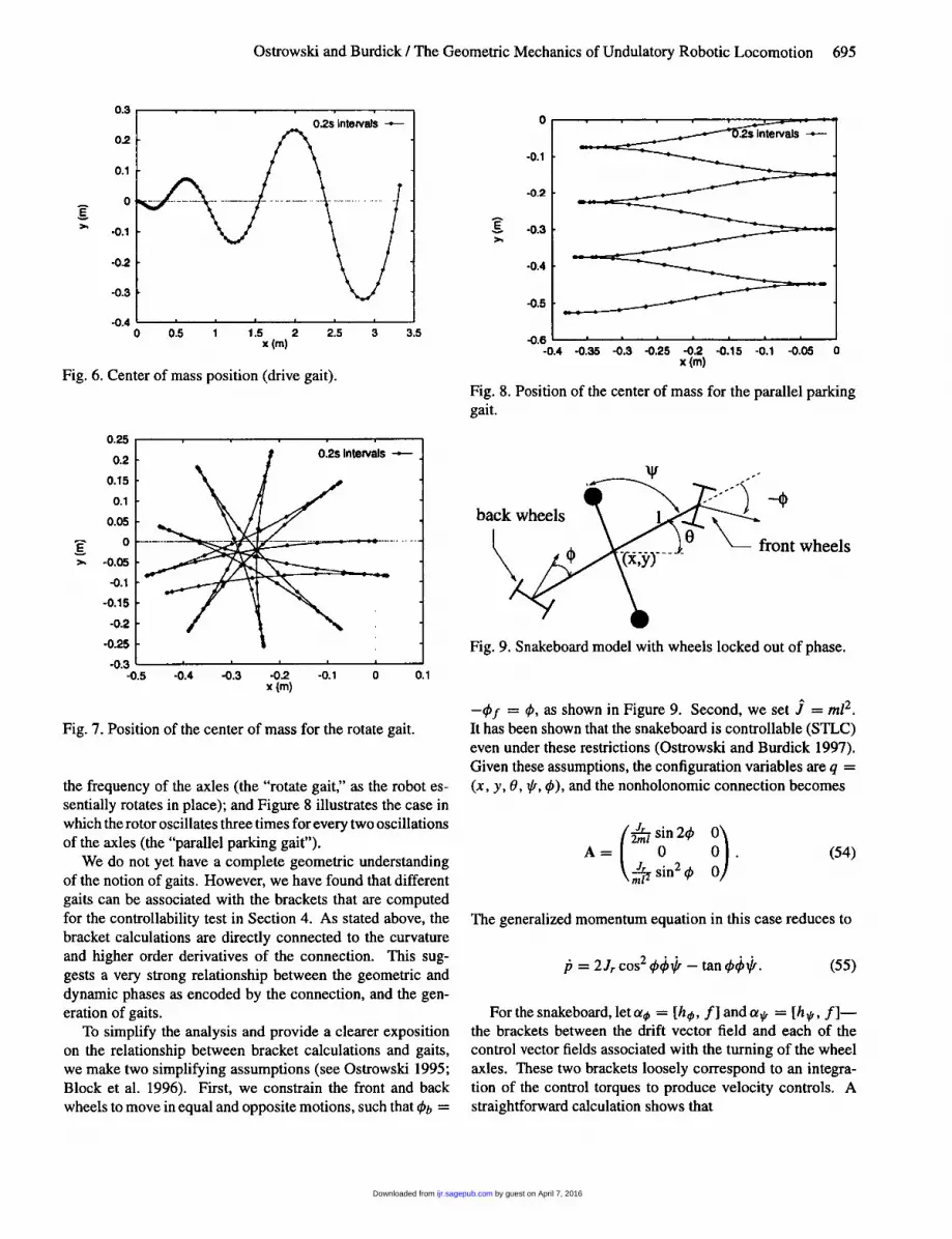
Fig. 6. Center of mass position (drive gait).

Fig. 7. Position of the center of mass for the rotate gait.

the frequency of the axles (the &dquo;rotate gait,&dquo; as the robot es-sentially rotates in place); and Figure 8 illustrates the case inwhich the rotor oscillates three times for every two oscillationsof the axles (the &dquo;parallel parking gait&dquo;).We do not yet have a complete geometric understanding

of the notion of gaits. However, we have found that differentgaits can be associated with the brackets that are computedfor the controllability test in Section 4. As stated above, thebracket calculations are directly connected to the curvatureand higher order derivatives of the connection. This sug-gests a very strong relationship between the geometric anddynamic phases as encoded by the connection, and the gen-eration of gaits.

To simplify the analysis and provide a clearer expositionon the relationship between bracket calculations and gaits,we make two simplifying assumptions (see Ostrowski 1995;Block et al. 1996). First, we constrain the front and backwheels to move in equal and opposite motions, such that Ob =

Fig. 8. Position of the center of mass for the parallel parkinggait.

Fig. 9. Snakeboard model with wheels locked out of phase.

-of = 0, as shown in Figure 9. Second, we set 7 = m12.It has been shown that the snakeboard is controllable (STLC)even under these restrictions (Ostrowski and Burdick 1997).Given these assumptions, the configuration variables are q =(x, y, 8,1/1, ~), and the nonholonomic connection becomes

The generalized momentum equation in this case reduces to

For the snakeboard, let at/> = [h 0, f ] and a 1/1 = [h 1/1, f ]-the brackets between the drift vector field and each of thecontrol vector fields associated with the turning of the wheelaxles. These two brackets loosely correspond to an integra-tion of the control torques to produce velocity controls. Astraightforward calculation shows that



696

and

Notice that these vector fields have 1 s in the appropriate veloc-ity directions. As mentioned above, this loosely correspondsto integrating the control torques to velocity controls. Noticethat this will also encode the information given by the localform of the connection, A(r), since the connection relates in-put velocities to fiber velocities. It is also easy to show thatthe only other first-order bracket, )7t~, h~], involving just thecontrol inputs, is identically zero.

The vector fields above imply control of the shape variables(assumed to be controllable). To show accessibility and con-trollability (STLC), we need also to compute the accessibilitydistribution on the Lie algebra. It is in these calculations thatthe correlation between gaits and brackets becomes apparent.

For the drive gait (Fig. 6), which employs a 1 : frequencyratio of rotor and axle oscillations, the corresponding 1 : 1

bracket [cio, ap evaluated at the origin is

Notice that this vector has nonzero terms only in thei com-ponent, which corresponds to forward motion of the vehicle.Similarly, the rotate gait (Fig. 7) employs a 2:1 frequency ratioof the rotor and axle oscillations. The two-level bracket,

where a, appears two times, has nonzero terms only in the 6direction, and thus corresponds to the rotation gait. Finally,the parallel parking gait (Fig. 8) generated by a 3:2 frequencyratio exhibits the same direct correlation to a 3:2 bracket,

Thus, the controllability analysis of Section 4 has been usefulin identifying candidate gaits.

To complete the analysis of controllability for the snake-board, we must show that the momentum direction can also be

generated. It suffices to satisfy conditions 2 and 3 of Propo-sition 3 regarding the form of the u¡;’ term in the generalizedmomentum equation. As a quadratic form on the shape ve-locities, this term can be written as

This satisfies both conditions, since the diagonal elements arezero, and it is surjective (as a mapping into the momentumspace, R). Interestingly, the momentum direction is generatedby a bracket of the form [ho, aýl].

Additionally, we see that momentum is generated over onegait cycle only by the 1 : gait. For the 1:2 gait and the 3:2 gait,the generalized momentum p is built up and taken away, sothat the final state after one gait cycle is a finite displacementaway from the original state, but with zero momentum. Thegeneralized momentum equation (eq. (55)) can be integratedusing an integration factor of Cos 1 0 giving an equation for p:

(in fact, this same integration can be done for the fully generalsystem). From this equation it is straightforward to show thatgiven any l:n gait, the net momentum after one cycle will benonzero if and only if n is odd.

5.2. Gaits for the Kinematic Snake

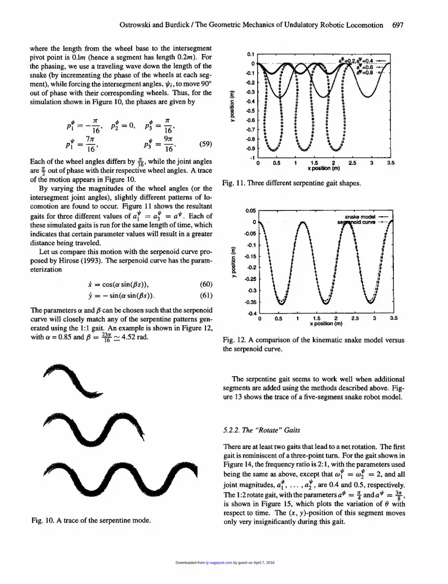
We now consider the undulatory gait employed by manysnakes. Hirose (1993) described this gait as being closestto a &dquo;serpenoid&dquo; curve, and we show below that one of thegaits generated by our approach is strikingly similar to theserpenoid curve. We also present two other gaits not nor-mally seen in nature, but which arise for the particular modelwe are using. Like the snakeboard, the gaits are based onintegrally related frequencies of the shape inputs. The ratiosrelate the frequency of bending of the intersegment angle, 1/1¡,with the frequency of the wheel rotations, Oi.

5.2. l. The &dquo;Serpentine &dquo; Gait

Forward motion can be created by using a 1 : frequency ratio.For this, we use periodic control inputs of the form

where similar values for 1/1; will be superscripted with a 1/1.The serpentine gait can be demonstrated using the values



697

where the length from the wheel base to the intersegmentpivot point is O.Im (hence a segment has length 0.2m). Forthe phasing, we use a traveling wave down the length of thesnake (by incrementing the phase of the wheels at each seg-ment), while forcing the intersegment angles, 1/1;, to move 90°out of phase with their corresponding wheels. Thus, for thesimulation shown in Figure 10, the phases are given by

Each of the wheel angles differs by f6’ while the joint anglesare f out of phase with their respective wheel angles. A traceof the motion appears in Figure 10.

By varying the magnitudes of the wheel angles (or theintersegment joint angles), slightly different patterns of lo-comotion are found to occur. Figure 11 shows the resultant

gaits for three different values of at = at = a*. Each ofthese simulated gaits is run for the same length of time, whichindicates that certain parameter values will result in a greaterdistance being traveled.

Let us compare this motion with the serpenoid curve pro-posed by Hirose (1993). The serpenoid curve has the param-eterization

The parameters a and {3 can be chosen such that the serpenoidcurve will closely match any of the serpentine patterns gen-erated using the 1:1 gait. An example is shown in Figure 12,with a = 0.85 and {3 = i6 ^~ 4.52 rad.

Fig. 10. A trace of the serpentine mode.

Fig. 11. Three different serpentine gait shapes.

Fig. 12. A comparison of the kinematic snake model versusthe serpenoid curve.

The serpentine gait seems to work well when additionalsegments are added using the methods described above. Fig-ure 13 shows the trace of a five-segment snake robot model.

5.2.2. The &dquo;Rotate&dquo; Gaits

There are at least two gaits that lead to a net rotation. The firstgait is reminiscent of a three-point turn. For the gait shown inFigure 14, the frequency ratio is 2 : 1, with the parameters usedbeing the same as above, except that wt = co2 = 2, and alljoint magnitudes, af, ... , a2 , are 0.4 and 0.5, respectively.The 1:2 rotate gait, with the parameters a’ = 4 and a ~’ = 38 ,is shown in Figure 15, which plots the variation of 0 withrespect to time. The (x, y)-position of this segment movesonly very insignificantly during this gait.



698

Fig. 13. Traces of the five-link kinematic snakes.

Fig. 14. A trace of the 2:1 gait.

6. Discussion: Toward Developing a UnifiedLocomotion Analysis Paradigm

In the preceding section, we have tried to give some examplesof why our approach is useful for locomotion analysis. In

this section, we briefly discuss how the ideas presented in thispaper may provide a foundation for a more unified approachto robotic locomotion analysis, design, and control.

One may interpret eq. (32) as a normal form for the me-chanics of undulatory locomotion systems. Let us makethe analogy with linear control theory. If the dynamics ofan electromechanical system can be put in the linear formx = Ax + Bu, there exists a substantial body of results fromlinear control theory that can be used to analyze the behaviorof such systems and to design trajectory generation algorithms

Fig. 15. A trace of the angle 0 for the 1:2 gait.

and feedback controllers for a given system. Hence, one ap-proach for developing a unified theory for robotic locomotionis to determine the normal form, or a small set of normalforms, that can capture the mechanics of a very large class oflocomotion mechanisms. To what extent is eq. (32) a generalnormal form for locomotion systems?

Recall that our intuitive notion of undulatory locomotionfocused on the generation of movement via a coupling of in-ternal shape deformations to constraints between the robotand its environment. In this paper, we explicitly developedthe connection and generalized momentum equations for thecase where the interaction constraints could be modeled asa nonholonomic kinematic constraint. Such constraints area good model for snake-like systems whose biological coun-terparts have scales that effectively enforce no-slip nonholo-nomic constraints. However, many biological organisms useother types of constraints, such as viscous friction for sluglocomotion, and fluid/surface interactions for paramecia-likeand fish-like locomotion. To what extent do our principlesapply in these cases?

First, it is always true that the net motion of a locomotingrobot’s body fixed frame occurs in a Lie group. Hence, alllocomotion systems can be modeled on a principal fiber bun-dle. Furthermore, when the constraints satisfy certain invari-ance properties (which has always been the case so far), themechanics of these locomotion systems will have a connec-tion that encodes the interaction of the symmetry constraintsand the external constraints (which may be nonholonomic,viscous, or fluid constraints, for example). The actual formof the connection and generalized momentum equations mayhave small variations, depending upon the particular classof constraint. For example, Kelly and Murray (1995) haveshown that if the constraint between the robot and the terrain

is viscous (such as slug locomotion), then in the limit thatthe viscous drag force dominates inertial force, the connec-tion (which they term the viscous connection) takes exactly



699

the same form as eq. (40). Further, one can interpret the re-sults of Shapere and Wilczek (1989) to show that the motionof paramecia-like vehicles (which move by an interaction ofa periodically vibrating boundary and the surrounding fluid)in either highly viscous or inviscid fluids can be modeled byconnections having exactly the same form as eq. (40). Morerecently, Kelly and Murray (1995) have shown that the me-chanics of fish whose flapping tails generate trailing vorticeshave nearly the same form as eq. (32), where the generalizedmomentum equation is now an infinite dimensional partialdifferential equation, and the momentum equation may in-clude a dissipation term to model energy loss. Hence, studiesof a wide variety of locomotion systems have shown that eq.(32) is very representative of a large class of locomotion sys-tems. We believe that there is an underlying reason for thiscommonality, and we hope to uncover this principle in futurework. It is important to note that none of our modeling effortshave yet attempted to include energy storage or complianceterms in our geometric mechanics paradigm. There is am-

ple evidence that energy storage is an important principle inlegged locomotion systems, though our work indicates thatit is in fact not the dominant effect in any commonly seenundulatory locomotion.

Our studies suggest that a general control theory shouldbe developed for locomotion systems, whose equations ofmotion take the form of eq. (32). In general, if a nonlin-

ear affine control system of the form of eq. (50) is feedbacklinearizable, then explicit nonlinear controllers can be devel-oped. However, no undulatory locomotion systems are feed-back linearizable. Trajectory generation and feedback controlschemes have been developed for systems that can be put intothe specialized principal kinematic form of eq. (40) (Laumondet al. 1994; M’Closkey and Murray 1995; Teel, Murray, andWalsh forthcoming). However, a rigorous nonlinear controltheory for mixed kinematic and dynamic systems such as thesnakeboard is currently beyond the state of the art of non-linear control theory. We hope to address this problem infuture work, and believe that our controllability results willbe a useful starting point for this investigation.

Legged mechanisms are an extremely important class oflocomotion mechanisms. Can any of these ideas be extendedto the legged case? Preliminary work has shown that suchan extension might proceed as follows. During the motion ofa legged robot, a leg will repeatedly make and break contactwith the supporting terrain. This nonsmooth interaction withthe environment can be modeled as a system that evolves on a

configuration manifold, Q, with a boundary, a Q. The bound-ary corresponds to those states where the leg contacts the ter-rain. More generally, a multilegged system can be modeledas dynamical system that evolves on a stratified configurationspace. For example, in the case of a biped robot, one stratawill correspond to all configurations of the biped during freeflight, one strata will correspond to all configurations wherethe right leg contacts the ground, one strata will correspond to

all configurations where the left leg contacts the ground, andone strata will correspond to all configurations where bothlegs contact the ground. It is possible to express the dynam-ics of the system on each strata in a form that is analogousto eq. (32). While our dynamics methodology extends easilyto this case, the issue of controllability becomes more com-plex. We have recently shown how to extend controllabilitytests to these stratified systems (Goodwine and Burdick 1995),which provides strong evidence to support the idea that all ofthe methodology summarized in this paper can be extendedto the legged case.

7. Conclusions

Undulatory locomotors have no thrusters, tracks, or legs togenerate motion. Instead, motion is generated by a couplingof internal shape changes to external constraints. This pa-per focused on a class of systems with nonholonomic kine-matic constraints, which includes not only the snakeboard andHirose’s ACM, but also any undulatory robotic system thatuses wheels to provide motion constraints. Also, problems ofrigid-body reorientation and many of the snake- and worm-like systems discussed in (Chirikjian and Burdick 1995) canbe analyzed using these techniques. A key observation is thatthe constraints inherent in undulatory systems provide themeans to determine motion as a function of internal shapechange. When kinematic constraints do not uniquely de-termine a robot’s motion, dynamic symmetries provide theadditional constraints. We used the formal language of con-nections on principle bundles because the connection encom-passes much of the information that is essential to locomo-tion. Using these tools, we can parameterize the dynamics interms of physically meaningful variables of momenta, inter-nal shape, and robot reference-frame motion. The connectionalso leads directly to the analysis of locomotor controllability.We believe that this framework will ultimately form the basisof a unifying theory for robotic locomotion.

Appendix : Proof of Proposition 2Recall from Section 3 that the constraints may be written as aset of one-forms, oil, ... , ~, such that allowable velocitieslie in their kernel: cv‘ (~) - ~ = 0, for i = 1, ... , k. From thiswe can pick an invariant basis for the allowable velocities.Instead, let us use the invariance of the constraints to work atthe group identity, g = e. Thus, choose a basis fl, ... , fs,for the constrained Lie algebra, gq, such that wi (e, r, fa = 0,for = 1, ... ,k,a = 1, ... ,s.

Next, we define a reduced Lagrangian, I, by pulling theLagrangian L back to the identity

where ~ = g-lg e 9~. A straightforward calculation showsthat the Euler-Poincare equations (c.f., Marsden and Ratiu1994; Ostrowski 1995) describing the motion of the systemwith constraints can be written as



700

A reduced form of the generalized momentum can be written,by definition, as

Taking the derivative with respect to time yields the followingrelationship:

As above, we write the local forms of the mechanical con-nection and the locked inertia tensor as A and I, respectively.Next, we define the structure constants c-~, on the constrainedLie algebra by the relation

for ~q, 7q E 9,q.Recalling the reduced form of the connection, eq. (30):

we find that we can write the term a-’ in the following simpleform (Ostrowski and Burdick forthcoming; Ostrowski 1995):

With all of this information, we can then explicitly writethe expressions for the generalized momentum equation,

as desired. 0

Remarks.A few remarks are in order regarding the form of this equationin certain limiting cases:

1. Trivially for the purely kinematic case, there is no gen-eralized momentum and hence no generalized momen-tum equation.

2. For the unconstrained case, A = A, and so crrr = 0,i.e., there are no terms that are quadratic in the shapevelocities. This implies that all coupling of the shapemotions with the momenta is done linearly through theOpr term.

3. In cases for which the constrained Lie algebra gq isAbelian, the terms c-b are all zero (this is the case forall one-dimensional constrained Lie algebras, includingthe snakeboard and the roller racer). All terms for thiscase simplify significantly, but in particular this impliesthat a pp = 0 (no terms, which are quadratic in thegeneralized momenta). For the unconstrained case, thisis a result of the fact that the body and spatial momentaare equal (and constants, i.e., p = 0) if and only if thestructure group is Abelian.

AcknowledgmentsThis work was supported by an NSF graduate fellowshipfor Jim Ostrowski, by the Office of Naval Research (grantN00014-92-J-1920), and by the National Science Foundation(grant MSS-9157843). The authors greatly appreciate thegenerous assistance of Andrew Lewis, Richard Murray, andJerry Marsden.

References

Abraham, R., and Marsden, J. E. 1978. Foundations of Me-chanics, 2nd ed. Reading, MA: Addison-Wesley.

Bloch, A. M., Krishnaprasad, P. S., Marsden, J. E., and Mur-ray, R. M. 1996. Nonholonomic mechanical systems with

symmetry. Archive for Rational Mechanics and Analysis136:21-99.

Bloch, A. M., Reyhanoglu, M., and McClamroch, N. H.1992.Control and stabilization of nonholonomic dynamic sys-tems. IEEE Trans. Automat. Control 37(11):1746-1757.

Burdick, J., Radford, J., and Chirikjian, G. 1995. A "side-winding" locomotion gait for hyper-redundant robots.Adv. Robot. 9(3):195-216.

Byrnes, C. I., and Isidori, A. 1991. On the attitude stabiliza-tion of rigid spacecraft. Automatica 27:87-95.



701

Canudas de Wit, C., and Sørdalen, O. J.1992. Exponential sta-bilization of mobile robots with nonholonomic constraints.IEEE Trans. Automat. Control 37(11):1791-1797.

Chirikjian, G., and Burdick, J. 1995. The kinematics of

hyper-redundant locomotion. IEEE Trans. Robot. Au-

tomat. 11(6):781-793.Furusho, J., and Sano, A. 1990. Sensor-based control of a

nine-link biped. Int. J. Robot. Res. 9(2):83-98.Goodwine, B., and Burdick, J. 1995. Control systems on

manifolds with boundary. Technical Report RMS 95-01,California Institute of Technology.

Hirose, S. 1993. Biologically Inspired Robots: Snake-LikeLocomotors and Manipulators (transl.). Peter Cave and

Charles Goulden. Oxford: Oxford University Press.Hirose, S., Masui, T., Kikuchi, H., Fukuda, Y., and Umetani,

Y. 1985 (Tokyo, Japan). Titan III: A quadruped walkingvehicle. 2nd Int. Symp. on Robot. Res. Cambridge, MA:MIT Press.

Hirose, S., and Morishima, A. 1990. Design and control of amobile robot with an articulated body. Int. J. Robot. Res.9(2):99-114.

Hirose, S., and Umetani, Y. 1976. Kinematic control of ac-tive cord mechanism with tactile sensors. Proc. 2nd Int.

CISM-IFT Symp. on Theory and Practice of Robots andManipulators, pp. 241-252.

Isidori, A. 1989. Nonlinear Control Systems: An Introduc-tion. Berlin: Springer-Verlag.

Kajita, S., and Tani, K. 1991 (Sacramento, CA). Study of dy-namic biped locomotion on rugged terrain. Proc. IEEE

Int. Conf. Robot. and Automat. Los Alamitos, CA: IEEE,pp. 1405-1411.

Kelly, S. D., and Murray, R. M. 1995. Geometric phases andlocomotion. J. Robot. Sys. 12(6):417-431.

Koditschek, D., and Buhler, M.1991. Analysis of a simplifiedhopping robot. Int. J. Robot. Res. 10(6):587-605.

Krishnaprasad, P. S., and Tsakiris, D. P. 1994 (Lake BuenaVista, FL). G-snakes: Nonholonomic kinematic chains onLie groups. Proc. 33rd IEEE Conf. on Decision and Con-trol, IEEE, pp. 2955-2960.

Laumond, J.-P., Jacobs, P., Taix, M., and Murray, R. M. 1994.A motion planner for nonholonomic mobile robots. IEEETrans. on Robot. Automat. 10(5):577-593.

Marsden, J. E. 1992. Lectures on Mechanics. New York:

Cambridge University Press.Marsden, J. E., and Ratiu, T. S. 1994. Introduction to Me-

chanics and Symmetry. New York: Springer-Verlag.McGeer, T. 1990. Passive dynamic walking. Int. J. Robot.

Res. 9(2):62-82.M’Closkey, R., and Burdick, J. 1993. On the periodic mo-

tions of a hopping robot with vertical and forward motion.Int. J. Robot. Res. 12(3):197-218.

M’Closkey, R. T., and Murray, R. M. 1995. Exponential sta-bilization of driftless nonlinear control systems using ho-mogeneous feedback. Technical Report CIT/CDS 95-012,California Institute of Technology.

Miura, H., and Shimoyama, I. 1984. Dynamic walk of abiped. Int. J. Robot. Res. 3(2):60-74.

Montgomery, R. 1990. Isoholonomic problems and some ap-plications. Comm. Math. Physics 128(3):565-592.

Murray, R. M., Li, Z., and Sastry, S. S. 1994. A Mathemat-ical Introduction to Robotic Manipulation. Boca Raton,FL: CRC Press.

Murray, R. M., and Sastry, S. S. 1993. Nonholonomic motionplanning: Steering using sinusoids. IEEE Trans. Automat.Control 38(5):700-716.

Nakamura, Y., and Mukherjee, R. 1993. Exploiting nonholo-nomic redundancy of free-flying space robots. IEEE Trans.Robot. Automat. 9(4):499-506.

Ostrowski, J., and Burdick, J. 1997. Controllability tests formechanical systems with symmetries and constraints. J.

Appl. Math. Comp. Sci. 7(2):101-127.Ostrowski, J. P. 1995. The mechanics and control of undula-

tory robotic locomotion. Ph.D. Thesis, California Instituteof Technology, Pasadena, CA. Available electronically athttp://www.cis.upenn.edu/&sim;jpo/papers.html.

Ostrowski, J. P., and Burdick, J. W. forthcoming. Computingreduced equations for mechanical systems with constraintsand symmetries.

Ostrowski, J. P., Burdick, J. W., Lewis, A. D., and Murray,R. M. 1995 (Nagoya). The mechanics of undulatory lo-comotion : The mixed kinematic and dynamic case. Proc.IEEE Int. Robot. and Automat. IEEE, pp. 1945-1951.

Ostrowski, J. P., Lewis, A. D., Murray, R. M., and Burdick, J.W. 1994 (San Diego, CA). Nonholonomic mechanics andlocomotion: The snakeboard example. Proc. IEEE Int.

Conf. Robot. and Automat. IEEE, pp. 2391-2397.Raibert, M. 1986. Legged Robots that Balance. Cambridge,MA: MIT Press.

Rouchon, P., Fliess, M., Levine, J., and Martin, P. 1992. Flat-ness and motion planning: The car with n trailers. Proc.European Control Conf., pp. 1518-1522.

Shapere, A., and Wilczek, F. 1989. Geometry of self-propulsion at low Reynolds number. J. Fluid Mech.198:557-585.

Song, S., and Waldron, K. 1989. Machines that Walk: TheAdaptive Suspension Vehicle. Cambridge, MA: MIT Press.

Teel, A., Murray, R. M., and Walsh, G. 1995. Nonholonomiccontrol systems: From steering to stabilization with sinu-soids. Int. J. Control 62(4):849-870.

Tsakiris, D. P. 1995. Motion control and planning for non-holonomic kinematic chains. Ph.D. Thesis, University ofMaryland.

Vakakis, A., Burdick, J. W., and Caughey, T. 1991. An inter-esting attractor in the dynamics of a hopping robot. Int. J.of Robot. Res. 10(6):606-618.

Walsh, G. C., and Sastry, S. S. 1995. On reorienting linkedrigid bodies using internal motions. IEEE Trans. Robot.Automat. 11(1):139-146.



Documents

The Geometric Mechanics of Undulatory Robotic Locomotion