The DNL absorbing boundary condition: applications to wave problems

The DNL absorbing boundary condition: applications to waveproblems

M.A. Storti *, J. D'El�õa, R.P. Bonet Chaple, N.M. Nigro, S.R. Idelsohn

Centro Internacional de M�etodos Num�ericos en Ingenier�õa, CIMEC, INTEC (CONICET±UNL), G�uemes 3450, 3000 Santa Fe,

Argentina

Received 1 September 1998

Abstract

A general methodology for developing absorbing boundary conditions is presented. For planar surfaces, it is based on a

straightforward solution of the system of block di�erence equations that arise from partial discretization in the directions transversal to

the arti®cial boundary followed by discretization on a constant step 1D grid in the direction normal to the boundary. This leads to an

eigenvalue problem of the size of the number of degrees of freedom in the lateral discretization. The eigenvalues are classi®ed as right-

or left-going and the absorbing boundary condition consists in imposing a null value for the ingoing modes, leaving free the outgoing

ones. Whereas the classi®cation is straightforward for operators with de®nite sign, like the Laplace operator, a virtual dissipative

mechanism has to be added in the mixed case, usually associated with wave propagation phenomena, like the Helmholtz equation. The

main advantage of the method is that it can be implemented as a black-box routine, taking as input the coef®cients of the linear system,

obtained from standard discretization (FEM or FDM) packages and giving on output the absorption matrix. We present the appli-

cation of the DNL methodology to typical wave problems, like Helmholtz equations and potential ¯ow with free surface (the ship wave

resistance and sea-keeping problems). Ó 2000 Elsevier Science S.A. All rights reserved.

Keywords: Potential ¯ow; Finite element method; Wave resistance; Absorbing boundary condition; Free surface ¯ow; Partial

discretization

1. Introduction

When solving elliptic problems in unbounded domains with numerical methods, like the Finite ElementMethod (FEM) or Finite Di�erence Method (FDM) one faces the problem of truncating the domain at acertain arti®cial boundary. For positive de®nite operators, like the Laplace operator or the elasticityequations, imposing null Dirichlet conditions at an arti®cial boundary located far enough from the regionof interest is enough, in the sense that pushing this boundary to in®nity converges to the unbounded solution(i.e. the Cauchy problem). Essentially the same thing happens for Neumann or mixed boundary conditions.The convergence to the unbounded solution may depend on space dimension, and on the order of theperturbation (i.e. if it can be approximated by a single pole, dipole, or higher order term), and some nu-merical techniques, like coupling with an external Boundary Integral solution or in®nite elements, havebeen developed in order to minimize the computational effort.

In contrast, for wave-like problems like the Helmholtz equation, the situation is much more complex.The process of pushing the boundary to in®nity may be not convergent at all unless an appropriateboundary condition is imposed in the arti®cial boundary. For instance in 2D, the solution is known to

www.elsevier.com/locate/cmaComput. Methods Appl. Mech. Engrg. 182 (2000) 483±498

* Corresponding author. Tel.: +54-342-455-9175; fax: +54-342-455-0944.

E-mail address: [email protected] (M.A. Storti).

0045-7825/00/$ - see front matter Ó 2000 Elsevier Science S.A. All rights reserved.

PII: S 0 0 4 5 - 7 8 2 5 ( 9 9 ) 0 0 2 0 5 - 4

decay to in®nity at least as 1=��rp

(1=r in 3D) due to dispersion of the radiating energy and one could try toimpose homogeneous Dirichlet or Neumann boundary conditions at the arti®cial boundary. But doing so,the arti®cial boundary acts like a closed cavity which can enter in resonance modes, as the arti®cialboundary recedes to in®nity. Then the potential at a given point passes through in®nite values at least twiceeach time the radius of the arti®cial boundary is receded one wave-length, so that this is clearly not aconvergent process. A key-point in the understanding of this lack of convergence is that its origin is in theabsence of physical dissipation. Effectively, as the medium is non-dissipative, the energy ¯ux irradiated bythe body arrives to the arti®cial boundary and is re¯ected back to the center of the domain. When the gainof the closed loop is in®nity a resonance of the cavity occurs.

A small amount of dissipation regularizes the problem. For the Helmholtz equation, dissipation can beadded with a small positive imaginary part id to the refraction index of the medium. Let /d;R be the solutionfor a given viscosity parameter d! 0� and R!1 the radius of the arti®cial boundary. Then for d > 0 wecan consider the unbounded viscous solution

/d;1 � limR!1

/d;R: �1�

This solution is independent of the boundary conditions imposed at in®nity. Now, we can safely take the limitof negligible viscosity, and we arrive to the unbounded inviscid solution

/0;1 � limd!0�

limR!1

/d;R

n o: �2�

A key point is that the order in taking the limits does matter. A closer analysis of the unbounded inviscidsolution shows that only outgoing components are present in the far-®eld, where outgoing means here thatthe group velocity of the wave points from the domain interior to in®nity. Thus, absorbing boundaryconditions may be constructed by imposing null incoming components and leaving free the outgoing ones.The sense of propagation may be obtained either by coming back to the temporal form of the equation andcomputing the group velocity of the component, or adding a small dissipation term and determining thedirection in which the component decays. A closer analysis, shows that both de®nitions are equivalent.

The simplest absorbing boundary condition can be obtained by assuming that the wave is impingingnormally to the boundary and then a one-dimensional problem is obtained. This can be solved in closedform, and the ®rst order absorbing boundary condition is obtained. Here ®rst order, means that the re-¯ection coe�cient is proportional to the second power of the deviation angle of the wave-number vector tonormal incidence. Higher order absorbing boundary conditions, i.e. those ones whose re¯ection coef®cientsare proportional to higher powers of the deviation angle, have been proposed, based on different kinds ofexpansions in the deviation angle. On the other hand, exact absorbing boundary conditions have been alsodeveloped. They can be put at a ®nite distance and there is no need of pushing it to in®nity in order toconverge to the unbounded inviscid solution. In general they are based on matching the internal solutionwith a representation of the external ®eld in a form of series (the DtN method, see [8±10]), a BoundaryElement solution [19], or in®nite elements [2,5].

In this work we will present an exact boundary condition derived in a purely algebraic form. It is based onthe exact solution of the system of discrete di�erence equations (or the system of ODE's obtained by semi-discretization in the transversal directions). Standard operational techniques lead to a quadratic eigenvalueproblem (for second order elliptic equations) which is solved with standard routines. Eigenvalues are clas-si®ed as left- or right-going depending on their absolute value, and the far-®eld general form for the solutionis allowed to include only outgoing (i.e. right-going for a boundary at the right and left-going for a boundaryat the left). Algebraic manipulation of this general form leads to the wanted absorbing boundary condition.

2. General form of the discrete equations

We start with the simplest case, that is the Helmholtz equation with constant refraction index in acylinder formed by the extrusion of a certain 2D section Ryz in the yz plane with boundary Cyz, in the xdirection

484 M.A. Storti et al. / Comput. Methods Appl. Mech. Engrg. 182 (2000) 483±498

XL � x; y; z=�

ÿ L < x < L �y; z� 2X

yz

�: �3�

Dirichlet boundary conditions are imposed at the boundary R composed of all the points �x; y; z� such that�y; z� is in Cyz (see Fig. 1). As mentioned before, we add a small dissipation term, and impose homogeneousDirichlet boundary conditions at some section x � �L. The governing equations are, then

D/d;L � k2�1� id�/d;L � f in XL; �4�/d;L � 0 at R and x � �L: �5�

We assume that f has compact support, i.e.

f � 0 for jxj > xmax: �6�We proceed to a FEM discretization in two steps. First we semi-discretize in the yz variables and secondly a1D discretization with constant step size Dx in x. The ®rst step gives a coupled system of ODE's of the form

Muxx ÿ Ku� k2�1� id�Mu � f�x�; �7�where

/�x; y; z� �XNslab

k�1

uk�x�w�y; z�; �8�

is the FEM approximation in the section, and

Mkl �Z

Ryz

wk�y; z�wl�y; z� dy dz; �9�

Kkl �Z

Ryz

rwk�y; z� � rwl�y; z� dy dz; �10�

fk�x� �Z

Ryz

wk�y; z�f �x; y; z� dy dz; �11�

u�x� �u1�x�

..

.

uNslab�x�

264375 and f�x� �

f1�x�...

fNslab�x�

264375: �12�

Note that M and K are the typical FEM mass and sti�ness matrices for the section, and then they are spd(symmetric and positive de®nite).

1D FEM discretization in x of (7) with linear elements of constant size Dx � L=N is obtained byapproximating

Fig. 1. Cylinder shaped domain.

M.A. Storti et al. / Comput. Methods Appl. Mech. Engrg. 182 (2000) 483±498 485

u�x� �XNÿ1

l�ÿN�1

ulwl�x�; �13�

where wl are the typical hat interpolation functions, and gives

Auk�1 � Buk � Cukÿ1 � f 0k; for k � ÿN � 1; . . . ;N ÿ 1; �14�

where

A � C �M� 1

6��k2Mÿ K�Dx2; �15�

B � ÿ2�Mÿ �Dx2=3��k2Mÿ K�� 16�

and

f 0j � �Dx2=6��fj�1 � 4fj � fjÿ1�; �17�

�k2 � k2�1� id�: �18�Here uk stands for the vector of nodal potentials at the nodes on layer k. The Dirichlet boundary conditionsat x � �L are imposed by assuming u�N � 0. This same equations could be obtained by performing a fulldiscretization and afterwards a block splitting in blocks of size Nslab � Nslab. The system matrix results to beblock tri-diagonal, and the block coef®cient matrices are constant (i.e. not depending on j) and given by theA, B, C matrices given before.

3. Solution for the discrete equations

It is clear that such block-tridiagonal structure of the system matrix will be found whenever the operatoris linear and homogeneous (i.e. not depending on x), from positive de®nite operators like Laplace or theelasticity equations, to non-symmetric ones like the advection±diffusion equation. The DNL philosophyexploits the constant coef®cient block matrix system of difference (14) in order to ®nd an explicit form ofthe solution. Once this solution is found, it is used in order to develop absorbing boundary conditions.

Let us look for solutions to the homogeneous version of (14) in the form

uk � lk u: �19�Replacing in (14) results in the characteristic equation

�l2A� lB� C�u � 0: �20�This is a quadratic eigenvalue problem. By a simple transformation it can be transformed to a linear ei-genvalue problem. Let us de®ne

U � lu

u

� �: �21�

Then the quadratic eigenvalue problem is equivalent to the following linear one

ÿAÿ1B ÿ Aÿ1C

I 0

� �U � lU: �22�

For symmetric operators, like the Helmholtz or Laplace operators, it happens that C � A and then theproblem can be reduced to a generalized eigenvalue problem of size Nslab � Nslab by the transformation

g � �l� 1=l�=2: �23�


E�ectively, replacing (23) in (20) we arrive to

Bu � ÿ2gAu: �24�This is computationally more e�cient than solving (22). Once the gk are obtained, the lk can be obtained bysolving the quadratic (23). Note that each g gives raise to two l eigenvalues

l�k � ÿgk ��g2

k ÿ 1

q: �25�

It is easy to show that both roots satisfy l�k lÿk � 1, so that there are two possibilities.· Viscous case: jl�k j < 1 < jlÿk j or jlÿk j < 1 < jl�k j.· Inviscid case: jl�k j � 1.

In addition, in the viscous case we classify the eigenvalue which has jlj < 1 as right-going, and that onewhich is jlj > 1 as left-going. The reason for this is that the general solution for x! �1 should onlyinclude terms / lk with jlj < 1, so that we should impose those components with jlj > 1 to zero on rightboundaries. Recall now that the general rule for absorbing boundary conditions is to impose the incomingcomponents and to leave free the outgoing ones, so that this implies that jlj > 1 are incoming (i.e., left-going), and jlj < 1 are outgoing (i.e., right-going). Applying the reasoning to a left boundary gives the sameresult.

For the non-dissipative Helmholtz equations (d � 0) it happens that there is a set of inviscid eigenvaluesthat correspond physically to propagating modes, and viscous eigenvalues which correspond to evanescentmodes. In what follows we will extend the concept of right-going and left-going to this case. We can do it intwo equivalent forms. First, we can add a dissipative term and see in what direction move this inviscideigenvalues. This has to be done only for the sake of classi®cation, afterwards we can let d! 0 and recoverthe non-dissipative d � 0 case. The other possibility is to come back to the temporal equation and computethe group velocities, this will give undoubtedly a sense of propagation. We will see that both methods are infact equivalent in a very general setting.

Let us ®nd ®rst the eigenvalues for the d � 0 case. As K and M are spd, we can ®nd W (real, non-singular) and Kb � diagfb1; . . . ; bNslab

g (real, diagonal) be the solution to the following generalizedeigenvalue problem

KW �MWKb: �26�As both A and B are linear combinations of K and M, pre-multiplying (24) by Wÿ1Mÿ1 and post-multi-plying by W gives a decoupled system of equations which de®nes the g eigenvalues in terms of the b ei-genvalues

g � 1ÿ �Dx2=3� �k2�1� id� ÿ b�1� �Dx2=6� �k2�1� id� ÿ b� : �27�

As all the bk's are real we see from (27) that the gk's are also real for d � 0. Now, from (25) we can see thatfor real g the pair of eigenvalues are viscous if jgj > 1 and inviscid if jgj6 1. Consider now the inviscideigenvalues l�k as a function of d, i.e. l�k �d�, we will assume a regular expansion to ®rst order in d of theform

l�k �d� � l�k �0� �dldd

��lk��0�

d�O�d2�; �28�

and compute the derivative by the chain rule

dldd� dl

dgdgdd: �29�

The factor �dg=dd� can be computed straightforwardly from (27) and gives

dgdd

��d�0

� ÿiDx2=2

�1� �Dx2=6��k2 ÿ b��2 < 0: �30�


The factor �dl=dg� can be computed from (23) and gives

dldg

� �� ÿl=�l� g� � ÿl=��i

��1ÿ g2

p�; �31�

for the inviscid eigenvalues. Finally,

dldg

� �� l

1��1ÿ g2

p Dx2=2

�1� �Dx2=6��k2 ÿ b��2" #

: �32�

As the factor in brackets is real and positive it means that the eigenvalues move in the direction indicated byFig. 2. So that the l� are left-going and lÿ is right-going. The general homogeneous solution to (14) is ofthe form

uH ;j �XNslab

k�1

aRk �lR

k �j� � aL

k �lLk �j�wk: �33�

4. Absorbing boundary conditions

The development of absorbing boundary conditions is now straightforward. Consider ®rst a rightboundary. Due to (6), it results that the equation is homogeneous for j > xmax=Dx and then the generalsolution (33) applies. But, imposing the homogeneous boundary condition at x � L and letting L!1shows that only the decaying (i.e. the right-going components) may exist.

uj �XNslab

k�1

aRk �lR

k �jwk; �34�

then

uk�1 �XNslab

k�1

aRk �lR

k �jlRk wk; �35�

�WKRWÿ1uk; �36�� GRuk: �37�

Fig. 2. Perturbation analysis for the inviscid eigenvalues.


We can think at GR as the right propagator. Then

uN � GRuNÿ1; �38�is the absorbing boundary condition. Similarly, the left propagator is de®ned as

GL �W�KL�ÿ1Wÿ1 �39�

and

uÿN � GLuÿN�1; �40�is an absorbing boundary condition at a left boundary. For symmetric operators �KL�ÿ1 � KR and thenGL � GR.

5. General relation between sense of propagation and sense of decay

Consider a dispersive homogeneous medium and a non-dissipative branch of eigenvalues x�k� so thatwaves in this branch are proportional (spatially and temporally) to ei�kxÿx�k�t� for a given wave-number k.Suppose that we add a dissipative mechanism controlled by a small parameter d, such that the perturbeddispersion relation is �x�k; d�. As the term is dissipative, it means that, for d > 0 we should have ei�kxÿ �x�k;d�t�

decaying exponentially in time so that Imf �x�k; d�g > 0 for d > 0. That means that

Imo �xod

��d�0

( )> 0: �41�

Now we apply some periodic load / eÿixt (with real x) at x � 0 and look for solutions in x > 0. The wavenumber k of the solution will be given by the solution of �x�k; d� � x. For d � 0 this would have a realsolution k0, but for d > 0 this can have a complex solution kd, meaning an exponential grow or decaytowards x!1. Making a low order expansion around k � k0, d � 0

�x�k0; 0� � o �xok�kd ÿ k0� � o �x

odd � x; �42�

but �x�k0; 0� � x so that

�kd ÿ k0� � ÿ �o �x=od��o �x=ok� d: �43�

Now �o �x=ok� � vG is the well known group velocity and is real since x is real for k real, and then by (41)

sgn�Imfkdg� � sgn�Imfkd ÿ k0g� � sgnvG; �44�where sgn�� denotes the sign function. Then, eikdx will decay towards x! �1 for vG > 0 and towardsx! ÿ1 for vG < 0. Note that here we assumed that �x is analytic near k0, since vG is the derivative of �xalong the real axis, whereas the derivative appearing in (43) coming from the Taylor expansion in (42) isalong a non-real direction.

6. Implementation details and generalizations

6.1. Inhomogeneities, polar (or spherical) coordinates and tail problems

The DNL absorbing boundary condition results to be an exact condition in the sense that the numericalresults converge to the exact solution even if the position of the arti®cial boundary is not receded to in®nity,and resembles in this respect the DtN condition proposed in [8±10]. The main advantage of the DNLapproach is that it can be implemented as a black-box routine working on the layer matrices A, B and C


that are computed with a standard ®nite element package. Even if the method has been described here forhomogeneous operators on 1D structured meshes, it can (and in fact, its real possibilities of application tothe real world depends on this) be extended to more general situations.

First of all, the operator needs to be homogeneous only near the region, where the general solution (33)is needed. For instance, for absorbing boundary conditions this is only needed near the arti®cial boundary,so that one can have a non-homogeneous operator in the interior region and a non-structured grid, and asmall number of structured layers on a region of homogeneous operator at the arti®cial boundary.

If the block coe�cients depend on position (i.e. A � Aj), but in such a way that they merge smoothly inA1 as j!1, then some error is introduced when cutting the domain at certain j � N . These are called tailproblems. For instance a sea bottom that slowly approximates to the limit depth or a base ¯ow for thewave-resistance problem. 2D or 3D problems in polar or spherical geometry can be considered in the sameway if we map the exterior annular region to a rectangular one. Some terms proportional to powers of 1=rappear, and they can be seen as inhomogeneities. The strategy in this case is to create a structured con-densing layer covering J16 j6 J2. The planar DNL boundary condition is imposed at the exterior layer(j � J2) and then this condition is condensed back to j � J1. This condensation process involves somecomputational effort, but with an appropriate eigen-decomposition the computational effort scales as� Nslab�J2 ÿ J1� denotes the number of nodes in the condensing layer, and the additional requirement incore memory is negligible. In this way, the planar boundary condition can be effectively imposed at externallayers which are located several wave-lengths from the region of interest. In addition, convergence to theexact absorbing boundary condition can be improved by applying a Gaussian ®lter in the condensationregion, this is described in detail by Bonet et al. [3].

6.2. The virtual dissipative operator

For the simplest operator, like the Helmholtz operator, the classi®cation of the inviscid modes as right-or left-going is based on a simple analysis of the imaginary part of the eigenvalues. For more complexoperators (like variations of the potential ¯ow with free-surface problem for instance), the user shouldsupply, in addition to the matrix mentioned above, a virtual dissipative mechanism in the form of A�d�, B�d�,C�d�. But as only the limit d! 0 is needed, the user have only to supply the derivative �dA=dd� jd�0, and soon. The dissipation mechanism is in general evident from the physics of the problem and it may notcorrespond to a real physical mechanism, neither needs to be carefully selected in order to reduce thedissipation since in fact we let d! 0 after determination of the sense of propagation. For instance, for thewave-resistance problem it is well known that a term proportional to /xxx or ÿ/xxxxx are dissipative. Inpractice the ®rst results to be over-diffusive whereas the second is broadly used in the family of Dawsoncodes. But for the sake of the determination of the sense of propagation described here, both are acceptableand give the same results.

7. Numerical examples

7.1. Berkho� (Helmholtz) equation

The Berkho� (see [1]) equation models the propagation of gravity waves in a varying depth bathymetry.Assuming a certain variation of the velocity pro®le in the vertical direction it results in a Helmholtz-likeequation with a varying refraction index, so that the application of the DNL method described here isstraightforward. We consider here the parabolic shoal problem that has been extensively studied theoreti-cally and experimentally (see [11]). The geometry (see Fig. 3) consists in a parabolic variation of the bottomin the form h�x; y� � minfh1; h2 � �h1 ÿ h2��r=R�2g, where r is the distance to the center of the shoal, locatedat the origin, h1;2 � 0:15 and 0:05 m, R � 0:8 m and the period of the plane inciding wave is T � 0:511 s.(The wave-lengths computed from the dispersion relation are k1;2 � 0:31 and 0:4 m.) So that, roughly, ®vewave-lengths enter in the diameter of the shoal. In the limit of very high frequency the rays are focusedsomewhere near point A � �R; 0� at the exit of the shoal, resulting in a high concentration of energy whichpredicts high wave amplitudes. In Fig. 4 we see the wave pro®les at sections passing through the focus,


compared with those obtained with the ®rst order absorbing boundary condition. The outlet boundarycondition (marked as DE in the ®gure) is located at a distance R=2 of the circle. For the ®rst order results wesee a series of oscillations typical of re¯ections in the longitudinal direction that are absent in the resultsobtained with the DNL. Finally, in Fig. 5 we see the elevation view of the wave amplitude on the regionover the shoal.

7.2. Ship wave resistance problems

When a body moves near the free surface of a ¯uid, a pattern of trailing gravity waves is formed. Theenergy spent in building this pattern comes from the work done by the body against the wave resistance.Numerical modeling of this problem is a matter of high interest for ship design, and marine engineering (see[6,18,12,15]). As a ®rst approximation, the wave resistance can be computed with a potential model,whereas for the viscous drag it can be assumed that the position of the surface is held ®xed at the referencehydrostatic position, i.e. a plane. This is, basically, the Froude hypotheses [18].

We concentrate here in the computation of the ¯ow ®eld and wave resistance for a body in steadymotion, by means of a potential model for the ¯uid and a linearized free surface boundary condition. This is

Fig. 3. Parabolic shoal: geometrical description.

Fig. 4. Parabolic shoal: wave amplitude pro®les at several sections passing through the focus.


the basis for most ship design codes in industry. The governing equations are the Laplace equation with slipboundary conditions on the hull and channel walls, inlet/outlet conditions at the corresponding planes andthe free surface boundary condition. The free surface boundary condition amounts to a Neumann boun-dary condition with a source term proportional to the streamlined second derivative of the potential.However, the problem as stated so far is ill posed, in the sense that it is invariant under longitudinal co-ordinate inversion (x! ÿx), and it is clear then, that it cannot capture the characteristic trailing wavespropagating downstream. To do this, we can either add a dissipative numerical mechanism or impose somekind of absorbing boundary condition.

It can be shown that the addition of a third order derivative to the free surface boundary conditions,adds a dissipative mechanism and captures the correct sense of propagation for the wave pattern [6]. This isequivalent to use a non-centered discretization scheme for the second order operator and falls among thewell known upwind-techniques. The amount of viscosity added is related to the length of the mesh down-stream of the body. If the viscosity parameter is too low, the trailing waves arrive to the downstreamboundary, are re¯ected in the upstream direction and pollute the solution. If it is too high, the trailingwaves are damped and incorrect values of the drag are obtained. Extending the mesh in the downstreamdirection allows the use of a lower viscosity parameter, since the waves are damped in a larger distance, butincreases the computational cost (core memory). Numerical experiences show that this third orderstreamline viscosity term is too dissipative and the meshes should be extended downstream too much.Dawson then proposed a method, where the ®fth order derivative is used instead, with a very particular®nite difference discretization. The fact is astonishing that standard discretization of the same operatordoes not work, neither do higher order operators (say seventh order). As a result, most today codes are stillusing some kind of variant of the Dawson scheme. However, this very particular viscosity term is hard toextend to general boundary ®tted meshes, not mentioning to unstructured computational methods like®nite elements. It is by this cause that most codes are based on a highly structured panel formulation.

Another possibility that is investigated here is to use an absorbing boundary condition in the down-stream boundary. If such a numerical device could be found, then there is no need to add a numericalviscosity term, since the trailing waves are not re¯ected upstream, and a usual centered scheme can be usedfor the free surface boundary term. As a bonus, if such a centered scheme could be used, then the trailingwaves would not dampen and the drag could be computed in terms of the momentum ¯ow through a planearbitrarily located downstream of the body. Broeze and Romate [4] developed an absorbing boundarycondition for potential ¯ow with a panel method but in the context of following a temporal evolution of thefree surface problem and Lenoir and Tounsi [13] treated the sea-keeping problem, which is closer to theHelmholtz like equation than the wave-resistance problem.

Fig. 5. Parabolic shoal: 3D view of wave amplitude.


Application of the DNL methodology to the wave resistance problem is rather straightforward, but hasa particular feature with respect to the sense of propagation of the components. (Full details can be foundin [16,17,7]. Taking a computational domain in the form of a channel with rectangular section (for sim-plicity) with Nz nodes in the draft (vertical) direction and Ny in the beam (transversal) one it results thatthere are 2�Nz ÿ 1�Ny viscid eigenvalues and 2Ny inviscid ones. Note that the number of inviscid modescoincides with twice the number of nodes on the surface, which is a direct physical consequence that thesemodes are associated with surface propagating waves. Now, the addition of /xxx or ÿ/xxxxx as the virtualdissipative mechanism reveals that all the inviscid modes propagate in the downstream direction. Note thatthis coincides with the fact that the generated waves should propagate downstream. This poses a problemfrom the computational point of view, since a number of boundary conditions have to be moved from thedownstream exit plane to the upstream inlet plane.

Several numerical results will be shown in 2D and 3D situations. Fig. 6 shows the wave resistance co-e�cient for a dipole submerged at a depth f. Recall that a dipole is equivalent to a very small cylinder in apotential ¯ow, and the results are presented in terms of the diameter of the cylinder b. The exact waveresistance can be computed in closed form (see [12]) and is

Cw � Fx

qU 21b� 4p2�b=f �3Frÿ6eÿ2=Fr2

; �45�

where the Froude number is de®ned as Fr � U1=��gfp

. For the partially submerged bodies the curve ex-hibits a series of oscillations due to interference of the wave patterns produced by the bow and the stern,specially at low Froude numbers as is the case for a hover-craft problem with a parabolic pressure variationon the surface, as shown in Fig. 7. The analytic expression for the wave resistance coef®cient is

Cw � Fx

qU 21a� 16

�Ka cos Kaÿ sin Ka�2�Ka�3 : �46�

As in this case the support of the forcing term is compact, we can check for the invariance of the solutionwith respect to the position of the outlet boundary. We selected a � 1 so that the forcing term is non-null inthe range jxj < 1, and we consider two equal meshes with Dx � 0:1. One of them ends at x � 2 while theother is extended to x � 6, keeping Dx �cnst. The wave pro®le for both meshes at Fr � 0:8 is shown su-perimposed in Fig. 8. They coincide to machine precision, as expected.

Fig. 6. Drag curve for the submerged dipole (cylinder with vanishing diameter).


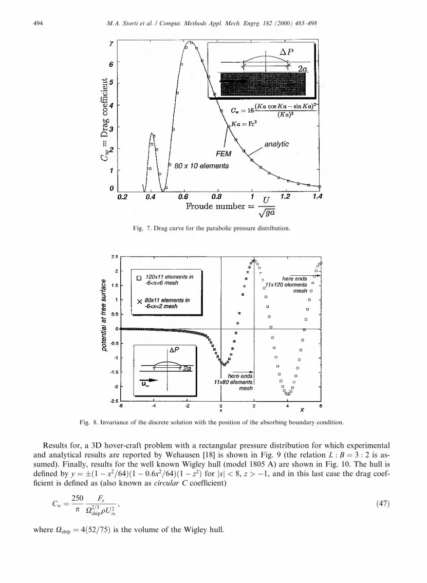
Results for, a 3D hover-craft problem with a rectangular pressure distribution for which experimentaland analytical results are reported by Wehausen [18] is shown in Fig. 9 (the relation L : B � 3 : 2 is as-sumed). Finally, results for the well known Wigley hull (model 1805 A) are shown in Fig. 10. The hull isde®ned by y � ��1ÿ x2=64��1ÿ 0:6x2=64��1ÿ z2� for jxj < 8, z > ÿ1, and in this last case the drag coef-®cient is de®ned as (also known as circular C coef®cient)

Cw � 250

pFx

X2=3shipqU 2

1; �47�

where Xship � 4�52=75� is the volume of the Wigley hull.

Fig. 7. Drag curve for the parabolic pressure distribution.

Fig. 8. Invariance of the discrete solution with the position of the absorbing boundary condition.


As can be seen from these numerical examples, drag curves computed with this method exhibit very wellde®ned secondary maxima, and computations can be carried out for a wide range of Froude numbers. Inaddition, as no numerical viscosity is used, the wave-resistance can be computed from a momentum ¯uxbalance and positive wave resistances are guaranteed [17].

Fig. 9. Drag curve for the rectangular pressure distribution.

Fig. 10. Drag curve for the Wigley hull.


7.3. The sea-keeping problem

Sea-keeping refers to performance and safety of ships at rough seas [15,14]. The typical problem con-sidered here is a plane wave impinging on a ¯oating body or marine structure see Fig. 11. The body os-cillates about its mean position due to these forces, and this movement originates in turn a pattern ofradiated waves, resulting in a ¯uid structure interaction problem. From the numerical point of view, theproblem amounts to solving (in 3D) the diffraction problem were the plane wave impinges on the bodywhich is kept ®xed, and a certain number of radiation problems were the impinging wave is not present, andthe pattern of radiated waves for a certain prescribed harmonic motion of the body is computed. Thenumber of radiation problems to be solved is equal to the number of degrees of freedom of the structure:three (two translations, one rotation) in 2D and six (three translations, three rotations) in 3D. The couplingof the ¯uid and the structure is made by solving a small system involving response coef®cients computed forthe ¯uid and the dynamical coef®cients of the structure itself (mass, inertia moments, stiffnesses). Weconcentrate here in the solution of each of the ¯uid problems, either radiation or diffraction. The governingequations are

D/j � 0; in X; �48�/j;n ÿ �x2=g�/j � 0 at Rfs; �49�/j;n � �uÿ u0�j � n at Rship; �50�/j � 0 or /j;n � 0 at Rbot; �51�appropriated radiation b:c:'s at Rout: �52�

Condition (49) is the linearized free surface boundary condition, and can be obtained from elimination ofthe elevation from the linearized kinematic and dynamic conditions. (50) is the perturbation imposedeither by the movement of the body or imposed by the impinging wave. Application of the DNL isstraightforward and follows the lines described for the wave resistance problem discussed previously butwith the di�erence that here the inviscid modes propagate in both directions, so that it results to be moresimilar to the Helmholtz equation. The problem is generally in cylindrical coordinates as shown in Fig.12, and three structured layers of nodes at the outer boundary serve for the computation of the DNLabsorbing matrix.

The example here is a pile of varying section oscillating in heave mode (i.e. vertically) at a frequency suchthat the characteristic wave-length of the waves is k � 2pg=x2 � 0:7, and the mean radius of the pile isR � 1. In Figs. 13 and 14 we see the absolute value of the potential at the surface with and without ab-sorbing boundary conditions, respectively. We see that with absorbing boundary condition, the result isalmost independent of the position of the arti®cial boundary. Results are shown with two meshes, oneending at rout � 3 and the other with rout � 5. Note that in the former case the outer boundary is at two orthree wave-lengths from the structure. In contrast, very small variations in the position of the outerboundary (from rout � 10 to rout � 9:5) cause large variations in the amplitude of the potential curve whenno absorbing boundary conditions (i.e. a Neumann b.c.) are used, even when the position of the outerboundary is located relatively far from the body (more than 10 wavelengths).

Fig. 11. Geometry description of the sea-keeping problem.


Fig. 12. Structured layers near the outlet cylindrical section for the computation of the DNL absorption matrix.

Fig. 13. Free surface elevation with DNL absorbing boundary conditions and two meshes of di�erent external radii.

Fig. 14. Free surface elevation without absorbing boundary conditions and two meshes of di�erent external radii.


8. Conclusions

A discrete non-local (DNL) absorbing boundary condition for the wave-like problems has been pre-sented. It is based on an eigen-decomposition of the system of ODE's that results from discretization in a1D structured mesh. The sense of the propagation of the eigen-modes is determined depending on the senseof decay of the corresponding solution, that is on whether the absolute value of the corresponding ei-genvalue is greater or lower than unity. For eigenvalues with unit absolute value the classi®cation is per-formed by perturbing the operator with a small dissipative term, and it is shown that this is equivalent tocomputing the group velocity in the temporal form of the equation. Application, with numerical examples,to the Helmholtz equation, wave-resistance and sea-keeping problems is discussed.

Acknowledgements

This work has received ®nancial support from Consejo Nacional de Investigaciones Cient�õ®cas y T�ecnicas(CONICET, Argentina), Banco Interamericano de Desarrollo (BID) and Universidad Nacional del Litoralthrough grants BID/CONICET 802/OC-AR Pid Nr. 26, CONICET PEI 232/97 and CAI+D UNL 94/95.The work was done in cooperation with Centro Internacional de M�etodos Num�ericos en Ingenier�õa (CIMNE,Barcelona). We made extensive use of freely distributed software as Linux OS, Octave, Fortran f2c com-piler, Tgif and many others. We acknowledge a free single-user license for MuPAD from SciFace Software.

References

[1] J.C. Berkho�, N. Book, A.C. Radder, Veri®cation of numerical wave propagation models for simple harmonic linear water waves,

Coastal Engrg. 6 (3) (1981) 255±279.

[2] P. Bettess, O.C. Zienkiewicz, Di�raction and refraction of surface waves using ®nite and in®nite elements, Internat. J. Numer.

Meth. Engrg. 11 (1977) 1271±1290.

[3] R.P. Bonet, N. Nigro, M.A. Storti, S.R. Idelsohn, Non-re¯ective planar boundary condition based on gauss ®ltering advances, In

preparation 1998.

[4] J. Broeze, J.E. Romate, Absorbing boundary conditions for free surface wave simulations with a panel method, J. Comput. Phys.

99 (1992) 146.

[5] D.S. Burnett, R.L. Holfrod, Prolate and oblate spheroidal acoustic in®nite elements, Comput. Methods Appl. Mech. Engrg. 158

(1998) 117±142.

[6] C.W. Dawson, A practical computer method for solving ship-wave problems, in: Proceedings of the second International

Conference on Numerical Ships Hydrodynamics 30 Berkeley, 1977.

[7] J. D'El�õa, Numerical methods for the Ship Wave-Resistance Problem, Ph.D. thesis, Univ. Nacional del Litoral (Santa Fe,

Argentina) 1997.

[8] D. Givoli, Non-re¯ecting boundary conditions, J. Comput. Phys. 94 (1991) 1±29.

[9] D. Givoli, J.B. Keller, A ®nite element method for large domains, Comput. Methods Appl. Mech. Engrg. 76 (1989) 41±66.

[10] D. Givoli, J.B. Keller, Non-re¯ecting boundary conditions for elastic waves, Wave Motion 12 (1990) 261±279.

[11] Y. Ito, K. Tanimoto, A method of numerical analysis of wave propagation ± application to wave di�raction and refraction, in:

Proceedings of the 13th International Conference on Coastal Engineering 1972, ASCE, New York.

[12] L. Landweber, Motion of Immersed and Flotanting Bodies, Handbook of Fluid Dynamics, McGraw-Hill, New York, 1961.

[13] M. Lenoir, A. Tounsi, The localized ®nite element method and its application to the two-dimensional sea-keeping problem, SIAM

J. Numer. Anal. 25 (1988) 729±752.

[14] J.N. Newman, Wave-drift of ¯oating bodies, J. ¯uid Mech. 249 (1993) 241±259.

[15] M. Ohkusu, Advances in Marine Hydrodynamics, Computational Mechanics Publications, Wessex, 1996.

[16] M. Storti, J.D'El�õa, S. Idelsohn, Algebraic discrete non-local (DNL) absorbing boundary condition for the ship wave resistance

problem, to appear, 1998a.

[17] M. Storti, J.D'El�õa, S. Idelsohn, Computating ship wave resistance from wave amplitude with the DNL absorbing boundary

condition, 1998b.

[18] J.V. Wehausen, The wave resistance of ships, Advances Appl. Mech. 13 (1973) 93±245.

[19] O.C. Zienkiewicz, D.W. Kelly, P. Bettess, Marriage �a la mode- or the best of both worlds. boundary integrals and ®nite element

procedures, in: Proceedings of the Conference on Innovative Methods of Numerical Computation, Versailles, France, 1977.


Documents

The DNL absorbing boundary condition: applications to wave problems