EXPLICIT FORMULAS FOR REPEATED GAMES WITH

ABSORBING STATES

Rida LARAKI

Février 2009

Cahier n° 2009-06

ECOLE POLYTECHNIQUE CENTRE NATIONAL DE LA RECHERCHE SCIENTIFIQUE

DEPARTEMENT D'ECONOMIE Route de Saclay

91128 PALAISEAU CEDEX (33) 1 69333033

http://www.enseignement.polytechnique.fr/economie/ mailto:chantal.poujouly@polytechnique.edu

hal-0

0362

421,

ver

sion

1 -

27 F

eb 2

009

Explicit Formulas for Repeated Games with Absorbing States∗

Rida LARAKI†

January 26, 2009

Abstract

Explicit formulas for the asymptotic value limλ→0 v(λ) and the asymptotic minmax limλ→0 w(λ)of finite λ-discounted absorbing games are provided. New simple proofs for the existence ofthe limits as λ goes zero are given. Similar characterizations for stationary Nash equilibriumpayoffs are obtained. The results may be extended to absorbing games with compact actionsets and jointly continuous payoff functions.

1 Introduction

Aumann and Maschler [1] introduced and studied long interaction two player zero-sum repeatedgames with incomplete information. They introduced the asymptotic and uniform approachesand obtained an explicit formulas for the asymptotic value when a player is fully informed (thefamous Cav(u) theorem). Mertens and Zamir [8] completed this work and obtained their elegantsystem of functional equations [8] that characterizes the asymptotic value of a repeated game withincomplete information on both sides. Unfortunately, very few repeated games have an explicitcharacterization of the asymptotic value .

Stochastic games are repeated games in which a state variable follows a markov chain con-trolled by the actions of the players. Shapley [10] introduced the two player zero-sum model withfinitely many states and actions (i.e. the finite model). He proved the existence of the valueof the λ-discounted game v (λ) by introducing a dynamic programming principle (the Shapleyoperator).

Kohlberg [5] proved the existence of the asymptotic value v = limλ→0 v (λ) in the subclassof finite absorbing games (i.e., stochastic games in which only one state is non-absorbing). Hisoperator appraoch uses the additional information obtained from the derivative of the Shapleyoperator at λ = 0 to deduce the existence of limλ→0 v (λ) and its characterization via variationalinequalities.

Laraki ([6], [7]) used a variational approach to study games in which each player controlsa martingale (including Aumann and Maschler repeated games). As in differential games withfixed duration, the approach starts with the dynamic programming principle, follows with anoptimal strategy for some player for a fixed discounted factor λ, relax the constraint of the otherplayer and lets the discount factor λ carefully tend to zero. This allows to show the existence oflimλ→0 v (λ) and its variational characterization.

The same approach gives, for absorbing games, a new proof for the existence of limλ→0 v (λ)and its characterization as the value of a one-shot game. When the probability of absorption iscontrolled by only one player (as in the big match), the formula can be simplified to the value of

∗I would like to thank Michel Balinski, Eilon Solan, Sylvain Sorin and Xavier Venel for their very usefulcomments.

†Main position: CNRS, Laboratoire d’Econometrie, Departement d’Economie, Ecole Polytechnique, Palaiseau,France. Associated to: Equipe Combinatoire, Universite Paris 6. Email: rida.laraki@polytechnique.edu

1

hal-0

0362

421,

ver

sion

1 -

27 F

eb 2

009

an underlying finite game. Coulomb [3] provided another explicit formula for limλ→0 v (λ) usingan algebraic approach.

Rosenberg and Sorin [9] extended the Kohlberg result to absorbing games when action sets areinfinite but compact and payoffs and transitions are separately continuous. However, no explicitformula is known for v.

The minmax w (λ) of a multi-player λ-discounted absorbing game is the level at which a teamof players could punish another player. From Bewley and Kohlberg [2] one deduces the existenceof lim w (λ) for any finite absorbing game. However, no explicit formula exists and it is not knownif the limit exists in infinite absorbing games.

The variational approach allows (1) to prove the existence of the asymptotic minmax w =limλ→0 w (λ) of any multi-player jointly continuous compact absorbing game and (2) providesan explicit formula for w. Similar formulas could be obtained for stationary Nash equilibriumpayoffs.

2 The value

Consider two finite sets I and J , two (payoff) functions f , g from I×J to [−1, 1] and a (probabilitytransition) function p from I × J to [0, 1] .

The game is played in discrete time. At stage t = 1, 2, ... player I chooses at random it ∈ I(according to some mixed action xt ∈ ∆ (I) 1) and, simultaneously, player J chooses at randomjt ∈ J (according to some mixed action yt ∈ ∆ (J) 2):

(i) the payoff is f (it, jt) at stage t;(ii) with probability 1 − p (it, jt) the game is absorbed and the payoff is g (it, jt) in all future

stages;and(iii) with probability p (it, jt) the interaction continues (the situation is repeated at step t+1).If the stream of payoffs is r(t), t = 1, 2, ..., the λ-discounted-payoff of the game is

∑∞t=1 λ(1−

λ)t−1r(t). Player I maximizes the expected discounted-payoff and player J minimizes that payoff.M+(I) = {α = (αi)i∈I : αi ∈ [0,+∞)} is the set of positive measures on I (the I-dimensional

positive orthant). For any i and j, let p∗(i, j) = 1 − p(i, j) and f∗(i, j) = [1 − p(i, j)] × g(i, j).For any (α, j) ∈ M+(I) × J and ϕ : I × J → [−1, 1] , ϕ is extended linearly as follows ϕ(α, j) =∑

i∈I αiϕ(i, j). Note that ∆(I) ⊂ M+(I).

Proposition 1 (Shapley 1953) Gλ has a value, v (λ) . It is the unique real in [0, 1] satisfying,

v (λ) = maxx∈∆(I)

minj∈J

[λf(x, j) + (1 − λ) p(x, j)v (λ) + (1 − λ) f∗(x, j)] . (1)

Equation (1) implies that player I has an optimal stationary strategy (that plays the samemixed action x at each period). This implies in particular that the proposition holds even if theplayers have no memory or do not observe past actions.

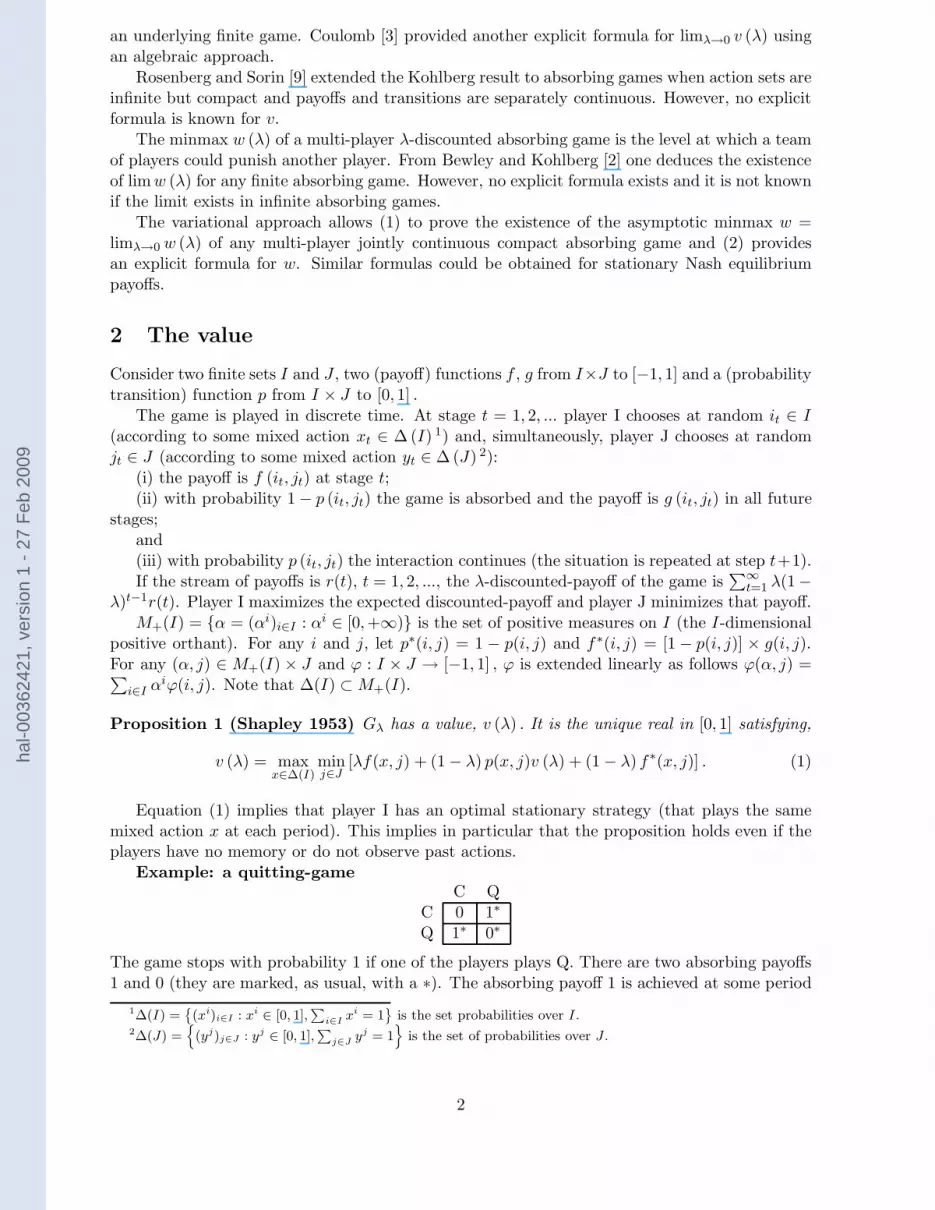
Example: a quitting-gameC Q

C 0 1∗

Q 1∗ 0∗

The game stops with probability 1 if one of the players plays Q. There are two absorbing payoffs1 and 0 (they are marked, as usual, with a ∗). The absorbing payoff 1 is achieved at some period

1∆(I) ={

(xi)i∈I : xi∈ [0, 1],

∑

i∈Ixi = 1

}

is the set probabilities over I .2∆(J) =

{

(yj)j∈J : yj∈ [0, 1],

∑

j∈Jyj = 1

}

is the set of probabilities over J .

2

hal-0

0362

421,

ver

sion

1 -

27 F

eb 2

009

if (C,Q) or (Q,C) is played. The absorbing payoff 0∗ is achieved if (Q,Q) is played. The game isnon-absorbed if both players decide to continue and play (C,C).

Consider the following strategy stationary profile in which player I plays at each period(xC, (1−x)Q) and player 2 (yC, (1−y)Q). The corresponding discounted payoff rλ(x, y) satisfies

rλ(x, y) = xy (λ × 0 + (1 − λ) rλ(x, y)) + ((1 − x)y + (1 − y)x) ,

so that

rλ(x, y) =x + y − 2xy

1 − xy(1 − λ).

The value vλ ∈ [0, 1] satisfies:

vλ = value

C QC (1 − λ)vλ 1Q 1 0

= maxx∈[0,1]

miny∈[0,1]

[xy(1 − λ)vλ + x(1 − y) + y(1 − x)]

= miny∈[0,1]

maxx∈[0,1]

[xy(1 − λ)vλ + x(1 − y) + y(1 − x)] .

It may be checked that

vλ = xλ = yλ =1 −

√λ

1 − λ.

The value and the optimal strategies are not rational fractions of λ (but admit a puiseux series inpower of λ). Bewley and Kohlberg [2] show this to hold for all finite stochastic games and deducefrom it the existence of lim v (λ).

Lemma 2 v (λ) satisfies

v (λ) = maxx∈∆(I)

minj∈J

λf(x, j) + (1 − λ) f∗(x, j)

λp(x, j) + p∗(x, j).

Proof. If in the λ-discounted game, player I plays the stationary strategy x and player Jplays a pure stationary strategy j ∈ J , the λ-discounted reward r (λ, x, j) satisfies:

r (λ, x, j) = λf(x, j) + (1 − λ) p(x, j)r (λ, x, j) + (1 − λ) f∗(x, j).

Since p∗ = (1 − p),

r (λ, x, j) =λf(x, j) + (1 − λ) f∗(x, j)

λp(x, j) + p∗(x, j).

The maximizer has a stationary optimal strategy and the minimizer has a pure stationary bestreply: this proves the lemma.

In the following, α ⊥ x means that for every i ∈ I, xi > 0 ⇒ αi = 0.

Theorem 3 As λ goes to zero v (λ) converges to

v = supx∈∆(I)

supα⊥x∈M+(I)

minj∈J

(

f∗(x, j)

p∗(x, j)1{p∗(x,j)>0} +

f(x, j) + f∗(α, j)

p(x, j) + p∗(α, j)1{p∗(x,j)=0}

)

.

Proof. Let w = limn→∞ v (λn) be an accumulation point of v (λ).Step 1: Consider an optimal stationary strategy x (λn) for player I and go to the limit using

Shapley’s dynamic programming principle. From the formula of v(λn), there exists x (λn) ∈ ∆(I)such that for every j ∈ J,

v (λn) ≤ λnf(x(λn), j) + (1 − λn) f∗(x(λn), j)

λnp(x(λn), j) + p∗(x(λn), j). (2)

3

hal-0

0362

421,

ver

sion

1 -

27 F

eb 2

009

By the compactness of ∆(I) it may be supposed that x (λn) → x.

Case 1: p∗(x, j) > 0. Letting λn go to zero implies w ≤ f∗(x,j)p∗(x,j) .

Case 2: p∗(x, j) =∑

i∈I xip∗(i, j) = 0. Thus,∑

i∈S(x) p∗(i, j) = 0 where S(x) = {i ∈ I : xi >

0} is the support of x. Let α(λn) =(

xi(λn)λn

1{xi=0}

)

i∈I∈ M+(I) so that α(λn) ⊥ x. Consequently,

∑

i∈I

xi (λn)

λnp∗(i, j) =

∑

i/∈S(x)

xi (λn)

λnp∗(i, j)

=∑

i∈I

αi (λn) p∗(i, j)

= p∗(α (λn) , j),

and∑

i∈I

xi (λn)

λnf∗(i, j) =

∑

i∈I

αi (λn) f∗(i, j) = f∗(α (λn) , j),

so, from equation (2), and because p(x, j) = 1,

w ≤ limn→∞

inff(x, j) + (1 − λn) f∗(α(λn), j)

p(x, j) + p∗(α(λn), j). (3)

Since J is finite, for any ε > 0, there is N(ε) such that, for every j ∈ J , w ≤ f(x,j)+f∗(α(λN(ε)),j)

p(x,j)+p∗(α(λN(ε)),j)+ε.

Consequently, w ≤ v.Step 2: Construct a strategy for player I in the λn-discounted game that guarantees v as

λn → 0. Let (αε, xε) ∈ M+(I)×∆(I) be ε-optimal for the maximizer in the formula of v. For λn

small enough, let xε(λn) be proportional to xε +λnαε (xε(λn) = µn(xε +λnαε) for some µn > 0).Let r(λn) be the unique real in the interval [0, 1] that satisfies,

r(λn) = minj∈J

[

λn [f(xε(λn), j)] + (1 − λn) (p(xε(λn), j)) r (λn)+ (1 − λn) f∗(xε(λn), j)

]

. (4)

By the linearity of f , p, f∗ and p∗ on x,

r (λn) = minj

λnf(xε + λnαε, j) + (1 − λn) f∗(xε + λnαε, j)

λnp(xε + λnαε, j) + p∗(xε + λnαε, j)

= minj

λnf(xε, j) + λ2nf(αε, j) + (1 − λn) f∗(xε, j) + (1 − λn) λnf∗(αε, j)

λnp(xε, j) + λ2np(αε, j) + p∗(xε, j) + λnp∗(αε, j)

.

Also, v(λn) ≥ r(λn) since r(λn) is the payoff of player I if he plays the stationary strategy xε(λn).Let jλn

∈ J be an optimal stationary pure best response for player J against xε(λn) (an elementof the arg min in (4)). Since J is finite and r(λn) bounded, one can switch to a subsequence and

suppose that jλnis constant (= j) and that r(λn) → r. If p∗(xε, j) > 0 then r = f∗(xε,j)

p∗(xε,j) . If

p∗(xε, j) = 0, clearly r = f(xε,j)+f∗(αε,j)p(xε,j)+p∗(αε,j) . Consequently, w ≥ v.

This proof shows that for each ε > 0, a player always admits an ε-optimal strategy in theλ-discounted game proportional to xε + λαε for all λ small enough. The quitting game exampleshows that a 0-optimal strategy of the λ-discounted game is not always of that form. Thisidentifies the asymptotic value as the value of what may be called the asymptotic game.

For any (α, β) ∈ M+(I) × M+(J) and ϕ : I × J → [−1, 1] , ϕ is extended linearly as followsϕ(α, β) =

∑

i∈I,j∈J αiβjϕ(i, j). For player I let

Λ(I) = {(x, α) ∈ ∆(I) × M+(I) : α ⊥ x}

and similarly for player J .

4

hal-0

0362

421,

ver

sion

1 -

27 F

eb 2

009

Corollary 4 v satisfies the following equations:

v = sup(x,α)∈Λ(I)

inf(y,β)∈Λ(J)

(

f∗(x,y)p∗(x,y)1{p∗(x,y)>0}

+ f(x,y)+f∗(α,y)+f∗(x,β)p(x,y)+p∗(α,y)+p∗(x,β) 1{p∗(x,y)=0}

)

= inf(y,β)∈Λ(I)

sup(x,α)∈Λ(I)

(

f∗(x,y)p∗(x,y)1{p∗(x,y)>0}

+ f(x,y)+f∗(α,y)+f∗(x,β)p(x,y)+p∗(α,y)+p∗(x,β) 1{p∗(x,y)=0}

)

= sup(x,α)∈Λ(I)

infy∈∆(J)

(

f∗(x,y)p∗(x,y)1{p∗(x,y)>0}

+ f(x,y)+f∗(α,y)p(x,y)+p∗(α,y) 1{p∗(x,y)=0}

)

.

Proof. Consider an ε-optimal strategy xε(λ) proportional to xε + λαε in the λ-discountedgame. Taking any strategy of Player J proportional to y (λ) = y + λβ yields

v (λ) − ε ≤ λf(xε + λαε, y + λβ) + (1 − λ) f∗(xε + λαε, y + λβ)

λp(xε + λαε, y + λβ) + p∗(xε + λαε, y + λβ).

p∗(xε, y) > 0 implies v = lim v (λ) ≤ f∗(xε,y)p∗(xε,y) . If p∗(xε, y) = 0 then f∗(xε, y) = 0. Using the

multi-linearity of f , f∗, p and p∗ and dividing by λ imply:

v (λ) − ε ≤ f(xε + λαε, y + λβ) + (1 − λ) f∗(αε, y) + (1 − λ) f∗(xε, β) + (1 − λ) λf∗(αε, β)

p(xε + λαε, y + λβ) + p∗(αε, y) + f∗(xε, β) + λp∗(αε, β).

Going to the limit,

v ≤ f(xε, y) + f∗(αε, y) + f∗(xε, β)

p(xε, y) + p∗(αε, y) + f∗(xε, β),

which holds for all (y, β). Thus,

v ≤ sup(x,α)∈Λ(I)

inf(y,β)∈Λ(J)

(

f∗(x,y)p∗(x,y)1{p∗(x,y)>0}

+ f(x,y)+f∗(α,y)+f∗(x,β)p(x,y)+p∗(α,y)+p∗(x,β) 1{p∗(x,y)=0}

)

.

And similarly for the other inequality. Since the inf sup is always higher than the sup inf the firsttwo equalities follow.

Taking β = 0 in the last inequality implies:

v ≤ sup(x,α)∈Λ(I)

infy∈∆(J)

(

f∗(x,y)p∗(x,y)1{p∗(x,y)>0}

+ f(x,y)+f∗(α,y)p(x,y)+p∗(α,y) 1{p∗(x,y)=0}

)

,

and from the formula of v in theorem 3, one obtains the last equality of the corollary.

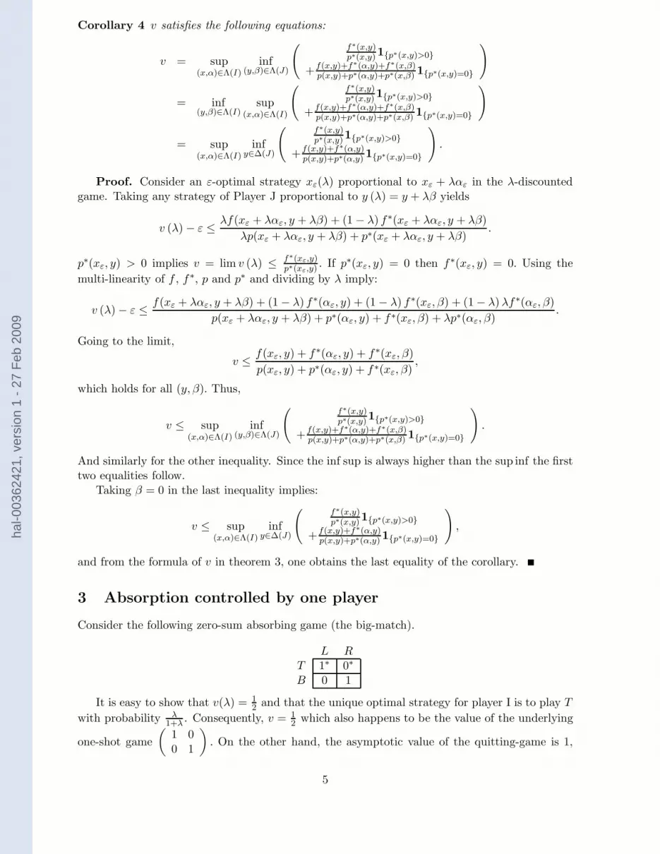
3 Absorption controlled by one player

Consider the following zero-sum absorbing game (the big-match).

L RT 1∗ 0∗

B 0 1

It is easy to show that v(λ) = 12 and that the unique optimal strategy for player I is to play T

with probability λ1+λ . Consequently, v = 1

2 which also happens to be the value of the underlying

one-shot game

(

1 00 1

)

. On the other hand, the asymptotic value of the quitting-game is 1,

5

hal-0

0362

421,

ver

sion

1 -

27 F

eb 2

009

which is not the value of the underlying one-shot game

(

0 11 0

)

. A natural question arises:

what are the absorbing games when v is the value of an underlying one-shot game?A game is partially-controlled by player I if the the transition function p(i, j) depends only

on i (but not the associated payoffs).

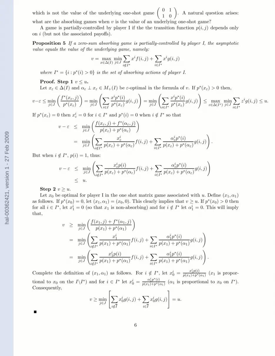
Proposition 5 If a zero-sum absorbing game is partially-controlled by player I, the asymptoticvalue equals the value of the underlying game, namely:

v = maxx∈∆(I)

minj∈J

∑

i/∈I∗

xif(i, j) +∑

i∈I∗

xig(i, j)

where I∗ = {i : p∗(i) > 0} is the set of absorbing actions of player I.

Proof. Step 1 v ≤ u.Let xε ∈ ∆(I) and αε ⊥ xε ∈ M+(I) be ε-optimal in the formula of v. If p∗(xε) > 0 then,

v−ε ≤ minj∈J

(

f∗(xε, j)

p∗(xε)

)

= minj∈J

(

∑

i∈I

xip∗(i)

p∗(xε)g(i, j)

)

= minj∈J

(

∑

i∈I∗

xip∗(i)

p∗(xε)g(i, j)

)

≤ maxz∈∆(I∗)

minj∈J

∑

i∈I∗

zig(i, j) ≤ u.

If p∗(xε) = 0 then xiε = 0 for i ∈ I∗ and p∗(i) = 0 when i /∈ I∗ so that

v − ε ≤ minj∈J

(

f(xε, j) + f∗(αε, j)

p(xε) + p∗(αε)

)

= minj∈J

(

∑

i/∈I∗

xiε

p(xε) + p∗(αε)f(i, j) +

∑

i∈I∗

αiεp

∗(i)

p(xε) + p∗(αε)g(i, j)

)

.

But when i /∈ I∗, p(i) = 1, thus:

v − ε ≤ minj∈J

(

∑

i/∈I∗

xiεp(i)

p(xε) + p∗(αε)f(i, j) +

∑

i∈I∗

αiεp

∗(i)

p(xε) + p∗(αε)g(i, j)

)

≤ u.

Step 2 v ≥ u.Let x0 be optimal for player I in the one shot matrix game associated with u. Define (x1, α1)

as follows. If p∗(x0) = 0, let (x1, α1) = (x0, 0). This clearly implies that v ≥ u. If p∗(x0) > 0 thenfor all i ∈ I∗, let xi

1 = 0 (so that x1 is non-absorbing) and for i /∈ I∗ let αi1 = 0. This will imply

that,

v ≥ minj∈J

(

f(x1, j) + f∗(α1, j)

p(x1) + p∗(α1)

)

= minj∈J

(

∑

i/∈I∗

xi1

p(x1) + p∗(α1)f(i, j) +

∑

i∈I∗

αi1p

∗(i)

p(x1) + p∗(α1)g(i, j)

)

= minj∈J

(

∑

i/∈I∗

xi1p(i)

p(x1) + p∗(α1)f(i, j) +

∑

i∈I∗

αi1p

∗(i)

p(x1) + p∗(α1)g(i, j)

)

.

Complete the definition of (x1, α1) as follows. For i /∈ I∗, let xi0 =

xi1p(i)

p(x1)+p∗(α1) (x1 is propor-

tional to x0 on the I\I∗) and for i ∈ I∗ let xi0 =

αi1p∗(i)

p(x1)+p∗(α1) (α1 is proportional to x0 on I∗).Consequently,

v ≥ minj∈J

∑

i/∈I

xi0g(i, j) +

∑

i∈I

xi0g(i, j)

= u.

6

hal-0

0362

421,

ver

sion

1 -

27 F

eb 2

009

4 The minmax

A team of N players (named I) play against player (J). Assume the finiteness of all the strategysets. Each player k in team I has a finite set of actions Ik. Player J has a finite set of actionsJ . Let I = I1 × ... × IN and f , g from I × J → [−1, 1] and p : I × J → [0, 1] . The gameis played as above, except that (1) at each period, players in team I randomize independently(they are not allowed to correlate their random moves); and (2) team I minimizes the expectedλ-discounted-payoff and player J maximizes the payoff (players in I try to punish player J).

Let ∆ = ∆(I1) × ... × ∆(IN ), p∗ (·) = 1 − p (·) , f∗ (·) = p∗ (·) × g (·) and M+ = M+(I1) ×... × M+(IN ). For x ∈ X, j ∈ J, k ∈ N and α ∈ M+, a function ϕ : I × J → [−1, 1] is extendedmulti-linearly as follows:

ϕ(x, j) =∑

i=(i1,...,iN)∈I

xi11 × ... × xiN

N ϕ(i, j)

ϕ(αk, x−k, j) =∑

i=(i1,...,iN)∈I

xi1

1 × ... × xik−1

k−1 × αik

k × xik+1

k+1 ... × xiN

n ϕ(i, j).

Let w (λ) denote the minimum payoff that team I can guarantee against player J. From Bewleyand Kohlberg [2] one can deduce the existence of w (λ) . However, no explicit formula exists.

Theorem 6 w (λ) = minx∈∆ maxj∈Jλf(x,j)+(1−λ)f∗(x,j)

λp(x,j)+p∗(x,j) and, as λ → 0, converges to

w = inf(x,α)∈∆×M+:∀k,αk⊥xk

maxj∈J

f∗(x,j)p∗(x,j)1{p∗(x,j)>0}

+f(x,j)+

∑Nk=1 f∗(αk ,x−k,j)

p(x,j)+∑N

k=1 p∗(αk ,x−k,j)1{p∗(x,j)=0}

= inf(x,α)∈∆×M+:∀k,αk⊥xk

maxy∈∆(J)

f∗(x,y)p∗(x,y)1{p∗(x,y)>0}

+f(x,y)+

∑Nk=1 f∗(αk ,x−k,y)

p(x,y)+∑N

k=1 p∗(αk ,x−k,y)1{p∗(x,y)=0}

.

Proof. For the first formula, follow the ideas in the proof of theorem 3 and corollary 4. Letv = limn→∞ w (λn) where λn → 0.

Modifications in step 1 in theorem 3: let x (λn) → x be such that for every j ∈ J,

w (λn) ≥ λnf(x(λn), j) + (1 − λn) f∗(x(λn), j)

λnp(x(λn), j) + p∗(x(λn), j).

Let y(λn) = x (λn) − x → 0 so that:

p∗(x(λn), j) =∑

i=(i1,...,iN)∈I

xi11 (λn) × ... × xiN

N (λn)p(i, j)

=∑

i=(i1,...,iN)∈I

(yi11 (λn) + xi1

1 ) × ... × (yiNN (λn) + xiN

N )p(i, j)

= p∗(x, j) +

N∑

k=1

p∗(yk(λn), x−k, j) + o(

N∑

k=1

p∗(yk(λn), x−k, j))

If p∗(x, j) > 0 then w ≥ f∗(x,j)p∗(x,j) . If p∗(x, j) = 0 and if αk(λn) =

(

xik

k(λn)

λn1{

xik

k=0}

)

ik∈Ik

∈ M+(Ik)

then αk(λn) ⊥ xk and

p∗(x(λn)

λn, j) =

N∑

k=1

p∗(αk(λn), x−k, j) + o(N∑

k=1

p∗(αk(λn), x−k, j))

7

hal-0

0362

421,

ver

sion

1 -

27 F

eb 2

009

and the same is true for f∗ so that

w ≥ lim supn→∞

f(x, j) +∑N

k=1 f∗(αk(λn), x−k, j)

p(x, j) +∑N

k=1 f∗(αk(λn), x−k, j)

which implies that w ≥ v.Modifications in step 2 in theorem 3: take (αε, xε) to be ε-optimal for the minimizer in the

formula of w and define xεk(λn) to be proportional to xε

k + λnαεk and deduce that w ≤ v.

For the second formula, follow corollary 4. For each ε > 0, the proof above implies thatplayers in I have an ε-optimal strategy (xε

k(λ))k∈I where xεk(λ) is proportional to xε

k + λαεk in the

λ-discounted game for all λ small enough. This implies that for any y ∈ ∆(J),

w (λ) + ε ≥ λf(xεk(λ), y) + (1 − λ) f∗(xε

k(λ), y)

λp(xεk(λ), y) + p∗(xε

k(λ), y).

where the right hand is a fractional function of λ. Consequently, it admits a limit which may becomputed as in step 1 (using the multi-linearity of payoffs and transitions). This will imply that

w ≥ infx∈∆

infα∈M+:∀k,αk⊥xk

maxy∈∆(J)

f∗(x,y)p∗(x,y)1{p∗(x,y)>0}

+f(x,y)+

∑Nk=1 f∗(αk,x−k,y)

p(x,y)+∑N

k=1 p∗(αk ,x−k,y)1{p∗(x,y)=0}

.

The first formula of w and the fact that J ⊂ ∆(J) imply the other inequality.

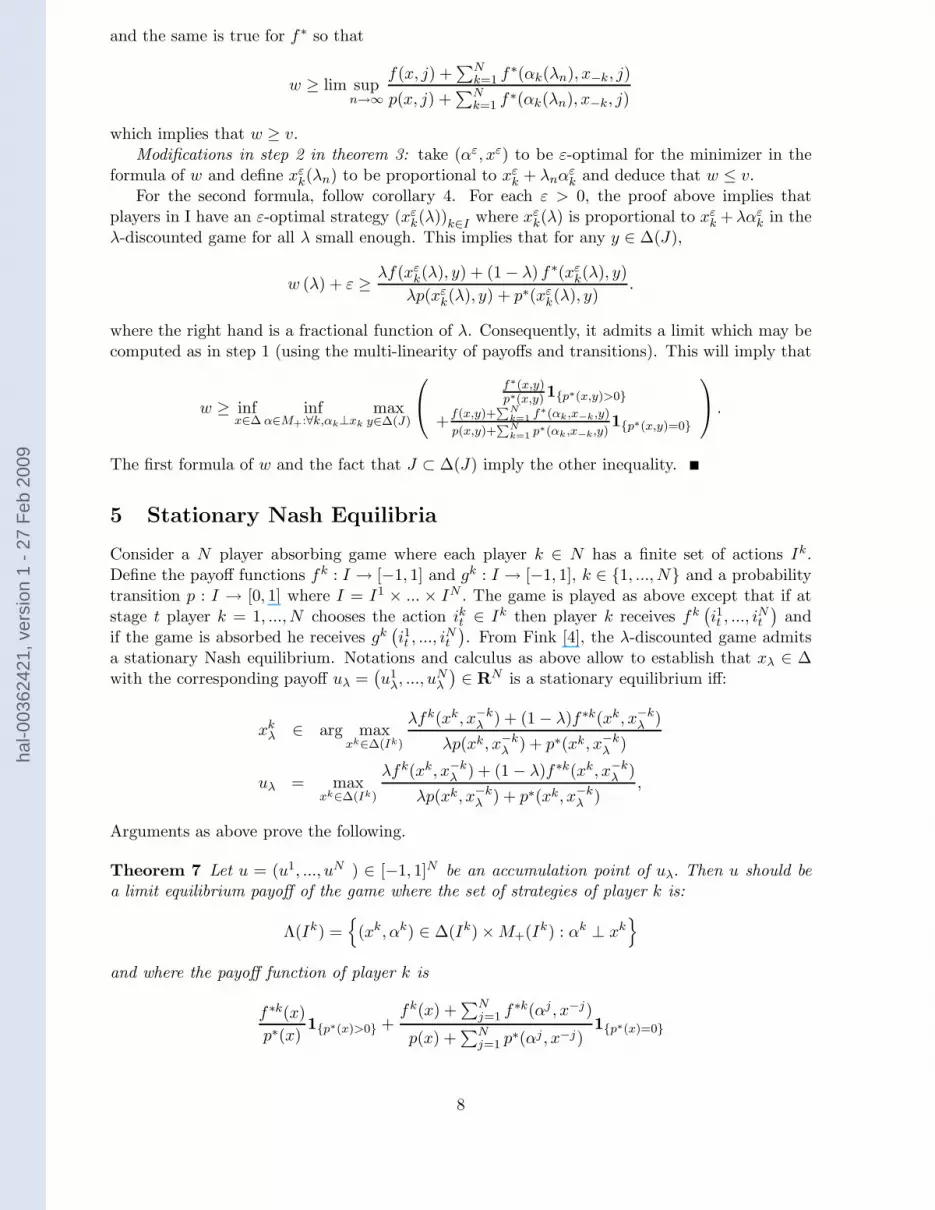
5 Stationary Nash Equilibria

Consider a N player absorbing game where each player k ∈ N has a finite set of actions Ik.Define the payoff functions fk : I → [−1, 1] and gk : I → [−1, 1], k ∈ {1, ..., N} and a probabilitytransition p : I → [0, 1] where I = I1 × ... × IN . The game is played as above except that if atstage t player k = 1, ..., N chooses the action ikt ∈ Ik then player k receives fk

(

i1t , ..., iNt

)

andif the game is absorbed he receives gk

(

i1t , ..., iNt

)

. From Fink [4], the λ-discounted game admitsa stationary Nash equilibrium. Notations and calculus as above allow to establish that xλ ∈ ∆with the corresponding payoff uλ =

(

u1λ, ..., uN

λ

)

∈ RN is a stationary equilibrium iff:

xkλ ∈ arg max

xk∈∆(Ik)

λfk(xk, x−kλ ) + (1 − λ)f∗k(xk, x−k

λ )

λp(xk, x−kλ ) + p∗(xk, x−k

λ )

uλ = maxxk∈∆(Ik)

λfk(xk, x−kλ ) + (1 − λ)f∗k(xk, x−k

λ )

λp(xk, x−kλ ) + p∗(xk, x−k

λ ),

Arguments as above prove the following.

Theorem 7 Let u = (u1, ..., uN ) ∈ [−1, 1]N be an accumulation point of uλ. Then u should bea limit equilibrium payoff of the game where the set of strategies of player k is:

Λ(Ik) ={

(xk, αk) ∈ ∆(Ik) × M+(Ik) : αk ⊥ xk}

and where the payoff function of player k is

f∗k(x)

p∗(x)1{p∗(x)>0} +

fk(x) +∑N

j=1 f∗k(αj , x−j)

p(x) +∑N

j=1 p∗(αj , x−j)1{p∗(x)=0}

8

hal-0

0362

421,

ver

sion

1 -

27 F

eb 2

009

More precisely, for any ε > 0, there exists (xε, αε) such that:

uk = limε→0

f∗k(xε)

p∗(xε)1{p∗(xε)>0} +

fk(xε) +∑N

j=1 f∗k(αjε, x

−jε )

p(xε) +∑N

j=1 p∗(αjε, x

−jε )

1{p∗(xε)=0}

≥ sup(xk,αk)∈Λ(Ik)

f∗k(xk,x−kε )

p∗(xk ,x−kε )

1{p∗(xk ,x−kε )>0}

+fk(xk,x−k

ε )+f∗k(αk ,x−kε )+

∑Nj 6=k f∗j(αj

ε,xk,x−{k,j}ε )

p(xk,x−kε )+p∗k(αk ,x−k

ε )+∑N

j 6=k p∗(αjε,xk,x

−{k,j}ε )

1{p∗(xk ,x−kε )=0}

− ε

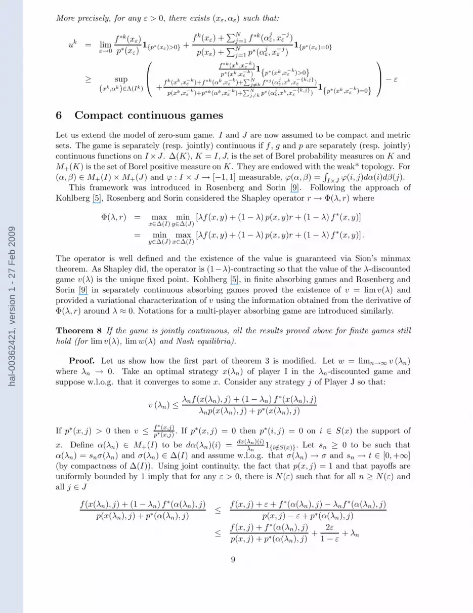
6 Compact continuous games

Let us extend the model of zero-sum game. I and J are now assumed to be compact and metricsets. The game is separately (resp. jointly) continuous if f , g and p are separately (resp. jointly)continuous functions on I×J . ∆(K), K = I, J, is the set of Borel probability measures on K andM+(K) is the set of Borel positive measure on K. They are endowed with the weak* topology. For(α, β) ∈ M+(I) × M+(J) and ϕ : I × J → [−1, 1] measurable, ϕ(α, β) =

∫

I×J ϕ(i, j)dα(i)dβ(j).This framework was introduced in Rosenberg and Sorin [9]. Following the approach of

Kohlberg [5], Rosenberg and Sorin considered the Shapley operator r → Φ(λ, r) where

Φ(λ, r) = maxx∈∆(I)

miny∈∆(J)

[λf(x, y) + (1 − λ) p(x, y)r + (1 − λ) f∗(x, y)]

= miny∈∆(J)

maxx∈∆(I)

[λf(x, y) + (1 − λ) p(x, y)r + (1 − λ) f∗(x, y)] .

The operator is well defined and the existence of the value is guaranteed via Sion’s minmaxtheorem. As Shapley did, the operator is (1−λ)-contracting so that the value of the λ-discountedgame v(λ) is the unique fixed point. Kohlberg [5], in finite absorbing games and Rosenberg andSorin [9] in separately continuous absorbing games proved the existence of v = lim v(λ) andprovided a variational characterization of v using the information obtained from the derivative ofΦ(λ, r) around λ ≈ 0. Notations for a multi-player absorbing game are introduced similarly.

Theorem 8 If the game is jointly continuous, all the results proved above for finite games stillhold (for lim v(λ), lim w(λ) and Nash equilibria).

Proof. Let us show how the first part of theorem 3 is modified. Let w = limn→∞ v (λn)where λn → 0. Take an optimal strategy x(λn) of player I in the λn-discounted game andsuppose w.l.o.g. that it converges to some x. Consider any strategy j of Player J so that:

v (λn) ≤ λnf(x(λn), j) + (1 − λn) f∗(x(λn), j)

λnp(x(λn), j) + p∗(x(λn), j)

If p∗(x, j) > 0 then v ≤ f∗(x,j)p∗(x,j) . If p∗(x, j) = 0 then p∗(i, j) = 0 on i ∈ S(x) the support of

x. Define α(λn) ∈ M+(I) to be dα(λn)(i) = dx(λn)(i)λn

1{i/∈S(x)}. Let sn ≥ 0 to be such thatα(λn) = snσ(λn) and σ(λn) ∈ ∆(I) and assume w.l.o.g. that σ(λn) → σ and sn → t ∈ [0,+∞](by compactness of ∆(I)). Using joint continuity, the fact that p(x, j) = 1 and that payoffs areuniformly bounded by 1 imply that for any ε > 0, there is N(ε) such that for all n ≥ N(ε) andall j ∈ J

f(x(λn), j) + (1 − λn) f∗(α(λn), j)

p(x(λn), j) + p∗(α(λn), j)≤ f(x, j) + ε + f∗(α(λn), j) − λnf∗(α(λn), j)

p(x, j) − ε + p∗(α(λn), j)

≤ f(x, j) + f∗(α(λn), j)

p(x, j) + p∗(α(λn), j)+

2ε

1 − ε+ λn

9

hal-0

0362

421,

ver

sion

1 -

27 F

eb 2

009

Consequently,

w ≤ supx∈∆(I)

supα⊥x∈M+(I)

minj∈J

(

f∗(x, j)

p∗(x, j)1{p∗(x,j)>0} +

f(x, j) + f∗(α, j)

p(x, j) + p∗(α, j)1{p∗(x,j)=0}

)

.

Step 2 of theorem 1 needs no modification. The other proofs are adapted in a similar way.

References

[1] Aumann R.J. and M. Maschler (1995). Repeated Games with Incomplete Information, M.I.T.Press.

[2] Bewley, T. and Kohlberg E. (1976). The Asymptotic Theory of Stochastic Games. Mathe-matics of Operation Research, 1, 197-208.

[3] Coulomb, J. M. (2001). Repeated Games with Absorbing States and Signaling Structure.Mathematics of Operation Research, 26, 286-303.

[4] Fink, A. M. (1964). Equilibrium in a Stochastic N -Person Game. J. Sci. Hiroshima Univ.28, 89-93.

[5] Kohlberg, E. (1974). Repeated Games with Absorbing States. Annals of Statistics, 2, 724-738.

[6] Laraki, R. (2001a). The Splitting Game and Applications. International Journal of GameTheory, 30, 359-376.

[7] Laraki, R. (2001b). Variational Inequalities, System of Functional Equations, and IncompleteInformation Repeated Games. SIAM Journal of Control and Optimization, 40(2), 516-524.

[8] Mertens J.-F. and S. Zamir (1971). The Value of Two-Person Zero-Sum Repeated Gameswith Lack of Information on Both Sides, International Journal of Game Theory, 1, 39-64.

[9] Rosenberg, D. and S. Sorin (2001). An Operator Approach to Zero-sum Repeated Games.Israel Journal of Mathematics, 121, 221-246.

[10] Shapley, L. S. (1953) Stochastic Games, Proceedings of the National Academy of Sciences ofthe U. S. A., 39, 1095-1100.

10

hal-0

0362

421,

ver

sion

1 -

27 F

eb 2

009