Embed Size (px)
Citation preview

Absorbing Interface Conditions for Domain
Decomposition Methods: a General Presentation
Yvon Maday∗ Frederic Magoules†
October 22, 2004
Abstract: The continuity conditions and the transmission conditions involvedin domain decomposition methods are of major importance for the fast and ro-bust convergence of these algorithms. This review paper presents step by step themethodology to derive various continuity conditions and compatible transmissionconditions for two different type of problems, i.e. the Laplace equation and theHelmholtz equation. An original homogeneous formulation is also presented bothin the continuous and in the discrete analysis. Numerical experiments show the rel-ative efficiency of these continuity conditions and of these transmission conditionson academic problems.
Keywords: absorbing interface conditions, domain decomposition, Schur Primal,Schur Dual, FETI, FETI-H, Schwarz
Resume: Les conditions de continuites et les conditions de transmissions utiliseesdans les methodes de decomposition de domaines sont fondamentales pour obtenirune convergence robuste et rapide de ces methodes. Cet article presente etapepar etape la methodologie a suivre pour definir plusieurs types de conditions decontinuites et de conditions de transmissions pour l’equation de Laplace et pourl’equation de Helmholtz. Une analyse originale est presentee de facon homogeneen continue et en discret. Des experiences numeriques illustrent la robustesse etl’efficacite de ces methodes sur des exemples academiques.
Mots clefs: conditions aux limites absorbantes, methodes de decomposition dedomaines, Schur Primal, Schur Dual, FETI, FETI-H, Schwarz
∗Laboratoire Jacques-Louis Lions, Universite Pierre et Marie Curie, BP 187,75252 Paris Cedex 05, France, [email protected]
†Institut Elie Cartan de Nancy, Universite Henri Poincare, BP 239, 54506 Vandoeuvre-les-Nancy Cedex, France, [email protected]
1

1 Introduction
Domain decomposition methods are very efficient algorithms to compute inparallel the solution of large scale problems, see for example [3, 30, 1, 28,19, 31] and references therein. These methods mainly consist in splittingthe global domain into several sub-domains and to compute the solution onthe global domain through the resolution of the problem associated witheach sub-domains. For example, the solution of the Laplace equation in oneglobal domain can be expressed as the solution of two Laplace equations intwo sub-domains, as soon as some continuity conditions are ensured on theinterface [24]. Using Dirichlet or Neumann type transmission conditions onthe interface leads to the Primal Schur complement [23], to the Dual Schurcomplement [7, 10] or to the Complete Schur complement methods. For theHelmholtz equation, even if the continuity conditions are the same in the-ory as for the Laplace equation, Robin type transmission conditions mustbe introduced on the interface in order to avoid any possible resonance’sfrequency inside the sub-domains [2, 25]. Using such Robin type transmis-sion conditions leads to the Dual Augmented Schur complement or to theComplete Augmented Schur complement methods. Changing the continu-ity conditions on the interface by Robin type continuity conditions can beinterpreted as a local preconditioning technique. It can be shown that usingRobin type continuity conditions and Robin type transmission conditions inthe previous domain decomposition methods is equivalent to use a modifiednon-overlapping Schwarz method as introduced in [20, 21, 2].
This review paper presents step by step a methodology to derive severalcontinuity conditions and transmission conditions for the Laplace equationand for the Helmholtz equation. Both a continuous and a discrete analysisare performed for an original formulation. Several numerical experimentsperformed on general mesh partitioning illustrate the relative efficiency ofthese continuity conditions and of these transmission conditions.
The structure of this paper is the following. Section 2 presents a continu-ous analysis of the absorbing interface conditions involved in non-overlappingdomain decomposition methods. These absorbing interface conditions ap-pear in the continuity conditions and in the transmission conditions when theglobal domain is split into several sub-domains. Dirichlet and Neumann typetransmission conditions are first introduced in Section 2.1 for the Laplaceequation. Then Robin type transmission conditions are introduced in Sec-tion 2.2 for the Helmholtz equation. In Section 2.3, the continuity conditionsare modified and interpreted as a local preconditioning technique. Followingthe same approach as in Section 2, Section 3 presents the discrete analysis
2

of the absorbing interface conditions. Section 4 presents some numericalexperiments and compares the convergence of several domain decomposi-tion methods equipped with these absorbing interface conditions. Finally,in Section 5 the conclusion of this paper is presented.
2 Continuous Analysis
In this section a synthetic presentation of the continuity conditions andcompatible transmission conditions involved in the non-overlapping domaindecomposition methods is presented. The cases of the Laplace and of theHelmholtz equation are analyzed respectively.
2.1 Dirichlet and Neumann Transmission Conditions on the
Interface
For the sake of clarity, the continuous analysis is first performed on the onedimensional Laplace equation. The formulation of the problem upon thevariable u in the domain Ω = [0, 1] reduces to
−∆u = f, x ∈]0, 1[u(0) = a (2.1)u(1) = b
where a and b are the prescribed Dirichlet boundary conditions and f isa given function in the Lebesgue space L
2(0, 1). The solution to such aproblem is known to belong to the Sobolev space H2(0, 1).
2.1.1 Coupling of Sub-domain Problems
If the domain Ω = [0, 1] is split into two non-overlapping sub-domains Ω(1) =[0, α] and Ω(2) = [α, 1] with an interface Γ = α, α ∈]0, 1[, a first theoremcan be announced.
Theorem 2.1 The problem (2.1) is equivalent to the following system ofsubproblems
−∆u(1) = f (1), x ∈]0, α[ (2.2)u(1)(0) = a (2.3)
3

−∆u(2) = f (2), x ∈]α, 1[ (2.4)u(2)(1) = b (2.5)
with the coupling equations on the interface:
u(1)(α) = u(2)(α) (2.6)∂xu(1)(α) = ∂xu(2)(α). (2.7)
Proof Under the regularity hypothesis made on the right hand side, theequalities in (2.1), (2.2)-(2.3) and (2.4)-(2.5) hold in L
2, the functions u,u(1) and u(2) thus belong to C1. Then (2.1) implies obviously (2.2)-(2.3)and (2.4)-(2.5) and the C1 continuity implies (2.6) and (2.7). Reciprocally,conditions (2.6) and (2.7) are those necessary for stating that the Laplaceoperator in the sense of distributions applied to piecewise C1 functions is theglobal Laplace operator and no Dirac mass appears.
Equations (2.6) and (2.7) are usually called continuity conditions in theliterature, since they represent the continuity of the solution and the con-tinuity of the normal derivative along the interface. From this first theo-rem a wide range of domain decomposition methods can already be derivedthrough the introduction of new variables defined along the interface.
2.1.2 Primal Schur Complement Method
One way to solve the coupling subproblems (2.2)-(2.7), is to assume thatthe solution is known on the interface. This means that the first continuitycondition u(1)(α) = u(2)(α) = g, is assumed to be satisfied with g as a knownvalue. In this case the solution of the subproblems
−∆u(1) = f (1), x ∈]0, α[ (2.8)u(1)(0) = a (2.9)u(1)(α) = g (2.10)
−∆u(2) = f (2), x ∈]α, 1[ (2.11)u(2)(1) = b (2.12)u(2)(α) = g (2.13)
4

gives u(1)(x) = u(1)(x; g, a, f (1)) and u(2)(x) = u(2)(x; g, b, f (2)) with
u(1)(x; g, a, f (1)) = a +
∫ x
a
F (1)(t) dt + (g − a)x
α
and u(2)(x; g, b, f (2)) = b −
∫ x
1F (2)(t) dt + (g − b)
1 − x
1 − α
where F (s) denotes the primitive function of f (s) with zero average over[0, α] for s = 1 and over [α, 1] for s = 2. The second continuity condition∂xu(1)(α) = ∂xu(2)(α) must be imposed in order to have the equivalence ofthe subproblems (2.8)-(2.13) with the problem (2.1). This leads to a uniquevalue of g that is convenient. Indeed, after substitution of u(1)(x; g, a, f (1))and u(2)(x; g, b, f (2)) in the second continuity conditions and taking intoaccount the linearity, this leads to
∂xu(1)(α; g, 0, 0)−∂xu(2)(α; g, 0, 0) = −∂xu(1)(α; 0, a, f (1))+∂xu(2)(α; 0, b, f (2)).
The solution of this system gives g and thus the value u(1) (resp. u(2)) can beobtained from the solution of (2.8)-(2.10) (resp. (2.11)-(2.13)). More detailson this method, called the Primal Schur complement method, can be foundin [23, 24].
2.1.3 Dual Schur Complement Method
In contrary to the Primal Schur complement method, the Dual Schur com-plement method [7, 10, 11, 24], is based on the hypothesis that the secondcontinuity conditions ∂xu(1)(α) = ∂xu(2)(α) = gx is satisfied, with gx as aknown value. Then, the solution of the subproblems
−∆u(1) = f (1), x ∈]0, α[ (2.14)u(1)(0) = a (2.15)∂xu(1)(α) = gx (2.16)
−∆u(2) = f (2), x ∈]α, 1[ (2.17)u(2)(1) = b (2.18)∂xu(2)(α) = gx (2.19)
gives u(1)(x) = u(1)(x; gx, a, f (1)) and u(2) = u(2)(x; gx, b, f (2)) with
u(1)(x; gx, a, f (1)) = a +
∫ x
a
F (1)(t) dt + gx x
and u(2)(x; gx, b, f (2)) = b −
∫ x
1F (2)(t) dt + gx (1 − x)
5

where
F (s) =
∫ x
α
f (s)(t) dt.
The first continuity condition u(1)(α) = u(2)(α) must be imposed in or-der to have the equivalence between the subproblems (2.14)-(2.19) with theproblem (2.1). This also leads to a unique gx that is convenient. Aftersubstitution the relation
u(1)(α; gx, a, f (1)) − u(2)(α; gx, b, f (2)) = 0
is obtained and by taking into account the linearity
u(1)(α; gx, 0, 0) − u(2)(α; gx, 0, 0) = −u(1)(α; 0, a, f (1)) + u(2)(α; 0, b, f (2)).
The solution of this system gives gx and thus the value u(1) (resp. u(2)) canbe obtained from the solution of (2.14)-(2.16) (resp. (2.17)-(2.19)).
Let us now consider the case of a mesh partitioning into three non-overlapping sub-domains Ω(1) = [0, α], Ω(2) = [α, β] and Ω(3) = [β, 1], with0 < α < β < 1. The Dual Schur complement method consists of imposingthe continuity conditions
∂xu(1)(α) = ∂xu(2)(α) = gx,α
∂xu(2)(β) = ∂xu(3)(β) = gx,β .
As a consequence, the subproblem in the domain Ω(2) reduces to
−∆u(2) = f (2), x ∈]α, β[∂xu(2)(α) = gx,α
∂xu(2)(β) = gx,β .
Since only Neumann transmission conditions are defined on the boundaryof this sub-domain, this subproblem is non well-posed. An additional pro-cedure for the detection of the rigid body motions should be used. Moredetails on this approach, called the Finite Element Tearing and Intercon-necting (FETI) method can be found in [7, 10, 11, 24]. Note that the PrimalSchur complement method does not involve this problem for multidomaindecomposition.
6

2.1.4 Complete Schur Complement Method
In the Primal and in the Dual Schur complement method, the same Dirichletor the same Neumann conditions are imposed on both sides of the interface.It is possible to relax this constraint and to assume two different type ofboundary conditions on each side of the interface. For example
u(1)(α) = g and ∂xu(2)(α) = gx
or
∂xu(1)(α) = gx and u(2)(α) = g
where both gx and g are given values. This is the meaning of ’Complete’Schur complement method. For example if the second case is considered,the solution of the subproblems can be
−∆u(1) = f (1), x ∈]0, α[ (2.20)u(1)(0) = a (2.21)∂xu(1)(α) = gx (2.22)
−∆u(2) = f (2), x ∈]α, 1[ (2.23)u(2)(1) = b (2.24)u(2)(α) = g (2.25)
which gives u(1)(x) = u(1)(x; gx, a, f (1)) and u(2)(x) = u(2)(x; g, b, f (2)). Ofcourse, because two un-coupled conditions (2.22) and (2.25) are assumed, thetwo continuity conditions u(1)(α) = u(2)(α) and ∂xu(1)(α) = ∂xu(2)(α), mustnow be both imposed. These continuity conditions give after substitutionand linearity
u(1)(α; gx, 0, 0) − u(2)(α; g, 0, 0) =−u(1)(α; 0, a, f (1)) + u(2)(α; 0, b, f (2))
∂xu(1)(α; gx, 0, 0) − ∂xu(2)(α; g, 0, 0) =−∂xu(1)(α; 0, a, f (1)) + ∂xu(2)(α; 0, b, f (2)).
The solution of this system leads to the only convenient values of g and gx,and thus the values of u(1) and u(2) can be obtained.
7

2.2 Robin Transmission Conditions on the Interface
In the following section the one dimensional Helmholtz equation is consid-ered. The formulation of the problem upon the variable u in the domainΩ = [0, 1] reduces to
(−∆ − ω2)u = f, x ∈]0, 1[u(0) = a (2.26)(∂x + iw)u(1) = b
where a is the Dirichlet boundary condition, b is the Robin boundary con-dition, f is the right hand side, and ω (called the wavenumber) is a realpositive number. In the following, ω2 is assumed not to be an eigenvalue ofthe Laplace-operator in the domain Ω.
2.2.1 Coupling of Sub-domain Problems
It can be shown that in the case of a decomposition of the domain Ω intotwo sub-domains, the equivalence of problem (2.26) with two Helmholtzsubproblems is guaranteed as soon as the continuity conditions (2.6) and(2.7) are satisfied. However setting Dirichlet or Neumann transmission con-ditions on the interface can make ω2 a sub-domain’s resonance frequency inthe sub-domain Ω(1). For this reason, neither the Primal, the Dual nor theComplete Schur complement methods are safe to be used. Another trans-mission conditions can be defined along the interface, as proposed in thefollowing theorem.
Theorem 2.2 For any operator A(1) and A(2) such that the following twoproblems are well posed for any given value of λ(1) and λ(2):
(−∆ − ω2)u(1) = f (1), x ∈]0, α[ (2.27)u(1)(0) = a (2.28)(∂x + A(1))u(1)(α) = λ(1) (2.29)
(−∆ − ω2)u(2) = f (2), x ∈]α, 1[ (2.30)(∂x + iw)u(2)(1) = b (2.31)(∂x −A(2))u(2)(α) = −λ(2) (2.32)
8

there exists one and only one pair (λ(1), λ(2)) that satisfies:
u(1)(α) = u(2)(α) (2.33)λ(1) + λ(2) = A(1)u(1)(α) + A(2)u(2)(α). (2.34)
The corresponding problem is then equivalent to (2.26).
Proof The existence part is easy, as if u is the (only) solution to (2.26),then λ(1) = [∂xu + A(1)u](α) and λ(2) = −[∂xu − A(2)u](α) allows to getu(i) = u|Ω(i) . Reciprocally, let λ(1) and λ(2) be such that (2.27) up to (2.34)
are satisfied. It results that (2.26) hold and then, from theorem 2.1, u(i) =u|Ω(i) and there is no other choice than having λ(1) = [∂xu + A(1)u](α) and
λ(2) = −[∂xu −A(2)u](α).
2.2.2 Dual Augmented Schur Complement Method
In the previous theorem, if A(1) = −A(2) = A, the continuity conditions (2.33)and (2.34) reduce to
u(1)(α) = u(2)(α)λ(1) + λ(2) = 0 ⇐⇒ λ(1) = −λ(2) = λ.
If λ is assumed to be given, subproblems (2.27)-(2.29) and (2.30)-(2.32) arethen
(−∆ − ω2)u(1) = f (1), x ∈]0, α[ (2.35)u(1)(0) = a (2.36)(∂x + A)u(1)(α) = λ (2.37)
(−∆ − ω2)u(2) = f (2), x ∈]α, 1[ (2.38)(∂x + iw)u(2)(1) = b (2.39)(∂x + A)u(2)(α) = λ (2.40)
and the solution gives u(1)(x) = u(1)(x; λ, a, f (1)) and u(2)(x) = u(2)(x; λ, b, f (2)).The first continuity condition u(1)(α) = u(2)(α) that must be imposed, leadsafter substitution and linearity to
u(1)(α; λ, 0, 0) − u(2)(α; λ, 0, 0) = −u(1)(α; 0, a, f (1)) + u(2)(α; 0, b, f (2)).
9

The solution to this system gives the correct value of λ and thus the valuesu(1) and u(2) can be obtained. This method is called the Dual AugmentedSchur complement method because in the variational formulation the oper-ator ±A is added to the ∆-operator in each sub-domain. The interest ofthis addition is in the possibility to ensure that ω2 is not a sub-domain’sresonance frequency. More details on this method often called the FETI-H(H for Helmholtz) method if an additional global preconditioner is applied,can be found in [8, 25].
2.2.3 Complete Augmented Schur Complement Method
In order to solve subproblems (2.27)-(2.34), it can be assumed, as it was thecase for the Complete Schur complement method, that both λ(1) and λ(2) areknown but not linked directly. In this case the solution of the subproblems:
(−∆ − ω2)u(1) = f (1), x ∈]0, α[u(1)(0) = a(∂x + A(1))u(1)(α) = λ(1)
(−∆ − ω2)u(2) = f (2), x ∈]α, 1[(∂x + iw)u(2)(1) = b(∂x −A(2))u(2)(α) = −λ(2)
gives u(1)(x) = u(1)(x; λ(1), a, f (1)) and u(2)(x) = u(2)(x; λ(2), b, f (2)). Thetwo continuity conditions
u(1)(α) = u(2)(α)λ(1) + λ(2) = A(1)u(1)(α) + A(2)u(2)(α)
must be imposed in order to have the equivalence of the subproblems withthe problem (2.26). After substitution and linearity, the following is obtained
u(1)(α; λ(1), 0, 0) − u(2)(α; λ(2), 0, 0) =−u(1)(α; 0, a, f (1)) + u(2)(α; 0, b, f (2))
λ(1) + λ(2) −A(1)u(1)(α; λ(1), 0, 0) −A(2)u(2)(α; λ(2), 0, 0) =A(1)u(1)(α; 0, a, f (1)) + A(2)u(2)(α; 0, b, f (2)).
The solution of this system gives the only correct value of λ(1) and λ(2),and thus the values u(1) and u(2) can be obtained. In this new method
10

the sub-domain’s resonance frequencies are also avoided by the addition ofproper operators A(s) to the ∆-operator in each sub-domain Ω(s), ∀s. Even ifthis new formulation uses different type continuity conditions, this methodis very efficient as shown for the first time in the numerical experimentssection.
2.3 Mixed Continuity Conditions
2.3.1 Coupling of Sub-domains Problems
Rather than considering the continuity conditions (2.33) and (2.34) on theinterface, it may be interesting to consider other continuity conditions. Sincethe transmission conditions (2.29) and (2.32) are of Robin type it may beinteresting to consider some continuity conditions of the same type. In thiscase the following statement is an immediate consequence of theorem 2.2:
Corollary 2.1 For any operator A(1) and A(2) as in theorem 2.2 and suchthat A(1) + A(2) is one to one, there is one and only one associated valueλ(1) and λ(2) such as the following subproblems
(−∆ − ω2)u(1) = f (1), x ∈]0, α[ (2.41)u(1)(0) = a (2.42)(∂x + A(1))u(1)(α) = λ(1) (2.43)
(−∆ − ω2)u(2) = f (2), x ∈]α, 1[ (2.44)(∂x + iw)u(2)(1) = b (2.45)(∂x −A(2))u(2)(α) = −λ(2) (2.46)
with the coupling conditions on the interface
λ(1) + λ(2) = (A(1) + A(2))u(2)(α) (2.47)λ(1) + λ(2) = (A(1) + A(2))u(1)(α) (2.48)
are equivalent to the problem (2.26).
2.3.2 Preconditioned Complete Augmented Schur Complement
Method
A variant of the Complete Augmented Schur complement method can beeasily derived from the previous corollary. If λ(1) and λ(2) are assumed to
11

be known and not directly linked together, the solution of
(−∆ − ω2)u(1) = f (1), x ∈]0, α[u(1)(0) = a(∂x + A(1))u(1)(α) = λ(1)
(−∆ − ω2)u(2) = f (2), x ∈]α, 1[(∂x + iw)u(2)(1) = b(∂x −A(2))u(2)(α) = −λ(2)
gives u(1)(x) = u(1)(x; λ(1), a, f (1)) and u(2)(x) = u(2)(x; λ(2), b, f (2)). Thetwo continuity conditions to be imposed, which are:
λ(1) + λ(2) = (A(1) + A(2))u(2)(α)λ(1) + λ(2) = (A(1) + A(2))u(1)(α)
leads to the following system in λ(1) and λ(2)
λ(1) + λ(2) − (A(1) + A(2))u(2)(α; λ(2), 0, 0) = (A(1) + A(2))u(2)(α; 0, b, f (2))λ(1) + λ(2) − (A(1) + A(2))u(1)(α; λ(1), 0, 0) = (A(1) + A(2))u(1)(α; 0, a, f (1)).
It is important to notice that in this method changing the continuity con-ditions leads to a completely different interface problem than in the previ-ous methods. This interface problem can be obtained through a precondi-tioner applied to the system of the Complete Augmented Schur complementmethod. This point will be further discussed in Section 3.
2.3.3 Interpretation as an Additive Schwarz Algorithm
In the previous subsection the subproblems have been uncoupled by theuse of two transmission conditions involving the variables λ(1) and λ(2); twocontinuity conditions have appeared in order to ensure the equivalence ofthese subproblems with the initial problem. In this section, the conditionson the variables λ(1) and λ(2) are relaxed and it is shown that the obtainedalgorithm is similar to the additive Schwarz algorithm with no-overlap asintroduced by P.-L. Lions in [20, 21, 22], then in [2].
Starting from subproblems (2.41)-(2.47), the following set of equationscomposed of the transmission conditions and of the continuity conditions is
12

considered
(∂x + A(1))u(1)(α) = λ(1)
(∂x −A(2))u(2)(α) = −λ(2)
λ(1) + λ(2) = (A(1) + A(2))u(1)(α)λ(1) + λ(2) = (A(1) + A(2))u(2)(α).
The elimination of λ(2) by insertion of the second equation into the fourth,and the elimination of λ(1) by insertion of the first equation into the thirdgives
−λ(2) = (∂x −A(2))u(1)(α)λ(1) = (∂x + A(1))u(2)(α).
Finally, the substitution of λ(1) and λ(2) in (2.41)-(2.46) leads to :
(−∆ − ω2)u(1) = f (1), x ∈]0, α[u(1)(0) = a(∂x + A(1))u(1)(α) = (∂x + A(1))u(2)(α)
(−∆ − ω2)u(2) = f (2), x ∈]α, 1[(∂x + iw)u(2)(1) = b(∂x −A(2))u(2)(α) = (∂x −A(2))u(1)(α).
If an iterative Jacobi algorithm is used to solve this problem, i.e. at theiteration n + 1 the following equations are solved:
(−∆ − ω2)u(1)n+1 = f (1), x ∈]0, α[
u(1)n+1(0) = a
(∂x + A(1))u(1)n+1(α) = (∂x + A(1))u(2)
n (α)
(−∆ − ω2)u(2)n+1 = f (2), x ∈]α, 1[
(∂x + iw)u(2)n+1(1) = b
(∂x −A(2))u(2)n+1(α) = (∂x −A(2))u(1)
n (α)
this algorithm is exactly the additive Schwarz algorithm with no-overlapintroduced in [20, 21, 22].
13

Ω(1)
Ω(2)
Γ
Figure 1: Non-overlapping domain splitting.
3 Discrete Analysis
In this section the discrete analysis is performed on general matrices. Thesematrices can be issued from the finite element discretization of the Laplaceor the Helmholtz problem analyzed in the previous sections. The Lagrangemultipliers and the augmented matrices involved in the algebraic formulationof domain decomposition methods are now presented.
3.1 Formulation with Lagrange Multipliers
3.1.1 Coupling of Sub-domain Problems
The domain Ω ∈ Rd, d = 1, 2, 3, is split into two non-overlapping sub-
domains Ω(1) and Ω(2) with an interface Γ, as shown in Figure 1. Consideringthat subscripts i and p denotes the degrees of freedom located inside sub-domain Ω(s) and on the interface Γ then the contribution of sub-domainΩ(s), s = 1, 2 to the sub-domain matrix and the right-hand side can bewritten [11, 24]:
K(s) =
(
K(s)ii K
(s)ip
K(s)pi K
(s)pp
)
, b(s) =
(
b(s)i
b(s)p
)
.
In the following it is assumed that matrix K(s)ii is non-singular for s =
1, 2. The global problem is a block system obtained by assembling localcontribution of each sub-domain:
K(1)ii 0 K
(1)ip
0 K(2)ii K
(2)ip
K(1)pi K
(2)pi Kpp
x(1)i
x(2)i
xp
=
b(1)i
b(2)i
bp
. (3.1)
14

The matrices K(1)pp and K
(2)pp represent the interaction matrices between the
nodes on the interface obtained by integration on Ω(1) and on Ω(2). Block
Kpp is the sum of these two blocks. In the same way the term bp = b(1)p +b
(2)p
is obtained by local integration of the right hand side over each sub-domainand summation on the interface. With these notations problem (3.1) isequivalent to the following coupled problems:
(
K(1)ii K
(1)ip
K(1)pi K
(1)pp
)(
x(1)i
xp
)
=
(
b(1)i
bp − K(2)pi x
(2)i − K
(2)pp xp
)
(3.2)
(
K(2)ii K
(2)ip
K(2)pi K
(2)pp
)(
x(2)i
xp
)
=
(
b(2)i
bp − K(1)pi x
(1)i − K
(1)pp xp
)
(3.3)
where Kpp = K(1)pp + K
(2)pp . In this case the following theorem can be intro-
duced:
Theorem 3.1 Assuming the form of Kpp = K(1)pp +K
(2)pp and bp = b
(1)p +b
(2)p ,
there is one and only one associated value λ(1), λ(2) such as the followingsubproblems:
(
K(1)ii K
(1)ip
K(1)pi K
(1)pp
)(
x(1)i
x(1)p
)
=
(
b(1)i
b(1)p + λ(1)
)
(3.4)
(
K(2)ii K
(2)ip
K(2)pi K
(2)pp
)(
x(2)i
x(2)p
)
=
(
b(2)i
b(2)p + λ(2)
)
(3.5)
with the coupling equations:
x(1)p − x(2)
p = 0 (3.6)
λ(1) + λ(2) = 0 (3.7)
are equivalent to problem (3.1).
Proof The admissibility condition (3.6) derives from the relation x(1)p =
x(2)p = xp.
If x(1)p = x
(2)p = xp, the first rows of local systems (3.4) and (3.5) are the
same as the two first rows of global system (3.1) and adding together thelast rows of local systems (3.4) and (3.5) gives:
K(1)pi x
(1)i + K
(2)pi x
(2)i + Kpp xp − bp = λ(1) + λ(2).
15

So, the last equation of global system (3.1) is satisfied only if:
λ(1) + λ(2) = 0.
Conversely, if x(1)p , x
(2)p and xp are derived from global system (3.1), then
local systems (3.4) and (3.5) define λ(1) and λ(2) in a unique way.
It follows from the theorem 3.1 that the subproblems (3.4) and (3.5)with the continuity conditions (3.6) and (3.7) are equivalent to the coupledsubproblems (3.2)-(3.3). The two relations (3.6) and (3.7) represent the ad-missibility constraint and the equilibrium constraint ensured by the interface
variables x(1)p , λ(1) and x
(2)p , λ(2) in order to have the equivalence between
the coupled subproblems.
3.1.2 Primal Schur Complement Method
Similar to the continuous analysis, one way to solve the subproblems (3.4)and (3.5), is to assume that the first continuity condition (3.6) is satisfied, i.e.
x(1)p = x
(2)p = xp, with xp being an arbitrary known value. After elimination
of x(1)i and x
(2)i in favor of xp inside (3.4) and (3.5) the following is obtained:
λ(1) = S(1)xp − c(1)p , λ(2) = S(2)xp − c(2)
p
where S(s) = K(s)pp − K
(s)pi [K
(s)ii ]
−1K
(s)ip is the Schur complement matrix and
c(s)p = b
(s)p −K
(s)pi [K
(s)ii ]
−1b(s)i is the condensed right hand side in sub-domain
Ω(s), for s = 1, 2. After substitution of λ(1) and λ(2) in (3.7) the followinglinear system is obtained:
(S(1) + S(2))xp = c(1)p + c(2)
p .
The solution of this linear system leads to the unique correct value of xp,and the first line of (3.4) and (3.5):
x(1)i = [K
(1)ii ]
−1(b
(1)i − K
(1)ip x(1)
p ), x(2)i = [K
(2)ii ]
−1(b
(2)i − K
(2)ip x(2)
p )
gives respectively the values of x(1)i and x
(2)i .
3.1.3 Dual Schur Complement Method
Similar to the continuous analysis, the second continuity conditions λ(1) =−λ(2) = λ, with λ being an arbitrary known value can be assumed. A direct
16

relation between x(s)p , for s = 1, 2 and λ can be obtained from (3.4) and
(3.5):
x(1)p = [S(1)]
−1(c(1)
p + λ), x(2)p = [S(2)]
−1(c(2)
p − λ).
The substitution of x(1)p and x
(2)p in (3.6) leads to the following linear system:
([S(1)]−1
+ [S(2)]−1
)λ = −[S(1)]−1
c(1)p + [S(2)]
−1c(2)p .
The solution of this linear system leads to the unique convenient value of λ.
Then, the solution of (3.4) and (3.5) gives the values of x(1)i , x
(1)p and x
(2)i ,
x(2)p .
3.1.4 Complete Schur Complement Method
The Complete Schur complement method is based on the hypothesis thatone interface variable inside each sub-domain is supposed to be a known
value. Let us consider the case where λ(1) = λ and x(2)p = xp, with λ and xp
being an arbitrary known value. The expression of x(1)p (resp. λ(2)) in favor
of λ (resp. xp) in (3.4) (resp. (3.5)) leads to:
x(1)p = [S(1)]
−1(c(1)
p + λ), (resp. λ(2) = S(2)xp − c(2)p )
and after substitution in (3.6) and (3.7) the following linear system is ob-tained:
(
[S(1)]−1
−I
I S(2)
)
(
λxp
)
=
(
−[S(1)]−1
c(1)p
c(2)p
)
.
The solution of this linear system leads to the unique correct value of xp
and of λ. The first line of (3.5):
x(2)i = [K
(2)ii ]
−1(b
(2)i − K
(2)ip xp)
gives the value of x(2)i , and the solution of (3.4) gives the values of x
(1)i and
x(1)p .
3.2 Formulation with Lagrange Multipliers and Augmented
Matrices
3.2.1 Coupling of Sub-domain Problems
A new theorem is introduced:
17
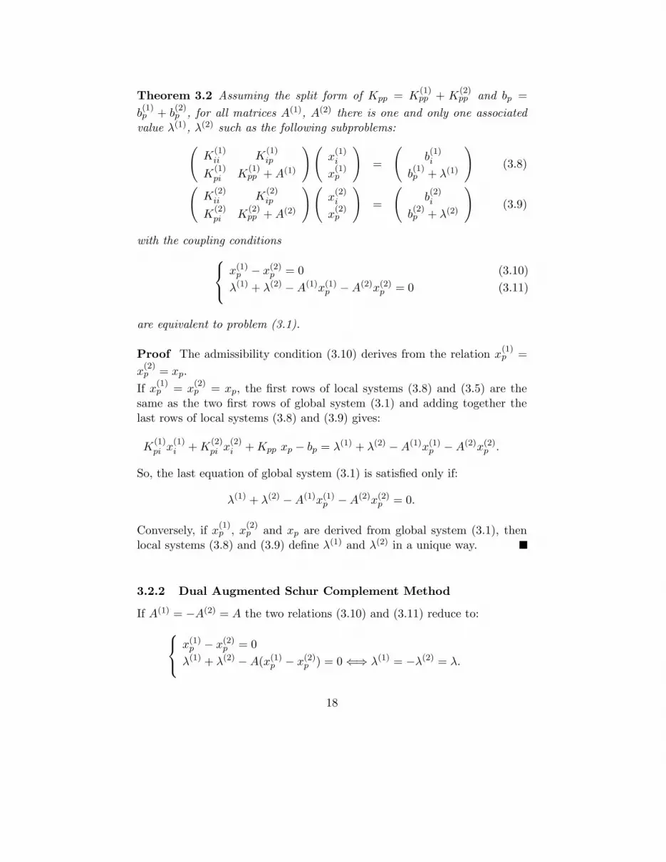
Theorem 3.2 Assuming the split form of Kpp = K(1)pp + K
(2)pp and bp =
b(1)p + b
(2)p , for all matrices A(1), A(2) there is one and only one associated
value λ(1), λ(2) such as the following subproblems:
(
K(1)ii K
(1)ip
K(1)pi K
(1)pp + A(1)
)(
x(1)i
x(1)p
)
=
(
b(1)i
b(1)p + λ(1)
)
(3.8)
(
K(2)ii K
(2)ip
K(2)pi K
(2)pp + A(2)
)(
x(2)i
x(2)p
)
=
(
b(2)i
b(2)p + λ(2)
)
(3.9)
with the coupling conditions
x(1)p − x(2)
p = 0 (3.10)
λ(1) + λ(2) − A(1)x(1)p − A(2)x(2)
p = 0 (3.11)
are equivalent to problem (3.1).
Proof The admissibility condition (3.10) derives from the relation x(1)p =
x(2)p = xp.
If x(1)p = x
(2)p = xp, the first rows of local systems (3.8) and (3.5) are the
same as the two first rows of global system (3.1) and adding together thelast rows of local systems (3.8) and (3.9) gives:
K(1)pi x
(1)i + K
(2)pi x
(2)i + Kpp xp − bp = λ(1) + λ(2) − A(1)x(1)
p − A(2)x(2)p .
So, the last equation of global system (3.1) is satisfied only if:
λ(1) + λ(2) − A(1)x(1)p − A(2)x(2)
p = 0.
Conversely, if x(1)p , x
(2)p and xp are derived from global system (3.1), then
local systems (3.8) and (3.9) define λ(1) and λ(2) in a unique way.
3.2.2 Dual Augmented Schur Complement Method
If A(1) = −A(2) = A the two relations (3.10) and (3.11) reduce to:
x(1)p − x(2)
p = 0
λ(1) + λ(2) − A(x(1)p − x(2)
p ) = 0 ⇐⇒ λ(1) = −λ(2) = λ.
18

Following the same steps than in the Dual Schur complement method, thelinear system becomes :
([S(1) + A]−1
+ [S(2) − A]−1
)λ = −[S(1) + A]−1
c(1)p + [S(2) − A]
−1c(2)p .
The solution of this system gives the only convenient value of λ and then
x(1)i , x
(1)p , x
(2)i and x
(2)p can be obtained. The main advantage of the Dual
Augmented Schur complement method arises when the subproblems in theDual Schur complement method are non invertible. In this case, the aug-mented matrix A can be chosen in such a way that these singularities dis-appear in the local subproblems of the Dual Augmented Schur complementmethod. Such an approach can be seen as a nice alternative to the use of thepseudo-inverses in the classical Dual Schur complement method [7, 10, 11].
3.2.3 Complete Augmented Schur Complement Method
If no restrictions are imposed on the interface variables, the expression of
x(1)p and x
(2)p can be obtained from (3.8) and (3.9):
x(1)p = [S(1) + A(1)]
−1(c(1)
p + λ(1)), x(2)p = [S(2) + A(2)]
−1(c(2)
p + λ(2)).
The only restriction on the choice of the matrices A(1) and A(2) is of course toensure that both matrices [S(1)+A(1)] and [S(2)+A(2)] are non singular. Theequivalence with the global problem is obtained through the two continuity
conditions (3.6) and (3.7). After substitution of x(1)p and x
(2)p in (3.10) and
(3.11) the following linear system is obtained:(
[S(1) + A(1)]−1
−[S(2) + A(2)]−1
I − A(1)[S(1) + A(1)]−1
I − A(2)[S(2) + A(2)]−1
)
(
λ(1)
λ(2)
)
=
(
−[S(1) + A(1)]−1
c(1)p + [S(2) + A(2)]
−1c(2)p
A(1)[S(1) + A(1)]−1
c(1)p + A(2)[S(2) + A(2)]
−1c(2)p
)
. (3.12)
Because the two continuity conditions are ensured at the same time, thesize of this unusual linear system is two times bigger than the size of thelinear systems arising from the classical domain decomposition algorithmspresented before.
Remark 3.1 Of course, all the matrices involved in the different linearsystems on the interface are not computed explicitly and the linear systemsare usually solved through iterative methods. The block form of the matricesof these linear systems are only presented to analyze the iterative algorithm.
19

3.2.4 Continuity Conditions as Local Preconditioner
In this section, it is still assumed that the matrices [S(1) + A(1)] and [S(2) +A(2)] are non singular. Rather than to ensure the continuity conditions (3.10)and (3.11) on the interface, it may be interesting to consider another condi-tions, like:
+A(1) (3.10) + (3.11) = 0−A(2) (3.10) + (3.11) = 0
which are equivalent to the initial continuity conditions, as soon as the twomatrices A(1) and A(2) satisfy the property [A(1)+A(2)] invertible. Followingthe same steps as in Section 3.2.3, the matrix and the right hand side of thelinear system take the block form:
(
I I − (A(1) + A(2))[S(2) + A(2)]−1
I − (A(1) + A(2))[S(1) + A(1)]−1
I
)
(
λ(1)
λ(2)
)
=
(
(A(1) + A(2))[S(2) + A(2)]−1
c(2)p
(A(1) + A(2))[S(1) + A(1)]−1
c(1)p
)
.
The key point is to notice that this manipulation of the continuity conditionscorresponds to a simple left multiplication of the linear system (3.12) by thefollowing preconditioner:
(
A(1) I
−A(2) I
)
.
Previous work has been done on this method in the recent years for differentmatrices A(1) and A(2) (see for example [2, 27, 4, 5, 8, 25, 13] and referencestherein).
4 Numerical Experiments
In order to illustrate the domain decomposition methods described in thispaper, two basic numerical experiments are now presented.
4.1 Laplace Equation
The two dimensional Laplace equation is first considered. The problemconsists on solving the homogeneous Laplace equation inside a square shaped
20

domain, with Dirichlet boundary conditions on the boundary. The problemcan be expressed as:
−∆u = f, ∀(x, y) ∈ ]0, 1[×]0, 1[u(x, y) = 16((2x − 1)2 − (2y − 1)2), x, y = 0, 1
and the solution is shown Figure 2.
0 0.2
0.4 0.6
0.8 1 0
0.2 0.4
0.6 0.8
1
-20-15-10-5 0 5
10 15 20
Figure 2: Solution of the Laplace equation. (h := 1/50)
The Primal Schur complement method and the Dual Schur complementmethod have been implemented in parallel within an object oriented FOR-TRAN 90 code. The data exchange between the processors are performedwith the MPI library. The sub-domains matrices are factorized in a LDLT
form, so each product by the inverse of the matrix involves a forward-backward procedure. The condensed interface problem is solved iterativelywith a Conjugate Gradient (CG) iterative algorithm [29]. The stopping cri-terion is ||rn||2 < 10−6 ||r0||2, where rn and r0 are the nth and initial globalresiduals.
The global domain is first split into two rectangular shaped sub-domains.In this configuration external Dirichlet boundary conditions are defined on
21

the boundary of each sub-domain. As a consequence the sub-domains ma-trices are non-singular. The number of iterations required by the PrimalSchur complement method and by the Dual Schur complement method arereported Table 1.
Mesh size Primal Schur method Dual Schur method
1/50 25 161/100 36 231/200 51 321/400 63 43
Table 1: Number of iterations for different mesh size parameter for theLaplace equation. (Ns := 2)
The global domain is now split into two, four, eight and sixteen sub-domains with the METIS software [17, 18], as shown Figure 3. It is inter-esting to notice that the interfaces between the sub-domains are irregularand that several cross points, i.e. points where more than two sub-domainsintersect, exist.
In the mesh partitioning into sixteen sub-domains, three sub-domainsdo not have external boundary conditions defined on their boundary. Inthe Dual Schur complement method, Neumann transmission conditions areimposed on the interface between the sub-domains. The subproblem ma-trices of these three sub-domains are thus singular, and the Dual Schurcomplement method can not converge anymore. An additional procedurefor the detection of the rigid body motions is mandatory as discussed inSection 2.1.3 [11]. The number of iterations required by the Primal Schurcomplement method and by the Dual Schur complement method are re-ported Table 2.
Number of Primal Schur method Dual Schur method Dual Schur methodsub-domains with rigid body motions
2 72 48 484 105 79 798 134 105 10516 161 — 121
Table 2: Number of iterations for different number of sub-domains for theLaplace equation. The mesh partitioning is obtained with METIS. (h :=1/400)
22

two sub-domains four sub-domains
eight sub-domains sixteen sub-domains
Figure 3: Mesh partitioning obtained with METIS.
23

4.2 Helmholtz Equation
4.2.1 Model Problem
The two dimensional Helmholtz equation is now considered. The problemconsists of solving the Helmholtz equation inside a square, with homogeneousRobin boundary conditions around. A Dirac source of real amplitude equalto one is set at the center of the domain. The real and imaginary part ofthe solution are presented Figure 4 and Figure 5.
0 0.2
0.4 0.6
0.8 0
0.2
0.4
0.6
0.8
1-0.4-0.2
0 0.2 0.4 0.6 0.8
1
x
y
Figure 4: Real part of the solution of the Helmholtz equation. (h := 1/50,F := 2000 Hz).
4.2.2 Basic Robin Transmission Conditions
The Dual Augmented Schur complement method has been implemented inthe case of augmented terms A(s) equal to ±iω, ∀s. These choices corre-spond after discretization to augmented matrices equal to A(s) := ±iωMΓ,∀s, where MΓ is a surface mass matrix. The Complete Augmented Schurcomplement method and the Schwarz method have been implemented whenA(s) := iω, ∀s. These choices correspond after discretization to augmentedmatrices equal to A(s) := iωMΓ, ∀s.
The condensed interface problem is solved iteratively with an ORTHODIRalgorithm [29]. The number of iterations required by the Dual AugmentedSchur complement, the Complete Augmented Schur complement and the
24

0 0.2
0.4 0.6
0.8 0
0.2
0.4
0.6
0.8
1
-0.4-0.3-0.2-0.1
0 0.1 0.2 0.3
x
y
Figure 5: Imaginary part of the solution of the Helmholtz equation. (h :=1/50, F := 2000 Hz).
Schwarz methods are reported Table 3, in the case of a mesh partitioninginto two rectangular shaped sub-domains.
Mesh size Dual Augmented Schur Complete Augmented Schur Schwarzmethod method method
1/50 20 29 311/100 23 32 411/200 27 38 471/400 32 48 50
Table 3: Number of iterations for different mesh size parameter for theHelmholtz equation. (Ns := 2, F := 2000 Hz)
Table 4 shows the number of iterations required by the different methodsfor different frequencies. The relation between the wavenumber ω and thefrequency F is given by ω = 2πF
cwhere c is the sound celerity equal here to
c := 340 ms−1.Table 5 shows the number of iterations required by the different methods
in the general case of a mesh partitioning into two, four, eight and sixteensub-domains obtained with METIS.
25

Frequency Dual Augmented Schur Complete Augmented Schur Schwarz(Hz) method method method
500 25 33 351000 25 36 422000 27 38 474000 35 36 49
Table 4: Number of iterations for different frequency parameter for theHelmholtz equation. (h := 1/200, Ns := 2)
Number of Dual Augmented Schur Complete Augmented Schur Schwarzsub-domains method method method
2 30 52 914 59 74 1188 83 99 13816 139 143 151
Table 5: Number of iterations for different number of sub-domains for theHelmholtz equation. The mesh partitioning is obtained with METIS. (h :=1/200, F := 2000 Hz)
4.2.3 Advanced Robin Transmission Conditions
In order to illustrate the influence of the transmission conditions on theconvergence of the iterative algorithm, several Robin transmission conditionshave been implemented for the Schwarz method. The available choice forthe augmented term A(s), ∀s can be summarized below:
TO0: A(s)(u) := iω u
TO2: A(s)(u) := iω u −i
2ω∂yyu
OO0: A(s)(u) := α u
OO2: A(s)(u) := α u + β ∂yyu
where α and β denote two complex coefficients issue from an optimizationprocedure as described in [13, 25]. These transmission conditions are usuallycalled Taylor Order Zero (TO0), Taylor Order Two (TO2), Optimized OrderZero (OO0), Optimized Order Two (OO2) transmission conditions in theliterature [27, 4, 12]
The results reported Table 6 show the number of iterations of the domaindecomposition methods upon the mesh size parameter, in the case of a meshpartitioning into two rectangular shaped sub-domains. It it clear that thedefinition of the transmission conditions are of major importance for the
26

fast and robust convergence of the iterative algorithm.The results reported Table 7 show the number of iterations upon the
frequency parameter. The better the transmission conditions, the lower thenumber of iterations.
The case of several sub-domains is now analyzed. The mesh partitioninginto two, four, eight and sixteen sub-domains is obtained with the METISsoftware, as represented Figure 3. Table 8 shows the number of iterations re-quired by the Schwarz method upon the transmission conditions considered.
Mesh size Schwarz method Schwarz method Schwarz method Schwarz methodTO0 TO2 OO0 OO2
1/50 31 28 19 81/100 41 36 24 101/200 47 46 27 121/400 50 60 32 15
Table 6: Number of iterations for different mesh size parameter for theHelmholtz equation. (Ns := 2, F := 2000 Hz)
Frequency Schwarz method Schwarz method Schwarz method Schwarz method(Hz) TO0 TO2 OO0 OO2
500 35 48 23 141000 42 40 25 142000 47 46 27 124000 49 59 27 12
Table 7: Number of iterations for different frequency parameter for theHelmholtz equation. (h := 1/200, Ns := 2)
Number of Schwarz method Schwarz method Schwarz method Schwarz methodsub-domains TO0 TO2 OO0 OO2
2 91 126 41 284 118 221 55 338 138 332 71 4216 151 412 90 49
Table 8: Number of iterations for different number of sub-domains for theHelmholtz equation. The mesh partitioning is obtained with METIS. (h :=1/200, F := 2000 Hz)
27

5 Conclusions
In this paper, a review of the absorbing interface conditions involved in do-main decomposition methods has been presented. These absorbing interfaceconditions defined on the interface between the sub-domains appear whenthe global domain is split into several sub-domains. These conditions canbe classified in two family: the continuity conditions and the transmissionconditions. The continuity conditions must be ensured by the solutions ofthe local subproblems. The transmission conditions are used to avoid thenon-well posedness of the subproblems.
The methodology to define these continuity and these transmission con-ditions has been presented in an original continuous and discrete analysis.Changing the continuity and the transmission conditions has a strong influ-ence on the convergence of the iterative algorithm used for the solution ofthe interface problem. The numerical experiments performed on two aca-demic problems illustrate the respective efficiency of these continuity and ofthese transmission conditions.
References
[1] Y. Achdou. Decomposition de domaine pour les equations aux deriveespartielles, Matapli, 1999.
[2] J.-D. Benamou and B. Despres. A domain decomposition method for theHelmholtz equation and related optimal control problems. J. of Comp.Physics. 1997. 136, 68–82.
[3] C. Bernardi, Y. Maday and A.T. Patera. A new non conforming ap-proach to domain decomposition: the mortar element method, Nonlin-ear Partial Differential Equations and their Applications, H. Brezis andJ.L. Lions eds., Pitman, Boston, 1992.
[4] P. Chevalier and F. Nataf. Symmetrized method with optimized second-order conditions for the Helmholtz equation. Contemporary Mathemat-ics, 1998. 218, 400-407
[5] F. Collino, S. Ghanemi and P. Joly. Domain decomposition method forharmonic wave propagation: a general presentation. Computer methodsin applied mechanics and engineering, 2000. 184, 171-211
[6] B. Engquist and A. Majda. Absorbing boundary conditions for thenumerical simulation of waves. Math. Comp., 1977. 31(139):629–651.
28

[7] C. Farhat. A Lagrange multiplier based on divide and conquer finiteelement algorithm. J. Comput. System Engng, 1991. 2. 149-156.
[8] C. Farhat, A. Macedo, M. Lesoinne, F.-X. Roux, F. Magoules and A. dela Bourdonnaye. Two-level domain decomposition methods with La-grange multipliers for the fast iterative solution of acoustic scatteringproblems. Computer Methods in Applied Mechanics and Engineering,2000. 184(2), 213–240.
[9] C. Farhat, A. Macedo and R. Tezaur. FETI-H: a scalable domain de-composition method for high frequency exterior Helmholtz problems. Do-main Decomposition Press. eds. C.J. Lai, P. Bjorstad, M. Cross andO. Widlund. 1999. 228-238.
[10] C. Farhat and F.-X. Roux. A Method of Finite Element Tearing andInterconnecting and its Parallel Solution Algorithm. Int. J. Numer.Meth. Engng. 1991. 32, 1205–1227.
[11] C. Farhat and F.X. Roux. Implicit parallel processing in structuralmechanics. Comput. Mech. Adv., 1994. 2, 1–124.
[12] M. Gander, L. Halpern and F. Nataf. Optimal convergence for overlap-ping and non-overlapping Schwarz waveform relaxation. Proceedings ofthe 11th international symposium on Domain Decomposition Methods,1999.
[13] M. Gander, F. Magoules and F. Nataf. Optimized Schwarz methodswithout overlap for the Helmholtz equation. SIAM Journal on ScientificComputing, 2002. 24(1), 38–60.
[14] S. Ghanemi. A domain decomposition method for Helmholtz scatteringproblems. Ninth International Conference on Domain DecompositionMethods, 1997. eds. P. E. Bjørstad, M. Espedal and D. Keyes. 105–112.
[15] L. Halpern. Absorbing boundary conditions for the discretizationschemes of the one dimensional wave equation. Math. of Comp., 1982.38:415–429.
[16] P. Joly and O. Vacus. Sur l’analyse des conditions aux limites ab-sorbantes pour l’equation de Helmholtz. INRIA, rapport de recherche,1996. 28-50.
29

[17] G. Karypis and V. Kumar. METIS - unstructured graph partitioningand sparse matrix ordering system - version 2.0. University of Min-nesota, 1995.
[18] G. Karypis and V. Kumar. METIS : a software package for partitioningunstructured graphs, partitioning meshes, and computing fill-reducingorderings of sparse matrices. University of Minnesota, 1997. Availablevia http://www.cs.umn.edu/∼karypis.
[19] D.E. Keyes. Domain Decomposition Methods in the Mainstream ofComputational Science, Proceedings of the 14th International Confer-ence on Domain Decomposition Methods, UNAM Press, Mexico City,pp.79-93, 2003.
[20] P.-L. Lions. On the Schwarz alternating method. I.. SIAM Philadelphia,PA, 1988. eds. R. Glowinski, G.H. Golub, G.A. Meurant and J. Periaux.1–42.
[21] P.-L. Lions. On the Schwarz alternating method. II.. SIAM Philadel-phia, PA, 1989. eds. T. Chan, R. Glowinski, J. Periaux and O. Widlund.47–70.
[22] P.-L. Lions. On the Schwarz alternating method. III: A variantfor nonoverlapping subdomains. SIAM Philadelphia, PA, 1989. eds.T. Chan, R. Glowinski, J. Periaux and O. Widlund.
[23] P. Le Tallec. Domain decomposition methods in computational mechan-ics. North-Holland, 1994. eds. Oden, J. Tinsley. 1(2). 121–220.
[24] F. Magoules. Parallel Algorithms for Coercive Elliptic Problems. Saxe-Coburg Publications, 2002. ed. B.H.V. Topping. 135–150.
[25] F. Magoules. Parallel Algorithms for Time-harmonic Hyperbolic Prob-lems. Saxe-Coburg Publications, 2002. ed. B.H.V. Topping. 151–183.
[26] F. Magoules, F.-X. Roux and S. Salmon. Optimal discrete transmis-sion conditions for a non-overlapping domain decomposition method forthe Helmholtz equation. SIAM Journal on Scientific Computing, 2004.25(5), 1497–1515.
[27] F. Nataf, F. Rogier and E. de Sturler. Optimal Interface Conditions forDomain Decomposition Methods. CMAP (Ecole Polytechnique), 1994.
30

[28] A. Quarteroni and A. Valli. Domain Decomposition Methods for PartialDifferential Equations, Oxford University Press, Ofxord, 1999.
[29] Y. Saad. Iterative methods for linear systems. PWS Publishing, Boston,1996.
[30] B. Smith, P. Bjorstad and W. Gropp. Domain Decomposition: ParallelMultilevel Methods for Elliptic Partial Differential Equations, Cam-bridge University Press, 1996.
[31] A. Toselli and O.B. Widlund. Domain Decomposition Methods: Al-gorithms and Theory, Springer Series in Computational Mathematics,vol.34, 2004.
31


