Embed Size (px)
Citation preview

Subproject H3: Strange Hadrons – Strangeness in Strongly Inter-acting Particles
D. von Harrach / J. Pochodzalla
Patrick ACHENBACH, Carlos AYERBE GAYOSO, Dagmar BAUMANN, Jan BERNAUER,Ralph BÖHM, Michael O. DISTLER, Luca DORIA, Jörg FRIEDRICH, Klaus Werner KRY-GIER, Harald MERKEL, Ulrich MÜLLER, Reiner NEUHAUSEN, Lars NUNGESSER, JosefPOCHODZALLA, Salvador SÁNCHEZ MAJOS, Thomas WALCHER, Markus WEINRIEFER
H3.1 Experimental programme
H3.1.1 Threshold electroproduction of charged kaons
The elementary electroproduction of hyperons off the proton is used mainly as a test of produc-tion mechanisms through resonant baryon formation and kaon exchange. Compared to photo-production, where a good data set of measured cross sections exist now from the CLAS andthe SAPHIR detectors, electroproduction can address the longitudinal coupling of the photonsin the initial state, and electromagnetic and hadronic form factors. The SAPHIR detector isnow disassembled. The CLAS detector allows also for electroproduction experiments and pro-vides good resolutions for charged particles in the final state. While the toroidal configurationof the magnetic field maximises the acceptance for angles beyond 10, a study at forward an-gles is not possible. The electroproduction data [1, 2] is even more scarce than in the case ofphotoproduction processes and have been obtained in a rather small phase space region.
Transverse polarisation0 0.1 0.2 0.3 0.4 0.5 0.6
)2/c2
Fo
ur-
mo
men
tum
tra
nsf
er (
GeV
0
0.1
0.2
0.3
0.4
0.5
0.6
0.7
1.1 = E1.2 = E1.3 = E1.4 = E1.5 = E
= 1.05ω
= 1.11ω
= 1.16ω
= 1.21ω
= 1.27ω
= 1.32ω
= 1.37ω
= 30eΘ
= 45eΘ
= 60eΘ
= 75eΘ
= 90eΘ
Figure H3.1: The Q2 − ε plane for a measurement at invariant energy W = 1.66GeV. Lines of constantscattering angle, θe, constant energy transfer, ω, and constant beam energy, E, are shown. The pilotexperiment has been designed for Q2 = 0.2 GeV2/c2.
As a pilot experiment on kaon electroproduction in Mainz, the separation of transverse and lon-gitudinal structure functions in parallel kinematics [3] is planned. Due to the lack of availabledata for the longitudinal component, σL, at low squared four-momentum transfer, Q2, and lowhadronic invariant energy, W , a new precision measurement in this kinematical region should
153

154 CHAPTER 2. EXPERIMENTS AT MAMI AND THEORY
serve to constrain and refine isobaric models. This measurement shall become the starting pointfor a series of experiments on kaon electroproduction.
For unpolarised electrons and unpolarised target, the virtual photoproduction differential crosssection can be written as [4, 5]: dσv
dΩK= dσT
dΩK+εL
dσLdΩK
+√
2εL(1+ ε) dσLTdΩK
cosφK +ε dσTTdΩK
cos2φK .The different terms correspond to the coupling of the final state to the different polarisationcomponents of the virtual photon, and are functions of W,Q2, and θK . In parallel kinematics(3-momentum transfer parallel to kaon momentum) the interference terms σLT and σTT vanishdue to their sin θK and sin2 θK dependence, respectively, Integrating the cross section over thefull range of φK leaves only the combined contributions from the transverse and longitudinalcross sections. Then, by varying the polarisation factor, ε, the longitudinal and transverse con-tributions can be disentangled by Rosenbluth separation. When keeping W and Q2 constant, thevariation must be accomplished by changing the beam energy E . To illustrate the kinematicalcoverage for a measurement at invariant energy W = 1.66GeV the accessible Q2 − ε region ispresented in Fig. H3.1.
For performing a longitudinal-transverse separation, it is important to have the lever arm in ε aslarge as possible. Obviously, the accessible ε range for fixed W is largest at small values of Q2.For the pilot experiment a kinematics at W = 1.66GeV and Q2 = 0.2 GeV2/c2 has been chosen.The minimum electron scattering angle θe ≥ 40 does not allow a measurement at values of εabove 0.32. The virtual photon flux decreases by orders of magnitude with increasing electronscattering angle. Therefore, we limit the measurements to scattering angles smaller 60 degrees.Simulation results and count rate estimates have been shown in the previous biannual report.
H3.1.2 Electroproduction of hypernuclei
Information on baryon-baryon interactions is mainly obtained from nuclear experiments withprojectiles and targets out of ordinary nucleons, addressing interactions in flavour SU(2) only.The difficulties to study YN and YY interactions by reaction experiments is related to the prac-tical problems in the preparation of low energy hyperon beams and that no hyperon targets areavailable due to the short lifetimes of hyperons. However, it has already been demonstratedthat hypernuclei can be used as a micro-laboratory to study YN and YY interactions.
1000 1200 1400 1600 1800 2000Photon energy HMeVL
100
200
300
400
500
600
Rec
oilm
om
entu
mHMeV
cL
20°10°0°
0 500 1000 1500 2000Beam momentum HMeVcL
100
200
300
400
500
600
Rec
oilm
om
entu
mHMeV
cL
20°10°0°
Figure H3.2: Recoil momentum for strangeness electroproduction (e,e′K+) and strangeness exchange(K−,π−) reactions at three different kaon angles are shown.
Electron beams have excellent spatial and energy definitions, and targets can be physicallysmall and thin (10 − 50 mg/cm2) allowing studies of almost any isotope. The small cross
SUBPROJECT H3: STRANGE HADRONS 155
section for the reaction, σ ∼ 140 nb/sr on a 12C target [6], compared to strangeness exchangen(K−,π−)Λ or associated production n(π+,K+)Λ is well compensated by the available largeelectron beam intensities. Even though a number of new experiments have been performed inhypernuclear reaction spectroscopy in the last decade, our knowledge on hypernuclei is stilllimited to some global properties of a small number of isotopes.
The (K−,π−) reaction is characterised by the existence of a "magic momentum" where therecoil momentum of the hyperon becomes zero, see Fig. H3.2. It populates, consequently,substitutional states in which a nucleon is converted to a Λ in the same state. The (e,e ′,K+)reaction, on the other hand, produces neutron-rich Λ hypernuclei converting a proton to a Λhyperon and transfers a large recoil momentum to a hypernucleus. This reaction is preferablewhen high-spin hypernuclear states are studied. In addition, this reaction has the unique char-acteristic of providing large amplitudes for the population of spin-flip hypernuclear states withunnatural parities [7], such as (ν p−1
3/2,Λ s1/2)2−, where the spin quantum number, JP = 2−, of
the nucleon-hole Λ-particle state has maximum J =ν l +Λl +1 = 1+0+1 = 2.
In the case of ΛN interaction, the spin-orbit term has been found to be smaller than that for thenucleon. In a recent experiment at BNL the spacing of the (5/2+,3/2+) doublet in 9
ΛBe wasmeasured to be (43± 5)keV [8]. Although these small spin splittings can only be observedusing gamma spectroscopy, reaction spectra are equally important because they provide thecomplete spectrum of excitations with a strength that not only gives the spectroscopic factor,but the transition matrix. In addition, experimental data on medium to heavy single Λ hyper-nuclei have shown a much larger spin-orbit splitting than observed in light hypernuclei [9].
Photon energy (MeV)800 1000 1200 1400 1600
Mo
men
tum
(M
eV/c
)
0
200
400
600
800
= 0 degKθ = 4 degKθ = 8 degKθ = 12 degKθ = 16 degKθ
Photon energy (MeV)800 1000 1200 1400 1600
Sti
ckin
g p
rob
abili
ty
0
0.01
0.020.03
0.04 = 0 degKθ = 4 degKθ = 8 degKθ
= 12 degKθ = 16 degKθ
Photon energy (MeV)800 1000 1200 1400 1600F
igu
re O
f M
erit
00.5
1
1.52
-610× = 0 degKθ = 4 degKθ = 8 degKθ = 12 degKθ = 16 degKθ
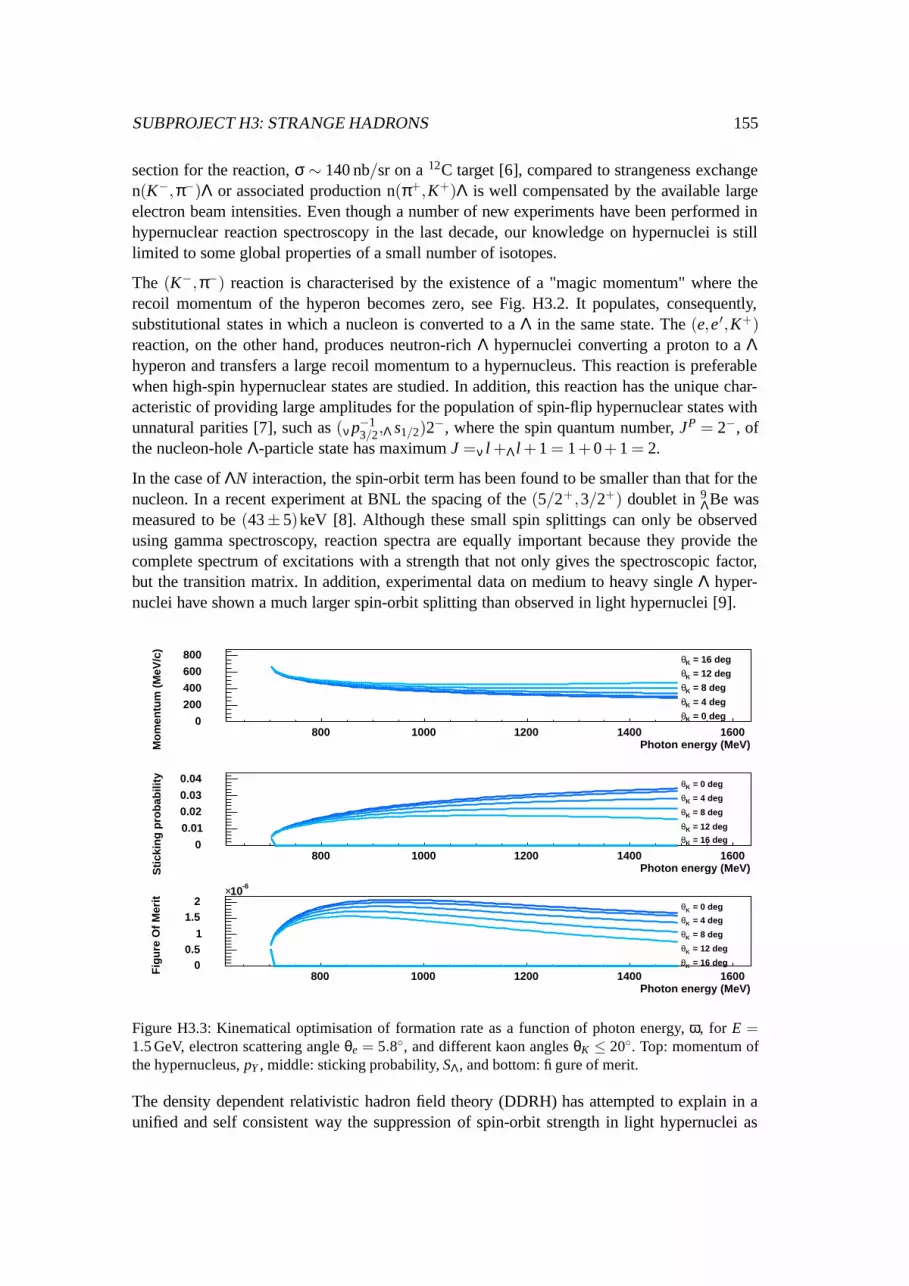
Figure H3.3: Kinematical optimisation of formation rate as a function of photon energy, ω, for E =1.5 GeV, electron scattering angle θe = 5.8, and different kaon angles θK ≤ 20. Top: momentum ofthe hypernucleus, pY , middle: sticking probability, SΛ, and bottom: figure of merit.
The density dependent relativistic hadron field theory (DDRH) has attempted to explain in aunified and self consistent way the suppression of spin-orbit strength in light hypernuclei as

156 CHAPTER 2. EXPERIMENTS AT MAMI AND THEORY
well as the spin-orbit structure observed in more massive nuclei [10]. It is argued that in lighthypernuclei particle threshold effects are superimposed on the general delocalisation of the Λwave function, responsable for the still partially reduced splitting for heavier nuclei, producingan effective squeezing of the single particle levels close to threshold and the disappearance ofspin-orbit potential effects. A deeper understanding of this phenomenon relies on obtaininghigh quality data for medium and heavy hypernuclei. The present experimental data on hyper-nuclear binding energies and detailed spectroscopic features are limited in quantity and qualityand it refers, mostly, to light (s- and p-shell) hypernuclei.
Electroproduction of hypernuclei will be possible at MAMI in the near future. High resolutionspectroscopic studies of medium and heavy hypernuclei will be performed in order to providethe most valuable experimental information on the Λ spin-orbit dynamics in finite nuclei. Inaddition, as it has been discussed in a previous biannual report already, using electroproduc-tion the wave function inside the nucleus can be mapped out by measuring the kaon angulardistribution [11, 12].
Hypernuclear formation in impulse approximation
One of the factors decisive for the feasibility of an experiment at MAMI is of course the reac-tion rate. To optimise the reaction rate as a function of angles and energies the characteristics ofthe hypernuclear formation in impulse approximation has been studied. In order to produce ahypernucleus, the hyperon emerging from the reaction has to stay in the nucleus. This “stickingprobability” depends very much on the transferred momentum to the hyperon. If the momen-tum transfer is large compared with typical nuclear Fermi momenta, the hyperon will leave thenucleus.
Assuming 3-momentum conservation at the vertices of the Feynman diagram in impulse ap-proximation the transferred momentum can be written as the difference between Λ momentum,~pΛ, and core nucleus momentum, ~pA−1, and is a function of the momentum of the virtual pro-ton,~k, and the recoil momentum of the hypernucleus, ~pY : q(k)≡
∣∣~pΛ−~pA−1∣∣=∣∣~pY +2~k
∣∣. Withan approximate Fermi Gas distribution for the virtual proton, F = 2π
R ∞0 n(k)k2 dk, where the
distribution function, n(k), is Gaussian, n(k) = (2−4kF√
π)−3 exp−√
2k2/k2F , and modelling
the sticking probability with an exponential function, SΛ =RR
exp(−q(k)/σp)n(k)k2 dk d cos θ,the probability can be evaluated as a function of the kinematic variables:
SΛ = 12pY σp
exp k2
F√2σ2
p− pY
σp
((−√
2k2F + pY σp
)Erfc
[− pY√
2√
2kF
+kF√√
2σp
]
+exp2pY
σp
(√2k2
F + pY σp
)Erfc
[ pY√2√
2kF
+kF√√
2σp
]).
Since electroproduction is a high momentum transfer reaction similar to (π+,K+), the stickingprobability takes a minimum at threshold and increases as the virtual photon energy increases.In this model typical values of σp = 100 MeV/c and kF = 200 MeV/c were assumed. A morerigorous definition of the sticking probability is given, for example, in [13], for the case ofharmonic oscillator wave functions. Using this definition, also at low q, the sticking probabil-ity prevails and substitutional states are exclusively populated, and at q ∼ kF , high quantumnumbers and stretched states are favoured.
The cross section for electroproduction can be written in a very intuitive form by separating outa factor, Γ, which multiplies the off-shell (virtual) photoproduction cross sections. This factor

SUBPROJECT H3: STRANGE HADRONS 157
may be interpreted as the flux of the virtual photon field per scattered electron into dE ′dΩ and
can be written as Γ = α2π2
E ′E
kγQ2
11−ε , with kγ = (W 2−m2
i )/2mi and ε =(1+2 |q|2
Q2 tan2 θ2
)−1, where
q is the virtual photon three-momentum. The virtual photon flux factor has the feature that itis very forward peaked. While flux factor for a fixed photon energy, ω = Ee −E ′
e , increaseswith beam energy, so does the resolution and background. One can perform a kinematicaloptimisation using a Figure Of Merit for the formation rate defining FOM = SΛ×Γ. Fig. H3.3shows pY , SΛ and the figure of merit as a function of the virtual photon energy, ω, for the e+12C→ e′ + K++11
Λ B reaction. The kinematics was calculated for E = 1.5 GeV, angle of scatteredelectron θe = 5.8, and different kaon angles θK ≤ 20. A maximum was found at ω≈ 850 MeVand the proposed kinematic setting for a first hypernuclear formation experiment has beendefined as follows: Q2 = 0.01 GeV2/c2, W = 11.995 GeV, E = 1.50 GeV, E ′ = 0.650 GeV,θe = 5.8, pK = 0.446 GeV/c, pY = 0.423 GeV/c, and θK = 5.5.
H3.2 Apparative aspects
H3.2.1 Progress report on the set-up of the spectrometer
With the existing set-up of the three-spectrometer facility in Mainz the detection of kaons undersmall scattering angles is not possible due to the short live-time of the kaons (cτK = 3.71 m) andthe long flight path through the spectrometers (close to 10 m for spectrometer C). Therefore,kaons under forward scattering angles have to be analysed with a new short-orbit spectrometer.
H3.2.1.1 Installation of the spectrometer
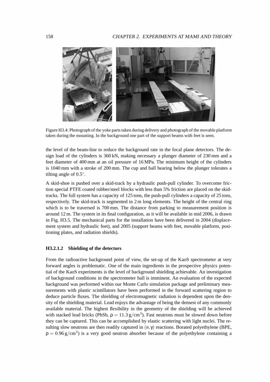
KaoS is a very compact magnetic spectrometer suitable especially for the detection of kaons.It was built by the GSI in Darmstadt for heavy ion induced experiments [14]. During May andJune 2003 the KaoS magnets together with associated electronics and detectors were broughtto Mainz. The existing support structures with a laffette on air cushions could not be used inMainz. Though, the re-installation of the spectrometer is based on a compact, mobile and ad-justable platform with a support structure on hydraulic feet. The platform with the spectrometercan be moved from a parking position to a measurement position via a displacement systemwith hydraulic pressure cylinders on segmented tracks, see Fig. H3.4. With this concept nosupport to the pivot bearing is needed and a partial deinstallation enables the complete cover-age of the forward region through the existing spectrometers. The kinematics of the proposedexperiments with KaoS defines the exact position of the magnetic system. A flexible position-ing with respect to the target and the beam-dump can be achieved with hydraulic positioningfeet. Such feet, hydraulic cylinders of large dimensions have been purchased.
The hydraulic cylinders of Rexroth Hydraudyne BV should carry the load of the spectrometermagnets and – at the same time – allow for a precise positioning and alignment of the spectrom-eter. There is no need for rails. Instead, very accurately machined positioning plates (grindedto Ra = 0.8) for the hydraulic cylinders to slide on are going to be installed in the inner sectorof the spectrometer facility, soon. In addition, the cylinders allow a vertical lifting by means ofa plunger. The plunger has a double function. It will lift the platform from its support, so thatthe Hydrospex skidding system can removed. Further, it allows a precise vertical alignment ofthe spectrometer. It is planned to separate the mid-plane of the magnet by 50− 100 mm from
158 CHAPTER 2. EXPERIMENTS AT MAMI AND THEORY
Figure H3.4: Photograph of the yoke parts taken during delivery and photograph of the movable platformtaken during the mounting. In the background one part of the support beams with feet is seen.
the level of the beam-line to reduce the background rate in the focal plane detectors. The de-sign load of the cylinders is 360 kN, making necessary a plunger diameter of 230 mm and afeet diameter of 400 mm at an oil pressure of 16 MPa. The minimum height of the cylindersis 1040 mm with a stroke of 200 mm. The cup and ball bearing below the plunger tolerates atilting angle of 0.5.
A skid-shoe is pushed over a skid-track by a hydraulic push-pull cylinder. To overcome fric-tion special PTFE coated rubber/steel blocks with less than 5% friction are placed on the skid-tracks. The full system has a capacity of 125 tons, the push-pull cylinders a capacity of 25 tons,respectively. The skid-track is segmented in 2 m long elements. The height of the central ringwhich is to be traversed is 700 mm. The distance from parking to measurement position isaround 12 m. The system in its final configuration, as it will be available in mid 2006, is drawnin Fig. H3.5. The mechanical parts for the installation have been delivered in 2004 (displace-ment system and hydraulic feet), and 2005 (support beams with feet, movable platform, posi-tioning plates, and radiation shields).
H3.2.1.2 Shielding of the detectors
From the radioactive background point of view, the set-up of the KaoS spectrometer at veryforward angles is problematic. One of the main ingredients in the prospective physics poten-tial of the KaoS experiments is the level of background shielding achievable. An investigationof background conditions in the spectrometer hall is imminent. An evaluation of the expectedbackground was performed within our Monte Carlo simulation package and preliminary mea-surements with plastic scintillators have been performed in the forward scattering region todeduce particle fluxes. The shielding of electromagnetic radiation is dependent upon the den-sity of the shielding material. Lead enjoys the advantage of being the densest of any commonlyavailable material. The highest flexibility in the geometry of the shielding will be achievedwith stacked lead bricks (PbSb, ρ = 11.3 g/cm3). Fast neutrons must be slowed down beforethey can be captured. This can be accomplished by elastic scattering with light nuclei. The re-sulting slow neutrons are then readily captured in (n,γ) reactions. Borated polyethylene (BPE,ρ = 0.96 g/cm3) is a very good neutron absorber because of the polyethylene containing a

SUBPROJECT H3: STRANGE HADRONS 159
Figure H3.5: Technical drawings showing the skid-track, the hydraulic cylinders, the positioning plates,and the platform in the final configuration.The height of the central ring which is to be traversed is700 mm. The distance from parking to measurement position is around 12 m.
high proportion of hydrogen for moderation and the boron carbide (B4C, between 5 to 10%by weight) providing a large cross section for neutron capture. Boron oxide, also known asdiboron trioxide (B2O3), seems to be an alternative agent in polyethylene shields. A key pointconcerning neutron shielding is that the capture produces secondary gamma-ray emissions inthe shield material (most gamma-rays in BPE are produced from the neutrons’ interaction withcarbon and boron, instead of hydrogen). Thus, a combined system of electromagnetic and neu-tron shields has to be considered.
A statics calculation of the mechanical aspects of a radiation shield was performed byBretschneider Beratende Ingenieure (BBI, Mainz) in May 2005. They calculated that a sym-metric set-up of side (load per unit length γ = 22.8 kN/m2) and backward (γ = 11.4 kN/m2)lead walls leading to tensile stresses of σv = 18 kN/cm2 is already exhausting 85% of the ten-sile strength of the planned steel construction. Based on this calculation it was decided to gofor a demountable shielding house separate to the magnet and detector platform. A preliminarydesign was used to estimate the necessary volume of shielding material. We bought neutronshielding material (BPE plates with 15% diboron trioxide by weight covering 20 m2) and elec-tromagnetic shielding material (1000 lead bricks of standard dimensions 50×100×200 mm3)to build side walls.
H3.2.1.3 Preparation for the installation of a magnetic chicane
When operating KaoS close to 0 the primary beam will pass through the dipole field of KaoSand will be bent away from its original axis. Thus, a magnetic chicane is mandatory. Thesolution for a chicane upstream of the target comprises two compensating magnets which areavailable as spare 30 sector magnets (DCI). For a field of 1 T in KaoS the first dipole has to

160 CHAPTER 2. EXPERIMENTS AT MAMI AND THEORY
deflect the beam by 9, the second one by approximately twice the angle in opposite direction.With the resulting beam inclination of 16 the KaoS dipole will deflect the beam straight intothe beam-dump with an angle of only 1.47 relative to the axis.
Figure H3.6: Beam transport through chicane and a KaoS dipole field of 1.75 T to beam dump. Theangle at the target with respect to the entrance beam-line is 24.5.
The angle through which the KaoS dipole bends the beam depends on the field strength and thedipole position. Therefore, the beam angle at the target has to be flexible. This can be achievedby adjusting the strength of both fields and the position of the second DCI magnet. An exampleof the beam transport for a field of 1.75 T in KaoS is shown in Fig. H3.6.
The power supplies for the two DCI dipoles have been bought from Danfysik. For the firstset of measurements a magnetic field of 1.1 T (0.55 T) in the pole gap of 35 mm in the DCImagnets is needed, corresponding to primary coil currents of 400 A, respectively 200 A. Thepower supplies deliver a terminal voltage of 10 V, which is calculated from 5 V voltage dropin the input leads with 120 mm2 cross section and a load of 0.014 Ω in the coils. The powersupplies are provided with 16 bit ADC current read-back ±3 ppm current stability (in 8 hours).Controls and interfaces are adapted to the power supplies of the MAMI-C extraction magnetsto minimise development and software programming work.
H3.2.2 Progress report on detector developments
H3.2.2.1 Development of new focal plane detectors
The multi-cladding fibres:
The fibres are of type Kuraray SCSF-78 with double cladding and ∅ = 0.83 mm diameter. Thecladding thickness is 12%∅ ≈ 0.1mm, leading to a 0.73 mm core made from polystyrene (PS)of refractive index ncore = 1.6. The outer cladding is made from a fluorinated polymer (FP)of refractive index nclad′ = 1.42 and the inner cladding is made from polymethylmethacrylate(PMMA) of refractive index nclad = 1.49. The latter gives mechanical support between the coreand the outer cladding which are mechanically incompatible [15]. The scintillation light has anemission peak at 450 nm. In the fibre core a certain fraction of the scintillation light, called core

SUBPROJECT H3: STRANGE HADRONS 161
light, is trapped by total internal reflections at the core-cladding interface. Light not trapped inthe fibre core is refracted into the cladding and again some portion of this light is trappedby total internal reflections at the inner-to-outer cladding interface, called cladding light. Fora double cladding fibre the critical axial angle is given by θcrit = arccos nclad′/ncore = 26.7.The trapping efficiency for photons produced close to the axis of the fibre is 5.3% giving 70%more light than single cladding fibres, where the efficiency for light trapped between core andcladding is only 3.1%.
Figure H3.7: Detector configurations with slanting columns (four fibres each) and column angles from10 to 80 with a detector base angle of 50 are shown, where configurations with closed rows and closedcolumns are separately drawn. For column angles of 30 and 60 the packing of fibres is hexagonal. Fora column angle of 45 with closed columns the packing of fibres is straight.
Design of the fibre array:
Scintillating fibres are sometimes grouped together to form ribbons. A fibre doublet structureis formed from two single layers of fibres, with one of the fibre layers off-set relative to theother by half a fibre spacing. The virtue of this configuration is the high fraction of overlappingfibres, i.e. a high detection efficiency, and a small pitch leading to a good spatial resolution.Several of such double layers are introduced if the number of photoelectrons per fibre is toosmall to be detected with the required efficiency.
In case the minimum ionising particles are crossing the fibre array at right angle to the detectorbase the total thickness of the active scintillator can be increased arbitrarily until a physicallimit or restrictions in terms of small angle scattering are reached. If the ionising particlescrosses the fibre array with a finite angle with respect to the vertical direction it is likely totraverse neighbouring columns, compromising the tracking capabilities of such a detector: thefibre array geometry has to be adapted to the particles’ incoming angles by grouping slantingcolumns to one common read-out channel. The most efficient way to pack fibres together toform slanting columns is not obvious. Fibre arrays with different slanting columns (four fibreseach) are shown in Fig. H3.7. In this figure detector configurations with column angles from

162 CHAPTER 2. EXPERIMENTS AT MAMI AND THEORY
10 to 80 at an detector base angle of 50 are shown, where configurations with closed rowsand closed columns are separately drawn. Each configuration corresponds to a different fractionof overlapping fibres, a different pitch, and a different detector width and length for a givennumber of double layers and read-out channels. For column angles of 30 and 60 the packingof fibres is hexagonal. For a column angle of 45 with closed columns the packing of fibres isstraight.
Fig. H3.8 illustrates the relevant design criteria for choosing the detector configuration. Theleft plot shows the ratio of the column pitch with the fibre radius, i.e. the distance betweentwo fibre centres in units of fibre radius, as a function of the column angle. The main branchstarting at a ratio of 2 corresponds to a configuration with closed rows and closed columns,so that the pitch ratio p/r equals 2cosα with α as the column angle. The branch splitting offat α = 30 corresponds to a configuration with closed columns, where the pitch ratio equals4sin αcosα. For the main branch the rows are closed. The curve splitting off at α = 60 hasa pitch ratio of 4sin(arctan tan(α/3))cos α. The right plot shows the overlapping radius, o/rfrom two neighbouring fibre columns in units of the fibre radius which is directly related to thepitch ratio by o/r = (2− p/r)/2.
Column angle (deg)0 10 20 30 40 50 60 70
Pit
ch/r
adiu
s
0
0.2
0.4
0.6
0.8
1
1.2
1.4
1.6
1.8
2
2.2
Column angle (deg)0 10 20 30 40 50 60 70
Ove
rlap
pin
g f
ibre
fra
ctio
n
0
0.1
0.2
0.3
0.4
0.5
0.6
0.7
0.8
Figure H3.8: The left plot shows the ratio of the column pitch with the fibre radius as a function ofthe fibre array column angle. The right plot shows the overlapping radius from two neighbouring fibrecolumns in units of the fibre radius. Different curves correspond to configurations with closed columnsor with closed rows.
In theory, every angle between fibre column and the detector base line is possible as a detectorconfiguration. There is a well-developed theory of circle packing in the context of discreteconformal mapping. In practice, only these configurations can be built which allow precisemounting and alignment during all stages of the processing: gluing, bending, and installation.For the focal plane detector a column angle of α = 60 with hexagonal packing has beenchosen. The hexagonal packing, in which the centres of the fibres are arranged in a hexagonallattice, and each fibre is surrounded by 6 other fibres has the highest density of π√
12' 0.9069.
The diameter and overlapping fraction directly relate to the theoretical spatial resolution of fibrearrays: for D = 0.83mm diameter fibres in a straight hexagonal packed array the total overlapis o = D(1−1/
√2) ≈ 0.24mm with a pitch of p = D/
√2 ≈ 0.59mm. The theoretical spatial
resolution of such an array is σ = D√12
(1−o
√2/D) ·σN=1 +o
√2/D ·σN=2
= D√
12
9/√
2−6≈ 0.1D = 0.08mm, which is to be compared to the theoretical spatial resolution for a single
layer of fibres σ =√
x2 − x2 =√
1D
R D/2−D/2 x2 dx = D√
12= 0.24mm.

SUBPROJECT H3: STRANGE HADRONS 163
Position (mm)-0.4 -0.2 0 0.2 0.4 0.6 0.8 1 1.2
Th
ickn
ess/
Dia
met
er
0
0.2
0.4
0.6
0.8
1
1.2
1.4
1.6
1.8
2
Position (mm)-0.4 -0.2 0 0.2 0.4 0.6 0.8 1 1.2
Th
ickn
ess/
Dia
met
er
0
0.2
0.4
0.6
0.8
1
1.2
1.4
1.6
1.8
2
Position (mm)-0.4 -0.2 0 0.2 0.4 0.6 0.8 1 1.2
Th
ickn
ess/
Dia
met
er
0
0.2
0.4
0.6
0.8
1
1.2
1.4
1.6
1.8
2
Position (mm)-0.4 -0.2 0 0.2 0.4 0.6 0.8 1 1.2
Th
ickn
ess/
Dia
met
er
0
0.2
0.4
0.6
0.8
1
1.2
1.4
1.6
1.8
2
Figure H3.9: Double layer thickness variation as a function of the base coordinate for different fibrearray configurations: column angle α = 0 (top left), α = 45 (top right), α = 60 (bottom left), andα = 70 (bottom right). Different curves correspond to configurations with closed columns or withclosed rows.
The detector thickness and its variation directly influence the amount of multiple scattering.Fig. H3.9 shows how the double layer thickness varies as a function of the base coordinatefor different fibre array configurations. The choice of the configuration was guided by theseconsiderations.
Monte Carlo simulation of the fibre detector:
To study the characteristics of the focal plane detector fibres were included in a Geant4 simula-tion. The simulation gives information on the energy deposition in the fibres and on interactionsof the electrons with the material, e.g. small angle scattering, ionisation and bremsstrahlung.Electrons were tracked through the fibres and the energy deposition was calculated. The chan-nels where the energy deposition in the core of the four corresponding fibres was above agiven threshold were used to calculate hits and multiplicities. This information can be used toconstruct an intelligent trigger logic.
Multiple scattering through small angles is given by the width θ0 = θRMSplane = θRMS
space/√
2 =
13.6MeV (z=1)(β=1)cp ·
√x/X0 · (1+0.038 lnx/X0) [16, 17]. The amount of scattering depends pri-
marily on the momentum and the thickness of the scattering medium (radiation length X0 =42.4cm for a polystyrene scintillator). In the focal plane detector the latter depends also slightlyon the momentum because tracks for different momenta pass the focal plane detector at dif-ferent places under slightly different angles. The detector configuration leads to a thicknessvariation of ±40%∅ ≈±0.3mm/layer. The average thickness and its variation was simulatedfor electrons traversing the focal plane to be x = (4.70 ± 1.29) mm. This number translates

164 CHAPTER 2. EXPERIMENTS AT MAMI AND THEORY
Momentum (MeV/c)270 280 290 300 310 320 330 340 350 360
Sca
tter
ing
an
gle
RM
S (
deg
)
0
0.05
0.1
0.15
0.2
0.25
0.3
Figure H3.10: Simulated (round symbols) and calculated (square symbols) width of scattering angledistributions. The scattering distributions were fitted with Gaussians for small deflection angles.
Incident angle - column angle (deg)-20 -15 -10 -5 0 5 10 15 20
Co
un
ts
0
5000
10000
15000
20000
25000
30000
Channel multiplicity2 4 6 8 10 12
Co
un
ts
0
10000
20000
30000
40000
50000
60000
70000
80000
90000
Figure H3.11: The simulated angular distribution of electrons in the focal plane (left) and the simulatedchannel multiplicity for a 60 detector (right). The electrons have been tracked through the KaoS field.
into a width of θ0 = 0.227 for p = 300 MeV/c, consistent with the simulated scattering angledistribution as shown in Fig. H3.10. The scattering distributions were fitted with Gaussians forsmall deflection angles. The full simulation results in systematically higher scattering anglesthan the calculation from the detector thickness with a width of the scattering angle distribu-tion of θ0 = 0.229 at p = 300 MeV/c. The difference is attributed to the additional scatteringcontributions by bremsstrahlung. These simulations also show that there is an increase of 7.4%in the channel multiplicity due to secondary electrons produced by ionisation, which triggerchannels that were not initially hit by the primary particle.
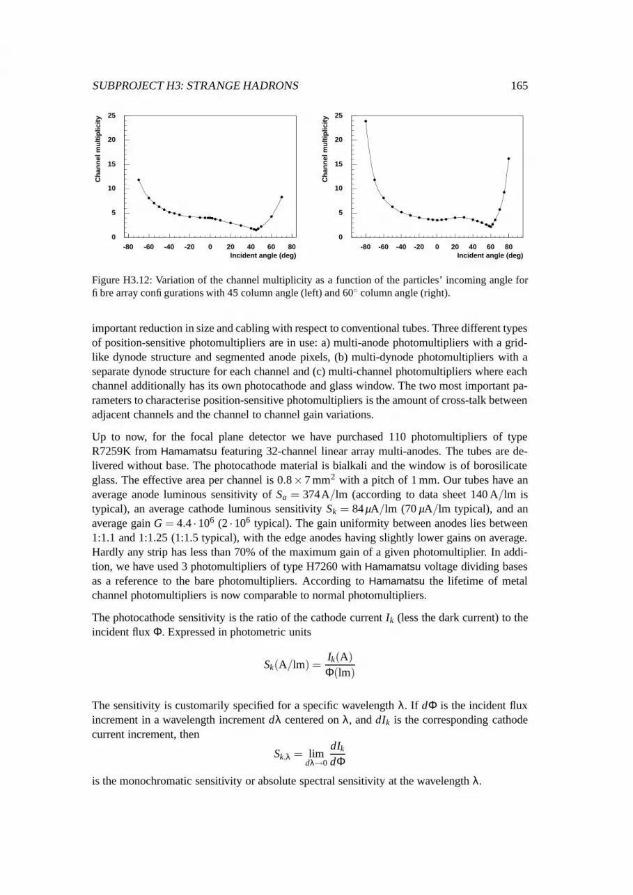
The main consequence of the particles’ incoming angles distribution, shown in Fig. H3.11(left),is an increased channel multiplicity, see Fig. H3.11(right). The pure geometrical effect wasstudied in a simulation of a 45 and a 60 detector, see Fig. H3.12 for the full curve. Incidentangles in the focal plane detector are lying on the steep rising branch above 60.
The multi-anode photomultiplier:
Position-sensitive photomultipliers are especially suitable for fibre read-out because of thegood match between photomultiplier segmentation and common fibre diameters, offering an
SUBPROJECT H3: STRANGE HADRONS 165
Incident angle (deg)-80 -60 -40 -20 0 20 40 60 80
Ch
ann
el m
ult
iplic
ity
0
5
10
15
20
25
Incident angle (deg)-80 -60 -40 -20 0 20 40 60 80
Ch
ann
el m
ult
iplic
ity
0
5
10
15
20
25
Figure H3.12: Variation of the channel multiplicity as a function of the particles’ incoming angle forfibre array configurations with 45 column angle (left) and 60 column angle (right).
important reduction in size and cabling with respect to conventional tubes. Three different typesof position-sensitive photomultipliers are in use: a) multi-anode photomultipliers with a grid-like dynode structure and segmented anode pixels, (b) multi-dynode photomultipliers with aseparate dynode structure for each channel and (c) multi-channel photomultipliers where eachchannel additionally has its own photocathode and glass window. The two most important pa-rameters to characterise position-sensitive photomultipliers is the amount of cross-talk betweenadjacent channels and the channel to channel gain variations.
Up to now, for the focal plane detector we have purchased 110 photomultipliers of typeR7259K from Hamamatsu featuring 32-channel linear array multi-anodes. The tubes are de-livered without base. The photocathode material is bialkali and the window is of borosilicateglass. The effective area per channel is 0.8× 7 mm2 with a pitch of 1 mm. Our tubes have anaverage anode luminous sensitivity of Sa = 374A/lm (according to data sheet 140 A/lm istypical), an average cathode luminous sensitivity Sk = 84µA/lm (70 µA/lm typical), and anaverage gain G = 4.4 · 106 (2 · 106 typical). The gain uniformity between anodes lies between1:1.1 and 1:1.25 (1:1.5 typical), with the edge anodes having slightly lower gains on average.Hardly any strip has less than 70% of the maximum gain of a given photomultiplier. In addi-tion, we have used 3 photomultipliers of type H7260 with Hamamatsu voltage dividing basesas a reference to the bare photomultipliers. According to Hamamatsu the lifetime of metalchannel photomultipliers is now comparable to normal photomultipliers.
The photocathode sensitivity is the ratio of the cathode current Ik (less the dark current) to theincident flux Φ. Expressed in photometric units
Sk(A/lm) =Ik(A)
Φ(lm)
The sensitivity is customarily specified for a specific wavelength λ. If dΦ is the incident fluxincrement in a wavelength increment dλ centered on λ, and dIk is the corresponding cathodecurrent increment, then
Sk,λ = limdλ→0
dIk
dΦ
is the monochromatic sensitivity or absolute spectral sensitivity at the wavelength λ.
166 CHAPTER 2. EXPERIMENTS AT MAMI AND THEORY
The quantum efficiency, ρ, another way of expressing cathode sensitivity, is the ratio of thenumber of photoelectrons emitted, nk , to the number of incident photons, np. It is usuallyspecified for monochromatic light and is related to the absolute spectral sensitivity by
ρ =nk
np= Sk,λ
hνe
= Sk,λhceλ
,
where e is electron charge, h is Planck’s constant, and c is the speed of light in vacuum [18].
The voltage generating PMT base:
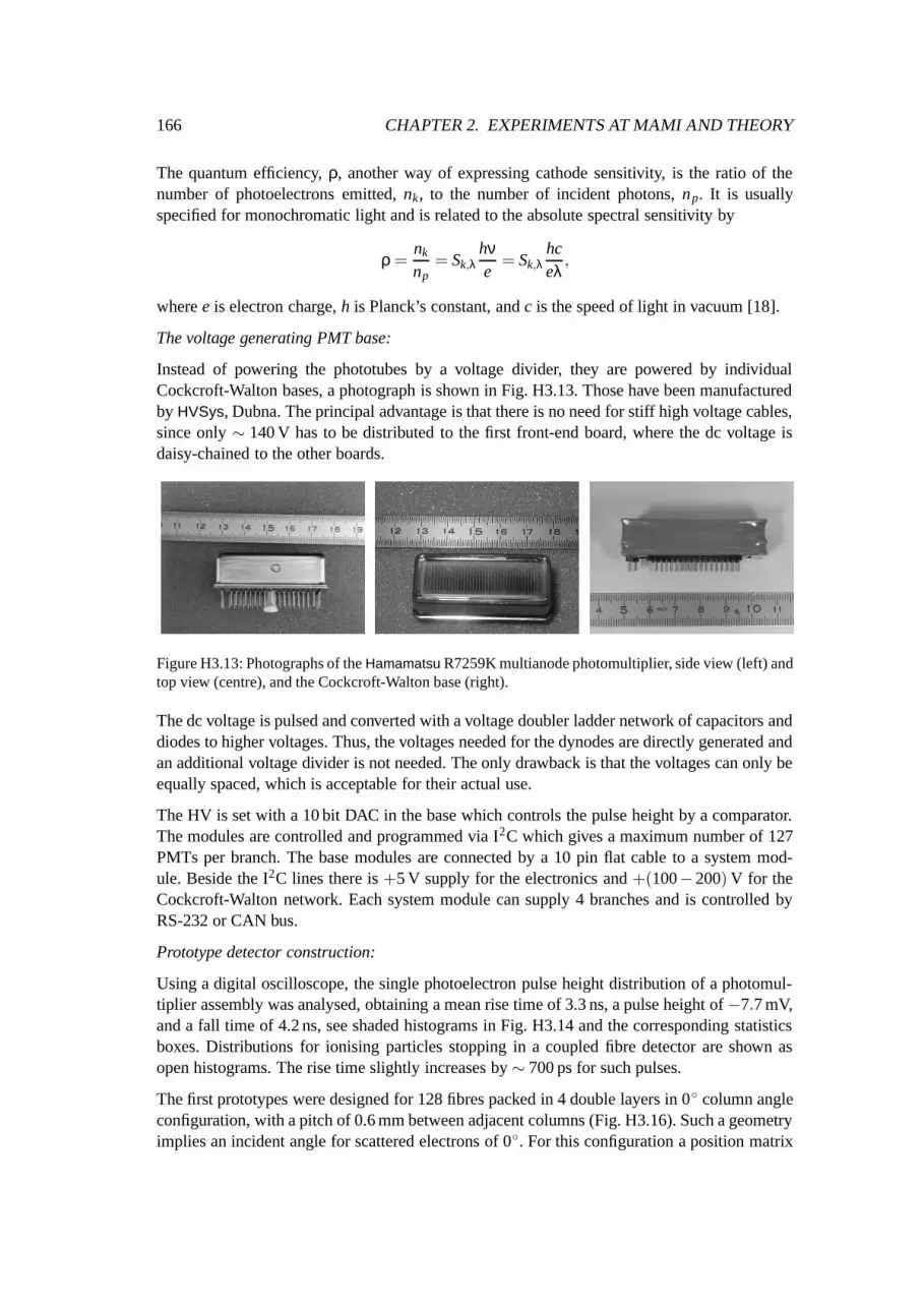
Instead of powering the phototubes by a voltage divider, they are powered by individualCockcroft-Walton bases, a photograph is shown in Fig. H3.13. Those have been manufacturedby HVSys, Dubna. The principal advantage is that there is no need for stiff high voltage cables,since only ∼ 140 V has to be distributed to the first front-end board, where the dc voltage isdaisy-chained to the other boards.
Figure H3.13: Photographs of the Hamamatsu R7259K multianode photomultiplier, side view (left) andtop view (centre), and the Cockcroft-Walton base (right).
The dc voltage is pulsed and converted with a voltage doubler ladder network of capacitors anddiodes to higher voltages. Thus, the voltages needed for the dynodes are directly generated andan additional voltage divider is not needed. The only drawback is that the voltages can only beequally spaced, which is acceptable for their actual use.
The HV is set with a 10 bit DAC in the base which controls the pulse height by a comparator.The modules are controlled and programmed via I2C which gives a maximum number of 127PMTs per branch. The base modules are connected by a 10 pin flat cable to a system mod-ule. Beside the I2C lines there is +5 V supply for the electronics and +(100− 200) V for theCockcroft-Walton network. Each system module can supply 4 branches and is controlled byRS-232 or CAN bus.
Prototype detector construction:
Using a digital oscilloscope, the single photoelectron pulse height distribution of a photomul-tiplier assembly was analysed, obtaining a mean rise time of 3.3 ns, a pulse height of −7.7 mV,and a fall time of 4.2 ns, see shaded histograms in Fig. H3.14 and the corresponding statisticsboxes. Distributions for ionising particles stopping in a coupled fibre detector are shown asopen histograms. The rise time slightly increases by ∼ 700 ps for such pulses.
The first prototypes were designed for 128 fibres packed in 4 double layers in 0 column angleconfiguration, with a pitch of 0.6 mm between adjacent columns (Fig. H3.16). Such a geometryimplies an incident angle for scattered electrons of 0. For this configuration a position matrix

SUBPROJECT H3: STRANGE HADRONS 167
Entries 1716Mean 3.298RMS 0.4437
Rise time (ns)0 1 2 3 4 5 6 7 8 9 10
Co
un
ts
0
0.02
0.04
0.06
0.08
0.1
0.12
0.14
0.16
0.18
Entries 1716Mean 3.298RMS 0.4437
Entries 1501Mean -6.821RMS 0.6559
Peak height (mV)-60 -50 -40 -30 -20 -10 0 10
Co
un
ts
0
0.1
0.2
0.3
0.4
0.5
0.6
0.7
0.8
0.9
Entries 1501Mean -6.821RMS 0.6559
Entries 1716Mean 4.183RMS 0.9582
Fall time (ns)0 5 10 15 20 25
Co
un
ts
0
0.05
0.1
0.15
0.2
0.25
0.3
Entries 1716Mean 4.183RMS 0.9582
Figure H3.14: MAPMT response distributions for single photoelectrons are shown as shaded histogramswith a mean rise time of 3.3 ns (left), a peak height of −6.7 mV (right), and a fall time of 4.2 ns (bottom).Distributions for ionising particles stopping in a coupled fibre detector are shown as open histograms.
was designed, allowing mounting and alignment of the fibres with the desired pitch. The con-struction procedure was to glue single fibre layers (16 fibres) fixed in grooved aluminium plateson top of each other with acrylic white paint, leading to a total of 8 single layers comprising32 channels. The bundles were glued to cookies by placing the fibres one by one into the cor-responding holes, then applying two components optical glue. Bundles are polished using adiamond cutting tool purchased from Mutronic. Some of the bundles have to be bent. They areput into an oven at a temperature of 70 C for about 1 hour.
Detectors with this configuration and an active area of 150×20 mm2 were used for laboratorymeasurements. Results from tests with a 90Sr source resulted in a light yield of 4−5 photoelec-trons per pixel with a multiplicity of 3 pixels, corresponding to 15 photoelectrons per crossingelectron.
Finally, in order to test a complete module, a triple detector was built, see Fig. H3.15 forphotographs. The detector has 96 channels in three joined fibre segments comprising 384 fibresand an active area of 58.4× 150 mm2, bare PMTs, and Cockcroft-Walton voltage multipliersmounted on a front-end board. Two of the bundles were aluminised (middle and right) and onethat was not aluminised (left).
For a set-up in the electron focal plane of the kaon spectrometer, this column angle is not usefulsince the scattered electrons have an inclination with respect to the normal of the focal plane.The natural change of the array configuration, keeping the same pitch, is the 45 configuration(Fig. H3.17). Two bundles were built in steps putting fibre column after fibre column intoa ladder, instead of positioning layer after layer. This construction method was inconvenientand lead to visible dislocations in fibre bundles of these “early generation” detectors. The low

168 CHAPTER 2. EXPERIMENTS AT MAMI AND THEORY
Figure H3.15: Photographs of a prototype triple detector with three 0 fibre bundles, bare PMTs, andCockcroft-Walton voltage multipliers mounted on a front-end board (top). Top view of the three joinedfibre segments comprising 384 fibres (bottom) with two aluminised bundles (middle and right) and onethat was not aluminised (left).
position resolution achieved with these detectors, see H3.2.2.1, was caused by these problems.With later detector generations better construction methods were applied.
Latest simulations showed that the necessary column angle is closer to 55 than 45, and afterexperiencing the difficulties with the 45 column angle configuration, the hexagonal packingwas chosen. It also has the advantage that the construction proceeds similar to the 0 construc-tion. A new position matrix was designed and prototype detectors are shown in Fig. H3.18.The high packing density of the slanted columns has simplified the construction of fibre bun-dles of these “later generation” detectors. Only small dislocations can be found where there isan excess of paint. In such a case, the surrounding columns are not straight, but instead bendaround the edge of the excess so that the structure is perfectly ordered on either side.
From the experience in building the bundles one can conclude that the misalignment of the
Figure H3.16: Scheme of a 0 column angle configuration (right) and photograph of an assembled andpolished fibre bundle (left). Detectors with this configuration were used for laboratory measurements.Practically no dislocations are visible.

SUBPROJECT H3: STRANGE HADRONS 169
Figure H3.17: Scheme of a 45 column angle configuration (right) and photographs of two assembled45 fibre bundles (left). The slanted columns have introduced complications in the construction whichlead to visible dislocations in fibre bundles of these “early generation” detectors.
fibres is strongly dependent on the fibre array configuration and in the 60 configuration arisesonly from excess of paint between layers.
The small dimension of the dynode channels on the electrode plate, 0.8 mm, and the diameterof the fibres, 0.83 mm, makes it clear that the alignment has to be very precise. A series ofphotographs has been taken through the photocathodes of a sample of 10 PMTs and the relativepositions of a single channels was measured by means of an alignment hole at a fixed positionwith respect to the PMT socket. Fig. H3.19 shows three photographs where the arrows indicatethe dynode channels. The accuracy of this method was of the order of 0.5µm and two ofthe channel positions were identical within this accuracy, whereas the third position shows adeviation of 0.5µm. The deviation of the positions of the dynode channels of the other PMTswere less or equal to the shown deviation. These tolerances have to be balanced during themounting.
In order to increase the light yield, fibre bundles are aluminised at the polished free end faceto reflect as much as possible of the light that initially was trapped in this direction back toPMT. We utilised a vaporisation chamber (vacuum chamber with an electric oven in which asmall pellet can be placed). The aluminium proves to attach well and smooth to the bundle.The increase of light yield was tested with a single detector and a 90Sr source. The result of thetest clearly shows an increase of the light yield of about 15 ADC channels in the spectrum, seeFig. H3.20.
Design of the focal plane detectors:
The main focal plane detector will consist of 2 horizontal planes, covering an area of 1500×300 mm2, and comprising close to 2000 channels per plane (63 detectors on 21 triple boards).The supporting frame for the whole system is under development. In principle, the assembly of

170 CHAPTER 2. EXPERIMENTS AT MAMI AND THEORY
Figure H3.18: Scheme of a 60 column angle configuration (right) and photographs of two assembled60 fibre bundles (left). Straight lines indicate the fibre columns. The high packing density of the slantedcolumns has simplified the construction of fibre bundles of these “later generation” detectors. Only inthe upper photograph small dislocations can be found where there is an excess of paint.
three bundles with cookies will be attached to the vacuum chamber from top and then the tripleboard will be positioned and aligned from below. Fig. H3.21 shows a graphical visualisationof a model of the focal plane detector showing the PMT assemblies with straight fibre bundlesand a simple plate representing the vacuum chamber. The small space between adjacent tripleboards, with a pitch of only 79.6 mm, poses some problems on positioning and alignment.
Detector characterisation at the electron beam:
We have employed spectrometer A to carry out a characterisation of a 32-channel fibre detectorprototype. The detector was sandwiched between the drift chambers and the scintillator paddlesof the focal plane detector system. The arrival time of the electrons was measured in the fibredetector with respect to the following two overlapping paddles. The electron track was recon-structed with the position information of the drift chambers and the electron hit position was ex-
Figure H3.19: Measurement of the relative deviation of the dynode channels seen through the photo-cathode. The relative deviation of the left and middle channels against the right one is ∆x = 50µm. Thedistance between two long markers is 1 mm.

SUBPROJECT H3: STRANGE HADRONS 171
Mean 34.117238Integral 1
ADC channel0 10 20 30 40 50 60 70 80 90 100
AD
C c
han
nel
x c
ou
nts
∑C
ou
nts
/
-610
-510
-410
-310
-210
-110
Mean 34.117238Integral 1
Figure H3.20: Pulse height spectra normalised to total number of entries showing the difference in thefibre bundle light yield between before (dark line) and after (clear line) the aluminisation.
trapolated from the drift chamber planes to the fibre detector plane. Fig. H3.22 (top left) showsthe geometrical acceptance covered by the fibre detector inside the spectrometer, determined bysuch an extrapolation. A simple estimator for the x-position x = ∑N
i=1 x(fibrei)/N +offset wasused, where x(fibrei) is the geometrical position of the ith fibre and N the hit multiplicity. Thatposition is compared to the reconstructed x-position projected onto the detector base coordi-nate, see Fig. H3.22 (top right). Small non-linearities at the edges indicate that better estimatorsare needed. However, position estimators based on weighted averages suffer from fluctuationsin pulse heights. The detection efficiency obtained from the drift chamber track reconstructionas a function of the lower level threshold was around 99% as seen in the figure’s bottom leftpanel. The simulated channel multiplicity for a 45 detector is N ≈ 1.6 as can be read fromFig. H3.12 (left). The large average multiplicity of N ≈ 4 seen in Fig. H3.22 (bottom right) is aconsequence of the dislocations in the fibre bundles of the 45 detectors, see H3.2.2.1, a com-plicated but necessary bending of the fibres into a geometrical shape adapted to the spectrom-eter, a problematic mounting because of space requirements, and some amount of cross talk inthe detector. Fig. H3.23 (left) shows the position resolution of the fibre detector defined as thedifference between reconstructed and measured track assuming that the resolution of the driftchambers is much better the resolution of the fibre detector. Because of the large multiplicitesits position resolution is only mediocre, so that this aspect has been studied in laboratory mea-surements with some improvement. Fig. H3.23 (right) shows the time resolution obtained fromthe coincidence timing with the scintillator paddle detectors after walk correction of the paddletiming. The FWHM of ≈ 1 ns is rather good for the small amount of light from the fibres.
H3.2.2.2 Development of new front-end electronics
A 12-layer front-end board able to accommodate three 32-channel multi-anode photomultipli-ers with minimum time jitter was designed, see Fig. H3.24. It houses the low voltage powersupply for the Cockcroft-Walton voltage multiplier bases of the photomultipliers, the RJ-45connectors for analogue output to the discriminators and, in the near future, APV25 chips foramplifying, sampling and multiplexing the signal amplitudes.

172 CHAPTER 2. EXPERIMENTS AT MAMI AND THEORY
Figure H3.21: Graphical visualisation of a model of the focal plane detector showing the PMT assem-blies with straight fibre bundles and a simple plate representing the vacuum chamber. The small spacebetween two adjacent triple boards, with a pitch of only 79.6 mm, is clearly visible.
It is forseen to implement the APV25 chip on the front-end board. Each of the 128 channelsof the APV25 contains a preamplifier and shaper, with a 50 ns peaking time, followed by a192 states deep memory into which samples are written at 40 MHz. Locations of data awaitingread-out are flagged. Following a trigger, three samples from the memory are processed with adeconvolution filter. The chip can be operated in three modes: peak mode, in which the outputsample corresponds to the peak amplitude following a trigger, deconvolution mode, in whichthe output corresponds to the peak amplitude of the filter, or multi-mode, where three samplesare read out. Behind the filter, the data is held in a further memory buffer prior to switchingthrough an output analogue multiplexer. This is required so that one event can be multiplexedout while another is prepared for transmission. The APV also contains system features includ-ing programmable on-chip analogue bias networks, a remotely controllable internal test pulsegeneration system and a slow control communication interface.
The full scheme for the read-out of analogue and digital information from the focal planedetector can be found in Fig. H3.25. A 32-channel discriminator board with 4 integrated low-walk double threshold discriminators (DTDs) for amplitude compensated timing was built bythe electronics workshop of the Institut für Kernphysik, see Fig. H3.26 (left) for a photographof the DTD board. The detectors are connected to the board by RJ-45 cables (with 4 channelsper cable). The DTD boards have two multiplexed Lemo analogue outputs for debugging andtwo LVDS outputs with the signals being compatible to COMPASS electronics, one to beconnected to TDC modules, and one to the trigger modules. A 32-channel analogue outputboard can be attached to the discriminator board for a complete analysis during the prototypingstage. Up to 20 DTD boards fit into a VME 6U crate together with a controller board, seeFig.H3.26 (right) for a photograph. The communication with a PC is done via parallel port.Timing measurements are done with TDC CATCH boards. These boards, developed for theCOMPASS collaboration, are equipped with 4 mezzanine cards for a total of 32 channels.The trigger will be derived with GSI VME logic modules. Such a module is equipped with aVIRTEX4 FPGA, up to 32 ECL front panel inputs and up to 32 outputs. All functions of the

SUBPROJECT H3: STRANGE HADRONS 173
250 260 270 280 290 300
−50
0
50
100
150
200
y vdc
(m
m)
xvdc (mm)250 260 270 280 290 300
250
260
270
280
290
300
x fib
re (
mm
)
xvdc (mm)
Threshold (mV)0 10 20 30 40 50
Det
ecti
on
Eff
icie
ncy
0.7
0.75
0.8
0.85
0.9
0.95
1
0 5 10 15 20 0
10
20
30
40
Cou
nts
(x
103 )
Multiplicity
Figure H3.22: Geometrical acceptance covered by the fibre detector inside the spectrometer shownby the track positions reconstructed with the drift chambers (top left). The top right panel shows thereconstructed x-position projected onto the base coordinate versus the measured x-position obtainedwith a simple estimator from the fibre detector. The detection efficiency for the fibre detector obtainedfrom the drift chamber track reconstruction as a function of the lower level threshold is shown in thebottom left panel and the channel multiplicity of detector in the bottom right panel.
−5 0 5 0
5
10
fit result :
−5 0 5 0
5
10
Cou
nts
(x
103 )
xres (mm)
MAX : 10532 countsMAX at: 0.123 mmFWHM : 1.105 mmBackgd: 0 counts
−5 0 5 0
5
10
−5 0 5 0
200
400
600
800
Cou
nts
∆t (ns)
∆t + channel offsets
−5 0 5 0
200
400
600
800
∆t + channel offsets + walk correction
fit result :
−5 0 5 0
200
400
600
800
MAX : 693 countsMAX at: 0.614 nsFWHM : 1.244 nsBackgd: 0 counts
−5 0 5 0
200
400
600
800
fit result :
−5 0 5 0
200
400
600
800
MAX : 811 countsMAX at: −0.074 nsFWHM : 1.048 nsBackgd: 0 counts
−5 0 5 0
200
400
600
800
Figure H3.23: Position resolution of the fibre detector obtained from the drift chamber track reconstruc-tion and time resolution of the fibre detector obtained from the coincidence timing with the scintillatorpaddle detectors.

174 CHAPTER 2. EXPERIMENTS AT MAMI AND THEORY
Figure H3.24: Photograph and circuit scheme of the triple front-end board showing the three PMTsockets (lower left) and the output sockets. The site for the APV chip is indicated.
module are programmable through the FPGA which can be easily reconfigured from FLASHmemory or directly via the VME interface.
H3.2.2.3 Upgrade of existing electronic read-out systems
The H3 project foresees the upgrade of the existing read-out electronics of one of the mainspectrometers of the A1 Collaboration (A, B, or C) with an electronic system based on CATCH,the COMPASS Accumulate, Transfer and Control Hardware. The system includes VME cratesof 9U size each filled with 12 CATCH modules equipped with 4 TDC mezzanine cards pro-viding a total of 32× 4× 12 = 1536 TDC read-out channels per crate. The CATCH modulenot only serves as an interface between front-end electronics and the data taking processor, butalso acts as an integral part of the trigger distribution and time synchronisation system (TCS).At the heart of the TDC mezzanine cards there are the so-called F 1 chips, developed by theFaculty of Physics of the University of Freiburg, Germany, for the COMPASS experiment, with8 channels of ∼ 120 ps resolution (least significant bit) each.
The H3 project plans the set-up of a pilot coincidence experiment with the KaoS spectrom-eter as the hadron arm and the upgraded spectrometer B as the electron arm. However, aseries of measurements, among them the detection of hypernuclei at very forward angles,is envisaged for the medium-term future where these measurements will be made possibleby the use of the KaoS spectrometer as a double spectrometer and the detection of elec-trons with a new focal plane detector package consisting of scintillating fibres. The totalof ∼ 4000 channels of this detector system will be read out with CATCH TDC mezzanine

SUBPROJECT H3: STRANGE HADRONS 175
Figure H3.25: Schematic presentation showing the connection of the triple boards to the DTD discrim-inator cards housed in 6U VME crates, and to the CATCH cards housed in 9U VME crates.
cards as well. The development of the necessary front-end boards to discriminate the ana-logue signals and deliver signal levels compatible with CATCH standards (LVDS) is welladvanced at our electronics workshop in Mainz (see H3.2.2.2). A proposed share of phys-ically the same hardware between the KaoS spectrometer and spectrometer B poses somelogistical problems. An experiment as complex as the designed experiment on hypernucleiin electroproduction with its special need for a kaon trigger will suffer with each disassem-bling and assembling of electronic modules and crates. Enduring changes to the sophisticatedtrigger system and data flow control of the CATCH by disassembling and assembling are ex-pected to lead to trigger and timing problems. Therefore, we plan a permanent upgrade ofthe electronics of spectrometer B without the need for disassembling when running the kaonspectrometer.
In a first implementation step towards the data acquisition with the COMPASS electronicsat the A1 Collaboration, the CATCH modules have been used together with the F 1 TDCmezzanine cards and the TCS system in a test set-up for the scintillating fibre detector prototypeof the KaoS spectrometer. The read-out of the CATCH via VME bus has been implemented inthe A1 data acquisition package AQUA++. The test set-up has been operated independently aswell as together with spectrometer A. First tests of AQUA++ towards the full COMPASS dataacquisition chain, i.e. read-out of the CATCH module via PC-hosted Readout Buffer Cards("ROB", aka "Spillbuffer"), which are connected to the CATCH module with a high speedoptical link (SLink), have been already done as well.

176 CHAPTER 2. EXPERIMENTS AT MAMI AND THEORY
Figure H3.26: The double threshold discriminator board (left). The two LVDS outputs are visible at thebottom of the module. The RJ-45 inputs are at the top left of the module and the two Lemo outputs atcentre left. The analogue output board can be attached for debugging (middle). The controller board forthe double threshold discriminator board (right).
In addition to timing measurements via CATCH and F 1-TDC, an ADC system capable of han-dling high channel counts is also needed, especially for the future scintillating fibre detectorof the KaoS spectrometer. For this purpose, another component of the COMPASS electronicsis under investigation, namely the electronics around the APV-Chip and the GeSiCa data col-lector card. This system has been mainly developed by the Faculty of Physics of the TechnicalUniversity of Munich, Germany, for the RICH subdetector of the COMPASS set-up. With 128input channels, each performing synchronous analogue sampling at 40 MHz, the APV chip actsas an analogue ring-buffer, which on demand multiplexes the appropriate 128-channel sampleand sends it to an attached ADC. The GeSiCa module provides a similar functionality as theCATCH module, i.e. set-up of the attached front-end electronics (here the APV chip itself andits attached ADC), TCS information processing, data collection, data concentration and datatransfer to PC-based read-out buffer cards via SLink.
As stated before, it is planned to upgrade one of the main spectrometers of the A1 spectrometerfacility with new read-out electronics. Here, spectrometer B is the primary candidate, because itwill be operated in coincidence with the KaoS spectrometer. Since the other two spectrometersdon’t differ greatly with respect to their basic detector systems, their possible upgrade will besimilar to that of spectrometer B.
From the read-out electronics point of view, spectrometer B features 1472 signal lines fromthe vertical drift chamber (VDC), 45 signal lines from the scintillation detector and 5 fromthe Cherenkov detector. Spectrometer A and C both have 60 lines for the scintillator, 12 for theCherenkov and 1472 (A), resp. 1600 (C) for the VDC. For the VDC, just the timing informationneeds to be recorded, whereas for the scintillation and the Cherenkov detector signals both thecharge and the timing are measured. The timing information of all detectors will be read out byCATCH modules equipped with F 1-TDC cards. For the signal charge of the trigger signals,the APV system will be investigated.
The VDC timing signals are generated by detector mounted preamplifier/discriminator cards(LeCroy 2735) and have ECL signal levels. Therefore they need to get converted to LDVSbefore the CATCH-mounted F 1-TDC card is able to process them. NIM converter modulesare foreseen for this task. Two test modules have been build recently and are about to be tested.

SUBPROJECT H3: STRANGE HADRONS 177
Especially, it is planned to operate the old LeCroy 4299 TDC-system and the new CATCH/F 1-System in parallel to ensure that both give the same results.
H3.2.2.4 Systematic study of timing with plastic scintillators
The particle identification (PID) of charged particles at KaoS is assumed to be performedwith the time-of-flight method from a segmented scintillator array. For the higher momentaa Cherenkov detector is planned. For the future PANDA experiment at FAIR the PID can beperformed by the detection of internally reflected Cherenkov (DIRC) light. The measurementof the time of propagation (TOP) in a DIRC counter can naturally be combined with the reg-ular time-of-flight information. Our expertise in pixelized photon detectors and single photoncounting is supporting the development of such a combined detector. Timing properties of scin-tillators and photomultipliers as well as theoretical and experimental studies of time resolutionof scintillation counters have been performed.
The timing properties scintillators are usually defined in terms of a coincidence time resolutionbetween identical counters. For small counters a time resolution in the range of σtot ≈ 25−100 ps can be achieved. For larger scintillators there are several effects degrading the timeresolution, namely the scintillation process with its decay time σsci and the scintillator as a lightguide with corresponding pulse dispersion σdisp. The contribution of the photomultiplier tubeto the time width of the observed output pulse is determined by the electron transit time spread,σTT S, where the transit time is the time difference between photo-emission at the cathode andthe arrival of the subsequent electric signal at the anode. Further, the discriminator, whichcould be either of type leading edge or constant fraction, and any noise in the electronic circuitscontribute to the timing. They may shift the response time with signal amplitude (“time walk”).Time walk effects can get corrected by various means, either in hardware or software [19].
One intrinsic limit on the time resolution of low mass scintillation counters comes as a conse-quence of the statistical processes involved in the generation of the signal. Obviously, the sig-nal amplitude depends on the number of photoelectrons, N, appearing during some integrationtime, T . This number fluctuates from one pulse to another. The mean number of photoelec-trons per pulse, N, and its variance, σN , are characteristic of the photoelectron statistics. As thenumber of photoelectrons increases, a larger number of time intervals is sampled. In a semi-classical model the probability for observing N photoelectrons over a time interval T is givenby a Poissonian distribution P(N,N). For larger numbers of photoelectrons, the distributionis assumed to be Gaussian, so that the signal amplitude should vary with
√N. In general, the
voltage pulse of a photomultiplier, VPMT, can be expressed as a linear superposition of Npe sin-gle photoelectron pulses, vi, arriving at individual times due to time uncertainties in the energytransfer to the optical scintillator levels, tdep, the decay time of the light emitting states, temit, the
propagation time, tpro, and the transit time, tTT: VPMT(t) = ∑Npe
i=1 vi(t − (tdep + temit + tpro + tTT)i).
Post and Schiff [20] have first discussed the limitations on timing that arise from the statisticsof photon detection. The spread of photon arrival times due to propagation length differencesis given by ∆tpro = nd
c ( 1cosθ − 1) for a point like source of light placed at a distance d from
the end face of a cylindrical scintillator with refractive index n. Fig. H3.27 illustrates the ge-ometry where d = L/2 and θ represents the complement of the total internal reflection angle,θ = arccos next
n . The geometry of the problem gets more complicated for rectangular shapedscintillators, but is solvable with Monte Carlo simulations.

178 CHAPTER 2. EXPERIMENTS AT MAMI AND THEORY
PMTθ
Figure H3.27: Schematic representation of the arrangement of plastic scintillator, slit and PMT in twosituations. Right: photon travelling in a straight line. Left: photon travelling with an axial angle equal tothe complement of total internal reflection angle.
The probability density function of arrival times of photons at the photocathode, dN/(Ndt),produced by an event at t = 0, can be calculated from the angular distribution of photons insidethe scintillator, dN = 2πd cos θ with cosθ = Ln/(ct). It follows that dN/dt = −2πLn/(ct 2)and N =
R tmaxtmin
dNdt dt = 2π(cos θ − 1) with tmin = Ln/c and tmax = Ln/(ccos θmax), so that
dN/(Ndt) = Ln/((cos θ−1)ct2).
The average number of photoelectrons detected in the interval between tmin and t is p(t) =R t
tmindN/(Ndt ′)dt ′. From Poisson statistics and assuming the amplification of primary photo-
electrons without time spread the timing of an output pulse being fed into a discriminator thattriggers when a definite number of photoelectrons, Nthr, have accumulated can be calculated:PN = N dN
dt
( N−1Nthr−1
)pNthr−1(1− p)N−Nthr , which is to be normalised: P = PN ÷R tmax
tminPNdt. The cal-
culated distributions of pulse timing for for L= 1 m, n= 1.58, N=60 for a range of thresholds,and for L = 1 m, n = 1.58, and Nthr = 2 for a range of pulse heights can be found in Fig. H3.28.
5250 5500 5750 6000 6250 6500 6750Pulse timing HpsL
0.0025
0.005
0.0075
0.01
0.0125
0.015
0.0175
0.02
Pro
bab
ility
den
sity
HperpsL
Thr=30Thr=20Thr=10Thr= 5Thr= 2
5250 5500 5750 6000 6250 6500 6750Pulse timing HpsL
0.0025
0.005
0.0075
0.01
0.0125
0.015
0.0175
0.02
Pro
bab
ility
den
sity
HperpsL
N= 5N=10N=20N=30N=60
Figure H3.28: Calculated distributions of pulse timing for L= 1 m, n= 1.58, N=60 for a range of thresh-olds (left), and for L = 1 m, n = 1.58, and Nthr = 2 for a range of pulse heights (right).
The limit on time resolution arising from statistics of photon detection can now be calculatedusing the relations 〈tp〉 =
R tmaxtmin
t ′Pdt ′, 〈t2p〉 =
R tmaxtmin
t ′2Pdt ′, and Var(tp) = 〈t2p〉− 〈tp〉2. The time
resolution is shown for a range of thresholds, Nthr= 2,5,10,20,30 in Fig. H3.29 with the blackcurves indicating a σ ∝ 1/N behaviour.
To predict the time resolution of a scintillation counter, the probability density function ofthe transit time spread of electrons in the photomultiplier, PTTS, has to be folded in dN ′/dt =dN/dt ×PTTS(t). Further, the distribution of decay times of light emitting states is to be in-cluded with a light pulse shape of the form: i(t) =
(e−t/τ − e−t/τ1
)τ/(τ− τ1), where τ and τ1
are scintillation time constants. The distribution of photon arrival times is then changed ac-cording to Fig. H3.30. At this point a full photon tracking simulation with the correct geometry
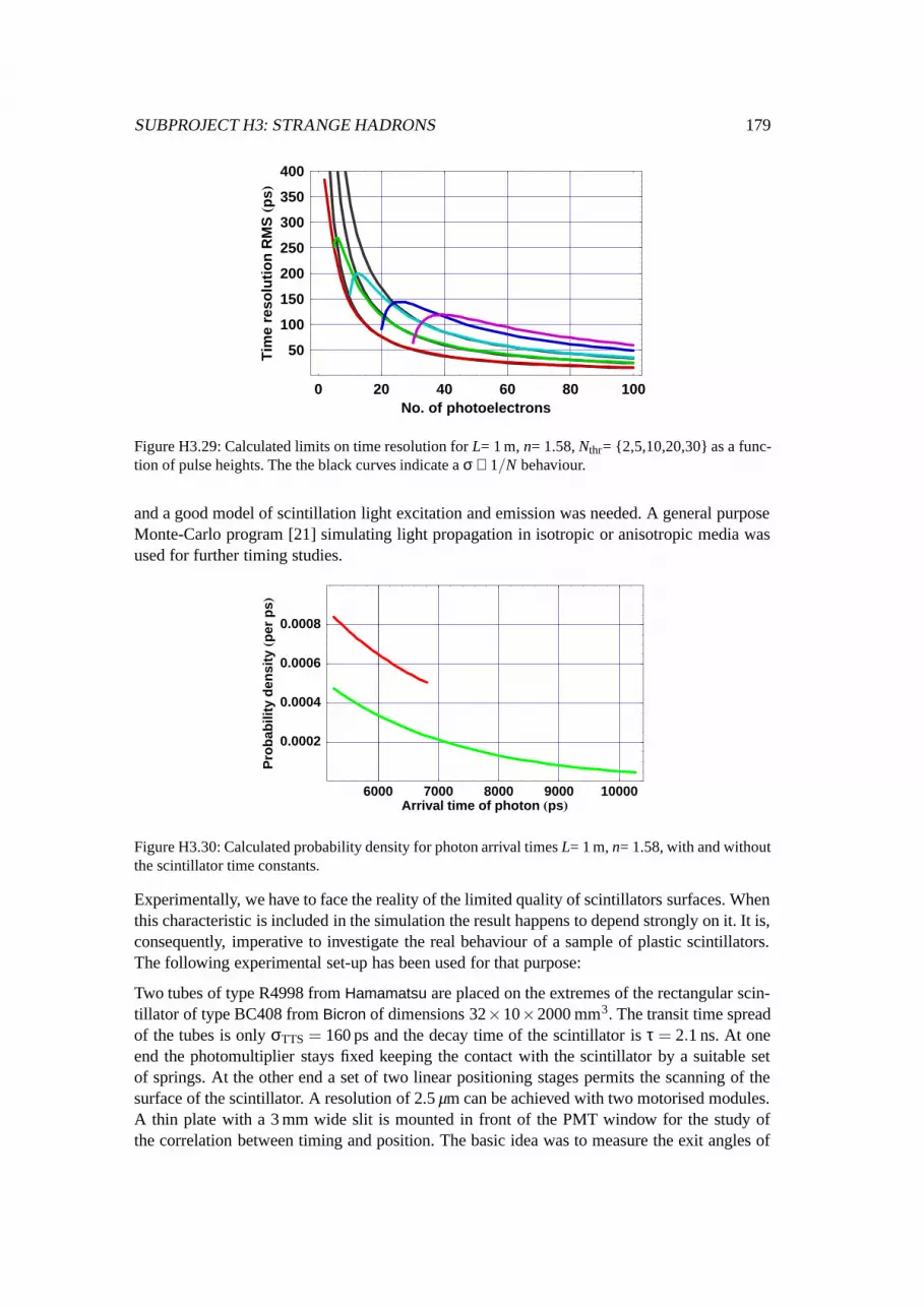
SUBPROJECT H3: STRANGE HADRONS 179
0 20 40 60 80 100No. of photoelectrons
50
100
150
200
250
300
350
400
Tim
ere
solu
tio
nR
MS
HpsL
Figure H3.29: Calculated limits on time resolution for L= 1 m, n= 1.58, Nthr= 2,5,10,20,30 as a func-tion of pulse heights. The the black curves indicate a σ ∝ 1/N behaviour.
and a good model of scintillation light excitation and emission was needed. A general purposeMonte-Carlo program [21] simulating light propagation in isotropic or anisotropic media wasused for further timing studies.
6000 7000 8000 9000 10000Arrival time of photon HpsL
0.0002
0.0004
0.0006
0.0008
Pro
bab
ility
den
sity
HperpsL
Figure H3.30: Calculated probability density for photon arrival times L= 1 m, n= 1.58, with and withoutthe scintillator time constants.
Experimentally, we have to face the reality of the limited quality of scintillators surfaces. Whenthis characteristic is included in the simulation the result happens to depend strongly on it. It is,consequently, imperative to investigate the real behaviour of a sample of plastic scintillators.The following experimental set-up has been used for that purpose:
Two tubes of type R4998 from Hamamatsu are placed on the extremes of the rectangular scin-tillator of type BC408 from Bicron of dimensions 32×10×2000 mm3. The transit time spreadof the tubes is only σTTS = 160 ps and the decay time of the scintillator is τ = 2.1 ns. At oneend the photomultiplier stays fixed keeping the contact with the scintillator by a suitable setof springs. At the other end a set of two linear positioning stages permits the scanning of thesurface of the scintillator. A resolution of 2.5 µm can be achieved with two motorised modules.A thin plate with a 3 mm wide slit is mounted in front of the PMT window for the study ofthe correlation between timing and position. The basic idea was to measure the exit angles of

180 CHAPTER 2. EXPERIMENTS AT MAMI AND THEORY
Figure H3.31: The left photograph of the experimental set-up shows the PMT housing, the metallic tubewith lead collimators, and the remote controllers of the positioning units. The right photograph showsthe positioning units and the PMT equipped with plastic slit. The motion takes place in the directionperpendicular to the small dimension of the scintillator.
the photons as these carry the information of the propagation time by displacing the tube by1 cm. The 2 m long scintillator was placed along the longitudinal axis of a black metallic tubein which a set of connectors for the scintillator excitation have been installed, see Fig. H3.31.A 90Sr source and a fast pulsed ultraviolet laser can be used for the measurements. The laserhas a pulse duration FWHM < 100 ps. The signals were digitised by a LeCroy charge integrat-ing analog-to-digital converter (LeCroy 1885F, 50 fC/count) and by a LeCroy time-to-digitalconverter (LeCroy 1875, 25 ps/count). The TDC digitisation corresponds to a time resolutionof 25√
12ps = 7 ps. The large range of variation of signal amplitudes obligates a detailed investi-
gation of any possible walk effect. A full scanning of the amplitudes was performed by meansof filters placed in front of the movable PMT. The constant fraction discriminators provideda small modification of the timing signal. The remaining “walk” was fitted and used for thecorrection of the TDC information.
Pulse charge (pC)0 10 20 30 40 50 60 70 80 90
(p
s)σ
Tim
e re
solu
tio
n
0
20
40
60
80
100
120
p0 26.45p1 605.9p2 -1.259
p0 26.45p1 605.9p2 -1.259
Figure H3.32: Measured time resolution (standard deviation σ) obtained with a BC-408 scintillator anda laser of varying primary light intensity as a function of the pulse charge.
The time resolution achieved for low light intensities was σ ≈ 100 ps. With increasing lightintensity the resolution improves until it levels off at about σ ≈ 40 ps (see Fig. H3.32), demon-strating that at high intensities the photon statistics is no longer decisive and the resolution is

SUBPROJECT H3: STRANGE HADRONS 181
supposedly dominated by electronic noise.
PMT position (mm)-10 -5 0 5 10
Tim
e d
iffe
ren
ce (
ps)
0
100
200
300
400
500L= 100cm
PMT position (mm)0 2 4 6 8 10
Tim
e d
iffe
ren
ce (
ps)
0
100
200
300
400
500L= 140cm
L= 100cm
L= 80cm
Figure H3.33: Measured mean timing as a function of the slit position when the scintillator is excited bythe UV laser at L = 100cm, and for three different positions of the UV laser at L = 80, 100, and 140 cm.
Position of 3 mm wide PMT slit13 14 15 16 17 18 19 20
Tim
e d
iffe
ren
ce (
ps)
0
100
200
300
400
500L= 100cm
No. of photoelectrons0 50 100 150 200 250
Tim
e re
solu
tio
n R
MS
(p
s)
0
10
20
30
40
50
60
70
80
Figure H3.34: Simulated mean timing as a function of the position of a 3 mm wide PMT slit (left) andsimulated time resolution of a full coverage PMT as a function of the number of photoelectrons for asingle photoelectron threshold (right). The characteristics of the scintillation light and the geometry ofthe scintillator have been adapted to the above experiments.
Fig. H3.33 shows the variation of the mean pulse timing as a function of the position of the slitwith respect to the centre, when the laser light is injected at d = 1 m. When this experimentis repeated for three different positions of the laser source the expected variation of the timedifference, approximately linear with the distance for a given slit position, is observed. Thelight propagation is simulated in detail with a Monte Carlo code. The observed variation of themean pulse timing with position was verified, as shown in Fig. H3.34(left). The code was alsoused to simulate the time resolution of a full coverage PMT as a function of the number of pho-toelectrons. These simulations serve as an important guide for the detector development [22].
One example, where the contribution of the propagation time spread σpro gets significant is pro-vided by the Cylindrical Time-of-Flight Counter being developed for PANDA [23]. A thicknessof only 5 mm would allow to mount the scintillator strips together with the DIRC radiators, butreduces the number of photoelectrons to 〈Npe〉 ' 100 at d = 1 m. A Monte Carlo simulationincluding a finite decay time of the scintillator predicts a minimum achievable time resolutionof σmin ' 130 ps, depending a little on threshold.
These results have brought forward the idea of improving the timing resolution of a scintil-lation counter through position sensitive photon detection. An analogy of this method is used

182 CHAPTER 2. EXPERIMENTS AT MAMI AND THEORY
successfully in DIRC-like detectors using glass slabs for measuring the Cherenkov angle, butwas never investigated in scintillators.
References
[1] G. Niculescu et al. (E93-018 Collaboration), Phys. Rev. Lett. 81, 1805 (1998).
[2] R.M. Mohring et al. (E93-018 Collaboration), Phys. Rev. C67, 055205 (2003).
[3] P. Achenbach et al. (A1 Collaboration), accepted proposal MAMI-A1/1-03, 2003.
[4] E. Amaldi, S. Fubini, and G. Furlan. Pion-Electroproduction (Springer Tracts in ModernPhysics 83). Springer, Berlin, 1979.
[5] A. Donnachie and G. Shaw. Electromagnetic Interactions of Hadrons. Plenum, NewYork, 1978.
[6] T. Miyoshi et al., Phys. Rev. Lett. 90, 232502 (2003).
[7] T. Motoba et al., Prog. Theor. Phys. 117, 123 (1994).
[8] H. Tamura et al., Nucl. Phys. A 754, 58 (2005).
[9] T. Nagae, Nucl. Phys. A 670, 269c (2000).
[10] C.M. Keil et al., Phys. Rev. C 61, 064309 (2000).
[11] S. Shinmura, Prog. Theor. Phys. 92, 571 (1994).
[12] C. Bennhold et al., nucl-th/0011022, 1999.
[13] H. Bando, T. Motoba and J. Zofka, J. Mod. Phys. A5, 4021 (1990).
[14] P. Senger et al. (KaoS Collaboration), Nucl. Inst. Meth. in Phys. Res. A327, 393 (1993).
[15] R.C. Ruchti, Annu. Rev. Nucl. Part. Sci. 46, 281 (1996).
[16] H.A. Bethe, Phys. Rev. 89, 1256 (1953).
[17] W.T. Scott, Rev. Mod. Phys. 35, 231 (1963).
[18] Photonis, Photomultiplier tubes: Principles & applications, 2002, Photonis, France.
[19] H. Spieler, IEEE Trans. Nucl. Sci. 29, 1142 (1982).
[20] M. Post and L.J. Schiff, Phys. Rev. 80, 113 (1950).
[21] F.-X. Gentit, Nucl. Inst. Meth. in Phys. Res. A486, 35 (2002).
[22] P. Achenbach et al., Measurement of photon angles for highly resolved TOF detectors,in GSI Scientific Report 2005, GSI, Darmstadt.
[23] Technical progress report for PANDA: strong interaction studies with antiprotons, Jan.2005, GSI, Darmstadt.


