Embed Size (px)
Citation preview
Neurocomputing 74 (2011) 2780–2789
Contents lists available at ScienceDirect
Neurocomputing
0925-23
doi:10.1
� Corr
E-m
SunMin
journal homepage: www.elsevier.com/locate/neucom
Stochastic neighbor projection on manifold for feature extraction
Songsong Wu �, Mingming Sun, Jingyu Yang
School of Computer Science and Technology, Nanjing University of Science and Technology, Nanjing 210094, China
a r t i c l e i n f o
Article history:
Received 18 January 2010
Received in revised form
15 March 2011
Accepted 19 March 2011
Communicated by T. Heskesdistance metric, then the same distribution is required to be hold in feature space. This learning
Available online 26 May 2011
Keywords:
Feature extraction
Dimensionality reduction
Manifold learning
Visualization
Biometrics
12/$ - see front matter Crown Copyright & 2
016/j.neucom.2011.03.036
esponding author.
ail addresses: [email protected], ssw
[email protected] (M. Sun), [email protected]
a b s t r a c t
This paper develops a manifold-oriented stochastic neighbor projection (MSNP) technique for feature
extraction. MSNP is designed to find a linear projection for the purpose of capturing the underlying
pattern structure of observations that actually lie on a nonlinear manifold. In MSNP, the similarity
information of observations is encoded with stochastic neighbor distribution based on geodesic
criterion not only empowers MSNP to extract nonlinear feature through a linear projection, but makes
MSNP competitive as well by reason that distribution preservation is more workable and flexible than
rigid distance preservation. MSNP is evaluated in three applications: data visualization for faces image,
face recognition and palmprint recognition. Experimental results on several benchmark databases
suggest that the proposed MSNP provides a unsupervised feature extraction approach with powerful
pattern revealing capability for complex manifold data.
Crown Copyright & 2011 Published by Elsevier B.V. All rights reserved.
1. Introduction
The data to be processed in many applications of modernmachine intelligence, e.g., pattern recognition, image retrieval,knowledge discovery and computer vision, are often acquiredor modeled in high-dimensional form. It is well acknowledgedthat high-dimensional data pose many challenges, such as highcomputational complexity, huge storage demand and poor out-come performance, to data processing [1,2]. Feature extraction, asa branch of dimensionality reduction, overcomes the curse ofdimensionality [2] problem by mapping high-dimensional datainto a low-dimensional subspace, in which data redundancy isreduced. The goal of feature extraction is to find meaningful low-dimensional representations of high-dimensional data and simul-taneously discover the underlying pattern structure. Featureextraction methods can be broadly categorized into two classes:Linear subspace methods such as PCA and LDA, and nonlinearapproaches such as kernel-based techniques and geometry-basedtechniques.
Linear feature extraction tries to find a linear subspace asfeature space so as to preserve certain kind of characteristicsof observed data. Specifically, PCA [3] projects data along thedirections that maximize the total variance of features. MDS [4]seeks the low-rank projection that best preserves the inter-pointdistances given by pairwise distance matrix. PCA and MDS are
011 Published by Elsevier B.V. All
[email protected] (S. Wu),
st.edu.cn (J. Yang).
equivalent in theory when Euclidean distance is employed. ICA[5] attempts to make the probability distribution of features ineach projection direction is statistically independent of oneanother. Compared with PCA, MDS and ICA, whose linear sub-space contains no discriminant information, LDA [6] learns alinear projection with the assistance of class labels. LDA magnifiesthe inter-class scatter meanwhile shrinks the intra-class scatter infeature space for the purpose of better separability. Recently,GMMS [7], HMSS [8] and MMDA [9] markedly improve theperformance of LDA by solving the knotty problem of classicalLDA that fractional classes could emerge with each other whenfeature dimension is lower than class number. GMMS achieves itsimprovement by employing a general geometric mean function inthe criterion. HMSS implicitly replaces the arithmetic mean used inLDA with the harmonic mean. MMDA performs discriminantanalysis with a novel criterion that directly maximizes the mini-mum pairwise distance of all classes so as to separate all classes inthe low-dimensional subspace. Generally speaking, linear subspacemethod shows good performance on feature extraction for linearstructure data, but may be suboptimal for the data containingcomplicated nonlinear structure, such as nonlinear submanifoldembedded in observation space.
To deal with nonlinear structural data, a number of nonlinearapproaches have been developed for dimensionality reduction orfeature extraction, with two in particular attracting wide atten-tions: kernel-based techniques and geometry-based techniques.Kernel-based techniques implicitly map raw data into a poten-tially much higher dimensional feature space in order to convertdata from nonlinear structure to linear structure. With the aid ofkernel function, kernel-based methods extract nonlinear feature
rights reserved.
S. Wu et al. / Neurocomputing 74 (2011) 2780–2789 2781
by applying linear techniques in the implicit feature space.The representative kernel-based methods include KPCA [10], KICA[11] and KLDA [12,13] and they are proven to be effective forfeature extraction task in nonlinear case. In contrast with kernel-based methods, geometry-based methods are motivated byadopting geometrical perspective to explore the immanent struc-ture of data. The representative methods include the so-calledmanifold learning and its extensions. The well known manifoldlearning algorithms such as Isomap [14], LLE [15], LE [16], HLLE[17] and LTSA [18] are all developed for nonlinear dimensionalityreduction with the help of differential geometry. Isomap calcu-lates pairwise geodesic distance of observations and preserves thedistance by classical MDS in embedding space so as to unfoldingnonlinear manifold. LLE focus on local neighborhood of each datain which the error of linearly reconstructing the data with itsneighbors is minimal for both the sample data and the corre-sponding embeddings. LE is developed based on Laplace Betltramioperator on manifold. LE constructs an undirected weightedgraph that indicates the neighbor relations of the pairwise points,then recover the structure of manifold through graph manipula-tion. HLLE estimates the Hessian matrix based on neighborhoodsto capture local property and obtains the low-dimensionalembeddings through eigenvalue decomposition of the Hessianmatrix. LTSA first uses approximated local tangent space toencode local geometry, then aligns all the local tangent spacesto obtain a global embedding. Since manifold learning methodsobtain low-dimensional embeddings without a explicit mapping,it is intractable for them to extract feature beyond training sampleset. Many endeavors have been done to overcome the out-of-sample problem [19]. NPE [20] try to find a linear subspace thatpreserves local structure under the same principle of LLE. LPP [21]seeks optimal linear approximation to eigenfuction of LaplacianBetltrami operator on manifold. LLTSA [22] finds the linear projec-tion that approximates the affine transform of LTSA, and DLA [23]is another linear extension of LTSA which takes account ofdiscriminant information. Besides, in order to understand thecommon properties of different approaches for dimensionalityreduction and to investigate their intrinsic relationships, the graphembedding framework [24] and the patch alignment framework[25] have been proposed. The graph embedding framework modelsthe dimensionality reduction problem with graph language andgraph theory, and the patch alignment framework adopts theviewpoint of local property exploring with global alignment. Thetheoretical frameworks not only help deepen our understandingtowards various algorithms that have been developed for dimen-sionality reduction, they also present potential to develop moreeffective methods. For instance, MEN [26] combines spars projec-tion with manifold learning principle, and TCA [27] is a semi-supervised feature extraction method based on graph-theoreticframework with its orthogonal extension.
More recently, there are a lot of interest in a novel dimension-ality reduction method called SNE [28]. SNE converts pairwisedissimilarity of inputs to probability distribution related toGaussian in high-dimensional space, then requires the embed-dings to retain the same probability distribution. SNE can be seenas a manifold learning approach as it captures the intrinsicstructure of data through preserving neighboring identities.t-SNE [29] extends SNE by using student t-distribution to modelpairwise dissimilarities in low-dimensional space. SNE and t-SNEachieve impressive results on recovering underlying structure ofdata manifold, but they are embarrassed by two congenitalshortages. Firstly, SNE and t-SNE model pairwise similarity basedon Euclidean distance in raw data space, then perform dimensionreduction subject to the pairwise similarity. However, as Euclideandistance can not faithfully reflect the intrinsic similarity relationwhen data lie on a nonlinear manifold, the capability of SNE and
t-SNE to unfold manifold is constrained by the inaccurate prioriknowledge of similarity relationship. Secondly, SNE and t-SNEencounter the embarrassment of out-of-sample problem as Isomap,LLE and LE do, which incurs inconvenience for feature extractiontask. The reason is SNE and t-SNE obtain the low-dimensionalcoordinates just for training samples without constructing anexplicit mapping between input space and output space.
Inspired by SNE and t-SNE, we explored how to measuresimilarity on manifold more accurately, and proposed a projectionapproach called MSNP for feature extraction. To be specific,the pairwise similarities of raw data are calculated in the formof probability distribution based on geodesic distance, and in asimilar way, the similarity relationship of feature points ismodeled as another probability distribution based on Cauchydistribution. We construct a criterion with respect to the projec-tion matrix that minimizes the KL-divergence of two distributionsso as to preserve the intrinsic geometry of data. An efficientiterative algorithm is designed to solve our model by usingconjugate gradient method. MSNP provides a simple unsuper-vised feature extraction approach that is sensitive to nonlinearmanifold structure. Experimental results show that the featureproduced by MSNP exactly recovers the intrinsic pattern struc-ture, and demonstrate that MSNP outperforms many competingunsupervised feature extraction methods in biometrics.
The paper is structured as follows: in Section 2, we provide abrief review of SNE and t-SNE. Section 3 describes the detailedAlgorithm derivation of MSNP. The experimental results andanalysis are presented in Section 4. Finally, we provide someconcluding remarks in Section 5.
2. SNE and t-SNE
Considering the problem of representing n-dimensional datavectors x1,x2, . . . ,xN , by d-dimensional ðd5nÞ vectors y1,y2, . . . ,yN
such that yi represents xi. The basic principle of SNE is to convertpairwise Euclidean distances into probabilities of selecting neighborsto model pairwise similarities. In particular, the similarity of data-point xj to datapoint xi is depicted as the following conditionalprobability pjji which means xi how possible to pick xj as its neighbor:
pjji ¼expð�Jxi�xjJ
2=2s2i ÞP
ka iexpð�Jxi�xkJ2=2s2
i Þð1Þ
In formula (1), s2i is the variance parameter of Gaussian and its effect
is related to the number of effective neighbors [28].For low-dimensional representations, SNE induces the prob-
ability of point i picking point j as its neighbor via the followingexpression:
qjji ¼expð�Jyi�yjJ
2ÞP
ka iexpð�Jyi�ykJ2Þ
ð2Þ
SNE finds the optimal low-dimensional representations formatching pjji and qjji to the greatest extent. This is achieved byminimizing the following penalty function, which is the sum ofKullback–Leibler divergences measuring the difference betweentwo probability distributions
CðYÞ ¼X
i
KLðPiJQiÞ ¼X
i,j
pjjilogpjji
qjjið3Þ
SNE calculates the optimal low-dimensional representation Y byminimizing C(Y) over all datapoints with a gradient descent search.
As extension of SNE, t-SNE utilizes a joint probability to modelsimilarity in high-dimensional space:
pij ¼expð�Jxi�xjJ
2=2s2ÞPka lexpð�Jxk�xlJ
2=2s2Þð4Þ
S. Wu et al. / Neurocomputing 74 (2011) 2780–27892782
and moreover, t-SNE employs Student t-distribution with onedegree of freedom to model the similarity of image yj to image yi
as follows:
qij ¼ð1þJyi�yjJ
2Þ�1
Pka lð1þJyk�ylJ
2Þ�1
ð5Þ
As Student t-distribution is a heavier tail distribution thanGaussian distribution, t-SNE allows a moderate distance in thehigh-dimensional space to be faithfully modeled by a much largerdistance in the low-dimensional embedding space. Accordinglyt-SNE eliminates the ‘‘Crowding Problem’’ [29] in SNE, whichmeans unwanted attractive forces make dissimilar images crowdtogether.
3. Stochastic neighborhood projection on manifold
In this section, we introduce the MSNP algorithm that focuseson both capturing nonlinear geometrical structure by preservingthe probability distribution related to similarity and exploringan explicit mapping from raw data to features. We begin witha description of measuring the real pairwise similarities onmanifold.
3.1. Learning similarity from manifold
For nonlinear manifold, its geometry can be discoveredthrough learning the intrinsic similarity relationship of data.Distance metric is a fundamental factor in modeling similarityrelationship, therefore it plays an important part in determiningthe quality of final result. As far as the present dimensionalityreduction algorithms are concerned, such as PCA, LPP, SNE andt-SNE, Euclidean distance is used as distance metric by reasonthat its natural adaption to Euclidean space and simplicity incomputation. Nevertheless, when input data are sampled from acurved manifold embedded within Euclidean space, these algo-rithms may be misguided by Euclidean distance for its ‘‘straight-line’’ property. The obtained embeddings educed by illusivesimilarities cannot reflect the true intrinsic structure. In this case,nonlinear distance metric is more effective to measure the truedistance that reflect the similarity relationship hidden in non-linear data. For the purpose of learning the similarity on manifoldwith high accuracy, MSNP uses geodesic distance for characteriz-ing data similarity.
In practice, we calculate geodesic distance by using a two-phase method. In the first step, a adjacency graph G of observa-tions is constructed with its ledges and sample-minded weightare defined by K-nearest neighbor strategy. Then in the secondstep, the desired geodesic distance is approximated by the short-est path of graph G. This procedure is proposed in Isomap toestimate geodesic distance and the detail calculation steps can befind in [14].
We can model the similarities of each sample to other samplesas soon as the pairwise geodesic distances are available. Giventwo arbitrary points xi and xj selected from N training samplesx1,x2, . . . ,xN in Rn, we measure the similarity of xi and xj by a jointprobability pij defined as
pij ¼expð�Dgeo
ij =2ÞPka iexpð�Dgeo
ik =2Þð6Þ
where Dijgeo denotes the geodesic distance from xi to xj (substituted
by shortest path of adjacency graph in practice), pij representshow possible xi and xj may be neighbors with each other understochastic choice (pii is set as 0 to satisfy the mathematicalproperty of probability). The larger the pij is, the more similar
the two different observations are. Similarity definition (6) differsfrom formula (1) of SNE and formula (4) of t-SNE in two aspects:A our model introduces a ‘‘flectional distance metric’’ into pij,making pij more faithfully reflect the true similarity relation of xi
and xj given their nonlinear structure; B in our model, pij has noparameters, or it can be regraded as the special case that varianceparameter s2
i equals to 1. The fixed parameter s2i limits the
presentation ability of pij, but it makes the modeling proceduresimple. It has been our experience that pij defined in (6) providesa widely acceptable modeling results. The experimental results ofdata visualization in Section 4.3 demonstrate the effectivenessand superiority of geodesic distance compared with Euclideandistance in the context.
3.2. Algorithm derivation of MSNP
As mentioned in Section 3.1, MSNP learns the similarityrelationship of high-dimensional samples by estimating neigh-borhood distribution based on geodesic distance metric. In low-dimensional space, we want to make the images preserve thesame probability distribution of choosing neighbors and mean-while eliminate the ‘‘Crowding problem’’. Rather than standardStudent t-distribution used in t-SNE, we employ Cauchy distribu-tion with g degree of freedom to construct joint probability qij.The probability qij indicates how possible image i and image j canbe stochastic neighbors is defined as
qij ¼pg 1þ
yi�yj
g
������
� �h i�1
Pka l pg 1þ yk�yl
g
������
� �h i�1ð7Þ
where y1,y2, . . . ,yN are low-dimensional images obtained througha linear projection: yi ¼ Axi ðAARd�nÞ, and g is the freedom degreeparameter of Cauchy distribution. We set that qii ¼ 0 to satisfyprobability definition. By simple algebra formulation, qij has thefollowing equivalent expression with respect to linear projection A
qij ¼½g2þðxi�xjÞ
T AT Aðxi�xjÞ��1
Pka l½g2þðxk�xlÞ
T AT Aðxk�xlÞ��1
ð8Þ
There are several reasons for our choice of Cauchy distributionto construct stochastic neighbor probability in low-dimensionalsubspace. First of all, Cauchy distribution has a campaniform p.d.fsimilar to the one in Gaussian distribution, which make it fit formeasuring pairwise similarity among feature points. Second,aware of the fact that Cauchy distribution is a heavy-tail dis-tribution beyond student t-distribution, it allows a moderatedistance in high-dimensional space to be faithfully modeled bya much larger distance in low-dimensional feature space. There-fore, utilizing Cauchy distribution can eliminates the ‘‘Crowdingproblem’’ as well. Last but not least, to variant pattern hidden indifferent data sets such as digital numbers and face images, it iseasy to adjust the only parameter g as freedom degree foradaption to data pattern.
In order to keep pairwise similarities in feature space, theqij (defined in Eq. (6)) should be mostly the same as the pij
(defined in Eq. (8)) in statistics for each j ðj¼ 1,2, . . . ,N and ja iÞ.As Kullback–Leiber divergence [30] is wildly used to quantify theproximity of two probability distributions, it is chosen here tobuild our penalty function, i.e.,
CiðAÞ ¼ KLðPiJQiÞ ¼Xja i
pijlogpij
qijð9Þ
The smaller the Ci(A) is, the more the similarity informationbetween image i and other images is kept. For all the samplepoints, the total sum of penalty function value should be
Algorithm 1. The MSNP algorithm
Data: sample matrix X ¼ ½x1,x2, . . . ,xN�, K-nearest neighborhoodparameter k(for geodesic distance), Cauchy distributionparameter g, the maximum number of iterations T.Result: linear projection matrix A.begin
compute geodesic distance Dgeoij on X;
compute joint probability pij by utilizing Eq: ð6Þ;
ðif necessaryÞ perform PCA on X to get projection matrix W ;
Initialize A0 with random elements satisfying uniform
distribution on ð0,1Þ;
repeat
compute joint probability qij by utilizing Eq: ð8Þ;
compute gradient dCðAÞdA by utilizing Eq: ð14Þ;
update AðtÞ based on Aðt�1Þ by conjugate gradient operation:
��������until AðtÞ converges to a stable solution, or t reaches the
maximum value T;
If PCA is performed then
jA¼ AðtÞW
else
jA¼ AðtÞ
end
�����������������������������������������end
S. Wu et al. / Neurocomputing 74 (2011) 2780–2789 2783
minimized. So we get the objective function of MNSP
min CðAÞ ¼X
i
CiðAÞ ¼X
i,j
pijlogpij
qijð10Þ
There are many possible ways to minimize C(A). We just carryout the search with the conjugate gradient method in this paper.Thus, the major working content is to calculate the gradient ofC(A). In order to make the derivation less cluttered, two auxiliaryvariables wij and uij are defined as follows:
wij ¼ ½g2þðxi�xjÞT AT Aðxk�xlÞ�
�1 ð11Þ
uij ¼ ðpij�qijÞwij ð12Þ
Then the gradient C(A) with respect to A is given by
dCðAÞ
dA¼ 2A
Xij
pijwijðxi�xjÞðxi�xjÞT�Xka l
qklwklðxk�xlÞðxk�xlÞT
24
35
ð13Þ
Let X ¼ ½x1,x2, . . . ,xN� be the sample matrix, U be the N ordermatrix with element uij. Note that qkkzkkðxk�xkÞðxk�xkÞ
T is alwaysequal to zero and U is a symmetric matrix, the gradient expres-sion (13) can be reduced to
dCðAÞ
dA¼ 2A
Xij
uijðxi�xjÞðxi�xjÞT
¼ 2AX
i,j
uijxixTi þX
i,j
uijxjxTj �X
i,j
uijxixTj �X
i,j
uijxjxTi
0@
1A
¼ 4AðXDXT�XUXT
Þ ð14Þ
where D is a diagonal matrix that each entry is column (or row,since U is symmetric) sum of U, Dii ¼
Pjuij.
Once the gradient is calculated, our optimal problem (10) canbe solved by an iterative procedure based on the conjugategradient method. The main steps of MSNP are illustrated inAlgorithm 1. It should be noted that the cost function C(A) has aideal global optimum 0 signifying that the stochastic neighboringdistributions are completely matched in observation space andfeature space. However, because objective function C(A) is notconvex with regard to matrix A due to the concavity of Kullback–Leiber divergence function, Algorithm 1 cannot guarantee toconverge to the ideal global optimum within limit iterations.But in our experience, Algorithm 1 always rapidly converges to alocal optimal solution which is nearby the ideal one. Besides, forhigh-dimensional data like face images, calculating gradientbrings about high computation complexity. If it does, we take a‘‘midway-reduction strategy’’ using PCA to accelerate the compu-tation of MSNP. In particular, after constructing pij, we performPCA on samples to project them into the principle componentsubspace. Finally we minimize C(A) in the low-dimensionalprinciple component subspace. The final projection matrix isA¼ AoptW , where W is the projection matrix produced by PCAand Aopt is the optimal matrix of C(A) calculated in the principlecomponent subspace. The preprocessing of PCA makes iterativeoperation for Aopt much faster, but also reduces the noise ofraw data, which is beneficial to make local optimal solutionapproaches the ideal optimal solution.
4. Experimental results
In this section, we evaluate the effectiveness of our MSNPmethod for feature extraction. Several experiments are carriedout on typical databases to demonstrate its good behavior onexploring nonlinear pattern structure and extracting validatefeature for recognition task.
4.1. Face image representation using MSNP
We investigate the property of projection basis of MSNP onORL face database [31]. ORL consists of gray images of faces from40 distinct subjects, with 10 pictures for each subject. For everysubject, the images were taken at different times, with variedlighting condition and different facial expressions (open/closed-eyes, smiling/not-smiling) and facial details (glasses/no-glasses).The original size of each image is 112�92 pixels, with 256 graylevels per pixel. Fig. 1 illustrates a sample subject of the ORLdatabase.
We use MSNP to project face images from face space into a low-dimensional feature subspace in order to eliminate the redundancyamong image pixels. The feature subspace is spanned by a set ofbasis vectors that actually are the columns of projection matrix A
obtained using Algorithm 1. After transforming the MSNP basisvectors into images, we discover that they are shown as deformedfaces, thus we call them MSNPfaces. We present the first 10MSNPfaces in Fig. 2, together with Eigenfaces [3], LLTSAfaces [22](basis vectors of LLTSA), Laplacianfaces [21] and NPEfaces [20](basis vectors of NPE).
From Fig. 2, we can see that MSNPfaces are different fromEigenfaces while sharing some common characteristics with theother four methods. On the one hand, MSNP can be viewed as alocal method for exploiting geometric structure of data, as tworemote samples have negligible effects on the objective functionof MSNP. On the other hand, considering that MSNP captures thegeometry by preserving stochastic neighboring distribution ratherthan the pairwise distances, it is not difficult to understand thedifferences between MSNPfaces and Laplacianfaces, LLTSAfaces,NPEfaces in detail. That is MSNPfaces represent the directionsalone with which face features preserve the pairwise similaritieson face manifold.
4.2. Face image visualization using MSNP
We apply MSNP to data visualization task to evaluate itscapability of nonlinear manifold detection. The experiment is
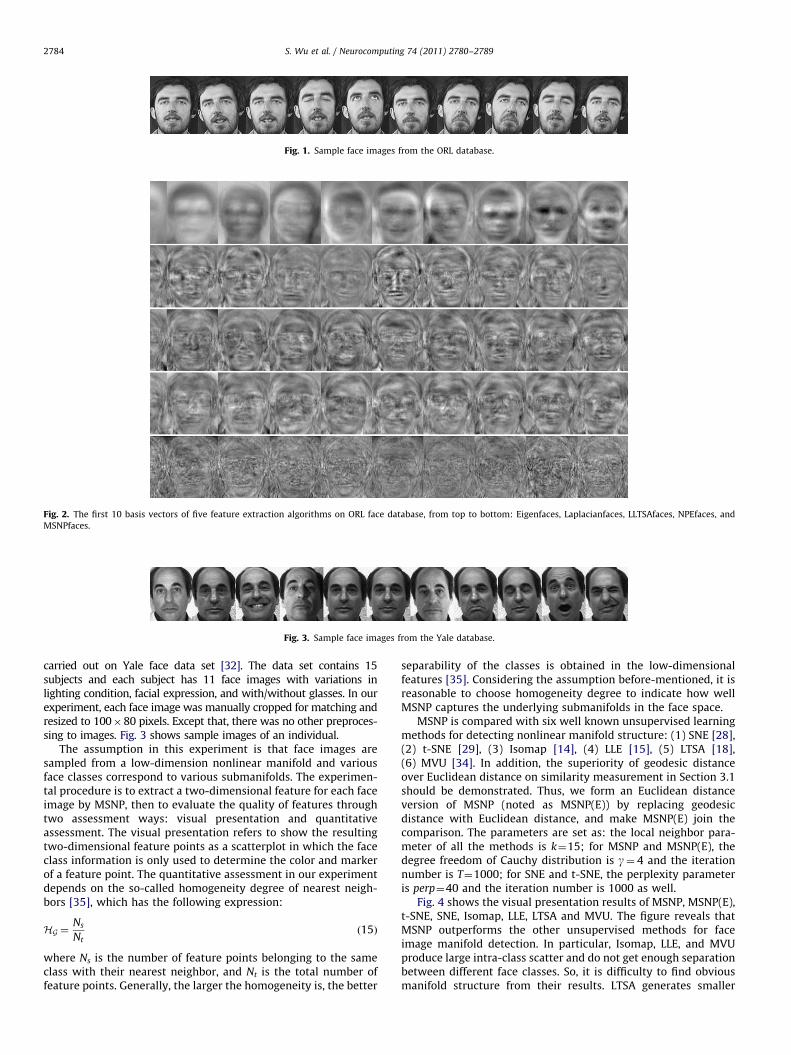
Fig. 1. Sample face images from the ORL database.
Fig. 2. The first 10 basis vectors of five feature extraction algorithms on ORL face database, from top to bottom: Eigenfaces, Laplacianfaces, LLTSAfaces, NPEfaces, and
MSNPfaces.
Fig. 3. Sample face images from the Yale database.
S. Wu et al. / Neurocomputing 74 (2011) 2780–27892784
carried out on Yale face data set [32]. The data set contains 15subjects and each subject has 11 face images with variations inlighting condition, facial expression, and with/without glasses. In ourexperiment, each face image was manually cropped for matching andresized to 100�80 pixels. Except that, there was no other preproces-sing to images. Fig. 3 shows sample images of an individual.
The assumption in this experiment is that face images aresampled from a low-dimension nonlinear manifold and variousface classes correspond to various submanifolds. The experimen-tal procedure is to extract a two-dimensional feature for each faceimage by MSNP, then to evaluate the quality of features throughtwo assessment ways: visual presentation and quantitativeassessment. The visual presentation refers to show the resultingtwo-dimensional feature points as a scatterplot in which the faceclass information is only used to determine the color and markerof a feature point. The quantitative assessment in our experimentdepends on the so-called homogeneity degree of nearest neigh-bors [35], which has the following expression:
HG ¼Ns
Ntð15Þ
where Ns is the number of feature points belonging to the sameclass with their nearest neighbor, and Nt is the total number offeature points. Generally, the larger the homogeneity is, the better
separability of the classes is obtained in the low-dimensionalfeatures [35]. Considering the assumption before-mentioned, it isreasonable to choose homogeneity degree to indicate how wellMSNP captures the underlying submanifolds in the face space.
MSNP is compared with six well known unsupervised learningmethods for detecting nonlinear manifold structure: (1) SNE [28],(2) t-SNE [29], (3) Isomap [14], (4) LLE [15], (5) LTSA [18],(6) MVU [34]. In addition, the superiority of geodesic distanceover Euclidean distance on similarity measurement in Section 3.1should be demonstrated. Thus, we form an Euclidean distanceversion of MSNP (noted as MSNP(E)) by replacing geodesicdistance with Euclidean distance, and make MSNP(E) join thecomparison. The parameters are set as: the local neighbor para-meter of all the methods is k¼15; for MSNP and MSNP(E), thedegree freedom of Cauchy distribution is g¼ 4 and the iterationnumber is T¼1000; for SNE and t-SNE, the perplexity parameteris perp¼40 and the iteration number is 1000 as well.
Fig. 4 shows the visual presentation results of MSNP, MSNP(E),t-SNE, SNE, Isomap, LLE, LTSA and MVU. The figure reveals thatMSNP outperforms the other unsupervised methods for faceimage manifold detection. In particular, Isomap, LLE, and MVUproduce large intra-class scatter and do not get enough separationbetween different face classes. So, it is difficulty to find obviousmanifold structure from their results. LTSA generates smaller
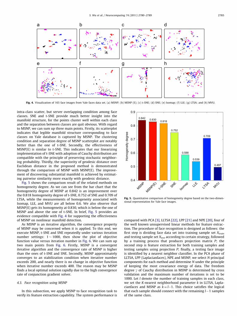
Fig. 4. Visualization of 165 face images from Yale faces data set. (a) MSNP; (b) MSNP (E); (c) t-SNE; (d) SNE; (e) Isomap; (f) LLE; (g) LTSA; and (h) MVU.
MSNP
MSNP(E)
t−SNE
SNE
Isomap LL
ELT
SAMVU
0.4
0.5
0.6
0.7
0.8
0.9
Hom
ogen
eity
deg
ree
0.830 0.818
0.752
0.588
0.539
0.709
0.497
0.842
Fig. 5. Quantitative comparison of homogeneity degree based on the two-dimen-
sional representation for Yale face images.
S. Wu et al. / Neurocomputing 74 (2011) 2780–2789 2785
intra-class scatter, but server overlapping condition among faceclasses. SNE and t-SNE provide much better insight into themanifold structure, for the points cluster well within each classand the separation between classes are quit obvious. With regardto MSNP, we can sum up three main points. Firstly, its scatterplotindicates that legible manifold structure corresponding to faceclasses on Yale database is captured by MSNP. The clusteringcondition and separation degree of MSNP scatterplot are notablybetter than the one of t-SNE. Secondly, the effectiveness ofMSNP(E) is similar to t-SNE. This indicates that our linearizingimplementation of t-SNE with adoption of Cauchy distribution arecompatible with the principle of preserving stochastic neighbor-ing probability. Thirdly, the superiority of geodesic distance overEuclidean distance in the proposed method is demonstratedthrough the comparison of MSNP with MSNP(E). The improve-ment of discovering substantial manifold is achieved by estimat-ing pairwise similarity more exactly with geodesic distance.
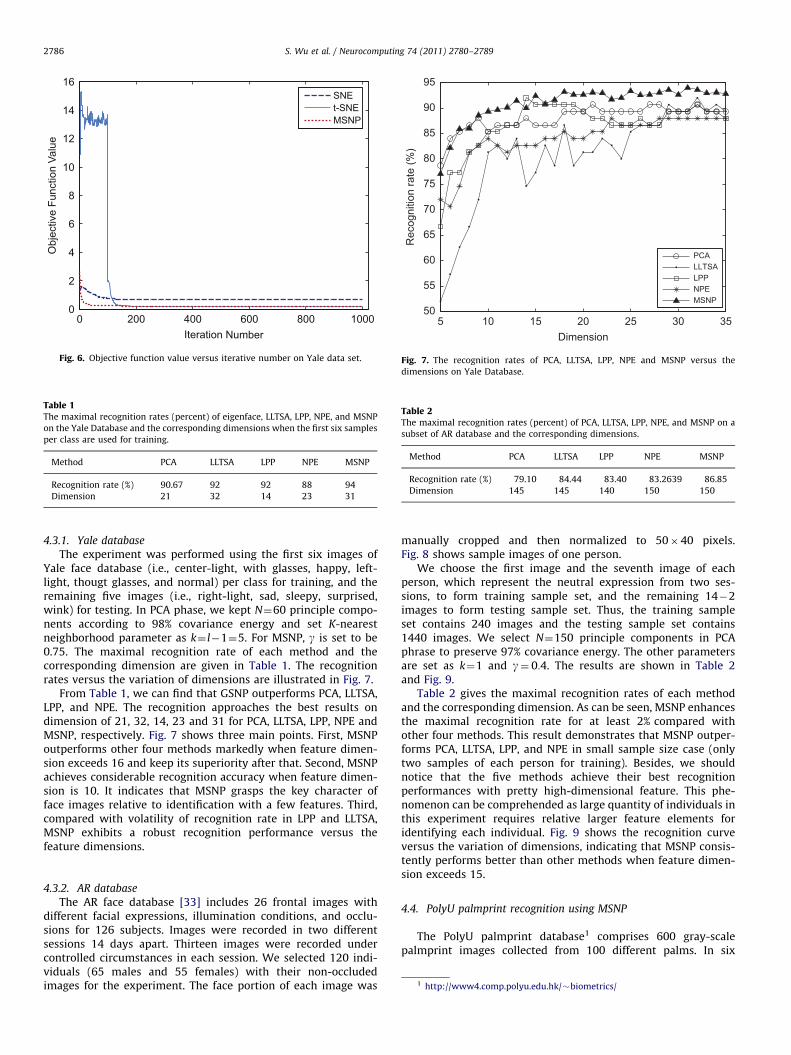
Fig. 5 shows the comparison result of the related methods onhomogeneity degree. As we can see from the bar chart that thehomogeneity degree of MSNP at 0.842 is an improvement overthe 0.818 homogeneity degree of t-SNE, 0.752 of SNE and 0.709 ofLTSA, while the measurements of homogeneity associated withIsomap, LLE, and MVU are all below 0.6. We also observe thatMSNP(E) gets its homogeneity at 0.830, which is below the one ofMSNP and above the one of t-SNE. In brief, Fig. 5 provides anevidence compatible with Fig. 4 for supporting the effectivenessof MSNP on nonlinear manifold detection.
As MSNP is an iterative algorithm, the convergence propertyof MSNP may be concerned when it is applied. To this end, weexecute MSNP, t-SNE and SNE repeatedly under various iterationnumber settings: 1� 1000, then show the plot of objectivefunction value versus iteration number in Fig. 6. We can sum uptwo main points from Fig. 6. Firstly, MSNP is a convergentiterative algorithm and the convergence rate of MSNP is higherthan the ones of t-SNE and SNE. Secondly, MSNP approximatelyconverges to an stabilization condition when iterative numberexceeds 200, and nearly there is no change in objective functionwhen iterative number exceeds 400. The reason may be MSNPfinds a local optimal solution rapidly due to the high convergencerate of conjunction gradient solver.
4.3. Face recognition using MSNP
In this subsection, we apply MSNP to face recognition task toverify its feature extraction capability. The system performance is
compared with PCA [3], LLTSA [22], LPP [21] and NPE [20], four ofthe well known unsupervised linear methods for feature extrac-tion. The procedure of face recognition is designed as follows: thefirst step is dividing face data set into training sample set Xtrain
and testing sample set Xtest according to certain strategy, followedby a training process that produces projection matrix P; thesecond step is feature extraction for both training samples andtesting samples using projection P; finally, a testing face imageis identified by a nearest neighbor classifier. In the PCA phase ofLLTSA, LPP (Laplacianfaces), NPE and MSNP, we select N principalcomponents for each method and determine N under the principleof keeping the most covariance energy of data. The freedomdegree g of Cauchy distribution in MSNP is determined by crossvalidation and the maximum number of iterations is set to be1000. Let l denote the number of training samples in each class,we set the K-nearest neighborhood parameter k in LLTSA, Lapla-cianfaces and MSNP as k¼ l�1. This choice satisfies the logicalthat each sample should connect with the remaining l�1 samplesof the same class.
16
14
12
10
8
6
4
2
00 200 400 600 800 1000
Iteration Number
Obj
ectiv
e Fu
nctio
n Va
lue
SNEt-SNEMSNP
Fig. 6. Objective function value versus iterative number on Yale data set.
Table 1The maximal recognition rates (percent) of eigenface, LLTSA, LPP, NPE, and MSNP
on the Yale Database and the corresponding dimensions when the first six samples
per class are used for training.
Method PCA LLTSA LPP NPE MSNP
Recognition rate (%) 90.67 92 92 88 94
Dimension 21 32 14 23 31
5 10 15 20 25 30 3550
55
60
65
70
75
80
85
90
95
Dimension
Rec
ogni
tion
rate
(%)
PCALLTSALPPNPEMSNP
Fig. 7. The recognition rates of PCA, LLTSA, LPP, NPE and MSNP versus the
dimensions on Yale Database.
Table 2The maximal recognition rates (percent) of PCA, LLTSA, LPP, NPE, and MSNP on a
subset of AR database and the corresponding dimensions.
Method PCA LLTSA LPP NPE MSNP
Recognition rate (%) 79.10 84.44 83.40 83.2639 86.85
Dimension 145 145 140 150 150
S. Wu et al. / Neurocomputing 74 (2011) 2780–27892786
4.3.1. Yale database
The experiment was performed using the first six images ofYale face database (i.e., center-light, with glasses, happy, left-light, thougt glasses, and normal) per class for training, and theremaining five images (i.e., right-light, sad, sleepy, surprised,wink) for testing. In PCA phase, we kept N¼60 principle compo-nents according to 98% covariance energy and set K-nearestneighborhood parameter as k¼ l�1¼5. For MSNP, g is set to be0.75. The maximal recognition rate of each method and thecorresponding dimension are given in Table 1. The recognitionrates versus the variation of dimensions are illustrated in Fig. 7.
From Table 1, we can find that GSNP outperforms PCA, LLTSA,LPP, and NPE. The recognition approaches the best results ondimension of 21, 32, 14, 23 and 31 for PCA, LLTSA, LPP, NPE andMSNP, respectively. Fig. 7 shows three main points. First, MSNPoutperforms other four methods markedly when feature dimen-sion exceeds 16 and keep its superiority after that. Second, MSNPachieves considerable recognition accuracy when feature dimen-sion is 10. It indicates that MSNP grasps the key character offace images relative to identification with a few features. Third,compared with volatility of recognition rate in LPP and LLTSA,MSNP exhibits a robust recognition performance versus thefeature dimensions.
1 http://www4.comp.polyu.edu.hk/�biometrics/
4.3.2. AR database
The AR face database [33] includes 26 frontal images withdifferent facial expressions, illumination conditions, and occlu-sions for 126 subjects. Images were recorded in two differentsessions 14 days apart. Thirteen images were recorded undercontrolled circumstances in each session. We selected 120 indi-viduals (65 males and 55 females) with their non-occludedimages for the experiment. The face portion of each image was
manually cropped and then normalized to 50�40 pixels.Fig. 8 shows sample images of one person.
We choose the first image and the seventh image of eachperson, which represent the neutral expression from two ses-sions, to form training sample set, and the remaining 14�2images to form testing sample set. Thus, the training sampleset contains 240 images and the testing sample set contains1440 images. We select N¼150 principle components in PCAphrase to preserve 97% covariance energy. The other parametersare set as k¼1 and g¼ 0:4. The results are shown in Table 2and Fig. 9.
Table 2 gives the maximal recognition rates of each methodand the corresponding dimension. As can be seen, MSNP enhancesthe maximal recognition rate for at least 2% compared withother four methods. This result demonstrates that MSNP outper-forms PCA, LLTSA, LPP, and NPE in small sample size case (onlytwo samples of each person for training). Besides, we shouldnotice that the five methods achieve their best recognitionperformances with pretty high-dimensional feature. This phe-nomenon can be comprehended as large quantity of individuals inthis experiment requires relative larger feature elements foridentifying each individual. Fig. 9 shows the recognition curveversus the variation of dimensions, indicating that MSNP consis-tently performs better than other methods when feature dimen-sion exceeds 15.
4.4. PolyU palmprint recognition using MSNP
The PolyU palmprint database1 comprises 600 gray-scalepalmprint images collected from 100 different palms. In six
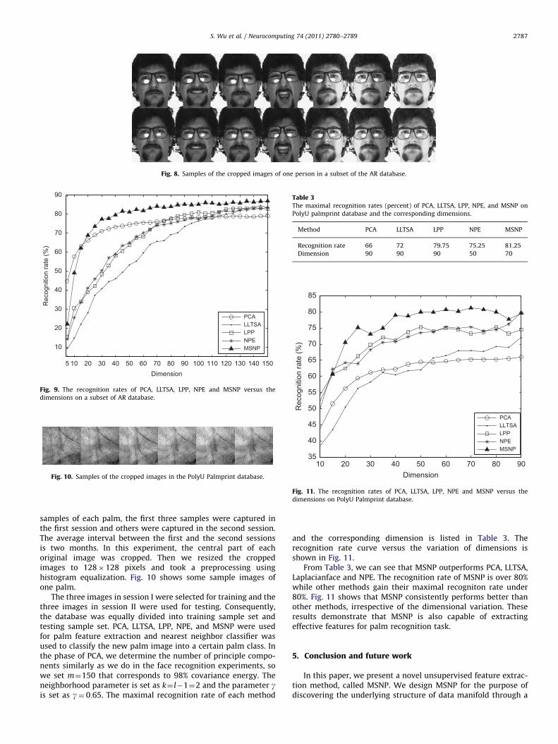
Fig. 8. Samples of the cropped images of one person in a subset of the AR database.
5 10 20 30 40 50 60 70 80 90 100 110 120 130 140 150
10
20
30
40
50
60
70
80
90
Dimension
Rec
ogni
tion
rate
(%)
PCALLTSALPPNPEMSNP
Fig. 9. The recognition rates of PCA, LLTSA, LPP, NPE and MSNP versus the
dimensions on a subset of AR database.
Fig. 10. Samples of the cropped images in the PolyU Palmprint database.
Table 3The maximal recognition rates (percent) of PCA, LLTSA, LPP, NPE, and MSNP on
PolyU palmprint database and the corresponding dimensions.
Method PCA LLTSA LPP NPE MSNP
Recognition rate 66 72 79.75 75.25 81.25
Dimension 90 90 90 50 70
10 20 30 40 50 60 70 80 9035
40
45
50
55
60
65
70
75
80
85
Dimension
Rec
ogni
tion
rate
(%)
PCALLTSALPPNPEMSNP
Fig. 11. The recognition rates of PCA, LLTSA, LPP, NPE and MSNP versus the
dimensions on PolyU Palmprint database.
S. Wu et al. / Neurocomputing 74 (2011) 2780–2789 2787
samples of each palm, the first three samples were captured inthe first session and others were captured in the second session.The average interval between the first and the second sessionsis two months. In this experiment, the central part of eachoriginal image was cropped. Then we resized the croppedimages to 128�128 pixels and took a preprocessing usinghistogram equalization. Fig. 10 shows some sample images ofone palm.
The three images in session I were selected for training and thethree images in session II were used for testing. Consequently,the database was equally divided into training sample set andtesting sample set. PCA, LLTSA, LPP, NPE, and MSNP were usedfor palm feature extraction and nearest neighbor classifier wasused to classify the new palm image into a certain palm class. Inthe phase of PCA, we determine the number of principle compo-nents similarly as we do in the face recognition experiments, sowe set m¼150 that corresponds to 98% covariance energy. Theneighborhood parameter is set as k¼ l�1¼2 and the parameter gis set as g¼ 0:65. The maximal recognition rate of each method
and the corresponding dimension is listed in Table 3. Therecognition rate curve versus the variation of dimensions isshown in Fig. 11.
From Table 3, we can see that MSNP outperforms PCA, LLTSA,Laplacianface and NPE. The recognition rate of MSNP is over 80%while other methods gain their maximal recogniton rate under80%. Fig. 11 shows that MSNP consistently performs better thanother methods, irrespective of the dimensional variation. Theseresults demonstrate that MSNP is also capable of extractingeffective features for palm recognition task.
5. Conclusion and future work
In this paper, we present a novel unsupervised feature extrac-tion method, called MSNP. We design MSNP for the purpose ofdiscovering the underlying structure of data manifold through a
S. Wu et al. / Neurocomputing 74 (2011) 2780–27892788
linear projection. MSNP models the structure of manifold bystochastic neighbor distribution in the high-dimensional observa-tion space. Using Cauchy distribution to model stochastic dis-tribution of features, MSNP recover the manifold structurethrough a linear projection by requiring the two distributions tobe similar. MSNP benefits from geodesic distance, stochasticneighbor distribution preserving strategy and linear projectionmanner to endow with nice properties, such as sensitivityto nonlinear manifold structure and convenience for featureextraction. The experimental results on ORL, Yale, AR, and PolyUdatabases demonstrate that MSNP can substantially enhancethe quality of data visualization compared with many competitivemanifold learning algorithms and improve the recognition accu-racy in biometrics recognition task. This verifies that the proposedMSNP is an effective feature extraction method.
In MSNP, we use geodesic distance such a global metric tomeasure the distance on manifold, but it is not the only way touncover manifold structure. The previous work [15,16,18] showsthat manifold can be unfolded in a local analysis manner. There-fore, one alternative is to implement stochastic neighbor projec-tion in local neighborhood. Another extension of our work is toconsider class label information in the recognition task. Since thesimilarity of labeled samples reflects not only the structuralrelationship but also the semantic relationship, we believe thatthe labeled samples are of great value for classification purpose.Accordingly, supervised extension or semi-supervised extensionof MSNP may result in more effective features for patternrecognition task. We are currently exploring these problems intheory and practice.
Acknowledgements
The authors would like to thank the anonymous reviewers fortheir critical and constructive comments and suggestions. Thisproject was partially supported by National Natural ScienceFoundation of China (Nos. 60632050, 60775015).
References
[1] D. Donoho, High-Dimensional Data Analysis: The Curses and Blessings ofDimensionality, AMS Math Challenges Lecture, 2000.
[2] R. Bellman, Adaptive Control Processes: A Guided Tour, Princeton UniversityPress, 1961.
[3] M. Turk, A. Pentland, Eigenfaces for recognition, Journal of Cognitive Neuroscience3 (1) (1991) 71–86.
[4] T. Cox, M. Cox, Multidimensional Scaling, Chapman and Hall, 1994.[5] P. Common, Independent component analysis—a new concept? Signal
Processing 36 (1994) 287–314.[6] P.N. Belhumeur, J.P. Hespanha, D.J. Kriegman, Eigenfaces vs fisherfaces:
recognition using class specific linear projection, IEEE Transaction on PatternAnalysis and Machine Intelligence 19 (7) (1991) 711–720.
[7] D. Tao, X. Li, X. Wu, S.J. Maybank, Geometric mean for subspace selection,IEEE Transactions on Pattern Analysis and Machine Intelligence 31 (2) (2009)260–274.
[8] W. Bian, D. Tao, Harmonic mean for subspace selection, in: 19th InternationalConference on Pattern Recognition, 2008, pp. 1C4.
[9] W. Bian, D. Tao, Max–Min distance analysis by using sequential SDPrelaxation for dimension reduction, IEEE Transactions on Pattern Analysisand Machine Intelligence (2010). doi:10.1109/TPAMI.2010.189.
[10] B. Scholkopf, A. Smola, K.R. Muller, Nonlinear component analysis asa kernel eigenvalue problem, Neural Computation 10 (5) (1998) 1299–1319.
[11] F.R. Bach, M.I. Jordan, Kernel independent component analysis, Journal ofMachine Learning Research 3 (2002) 1–48.
[12] S. Mika, G. Ratsch, B. Scholkopf, A. Smola, J. Weston, K.R. Muller, Invariantfeature extraction and classification in kernel spaces, Advances in NeuralInformation Processing Systems 12 (1999).
[13] J. Yang, A.F. Frangi, J.-Y. Yang, D. Zhang, J. Zhong, KPCA plus LDA: a completekernel fisher discriminant framework for feature extraction and recognition,IEEE Transactions on Pattern Analysis and Machine Intelligence 27 (2) (2005)230–244.
[14] J. Tenenbaum, V. de Silva, J.C. Langford, A global geometric framework fornonlinear dimensionality reduction, Science 290 (2000) 2319–2323.
[15] S.T. Roweis, K.S. Lawrance, Nonlinear dimensionality reduction by locallylinear embedding, Science 290 (2000) 2323–2326.
[16] M. Belkin, P. Niyogi, Laplacian eigenmaps for dimensionality reduction anddata representation, Neural Computation 15 (6) (2003) 1373–1396.
[17] D.L. Donoho, C. Grimes, Hessian eigenmaps: new locally linear embeddingtechniques for high-dimensional data, in: Proceedings of National Academyof Sciences USA, vol. 100(10), 2003, pp. 5591–5596.
[18] Z. Zhang, H. Zha, Principal manifolds and nonlinear dimension reduction vialocal tangent space alignment, SIAM Journal on Scientific Computing 26 (1)(2004) 313–338.
[19] Y. Bengio, J. Paiement, P. Vincent, O. Dellallaeu, L. Roux, M. Quimet, Out-ofSample Extensions for LLE, Isomap, MDS, Eigenmaps, and Spectral Clustering,Advances in Neural Information Processing System, 2004.
[20] X. He, D. Cai, S. Yan, H.-J. Zhang, Neighborhood preserving embedding,in: Proceedings of IEEE International Conference on Computer Vision,IEEE Computer Society, Washington, DC, USA, 2005, pp. 1208–1213.
[21] X. He, S. Yan, Y. Hu, P. Niyogi, H.-J. Zhang, Face recognition using Laplacian-faces, IEEE Transactions on Pattern Analysis and Machine Intelligence 27 (3)(2005) 328–340.
[22] T. Zhang, J. Yang, D. Zhao, X. Ge, Linear local tangent space alignmentand application to face recognition, Neurocomputing 70 (7–9) (2007)1547–1553.
[23] T. Zhang, D. Tao, J. Yang, Discriminative locality alignment, in: Proceedings ofthe 10th European Conference on Computer Vision, Marseille, France, 2008,Part I, pp. 725–738.
[24] S. Yan, D. Xu, B. Zhang, H. Zhang, Q. Yang, S. Lin, Graph embeddingand extensions: a general framework for dimensionality reduction, IEEETransactions on Pattern Analysis and Machine Intelligence 29 (1) (2007)40–51.
[25] T. Zhang, D. Tao, X. Li, J. Yang, Patch alignment for dimensionality reduction,IEEE Transactions on Knowledge and Data Engineering 21 (9) (2009)1299–1313.
[26] T. Zhou, D. Tao, X. Wu, Manifold elastic net: a unified framework for sparsedimension reduction, Data Mining and Knowledge Discovery (2010) 1–32.
[27] W. Liu, D. Tao, J. Liu, Transductive component analysis, in: The 8th IEEEInternational Conference on the Data Mining, 2008.
[28] G. Hinton, S.T. Roweis, Stochastic neighbor embedding, Advances in NeuralInformation Processing Systems (2002).
[29] L. Maaten, G. Hinton, Visualizing data using t-SNE, Journal of MachineLearning Research 9 (2008) 2579–2605.
[30] S. Kullback, Information Theory and Statistics, Dover, New York, 1968.[31] F. Samaria, A. Harter, Parameterisation of a stochastic model for human face
identification, in: Proceedings of the Second IEEE Workshop on Applicationsof Computer Vision, Sarasota, USA, 1994.
[32] YaleUniv. FaceDatabase, /http://cvc.yale.edu/projects/yalefaces/�yalefaces.htmlS, 2002.
[33] A.M. Martinez, R. Benavente, The AR face database, CVC Technical ReportNo. 24, June 1998.
[34] K.Q. Weinberger, L.K. Saul, Unsupervised learning of image manifolds bysemidefinite programming, in: Proceedings of the 2004 IEEE ComputerSociety Conference on Computer Vision and Pattern Recognition (CVPR2004),vol. 2, pp. 988–995.
[35] Z. Yang, I. King, Z. Xu, E.I Oja, Heavy-tailed symmetric stochastic neighborembedding, Advances in Neural Information Processing Systems, 2009.
Songsong Wu obtained his Bachelor’s degree in Infor-mation and Computing Sciences from Nanjing Univer-sity of Posts and Telecommunications in 2004, and theMaster’s degree in Measuring and Testing Technolo-gies and Instruments from Nanjing Forestry Universityin 2007. Currently, he is a PhD candidate in the schoolof Computer Science and Technology on the subject ofPattern Recognition and Intelligence Systems, NanjingUniversity of Science and Technology. His currentresearch interests include manifold learning, patternrecognition and computer vision.
Mingming Sun obtained his Bachelor of Science inMathematics at the Xinjiang University in 2002 and hisPhD at the Nanjing University of Science and Technology(NUST) in the Department of Computer Science on thesubject of Pattern Recognition and Intelligence Systemsin 2007. He is now a lecture at the School of ComputerScience and Technology at the Nanjing University ofScience and Technology. His current research interestsinclude pattern recognition, machine learning and imageprocessing.

S. Wu et al. / Neurocomputing 74 (2011) 2780–2789 2789
Jingyu Yang received the BS Degree in ComputerScience from Nanjing University of Science and Tech-nology (NUST), Nanjing, China. From 1982 to 1984 hewas a visiting scientist at the Coordinated ScienceLaboratory, University of Illinois at Urbana—
Champaign. From 1993 to 1994 he was a visitingprofessor at the Department of Computer Science,Missuria University. And in 1998, he acted as a visitingprofessor at Concordia University in Canada. He iscurrently a professor and Chairman in the departmentof Computer Science at NUST. He is the author of over300 scientific papers in computer vision, pattern
recognition, and artificial intelligence. He has wonmore than 20 provincial awards and national awards. His current researchinterests are in the areas of pattern recognition, robot vision, image processing,data fusion, and artificial intelligence.