Uncertain Nearest Neighbor Classification

Uncertain Nearest Neighbor Classification

Fabrizio Angiulli, Fabio Fassetti

DEIS, Universita della Calabria

Via P. Bucci, 41C

87036 Rende (CS), Italy

{f.angiulli,f.fassetti}@deis.unical.it

This work deals with the problem of classifying uncertain data. With this aim the UncertainNearest Neighbor (UNN) rule is here introduced, which represents the generalization of the deter-ministic nearest neighbor rule to the case in which uncertain objects are available. The UNN rule

relies on the concept of nearest neighbor class, rather than on that of nearest neighbor object.The nearest neighbor class of a test object is the class that maximizes the probability of providingits nearest neighbor. It is provided evidence that the former concept is much more powerful thanthe latter one in the presence of uncertainty, in that it correctly models the right semantics of the

nearest neighbor decision rule when applied to the uncertain scenario. An effective and efficientalgorithm to perform uncertain nearest neighbor classification of a generic (un)certain test objectis designed, based on properties that greatly reduce the temporal cost associated with nearest

neighbor class probability computation. Experimental results are presented, showing that theUNN rule is effective and efficient in classifying uncertain data.

Categories and Subject Descriptors: H.2.8 [Database Applications]: Data mining

General Terms: Algorithms

Additional Key Words and Phrases: Classification, uncertain data, nearest neighbor rule, proba-

bility density functions, nearest neighbor

1. INTRODUCTION

Classification is one of the basic tasks in data mining and machine learning [Tanet al. 2005; Mitchell 1997]. Given a set of examples or training set, that is a set ofobjects xi with associated class labels l(xi), the goal of classification is to exploit thetraining set in order to build a classifier for prediction purposes, that is a functionmapping unseen objects to one of the predefined class labels. Traditional classifica-tion techniques deal with feature vectors having deterministic values. Thus, datauncertainty is usually ignored in the learning problem formulation. However, itmust be noted that uncertainty arises in real data in many ways, since the datamay contain errors or may be only partially complete [Lindley 2006].

The uncertainty may result from the limitations of the equipment, indeed physicaldevices are often imprecise due to measurement errors. Another source of uncer-tainty are repeated measurements, e.g. sea surface temperature could be recordedmultiple times during a day. Also, in some applications data values are continuouslychanging, as positions of mobile devices or observations associated with natural phe-nomena, and these quantities can be approximated by using an uncertain model.

Simply disregarding uncertainty may led to less accurate conclusions or even in-exact ones. This has created the need for uncertain data management techniques[Aggarwal and Yu 2009], that are techniques managing data records typically repre-sented by probability distributions ([Bi and Zhang 2004; Achtert et al. 2005; Kriegel

Journal Name, Vol. V, No. N, 8 2011, Pages 1–0??.

2 · F. Angiulli and F. Fassetti

and Pfeifle 2005; Ngai et al. 2006; Aggarwal and Yu 2008] to cite a few).This work deals with the problem of classifying uncertain data. Specifically, here

it is assumed that an uncertain object is an object whose actual value is modeledby a multivariate probability density function. This notion of uncertain object hasbeen extensively adopted in the literature and corresponds to the attribute leveluncertainty model viewpoint [Green and Tannen 2006].

Classification methods often rely on the use of distances or similarity metrics inorder to implement their decision rule. It must be noted that different concepts ofsimilarity between uncertain objects have been proposed in the literature, amongthem the distance between means, the expected distance, and probabilistic thresholddistance [ Lukaszyk 2004; Cheng et al. 2004; Tao et al. 2007; Agarwal et al. 2009;Angiulli and Fassetti 2011]. Thus, a seemingly suitable strategy to classify uncertaindata is to make use of ad-hoc similarity metrics in order to apply to such kind ofdata classification techniques already designed for the deterministic setting. Wecall this strategy the naive approach.

However, in this work we provide evidence that the above depicted approach istoo weak, since there is no guarantee on the quality of the class returned by the naiveapproach. As a matter of fact, the naive approach may return the wrong class evenif the probability for the object to belong to that class approaches to zero. Hence, asa major contribution, we provide a novel classification rule which directly builds oncertain similarity metrics, rather than directly exploiting ad-hoc uncertain metrics,but anyway implements a decision rule which is suitable for classifying uncertaindata.

Specifically, we conduct our investigation in the context of the Nearest Neighborrule [Cover and Hart 1967; Devroye et al. 1996], since it allows to directly exploitsimilarity metrics to the classification task. The nearest neighbor rule assigns to anunclassified object the label of the nearest of a set of previously classified objects,and can be generalized to the case in which the k nearest neighbors are taken intoaccount [Fukunaga and Hostetler 1975]. Despite its seemingly simplicity, it is veryeffective in classifying data [Stone 1977; Devroye 1981; Wu et al. 2008].

As already pointed out, as the main contribution of this work a novel classificationrule for the uncertain setting is introduced, called the Uncertain Nearest Neighbor(UNN, for short). The uncertain nearest neighbor rule relies on the concept ofnearest neighbor class, rather than on that of nearest neighbor object, the latterconcept being the one the naive approach implemented through the use of thenearest neighbor rule relies on. Consider the binary classification problem withclass labels c and c′: c (c′, resp.) is the nearest neighbor class of the test object q ifthe probability that the nearest neighbor of q comes from class c (c′, resp.) is greaterthan the probability that it comes from the other class. Such a probability takessimultaneously into account the distribution functions of all the distances separatingq by the training set objects.

Summarizing, the contributions of the work are those reported in the following:

—the concept of nearest neighbor class is introduced and it is shown to be muchmore powerful than the concept of nearest neighbor in presence of uncertainty;

—based on the concept of nearest neighbor class, the Uncertain Nearest Neighborclassification rule (UNN) is defined. Specifically, it is precisely shown that UNN

Journal Name, Vol. V, No. N, 8 2011.

Uncertain Nearest Neighbor Classification · 3

represents the generalization of the certain nearest neighbor rule to the case inwhich uncertain objects, represented by means of arbitrary probability densityfunctions, are taken into account.

—it is show than the UNN rule represents a viable way to compute the mostprobable class of the test object, since properties to efficiently compute the nearestneighbor class probability are presented;

—based on these properties, an effective algorithm to perform uncertain nearestneighbor classification of a generic (un)certain test object is designed.

—the experimental campaign confirms the superiority of the UNN rule with respectto classical classification techniques in presence of uncertainty and with respectto density based classification methods specifically designed for uncertain data.Moreover, the meaningfulness of UNN classification is illustrated through a real-life prediction scenario involving wireless mobile devices.

The rest of the paper is organized as follows. Section 2 introduces the uncertainnearest neighbor classification rule. In Section 3 the properties of the uncertainnearest neighbor rule are stated and an efficient algorithm solving the task at handis described. Section 4 discusses relationship with related works. Section 5 reportsexperimental results. Finally, Section 6 draws the conclusions.

2. UNCERTAIN NEAREST NEIGHBOR CLASSIFICATION

In this section the Uncertain Nearest Neighbor rule is introduced. The section isorganized as follows. First, uncertain objects are formalized (Section 2.1), then thebehavior of the nearest neighbor rule in presence of uncertain objects is analyzed(Section 2.2) and, finally, the uncertain nearest neighbor rule is introduced (Section2.3).

2.1 Uncertain objects

Let (D, d) denote a metric space, where D is a set, also called domain, and d is adistance metric on D (e.g., D is the d-dimensional real space R

d equipped with theEuclidean distance d).

A certain object v is an element of D. An uncertain object x is a random variablehaving domain D with associated probability density function fx, where fx(v)denotes the probability for x to assume value v. A certain object v can be regardedas an uncertain one whose associated pdf fv is δv(t), where δv(t) = δ(0), for t = v,and δv(t) = 0, otherwise, with δ(t) denoting the Dirac delta function.

Given two uncertain objects x and y, d(x, y) denotes the continuous randomvariable representing the distance between x and y.

Given a set S = {x1, . . . , xn} of uncertain objects, an outcome IS of S is a set{v1, . . . , vn} of certain objects such that fxi(vi) > 0 (1 ≤ i ≤ n). The probabilityPr(IS) of the outcome IS is

Pr(IS) =n∏

i=1

fxi(vi).

Given an object v of D, BR(v) denotes the set of values {w ∈ D | d(w, v) ≤ R},namely the hyperball having center v and radius R.



2.2 The nearest neighbor rule in presence of uncertain objects

In this section the classic Nearest Neighbor rule is recalled and, furthermore, it isshown that its direct application to the classification of uncertain data is misleading.Hence, the concept of nearest neighbor class is introduced, which captures the rightsemantics of the nearest neighbor rule when applied to objects modeled by meansof arbitrary probability density functions. The nearest neighbor class forms thebasis upon the novel Uncertain Nearest Neighbor classification rule is built on.

Nearest Neighbor classification rule. Let v be an (un)certain object. The class labelassociated with v is denoted by l(v).

Given a set of certain objects T ′ and a certain object v, the nearest neighbornnT ′(v) of v in T ′ is the object u of T ′ such that for any other object w of T ′ itholds that d(v, u) ≤ d(v, w) (ties are arbitrarily broken).

The k-th nearest neighbor nnkT ′(v) of v in T ′ is the object u of T ′ such that there

exist exactly k − 1 other objects w of T ′ for which it holds that d(v, w) ≤ d(v, u)(also in this case, ties are arbitrarily broken).

In the following, q denotes a generic certain test object.Given a labelled set of certain objects T ′, the (certain) Nearest Neighbor rule

NNT ′(q) [Cover and Hart 1967] assigns to the certain test object q the label of itsnearest neighbor in T ′, that is

NNT ′(q) = l(nnT ′(q)).

The nearest neighbor rule can be generalized to take into account the k nearestneighbors of the test object q: The (certain) k Nearest Neighbor rule NNk

T ′(q)[Fukunaga and Hostetler 1975; Devroye et al. 1996] (or, simply, NNT ′(q), wheneverthe value of k is clear from the context) assigns the object q to the class with themost members present among its k nearest neighbors in the training set T ′.

Applying the Nearest Neighbor rule to uncertain data. In order to be applied, thenearest neighbor rule merely requires the availability of a distance function. In thecontext of uncertain data, different similarity measures have been defined, amongthem the distance between means, representing the distance between the expectedvalues of the two uncertain objects, and the expected distance [ Lukaszyk 2004],representing the mean of distances between all the outcomes of the two uncertainobjects.

Thus, a seemingly faithful strategy to correctly classify uncertain data is to di-rectly exploit the nearest neighbor rule in order to determine the training set objecty most similar to the test object q and then to return the class label l(y) of y, alsoreferred to as naive approach in the following. However, it is pointed out here thatthere is no guarantee on the quality of the class returned by the naive approach.Specifically, this approach is defective since it can return the wrong class even if itsprobability approaches to zero. Next an illustrative example it is discussed.

Example 2.1. Consider Figure 1(a), reporting four 2-dimensional uncertaintraining set objects whose support is delimited by circles/ellipsis. The certain testobject q is located in (0, 0). The blue class consists of one normally distributeduncertain object (centered in (0, 4)), while the red class consists of three uncertainobjects, all having bimodal distribution. To ease computations, probability values



−8 −6 −4 −2 0 2 4 6 8−8

−6

−4

−2

0

2

4

6

8

q

1.0

0.5

0.5

0.5

0.5

0.5 0.5

(a)

−8 −6 −4 −2 0 2 4 6 8−8

−6

−4

−2

0

2

4

6

8

q

1.0

0.5

0.5

0.5

0.5

0.5 0.5

1.0

1.0

Rqmax

Rqmin

x4

x5

x6

x1

x2

x3

(b)

Fig. 1. Example of comparison between the nearest neighbor object and class.

are concentrated in the points identified by crosses.It can be noticed that the object closest to q according to the naive approach is

that belonging to the blue class. However, it appears that the probability that a redobject is closer to q than a blue one is 1 − 0.53 = 0.875. Thus, in the 87.5% ofthe outcomes of this training set the nearest neighbor of q comes from the red class,but the naive approach outputs the opposite one! Note that the probability of theblue class can be made arbitrarily small by adding other red objects similar to thosealready present. With n red objects, the probability Pr(D(q, red) < D(p, blue)) is1− 0.5n, that rapidly approaches to 1.

The poor performance of the nearest neighbor rule can be explained by noticingthat it takes into account the occurrence probabilities of the training set objectsone at a time, a meaningless strategy in presence of many objects whose outcome isuncertain. In the following the concept of most probable class is introduced, whichtakes simultaneously into account the distribution functions of all the distancesseparating the test object by the training set objects.

Most probable class. Let T = {x1, . . . , xn} denote a labelled training set of uncertainobjects. The probability Pr(NNT (q) = c) that the object q will be assigned to classc by means of the nearest neighbor rule can be computed as:

Pr(NNT (q) = c) =

∫

Dn

Pr(IT ) · Ic(NNIT (q)) dIT , (1)

where the function Ic(·) outputs 1 if its argument equals c, and 0 otherwise. Infor-mally speaking, the probability that the nearest neighbor class of q in T is c, is thesummation of the occurrence probabilities of all the outcomes IT of the training setT for which the nearest neighbor object of q in IT has class c.

Thus, when uncertain objects are taken into account the nearest neighbor decisionrule should output the most probable class c∗ of q, that is the class c∗ such that

c∗ = arg maxcPr(NNT (q) = c). (2)



For u an uncertain test object, Equation (1) becomes:

Pr(NNT (u) = c) =

∫

Dn+1

fu(q) · Pr(IT ) · Ic(NNIT (q)) dq dIT , (3)

that is Equation (1) extended by taking into account also the occurrence probabilityof the test object q.

It is clear from Equations (1) and (3), that in order to determine the most proba-ble class of q it is needed to compute a multi-dimensional integral (with integrationdomain D

n or Dn+1), involving simultaneously all the possible outcomes of the testobject and of the training set objects.

In the following section, the uncertain nearest neighbor rule is introduced, thatprovides an effective method for computing the most probable class of a test objectaccording to the nearest neighbor decision rule.

2.3 The uncertain nearest neighbor rule

In this section the Uncertain Nearest Neighbor classification rule (UNN) is intro-duced. First, the concept of distance between an object and a class is defined,which is conducive to the definition of nearest neighbor class forming the basis ofthe uncertain nearest neighbor rule. Definitions, firstly introduced for k = 1, forthe binary classification task, and for q a certain test object, are readily generalizedto the case k ≥ 1, the multiclass setting, and q a possibly uncertain test object,respectively. To complete the contribution, it is formally shown that the UNN ruleoutputs the most probable class of the test object.

Nearest neighbor class and UNN rule. Let c be a class label and q a certain object.The distance between (object) q and (class) c, denoted by D(q, c), is the randomvariable whose outcome is the distance between q and its k-th training set nearestneighbor having class label c.

Next it is shown how the cumulative density function of D(q, c) can be computed.Let us start by considering the case k = 1.

Let Tc denote the subset of the training set composed of the objects having classlabel c, that is

Tc = {xi ∈ T : l(xi) = c}.

Let pi(R) = Pr(d(q, xi) ≤ R) denote the cumulative density function representingthe relative likelihood for the distance between q and training set object xi toassume value less than or equal to R, that is

Pr(d(q, xi) ≤ R) =

∫

BR(q)

fxi(v) dv, (4)

where BR(q) denotes the hyper-ball having radius R and centered in q.Then, the cumulative density function associated with D(q, c) can be obtained

as follows:

Pr(D(q, c) ≤ R) = 1−

(

∏

xi∈Tc

(1− pi(R))

)

, (5)

that is one minus the probability that no object of the class c lies within distanceR from q.



−3 −2 −1 0 1 2 30

0.5

1

1.5

2

2.5

3

3.5

(a)

0 0.5 1 1.5 2 2.5 30

0.1

0.2

0.3

0.4

0.5

0.6

0.7

0.8

0.9

1

R

Pro

babi

lity

Pr(D(q,c)<R)Pr(D(q,c’)<R)Pr(D(q,c)<D(q,c’))

(b)

Fig. 2. Example of distances between an object and two classes.

Example 2.2. Figure 2(a) shows a one-dimensional example training set com-posed of four uncertain objects. The abscissa reports the domain values, while theordinata reports the pdf values associated with the (normally distributed) uncertainobjects. From left to right, means µi and standard deviations σi are µ1 = −2 andσ1 = 0.125, µ2 = −2 and σ2 = 0.55, µ3 = 1.9 and σ3 = 0.125, and µ4 = 2.5and σ4 = 0.15. The two objects on the left belong to class c (blue), while the twoother objects belong to class c′ (red). Consider the certain test object q = 0. Thedashed blue (dotted red, resp.) curve represents the probability Pr(D(q, c) ≤ R)(Pr(D(q, c′) ≤ R), resp.), where R = |v| and v denotes the abscissa value.

Consider the binary classification problem, in which there are exactly two classes,with labels c and c′, respectively. The nearest neighbor class of q is c if

Pr(D(q, c) < D(q, c′)) ≥ 0.5 (6)

holds, and c′ otherwise. In the following, the probability Pr(D(q, c) < D(q, c′)) isalso referred to as nearest neighbor probability of class c (w.r.t. class c′).

According to Equation (6), class c is the nearest neighbor class of q if the probabil-ity that the nearest neighbor of q comes from class c is greater than the probabilitythat it comes from class c′.

In particular, the above probability can be computed by means of the followingone-dimensional integral:

Pr(D(q, c) < D(q, c′)) =

∫ +∞

0

Pr(D(q, c) = R) · Pr(D(q, c′) > R) dR. (7)

The Uncertain Nearest Neighbor Rule (UNN, for short) assigns to the test objectq the label of its nearest neighbor class.

Example 2.3. Figure 2(b) reports the probabilities Pr(D(q, c) ≤ R) (dashedcurve) and Pr(D(q, c′) ≤ R) (dotted curve) associated with objects in Figure 2(a),together with the value of the integral in Equation (7) computed in the interval [0, R](solid curve; for large values of R this curve represents the probability Pr(D(q, c) <D(q, c′))). In this case the probability Pr(D(q, c) < D(q, c′)) is equal to 0.569.



Thus, the nearest neighbor class of q is c (the blue class, composed of the twoobjects on the left).

Other the returning the nearest neighbor class c of q, the UNN rule is also able tooutput the probability p = Pr(D(q, c) < D(q, c′)) (p′ = 1 − p, resp.) that objectq belongs to class c (c′, resp.), and it is worth to notice that the naive approachcannot provide such a value.

Moreover, it is also important to point out that enabling the nearest neighborrule to handle uncertain data makes it more robust to noise with respect to thecase in which the uncertainty associated with data is ignored.

Example 2.4. As an example, consider the uncertain objects in Figure 1(a) andassume to disregard uncertainty by replacing them with their means. In such a case,the certain nearest neighbor rule will erroneously output the blue label, since thenoisy blue object (centered in (4, 0)) is closer to q than the red ones. Contrarily, theuncertain nearest neighbor correctly classifies q, since it simultaneously considersthe whole class distribution.

Informally speaking, it can be said the distribution of the closest class tends toovershadow noisy objects.

Generalizing the UNN rule. The Uncertain Nearest Neighbor rule can be readilygeneralized in order (a) to take into account arbitrary values of k, (b) to considerpossibly uncertain test objects and (c) to deal with the multiclass problem, asaccounted for in the following.

(a) The first point can be achieved by properly redefining the probability Pr(D(q, c) ≤R). For k ≥ 1, the probability Pr(D(q, c) ≤ R) can be expressed as follows:

1−

∑

S⊆Tc:|S|<k

(

∏

xi∈S

pi(R)

)

·

∏

xi∈(Tc\S)

(1− pi(R))

, (8)

that is one minus the probability of having less than k objects of class c lying withindistance R from q.

In particular, for k = 1, the summation involves only the empty set S = ∅ (whichis the unique subset of Tc having size smaller than one), and the expression reducesto 1− (

∏

xi∈Tc(1−pi(R))), that is the expression already reported in Equation (5).

(b) Assume now to have an uncertain test object u. In this case, it holds that

Pr(D(u, c) < D(u, c′)) =

∫

D

fu(q) · Pr(D(q, c) < D(q, c′)) dq =

=

∫

D

∫ +∞

0

fu(q) · Pr(D(q, c) = R) · Pr(D(q, c′) > R) dR dq,

(9)and the nearest neighbor class of q is defined as that class c such that Pr(D(u, c) <D(u, c′)) ≥ 0.5.

(c) Till now only the binary classification problem has been taken into account.In order to deal with the multiclass classification problem, the one-against-all -like[Rifkin and Klautau 2004] approach is adopted. Assume there are m classes, with



labels c1, c2, . . . , cm. For each class cj , let cj denote a novel class representing theunion of all classes except for cj . Then object xi belongs to class cj (and, hence,l(xi) = cj) if l(xi) 6= cj (1 ≤ j ≤ m). The (uncertain) nearest neighbor class of the(un)certain test object q is

arg maxcj

Pr (D(q, cj) < D(q, cj)) , (10)

that is the class that maximizes the probability to provide the k-nearest neighborsof the test object.

Equivalence with the most probable class. One of the main properties of the UNNrule is now stated. Indeed, the following theorem formally proves that the uncertainnearest neighbor rule captures the right semantics of the nearest neighbor rule whenuncertain data is taken into account.

Theorem 2.5. The Uncertain Nearest Neighbor rule outputs the most probableclass (see Equation (2)) of the test object.

In order to prove the above statement, first it is introduced the nearest distancedecision rule and then it is shown that it relates the certain and the uncertainnearest neighbor rules.

Let T ′ be a certain training set, with objects coming from two classes with labelsc and c′, respectively, and let k be a positive integer. Then, the nearest distanceNDk

T ′(q) is the following decision rule: output class c, if

d(q, nnkT ′

c(q)) < d(q, nnk

T ′

c′(q)), (11)

and output class c′, otherwise.

Proposition 2.6. Consider the binary classification problem, and let k be anodd positive integer. Then, it holds that

NNkT ′(q) = ND

⌈ k2⌉

T ′ (q).

Proof. Assume that NNkT ′(q) outputs class c. Then, among the k nearest neigh-

bors of q in T ′ there are at least k′ = ⌈k2 ⌉ objects coming from class c, since themajority of the k nearest neighbors have class label c, and less than k′ objectscoming from class c′. Thus, it holds that

d(q, nn⌈ k

2⌉

T ′

c(q)) ≤ d(q, nnk

T ′(q)) < d(q, nn⌈ k

2⌉

T ′

c′(q)),

that is the distance separating q from its k′-th nearest neighbor in class c′ (beinggreater than d(q, nnk

T ′(q))) is greater than the distance separating q from its k′-th

nearest neighbor in class c (being not greater than d(q, nnkT ′(q))), and NDk′

T ′(q)outputs class c as well.

Vice versa, assume that NDk′

T ′(q) outputs class c. Then, the distance separatingq from its k′-th nearest neighbor in class c is stricly smaller than the distanceseparating q from its k′-th nearest neighbor in class c′. Thus, being 2k′ = k + 1,it is the case that among the k nearest neighbors of q in T ′ there are at least k′

objects coming from class c and at most k′−1 objects coming from class c′. Hence,NNk

T ′(q) outputs class c as well.



According to the above property, it is the case that NN1T ′(q) = ND1

T ′(q), NN3T ′(q) =

ND2T ′(q), NN5

T ′(q) = ND3T ′(q), NN7

T ′(q) = ND4T ′(q), and so on.

Now, the proof of Theorem 2.5 can be given.

Proof of Theorem 2.5. The proof follows from Proposition 2.6 and Equa-tions (6) and (11), by noticing that D(q, c) is the random variable representing thedistance between the certain test object q and its k-th nearest neighbor in the classc of the uncertain dataset.

3. CLASSIFYING A TEST OBJECT

This section presents then UNN classification algorithm. First, some preliminarydefinitions are provided (Section 3.1), then properties of the nearest neighbor classprobability are stated (Section 3.2) and it is shown how this probability can becomputed (Section 3.3) and, finally, the UNN classification algorithm is described(Section 3.4). The last Section 3.5, discusses how some steps of the UNN algorithmcan be accelerated in practice.

3.1 Preliminaries

Without loss of generality it is assumed that each uncertain object x is associatedwith a finite region SUP(x), containing the support of x, namely the region suchthat Pr(x 6∈ SUP(x)) = 0 holds. If the support of x is infinite, then SUP(x) is suchthat Pr(x 6∈ SUP(x)) ≤ α, for a fixed small value α, and the probability for x toexist outside SUP(x) is considered negligible.

It must be noticed that these assumptions are not restrictive, since the errorǫ = α2 involved in the calculation of the probability Pr(d(x, y) ≤ R), with x andy two uncertain objects, can be made arbitrarily small by properly selecting theregions SUP(x) and SUP(y) and, hence, the value α.

For example, assume that the data set objects x ∈ Rd are normally distributed

with mean µj and standard deviation σj along each dimension j (1 ≤ j ≤ d). If theregion SUP(x) is defined as [µj − 4σj , µj + 4σj ]

d then the probability α = Pr(x 6∈SUP(x)) is α = (2 · Φ(−4))d ≈ 0.00006d and the maximum error is ǫ = α2 ≈(4 · 10−9)d.

The region SUP(x) can be defined as an hyperball or an hypercube. In the formercase, SUP(x) is identified by means of its center c(x) and its radius r(x), wherec(x) is a certain object and r(x) is a positive real number.

The minimum distance mindist(x, y) between x and y is defined as

min{d(v, w) : v ∈ SUP(x) ∧ w ∈ SUP(y)} = max{0, d(c(x), c(y))− r(x)− r(y)},

while the maximum distance maxdist(x, y) between x and y is defined as

max{d(v, w) : v ∈ SUP(x) ∧ w ∈ SUP(y)} = d(c(x), c(y)) + r(x) + r(y).

Given a set of objects S, let innerS(q,R) denote the set {x ∈ S : maxdist(q, x) ≤R}, that is the subset of S composed of all the objects x whose maximum distancefrom q is not greater than R.

Let Rqc denote the positive real number

Rqc = min{R ≥ 0 : |innerTc

(q,R)| ≥ k}, (12)



representing the smallest radius R for which there exist at least k objects of theclass c having maximun distance from q not greater than R.

Moreover, let Rqmax be defined as

Rqmax = min{Rq

c , Rqc′}, (13)

and let Rqmin be defined as

Rqmin = min

x∈Tmindist(q, x). (14)

3.2 Properties

This section presents two important properties of the nearest neighbor class prob-ability. In particular, it is shown that in order to compute the probability reportedin Equation (7) a specific finite domain can be considered instead of R+

0 (Proposi-tion 3.1) and also a specific subset of the training set of objects can be taken intoaccount instead of the whole training set (Proposition 3.3).

These properties have direct practical implications, since they allow the com-putation of the nearest neighbor class probability by means of a less demandingintegration formula (see Equation (15) at the end of the section).

Let us start by considering the integration domain.

Proposition 3.1. It holds that

Pr(D(q, c) < D(q, c′)) =

∫ Rqmax

Rq

min

Pr(D(q, c) = R) · Pr(D(q, c′) > R) dR.

Proof. Assume that Rqmax be Rq

c′ , then there exist (at least) k objects xj1 , . . .,xjk of the class c′ such that maxdist(q, xji) ≤ Rq

max (1 ≤ i ≤ k). For R > Rqmax, it

holds that pji(R) = 1, since the support SUP(xji) of xji is within distance R fromq. Thus, in Equation (5) the summation over all subsets S of Tc having size strictlyless than k evaluates to zero, and Pr(D(q, c′) ≤ R) = 1. Indeed, for each subset Sof Tc, there exists at least one object xjh in the set {xj1 , . . . , xjk} which is not inS, and, hence, at least one term (1− pjh(R)) = 1− 1 = 0 in the productory. As aconsequence, for each R > Rq

max, the term Pr(D(q, c′) > R) = 1−Pr(D(q, c′) ≤ R)in the integral of Equation (7) is null, and the computation of the integral can berestricted to the interval [0, Rq

max].Conversely, assume that l(xq) = c. By adopting a very similar line of reasoning,

it can be concluded that for each R > Rqmax the probability Pr(D(q, c) = R) is

null.Since for R < Rq

min, Pr(D(q, c) < D(q, c′)) is zero, the result follows.

From the practical point of view, the above property has the important implicationthat in order to determine the probability Pr(D(q, c) < D(q, c′)), it suffices tocompute the integral reported in Equation (7) on the finite domain [Rq

min, Rqmax].

Example 3.2. Consider Figure 1(b). For k = 1, the value Rqmax denotes the

radius of the smallest hyperball centered in q that entirely contains the support ofone training set object, hence it is equal to maxdist(q, x2). The value Rq

min denotesthe radius of the greatest hyperball centered in q that does not contain the supportof any training set object, hence it is equal to mindist(q, x3).



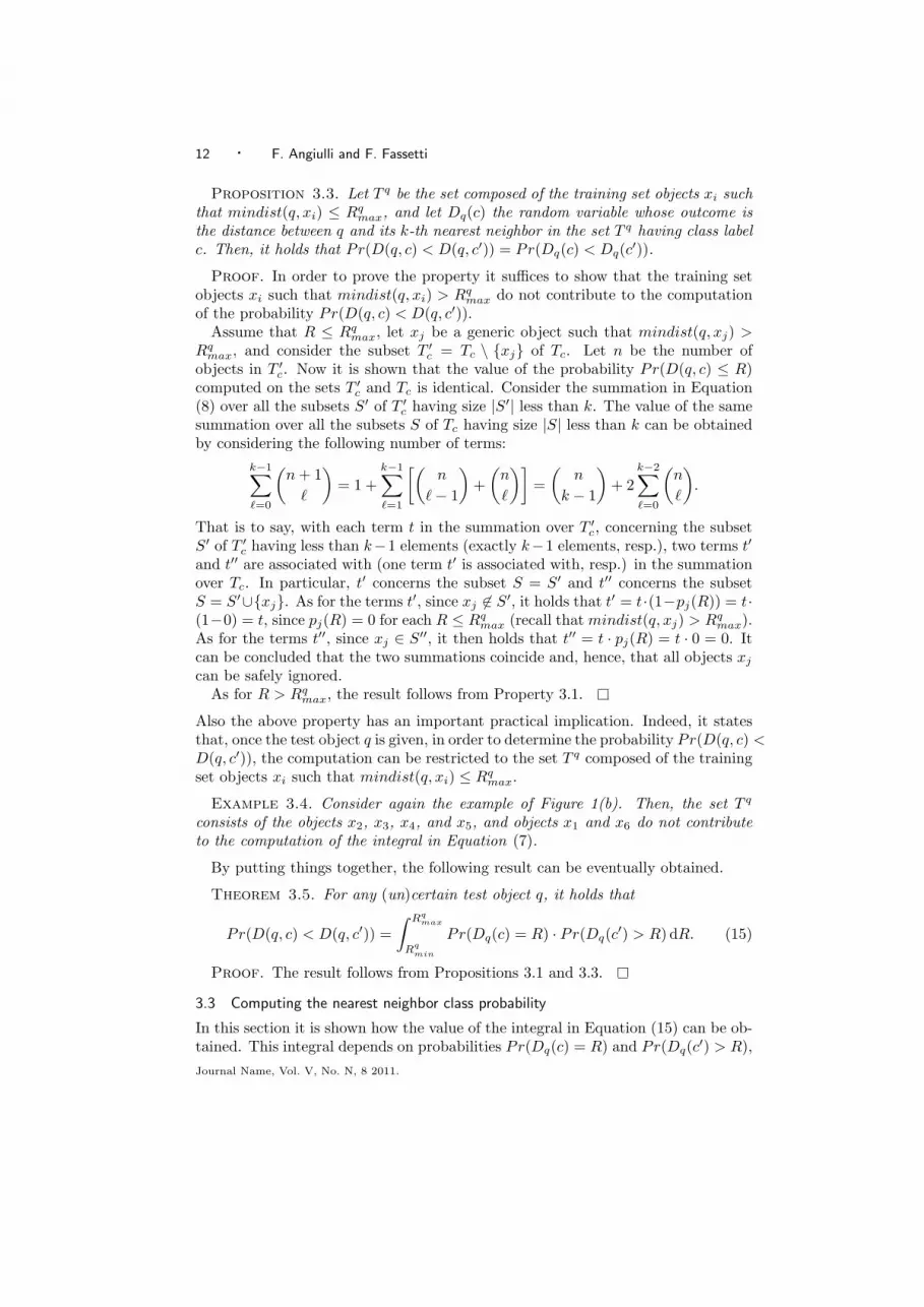
Proposition 3.3. Let T q be the set composed of the training set objects xi suchthat mindist(q, xi) ≤ Rq

max, and let Dq(c) the random variable whose outcome isthe distance between q and its k-th nearest neighbor in the set T q having class labelc. Then, it holds that Pr(D(q, c) < D(q, c′)) = Pr(Dq(c) < Dq(c′)).

Proof. In order to prove the property it suffices to show that the training setobjects xi such that mindist(q, xi) > Rq

max do not contribute to the computationof the probability Pr(D(q, c) < D(q, c′)).

Assume that R ≤ Rqmax, let xj be a generic object such that mindist(q, xj) >

Rqmax, and consider the subset T ′c = Tc \ {xj} of Tc. Let n be the number of

objects in T ′c. Now it is shown that the value of the probability Pr(D(q, c) ≤ R)computed on the sets T ′c and Tc is identical. Consider the summation in Equation(8) over all the subsets S′ of T ′c having size |S′| less than k. The value of the samesummation over all the subsets S of Tc having size |S| less than k can be obtainedby considering the following number of terms:

k−1∑

ℓ=0

(

n+ 1

ℓ

)

= 1 +k−1∑

ℓ=1

[(

n

ℓ− 1

)

+

(

n

ℓ

)]

=

(

n

k − 1

)

+ 2k−2∑

ℓ=0

(

n

ℓ

)

.

That is to say, with each term t in the summation over T ′c, concerning the subsetS′ of T ′c having less than k−1 elements (exactly k−1 elements, resp.), two terms t′

and t′′ are associated with (one term t′ is associated with, resp.) in the summationover Tc. In particular, t′ concerns the subset S = S′ and t′′ concerns the subsetS = S′∪{xj}. As for the terms t′, since xj 6∈ S

′, it holds that t′ = t·(1−pj(R)) = t·(1−0) = t, since pj(R) = 0 for each R ≤ Rq

max (recall that mindist(q, xj) > Rqmax).

As for the terms t′′, since xj ∈ S′′, it then holds that t′′ = t · pj(R) = t · 0 = 0. It

can be concluded that the two summations coincide and, hence, that all objects xjcan be safely ignored.

As for R > Rqmax, the result follows from Property 3.1.

Also the above property has an important practical implication. Indeed, it statesthat, once the test object q is given, in order to determine the probability Pr(D(q, c) <D(q, c′)), the computation can be restricted to the set T q composed of the trainingset objects xi such that mindist(q, xi) ≤ Rq

max.

Example 3.4. Consider again the example of Figure 1(b). Then, the set T q

consists of the objects x2, x3, x4, and x5, and objects x1 and x6 do not contributeto the computation of the integral in Equation (7).

By putting things together, the following result can be eventually obtained.

Theorem 3.5. For any (un)certain test object q, it holds that

Pr(D(q, c) < D(q, c′)) =

∫ Rqmax

Rq

min

Pr(Dq(c) = R) · Pr(Dq(c′) > R) dR. (15)

Proof. The result follows from Propositions 3.1 and 3.3.

3.3 Computing the nearest neighbor class probability

In this section it is shown how the value of the integral in Equation (15) can be ob-tained. This integral depends on probabilities Pr(Dq(c) = R) and Pr(Dq(c′) > R),



which in their turn depend on probabilities pi(R). Moreover, functions pi(R) de-pend on the objects xi and q and, for any given value of R, they involve the compu-tation of one multi-dimensional integral with domain of integration the hyper-ballin D of center q and radius R.

Next methods to compute as efficiently as possible probabilities pi(R) (Section3.3.1), the class distance probability (Section 3.3.2), and the nearest neighbor class(Section 3.3.3) are described.

3.3.1 Computation of the probabilities pi(R). Next, it is considered the mostgeneral case of arbitrarily shaped multi-dimensional pdfs, having as domain D thed-dimensional Euclidean space R

d. It is known [Lepage 1978] that given a functiong, if N points w1, w2, . . ., wN are randomly selected according to a given pdf f ,then the following approximation holds

∫

g(v) dv ≈1

N

N∑

j=1

g(wj)

f(wj). (16)

Thus, in order to compute the value pi(R), the function gi(v) = fxi(v) if d(q, v) ≤R, and gi(v) = 0 otherwise, can be integrated by evaluating formula in Equation(16) with the points wj randomly selected according to the pdf fxi . This procedurereduces to compute the relative number of sample points wj lying at distance notgreater than R from q, that is

pi(R) =|{wj : d(q, wj) ≤ R}|

N.

More precisely, by exploiting this kind of strategy a suitable approximation of thewhole cumulative distribution function pi can be computed with only one singleintegration operation, as shown in the following.

With each function pi an histogram Hi of h slots (with h a parameter used toset the resolution of the histogram) representing the value of the function pi in theinterval [Rq

min, Rqmax] is associated. Let ∆R be

∆R =(Rq

max −Rqmin)

h

and Rl be

Rl = Rqmin + l ·∆R,

then the lth slot Hi(l) of Hi stores the value pi(Rl) (1 ≤ l ≤ h). After havinggenerated the N points w1, w2, . . . , wN according to the pdf fxi , each entry Hi(l)can be eventually obtained as

Hi(l) =|{wj : d(q, wj) ≤ Rl}|

N,

where distances d(q, wj) are computed once and reused during the computation ofeach slot value.

3.3.2 Class distance probability computation. In this section we show how theprobability Pr(Dq(c) ≤ R) of having at least k objects within distance R from q,can be computed.



Assume that an arbitrary order among the elements of the set T qc is given, namely

T qc = {x1, . . . , x|T q

c |}. Then, the probability Dq(c) corresponds to the probabilitythat an element of T q

c is actually the k-th object (according to the established order)lying within distance R from q.

By letting P qc (i, j) denote the probability that exactly i objects among the first

j objects of T qc lie within distance R from q (i ≥ 0, j ≤ |T q

c |), it follows that

pj(R) · P qc (k − 1, j − 1)

represents the probability that the j-th element of T qc lies within distance R from

q and exactly k − 1 objects preceding xj in T qc lie within distance R from q.

Thus, the probability Pr(Dq(c) ≤ R) can be rewritten as

Pr(Dq(c) ≤ R) =∑

1≤j≤|T qc |

pj(R) · P qc (k − 1, j − 1). (17)

The probability P qc (i, j) can be recursively computed as follows:

P qc (i, j) = pj(R) · P q

c (i− 1, j − 1) + (1− pj(R)) · P qc (i, j − 1). (18)

Indeed, the probability P qc (i, j) corresponds to the probability that xj lies within

distance R from q and exactly i− 1 objects among the first j − 1 objects of Tc liewithin distance R from q, plus the probability that xj does not lie within distanceR from q and exactly i objects among the first j−1 objects of Tc lie within distanceR from q.

As for the properties of P qc (i, j), we note that

1. P qc (0, 0) = 1: since it corresponds to the probability that exactly 0 objects among

the first 0 objects of T qc lie within distance R from q;

2. P qc (0, j) = Π1≤h≤j(1−ph(R)), with j > 0: since it corresponds to the probability

that none of the first j objects of T qc lie within distance R from q;

3. P qc (i, j) = 0 with i > j: since if j < i it is not possible that i objects among the

first j objects of T qc lie within distance R from q.

Technically, the probability P qc (i, j) can be computed by means of a dynamic pro-

gramming procedure, similarly to what shown in [Rushdi and Al-Qasimi 1994]. Theprocedure makes use of a k × (|T q

c |+ 1) matrix Mqc : The generic element Mq

c (i, j)stores the the probability P q

c (i, j). Due to property 3 above, Mqc is an upper tri-

angular matrix, namely all the elements below the main diagonal are equal to 0.The first row of M q

c is computed by applying properties 1 and 2 above. Then,the procedure fills the matrix Mq

c (from the second to the k-th row) by applyingEquation (18). The value of D(q, c) is, finally, computed by exploiting the elementsof the last row of Mq

c in Equation (17).As for the temporal cost required to compute Equation (17), assuming that the

values ph(R) are already available (1 ≤ h ≤ |T qc |), from the above analysis it follows

that the temporal cost is O(k · |T qc |), hence linear both in k and in the size |T q

c | ofT qc . As far as the spatial cost is concerned, in order to fill the i-th row of Mq

c , onlythe elements of the (i− 1)-th and i-th rows of Mq

c are required, then the procedureemploys just two arrays of |T q

c | floating point numbers, and hence the space is linearin the size |T q

c | of T qc .



3.3.3 Computation of the class probability. In order to compute the integralreported in Equation (15), an histogram Fc composed of h slots is associatedwith the class c. In particular, the slot Fc(l) (1 ≤ l ≤ h) of Fc stores the valuePr(Dq(c) ≤ Rl) computed by exploiting the procedure described in Section 3.3.2.

Then, the probability Pr(Dq(c) = Rl) can be obtained as

Pr(Dq(c) ≤ Rl)− Pr(Dq(c) ≤ Rl−1)

∆R=Fc(l)− Fc(l − 1)

∆R,

and the probability Pr(Dq(c) < Dq(c′)) as

h∑

l=1

[Pr(Dq(c) = Rl) · Pr(Dq(c′) > Rl) ·∆R] .

To conclude, the previous summation can be finally simplified thus obtaining thefollowing formula

h∑

j=1

[(Fc(l)− Fc(l − 1)) · (1− Fc′(l))] , (19)

whose value corresponds to the probability Pr(D(q, c) < D(q, c′)).

If the test object u is uncertain, the nearest neighbor probability of class c isexpressed by the integral reported in Equation (9). By using formula in Equation(16) with g(q) = fu(q) ·Pr(D(q, c) < D(q, c′)) and f(q) = fu(q) and by generatingN points q1, q2, . . . , qN according to the pdf fu, the value of the integral in Equation(9) can be obtained as

1

N

N∑

i=1

Pr(D(qi, c) < D(qi, c′)), (20)

where the terms Pr(D(qi, c) < D(qi, c′)) are computed by exploiting the expression

in Equation (19).

3.4 Classification Algorithm

Figure 3 shows the Uncertain Nearest Neighbor Classification algorithm, whichexploits properties introduced in Sections 3.2 and 3.3 in order to classify certaintest objects.

The step 1 of the algorithm determines Rqmax (see Equation (13) and Proposition

3.1), while the step 2 determines the set T q (see Proposition 3.3). As for the step3, if one of the two classes has less than k objects in T q, then the object q issafely assigned to the other class. Otherwise, the nearest neighbor class probabilitymust be computed, which is accounted for in the subsequent steps by exploitingthe technique described in Section 3.3.

Temporal cost. As far as the temporal cost of the algorithm is concerned, bothsteps 1 and 2 cost O(nd), where n is the number of training set objects and O(d)is the cost of evaluating the distance between two certain objects. Let nq (≤ n) bethe cardinality of the set T q. Step 3 costs O(nq), while step 4 costs O(nqd). As forstep 5, it involves the computation of nq histograms Hi, each of which costs O(Nd),



Uncertain Nearest Neighbor Classification

Input: training set T , with two class labels c and c′, integer k > 0, and certaintest object qOutput: nearest neighbor class of q in T (with its associated probability)Method:

(1) Determine the value Rqmax = min{Rq

c , Rqc′} (Equation (13));

(2) Determine the set T q composed of the training set objects xi such thatmindist(q, xi) ≤ Rq

max;

(3) If in T q there are less than k objects of the class c′ (c, resp.), then return c(c′, resp.) (with associated probability 1) and exit;

(4) Determine the value Rqmin = minimindist(q, xi) by considering only the

objects xi belonging to T q;

(5) Compute the histograms Hi associated with the cumulate density functionspi(R) (for R ∈ [Rq

min, Rqmax]) of the objects xi belonging to T q, and the

histograms Fc and Fc′ associated with the cumulate density functions Dq(c)and Dq(c′);

(6) Determine the nearest neighbor probability p of class c w.r.t. class c′ (Equa-tions (7) and (15)) by computing the summation reported in Equation (19);

(7) If the probability p is greater than or equal to 0.5 then return c (with asso-ciated probability p), otherwise return c′ (with associated probability 1− p).

Fig. 3. The uncertain nearest neighbor classification algorithm.

with N the number of points considered during integration. The computation ofhistograms Fc and Fc′ costs O(nqkh), with h the resolution of the histograms.Finally, step 6 costs O(h).

It can be noticed that the term nqkh is negligible with respect to the term nqNd,since k is a small integer number (k = 1 by default, and, in any case, it is a verysmall integer), while it has been experimentally verified that h = 100 provides goodquality results. Summarizing, the temporal cost of the algorithm is O(nqNd), withnq expected to be much smaller than n.

As for uncertain test objects, in order to classify them the summation in Equation(20) has to be computed. This can be accomplished by executing N times thealgorithm in Figure 3, with a total temporal cost O(nqN

2d) and with no additionalspatial cost.

Spatial cost. As far as the spatial cost of the algorithm is concerned, the methodneeds to store, other than the training set, the nq identifiers of the objects in T q,the histograms Hi, and the two histograms Fc and Fc′ consisting of h floating pointnumbers. Summarizing, the spatial cost is O(nqh).

3.5 Accelerating the computation of the set T q.

Before leaving the section, the computation of the set T q is discussed.The basic strategy to compute the set T q consists in performing two linear scans

of the training set objects in order to determine the radius Rqmax (step 1 of the



algorithm) and to collect objects xi such that maxdist(q, xi) ≤ Rqmax (step 2 of the

algorithm).It can be noted that step 1 of the UNN algorithm corresponds to a nearest neigh-

bor query search with respect to the value maxdist(q, xi), while step 2 correspondsto a range query search with radius Rq

max with respect to the value mindist(q, xi).Let p be a certain object and v and w be two certain objects. Let δp(v, w) denote

the positive real value |d(v, p)− d(p, w)|. Then, the two following relationships aresatisfied:1

δpj(c(q), c(xi)) + r(q) + r(xi) ≤ maxdist(q, xi),

and

δpj(c(q), c(xi))− r(q)− r(xi) ≤ mindist(q, xi).

Indeed, by the reverse triangle inequality it is the case that δpj(c(q), c(xi)) ≤

d(c(q), c(xi)).Thus, the two above introduced inequalities can be used as pruning rules to be

embedded in exiting certain similarity search methods for metric spaces, such aspivot-based indexes, VP-trees, and others [Chavez et al. 2001], in order to fastenexecution of steps 1 and 2.

It can be noticed that the above depicted strategy does not modify the asymptotictime complexity of the algorithm.

However, in practice the execution time of the algorithm can take advantage ofthis strategy when the cost of computing the probability pi(R) is comparable tothe cost of computing the distance between the center of the test object c(q) andthe center of the training set object c(xi) and, moreover, the number of trainingset objects is very large (as an example, consider pdfs stored in histograms of fixedsize).

4. RELATED WORK

Besides the literature concerning the classic nearest neighbor rule [Cover and Hart1967; Stone 1977; Fukunaga and Hostetler 1975; Devroye 1981; Devroye et al. 1996],the works most related to the present one concern similarity search methods foruncertain data and classification in presence of uncertainty.

Several similarity search methods designed to efficiently retrieve the most similarobjects of a query object have been designed [Chavez et al. 2001; Zezula et al. 2006].These methods can be partitioned in those suitable for vector spaces [Bentley 1975;Beckmann et al. 1990; Berchtold et al. 1996], which allow to use geometric andcoordinate information, and those applicable in general metric spaces [Yianilos1993; Mico et al. 1994; Chavez et al. 2001; Zezula et al. 2006], where the aboveinformation is unavailable. The certain nearest neighbor rule may benefit of thesemethods since they fasten the search for the nearest neighbor of the test object.Moreover, as discussed in Section 3.5, these methods can be employed within thetechnique here described in order to accelerate some basic steps of the computationof the nearest neighbor class.

The above mentioned methods have been designed to be used with similaritymeasures involving certain data. Different concepts of similarity between uncertain

1If q is a certain object, the c(q) = q and r(q) = 0.



objects have been proposed in the literature, among them the distance betweenmeans, the expected distance, and probabilistic threshold distance [ Lukaszyk 2004;Cheng et al. 2004; Tao et al. 2007; Agarwal et al. 2009]. Based on some of thesenotions, similarity search methods designed to efficiently retrieve the most simi-lar objects of a query object have been also designed. The problem of searchingover uncertain data was first introduced in [Cheng et al. 2004] where the authorsconsidered the problem of querying one-dimensional real-valued uniform pdfs. In[Ngai et al. 2006] various pruning methods to avoid the expensive expected distancecalculation are introduced. Since the expected distance is a metric, the triangle in-equality, involving some pre-computed expected distances between a set of anchorobjects and the uncertain data set objects, can be straightforwardly employed inorder to prune unfruitful distance computations. [Singh et al. 2007] considered theproblem of indexing categorical uncertain data. To answer uncertain queries [Taoet al. 2007] introduced the concept of probabilistic constrained rectangles (PCR) ofan object. [Angiulli and Fassetti 2011] introduced a technique to efficiently answerrange queries over uncertain objects in general metric spaces.

While certain neighbor classification can be almost directly built on top of efficientindexing techniques for nearest neighbor search, we have already showed that thestraight use of uncertain nearest neighbor search methods for classification purposesleads to a poor decision rule in the uncertain scenario. Thus, it must be pointed outthat the UNN method is only loosely related to uncertain nearest neighbor indexingtechniques. Moreover, as far as the efficiency of the UNN is concerned, none of theseindexing methods can be straightforwardly employed to improve execution time ofUNN, since they are tailored on a specific notion of similarity among uncertainobjects, while UNN relies on the concept of nearest neighbor class which is directlybuilt on a certain similarity metrics.

Recently, several mining tasks have been investigated in the context of uncertaindata, including clustering, frequent pattern mining, and outlier detection [Ngaiet al. 2006; Achtert et al. 2005; Kriegel and Pfeifle 2005; Aggarwal and Yu 2008;Aggarwal 2009; Aggarwal and Yu 2009]. Particularly, a few classification meth-ods dealing with uncertain data have been proposed in the literature, among them[Mohri 2003; Bi and Zhang 2004; Aggarwal 2007]. [Mohri 2003] considered theproblem of classifying uncertain data represented by means of distributions over se-quences, such as weighted automata, and extended support vector machines to dealwith distributions by using general kernels between weighted automata. This kindof technique is particularly suited for natural language processing applications. [Biand Zhang 2004] investigates a learning model in which the input data is corruptedwith noise. It is assumed that input objects x′i = xi + ∆xi are subject to additivenoise, where xi is a certain object and the noise ∆xi follows a specific distribution.Specifically, a bounded uncertainty model is considered, that is to say ||∆xi|| ≤ δiwith uniform priors, and a novel formulation of support vector classification, calledtotal support vector classification (TSVC) algorithm, is proposed to manage thiskind of uncertainty. In [Aggarwal 2007] a method for handling error-prone andmissing data with the use of density based approaches is presented. The estimatederror associated with the jth dimension (1 ≤ i ≤ d) of the d-dimensional datapoint xi is denoted by ψj(xi). This error value may be for example the standard



Data set Dim. (d) Size (n) Classes Class 1 Class 2 Class 3

Ionosphere 2 351 2 225 126 –Haberman 3 306 2 225 81 –

Iris 4 150 3 50 50 50Transfusion 4 748 2 570 178 –

Table I. Datasets employed in experiments.

deviation of the observations over a large number of measurements. The basic ideaof the framework is to construct an error-adjusted density of the data set by ex-ploiting kernel density estimation and, then, to use this density as an intermediaterepresentation in order to perform mining tasks. An algorithm for the classificationproblem is presented, consisting in a density based adaptation of rule-based classi-fiers. Intuitively, the methods seeks for the subspaces in which the instance-specificlocal density of the data for a particular class is significantly higher than its densityin the overall data.

It must be noticed that none of these methods investigates the extension of thenearest neighbor decision rule to the handling of uncertain data. Moreover, inthe experimental section comparison between UNN and density based methods forclassification will be investigated.

5. EXPERIMENTAL RESULTS

This section presents results obtained by experimenting the UNN rule.Experiments are organized as follows. Section 5.2 studies the effect of disregard-

ing data uncertainty on classification accuracy. Section 5.3 investigates the behaviorof UNN on test objects whose label is independent of the theoretical prediction andits sensitivity to noise. Section 5.4 reports execution time by using both certainand uncertain test objects. Section 5.5 compares the approach here proposed withdensity based classification methods for uncertain data. Section 5.6 describes areal-life scenario in which data are naturally modelled as multi-dimensional pdfs.

First of all, the following section describes the characteristics of some of thedatasets employed in the experimental activity.

5.1 Datasets description

Table I reports datasets employed in the experiments and their characteristics. Allthe datasets are from the UCI ML Repository [Asuncion and Newman 2007]. Asfor the Ionosphere dataset, it has been projected on the two principal components.

For each dataset above listed, a family of uncertain training sets has been ob-tained. Each training set of the family is characterized by a parameter s (for spread)used to determine the degree of uncertainty associated with dataset objects. Inparticular, for each certain object xi = (xi,1, . . . , xi,d) in the original dataset, anuncertain object x′i has been associated with, having pdf f i(v1, . . . , vd) = f i1(v1) ·. . .·f id(vd). Each one dimensional pdf f ij is randomly set to a normal or to a uniformdistribution, with mean xi,j and support [a, b] depending on the parameter s. Inparticular, let r be a randomly generated number in the interval [0.01·s·σj , s·σj ],where σj denotes the standard deviation of the dataset along the jth coordinate,then a = xi,j − 4 · r and b = xi,j + 4 · r.

In the experiments, the parameter N , determining the resolution of integrals,



0 0.05 0.1 0.15 0.280

85

90

95

100Ionosphere dataset (k=1)

Spread

Cla

ssifi

catio

n ac

cura

cy

UNNeKNN

0 0.05 0.1 0.15 0.288

90

92

94

96

98


Spread

Cla

ssifi

catio

n ac

cura

cy

UNNeKNN

0 0.05 0.1 0.15 0.292

94

96

98


Spread

Cla

ssifi

catio

n ac

cura

cy

UNNeKNN

0 0.05 0.1 0.15 0.275

80

85

90

95

100Haberman dataset (k=1)

Spread

Cla

ssifi

catio

n ac

cura

cy

UNNeKNN

0 0.05 0.1 0.15 0.280

85

90

95


Spread

Cla

ssifi

catio

n ac

cura

cy

UNNeKNN

0 0.05 0.1 0.15 0.288

90

92

94

96

98


Spread

Cla

ssifi

catio

n ac

cura

cy

UNNeKNN

0 0.05 0.1 0.15 0.290

92

94

96

98

100Iris dataset (k=1)

Spread

Cla

ssifi

catio

n ac

cura

cy

UNNeKNN

0 0.05 0.1 0.15 0.292

94

96

98


Spread

Cla

ssifi

catio

n ac

cura

cy

UNNeKNN

0 0.05 0.1 0.15 0.294

95

96

97

98

99


Spread

Cla

ssifi

catio

n ac

cura

cyUNNeKNN

0 0.05 0.1 0.15 0.275

80

85

90

95

100Transfusion dataset (k=1)

Spread

Cla

ssifi

catio

n ac

cura

cy

UNNeKNN

0 0.05 0.1 0.15 0.280

85

90

95


Spread

Cla

ssifi

catio

n ac

cura

cy

UNNeKNN

0 0.05 0.1 0.15 0.288

90

92

94

96

98


Spread

Cla

ssifi

catio

n ac

cura

cy

UNNeKNN

Fig. 4. Accuracy using random certain queries.

has been set to N = 100 · 2d, while the histogram resolution h has been set to 100.Furthermore, experimental results are averaged on ten runs.

5.2 The effect of disregarding uncertainty

The goal of this experiment is to show that whenever uncertain data are available,taking into account uncertainty leads to superior classification results.

With this aim, two algorithms have been implemented to be compared with UNN,namely the Random and the eKNN (for expected k-nearest neighbor) algorithms.The Random algorithm approximates the expression reported in Equation (1) byrandomly generating M outcomes IT of the uncertain training set T , and, hence,determines the most probable class of the test object (see Equation (2)). TheeKNN algorithm randomly generates M outcomes IT of the uncertain training setT , classifies test objects by applying the k′ nearest neighbor rule with training setIT (k′ is set to 2k−1, according to Proposition 2.6) and, finally, reports the average



s = 0.05 s = 0.10 s = 0.20k = 1 k = 2 k = 3 k = 1 k = 2 k = 3 k = 1 k = 2 k = 3

Spiral 63.3 63.2 66.2 59.9 62.4 64.8 56.9 59.9 62.1Ionosphere 78.6 73.7 73.1 68.7 67.9 68.6 62.9 66.5 71.2

Haberman 83.5 78.0 76.8 73.0 70.1 70.8 66.4 68.8 73.6Iris 91.9 87.2 88.1 83.6 81.8 83.8 75.3 78.4 82.2

Transfusion 75.1 83.0 87.6 74.2 82.2 87.0 74.0 82.2 87.0

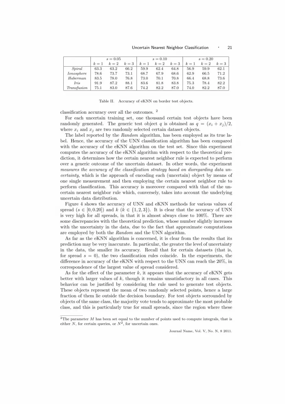
Table II. Accuracy of eKNN on border test objects.

classification accuracy over all the outcomes. 2

For each uncertain training set, one thousand certain test objects have beenrandomly generated. The generic test object q is obtained as q = (xi + xj)/2,where xi and xj are two randomly selected certain dataset objects.

The label reported by the Random algorithm, has been employed as its true la-bel. Hence, the accuracy of the UNN classification algorithm has been comparedwith the accuracy of the eKNN algorithm on the test set. Since this experimentcomputes the accuracy of the eKNN algorithm with respect to the theoretical pre-diction, it determines how the certain nearest neighbor rule is expected to performover a generic outcome of the uncertain dataset. In other words, the experimentmeasures the accuracy of the classification strategy based on disregarding data un-certainty, which is the approach of encoding each (uncertain) object by means ofone single measurement and then employing the certain nearest neighbor rule toperform classification. This accuracy is moreover compared with that of the un-certain nearest neighbor rule which, conversely, takes into account the underlyinguncertain data distribution.

Figure 4 shows the accuracy of UNN and eKNN methods for various values ofspread (s ∈ [0, 0.20]) and k (k ∈ {1, 2, 3}). It is clear that the accuracy of UNNis very high for all spreads, in that it is almost always close to 100%. There aresome discrepancies with the theoretical prediction, whose number slightly increaseswith the uncertainty in the data, due to the fact that approximate computationsare employed by both the Random and the UNN algorithm.

As far as the eKNN algorithm is concerned, it is clear from the results that itsprediction may be very inaccurate. In particular, the greater the level of uncertaintyin the data, the smaller its accuracy. Recall that for certain datasets (that is,for spread s = 0), the two classification rules coincide. In the experiments, thedifference in accuracy of the eKNN with respect to the UNN can reach the 20%, incorrespondence of the largest value of spread considered.

As for the effect of the parameter k, it appears that the accuracy of eKNN getsbetter with larger values of k, though it remains unsatisfactory in all cases. Thisbehavior can be justified by considering the rule used to generate test objects.These objects represent the mean of two randomly selected points, hence a largefraction of them lie outside the decision boundary. For test objects sorrounded byobjects of the same class, the majority vote tends to approximate the most probableclass, and this is particularly true for small spreads, since the region where these

2The parameter M has been set equal to the number of points used to compute integrals, that iseither N , for certain queries, or N2, for uncertain ones.



0 0.05 0.1 0.15 0.275

80

85

90

95


Spread

Cla

ssifi

catio

n ac

cura

cy

UNNeKNN

0 0.05 0.1 0.15 0.285

90

95


Spread

Cla

ssifi

catio

n ac

cura

cy

UNNeKNN

0 0.05 0.1 0.15 0.288

90

92

94

96

98


Spread

Cla

ssifi

catio

n ac

cura

cy

UNNeKNN

0 0.05 0.1 0.15 0.275

80

85

90

95


Spread

Cla

ssifi

catio

n ac

cura

cy

UNNeKNN

0 0.05 0.1 0.15 0.285

90

95


Spread

Cla

ssifi

catio

n ac

cura

cy

UNNeKNN

0 0.05 0.1 0.15 0.288

90

92

94

96

98


Spread

Cla

ssifi

catio

n ac

cura

cy

UNNeKNN

0 0.05 0.1 0.15 0.285

90

95


Spread

Cla

ssifi

catio

n ac

cura

cy

UNNeKNN

0 0.05 0.1 0.15 0.288

90

92

94

96

98


Spread

Cla

ssifi

catio

n ac

cura

cy

UNNeKNN

0 0.05 0.1 0.15 0.288

90

92

94

96

98


Spread

Cla

ssifi

catio

n ac

cura

cyUNNeKNN

0 0.05 0.1 0.15 0.270

75

80

85

90

95


Spread

Cla

ssifi

catio

n ac

cura

cy

UNNeKNN

0 0.05 0.1 0.15 0.280

85

90

95


Spread

Cla

ssifi

catio

n ac

cura

cy

UNNeKNN

0 0.05 0.1 0.15 0.285

90

95


Spread

Cla

ssifi

catio

n ac

cura

cy

UNNeKNN

Fig. 5. Accuracy using random uncertain queries.

test objects are located tends to present non-null probability for only one of thetwo classes.

In order to study the behavior on critical test objects, that are objects locatedalong the decision boundary, the above experiment was repeated on a further set ofone thousand test objects, called border test objects, determined as explained next.The generic border test object q is obtained as q = (xi +xj)/2, where xi and xj aretwo randomly selected certain dataset objects and q satisfies the condition that themean distances dqc = 1

k

∑

i nni(q, Tc) and dqc′ = 1k

∑

i nni(q, Tc′) are similar (namelytheir difference is within the ten percent), that is |dqc − d

qc′ |/max{dqc , d

qc′} ≤ 0.1.

On these objects, the behavior of UNN is similar to that exhibited on the randomtest objects. Table II reports the accuracy of eKNN on the border test objectsfor the various values of spread s and nearest neighbors k. It is clear that theaccuracy of eKNN further deteriorates: the accuracy may decrease of an additional20% percent with respect to the previous experiment. Moreover, the advantage of



increasing the value of k becomes less evident. In some cases the accuracy does notvary with k or may even get worse for larger values.

Figure 5 shows the accuracy of UNN and eKNN for random uncertain test objects.The uncertain test objects have been obtained by centering multi-dimensional pdfs,generated according to the policy used for the training set objects, on the certaintest objects employed in the experiment of Figure 4. The trend of these curves issimilar to that associated with curves obtained for certain test objects. Particularly,in many cases the accuracy of eKNN worsens by some percentage points with respectto the certain test objects. This can be explained since in this experiment the datauncertainty has increased.

Concluding, the experimental results presented in this section confirm that clas-sification results benefit from taking into accout data uncertainty.

5.3 Experiments on real labels and robustness to noise

In this experiment the accuracy of the UNN, the eKNN, and the certain k nearestneighbor algorithm (referred to as KNN in the following) has been compared bytaking into account the original dataset labels of the test objects.

The range of values for the spread s and for the number of nearest neighborsk considered are s ∈ [0, 0.2] and k ∈ {1, 2, 3}, respectively, which are the sameemployed in the experiment described in the previous section. UNN and eKNNhave been executed on the uncertain version of the dataset, while KNN has beenexecuted on the certain dataset. Accuracy has been measured by means of ten foldcross validation.

Note that, while the certain dataset can be assimilated to a generic outcome ofan hypothetical true uncertain dataset which is unknown, the uncertain datasethere employed has been syntetically generated by using arbitrary distributions cen-tered on the certain dataset objects (as already explained at the beginning of theexperimental result section) and it is not intended to represent the (unknown) trueuncertain dataset.

Thus, it is important to point out that the purpose of this experiment is neither todemonstrate that that UNN peforms better than KNN (as a matter of fact the twomethods are designed for two very different application scenarios; recall that UNNis executed on uncertain data, while KNN can be executed only on certain data) norto show that better classification results can be achieved by injecting uncertainty inthe data. Rather, the goal of the experiment is to study the behavior of UNN on testobjects whose label is independent of the theoretical prediction and, particularly,to appreciate the sensitivity of UNN to noise. With this aim, the accuracy of KNNwill be employed as a baseline to assess the accuracy of UNN, since the outputof KNN represents the classification achieved on the considered datasets by thenearest neighbor classification rule when uncertainty disappears.

Figure 6 shows the result of the experiment. Curves report the accuracy of UNN(solid lines), eKNN (dashed lines), and KNN (dotted lines). On the Ionosphere,Haberman, and Transfusion datasets the accuracy of UNN is above than that ofKNN. Moreover, on the two latter datasets, the accuracy is slightly increasing withthe data uncertainty (spread). The difference in accuracy can be justified by notic-ing that UNN mitigates the effect of noisy points since it takes simultaneously intoaccount the whole class probability, according to the theoretical analysis depicted



0.05 0.1 0.15 0.280

82

84

86

88


Spread

Acc

urac

y [%

]

UNNeKNNKNN

0.05 0.1 0.15 0.285

85.5

86

86.5

87

87.5


Spread

Acc

urac

y [%

]

UNNeKNNKNN

0.05 0.1 0.15 0.286

86.5

87

87.5Ionosphere dataset (k=3)

Spread

Acc

urac

y [%

]

UNNeKNNKNN

0.05 0.1 0.15 0.265

70


Spread

Acc

urac

y [%

]

UNNeKNNKNN

0.05 0.1 0.15 0.265

70


Spread

Acc

urac

y [%

]

UNNeKNNKNN

0.05 0.1 0.15 0.271

72

73

74


Spread

Acc

urac

y [%

]

UNNeKNNKNN

0.05 0.1 0.15 0.293

93.5

94

94.5

95

95.5


Spread

Acc

urac

y [%

]

UNNeKNNKNN

0.05 0.1 0.15 0.295

95.2

95.4

95.6

95.8


Spread

Acc

urac

y [%

]

UNNeKNNKNN

0.05 0.1 0.15 0.295

95.5

96

96.5


Spread

Acc

urac

y [%

]

UNNeKNNKNN

0.05 0.1 0.15 0.250

55

60

65

70

75


Spread

Acc

urac

y [%

]

UNNeKNNKNN

0.05 0.1 0.15 0.265

70

75


Spread

Acc

urac

y [%

]

UNNeKNNKNN

0.05 0.1 0.15 0.265

70

75


Spread

Acc

urac

y [%

]

UNNeKNNKNN

Fig. 6. Ten-fold cross validation results.

in Section 2. As for the Iris dataset, the accuracy of UNN is practically the sameas that of KNN. This can be justified since this dataset contains a little amount ofnoise and it is composed of well-separated classes.

As far as the comparison of UNN and eKNN is concerned, the former methodperforms always better than the latter, thus confirming the result of the analysisconducted in the previous section. As for the effect of the parameter k on theaccuracy, as already discused the accuracy of eKNN improves for larger values ofk. However, it is well-known that it is difficult to select a nearly optimum value ofk to approach the lowest possible probability of error. In particular, as k increasesbeyond a certain value, which depends on the nature of the dataset, the probabilityof error may begin to increase. The plots show that UNN achieves very good resultsby using the smallest possible value for k, that is k = 1, and that in different casesthe maximum accuracy is achieved for values of k smaller than the greatest valuehere considered (e.g., see Ionosphere for k = 1 and s = 0.1, or Haberman for k = 2



1 1.5 2 2.5 30

0.02

0.04

0.06

0.08

Number of neighbors, k

Exe

cutio

n tim

e [s

ec]

Haberman dataset

s=0.20s=0.10s=0.05

1 1.5 2 2.5 30

0.05

0.1

0.15

0.2


Exe

cutio

n tim

e [s

ec]

Iris dataset

s=0.20s=0.10s=0.05

1 1.5 2 2.5 30

0.1

0.2

0.3

0.4

0.5


Exe

cutio

n tim

e [s

ec]

Transfusion dataset

s=0.20s=0.10s=0.05

1 1.5 2 2.5 30

0.02

0.04

0.06

0.08


Exe

cutio

n tim

e [s

ec]

Haberman dataset

s=0.20s=0.10s=0.05

1 1.5 2 2.5 30

0.05

0.1

0.15

0.2

0.25

0.3


Exe

cutio

n tim

e [s

ec]

Iris dataset

s=0.20s=0.10s=0.05

1 1.5 2 2.5 30.2

0.3

0.4

0.5

0.6

0.7


Exe

cutio

n tim

e [s

ec]

Transfusion dataset

s=0.20s=0.10s=0.05

Fig. 7. UNN execution time.

and s = 0.2)Thus, these experimental results confirm the discussion of Section 2, where it is

pointed out that the concept of nearest neighbor class is more powerful than thatof nearest neighbor in presence of uncertainty.

5.4 Execution time

Figure 7 reports the time employed by UNN to classify one single test object.3

Plots in the first (second, resp.) row of Figure 7 show the execution time onthe Haberman, Iris, and Transfusion datasets when certain (uncertain, resp.) testobjects are employed. Clearly, the execution time increases both with k and withthe data uncertainty: The larger the spread, the greater the execution time; more-over, classifying uncertain test objects requires more time than classifying certainones. Indeed, the larger the uncertainty (k, resp.), the larger the radius Rq

max and,consequently, the number of integrals to be computed.

The following table reports the relative execution time of UNN, that is the ratiobetween the execution time of the UNN algorithm (which computes the integral inEquation (15)) and the time needed to compute the integral in Equation (7) whenall the training set objects are taken into account. Thus, the table shows the timesavings obtained by exploiting techniques reported in Section 3.

Test set Datasets = 0.05 s = 0.10 s = 0.20

k=1 k=2 k=3 k=1 k=2 k=3 k=1 k=2 k=3

Certain

Haberman 0.01 0.02 0.02 0.03 0.05 0.05 0.09 0.11 0.13Iris 0.01 0.01 0.01 0.04 0.05 0.06 0.11 0.12 0.13

Transfusion 0.05 0.06 0.06 0.08 0.09 0.09 0.13 0.14 0.15

Uncertain

Haberman 0.08 0.09 0.10 0.13 0.16 0.19 0.25 0.31 0.37Iris 0.03 0.04 0.05 0.07 0.11 0.12 0.19 0.22 0.24

Transfusion 0.11 0.12 0.13 0.15 0.17 0.18 0.23 0.25 0.27

3Experiments were executed on a CPU Core 2 Duo 2.40GHz with 4GB of main memory underthe Linux operating system.



0 0.5 1 1.5 2 2.5 376

77

78

79

80

81

82Adult dataset

Spread

Acc

urac

y [%

]UNNDensity Based

0 0.5 1 1.5 2 2.5 340

50

60

70

80

90

100Forest Cover Type dataset

Spread

Acc

urac

y [%

]

UNNDensity Based

Fig. 8. Comparison with the Density Based classification algorithm.

The relative execution times reported in the table show that properties exploitedby UNN to accelerate computation guarantee time savings in all cases. For certaintest objects, in most cases the relative execution time is approximatively below0.10, and in some cases it is even close to 0.01, e.g., see the Haberman and Irisdatasets. Also for uncertain test objects, in many cases it is approximatively below0.15, though in different cases it is much smaller.

For spread s = 0.2 a considerable fraction of the dataset objects are within dis-tance Rq

max from the test object q and, hence, the relative execution time increases.This effect is more evident when uncertain test objects are taken into account. How-ever, it can be noted that the spread s = 0.2 is very large, in fact in this case thesupports of the training set objects are rather wide and tend to partially overlap.

5.5 Comparison with density based methods

This section describes comparison between UNN and the Density Based classifica-tion algorithm proposed in [Aggarwal 2007], where a general framework for dealingwith uncertain data is presented.

The same experimental setting described in [Aggarwal 2007] is considered. Fol-lowing the methodology therein proposed, an uncertain dataset is generated start-ing from a certain one, as described next. First of all, just the numerical at-tributes are taken into account, let d be their number. Then, for each objectxi = (xi,1, . . . , xi,d) in the original certain dataset, an uncertain object x′i with pdff i(v1, . . . , vd) = f i1(v1) · . . . · f id(vd) is generated. Each one dimensional pdf f ij is anormal distribution with mean xi,j and standard deviation equal to [0, 2 · s · σj ],where σj is the standard deviation of the dataset objects along the j-th attribute.Thus, the value of the spread s determines the uncertainty level of the dataset andhas been varied in the range [0, 3].

Two datasets coming from the UCI ML Repository [Asuncion and Newman 2007],that are Adult and Forest Cover Type, are employed. The former contains dataextracted from the census bureau database. It consists of 32,561 objects and six



numerical attributes. The latter dataset contains data about forest cover type offour areas located in the northern Colorado. It consists of 581,012 objects and tennumerical attributes.

Figure 8 reports experimental results. In all cases UNN exhibited a better classi-fication accuracy than the Density Based algorithm. The accuracy of both methodsdegrades with the spread s. It can be noticed that the difference between the cases = 0 and the case s = 3 is substantial for both methods, and this can be justifiedby noticing that in the latter case the level of uncertainty is very high, with a lotof dataset objects having overlapping domain. However, UNN shows itself to besensibly more accurate for all levels of uncertainty, thus confirming the effectivenessof the concept of nearest neighbor class.

5.6 A real-life example application scenario

This section describes a real-life prediction scenario in which data can be naturallymodelled by means of multi-dimensional continuous pdfs, that is the most generalform of uncertain objects managed by the technique here introduced, and illustratesthe meaningfulness of uncertain nearest neighbor classification within the describedtask.

The scenario concerns Mobile Ad hoc NETworks (or MANETs). A MANET [Baiand Helmy 2006] is a collection of wireless mobile nodes forming a self-configuringnetwork without using any existing infrastructure. Potential applications of MANETsare mobile classrooms, battlefield communication, disaster relief, and others. Themobility model of a MANET is designed to describe the movement pattern of mo-bile users, and how their location, velocity and acceleration change over time. Onefrequently used mobility model in MANET simulations is the Random Waypointmodel [Broch et al. 1998], in which nodes move independently to a randomly cho-sen destination with a randomly selected velocity within a certain simulation area.For such a model, the spatial node distribution is such that the node density ismaximum at the center of the simulation area, whereas the density is almost zeroaround the boundary of the area, hence the distribution is non-uniform. Moreover,no matter how fast the nodes move, the spatial node distribution at a certain po-sition is only determined by its location [Bettstetter et al. 2004]. For a squaredarea of size a by a, centered in (x0, y0), the pdf of the random waypoint model isprovided by the following analytical expression:

frw(x, y) ≈36

a6·

(

(x− x0)2 −a2

4

)

·

(

(y − y0)2 −a2

4

)

,

for x ∈[

x0 −a2 , x0 + a

2

]

and y ∈[

y0 −a2 , y0 + a

2

]

, and frw(x, y) = 0 outside. Figure9 shows the function frw.

In such networks the nodes may dynamically enter the network as well as leaveit. The nodes of a MANET are typically distinguished by their limited power, pro-cessing, and memory resources, as well as high degree of mobility. Since nodes arenot able to be re-charged in an expected time period, energy conservation is crucialto maintaining the life-time of nodes. One of the goals of protocols is to minimizeenergy consumption through techinques for routing, for data dissemination, and forvarying transmission power (and, consequently, transmission range). Multiple hopsare usually needed for a node to exchange information with any other node in the



Fig. 9. The pdf frw of the Random waypoint model for MANETs.

network, and nodes take adavantage of their neighbors in order to communicatewith the rest of the network nodes.

As a matter of fact, the needed transmission power is inversely proportional tothe squared distance separating the transmitter to the receiver [Wesolowski 2002].For an isotropic antenna the radiation Pr at a distance R is

Pr(R) =Pt

Rα,

where Pt is the transmitted signal strength and α is the path loss factor, whichdepends on the given propagation environment and whose value is typically between2 (in free space) and 6. Since a node can correctly receive packets if the signalstrength Pr of the packet at that node is above a certain threshold, and since mobiledevices exploit variable-range transmission as a powersave strategy, the minimumpower to be supplied by a node v connected to the network W is:

powW (v) ∝

∫ +∞

0

Rα · Pr(d(v, nnW (v)) = R) dR. (21)

Thus, pdfs frw naturally model uncertain objects representing mobile devices,also called nodes in the following. In the experiment described in this section, anuncertain training set of nodes partitioned in two classes, representing two differentMANET networks, is considered. The simulation area is the unit square centeredin the origin. The red network has ten nodes randomly positioned in the wholesimulation area and allowed to move in squares of size 0.2 by 0.2 (these centersare identified in Figure 10(a) by means of plus-marks), while the blue network hasfive nodes randomly positioned in the lower-right corner of the simulation area andallowed to move in squares of size 0.05 by 0.05 (these centers are identified in Figure10(a) by means of x-marks). Certain objects are the points of the plane. A set of2,500 randomly generated points within the simulation square has been employed



(a) (b)

Fig. 10. Experimental results on the MANET training set.

as test set. These points have been labelled as either red or blue depending onthe minimum achievable power consumption of the node, namely the label of thecertain test object q is determined as

arg minW∈{red,blue}

powW (q).

Thus, the classification task considered consists in the prediciton of the less de-manding network in terms of energy to be expended.

The UNN applied to the above described dataset returns the nearest neighborclass of a test object, that is to say the network (class) that minimizes the expecteddistance from the position of a node determined to join a neighborhood MANET(the test object) and the uncertain position of one of its nodes (members).

Figure 10 reports the classification of the points of the plane for k = 1. In Figure10(b) points are colored according to the probability to belong to one of the twoclasses. In Figure 10(a) the solid black curve represents the decision boundary,that is the points for which the nearest neighbor class probability equals 0.5. Thetwo dashed curves correspond to the points having red class probability 0.75 and0.25. The form of the decision boundary is informative, since it differs from thecommon facets of the adjacent Voronoi cells associated with objects belonging toopposite classes, that is the decision boundary of the certain nearest neighbor rule.In particular, it can be observed that the centers of two red nodes are within thesupport of the blue class (and that the probability of the red class is below 0.25 incorrespondence of both these two centers). This can be justified by noticing thatthese two centers are close to the centers of two blue nodes, and that the mobilityof blue nodes is smaller than that of red ones.

The accuracy of UNN on the test set has been measured and compared with thatof eKNN. The accuracy of UNN was 0.986, while that of eKNN was 0.938. Thegood performance of nearest neighbor based classification methods is due to thefact that power consumption is related to the Euclidean distance between devices.Note that, while the uncertain nearest neighbor rule reports the class which mostprobably provides the nearest neighbor, the power (Equation (21)) depends also onthe distribution of the distance separating the transmitter to its nearest neighbor,



and this explains why there are misclassifications. Also in this experiment, UNNperforms better than eKNN, and this can be explained since the former rule basesits decision on the concept of nearest neighbor class, thus confirming the superiorityof the uncertain nearest neighbor rule even with respect to classical classificationtechniques in presence of uncertainty.

6. CONCLUSIONS

In this work the uncertain nearest neighbor rule, representing the generalization ofthe certain nearest neighbor rule to the uncertain scenario, has been introduced.It has been provided evidence that the uncertain nearest neighbor rule correctlymodels the right semantics of the nearest neighbor decision rule when applied to theuncertain scenario. Moreover, an algorithm to perform uncertain nearest neighborclassification of a generic (un)certain test object has been presented, together withsome properties precisely designed to significantly reduce the temporal cost associ-ated with nearest neighbor class probability computation. The theoretical analysisand the experimental campaign here presented have shown that the proposed algo-rithm is efficient and effective in classifying uncertain data.

REFERENCES

Achtert, E., Bohm, C., Kriegel, H.-P., and Kroger, P. 2005. Online hierarchical clusteringin a data warehouse environment. In ICDM. 10–17.

Agarwal, P., Cheng, S.-W., Tao, Y., and Yi, K. 2009. Indexing uncertain data. In PODS.

137–146.

Aggarwal, C. 2007. On density based transforms for uncertain data mining. In ICDE.

Aggarwal, C. 2009. Managing and Mining Uncertain Data. Advances in Database Systems,

vol. 35. Springer.

Aggarwal, C. and Yu, P. 2008. Outlier detection with uncertain data. In SDM. 483–493.

Aggarwal, C. and Yu, P. 2009. A survey of uncertain data algorithms and applications. IEEE

Trans. Knowl. Data Eng. 21, 5, 609–623.

Angiulli, F. and Fassetti, F. 2011. Indexing uncertain data in general metric spaces. IEEETransactions on Knowledge and Data Engineering. to appear.

Asuncion, A. and Newman, D. 2007. UCI machine learning repository.

Bai, F. and Helmy, A. 2006. Wireless Ad Hoc and Sensor Networks. Springer, Chapter A Surveyof Mobility Modeling and Analysis in Wireless Adhoc Networks.

Beckmann, N., Kriegel, H.-P., Schneider, R., and Seeger, B. 1990. The r*-tree: An efficientand robust access method for points and rectangles. In Proc. of the SIGMOD Conference.322–331.

Bentley, J. 1975. Multidimensional binary search trees used for associative searching. Commu-nications of the ACM 18, 509–517.

Berchtold, S., Keim, D., and Kriegel, H.-P. 1996. The x-tree: An index structure for high-

dimensional data. In Proc. of the Conf. on VLDB. 28–39.

Bettstetter, C., Hartenstein, H., and Perez-Costa, X. 2004. Stochastic properties of therandom waypoint mobility model. Wireless Networks 10, 5, 555–567.

Bi, J. and Zhang, T. 2004. Support vector classification with input data uncertainty. In NIPS.161–168.

Broch, J., Maltz, D., Johnson, D., Hu, Y.-C., and Jetcheva, J. 1998. A performance com-parison of multi-hop wireless ad hoc network routing protocols. In MobiCom ’98: Proceedingsof the 4th annual ACM/IEEE international conference on Mobile computing and networking.

85–97.

Chavez, E., Navarro, G., Baeza-Yates, R., and Marroquın, J. 2001. Searching in metricspaces. ACM Computing Surveys 33, 3, 273–321.



Cheng, R., Xia, Y., Prabhakar, S., Shah, R., and Vitter, J. 2004. Efficient indexing methodsfor probabilistic threshold queries over uncertain data. In VLDB. 876–887.

Cover, T. and Hart, P. 1967. Nearest neighbor pattern classification. IEEE Trans. Inform.Theory 13, 21–27.

Devroye, L. 1981. On the inequality of cover and hart in nearest neighbor discrimination. IEEETrans. Pattern Anal. Mach. Intell. 3, 1 (January), 75–78.

Devroye, L., Gyorfy, L., and Lugosi, G. 1996. A Probabilistic Theory of Pattern Recognition.

Springer.

Fukunaga, K. and Hostetler, L. 1975. k-nearest-neighbor bayes-risk estimation. IEEE Trans.

Inform. Theory 21, 285–293.

Green, T. and Tannen, V. 2006. Models for incomplete and probabilistic information. IEEEData Eng. Bull. 29, 1, 17–24.

Kriegel, H.-P. and Pfeifle, M. 2005. Density-based clustering of uncertain data. In KDD.672–677.

Lepage, G. 1978. A new algorithm for adaptive multidimensional integration. Journal of Com-putational Physics 27.

Lindley, D. 2006. Understanding Uncertainty. Wiley-Interscience.

Lukaszyk, S. 2004. A new concept of probability metric and its applications in approximationof scattered data sets. Comput. Mech. 33, 4, 299–304.

Mico, L., Oncina, J., and Vidal, E. 1994. A new version of the nearest-neighbour approxi-mating and eliminating search algorithm (aesa) with linear preprocessing time and memory

requirements. Pattern Recognition Letters 15, 1, 9–17.

Mitchell, T. 1997. Machine Learning. Mac Graw Hill.

Mohri, M. 2003. Learning from uncertain data. In COLT. 656–670.

Ngai, W., Kao, B., Chui, C., Cheng, R., Chau, M., and Yip, K. 2006. Efficient clustering of

uncertain data. In ICDM. 436–445.

Rifkin, R. and Klautau, A. 2004. In defense of one-vs-all classification. J. Mach. Learn. Res. 5,

101–141.

Rushdi, A. and Al-Qasimi, A. 1994. Efficient computation of the p.m.f. and the c.d.f. of thegeneralized binomial distribution. Microeletron. Reliab. 34, 9, 1489–1499.

Singh, S., Mayfield, C., Prabhakar, S., Shah, R., and Hambrusch, S. 2007. Indexing uncer-tain categorical data. In ICDE. 616–625.

Stone, C. 1977. Consistent nonparametric regression. Ann. Statist. 5, 595–620.

Tan, P.-N., Steinbach, M., and Kumar, V. 2005. Introduction to Data Mining. Addison-WesleyLongman.

Tao, Y., Xiao, X., and Cheng, R. 2007. Range search on multidimensional uncertain data.ACM Trans. on Database Systems 32, 3, 15.

Wesolowski, K. 2002. Mobile Communication Systems. John Wiley & Sons.

Wu, X., Kumar, V., Quinlan, J., Ghosh, J., Yang, Q., Motoda, H., McLachlan, G., Ng, A.,Liu, B., Yu, P., Zhou, Z.-H., Steinbach, M., Hand, D., and Steinberg, D. 2008. Top 10

algorithms in data mining. Knowl. Inf. Syst. 14, 1, 1–37.

Yianilos, P. 1993. Data structures and algorithms for nearest neighbor search in general metric

spaces. In ACM-SIAM Symp. on Discrete Algorithms (SODA). 311–321.

Zezula, P., Amato, G., Dohnal, V., and Batko, M. 2006. Similarity Search: The Metric SpaceApproach. Advances in Database Systems, vol. 32. Springer.


Documents

Uncertain Nearest Neighbor Classification