Four Manifold Topology

Four Manifold Topology

George Torres

M392C - Fall 2018 - Professor Bob Gompf

1 Introduction 21.1 Examples of 4-Manifolds . . . . . . . . . . . . . . . . . . . . . . . . . . . . . . . . . . . . . . . . . . 2

2 Signatures and 4-Manifolds 42.1 Signatures of Smooth Manifolds . . . . . . . . . . . . . . . . . . . . . . . . . . . . . . . . . . . . . 42.2 Complex Projective Varieties . . . . . . . . . . . . . . . . . . . . . . . . . . . . . . . . . . . . . . . . 42.3 Unimodular Forms . . . . . . . . . . . . . . . . . . . . . . . . . . . . . . . . . . . . . . . . . . . . . 62.4 Realizing Unimodular Forms . . . . . . . . . . . . . . . . . . . . . . . . . . . . . . . . . . . . . . . 7

3 Handlebodies and Kirby Diagrams 83.1 Attaching a handle to the disk . . . . . . . . . . . . . . . . . . . . . . . . . . . . . . . . . . . . . . . 93.2 Handlebodies . . . . . . . . . . . . . . . . . . . . . . . . . . . . . . . . . . . . . . . . . . . . . . . . 103.3 Handle operations . . . . . . . . . . . . . . . . . . . . . . . . . . . . . . . . . . . . . . . . . . . . . 113.4 Dimension 3 - Heegaard Diagrams . . . . . . . . . . . . . . . . . . . . . . . . . . . . . . . . . . . . 123.5 Dimension 4 - Kirby Diagrams . . . . . . . . . . . . . . . . . . . . . . . . . . . . . . . . . . . . . . 133.6 Framings and Links . . . . . . . . . . . . . . . . . . . . . . . . . . . . . . . . . . . . . . . . . . . . . 13

4 Kirby Calculus and Surgery Theory 164.1 Blowups and Kirby Calculus . . . . . . . . . . . . . . . . . . . . . . . . . . . . . . . . . . . . . . . . 164.2 Surgery . . . . . . . . . . . . . . . . . . . . . . . . . . . . . . . . . . . . . . . . . . . . . . . . . . . . 164.3 Surgery in 3-manifolds . . . . . . . . . . . . . . . . . . . . . . . . . . . . . . . . . . . . . . . . . . . 194.4 Spin Structures . . . . . . . . . . . . . . . . . . . . . . . . . . . . . . . . . . . . . . . . . . . . . . . 20

A Appendix 22A.1 Bonus Lecture: Exotic R4 . . . . . . . . . . . . . . . . . . . . . . . . . . . . . . . . . . . . . . . . . . 22A.2 Solutions to selected Exercises . . . . . . . . . . . . . . . . . . . . . . . . . . . . . . . . . . . . . . . 22

Last updated February 13, 2019

1

1. Introductionv

The main question in the theory of manifolds is classification. Manifolds of dimension 1 and 2 have beenclassified since the 19th century. Though 3 dimensional manifolds are not yet classified, they have been well-understood throughout the 20th century to today. A seminal result was the Poincaré Conjecture, which wassolved in the early 2000’s. For dimensions n ≥ 4, manifolds can’t be classified due to an obstruction of decid-ability on the fundamental group. One way around this is to consider simply connected n-manifolds; in thiscase there are some limited classification theorems. For n ≥ 5, tools like surgery theory and the S-cobordismtheorem developed in the 1960’s allowed mathematicians to approach classification theorems as well. The caseof n = 4 does not have the same machinery, but work by Freedman in 1981 resulted in a classification of sim-ply connected closed topological 4-manifolds. A year later, Donaldson showed that smooth 4-manifolds arevery different from higher dimensional smooth manifolds. Modern incarnations of Donaldson’s theory includeSeiberg-Witten theory and Heegaard-Floer theory.

1.1 Examples of 4-Manifolds v

The primary objects of study for this class are closed simply connected 4-manifolds. Some examples of suchobjects are S4, S2 × S2 and #nS2 × S2 (the n-fold connected sum of S2 × S2, see Definition below). Notethat while the first homology H1(X) clearly doesn’t distinguish these, the second homology group does. Thesecond homology group plays an important role in 4-manifold theory. By Poincaré Duality,H3(X) = 0 as well.The second homology also has no torsion, since H1(X) has no torsion. Thus the homology picture of a simplyconnected closed 4-manifold is just the second Betti number b2.

Definition 1.1. If X and Y are oriented n manifolds, then the connected sum X#Y is the space obtained bygluing X and Y along the boundary of embedded disks in X and Y .

One can prove with Mayer-Vietoris that:

Proposition 1.2. There is a canonical isomorphism Hi(X#Y ) ∼= Hi(X)⊕Hi(Y ) for 1 ≤ i ≤ n− 1.

Another example of a simply connected 4-manifold is CP2, which is also a complex manifold. It can alsobe seen as CP1 tf B4, where f is the Hopf fibration. The second Betti number is b2 = 1, which is odd. It thenfollows that #nCP2 is a simply connected 4 manifold with b2 = n.

While S2 × S2 and CP2#CP2 have the same Betti numbers, and hence homology, there is yet a homologicalinvariant that distinguishes them. This is the intersection pairing. Recall that if X is a compact, connected,oriented nmanifold, the intersection pairing:

QX : Hk(X)×Hn−k(X)→ Z

In low dimensions (n ≤ 4), we will prove that every homology class is represented by a compact orientedsubmanifold. Hence the intersection pairing can be defined by [Y ] · [Z] = Y · Z = I(Y,Z). In dimension 4, theonly interesting intersection pairing is on the middle homology. Since n = 2k for k even, QX is symmetric. Tocompute QS2×S2 , choose a basis of H2 as α = S2 × p and β = q × S2. It is an exercise to compute thatα · α = β · β = 0 and α · β = 1, hence:

QS2×S2 =

[0 11 0

]While the matrix itself is not an invariant, the associated bilinear form is an invariant. One can check as acorollary of the above proposition that QX#Y = QX ⊕QY . Therefore:

Q#nS2×S2 =

n⊕QS2×S2

To compute QCP2 , we choose a basis of H2(CP2) ∼= Z. One such generator is e = [CP1], where we are seeingCP1 as a complex line in CP2. Any two representatives of e are complex lines in CP2, which always meet at

2

1 Introduction

exactly one point. Therefore e · e = ±1. To determine the sign of this intersection, we make a short digressionto complex geometry.

Proposition 1.3. Complex manifolds have canonical orientations.

Proof:Given a C-linear isomorphism L : Cn → Cn in GL(n,C), it can be seen as an element of GL(2n,R)that commutes with the map J : R2n → R2n representing multiplication by i. Moreover, detR L =|detC L|2 > 0.a Therefore L preserves orientation. A smooth f : Cn → Cn is holomorphic iff df isC-linear, since df J = J df is equivalent to the Cauchy-Riemann equations. Therefore the transitionfunctions of the atlas are complex linear and thus preserve orientation. Once Cn has been oriented inthe natural way (as a direct sum of n copies of C), every local coordinate chart is oriented and everytransition preserves orientation. Therefore any complex manifold is oriented.

aThis can be seen by diagonalizing L.

Theorem 1.4. Two transverse complex submanifolds of a complex manifold intersect positively.

Returning to CP2, we see that e is canonically oriented and e · e = 1. Therefore QCP2 = 〈[1]〉 (where thebrackets denote the bilinear form generated by the matrix [1]). Thus the intersection form on CP2 is multipli-cation of integers. Note that (me) · (me) = m2 > 0, so it is also positive definite. Note that QCP2 = 〈[−1]〉,where CP2 is CP2 with the opposite orientation. This is a negative definite intersection form, and therefore CP2

and CP2 have different intersection forms and are therefore different as oriented manifolds. In fact they are nothomeomorphic (preserving orientation) not homotopy equivalent (preserving orientation).

Now we can conclude that:Q

#kCP2#`CP2 =

[Ik 00 −I`

]Theorem 1.5. Every symmetric bilinear form on Rm is uniquely diagonalizable; i.e. there exists a basis in which it isgiven by: Ib+ 0 0

0 Ib− 00 0 0n

and therefore b+, b− and n are invariants of the form.

We note that for M = #kCP2#`CP2, the invariants are b+ = k, b− = `, n = 0. More generally, for a4m dimensional manifold (closed and oriented), QX is unimodular (i.e. detQX = ±1) and hence n = 0 andb+ + b− = b2m(X). The signature of a compact oriented 4k-manifold is σ(X) := b+ − b−. The signature of amanifold of any other dimension is defined to be zero.

Exercise 1.6. Show that σ(S2 × S2) = 0, thus distinguishing S2 × S2 from CP2#CP2. Show further that, eventhough σ(CP2#CP2) = σ(S2 × S2), the manifolds S2 × S2 and CP2#CP2 are not diffeomorphic.

Proposition 1.7. The set of 4-manifolds #nS2×S2,#kCP2#`CP2 are all different oriented homotopy types for n > 0and k, ` ≥ 0.

As an example, we solve the second part of Exercise 1.6. Recall the basis α, β the basis for H2(S2 × S2).Note that (aα+ bβ)2 = 2ab. Thus the square of any homology class must be even (this meansQS2×S2 is even asa symmetric bilinear form). However, in H2(CP2#CP2)the generators e1, e2 have odd square and hence thebilinear form QCP2#CP2 is not even.

Definition 1.8. A symmetric bilinear form on Zn is even if every element has even square. Otherwise it is odd.Equivalently, it is even if every basis consists of elements of even square.

3

2. Signatures and 4-Manifoldsv

2.1 Signatures of Smooth Manifolds v

Recall our definition of the signature of a manifold:

Definition 2.1. The signature of a compact oriented 4k-manifold is σ(X) := b+ − b−, where b+ is the dimensionof a maximal positive definite subspace and b− is the dimension of a maximal negative definite subspace. Thesignature of a manifold of any other dimension is defined to be zero.

Some properties of the signature that can be taken as exercises to prove are:

• If ∂X = ∅ and X = Y ∪∂ Z then σ(X) = σ(Y ) + σ(Z).

• σ(X) = −σ(X).

• If X = ∂W withW compact and oriented, then σ(X) = 0.

• σ(X × Y ) = σ(X)σ(Y ).

Definition 2.2. Let X,Y be closed, oriented k-manifolds. Then X and Y are cobordant if there exists a compactorientedW such that ∂W = X t Y .

Cobordism is an equivalence relation on closed orientedmanifolds of a given dimension, denoted by Ωk. Wecan add cobordism classes by disjoint union. We can also multiply by Cartesian product. One can show that Ωkis an abelian group (with additive inverses given by reversing orientation). Hence Ω∗ =

⊕k Ωk is a ring (called

the oriented cobordism ring). Moreover, σ is well-defined on cobordism classes and is compatible with disjointunion and Cartesian product. Therefore σ : Ω∗ → Z is a ring homomorphism (in fact surjective).

Exercise 2.3. Show that Ωk = Z for k = 0 and Ωk = 0 for k = 1, 2.

By tensoring with Q, the ring Ω∗ ⊗Q is a polynomial ring generated by CP2k for k ∈ N.

2.2 Complex Projective Varieties v

Recall that a collection of homogeneous polynomials in n+1 complex variables cut out a well-defined zero locusin CPn, called a projective variety. As usual, singularities will exist for general polynomials, but we are mostinterested in those which are smooth. In this case, the resulting manifold will be a complex manifold.

Example 2.4. Let p be a homogenous polynomial of degree d > 0. Then the associated variety V (p) ⊂ CPn iscalled a hypersurface. “Most of the time” this surface is non-singular. In fact:

Theorem 2.5. For generic p ∈ C[x0, ..., xn] homogenous, V (p) ⊂ CPn is a manifold and the diffeomorphism type dependson n.

Proof idea:We can prove non-singularity by using the usual regular value theory. Writing down the conditionfor the variety to be singular, it is easy to see that the parameter set of homogenous polynomials inC[x0, ..., xn](n) for which V (p) is singular is itself a projective variety Z inCPN for someN . In particular,codimC(Z) ≥ 1 ⇒ codimR(Z) ≥ 2. Therefore any two non-singular varieties can be connected by a 1-parameter family of non-singular varities (since the real codimension is at least 2).

4

2 Signatures and 4-Manifolds

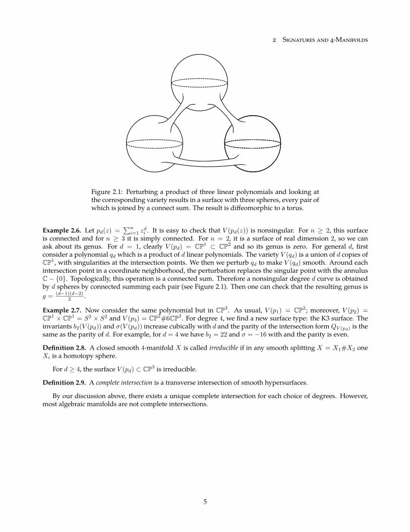
Figure 2.1: Perturbing a product of three linear polynomials and looking atthe corresponding variety results in a surface with three spheres, every pair ofwhich is joined by a connect sum. The result is diffeomorphic to a torus.

Example 2.6. Let pd(z) =∑ni=1 z

di . It is easy to check that V (pd(z)) is nonsingular. For n ≥ 2, this surface

is connected and for n ≥ 3 it is simply connected. For n = 2, it is a surface of real dimension 2, so we canask about its genus. For d = 1, clearly V (pd) = CP1 ⊂ CP2 and so its genus is zero. For general d, firstconsider a polynomial qd which is a product of d linear polynomials. The variety V (qd) is a union of d copies ofCP1, with singularities at the intersection points. We then we perturb qd to make V (qd) smooth. Around eachintersection point in a coordinate neighborhood, the perturbation replaces the singular point with the annulusC − 0. Topologically, this operation is a connected sum. Therefore a nonsingular degree d curve is obtainedby d spheres by connected summing each pair (see Figure 2.1). Then one can check that the resulting genus isg = (d−1)(d−2)

2 .

Example 2.7. Now consider the same polynomial but in CP3. As usual, V (p1) = CP2; moreover, V (p2) =CP1 × CP1 = S2 × S2 and V (p3) = CP2#6CP2. For degree 4, we find a new surface type: the K3 surface. Theinvariants b2(V (pd)) and σ(V (pd)) increase cubically with d and the parity of the intersection formQV (pd) is thesame as the parity of d. For example, for d = 4 we have b2 = 22 and σ = −16 with and the parity is even.

Definition 2.8. A closed smooth 4-manifold X is called irreducible if in any smooth splitting X = X1#X2 oneXi is a homotopy sphere.

For d ≥ 4, the surface V (pd) ⊂ CP3 is irreducible.

Definition 2.9. A complete intersection is a transverse intersection of smooth hypersurfaces.

By our discussion above, there exists a unique complete intersection for each choice of degrees. However,most algebraic manifolds are not complete intersections.

5


2.3 Unimodular Forms v

The following is an important example of an even symmetric bilinear form of rank 8

E8 =

⟨

2 1 0 0 0 0 0 01 2 1 0 0 0 0 00 1 2 1 0 0 0 00 0 1 2 1 0 0 00 0 0 1 2 1 0 10 0 0 0 1 2 1 00 0 0 0 0 1 2 00 0 0 0 1 0 0 2

⟩

As an exercise, diagonalize this matrix overQ and show that its determinant is 1. Therefore it is unimodular.The diagonalization will also show that it is positive definite (i.e. b+ = 8 and b− = 0). Therefore its signature is8 as well. We would like to understand if there is a closed manifold X whose intersection form is E8.

2.3.1 Indefinite Forms

Example 2.10. Some examples of indefinite unimodular forms that we can now make are:

⊕k〈1〉 ⊕ `〈−1〉

±(⊕kE8 ⊕ `H), (H = QS2×S2)

The first class of signatures can be any rank, any signature, and are odd. The second class can realize any rank,have signature divisible by 8 and are even.

Theorem 2.11. Indefinite forms are classified by their rank, signature, and parity.

As a result, since the second Betti number, signature and parity of a K3 surface are known, we can concludefrom the above theorem that QK3

∼= −(⊕2E8 ⊕ 3H). The following theorem completes our classification ofindefinite forms:

Theorem 2.12. If Q is an even unimodular symmetric bilinear form, then σ(Q) is divisible by 8.

Consider any unimodular symmetric bilinear form Q on A ∼= Zn, we can reduce mod 2 to get Q|2 overA|2 = A ⊗ Z/2 = Z/2n. Given x, y ∈ A|2, then (x + y)2 = x2 + y2 in A|2. Therefore φ : A|2 → Z/2 sendingy 7→ y2 is a homomorphism. Since φ ∈ (A|2)∗, we can represent it as (−) · x for some unique x ∈ A|2. A lift of xto A is known as a characteristic element:

Definition 2.13. A characteristic element of A is any x ∈ A such that for all y ∈ A, x · y ≡ y · y mod 2.

We have just shown that characteristic elements always exist and form a coset of 2A in A.

Lemma 2.14. If x is characteristic for Q, a unimodular symmetric bilinear form, then x2 ≡ σ(Q) mod 8.

Proof:We first make the observation that if x and y are characteristic elements forQ1 andQ2, respectively, thenx+y is characteristic forQ1⊕Q2. Now consider the formQ′ = Q⊕〈1〉⊕〈−1〉. This is odd and indefiniteand thus by Theorem 2.11 and Example 2.10, it is isomorphic to⊕k〈1〉⊕`〈−1〉. Clearly the Lemma is truefor 〈1〉 and 〈−1〉. Therefore the square of the characteristic element x′ of Q′ is the sum of the squares ofthe characteristic elements of the 〈±1 components, which shows x′2 = k− `. By the way we constructedQ′, the characteristic element x of Q has the same square as x′, therefore (x′)2 = x2 = k − ` = σ(Q′).Moreover, σ(Q) = σ(Q′).

Finally, we claim that if x and y are characteristic, then x2 ≡ y2 mod 8. This follows by writingy = x+ 2z and expanding.

6


Proof of Theorem 2.12:If Q is even, then 0 is characteristic for Q, hence by the above lemma 0 = 02 ≡ σ(Q) mod 8.

2.3.2 Definite Forms

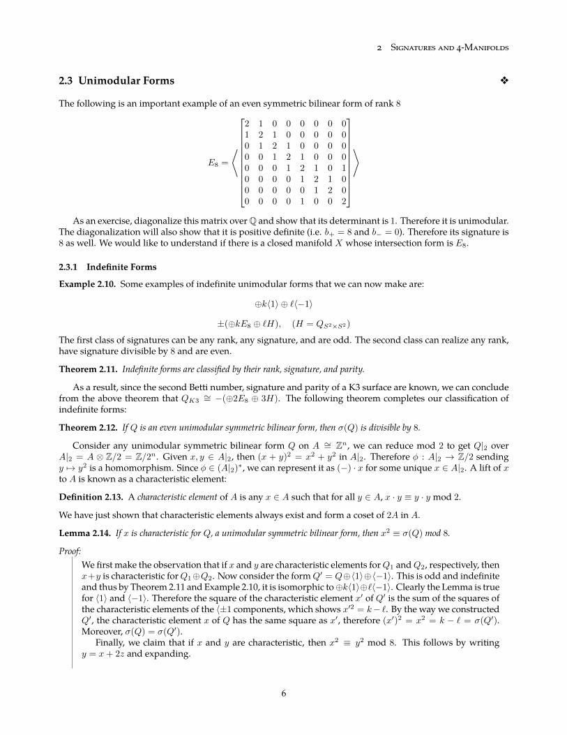
In the definite case, |σ(Q)| = rank(Q). Since we know that σ(Q) must be divisible by 8, the number of positivedefinite even forms is given in Figure 2.2. For even or odd definite forms, the number of forms of a particularrank is finite; however, the number grows very fast with the rank, unlike what we foundwith the indefinite case.

Rank Number of even, positive definite forms8 116 224 24...

...40 > 1050

Figure 2.2: Number of positive definite even unimodular forms of a given rank.The number grows super exponentially.

2.4 Realizing Unimodular Forms v

The connection between unimodular forms and classifying topological 4-manifolds was solved by Freedman inthe 1980’s. His classification is stated as follows:

1. Every even form is realized by exacly one such manifold.

2. Every odd form is realized by exactly two such manifolds, distinguished by the Kirby-Siebermann invari-ant ks ∈ H4(X;Z/2) ∼= Z/2.

We will return to this in more detail later in the course. Work on topological manifolds and smooth manifoldsin the mid 20th century led to the discovery that ks(X) 6= 0 ⇒ X not smoothable. Therefore, as a corollary ofFreedman’s classification, there exist closed simply connected topological 4-manifoldswith no smooth structure.

Theorem 2.15 (Rokhlin). Every closed, smooth, simply connected even 4-manifold has signature divisible by 16.

If X is even and simply connected (not necessarily smoothable), then ks(X) = σ(X)/8 mod 2, so Rokhlin’stheorem can be seen as a precursor to the Kirby-Siebermann invariant.

Theorem 2.16 (Donaldson). If a closed, oriented, smooth 4-manifold has a definite form, then it is diagonalizable over Z.

Corollary 2.17. Every closed, simply connected, odd, smooth 4-manifold is homeomorphic to #± CP2.

This follows from the fact that the odd indefinite forms from Example 2.10 are diagonalizable and the evenindefinite forms from that Example are not diagonalizable.

7

3. Handlebodies and Kirby Diagramsv

Definition 3.1. Given manifolds X,Y and an embedding φ0 : Y → int(X), an isotopy of φ0 is a homotopyφt : Y → X through embeddings defined at t = 0.

Theorem 3.2 (Smooth Isotopy Extension). Given an isotopy φt : Y → int(X) with Y compact, then this extends to anambient isotopy; i.e. there exists an isotopy Φt : X → X through diffeomorphisms such that Φ0 = idX and Φt φ0 = φtfor all t. Moreover, Φt has compact support in the interior of X .

For a proof, see [1]

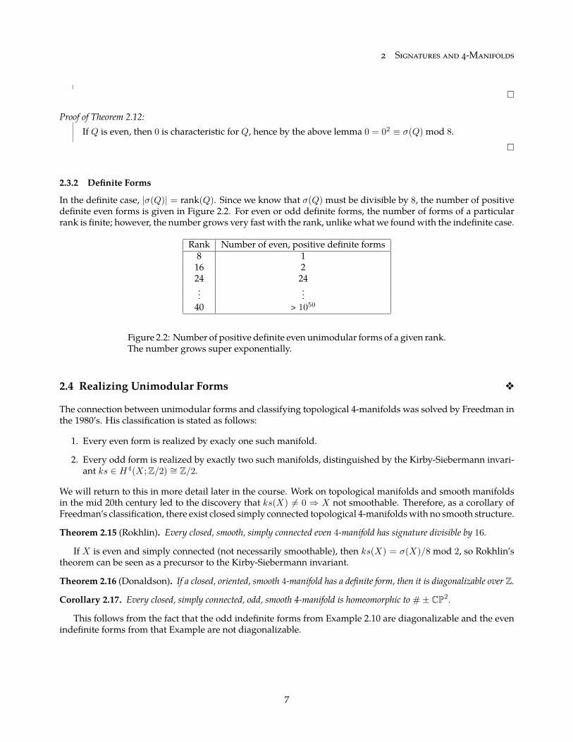
Definition 3.3. An n-dimensional k-handle is H = Dk × Dn−k attached to a manifold Xn by an embeddingφ : ∂Dk ×Dn−k → ∂X (the resulting space is denotedX ∪φH). The core of the handle isDk ×0, the attachingsphere is ∂Dk×0, the attaching region is ∂Dk×Dn−k, the cocore is 0×Dn−k, and the belt sphere is 0×∂Dn−k

(see Figure 3.1).

Belt sphere

Attaching sphere

Cocore Core

Figure 3.1: Anatomy of a handle [1].

Remark 3.4. As described in the above definition, the resultingmanifold with an n handle has corners. However,there is a canonical way to smooth such a manifold, which we relegate to [1]. Therefore we take any manifoldwith a handle attached to be smooth in this context.Remark 3.5. In the homotopy category, the attaching of a k-handle is the same as attaching a k-cell (i.e. theyare homotopic). However, we want the thickness of a handle so that we can smooth the resulting manifold andwork in the smooth category.

Proposition 3.6. If (H,φ) is a k-handle, the diffeomorphism type of X ∪φ H is determined by the isotopy class of φ.

Proof:We work in a collar I × ∂X of ∂X inX . Gluing a handle (H,φ0) on 0 × ∂X and (H,φ1) on 1 × ∂X ,we can take an isotopy φt of φ0 and φ1 and extend it to the collared X via the Isotopy Extension Theorem.This produces the desired diffeomorphism. For details see [1].

8

3 Handlebodies and Kirby Diagrams

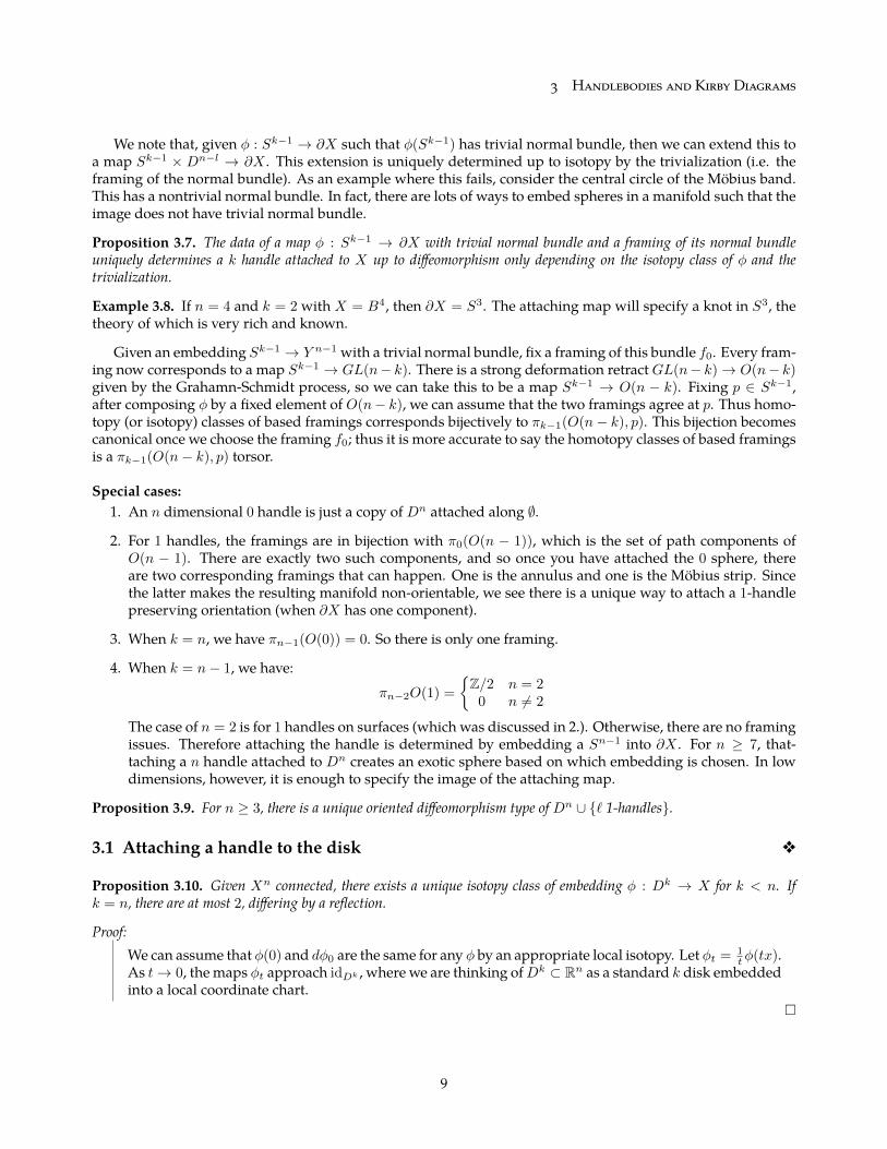
We note that, given φ : Sk−1 → ∂X such that φ(Sk−1) has trivial normal bundle, then we can extend this toa map Sk−1 × Dn−l → ∂X . This extension is uniquely determined up to isotopy by the trivialization (i.e. theframing of the normal bundle). As an example where this fails, consider the central circle of the Möbius band.This has a nontrivial normal bundle. In fact, there are lots of ways to embed spheres in a manifold such that theimage does not have trivial normal bundle.

Proposition 3.7. The data of a map φ : Sk−1 → ∂X with trivial normal bundle and a framing of its normal bundleuniquely determines a k handle attached to X up to diffeomorphism only depending on the isotopy class of φ and thetrivialization.

Example 3.8. If n = 4 and k = 2 with X = B4, then ∂X = S3. The attaching map will specify a knot in S3, thetheory of which is very rich and known.

Given an embedding Sk−1 → Y n−1 with a trivial normal bundle, fix a framing of this bundle f0. Every fram-ing now corresponds to a map Sk−1 → GL(n− k). There is a strong deformation retractGL(n− k)→ O(n− k)given by the Grahamn-Schmidt process, so we can take this to be a map Sk−1 → O(n − k). Fixing p ∈ Sk−1,after composing φ by a fixed element of O(n− k), we can assume that the two framings agree at p. Thus homo-topy (or isotopy) classes of based framings corresponds bijectively to πk−1(O(n− k), p). This bijection becomescanonical once we choose the framing f0; thus it is more accurate to say the homotopy classes of based framingsis a πk−1(O(n− k), p) torsor.

Special cases:1. An n dimensional 0 handle is just a copy of Dn attached along ∅.

2. For 1 handles, the framings are in bijection with π0(O(n − 1)), which is the set of path components ofO(n − 1). There are exactly two such components, and so once you have attached the 0 sphere, thereare two corresponding framings that can happen. One is the annulus and one is the Möbius strip. Sincethe latter makes the resulting manifold non-orientable, we see there is a unique way to attach a 1-handlepreserving orientation (when ∂X has one component).

3. When k = n, we have πn−1(O(0)) = 0. So there is only one framing.

4. When k = n− 1, we have:πn−2O(1) =

Z/2 n = 2

0 n 6= 2

The case of n = 2 is for 1 handles on surfaces (which was discussed in 2.). Otherwise, there are no framingissues. Therefore attaching the handle is determined by embedding a Sn−1 into ∂X . For n ≥ 7, that-taching a n handle attached to Dn creates an exotic sphere based on which embedding is chosen. In lowdimensions, however, it is enough to specify the image of the attaching map.

Proposition 3.9. For n ≥ 3, there is a unique oriented diffeomorphism type of Dn ∪ ` 1-handles.

3.1 Attaching a handle to the disk v

Proposition 3.10. Given Xn connected, there exists a unique isotopy class of embedding φ : Dk → X for k < n. Ifk = n, there are at most 2, differing by a reflection.

Proof:We can assume that φ(0) and dφ0 are the same for any φ by an appropriate local isotopy. Let φt = 1

tφ(tx).As t→ 0, the maps φt approach idDk , where we are thinking ofDk ⊂ Rn as a standard k disk embeddedinto a local coordinate chart.

9


Corollary 3.11. There is a unique unknotted embedding Sk−1 → Sn−1 when k < n.

If we attach a k-handle H to Dn = Dk ×Dn−k along an unknotted Sk−1, without loss of generality we canassume the attaching map sends Sk−1 × Dn−k ⊂ H to Sk−1 → Dn−k ⊂ Dn. Collapsing the Dn−k dimensionof the resulting space produces a Dn−k bundle over Sk with structure group O(n − k)1. In fact, every Dn−k

bundle over Sk arises this way. Therefore manifolds obtained by attaching a handle to a disk are classified bydisk bundles over a sphere.

Example 3.12. Recall attaching a 1 handle to D1 gave either an annulus or a Möbius band; these are the onlytwo disk bundles over S1 up to diffeomorphism. This classification holds for attaching a 1 handle to any Dn.

Example 3.13. Now consier a 2 handle attached to Dn. The structure group is π1(O(n− 2)), which is:

π1(O(n− 2)) =

0 n ≤ 3Z n = 4Z/2 n ≥ 5

Forn = 4, theZ structure groupdescribes the twisting of the framing aroundS2. Each elementn ∈ Zdeterminesthe resulting 4manifoldXn, wherewe arewritingX0 = S2×D2 (the trivialD2 bundle). The next exercise showsthat the intersection forms are:

QXn∼= 〈[n]〉

Additionally, the Euler number of Xn is n.

Exercise 3.14. Let Xn be a manifold constructed in the previous example. Show that H2(Xn) ∼= Z and thatQXn

∼= 〈[n]〉. A solution can be found in Appendix A.2.

More generally, considerDm bundles overS2 form ≥ 3. The structure group is nowπ1(O(m)) = π2(SO(m)) =Z/2. Therefore we end up with exactly two classes of S2 bundles: S2 × Dm and S2×Dm. Each of these hasboundary S2 × Sm−1 and S2×Sm−1. In particular, we care about the case withm = 3, which is the four mani-fold S2×S2.

3.2 Handlebodies v

Definition 3.15. A handlebody is a compact manifoldXn exhibited as built by handles from ∅. IfX has boundary∂X = ∂−X t ∂+X , then a relative handlebody is an exhibition of X built by attaching handles to I × ∂−X .

Theorem 3.16. Every smooth compact manifold X has a handle decomposition (or relative handle decomposition).

The proof of this idea uses Morse theory. Start with a smooth f : X → I with f−1(0) = ∂−X and f−1(1) =∂+X . Then f can be perturbed generically so that the critical points are nondegenerate and quadratic having alocal model f(x1, ..., xn) = −

∑ki=1 x

2i +

∑ni=k+1 x

2i . The integer k is called the index of the critical point. One

can show that fo each critical point of index k corresponds to attaching a k-handle. There is a similar theoremand proof in the PL (piecewise linear) category as well.

Theorem 3.17. Every TOP n-manifold admits a handle decomposition except for unsmoothable such 4-manifolds.

Example 3.18. There is a handle decomposition of CPn given by considering the coordinate patches ψi : Cn →CPn, (z1, ..., zn) 7→ [z1 : ... : 1 : ... : zn]. LetD ⊂ C be the unit disk and consider the “poly disk”D×....×D ⊂ Cn.For each i let Bi = ψi(D × ... ×D) ⊂ CPn. Normalize homogeneous coordinates on CPn so that each |zi| ≤ 1and there exists at least one coordinate with |zi| = 1. This shows that CPn =

⋃ni=0Bi. The Bi intersect only on

their boundaries. We can think of B0 as a 0-handle, B1 as a 2-handle attached to it along ψ0(S1 ×D × ...×D).Repeating this, we see that each Bk is a 2k handle attached to

⋃k−1i=0 Bi. This exhibits the handle decomposition

of CPn and the reader will note that it mimics the cell decomposition of CPn.1Equivalently, a rank n− k vector bundle over Sk .

10


Example 3.19. In the case of CP2, the decomposition is 0-handle ∪ 2-handle ∪ 4-handle. By our analysis in theprevious section, this is some surface Xn with a 4-handle attached. It turns out that n = 1. Since ∂X1 = S3,restricting the S2 bundle X1 to its boundary gives the Hopf fibration S1 → S3 → S2.

Exercise 3.20. Exhibit a handlebodydecomposition of the torusT 2 andRP2. See [1] for hints andmore examples.

Theorem 3.21. Every handlebody can be perturbed so that the handles are attached in order of increasing index.

Proof:Suppose H is a k handle and G is an ` handle with l ≤ k and consider (X ∪ H) ∪ G. We would liketo show that this is isotopic to (X ∪ G) ∪ H . The belt sphere of H has dimension n − k + 1 and thedimension of the attaching sphere of G is ` − 1. The sum of these dimensions is n + (` − k) − 2. Sincel ≤ k, this sum is less than n − 1 = dim ∂X . Therefore the belt sphere of H and the attaching sphereof G can be taken to be disjoint by transversality. Now we can construct an isotopy that pushes G off ofH by flowing along a vector field that pushes off of the cocore of H . Thus in gluing G to X ∪H we canassume that H and G are disjoint, proving the claim.

We assume from now on that handlebodies are constructed by attaching handles by increasing index.

Definition 3.22. Given a handle decomposition of (X, ∂−X), there is a dual decomposition of (X, ∂+X) given by“turning X upside down.” Begin with a collar I × ∂+X glued to X alon ∂+X and remove the collar I × ∂−Xon which the handlebody is built. Then notice that every k handle of the decomposition corresponds can bethought of as an (n− k) handle glued to the part of X above it.

3.3 Handle operations v

In this subsection we describe two important handle operations: cancellation and sliding. Consider a manifoldX with a copy of Dn = Dk × Dn−k boundary connected summed to ∂X along the lower hemisphere Dk−1

−of ∂Dk = Sk−1. This does not change the diffeomorphism type of X , since it is gluing along a contractibleregion. Now take a neighborhood of the upper hemisphere Dk−1

+ of ∂Dk, which gives us the decompositionDk = Dk

0 ∪Dk−1+

Dk−1+ × I . ThenDk−1

+ × I ×Dn−k is a k− 1 handle attached to ∂X andDk0 ×Dn−k is a k handle

attached to that. This is an example of a cancelling pair of handles (see [1] Figure 4.7).

Proposition 3.23. A k − 1 handle hk−1 and a k handle hk can be cancelled providing that the attaching sphere of hkinterescts the belt sphere of hk−1 transversely at a single point.

A proof of this Proposition can be found in [1]. Recall from our proof of Theorem 3.21 that we were able toconstruct a slide of one handle off of another. This is an example of a more general operation called a handleslide. Given two handles h1 and h2 of the same index attached to ∂X , a handle slide of h1 over h2 is the operationof moving the attaching sphere A of h1 across the belt sphere B of h2 through isotopy. Since h1 and h2 have thesame index, there is a point p at which h1 and h2 intersect transversely and at which their tangent spaces spana codimension 1 subspace. Therefore there are exactly two directions to push A off of B to make them disjoint(as in the proof of Proposition 3.21) in a handle slide procedure.

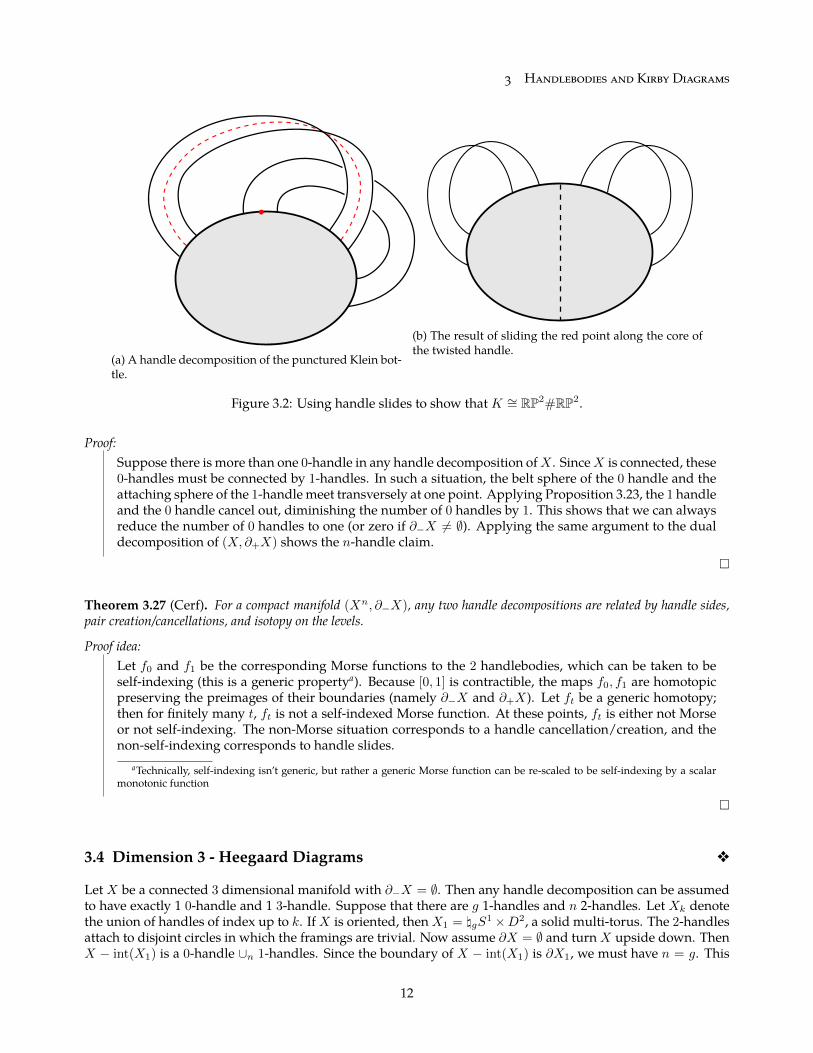
Example 3.24. TheKlein bottleK has a handle decomposition given by attaching two 1 handles, onewith a twist,toD2 (shown in the left of Figure 3.2) and 2 handle to cap it off. Using a handle slide, we can slide the untwistedhandle along the core of the twisted handle to untangle the handles (shown on the right). What results is twotwisted handles that are attached to a disk. The resulting space can then be interpreted as the boundary sumof two copies puctured RP2’s (the dotted line indicating where the sum is taking place). Attaching the final 2handle, we have shown thatK ∼= RP2#RP2.

Exercise 3.25. Classify compact dimension 2 manifolds using handle slide theory.

Proposition 3.26. Every compact connected (X, ∂−X) has a relative handle decomposition with no 0-handles if ∂−X 6= ∅and exactly one 0-handle if ∂−X = ∅. Moreover, there is exactly 1 n-handle if ∂+X = ∅ and no n-handle if ∂+X 6= ∅.

11


(a) A handle decomposition of the punctured Klein bot-tle.

(b) The result of sliding the red point along the core ofthe twisted handle.

Figure 3.2: Using handle slides to show thatK ∼= RP2#RP2.

Proof:Suppose there is more than one 0-handle in any handle decomposition ofX . SinceX is connected, these0-handles must be connected by 1-handles. In such a situation, the belt sphere of the 0 handle and theattaching sphere of the 1-handle meet transversely at one point. Applying Proposition 3.23, the 1 handleand the 0 handle cancel out, diminishing the number of 0 handles by 1. This shows that we can alwaysreduce the number of 0 handles to one (or zero if ∂−X 6= ∅). Applying the same argument to the dualdecomposition of (X, ∂+X) shows the n-handle claim.

Theorem 3.27 (Cerf). For a compact manifold (Xn, ∂−X), any two handle decompositions are related by handle sides,pair creation/cancellations, and isotopy on the levels.

Proof idea:Let f0 and f1 be the corresponding Morse functions to the 2 handlebodies, which can be taken to beself-indexing (this is a generic propertya). Because [0, 1] is contractible, the maps f0, f1 are homotopicpreserving the preimages of their boundaries (namely ∂−X and ∂+X). Let ft be a generic homotopy;then for finitely many t, ft is not a self-indexed Morse function. At these points, ft is either not Morseor not self-indexing. The non-Morse situation corresponds to a handle cancellation/creation, and thenon-self-indexing corresponds to handle slides.

aTechnically, self-indexing isn’t generic, but rather a generic Morse function can be re-scaled to be self-indexing by a scalarmonotonic function

3.4 Dimension 3 - Heegaard Diagrams v

Let X be a connected 3 dimensional manifold with ∂−X = ∅. Then any handle decomposition can be assumedto have exactly 1 0-handle and 1 3-handle. Suppose that there are g 1-handles and n 2-handles. Let Xk denotethe union of handles of index up to k. IfX is oriented, thenX1 = \gS

1 ×D2, a solid multi-torus. The 2-handlesattach to disjoint circles in which the framings are trivial. Now assume ∂X = ∅ and turnX upside down. ThenX − int(X1) is a 0-handle ∪n 1-handles. Since the boundary of X − int(X1) is ∂X1, we must have n = g. This

12


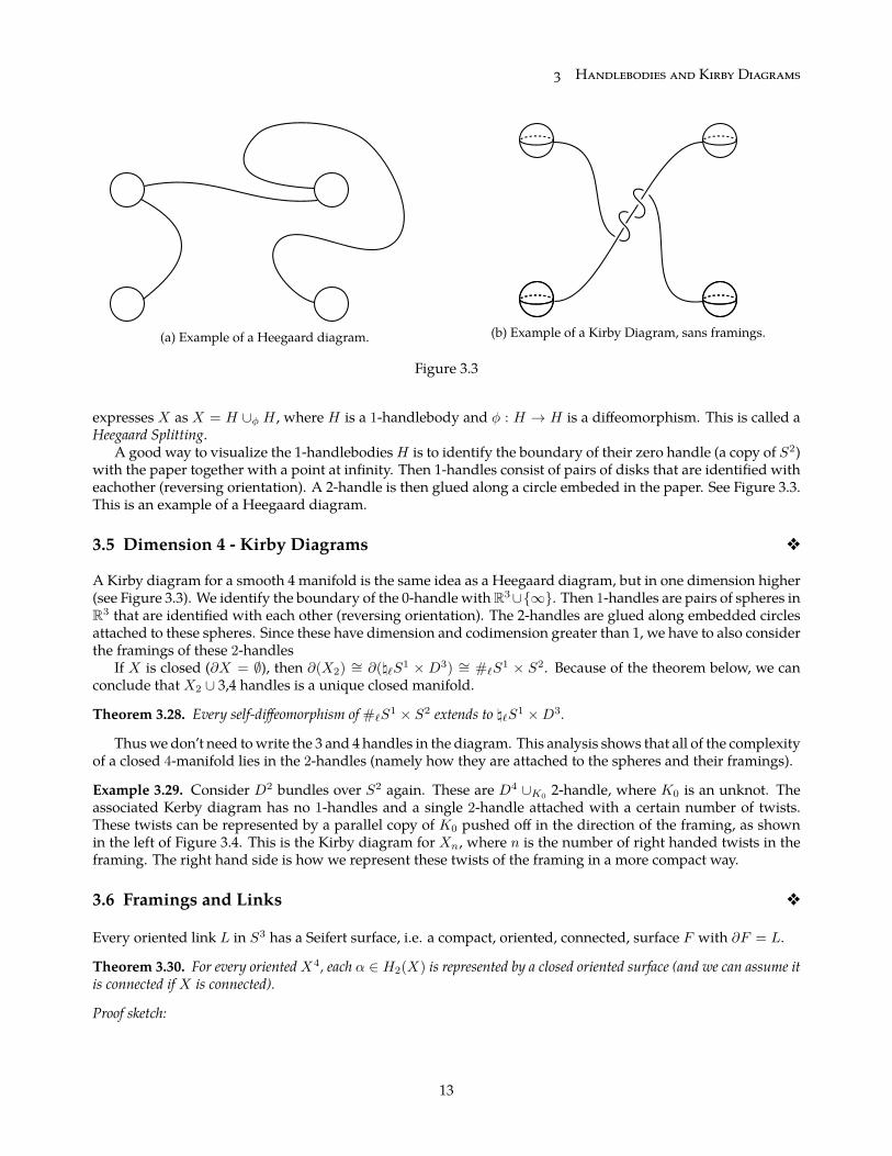
(a) Example of a Heegaard diagram. (b) Example of a Kirby Diagram, sans framings.

Figure 3.3

expresses X as X = H ∪φ H , where H is a 1-handlebody and φ : H → H is a diffeomorphism. This is called aHeegaard Splitting.

A good way to visualize the 1-handlebodiesH is to identify the boundary of their zero handle (a copy of S2)with the paper together with a point at infinity. Then 1-handles consist of pairs of disks that are identified witheachother (reversing orientation). A 2-handle is then glued along a circle embeded in the paper. See Figure 3.3.This is an example of a Heegaard diagram.

3.5 Dimension 4 - Kirby Diagrams v

A Kirby diagram for a smooth 4 manifold is the same idea as a Heegaard diagram, but in one dimension higher(see Figure 3.3). We identify the boundary of the 0-handle withR3∪∞. Then 1-handles are pairs of spheres inR3 that are identified with each other (reversing orientation). The 2-handles are glued along embedded circlesattached to these spheres. Since these have dimension and codimension greater than 1, we have to also considerthe framings of these 2-handles

If X is closed (∂X = ∅), then ∂(X2) ∼= ∂(\`S1 × D3) ∼= #`S

1 × S2. Because of the theorem below, we canconclude that X2 ∪ 3,4 handles is a unique closed manifold.

Theorem 3.28. Every self-diffeomorphism of #`S1 × S2 extends to \`S1 ×D3.

Thuswe don’t need towrite the 3 and 4 handles in the diagram. This analysis shows that all of the complexityof a closed 4-manifold lies in the 2-handles (namely how they are attached to the spheres and their framings).

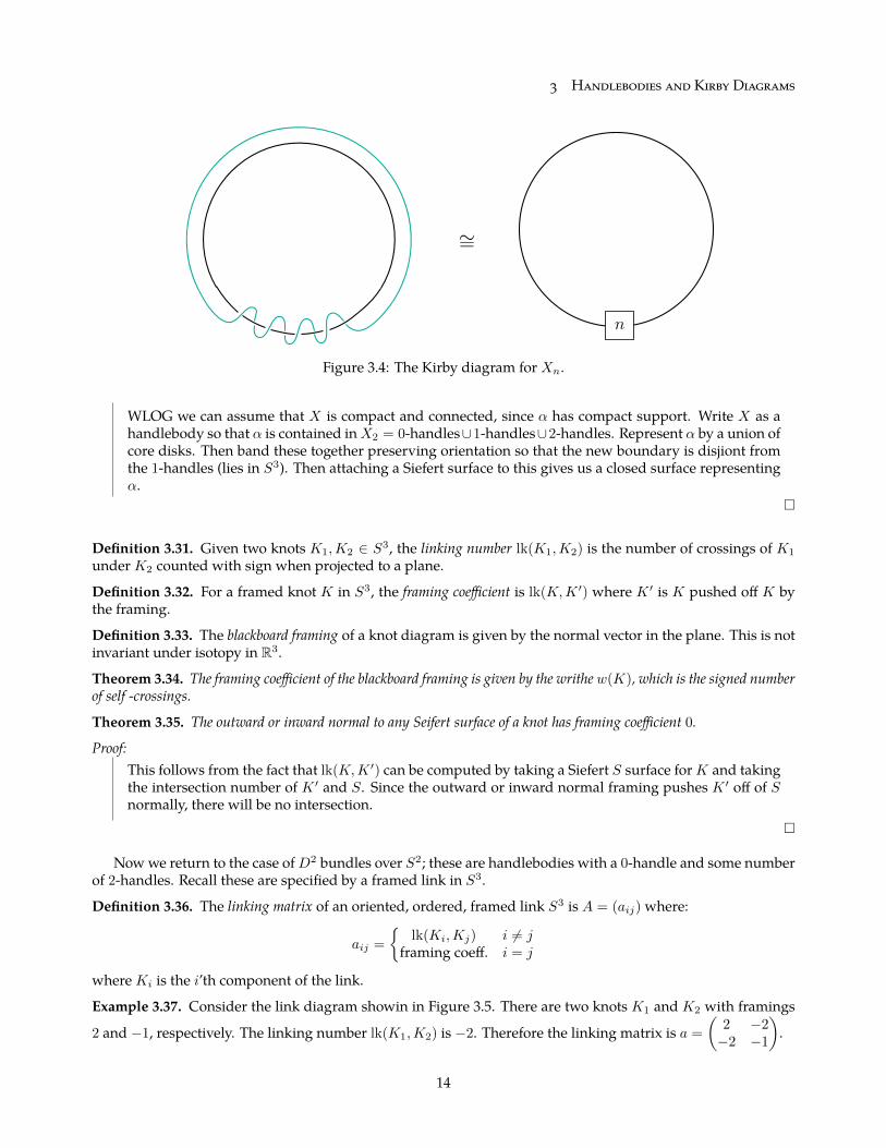
Example 3.29. Consider D2 bundles over S2 again. These are D4 ∪K02-handle, where K0 is an unknot. The

associated Kerby diagram has no 1-handles and a single 2-handle attached with a certain number of twists.These twists can be represented by a parallel copy of K0 pushed off in the direction of the framing, as shownin the left of Figure 3.4. This is the Kirby diagram for Xn, where n is the number of right handed twists in theframing. The right hand side is how we represent these twists of the framing in a more compact way.

3.6 Framings and Links v

Every oriented link L in S3 has a Seifert surface, i.e. a compact, oriented, connected, surface F with ∂F = L.

Theorem 3.30. For every orientedX4, each α ∈ H2(X) is represented by a closed oriented surface (and we can assume itis connected if X is connected).

Proof sketch:

13


∼=

n

Figure 3.4: The Kirby diagram for Xn.

WLOG we can assume that X is compact and connected, since α has compact support. Write X as ahandlebody so that α is contained inX2 = 0-handles∪1-handles∪2-handles. Represent α by a union ofcore disks. Then band these together preserving orientation so that the new boundary is disjiont fromthe 1-handles (lies in S3). Then attaching a Siefert surface to this gives us a closed surface representingα.

Definition 3.31. Given two knots K1,K2 ∈ S3, the linking number lk(K1,K2) is the number of crossings of K1

underK2 counted with sign when projected to a plane.

Definition 3.32. For a framed knot K in S3, the framing coefficient is lk(K,K ′) where K ′ is K pushed off K bythe framing.

Definition 3.33. The blackboard framing of a knot diagram is given by the normal vector in the plane. This is notinvariant under isotopy in R3.

Theorem 3.34. The framing coefficient of the blackboard framing is given by the writhew(K), which is the signed numberof self -crossings.

Theorem 3.35. The outward or inward normal to any Seifert surface of a knot has framing coefficient 0.

Proof:This follows from the fact that lk(K,K ′) can be computed by taking a Siefert S surface forK and takingthe intersection number of K ′ and S. Since the outward or inward normal framing pushes K ′ off of Snormally, there will be no intersection.

Nowwe return to the case ofD2 bundles over S2; these are handlebodies with a 0-handle and some numberof 2-handles. Recall these are specified by a framed link in S3.

Definition 3.36. The linking matrix of an oriented, ordered, framed link S3 is A = (aij) where:

aij =

lk(Ki,Kj) i 6= j

framing coeff. i = j

whereKi is the i’th component of the link.

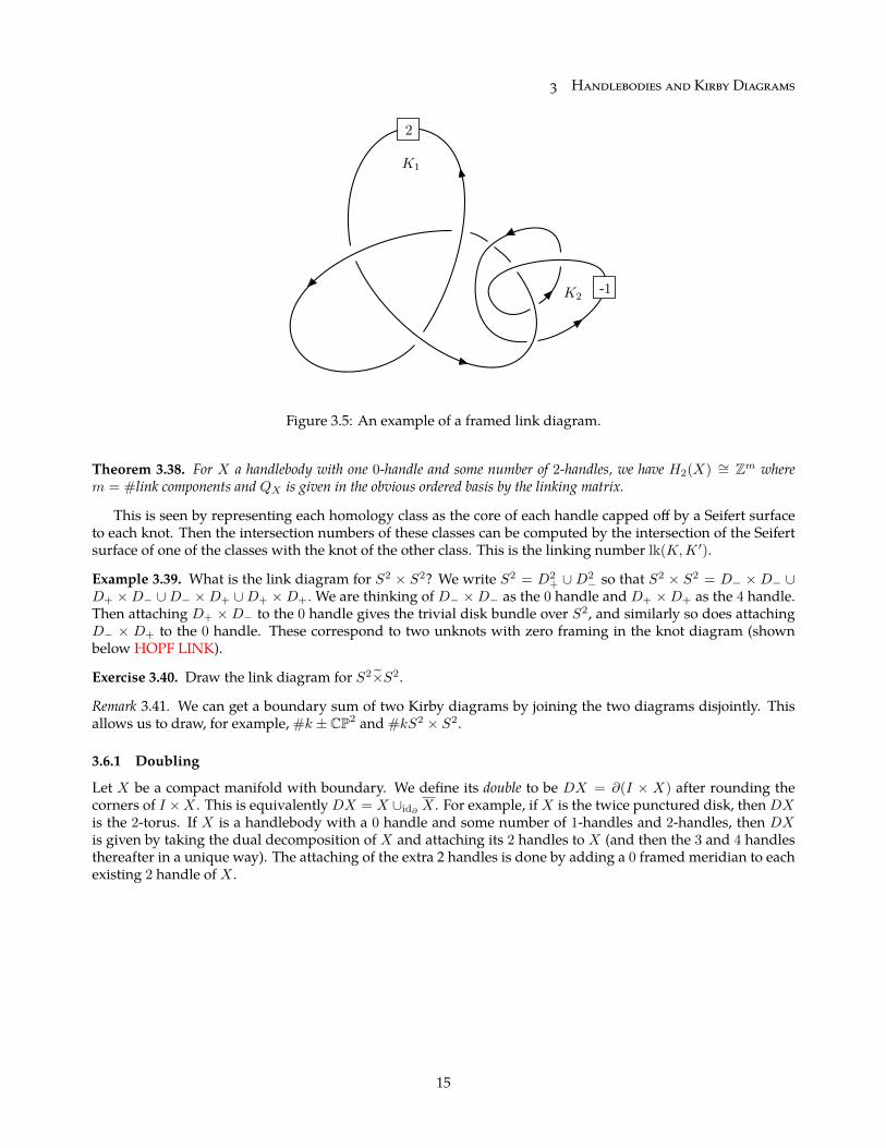
Example 3.37. Consider the link diagram showin in Figure 3.5. There are two knots K1 and K2 with framings

2 and −1, respectively. The linking number lk(K1,K2) is −2. Therefore the linking matrix is a =

(2 −2−2 −1

).

14


K1

2

K2-1

Figure 3.5: An example of a framed link diagram.

Theorem 3.38. For X a handlebody with one 0-handle and some number of 2-handles, we have H2(X) ∼= Zm wherem = #link components and QX is given in the obvious ordered basis by the linking matrix.

This is seen by representing each homology class as the core of each handle capped off by a Seifert surfaceto each knot. Then the intersection numbers of these classes can be computed by the intersection of the Seifertsurface of one of the classes with the knot of the other class. This is the linking number lk(K,K ′).

Example 3.39. What is the link diagram for S2 × S2? We write S2 = D2+ ∪D2

− so that S2 × S2 = D− ×D− ∪D+ ×D− ∪D− ×D+ ∪D+ ×D+.We are thinking of D− ×D− as the 0 handle and D+ ×D+ as the 4 handle.Then attaching D+ ×D− to the 0 handle gives the trivial disk bundle over S2, and similarly so does attachingD− × D+ to the 0 handle. These correspond to two unknots with zero framing in the knot diagram (shownbelow HOPF LINK).

Exercise 3.40. Draw the link diagram for S2×S2.

Remark 3.41. We can get a boundary sum of two Kirby diagrams by joining the two diagrams disjointly. Thisallows us to draw, for example, #k ± CP2 and #kS2 × S2.

3.6.1 Doubling

Let X be a compact manifold with boundary. We define its double to be DX = ∂(I × X) after rounding thecorners of I ×X . This is equivalentlyDX = X ∪id∂

X . For example, ifX is the twice punctured disk, thenDXis the 2-torus. If X is a handlebody with a 0 handle and some number of 1-handles and 2-handles, then DXis given by taking the dual decomposition of X and attaching its 2 handles to X (and then the 3 and 4 handlesthereafter in a unique way). The attaching of the extra 2 handles is done by adding a 0 framed meridian to eachexisting 2 handle of X .

15

4. Kirby Calculus and Surgery Theoryv

4.1 Blowups and Kirby Calculus v

Exercise 4.1. If P is the E8 plumbing, then P#CP2 is the diagram with lefthanded trefoil knot (framing −1)connected sum with CP2#7CP2. Hint: blow up at the fart left link of P .

Exercise 4.2. Given a framed link L ⊂ S3, prove any handle slide can be realized by blowing up and down ±1framed unknots.

The previous exercise shows that handle slides can be realized as an algebraic operation via the Kirby dia-gram. In a similar manner, handle cancellation can also visulized using the Kirby diagram (CANCELLATION-FIG).

Theorem 4.3. A 2-3 handle pair can be cancelled in a Kirby diagram of a closed oriented 4 manifold after handle slides ifand only if there exist slides producing the zero framed unknot separate from the rest of the diagram.

Exercise 4.4. a) If X = 0-handles ∪m 2-handles, then show DX ∼= #mS2 × S2 or #mCP2#mCP2.

b) If X = 01-handle ∪` 11-handles ∪ 2handles is simply connected, then DX#`S2 × S2 ∼= #mS2 × S2 or#mCP2#mCP2.

4.2 Surgery v

What happens to the boundary of a manifold when we attach a k-handle? Attaching a handle of one dimensionhigher than the boundary is an example of surgery on the boundary:

Definition 4.5. Given φ0 : S` → Mm a framed embedding (up to isotopy), this extends uniquely up to isotopyto φ : S` × Dm−` → Mm. Then an ` surgery on φ0 is the process of cutting out S` × int(Dm−1) and gluing inD`+1 × Sm−`−1 by idS`×Sm−`−1 .

Conversely, we can think of any surgery operation as attaching an `+1 handle to I×M and looking at ∂+M .Specifically, surgery on (Mm, φ0) is obtained fromM − int(S` ×Dm−`) by attaching an `+ 1 handle and anmhandle.

Theorem 4.6. Two closed, oriented dimension m manifolds are oriented (cobordant) if and only if they are related by asequence of surgeries (where 0 surgeries preserve orientation).

Proof Sketch:Given a cobordismW , take a morse function f such that f−1(0) = ∂−W and f−1(1) = ∂+W and buildthe handle structure in the usual way via critical points. The other direction works in the opposite way;take a morse function that realizes the handle decomposition.

Corollary 4.7. Two oriented 4-manifolds are related by surgery if and only if they have the same signature.

Theorem 4.8. Suppose N ⊂ M is a properly embedded submanifold of codimension r. Then the map i∗π1(M −N) →π1(M) is an isomorphism if r ≥ 3 and an epimorphism if r = 2. Moreover, when r = 2, then ker(i∗) is generated bymeridians of N connected to the basepoint.

Proof:

16

4 Kirby Calculus and Surgery Theory

Given α ∈ π1(M), if r ≥ 2, then α is represented by a loop disjoint fromN by dimension considerations.Therefore i∗ is onto. If r ≥ 3, then every map of a disk can be assumed disjoint from N . Thereforeanything in the kernel of i∗, which has a bounding disk inM that can be perturbed to be disjoint fromN , is zero. The remainder of the proof is left as an exercise.

Given an orientable manifold Mm with m ≥ 4 and a map⊔k

1 S1 → M , let M ′ be obtained by surgery on

these circles. Then we claim that π1(M ′) ∼= π1(M)/〈γ1, ..., γk〉, where γ1 is the homotopy class of the ith circle inπ1(M). This follows from the fact that removing int(S1 ×Dm−1) does not affect change π1(M) by the previoustheorem (the circle have codimension 3). But then gluing in the handles annhilates the circles in homotopy.

Theorem 4.9. Form ≥ 4 every finitely presented group G is π1(M) for some closed, smooth, orientedMm.

Proof:First create #nS

1 × Sm−1 where n is the number of generators of G. The fundamental group is nowthe free group on the number of generators. Then we can represent the relators by embedded circlesand surger them out. The resulting manifold XG is the boundary XG = ∂WG where WG has 0,1 and2 handles. In fact, WG = I × YG = DYG where YG is a 4-manifold with a 0 handle, k 1-handles and `2-handles (where k is the number of generators and ` is number of relations). The surgery to kill therelators can be represened in a Kirby diagram of YG by attaching various 2 handles. Then doubling givesa Kirby diagram for XG.

If we choose to do this construction on the balanced trivial presentation (with k = `), thenW is contractiblebecause it is simply connected andhas no homologypast dimension two2. Therefore ∂W is homotopy equivalentto S4. This implies it is homeomorphic to S4 by Freedman’s Theorem.

Theorem4.10. SupposeC ⊂ X4 is a nullhomotopic circle. Then surgery onC isX#S whereS = S2×S2 orS = S2×S2

depending on framing.

Proof:First note that generically homotopy⇒ isotopy for circleswhen n ≥ 4 for dimension reasons (by pushingoff the homotopy annuli off each other). Without loss of generality, writeX ∼= X#S4 andC = S1×p ⊂∂(D2 ×D3). Now surgery on C in S4 is ∂(D2 ×D3 ∪D2×∂0 D

2 ×D3), which is the boundary of a D3

bundle over S2. There are only two such manifolds: S2 × S2 and S2×S2.

Theorem 4.11. IfX is odd and simply connected, then both surgeries on a nullhomotopic circle yield diffeomorphic man-ifolds.

Proof:Simple connectivity and the Hurewicz theorem tell us that H2(X) ∼= π2(X). Observe that since QX isodd, there exists α ∈ H2(X) such that α2 is odd. By our first observation, α is represented by a sphereS with only transverse double point singularities. It is not hard to show that:

α2 = e(νS) + 2(#double points)

where e(−) is the Euler number. Therefore we conclude that e(νS) is odd. Going back to the nullho-motopic circle C, we can assume that C is the Arctic circle in S. When we push C down to the Southpolar cap, the framing of C changes by a sign since the normal bundle of S has an odd twist. There-

2k = ` implies that χ(M) = 1

17


fore performing on either the south or north cap of S gives the two possibilities of X#S2 × S2 andX#S2×S2.

An application of these theorems is:

Theorem 4.12 (Markov). There is no algorithm for classifying smooth, closed, oriented 4-manifolds.

Proof:Let P = 〈g1, ..., gk | r1, ..., r`〉 be a presentation. A fact from combinatorial group theory is that thereis no algorithm for determining whether P presents the trivial group. Construct XP = ∂WP suchthat π1(XP ) is presented by P , by Theorem 4.9. Let ZP be obtained by surgering out the 1 handles inXP . In other words, we are sending X1 = #kS

1 × D3 → #kD2 × S2. Thus ZP = 0-handle ∪k+` 2-

handles. By theorem 4.10, we have DZP#CP2 = #k+`S2×S2#CP2 = (k + ` + 1)CP2#(k + `)CP2. If

π1(X) is trivial, then by theorem 4.11, then DZP#CP2 ∼= X#(k + 1)CP2#kCP2. If π1(X) is not trivial,then π1(DZP ) = 1 and hence DZP#CP2 6∼= X#(k + 1)CP2#kCP2. Then if we have an algorithm thatdetermines if (k + ` + 1)CP2#(k + `)CP2 ∼= X#(k + 1)CP2#CP2, then that will in turn determine ifπ1(X) is trivial or not. Therefore such an algorithm can’t exist.

Theorem 4.13 (Wall). Suppose thatX,Y are smooth, closed, simply connected and oriented 4 manifolds withQX ∼= QY .Then:

(a) There exists k ∈ Z+ such that X#kS2 × S2 ∼= Y#kS

2 × S2 (X and Y are stably diffeomorphic).

(b) X and Y are h-cobordant, i.e. there exists a cobordismW fromX to Y with inclusionsX,Y →W that are homotopyequivalences.

Given any two closed simply connected 4manifolds, we can connect sumwith appropriate numbers of±CP2

to make the rank, signature, and pairity of thier intersection forms coincide. Since we can ensure that theseforms are indefinite, these three characteristics determine their forms and hence QX ∼= QY . Then applying thetheorem above proves:

Corollary 4.14. Any two closed, smooth, simply connected 4 manifolds are diffeomorphic after connect-summing withenough ±CP2.

Theorem 4.15 (Freedman). A simply connected h-cobordism between topological 4-manifoldsX,Y is homeomorphic toI ×X .

Theorem 4.16 (Freedman). Let Σ3 be a homology 3-sphere. Then Σ = ∂∆ for some contractible topological 4-manifold∆.

Proof:Look at Σ×S1 and S3×S1, which have the same homology. Note that π1(Σ×S1) = π1(Σ)×Z. Nowwesurger out π1(Σ) to getX ∼= S3×S1#kS2×S2, which is a homology equivalence. Now π1(X) ∼= Z. Weuse Freedman to surger out new S2×S2’s giving us a topologicalmanifold Y with the same homology asS3×S1 and π1(Y ) ∼= Z. Therefore Y is a homotopy equivalence to S3×S1. Now consider the universalcover Y ∼= S3 × R which contains a copy of Σ. One-point compactifying at each end gives S4 ⊃ Σ.Cutting this space along Σ and taking one component gives the required ∆.

18


4.3 Surgery in 3-manifolds v

Let Tn be the n-torus, which can be thought of as Rn/Zn. Notice that every element of SL(n,Z) gives an ori-entation preserving diffeomorphism of Tn. This gives an injection SL(n,Z) → π0(Diff+(Tn)) (the “diffeotopygroup of Tn”, which is the diffeomorphisms of Tn up to isotopy). This is in fact an isomorphism when n ≤ 3.This shows that there are lots of self-diffeomorphisms of T 2 = S1 × S1 = ∂(S1 ×D2).

Definition 4.17. ADehn surgery on a 3-manifoldM cuts out S1×D2 and glues it back in by any diffeomorphismof its boundary.

A solid torus S1 × D2 is determined by a framed knot. Note that a Dehn surgery the same as gluing a2-handle ∪ 3-handle to a new boundary S1 × S1, and therefore this gluing is determined by the image of aprimitive homology class α ∈ H1(S1×S1). We orient the knotK, which gives us a meridian µ and longitude λ.Now α = pµ+ qλ for some relatively prime p, q. Changing the orientation ofK flips the sign of λ and µ, but theresulting 3-manifold doesn’t change. Therefore only the pair ±(p, q) matters, which is to say that the rationalnumber pq ∈ Q ∪ ∞ uniquely determines the Dehn surgery. This is called the surgery coefficient or slope.

Remark 4.18. A link in S3 with elements of Q ∪ ∞ attached to the components uniquely determines a 3-manifoldM by applying Dehn surgery. This is called Dehn surgery diagram. If all coefficients are in Z (calledintegral Dehn surgery), thenM is exhibited as ∂(0-handle∪2-handles), where the framings of the 2 handles arethe surgery coefficients of the links.

Example 4.19. Surgery on any link inM with surgery coefficient∞ (i.e. q = 0) is a trivial operation.

Example 4.20. IfK is an unknot with the ratio −pq attached, the Dehn surgery produces the Lens space L(p, q).When q = 1, the space L(p, 1) is an S1 bundle over S2. As an exercise, show that L(2, 1) ∼= RP3.

Theorem 4.21. Ω3 = 0.

Proof sketch:Given a closed oriented 3-manifoldM , we can find an immersionM → R5. The singular set is a unionof circles. We surger on these circles to getM ′ ⊂ R5 withM ′ cobordant toM . SinceM ′ is a manifold ofcodimension 2, it admits a Seifert “hypersurface.” This shows thatM ′ (and henceM ) is null-cobordant.

Theorem 4.22. Integral Dehn surgery on S3 gives all closed oriented 3-manifolds.

Proof:GivenM closed and oriented, writeM = ∂X4 by above. Then we can surger out the 1 and 3 handles toensure that X = 0-handle ∪ 2-handles. ThereforeM can be obtained by integral Dehn surgery, since Xhas only 2 and 0 handles.

Theorem 4.23. Any two integral Dehn surgery diagrams of a fixedM3 are related by blowing up/down.

4.3.1 Rolfsen Moves and Slam Dunks

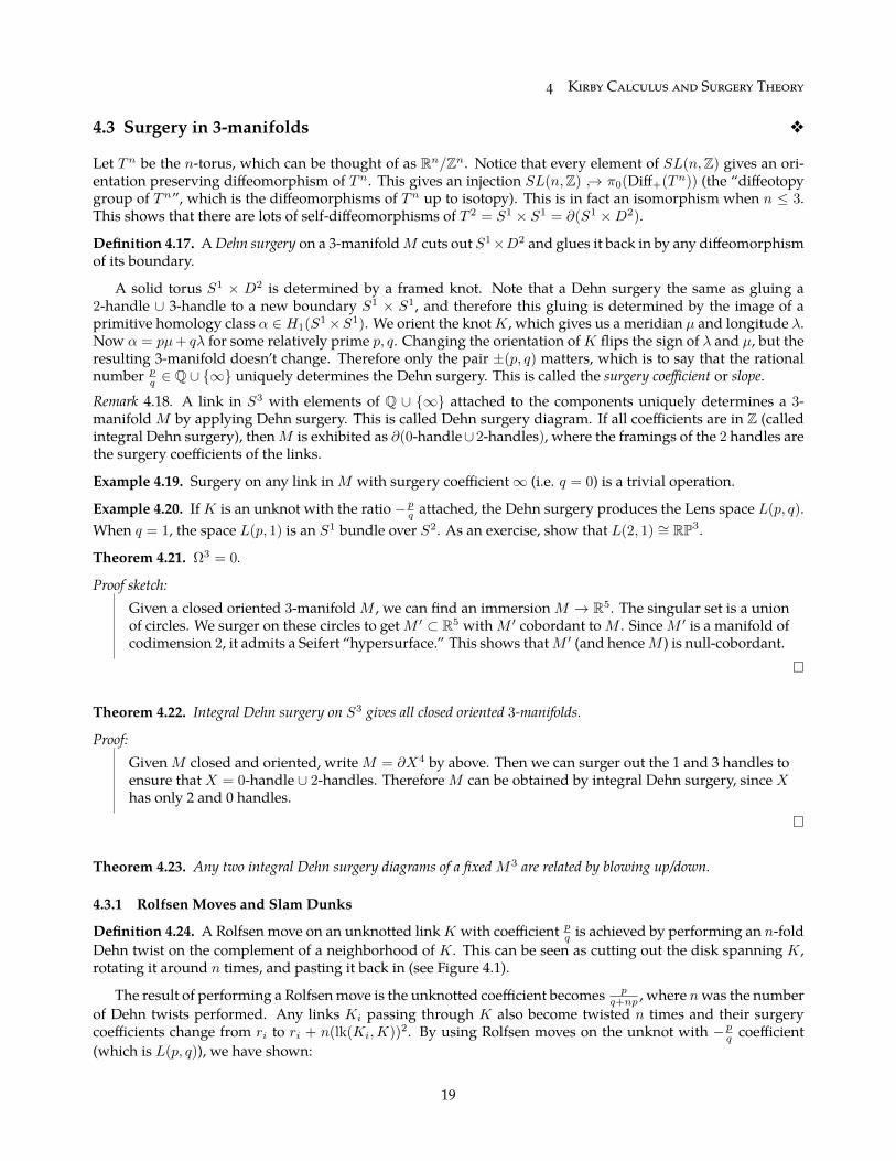
Definition 4.24. A Rolfsen move on an unknotted linkK with coefficient pq is achieved by performing an n-foldDehn twist on the complement of a neighborhood of K. This can be seen as cutting out the disk spanning K,rotating it around n times, and pasting it back in (see Figure 4.1).

The result of performing a Rolfsenmove is the unknotted coefficient becomes pq+np , where nwas the number

of Dehn twists performed. Any links Ki passing through K also become twisted n times and their surgerycoefficients change from ri to ri + n(lk(Ki,K))2. By using Rolfsen moves on the unknot with −pq coefficient(which is L(p, q)), we have shown:

19


−→

n

pq

pq+np

Figure 4.1: A Rolfsen twist, which is performed by applying an n-fold Dehntwist to the complement of the unknotted component (which is a torus).

Corollary 4.25. L(p, q) ∼= L(p, q + np).

A related operation is called the slam-dunk. LetK1,K2 be components of a link such thatK1 is a meridian ofK2 and let pq be the surgery coefficient ofK1. Also suppose that the surgery coefficient ofK2 is integral. IfM isthe manifold obtained by surgery on justK2, thenK1 is a knot inM . We can pull this knot into the gluing torusT ofK2 so that T is also a tubular neighborhood ofK1. But then performing the surgery onK1 is cutting out Tagain and gluing by p

q . We can instead combine the two gluings into one, and one can work out that the correctsurgery coefficient is n− q

p .

Exercise 4.26. Let K be the Hopf link where one link has coefficient 0 and the other has coefficient n. Showusing Slam Dunks that the resulting manifold by applying surgery is S3.

4.4 Spin Structures v

4.4.1 Constructing a Characteristic Class

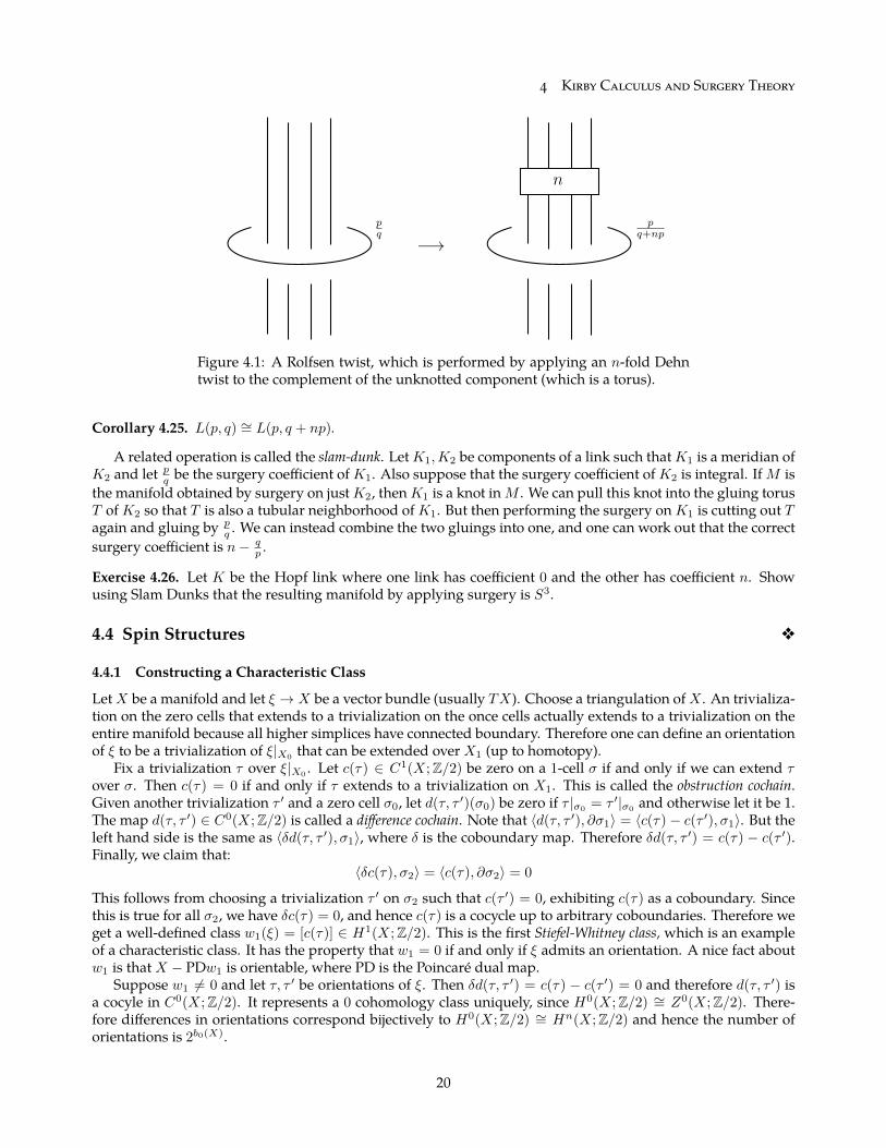
LetX be a manifold and let ξ → X be a vector bundle (usually TX). Choose a triangulation ofX . An trivializa-tion on the zero cells that extends to a trivialization on the once cells actually extends to a trivialization on theentire manifold because all higher simplices have connected boundary. Therefore one can define an orientationof ξ to be a trivialization of ξ|X0 that can be extended over X1 (up to homotopy).

Fix a trivialization τ over ξ|X0. Let c(τ) ∈ C1(X;Z/2) be zero on a 1-cell σ if and only if we can extend τ

over σ. Then c(τ) = 0 if and only if τ extends to a trivialization on X1. This is called the obstruction cochain.Given another trivialization τ ′ and a zero cell σ0, let d(τ, τ ′)(σ0) be zero if τ |σ0

= τ ′|σ0and otherwise let it be 1.

The map d(τ, τ ′) ∈ C0(X;Z/2) is called a difference cochain. Note that 〈d(τ, τ ′), ∂σ1〉 = 〈c(τ)− c(τ ′), σ1〉. But theleft hand side is the same as 〈δd(τ, τ ′), σ1〉, where δ is the coboundary map. Therefore δd(τ, τ ′) = c(τ) − c(τ ′).Finally, we claim that:

〈δc(τ), σ2〉 = 〈c(τ), ∂σ2〉 = 0

This follows from choosing a trivialization τ ′ on σ2 such that c(τ ′) = 0, exhibiting c(τ) as a coboundary. Sincethis is true for all σ2, we have δc(τ) = 0, and hence c(τ) is a cocycle up to arbitrary coboundaries. Therefore weget a well-defined class w1(ξ) = [c(τ)] ∈ H1(X;Z/2). This is the first Stiefel-Whitney class, which is an exampleof a characteristic class. It has the property that w1 = 0 if and only if ξ admits an orientation. A nice fact aboutw1 is that X − PDw1 is orientable, where PD is the Poincaré dual map.

Suppose w1 6= 0 and let τ, τ ′ be orientations of ξ. Then δd(τ, τ ′) = c(τ) − c(τ ′) = 0 and therefore d(τ, τ ′) isa cocyle in C0(X;Z/2). It represents a 0 cohomology class uniquely, since H0(X;Z/2) ∼= Z0(X;Z/2). There-fore differences in orientations correspond bijectively to H0(X;Z/2) ∼= Hn(X;Z/2) and hence the number oforientations is 2b0(X).

20


4.4.2 Constructing Spin Structures

Let ξ → X be an orientable vector bundle of rank at least 3. To construct a spin structure on ξ, we can follow asimilar construction to above but shifted up by one:

Definition 4.27. A spin structure on ξ → X (where X is given a cell structure) is an orientation preservingtrivialization of ξ|X1

that extends over ξ|X2(up to homotopy).

Note that the fact that ξ is orientablemeans there always exists a trivialization of ξ|X1 . Given such a trivializa-tion τ , we get an obstruction cochain c(τ) ∈ C2(X;Z/2) defined as we did with w1. Given another trivializationτ ′ and assume without loss of generality (after a homotopy) that τ |X0

= τ ′|X0(i.e. they determine the same

orientation), we get a difference cochain which compares τ and τ ′ on 1-simplices. Once again we get:

〈δd(τ, τ ′), σ2〉 = 〈d(τ, τ ′), ∂σ2〉 = 〈c(τ)− c(τ ′), σ2〉

Therefore δd(τ, τ ′) = c(τ)−c(τ ′). Moreover c(τ) is a cocycle independent of τ up to coboundaries (which can beshown in the same way as before). Now we get the second Stiefel-Whitney class w2(ξ) := [c(τ)] ∈ H2(X;Z/2),which is independent of τ . It has the property that w2(ξ) = 0 if and only if ξ admits a spin structure.Remark 4.28. We can alternatively define a spin structure to be a trivialization of ξ|X2

. Since π2(SO(n)) = 0,given a trivialization over X1 there is only one way to extend it to a trivialization on X2, so this definition isindeed equivalent to our first one. The same argument shows that it extends over X3.

Proposition 4.29. For an oriented 3-manifold X , we have w2(X) := w2(TX) = 0.

Corollary 4.30. If X is an oriented 3-manifold, then TX is trivial.

IfX4 is closed and connected, then the obstructions to trivializing TX are the first two Stiefel-Whitney classesw1, w2, the first Pontryagin class p1 and the Euler class e. If X is spin (i.e. TX admits a spin stucture), then thisreduces to just p1 and e.

If τ, τ ′ are spin structures on X , we homotope them so that τ = τ ′ on X0. Therefore the difference cochaind(τ, τ ′) is well defined and is a cocycle (because c(τ) = c(τ ′) = 0). Changing the homotopy changes d(τ, τ ′) by δbfor some b. Therefore we get a difference class ∆(τ, τ ′) = [d(τ, τ ′)] ∈ H1(X;Z/2). Thus we see that H1(X;Z/2)is a torsor for the group of spin structures on X . In other words, spin structures are classified by H1(X;Z/2).

Proposition 4.31. Given ξ → X and ξ′ → X ′ (where X and X ′ have cell structures) and suppose there is a mapf : X → X ′ lifting to a bundle map F : ξ → ξ′. Then w2(ξ) = f∗w2(ξ′), every spin structure s on ξ′ pulls back to a spinstructure f∗s on ξ and ∆(f∗s1, f

∗s2) = f∗∆(s1, s2).

Proof:After homotopy, we can assume that for each k, f(Xk) ⊂ X ′k (i.e. we can assume f is a cell map). Thenevery trivialization τ over X ′1 pulls back to f∗τ on X1. Then it is not hard to see that f ]c(τ) = c(f∗τ),where f ] is the inducedmap on cochains. Passig to cohomology this formula becomesw2(ξ) = f∗w2(ξ′).The other two statements follow similarly.

To see that this equality holds independent of homotopy, suppose we have a homotopy F of f . With-out loss of generality, F (I ×Xk) ⊂ X ′k+1. Since spin structures extend over X2, f∗τ is independent ofhomotopy.

Corollary 4.32. Spin structures are independent of the choice of cell structure.

Proof:Apply the previous proposition to f = idX between cell structures.

21

Appendix

A.1 Bonus Lecture: Exotic R4 v

This lecture follows §9.4 of [1]. Let X = CP2#9CP2. Then b+ = 1 and b− = 9. Let the generators of H2(X) bee0, e1, ...e9 with e0 · e0 = 1 and ei · ei = −1 for i > 1. Let α = 3e0 +

∑8i=1 ei ∈ H2(X). Then α2 = 9 − 8 = 1

and α is characteristic in 〈1〉 ⊕ 8〈−1〉. Then 〈α〉⊥ is negative definite (because α2 = 1) and odd, and therefore〈α〉⊥ ∼= −E8 ⊕ 〈−1〉.

Proposition A.1. α as above is not represented by a smoothly embedded sphere.

Proof:If it were, then there would be a sphere S ⊂ X with normal Euler number 1. Then a tubular neighbor-hood of S is diffeomorphic to the D2 bundle X1, which is CP2 − B4. Excising this submanifold fromX and gluing a disk in its place yields a smooth manifold with intersection form −E8 ⊕ 〈−1〉. Thiscontradicts Donaldson’s theorem.

As a consequence of the Hurewicz theorem, α can be represented by an immersed sphere, however. By at-taching a Casson handle, we can obtain the same situation as in the proof above, but instead the tubular neigh-borhood U of S is homeomorphic to CP2 −pt ⊃ CP2 − int(D4). Let R denote the complement of CP2 − int(D4)inside CP2 − pt. Then R is homeomorphic to R4, but it is not diffeomorphic to R4 because otherwise wecould smoothly embed it into S4 (which is negative definite). Then replacing this S4 with U would contradictDonaldson’s theorem as before. This is an example of an exotic R4, a space that is homeomorphic to R4 but notdiffeomorphic. Note that R 6∼= R, and so R and R\R are also exotic R4’s.

A.2 Solutions to selected Exercises v

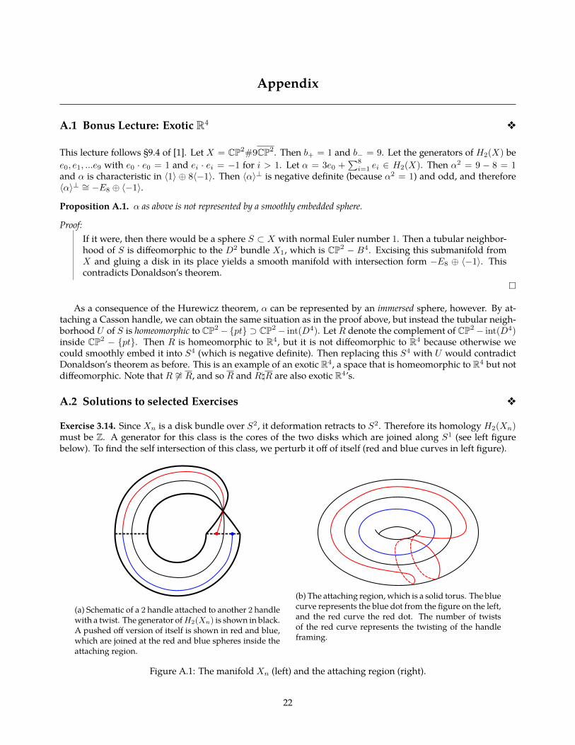
Exercise 3.14. Since Xn is a disk bundle over S2, it deformation retracts to S2. Therefore its homology H2(Xn)must be Z. A generator for this class is the cores of the two disks which are joined along S1 (see left figurebelow). To find the self intersection of this class, we perturb it off of itself (red and blue curves in left figure).

(a) Schematic of a 2 handle attached to another 2 handlewith a twist. The generator ofH2(Xn) is shown in black.A pushed off version of itself is shown in red and blue,which are joined at the red and blue spheres inside theattaching region.

(b) The attaching region, which is a solid torus. The bluecurve represents the blue dot from the figure on the left,and the red curve the red dot. The number of twistsof the red curve represents the twisting of the handleframing.

Figure A.1: The manifold Xn (left) and the attaching region (right).

22

A Appendix

We see that, in order to make the red and blue curves coincide on the right figure, the red curve will have tointersect the black curve n times. Each of these intersections is positive. This shows that the self intersection ofthis generator is n, and so QXn

∼= 〈[n]〉.

23

References

[1] Gompf, Robert. Stipsicz, András. 4-Manifolds and Kirby Calculus. Graduate Studies inMathematics, AmericanMathematical Society.

Documents

Four Manifold Topology