SOME EXTENSIONS IN THE THEORETICAL STRUCTURE

OF SAMPLING FROM

DIVARIATE TWO-VALUED STOCHASTIC PROCESSES

A THESIS

Presented to

The Faculty of the

Division of Graduate Studies and Research

by

Ronald Eugene Stemmler

In Partial Fulfillment

of the Requirements for the Degree

Doctor of Philosophy

the School of Industrial and Systems Engineering

Georgia Institute of Technology

August, 1971

SOME EXTENSIONS IN THE THEORETICAL STRUCTURE

OF SAMPLING FROM

DIVARIATE TWO-VALUED STOCHASTIC PROCESSES

Approved:

ii

ACKNOWLEDGMENTS

I am grateful for the many hours of guidance and help that I have

received for the last five years from Dr. William W. Hines, first as my

academic advisor and later as my thesis advisor. He introduced me to the

research area and constructively guided my progress.

Dr. Robert B. Cooper,, Dr. Harrison M. Wadsworth, and Dr. James W.

Walker were members of my thesis advisory committee. I thank them for

their many helpful suggestions in the preparation of this thesis.

For the first four years of my graduate program, Mr. Harry L. Baker,

Jr., employed me in the Office of Research Administration. I enjoyed my

association with Harry, and I thank him for the invaluable work experience.

I appreciate having been a member of the faculty in the School of

Industrial and Systems Engineering. For that opportunity I thank Dr.

Robert N. Lehrer.

For two years I received support from the National Science Founda­

tion while working on research project GK-1734 with Dr. Hines. I am grate­

ful to Dr. Hines and the Foundation for the research experience.

And I acknowledge the patience, understanding, and sacrifice that

Dorothy has offered for the past five years. I dedicate this work to her.

iii

TABLE OF CONTENTS

Page ACKNOWLEDGMENTS ii

LIST OF FIGURES v

SUMMARY vi

CHAPTER

I. INTRODUCTION 1

Purpose and Importance of Study Principal Objectives and Scope of Study Study Procedure a n d Methodology

II. SURVEY OF THE LITERATURE 6

III. THE DEFINITION AND OBSERVATION OF A SIMPLEX REALIZATION 24

Introduction A Simplex Realization Observing a Simplex Realization

IV. STATISTICAL ANALYSIS OF A SIMPLEX REALIZATION SAMPLE FUNCTION 37

Introduction Statistical Analysis of a Finite Population Statistical Analysis of the Two Sampling Plans

V. STATISTICAL ANALYSIS OF A SIMPLE RANDOM SAMPLE 46

Introduction Statistical Analysis of a Simple Random Sample

VI. STATISTICAL ANALYSIS OF A SYSTEMATIC RANDOM SAMPLE 63

Introduction Statistical Analysis of a Systematic Random Sample

iv

CHAPTER Page

VII. A COMPARISON OF SYSTEMATIC AND SIMPLE RANDOM SAMPLING PLANS 86

Introduction Comparison of Sampling Plans Autocorrelation Functions from Practical Applications Autocorrelation Functions from Spectral Analysis

VIII. CONCLUSIONS, RECOMMENDATIONS, AND EXTENSIONS. 114

Conclusions Recommendations and Extensions

APPENDIX A • 120

APPENDIX B , 136

APPENDIX C 156

APPENDIX D 167

BIBLIOGRAPHY 178

VITA I 8 1

V

LIST OF FIGURES

Figure Page

3.1 Typical Simplex Realization 27

3.2 Simplex Realization and Corresponding Sample Function . . . . . 33

3.3 Typical Outcomes of Random Sampling Plans 36

7.1 Effect of the Damping Rate & and the Oscillating Rate $ Ill

B.l Typical Multiplex Realization 140

vi

SUMMARY

The purpose of this research is to provide some extensions to the

theoretical structure underlying the systematic random sampling of those

dichotomous activities that may be described as being divariate two-valued

stochastic processes. In particular it is desired that the investigation

will extend the usefulness of the systematic random sampling scheme. This

end is sought by studying the theoretical nature of certain divariate two-

valued stochastic processes in order to ascertain those processes that are

more precisely sampled by using a systematic random scheme than by using a

simple random scheme.

The general objective of this research is to make a quantitative

comparison of the systematic random sampling plan and the simple random

sampling plan. This is done by developing a set of meaningful statistics

relating to each sampling plan, and then comparing these statistics for

the plans. It is known that the autocorrelation function of a stochastic

process can play a large role in such a comparison and that the autocor­

relation function can appear in the formulation of certain statistics.

Thus it is important that some general classes of autocorrelation functions

be included in this investigation.

The procedure utilized in this investigation may be outlined in four

steps. The first step includes the definition and characterization of a

simplex realization from a zero-one stochastic process. A continuous pa­

rameter, two-valued, divariate stochastic process (having mean and co-

variance stationarity) is introduced and symbolized as X(t) . Its mean

vii

value M , variance 1/ = M - M , and covariance kernel f*A(u) are

defined and certain of their properties are demonstrated. A typical reali­

zation of the process on an interval [0,T] is introduced and symbolized

as X(t) . Then the realization mean is defined:

X(t) dt 0

the mean of the realization mean is found:

E[m R] = M : ,

the variance of the realization mean is formulated and shown to be bounded:

Var[m ] == — (T - u>-A(u)•du , T J 0

0 <. Var[m R] £ 1/4

the realization variance is defined:

v R T J 0 (X(t) - m R ) 2 dt = ir - m R

2 , 0 <: v R £ 1/4 ,

and the mean of this realization variance and its boundaries are found, and

it is related to the variance of the realization mean:

E[v_] = V - ~ \ (T - u)-A(u) du , R T J 0

0 <• E[v R] ^ 1/4 ,

viii

E[v R] + Vartn^] = 1/

The second step in the investigation is concerned with the sample

function of the simplex realization, which is referred to as the finite

population of the realization and is symbolized by the set ^ xj-^ • This

finite population is defined and then characterized by establishing some

of its statistical properties. The finite population mean is defined:

1 N

the mean of the finite population mean is found:

E[mp] = M ,

the variance of the finite population mean and its boundaries are found:

V ")[) Vartmp] = ^ + ^ \ (N-u)-A(tu) , 0 * V a r ^ ] £ 1/ £ 1/4 ,

N u=l

the finite population variance is defined:

N 1 2 2

VP = N £ ( xi ~ V = ~ ' 0 £ v p <; 1/4 ,

j=l J

and the mean of this finite population variance and its boundaries are

found, and it is related to the variance of the population mean:

N u=l

ix

0 E[v p] * 'V ^ 1/4

E[v p] + Vartmp] = V .

The third phase of this investigation treats the statistical analysis

of two methods for sampling the finite population: systematic random sam­

pling and simple random sampling. In presenting the analysis, two types of

expectation are used and their meanings must be distinguished. When the

expectation is taken treating the sample as a function of the realization

from the stochastic process, the symbol E is employed and the term mean

is used. When the sample is treated as a function of the finite population,

the symbol e is employed and the term average is used. Similarly when

dealing with second moments, either the symbol Var and the term variance

will be used in relating the statistics to the realization, or else the

symbol var and the term dispersion will be used when treating the sample

as a function of the finite population.

The two samples are defined and then characterized by formulating

some of their statistical properties, using the subscripts "Sim" and

"Sys" to specify the particular sampling plan. The two sample means are

defined:

1 1 1

± I x g ; s.e{l,2,3,...,N} , i==l i

1 n

n X Xs+(i-l)k ; sc{l,2,3,...,k} > i=l

the average of the sample mean for each of the two plans is found:

m, Sim

lSys

e { m S i m } = e { m S y s } = "P '

the mean of the average sample mean is found for both plans:

E[ e{m s. m}] = E[e{m S y s}] = M ,

the variance of the average sample mean is found for both plans

N u=l

the two means of the sample mean are found:

E[mc. ]| = E[mc ] = M L Sim L Sys J '

the dispersion of the sample mean is found for each of the sampling plans

• r t N - n V a r { m S i m } = nTN=iy VP '

^ 2 n~l N-ku v a r { m S y s } " n" vP + to I I ( X J " V ( x k u + J " V

J U = l J = l

the mean dispersion of the sample mean is found for each plan:

E[var< m s i m}] = 1 - ^ T (N -u=l

E[var{mc }] = ^ IA ( 1 - * n , ^ (N-u)A(t ) + ^ (n-u)A(t Sys Nn \ N(N-n) ^ u n(N-n) ^ u

the variance of the sample mean is found for each of the two plans:

xi

1/ 21/ n _ 1 n

n 1=1 j=i+l j l

V a r t m S y S ] " l + 1lX • ( n- u ) A ( tk» ) ' n u=l

the average variance of the sample mean is found for each plan and then

combined with previous results to indicate relationships:

u=l

1/ 21/ n " e{Var[m ]} = - + -j J ( n - u W ^ ) = Vartms ] ,

n u=l 17

e{Var[m S i m]} = E[var{» m}]" + Var[«{m^ }] ,

e{Var[m S y g]} = E[var{m }] + Var[e{m }]

the two sample variances are defined:

v„. = — ) (x - m„. ) Sim = n * < V " " W = mSim " ^ i m i=l i

1 r , .2 2 Sys n s+(i-l)k Sys Sys Sys '

the average of the sample variance, for each of the sampling plans, is

found and related to the dispersion of the sample mean:

, , k(n-l)

xii

n-1 2 n~"^ ^-ku e { v S y s } = ^ - V P " to ^ -l ( X J ' V ( x k u M " V

11=1 J=l

e{vc. } + var{m_. } = v_ , var{m_. } = . j\ »e{v0 } , Sim Sim P ' Sim k(n-l) Sim '

e{vc } + var{m_ } = v_. , Sys Sys P

the mean of the average sample variance is found for each sample and then

related to the average variance of the sample mean:

E[ S{v S y s}] + e{Var[m S y s] = V ,

and finally the mean of the sample variance is found for each of the sam­

pling plans and then related to the variance of the sample mean:

E[vQ. ] = Szi 1/ - Y I A(t ) , S l m n n 2 i=l S3" Si

E[v c ] = 1/ - ^ Y (n-u)A(t, ) , Sys n 2 u- ku n u=l

E[v s. m] + Var[m s. m] = 1/ ,

E[vc I + Var[mc ] = V Sys L Sys

xiii

The fourth and last phase of the investigation was directed toward

comparing the precision of the two sampling plans. A number of known sam­

pling theoretic results were verified in the sense that necessary-and-

sufficient conditions for the superiority of a systematic random sampling

plan were formulated. The principal result established that on the average

systematic random sampling is at least as precise as simple random sampling

if-and-only-if:

l£l X ( N " k U ) ' A ( ^ S Nil X ( N " U ) ' A ( t u } • u=l u=l

The importance of the autocorrelation function for establishing the superi­

ority of the systematic plan is evident from this expression. With such an

autocorrelation function in hand, it becomes a computational problem to

ascertain whether or not the inequality holds.

An important result due to William G. Cochran was investigated. He

has shown that a convex, non-increasing, and non-negative autocorrelation

function is sufficient to insure that the systematic random sampling scheme

is more precise. The present investigation has established the same con­

clusion without requiring non-negativity of the autocorrelation function.

Finally, a general class of damped oscillatory autocorrelation

functions was investigated. The damping parameter and the oscillating

parameter are shown to affect the comparison of the two random sampling

schemes. When the damping parameter exceeds the oscillating parameter, it

appears that the systematic scheme will always be superior. For greater

oscillation, care must be given to the selection of the sampling intensity.

xiv

Some guidelines for this selection are given so that the practitioner can

be assured that a systematic sampling plan is more precise.

1

CHAPTER I

INTRODUCTION

A process that is evolving in time and developing in a manner con­

trolled or governed by theoretical probability laws is called a stochastic

process. A stochastic process whose range space contains two elements is

called two-valued. A two-valued stochastic process whose two values are

assumed alternately and maintained for durations of time that are distri­

buted alternately as two independent random variables having stationary

distirubitons, is called a divariate two-valued stochastic process. Presen­

tation of a suggested taxonomy for a certain sub-class of stochastic

processes is included as Appendix A. This taxonomy presents and qualifies

stochastic process descriptors such as divariate.

An interesting example of a divariate two-valued stochastic process

is provided by a simple activity structure such as in a typical work

sampling problem. A simple activity structure is defined as the activity

of one subject (animate or inanimate) with all activity being dichotomous,

that is, classified as belonging to some state of interest or else belong­

ing to the complement of that state of interest. In work sampling studies,

the subject (man or machine) can either be in a working state or a non-

working state. Thus work sampling is modeled as a divariate, two-valued

stochastic process.

A stochastic process is essentially an abstract concept. Prac­

ticability requires that some sort of concrete actualization of the process

2

be possible so that the abstract process can be analyzed. Thus, from the

set of all possible actualizations (the set of all possible random func­

tions to which the stochastic process may give rise), a typical actualiza­

tion on some finite interval is employed for investigation. It is referred

to as a. realization of the stochastic process. A realization from a single

two-valued stochastic process is called a simplex realization, referring to

the simple dichotomous nature of the states for the process under investiga­

tion. Often there is interest in more than a single two-valued stochastic

process, for example in simultaneously investigating a group of dichotomous

activities. A realization from a group of two-valued processes is called

a multiplex realization and is, in a sense, a grouping of multiple simplex

realizations. The term complex realization is a more general description

and is reserved for a realization that is not necessarily two-valued. Thus

a three-valued process would give rise to a complex realization, as would a

sum of two-valued processes.

A realization is assumed to be observable in the sense that its

state or value can be ascertained at any point on the finite interval.

Thus it is possible to obtain the mean value or average state of the reali­

zation. It is assumed that, for reasons of economy, a continuous observa­

tion of the whole realization is not acceptable. Two sampling methods are

considered: the simple random sampling plan and the systematic random

sampling plan. Either of these sampling plans will lead to an unbiased

mean value estimator. However, it is likely that in any given situation

one type of sample will lead to a more precise estimator than the other

type. The word "precise" is used in a statistical sense; that is, the

mean value estimator having the smaller variance is said to be more

3

precise. In a sampling situation, the sampling plan yielding the more

precise estimator of the mean is preferred.

Purpose and Importance of Study

The purpose of the research is to provide some extensions to the

theoretical structure underlying the systematic random sampling of those

dichotomous activities that may be described as being divariate two-valued

stochastic processes. The primary thesis of this investigation is that

the systematic random sampling plan can and should be utilized more widely.

In particular it is desired that the investigation will extend the

usefulness of the systematic random sampling scheme. This end is sought

by studying the theoretical nature of certain divariate two-valued sto­

chastic processes in order to ascertain those processes that are more

precisely sampled by using a systematic random scheme than by using a

simple random scheme.

A preference for systematic random sampling.stems from two quali­

tative factors: the ease aiid convenience of taking observations at equal

intervals of time and the intuitive feeling that, for most cases, more

heterogeneous representation of the total realization will be achieved.

What is required then is quantitative justification.

Principal Objectives and Scope of Study

The general objective of this research is to make a quantitative

comparison of the systematic random sampling plan and the simple random

sampling plan. This is done by developing a set of sample statistics

4

relating to each of the two sampling plans and then comparing these sta­

tistics.

It is known that the autocorrelation function of a stochastic process

can play a large role in such a comparison and that the autocorrelation

function can appear in the formulation of certain sample statistics. Thus

it is important that some general classes of autocorrelation functions be

investigated. In particular, the class of convex decreasing, non-negative

autocorrelation functions and the class of damped oscillatory autocorrela­

tion functions receive attention within the scope of the investigation.

Both of these classes of autocorrelation functions have been found to

appear in various work sampling studies reported in the literature *

A secondary objective of the investigation is to provide an intro­

duction to the theoretical structure for the statistical analysis of

multiple dichotomous activities, as modeled by a stochastic vector or a

vector of stochastic processes. This presentation is included as Appendix

B. It provides a path for the comparative investigation of simultaneous

sampling of realizations from multiple divariate stochastic processes,

that is, multiplex realizations.

Study Procedure and Methodology

The methodology employed in this investigation was analytical,

especially in the formulation of the sample statistics and in the in­

vestigation of convex decreasing, non-negative autocorrelation functions.

The work with damped oscillatory autocorrelation functions required an

additional numerical analytic approach.

5

The procedure utilized in this investigation may be outlined in

four steps. The first step includes the definition and characterization

of a simplex realization. Treating the realization as a random function

of the stochastic process its mean and variance are defined and certain

of its properties are developed: the mean of the realization mean, the

variance of the realization mean, and the mean of the realization variance.

Upper and lower bounds are established for the appropriate terms.

For the second step, the sample function of the simplex realization

is introduced in the form of a finite population. Statistical analysis

leads to definitions for the population mean and variance and to the

formulation of certain properties of this finite population such as the

mean of the realization mean, the variance of the population mean, and

the mean of the population variance. Appropriate upper and lower bounds

are stated. The third step is concerned with investigating the two methods

(systematic and simple random) of sampling a subset from the finite popu­

lation. The statistical analysis of the samples resulting from each of

the two sampling plans includes treatment of the samples both as a sample

function of the stochastic process (called E-expectation) and as a sample

function of the finite population (called e-averaging).

The fourth step in the procedure involves an evaluation of the two

sampling plans by a comparison of their statistics. It included the two

special cases wherein the stochastic process whose realization is being

sampled has an autocorrelation function that is either convex decreasing

and non-negative or damped oscillatory.

6

CHAPTER II

SURVEY OF THE LITERATURE

The purpose of this chapter is to report on a survey of the litera­

ture pertaining to the research presented in this thesis. Some literature

from the theory of stochastic processes and from sampling theory is men­

tioned. Then contributions important to the present investigation will be

presented from the literature that represents a combination of these two

theories.

A few of the source documents from the general area of mathematics

that is referred to as stochastic processes are textbooks by Parzen [26],

Papoulis [25], Feller [6], and Prabhu [28]; a collection of papers on time

series analysis by Parzen [27]; and other publications on time series

analysis by Hannan [8], Grenander and Rosenblatt [7], Cox and Lewis [4],

Kendall and Stuart [14], and Varadhan [29]. The books by Parzen [26],

Kendall and Stuart [14], and Papoulis [25] were the most useful to the

investigation.

The area of applied mathematical statistics known as sampling

methods is presented in books by Cochran [3], Yates [32], Kendall and

Stuart [14], and Hansen, Hurwitz, and Madow [9]. A review of the litera­

ture of systematic sampling prior to 1950 has been provided by Buckland

[l]. A review of the literature contributing to the development of activ­

ity sampling and, in particular, systematic activity sampling is available

in Chapter III and Appendix A of a doctoral thesis in 1964 by Hines [10].

In connection with the present investigation, it is important to discuss

7

publications by the Madows [19], [20], [21], and [22], Yates [31], Cochran

[2], Davis [5], and Hines and Moder [ll].

The Madows [20] in 1944 published the first treatise dealing exclu­

sively with systematic sampling. Although their research dealt with the

theory of sampling both single elements and clusters of elements, this

first publication of results concentrated solely upon the sampling of

single elements. The theory was presented both for sampling from a stra­

tified population^^ and for sampling from an unstratified population.

Using the sample mean as an estimator for the population mean, formulas

are-derived for the mean value and the variance of the estimator. In

order to derive the variance of the mean value estimator, it was necessary

to assume some knowledge regarding the variance and the serial correlation

of the population being sampled. A biased and inconsistent estimate of

this variance is also derived. The authors compared sampling plans by

comparing the variances of the mean value estimators for different sampling

methods since: "It has become customary, on the basis of limiting distri­

bution theory and the theory of best linear unbiased estimates, to use the

standard deviation of the sample estimate about the character estimated as

the measure of sampling error." As the basic results of this first paper

[20], the authors reported that:

(1) It was assumed throughout the investigation that the population is finite with size N ~ n«k (n and k integers) since, as the Madows stated in the paper: "To do away with that assumption would not add much in the way of generality while it would require some fairly detailed dis­cussion. It may be remarked that when N is not exactly n«k , then systematic sampling procedures in which all starting points have equal probability of selection are biased, although the bias is usually trivial. If N is known, this bias can be removed by sampling proportionate to possible size of sample."

8

(a) If the serial correlations have a positive sum, systematic sampling is worse than simple random sampling,

(b) If the serial correlations have a sum that is approximately zero, systematic sampling is approximately equivalent to simple random sampling, and

(c) If the serial correlations have a negative sum, systematic sampling is better than simple random sampling.

L. H. Madow [19] in 1946 presented an applied statistics and "less

technical" version of the earlier paper, wherein the major change was an

approach that treated systematic random sampling as a special case of

cluster sampling, that is, "the case in which only one cluster is sampled

and there is no subsampling within the cluster." From her experience

with analysis of data from various applications of the sampling methods,

the author gained enough confidence to make a statement regarding the

efficiency of systematic sampling: "In the cases where the systematic

design is more efficient than the stratified random design, the systematic

design is about twice as efficient as the stratified random design, where­

as in most of the cases in which the systematic design is less efficient

than the stratified random design, the stratified design has only a slight

gain over the systematic design."

It was also in 1946 that the Cochran paper [2] appeared. This

paper adopted a broader approach to the sampling of finite populations,

in that Cochran regarded the finite population as being drawn at random

from an infinite superpopulation that possesses certain properties. His

approach is based on the principal that one way of describing the class

of finite populations for which a given sampling method is efficient, is

to describe the infinite superpopulation from which such a finite popu­

lation might have been drawn at random. The results that Cochran achieves

9

do not apply to any single finite population, but to the average of all

finite populations that can be drawn from the infinite superpopulation.

This approach would today be described as the observation of the activity

and the resulting set of sample elements or observation points treated as

the finite population arising from a simple realization of a stationary

stochastic process.

Since Cochran's work has provided a basis for much of the present

research, it is useful to discuss the method by which he related the form

of the autocorrelation function to the relative precision of systematic

sampling. He considered a finite population consisting of the elements

, i = l,2,«'«,nk , (where n and k are integers) to be drawn

from a population in which;

2 2 ' E[x. ] = p. , E[(x - |i) '] = a , and E[(x - LI) (x - LI) ] = p -a' 1 1 1 H~U U

where p is a serial correlation and p ^ p > 0 whenever u < v . u v

Since sampling is considered to be from a finite population and without

replacement, Cochran begins with a well-known definition for the variance

(with respect to the finite population) of a simple random sample mean:

1 kn-n 1 r , - s2 — 1 T'\— 1 (x. - x) n kn-1 kn I i=l

where x is the mean of the finite population. He formulates the expecta­

tion of this quantity, calls it the variance among simple random samples,

and states it as the result:

10

2 a 2 n 1, (r 2 k n _ 1 . \

a = (1 - 7 " ) ' 1 1 " 1—7i——TV' L ( k n - u)p ) r n k \ kn(kn-l) L. v Ku/

u=l

For the systematic random sample Cochran does not begin with an expres­

sion for the variance of the sample mean, but rather breaks the finite

population variance into its two components: total variance in the

•population equals variance 'among samples plus variance within samples.

Then, from the expectation of the finite population variance he subtracts

the expectation of the variance within systematic samples and achieves an

expression for the expectation of the variance among systematic samples,

which he states as the result:

^2 c j 2 1, / 2 k n _ 1 ' 2k n r 1 . , \ CT = (1 - r-)«ll - z—-p.—rr-. ) (kn-u)p + — t ^ — r v * I (n-u)p. J sy n k \ kn(k-l) L^ u n(k-l) L- ku/ u=l u=l

After introducing a hypothesis that the second forward difference of the

serial correlation be non-negative (convexity condition), Cochran is able

to establish the important: result that:

2 2 a £ a sy r

It is stated that, under the hypotheses, systematic random sampling is

"on the average" at least as precise as simple random sampling.

A paper by Frank Yates [3l] in 1948 made use of Cochran's concept

of expected variances. Significantly, Yates was the first to report the

application of a systematic random scheme to the sampling of attributes,

11

that is, sampling two-valued processes. However, he limited the investi­

gation to a single occurrence of the activity (or attribute) of interest

within the realization. He concluded that the relative performance of

systematic and simple random sampling depends upon the relationship between

the sampling interval or intensity (k) and the duration of the activity of

interest. If the sampling interval is much larger than the activity dura­

tion, then the two sampling plans are of about equal precision, and as the

activity duration increases relative to the sampling interval, systematic

sampling gains in relative precision.

Another paper concerned with the relative precision of different

sampling plans appeared in 1955, written by H. Davis [5]. An interesting

aspect of the paper is his definition of the work sampling problem. He

defines the problem to be that of taking a sample of size N from a

realization of a stationary, two-valued stochastic process. The process

alternately changes its state after intervals of time that are governed,

alternately, by two independent random variables.

The rest of Davis' paper suffers from his apparent unawareness of

work previously done by such sampling theorists as Yates, Cochran, and

the Madows. His statistical formulations have, for the most part, not

coincided with other known results and his overall approach is question­

able. For example, as one of his sampling plans he considers a non-random

method of sampling at M specified, regularly-spaced intervals of time

and develops an expression for the expected variance of the mean from such

a sample:

2 N N GA<^*> ' I I P(T±,T ) , N = M ,

A N i=l j=l 1 J

12

where p is the autocorrelation of the process between the times T\ and

. This plan is compared to another sampling plan wherein the same M

points are available for sampling, but the selection is performed randomly

and with replacement so that the sample is composed of N (?» M) distinct

elements. An expression is developed for the expected variance of the mean

of this sample:

Davis goes to some length to establish that the first sampling plan is

better than the second, in the sense that the first variance above is

smaller than the second variance. He assumes that each of the independent

random variables for the process is negative-exponentially distributed.

This leads to an explicit formulation for p that is substituted into

the two expressions. In simplifying, Davis yields to approximate 2 2

expressions for o\ ((i*) and a which are then compared in order

to establish that the first sampling plan is better.

"sampling schemes" can be established much more easily. Since the auto­

correlation function, p(T.,T.) , is never greater than one:

2 N +

Davis failed to observe that the most general comparison of his

2

and the second sampling plan is never better than the first. Regardless of

13

his unconventional approach, Davis must be credited with recognizing the

importance of the autocorrelation function in selecting from a choice of

sampling plans. Unfortunately, some of the people who have used Davis1

work have mis-interpreted his results (e.g., [11], [12], [13], and [23]).

They have assumed that his first sampling scheme is systematic random

sampling and that his second sampling scheme is simple random sampling

without replacement.

In 1965 Hines and Moder [11] reported a number of extensions to

systematic activity sampling. They conventionally define the sampling

problem in terms of observing a realization from a two-valued stochastic

process, and their statistical development is consistent with the work

of previous investigators. Extending Yates [31] work with the special

and limited case of a single occurrence of the activity of interest,

the authors present both the Bernoulli distribution for the systematic

random sample mean value estimator and a confidence statement assuring

that this estimator is always within 1/n of the true mean (n is the

number of observations constituting the sample). They conclude that

systematic random sampling is uniformly (for all sampling intensities)

more precise than simple random sampling, whenever the activity of

interest occurs only once during the time period of the sampling survey.

In another special case investigated by Hines and Moder, they

assume that the interval between observations is smaller than all

occurrences of both the activity of interest and its complement. Thus

at least one observation of each consecutive occurrence of the activity

and each consecutive occurrence of the inactivity is assured; no

14

activity or inactivity goes undetected. A sample estimate of the process

mean value, an easily calculated upper bound to the variance of this

estimate, and confidence statements on the true mean value (using

Tchebycheff1s Inequality) are presented. For this case it is concluded

that systematic random sampling is superior to simple random sampling

in most of the practical sampling situations encountered. Letting M

represent the maximum number of times on the realization [0,T] that

either the activity or its complement occurs, the authors demonstrate the

clear superiority of systematic random sampling for a sufficiently large

sample size: n > (2/3)-M .

Recognizing the restrictive nature of these special cases, Hines

and Moder generalize their study of divariate, two-valued processes by

removing the previous limitations. The activity of interest and its

complement are assumed to have consecutive durations that are alternately

governed by separate probability distribution functions. The serial

correlation or autocorrelation function was sought so that the applica­

bility of Cochran's theorem could be decided. They consider two separate

classes of processes: the first being when both of the probability

distribution functions are gamma and the second being when both are

normal and truncated at zero. Using Monte Carlo simulation, the authors

obtain two sets of nine correlograms, each set representing nine

different combinations of parameters for the particular probability

distributions, that is, nine gamma-generated correlograms and nine

normal-generated correlograms. Analysis of these eighteen correlograms

15

leads the authors to a summary of some useful conclusions. According

to Hines and Moder: "the general behavior of the correlograms for all

the cases may be termed as damped periodic." It must be pointed out

that the authors interpreted their simulation results using a condition

that they believed to be "necessary and sufficient" for systematic

sampling to be more accurate than simple random sampling. Since the

condition involved simple random sampling with replacement, their

condition is necessary but not sufficient.

The attainment of an autocorrelation function for a divariate

two-valued stochastic process has been the goal of other investigations,

often in contexts other than sampling theory. For example, in the general

treatment of stochastic processes and time series analysis, an important

role has been played by the so-called variance spectrum or, more commonly,

the spectral density function of the stochastic process. Its importance

was recognized by Norbert Wiener [30] and A. Ya Khintchine [15], each

of whom independently applied the theories of Fourier series and Fourier

integrals to the stochastic processes. The spectral density function thus

(2) Let R represent the ratio between the largest true mean activity (or inactivity) duration and the smallest true mean duration; let L represent the true mean cycle length, that is, the sum of the true mean activity duration and the true mean inactivity duration; let C represent the coefficient of variation for the true mean activity/ inactivity cycle length, that is, the ratio of the standard deviation of the cycle length to the mean of the cycle length; and let D repre­sent the duration of the interval between observations. If D < 3/4*L, R < 3 , and C > 1/10 , then systematic random sampling seems to be superior to simple random sampling. If D < 1/4*L , then it seems that no further conditions on R and C will be required in order for systematic sampling to be superior.

16

obtained is frequently the only tool available to assist in analyzing the

phenomenon which generates a particular stochastic process. However by

applying the Fourier transformations, usually referred to as either the (3)

"Wiener-Khintchine Relations" or the "Wiener Theorem for Autocorrela­

tion," one is often able to map from the frequency domain of the spectral

density function to the time domain of the autocorrelation function.

A rigorous and complete development of the spectral density function

is presented by Y. W. Lee |_18] for a generalized stochastic process or,

as Lee refers to it, a random function. Both Lee and A. Papoulis [25]

state and prove the basic properties of both the autocorrelation function (4)

and the spectral density function for a stochastic process . Lee's work,

especially, has laid the foundation for pertinent extensions.

An interesting use of Lee's development was made by Hitoshi Kume

[16] in 1964, in analyzing those processes that are central to the present

investigation: divariate, two-valued, stationary stochastic processes. 2

Letting X(t) be such a process having mean |i and variance a , he

begins with three assumptions suggested by Parzen [26] : (3) The autocorrelation function of a stochastic process and the spectral density function of that stochastic process are related to each other by Fourier integral transformations (in particular, by Fourier cosine transformations).

(4) If the stochastic process is real and stationary, then: (a) Both the autocorrelation function and the spectral density function are real functions and are even functions, (b) The autocorrelation function always attains its maximum value of 1 when it has zero lag, and approaches zero when the lag for a non-periodic process approaches infinity, and (c) The spectral density function is everywhere non-negative and as <JU approaches infinity, the spectral distribution function (spectral density function integrated between -«> and oo) approaches a definite limit, which is a function of the autocorrelation function with zero lag.

17

(a) The duration of time required for the two-valued process to change

from zero to one is distributed as a random variable U , having

a probability density function ^qC11) > a mean e[u] = u-q ,

and a characteristic function E[e1UJ^T] - $q •

(b) The duration of time required for the two-valued process to change

from one to zero is distributed as a random variable V , having

a probability density function f^(v) , a mean E[v] = M- , and

a characteristic function

(c) The random variables U and V are independent.

Kume applies Fourier analysis to the process and, after much simplification,

obtains a well-known expression for the spectral density function of the

process:

T S (oj) = lim E[ i | [ X(t).e" l u J tdt| 2]

= lim E[S (uu)] T •-•00

He continues his development by defining a realization x(t) on the

interval [0,to ] ; a Fourier transform of x(t) on [0,t ] : Zn ^n

and a spectral density function for the realization on l-^»t2n^

2 n C2n

18

This spectral density function is extended to the non-negative real line

S (uj) = lim E[S 2 (u))] n -.00

2 , / ; . _ r

2 V $ i " (*o + *i> 7 2* 1 + Re["^—f h

Then the autocovariance function:

R(u) = E',[(X(t) - u,)(X(t+u) - n)]

is defined by the Wiener Theorem to be, for this process:

i r"

R(u) = —" S (ao) •Cos(aou) .doo

From this expression, a simple step leads to the autocorrelation function / \ R(u) p(u) = £

Kume presents an example where U and V are both negative

exponentially distributed, and illustrates how the Fourier cosine trans­

formation of the spectral density function yields the covariance function

and leads (in this case) to the determination of a convex decreasing,

non-negative autocorrelation f u n c t i o n T h e spectral density function

(5) Note that an exponential/exponential stochastic process is more precisely sampled by using a systematic random sampling plan, since the autocorrelation function for this process satisfies Cochran's hypotheses.

19

that Kume achieves for this case (with e[u] = •"•/aQ a n < ^ ECv]

1/a^) is given by:

2-vai S (oo) = 2 2

ao + a i 0 0 + ( ao + a P

It is interesting that by rewriting Kume's expression:

2-TT.a *a a + a 8(0,) = . [ I . _ S L _ ] f

( ao + a i ) m + ( ao + a i )

2-TT-a - a

• £ f • (aQ + V

2 »

where -^^^ i s recognized as a Cauchy probability density function,

Therefore:

R(u) = ^ S (oo) »e duo ,

a0* al T ioou (aQ + ap -oo

J e1U3U.fw(uj)du) ,

Vai e " ( a 0 + a i ) U ] 2 L

l a 0 + V

since the integral represents $TT(u) , the characteristic function of the w

Cauchy random variable W This is the same result that Kume achieved

with a different approach,,

20

Another example is discussed by Kume, where both random variables

are normally distributed. For this case graphical results (two correlo­

grams) are presented; no closed form solution for the autocorrelation

function is given. Kume offers no indication of the method that he used

to transform the rather complex spectral density function for this case,

and it is likely that a numerical integration was used. It is noteworthy

that his correlograms for the case of normal/normal distributions exhibit

the same damped oscillatory nature as those that Hines [10] achieved from

his simulations.

Meyer-Plate [24] in 1968 was concerned with the determination of

the autocorrelation functions for several classes of divariate, two-valued

stochastic processes. Beginning with Kume's spectral density function in

terms of the expected values and characteristic functions of the random

variables U and V , Meyer-Plate was able to formulate an explicit spectral

density function for six cases.

Case 1: U = Constant(c) ; V « Negative Exponential (1/X)

S(u>) = 2 X (1 - Cosouc) (c+X) (1 - Cosooc) + (XCJO + SintDc)

Case 2: U = Constant(c) V Uniform(0,2t)

S(tt)) = 2 (CJO t - Sin out) (1 - COSCJOC) t + Sin u)t + 2a>tSina>tCosa>(c+t)

21

2

2 2 O,„A - 2 (1 - e"(" CT )(1 - Cosax) MU); - • 2 T 2~~2

(c+t)a)2 1 + e _ U ) CT' - 2.e _ U ) CT 1 1 .Cosu)(c+t)

2 Case 4: U « Negative Exponential (1/X) ; V « Normal a )

S(u>) = 2 2

2 X (1 - e «Cosa)|i) 2 2 2 2 ,,,, / n -u) a /2 _ .2 , . • . -OJ a /2 _. .2 u+X (1 - e »Cosu)|i) + (Xu) + e 'SinujjJ.)

2 2 Case 5: U « Normal (a^Og) ; V « Normal (u^ ,0^)

2 9 ' 2 2 2 Let A = U) o-q , B = U) , and C = (u^ + p.1>U)

-A-B -A/2,, -B> -B/2 -A. _ 1 - e -e (1-e )Cos|i0U) - e (1-e )Cosp..,U} S(o)) = f C - „ -(A+B)/2„ , , «

1 - 2'e Cos(|i0 + |j,)u) - e -A-B

Case 6: U « Gamma(rQ, IAq) 5 V « Gamma(r^, 1/X^)

2 2 -r /2 2 2 -r 12 Let C = (1 + xV) o' , D = (1 + Xftt) ) V ,

Q = t a n " 1 ^ , R = tan"10jX1 .

S(OJ) =

2 2 2 2 1 - C D - C(l-D )Cosr0Q - D(l-C )Cosr1R

(X ( )r 0+X 1r 1)uj 2 1 + C 2 D 2 - 2CD-Cos(r0Q + r ] R )

Case 3: U = Constant (c) ; V « Normal a )

22

In pursuing the autocovariance functions by applying the Fourier

cosine transformation, Meyer-Plate faced the same analytical integration

difficulties that Kume apparently faced. For all but the sixth case

(gamma/gamma), Meyer-Plate utilized a compound form of Simpson's rule,

employing an ALGOL computer program, to integrate numerically the spectral

density functions. In each case he selected the upper bound of each

integral in such a fashion that the calculation error would not exceed

0.004 . For Case 1 he selected sixteen combinations of parameter pairs

for the random variables, and achieved sixteen graphs that he presented

as correlograms. Case 2 led to eighteen correlograms, Case 3 to eight

correlograms, Case 4 to ten, and Case 5 led to eight correlograms.

Examination of his sixty correlograms permits some interesting observa­

tions: they all exhibit oscillation patterns and they all exhibit damping

qualities. This leads Meyer-Plate to draw some tentative "experimental"

conclusions. Concerning the period of oscillation in the correlograms,

Meyer-Plate states:

The autocorrelation functions associated with processes with normal, exponential, uniform or constant distribution of span length (or any combination thereof) oscillate with periods between two consecutive maxima equal (to) the mean cycle length of the process, provided the coefficient of variation does not exceed 0.25.

With respect to the damping of the correlograms, he concluded that "it

appears certain that an increasing coefficient of variation accelerates

the damping of the oscillations." Meyer-Plate added that his results are

intended to broaden the base for future research in activity sampling

but that his investigation "does not, however, concern itself with the

23

problem of drawing conclusions about the superiority of either of the

sampling procedures on the basis of its results."

Kume [17] recently studied the precision of a systematic random

sample compared to a simple random sample, when sampling from an infinite

population. His method was directed toward studying the effects of

periodicity in the stochastic process as shown in its autocorrelation

function. He ignored consideration of any damping effects. Utilizing a

Fourier series expansion for two strictly periodic zero-one processes,

a sine wave and a rectangular wave, Kume's interest was in determining

"safe" sampling intensities. Letting T be the period of the process,

Kume investigated sampling at intervals k = r.T for several values of

r (0 £ r £ 1) . His graphical results indicate that for the sine

wave, values of r on [0„2, 0.8] ensure that systematic random sampling

from an infinite population is more precise than simple random sampling,

whenever the sample size is greater than four. With the rectangular wave

no generalizations were made since harmonics of the wave must be avoided

in many cases. A further result by Kume showed that if r is assumed

to be a uniform random variable on (0,1) , then averaging over all choices

of sampling interval the two sampling methods have equal variance

( = a 2/n ) .

24

CHAPTER III

THE DEFINITION AND.OBSERVATION OF A SIMPLEX REALIZATION

Introduction

The objective of this chapter is to develop a description and

characterization for a simplex realization, and then to establish a fun­

damental basis for the random sampling of this type of realization. It

is first established that a zero-one stochastic process is a suitable

mathematical model for representing the theoretical structure of simple

activity. The phrase "simple activity structure" is defined to mean the

activity of a single, either animate or inanimate, observable object that

can only be dichotomously observed. In other words, the object is either

observed as being in some state of interest (say state 1) or else observed

as being in the complementary state of interest (say state 0). Thus, a

zero-one stochastic process is embodied by this type of structure and the

process is suitable as a mathematical model for the theoretical structure

of simple activity.

Consider a continuous parameter, two-valued, divariate stochastic

process whose two values are zero and one. This process is symbolized as

X[(0,l);t] or, more simply, as X(t). Let the process mean value function,

E[X(t)] , be constant (equal to M), thus ensuring stationarity of the mean.

The following properties are presented as a basis for the analysis to

follow in later sections.

25

Property 3.1: For a zero-one process that does not degenerate to one or

the other of its states, 0 < M < 1 .

To show that this property holds, a well-known lemma is useful.

Lemma: If X is a random variable such that Pr[x ^ 0] = 1 ,

Pr[x > 0] > 0 , and e[x] exists, then E[x] > 0 . Letting X(t) = X

and applying the lemma yields: E[X(t)] = M > 0 . Letting 1 - X(t) = X

and applying the lemma yields: E[l - X(t)] = 1 - M > 0 and M < 1.

Property 3.2: For a zero-one process, since X(t) 2 = X(t), then

V = E[X(t)2] - E2[X(t)] = M - M2

and the process variance is stationary. Since 0 < M < 1 and M - M2 is

maximized at 1/4 (when M = 1/2 ), then 0 < V <• 1/4 .

Suppose the process X(t) has a continuous autocovariance kernel^

given by K(t, t+u) = Cov[X(t); X(t+u)] . Let this autocovariance kernel

be a function only of the time increment u , thus ensuring a stationarity

of the autocovariance. Letting A(u) be the autocorrelation function of

X(t) , the autocovariance kernel is expressed as:

Cov[X(t); X(t+u>] = l/-A(u)

(2)

Property 3.3: The zero-one stochastic process is periodic with period

u* , if and only if A(u*) = 1 . If X(t) is periodic with period u* , then X(t+u*) = X(t) .

(1) For an important example of such a process see Kume [16]. Related processes are discussed in renewal theory literature.

(2) Strictly speaking this property only holds almost surely, that is, everywhere except on a set of probability zero. In this paper the distinction between certainty and almost certainty will not be drawn.

26

By the definition of a covariance kernel:

l/-A(u*) = Cov[X(t); X(t+u*)]

= E[X(t)-X(t+u*)] - E[X(t)]-E[X(t+u*)]

= E[X(t)2] - E2[X(t)] ,

= 1/

Since V > 0 , then A(u*) = 1

To show the sufficiency of the condition, the following are defined

M = E[X(t)] = J i-Pr[X(t) = i] = Pr[X(t) = l] . i

E[X(t)-X(t+u*)] = . I i.j-Pr[X(t) = i,X(t+u*) = j] , i,j

== Pr[X(t) = l,X(t+u*) = 1]

Pr[X(t+u*) = 1 | X(t) = l]-Pr[X(t) = 1]

.Pr[X(t) = 1 | X(t+u*) = 1]-Pr[X(t+u*) = l]

"Pr[X(t+u*) = 1 |X(t) = l]-M

Pr[X(t) = 1 | X(t+u*) = 1] -M

If A(u*) = 1 , then l/-A(u*) = 1/ = M - M2 . By definition: l/-A(u*) = Cov[X(t) ;X(t+u*)] ,

= E[X(t)-X(t+u*)] - E[X(t)].E[X(t+u*)] , = E[X(t)-X(t+u*)] - M2 .

27

Thus:

E[X(t)-X(t+u*)] = M ,

Pr[X(t+u*) = 1 | X(t) = 1]-M = M

Pr[X(t) = 1 | X(t+u*) = 1]-M = M

Pr[X(t+u*) = 1 | X(t) = 1] = 1

Pr[X(t) = 1 | X(t+u*) = 1] = 1 .

The last expression shows that: X(t+u*) = X(t). .

A Simplex Realization

Let two arbitrary points in time, T^ and , be chosen as the

beginning and ending instants of interest for a typical realization of the

stochastic process, X(t) . With no loss of generality one may simply

translate the interval [ T ^ T ^ onto the interval [O,^-^] = [0,T]

and then consider the realization of X(t) for t e [0,T] . This realiza­

tion may be represented by either (X(t); t e [0,T]} or more simply by

X(t) , and may be pictorially represented as in Figure 3.1. Since this is

a realization from the stochastic process that is embodied by a simple

activity structure, it is given the name simplex realization.

x(t ) l

— I 1+

Figure 3.1: Typical Simplex Realization

28

There are certain statistics relative to the simplex realization,

when it is treated as a sample function of the stochastic process, X(t)

In observing a stochastic process continuously over the interval 0 ^ t

£ T , the simplex realization mean is:

T X(t) dt .

0

Two properties of the simplex realization mean follow.

Property 3.4: The mean of the realization mean is equal to the process

mean, that is, Et i n^^ = M .

Since E[X(t)] = E[X(t)] = M , a constant and therefore con­

tinuous, then the linear operations of integration and forming expectations

commute and:

E[X(t)] dt = M

Property 3.5: The variance of the realization mean is given by

Var[m R] = -~ 0

(T - u)-A(u) du

It has been shown by many authors, for example Parzen [26], that for

a stochastic process whose autocovariance kernel is a continuous function:

Var[m ] == Var R

r i -L _ T %

X(t) dt

29

T Var[m R] = -j j K(t, s) ds dt

0

Because K(t, s) is a symmetric function ( = K(s, t) )

Var[mR] = --T 0"t

K(t, s) ds dt ,

•T-t K(t, s) d(s-t) dt 0"0

Letting s = t + u and using the covariance stationarity

Var[m ] = ^ ,Tr.T-t K(t, t+u) du dt ,

,T .T-u K(t, t+u) dt du ,

f«A(u) dt du

"I r <T"u)*A(u) d u ' T 0

Using the property of an autocorrelation function that A(u) ^ 1 for

all u :

21/ r

Var[mD] <: -- (T-u)-l du = 1/ T J 0 Thus:

30

0 ^ Var [n^] V * 1/4

For the continuous observation of a stochastic process over the

interval [0,T] , it is of interest to define the simplex realization

variance:

V R =

r>T [X(t) - T I L , ] 2 dt

0 ^

2

In a zero-one process, [X(t)] = X(t) and the simplex realization vari­

ance is:

V R = " "R 2 •

2

It is observed that, since - m R is maximized when m R = 1/2 , the

relationship 0 ^ v_ £ 1/4 holds. Two interesting properties of the K.

simplex realization variance follow.

Property 3.6: The mean of the realization variance is given by:

21/ rT

E[v p] = (T-u)-A(u) du . T J 0

Since V a r ^ ] = Etn^ 2] - E 2 [m^] = E t ^ 2 ] - M 2 , then

E[v R] = E[m R] - E[m R2] ,

= E[m R] - (Var[mR] + M 2) ,

31

T 21/ r 2 E[v_] = M - ~ (T-u)-A(u) du - M T O

T

T 2 J (T-u)-A(u) du 0

Property 3.7: Adding the variance of the realization mean to the mean of

the realization variance yields the variance of the stochastic process,

that is:

Var[m R] + E[v R] = V .

This property is interpreted as indicating that the variance of the

stochastic process is composed of two components. One, Var[m R] , is an

among realizations variance in the sense that it represents the variance

among the means of all possible realizations, averaged for a typical reali­

zation. The other, E[v ] is a within realizations variance in the K

sense that it represents the variance within a typical realization, averaged

over all possible realizations. From this property and the bounds placed

on Vartn^] it is seen that 0 £ E t vR ] * V •

There are other interesting properties of the simplex realization:

its autocovariance and autocorrelation functions in both the conventional

and the serial forms, and a necessary and sufficient condition for peri­

odicity in the simplex realization. These properties are not as important

for the development of succeeding chapters as are the properties already

discussed. Thus they are presented in Appendix C.

32

Observing a Simplex Realization

A zero-one stochastic process is a mathematical model suitable for

representing the activity (state 1) and inactivity (state 0) of some

object. A realization of this process on [0,T] has a realization mean,

, that indicates the proportion of time on [0,T] during which the c

object is active. This proportion is useful for establishing and maintain­

ing measures of effectiveness for the object. Therefore, ascertaining m^

is desirable. But the determination of m requires the continuous obser-

vation of X(t) , a practice that is disadvantageous for reasons to be

given. Instead, a finite sampling of the realization is to be employed.

Point estimators determined from this sampling can then be applied to the

measures of effectiveness for the object.

The interval of the realization to be observed, [0,T] , can be

broken into some number, say N , of mutually exclusive and collectively

exhaustive subintervals; call them At , j - 1,2,***,N . For present

purposes these subintervals of time are considered to be of equal length

At . The only limitation to be placed on the subintervals is to require

that they be large enough (sufficiently long in duration) for the state of

the activity to be distinctly observable by the observer or observing

mechanism, with whatever physiological or mechanical limitations they have.

For some investigations, N may be unlimited. This occurs whenever

T , the total time available during which the sampling may be conducted, is

unlimited. In this case ascertaining the appropriate study duration, T ,

becomes one of the design parameters of the study. This investigation is

concerned with the case where N is limited, since N = T / At .

33

Consider the N distinct epochs (instants of time) available for

possible observation and denote them by tj , j = 1,2,*"'.N . Define

an indicator transformation, \|r , such that \|f is the identity transfor­

mation for t - t , j := 1,2,*#,,N and \|r is the null transformation

otherwise. From this transformation comes the sample function x(t)

= \|f[X(t)] with range containing the two elements, zero and one, and

domain consisting of the set J = 1>2, , # ,,N} . This concept is

illustrated in Figure 3.2.

x(t)

X(t)

It g o o o o o o o o o *

0-*—e-

11 ti t 2 t 3

-0 Q. 9-

N

AA/V T t

Figure 3.2: Simplex Realization and Corresponding Sample Function

Observation of the simplex realization, or its corresponding sample

function, can be either continuous or sampled. A continuous observation

(sometimes called a production study or all-day time study) is one wherein,

by design, the activity or realization is to be observed on every possible

subinterval of time on [0,T] . Anything else is called a sampled obser­

vation, or simply a sample. The use of continuous observation of the

activity for the full realization is ruled out on such grounds as the fol­

lowing :

34

(a) reduced cost by observing something less that the full [0,T]

realization,

(b) reduced cost and increased speed of analyzing and summarizing

fewer data,

(c) increased scope of study, that is, possibly more than one

object may be observed during [0,T] by the same observer or

observing mechanism, and

(d) for the same cost a longer time period can often be studied,

allowing observation of period to period variation.

The phrase realization sampling (sometimes called activity sampling)

means the following: from the set of all N epochs available for possible

observation of the stochastic process on [0,T] , exactly n ( •* N) of

them will be chosen by some method and will constitute the sampled observa­

tion; in other words, a sample of n epochs is drawn. Since interest lies

in providing a statistical analysis of the stochastic process, the choice

of methods is limited to those sampling plans to which applications of

probability theory are possible. This implies that it must be possible to

specify the probabilities or chances of selection for all possible samples.

Consideration of rule-df-thumb techniques is avoided. Besides not having

a theoretical basis, they usually have some inherent bias. Instead, two

random-designed sampling plans are considered.

The most common random sampling plan is referred to as the simple

random sampling plan or the unrestricted random sampling plan. A well-

known combinatorial formula states: the number of distinct samples of

size n that can be drawn without replacement from a finite population of

N distinct elements is:

35

J nl(N-n)! N!

A simple random sampling plan is defined as a method of selecting n epochs

pies has an equal chance of being chosen, that is, has a probability equal

The method of choosing n of the N epochs is not required to be

completely unrestricted (simple random sampling). Many restricted random

designs are available. One important class of such plans is composed of

the cluster sampling plans.. Within the class of cluster sampling plans

there is one that is important in the present investigation.

Let the population of N epochs from the realization be ordered or

arranged (the ordering is natural for a stochastic process developing in

time) in a single sequence containing all N epochs. Consider this popu­

lation to be divided into n mutually exclusive and collectively exhaustive

subpopulations or groups called strata. Restrict this division to be such (3)

that each and every stratum contains exactly k of the total N epochs.

Thus N = n»k . By convention, those epochs that occupy the same relative

position in each of the successive strata are collectively referred to as a

cluster. An example of such a cluster is the set of epochs: (3) It is implicitly assumed here that k is an integer, but it has

been stated by different sampling theorists ([3], [9], and [20]) that little loss of generality is incurred by this assumption, especially for N » n . That is, the situation wherein some of the n subpopulations contain one greater (or one less) epoch than others of the subpopulations, is believed to have little effect on the results of statistical analysis when the ratio N/n is large. Furthermore, in the present application, even though N is assumed to be limited, a readjustment of the interval [0,T] can add or subtract sufficient epochs to make k an integer.

out of the N possible, in such a manner that every one of the sam-

to

36

{2, k+2, 2k+2, 3k+2,---, (n-l)k+2}

A systematic random sampling plan is defined as a method of selecting one

cluster from the k clusters that are available, in such a manner that

every one of the k clusters has an equal chance of being chosen, that is,

has a probability equal to 1/k attached to it.

Many other classes of sampling designs are available to the practi­

tioner. But the primary interest in this investigation lies with a com­

parison of the simple random and systematic random sampling plans. For a

comparison of the simple random and systematic random sampling plans, it

becomes necessary to consider the utility of each of them for the statistical

analysis of a simplex realization. This problem is treated in detail in

succeeding chapters. To clarify the foregoing definitions of the two sam­

pling plans, an illustration of each of them, in conjunction with a typical

simplex realization and its sample function, is provided in Figure 3.3.

1 + X(t)

x(t)

AW O O O O O C i O O O O O O o o o o o o o o o

Simple \ Random Plan

Systematic| Random Plan

-O O O O O - -o a o- -0 o o o

MA ^—^—v v y

W — 1 T TT7

Figure 3.3: Typical Outcomes of Random Sampling Plans

37

CHAPTER IV

STATISTICAL ANALYSIS OF A SIMPLEX REALIZATION SAMPLE FUNCTION

Introduction

The objective of this chapter is to provide some analysis of the

sample function obtained from a simplex realization. This sample function

will be loosely referred to as the finite population. It is important that

a distinction between the term sample function and the term finite popula­

tion be made. The term finite population is the name given to the collec­

tion of outcomes from the range of the sample function, x(t) . In other

words, after choosing a particular set of N distinct epochs, t_. , for

observation of the sample function, the sample function is observed and the

1 x N vector of outcomes is called the finite population.

Statistical Analysis of a Finite Population

The sample function corresponding to a simplex realization has been

derived. This sample function is defined by x(t) = \|r[X(t)] , where t|r

is an indicator transformation whose range is a finite set of points located

at the epochs t , called the domain of x(t) . The finite population is

composed of N elements, called x ( ) or, more simply, x_.; j = 1,2,

3,'««,N . Each x^ is a zero-one random variable and represents the state

of the simplex realization at the j-th epoch of time on [0,T] , that is,

the state of the realization at time t. . Assume that the observation J

associated with epoch t. occurs at the end of subinterval At. . Thus 3 3

t. = j.T/N ( and t = 0 ) .

38

The simplex realization of a stochastic process observed at a finite

number of points on the interval [0,T] gives rise to certain statistics.

The finite population mean is:

1 N

3=1

Two properties of the finite population mean follow.

Property 4.1; The population mean is an unbiased estimator of the mean of

the stochastic process, that is, E[nip] = M .

N N N Elmpj = i I Elx j - I I E[X(t )] = ± I M = M .

j=l J j=l J j=l

Property 4.2: The variance of the population mean is given by:

1/ 21/ N ~ 1

Varf " • Z V

N u=l J

Beginning with the standard definition of variance, using algebraic

manipulation, and applying the definition of an autocovariance function

shows:

Varlnip] = E ^ 2 ] - ( E ^ ] ) 2

n N 91 i N 9 El-4? ( I *P - -V ( I Elx j ) 2

N Z j=l 2 2 K L Ai N Z j=l J

N N ~ I I (E[x.x ] - E[x ]-E[x ]) , N i=l j=l 3 3

39

N N = h I I (E[X(t.).X(t,)] - E[X(t.)].E[X(t,)]) ,

N i=l i=l J

N N ±j I I Cov[X(t.); X(t.)] , N i=l j=l 3

ry N N \ I I A(t -t ±) . IT i=l j=l J 1

Since A is a symmetrical function and since A(0) = 1 and A(t^-t^)

= A(t. .) = A(t. .) , then: J-i i-J

y N N-l N Var [hl,] = ^ \ A(0) + 2 \ \ A(t.-t.) ,

N i=l i=l i=i+l J

1/ . 2(/ N

N i=l j=i+l 3 1

1/ 2 V M - 1 N _ 1 + I • I A(t ) , N i=l j-i=l J

N i-1 u=l

N u=l 1=1

1/ . 21/ N " 1

Varlmp] = ^ + I (N-u)-A(tu) N u=l

Using the property of an autocorrelation function that A(t u) ^ 1

for all t u

40

V 91/ N " 1

Vartmp] * + I ( N - u M = 1/ . N u=l

Thus: 0' £ Vartnip] £ • 1/ £ • 1/4 .

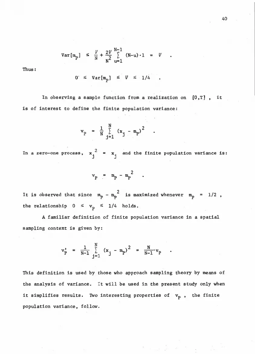
In observing a sample function from a realization on [0,T] , it

is of interest to define the finite population variance:

N

J=l

In a zero-one process, " = x . and the finite population variance is

vp = »p - v • 2

It is observed that since nip - nip is maximized whenever nip = 1/2 ,

the relationship 0 ^ v p ^ 1/4 holds.

A familiar definition of finite population variance in a spatial

sampling context is given by:

N 1 r , .2 N VP = N=l A„ ( X j " m P ) = N=T VP

This definition is used by those who approach sampling theory by means of

the analysis of variance. It will be used in the present study only when

it simplifies results. Two interesting properties of V p , the finite

population variance, follow,

Property 4.3: The mean of the finite population variance is given by:

E[vp] - ^ - " - 4 . T (N-u)-A(tu) . N u=l

Since vartmp] = E[mp 2] - E 2 ^ ] = E[nip2] - M 2 ,

then:

E[v p] = Etnip] - E[mp 2] ,

= E[mp] - (Vartmp] + M 2)

" M " ( f f + 1 f T (N-u)-A(tu) + M 2 ) , N u=l

N u=l

This result was reported by Cochran [2] in a slightly different form.

Property 4.4: Adding the variance of the finite population mean to the

mean of the finite population variance yields the variance of the sto­

chastic process, that is:

Var [nip] + E[v p] = 1/ .

This property is interpreted as indicating that the variance of

the stochastic process is composed of two components. One, Var[nip] ,

is an among "populations variance in the sense that it represents the

variance among the means of all possible finite populations of size N

averaged for a typical population. The other, E[v ] , is a within

42

populations variance in the sense that it represents the variance within a

typical population, averaged over all possible populations of size N .

This result has been reported in the literature, for example, Madow [21].

From this property and the bounds placed on Var[mp], it is seen that:

•0 < E[v ] < 1/ ^ 1/4

It is noted that the companion definition of population variance

leads to a slightly different result.

E [ v P ] " " N O W ) Y (N-u).A(tu) .

u=l

From this expression the utility of the v^ definition of finite popu­

lation variance is clear. For a white noise process A(t^) = 0 for

all u ^ 0 , and thus E.[.Vp] = V . In spatial sampling, the analogy

to white noise is a parent population or superpopulation in random order

so that the autocorrelation function is zero. In this case the finite

population variance is an unbiased estimate of the superpopulation variance.

There are other interesting properties of the finite population:

its autocovariance and autocorrelation functions In both the conventional

and the serial forms, and a necessary and sufficient condition for

periodicity in the finite population. These properties are not as impor­

tant for the development of succeeding chapters as are the properties

already discussed. Thus they are presented in Appendix D.

Statistical Analysis of the Two Sampling Plans

The finite population having N elements available for observation

allows the gaining of considerable insight into the simplex realization.

However, it is not convenient to observe all N possible epochs and

attention is directed to a subset or sample of the elements. Let n

43

represent the actual number of observed epochs that comprise the sample,

regardless of which of the two sampling schemes is utilized. Thus the

sample size is n .

Since both sampling schemes are random sampling plans, it is neces­

sary to introduce this randomness into the N ordered epochs. Let this

be accomplished by a slight alteration of the notation, introducing S as

a point set consisting of all N of the x.'s where each x. is the 3 3

random variable associated with epoch t. . Let the elements of S be 3

denoted by x . Thus S = {x } and for any j = 1,2,»'»«,N , it S • s # J 3 is only by coincidence that: j = s_. .

It is of interest to define certain statistics relative to the

sample of size n , treating it as a sample function of the finite popu­

lation. This is accomplished in the next two chapters. But first it is

noted that the particular sampling plan utilized will often affect the

formulation of the statistic. That is, a simple random sampling plan will

result in certain statistics that have different formulations than the

corresponding ones obtained from a systematic random sampling plan. Since

the statistics can be dependent upon the sampling plan utilized, it is

better to develop the statistics separately. The subscript Sim is affixed

to all statistics calculated from data selected by a simple random sampling

plan. The subscript Sys is affixed to all statistics calculated from data

selected by a systematic random sampling plan. Whenever corresponding

statistics are equivalent for the two sampling plans, this fact is noted.

Statistical analysis applied to a single particular sample, say

{x , x , x x } , can lead to results that are valid only for S l S 2 S 3 S n

44

that particular sample, and cannot be used to draw inferences about the

finite population. Thus there is reason for directing attention to a

representative average sample, where the averaging is done with respect

to all possible samples that can result when repeatedly applying to the

particular finite population, the two sampling techniques under consider­

ation. It has been established that, when sampling without replacement,

there are (^j possible, different simple random samples and k possible,

different systematic random samples. The statistical analysis of the next

two chapters includes this average statistical analysis; it represents

statistical analysis averaged over all possible, different samples avail­

able under each of the two sampling schemes being compared.

Where averaging is done with respect to the finite population of N

elements, the expectation will be denoted by the symbol e . The symbol

E will continue to be utilized for expectation with respect to the sto­

chastic process.

It becomes ambiguous to refer to the expectation of the sample mean,

without specifying whether it is expectation with respect to the finite

population or expectation with respect to the stochastic process. To avoid

possible misinterpretation, the following definitions are adopted. The

expectation of the sample mean with respect to the stochastic process is

referred to as the mean of the sample mean. The expectation of the sample

mean with respect to the finite population is referred to as the average

of the sample mean. It is noted that in the case where n = N , the

mean of the sample mean becomes equivalent to the mean of the finite popu­

lation mean.

45

Similar ambiguity is possible whenever reference is made to the

variance of the sample mean. The ambiguity is avoided by using the term

variance of the sample mean when the variance of the sample mean with

respect to the stochastic process is meant. When variance of the sample

mean with respect to the finite population is discussed, there is no

acceptable word corresponding to variance in the manner that average cor­

responds to mean. Since the word dispersion is frequently used in a

practical explanation of the phenomenon that is statistically measured as

variance, in this paper variance of the sample mean with respect to the

finite population is referred to as dispersion of the sample mean.

46

CHAPTER V

STATISTICAL ANALYSIS OF A SIMPLE RANDOM SAMPLE

Introduction

The objective of this chapter is to provide an analytical development

of some statistics characterizing a simple random sample chosen from some

finite population. In the last chapter the finite population of interest was

defined as a collection of outcomes from the range space of the simplex

realization sample f u n c t i o n , a s s u m e d to h a v e b e e n o b s e r v e d on L0>t3. This

finite population is comprised of N elements, each of them a random varia­

ble, X j , representing the state of the simplex realization at the jth epoch

of time on [0,T]. The population is denoted as: [x^ : j = 1,2,...,n}.

From this population, a subset of n-elements is chosen and subjected

to statistical analysis. The method of selecting this subset has been de­

scribed in Chapter III as the "simple random sampling plan." The subset of

n-elements is assumed to be chosen from the finite population of N-elements

in such a manner that it is just as likely of being chosen as are any of the / N V 1

other I J possible subsets. This subset will be referred to as a "simple random sample" and will be denoted as: [x : i = l,2,...,n],

i

where each s^ is an integer, equally likely of assuming any one of the

integer values on [l,N] .

Statistical Analysis of a Simple Random Sample

Treating the simple random sample as a function of the finite

population, certain statistics relative to this sample are of interest.

47

A simple random sample selected from the finite population has a sample

mean:

1 n

m c i n , = 7T I xc ; s c{l,2,...,N) Sim n . - s. 1 i=l l

This simple random sample mean has a number of interesting properties.

Property 5.1 .: The average of the sample mean is the finite population

mean, that is, the sample mean is an unbiased estimator of the finite

population mean.

This property has been reported in the literature (see, for example, N Cochran [3] or Hansen, Hurwitz, and Madow [9]) and, letting K =

can be demonstrated^^ as follows:

l K l n l l n K

{ mSim } = I A (n X Xs. }k ' In X A ( Xs. }k k=l " i=l i " i V " i=l k=l "i

(1) An alternative demonstration is also possible.

1 n 1 n

e f mSim } = e { n X**.] = " X*[X*.] i=l l i=l i But with respect to the finite population:

N N

e " .' 1

{x } = Y x.«Pr{x = x.l = T x.•— l j=l J i J j=l J

Thus:

48

Since takes on the value j with probability equal to 1/N in each

of the K possible simple random samples:

1 1 n N 1 1 N

c SimJ K n .L- ,L> yw N .L j ? 1=1 j=l J j=l J

It is noted that the mean of the average sample mean is the process

mean, that is : E ^ e f m s i m ^ = E[nip] = M > and similarly that:

v o f / N _ 1

Var[€{m }] = Var[m ] = ± + ^ £ (N - U)-A(t) S l m P N 2 u=l u

Property 5.2 : The mean of the sample mean is the stochastic process mean,

that is, the sample mean is an unbiased estimator of the process mean.

^ JE[X(t s_)] = M . 1=1 1

The next statistic of interest is the dispersion of the simple random

sample mean.

Property 5.3 : The dispersion of the sample mean provides an estimate of

the finite population variance and is given by:

v v' f N-n P N-n P var[m ] = rr^r-— = — — Sim N-i n N n

This property has been reported in the spatial sampling literature (see,

for example, Cochran [3], Hansen, Hurwitz, and Madow [9], and Kendall and

Slm n # i s. 1=1 l

49

Stuart [14]) where the coefficient is referred to as the "finite population

correction" factor and has a denominator of either N or N-1 , depending

upon the definition given to the finite population variance.

The demonstration of this property is interesting and is included

as follows:

: { mSim ] = e t ( m S i

I Xs n=l Si

n

n

n 1=1 1

Recall the identity from analysis of variance:

n-1

So that:

1 n 2 n-1 n

I - 1

50

It has been stated that x takes on the value x , (I = 1,2,...,N) , S . I

1 with a probability measure equal to 1/N. That is, Pr{x = x } = 1/N

S • J_ 1

for all I .

Thus:

2 N 2 1 ? 2 e{(xs - mp) } = 3>.(x - nip) .pr{xg = x ^ = - J" ( X j - m p) = v p

i 1=1 i 1=1

Therefore, the first summation term in the dispersion formula becomes:

1 n

n i=l i 1

= ~ 9 I V l i=l v p/n

It is desired to simplify the second summation term in the dispersion

equation. To accomplish this it is necessary to find an expression for

Pr[x = x T, x = x,l for appropriate values of I and J , I ^ J . s. I s . J i J

P r [ x s . = X I ' X s . = X J ] = P r [ x s . = X j K . = X I ] - P r [ x s . = X I ] =

i l i i i

So that:

H N e{(xg - V ( x s. " V } =

I " V ( X J * V N^Ti-1 J 1=1 J=l

I * J

2 N-l N = I P ) J x j j + 1 2 ( xi" V ( x j " V

51

Recalling an identity from analysis of variance and applying it to the right

hand side:

i j 1=1 1=1

The first term inside the brackets is equal to zero by the definition of

m p , and by the definition of v p the second term is equal to N*v p .

Thus:

1 ~ VP ef(x - HI ) (x - ni )} = , ' . [-N*v 1 = — r l v s i p' v s^ Y } N(N-l) L P J N-1

Therefore the second summation term in the dispersion equation is

n-1 ri n-1 n (-vp) - 2 : \ J. + 1

e f ( xs. - V ( xs. - VJ • - 2 I , £ —

n i=l j=i+l j j n i=l j=i+l

^1 n^n-l) 2 2 n (N-1)

(n-l)vp

n(N-l)

Combining the two summation terms leads to the final expression for the

dispersion of the simple random sample mean, when sampling is done

52

(2)

V a r l m S i m j = T - n(N-l) = N^T'T

When reference is made to this property in the literature, authors

sometimes do not make a distinction between variance of a sample mean with

respect to the finite population and variance of the sample mean with re­

spect to an underlying stochastic process. Usually the quantity v a r ^ m g i m ^

is referred to simply as the variance of the sample mean. This investiga­

tion distinguishes the two quantities. Since v p ^ 1/4, it is seen that:

The next property will be important in Chapter VII. It relates the

average sample statistic to the stochastic process.

(2) Whenever the simple random sampling is done with replacement

x and x are independent and: Si Sj

P r [ xs = x r x

s . = x j ] = P r [ xs = x i ] ' P r [ x

s = x j ] • 1 J 1 / j

Thus:

e{( xs " m p ) * ( x

s " mp ) T = e £ x

s " m p)-e{x g - n^} = 0-0 , i j i j

and:

var {m„ . } T m = v /n L SimJWR P

This result agrees with intuition since sampling a finite population with

replacement is akin to sampling from an infinite population with variance

equal to v p .

without replacement

53

Property 5.4 : The mean dispersion of the sample mean is given by:

E[varK,lm}] = jj=S,(,.(l . jV„)A(t u)) '

Using the definition for dispersion of the sample mean and the

definition for the mean of the finite population variance:

I-- v

E[var(msim}] = E[f^j = ^ . I.E[v p]

' U=l

(3)

This result appears in Cochran's paper [2] with a name that is

confusing. It is noted that the mean dispersion of the sample mean has the

same bounds as the dispersion of the sample mean.

The next statistic of interest directly relates the simple random

sample mean to the stochastic process. Property 5.5 : The variance of the sample mean is given by:

if «ii n-1 n V a r U . ] = t + 4 I I A(t ) . Slm n 2 ,L. ,L . v s . - s n i=l j=i+l j i

(3) The averaging operation of the present paper is equivalent to the one assumed by Cochran, that is, averaging "over all finite populations drawn from the infinite population"' (superpopulation). However, Cochran identifies this mean dispersion as an "average variance." This name is confusing since it literally indicates that the averaging is applied to the variance of the sample mean when, in fact, expectation is applied to the dispersion of the sample mean.

54

By the standard definition of variance, the definition of the

autocovariance function for the stochastic process, and algebraic manipula

tion, this result can be demonstrated.

V a r [ m S i m ] " E [ m s i m ] " ( E [ m S i m ] ) 2

? \2 / _ i S \ 2 V a ^ s i m ] • E [ ( i K ) : - ( E ^ . I x s >

i=l I i=l I

, n n i n n

1 « [ I I xs X s ] - 2 ( I E [ x s ^ E [ x s ] ) ' n i=l j=l i j n i=l i j = l j

\ I l {E[xs - x ] - E[x s ].E[x ] } , n i=l j=l i j i j

\ I I {ECX(t8 )-X(t )] - E[X(t )]-E[X(t )]} n i=l j=l ^ i j i j

i n n

- \ I I ^-A(t - t ) , nl i=l j=l Sj Si

Var[mQ. ] = V- •+ 21 ^ £ A ( t ) Sim n 2 - - - . i s . - s . n i=l j=i+l j l

Using the properties of an autocorrelation function that A(t S # •* s J

A(t ) i 1 for all t : s . - s . i J

n i=l j=i+l

55

Thus:

0 £ Var[m0 . '] £ 1/ £ 1/4 Sim

The variance of the sample mean is seen to be a function that depends

upon the time epochs t and t . Since the selection of these epochs s # s # 1 J

is equivalent to the selection of the observations that are associated with

them, they are essentially random variables. Thus, the e-averaging operator

may be applied in order to average the variance of the sample mean over all

possible selections from the finite population (in this case, a finite popu­

lation of time epochs). The result of this operation is reported as the

following property.

Property 5.6 : The average variance of the sample mean is given by:

e{Var[mc. ]} = - + l^1^ ^(H-u)A(t ) . u Sim n nN(N-l) L, u u=l

Using an intermediate equation from the derivation for the variance

of the sample mean in Property 5.5 :

*{Var[ms.m]} = c{ -L j j (E[X x ] - E[x ]E[x ])} , n i=l J=l i j i j

n i=l l l

n i=l j=i+l l j l j

5 6

But:

E[x 2 ] - (E[x ] ) 2 = E[x ] - (E[x ] ) 2 = M - M 2 = 1/ s # s, s, s. 1 1 1 1

And:

E[x ] - e [ x ] = M - M = M ' s. s. 1 J

Thus:

^ ^ J ) - \ l e{t/} + \ *l f «{E[x B . x a ] ] n n=l n 1=1 j=i+l i j

9 n-1 n \ I I e { M 2 } . n i=l j=i+l

n-1 n Now by the nature of £ £ x »x , E[«], and e{*} it can be shown

that:

. i . . , 1 s . s . i=l j=i+l i j

e{E[x -x ]} = E[e{x .x }]

And using the same probability argument used in the derivation for the

dispersion of the simple mean: »

efx *x } s. s . i J

N-1 I 1=1 J=I+1

2 x i V i ) (NTT>

57

Therefore:

n-1 N r N-1 N e{Var[m . ]} = - + -4r Y Y E / 1 X Y Y x x 1 L Sim J 3 n 2 . , ,« L N(N-l) T

L1 _ I J-

n i=l j=i+l 1-1 J=I+1 - (^)M 2

n

u o/ 1 N N-1 N 0 / 1 N N-1 N 0 = J/ 2 (n-1) y y r -, _ 2(n-l) y y ^2

n nN(N-l) l{ Jm\+*lW nN(N-l) ^ J = ^ M *

= I- +. n N-1 N

., ... N-1 N

N-1 e{Var[in . ]] = ^ + i ; ^ £ ^ 7 I (N-u)A(t ) . Sim J J n nN(N-l) u

The average variance of the sample mean has an interesting relation­

ship with the mean dispersion of the sample mean:

efvar[ms.m]} - E[Var{m S i ml] = V a r ^ ]

Thus it is clear that the two quantities differ by an amount equal to the

variance of the population, mean. Furthermore, the average variance of the

sample mean is never smaller than the mean dispersion of the sample mean.

This relationship is interpreted as indicating that more of the variation

in the sample mean is likely to be revealed by considering variance with

respect to the process than by considering variance with respect to the

finite population.

58

There is also a coniponents-of-variance interpretation embedded in

this relationship. Since Var[e{mg_^}] = Var[nip] , the relationship

can be rewritten as:

e{Var[m . ]} = E[var{m ]] + Var[e{m }] Sim Sim Sim

This relationship is interpreted as indicating that the variance of the

sample mean, averaged over all possible simple random samples, is composed

of two components. One, E[var{nig m}] , is a within samples contribution

in the sense that it represents the expectation of the dispersion within a

typical simple random sample. The other, Var[ e( mgj_ m-^ » ^ s a n °onong

samples contribution in the sense that it represents the variance among the

average sample means of all possible simple random samples.

In analyzing a simple random sample selected from the finite popula­

tion described earlier, it is also of interest to define the sample variance

1 n

— y (x m„. ) n , L. v s .. Sim' v„ .. S lm - . -,

i=l I 2 With zero-one random variables, x = x , and the simple random s. s. i i

sample variance is:

2 v_. = m„. - m„. Sim Sim Sim

2 It is observed that, since m_. - m_. is maximized when m„. = 1/2, Sim Sim Sim the relationship 0 £ v„. ' < 1/4 holds.

S im

A familiar definition of the sample variance, often used in spatial

sampling literature, is given by:

59

— ? (x - m ) 2 = — v VSim n-1 X s . " mSiirr n-1 VSim i=l 1

It will be used in the present study only when it simplifies results.

There are a number of interesting properties involving the simple

random sample variance. The first one relates it to the finite population.

Property 5.7 : The sample variance is a biased estimator of the population

variance, but with known bias, that is, the average of the sample variance

is given by:

r i N(n-l)

2 2 2 2 Since var{m_. } = e [m_. } - (eU . }) = e{m_. } - m_ ; L Sim Sinr Sinr ^ Sim J P '

e f m„. } = in ; var {m. } = ^ n,. * v„ ; and v„ = ni m 2 , L Sinr P L SimJ n(N-l) P ' P P P '

then: € [ v S i m } = &[mSiJ " e [ mSim^ '

= mp - (var{m s i m} + m2,)

N-n = N(n-l) VP " n(N-l) VP n(N-l) *VP

A simplified version of this property appears in Cochran [3]

efv1 1 = v 1 6 1 Simj P

Property 5.8 : Adding the dispersion of the sample mean to the average of

the sample variance yields the variance of the finite population from which

60

the sample was selected, that is:

varfm }'•+ e{ v_ ) = v Sim Sim r

This property is interpreted as indicating that the population

variance is composed of two components. One, var(m_. } , is an among Sim

samples variance in the sense that it represents the dispersion among the

means of all possible simple random samples of size n that could be

selected from the same finite population. The other, e{v . } , is a * Sinr '

within samples variance in the sense that it represents the variance within

a typical simple random sample, averaged over all such samples. This re­

sult appears in Kendall and Stuart [14] and is attributed to Kish.

Both the dispersion of the sample mean and the average of the sample

variance are related to the finite population variance. Thus the dispersion

of the sample mean is proportional to the average of the sample variance,

with a known factor of proportionality: var [m_ . } = n., N • e [v_ . } L Sinr N(n-l) Sinr

Property 5.9 : The mean of the average sample variance is given by:

E ^ v s l m " - 3 ± { V - ifcYa. " »>*<*„)) • u=l

Using the definition of E[y p] from Chapter IV and applying the

expectation operator to Property 5.7 leads to the result. Adding the

average variance of the sample mean to the mean of the average sample

variance yields the variance of the stochastic process, that is:

61

1/ = e[Var-[m ]} + e[*{v , } ] . bim bim

This result has a components-of-variance interpretation, but it is not

given. Instead, another interesting property of the sample variance is

presented. It directly relates the sample variance to the stochastic pro­

cess.

Property 5.10 : The expectation of the sample variance is given by:

. n-1 n

e[vc. ^ = s=±v - i i A(t ) Sim n 2 . L - - . i i * 8 - s #

n 1=1 j=i+l j l

Since E [ m s l m2 ] = V a r t m ^ ] + ( E C n^J) 2 = Var&^J + M 2 ;

2 E[m . ] = M ; and M - M = 1/ , then by applying the definition of Sim

Var[m0. ] from Property 5.5 and simplifying: S im

E [ v S i m ] " E [ m s i m ] " E [ m S i m 2 ] >

= M - M 2 - . Var[m s l m] ' ,

. , . £ . i l f i A ( t ) . n 2 . « . •i-i s. — s. n i=l j=i+l j l

. o l / n-1 n n-1 (/ 2v

n i=l j=i+l j l

Property 5.11 : Adding the mean of the sample variance to the variance of

the sample mean yields the variance of the stochastic process, that is:

Sim bim

62

This property is interpreted as indicating that the variance of the

stochastic process is composed of two components. One, Var[in . ] , is an S i m

among samples variance in the sense that it represents the variance among

the means of different simple random samples of size n selected from the

N available observations. The other, e [ v „ . ], is a within samples S i m

variance in the sense that it represents expectation of the variance within

a simple random sample.

The mean of the sample variance is seen to be a function that depends

upon the time epochs t and t . Therefore, as was done in Property s # S • # •

1 J 5.6 for the variance of the sample mean, this expression can be €-averaged over all possible selections of s. and s. .

l j

Property 5.12 : The average of the mean sample variance is equal to the

mean of the average sample variance, that is:

e{E[vsim]} - E[c{vsim}] - ! _ ( „ - jJtf- Y ( N - u )A(t u)) . u=l

Applying the ^-operator to the equation of Property 5.11 and then

solving it simultaneously with the components-of-variance equation appearing

under Property 5.9 establishes the result.

This concludes the statistical analysis of a simple random sample.

Attention is next directed toward the analysis of a systematic random sample,

so that the statistics from these two plans can be compared.

63

CHAPTER VI

STATISTICAL ANALYSIS OF A SYSTEMATIC RANDOM SAMPLE

Introduction

The objective of this chapter is to provide an analytical develop­

ment of some statistics characterizing a systematic random sample chosen

from some finite population., The order of presentation Is the same as

that for the analysis of a simple random sample in the previous chapter.

The finite population was defined in Chapter IV and, as in the

previous chapter, is considered to be comprised of N elements, each a

random variable representing the state of the simplex realization at the

j-th epoch of time on [0,T] . As is common in the systematic sampling

literature, it is assumed that N can be factored by n and k , so that

the finite population may be denoted as: {x_. : j = l,2,*««,nk} .

From this population, a subset of n elements is chosen and sub­

jected to statistical analysis. The. method of selecting this subset was

described in Chapter III as the "systematic random sampling plan." The

first element of the subset is assumed to be chosen from the first k

ordered elements of the finite population by a simple random sampling

scheme. Then, starting with that element, every k-th ordered element

of the finite population is systematically selected as a member of the

subset, until the n-th member is selected. Thus subset is referred to

as a "systematic random sample" and is denoted as {x ,,. : i = r s+(i-l)k

l,2,«'«,n} , where s is an integer, equally likely of assuming any one

of the integer values on [l,k] .

64

Statistical Analysis of a Systematic Random Sample

Treating the systematic random sample as a function of the finite

population, certain statistics relative to this sample are of interest.

A systematic random sample selected from the finite population has a sam­

ple mean:

1 n

Sys n ^ s+(i-l)k' ' ' *

This systematic random sample mean has a number of interesting properties.

Property 6.1: The average of the sample mean is the finite population

mean, that is, the sample mean is an unbiased estimator of the finite popu­

lation mean.

This property has been reported (for example, Cochran [3] or Hansen,

Hurwitz, and Madow [9]). It can be demonstrated^ as follows:

(1) An alternative demonstration is also possible.

1 n 1 n

e{m_ } = e{— 7 x 1 N 1 } = — 7 e{x l N 1 } Sys n fj s+(i-l)k n ^ s+(i-l)k

But with respect to the finite population:

N N 1 e(x t m } = 7 x.«Pr{x , ,. ,>., = x.} = 7 x.(—) s+(i-l)k . L- j s+(i-l)k j , L- j N J=l J J J=l

Thus:

1 n N 1 1 N

e {m_ 1 = — 7 y x. (—) = T7 I x. = m_. Sys n i N N i T i=l j=l J j=l J

65

1 k fl n

e { m S y s } = k J=1 In ±l± Xs+(i-l)k;S

^ ^ n k ^ nk = i=l s=l X s + ( i - 1 ) k

j = i XJ = '

It is noted that the mean of the average sample mean is the process

mean, that is: E[ ^ mS y s ^ ] = E[mp] = W , and similarly that:

Varied }] = £ + ^ J (H-u)A(t ) N u=l

Property 6.2: The mean of the sample mean is; the stochastic process mean,

that is, the sample mean is an unbiased estimator of the process mean.

1=1 1=1

The next statistic of interest is the dispersion of the systematic

random sample mean.

Property 6.3: The dispersion of the sample mean is given by:

^ 2 n - l N-ku V a r { m S y s } = n V P + n¥ I J, (xj"V ( xku+J " V

u=l J=l

This property appears in spatial sampling literature (for example, Cochran

[3]) in a form that can be written with the present notation as follows:

r i 1 . n-1 var {m_ i = — v^ + • v_ • p , Sys n P n P w

66

where p is defined to be the correlation coefficient between pairs of w v

sampling units that are in the same systematic sample. The demonstration

of this property is interesting and is included.

v a r { m S y s } = e { ( m S y s " e { m S y s } ) 2 } = e { ( m S y s "

i=l 1=1

= j < xs +(i-l)k - V )'> •

h ( xs+(i-Dk - v ) 2 }

n 1=1

Apply the identity from analysis of variance:

( (X8+(i-l)k " = \ (XS+(i-l)k ' V 1=1 1=1

n-1 n + 2 i i j - L ( x « + < ^ » " v ^ + u - D k - v

Thus:

var i r n

{ m S y s } = T (xs+(i-l)k " V J n i=l

n-1 n ii j_ ii / -\

+ 2i=l j-i+l <X«+(i-l)k " V * (xs+(j-l)k " V i •

67

var 1 f n

{ m S y s } = T e l . ^ (xs+(i-l)k " V n i=l

..n-1 n + ^ e i . I ( Xs+(i-Dk _ V (xs+(j-l)k " V / n i=l j = i+l J

It has been stated that x ,,. 1 N 1 takes on the value x T , (I = 1, s+(i-l)k I

2,***,N) , with a probability measure equal to 1/N . That is,

P r { xs+(i-l)k = X I } • 1 / N f o r a 1 1 1 • Thus :

2 N 2

:{(xs+(i-l)k " V } =

Tl± ( X I ' V 'Pr{xs+(i-l)k = X I } '

1 N 2 = N Tl±

( X I " V = VP *

Therefore the first summation term in the dispersion equation is:

h X e { ( x s + ( i - D k - V 2 } = 1 / 1 , 2 • I, VP = ^ V P • n i=l i=l

In order to simplify the second summation term in the dispersion equation,

it is convenient to make a change of notation:

Xs+(i-l)k = Xs+(i-l)k " INP a n d Xs+(j-l)k = xs+(j-l)k " ™P 9

so that the second summation term becomes:

2 n-1 n

7*1-1 j-Ll i , { < X " + a - D k " V ( xs+(j-l)k ' V }

68

2 n-1 n = 7 i = i j - L ' ^ ( i - D l ' W D k 1

By expanding the double summation:

n-1 n i=l j-i+l e { Xs+(i-Dk* Xs+(j-l)k }

= e{x'-x' } + e{x' •x,,01'} + •••+ e{x,.-x,,/

s s+k s s+2k s s+(n-l)k

+ e { xs+k* Xs+2k } + e { x s + k > X s + 3 k } + ••• + e { xs+k* Xs+(n-l)k }

+ e { xs+(n-3)k* Xs+(n-2)k } + e { xs+(n-3)k* Xs+(n-l)k }

t xs+(n+2)k s+di-Dk 1

Since s is randomly selected from the integers on [l,k]

k i •{x'.x' } = I xL-x' ( r )

s s+k fj J J+k k '

1 e { xs* Xs+2k } = I " j ^ W k * ' J=l

1 e{x ,-x ,. / N M } - I x T * X T _ l / I M ( r ) » s x+(n-l)k £ J J+(n-l)k k' '

69

2k 1

e { x s + k * x s + 2 k } = T I *j'xM<d '

J=k+1

2k ^ . • 1

e { xs+k* xs+3k } = _. % ^j'^J+lkQ J=k+1

E { X * . X ' > S + K X

S + ( N - L ) K '

2k

J=K+1 X J X J + ( N - 2 ) K V

(n-2)k 1

e { xs +(n-3)k' xs +(n-2)k } ' | « I " « W K > " •

(n-2)k x

e{xs+(n-3)k*Xs+(ri-l)k} = T , . L n XJ' XJ+2k (k }

J = (.11— J J K T ±

(n-l)k x

e { xs+(n-2)k' Xs+(n-l)k } = _ , ^ _^ ^ J ^ J + k ^ * J=v.n-z ; k+l

Gather those terms wherein the indices on x!*x! differ by k . There 1 J

are n-1 of these terms. Then gather those n-2 terms whose indices

differ-by 2k ; those n-3 terms whose indices differ by 3k ; and so

forth until the last single term whose indices differ by (n-l)k . Adding

them in this fashion yields:

n-1 n i-1 j-i+1 e { Xs+(i-l)k' Xs+(j-l)k }

70

± (n-l)k ± (n-2)k

J=l J=l J+2k .

x 2k k + k J Xj' XJ+(n-2)k + k J XJ* XJ+(n-l)k

Returning to the original notation, the double summation appears as

n-1 n

i-l j-Ll "{(X«+(i-Wk " V(xs+(j-l)k " *p)}

x (n-l)k (n-2)k = k J (xj"V ( x j+ k -V + k l

( x j - V ( xj+2k - V +

2k k + k Jx

( x J - V ( xJ+(n-2)k- mP ) + k I ( x r V ( xJ+(n-l)k- mP )

Collecting terms yields:

n-1 n

i-l J-i+l e { < Xs+(i-l)k" mP ) ( Xs+(J-l)k" mP ) }

j- n-1 N-ku = k I I ( x J - m P ) ( xku+J- n lP )

u=l J=l

Combine this result with the result for the first summation term. Then the

dispersion of the sample mean is:

71

^ 2 n-1 N-ku V a r { m S y s } = n V P + S f \ I (XJ-V (xku+J-mP) •

u=l J=l

The following property will be important in the next chapter. It

relates the average sample statistic to the stochastic process.

Property 6.4: The mean dispersion of the sample mean is given by:

N / 9 N _ 1

E[var{mc }] = | p (Ml - * n £ (N-u)A(t ) Sys Nn \ N(N-n) , u u=l

+ I 1 (n-u)A(t )) . n(N-n) £j_ ku / u=l

This expression can be developed as follows:

r-v 2 n-1 N-ku E[var{ms }] = E [ - + - J J ( x J _ m p ) ( xku+J - mP )J '

u=l J=l

Expanding the product under the double summation and then using the linearity

property of expectation yields:

1 ? n-1 N-ku , E[var{m }] = - E [ v p ] + ^ \ \ [ilxyx^l

u=l J=l

Thus there are five terms involving expectations that are required for the

expression. The first one, ~ E[v p] , is easily obtained since an

expression for E[v_] was derived in Chapter IV.

72

£ E [V • in 1 " - h X (H~u)A<t»)

nN u=l

The next term is also easily obtained since

2 n-1 N-ku n¥ E I E [ xj" xl«rfJ ]

u=l J=l

„ n-1 N-ku ,

U = l J = l

9 n-1 N-ku / 9

sf X I ( E[vW- B £ xj ]- E tW + M

u=l J=l

9 n-1 N-ku / s jL I I ( i W V - X f ^ ) ] -E[X( t j)].E[X(t k u + J)]j

u=l J=l

0 n-1 N-ku

U = l J = l

n-1 N-ku 9

u=l J=l

n-1 N-ku \ I I l/.A(t. ) + M 2 , nN i T

L1 ku n u=l J=l

^ Y (n-u)k.A(t. ) + M 2

nN Ln ku n u=l

-i X (n-u)A(t^+^ m2

n u=l

73

The third and fourth termsare more difficult to obtain. The analy

sis of the fourth term follows a procedure analogous to that of the third

one, so that it suffices to obtain the third term. By the definition of

m„ :

2_ n N

n-1 N-ku n-1 N-ku ^x T N

u=l J=l u=l J=l j=l J

n-1 N-ku N

I I I E[x Tx 1 , O L L L - U " T " .

N n u=l J=l j=l J

n-1 N-ku N RJ 11 X 11 IX.U. 1H i

4" l I l (EtXj-x ] - ElXjJ.Etx ] N n u=l J=l j=l J J

+E[Xj]-E[x]J ,

n-1 N-ku N -y- I I I (cov[X(t );X(t )] + N"n u=l J=l j=l J

n-1 N-ku N o l , ii-J. IM-^U J.N 0 n - 1 N-ku N 0

N " n u=l J=l j=l J N n u=l J=l j=l

n-1 N-ku N O R / 11—J. IN K.U IN

N n u=l J=l 3=1 J

M 2

It is known that A is symmetric about t , that is: A(t T .) o J-j

= ACt^j) . Thus:

74

n-1 N-uk N I I I A(t )

u=l J=l j=l 3

n-1 N-uk . J N I I ( l A ( t j ) +• I A(t )

u=l J=l Vj=l J J j=J+l 3 J

n-1 N-uk J n-1 N-uk N I I I A<t > + 1 1 I A(t :

u==l J=l j=l J J u=l J=l j-J+1 3 J

But A(t ) = 1 so that the first triple summation can be rewritten as o

n-1 N-uk J n-1 r N-uk J-l I I I A(tj ,) - I [ l + I ( I A(t ) -HI)] ,

u=l J=l j=l J 3 u=l L J=2 j-l J 3 J

n-1 _ N-uk J-l _. I [N - uk + I I A(t )

u=l L J=2 j=l J 3 J

n-1 N-uk J-l ^ + I I I A ( t j . ) .

u=l J=2 j=l J 3

(2)

The second triple summation term can also be developed further. Letting

the index u be rewritten as v and introducing a change of variable for

the index j :

n-1 N-vk N n-1 N-vk N-J I I I A(t ) - I I I A(t ) .

v=l J=l j=J+l 3 v=l J=l j=l 3

(2) Analysis of the terms in this triple summation shows that, for each value of u , the terms can be arranged in a lower triangular matrix by moving down the rows as J goes from 2 to (N-uk) and by filling the columns from right-to-left as j goes from 1 to J-l . Thus the i-th column of the lower triangular matrix is a vector containing (N-uk-i) elements, all of which are A(t^)'s .

75

For a finite sum, letting an index range from a to b in increments of

one is equivalent to letting the index range from b to a in decrements

of one. Applying this fact: to the triple summation yields:

n-1 N-vk N n-1 N-vk vk-J+1 I I I Act ) = 1 1 I A ( t :

v=l J=l j=J+l J v=l J=l j=l J

(3)

The two triple summation terms can now be combined, simplified, and

displayed as: n-1 N-uk N xt/ i \ • N-1

I I I A(t. ) = l^zl! + (n-1) I (N-u)A(t) . u=l J=l j=l J " J 2 u=l u

Thus the third term in the expression for the mean dispersion of the sample

mean can be written as:

(3) If v is chosen in such a way that v + u = n , that is, v = n - u , then each value of v will lead to terms that, when properly arranged, will extend the lower triangular matrix introduced in the last footnote. For each value of u , the first triple summation will fill the first N - uk - 1 rows of a lower triangular matrix. For each value of v , the second triple summation will fill the next uk rows of the lower tri­angular matrix in exactly the same manner as described above. Thus for each pair (u,v) = (u,n-u) , analysis of summations will lead to a lower tri­angular matrix whose i-th column is a vector containing N-i elements, all of which are A(t±) fs (i = 1,2,»»»,N-1) . Interest lies with the summation of all these terms, a quantity that can be expressed as:

N-1 I (N-i).A(t.) i=l

Since there are n-1 pairs, each one of which fills a lower triangular matrix, there are n-1 of these last summations.

76

n-1 N-ku 0 | / . f . N-1 \ n 0

3 ^ J " ' W " 4 - p ^ + ( - l ) I ( N - u ) A ( t u ) ) + ^ M2

u=l J=l N n u=l

M a i l + HtI»-iL Y ( N . u ) A ( t ) + s=i M2 . Nn .T2 • u n N n u=l

The fourth term in the dispersion expression is analyzed in much (4)

the same manner as the third. The result is the same as that for the

third term.

0 n-1 N-ku ... . o t t , N-1 h i i E w v • ^ - " ^ r(N - u ) A(t u ) + ^ M ^

u=l J=l N n u=l

The fifth and last term required by the expression for dispersion

of the sample mean is more easily obtained. Since the indices u and J 2

have no effect on E[nip ] :

„ n-1 N-ku .„ 2E[m?] n-1 N-ku n _ h I I ^ - t l < « • •

u=l J=l u=l J=l

2 2 But E[nip] = Var[nLp] + (E[nip]) and was implicitly defined in Chapter

IV. Thus the fifth term in the dispersion expression is:

% Y T - ^s=-11 + Y (N-u)A(t ) + a=i u 2

nN L^ T

L, r Nn „2 L- u n u=l J=l N n u=l

(4) The roles of the two triple summation terms are reversed in the sense that the second one is used to fill a lower triangular matrix and then the first one extends it to a larger lower triangular matrix.

77

The five mean dispersion terms are combined and the final expression for

the mean dispersion of the sample mean is given by:

M_ / 9 N-1 E[var{mQ } ] = £-3- (Ml - „ 2 n , £ (N-u)A(t ) Sys Nn \ N(N-n) ^ u u=l

< n " u ) A ( t « » ) ) •

This result has been obtained through a different argument by Cochran [2]

for spatial sampling applications. Cochran again refers to the quantity

as an "average variance" (see the comment in the third footnote in Chapter

V) .

The next statistic of interest directly relates the systematic ran­

dom sample mean to the stochastic process.

Property 6.5: The variance of the sample mean is given by:

Var[mc ] = - + ^ J (n-u)A(t, ) Sys n 2 ku n u=l

Using the standard definition of variance, the definition of a sys­

tematic random sample mean, the definition of the autocovariance function

for the stochastic process, and algebraic manipulation, this result is

demonstrated.

Var[mc ] = E[m2 ] - (E[m0 ] ) 2

L Sys J Sys Sys '

78

E [ ( n ± l ± Xs+(i-l)k r J

n

" ( E £ I x s + ( i - l ) k O :

s e { i , 2 , - - . , k } ,

K B

n n

n

2 J L ± Xs+(i-l)k-As+(j-l)k.

i r n "i r n 7 x s + ( i - i ) k j - E y l x s + ( j - D k -

n n

7 i - l j - l i E [ X s + ( i - l ) k , X s + ( j - l ) k ]

- E [ x s + ( i - l ) k 1 - E [ x s + ( j - l ) k ] } •

n n

n i - l j - l ) ]

- E l X ( t . + ( i - D k ) ] - E W V ( j - i ) k > ] } •

n n ^ u 4 i

^2 ± l ± . l ± V , A ( t 8 + ( j - l ) k " t 8 + ( l - l ) k ) '

n n

" T I A ( t ( j - i ) k > • n i = l j = l J 7

n + T . i ^ ( j - D f c ) > n i = l j = i + l J

79

1/ 21/ n _ 1 n " 1 ' " n" + ^ I I A ( t(i-i)k> ' n n i=l j- i=l U 1 ; *

Letting J = j - i and replacing the index i by u

9 (, n-1 n-u V-t»Sys] - £ + 4 Z X A(tkJ) , n u=l J=l

n u=l

Using the property of an autocorrelation function that ^(t^ u) £ 1

for all t, ku

1/ 9(7 1 1 - 1

V a r t m S y s ] S ^ R J (n"u)-(1) " " • n u=l

Thus:

0 ^ Var[m_ ] <l 1 / ^ 1 / 4 SysJ

The variance of the systematic random sample mean does not have the

dependence on the time epochs that the variance of the simple random sample

has. Thus, the expression is invariant under the finite population averag­

ing operation and the average variance of the sample mean is equal to the

variance of the sample mean.

u 9 u n 1 *{Var[ms ]} = Var[m ] = - + -j \ (n-u)A(t k u)

J n u=l

80

The average variance of the sample mean has an interesting relation­

ship with the mean dispersion of the sample mean:

e{Var[m S y g]} - E[var{m }] = V a r ^ ] .

Thus it is clear that the two quantities differ by an amount equal to the

variance of the population mean. The average variance of the sample mean

is never smaller than the mean dispersion of the sample mean. This expres­

sion also indicates that the variance of the systematic random sample mean

is never smaller than the variance of the finite population mean:

Var[m S y g] - E[var{m S y g}] = Var[mp]

And there is a components-of-variance interpretation embedded in this

relationship. Since Var[e{m S y g}] = Var[nLp] , the relationship can be

rewritten as:

e{Var[m g y g]} = E[var{m S y g}] + Var[ {m S y g}]

This relationship is interpreted as indicating that the variance of the

sample mean, averaged over all possible systematic random samples, is

composed of two components. One, E[var{nigyg}] , is a within samples

contribution in the sense that it represents the expectation of the dis­

persion within a typical systematic random sample. The other,

Var[e{m S y g}] , is an among samples contribution in the sense that it

represents the variance among the average sample means of all possible

systematic random samples.

81

In analyzing a systematic random sample selected from the finite

population described earlier, it is also of interest to define the sample

variance:

1 vSys = n ±l±

( xs+(i-l)k " mSys }

2

2 With zero-one random variables, ( x

s+(i l)k^ = Xs+(i-l)k ' a n d t* l e

systematic random sample variance is:

2

Sys Sys Sys

2 It is observed that, since m_ - m_, is maximized when m_, = 1/2 ,

Sys Sys Sys ' the relationship 0 £ v 0 ^ 1/4 holds.

Sys

A familiar definition of the sample variance, often used in spatial

sampling literature, is given by: n n v, 1 VSys = n^I J ( xs+(i-l)k " mSys ) n-1 Sys

It will be used in the present study only when it simplifies results.

There are a number of interesting properties involving the systematic

random sample variance. The first one relates it to the finite population.

Property 6.6: The average of the sample variance is given by:

n _ 1 2 n-1 N-ku

e { v S y s } = ^ VP " nN I I j'V ( xku+J " mP

) • u=l J=l

This property can be demonstrated as follows:

82

6 { v S y s } " 6 { m S y s } " >

= e{m S y s} - [var{m S y s> + ( e { m S y s » 2 ] ,

= mp - m 2 - var{m S y s} ,

2 VP 2 n _ 1 N ~ k u = r^-r^- — -— I I (x - n) (x - mp)- , u=l J=l

n-1 2 ^ ~ k u

^~ VP - s r i -Uj - v ( xku - v • u:=l J=l

Property 6.7: Adding the dispersion of the sample mean to the average of

the sample variance yields the variance of the finite population from which

the sample was selected, that is:

V a r { m S y s } + e { v S y s } = VP

This property is interpreted as indicating that the finite population

variance is composed of two components. One, var{mg y g} , is an among

samples variance in the sense that it represents the dispersion among the

means of all possible systematic random samples of size n that could be

selected from the population. The other, e"fvsyS^ » ^ s a ^thin samples

variance in the sense that it represents the variance within a typical

systematic random sample, averaged over all such possible samples. This

result appears in Kendall and Stuart [14] and is attributed to L. Kish.

Property 6.8: The mean of the average sample variance is given by:

83

n u=l

This property is demonstrated using Property 6.7; the definition for

E[v ] from Chapter IV; and the definition for E[var{m }] from Property r oys 6.4.

E[e{v S y s}] = E[v p - var{m g y s}] ,

E[v p] - E[var{m S y g}]

n u=l

Adding the average variance of the sample mean to the mean of the average

sample variance yields the variance of the stochastic process, that is:

V = e{Var[m S y s]} +E[«{v }] .

This result has a components-of-variance interpretation, but it is not

given. Instead, another interesting property of the systematic random

sample variance is presented. The property directly relates the sample

variance to the stochastic process.

Property 6.9: The mean of the sample variance is equal to the mean of the

average sample variance, that is:

E K ; y s ] - E[c{v }] = S i 1/ - 2f T > - u ) A ( t k u ) J J n u=l

84

Since E [ m S y s2 ] = Vart-^] + ( E [ m S y s ] ) 2 ; E [ m S y s ] . M ; and

E[vc ] = E[mc - ml ] , Sys Sys SysJ *

= E[m S y s] - Var[m S y s] - ( E [ m S y s ] ) 2 ,

= U - I - *1 I (n-u)A(t. ) - M 2 , n 2 u . ku n u=l

B Z L U - ^ T c n-u)^) . n u=l

The mean of the sample variance is invariant under the finite population

e-averaging operation so that:

s<E[v S y s]} = E [ v S y s ] > ( = E[s{v S y s}])

Property 6.10: Adding the mean of the sample variance to the variance of

the sample mean yields the variance of the stochastic process, that is:

1/ = E[v_ ] + Var[m_ ] Sys Sys J

This property is interpreted as indicating that the variance of the

stochastic process is composed of two components. One, Var[mg y g] , is

an among samples variance in the sense that it represents the variance

among the means of different systematic random samples of size n

M - M = 1/ , then by applying the definition of Var[m S y g] from

Property 6.5 and simplifying:

2

85

selected from the N available observations. The other, E[v_ 1 , is ' Sys '

a within samples variance in the sense that it represents expectation of

the variance within a systematic random sample.

The importance of the mean dispersion of the sample mean is sum­

marized in the following property.

Property 6.11:

E[v p] - E [ v S y s ] = E[var{m S y s}] = Var[m S y s] - V a r ^ ] .

When a systematic ra.ndom sample is heterogeneous with respect to the

stochastic process, then the sample variance will be almost as large as the

finite population variance and the mean dispersion of the sample mean will

be relatively small. Equivalently, a heterogeneous sample indicates that

the sample-to-sample variation will not be much larger than the variation

in the finite population mean and that the mean dispersion in the systematic

sample mean is relatively small.

This concludes the statistical analysis of a systematic random sam­

ple. Attention is next directed toward a comparison of this type of sample

with the simple random type.

86

CHAPTER VII

A COMPARISON OF SYSTEMATIC AND SIMPLE RANDOM SAMPLING PLANS

Introduction

The objective of this chapter is to make a comparison of the

systematic random sampling plan and the simple random sampling plan. The

simple random sampling plan is probably the most common in an industrial

setting, primarily because it is the most familiar. However, there are

reasons for preferring a systematic random sampling plan. It is more

convenient for a practitioner to draw a systematic sample, since the only

random observation occurs in the first stratum. Thereafter one systemati­

cally samples at every k-th epoch, thereby having constant inter-epoch

periods of time to devote to other activities, perhaps even systematically

sampling one or more other zero-one processes. Also there is an intuitive

feeling that a calculated sample mean resulting from the selection of one

observation from each of the n strata is likely to be more representative

of the complete process realization than one resulting from a random

sampling plan. The latter allows for the possibility of some rather non-

representative observations of the realization.

There is one important reason for not preferring a systematic random

sampling plan. This arises whenever the zero-one stochastic process whose

realization is being sampled has periodicity and concurrently the sampling

stratum width, k, coincides with this periodicity (or with any integral

multiple of the period). In this case every observation will be equal and

87

the calculated sample mean will be an unbiased estimator of M , the

process mean; but the variance of the calculated sample mean will be

extremely large.

What is desired, then, is a quantitative method of comparing the

two sampling plans. In this investigation the comparison will be based

upon the sample mean that is calculated from n observations, chosen

either by a simple random plan or a systematic random plan. Recognizing

that such a sample mean is itself a random variable possessing a

theoretical probability distribution function, attention will be directed

towards properties of that: random variable. It has already been

demonstrated that both of the sampling plans result in a calculated sample

mean that is an unbiased estimator of the process mean, that is, the

expectation of the random variable is equal to M , the mean of the zero-

one stochastic process. What about the variance of the random variable?

Since mean value estimators resulting from both simple random and

systematic random samples are unbiased estimators of M and nip the

variance of the sample mean has been found to provide an excellent compari­

son of the two sampling plans. First of all, the variance of the sample

mean is directly dependent: upon the sampling plan utilized. Secondly,

one of the sampling plans frequently results in a sample mean whose variance

is smaller than that of the sample mean calculated from the other sampling

plan. When this occurs it is said that the estimator with the smaller

variance is the more precise estimator. The more precise estimator is

preferred in the statistical analysis because it allows stronger confidence

statements, that is, shorter confidence intervals at the same confidence

level.

88

It has been demonstrated that there is a relationship between the

sample variance and the variance of the sample mean. Therefore, the

sample variance will also be useful in the comparison of the two random

sampling plans.

Comparison of Sampling Plans

Qualitative reasons for preferring systematic random sampling over

simple random sampling have already been stated. Because of this preference

all of the comparisons in this section will be stated from the viewpoint of

establishing the conditions for quantitative superiority (or at worst

equivalence) of the systematic plan to the simple plan.

Property 7.1: Relative Variance of the Average Sample Means:

Var[e{m S y s}] = Var[e{m s i m}] = Var[m p]

That is, the variance of an average systematic random sample mean is equal

to the variance of an average simple random sample mean.

This property will be useful later and is here interpreted as

indicating that the average of a systematic random sample and the average

of a simple random sample are two different random variables whose variances

are equal.

Property 7.2: Relative Dispersion of the Sample Means:

varfnr } £ var|m . 1 •*->• e{v0 } ^ 77—7 v L Sys J Sinr L Sys J N-1 p

That is, the dispersion of a systematic random sample mean does not exceed

the dispersion of a simple random sample mean if-and-only-if the average

89

of the systematic random sample variance accounts for at least a given

proportion of the finite population variance. This property, in a slightly

different form, is recognized as a familiar result from sampling theory,

for example, Cochran [3] :

varfiiL, } ^ varjV . } -<->• efv' } ^ v' L Sys J L SimJ L Sys J P

This important result states that systematic random sampling is at

least as precise as simple random sampling if-and-only-if the average

"systematic sample variance," e{vg y g} y- is at least as large as the

finite population variance, v p . This indicates that systematic sampling

is an imprecise plan whenever observations within a systematic sample are

homogeneous, that is, have a tendency to report the same information. If

there is small variation within a systematic random sample (relative to the

variation in the finite population), then the observations in that system­

atic sample are more-or-less repeating the same information and the sample

is not representative of the finite population. In the extreme case where

the finite population has periodicity corresponding to the sampling interval

k , then the systematic sample variance is zero for all possible systematic

samples and the sampling plan is completely unacceptable.

There is another result related to this comparison. It is required

to introduce an expression defining the coefficient of intraclass

correlation for the population.

2 -i 111 "1 N-ku D = — : — T T T Y (x - nr) (x_ . - m)

" Lu<n-l)v J u £ 1 J P M X k u + J P'

90

This intraclass correlation statistic, p , represents the correlation

between all of the possible pairs of observations that lie within the same

systematic random sample, for all k possible systematic samples in the

finite population. Some authors refer to it as a measure of homogeneity

in the sample. It appears in the comparison as follows:

var{m_ } £ var{m_. } «-*• p -5 —-f Sys J 1 Sinr - N - 1

For large N , the essence of this property is tantamount to requiring

simply that the intraclass correlation be negative.

It is important to note that p is a function of k in the sense

that in designing a sampling plan one decides n , the size of the sample,

and therefore decides k =: N/n . The intraclass correlation coefficient

is clearly dependent upon the number of possible observations , k , which

lie within each of the strata. Therefore, the relationship between the

simple and systematic sampling plans may hold for certain sampling

intervals , k , and fail to hold for others. This characteristic of the

sampling interval , k , will reappear in later discussion.

The next comparison of interest concerns the relationship between

the dispersions of the sample means when they are related to the stochastic

process by the expectation operator. If establishes a necessary and

sufficient condition for superiority of the systematic random sampling

plan. The condition depends only upon the autocorrelation function of the

stochastic process. Although Cochran [2] never expressed this condition,

when he spoke of "average variances" he was referring to the mean dispersions

that are related in this comparison.

91

Property 7.3: Relative Mean Dispersion of the Sample Means:

1 n-1

n-1 E[var (j Sys )] * E[var{m }] +-» S im I (N-ku)A(t )

u=l

. N-1

u=l

This is, the right-hand side of the expression is a necessary and sufficient

condition for superiority of the systematic random sampling plan whenever

superiority is defined as: the dispersion within a typical systematic ran­

dom sample mean has an expectation no larger than the expected dispersion

within a typical simple random sample mean. This property represents an

important result. Knowing the form of the autocorrelation function, it

becomes a numerical task to determine whether the systematic plan is

superior for a given sampling interval, k .

The next comparison relates the variance of the two random sample

means. No averaging over the finite population is required for this

comparison. Although the present result is not applicable in a general

sense, it does relate the variances for particular sample means.

Property 7.4: Relative Variance of the Sample Mean:

n-1 n Var[m Sys ^ Var[m . ] Sim

That is, the systematic random sample mean has a variance at most as large

as the simple random sample mean if-and-only-if the time epochs for the

92

simple random sample are chosen in such a manner that the autocorrelation

inequality holds.

The presence of s and su > since they are dependent upon the

particular simple random sample chosen, inhibit the expression from being

general. Thus there is reason for directing attention to a comparison of

the average variance among samples, that is, the variance among the different

random sample means, averaged over all the random samples possible from each

of the two sampling plans,,

Property 7.5: Relative Average Variance of the Sample Means:

e{Var[m S y s]} £ eCvarLm^]} ~ ^ \ (N-ku)A(tku) n-1 I

u=l

. N-1 * N^T * CH-»)A.(tu)

u=l

That is, on the average systematic random sampling is at least as precise

as simple random sampling if-and-only-if the condition on the autocorrela­

tion function of the stochastic process holds.

It is observed that this necessary and sufficient condition is the

same as that of Property 7.3 . Thus:

E[varfni }] £ E[var{m_. ]] e{Var[m_ ].} £ e{Var[m_, ]] L 1 Sys J J L Sim J J L Sys J J L Sim

In some sense, this equivalence justifies use of the phrase "on the

average" to express the relationship between the precisions of the two

sampling plans, regardless of whether Property 7.3 or Property 7.5 is meant

93

There are other equivalent relationships for comparing the two

sampling plans, based upon the systematic random sample variance, v , bys

and the simple random sample variance, v g ^ m • Since the relationships

are equivalent to earlier properties, they will be presented as one final

property.

Property 7.6: Equivalent Comparisons of the Sampling Plans:

The necessary and sufficient condition for the mean of the systematic

random sample variance to be no smaller than the mean of the simple random

sample variance is equivalent to the necessary and sufficient condition

establishing that the variance of a systematic random sample mean be no

greater than the variance of the simple random sample mean, that is:

The necessary and sufficient condition for the average systematic

random sample variance to be no smaller than the average simple random

sample variance is equivalent to the necessary and sufficient condition

establishing that the dispersion of a systematic random sample mean be no

greater than the dispersion of the simple random sample mean, that is:

E[v c. ] £ E[vc ] Sim Sys Var[m Sys

L Sinr L Sys J var [m, Sys

Both of these relations indicate the importance of heterogeneity

in a systematic random sample, so that its sample variance will be

correspondingly large and will reflect a larger portion of the total

variance.

94

All the comparisons to this point have been concerned with conditions

which are both necessary and sufficient to insure the superiority of system­

atic random sampling. They have related these conditions in terms of the

generalized autocorrelation functions A(t ) and A(t, ) . There are ° u' ku particular autocorrelation functions that have been found to be naturally

occurring with particular classes of zero-one processes. Some of them arise

in practical applications and are due to empirical analysis by the practi­

tioner. Others result from a spectral analysis of certain classes of zero-

one processes, which are also found to be naturally occurring. The next

two sections are concerned with both of these cases.

Autocorrelation Functions from Practical Applications

In the realm of time series analysis, several theoretical autocor­

relation functions have been proposed by practitioners as suitable models

for specific stochastic processes being studied. In 1938 Wold suggested:

/L-t M , 0 * t * L

A(t) = {

t > L

as a good autocorrelation model for certain types of economic time series

Kendall and Stuart [14] mention, for stationary time series, the wide

applicability of the function:

A(t) = p t ; 0 < p < 1

A particular class of zero-one processes was found by Kume [16] to have

the autocorrelation function:

95

A(t) = e a ; a > 0

but this is a special case of the previous function, selecting p = l/e a .

This special case, however, is also reported in the literature (for example,

Cochran [2] ) as a suitable model for spatial sampling applications,

especially in forestry, agriculture, and other land use surveys. A damped

oscillatory autocorrelation function:

An-\ - P^intet+P) . A ( t ) " Sin-(p)

has also been proposed by Kendall and Stuart [14] as having applicability

in the analysis of stationary time series.

The work in spatial sampling by Cochran has been especially signifi­

cant. He has shown that convexity in the autocorrelation function is

sufficient to ensure that the average variance of a systematic sample mean,

E[var{nigys}] , does not exceed the average variance of a simple random

sample mean, E[var(m_. }] . S im

The present investigation has relaxed the condition of sufficiency,

and has extended the result to a wider class of autocorrelation functions

and stochastic processes. Cochran required that the autocorrelation function

be convex, non-increasing, and non-negative. The present study resulted in

an alternative proof of Cochran's conclusion, where the non-negativity

condition is not required. Since it is pertinent to the temporal sampling

of zero-one processes, it is worthwhile to include the proof here. It is

useful to state a well-known lemma.

96

Lemma: If a set of d\ , (i = 1,2,...,n) , are non-increasing and i

non-negative and if a set of c. is such that C. = / c. ^ 0 (for n J

all i), then Y c.«d. £ 0 . • i i 1

i=l This lemma will be used to establish the following important result

Theorem 7.1: On the Superiority of the Systematic Random Sample:

If the autocorrelation function for a stochastic process is convex

and non-increasing, then a systematic random sample will on the average

be at least as precise an estimator of the process mean value as a simple

random sample.

Recall that a necessary and sufficient condition for the conclusion

of this theorem to hold is given by:

jjij Y(N-u)A(tu) * ^ " ( N -ku)A(t k u) u=l u=l

Thus the conclusion holds if Q ^ 0 , where

1 N-1 , n-1 Q = rr-rr Y (N - u)A(t ) - — Y (n - u)A(tt ) N-1 u . , u n-1 L, ku u=.L u=l

Letting d^ = A(t^) - A(t u +^) , some substitutions are possible

Rewriting the first summation term of Q :

N-1 , N-1 r- N-1 N^T \<* ' U ) A ( t u } == i lT* " u( T d. + A(t )] ,

u-i U=l j=u J

I N; 1 N-1 A(t ) N-1 = : NTT I I (N u)d + ^ I (N - u)

u=l j=u J N-1 u=l

97

' N-1 N-1 A(t ) , - v

j=l u=N-j J

N-1 N-1 N-A(t ) •J 11 J> 11 — X

j=l J u=N-j

N: 1 w,..n _ ,2 N-A(t N) N 1_ j .1(2n-l) - r d +

- 1 j_ X 2 J

The second summation of Q can be rewritten:

k n-1 , n-1 VN-1 — T I (n-u)A(t, == -4r I (n-u) 7 d. + A(t ) n-1 u = 1 ku) n-1 u ^ ^ L ^ k u j N ;J

k n-1 N-1 kA(t ) n-1 nTf I I <n-u)d + S_ j; ( n . u )

u=l j=ku J n-1 u=l

j = l j = j k i = n - j n-1 2

'-i- V ( jf)k"1d 'J<*-i>--i2 +

N A ( t N }

n " 1 j=l u=jk U 2 2

^ 9 « - l N . 4 2 ( J + ^ k - l NA(t ) d + w J < _ y - H 2 n - l ) - r V Jy

n-1 / n 2 Z. j = l U = j jk u 2

98

And therefore Q can be rewritten:

i N _ 1 - / O K i n - 2 i n—1 . / « -i\ .2 (j+l)k-l Q = y J(2N-1) J L 1_ d _ JL_ V J(2n-l)-j V J

y

^ N-1 * 2 dj n-1 /- 2 * u j=l J j=l u=jk

Further simplification of Q can be made. The index of the first summation

can be rewritten as:

J ^ V ,j(2N-l)-,i2 _ _ 1 _ . "y1 (ik+1)(2N-l)-(lk+1)2

N - l j i x 2 j N - 1 i k | j = 1 2 dik+3 •

The second term in Q can be rewritten as:

n " 1 j-i 2 i j k d u

. n-1 (i+l)k-l . / 0 1 N .2 , = V V i(2n-l)-i .d

n-1 . i 2 U

i=l u=ik

. n-1 k-1 . / 0 1 N .2 k . v v i(2n-l)-i d. n-l" I ' I 2 ~"ik+j i=l j=0

_k_. Ny

_ 1 i(2n-l)-i2

n-1 ikij=1 2 ik+j >

j = 0,1,2,...,k-l ;

i = 0,1,2,...,n-l

99

The two terms can be combined and Q can be written in the following

useful form.

N-1 Q = ^ Cik+j' dik+j ; J* = O' 1' 2* • • • > k- 1 ' 1 = 0,1,2,... ,n-l

where:

for j = 6,1,2,...,k-l and for i = 0,1,2,...,n-l

The importance of this latest expression for Q lies in the fact

that it is amenable to application of the lemma. By the definition of

d., ,'. and the hypothesis that the autocorrelation function is non-ik+j increasing, it is known that ^ik+j ^ ^ . By the hypothesis of convexity

in the autocorrelation function, it is known that the d.. ,. are non-lk+j

increasing, that is, d.. ,.-d.. ^ 0 . To establish the superiority lk+j ik+j+1

of the systematic random sampling plan, it remains to show:

ik+j Cik+i = I Cm ^ ° ' j = °> l> 2>---> k- 1 " 1 = 0,1,2,...,n-l

J m=l so that the lemma applies. But C., ,. is seen to be the partial sum of the

r r ik+j c and can be obtained. m

ik k(i-l)(3n-i-l)+3(j+l)(2n-i-l) 6(n-l)L

for j = 0,1,2,...,k-l and for i = 0,1,2,...,n-l

100

To investigate whether the condition C , , . ^ 0 holds for all values ik+j

of ik+j , it is necessary to rewrite this equation. Multiplying by

6(N-l)(n-l) yields:

Inspection of this expression indicates that there are only two places where

negativity is possible, both indicated by a set of braces in the expression.

However, since i can never be greater than n-1 and j can never be

greater than k-1 , the quantity within the first set of braces can never be

negative. The only time that the quantity within the second set of braces

can be negative is whenever i attains its maximum value of n-1 and in

that case the most negative that it can be is -k . But even in that case,

the other terms within the brackets cause the whole expression to be posi­

tive. The conclusion of the theorem therefore holds.

The theorem has established the superiority of the systematic random

sampling plan for a certain class of stochastic processes. This superiority

is defined as meaning that the systematic random sample mean used as an

estimator of the process mean value will on the average have a smaller

variance and be more precise than a simple random sample mean. The

stochastic process whose realization is being sampled is required to have

an autocorrelation function that is convex and non-increasing. Cochran

[2] has indirectly established the same result. But in his development he

also required that the autocorrelation function be non-negative. Thus this

(j+2)} + 3ijk + ik

+ 1 i(k-l)(ik+3j) + (nk-l){3(k-l)(n-i) -

101

theorem represents an extension of known results for a class of stochastic

processes. Although this is an important class of processes, there are

other classes that arise in realistic situations and deserve attention. To

study some other classes of stochastic processes, the technique of spectral

analysis has been found useful by many investigators.

Autocorrelation Functions from Spectral Analyses

In the general treatment of stochastic processes and time series

analysis, an important role is played by the so-called variance spectrum

or spectral density function of the stochastic process. Its importance is

primarily due to investigations performed independently by Wiener and

Khintchine and leading to the "Wiener-Khintchine Relations" or "Wiener

Theorem for Autocorrelation": The autocorrelation function of a stochastic

process and the spectral density function of that process are related to

each other by Fourier integral transformations (in particular, Fourier

cosine transformations). As has been shown by Lee, one is often able to

develop a spectral density function for a stochastic process and then map

from the frequency domain of this function to the time domain of the auto­

correlation function. In this manner one may analyze the variance spectrum

in order to gain information about the behavior of the autocorrelation

function and stochastic process.

In this paper interest lies with a divariate zero-one stochastic

process, X(t) , and, for the spectral analysis of this type of process,

fundamental credit must be given to Kume [16] . He characterizes the

process as one having the following properties.

1. The duration of time required for the two-valued process to change

102

from zero to one is distributed as a random variable U , having

a probability density function f (u) , a mean E[u] = > > ar*d o o

, . . ~ r iOOU-i a characteristic function Ele I = $ o 2. The duration of time required for the two-valued process to change

from one to zero is distributed as a random variable V , having a

probability density function f^(v) , a mean E[v] = , and a

characteristic function E[ela)^] = $^ .

3. The random variables U and V are independent.

The spectral density function is formulated as:

s ( c n ) . L { 1 + R e ( ° \ ' > } (M-O + P<1)OD *o 1

For a given pair of random variables, U and V , the means and character­

istic functions are substituted into this expression and then a Fourier

cosine transformation is applied. When the analytic integration can be

performed, it yields the autocovariance function:

R(u) = i TT

S (oo) 'Cos (oou) doo , 0

that is required in order to express the desired autocorrelation function.

When analytical integration is intractable, numerical integration is

performed and one achieves a discrete set of points that can be displayed

in a correlogram. Meyer-Plate [24] has done this for the cases where the

two random variables, say U/V , have distributions that are of the following

forms: Constant/Exponential, Constant/Uniform, Constant/Normal, Exponential/

103

Normal, and Normal/Normal. His results have been examined and the most

important observation has been that many of the autocorrelation functions,

especially those involving a normal random variable, display a damped

oscillating behavior. The correlograms reported by Hines from a simulation

study of the Gamma/Gamma and the Normal/Normal cases exhibited the same

property. Thus the numerical analytic work of Meyer-Plate tends to rein­

force Hines' [10] simulation work and this suggests further investigation

of the sampling of processes whose autocorrelation functions exhibit damped

oscillation.

A comparison of the two sampling plans for stochastic processes

whose autocorrelation functions have a damped oscillatory nature does not

appear to have been studied. To investigate this comparison, a general

expression for damped oscillation in an autocorrelation function was assumed

This equation represents a simply damped oscillation where the parameter <y

is the damping rate and the parameter 3 is the oscillating rate or rate

of periodicity. Using the exponential definition for the cosine function,

this expression is rewritten:

A(t) = e -at Cospt ; a > 0, 0 > 0

2 v + e

With the autocorrelation function so defined, a number of pertinent

expressions are developed.

104

nk-1 nk 2 I (nk-u)A(u) = 2 I (nk-u)A(u)

u=l u=l

u=l

nk "l e - ( a + i f l ) U + nk Te"(""I?)" U = l 11=1

, nr -(orMP)u , nr -(a-ip)u + ue + I ue u=l u=l

By a well-known theorem for finite sums, the first and second terms are:

nk nk I

u=l -(a±iP)' u e-(a±iP) _ e-(a±iP)(nk+l)

= nk — 1 - e -(a±iP)

r- , . , (o/±i B) . • . , , By an extension of that theorem, with e acting as a dummy variable

the third and fourth summation terms are:

V * . -(aiip) L u=l u=l de " -(of±iP)~Hi

J

= e -(<*±ip) d , -(a±iP) -I de u=l

n ^ |"e-(a:±iP)ju

105

-toipO d e - ( ^ P ) . e-(o*iP)(nk +l) 6 d e-toiP) L

x _ e-(a±ip) J '

e-(a±ip) _ e-(a±ip)(nk+l) n k e-(a±ip)(nk+1) [1 . e-(a±li3]2 x . e-(a±iP)

Therefore the summations are replaced by these explicit formulations, and

the expression is simplified by recalling and inversely applying the

exponential definition of the cosine function. To display the result, it

is convenient to define:

P 1 = e~2a Cosp(nk-l) - 2e~QfCosp,nk + Cosp(nk+l) ,

Q x = (nk-l)Cosp - e"a(nkCos2p + 2nk-2) + e"2a(3nk-l)Cosp - nke~3(*

R r = e " 2 a - 2e"aCosP + 1

It can then be stated that:

nk-1 -a(nk+l)P1 + e"aQ I (nk-u)A(u) = £ — l - ^

u=l 2R„

With an analogous development, the following expressions are also

stated.

n-1 n 2 I (n-u)A(ku) = 2 1 (n-u)A(ku)

u=l u=l

106

11=1

u=l u=l

, v -(cH-i^ku^ n -(a-iP)ku + i ue + i ue u=l u=l

Again applying the finite-sum theorem to the first and second terms:

? r -(«HB)k1u e-(a±1Mk - e-fa*ie>k("+1> And applying its extension to the third and fourth summation terms:

y f -((y±iP)k"|u _ -(a±iP)k ? d l~ -(cy±ift)k' Jl1' J = 6 u-1 d e - ^ P ) "

-(o±iP)k _ -(cyii^kCn+l)

ne-(cy±iB)k(n+l) x _ e-(a±iP)k

The summations are replaced by these explicit formulations, and the ex­

pression is simplified by applying the exponential definition of the cosine

function. To display the result, it is convenient to define:

107

- 2<Vk -A/IC P 2 = e Cospk(n-l) - 2e Cosgnk + Cos'Pk(n+l)

q 2 = (n-l)Cospk - e"cyk(nCos2pk + 2n-2) + e~2<*k(3n-l)Cospk - n e " 3 a k

R 2 = E " 2 A K - 2e" a kCospk + 1 .

It can then be stated that:

n-1 e-Qfk(n+l) _ + e-ck Q

I (n-u)A(ku) = — -u=l 2R 2

These explicit results can be combined and used to state an important

comparison.

Theorem 7.2: On the Superiority of the Systematic Random Sample:

If the autocorrelation function for a stochastic process has damped

oscillation with damping parameter ot and oscillating parameter (3 , and

if:

-or(nk+l) -or -ork(n+l) -ofr 1 ^1 k(nk-l) r 2 ^2 - — 1 • ^ 0

2 R l2

then a systematic random sample of size n will on the average be at least

as precise an estimator of the process mean value as a simple random sample.

Since the argument of A is arbitrary, let A(t^) be replaced by

A(u) . It was established in Property 7.3 and Property 7.5 that if the

condition:

(nk-u)A(u) - M 1 ^ ; 1 ) I (n-u)A(ku) ^ 0 u=l u=l

108

holds, then the conclusion of this theorem holds. For a damped oscillating

autocorrelation function of the form:

A(u) = e"^U.Cospu •; 01 > 0 , P > 0

it has just been shown that this condition of sufficiency is equivalent to

the expression, explicit in a, P , n, and k , which is stated in Theorem

7.2. Therefore, by the sufficient condition of Property 7.3 and Property

7.5, the theorem holds. For a given sample size n , and sampling interval

k , when the parameters ot and P are such that the expression in Theorem

7.2 holds, then systematic random sampling is superior to simple random

sampling.

Several attempts have been made to simplify the expression so that

the applicability of the theorem can be more easily ascertained. No

simplification has been found. As the formulation now stands, one would

need to know the two parameters o> and p . Then it would be necessary to

determine those values of the sampling interval, k , for which the expres­

sion is non-negative, so that the systematic random sampling scheme is

preferable,,

To make the theorem more useful, a numerical analysis of the

expression has been performed for several carefully selected values of a,

8 , n, and k . Selection of some appropriate values for o> was aided by

the correlograms offered in the works of Meyer-Plate [24] , Kume [16] ,

and Hines [10] .

If one defines the period, or cycle length (CL) , of the divariate

process as U + V , then the expectation of the cycle length is:

1 0 9

e [ c l ] = e [ u + v] = e [ u ] + e [ v ] = \in + \l.

t h e v a r i a n c e o f t h e c y c l e l e n g t h i s :

V a r [ C L ] = V a r [ u + v] = V a r [ u ] + V a r [ v ] = a . 2 + a. 2

0 1

a n d t h e c o e f f i c i e n t o f v a r i a t i o n f o r t h e c y c l e l e n g t h i s :

C V = 7 v a r[CL] ' e [ _ c l ]

0 2 2

I t h a s b e e n f o u n d b y t r i a l - a n d - e r r o r t h a t t h e b e h a v i o r o f ot i s s i m i l a r t o

t h a t o f t h e e x p r e s s i o n :

A r a n g e o f 0 . 0 1 t o 1 . 0 0 f o r t h i s e x p r e s s i o n c o v e r s a s i g n i f i c a n t n u m b e r o f

i n t e r e s t i n g c a s e s . I t i s t h e r e f o r e a s s u m e d t h a t a r a n g e f o r ot o f 0 . 0 1 t o

1 . 0 0 w i l l s i m i l a r l y c o v e r a l a r g e n u m b e r o f i n t e r e s t i n g c a s e s .

( 1 ) T h e a c t u a l v a l u e s t h a t w e r e i n v e s t i g a t e d a r e a s f o l l o w s . T h e v a l u e s f o r (3 a r e s h o w n i n d e g r e e s b u t w e r e i n v e s t i g a t e d i n r a d i a n f o r m .

o? = ( . 0 1 , . 0 2 , . 0 4 , . 0 5 , . 0 6 , . 0 8 , . 1 0 , . 1 1 , . 1 5 , . 1 6 , . 2 0 , . 2 2 , . 2 5 , . 2 9 , . 3 0 , . 3 5 , . 3 6 , . 4 0 , . 4 3 , . 4 5 , . 5 0 , . 5 1 , . 6 0 , . 6 9 , . 7 0 , . 8 0 , . 9 0 , . 9 2 , 1 . 0 0 , 1 . 0 5 ) .

P1 = ( 4 , 6 , 8 , 1 0 , 1 2 , 1 5 , 1 8 , 2 1 , 2 4 , 2 7 , 3 0 , 3 3 , 3 6 , 3 9 , 4 2 , 4 5 , 4 8 , 5 1 , 5 4 , 5 7 , 6 0 , 6 5 , 7 0 , 7 5 , 8 0 , 8 5 , 9 0 , 9 5 , 1 0 0 , 1 0 5 , 1 1 0 , 1 1 5 , 1 2 0 , 1 3 0 , 1 4 0 , 1 5 0 , 1 6 5 , 1 8 0 ) , i n d e g r e e s .

n = ( 5 , 1 0 , 1 5 , 6 0 ) .

k = ( 2 , 3 , 4 , . . . , 9 9 , 1 0 0 , 1 0 2 , 1 0 4 , 2 0 0 ) .

110

The parameter, f3 , for damped oscillation represents the period

of the autocorrelation function and should therefore be expected to be

inversely proportional to the expected cycle length:

p e T c l T •

A range of 2 time units to 90 time units for the expected cycle length is

believed to be reasonable. Thus (3 was taken to lie between 0.0698

radians and 3.4161 radians (4° to 180°) .

With few exceptions, the condition of the theorem was found to be

monotone in the sample size, n . Thus it was assumed sufficient to inves­

tigate n between 5 and 60 in increments of 5 units.

The behavior of the condition as a function of the sampling period or

sampling intensity, k , is known to be periodic with period approximately

equal to the expected cycle length. To assure that at least 10 cycle

lengths would always be analyzed, an upper limit of 200 for k was assumed.

The increment was set equal to one for k between two and 100, since the

behavior of the condition is much more regular for k in this range. For

k between 100 and 200, the increment was set equal to 2. With n and k

defined in this manner, the effective range of N = nk was 10 to 12,000.

A FORTRAN program was written to evaluate the condition at the

selected values of a, (3, n, and k . It was executed on the Georgia Tech

Univac 1108 computer and resulted in approximately 750,000 output points.

In examining the data for combinations of values leading to non-negativity

of the condition, an interesting relationship was uncovered. The relation­

ship is shown in Figure 7.1, where o> , the damping rate, is plotted

against f3 , the oscillating rate.

Ill

I ' 1 1 I I i V i 1 f f I ^ i ' i ' Y t t - T 0 1 2 2 4 3 6 4 8 6 0 7 0 8 0 9 0 1 2 0 1 5 0 1 8 0

3 ^ ( i n d e g r e e s )

F i g u r e 7 . 1 : E f f e c t o f t h e D a m p i n g R a t e ot a n d t h e O s c i l l a t i n g R a t e (3

S i n c e t h e c o n d i t i o n o f t h e t h e o r e m i s e s s e n t i a l l y m o n o t o n e i n n

( e i t h e r p o s i t i v e i n c r e a s i n g o r n e g a t i v e d e c r e a s i n g ) , t h i s v a r i a b l e m a y b e

r e m o v e d f r o m c o n s i d e r a t i o n . A s p r e v i o u s l y d i s c u s s e d , h o w e v e r , t h e s a m p l i n g

i n t e r v a l k h a s a m o r e i m p o r t a n t r o l e . T h e u n s h a d e d a r e a i n t h e f i g u r e

r e p r e s e n t s t h o s e p a r a m e t e r p a i r s (a, (3) f o r w h i c h t h e c o n d i t i o n i s p o s i ­

t i v e , r e g a r d l e s s o f t h e v a l u e o f k . F o r a n y p a i r (a, (3) w h i c h l i e s i n

t h i s u n s h a d e d a r e a , T h e o r e m 7 . 2 e s t a b l i s h e s t h a t a s y s t e m a t i c r a n d o m s a m p ­

l i n g p l a n i s s u p e r i o r t o a s i m p l e r a n d o m s a m p l i n g p l a n .

T h e h a t c h e d a r e a in. t h e f i g u r e r e p r e s e n t s t h o s e p a i r s (ot, $ ) f o r w h i c h

s y s t e m a t i c s a m p l i n g i s s u p e r i o r w h e n e v e r k h a s t h e f o l l o w i n g r e s t r i c t i o n :

112

k £ I * e [ c l ] ± .2E [CL] ; I, a positive integer,

that is, k must be some integer that does not lie 20% of an expected cycle

length on either side of an integral multiple of the expected cycle length.

For example, if e [ c l ] = 10 , then

k k [8, 9, 10, 11, 12; 18, 19, 20, 21, 22; ...}

In this case one must be careful in the selection of the sampling intensity

if a systematic scheme is to be used.

The cross-hatched area in Figure 7-1 represents pairs ( a t 3 ) for

which k is severely restricted in the sense that: if k is required to

be less than four times the expected cycle length, and if k has the

additional restriction specified above, then systematic random sampling

is superior. For example, if e [ c l ] = 10, then only a value of k

selected from the set:

[2,3,4,5,6,7; 13,14,15,16,17; 23,24,25,26,27; 33,34,35,36,37}

will insure that the systematic scheme is superior.

These restrictions tend to complicate the use of Figure 7.1 Super­

imposed on the unshaded area of the figure is the line:

oi = 3 = 3 1 -2rr/360

For those cases where the ratio oil3 is greater than one (a > (3 ) , a

systematic sample should be used. Since a is large whenever the variance 2 2

of either the activity or its complement (an and o~) is large and since

113

P is small whenever the expected cycle length .'(p. + p, ) is large,

then the industrial practitioner may be able to decide whether the ratio

appears to be greater than one. Alternately, if the coefficient of

variation is greater than one for each of the random variables and if one

of the means is much greater than the other, then the condition on the

ratio (oVP > 1) will usually be met.

It is worthwhile to point out that the autocorrelation function

investigated in this section is only one of many forms displaying a damped

oscillation. The significance of the results in this section lies in the

demonstration that, for one such class of damped oscillating autocorrelation

function, there exist many cases wherein the divariate zero-one process

giving rise to that autocorrelation function is better sampled using a

systematic random sampling scheme.

114

CHAPTER VIII

CONCLUSIONS, RECOMMENDATIONS, AND EXTENSIONS

Conclusions

The primary thesis of this investigation is that the systematic

random sampling plan can and should be utilized more widely. Some wider .

(than formerly believed) classes of sampling situations have been found

for which the industrial practitioner may be assured that a systematic

random sampling plan will be superior to a simple random sampling plan.

It has been shown that, even with theoretical periodicity in the

autocorrelation function, there is wide latitude for the application of a

systematic sampling plan to work sampling studies.

The purpose of the research was to provide some extensions to the

theoretical structure underlying the systematic random sampling of

dichotomous activities, that is, activities that may be described as being

divariate, two-valued stochastic processes. There are a number of qualita­

tive reasons for preferring a systematic plan; the research objective was

to provide some quantitative reasons. This was done by first developing a

set of meaningful statistics relating to each of the two sampling plans, and

then comparing these statistics. As expected because of previous research

reported by other authors, the autocorrelation function for the stochastic

process was found to play an important part in the formulation of statistics.

The purpose of the sampling plan is to obtain a "good" estimate of

the mean value of the stochastic process. Recognizing that estimates

115

calculated from such a sample are, by their nature, random variables pos­

sessing a theoretical probability density function, a natural quantitative

comparison of sampling plans can be accomplished by comparing properties

of their probability density functions. In particular the mean and the

variance of the estimators are considered. Both sampling plans lead to an

unbiased estimate of the process mean value. Therefore, the mean of the

systematic random sample mean is equal to the mean of the simple random

sample mean, and no basis for preference is yet available.

For investigating the variance in the estimator (for each of the

sampling plans) two operations are performed. First the variance of the

estimator "with respect to the finite population from which the sample was

selected" is defined. Then the expectation of this quantity "with respect

to the stochastic process" is performed, leading to an expression for the

"average variance" of the sample mean.

The principal result of the research is founded on the comparison

of the average variances. On the average, systematic random sampling is

at least as precise as simple random sampling if-and-only-if

u=l u=l

Thus, for any given autocorrelation function, one needs only to verify the

inequality in order to insure the quantitative superiority of the systematic

random sampling plan. This result can be programmed into a computer and

then a research procedure can be inaugurated to seek the particular sampling

intervals, k ( = N/n) , for which the condition for superiority of

systematic sampling is satisfied.

116

Another major conclusion has been a theorem stating that, if the

stochastic process has an autocorrelation function that is convex and non-

increasing, then this condition is sufficient to ensure that the important

inequality holds and that a systematic random sampling plan is preferred„

This same conclusion had been reached by Cochran [2], but he additionally

required that the autocorrelation function be non-negative. Thus the class

of stochastic processes to which the result applies has been extended. It

now includes a number of the cases reported by Meyer-Plate [24] where the

autocorrelation function is convex and non-increasing on the interval of

interest. And it includes cases such as reported by Hines [10] where convex

and non-increasing corellograms arise from actual sample data (collected

from local industry).

A third major conclusion is related to the damped, oscillating type

of autocorrelation function that was exhibited in the works of Hines [10],

Kume [16], and Meyer-Plate [24]. The study treated the general class of

damped oscillatory autocorrelation functions:

A(u) = e~aU -CosPu

where a is the damping rate and (3 is the oscillation rate. It is shown

from a numerical analysis that systematic random sampling is more precise

than simple random sampling whenever the sampling interval is carefully

selected. Guidelines for its choice are given. And it is generally

concluded that, whenever the damping rate exceeds the oscillating rate

(o/ > 3 ) , the systematic sampling plan is superior.

117

Recommendations and Extensions

The research reported in this dissertation represents some exten­

sions to the theory of systematic random sampling. It provides some good

arguments for the industrial practitioner to make wider use of this method

of sampling. But it has also shed light on other possible investigations

having potential for even further extensions. It is recommended that

additional study be directed towards the following major extensions.

Further attention should be given to the necessary and sufficient

condition for systematic random sampling to be, on the average, at least

as precise as simple random sampling. It is known, for example, that the

condition can be weakened to the extent of the sufficiency of a convex,

non-increasing autocorrelation function. But this is a rather restrictive

condition for practical sampling situations, especially in light of all

the corellograms which have previously been described as having a damped

oscillatory nature. The sufficiency of a particular class of damped,

oscillating autocorrelation functions, with certain conditions on its

parameters, has been demonstrated but only by a numerical analysis. It

should be verified analytically.

There are other classes of damped, oscillating autocorrelation

functions that should be investigated. Different damping characteristics

should be examined by investigating other classes of decay functions, for

example, (yu + 1) . Different oscillating characteristics should be

examined by investigating other classes of sinusoidal functions, for

example Cos f3u which has a growing period for y < 1 . By considering

other such classes, it is likely that a theoretical autocorrelation function

can be found which is more closely "fitted" by the corellograms reported in

118

the literature. However, it may be more advantageous to approach this

problem from the direction of spectral densities.

A number of spectral density functions have been formulated, each

representing a class of stochastic processes expected to arise in practical

sampling situations. If any one (or more) of these functions could be

analytically integrated it would be a significant step. The resulting

autocorrelation function could be examined to see if its form is sufficient

to assure the superiority of the systematic random sampling plan. Such a

result would constitute a very worthwhile extension. It would also be

worthwhile to investigate the autocorrelation function for a hyper-

exponential/hyper-exponential two-valued stochastic process.

There is possibly a significant numerical analytic study combining

the results of Meyer-Plate's thesis with those contained in the present

investigation. One may take, for example, Meyer-Plate's formulation of

the normal/normal spectral density function. A well-designed experiment

might numerically integrate this function for suitably selected parametric

combinations. These results would then become the input to a numerical

procedure for verifying the applicability of the necessary-and-sufficient

condition:

± . I (N - ku)A( t k u) * i T T- Ni (N - »)A(tu) U=l U=l

for different choices of k , the sampling intensity. It is believed

likely that some general statements, useful to the industrial practitioner,

could be made from such a study.

119

The final recommended extension to the investigation involves a

slight departure from the general orientation of the other extensions.

Given the results from the comparison of the two methods for sampling a

simplex realization, one is led to wonder how the two sampling plans would

compare when the interest lies with the simultaneous sampling of a number

(say M) of simplex realizations. Since this study is different in context

than the other suggested extensions, it is worthwhile to treat it separately.

Therefore this recommendation for future study is included as Appendix B.

120

APPENDIX A

121

APPENDIX A

A TAXONOMY FOR CERTAIN STOCHASTIC PROCESSES

Stochastic processed lend themselves to various classifications. A

stochastic process is referred to as being a k-dimensional process when­

ever a realization of that process is (k-1)-dimensional. Interest here

will center upon the simplest type, the three-dimensional stochastic process

having two-dimensional realizations. The two-dimensional stochastic process

is trivial, being a process that is constant over time.

Three dimensional stochastic processes can be classified by their

type of time space or parameter space, T . If T = {t : - 0 0 ^ t °°}

then the process is called a continuous-parameter stochastic process. If

T = {t ± : i€l} , I = {•••,-2,-1,0,1,2,•} , the process is called a

discrete-parameter stochastic process. In this case T is often called

the index set. These processes can also be classified by the nature of

the value space, V . If V is any connected subset of R = {x : -°°

<. x ^ 0 0} , the process is called a real-valued stochastic process. If

V c I , the process is called a discrete-valued, vector-valued, or integer-

valued stochastic process. Interest here will center upon continuous-

parameter, integer-valued, three-dimensional stochastic processes. Hence­

forth in this appendix, unless otherwise specified, usage of the term

"stochastic process" will imply this particular class. A further classi­

fication of this class of stochastic processes is useful for the present

study.

122

Let X[v;t] represent the stochastic process, where v is the

vector of discrete values that the stochastic process is capable of assum­

ing. Observe that v is the range space of a realization. The case

where v degenerates into a scalar, say c , is the trivial and unin­

teresting case where X[c;t] is constant for all time. Thus the primary

class of interest is the two-valued or two-state process.

Two-State Stochastic Processes

A two-state stochastic process may, at any time t , assume either

some value A or some complementary value B(=A ) . This process will be

denoted by X[(A,B);t] . Observe that this two-valued process, X[(A,B);t]

can be linearly transformed into a more tractable two-valued stochastic

process, X[(0,l);t] , called a Zero-One Process:

Very frequently X[(0,l);t] lends itself more readily to analysis and

interpretation, results of which can then be generalized to X[(A,B);t] ,

by the linear inverse transformation:

The discussion will pursue the Zero-One Process, X[(0,l);t] , a

two-valued, continuous-parameter, three-dimensional stochastic process

whose realizations develop in time in a manner controlled by probabilistic

laws.

X[(0,l);t] = ^ . X E C A ^ s t - J

Thus: A B

X[(A,B);t] == (B-A)-X[(0,l);t] + A

123

Before considering the nature of the probabilistic laws note that

this Zero-One Process could, under certain conditions encompass part of

another class of stochastic processes: the real-valued processes. As an

example, consider the electromagnetic theory of statistical detection

where, in the derivation of the arc-sine law , one is confronted first

with a real-valued process denoted by /[x;t] with -» x «> 9 that is,

the range space of a realization is the real line. This real-valued process

becomes the input to a "black box" (a symmetrical clipper in series with an

amplifier of infinite gain) denoted by the symbol $ , and results in a

two-state integer-valued stochastic process, X[(A,B);t] . This derivation

can be modeled as:

• , V X such that X[(A,B);t] = fa « * £ .

Therefore at least a limited analysis of the real-valued process /[x;t]

can be achieved from the study of the two-valued process X[(A,B);t] .

Observe that if L=0 , then the number of times that a realization

of X[(A,B);t] changes its value in some interval, say [t^,t2] , is

equal to the number of zeros which the corresponding realization of /[x;t]

has in that interval. Determination of this number is called the "zero-

crossing problem" and remains, in general, unsolved (see Parzen [26]).

In considering the nature of the probabilistic laws governing a two-

state stochastic process, the simplest type will be described as being

monovariate. And, loosely, one may refer to stochastic processes governed

by monovariate probabilistic laws as monovariate stochastic processes.

The term monovariate describes the stochastic process X[(A,B);t]

that changes state in accordance with the behavior of a single random

124

variable. This should not be confused with the description "univariate"

that refers to the fact that the range space for the random variable is

one-dimensional.

A monovariate two-valued process would therefore be characterized

as one wherein the state durations are distributed according to a simple

first order (univariate) probability distribution function. The state

durations are the successive periods of time between the successive epochs

(points in time) at which the process changes state. From another view­

point, a monovariate two-valued stochastic process can be characterized

as one wherein, in a short interval of time, the probabilities of either

transitioning from the one state to the other state or else remaining in

the same state are governed by a single first-order probability distribu­

tion function. In the case where the first-order probability distribution

function is negative exponential, the process represents a particular class

of Markov chain processes.

An interesting example of a monovariate two-valued stochastic process

is provided by the so-called "random telegraph signal," X[(-l,l);t] ,

which is a "one-minus one" process. For t^O , let W[I ;t] be the (non-o

negative) number of times, in the interval [0,t] , that X[(l,-l);t] has

changed its value. Thus W[I ;t] may be called the counting process for

the "one-minus one" process. Noting that W[I q;0] = 0 . X[(l,-l);t]

may be expressed as:

X[(l,-l);t] = X[(l,-l);0]-(-l) W [ I° ; t ] ,

where X[(l,-1);0] is the initial value of the "one-minus one" process.

125

Now, a monovariate two-valued stochastic process X[(l,-l);t] is called

a random telegraph signal if:

1.) its values are +1 - and -1 successively,

2.) the initial value X[(l,-1);0] is a random variable equally

likely of being +1 or -1, and

3.) the times at which the value changes are distributed according

to W[I Q;t] , which is a Poisson process.

Finally, it is noted that this monovariate, continuous-parameter, two-

valued stochastic process has an analog in the class of monovariate,

discrete-parameter, two-valued stochastic processes. There it is called a

"binary transmission" process, as exemplified by a coin-tossing process,

a two-state random walk, etc.

The next type of probabilistic law governing a two-valued stochastic

process is described as being divariate^ . The stochastic process governed

by divariate probabilistic laws may be referred to as a divariate stochastic

process.

The term divariate describes the stochastic process, X[(A,B);t] ,

that changes state in accordance with the behavior of two random variables,

alternately. This should not be confused with the description of a "bi-

variate" stochastic process, which refers to the fact that the range space

^ T h e reader may have observed that the prefixes being used in the descriptions of the probabilistic laws (mono- and di-) are the prefixes of Greek origin that are also commonly used in studies of the Chemical, Physical, and Medical Sciences, Mathematics (Geometry and Logic), Music, etc. Thus, it is to be anticipated that the prefixes tri-, tetra-, penta-, etc., and in general, poly-, will be employed in the ensuing discussion.

126

for the random variable is two-dimensional, for example, a two-dimensional

Brownian motion.

A divariate two-valued stochastic process would be characterized as

one wherein the state durations are distributed, alternately, according to

two first-order probability distribution functions. The duration in state

A before transitioning to state B is distributed as one random variable

and the duration in state B before transitioning to state A is dis­

tributed as another random variable. From another viewpoint, a divariate

two-valued stochastic process can be characterized as one wherein, in a

short interval of time, the probabilities of either transitioning from one

state to the other state or else remaining in the same state are governed

by two separate first-order probability distribution functions, one for

each state. The general case of the familiar two-state Markov chain

process arises when two negative-exponential probability distribution

functions are involved. As an example, consider a simple two-state model

for system reliability.

An interesting example of a divariate two-valued stochastic process

is provided by a simple activity structure. A simple activity structure

is defined as the activity of one subject (animate or inanimate) with all

activity being dichotomous, that is, classified as belonging to some state

of interest or else belonging to the complement of that state of interest.

Here one desires to study the process giving rise to changes in state and

to ascertain some specific properties, among which are:

1.) the two probabilities, p. and p_ , that the process A" o

X[(A,B);t] , at any time t , will be in each of its pos­

sible states,

127

2.) the probability law, say y(t) , governing the fraction of

time during [0,t] that the process has a particular value,

say A , and

3.) the simple parameters E{X[(A,B);t]} and

Cov {X[A,B);t:]| ; X[(A,B) ;t+u]}

A two-state process changing state in accordance with the behavior

of three separate first-order probability distribution functions is de­

scribed as being a trivariate two-valued stochastic process. There are

many situations in which a trivariate two-state model would be appropriate.

The most likely of these is whenever either the structure of the activity

of interest or else the structure of its complement has some type of in­

herent dichotomous nature itself.

Consider a machining operation where the inactivity of the machine

during loading and unloading is of interest. Random variables U , V ,

and W could then describe this process where U is the random variable

representing the amount of time required to load the machine, V is the

random variable representing the processing time or machine time, and W

is the random variable representing the amount of time required to unload

the machine. Thus, for the two-state characterization of this operation,

the time required to change from one state to the other state is distributed

as V , and the amount of time required to return is distributed as the

random variable U+W .

There are also two-valued stochastic processes that could be des­

cribed as tetvavaviate, pentavariate, etc., and which have obvious defini­

tions, but possibly dubious applications. But consider, instead, the

128

phenomenon that is described as a polyv"aviate two-valued stochastic

process.

Let the activity giving rise to the stochastic process be such that

each successive occurrence of the activity and its complement (over a

finite arbitrary interval of time, say [0,T] ) is characterized by a set

of probability distribution parameters differing from the previous one, or

possibly even characterized by an altogether different probability distri­

bution function. In this case, a process is created in which the time

that it takes for the process or change state ( A to B or B to A ) th

for the n time is distributed as a random variable U , and the time n

th that it takes to return for the n time is distributed as a random vari­able V .

n

This yields a two-state process that, over a finite interval of time,

changes state in accordance with the behavior of, say, N first-order pro­

bability distribution functions. If Max {n} = N* , then the relation-

te[0,T]

ship between N and N* is such that either N = 2N* or N = 2N*-1

holds.

As a simple and general example of a polyvariate two-valued stochastic

process wherein the parameters at each occurrence (of activity or inactivity)

differ from the parameters at the previous occurrence, consider any two-

valued stochastic process that is non-stationary or evolutionary, for

example, suppose any one of the probability distribution parameters is

increasing with time.

As a simple and particular example of a polyvariate two-valued sto­

chastic process wherein altogether different probability distribution

129

functions apply at each consecutive occurrence, consider a precision mill­

ing machine in a job shop where the two states of interest are the setup

or loading state, say A , and the processing or milling state, say B .

Assume that unloading time is relatively negligible. Thus the pair (U n,

V ) represents the n-th job processed on the machine, with U being a

random variable representing the time required to setup the n-th job,

that is, the time required for the stochastic process to change from state

A to state B at the n-th cycle. And is a random variable rep­

resenting the time required to process the n-th job, that is, the time

required for the stochastic process to return from state B to state A

at the n-th cycle.

A three-state stochastic process may, at any time t , assume either

some value A or some value B or some value C , exclusively. This

process will be denoted by X[(A,B,C);t] . Observe that this three-valued

process X[(A,B,C);t] can be transformed into a more tractable three-valued

stochastic process, X[(l,0,-1);t] , called a "one-zero-minus one" process.

Three-State Stochastic Processes

X[(l,0,-1);] X[(A,B,C);t] ~ B X[(A,B,C);t] - C A-B A-C

+ X[(A,B,C);t] - B X[(A,B,C);t] - A B-C B-A Thus:

X[(l,0,-l);t] == 1, if X[(A,B,C);t] = A 0, if X[(A,B,C);t] = B

-1, if X[(A,B,C);t] = C

Very frequently X[(1,0,-1);t] lends itself more readily to analysis and

130

interpretation, results of which can then be generalized to X[(A,B,C);t]

by an inverse transformation that is not worthwhile to include here.

Before considering the nature of the probabilistic laws governing a

three-valued, continuous-parameter stochastic process, note that this

process could, uncer certain conditions, encompass part of another class

of stochastic processes: the real-valued processes.

For example, one may be interested in analyzing some process govern­

ing the production of a certain item having a measurable property. Suppose

that this measure must lie between two limits, and , with

> , in order to be acceptable at inspection. Then the stochastic

process describing the behavior of that measure over time may be denoted

by V[x;t] with -oo<x<oo . That is, the theoretic range space of a reali­

zation is the real line. This real-valued process ./-[x;t] can be trans­

formed into a three-state, integer-valued stochastic process, X[(A,B,C);t] ,

by a mapping $ : V-*K such that:

and at least a limited analysis of the real-valued process, /[x;t] , can

be achieved from the stud}r of the three-valued process, X[(A,B,C);t] .

Now, the simplest type of probabilistic law governing a three-valued

or three-state, continuous-parameter stochastic process would again be

monovariate. For example, X[(A,B,C);t] from the ^-mapping above would

become a monovariate three-state stochastic process whenever the real-

valued process, /[x;t] , is a Wiener process.

131

Next, in order, is the divariate three-valued stochastic process,

where two first-order probability distribution functions are involved in

the state changes. One way in which this case can occur is through adding

two monovariate and two-valued "one-minus one" processes, for example

X1[(l,-l);t] = X 1[(l,-l);0].(-l) W l , : io ; t ]

and

X2[(l,-l);t] = X 2[(l,-l);0].(-l) W 2 , : i o ; t ] '

where W^[I0;t] and W^IoJt] are both counting processes and together

suffice as the first-order probability distribution functions required.

Both X^U,-!) ;0] and X[(l,-1);0] are initial values, equally likely

of being either +1 or -1 . Forming the expression 1/2{X^[(1,-1);t]

+ X2[(l,-1);t]} provides the "one-zero-minus one" process, X[(1,0,-1);t] ,

a divariate, three-valued stochastic process.

For a trivariate three-valued stochastic process, three probability

distribution functions are required. Reliability theory provides examples.

First consider two components arranged in a standby redundant configuration

(parallel consecutivity) with perfect switching. One component is on-line

and operating; then at failure a perfect switch immediately places the next

component on-line and operating until its failure, at which time the system

enters a down-time state until both components are renewed. Second consider

two components arranged in a simple active redundancy configuration (parallel

simultaneity) so that eitheir both of the components are operating, or one of

the components has failed, or both of the components have failed and the

system is in the down state.

132

A tetravariate three-valued stochastic process could occur, for

example, as a sum of two divariate zero-one processes. Proceeding on to

the polyvariate three-valued stochastic process where state changes are

governed by, say, N first-order probability distribution functions, this

case is illustrated by simply extending the foregoing example.

Consider the sum of two polyvariate zero-one processes. Over a

finite interval of time, say [0,T] , the time that it takes for the first

process to change from zero to one for the n-th time is distributed as

the random variable IL and the time that it takes for the first process

to change from one to zero for the n-th time is distributed as the random

variable V- . Similarly, for the second process these random variables l,n • f r

are U« and V„ . Define Max {n} = N* and Max {m} = M* . It can , m , m te[0,T] t€[0,T] (2)

be shownv ' that either N = 2N* + 2M* or N = 2N* + 2M* - 1 or

N = 2N* + 2M* - 2.

M--State Stochastic Processes

Multi-state processes such as the four-state, five-state, etc., sto­

chastic processes can be generalized and classified as particular cases of

(2) If the largest values that n and m achieve on [0,T] are N*

and M* , respectively, then the first process changes state either 2N* times (even) or 2N*-1 (odd) and the second process changes state either 2M* times or 2M*-1 times. Thus the sum of the two processes changes state either 2N* + 2M* times or 2N* + 2M* - 1 times or 2N* + 2M* - 2 times.

It is interesting to note that if the two polyvariate zero-one processes are independent and identically distributed, then N is a priori distributed binomially on the interval [2N*+2M*-2,2N*+2M*J . For let p = probability that process 1 changes state on even number of times = probability that process 2 changes state on even number of times. Then Pr{N = 2N* + 2M*> = p.p , Pr{N = 2N* + 2M* - 1} = 2pq , and Pr{N = 2N* + 2M* - 2} = q-q .

133

the M-state stochastic process. An M-state or M-valued stochastic process

can, at any time t , assume either the value A^ or the value A.^ or

the value A^ or ... or the value A . , exclusively. This process will

be denoted by XI(A^^yA^,... jA^ ;t] , or more concisely by X[{Am};t] .

Observe that this general M-valued stochastic process X[(A^,A2

A j) ;t] can be transformed into a more facile M-valued stochastic process

X[(l,2,...,M);t] , or X[{m};t] , by the following one-to-one trans­

formation:

M M X[{A };t] - A. X[{m};t] = I m- n , % . A

1 . m=l 1=1 m i

This transformation assures that XI(1,2,...,m,...,M);t] assumes the value

m whenever XI(A^,A2,... ,Am, jA^) ;t] assumes the value A^ , for all

m = 1,2,...,M . And X[{m};t] lends itself more readily to analysis

and interpretation of results. It is mentioned, however, that the trans­

formation for inversion, say X[{Am);t] = *'(XI{m};t]) , is nearly

intractable in a general form.

Before considering the nature of the probabilistic laws governing an

M-valued, continuous-parameter stochastic process, note that this process

could, under certain conditions, encompass part of another class of sto­

chastic processes: the real-valued processes. A particular case of this

device would apply in the situation where V[x;t] , a real-valued stochastic

process, has the range (0,M) ; that is 0<x<M . Then using the simple

transformation $[[ ]J , where [I*]] is defined to mean the integer por­

tion of * , yields X[{m};t] = II/[x;t]]] , an M-state stochastic process.

134

Now, the simplest type of probabilistic law governing an M-valued

or M-state stochastic process would once again be the monovariate. One

illustration of a monovariate M-valued stochastic process is provided by

the real-valued process K[x,t] , on (0,M) analyzed as an integer-

valued process, as just described.

The next case is the divariate M-valued stochastic process, that

is, two first-order probability distribution functions are involved in the

state changes. If consideration is given to the sum of two monovariate

stochastic processes (one of which is M^-valued, the other is M2~valued and

M 1 + M 2 = M ) then a divariate M-valued stochastic process is obtained.

Also, many simple birth-and-death (waiting-line or queuing) processes could

be classified as being divariate M-valued stochastic processes, with one

random variable governing arrivals and the other governing departures.

The trivariate, tetravariate, pentavariate, etc., M-valued stochastic

processes could be defined and illustrated, but proceed to the general case

of interest, the polyvariate M-valued stochastic process. It is in this

case where state changes are governed by, say, N first-order probability

distribution functions.

Consider the sum of M-l polyvariate zero-one processes. This

yields X{(0,1,2,...,M-1);t] , an N-variate, M-valued stochastic process.

Here the i-th polyvariate zero-one process is assumed n^-variate so that

M-l N = Z,, ,n. . Thus the sum of M-l monovariate zero-one processes creates i=l 1 an (M-l)-variate, M-valued stochastic process and the sum of M-l divariate

zero-one processes creates a 2(M-l)-variate, M-valued stochastic process.

Studies of the reliability of many various systems of components can

also be modeled as polyvariate M-valued stochastic processes. Consider

135

M-l components, each having a life time governed by a first-order proba­

bility distribution function, arranged either in a standby redundant

(parallel consecutivity) configuration with perfect switching or in a

simple active redundant (parallel simultaneity) configuration. Consider

down-time to be governed by another first-order probabilityddistribution

function. Letting the stochastic process describe the number of components

not yet having failed at time t , we achieve an M-variate, M-valued sto­

chastic process.

Finally, consider an n-component system where all components are

mutually independent and have the same constant hazard function (operating

times are all negative exponential distributed) and where repair or replace

rates for all components are also independently and identically negative

exponential distributed. Considering that only two states are possible for

each component implies that N = 2n and M = 2 n . Thus N = log M

/ log ,/2 and the system is an N-variate, M-valued stochastic process,

that, incidentally, manifests itself as an MxM Markov transition matrix.

136

APPENDIX B

137

APPENDIX B

SAMPLING MULTIPLEX REALIZATIONS

The objective of this appendix is to develop a description and

characterization for a multiplex realization, and then to establish a fun­

damental basis for the random sampling of this type of realization. It

must first be agreed that an (M+l)-valued stochastic process is a suitable

mathematical model for representing the theoretical structure of multiple

activity. The phrase multiple activity structure is defined to mean the

simultaneous activity of a number, say M, of either animate or inanimate

observable objects, each of which can only be dichotomously observed. In

other words, each of the M objects is either observed as being in some

state of interest (say state 1) or else observed as being in the comple­

mentary state (say state 0). Thus, an (M+l)-valued stochastic process is

embodied by this type of structure and the process is suitable as a mathe­

matical model for the theoretical structure of multiple activity.

Let ^ m(t) represent a continuous parameter, two-valued, divariate

stochastic process. Let [X (t) ] represent an M x 1 vector of such sto­

chastic processes, that is, a stochastic vector. Let [ E[Xm(t)] ] =

[ M m ] be a vector of mean value functions, each being a constant and

assuring stationarity of the means. Let [ ACov[X (t); X (t+u)l 1 be a m ' m

vector of autocovariance kernels where, for each process:

ACov[X (t); X (t+u)] = E[X (t).X (t+u)] - E[X(t) ]-E[X.(t+u)] xn TTI 1Y1 TRL TTI TTI

138

is a continuous function of only the time increment u , thus ensuring

stationarity of the autocovariances. If U m and ^(u) represent,

respectively, the variance and autocorrelation function of the m-th

individual process, then the autocovariance vector can be expressed as:

[ 1/ *A (u) ] , where it can be shown that each V = M - M s . m m m m m

Let [ CCov[Xm(t); X^Ct+u)] ] be a symmetric matrix of cross-

covariance kernels where, for any two of the stochastic processes:

CCov[X (t); X (t+u)] = E[X (t)-X (t+u)] - E[X (t)]-E[X (t+u)] m n m n m n

is assumed to be a function of only the time increment u , thus ensuring

cross-covariance stationarity. If C represents the covariance of the m,n

m-th and n-th processes, that is:

C = E[X (t)-X(t)] - E[X (t)].E[X (t) ] m,n m n m n

and if R (u) represents the cross-correlation of the m-th and n-th m,n processes, then the cross-covariance matrix can be expressed as:

[ CCov [X (t); X (t+u)] ] = [C .R (u) ] . m n m , n m , n

Consider a measure of the activity level of the stochastic vector.

Let W(t) be the proportion of individual stochastic processes that are

in state 1 at time t , that is:

M w<t) = i I X (t) M L_ m m=l

Thus W(t) is an (M+l)-valued stochastic process, and it is useful to

139

define its mean and variance:

«[«t>] - ig j X m(t)] - i j E t X m ( t ) ] - I I u = % . m-.L m-l m=l

Var[W(t)] = E[«/(t)a] - (E[W(t)])2

m-l m=l

r r M M-l M _ —a \ I X (t) a + 2 I I \(t)-X (.t> M 2 Lm=l m

m=l n=m+l m n J

M " — ( I E[X(t)]) 2 ,

m 2 _ _ i m M^ m=l

1 M M-l M ^ Z_ E[Xm(t)] + i - I I E [ X J t ) - X J t ) ] M 2 m=l M^ m=l n=m+l m n

i M o M-l M

- — I Vt)]2 I I E[Xm(t)].E[X„(t)] , M 2 m=l M 2 m=l n=m+l n

M — I {E[Xm(t)] - E[X^(t)]2} M 2 m=l m m

2 M-l M + — X- I {E[X (t).X (t)] - E[X (t)].E[X (t)]}

M 2 m==l n=m+l m n m n

M i - M-l M Var[«/(t)] = — I V + ~ I I C = V

M 2 m=l m M 2 m=l n=m+l m ' n M

Consider a typical realization of W(t) on [0,T] , denoted by

140

W(t) and represented pictorially in Figure B.l. Since this realization is

essentially the sum of multiple simplex realizations, it is given the name

mult'iTplex vealizat'iori and may be formulated as:

W(t) = 1 M

m=l

where the X (t) are simplex realizations m .

W(t) "L u—r

Figure B.l. Typical Multiplex Realization.

One may define certain statistics relative to the multiplex reali­

zation, treating it as a sample function of the stochastic process W(t)

In observing a stochastic process continuously over the interval [0,T] ,

it is of interest to define the multiplex realization mean:

"MR 1 r 1

f w(t) dt J o T M

0 m=l

M M L, T J m=l

X m(t) dt m

141

1 M

m=l

This last summation is recognized as a sum of the simplex realization means,

as defined in Chapter III. Since the multiplex realization mean is a random

function, it is of interest to seek its mean and variance:

m=l m=l m=l

V a r [ m M R ] " ^ 1 - E»[^]

T T E[d f W(t) dt) 2] - ( e £ [ W(t) dt]) 2

1 J 0 J 0

E ^ T J W(t) dt)-e W(t+u)d(t+u))]

T T - r w(t) dt].E[ r w(t+u)d(t+u)] 0

W(t)-W(t+u)d(t+u) dt] 0

T O E[W(t)] dt-j E[W(t+u)]d(t+u)

T „T = — | f E[W(t)-W(t+u)]d(t+u) dt

- 2 <Jn J n T* 0 "0

1_ T 2 " 0

E[W(t)]-E[W(t+u)]d(t+u) dt

J „T — [ f (E[W(t)-W(t+u)] - E[W(t)]-E[W(t+u)]} d(t+u) dt . T 0 J 0

142

Now:

And:

So:

ElW(t)-W(tfu)] == E[i I X m ( t ) ^ f X(tfu)] , m=l m=l

•1 M

— E[ I X (tJ'Xjt+u) M 2 m=l m m

M-l M + 2 I I X m(t)-X n(tfu)], ,

m=l n=m+l m n

1 M

— I E[X (t)-X(t+u)] M m-l m m

2 M-l M + - I I E[X (t)-X (t+u)]

M m=l n=m+l m n

E[W(t)].E[W(t+u.)] = E[i f X m(t)].E[^ J X (t-hi) ] , m=l m=l

, M M = — I E[X (t)]- I E[X(t+u)] ,

M 3 m = l m m=l m

1 M

= —• I E[Xm(t)]-E[X (t+u)] M 2 m=l

2 M-l M + ~ 5 I I E[X(t)].E[X (t+u)] M 2 m = l n=m+l m n

X T M V a r [ m M R J = — I \ {— I E[X (t)-Xm(t+u)] ™* T 2 J 0 J 0 l M 2 m-l m m

143

M-l M + — I I E[X (t)-X (t+u)]

M 2 m = l n=m+l m n

M -— I E{X (t)]-ElX (t+u)] M 2 m=l

M-l M - — I I E[Xm(t)]-E[X (t+u)]} d(t+u) dt , M 2 m=l n=m+l

1 1 T J M I {E[X. (t)-X(t+u)]

M a T 3 "0 '0i=l m m

- E[X (t)]-E[X (t+u)]}d(t+u) dt m m

2 1 2 m 2 «J M T

.T M-l. M I I {E[X. (t)-X-(t+u)]

0 " 0 m=l n=m+l m n

- E[Xm(t)] E[Xn(t+u)]}d(t+u) dt

M

M 2 m=l T c °

T {E[X (t)-X (t+u)] m m

- E[X (t)]-E[X(t+u)]}d(t+u) dt m m

9 M-l M - »T rtT

M 2 m=l n=m+l T 3 " 0 v 0 r r {E[xm(t)-xn(t+u)]

- E[Xm(t:)] E[Xn(t+u)]}d(t+u) dt

The first integrand is the autocovariance function for the m-th stochastic

process and can be expressed as 1/ *A (u) . Since A (u) is symmetric m m m

144

about zero:

— ! — f T * > d(t-hi) dt = ~ I M 2 m=l T O J 0 M m=l T

M 2l/m * T

0 (T-u) A (u) du m

This summation is a sum of the variances of simplex realization means. The

second integrand in the expression represents the cross-covariance function

of the m-th and n-th stochastic processes, which can be expressed as

C *R (u) . It is known that R (u) , the cross-correlation function, m,n m,n m,n is symmetric about zero. Therefore:

0 M-l M 1 ™ T

M 2 m=l n=m+l T O '

T C -R (u)d(t+u) dt m,n m,n

And:

M-l M 2C - — I I f (T-u)Rn (u) du

M 2 m = l n=m+l T 0 m ' n

Var M 2l/m ^ T

M 2 m=l (T-u)A (u) du m

M-l M 2C „T m.n M m=l n=m+l T

(T-u)R (u) du 0 m.n

If the individual stochastic processes are not cross-correlated, the second

term vanishes and the variance of a multiplex realization mean is the sum

of the variances of the simplex realization means.

In the continuous observation of the stochastic process over the

interval [0,T] , it is of interest to define the multiplex realization

variance:

145

MR T

= T J { W ( t ) " "-MR^ d t •

i r T

T

0

T . 2 dt •-

0

T, M M-l M

_ 2

* I X n ( t ) 3 + 2 [ J Xm(t).X (t)} dt -O M 2 m=l m m=l n=m+l m n

t n 2

"MR

M - «T M-l M . „T 1 I /. x ,. . 2 v v 1 M m=l T J q m M 2 m=l n=m+l T

X m(t).X n(t) d t - r n ^

"MR MR M m=l n=m+l 0

If, for realizations m and n , the simplex realization covariance is

defined as:

m,n T T

{ x

m

( t > " k f x j V d t } - { x ( t ) - h \ x ( t ) d t } d t m 1 J ~ m n I J n n 0

T X (t).X(t) dt - -

0 m n T

T X (t) dt X (t) dt n

then it can be shown that:

M I

M 2 m=l

M-l M MR M 2 m=l n=m+l m.n

This last form shows the manner in which the simplex realization variances

contribute to the multiplex realization variance.

Since the multiplex realization variance is a random function, it

is of interest to determine its mean.

M

M-l M „T + — I I i E[X (t)-X (t)] dt , M 2 m=l n=m+l T 0 m n

„ M-l M . + — I I E[X (t)-X n(t)]^

M 2m=ln=m+1

T dt

1 M M 0 M-l M — I'M J M 2 - — J I M «M M 2 m=l M 2 m=l m M 2 m-l n=m+l " ' m n

? M-l M

M 2 m = l n=m+l m n

M 2 m=l 2 M-l M

+ —• I I {E[X. (t) X (t)] - E[X (t)] E[X (t)]} , M 2 m = l n=m+l n m n

-, M M-l M — I V - V a r [ m l + — Y Y C M m=l M m=l n=m+l ' '

-i M • M 21/ «T — I v - — I m

M 2 m=l m M m=l T 2 0 (T-u)A (u) du m

0 M-l M 2C T

M 2 m=l n=m+l. T 2 Jo (T-u)R (u) du m.n

146

M-l M + M2m=l nJLl °m'n >

147

M T E [ V M R ] = H 1

V m [ 1 - - J ^ A J ^ d ^ m M 2 m = l m T 0 m

9 1 1 - 1 M 9 ,

M m=l n=m+l m ' n T 2 J 0 m ' n

T

From this expression and the definition of process variance, it is

seen that the variance of an (M+l)-valued stochastic process has two com­

ponents; an among multiplex realizations variance, Varfm^] , and a

within multiplex realizations variance, E[v„J : MR

VM = V a r t m M R ] + E [ V M R ] •

The (M+l)-valued stochastic process is a suitable mathematical mo­

del for representing multiple activity. A realization on [0,T] yields

a multiplex realization mean, m ^ that is equal to the average pro­

portion of time on [0,T] during which all activities are active. Since

this statistic, representing the overall activity level, can be used to

establish and maintain measures of effectiveness for the multiple activity,

ascertaining it is desirable. But the determination of m ^ requires the

continuous observation of all M simplex realizations, a practice that is

assumed to be disadvantageous. A finite sampling of the multiplex reali­

zation is preferred.

Let the realization interval, [0,T] , be broken into a number, say

N , of sub-intervals of equal length, At = T/N . The N distinct

epochs or instants of time at which the realization may possibly be observed

are defined as the set of etpochs t ; j = 1,2,***,N . Define an

148

indicator transformation, , operating an X(t) in such a manner that

\|f is the identity transformation for t = t_. and \|r is the null trans­

formation otherwise. This transformation gives rise to a multiplex sample

function w(t) = \|/[W(t) ] having a domain consisting of the epochs t ,

and having a range containing the M+l values; 0, 1/M, 2/M, M/M

= 1 . Defined in this manner, the sample function w(t) may be expressed

as:

M m m=l

the xf f i(t) are simplex realization sample functions as defined in Chapter

III, and it is assumed that all M simplex realizations may be simulta­

neously observed.

The multiplex sample function may be loosely referred to as a finite

multiple population ^ , since it gives rise to a finite set of elements.

Suppose that these elements are denoted by w(tj) » o r m o r e simply, by

w_. ; j = l,2,-«-,N , where:

1 M

w. = — y (x.) 1 M 1 m J m=l J

and each ^ x j ^ m ^ s a zero-one random variable representing the state of

(1) The term finite population is the name given to the collection of outcomes from the range of the multiplex sample function, w(t) . In other words, after choosing a particular set of N distinct epochs, t. , for observation of the multiplex sample function, the sample function 3

is observed and the 1 x N vector of outcomes is called the finite popu­lation.

149

the m-th simplex realization at the j-th epoch of time. It is assumed that the observation associated with epoch t occurs at the end of sub-interval At. so that t. = i-T/N (and t = 0) .

J .] o

Certain statistics relative to the finite multiple population may

be defined, treating the multiple population as a sample function of the

multiplex realization. In observing a multiplex realization of a stochastic

process at a finite number of points on the interval [0,T] , it is of

interest to define the finite multiple population mean:

This last summation is recognized as a sum of simple finite population

means, as defined in Chapter IV. Since the finite multiple population mean

is a random variable, it is of interest to express its mean and variance:

. N M 1 r 1 r

1 M 1

m=l J

150

m=l

This expression demonstrates that the multiple population mean is an un­

biased estimator of the mean of the (M+l)-valued stochastic process. The

variance of the multiple population mean is not so easily attained.

Varlm^] = E [ m ^ ] - ( E ^ ] ) 2 ,

N . N E[(| J w ) 3 ] - (E[i I w ])

J = l J j = l J

N N

— I' I {E[w -w.] - E[w ]-E[w ]} N 2 i=l j=l J J

N N M _ M

N i:=l 1=1 m=l n=l M M

m=l n=l J

N N M M — J I { — E[ I I ( x j - ( X . ) ] N 2 i=l j=l M 2 m=l n=l ^ n

M M - — I E[(x.) £ E[(x.) ]} , M 2 m = l 1 m n=l J n

, N N M M —" I I' I I {EKxJ .(x.) ] v S ^ J - i . i i i i m i n If IT i=l 1=1 m=l n=l J

- E[(x )J E[(x ) ]} , l m j n

151

N N M M • 7 7 I I I I '{ElXJt.)-X (t.)j M^N i=l j=l m-l n-1 m 1 n J

E[Xm(ti)].E[Xn(t:j)]} ,

- N N M M ~ I I I I CCov[X (t ); X (t )] , M^N 2 1=1 j=l m=l n=l 3

1 N N M M 3.J3 - - ^m,n ^m.n^j " ti^ N i=l j=l m=l n=l ' ' J

2 N 8 m=l n-1 m ' n J = 1

M M ? „

M 2^

N-1 N + 2 X X R (t. .)} ,

4 1 • m,n 1 - 1 ' 1=1 j=i+l J

- M M N N-1 N-i — I I C { I (1) + 2 I I R (t. .)} M^N 2 m=l n=l m ' n j=l 1=1 j-i=l m ' n ^

, M M N-1 N-i — - I J C {N + 2 X I R (t )} , M 2N 3 m=l n-X i-1 u-1 m ' n U

- M M - N-1 N-u I I C {N + 2 I I R (t )} ,

M^N 2 m=l n-1- m ' n u=l i=l m » n U

1 M M N-1 — I I C {N+"2 [(N-u)R (t)} M 2^ 3 m=l n-1 m , n u-1 m ' n U

1 M N-1 —- I C {N + 2 I (N-u)R (t )} M 2* 3 m=l m ' m u=l m ' m u

152

9 M-l M N-1 + ~ — I I C {N + 2 I (N-u)R (t )} ,

M V m=l n=m+l m ' n u=l m ' n U

M N-1 I 1/ {N + 2 J (N-u)A(t )}

M 3 ^ m-l m u=l

9 M-l M N - 1 + - — I I C { N + 2 J (N- u ) R (t )} ,

M 3 X J 3 i f\, m,n i m,n u M I T m=l n=m+l u=l

M ._ M-l M — I i/ + — I I c M2 N m=l m M % m=l n=m+l m , n

9 M N-1 + I ^ I ( N - ^ ^ C t ) M aN 2 m-l m u-1 . m u

M-l M N-1 + I I 2C I ( N-u) R

m n ( 0 , MpN2 m-l n-m+1 m ' n u-1 m ' n U

M 21/ N-1

m=l M 1ST u=l

M-l M 4C N-1 + I I - r f I <N-u)R a n(t u)

m-l n=m+l M^N u=l m ' n U

In observing a multiplex realization of a stochastic process at a

finite number of points on the interval [0,T] , it is also of interest

to define the multiple population variance:

N

j-l

J=l J J

153

1 N

N . M

j=l m=l J

- N M M-l M

j=l m-l J m m-l n=m+l 3 3 ™

M , N N M-l M

M m=l j=l J r N ]=1 m-l n=m+l J J

M „ M-l M , N

M m=l M m=l n=m+l j=l

M-l M , N VMP M " ^MP + j4 ^ X | . 1 ^ V ^ ^ n • M m=l n=m+l j=l J J

If, for finite populations m and n, the finite populations covariance is

defined as;

cov m.n J=l J=l J J J=l J

1 N

= N X ^ m ^ n ' ( V m ' ( V n ' 1=1 J J

then it can be shown that:

1 M M-l M

v = — y (v^) + — y y cov MP v r 2 1 P m v r 2 1 Z , i m,n

M^ m=l M 3 m=l n=m+l

154

This last form demonstrates the manner in which the individual finite

population variances contribute to the multiple population variance.

Since the multiple population variance is a random variable, it

is of interest to determine its expectation:

1 M o M _ 1 M

^ - ^ i *iw+h\ L E [ c o v « . n ] • m=l m=l n=m+l

But: ,, - 21/ N-1

E[(vp) ] = 2 - ± V - - I (N-u)A (t ) . P m N m «a , m u

N u=l And:

N N N E [ c o v ™ J = N I E[(x ) -(x.)^] - - E[ I (x.) • I (x.)l m,n N ^ j m j n N 2 i m j n

1 N N N | I E[(x.) .(x.) ] - ^ E [ I I (x) -(x)] ,

j=l 3

m

3 N N 2 i=l j-l 1 m J n

N N-1 N — I E[(x.).(x.) 1 - - I I E[(x) m-(x) ] , N 2 j-i J M J N

N 2 ±ii j-i+i 1 m 3 n

M-l N

^ J E[X (t )-X (t )] N 2 j-l m 3 n 3

N-1 N

N 2 i=l j-i+1 m J n J

M 1 N M 1 N

£ ± I E[X. (t.).X.(t.)] - I M .Mn

N 2 j-l m 3 n 3 N 2 j=l

N-1 N N-1 N ^ V V -r-.r\ss.

N 2 I I E[X (t.).X (t.)] + — I I Mm-M , i-l j-i+1 M 1 N

3 N 2 i-l j-i+1 m n

155

So:

N N-1 N — I c - — Z ' X C -R (t. - t j , N 2 J-l m ' n N 2 i = l m ' n m ' n J 1

N = l C - — H U H J (N-u)R (t ) N m > n N 2 u-1 m , n U

E ' V - ^ I ^ > W > M m-l N u=l

9 M-l M 2 r r rN-l

+ A _ y y { £ z i c

m 2 -i .-, N m,n M^ m=l n=m+l ' 2C N-1

N a u=l

From this expression and the definition of process variance, l/ ,

it is seen that the variance of an (M+l)-valued stochastic process has two

components; an among multiple populations variance, Varfm^p] , and a

within multiple populations variance, Et vMjJ :

"m " T a r I " n P ] + E [ V M P ] •

This completes the description and characterization of a multiplex

realization and the development of a fundamental basis for the random

sampling of the realization. The next step is to select a subset of the

epochs, t_. , by each of the two random sampling plans, and then to

observe the multiplex realization at the selected epochs. The two samples

achieved can be submitted to the type of statistical analysis illustrated

in Chapters V and VI, and, finally, can be compared in the manner of

Chapter VII. These studies are yet to be performed.

156

APPENDIX C

157

APPENDIX C

OTHER PROPERTIES OF A SIMPLEX REALIZATION

There are several interesting properties that aid in the analysis

of a simplex realization, but are not necessary to the studies of sampling

the realization. Among these properties are those relating to the simplex

realization autocovariance function that is given by:

1 r T _ u 1 r 1 " 1 1

C R ( U > " T ^ T - J { X ( t ) " T ^ L X ( t ) d t }

T-u

0

.T-u {X(t+u) - T-u j

X(t+u) dt }dz

T-u J ,T-u

X(t)X(t+u) dt 0 T-u

.T-u X(t) dt

0 T-u J T-u

0 X(t+u) dt

This autocovariance function is a random variable and has the

following properties.

Property C.l: The mean of the simplex realization autocovariance is

E[c_(u)] = 1/ A(u) ' R (T-u) 2

T-u

0 u-t

.T-t A( t) dT dt

This property can be demonstrated as follows:

r.T-u E[cR(u)J = E [ ^ X(t)x(t+u) dt ] +

.T-u E[X(t)]E[X(t+u)] dt

158

„T-u - EI-T-u J X(t) dt T-u X(t+u) dt ] ,

„T-u T-u {E[X(t)X(t+u)] - E[X(t)]E{X(t+u)]} dt

.T-u T

(T-u) 2 J 0 ^u E[X(t) -X(T) J dT dt + M s ,

(T-u) .T-u

l/-A(u) dt

.T-u

(T-u) J 0 J u { E [ X ( t ) - X ( T ) ] - E[X(t>] E [ X ( t)]> dT dt

= l/-A(u) -(T-u) 2

,T-u (/•A(T-t) dT dt

0 "u

r,T-U = 1/ A(u) -

(T-u) 2 «Jn «J

,T-t A ( t ) dT dt

0 u-t

Whenever either T is large enough, or u is small enough in rela­

tion to T , the following approximations are useful:

,T-u T-u J X(t) dt X(t) dt =

and T-u .T-u

X(t-hi) dt = T-u J X(t+u)d(t+u)

T-u X(s)ds ,

159

i r T . X(t) dt =

For analytical convenience, c (u) is then defined: R

„T-u C R ( U ) ~ T=uJ {X(t) - m RHX(t+u) - m R} dt

and this expression is simplified as:

T-u X(t)-X(t+u) dt - m^

Thus: , rT-u

E[cR(u) ] - El— J X(t)X(t+u) dt - nj|]

,T--u j E[X(t)X(t+u>] dt - E[m R]

Since VarCrn^ = Etm^] + E 2 [m R] ,

Et cR< U>] - T=u" ,T-u

E[X(t)X(t+u)] dt - E 3 [mR] - Var[m R]

1 .T-u ,T-u j E[X(t)X(t+u)] dt - ilf * r~~ T-u J Q T-u * o dt - Var

T-u ,T-u

{E[X(t).X(t+u)] - E[X(t)]E[X(t+u)]} dt - Varfn^]

i r T" u 21/ r l/-A(u) dt - — (T-u)A(u) du T-uJ Q T 2 J

0

160

(T-u)A(u) du

From this last expression it is observed that:

E[cp(u)J A(u)-ElvR] - (l-A(u))Var

It is important to note the danger that lies in the foregoing assump­

tions. If T is not large enough or u is too large, it is possible for

the autocovariance to exceed the variance (theoretically impossible).

In light of the stationarity condition and with T yet large, it

is interesting to make another simplification by assuming that the reali­

zation is periodic with period T so that X(t+T) = X(t) . This avoids

the above-mentioned danger and yields a realization circular autocovariance

function:

There is another property of the realization on [0,T] that is of

interest, the realization autocorrelation. The autocorrelation, sometimes

called the serial correlation, may be thought of as a measure of the

linearity relationship existing between the realization at time t and

the realization at some other time t + u . The realization autocorrelation

function is given by:

E[cl(u)] = l/-A(u) - — f (T-u)A(u) du T 0

161

where:

c R(u) a R ( u ) = V, (u).V0(u) '

V 1 ( U ) " VT-u .T-u ,T-u

(X(t) - T-u J X(t) dt } 2 dt) 1/2

and:

.T-u T-u \ {X(t+u) - X(t+u) dt } 3 dt

0 T " u J 0 '

1/2

It is observed that the numerator of this expression is the autocovariance

function. Whenever either T is large enough or u is small enough in

relation to T , the approximations used earlier are again useful. This

yields an approximate realization autocorrelation function:

1 T-u

.T-u X(t)X(t+u) dt - m|

aR(u) R

And by assuming that the realization is periodic with period T , many

authors find utility in the realization circular autocorrelation function:

«i<u) c'(u)

R

Calculating the mean (or expectation) of any one of these expres­

sions for the realization autocorrelation becomes difficult since the

autocorrelation is a ratio of random variables.

162

An approximation is attained by expanding a (u) in a Taylor ft

series about the point (E[ct)(u)],E[v ]) . In this case it would be an ft ft.

admittedly weak approximation. Since there are no expressions available

for Var[c_.(u)] , Varfv ] , and Cov[c_.(u); v_J , only the first term ft ' f t ft ft

of the Taylor series approximation could be retained:

E[c-(u)] l R ^ / J E[vR]

By substitution: A(u)E[vR] - ( l - A ^ V a r ^ ]

E[aR(u)] -E[v R]

And by simplifying: Var[mJ

E[a..(u)] - A(u) - (l-A(u)) ^_ E[v R]

There is one other property of a simplex realization from a zero-

one stationary stochastic process that is of interest.

Property C.2 : Periodicity of the Simplex Realization: The simplex reali­

zation, X(t) , is periodic with period u* , if and only if

aR(u*) = 1 .

This property can be demonstrated, treating the sufficiency first,

as follows.

a.) Assume that X(t) is periodic with period u* .

Thus:

X(t+u*) = X(t)

Thus, in the expression for the simplex realization autocorrelation

163

function:

T-«T-u* pT-u* q? J W O - J « t ) dt } 2 dt

a R(u) x ^T-u* _ „T-u*

T-u*

= 1

{X(t) - | X(t) dt } 2 dt

b.) To show a_(u*) = 1 implies that X(t) is periodic with

period u* , two preliminary lemmas are useful.

Lemma C.l: If X(t+u*) == A»X(t) + B , then X(t+u*) = X(t) . That

is, if a linear relationship exists between two zero-one processes, then

they are equal.

Since: The only non-degenerate possibilities for the linear relationships

are:

a.) X(t+u*) = -X(-t) + 1

b.) X(t+u*) = X(t)

then the condition requiring stationarity of the mean rules out the first

as, in general, E[X(t+u*)] 1 E[-X(t) + 1 ] .

Therefore X(t+u*) = X(t) .

Lemma C.2: Let g be some function, for example, g(t,u*;y Q).

If Var[g] = 0 , then Pr{g = E[g]} = 1 .

Since: By a form of Chebyshev's Inequality, with € > 0:

Pr{|g - E[g]| * €} £ ^ L s l = 0 .

164

Thus:

Pr{|g-E[g]| < c> = 1 ,

Pr{E[g] - € < g < E[g] + €} = 1

Choosing e arbitrarily small establishes the lemma. The proof to

Property C .2 is now continued.

,.T-u* Let g(t,u*;y) = {X(t) - T-u* X(t) dt }

,T-u* + y{X(t+u*) - -—^ J X(t+u*) dt }

Now f(t,u*;y) T-u* T-u*

[g(t,u*;y)]2 dt ^ 0

Letting:

T-u J .T-u ,T-u

X(t) dt s K and -=^- \ X(t+u) dt = 0 1 L~ u J0

K,

and expanding the function g 2 , yields:

f(t,u*;y) = T-u* .T-u*

[(XCt)-^) 2 + 2y(X(t)-K1)(X(t+u*) - K 2)

+ y a (X(t+u*)-K2)2] dt

,T-u* i J ( X ( t ) - y a dt > 2y ^

.T-u* (XCt)-^)

(X(t+u*)-K2) dt + y 2 ,T-u

(X(t+u*) - K 2 ) 2 dt ,

165

which is a quadratic expression in y .

Now the discriminant of the quadratic is D = b 2-4ac.

.T-u* T-u* D = (—-j. J (X(t)-K])(X(t+u*) - K 2) dt ) 2 - 4 J (X(t) - K x)

1 T-u* J

T-u* (X(t+u*) - K 2 ) 3 dt .

Since aR(u*) = 1 , then a R(u*) 2 = 1 , and from the definition of

"R<«> =

r>T"U* T-u* 'T-u* (X(t) - K^CXCt+u*) - K 2 ) dt ) 2 = J (X(t) - K±) dt

T-u* .T-u*

(X(t+u*) - K 2 ) 2 dt ) .

Therefore the discriminant, D , equals zero. Thus, the quadratic

f(t,u*;y) has the value zero at some point y Q , that is, f(t,u*;yQ)

= 0. Since g(t,u*;yQ) is a function of the simplex realization on

[0,T-u*] ,

E[g(t,u*;yo)] = ^ j f j 8(t,u*;yQ) dt .T-u*

rJ-u*

T-u* [{X(t) - 1^} + yQ{X(t+u*0 - K 2>

" ( K 1 " Kl> + y o ( K 2 " V " 0

166

Also:

T-u* E[{g(t,u*;yo)}2] = \ {g(t,u*;yj} dt ,

o o

= f(t,u*;yo) = 0 . Thus:

Var[g(t,u*;yo)] = E[{g(t:,u*;yo) } 2] - (E[g(t,u*;yo) ] ) 2 = 0 - 0 = 0

From Lemma C.2 it is seen that Pr{g - 0} = 1 , so that:

X(t) - K + yQ(X((t+u*) - K 2) = 0 with probability equal to one,

Rewriting this last expression as:

X(fhl*) = f + ( K i y y ° K 2

demonstrates that there is a linear relationship between the two zero-one

processes, X(t+u*) and X(t) . From Lemma C.l X(t+u*) = X(t) and

X(t) is therefore periodic with period u* , as was to be shown.

167

APPENDIX D

168

APPENDIX D

OTHER PROPERTIES OF A FINITE POPULATION

There are several interesting properties that contribute to the

analysis of a finite population, but which are not necessary to studies

of sampling from the finite population. Among these properties are those

relating to the finite population autocovariance function that is defined

as:

^ N-u ^ N-u N-u c p ( u ) V ^ I ^ { X J • 5 ^ J ^ J ^ J * . • N ^ ^ W •

^ N-u ^ N-u ^ N-u N-u Xj Xj+u " N-"u ^ Xj*N^u" ^ Xj+u *

This autocovariance function is a random variable and has the

following properties.

PROPERTY D.1 : The mean of the finite population autocovariance is:

„ N-u N-j E[c (u)] = I/.A (tO - -X— I I k{t.) .

(N-u) j=l i=u+l-j 1

This property can be demonstrated as follows:

E[C P(U)] = E C ^ L - Y X J X J + U ] ± - I J Y E [ X J ] - E [ X J + U ]

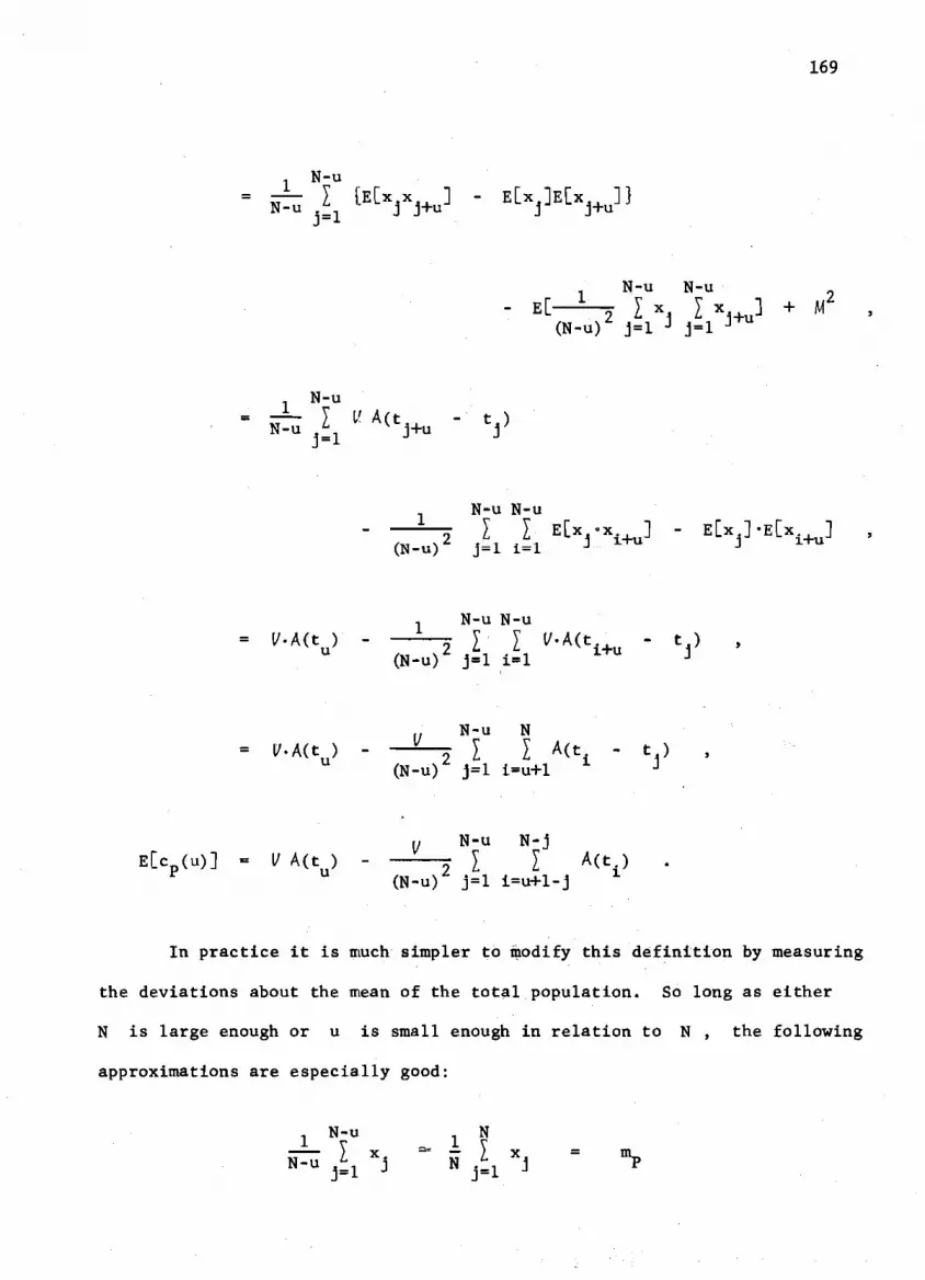
169

JJ^T [ E [ x j X j + u ] - E[ X j]E[x J + u]}

N-u N-u - E [ - ^ I x I x ] + M

(N-u) Z j=l J j = l J ™

- N-u N-u ^ v j+u

N-u N-u — o I I- ' E[x -x,, ] - • E[X.]«E[X., ] (N-u) j=l i=l J J

x N-u N-u = l/.A(t ) J- I l/.A(t + u - t ) ,

(N-u) Z j=l i=l J

^ N-u N = l/.A(t ) - — ^ X X A(t - t ) ,

(N-u) j=l i-u+1 1 2

u N-u N-j E[c (u)] - 1/ A(t ) - • -r I X A(t ) .

(N-ur j=l i=u+l-j

In practice it is much simpler to modify this definition by measuring

the deviations about the mean of the total population. So long as either

N is large enough or u is small enough in relation to N , the following

approximations are especially good:

170

and

N-u , N -, N NTu Xi+u = N-u J Xj ~ N . 1 Xj

J = l J j=u J j=l

For analytical convenience, c (u) is then defined: R

N-u' 1 c (u) — —— y fx-. - ni }[x., - m l ? K } N-u ^ 1 j P J L j+u T J

and this expression is simplified as:

N-u

Thus:

c (u) — •• > x.x,, - nu P v y N-u j j+u P

E[cp(u)] ^ E[-l-YXjXj+u . $ N-u I E[x x ] - E [ m p ] J=l

2 2 And since Var [nip] = E[m p] - (E [nip])

N-u [ C P ( U ) ] ~ N-u I E [ x i X i + u ] " ^ [ n L p l ) 2 - Var[mp] ,

j = l

N-u 0 , N-u = ZT- I E C X . X . ^ ] - M 2. -i- j; 1 - Var[m_] , N-u , L. j j+u N-u . P j=l j=l

n N-u = ^ ^ {E[X[(0,l);tj]-X[(0,l);tj+u]]

171

- E[X[(0,l);tj]]'E[X[(0,l);t ]]} - Var[mp] ,

1 N-u * N T I Cov[X[(0,l);t.],X[(0,l);t ]] - Var[m p]

j = l

N-u = I V A(t ) * Var[mJ

N-u , u. v u P J '

(/ 9 (/ N-1 E[cp(u)] - 1/ A(t u) - I - i| J (N-u)A(tu)

N u=l

From this last expression it is observed that

E[cp(u)] - A(t u) E[v p] - (1 - A(tu))Var[mp]

It is important to note the risk that lies in the foregoing

assumptions. If N is not large enough or if u is too large in relation

to N , it becomes possible for the autocovariance to exceed the variance

(theoretically impossible).

In light of the stationarity of the underlying process and with N

still large, it is interesting to make another simplification. Assume that

the finite population is periodic with period N so that x.,„ = x.. j+N j

This avoids the above-mentioned risk and yields a finite population circular

autocovariance function:

N c'(u) = — ) x.x., - m_ P N j j+u P

\l 917 N _ 1

E[c'(u)] = 1/ A(t ) - £ - ^ I (N-u)A(t ) , P N u=l

172

There is another property of the finite population derived from the

realization on [0,T] that is of interest. For series of observations that

are not random there will be dependencies of one kind or another between

successive observations. The population autocorrelation, sometimes called

the serial correlation, can be thought of as a measure of the linear

relationship which exists between the observation at time t. and the J

observation at another time t. + t = t., The finite population j u j+u

autocorrelation function is given by:

R N-u r N-u N-u _L_ v. f x _ _L_ V x } f x - —^- V x } N-u L L j N-u L j .j+u N-u L j+uJ

j=l j-l j-l a p(u) =

1 N-u 1 N-u \% / l N-u l N-u N-u I txj " Ixjl S I { xj+ u " N^I I x

j+u^ j = l j = l J \ j-l j-l

It is observed that the numerator of this expression is the autocovariance

function. Whenever either N is large enough or u is small enough in

relation to N , the approximations used earlier are again useful. This

yields an approximate population autocorrelation function:

1 N " U 2 V x . x . , - ni

N-u J J+u P a^Cu) - -LJ . —

And by assuming that the finite population is periodic with period N ,

many authors find utility in the finite population circular auto­

correlation function:

173

cl(u) a'(u) = —

Calculating the mean (or expectation) of any one of these

expressions for the population autocorrelation becomes difficult since

the autocorrelation is a ratio of random variables whenever expectation

is performed with respect to the stochastic process.

An approximation is attained by expanding ap(u) in a Taylor series

about the point (E[cp(u)],E[vp]). In this case it would be an admittedly

weak approximation. Since there are no expressions available for

Var[cp(u)], Var[vp], and Cov[cp(u);Vp] , only the first term of the

Taylor series approximation could be retained:

E[c (u)] E[a (u)] -

P E[vp]

By substitution:

E[a„(u)] A(tu)E[vp] - (1 - A(tu))Var[mp]

p V ~ / J E[vp]

Simplifying:

Var[mp] E[ap(u)] =- A(t u) - (1 - A(t u)) .

P

There is one other interesting property of an ordered finite

population arising from a sample function.

174

PROPERTY D.2 : Periodicity in a Finite Population

The ordered finite population [x^ ; j=l,2,...,N} is periodic

with period u* , if and only if a p(u*) = 1 .

This property can be demonstrated, treating the sufficiency first, as

follows.

a.) Assume that x, is periodic with period u*. J

Thus:

Xj+u* = Xj '

And in the expression for the autocorrelation function:

N-u* , N-u* 0 —* y (x. -—y x. " u * . 1 J N-u* j J=l J=l

a„(u) = — = 1 P N-u* N-u* 2

Shu* ^ Xj •"" N^u* j=l J j=l

N

b.) To show that a p(u*) = 1 implies x^ is periodic with

period u* , a preliminary lemma will be useful.

LEMMA D.l :

If x.. „ = A*x. + B , then x., „ = x. . That is, if j+u* j j+u* j

some linear relationship exists between all elements that are u* units

apart in an ordered finite population, then all elements u* units apart

are equal.

Since: The only non-degenerate possibilities for the linear relationships

(in order to preserve the zero-one nature of the variables) are:

Xi+u* = » x. + 1 and x., „ = x. , J J+u* j

175

Then: Then the condition requiring stationarity of the mean rules out

the first since, in general, e L X ^ ^ ] 4 E^" xj + ^ *

Therefore x., „ =: x. .

The demonstration of the property can be continued.

Let:

j N-u* x N-u* g(j,u*;y) = {x. - ~ » I x.} - y.{x. + u„ - fi^> ^ x

j + u * 5

Now:

, N-u* f(j,u*;y) = ~ « I [g(jVu*;y)] z ^ 0

Defining:

l N-u . N-U - — I x. = K. and -— Y x. , = K N-u . - i 1 N-u , L. j+u J=l J J=l 2

2

and expanding the finite series g , yields an expression that is

quadratic in y : N - u *

f<J» u*;y> = g b * . X [ ( x i " K i ) 2 _ 2 y ( x i " K i ) ( x i + u * " V

+ ^ Xj + u * - K 2 ) 2 ^

N-u* N-u* N-u* . L, 1 1 ;N-u* . , j 1 .3 = 1 J = l

N-u*

176

2

N-u* D = "

5 ^ * lx <XJ - V ( x j + u * " V ,

, N-u* „ , N-u* 2

- 4 - — s , I (x. - K-) — . T (x., ., - K_) N-u* .\ v j l 7 N-u* v i+u* 2

2 Since a p(u*) = 1, then a p(u*) = 1 and from the definition of a p(u)

N-u* N-u* I fx- " K I H X . _ L * " K.}) = I fx. - K.}).

J=l J=l

1 N _ u * (N^u* ^ ^ Xj+u* " K 2 ^

Therefore the discriminant, D, equals zero. Thus, the quadratic

f(j,u*;y) has the value zero at some point y , that is, f(j,u*;yQ) =

0. Since g(j,u*;yQ) is a function of the simplex realization on

[0,T-u*] and x^ = X ^ N ^ = X ^ T ) » then:

l N-u* E[g(j,u*;yo)] = — * I g(j,u*;yo) ,

j = l

N-u* - ' ™ — I [fx. - K, } - y {x., „ - K 0}] N-u* fl J 1 0 J+u* 2

= {Kx - K x} - y o{K 2 - K 2} = 0 .

The discriminant of the quadratic, D = b - 4ac, is

177

Also:

N-u* E[{g(j,u*;y o)T 2] = ^ I {g(j,u*;yo)}:

j = 1

= f(j,u*;yo) = 0 .

Thus:

Var[g(j,u*;yo)] = e[ {g(.j ,u*;yQ) } 2 ] - (E[g(j,u*;y o)]) 2 = 0 - 0 = 0

From lemma C.2 in Appendix C for the corresponding result in the simplex

realization, it is seen that: Pr [g = 0} = 1 , so that :

:. - Kn - y (x., „ - K.) = 0 j 1 Jo j+u* 2 '

with a probability equal to one. Rewriting this as

i K n + y K _ - / 1 \ <

1 ° 2 \ x. , „ = (—)x. - ( ) t + U * y 1 y J o o

demonstrates that a linear relationship exists between all elements that

are u* units apart. From lemma D.l x., „ = x. and the ordered x. J+u* j j

are if fact periodic with period equal to u* , as was to be shown.

178

BIBLIOGRAPHY

(1) Buckland, W. R., "A Review, of the Literature of Systematic Sampling," Journal of the Royal Statistical Society, B, Vol. 13, 1951, pp. 208-215.

(2) Cochran, William G., "Relative Accuracy of Systematic and Stratified Random Samples for a Certain Class of Populations," Annals of Mathe­matical Statistics, Volume 17, 1946, pp. 164-177.

(3) Cochran, William G., Sampling Techniques, Second Edition, John Wiley & Sons, Inc., New York, 1963, 413 pp.

(4) Cox, D. R. and P. A. W. Lewis, The Statistical Analysis of Series of Events, Methuen and Co. Ltd., London, 1966, 285 pp.

(5) Davis, Harold, "A Mathematical Evaluation of a Work Sampling Tech­nique," Naval Research Logistics Quarterly, Volume 2, Numbers 1 and 2, March-June, 1955, pp. 111-117.

(6) Feller, William, An Introduction to Probability Theory and its Appli­cations , Volume 1, Second Edition, John Wiley & Sons, Inc., New York, 1957, 461 pp.

(7) Grenander, Ulf and Murray Rosenblatt, Statistical Analysis of Sta­tionary Time Series, John Wiley & Sons, Inc., New York, 1957, 300 pp.

(8) Hannan, E. J., Time Series Analysis, Methuen and Co., Ltd., London, 1960, 152 pp.

(9) Hansen, Morris H„, William N. Hurwitz, and William G. Madow, Sample Survey Methods and Theory, Volume II, John Wiley & Sons, Inc., New York, 1953, 332 pp."

(10) Hines, William W„, "The Relationship Between the Properties of Certain Sample Statistics and the Structure of Activity in Systematic Activi­ty Sampling," Doctoral Dissertation, Georgia Institute of Technology, 1964, 279 pp.

(11) Hines, William W. and Joseph J. Moder, "Recent Advances in Systema­tic Activity Sampling," Journal of Industrial Engineering, Volume 16, 1965, pp. 295-304.

(12) Jones, Ned Gene and P. M. Ghare, "Confidence Intervals for Systema­tic Activity Sampling," Journal of Industrial Engineering, Volume 15, 1964, pp. 141-147.

(13) Jones, Ned Gene and P. M 0 Ghare, "Statistical Standards," AIIE Transactions, Volume 2, 1970, pp. 37-45.

179

(14) Kendall, Maurice G. and Alan Stuart, The Advanced Theory of Statis­tics , Volume III; Design and Analysis, and Time Series, Hafner Pub­lishing Company, New York, 1966, 552 pp.

(15) Khintchine, A. Ya, "Correlation Theory of Stationary Stochastic Processes," Mathematische Annalen, Volume 109, 1934, pp. 415-458.

(16) Kume, Hitoshi, "On the Spectral Analysis of Zero-One Processes," Technology Reports of the Seikei University, Number 3, Shinjuku, Tokyo, Japan, 1965~ pp. 149-158.

(17) Kume, Hitoshi, "A Problem of Errors in Systematic Sampling," Seikei University, Shinjuku, Tokyo, Japan, Received for review, 1968, 12 pp.

(18) Lee, Y. W., Statistical Theory of Communication, John Wiley & Sons, Inc., New York, 1960, 509 pp.

(19) Madow, Lillian H., "Systematic Sampling and Its Relation to Other Sampling Designs," Journal of the American Statistical Association, Volume 41, 1946, pp. 204-217.

(20) Madow, William G. and Lillian H. Madow, "On the Theory of Systematic Sampling, I," Annals of Mathematical Statistics, Volume 15, 1944, pp. 1-24.

(21) Madow, William G., "On the Theory of Systematic Sampling, II," Annals of Mathematical Statistics, Volume 20, 1949, pp. 333-354.

(22) Madow, William G., "On the Theory of Systematic Sampling, III," Annals of Mathematical Statistics, Volume 24, 1953, pp. 101-106.

(23) Moder, Joseph J., Henry D. Kahn, and Ramon S. Gomez, "Restricted Random Sampling of a Time-Based Process," Department of Industrial Engineering and Systems Analysis, University of Miami, Florida, Report No. 70-1, September, 1970, 22 pp.

(24) Meyer-Plate, Ingolf, "Spectral Analysis of Two-Variate Stochastic Processes," Master's Dissertation, Georgia Institute of Technology, 1968, 207 pp.

(25) Papoulis, Athanasios, Probability, Random Variables, and Stochastic Processes, McGraw-Hill Book Company, New York, 1965, 583 pp.

(26) Parzen, Emanuel, Stochastic Processes, Holden-Day, Inc., San Fran­cisco, 1962, 324 pp.

(27) Parzen, Emanuel, Time Series Analysis Papers, Holden-Day, Inc., San Francisco, 1967, 565 pp.

(28) Prabhu, N. U., Stochastic Processes, The Macmillan Company, New York, 1965, 233 pp.

180

(29) Varadhan, S. R„ S., Stochastic Processes, Courant Institute of Mathematical Sciences, New York University, New York, 1968, 190 pp.

(30) Wiener, Norbert, "Generalized Harmonic Analysis," Acta Mathematica, Volume 55, 1930, p. 117.

(31) Yates, Frank, "Systematic Sampling," Philosophical Transactions of the Royal Society of London, Series A, Volume 241, 1948, pp. 345-377.

(32) Yates, Frank, Sampling Methods for Censuses and Surveys, Third Edition, Hafner Publishing Company, New York, 1960, 440 pp.

181

VITA

Ronald E. Stemmler was born in Latrobe, Pennsylvania, on April 19,

1940. He attended public schools in Derry, Pennsylvania, where he was

graduated from high school in June, 1958. He received his B.S.I.E. from

the University of Miami in 1963 and his M.S.I.E„ from the same institu­

tion in 1965.

The author spent a year as Assistant Professor at Fresno State

College before enrolling in the Ph. D. program at Georgia Tech in

September, 1966. He was employed as Assistant to the Director of Research

Administration at Georgia Tech from July, 1966 to September, 1970, at

which time he became a Lecturer on the faculty of the School of Industrial

and Systems Engineering. After completing his graduate studies, the

author accepted an Assistant Professorship at Ohio University in Athens.

The author is married and has a son and a daughter.