THE EMERGENCE OF THE ELECTROSTATIC FIELD AS

A FEYNMAN SUM IN RANDOM TILINGS WITH HOLES

Mihai Ciucu

School of Mathematics, Georgia Institute of TechnologyAtlanta, Georgia 30332-0160

Abstract. We consider random lozenge tilings on the triangular lattice with holes Q1, . . . ,Qn in some fixedposition. For each unit triangle not in a hole, consider the average orientation of the lozenge covering it. Weshow that the scaling limit of this discrete field is the electrostatic field obtained when regarding each hole Qi asan electrical charge of magnitude equal to the difference between the number of unit triangles of the two differentorientations inside Qi. This is then restated in terms of random surfaces, yielding the result that the averageover surfaces with prescribed height at the union of the boundaries of the holes is, in the scaling limit, a sum ofhelicoids.

Introduction

The study of correlations of holes in random tilings was launched by Fisher and Stephenson [9], whoconsidered in particular the monomer-monomer correlation and obtained exact data suggesting rotationalinvariance in the scaling limit. Motivated by this, we studied correlations of a finite number of holesof various sizes and shapes in [1], [2] and [3], and found that in the scaling limit they are given by amultiplicative version of the superposition principle for energy in electrostatics. In this paper we showhow the actual electric field comes about as the scaling limit of a discrete field naturally associated withrandom tilings with holes.

Consider the unit equilateral triangular lattice drawn in the plane so that some of the lattice lines arevertical. The union of any two unit triangles that share an edge is called a lozenge. Inspired by Feynman’sdescription of the reflection of light in [8, Ch. 2] and given the connections between lozenge tilings withholes and electrostatics discussed in [2] we construct a discrete vector field as follows. Let ∆1, . . . , ∆n

be holes in the lattice whose boundaries are lattice triangles of even side-lengths. As one ranges over theset of lozenge tilings of the plane with these holes (a portion of such a tiling is illustrated in Figure 5.4(a)),any given left-pointing unit triangle e in the complement of the holes is covered by a lozenge having oneof three possible orientations: pointing in the polar direction 0, the polar direction 2π/3, or the polardirection 4π/3. Define F(e) to be the average of these orientations over all tilings (the precise definitionsare given in the next section).

Now apply a homothety of modulus 1/R to our lattice with holes, and “drag outward” the images ofthe holes and the image of e so that they shrink to points z1, . . . , zn and respectively z0 in the complexplane, as R→∞.

Our main result can be phrased as follows.

Theorem. As R→∞ we have

F(e) ∼ 3

4πR

n∑

i=0

ch(∆i)ri0

|z0 − zi|,

where ri0 is the unit vector pointing from zi in the direction of z0 and ch(Q) denotes the difference betweenthe number of right- and left-pointing unit triangles in the lattice region Q.

Research supported in part by NSF grant DMS 0500616.

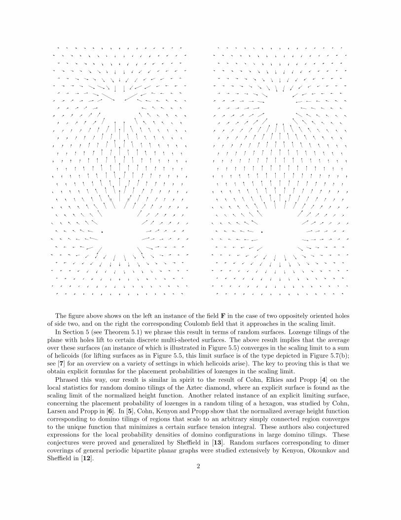
The figure above shows on the left an instance of the field F in the case of two oppositely oriented holesof side two, and on the right the corresponding Coulomb field that it approaches in the scaling limit.

In Section 5 (see Theorem 5.1) we phrase this result in terms of random surfaces. Lozenge tilings of theplane with holes lift to certain discrete multi-sheeted surfaces. The above result implies that the averageover these surfaces (an instance of which is illustrated in Figure 5.5) converges in the scaling limit to a sumof helicoids (for lifting surfaces as in Figure 5.5, this limit surface is of the type depicted in Figure 5.7(b);see [7] for an overview on a variety of settings in which helicoids arise). The key to proving this is that weobtain explicit formulas for the placement probabilities of lozenges in the scaling limit.

Phrased this way, our result is similar in spirit to the result of Cohn, Elkies and Propp [4] on thelocal statistics for random domino tilings of the Aztec diamond, where an explicit surface is found as thescaling limit of the normalized height function. Another related instance of an explicit limiting surface,concerning the placement probability of lozenges in a random tiling of a hexagon, was studied by Cohn,Larsen and Propp in [6]. In [5], Cohn, Kenyon and Propp show that the normalized average height functioncorresponding to domino tilings of regions that scale to an arbitrary simply connected region convergesto the unique function that minimizes a certain surface tension integral. These authors also conjecturedexpressions for the local probability densities of domino configurations in large domino tilings. Theseconjectures were proved and generalized by Sheffield in [13]. Random surfaces corresponding to dimercoverings of general periodic bipartite planar graphs were studied extensively by Kenyon, Okounkov andSheffield in [12].

2

One notable difference between our result and the above mentioned ones is the presence of holes. Thiscauses the lifting surfaces to be multi-sheeted. The holes are also responsible for creating the field we arestudying — without them the field would be zero. So, when specialized to the hexagonal lattice with unitweights, [12] gives the variance of the height function (the field being zero), while our result gives the(nonzero) expected value of the field created by the holes.

It may also be worth noting that for instance in [6] the boundary is the boundary of a lattice hexagon,and remains of fixed size throughout the scaling process, while in our case the boundary consists of theunion of finitely many boundaries of triangular holes, each of them shrinking to a point in the scaling limit.Related to this is the fact that, unlike the results from the literature mentioned above, we consider theaverage of un-normalized lifting surfaces — the average of the normalized ones is identically zero.

1. Definitions and statement of results

Let Qj be a finite union of lattice triangular holes of side two with mutually disjoint interiors, forj = 1, . . . , n (even when Qj is not connected, we still view it as a single generalized hole, often referredto as a multihole). The joint correlation ω(Q1, . . . , Qn) is defined in [3] (and recalled in Section 5 of thepresent paper) by means of limits of tori; the definition is readily extended to allowing some of the Qj ’s tobe lozenges. It follows from that definition that if L is any possible lozenge location, the probability thatL is occupied by a lozenge in a random lozenge tiling with holes at Q1, . . . , Qn is given by the ratio

ω(L, Q1, . . . , Qn)

ω(Q1, . . . , Qn)

(see Section 5 for the details). It follows thus that the vector F(e) = F(e; Q1, . . . , Qn) described in theIntroduction is given by

F(e) =ω(L1, Q1, . . . , Qn)

ω(Q1, . . . , Qn)e1 +

ω(L2, Q1, . . . , Qn)

ω(Q1, . . . , Qn)e2 +

ω(L3, Q1, . . . , Qn)

ω(Q1, . . . , Qn)e3, (1.1)

where L1, L2 and L3 are the lozenge locations containing the left-pointing unit triangle e and pointing inthe 0, 2π/3 and 4π/3 polar directions, respectively, and the ej ’s are unit vectors pointing in the directionsof the long diagonals of the Lj ’s.

Note that we can specify the location of any left- or right-pointing unit triangle (for short, we willcall them left- and right-monomers) by indicating the location of the midpoint of its vertical side. Themidpoints of the vertical sides of the unit triangles in our lattice can naturally be coordinatized by pairsof integers using a 60◦ coordinate system with axes pointing in the polar directions ±π/3.

Let Ea,b be the east-pointing lattice triangle of side 2 whose central monomer has coordinates (a, b).Let Wa,b be the similarly defined west-pointing lattice triangle. We regard both of them as holes.

For any q ∈ Q and any strictly increasing list of integers a = (a1, . . . , as) for which qai ∈ Z and theEai,qai ’s (equivalently, the Wai,qai ’s) are mutually disjoint, i = 1, . . . , s, define the multiholes Eq

aand W q

a

by

Eqa = Ea1,qa1 ∪ . . . ∪ Eas,qas

W qa = Wa1,qa1 ∪ . . . ∪Was,qas .

For a hole Q in the lattice, let Q(x, y) stand for its translation by the vector (x, y) in our coordinatesystem. We say that an integer divides a rational number if it divides the numerator of a lowest termsrepresentation of it.

We can now give the precise statement of our main result.

Theorem 1.1. Let x(R)0 , . . . , x

(R)m , y

(R)0 , . . . , y

(R)m , z

(R)0 , . . . , z

(R)n and w

(R)0 , . . . , w

(R)n be sequences of integers

so that limR→∞ x(R)i /R = xi, limR→∞ y

(R)i /R = yi, limR→∞ z

(R)j /R = zj and limR→∞ w

(R)j /R = wj for

0 ≤ i ≤ m and 1 ≤ j ≤ n. Assume the (xi, yi)’s and (zj , wj)’s are all distinct.3

Then for any multiholes Eqa1

, . . . , Eqam

and W qb1

, . . . , W qbn

with 3|1− q, the field

F(

x(R)0 , y

(R)0

)

= F(

x(R)0 , y

(R)0 ; Eq

a1(x

(R)1 , y

(R)1 ), . . . , W q

bn(z(R)

n , w(R)n )

)

defined by (1.1) has orthogonal projections on our coordinate axes with asymptotics

Fx

(

x(R)0 , y

(R)0

)

=3

4πR

{

m∑

i=1

si2(x0 − xi) + y0 − yi

(x0 − xi)2 + (x0 − xi)(y0 − yi) + (y0 − yi)2

−n∑

j=1

tj2(x0 − zj) + y0 − wj

(x0 − zj)2 + (x0 − zj)(y0 − wj) + (y0 − wj)2

+ o

(

1

R

)

(1.2)

and

Fy

(

x(R)0 , y

(R)0

)

=3

4πR

{

m∑

i=1

six0 − xi + 2(y0 − yi)

(x0 − xi)2 + (x0 − xi)(y0 − yi) + (y0 − yi)2

−n∑

j=1

tjx0 − zj + 2(y0 − wj)

(x0 − zj)2 + (x0 − zj)(y0 − wj) + (y0 − wj)2

+ o

(

1

R

)

, (1.3)

where si and tj are the lengths of ai and bj , respectively.Furthermore, for any ε > 0 and any bounded set B in the plane the implicit constants above are uniform

over all choices of the limits for which each distance among the points (x0, y0), . . . , (zn, wn) ∈ B is atleast ε.

Note that in our oblique coordinate system the Euclidean distance between the points (x, y) and (x′, y′)is√

(x− x′)2 + (x− x′)(y − y′) + (y − y′)2, and the orthogonal projections of (x, y) on the coordinate axes

are x+ 12y and 1

2x+y. Note also that the multihole E1(0,2,4,...,2s−2) consists of a contiguous horizontal string

of right-pointing triangular holes of side two. Due to forced lozenges in its complement, E1(0,2,4,...,2s−2) has

precisely the same effect as the right-pointing triangular hole of side 2s that contains it; a similar statementholds for W -multiholes. Since ch(Eq

ai) = 2si and ch(W q

bj) = −2tj , one sees that the theorem stated in the

Introduction follows as a special case of Theorem 1.1.

2. Reducing the problem to exact determinant evaluations

One crucial ingredient for proving the results of [3] was an exact determinant formula for the jointcorrelation of an arbitrary collection of disjoint lattice-triangular holes of size two. The arguments presentedthere prove in fact a more general statement, which we will need in the current paper.

Our determinant formula involves the coupling function P (x, y), x, y ∈ Z specified by

P (x, y) =1

2πi

∫ e4πi/3

e2πi/3

t−y−1(−1− t)−x−1dt, x ≤ −1 (2.1)

and the symmetries P (x, y) = P (y, x) = P (−x− y − 1, x) (see Kenyon [11]), and the coefficients Us of itsasymptotic series

P (−3r − 1 + a,−1 + b) ∼∞∑

s=0

(3r)−s−1Us(a, b), r →∞, a, b ∈ Z. (2.2)

Let r(a, b) and l(a, b) denote the right- and left-pointing monomers of coordinates (a, b), respectively.4

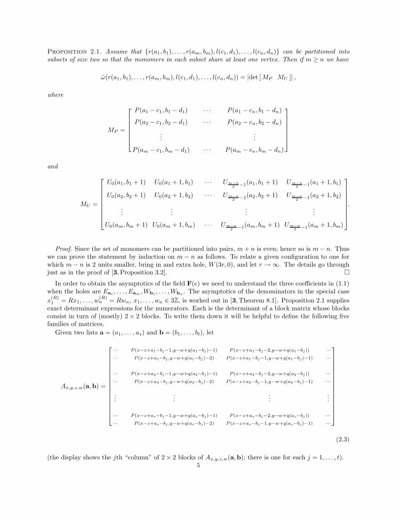
Proposition 2.1. Assume that {r(a1, b1), . . . , r(am, bm), l(c1, d1), . . . , l(cn, dn)} can be partitioned intosubsets of size two so that the monomers in each subset share at least one vertex. Then if m ≥ n we have

ω(r(a1, b1), . . . , r(am, bm), l(c1, d1), . . . , l(cn, dn)) = |det [ MP MU ]| ,

where

MP =

P (a1 − c1, b1 − d1) · · · P (a1 − cn, b1 − dn)

P (a2 − c1, b2 − d1) · · · P (a2 − cn, b2 − dn)

......

P (am − c1, bm − d1) · · · P (am − cn, bm − dn)

and

MU =

U0(a1, b1 + 1) U0(a1 + 1, b1) · · · Um−n2 −1(a1, b1 + 1) Um−n

2 −1(a1 + 1, b1)

U0(a2, b2 + 1) U0(a2 + 1, b2) · · · Um−n2 −1(a2, b2 + 1) Um−n

2 −1(a2 + 1, b2)

......

......

U0(am, bm + 1) U0(am + 1, bm) · · · Um−n2 −1(am, bm + 1) Um−n

2 −1(am + 1, bm)

.

Proof. Since the set of monomers can be partitioned into pairs, m + n is even; hence so is m− n. Thuswe can prove the statement by induction on m − n as follows. To relate a given configuration to one forwhich m− n is 2 units smaller, bring in and extra hole, W (3r, 0), and let r →∞. The details go throughjust as in the proof of [3, Proposition 3.2]. �

In order to obtain the asymptotics of the field F(e) we need to understand the three coefficients in (1.1)when the holes are Ea1 , . . . , Eam , Wb1 , . . . , Wbn . The asymptotics of the denominators in the special case

x(R)1 = Rx1, . . . , w

(R)n = Rwn, x1, . . . , wn ∈ 3Z, is worked out in [3, Theorem 8.1]. Proposition 2.1 supplies

exact determinant expressions for the numerators. Each is the determinant of a block matrix whose blocksconsist in turn of (mostly) 2× 2 blocks. To write them down it will be helpful to define the following fivefamilies of matrices.

Given two lists a = (a1, . . . , as) and b = (b1, . . . , bt), let

Ax,y,z,w(a,b) =

··· P (x−z+a1−bj−1,y−w+q(a1−bj)−1) P (x−z+a1−bj−2,y−w+q(a1−bj)) ······ P (x−z+a1−bj ,y−w+q(a1−bj)−2) P (x−z+a1−bj−1,y−w+q(a1−bj)−1) ···

··· P (x−z+a2−bj−1,y−w+q(a2−bj)−1) P (x−z+a2−bj−2,y−w+q(a2−bj)) ······ P (x−z+a2−bj ,y−w+q(a2−bj)−2) P (x−z+a2−bj−1,y−w+q(a2−bj)−1) ···

......

......

··· P (x−z+as−bj−1,y−w+q(as−bj)−1) P (x−z+as−bj−2,y−w+q(as−bj)) ······ P (x−z+as−bj ,y−w+q(as−bj)−2) P (x−z+as−bj−1,y−w+q(as−bj)−1) ···

(2.3)

(the display shows the jth “column” of 2× 2 blocks of Ax,y,z,w(a,b); there is one for each j = 1, . . . , t).5

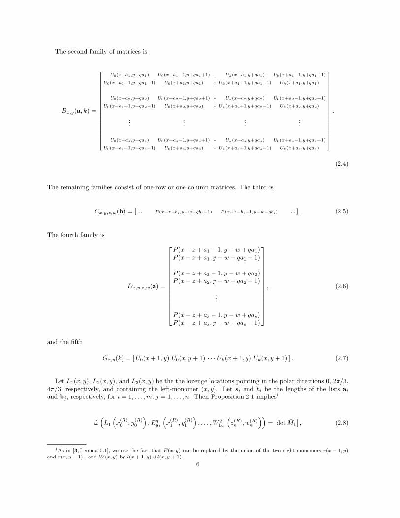
The second family of matrices is

Bx,y(a, k) =

U0(x+a1,y+qa1) U0(x+a1−1,y+qa1+1) ··· Uk(x+a1,y+qa1) Uk(x+a1−1,y+qa1+1)

U0(x+a1+1,y+qa1−1) U0(x+a1,y+qa1) ··· Uk(x+a1+1,y+qa1−1) Uk(x+a1,y+qa1)

U0(x+a2,y+qa2) U0(x+a2−1,y+qa2+1) ··· Uk(x+a2,y+qa2) Uk(x+a2−1,y+qa2+1)

U0(x+a2+1,y+qa2−1) U0(x+a2,y+qa2) ··· Uk(x+a2+1,y+qa2−1) Uk(x+a2,y+qa2)

......

......

U0(x+as,y+qas) U0(x+as−1,y+qas+1) ··· Uk(x+as,y+qas) Uk(x+as−1,y+qas+1)

U0(x+as+1,y+qas−1) U0(x+as,y+qas) ··· Uk(x+as+1,y+qas−1) Uk(x+as,y+qas)

.

(2.4)

The remaining families consist of one-row or one-column matrices. The third is

Cx,y,z,w(b) = [ ··· P (x−z−bj ,y−w−qbj−1) P (x−z−bj−1,y−w−qbj) ··· ] . (2.5)

The fourth family is

Dx,y,z,w(a) =

P (x− z + a1 − 1, y − w + qa1)P (x− z + a1, y − w + qa1 − 1)

P (x− z + a2 − 1, y − w + qa2)P (x− z + a2, y − w + qa2 − 1)

...

P (x− z + as − 1, y − w + qas)P (x− z + as, y − w + qas − 1)

, (2.6)

and the fifth

Gx,y(k) = [ U0(x + 1, y) U0(x, y + 1) · · · Uk(x + 1, y) Uk(x, y + 1) ] . (2.7)

Let L1(x, y), L2(x, y), and L3(x, y) be the the lozenge locations pointing in the polar directions 0, 2π/3,4π/3, respectively, and containing the left-monomer (x, y). Let si and tj be the lengths of the lists ai

and bj , respectively, for i = 1, . . . , m, j = 1, . . . , n. Then Proposition 2.1 implies1

ω(

L1

(

x(R)0 , y

(R)0

)

, Eqa1

(

x(R)1 , y

(R)1

)

, . . . , W qbn

(

z(R)n , w(R)

n

))

=∣

∣det M1

∣

∣ , (2.8)

1As in [3, Lemma 5.1], we use the fact that E(x, y) can be replaced by the union of the two right-monomers r(x − 1, y)and r(x, y − 1) , and W (x, y) by l(x + 1, y) ∪ l(x, y + 1).

6

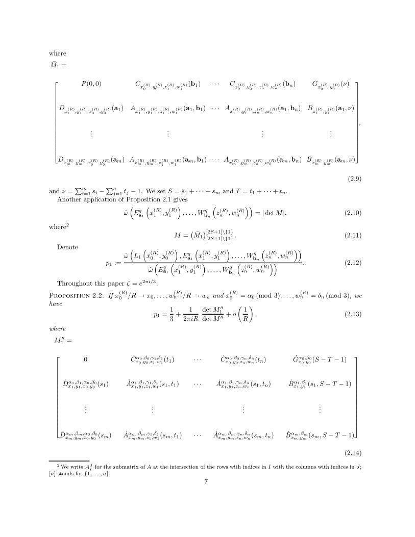
where

M1 =

P (0, 0) Cx(R)0 ,y

(R)0 ,z

(R)1 ,w

(R)1

(b1) · · · Cx(R)0 ,y

(R)0 ,z

(R)n ,w

(R)n

(bn) Gx(R)0 ,y

(R)0

(ν)

Dx(R)1 ,y

(R)1 ,x

(R)0 ,y

(R)0

(a1) Ax(R)1 ,y

(R)1 ,z

(R)1 ,w

(R)1

(a1,b1) · · · Ax(R)1 ,y

(R)1 ,z

(R)n ,w

(R)n

(a1,bn) Bx(R)1 ,y

(R)1

(a1, ν)

......

......

Dx(R)m ,y

(R)m ,x

(R)0 ,y

(R)0

(am) Ax(R)m ,y

(R)m ,z

(R)1 ,w

(R)1

(am,b1) · · · Ax(R)m ,y

(R)m ,z

(R)n ,w

(R)n

(am,bn) Bx(R)m ,y

(R)m

(am, ν)

,

(2.9)

and ν =∑m

i=1 si −∑n

j=1 tj − 1. We set S = s1 + · · ·+ sm and T = t1 + · · ·+ tn.Another application of Proposition 2.1 gives

ω(

Eqa1

(

x(R)1 , y

(R)1

)

, . . . , W qbn

(

z(R)n , w(R)

n

))

= | det M |, (2.10)

where2

M =(

M1

)[2S+1]\{1}[2S+1]\{1} . (2.11)

Denote

p1 :=ω(

L1

(

x(R)0 , y

(R)0

)

, Eqa1

(

x(R)1 , y

(R)1

)

, . . . , W qbn

(

z(R)n , w

(R)n

))

ω(

Eqa1

(

x(R)1 , y

(R)1

)

, . . . , W qbn

(

z(R)n , w

(R)n

)) . (2.12)

Throughout this paper ζ = e2πi/3.

Proposition 2.2. If x(R)0 /R→ x0, . . . , w

(R)n /R→ wn and x

(R)0 = α0 (mod 3), . . . , w

(R)n = δn (mod 3), we

have

p1 =1

3+

1

2πiR

det M ′′1

det M ′′ + o

(

1

R

)

, (2.13)

where

M ′′1 =

0 Cα0,β0,γ1,δ1x0,y0,z1,w1

(t1) · · · Cα0,β0,γn,δnx0,y0,zn,wn

(tn) Gα0,β0x0,y0

(S − T − 1)

Dα1,β1,α0,β0x1,y1,x0,y0

(s1) Aα1,β1,γ1,δ1x1,y1,z1,w1

(s1, t1) · · · Aα1,β1,γn,δnx1,y1,zn,wn

(s1, tn) Bα1,β1x1,y1

(s1, S − T − 1)

......

......

Dαm,βm,α0,β0xm,ym,x0,y0

(sm) Aαm,βm,γ1,δ1xm,ym,z1,w1

(sm, t1) · · · Aαm,βm,γn,δnxm,ym,zn,wn

(sm, tn) Bαm,βmxm,ym

(sm, S − T − 1)

(2.14)

2 We write AJ

Ifor the submatrix of A at the intersection of the rows with indices in I with the columns with indices in J ;

[n] stands for {1, . . . , n}.

7

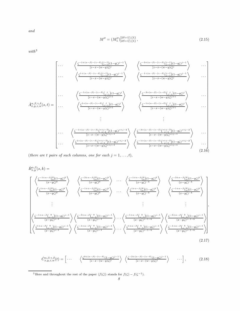
and

M ′′ = (M ′′1 )

[2S+1]\{1}[2S+1]\{1} , (2.15)

with3

Aα,β,γ,δx,y,z,w(s, t) =

· · ·⟨

ζ−1+(α−β)−(γ−δ)(j−1j−1)(1−qζ)j−1

[z−x−(w−y)ζ]j

⟩ ⟨

ζ−3+(α−β)−(γ−δ)(j−1j−1)(1−qζ)j−1

[z−x−(w−y)ζ]j

⟩

· · ·

· · ·⟨

ζ1+(α−β)−(γ−δ)(j−1j−1)(1−qζ)j−1

[z−x−(w−y)ζ]j

⟩ ⟨

ζ−1+(α−β)−(γ−δ)(j−1j−1)(1−qζ)j−1

[z−x−(w−y)ζ]j

⟩

· · ·

· · ·⟨

ζ−1+(α−β)−(γ−δ)( jj−1)(1−qζ)j

[z−x−(w−y)ζ]j+1

⟩ ⟨

ζ−3+(α−β)−(γ−δ)( jj−1)(1−qζ)j

[z−x−(w−y)ζ]j+1

⟩

· · ·

· · ·⟨

ζ1+(α−β)−(γ−δ)( jj−1)(1−qζ)j

[z−x−(w−y)ζ]j+1

⟩ ⟨

ζ−1+(α−β)−(γ−δ)( jj−1)(1−qζ)j

[z−x−(w−y)ζ]j+1

⟩

· · ·

......

· · ·⟨

ζ−1+(α−β)−(γ−δ)(s+j−2j−1 )(1−qζ)s+j−2

[z−x−(w−y)ζ]s+j−1

⟩ ⟨

ζ−3+(α−β)−(γ−δ)(s+j−2j−1 )(1−qζ)s+j−2

[z−x−(w−y)ζ]s+j−1

⟩

· · ·

· · ·⟨

ζ1+(α−β)−(γ−δ)(s+j−2j−1 )(1−qζ)s+j−2

[z−x−(w−y)ζ]s+j−1

⟩ ⟨

ζ−1+(α−β)−(γ−δ)(s+j−2j−1 )(1−qζ)s+j−2

[z−x−(w−y)ζ]s+j−1

⟩

· · ·

(2.16)(there are t pairs of such columns, one for each j = 1, . . . , t),

Bα,βx,y (s, k) =

⟨

ζ−1+α−β(00)(1−qζ)0

(x−yζ)0

⟩ ⟨

ζ−3+α−β(00)(1−qζ)0

(x−yζ)0

⟩

· · ·⟨

ζ−1+α−β(k0)(1−qζ)0

(x−yζ)−k

⟩ ⟨

ζ−3+α−β(k0)(1−qζ)0

(x−yζ)−k

⟩

⟨

ζ1+α−β(00)(1−qζ)0

(x−yζ)0

⟩ ⟨

ζ−1+α−β(00)(1−qζ)0

(x−yζ)0

⟩

· · ·⟨

ζ1+α−β(k0)(1−qζ)0

(x−yζ)−k

⟩ ⟨

ζ−1+α−β(k0)(1−qζ)0

(x−yζ)−k

⟩

......

...

⟨

ζ−1+α−β( 0s−1)(1−qζ)s−1

(x−yζ)s−1

⟩⟨

ζ−3+α−β( 0s−1)(1−qζ)s−1

(x−yζ)s−1

⟩

· · ·⟨

ζ−1+α−β( ks−1)(1−qζ)s−1

(x−yζ)s−1−k

⟩⟨

ζ−3+α−β( ks−1)(1−qζ)s−1

(x−yζ)s−1−k

⟩

⟨

ζ1+α−β( 0s−1)(1−qζ)s−1

(x−yζ)s−1

⟩ ⟨

ζ−1+α−β( 0s−1)(1−qζ)s−1

(x−yζ)s−1

⟩

· · ·⟨

ζ1+α−β( ks−1)(1−qζ)s−1

(x−yζ)s−1−k

⟩ ⟨

ζ−1+α−β( ks−1)(1−qζ)s−1

(x−yζ)s−1−k

⟩

,

(2.17)

Cα,β,γ,δx,y,z,w(t) =

[

· · ·⟨

ζ0+(α−β)−(γ−δ)(1−qζ)j−1

[z−x−(w−y)ζ]j

⟩ ⟨

ζ−2+(α−β)−(γ−δ)(1−qζ)j−1

[z−x−(w−y)ζ]j

⟩

· · ·]

, (2.18)

3 Here and throughout the rest of the paper 〈f(ζ)〉 stands for f(ζ) − f(ζ−1).

8

Dα,β,γ,δx,y,z,w(s) =

⟨

ζ−2+(α−β)−(γ−δ)(1−qζ)0

[z−x−(w−y)ζ]

⟩

⟨

ζ0+(α−β)−(γ−δ)(1−qζ)0

[z−x−(w−y)ζ]

⟩

⟨

ζ−2+(α−β)−(γ−δ)(1−qζ)1

[z−x−(w−y)ζ]2

⟩

⟨

ζ0+(α−β)−(γ−δ)(1−qζ)1

[z−x−(w−y)ζ]2

⟩

...

⟨

ζ−2+(α−β)−(γ−δ)(1−qζ)s−1

[z−x−(w−y)ζ]s

⟩

⟨

ζ0+(α−β)−(γ−δ)(1−qζ)s−1

[z−x−(w−y)ζ]s

⟩

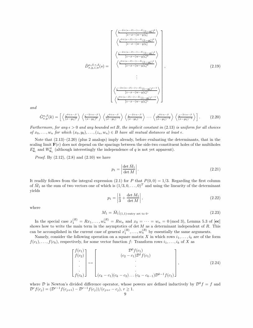
, (2.19)

and

Gα,βx,y (k) =

[ ⟨

ζ0+α−β

(x−yζ)0

⟩ ⟨

ζ−2+α−β

(x−yζ)0

⟩ ⟨

ζ0+α−β

(x−yζ)−1

⟩ ⟨

ζ−2+α−β

(x−yζ)−1

⟩

· · ·⟨

ζ0+α−β

(x−yζ)−k

⟩ ⟨

ζ−2+α−β

(x−yζ)−k

⟩ ]

. (2.20)

Furthermore, for any ε > 0 and any bounded set B, the implicit constant in (2.13) is uniform for all choicesof x0, . . . , wn for which (x0, y0), . . . , (zn, wn) ∈ B have all mutual distances at least ε.

Note that (2.13)–(2.20) (plus 2 analogs) imply already, before evaluating the determinants, that in thescaling limit F(e) does not depend on the spacings between the side-two constituent holes of the multiholesEq

aiand W q

bj(although interestingly the independence of q is not yet apparent).

Proof. By (2.12), (2.8) and (2.10) we have

p1 =

∣

∣

∣

∣

det M1

det M

∣

∣

∣

∣

. (2.21)

It readily follows from the integral expression (2.1) for P that P (0, 0) = 1/3. Regarding the first columnof M1 as the sum of two vectors one of which is (1/3, 0, . . . , 0)T and using the linearity of the determinantyields

p1 =

∣

∣

∣

∣

1

3+

det M1

det M

∣

∣

∣

∣

, (2.22)

whereM1 = M1|(1,1)-entry set to 0. (2.23)

In the special case x(R)1 = Rx1, . . . , w

(R)n = Rwn and x0 = · · · = wn = 0 (mod 3), Lemma 5.3 of [ec]

shows how to write the main term in the asymptotics of det M as a determinant independent of R. This

can be accomplished in the current case of general x(R)1 , . . . , w

(R)n by essentially the same arguments.

Namely, consider the following operation on a square matrix X in which rows i1, . . . , ik are of the formf(c1), . . . , f(ck), respectively, for some vector function f : Transform rows i1, . . . , ik of X as

f(c1)f(c2)

.

.

.f(ck)

7→

D0f(c1)(c2 − c1)D1f(c1)

.

.

.(ck − c1)(ck − c2) . . . (ck − ck−1)Dk−1f(c1)

, (2.24)

where D is Newton’s divided difference operator, whose powers are defined inductively by D0f = f andDrf(cj) = (Dr−1f(cj+1)−Dr−1f(cj))/(cj+r − cj), r ≥ 1.

9

This operation has an obvious analog for columns.As noted in [3, §5] (and as can be seen by looking at (2.11), (2.9), (2.3) and (2.4)), operation (2.24)

can be applied a total of 2m + 2n different times to the matrix M : each row of block matrices in theexpression for M given by (2.11) and (2.9) provides two opportunities (along the odd-indexed rows andalong the even-indexed ones), and each column consisting of A-blocks provides two more. Let M ′ be thematrix obtained from M after applying these 2m + 2n operations.

Since operations (2.24) preserve the determinant (see [3, Lemma 5.2]),

det M = det M ′. (2.25)

Moreover, by construction, the 2× 2 blocks of M ′ are obtained by replacing Rx1 ← x(R)1 , . . . , Rwn ← w

(R)n

in formulas [3, (5.6)–(5.9)]. Propositions 4.1 and 4.5 and the arguments in the proof of [3, Lemma 5.3]imply then that4

detbbM ′cc =

(

1

2πi

)2S m∏

j=1

∏

1≤k<l≤sj

(ajk − ajl)2

n∏

j=1

∏

1≤k<l≤tj

(bjk − bjl)2

× det(M ′′) R2{P

1≤k<l≤m sksl+P

1≤k<l≤n tktl−Pm

k=1

Pnl=1 sktl},

(2.26)

where ak = (ak1, . . . , ak,sk) and bl = (bl1, . . . , bl,tl

) for all k and l.By (2.25) and (2.26) we get

det M =

(

1

2πi

)2S m∏

j=1

∏

1≤k<l≤sj

(ajk − ajl)2

n∏

j=1

∏

1≤k<l≤tj

(bjk − bjl)2

× det(M ′′) R2{P

1≤k<l≤m sksl+P

1≤k<l≤n tktl−Pm

k=1

Pnl=1 sktl}

+ o(

R2{P

1≤k<l≤m sksl+P

1≤k<l≤n tktl−Pm

k=1

Pnl=1 sktl}

)

. (2.27)

Propositions 4.1 and 4.5 imply that the implicit constant above is uniform in x1, . . . , wn.Next we turn to the asymptotics of det M1. Note that all the 2m + 2n operations of type (2.24) we

applied to M are also well-defined as operations on M1. Indeed, it is apparent from (2.9) and (2.3)–(2.6)that each of the 2m + 2n times we applied (2.24), the extensions to M1 of the involved rows or columns ofM are also of the form required by this operation. Let M ′

1 be the matrix obtained from M1 after applyingthese 2m + 2n operations.

A calculation similar to the one that gave (2.26) yields

detbbM ′1cc =

(

1

2πi

)2S+1 m∏

j=1

∏

1≤k<l≤sj

(ajk − ajl)2

n∏

j=1

∏

1≤k<l≤tj

(bjk − bjl)2

× det(M ′′1 ) R2{

P

1≤k<l≤m sksl+P

1≤k<l≤n tktl−Pm

k=1

Pnl=1 sktl}−1. (2.28)

By the preservation of the determinant we get

det M1 =

(

1

2πi

)2S+1 m∏

j=1

∏

1≤k<l≤sj

(ajk − ajl)2

n∏

j=1

∏

1≤k<l≤tj

(bjk − bjl)2

× det(M ′′1 ) R2{

P

1≤k<l≤m sksl+P

1≤k<l≤n tktl−Pm

k=1

Pnl=1 sktl}−1

+ o(

R2{P

1≤k<l≤m sksl+P

1≤k<l≤n tktl−Pm

k=1

Pnl=1 sktl}−1

)

, (2.29)

4 For a matrix A whose entries depend on a large parameter, bbAcc stands for the matrix obtained from it by replacingeach entry by the dominant part in its asymptotics as the parameter approaches infinity.

10

and the implicit constant is again uniform in x1, . . . , wn by Propositions 4.1 and 4.5. The statement of theProposition follows now by (2.22), (2.27) and (2.29). �

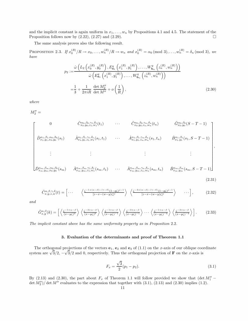
The same analysis proves also the following result.

Proposition 2.3. If x(R)0 /R→ x0, . . . , w

(R)n /R→ wn and x

(R)0 = α0 (mod 3), . . . , w

(R)n = δn (mod 3), we

have

p2 :=ω(

L2

(

x(R)0 , y

(R)0

)

, Eqa1

(

x(R)1 , y

(R)1

)

, . . . , W qbn

(

z(R)n , w

(R)n

))

ω(

Eqa1

(

x(R)1 , y

(R)1

)

, . . . , W qbn

(

z(R)n , w

(R)n

))

=1

3+

1

2πiR

det M ′′2

det M ′′ + o

(

1

R

)

, (2.30)

where

M ′′2 =

0 Cα0,β0,γ1,δ1x0,y0,z1,w1

(t1) · · · Cα0,β0,γn,δnx0,y0,zn,wn

(tn) Gα0,β0x0,y0

(S − T − 1)

Dα1,β1,α0,β0x1,y1,x0,y0

(s1) Aα1,β1,γ1,δ1x1,y1,z1,w1

(s1, t1) · · · Aα1,β1,γn,δnx1,y1,zn,wn

(s1, tn) Bα1,β1x1,y1

(s1, S − T − 1)

......

......

Dαm,βm,α0,β0xm,ym,x0,y0

(sm) Aαm,βm,γ1,δ1xm,ym,z1,w1

(sm, t1) · · · Aαm,βm,γn,δnxm,ym,zn,wn

(sm, tn) Bαm,βmxm,ym

(sm, S − T − 1)

,

(2.31)

Cα,β,γ,δx,y,z,w(t) =

[

· · ·⟨

ζ−1+(α−β)−(γ−δ)(1−qζ)j−1

[z−x−(w−y)ζ]j

⟩ ⟨

ζ−3+(α−β)−(γ−δ)(1−qζ)j−1

[z−x−(w−y)ζ]j

⟩

· · ·]

, (2.32)

and

Gα,βx,y (k) =

[ ⟨

ζ−1+α−β

(x−yζ)0

⟩ ⟨

ζ−3+α−β

(x−yζ)0

⟩ ⟨

ζ−1+α−β

(x−yζ)−1

⟩ ⟨

ζ−3+α−β

(x−yζ)−1

⟩

· · ·⟨

ζ−1+α−β

(x−yζ)−k

⟩ ⟨

ζ−3+α−β

(x−yζ)−k

⟩ ]

. (2.33)

The implicit constant above has the same uniformity property as in Proposition 2.2.

3. Evaluation of the determinants and proof of Theorem 1.1

The orthogonal projections of the vectors e1, e2 and e3 of (1.1) on the x-axis of our oblique coordinate

system are√

3/2, −√

3/2 and 0, respectively. Thus the orthogonal projection of F on the x-axis is

Fx =

√3

2(p1 − p2). (3.1)

By (2.13) and (2.30), the part about Fx of Theorem 1.1 will follow provided we show that (det M ′′1 −

det M ′′2 )/ det M ′′ evaluates to the expression that together with (3.1), (2.13) and (2.30) implies (1.2).

11

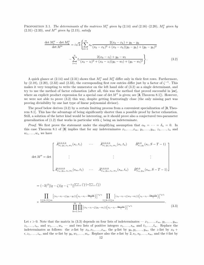
Proposition 3.1. The determinants of the matrices M ′′1 given by (2.14) and (2.16)–(2.20), M ′′

2 given by(2.31)–(2.33), and M ′′ given by (2.15), satisfy

det M ′′1 − det M ′′

2

det M ′′ = i√

3

{

m∑

k=1

sk2(x0 − xk) + y0 − yk

(x0 − xk)2 + (x0 − xk)(y0 − yk) + (y0 − yk)2

−n∑

l=1

tl2(x0 − zl) + y0 − wl

(x0 − zl)2 + (x0 − zl)(y0 − wl) + (y0 − wl)2

}

. (3.2)

A quick glance at (2.14) and (2.31) shows that M ′′1 and M ′′

2 differ only in their first rows. Furthermore,by (2.18), (2.20), (2.32) and (2.33), the corresponding first row entries differ just by a factor of ζ−1. Thismakes it very tempting to write the numerator on the left hand side of (3.2) as a single determinant, andtry to use the method of factor exhaustion (after all, this was the method that proved successful in [ec],where an explicit product expression for a special case of det M ′′ is given; see [3, Theorem 8.1]). However,we were not able to prove (3.2) this way, despite getting frustratingly close (the only missing part wasproving divisibility by one last type of linear polynomial divisor).

The proof below derives (3.2) by a certain limiting process from a convenient specialization of [3, Theo-rem 8.1]. This has the advantage of being significantly shorter than a possible proof by factor exhaustion.Still, a solution of the latter kind would be interesting, as it should prove also a conjectured two-parametergeneralization of (1.2) that works in particular with ζ being an indeterminate.

Proof. We first prove the statement under the simplifying assumption that α0 = · · · = δn = 0. Inthis case Theorem 8.1 of [3] implies that for any indeterminates x1, . . . , xm, y1, . . . , ym, z1, . . . , zn andw1, . . . , wn we have

det M ′′ = det

A0,0,0,0x1,y1,z1,w1

(s1, t1) · · · A0,0,0,0x1,y1,zn,wn

(s1, tn) B0,0x1,y1

(s1, S − T − 1)

......

...

A0,0,0,0xm,ym,z1,w1

(sm, t1) · · · A0,0,0,0xm,ym,zn,wn

(sm, tn) B0,0xm,ym

(sm, S − T − 1)

= (−3)S[(q − ζ)(q − ζ−1)]Pm

k=1 (sk2 )+

Pnl=1 (tl

2 )

×

∏

1≤k<l≤m

h

(xk−xl−ζ(yk−yl))“

xk−xl− yk−ylζ

”isksl∏

1≤k<l≤n

h

(zk−zl−ζ(wk−wl))“

zk−zl−wk−wlζ

”itktl

m∏

k=1

n∏

l=1

h

(xk−zl−ζ(yk−wl))“

xk−zl− yk−wlζ

”isktl

.(3.3)

Let ε > 0. Note that the matrix in (3.3) depends on four lists of indeterminates — x1, . . . , xm, y1, . . . , ym,z1, . . . , zn, and w1, . . . , wn — and two lists of positive integers s1, . . . , sm and t1, . . . , tn. Replace theindeterminates as follows: the x-list by x0, x1, . . . , xm, the y-list by y0, y1, . . . , ym, the z-list by x0 +ε, z1, . . . , zn, and the w-list by y0, w1, . . . , wn. Replace also the s-list by 2, s1, s2, . . . , sm, and the t-list by

12

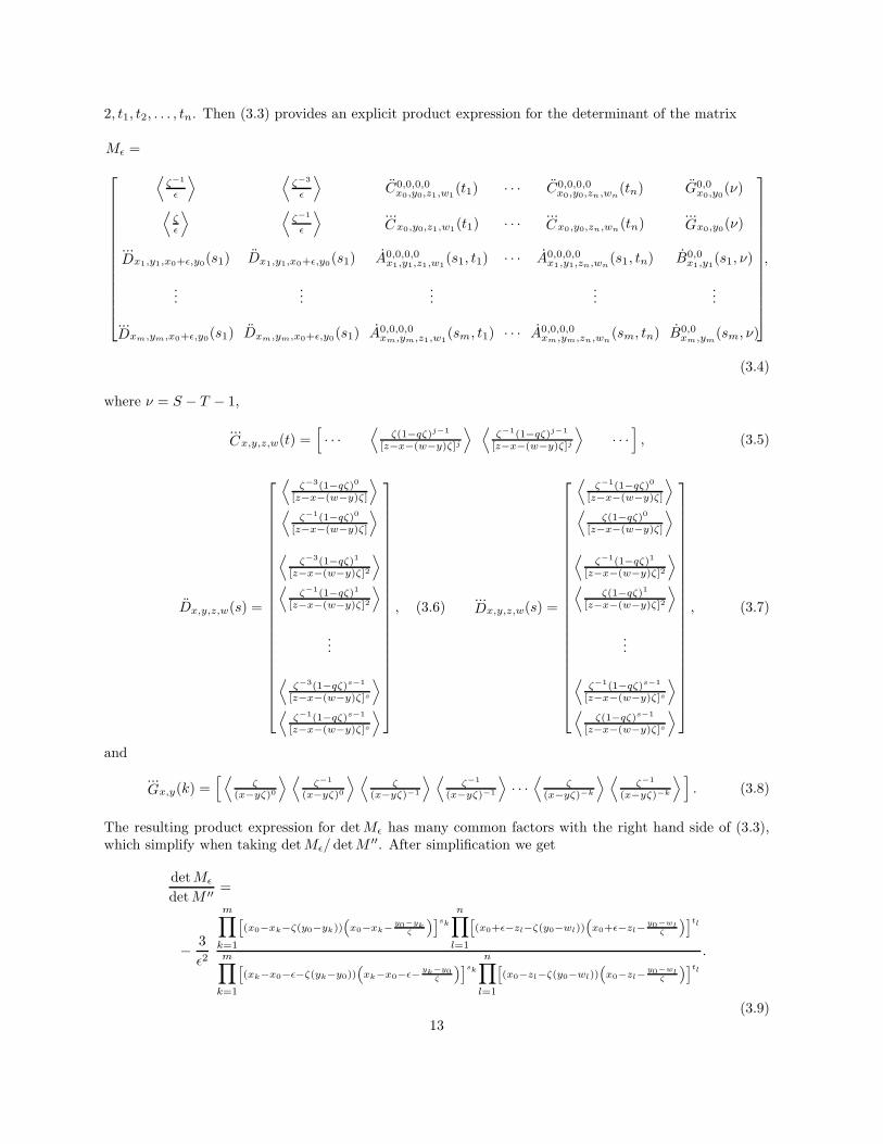
2, t1, t2, . . . , tn. Then (3.3) provides an explicit product expression for the determinant of the matrix

Mε =

⟨

ζ−1

ε

⟩ ⟨

ζ−3

ε

⟩

C0,0,0,0x0,y0,z1,w1

(t1) · · · C0,0,0,0x0,y0,zn,wn

(tn) G0,0x0,y0

(ν)

⟨

ζε

⟩ ⟨

ζ−1

ε

⟩ ...Cx0,y0,z1,w1(t1) · · · ...

Cx0,y0,zn,wn(tn)...Gx0,y0(ν)

...Dx1,y1,x0+ε,y0(s1) Dx1,y1,x0+ε,y0(s1) A0,0,0,0

x1,y1,z1,w1(s1, t1) · · · A0,0,0,0

x1,y1,zn,wn(s1, tn) B0,0

x1,y1(s1, ν)

......

......

...

...Dxm,ym,x0+ε,y0(s1) Dxm,ym,x0+ε,y0(s1) A0,0,0,0

xm,ym,z1,w1(sm, t1) · · · A0,0,0,0

xm,ym,zn,wn(sm, tn) B0,0

xm,ym(sm, ν)

,

(3.4)

where ν = S − T − 1,

...Cx,y,z,w(t) =

[

· · ·⟨

ζ(1−qζ)j−1

[z−x−(w−y)ζ]j

⟩ ⟨

ζ−1(1−qζ)j−1

[z−x−(w−y)ζ]j

⟩

· · ·]

, (3.5)

Dx,y,z,w(s) =

⟨

ζ−3(1−qζ)0

[z−x−(w−y)ζ]

⟩

⟨

ζ−1(1−qζ)0

[z−x−(w−y)ζ]

⟩

⟨

ζ−3(1−qζ)1

[z−x−(w−y)ζ]2

⟩

⟨

ζ−1(1−qζ)1

[z−x−(w−y)ζ]2

⟩

...

⟨

ζ−3(1−qζ)s−1

[z−x−(w−y)ζ]s

⟩

⟨

ζ−1(1−qζ)s−1

[z−x−(w−y)ζ]s

⟩

, (3.6)...Dx,y,z,w(s) =

⟨

ζ−1(1−qζ)0

[z−x−(w−y)ζ]

⟩

⟨

ζ(1−qζ)0

[z−x−(w−y)ζ]

⟩

⟨

ζ−1(1−qζ)1

[z−x−(w−y)ζ]2

⟩

⟨

ζ(1−qζ)1

[z−x−(w−y)ζ]2

⟩

...

⟨

ζ−1(1−qζ)s−1

[z−x−(w−y)ζ]s

⟩

⟨

ζ(1−qζ)s−1

[z−x−(w−y)ζ]s

⟩

, (3.7)

and

...Gx,y(k) =

[ ⟨

ζ(x−yζ)0

⟩ ⟨

ζ−1

(x−yζ)0

⟩ ⟨

ζ(x−yζ)−1

⟩ ⟨

ζ−1

(x−yζ)−1

⟩

· · ·⟨

ζ(x−yζ)−k

⟩ ⟨

ζ−1

(x−yζ)−k

⟩ ]

. (3.8)

The resulting product expression for det Mε has many common factors with the right hand side of (3.3),which simplify when taking det Mε/ detM ′′. After simplification we get

det Mε

det M ′′ =

− 3

ε2

m∏

k=1

h

(x0−xk−ζ(y0−yk))“

x0−xk− y0−ykζ

”isk

n∏

l=1

h

(x0+ε−zl−ζ(y0−wl))“

x0+ε−zl− y0−wlζ

”itl

m∏

k=1

h

(xk−x0−ε−ζ(yk−y0))“

xk−x0−ε− yk−y0ζ

”isk

n∏

l=1

h

(x0−zl−ζ(y0−wl))“

x0−zl− y0−wlζ

”itl

.

(3.9)13

Replace the first column in (3.4) by the negative of the sum of the first two columns. Using ζ3 = 1,−ζ−1 − ζ−3 = ζ−2, and −ζ − ζ−1 = 1, we obtain

− det Mε =

∣

∣

∣

∣

∣

∣

∣

∣

∣

∣

∣

∣

∣

∣

∣

∣

∣

∣

∣

∣

∣

∣

ζ−ζ−1

ε 0 C0,0,0,0x0,y0,z1,w1

(t1) · · · C0,0,0,0x0,y0,zn,wn

(tn) G0,0x0,y0

(ν)

0 ζ−1−ζε

...Cx0,y0,z1,w1(t1) · · · ...

Cx0,y0,zn,wn(tn)...Gx0,y0(ν)

D0,0,0,0x1,y1,x0+ε,y0

(s1) Dx1,y1,x0+ε,y0(s1) A0,0,0,0x1,y1,z1,w1

(s1, t1) · · · A0,0,0,0x1,y1,zn,wn

(s1, tn) B0,0x1,y1

(s1, ν)

......

......

...

D0,0,0,0xm,ym,x0+ε,y0

(s1) Dxm,ym,x0+ε,y0(s1) A0,0,0,0xm,ym,z1,w1

(sm, t1) · · · A0,0,0,0xm,ym,zn,wn

(sm, tn) B0,0xm,ym

(sm, ν)

∣

∣

∣

∣

∣

∣

∣

∣

∣

∣

∣

∣

∣

∣

∣

∣

∣

∣

∣

∣

∣

∣

.

(3.10)

Denote the matrix on the right hand side above by N = (Nij)1≤i,j≤2S+1. As ε → 0, the only divergingentries of N are N11 and N22. It follows from (3.10) that

det Mε =(ζ − ζ−1)2

ε2det N

[2S+1]\{1,2}[2S+1]\{1,2} +

ζ−1 − ζ

ε

[

det N[2S+1]\{1}[2S+1]\{1} − det N

[2S+1]\{2}[2S+1]\{2}

]

+ O(1), ε→ 0, (3.11)

where N is the matrix obtained from N by replacing N11 and N22 by 0. But N[2S+1]\{2}[2S+1]\{2} is just the matrix

M ′′2 of (2.31), and N

[2S+1]\{1,2}[2S+1]\{1,2} = M ′′. Furthermore, by Lemma 3.2, det N

[2S+1]\{1}[2S+1]\{1} = det M ′′

1 . Therefore,

(3.11) impliesdet Mε

det M ′′ = − 3

ε2+

ζ−1 − ζ

ε

det M ′′1 − det M ′′

2

det M ′′ + O(1), ε→ 0. (3.12)

Extracting the coefficient of 1/ε in the asymptotics of (3.9) as ε → 0 and comparing it with the secondterm in (3.12) gives (3.2).

Next we show how the case of general residues α0, . . . , δn modulo 3 reduces to the above case of all zeroresidues.

Consider the general matrix M ′′1 given by (2.14) and (2.16)–(2.20). Except for its first row and column,

it consists of 2× 2 blocks of the type in Lemma 3.3. Furthermore, the corresponding value of a is constantover each block Aαk,βk,γl,δl

xk,yk,zl,wl(sk, tl), and equals (αk − βk) − (γl − δl). It is also constant over each block

Bαk ,βkxk,yk

(sk, S − T − 1), and equals αk − βk. Thus in each 2× 2 block of type (3.13) in M ′′1 the value of the

a of Lemma 3.3 is a difference of two quantities, the first being constant along each row of M ′′1 , and the

second constant along each column of M ′′1 . Therefore Lemma 3.3 can be used to transform the general M ′′

1

matrix by row and column operations into the specialization of M ′′1 when all residues are 0 except α0 and

β0, and the overall effect on the determinant is that it is multiplied by σ, where σ ∈ {1,−1}. The verysame row and column operations transform M ′′

2 into M ′′2 |α1=0,...,δn=0 and M ′′ into M ′′|α1=0,...,δn=0, with

the effect on their determinants being multiplication by the same σ. Therefore

det M ′′1 − det M ′′

2

det M ′′ =det M ′′

1 |α1=0,...,δn=0 − det M ′′2 |α1=0,...,δn=0

det M ′′|α1=0,...,δn=0.

However, Lemma 3.4 provides determinant preserving operations that transform all three determinantsabove into their α0 = 0, β0 = 0 specializations. �

14

Lemma 3.2. det N[2S+1]\{1}[2S+1]\{1} = det M ′′

1 .

Proof. Repeated application of Lemma 3.4 transforms the first row and column of the matrix N[2S+1]\{1}[2S+1]\{1}

(see (3.5), (3.7) and (3.8)) into the first row and column of the matrix M ′′1 (see (2.18)–(2.20)). All the other

entries of N[2S+1]\{1}[2S+1]\{1} and det M ′′

1 agree, and are left in agreement by the above applications of Lemma 3.4.

This proves the claim. �

Lemma 3.3. Let f be a function defined at ζ and ζ−1, and let a ∈ Z. Let

A(a) =

[

⟨

ζa−1f(ζ)⟩ ⟨

ζa−3f(ζ)⟩

⟨

ζa+1f(ζ)⟩ ⟨

ζa−1f(ζ)⟩

]

.

Denote its rows by R1 and R2, and its columns by C1 and C2.(a). Simultaneously replacing {R1 ← R2, R2 ← −R1 −R2} turns matrix A(a) into A(a− 1).(b). Simultaneously replacing {C2 ← C1, C1 ← −C1 − C2} turns matrix A(a) into A(a + 1).

Proof. Since ζ3 = 1, the second row of A(a) is the same as the first row of A(a − 1). The negative ofthe sum of the entries in the first column of A(a) is

−(

ζa−1f(ζ)− ζ−a+1f(ζ−1))

−(

ζa+1f(ζ)− ζ−a−1f(ζ−1))

= ζaf(ζ)− ζ−af(ζ−1) = 〈ζaf(ζ)〉 ,

as −ζk − ζk+2 = ζk+1 for all integers k. One similarly checks that the negative of the sum of the entriesin the second column of A(a) equals

⟨

ζa−2f(ζ)⟩

. This proves (a). Part (b) follows analogously. �

By a similar calculation one can easily check the following.

Lemma 3.4. Let f be a function defined at ζ and ζ−1, and let α, β, γ ∈ Z. Form the matrix

0⟨

ζ1+αf(ζ)⟩ ⟨

ζ−1+αf(ζ)⟩

⟨

ζ−3+βf(ζ)⟩ ⟨

ζ−1+γf(ζ)⟩ ⟨

ζ−3+γf(ζ)⟩

⟨

ζ−1+βf(ζ)⟩ ⟨

ζ1+γf(ζ)⟩ ⟨

ζ−1+γf(ζ)⟩

.

Denote its rows by R1, R2, R3, its columns by C1, C2, C3. Then the result of the simultaneous columnoperations {C2 ← −C2−C3, C3 ← C2}, followed by the simultaneous row operations {R2 ← −R2−R3, R3 ←R2}, is the matrix

0 〈ζαf(ζ)〉⟨

ζ−2+αf(ζ)⟩

⟨

ζ−2+βf(ζ)⟩ ⟨

ζ−1+γf(ζ)⟩ ⟨

ζ−3+γf(ζ)⟩

⟨

ζβf(ζ)⟩ ⟨

ζ1+γf(ζ)⟩ ⟨

ζ−1+γf(ζ)⟩

.

Proof of Theorem 1.1. Part (1.2) of the statement follows from (3.1), (2.13) and (3.2). Interchangingthe roles of the coordinate axes we get (1.3). �

4. A finer integral asymptotics

Let D denote Newton’s divided difference operator, whose powers are defined inductively by D0f = fand Drf(cj) = (Dr−1f(cj+1) − Dr−1f(cj))/(cj+r − cj), r ≥ 1. We will need the following result on theasymptotics of the coupling function P when acted on in the indicated way by powers of D.

Theorem 4.1. Let rn and sn be integers so that limn→∞ rn/n = u, limn→∞ sn/n = v, and (u, v) 6= (0, 0).Then for any integers k, l ≥ 0 and any rational number q with 3|1− q we have

Dly

{

Dkx P (rn + x + y, sn + q(x + y))|x=a1

}∣

∣

y=b1=

1

2πi

(

k + l

k

)⟨

ζrn−sn−1(1− qζ)k+l

(−rn + snζ)k+l+1

⟩

+ O

(

1

nk+l+2

)

, (4.1)

15

where ζ = e2πi/3, Dkx acts with respect to a fixed integer sequence a1, a2, . . . , and Dl

y acts with respect toan integer sequence b1, b2, . . . satisfying qbj ∈ Z for all j ≥ 1. Furthermore, for any open set U containingthe origin the implicit constant above is uniform for all (u, v) /∈ U .

We note that Proposition 7.1 of [3] corresponds to the special case when rn = −un and sn = −vn. Itwill be crucial in our proof of the scaling limit of the average lifting surface to know that the leading termon the right hand side of (4.1) is independent of the way rn/n and sn/n approach their limits.

We deduce Theorem 4.1 from the following auxiliary results. Let P denote the counterclockwise orientedarc of the unit circle connecting ζ = e2πi/3 to −1; P [ζ,−1) stands for this path minus the point −1.

Lemma 4.2. Let rn and sn be integers, and assume limn→∞ rn/n = u ≥ ε > 0. Then if q ∈ C0(P [ζ,−1))has a pole of finite order at −1, for any integer k ≥ 0 we have

∫ −1

ζ

(−1− t)rntsn(t− ζ)kq(t) dt = O

(

1

nk+1

)

, (4.2)

where the implicit constant depends only on k, ε and q(t) (in particular, it works for all u ≥ ε and allintegers sn).

Proof. Let I denote the integral above. Write q(t) = q(t)/(t + 1)l, with l ≥ 0 and q ∈ C0(P). Makingthe change of variable t = eiθ we obtain

I = (−1)rn

∫ −1

ζ

(1 + t)rn−ltsn(t− ζ)k q(t) dt

= (−1)rn

∫ π

2π/3

(

2 cosθ

2eiθ/2

)rn−l

eiθsn

(

eiθ − e2πi/3)k

q(

eiθ)

ieiθ dθ

= (−1)rn

∫ π/3

0

[

2 cos(π

3+

τ

2

)

ei(π/3+τ/2)]rn−l

ei(2π/3+τ)sn

×[

e2πi/3(

eiτ − 1)

]k

q(

ei(2π/3+τ))

iei(2π/3+τ) dτ. (4.3)

Since the graph of 2 cos(π/3 + τ/2) is concave for τ ∈ [0, π/3], it lies below its tangent at τ = 0. Thisimplies

2 cos(π

3+

τ

2

)

≤ 1−√

3

2τ < 1− τ

2, 0 ≤ τ ≤ π/3.

The elementary inequality |ey − 1| ≤ |y|e|y| implies

|eiτ − 1| ≤ τeτ < 3τ, τ ∈ [0, π/3].

The above two inequalities combined with (4.3) give

|I | ≤∫ π/3

0

(

1− τ

2

)rn−l

(3τ)k∣

∣

∣q(

ei(2π/3+τ))∣

∣

∣dτ

≤ 3k supτ∈P|q(t)|

∫ π/3

0

(

1− τ

2

)rn−l

τk dτ. (4.4)

However, integration by parts implies

J(r, k) :=

∫ π/3

0

(

1− τ

2

)r

τk dτ

=− 2

r + 1

(

1− π

6

)r+1 (π

3

)k

+2k

r + 1J(r + 1, k − 1).

16

Repeated application of this, together with

J(r + k, 0) = − 2

r + k + 1

(

1− π

6

)r+k+1

+2

r + k + 2

shows that J(r, k) is equal to a sum of k + 1 terms each exponentially small in r, plus

2

r + k + 2

(2k)(2k − 2) · · · 2(r + 1)(r + 2) · · · (r + k)

.

Since rn − l + 1, . . . , rn − l + k + 2 ≥ 12nu for n large enough, it follows that the integral in the second

line of (4.4) is majorized for n large enough by 22k+3k!/(nu)k+1 ≤ 22k+3k!/(ε)k+11/nk+1, and the proof iscomplete. �

Lemma 4.3. Let q(t) = (t− ζ)kq1(t), where q1(t) ∈ C1(P), k is a non-negative integer, and q1(ζ) 6= 0. Letrn, sn ∈ Z so that limn→∞ rn/n = u > 0.

(a). If k = 0,∫ −1

ζ

(−1− t)rntsnq(t) dt =ζsn−rnq(ζ)

rnζ − snζ−1+ O

(

1

n2

)

. (4.5)

(b). If k ≥ 1,

∫ −1

ζ

(−1− t)rntsnq(t) dt =1

rnζ − snζ−1

∫ −1

ζ

(−1− t)rntsnq′(t) dt + O

(

1

nk+2

)

. (4.6)

Furthermore, for any ε > 0, each implicit constant above can be chosen to be uniform for u ∈ [ε,∞) andindependent of sn.

Proof. For l = 2, 3, . . . , 7, define

hl(t) :=∑

i≥0

1

l + 6j(t− ζ)l+6j , t ∈ P [ζ,−1). (4.7)

One readily checks that the Taylor series expansions of ln t and ln(−1− t) around t = ζ can then be writtenas

ln t = ln ζ + ζ−1(t− ζ) − ζ−1h4 + ζ−1h7 − ζh2 + ζh5 + h3 − h6,

and

ln(−1− t) = ln(−1− ζ)− ζ(t− ζ)− ζh4 − ζh7 − ζ−1h2 − ζ−1h5 − h3 − h6.

Therefore we have

r ln(−1− t) + s ln t = r ln(−1− ζ) + s ln ζ + (sζ−1 − rζ)(t − ζ)

+ (−rζ−1 − sζ)h2(t) + (−r + s)h3(t) + (−rζ − sζ−1)h4(t)

+ (−rζ−1 + sζ)h5(t) + (−r − s)h6(t) + (−rζ + sζ−1)h7(t), t ∈ P [ζ,−1). (4.8)

Let r, s ∈ Z and denote

I(r, s) :=

∫ −1

ζ

(−1− t)rtsq(t) dt.

17

Using (4.8) and ζ3 = 1, integration by parts gives

I(r, s) =

∫ −1

ζ

er ln(−1−t)+s ln tq(t) dt

= ζs−r

∫ −1

ζ

e(sζ−1−rζ)(t−ζ)e(−rζ−1−sζ)h2+···+(−rζ+sζ−1)h7q(t) dt

= ζs−r

e(sζ−1−rζ)(t−ζ)

sζ−1 − rζeb(t)q(t)

∣

∣

∣

∣

∣

−1

ζ

− 1

sζ−1 − rζ

∫ −1

ζ

e(sζ−1−rζ)(t−ζ)[

(

(−rζ−1 − sζ)h′2(t) + · · ·+ (−rζ + sζ−1)h′

7(t))

eb(t)q(t) + eb(t)q′(t)]

dt

}

,

where

b(t) := (−rζ−1 − sζ)h2(t) + (−r + s)h3(t) + (−rζ − sζ−1)h4(t)

+ (−rζ−1 + sζ)h5(t) + (−r − s)h6(t) + (−rζ + sζ−1)h7(t).

Since ζs−re(sζ−1−rζ)(t−ζ)eb(t) = (−1−t)rts, we see that the upper limit in the first term of the expressionin the large curly braces above equals 0 whenever r > k. Thus, for r > k we obtain

I(r, s) =ζs−rq(ζ)

rζ − sζ−1+ ζs−r

{−rζ−1 − sζ

rζ − sζ−1

∫ −1

ζ

e(sζ−1−rζ)(t−ζ)eb(t)q(t)h′2(t) dt + · · ·

+−rζ + sζ−1

rζ − sζ−1

∫ −1

ζ

e(sζ−1−rζ)(t−ζ)eb(t)q(t)h′7(t) dt

}

+ζs−r

rζ − sζ−1

∫ −1

ζ

e(sζ−1−rζ)(t−ζ)eb(t)q′(t) dt. (4.9)

If |r| ≥ |s| we have∣

∣

∣

∣

−rζ−1 − sζ

rζ − sζ−1

∣

∣

∣

∣

=

∣

∣

∣

∣

1 + s/r ζ−1

1− s/r ζ

∣

∣

∣

∣

≤ 1 + |s/r||Re(1− s/r ζ)| ≤

2

1/2= 4. (4.10)

A similar argument shows that the above inequality holds in fact also when |s| ≥ |r|. All six fractions infront of the integrals in the expression in curly braces above are thus seen to be majorized in absolute valueby 4.

Regard I(rn, sn) as the sum of the three quantities provided by (4.9). To deduce part (a) of the Lemma,assume k = 0. All six terms of the second quantity are O(1/n2) thanks to (4.10) and an applicationof Lemma 4.2 with k = 1 (which applies since h′

2(t), . . . , h′7(t) are all of the form (t − ζ)g(t), where

g ∈ C∞(P [ζ,−1)) has a simple pole at t = −1), followed by an application of Lemma 3.4 with k = 0 forthe resulting integral on the right hand side of (4.6). Finally, the third quantity provided by (4.9) is alsoO(1/n2), due to the fraction in front of the integral and another application of Lemma 4.2 with k = 0.

For part (b), assume k ≥ 1. Then q(ζ) = 0, and (4.9) provides an expression for I(rn, sn) as a sum ofjust two quantities. All six terms in the first quantity are O(1/nk+2) due to (4.10) and Lemma 4.2 appliedwith k replaced by k + 1 (as explained in the previous paragraph, this unit increment comes about by thepresence of the h′

l(t) factors in the integrands). This proves (4.6).The uniformity of the implicit constant follows because both the majorant in (4.10) and the implicit

constant in (4.2) are uniform. �

Repeated application of part (b) of the above lemma and one final application of part (a) yields thefollowing result.

18

Proposition 4.4. Let q(t) = (t− ζ)kq1(t), where k ≥ 0, q1 ∈ Ck+1(P [ζ,−1)) has a pole of finite order att = −1, and q1(ζ) 6= 0. Let rn, sn ∈ Z so that limn→∞ rn/n = u > 0. Then

∫ −1

ζ

(−1− t)rntsnq(t) dt =ζsn−rnq(k)(ζ)

(rnζ − snζ−1)k+1+ O

(

1

nk+2

)

. (4.11)

Furthermore, for any ε > 0 the implicit constant is uniform for u ∈ [ε,∞) and independent of sn. �

Proof of Theorem 4.1. Suppose first that u < 0. Then (2.1) holds for large enough n, and for 3|1 − q[3, (7.11)] and [3, Lemma 7.4] give

Dly

{

Dkx P (rn + x + y, sn + q(x + y))|x=a1

}∣

∣

y=b1

=1

2πi

⟨∫ −1

ζ

(−1− t)−rnt−sn(t− ζ)k+l

{

1

k! l!(ζ − qζ−1)k+l(t− ζ)k+l

+ ck+l+1(t− ζ)k+l+1 + · · ·}⟩

.

Proposition 4.4 applied to the right hand side above yields

Dly

{

Dkx P (rn + x + y, sn + q(x + y))|x=a1

}∣

∣

y=b1

1

2πi

⟨

ζsn−rn 1k! l! (ζ − qζ−1)k+l(k + l)!

(rnζ − snζ−1)k+l+1

⟩

+ O

(

1

nk+l+2

)

, (4.12)

which is just what (4.1) states. The uniformity of the implicit constant above follows by the uniformity ofthe implicit constant in (4.11).

Since (u, v) 6= (0, 0), at least one of u < 0, v < 0, and −u − v < 0 is true. The symmetries P (α, β) =P (−α−β−1, α) and P (α, β) = P (β, α) of the coupling function allow one to use the same arguments thatproved the case u < 0 to deduce the other two cases (see the proof of Proposition 7.1 in [3] for details). �

Proposition 4.5. Let rn, sn ∈ Z so that limn→∞ rn/n = u and limn→∞ sn/n = v. Then for any integersk, l ≥ 0 and any rational number q with 3|1− q we have

Dkx Ul(rn + x, sn + qx)|x=a1 =

1

2πi

(

l

k

)

⟨

ζrn−sn−1(1− qζ)k(rn − snζ)l−k⟩

+ O(

nl−k−1)

, (4.13)

where Dkx acts with respect to some fixed integer sequence a1, a2, . . . . Given any bounded set B in the plane,

the implicit constant can be chosen so that it is uniform for (u, v) ∈ B.

Proof. By [3, (6.8)] one has

Ul(a, b) =1

2πi

⟨

ζa−b−1(a− bζ)l⟩

+ monomials in a and b of joint degree < l.

This implies, for 3|1− q, that

Ul(rn + x, sn + qx) =1

2πi

⟨

ζrn−sn−1[(1− qζ)x + (rn − snζ)]l⟩

+∑

α,β≥0α+β<l

cα,β(rn + x)α(sn + qx)β , (4.14)

19

where cα,β is independent of rn and sn for all α and β.On the other hand, the argument that proved [3, Lemma 6.4] implies that for any constants A, B, C ∈ C

Dkx(Ax + Brn + Csn)l|x=a1 =

(

l

k

)

Ak(Brn + Csn)l−k + O(

nl−k−1)

, (4.15)

with implicit constant uniform for (u, v) ranging over any bounded set. Combining (4.14) and (4.15) yieldsthe statement of the proposition. �

5. Interpretation in terms of height functions

Lozenge tilings of regions with no holes are well known to be interpretable as lattice surfaces (see e.g.[14][6]). Regard the unit triangular lattice T on which the tiled region lives as being in a horizontal plane,

and let L be a copy of the lattice(√

32Z

)3

placed so that one family of its body-diagonals is vertical,

intersecting this plane at the vertices of T . Then each segment joining two nearest neighbors of L projectsonto a unit lattice segment of T .

Orient the lattice segments of T so that they point in one of the polar directions π/2, −π/6, or −5π/6.Then we can lift a lozenge tiling of a lattice region on T by starting from some lattice point, tracing aroundits tiles one after another, and at each traversal of a lattice segment s of T , moving either up or downon the corresponding lattice segment of L, according as the traversal respected or violated the orientationof s. Tracing around a lozenge results in going around a lattice square of L whose orthogonal projectionon the plane of T is that lozenge.

If the tiling has no holes, the node of L we are finding ourselves at is independent of the way we tracedaround the tiles to get there, and what results is a lattice surface in L whose lattice square faces are in oneto one correspondence with the tiles.

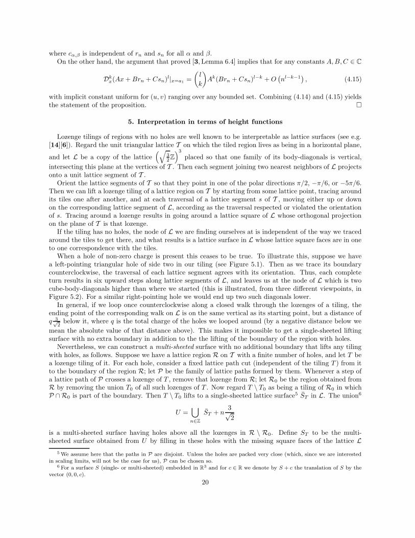
When a hole of non-zero charge is present this ceases to be true. To illustrate this, suppose we havea left-pointing triangular hole of side two in our tiling (see Figure 5.1). Then as we trace its boundarycounterclockwise, the traversal of each lattice segment agrees with its orientation. Thus, each completeturn results in six upward steps along lattice segments of L, and leaves us at the node of L which is twocube-body-diagonals higher than where we started (this is illustrated, from three different viewpoints, inFigure 5.2). For a similar right-pointing hole we would end up two such diagonals lower.

In general, if we loop once counterclockwise along a closed walk through the lozenges of a tiling, theending point of the corresponding walk on L is on the same vertical as its starting point, but a distance ofq 3√

2below it, where q is the total charge of the holes we looped around (by a negative distance below we

mean the absolute value of that distance above). This makes it impossible to get a single-sheeted liftingsurface with no extra boundary in addition to the the lifting of the boundary of the region with holes.

Nevertheless, we can construct a multi-sheeted surface with no additional boundary that lifts any tilingwith holes, as follows. Suppose we have a lattice region R on T with a finite number of holes, and let T bea lozenge tiling of it. For each hole, consider a fixed lattice path cut (independent of the tiling T ) from itto the boundary of the region R; let P be the family of lattice paths formed by them. Whenever a step ofa lattice path of P crosses a lozenge of T , remove that lozenge from R; let R0 be the region obtained fromR by removing the union T0 of all such lozenges of T . Now regard T \ T0 as being a tiling of R0 in whichP ∩R0 is part of the boundary. Then T \ T0 lifts to a single-sheeted lattice surface5 ST in L. The union6

U =⋃

n∈Z

ST + n3√2

is a multi-sheeted surface having holes above all the lozenges in R \ R0. Define ST to be the multi-sheeted surface obtained from U by filling in these holes with the missing square faces of the lattice L

5 We assume here that the paths in P are disjoint. Unless the holes are packed very close (which, since we are interestedin scaling limits, will not be the case for us), P can be chosen so.

6 For a surface S (single- or multi-sheeted) embedded in R3 and for c ∈ R we denote by S + c the translation of S by the

vector (0, 0, c).

20

Figure 5.1. A tiling with a triangular hole of size two.

Figure 5.2. Three views of ST for the tiling T above.

above the lozenges in R \ R0. One readily sees that ST is independent of the family of cuts P . Thesurface corresponding to the tiling in Figure 5.1 is illustrated in Figure 5.3. An instance with three holesis pictured in Figures 5.4 and 5.5.

The detailed definition of the joint correlation ω is the following (see [3]). For j = 1, . . . , k, let Qj beeither a lozenge-hole or a lattice triangular hole of side two.

It is enough to define ω(Q1, . . . , Qk) when q =∑k

j=1 ch(Qj) ≥ 0 (the other case reduces to this by

reflection across a vertical lattice line). Our definition is inductive on q:

(i). If q = 0, let N be large enough so that the lattice rhombus of side N centered at the origin enclosesall Qj ’s, and denote by TN the torus obtained from this large lattice rhombus by identifying its oppositesides. Set7

ω(Q1, . . . , Qk) := limN→∞

M (TN \Q1 ∪ · · · ∪Qk)

M (TN). (5.1)

(ii). If q > 0, defineω(Q1, . . . , Qk) := lim

R→∞Rq ω (Q1, . . . , Qk, WR,0) . (5.2)

The above limits exist by Proposition 2.1.Let ∆1, . . . , ∆k be fixed lattice triangular holes of side two, and let L be a fixed lozenge position. Assume

q =∑k

j=1 ch(∆j) = 0. In the limit measure of the uniform measures on the tori TN \∆1 ∪ . . . ∪ ∆k, theprobability that L is occupied by a lozenge in a random tiling is

Prob {L is occupied} = limN→∞

M (TN \ L ∪∆1 ∪ · · · ∪∆k)

M (TN \∆1 ∪ · · · ∪∆k)=

ω(L, ∆1, . . . , ∆k)

ω(∆1, . . . , ∆k). (5.3)

7 M(R) denotes the number of lozenge tilings of the lattice region R.

21

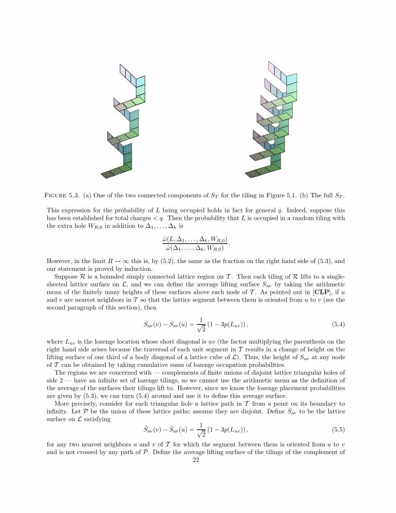
Figure 5.3. (a) One of the two connected components of ST for the tiling in Figure 5.1. (b) The full ST .

This expression for the probability of L being occupied holds in fact for general q. Indeed, suppose thishas been established for total charges < q. Then the probability that L is occupied in a random tiling withthe extra hole WR,0 in addition to ∆1, . . . , ∆k is

ω(L, ∆1, . . . , ∆k, WR,0)

ω(∆1, . . . , ∆k, WR,0).

However, in the limit R→∞ this is, by (5.2), the same as the fraction on the right hand side of (5.3), andour statement is proved by induction.

Suppose R is a bounded simply connected lattice region on T . Then each tiling of R lifts to a single-sheeted lattice surface on L, and we can define the average lifting surface Sav by taking the arithmeticmean of the finitely many heights of these surfaces above each node of T . As pointed out in [CLP], if uand v are nearest neighbors in T so that the lattice segment between them is oriented from u to v (see thesecond paragraph of this section), then

Sav(v)− Sav(u) =1√2

(1− 3p(Luv)) , (5.4)

where Luv is the lozenge location whose short diagonal is uv (the factor multiplying the parenthesis on theright hand side arises because the traversal of each unit segment in T results in a change of height on thelifting surface of one third of a body diagonal of a lattice cube of L). Thus, the height of Sav at any nodeof T can be obtained by taking cumulative sums of lozenge occupation probabilities.

The regions we are concerned with — complements of finite unions of disjoint lattice triangular holes ofside 2 — have an infinite set of lozenge tilings, so we cannot use the arithmetic mean as the definition ofthe average of the surfaces their tilings lift to. However, since we know the lozenge placement probabilitiesare given by (5.3), we can turn (5.4) around and use it to define this average surface.

More precisely, consider for each triangular hole a lattice path in T from a point on its boundary toinfinity. Let P be the union of these lattice paths; assume they are disjoint. Define Sav to be the latticesurface on L satisfying

Sav(v)− Sav(u) =1√2

(1− 3p(Luv)) , (5.5)

for any two nearest neighbors u and v of T for which the segment between them is oriented from u to vand is not crossed by any path of P . Define the average lifting surface of the tilings of the complement of

22

Figure 5.4. (a) A tiling T with three holes. (b) A view of ST .

the holes by

Sav =⋃

n∈Z

Sav + n3√2.

This definition is readily seen to be independent of the family of cuts P .We note that in the case when there are no holes, the average surface can be defined in terms of

the translation invariant ergodic measure on the hexagonal lattice (the lattice whose dimer coverings areequivalent to lozenge tilings of the triangular lattice), which follows by a general result of Sheffield (see[13][12]) to be unique and given by a limit of uniform measures on tori. Due to the presence of holes oursetting does not seem to fit that context.

The helicoid H(a, b; c) is the surface whose parametric equations in Cartesian coordinates are

x = a + ρ cos θ

y = b + ρ sin θ, −∞ < ρ, θ <∞. (5.6)

z = cθ

The half helicoid H+(a, b; c) is obtained by restricting the range of ρ in the above to (0,∞). The dotted

helicoid H(a, b; c) is H(a, b; c) minus the vertical axis x = a, y = b.23

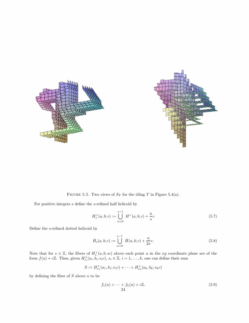
Figure 5.5. Two views of ST for the tiling T in Figure 5.4(a).

For positive integers s define the s-refined half helicoid by

H+s (a, b; c) :=

s−1⋃

n=0

H+(a, b; c) +n

sc (5.7)

Define the s-refined dotted helicoid by

Hs(a, b; c) :=

s−1⋃

n=0

H(a, b; c) +n

2sc. (5.8)

Note that for s ∈ Z, the fibers of H+s (a, b; sc) above each point u in the xy coordinate plane are of the

form f(u) + cZ. Thus, given H+si

(ai, bi; sic), si ∈ Z, i = 1, . . . , k, one can define their sum

S := H+s1

(a1, b1; s1c) + · · ·+ H+sk

(ak, bk; skc)

by defining the fiber of S above u to be

f1(u) + · · ·+ fk(u) + cZ. (5.9)24

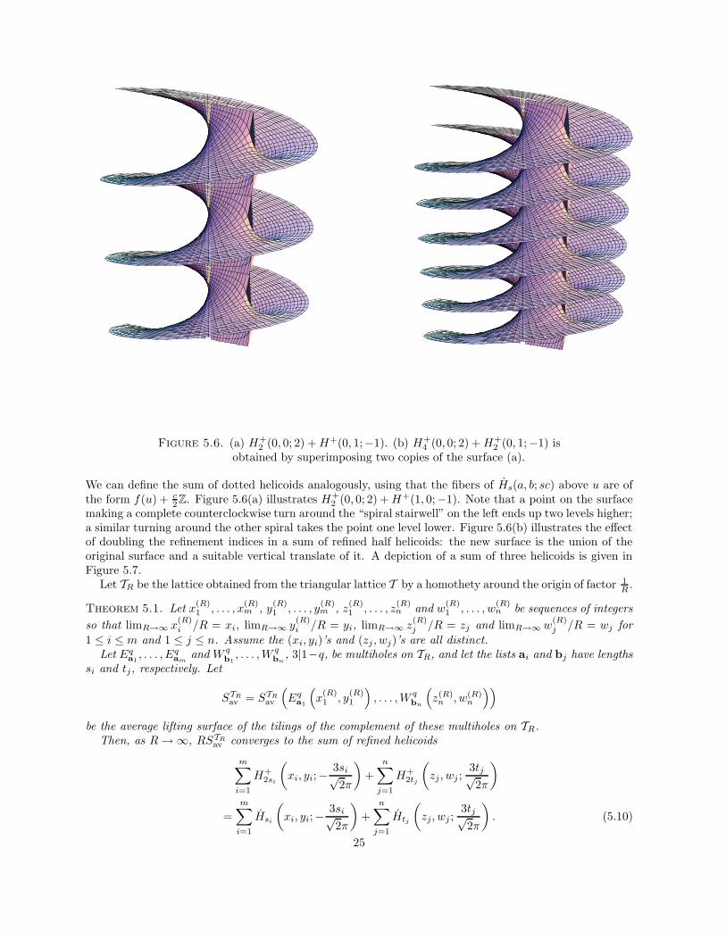
Figure 5.6. (a) H+2 (0, 0; 2) + H+(0, 1;−1). (b) H+

4 (0, 0; 2) + H+2 (0, 1;−1) is

obtained by superimposing two copies of the surface (a).

We can define the sum of dotted helicoids analogously, using that the fibers of Hs(a, b; sc) above u are ofthe form f(u) + c

2Z. Figure 5.6(a) illustrates H+2 (0, 0; 2) + H+(1, 0;−1). Note that a point on the surface

making a complete counterclockwise turn around the “spiral stairwell” on the left ends up two levels higher;a similar turning around the other spiral takes the point one level lower. Figure 5.6(b) illustrates the effectof doubling the refinement indices in a sum of refined half helicoids: the new surface is the union of theoriginal surface and a suitable vertical translate of it. A depiction of a sum of three helicoids is given inFigure 5.7.

Let TR be the lattice obtained from the triangular lattice T by a homothety around the origin of factor 1R .

Theorem 5.1. Let x(R)1 , . . . , x

(R)m , y

(R)1 , . . . , y

(R)m , z

(R)1 , . . . , z

(R)n and w

(R)1 , . . . , w

(R)n be sequences of integers

so that limR→∞ x(R)i /R = xi, limR→∞ y

(R)i /R = yi, limR→∞ z

(R)j /R = zj and limR→∞ w

(R)j /R = wj for

1 ≤ i ≤ m and 1 ≤ j ≤ n. Assume the (xi, yi)’s and (zj , wj)’s are all distinct.Let Eq

a1, . . . , Eq

amand W q

b1, . . . , W q

bn, 3|1−q, be multiholes on TR, and let the lists ai and bj have lengths

si and tj, respectively. Let

STRav = STR

av

(

Eqa1

(

x(R)1 , y

(R)1

)

, . . . , W qbn

(

z(R)n , w(R)

n

))

be the average lifting surface of the tilings of the complement of these multiholes on TR.Then, as R→∞, RSTR

av converges to the sum of refined helicoids

m∑

i=1

H+2si

(

xi, yi;−3si√2π

)

+

n∑

j=1

H+2tj

(

zj , wj ;3tj√2π

)

=

m∑

i=1

Hsi

(

xi, yi;−3si√2π

)

+

n∑

j=1

Htj

(

zj , wj ;3tj√2π

)

. (5.10)

25

Figure 5.7. (a) The sum of the refined half helicoids H+2 (−1, 0;−2), H+

3 (0, 0; 3) and H+4 (1, 0; 4). (b) Two

copies of the latter give H+4 (−1, 0;−2) + H+

6 (0, 0; 3) + H+8 (1, 0; 4).

For any bounded set B and any open set U containing (x1, y1), . . . , (xm, ym) and (z1, w1), . . . , (zn, wn), theconvergence is uniform on B \ U .

Proof. In addition to our 60◦ oblique coordinate system O in the plane of the unit triangular lattice T ,consider also a Cartesian system of coordinates C having the origin at the node of T just below the originof O , the x-axis in the polar direction 0 and the y-axis in the polar direction π/2. One readily sees that

the nodes of T have C-coordinates(

a√

32 , b 1

2

)

, a, b ∈ Z, a + b even, and that the midpoint of the segment

connecting the nodes(

a√

32 , b 1

2

)

and(

a√

32 , (b + 2) 1

2

)

of T has O-coordinates(

a−b2 , a+b

2

)

.

We will use Cartesian coordinates to specify points at which STRav is evaluated, and oblique coordinates

for the lozenges whose placement probabilities come up.26

We have by (5.5)

RSTRav

(

x(R)0

R

√3

2,y(R)0 + 2

R

1

2

)

−RSTRav

(

x(R)0

R

√3

2,y(R)0

R

1

2

)

=1√2

(

1− 3p1

(

x(R)0 − y

(R)0

2R,x

(R)0 + y

(R)0

2R

))

=1√2

(

1− 3p1

(

x(R)0 − y

(R)0

2,x

(R)0 + y

(R)0

2

))

, (5.11)

where p1 is given by (2.12). The second equality holds because placement probabilities are clearly invari-ant under scaling. Analogous equations relate the change of RSTR

av when moving a distance of 1R from

(

x(R)0

R

√3

2 ,y(R)0

R12

)

in the polar directions π2 + k π

3 , k ∈ Z.

The asymptotics of p1

(

x(R)0 , y

(R)0

)

− p2

(

x(R)0 , y

(R)0

)

follows by (3.1) and (1.2). One obtains the asymp-

totics of p1

(

x(R)0 , y

(R)0

)

−p3

(

x(R)0 , y

(R)0

)

similarly from (1.3). Adding up the two and using p1+p2+p3 = 1

yields

1− 3p1

(

x(R)0 , y

(R)0

)

= −3√

3

2π

{

m∑

i=1

six0 − xi + y0 − yi

(x0 − xi)2 + (x0 − xi)(y0 − yi) + (y0 − yi)2

−n∑

j=1

tjx0 − zj + y0 − wj

(x0 − zj)2 + (x0 − zj)(y0 − wj) + (y0 − wj)2

1

R+ o

(

1

R

)

,(5.12)

with the implicit constant uniform for (x0, y0) ∈ B \ U . Similar expressions follow for the asymptotics ofp2 and p3.

This allows us to deduce that limR→∞ RSTRav exists. Indeed, the height of RSTR

av at any node of TR

can be obtained by taking cumulative sums of (5.11) and its two analogs. By (5.12) and its analogs, theresulting error terms have a zero effect in the limit R → ∞: even though they do add up, and there aremore and more of them as R gets large, since the individual errors are small and the factor 1

R is present,the combined contribution of the error terms is small.

Furthermore, we can find the gradient of the limiting surface S by dividing the left hand side of (5.11) by1R — the distance between the two points where the heights of RSTR

av are examined — and letting R→∞.This yields

∂S∂y

(

x0

√3

2, y0

1

2

)

= − 3√2π

m∑

i=1

si

√3

2 (x0 − xi)34 (x0 − xi)2 + 1

4 (y0 − yi)2−

n∑

j=1

tj

√3

2 (x0 − zj)34 (x0 − zj)2 + 1

4 (y0 − wj)2

,

for (x0, y0) different from (x1, y1), . . . , (xm, ym) and (z1, w1), . . . , (zn, wn). After a change of variables thisbecomes

∂S∂y

(x0, y0) = − 3√2π

m∑

i=1

si(x0 − xi)

(x0 − xi)2 + (y0 − yi)2−

n∑

j=1

tj(x0 − zj)

(x0 − zj)2 + (y0 − wj)2

. (5.13)

The analog of (5.11) corresponding to moving one unit in the polar direction π6 yields by a similar calcu-

lation the directional derivative of S along this polar direction. Writing ∂/∂x as the appropriate linearcombination of this directional derivative and ∂/∂y we arrive at

∂S∂x

(x0, y0) =3√2π

m∑

i=1

si(y0 − yi)

(x0 − xi)2 + (y0 − yi)2−

n∑

j=1

tj(y0 − wj)

(x0 − zj)2 + (y0 − wj)2

. (5.14)

27

On the other hand, the gradient at (x, y) of the half helicoid H+(a, b; c) — and hence of any refinement

of it — is(

− c(y−b)(x−a)2+(y−b)2 , c(x−a)

(x−a)2+(y−b)2

)

. Thus, if H is the sum of refined helicoids

H =

m∑

i=1

H+2si

(

xi, yi;−3si√2π

)

+

n∑

j=1

H+2tj

(

zj , wj ;3tj√2π

)

, (5.15)

we have that the gradients of H and S agree on R2 \ {(x1, y1), . . . , (zn, wn)}.By construction, each lifting surface of a tiling of the complement of our multiholes has fibers of the form

c + 3√2Z. Thus so does RSTR

av for all R, and also the limit surface S. The same is true for each summand

in (5.15), and therefore for H. Then the surface S0 = S −H is well defined by (5.9). By construction, asu approaches (x1, y1) the fiber of S above u approaches 0 + 3√

2Z. It follows from the definition of H that

the same is true for the fibers of H. This, together with the fact that its gradient is zero, implies that S0

is the surface 0 + 3√2Z. So S = H, justifying the first expression in (5.10). The second expression follows

using the elementary fact that H+(a, b; c) ∪(

H+(a, b; c) + c2

)

= H(a, b; c) (an instance of this can be seenin Figure 5.6(a)). The stated uniformity of the convergence is implied by the uniformity of the error termsin (5.12) and its analogs. �

6. Physical interpretation

The results of [2] and [3] already show a close connection between random lozenge tilings with holes andelectrostatics: the joint correlation of holes is given, in the scaling limit, by the electrostatic energy of thecorresponding system of electrical charges. Theorem 1.1 strengthens this connection by showing that theelectrostatic field itself can be viewed as the scaling limit of the discrete field of the average orientation oflozenges in a random tiling of the complement of the holes.

Following [2, §2], suppose one pictures the two dimensional universe as being spatially quantized con-sisting of a very fine lattice of triangular quanta of space.

Associate the complement of the holes with the vacuum of empty space. The quantum fluctuations of thevacuum cause virtual electron-virtual positron pairs to be ceaselessly created and annihilated. Associatevirtual electrons with left-pointing unit triangles and virtual positrons with right-pointing unit triangles.Then a lozenge corresponds to the annihilation of a virtual electron-virtual positron pair, and a lozengetiling to one way for all virtual electron-virtual positron pairs to annihilate.

Averaging over all possible tilings arises then naturally as corresponding to the Feynman sum over allpossible ways the virtual electrons and virtual positrons can annihilate in pairs. Our result states thatif the distances between the hole-charges and the distances between them and the point where we aremeasuring the F-field are much larger than the lattice spacing of the quantas of space, then this field isalmost exactly the same as the electric field. From this perspective, one sees as the result of an exactcalculation how the (two dimensional) electric field emerges from the quantum fluctuations of the vacuum.This view provides an electric field which very closely approximates the Coulomb field, but is not exactlyequal to it: by Theorem 1.1, the latter occurs only in the limit when the size of the quantas of spaceapproaches zero. The discrepancy gets noticeable only at very small distances. This is in agreement withthe expectation of some physicists that linear superposition for the electric field might break down in thesubatomic domain (see e.g. Jackson [10, §I.3]).

In quantum mechanics, when a virtual electron and a virtual positron annihilate, two photons result,which are sent away in opposite directions. The unit contribution to F(e) of each lozenge covering e ina tiling could be regarded as corresponding to one of these two photons (this assumes that the commondirection of the two ejected photons is the straight line connecting the annihilating virtual particles). ThenTheorem 1.1 states that in the scaling limit, the thus generated “jet” of photons at e averages precisely tothe electrostatic field. This could then be viewed as a “mechanism” for the coming about of the electrostaticfield.

The discussion in the previous paragraph leaves the second photon unaccounted for. However, underlyingin our considerations there is a second discrete vector field we have not mentioned yet: the one given by

28

the average orientation of the lozenge that covers any fixed right-pointing unit triangle! Denote it by F′.An argument similar to the one that proved Theorem 1.1 shows that F′ = −F in the scaling limit.

We conclude by mentioning another, quite different way to define a vector field via random tilings withholes. Let Q1, . . . , Qn be a fixed collection of holes on the unit triangular lattice. For any x, y, α, β ∈ Z

define

Tα,β(x, y) :=1

√

α2 + αβ + β2

(

ω (Ex,y, Q1, . . . , Qn)

ω (Q1, . . . , Qn)− 1

)

(i.e., the hole Ex,y plays the role of a “test charge,” and the effects of its displacement are recorded). Thenit can be shown (details will appear in a separate paper) that there exists a vector field T so that in thescaling limit Tα,β(x, y) is the orthogonal projection of T(x, y) onto the vector (α, β). Furthermore, up to aconstant multiple, the field T turns out to be the same as F. Thus, unlike in physics where the electric fieldis defined by means of a test charge, in our model there are two different ways to define the correspondingfield, and one of them does not use test charges.

We note that the agreement in the previous paragraph is not a matter of course, as it does not hold forinstance on the critical Fisher lattice — the planar lattice of equilateral triangles and regular dodecagonswhere the edges of the triangles have weight 1, and the inter-triangle edges have weight

√3 (this follows

from not yet published joint work with David Wilson).

References

[1] M. Ciucu, Rotational invariance of quadromer correlations on the hexagonal lattice, Adv. in Math.

191 (2005), 46-77.

[2] M. Ciucu, A random tiling model for two dimensional electrostatics, Mem. Amer. Math. Soc. 178

(2005), no. 839, 1–104.

[3] M. Ciucu, The scaling limit of the correlation of holes on the triangular lattice with periodic bound-

ary conditions, arXiv preprint math-ph/0501071 (front.math.ucdavis.edu/math-ph/0501071).

[4] H. Cohn, N. Elkies, and J. Propp, Local statistics for random domino tilings of the Aztec diamond,

Duke Math. J. 85 (1996), 117-166.

[5] H. Cohn, R. Kenyon, and J. Propp, A variational principle for domino tilings, J. Amer. Math. Soc.

14 (2001), 297–346

[6] H. Cohn, M. Larsen, and J. Propp, The shape of a typical boxed plane partition, New York J. of

Math. 4 (1998), 137–165.

[7] T. H. Colding and W. P. Minicozzi II, Disks that are double spiral staircases, Notices Amer. Math.

Soc. 50 (2003), 327–339.

[8] R. P. Feynman, “QED: The strange theory of light and matter,” Princeton University Press, Prince-

ton, New Jersey, 1985.

[9] M. E. Fisher and J. Stephenson, Statistical mechanics of dimers on a plane lattice. II. Dimer

correlations and monomers, Phys. Rev. (2) 132 (1963), 1411–1431.

[10] J. D. Jackson, “Classical Electrodynamics,” Third Edition, Wiley, New York, 1998.

[11] R. Kenyon, Local statistics of lattice dimers, Ann. Inst. H. Poincare Probab. Statist. 33 (1997),

591–618.

[12] R. Kenyon, A. Okounkov, and S. Sheffield, Dimers and Amoebae, arXiv preprint math-ph/0311005

(front.math.ucdavis.edu/math-ph/0311005).

[13] S. Sheffield, Random Surfaces, Asterisque, 2005, No. 304.

[14] W. P. Thurston, Conway’s tiling groups, Amer. Math. Monthly 97 (1990), 757–773.

29