Stability of prograde and retrograde planets in circular binary

Mon. Not. R. Astron. Soc. 424, 52–64 (2012) doi:10.1111/j.1365-2966.2012.21151.x

Stability of prograde and retrograde planets in circular binary systems

M. H. M. Morais� and C. A. GiupponeDepartment of Physics & I3N, University of Aveiro, Campus Universitario de Santiago, 3810-193 Aveiro, Portugal

Accepted 2012 April 20. Received 2012 April 9; in original form 2012 February 27

ABSTRACTWe investigate the stability of prograde versus retrograde planets in circular binary systemsusing numerical simulations. We show that retrograde planets are stable up to distances closerto the perturber than prograde planets. We develop an analytical model to compute the progradeand retrograde mean motion resonances’ locations and separatrices. We show that instabilityis due to single resonance forcing, or caused by nearby resonances’ overlap. We validate ourresults regarding the role of single resonances and resonances’ overlap on orbit stability, bycomputing surfaces of section of the circular restricted three-body problem. We concludethat the observed enhanced stability of retrograde planets with respect to prograde planets isdue to essential differences between the phase-space topology of retrograde versus prograderesonances (at p/q mean motion ratio, the prograde resonance is of order p − q while theretrograde resonance is of order p + q).1

Key words: chaos – celestial mechanics – planets and satellites: dynamical evolution andstability – binaries: general – planetary systems.

1 IN T RO D U C T I O N

The stability of coplanar prograde planet orbits in binary systemshas been investigated numerically by Holman & Wiegert (1999).Mudryk & Wu (2006) showed that instability in eccentric binariesis due to overlap of sub-resonances associated with certain meanmotion ratios p/q. These sub-resonances are split due to the pre-cession rate induced by the secondary star; hence, the overlap ofsub-resonances for a given mean motion ratio p/q extends over awide region and explains the instability regions in eccentric bina-ries. Additionally, Mudryk & Wu (2006) suggest that the cause forinstability in circular binaries is the overlap of sub-resonances as-sociated with the 3/1 mean motion ratio. However, this cannot workfor circular binaries since in this case there is only one resonantangle.

The circular restricted three-body problem (CR3BP) is the sim-plest theoretical tool to understand planet stability within a binarysystem. The existence of an integral of motion (Jacobi constant) re-duces the number of variables of the coplanar problem from 4 to 3.Therefore, the phase space topology can be investigated by usingsurfaces of section for any given mass ratio μ. The Jacobi constantand associated zero velocity curves (ZVC) can impose bounds onthe test particle’s motion. In particular, it is useful to compare theJacobi constant with the values at the collinear Lagrange points (L1,L2 and L3). When the Jacobi constant exceeds the value at L1, thetest particle must remain in orbit around either primary or secondary

�E-mail: [email protected] Correction added after online publication 2012 June 19: typesetting errorcorrected.

stars (concept of Hill stability; Szebehely 1980). When the Jacobiconstant is smaller than the value at L1, the test particle can orbitboth stars and will eventually collide with one of them, althoughthese capture episodes can be long-lived (Winter & Vieira Neto2001; Astakhov et al. 2003). When the Jacobi constant is smallerthan the values at L2 or L3, the test particle can escape through thesepoints. However, it is well known that these are necessary but notsufficient conditions for instability (Szebehely 1980).

Eberle, Cuntz & Musielak (2008) investigated the stability ofprograde planet orbits within circular binary systems, based onthe Jacobi constant criterion. Quarles et al. (2011) validated theseresults by computing the maximum Lyapunov exponent which is ameasure of chaos and associated instability. Quarles et al. (2011)show that if the ZVC opens at L3, then the orbit is unstable but whenthe ZVC opens at L1 or L2, the orbit is not necessarily unstable.The interpretation of these results is not obvious and it may dependon the particular choice of initial conditions.

Chirikov (1960) established the resonance overlap criterion toexplain the onset of chaotic motion in Hamiltonian deterministicsystems. Wisdom (1980) obtained a resonance overlap criterion forthe onset of chaos in the CR3BP valid when μ � 1. Wisdom (1980)showed that first-order mean motion resonances with the secondaryoverlap in a region of width ∼μ2/7. Orbits in this region exhibitchaotic diffusion of eccentricity and semi-major axis until escapeor collision occurs. When μ � 1, individual resonances cannotincrease the eccentricity or semi-major axis up to escape values.However, in binary star systems, μ ∼ 1; thus, the effect of singleresonances is not necessarily negligible.

Recently, it was possible to detect the Rossiter–MacLaughin ef-fect on transiting extra-solar planets (Triaud et al. 2010). This ef-fect allows us to measure the orientation of the planet’s orbit with

C© 2012 The AuthorsMonthly Notices of the Royal Astronomical Society C© 2012 RAS

Dow

nloaded from https://academ

ic.oup.com/m

nras/article/424/1/52/1006830 by guest on 01 June 2022

Stability of prograde and retrograde planets 53

respect to the parent star’s equator. Contrary to what happens in theSolar system, extra-solar planets’ orbits can be misaligned with thehost star’s equator with angles that range from 0◦ to 180◦. Severalmechanisms have been proposed to explain these misaligned plan-ets. These include classic Kozai oscillations due to a nearby starwith subsequent tidal drift (Correia et al. 2011), secular interactionwith a companion brown dwarf or giant planet followed by tidaldrift (Naoz et al. 2011), secular chaos and tides in multiple-planetsystems (Wu & Lithwick 2011), orbit interaction in multiple-planetsystems with a companion star (Kaib, Raymond & Duncan 2011)or planet–planet scattering and tides (Beauge & Nesvorny 2012).

Gayon & Bois (2008) used the mean exponential growth ofnearby orbits (MEGNO) chaos indicator (Cincotta & Simo 2000)to show that a retrograde resonance in two-planet systems is morestable than the equivalent prograde resonance. Therefore, they sug-gest that the retrograde resonance could explain the radial veloc-ity data of extra-solar systems where the prograde resonance isunstable (Gayon-Markt & Bois 2009). In Gayon, Bois & Scholl(2009), an expansion of the Hamiltonian for the retrograde reso-nance in two-planet systems is developed. However, the numer-ical exploration in Gayon et al. (2009) is limited to a small setof initial conditions which could explain why they do not con-clude on the essential differences between prograde and retrograderesonances.

Planets in retrograde orbits within a binary system are a theoret-ical possibility although none was confirmed to date. A planet on aretrograde orbit has been suggested as an explanation for a periodicsignal of 416 d in the ν-Octantis A radial velocity curve (Rammet al. 2009). The star ν-Octantis A orbits its companion (ν-OctantisB) on a 2.9 yr orbit. Such a tight binary orbit implies that a progradeplanet at 416 d is unstable but a retrograde planet could be stable atleast up to 106 yr (Eberle & Cuntz 2010). Nevertheless, there arealternative hypotheses that claim that ν-Octantis A radial velocitycould be explained, without the need of a planet, if ν-Octantis Bwas a double star (Morais & Correia 2012).

The purpose of this paper is to investigate the stability of coplanarprograde and retrograde planet orbits in circular binary systems.Contrary to previous works, we will not only perform simulationsbut also provide theoretical explanations for the onset of instabilitybased on the effect of single resonances or due to resonance overlap.

2 EX PA N S I O N O F TH E D I S T U R B I N GF U N C T I O N IN TH E C R 3 B P

We consider the planar CR3BP composed of a test particle orbiting aprimary m0 and perturbed by a secondary m2. The primary and sec-ondary have a circular orbit with frequency n2 =

√G(m0 + m2)/a3

2

and radius a2. Since we want to model the perturbation from thesecondary, we write the equation of motion in the frame with originat the primary:

r1 = −∇ (U0 + U ) , (1)

where U0 = G m0/r1, G is the gravitational constant and U is thedisturbing potential due to the perturber m2.

When U = 0 (i.e. m2 = 0), the solution to equation (1) is aKeplerian elliptical orbit with the mean motion n1 =

√G m0/a

31 ,

semi-major axis a1, eccentricity e1, longitude of pericentre � 1 andtrue anomaly f 1.

The disturbing potential is

U = G m2

(1

�− α

a2

r1

a1cos S

), (2)

where

� = ||r1 − r2|| =√

r21 + a2

2 − 2 r1 a2 cos S, (3)

α = a1/a2 < 1 and S is the angle between r1 and r2.In the prograde case, the primary–secondary and test particle orbit

in the same direction. In the retrograde case, the test particle orbitsin the opposite direction of the primary–secondary. The primary–secondary relative position vector is r2 = a2 (cos(λ2), sin(λ2)). Thetest particle (m1 = 0) position vector with respect to the primary isr1 = r1 (cos(f1 + �1), sin(f1 + �1)) with r1 = a1 (1 − e2

1)/(1 +e1 cos f1). Hence,

cos S = cos(f1 + �1 − λ2), (4)

where λ2 = ±n2t, and the ± sign applies to the prograde or retro-grade cases, respectively.

The first and second terms in equation (2) are known as directand indirect parts, respectively. The disturbing potential (equation 2)can be expressed in the orbital elements (a1, e1, f 1, � 1) by usingLaplace coefficients (literal expansion). The direct part is written asa Taylor series in ε = (r1/a1 − 1), i.e.

1

�=

(1 +

∞∑i=1

1

i!εi αi di

diα

)1

ρ(5)

with

1

ρ= 1

a2(1 + α2 − 2 α cos S)−1/2

= 1

a2

∑j

1

2b

j1/2(α) cos(j S), (6)

where bj1/2(α) is a Laplace coefficient.

Since

cos(j S) = cos(j (f1 + �1 − λ2)) , (7)

using elliptic expansions for r1/a1, cos f 1 and sin f 1, we obtain forany given j, the direct and indirect parts of equation (2). This isdone in Ellis & Murray (2000) for prograde resonances. In theplanar CR3BP, we consider only those terms in the expansion fromEllis & Murray (2000) that depend on e1. These terms consist ofcosines of angles which are combinations of the mean longitudesλ2 = n2t, λ1 = n1 (t − τ ) + � 1 (where τ is the time of passageat the pericentre) and the longitude of the pericentre � 1. From thediscussion above, we conclude that for retrograde resonances theterms are exactly the same, although we must replace λ2 = −n2t.

By inspecting the expansion of the disturbing potential in Ellis& Murray (2000), we see that at first order in e1, terms of the type(j − 1) λ1 − j λ2 + � 1 appear (4D1.1 in Ellis & Murray 2000).If j ≥ 2, these terms correspond to a j/(j − 1) prograde resonancesince λ1 = n1 and λ2 = n2; thus, the time variation of the angleis (j − 1) n1 − j n2 ≈ 0. In the retrograde case, λ2 = −n2; hence,the previous terms are non-resonant. At second order in e1, terms ofthe type (j − 2) λ1 − j λ2 + 2 � 1 appear (4D2.1 in Ellis & Murray2000), which correspond to a j/(j − 2) prograde resonance (j ≥ 3) orthe 1/1 retrograde resonance when j = 1. At third order in e1, termsof the type (j − 3) λ1 − j λ2 + 3 � 1 appear (4D3.1 in Ellis & Murray2000) which correspond to a j/(j − 3) prograde resonance (j ≥ 4) orthe 2/1 retrograde resonance when j = 2. At fourth order in e1, termsof the type (j − 4) λ1 − j λ2 + 4 � 1 appear (4D4.1 in Ellis & Murray2000) which correspond to a j/(j − 4) prograde resonance (j ≥ 5) orthe 3/1 retrograde resonance when j = 3. It can be shown that at fifthorder in e1, terms of the type (j − 5) λ1 − j λ2 + 5 � 1 appear whichcorrespond to a j/(j − 5) prograde resonance (j ≥ 6) or to the 3/2

C© 2012 The Authors, MNRAS 424, 52–64Monthly Notices of the Royal Astronomical Society C© 2012 RAS

Dow


ic.oup.com/m


54 M. H. M. Morais and C. A. Giuppone

retrograde resonance when j = 3 and the 4/1 retrograde resonancewhen j = 4. Therefore, we see that p/q prograde resonances are oforder p − q while p/q retrograde resonances are of order p + q.2 Theonly resonant terms in the indirect part of the disturbing function(CR3BP) correspond to the 1/1 prograde resonance (4E0.1 in Ellis& Murray 2000) and to the 1/1 retrograde resonance (4E2.2 in Ellis& Murray 2000). The secular term is obtained by averaging overthe mean longitudes λ1 and λ2; hence, it is the same in the progradeor retrograde case (4D0.1 in Ellis & Murray 2000).

3 A NA LY T I C MO D E L F O R TH E M E A NM OT I O N R E S O NA N C E I N T H E C R 3 B P

Here, we briefly review the analytic model for the first, second andthird-order prograde resonances from Murray & Dermott (1999).In Appendix A, we derive in detail this Hamiltonian model in theframework of the CR3BP. We extend the model to the retrograderesonance of lowest (third) order. We explain how we can use themodel to obtain resonance widths for initially circular orbits.

3.1 Hamiltonian model for the prograde/retrograde resonance

In the CR3BP, a j/(j − k) prograde resonance is of order k while aj/(k − j) retrograde resonance3 is of order k.4 The resonant angle is

θ = (j − k) λ1 − j λ2 + k �1. (8)

Here, we will summarize the results for the prograde j/(j − k)resonances of first, second and third order (k = 1, 2, 3) and wewill extend these results to the retrograde 2/1 resonance which isof third (lowest) order (j = 2, k = 3). The resonant Hamiltonian(equation A18) depends on a single parameter (equation A19)

δ = A[(j − k) n∗

1 ∓ j n2 + k � ∗1

]/k, (9)

where n∗1 = n1 + λ∗

1,

A =(

24−k

32−k

j k−8/3(j − k)k−4/3k4−2 k

μ2 fd(α)2

) 14−k

, (10)

and from equations (A7) and (A8) with e1 � 1

� ∗1 ≈ 2 m2

m0α fs(α) n1

(11)

λ∗1 ≈ e2

1

2� ∗

1 (12)

with values of fs(α) at resonant α = [j/|j − k|]−2/3 shown inTable 1.

The Hamiltonian (equation A18) is expressed in Cartesian canon-ical variables

x = R cos(θ/k) (13)

y = R sin(θ/k), (14)

where the scaling factor is (equation A20)

R =[

3 (−1)k

fd(α) μ

(j − k)4/3j 2/3

k2

] 14−k

e1 (15)

with values of fd(α) at resonant α = [j/|j − k|]−2/3 shown in Table 1.

2 Correction added after online publication 2012 June 19: typesetting errorcorrected.3 We will use the notation j/(k − j) retrograde resonance or j/(j − k) reso-nance: e.g. 2/1 retrograde resonance or 2/−1 resonance (j = 2, k = 3).4 Correction added after online publication 2012 June 27: typesetting errorcorrected.

Table 1. Values of secular and resonant functionsat resonant α = (j/|j − k|)−2/3, k = 1, 2, 3.

Resonance α α fs(α) α fd(α)

4/1 0.396 85 0.032 355 −0.096 983/1 0.480 75 0.068 381 +0.287 855/2 0.542 88 0.116 00 −0.615 032/1 0.629 96 0.244 19 −0.749 962/1 0.629 96 0.244 19 −0.253 045/3 0.711 38 0.515 66 +2.328 923/2 0.763 14 0.879 75 −1.545 53

Obviously, this analytic model is valid only for small perturba-tion, i.e. (equations A1, A2, A3)

Ures

H0= 1

2

m2

m0α fd(α) ek

1 � 1, (16)

Usec

H0= 1

2

m2

m0α fs(α) e2

1 � 1. (17)

In Table 1, we show the values of αfd(α) and αfs(α) at the resonantvalue α = [j/|j − k|]−2/3. These provide a measure of the analyticmodel validity. In particular, the resonance location (δ = 0, equa-tion 9) depends on the secular term (�1, equation 11); hence, it isonly accurate when equation (17) is verified. From Table 1 we seethat the secular term (equation 17) at the 4/1 resonance is about0.47, 0.28 and 0.13 times that at the 3/1, 5/2 and 2/1 (or 2/−1) res-onances, respectively. Therefore, the secular term (equation 17) isapproximately the same when μ = 0.2, μ = 0.09, μ = 0.07 and μ =0.03 at the 4/1, 3/1, 5/2 and 2/1 (or 2/−1) resonances, respectively.

3.2 First-, second- and third-order resonances

The Hamiltonian (equation A18) when k = 1 is

H1 = δ

2(x2 + y2) + 1

4(x2 + y2)2 − 2 x. (18)

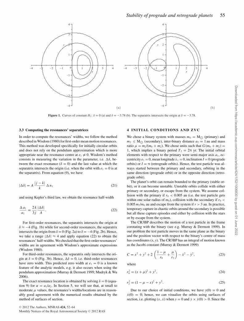
When δ < −3 there is a single stable equilibrium point (Fig. 1a).At δ = −3, an unstable equilibrium point appears which bifurcatesinto a stable/unstable pair visible when δ < −3 (Fig. 1b).

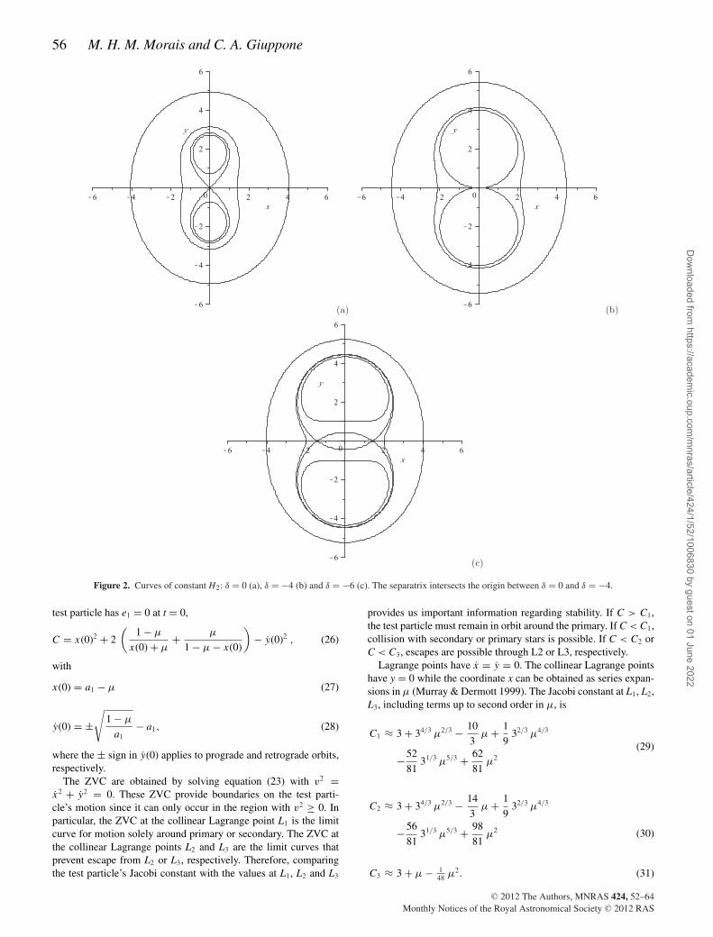
The Hamiltonian (equation A18) when k = 2 is

H2 = δ

2(x2 + y2) + 1

4(x2 + y2)2 + 2 (x2 − y2). (19)

At δ = 4 the origin becomes an unstable point and two stable pointsappear at φ = ±π/2 which move away from the origin as δ increases[see δ = 0 (Fig. 2a) and δ = −4 (Fig. 2b)]. At δ = −4, the originagain becomes a stable point (Fig. 2b) and two unstable pointsappear at φ = 0, π that are visible when δ < −4 (Fig. 2c).

The Hamiltonian (equation A18) when k = 3 is5

H3 = δ

2(x2 + y2) + 1

4(x2 + y2)2 − 2 x (x2 − 3 y2). (20)

At δ = 9, the origin is a stable point and three pairs of stable/unstablepoints appear at φ = 0, ±2π/3. The three stable points move awayfrom the origin while the three unstable points move towards theorigin (Fig. 3a), until they coincide with it at δ = 0 (Fig. 3b). Atδ = 0 (exact resonance), the origin bifurcates into a stable point andthree unstable points at φ = ±π/3, π. These unstable points moveaway from the origin as δ decreases (Fig. 3c).

5 The diagrams with curves of constant H3 in Murray & Dermott (1999)should be rotated by π/3.


Dow


ic.oup.com/m



Figure 1. Curves of constant H1: δ = 0 (a) and δ = −3.78 (b). The separatrix intersects the origin at δ = −3.78.

3.3 Computing the resonances’ separatrices

In order to compute the resonances’ widths, we follow the methoddescribed in Wisdom (1980) for first-order mean motion resonances.This method was developed specifically for initially circular orbitsand does not rely on the pendulum approximation which is moreappropriate near the resonance centre at e1 �= 0. Wisdom’s methodconsists in measuring the variation in the parameter, i.e. �δ, be-tween the exact resonance (δ = 0) and the last value at which theseparatrix intersects the origin (i.e. when the orbit with e1 = 0 is atthe separatrix). From equation (9), we have

|�δ| = A|j − k|

k� n1 (21)

and using Kepler’s third law, we obtain the resonance half-width

� a1

a1= 2 k

3j

|�δ|A

. (22)

For first-order resonances, the separatrix intersects the origin atδ ≈ −4 (Fig. 1b) while for second-order resonances, the separatrixintersects the origin from δ = 0 (Fig. 2a) to δ = −4 (Fig. 2b). Hence,we take a range |�δ| ≈ 4 and apply equation (22) to obtain theresonances’ half-widths. We checked that the first-order resonances’widths are in agreement with Wisdom’s approximate expressions(Wisdom 1980).

For third-order resonances, the separatrix only intersects the ori-gin at δ = 0 (Fig. 3b). Hence, �δ = 0, i.e. third-order resonanceshave zero width. This predicted zero width at e1 = 0 is a knownfeature of the analytic models, e.g. it also occurs when using thependulum approximation (Murray & Dermott 1999; Mudryk & Wu2006).

The exact resonance location is obtained by solving δ = 0 (equa-tion 9) for α = a1/a2. In Section 5, we will see that, at small tomoderate μ values, the resonance’s widths/locations are in reason-ably good agreement with the numerical results obtained by themethod of surfaces of section.

4 IN I T I A L C O N D I T I O N S A N D Z V C

We chose a binary system with masses m0 = M (primary) andm2 ≤ M (secondary), inter-binary distance a2 = 1 au and massratio μ = m2/(m0 + m2). We chose units such that G (m0 + m2) =1, which implies a binary period T2 = 2π yr. The initial orbitalelements with respect to the primary were semi-major axis a1, ec-centricity e1 = 0, mean longitude λ1 = 0, inclination I = 0 (progradeorbits) or I = π (retrograde orbits). Hence, the test particle was al-ways started between the primary and secondary, orbiting in thesame direction (prograde orbit) or in the opposite direction (retro-grade orbit).

The planet’s orbit can remain bounded to the primary (stable or-bit), or it can become unstable. Unstable orbits collide with eitherprimary or secondary, or escape from the system. We assume col-lision with the primary if r0 < 0.005 au (i.e. the test particle getswithin one solar radius of m0), collision with the secondary if r0 <

0.005 m2/m0 au and escape from the system if r > 3 au. In practice,temporary capture in chaotic orbits around the secondary is possiblebut all these capture episodes end either by collision with the starsor by escape from the system.

The CR3BP describes the motion of a test particle in the framecorotating with the binary (see e.g. Murray & Dermott 1999). Inour problem the test particle moves in the same plane as the binaryand the position vector with respect to the binary’s centre of masshas coordinates (x, y). The CR3BP has an integral of motion knownas the Jacobi constant (Murray & Dermott 1999)

C = x2 + y2 + 2

(1 − μ

r0+ μ

r2

)− x2 − y2, (23)

where

r20 = (x + μ)2 + y2, (24)

r22 = (1 − μ − x)2 + y2. (25)

Due to our choice of initial conditions, we have y(0) = 0 andx(0) = 0; hence, we can visualize the orbits using surfaces ofsection, i.e. plotting (x, x) when y = 0 and y × y(0) > 0. Since the


Dow


ic.oup.com/m



(a) (b)

(c)

Figure 2. Curves of constant H2: δ = 0 (a), δ = −4 (b) and δ = −6 (c). The separatrix intersects the origin between δ = 0 and δ = −4.

test particle has e1 = 0 at t = 0,

C = x(0)2 + 2

(1 − μ

x(0) + μ+ μ

1 − μ − x(0)

)− y(0)2 , (26)

with

x(0) = a1 − μ (27)

y(0) = ±√

1 − μ

a1− a1, (28)

where the ± sign in y(0) applies to prograde and retrograde orbits,respectively.

The ZVC are obtained by solving equation (23) with v2 =x2 + y2 = 0. These ZVC provide boundaries on the test parti-cle’s motion since it can only occur in the region with v2 ≥ 0. Inparticular, the ZVC at the collinear Lagrange point L1 is the limitcurve for motion solely around primary or secondary. The ZVC atthe collinear Lagrange points L2 and L3 are the limit curves thatprevent escape from L2 or L3, respectively. Therefore, comparingthe test particle’s Jacobi constant with the values at L1, L2 and L3

provides us important information regarding stability. If C > C1,the test particle must remain in orbit around the primary. If C < C1,collision with secondary or primary stars is possible. If C < C2 orC < C3, escapes are possible through L2 or L3, respectively.

Lagrange points have x = y = 0. The collinear Lagrange pointshave y = 0 while the coordinate x can be obtained as series expan-sions in μ (Murray & Dermott 1999). The Jacobi constant at L1, L2,L3, including terms up to second order in μ, is

C1 ≈ 3 + 34/3 μ2/3 − 10

3μ + 1

932/3 μ4/3

−52

8131/3 μ5/3 + 62

81μ2

(29)

C2 ≈ 3 + 34/3 μ2/3 − 14

3μ + 1

932/3 μ4/3

−56

8131/3 μ5/3 + 98

81μ2 (30)

C3 ≈ 3 + μ − 148 μ2. (31)


Dow


ic.oup.com/m



(a) (b)

(c)

Figure 3. Curves of constant H3: δ = 8 (a), δ = 0 (b) and δ = −8 (c). The separatrix intersects the origin only at δ = 0 (exact resonance).

In the next section, we will plot the initial conditions that have C =C1, C = C2 and C = C3 (where C is given by equation 26). We willsee that, as expected, these curves separate the regions of differentend states for the test particle.

5 NUMERICAL STABILITY STUDY

We constructed grids of initial conditions in the plane (α, μ) witha step �μ = 0.002 and �α = 0.005 au. Each point in the grid wasthen numerically integrated over 50 ∼ kyr (around 12 000 binary pe-riods, depending on μ) using a Burlisch–Stoer-based N-body code(precision better than 10−12) using astrocentric osculating variables.During the integrations, we computed the averaged MEGNO chaosindicator 〈Y〉 (Cincotta & Simo 2000). We show these MEGNOmaps in Figs 4(a) and 8(a).

The MEGNO chaos maps use a threshold that is chosen in or-der to avoid excluding stable orbits that did not converge to theirtheoretical value or those orbits that are weakly chaotic. Thus, thecolour scale shows ‘stable’ orbits in blue up to 〈Y〉 ≈ 2.0 (a partic-

ular choice based on integration of individual orbits for very longtimes and due to the characteristics of this system).

MEGNO is a fast chaos indicator that allows us to distinguishrapidly between regular and chaotic orbits. Within the integrationtime, all the orbits identified as unstable (red) either collide withprimary or secondary, or escape from the system as we can see inFigs 4(b) and (c) and Figs 8(b) and (c). The thin region colouredwith light blue in the transition between chaos/regularity is typicallyunstable within ∼10 000–15 000 binary periods. We integrated thegrids with less resolution for 2.5 × 105 binary periods and noadditional signs of instability were observed.

5.1 Prograde case

In Fig. 4 we show, for prograde orbits, the maps with (a) the MEGNOchaos indicator; (b) times of disruption of a three-body system and(c) planet end states (stable, collision or escape). In Fig. 5, we showa zoom-in view of Fig. 4(a).


Dow


ic.oup.com/m



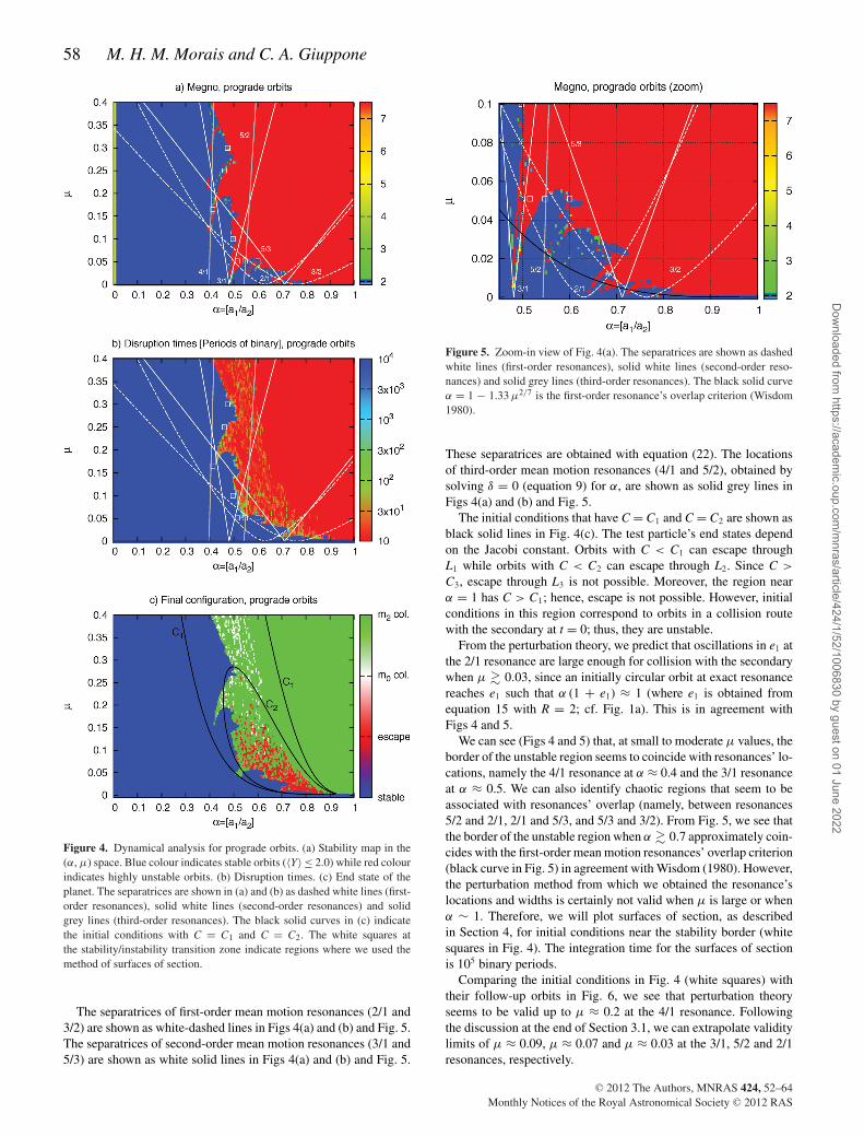
Figure 4. Dynamical analysis for prograde orbits. (a) Stability map in the(α, μ) space. Blue colour indicates stable orbits (〈Y〉 ≤ 2.0) while red colourindicates highly unstable orbits. (b) Disruption times. (c) End state of theplanet. The separatrices are shown in (a) and (b) as dashed white lines (first-order resonances), solid white lines (second-order resonances) and solidgrey lines (third-order resonances). The black solid curves in (c) indicatethe initial conditions with C = C1 and C = C2. The white squares atthe stability/instability transition zone indicate regions where we used themethod of surfaces of section.

The separatrices of first-order mean motion resonances (2/1 and3/2) are shown as white-dashed lines in Figs 4(a) and (b) and Fig. 5.The separatrices of second-order mean motion resonances (3/1 and5/3) are shown as white solid lines in Figs 4(a) and (b) and Fig. 5.

Figure 5. Zoom-in view of Fig. 4(a). The separatrices are shown as dashedwhite lines (first-order resonances), solid white lines (second-order reso-nances) and solid grey lines (third-order resonances). The black solid curveα = 1 − 1.33 μ2/7 is the first-order resonance’s overlap criterion (Wisdom1980).

These separatrices are obtained with equation (22). The locationsof third-order mean motion resonances (4/1 and 5/2), obtained bysolving δ = 0 (equation 9) for α, are shown as solid grey lines inFigs 4(a) and (b) and Fig. 5.

The initial conditions that have C = C1 and C = C2 are shown asblack solid lines in Fig. 4(c). The test particle’s end states dependon the Jacobi constant. Orbits with C < C1 can escape throughL1 while orbits with C < C2 can escape through L2. Since C >

C3, escape through L3 is not possible. Moreover, the region nearα = 1 has C > C1; hence, escape is not possible. However, initialconditions in this region correspond to orbits in a collision routewith the secondary at t = 0; thus, they are unstable.

From the perturbation theory, we predict that oscillations in e1 atthe 2/1 resonance are large enough for collision with the secondarywhen μ � 0.03, since an initially circular orbit at exact resonancereaches e1 such that α (1 + e1) ≈ 1 (where e1 is obtained fromequation 15 with R = 2; cf. Fig. 1a). This is in agreement withFigs 4 and 5.

We can see (Figs 4 and 5) that, at small to moderate μ values, theborder of the unstable region seems to coincide with resonances’ lo-cations, namely the 4/1 resonance at α ≈ 0.4 and the 3/1 resonanceat α ≈ 0.5. We can also identify chaotic regions that seem to beassociated with resonances’ overlap (namely, between resonances5/2 and 2/1, 2/1 and 5/3, and 5/3 and 3/2). From Fig. 5, we see thatthe border of the unstable region when α � 0.7 approximately coin-cides with the first-order mean motion resonances’ overlap criterion(black curve in Fig. 5) in agreement with Wisdom (1980). However,the perturbation method from which we obtained the resonance’slocations and widths is certainly not valid when μ is large or whenα ∼ 1. Therefore, we will plot surfaces of section, as describedin Section 4, for initial conditions near the stability border (whitesquares in Fig. 4). The integration time for the surfaces of sectionis 105 binary periods.

Comparing the initial conditions in Fig. 4 (white squares) withtheir follow-up orbits in Fig. 6, we see that perturbation theoryseems to be valid up to μ ≈ 0.2 at the 4/1 resonance. Followingthe discussion at the end of Section 3.1, we can extrapolate validitylimits of μ ≈ 0.09, μ ≈ 0.07 and μ ≈ 0.03 at the 3/1, 5/2 and 2/1resonances, respectively.


Dow


ic.oup.com/m



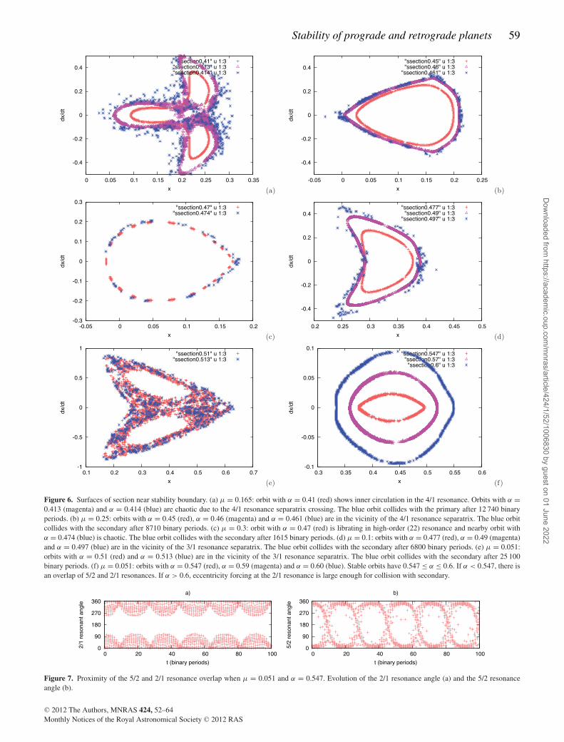
Figure 6. Surfaces of section near stability boundary. (a) μ = 0.165: orbit with α = 0.41 (red) shows inner circulation in the 4/1 resonance. Orbits with α =0.413 (magenta) and α = 0.414 (blue) are chaotic due to the 4/1 resonance separatrix crossing. The blue orbit collides with the primary after 12 740 binaryperiods. (b) μ = 0.25: orbits with α = 0.45 (red), α = 0.46 (magenta) and α = 0.461 (blue) are in the vicinity of the 4/1 resonance separatrix. The blue orbitcollides with the secondary after 8710 binary periods. (c) μ = 0.3: orbit with α = 0.47 (red) is librating in high-order (22) resonance and nearby orbit withα = 0.474 (blue) is chaotic. The blue orbit collides with the secondary after 1615 binary periods. (d) μ = 0.1: orbits with α = 0.477 (red), α = 0.49 (magenta)and α = 0.497 (blue) are in the vicinity of the 3/1 resonance separatrix. The blue orbit collides with the secondary after 6800 binary periods. (e) μ = 0.051:orbits with α = 0.51 (red) and α = 0.513 (blue) are in the vicinity of the 3/1 resonance separatrix. The blue orbit collides with the secondary after 25 100binary periods. (f) μ = 0.051: orbits with α = 0.547 (red), α = 0.59 (magenta) and α = 0.60 (blue). Stable orbits have 0.547 ≤ α ≤ 0.6. If α < 0.547, there isan overlap of 5/2 and 2/1 resonances. If α > 0.6, eccentricity forcing at the 2/1 resonance is large enough for collision with secondary.

Figure 7. Proximity of the 5/2 and 2/1 resonance overlap when μ = 0.051 and α = 0.547. Evolution of the 2/1 resonance angle (a) and the 5/2 resonanceangle (b).


Dow


ic.oup.com/m



In Fig. 6(a), instability is associated with the 4/1 resonance sep-aratrix (δ < 0 case; cf. Fig. 3c). In Fig. 6(b), instability is alsoassociated with the 4/1 resonance separatrix (9 > δ > 0 case; cf.Fig. 3a). In Fig. 6(c), we identify a high-order (k = 22) resonance.In Figs 6(d) and (e), instability is associated with the 3/1 resonanceseparatrix (δ < −4 case; cf. Fig. 2c). In Fig. 6(f), we show stableorbits associated with the 2/1 resonance (0.547 ≤ α ≤ 0.6). Whenα < 0.547, there is chaos due to overlap with the 5/2 resonance.When α > 0.6, eccentricity forcing at the 2/1 resonance is largeenough for collision with secondary, as seen above.

We conclude that instability for prograde orbits is either due tosingle resonance forcing or resonance overlap. Regarding the lattermechanism, we infer resonance overlap from the observation ofa main resonance’s chaotic separatrix. We know from Chrikov’scriterion that widespread chaos in Hamiltonian systems is causedby resonances overlapping. However, we cannot always identify theresonance(s) that overlap with the main resonance. These are likelyto be high-order resonances which are difficult to identify in thesurfaces of section, in particular in the chaotic regions where theresonances’ overlap.

In Fig. 7, we present a case where we identify the overlappingresonances. We show the evolution of the 2/1 and 5/2 resonant an-gles when μ = 0.051 and α = 0.547 (red orbit in the surface ofsection; Fig. 6f). The 5/2 resonant angle alternates between libra-tion and circulation since it is at the separatrix. When α < 0.547both separatrices overlap and the orbits are unstable. These reso-nant angles are obtained from osculating elements with respect tothe primary. When the perturbation from the secondary is small,the osculating elements are approximately Keplerian in the shortterm. Here, we can see that the resonant angles exhibit short-termoscillations which indicate that the assumption of Keplerian oscu-lating elements is not very good, despite the moderate mass ratio(μ = 0.051). Therefore, the osculating elements cannot be used toidentify the resonances at larger mass ratio μ or when α ∼ 1. Themethod of surfaces of section is always valid; thus, it is very usefulto identify the main resonances and their chaotic separatrices.

5.2 Retrograde case

In Fig. 8 we show, for retrograde orbits, the maps with (a) theMEGNO chaos indicator; (b) times of disruption of a three-bodysystem and (c) planet end states (stable, collision or escape).

The location of the 2/−1 mean motion resonance, obtained bysolving δ = 0 (equation 9) for α is shown as a white solid line inFigs 8(a) and (b). For moderate to large μ values, equation (11)overestimates the precession rate; hence, it displaces the theoreticalresonance location to the left. We obtain a ‘corrected’ 2/−1 meanmotion resonance location by solving δ = 0 for α while taking intoaccount the precession rate measured in the numerical integrations(this is shown as a white-dashed line in Figs 8a and b).

The initial conditions that have C = C1, C = C2 and C = C3 areshown as black solid lines in Fig. 8(c) (these curves approximatelycoincide). We know that the test particle’s end states depend on theJacobi constant. However, although orbits in between the curves C =C1, C = C2 or C = C3 can escape through L1, L2 or L3, respectively,in practice they only escape due to the effect of resonances. Thestable region near α = 1 corresponds to test particles orbiting thesecondary at t = 0, and is in agreement with the Jacobi constantcriterion (C > C1).

In Fig. 8, we see that chaos and instability occur at large valuesof the mass ratio μ or when α ∼ 1. However, from the discussion atthe end of Section 3.1 and the results in Section 5.1, we conclude

Figure 8. Dynamical analysis for retrograde orbits following the same cri-teria as in Fig. 4. (a) Stability map in the (α, μ) space showing 〈Y〉. (b)Disruption times. (c) End state of the planet. The theoretical 2/−1 reso-nance location shown in (a) and (b) as the white solid line is over-displacedto the left when μ � 0.05. We show the ‘corrected’ 2/−1 resonance loca-tion as the white dashed line (see the text for explanation). The black solidcurves in (c) indicate the initial conditions with C = C1, C = C2 and C = C3.The white squares at the stability/instability transition zone indicate regionswhere we used the method of surfaces of section. The white circle is theinitial condition for the red orbit in Fig. 10.

that perturbation theory is valid only up to μ ≈ 0.03 at the 2/−1resonance. This threshold is well below the instability region whichat the 2/−1 resonance occurs only when μ > 0.15 (Fig. 8). There-fore, perturbation theory cannot be used and instead we will plotsurfaces of section, as described in Section 4, for initial conditions


Dow


ic.oup.com/m



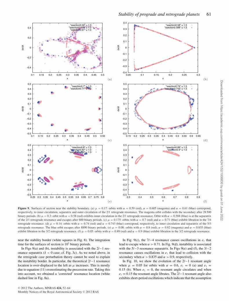
Figure 9. Surfaces of section near the stability boundary. (a) μ = 0.17: orbits with α = 0.59 (red), α = 0.605 (magenta) and α = 0.61 (blue) correspond,respectively, to inner circulation, separatrix and outer circulation of the 2/1 retrograde resonance. The magenta orbit collides with the secondary after 28 500binary periods. (b) μ = 0.3: orbit with α = 0.58 (red) exhibits inner circulation in the 2/1 retrograde resonance. Orbit with α = 0.588 (blue) is at the separatrixof the 2/1 retrograde resonance and escapes after 600 binary periods. (c) μ = 0.175: orbits with α = 0.7 (red) and α = 0.71 (blue) exhibit libration in the 7/4retrograde resonance. (d) μ = 0.14: orbits with α = 0.74 (red) and α = 0.743 (blue) correspond, respectively, to inner circulation and separatrix of the 5/3retrograde resonance. The blue orbit escapes after 8890 binary periods. (e) μ = 0.08: orbits with α = 0.8 (red), α = 0.82 (magenta) and α = 0.835 (blue)exhibit libration in the 3/2 retrograde resonance. (f) μ = 0.05: orbits with α = 0.89 (red) and α = 0.9 (blue) exhibit libration in the 3/2 retrograde resonance.

near the stability border (white squares in Fig. 8). The integrationtime for the surfaces of section is 105 binary periods.

In Figs 9(a) and (b), instability is associated with the 2/−1 res-onance separatrix (δ < 0 case; cf. Fig. 3c). As we noted above, inthe retrograde case perturbation theory cannot be used to explainthe instability border. In particular, the theoretical 2/−1 resonancelocation is over-displaced to the left as μ increases. This is mostlydue to equation (11) overestimating the precession rate. Taking thisinto account, we obtained a ‘corrected’ resonance location (whitedashed line in Fig. 8a).

In Fig. 9(c), the 7/−4 resonance causes oscillations in e1 thatlead to escape when α > 0.71. In Fig. 9(d), instability is associatedwith the 5/−3 resonance separatrix. In Figs 9(e) and (f), the 3/−2resonance causes oscillations in e1 that lead to collision with thesecondary when α > 0.835 and α > 0.9, respectively.

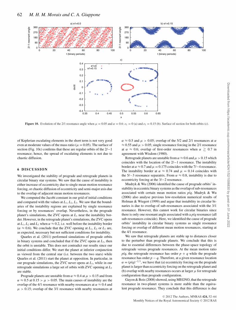
In Fig. 10, we show the evolution of the 2/−1 resonant anglewhen μ = 0.05 for orbits with α = 0.6, e1 = 0 (a) and e1 =0.15 (b). When e1 = 0, the resonant angle circulates and whene1 = 0.15 the resonant angle librates. The 2/−1 resonant angle alsoexhibits short-period oscillations which indicate that the assumption


Dow


ic.oup.com/m



Figure 10. Evolution of the 2/1 resonance angle when μ = 0.05 and α = 0.6: e1 = 0 (a) and e1 = 0.15 (b). Surface of section for both orbits (c).

of Keplerian osculating elements in the short term is not very goodeven at moderate values of the mass ratio (μ = 0.05). The surface ofsection (Fig. 10c) confirms that these are regular orbits of the 2/−1resonance; hence, the spread of osculating elements is not due tochaotic diffusion.

6 D ISCUSSION

We investigated the stability of prograde and retrograde planets incircular binary star systems. We saw that the cause of instability iseither increase of eccentricity due to single mean motion resonanceforcing, or chaotic diffusion of eccentricity and semi-major axis dueto the overlap of adjacent mean motion resonances.

We computed the Jacobi constant in our grid of initial conditionsand compared with the values at L1, L2, L3. We saw that the bound-aries of the instability regions are explained by single resonanceforcing or by resonances’ overlap. Nevertheless, in the progradeplanet’s simulations, the ZVC opens at L1 near the instability bor-der. However, in the retrograde planet’s simulations, the ZVC opensat L1, L2 and L3 when α ≈ 0.2, i.e. well before the instability border(α ≈ 0.6). We conclude that the ZVC opening at L1, L2 or L3 are,as expected, necessary but not sufficient conditions for instability.

Quarles et al. (2011) performed simulations of prograde orbitsin binary systems and concluded that if the ZVC opens at L3, thenthe orbit is unstable. This does not contradict our results since ourinitial conditions differ. We start the planet at inferior conjunctionas viewed from the central star (i.e. between the two stars) whileQuarles et al. (2011) start the planet at opposition. In particular, inour prograde simulations, the ZVC never opens at L3, while in ourretrograde simulations a large set of orbits with ZVC opening at L3

are stable.Prograde planets are unstable from α ≈ 0.4 at μ > 0.15 and from

α ≈ 0.5 at 0.15 > μ > 0.05. The main causes of instability are theoverlap of the 4/1 resonance with nearby resonances at α ≈ 0.4 andμ > 0.15; overlap of the 3/1 resonance with nearby resonances at

α ≈ 0.5 and μ > 0.05; overlap of the 5/2 and 2/1 resonances at α

≈ 0.55 and μ > 0.05; single resonance forcing in the 2/1 resonanceat α ≈ 0.6; overlap of first-order resonances when α � 0.7 inagreement with Wisdom (1980).

Retrograde planets are unstable from α ≈ 0.6 and μ > 0.15 whichcoincides with the location of the 2/−1 resonance. The instabilityborder at α ≈ 0.7 and μ = 0.175 coincides with the 7/−4 resonance.The instability border at α ≈ 0.74 and μ = 0.14 coincides withthe 5/−3 resonance separatrix. From α ≈ 0.8, instability is due toeccentricity forcing at the 3/−2 resonance.

Mudryk & Wu (2006) identified the cause of prograde orbits’ in-stability in eccentric binary systems as the overlap of sub-resonancesassociated with certain mean motion ratios p/q. Mudryk & Wu(2006) also analyse previous low-resolution numerical results ofHolman & Wiegert (1999) and argue that instability in circular bi-naries is due to overlap of sub-resonances associated with the 3/1resonance. However, this cannot work for circular binaries sincethere is only one resonant angle associated with a p/q resonance (allsub-resonances coincide). Here, we identified the cause of progradeorbits’ instability in circular binary systems as single resonanceforcing or overlap of different mean motion resonances, starting atthe 4/1 resonance.

We saw that retrograde planets are stable up to distances closerto the perturber than prograde planets. We conclude that this isdue to essential differences between the phase-space topology ofretrograde versus prograde resonances. At the mean motion ratiop/q, the retrograde resonance has order p + q while the prograderesonance has order p − q. Therefore, at a given resonance locationα = (p/q)−2/3, we have that (a) eccentricity forcing on the progradeplanet is larger than eccentricity forcing on the retrograde planet and(b) overlap with nearby resonances occurs at larger μ for retrogradeconfiguration than prograde configuration.

Gayon & Bois (2008) showed, using MEGNO, that the retrograderesonance in two-planet systems is more stable than the equiva-lent prograde resonance. They conclude that this difference is due


Dow


ic.oup.com/m



to close approaches being much faster and shorter for counter-revolving configurations than for the prograde ones (Gayon & Bois2008). While this is true, we believe that the essential difference isnot the duration of close approaches but instead, as explained above,the phase-space topology of prograde versus retrograde resonances.An expansion of the Hamiltonian for the retrograde resonance intwo-planet systems is presented in Gayon et al. (2009) but the nu-merical exploration of the model is limited to a small set of initialconditions and they do not conclude on the essential differencesbetween the prograde and retrograde resonances.

Finally, we refer that a similar mechanism could also explainthe enhanced stability of retrograde satellites with respect to pro-grade satellites that has been observed, for instance, by Henon(1970), Hamilton & Krivov (1997), Nesvorny et al. (2003), Shen &Tremaine (2008) and Hinse et al. (2010). However, satellite motionis a problem distinct from that presented in this paper (planet withina binary system) as the hierarchy of masses is very different.

AC K N OW L E D G M E N T S

We thank Fathi Namouni for helpful discussions regarding theresonance Hamiltonian model. We acknowledge financial sup-port from FCT-Portugal (grants PTDC/CTE-AST/098528/2008 andPEst-C/CTM/LA0025/2011).

R E F E R E N C E S

Astakhov S. A., Burbanks A. D., Wiggins S., Farrelly D., 2003, Nat, 423,264

Beauge C., Nesvorny D., 2012, ApJ, 751, 119Chirikov B. V., 1960, J. Nucl. Energy C: Plasma Phys., 1, 253Cincotta P. M., Simo C., 2000, A&AS, 147, 205Correia A. C. M., Laskar J., Farago F., Boue G., 2011, Celest. Mech. Dyn.

Astron., 111, 105Eberle J., Cuntz M., 2010, ApJ, 721, L168Eberle J., Cuntz M., Musielak Z. E., 2008, A&A, 489, 1329Ellis K. M., Murray C. D., 2000, Icarus, 147, 129Gayon J., Bois E., 2008, A&A, 482, 665Gayon J., Bois E., Scholl H., 2009, Celest. Mech. Dyn. Astron., 103, 267Gayon-Markt J., Bois E., 2009, MNRAS, 399, L137Hamilton D. P., Krivov A. V., 1997, Icarus, 128, 241Henon M., 1970, A&A, 9, 24Henrard J., Lemaitre A., 1983, Celest. Mech., 30, 197Hinse T. C., Christou A. A., Alvarellos J. L. A., Gozdziewski K., 2010,

MNRAS, 404, 837Holman M. J., Wiegert P. A., 1999, AJ, 117, 621Kaib N. A., Raymond S. N., Duncan M. J., 2011, ApJ, 742, L24Morais M. H. M., Correia A. C. M., 2012, MNRAS, 419, 3447Mudryk L. R., Wu Y., 2006, ApJ, 639, 423Murray C. D., Dermott S. F., 1999, Solar System Dynamics. Cambridge

Univ. Press, CambridgeNaoz S., Farr W. M., Lithwick Y., Rasio F. A., Teyssandier J., 2011, Nat,

473, 187Nesvorny D., Alvarellos J. L. A., Dones L., Levison H. F., 2003, AJ, 126,

398Peale S. J., 1976, ARA&A, 14, 215Quarles B., Eberle J., Musielak Z. E., Cuntz M., 2011, A&A, 533, A2Ramm D. J., Pourbaix D., Hearnshaw J. B., Komonjinda S., 2009, MNRAS,

394, 1695Shen Y., Tremaine S., 2008, AJ, 136, 2453Szebehely V., 1980, Celest. Mech., 22, 7Triaud A. H. M. J. et al., 2010, A&A, 524, A25Winter O. C., Vieira Neto E., 2001, A&A, 377, 1119Wisdom J., 1980, AJ, 85, 1122Wu Y., Lithwick Y., 2011, ApJ, 735, 109

A P P E N D I X A : R E S O NA N C E H A M I LTO N I A N

Here, we follow partly the derivations in Peale (1976), Wisdom(1980), Henrard & Lemaitre (1983) and Murray & Dermott (1999)to model first-, second- and third-order prograde resonances, and weextend this to model the third-order retrograde resonance (2/−1).

The Hamiltonian of the CR3BP near a j/(j − k) prograde orretrograde resonance is

H = − (1 − μ)

2 a1+ Ures + Usec, (A1)

where G m0 = 1 − μ = n21 a3

1 and G m2 = μ. The resonant term is

Ures = − μ

a2fd(α)ek

1 cos((k − j ) λ1 + j λ2 − k �1), (A2)

and the secular term is

Usec = − μ

a2fs(α)e2

1. (A3)

From Lagrange’s equations (Murray & Dermott 1999), � 1 and λ1

change due to the secular term, while a1 and e1 do not change;hence, we can write

H = − (1 − μ)2

2 �2+ Ures − � � ∗

1 + � λ∗1, (A4)

where we used Poincare canonical variables

� = n1 a21 , λ1 (A5)

� = n1 a21

(1 −

√1 − e2

1

), −�1, (A6)

and the secular variations in � 1 and λ1 are

� ∗1 = −

√1 − e2

1

n1 a21 e1

∂Usec

∂e1(A7)

λ∗1 =

(1 −

√1 − e2

1

)� ∗

1 . (A8)

Now, we change to resonant variables

� = k � − (k − j ) �

k, φ = λ1 − λ2 (A9)

� = �, ψ = [(k − j ) λ1 + j λ2 − k �1]/k (A10)

via the generating function6

F = ψ � + φ �. (A11)

Since F is time dependent (λ2 = ±n2t), the transformation intro-duces the term ∂F/∂t in the new Hamiltonian, which is

H = − (1 − μ)2

2(� − (j−k)

k�

)2 + Ures ± j

kn2 � ∓ n2 �

−� � ∗1 +

(� − (j − k)

k�

)λ∗

1.(A12)

Since H does not depend on φ, the momentum � is a conservedquantity. Moreover, if e1 � 1, then � ≈ � e2

1/2 and thus we expandthe first term in H up to second order around � = 0. Hence, dropping

6 For a mixed variable transformation φ = ∂F/∂�, ψ = ∂F/∂�, � =∂F/∂λ1, � = −∂F/∂�1.


Dow


ic.oup.com/m



constant terms that depend only on �, and changing the sign of H,we obtain7

H = γ� + β �2 + (−1)k ε(2 �)k/2 cos(k ψ), (A13)

where8

γ =[(j − k)

(n1 + λ∗

1

)∓ j n2 + k � ∗

1

]/k (A14)

β = 3

2

(j − k)2

k2 a21

(A15)

ε = μ

a2fd(α) n

−k/21 a−k

1 . (A16)

As explained in Murray & Dermott (1999), by introducing a scaledmomentum

7 Where ( − 1)k is introduced because ε > 0 if k is even and ε < 0 if k isodd.8 Note that β differs from the expression in Murray & Dermott (1999) (nomass).

� =(

ε

2 β (−1)k

) 2k−4

�, (A17)

this can be written as a single-parameter Hamiltonian

H = δ� + �2 + 2 (−1)k (2 �)k/2 cos(k ψ) (A18)

with

δ = γ

(4

ε2 β2−k

) 14−k

. (A19)

The Hamiltonian (equation A18) can be expressed in Cartesiancanonical variables (x = R cos (ψ), y = R sin (ψ)) where the scalingfactor is

R =√

2 �. (A20)

This paper has been typeset from a TEX/LATEX file prepared by the author.


Dow


ic.oup.com/m


Documents

Stability of prograde and retrograde planets in circular binary