The TRAPPIST survey of southern transiting planets

arX

iv:1

201.

2789

v1 [

astr

o-ph

.EP

] 13

Jan

201

2Astronomy & Astrophysicsmanuscript no. WASP-43 c© ESO 2012January 16, 2012

The TRAPPIST survey of southern transiting planets. IThirty eclipses of the ultra-short period planet WASP-43 b⋆

M. Gillon1, A. H. M. J. Triaud2, J. J. Fortney3, B.-O. Demory4, E. Jehin1, M. Lendl2, P. Magain1, P. Kabath5,D. Queloz2, R. Alonso2, D. R. Anderson6, A. Collier Cameron7, A. Fumel1, L. Hebb8, C. Hellier6, A. Lanotte1,

P. F. L. Maxted6, N. Mowlavi2, B. Smalley6

1 Universite de Liege, Allee du 6 aout 17, Sart Tilman, Li`ege 1, Belgium2 Observatoire de Geneve, Universite de Geneve, 51 Chemindes Maillettes, 1290 Sauverny, Switzerland3 Department of Astronomy and Astrophysics, University of California, Santa Cruz, CA 95064, USA4 Department of Earth, Atmospheric and Planetary Sciences, Department of Physics, Massachusetts Institute of Technology, 77Massachusetts Ave., Cambridge, MA 02139, USA5 European Southern Observatory, Alonso de Cordova 3107, Casilla 19001, Santiago, Chile6 Astrophysics Group, Keele University, Staffordshire ST5 5BG, UK7 School of Physics and Astronomy, University of St. Andrews,North Haugh, Fife, KY16 9SS, UK8 Department of Physics and Astronomy, Vanderbilt University, Nashville, TN 37235, USA

Received date/ accepted date

ABSTRACT

We present twenty-three transit light curves and seven occultation light curves for the ultra-short period planet WASP-43 b, in additionto eight new measurements of the radial velocity of the star.Thanks to this extensive data set, we improve significantly the parametersof the system. Notably, the largely improved precision on the stellar density (2.41±0.08ρ⊙) combined with constraining the age to beyounger than a Hubble time allows us to break the degeneracy of the stellar solution mentioned in the discovery paper. Theresultingstellar mass and size are 0.717± 0.025 M⊙ and 0.667± 0.011R⊙. Our deduced physical parameters for the planet are 2.034± 0.052MJup and 1.036±0.019RJup. Taking into account its level of irradiation, the high density of the planet favors an old age and a massivecore. Our deduced orbital eccentricity, 0.0035+0.0060

−0.0025, is consistent with a fully circularized orbit. We detect the emission of the planetat 2.09µm at better than 11-σ, the deduced occultation depth being 1560± 140 ppm. Our detection of the occultation at 1.19µm ismarginal (790± 320 ppm) and more observations are needed to confirm it. We place a 3-σ upper limit of 850 ppm on the depth ofthe occultation at∼0.9µm. Together, these results strongly favor a poor redistribution of the heat to the night-side of the planet, andmarginally favor a model with no day-side temperature inversion.

Key words. stars: planetary systems - star: individual: WASP-43 - techniques: photometric - techniques: radial velocities

1. Introduction

There are now more than seven hundreds planets known to or-bit around other stars than our Sun (Schneider 2011). A signifi-cant fraction of them are Jovian-type planets orbiting within 0.1AU of their host stars. Their very existence poses an interest-ing challenge for our theories of planetary formation and evo-lution, as such massive planets could not have formed so closeto their star (D’Angelo et al. 2010; Lubow & Ida 2010). Longneglected in favor of disk-driven migration theories (Lin et al.1996), the postulate that past dynamical interactions combinedwith tidal dissipation could have shaped their present orbit hasraised a lot of interest recently (e.g. Fabrycky & Tremaine 2007,Naoz et al. 2011, Wu & Lithwick 2011), partially thanks to thediscovery that a significant fraction of these planets have highorbital obliquities that suggest past violent dynamical perturba-tions (e.g. Triaud et al. 2010).

Send offprint requests to: [email protected]⋆ Based on data collected with the TRAPPIST andEuler telescopes

at ESO La Silla Observatory, Chile, and with the VLT/HAWK-I instru-ment at ESO Paranal Observatory, Chile (program 086.C-0222).

Not only the origin of these planets but also their fate raisesmany questions. Their relatively large mass and small semi-major axis imply tidal interactions with the host star that shouldlead in most cases to a slow spiral-in of the planet and to a trans-fer of angular momentum to the star (e.g. Barker & Ogilvie 2009,Jackson et al. 2009, Mastumura et al. 2010), the end result be-ing the planet’s disruption at the Roche limit of the star (Guetal. 2003). The timescale of this final disruption depends mostlyon the timescale of the migration mechanism, the tidal dissipa-tion efficiency of both bodies, and the efficiency of angular mo-mentum losses from the system due to magnetic braking. Thesethree parameters being poorly known, it is desirable to detectand study in depth ‘extreme’ hot Jupiters, i.e. massive planetshaving exceptionally short semi-major axes that could be inthefinal stages of their tidal orbital decay.

The WASP transit survey detected two extreme examples ofsuch ultra-short period planets, WASP-18 b (Hellier et al. 2009)and WASP-19 b (Hebb et al. 2010), both having an orbital periodsmaller than one day. Thanks to their transiting nature, these sys-tems were amenable for a thorough characterization that madepossible a study of the effects of their tidal interactions (Brownet al. 2011). Notably, photometric observations of some of their

1

http://arxiv.org/abs/1201.2789v1

M. Gillon et al.: Thirty eclipses of the ultra-short period planet WASP-43 b

occultations made possible not only to probe both planets’ day-side emission spectra but also to bring strong constraints on theirorbital eccentricity (Anderson et al. 2010, Gibson et al. 2010,Nymeyer et al. 2011), a key parameter to assess their tidal his-tory and energy budget. The same WASP survey has recently an-nounced the discovery of a third ultra-short period Jovian planetcalled WASP-43 b (Hellier et al. 2011b, hereafter H11). Its or-bital period is 0.81 d, the only hot Jupiter having a smaller pe-riod being WASP-19 b (0.79 d). Furthermore, it orbits aroundavery cool K7-type dwarf that has the lowest mass among all thestars orbited by a hot Jupiter (0.58±0.05M⊙, Te f f = 4400±200K, H11), except for the recently announced M0 dwarf KOI-254(0.59 ± 0.06M⊙, Te f f = 3820± 90 K, Johnson et al. 2011).Nevertheless, H11 presented another plausible solution for thestellar mass that is significantly larger, 0.71± 0.05M⊙. This de-generacy translates into a poor knowledge of the physical pa-rameters of the system.

With the aim to improve the characterization of this interest-ing ultra-short period planet, we performed an intense ground-based photometric monitoring of its eclipses (transits andoccul-tations), complemented with new measurements of the radialve-locity (RV) of the star. These observations were carried outin theframe of a new photometric survey based on the 60cm robotictelescope TRAPPIST1 (TRAnsiting Planets andPlanetesImalsSmall Telescope; Gillon et al. 2011a, Jehin et al. 2011). Theconcept of this survey is the intense high-precision photomet-ric monitoring of the transits of southern transiting systems, itsgoals being (i) to improve the determination of the physicalandorbital parameters of the systems, (ii) to assess the presence ofundetected objects in these systems through variability studiesof the transit parameters, and (iii) to measure or put an upperlimit on the very-near-IR thermal emission of the most highlyirradiated planets to constrain their atmospheric properties. Wecomplemented the data acquired in the frame of this program forthe WASP-43 system by high-precision occultation time-seriesphotometry gathered in the near-IR with the VLT/HAWK-I in-strument (Pirard et al., 2004, Casali et al. 2006) in our program086.C-0222. We present here the results of the analysis of thisextensive data set. Section 2 below presents our data. Theiranal-ysis is described in Sec. 3. We discuss the acquired results anddrawn inferences about the WASP-43 system in Sec. 4. Finally,we give our conclusions in Sec. 5.

2. Data

2.1. TRAPPIST I+z filter transit photometry

We observed 20 transits of WASP-43 b with TRAPPIST and itsthermoelectrically-cooled 2k× 2k CCD camera with a field ofview of 22’× 22’ (pixel scale= 0.65”). All the 20 transits wereobserved in an Astrodon ‘I+z’ filter that has a transmittance>90% from 750 nm to beyond 1100 nm2, the red end of the effec-tive bandpass being defined by the spectral response of the CCD.This wide red filter minimizes the effects of limb-darkeningand differential atmospheric extinction while maximizing stel-lar counts. Its effective wavelength forTe f f = 4400± 200 Kis λe f f = 843.5 ± 1.2 nm. The mean exposure time was 20s.The telescope was slightly defocused to minimize pixel-to-pixeleffects and to optimize the observational efficiency. We gener-ally keep the positions of the stars on the chip within a box ofa few pixels of side to improve the photometric precision of our

1 see http://www.ati.ulg.ac.be/TRAPPIST2 see http://www.astrodon.com/products/filters/near-infrared/

TRAPPIST time-series, thanks to a ‘software guiding’ systemderiving regularly astrometric solutions on the science imagesand sending pointing corrections to the mount if needed. It couldunfortunately not be used for WASP-43, because the star liesina sky area that is not covered by the used astrometric catalogue(GSC1.1). This translated into slow drifts of the stars on the chip,the underlying cause being the imperfection of the telescope po-lar alignment. The amplitudes of those drifts on the total durationof the runs were ranging between 15 and 85 pixels in the rightascension direction and between 5 and 75 pixels in the declina-tion direction. Table 1 presents the logs of the observations. Thefirst of these 20 transits was presented in H11.

After a standard pre-reduction (bias, dark, flatfield correc-tion), the stellar fluxes were extracted from the images using theIRAF/DAOPHOT3 aperture photometry software (Stetson, 1987).For each transit, several sets of reduction parameters weretested,and we kept the one giving the most precise photometry for thestars of similar brightness as WASP-43. After a careful selectionof reference stars, differential photometry was then obtained.The resulting light curves are shown in Fig. 1 and 2.

2.2. Euler Gunn-r′ filter transit photometry

Three transits of WASP-43 b were observed in the Gunn-r′ fil-ter (λe f f = 620.4 ± 0.5 nm) with the EulerCAM CCD cameraat the 1.2-mEuler Swiss telescope, also located at ESO La SillaObservatory. EulerCAM is a nitrogen-cooled 4k× 4k CCD cam-era with a 15’× 15’ field of view (pixel scale=0.23”). Here too,the telescope was slightly defocused to optimize the photometricprecision. The mean exposure time was 85s. The stars were keptapproximately on the same pixels, thanks to a ‘software guiding’system similar to TRAPPIST’s but using the UCAC3 catalogue.The calibration and photometric reduction procedures weresim-ilar to the ones performed on the TRAPPIST data. The logs oftheseEuler observations are shown in Table 1, while the result-ing light curves are visible in Fig. 2. Notice that the first oftheseEuler transits was presented in H11.

2.3. TRAPPIST z′ filter occcultation photometry

Five occultations of WASP-43 b were observed with TRAPPISTin a Sloanz’ filter (λe f f = 915.9± 0.5 nm). Their logs are pre-sented in Table 1. The mean exposure time was 40s. The cali-bration and photometric reduction of these occultation data weresimilar to the ones of the transits. Fig. 3 shows the resulting lightcurves with their best-fit models.

2.4. VLT/HAWK-I 1.19 and 2.09 µm occultation photometry

We observed two occultations of WASP-43 b with the cryogenicnear-IR imager HAWK-I at the ESO Very Large Telescope inour program 086.C-0222. HAWK-I is composed of four Hawaii2RG 2048× 2048 pixels detectors (pixel scale= 0.106”), its to-tal field of view on the sky being 7.5’×7.5’. We choose to ob-serve the occultations within the narrow band filters NB2090(λ = 2.095µm, width = 0.020µm) and NB1190 (λ = 1.186µm, width= 0.020µm), respectively. The small width of thesecosmological filters minimizes the effect of differential extinc-tion. Furthermore, they avoid the largest absorption and emis-

3 IRAF is distributed by the National Optical AstronomyObservatory, which is operated by the Association of Universitiesfor Research in Astronomy, Inc., under cooperative agreement with theNational Science Foundation.

2

http://www.ati.ulg.ac.be/TRAPPIST

http://www.astrodon.com/products/filters/near-infrared/


Date Instrument Filter Np Epoch Baseline σ σ120s βw βr CFfunction [%] [%]

06 Dec 2010 TRAPPIST I+z 393 11 p(t2) 0.35, 0.36 0.14, 0.17 1.26, 1.30 1.00, 1.90 1.26, 2.47

09 Dec 2010 VLT/HAWK-I NB2090 183 13.5 p(t2) + p(l1) + p(xy1) 0.055, 0.055 0.036, 0.036 1.04, 1.04 1.09, 1.14 1.14, 1.18




28 Dec 2010 Euler Gunn-r′ 111 38 p(t2) + p(xy2) 0.10, 0.10 0.10, 0.10 1.54, 1.64 1.04, 1.15 1.61, 1.90

30 Dec 2010 TRAPPIST z′ 332 40.5 p(t2) 0.30, 0.30 0.14, 0.14 1.04, 1.04 1.00, 1.00 1.04, 1.04

01 Jan 2011 TRAPPIST I+z 407 43 p(t2) + p(xy2) 0.27, 0.27 0.11, 0.12 1.00, 1.01 1.00, 1.00 1.00, 1.01

06 Jan 2011 TRAPPIST I+z 273 49 p(t2) 0.24, 0.24 0.11, 0.11 1.07, 1.09 1.00, 1.38 1.07, 1.50

09 Jan 2011 VLT/HAWK-I NB1190 115 51.5 p(t2) + p(b1) + p(xy1) 0.087, 0.087 0.047, 0.048 2.22, 2.22 1.00, 1.00 2.22, 2.22



23 Jan 2011 TRAPPIST I+z 244 70 p(t2) + p(xy2) 0.20, 0.20 0.08, 0.09 1.02, 1.02 1.00, 1.00 1.02, 1.02

28 Jan 2011 Euler Gunn-r′ 114 76 p(t2) + p(xy1) 0.13, 0.13 0.13, 0.13 1.36, 1.42 1.17, 1.24 1.59, 1.76

06 Feb 2011 Euler Gunn-r′ 107 87 p(t2) 0.13, 0.15 0.13, 0.15 0.92, 1.07 1.10, 1.86 1.02, 1.99

14 Feb 2011 TRAPPIST I+z 311 97 p(t2) 0.21, 0.22 0.11, 0.12 1.05, 1.08 1.00, 1.42 1.05, 1.53

08 Mar 2011 TRAPPIST I+z 285 124 p(t2) 0.21, 0.22 0.11, 0.13 1.11, 1.15 1.00, 2.00 1.11, 2.30

10 Mar 2011 TRAPPIST z′ 216 126.5 p(t2) 0.22, 0.22 0.17, 0.17 1.09, 1.09 1.00, 1.00 1.09, 1.09



28 Mar 2011 TRAPPIST z′ 195 148.5 p(t2) 0.28, 0.28 0.18, 0.18 0.81, 0.81 1.03, 1.04 0.84, 0.84


02 Apr 2011 TRAPPIST z′ 160 154.5 p(t2) + p(b1) 0.18, 0.18 0.11, 0.11 0.93, 0.93 1.27, 1.30 1.19, 1.21

13 Apr 2011 TRAPPIST I+z 293 168 p(t2) + p(xy2) 0.23, 0.23 0.12, 0.13 1.00, 1.01 1.00, 1.00 1.00, 1.01

17 Apr 2011 TRAPPIST I+z 289 173 p(t2) 0.26, 0.27 0.13, 0.15 1.05, 1.09 1.00, 1.26 1.05, 1.36

30 Apr 2011 TRAPPIST I+z 327 189 p(t2) 0.32, 0.33 0.16, 0.17 1.31, 1.33 1.07, 1.30 1.40, 1.73

09 May 2011 TRAPPIST I+z 280 200 p(t2) 0.19, 0.20 0.10, 0.12 0.98, 1.05 1.00, 1.77 0.98, 1.85

11 May 2011 TRAPPIST z′ 214 202.5 p(t2) 0.21, 0.21 0.14, 0.14 1.03, 1.03 1.23, 1.29 1.27, 1.33

18 May 2011 TRAPPIST I+z 250 211 p(t2) 0.18, 0.18 0.10, 0.11 0.93, 0.96 1.10, 1.48 1.02, 1.42

13 Jun 2011 TRAPPIST I+z 605 243 p(t2) 0.33, 0.34 0.13, 0.14 0.97, 0.99 1.25, 1.87 1.22, 1.84

Table 1.WASP-43 b photometric eclipse time-series used in this work. For each light curve, this table shows the date of acquisition,the used instrument and filter, the number of data points, theepoch based on the transit ephemeris presented in H11, the selectedbaseline function (see Sec. 3.1), the standard deviation ofthe best-fit residuals (unbinned and binned per intervals of2 min), andthe deduced values forβw, βr, andCF = βr × βw (see Sec. 3.1). For the baseline function,p(ǫN) denotes, respectively, aN-orderpolynomial function of time (ǫ = t), the logarithm of time (ǫ = l), x andy positions (ǫ = xy), and background (ǫ = b). For thelast five columns, the first and second value correspond, respectively, to the individual analysis of the light curve and to the globalanalysis of all data.

sion bands that are present inJ andK bands, reducing thus sig-nificantly the correlated photometric noise caused by the com-plex spatial and temporal variations of the background due tothe variability of the atmosphere. As this correlated noiseis themain precision limit for ground-based near-IR time-seriespho-tometry, the use of these two narrow-band filters optimizes thephotometric quality of the resulting light curves. This is espe-cially important in the context of the challenging measurementof the emission of exoplanets.

The observation of the first occultation (NB2090 filter) tookplace on 2010 Dec 9 from 5h37 to 9h07 UT. Atmospheric con-ditions were very good, with a stable seeing and extinction.Airmass decreased from 2.1 to 1.05 during the run. Each of the185 exposures was composed of 17 integrations of 1.7s each (theminimum integration time allowed for HAWK-I). We choose todo not apply a jitter pattern. Indeed, the background contributionin the photometric aperture is small enough to ensure that thelow-frequency variability of the background cannot cause corre-lated noises with an amplitude larger than a few dozens of ppmin our light curves, making the removal of a background im-age unnecessary. Furthermore, staying on the same pixels during

the whole run allows minimizing the effects of interpixel sensi-tivity inhomogeneity (i.e. the imperfect flat field). The analysisof HAWK-I calibration frames showed us that the detector isnearly linear up to 10-12 kADU. The peak of the target imagewas above 10 kADU in the first images, so a slight defocus wasapplied to keep it below this level during the rest of the run.The mean full-width at half maximum of the stellar point-spreadfunction (PSF) was 7.3 pixels= 0.77”, its standard deviation forthe whole run being 0.57 pixels= 0.06”. The pointing was care-fully selected to avoid cosmetic defects on WASP-43 or on thecomparison stars.

The second occultation (NB1190 filter) was observed on2011 Jan 9 from 4h57 to 9h27 UT. The seeing varied stronglyduring the all run (mean value in our images=0.76”, with a stan-dard deviation= 0.19”, minimum= 0.51”, maximum= 1.22”)while the extinction was stable during the first part of the run andslightly variable during the second part. No defocus was applied,the peak of the target being in the linear part of the detectordy-namic in all images. Airmass decreased from 1.37 to 1.03, thenincreased to 1.13 during the run. Here too, no jitter patternwas

3


Fig. 1. Le f t : WASP-43 b transit photometry (12 first TRAPPIST transits) used in this work, binned per 2 min, period-folded onthe best-fit transit ephemeris deduced from our global MCMC analysis (see Sec. 3.3), and shifted along they-axis for clarity. Thebest-fit baseline+transit models are superimposed on the light curves. The fifth and ninth models (from the top) show some wigglesbecause of their position-dependent terms.Right: best-fit residuals for each light curve binned per intervalof 2 min.

applied. Each of the 241 exposures was composed of 17 integra-tions of 1.7s.

After a standard calibration of the images (dark-subtraction,flatfield correction), a cosmetic correction was applied. This cor-rection was done independently for each image and based on anautomatic detection of the stars followed by a detection of out-lier pixels. This latter was based on a comparison of the value ofeach pixel to the median value of the eight adjacent pixels. Fora pixel within a stellar aperture, a detection threshold of 50-σwas used, while it was 5-σ for the background pixels. Outlierpixels had their value replaced by the median value of the ad-

jacent pixels. At this stage, aperture photometry was performedwith DAOPHOT for the target and comparison stars, and differ-ential photometry was obtained for WASP-43. Table 1 presentsthe logs of our HAWK-I observations, while Fig. 3 shows theresulting light curves with their best-fit models.

2.5. Euler/CORALIE spectra and radial velocities

We gathered eight new spectroscopic measurements of WASP-43 with theCORALIE spectrograph mounted onEuler. The spec-troscopic measurements were performed between 2011 Feb 02

4


Fig. 2. Le f t : WASP-43 b transit photometry (8 last TRAPPIST transits+ the 3Euler transits) used in this work, binned per 2 min,period-folded on the best-fit transit ephemeris deduced from our global MCMC analysis (see Sec. 3.3), and shifted along they-axisfor clarity. The best-fit baseline+transit models are superimposed on the light curves (red= TRAPPISTI + z filter; green= EulerGunn-r′ filter). The third, ninth and tenth models (from the top) showsome wiggles because of their position-dependent terms.Right: best-fit residuals for each light curve binned per intervalof 2 min.

and March 12, the integration time being 30 min for all of them.RVs were computed from the calibrated spectra by weightedcross-correlation (Baranne et al. 1996) with a numerical spec-tral template. They are shown in Table 2. We analyzed these newRVs globally with the RVs presented in H11 and with our eclipsephotometry (see Sec. 3.3).

3. Data analysis

Our analysis of the WASP-43 data was divided in two steps. In afirst step, we analyzed independently the 30 eclipse light curvesto search for potential variability among the eclipse parameters(Sec. 3.2). We then performed a global analysis of the wholedata set, including the RVs, with the aim to obtain the strongestconstraints on the system parameters (Sec. 3.3).

5


Fig. 3. Le f t : WASP-43 b occultation photometry, binned per intervals of2 min, period-folded on the best-fit transit ephemerisdeduced from our global MCMC analysis (see Sec. 3.3), and shifted along they-axis for clarity. The best-fit baseline+occultationmodels are superimposed on the light curves (blue= TRAPPISTz′-filter; green= VLT /HAWK-I NB1190 filter; red= VLT /HAWK-I NB2090 filter).Right: same light curves divided by their best-fit baseline models. The corresponding best-fit occultation modelsare superimposed.

3.1. Method and models

Our data analysis was based on the most recent version ofour adaptive Markov Chain Monte-Carlo (MCMC) algorithm(see Gillon et al. 2010 and references therein). To summa-rize, MCMC is a Bayesian stochastic simulation algorithm de-signed to deduce the posterior Probability Distribution Functions(PDFs) for the parameters of a given model (e.g. Gregory 2005,Carlin & Louis 2008). Our implementation of the algorithmassumes as model for the photometric time-series the eclipse

model of Mandel & Agol (2002) multiplied by a baseline modelaiming to represent the other astrophysical and instrumentalmechanisms able to produce photometric variations. For theRVs, the model is based on Keplerian orbits added to a modelfor the stellar and instrumental variability. Our global model caninclude any number of planets, transiting or not. For the RVsobtained during a transit, a model of the Rossiter-McLaughlineffect is also available (Gimenez, 2006). Comparison betweentwo models can be performed based on their Bayes factor, thislatter being the product of their prior probability ratio multiplied

6


Time RV σRV BS(BJDT DB-2,450,000) (km s−1) (m s−1) (km s−1)

5594.848273 -3.921 21 0.021

5604.730390 -4.149 19 0.052

5605.677373 -3.862 15 0.044

5626.663879 -4.123 18 0.035

5627.670365 -3.759 21 –0.039

5628.713064 -3.059 18 0.061

5629.686781 -3.388 17 –0.009

5632.715791 -3.126 22 0.115

Table 2. CORALIE radial-velocity measurements for WASP-43(BS= bisector spans).

by their marginal likelihood ratio. The marginal likelihood ra-tio of two given models is estimated from the difference of theirBayesian Information Criteria (BIC; Schwarz 1978) which aregiven by the formula:

BIC = χ2 + k log(N) (1)

wherek is the number of free parameters of the model,N is thenumber of data points, andχ2 is the smallest chi-square foundin the Markov chains. From the BIC derived for two models, thecorresponding marginal likelihood ratio is given bye−∆BIC/2.

For each planet, the main parameters that can be randomlyperturbed at each step of the Markov chains (calledjump param-eters) are

– the planet/star area ratiodF = (Rp/R⋆)2, Rp andR⋆ beingrespectively the radius of the planet and the star;

– the occultation depth(s) (one per filter)dFocc;– the parameterb′ = a cosip/R⋆ which is the transit impact

parameter in case of a circular orbit,a andip being respec-tively the semi-major axis and inclination of the orbit;

– the orbital periodP;– the time of minimum lightT0 (inferior conjunction);– the two parameters

√e cosω and

√e sinω, e being the or-

bital eccentricity andω being the argument of periastron;– the transit width (from first to last contact)W;– the parameterK2 = K

√1− e2 P1/3, K being the RV orbital

semi-amplitude;– the parameters

√v sinI⋆ cosβ and

√v sinI⋆ sinβ, v sinI⋆

andβ being respectively the projected rotational velocity ofthe star and the projected angle between the stellar spin axisand the planet’s orbital axis.

Uniform or normal prior PDFs can be assumed for the jump andphysical parameters of the system. Negative values are not al-lowed fordF, dFocc, b′, P, T0, W andK2.

Two limb-darkening laws are implemented in our code,quadratic (two parameters) and non-linear (four parameters).For each photometric filter, values and error bars for the limb-darkening coefficients are interpolated in Claret & Bloemen’stables (2011) at the beginning of the analysis, basing on inputvalues and error bars for the stellar effective temperatureTeff ,metallicity [Fe/H] and gravity logg. For the quadratic law, thetwo coefficientsu1 andu2 are allowed to float in the MCMC,using as jump parameters not these coefficients themselves butthe combinationsc1 = 2× u1 + u2 andc2 = u1 − 2× u2 to mini-mize the correlation of the obtained uncertainties (Holmanet al.2006). In this case, the theoretical values and error bars for u1

Filter u1 u2

I+z N(0.440, 0.0352) N(0.180, 0.0252)

Gunn-r′ N(0.625, 0.0152) N(0.115, 0.0102)

Table 3. Prior PDF used in this work for the quadratic limb-darkening coefficients.

andu2 deduced from Claret’s tables can be used in normal priorPDFs. In all our analyses, we assumed a quadratic law and letu1 andu2 float under the control of the normal prior PDFs de-duced from Claret & Bloemen’s tables. The prior PDFs deducedfor WASP-43 are shown in Table 3. They were computed forTeff = 4400±200K, logg = 4.5±0.2 and [Fe/H] = −0.05±0.17(H11).

At each step of the Markov chains, the stellar density de-duced from the jump parameters and values forTe f f and [Fe/H]drawn from normal distributions based on input values and er-rors can be used as input for a modified version of the stellarmass calibration law deduced by Torres et al. (2010) from well-constrained detached binary systems (see Gillon et al. 2011b fordetails). Using the resulting stellar mass, the physical parame-ters of the system are then deduced from the jump parameters ateach MCMC step. Alternatively, a value and error for the stel-lar mass can be imposed. In this case, a stellar mass value isdrawn from the corresponding normal distribution at each stepof the MCMC, allowing the code to deduce the other physicalparameters. In the present case, we preferred this second option,as WASP-43 was potentially lying at the lower edge of the massrange for which the calibration law is valid,∼ 0.6M⊙.

If measurements for the rotational period of the star and forits projected rotational velocity are available, they can be usedin addition to the stellar radius values deduced at each stepofthe MCMC to derive a posterior PDF for the inclination of thestar (Watson et al. 2010, Gillon et al. 2011b). We did not usethis option here despite that the rotational period of the star wasdetermined from WASP photometry to be 15.6± 0.4 days (H11),because theV sinI∗ measurement presented by H11 (4.0 ± 0.4km s−1 ) was presented by these authors as probably affected bya systematic error due to additional broadening of the lines.

Several chains of 100,000 steps were performed for eachanalysis, their convergences being checked using the statisti-cal test of Gelman and Rubin (1992). After election of the bestmodel for a given light curve, a preliminary MCMC analysiswas performed to estimate the need to rescale the photometricerrors. The standard deviation of the residuals was compared tothe mean photometric errors, and the resulting ratiosβw werestored.βw represents the under- or overestimation of the whitenoise of each measurement. On its side, the red noise presentinthe light curve (i.e. the inability of our model to representper-fectly the data) was taken into account as described by Gillon etal. (2010), i.e. a scaling factorβr was determined from the stan-dard deviations of the binned and unbinned residuals for differ-ent binning intervals ranging from 5 to 120 minutes, the largestvalues being kept asβr. At the end, the error bars were mul-tiplied by the correction factorCF = βr × βw. For the RVs, a‘jitter’ noise could be added quadratically to the error bars afterthe election of the best model, to equal the mean error with thestandard deviation of the best-fit model residuals. In this case, itwas unnecessary.

Our MCMC code can model very complex baselines for thephotometric and RV time-series, with up to 46 parameters foreach light curve and 17 parameters for each RV time-series. Our

7


strategy here was first to fit a simple orbital/eclipse model and toanalyze the residuals to assess any correlation with the externalparameters (PSF width, time, position on the chip, line bisector,etc.), then to use the Bayes factor as indicator to find the optimalbaseline function for each time-series, i.e. the model minimiz-ing the number of parameters and the level of correlated noise inthe best-fit residuals. For ground-based photometric time-series,we did not use a model simpler than a quadratic polynomial intime, as several effects (color effects, PSF variations, drift onthe chip, etc) can distort slightly the eclipse shape and canthuslead to systematic errors on the deduced transit parameters. Thisis especially important to include a trend in the baseline modelfor transit light curve with no out-of-transit data before or af-ter the transit, and/or with a small amount of out-of-transit data.Having a rather small amount of out-of-transit data is quitecom-mon for ground-based transit photometry, as the target starisvisible under good conditions (low airmass) during a limited du-ration per night. In such conditions, an eclipse model can haveenough degrees of freedom to compensate for a small-amplitudetrend in the light curve, leading to an excellent fit but also to bi-ased results and overoptimistic error bars. Allowing the MCMCto ‘twist’ slightly the light curve with a quadratic polynomial intime compensates, at least partially, for this effect.

For the RVs, our minimal baseline model is a scalarVγ repre-senting the systemic velocity of the star. It is worth noticing thatmost of the baseline parameters are not jump parameters in theMCMC, they are deduced by least-square minimization from theresiduals at each step of the chains, thanks to their linear naturein the baseline functions (Gillon et al. 2010).

3.2. Individual analysis of the eclipse time-series

As mentioned above, we first performed an independent analysisof the transits and occultations aiming to elect the optimalmodelfor each light curve and to assess the variability and robustnessof the derived parameters. For all these analyses, the orbital pe-riod and eccentricity were kept respectively to 0.813475 daysand zero (H11), and the normal distributionN(0.58, 0.052) M⊙(H11) was used as prior PDF for the stellar mass. For the transitlight curves, the jump parameters weredF, b′, W andT0. For theoccultations, the only jump parameter was the occultation depthdFocc, the other system parameters being drawn at each step ofthe MCMC from normal distributions deduced from the values+ errors derived in H11.

Table 1 presents the baseline function selected for each lightcurve, the derived factorsβw, βr, CF, and the standard deviationof the best-fit residuals, unbinned and binned per 120s. Theseresults allow us to assess the photometric precision of the usedinstruments.The TRAPPIST data show mean values forβw andβr very close to 1, theI+z data having< βw >= 1.03 and< βr >=1.05, while thez′ data have< βw >= 0.98 and< βr >= 1.11.This suggests that the photometric errors of each measurementare well approximated by a basic error budget (photon, read-out, dark, background, scintillation noises), and that thelevel ofcorrelated noise in the data is small. Furthermore, we notice thatmost TRAPPIST light curves are well modeled by the ‘minimalmodel’, i.e. the sum of an eclipse model and a quadratic trendintime. Only one TRAPPIST transit light curve requires additionalterms inx andy, while one occultation light curve acquired whenthe moon was close to full requires a linear term in background.The mean photometric errors per 2 min intervals can also beconsidered as very good for a 60cm telescope monitoring aV =12.4 star: 0.11% and 0.15% in theI+z andz′ filters, respectively,which is similar to the mean photometric error ofEuler data,

0.12%.Euler data show also small mean values of< βw >=

1.27 and< βr >= 1.05. Their modeling requires PSF positionterms for 2 out of 3 eclipses, despite the good sampling of thePSF and the active guiding system keeping the stars nearly onthe same pixels. This could indicate that the flatfields’ quality isperfectible.

For the first HAWKI light curve, taken in the NB2090 filter,we notice that we have to account for a ‘ramp’ effect (the log(t)term) similar to the well-documented sharp variation of theef-fective gain of theSpitzer/IRAC detector at 8µm (e.g. Knutsonet al. 2008), and also for a dependance of the measured flux withthe exact position of the PSF center on the chip. This positioneffect could be decreased by spreading the flux on more pixels(defocus), but this would also increase the background’s contri-bution to the noise budget, potentially bringing not only morewhite noise but also some correlation of the measured countswith the variability of the local thermal structure. The photomet-ric quality reached by these NB2090 data (βr = 1.09, mean errorof 360 ppm per 2 min time interval), can be judged as excellent.For the NB1190 HAWKI data, we had to include a dependancein the PSF width in the model. This is not surprising, consider-ing the large variability of the seeing during the run. We also no-tice for these data that our error budget underestimated stronglythe noise of the measurements (βw = 2.22), suggesting an un-accounted noise source. Still, the reached photometric qualityremains excellent (βr= 1, mean error of 470 ppm per 2 min timeinterval).

Table 4 presents for each eclipse light curve the values anderrors deduced for the jump parameters. Several points can benoticed.

– The emission of the planet is clearly (10-σ) detected at 2.09µm. At 1.19 µm, it is barely detected (∼ 2.3-σ). It is notdetected in any of thez′-band light curves.

– The transit shape parametersb′, W, anddF, show scattersslightly larger than their average error, the corresponding ra-tio being, respectively, 1.24, 1.26, and 1.54. Furthermore,these parameters show significant correlation, as can be seenin Fig. 4.

– Fitting a transit ephemeris by linear regression with themeasured transit timings shown in Table 4, we ob-tained T (N) = 2, 455, 528.868289(±0.000072)+ N ×0.81347728(±0.00000060)BJDT DB. Table 4 shows (last col-umn) the resulting transit timing residuals (observed minuscomputed, O-C). Fig. 5 (upper panel) shows them as a func-tion of the transit epochs. The scatter of these timing resid-uals is 2.1 times larger than the mean error, 18s. No clearpattern is visible in the O-C diagram.

The apparent variability of the four transit parameters is presentin both TRAPPIST andEuler results. The correlation of the de-rived transit parameters is not consistent with actual variationsof these parameters and favors biases from instrumental and/orastrophysical origin. This apparent variability of the transit pa-rameters could be explained by the variability of the star itself.Indeed, WASP-43 is a spotted star (H11), and occulted spots(and faculae) can alter the observed transit shape and bias themeasured transit parameters (e.g. Huber et al. 2011, Berta et al.2011). We do not detect clear spot signatures in our light curves,but our photometric precision could be not high enough to de-tect such low-amplitude structures, so we do not reject thishy-pothesis. On their side, unocculted spots should have a negligi-ble impact on the measured transit depths, considering the lowamplitude of the rotational photometric modulation detected inWASP data (6± 1 mmag). Still, they could alter the slope of the

8


Fig. 4. Correlation diagrams for the transit parameters deducedfrom the individual MCMC analysis of the 23 transit lightcurves.Top left: transit depthvs transit impact parameter.Topright: transit durationvs transit impact parameter.Bottom left:transit durationvs transit depth.Bottom right: TTV (observedminus calculated transit timing)vs transit duration. The filledblack and open red symbols correspond, respectively, to theTRAPPIST andEuler light curves.

photometric baseline and make it more complex. We representthis baseline as an analytical function of several externalparam-eters in our MCMC simulations, but the unavoidable inaccuracyof the chosen baseline model can also bias the derived results. Asdescribed in Sec. 2.1, no pointing corrections were applieddur-ing the TRAPPIST runs because of a stellar catalogue problem.Even if the resulting drifts did not introduce clear correlations ofthe measured fluxes with PSF positions, they could have slightlyaffected the shape of the transits. These considerations reinforcethe interest of performing global analysis of extensive data sets(i.e. many eclipses) in order to minimize systematic errorsandto reach high accuracies on the derived parameters.

3.3. Global analysis of photometry and radial velocities

The global MCMC analysis of our data set was divided in threesteps. For each step of the analysis, the MCMC jump parametersweredF, W, b′, T0, P,

√e cosω,

√e sinω, threedFocc (for the

z′, NB1190, and NB2090 filters),K2, and the limb-darkening co-efficientsc1 andc2 for theI+ z and Gunn-r′ filters. No model forthe Rossiter-McLaughlin was included in the global model, as noRV was obtained at the transit phase. For each light curve, weas-sumed the same baseline model than for the individual analysis.The assumed baseline for the RVs was a simple scalar (systemicvelocityVγ).

In a first step, we performed a chain of 100,000 steps withthe aim to redetermine the scaling factors of the photometric er-rors. The deduced values are shown in Table 1. It can be noticedthat the mean< βr > for the 20 transits observed by TRAPPISTin I + z filter is now 1.52, for 1.05 after the individual analysis

Epoch

0 50 100 150 200 250

-2

-1

0

1

2

Epoch

0 50 100 150 200 250

-2

-1

0

1

2

Fig. 5.Top: Observed minus calculated transit timings obtainedfrom the individual analysis of the transit light curves as afunc-tion of the transit epoch. The filled black and open red sym-bols correspond, respectively, to the TRAPPIST andEuler lightcurves.Bottom: same but deduced from the global analysis of alltransits.

of the lightcurves. We notice the same tendency for theEulerGunn-r′ transits:< βr > goes up from 1.05 to 1.42. Consideringthe apparent variability of the transit parameters deducedfromthe individual analysis of the light curves and their correlations,our interpretation of this increase of the< βr > is that a part ofthe correlated noise (from astrophysical source or not) of atran-sit light curve can be ‘swallowed’ in the transit+baseline model,leading to a good fit in terms of merit function but also to bi-ased derived parameters. By relying on the assumption that alltransits share the same profile, the global analysis allows to bet-ter separate the actual transit signal from the correlated noisesof similar frequencies, leading to larger< βr > values. It is alsoworth noticing that the< βr > for the transits, 1.50, is largerthan the one for the occultations, 1.12, which is consistentwiththe crossing of spots by the planet during transit, but can alsobe explained by the much larger number of transits than occul-tations.

In a second step, we used the updated error scaling factorsand performed a MCMC of 100,000 steps to derive the marginal-ized PDF for the stellar densityρ⋆. This PDF was used as inputto interpolate stellar tracks. As in Hebb et al. (2009), we usedρ−1/3⋆ , mostly for practical reasons. Other inputs were the stel-

lar effective and metallicity derived by H11,Teff = 4400± 200K and [Fe/H] = -0.05± 0.17 dex. Those parameters were as-sumed distributed as a Gaussian. For eachρ−1/3

⋆ value from theMCMC, a random Gaussian value was drawn for stellar param-eters. That point was placed among the Geneva stellar evolu-tion tracks (Mowlavi et al. submitted); a mass and age wereinterpolated. If the point fell off the tracks, it was discarded.Because of the way stars behave at these small masses, withinthe (ρ−1/3

⋆ , Teff , [Fe/H]) space, the parameter space over whichthe tracks were interpolated covered stellar ages well above a

9


Epoch Filter dFocc b dF W T0 O-C[%] [%] [h] [BJDT DB-2450000] [min]

11 I + z 0.682+0.028−0.035 2.92+0.14

−0.13 1.250+0.038−0.034 5537.81648+0.00043

−0.00048 −0.09± 0.69

13.5 NB2090 0.156+0.015−0.016

22 I + z 0.673+0.030−0.036 2.50+0.10

−0.11 1.234+0.024−0.029 5546.76490± 0.00020 0.16± 0.29

27 I + z 0.716+0.019−0.021 2.721± 0.077 1.250± 0.018 5550.83228+0.00014

−0.00013 0.15± 0.20

38 I + z 0.645+0.043−0.052 2.43+0.11

−0.09 1.224+0.029−0.026 5559.78038± 0.00021 −0.07± 0.30

38 Gunn-r′ 0.640+0.035−0.041 2.423+0.088

−0.083 1.181+0.019−0.020 5559.78092± 0.00016 0.71± 0.22

40.5 z′ 0.090+0.061−0.053

43 I + z 0.573+0.043−0.047 2.60± 0.17 1.176+0.022

−0.024 5563.84773± 0.00023 −0.12± 0.33

49 I + z 0.611+0.042−0.048 2.425+0.090

−0.079 1.210+0.020−0.021 5568.72830+0.00018

−0.00017 −0.54± 0.26

51.5 NB1190 0.082+0.035−0.037

59 I + z 0.643+0.022−0.027 2.534+0.067

−0.070 1.219± 0.029 5576.86380± 0.00015 0.51± 0.22

65 I + z 0.651+0.025−0.030 2.378+0.064

−0.060 1.212± 0.014 5581.74412+0.00012−0.00013 −0.28± 0.19

70 I + z 0.667+0.026−0.032 2.60+0.24

−0.22 1.222+0.041−0.038 5585.81211+0.00039

−0.00038 0.59± 0.56

76 Gunn-r′ 0.546+0.058−0.073 2.37+0.10

−0.09 1.158+0.023−0.020 5590.69260+0.00017

−0.00016 0.05± 0.25

87 Gunn-r′ 0.656+0.030−0.037 2.649+0.089

−0.087 1.257+0.019−0.020 5599.64042± 0.00017 −0.57± 0.25

97 I + z 0.643+0.032−0.041 2.456+0.068

−0.075 1.188+0.017−0.018 5607.77515+0.00014

−0.00015 −0.63± 0.22

124 I + z 0.619+0.028−0.029 2.456+0.064

−0.059 1.213± 0.014 5629.74002+0.00014−0.00013 0.79± 0.20

126.5 z′ 0.034+0.033−0.023

140 I + z 0.698+0.020−0.024 2.570+0.070

−0.072 1.223± 0.018 5642.75451+0.00016−0.00017 −0.86± 0.25

141 I + z 0.633+0.029−0.037 2.712+0.093

−0.094 1.240± 0.020 5643.56871+0.00019−0.00018 0.18± 0.27

148.5 z′ 0.039+0.042−0.027

152 I + z 0.725+0.023−0.027 2.82± 0.11 1.268+0.024

−0.023 5652.51581+0.00021−0.00023 −1.48± 0.33

154.5 z′ 0.042+0.050−0.029

168 I + z 0.606+0.033−0.036 2.42± 0.12 1.191+0.018

−0.016 5665.53222+0.00022−0.00021 −0.36± 0.32

173 I + z 0.670+0.029−0.030 2.741+0.098

−0.084 1.274+0.029−0.026 5669.59946± 0.00025 −0.58± 0.36

189 I + z 0.596+0.051−0.072 2.41+0.10

−0.11 1.214+0.024−0.026 5682.61592+0.00020

−0.00021 0.61± 0.30

200 I + z 0.677+0.017−0.021 2.738+0.060

−0.070 1.218+0.016−0.015 5691.56378+0.00013

−0.00012 0.05± 0.19

202.5 z′ 0.065+0.054−0.044

211 I + z 0.642+0.022−0.031 2.400+0.067

0.073 1.207+0.014−0.017 5700.51232+0.00015

−0.00014 0.47± 0.22

243 I + z 0.687+0.047−0.052 2.56+0.19

−0.16 1.236+0.050−0.043 5726.54436+0.00056

−0.00044 1.57± 0.81

Table 4.Median and 1-σ errors of the posterior PDFs deduced for the jump parametersfrom the individual analysis of the eclipselight curves. For each light curve, this table shows the epoch based on the transit ephemeris presented in H11, the filter,and thederived values for the occultation depth, impact parameter, transit depth, transit duration, and transit time of minimum light. The lastcolumn shows for the transits the difference (and its error) between the measured timing and the one deduced from the best-fittingtransit ephemeris computed by linear regression,T (N) = 2455528.868289(0.000072)+ N × 0.81347728(0.00000060) BJDT DB.

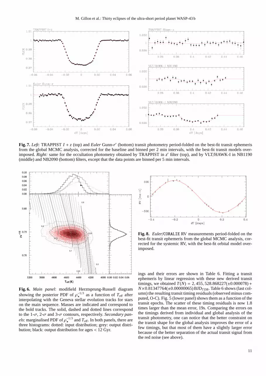
Hubble time. A restriction on the age was therefore added. Onlytaking ages< 12 Gyr, we obtained the distribution as shown inFig. 6, refining the stellar parameters toTeff = 4520± 120 Kand [Fe/H] = -0.01± 0.12 dex. The stellar mass is estimated toM⋆ = 0.717± 0.025M⊙. The output distribution is very closeto Gaussian as displayed in Fig. 6. In addition the outputρ

−1/3⋆

distribution has not been affected. Thus, our strongly improvedprecision on the stellar density combined with a constrainton theage (to be younger than a Hubble time) allows us to reject themain stellar solution proposed by H11 (M⋆ = 0.58± 0.05M⊙).Because the allowed (ρ−1/3

⋆ , Teff, [Fe/H]) space within the tracksstill covers quite a large area, it is impossible at the moment toconstrain the stellar age. The process is described in Triaud 2011(PhD thesis).

We then performed a third MCMC step, using as prior distri-butions forM⋆, Teff, and [Fe/H], the normal distributions match-ing the results of our stellar modeling, i.e.N(0.717, 0.0252) M⊙,

N(4520, 1202) K, and N(−0.01, 0.122) dex, respectively. Thebest-fit photometry and RV models are shown respectively inFig. 7 and 8, while the derived parameters and 1-σ error bars areshown in Table 5.

Global analysis of the 23 transits with free timings

As a complement to our global analysis of the whole data set, weperformed a global analysis of the 23 transit light curves alone.The goal here was to benefit from the strong constraint broughton the transit shape by the 23 transits to derive more accuratetransit timings and to assess the periodicity of the transit. In thisanalysis, we kept fixed the parametersT0 and P to the valuesshown in Table 5, and we added a timing offset as jump param-eter for each transit. The orbit was assumed to be circular. Theother jump parameters weredF, W, b′, and the limb-darkeningcoefficientsc1 andc2 for both filters. The resulting transit tim-

10


Fig. 7. Left: TRAPPISTI + z (top) andEuler Gunn-r′ (bottom) transit photometry period-folded on the best-fit transit ephemerisfrom the global MCMC analysis, corrected for the baseline and binned per 2 min intervals, with the best-fit transit modelsover-imposed.Right: same for the occultation photometry obtained by TRAPPIST inz′ filter (top), and by VLT/HAWK-I in NB1190(middle) and NB2090 (bottom) filters, except that the data points are binned per 5 min intervals.

Fig. 6. Main panel: modifield Herztsprung-Russell diagramshowing the posterior PDF ofρ−1/3

⋆ as a function ofTeff afterinterpolating with the Geneva stellar evolution tracks forstarson the main sequence. Masses are indicated and correspond tothe bold tracks. The solid, dashed and dotted lines correspondto the 1-σ, 2-σ and 3-σ contours, respectively.Secondary pan-els: marginalised PDF ofρ−1/3

⋆ andTeff. In both panels, there arethree histograms: dotted: input distribution; grey: output distri-bution; black: output distribution for ages< 12 Gyr.

Fig. 8. Euler/CORALIE RV measurements period-folded on thebest-fit transit ephemeris from the global MCMC analysis, cor-rected for the systemic RV, with the best-fit orbital model over-imposed.

ings and their errors are shown in Table 6. Fitting a transitephemeris by linear regression with these new derived transittimings, we obtainedT (N) = 2, 455, 528.868227(±0.000078)+N×0.81347764(±0.00000065)BJDT DB. Table 6 shows (last col-umn) the resulting transit timing residuals (observed minus com-puted, O-C). Fig. 5 (lower panel) shows them as a function of thetransit epochs. The scatter of these timing residuals is now1.8times larger than the mean error, 19s. Comparing the errors onthe timings derived from individual and global analysis of thetransit photometry, one can notice that the better constraint onthe transit shape for the global analysis improves the errorof afew timings, but that most of them have a slightly larger errorbecause of the better separation of the actual transit signal fromthe red noise (see above).

11


MCMC Jump parameters

Planet/star area ratio (Rp/R⋆)2 [%] 2.542+0.024−0.025

b′ = a cosip/R⋆ [R⋆] 0.656± 0.010

Transit widthW [h] 1.2089+0.0055−0.0050

T0 − 2450000 [BJDT DB] 5726.54336± 0.00012

Orbital periodP [d] 0.81347753± 0.00000071

RV K2 [m s−1 d1/3] 511.5+5.1−5.0√

e cosω 0.020+0.022−0.023√

e sinω −0.025+0.066−0.064

dFocc,z′ [ppm] 210+190−130, < 850 (3-σ)

dFocc,NB1190 790+320−310, < 1700 (3-σ)

dFocc,NB2090 1560± 140

c1I+z 0.983± 0.050

c2I+z 0.065± 0.060

c1r′ 1.363± 0.047

c2r′ 0.401± 0.051

Deduced stellar parameters

u1I+z 0.406± 0.026

u2I+z 0.171± 0.024

u1r′ 0.625± 0.024

u2r′ 0.112± 0.020

Vγ [km s−1] −3.5950± 0.0040

Densityρ⋆ [ρ⊙] 2.410+0.079−0.075

Surface gravity logg⋆ [cgs] 4.645+0.011−0.010

MassM⋆ [M⊙] 0.717± 0.025

RadiusR⋆ [R⊙] 0.667+0.010−0.011

Teff [K] a 4520± 120

[Fe/H] [dex]a −0.01± 012

Deduced planet parameters

RV K [ m s−1 ] 547.9+5.5−5.4

Rp/R⋆ 0.15945+0.00076−0.00077

btr [R⋆] 0.6580+0.0089−0.0095

boc [R⋆] 0.655+0.012−0.013

Toc − 2450000 [BJDT DB] 5726.95069+0.00084−0.00078

Orbital semi-major axisa [AU] 0 .01526± 0.00018

Roche limitaR [AU] 0 .00768± 0.00016

a/aR 1.986+0.030−0.029

a/R⋆ 4.918+0.053−0.051

Orbital inclinationip [deg] 82.33± 0.20

Orbital eccentricitye 0.0035+0.0060−0.0025, < 0.0298 (3-σ)

Argument of periastronω [deg] −32+115−34

Equilibrium temperatureTeq [K] b 1440+40−39

Densityρp [ρJup] 1.826+0.084−0.078

Densityρp [g/cm3] 1.377+0.063−0.059

Surface gravity loggp [cgs] 3.672+0.013−0.012

MassMp [MJup] 2.034+0.052−0.051

RadiusRp [RJup] 1.036± 0.019

Table 5. Median and 1-σ limits of the posterior marginalizedPDFs obtained for the WASP-43 system derived from our globalMCMC analysis.aFrom stellar evolution modeling (Sect. 3.3).bAssumingA=0 andF=1.

Epoch Filter Ttr O-C[BJDT DB-2450000] [min]

11 I + z 5537.81673+0.00047−0.00046 0.36± 0.68

22 I + z 5546.76494± 0.00022 0.30± 0.32

27 I + z 5550.83219+0.00015−0.00016 0.10± 0.23

38 I + z 5559.78033± 0.00021 −0.07± 0.30

38 Gunn-r′ 5559.78078+0.00016−0.00017 0.58± 0.24

43 I + z 5563.84771± 0.00022 −0.08± 0.32

49 I + z 5568.72836± 0.00015 −0.39± 0.22

59 I + z 5576.86380+0.00016−0.00015 0.57± 0.23

65 I + z 5581.74410± 0.00020 −0.25± 0.29

70 I + z 5585.81205+0.00021−0.00022 0.56± 0.32

76 Gunn-r′ 5590.69259± 0.00018 0.09± 0.26

87 Gunn-r′ 5599.64043+0.00026−0.00025 −0.51± 0.37

97 I + z 5607.77517± 0.00014 −0.56± 0.20

124 I + z 5629.73995+0.00019−0.00018 0.71± 0.27

140 I + z 5642.75450± 0.00015 −0.86± 0.22

141 I + z 5643.56872± 0.00028 0.21± 0.40

152 I + z 5652.51586+0.00024−0.00025 −1.39± 0.36

168 I + z 5665.53229+0.00019−0.00018 −0.26± 0.27

173 I + z 5669.59976± 0.00023 −0.14± 0.33

189 I + z 5682.61584+0.00022−0.00023 0.49± 0.33

200 I + z 5691.56383+0.00022−0.00023 0.11± 0.33

211 I + z 5700.51237+0.00014−0.00015 0.52± 0.22

243 I + z 5726.54399± 0.00035 1.00± 0.50

Table 6. Median and 1-σ errors of the posterior PDFs de-duced for the timings of the transits from their global analy-sis. The last column shows the difference (and its error) be-tween the measured timing and the one deduced from the best-fitting transit ephemeris computed by linear regression,T (N) =2455528.868227(0.000078)+ N × 0.81347764(0.00000065)BJDT DB.

4. Discussion

4.1. The physical parameters of WASP-43 b

Comparing our results for the WASP-43 system with the onespresented in H11, we notice that our derived parameters agreewell with the second solution mentioned in H11, while being sig-nificantly more precise. WASP-43 b is thus a Jupiter-size planet,twice more massive than our Jupiter, orbiting at only∼0.015AU from a 0.72M⊙ main-sequence K-dwarf. Despite having thesmallest orbital distance among the hot Jupiters, WASP-43 bisfar from being the most irradiated known exoplanet, becauseofthe small size and temperature of its host star. Assuming a solar-twin host star, its incident flux∼9.6 108 erg s−1 cm−2 would cor-respond to aP = 2.63 d orbit (a = 0.0374 AU), i.e. to a rathertypical hot Jupiter. With a radius of 1.04RJup, WASP-43 b liestoward the bottom of the envelope described by the publishedplanets in theRp vs. incident flux plane (Fig. 9). Taking intoaccount its level of irradiation, the high density of the planetfavors an old age and a massive core under the planetary struc-ture models of Fortney et al. (2010). Our results are consistentwith a circular orbit, and we can put a 3-σ upper limit <0.03to the orbital eccentricity. Despite its very short period,WASP-43 b has a semi-major axis approximatively twice larger thanitsRoche limitaR, which is typical for hot Jupiters (Ford & Rasio

12


1011 1010 109 108 107 106 105

Incident flux [erg s-1 cm-2]

0.0

0.5

1.0

1.5

2.0

2.5R

adiu

s [R

Jup]

Fig. 9. Planetary radii as a function of incident flux. WASP-43 b is shown as a black square. Grey filled circles areKepler planetary candidates (see Demory & Seager 2011).Transiting giant planets previously published, and mostlyfromground-based surveys, are shown as grey triangles. The rel-evant parametersRp, Rs, Te f f and a have been drawn fromhttp://www.inscience.ch/transits on August 29, 2011.

2006, Mastumura et al. 2010). As noted by these authors, theinner edge of the distribution of most hot Jupiters at∼2 aR fa-vors migrational mechanisms based on the scattering of planetson much wider orbit and the subsequent tidal shortening and cir-cularization of their orbits. Thus, WASP-43 b does not appear tobe a planet exceptionally close to its final tidal disruption, unlikeWASP-19 b that orbits at only 1.2aR (Hellier et al. 2011a).

4.2. The atmospheric properties of WASP-43 b

We have modeled the atmosphere of WASP-43 b using the meth-ods described in Fortney et al. (2005, 2008) and Fortney &Marley (2007). In Fig. 10, we compare the planet-to-star fluxratio data to three atmosphere models. The coldest model (or-ange) uses a dayside incident flux decreased by 1/2 to simulatethe loss of half of the absorbed flux to the night side of the planet.Clearly the planet is much warmer than this model. In blue andred are two models where the dayside incident flux is increasedby a factor of 4/3 to simulate zero redistribution of absorbed flux(see, e.g., Hansen 2008). The red model features a dayside tem-perature inversion due to the strong optical opacity of TiO andVO gases (Hubeny et al. 2003, Fortney et al. 2006). The bluemodel is run in the same manner as the red model, but TiO andVO opacity are removed.

The blue and red models are constructed to maximize theemission from the dayside of the planet. Figure 10 shows thatonly such bright models could credibly match the data points.While a dayside with no temperature inversion is slightly favoredby the 1.2µm data point, it is difficult to come to a firm conclu-sion. Day-side emission measurements fromWarm Spitzer willhelp to better constrain the atmosphere as well. They will alsoallow getting an even smaller upper-limit on the orbital eccen-tricity.

Fortney et al. model fits to near infrared photometry of othertransiting planets (e.g., Croll et al. 2010) have generallyfa-vored inefficient temperature homogenization between the dayand night hemispheres, although the warm dayside of WASP-

Fig. 10. Model planet-to-star flux ratios compare to the threedata points. The data are green diamonds with 1−σ error barsshown. The orange model assumes planet-wide redistribution ofabsorbed flux. The red and blue models assume no redistributionof absorbed flux, to maximize the day-side temperature. The redmodel includes gaseous TiO and VO and has a temperature in-version. [See the figure inset.] The blue and orange models haveTiO and VO opacity removed, and do not have a temperatureinversion. For each model, filled circles are model fluxes aver-aged over each bandpass. The data slightly favor a model withno day-side temperature inversion.

43 b appears to be at the most inefficient end of this contin-uum. The apparent effeciency of temperature homogenization isexpected to vary with wavelength. In particular, near infraredbands, at minima in water vapor opacity, are generally expectedto probe deeper into atmospheres than theSpitzer bandpasses.

4.3. Transit timings

Dynamical constraints can be placed on short orbits companionplanets from the 23 transits obtained in this study. The linear fitto the transit timings described above yields a reducedχ2 of 4.6and therms of its residuals is 38s. Two transits (epochs 140 and152) have a O-C different from zero at the∼4-σ level. The mostplausible explanation for the significant scatter observedin thetransit timings is systematic errors on the derived timingsdue tothe influence of correlated noise. Another potential explanationis asymmetries in the transit light curves caused by the crossingof one or several star spots by the planet. In such cases, the fittedtransit profile is shifted with time, producing timing variations.

We also explored the detectability domain of a second planetin the WASP-43 system. To this end, we followed Agol etal. (2005) and used the Mercury n-body integrator package(Chambers 1999). We simulated 3-body systems including a sec-ond companion with orbital periods ranging between 1.3 and50 days, masses from 0.1M⊕ to 2.0 MJup and an orbital ec-centricities ofec = 0 andec = 0.05. For each simulation, wecomputed therms of the computed transits timings variations.The results are shown on Fig.11 where the computed 1-σ (red)and 3-σ (black) detection thresholds are plotted for each point inthe mass-period plane. We also added RV detectability thresholdcurves based on 5 (solid), 10 (dash) and 15 (dot) m s−1 semi-amplitudes (K).

Based on the present set of timings, the timings variationscaused by a 5 Earth mass companion in 2:1 resonance would

13

http://www.inscience.ch/transits


1.5 2.0 2.5 3.0Orbital Period [days]

0.1

1.0

10.0

100.0

1000.0

Det

ecta

ble

Mas

s [M

Ear

th]

Fig. 11.Detectivity domain for a putative WASP-43 c planet, as-sumingec = 0 (black) andec = 0.05 (red). The solid curves de-limit the mass-period region where planets yield maximum TTVon WASP-43 b above 114 s (3-σ detection based on the presentdata). The dotted curves show the 1-σ threshold. Nearly hori-zontal solid, dashed and dotted lines shows RV detection limitsfor RV semi-amplitudeK=5, 10 and 15 m s−1 respectively.

have been detected with 3-σ confidence, while unseen with ra-dial velocities alone.

5. Conclusions

In this work we have presented 23 transit light curves and 7 oc-cultation light curves for the ultra-short period planet WASP-43 b. We have also presented 8 new measurements of the ra-dial velocity of the star. Thanks to this extensive data set,we have significantly improved the parameters of the system.Notably, our strongly improved precision on the stellar den-sity (2.41± 0.08ρ⊙) combined with a very reasonable constrainton its age (to be younger than a Hubble time) allowed us tobreak the degeneracy of the stellar solution mentioned by H11.The resulting stellar mass and size are 0.717± 0.025M⊙ and0.667±0.011R⊙. Our deduced physical parameters for the planetare 2.034± 0.052MJup and 1.036± 0.019RJup. Taking into ac-count its level of irradiation, the high density of the planet favorsan old age and a massive core. Our deduced orbital eccentricity,0.0035+0.0060

−0.0025, is consistent with a fully circularized orbit.The parameters deduced from the individual analysis of the

23 transit light curves show some extra scatter that we attributeto the correlated noise of our data and, possibly, to the crossingof spots during some transits. This conclusion is based on thecorrelation observed among the transit parameters. These resultsreinforce the interest of performing global analysis of extensivedata sets in order to minimize systematic errors and to reachhighaccuracies on the derived parameters.

We detected the emission of the planet at 2.09µm at betterthan 11-σ, the deduced occultation depth being 1560±140 ppm.Our detection of the occultation at 1.19µm is marginal (790±320 ppm) and more observations would be needed to confirmit. We place a 3-σ upper limit of 850 ppm on the depth of theoccultation at∼0.9µm. Together, these results strongly favor apoor redistribution of the heat from the dayside to the nightsideof the planet, and marginally favor a model with no day-sidetemperature inversion.

Acknowledgements. TRAPPIST is a project funded by the Belgian Fundfor Scientific Research (Fond National de la Recherche Scientifique, F.R.S-

FNRS) under grant FRFC 2.5.594.09.F, with the participation of the SwissNational Science Fundation (SNF). M. Gillon and E. Jehin areFNRS ResearchAssociates. We are grateful to ESO La Silla and Paranal staffs for their continu-ous support.

References

Agol, E., Steffen, J., Sari, R., & Clarkson, W. 2005, MNRAS, 359, 567Anderson, D. R., Gillon, M., Maxted P., et al. 2010, A&A, 513,L3Baranne, A., Queloz, D., Mayor, M. et al. 1996, A&AS, 119, 373Barker, A. J. & Ogilvie, G. I. 2009, MNRAS, 395, 2268Berta, Z. K., Charbonneau, D., Bean, J., et al. 2011, ApJ, 736, 12Brown, D. J. A., Collier Cameron, A., Hall, C., et al. 2011, MNRAS, 415, 605Carlin, B. P. & Louis, T. A. 2008,Bayesian Methods for Data Analysis, Third

Edition (Chapman & Hall/CRC)Casali, M., Pirard, J.-F., Kissler-Patig, M. et al. 2006, SPIE, 6269, 29Chambers J. E., 1999, MNRAS, 304, 793Claret, A. & Bloemen, S. 2011, A&A, 529, A75Croll, B., Jayawardhana, R., Fortney, J. J., Lafreniere, D., & Albert, L. 2010,

ApJ, 718, 920D’Angelo, G., Durisen, R. H., Lissauer, J. J. 2010,Exoplanets, ed. S. Seager,

University of Arizona Press, p. 319Demory, B.-O., & Seager, S. 2011, ApJS, 197, 12Fabrycky, D. C. & Tremaine, S. 2007, ApJ, 669, 1298Ford, E. B. & Rasio, F. A. 2006, ApJ, 638, L45Fortney, J. J., Marley, M. S., Lodders, K., Saumon, D., & Freedman, R. S. 2005,

ApJ, 627, L69Fortney, J. J., Saumon, D., Marley, M. S., Lodders, K., & Freedman, R. S. 2006,

ApJ, 642, 495Fortney, J. J., Marley, M. S., Barnes, J. W. 2007, ApJ, 659, 1661Fortney, J. J. & Marley, M. S. 2007, ApJ, 666, L45Fortney, J. J., Lodders, K., Marley, M. S., & Freedman, R. S. 2008, ApJ, 678,

1419Gelman, A. & Rubin D. 1992, Statist. Sci., 7, 457Gibson, N. P., Aigrain, S., Pollaco, D. L., et al. 2010, MNRAS, 404, L14Gillon, M., Lanotte, A. A., Barman, T., et al. 2010, A&A, 511,3Gillon, M., Jehin, E., Magain, P., et al. 2011a,Detection and Dynamics of

Transiting Exoplanets, Proceedings of OHP Colloquium (23-27 August2010), eds. F. Bouchy, R. F. Diaz & C. Moutou, Platypus Press

Gillon, M., Doyle, A., Maxted, P., et al. 2011b, A&A, 533, A88Gimenez, A. 2006, ApJ, 650, 408Gregory, P. C. 2005,Bayesian Logical Data Analysis for the Physical Sciences,

Cambridge University PressGu, P.-G., Lin, D. N. C., Bodenheimer, P. H. 2003, ApJ, 588, 509Hansen, B. M. S., 2008, ApJS, 179, 484Hebb, L., Collier Cameron, A., Loeillet, B., et al. 2009, ApJ, 693, 1920Hebb, L., Collier Cameron, A., Triaud, A. H. M. J., et al. 2010, ApJ, 708, 224Hellier, C., Anderson, D. R., Collier Cameron, A., et al. 2009, Nature, 460, 1098Hellier, C., Anderson, D. R., Collier Cameron, A., et al. 2011a, ApJ, 730, L31Hellier, C., Anderson, D. R., Collier Cameron, A., et al. 2011b, A&A, 535, L7Holman, M. J., Winn, J. N., Latham, D. W., et al. 2006, ApJ, 652, 1715Hubeny, I., Burrows, A., & Sudarsky, D., 2003, ApJ, 594, 1011Huber, H. F., Czesla, S., Wolter, U., & Schmitt, J. H. M. M., 2010, A&A, 514,

A39Jackson, B., Barnes, R., Greenberg, R. 2009, ApJ, 698, 1357Jehin, E., Gillon, M., Queloz, D., et al. 2011, The Messenger, 145, 2Johnson, J. A., Gazack, J. Z., Apps, K., et al. 2011 (submitted), arXiv:1112.0017Knutson, H. A., Charbonneau, D., Allen, L. E., et al. 2008, ApJ, 673, 526Lubow, S. H. & Ida, S. 2010,Exoplanets, ed. S. Seager, University of Arizona

Press, p. 347Lin, D. N. C., Bodenheimer, P., Richardson, D. C. 1996, Nature, 380, 606Mandel, K. & Agol, E. 2002, ApJ, 580, 181Mastumura, S., Peale, S. J., Rasio, F. R. 2011, ApJ, 725, 1995Naoz, S., Farr, W. M., Lithwick, Y., et al. 2011, Nature, 473,187Nymeyer, S., Harrington, J., Hardy, R., et al. 2011, ApJ, 742, 35Pirard, J.-F., Kissler-Patig, M., Moorwood, A., et al. 2004, SPIE, 5492, 510Schneider, J. 2011, http://exoplanet.eu/catalog-all.phpSchwarz, G. E. 1978, Annals of Statistics, 6, 461Stetson, P. B. 1987, PASP, 99, 111Torres, G., Andersen, J., Gimenez, A. 2010, A&ARv, 18, 67Triaud, A. H. M. J., Collier Cameron, A., Queloz, D., et al. 2010, A&A, 524,

A25Triaud, A. H. M. J., 2011, Constraints on planetary formation from the discovery

and study of transiting extrasolar planets, PhD thesis, Geneva University, no.Sc. 4342, http://archive-ouverte.unige.ch/unige:18065

Watson, C. A., Littlefair, S. P., Collier Cameron, A., et al.2010, MNRAS, 408,1606

14

http://arxiv.org/abs/1112.0017

http://exoplanet.eu/catalog-all.php

http://archive-ouverte.unige.ch/unige:18065


Wu, Y & Lithwick, Y. 2011, ApJ, 735, 109

15

Documents

The TRAPPIST survey of southern transiting planets