Rotational stability of dynamic planets with

elastic lithospheres

I. Matsuyama,1,2 J. X. Mitrovica,3 M. Manga,4 J. T. Perron,4 and M. A. Richards4

Received 13 April 2005; revised 21 October 2005; accepted 3 November 2005; published 14 February 2006.

[1] We revisit the classic problem of the secular rotational stability of planets in responseto loading using the fluid limit of viscoelastic Love number theory. Gold (1955) andGoldreich and Toomre (1969) considered the stability of a hydrostatic planet subject to anuncompensated surface mass load and concluded that a mass of any size would drive truepolar wander (TPW) that ultimately reorients the load to the equator. Willemann(1984) treated the more self-consistent problem where the presence of a lithosphere leadsto both imperfect load compensation and a remnant rotational bulge. Willemannconsidered axisymmetric loads and concluded that the equilibrium pole location wasgoverned by a balance, independent of elastic lithospheric thickness, between the load-induced TPW and stabilization by the remnant bulge. Our new analysis demonstrates thatthe equilibrium pole position is a function of the lithospheric strength, with a convergenceto Willemann’s results evident at high values of elastic thickness (>400 km for anapplication to Mars), and significantly larger predicted TPW for planets with thinlithospheres. Furthermore, we demonstrate that nonaxisymmetric surface mass loads andinternal (convective) heterogeneity, even when these are small relative to axisymmetriccontributions, can profoundly influence the rotational stability. Indeed, we derive therelatively permissive conditions under which nonaxisymmetric forcing initiates an inertialinterchange TPW event (i.e., a 90� pole shift). Finally, Willemann’s analysis is oftencited to argue for a small (<18�) TPW of Mars driven by the development of a Tharsis-sized load. We show that even in the absence of the destabilizing effects of loadasymmetry, the equations governing rotational stability permit higher excursions of theMartian rotation vector than has previously been appreciated.

Citation: Matsuyama, I., J. X. Mitrovica, M. Manga, J. T. Perron, and M. A. Richards (2006), Rotational stability of dynamic planets

with elastic lithospheres, J. Geophys. Res., 111, E02003, doi:10.1029/2005JE002447.

1. Introduction

[2] The long-term (secular) rotational stability of terres-trial planets subject to surface mass loading and internalconvective dynamics is a long-standing problem in geo-physics framed by a series of seminal studies [e.g., Gold,1955; Goldreich and Toomre, 1969]. Figure 1 provides aschematic illustration of the basic physical elements thathave defined this classic discussion.[3] Gold [1955], for example, discussed the stability of a

hydrostatic planet subject to an anomalous (i.e., nonhydro-static or imperfectly compensated) load (Figures 1a–1c)[see also Steinberger and O’Connell, 2002, Figure 1]. Theuncompensated load would act to push the rotation pole

away (green arrow, Figure 1b) in a reference frame fixed tothe load. In the short term, the hydrostatic bulge would actto stabilize the pole (i.e., retard polar motion). However,since the hydrostatic rotational bulge of the planet would, intime, relax to any new orientation of the rotation pole (e.g.,Figure 1b), all memory of this previous orientation wouldultimately vanish (Figures 1b and 1c). That is, a hydrostaticbulge provides no long-term rotational stability and thereorientation of the pole, or so-called true polar wander(TPW), would be governed solely by the location of theuncompensated surface mass load. In particular, a massexcess of any size (indeed, as small as Gold’s beetle) woulddrive a TPW that would eventually reorient the load to theequator (Figure 1c). Mathematically, the new (final) poleposition would be governed by the principal axis of thenonhydrostatic components of the inertia tensor introducedby the uncompensated load. Gold’s [1955] arguments wereextended by Goldreich and Toomre [1969], who demon-strated that a group of anomalous masses moving randomlyon the surface (e.g., a set of scurrying beetles) could driverapid (relative to the speed of the masses) reorientation ofthe rotation pole.[4] The Gold [1955] analysis, while providing significant

insight into the secular rotational stability of planets, in-

JOURNAL OF GEOPHYSICAL RESEARCH, VOL. 111, E02003, doi:10.1029/2005JE002447, 2006

1Department of Astronomy and Astrophysics, University of Toronto,Toronto, Ontario, Canada.

2Now at Department of Terrestrial Magnetism, Carnegie Institution ofWashington, Washington, D.C., USA.

3Department of Physics, University of Toronto, Toronto, Ontario,Canada.

4Department of Earth and Planetary Science, University of California,Berkeley, California, USA.

Copyright 2006 by the American Geophysical Union.0148-0227/06/2005JE002447$09.00

E02003 1 of 17

volved an underlying inconsistency that was highlighted,and addressed, by Willemann [1984]. The hydrostatic figureis the form achieved by a rotating planet with no elastic (i.e.,long-term) strength. Such a form would presumably havebeen established very early in the planet’s history (Figure 1d).Subsequent cooling of the planet and development of a

lithosphere would not alter the flattening of this hydrostaticform (Figure 1e); however, the presence of such a litho-sphere is the reason why surface mass loads or beetleswould not be perfectly compensated. The shortcoming inGold’s [1955] analysis is that the growth of a lithospherewould also ensure that the initial hydrostatic figure of the

Figure 1. Schematic highlighting some basic physical principles governing, and common approxima-tions applied to, the study of the secular stability of planetary rotation. Figures 1a–1c illustrate argumentsdescribed by Gold [1955]. An otherwise hydrostatic planet is subject to a surface mass load (the green‘‘beetle’’) that is at least partially uncompensated. The load pushes the rotation axis away (green arrow)leading to TPW (black arrow) and, after a time period that is long relative to the relaxation of thehydrostatic flattening, the bulge is assumed to perfectly relax to the new pole location (Figures 1b and1c); there is no memory of the initial pole location. The process continues until the load reaches theplanetary equator and TPW ceases. Figures 1d–1f illustrate the extension to Gold’s [1955] analysisdescribed by Willemann [1984]. In this case, the (uncompensated) load-induced push on the rotation poleis retarded (blue arrow) by the incomplete relaxation of the rotational bulge in the presence of an elasticlithosphere (blue shell). The presence of a remnant rotational bulge is evident in the lack of symmetry ofthe bulge relative to the rotation axis. The final position of the rotation axis (Figure 1f) is defined by abalance between the load-induced push and the nonhydrostatic remnant bulge stabilization (green andblue arrows, respectively); the load does not, in general, reach the equator (as it does in Figure 1c, wherethe latter stabilizing effect is absent). Figures 1g–1i extend Figures 1d–1f to consider the potentialinfluence of internal convective dynamics on the rotational state. This impact will depend on theamplitude and (principal axis) orientation of convection-induced perturbations to the inertia tensor (hencethe question marks attached to the red arrows in Figures 1h and 1i). The cartoon shows the specific casewhere convection acts to increase the ellipticity of the rotating planet (compare Figures 1d and 1g); in thiscase, the ‘‘excess’’ ellipticity will act to stabilize the rotation pole relative to the imposition of the load.The net effect (Figure 1i) is a more subdued TPW relative to the case shown in Figure 1f.

E02003 MATSUYAMA ET AL.: ROTATIONAL STABILITY OF PLANETS

2 of 17

E02003

planet could not entirely relax to any new orientationassociated with TPW (Figures 1e and 1f). Simply put, onecannot have an uncompensated surface mass load and acompletely relaxed hydrostatic bulge. This was the centralpoint underlying Willemann’s [1984] analysis. In this case,all memory of the original rotation does not vanish, and the‘‘remnant of the rotational flattening’’ [Willemann, 1984]will act to stabilize the rotation vector.[5] What would the final, equilibrium position of the

rotation vector be? The final, equilibrium position of therotation vector is governed by a balance between the TPWdriven by the uncompensated component of the load (whichacts to move the load to the equator; green line, Figure 1f)and the nonhydrostatic remnant rotational effect (which actsto resist any reorientation of the pole; blue line, Figure 1f).Willemann [1984] concluded that the TPW angle willdepend on the initial position of the load and its uncom-pensated size (measured in terms of the degree two geo-potential perturbation) relative to the rotational bulge. Hefurthermore came to the surprising conclusion that thereorientation was independent of the thickness of thelithosphere.[6] In this paper we revisit the general problem addressed

by Willemann [1984] using a fluid Love number formula-tion for the response of the planetary model to surface massand rotational loading. The analysis makes use of simple,well-documented relationships involving viscoelastic Lovenumber theory [e.g., Peltier, 1974; Mitrovica and Peltier,1989], and provides a relatively succinct derivation ofthe various contributions to the nonhydrostatic inertiatensor. We use our expressions to generalize (and correct)Willemann’s [1984] results, to explore a series of importantspecial cases (e.g., the Gold [1955] assumption that thehydrostatic bulge relaxes completely in response to a newpole position), and to comment on some more recentanalyses of rotational stability which do not appear to haveincorporated a remnant rotational bulge [Bills and James,1999].[7] We complete our analysis by including a separate

section that incorporates nonhydrostatic contributions tothe inertia tensor driven by internal convective dynamics(Figures 1g–1i). Since the amplitude and orientation ofsuch contributions are unknown for all planets with thepossible exception of the Earth, this section is by necessitygeneral (note the question marks in Figure 1i); nevertheless,the expressions we derive will be useful for those interestedin the sensitivity of traditional predictions of planetaryrotational stability (which focus on external loading) tothe presence of potential convective regimes. That suchregimes are unconstrained for other planets does not dimin-ish their potential relevance; indeed, it would be difficult toargue that the massive Tharsis rise on Mars, the subject ofsignificant interest in the field of Martian rotation stability[e.g., Willemann, 1984; Bills and James, 1999], does notreflect the action of both external and internal processes.The existence of the latter will alter the TPW that would beinferred by considering a purely external forcing (compareFigures 1f and 1i).[8] Following Willemann [1984], the analysis described

below involves two principal assumptions. First, we adoptspherically symmetric planetary models, and thus anyelastic lithospheric lid is treated as uniform (and hence

unbroken). Second, we ignore any time history of polarwander and consider only the final, equilibrium positionof the pole subsequent to an episode of loading. Inpractice, the latter, which we will term the ‘‘secularrotational stability,’’ implies that the pole position isgoverned by the principal axis of the nonhydrostaticinertia tensor; thus we circumvent the solution of thetime-dependent Liouville equation [e.g., Ricard et al.,1993]. (Another way to interpret this is that we assumethat the timescale over which the load acts is very longrelative to the bulge and boundary deformation relaxationtimescales; this simplifying assumption permits greaterclarity in discussing ‘‘before and after,’’ or end-memberscenarios.) The time required to achieve the final poleposition will depend on both the decay times of theplanetary modes of viscous relaxation and on the size ofthe load; in the absence of Willemann’s remnant rota-tional bulge, Gold’s beetle will reach the equator, but itmay take many billions of years to do so.

2. External Loading

[9] The secular rotational state of the planet is governedby nonhydrostatic variations in the planetary form. In thissection we consider perturbations in the inertia tensor,which we denote by Iij, arising from the external loadingof the planet. We specify three classes of perturbationassociated with: (1) the direct effect of any external surfacemass load; (2) the deformation of the planet driven by thissurface loading; and (3) incomplete relaxation of the rota-tional (hydrostatic) flattening due to the presence of alithosphere.

2.1. Theory

[10] In the following sections we derive expressions foreach of these three contributions, making use of Lovenumber theory [Peltier, 1974] as well as simple relation-ships between perturbations in the inertia tensor and thegravitational potential. We will assume that our sphericalcoordinate system is oriented such that the z axis is fixed tothe initial rotation axis of the planet (i.e., prior to loading);in this case, the initial angular velocity vector is given by (0,0, W).2.1.1. A Mapping Between Gravitational Potential andInertia Perturbations[11] Let us assume that a redistribution of mass, either

on the surface of the planet or within its interior, givesrise to a perturbation in the gravitational potential, G.We can represent G in terms of a spherical harmonicdecomposition

G q; f; tð Þ ¼X1‘¼0

X‘

m¼�‘

G‘m tð ÞY‘m q;fð Þ; ð1Þ

where q and f are the colatitude and east longitude, t is time,and the Y‘m are (complex) surface spherical harmonics. Inour derivations, we will normalize these spherical harmonicbasis functions such that

ZS

Yy‘0m0 q;fð ÞY‘m q;fð ÞdS ¼ 4pd‘‘0dmm0 ; ð2Þ

E02003 MATSUYAMA ET AL.: ROTATIONAL STABILITY OF PLANETS

3 of 17

E02003

where S represents the surface of the unit sphere and d‘‘0 isthe Kronecker delta. Note that Y‘,�m = (�1)mY‘m

y , where yrepresents the complex conjugate.[12] With this normalization, one can show (e.g., with

suitable normalization [Lambeck, 1980]) that perturbationsto the components of the inertia tensor are related toperturbations in the geopotential by

I11 tð Þ ¼ Ma

g

2

3G00 tð Þ þ

ffiffiffi5

p

3G20 tð Þ

��

ffiffiffiffiffi10

3

rRe G22 tð Þð Þ

#;

I22 tð Þ ¼ Ma

g

2

3G00 tð Þ þ

ffiffiffi5

p

3G20 tð Þ

�þ

ffiffiffiffiffi10

3

rRe G22 tð Þð Þ

#;

I33 tð Þ ¼ Ma

g

2

3G00 tð Þ � 2

ffiffiffi5

p

3G20 tð Þ

� �; ð3Þ

I12 tð Þ ¼ Ma

g

ffiffiffiffiffi10

3

rIm G22 tð Þð Þ;

I13 tð Þ ¼ Ma

g

ffiffiffiffiffi10

3

rRe G21 tð Þð Þ;

I23 tð Þ ¼ �Ma

g

ffiffiffiffiffi10

3

rIm G21 tð Þð Þ;

where M and a are the mass and radius of the planet,respectively, g is the surface gravitational acceleration,and the symbols Re and Im refer to the real andimaginary parts.2.1.2. Inertia Perturbations: The Surface Mass Load[13] In this section we focus on predictions of perturba-

tions in the inertia tensor associated with the direct anddeformational effects of the surface mass load. As in treat-ments of post-glacial load-induced variations in the Earth’srotational state (for a new analysis, see Mitrovica et al.[2005]), we make the assumption that the planet may bemodeled as a spherically symmetric, linear (Maxwell)viscoelastic body and make use of viscoelastic Love numbertheory.[14] We begin by denoting an arbitrary surface mass load

as L(q, f, t), with spherical harmonic coefficients given byL‘m(t). If the mass of the planet is conserved in creating thesurface mass load, then L00(t) = 0.[15] Next, we introduce the nondimensional surface load

k Love number. In the time domain, this Love number hasthe form [Peltier, 1974, 1976]

kL‘ tð Þ ¼ kL;E‘ d tð Þ þ

XKk¼1

r‘ke�s‘

kt; ð4Þ

where d(t) is the Dirac-delta function. The right-hand sideof this expression represents a superposition of animmediate elastic response (note the superscript E) anda nonelastic relaxation governed by a sum of K normalmodes of pure exponential decay. These modes aredefined by a decay time, 1/sk

‘, and amplitude, rk‘. We will

consider the case where the time elapsed since loading ismuch longer than the decay times associated with theviscoelastic normal modes in equation (4). That is, allviscous stresses are presumed to have relaxed. In thiscase, our calculations require the so-called fluid loadLove number at spherical harmonic degree two, which wedenote by kf

L. In principle, this number may be computed

by taking the Laplace-transform of equation (4) andconsidering the fluid, s = 0 limit to obtain [Peltier, 1976]

kLf ¼ kL;E‘¼2 þ

XKk¼1

r‘¼2k

s‘¼2k

: ð5Þ

In practice, the fluid Love number may be accuratelycomputed using a model in which all regions of theplanet, with the exception of a purely elastic lithosphericplate, are treated as inviscid [Peltier et al., 1986].[16] As shown in Appendix A, the load-induced pertur-

bations in the geopotential at degree two can then be writtenas

GL2m ¼ 4pa3g

5ML2m ð6Þ

GL�D2m ¼ 4pa3g

5ML2mk

Lf : ð7Þ

The superscripts L and L � D represent componentsassociated with the direct mass attraction of the surface loadand the deformation induced by this surface load,respectively.[17] These equations may now be applied to the mapping

equation (3). In particular, for a surface load that conservesmass, the total inertia tensor perturbation due to the effectsof mass loading,

IL;L�Dij � ILij þ IL�D

ij ; ð8Þ

is

IL;L�D11 ¼ 4pa4 1þ kLf

� 1

3ffiffiffi5

p L20 �ffiffiffiffiffi2

15

rRe L22ð Þ

" #;

IL;L�D22 ¼ 4pa4 1þ kLf

� 1

3ffiffiffi5

p L20 þffiffiffiffiffi2

15

rRe L22ð Þ

" #;

IL;L�D33 ¼ � 8pa4

3ffiffiffi5

p 1þ kLf

� L20;

IL;L�D12 ¼ 8pa4ffiffiffiffiffi

30p 1þ kLf

� Im L22ð Þ; ð9Þ

IL;L�D13 ¼ 8pa4ffiffiffiffiffi

30p 1þ kLf

� Re L21ð Þ;

IL;L�D23 ¼ � 8pa4ffiffiffiffiffi

30p 1þ kLf

� Im L21ð Þ;

where the harmonics L‘m represent the final state of theload (and, once again, after all viscous stresses haverelaxed).[18] When there is no elastic lithosphere, the planet

behaves as a purely inviscid material over very long time-scales, and the fluid Love number (at spherical harmonicdegree two), kf

L, approaches very close to �1. Thus load-induced perturbations in the inertia tensor vanish (1 + kf

L �0) since the load will be (essentially) perfectly compensated.The existence of a nonzero elastic lithosphere introduces asignificant departure from this state since the lithosphere

E02003 MATSUYAMA ET AL.: ROTATIONAL STABILITY OF PLANETS

4 of 17

E02003

will provide some (elastic) support for the load (i.e., 1 +kfL 6¼ 0 [Wu and Peltier, 1984]).2.1.3. Inertia Perturbations: Rotational Effects[19] The initial, hydrostatic rotational form of a planet

will be established during a time when the effective elasticlithospheric thickness is close to zero. As the planet cools,the development over time of an elastic lithosphere ofnonzero thickness guarantees that the hydrostatic rotationalflattening will never perfectly readjust to a change in theorientation of the rotation pole. In other words, if rotationwere to cease, the planet, by virtue of the development of apost-accretion lithosphere, would not assume a sphericalform (even in the absence of uncompensated surface loadsand internal dynamics). This ‘‘partially relaxed remnant ofthe rotational flattening’’ [Willemann, 1984, p. 703] con-tributes a nonhydrostatic component to the inertia tensorthat serves as the focus of this section.[20] Following our normalization for the spherical har-

monics, the centrifugal potential at the surface of the planetin its initial state is given by

L q;f; tð Þ ¼ L00Y00 q;fð Þ þ L20Y20 q;fð Þ; ð10Þ

where the harmonic coefficients are given by

L00 ¼a2W2

3

L20 ¼ � a2W2

3ffiffiffi5

p :

ð11Þ

[21] The response of the planet to a potential forcing isgoverned by tidal (or tidal effective) Love numbers. Inanalogy with equation (4), the time domain form of theviscoelastic tidal k Love number is [Peltier, 1974]

kT‘ tð Þ ¼ kT ;E‘ d tð Þ þ

XKk¼1

r0‘k e�s‘

kt: ð12Þ

As in the surface load case, we will be concerned solelywith the response of the planet over timescales much longerthan the decay times 1/sk

‘; this response is governed by thefluid tidal Love numbers at degree two,

kTf ¼ kT ;E‘¼2 þ

XKk¼1

r0‘¼2k

s‘¼2k

; ð13Þ

and at degree zero,

kTf ;0 ¼ kT ;E‘¼0 þ

XKk¼1

r0‘¼0k

s‘¼0k

: ð14Þ

In this case, the spherical harmonic coefficients of theperturbation to the gravitational equipotential are given by

GR2m ¼ L2mk

Tf ð15Þ

GR00 ¼ L00k

Tf ;0: ð16Þ

Equations (3), (11), (15) and (16) can be combined toyield

IL11 ¼MW2a3

9g2kTf ;0 � kTf

� ;

IL22 ¼MW2a3

9g2kTf ;0 � kTf

� ; ð17Þ

IL33 ¼MW2a3

9g2kTf ;0 þ 2kTf

� ;

IL12 ¼ IL13 ¼ IL23 ¼ 0:

[22] The fluid Love numbers in equation (17) are func-tions of the elastic lithospheric thickness adopted for theplanetary model. In the case where there is no long-termelastic strength in the lithosphere, we will denote the fluidLove numbers as kf

T,* (for degree two) and kf,0T, * (at degree

zero). Using these values in equation (17) yields thehydrostatic form of the planet to the accuracy implied byLove number theory. As we discussed above, the remnant(i.e., nonhydrostatic) rotational flattening associated withthe development of an elastic lithosphere is the differencebetween the rotational forms computed via equation (17)using models with and without an elastic lithosphere. Thatis,

IROT11 ¼ MW2a3

9g2 k

T*f ;0 � kTf ;0

� � k

T*f � kTf

� h i;

IROT22 ¼ MW2a3

9g2 k

T*f ;0 � kTf ;0

� � k

T*f � kTf

� h i; ð18Þ

IROT33 ¼ MW2a3

9g2 k

T*f ;0 � kTf ;0

� þ 2 k

T*f � kTf

� h i;

IROT12 ¼ IROT13 ¼ IROT23 ¼ 0:

[23] Note that the degree zero contribution to the inertiatensor perturbation is constant for the diagonal elements andzero elsewhere. Hence these degree zero components willyield the inertia tensor of a sphere and thus will have noeffect on the orientation and ordering of the principal axes.Accordingly, they do not impact the ultimate reorientationof the pole. We can therefore drop these perturbations togenerate the degree-two-only expressions,

IROT11 ¼ �MW2a3

9gkT*f � kTf

� ;

IROT22 ¼ �MW2a3

9gkT*f � kTf

� ; ð19Þ

IROT33 ¼ 2MW2a3

9gkT*f � kTf

� ;

IROT12 ¼ IROT13 ¼ IROT23 ¼ 0:

[24] We emphasize that our mathematical treatment ofthe remnant rotational flattening assumes, following theWillemann [1984] analysis, a specific sequence of events.In stage I, the hydrostatic form of the planet is establishedduring a period when there is no long-term (elastic) litho-spheric strength. This hydrostatic form will perfectly adjustto an arbitrary amount of TPW during stage I. In stage II, an

E02003 MATSUYAMA ET AL.: ROTATIONAL STABILITY OF PLANETS

5 of 17

E02003

elastic lithospheric shell develops in response to the coolingof the planet. The theory assumes that this developmentoccurs during a period of no TPW; hence the remnant bulgealigns perfectly with the orientation of the rotational polewithin this stage. Finally, in stage III, (internal and/orexternal) loading drives TPW in the presence of thisremnant bulge. The theory can easily be extended toaccount for a continuous phase of both TPW and litho-spheric development prior to loading. In this case, theremnant rotational flattening would be determined via anintegration that incorporates slow changes in the lithosphericthickness and any reorientation of the pole (where theintegration extends from the formation of the hydrostaticplanet to the onset of loading).2.1.4. Total Inertia Perturbations[25] An expression for the total inertia tensor perturba-

tion due to the effects of an external surface massloading,

IL;L�D;ROTij ¼ ILij þ IL�D

ij þ IROTij ; ð20Þ

can be derived by combining equations (9) and (19),

IL;L�D;ROT11 ¼ 4pa4 1þ kLf

� " 1

3ffiffiffi5

p L20 �ffiffiffiffiffi2

15

rRe L22ð Þ

#

�MW2a3

9gkT*f � kTf

� ;

IL;L�D;ROT22 ¼ 4pa4 1þ kLf

� " 1

3ffiffiffi5

p L20 þffiffiffiffiffi2

15

rRe L22ð Þ

#

�MW2a3

9gkT*f � kTf

� ;

IL;L�D;ROT33 ¼ � 8pa4

3ffiffiffi5

p 1þ kLf

� L20 þ 2MW2a3

9gkT*f � kTf

� ; ð21Þ

IL;L�D;ROT12 ¼ 8pa4ffiffiffiffiffi

30p 1þ kLf

� Im L22ð Þ;

IL;L�D;ROT13 ¼ 8pa4ffiffiffiffiffi

30p 1þ kLf

� Re L21ð Þ;

IL;L�D;ROT23 ¼ � 8pa4ffiffiffiffiffi

30p 1þ kLf

� Im L21ð Þ:

[26] It will be convenient, for the purposes of compar-ison with previous work (specifically, Willemann [1984]),to consider the special case of a disk load with azimuthalsymmetry centered at an arbitrary geographic position (qL,fL). Let us say that this load, if centered on the NorthPole, was described by spherical harmonic coefficientsL0‘0. Then it is straightforward to show that the harmoniccoefficients at degree two for the load centered at (qL, fL)are given by

L2m ¼ L020Yy2m qL;fLð Þffiffiffi

5p : ð22Þ

The size of the disk load may be conveniently normalizedby considering the ratio of the degree two gravitationalpotential perturbations due to the direct effect of the loadand the hydrostatic rotational bulge. If we denote this ratio

as Q0 (following the symbolism adopted by Willemann[1984]), then equations (6), (11), and (15) yield

Q0 ¼ �4pa3g5M

L020�1

3ffiffi5

p a2W2kT*f

: ð23Þ

[27] Using equations (22) and (23) in our expressions forthe total inertia perturbation (21) gives

IL;L�D;ROT11 ¼ 1

3m0 Q0a

"1ffiffiffi5

p Y20 qLð Þ(

�ffiffiffi6

5

rRe Y

y22 qL;fLð Þ

� #� 1

);

IL;L�D;ROT22 ¼ 1

3m0 Q0a

"1ffiffiffi5

p Y20 qLð Þ(

þffiffiffi6

5

rRe Y

y22 qL;fLð Þ

� #� 1

);

IL;L�D;ROT33 ¼ � 2

3m0 Q0a

1ffiffiffi5

p Y20 qLð Þ � 1

� �;

IL;L�D;ROT12 ¼ 1

3m0Q0a

ffiffiffi6

5

rIm Y

y22 qL;fLð Þ

� ; ð24Þ

IL;L�D;ROT13 ¼ 1

3m0Q0a

ffiffiffi6

5

rRe Y

y21 qL;fLð Þ

� ;

IL;L�D;ROT23 ¼ � 1

3m0Q0a

ffiffiffi6

5

rIm Y

y21 qL;fLð Þ

� ;

where

m0 ¼ 1

3

MW2a3

gkT*f � kTf

� ð25Þ

a ¼1þ kLf

1� kTf =kT*f

: ð26Þ

[28] Note that the values m0 and a only involve param-eters associated with the planetary model (fluid Lovenumbers, radius, mass, rotation rate). The size of the loadis embedded in Q0 and its location governs the evaluation ofthe surface spherical harmonics Y2m in equation (24).[29] As one further simplification to the equations for the

inertia tensor perturbations, we can assume, with no loss ofgenerality, that the load is placed along the great circle ofzero longitude (fL = 0). In this case,

IL;L�D;ROT11 ¼ 1

3m0 Q0a P20 qLð Þ � 1

2P22 qLð Þ

� �� 1

� �;

IL;L�D;ROT22 ¼ 1

3m0 Q0a P20 qLð Þ þ 1

2P22 qLð Þ

� �� 1

� �;

IL;L�D;ROT33 ¼ � 2

3m0 Q0aP20 qLð Þ � 1½ �; ð27Þ

IL;L�D;ROT13 ¼ 1

3m0Q0aP21 qLð Þ;

IL;L�D;ROT12 ¼ I

L;L�D;ROT23 ¼ 0;

where the P2m refer to unnormalized Legendre polynomials(P20(q) = (3 cos2 q � 1)/2; P21 = �3 sin q cos q; P22 =3 sin2 q).2.1.5. Willemann [1984] Revisited[30] Equation (27) can be directly compared with the

derivation by Willemann [1984] for inertia tensor perturba-

E02003 MATSUYAMA ET AL.: ROTATIONAL STABILITY OF PLANETS

6 of 17

E02003

tions due to external surface mass loading. His results (seeequations (21–24)) are

IL;L�D;ROT11 ¼ 1

3m00 Q0 P20 qLð Þ � 1

2P22 qLð Þ

� �� 1

� �;

IL;L�D;ROT22 ¼ 1

3m00 Q0 P20 qLð Þ þ 1

2P22 qLð Þ

� �� 1

� �;

IL;L�D;ROT33 ¼ � 2

3m00 Q0P20 qLð Þ � 1½ �; ð28Þ

IL;L�D;ROT13 ¼ 1

3m00Q0P21 qLð Þ;

IL;L�D;ROT12 ¼ I

L;L�D;ROT23 ¼ 0;

where

m00 ¼ 1

2

MW2a3

g1� cð Þ ð29Þ

and c is ‘‘the degree of compensation of a load’’[Willemann, 1984, p. 703] (see discussion below).[31] There are two notable differences between our equa-

tion (27) and equation (28). First, the parameters m0 and m00

differ by a factor of 3/2. This factor arises because of anerror in Willemann’s [1984] expressions for the degree two,order zero potential perturbations associated with both themass loading and the remnant of the rotational flattening.Since the error is the same for all components of the inertiatensor, it has no effect on the determination of the principalaxes and, thus, the orientation of the rotation axis.[32] A second, more important difference is manifest both

in the absence of the term a in equation (28) and in a seconddifference between the parameters m0 and m00. In regard tothe latter, m0 includes the factor kf

T* � kfT, while m00 has (1 �

c). These differences are a consequence of Willemann’s[1984] assumption that at degree two the planetary responseto a surface mass load is identical to the response to apotential forcing. While Willemann [1984] did not adopt aLove number terminology for the load response, his valueof c is identical to �kf

L, and thus the term (1 � c) in equation(29) can be replaced by (1 + kf

L). His assumption that theresponse to a mass load and potential forcing are equivalentis, in Love number terminology, the same as assuming thatkfT = � kf

L (and therefore that kfT* = � kf

L*). If one notesthat kf

L* is equal to �1 because a load on a planet with noelastic lithosphere will ultimately be perfectly compensated,thenWillemann’s [1984] assumption applied to equation (27)leads to a = 1 and kf

T*� kfT = 1 + kf

L. That is, equation (28) isobtained.[33] The error within the term m00 introduced by this

assumption is of no consequence since it impacts all theinertia components by the same factor. However, the errorintroduced by assuming that a = 1 will impact the calcu-lated orientation of the rotation pole. This error will,moreover, be dependent on the planetary model, specifically,the density structure and the thickness and rigidity of theelastic lithosphere. Willemann [1984] concluded that thereorientation of the planetary rotation axis in response to asurface mass load is independent of the lithospheric thick-ness (LT). This is incorrect. The corrected theory (27), and inparticular the appearance of the term a, introduces a depen-dence on LT, and, more generally, on the detailed internal

structure of the planet (since the fluid Love numbers dependon both).

2.2. Results

[34] The long-term, equilibrium, orientation of the rota-tion vector is governed by the principal axis of the non-hydrostatic inertia tensor. In this section we use theexpressions for the latter derived above to evaluate TPWdriven by surface mass loading under a variety of illustra-tive cases.2.2.1. Axisymmetric Loads[35] We start with the special case treated by Gold [1955]

and Goldreich and Toomre [1969]: a ‘‘quasi-rigid’’ plane-tary model in which the surface load (beetle) is not entirelycompensated by deformation, while the rotational bulge isable to fully relax to any reorientation of the pole (and thusprovides no long-term resistance to TPW). If we adopt thesimplified expressions appropriate for an axisymmetric diskload emplaced on the great circle fL = 0 (equation 27), andignore the terms associated with the fossil rotational bulge,then the nonhydrostatic inertia tensor for this special ‘‘qua-si-rigid’’ case is given by

IL;L�D11 ¼ 1

3m0Q0 1þ kLf

� P20 qLð Þ � 1

2P22 qLð Þ

� �;

IL;L�D22 ¼ 1

3m0Q0 1þ kLf

� P20 qLð Þ þ 1

2P22 qLð Þ

� �;

IL;L�D33 ¼ � 2

3m0Q0 1þ kLf

� P20 qLð Þ; ð30Þ

IL;L�D13 ¼ 1

3m0Q0 1þ kLf

� P21 qLð Þ;

IL;L�D12 ¼ I

L;L�D23 ¼ 0:

If we define d as the TPW angle (i.e., the angle between theinitial and final rotation axis, where TPW away from theload is taken as positive), then one can show, after somealgebra, that the diagonalization of the nonhydrostaticinertia tensor defined by equation (30) yields

d ¼p2� qL Q0 > 0

�qL Q0 < 0:

(ð31Þ

The final colatitude of the load, which we will denote by qLf ,

is given by d + qL. Thus a mass excess (Q0 > 0) will drive aTPW that brings the load onto the equator (regardless ofthe size of Q0) relative to the final pole location (i.e., qL

f = d +qL = p/2). Physically, the uncompensated surface mass loadwill move to the equator without any long term resistance(in this special, ‘‘quasi-rigid’’ case) from a remnantrotational bulge. (As discussed in section 1, the timerequired to reach this final state will depend on the size ofthe load and the decay times of the planetary modes ofrelaxation.) This is, of course, a classic result in rotationaldynamics [Gold, 1955] (Figures 1a–1c), and it leads to asecond equally seminal result [Goldreich and Toomre,1969], namely that a set of mass loads moving randomly onthe surface can drive large changes in the orientation of thepole with a timescale that may be fast relative to the motionof the surface masses. For completeness, we note that TPWdriven by a surface mass deficit (i.e., Q0 < 0) on a ‘‘quasi-

E02003 MATSUYAMA ET AL.: ROTATIONAL STABILITY OF PLANETS

7 of 17

E02003

rigid’’ planet will act to bring the load onto the pole (casetwo in equation (31); qL

f = 0).[36] Next, we move to the more general case where the

presence of an elastic lithospheric shell leads, in addition toan imperfect compensation of the surface mass load, to theincomplete relaxation of the rotational bulge. This was theproblem addressed by Willemann [1984]. For the axisym-metric disk load applied on the great circle fL = 0, equation(27) provides expressions for the nonhydrostatic inertiaelements in this case. As a first step, diagonalization ofthese elements yields (again, after some algebra)

IL;L�D;ROT11 ¼ 1

3m0 Q0a 3 cos2 q f

L � 2�

� 3 cos2 dþ 2h i

;

IL;L�D;ROT22 ¼ 1

3m0 Q0a� 1ð Þ; ð32Þ

IL;L�D;ROT33 ¼ � 1

3m0 Q0a 3 cos2 q f

L � 1� h

� 3 cos2 dþ 1i;

IL;L�D;ROT13 ¼ 1

2m0 �Q0a sin 2q f

L

� þ sin 2dð Þ

h i;

IL;L�D;ROT12 ¼ I

L;L�D;ROT23 ¼ 0;

ð33Þ

where d is the TPW angle that diagonalizes the inertiatensor. This diagonalization process is completed by settingI13 = 0, which gives

d ¼ 1

2arcsin Q0a sin 2q f

L

� h i; ð34Þ

or, in terms of the initial load colatitude,

d ¼ 1

2arctan

Q0a sin 2qLð Þ1� Q0a cos 2qLð Þ

� �: ð35Þ

[37] As would be expected from the discussion in the lastsection, equation (34) is identical to Willemann’s [1984]result (see his equation (28)) with the exception that our Q0areplaces Q0. We will emphasize this connection by definingQeff � Q0a.[38] The final location of the pole in this general case is

governed by a balance (see Figures 1d–1f) between theload-induced TPW highlighted above (which acts to move amass excess to the equator and a mass deficit to the pole)and the stabilizing effect of the remnant rotational flattening(which acts to resist any reorientation of the pole away fromits initial location). Under Willemann’s [1984] assumptionthat the load and rotational forcing are subject to the samelevel of compensation (a = 1), the level of TPW whichachieves this balance is independent of the lithosphericthickness. The appearance of a in equation (34) (and 27)alters the TPW with which this balance is achieved; since ais a function of the thickness and rigidity of the lithosphereas well as the planetary density structure, so too will be thepredicted TPW.[39] Figure 2 plots various families of solutions to

equation (34) as a function of the TPW angle d, Qeff,the initial load co-latitude (qL) and the final load colati-tude (qL

f ). Figure 2a (solid lines), for example, showscalculations of d versus the initial colatitude of thesurface mass load for a suite of different values of Qeff

(since Qeff > 0, we are assuming in all cases a massexcess). The dashed lines in this frame join solutions withthe same final load colatitude. In contrast, Figure 2bshows d as a function of final load colatitude for thesame suite of Qeff values; note, in this case, that resultsfor Qeff = x and 1/x are symmetrical around the Qeff = 1solution. Finally, Figure 2c plots Qeff versus qL

f for a suiteof different initial load locations (see caption). This plotmakes it simple to assess how high Qeff must be to attaina final load location for a specific starting location.

Figure 2. TPW solutions based on equations (34) and (35). (a) Solid lines denote TPW angle, d, versusinitial colatitude of the surface mass load, qL, for a suite of different values of the effective load size, Qeff

(as labeled). Dashed lines join (d, qL, Qeff) solutions with a common final load colatitude, qLf . These lines

begin at qLf = 10� at bottom left and increase in increments of 10� (up to qL

f = 90�). (b) TPW angle, d,versus final load location, qL

f , for the same set of Qeff values shown in Figure 2a. The shaded region at topleft masks physically impossible solutions in which the TPW angle is greater than the final load location.(c) Relationship between Qeff and the final load colatitude, qL

f , for different values of the initial loadlocation, qL. The value of the latter for each of the lines on the figure can be inferred from the Qeff = 0intercept (i.e., when Qeff = 0 the pole does not reorient and therefore the initial and final load locations arethe same).

E02003 MATSUYAMA ET AL.: ROTATIONAL STABILITY OF PLANETS

8 of 17

E02003

[40] When Qeff = 1, the TPW angle d is identical to theangle from the final equator to the load (i.e., the finallatitude of the load); that is, reorientation of the pole isequal to the residual distance between the load and theequator. Mathematically, d = p/2 � qL

f, which is clear fromthe Qeff = 1 solution on Figure 2b. As Qeff ! 1, theuncompensated load dominates any remnant rotationalbulge and the final load location approaches the equator.Conversely, when Qeff ! 0, the remnant rotational bulgedominates and the pole is negligibly perturbed by thesurface loading. (Both limits are evident on each of theframes on the figure.)[41] The results for Qeff = 1 and qL = 0 are worthy of

further comment. In this case alone, the degree two compo-nent of the compensated load ‘‘cancels’’ the remnant rota-tional bulge and all inertia perturbations in equation (33) willbe zero (note that when qL = 0, qL

f is the same as d). Thus thepolar motion will be undefined since there is no principalaxis orientation, and this is reflected in our vertical solidline at qL = 0 in Figure 2a. Since the orientation of theremnant bulge is governed by the initial rotation axis, thiscancellation is only possible when qL = 0.[42] This special case provides one explanation for the

clustering of the Qeff > 1 and, separately, the Qeff < 1solutions when qL � 0 in Figure 2a. In particular, consider avalue of Qeff = 1 + �. The first term on the RHS of thisexpression may be interpreted as that portion of Qeff whichwill cancel the inertia perturbation associated with theremnant rotational effect (when qL = 0). Thus the sign of �will govern the final position of the pole: If � > 0, there willbe a mass excess at the pole (relative to the remnantrotational bulge) and, regardless of the magnitude of thisexcess (that is, the size of �), the load will ultimately moveto the equator (i.e., all Qeff > 1 solutions cluster at d = 90�when qL � 0); alternatively, if � < 0, there will be a massdeficit at the pole and the load will stay at the pole (i.e., allQeff < 1 solutions cluster at d = 0� when qL � 0).[43] In the parlance of rotation theory, the 90� shift in the

rotation pole when Qeff > 1 and qL = 0 is a so-called inertialinterchange true polar wander (IITPW) event [Goldreichand Toomre, 1969]. Such instabilities occur when the

(diagonalized) maximum and intermediate nonhydrostaticinertia elements are exchanged by any process. In our case,we have chosen fL = 0, I22 > I11, and thus the IITPWcondition becomes I22 � I33. Using equation (33), thiscondition may be written as: Qeff cos

2 qLf � cos2 d. However,

for qL = 0, qLf = d, and therefore the IITPW condition is

simply Qeff � 1, as we discussed above.[44] In the absence of a remnant rotational bulge a beetle

of arbitrary size will move to the equator [Gold, 1955]. Fora planet with a lithosphere this level of rotational instabilitywill occur in two special cases: (1) when Qeff � 1, and thusthe size of the load is sufficiently large that the remnant bulgebecomes inconsequential; and (2) when the (axisymmetric)load is placed near the initial rotation pole (qL = 0) and ithas a (degree two) amplitude in excess of the bulge signal(Qeff > 1).[45] The above discussion of rotational stability may also

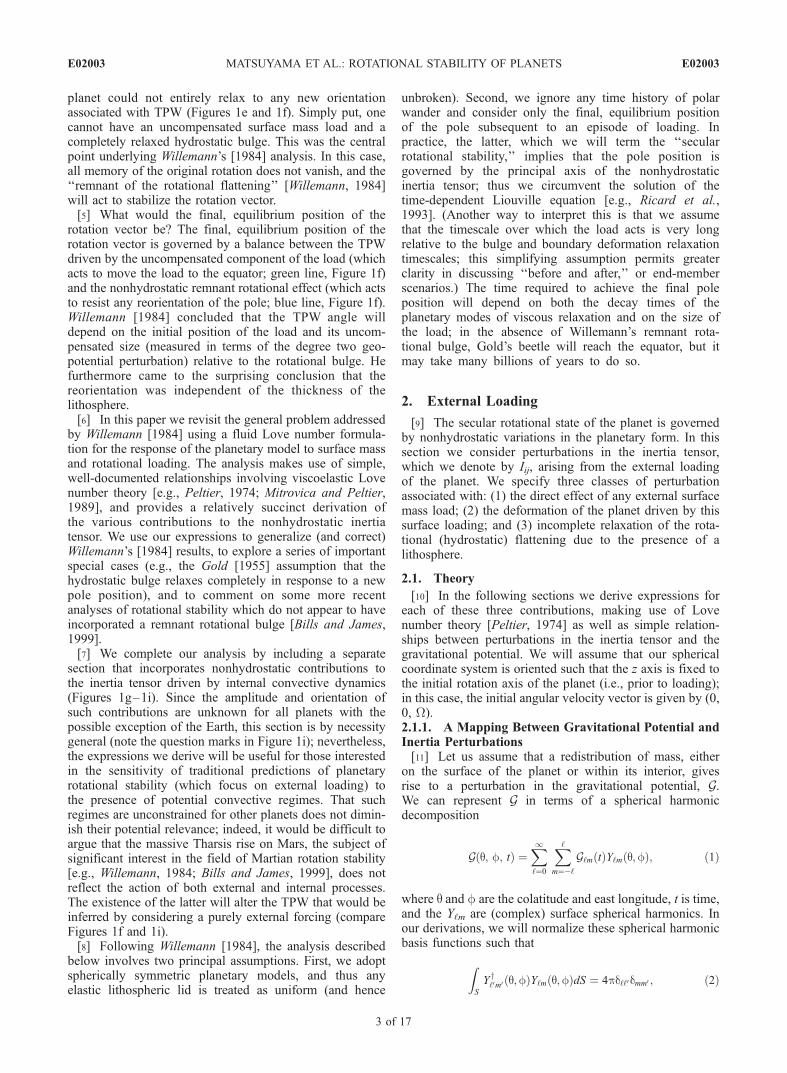
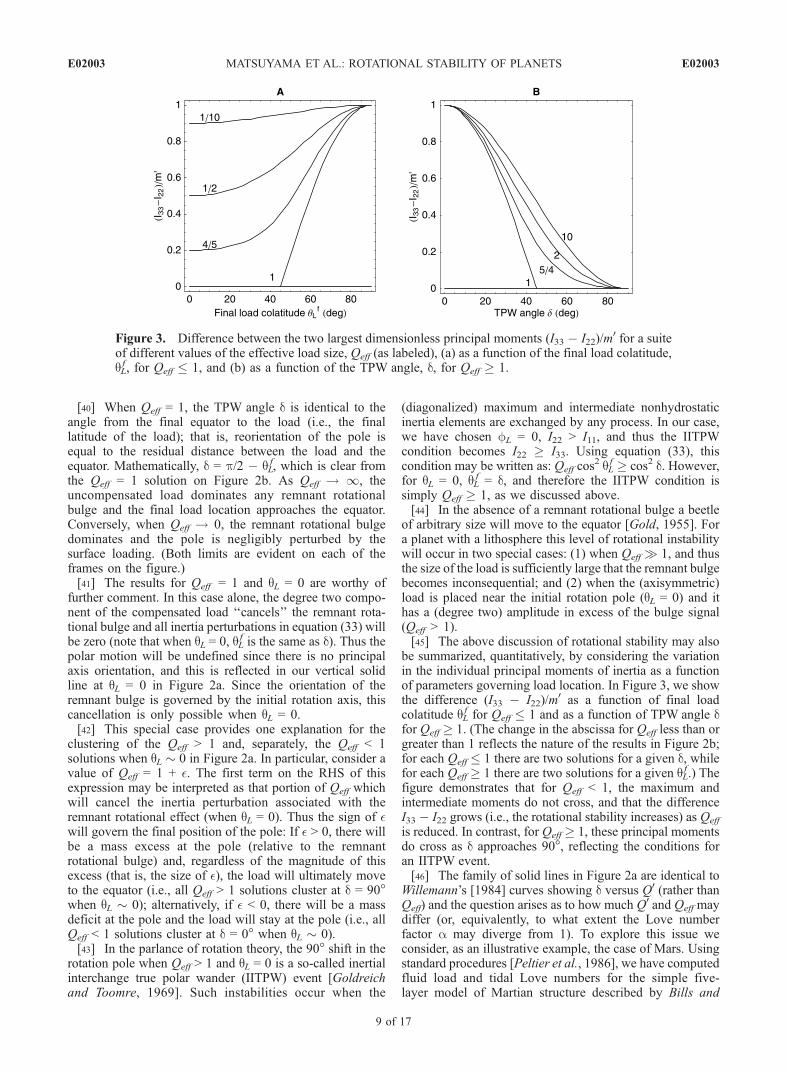
be summarized, quantitatively, by considering the variationin the individual principal moments of inertia as a functionof parameters governing load location. In Figure 3, we showthe difference (I33 � I22)/m

0 as a function of final loadcolatitude qL

f for Qeff � 1 and as a function of TPW angle dfor Qeff � 1. (The change in the abscissa for Qeff less than orgreater than 1 reflects the nature of the results in Figure 2b;for each Qeff � 1 there are two solutions for a given d, whilefor each Qeff � 1 there are two solutions for a given qL

f .) Thefigure demonstrates that for Qeff < 1, the maximum andintermediate moments do not cross, and that the differenceI33 � I22 grows (i.e., the rotational stability increases) as Qeff

is reduced. In contrast, for Qeff � 1, these principal momentsdo cross as d approaches 90�, reflecting the conditions foran IITPW event.[46] The family of solid lines in Figure 2a are identical to

Willemann’s [1984] curves showing d versus Q0 (rather thanQeff) and the question arises as to how much Q0 and Qeff maydiffer (or, equivalently, to what extent the Love numberfactor a may diverge from 1). To explore this issue weconsider, as an illustrative example, the case of Mars. Usingstandard procedures [Peltier et al., 1986], we have computedfluid load and tidal Love numbers for the simple five-layer model of Martian structure described by Bills and

Figure 3. Difference between the two largest dimensionless principal moments (I33 � I22)/m0 for a suite

of different values of the effective load size, Qeff (as labeled), (a) as a function of the final load colatitude,qLf , for Qeff � 1, and (b) as a function of the TPW angle, d, for Qeff � 1.

E02003 MATSUYAMA ET AL.: ROTATIONAL STABILITY OF PLANETS

9 of 17

E02003

James [1999]. These values, together with the factora (equation (26)) are provided in Table 1 for a sequenceof elastic LT ranging from 50 km to 400 km. Note thata diverges monotonically from 1 for progressively lowervalues of lithospheric thickness, reaching a value of 1.27 forthe case LT = 50 km.[47] Ultimately, applying the rotational stability theory

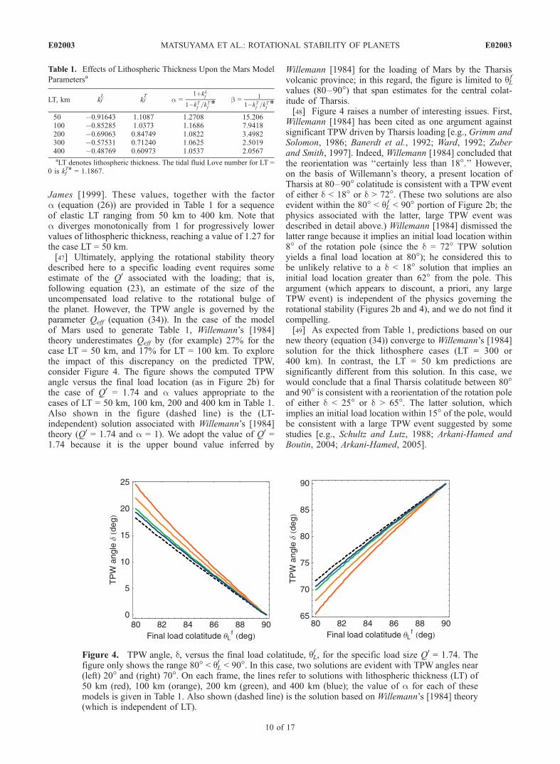
described here to a specific loading event requires someestimate of the Q0 associated with the loading; that is,following equation (23), an estimate of the size of theuncompensated load relative to the rotational bulge ofthe planet. However, the TPW angle is governed by theparameter Qeff (equation (34)). In the case of the modelof Mars used to generate Table 1, Willemann’s [1984]theory underestimates Qeff by (for example) 27% for thecase LT = 50 km, and 17% for LT = 100 km. To explorethe impact of this discrepancy on the predicted TPW,consider Figure 4. The figure shows the computed TPWangle versus the final load location (as in Figure 2b) forthe case of Q0 = 1.74 and a values appropriate to thecases of LT = 50 km, 100 km, 200 and 400 km in Table 1.Also shown in the figure (dashed line) is the (LT-independent) solution associated with Willemann’s [1984]theory (Q0 = 1.74 and a = 1). We adopt the value of Q0 =1.74 because it is the upper bound value inferred by

Willemann [1984] for the loading of Mars by the Tharsisvolcanic province; in this regard, the figure is limited to qL

f

values (80–90�) that span estimates for the central colat-itude of Tharsis.[48] Figure 4 raises a number of interesting issues. First,

Willemann [1984] has been cited as one argument againstsignificant TPW driven by Tharsis loading [e.g., Grimm andSolomon, 1986; Banerdt et al., 1992; Ward, 1992; Zuberand Smith, 1997]. Indeed, Willemann [1984] concluded thatthe reorientation was ‘‘certainly less than 18�.’’ However,on the basis of Willemann’s theory, a present location ofTharsis at 80–90� colatitude is consistent with a TPW eventof either d < 18� or d > 72�. (These two solutions are alsoevident within the 80� < qL

f < 90� portion of Figure 2b; thephysics associated with the latter, large TPW event wasdescribed in detail above.) Willemann [1984] dismissed thelatter range because it implies an initial load location within8� of the rotation pole (since the d = 72� TPW solutionyields a final load location at 80�); he considered this tobe unlikely relative to a d < 18� solution that implies aninitial load location greater than 62� from the pole. Thisargument (which appears to discount, a priori, any largeTPW event) is independent of the physics governing therotational stability (Figures 2b and 4), and we do not find itcompelling.[49] As expected from Table 1, predictions based on our

new theory (equation (34)) converge to Willemann’s [1984]solution for the thick lithosphere cases (LT = 300 or400 km). In contrast, the LT = 50 km predictions aresignificantly different from this solution. In this case, wewould conclude that a final Tharsis colatitude between 80�and 90� is consistent with a reorientation of the rotation poleof either d < 25� or d > 65�. The latter solution, whichimplies an initial load location within 15� of the pole, wouldbe consistent with a large TPW event suggested by somestudies [e.g., Schultz and Lutz, 1988; Arkani-Hamed andBoutin, 2004; Arkani-Hamed, 2005].

Table 1. Effects of Lithospheric Thickness Upon the Mars Model

Parametersa

LT, km kfL

kfT

a =1þkL

f

1�kTf=kT

f*

b = 1

1�kTf=kT

f*

50 �0.91643 1.1087 1.2708 15.206100 �0.85285 1.0373 1.1686 7.9418200 �0.69063 0.84749 1.0822 3.4982300 �0.57531 0.71240 1.0625 2.5019400 �0.48769 0.60973 1.0537 2.0567aLT denotes lithospheric thickness. The tidal fluid Love number for LT =

0 is kfT* = 1.1867.

Figure 4. TPW angle, d, versus the final load colatitude, qLf , for the specific load size Q0 = 1.74. The

figure only shows the range 80� < qLf < 90�. In this case, two solutions are evident with TPW angles near

(left) 20� and (right) 70�. On each frame, the lines refer to solutions with lithospheric thickness (LT) of50 km (red), 100 km (orange), 200 km (green), and 400 km (blue); the value of a for each of thesemodels is given in Table 1. Also shown (dashed line) is the solution based on Willemann’s [1984] theory(which is independent of LT).

E02003 MATSUYAMA ET AL.: ROTATIONAL STABILITY OF PLANETS

10 of 17

E02003

[50] Table 1 suggests that the divergence between ourresults and those derived from Willemann’s [1984] theorywill continue as the lithosphere is further thinned andthus that there will be a marked trend toward greaterrotational instability for planets with progressively thinnerelastic shells. Applying the rotational stability theory tothe loading of Mars by Tharsis raises an important issue;namely, the LT used in the theory refers to the thicknessof the lithosphere at the time of Tharsis development.This thickness is uncertain, particularly given the ancientnature of Tharsis (�4 Ga). As we discussed at the end ofsection 2.1.3, the remnant rotational flattening active atthe time of Tharsis loading should actually reflect, in anintegral sense, changes in both the pole position andlithospheric thickness across a time interval from theformation of the hydrostatic planet to the onset of Tharsisloading; the TPW calculations above (and those appearingin the work of Willemann [1984]) assume that thelithospheric thickness at the time of Tharsis loadingdeveloped during a period of little TPW and thus theremnant bulge is aligned with the unique orientation ofthe pole during this period.2.2.2. Bills and James [1999][51] In application to Mars, Bills and James [1999] also

considered the rotational stability of the planet in responseto surface mass loading. Their equation governing thesecular rotational stability was stated as (see their equation(49))

JL2 � 2JL22; ð36Þ

where J2L and J22

L represent the degree two zonal andnonzonal components of the potential perturbation

associated with the surface mass load. These harmonicsare renormalized versions of the coefficients appearing inequation (1). This stability criterion is identical to

IL33 þ IL�D33 � IL22 þ IL�D

22 ; ð37Þ

where each side of this equation represents a principalaxis. That is, Bills and James [1999] assume that the polelocation is governed by the diagonalization of anonhydrostatic inertia tensor whose sole contributionarises from surface mass loading. The stabilization ofthe pole due to a remnant rotational bulge is ignored.[52] Bills and James [1999] were, in particular, interested

in the impact on the rotational state of departures from loadaxial symmetry. This issue is the subject of the next section.2.2.3. Nonaxisymmetric Loads[53] Thus far we have only considered simple, axisym-

metric disk loads. To end this section we explore thepotential impact on the rotational stability of any departuresfrom axisymmetry. Specifically, we will consider TPWdriven by the spherical harmonic degree two componentsof the simple set of disks shown schematically in Figure 5.The total load is composed of two parts. The first, axisym-metric central dome has an uncompensated, effective loadsize of Q1. The second, smaller disk has an uncompensated,effective size of Q2. We will consider two cases distin-guished on the basis of the location of this smaller disk:either on the great circle joining the initial rotation pole andthe larger disk (Case 1) or 90� from this great circle (Case2). To this point we have been concerned with computingthe TPWangle d along this great circle. The natural questionthat arises is the following: How effective is the non-axisymmetric component of the surface load in drivingTPW off this great circle? Since no real load (or set ofloads) is perfectly axisymmetric, Tharsis being a notableexample, this question has important relevance to anygeneral consideration of rotational stability.[54] To consider this issue, we have performed a suite of

calculations in which we adopt a specific initial loadlocation q1 close to the initial rotation axis and fix Q2 tosome small fraction of Q1. We then track the computedTPW while varying the central load amplitude Q1. Thesesolutions map out a curve on the surface of the sphere. Wehave repeated the calculation for various placements of thesecondary disk.[55] In these tests, which we summarize in Figures 6 and

7, the TPW is driven by three contributions to the planetaryinertia tensor, where each contribution has its preferred polelocation: the fossil rotational bulge acts to move the poletoward the original pole location, while the two surfacemass loads drive the pole toward great circles perpendicularto the respective load location vectors (these great circlesare given by the solid red and blue lines in Figures 6 and 7).The equilibrium pole location is given by the balance ofthese three contributions.[56] As an example, the top row of Figure 6 shows

calculations for the Case 1 orientation of the secondaryload disk when q1 = 1� and q2 = 11� (or 10� further from theinitial pole than the primary disk). As Q1 is increased fromzero to values just above 1, the TPW solutions move along

Figure 5. Schematic illustration of the initial orientation ofthe nonaxisymmetric surface mass load discussed within thetext. In particular, the central, axisymmetric load of size Q1

and initial colatitude q1 (as in Figures 2 and 3) is augmentedto include a smaller second disk of size Q2. The latteris positioned either on the great circle joining the centraldisk to the initial pole (Case 1) or 90� from this great circle(Case 2).

E02003 MATSUYAMA ET AL.: ROTATIONAL STABILITY OF PLANETS

11 of 17

E02003

the path followed by the black line. For values of Q1 > 1.1the pole is within a region bounded by the principal axesassociated with the primary and secondary loads, respec-tively; in this situation, the primary load continues to pushthe pole toward the equator, while the secondary load (and

remnant rotational bulge) resist this trend. At Q1 � 1.31, thepole experiences a major instability defined by a 90� shiftaway from this great circle. This instability is an IITPWevent. In this scenario, since q1 6¼ 0, the primary load isunable to perfectly cancel the nonhydrostatic remnant

Figure 6. Predicted TPW for the nonaxisymmetric load scenario shown by Case 1 in Figure 5 (i.e., thesecondary load falls on the great circle connecting the initial pole location to the primary load). (top left)Predicted TPW for a suite of predictions based on varying the effective size of the primary load, Q1 (aslabeled). In this case q1 = 1�, q2 = 11� andQ2 = 0.1Q1. The blue and red great circle arcs are perpendicular tothe axes of the primary and secondary loads, respectively. An IITPW event occurs for Q1 = 1.31 and therotation pole moves to the intersection of the blue and red great circles (i.e., 90� from both the primary andsecondary loads; given the symmetry of the problem, the pole can move either clockwise orcounterclockwise during this event, hence the two paths shown on the figure). (top middle and right)The effective primary load, Q1, required to produce an IITPW event, as well as the colatitude of the polewhen this event is initiated, as a function of the initial load colatitude, q1. Each frame shows results for twoscenarios:Q2 = 0.1Q1 andQ2 = 0.2Q1. (bottom) As in the top row, except for the case where the secondaryload is displaced 70� from the primary load. In this case, the middle and right frames explore results for q1values up to 20�.

Figure 7. Predicted TPW for the nonaxisymmetric load scenario shown by Case 2 in Figure 5 (i.e., thegreat circles connecting the initial pole location to the primary and secondary loads are perpendicular). Inboth frames Q2 = 0.1 Q1 and q1 = 1�, and the black line joins results for a sequence of progressively largervalues of Q1 (as labeled). The frames are distinguished on the basis of the position of the secondary load:(a) q2 = 11� or (b) q2 = 71�.

E02003 MATSUYAMA ET AL.: ROTATIONAL STABILITY OF PLANETS

12 of 17

E02003

rotational bulge; however, the additional inertia tensorcontribution from the secondary load makes such a cancel-lation possible. Note that for values of Q1 > 1.31 the poleposition is stable and located at the intersection of theequatorial great circles (red and blue lines) defined by thetwo loads. As discussed above, the ‘‘residual’’ effectiveloads (that is, the effective loads after removal of the portionthat cancels the remnant rotational bulge), no matter theirsize, will govern the location of the pole.[57] As in the axisymmetric case, we can write expres-

sions for the inertia tensor perturbations, diagonalize thetensor and derive conditions for both the equilibrium polelocation and IITPW. Lengthy algebra yields the followingcondition for the pole location and the point at which anequality between I22 and I33 is achieved,

Q1 sin 2q f1

� þ Q2 sin 2q f

2

� ¼ sin 2dð Þ

Q1 cos2 q f

1

� þ Q2 cos

2 q f2

� ¼ cos2 dð Þ:

ð38Þ

Simultaneous solution of these equations can be used topredict the effective load magnitude (Q1) and the colatitude(measured from the original pole location) at which theIITPW event occurs.[58] The remaining frames on the top row of Figure 6

show summary results for cases in which q1 is varied up to5� and the secondary load is either 10% (as above) or 20%of the primary load. We retain the 10� shift between loadcenters. The middle frame shows the Q1 value necessary foran IITPW event, and the right frame shows the colatitude atwhich the event will occur. The main point in these results isthat as the primary load is moved away from the originalpole, the size of the load required to initiate an IITPW eventgrows rapidly. Indeed, in the case of q1 = 5� and Q2 = 0.1Q1,a value Q1 = 4.7 is required to initiate an IITPW event.[59] In the bottom frames of Figure 6 we consider a second

Case 1 scenario in which the displacement between theprimary and secondary loads is increased to 70�. For q1 =1� and Q2 = 0.1Q1, a Q1 value above 0.97 will bring therotation pole into a region within the great circles perpendic-ular to the two load axes (left frame). Furthermore, in thesame case, a value of Q1 = 1.02 initiates an IITPWevent at acolatitude of �30�. As q1 is increased up to 20� (middle andright frames), the Q1 value necessary for the onset of IITPWincreases to just 2.4, while the colatitude at which theinstability occurs increases to �55�. These values drop to1.8 and 45�, respectively, when Q2 = 0.2 Q1. Clearly, givensome upper bound on the size of the primary load, a largerdisplacement between the primary and secondary loadsyields a broader range of load locations that may yield anIITPW event.[60] In Figure 7 we turn our attention to the Case 2

scenario of Figure 5, and show a sequence of results (forincreasing Q1) for q1 = 1� and a displacement between loadsof either 10� (Figure 7a) or 70� (Figure 7b). In this case, thesecondary load acts to deflect the pole location off the greatcircle joining the initial pole and the primary load. The sizeof this deflection decreases as the displacement between theprimary and secondary loads increases since the great circleperpendicular to the secondary load axis comes into closeralignment with the great circle joining the initial pole and

primary load (compare the red great circles in Figures 7aand 7b). As the size of the primary load (Q1) is increased,the pole first moves off the latter great circle, but eventuallyreturns toward this great circle. The pole returns to thislongitude since it is where the great circles that are perpen-dicular to the load axes intersect. Consider the q2 = 11�scenario (Figure 7a), for values of Q1 � 1.5, the equilibriumpole position has reached close to the point of intersectionbetween the two great circles that are perpendicular to theload axes. In contrast, for Q1 ] 0.92, the pole will bedeflected �45� from this longitude. In any event, the Case 2scenario does not produce an IITPW instability; that is, thepositioning of the loads along perpendicular trajectoriesfrom the initial rotation pole (Figure 5) will not lead to asituation where the maximum and intermediate nonhydro-static moments of inertia become equal.[61] These scenarios are highly simplified, but they

provide significant insight into the connection between loadasymmetry and rotational stability. The main result is thateven small levels of asymmetry can profoundly influencethe rotational stability. For components of asymmetryaligned with the great circle joining the initial pole andthe primary load, this impact includes the potential initiationof IITPW events.

3. Impact of Internally Supported InertiaPerturbations

[62] In this section we augment the theory outlined aboveto include perturbations in the inertia tensor dynamicallysupported by internal, convective motions (Figures 1g–1i).Few, if any, constraints currently exist on the amplitude and/or orientation of internal convective motions on planetsother than Earth. Accordingly, the mathematics outlinedbelow is, by necessity, general.[63] We begin by assuming the total gravitational poten-

tial perturbation associated with internal convective flow(including the mass heterogeneity and its induced surfacedeformation) is known. If we denote these harmonics byG‘mINT(t) then equation (3) gives

I INT11 tð Þ ¼ Ma

g

ffiffiffi5

p

3GINT20 tð Þ � 2

ffiffiffi5

6

rRe GINT

22 tð Þ� �" #

;

I INT22 tð Þ ¼ Ma

g

ffiffiffi5

p

3GINT20 tð Þ þ 2

ffiffiffi5

6

rRe GINT

22 tð Þ� �" #

;

I INT33 tð Þ ¼ � 2ffiffiffi5

p

3

Ma

gGINT20 tð Þ; ð39Þ

I INT12 tð Þ ¼ 2

ffiffiffi5

6

rMa

gIm GINT

22 tð Þ� �

;

I INT13 tð Þ ¼ 2

ffiffiffi5

6

rMa

gRe GINT

21 tð Þ� �

;

I INT23 tð Þ ¼ �2

ffiffiffi5

6

rMa

gIm GINT

21 tð Þ� �

;

where we have assumed that the degree zero potentialharmonic is zero. We remind the reader that the sphericalharmonic decomposition will be based on a reference framein which the north pole refers to the initial rotation axis (i.e.,the rotation axis that defines the orientation of the remnantrotational bulge).

E02003 MATSUYAMA ET AL.: ROTATIONAL STABILITY OF PLANETS

13 of 17

E02003

[64] In this case, the total inertia tensor perturbation is

Iij tð Þ ¼ ILij þ IL�Dij þ IROTij þ I INTij tð Þ; ð40Þ

where a general expression for the first three terms on theright hand side is given by equation (21). Note that weretain the time dependence in the evolving contributionfrom convective flow but we continue to assume that thetimescale associated with this flow is much longer thanthe decay times that govern the viscous adjustment of therotational bulge. We also assume that the geoid/inertiacontributions from convective motions, if they were to becomputed using viscous flow calculations, would involve anelastic lithosphere with thickness consistent with theremaining terms in equation (40).[65] At this point, we can consider a special case. As in

the treatment of the surface mass disk load, let us assumethat gravitational potential associated with internal flow isaxisymmetric relative to a geographic point (qI, fI). Let usfurthermore denote the degree two zonal component ofthe potential (in a reference frame in which the axis ofsymmetry is at the pole) by G20

0INT(t). Then, in analogy withequation (22), we have

GINT2m tð Þ ¼ G0;INT

20 tð Þ Yy2m qI ;fIð Þffiffiffi

5p : ð41Þ

If we furthermore normalize this signal relative to thepotential perturbation associated with the hydrostaticrotational bulge,

Q00 tð Þ ¼ � G0;INT20 tð Þ

�1

3ffiffi5

p a2W2kT*f

; ð42Þ

then equation (39) becomes

I INT11 tð Þ ¼ 1

3m0Q00 tð Þb

"1ffiffiffi5

p Y20 qIð Þ�ffiffiffi6

5

rRe Y

y22 qI ;fIð Þ

� #;

I INT22 tð Þ ¼ 1

3m0Q00 tð Þb

"1ffiffiffi5

p Y20 qIð Þþffiffiffi6

5

rRe Y

y22 qI ;fIð Þ

� #;

IINT tð Þ33 ¼ � 2

3m0Q00 tð Þb 1ffiffiffi

5p Y20 qIð Þ; ð43Þ

I INT12 tð Þ ¼ 1

3m0Q00 tð Þb

ffiffiffi6

5

rIm Y

y22 qI ;fIð Þ

� ;

I INT13 tð Þ ¼ 1

3m0Q00 tð Þb

ffiffiffi6

5

rRe Y

y21 qI ;fIð Þ

� ;

I INT23 tð Þ ¼ � 1

3m0Q00 tð Þb

ffiffiffi6

5

rIm Y

y21 qI;fIð Þ

� ;

Figure 8. TPW driven by a combination of surface mass and internal loading. The internal load is fixed,and is characterized by an excess ellipticity which is 1% of the hydrostatic bulge of the planet (Q00 =0.01). The principal axis for this component is given by the dashed red line (qI = 80�); the great circleperpendicular to this axis is given by the solid red line. (top) Predicted pole positions for the case wherethe surface mass load has an initial colatitude qL = 4� and Q0 is varied (as labeled). The frames aredistinguished by the choice of lithospheric thickness: (a) 50 km or (b) 400 km. (c) The effective surfaceload size (Q0) required to produce an IITPWevent, as well as (d) the colatitude of the pole when this eventis initiated, as a function of the initial load colatitude qL. Figures 8c and 8d show results for LT = 50 kmand 400 km.

E02003 MATSUYAMA ET AL.: ROTATIONAL STABILITY OF PLANETS

14 of 17

E02003

where

b ¼ 1

1� kTf =kT*f

: ð44Þ

[66] In applying equation (40), the appropriate expressionfor Iij

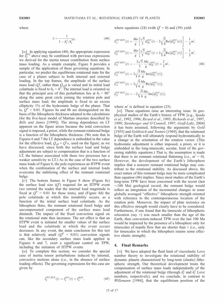
INT above may be combined with previous expressionswe derived for the inertia tensor contribution from surfacemass loading. As a simple example, Figure 8 provides asample of the application of these governing equations. Inparticular, we predict the equilibrium rotational state for thecase of a planet subject to both internal and externalloading. In the top frames, the amplitude of the surfacemass load (Q0, rather than Qeff) is varied and its initial loadcolatitude is fixed to qL = 4�. The internal load is oriented sothat the principal axis of this perturbation lies at qI = 80�along the same great circle joining the rotation pole andsurface mass load; the amplitude is fixed to an excessellipticity 1% of the hydrostatic bulge of the planet. Thatis, Q00 = 0.01. Figures 8a and 8b are distinguished on thebasis of the lithospheric thickness adopted in the calculations(for the five-layer model of Martian structure described byBills and James [1999]). The strong dependence on LTapparent on the figure arises because the total convectionsignal is imposed, a priori, while the remnant rotational bulgeis a function of the lithospheric thickness. (We note that inFigures 6 and 7 the LT dependence is embedded in the valuefor the effective load, Qeff = Q0a, used on the figure; as wehave discussed, since both the surface load and bulgeadjustment are subject to compensation that is a function ofLT, the balance associated with these two processes has aweaker sensitivity to LT.) As in the case of the two surfacemass loads of Figure 6, the pole experiences an IITPWeventwhen the combination of the surface and internal loadsovercome the stabilizing effect of the remnant rotationalbulge.[67] The bottom frames in Figure 8 show (Figure 8c)

the surface load size (Q0) required for an IITPW event(we remind the reader that the internal load magnitude isfixed at Q00 = 0.01 for these tests), and (Figure 8d) thepole colatitude at which this instability occurs, as afunction of the initial surface load colatitude. As thelithosphere thins, the remnant rotational fossil bulge anduncompensated component of the surface mass loaddiminish. The impact of the fixed convection signal onthe rotational state thus increases. The net effect is that anIITPW event is initiated for smaller values of the surfaceload and the colatitude at which the event occursdecreases. In any event, the main conclusion for this testis that relatively small (Q00 = 0.01) convection signalscan, like the secondary surface mass loads applied inFigures 6 and 7, exert a significant control on TPW,including the initiation of IITPW events.[68] To complete this section, we consider the special

case of inertia tensor perturbations induced by internal,convective motions alone (i.e., in the absence of surfaceloading effects). The governing expressions for this case aregiven by

IINT ;ROTij tð Þ ¼ I INTij tð Þ þ IROTij ; ð45Þ

where equations (24) (with Q0 = 0) and (39) yield

IINT ;ROT11 tð Þ ¼ Ma

g

ffiffiffi5

p

3GINT20 tð Þ

�� 2

ffiffiffi5

6

rRe GINT

22 tð Þ� �#

� 1

3m0;

IINT ;ROT22 tð Þ ¼ Ma

g

ffiffiffi5

p

3GINT20 tð Þ

�þ 2

ffiffiffi5

6

rRe GINT

22 tð Þ� �#

� 1

3m0;

IINT ;ROT33 tð Þ ¼ � 2

ffiffiffi5

p

3

Ma

gGINT20 tð Þ þ 2

3m0; ð46Þ

IINT ;ROT12 tð Þ ¼ 2

ffiffiffi5

6

rMa

gIm GINT

22 tð Þ� �

;

IINT ;ROT13 tð Þ ¼ 2

ffiffiffi5

6

rMa

gRe GINT

21 tð Þ� �

;

IINT ;ROT23 tð Þ ¼ �2

ffiffiffi5

6

rMa

gIm GINT

21 tð Þ� �

;

where m0 is defined in equation (25).[69] These equations raise an interesting issue. In geo-

physical studies of the Earth’s history of TPW [e.g., Spadaet al., 1992, 1996; Ricard et al., 1993; Richards et al., 1997,1999; Steinberger and O’Connell, 1997; Greff-Leftz, 2004]it has been assumed, following the arguments by Gold[1955] and Goldreich and Toomre [1969], that the rotationalbulge of the Earth will ultimately respond hydrostatically toa change in the orientation of the rotation vector. (Thishydrostatic adjustment is either imposed, a priori, or it isembedded in the long-timescale, secular, limit of the gov-erning stability equations.) That is, the assumption is madethat there is no remnant rotational flattening (i.e., m0 = 0).However, the development of the Earth’s lithosphereimplies that a nonzero remnant rotational bulge may con-tribute to the rotational stability. As discussed above, theexact nature of this remnant bulge may be more complicatedthan equation (46) implies. Since most studies of the Earth’slong-term TPW have been concerned with the recent (last�100 Ma) geological record, the remnant bulge wouldreflect an integration of the incremental changes in someglobally averaged ‘‘effective’’ lithospheric strength orientedwith reference to the contemporaneous location of therotation pole. Moreover, the impact of plate tectonics onthis effective strength would clearly have to be considered.Furthermore, if one found that the timescale of lithosphericrelaxation (say t) was much smaller than the age of theEarth, then convection-induced TPW over the last 100 Mawould be impacted by the presence of a lithosphere only fortimescales of mantle flow that are shorter than t (i.e., onlyfor timescales in which the lithosphere retains some effec-tive elastic strength).

4. Final Remarks

[70] We have adopted the fluid limit of viscoelastic Lovenumber theory to investigate the rotational stability ofdynamic planets characterized by long-term (elastic) litho-spheric strength. Our theoretical development treats thecompensation of surface mass loads independently of theadjustment of the rotational bulge (through kf

L and kfT Love

numbers, respectively), and we conclude, in contrast toWillemann [1984], that the equilibrium position of the

E02003 MATSUYAMA ET AL.: ROTATIONAL STABILITY OF PLANETS

15 of 17

E02003

rotation vector is a function of the lithospheric thickness(LT). Using fluid Love numbers computed for a model ofMartian structure, we find that the TPW driven by axisym-metric surface mass loading is progressively larger thanWillemann’s [1984] predictions as the lithosphere is thinned(Figure 4); indeed, the predictions only converge for LTvalues greater than �400 km.[71] Our analysis of TPW driven by axisymmetric loads,

summarized in Figures 2 and 3, bridges results from earlier,classic studies of Gold [1955] and Willemann [1984]. As anexample, Gold [1955] argued that TPW on a hydrostaticplanet (i.e., a planet in which the rotational bulge willeventually reorient perfectly to a change in pole position)will ultimately move any uncompensated surface mass loadto the equator. In the case of a planet with an elasticlithosphere, both the surface mass load and the rotationalbulge will experience incomplete compensation. For sucha planet, a reorientation of the load to the equator willoccur in two situations (see Figure 2): (1) when the surfacemass load is extremely large (i.e., Qeff � 1) or (2) when aload which exceeds the size of the remnant rotational bulge(Qeff > 1) is placed at the initial pole position. In the lattercase, the remnant rotational bulge is ‘‘canceled’’ by thecomponent of the surface mass load up to Qeff = 1 andthe residual (i.e., a load component of any size in excess ofQeff = 1) will drive an IITPW instability.[72] We have also extended Willemann’s [1984] analysis

to consider the impact of nonaxisymmetric surface massloads and arbitrary, convectively supported contributions tothe nonhydrostatic inertia tensor, on predicted TPW paths.We find that these contributions can exert a profoundinfluence on the rotational stability (Figures 6–8). Forexample, surface mass load asymmetry modeled by includ-ing a secondary load along the same great circle joining theprimary (axisymmetric) load and the initial rotation pole(Case 1 in Figure 5) is capable of inducing an IITPW event.We have derived the stability conditions governing thisevent (see equations 38); for a given upper bound on thesize of the effective surface load, a larger displacementbetween the primary and secondary loads increases the rangeof load locations that can give rise to IITPW (Figure 6). Incontrast, load asymmetries modeled by incorporating asecondary load in a location perpendicular to the great circlejoining the primary load and the initial rotation pole (Case 2in Figure 5) act to deflect the pole from this great circle. Thelevel of deflection depends on the size and location of theprimary and secondary loads; we note from Figure 7 thatmoving the secondary load closer to the initial rotation poleacts to increase the excursion of the rotation vector from thegreat circle.[73] The impact on the rotational dynamics of convec-

tively induced perturbations in the planetary shape(Figure 8) can be understood in these same terms, sincesuch contributions can be expressed as equivalent uncom-pensated components of the surface mass load. That is, thedivergence of the pole position from simple TPW pathspredicted on the basis of an axisymmetric surface mass loadwill depend on the magnitude and orientation (relative tothe initial pole and axisymmetric surface load) of theconvection signal.[74] We conclude that the rotational stability of planets

will be overestimated by analyses which are limited to

simple axisymmetric loads of the type introduced byWillemann [1984] (and treated in our Figures 2–4). TheTPW on Mars driven by Tharsis, an example discussed atvarious stages through this article, warrants several com-ments in this regard. First, our correction of Willemann’s[1984] theory for axisymmetric loads yields a broader rangeof TPW scenarios for a Tharsis-sized load (Figure 4) in thecase of a relatively thin elastic lithosphere at the time ofTharsis formation. Second, in contrast to previous assertions,the equations governing the rotational stability permit a large(>65�) excursion of the Martian rotation pole in consequenceof an axisymmetric Tharsis-sized loading (Figure 4). Third,asymmetries in the surface mass loading, either due toTharsis structure or the presence of secondary loads (e.g.,Elysium) on Mars, or contributions to the nonhydrostaticinertia tensor from convective processes, will introducepotentially large pole excursions off the great circle joiningthe initial rotation pole and the main Tharsis load. Indeed,these excursions may include an IITPW event.[75] Finally, we note that the Love number theory de-

scribed herein assumes a viscoelastic planetary model with asingle, uniform elastic plate. A new generation of finiteelement models have been developed to consider theresponse of 3-D Earth models to generalized loading [e.g.,Wu and van der Wal, 2003; Zhong et al., 2003; Latychev etal., 2005]. In future work, we will use such models toinvestigate the impact of plate boundaries and thicknessvariations on the computed rotational stability. These resultswill be used to reassess predictions of TPW on Earth overthe last 100 Myr (see the discussion below equation (46))and TPW driven by Tharsis loading in the event of tectonicactivity on early Mars.

Appendix A: Load-Induced GeopotentialPerturbations

[76] The geopotential perturbation associated with surfaceloading can be written as a space-time convolution of theviscoelastic Green’s function for the geopotential anomalywith the surface mass load, L(q, f, t),

G q;f; tð Þ ¼Z t

�1

ZS

L q0;f0; t0ð Þ � GF g; t � t0ð ÞdS0dt0; ðA1Þ

where S represents the surface of the unit sphere, GF is theGreen’s function and g is the angular distance from (q, f) to(q0, f0) given by

cos g ¼ cos q cos q0 þ sin q sin q0 cos f� f0ð Þ: ðA2Þ

We note that on a spherically symmetric planet, the responseis dependent on the angular distance from the load andindependent of azimuth. The viscoelastic Green’s Functionassociated with the geopotential is given by [Mitrovica andPeltier, 1989]

GF g; tð Þ ¼ ag

M

X1‘¼0

d tð Þ þ kL‘ tð Þ� �

P‘ cosgð Þ; ðA3Þ

where P‘ is the unnormalized Legendre polynomial atdegree ‘. In the square brackets on the right-hand-side of

E02003 MATSUYAMA ET AL.: ROTATIONAL STABILITY OF PLANETS

16 of 17

E02003

equation (A3), the delta function refers to the direct effect ofthe surface mass load, while the Love number k‘

L(t) (seeequation (4)) accounts for the planetary deformationassociated with this load.[77] Using the normalization we have adopted (see equa-

tion (2)), the addition theorem of spherical harmonics yields

ZS

L q0;f0ð ÞP‘ cosgð ÞdS0 ¼ 4pa2

2‘þ 1

X‘

m¼�‘

L‘m tð ÞY‘m q;fð Þ: ðA4Þ

Next, we apply equation (A3) in equation (A1) and useequation (A4) to perform the spatial convolution analyti-cally. For each harmonic coefficient we obtain

G‘m tð Þ ¼ 4pa3gM 2‘þ 1ð Þ L‘m tð Þ * d tð Þ þ kL‘ tð Þ

� �; ðA5Þ

where the asterisk denotes a time convolution. In general wewill be interested in load-induced perturbations at degreetwo, and in this case we can write

G2m tð Þ ¼ 4pa3g5M

L2m tð Þ * d tð Þ þ kL2 tð Þ� �

: ðA6Þ

It will be instructive to separate the perturbation intocomponents associated with the direct mass attraction of thesurface load and the deformation induced by this surfaceload (since, as we discussed in the main text, these arecommonly thought of as two of the three contributions tochanges in the inertia tensor components). If we denotethese terms by the superscript L and L � D, respectively, wehave

GL2m tð Þ ¼ 4pa3g

5ML2m tð Þ * d tð Þ ¼ 4pa3g

5ML2m tð Þ ðA7Þ

GL�D2m tð Þ ¼ 4pa3g

5ML2m * kL2 tð Þ; ðA8Þ

where G2,�m(t) = (�1)mG2my (t). In the limit of infinite time

after the application of the surface mass load, theseequations yield the expressions (6) and (7) within the maintext.

[78] Acknowledgments. The authors thank David Stevenson and theAssociate Editor for constructive reviews. We also thank David Stevensonand Victor Tsai for providing us with a copy of their manuscript prior topublication. We acknowledge support from the Canadian Institute forTheoretical Astrophysics, the Miller Institute for Basic Research, theCanadian Institute for Advanced Research, NSERC, and the NASAAstrobiology Institute.

ReferencesArkani-Hamed, J. (2005), Giant impact basins trace the ancient equator ofMars, J. Geophys. Res., 110, E04012, doi:10.1029/2004JE002343.

Arkani-Hamed, J., and D. Boutin (2004), Paleomagnetic poles of Mars:Revisited, J. Geophys. Res., 209, E03011, doi:10.1029/2003JE002229.

Banerdt, W. B., M. P. Golombek, and K. L. Tanaka (1992), Stress andtectonics on Mars, in Mars, edited by H. H. Kieffer et al., pp. 249–297, Univ. of Ariz. Press, Tucson.

Bills, B. G., and T. S. James (1999), Moments of inertia and rotationalstability of Mars: Lithospheric support of subhydrostatic rotational flat-tening, J. Geophys. Res., 104, 9081–9096.

Gold, T. (1955), Instability of the Earth’s axis of rotation, Nature, 175,526–529.

Goldreich, P., and A. Toomre (1969), Some remarks on polar wandering,J. Geophys. Res., 74, 2555–2567.

Greff-Leftz, A. (2004), Upwelling plumes, superwells and true polarwander, Geophys. J. Int., 159, 1125–1137.

Grimm, R. E., and S. C. Solomon (1986), Tectonic tests of proposed polarwander paths for Mars and the moon, Icarus, 65, 110–121.

Lambeck, K. (1980), The Earth’s Variable Rotation: Geophysical Causesand Consequences, Cambridge Univ. Press, New York.

Latychev, K., J. X. Mitrovica, J. Tromp, M. E. Tamisiea, D. Komatitsch,and C. Christara (2005), Glacial isostatic adjustment on 3-D Earth mod-els: A new finite-element formulation, Geophys. J. Int., 161, 421–444.

Mitrovica, J. X., and W. R. Peltier (1989), Pleistocene deglaciation and theglobal gravity field, J. Geophys. Res., 94, 13,651–13,671.

Mitrovica, J. X., J. Wahr, I. Matsuyama, and A. Paulson (2005), The rota-tional stability of an ice-age Earth, Geophys. J. Int., 161, 491–506.

Peltier, W. R. (1974), The impulse response of a Maxwell Earth, Rev.Geophys., 12, 649–669.

Peltier, W. R. (1976), Glacial isostatic adjustment: 2. The inverse problem,Geophys. J. R. Astron. Soc., 46, 669–706.

Peltier, W. R., R. A. Drummond, and A. M. Tushingham (1986), Post-glacial rebound and transient lower mantle rheology, Geophys. J. R.Astron. Soc., 87, 79–116.

Ricard, Y., G. Spada, and R. Sabadini (1993), Polar wandering of a dy-namic Earth, Geophys. J. Int., 113, 282–298.

Richards,M. A., Y. Ricard, C. Lithgow-Bertelloni, G. Spada, andR. Sabadini(1997), An explanation for the long-term stability of Earth’s rotation axis,Science, 275, 372–375.

Richards, M. A., H. P. Bunge, and Y. Ricard (1999), Polar wandering inmantle convection models, Geophys. Res. Lett., 26, 1777–1780.

Schultz, P. H., and A. B. Lutz (1988), Polar wandering of Mars, Icarus, 73,91–141.

Spada, G., Y. Ricard, and R. Sabadini (1992), Excitation of true polarwander by subduction, Nature, 360, 452–454.

Spada, G., R. Sabadini, and E. Boschi (1996), Long-term rotation andmantle dynamics of the Earth, Mars, and Venus, J. Geophys. Res., 101,2253–2266.

Steinberger, B., and R. J. O’Connell (1997), Changes of the Earth’s rotationaxis owing to advection of mantle density heterogeneities, Nature, 387,169–173.

Steinberger, B., and R. J. O’Connell (2002), The convective mantle flowsignal in rates of true polar wander, in Ice Sheets, Sea Level and theDynamic Earth, Geodyn. Ser., vol. 29, edited by J. X. Mitrovica andL. L. A. Vermeersen, pp. 233–256, AGU, Washington, D. C.

Ward, W. R. (1992), Long-term orbital and spin dynamics of Mars, inMars,edited by H. H. Kieffer et al., pp. 298–320, Univ. of Ariz. Press, Tucson.

Willemann, R. J. (1984), Reorientation of planets with elastic lithospheres,Icarus, 60, 701–709.

Wu, P., and W. R. Peltier (1984), Pleistocene deglaciation and theEarth’s rotation: A new analysis, Geophys. J. R. Astron. Soc., 76,753–792.

Wu, P., and W. van der Wal (2003), Postglacial sealevels on a spherical,self-gravitating viscoelastic Earth: Effects of lateral viscosity variations inthe upper mantle on the inference of viscosity contrasts in the lowermantle, Earth Planet. Sci. Lett., 211, 57–68.

Zhong, S., A. Paulson, and J. Wahr (2003), Three-dimensional finiteelement modelling of Earth’s viscoelastic deformation: Effects of lat-eral variations in lithospheric thickness, Geophys. J. Int., 155, 679–695.

Zuber, M. T., and D. E. Smith (1997), Mars without Tharsis, J. Geophys.Res., 102, 28,673–28,686.

�����������������������I. Matsuyama, Department of Terrestrial Magnetism, Carnegie Institution

of Washington, 5241 Broad Branch Road, NW, Washington, DC 20015-1305, USA. (matsuyama@dtm.ciw.edu)J. X. Mitrovica, Department of Physics, University of Toronto, 60 St.

George Street, Toronto, ON, Canada M5S 1A7.M. Manga, J. T. Perron, and M. A. Richards, Department of Earth and

Planetary Science, University of California, Berkeley, CA 94720-4767,USA.

E02003 MATSUYAMA ET AL.: ROTATIONAL STABILITY OF PLANETS

17 of 17

E02003