Sound Field Diffusion Coefficient: Absolute Values

ICSV22, Florence (Italy) 12-16 July 2015 1

SOUND FIELD DIFFUSION COEFFICIENT: ABSOLUTE VALUES

Alejandro Bidondo, Mariano Arouxet, Sergio Vazquez, Javier Vazquez, Germán

Heinze and Adrián Saavedra

Universidad Nacional de Tres de Febrero, UNTREF, Departamento de Ciencia y Tecnología,

Buenos Aires, Argentina

e-mail: [email protected]

This research addresses the pursuit and establishment of third octave maximum values for the

calculation of an absolute Sound Field Diffusion Coefficient. It quantifies the degree of diffu-

sion in a third octave band basis of a sound field from a monaural, broadband, omnidirectional,

high S/N impulse response. Maximum, for each band, values were find just from big room’s

impulse responses analysis. The coefficient range varies between “0” and “1”, zero being “no

diffuseness” and “1” being maximum diffusion for rooms with Schroeder frequency below

100Hz and impulse responses registered in the far field from diffusing boundaries.

1. Introduction

For decades diffusion of a sound field has been a phenomena without exact and precise measure

method and / or number to quantify it. Some attempts were made by counting peaks of impulse re-

sponses registered at different places inside a room [1], analyzing the curvature of decays, the varia-

tion of reverberation time with position, analyzing the uniformity of sound energy captured by a

rotating directional microphone [2], defining the degree of sound diffusion with two indices: the num-

ber of reflected sound rays (RN) and the energy summation (RE) within the lapsed time of the effec-

tive amplitude drop [3], [4]. Later, a numerical method to describe the probability of existence of high

amplitude local peaks appeared [5]. Following this later path, the main objective of this research was

to define and develop an absolute Sound Field Diffusion Coefficient, SFDC, and its way of calculus

from a monaural impulse response (IR).

Classically, a diffuse sound field is defined as one in which there is an equal-probability direction

of sound energy flow [9]. Related to the subject of diffuse fields, must be distinguished between a

sound field in that region of the spectrum where the wave model is valid and that where the geometric

model is valid. Below the Schroeder frequency approximately, a diffuse field is one where there is

spatial uniformity of modal sound energy, while above it, a diffuse field is one where there is ran-

domness in the flow of sound energy. It should be noted that both descriptions meet the condition of

isotropy [6] or directional uniformity in the propagation of sound, but are phenomena to be observed

differently. That is to say, that for a range of the spectrum, the diffusion effect is manifested as a

spatial effect, while in another, as temporal one.

https://www.researchgate.net/publication/252595958_Counting_local_peaks_in_impulse_responses_for_evaluation_of_the_in-situ_diffusion_in_concert_halls?el=1_x_8&enrichId=rgreq-17491e00fd5573a62f53bd57afb6f618-XXX&enrichSource=Y292ZXJQYWdlOzI4MDEzMjg3MjtBUzoyNTI5ODAxMDAzMzM1NjhAMTQzNzMyNjU2NDMwNw==

The 22nd International Congress on Sound and Vibration

ICSV22, Florence, Italy, 12-16 July 2015 2

A diffusion coefficient of a sound field, should reflect both the degree of uniformity of reflections

distributed in time as well as their audibility, the latter reflected in the energy of the third octave

frequency bands in relation to the total energy of the IR.

2. Sound Field Diffusivity Coefficient

The Sound Field Diffusivity Coefficient, SFDC, is the result of an amplitude control and temporal

reflections distribution uniformity study of a monaural impulse response, after subtracting the decay

and normalizing it respect its reverberation time. This process can be done for a tsplit of 80, 50, 30

ms or user selectable, depending the case analyzed, considering an almost constant density of reflec-

tions into the time unit.

2.1 Definitions and constrains

The SFDC, whose values range between 0 and 1, describes the degree of uniformity that a set of

reflections has in terms of reflection’s temporal distribution and reflection’s amplitude control within

a time interval. This time interval can be “early” or “late”, divided by a time selection, tsplit. This

way, the early interval is defined between the beginning of the IR – excluding the direct sound “re-

flections package” – and “tsplit” and, the “late” interval from “tsplit” to the end of the analysis time

of the IR. There are two SFDCs: the Global SFDC and the SFDC by band. The Global SFDC is the

average of the SFDC by bands results. It describes the average reflection’s amplitude control and

distribution uniformity into a time interval; as the method allows to select bands, it can be said that

the Global SFDC is the average SFDC of a limited bandwidth impulse response (IR). The diffusion

coefficients SFDC by third octave bands describe the temporal uniformity distribution of the reflec-

tions and reflection’s amplitude control into a time interval of a filtered impulse response using nor-

malized band pass filters according to IEC 61260 [7]. Depending on each case both tsplit and Bands

Energy Level, BEL, can be defined. The BEL is the fallen amplitude in dB from the maximum of the

IR, which stablishes the end of the analysis time for the SFDC.

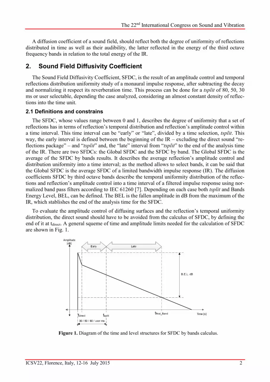
To evaluate the amplitude control of diffusing surfaces and the reflection’s temporal uniformity

distribution, the direct sound should have to be avoided from the calculus of SFDC, by defining the

end of it at tdirect. A general squeme of time and amplitude limits needed for the calculation of SFDC

are shown in Fig. 1.

Figure 1. Diagram of the time and level structures for SFDC by bands calculus.



It is recommended to use tsplit of 80 ms for large and reverberant rooms such as concert halls,

theaters, and auditorias. A tsplit of 30 ms is recommended for rooms with short RT such as control

rooms and studios.

Nevertheless, to proceed to the comparison of different results of SFDC by bands under identical

conditions of analysis, the SFDC should be accompanied by the time interval analysed and tsplit used

(Examples: SFDC, late, 50ms, SFDC, early, 80ms), and the included bands for the Global SFDC.

Certainly, the SFDC is not related to the length of the analysis time interval, or the number of

reflections, or the RT, nor the energies involved. Only analyses the uniformity of the existing reflec-

tions, whether many or few, in the time range of analysis independently if it is short or long. There

may be a high value of SFDC in a very short time period analysed (eg.: between 80 ms and 120 ms),

and a very low value of SFDC in a long time analysis interval (eg.: from 80 ms to 2500 ms), and

viceversa.

SFDC is intended to be applied on a monaural IR, captured with an omnidirectional measurement

microphone. All other type of microphones would yield to equal or lesser SFDC results. Also, the IR

registering method should bring the largest signal to noise level (S/N) possible. That’s why is recom-

mended to use logarithmic sound sweep as stimulus signal, assuring the best possible environmental

conditions inside the room to measure (avoiding impulsive noises, and reducing background station-

ary noise as possible).

To get results between 0 and 1, maximum absolute values are needed to compare with. As the

theoretical condition of total diffusion is not achievable [9], real maximum values were found.

Results of SFDC on the same IR was found to vary mainly in function of selected tsplit, tdirect

and BEL [dB]. The only variable that depends on the quality of the IR is BEL.

It was found that exists a BEL interval for which most of the band’s results remain constant.

3. Absolute values

3.1 Relative to Absolute

The SFDC is the multiplication of the reflection’s time uniformity distribution and the reflection’s

energy control:

(1) 𝑆𝐹𝐷𝐶 = (𝑇𝑒𝑚𝑝𝑜𝑟𝑎𝑙 𝐷𝑖𝑠𝑡𝑟𝑖𝑏𝑢𝑡𝑖𝑜𝑛 𝑢𝑛𝑖𝑓𝑜𝑟𝑚𝑖𝑡𝑦) ∙ (𝐴𝑚𝑝𝑙𝑖𝑡𝑢𝑑𝑒 𝐶𝑜𝑛𝑡𝑟𝑜𝑙)

The SFDC reflection’s temporal distribution uniformity is named distr_coef, and is inversely pro-

portional to the normalized kurtosis, k0 [8] of the amplitude’s reflections at each time interval, as seen

in Eq. 2, Eq. 3 and Eq. 4.

(2) 𝑑𝑖𝑠𝑡𝑟_𝑐𝑜𝑒𝑓 =1

𝑘0∙0.02

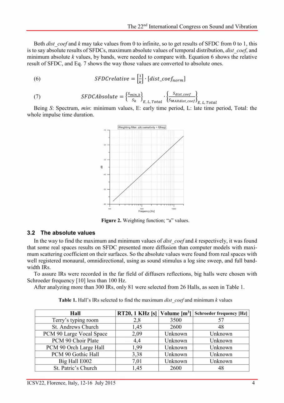
On the other hand, k value is the one that takes the ratio of Eq. 3, by one-third octave bands, to a

group of fixed “a” values of Fig. 2 to overcome the “wave problem”.

(3) 𝑧(𝑘) =𝑅(𝑘)

𝑅𝑇𝑂𝑇𝐴𝐿,

Where:

(4) 𝑅𝑇𝑂𝑇𝐴𝐿 = ∫ ℎ2(𝑡)𝑑𝑡𝑡2

𝑡1

(5) 𝑅(𝑘) = ∫ ℎ2>𝑘(𝑡)𝑑𝑡

𝑡2

𝑡1

The larger k, less amplitude control shows the IR, due it evidences the existence of discrete high-

amplitude reflections; thus a low k value means high reflection’s energy control or uniformity of

amplitudes into the analysed IR.



Both dist_coef and k may take values from 0 to infinite, so to get results of SFDC from 0 to 1, this

is to say absolute results of SFDCs, maximum absolute values of temporal distribution, dist_coef, and

minimum absolute k values, by bands, were needed to compare with. Equation 6 shows the relative

result of SFDC, and Eq. 7 shows the way those values are converted to absolute ones.

(6) 𝑆𝐹𝐷𝐶𝑟𝑒𝑙𝑎𝑡𝑖𝑣𝑒 = [1

𝑘] ∙ [𝑑𝑖𝑠𝑡_𝑐𝑜𝑒𝑓𝑛𝑜𝑟𝑚]

(7) 𝑆𝐹𝐷𝐶𝐴𝑏𝑠𝑜𝑙𝑢𝑡𝑒 = {𝑆𝑚𝑖𝑛_𝑘

𝑆𝑘}

𝐸, 𝐿, 𝑇𝑜𝑡𝑎𝑙∙ {

𝑆𝑑𝑖𝑠𝑡_𝑐𝑜𝑒𝑓

𝑆𝑀𝐴𝑋𝑑𝑖𝑠𝑡_𝑐𝑜𝑒𝑓}

𝐸, 𝐿, 𝑇𝑜𝑡𝑎𝑙

Being S: Spectrum, min: minimum values, E: early time period, L: late time period, Total: the

whole impulse time duration.

3.2 The absolute values

In the way to find the maximum and minimum values of dist_coef and k respectively, it was found

that some real spaces results on SFDC presented more diffusion than computer models with maxi-

mum scattering coefficient on their surfaces. So the absolute values were found from real spaces with

well registered monaural, omnidirectional, using as sound stimulus a log sine sweep, and full band-

width IRs.

To assure IRs were recorded in the far field of diffusers reflections, big halls were chosen with

Schroeder frequency [10] less than 100 Hz.

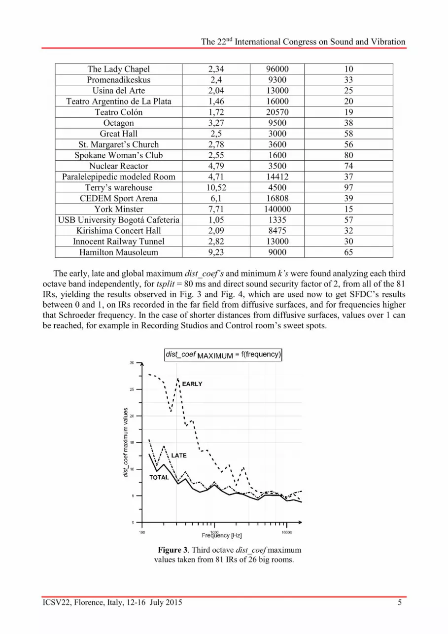
After analyzing more than 300 IRs, only 81 were selected from 26 Halls, as seen in Table 1.

Table 1. Hall’s IRs selected to find the maximum dist_coef and minimum k values

Hall RT20, 1 KHz [s] Volume [m3] Schroeder frequency [Hz]

Terry’s typing room 2,8 3500 57

St. Andrews Church 1,45 2600 48

PCM 90 Large Vocal Space 2,09 Unknown Unknown

PCM 90 Choir Plate 4,4 Unknown Unknown

PCM 90 Orch Large Hall 1,99 Unknown Unknown

PCM 90 Gothic Hall 3,38 Unknown Unknown

Big Hall E002 7,01 Unknown Unknown

St. Patric’s Church 1,45 2600 48

Figure 2. Weighting function; “a” values.



The Lady Chapel 2,34 96000 10

Promenadikeskus 2,4 9300 33

Usina del Arte 2,04 13000 25

Teatro Argentino de La Plata 1,46 16000 20

Teatro Colón 1,72 20570 19

Octagon 3,27 9500 38

Great Hall 2,5 3000 58

St. Margaret’s Church 2,78 3600 56

Spokane Woman’s Club 2,55 1600 80

Nuclear Reactor 4,79 3500 74

Paralelepipedic modeled Room 4,71 14412 37

Terry’s warehouse 10,52 4500 97

CEDEM Sport Arena 6,1 16808 39

York Minster 7,71 140000 15

USB University Bogotá Cafeteria 1,05 1335 57

Kirishima Concert Hall 2,09 8475 32

Innocent Railway Tunnel 2,82 13000 30

Hamilton Mausoleum 9,23 9000 65

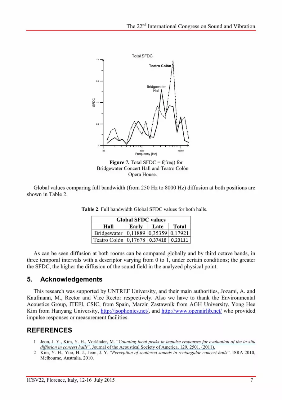
The early, late and global maximum dist_coef’s and minimum k’s were found analyzing each third

octave band independently, for tsplit = 80 ms and direct sound security factor of 2, from all of the 81

IRs, yielding the results observed in Fig. 3 and Fig. 4, which are used now to get SFDC’s results

between 0 and 1, on IRs recorded in the far field from diffusive surfaces, and for frequencies higher

that Schroeder frequency. In the case of shorter distances from diffusive surfaces, values over 1 can

be reached, for example in Recording Studios and Control room’s sweet spots.

Figure 3. Third octave dist_coef maximum

values taken from 81 IRs of 26 big rooms.



4. Results and discussion

With the absolute values previously found, comparisons between spaces and positions can be

made, among other studies. In the following Fig. 5, Fig. 6 and Fig. 7, a comparison was made between

Teatro Colón of Buenos Aires and Bridgewater Hall [11] of Manchester.

Figure 4. Third octave minimum k values

taken from 81 IRs of 26 big rooms.

Figure 5. Early SFDC = f(freq) for

Bridgewater Concert Hall and Teatro Colón

Opera House.

Figure 6. Late SFDC = f(freq) for


Opera House.



Global values comparing full bandwidth (from 250 Hz to 8000 Hz) diffusion at both positions are

shown in Table 2.

Global SFDC values

Hall Early Late Total

Bridgewater 0,11889 0,35359 0,17921

Teatro Colón 0,17678 0,37418 0,23111

As can be seen diffusion at both rooms can be compared globally and by third octave bands, in

three temporal intervals with a descriptor varying from 0 to 1, under certain conditions; the greater

the SFDC, the higher the diffusion of the sound field in the analyzed physical point.

5. Acknowledgements

This research was supported by UNTREF University, and their main authorities, Jozami, A. and

Kaufmann, M., Rector and Vice Rector respectively. Also we have to thank the Environmental

Acoustics Group, ITEFI, CSIC, from Spain, Marzin Zastawnik from AGH University, Yong Hee

Kim from Hanyang University, http://isophonics.net/, and http://www.openairlib.net/ who provided

impulse responses or measurement facilities.

REFERENCES

1 Jeon, J. Y., Kim, Y. H., Vorländer, M. “Counting local peaks in impulse responses for evaluation of the in‐situ

diffusion in concert halls”. Journal of the Acoustical Society of America, 129, 2501. (2011).

2 Kim, Y. H., Yoo, H. J., Jeon, J. Y. “Perception of scattered sounds in rectangular concert halls”. ISRA 2010,

Melbourne, Australia. 2010.

Figure 7. Total SFDC = f(freq) for


Opera House.

Table 2. Full bandwidth Global SFDC values for both halls.

http://isophonics.net/

http://www.openairlib.net/





3 Kim, Y. H. “Evaluation of Wall Diffusers for the Acoustical Design of Concert Halls”. Doctoral dissertation.

Department of Sustainable Architectural Engineering Graduate School, Hanyang University. (2011).

4 Jeon, J. Y., Kim, Y. H. “Investigation of sound diffusion characteristics using scale models in concert halls”.

NAG/DAGA International Conference on Acoustics 2009. The Netherlands. (2009).

5 Hanyu, T. “Analysis method for estimating diffuseness of sound fields by using decay-cancelled impulse response”.

ISRA 2013. Canada. (2013).

6 Randall, K. E. “The measurement of sound diffusion index n small rooms”. Research department Report No.

1969/16. UDC 534.84. BBC. (1969).

7 IEC 61260 ED. 1.0 B:1995. (1995).

8 Rose, P. Forensic Speaker identification. Ch. 8. Taylor & Francis. (2002).

9 Kutruff, H. “Room Acoustics”. Ch. 8. 4th Edition. Spon Press. (2000).

10 Skålevik, M. “Schroeder Frequency Revisited”. Akutek. Forum Acusticum. 2011.

11 https://acousticengineering.wordpress.com

Documents

Sound Field Diffusion Coefficient: Absolute Values