SERDP Final Report EPA WP_1247 4_12_2010 r1

FINAL REPORT Temporal and Modal Characterization

of DoD Source Air Toxic Emission Factors

SERDP Project WP-1247 EPA # RW-96-92280901-0

APRIL 2010

Brian K. Gullett U.S. Environmental Protection Agency This document has been approved for public release.

This report was prepared under contract to the Department of Defense Strategic Environmental Research and Development Program (SERDP). The publication of this report does not indicate endorsement by the Department of Defense, nor should the contents be construed as reflecting the official policy or position of the Department of Defense. Reference herein to any specific commercial product, process, or service by trade name, trademark, manufacturer, or otherwise, does not necessarily constitute or imply its endorsement, recommendation, or favoring by the Department of Defense.

i

Table of Contents

List of Tables ................................................................................................................................. iv

List of Figures ................................................................................................................................ iv

List of Acronyms ......................................................................................................................... viii

Keywords: ....................................................................................................................................... x

Acknowledgements........................................................................................................................ xi

Abstract ......................................................................................................................................... xii

Executive Summary..................................................................................................................... xiii

Objectives ................................................................................................................................... xvii

1. Background................................................................................................................................1

1.1 Emission Factors ...................................................................................................................1

1.2 Monitoring for Organic Toxics .............................................................................................1

1.3 Related Real-time Technologies for Monitoring of Trace Organic Pollutants .....................2

1.4 Related REMPI-TOFMS Studies on Vehicle Exhausts ........................................................2

1.5 Monitoring for Metals ...........................................................................................................3

1.6 Optical Path Methods and Field Measurements....................................................................3

2. Description of Equipment and Methods ....................................................................................5

2.1 REMPI-TOFMS ....................................................................................................................5

2.1.1 Laser Systems................................................................................................................7

2.1.2 Valve Inlet Systems.......................................................................................................9

2.1.3 Time of Flight Mass Spectrometer ..............................................................................10

2.1.4 REMPI-TOFMS Instrument ........................................................................................11

2.1.5 Operating Procedures REMPI-TOFMS.......................................................................12

2.2 LIBS ....................................................................................................................................14

2.3 ORS .....................................................................................................................................15

3. REMPI-TOFMS: Field Ready Development and Performance Evaluation and Improvement ............................................................................................................................17

3.1 Laser Systems......................................................................................................................17

3.1.1 Continuum Laser .........................................................................................................17

3.1.2 OPOTEK Laser............................................................................................................17

3.2 Pulsed Valve Operation.......................................................................................................18

3.3 Data Acquisition Software ..................................................................................................19

3.4 Calibration of REMPI-TOFMS System..............................................................................20

4. Sampling from DoD Sources ...................................................................................................21

5. Source 1: Validation of REMPI-TOFMS Measurements on a U.S. Marine Corps Diesel Generator ......................................................................................................................22

5.1 Experimental section ...........................................................................................................22

ii

5.2 Results and Discussion........................................................................................................23

5.2.1 Steady State Diesel Generator Results ........................................................................23

5.2.2 Transient Diesel Generator Results .............................................................................31

6. Source 1: U.S. Marine Corps Diesel Generator Air Toxic Emission Characterization...........34

6.1 Experimental .......................................................................................................................34


6.2.1 Steady State Emissions................................................................................................37

6.2.2 Emissions during Startups ...........................................................................................37

6.2.3 Emissions during Load Variation ................................................................................41

7. Source 2: Real-Time Measurement of Trace Aromatics during Operation of Aircraft Ground Equipment...................................................................................................................44

7.1 Experimental .......................................................................................................................44

7.1.1 AGE.............................................................................................................................44

7.1.2 Operating and Sampling Procedures ...........................................................................45


7.3 ORS Measurements during AGE sampling.........................................................................56

7.3.1 Experimental Design ...................................................................................................56

7.3.2 ORS Instrument-Retro reflector Distance ...................................................................57

7.4 Data Processing ...................................................................................................................57

7.4.1 ORS Results.................................................................................................................58

8. Source 3: Verification Results of REMPI-TOFMS as a Real-Time PCDD/F Emission Monitor ....................................................................................................................................61

8.1 Materials and Methods ........................................................................................................61

8.1.1 Boiler testing................................................................................................................61

8.1.2 REMPI-TOFMS Testing .............................................................................................62

8.1.3 Indicator Compounds ..................................................................................................63


8.2.1 Pre-ETV results ...........................................................................................................64

8.2.2 ETV Results.................................................................................................................64

9. Source 4: Sampling from MWC Flue Gas...............................................................................68

9.1 Portsmouth Naval Shipyard Waste Combustor 2004..........................................................68

9.2 Experimental Approach.......................................................................................................68

9.3 Test Matrix ..........................................................................................................................69

9.4 Results .................................................................................................................................70

9.4.1 General On-site REMPI-TOFMS Instrument Performance ........................................70

9.4.2 REMPI-TOFMS results...............................................................................................70

9.4.3 Method 0023 and Method 0010 Results......................................................................73

9.5 Portsmouth Naval Shipyard Waste Combustor 2006..........................................................73

9.6 Materials and Methods ........................................................................................................75

iii

9.7 Results .................................................................................................................................76

10. Source 5: Emission Responses from HMMWVs, the M1 Abrams Tank, and the Bradley IFV .............................................................................................................................79

10.1 Experimental .......................................................................................................................79

10.1.1 Platforms Tested ..........................................................................................................79

10.1.2 Test Protocols ..............................................................................................................80

10.1.3 Sampling Approach .....................................................................................................80


10.2.1 WV Cycle ....................................................................................................................83

10.2.2 HWFET Cycle .............................................................................................................85

10.2.3 Velocity/Gradient Cycle ..............................................................................................85

10.2.4 Startups ........................................................................................................................86

10.2.5 Bradley and Abrams ....................................................................................................87

10.2.6 Number Size Distributions (NSDs) .............................................................................90

10.3 Emission Correlations .........................................................................................................90

11. Source 6: F-15 and F-22 Aircraft Engine Emissions...............................................................93

11.1 Experimental Method..........................................................................................................93

11.1.1 Aircraft/Engine ............................................................................................................93

11.1.2 Testing Venue..............................................................................................................94

11.1.3 Exhaust Sampling........................................................................................................95

11.1.4 REMPI-TOFMS Sampling Approach .........................................................................95

11.1.5 REMPI-TOFMS Data Analysis Procedure..................................................................96

11.2 Results .................................................................................................................................97

11.2.1 F-15 Tests ....................................................................................................................97

11.2.2 F-22 Tests ..................................................................................................................100

12. Conclusions............................................................................................................................108

13. References..............................................................................................................................110

14. Appendix A: List of Scientific/Technical Publications .........................................................116

14.1.1 Journal Articles..........................................................................................................116

14.2 Oral and Poster Presentations............................................................................................116

iv

List of Tables

Table 4-1. Source testing............................................................................................................21

Table 6-1. EPA sampling methods.............................................................................................35

Table 6-2. Air toxic emission factors determined by jet REMPI-TOFMS, OLGC, and EPA reference methods, and listed in AP-42. ..........................................................39

Table 6-3. RA of the three measurement methods during parallel sampling.............................40

Table 7-1. Emission factors for BTEX compounds during idle and full load operation. Comparison with published values. ..........................................................................52

Table 7-2. Emission factors for PAH compounds during idle and full load operation. Comparison with published values. ..........................................................................53

Table 7-3. Emission factors for aldehydes compounds during idle and full load operation. Comparison with published values..........................................................54

Table 8-1. Candidate TEQ surrogate compounds from pre-ETV Method 0010 sampling....................................................................................................................63

Table 9-1. R2 for PCDD/F TEQ based on 36, 5-min samples at the MWI. ...............................75

Table 9-2. PCDD/F TEQ emission rates from HRGC/HRMS analyses. ...................................76

Table 10-1. Emission factors of M1097 and M1114 HMMWVs. ...............................................84

Table 11-1. Engine power settings tested.....................................................................................94

Table 11-2. Summary of F-15 engine tests. .................................................................................97

Table 11-3. Test schedule for the F-22 engine tests...................................................................101

Table 11-4. A comparison between Summa canister, REMPI-TOFMS and PTR-MS data with the PTR-MS average calculated from provided Battelle data and canister sampling time. ...........................................................................................102

List of Figures

Figure 2-1. REMPI-TOFMS instrument........................................................................................5

Figure 2-2 (a, b, c). REMPI ionization principles.........................................................................6

Figure 2-3. Top View of the Movable Inlet Mounting Plate. ......................................................10

Figure 2-4. Schematic of LR10 compact 19” rack-mount reflectron TOFMS............................11

Figure 2-5. Two views of large REMPI-TOFMS system. ..........................................................11

Figure 2-6. Compact REMPI-TOFMS instrument. .....................................................................12

Figure 2-7. Detection of multiple analytes using wavelength-dependent ionization. .................13

Figure 2-8. Transient benzene concentrations detected in vehicle exhaust while running a dynamometer-based RS. ........................................................................................13

Figure 2-9. REMPI-TOFMS mass spectrum at benzene (78) wavelength as observed in vehicle exhaust..........................................................................................................14

Figure 2-10. Schematic setup of LIBS system. ............................................................................15

v

Figure 2-11. Setup ORS during sampling......................................................................................16

Figure 3-1. Wavelength emitted from laser with increased ambient temperature (increase in temperature for scan 1 to 9)...................................................................18

Figure 3-2. Snapshot of data acquisition software in operation. .................................................20

Figure 5-1. U.S. Marine Corps tactical utility generator. ............................................................23

Figure 5-2. A 3D survey scan (mass, wavelength, ion signal) ....................................................24

Figure 5-3. Time-of-flight mass spectrum recorded at (A) optimum styrene (287.7 nm) and (B) Benzene (259.0 nm) ionization wavelength in diesel generator exhaust. .....................................................................................................................25

Figure 5-4. Comparison of 1+1 REMPI wavelength spectrum recorded for toluene in diesel generator exhaust and from calibration gas standard (the latter scaled to equal intensity)......................................................................................................26

Figure 5-5. Monitored REMPI-TOFMS signal for reference gas (C6D6) and benzene in exhaust diesel generator............................................................................................26

Figure 5-6. On-line REMPI-TOFMS ion signal traces of nine individual target analytes, labeled with mass, chemical name and used, most favorable ionization wavelength. ...............................................................................................................27

Figure 5-7. Recorded ion signals during nine repeats of the analyte cycle. ................................28

Figure 5-8. Observed day to day variations in estimated concentrations of BTEX-like analytes in exhaust diesel generator..........................................................................29

Figure 5-9. Comparison between extractive and REMPI-TOFMS concentrations for three exhaust analytes. ..............................................................................................30

Figure 5-10 (a, b). (a) Real-time transient benzene emissions following a cold start. (b) Normalized ion signal traces for single aromatic ring (thin lines) and double aromatic ring (fat lines) analytes. .............................................................................32

Figure 5-11. Transient REMPI-TOFMS results. ...........................................................................33

Figure 6-1. Cold and hot start-up emissions of benzene, naphthalene, CO, and CO2 with exhaust temperature. .................................................................................................38

Figure 6-2. Temporal temperature and particle-bound PAH concentrations in the diesel exhaust. .....................................................................................................................41

Figure 6-3. Load change emissions of benzene, naphthalene, CO, and CO2 with exhaust temperature. ..............................................................................................................42

Figure 6-4. Temperature distribution and particle-bound PAH concentrations under varying loads.............................................................................................................43

Figure 7-1. Aircraft ground equipment outside EPA facilities....................................................45

Figure 7-2. REMPI-TOFMS time-resolved trace of cold startup, idle (low) load, and high load conditions..................................................................................................47

Figure 7-3. REMPI-TOFMS wavelength-resolved trace during idle (low) load condition...................................................................................................................................48

Figure 7-4. Comparison of (selected) AGE wavelength spectra versus the TO-14 calibrated gas standard..............................................................................................49

vi

Figure 7-5. Comparison between GC/MS and REMPI-TOFMS analysis of summa canister gases. ...........................................................................................................50

Figure 7-6. Comparison between REMPI-TOFMS measurements at low load and TO15 method analyses by two laboratories. .......................................................................50

Figure 7-7. REMPI-TOFMS and CO and CO2 CEM concentrations during a series of startups (the initial startup was a cold start) and shutdowns (for refueling), operating at high, high, then idle load. Range of data (barely visible) are shown for benzene. ...................................................................................................51

Figure 7-8. Comparison of startup responses of benzene and naphthalene for the AGE and diesel generator. .................................................................................................56

Figure 7-9. ORS measurement configuration..............................................................................57

Figure 7-10. Comparison of the reference spectrum of formaldehyde (blue trace) to a measured spectrum of the turbine plume (red trace) ................................................59

Figure 7-11. Comparison of the reference spectrum of ethylene (red trace) to a measured spectrum of the turbine plume (blue trace)...............................................................59

Figure 7-12. Comparison of the reference spectrum of n-octane (red trace) to a measured spectrum of the turbine plume (blue trace)...............................................................60

Figure 7-13. Comparison between CEM and ORS measurements................................................60

Figure 8-1. Marine package boiler at EPA facilities. ..................................................................62

Figure 8-2. Pre-ETV phase determination of MClBz as a PCDD/F TEQ surrogate...................65

Figure 8-3. REMPI-TOFMS mass spectrum of MClBz with inset of relevant mass range. 0.1 ppb for a 4 min averaging period, S/N = 3. ........................................................65

Figure 8-4. ETV phase comparison of TEQ from Method 23 and MClBz prediction from REMPI-TOFMS measurements.......................................................................66

Figure 8-5. Comparison of M-10 and time-integrated REMPI predictions of PCDD/F TEQ with actual M-23 measurements. .....................................................................67

Figure 9-1. Comparison between real time results for PAHs acquired with REMPI-TOFMS at identical Boiler A and Boiler B for two 4-h intervals that were typical of the normal (steady state) operation...........................................................71

Figure 9-2. Emissions of PAHs during shutdown of boiler. Break in data during filter change. ......................................................................................................................71

Figure 9-3. A 3-dimensional qualitative depiction PAH emissions during the startup of a boiler (at ~ t=10 min)................................................................................................72

Figure 9-4. Emissions of selected PAHs and monochlorobenzene during startup of boiler (at ~ 9:00 AM)................................................................................................72

Figure 9-5. Comparison between REMPI-TOFMS time averaged concentrations and those from conventional Method 0010 sampling during the course of the sampling campaign. ..................................................................................................74

Figure 9-6. Mass spectrum recorded at monochlorobenzene wavelength (~ 270.8 nm).............74

Figure 9-7. PCDD/F TEQ, conventional 1,2,4 triClBz and mass 18- REMPI-TOFMS ion signal over the coarse of the four day sampling campaign.................................77

Figure 9-8. Recorded REMPI-TOFMS ion signals for mass 180/182/184. ................................78

vii

Figure 10-1. Emission transients for the M1097 and M1114 HMMWVs. A: West Virginia and B: Highway HWFET cycles. ...............................................................80

Figure 10-2. Steady-state benzene, naphthalene, methylnaphthalene, CO, and CO2 emissions from the M1097 and M1114 HMMWVs during a velocity and gradient stepped cycle...............................................................................................86

Figure 10-3. Cold start emissions of benzene, naphthalene, methylnaphthalene, CO, and CO2 and PM size distribution for the M1097 (left) and M1114 (right) HMMWVs. ...............................................................................................................87

Figure 10-4. Steady state organic emissions at analyte-specific wavelengths, A: M1 Abrams, low and high idle conditions, and B: Bradley IFV, idle 0 and 2 trials. Inset: real-time variance of organics at low idle.............................................88

Figure 10-5. Cold and warm start emissions of benzene, naphthalene, and methylnaphthalene for the Bradley IFV and M1 Abrams. .......................................89

Figure 10-6. Benzene, naphthalene, and methylnaphthalene emissions during a shutdown of the M1 Abrams. ....................................................................................................89

Figure 10-7. Steady state PM size distribution for the M1097 HMMWV (top) and M1114 HMMWV (bottom) during a stepped velocity and gradient cycle. ..........................91

Figure 10-8. Steady state REMPI, ELPI, and CEM data for the M1097 (left) and M1114 (right). .......................................................................................................................92

Figure 11-1. Trimpad and location of probe and instrument trailers with respect to aircraft........95

Figure 11-2. Concentration profiles during F-15 engines testing..................................................98

Figure 11-3. Concentration profiles during second sequence of F-15 engine testing. ..................98

Figure 11-4. Concentration profiles during the 30 minute test 2B1. .............................................99

Figure 11-5. Complete 2B series. ..................................................................................................99

Figure 11-6. Concentration during first sampling of F-22 engine...............................................103

Figure 11-7. Concentrations during 4A and 4B sampling of F-22 engine. .................................103

Figure 11-8. Concentrations for other REMPI-TOFMS detectable analytes. .............................104

Figure 11-9. Comparison between REMPI-TOFMS and PTR-MS. ...........................................104

Figure 11-10. Benzene and PAHs response during afterburner test. ........................................105

Figure 11-11. Comparison REMPI-TOFMS with PTR-MS for benzene and naphthalene. 106

Figure 11-12. Comparison between time averaged REMPI-TOFMS benzene data and Summa canister results. ..........................................................................................106

Figure 11-13. Benzene concentrations as function of thrust level F-22 engine........................107

Figure 11-14. Benzene emission factor (µg/g carbon burned) for F-22 engines. .....................107

viii

List of Acronyms

AFB Air Force Base AGE Aircraft Ground Equipment APCS Air Pollution Control System APIMS Air Permit Information Management System APU Auxiliary Power Unit AVG Average AWMA Air and Waste Management Association AZ Arizona BTEX Benzene, Toluene, Ethylbenzene, and Xylenes CAA Clean Air Act CEM Continuous Emission Monitors CLS Classical Least Squares CO Carbon monoxide CO2 Carbon Dioxide DNPH 2,4-Dinitrophenylhydrazine DoD Department of Defense DOE Department of Energy ECD Electron Capture Detector ELPI Electrical Low Pressure Impactor EPA Environmental Protection Agency ETV Environmental Technology Verification FID Flame Ionization Detector FTIR Fourier Transform Infrared Spectroscopy FWHM Full Width Half Maximum GC Gas Chromatography GC/MS Gas Chromatography/Mass Spectrometry GHz Gigahertz HAP Hazardous Air Pollutants HEPA High Efficiency Particulate Arresting HMMWV High Mobility Multipurpose Wheeled Vehicle HPLC High Performance Liquid Chromatography HRGC High Resolution Gas Chromatography HRMS High Resolution Mass Spectroscopy HWFET Highway Fuel Economy Test IFV Infantry Fighting Vehicles LACEA Laser Applications to Chemical and Environmental Analysis LIBS Laser Induced Breakdown Spectroscopy LRMS Low Resolution Mass Spectrometry LTA Low Temperature Ashing MHz Megahertz MS Mass Spectrometry MWC Municipal Waste Combustor ND Non Detect NDIR Non-dispersive Infrared Analyzer

ix

NIST National Institute of Standards and Technology NO Nitric Oxide NSD Number Size Distributions OLGC On Line Gas Chromatography OP-FTIR Open Path Fourier Transform Infrared OPO Optical Parametric Oscillators ORS Optical Remote Sensing PAC Path Average Concentration PAH Polycyclic Aromatic Hydrocarbons PAS Photoelectric Aerosol Sensor PCDD Polychlorinated Dibenzodioxins Dibenzofurans PCDD/F PolyChlorinated Dibenzo-p-Dioxin and polychlorinated

dibenzoFuran PIC Products of Incomplete Combustion PM Particulate Matter PTFE PolyTetraFluoroEthylene PTRMS Proton Transfer Reaction Mass Spectrometer PTR-MS Proton Transfer Reaction - Mass Spectrometry RA Relative Accuracy RDF Refuse Derived Fuel REMPI Resonance Enhanced Multi Photon Ionization REMPI-TOFMS Time of Flight Mass Spectrometry RPM Revolutions per Minute RSD Relative Standard Deviation RTP Research Triangle Park RWS Roadway Simulator S/N Signal Noise SDA Spray Dryer Catwalk Area STP Standard Pressure SVOC Semi Volatile Organic Compounds TEF Toxic Equivalency Factor TEQ Toxicity Equivalent TIC Tentatively Identified Compounds TOFMS Time of Flight Mass Spectrometry U.S. United States UV Ultraviolet VOC Volatile Organic Compounds

x

Keywords:

Resonance-enhanced multiphoton ionization spectroscopy REMPI Time of flight mass spectrometry TOFMS Laser-induced breakdown spectroscopy LIBS Open path measurements Air toxics Air pollutants Measurement Emission factors Diesel generator Auxiliary power unit Municipal waste combustor HMMWV Abrams tank Bradley Infantry Fighting Vehicle F-15 F-22

xi

Acknowledgements

The investigators and authors would like to extend their appreciation and acknowledge to the SERDP organization for funding this research program, and would also like to thank the following organizations and individuals that contributed to the success of this project:

• Drs. Abderrahmane Touati and Lukas Oudejans of Arcadis U.S., Inc. enacted the testing programs and performed the organic measurements throughout this project.

• Drs. Harald Oser and Michael Coggiola of SRI International were critical providers of the resonance enhanced multi photon ionization (REMPI) technology and able consultants throughout the program.

• Dr. Andrzej Miziolek of the Army Research Laboratory was the primary motivator of the laser induced breakdown spectroscopy (LIBS)-related work.

• Drs. Shannon Serre and Emily Gibb-Snyder (United States (U.S.) Environmental Protection Agency (EPA), National Homeland Security Research Center) provided critical expertise with the LIBS instrument and experimentation.

• Messrs. Whaley, Huffman, and Winberry from U.S. Marine Corps at Camp Lejeune for loan of the tactical generator

• Col. Steven Aylor, SMSgt David Caldwell, and Sgts. Thomas Clemens, George Garnot, and James Scaccia from Pope Air Force Base (AFB) for the loan of the AGE.

• Dr. Ken Cowen from Battelle Memorial Institute

• Messrs. Michael Barnett and Jeff Landrum from the Southern Public Service Authority Power Plant (Portsmouth, Virginia)

• Messrs. William Bolt, Jason Jack, and Gregg Schultz from the Aberdeen Test Center, Maryland, for access to vehicles and the Roadway Simulator (RWS).

• Dr. Howard Mayfield from Tyndall AFB, Panama City, Florida

xii

Abstract

This project tested three, real-/near real-time monitoring techniques to develop air toxic emission factors for Department of Defense (DoD) platform sources. These techniques included: resonance enhanced multi photon ionization time of flight mass spectrometry (REMPI-TOFMS) for organic air toxics, laser induced breakdown spectroscopy (LIBS) for metallic air toxics, and optical remote sensing (ORS) methods for measurement of criteria pollutants and other hazardous air pollutants (HAPs). Conventional emission measurements were used for verification of the real-time monitoring results. The REMPI-TOFMS system was demonstrated on the following:

• a United States U.S. Marine Corps (USMC) diesel generator,

• a U.S. Air Force auxiliary power unit (APU),

• the waste combustor at the Portsmouth Naval Shipyard, during a multi-monitor Environmental Technology Verification (ETV) test for dioxin monitoring systems,

• two dynamometer-driven high mobility multi-purpose wheeled vehicles (HMMWVs),

• an idling Abrams battle tank,

• a Bradley infantry fighting vehicle (IFV), and

• an F-15 and multiple F-22 U.S. Air Force aircraft engines. LIBS was tested and applied solely to the U.S. Marine Corps diesel generator. The high detection limits of LIBS for toxic metals limited its usefulness as a real time analyzer for most DoD sources. ORS was tested only on the APU with satisfactory results for non-condensable combustion products [carbon monoxide (CO), carbon dioxide (CO2)] but with limited success on condensable volatile organic by-products. This program demonstrated the ability to measure trace aromatics with REMPI-TOFMS in harsh environments and with a high degree of accuracy and precision.

xiii

Executive Summary

The Department of Defense (DoD) quantifies air pollutant emissions from its facilities and weapon platforms in order to identify potential sources needing remediation and to comply with base permitting requirements. These pollutants include the so-called criteria pollutants such as nitrogen oxides and particulate matter (PM) as well as trace air toxics. This information further enables DoD to employ measures such as adoption of preventive operational modes or equipment substitution in order to minimize disruption of training and operational activities. Information on source air toxics is particularly limited, primarily due to lack of automated methods of sample analysis, underscoring the need for innovative approaches, instruments, and methods to achieve these ends. Since a large portion of DoD sources are mobile sources that operate under non-steady state modes, most of the current extractive methods cannot resolve modal or temporal changes in emissions that result from such type of sources, leading to gaps in the overall DoD air toxics emissions inventory. The United States Environmental Protection Agency (EPA), under a DoD Strategic Environmental Research and Development Program, “Source and Ambient Air Monitoring for DoD Operations (WP/CP1247),” initiated and completed a research project to develop and validate the latest state-of-the-art technologies for these measurements. These technologies would provide modal and time resolved measurements of air toxics emissions from various types of point- and mobile-sources. Such information could be used, for example, in the Air Force's Air Permit Information Management System (APIMS), an emission inventory system currently used by Hill AFB and being adopted DoD-wide, as well as to improve EPA's AP-42 emission factor system. This report presents the results of this project. The project objective was approached through the applied development of a combination of three unique, versatile, field-ready, real or near real-time monitoring techniques that can measure trace air toxic levels: resonance enhanced multi photon ionization time of flight mass spectrometry (REMPI-TOFMS) for organic air toxics, laser induced breakdown spectroscopy (LIBS) for metallic air toxics, and optical remote sensing (ORS) methods for verification and measurements of criteria pollutants and other hazardous air pollutants (HAPs). Conventional emission measurements were used for verification of the real-time monitoring results and assessment of their accuracy. A fast sampling method that separates particles from gases was successfully integrated in an overall sampling scheme designed to conserve the integrity of the sample, avoid any particle/gas partitioning, while bringing the quantity of target compounds above the detection limit of the REMPI-TOFMS measurement technique.

Satisfactory development of the REMPI-TOFMS system, from laboratory to a field-ready real or near real time monitor of trace organic aromatic pollutants system, was performed at the EPA research facility in Research Triangle Park (RTP), North Carolina. The system has been demonstrated on the following:

• a U.S. Marine Corps (USMC) diesel generator,

• a U.S. Air Force auxiliary power unit (APU),

• the waste combustor at the Portsmouth Naval Shipyard, during a multi-monitor Environmental Technology Verification (ETV) test for dioxin monitoring systems,

xiv

• two dynamometer-driven High Mobility Multi-purpose Wheeled Vehicles (HMMWVs),

• an idling Abrams battle tank,

• a Bradley infantry fighting vehicle (IFV), and

• an F-15 and multiple F-22 U.S. Air Force aircraft engines. LIBS was tested and applied solely to the U.S. Marine Corps diesel generator. The high detection limits of LIBS for toxic metals limited its usefulness as a real time analyzer for most DoD sources, resulting in the withdrawal of the U.S. Army Research Laboratory from the SERDP project. ORS was tested only on the APU with satisfactory results for non-condensable combustion products [carbon monoxide (CO), carbon dioxide (CO2)] but with limited success on condensable volatile organic by-products thereby eliminating the opportunity to directly compare the ORS and REMPI-TOFMS technology. During the SERDP funding period 2003-2008, the following (in approximate chronological order) achievements were made:

• A large laboratory scale size REMPI-TOFMS system has been applied to the exhaust of an USMC diesel generator. Steady state benzene, toluene, ethylbenzene, and xylenes (BTEX) emissions on the order of 100 ppb were observed. Cold start benzene emissions were observed on the order of 14 ppm, which lasted ~ 20-30 seconds. The REMPI-TOFMS results were successfully compared to measurements obtained by conventional certified EPA methods, and validated the system as responsive and functional with complex mixtures. LIBS results from the USMC diesel generator study were found to be unsatisfactory due to the lack of sensitivity for real time detection of metals in the exhaust gas and limited detection of metals on soot loaded filters collected during the sampling of the exhaust. LIBS plus low temperature ashing (LTA) showed positive results, improving metal discrimination from highly carbonaceous backgrounds. However, the examined DoD sources to date did not show sufficient metal emissions to be quantified by LIBS with LTA.

• Testing by SRI International on a compact REMPI-TOFMS indicated a minimal sacrifice of system quality and so the small system was approved for design and construction by SERDP. A first compact REMPI-TOFMS system was delivered to EPA in April 2004.

• REMPI-TOFMS emission measurements were completed on an Auxiliary Power Unit/Aircraft Ground Equipment (APU/AGE). This was a turbine engine compressor from Pope AFB (type A/M32A-95). Modal-dependent results for benzene, toluene, ethylbenzene, o-, m-, p-xylenes, and styrene showed excellent agreement with standard EPA sampling methods and gas chromatography/mass spectrometry (GC/MS) analysis. The ORS system was applied to this source, and measurements for criteria pollutants such as CO2 and CO emissions were completed. In addition to these species, absorption bands for formaldehyde, ethylene, and aliphatic mixtures that originated from the fuels were found in the measured spectra.

• A prototype compact REMPI-TOFMS developed under another project was taken into the field (December 2004) to the Portsmouth Naval Shipyard waste combustor and tested

xv

on the flue gas prior to the air-pollution-cleaning-device. The sampling system platform consisted of the REMPI-TOFMS system and a novel rotating filtering system designed to conserve the integrity of the sample and avoid or minimize any particle or gas partitioning. Real time detection of various small polycyclic aromatic hydrocarbons (PAHs) and monochlorobenzene in the flue gas of the combustor was accomplished. Results from parallel conventional sampling for dioxins and furans and semivolatiles were used to establish correlations between the aforementioned analyte classes.

• The design for the SERDP-funded REMPI-TOFMS field unit was submitted in February 2004 as a required SERDP “Go/No Go” deliverable. The design consisted primarily of a compact laser system and rack mounted TOFMS for organics measurements, with two distinct inlet types for increased flexibility. The simpler inlet system could be used with a fixed frequency laser system.

• The compact REMPI-TOFMS system was delivered to EPA in May, 2005 after an initial evaluation at SRI International.

• The REMPI-TOFMS system participated in an EPA ETV test at the EPA laboratories in RTP, NC. The ETV test verified the performance of four different detection systems for chlorinated dioxins, trace air toxics. This was the first fully international ETV test, with participants from Japan, Austria, and Germany complementing the EPA-SRI International participation. The ETV verification reports are available at http://www.epa.gov/etv/vt-ams.html#dems.

• The capabilities of REMPI-TOFMS towards detection of higher-chlorinated benzenes were extended after the addition of a second (fixed) wavelength option for a two color REMPI approach on one of the two compact systems. Results showed minimal loss in REMPI-TOFMS sensitivity with increasing level of chlorination while maintaining the ability to separate individual isomers.

• The REMPI-TOFMS instrument was taken to the Aberdeen Test Center’s RWS for sampling of exhausts from two different (M1097 and M1114) HMMWVs as driven on various simulated roadway profiles as well as steady state velocity profiles. It included parallel sampling for CO, CO2 and PM [via an electrical low pressure impactor, (ELPI)]. Additional data were obtained from the exhausts of M1 Abrams and Bradley track vehicles under start-up, shutdown, and stationary idle conditions. A journal paper detailing the performance of REMPI-TOFMS in characterizing real-time air toxic emissions during the Aberdeen RWS tests has been submitted to Atmospheric Environment entitled “Transient PAH, PM, CO, and CO2 Emission Responses from HMMWVs, the M1 Abrams tank, and the Bradley Infantry Fighting Vehicle” by Brian Gullett, Lukas Oudejans, and Abderrahmane Touati (2009).

• Two compact REMPI-TOFMS instruments were taken into the field (December 2006) to the Portsmouth Naval Shipyard waste combustor and tested on the flue gas before the gas entered the air-pollution-cleaning-system. One instrument monitored PAHs while the other (two-color) REMPI-TOFMS instrument was focused on real time detection of 1,2,4-trichlorobenzene as a potential indicator of dioxin toxicity based on previously obtained results at the same combustor facility.

xvi

• The REMPI-TOFMS instrument was deployed to Tyndall AFB, Florida, for sampling of jet engine exhausts in collaboration with Battelle Memorial Institute. Emission factors were obtained for individual engines from an F-15 jet aircraft and four F-22 aircraft as operated on a trimpad. Results were consistent and found to be in good (benzene) to fair (naphthalene) agreement with proton transfer reaction MS (PTRMS), another real time detection method for these compounds. A comparison of the time averaged REMPI-TOFMS data with conventionally sampled summa canisters was good across the whole (benzene) dataset. The results are currently (July, 2009) being written into a paper prime-authored by Battelle.

xvii

Objectives

This project applied state-of-the-art trace pollutant detection technologies for the determination of emission factors for Department of Defense (DoD) sources. Results from these technologies were to be verified via comparisons with conventional extractive sampling measurement techniques. The ultimate results will provide temporal and spatial measurements of the air toxics at tested DoD sources. The state-of-the-art technologies are:

• Jet Resonance Enhanced Multiphoton Ionization (REMPI)-Time of Flight Mass Spectrometer (TOFMS)

• Laser Induced Breakdown Spectroscopy (LIBS)

• Optical Remote Sensing (ORS)

The United States Environmental Protection Agency (EPA) regulates emissions of air toxics under the EPA - Clean Air Act (CAA) and DoD needs to address the potential impacts of these regulations on its operations. Identification of potential DoD sources which contribute to ambient air toxic levels, mobile sources in particular, will permit DoD to devise strategies to control and minimize emissions of air toxic pollutants from its facilities and from its on-road and non-road sources. Currently, the major DoD air emission database for toxic air compounds is very limited in scope since measurement methods for many of the 188 air toxics listed in the CAA have not yet been developed; further, when these measurement methods have been developed, most of them do not produce temporally and spatially resolved measurements. Spatially and temporally resolved emission measurements are needed to assess their impact, if any, on ambient air toxic levels, and to determine what operational modes contribute significantly to these emissions.

1

1. Background

1.1 Emission Factors

Source-specific emission factors are often required in order to comply with state reporting regulations or permit requirements which requires a quantitative emissions inventory of more than 500 species of toxic air pollutants (Levy et al., 1993). Preference is usually given to sampled information rather than use of generic emission factors. However, both sampling data and emission factors are limited in breadth since relatively few sources have been characterized for the approximately 188 defined hazardous air pollutants (HAPs) which include both organic and metallic compounds (EPA, 2004). This fact reflects the difficulty and cost of assessing a multitude of emissions from a myriad of sources. A further complication of emissions quantification is that many of these methods were validated on specific sources and are of uncertain universal applicability. Very few of the current extractive methods can resolve modal or temporal changes in emissions that can be related to, for example, load changes or start-ups. For some sources these non-steady-state emissions are suspected to be a significant portion of the total air pollution emitted, and hence, their quantification may be important towards determining average emission factors, pollutant exposure, and mode-specific pollutant minimization. Protocols for source emissions characterization are a function of sampling and analytical limitations. Analytical detection limits also determine sampling protocols, primarily related to sample volume collection time necessary to avoid non-detects. For HAPs, these limitations can be particularly influential, since HAP concentrations are typically significantly lower than other pollutants such as criteria pollutants NOx, CO, and SO2. Hence, sampling protocols for HAPs typically require long-term, steady state monitoring and this requirement prevents observation of HAP transients. 1.2 Monitoring for Organic Toxics

Analyses for trace organic HAPs typically require a 4 h extractive sample taken on an annual or less frequent basis and lengthy laboratory analyses which are not conducive to prompt feedback. From a regulatory or public interest viewpoint, this results in an infrequent and potentially minimally representative monitoring scheme. The conventional methods also provide little assurance that subsequent emissions remain controlled, especially during periods of transient upsets, such as startups and shutdowns, when emissions are typically higher. Real time detection, high sensitivity, and high selectivity are three key requirements toward process control for combustion-derived HAPs. Recent technological advances in measurement of HAPs show promise for continuous, real time monitoring. This raises the possibility of minimizing their formation through feedback to the combustion process control, assurance to the public of compliance, and minimization of over-design of gas cleaning systems. Since the typical ppq-level concentrations of the toxic HAP congeners are beyond the detection limits (~ 100 ppt)

2

of developing monitoring technologies, two strategies have been adopted: (1) use of higher concentration indicator, or surrogate, compounds to infer HAP concentrations of trace HAP compounds such as polychlorinated dibenzodioxins/dibenzofurans (PCDDs/Fs), and (2) concentration of emissions on a sorbent followed by a purge and analysis. Indicator compounds are determined by conventional sampling and analysis (GC/MS) and are chemically similar compounds to the target HAPs. These indicator compounds may be precursors to PCDDs/Fs or pollutants formed in similar, parallel reactions. The universality of these indicator compounds across facility types remains to be investigated, but they likely vary somewhat depending on the plant type, the waste and fuel types, and plant operating and combustion conditions. The presence of a real time monitor raises the first possibility to provide operational feedback to minimize the formation of HAPs, such as polychlorinated dibenzo-p-doxin and polychlorinated dibenzofuran (PCDD/F), as well as characterization of emissions during operational transients. This would be an important capability for distinguishing effects of operating modes or air pollution control equipment failures on HAP emissions. Indeed recent work (Gass, 2002; Gullett et al., 2006) has demonstrated seven-fold increases in PCDD/F emissions during 1 h combustor shutdowns and startups, consistent with other work (Gross et al., 2004; Neuer-Etscheidt et al., 2006) in which PCDD/F raw gas levels increased by one to two orders of magnitude during transient combustion conditions. The extent to which these transient emissions may affect short- and long-term stack emission values and, hence, compliance issues, is undetermined. The rapid variation of PCDD/F, as well as other co-pollutants, due to transients, fuel changes, and operating variations suggests that fast on-line monitoring is necessary in order to effect changes in operating conditions that will reduce or prevent conditions favorable to PCDD/F formation. Work with REMPI-TOFMS at an industrial hazardous waste incinerator was successfully able to monitor aromatics including monochlorobenzene during the introduction of barrels of liquid hazardous waste (Heger et al., 2001), finding transient evolution of the pollutants. The ability to measure facility transients for indicator concentrations with REMPI-TOFMS and to correlate their levels with toxicity equivalent (TEQ) values has yet to be established. 1.3 Related Real-time Technologies for Monitoring of Trace Organic Pollutants

Only a few studies exist in which low molecular weight hydrocarbons have been analyzed in detail for diesel trucks, air ground equipment or Army vehicles. The typical extractive method with GC or GC/MS analysis does not detect transient emission events, such as a cold starts, since the timescales of the event are much shorter than the typical sampling time of several minutes for extractive sampling. GC/MS also prevents full speciation of some isomers as in the case of xylenes. Developing technologies such as SPI-TOFMS or PTR-MS are able to detect most BTEX compounds as present in gasoline automobile exhaust in real time. However, these methods lack isomer selectivity and the generally encountered detection limits for SPI-TOFMS are insufficient to detect a fairly large subset of the aromatic compounds present in modern vehicle exhaust gas flows. 1.4 Related REMPI-TOFMS Studies on Vehicle Exhausts

The REMPI-TOFMS technique combined with a supersonic expansion has been developed over the last decade as an isomer selective, sensitive and real time monitor of aromatic organic compounds. The sensitivity and rapidity of REMPI-TOFMS outperforms current extractive

3

methods, enabling characterizations of transients and immediate feedback to the operator of the emissions source. The application of REMPI-TOFMS to vehicle exhaust so far has been limited to studies on exhaust gas emissions from gasoline engines and diesel engines (Franzen et al., 1995, Weickhardt et al., 1993, Boesl, 1998) emphasizing the real time and selective capabilities of REMPI-TOFMS without providing extensive emission factors. Laser MS work by Frey et al. (1995) examined time-resolved concentrations of benzene, toluene, xylenes, and trimethylbenzene under dynamic engine operation, such as load and speed changes as well as misfires and fuel mixture changes. Their compact mass spectrometer had a sensitivity of 1 ppm for aromatic hydrocarbons and a sampling period of 20 ms. Other related work (Nagel et al., 1996) examined formaldehyde and acetaldehyde emissions. Boesl et al. (1998, 2000) reviewed developments in REMPI with a time-of-flight mass spectrometer (REMPI-TOFMS) to measure engine transients on a spark-ignited, four-cylinder gasoline engine coupled to an electronic dynamometer. Extreme fluctuations of benzene, toluene, and xylenes concentrations were observed in the exhaust for the first 60 s of operation, after which levels dropped and stabilized. 1.5 Monitoring for Metals

LIBS is a simple, laser-based technique that characterizes the elemental composition of aerosols, liquids, gases, and solids in real time with a single laser pulse. LIBS instruments typically use a short pulse-duration laser (~ 3-10 nsec in duration and 20-150 mJ of pulse energy) that is focused through a lens onto a surface or into the volume to be analyzed. The high energy pulse creates a small plasma at the focal point of the system optics during the pulse. The resulting high temperature plasma (~ 20,000 K) is sufficient to vaporize, atomize, and electronically excite a small amount of the sample matter (pg to ng). These excited atoms and molecular fragments decay primarily by emission of photons whose wavelength spectrum is characteristic of the atoms in the plasma. The light from the emitting atoms is collected using standard optical techniques and dispersed in a monochromator or spectrograph depending on the design of the detector. The resulting frequency spectrum is a fingerprint of the elemental composition of the sample. Through calibration the intensity of each peak in the spectrum can be related to the quantity of the element giving rise to the spectral feature. LIBS development, pioneered by Dr. David Cremers of Los Alamos National Laboratory, has shown the ability to detect many metals, including beryllium, lead, chromium, and uranium. ADA Technologies, Inc. has adapted Dr. Cremers’ technology in several instruments with the demonstrated capability of measuring beryllium at levels below 2 µg/m3 in air with fieldable units. While LIBS is typically considered an in situ measurement, it can also be used to analyze solids (e.g., Be at 0.1 µg on a filter), enabling it to analyze PM-laden filters. This will be important to this effort, as many metals are expected to be below detection limits for real time sampling. 1.6 Optical Path Methods and Field Measurements

Researchers have developed strategies over the past decade to make measurements of gaseous and particulate pollutant emissions from agricultural operations and transportation activities using novel ORS and conventional point sampling techniques. This has included open-path Fourier transform infrared (OP-FTIR)) and laser-based technologies to estimate gaseous and PM emission fluxes and to map air pollution. OP-FTIR has the capability of identifying and detecting a wide range of gases and is an accepted technique to measure gaseous air toxics and volatile

4

organic compounds (VOCs). OP-FTIR instruments pass an infrared light along an open optical beam path up to 1 km long to measure and identify chemical contaminants directly in the field. This yields real-time data (<1 minute per sample) for multiple chemical species (25 of the 33 UAT compounds) typically with ppb detection levels. Detection limits for chemicals measured by OP-FTIR systems will vary depending on the chemical species, atmospheric conditions (humidity and temperature), and whether interfering compounds are present. Typical system detection limits for a 100 meter separation between the transmitter/receiver telescope and the retroreflector is from 0.1 to 15 ppb for most infrared-active chemicals. Ambient values for many of the air toxics of interest are at or below these levels but these values represent integrated concentrations collected over significant periods of time and cannot be temporally resolved. In other words, using conventional ambient measurement methods, one cannot differentiate between low background levels that remain constant and short-duration “spikes” in concentration that occur infrequently during the entire sampling period. The strength of ORS techniques lies in their ability to measure changes in pollutant concentration on a near-real time scale. Our recent work, as well as developmental work done by instrument manufacturers indicates that for many of the air toxics of interest, event-related source emissions will be measurable using OP-FTIR.

5

2. Description of Equipment and Methods

Aside from the conventional continuous emission monitors (CEM) for real time measurement of CO, CO2 and O2, three complementary technologies were used during this research project, namely REMPI-TOFMS, LIBS, and ORS. A description of these three methods is provided in the next sections. 2.1 REMPI-TOFMS

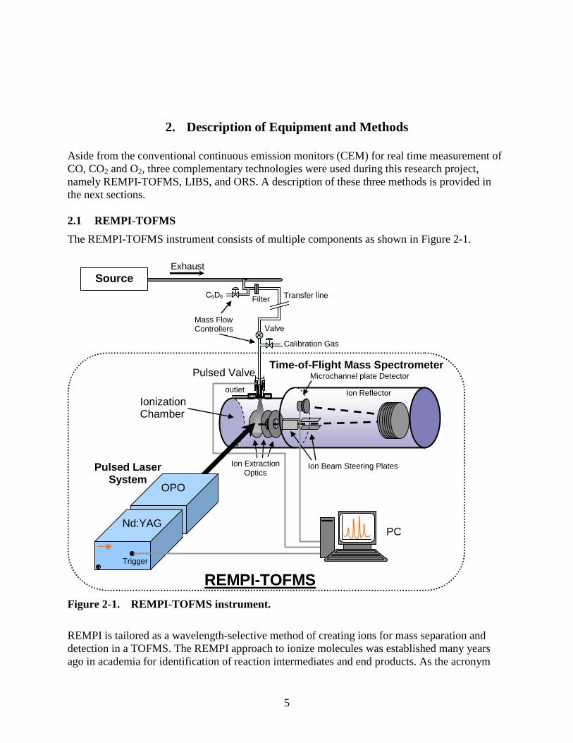
The REMPI-TOFMS instrument consists of multiple components as shown in Figure 2-1. Exhaust

Time-of-Flight Mass Spectrometer Microchannel plate Detector

Ion Beam Steering Plates Ion Extraction Optics

Pulsed Valve

Pulsed Laser System

C6D6

Calibration Gas

Filter Transfer line

Ion Reflector

REMPI-TOFMS

Nd:YAG

OPO

Trigger

PC

Ionization Chamber

Mass Flow Controllers Valve

outlet

Source

Figure 2-1. REMPI-TOFMS instrument.

REMPI is tailored as a wavelength-selective method of creating ions for mass separation and detection in a TOFMS. The REMPI approach to ionize molecules was established many years ago in academia for identification of reaction intermediates and end products. As the acronym

6

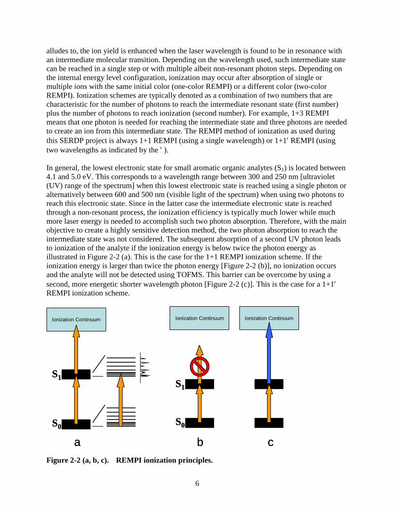
alludes to, the ion yield is enhanced when the laser wavelength is found to be in resonance with an intermediate molecular transition. Depending on the wavelength used, such intermediate state can be reached in a single step or with multiple albeit non-resonant photon steps. Depending on the internal energy level configuration, ionization may occur after absorption of single or multiple ions with the same initial color (one-color REMPI) or a different color (two-color REMPI). Ionization schemes are typically denoted as a combination of two numbers that are characteristic for the number of photons to reach the intermediate resonant state (first number) plus the number of photons to reach ionization (second number). For example, 1+3 REMPI means that one photon is needed for reaching the intermediate state and three photons are needed to create an ion from this intermediate state. The REMPI method of ionization as used during this SERDP project is always 1+1 REMPI (using a single wavelength) or 1+1′ REMPI (using two wavelengths as indicated by the ′ ). In general, the lowest electronic state for small aromatic organic analytes (S1) is located between 4.1 and 5.0 eV. This corresponds to a wavelength range between 300 and 250 nm [ultraviolet (UV) range of the spectrum] when this lowest electronic state is reached using a single photon or alternatively between 600 and 500 nm (visible light of the spectrum) when using two photons to reach this electronic state. Since in the latter case the intermediate electronic state is reached through a non-resonant process, the ionization efficiency is typically much lower while much more laser energy is needed to accomplish such two photon absorption. Therefore, with the main objective to create a highly sensitive detection method, the two photon absorption to reach the intermediate state was not considered. The subsequent absorption of a second UV photon leads to ionization of the analyte if the ionization energy is below twice the photon energy as illustrated in Figure 2-2 (a). This is the case for the 1+1 REMPI ionization scheme. If the ionization energy is larger than twice the photon energy [Figure 2-2 (b)], no ionization occurs and the analyte will not be detected using TOFMS. This barrier can be overcome by using a second, more energetic shorter wavelength photon [Figure 2-2 (c)]. This is the case for a 1+1′ REMPI ionization scheme.

S1

S0

Ionization Continuum

S1

S0

Ionization Continuum Ionization Continuum

a b c

S1

S0

Ionization Continuum

S1

S0

Ionization Continuum Ionization Continuum

a b c

Figure 2-2 (a, b, c). REMPI ionization principles.

7

So far, the REMPI process has been described as if the intermediate electronic state is a single discreet state. In reality, each electronic state, including the electronic ground state (S0) consists of numerous discrete states due to the internal vibration and rotation of the analyte. This leads to an energy level structure that is unique for each molecule. Consequently, when the wavelength of the absorbing photon is changed, multiple discrete wavelengths will exist within a fairly short wavelength window where ionization can take place. Such wavelength scan yields an absorption/ionization spectrum that can be considered as a fingerprint of the target analyte and are even isomer specific. There are four main reasons why a wavelength spectrum may not show these transitions as discrete, sharp, lines. First, the lifetime of the excited state may be extremely short (microseconds or less) which results in a (lifetime) broadening of the energy transitions, or spectral lines. Second, insufficient cooling in the expansion can broaden transitions. Third, the actual ionization scheme may involve ionization via a higher electronic (SN; N > 1) state with a higher density of available states, and fourth, the laser source of ionization cannot be fine tuned over a short wavelength range due to its own linewidth. The latter aspect appears when a comparison is made between the two laser systems that were used throughout this SERDP project. The combination of these four reasons means isomer selectivity cannot always be accomplished using REMPI. This is especially the case for heavier aromatic analytes like larger PAHs. REMPI as applied here is a soft ionization technique. Therefore, no significant fragmentation takes place and a mass spectrum essentially consists of the parent ion only. The single color 1+1 REMPI process at the lowest wavelength used of 250 nm also excludes detection of molecules with ionization energies above 9.2 eV. Consequently, interferences with aldehydes, for example, can be ignored since most have ionization energies well above this value. Note that the ionization efficiency of higher order REMPI processes is significantly smaller than that of 1+1 REMPI. It also requires higher power densities that are not present in the unfocussed laser beam. For the same reasons, the far more abundant exhaust gases such as nitrogen, steam and CO2 cannot be ionized and, therefore, do not interfere. 2.1.1 Laser Systems

Optical parametric oscillators (OPO) are solid-state devices which use non-linear optical conversion to provide tunable laser light over a very broad wavelength range covering the visible and IR spectrum. In combination with a frequency doubling module, UV light can be created from the OPO signal beam. The technology eliminates the need for handling, replacement and swapping of multiple dyes that are used in the nearest competitive laser technology, the dye laser. By doing away with the need to change between multiple different laser dyes in order to scan across a broad tuning range, the OPO provides an extremely flexible system and facilitates measurements that are not otherwise possible to perform in a timely manner. Two laser systems were used during the SERDP funding period. The initial tests were performed with a Continuum Sunlite EX OPO with FX-1 UV frequency extension. This OPO is pumped by the third harmonic (355 nm) of a Powerlite Precision 9000 Nd:YAG laser system. Its two-stage

8

design combines a narrowband oscillator with a high efficiency optical parametric amplifier to produce coherent light between 445 and 1750 nm. A computer control system maintains optimum crystal performance (phase matching) while moving over wide wavelength ranges. UV output energy, using the signal beam output and the frequency doubler, is between 5 and 10 mJ across the tuning range, with between 5 mJ and 7 mJ in the 250-280 nm range. The laser spectral line width was tested by the manufacturer to be ~ 0.2 cm-1. The major drawback of this Continuum laser system is its size; it just fits on a 3’x 8’ table which makes it too large for field deployment. Therefore, the smaller REMPI-TOFMS systems (about 2’ x 4’) utilized a more compact laser system. OPOTEK (Carlsbad, CA) manufactures efficient compact and widely tunable solid-state laser systems based on its patented OPO designs. The OPOTEK system is designed to be compact, and rugged. Their current Vibrant II-355nm with frequency-doubling laser system has sufficient power for sensitive measurements and produces continuously tunable light across a wide range of wavelengths to accommodate the detection of a large variety of species. This system is also compact and rugged enough to be used during field experiments. The standard Vibrant II-355 nm laser system from OPOTEK is a compact all-in-one tunable laser system which can generate tunable output from 210 nm to 2.6 µm, based on OPO technology. Due to the all-solid state nature of this system, there is no need to circulate or change laser dyes that have typically been used to generate tunable light at these wavelengths. The system consists of the Nd:YAG pump laser, associated second and third harmonic generation, OPO, UV extensions, and control electronics all on one rigid frame. This packaging not only leads to a compact unit, but also significantly adds to the ruggedness of the product by eliminating the alignment problems that come from the scattered discrete components usually found in this type of system. These attributes made this system an ideal starting-point for the integration into a field capable system. The UV output energy is between 1.5 and 3.5 mJ across the tuning range, with between 2.0 mJ to 3.5 mJ in the 250 to 280 nm range used during our preliminary studies. The laser spectral linewidth was tested by the manufacturer to be approximately 4 cm-1. The assessment of the increase in linewidth with respect to the large laser system is part of the evaluation. When using a single color wavelength, the use of the REMPI method is restricted to analytes with an intermediate electronic state with an energy value above half that needed to create an ion. In the case of multiple chlorinated aromatics, the intermediate state lies below half the ionization energy and no ions are formed. In order to overcome this limitation, one of the OPOTEK laser systems was modified to include the generation of a higher energy laser photon as a second color / wavelength option for ionization. This is accomplished by generating 213nm (fifth overtone of fundamental of Nd:YAG) laser light through the mixing of residual 355 nm and 532 nm laser light onto a BBO crystal. This method generates 2 to 3 mJ of this highly energetic laser light which is combined with the tunable UV from the OPO system using a dichroic mirror. With the combination of the tunable UV and fixed wavelength 213 nm laser light, detection of higher chlorinated benzenes (up to hexachlorobenzene), chlorinated furans (up to tetrachlorofuran) have been confirmed with only moderate losses in sensitivity with increased chlorination.

9

2.1.2 Valve Inlet Systems

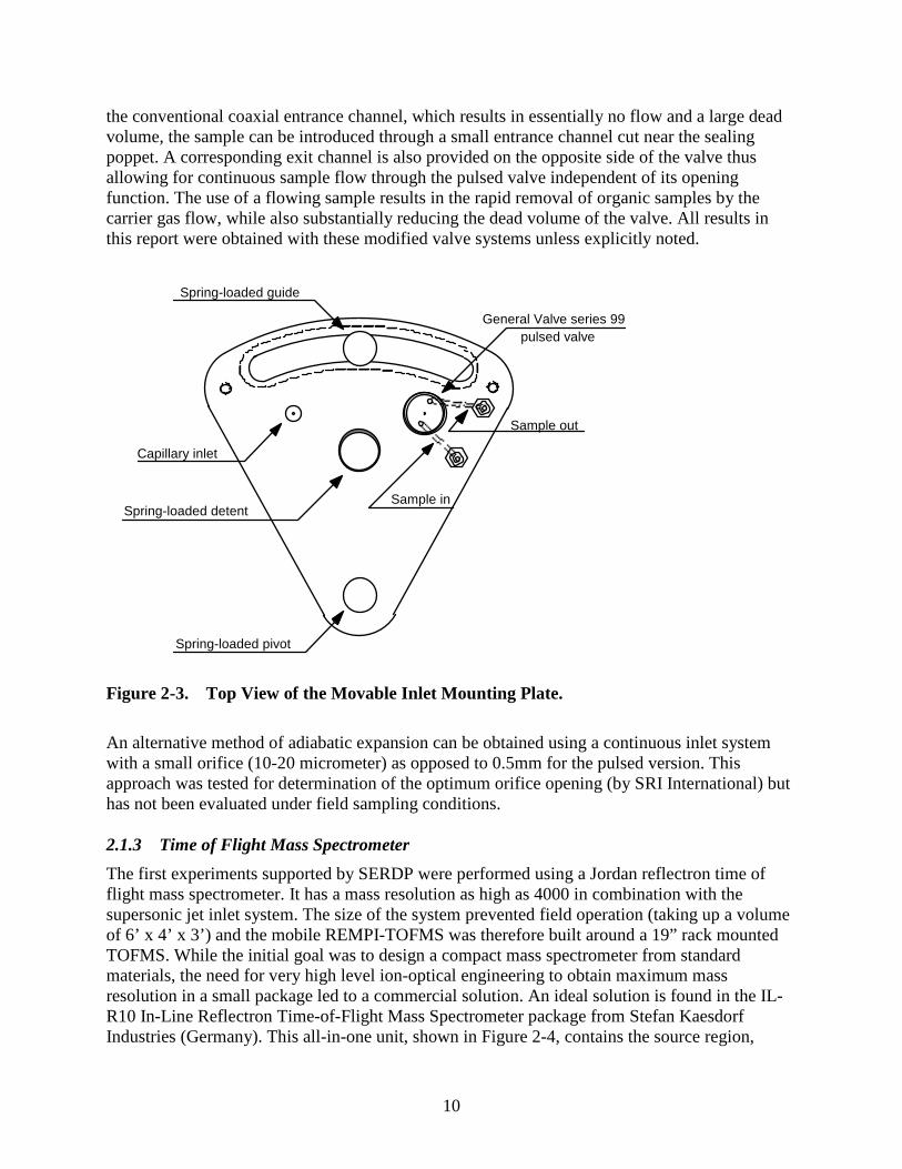
Under atmospheric conditions, individual (ro)-vibrational lines are broadened due to collisions with abundant molecules like nitrogen, oxygen and air. Consequently, wavelength spectroscopy under these conditions will result in unresolved features which lead to low or no wavelength selectivity. This applies for recorded wavelength spectra when using an effusive inlet source. Such loss in selectivity can be avoided by the use of a pulsed valve inlet system. The adiabatic expansion into vacuum creates a supersonic jet in which rotational and vibrational cooling of the target analytes takes place. Consequently, the population in the electronic ground state that was originally spread over a large number of (ro-) vibrational states is transferred into only the lowest (ro-) vibrational states. This cooling results in more discernible spectra, enhancing the selectivity in comparison with effusive-source ionization spectra. In addition, since the ion signal is proportional to the population in the initial state, transitions starting from this smaller set of populated states appear stronger than in the case where the population is spread over a larger number of initial states. All results described in this report are obtained using Parker-Hannifin Corporation Series 99 Pulse Valves that are mounted in various ways as described here. During the first part of the SERDP research efforts with the large time of flight mass spectrometer, four valves were mounted onto a single stainless steel block. Because the valve itself serves as a vacuum seal between the sample inlet line and the ion source chamber, removing the valve necessitates venting the entire instrument. While a sliding gate valve could be incorporated between the exit of the pulsed valve and the ion source, such an arrangement adds undesirable distance between the exit orifice and the ionization region. As an alternative to this approach, SRI International had previously developed a configuration that incorporates four pulsed valves on a single sliding mount. This arrangement allows any one of the four valves to be aligned with an entrance channel to the source region while keeping the remaining three valves isolated from the vacuum, and hence free to be removed and replaced as necessary. However, the size of this four-valve configuration restricts its use to the larger ion source chamber. Because of the migration of the laser ionization mass spectrometer to a smaller platform, a new multi-valve design was required. In order to incorporate a combined valve/GC capillary inlet unit on this instrument, it was necessary to have the manufacturer modify the valve-mount vacuum flange. The new flange design, which is shown in Figure 2-3, features a larger, flat surface in close proximity to the ionization region. Even with the modified flange design, the new valve-mounting configuration can only accommodate two pulsed valves or one pulsed valve and one capillary inlet. The two inlet types are mounted onto a single, wedge-shaped plate that pivots near its apex. A system of slots and precision spring-loaded guides allows the plate to rotate ±30˚ about its midpoint while maintaining adequate compression of a high-temperature Kalrez o-ring seal placed around the sample entrance orifice on the vacuum flange. When the valve mounting plate is in either of its extreme positions, the exit aperture of the pulsed valve or capillary is precisely aligned with the sample entrance orifice. A positive detent mechanical lock secures the valve plate in either position, and ensures reproducible location. In addition, a third locking position is provide midway between the two extremes that effectively seals the vacuum chamber and allows either of the valve or the capillary to be removed. The design incorporates several other important features. The valve seat has been modified to significantly reduce the dead volume between the sample gas and the exit orifice. Rather than introducing the sample through

10

the conventional coaxial entrance channel, which results in essentially no flow and a large dead volume, the sample can be introduced through a small entrance channel cut near the sealing poppet. A corresponding exit channel is also provided on the opposite side of the valve thus allowing for continuous sample flow through the pulsed valve independent of its opening function. The use of a flowing sample results in the rapid removal of organic samples by the carrier gas flow, while also substantially reducing the dead volume of the valve. All results in this report were obtained with these modified valve systems unless explicitly noted.

Spring-loaded guide

Spring-loaded pivot

Spring-loaded detent

General Valve series 99 pulsed valve

Capillary inlet

Sample out

Sample in

Figure 2-3. Top View of the Movable Inlet Mounting Plate.

An alternative method of adiabatic expansion can be obtained using a continuous inlet system with a small orifice (10-20 micrometer) as opposed to 0.5mm for the pulsed version. This approach was tested for determination of the optimum orifice opening (by SRI International) but has not been evaluated under field sampling conditions. 2.1.3 Time of Flight Mass Spectrometer

The first experiments supported by SERDP were performed using a Jordan reflectron time of flight mass spectrometer. It has a mass resolution as high as 4000 in combination with the supersonic jet inlet system. The size of the system prevented field operation (taking up a volume of 6’ x 4’ x 3’) and the mobile REMPI-TOFMS was therefore built around a 19” rack mounted TOFMS. While the initial goal was to design a compact mass spectrometer from standard materials, the need for very high level ion-optical engineering to obtain maximum mass resolution in a small package led to a commercial solution. An ideal solution is found in the IL-R10 In-Line Reflectron Time-of-Flight Mass Spectrometer package from Stefan Kaesdorf Industries (Germany). This all-in-one unit, shown in Figure 2-4, contains the source region,

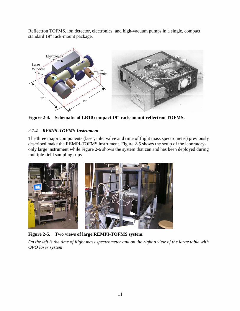
11

Reflectron TOFMS, ion detector, electronics, and high-vacuum pumps in a single, compact standard 19” rack-mount package.

Electronics

Laser Window

Gauge

19” 17.5

Figure 2-4. Schematic of LR10 compact 19” rack-mount reflectron TOFMS.

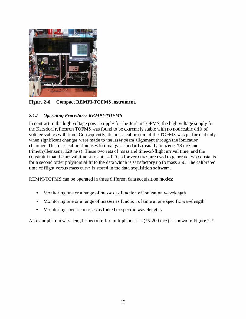
2.1.4 REMPI-TOFMS Instrument

The three major components (laser, inlet valve and time of flight mass spectrometer) previously described make the REMPI-TOFMS instrument. Figure 2-5 shows the setup of the laboratory-only large instrument while Figure 2-6 shows the system that can and has been deployed during multiple field sampling trips.

Figure 2-5. Two views of large REMPI-TOFMS system.

On the left is the time of flight mass spectrometer and on the right a view of the large table with OPO laser system

12

Figure 2-6. Compact REMPI-TOFMS instrument.

2.1.5 Operating Procedures REMPI-TOFMS

In contrast to the high voltage power supply for the Jordan TOFMS, the high voltage supply for the Kaesdorf reflectron TOFMS was found to be extremely stable with no noticeable drift of voltage values with time. Consequently, the mass calibration of the TOFMS was performed only when significant changes were made to the laser beam alignment through the ionization chamber. The mass calibration uses internal gas standards (usually benzene, 78 m/z and trimethylbenzene, 120 m/z). These two sets of mass and time-of-flight arrival time, and the constraint that the arrival time starts at t = 0.0 µs for zero m/z, are used to generate two constants for a second order polynomial fit to the data which is satisfactory up to mass 250. The calibrated time of flight versus mass curve is stored in the data acquisition software. REMPI-TOFMS can be operated in three different data acquisition modes:

• Monitoring one or a range of masses as function of ionization wavelength

• Monitoring one or a range of masses as function of time at one specific wavelength

• Monitoring specific masses as linked to specific wavelengths An example of a wavelength spectrum for multiple masses (75-200 m/z) is shown in Figure 2-7.

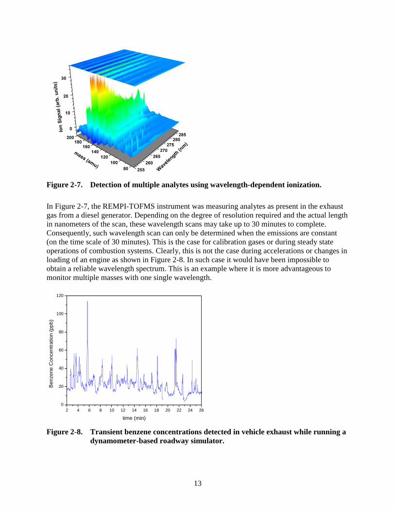
13

Figure 2-7. Detection of multiple analytes using wavelength-dependent ionization.

In Figure 2-7, the REMPI-TOFMS instrument was measuring analytes as present in the exhaust gas from a diesel generator. Depending on the degree of resolution required and the actual length in nanometers of the scan, these wavelength scans may take up to 30 minutes to complete. Consequently, such wavelength scan can only be determined when the emissions are constant (on the time scale of 30 minutes). This is the case for calibration gases or during steady state operations of combustion systems. Clearly, this is not the case during accelerations or changes in loading of an engine as shown in Figure 2-8. In such case it would have been impossible to obtain a reliable wavelength spectrum. This is an example where it is more advantageous to monitor multiple masses with one single wavelength.

2 4 6 8 10 12 14 16 18 20 22 24 260

20

40

60

80

100

120

Ben

zene

Con

cent

ratio

n (p

pb)

time (min)

Figure 2-8. Transient benzene concentrations detected in vehicle exhaust while running a dynamometer-based roadway simulator.

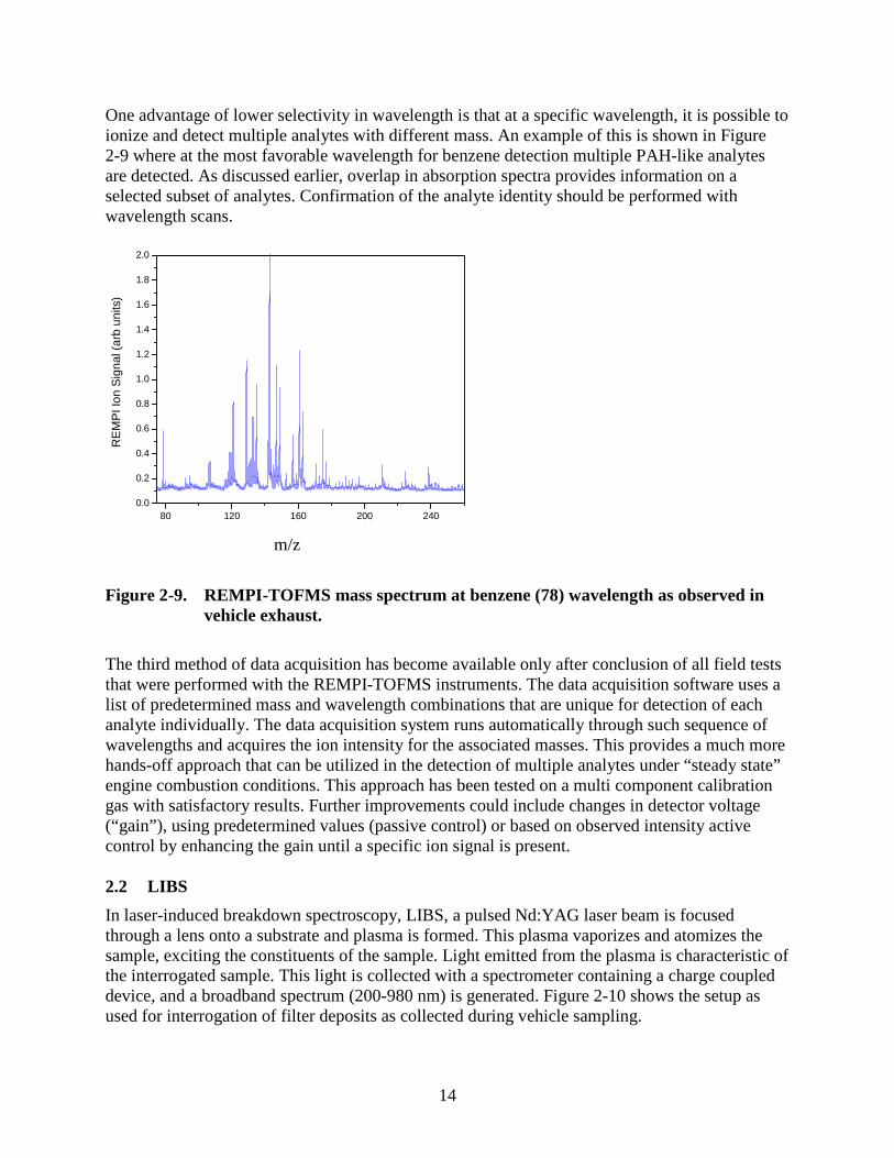
14

One advantage of lower selectivity in wavelength is that at a specific wavelength, it is possible to ionize and detect multiple analytes with different mass. An example of this is shown in Figure 2-9 where at the most favorable wavelength for benzene detection multiple PAH-like analytes are detected. As discussed earlier, overlap in absorption spectra provides information on a selected subset of analytes. Confirmation of the analyte identity should be performed with wavelength scans.

80 120 160 200 2400.0

0.2

0.4

0.6

0.8

1.0

1.2

1.4

1.6

1.8

2.0

RE

MP

I Ion

Sig

nal (

arb

units

)

m/Z

Figure 2-9. REMPI-TOFMS mass spectrum at benzene (78) wavelength as observed in vehicle exhaust.

The third method of data acquisition has become available only after conclusion of all field tests that were performed with the REMPI-TOFMS instruments. The data acquisition software uses a list of predetermined mass and wavelength combinations that are unique for detection of each analyte individually. The data acquisition system runs automatically through such sequence of wavelengths and acquires the ion intensity for the associated masses. This provides a much more hands-off approach that can be utilized in the detection of multiple analytes under “steady state” engine combustion conditions. This approach has been tested on a multi component calibration gas with satisfactory results. Further improvements could include changes in detector voltage (“gain”), using predetermined values (passive control) or based on observed intensity active control by enhancing the gain until a specific ion signal is present. 2.2 LIBS

In laser-induced breakdown spectroscopy, LIBS, a pulsed Nd:YAG laser beam is focused through a lens onto a substrate and plasma is formed. This plasma vaporizes and atomizes the sample, exciting the constituents of the sample. Light emitted from the plasma is characteristic of the interrogated sample. This light is collected with a spectrometer containing a charge coupled device, and a broadband spectrum (200-980 nm) is generated. Figure 2-10 shows the setup as used for interrogation of filter deposits as collected during vehicle sampling.

m/z

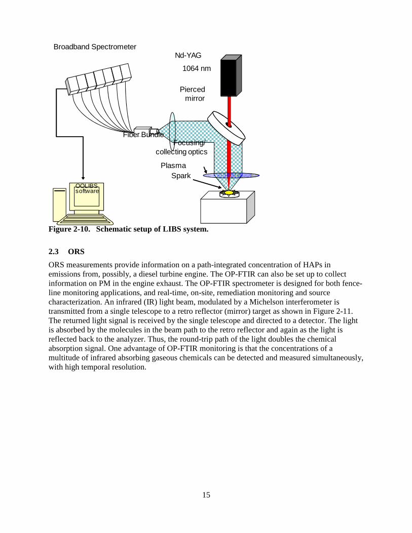
15

Broadband Spectrometer

Pierced mirror

Nd-YAG

1064 nm

PlasmaSpark

Focusing/collecting optics

Fiber Bundle

OOLIBS software

Figure 2-10. Schematic setup of LIBS system.

2.3 ORS

ORS measurements provide information on a path-integrated concentration of HAPs in emissions from, possibly, a diesel turbine engine. The OP-FTIR can also be set up to collect information on PM in the engine exhaust. The OP-FTIR spectrometer is designed for both fence-line monitoring applications, and real-time, on-site, remediation monitoring and source characterization. An infrared (IR) light beam, modulated by a Michelson interferometer is transmitted from a single telescope to a retro reflector (mirror) target as shown in Figure 2-11. The returned light signal is received by the single telescope and directed to a detector. The light is absorbed by the molecules in the beam path to the retro reflector and again as the light is reflected back to the analyzer. Thus, the round-trip path of the light doubles the chemical absorption signal. One advantage of OP-FTIR monitoring is that the concentrations of a multitude of infrared absorbing gaseous chemicals can be detected and measured simultaneously, with high temporal resolution.

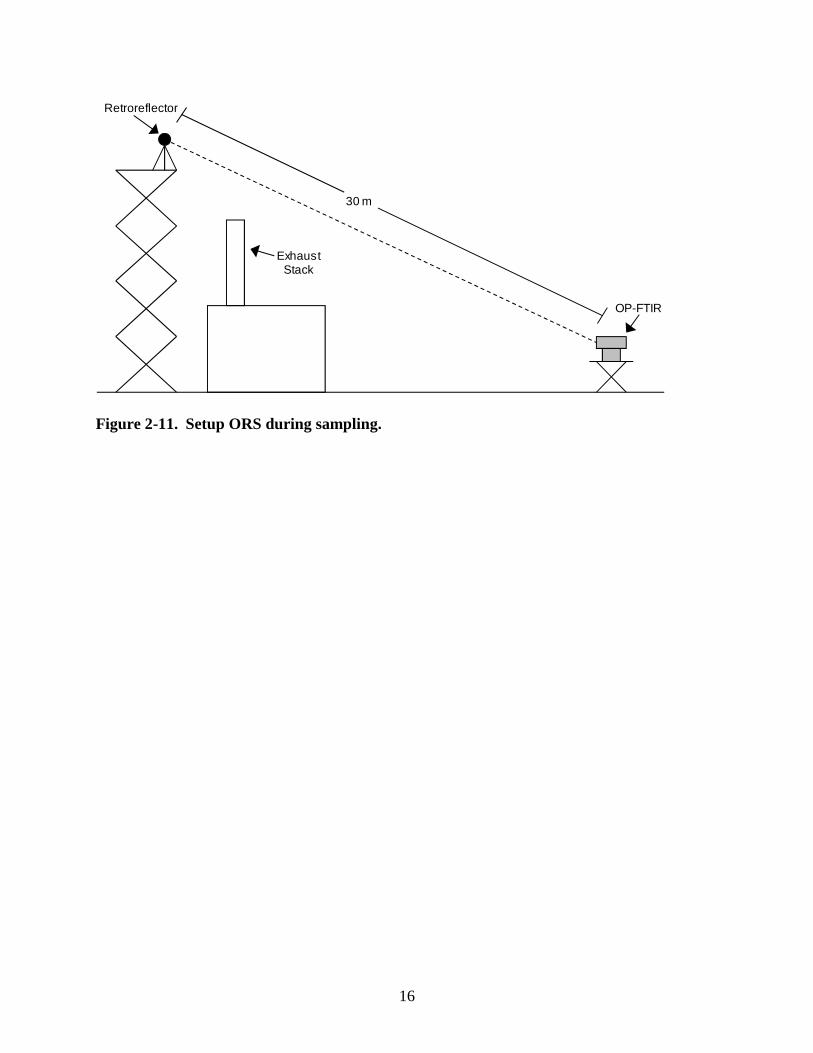
16

ExhaustStack

Retroreflector

OP-FTIR

30 m

Figure 2-11. Setup ORS during sampling.

17

3. REMPI-TOFMS: Field Ready Development and Performance Evaluation

and Improvement

At the onset of this SERDP project, a large REMPI-TOFMS system existed at the EPA facility which was suitable for emission characterization for sources located on-site. The experiences with this system were used to develop a smaller and field-ready unit. The evaluations of the critical instrument parts that were part of the SERDP project are described here. 3.1 Laser Systems

The performance of a laser system is in general sensitive to the environmental conditions in which it is placed. Although ultra-stable laser systems (both in laser energy output and absolute wavelength) exist, the laser systems used during the SERDP funded projects had limitations in their stability, especially considering their application in less favorable field conditions with potentially larger ambient temperature fluctuations and the presence of PM (dust) in air. 3.1.1 Continuum Laser

The large Continuum laser system is located in a laboratory equipped with an air conditioning system. However, slight changes in ambient temperature were found to have only a minimal effect on the emitted laser energy. The phase matching angles of the second and third harmonic crystals needed remote control adjustments only during the first 2-3 hours of operation). No appreciable wavelength shifts were noted over the course of a day of measurements. This in part due to the fact that the wavelength selection in this laser system is not determined by the OPO crystal (phase matching) angle but rather by a grating which is much less sensitive to temperature fluctuations. Phase matching angles adjustments of all crystals inside this Continuum Sunlite OPO system are performed using the software installed with the instrument. 3.1.2 OPOTEK Laser

Temperature changes inside the laser system, especially during the warm-up period, results in noticeable changes in laser energy as well as actual wavelength emitted from this laser. The changes in laser energy are due to changes in the phase matching angles of the second and third harmonic generating crystals which tend to shift when the temperature changes. Adjustments from the outside of the laser system can be made to correct for these changes and do not create a major concern in the performance of the laser system. OPOTEK has informed us that a more stable version with feedback control is now available but such improvement has not been implemented in the existing laser systems. Adjustments of the phase matching angle of the frequency doubling module can be performed using the software control of the OPOTEK laser system. Figure 3-1 shows an example of laser wavelength drift as a consequence of increased temperature inside the laser system. This is observed when the wavelength-dependent ion signal is monitored for a calibration gas. A suggested improvement to the manufacturer would be to elevate the temperature of the OPO crystal to well above ambient temperature in order to reduce these shifts. It should be noted that the application of this laser system for semi-high resolution

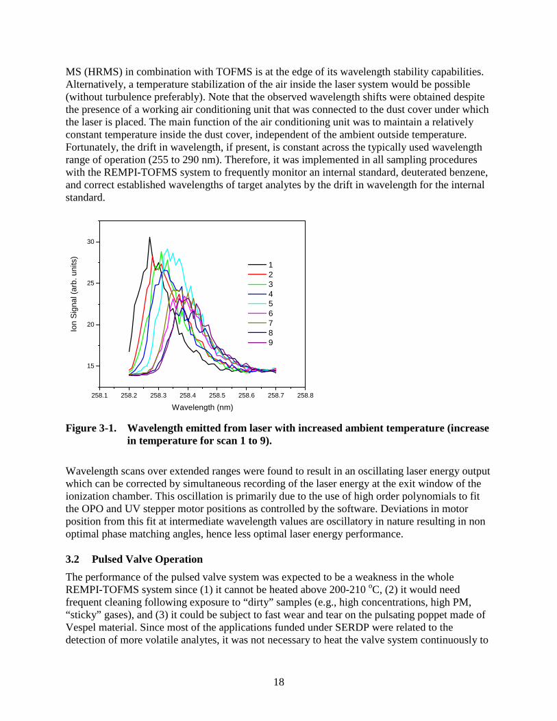
18

MS (HRMS) in combination with TOFMS is at the edge of its wavelength stability capabilities. Alternatively, a temperature stabilization of the air inside the laser system would be possible (without turbulence preferably). Note that the observed wavelength shifts were obtained despite the presence of a working air conditioning unit that was connected to the dust cover under which the laser is placed. The main function of the air conditioning unit was to maintain a relatively constant temperature inside the dust cover, independent of the ambient outside temperature. Fortunately, the drift in wavelength, if present, is constant across the typically used wavelength range of operation (255 to 290 nm). Therefore, it was implemented in all sampling procedures with the REMPI-TOFMS system to frequently monitor an internal standard, deuterated benzene, and correct established wavelengths of target analytes by the drift in wavelength for the internal standard.

258.1 258.2 258.3 258.4 258.5 258.6 258.7 258.8

15

20

25

30

1 2 3 4 5 6 7 8 9

Ion

Sig

nal (

arb.

uni

ts)

Wavelength (nm)

Figure 3-1. Wavelength emitted from laser with increased ambient temperature (increase in temperature for scan 1 to 9).

Wavelength scans over extended ranges were found to result in an oscillating laser energy output which can be corrected by simultaneous recording of the laser energy at the exit window of the ionization chamber. This oscillation is primarily due to the use of high order polynomials to fit the OPO and UV stepper motor positions as controlled by the software. Deviations in motor position from this fit at intermediate wavelength values are oscillatory in nature resulting in non optimal phase matching angles, hence less optimal laser energy performance. 3.2 Pulsed Valve Operation

The performance of the pulsed valve system was expected to be a weakness in the whole REMPI-TOFMS system since (1) it cannot be heated above 200-210 oC, (2) it would need frequent cleaning following exposure to “dirty” samples (e.g., high concentrations, high PM, “sticky” gases), and (3) it could be subject to fast wear and tear on the pulsating poppet made of Vespel material. Since most of the applications funded under SERDP were related to the detection of more volatile analytes, it was not necessary to heat the valve system continuously to

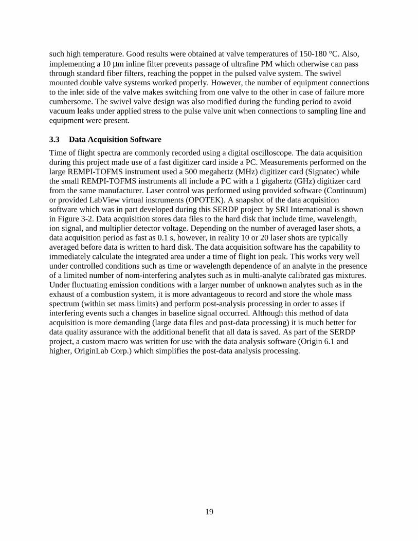
19

such high temperature. Good results were obtained at valve temperatures of 150-180 °C. Also, implementing a 10 µm inline filter prevents passage of ultrafine PM which otherwise can pass through standard fiber filters, reaching the poppet in the pulsed valve system. The swivel mounted double valve systems worked properly. However, the number of equipment connections to the inlet side of the valve makes switching from one valve to the other in case of failure more cumbersome. The swivel valve design was also modified during the funding period to avoid vacuum leaks under applied stress to the pulse valve unit when connections to sampling line and equipment were present. 3.3 Data Acquisition Software

Time of flight spectra are commonly recorded using a digital oscilloscope. The data acquisition during this project made use of a fast digitizer card inside a PC. Measurements performed on the large REMPI-TOFMS instrument used a 500 megahertz (MHz) digitizer card (Signatec) while the small REMPI-TOFMS instruments all include a PC with a 1 gigahertz (GHz) digitizer card from the same manufacturer. Laser control was performed using provided software (Continuum) or provided LabView virtual instruments (OPOTEK). A snapshot of the data acquisition software which was in part developed during this SERDP project by SRI International is shown in Figure 3-2. Data acquisition stores data files to the hard disk that include time, wavelength, ion signal, and multiplier detector voltage. Depending on the number of averaged laser shots, a data acquisition period as fast as 0.1 s, however, in reality 10 or 20 laser shots are typically averaged before data is written to hard disk. The data acquisition software has the capability to immediately calculate the integrated area under a time of flight ion peak. This works very well under controlled conditions such as time or wavelength dependence of an analyte in the presence of a limited number of nom-interfering analytes such as in multi-analyte calibrated gas mixtures. Under fluctuating emission conditions with a larger number of unknown analytes such as in the exhaust of a combustion system, it is more advantageous to record and store the whole mass spectrum (within set mass limits) and perform post-analysis processing in order to asses if interfering events such a changes in baseline signal occurred. Although this method of data acquisition is more demanding (large data files and post-data processing) it is much better for data quality assurance with the additional benefit that all data is saved. As part of the SERDP project, a custom macro was written for use with the data analysis software (Origin 6.1 and higher, OriginLab Corp.) which simplifies the post-data analysis processing.

20

Figure 3-2. Photo of data acquisition software in operation.

3.4 Calibration of REMPI-TOFMS System

External calibration of the detected ion signals was typically performed at the beginning and at the end of the day. This was accomplished by monitoring the response to a 100 ppb calibrated gas mixture in nitrogen containing 14 aromatic compounds (Scott Specialty Gases). The concentration of a target analyte is derived from the ratio between its ion signal intensity and that of the same analyte as present in the calibration gas mix, normalized for possible laser energy changes. Concentrations of those exhaust analytes not present in the calibration mix were derived from the ionization probability ratios between benzene and such analytes as found by Cool and coworkers (Velazquez et al., 1998). In the case of concentration calibration of compounds that are in their crystalline form at room temperature, such as PAHs, a diffusion-tube-based delivery system was designed and applied to generate a known concentration of a specific analyte in the gas phase. The absolute concentration of this delivery system was verified independently for each analyte of interest using external high resolution GC (HRGC) combined with low resolution MS (LRMS) analysis. System performance monitoring is provided by addition and measurement of fully deuterated benzene (C6D6) since it is unambiguously detected and is not an exhaust product. A linear REMPI-TOFMS response has been established over several orders of magnitude of concentration (ppt to ppm range) for all aromatic compounds of interest. Since the response to all compounds is linear with concentration, the measured response to the added C6D6 was used as an indicator for REMPI-TOFMS system performance. All recorded ion signals were corrected for possible changes in laser energy during post analysis processing of the experimental data. REMPI-TOFMS has the capability to individually identify a large set of aromatic compounds and this can be accomplished in real time with a 1 s resolution at a high pptv level concentration. No sample clean-up or extraction is needed and consequently, qualitative results are available instantaneously.

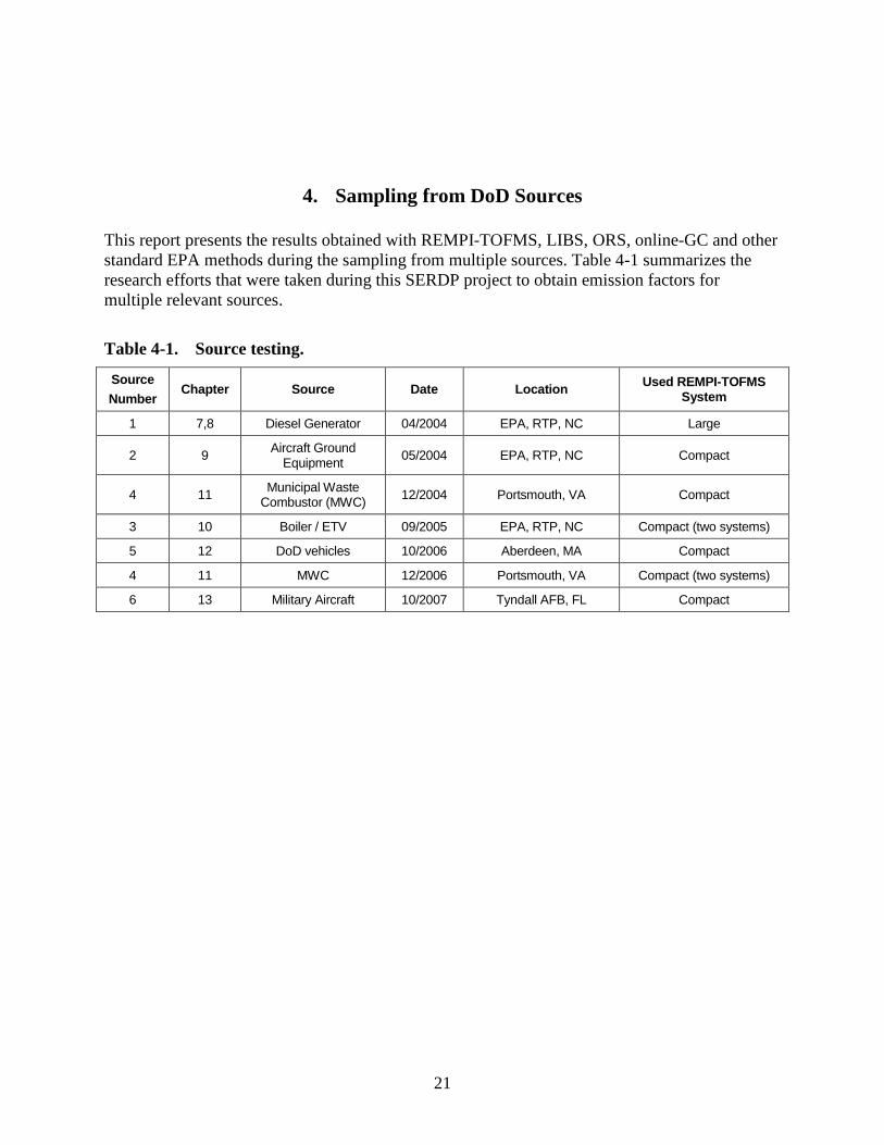
21

4. Sampling from DoD Sources

This report presents the results obtained with REMPI-TOFMS, LIBS, ORS, online-GC and other standard EPA methods during the sampling from multiple sources. Table 4-1 summarizes the research efforts that were taken during this SERDP project to obtain emission factors for multiple relevant sources.

Table 4-1. Source testing.

Source

Number Chapter Source Date Location Used REMPI-TOFMS

System

1 7,8 Diesel Generator 04/2004 EPA, RTP, NC Large

2 9 Aircraft Ground Equipment

05/2004 EPA, RTP, NC Compact

4 11 Municipal Waste Combustor (MWC) 12/2004 Portsmouth, VA Compact

3 10 Boiler / ETV 09/2005 EPA, RTP, NC Compact (two systems)

5 12 DoD vehicles 10/2006 Aberdeen, MA Compact

4 11 MWC 12/2006 Portsmouth, VA Compact (two systems)

6 13 Military Aircraft 10/2007 Tyndall AFB, FL Compact

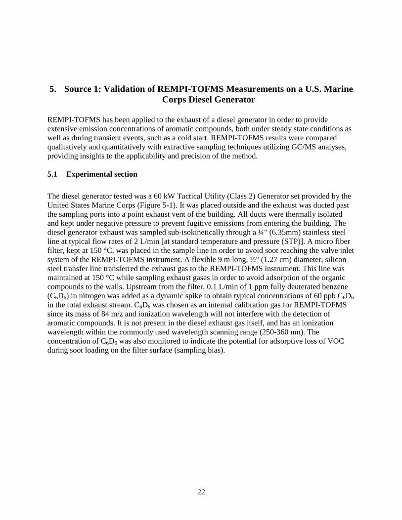
22

5. Source 1: Validation of REMPI-TOFMS Measurements on a U.S. Marine

Corps Diesel Generator

REMPI-TOFMS has been applied to the exhaust of a diesel generator in order to provide extensive emission concentrations of aromatic compounds, both under steady state conditions as well as during transient events, such as a cold start. REMPI-TOFMS results were compared qualitatively and quantitatively with extractive sampling techniques utilizing GC/MS analyses, providing insights to the applicability and precision of the method. 5.1 Experimental section

The diesel generator tested was a 60 kW Tactical Utility (Class 2) Generator set provided by the United States Marine Corps (Figure 5-1). It was placed outside and the exhaust was ducted past the sampling ports into a point exhaust vent of the building. All ducts were thermally isolated and kept under negative pressure to prevent fugitive emissions from entering the building. The diesel generator exhaust was sampled sub-isokinetically through a ¼" (6.35mm) stainless steel line at typical flow rates of 2 L/min [at standard temperature and pressure (STP)]. A micro fiber filter, kept at 150 °C, was placed in the sample line in order to avoid soot reaching the valve inlet system of the REMPI-TOFMS instrument. A flexible 9 m long, ½" (1.27 cm) diameter, silicon steel transfer line transferred the exhaust gas to the REMPI-TOFMS instrument. This line was maintained at 150 °C while sampling exhaust gases in order to avoid adsorption of the organic compounds to the walls. Upstream from the filter, 0.1 L/min of 1 ppm fully deuterated benzene (C6D6) in nitrogen was added as a dynamic spike to obtain typical concentrations of 60 ppb C6D6 in the total exhaust stream. C6D6 was chosen as an internal calibration gas for REMPI-TOFMS since its mass of 84 m/z and ionization wavelength will not interfere with the detection of aromatic compounds. It is not present in the diesel exhaust gas itself, and has an ionization wavelength within the commonly used wavelength scanning range (250-360 nm). The concentration of C6D6 was also monitored to indicate the potential for adsorptive loss of VOC during soot loading on the filter surface (sampling bias).

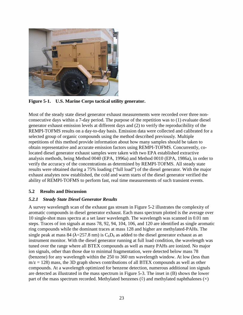
23

Figure 5-1. U.S. Marine Corps tactical utility generator.

Most of the steady state diesel generator exhaust measurements were recorded over three non-consecutive days within a 7-day period. The purpose of the repetition was to (1) evaluate diesel generator exhaust emission levels at different days and (2) to verify the reproducibility of the REMPI-TOFMS results on a day-to-day basis. Emission data were collected and calibrated for a selected group of organic compounds using the method described previously. Multiple repetitions of this method provide information about how many samples should be taken to obtain representative and accurate emission factors using REMPI-TOFMS. Concurrently, co-located diesel generator exhaust samples were taken with two EPA established extractive analysis methods, being Method 0040 (EPA, 1996a) and Method 0010 (EPA, 1986a), in order to verify the accuracy of the concentrations as determined by REMPI-TOFMS. All steady state results were obtained during a 75% loading (“full load”) of the diesel generator. With the major exhaust analytes now established, the cold and warm starts of the diesel generator verified the ability of REMPI-TOFMS to perform fast, real time measurements of such transient events. 5.2 Results and Discussion

5.2.1 Steady State Diesel Generator Results

A survey wavelength scan of the exhaust gas stream in Figure 5-2 illustrates the complexity of aromatic compounds in diesel generator exhaust. Each mass spectrum plotted is the average over 10 single-shot mass spectra at a set laser wavelength. The wavelength was scanned in 0.01 nm steps. Traces of ion signals at mass 78, 92, 94, 104, 106, and 120 are identified as single aromatic ring compounds while the dominant traces at mass 128 and higher are methylated-PAHs. The single peak at mass 84 (λ=257.8 nm) is C6D6 as added to the diesel generator exhaust as an instrument monitor. With the diesel generator running at full load condition, the wavelength was tuned over the range where all BTEX compounds as well as many PAHs are ionized. No major ion signals, other than those due to minimal fragmentation, were detected below mass 78 (benzene) for any wavelength within the 250 to 360 nm wavelength window. At low (less than m/z = 128) mass, the 3D graph shows contributions of all BTEX compounds as well as other compounds. At a wavelength optimized for benzene detection, numerous additional ion signals are detected as illustrated in the mass spectrum in Figure 5-3. The inset in (B) shows the lower part of the mass spectrum recorded. Methylated benzenes (◊) and methylated naphthalenes (×)

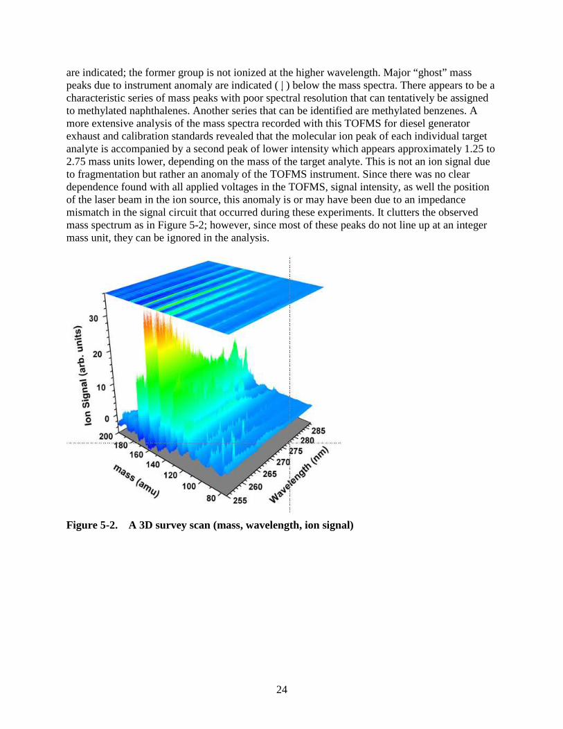
24

are indicated; the former group is not ionized at the higher wavelength. Major “ghost” mass peaks due to instrument anomaly are indicated ( | ) below the mass spectra. There appears to be a characteristic series of mass peaks with poor spectral resolution that can tentatively be assigned to methylated naphthalenes. Another series that can be identified are methylated benzenes. A more extensive analysis of the mass spectra recorded with this TOFMS for diesel generator exhaust and calibration standards revealed that the molecular ion peak of each individual target analyte is accompanied by a second peak of lower intensity which appears approximately 1.25 to 2.75 mass units lower, depending on the mass of the target analyte. This is not an ion signal due to fragmentation but rather an anomaly of the TOFMS instrument. Since there was no clear dependence found with all applied voltages in the TOFMS, signal intensity, as well the position of the laser beam in the ion source, this anomaly is or may have been due to an impedance mismatch in the signal circuit that occurred during these experiments. It clutters the observed mass spectrum as in Figure 5-2; however, since most of these peaks do not line up at an integer mass unit, they can be ignored in the analysis.

Figure 5-2. A 3D survey scan (mass, wavelength, ion signal)

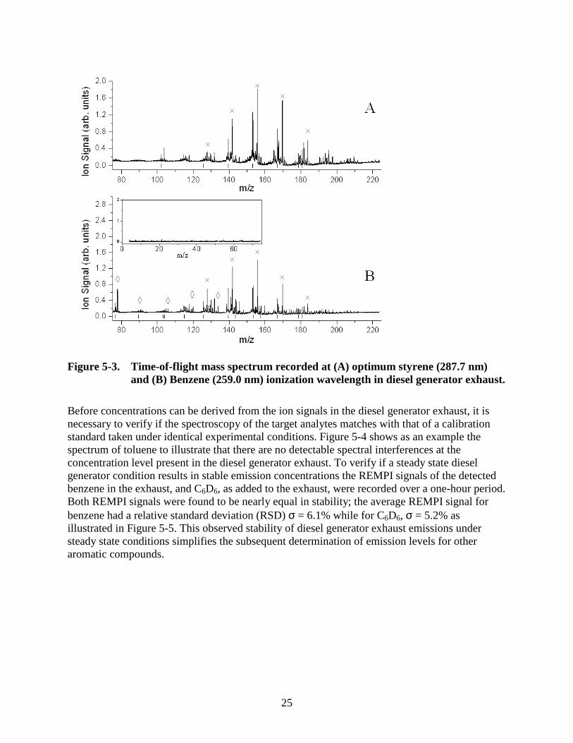
25

Figure 5-3. Time-of-flight mass spectrum recorded at (A) optimum styrene (287.7 nm) and (B) Benzene (259.0 nm) ionization wavelength in diesel generator exhaust.

Before concentrations can be derived from the ion signals in the diesel generator exhaust, it is necessary to verify if the spectroscopy of the target analytes matches with that of a calibration standard taken under identical experimental conditions. Figure 5-4 shows as an example the spectrum of toluene to illustrate that there are no detectable spectral interferences at the concentration level present in the diesel generator exhaust. To verify if a steady state diesel generator condition results in stable emission concentrations the REMPI signals of the detected benzene in the exhaust, and C6D6, as added to the exhaust, were recorded over a one-hour period. Both REMPI signals were found to be nearly equal in stability; the average REMPI signal for benzene had a relative standard deviation (RSD) σ = 6.1% while for C6D6, σ = 5.2% as illustrated in Figure 5-5. This observed stability of diesel generator exhaust emissions under steady state conditions simplifies the subsequent determination of emission levels for other aromatic compounds.

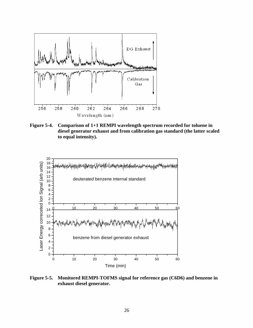
26

Figure 5-4. Comparison of 1+1 REMPI wavelength spectrum recorded for toluene in diesel generator exhaust and from calibration gas standard (the latter scaled to equal intensity).

0 10 20 30 40 50 600

2

4

6

8

10

12

14 0 10 20 30 40 50 6002468

101214161820

Time (min)

benzene from diesel generator exhaust

Las

er E

nerg

y co

rrec

eted

Ion

Sig

nal (

arb

units

)

deuterated benzene internal standard

Figure 5-5. Monitored REMPI-TOFMS signal for reference gas (C6D6) and benzene in exhaust diesel generator.

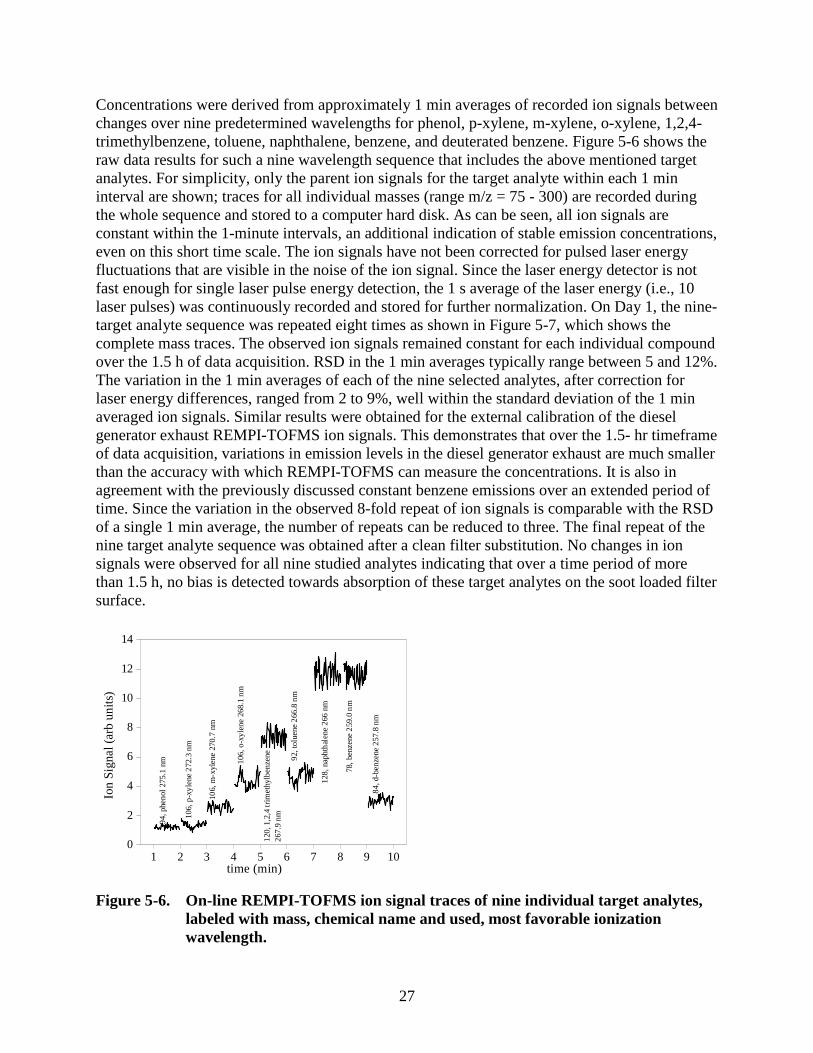
27

Concentrations were derived from approximately 1 min averages of recorded ion signals between changes over nine predetermined wavelengths for phenol, p-xylene, m-xylene, o-xylene, 1,2,4-trimethylbenzene, toluene, naphthalene, benzene, and deuterated benzene. Figure 5-6 shows the raw data results for such a nine wavelength sequence that includes the above mentioned target analytes. For simplicity, only the parent ion signals for the target analyte within each 1 min interval are shown; traces for all individual masses (range m/z = 75 - 300) are recorded during the whole sequence and stored to a computer hard disk. As can be seen, all ion signals are constant within the 1-minute intervals, an additional indication of stable emission concentrations, even on this short time scale. The ion signals have not been corrected for pulsed laser energy fluctuations that are visible in the noise of the ion signal. Since the laser energy detector is not fast enough for single laser pulse energy detection, the 1 s average of the laser energy (i.e., 10 laser pulses) was continuously recorded and stored for further normalization. On Day 1, the nine-target analyte sequence was repeated eight times as shown in Figure 5-7, which shows the complete mass traces. The observed ion signals remained constant for each individual compound over the 1.5 h of data acquisition. RSD in the 1 min averages typically range between 5 and 12%. The variation in the 1 min averages of each of the nine selected analytes, after correction for laser energy differences, ranged from 2 to 9%, well within the standard deviation of the 1 min averaged ion signals. Similar results were obtained for the external calibration of the diesel generator exhaust REMPI-TOFMS ion signals. This demonstrates that over the 1.5- hr timeframe of data acquisition, variations in emission levels in the diesel generator exhaust are much smaller than the accuracy with which REMPI-TOFMS can measure the concentrations. It is also in agreement with the previously discussed constant benzene emissions over an extended period of time. Since the variation in the observed 8-fold repeat of ion signals is comparable with the RSD of a single 1 min average, the number of repeats can be reduced to three. The final repeat of the nine target analyte sequence was obtained after a clean filter substitution. No changes in ion signals were observed for all nine studied analytes indicating that over a time period of more than 1.5 h, no bias is detected towards absorption of these target analytes on the soot loaded filter surface.

1 2 3 4 5 6 7 8 9 100

2

4

6

8

10

12

14

94,

phe

nol

275

.1 n

m

Ion

Sig

nal (

arb

un

its)

time (min)

106

, p

-xyl

ene

272

.3 n

m

106,

m-x

ylen

e 27

0.7

nm

106

, o

-xyl

ene

268.

1 n

m

120

, 1,2

,4 tr

imet

hylb

enze

ne2

67.9

nm

92

, tol

uene

266

.8 n

m

128

, na

phth

alen

e 2

66 n

m

78,

benz

ene

259

.0 n

m

84

, d-b

enze

ne 2

57.8

nm

Figure 5-6. On-line REMPI-TOFMS ion signal traces of nine individual target analytes, labeled with mass, chemical name and used, most favorable ionization wavelength.

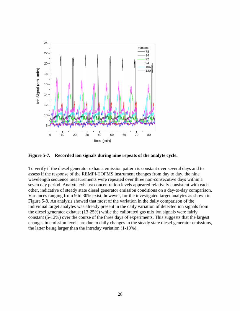
28

0 10 20 30 40 50 60 70 80

8

10

12

14

16

18

20

22

24

Ion

Sig

nal (

arb.

uni

ts)

time (min)

masses: 78 84 92 94 106 120

Figure 5-7. Recorded ion signals during nine repeats of the analyte cycle.

To verify if the diesel generator exhaust emission pattern is constant over several days and to assess if the response of the REMPI-TOFMS instrument changes from day to day, the nine wavelength sequence measurements were repeated over three non-consecutive days within a seven day period. Analyte exhaust concentration levels appeared relatively consistent with each other, indicative of steady state diesel generator emission conditions on a day-to-day comparison. Variances ranging from 9 to 30% exist, however, for the investigated target analytes as shown in Figure 5-8. An analysis showed that most of the variation in the daily comparison of the individual target analytes was already present in the daily variation of detected ion signals from the diesel generator exhaust (13-25%) while the calibrated gas mix ion signals were fairly constant (5-12%) over the course of the three days of experiments. This suggests that the largest changes in emission levels are due to daily changes in the steady state diesel generator emissions, the latter being larger than the intraday variation (1-10%).

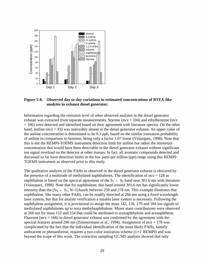
29

Day 1 Day 2 Day 30

20

40

60

80

100

120

140

160

180

200C

once

ntra

tion

(ppb

) phenol p-xylene m-xylene o-xylene 1,2,4 tmbz toluene naphthalene benzene styrene

Figure 5-8. Observed day to day variations in estimated concentrations of BTEX-like analytes in exhaust diesel generator.

Information regarding the emission level of other observed analytes in the diesel generator exhaust was extracted from separate measurements. Styrene (m/z = 104) and ethylbenzene (m/z = 106) were detected and identified based on their agreement with literature spectra. On the other hand, aniline (m/z = 93) was noticeably absent in the diesel generator exhaust. An upper value of the aniline concentration is determined to be 0.3 ppb, based on the similar ionization probability of aniline in comparison to benzene, being only a factor 1.67 lower (Velazquez, 1998). Note that this is not the REMPI-TOFMS instrument detection limit for aniline but rather the minimum concentration that would have been detectable in the diesel generator exhaust without significant ion signal overload on the detector at other masses. In fact, all aromatic compounds detected and discussed so far have detection limits in the low parts per trillion (ppt) range using this REMPI-TOFMS instrument as observed prior to this study. The qualitative analysis of the PAHs as observed in the diesel generator exhaust is obscured by the presence of a multitude of methylated naphthalenes. The identification of m/z = 128 as naphthalene is based on the spectral agreement of the S1 ← S0 band near 301.6 nm with literature (Velazquez, 1998). Note that for naphthalene, this band around 301.6 nm has significantly lower intensity than the (SN ← S1; N>1) bands between 250 and 278 nm. This example illustrates that naphthalene, like many other PAHs, can be readily detected at 266 nm using a fixed wavelength laser system, but that for analyte verification a tunable laser system is necessary. Following the naphthalene assignment, it is provisional to assign the mass 142, 156, 170 and 184 ion signals to methylated naphthalenes up to tetra methylnaphthalene. Minor mass contributions were observed at 266 nm for mass 152 and 154 that could be attributed to acenaphthylene and acenaphthene. Fluorene (m/z = 166) in diesel generator exhaust was confirmed by the agreement with the spectral features around 296 nm (Zimmermann et al., 1994). Assignment of m/z = 178 was complicated by the fact that the individual identification of the most likely PAHs, namely anthracene or phenanthrene, requires a two-color ionization scheme (1+1′ REMPI) and was beyond the scope of this work. The extractive sampling GC/MS analysis showed that only

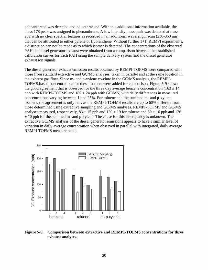
30

phenanthrene was detected and no anthracene. With this additional information available, the mass 178 peak was assigned to phenanthrene. A low intensity mass peak was detected at mass 202 with no clear spectral features as recorded in an additional wavelength scan (250-360 nm) that can be attributed to either pyrene or fluoranthene. Without further 1+1′ REMPI experiments, a distinction can not be made as to which isomer is detected. The concentrations of the observed PAHs in diesel generator exhaust were obtained from a comparison between the established calibration curves for each PAH using the sample delivery system and the diesel generator exhaust ion signals. The diesel generator exhaust emission results obtained by REMPI-TOFMS were compared with those from standard extractive and GC/MS analyses, taken in parallel and at the same location in the exhaust gas flow. Since m- and p-xylene co-elute in the GC/MS analysis, the REMPI-TOFMS based concentrations for these isomers were added for comparison. Figure 5-9 shows the good agreement that is observed for the three day average benzene concentration (163 ± 14 ppb with REMPI-TOFMS and 189 ± 24 ppb with GC/MS) with daily differences in measured concentrations varying between 1 and 25%. For toluene and the summed m- and p-xylene isomers, the agreement is only fair, as the REMPI-TOFMS results are up to 60% different from those determined using extractive sampling and GC/MS analyses. REMPI-TOFMS and GC/MS analyses measured, respectively, 83 ± 15 ppb and 120 ± 19 for toluene and 69 ± 16 ppb and 126 ± 10 ppb for the summed m- and p-xylene. The cause for this discrepancy is unknown. The extractive GC/MS analysis of the diesel generator emissions appears to have a similar level of variation in daily average concentration when observed in parallel with integrated, daily average REMPI-TOFMS measurements.

benzene toluene m+p xylene

0

50

100

150

200

250

1 2 31 2 3

Extractive Sampling REMPI-TOFMS

DG

Exh

aust

con

cent

ratio

n (p

pb)

1 2 3

Figure 5-9. Comparison between extractive and REMPI-TOFMS concentrations for three exhaust analytes.

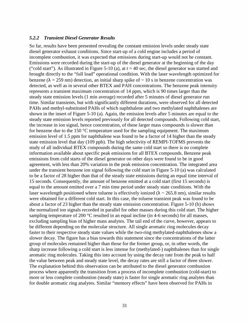
31

5.2.2 Transient Diesel Generator Results

So far, results have been presented revealing the constant emission levels under steady state diesel generator exhaust conditions. Since start-up of a cold engine includes a period of incomplete combustion, it was expected that emissions during start-up would not be constant. Emissions were recorded during the start-up of the diesel generator at the beginning of the day (“cold start”). As illustrated in Figure 5-10 (a), at t = 40 sec, the diesel generator was started and brought directly to the “full load” operational condition. With the laser wavelength optimized for benzene (λ = 259 nm) detection, an initial sharp spike of ~ 10 s in benzene concentration was detected, as well as in several other BTEX and PAH concentrations. The benzene peak intensity represents a transient maximum concentration of 14 ppm, which is 90 times larger than the steady state emission levels (1 min average) recorded after 5 minutes of diesel generator run time. Similar transients, but with significantly different durations, were observed for all detected PAHs and methyl-substituted PAHs of which naphthalene and two methylated naphthalenes are shown in the insert of Figure 5-10 (a). Again, the emission levels after 5 minutes are equal to the steady state emission levels reported previously for all detected compounds. Following cold start, the increase in ion signal, hence concentration, of these larger mass compounds is slower than for benzene due to the 150 °C temperature used for the sampling equipment. The maximum emission level of 1.5 ppm for naphthalene was found to be a factor of 14 higher than the steady state emission level that day (109 ppb). The high selectivity of REMPI-TOFMS prevents the study of all individual BTEX compounds during the same cold start so there is no complete information available about specific peak emissions for all BTEX compounds. Benzene peak emissions from cold starts of the diesel generator on other days were found to be in good agreement, with less than 20% variation in the peak emission concentration. The integrated area under the transient benzene ion signal following the cold start in Figure 5-10 (a) was calculated to be a factor of 28 higher than that of the steady state emissions during an equal time interval of 15 seconds. Consequently, the amount of benzene emitted at a cold start (first 15 seconds) is equal to the amount emitted over a 7 min time period under steady state conditions. With the laser wavelength positioned where toluene is effectively ionized (λ ~ 265.8 nm), similar results were obtained for a different cold start. In this case, the toluene transient peak was found to be about a factor of 23 higher than the steady state emission concentration. Figure 5-10 (b) shows the normalized ion signals recorded in parallel for other masses during this cold start. The higher sampling temperature of 200 °C resulted in an equal incline (in 4-6 seconds) for all masses, excluding sampling bias of higher mass analytes. The tail end of the curve, however, appears to be different depending on the molecular structure. All single aromatic ring molecules decay faster to their respective steady state values while the two-ring methylated-naphthalenes show a slower decay. The figure has a bias towards this statement since the concentrations of the latter group of molecules remained higher than those for the former group, or, in other words, the sharp increase following a cold start is less intense for (methylated-) naphthalenes than for single aromatic ring molecules. Taking this into account by using the decay rate from the peak to half the value between peak and steady state level, the decay rates are still a factor of three slower. The explanation behind this observation can be attributed to the diesel generator combustion process where apparently the transition from a process of incomplete combustion (cold-start) to more or less complete combustion (steady state) is faster for single aromatic ring analytes than for double aromatic ring analytes. Similar “memory effects” have been observed for PAHs in

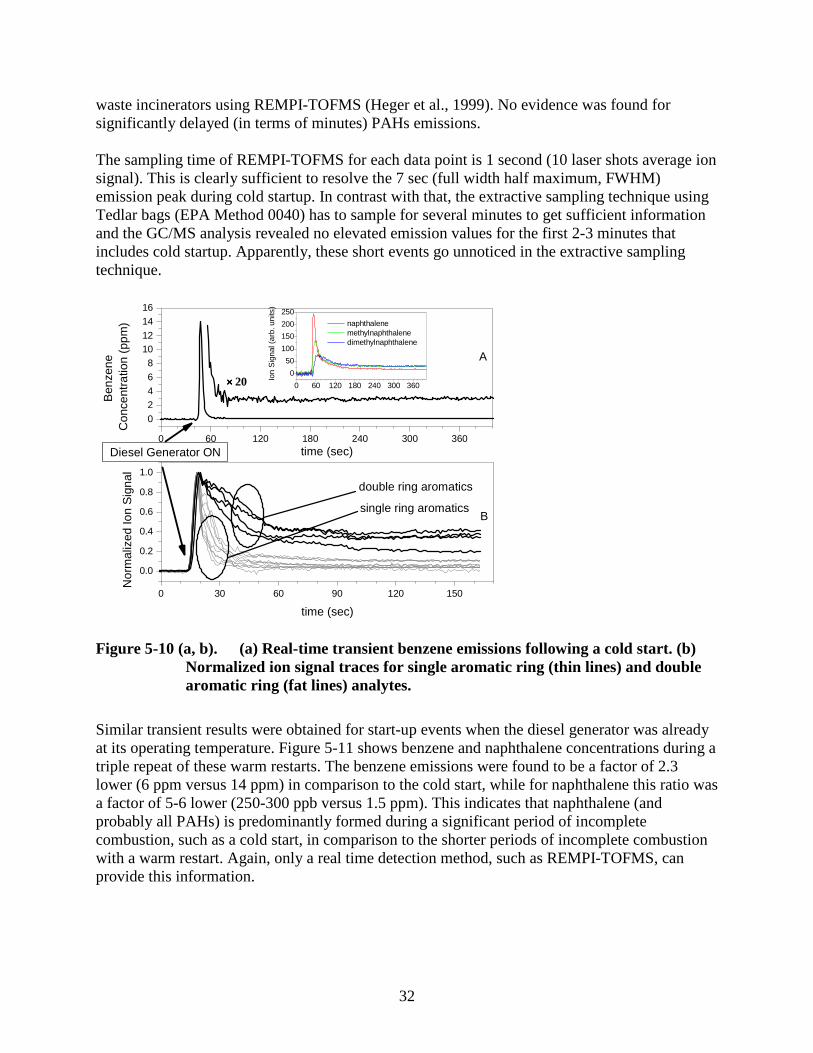
32

waste incinerators using REMPI-TOFMS (Heger et al., 1999). No evidence was found for significantly delayed (in terms of minutes) PAHs emissions. The sampling time of REMPI-TOFMS for each data point is 1 second (10 laser shots average ion signal). This is clearly sufficient to resolve the 7 sec (full width half maximum, FWHM) emission peak during cold startup. In contrast with that, the extractive sampling technique using Tedlar bags (EPA Method 0040) has to sample for several minutes to get sufficient information and the GC/MS analysis revealed no elevated emission values for the first 2-3 minutes that includes cold startup. Apparently, these short events go unnoticed in the extractive sampling technique.

0 60 120 180 240 300 360

0

50

100

150

200

250

0 30 60 90 120 150

0.0

0.2

0.4

0.6

0.8

1.0

B

Nor

mal

ized

Ion

Sig

nal

time (sec)

double ring aromatics

single ring aromatics

0 60 120 180 240 300 360

0

246

81012

1416

×××× 20

Ben

zene

C

once

ntra

tion

(ppm

)

time (sec)Diesel Generator ON

A

naphthalene methylnaphthalene dimethylnaphthalene

Ion

Sig

nal (

arb.

uni

ts)

Figure 5-10 (a, b). (a) Real-time transient benzene emissions following a cold start. (b) Normalized ion signal traces for single aromatic ring (thin lines) and double aromatic ring (fat lines) analytes.

Similar transient results were obtained for start-up events when the diesel generator was already at its operating temperature. Figure 5-11 shows benzene and naphthalene concentrations during a triple repeat of these warm restarts. The benzene emissions were found to be a factor of 2.3 lower (6 ppm versus 14 ppm) in comparison to the cold start, while for naphthalene this ratio was a factor of 5-6 lower (250-300 ppb versus 1.5 ppm). This indicates that naphthalene (and probably all PAHs) is predominantly formed during a significant period of incomplete combustion, such as a cold start, in comparison to the shorter periods of incomplete combustion with a warm restart. Again, only a real time detection method, such as REMPI-TOFMS, can provide this information.

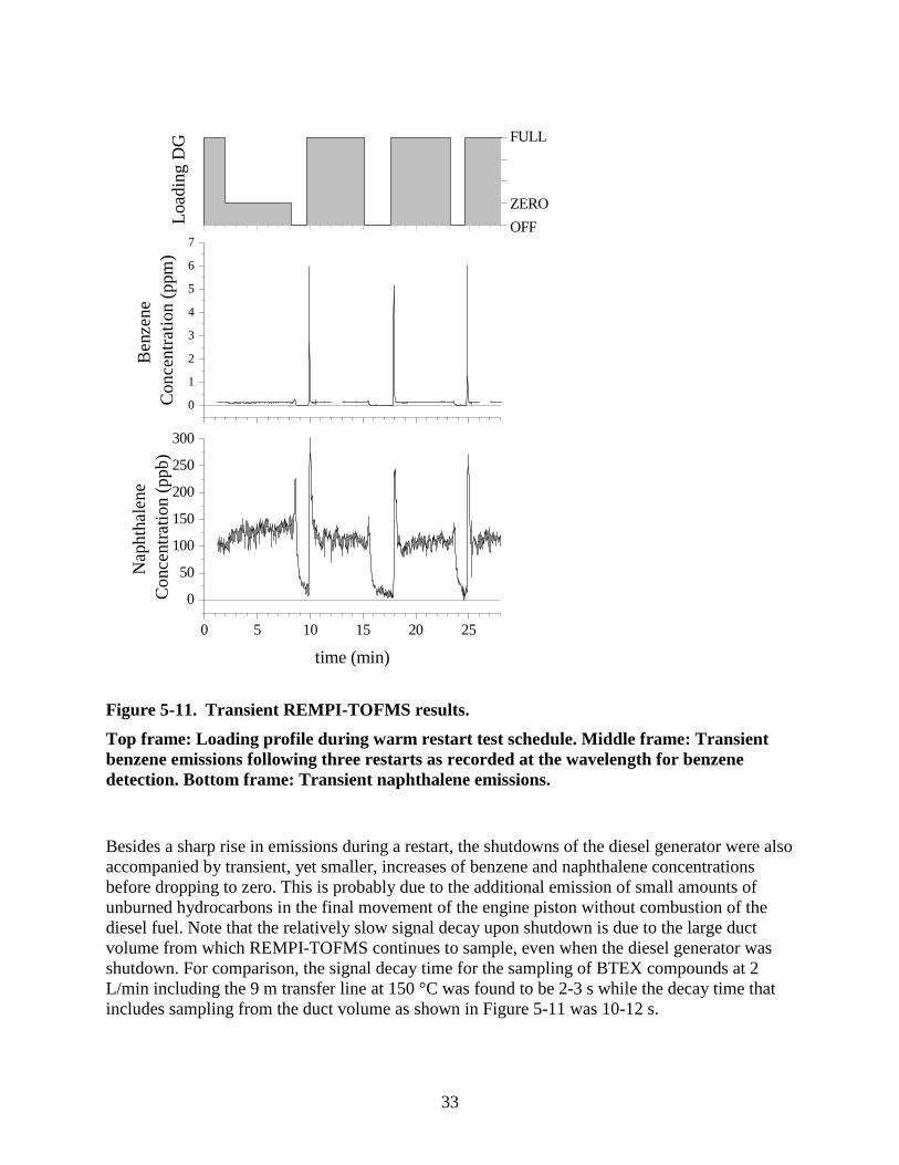
33

0 5 10 15 20 25

0

50

100

150

200

250

300

Na

phth

ale

ne

Con

cent

ratio

n (p

pb)

time (min)

0

1

2

3

4

5

6

7

Be

nze

ne

Con

cent

ratio

n (p

pm)

Loa

ding

DG

OFF

ZERO

FULL

Figure 5-11. Transient REMPI-TOFMS results.

Top frame: Loading profile during warm restart test schedule. Middle frame: Transient benzene emissions following three restarts as recorded at the wavelength for benzene detection. Bottom frame: Transient naphthalene emissions.

Besides a sharp rise in emissions during a restart, the shutdowns of the diesel generator were also accompanied by transient, yet smaller, increases of benzene and naphthalene concentrations before dropping to zero. This is probably due to the additional emission of small amounts of unburned hydrocarbons in the final movement of the engine piston without combustion of the diesel fuel. Note that the relatively slow signal decay upon shutdown is due to the large duct volume from which REMPI-TOFMS continues to sample, even when the diesel generator was shutdown. For comparison, the signal decay time for the sampling of BTEX compounds at 2 L/min including the 9 m transfer line at 150 °C was found to be 2-3 s while the decay time that includes sampling from the duct volume as shown in Figure 5-11 was 10-12 s.

34

6. Source 1: U.S. Marine Corps Diesel Generator Air Toxic Emission Characterization

This chapter continues the work described in Chapter 7 (Oudejans et al., 2004), by using REMPI-TOFMS to determine HAP emission factors for a diesel generator, both for steady state and transient operations, such as start-ups. Temporally-resolved and mode-relevant emission factors were determined for the most prevalent aromatic air toxics and compared to cumulative samples collected simultaneously via conventional EPA Methods. These measurements were compared to emission factors available in EPA databases to determine the efficacy of the REMPI-TOFMS method as well as the need for real time emission factors. Other online measurement techniques for VOC, fine particles, particle-bound PAHs, and O2, CO2, and CO were used in this study to complement the gaseous organic air toxics measurements and to highlight potential relationships. 6.1 Experimental

Air toxic emissions were characterized for a Tactical Utility Generator (Class 2, MEP6) provided by the United States Marine Corps. This is a Kurz & Root diesel-engine-driven, JP-8-fired, tactical, skid-mounted unit, Model MEP006A. The engine is a liquid-cooled, 6-cylinder, 4 stroke, and turbo-charged diesel. The generator is a 50/60 kW, brushless, air cooled, rotating field generator. The maintenance records are dated June, 1973; presumptively this is its initial year of operation. The hours of operation are unknown. The load bank was a 100-kW, variable load, Avtron model. The diesel generator set was placed outside the research facility, and the exhaust was connected to a 25.4 cm diameter duct of 350 cm length with sampling ports connected to the various sampling equipment. The exhaust gas was drawn past the sampling ports, through a dilution tunnel, and connected to a point exhaust on the building. The sampling duct was thermally insulated and under negative pressure to prevent any fugitive emissions. Various operational loads on the generator were established via connection to a variable, pre-set, 100-kW Avtron load bank. The organic air toxic emissions were characterized for cold and hot starts, different engine loads, and steady state operating conditions. Measurements were made using the REMPI-TOFMS, an on-line GC (OLGC) system (75 m RTX624 column), a photoelectric aerosol sensor (PAS 2000), an ELPI, and extractive EPA certified methods. Emission rates were determined for steady state conditions at a nominal load of 75% of the total load, or 45 kW power output, at least 30 minutes after start-ups. Data were taken for three consecutive days and reported as average daily concentrations and standard deviations thereof. The REMPI-TOFMS results were compared with reference data, obtained concurrently with the conventional EPA sampling/analytical methods listed in Table 6-1, as well as the OLGC. Steady state emission factors for the target organic pollutants obtained with the reference methods were compared to the integrated values obtained with the REMPI-TOFMS system.

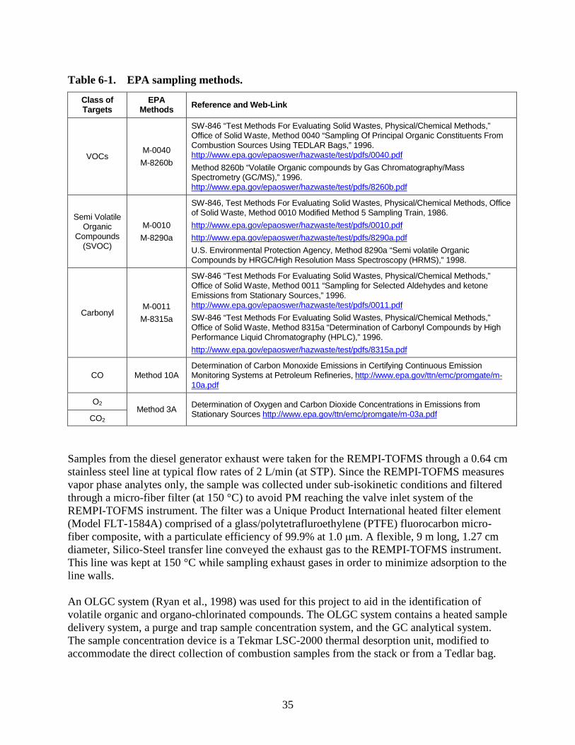
35

Table 6-1. EPA sampling methods.

Class of Targets

EPA Methods Reference and Web-Link

VOCs M-0040

M-8260b

SW-846 “Test Methods For Evaluating Solid Wastes, Physical/Chemical Methods,” Office of Solid Waste, Method 0040 “Sampling Of Principal Organic Constituents From Combustion Sources Using TEDLAR Bags,” 1996. http://www.epa.gov/epaoswer/hazwaste/test/pdfs/0040.pdf

Method 8260b “Volatile Organic compounds by Gas Chromatography/Mass Spectrometry (GC/MS),” 1996. http://www.epa.gov/epaoswer/hazwaste/test/pdfs/8260b.pdf

Semi Volatile Organic

Compounds (SVOC)

M-0010

M-8290a

SW-846, Test Methods For Evaluating Solid Wastes, Physical/Chemical Methods, Office of Solid Waste, Method 0010 Modified Method 5 Sampling Train, 1986.

http://www.epa.gov/epaoswer/hazwaste/test/pdfs/0010.pdf

http://www.epa.gov/epaoswer/hazwaste/test/pdfs/8290a.pdf

U.S. Environmental Protection Agency, Method 8290a “Semi volatile Organic Compounds by HRGC/High Resolution Mass Spectroscopy (HRMS),” 1998.

Carbonyl M-0011

M-8315a

SW-846 “Test Methods For Evaluating Solid Wastes, Physical/Chemical Methods,” Office of Solid Waste, Method 0011 “Sampling for Selected Aldehydes and ketone Emissions from Stationary Sources,” 1996. http://www.epa.gov/epaoswer/hazwaste/test/pdfs/0011.pdf

SW-846 “Test Methods For Evaluating Solid Wastes, Physical/Chemical Methods,” Office of Solid Waste, Method 8315a “Determination of Carbonyl Compounds by High Performance Liquid Chromatography (HPLC),” 1996.

http://www.epa.gov/epaoswer/hazwaste/test/pdfs/8315a.pdf

CO Method 10A Determination of Carbon Monoxide Emissions in Certifying Continuous Emission Monitoring Systems at Petroleum Refineries, http://www.epa.gov/ttn/emc/promgate/m-10a.pdf

O2

CO2

Method 3A Determination of Oxygen and Carbon Dioxide Concentrations in Emissions from Stationary Sources http://www.epa.gov/ttn/emc/promgate/m-03a.pdf

Samples from the diesel generator exhaust were taken for the REMPI-TOFMS through a 0.64 cm stainless steel line at typical flow rates of 2 L/min (at STP). Since the REMPI-TOFMS measures vapor phase analytes only, the sample was collected under sub-isokinetic conditions and filtered through a micro-fiber filter (at 150 °C) to avoid PM reaching the valve inlet system of the REMPI-TOFMS instrument. The filter was a Unique Product International heated filter element (Model FLT-1584A) comprised of a glass/polytetrafluroethylene (PTFE) fluorocarbon micro-fiber composite, with a particulate efficiency of 99.9% at 1.0 µm. A flexible, 9 m long, 1.27 cm diameter, Silico-Steel transfer line conveyed the exhaust gas to the REMPI-TOFMS instrument. This line was kept at 150 °C while sampling exhaust gases in order to minimize adsorption to the line walls. An OLGC system (Ryan et al., 1998) was used for this project to aid in the identification of volatile organic and organo-chlorinated compounds. The OLGC system contains a heated sample delivery system, a purge and trap sample concentration system, and the GC analytical system. The sample concentration device is a Tekmar LSC-2000 thermal desorption unit, modified to accommodate the direct collection of combustion samples from the stack or from a Tedlar bag.

36

The GC analytical system is an HP 5890 series II GC equipped with both a flame ionization detector (FID) and an electron capture detector (ECD). On-line monitoring of the diesel exhaust PM size distribution was performed using a Dekati Ltd. ELPI. Particles from the flue gas were sampled through a unipolar corona charger. The electric current carried by the charged particles into each impactor stage is measured in real time by a sensitive multi-channel electrometer. The particle collection into each impactor stage is dependent on the aerodynamic size of the particles. Measured current signals are converted to aerodynamic size distribution using particle size dependent relations describing the properties of the charger and the impactor stages. The particle-bound PAHs were monitored using a real-time PAS 2000 from EchoChem Analytics (Burtscher, 1992; Dunbar et al., 2001). This analyzer photoionizes PAHs on the surface of particles while the gas molecules and particles themselves remain neutral. The PAH-laden particles from the sample flow pass through a quartz tube with an excimer lamp mounted around it. The lamp operates at high frequency and high voltage, ionizing the surface of the particles. The charged particles then flow through a short tube to remove all negatively charged particles. Subsequently, the charged particles are collected on a filter element which is mounted in a Faraday cage. An electrometer measures the ion current associated with the charged particles, which is proportional to the concentrations of the PAHs (three or more aromatic rings) bound on their surface. The steady state emission results obtained by REMPI-TOFMS for organic compounds were compared with those obtained via EPA standard Methods 0040 (volatiles), 0011 (carbonyls), and 0010 (semi-volatile PAHs) and the OLGC technique. The method comparison used emission data obtained during nine sampling runs that occurred on three consecutive days. Since the reference methods are cumulative sampling techniques that provide a time-averaged concentration value, direct comparisons can only be made with the integrated values obtained with REMPI-TOFMS. Only compounds that had concentrations above the detection limit for all three measurements techniques were used. Since m- and p-xylene co-elute in the GC/MS analysis, the REMPI-TOFMS-based concentrations for these isomers were summed for comparison. Sub-isokinetic sampling for REMPI-TOFMS (to avoid particles in the detector) was equivalent to the isokinetic reference methods; even the semi-volatile PAH compounds were all found within the gas phase fraction, allowing direct comparison of the REMPI/TOFMS with the reference method measurements. The system performance of the REMPI-TOFMS was evaluated based on the relative accuracy (RA) measure (EPA, 2000a). The results presented here only provide a relative comparison of this technique with promulgated EPA techniques based on a limited number of parallel sampling tests (N = 5 and 3 for BTEX and naphthalene compounds, respectively). The RA is defined in this work as the absolute mean between the measured values of a specific compound determined by the REMPI-TOFMS system and the values determined by the reference method (RM) plus the 2.5% error confidence coefficient of a series of tests divided by the mean of the reference method.

37

100×

+=

RM

CCdRA

(1)

where d

is the absolute value of the mean of the difference between i pairs of data defined as

∑=

=n

iid

nd

1

_ 1

in which n is the number of parallel data points, CC is the absolute value of the

confidence coefficient defined as n

St d

975.0

in which dS is the standard deviation and t0.975 is the

Student’s t distribution for 0.975, and RM is the average of the reference method samples. 6.2 Results and Discussion

6.2.1 Steady State Emissions

Steady state emission measurements were compared between on-line REMPI-TOFMS, OLGC, and the standard reference methods that use extractive sampling and analysis for volatile and semi-volatile organic air toxic compounds (Table 6-2). Results were also compared with an emission factor for a related source (large stationary diesel) published in an EPA database (EPA, 1993), albeit under a different test cycle. In general, the emission factors measured by REMPI-TOFMS versus the reference methods vary by less than a factor of 2, which demonstrates the accuracy of the REMPI-TOFMS as an organic air toxic emission monitor. Generally good agreement was observed for the REMPI-TOFMS benzene emission measurements when compared to the OLGC results and the corresponding EPA reference method (Table 6-3). While additional tests would likely have improved the RA, these values are still noteworthy; for the m- and p–xylene and toluene, the RA was determined to be around 60-80%. Higher naphthalene concentrations were observed with the REMPI-TOFMS compared with the reference method, resulting in a RA of more than 110%. In general, standard deviations of the REMPI-TOFMS-measured compounds are in agreement with the corresponding standard deviations of the respective compounds measured with the OLGC or the reference methods. This suggests that the precision of each method is relatively the same. 6.2.2 Emissions during Startups

Cold and hot startups of the diesel engine caused immediate, sharp emission peaks for benzene and other BTEX compounds, as well as for all gas-phase PAHs and methyl-substituted PAHs as measured by REMPI-TOFMS. The very short response time of the REMPI-TOFMS for each data point (1 s for a 10-laser-shot average ion signal) was sufficient to resolve the transient emissions for each individual target organic air toxic; results for benzene and naphthalene are illustrated in Figure 6-1. The cold start benzene peak intensity (~ 15 ppm), which represents the maximum benzene concentration measured, was found to be about 100 times larger than the steady state emission levels (~ 150 ppb, 1 min average) recorded after 5 minutes of diesel run time. Similarly, the cold start naphthalene concentration (~ 1.5 ppm) was 14 times larger than its steady state emission level (~ 110 ppb, 1 min average). This concentration behavior is consistent

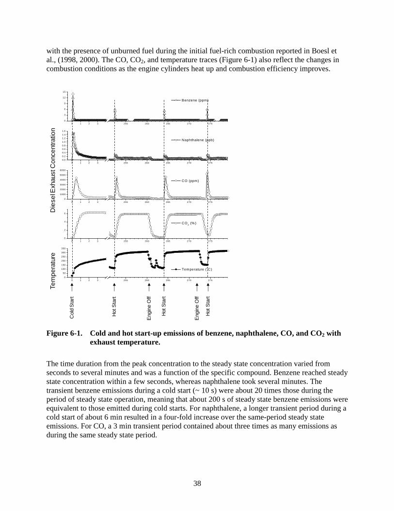
38

with the presence of unburned fuel during the initial fuel-rich combustion reported in Boesl et al., (1998, 2000). The CO, CO2, and temperature traces (Figure 6-1) also reflect the changes in combustion conditions as the engine cylinders heat up and combustion efficiency improves.

Col

d S

tart

Hot

Sta

rt

Hot

Sta

rt

Hot

Sta

rt

Eng

ine

Off

Eng

ine

Off

Die

sel E

xhau

st C

onc

ent

ratio

n

0 1 2 3 255 260 265 270 2750

50

100

150

200

250

300

350

0 1 2 3 255 260 265 270 2750

2

4

6

0 1 2 3 255 260 265 270 2750

1000

2000

3000

4000

5000

6000

0 1 2 3 255 260 265 270 2750.0

0.2

0.4

0.6

0.8

1.0

1.2

1.4

1.6

0 1 2 3 255 260 265 270 2750

3

6

9

12

15

Temperature (oC)

CO2 (% )

CO (ppm)

Naphthalene (ppb)

Benzene (ppm)

Tem

pe

ratu

re

Figure 6-1. Cold and hot start-up emissions of benzene, naphthalene, CO, and CO2 with exhaust temperature.

The time duration from the peak concentration to the steady state concentration varied from seconds to several minutes and was a function of the specific compound. Benzene reached steady state concentration within a few seconds, whereas naphthalene took several minutes. The transient benzene emissions during a cold start (~ 10 s) were about 20 times those during the period of steady state operation, meaning that about 200 s of steady state benzene emissions were equivalent to those emitted during cold starts. For naphthalene, a longer transient period during a cold start of about 6 min resulted in a four-fold increase over the same-period steady state emissions. For CO, a 3 min transient period contained about three times as many emissions as during the same steady state period.

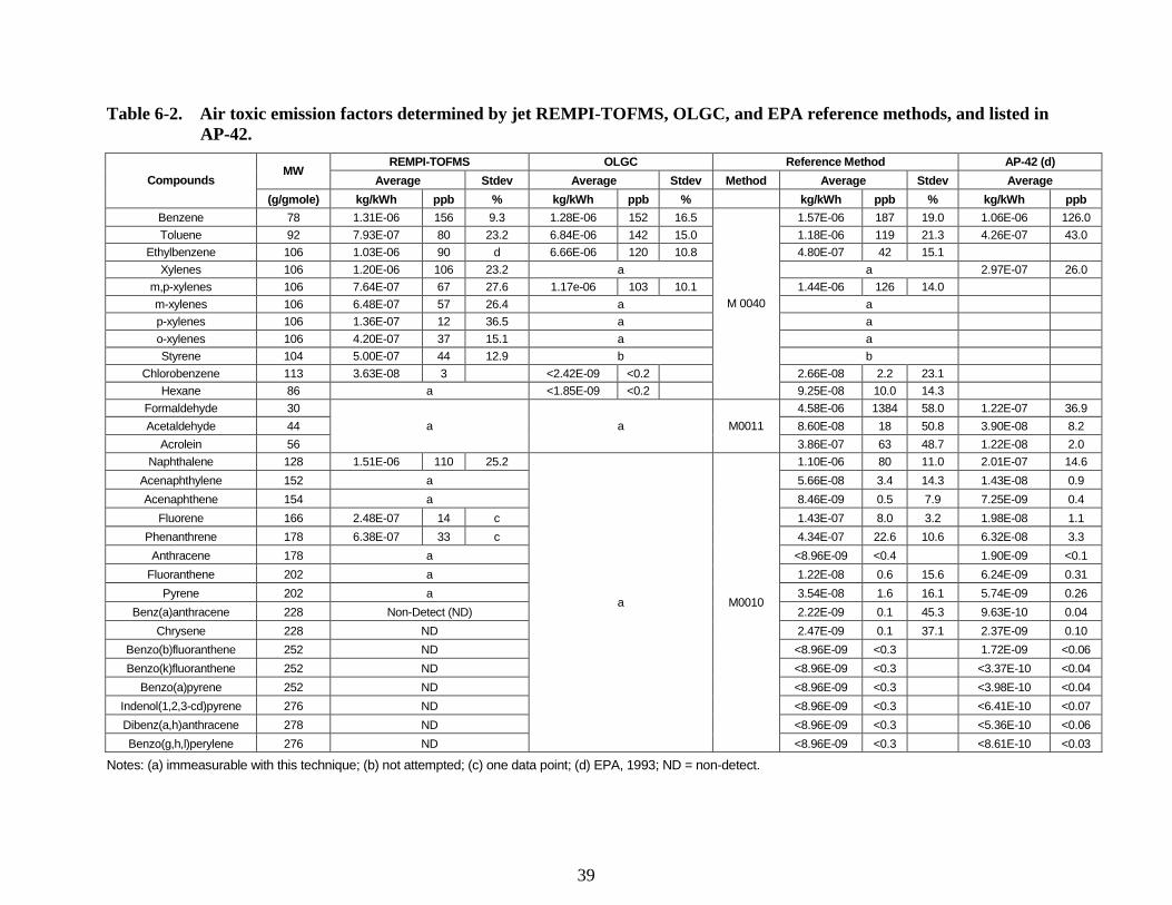
39

Table 6-2. Air toxic emission factors determined by jet REMPI-TOFMS, OLGC, and EPA reference methods, and listed in AP-42.

REMPI-TOFMS OLGC Reference Method AP-42 (d) MW

Average Stdev Average Stdev Method Average Stdev Average Compounds

(g/gmole) kg/kWh ppb % kg/kWh ppb % kg/kWh ppb % kg/kWh ppb

Benzene 78 1.31E-06 156 9.3 1.28E-06 152 16.5 1.57E-06 187 19.0 1.06E-06 126.0

Toluene 92 7.93E-07 80 23.2 6.84E-06 142 15.0 1.18E-06 119 21.3 4.26E-07 43.0

Ethylbenzene 106 1.03E-06 90 d 6.66E-06 120 10.8 4.80E-07 42 15.1

Xylenes 106 1.20E-06 106 23.2 a a 2.97E-07 26.0

m,p-xylenes 106 7.64E-07 67 27.6 1.17e-06 103 10.1 1.44E-06 126 14.0

m-xylenes 106 6.48E-07 57 26.4 a a

p-xylenes 106 1.36E-07 12 36.5 a a

o-xylenes 106 4.20E-07 37 15.1 a a

Styrene 104 5.00E-07 44 12.9 b b

Chlorobenzene 113 3.63E-08 3 <2.42E-09 <0.2 2.66E-08 2.2 23.1

Hexane 86 a <1.85E-09 <0.2

M 0040

9.25E-08 10.0 14.3

Formaldehyde 30 4.58E-06 1384 58.0 1.22E-07 36.9

Acetaldehyde 44 8.60E-08 18 50.8 3.90E-08 8.2

Acrolein 56

a a M0011

3.86E-07 63 48.7 1.22E-08 2.0

Naphthalene 128 1.51E-06 110 25.2 1.10E-06 80 11.0 2.01E-07 14.6

Acenaphthylene 152 a 5.66E-08 3.4 14.3 1.43E-08 0.9

Acenaphthene 154 a 8.46E-09 0.5 7.9 7.25E-09 0.4

Fluorene 166 2.48E-07 14 c 1.43E-07 8.0 3.2 1.98E-08 1.1

Phenanthrene 178 6.38E-07 33 c 4.34E-07 22.6 10.6 6.32E-08 3.3

Anthracene 178 a <8.96E-09 <0.4 1.90E-09 <0.1

Fluoranthene 202 a 1.22E-08 0.6 15.6 6.24E-09 0.31

Pyrene 202 a 3.54E-08 1.6 16.1 5.74E-09 0.26

Benz(a)anthracene 228 Non-Detect (ND) 2.22E-09 0.1 45.3 9.63E-10 0.04

Chrysene 228 ND 2.47E-09 0.1 37.1 2.37E-09 0.10

Benzo(b)fluoranthene 252 ND <8.96E-09 <0.3 1.72E-09 <0.06

Benzo(k)fluoranthene 252 ND <8.96E-09 <0.3 <3.37E-10 <0.04

Benzo(a)pyrene 252 ND <8.96E-09 <0.3 <3.98E-10 <0.04

Indenol(1,2,3-cd)pyrene 276 ND <8.96E-09 <0.3 <6.41E-10 <0.07

Dibenz(a,h)anthracene 278 ND <8.96E-09 <0.3 <5.36E-10 <0.06

Benzo(g,h,l)perylene 276 ND

a M0010

<8.96E-09 <0.3 <8.61E-10 <0.03

Notes: (a) immeasurable with this technique; (b) not attempted; (c) one data point; (d) EPA, 1993; ND = non-detect.

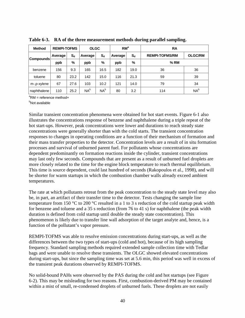
40

Table 6-3. RA of the three measurement methods during parallel sampling.

Method REMPI-TOFMS OLGC RMa RA

Average Sd Average Sd Average Sd REMPI-TOFMS/RM OLGC/RM Compounds

ppb % ppb % ppb % % RM

benzene 156 9.3 165 16.5 182 19.0 36 36

toluene 80 23.2 142 15.0 116 21.3 59 39

m-,p-xylene 67 27.6 103 10.2 121 14.0 79 34

naphthalene 110 25.2 NAb NAb 80 3.2 114 NAb

aRM = reference method+ bNot available

Similar transient concentration phenomena were obtained for hot start events. Figure 6-1 also illustrates the concentrations response of benzene and naphthalene during a triple repeat of the hot start-ups. However, peak concentrations were lower and durations to reach steady state concentrations were generally shorter than with the cold starts. The transient concentration responses to changes in operating conditions are a function of their mechanism of formation and their mass transfer properties to the detector. Concentration levels are a result of in situ formation processes and survival of unburned parent fuel. For pollutants whose concentrations are dependent predominantly on formation reactions inside the cylinder, transient concentrations may last only few seconds. Compounds that are present as a result of unburned fuel droplets are more closely related to the time for the engine block temperature to reach thermal equilibrium. This time is source dependent, could last hundred of seconds (Rakopoulos et al., 1998), and will be shorter for warm startups in which the combustion chamber walls already exceed ambient temperatures. The rate at which pollutants retreat from the peak concentration to the steady state level may also be, in part, an artifact of their transfer time to the detector. Tests changing the sample line temperature from 150 °C to 200 °C resulted in a 1 to 3 s reduction of the cold startup peak width for benzene and toluene and a 35 s reduction (from 76 to 41 s) for naphthalene (the peak width duration is defined from cold startup until double the steady state concentration). This phenomenon is likely due to transfer line wall adsorption of the target analyte and, hence, is a function of the pollutant’s vapor pressure. REMPI-TOFMS was able to resolve emission concentrations during start-ups, as well as the differences between the two types of start-ups (cold and hot), because of its high sampling frequency. Standard sampling methods required extended sample collection time with Tedlar bags and were unable to resolve these transients. The OLGC showed elevated concentrations during start-ups, but since the sampling time was set at 5.6 min, this period was well in excess of the transient peak durations observed by REMPI-TOFMS. No solid-bound PAHs were observed by the PAS during the cold and hot startups (see Figure 6-2). This may be misleading for two reasons. First, combustion-derived PM may be contained within a mist of small, re-condensed droplets of unburned fuels. These droplets are not easily

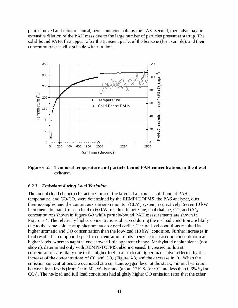
41

photo-ionized and remain neutral, hence, undetectable by the PAS. Second, there also may be extensive dilution of the PAH mass due to the large number of particles present at startup. The solid-bound PAHs first appear after the transient peaks of the benzene (for example), and their concentrations steadily subside with run time.

0 200 400 600 800 2000 2250 25000

50

100

150

200

250

300

350

0

20

40

60

80

100

120

Temperature

Tem

pera

ture

(o C

)

Run Time (Seconds)

Solid-Phase PAHs

PA

Hs

Con

cent

ratio

n @

14(

%)

O2 (

µg/m

3 )

Figure 6-2. Temporal temperature and particle-bound PAH concentrations in the diesel exhaust.

6.2.3 Emissions during Load Variation

The modal (load change) characterization of the targeted air toxics, solid-bound PAHs, temperature, and CO/CO2 were determined by the REMPI-TOFMS, the PAS analyzer, duct thermocouples, and the continuous emission monitor (CEM) system, respectively. Seven 10 kW increments in load, from no load to 60 kW, resulted in benzene, naphthalene, CO, and CO2 concentrations shown in Figure 6-3 while particle-bound PAH measurements are shown in Figure 6-4. The relatively higher concentrations observed during the no-load condition are likely due to the same cold startup phenomena observed earlier. The no-load conditions resulted in higher aromatic and CO concentration than the low-load (10 kW) condition. Further increases in load resulted in compound-specific concentration trends: benzene increased in concentration at higher loads, whereas naphthalene showed little apparent change. Methylated naphthalenes (not shown), determined only with REMPI-TOFMS, also increased. Increased pollutant concentrations are likely due to the higher fuel to air ratio at higher loads, also reflected by the increase of the concentrations of CO and CO2 (Figure 6-3) and the decrease in O2. When the emission concentrations are evaluated at a constant oxygen level at the stack, minimal variation between load levels (from 10 to 50 kW) is noted (about 12% Sd for CO and less than 0.6% Sd for CO2). The no-load and full load conditions had slightly higher CO emission rates that the other

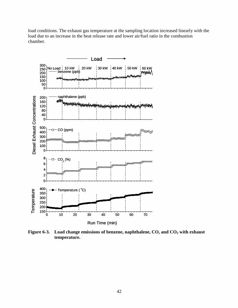
42

load conditions. The exhaust gas temperature at the sampling location increased linearly with the load due to an increase in the heat release rate and lower air/fuel ratio in the combustion chamber.

0 10 20 30 40 50 60 70150200250300350400

0

2

4

6

8

0100200300400500

04080

120160200

050

100150200250300

Temperature ( oC)

CO2 (%)

CO (ppm)

naphthalene (ppb)

benzene (ppb)No Load 10 kW 20 kW 30 kW 40 kW 50 kW 60 kW

Load

Run Time (min)

Tem

pera

ture

Die

sel E

xhau

st C

once

ntra

tions

0 10 20 30 40 50 60 70150200250300350400

0

2

4

6

8

0100200300400500

04080

120160200

050

100150200250300

Temperature ( oC)

CO2 (%)

CO (ppm)

naphthalene (ppb)

benzene (ppb)No Load 10 kW 20 kW 30 kW 40 kW 50 kW 60 kW

LoadLoad

Run Time (min)

Tem

pera

ture

Die

sel E

xhau

st C

once

ntra

tions

Figure 6-3. Load change emissions of benzene, naphthalene, CO, and CO2 with exhaust temperature.

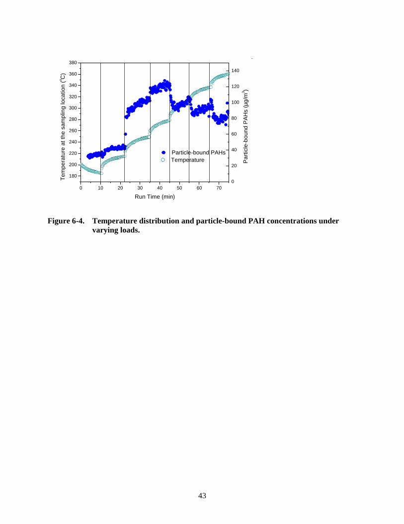
43

0 10 20 30 40 50 60 70

180

200

220

240

260

280

300

320

340

360

380

0

20

40

60

80

100

120

140

Tem

pera

ture

at t

he s

ampl

ing

loca

tion

(o C)

Run Time (min)

Temperature Par

ticle

-bou

nd P

AH

s (µ

g/m

3 )

Particle-bound PAHs

Figure 6-4. Temperature distribution and particle-bound PAH concentrations under varying loads.

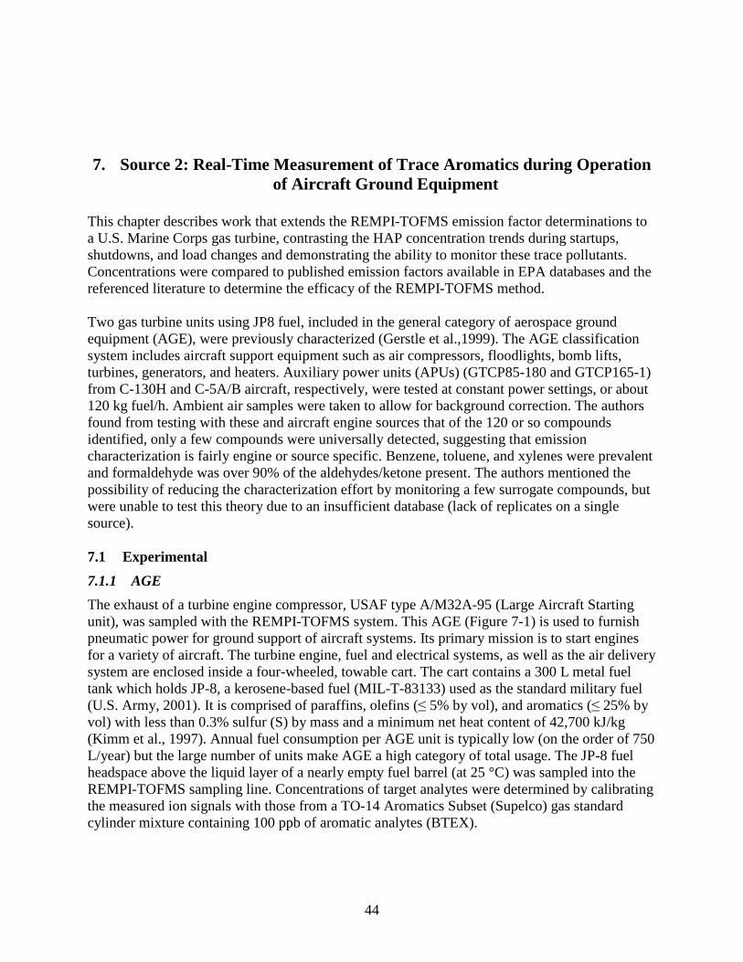
44

7. Source 2: Real-Time Measurement of Trace Aromatics during Operation

of Aircraft Ground Equipment

This chapter describes work that extends the REMPI-TOFMS emission factor determinations to a U.S. Marine Corps gas turbine, contrasting the HAP concentration trends during startups, shutdowns, and load changes and demonstrating the ability to monitor these trace pollutants. Concentrations were compared to published emission factors available in EPA databases and the referenced literature to determine the efficacy of the REMPI-TOFMS method. Two gas turbine units using JP8 fuel, included in the general category of aerospace ground equipment (AGE), were previously characterized (Gerstle et al.,1999). The AGE classification system includes aircraft support equipment such as air compressors, floodlights, bomb lifts, turbines, generators, and heaters. Auxiliary power units (APUs) (GTCP85-180 and GTCP165-1) from C-130H and C-5A/B aircraft, respectively, were tested at constant power settings, or about 120 kg fuel/h. Ambient air samples were taken to allow for background correction. The authors found from testing with these and aircraft engine sources that of the 120 or so compounds identified, only a few compounds were universally detected, suggesting that emission characterization is fairly engine or source specific. Benzene, toluene, and xylenes were prevalent and formaldehyde was over 90% of the aldehydes/ketone present. The authors mentioned the possibility of reducing the characterization effort by monitoring a few surrogate compounds, but were unable to test this theory due to an insufficient database (lack of replicates on a single source). 7.1 Experimental

7.1.1 AGE

The exhaust of a turbine engine compressor, USAF type A/M32A-95 (Large Aircraft Starting unit), was sampled with the REMPI-TOFMS system. This AGE (Figure 7-1) is used to furnish pneumatic power for ground support of aircraft systems. Its primary mission is to start engines for a variety of aircraft. The turbine engine, fuel and electrical systems, as well as the air delivery system are enclosed inside a four-wheeled, towable cart. The cart contains a 300 L metal fuel tank which holds JP-8, a kerosene-based fuel (MIL-T-83133) used as the standard military fuel (U.S. Army, 2001). It is comprised of paraffins, olefins (≤ 5% by vol), and aromatics (≤ 25% by vol) with less than 0.3% sulfur (S) by mass and a minimum net heat content of 42,700 kJ/kg (Kimm et al., 1997). Annual fuel consumption per AGE unit is typically low (on the order of 750 L/year) but the large number of units make AGE a high category of total usage. The JP-8 fuel headspace above the liquid layer of a nearly empty fuel barrel (at 25 °C) was sampled into the REMPI-TOFMS sampling line. Concentrations of target analytes were determined by calibrating the measured ion signals with those from a TO-14 Aromatics Subset (Supelco) gas standard cylinder mixture containing 100 ppb of aromatic analytes (BTEX).

45

Figure 7-1. Aircraft ground equipment outside EPA facilities

7.1.2 Operating and Sampling Procedures

The AGE was operated for two days to characterize its emissions under idle and full load conditions as well as start up and shut down scenarios. The idle and full load operating periods ranged from 1 to 4 h duration, interspersed with refueling times. Consecutive, ~ 2 h cycles of start up and shut down were completed over a 6-7 h sampling day. REMPI-TOFMS sampling was conducted using 5 cm diameter ports located about 30 cm below the top of a 4.9 m high, 0.84 m x 0.28 m rectangular carbon-steel duct covered with 7.6 cm fiberglass insulation. This duct was built to convey the AGE exhaust away from building air intakes. A 2 L/min isokinetic sample was pulled through a 15 m, 0.95 cm (inner diameter) heated (150 °C) transfer line to a heated (150 °C), filter. Filters were exchanged at least three times per day (1 to 3 h sampling time) to minimize capture of the target analytes on the carbon-laden filter. Beyond the filter, a 3 m long, 1.25 cm diameter silico steel coated transfer line (at 150 °C) conveyed the sample to the REMPI-TOFMS instrument. A small quantity of 1 ppm C6D6 in N2 calibration gas was added upstream of the filter as an internal calibrant. REMPI-TOFMS sampled directly from the 2 L/min exhaust with a slipstream of approximately 1 mL/min. Fourteen pre-determined wavelengths in the λ = 258 – 275 nm range were selected, based on established wavelength scan libraries, for their high probability of detecting discrete, individual (isomer selective) compounds. This wavelength changing sequence method was performed during steady state idle (low) and full load AGE operational modes where changes in concentration were expected to be gradual. The REMPI ion signal of a target analyte at its specific wavelength was recorded for 1 minute before switching to the next wavelength. This 15 minute sequence was repeated multiple times within the sampling time period as defined by the conventional extractive sampling methods. In addition, cold/hot starts and shutdowns were followed in real time at the most effective wavelength for toluene ionization (267 nm) without additional wavelength changes in order to eliminate losses in data acquisition during wavelength switches (~ 2 s).

46

Conventional extractive sampling techniques, based on EPA Methods, were used to validate the integrated REMPI/TOFMS measurements taken over the same sampling time. VOCs were sampled in parallel with the REMPI-TOFMS, using standard extractive sampling for volatiles from the duct into stainless-steel Summa canisters and analyzed by GC/MS (EPA 1999) for 60 target compounds and for unknown VOCs as tentatively identified compounds (TICs) using the National Institute of Standards and Technology (NIST) spectral database (NIST, 2005). Nine samples from the turbine stack were taken during the two days of sampling, four at idle load and five at full load. All samples were extracted from a 0.65 cm (1/4 inch) port through a 0.65 cm (1/4 inch) Teflon tube. All summa canister samplings were started with an initial vacuum of 76.2 cm (30 inches) Hg and ended with 1.2 to 0 cm Hg (3 to 0 inches of Hg) Two summa canisters were also used as a feed into the REMPI-TOFMS instrument as well as the GC/MS for further validation of the methods. PAHs were sampled using EPA Method 0010 (EPA, 1986a) and Method 5 (EPA, 1986b) sampling, and analyzed via a modified EPA Method 8270 (EPA 1996b) using a toluene extraction solvent and deuterated and fluorinated pre-sampling spikes. Formaldehydes and other carbonyl group compounds were sampled via EPA Method 0011 (EPA, 1996c). This method uses a sample train configuration adapted from EPA Method 5, wherein the sample gas is collected in an aqueous, acidic 2,4-dinitrophenyhydrazine (DNPH) solution, and analyzed via EPA Method 8315A (EPA, 1996d) using high performance liquid chromatography (HPLC). Results of the carbonyl groups were provided to develop additional emission factors for the AGE and not for the purpose of the REMPI/TOFMS validation. Emissions factors were calculated by dividing the concentration of the compound by the amount of fuel used, or g/kg of fuel. Graphical results are reported as the value ± 1 standard deviation, σ. Tabular results are reported as RSDs divided by the average value, or σ / average (AVG). Comparisons between measurement methods are made with matched pairs of each target analyte using a paired t test. 7.2 Results and Discussion

REMPI-TOFMS traces during AGE startups, low load, and high load operation show complex emissions of varying concentrations. Figure 7-2 shows a 3D time-resolved trace of the emissions during a cold start (commencing at 2 min, 20 s) followed by about 5 min of low load operation. The concentration is proportional to the ion signal strength and the mass values highlight the different compounds that are observed. The cold start results in a significant peak of toluene (m/z = 92) as well as a number of other methylated naphthalenes (m/z = 128 to 184). The trace shown is optimized for toluene detection at λ = 267.5 nm. At this wavelength, methylated naphthalenes are also efficiently ionized while benzene and other single ring aromatics are marginally detected. The initial concentrations decline within 1 min, then are mostly constant during the low load operation. At 6 min and 53 s a change to high load shows signal reduction across the whole mass range, indicating a large drop in the measured concentrations. The lower concentrations are expected due to dilution from the increased throughput air in the turbine and increased combustion efficiency.

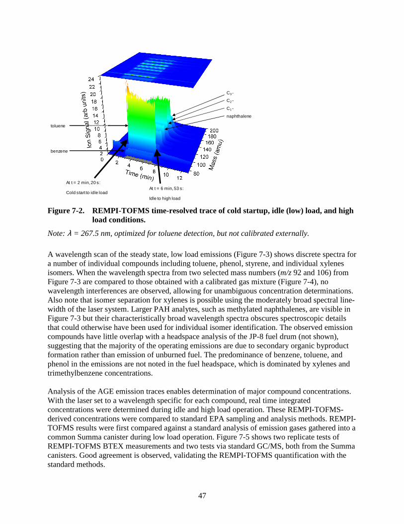
47

At t = 2 min, 20 s:

Cold start to idle loadAt t = 6 min, 53 s:

Idle to high load

naphthalene

C1 -

C2 -

C3 -

toluene

benzene

Figure 7-2. REMPI-TOFMS time-resolved trace of cold startup, idle (low) load, and high load conditions.

Note: λ = 267.5 nm, optimized for toluene detection, but not calibrated externally.

A wavelength scan of the steady state, low load emissions (Figure 7-3) shows discrete spectra for a number of individual compounds including toluene, phenol, styrene, and individual xylenes isomers. When the wavelength spectra from two selected mass numbers (m/z 92 and 106) from Figure 7-3 are compared to those obtained with a calibrated gas mixture (Figure 7-4), no wavelength interferences are observed, allowing for unambiguous concentration determinations. Also note that isomer separation for xylenes is possible using the moderately broad spectral line-width of the laser system. Larger PAH analytes, such as methylated naphthalenes, are visible in Figure 7-3 but their characteristically broad wavelength spectra obscures spectroscopic details that could otherwise have been used for individual isomer identification. The observed emission compounds have little overlap with a headspace analysis of the JP-8 fuel drum (not shown), suggesting that the majority of the operating emissions are due to secondary organic byproduct formation rather than emission of unburned fuel. The predominance of benzene, toluene, and phenol in the emissions are not noted in the fuel headspace, which is dominated by xylenes and trimethylbenzene concentrations. Analysis of the AGE emission traces enables determination of major compound concentrations. With the laser set to a wavelength specific for each compound, real time integrated concentrations were determined during idle and high load operation. These REMPI-TOFMS-derived concentrations were compared to standard EPA sampling and analysis methods. REMPI-TOFMS results were first compared against a standard analysis of emission gases gathered into a common Summa canister during low load operation. Figure 7-5 shows two replicate tests of REMPI-TOFMS BTEX measurements and two tests via standard GC/MS, both from the Summa canisters. Good agreement is observed, validating the REMPI-TOFMS quantification with the standard methods.

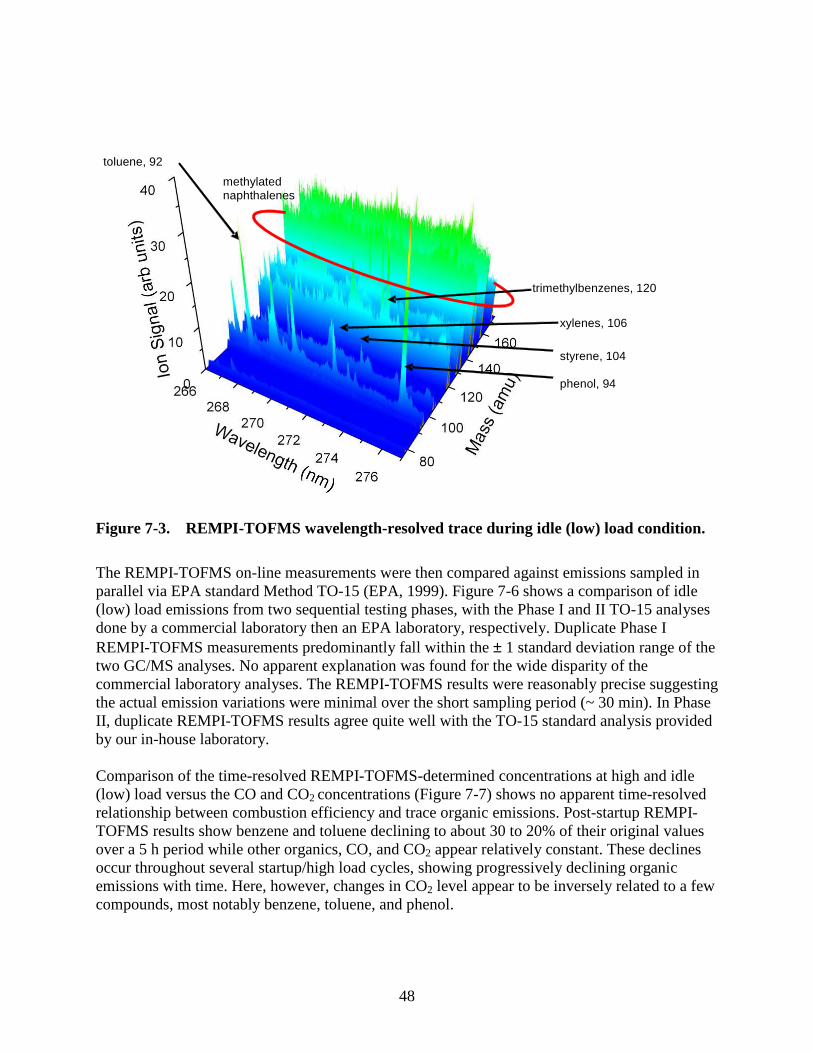
48

Figure 7-3. REMPI-TOFMS wavelength-resolved trace during idle (low) load condition.

The REMPI-TOFMS on-line measurements were then compared against emissions sampled in parallel via EPA standard Method TO-15 (EPA, 1999). Figure 7-6 shows a comparison of idle (low) load emissions from two sequential testing phases, with the Phase I and II TO-15 analyses done by a commercial laboratory then an EPA laboratory, respectively. Duplicate Phase I REMPI-TOFMS measurements predominantly fall within the ± 1 standard deviation range of the two GC/MS analyses. No apparent explanation was found for the wide disparity of the commercial laboratory analyses. The REMPI-TOFMS results were reasonably precise suggesting the actual emission variations were minimal over the short sampling period (~ 30 min). In Phase II, duplicate REMPI-TOFMS results agree quite well with the TO-15 standard analysis provided by our in-house laboratory. Comparison of the time-resolved REMPI-TOFMS-determined concentrations at high and idle (low) load versus the CO and CO2 concentrations (Figure 7-7) shows no apparent time-resolved relationship between combustion efficiency and trace organic emissions. Post-startup REMPI-TOFMS results show benzene and toluene declining to about 30 to 20% of their original values over a 5 h period while other organics, CO, and CO2 appear relatively constant. These declines occur throughout several startup/high load cycles, showing progressively declining organic emissions with time. Here, however, changes in CO2 level appear to be inversely related to a few compounds, most notably benzene, toluene, and phenol.

phenol, 94

toluene, 92

xylenes, 106

styrene, 104

trimethylbenzenes, 120

methylated naphthalenes

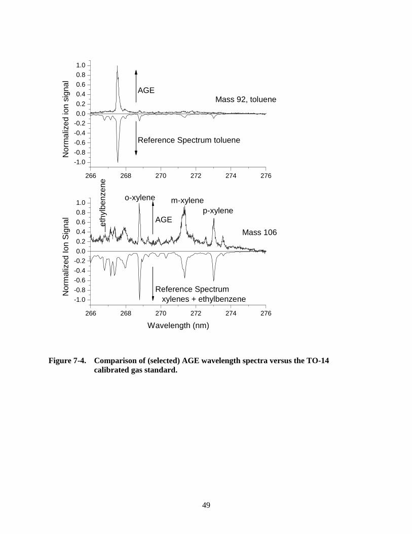
49

266 268 270 272 274 276

-1.0

-0.8

-0.6

-0.4

-0.2

0.0

0.2

0.4

0.6

0.8

1.0

Reference Spectrum toluene

Nor

mal

ized

ion

sign

al

Mass 92, tolueneAGE

266 268 270 272 274 276

-1.0

-0.8

-0.6

-0.4

-0.2

0.0

0.2

0.4

0.6

0.8

1.0

Mass 106

Nor

mal

ized

Ion

Sig

nal

Wavelength (nm)

Reference Spectrum xylenes + ethylbenzene

AGEp-xylene

m-xyleneo-xylene

ethy

lben

zene

Figure 7-4. Comparison of (selected) AGE wavelength spectra versus the TO-14 calibrated gas standard.

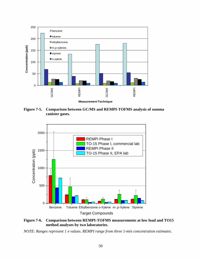
50

0

50

100

150

200

250

GC

/MS

RE

MP

I

GC

/MS

RE

MP

I

Co

nce

ntr

atio

n (p

pb

)

Measurement Technique

benzene

toluene

ethylbenzene

m,p-xylenes

styrene

o-xylene

Figure 7-5. Comparison between GC/MS and REMPI-TOFMS analysis of summa canister gases.

Benzene Toluene Ethylbenzene o-Xylene m-,p-Xylene Styrene0

500

1000

1500

2000

Con

cent

ratio

n (p

pb)

Target Compounds

REMPI Phase I TO-15 Phase I, commercial lab REMPI Phase II TO-15 Phase II, EPA lab

Figure 7-6. Comparison between REMPI-TOFMS measurements at low load and TO15 method analyses by two laboratories.

NOTE: Ranges represent 1 σ values. REMPI range from three 1-min concentration estimates.

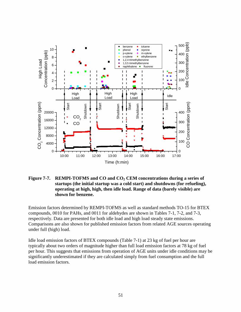
51

10:00 11:00 12:00 13:00 14:00 15:00 16:00 17:000

4000

8000

12000

16000

20000

0

100

200

300

400

0

2

4

6

8

10

0

100

200

300

400

500

CO

2 Con

cent

ratio

n (p

pm)

Time (h:min)

CO

Con

cent

ratio

n (p

pm)

CO2

CO

Idle

Sta

rt

Shu

tdow

n

High Load

High Load

Sta

rt

Shu

tdow

n

benzene toluene phenol styrene p-xylene m-xylene o-xylene ethylbenzene 1,2,4 trimethylbenzene 1,3,5 trimethylbenzene naphthalene fluorene

Hig

h Lo

adC

once

ntra

tion

(ppb

)

High Load

Sta

rt

Sta

rt

Shu

tdow

n

Idle

Con

cent

ratio

n (p

pb)

Figure 7-7. REMPI-TOFMS and CO and CO2 CEM concentrations during a series of startups (the initial startup was a cold start) and shutdowns (for refueling), operating at high, high, then idle load. Range of data (barely visible) are shown for benzene.

Emission factors determined by REMPI-TOFMS as well as standard methods TO-15 for BTEX compounds, 0010 for PAHs, and 0011 for aldehydes are shown in Tables 7-1, 7-2, and 7-3, respectively. Data are presented for both idle load and high load steady state emissions. Comparisons are also shown for published emission factors from related AGE sources operating under full (high) load. Idle load emission factors of BTEX compounds (Table 7-1) at 23 kg of fuel per hour are typically about two orders of magnitude higher than full load emission factors at 78 kg of fuel per hour. This suggests that emissions from operation of AGE units under idle conditions may be significantly underestimated if they are calculated simply from fuel consumption and the full load emission factors.

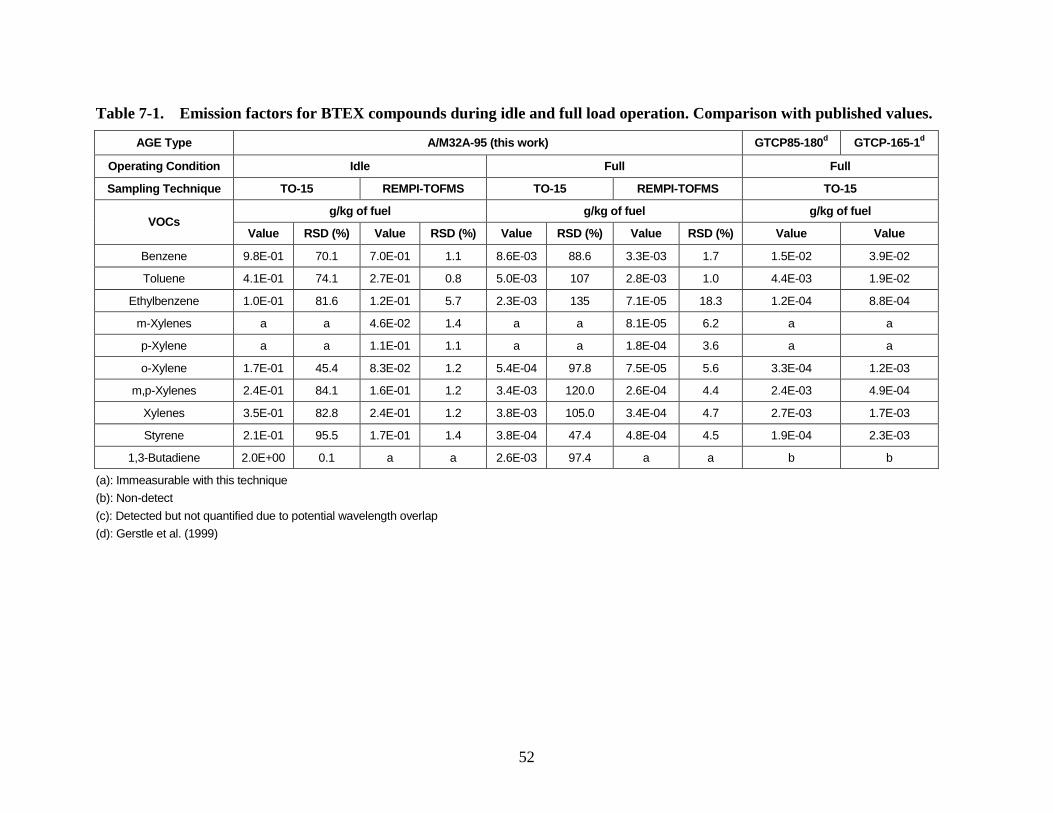
52

Table 7-1. Emission factors for BTEX compounds during idle and full load operation. Comparison with published values.

AGE Type A/M32A-95 (this work) GTCP85-180d GTCP-165-1d

Operating Condition Idle Full Full

Sampling Technique TO-15 REMPI-TOFMS TO-15 REMPI-TOFMS TO-15

g/kg of fuel g/kg of fuel g/kg of fuel VOCs

Value RSD (%) Value RSD (%) Value RSD (%) Value RSD (%) Value Value

Benzene 9.8E-01 70.1 7.0E-01 1.1 8.6E-03 88.6 3.3E-03 1.7 1.5E-02 3.9E-02

Toluene 4.1E-01 74.1 2.7E-01 0.8 5.0E-03 107 2.8E-03 1.0 4.4E-03 1.9E-02

Ethylbenzene 1.0E-01 81.6 1.2E-01 5.7 2.3E-03 135 7.1E-05 18.3 1.2E-04 8.8E-04

m-Xylenes a a 4.6E-02 1.4 a a 8.1E-05 6.2 a a

p-Xylene a a 1.1E-01 1.1 a a 1.8E-04 3.6 a a

o-Xylene 1.7E-01 45.4 8.3E-02 1.2 5.4E-04 97.8 7.5E-05 5.6 3.3E-04 1.2E-03

m,p-Xylenes 2.4E-01 84.1 1.6E-01 1.2 3.4E-03 120.0 2.6E-04 4.4 2.4E-03 4.9E-04

Xylenes 3.5E-01 82.8 2.4E-01 1.2 3.8E-03 105.0 3.4E-04 4.7 2.7E-03 1.7E-03

Styrene 2.1E-01 95.5 1.7E-01 1.4 3.8E-04 47.4 4.8E-04 4.5 1.9E-04 2.3E-03

1,3-Butadiene 2.0E+00 0.1 a a 2.6E-03 97.4 a a b b

(a): Immeasurable with this technique

(b): Non-detect

(c): Detected but not quantified due to potential wavelength overlap

(d): Gerstle et al. (1999)

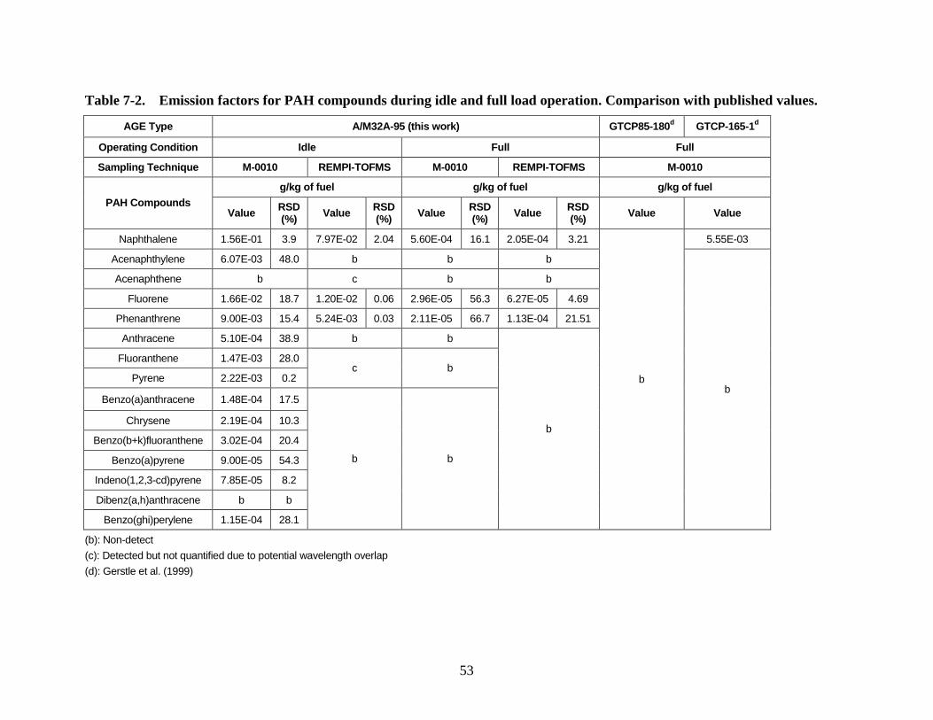
53

Table 7-2. Emission factors for PAH compounds during idle and full load operation. Comparison with published values.

AGE Type A/M32A-95 (this work) GTCP85-180d GTCP-165-1d


Sampling Technique M-0010 REMPI-TOFMS M-0010 REMPI-TOFMS M-0010

g/kg of fuel g/kg of fuel g/kg of fuel PAH Compounds

Value RSD (%) Value RSD

(%) Value RSD (%) Value RSD

(%) Value Value

Naphthalene 1.56E-01 3.9 7.97E-02 2.04 5.60E-04 16.1 2.05E-04 3.21 5.55E-03

Acenaphthylene 6.07E-03 48.0 b b b

Acenaphthene b c b b

Fluorene 1.66E-02 18.7 1.20E-02 0.06 2.96E-05 56.3 6.27E-05 4.69

Phenanthrene 9.00E-03 15.4 5.24E-03 0.03 2.11E-05 66.7 1.13E-04 21.51

Anthracene 5.10E-04 38.9 b b

Fluoranthene 1.47E-03 28.0

Pyrene 2.22E-03 0.2 c b

Benzo(a)anthracene 1.48E-04 17.5

Chrysene 2.19E-04 10.3

Benzo(b+k)fluoranthene 3.02E-04 20.4

Benzo(a)pyrene 9.00E-05 54.3

Indeno(1,2,3-cd)pyrene 7.85E-05 8.2

Dibenz(a,h)anthracene b b

Benzo(ghi)perylene 1.15E-04 28.1

b b

b

b b

(b): Non-detect

(c): Detected but not quantified due to potential wavelength overlap

(d): Gerstle et al. (1999)

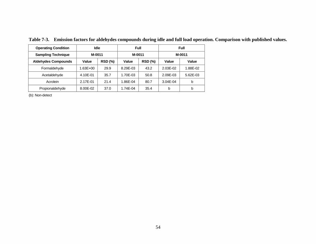
54

Table 7-3. Emission factors for aldehydes compounds during idle and full load operation. Comparison with published values.


Sampling Technique M-0011 M-0011 M-0011

Aldehydes Compounds Value RSD (%) Value RSD (%) Value Value

Formaldehyde 1.63E+00 29.9 8.29E-03 43.2 2.03E-02 1.88E-02

Acetaldehyde 4.10E-01 35.7 1.70E-03 50.8 2.09E-03 5.62E-03

Acrolein 2.17E-01 21.4 1.86E-04 80.7 3.04E-04 b

Propionaldehyde 8.00E-02 37.0 1.74E-04 35.4 b b

(b): Non-detect

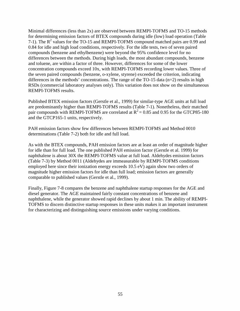
55

Minimal differences (less than 2x) are observed between REMPI-TOFMS and TO-15 methods for determining emission factors of BTEX compounds during idle (low) load operation (Table 7-1). The R2 values for the TO-15 and REMPI-TOFMS compound matched pairs are 0.99 and 0.84 for idle and high load conditions, respectively. For the idle tests, two of seven paired compounds (benzene and ethylbenzene) were beyond the 95% confidence level for no differences between the methods. During high loads, the most abundant compounds, benzene and toluene, are within a factor of three. However, differences for some of the lower concentration compounds exceed 10x, with REMPI-TOFMS recording lower values. Three of the seven paired compounds (benzene, o-xylene, styrene) exceeded the criterion, indicating differences in the methods’ concentrations. The range of the TO-15 data (n=2) results in high RSDs (commercial laboratory analyses only). This variation does not show on the simultaneous REMPI-TOFMS results. Published BTEX emission factors (Gerstle et al., 1999) for similar-type AGE units at full load are predominantly higher than REMPI-TOFMS results (Table 7-1). Nonetheless, their matched pair compounds with REMPI-TOFMS are correlated at R2 = 0.85 and 0.95 for the GTCP85-180 and the GTCP165-1 units, respectively. PAH emission factors show few differences between REMPI-TOFMS and Method 0010 determinations (Table 7-2) both for idle and full load. As with the BTEX compounds, PAH emission factors are at least an order of magnitude higher for idle than for full load. The one published PAH emission factor (Gerstle et al. 1999) for naphthalene is about 30X the REMPI-TOFMS value at full load. Aldehydes emission factors (Table 7-3) by Method 0011 (Aldehydes are immeasurable by REMPI-TOFMS conditions employed here since their ionization energy exceeds 10.5 eV) again show two orders of magnitude higher emission factors for idle than full load; emission factors are generally comparable to published values (Gerstle et al., 1999). Finally, Figure 7-8 compares the benzene and naphthalene startup responses for the AGE and diesel generator. The AGE maintained fairly constant concentrations of benzene and naphthalene, while the generator showed rapid declines by about 1 min. The ability of REMPI-TOFMS to discern distinctive startup responses in these units makes it an important instrument for characterizing and distinguishing source emissions under varying conditions.

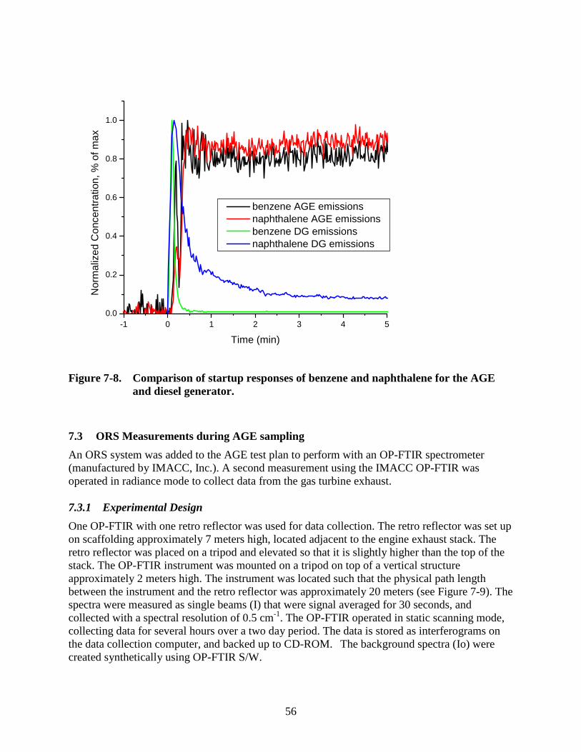
56

-1 0 1 2 3 4 50.0

0.2

0.4

0.6

0.8

1.0

Nor

mal

ized

Con

cent

ratio

n, %

of m

ax

Time (min)

benzene AGE emissions naphthalene AGE emissions benzene DG emissions naphthalene DG emissions

Figure 7-8. Comparison of startup responses of benzene and naphthalene for the AGE and diesel generator.

7.3 ORS Measurements during AGE sampling

An ORS system was added to the AGE test plan to perform with an OP-FTIR spectrometer (manufactured by IMACC, Inc.). A second measurement using the IMACC OP-FTIR was operated in radiance mode to collect data from the gas turbine exhaust. 7.3.1 Experimental Design

One OP-FTIR with one retro reflector was used for data collection. The retro reflector was set up on scaffolding approximately 7 meters high, located adjacent to the engine exhaust stack. The retro reflector was placed on a tripod and elevated so that it is slightly higher than the top of the stack. The OP-FTIR instrument was mounted on a tripod on top of a vertical structure approximately 2 meters high. The instrument was located such that the physical path length between the instrument and the retro reflector was approximately 20 meters (see Figure 7-9). The spectra were measured as single beams (I) that were signal averaged for 30 seconds, and collected with a spectral resolution of 0.5 cm-1. The OP-FTIR operated in static scanning mode, collecting data for several hours over a two day period. The data is stored as interferograms on the data collection computer, and backed up to CD-ROM. The background spectra (Io) were created synthetically using OP-FTIR S/W.

57

Retro-reflector

TurbinePlume

OP-FTIR

Plume Width = 0.5 m

Figure 7-9. ORS measurement configuration.

7.3.2 ORS Instrument-Retro reflector Distance

The physical distance between the OP-FTIR instrument and the retro reflector was measured using a Topcon, Inc. model GTS-211D theodolite. This distance is required for converting the products of incomplete combustion (PIC) data to path average concentration (PAC) values. PAC is equal to PIC divided by the optical path length. The optical path length is two times the physical distance, accounting for travel to and from the retro reflector. 7.4 Data Processing

The concentrations were determined by a regression fit to reference spectra using the Beers Law expression: I/Io = A = -Log10(αCL), where: I = single-beam measurement Io = background spectrum A = absorbance spectrum α = molecular absorptivity (extinction coefficient) C = concentration of the absorbing molecule L = total path-length of the infrared beam through the molecular plume The regression equation is written as: Af(ν) = ΣrAr(ν) + a + b ν + ε(ν) Data analysis was performed by the chemometric regression method that is referred to as classical least squares (CLS) and is written as:

58

Af(ν) = ΣrAr(ν) + a + b ν + ε(ν) Where: Af(ν)= measured field absorbance spectrum Ar(ν) = reference spectrum of chemical species, r a is a scalar that corrects for the baseline error b is a scalar that corrects for the baseline slope ε(ν) is the error or residual term The summation is over all species, r, that absorb in the region of analysis. 7.4.1 ORS Results

The 2-days of data gathering using the ORS equipment resulted in the measurements of criteria pollutants such as CO and CO2 as well as other compounds found in the absorption spectra such as formaldehyde, ethylene, and aliphatic mixture, the later which presumably originated from the fuel; n-octane is a major component of the aliphatic mixture and was used as a surrogate for the entire mixture. Other components include n-nonane, n-heptane, n-hexane and probably some bent-chain species. Data validation was performed by comparing the reference spectrum of a target species to the measured spectrum from the turbine plume. The trace emissions for formaldehyde, ethylene, and octane are presented in Figures 7-10, 7-11, and 7-12, respectively. The results of the ORS measurements were compared with stack measurements for CO and CO2, obtained using regular CEM instruments. The results were comparable for CO; however, the ORS results were not sensitive enough to differentiate between the high and low loads for CO2 as illustrated in Figure 7-13. Furthermore, drift of the ORS concentrations from those of the CEMs was observed throughout the day. This was due to an insufficient path length of the beam in the relatively small plume as well as effects of diurnal temperatures changes. The ORS system was not used for subsequent tests due to its limitations for measurement of point source emissions.

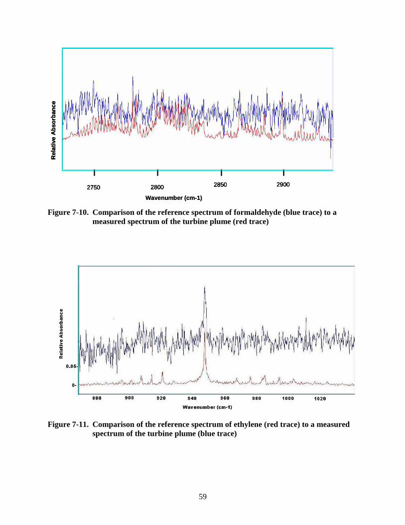
59

Wavenumber (cm-1)

2750 2800 2850 2900

Rel

ativ

e A

bso

rban

ce

Wavenumber (cm-1)

2750 2800 2850 2900

Rel

ativ

e A

bso

rban

ce

2750 2800 2850 29002750 2800 2850 2900

Rel

ativ

e A

bso

rban

ce

Figure 7-10. Comparison of the reference spectrum of formaldehyde (blue trace) to a measured spectrum of the turbine plume (red trace)

Figure 7-11. Comparison of the reference spectrum of ethylene (red trace) to a measured spectrum of the turbine plume (blue trace)

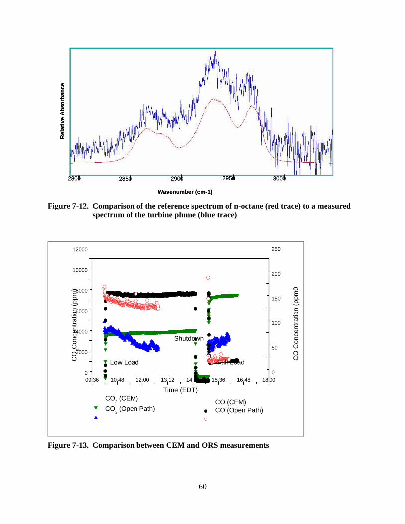
60

2800 2850 2900 2950 3000

Wavenumber (cm-1)

Rel

ativ

e A

bso

rban

ce

2800 2850 2900 2950 3000

Wavenumber (cm-1)

Rel

ativ

e A

bso

rban

ce

Figure 7-12. Comparison of the reference spectrum of n-octane (red trace) to a measured spectrum of the turbine plume (blue trace)

09:36 10:48 12:00 13:12 14:24 15:36 16:48 18:000

2000

4000

6000

8000

10000

12000

0

50

100

150

200

250

CO2 (CEM)

CO2 (Open Path)

CO

2Con

cent

ratio

n (p

pm)

Time (EDT)

CO

Con

cent

ratio

n (p

pm0

Shutdown

Full LoadLow Load

CO (CEM) CO (Open Path)

Figure 7-13. Comparison between CEM and ORS measurements

61

8. Source 3: Verification Results of REMPI-TOFMS as a Real-Time PCDD/F Emission Monitor

In 2005, REMPI with TOFMS was used in an international ETV test program monitoring levels of PCDD/F in a hazardous-waste-firing boiler (Cowen, 2006). Prediction of PCDD/F levels was based on prior determination of an indicator compound and intercorrelation of the indicator and PCDD/F concentrations. This chapter reports the determination of indicator compounds and the performance of REMPI-TOFMS during the ETV tests. 8.1 Materials and Methods

8.1.1 Boiler testing

An 860 KW capacity, 3-pass fire-tube, marine package boiler (Superior Boiler Works, Inc.), firing #2 fuel oil was used as the combustion gas source (Figure 8-1). The flue gas from the boiler passes through an exhaust duct to a manifold and then on to an air pollution control system (APCS). The APCS consists of a natural-gas-fired secondary combustion chamber, a fabric filter, and an acid gas scrubber to ensure proper removal of pollutants. The fuel oil was doped at a constant ratio of a surrogate hazardous waste (1,2-dichlorobenzene, DCB) and a source of metal catalyst (copper naphthenate) to promote PCDD/F formation. Fuel flows were measured with a total liquid volume meter. The amount of injected copper was set to simulate that of a refuse-derived fuel (RDF) ash (100 mg per kg of ash), conditions in which PCDD/F formation is favorable. The feed-rate of the mixture was varied to achieve a high (200-500 ppm) and low (10-50 ppm) target HCl concentration in the flue gas with the expectation of generating relatively high and low PCDD/F concentrations, respectively. Test runs of various durations were conducted under each set of operating conditions. Four 4-hours and two 8-hour sampling periods on successive days (i.e., totaling 16 hours per sample) were used to assess short-term and long-term accuracy of the measurements. The test campaigns sampled for PCDDs/Fs and semi-volatile PAHs using EPA methods 23 (EPA, 1996d), and 0010 (EPA, 1996a), respectively. Both Method 23 and Method 0010 consist of a 125 °C heated probe, 125 °C heated box containing a filter, water-cooled condenser, water-cooled XAD-2 resin cartridge, impinger train for water determination, vacuum line and pump, and a dry gas and orifice meter.

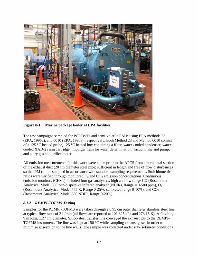
62

Figure 8-1. Marine package boiler at EPA facilities.

The test campaigns sampled for PCDDs/Fs and semi-volatile PAHs using EPA methods 23 (EPA, 1996d), and 0010 (EPA, 1996a), respectively. Both Method 23 and Method 0010 consist of a 125 °C heated probe, 125 °C heated box containing a filter, water-cooled condenser, water-cooled XAD-2 resin cartridge, impinger train for water determination, vacuum line and pump, and a dry gas and orifice meter. All emission measurements for this work were taken prior to the APCS from a horizontal section of the exhaust duct (20 cm diameter steel pipe) sufficient in length and free of flow disturbances so that PM can be sampled in accordance with standard sampling requirements. Stoichiometric ratios were verified through monitored O2 and CO2 emission concentrations. Continuous emission monitors (CEMs) included four gas analyzers: high and low range CO (Rosemount Analytical Model 880 non-dispersive infrared analyzer (NDIR), Range = 0-500 ppm), O2 (Rosemount Analytical Model 755 R, Range 0-25%, calibrated range 0-10%), and CO2 (Rosemount Analytical Model 880 NDIR, Range 0-20%). 8.1.2 REMPI-TOFMS Testing

Samples for the REMPI-TOFMS were taken through a 0.95 cm outer diameter stainless steel line at typical flow rates of 2 L/min (all flows are reported at 101.325 kPa and 273.15 K). A flexible, 9 m long, 1.27 cm diameter, Silico-steel transfer line conveyed the exhaust gas to the REMPI-TOFMS instrument. The line was kept at 150 °C while sampling exhaust gases in order to minimize adsorption to the line walls. The sample was collected under sub-isokinetic conditions

63

and filtered through a micro-fiber filter (at 150 °C) to avoid PM reaching the valve inlet system of the REMPI-TOFMS instrument. The REMPI-TOFMS underwent an in-situ calibration at the start of each test using fully deuterated benzene, C6D6, added to the exhaust stream. Deuterated benzene can be readily detected without spectral or mass interferences and is not an exhaust gas component. 8.1.3 Indicator Compounds

The use of indicator compound measurements to predict PCDD/F values requires a pre-determined correlation analysis to find the best indicator compound or compounds and to determine its mathematical relationship with the PCDD/F measure. These indicator correlations are likely to be source-specific, requiring an initial series of sampling tests for determining compound concentrations from which to run correlation analyses. Selection of the PCDD/F indicator compound was based on a “pre-ETV,” six-test measurement campaign of 31 compounds (Table 8-1). These 31 compounds were selected, in part, based on the general understanding that lower chlorinated compounds are more readily detectable with REMPI-TOFMS than the higher chlorinated compounds (Zimmermann et al., 1999). These pre-ETV tests replicated the high and low dopant loads that would occur under the subsequent actual ETV study. A correlation analysis was run on the results between the PCDD/F TEQ and other semi-volatile compounds sampled by EPA Method 0010 (EPA, 1996a). The highest correlation, R2, between the REMPI-detectable compounds and the TEQ values, and one that has a positive (+) coefficient, provides an indicator candidate.

Table 8-1. Candidate TEQ surrogate compounds from pre-ETV Method 0010 sampling.

Compounds: 1-Methylnaphthalene 1,3-Dichlorobenzene

2-MCDD 2-Chloronaphthalene 1,4-Dichlorobenzene

2,7- + 2,8-DiCDD 1-Chloronaphthalene 1,2-Dichlorobenzene

2,3-DiCDD Acenaphthylene 2-Chlorophenol

2,3,7-TriCDD Dibenzofuran 3- + 4-Chlorophenol

1-MCDF Fluorene 2,4-Dichlorophenol

3-MCDF Phenanthrene 2,5-Dichlorophenol

2-MCDF Fluoranthene 2,3-Dichlorophenol

naphthalene Pyrene 2,6-Dichlorophenol

2-Methylnaphthalene Chlorobenzene 3,4-Dichlorophenol

Compound concentrations are determined by monitoring pre-determined, compound-specific optimal wavelengths. After measurement of the emissions, an external calibration of the detected ion signals was accomplished with a 100-ppb calibrated gas mixture in nitrogen containing 14 aromatic compounds, including monochlorobenzene (MClBz). The concentration of a target analyte was derived from the ratio between its ion signal intensity and that of the same analyte present in the calibration gas mix, normalized for any laser energy changes. Time-integrated concentrations for the indicator compound, obtained with REMPI-TOFMS, are entered into the predictive correlation equation obtained from the pre-ETV tests to determine the

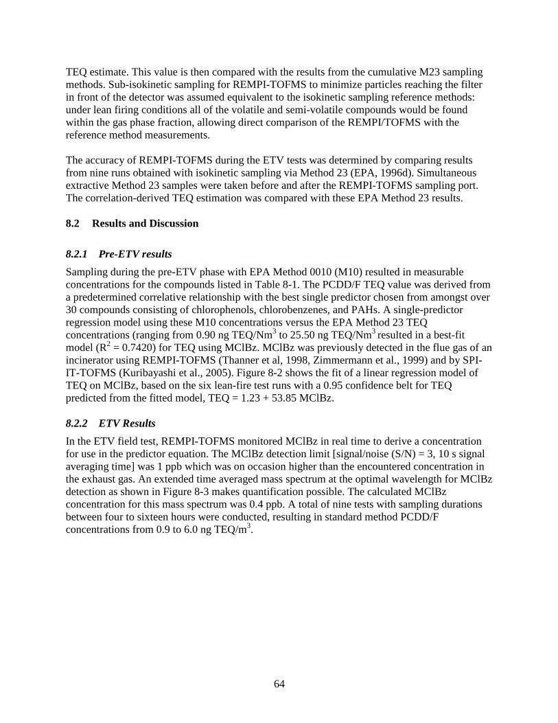
64

TEQ estimate. This value is then compared with the results from the cumulative M23 sampling methods. Sub-isokinetic sampling for REMPI-TOFMS to minimize particles reaching the filter in front of the detector was assumed equivalent to the isokinetic sampling reference methods: under lean firing conditions all of the volatile and semi-volatile compounds would be found within the gas phase fraction, allowing direct comparison of the REMPI/TOFMS with the reference method measurements. The accuracy of REMPI-TOFMS during the ETV tests was determined by comparing results from nine runs obtained with isokinetic sampling via Method 23 (EPA, 1996d). Simultaneous extractive Method 23 samples were taken before and after the REMPI-TOFMS sampling port. The correlation-derived TEQ estimation was compared with these EPA Method 23 results. 8.2 Results and Discussion

8.2.1 Pre-ETV results

Sampling during the pre-ETV phase with EPA Method 0010 (M10) resulted in measurable concentrations for the compounds listed in Table 8-1. The PCDD/F TEQ value was derived from a predetermined correlative relationship with the best single predictor chosen from amongst over 30 compounds consisting of chlorophenols, chlorobenzenes, and PAHs. A single-predictor regression model using these M10 concentrations versus the EPA Method 23 TEQ concentrations (ranging from 0.90 ng TEQ/Nm3 to 25.50 ng TEQ/Nm3 resulted in a best-fit model (R2 = 0.7420) for TEQ using MClBz. MClBz was previously detected in the flue gas of an incinerator using REMPI-TOFMS (Thanner et al, 1998, Zimmermann et al., 1999) and by SPI-IT-TOFMS (Kuribayashi et al., 2005). Figure 8-2 shows the fit of a linear regression model of TEQ on MClBz, based on the six lean-fire test runs with a 0.95 confidence belt for TEQ predicted from the fitted model, TEQ = 1.23 + 53.85 MClBz. 8.2.2 ETV Results

In the ETV field test, REMPI-TOFMS monitored MClBz in real time to derive a concentration for use in the predictor equation. The MClBz detection limit [signal/noise (S/N) = 3, 10 s signal averaging time] was 1 ppb which was on occasion higher than the encountered concentration in the exhaust gas. An extended time averaged mass spectrum at the optimal wavelength for MClBz detection as shown in Figure 8-3 makes quantification possible. The calculated MClBz concentration for this mass spectrum was 0.4 ppb. A total of nine tests with sampling durations between four to sixteen hours were conducted, resulting in standard method PCDD/F concentrations from 0.9 to 6.0 ng TEQ/m3.

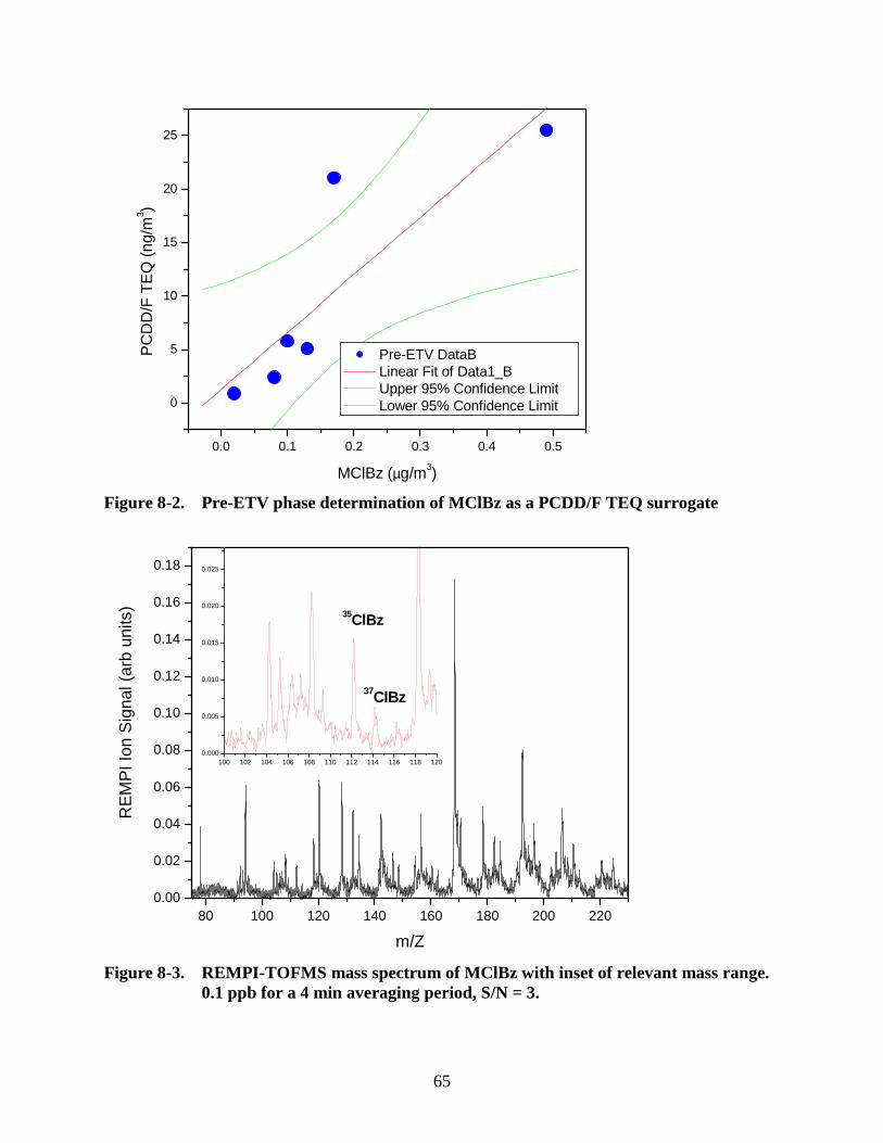
65

0.0 0.1 0.2 0.3 0.4 0.5

0

5

10

15

20

25P

CD

D/F

TE

Q (

ng/m

3 )

MClBz (µg/m3)

Pre-ETV DataB Linear Fit of Data1_B Upper 95% Confidence Limit Lower 95% Confidence Limit

Figure 8-2. Pre-ETV phase determination of MClBz as a PCDD/F TEQ surrogate

80 100 120 140 160 180 200 2200.00

0.02

0.04

0.06

0.08

0.10

0.12

0.14

0.16

0.18

100 102 104 106 108 110 112 114 116 118 1200.000

0.005

0.010

0.015

0.020

0.025

RE

MP

I Ion

Sig

nal (

arb

units

)

m/Z

37ClBz

35ClBz

Figure 8-3. REMPI-TOFMS mass spectrum of MClBz with inset of relevant mass range. 0.1 ppb for a 4 min averaging period, S/N = 3.

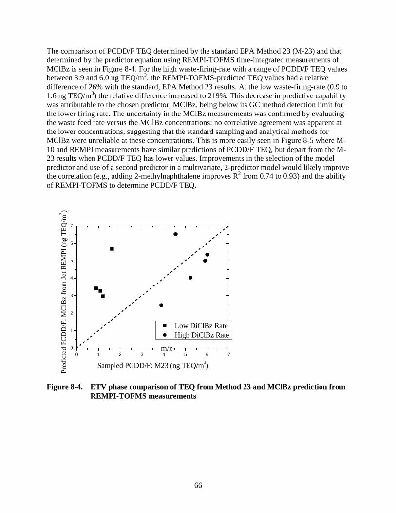
66

The comparison of PCDD/F TEQ determined by the standard EPA Method 23 (M-23) and that determined by the predictor equation using REMPI-TOFMS time-integrated measurements of MClBz is seen in Figure 8-4. For the high waste-firing-rate with a range of PCDD/F TEQ values between 3.9 and 6.0 ng TEQ/m3, the REMPI-TOFMS-predicted TEQ values had a relative difference of 26% with the standard, EPA Method 23 results. At the low waste-firing-rate (0.9 to 1.6 ng TEQ/m3) the relative difference increased to 219%. This decrease in predictive capability was attributable to the chosen predictor, MClBz, being below its GC method detection limit for the lower firing rate. The uncertainty in the MClBz measurements was confirmed by evaluating the waste feed rate versus the MClBz concentrations: no correlative agreement was apparent at the lower concentrations, suggesting that the standard sampling and analytical methods for MClBz were unreliable at these concentrations. This is more easily seen in Figure 8-5 where M-10 and REMPI measurements have similar predictions of PCDD/F TEQ, but depart from the M-23 results when PCDD/F TEQ has lower values. Improvements in the selection of the model predictor and use of a second predictor in a multivariate, 2-predictor model would likely improve the correlation (e.g., adding 2-methylnaphthalene improves R2 from 0.74 to 0.93) and the ability of REMPI-TOFMS to determine PCDD/F TEQ.

0 1 2 3 4 5 6 70

1

2

3

4

5

6

7

Pre

dict

ed

PC

DD

/F: M

ClB

z fr

om J

et R

EM

PI (

ng T

EQ

/m3 )

Sampled PCDD/F: M23 (ng TEQ/m3)

Low DiClBz Rate High DiClBz Rate

Figure 8-4. ETV phase comparison of TEQ from Method 23 and MClBz prediction from REMPI-TOFMS measurements

m/z

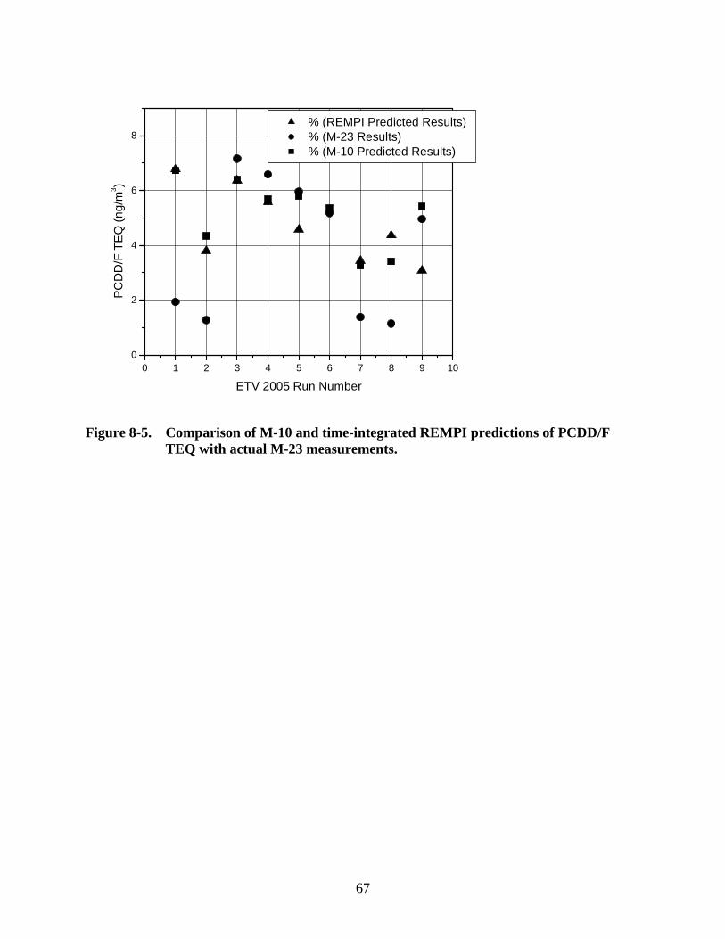
67

0 1 2 3 4 5 6 7 8 9 100

2

4

6

8 % (REMPI Predicted Results) % (M-23 Results) % (M-10 Predicted Results)

PC

DD

/F T

EQ

(ng

/m3 )

ETV 2005 Run Number

Figure 8-5. Comparison of M-10 and time-integrated REMPI predictions of PCDD/F TEQ with actual M-23 measurements.

68

9. Source 4: Sampling from MWC Flue Gas

Two field measurement campaigns have been performed at the same MWC site using REMPI-TOFMS instruments to monitor pre-determined target compounds in real time in the flue gas prior to the air pollution cleaning system. These campaigns were conducted under challenging conditions due to the presence of dust and large ambient temperature changes. 9.1 Portsmouth Naval Shipyard Waste Combustor 2004.

The primary objective of the first MWC study was the field demonstration of the REMPI-TOFMS technology to measure target organic compounds identified as potential indicators for PCDD/F TEQ determinations. Prior to the field study, the REMPI-TOFMS was found to measure easily, reliably, and potentially online or through a short pre-concentration step, PCDD/F TEQ indicators include compounds such as low chlorinated PCDD/F compounds, chlorobenzenes, chlorophenols, and PAHs. The main objective of this first test at this MWC was to test and validate the REMPI-TOFMS instrument in the field using the results from an initial MWC sampling campaign that provided correlations for potential indicators. This initial campaign of this project focused primarily on extractive flue gas samplings prior to the air pollution control system (APCS), which consists of a spray dryer and baghouse, and to a lesser extent at the stack. The primary sampling locations were the spray dryer catwalk area (SDA) at the exit of boilers 1 and 2. These locations were chosen to provide concentrations of the target compounds of interest that were sampled in a relatively reasonable time, and analyzed by the EPA-RTP Organic Laboratory using HRGC/ LRMS. A potentially multivariate, nonlinear, time-variant model was developed based on the initial sampling campaign (in 2003). The model relates the gas-phase concentration of one or more indicator compounds from sub-isokinetic samples from SDA2 with the PCDD/F TEQ and PCDD/F total (from SDA2-iso). This model was used to develop a test matrix that would optimize field-sampling data collection in the first field demonstration of the REMPI-TOFMS instrument. Validation of the system was performed using extractive methods for dioxins and furans. The main classes of compounds that were targeted in this project were primarily mono- to octa-chlorinated dioxins and furans (PCDD/Fs), chlorinated phenols (ClPhs), chlorinated benzenes (ClBzs), and PAHs. 9.2 Experimental Approach

The main objective of this test program was to develop potential organic indicator compounds that can mimic PCDD/F TEQ emissions, and test the validation of REMPI-TOFMS to produce sensitive, time resolved measurements of these target indicator compounds. To further examine REMPI-applicable indicator compounds, samples were taken from a MWC with multiple RDF fired boilers (>400 Mg/day) over a 9 day period for PCDD/F and other combustion by-products. Samples were drawn from the flue gas duct prior to the flue gas cleaning system; hence, concentrations do not represent stack emissions. Over the course of nine

69

days, 23 sampling periods were completed. Sampling for PCDD/F included 1 h Method 0023 (M23) samples and three 5-min M23 samples taken throughout a 1 h sampling period. Sampling for semi-volatiles (e.g., monochlorobenzene, phenol) was accomplished with REMPI-TOFMS and by standard extractive sampling via Method 0010 (M10). These runs paralleled the M23 sampling periods, and should be comparable. M10 samples were analyzed for semi-volatiles; in this case only the back half values are reported (in µg/m3, dry). These back half semi-volatile values should be directly comparable to the REMPI-TOFMS determinations, as they are both post-filter (akin to what the XAD “sees”) measurements. It should be noted that M10 samples were 1 h in duration whereas REMPI was on-line; hence many of the REMPI-detectable semi-volatiles reported by M10 were not above the on-line concentration detection limits of REMPI-TOFMS. 9.3 Test Matrix

The test matrix presented here refers to the first campaign of testing with the REMPI-TOFMS system. The proposed time sequence of the initial data was based on a statistical analysis of the initial MWC data. The time sequence of those sampling events recorded on the same axis as the CO stream data showed some evidences that the largest PCDD/F TEQ values observed followed a period of identifiable CO instability reflected by an upsurge of CO spikes above a 600 ppm threshold level. The sampling strategy for this testing campaign was to capture and identify delayed effects of the critical CO period on the PCDD/F formation with a minimal loss of instantaneous PCDD/F TEQ and other surrogates compounds in the process of averaging over any particular sampling time. Six identifiable phases of boiler operation were proposed in this sampling campaign to be characterized experimentally: Phase 1. Normal operation: This testing phase will start after normal operations that would have

lasted at least 6 hours after a startup without any sign of probable shutdown Phase 2. High frequency CO spiking without boiler shutdown: This sampling phase will

correspond to an identifiable period of CO instability due probably to a plug in the feed system. This transitional period last in general less than 2 hours.

Phase 3. Boiler leading to shut-down: This phase is expected to occur within 2 hours of phase 2

conditions. The shutdowns can be unscheduled, and due to high CO hourly averages or initiated by the boiler.

Phase 4. Actual boiler shutdown phase Phase 5. Boiler early startup: This sampling phase will start just after the boiler startup is

initiated after a scheduled or unscheduled shutdown Phase 6. Boiler late startup: This phase will be performed about 3 hours after the startup, after

the early startup phase is completed.

70

9.4 Results

9.4.1 General On-site REMPI-TOFMS Instrument Performance

The first field study of the first compact REMPI-TOFMS instrument (December 2004) was satisfactory based on the relative fast setup time (~ 6 hours) between arrival onsite and the first detection of flue gas constituents and the near 90% coverage of real time (2s sampling period) REMPI-TOFMS data during parallel conventional Method 0010 and Method 0023 sampling. In one occasion, the sampling periods were delayed in order to have REMPI-TOFMS available for parallel sampling after a system shutdown. This occurred after ultrafine fly-ash passed through the inline filter (or was pulled into the system during a swap of filters) and got trapped in the pulsed valve inlet system hereby obstructing the pulsed sample flow. The exchange of filter elements using a single housing unit resulted in a temporary loss in PAH signal intensity most likely due to the initial low temperature of the new filter element. Preheating a clean new element did resolve this issue and was implemented later in the sampling campaign. 9.4.2 REMPI-TOFMS results

The focus of REMPI-TOFMS during this sampling campaign was on the real time detection of PAHs and monochlorobenzene, if possible in real time. Over the course of a seven day period, the flue gas of the MWC was sampled with REMPI-TOFMS for a total of 58 hours. In parallel, 23 EPA Method 0010 (semi-volatiles) and 0023 (PCDD/Fs) samples were taken. After day 2, all sampling equipment was relocated to a different boiler (“B”) area due to unscheduled extended maintenance on the first boiler (“A”). This provided an opportunity to compare boiler performances under normal, “steady state” conditions. As illustrated in Figure 9-1, there are large differences in emissions of especially naphthalene over the course of a 4 hour time period. PAH emissions for boiler “B” were generally much higher during the shutdown of a boiler as shown in Figure 9-2. The observed transient naphthalene spikes are most likely due to residual smoldering waste with flare-ups. It should be pointed out that PAH concentrations are elevated under conditions of lower flow velocity in the duct from which the sample is taken which tend to enhance the concentration but not the actual emissions at that time. More dramatic changes in PAH concentrations occur during the period leading up to a shutdown of a boiler (B) as well as during the startup. An example of emissions during the startup of the boiler is shown in Figure 9-3. A similar transient response was observed during another startup of the same boiler. In that case, the REMPI-TOFMS wavelength was toggled between detection of PAHs and monochlorobenzene providing partial real time data for both as shown in Figure 9-4.

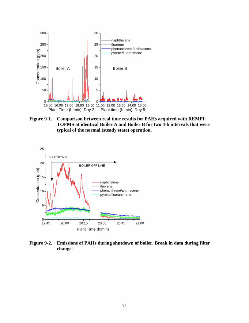
71

15:00 16:00 17:00 18:00 19:000

50

100

150

200

250

300

11:00 12:00 13:00 14:00 15:000

5

10

15

20

25

30

Con

cent

ratio

n (p

pb)

Plant Time (h:min), Day 2

Boiler A Boiler B

naphthalene fluorene phenanthrene/anthracene pyrene/fluoranthene

Plant time (h:min), Day 5

Figure 9-1. Comparison between real time results for PAHs acquired with REMPI-TOFMS at identical Boiler A and Boiler B for two 4-h intervals that were typical of the normal (steady state) operation.

19:45 20:00 20:15 20:30 20:45 21:000

5

10

15

20

25

naphthalene fluorene phenanthrene/anthracene pyrene/fluoranthrene

Con

cent

ratio

n (p

pb)

Plant Time (h:min)

BOILER OFF LINE

SHUTDOWN

Figure 9-2. Emissions of PAHs during shutdown of boiler. Break in data during filter change.

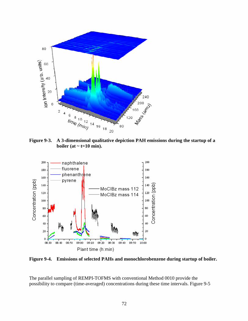
72

Figure 9-3. A 3-dimensional qualitative depiction PAH emissions during the startup of a boiler (at ~ t=10 min).

Figure 9-4. Emissions of selected PAHs and monochlorobenzene during startup of boiler.

The parallel sampling of REMPI-TOFMS with conventional Method 0010 provide the possibility to compare (time-averaged) concentrations during these time intervals. Figure 9-5

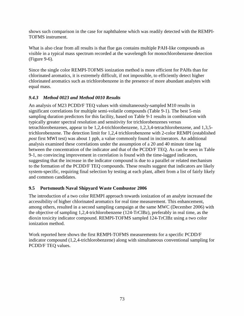
73

shows such comparison in the case for naphthalene which was readily detected with the REMPI-TOFMS instrument. What is also clear from all results is that flue gas contains multiple PAH-like compounds as visible in a typical mass spectrum recorded at the wavelength for monochlorobenzene detection (Figure 9-6). Since the single color REMPI-TOFMS ionization method is more efficient for PAHs than for chlorinated aromatics, it is extremely difficult, if not impossible, to efficiently detect higher chlorinated aromatics such as trichlorobenzene in the presence of more abundant analytes with equal mass. 9.4.3 Method 0023 and Method 0010 Results

An analysis of M23 PCDD/F TEQ values with simultaneously-sampled M10 results in significant correlations for multiple semi-volatile compounds (Table 9-1). The best 5-min sampling duration predictors for this facility, based on Table 9-1 results in combination with typically greater spectral resolution and sensitivity for trichlorobenzenes versus tetrachlorobenzenes, appear to be 1,2,4-trichlorobenzene, 1,2,3,4-tetrachlorobenzene, and 1,3,5-trichlorobenzene. The detection limit for 1,2,4 trichlorobenzene with 2-color REMPI (established post first MWI test) was about 1 ppb, a value commonly found in incinerators. An additional analysis examined these correlations under the assumption of a 20 and 40 minute time lag between the concentration of the indicator and that of the PCDD/F TEQ. As can be seen in Table 9-1, no convincing improvement in correlation is found with the time-lagged indicators, suggesting that the increase in the indicator compound is due to a parallel or related mechanism to the formation of the PCDD/F TEQ compounds. These results suggest that indicators are likely system-specific, requiring final selection by testing at each plant, albeit from a list of fairly likely and common candidates. 9.5 Portsmouth Naval Shipyard Waste Combustor 2006

The introduction of a two color REMPI approach towards ionization of an analyte increased the accessibility of higher chlorinated aromatics for real time measurement. This enhancement, among others, resulted in a second sampling campaign at the same MWC (December 2006) with the objective of sampling 1,2,4-trichlorobenzene (124-TrClBz), preferably in real time, as the dioxin toxicity indicator compound. REMPI-TOFMS sampled 124-TrClBz using a two color ionization method. Work reported here shows the first REMPI-TOFMS measurements for a specific PCDD/F indicator compound (1,2,4-trichlorobenzene) along with simultaneous conventional sampling for PCDD/F TEQ values.

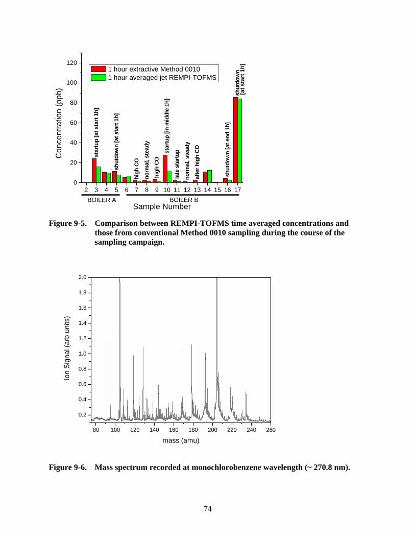
74

star

tup

[at s

tart

1h]

shut

dow

n [a

t sta

rt 1

h]

high

CO

norm

al, s

tead

y

high

CO

star

tup

[in m

iddl

e 1h

]

late

sta

rtup

norm

al, s

tead

y

afte

r hi

gh C

O

shut

dow

n [a

t end

1h]

shut

dow

n

2 3 4 5 6 7 8 9 10 11 12 13 14 15 16 170

20

40

60

80

100

120

[at

star

t 1h

]

BOILER B

Con

cent

ratio

n (p

pb)

Sample Number

1 hour extractive Method 0010 1 hour averaged jet REMPI-TOFMS

BOILER A

Figure 9-5. Comparison between REMPI-TOFMS time averaged concentrations and those from conventional Method 0010 sampling during the course of the sampling campaign.

80 100 120 140 160 180 200 220 240 260

0.2

0.4

0.6

0.8

1.0

1.2

1.4

1.6

1.8

2.0

Ion

Sig

nal (

arb

units

)

mass (amu)

Figure 9-6. Mass spectrum recorded at monochlorobenzene wavelength (~ 270.8 nm).

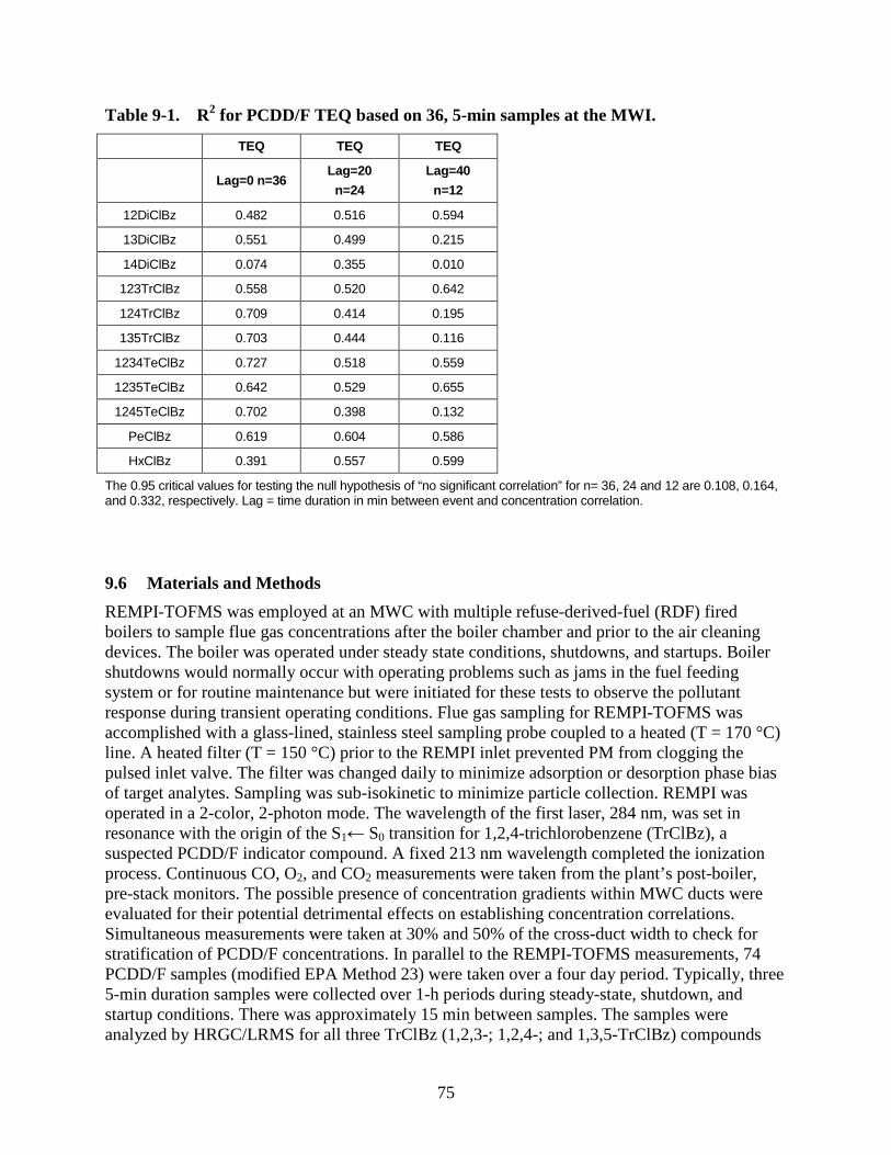
75

Table 9-1. R2 for PCDD/F TEQ based on 36, 5-min samples at the MWI.

TEQ TEQ TEQ

Lag=0 n=36 Lag=20

n=24

Lag=40

n=12

12DiClBz 0.482 0.516 0.594

13DiClBz 0.551 0.499 0.215

14DiClBz 0.074 0.355 0.010

123TrClBz 0.558 0.520 0.642

124TrClBz 0.709 0.414 0.195

135TrClBz 0.703 0.444 0.116

1234TeClBz 0.727 0.518 0.559

1235TeClBz 0.642 0.529 0.655

1245TeClBz 0.702 0.398 0.132

PeClBz 0.619 0.604 0.586

HxClBz 0.391 0.557 0.599

The 0.95 critical values for testing the null hypothesis of “no significant correlation” for n= 36, 24 and 12 are 0.108, 0.164, and 0.332, respectively. Lag = time duration in min between event and concentration correlation.

9.6 Materials and Methods

REMPI-TOFMS was employed at an MWC with multiple refuse-derived-fuel (RDF) fired boilers to sample flue gas concentrations after the boiler chamber and prior to the air cleaning devices. The boiler was operated under steady state conditions, shutdowns, and startups. Boiler shutdowns would normally occur with operating problems such as jams in the fuel feeding system or for routine maintenance but were initiated for these tests to observe the pollutant response during transient operating conditions. Flue gas sampling for REMPI-TOFMS was accomplished with a glass-lined, stainless steel sampling probe coupled to a heated (T = 170 °C) line. A heated filter (T = 150 °C) prior to the REMPI inlet prevented PM from clogging the pulsed inlet valve. The filter was changed daily to minimize adsorption or desorption phase bias of target analytes. Sampling was sub-isokinetic to minimize particle collection. REMPI was operated in a 2-color, 2-photon mode. The wavelength of the first laser, 284 nm, was set in resonance with the origin of the S1← S0 transition for 1,2,4-trichlorobenzene (TrClBz), a suspected PCDD/F indicator compound. A fixed 213 nm wavelength completed the ionization process. Continuous CO, O2, and CO2 measurements were taken from the plant’s post-boiler, pre-stack monitors. The possible presence of concentration gradients within MWC ducts were evaluated for their potential detrimental effects on establishing concentration correlations. Simultaneous measurements were taken at 30% and 50% of the cross-duct width to check for stratification of PCDD/F concentrations. In parallel to the REMPI-TOFMS measurements, 74 PCDD/F samples (modified EPA Method 23) were taken over a four day period. Typically, three 5-min duration samples were collected over 1-h periods during steady-state, shutdown, and startup conditions. There was approximately 15 min between samples. The samples were analyzed by HRGC/LRMS for all three TrClBz (1,2,3-; 1,2,4-; and 1,3,5-TrClBz) compounds

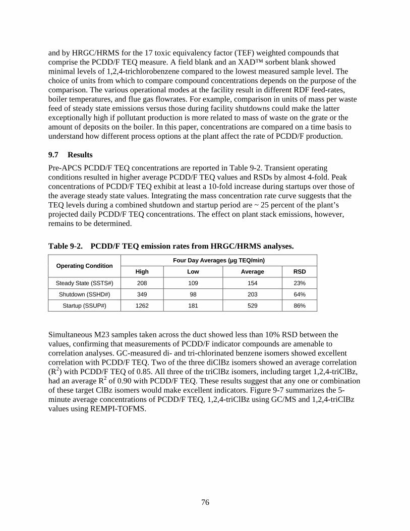
76

and by HRGC/HRMS for the 17 toxic equivalency factor (TEF) weighted compounds that comprise the PCDD/F TEQ measure. A field blank and an XAD™ sorbent blank showed minimal levels of 1,2,4-trichlorobenzene compared to the lowest measured sample level. The choice of units from which to compare compound concentrations depends on the purpose of the comparison. The various operational modes at the facility result in different RDF feed-rates, boiler temperatures, and flue gas flowrates. For example, comparison in units of mass per waste feed of steady state emissions versus those during facility shutdowns could make the latter exceptionally high if pollutant production is more related to mass of waste on the grate or the amount of deposits on the boiler. In this paper, concentrations are compared on a time basis to understand how different process options at the plant affect the rate of PCDD/F production. 9.7 Results

Pre-APCS PCDD/F TEQ concentrations are reported in Table 9-2. Transient operating conditions resulted in higher average PCDD/F TEQ values and RSDs by almost 4-fold. Peak concentrations of PCDD/F TEQ exhibit at least a 10-fold increase during startups over those of the average steady state values. Integrating the mass concentration rate curve suggests that the TEQ levels during a combined shutdown and startup period are ~ 25 percent of the plant’s projected daily PCDD/F TEQ concentrations. The effect on plant stack emissions, however, remains to be determined.

Table 9-2. PCDD/F TEQ emission rates from HRGC/HRMS analyses.

Four Day Averages (µg TEQ/min) Operating Condition

High Low Average RSD

Steady State (SSTS#) 208 109 154 23%

Shutdown (SSHD#) 349 98 203 64%

Startup (SSUP#) 1262 181 529 86%

Simultaneous M23 samples taken across the duct showed less than 10% RSD between the values, confirming that measurements of PCDD/F indicator compounds are amenable to correlation analyses. GC-measured di- and tri-chlorinated benzene isomers showed excellent correlation with PCDD/F TEQ. Two of the three diClBz isomers showed an average correlation (R2) with PCDD/F TEQ of 0.85. All three of the triClBz isomers, including target 1,2,4-triClBz, had an average R2 of 0.90 with PCDD/F TEQ. These results suggest that any one or combination of these target ClBz isomers would make excellent indicators. Figure 9-7 summarizes the 5-minute average concentrations of PCDD/F TEQ, 1,2,4-triClBz using GC/MS and 1,2,4-triClBz values using REMPI-TOFMS.

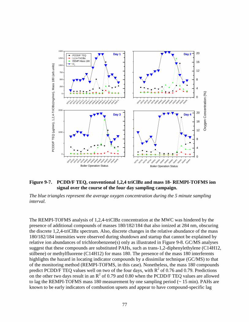
77

SSTS 1

SSTS 2

SSTS 3

SSTS 4

SSTS 5

SSTS 6

SSTS 7

SSHD 1

SSHD 2

SSHD 3

SSHD 4

SSUP 1

SSUP 2

SSUP 3

SSUP 4

SSUP 5

0

250

500

750

1000

1250

1500

SSTS1

SSTS2

SSTS3

SSTS4

SSTS5

SSHD1

SSHD2

SSHD4

SSHD5

SSUP1

SSUP2

SSUP3

SSUP4

SSUP5

SSTS1

SSTS2

SSTS3

SSTS4

SSTS5

SSHD1

SSHD2

SSHD3

SSHD4

SSHD5

SSUP1

SSUP2

SSUP3

SSUP4

SSUP5

0

1000

2000

SSTS1

SSTS2

SSTS3

SSTS4

SSHD1

SSHD2

SSHD3

SSHD4

SSHD5

SSUP1

SSUP2

SSUP3

SSUP4

0

4

8

12

16

20

0

4

8

12

16

20

Day 1P

CD

D/F

TE

Q (

µg/m

in),

1,2

,4-T

riClB

z(m

g/m

in),

Mas

s 18

0 (a

rb.u

nits

) PCDD/F TEQ 1,2,4-TriClBz REMPI Mass 180 O

2

Day 2

Day 3

Boiler Operation Status

Day 4

Boiler Operation Status

Oxy

gen

Con

cent

ratio

n (%

)

Figure 9-7. PCDD/F TEQ, conventional 1,2,4 triClBz and mass 18- REMPI-TOFMS ion signal over the course of the four day sampling campaign.

The blue triangles represent the average oxygen concentration during the 5 minute sampling interval.

The REMPI-TOFMS analysis of 1,2,4-triClBz concentration at the MWC was hindered by the presence of additional compounds of masses 180/182/184 that also ionized at 284 nm, obscuring the discrete 1,2,4-triClBz spectrum. Also, discrete changes in the relative abundance of the mass 180/182/184 intensities were observed during shutdown and startup that cannot be explained by relative ion abundances of trichlorobenzene(s) only as illustrated in Figure 9-8. GC/MS analyses suggest that these compounds are substituted PAHs, such as trans-1,2-diphenylethylene (C14H12, stilbene) or methylfluorene (C14H12) for mass 180. The presence of the mass 180 interferents highlights the hazard in locating indicator compounds by a dissimilar technique (GC/MS) to that of the monitoring method (REMPI-TOFMS, in this case). Nonetheless, the mass 180 compounds predict PCDD/F TEQ values well on two of the four days, with R2 of 0.76 and 0.79. Predictions on the other two days result in an R2 of 0.79 and 0.80 when the PCDD/F TEQ values are allowed to lag the REMPI-TOFMS mass 180 measurement by one sampling period (~ 15 min). PAHs are known to be early indicators of combustion upsets and appear to have compound-specific lag

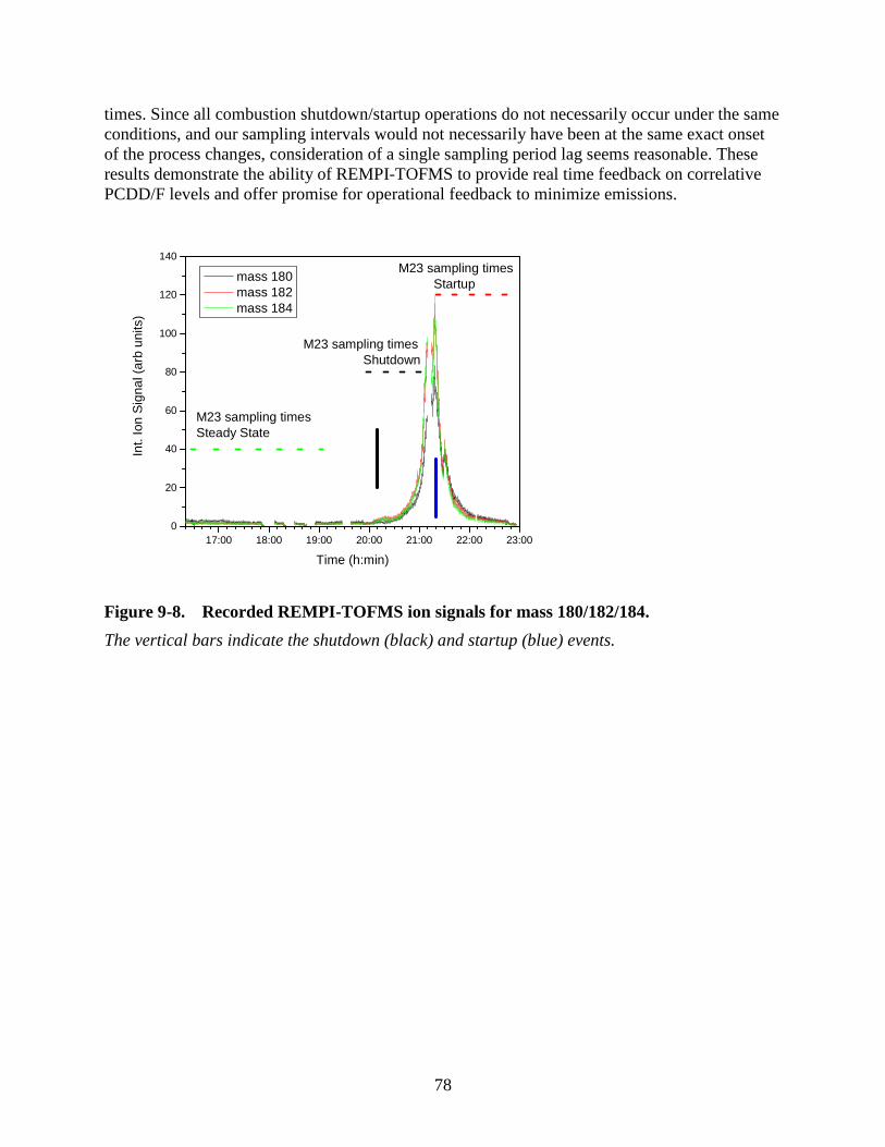
78

times. Since all combustion shutdown/startup operations do not necessarily occur under the same conditions, and our sampling intervals would not necessarily have been at the same exact onset of the process changes, consideration of a single sampling period lag seems reasonable. These results demonstrate the ability of REMPI-TOFMS to provide real time feedback on correlative PCDD/F levels and offer promise for operational feedback to minimize emissions.

17:00 18:00 19:00 20:00 21:00 22:00 23:000

20

40

60

80

100

120

140

mass 180 mass 182 mass 184

M23 sampling timesSteady State

M23 sampling times Startup

M23 sampling times Shutdown

Int.

Ion

Sig

nal (

arb

units

)

Time (h:min)

Figure 9-8. Recorded REMPI-TOFMS ion signals for mass 180/182/184.

The vertical bars indicate the shutdown (black) and startup (blue) events.

79

10. Source 5: Emission Responses from HMMWVs, the M1 Abrams Tank, and the Bradley Infantry Fighting Vehicle

Real time emission measurements of criteria pollutants, organic air toxics, and particles were made on two U.S. Army High Mobility Multi-purpose Wheeled Vehicles (HMMWVs), a Bradley Infantry Fighting Vehicle (IFV), and an Abrams M1 battle tank. The HMMWV emissions were measured while running on a dynamometer-based roadway simulator under the West Virginia and EPA Federal Highway Economy Test (HWFET) cycles, and under steady state, constant velocity conditions. REMPI-TOFMS emissions from cold and warm starts of the HMMWVs, the Bradley, and Abrams were recorded. The U.S. Army currently has over 99,000 tactical High Mobility Multi-purpose Wheeled Vehicles (HMMWVs) and over 12,000 tracked vehicles such as the M1 Abrams tank and Bradley IFV (https://www.osmisweb.army.mil/, 2008) that account for approximately half of the DoD vehicle fleet (http://www.globalsecurity.org/military/systems/ground/hmmwv-recap.htm). Some emissions data are available for the HMMWVs, primarily criteria pollutants, but none are known for the tracked vehicles. 10.1 Experimental

10.1.1 Platforms Tested

Criteria and organic pollutant emissions were characterized during transient operation of four U.S. Army weapon platforms at the U.S. Army Aberdeen Test Center, Roadway Simulator (RWS). The RWS is the world's largest dynamometer, supporting vehicles ranging from 2,300 kg (5,000 lb), 2-axle light vehicles (up to 192 km/h or 120 mph) to 27,300 kg (60,000 lb), tandem-axle tractor trailers (Schultz et al., 2005). Two versions of HMMWVs were tested for emissions on the RWS. These included a heavy HMMWV (M1097 A1) and a turbine engine, up-armored HMMWV (M1114). The HMMWV is currently the main transport vehicle for the DoD. These 6.2 L, General Motors vehicles consume almost 15 million gallons of JP-8 each year, making it the top-consuming vehicle type (17%) in the DoD inventory (Kemme et al., 2006). The 6.5 liter Turbo Diesel 142 kW (190 hp) up-armored M1114 version has a higher payload capacity (1,043 kg) for a gross vehicle weight of 5,489 kg (GlobalSecurity.org, 2008a) and is equipped with a heavy armor protection package instituted during the Iraq war. Both of these vehicles were tested with two driving cycle protocols (described later) and stepped velocity/gradient cycle. Two additional weapons platforms, an M1 Abrams tank and a Bradley IFV, were tested at the facility but not on the RWS due to weight and track restrictions. The 62 metric ton M1 Abrams main battle tank is manufactured by General Dynamics Land Systems and powered by a Honeywell AGT 1118 kW (1500 hp) gas turbine. The Allison hydrokenetic transmission has four forward and two reverse gears. The Bradley is powered by a 447 kW (600 hp) Cummins VTA-903T water-cooled 4 cycle diesel engine. It is a fully armored, fully tracked vehicle designed to

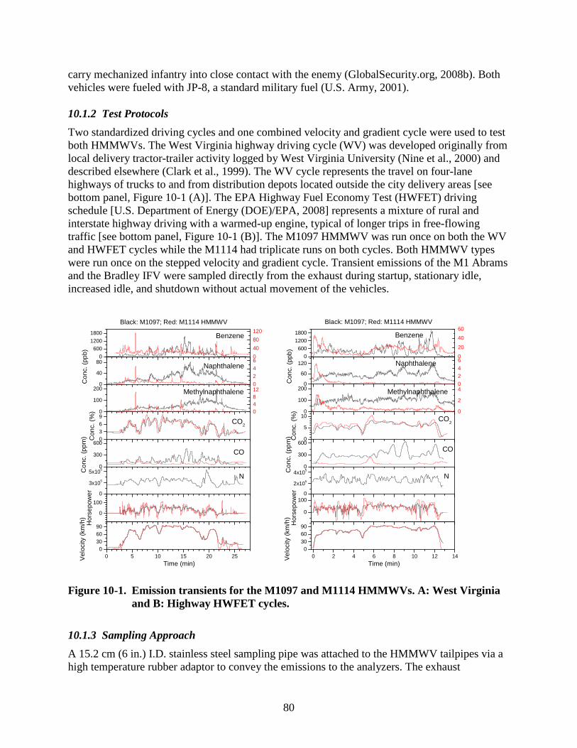
80

carry mechanized infantry into close contact with the enemy (GlobalSecurity.org, 2008b). Both vehicles were fueled with JP-8, a standard military fuel (U.S. Army, 2001). 10.1.2 Test Protocols

Two standardized driving cycles and one combined velocity and gradient cycle were used to test both HMMWVs. The West Virginia highway driving cycle (WV) was developed originally from local delivery tractor-trailer activity logged by West Virginia University (Nine et al., 2000) and described elsewhere (Clark et al., 1999). The WV cycle represents the travel on four-lane highways of trucks to and from distribution depots located outside the city delivery areas [see bottom panel, Figure 10-1 (A)]. The EPA Highway Fuel Economy Test (HWFET) driving schedule [U.S. Department of Energy (DOE)/EPA, 2008] represents a mixture of rural and interstate highway driving with a warmed-up engine, typical of longer trips in free-flowing traffic [see bottom panel, Figure 10-1 (B)]. The M1097 HMMWV was run once on both the WV and HWFET cycles while the M1114 had triplicate runs on both cycles. Both HMMWV types were run once on the stepped velocity and gradient cycle. Transient emissions of the M1 Abrams and the Bradley IFV were sampled directly from the exhaust during startup, stationary idle, increased idle, and shutdown without actual movement of the vehicles.

0

40

80

120

0

3x105

5x105

0

40

80

0

2

4

6

0

100

200

04812

0

6001200

1800

Con

c. (

ppb)

Benzene

0369

Con

c. (

%)

CO2

0

300

600

Con

c. (

ppm

)

CO

0

100

Hor

sepo

wer

0 5 10 15 20 250

306090

Time (min) Vel

ocity

(km

/h)

Black: M1097; Red: M1114 HMMWV

N

Naphthalene

Methylnaphthalene

0

20

40

60

0

2x105

4x105

0

60

120

0

2

4

6

0

100

200

0

2

4

0

600

1200

1800

Con

c. (

ppb)

Benzene

0

5

10

Con

c. (

%)

CO2

0

300

600

Con

c. (

ppm

)

CO

0

100

Hor

sepo

wer

0 2 4 6 8 10 12 140

306090

Time (min) Vel

ocity

(km

/h)

Black: M1097; Red: M1114 HMMWV

N

Naphthalene

Methylnaphthalene

Figure 10-1. Emission transients for the M1097 and M1114 HMMWVs. A: West Virginia and B: Highway HWFET cycles.

10.1.3 Sampling Approach

A 15.2 cm (6 in.) I.D. stainless steel sampling pipe was attached to the HMMWV tailpipes via a high temperature rubber adaptor to convey the emissions to the analyzers. The exhaust

81

temperature was measured at or below about 273 °C and the gas pipe was heat traced to about 200 °C. No dilution air was added, and the flow was monitored with an annubar pitot tube. Exhaust for the REMPI-TOFMS system, the particle measurement systems, and the continuous emissions monitors (CEMs) was sampled using separate heated lines maintained at about 125-150 °C. The Bradley and Abrams idle, cold start, and warm start emissions were sampled at a rate of 1 L/min by means of a 0.6 cm (¼-inch) diameter stainless probe inserted inside their exhaust line. In all studies, a slip stream of the sample exhaust was sampled through the pulsed valve of the REMPI-TOFMS system at a rate of 1 mL/min. The exhaust gas criteria pollutants were analyzed using a self-contained CEM bench that included two analyzers using EPA promulgated Method 10A (EPA, 2000b) for CO [low CO: Rosemount NGA 2000, high CO: California Analytical Instrument and two analyzers using EPA Method 3A (EPA, 2006), one for oxygen (O2: Rosemount NGA 2000) and one for CO2 (California Analytical Instrument)]. Each analyzer had a daily, 3-point calibration and a 3-point bias check before the start of the test, followed by a 3-point system calibration and bias check at the end of the test. Gas standards were introduced via the bias check port at the sample line inlets during pre-sampling CEM performance checks. The CEM is linked to a data acquisition system set for a sampling frequency of 10 s-1. The REMPI-TOFMS instrument measured aromatic organic air pollutants in real-time, parallel to the standard CEMs. BTEX, styrene, and gaseous PAHs, are among the non-exclusive list that were targeted for measurement. An approximately 1 L/min slipstream was pulled from the main sampling pipe through a 15 m long, 0.95 cm (3/8 in.) diameter Silico-Steel coated line at 150 °C towards the REMPI-TOFMS inlet. A glass microfiber filter (Unique Heated products) mounted directly downstream from the main sampling pipe prevents PM from reaching the REMPI-TOFMS instrument. Two filter housings were operated in parallel in order to have the capability to replace a filter element on an hourly basis without interruption of the sampling. The pulsed inlet valve (modified General Valve Series 99) of the REMPI-TOFMS instrument pulls approximately 1 mL/min into the ionization chamber of the TOFMS. Real time particle size distributions were measured with a Dakati ELPI. The ELPI is a 12-stage impactor with a single pre-stage knockout, measuring particle size distributions ranging from 30 nm to 10 µm at a frequency of 1 Hz. The ELPI generates a particle size distribution by charging the particles based on geometrical diameter prior to them entering into a cascade impactor. The charged particles land on the impactor stages based upon their inertia and their charge is converted into a particle number and mass, given a known density. The sample was conveyed via a non-static, conductive tubing, diluted with two 10:1 VKL (Palas) venturi-based dilutors in series (for a 100:1 dilution), totaling 10 L/min at ambient temperature and pressure. Dilution ratios are verified by using measurements of pre- and post-diluted CO and CO2. Daily quality control checks on the ELPI were performed by zeroing the electrometer using a flush of high efficiency particulate arresting (HEPA) purified air and by monitoring the current profiles of the ELPI while it samples room air and HEPA purified room air.

82

Longitudinal and lateral vehicle velocities and forces as well as engine rotation and vehicle speed data were provided by the RWS control system. Cold start emissions were evaluated in this study using a regression model (Heeb, 2001; as in Heeb and Weilenmann et al., 2005) which consists of a linear extrapolation to the ordinate of the idle state portion of the cumulative target compound (CO, CO2, benzene, naphthalene, methylnaphthalene, and others) evolution. The ordinate value is the target compound mass amount emitted from a single cold start event. The repeatability of the RWS facility operations and pollutant measurements were evaluated using the t-test statistical approach. RA is used to compare differences in the means of the target measurements between two cycles. All cycles within one type of driving profile (HWFET or WV) are compared with respect to the first cycle. The RA (%) is defined as follows:

100

975.0

×

+=

RM

n

Std

RA

d

(2) where:

d = the mean of the absolute values of the differences between measurements taken at the

same time during a complete cycle

975.0t = the t-value,

dS = the standard deviation of the differences between measurements taken at the same time

during a complete cycle

RM = the mean of the reference cycle n = number of measurements taken with a rolling average of 10 s during a complete cycle 10.2 Results and Discussion

REMPI -TOFMS and conventional CEMs were used to compare emissions from the diesel-powered heavy M1097 HMMWV with the armored-upfitted, turbine-driven M1114 HMMWV. Concentration values of benzene, naphthalene, methylnaphthalene, CO2, and CO as well as the total particle density (N), applied power (HP) and velocity (v) are shown for both vehicles on the WV and HWFET protocols, in Figure 10-1 (A) and Figure 10-1 (B), respectively. The RWS facility operations had excellent velocity repeatability between cycles for each driving cycle tested. The relative velocity accuracy for the HMMWV M1114 vehicle was 0.04% and 0.44% HWFET cycles, and 0.2% and 0.5% for the WV cycles. The RA for both HWFET and WV triplicate cycles, for the criteria compounds measured using conventional CEMs varied from 2.4% to 8.1% for CO2, and 7.4% to 31% for CO. The RA for the trace compounds concentrations measured by the REMPI-TOFMS system varied from 15% to 79% for benzene, 31% to 109% for naphthalene, and 47 to 214% for methylnaphthalene. The lower reproducibility of the emissions for naphthalene and methylnaphthalene are due to the compounding effect of their relatively low

83

concentration (sometimes just above the detection limit of the REMPI-TOFMS system) and the variance in the engine performance. It should be noted that the first two of the triplicate tests were run successively while the third test was performed later (4-5 h) on the same day with the lower reproducibility always between the non-successive runs. 10.2.1 WV Cycle

REMPI PAH measurements for the armored (M1114) HMMWV (red traces) on the WV cycle showed benzene peaks of about 120 ppb with a median value of 20 ppb [Figure 10-1 (A)]. Naphthalene and methylnaphthalene peaks of 6 and 12 ppb, respectively, were accompanied by median values of < 1 ppb. The average emission factors for benzene, naphthalene, and methylnaphthalene for the WV cycle were 325, 14, and 29 µg/km (see Table 10-1).

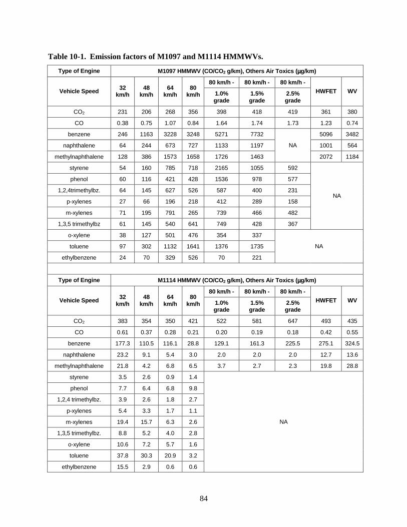
84

Table 10-1. Emission factors of M1097 and M1114 HMMWVs.

Type of Engine M1097 HMMWV (CO/CO2 g/km), Others Air Toxics (µµµµg/km)

80 km/h - 80 km/h - 80 km/h -

Vehicle Speed 32 km/h

48 km/h

64 km/h

80 km/h 1.0%

grade 1.5% grade

2.5% grade

HWFET WV

CO2 231 206 268 356 398 418 419 361 380

CO 0.38 0.75 1.07 0.84 1.64 1.74 1.73 1.23 0.74

benzene 246 1163 3228 3248 5271 7732 5096 3482

naphthalene 64 244 673 727 1133 1197 1001 564

methylnaphthalene 128 386 1573 1658 1726 1463

NA

2072 1184

styrene 54 160 785 718 2165 1055 592

phenol 60 116 421 428 1536 978 577

1,2,4trimethylbz. 64 145 627 526 587 400 231

p-xylenes 27 66 196 218 412 289 158

m-xylenes 71 195 791 265 739 466 482

1,3,5 trimethylbz 61 145 540 641 749 428 367

NA

o-xylene 38 127 501 476 354 337

toluene 97 302 1132 1641 1376 1735

ethylbenzene 24 70 329 526 70 221

NA

Type of Engine M1114 HMMWV (CO/CO2 g/km), Others Air Toxics (µµµµg/km)

80 km/h - 80 km/h - 80 km/h -

Vehicle Speed 32 km/h

48 km/h

64 km/h

80 km/h 1.0%

grade 1.5% grade

2.5% grade

HWFET WV

CO2 383 354 350 421 522 581 647 493 435

CO 0.61 0.37 0.28 0.21 0.20 0.19 0.18 0.42 0.55

benzene 177.3 110.5 116.1 28.8 129.1 161.3 225.5 275.1 324.5

naphthalene 23.2 9.1 5.4 3.0 2.0 2.0 2.0 12.7 13.6

methylnaphthalene 21.8 4.2 6.8 6.5 3.7 2.7 2.3 19.8 28.8

styrene 3.5 2.6 0.9 1.4

phenol 7.7 6.4 6.8 9.8

1,2,4 trimethylbz. 3.9 2.6 1.8 2.7

p-xylenes 5.4 3.3 1.7 1.1

m-xylenes 19.4 15.7 6.3 2.6

1,3,5 trimethylbz. 8.8 5.2 4.0 2.8

o-xylene 10.6 7.2 5.7 1.6

toluene 37.8 30.3 20.9 3.2

ethylbenzene 15.5 2.9 0.6 0.6

NA

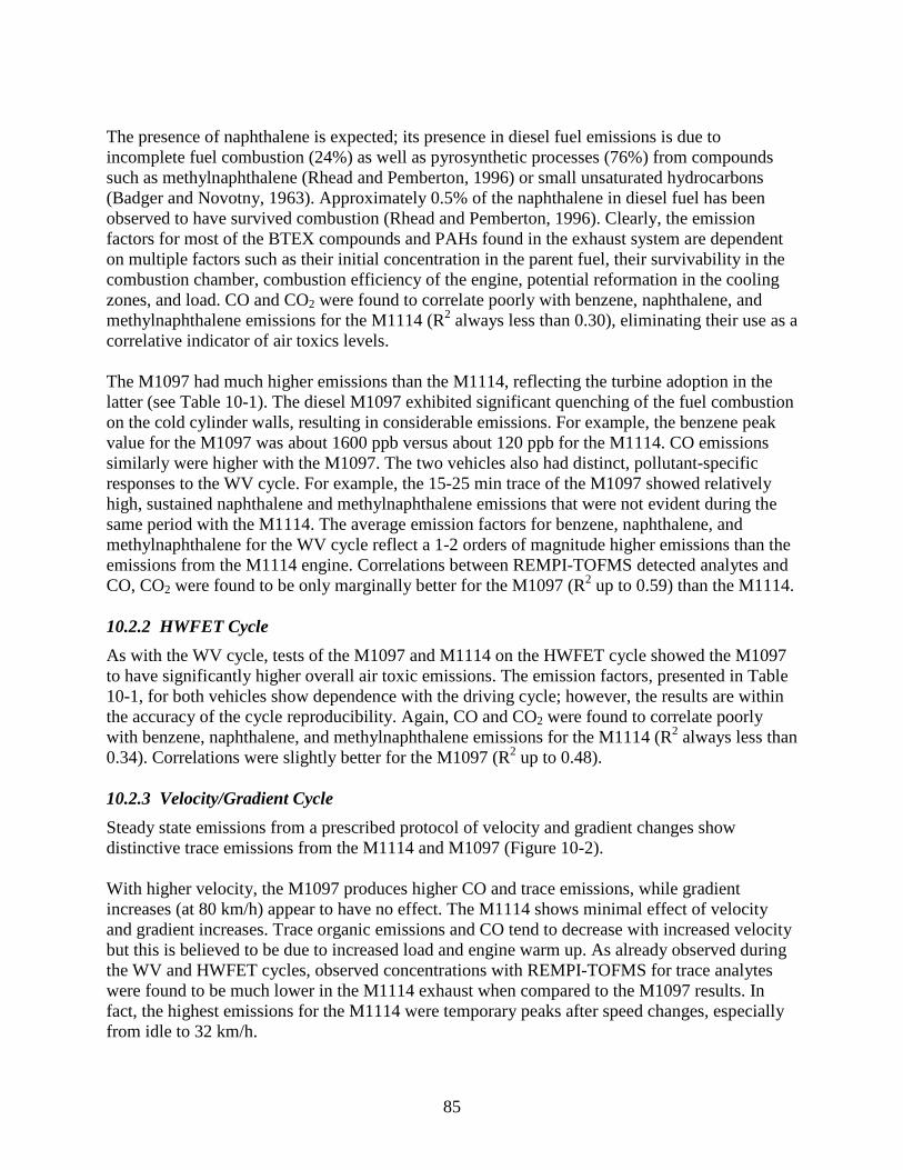
85

The presence of naphthalene is expected; its presence in diesel fuel emissions is due to incomplete fuel combustion (24%) as well as pyrosynthetic processes (76%) from compounds such as methylnaphthalene (Rhead and Pemberton, 1996) or small unsaturated hydrocarbons (Badger and Novotny, 1963). Approximately 0.5% of the naphthalene in diesel fuel has been observed to have survived combustion (Rhead and Pemberton, 1996). Clearly, the emission factors for most of the BTEX compounds and PAHs found in the exhaust system are dependent on multiple factors such as their initial concentration in the parent fuel, their survivability in the combustion chamber, combustion efficiency of the engine, potential reformation in the cooling zones, and load. CO and CO2 were found to correlate poorly with benzene, naphthalene, and methylnaphthalene emissions for the M1114 (R2 always less than 0.30), eliminating their use as a correlative indicator of air toxics levels. The M1097 had much higher emissions than the M1114, reflecting the turbine adoption in the latter (see Table 10-1). The diesel M1097 exhibited significant quenching of the fuel combustion on the cold cylinder walls, resulting in considerable emissions. For example, the benzene peak value for the M1097 was about 1600 ppb versus about 120 ppb for the M1114. CO emissions similarly were higher with the M1097. The two vehicles also had distinct, pollutant-specific responses to the WV cycle. For example, the 15-25 min trace of the M1097 showed relatively high, sustained naphthalene and methylnaphthalene emissions that were not evident during the same period with the M1114. The average emission factors for benzene, naphthalene, and methylnaphthalene for the WV cycle reflect a 1-2 orders of magnitude higher emissions than the emissions from the M1114 engine. Correlations between REMPI-TOFMS detected analytes and CO, CO2 were found to be only marginally better for the M1097 (R2 up to 0.59) than the M1114. 10.2.2 HWFET Cycle

As with the WV cycle, tests of the M1097 and M1114 on the HWFET cycle showed the M1097 to have significantly higher overall air toxic emissions. The emission factors, presented in Table 10-1, for both vehicles show dependence with the driving cycle; however, the results are within the accuracy of the cycle reproducibility. Again, CO and CO2 were found to correlate poorly with benzene, naphthalene, and methylnaphthalene emissions for the M1114 (R2 always less than 0.34). Correlations were slightly better for the M1097 (R2 up to 0.48). 10.2.3 Velocity/Gradient Cycle

Steady state emissions from a prescribed protocol of velocity and gradient changes show distinctive trace emissions from the M1114 and M1097 (Figure 10-2). With higher velocity, the M1097 produces higher CO and trace emissions, while gradient increases (at 80 km/h) appear to have no effect. The M1114 shows minimal effect of velocity and gradient increases. Trace organic emissions and CO tend to decrease with increased velocity but this is believed to be due to increased load and engine warm up. As already observed during the WV and HWFET cycles, observed concentrations with REMPI-TOFMS for trace analytes were found to be much lower in the M1114 exhaust when compared to the M1097 results. In fact, the highest emissions for the M1114 were temporary peaks after speed changes, especially from idle to 32 km/h.

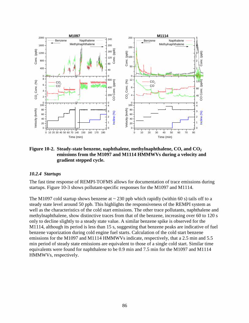
86

0

400

800

1200

1600

2000

0

40

80

120

160

200

240

0

2

4

6

8

0

200

400

600

0 10 20 30 40 50 60 70 140 150 160 170 180

0

20

40

60

80

100

0

1

2

3

4

Benzene

Con

c. (

ppb)

M1097 Napthalene Methylnaphthalene

Con

c. (

ppb)

CO2

CO

2 Con

c. (

%)

CO

CO

Con

c. (

ppm

)

Vel

ocity

(km

/h)

Time (min)

Incl

ine

(%)

0

50

100

150

200

0

1

2

3

4

5

0

4

8

12

0

40

80

120

0 10 20 30 40 50 60 70 80

0

20

40

60

80

100

0

1

2

3

4

M1114 Benzene

Con

c. (

ppb)

Napthalene Methylnaphthalene

Con

c. (

ppb)

CO2

CO

2 Con

c. (

%)

CO

CO

Con

c. (

ppm

)

Vel

ocity

(km

/h)

Time (min)

Incl

ine

(%)

Figure 10-2. Steady-state benzene, naphthalene, methylnaphthalene, CO, and CO2 emissions from the M1097 and M1114 HMMWVs during a velocity and gradient stepped cycle.

10.2.4 Startups

The fast time response of REMPI-TOFMS allows for documentation of trace emissions during startups. Figure 10-3 shows pollutant-specific responses for the M1097 and M1114. The M1097 cold startup shows benzene at ~ 230 ppb which rapidly (within 60 s) tails off to a steady state level around 50 ppb. This highlights the responsiveness of the REMPI system as well as the characteristics of the cold start emissions. The other trace pollutants, naphthalene and methylnaphthalene, show distinctive traces from that of the benzene, increasing over 60 to 120 s only to decline slightly to a steady state value. A similar benzene spike is observed for the M1114, although its period is less than 15 s, suggesting that benzene peaks are indicative of fuel benzene vaporization during cold engine fuel starts. Calculation of the cold start benzene emissions for the M1097 and M1114 HMMWVs indicate, respectively, that a 2.5 min and 5.5 min period of steady state emissions are equivalent to those of a single cold start. Similar time equivalents were found for naphthalene to be 0.9 min and 7.5 min for the M1097 and M1114 HMMWVs, respectively.

87

-1 0 1 2 3 4 5 60

2

4

50

150

250

0

50

100

150

200

250

0

2

4

6

8

10

12

14

16 C

O2 C

onc.

(%

)

Time (min)

CO2

CO

Ben

zene

Con

c. (

ppb)

Benzene Napthalene Methylnaphthalene

0 1 2 3 40

2

4

50

150

250

0

100

200

300

400

500

0

20

40

60

80

100

CO2

Time (min)

CO

CO

Con

c. (

ppm

)

Benzene Napthalene Methylnaphthalene

(M-)

Nap

htha

lene

Con

c. (

ppb)

Figure 10-3. Cold start emissions of benzene, naphthalene, methylnaphthalene, CO, and CO2 and PM size distribution for the M1097 (left) and M1114 (right) HMMWVs.

10.2.5 Bradley and Abrams

Figure 10-4 shows the 30 s average, steady state idle emissions from the Abrams and Bradley, respectively, of twelve organic compounds analyzed by REMPI. REMPI was sequentially set to each compound’s specific ionization wavelength throughout a 15 min period. Two types of idle measurements are reported for the Abrams (low and high idle) as well as the Bradley (“idle 0” and “idle 2” settings). The Bradley’s concentrations are about 100-1000-fold higher than those of the Abrams. The Bradley’s emissions are most abundant for the substituted naphthalenes and benzenes while the Abrams shows its highest concentrations in the lighter phenol, toluene, and benzene compounds. This may be due to a higher percentage of unburnt fuel in the Bradley exhaust versus the Abrams exhaust.

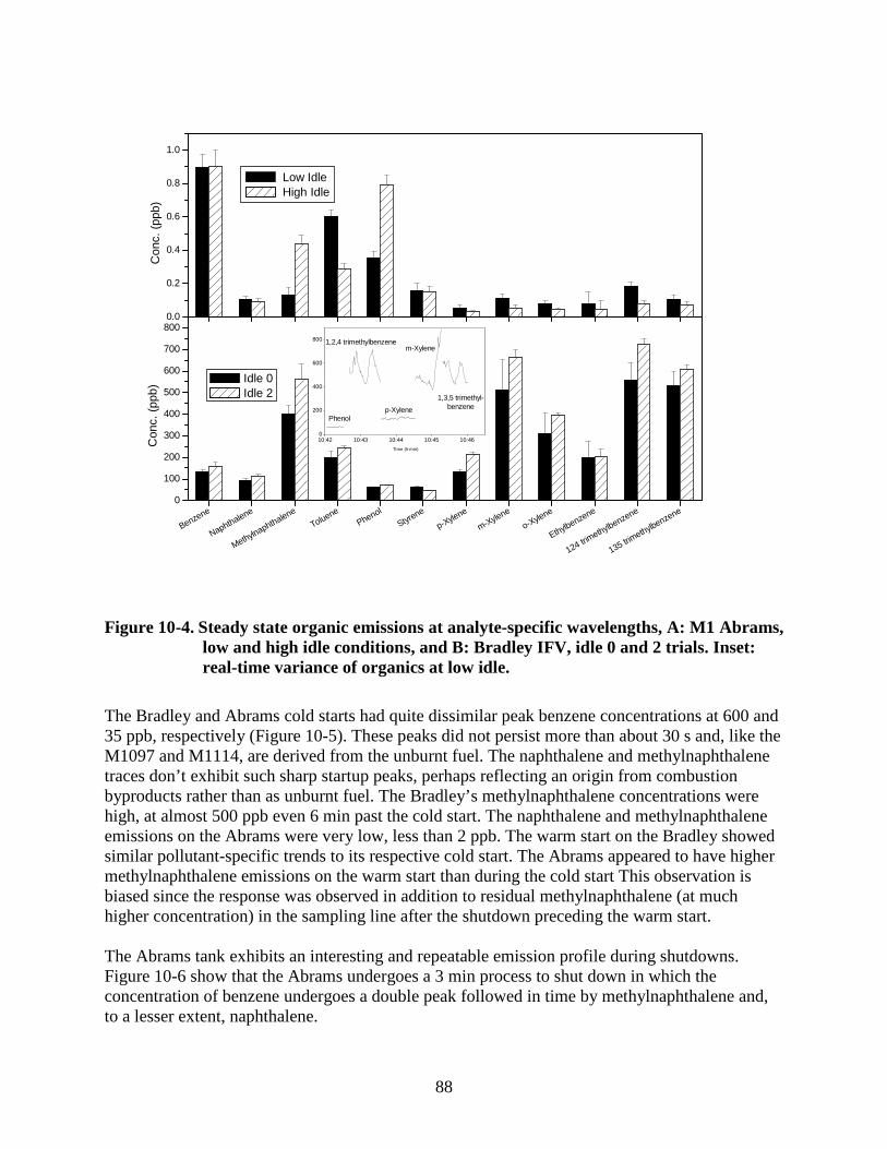
88

10:42 10:43 10:44 10:45 10:460

200

400

600

800

0.0

0.2

0.4

0.6

0.8

1.0

Low Idle High Idle

Con

c. (

ppb)

Benzene

Naphthalene

Methylnaphthalene

ToluenePhenol

Styrene

p-Xylene

m-Xylene

o-Xylene

Ethylbenzene

124 trimethylbenzene

135 trimethylbenzene

0

100

200

300

400

500

600

700

800

Con

c. (

ppb)

Idle 0 Idle 2 1,3,5 trimethyl-

benzene

m-Xylene

p-Xylene

Time (h:min)

Phenol

1,2,4 trimethylbenzene

Figure 10-4. Steady state organic emissions at analyte-specific wavelengths, A: M1 Abrams, low and high idle conditions, and B: Bradley IFV, idle 0 and 2 trials. Inset: real-time variance of organics at low idle.

The Bradley and Abrams cold starts had quite dissimilar peak benzene concentrations at 600 and 35 ppb, respectively (Figure 10-5). These peaks did not persist more than about 30 s and, like the M1097 and M1114, are derived from the unburnt fuel. The naphthalene and methylnaphthalene traces don’t exhibit such sharp startup peaks, perhaps reflecting an origin from combustion byproducts rather than as unburnt fuel. The Bradley’s methylnaphthalene concentrations were high, at almost 500 ppb even 6 min past the cold start. The naphthalene and methylnaphthalene emissions on the Abrams were very low, less than 2 ppb. The warm start on the Bradley showed similar pollutant-specific trends to its respective cold start. The Abrams appeared to have higher methylnaphthalene emissions on the warm start than during the cold start This observation is biased since the response was observed in addition to residual methylnaphthalene (at much higher concentration) in the sampling line after the shutdown preceding the warm start. The Abrams tank exhibits an interesting and repeatable emission profile during shutdowns. Figure 10-6 show that the Abrams undergoes a 3 min process to shut down in which the concentration of benzene undergoes a double peak followed in time by methylnaphthalene and, to a lesser extent, naphthalene.

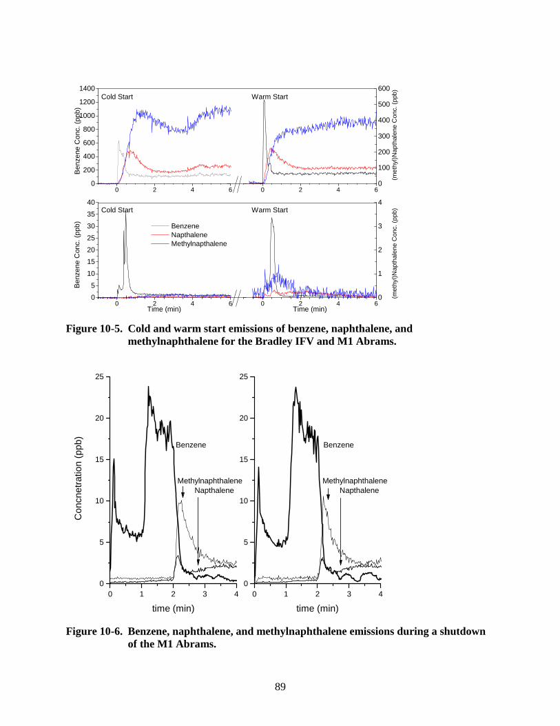
89

0

100

200

300

400

500

600

0

1

2

3

4

0 2 4 60

200

400

600

800

1000

1200

1400

Ben

zene

Con

c. (

ppb)

0 2 4 60

5

10

15

20

25

30

35

40

Cold Start

Benzene Napthalene Methylnapthalene

Ben

zene

Con

c. (

ppb)

Time (min)

Cold Start

0 2 4 6

Warm Start

(m

ethy

l)Nap

thal

ene

Con

c. (

ppb)

0 2 4 6Time (min)

Warm Start

(m

ethy

l)Nap

thal

ene

Con

c. (

ppb)

Figure 10-5. Cold and warm start emissions of benzene, naphthalene, and methylnaphthalene for the Bradley IFV and M1 Abrams.

0 1 2 3 40

5

10

15

20

25

0 1 2 3 40

5

10

15

20

25

Methylnaphthalene Napthalene

time (min)

Methylnaphthalene Napthalene

Benzene

Con

cnet

ratio

n (p

pb)

time (min)

Benzene

Figure 10-6. Benzene, naphthalene, and methylnaphthalene emissions during a shutdown of the M1 Abrams.

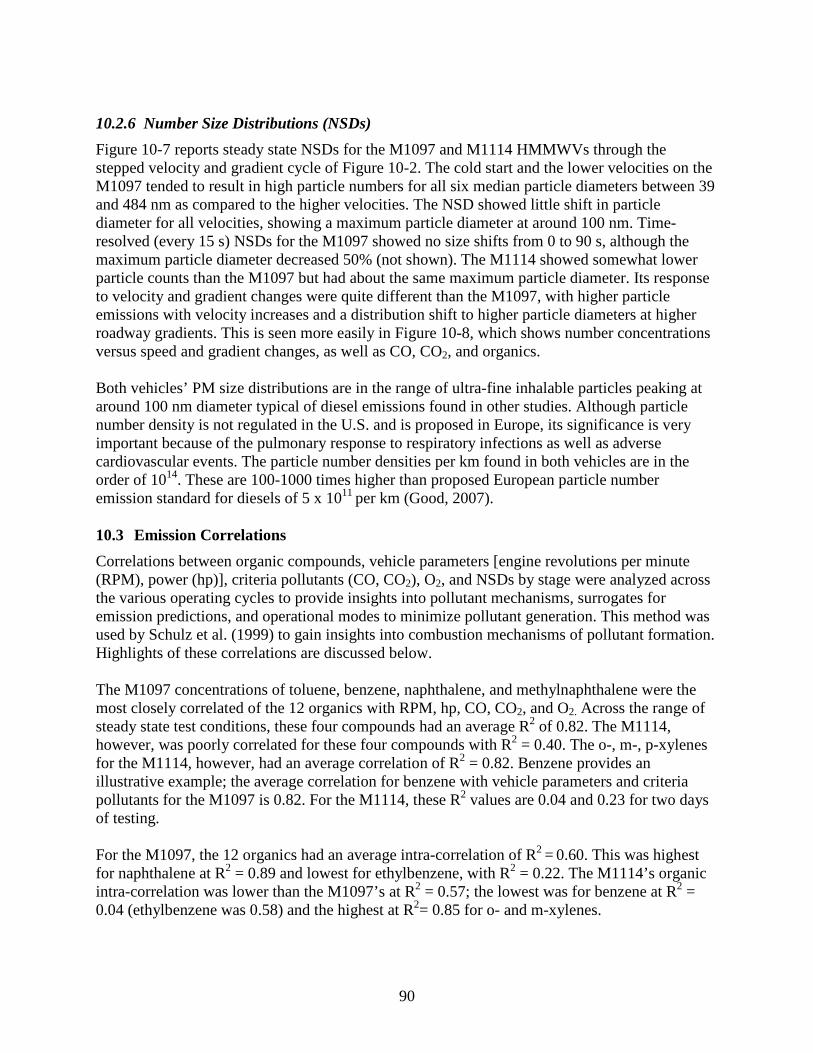
90

10.2.6 Number Size Distributions (NSDs)

Figure 10-7 reports steady state NSDs for the M1097 and M1114 HMMWVs through the stepped velocity and gradient cycle of Figure 10-2. The cold start and the lower velocities on the M1097 tended to result in high particle numbers for all six median particle diameters between 39 and 484 nm as compared to the higher velocities. The NSD showed little shift in particle diameter for all velocities, showing a maximum particle diameter at around 100 nm. Time-resolved (every 15 s) NSDs for the M1097 showed no size shifts from 0 to 90 s, although the maximum particle diameter decreased 50% (not shown). The M1114 showed somewhat lower particle counts than the M1097 but had about the same maximum particle diameter. Its response to velocity and gradient changes were quite different than the M1097, with higher particle emissions with velocity increases and a distribution shift to higher particle diameters at higher roadway gradients. This is seen more easily in Figure 10-8, which shows number concentrations versus speed and gradient changes, as well as CO, CO2, and organics. Both vehicles’ PM size distributions are in the range of ultra-fine inhalable particles peaking at around 100 nm diameter typical of diesel emissions found in other studies. Although particle number density is not regulated in the U.S. and is proposed in Europe, its significance is very important because of the pulmonary response to respiratory infections as well as adverse cardiovascular events. The particle number densities per km found in both vehicles are in the order of 1014. These are 100-1000 times higher than proposed European particle number emission standard for diesels of 5 x 1011 per km (Good, 2007). 10.3 Emission Correlations

Correlations between organic compounds, vehicle parameters [engine revolutions per minute (RPM), power (hp)], criteria pollutants (CO, CO2), O2, and NSDs by stage were analyzed across the various operating cycles to provide insights into pollutant mechanisms, surrogates for emission predictions, and operational modes to minimize pollutant generation. This method was used by Schulz et al. (1999) to gain insights into combustion mechanisms of pollutant formation. Highlights of these correlations are discussed below. The M1097 concentrations of toluene, benzene, naphthalene, and methylnaphthalene were the most closely correlated of the 12 organics with RPM, hp, CO, CO2, and O2. Across the range of steady state test conditions, these four compounds had an average R2 of 0.82. The M1114, however, was poorly correlated for these four compounds with R2 = 0.40. The o-, m-, p-xylenes for the M1114, however, had an average correlation of R2 = 0.82. Benzene provides an illustrative example; the average correlation for benzene with vehicle parameters and criteria pollutants for the M1097 is 0.82. For the M1114, these R2 values are 0.04 and 0.23 for two days of testing. For the M1097, the 12 organics had an average intra-correlation of R2 = 0.60. This was highest for naphthalene at R2 = 0.89 and lowest for ethylbenzene, with R2 = 0.22. The M1114’s organic intra-correlation was lower than the M1097’s at R2 = 0.57; the lowest was for benzene at R2 = 0.04 (ethylbenzene was 0.58) and the highest at R2= 0.85 for o- and m-xylenes.

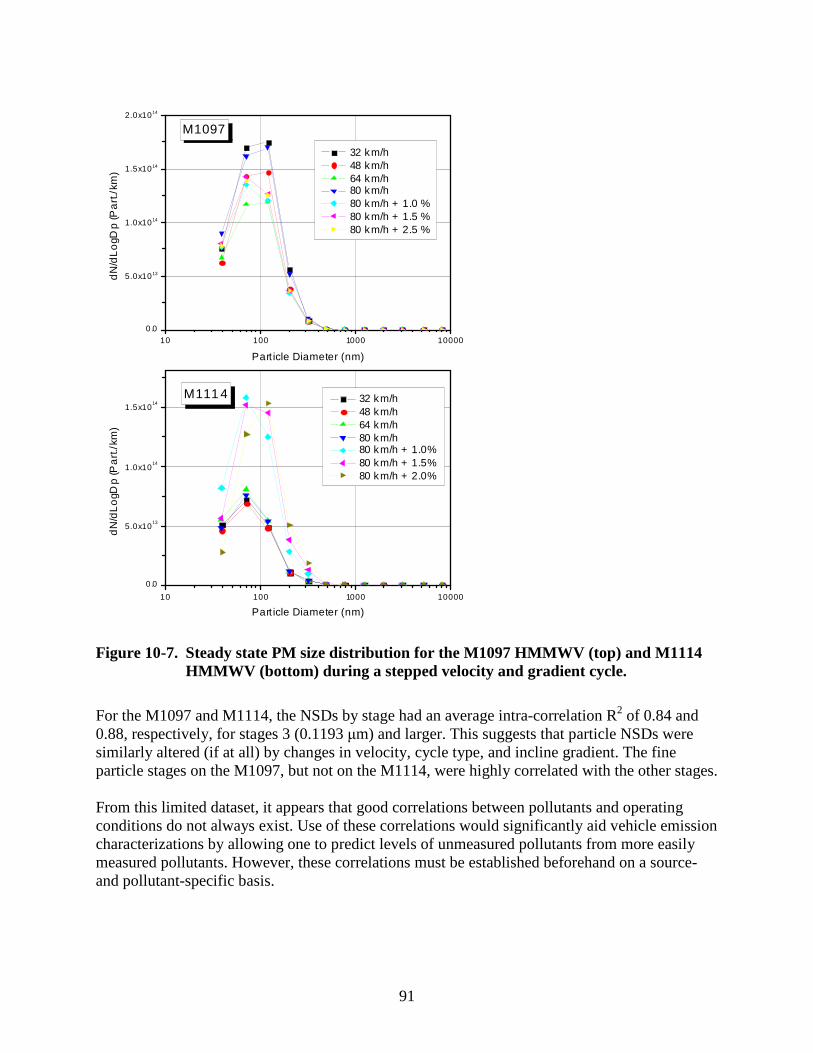
91

10 100 1000 10000

0.0

5.0x1013

1.0x1014

1.5x1014

M111 4

dN

/dL

ogD

p (P

art

./km

)

Part icle Diameter (nm)

32 km/h 48 km/h 64 km/h 80 km/h 80 km/h + 1.0% 80 km/h + 1.5% 80 km/h + 2.0%

10 100 1000 100000.0

5.0x1013

1.0x1014

1.5x1014

2.0x1014

32 km/h 48 km/h 64 km/h 80 km/h 80 km/h + 1.0 % 80 km/h + 1.5 % 80 km/h + 2.5 %

dN

/dL

ogD

p (P

art

./km

)

Part icle Diameter (nm)

M1097

Figure 10-7. Steady state PM size distribution for the M1097 HMMWV (top) and M1114 HMMWV (bottom) during a stepped velocity and gradient cycle.

For the M1097 and M1114, the NSDs by stage had an average intra-correlation R2 of 0.84 and 0.88, respectively, for stages 3 (0.1193 µm) and larger. This suggests that particle NSDs were similarly altered (if at all) by changes in velocity, cycle type, and incline gradient. The fine particle stages on the M1097, but not on the M1114, were highly correlated with the other stages. From this limited dataset, it appears that good correlations between pollutants and operating conditions do not always exist. Use of these correlations would significantly aid vehicle emission characterizations by allowing one to predict levels of unmeasured pollutants from more easily measured pollutants. However, these correlations must be established beforehand on a source- and pollutant-specific basis.

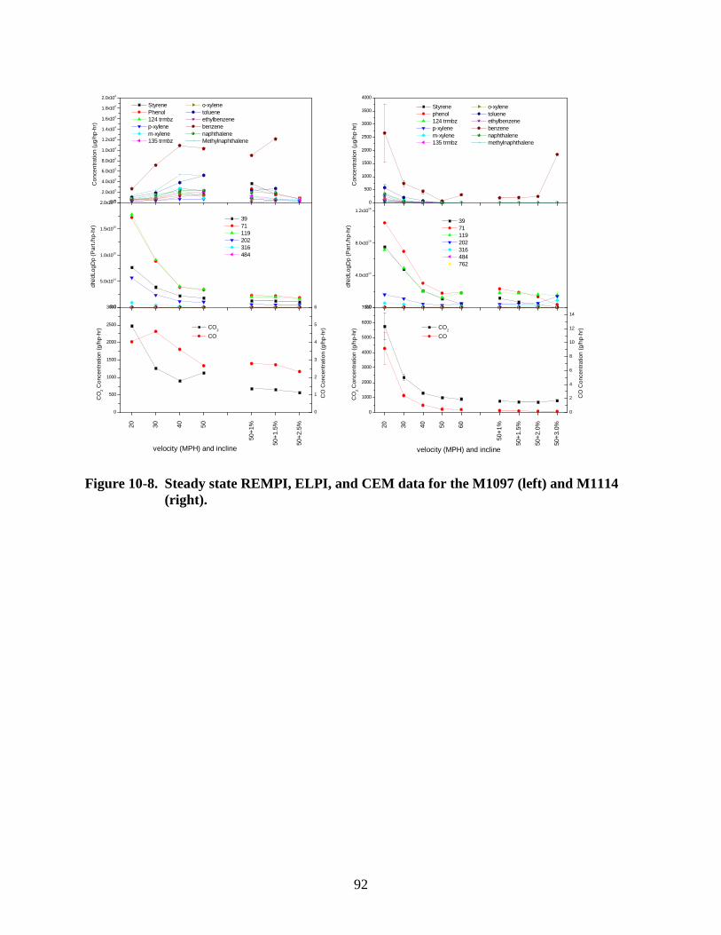
92

0.0

2.0x103

4.0x103

6.0x103

8.0x103

1.0x104

1.2x104

1.4x104

1.6x104

1.8x104

2.0x104

0.0

5.0x1014

1.0x1015

1.5x1015

2.0x1015

20 30 40 50

50+1

%

50+

1.5%

50+

2.5%

0

500

1000

1500

2000

2500

3000

0

1

2

3

4

5

6

0

500

1000

1500

2000

2500

3000

3500

4000

20 30 40 50 60

50+

1%

50+

1.5%

50+

2.0%

50+

3.0%

0

1000

2000

3000

4000

5000

6000

7000

0

2

4

6

8

10

12

14

0.0

4.0x1014

8.0x1014

1.2x1015

o-xylene toluene ethylbenzene benzene naphthalene Methylnaphthalene

Styrene Phenol 124 trmbz p-xylene m-xylene 135 trmbz

Con

cent

ratio

n (µ

g/hp

-hr)

39 71 119 202 316 484

dN

/dLo

gDp

(Par

t./hp

-hr)

CO2

CO

CO

2 Con

cent

ratio

n (g

/hp-

hr)

velocity (MPH) and incline

CO

Con

cent

ratio

n (g

/hp-

hr)

o-xylene toluene ethylbenzene benzene naphthalene methylnaphthalene

Styrene phenol 124 trmbz p-xylene m-xylene 135 trmbz

Con

cent

ratio

n (µ

g/hp

-hr)

CO2

CO

CO

2 Con

cent

ratio

n (g

/hp-

hr)

velocity (MPH) and incline

CO

Con

cent

ratio

n (g

/hp-

hr)

39 71 119 202 316 484 762

dN

/dLo

gDp

(Par

t./hp

-hr)

Figure 10-8. Steady state REMPI, ELPI, and CEM data for the M1097 (left) and M1114 (right).

93

11. Source 6: F-15 and F-22 Aircraft Engine Emissions

This chapter describes the results of a field study using multiple extractive sampling techniques as well as real time detection techniques to measure gaseous emissions from F-15 and F-22 fighter aircraft. Tests were performed between October 12 and 18, 2007 on the trim pad facility at Tyndall AFB in Panama City, Florida. Measurements were made on two different F100 engines, and eight different F119 engines mounted on in-use aircraft. 54 test runs were performed at engine power levels that ranged from idle to full “military power”, with additional test runs at full augmented power (afterburner). The approach adopted for these tests involved extractive sampling at a distance of approximately 20-25 nozzle diameters downstream of the engine exit plane with real-time measurements using REMPI-TOFMS and a PTRMS (Battelle). Integrated air samples were also collected and analyzed for VOC. 11.1 Experimental Method

11.1.1 Aircraft/Engine

The engines tested included the F100 engine associated with the F-15 Eagle and the F-16 Falcon aircraft and the F119 engine associated with the F-22 aircraft. The Pratt & Whitney F100 engine is the primary engine in the worldwide F-15 fleet and has gained overwhelming use with more than 85% of the world's air forces that fly the F-16. With more than 6,800 active installed engines worldwide and over 16 million flight hours, the F100 series represents a large proportion of the current fighter aircraft inventory. The F100 is an axial-flow turbofan produced in four variations: F-100-PE-100, F-100-PW-200, F-100-PW-220, and F-100-PW-229. The engines tested during this measurement campaign were F-100-PW-100 engines with normal thrust of 12,420 pounds, rising to a maximum thrust of 14,670 pounds at full military power. Maximum afterburning thrust is 23,830 pounds. The F-22 aircraft incorporates a pair of new, higher thrust engines, the Pratt & Whitney F119-PW-100, which is designed for efficient supersonic operation without afterburner. The F119 engine develops more than twice the thrust of current engines under supersonic conditions, and more thrust without afterburner than conventional engines with afterburner. Each F-22 is powered by two of these 35,000-pound-thrust-class engines. The experimental design called for duplicate test cycles to be performed on each test engine with individual test runs conducted at each of the engine power settings shown in Table 11-1 (nominal percentage of maximum thrust in parentheses). Due to the extreme conditions encountered in sampling the exhaust at afterburner power levels, these tests were performed only on the final day of testing.

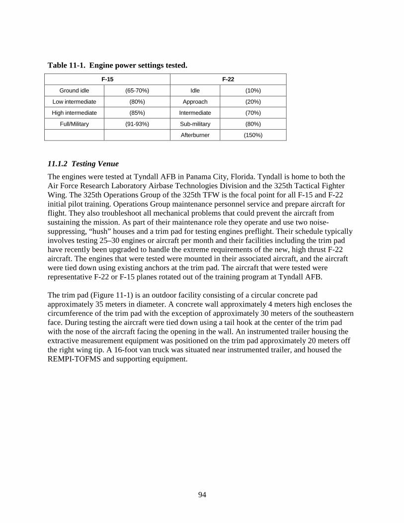
94

Table 11-1. Engine power settings tested.

F-15 F-22

Ground idle (65-70%) Idle (10%)

Low intermediate (80%) Approach (20%)

High intermediate (85%) Intermediate (70%)

Full/Military (91-93%) Sub-military (80%)

Afterburner (150%)

11.1.2 Testing Venue

The engines were tested at Tyndall AFB in Panama City, Florida. Tyndall is home to both the Air Force Research Laboratory Airbase Technologies Division and the 325th Tactical Fighter Wing. The 325th Operations Group of the 325th TFW is the focal point for all F-15 and F-22 initial pilot training. Operations Group maintenance personnel service and prepare aircraft for flight. They also troubleshoot all mechanical problems that could prevent the aircraft from sustaining the mission. As part of their maintenance role they operate and use two noise-suppressing, “hush” houses and a trim pad for testing engines preflight. Their schedule typically involves testing 25–30 engines or aircraft per month and their facilities including the trim pad have recently been upgraded to handle the extreme requirements of the new, high thrust F-22 aircraft. The engines that were tested were mounted in their associated aircraft, and the aircraft were tied down using existing anchors at the trim pad. The aircraft that were tested were representative F-22 or F-15 planes rotated out of the training program at Tyndall AFB. The trim pad (Figure 11-1) is an outdoor facility consisting of a circular concrete pad approximately 35 meters in diameter. A concrete wall approximately 4 meters high encloses the circumference of the trim pad with the exception of approximately 30 meters of the southeastern face. During testing the aircraft were tied down using a tail hook at the center of the trim pad with the nose of the aircraft facing the opening in the wall. An instrumented trailer housing the extractive measurement equipment was positioned on the trim pad approximately 20 meters off the right wing tip. A 16-foot van truck was situated near instrumented trailer, and housed the REMPI-TOFMS and supporting equipment.

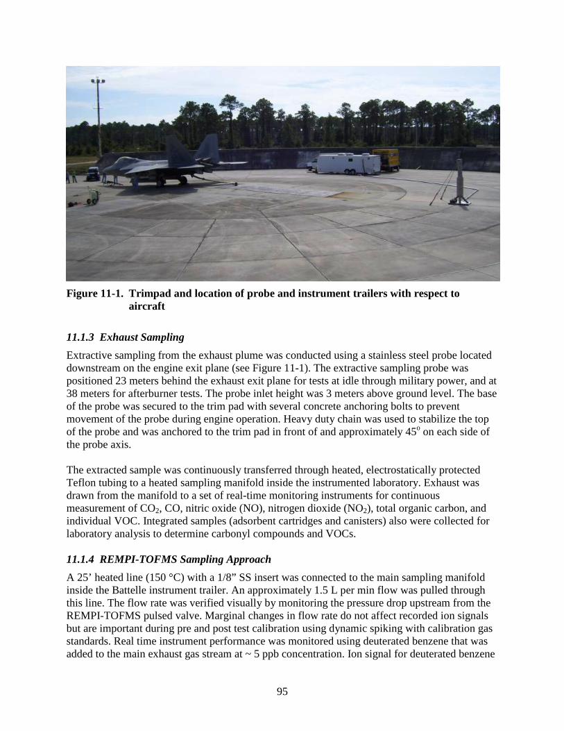
95

Figure 11-1. Trimpad and location of probe and instrument trailers with respect to aircraft

11.1.3 Exhaust Sampling

Extractive sampling from the exhaust plume was conducted using a stainless steel probe located downstream on the engine exit plane (see Figure 11-1). The extractive sampling probe was positioned 23 meters behind the exhaust exit plane for tests at idle through military power, and at 38 meters for afterburner tests. The probe inlet height was 3 meters above ground level. The base of the probe was secured to the trim pad with several concrete anchoring bolts to prevent movement of the probe during engine operation. Heavy duty chain was used to stabilize the top of the probe and was anchored to the trim pad in front of and approximately 45o on each side of the probe axis. The extracted sample was continuously transferred through heated, electrostatically protected Teflon tubing to a heated sampling manifold inside the instrumented laboratory. Exhaust was drawn from the manifold to a set of real-time monitoring instruments for continuous measurement of CO2, CO, nitric oxide (NO), nitrogen dioxide (NO2), total organic carbon, and individual VOC. Integrated samples (adsorbent cartridges and canisters) also were collected for laboratory analysis to determine carbonyl compounds and VOCs. 11.1.4 REMPI-TOFMS Sampling Approach

A 25’ heated line (150 °C) with a 1/8” SS insert was connected to the main sampling manifold inside the Battelle instrument trailer. An approximately 1.5 L per min flow was pulled through this line. The flow rate was verified visually by monitoring the pressure drop upstream from the REMPI-TOFMS pulsed valve. Marginal changes in flow rate do not affect recorded ion signals but are important during pre and post test calibration using dynamic spiking with calibration gas standards. Real time instrument performance was monitored using deuterated benzene that was added to the main exhaust gas stream at ~ 5 ppb concentration. Ion signal for deuterated benzene

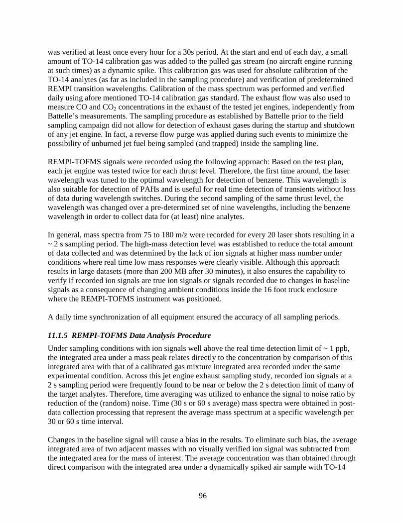
96

was verified at least once every hour for a 30s period. At the start and end of each day, a small amount of TO-14 calibration gas was added to the pulled gas stream (no aircraft engine running at such times) as a dynamic spike. This calibration gas was used for absolute calibration of the TO-14 analytes (as far as included in the sampling procedure) and verification of predetermined REMPI transition wavelengths. Calibration of the mass spectrum was performed and verified daily using afore mentioned TO-14 calibration gas standard. The exhaust flow was also used to measure CO and CO2 concentrations in the exhaust of the tested jet engines, independently from Battelle’s measurements. The sampling procedure as established by Battelle prior to the field sampling campaign did not allow for detection of exhaust gases during the startup and shutdown of any jet engine. In fact, a reverse flow purge was applied during such events to minimize the possibility of unburned jet fuel being sampled (and trapped) inside the sampling line. REMPI-TOFMS signals were recorded using the following approach: Based on the test plan, each jet engine was tested twice for each thrust level. Therefore, the first time around, the laser wavelength was tuned to the optimal wavelength for detection of benzene. This wavelength is also suitable for detection of PAHs and is useful for real time detection of transients without loss of data during wavelength switches. During the second sampling of the same thrust level, the wavelength was changed over a pre-determined set of nine wavelengths, including the benzene wavelength in order to collect data for (at least) nine analytes. In general, mass spectra from 75 to 180 m/z were recorded for every 20 laser shots resulting in a ~ 2 s sampling period. The high-mass detection level was established to reduce the total amount of data collected and was determined by the lack of ion signals at higher mass number under conditions where real time low mass responses were clearly visible. Although this approach results in large datasets (more than 200 MB after 30 minutes), it also ensures the capability to verify if recorded ion signals are true ion signals or signals recorded due to changes in baseline signals as a consequence of changing ambient conditions inside the 16 foot truck enclosure where the REMPI-TOFMS instrument was positioned. A daily time synchronization of all equipment ensured the accuracy of all sampling periods. 11.1.5 REMPI-TOFMS Data Analysis Procedure

Under sampling conditions with ion signals well above the real time detection limit of ~ 1 ppb, the integrated area under a mass peak relates directly to the concentration by comparison of this integrated area with that of a calibrated gas mixture integrated area recorded under the same experimental condition. Across this jet engine exhaust sampling study, recorded ion signals at a 2 s sampling period were frequently found to be near or below the 2 s detection limit of many of the target analytes. Therefore, time averaging was utilized to enhance the signal to noise ratio by reduction of the (random) noise. Time (30 s or 60 s average) mass spectra were obtained in post-data collection processing that represent the average mass spectrum at a specific wavelength per 30 or 60 s time interval. Changes in the baseline signal will cause a bias in the results. To eliminate such bias, the average integrated area of two adjacent masses with no visually verified ion signal was subtracted from the integrated area for the mass of interest. The average concentration was than obtained through direct comparison with the integrated area under a dynamically spiked air sample with TO-14

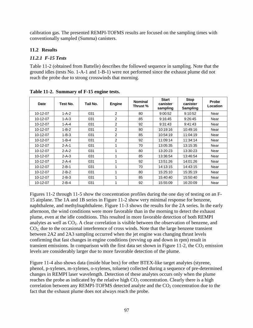
97

calibration gas. The presented REMPI-TOFMS results are focused on the sampling times with conventionally sampled (Summa) canisters. 11.2 Results

11.2.1 F-15 Tests

Table 11-2 (obtained from Battelle) describes the followed sequence in sampling. Note that the ground idles (tests No. 1-A-1 and 1-B-1) were not performed since the exhaust plume did not reach the probe due to strong crosswinds that morning.

Table 11-2. Summary of F-15 engine tests.

Date Test No. Tail No. Engine Nominal Thrust %

Start canister

sampling

Stop canister

Sampling

Probe Location

10-12-07 1-A-2 031 2 80 9:00:52 9:10:52 Near

10-12-07 1-A-3 031 2 85 9:16:45 9:26:45 Near 10-12-07 1-A-4 031 2 92 9:31:43 9:41:43 Near 10-12-07 1-B-2 031 2 80 10:19:16 10:49:16 Near 10-12-07 1-B-3 031 2 85 10:54:19 11:04:19 Near 10-12-07 1-B-4 031 2 92 11:09:14 11:34:14 Near 10-12-07 2-A-1 031 1 70 13:05:35 13:15:35 Near 10-12-07 2-A-2 031 1 80 13:20:23 13:30:23 Near 10-12-07 2-A-3 031 1 85 13:36:54 13:46:54 Near 10-12-07 2-A-4 031 1 92 13:51:26 14:01:26 Near 10-12-07 2-B-1 031 1 70 14:13:15 14:43:15 Near 10-12-07 2-B-2 031 1 80 15:25:10 15:35:19 Near 10-12-07 2-B-3 031 1 85 15:40:40 15:50:40 Near 10-12-07 2-B-4 031 1 92 15:55:09 16:20:09 Near

Figures 11-2 through 11-5 show the concentration profiles during the one day of testing on an F-15 airplane. The 1A and 1B series in Figure 11-2 show very minimal response for benzene, naphthalene, and methylnaphthalene. Figure 11-3 shows the results for the 2A series. In the early afternoon, the wind conditions were more favorable than in the morning to detect the exhaust plume, even at the idle conditions. This resulted in more favorable detection of both REMPI analytes as well as CO2. A clear correlation is visible between the observation of benzene, and CO2, due to the occasional interference of cross winds. Note that the large benzene transient between 2A2 and 2A3 sampling occurred when the jet engine was changing thrust levels confirming that fast changes in engine conditions (revving up and down in rpm) result in transient emissions. In comparison with the first data set shown in Figure 11-2, the CO2 emission levels are considerably larger due to more favorable detection of the plume. Figure 11-4 also shows data (inside blue box) for other BTEX-like target analytes (styrene, phenol, p-xylenes, m-xylenes, o-xylenes, toluene) collected during a sequence of pre-determined changes in REMPI laser wavelength. Detection of these analytes occurs only when the plume reaches the probe as indicated by the relative high CO2 concentration. Clearly there is a high correlation between any REMPI-TOFMS detected analyte and the CO2 concentration due to the fact that the exhaust plume does not always reach the probe.

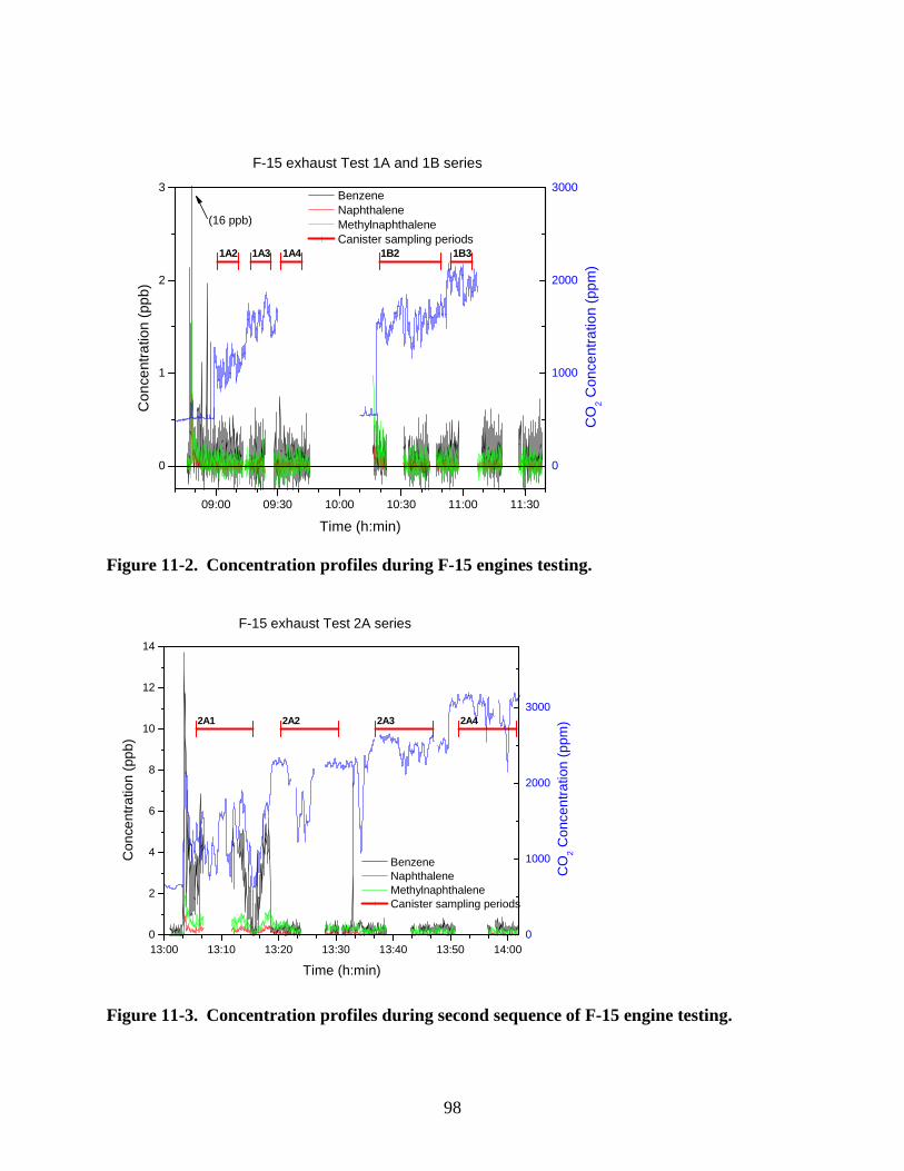
98

0

1000

2000

3000

1A2 1A3 1A4 1B2 1B3

09:00 09:30 10:00 10:30 11:00 11:30

0

1

2

3 Benzene Naphthalene Methylnaphthalene Canister sampling periods

Con

cent

ratio

n (p

pb)

Time (h:min)

F-15 exhaust Test 1A and 1B series

(16 ppb)

CO

2 Con

cent

ratio

n (p

pm)

Figure 11-2. Concentration profiles during F-15 engines testing.

0

1000

2000

30002A1 2A2 2A3 2A4

13:00 13:10 13:20 13:30 13:40 13:50 14:000

2

4

6

8

10

12

14

Benzene Naphthalene Methylnaphthalene Canister sampling periods

Con

cent

ratio

n (p

pb)

Time (h:min)

F-15 exhaust Test 2A series

CO

2 Con

cent

ratio

n (p

pm)

Figure 11-3. Concentration profiles during second sequence of F-15 engine testing.

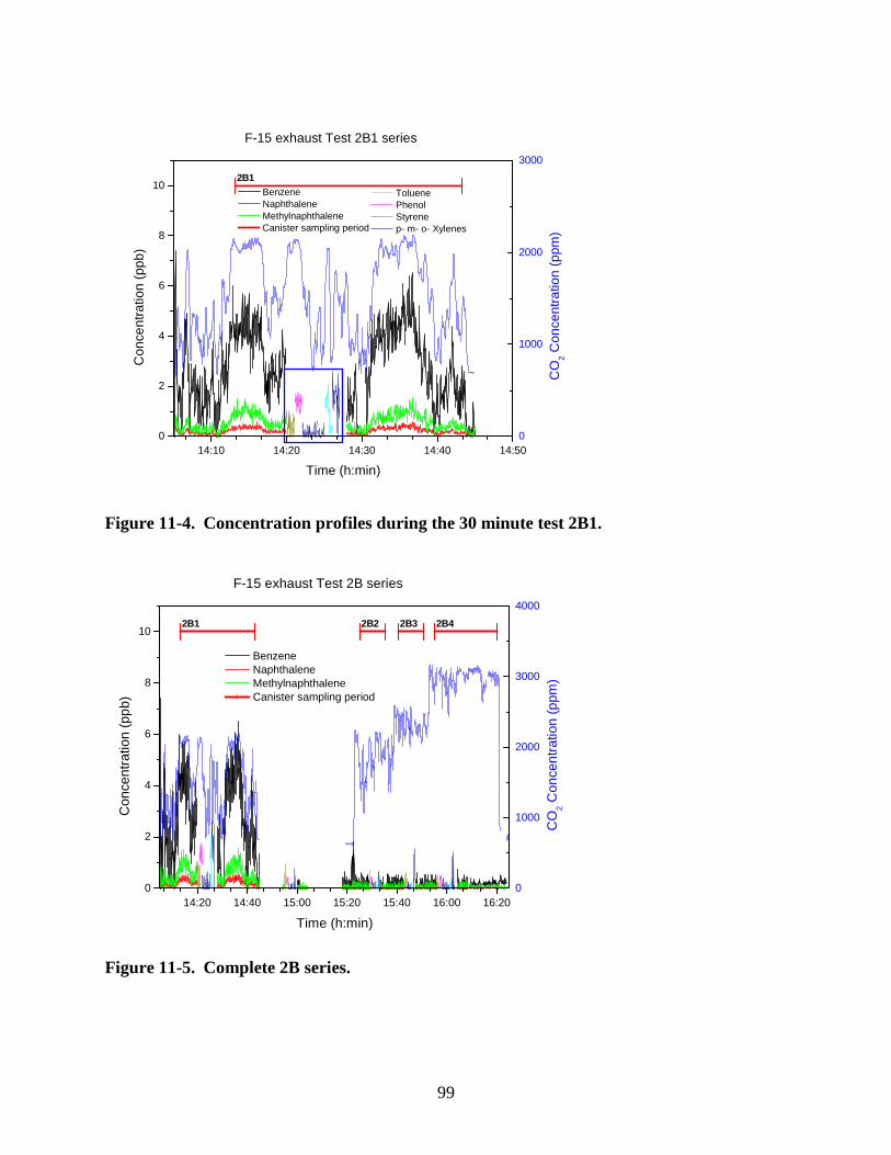
99

0

1000

2000

3000

2B1

14:10 14:20 14:30 14:40 14:500

2

4

6

8

10 Benzene Naphthalene Methylnaphthalene

Canister sampling period

Toluene Phenol Styrene p- m- o- Xylenes

Con

cent

ratio

n (p

pb)

Time (h:min)

F-15 exhaust Test 2B1 series

CO

2 Con

cent

ratio

n (p

pm)

Figure 11-4. Concentration profiles during the 30 minute test 2B1.

0

1000

2000

3000

4000

2B1 2B2 2B3 2B4

14:20 14:40 15:00 15:20 15:40 16:00 16:200

2

4

6

8

10

Benzene Naphthalene Methylnaphthalene Canister sampling period

Con

cent

ratio

n (p

pb)

Time (h:min)

F-15 exhaust Test 2B series

CO

2 Con

cent

ratio

n (p

pm)

Figure 11-5. Complete 2B series.

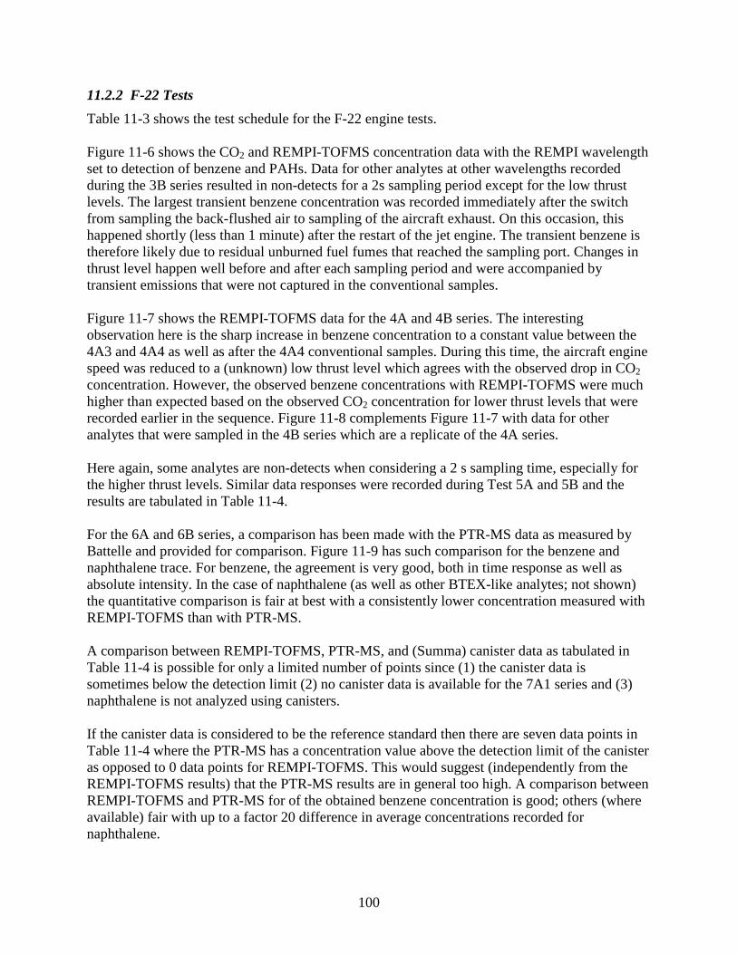
100

11.2.2 F-22 Tests

Table 11-3 shows the test schedule for the F-22 engine tests. Figure 11-6 shows the CO2 and REMPI-TOFMS concentration data with the REMPI wavelength set to detection of benzene and PAHs. Data for other analytes at other wavelengths recorded during the 3B series resulted in non-detects for a 2s sampling period except for the low thrust levels. The largest transient benzene concentration was recorded immediately after the switch from sampling the back-flushed air to sampling of the aircraft exhaust. On this occasion, this happened shortly (less than 1 minute) after the restart of the jet engine. The transient benzene is therefore likely due to residual unburned fuel fumes that reached the sampling port. Changes in thrust level happen well before and after each sampling period and were accompanied by transient emissions that were not captured in the conventional samples. Figure 11-7 shows the REMPI-TOFMS data for the 4A and 4B series. The interesting observation here is the sharp increase in benzene concentration to a constant value between the 4A3 and 4A4 as well as after the 4A4 conventional samples. During this time, the aircraft engine speed was reduced to a (unknown) low thrust level which agrees with the observed drop in CO2 concentration. However, the observed benzene concentrations with REMPI-TOFMS were much higher than expected based on the observed CO2 concentration for lower thrust levels that were recorded earlier in the sequence. Figure 11-8 complements Figure 11-7 with data for other analytes that were sampled in the 4B series which are a replicate of the 4A series. Here again, some analytes are non-detects when considering a 2 s sampling time, especially for the higher thrust levels. Similar data responses were recorded during Test 5A and 5B and the results are tabulated in Table 11-4. For the 6A and 6B series, a comparison has been made with the PTR-MS data as measured by Battelle and provided for comparison. Figure 11-9 has such comparison for the benzene and naphthalene trace. For benzene, the agreement is very good, both in time response as well as absolute intensity. In the case of naphthalene (as well as other BTEX-like analytes; not shown) the quantitative comparison is fair at best with a consistently lower concentration measured with REMPI-TOFMS than with PTR-MS. A comparison between REMPI-TOFMS, PTR-MS, and (Summa) canister data as tabulated in Table 11-4 is possible for only a limited number of points since (1) the canister data is sometimes below the detection limit (2) no canister data is available for the 7A1 series and (3) naphthalene is not analyzed using canisters. If the canister data is considered to be the reference standard then there are seven data points in Table 11-4 where the PTR-MS has a concentration value above the detection limit of the canister as opposed to 0 data points for REMPI-TOFMS. This would suggest (independently from the REMPI-TOFMS results) that the PTR-MS results are in general too high. A comparison between REMPI-TOFMS and PTR-MS for of the obtained benzene concentration is good; others (where available) fair with up to a factor 20 difference in average concentrations recorded for naphthalene.

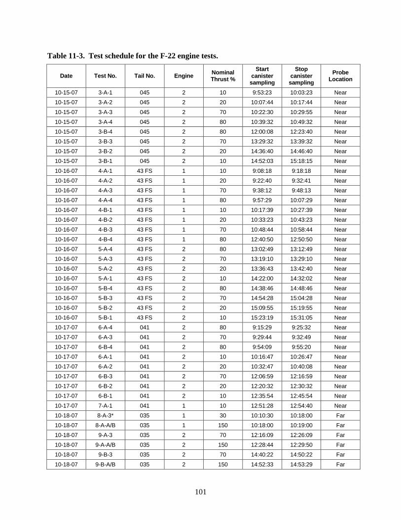
101

Table 11-3. Test schedule for the F-22 engine tests.

Date Test No. Tail No. Engine Nominal Thrust %

Start canister

sampling

Stop canister

sampling

Probe Location

10-15-07 3-A-1 045 2 10 9:53:23 10:03:23 Near

10-15-07 3-A-2 045 2 20 10:07:44 10:17:44 Near

10-15-07 3-A-3 045 2 70 10:22:30 10:29:55 Near

10-15-07 3-A-4 045 2 80 10:39:32 10:49:32 Near

10-15-07 3-B-4 045 2 80 12:00:08 12:23:40 Near

10-15-07 3-B-3 045 2 70 13:29:32 13:39:32 Near

10-15-07 3-B-2 045 2 20 14:36:40 14:46:40 Near

10-15-07 3-B-1 045 2 10 14:52:03 15:18:15 Near

10-16-07 4-A-1 43 FS 1 10 9:08:18 9:18:18 Near

10-16-07 4-A-2 43 FS 1 20 9:22:40 9:32:41 Near

10-16-07 4-A-3 43 FS 1 70 9:38:12 9:48:13 Near

10-16-07 4-A-4 43 FS 1 80 9:57:29 10:07:29 Near

10-16-07 4-B-1 43 FS 1 10 10:17:39 10:27:39 Near

10-16-07 4-B-2 43 FS 1 20 10:33:23 10:43:23 Near

10-16-07 4-B-3 43 FS 1 70 10:48:44 10:58:44 Near

10-16-07 4-B-4 43 FS 1 80 12:40:50 12:50:50 Near

10-16-07 5-A-4 43 FS 2 80 13:02:49 13:12:49 Near

10-16-07 5-A-3 43 FS 2 70 13:19:10 13:29:10 Near

10-16-07 5-A-2 43 FS 2 20 13:36:43 13:42:40 Near

10-16-07 5-A-1 43 FS 2 10 14:22:00 14:32:02 Near

10-16-07 5-B-4 43 FS 2 80 14:38:46 14:48:46 Near

10-16-07 5-B-3 43 FS 2 70 14:54:28 15:04:28 Near

10-16-07 5-B-2 43 FS 2 20 15:09:55 15:19:55 Near

10-16-07 5-B-1 43 FS 2 10 15:23:19 15:31:05 Near

10-17-07 6-A-4 041 2 80 9:15:29 9:25:32 Near

10-17-07 6-A-3 041 2 70 9:29:44 9:32:49 Near

10-17-07 6-B-4 041 2 80 9:54:09 9:55:20 Near

10-17-07 6-A-1 041 2 10 10:16:47 10:26:47 Near

10-17-07 6-A-2 041 2 20 10:32:47 10:40:08 Near

10-17-07 6-B-3 041 2 70 12:06:59 12:16:59 Near

10-17-07 6-B-2 041 2 20 12:20:32 12:30:32 Near

10-17-07 6-B-1 041 2 10 12:35:54 12:45:54 Near

10-17-07 7-A-1 041 1 10 12:51:28 12:54:40 Near

10-18-07 8-A-3* 035 1 30 10:10:30 10:18:00 Far

10-18-07 8-A-A/B 035 1 150 10:18:00 10:19:00 Far

10-18-07 9-A-3 035 2 70 12:16:09 12:26:09 Far

10-18-07 9-A-A/B 035 2 150 12:28:44 12:29:50 Far

10-18-07 9-B-3 035 2 70 14:40:22 14:50:22 Far

10-18-07 9-B-A/B 035 2 150 14:52:33 14:53:29 Far

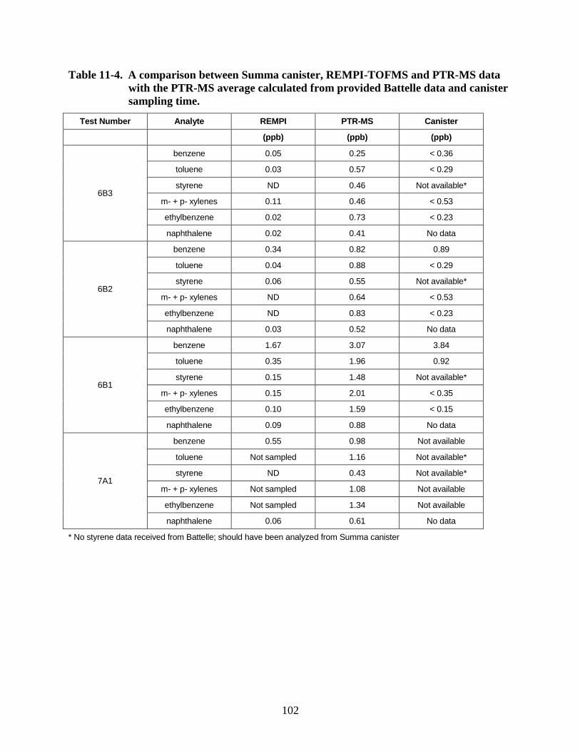
102

Table 11-4. A comparison between Summa canister, REMPI-TOFMS and PTR-MS data with the PTR-MS average calculated from provided Battelle data and canister sampling time.

Test Number Analyte REMPI PTR-MS Canister

(ppb) (ppb) (ppb)

benzene 0.05 0.25 < 0.36

toluene 0.03 0.57 < 0.29

styrene ND 0.46 Not available*

m- + p- xylenes 0.11 0.46 < 0.53

ethylbenzene 0.02 0.73 < 0.23

6B3

naphthalene 0.02 0.41 No data

benzene 0.34 0.82 0.89

toluene 0.04 0.88 < 0.29

styrene 0.06 0.55 Not available*

m- + p- xylenes ND 0.64 < 0.53

ethylbenzene ND 0.83 < 0.23

6B2


benzene 1.67 3.07 3.84

toluene 0.35 1.96 0.92

styrene 0.15 1.48 Not available*

m- + p- xylenes 0.15 2.01 < 0.35

ethylbenzene 0.10 1.59 < 0.15

6B1


benzene 0.55 0.98 Not available

toluene Not sampled 1.16 Not available*

styrene ND 0.43 Not available*

m- + p- xylenes Not sampled 1.08 Not available

ethylbenzene Not sampled 1.34 Not available

7A1


* No styrene data received from Battelle; should have been analyzed from Summa canister

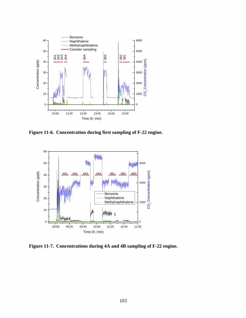
103

10:00 11:00 12:00 13:00 14:00 15:00

0

10

20

30

40

50

60

0

1000

2000

3000

4000

5000

6000

3A1

3A2

3A3

3A4

3B4

3B3

3B2

3B1

Benzene Naphthalene Methylnaphthalene Canister sampling

Con

cent

ratio

n (p

pb)

Time (h: min)

CO

2 Con

cent

ratio

n (p

pm)

Figure 11-6. Concentration during first sampling of F-22 engine.

09:00 09:20 09:40 10:00 10:20 10:40 11:00

0

10

20

30

40

50

60

0

1000

2000

3000

4A1 4A2 4A3 4A4 4B1 4B2 4B3

Con

cent

ratio

n (p

pb)

Time (h: min)

Benzene Naphthalene Methylnaphthalene

CO

2 C

once

ntra

tion

(ppm

)

Figure 11-7. Concentrations during 4A and 4B sampling of F-22 engine.

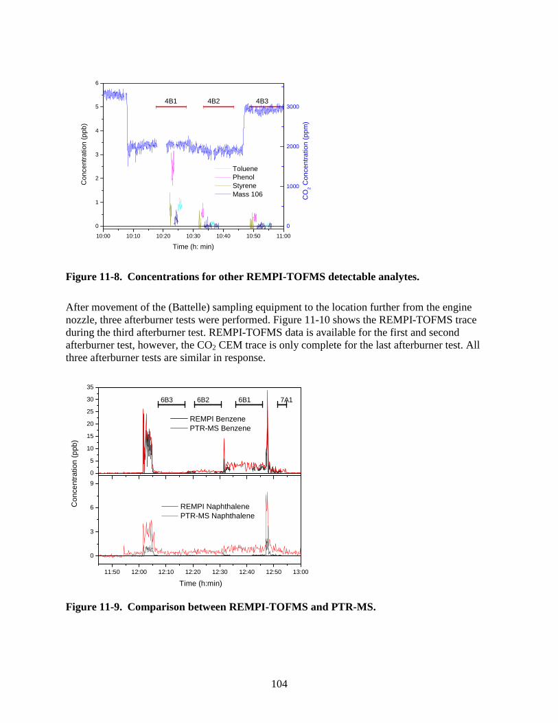
104

10:00 10:10 10:20 10:30 10:40 10:50 11:00

0

1

2

3

4

5

6

0

1000

2000

3000

Toluene Phenol Styrene Mass 106

Con

cent

ratio

n (p

pb)

Time (h: min)

4B1 4B2 4B3

CO

2 Con

cent

ratio

n (p

pm)

Figure 11-8. Concentrations for other REMPI-TOFMS detectable analytes.

After movement of the (Battelle) sampling equipment to the location further from the engine nozzle, three afterburner tests were performed. Figure 11-10 shows the REMPI-TOFMS trace during the third afterburner test. REMPI-TOFMS data is available for the first and second afterburner test, however, the CO2 CEM trace is only complete for the last afterburner test. All three afterburner tests are similar in response.

0

5

10

15

20

25

30

35

11:50 12:00 12:10 12:20 12:30 12:40 12:50 13:00

0

3

6

9

6B3 6B2 6B1 7A1

REMPI Benzene PTR-MS Benzene

Con

cent

ratio

n (p

pb)

REMPI Naphthalene PTR-MS Naphthalene

Time (h:min)

Figure 11-9. Comparison between REMPI-TOFMS and PTR-MS.

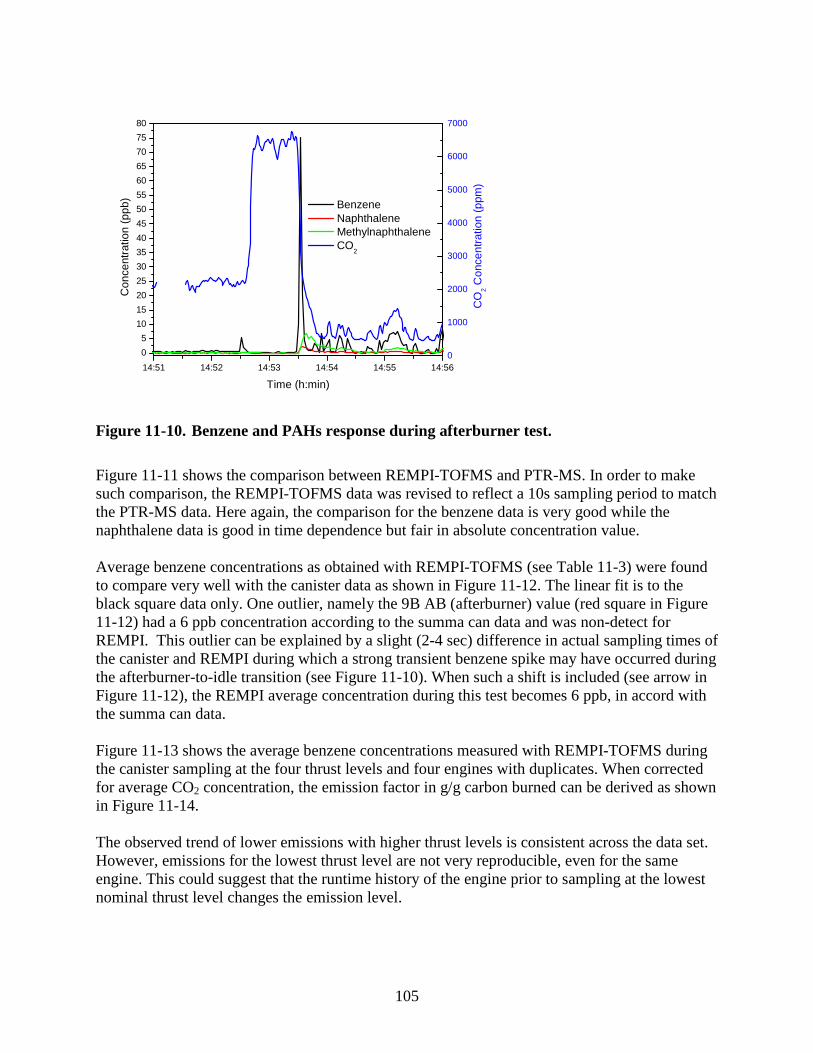
105

14:51 14:52 14:53 14:54 14:55 14:56

0

5

10

15

20

25

30

35

40

45

50

55

60

65

70

75

80

0

1000

2000

3000

4000

5000

6000

7000C

once

ntra

tion

(ppb

)

Benzene Naphthalene Methylnaphthalene CO

2

Time (h:min)

CO

2 C

once

ntra

tion

(ppm

)

Figure 11-10. Benzene and PAHs response during afterburner test.

Figure 11-11 shows the comparison between REMPI-TOFMS and PTR-MS. In order to make such comparison, the REMPI-TOFMS data was revised to reflect a 10s sampling period to match the PTR-MS data. Here again, the comparison for the benzene data is very good while the naphthalene data is good in time dependence but fair in absolute concentration value. Average benzene concentrations as obtained with REMPI-TOFMS (see Table 11-3) were found to compare very well with the canister data as shown in Figure 11-12. The linear fit is to the black square data only. One outlier, namely the 9B AB (afterburner) value (red square in Figure 11-12) had a 6 ppb concentration according to the summa can data and was non-detect for REMPI. This outlier can be explained by a slight (2-4 sec) difference in actual sampling times of the canister and REMPI during which a strong transient benzene spike may have occurred during the afterburner-to-idle transition (see Figure 11-10). When such a shift is included (see arrow in Figure 11-12), the REMPI average concentration during this test becomes 6 ppb, in accord with the summa can data. Figure 11-13 shows the average benzene concentrations measured with REMPI-TOFMS during the canister sampling at the four thrust levels and four engines with duplicates. When corrected for average CO2 concentration, the emission factor in g/g carbon burned can be derived as shown in Figure 11-14. The observed trend of lower emissions with higher thrust levels is consistent across the data set. However, emissions for the lowest thrust level are not very reproducible, even for the same engine. This could suggest that the runtime history of the engine prior to sampling at the lowest nominal thrust level changes the emission level.

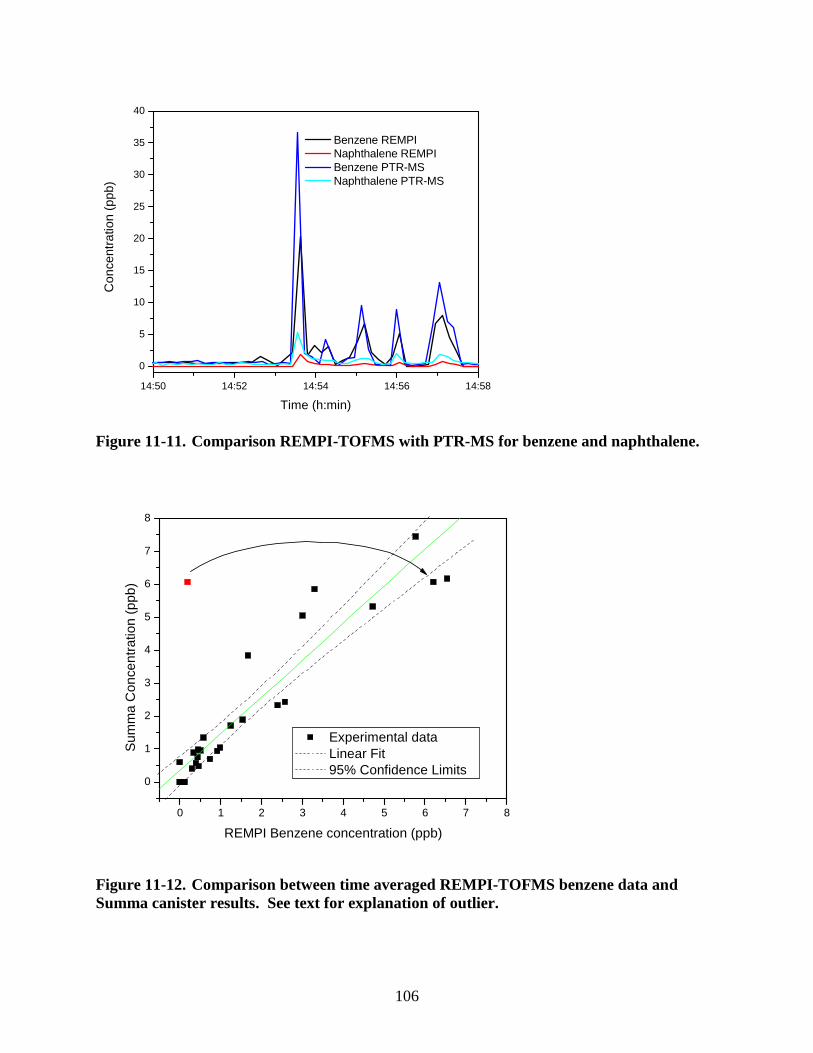
106

14:50 14:52 14:54 14:56 14:58

0

5

10

15

20

25

30

35

40

Benzene REMPI Naphthalene REMPI Benzene PTR-MS Naphthalene PTR-MS

Con

cent

ratio

n (p

pb)

Time (h:min)

Figure 11-11. Comparison REMPI-TOFMS with PTR-MS for benzene and naphthalene.

0 1 2 3 4 5 6 7 8

0

1

2

3

4

5

6

7

8

Sum

ma

Con

cent

ratio

n (p

pb)

REMPI Benzene concentration (ppb)

Experimental data Linear Fit 95% Confidence Limits

Figure 11-12. Comparison between time averaged REMPI-TOFMS benzene data and Summa canister results. See text for explanation of outlier.

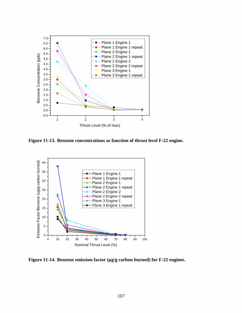
107

1 2 3 4-0.5

0.0

0.5

1.0

1.5

2.0

2.5

3.0

3.5

4.0

4.5

5.0

5.5

6.0

6.5

7.0B

enze

ne C

once

ntra

tion

(ppb

)

Thrust Level (% of max)

Plane 1 Engine 1 Plane 1 Engine 1 repeat Plane 2 Engine 1 Plane 2 Engine 1 repeat Plane 2 Engine 2 Plane 2 Engine 2 repeat Plane 3 Engine 1 Plane 3 Engine 1 repeat

Figure 11-13. Benzene concentrations as function of thrust level F-22 engine.

0 10 20 30 40 50 60 70 80 90 1000

5

10

15

20

25

30

35

40

Plane 1 Engine 1 Plane 1 Engine 1 repeat Plane 2 Engine 1 Plane 2 Engine 1 repeat Plane 2 Engine 2 Plane 2 Engine 2 repeat Plane 3 Engine 1 Plane 3 Engine 1 repeat

Em

issi

on F

acto

r B

enze

ne (

ug/g

-car

bon

burn

ed)

Nominal Thrust Level (%)

Figure 11-14. Benzene emission factor (µg/g carbon burned) for F-22 engines.

108

12. Conclusions

This project has developed a technology termed REMPI-TOFMS for real time detection of trace aromatic organic compounds in complex (combustion exhaust) matrices. During this project the REMPI-TOFMS technology was transformed from a laboratory type, large frame research instrument to a compact system that was taken into the field and used to characterize trace aromatic air toxics. The REMPI-TOFMS system versatility was demonstrated by sampling on a broad range of sources from an MWC to an M1 Abrams battle tank. The system also proved portable, functional in harsh environments, reproducible, sensitive, and quick to respond, making it ideal for characterization of multiple source types and compound types. Operation of the LIBS system for detection of metals showed that its use was limited by the presence of carbonaceous soot. An LTA procedure prior to analysis looked promising but was not pursued due to the departure from the project of the LIBS cooperator, the U.S. Army Research Laboratory. Testing with ORS instrumentation did not prove fruitful, as daily drift of the criteria pollutant readings (compared to on-line CEMs) lent doubt to the value of these measurements for point source measurement. The low ppbv detection limit of REMPI-TOFMS is sufficient for detection of BTEX and small PAHs in exhaust gas streams from vehicles in real time. This is a capability not previously accomplished on such a wide variety of sources and to such an extent. Only in cases of significant exhaust dilution (high load AGE and higher thrust levels of jet engines) were the real time detection limits of the instrument insufficient to provide real time results. Variation of the system procedures allowed collection of an averaged response up to 1 minute in duration to greatly enhance the sensitivity of the instrument, resulting in minimal species non-detects. Emission factors for many small organic aromatic compounds in exhausts from a diesel generator, aircraft ground equipment, waste combustor, two HMMWVs, Abrams and Bradley vehicles, and F-15 and F-22 aircraft engines have been reported for the first time. Strong and significant transient emissions appear during changes in engine conditions, including shutdown and restarts. Steady state conditions were, in general, found to be constant over an extended period of time. REMPI-TOFMS was able to clearly distinguish effects of engine type (diesel, turbine) on emission characteristics. In critical operations, the REMPI-TOFMS instrument can be used to provide operational feedback, improving efficiency and reducing emissions. The speed and sensitivity of the REMPI instrument allows transient and steady state characterization of target pollutants emissions that can be used in assessing or developing new exhaust gas treatment systems for mobile sources or in developing emission factors by use-mode. For reasonably high ambient levels of air toxics, REMPI-TOFMS can also be used as an ambient air monitor. Its recent application to a near-road, highway emissions study proved its usefulness in open source sampling. Both of these

109

applications, point source or area source, are appropriate for REMPI-TOFMS and, thus, the technology could prove useful in a diagnostic and characterization capacity.

110

13. References

Badger, G. and Novotny, J., 1963. Mode of Formation of 3,4-Benzopyrene at High Temperatures. Nature 198, 1086 Blumenstock, M.; Zimmermann, R.; Schramm, K.-W.; Kettrup, 2000. Influence of combustion conditions on the PCDD/F-, PCB-, PCBz- and PAH-concentrations in the post-combustion chamber of a waste incineration pilot plant. Chemosphere 40, 987-993. Blumenstock, M.; Zimmermann, R.; Schramm, K.-W.; Kettrup, 2001. Identification of surrogate compounds for the emission of PCDD/F (I-TEQ value) and evaluation of their on-line real-time detectability in flue gases of waste incineration plants by REMPI–TOFMS mass spectrometry. Chemosphere 42, 507-518. Boesl, U., Nagel, H., Weickhardt, C., Frey, R., Schlag, E., 1998. Vehicle exhaust emission time-resolved multicomponent analysis by laser mass spectrometry. In: Meyers, R.A. (Ed), The Encyclopedia of Environmental Analysis and Remediation, Volume 87. John Wiley, New York, 5000–5022. Boesl, U., Heger, H. , Zimmermann, R., Püffel, P., Nagel, H., 2000. Laser mass spectrometry in trace analysis. In: Meyers, R.A. (Ed), Encyclopedia of Chemical Analysis. Wiley, New York, 2087–2118. Burtscher, H., 1992. Measurement and characteristics of combustion aerosols with special consideration of photoelectric charging and charging by flame ions. Journal of Aerosol Science 23, 549-595. Clark, N., Daley, J.J., Nine, R.D. and Atkinson, C.M., 1999. Application of the new City-Suburban Heavy Vehicle Route (CSHVR) to Truck Emissions Characterization. SAE Paper 1999-01-1467. Cowen K., Kelly T., Dindal A., Willenberg Z., Riggs K., 2006. Environmental Technology Verification Report: SRI International Jet-REMPI (Resonance Enhanced Multi-Photon Ionization), Battelle. Dunbar, J.C., Lin, C.-I., Vergucht, I., Wong, J., Durant, J.L., 2001. Estimating the contributions of mobile sources of PAH to urban air using real-time PAH monitoring. Science of the Total Environment 279, 1–19. Franzen, J., Frey, R., Nagel, H, 1995. Fast monitoring of motor exhaust components by resonant multi-photon ionisation and time-of-flight mass spectrometry. Journal of Molecular Structure 347, 143-52.

111

Frey, R., Nagel, H., Franzen, J, Rikeit, H.-E., 1995. Time-resolved measurement of individual aromatic hydrocarbons in automotive exhaust at transient engine operation. SAE Technical Paper Series No. 951053, Society of Automotive Engineers International, Warrendale, PA. Gass, H., Lüder, K., Wilken, M., 2002. PCDD/F- Emissions during cold start-up and shut-down of municipal waste incinerator. Organohalogen Compounds, 56, 193 Gerstle, T., Virag, P., Wade, M.D., Brown, P.P., 1999 Aircraft Engine and Auxiliary Power Unit Emissions Testing: Final Report. Addendum. F119-PW-100 Engine Emissions Testing Report; USAF, IERA, IERA-R2-BR-TR-1999-0006, March 1999. GlobalSecurity.org, 2008a, http://www.globalsecurity.org/military/systems/ground/images/m1114-up-armored-specs01.jpg (accessed January 2009) GlobalSecurity.org, 2008b, http://www.globalsecurity.org/military/systems/ground/m1-specs.htm (accessed January 2009) Good, Phillip, “An Overview of European Emissions Legislation for Light Duty Vehicles,” International Conference on Transport and Environment Milan, 19-21 March 2007. http://transportenv07.jrc.ec.europa.eu/pdf/D/D_1_19_Good_P_An%20overview%20of%20%20EU%20Emissions%20Legislation.pdf (accessed January 2009) Gross, M.; Cernuschi, S.; Palini, E.; Lodi, M.; Mariani, G. 2004. PCDD/Fs release during normal and transient operation of a full scale MSWI plant. Organohalogen Compounds 66, 1227. Gullett, B. K. and Wikström, E., 2000. Mono- to tri-chlorinated dibenzodioxin (CDD) and dibenzofuran (CDF) congeners/homologues as indicators of CDD and CDF emissions from municipal waste and waste/coal combustion. Chemosphere 40, 1015-1019. Gullett, B.; Touati, A.; Oudejans, L.; Ryan, S.; Tabor, D., 2006. Transient PCDD and PCDF concentrations in an MWC. Organohalogen Compounds 68, 143. Gullett, B.; Touati, A.; Oudejans, L.; Tabor, D. 2007. AWMA Hazardous Waste Combustor Conference, Charleston, SC, March 13-14, 2007. Heeb, N., Forss, A.-M., Wilhelm, P., 2001. Comparison of methane, benzene and alkyl benzenes cold start emission data of EURO I and EURO II three-way catalyst passenger cars and light duty vehicles from time resolved exhaust gas analysis. Proceedings International Symposium Transport and air pollution, Boulder Colorado USA, 17–19 September 2001. Heger, H. J.; Zimmermann, R.; Dorfner, R.; Beckmann, M.; Griebel, H.; Kettrup, A.; Boesl, U., 1999. In-Line Catalytic Derivatization Method for Selective Detection of Chlorinated Aromatics with a Hyphenated Gas Chromatography/Laser Mass Spectrometry Technique: A Concept for Comprehensive Detection of Isomeric Ensembles. Analytical Chemistry 71, 46-57.

112

Heger, H., Zimmermann, R., Blumenstock, M., Kettrup, A., 2001. On-line real-time measurements at incineration plants: PAHs and a PCDD/F surrogate compound at stationary combustion conditions and during transient emission puffs. Chemosphere 42, 691–696. Kemme, M.R.; Brown, W.T., Frame, E.A., and Alvarez, R.A. 2006. Diesel-Powered Equipment Properties and Activity Database for DoD Off-Road Sources, SERDP Project WP-1338, ERDC/CERL TR-06-6, March 2006. Kimm, L., Sylvia, D., Gerstle, T., Virag, P., 1997. Proceedings of the Air & Waste Management Association Annual Meeting, June 8-13, 1997, Toronto, Ontario, Canada. Kuribayashi S., Yamakoshi H., Danno M., Sakai S., Tsuruga S., Futami H., Morii S., 2005. VUV single-photon ionization ion trap time-of-flight mass spectrometer for on-line, real-time monitoring of chlorinated organic compounds in waste incineration flue gas. Analytical Chemistry 77, 1007–1012 Levy, Jr., J.A., Schawitsch, T.L., Thoreson, H.F., Walter, J.K., 1993. Estimation of toxic air pollutant emissions and development of a supporting information management system for Vandenberg Air Force Base. 86th Annual Meeting & Exhibition, Paper 93-TP-30B.02, Air & Waste Management Association, June 13–18, Denver, CO. Nagel, H., Frey, R., and Boesel, U., 1996. On-line analysis of formaldehyde and acetaldehyde in non-stationary engine operation using laser mass spectrometry. SAE Technical Paper Series No. 961084, Society of Automotive Engineers International, Warrendale, PA. Neuer-Etscheidt, K.; Nordsiek, H.; Liu, Y.; Kettrup, A.; Zimmermann, R., 2006. PCDD/F and Other Micropollutants in MSWI Crude Gas and Ashes during Plant Start-Up and Shut-Down Processes. Environment Science Technology 40, 342. Nine, R.D., Clark, N.N., and Norton, P., 2000. Effects of Multiple Driving Test Schedules Performed on Two Heavy-Duty Vehicles”, SAE Fuels & Lubricants Meeting, Baltimore, Oct. 2000, SAE Paper 2000-01-2818. NIST Mass Spec Data Center, S.E. Stein, director, "Mass Spectra" in NIST Chemistry WebBook, NIST Standard Reference Database Number 69, Eds. P.J. Linstrom and W.G. Mallard, June 2005, National Institute of Standards and Technology, Gaithersburg MD, 20899 http://webbook.nist.gov. Oudejans, L., Touati, A. , Gullett, B., 2004. Real-Time, On-Line Characterization of Diesel Generator Air Toxic Emissions by Resonance Enhanced Multi-Photon Ionization Time of Flight Mass Spectrometry, Analytical Chemistry 76(9), 2517–2524. Rakopoulos, C.;Mavropoulos, G., Hountalas, D., 1998. Modeling the Structural Thermal Response of An Air-Cooled Diesel Engine Under Transient Operation Including a Detailed Thermodynamic Description of Boundary Conditions. Society of Automotive Engineers, SAE Technical Paper Series No. 981024.

113

Rhead, M. and Pemberton, R. Sources of Naphthalene in Diesel Exhaust Emissions. Energy & Fuels 10, 837-843, 1996. Ryan, J., Lemieux, P., Preston, W., 1998. Near-real-time measurement of trace volatile organic compounds from combustion processes using an on-line gas chromatograph. Waste Management 18, 403–410. Schultz, G., Tong, I., Kefauver, K. and Ishibashi, J., 2006. Steering and Handling Testing Using Roadway Simulator Technology. International Journal of Vehicle Systems Modeling and Testing, Vol. 1, No. 1/2/3, pp. 32-47. Schulz, H., De Melo, B., and Ousmanov, F., 1999. Volatile Organic Compounds and Particulates as Components of Diesel Engine Exhaust Gas. Combustion and Flame 118, 179-190. Thanner R., Oser H., Grotheer H.-H., 1998. Time-resolved monitoring of aromatic compounds in an experimental incinerator using an improved jet-resonance-enhanced multi-photon ionization system jet-REMPI. European Mass Spectrometry 4, 215–222 U.S. Army, JP-8, The Single Fuel Forward, Armaments Command Research, Development, and Engineering Center, MI, 2001. http://www.mfp.usmc.mil/TeamApp/G4/, “JP-8 Single Fuel Info Compendium U.S. Environmental Protection Agency, SW-846 On-line, Test methods for evaluating solid wastes, Physical/Chemical methods, Office of Solid Waste, Method 0010 Modified Method 5 Sampling Train, 1986a, at URL http://www.epa.gov/epaoswer/hazwaste/test/pdfs/0010.pdf, accessed on November 12, 2003. U.S. EPA Method 5 “Determination of Particulate Matter Emissions from Stationary Sources,” found in 40 CFR part 60, appendix A, 1986b. http://www.epa.gov/ttn/emc/promgate/m-05.pdf (accessed January 2009) U.S. Environmental Protection Agency, 1993. Emission factor documentation for AP-42 section 3.4, large stationary diesel & all stationary dual fuel engines. http://www.epa.gov/ttn/chief/ap42/ch03/bgdocs/b03s04.pdf (accessed January 2009). U.S. Environmental Protection Agency, SW-846 On-line, Test methods for evaluating solid wastes, Physical/Chemical methods, Office of Solid Waste, Method 0040 Sampling of Principal Organic Constituents from Combustion Sources using TEDLAR Bags, 1996a, at URL http://www.epa.gov/epaoswer/hazwaste/test/pdfs/0040.pdf, (accessed January 2009). U.S. EPA Method 8270 in SW-846 Test Methods for Evaluating Solid Waste, Physical/Chemical Methods, Office of Solid Waste, 1996b. http://www.epa.gov/epawaste/hazard/testmethods/sw846/pdfs/8270d.pdf (accessed January 2009)

114

U.S. EPA Method 0011 in SW-846 Test methods for evaluating solid wastes, Physical/Chemical methods, Office of Solid Waste, 1996c. http://www.epa.gov/epawaste/hazard/testmethods/sw846/pdfs/0011.pdf (accessed January 2009) U.S. EPA Method 8315a in SW-846 Test methods for evaluating solid wastes, Physical/Chemical methods, Office of Solid Waste, 1996d. http://www.epa.gov/epawaste/hazard/testmethods/sw846/pdfs/8315a.pdf (accessed January 2009) U.S. EPA M-23A, Test Method 23A, Sampling method for polychlorinated dibenzo-p dioxins and polychlorinated dibenzofuran emissions from stationary sources. EPA-SW 846 On-Line, 3rd ed., 1996d. Available at: http://www.epa.gov/epawaste/hazard/testmethods/sw846/pdfs/0023a.pdf. U.S. EPA Method TO-15 “Determination of Volatile Organic Compounds (VOCs) in Air collected in Specially-Prepared Canisters and Analyzed by Gas Chromatography/Mass Spectrometry (GC/MS)”, 1999. http://www.epa.gov/ttn/amtic/files/ambient/airtox/to-15r.pdf (accessed January 2009) U.S. Environmental Protection Agency, 2000a. Performance specification 2 specifications and test procedures for SO2 and NOX continuous monitoring systems in stationary sources. 40 CFR Ch.1 Pt.60, App. B, Spec.2. http://www.epa.gov/ttn/emc/specs/prompspec2.html (accessed January 2009). U.S. EPA, 2000b, Method 10A: “Determination Of Carbon Monoxide Emissions In Certifying Continuous Emission Monitoring Systems At Petroleum Refineries,” http://www.epa.gov/ttn/emc/promgate/m-10a.pdf. U.S. Environmental Protection Agency, 2004. EPA original list hazardous pollutants http://www.epa.gov/ttn/atw/188polls.html (accessed March 2005). U.S. EPA, 2006, Method 3A, “Determination of Oxygen and Carbon Dioxide Concentrations in Emissions from Stationary Sources (Instrumental Analyzer Procedure),” http://www.epa.gov/ttn/emc/promgate/m-03a.pdf Velazquez, J.; Voloboueva, L. A.; Cool, T. A., Selective Detection of Dibenzodioxin, Dibenzofuran and Some Small Polycyclic Aromatics. Combustion Science Technology 134, 139-163. Weickhardt, C.; Boesl, U., 1993. Time resolved trace analysis of exhaust gas by means of laser mass spectrometry. Ber. Bunsenges. Phys. Chem. 97, 1716-19. Zimmermann, R.; Boesl, U.; Weickhardt, C.; Lenoir, D.; Schramm, K.-W.; Kettrup, A.; Schlag, E.W., 1994. Isomer-selective ionization of chlorinated aromatics with lasers for analytical time-of-flight mass spectrometry: First results for polychlorinated dibenzo-p-dioxins (PCDD), biphenyls (PCB) and benzenes (PCBz). Chemosphere 29, 1877-88.

115

Zimmermann R., Heger H., Blumenstock M., Dorfner R., Schramm K.-W., Boesl U., Kettrup A., 1999. On-line measurement of chlorobenzene in wast incineration fl ue gas as a surrogate for the emission of polychlorinated dibenzo-p-dioxins/Furans (I-TEQ) using mobile resonance laser ionization time-of-flight mass spectrometry. Rapid Communications Mass Spectrometry 13, 307–314.

116

14. Appendix A: List of Scientific/Technical Publications

14.1.1 Journal Articles

• L. Oudejans, A. Touati, and B.K. Gullett, “Real-Time, On-Line Characterization of Diesel Generator Air Toxic Emissions by REMPI-TOFMS”, Anal Chem., 76, 2517-2524 (2004)

• Brian K. Gullett, Abderrahmane Touati, Lukas Oudejans, and Shawn P. Ryan, “Real-time emission characterization of organic air toxic pollutants during steady state and transient operation of a medium duty diesel engine”, Atmosph. Envir., 40, 4037–4047 (2006)

• Brian Gullett, Abderrahmane Touati, and Lukas Oudejans, “Use of REMPI–TOFMS for real-time measurement of trace aromatics during operation of aircraft ground equipment”, Atmosph. Envir., 42, 2117–2128 (2008)

• Brian Gullett, Lukas Oudejans, Abderrahmane Touati, Shawn Ryan, and Dennis Tabor, “Verification results of jet resonance-enhanced multiphoton ionization as a real-time PCDD/F emission monitor”, J. Mater. Cycles Waste Manag., 10, (2008) 32–37

• submitted to Environmental Science & Technology, entitled “Transient PAH, PM, CO, and CO2 Emission Responses from HMMWVs, the M1 Abrams tank, and the Bradley Infantry Fighting Vehicle” by Brian Gullett, Lukas Oudejans, and Abderrahmane Touati (2009).

14.2 Oral and Poster Presentations

Results obtained during this project were presented to (international) audiences at the following conferences:

• Annual conferences:

o Partners in Environmental Technology Technical Symposium & Workshop, Washington, DC, annual, 2000-2007 (Posters)

o International Karasek Conference, annual, 2001-2008 (oral and/or poster)

• Individual conferences:

o Seventh International Congress on Toxic Combustion By-Products, NIEHS, Research Triangle Park, NC (2001) (Oral)

o 26th Annual EPA-Air & Waste Management Association Information Exchange EPA, RTP (2001) (Oral)

o 22nd International Symposium on Halogenated Environmental Organic Pollutants and POPs (Dioxin 2002), Barcelona, Spain (2002) (Oral)

o 27th Annual EPA-Air & Waste Management Association Information Exchange EPA, RTP (2002) (Oral)

o Eighth International Congress on Toxic Combustion By-Products, NIEHS, at University of Arizona, Tucson, AZ (2003) (Poster)

117

o Laser Applications to Chemical and Environmental Analysis (LACEA) conference, Annapolis (2004) (Poster)

o 3rd International Conference on Combustion, Incineration/Pyrolysis and Emission Control (3rd i-CIPEC), Hangzhou, China, (2004). (Oral)

o Air and Waste Management Association (AWMA) Symposium on Air Quality Measurements and Technology, Durham, NC (2006) (Oral)

o 10th International Congress on Combustion By-Products and their Health Effects, Ischia, Italy (2007) (Oral)

Documents

SERDP Final Report EPA WP_1247 4_12_2010 r1