Embed Size (px)
Citation preview

UNIVERSITY LUMIÈRE LYON 2
DOCTORAL SCHOOL INFOMATHSINFORMATIQUE ET MATHÉMATIQUES (ED 512)
P H D T H E S I Sto obtain the title of
PhD of Science
Specialty : Computer Science
Defended by
Marian-Andrei RIZOIU
Semi-supervised structuring ofcomplex data
Thesis Advisers : Stéphane LALLICH and Julien VELCIN
prepared at the ERIC laboratorydefended on June 24th, 2013
Jury :
Reviewers : Adrião Dória Neto - Universidade Federal do Rio Grande do NorteChristel Vrain - LIFO Laboratory, Univ. Orleans
Advisers : Stéphane Lallich - ERIC Laboratory, Univ. Lyon 2Julien Velcin - ERIC Laboratory, Univ. Lyon 2
Examiners : Maria Rifqi - LIP6 Laboratory, Univ. Panthéon-AssasFrédéric Precioso - I3S Laboratory, Univ. Nice Sophia AntipolisGilbert Ritschard - Institute IDEMO, Univ. de Genève

Semi-Supervised Structuring of Complex Data
Abstract :The objective of this thesis is to explore how complex data can be treated using unsu-
pervised machine learning techniques, in which additional information is injected to guidethe exploratory process. The two main research challenges addressed in this work are (a)leveraging semantic information into data numerical representation and into the learningalgorithms and (b) making use of the temporal dimension when analyzing complex data.The main research challenges are derived, through a dialectical relation between theory andpractice, into more specific learning tasks, which vary from (i) detecting typical evolutionpatterns to (ii) improving data representation by using semantics to (iii) embedding expertinformation into image numerical description or to (iv) using semantic resources (e.g., Word-Net) when evaluation topics extracted from text. The methods we privilege when tacklingwith our learning tasks are unsupervised and, mainly, semi-supervised clustering. Therefore,the general context of this thesis lies at the intersection of the two large domains of complexdata analysis and semi-supervised clustering.
We divide our work into four parts. The first is dedicated to the temporal component ofdata, in which we propose a temporal clustering algorithms, with contiguity constraints, anduse it to detect typical evolutions. The second part is dedicated to semantic reconstructionof the description space of the data, and we propose an unsupervised feature constructionalgorithm, which replaces highly correlated pairs of features with conjunctions of literals.In the third part, we tackle the problem of constructing a semantically-enriched imagerepresentation starting from a baseline representation, and we propose two approachestoward leveraging external expert knowledge, under the form of non-positional labels.We dedicate the fourth part of our work to textual data, and more precisely towards thetask of topic extraction, using an overlapping text clustering algorithm, topic labeling,using frequent complete phrases, and semantic topic evaluation, by using an externalconcept hierarchy. We add a fifth part, which describes the applied part of our work,CommentWatcher, an open-source platform for analyzing online discussion forums.
Keywords : complex data analysis, semi-supervised clustering, semantic data repre-sentation, temporal clustering, topic extraction, semantic-enriched image representation,feature construction

Structuration semi-supervisée des données complexes
Résumé :L’objectif du travail présenté dans cette thèse est d’explorer comment les données com-
plexes peuvent être analysées en utilisant des techniques d’apprentissage automatique non-supervisé, dans lequel des connaissances supplémentaires sont introduits pour guider le pro-cessus exploratoire. Ce travail de recherche traite deux grandes problématiques : d’une part,l’utilisation d’informations sémantiques dans la construction de la représentation numériqueainsi que dans les algorithmes d’apprentissage automatique, et d’autre part, l’utilisation dela dimension temporelle dans l’analyse de données complexes. De ces problématiques derecherche ont émergé, au travers d’une relation dialectique entre la théorie et la pratique,des tâches plus précises, à savoir : (i) la détection d’évolutions typiques, (ii) l’améliorationde la représentation des données en utilisant leur sémantique, (iii) l’introduction d’informa-tions expertes dans la représentation numérique des images et (iv) l’utilisation de ressourcessémantiques additionnelles (comme WordNet) pour l’évaluation des thématiques extraitesà partir du texte. Les méthodes qu’on privilégie dans notre travail sont des méthodes non-supervisées et, notamment, des méthodes semi-supervisées. Par conséquent, le contextegénérale de cette thèse cette thèse se situe à au croisement des domaines de l’analyse dedonnées complexes et du clustering semi-supervisé.
Nous divisons notre travail en quatre parties. La première partie est dédiée à ladimension temporelle des données, et dans cette optique nous proposons un algorithme declustering temporel avec des contraintes de contiguïté, que nous appliquons à la détectiond’évolutions typiques. La deuxième partie quant à elle s’intéresse à la reconstructionsémantique de l’espace de représentation, tâche pour laquelle nous proposons un algorithmenon-supervisé de construction d’attributs, dont le principe de base est de remplacer lespaires d’attributs hautement corrélés par des conjonctions de ceux-ci. Dans la troisièmepartie, nous traitons le problème de la construction de représentations numériques séman-tiquement enrichies des images et pour cela nous proposons deux approches qui utilisent desconnaissances expertes sous la forme d’annotations. Enfin, la dernière partie de nos travauxthéoriques est dédiée aux données textuelles, plus précisément aux tâches d’extractionde thématiques à l’aide d’un algorithme de clustering avec recouvrement, de nommagede thématiques par des expressions intelligibles, ainsi qu’à l’évaluation sémantique desthématiques, en utilisant une hiérarchie de concepts. A ce travail vient s’ajouter unecinquième partie pratique, dont l’aboutissement est la plateforme CommentWatcher quipermet d’analyser les forums de discussion en ligne.
Mots clés : analyse de données complexes, clustering semi-supervisé, représentationsémantique de données, clustering temporel, extraction de thématiques, représentation desimages enrichi avec de la sémantique, construction non-supervisée des attributs

Acknowledgments
First of all, I would like to thank my two PhD advisers, Stéphane Lallich and JulienVelcin, for accompanying me on this four-year journey. They have shown me what researchmeans and they have taught me how to appreciate it. They have shown me how one can berigorous, while creative, and they have become, in the meanwhile, my role-models.
I would also like to thank Christel Vrain and Adrião Dória Neto for accepting to dedicatetheir time and energy towards reviewing my thesis. I equally thank the examiners in my jury,Maria Rifqi, Frédéric Precioso and Gilbert Ritschard, for doing me the honor of participatingto the jury of my thesis.
A special thanks goes towards Julien Ah-Pine, who, in addition to being a good andsupportive friend, has kindly accepted to read this manuscript and to provide educatedopinions, which often made me see things in a new light. I also acknowledge my workcolleagues and friends, Adrien and Mathilde, who transformed the office into an exhilaratingplace.
And last, but not least, I thank my friends and family for putting up with me.

Contents
1 Introduction 11.1 The big picture . . . . . . . . . . . . . . . . . . . . . . . . . . . . . . . . . . 11.2 Research project . . . . . . . . . . . . . . . . . . . . . . . . . . . . . . . . . 31.3 The constituent parts of the thesis . . . . . . . . . . . . . . . . . . . . . . . 51.4 Content of the different chapters . . . . . . . . . . . . . . . . . . . . . . . . 6
2 Overview of the Domain 92.1 Complex Data Mining . . . . . . . . . . . . . . . . . . . . . . . . . . . . . . 9
2.1.1 Specificities of complex data . . . . . . . . . . . . . . . . . . . . . . 112.1.2 Dealing with complex data of different natures . . . . . . . . . . . . 132.1.3 Temporal/dynamic dimension . . . . . . . . . . . . . . . . . . . . . . 162.1.4 High data dimensionality . . . . . . . . . . . . . . . . . . . . . . . . 18
2.2 Semi-Supervised Clustering . . . . . . . . . . . . . . . . . . . . . . . . . . . 202.2.1 Similarity-based approaches . . . . . . . . . . . . . . . . . . . . . . . 242.2.2 Search-based approaches . . . . . . . . . . . . . . . . . . . . . . . . . 26
3 Detecting Typical Evolutions 293.1 Learning task and motivations . . . . . . . . . . . . . . . . . . . . . . . . . . 293.2 Formalisation . . . . . . . . . . . . . . . . . . . . . . . . . . . . . . . . . . . 313.3 Related work . . . . . . . . . . . . . . . . . . . . . . . . . . . . . . . . . . . 343.4 Temporal-Driven Constrained Clustering . . . . . . . . . . . . . . . . . . . . 34
3.4.1 The temporal-aware dissimilarity measure . . . . . . . . . . . . . . . 353.4.2 The contiguity penalty function . . . . . . . . . . . . . . . . . . . . . 373.4.3 The TDCK-Means algorithm . . . . . . . . . . . . . . . . . . . . . . 383.4.4 Fine-tuning the ratio between components . . . . . . . . . . . . . . . 40
3.5 Experiments . . . . . . . . . . . . . . . . . . . . . . . . . . . . . . . . . . . . 433.5.1 Dataset . . . . . . . . . . . . . . . . . . . . . . . . . . . . . . . . . . 433.5.2 Qualitative evaluation . . . . . . . . . . . . . . . . . . . . . . . . . . 433.5.3 Evaluation measures . . . . . . . . . . . . . . . . . . . . . . . . . . . 453.5.4 Quantitative evaluation . . . . . . . . . . . . . . . . . . . . . . . . . 463.5.5 Impact of parameters β and δ . . . . . . . . . . . . . . . . . . . . . . 493.5.6 The tuning parameter α . . . . . . . . . . . . . . . . . . . . . . . . . 50
3.6 Current work: Role identification in social networks . . . . . . . . . . . . . . 523.6.1 Context . . . . . . . . . . . . . . . . . . . . . . . . . . . . . . . . . . 523.6.2 The framework for identifying social roles . . . . . . . . . . . . . . . 533.6.3 Preliminary experiments . . . . . . . . . . . . . . . . . . . . . . . . . 54
3.7 Conclusion and future work . . . . . . . . . . . . . . . . . . . . . . . . . . . 57
viii Contents
4 Using Data Semantics to Improve Data Representation 594.1 Learning task and motivations . . . . . . . . . . . . . . . . . . . . . . . . . . 59
4.1.1 Why construct a new feature set? . . . . . . . . . . . . . . . . . . . . 614.1.2 A brief overview of our proposals . . . . . . . . . . . . . . . . . . . . 62
4.2 Related work . . . . . . . . . . . . . . . . . . . . . . . . . . . . . . . . . . . 634.3 uFRINGE - adapting FRINGE for unsupervised learning . . . . . . . . . . . 664.4 uFC - a greedy heuristic . . . . . . . . . . . . . . . . . . . . . . . . . . . . . 67
4.4.1 uFC - the proposed algorithm . . . . . . . . . . . . . . . . . . . . . 684.4.2 Searching co-occurring pairs . . . . . . . . . . . . . . . . . . . . . . . 704.4.3 Constructing and pruning features . . . . . . . . . . . . . . . . . . . 71
4.5 Evaluation of a feature set . . . . . . . . . . . . . . . . . . . . . . . . . . . . 714.5.1 Complexity of the feature set . . . . . . . . . . . . . . . . . . . . . . 724.5.2 The trade-off between two opposing criteria . . . . . . . . . . . . . . 74
4.6 Initial Experiments . . . . . . . . . . . . . . . . . . . . . . . . . . . . . . . . 754.6.1 uFC and uFRINGE: Qualitative evaluation . . . . . . . . . . . . . 764.6.2 uFC and uFRINGE: Quantitative evaluation . . . . . . . . . . . . 794.6.3 Impact of parameters λ and limititer . . . . . . . . . . . . . . . . . . 794.6.4 Relation between number of features and feature length . . . . . . . 81
4.7 Improving the uFC algorithm . . . . . . . . . . . . . . . . . . . . . . . . . . 824.7.1 Automatic choice of λ . . . . . . . . . . . . . . . . . . . . . . . . . . 834.7.2 Stopping criterion. Candidate pruning technique. . . . . . . . . . . . 83
4.8 Further Experiments . . . . . . . . . . . . . . . . . . . . . . . . . . . . . . . 844.8.1 Risk-based heuristic for choosing parameters . . . . . . . . . . . . . . 844.8.2 Pruning the candidates . . . . . . . . . . . . . . . . . . . . . . . . . 864.8.3 Algorithm stability . . . . . . . . . . . . . . . . . . . . . . . . . . . . 89
4.9 Usage of the multi-objective optimization techniques . . . . . . . . . . . . . 904.10 Conclusion and future work . . . . . . . . . . . . . . . . . . . . . . . . . . . 92
5 Dealing with images: Visual Vocabulary Construction 975.1 Learning task and motivations . . . . . . . . . . . . . . . . . . . . . . . . . . 97
5.1.1 An overview of our proposals . . . . . . . . . . . . . . . . . . . . . . 995.1.2 Constructing a baseline “bag-of-features” image numerical description 100
5.2 Context and related work . . . . . . . . . . . . . . . . . . . . . . . . . . . . 1015.2.1 Sampling strategies and numerical description of image features . . . 1025.2.2 Unsupervised visual vocabulary construction . . . . . . . . . . . . . 1035.2.3 Leveraging additional information . . . . . . . . . . . . . . . . . . . 103
5.3 Improving the BoF representation using semantic knowledge . . . . . . . . 1065.3.1 Dedicated visual vocabulary generation . . . . . . . . . . . . . . . . 1075.3.2 Filtering irrelevant features . . . . . . . . . . . . . . . . . . . . . . . 108
5.4 Experiments and results . . . . . . . . . . . . . . . . . . . . . . . . . . . . . 1105.4.1 Experimental protocol . . . . . . . . . . . . . . . . . . . . . . . . . . 1115.4.2 The learning task: content-based image classification . . . . . . . . . 1125.4.3 Datasets . . . . . . . . . . . . . . . . . . . . . . . . . . . . . . . . . . 1135.4.4 Qualitative evaluation . . . . . . . . . . . . . . . . . . . . . . . . . . 1135.4.5 Quantitative evaluation . . . . . . . . . . . . . . . . . . . . . . . . . 114
Contents ix
5.4.6 Overfitting . . . . . . . . . . . . . . . . . . . . . . . . . . . . . . . . 1195.4.7 Influence of parameter α . . . . . . . . . . . . . . . . . . . . . . . . . 120
5.5 Conclusions and future work . . . . . . . . . . . . . . . . . . . . . . . . . . . 121
6 Dealing with text: Extracting, Labeling and Evaluating Topics 1256.1 Learning task and motivations . . . . . . . . . . . . . . . . . . . . . . . . . . 1256.2 Transforming text into numerical format . . . . . . . . . . . . . . . . . . . . 128
6.2.1 Preprocessing . . . . . . . . . . . . . . . . . . . . . . . . . . . . . . . 1286.2.2 Text numeric representation . . . . . . . . . . . . . . . . . . . . . . . 129
6.3 An overview on Topic Extraction . . . . . . . . . . . . . . . . . . . . . . . . 1316.3.1 Text Clustering . . . . . . . . . . . . . . . . . . . . . . . . . . . . . . 1326.3.2 Topic Models . . . . . . . . . . . . . . . . . . . . . . . . . . . . . . . 1346.3.3 Topic Labeling . . . . . . . . . . . . . . . . . . . . . . . . . . . . . . 1366.3.4 Topic Evaluation and Improvement . . . . . . . . . . . . . . . . . . . 139
6.4 Extract, Evaluate and Improve topics . . . . . . . . . . . . . . . . . . . . . . 1406.4.1 Topic Extraction using Overlapping Clustering . . . . . . . . . . . . 1416.4.2 Topic Evaluation using a Concept Hierarchy . . . . . . . . . . . . . . 148
6.5 Applications . . . . . . . . . . . . . . . . . . . . . . . . . . . . . . . . . . . . 1596.5.1 Improving topics by Removing Topical Outliers . . . . . . . . . . . . 1596.5.2 Concept Ontology Learning . . . . . . . . . . . . . . . . . . . . . . . 161
6.6 Conclusion and future work . . . . . . . . . . . . . . . . . . . . . . . . . . . 163
7 Produced Prototypes and Software 1677.1 Introduction . . . . . . . . . . . . . . . . . . . . . . . . . . . . . . . . . . . . 1677.2 Discussion Forums . . . . . . . . . . . . . . . . . . . . . . . . . . . . . . . . 169
7.2.1 Current limitations . . . . . . . . . . . . . . . . . . . . . . . . . . . . 1697.2.2 Related works . . . . . . . . . . . . . . . . . . . . . . . . . . . . . . . 1707.2.3 Introducing CommentWatcher . . . . . . . . . . . . . . . . . . . . . 171
7.3 Platform Design . . . . . . . . . . . . . . . . . . . . . . . . . . . . . . . . . 1717.3.1 Software technologies . . . . . . . . . . . . . . . . . . . . . . . . . . . 1717.3.2 Platform architecture . . . . . . . . . . . . . . . . . . . . . . . . . . 1717.3.3 The fetching module . . . . . . . . . . . . . . . . . . . . . . . . . . . 1727.3.4 Topic extraction and textual classification . . . . . . . . . . . . . . . 1737.3.5 Visualization . . . . . . . . . . . . . . . . . . . . . . . . . . . . . . . 173
7.4 License and source code . . . . . . . . . . . . . . . . . . . . . . . . . . . . . 1757.5 Conclusion and future work . . . . . . . . . . . . . . . . . . . . . . . . . . . 175
8 Conclusion and Perspectives 1778.1 Thesis outline . . . . . . . . . . . . . . . . . . . . . . . . . . . . . . . . . . . 1778.2 Original contributions . . . . . . . . . . . . . . . . . . . . . . . . . . . . . . 1798.3 General conclusions . . . . . . . . . . . . . . . . . . . . . . . . . . . . . . . . 1808.4 Current and Future work . . . . . . . . . . . . . . . . . . . . . . . . . . . . 182
8.4.1 Current work . . . . . . . . . . . . . . . . . . . . . . . . . . . . . . . 1838.4.2 Future work . . . . . . . . . . . . . . . . . . . . . . . . . . . . . . . . 184

x Contents
A Participation in Research Projects 187A.1 Participation in projects . . . . . . . . . . . . . . . . . . . . . . . . . . . . . 187A.2 The ImagiWeb project . . . . . . . . . . . . . . . . . . . . . . . . . . . . . 187
B List of Publications 191
Bibliography 193
Chapter 1
Introduction
Contents1.1 The big picture . . . . . . . . . . . . . . . . . . . . . . . . . . . . . . . 11.2 Research project . . . . . . . . . . . . . . . . . . . . . . . . . . . . . . 31.3 The constituent parts of the thesis . . . . . . . . . . . . . . . . . . . 51.4 Content of the different chapters . . . . . . . . . . . . . . . . . . . . 6
1.1 The big picture
The early stages of the Web (i.e., the Web 1.0 ) was made out of static pages, usercould consult their content, but not contribute to it. The Web 2.0 allowed users to interactand collaborate with each, while dynamically generating the content of web pages. The newparadigm contributed to the change of the way in which information is produced, shared andconsumed. Users read, watch, listen existing material, then they react, post, describe andtag, therefore enriching the available information. All this freely accessible information is anon-exhaustible source of data. Internet-originating data is just one example of a broaderclass of data, called complex data. Complex data are heterogeneous data (e.g., text,images, video, audio etc.), which are further interlinked through the structure of the complexdocument (i.e., the webpage, in the case of Internet) in which they reside. These data have abig dimensionality and very often they have a temporal dimension attached. The temporalaspect is particularly important for news articles or online social network postings.
The difficulties of dealing with the complex data originating from the Web 2.0 (i.e.,the immense quantities of unstructured and semi-structured heterogeneous data) are thecentral points of the main applications related to the Internet, such as Information Searchand Retrieval (finding useful information in the enormous amounts of available data is stillthe most prevalent user task on the internet), Categorization (a collective effort to organizethe available information, e.g., folksonomies such as Delicious 1), or Recommender Systems(recommending new content based on the habits of the user inferred from the currentlyviewed content).
The difficulties introduced by the Web 2.0 led to the emergence of the Semantic Web 2,which is linked to converting the current unstructured and semi-structured documents into a“Web of data”, by including machine-readable semantic content into web pages. The purposeof the Semantic Web is to provide a common framework that allows information to be shared
1. https://delicious.com/2. Semantic Web and Web 3.0 are often used as synonyms, their definition is not yet standardized.
2 Chapter 1. Introduction
and reused across application, enterprise and community boundaries. It involves publishingin languages specifically designed for data (such RDF 3, OWL 4 and XML 5). The machine-readable descriptions enable content managers to add meaning to the content. In this way,the machine can process information at a semantic level, instead of text, thereby obtainingmore meaningful results. This semantic information is gathered in knowledge repositories,such as freely accessible ontologies (e.g., DBpedia 6 [Bizer et al. 2009], Freebase 7). One ofthe main challenges of the Semantic Web is obtaining a semantic representation of data. Themain problem of representing data of different natures (e.g., image, text) is that low-levelfeatures used to digitally represent data are far removed from the semantics of the content.
Our work: research challenges and privileged methods. The main research chal-lenge of the work presented in this thesis is leveraging semantics when dealing withcomplex data. Chapters 4, 5 and 6 approach the problems of introducing human knowledge(e.g., labels, knowledge repositories) into the learning process and semantically reconstruct-ing the description space of data. We distinguish between two sub-challenges: (i) translatingdata into a semantic-aware representation space, which deals with constructing a represen-tation space that better embeds the semantics and which can be used directly with classicalmachine learning algorithm, and (ii) injecting knowledge into machine learning algorithms,which deals with modifying the machine learning algorithms so that they take into accountsemantics while inferring knowledge.
The second research challenge of this thesis is leveraging the temporal dimensionof complex data. The temporal dimension is more than just another descriptive dimensionof data, since it profoundly changes the learning problem. The description of data becomescontextualized (i.e., a certain description is true during a given time frame) and new learn-ing problems arise: following the temporal evolution of individuals, detecting trends, topicburstiness, popular events tracking, etc. The temporal dimension is intimately related tothe interactive aspect of the Web 2.0. We approach the temporal dimension in Chapter 3,where we develop a clustering algorithm in which we take time into account to constructtemporally coherent clusters. In the work presented in this thesis, we deal with each of theseresearch challenges individually. We currently have undergoing work (detailed in Chapter 8),which will allow to integrate together our two research challenges.
The methods we privilege when tackling with our two major research problems are unsu-pervised and, mainly, semi-supervised clustering. Semi-supervised clustering [Davidson& Basu 2007] is essentially an unsupervised learning technique, in which partial knowledge isleveraged in order to guide the clustering process. Unlike semi-supervised learning [Chapelleet al. 2006], where the accent is on dealing with missing data in supervised algorithms,semi-supervised clustering is used when the expert knowledge is incomplete or in such lowquantity that it would be impossible to apply supervised techniques. We use semi-supervisedpartial knowledge to model the semantic information and the temporal dimension when an-alyzing complex data. Therefore, the general context of this thesis lies at the intersection
3. http://www.w3.org/RDF/4. http://www.w3.org/OWL/5. http://www.w3.org/XML/6. http://www.dbpedia.org7. http://www.freebase.com/
1.2. Research project 3
Text
Image
NumericData
TemporalData
Semantic Representation
Leveragingthe Temporal
dimension
Temporal Data
Clustering
Description Space
Reconstruction
Content-based
Image Classification
Topic Extraction,
Labeling and
Evaluation
Social RoleIdentification
InformationAccess
Knowledge Discoveryfrom Data
CommentWatcher
Social NetworkAnalysis
Human Knowledge /
Metadata
Sem
i-S
up
ervi
sed
an
d
Un
sup
ervi
s ed
Mac
hin
e L
earn
ing
ComplexData
Methodsand Tools
Research Challenges TasksApplications(examples)
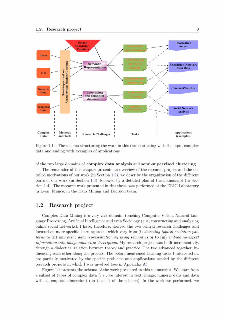
Figure 1.1 – The schema structuring the work in this thesis: starting with the input complexdata and ending with examples of applications.
of the two large domains of complex data analysis and semi-supervised clustering.The remainder of this chapter presents an overview of the research project and the de-
tailed motivations of our work (in Section 1.2), we describe the organization of the differentparts of our work (in Section 1.3), followed by a detailed plan of the manuscript (in Sec-tion 1.4). The research work presented in this thesis was performed at the ERIC Laboratoryin Lyon, France, in the Data Mining and Decision team.
1.2 Research project
Complex Data Mining is a very vast domain, touching Computer Vision, Natural Lan-guage Processing, Artificial Intelligence and even Sociology (e.g., constructing and analyzingonline social networks). I have, therefore, derived the two central research challenges andfocused on more specific learning tasks, which vary from (i) detecting typical evolution pat-terns to (ii) improving data representation by using semantics or to (iii) embedding expertinformation into image numerical description. My research project was built incrementally,through a dialectical relation between theory and practice. The two advanced together, in-fluencing each other along the process. The before mentioned learning tasks I interested in,are partially motivated by the specific problems and applications needed by the differentresearch projects in which I was involved (see in Appendix A).
Figure 1.1 presents the schema of the work presented in this manuscript. We start froma subset of types of complex data (i.e., we interest in text, image, numeric data and datawith a temporal dimension) (on the left of the schema). In the work we performed, we
4 Chapter 1. Introduction
analyze each type of data independently. A perspective of our work is a broader integrationof all the information provided by complex data, in order to take profit from every availablepiece of information. At the right side of the schema in Figure 1.1 are the final abstractapplications of our work, such as Information Access, Knowledge Discovery from Data, So-cial Network Analysis or CommentWatcher, an online media analysis tool, the result of ourapplied work. In between we present, from right to left (from the purpose of our work, i.e.,the output, to the input), (a) the more specific learning tasks we approach in our work,(b) the research challenges that derive in the learning tasks and (c) methods and tools weprivilege in order to attain our research challenges. The arrows indicate how the differentparts were used in our research. For example, we interest in leveraging semantics into theconstruction of the representation for images, text or numeric data. Similarly, the researchchallenge of leveraging the temporal dimension is derived into the two specific tasks of tem-poral data clustering and social role identification. These can be, in turn, used in applicationas Knowledge Discovery from Data, Social Network Analysis or into CommentWatcher, thedeveloped software.
The motivations of our work The motivations behind our work can be resumed atdifferent abstraction levels.
On an applied level, our work is related to the various research needs of the projects Iwas involved (more details in Annex A). The task of detecting typical evolution patterns isin relation with the interest of researched in Political Sciences, involved in the ImagiWebproject 8. Another example is the multi-sided link between the research collaboration withthe Technicolor laboratories 9, the Crtt-Eric project, our work concerning the textualdimension, the task of Social Role Identification and CommentWatcher (which presented indetail in Chapter 7).
On the problems and solutions level, our work was motivated by the need to pro-pose solutions for a series of specific learning tasks. We proposed new algorithms (e.g., thetemporal clustering algorithms TDCK-Means, the feature construction algorithm uFC),new measures (e.g., the temporal-aware dissimilarity measure), parameter choice heuristics(e.g., the χ2 hypothesis testing-based heuristic), etc.
On the research challenges level, at the core of our research work are the two researchchallenges detailed earlier: (a) embedding semantics into data representation and machinelearning algorithms and (b) leveraging the temporal dimension.
The abstract applications level. At a meta level, our work is motivated and canbe used in application as Information Access, Knowledge Discovery from Data or SocialNetwork Analysis.
The three most important original ideas in our work Throughout this manuscript,the reader will find a number of original proposals. In the following, we single out three ofthe most important ideas of our research.
Taking into account both the temporal dimension and the descriptive dimension into aclustering framework. The resulted clusters are coherent from both the temporal and the
8. http://eric.univ-lyon2.fr/~jvelcin/imagiweb/9. https://research.technicolor.com/rennes/
1.3. The constituent parts of the thesis 5
descriptive point of view. Constraints are added to ensure the entity segmentation contiguity.Unsupervised construction of a feature set based on the co-occurrences issued from the
dataset. This allows adapting a feature set to the dataset’s semantics. The new features areconstructed as conjunctions of the initial features and their negations, which renders theresult comprehensible for the human reader.
Using non-positional user labels (denoting objects) to filter irrelevant visual features andto construct a semantically aware visual vocabulary for a “bag-of-feature” image represen-tation. We use the information about the presence of objects in images to detect and re-move features unlikely to belong to the given object. Dedicated visual vocabularies areconstructed, resulting in a numerical description which yields higher object categorizationaccuracy.
1.3 The constituent parts of the thesis
Given the great diversity of the approached subjects, I divide my work into four distinct,yet complementary parts. The four parts deal, respectively, with (a) the temporal dimension,(b) semantic data representation, and the different natures of complex data, i.e., (c) imageand (d) text. Each part is dealt with in an individual chapter, which contains an overview ofthe state of the art of the domain, the proposals, conclusions about the work and some plansfor future work. A fifth chapter is dedicated to the practical aspects of my work, most notablyCommentWatcher, an open-source platform for online discussion analysis. Therefore, each ofthe five chapters can be seen as autonomous, while remaining connected the directiveguidelines, the transverse links between them and the conceptual articulation. Eachof these is further detailed in the following paragraphs.
Directive guidelines The core research challenges are translated into directive guide-lines, that run throughout my research: (i) human comprehension, (ii) translating data ofdifferent natures into a semantic-aware description space and (iii) devising algorithms andmethods that embed semantics and the temporal component.
In each of our proposals, we consider crucial to generate human comprehensible out-puts. Black-box approaches exist for many problems (e.g., Principal Component Analysisis a solution for re-organizing the description space), but the semantic meaning of theiroutput is not always clear and, therefore, the latter are difficult to interpret. Our proposalsare developed with human comprehensibility in mind.
Another directive guideline of our work is translating data of different naturesinto a semantic-aware description space, which we call throughout this manuscriptthe Numeric Vectorial Space. Constructing such a description space usually consists in (a)rendering the data into a common usable numeric format, which succeeds in capturing theinformation present in the native format, and in (b) efficiently using external informationfor improving the numeric representation.
Finally, a central axis of our research is devising algorithms and methods thatembed semantics and the temporal component, based on unsupervised and semi-supervised techniques. Often additional information and knowledge is attached to the data,under the form of (a) user labels, (b) structure of interconnected documents or (c) external
6 Chapter 1. Introduction
knowledge bases. We use this additional knowledge at multiple instances, usually usingsemi-supervised clustering techniques. We also use semi-supervised constraints to modelthe temporal dependencies in the data.
Transverse links There are multiple transverse links between the individual partsof our research. Our work with textual data is intimately linked with the softwareCommentWatcher. The text from online discussion forums is retrieved, we extract topicsfrom it and infer a social network using the forum’s reply-to relation. The social network ismodeled and visualized as a multidigraph, in which links between nodes are associated totopics. Furthermore, the temporal-driven clustering we propose is applied to detect socialroles in the social network. Another transverse link concerns our feature construction algo-rithms, which was initially motivated by the need to re-organize the user label set we use tocreate the semantic-enabled image representation. We also have ongoing work which dealswith embedding the temporal dimension into this feature construction algorithm. The ideais to detect if features are correlated with a certain time lag.
Conceptual articulation of the different parts It is noteworthy that the work pre-sented in this thesis is not a blueprint of an integrated complex data analysis system.Realizing such a system would have been possible in the context of a very specific (applied)problem, which is not the case of the different collaborations and projects in which I wasinvolved. Whatsoever, a conceptual articulation exists between all the parts of our work:data of different natures is translated into a common semantic-aware numeric format, whichis afterwards used together with the temporal dimension or with external knowledge bases.During the next chapters, we evolve the schematic representation of our work in Figure 1.1to a complete conceptual integration of our proposals. At the end of each chapter, the readeris shown how the work presented in the given chapter can be conceptually integrated withthe work in previous chapters. We incrementally evolve the schema in Figure 1.1 in Fig-ures 3.1 (p. 30), 4.17 (p. 93), 5.13 (p. 122) and 6.13 (p. 165) into the complete schema inFigure 8.1 (p. 182).
1.4 Content of the different chapters
Excepting the current chapter, this manuscript is structured over six chapters, as follows.In Chapter 2, we present a general overview of complex data mining. Starting from
the specificities of complex data, we identify some of the difficulties of analyzing them andwe present some of the solutions existing in the literature. We present the field of semi-supervised clustering in a similar fashion: we start from the necessities of semi-supervisedclustering, the advantages and difficulties. We present the taxonomy and briefly presentsome of the most relevant existing approaches. All along this chapter, we position our workin the broader context of these two domains.
In Chapter 3, we leverage the temporal dimension of the complex data and we ap-ply our proposals to the learning task of detecting typical evolution patterns. We proposea new temporal-aware dissimilarity measure and a segmentation contiguity penalty func-tion. We combine the temporal dimension of complex data with a semi-supervised clus-
1.4. Content of the different chapters 7
tering technique. We propose a novel time-driven constrained clustering algorithm, calledTDCK-Means, which creates a partition of coherent clusters, both in the multidimensionalspace and in the temporal space. We also show how this temporal clustering algorithm canbe applied to a different task: finding behavioral roles in an online community.
In Chapter 4, we regroup our research concerning the task of semantic descriptionspace reconstruction. We seek to construct, in an unsupervised way, a new description spacewhich embeds some of the semantics present in a given dataset. The constructed features(i.e., the dimensions of the new description space) are, at the same time, comprehensible fora human user. We propose two algorithms that construct the new features as conjunctionsof the initial primitive features or their negations. The generated feature sets have reducedcorrelations between features and succeed in catching some of the hidden relations betweenindividuals in a dataset. We also propose a method based on statistical testing for settingthe values of parameters.
Chapter 5 presents our research concerning image data. We are particularly inter-ested in the task of improving image representation using semi-supervised visual vocabularyconstruction. We present the “bag-of-features” representation, one of the most widely usedmethods for translating images from their native format to a numeric Vectorial Space. Weare interested in using expert knowledge, under the form of non-positional labels attachedto the images, in the process of creating the numerical representation. We propose two ap-proaches: the first one is a label-based visual vocabulary construction algorithm, while thesecond deals with filtering the irrelevant features for a given object, in order to improveobject categorization accuracy.
Chapter 6 presents in detail our research concerning textual data, and more precisely,we are interested in the task of topic extraction and evaluation. After a presentation of the“bag-of-words” representation, we make an in-depth review of topic extraction and evalu-ation literature, while referencing methods related to our general domain of interest (e.g.,incorporating the temporal dimension or external semantic knowledge). We complete thisbibliographic research with the presentation of a textual clustering-based topic extractionsystem and a topic evaluation systems based on an external semantic knowledge base. Atthe end of the chapter, we present some applications of this system to the Ontology Learningprocess, and to topic improvement by removing spurious words.
Chapter 7 presents the practical prototype production. The most prominent producedsoftware is CommentWatcher, an open source tool for analyzing discussions on web forums.Constructed as a web platform, CommentWatcher features (i) automatic fetching of forums,using a versatile parser architecture, (ii) topic extraction from a selection of texts and (iii)a temporal visualization of extracted topics and the underlying social network of users. Itaims both the media watchers (it allows quick identification of important subjects in theforums and user interest) and the researchers in social media (who can use it to constitutetemporal textual datasets).
In the last chapter, Chapter 8, we draw some general conclusions about our work. Wealso present in this chapter the work we are currently undergoing and plan other researchof near term and long term future.

Chapter 2
Overview of the Domain
Contents2.1 Complex Data Mining . . . . . . . . . . . . . . . . . . . . . . . . . . 9
2.1.1 Specificities of complex data . . . . . . . . . . . . . . . . . . . . . . . 112.1.2 Dealing with complex data of different natures . . . . . . . . . . . . . 132.1.3 Temporal/dynamic dimension . . . . . . . . . . . . . . . . . . . . . . . 162.1.4 High data dimensionality . . . . . . . . . . . . . . . . . . . . . . . . . 18
2.2 Semi-Supervised Clustering . . . . . . . . . . . . . . . . . . . . . . . 20
2.2.1 Similarity-based approaches . . . . . . . . . . . . . . . . . . . . . . . . 242.2.2 Search-based approaches . . . . . . . . . . . . . . . . . . . . . . . . . . 26
The purpose of this chapter is to present a general overview and familiarize our reader, ifnot already the case, with the two large domains around which our work revolves: ComplexData Mining (in Section 2.1) and Semi-Supervised Clustering (in Section 2.2). We discussfor each domain the motivations, the difficulties that arise and some of the solutions presentin the literature. All along this chapter, we relate our work to the domain and position ourproposals relative to existing solutions.
2.1 Complex Data Mining
In this section, we present a general overview of the domain of Complex Data Mining.Using the example of a Wikipedia article, we incrementally single out the particularitiesof complex data. In Section 2.1.1, we identify and summarize the most important fivespecificities that define complex data, and we point out how our proposals address them.We further detail some of the identified specificities (in Sections 2.1.2, 2.1.3 and 2.1.4), bypresenting the difficulties they pose and some of the existing solutions in the literature.Each of these subsections ends with a paragraph in which we position our work.
Complex Data Mining is a very vast domain, incorporating a large range of relatedproblems. A definition of Data Mining is the computational process of discovering patterns inlarge data sets involving methods issued from the domains of artificial intelligence, machinelearning, statistics, and database systems. Complex Data Mining is the application of DataMining to Complex Data, i.e., data with a series of particularities that we identify later inthis section, and which is a non-standard input for classical data mining algorithms.
10 Chapter 2. Overview of the Domain
Vectorial description space. The input data format for classical data mining algorithmsis the (attribute, value) pair format. In this format, each individual is described by a setof measurements over a set of attributes. Each measurement is (a) a real value (numericattributes), (b) a choice from a set of available options (categorical attributes) or (c)a value of true or false (boolean attributes). When considering the numeric variables,this format can be associated with a multidimensional vectorial description space, inwhich each individual is described by its measurements vector. The assumption is that, inthis multidimensional description vectorial space, machine learning algorithms are efficient(e.g., it is separable by means of a classification algorithm).
Complex Data Complex data are profoundly heterogeneous data. Excepting the classic(attribute, value) numeric format, a complex document can contain data of different natures(e.g., text, images, video, audio etc.). These data are interlinked through the structure (e.g.,titles, paragraphs, sections) of the complex document in which they reside. In addition,complex data can have expert knowledge attached (e.g., expert categorize documents usinglabels). Sometimes, complex data have attached a temporal dimension: it either records theevolution of an entity/object over time, or the complex document suffers modifications overtime.
Each of the evoked particularities are facets of the considered complex document andthey all must be taken into account in the learning process in order to infer completeknowledge [Zighed et al. 2009]. On a more abstract level, semantics are the main challengewhen dealing with complex data. Complex data come in high volumes and many differenttypes, and the main objective is to piece together the underlying knowledge and recreatethe semantic links. Semantics are crucial for the comprehension of the generated results,especially from a human point of view. The semantic representation of complex data canbe improved by using the freely accessible resources of the new Semantic Web. Knowledgerepositories are increasingly available, most often under the form of (a) ontologies, such asthe general purpose DBpedia 1 [Bizer et al. 2009] and Freebase 2, which are further inter-linked by projects such as Linking Open Data 3 of (b) more specialized datasets, issued fromthe domains of Social Sciences and Humanities (e.g., History, Communication sciences, So-ciology etc.). It is not uncommon to tap into these distributed external repositories in orderto introduce semantics into the learning process. Leveraging semantics and the temporaldimension into the analysis of complex data are the main research challenges of our work,presented in this thesis.
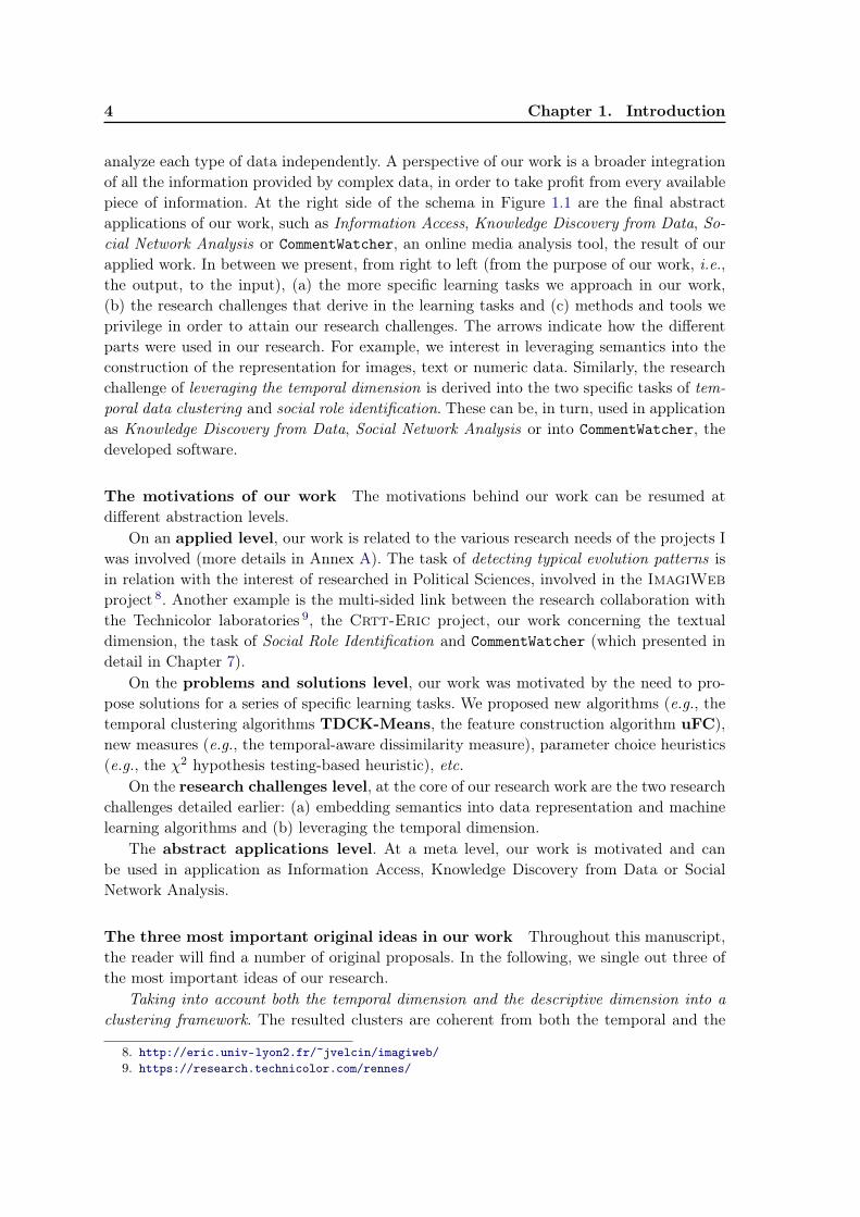
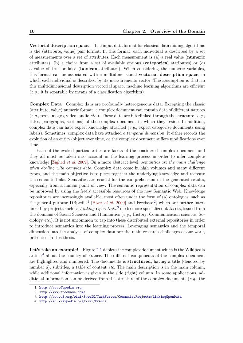
Let’s take an example! Figure 2.1 depicts the complex document which is the Wikipediaarticle 4 about the country of France. The different components of the complex documentare highlighted and numbered. The documents is structured, having a title (denoted bynumber 6), subtitles, a table of content etc. The main description is in the main column,while additional information is given in the side (right) column. In some applications, ad-ditional information can be derived from the structure of the complex documents (e.g., the
1. http://www.dbpedia.org2. http://www.freebase.com/3. http://www.w3.org/wiki/SweoIG/TaskForces/CommunityProjects/LinkingOpenData4. http://en.wikipedia.org/wiki/France
2.1. Complex Data Mining 11
Description (text)
Hyperlink (external knowledge repositories)
Map (image)
Flag and emblem(image)
1 2
2
Anthem (audio)3
5
Title (structure) 6
Indicators (numeric format) 4
Figure 2.1 – A Wikipedia article is a complex document, containing text (1), images (2),audio (3), numeric indicators (4), links to other pages (5) and a structure (6).
structure of a social network, i.e., how users are interlinked, is sometimes more informativethan the content posted by the users).
In Figure 2.1, text (numbered 1) is mainly used to give the information about geographicposition, history, political system etc. Data of other natures could be used to complete theinformation. Images (number 2) are added to portray the country’s flag, emblem and ge-ographic map. Audio data (number 3) is included to give the national anthem and evenvideo is used to present specific events (e.g., in the original Wikipedia article, a video se-quence is used to show the French territorial evolution from 985 to 1947). Information likethe country’s surface, population, gross domestic product (GDP), geographic coordinatesetc. are given in an (attribute, value) numerical format (number 4). Finally, hyperlinks(number 5) are present in the text, most often linking this article with other articles. Hy-perlinks can also point towards external resources in a knowledge ontology, thereforelinking the complex document to structured information and, also, with more semantics.The complex data can also have a temporal dimension. In the Wikipedia article, thedata can be updated yearly with the latest information about political events. Furthermore,the track of past values for social and economic indicators are good hints for current events(e.g., high levels of debt and leverage in the banking system were early indicators of theeconomic crisis of 2008).
2.1.1 Specificities of complex data
In the following, we summarize and structure the before mentioned specificities of com-plex data.
– diverse nature of data. (text, image or audio/video) Dealing with non-numeric
12 Chapter 2. Overview of the Domain
data raises problems, out of which we mention the fact that (a) they are not directly“understandable” by a machine (i.e., they need to be translated first to a numericalspace) and (b) the numerical space in which they are translated captures few semanticinformation and, consequently, machine learning algorithms exhibit low performances.Some approaches (more details in Section 2.1.2) deal with this problem by using dataof different natures (e.g., images and text) to better guide the learning process.
– additional information (e.g., external knowledge) External information or resourcesmight be available to complete the semantic information present in the data. Thisadditional information can be under the form of (a) expert provided tags of labels or(b) interlinked knowledge repositories (i.e., ontologies).
– temporal/dynamic dimension. It often happens that the same entity is describedaccording to the same characteristics at different times or different places (e.g., a pa-tient may often consult several doctors, at different moments of time). These differentdata are associated with the same entity and the complex data describes the evolutionof the entity in the given description space. A special kind of temporal data is thedynamic data, which is available as a stream (this data cannot be stored and it mustbe analyzed online). We give more details about the temporal dimension and dynamicdata in Section 2.1.3.
– high dimensionality. Taking into account data of multiple natures and externalknowledge repositories raises dimensionality problems. This dimensionality problemcan either concern the high volumes of data that need to be dealt with (the “scalability”problem), or, most often, the high dimensionality of the description space (the “curseof dimensionality”). In Section 2.1.4, we present in detail how this problem affects thelearning process and some existing solutions.
– distributed and diverse sources. The complex data can originate from differentsources, which, furthermore, do not need to be collocated. This is not a new problem(e.g., in older times, the same information could be found in different books, in differ-ent libraries), but it has been exacerbated with the arrival of the Web 2.0. Informationis nowadays essentially distributed into many sources, instead of being centralized inlibraries. The retrieval paradigm also shifted from classification (e.g., sorting books ina library based on a set of criteria) to searching (e.g., modern days web-search enginesquery multiple distributed knowledge repositories to compile an answer).
Positioning our work In our work, we have addressed multiple learning tasks related tothe specificities of complex data identified here above. We deal with complex data of twodifferent natures. We deal with image data in Chapter 5, in which we propose a methodto introduce semantic knowledge into the image numerical representation. We deal withtextual data in Chapter 6, in which we present address the tasks of topic extraction, topiclabeling and topic evaluation. Topic labeling is important for the human comprehension ofextracted labels, whereas for the topic evaluation we employ semantic knowledge.
Leveraging semantic information into data numerical representation and into thelearning algorithms is one of the central research challenges of this thesis. In Chapter 5,we deal specifically with embedding semantic information under the form of labels into thenumeric representation of images. In Chapter 6 we use external semantic resource (i.e.,WordNet) for mapping the statistically constructed topics to a semantic-aware structure
2.1. Complex Data Mining 13
and for evaluating and improving topics extracted from text. The second research challengethat we address in our work is the temporal dimension of complex data. In Chapter 3 wepropose a new temporal-aware constrained clustering algorithm (TDCK-Means), which con-structs temporally coherent clusters and contiguously segments the temporal observationsbelonging to an entity.
In the following subsections, we further detail some of the specificities of complex data(i.e., dealing data of different natures, the temporal dimension and the dimensionality), weshow some of the difficulties associated with each one and some of the solutions present inthe literature.
2.1.2 Dealing with complex data of different natures
Traditional Data Mining algorithms (e.g., clustering algorithm, classification tree learn-ing algorithms etc.) were not designed to deal with data of diverse natures. Text and imageare the two natures of data most widely used (for example in Internet), but other are alsopopular, like the audio and video. The difficulty in analyzing data of different natures isthat, while they are easy to be transformed, stored and reproduced into/from a digitalformat, this format captures little semantic information needed by machine learning algo-rithms. Therefore, one of the main challenges when dealing with data of different natures isto translate them into a semantic-aware numeric description space, on which the results ofa machine learning algorithm are “relevant”. In our context, we consider results “relevant”when, in addition to being the answer to a given task, they are also comprehensible for ahuman being. Therefore, we summarize the difficulties related to the most common naturesof complex data, as follows:
– text. The morphological and syntactic rules of languages are not directly machine“comprehensible”. Furthermore, in most representations, the text is encoded at thelevel of a character and the presence of a given character (e.g., the character ‘b’ orthe space) gives almost no hints about the subject of the text.
– images. The native digital format for images is the pixel based format. An image isrepresented as a matrix of pixels, where each pixel has a certain color. Low level imagefeatures (e.g., the pixel’s color) capture very little of the semantics of the image (e.g.,the objects represented in the image). Passing from low-level features to high-levelfeatures, while capturing the semantics of the image, is known as the semantic gap.
– video. The video is digitally represented as a sequence of images, therefore video datacan be considered as image data with a temporal component [Zaiane et al. 2003].Consequently, the difficulties of processing video data inherit the those concerningimages, to which new ones are added with respect of the temporal evolution (e.g.,tracking objects, finding patterns in the sequence of images etc.).
– audio. Audio data is digitally represented by the frequencies of the sound presentin the audio document. Knowing the presence of a certain frequency in an audio filegives little information about the overall genre of music. Other, more high-level tasks(e.g., speech recognition [de Andrade Bresolin et al. 2008]), are even more difficultwithout thorough pre-processing.
The above mentioned types of data can be translated into a numeric description space,on which classical machine learning algorithms can be applied. The general schema of this
14 Chapter 2. Overview of the Domain
Data in the Numeric Vectorial Space
Image Numerical RepresentationConstruction
Text Numerical RepresentationConstruction
Data Miningalgorithm
Useful knowledge
ImageData
TextData
Classic Numeric
Data
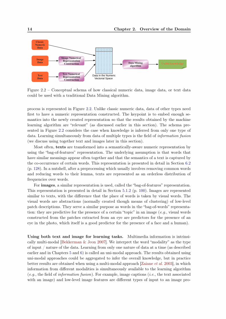
Figure 2.2 – Conceptual schema of how classical numeric data, image data, or text datacould be used with a traditional Data Mining algorithm.
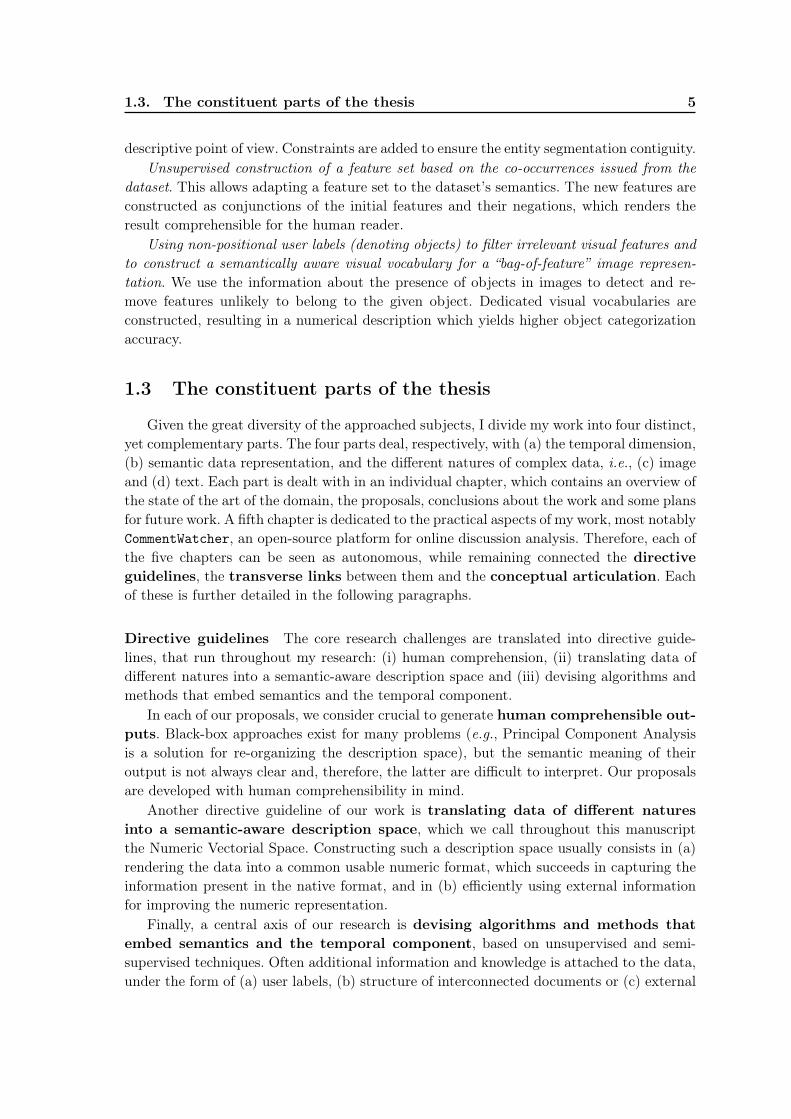
process is represented in Figure 2.2. Unlike classic numeric data, data of other types needfirst to have a numeric representation constructed. The keypoint is to embed enough se-mantics into the newly created representation so that the results obtained by the machinelearning algorithm are “relevant” (as discussed earlier in this section). The schema pre-sented in Figure 2.2 considers the case when knowledge is inferred from only one type ofdata. Learning simultaneously from data of multiple types is the field of information fusion(we discuss using together text and images later in this section).
Most often, texts are transformed into a semantically-aware numeric representation byusing the “bag-of-features” representation. The underlying assumption is that words thathave similar meanings appear often together and that the semantics of a text is captured bythe co-occurrence of certain words. This representation is presented in detail in Section 6.2(p. 128). In a nutshell, after a preprocessing which usually involves removing common wordsand reducing words to their lemma, texts are represented as an orderless distribution offrequencies over words.
For images, a similar representation is used, called the “bag-of-features” representation.This representation is presented in detail in Section 5.1.2 (p. 100). Images are representedsimilar to texts, with the difference that the place of words is taken by visual words. Thevisual words are abstractions (normally created though means of clustering) of low-levelpatch descriptions. They serve a similar purpose as words in the “bag-of-words” representa-tion: they are predictive for the presence of a certain “topic” in an image (e.g., visual wordsconstructed from the patches extracted from an eye are predictors for the presence of aneye in the photo, which itself is a good predictor for the presence of a face and a human).
Using both text and image for learning tasks. Multimedia information is intrinsi-cally multi-modal [Bekkerman & Jeon 2007]. We interpret the word “modality” as the typeof input / nature of the data. Learning from only one nature of data at a time (as describedearlier and in Chapters 5 and 6) is called an uni-modal approach. The results obtained usinguni-modal approaches could be aggregated to infer the overall knowledge, but in practicebetter results are obtained when using a multi-modal approach [Zaiane et al. 2003], in whichinformation from different modalities is simultaneously available to the learning algorithm(e.g., the field of information fusion). For example, image captions (i.e., the text associatedwith an image) and low-level image features are different types of input to an image pro-
2.1. Complex Data Mining 15
cessing system and can, therefore, be considered as two separate modalities. Image captionstend to describe events captured on the image (i.e., they capture semantic information),while image features convey visual information to the system. Consequently, using multiplemodalities in the learning process can yield higher performances, as each modality can beused to guide the learning process of another.
We present some of the most common learning tasks that can benefit from using boththe text and image natures of data. These tasks share a common trait: low-level visualfeatures (e.g., color, texture, shape, spatial layout, local descriptors etc.) used to describeimages capture very little of the semantics of images. Their performance can be improvedby using text alongside images.
– Image classification. Object-based image classification is challenging due to widevariation in object appearance, pose, and illumination effects. Low-level image featuresare far removed from the semantics of the scene, making it difficult to use them toinfer object presence, and it is expensive to obtain enough manually labeled examplesfrom which to learn. To cope with these constraints, text that often accompaniesvisual data can be leveraged to learn more robust models. Such approaches [Mooneyet al. 2008,Wang et al. 2009] make use of collections of unlabeled images and theirtextual snippets, usually issued from the Internet.
– Automatic images categorization. Unlike the image classification application, inautomatic categorization there are no predefined classes. Images are automaticallyorganized based on their similarity through means of clustering. Being fully unsu-pervised, clustering methods often demonstrate poor performance when performedbased only on low-level image features. Clustering results can be improved by usinga multi-modal learning paradigm, where image captions and annotations are usedalongside image features. Text has been used to help image clustering in number ofapplications, such as image clustering [Bekkerman & Jeon 2007], in Web image searchresults clustering [Cai et al. 2004] or image sense discrimination [Loeff et al. 2006].
– Improving image numerical description. Low performances in the tasks de-scribed earlier (i.e., image categorization and image clustering) is usually due to thelow semantic quality of the image numerical representation: the images are translatedinto a numerical space which is not easily learnable by machine learning algorithms.Performances can be improved by using the text associated with the images, eitherin the learning algorithm (as previously seen) or in the creation of the numeric repre-sentation [Quattoni et al. 2007,Ji et al. 2010]. The goal is to embed textual semanticsinto the image representation and to improve learning in future image-related learn-ing problems. Our work with the images (in Chapter 5), deals with improving thenumerical description.
– Content-based image retrieval. Content-based image retrieval deals with efficientimage searching, browsing and retrieval, with applications in crime prevention, fash-ion, publishing, medicine, architecture, etc. Humans tend to use high-level features(concepts), such as keywords, text descriptors, to search and interpret images andmeasure their similarity. Features automatically extracted using computer vision tech-niques are mostly low-level features and, in general, there is no direct link betweenthe high-level concepts and the low-level features [Sethi et al. 2001] (also called the“semantic gap”). Some content-based image retrieval systems [Cai et al. 2004,Zhuang
16 Chapter 2. Overview of the Domain
et al. 1999] use both the visual content of images and the textual information forbridging the semantic gap. Other techniques exist which do not rely on the usageof associated text [Liu et al. 2007] (i.e., (a) using an object ontology, (b) associat-ing low-level features with query concepts, (c) introducing relevance feedback intothe retrieval loop or (d) generating semantic template to support high-level imageretrieval).
– Automatic image annotation. This task deals with automatically annotating im-ages with one or multiple labels, accordingly to their content. One of the difficulties isthe huge number of candidate labels and scarce training examples. Automatic imageannotation systems [Lu et al. 2009,Yang et al. 2010] search to find a correspondencebetween text words and the visual features describing an image. This is most oftenachieved by using a machine translation approach, where the image-text pairs areseen as bilingual texts and alignment methods are applied [Barnard et al. 2003].
– Human-computer interface systems use multiple modes of input and output toincrease robustness in the presence of noise (e.g. by performing audio-visual speechrecognition) and to improve the naturalness of the interaction (e.g. by allowing gestureinput in addition to speech). Such systems often employ classifiers based on supervisedlearning methods, which require manually labeled data. This usually is costly, espe-cially for systems that must handle multiple users and realistic (noisy) environments.Semi-supervised learning techniques can be leveraged [Christoudias et al. 2006] tolearn multi-modal (i.e., audio-visual speech and gesture) classifiers, thus eliminatingthe need of obtaining large amounts of labeled data.
Positioning our work In our work concerning textual data (presented in Chapter 6),we have used a classical “bag-of-words” representation, and concentrated mainly on intro-ducing semantic knowledge into topic evaluation, through a concept-topic mapping. Ourwork concerning image data (presented in Chapter 5) deals with embedding semantics intothe image representation. We show how a semantic-enriched representation can be obtainedstarting from a baseline representation by employing non-positional labels (i.e., only thepresence of objects in the images is known, but not their position).
In our work, we have not dealt with text and image simultaneously. One of the venuesin this direction would be to use text instead of non-positional labels. Whatsoever, weuse a complete labeling paradigm, in which the absence of a label implies the absence ofthe object in the image, Passing from the strict labeling to a more relaxed labeling (i.e.,authorize missing labels) is one of the perspectives of our work and discussed in Sections 5.3.2(p. 108). Once this passing done, using the text alongside images is foreseeable. Anotherresearch direction would be to embed into images semantic information originating from aconcept hierarchy, by passing through text and using the mapping between topics (extractedfrom text) and concepts.
2.1.3 Temporal/dynamic dimension
Introducing the temporal dimension usually changes the definition of the learning prob-lem: the description of entities in contextualized (i.e., the description is valid for a periodof time) and new learning problems emerge, e.g., detecting evolutions and trends, tracking
2.1. Complex Data Mining 17
through time etc. Leveraging and interpreting the temporal dimension is one of the centralresearch challenges of this thesis and intrinsically connected to complex data. As discussedearlier, complex data often have a temporal dimension, describing the evolution of a num-ber of entities throughout a period of time. For example, in Chapter 3, we detect typicalevolutions of entities and we apply our proposal to a dataset which records the value of anumber of socio-economical indicators for a set of countries, over a period of 50 years.
Temporal Data Mining is the sub-domain of Data Mining, closely associated withComplex Data Analysis, which deals with detecting surprising regularities in data withtemporal inter-dependencies. Datasets which contain temporal inter-dependencies are calledsequential datasets, where sequential data are data ordered by some index. In the case oftemporal datasets, the index is the timestamp associated with the observations. Time-seriesis a popular class of sequential data, which has enjoyed a lot of attention, especially fromthe statistics community. Time-Series Analysis [Brillinger 2001] has many applications, outof which we mention weather forecast, financial and stock market predictions etc. A numberof differences exist between Temporal Data Mining and Time-Series Analysis [Laxman &Sastry 2006], the most important being (a) the size and the nature of the studied dataset and(b) the purpose of the study. Temporal Data Analysis deals with prohibitive size datasets,and the data is not always numerical. This are two of the characteristics of complex data.Furthermore, the purpose of Temporal Data Mining goes beyond the forecast of futuresvalues in the series. Some of the learning tasks in Temporal Data Mining can be summarizedas follows [Laxman & Sastry 2006]:
– prediction. The prediction task has to do with forecasting (typically) future valuesof the time series based on its past samples. In order to do this, one needs to build apredictive model [Dietterich & Michalski 1985,Hastie et al. 2005].
– classification. In sequence classification, each sequence is assumed to belong to oneof finitely many (predefined) classes or categories and the goal is to automatically de-termine the corresponding category for the given input sequence. Applications of se-quence classification include speech recognition [O’Shaughnessy 2000,Gold et al. 2011],gesture recognition [Darrell & Pentland 1993], handwritten word recognition [Plam-ondon & Srihari 2000].
– clustering. Clustering of sequences or time series [Kisilevich et al. 2010] is concernedwith grouping a collection of time series (or sequences) based on their similarity.Applications are extremely variate and include analyzing patterns in web activitylogs, patterns in weather data [Hoffman et al. 2008] and trajectories of moving ob-jects [Nanni & Pedreschi 2006], finding similar trends in financial data, regrouping ofsimilar biological sequences like proteins or nucleic acids [Osato et al. 2002].
– search and retrieval. This task problem is concerned with efficiently locating sub-sequences in a database of sequences. Query-based searches have been extensivelystudied in language and automata theory. While the problem of efficiently locatingexact matches of substrings is well solved, the situation is quite different when look-ing for approximate matches [Navarro 2001]. In typical data mining applications likecontent-based retrieval, it is approximate matching that we are more interested in.
– pattern discovery. Unlike the search and retrieval task, in pattern discoverythere is no specific query with which to search the dataset. The objective is simplyto unearth all patterns of interest. Two popular frameworks for frequent pattern dis-
18 Chapter 2. Overview of the Domain
covery are sequential patterns [Agrawal & Srikant 1995, Fournier-Viger et al. 2011]and episodes [Mannila et al. 1997]. Sequential pattern mining is essentially an ex-tension of the original association rule mining framework proposed for a database ofunordered transaction records [Agrawal et al. 1993], which is known as the Apriorialgorithm. The extensions deals with incorporating the temporal ordering informationinto the patterns being discovered. In the frequent episodes framework, we are givena collection of sequences and the task is to discover (ordered) sequences of items (i.e.sequential patterns) that occur in sufficiently many of those sequences.
Dynamic data There is fundamental difference between temporal data and dynamicdata. Dynamic data are data evolving over time, as new data arrive and old data becomeobsolete. Furthermore, the updates may change the structures learned so far. Dynamic datais intimately linked with the Internet, where enormous quantities of data are constantlycreated and need to be dealt with. These data are usually available as a stream, arriving ata rapid rate and cannot be stored for later analyzing.
The temporal-aware algorithms described so far in this section (as well as our proposedTDCK-Means algorithm, which will be described later in Chapter 3) consider the temporaldata as recordings of the state of a set of individuals at different moments of time (e.g.,macro-economical indicators for countries). These data are stored and studied offline (aposteriori), usually for determining causalities, evolutions etc. Such “static” algorithms arenot appropriate for dynamic data, because (a) huge amounts of data are accumulated overtime and cannot be stored, (b) the generative distribution might change over time (whichis known in supervised learning as “concept drift”), (c) only one-pass access to the data isavailable and (d) the data arrives at a rapid rate. Many online algorithms have been pro-posed, out of which we mention CluStream [Aggarwal et al. 2003], which performs an onlinesummarization and an offline clustering, and Single pass K-Means [Farnstrom et al. 2000],which is an extension of K-Means for streams and which performs the clustering in batchesthat fit into memory.
Positioning our work Our work concerning the temporal dimension does not deal withthe dynamic data paradigm, therefore we consider that our dataset is stored in a databaseand available for querying and transforming to our needs.
The learning task for which our TDCK-Means temporal clustering algorithm was con-structed is not a classical clustering task (as defined in Temporal Data Mining), but rathermore similar to sequential itemset mining. Among the above defined tasks of TemporalData Mining, TDCK-Means would be classified as a special case of pattern discovery.There is a fundamental difference between the algorithms in the clustering category andTDCK-Means: the nature of the individuals that they cluster. For the former, an individualis an entire time-series: they employ similarity measures between time-series and they seekto regroup similar time-series together. For the latter (TDCK-Means), the individuals thatit clusters are the observations (i.e., an observation is the description/state of an entity at agiven time moment, a tuple (entity, timestamp, description). A time-series is composed ofall the observations corresponding to an entity for all the moments of time). TDCK-Meanssearches to detect groups of similar observations (preferably contiguous, therefore parts ofa time-series), in order to detect similar evolutions.
2.1. Complex Data Mining 19
–
“curse of dimensionality”
Groups of similar (“dense”) points may be identified when considering
relevant attribute/
relevant subspace
irre
lev
an
t att
rib
ute
(a)
–
“curse of dimensionality”
Groups of similar (“dense”) points may be identified when considering this
(b)
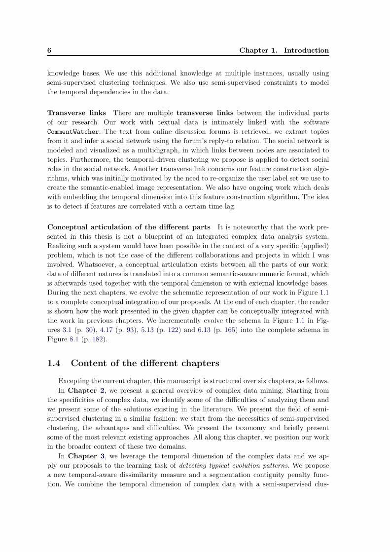
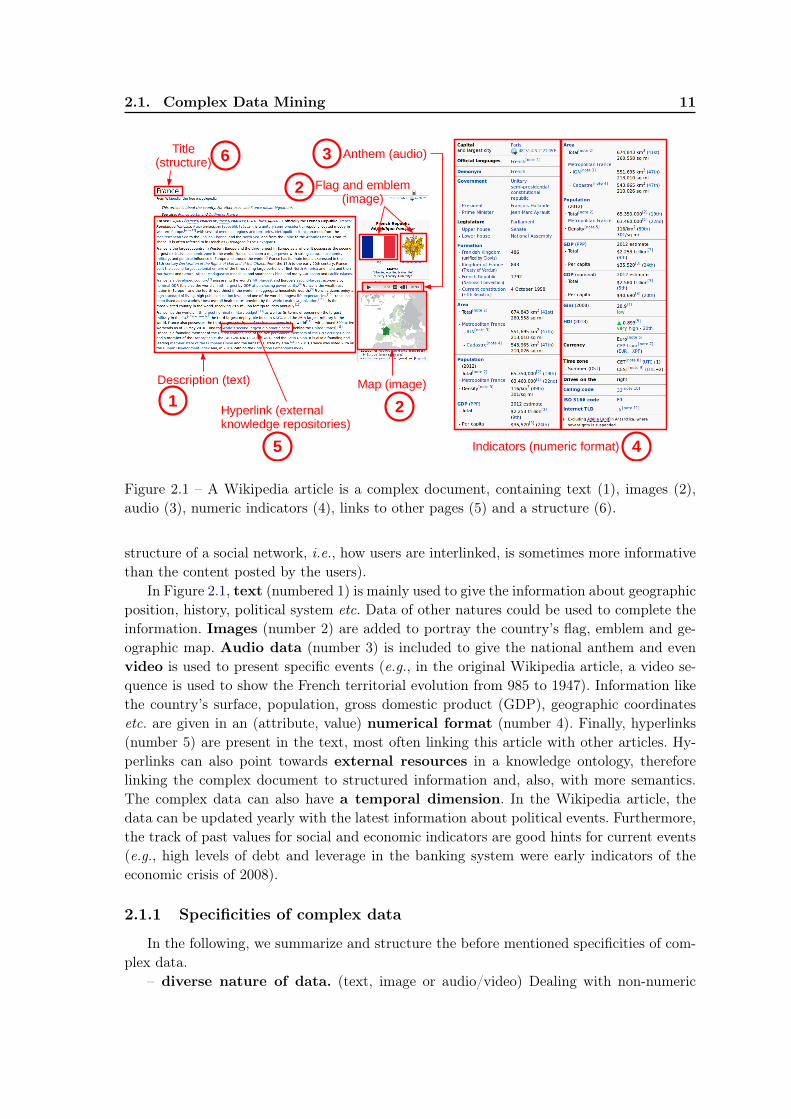
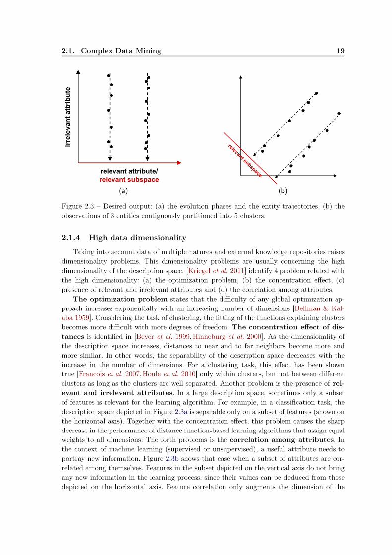
Figure 2.3 – Desired output: (a) the evolution phases and the entity trajectories, (b) theobservations of 3 entities contiguously partitioned into 5 clusters.
2.1.4 High data dimensionality
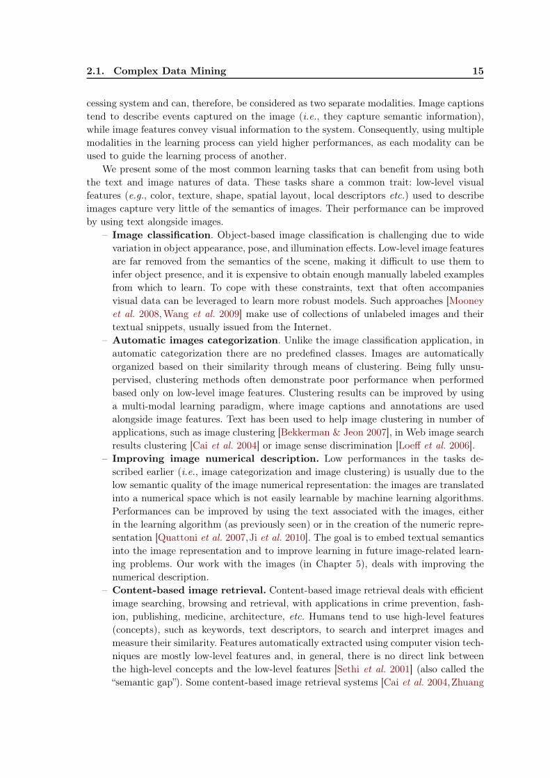
Taking into account data of multiple natures and external knowledge repositories raisesdimensionality problems. This dimensionality problems are usually concerning the highdimensionality of the description space. [Kriegel et al. 2011] identify 4 problem related withthe high dimensionality: (a) the optimization problem, (b) the concentration effect, (c)presence of relevant and irrelevant attributes and (d) the correlation among attributes.
The optimization problem states that the difficulty of any global optimization ap-proach increases exponentially with an increasing number of dimensions [Bellman & Kal-aba 1959]. Considering the task of clustering, the fitting of the functions explaining clustersbecomes more difficult with more degrees of freedom. The concentration effect of dis-tances is identified in [Beyer et al. 1999,Hinneburg et al. 2000]. As the dimensionality ofthe description space increases, distances to near and to far neighbors become more andmore similar. In other words, the separability of the description space decreases with theincrease in the number of dimensions. For a clustering task, this effect has been showntrue [Francois et al. 2007,Houle et al. 2010] only within clusters, but not between differentclusters as long as the clusters are well separated. Another problem is the presence of rel-evant and irrelevant attributes. In a large description space, sometimes only a subsetof features is relevant for the learning algorithm. For example, in a classification task, thedescription space depicted in Figure 2.3a is separable only on a subset of features (shown onthe horizontal axis). Together with the concentration effect, this problem causes the sharpdecrease in the performance of distance function-based learning algorithms that assign equalweights to all dimensions. The forth problems is the correlation among attributes. Inthe context of machine learning (supervised or unsupervised), a useful attribute needs toportray new information. Figure 2.3b shows that case when a subset of attributes are cor-related among themselves. Features in the subset depicted on the vertical axis do not bringany new information in the learning process, since their values can be deduced from thosedepicted on the horizontal axis. Feature correlation only augments the dimension of the
20 Chapter 2. Overview of the Domain
description space, without increasing the relevance of the descriptive space.
Our work presented in Chapter 4 is specifically targeted at the relevance of the descrip-tive space, with respect to a given dataset. In Section 4.2 (p. 63), we identify three types ofsolutions for this problem:
– feature selection. Feature selection techniques [Lallich & Rakotomalala 2000,Mo& Huang 2011] seek to filter the original feature set in order to remove redundantfeatures.
– feature extraction. Feature extraction involves generating a new set of featuresthrough means of functional mapping so that the new description space is relevantfor the learning task. Examples of such approaches are the SVM’s kernel [Cortes &Vapnik 1995] and principal component analysis (PCA) [Dunteman 1989].
– feature construction. Feature construction is a process that discovers missing in-formation about the relationships between features. Most constructive induction sys-tems [Pagallo & Haussler 1990, Zheng 1998] construct features as conjunctions ordisjunctions of initial attributes.
There are fundamental differences between feature extraction and feature construc-tion algorithms: (i) the comprehensibility of the new description space, (ii) the underlyingpurpose of the process and (iii) the dimension of the new space. (i) The description spaceresulted from feature extraction algorithms is either completely synthetic (for PCA) or hid-den/functioning as a black box (for SVM). This renders the interpretation of the resultsrather difficult. In the case of feature construction, the new attributes are easily compre-hensible (e.g., a feature entitled motorbike and driver is easier to interpret than the thirdaxis of PCA). (ii) The underlying purpose of feature extraction is just improving the nu-merical relevance of the description space, whereas the purpose of feature construction isalso discovering hidden relations between attributes (e.g., the correlation of people and grassfor a subset of pictures has a certain meaning when portraying a barbecue). (iii) Featureextraction algorithms either output a description space of (a) a lower (e.g., for PCA orManifold Learning [Huo et al. 2006]) or (b) a higher (e.g., the SVM kernel into a veryhigh dimensional space, even an infinitely dimensional space for the RBF kernel [Changet al. 2010]) dimensionality than the original space. Conversely, the feature constructionalgorithms invariably increase the number of dimensions.
Positioning our work Our work concerning the description space and presented in Chap-ter 4 proposes a feature construction algorithm for discovering missing semantic links be-tween the attributes describing a dataset. The novelty of the proposed algorithm is that,unlike the rest of the feature construction algorithms present in literature, we constructfeatures in an unsupervised context, based only on the correlations present in the dataset.Our uFC algorithm adapts the description space to the semantics of the given dataset. Ourexperiments in Section 4.6 (p. 75) show that the constructed features are highly compre-hensible, while the constructed description space achieves a lesser total correlation betweendimensions.
2.2. Semi-Supervised Clustering 21
2.2 Semi-Supervised Clustering
In the previous sections, we have shown that complex data often comes bundled withadditional information. For example, researchers in human sciences tag documents for easyreferencing, medical doctors annotate the files of their patients. The modern Internet isa prolific source of additional information. Many photo sharing online platforms (e.g., In-stagram 5, Flickr 6) allow their users to tag the presence of certain objects or persons intheir photos. Furthermore, general purpose knowledge ontologies (e.g., Dbpedia, Freebase)are freely accessible and contain millions of records of general fact, such as informationabout countries, persons, events, movies etc. They are interconnected with more specificontologies, depicting facts about geo-localization, transport infrastructure etc. Together,they form an enormous inter-linked reservoir of knowledge, that can be used as guidance inmany learning applications.
Making best use of the knowledge. In traditional machine learning, the learningguidance is performed through supervision, by showing the algorithm a number of cor-rectly classified examples and demanding it to learn to distinguish between classes. Thisfield of Machine Learning is mature enough, and modern classification algorithm (such asSVM [Cortes & Vapnik 1995]) show impressive results. There is a number of applications re-lated to complex data for which the supervised learning paradigm can difficultly be appliedbecause (a) there might not be enough examples for each class, (b) not all classes are knownbeforehand (sometimes not even the number of classes is known) or (c) class information isnot available at all, the only available information is about the relations between a subset ofindividuals. For example, in an image dataset, the presence of some of the objects might belabeled in some of the images. For this application, a supervised learning approach cannotbe employed to learn how to differentiate between objects, since the quantity of examplesfor each label is not sufficient and no assumption can be made about the total number ofobjects.
Leveraging partial expert knowledge is the domain of semi-supervised learning. Partialknowledge is either not complete (e.g., only the relations between certain individuals areknown) or simply not enough examples are known for supervised algorithms to function.The domains of semi-supervised learning can be broadly be divided into two categories:semi-supervised classification and semi-supervised clustering. In order to better differentiatethe two approaches, we take into account two dimensions: (i) the type of the learningproblem to be solved and (ii) the quantity of available supervision. The learning problemcan be essentially supervised (i.e., learning to distinguish between predefined classes) ornon-supervised (i.e., to discover automatically a typology of the data).
– semi-supervised classification [Zhu 2005,Chapelle et al. 2006] is an essentially su-pervised task, and it can be applied to supervised learning problems, in the presenceof low quantities of supervision. Such methods can learn from a low number of exam-ples for each category, by enabling the learning from both labeled and unlabeled data.They still inherit from supervised methods a number of restrictions, among which (a)
5. http://instagram.com/6. http://www.flickr.com/
22 Chapter 2. Overview of the Domain
the number of categories must be fixed and known beforehand and (b) labeled exam-ples must be present for each category. These restrictions can prove to be too severefor complex data, for which the classification typology might not be known before-hand (or not even the number of classes). Furthermore, supervised information mightbe available only under the form of some pairwise connections (e.g., it can be knownthe fact that two individuals should be classified together, but no other informationis known towards the category under which they should be classified). We, therefore,consider that semi-supervised classification approaches are not completely adapted tocomplex data.
– semi-supervised clustering is an essentially unsupervised task, which is adaptedto handle non-supervised learning problems, for which some supervised informationis available. These methods deal with using the supervision in order to guide the clus-tering. Semi-supervised clustering is useful when (i) classes are not known beforehandor not enough examples are available for each class and (ii) the available knowledgeis not representative. We consider that this approach is more suitable to take into ac-count the additional information embedded in complex data and, therefore, we furtherdetail it in the rest of this section.
(a) (b) (c)
Figure 2.4 – Three clustering problems: (a) an easy problem, (b) a difficult problem and (c)an impossible problem.
Why guide the clustering? Traditional clustering algorithms are adapted to structuredata from previously unknown domains (e.g., the Yahoo! problem [Cohn et al. 2003]), butit fails to raise to the expectations when some background knowledge exists. For example,if the data naturally form tight clusters that are well-separated (as in Figure 2.4a), thereis no need for background knowledge at all, any reasonable clustering algorithm will detectthe desired clusters. Likewise, if no distinction can be made between classes in descriptionspace (as in Figure 2.4c), then little useful information can be found in the data itself, andsupervision will again be of little use. Background knowledge will therefore be most usefulwhen patterns are at least partially present in the data, but a clustering algorithm willnot detect them correctly without assistance (as seen in Figure 2.4b). The idea is to usethe available background knowledge to guide the clustering algorithm to find the “correct”partition.
2.2. Semi-Supervised Clustering 23
How to model the supervision? The expert knowledge can be modeled either by usingclass labels (i.e., like in supervised learning), or by using constraints. Constraints can beset, for example, on a subset of individuals or on the clusters (e.g., when we want to formclusters respecting a certain condition apart the implicit cohesion). The constraints mostused in the literature [Davidson & Basu 2007] are the constraints that model the relationsbetween pairs of individuals, the pairwise constraints.
In [Wagstaff & Cardie 2000], two types of pairwise constraints are introduced. A “must-link” constraints between individuals x and y means that in the created partition, x andy must be placed into the same cluster. Similarly, a “cannot-link” constraint between x
and y means that the two individuals cannot be placed into the same cluster. Must-linkconstraints are transitive (i.e., (x, y) ∈ M and (y, z) ∈ M ⇒ (x, z) ∈ M, whereM is theset of must-link constraints), which means that the pairwise constraints set can be enrichedwith new constraints by calculating the transitive closure of the must-link set.
In the next two paragraphs, we show that instance-level constraints are very versatile,being capable to model different types of information (e.g., class labels, cluster conditions),as well as incomplete information.
Modeling different types of information using instance-level constraints Super-vision under the form of class labels can be considered a special case of supervision usingpairwise constraints. Given a subset of labeled individuals, the expert information can betranslated into the pairwise constraints form by adding must-link constraints between allindividuals sharing a label and cannot-link constraints between any two individuals labeleddifferently. Furthermore, supervision in the form of constraints is generally more practicalthan providing class labels in the clustering framework [Basu et al. 2003], since true labelsmay be unknown a priori and it is easier for a human expert to specify whether pairs ofpoints belong to the same cluster or different clusters. For example, in [Cohn et al. 2003],human interaction is used to iterativelly ameliorate a document partition, by letting theuser decide which pairs of documents are wrongly classified.
We have a similar situation for cluster-level constraints. For example, in [Davidson &Ravi 2005], two types of cluster level constraints are defined: (a) the ε-constraint enforceseach point in a cluster to have a neighbor within a distance of at most ε (i.e., constraintto prevent “rare” clusters, in which individuals are distanced); (b) the δ-constraint enforcesthat every individual in a cluster to be at a distance of at least δ from every individual inevery other cluster (i.e., constraint to enforce the separability of clusters). The two cluster-level constraints can be easily specified using instance-level constraints: the ε-constraint canbe represented as a disjunction of must-link constraints (for every individual x, must-linkto at least another individual y so that ||x − y|| ≤ ε) and the δ-constraint translates by aconjunction of must-link constraints (for every individual x, must-link to all individuals y,so that ||x− y|| < δ).
In Chapter 3, we use the pairwise constraints to model the temporal information, whentrying to contiguously segment series of observations. We add must-link constraints be-tween each pair of observations belonging to the same entity and inflict a penalty inverselyproportional with their time difference when breaking the constraint.
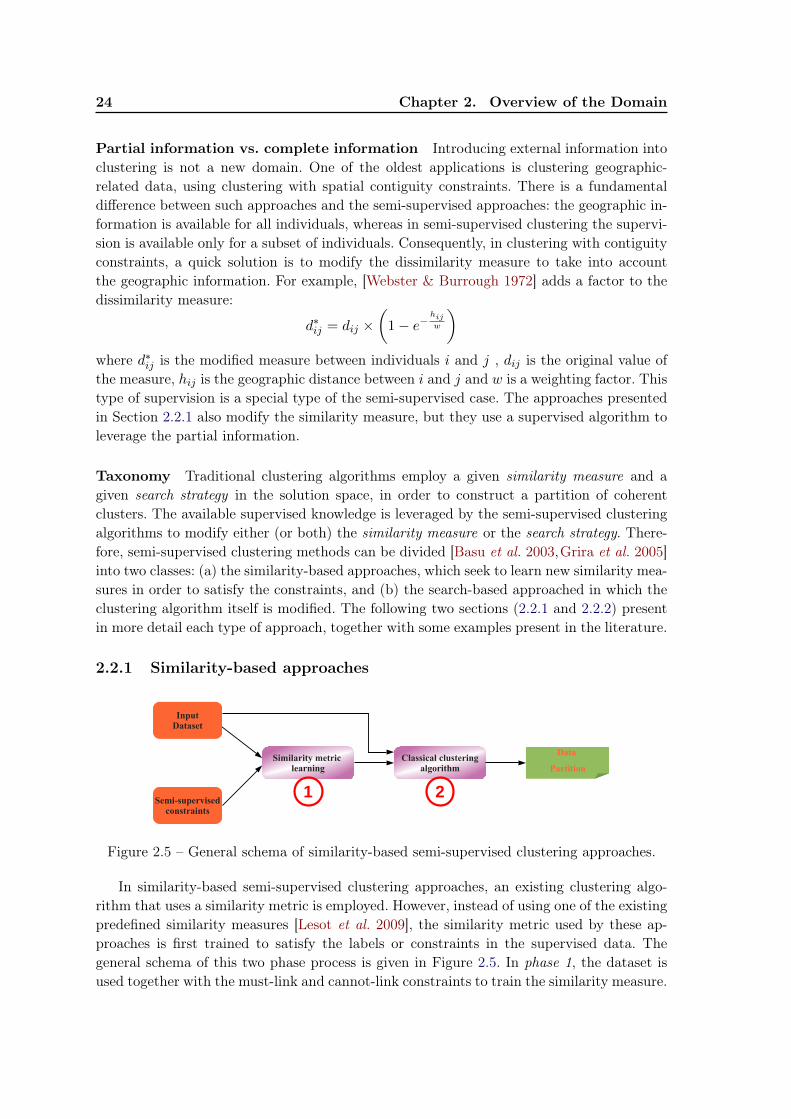
24 Chapter 2. Overview of the Domain
Partial information vs. complete information Introducing external information intoclustering is not a new domain. One of the oldest applications is clustering geographic-related data, using clustering with spatial contiguity constraints. There is a fundamentaldifference between such approaches and the semi-supervised approaches: the geographic in-formation is available for all individuals, whereas in semi-supervised clustering the supervi-sion is available only for a subset of individuals. Consequently, in clustering with contiguityconstraints, a quick solution is to modify the dissimilarity measure to take into accountthe geographic information. For example, [Webster & Burrough 1972] adds a factor to thedissimilarity measure:
d∗ij = dij ×(
1− e−hijw
)where d∗ij is the modified measure between individuals i and j , dij is the original value ofthe measure, hij is the geographic distance between i and j and w is a weighting factor. Thistype of supervision is a special type of the semi-supervised case. The approaches presentedin Section 2.2.1 also modify the similarity measure, but they use a supervised algorithm toleverage the partial information.
Taxonomy Traditional clustering algorithms employ a given similarity measure and agiven search strategy in the solution space, in order to construct a partition of coherentclusters. The available supervised knowledge is leveraged by the semi-supervised clusteringalgorithms to modify either (or both) the similarity measure or the search strategy. There-fore, semi-supervised clustering methods can be divided [Basu et al. 2003,Grira et al. 2005]into two classes: (a) the similarity-based approaches, which seek to learn new similarity mea-sures in order to satisfy the constraints, and (b) the search-based approached in which theclustering algorithm itself is modified. The following two sections (2.2.1 and 2.2.2) presentin more detail each type of approach, together with some examples present in the literature.
2.2.1 Similarity-based approaches
Similarity metric learning
Data
PartitionClassical clustering
algorithm
InputDataset
Semi-supervisedconstraints
1 2
Figure 2.5 – General schema of similarity-based semi-supervised clustering approaches.
In similarity-based semi-supervised clustering approaches, an existing clustering algo-rithm that uses a similarity metric is employed. However, instead of using one of the existingpredefined similarity measures [Lesot et al. 2009], the similarity metric used by these ap-proaches is first trained to satisfy the labels or constraints in the supervised data. Thegeneral schema of this two phase process is given in Figure 2.5. In phase 1, the dataset isused together with the must-link and cannot-link constraints to train the similarity measure.
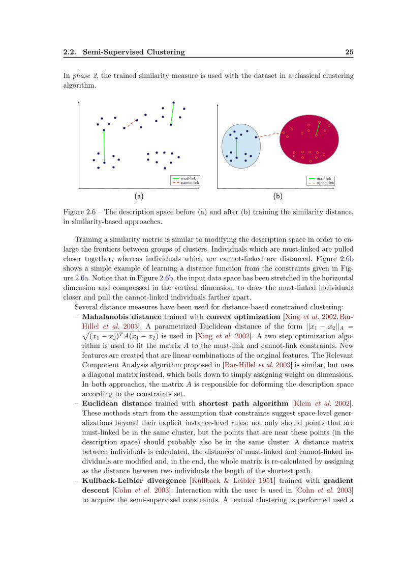
2.2. Semi-Supervised Clustering 25
In phase 2, the trained similarity measure is used with the dataset in a classical clusteringalgorithm.
must-linkcannot-link
(a)
must-linkcannot-link
(b)
Figure 2.6 – The description space before (a) and after (b) training the similarity distance,in similarity-based approaches.
Training a similarity metric is similar to modifying the description space in order to en-large the frontiers between groups of clusters. Individuals which are must-linked are pulledcloser together, whereas individuals which are cannot-linked are distanced. Figure 2.6bshows a simple example of learning a distance function from the constraints given in Fig-ure 2.6a. Notice that in Figure 2.6b, the input data space has been stretched in the horizontaldimension and compressed in the vertical dimension, to draw the must-linked individualscloser and pull the cannot-linked individuals farther apart.
Several distance measures have been used for distance-based constrained clustering:– Mahalanobis distance trained with convex optimization [Xing et al. 2002,Bar-
Hillel et al. 2003]. A parametrized Euclidean distance of the form ||x1 − x2||A =√(x1 − x2)TA(x1 − x2) is used in [Xing et al. 2002]. A two step optimization algo-
rithm is used to fit the matrix A to the must-link and cannot-link constraints. Newfeatures are created that are linear combinations of the original features. The RelevantComponent Analysis algorithm proposed in [Bar-Hillel et al. 2003] is similar, but usesa diagonal matrix instead, which boils down to simply assigning weight on dimensions.In both approaches, the matrix A is responsible for deforming the description spaceaccording to the constraints set.
– Euclidean distance trained with shortest path algorithm [Klein et al. 2002].These methods start from the assumption that constraints suggest space-level gener-alizations beyond their explicit instance-level rules: not only should points that aremust-linked be in the same cluster, but the points that are near these points (in thedescription space) should probably also be in the same cluster. A distance matrixbetween individuals is calculated, the distances of must-linked and cannot-linked in-dividuals are modified and, in the end, the whole matrix is re-calculated by assigningas the distance between two individuals the length of the shortest path.
– Kullback-Leibler divergence [Kullback & Leibler 1951] trained with gradientdescent [Cohn et al. 2003]. Interaction with the user is used in [Cohn et al. 2003]to acquire the semi-supervised constraints. A textual clustering is performed used a
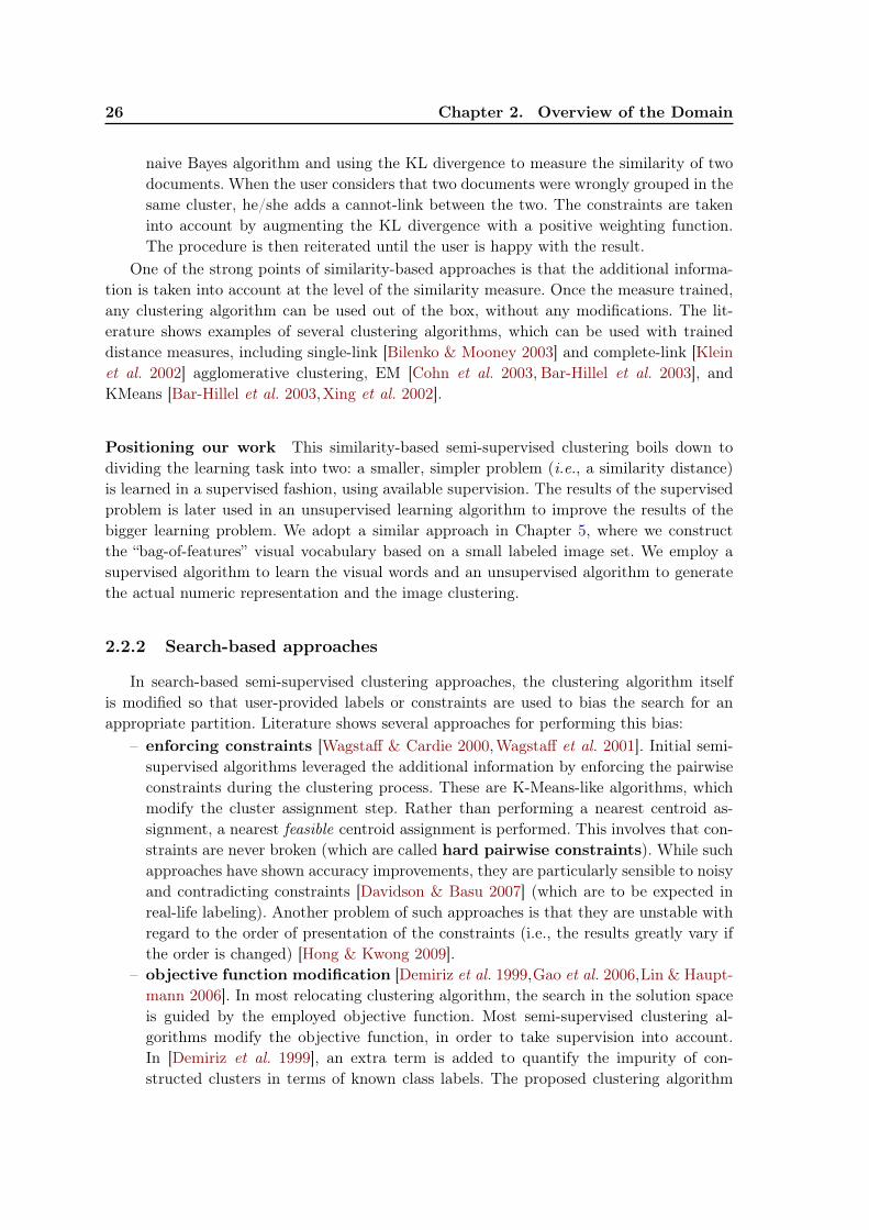
26 Chapter 2. Overview of the Domain
naive Bayes algorithm and using the KL divergence to measure the similarity of twodocuments. When the user considers that two documents were wrongly grouped in thesame cluster, he/she adds a cannot-link between the two. The constraints are takeninto account by augmenting the KL divergence with a positive weighting function.The procedure is then reiterated until the user is happy with the result.
One of the strong points of similarity-based approaches is that the additional informa-tion is taken into account at the level of the similarity measure. Once the measure trained,any clustering algorithm can be used out of the box, without any modifications. The lit-erature shows examples of several clustering algorithms, which can be used with traineddistance measures, including single-link [Bilenko & Mooney 2003] and complete-link [Kleinet al. 2002] agglomerative clustering, EM [Cohn et al. 2003, Bar-Hillel et al. 2003], andKMeans [Bar-Hillel et al. 2003,Xing et al. 2002].
Positioning our work This similarity-based semi-supervised clustering boils down todividing the learning task into two: a smaller, simpler problem (i.e., a similarity distance)is learned in a supervised fashion, using available supervision. The results of the supervisedproblem is later used in an unsupervised learning algorithm to improve the results of thebigger learning problem. We adopt a similar approach in Chapter 5, where we constructthe “bag-of-features” visual vocabulary based on a small labeled image set. We employ asupervised algorithm to learn the visual words and an unsupervised algorithm to generatethe actual numeric representation and the image clustering.
2.2.2 Search-based approaches
In search-based semi-supervised clustering approaches, the clustering algorithm itselfis modified so that user-provided labels or constraints are used to bias the search for anappropriate partition. Literature shows several approaches for performing this bias:
– enforcing constraints [Wagstaff & Cardie 2000,Wagstaff et al. 2001]. Initial semi-supervised algorithms leveraged the additional information by enforcing the pairwiseconstraints during the clustering process. These are K-Means-like algorithms, whichmodify the cluster assignment step. Rather than performing a nearest centroid as-signment, a nearest feasible centroid assignment is performed. This involves that con-straints are never broken (which are called hard pairwise constraints). While suchapproaches have shown accuracy improvements, they are particularly sensible to noisyand contradicting constraints [Davidson & Basu 2007] (which are to be expected inreal-life labeling). Another problem of such approaches is that they are unstable withregard to the order of presentation of the constraints (i.e., the results greatly vary ifthe order is changed) [Hong & Kwong 2009].
– objective function modification [Demiriz et al. 1999,Gao et al. 2006,Lin & Haupt-mann 2006]. In most relocating clustering algorithm, the search in the solution spaceis guided by the employed objective function. Most semi-supervised clustering al-gorithms modify the objective function, in order to take supervision into account.In [Demiriz et al. 1999], an extra term is added to quantify the impurity of con-structed clusters in terms of known class labels. The proposed clustering algorithm
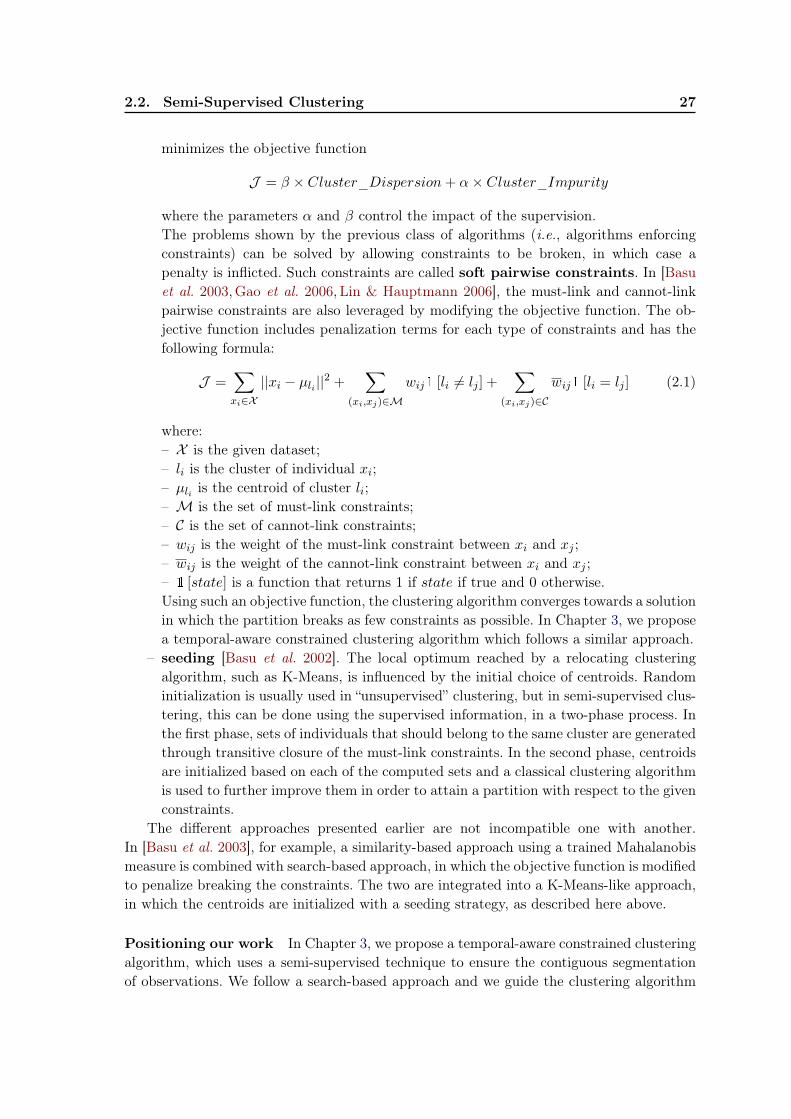
2.2. Semi-Supervised Clustering 27
minimizes the objective function
J = β × Cluster_Dispersion+ α× Cluster_Impurity
where the parameters α and β control the impact of the supervision.The problems shown by the previous class of algorithms (i.e., algorithms enforcingconstraints) can be solved by allowing constraints to be broken, in which case apenalty is inflicted. Such constraints are called soft pairwise constraints. In [Basuet al. 2003,Gao et al. 2006, Lin & Hauptmann 2006], the must-link and cannot-linkpairwise constraints are also leveraged by modifying the objective function. The ob-jective function includes penalization terms for each type of constraints and has thefollowing formula:
J =∑xi∈X
||xi − µli ||2 +
∑(xi,xj)∈M
wij1 [li 6= lj ] +∑
(xi,xj)∈C
wij1 [li = lj ] (2.1)
where:– X is the given dataset;– li is the cluster of individual xi;– µli is the centroid of cluster li;– M is the set of must-link constraints;– C is the set of cannot-link constraints;– wij is the weight of the must-link constraint between xi and xj ;– wij is the weight of the cannot-link constraint between xi and xj ;– 1 [state] is a function that returns 1 if state if true and 0 otherwise.Using such an objective function, the clustering algorithm converges towards a solutionin which the partition breaks as few constraints as possible. In Chapter 3, we proposea temporal-aware constrained clustering algorithm which follows a similar approach.
– seeding [Basu et al. 2002]. The local optimum reached by a relocating clusteringalgorithm, such as K-Means, is influenced by the initial choice of centroids. Randominitialization is usually used in “unsupervised” clustering, but in semi-supervised clus-tering, this can be done using the supervised information, in a two-phase process. Inthe first phase, sets of individuals that should belong to the same cluster are generatedthrough transitive closure of the must-link constraints. In the second phase, centroidsare initialized based on each of the computed sets and a classical clustering algorithmis used to further improve them in order to attain a partition with respect to the givenconstraints.
The different approaches presented earlier are not incompatible one with another.In [Basu et al. 2003], for example, a similarity-based approach using a trained Mahalanobismeasure is combined with search-based approach, in which the objective function is modifiedto penalize breaking the constraints. The two are integrated into a K-Means-like approach,in which the centroids are initialized with a seeding strategy, as described here above.
Positioning our work In Chapter 3, we propose a temporal-aware constrained clusteringalgorithm, which uses a semi-supervised technique to ensure the contiguous segmentationof observations. We follow a search-based approach and we guide the clustering algorithm

28 Chapter 2. Overview of the Domain
by modifying the objective function. In order to ensure the contiguous segmentation of thetemporal observations of an entity, we add soft pairwise must-link constraints between allobservations belonging to the same entity. We penalize breaking these constraints using apenalization function which is dependent on the time difference between the constraints(the wij in Equation 2.1, while wij are set to zero).
Chapter 3
Detecting Typical Evolutions
Contents3.1 Learning task and motivations . . . . . . . . . . . . . . . . . . . . . 293.2 Formalisation . . . . . . . . . . . . . . . . . . . . . . . . . . . . . . . . 313.3 Related work . . . . . . . . . . . . . . . . . . . . . . . . . . . . . . . . 343.4 Temporal-Driven Constrained Clustering . . . . . . . . . . . . . . . 34
3.4.1 The temporal-aware dissimilarity measure . . . . . . . . . . . . . . . . 353.4.2 The contiguity penalty function . . . . . . . . . . . . . . . . . . . . . . 373.4.3 The TDCK-Means algorithm . . . . . . . . . . . . . . . . . . . . . . . 383.4.4 Fine-tuning the ratio between components . . . . . . . . . . . . . . . . 40
3.5 Experiments . . . . . . . . . . . . . . . . . . . . . . . . . . . . . . . . 433.5.1 Dataset . . . . . . . . . . . . . . . . . . . . . . . . . . . . . . . . . . . 433.5.2 Qualitative evaluation . . . . . . . . . . . . . . . . . . . . . . . . . . . 433.5.3 Evaluation measures . . . . . . . . . . . . . . . . . . . . . . . . . . . . 453.5.4 Quantitative evaluation . . . . . . . . . . . . . . . . . . . . . . . . . . 463.5.5 Impact of parameters β and δ . . . . . . . . . . . . . . . . . . . . . . . 493.5.6 The tuning parameter α . . . . . . . . . . . . . . . . . . . . . . . . . . 50
3.6 Current work: Role identification in social networks . . . . . . . . 523.6.1 Context . . . . . . . . . . . . . . . . . . . . . . . . . . . . . . . . . . . 523.6.2 The framework for identifying social roles . . . . . . . . . . . . . . . . 533.6.3 Preliminary experiments . . . . . . . . . . . . . . . . . . . . . . . . . . 54
3.7 Conclusion and future work . . . . . . . . . . . . . . . . . . . . . . . 57
3.1 Learning task and motivations
We consider that leveraging the temporal dimension into the learning processis a crucial point and it is one of the central research challenges of this thesis. The temporaldimension is more than just another descriptive dimension of data, since it profoundlychanges the learning problem. The description of data becomes contextualized (i.e., a certaindescription is true during a given time frame) and new learning problems arise: followingthe temporal evolution of individuals, detecting trends, topic burstiness, popular eventstracking, etc. The temporal dimension is intimately related to the interactive Web 2.0,where the time is primordial for many learning tasks. In Section 2.1.3 (p. 16), we havediscussed the difference between temporal algorithms and online (“on the fly”) algorithms.Online algorithms have seen a lot of attention, especially given the huge amounts of data
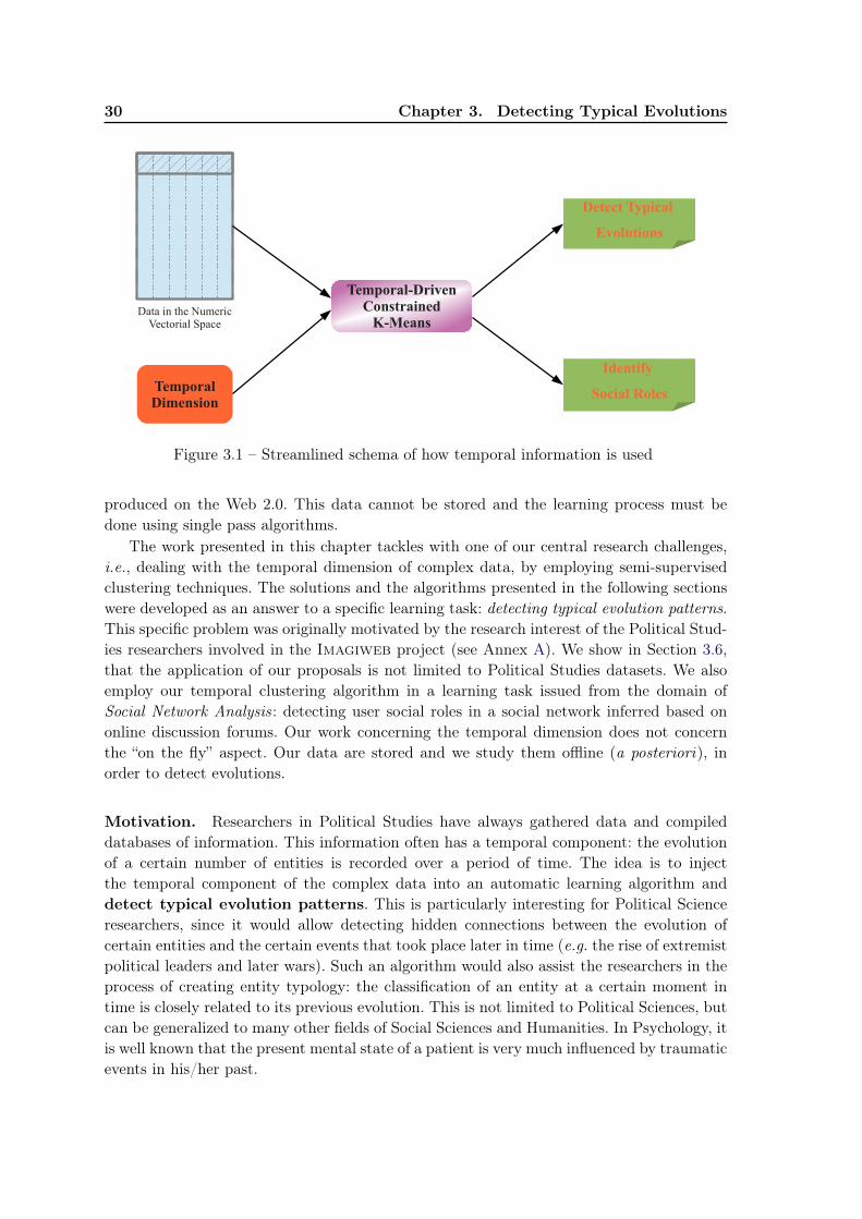
30 Chapter 3. Detecting Typical Evolutions
Temporal-DrivenConstrained
K-Means
Detect Typical
Evolutions
Identify
Social RolesTemporalDimension
Data in the Numeric Vectorial Space
Figure 3.1 – Streamlined schema of how temporal information is used
produced on the Web 2.0. This data cannot be stored and the learning process must bedone using single pass algorithms.
The work presented in this chapter tackles with one of our central research challenges,i.e., dealing with the temporal dimension of complex data, by employing semi-supervisedclustering techniques. The solutions and the algorithms presented in the following sectionswere developed as an answer to a specific learning task: detecting typical evolution patterns.This specific problem was originally motivated by the research interest of the Political Stud-ies researchers involved in the Imagiweb project (see Annex A). We show in Section 3.6,that the application of our proposals is not limited to Political Studies datasets. We alsoemploy our temporal clustering algorithm in a learning task issued from the domain ofSocial Network Analysis: detecting user social roles in a social network inferred based ononline discussion forums. Our work concerning the temporal dimension does not concernthe “on the fly” aspect. Our data are stored and we study them offline (a posteriori), inorder to detect evolutions.
Motivation. Researchers in Political Studies have always gathered data and compileddatabases of information. This information often has a temporal component: the evolutionof a certain number of entities is recorded over a period of time. The idea is to injectthe temporal component of the complex data into an automatic learning algorithm anddetect typical evolution patterns. This is particularly interesting for Political Scienceresearchers, since it would allow detecting hidden connections between the evolution ofcertain entities and the certain events that took place later in time (e.g. the rise of extremistpolitical leaders and later wars). Such an algorithm would also assist the researchers in theprocess of creating entity typology: the classification of an entity at a certain moment intime is closely related to its previous evolution. This is not limited to Political Sciences, butcan be generalized to many other fields of Social Sciences and Humanities. In Psychology, itis well known that the present mental state of a patient is very much influenced by traumaticevents in his/her past.
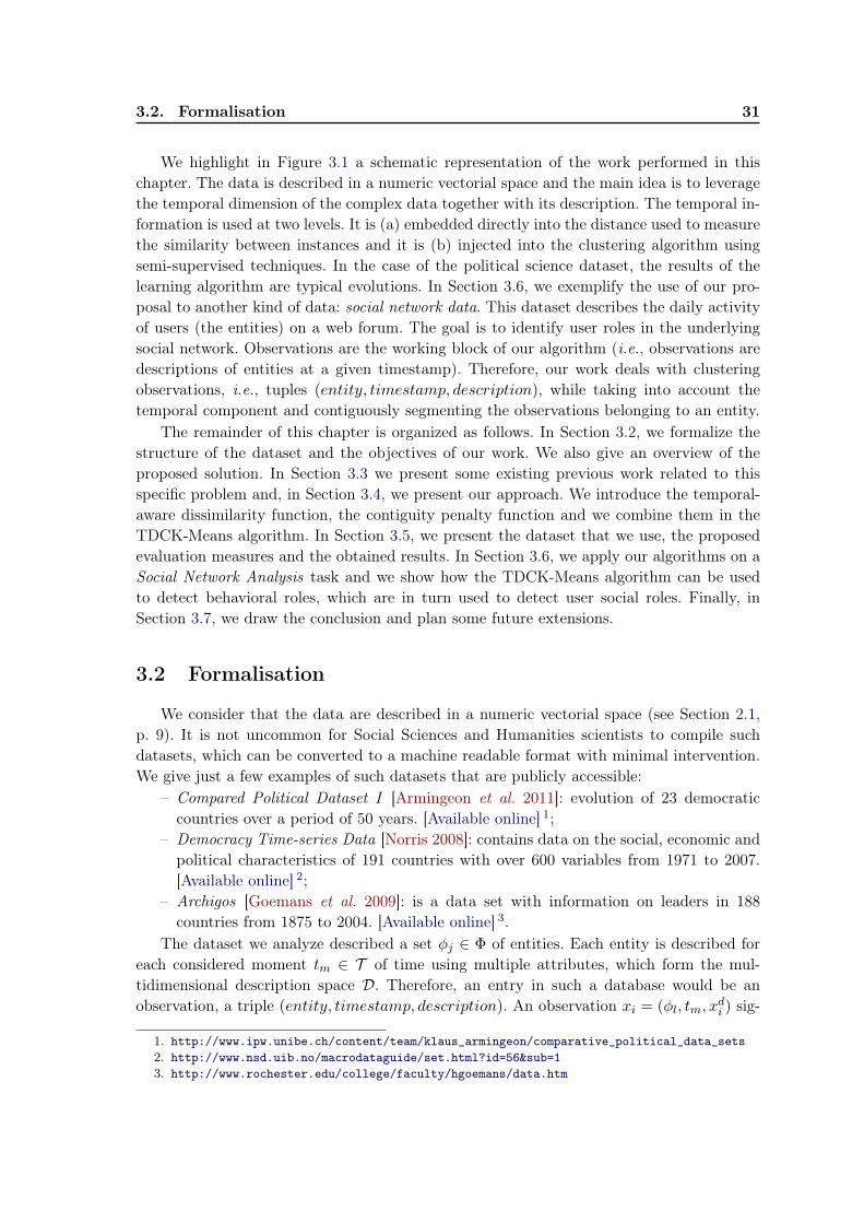
3.2. Formalisation 31
We highlight in Figure 3.1 a schematic representation of the work performed in thischapter. The data is described in a numeric vectorial space and the main idea is to leveragethe temporal dimension of the complex data together with its description. The temporal in-formation is used at two levels. It is (a) embedded directly into the distance used to measurethe similarity between instances and it is (b) injected into the clustering algorithm usingsemi-supervised techniques. In the case of the political science dataset, the results of thelearning algorithm are typical evolutions. In Section 3.6, we exemplify the use of our pro-posal to another kind of data: social network data. This dataset describes the daily activityof users (the entities) on a web forum. The goal is to identify user roles in the underlyingsocial network. Observations are the working block of our algorithm (i.e., observations aredescriptions of entities at a given timestamp). Therefore, our work deals with clusteringobservations, i.e., tuples (entity, timestamp, description), while taking into account thetemporal component and contiguously segmenting the observations belonging to an entity.
The remainder of this chapter is organized as follows. In Section 3.2, we formalize thestructure of the dataset and the objectives of our work. We also give an overview of theproposed solution. In Section 3.3 we present some existing previous work related to thisspecific problem and, in Section 3.4, we present our approach. We introduce the temporal-aware dissimilarity function, the contiguity penalty function and we combine them in theTDCK-Means algorithm. In Section 3.5, we present the dataset that we use, the proposedevaluation measures and the obtained results. In Section 3.6, we apply our algorithms on aSocial Network Analysis task and we show how the TDCK-Means algorithm can be usedto detect behavioral roles, which are in turn used to detect user social roles. Finally, inSection 3.7, we draw the conclusion and plan some future extensions.
3.2 Formalisation
We consider that the data are described in a numeric vectorial space (see Section 2.1,p. 9). It is not uncommon for Social Sciences and Humanities scientists to compile suchdatasets, which can be converted to a machine readable format with minimal intervention.We give just a few examples of such datasets that are publicly accessible:
– Compared Political Dataset I [Armingeon et al. 2011]: evolution of 23 democraticcountries over a period of 50 years. [Available online] 1;
– Democracy Time-series Data [Norris 2008]: contains data on the social, economic andpolitical characteristics of 191 countries with over 600 variables from 1971 to 2007.[Available online] 2;
– Archigos [Goemans et al. 2009]: is a data set with information on leaders in 188countries from 1875 to 2004. [Available online] 3.
The dataset we analyze described a set φj ∈ Φ of entities. Each entity is described foreach considered moment tm ∈ T of time using multiple attributes, which form the mul-tidimensional description space D. Therefore, an entry in such a database would be anobservation, a triple (entity, timestamp, description). An observation xi = (φl, tm, x
di ) sig-
1. http://www.ipw.unibe.ch/content/team/klaus_armingeon/comparative_political_data_sets2. http://www.nsd.uib.no/macrodataguide/set.html?id=56&sub=13. http://www.rochester.edu/college/faculty/hgoemans/data.htm
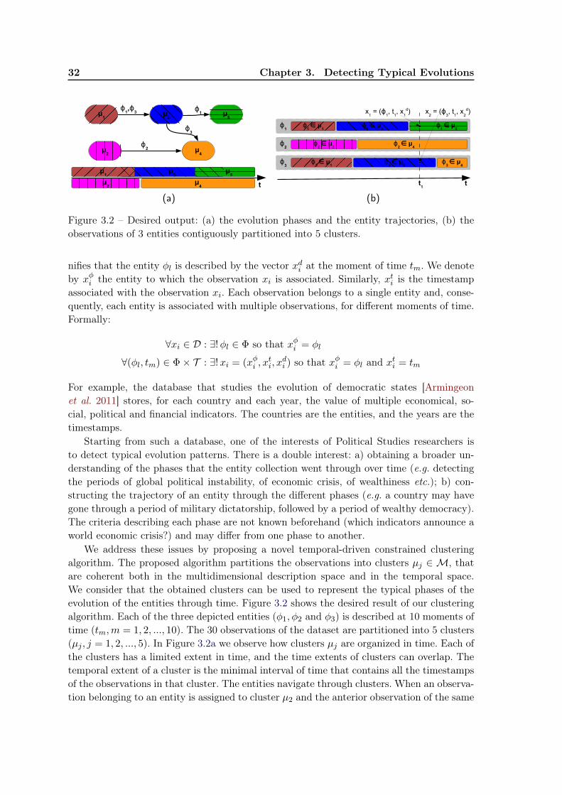
32 Chapter 3. Detecting Typical Evolutions
μ
3
μ4
μ4
μ5
t
ϕ1,ϕ
3 ϕ1
ϕ2
ϕ3
μ2
μ1
μ3
μ1
μ2
μ5
(a)
ϕ1
∈ μ1
ϕ1
∈ μ3
ϕ1
∈ μ5
ϕ1
ϕ2
ϕ3
∈ μ1
ϕ3
∈ μ3
ϕ3
ϕ2
∈ μ4
ϕ3
∈ μ4
tt1
x1 = (ϕ
1, t
1, x
1
d) x2 = (ϕ
3, t
1, x
2
d)
ϕ2
∈ μ2
(b)
Figure 3.2 – Desired output: (a) the evolution phases and the entity trajectories, (b) theobservations of 3 entities contiguously partitioned into 5 clusters.
nifies that the entity φl is described by the vector xdi at the moment of time tm. We denoteby xφi the entity to which the observation xi is associated. Similarly, xti is the timestampassociated with the observation xi. Each observation belongs to a single entity and, conse-quently, each entity is associated with multiple observations, for different moments of time.Formally:
∀xi ∈ D : ∃!φl ∈ Φ so that xφi = φl
∀(φl, tm) ∈ Φ× T : ∃!xi = (xφi , xti, x
di ) so that xφi = φl and xti = tm
For example, the database that studies the evolution of democratic states [Armingeonet al. 2011] stores, for each country and each year, the value of multiple economical, so-cial, political and financial indicators. The countries are the entities, and the years are thetimestamps.
Starting from such a database, one of the interests of Political Studies researchers isto detect typical evolution patterns. There is a double interest: a) obtaining a broader un-derstanding of the phases that the entity collection went through over time (e.g. detectingthe periods of global political instability, of economic crisis, of wealthiness etc.); b) con-structing the trajectory of an entity through the different phases (e.g. a country may havegone through a period of military dictatorship, followed by a period of wealthy democracy).The criteria describing each phase are not known beforehand (which indicators announce aworld economic crisis?) and may differ from one phase to another.
We address these issues by proposing a novel temporal-driven constrained clusteringalgorithm. The proposed algorithm partitions the observations into clusters µj ∈ M, thatare coherent both in the multidimensional description space and in the temporal space.We consider that the obtained clusters can be used to represent the typical phases of theevolution of the entities through time. Figure 3.2 shows the desired result of our clusteringalgorithm. Each of the three depicted entities (φ1, φ2 and φ3) is described at 10 moments oftime (tm,m = 1, 2, ..., 10). The 30 observations of the dataset are partitioned into 5 clusters(µj , j = 1, 2, ..., 5). In Figure 3.2a we observe how clusters µj are organized in time. Each ofthe clusters has a limited extent in time, and the time extents of clusters can overlap. Thetemporal extent of a cluster is the minimal interval of time that contains all the timestampsof the observations in that cluster. The entities navigate through clusters. When an observa-tion belonging to an entity is assigned to cluster µ2 and the anterior observation of the same
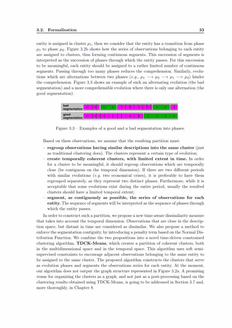
3.2. Formalisation 33
entity is assigned in cluster µ1, then we consider that the entity has a transition from phaseµ1 to phase µ2. Figure 3.2b shows how the series of observations belonging to each entityare assigned to clusters, thus forming continuous segments. This succession of segments isinterpreted as the succession of phases through which the entity passes. For this successionto be meaningful, each entity should be assigned to a rather limited number of continuoussegments. Passing through too many phases reduces the comprehension. Similarly, evolu-tions which are alternations between two phases (e.g., µ1 −→ µ2 −→ µ1 −→ µ2) hinderthe comprehension. Figure 3.3 shows an example of such an alternating evolution (the badsegmentation) and a more comprehensible evolution where there is only one alternation (thegood segmentation).
goodsegmentation
badsegmentation
Figure 3.3 – Examples of a good and a bad segmentation into phases.
Based on these observations, we assume that the resulting partition must:
– regroup observations having similar descriptions into the same cluster (justas traditional clustering does). The clusters represent a certain type of evolution;
– create temporally coherent clusters, with limited extent in time. In orderfor a cluster to be meaningful, it should regroup observations which are temporallyclose (be contiguous on the temporal dimension). If there are two different periodswith similar evolutions (e.g. two economical crises), it is preferable to have themregrouped separately, as they represent two distinct phases. Furthermore, while it isacceptable that some evolutions exist during the entire period, usually the resultedclusters should have a limited temporal extent;
– segment, as contiguously as possible, the series of observations for eachentity. The sequence of segments will be interpreted as the sequence of phases throughwhich the entity passes.
In order to construct such a partition, we propose a new time-aware dissimilarity measurethat takes into account the temporal dimension. Observations that are close in the descrip-tion space, but distant in time are considered as dissimilar. We also propose a method toenforce the segmentation contiguity, by introducing a penalty term based on the Normal Dis-tribution Function. We combine the two propositions into a novel time-driven constrainedclustering algorithm, TDCK-Means, which creates a partition of coherent clusters, bothin the multidimensional space and in the temporal space. This algorithm uses soft semi-supervised constraints to encourage adjacent observations belonging to the same entity tobe assigned to the same cluster. The proposed algorithm constructs the clusters that serveas evolution phases and segments the observations series for each entity. At the moment,our algorithm does not output the graph structure represented in Figure 3.2a. A promisingvenue for organizing the clusters as a graph, and not just as a post-processing based on theclustering results obtained using TDCK-Means, is going to be addressed in Section 3.7 and,more thoroughly, in Chapter 8.
34 Chapter 3. Detecting Typical Evolutions
3.3 Related work
The semi-supervised techniques seen in Section 2.2 are not limited to introducing expertknowledge into the clustering process. They can be used to inject any type of informationexternal to the dataset. Previous works which model temporal information using semi-supervised tools already exist. The literature presents some examples of algorithms usedto segment a series of observations into continuous chunks. In [Lin & Hauptmann 2006],the daily tasks of a user are detected by segmenting scenes from the recordings of hisactivities. Semi-supervised must-link constraints are set between all pairs of observations,and a fixed penalty is inflicted when the following conditions are fulfilled simultaneously:the observations are not assigned to the same cluster and the time difference between theirtimestamps is less than a certain threshold. A similar technique is used in [De la Torre &Agell 2007], where constraints are used to penalize non-smooth changes (over time) on theassigned clusters. This segmenting technique is used to detect tasks performed during aday, based on video, on sound and on GPS information. In [Sanders & Sukthankar 2001],the objects appearing in an image sequence are detected by using a hierarchical descendingclustering, that regroups pixels into large temporally coherent clusters. This method seeks tomaximize the cluster size, while guaranteeing intra-cluster temporal consistency. All of thesetechniques consider only one series of observations (a single entity) and must be adaptedfor the case of multiple series. The main problem of a threshold based penalty functionis to set the value of the threshold, which is usually data-dependent. Optimal matchingis used in [Widmer & Ritschard 2009] to discover trajectory models, while studying thede-standardization of typical life courses.
The temporal dimension of the data is also used in some other fields of Information Re-trieval. In [Talukdar et al. 2012], constrained clustering is used to scope temporal relationalfacts in the knowledge bases, by exploiting temporal containment, alignment, succession,and mutual exclusion constraints among facts. In [Chen et al. 2009], clustering is used tosegment temporal observations into continuous chunks, as a preprocessing phase. A graph-ical model is proposed in [Qamra et al. 2006], that uses a probabilistic model in whichthe timestamp is part of the observed variables, and the story is the hidden variable to beinferred. But still, none of these approaches seek to create temporally coherent partitionsof the data, mainly using the temporal dimension as a secondary information.
In the following sections, we propose a dissimilarity measure, a penalty function and aclustering algorithm in which the temporal dimension has a central role, and which addressthe limitations existing in the above presented work.
3.4 Temporal-Driven Constrained Clustering
The observations xi ∈ X that need to be structured can be written as triples(entity, time, description): xi = (xφi , x
ti, x
di ). x
di ∈ D is the vector in the multidimensional
description space which describes the entity xφi ∈ Φ at the moment of time xti ∈ T .Traditional clustering algorithms input a set of multidimensional vectors, which they re-
group in such a way that observations inside a group resemble each other as much as possible,and resemble observations in other groups as little as possible. K-Means [MacQueen 1967] isa clustering algorithm based on iterative relocation, that partitions a dataset into k clusters,
3.4. Temporal-Driven Constrained Clustering 35
locally minimizing the sum of distances between each data points xi and its assigned clustercentroids µj ∈M. At each iteration, the objective function
I = Σµj∈MΣxi∈Cj ||xdi − µdj ||2
is minimized until it reaches a local optimum.Such a system is appropriate for constructing partitions based solely on xdi , the descrip-
tion in the multidimensional space. It does not take into account the temporal order of theobservations, nor the structure of the dataset, the fact that observations belong to entities.We extend to the temporal case by adding to the centroids a temporal dimension µtj , de-scribed in the same temporal space T as the observations. Just like its multidimensionaldescription vector µdj , the temporal component does not necessary need to exist in the tem-poral set of the observation. It is an abstraction of the temporal information in the group,serving as a cluster timestamp. Therefore, a centroid µj will be the couple (µtj , µ
dj ).
We propose to adapt the K-Means algorithm to the temporal case by adapting theEuclidean distance, normally used to measure the distance between an element and its cen-troid. This novel temporal-aware dissimilarity measure takes into account both the distancein the multidimensional space and in the temporal space. In order to ensure the temporalcontiguity of observations for the entities, we add a penalty whenever two observations thatbelong to the same entity are assigned to different clusters. The penalty depends on the timedifference between the two: the lower the difference, the higher the penalty. We integrateboth into the Temporal-Driven Constrained K-Means (TDCK-Means), which is atemporal extension of K-Means. TDCK-Means searches to minimize the following objectivefunction:
J =∑µj∈M
∑xi∈Cj
||xi − µj ||TA +∑xk 6∈Cjxφk=xφi
w(xi, xk)
(3.1)
where || • ||TA is our temporal-aware (TA) dissimilarity measure (detailed in the next sec-tion), w(xi, xj) is the cost function that determines the penalty of clustering adjacent obser-vations of the same entity into different clusters, and Cj is the set of observations in clusterj.
3.4.1 The temporal-aware dissimilarity measure
The proposed temporal-aware dissimilarity measure ||xi − xj ||TA combines the Eu-clidean distance in the multidimensional space D and the distance between the timestamps.We propose to use the following formula:
||xi − xj ||TA = 1−
(1−||xdi − xdj ||2
∆x2max
)(1−||xti − xtj ||2
∆t2max
)(3.2)
where || • || is the classical L2 norm and ∆xmax and ∆tmax are the diameters of D, and Trespectively (the largest distance encountered between two observations in the multidimen-sional description space and, respectively, in the temporal space). The following propertiesare immediate:
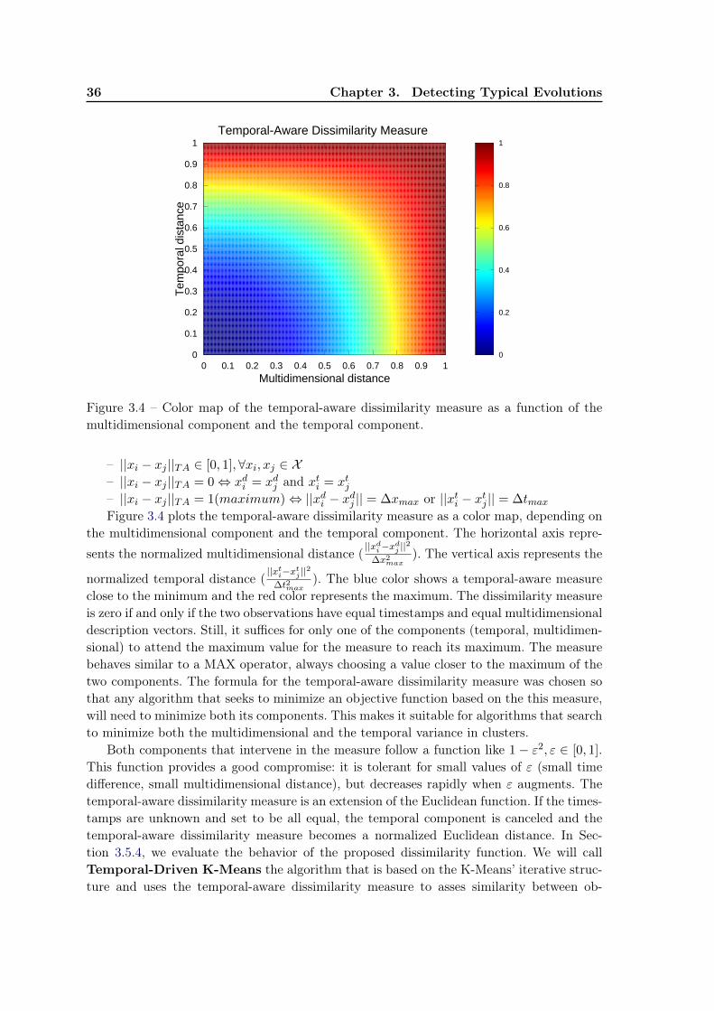
36 Chapter 3. Detecting Typical Evolutions
Temporal-Aware Dissimilarity Measure
0 0.1 0.2 0.3 0.4 0.5 0.6 0.7 0.8 0.9 1
Multidimensional distance
0
0.1
0.2
0.3
0.4
0.5
0.6
0.7
0.8
0.9
1
Tem
pora
l dis
tance
0
0.2
0.4
0.6
0.8
1
Figure 3.4 – Color map of the temporal-aware dissimilarity measure as a function of themultidimensional component and the temporal component.
– ||xi − xj ||TA ∈ [0, 1], ∀xi, xj ∈ X– ||xi − xj ||TA = 0⇔ xdi = xdj and xti = xtj– ||xi − xj ||TA = 1(maximum)⇔ ||xdi − xdj || = ∆xmax or ||xti − xtj || = ∆tmaxFigure 3.4 plots the temporal-aware dissimilarity measure as a color map, depending on
the multidimensional component and the temporal component. The horizontal axis repre-sents the normalized multidimensional distance (
||xdi−xdj ||2
∆x2max). The vertical axis represents the
normalized temporal distance (||xti−xtj ||2
∆t2max). The blue color shows a temporal-aware measure
close to the minimum and the red color represents the maximum. The dissimilarity measureis zero if and only if the two observations have equal timestamps and equal multidimensionaldescription vectors. Still, it suffices for only one of the components (temporal, multidimen-sional) to attend the maximum value for the measure to reach its maximum. The measurebehaves similar to a MAX operator, always choosing a value closer to the maximum of thetwo components. The formula for the temporal-aware dissimilarity measure was chosen sothat any algorithm that seeks to minimize an objective function based on the this measure,will need to minimize both its components. This makes it suitable for algorithms that searchto minimize both the multidimensional and the temporal variance in clusters.
Both components that intervene in the measure follow a function like 1− ε2, ε ∈ [0, 1].This function provides a good compromise: it is tolerant for small values of ε (small timedifference, small multidimensional distance), but decreases rapidly when ε augments. Thetemporal-aware dissimilarity measure is an extension of the Euclidean function. If the times-tamps are unknown and set to be all equal, the temporal component is canceled and thetemporal-aware dissimilarity measure becomes a normalized Euclidean distance. In Sec-tion 3.5.4, we evaluate the behavior of the proposed dissimilarity function. We will callTemporal-Driven K-Means the algorithm that is based on the K-Means’ iterative struc-ture and uses the temporal-aware dissimilarity measure to asses similarity between ob-
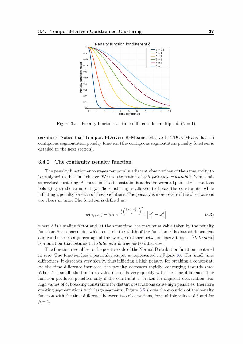
3.4. Temporal-Driven Constrained Clustering 37
0 1 2 3 4 5 6 7 8 9 100
0,1
0,2
0,3
0,4
0,5
0,6
0,7
0,8
0,9
1Penalty function for different δ
δ = 0.5δ = 1δ = 2δ = 3δ = 4δ = 5
Time difference
Pe
na
lty
fu
nc
tio
n v
alu
e
Figure 3.5 – Penalty function vs. time difference for multiple δ. (β = 1)
servations. Notice that Temporal-Driven K-Means, relative to TDCK-Means, has nocontiguous segmentation penalty function (the contiguous segmentation penalty function isdetailed in the next section).
3.4.2 The contiguity penalty function
The penalty function encourages temporally adjacent observations of the same entity tobe assigned to the same cluster. We use the notion of soft pair-wise constraints from semi-supervised clustering. A “must-link” soft constraint is added between all pairs of observationsbelonging to the same entity. The clustering is allowed to break the constraints, whileinflicting a penalty for each of these violations. The penalty is more severe if the observationsare closer in time. The function is defined as:
w(xi, xj) = β ∗ e− 1
2
(||xti−x
tj ||
δ
)2
1
[xφi = xφj
](3.3)
where β is a scaling factor and, at the same time, the maximum value taken by the penaltyfunction; δ is a parameter which controls the width of the function. β is dataset dependentand can be set as a percentage of the average distance between observations. 1 [statement]
is a function that returns 1 if statement is true and 0 otherwise.The function resembles to the positive side of the Normal Distribution function, centered
in zero. The function has a particular shape, as represented in Figure 3.5. For small timedifferences, it descends very slowly, thus inflicting a high penalty for breaking a constraint.As the time difference increases, the penalty decreases rapidly, converging towards zero.When δ is small, the functions value descends very quickly with the time difference. Thefunction produces penalties only if the constraint is broken for adjacent observation. Forhigh values of δ, breaking constraints for distant observations cause high penalties, thereforecreating segmentations with large segments. Figure 3.5 shows the evolution of the penaltyfunction with the time difference between two observations, for multiple values of δ and forβ = 1.
38 Chapter 3. Detecting Typical Evolutions
An advantage of the proposed function is that it requires no time discretization or settinga fixed window width, as proposed in [Lin & Hauptmann 2006]. The δ parameter permits thefine tuning of the penalty function. In Section 3.5.4, we evaluate Constrained K-Means,which is an extension of K-Means, to which we add the proposed contiguity penalty function(but which does not take into account the temporal dimension when measuring the distancebetween observations). The influence of both β and δ will be studied in Section 3.5.5.
3.4.3 The TDCK-Means algorithm
The time dependent distance ||xi−µj ||TA encourages the decrease of both the temporaland multidimensional variance of clusters; meanwhile the penalty function w(xi, xj) favorsthe adjacent observations belonging to the same entity to be assigned to the same cluster.The rest of the TDCK-Means algorithm is similar to the K-Means algorithm. It seeks tominimize J by iterating an assignment phase and a centroid update phase until the partitiondoes not change between two iterations. The outline of the algorithm is given in Algorithm 1.
The choose_random function chooses randomly, for each centroid µj , an observationxi and sets µj = (xti, x
di ). Furthermore, in the initialization phase we perform a K-Means
iteration in order to calculate an initial affectation of observations to clusters. For eachindividual the best_initial_cluster function solves the following equation:
best_initial_cluster(i) = argminj=1,2,...,k
(||xi − µ(iter−1)
j ||2TA)
(3.4)
therefore affecting each observation to the closest centroid, in terms of temporal-awaredissimilarity measure. In the assignment phase, for every observation xi, the best_clusterfunction chooses a cluster Cj so that the temporal-aware dissimilarity measure from xi tothe cluster’s centroid µj , added to the cost of penalties possibly incurred by this clusterassignment, is minimized. This function is similar to the best_initial_cluster functionin Equation 3.4, to which the penalty term is added. It resumes to solving the followingequation:
best_cluster(i) = argminj=1,2,...,k
||xi − µ(iter−1)j ||2TA +
xφk=xφi∑xk 6∈C
(iter−1)j
w(xi, xk)
(3.5)
This guaranties that the contribution of xi to the value of J diminishes or stays constant.Overall, this assures that J diminishes in the assignment phase (or stays constant). It isnoteworthy that, in Equation 3.5, the affectation of an observation in the current iterationis dependent on the affectation of the other observations in the previous iteration. This isalso the reason why an extra K-Means iteration was necessary in the initialization of thealgorithm and why the best_initial_cluster function was defined.
In the centroid update phase, the update_centroid function recalculates the clustercentroids using the observations in X and the assignment at the previous iteration. Thereforethe contribution of each cluster to the J function is minimized. Each of the temporal andthe multidimensional components is calculated individually. In order to find the values thatminimize the objective function, we need to solve the equations:
∂J∂µdj
= 0 ;∂J∂µtj
= 0 (3.6)
3.4. Temporal-Driven Constrained Clustering 39
Algorithm 1 Outline of the TDCK-Means algorithm.Input: xi ∈ X - observations to cluster;Input: k - number of requested clusters;Output: Cj , j = 1, 2, ..., k - k clusters;Output: µj , j = 1, 2, ..., k - centroids for each cluster;for j = 1, 2, .., k doµj ← choose_random(X )C0j ← ∅
for xi ∈ X doC0j = C0
j ∪ xi| where j = best_initial_cluster(X ,M0)iter ← 0
M(iter) ← ∅ //set of centroidsP(iter) ← ∅ //set of clustersrepeatiter ← iter + 1
for j = 1, 2, ..., k doC(iter)j ← ∅
// assignment phasefor xi ∈ X doC(iter)j = C(iter)
j ∪ xi| where j = best_cluster(X ,M(iter−1), P(iter−1))// centroids update phasefor j = 1, 2, ..., k do
(µφ,(iter)j , µ
t,(iter)j )← update_centroid(j, X ,M(iter−1), P(iter−1))
M(iter) ← {µ(iter)j |j = 1, 2, ..., k}
P(iter) ← {C(iter)j |j = 1, 2, ..., k}
until C(iter)j = C(iter−1)
j , ∀j ∈ [1, k]
By replacing equations (3.2) and (3.3) in (3.1), we obtain the following formula for theobjective function:
J = |X | −k∑j=1
∑xi∈Cj
[(1−||xdi − µdj ||2
∆x2max
)(1−||xti − µtj ||2
∆t2max
)]
+∑xi∈X
∑xk 6∈Cj
β ∗ e− 1
2
(||xti−x
tj ||
δ
)2
1
[xφi = xφj
](3.7)
We exemplify the calculation for the update formula of µtj .
∂J∂µtj
= 0⇔ ∂
∂µtj
k∑l=1
∑xi∈Cl
[(1−||xdi − µdl ||2
∆x2max
)(1−
(xti − µtl)2
∆t2max
)] = 0
⇔ 2
∆t2max×∑xi∈Cj
[(xti − µtj
)(1−||xdi − µdj ||2
∆x2max
)]= 0
40 Chapter 3. Detecting Typical Evolutions
⇔∑xi∈Cj
[(xti − µtj
)(1−||xdi − µdj ||2
∆x2max
)]= 0
⇔∑xi∈Cj
xti ×
(1−||xdi − µdj ||2
∆x2max
)=∑xi∈Cj
µtj ×
(1−||xdi − µdj ||2
∆x2max
)
⇔ µtj =
∑xi∈Cj x
ti ×(
1− ||xdi−µdj ||2
∆x2max
)∑
xi∈Cj
(1− ||x
di−µdj ||2
∆x2max
)Therefore, from equations (3.6) and (3.7), we obtain the centroid update formulas:
µdj =
∑xi∈Cj x
di ×
(1− ||x
ti−µtj ||2
∆t2max
)∑
xi∈Cj
(1− ||x
ti−µtj ||2
∆t2max
)
µtj =
∑xi∈Cj x
ti ×(
1− ||xdi−µdj ||2
∆x2max
)∑
xi∈Cj
(1− ||x
di−µdj ||2
∆x2max
) (3.8)
Just like the centroid update phase in K-Means, the new centroids in TDCK-Means arealso averages over the observations. Unlike K-Means, the averages are weighted for eachcomponent, using the distance from the other. For example, each observation contributesto the multidimensional description of the new centroid, proportional with its temporalcentrality in the cluster. Observations that are more distant in time (from the centroid)contribute less to the multidimensional description than the ones being closer in time. Asimilar logic applies to the temporal component. The consequence is that the new clustersare coherent both in the multidimensional space and in the temporal one.
Algorithm’s complexity Equation (3.7) shows that TDCK-Means’ complexity isO(n2k), due to the penalty term. Still, the equation can be rewritten, so that only ob-servations belonging to the same entity are tested. If p is the number of entities and q is themaximum number of observations associated with each entity, then n = p × q. The com-plexity of TDCK-Means is O(pq2k), which is well adapted to Social Science and Humanitiesdatasets, where often a large number of individuals is studied over a relatively short periodof time (p > q).
3.4.4 Fine-tuning the ratio between components
The temporal-aware dissimilarity measure, as presented in equation (3.2), gives equal im-portance to both the multidimensional component and the temporal component. This mightpose problems when the data are not uniformly distributed both in the multidimensionaldescriptive space and in the temporal space. If the medium standard deviation reported tothe medium distance between pairs of observations is greater in one space than in the other,giving equal weight to the components can lead to important bias in the clustering process.
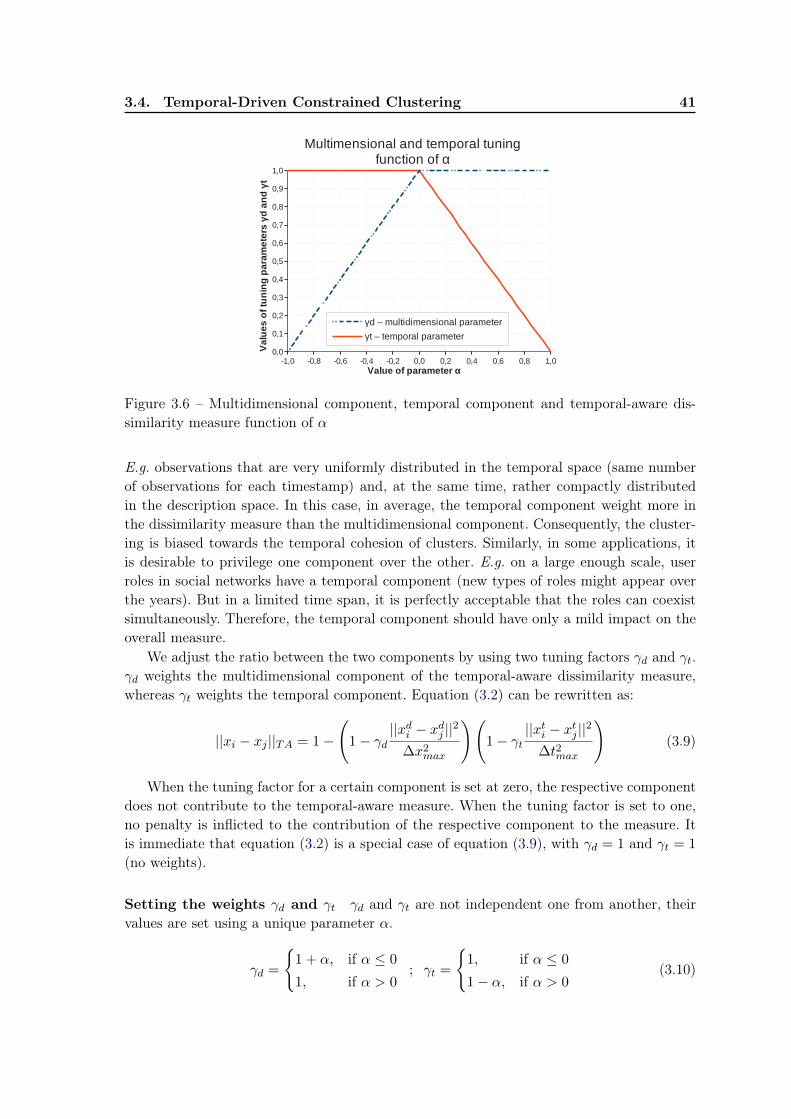
3.4. Temporal-Driven Constrained Clustering 41
-1,0 -0,8 -0,6 -0,4 -0,2 0,0 0,2 0,4 0,6 0,8 1,00,0
0,1
0,2
0,3
0,4
0,5
0,6
0,7
0,8
0,9
1,0
Multimensional and temporal tuningfunction of α
γd – multidimensional parameter
γt – temporal parameter
Value of parameter α
Va
lue
s o
f tu
nin
g p
ara
me
ters
γd
an
d γ
t
Figure 3.6 – Multidimensional component, temporal component and temporal-aware dis-similarity measure function of α
E.g. observations that are very uniformly distributed in the temporal space (same numberof observations for each timestamp) and, at the same time, rather compactly distributedin the description space. In this case, in average, the temporal component weight more inthe dissimilarity measure than the multidimensional component. Consequently, the cluster-ing is biased towards the temporal cohesion of clusters. Similarly, in some applications, itis desirable to privilege one component over the other. E.g. on a large enough scale, userroles in social networks have a temporal component (new types of roles might appear overthe years). But in a limited time span, it is perfectly acceptable that the roles can coexistsimultaneously. Therefore, the temporal component should have only a mild impact on theoverall measure.
We adjust the ratio between the two components by using two tuning factors γd and γt.γd weights the multidimensional component of the temporal-aware dissimilarity measure,whereas γt weights the temporal component. Equation (3.2) can be rewritten as:
||xi − xj ||TA = 1−
(1− γd
||xdi − xdj ||2
∆x2max
)(1− γt
||xti − xtj ||2
∆t2max
)(3.9)
When the tuning factor for a certain component is set at zero, the respective componentdoes not contribute to the temporal-aware measure. When the tuning factor is set to one,no penalty is inflicted to the contribution of the respective component to the measure. Itis immediate that equation (3.2) is a special case of equation (3.9), with γd = 1 and γt = 1
(no weights).
Setting the weights γd and γt γd and γt are not independent one from another, theirvalues are set using a unique parameter α.
γd =
{1 + α, if α ≤ 0
1, if α > 0; γt =
{1, if α ≤ 0
1− α, if α > 0(3.10)
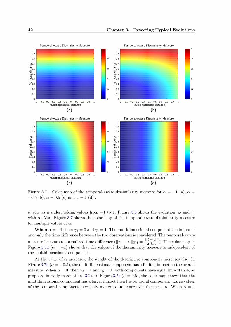
42 Chapter 3. Detecting Typical Evolutions
Temporal-Aware Dissimilarity Measure
0 0.1 0.2 0.3 0.4 0.5 0.6 0.7 0.8 0.9 1
Multidimensional distance
0
0.1
0.2
0.3
0.4
0.5
0.6
0.7
0.8
0.9
1
Tem
pora
l dis
tance
0
0.2
0.4
0.6
0.8
1
(a)
Temporal-Aware Dissimilarity Measure
0 0.1 0.2 0.3 0.4 0.5 0.6 0.7 0.8 0.9 1
Multidimensional distance
0
0.1
0.2
0.3
0.4
0.5
0.6
0.7
0.8
0.9
1
Tem
pora
l dis
tance
0
0.2
0.4
0.6
0.8
1
(b)
Temporal-Aware Dissimilarity Measure
0 0.1 0.2 0.3 0.4 0.5 0.6 0.7 0.8 0.9 1
Multidimensional distance
0
0.1
0.2
0.3
0.4
0.5
0.6
0.7
0.8
0.9
1
Tem
pora
l dis
tance
0
0.2
0.4
0.6
0.8
1
(c)
Temporal-Aware Dissimilarity Measure
0 0.1 0.2 0.3 0.4 0.5 0.6 0.7 0.8 0.9 1
Multidimensional distance
0
0.1
0.2
0.3
0.4
0.5
0.6
0.7
0.8
0.9
1
Tem
pora
l dis
tance
0
0.2
0.4
0.6
0.8
1
(d)
Figure 3.7 – Color map of the temporal-aware dissimilarity measure for α = −1 (a), α =
−0.5 (b), α = 0.5 (c) and α = 1 (d) .
α acts as a slider, taking values from −1 to 1. Figure 3.6 shows the evolution γd and γtwith α. Also, Figure 3.7 shows the color map of the temporal-aware dissimilarity measurefor multiple values of α.
When α = −1, then γd = 0 and γt = 1. The multidimensional component is eliminatedand only the time difference between the two observations is considered. The temporal-awaremeasure becomes a normalized time difference (||xi− xj ||TA =
||xti−xtj ||2
∆t2max). The color map in
Figure 3.7a (α = −1) shows that the values of the dissimilarity measure is independent ofthe multidimensional component.
As the value of α increases, the weight of the descriptive component increases also. InFigure 3.7b (α = −0.5), the multidimensional component has a limited impact on the overallmeasure. When α = 0, then γd = 1 and γt = 1, both components have equal importance, asproposed initially in equation (3.2). In Figure 3.7c (α = 0.5), the color map shows that themultidimensional component has a larger impact then the temporal component. Large valuesof the temporal component have only moderate influence over the measure. When α = 1
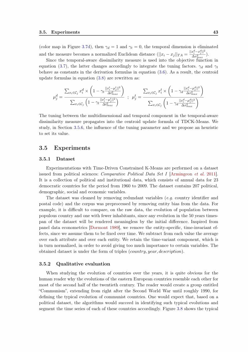
3.5. Experiments 43
(color map in Figure 3.7d), then γd = 1 and γt = 0, the temporal dimension is eliminated
and the measure becomes a normalized Euclidean distance (||xi − xj ||TA =||xdi−xdj ||2
∆x2max).
Since the temporal-aware dissimilarity measure is used into the objective function inequation (3.7), the latter changes accordingly to integrate the tuning factors. γd and γtbehave as constants in the derivation formulas in equation (3.6). As a result, the centroidupdate formulas in equation (3.8) are rewritten as:
µdj =
∑xi∈Cj x
di ×
(1− γt
||xti−µtj ||2
∆t2max
)∑
xi∈Cj
(1− γt
||xti−µtj ||2∆t2max
) ; µtj =
∑xi∈Cj x
ti ×(
1− γd||xdi−µdj ||2
∆x2max
)∑
xi∈Cj
(1− γd
||xdi−µdj ||2∆x2max
)The tuning between the multidimensional and temporal component in the temporal-awaredissimilarity measure propagates into the centroid update formula of TDCK-Means. Westudy, in Section 3.5.6, the influence of the tuning parameter and we propose an heuristicto set its value.
3.5 Experiments
3.5.1 Dataset
Experimentations with Time-Driven Constrained K-Means are performed on a datasetissued from political sciences: Comparative Political Data Set I [Armingeon et al. 2011].It is a collection of political and institutional data, which consists of annual data for 23democratic countries for the period from 1960 to 2009. The dataset contains 207 political,demographic, social and economic variables.
The dataset was cleaned by removing redundant variables (e.g. country identifier andpostal code) and the corpus was preprocessed by removing entity bias from the data. Forexample, it is difficult to compare, on the raw data, the evolution of population betweenpopulous country and one with fewer inhabitants, since any evolution in the 50 years times-pan of the dataset will be rendered meaningless by the initial difference. Inspired frompanel data econometrics [Dormont 1989], we remove the entity-specific, time-invariant ef-fects, since we assume them to be fixed over time. We subtract from each value the averageover each attribute and over each entity. We retain the time-variant component, which isin turn normalized, in order to avoid giving too much importance to certain variables. Theobtained dataset is under the form of triples (country, year, description).
3.5.2 Qualitative evaluation
When studying the evolution of countries over the years, it is quite obvious for thehuman reader why the evolutions of the eastern European countries resemble each other formost of the second half of the twentieth century. The reader would create a group entitled“Communism”, extending from right after the Second World War until roughly 1990, fordefining the typical evolution of communist countries. One would expect that, based on apolitical dataset, the algorithms would succeed in identifying such typical evolutions andsegment the time series of each of these countries accordingly. Figure 3.8 shows the typical
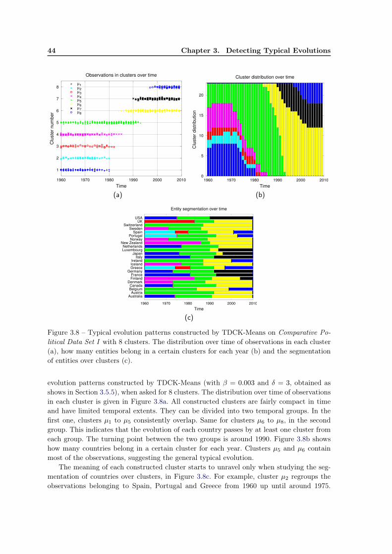
44 Chapter 3. Detecting Typical Evolutions
1
2
3
4
5
6
7
8
1960 1970 1980 1990 2000 2010
Clu
ste
r num
ber
Time
Observations in clusters over time
µ1µ2µ3µ4µ5µ6µ7µ8
(a)
0
5
10
15
20
1960 1970 1980 1990 2000 2010
Clu
ste
r dis
trib
ution
Time
Cluster distribution over time
(b)
AustraliaAustria
BelgiumCanada
DenmarkFinlandFrance
GermanyGreeceIcelandIreland
ItalyJapan
LuxembourgNetherlands
New ZealandNorway
PortugalSpain
SwedenSwitzerland
UKUSA
1960 1970 1980 1990 2000 2010
Time
Entity segmentation over time
(c)
Figure 3.8 – Typical evolution patterns constructed by TDCK-Means on Comparative Po-litical Data Set I with 8 clusters. The distribution over time of observations in each cluster(a), how many entities belong in a certain clusters for each year (b) and the segmentationof entities over clusters (c).
evolution patterns constructed by TDCK-Means (with β = 0.003 and δ = 3, obtained asshows in Section 3.5.5), when asked for 8 clusters. The distribution over time of observationsin each cluster is given in Figure 3.8a. All constructed clusters are fairly compact in timeand have limited temporal extents. They can be divided into two temporal groups. In thefirst one, clusters µ1 to µ5 consistently overlap. Same for clusters µ6 to µ8, in the secondgroup. This indicates that the evolution of each country passes by at least one cluster fromeach group. The turning point between the two groups is around 1990. Figure 3.8b showshow many countries belong in a certain cluster for each year. Clusters µ5 and µ6 containmost of the observations, suggesting the general typical evolution.
The meaning of each constructed cluster starts to unravel only when studying the seg-mentation of countries over clusters, in Figure 3.8c. For example, cluster µ2 regroups theobservations belonging to Spain, Portugal and Greece from 1960 up until around 1975.
3.5. Experiments 45
Historically, this coincides with the non-democratic regimes in those countries (Franco’sdictatorship in Spain, the “Regime of the Colonels” in Greece). Likewise, cluster µ4 con-tains observations of countries like Denmark, Finland, Iceland, Norway, Sweden and NewZealand. This cluster can be interpreted as the “Swedish Social and Economical Model” ofthe Nordic countries, to which the algorithm added, interestingly enough, New Zealand. Inthe second period, cluster µ8 regroups observations of Greece, Ireland, Spain, Portugal andBelgium, the countries which seemed the most fragile in the aftermaths of the economicalcrises of 2008.
3.5.3 Evaluation measures
Since the dataset contains no labels to report to as ground truth, we use the classicalInformation Theory measures in order to numerically evaluate the proposed algorithms. Weevaluate separately each of the three goals that we propose in Section 3.2.
Create clusters that are coherent in the multidimensional description space. Itis desirable that observations that have similar multidimensional descriptions to be par-titioned under the same cluster. The similarity in the description space is measured bythe multidimensional component of the temporal-aware dissimilarity measure. This goal ispursued by all classical clustering algorithms (like K-Means) and any traditional clusteringevaluation measure [Halkidi et al. 2001] can be used to asses it. We choose the mean clustervariance, which is traditionally used in clustering to quantify the dispersion of observationsin clusters. The MDvar measure is defined as:
MDvar =1
|X |×
k∑j=1
∑xi∈Cj
||xdi − µdj ||2
Create temporally coherent clusters, with limited extend in time. This goal isvery similar to the previous one, translated in the temporal space. It is desirable that obser-vations that are assigned to the same cluster to be similar in the temporal space (i.e. to beclose in time). The similarity in the temporal space is measured by the temporal componentin the temporal-aware dissimilarity measure. The limited time extent of a centroid impliessmall temporal distances between observations timestamp and the centroid timestamp. Asa result, the variance can also be used to measure the dispersion of clusters in the temporalspace. Similarly to MDvar, the Tvar measure is defined as:
Tvar =1
|X |×
k∑j=1
∑xi∈Cj
||xti − µtj ||2
Segment the temporal series of observations of each entity into a relatively smallnumber of contiguous segments. The goal is to have successive observations belongingto an entity grouped together, rather that scattered in different clusters. The Shannonentropy can quantify the number of clusters which regroup the observations of an entity, butit is insensible to alternations between two classes (evolutions like µ1 −→ µ2 −→ µ1 −→ µ2).
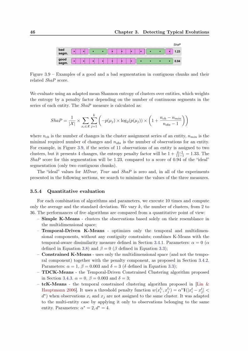
46 Chapter 3. Detecting Typical Evolutions
goodsegm.
badsegm.
ShaP
1.23
0.94
Figure 3.9 – Examples of a good and a bad segmentation in contiguous chunks and theirrelated ShaP score.
We evaluate using an adapted mean Shannon entropy of clusters over entities, which weightsthe entropy by a penalty factor depending on the number of continuous segments in theseries of each entity. The ShaP measure is calculated as:
ShaP =1
|X |×∑xi∈X
k∑j=1
(−p(µj)× log2(p(µj))×
(1 +
nch − nminnobs − 1
))
where nch is the number of changes in the cluster assignment series of an entity, nmin is theminimal required number of changes and nobs is the number of observations for an entity.For example, in Figure 3.9, if the series of 11 observations of an entity is assigned to twoclusters, but it presents 4 changes, the entropy penalty factor will be 1 + 4−1
11−1 = 1.33. TheShaP score for this segmentation will be 1.23, compared to a score of 0.94 of the “ideal”segmentation (only two contiguous chunks).
The “ideal” values for MDvar, Tvar and ShaP is zero and, in all of the experimentspresented in the following sections, we search to minimize the values of the three measures.
3.5.4 Quantitative evaluation
For each combination of algorithms and parameters, we execute 10 times and computeonly the average and the standard deviation. We vary k, the number of clusters, from 2 to36. The performances of five algorithms are compared from a quantitative point of view:
– Simple K-Means - clusters the observations based solely on their resemblance inthe multidimensional space;
– Temporal-Driven K-Means - optimizes only the temporal and multidimen-sional components, without any contiguity constraints; combines K-Means with thetemporal-aware dissimilarity measure defined in Section 3.4.1. Parameters: α = 0 (αdefined in Equation 3.8) and β = 0 (β defined in Equation 3.3);
– Constrained K-Means - uses only the multidimensional space (and not the tempo-ral component) together with the penalty component, as proposed in Section 3.4.2.Parameters: α = 1, β = 0.003 and δ = 3 (δ defined in Equation 3.3);
– TDCK-Means - the Temporal-Driven Constrained Clustering algorithm proposedin Section 3.4.3. α = 0, β = 0.003 and δ = 3;
– tcK-Means - the temporal constrained clustering algorithm proposed in [Lin &Hauptmann 2006]. It uses a threshold penalty function w(xtii , x
tij ) = α∗1(|xti − xtj | <
d∗) when observations xi and xj are not assigned to the same cluster. It was adaptedto the multi-entity case by applying it only to observations belonging to the sameentity. Parameters: α∗ = 2, d∗ = 4.
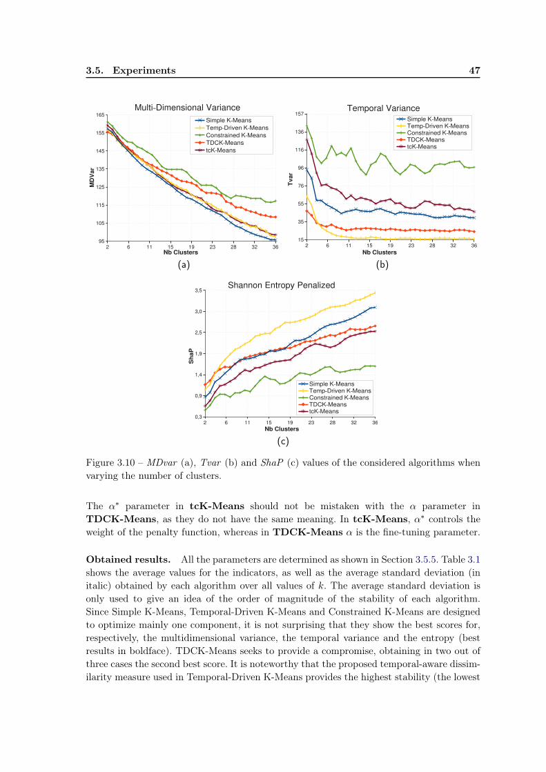
3.5. Experiments 47
2 6 11 15 19 23 28 32 3695
105
115
125
135
145
155
165
Multi−Dimensional Variance
Simple K−Means
Temp−Driven K−Means
Constrained K−Means
TDCK−Means
tcK−Means
Nb Clusters
MD
Va
r
(a)
2 6 11 15 19 23 28 32 3615
35
55
76
96
116
136
157Temporal Variance
Simple K−MeansTemp−Driven K−MeansConstrained K−MeansTDCK−MeanstcK−Means
Nb Clusters
Tv
ar
(b)
2 6 11 15 19 23 28 32 360,3
0,9
1,4
1,9
2,5
3,0
3,5Shannon Entropy Penalized
Simple K−MeansTemp−Driven K−MeansConstrained K−MeansTDCK−MeanstcK−Means
Nb Clusters
Sh
aP
(c)
Figure 3.10 – MDvar (a), Tvar (b) and ShaP (c) values of the considered algorithms whenvarying the number of clusters.
The α∗ parameter in tcK-Means should not be mistaken with the α parameter inTDCK-Means, as they do not have the same meaning. In tcK-Means, α∗ controls theweight of the penalty function, whereas in TDCK-Means α is the fine-tuning parameter.
Obtained results. All the parameters are determined as shown in Section 3.5.5. Table 3.1shows the average values for the indicators, as well as the average standard deviation (initalic) obtained by each algorithm over all values of k. The average standard deviation isonly used to give an idea of the order of magnitude of the stability of each algorithm.Since Simple K-Means, Temporal-Driven K-Means and Constrained K-Means are designedto optimize mainly one component, it is not surprising that they show the best scores for,respectively, the multidimensional variance, the temporal variance and the entropy (bestresults in boldface). TDCK-Means seeks to provide a compromise, obtaining in two out ofthree cases the second best score. It is noteworthy that the proposed temporal-aware dissim-ilarity measure used in Temporal-Driven K-Means provides the highest stability (the lowest
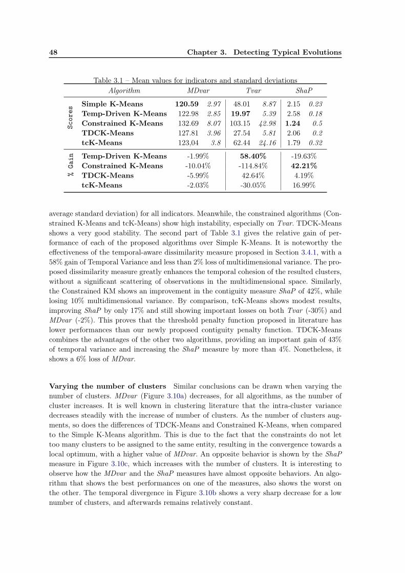
48 Chapter 3. Detecting Typical Evolutions
Table 3.1 – Mean values for indicators and standard deviationsAlgorithm MDvar Tvar ShaP
Scor
es
Simple K-Means 120.59 2.97 48.01 8.87 2.15 0.23Temp-Driven K-Means 122.98 2.85 19.97 5.39 2.58 0.18Constrained K-Means 132.69 8.07 103.15 42.98 1.24 0.5TDCK-Means 127.81 3.96 27.54 5.81 2.06 0.2tcK-Means 123,04 3.8 62.44 24.16 1.79 0.32
%Ga
in Temp-Driven K-Means -1.99% 58.40% -19.63%Constrained K-Means -10.04% -114.84% 42.21%TDCK-Means -5.99% 42.64% 4.19%tcK-Means -2.03% -30.05% 16.99%
average standard deviation) for all indicators. Meanwhile, the constrained algorithms (Con-strained K-Means and tcK-Means) show high instability, especially on Tvar. TDCK-Meansshows a very good stability. The second part of Table 3.1 gives the relative gain of per-formance of each of the proposed algorithms over Simple K-Means. It is noteworthy theeffectiveness of the temporal-aware dissimilarity measure proposed in Section 3.4.1, with a58% gain of Temporal Variance and less than 2% loss of multidimensional variance. The pro-posed dissimilarity measure greatly enhances the temporal cohesion of the resulted clusters,without a significant scattering of observations in the multidimensional space. Similarly,the Constrained KM shows an improvement in the contiguity measure ShaP of 42%, whilelosing 10% multidimensional variance. By comparison, tcK-Means shows modest results,improving ShaP by only 17% and still showing important losses on both Tvar (-30%) andMDvar (-2%). This proves that the threshold penalty function proposed in literature haslower performances than our newly proposed contiguity penalty function. TDCK-Meanscombines the advantages of the other two algorithms, providing an important gain of 43%of temporal variance and increasing the ShaP measure by more than 4%. Nonetheless, itshows a 6% loss of MDvar.
Varying the number of clusters Similar conclusions can be drawn when varying thenumber of clusters. MDvar (Figure 3.10a) decreases, for all algorithms, as the number ofcluster increases. It is well known in clustering literature that the intra-cluster variancedecreases steadily with the increase of number of clusters. As the number of clusters aug-ments, so does the differences of TDCK-Means and Constrained K-Means, when comparedto the Simple K-Means algorithm. This is due to the fact that the constraints do not lettoo many clusters to be assigned to the same entity, resulting in the convergence towards alocal optimum, with a higher value of MDvar. An opposite behavior is shown by the ShaPmeasure in Figure 3.10c, which increases with the number of clusters. It is interesting toobserve how the MDvar and the ShaP measures have almost opposite behaviors. An algo-rithm that shows the best performances on one of the measures, also shows the worst onthe other. The temporal divergence in Figure 3.10b shows a very sharp decrease for a lownumber of clusters, and afterwards remains relatively constant.
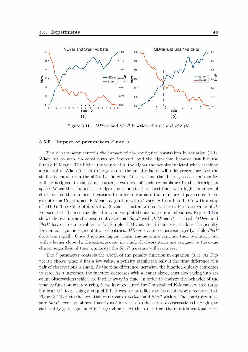
3.5. Experiments 49
0 1 2 3 4 5 6 7 8 9 10 11 12 13 14 15 16 17
149
151
152
153
154
155
156
0,68
0,77
0,86
0,94
1,03
1,12
1,21MDvar and ShaP vs beta
MDvar
ShaP
beta * 10³
MD
va
r
Sh
aP
(a)
0 1 2 3 4 5 6 7 8
136
138
141
143
145
148
150
0,6
0,8
1,0
1,2
1,4
1,6
1,8MDvar and ShaP vs delta
MDvar
ShaP
delta
MDvar
ShaP
(b)
Figure 3.11 – MDvar and ShaP function of β (a) and of δ (b)
3.5.5 Impact of parameters β and δ
The β parameter controls the impact of the contiguity constraints in equation (3.3).When set to zero, no constraints are imposed, and the algorithm behaves just like theSimple K-Means. The higher the values of β, the higher the penalty inflicted when breakinga constraint. When β is set to large values, the penalty factor will take precedence over thesimilarity measure in the objective function. Observations that belong to a certain entitywill be assigned to the same cluster, regardless of their resemblance in the descriptionspace. When this happens, the algorithm cannot create partitions with higher number ofclusters than the number of entities. In order to evaluate the influence of parameter β, weexecute the Constrained K-Means algorithm with β varying from 0 to 0.017 with a stepof 0.0005. The value of δ is set at 3, and 5 clusters are constructed. For each value of β,we executed 10 times the algorithm and we plot the average obtained values. Figure 3.11ashows the evolution of measures MDvar and ShaP with β. When β = 0 both MDvar andShaP have the same values as for Simple K-Means. As β increases, so does the penaltyfor non-contiguous segmentation of entities. MDvar starts to increase rapidly, while ShaPdecreases rapidly. Once β reaches higher values, the measures continue their evolution, butwith a leaner slope. In the extreme case, in which all observations are assigned to the samecluster regardless of their similarity, the ShaP measure will reach zero.
The δ parameter controls the width of the penalty function in equation (3.3). As Fig-ure 3.5 shows, when δ has a low value, a penalty is inflicted only if the time difference of apair of observations is small. As the time difference increases, the function quickly convergesto zero. As δ increases, the function decreases with a leaner slope, thus also taking into ac-count observations which are farther away in time. In order to analyze the behavior of thepenalty function when varying δ, we have executed the Constrained K-Means, with δ rang-ing from 0.1 to 8, using a step of 0.1. β was set at 0.003 and 10 clusters were constructed.Figure 3.11b plots the evolution of measures MDvar and ShaP with δ. The contiguity mea-sure ShaP decreases almost linearly as δ increases, as the series of observations belonging toeach entity gets segmented in larger chunks. At the same time, the multidimensional vari-
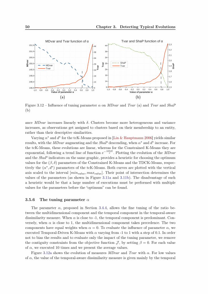
50 Chapter 3. Detecting Typical Evolutions
-1,0 -0,8 -0,6 -0,4 -0,2 0,0 0,2 0,4 0,6 0,8 1,0148,0
148,5
149,0
149,5
150,0
150,5
151,0
151,5
9
14
19
24
29
34
39
44
MDvar and Tvar function of α
MDvarTvar
Value of parameter α
MD
va
r
Tv
ar
(a)
-1,0 -0,8 -0,6 -0,4 -0,2 0,0 0,2 0,4 0,6 0,8 1,09
14
19
24
29
34
39
44
1,5
1,6
1,7
1,8
1,9
2,0
2,1
2,2
2,3
Tvar and ShaP function of α
ShaPTvar
Value of parameter α
Tv
ar
Sh
aP
(b)
Figure 3.12 – Influence of tuning parameter α on MDvar and Tvar (a) and Tvar and ShaP(b)
ance MDvar increases linearly with δ. Clusters become more heterogeneous and varianceincreases, as observations get assigned to clusters based on their membership to an entity,rather than their descriptive similarities.
Varying α∗ and d∗ for the tcK-Means proposed in [Lin & Hauptmann 2006] yields similarresults, with theMDvar augmenting and the ShaP descending, when α∗ and d∗ increase. Forthe tcK-Means, these evolutions are linear, whereas for the Constrained K-Means they areexponential, following a trend line of function e−
constx . Plotting the evolution of the MDvar
and the ShaP indicators on the same graphic, provides a heuristic for choosing the optimumvalues for the (β, δ) parameters of the Constrained K-Means and the TDCK-Means, respec-tively the (α∗, d∗) parameters of the tcK-Means. Both curves are plotted with the verticalaxis scaled to the interval [minvalue,maxvalue]. Their point of intersection determines thevalues of the parameters (as shown in Figure 3.11a and 3.11b). The disadvantage of sucha heuristic would be that a large number of executions must be performed with multiplevalues for the parameters before the “optimum” can be found.
3.5.6 The tuning parameter α
The parameter α, proposed in Section 3.4.4, allows the fine tuning of the ratio be-tween the multidimensional component and the temporal component in the temporal-awaredissimilarity measure. When α is close to -1, the temporal component is predominant. Con-versely, when α is close to 1, the multidimensional component takes precedence. The twocomponents have equal weights when α = 0. To evaluate the influence of parameter α, weexecuted Temporal-Driven K-Means with α varying from -1 to 1 with a step of 0.1. In ordernot to bias the results and to evaluate only the impact of the tuning parameter, we removethe contiguity constraints from the objective function J , by setting β = 0. For each valueof α, we executed 10 times and we present the average values.
Figure 3.12a shows the evolution of measures MDvar and Tvar with α. For low valuesof α, the value of the temporal-aware dissimilarity measure is given mainly by the temporal
3.5. Experiments 51
component, so Tvar shows its lowest value, while MDvar presents its maximum. As αincreases,MDvar decreases as more importance is given to the multidimensional component.For α ∈ (−1, 0], the importance of the temporal component remains intact, the increase ofTvar is solely the result of the algorithm converging to a local optimum which also takes intoaccount the multidimensional component. For α ∈ [0, 1), the impact of the multidimensionalcomponent stays constant, whereas the importance of the temporal components diminishes.As a result, MDvar continues its decrease and Tvar increases sharply. For α = 1 thetemporal component is basically ignored from the measure. The Temporal-Driven K-Meansbehaves just like Simple K-Means. Figure 3.12b shows the evolution of ShaP alongsideMDvar. Even if the contiguity penalty component was neutralized by setting β = 0, thevalue of ShaP is not constant, but it descends with α. For low values of α, the temporalcomponent is predominant in the similarity measure. This generates partitions where everycluster regroups all observations from a specific period, regardless of their multidimensionaldescription. This means that all entities have segments in all the clusters, which leads to ahigh value of ShaP.
It is noteworthy that the evolution of the indicators is not linear with α. As α increases,Tvar augments only very slowly and picks up the pace only for large values of α. This in-dicates that the temporal component has an inherent advantage over the multidimensionalone. As we presumed in Section 3.4.4, this is due to the intrinsic nature of the dataset andthe main reason why the tuning parameter α was introduced. The distributions of obser-vations in the multidimensional and temporal spaces is different: in the temporal space,the observations tend to be evenly distributed, whereas in the multidimensional descrip-tion space, they cluster together. To quantify this, we calculate the ratio between averagestandard deviation and average distances between pairs of observations:
rdim =1
|X |
|X |∑i=1
stdev({||xdimi − xdimj ||2
∣∣∣xj ∈ X , i 6= j})
1
|X |∑|X |
j=1j 6=i||xdimi − xdimj ||2
where dim is replaced with d or t ( the descriptive or the temporal dimension). On Com-parative Political Data Set I, rd = 29.5% and rt = 65.3%. This shows that observations area lot more dispersed in the temporal space than in the multidimensional description space.This explains why Tvar augments very slowly with α and starts to increase more rapidlyonly starting from α = 0.4.
Following the heuristic proposed in Section 3.5.5, we can determine a “compromise”value for α. As shown in Figure 3.12, all vertical axes are magnified between their functions’minimum and maximum values. The “compromise” value for α is found at the intersectionpoint of MDvar and Tvar (and MDvar and Shap). This value is set around 0.7, showing thedataset’s bias towards the temporal component. This technique for setting the value of thetunning parameter is just a heuristic, the actual value of α is dependent on the dataset. Thisis why we are currently working on a method, inspired from multi-objective optimizationusing evolutionary algorithms [Zhang & Li 2007] to automatically determine the values ofα, as well as the other parameters of TDCK-Means (β and δ).
52 Chapter 3. Detecting Typical Evolutions
3.6 Current work: Role identification in social networks
We are at present working on multiple extensions and applications of our work. Inthis section, we present the most advanced of them: the application of TDCK-Means touser social role identification in social networks. This is an ongoing work, the result ofthe research collaboration with the Technicolor’s Research & Innovation Laboratories 4 inRennes, France. Technicolor’s research interests include those parts of the Web related toCinema and Television, e.g. Web forums, social media, and professional sites. The endpurpose is to enrich the content by linking meta-data, extracted by analyzing the usagepatterns and semantic information. This collaboration allows us to test and further analyzethe behavior of our proposed TDCK-Means algorithm to social network data. This work isin an advanced state: the submission of an article is already planned.
In the remainder of this section, we present the general context of this application ofTDCK-Means and the used dataset (in Section 3.6.1), followed by the description of theuser role identification framework (in Section 3.6.2) and some preliminary results that weobtained (in Section 3.6.3).
3.6.1 Context
The base hypothesis of this work is that, when interacting in an online community,a user plays multiple roles, during the given period of time. These roles are temporallycoherent (when in a role, the user’s activity is uniformly similar) and he/she can changebetween roles. We denote these roles as behavioral roles. The global social role is constructedas a mixture of different behavioral roles, which incorporates the dynamics of behavioraltransitions. Therefore, we define the user social role as a succession of behavioral roles.
We construct the user social roles, based on a social network, inferred from online dis-cussion forums. The social roles are identified in a three phase framework: (a) behavioralcharacteristics are identified, based on the structure of the inferred social network, (b) be-havioral roles are created using TDCK-Means and (c) the user social roles are determinedbased in the transitions between behavioral roles.
Dataset and social network creation In this application of the TDCK-Means, weused the TWOP [Anokhin et al. 2012] dataset, which is an online forum discussion dataset.We discuss in more details the forum discussion online environment in Chapter 7, wherewe introduce CommentWatcher, an online forum analysis platform. In online forums, userscan start new discussion threads or they reply to other users’ messages, through a quoteciting mechanism. Discussions are formed by multiple users simultaneously answering oneto another. This structure can be used to infer an implicit online social network of users:two users are considered to have a relation when they reply one to another. This implicitsocial network is modeled as an oriented weighted graph. The nodes of the graph are theusers posting in the forums, whereas the arcs signal their relations. A directed arc is addedfrom user A to user B when A replies to B. The strength of the relation between A and Bis directly proportional with the number of replies of A to B.
4. https://research.technicolor.com/rennes/
3.6. Current work: Role identification in social networks 53
The TWOP dataset is constructed based on the Television Without Pity 5 forum website.It contains 58994 post of 7066 authors. It was constructed by parsing messages posted in 6forums, corresponding to 6 TV series, during the year of 2007.
3.6.2 The framework for identifying social roles
The social roles are identified by passing through behavioral roles. The underlying as-sumption is that the user’s behavior might change during the observed period of time. Forexample, he/she might be very active during a certain period, follow by a period of beingabsent from the online community or simply exchanging less with other users. We considerthis temporally coherent periods as being part of the same behavioral role. We, therefore,define the general social role as a succession of behavioral roles. We determine the socialroles using a three-phase framework:
(a) we calculate the temporal behavioral characteristics, based on the structure of theinferred social network;
(b) the behavioral roles are extracted using TDCK-Means, by constructing temporallycoherent clusters and contiguously segmenting the temporal measurement vectors as-sociated to each users;
(c) the user social roles are determined based on the transitions between the behavioralroles.
In the next paragraphs of this section, we detail each of these phases.
Determining behavioral characteristics The users interactions are quantified inphase (a) as shown in [Anokhin et al. 2012], by analyzing the directed graph of user interac-tions. We use measures adapted from the citation analysis literature to provide a measureof interaction and importance to our forum users. In particular, two well-known citationmetrics are adapted: the h-index [Hirsch 2005] and its successor, the g-index [Egghe 2006].The following characteristics are computed and used to describe the activity of a user:
– the node’s in/out g-Index. Based on the g-index, it measures how active is the neigh-borhood of the node.
– catalitic power. This indicator can differentiate between people who constantly receivereplies and those who start just one or two debates.
– weighted in/out-degree. It measures the “quantity” of communication in the neighbor-hood of the node.
– activity is the number of posts of the user.– cross-thread entropy measures the user’s focus on a thread.
These measures are rendered temporal by calculating them on an adaptive-length timewindow, which ensures that periods with low activity do not bias the temporal clustering(i.e., in the summer there is no broadcast of TV series and, consequently, there is almostno activity on the chosen television forum site in the summer).
Creating user behavioral roles In phase (b), the proposed temporal-aware constrainedclustering algorithm (TDCK-Means) is used to detect the behavioral roles. In Section 3.4,
5. http://www.televisionwithoutpity.com/
54 Chapter 3. Detecting Typical Evolutions
the clustered observations are triples (entity, time, description). In the case of user roledetection application, the entities are the users and the description vector is defined in themulti-dimensional description space, in which each behavioral measure is a dimension. Asalready discussed in Section 3.4.4, the importance of the temporal component is dependenton the application. There is a difference between the application of TDCK-Means to thedetection of country evolutions and the construction of behavioral roles. Evolution phasesof countries are inherently temporal, while the behavioral roles can appear during the entireobserved period. Consequently, we reduce the importance of the temporal component bysetting the α parameter (see Section 3.5.6) to values close to 1. The result of executingTDCK-Means are k temporal coherent clusters (µl, l = 1, 2, ..., k), which are interpreted asbehavioral roles. This already allows, for a given user, to evaluate the stability of his/herbehavior.
Creating user social roles In phase (c), for each user ui, we estimate the transitionmatrix Ψi = {ψis,t}, where ψis,t is the probability of user ui to have a transition fromthe behavioral state µs to the behavioral state µt. The matrices Ψi have the tendency ofbeing rare and have high values on the main diagonal, since TDCK-Means privileges (a)consecutive observation to belong to the same behavioral role and (b) that a user passesthrough rather few behavioral roles (see the discussion in Section 3.2).
Each social role is a mixture of different behavioral roles and it incorporates the dynam-ics of behavioral transitions. In other words, we interpret as a social role a succession oftransition through behavioral roles (similar to our previous application, the typical evolu-tions of countries). We use a simple K-Means to regroup the users’ transition probabilities.Notice that, in this second clustering, the individuals being clustered are the entities (i.e.,the users) and not the observations, as it was in the case of TDCK-Means. The users’transitions are represented by the matrices Ψi and the obtained cluster centroids are (a)described in the same numeric space as the clustered instances and (b) interpreted as thesocial roles. Each social role is, therefore, a matrix which gives two types of information: (a)the probability of transitions from one role to the other and (b) the mixture of behavioralroles, denoted by the values on the main diagonal (ψis,s is the probability that the user uipasses from the behavioral role µs to µs, which can be interpreted as the proportion of thetime in which ui stays in the behavioral role µs).
Such a representation has the inconvenient of being time orderless: it gives the proportionin which behavioral roles are present in each social role, but it does not give their temporalorder of succession. One of the current work we are undergoing at the present deals withinferring a graph structure for the constructed clusters (more details in Section 3.7 and inChapter 8). A graph approach would solve the order problem and detecting a social rolebecomes detecting frequent paths in the generated graph.
3.6.3 Preliminary experiments
This section presents the experiments and the preliminary results that were performedand obtained with the framework presented in Section 3.6.2. There is still work to be done,mainly in parameter choice, interpretation and qualitative evaluation. A thorough parametersweep needs to be performed to motivate the choice of parameters and qualitative evaluation
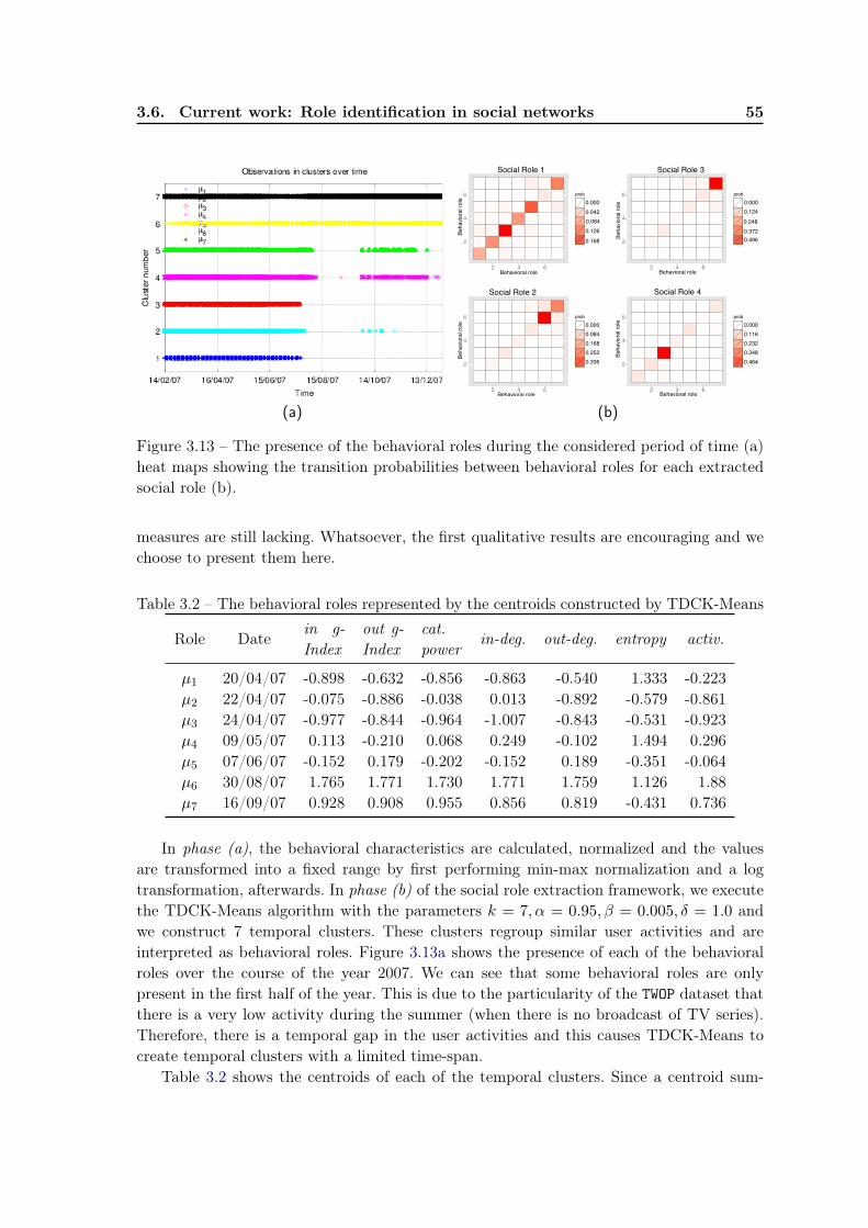
3.6. Current work: Role identification in social networks 55
(a)
2
4
6
2 4 6Behavioral role
Beha
vior
al ro
le
prob0.0000.0420.0840.1260.168
2
4
6
2 4 6Behavioral role
Beha
vior
al ro
le
prob0.0000.0840.1680.2520.336
Social Role 2
2
4
6
2 4 6Behavioral role
Beha
vior
al ro
le
prob0.0000.1240.2480.3720.496
Social Role 3
2
4
6
2 4 6Behavioral role
Beha
vior
al ro
le
prob0.0000.1160.2320.3480.464
Social Role 4
Social Role 1
(b)
Figure 3.13 – The presence of the behavioral roles during the considered period of time (a)heat maps showing the transition probabilities between behavioral roles for each extractedsocial role (b).
measures are still lacking. Whatsoever, the first qualitative results are encouraging and wechoose to present them here.
Table 3.2 – The behavioral roles represented by the centroids constructed by TDCK-Means
Role Datein g-Index
out g-Index
cat.power
in-deg. out-deg. entropy activ.
µ1 20/04/07 -0.898 -0.632 -0.856 -0.863 -0.540 1.333 -0.223µ2 22/04/07 -0.075 -0.886 -0.038 0.013 -0.892 -0.579 -0.861µ3 24/04/07 -0.977 -0.844 -0.964 -1.007 -0.843 -0.531 -0.923µ4 09/05/07 0.113 -0.210 0.068 0.249 -0.102 1.494 0.296µ5 07/06/07 -0.152 0.179 -0.202 -0.152 0.189 -0.351 -0.064µ6 30/08/07 1.765 1.771 1.730 1.771 1.759 1.126 1.88µ7 16/09/07 0.928 0.908 0.955 0.856 0.819 -0.431 0.736
In phase (a), the behavioral characteristics are calculated, normalized and the valuesare transformed into a fixed range by first performing min-max normalization and a logtransformation, afterwards. In phase (b) of the social role extraction framework, we executethe TDCK-Means algorithm with the parameters k = 7, α = 0.95, β = 0.005, δ = 1.0 andwe construct 7 temporal clusters. These clusters regroup similar user activities and areinterpreted as behavioral roles. Figure 3.13a shows the presence of each of the behavioralroles over the course of the year 2007. We can see that some behavioral roles are onlypresent in the first half of the year. This is due to the particularity of the TWOP dataset thatthere is a very low activity during the summer (when there is no broadcast of TV series).Therefore, there is a temporal gap in the user activities and this causes TDCK-Means tocreate temporal clusters with a limited time-span.
Table 3.2 shows the centroids of each of the temporal clusters. Since a centroid sum-
56 Chapter 3. Detecting Typical Evolutions
marizes the main features of the user activities in its cluster, we interpret the behavioralroles based on the associated centroids µl (in the following discussion we also denote abehavioral role with the name of the associated centroid). We can see, for example, thatuser activities that fall into the behavioral role µ1 describe users who post across multipleforums (hence the high entropy), but do not seem to engage other community members(low in/out g-Index, low in/out-degree, low catalytic power). By contrast, behavioral role µ4
also exhibits a high entropy, but there is evidence that users in this role are receiving replies(high in-degree). However, their replies are not from highly connected users, evidenced bythe slightly positive in g-Index value.
In phase (c), a K-Means clustering is performed on the behavioral transition probabilityvectors, as described in Section 3.6.2 and 4 clusters are constructed, which are interpretedas social roles. The social role is constructed as a mixture of different behavioral roles.Figure 3.13b shows, for each constructed social role, the obtained transition probabilities,depicted as heat maps. Most of the non-null values are on the main diagonal (lines arenumbered from bottom to top, columns from left to right). The values on the main diagonalgive the behavioral composition within each social role. Role 1 represents users who areactive members, able to generate and participate in active conversations within the forum.Sometimes, these conversations are with highly connected users, though mostly at random.Role 2 represents highly influential central figures, who take part and form the basis ofconversation in multiple sub-forums. Role 3 represents the slightly less active and morefocused users. Role 4 regroups users who are present throughout the peak of conversations,and reduce their activity afterwards.
Interestingly, although users present in Role 1 move between nearly all the behavioralroles, they are very rarely present in µ6. Table 3.2 shows that in this behavioral role, usersare highly central to conversation on more than one forum. This shows that most of theusers on the TWOP forum are only interested in a single show, and subsequently will alwayshave low entropy. Another distinct role played within the forum is the behavioral role µ4.Users presenting this role, although they are unable to generate (or contribute to) anyconversation, remain on the forum. Despite being ignored, users presenting the behavioralrole µ4 continue to participate in conversations.
In conclusion This section presented some of the work we are currently performing withthe TDCK-Means algorithm in particular, and with the temporal dimension of data ingeneral. We have shown that our proposed temporal-aware clustering algorithm has newpromising investigation fields and can be applied to other type of data than the one pre-sented in Section 3.5. The interpretation of the constructed social roles is still difficult,given that they are expressed as an orderless mixture of behavioral roles. Our plans areto extend TDCK-Means to include the inference of a graph structure of the constructedclusters. Constructing the social roles as a path in the behavioral role graph would renderthe interpretation easier.
3.7. Conclusion and future work 57
3.7 Conclusion and future work
In this chapter we have studied the detection of typical evolutions from a collection ofobservations. The presented work tackles with one of our central research challenges, i.e.,dealing with the temporal dimension of complex data. As we discussed at the beginning ofthe chapter, we consider that the temporal dimension is more than just another descriptivedimension of data, since it changes the definition of the learning problem. Therefore, one ofthe original contributions presented in this chapter is a novel method to introduce temporalinformation directly into the dissimilarity measure, weighting the descriptive componentby the temporal component. This new measure allows us to weight the importance of thetemporal component relative to the descriptive component and fine-tune its impact on thelearning process.
We have also proposed TDCK-Means, an extension of K-Means, which uses thetemporal-aware dissimilarity measure and a new objective function which takes into consid-eration the temporal dimension. We use a penalty factor to make sure that the observationseries related to an entity get segmented into continuous chunks. We infer a new centroidupdate formula, where elements distant in time contribute less to the centroid than thetemporally close ones. We have shown that our proposition consistently improves temporalvariance, without any significant losses in the multidimensional variance. The algorithmcan be used in other applications where the detection of typical evolutions is required, e.g.career evolution of politicians or abnormal disease evolution. We have shown how our pro-posal can be adapted to another specific problem, i.e. role identification in social networks,and another dataset.
Perspectives of our work In our current work, we have only detected the centroids thatserve as the evolution phases. We are currently working on an extension of TDCK-Means,which has embedded in the algorithm the construction of the evolution graph (as shownin Figure 3.2a, p. 32). The objective is to construct, starting from the available complexdata, a graph structure of the clusters. The idea is to estimate, in addition to the cen-troids and the temporal membership of observation to clusters, an adjacency matrix thatdefines the graph. This will allow an succinct description of the evolution of an entity asa path thought the constructed graph. Another direction of research will be describing theclusters in a human readable form. We work on means to provide them with an easily com-prehensible description by introducing temporal information into the unsupervised featureconstruction algorithm (we give more details about this current work in Chapters 4 and 8).We are also experimenting a method for setting automatically the values of TDCK-Means’sparameters (α, β and δ), by using an approach inspired from multi-objective optimizationusing evolutionary algorithms [Zhang & Li 2007].
The work presented in this chapter was published in the 24th IEEE International Confer-ence on Tools with Artificial Intelligence, receiving the Best Student Paper Award [Ri-zoiu et al. 2012].

Chapter 4
Using Data Semantics to ImproveData Representation
Contents4.1 Learning task and motivations . . . . . . . . . . . . . . . . . . . . . 59
4.1.1 Why construct a new feature set? . . . . . . . . . . . . . . . . . . . . . 614.1.2 A brief overview of our proposals . . . . . . . . . . . . . . . . . . . . . 62
4.2 Related work . . . . . . . . . . . . . . . . . . . . . . . . . . . . . . . . 634.3 uFRINGE - adapting FRINGE for unsupervised learning . . . . . 664.4 uFC - a greedy heuristic . . . . . . . . . . . . . . . . . . . . . . . . . 67
4.4.1 uFC - the proposed algorithm . . . . . . . . . . . . . . . . . . . . . . 684.4.2 Searching co-occurring pairs . . . . . . . . . . . . . . . . . . . . . . . . 704.4.3 Constructing and pruning features . . . . . . . . . . . . . . . . . . . . 71
4.5 Evaluation of a feature set . . . . . . . . . . . . . . . . . . . . . . . . 714.5.1 Complexity of the feature set . . . . . . . . . . . . . . . . . . . . . . . 724.5.2 The trade-off between two opposing criteria . . . . . . . . . . . . . . . 74
4.6 Initial Experiments . . . . . . . . . . . . . . . . . . . . . . . . . . . . 754.6.1 uFC and uFRINGE: Qualitative evaluation . . . . . . . . . . . . . . 764.6.2 uFC and uFRINGE: Quantitative evaluation . . . . . . . . . . . . . 794.6.3 Impact of parameters λ and limititer . . . . . . . . . . . . . . . . . . . 794.6.4 Relation between number of features and feature length . . . . . . . . 81
4.7 Improving the uFC algorithm . . . . . . . . . . . . . . . . . . . . . . 824.7.1 Automatic choice of λ . . . . . . . . . . . . . . . . . . . . . . . . . . . 834.7.2 Stopping criterion. Candidate pruning technique. . . . . . . . . . . . . 83
4.8 Further Experiments . . . . . . . . . . . . . . . . . . . . . . . . . . . 844.8.1 Risk-based heuristic for choosing parameters . . . . . . . . . . . . . . 844.8.2 Pruning the candidates . . . . . . . . . . . . . . . . . . . . . . . . . . 864.8.3 Algorithm stability . . . . . . . . . . . . . . . . . . . . . . . . . . . . . 89
4.9 Usage of the multi-objective optimization techniques . . . . . . . . 904.10 Conclusion and future work . . . . . . . . . . . . . . . . . . . . . . . 92
4.1 Learning task and motivations
Leveraging semantics when dealing with complex data is one of the core research chal-lenges of the work in this thesis. This chapter tackles the crucial learning task of con-structing a semantic-improved representation space for describing the data. While
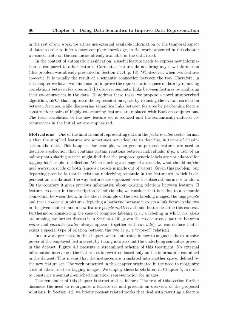
60 Chapter 4. Using Data Semantics to Improve Data Representation
in the rest of our work, we either use external available information or the temporal aspectof data in order to infer a more complete knowledge, in the work presented in this chapterwe concentrate on the semantics already available in the data itself.
In the context of automatic classification, a useful feature needs to express new informa-tion as compared to other features. Correlated features do not bring any new information(this problem was already presented in Section 2.1.4, p. 18). Whatsoever, when two featuresco-occur, it is usually the result of a semantic connection between the two. Therefore, inthis chapter we have two missions: (a) improve the representation space of data by removingcorrelations between features and (b) discover semantic links between features by analyzingtheir co-occurrences in the data. To address these tasks, we propose a novel unsupervisedalgorithm, uFC, that improves the representation space by reducing the overall correlationbetween features, while discovering semantics links between features by performing featureconstruction: pairs of highly co-occurring features are replaced with Boolean conjunctions.The total correlation of the new feature set is reduced and the semantically-induced co-occurrences in the initial set are emphasized.
Motivations One of the limitations of representing data in the feature-value vector formatis that the supplied features are sometimes not adequate to describe, in terms of classifi-cation, the data. This happens, for example, when general-purpose features are used todescribe a collection that contains certain relations between individuals. E.g., a user of anonline photo sharing service might find that the proposed generic labels are not adapted fortagging his/her photo collection. When labeling an image of a cascade, what should he/sheuse? water, cascade or both (since a cascade is made out of water). Given this problem, ourdeparting premise is that it exists an underlying semantic in the feature set, which is de-pendent on the dataset: the way features are organized over the observations is not random.On the contrary it gives precious information about existing relations between features. Iffeatures co-occur in the description of individuals, we consider that it is due to a semanticconnection between them. In the above example of the user labeling images, the tags peopleand trees co-occur in pictures depicting a barbecue because it exists a link between the twoin the given context, and a new feature people and trees should better describe this context.Furthermore, considering the case of complete labeling (i.e., a labeling in which no labelsare missing, we further discuss it in Section 4.10), given the co-occurrence pattern betweenwater and cascade (water always appears together with cascade), we can deduce that itexists a special type of relation between the two (e.g., a “type-of” relation).
In our work presented in this chapter, we are interested in how to augment the expressivepower of the employed features set, by taking into account the underlying semantics presentin the dataset. Figure 4.1 presents a streamlined schema of this treatment. No externalinformation intervenes, the feature set is rewritten based only on the information containedin the dataset. This means that the instances are translated into another space, defined bythe new feature set. The work presented in this chapter originated in the need to reorganizea set of labels used for tagging images. We employ these labels later, in Chapter 5, in orderto construct a semantic-enriched numerical representation for images.
The remainder of this chapter is structured as follows. The rest of this section furtherdiscusses the need to re-organize a feature set and presents an overview of the proposedsolutions. In Section 4.2, we briefly present related works that deal with rewriting a feature
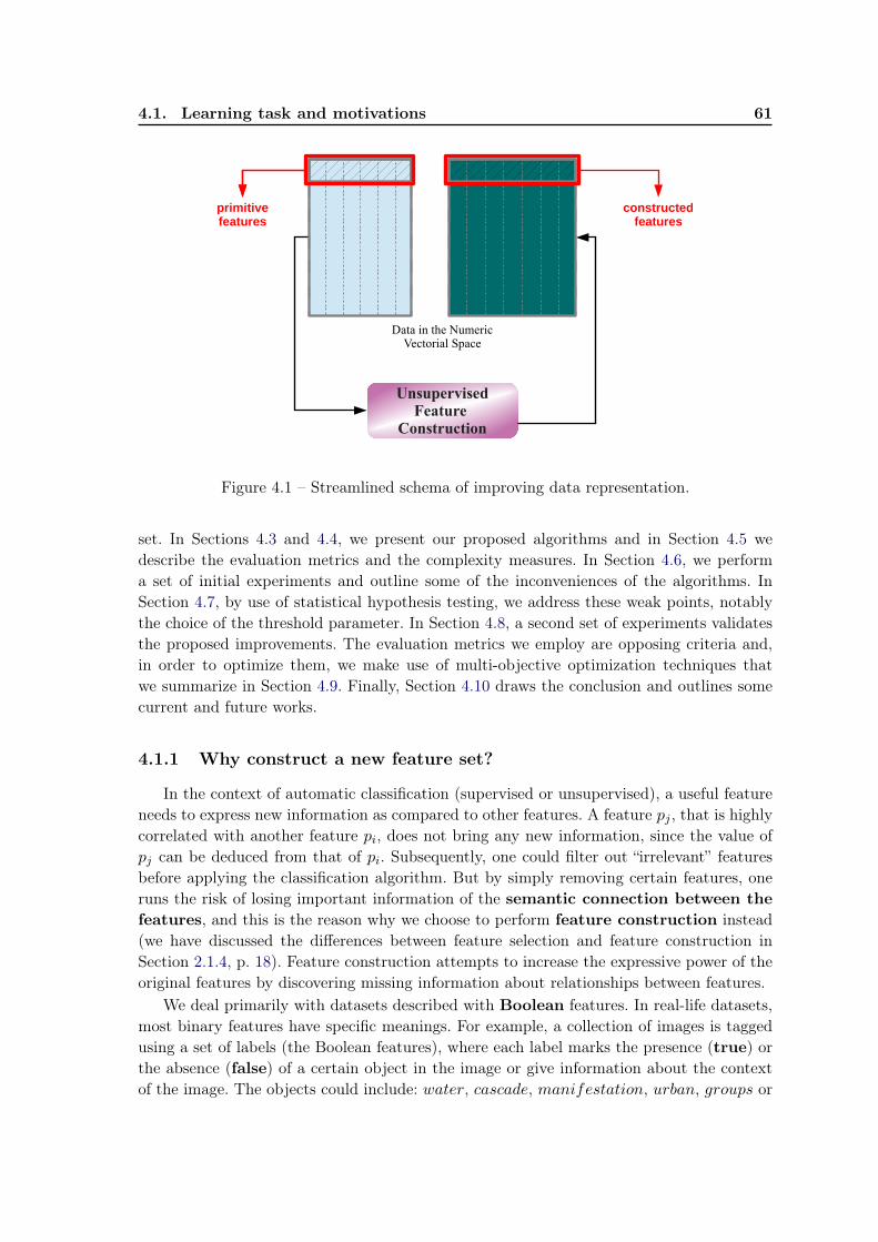
4.1. Learning task and motivations 61
Data in the Numeric Vectorial Space
UnsupervisedFeature
Construction
constructedfeatures
primitivefeatures
Figure 4.1 – Streamlined schema of improving data representation.
set. In Sections 4.3 and 4.4, we present our proposed algorithms and in Section 4.5 wedescribe the evaluation metrics and the complexity measures. In Section 4.6, we performa set of initial experiments and outline some of the inconveniences of the algorithms. InSection 4.7, by use of statistical hypothesis testing, we address these weak points, notablythe choice of the threshold parameter. In Section 4.8, a second set of experiments validatesthe proposed improvements. The evaluation metrics we employ are opposing criteria and,in order to optimize them, we make use of multi-objective optimization techniques thatwe summarize in Section 4.9. Finally, Section 4.10 draws the conclusion and outlines somecurrent and future works.
4.1.1 Why construct a new feature set?
In the context of automatic classification (supervised or unsupervised), a useful featureneeds to express new information as compared to other features. A feature pj , that is highlycorrelated with another feature pi, does not bring any new information, since the value ofpj can be deduced from that of pi. Subsequently, one could filter out “irrelevant” featuresbefore applying the classification algorithm. But by simply removing certain features, oneruns the risk of losing important information of the semantic connection between thefeatures, and this is the reason why we choose to perform feature construction instead(we have discussed the differences between feature selection and feature construction inSection 2.1.4, p. 18). Feature construction attempts to increase the expressive power of theoriginal features by discovering missing information about relationships between features.
We deal primarily with datasets described with Boolean features. In real-life datasets,most binary features have specific meanings. For example, a collection of images is taggedusing a set of labels (the Boolean features), where each label marks the presence (true) orthe absence (false) of a certain object in the image or give information about the contextof the image. The objects could include: water, cascade, manifestation, urban, groups or
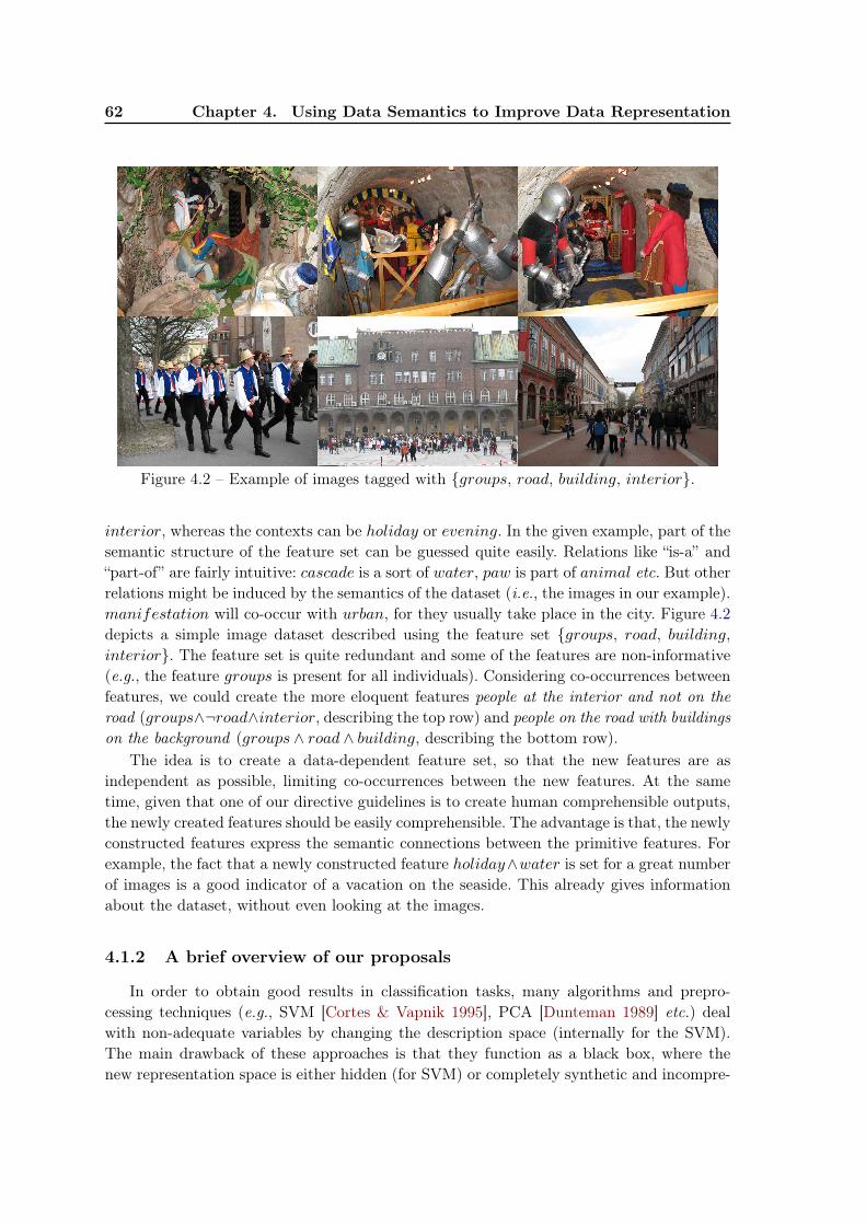
62 Chapter 4. Using Data Semantics to Improve Data Representation
Figure 4.2 – Example of images tagged with {groups, road, building, interior}.
interior, whereas the contexts can be holiday or evening. In the given example, part of thesemantic structure of the feature set can be guessed quite easily. Relations like “is-a” and“part-of” are fairly intuitive: cascade is a sort of water, paw is part of animal etc. But otherrelations might be induced by the semantics of the dataset (i.e., the images in our example).manifestation will co-occur with urban, for they usually take place in the city. Figure 4.2depicts a simple image dataset described using the feature set {groups, road, building,interior}. The feature set is quite redundant and some of the features are non-informative(e.g., the feature groups is present for all individuals). Considering co-occurrences betweenfeatures, we could create the more eloquent features people at the interior and not on theroad (groups∧¬road∧interior, describing the top row) and people on the road with buildingson the background (groups ∧ road ∧ building, describing the bottom row).
The idea is to create a data-dependent feature set, so that the new features are asindependent as possible, limiting co-occurrences between the new features. At the sametime, given that one of our directive guidelines is to create human comprehensible outputs,the newly created features should be easily comprehensible. The advantage is that, the newlyconstructed features express the semantic connections between the primitive features. Forexample, the fact that a newly constructed feature holiday∧water is set for a great numberof images is a good indicator of a vacation on the seaside. This already gives informationabout the dataset, without even looking at the images.
4.1.2 A brief overview of our proposals
In order to obtain good results in classification tasks, many algorithms and prepro-cessing techniques (e.g., SVM [Cortes & Vapnik 1995], PCA [Dunteman 1989] etc.) dealwith non-adequate variables by changing the description space (internally for the SVM).The main drawback of these approaches is that they function as a black box, where thenew representation space is either hidden (for SVM) or completely synthetic and incompre-
4.1. Learning task and motivations 63
hensible to human readers (PCA). The literature also proposes algorithms that constructfeatures based on the original user-supplied features. However, to our knowledge, all of thesealgorithms construct the feature set in a supervised way, based on the class information,supplied a priori with the data.
The novelty of our proposals Relative to existing solutions in the literature, our novelsolutions have two advantages. In addition to constructing a representation space in whichfeatures co-occur less, they (a) produce humanly comprehensible features and (b) theyfunction in the absence of pre-classified examples, in an unsupervised manner. The firstalgorithm we propose is an adaptation of an established supervised algorithm, making itunsupervised. For the second algorithm, we have developed a completely new heuristicthat selects, at each iteration, pairs of highly correlated features and replaces them withconjunctions of literals. Therefore, the overall redundancy of the feature set is reduced. Lateriterations create more complex Boolean formulas, which can contain negations (meaningabsence of features). We use statistical considerations (hypothesis testing) to automaticallydetermine the value of parameters depending on the dataset, and a Pareto front [Sawaragiet al. 1985]-inspired method for the evaluation. The main advantage of the proposed methodsover PCA or the kernel of the SVM is that the newly-created features are comprehensible tohuman readers (features like people∧manifestation∧urban and people∧¬urban∧forest areeasily interpretable). As mentioned earlier, our algorithms function in a complete labelingparadigm. We discuss in Section 4.10 how our approaches can be adapted to function withmissing label.
Using Boolean features Just like many other algorithms in the feature constructionliterature, our algorithms are limited to binary features. Any dataset described using thefeature-value vector format can be converted to a binary format using discretization andbinarization. Data Mining presents extensive work [Fayyad & Irani 1993] on the discretiza-tion of continuous features. While it is true that such a process has its drawbacks (e.g.,loss of details and order), there are advantages to discretization: it renders the learningalgorithms less sensible to outliers and noise, it deals better with missing values, by cre-ating a special feature which regroups them and it avoids the problems of asymmetry ofthe distribution of observations corresponding to a variable. Some researchers [Kotsiantis& Kanellopoulos 2006,Elomaa & Rousu 2004] even conclude that “most machine learningalgorithms produces better models when performing discretization on continuous variables”.
Some of the shortcomings of discretization can be overcomed by using cut-points. Insteadof discretizing by creating the feature “a ∈ [v1, v2]”, we can create two features “a < v1” and“a < v2”. A value lower than v1 would have both “a < v1” and “a < v2” set to true. In thisway the order relation between the binary features is preserved. This type of discretizationis inspired from the proportional-odds cumulative model, used with ordinal data in the fieldof logistic regression [Agresti 2002].
64 Chapter 4. Using Data Semantics to Improve Data Representation
4.2 Related work
The literature proposes methods for augmenting the descriptive power of features. [Liu &Motoda 1998] collects some of them and divides them into three categories: feature selection,feature extraction and feature construction.
Feature selection [Lallich & Rakotomalala 2000,Mo & Huang 2011] seeks to filter theoriginal feature set in order to remove redundant features. This results in a representationspace of lower dimensionality. These approaches address directly the problem of high datadimensionality (described in Section 2.1.4, p. 18)) and created a space which is more adaptedfor machine learning. Whatsoever, removing features runs the risk of loosing potentiallyinteresting information. In the example of the co-occurrence between cascade and water, afeature selection approach might remove the cascade, since water is more general. But the“is-a” induced by the dataset would be lost. Therefore, we do not consider any further thiskind of approaches.
Feature extraction is a process that builds a set of new features from the originalfeatures through functional mapping [Motoda & Liu 2002]. For example, while the SVMalgorithm [Cortes & Vapnik 1995] does not properly build a new description space (thekernel function only maps the description space into a predefined larger space, which isseparable in the context of supervised learning), we can assimilate this approach to afeature extraction since the purpose is to better describe the data and the new space isdifficult to comprehend from a semantic point of view. Furthermore, supervised and non-supervised algorithms can be boosted by pre-processing with principal component anal-ysis (PCA) [Dunteman 1989]. PCA is a mathematical procedure that uses an orthogonaltransformation to convert a set of observations of possibly correlated variables into a set ofvalues of uncorrelated variables, called principal components.
Another technique which can be associate with feature extraction is Manifold learn-ing [Huo et al. 2006], which pursuits the goal to embed data that originally lies in a non-linear manifold into a lower dimensional space, while preserving characteristic properties. Itcan be assimilated to feature extraction methods, since the purpose is to build a new lowerdimensional description space for the data.
Feature extraction mainly seeks to reduce the description space and redundancy betweenfeatures (exception the SVM, which builds a higher dimensional space than the originaldata). The problem with these approaches is that newly created features are rarely humancomprehensible and difficult to interpret, from a semantic point of view. Therefore, weconsider feature extraction methods inadequate for detecting relations between the originalfeatures.
Feature Construction Feature Construction is a process that discovers missing informa-tion about the relationships between features and augments the space of features by inferringor creating additional features [Motoda & Liu 2002]. The accent in feature construction,unlike feature extraction presented earlier, is on the comprehensibility of the newly createdfeatures. These methods usually construct a representation space with a larger dimensionthan the original space. Constructive induction [Michalski 1983] is a process of construct-ing new features using two intertwined searches [Bloedorn & Michalski 1998]: one in therepresentation space (modifying the feature set) and another in the hypothesis space (using
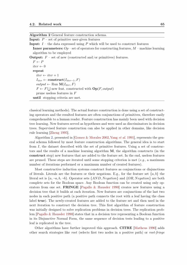
4.2. Related work 65
Algorithm 2 General feature construction schema.Input: P – set of primitive user-given featuresInput: I – the data expressed using P which will be used to construct featuresInner parameters: Op – set of operators for constructing features,M – machine learningalgorithm to be employed
Output: F – set of new (constructed and/or primitives) features.F ← P
iter ← 0
repeatiter ← iter + 1
Iiter ← construct(Iiter−1, F )output← Run M(Iiter, F )F ← F
⋃new feat. constructed with Op(F, output)
prune useless features in Funtil stopping criteria are met.
classical learning methods). The actual feature construction is done using a set of construct-ing operators and the resulted features are often conjunctions of primitives, therefore easilycomprehensible to a human reader. Feature construction has mainly been used with decisiontree learning. New features served as hypotheses and were used as discriminators in decisiontrees. Supervised feature construction can also be applied in other domains, like decisionrule learning [Zheng 1995].
Algorithm 2, presented in [Gomez & Morales 2002,Yang et al. 1991], represents the gen-eral schema followed by most feature construction algorithms. The general idea is to startfrom I, the dataset described with the set of primitive features. Using a set of construc-tors and the results of a machine learning algorithm M, the algorithm constructs (in theconstruct step) new features that are added to the feature set. In the end, useless featuresare pruned. These steps are iterated until some stopping criterion is met (e.g., a maximumnumber of iterations performed or a maximum number of created features).
Most constructive induction systems construct features as conjunctions or disjunctionsof literals. Literals are the features or their negations. E.g., for the feature set {a, b} theliteral set is {a,¬a, b,¬b}. Operator sets {AND,Negation} and {OR,Negation} are bothcomplete sets for the Boolean space. Any Boolean function can be created using only op-erators from one set. FRINGE [Pagallo & Haussler 1990] creates new features using adecision tree that it builds at each iteration. New features are conjunctions of the last twonodes in each positive path (a positive path connects the root with a leaf having the classlabel true). The newly-created features are added to the feature set and then used in thenext iteration to construct the decision tree. This first algorithm of feature constructionwas initially designed to solve replication problems in decision trees. The replication prob-lem [Pagallo & Haussler 1990] states that in a decision tree representing a Boolean functionin its Disjunctive Normal Form, the same sequence of decision tests leading to a positiveleaf is replicated in the tree.
Other algorithms have further improved this approach. CITRE [Matheus 1990] addsother search strategies like root (selects first two nodes in a positive path) or root-fringe
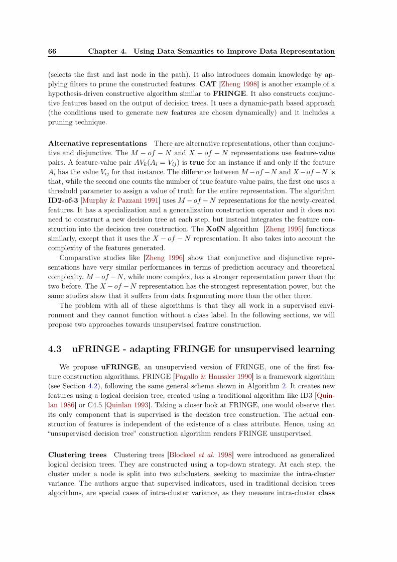
66 Chapter 4. Using Data Semantics to Improve Data Representation
(selects the first and last node in the path). It also introduces domain knowledge by ap-plying filters to prune the constructed features. CAT [Zheng 1998] is another example of ahypothesis-driven constructive algorithm similar to FRINGE. It also constructs conjunc-tive features based on the output of decision trees. It uses a dynamic-path based approach(the conditions used to generate new features are chosen dynamically) and it includes apruning technique.
Alternative representations There are alternative representations, other than conjunc-tive and disjunctive. The M − of − N and X − of − N representations use feature-valuepairs. A feature-value pair AVk(Ai = Vij) is true for an instance if and only if the featureAi has the value Vij for that instance. The difference betweenM−of−N and X−of−N isthat, while the second one counts the number of true feature-value pairs, the first one uses athreshold parameter to assign a value of truth for the entire representation. The algorithmID2-of-3 [Murphy & Pazzani 1991] uses M − of −N representations for the newly-createdfeatures. It has a specialization and a generalization construction operator and it does notneed to construct a new decision tree at each step, but instead integrates the feature con-struction into the decision tree construction. The XofN algorithm [Zheng 1995] functionssimilarly, except that it uses the X − of −N representation. It also takes into account thecomplexity of the features generated.
Comparative studies like [Zheng 1996] show that conjunctive and disjunctive repre-sentations have very similar performances in terms of prediction accuracy and theoreticalcomplexity. M −of −N , while more complex, has a stronger representation power than thetwo before. The X − of −N representation has the strongest representation power, but thesame studies show that it suffers from data fragmenting more than the other three.
The problem with all of these algorithms is that they all work in a supervised envi-ronment and they cannot function without a class label. In the following sections, we willpropose two approaches towards unsupervised feature construction.
4.3 uFRINGE - adapting FRINGE for unsupervised learning
We propose uFRINGE, an unsupervised version of FRINGE, one of the first fea-ture construction algorithms. FRINGE [Pagallo & Haussler 1990] is a framework algorithm(see Section 4.2), following the same general schema shown in Algorithm 2. It creates newfeatures using a logical decision tree, created using a traditional algorithm like ID3 [Quin-lan 1986] or C4.5 [Quinlan 1993]. Taking a closer look at FRINGE, one would observe thatits only component that is supervised is the decision tree construction. The actual con-struction of features is independent of the existence of a class attribute. Hence, using an“unsupervised decision tree” construction algorithm renders FRINGE unsupervised.
Clustering trees Clustering trees [Blockeel et al. 1998] were introduced as generalizedlogical decision trees. They are constructed using a top-down strategy. At each step, thecluster under a node is split into two subclusters, seeking to maximize the intra-clustervariance. The authors argue that supervised indicators, used in traditional decision treesalgorithms, are special cases of intra-cluster variance, as they measure intra-cluster class
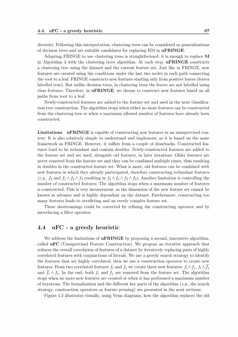
4.4. uFC - a greedy heuristic 67
diversity. Following this interpretation, clustering trees can be considered as generalizationsof decision trees and are suitable candidates for replacing ID3 in uFRINGE.
Adapting FRINGE to use clustering trees is straightforward: it is enough to replace Min Algorithm 2 with the clustering trees algorithm. At each step, uFRINGE constructsa clustering tree using the dataset and the current feature set. Just like in FRINGE, newfeatures are created using the conditions under the last two nodes in each path connectingthe root to a leaf. FRINGE constructs new features starting only from positive leaves (leaveslabelled true). But unlike decision trees, in clustering trees the leaves are not labelled usingclass features. Therefore, in uFRINGE, we choose to construct new features based on allpaths from root to a leaf.
Newly-constructed features are added to the feature set and used in the next classifica-tion tree construction. The algorithm stops when either no more features can be constructedfrom the clustering tree or when a maximum allowed number of features have already beenconstructed.
Limitations uFRINGE is capable of constructing new features in an unsupervised con-text. It is also relatively simple to understand and implement, as it is based on the sameframework as FRINGE. However, it suffers from a couple of drawbacks. Constructed fea-tures tend to be redundant and contain doubles. Newly-constructed features are added tothe feature set and are used, alongside old features, in later iterations. Older features arenever removed from the feature set and they can be combined multiple times, thus resultingin doubles in the constructed feature set. What is more, old features can be combined withnew features in which they already participated, therefore constructing redundant features(e.g., f2 and f1 ∧ f2 ∧ f3 resulting in f2 ∧ f1 ∧ f2 ∧ f3). Another limitation is controlling thenumber of constructed features. The algorithm stops when a maximum number of featuresis constructed. This is very inconvenient, as the dimension of the new feature set cannot beknown in advance and is highly dependent on the dataset. Furthermore, constructing toomany features leads to overfitting and an overly complex feature set.
These shortcomings could be corrected by refining the constructing operator and byintroducing a filter operator.
4.4 uFC - a greedy heuristic
We address the limitations of uFRINGE by proposing a second, innovative algorithm,called uFC (Unsupervised Feature Construction). We propose an iterative approach thatreduces the overall correlation of features of a dataset by iteratively replacing pairs of highlycorrelated features with conjunctions of literals. We use a greedy search strategy to identifythe features that are highly correlated, then we use a construction operator to create newfeatures. From two correlated features fi and fj we create three new features: fi∧fj , fi∧fjand fi ∧ fj . In the end, both fi and fj are removed from the feature set. The algorithmstops when no more new features are created or when it has performed a maximum numberof iterations. The formalization and the different key parts of the algorithm (e.g., the searchstrategy, construction operators or feature pruning) are presented in the next sections.
Figure 4.3 illustrates visually, using Venn diagrams, how the algorithm replaces the old
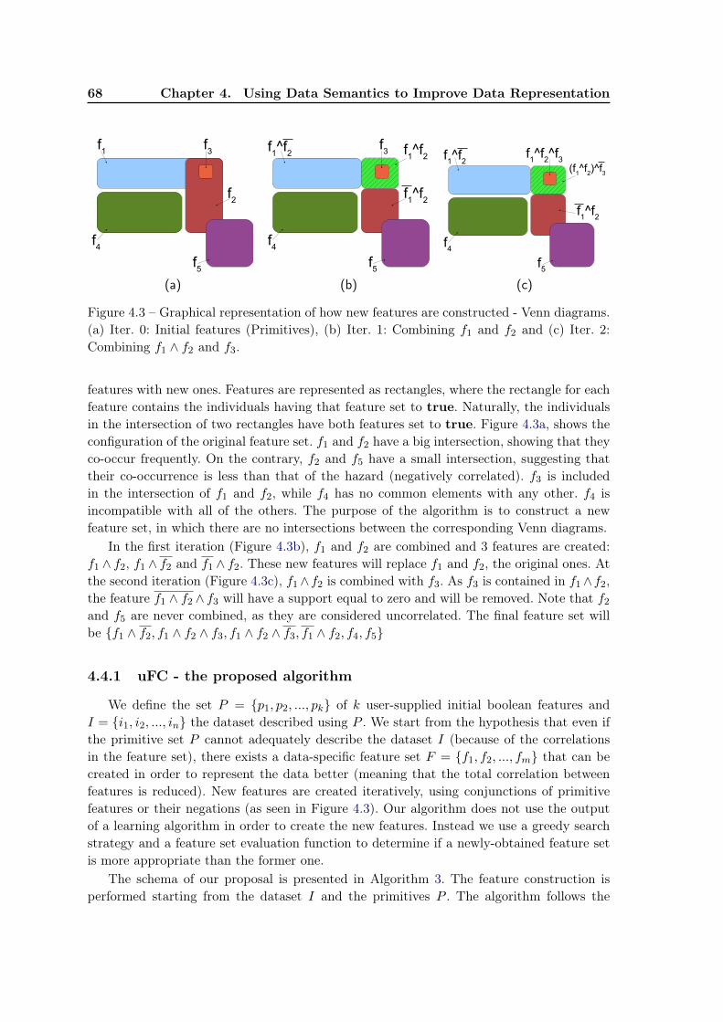
68 Chapter 4. Using Data Semantics to Improve Data Representation
f2
f3
f5
f4
f1
(a)
f1^f
2
f1^f
2
f4
f5
f1^f
2f3
(b)
f1^f
2^f
3(f
1^f
2)^f
3
f4
f5
f1^f
2
f1^f
2
(c)
Figure 4.3 – Graphical representation of how new features are constructed - Venn diagrams.(a) Iter. 0: Initial features (Primitives), (b) Iter. 1: Combining f1 and f2 and (c) Iter. 2:Combining f1 ∧ f2 and f3.
features with new ones. Features are represented as rectangles, where the rectangle for eachfeature contains the individuals having that feature set to true. Naturally, the individualsin the intersection of two rectangles have both features set to true. Figure 4.3a, shows theconfiguration of the original feature set. f1 and f2 have a big intersection, showing that theyco-occur frequently. On the contrary, f2 and f5 have a small intersection, suggesting thattheir co-occurrence is less than that of the hazard (negatively correlated). f3 is includedin the intersection of f1 and f2, while f4 has no common elements with any other. f4 isincompatible with all of the others. The purpose of the algorithm is to construct a newfeature set, in which there are no intersections between the corresponding Venn diagrams.
In the first iteration (Figure 4.3b), f1 and f2 are combined and 3 features are created:f1 ∧ f2, f1 ∧ f2 and f1 ∧ f2. These new features will replace f1 and f2, the original ones. Atthe second iteration (Figure 4.3c), f1∧f2 is combined with f3. As f3 is contained in f1∧f2,the feature f1 ∧ f2 ∧ f3 will have a support equal to zero and will be removed. Note that f2
and f5 are never combined, as they are considered uncorrelated. The final feature set willbe {f1 ∧ f2, f1 ∧ f2 ∧ f3, f1 ∧ f2 ∧ f3, f1 ∧ f2, f4, f5}
4.4.1 uFC - the proposed algorithm
We define the set P = {p1, p2, ..., pk} of k user-supplied initial boolean features andI = {i1, i2, ..., in} the dataset described using P . We start from the hypothesis that even ifthe primitive set P cannot adequately describe the dataset I (because of the correlationsin the feature set), there exists a data-specific feature set F = {f1, f2, ..., fm} that can becreated in order to represent the data better (meaning that the total correlation betweenfeatures is reduced). New features are created iteratively, using conjunctions of primitivefeatures or their negations (as seen in Figure 4.3). Our algorithm does not use the outputof a learning algorithm in order to create the new features. Instead we use a greedy searchstrategy and a feature set evaluation function to determine if a newly-obtained feature setis more appropriate than the former one.
The schema of our proposal is presented in Algorithm 3. The feature construction isperformed starting from the dataset I and the primitives P . The algorithm follows the
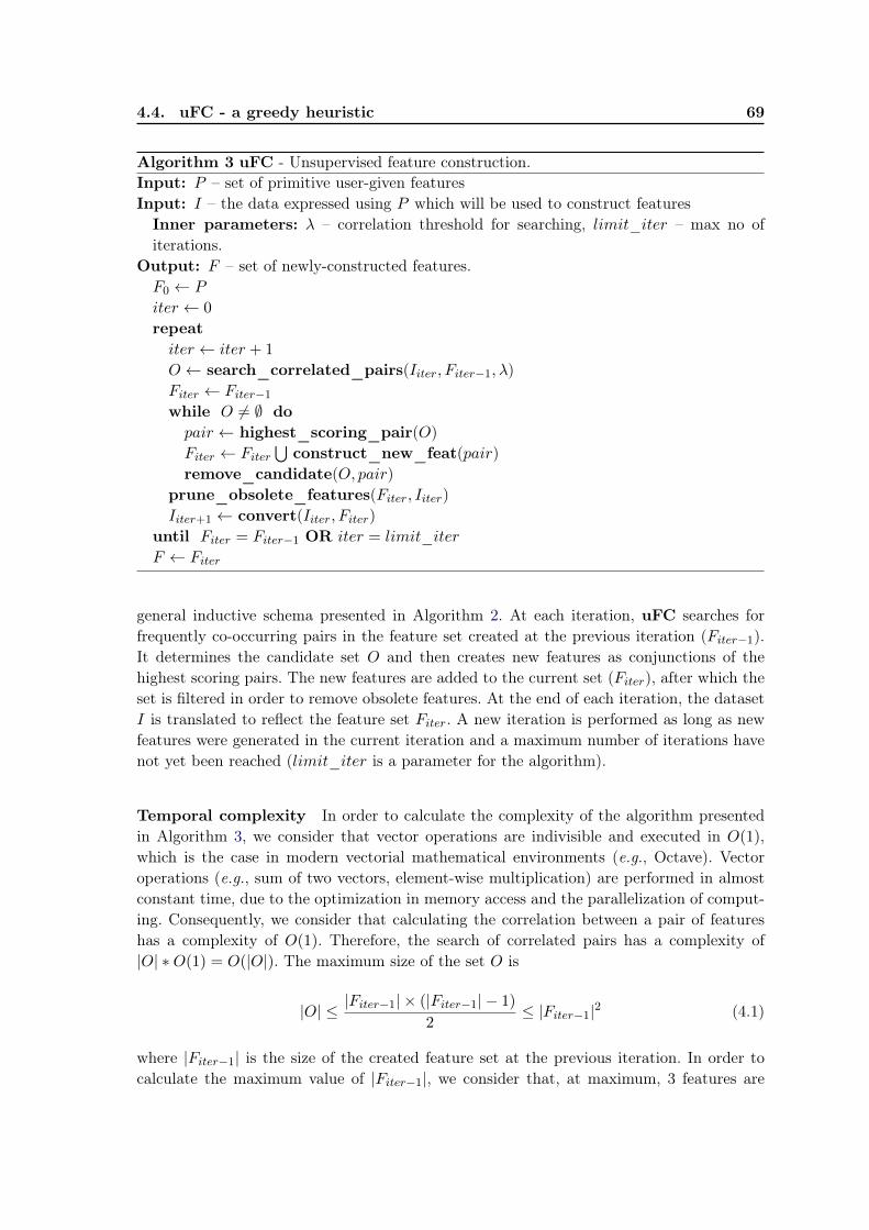
4.4. uFC - a greedy heuristic 69
Algorithm 3 uFC - Unsupervised feature construction.Input: P – set of primitive user-given featuresInput: I – the data expressed using P which will be used to construct featuresInner parameters: λ – correlation threshold for searching, limit_iter – max no ofiterations.
Output: F – set of newly-constructed features.F0 ← P
iter ← 0
repeatiter ← iter + 1
O ← search_correlated_pairs(Iiter, Fiter−1, λ)Fiter ← Fiter−1
while O 6= ∅ dopair ← highest_scoring_pair(O)Fiter ← Fiter
⋃construct_new_feat(pair)
remove_candidate(O, pair)prune_obsolete_features(Fiter, Iiter)Iiter+1 ← convert(Iiter, Fiter)
until Fiter = Fiter−1 OR iter = limit_iterF ← Fiter
general inductive schema presented in Algorithm 2. At each iteration, uFC searches forfrequently co-occurring pairs in the feature set created at the previous iteration (Fiter−1).It determines the candidate set O and then creates new features as conjunctions of thehighest scoring pairs. The new features are added to the current set (Fiter), after which theset is filtered in order to remove obsolete features. At the end of each iteration, the datasetI is translated to reflect the feature set Fiter. A new iteration is performed as long as newfeatures were generated in the current iteration and a maximum number of iterations havenot yet been reached (limit_iter is a parameter for the algorithm).
Temporal complexity In order to calculate the complexity of the algorithm presentedin Algorithm 3, we consider that vector operations are indivisible and executed in O(1),which is the case in modern vectorial mathematical environments (e.g., Octave). Vectoroperations (e.g., sum of two vectors, element-wise multiplication) are performed in almostconstant time, due to the optimization in memory access and the parallelization of comput-ing. Consequently, we consider that calculating the correlation between a pair of featureshas a complexity of O(1). Therefore, the search of correlated pairs has a complexity of|O| ∗O(1) = O(|O|). The maximum size of the set O is
|O| ≤ |Fiter−1| × (|Fiter−1| − 1)
2≤ |Fiter−1|2 (4.1)
where |Fiter−1| is the size of the created feature set at the previous iteration. In order tocalculate the maximum value of |Fiter−1|, we consider that, at maximum, 3 features are
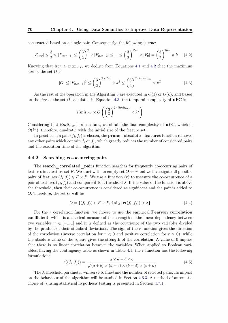
70 Chapter 4. Using Data Semantics to Improve Data Representation
constructed based on a single pair. Consequently, the following is true:
|Fiter| ≤3
2× |Fiter−1| ≤
(3
2
)2
× |Fiter−2| ≤ ... ≤(
3
2
)iter× |F0| =
(3
2
)iter× k (4.2)
Knowing that iter ≤ maxiter, we deduce from Equations 4.1 and 4.2 that the maximumsize of the set O is:
|O| ≤ |Fiter−1|2 ≤(
3
2
)2×iter× k2 ≤
(3
2
)2×limititer× k2 (4.3)
As the rest of the operation in the Algorithm 3 are executed in O(1) or O(k), and basedon the size of the set O calculated in Equation 4.3, the temporal complexity of uFC is
limititer ×O
((3
2
)2×limititer× k2
)
Considering that limititer is a constant, we obtain the final complexity of uFC, which isO(k2), therefore, quadratic with the initial size of the feature set.
In practice, if a pair (fi, fj) is chosen, the prune_obsolete_features function removesany other pairs which contain fi or fj , which greatly reduces the number of considered pairsand the execution time of the algorithm.
4.4.2 Searching co-occurring pairs
The search_correlated_pairs function searches for frequently co-occurring pairs offeatures in a feature set F . We start with an empty set O ← ∅ and we investigate all possiblepairs of features (fi, fj) ∈ F × F . We use a function (r) to measure the co-occurrence of apair of features (fi, fj) and compare it to a threshold λ. If the value of the function is abovethe threshold, then their co-occurrence is considered as significant and the pair is added toO. Therefore, the set O will be
O = {(fi, fj) ∈ F × F, i 6= j | r((fi, fj)) > λ} (4.4)
For the r correlation function, we choose to use the empirical Pearson correlationcoefficient, which is a classical measure of the strength of the linear dependency betweentwo variables. r ∈ [−1, 1] and it is defined as the covariance of the two variables dividedby the product of their standard deviations. The sign of the r function gives the directionof the correlation (inverse correlation for r < 0 and positive correlation for r > 0), whilethe absolute value or the square gives the strength of the correlation. A value of 0 impliesthat there is no linear correlation between the variables. When applied to Boolean vari-ables, having the contingency table as shown in Table 4.1, the r function has the followingformulation:
r((fi, fj)) =a× d− b× c√
(a+ b)× (a+ c)× (b+ d)× (c+ d)(4.5)
The λ threshold parameter will serve to fine-tune the number of selected pairs. Its impacton the behaviour of the algorithm will be studied in Section 4.6.3. A method of automaticchoice of λ using statistical hypothesis testing is presented in Section 4.7.1.
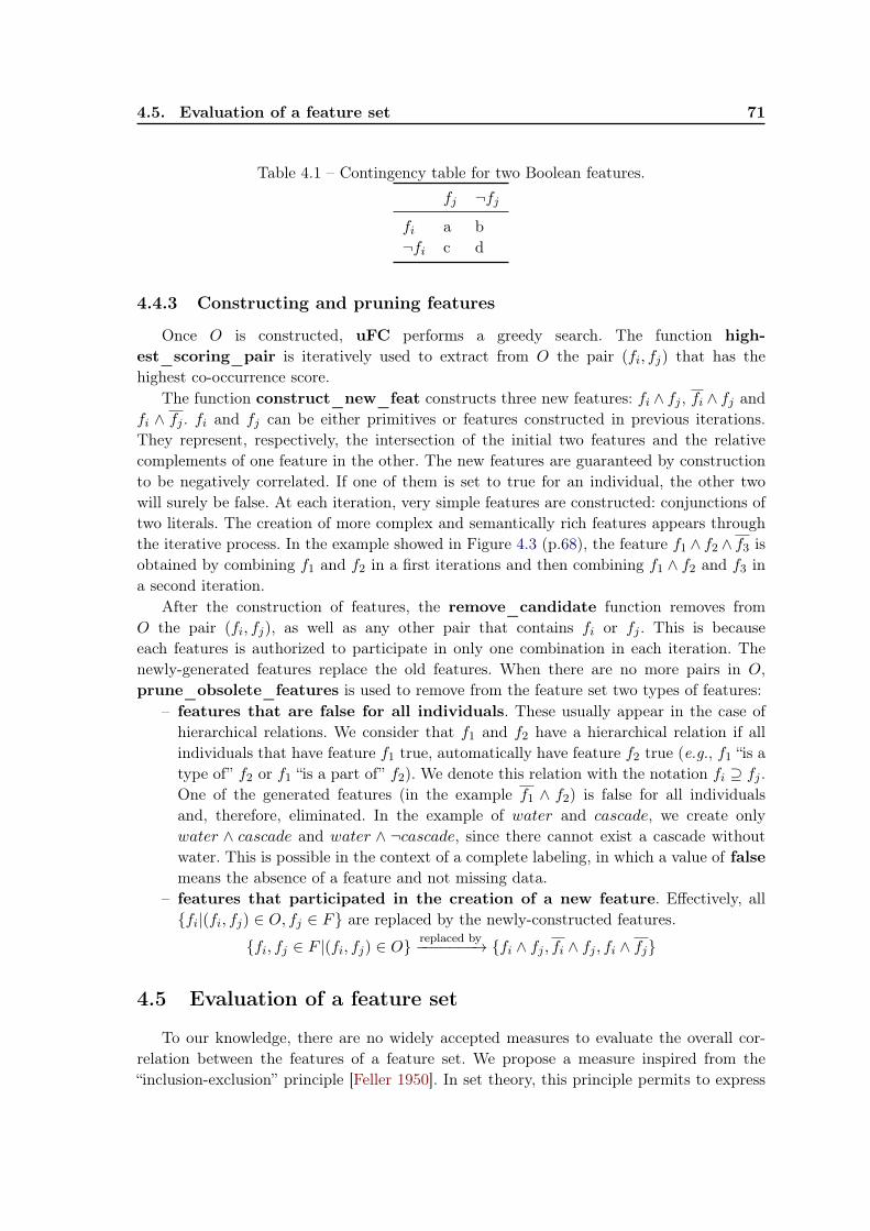
4.5. Evaluation of a feature set 71
Table 4.1 – Contingency table for two Boolean features.fj ¬fj
fi a b¬fi c d
4.4.3 Constructing and pruning features
Once O is constructed, uFC performs a greedy search. The function high-est_scoring_pair is iteratively used to extract from O the pair (fi, fj) that has thehighest co-occurrence score.
The function construct_new_feat constructs three new features: fi ∧ fj , fi ∧ fj andfi ∧ fj . fi and fj can be either primitives or features constructed in previous iterations.They represent, respectively, the intersection of the initial two features and the relativecomplements of one feature in the other. The new features are guaranteed by constructionto be negatively correlated. If one of them is set to true for an individual, the other twowill surely be false. At each iteration, very simple features are constructed: conjunctions oftwo literals. The creation of more complex and semantically rich features appears throughthe iterative process. In the example showed in Figure 4.3 (p.68), the feature f1 ∧ f2 ∧ f3 isobtained by combining f1 and f2 in a first iterations and then combining f1 ∧ f2 and f3 ina second iteration.
After the construction of features, the remove_candidate function removes fromO the pair (fi, fj), as well as any other pair that contains fi or fj . This is becauseeach features is authorized to participate in only one combination in each iteration. Thenewly-generated features replace the old features. When there are no more pairs in O,prune_obsolete_features is used to remove from the feature set two types of features:
– features that are false for all individuals. These usually appear in the case ofhierarchical relations. We consider that f1 and f2 have a hierarchical relation if allindividuals that have feature f1 true, automatically have feature f2 true (e.g., f1 “is atype of” f2 or f1 “is a part of” f2). We denote this relation with the notation fi ⊇ fj .One of the generated features (in the example f1 ∧ f2) is false for all individualsand, therefore, eliminated. In the example of water and cascade, we create onlywater ∧ cascade and water ∧ ¬cascade, since there cannot exist a cascade withoutwater. This is possible in the context of a complete labeling, in which a value of falsemeans the absence of a feature and not missing data.
– features that participated in the creation of a new feature. Effectively, all{fi|(fi, fj) ∈ O, fj ∈ F} are replaced by the newly-constructed features.
{fi, fj ∈ F |(fi, fj) ∈ O}replaced by−−−−−−−→ {fi ∧ fj , fi ∧ fj , fi ∧ fj}
4.5 Evaluation of a feature set
To our knowledge, there are no widely accepted measures to evaluate the overall cor-relation between the features of a feature set. We propose a measure inspired from the“inclusion-exclusion” principle [Feller 1950]. In set theory, this principle permits to express
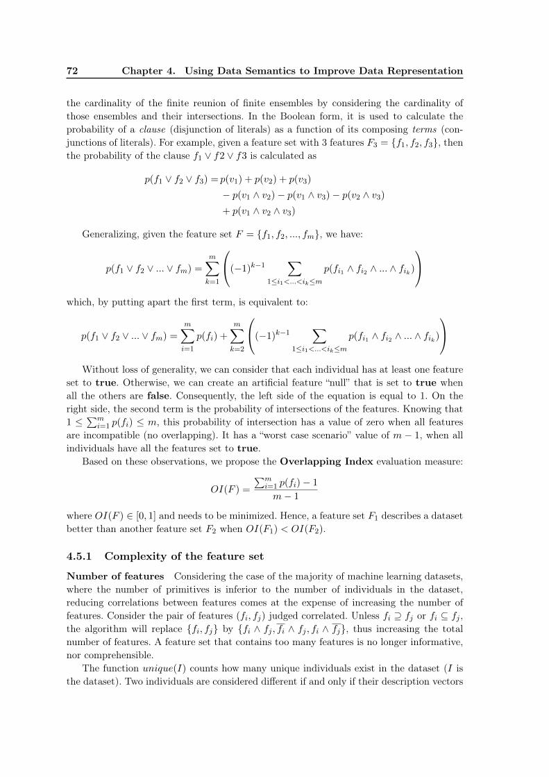
72 Chapter 4. Using Data Semantics to Improve Data Representation
the cardinality of the finite reunion of finite ensembles by considering the cardinality ofthose ensembles and their intersections. In the Boolean form, it is used to calculate theprobability of a clause (disjunction of literals) as a function of its composing terms (con-junctions of literals). For example, given a feature set with 3 features F3 = {f1, f2, f3}, thenthe probability of the clause f1 ∨ f2 ∨ f3 is calculated as
p(f1 ∨ f2 ∨ f3) = p(v1) + p(v2) + p(v3)
− p(v1 ∧ v2)− p(v1 ∧ v3)− p(v2 ∧ v3)
+ p(v1 ∧ v2 ∧ v3)
Generalizing, given the feature set F = {f1, f2, ..., fm}, we have:
p(f1 ∨ f2 ∨ ... ∨ fm) =m∑k=1
(−1)k−1∑
1≤i1<...<ik≤mp(fi1 ∧ fi2 ∧ ... ∧ fik)
which, by putting apart the first term, is equivalent to:
p(f1 ∨ f2 ∨ ... ∨ fm) =m∑i=1
p(fi) +m∑k=2
(−1)k−1∑
1≤i1<...<ik≤mp(fi1 ∧ fi2 ∧ ... ∧ fik)
Without loss of generality, we can consider that each individual has at least one feature
set to true. Otherwise, we can create an artificial feature “null” that is set to true whenall the others are false. Consequently, the left side of the equation is equal to 1. On theright side, the second term is the probability of intersections of the features. Knowing that1 ≤
∑mi=1 p(fi) ≤ m, this probability of intersection has a value of zero when all features
are incompatible (no overlapping). It has a “worst case scenario” value of m − 1, when allindividuals have all the features set to true.
Based on these observations, we propose the Overlapping Index evaluation measure:
OI(F ) =
∑mi=1 p(fi)− 1
m− 1
where OI(F ) ∈ [0, 1] and needs to be minimized. Hence, a feature set F1 describes a datasetbetter than another feature set F2 when OI(F1) < OI(F2).
4.5.1 Complexity of the feature set
Number of features Considering the case of the majority of machine learning datasets,where the number of primitives is inferior to the number of individuals in the dataset,reducing correlations between features comes at the expense of increasing the number offeatures. Consider the pair of features (fi, fj) judged correlated. Unless fi ⊇ fj or fi ⊆ fj ,the algorithm will replace {fi, fj} by {fi ∧ fj , fi ∧ fj , fi ∧ fj}, thus increasing the totalnumber of features. A feature set that contains too many features is no longer informative,nor comprehensible.
The function unique(I) counts how many unique individuals exist in the dataset (I isthe dataset). Two individuals are considered different if and only if their description vectors
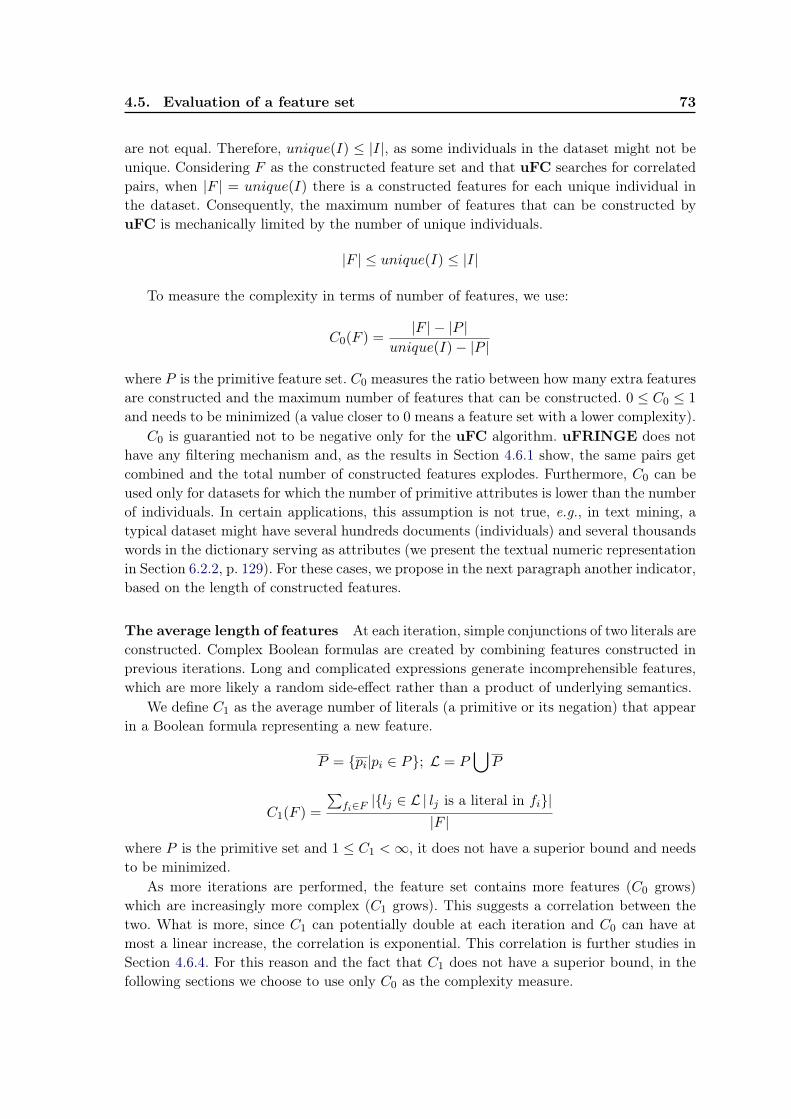
4.5. Evaluation of a feature set 73
are not equal. Therefore, unique(I) ≤ |I|, as some individuals in the dataset might not beunique. Considering F as the constructed feature set and that uFC searches for correlatedpairs, when |F | = unique(I) there is a constructed features for each unique individual inthe dataset. Consequently, the maximum number of features that can be constructed byuFC is mechanically limited by the number of unique individuals.
|F | ≤ unique(I) ≤ |I|
To measure the complexity in terms of number of features, we use:
C0(F ) =|F | − |P |
unique(I)− |P |
where P is the primitive feature set. C0 measures the ratio between how many extra featuresare constructed and the maximum number of features that can be constructed. 0 ≤ C0 ≤ 1
and needs to be minimized (a value closer to 0 means a feature set with a lower complexity).C0 is guarantied not to be negative only for the uFC algorithm. uFRINGE does not
have any filtering mechanism and, as the results in Section 4.6.1 show, the same pairs getcombined and the total number of constructed features explodes. Furthermore, C0 can beused only for datasets for which the number of primitive attributes is lower than the numberof individuals. In certain applications, this assumption is not true, e.g., in text mining, atypical dataset might have several hundreds documents (individuals) and several thousandswords in the dictionary serving as attributes (we present the textual numeric representationin Section 6.2.2, p. 129). For these cases, we propose in the next paragraph another indicator,based on the length of constructed features.
The average length of features At each iteration, simple conjunctions of two literals areconstructed. Complex Boolean formulas are created by combining features constructed inprevious iterations. Long and complicated expressions generate incomprehensible features,which are more likely a random side-effect rather than a product of underlying semantics.
We define C1 as the average number of literals (a primitive or its negation) that appearin a Boolean formula representing a new feature.
P = {pi|pi ∈ P}; L = P⋃P
C1(F ) =
∑fi∈F |{lj ∈ L | lj is a literal in fi}|
|F |
where P is the primitive set and 1 ≤ C1 <∞, it does not have a superior bound and needsto be minimized.
As more iterations are performed, the feature set contains more features (C0 grows)which are increasingly more complex (C1 grows). This suggests a correlation between thetwo. What is more, since C1 can potentially double at each iteration and C0 can have atmost a linear increase, the correlation is exponential. This correlation is further studies inSection 4.6.4. For this reason and the fact that C1 does not have a superior bound, in thefollowing sections we choose to use only C0 as the complexity measure.
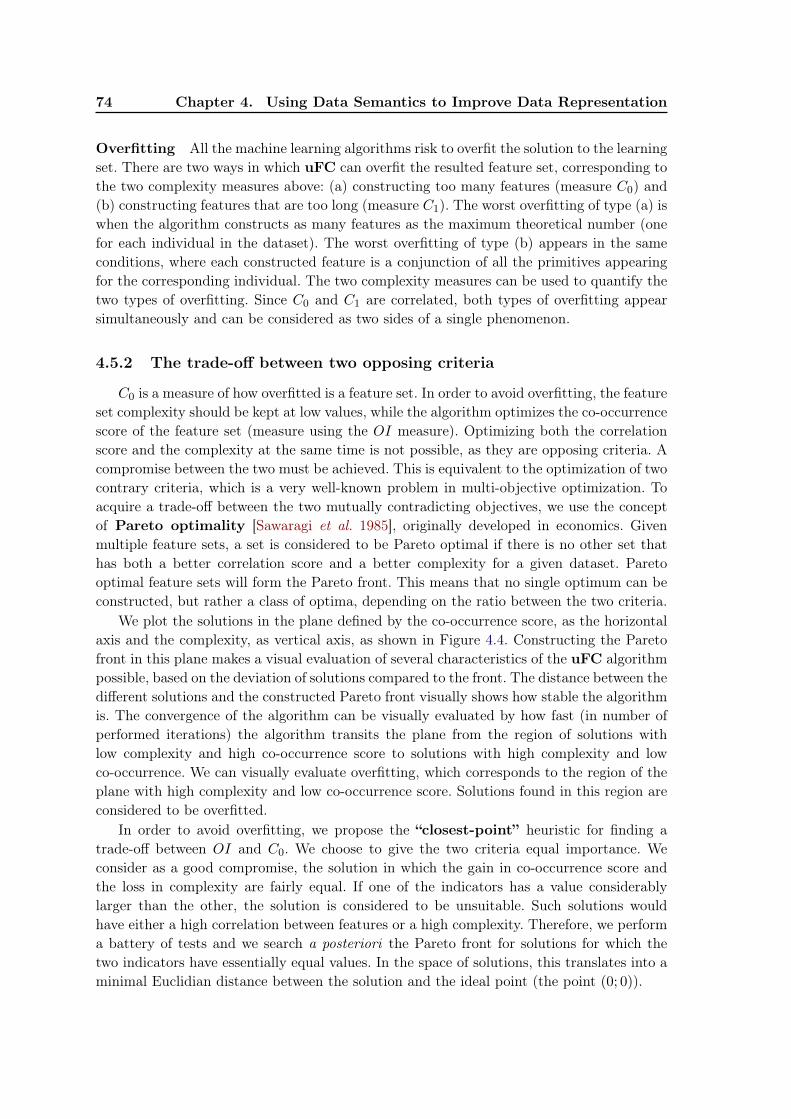
74 Chapter 4. Using Data Semantics to Improve Data Representation
Overfitting All the machine learning algorithms risk to overfit the solution to the learningset. There are two ways in which uFC can overfit the resulted feature set, corresponding tothe two complexity measures above: (a) constructing too many features (measure C0) and(b) constructing features that are too long (measure C1). The worst overfitting of type (a) iswhen the algorithm constructs as many features as the maximum theoretical number (onefor each individual in the dataset). The worst overfitting of type (b) appears in the sameconditions, where each constructed feature is a conjunction of all the primitives appearingfor the corresponding individual. The two complexity measures can be used to quantify thetwo types of overfitting. Since C0 and C1 are correlated, both types of overfitting appearsimultaneously and can be considered as two sides of a single phenomenon.
4.5.2 The trade-off between two opposing criteria
C0 is a measure of how overfitted is a feature set. In order to avoid overfitting, the featureset complexity should be kept at low values, while the algorithm optimizes the co-occurrencescore of the feature set (measure using the OI measure). Optimizing both the correlationscore and the complexity at the same time is not possible, as they are opposing criteria. Acompromise between the two must be achieved. This is equivalent to the optimization of twocontrary criteria, which is a very well-known problem in multi-objective optimization. Toacquire a trade-off between the two mutually contradicting objectives, we use the conceptof Pareto optimality [Sawaragi et al. 1985], originally developed in economics. Givenmultiple feature sets, a set is considered to be Pareto optimal if there is no other set thathas both a better correlation score and a better complexity for a given dataset. Paretooptimal feature sets will form the Pareto front. This means that no single optimum can beconstructed, but rather a class of optima, depending on the ratio between the two criteria.
We plot the solutions in the plane defined by the co-occurrence score, as the horizontalaxis and the complexity, as vertical axis, as shown in Figure 4.4. Constructing the Paretofront in this plane makes a visual evaluation of several characteristics of the uFC algorithmpossible, based on the deviation of solutions compared to the front. The distance between thedifferent solutions and the constructed Pareto front visually shows how stable the algorithmis. The convergence of the algorithm can be visually evaluated by how fast (in number ofperformed iterations) the algorithm transits the plane from the region of solutions withlow complexity and high co-occurrence score to solutions with high complexity and lowco-occurrence. We can visually evaluate overfitting, which corresponds to the region of theplane with high complexity and low co-occurrence score. Solutions found in this region areconsidered to be overfitted.
In order to avoid overfitting, we propose the “closest-point” heuristic for finding atrade-off between OI and C0. We choose to give the two criteria equal importance. Weconsider as a good compromise, the solution in which the gain in co-occurrence score andthe loss in complexity are fairly equal. If one of the indicators has a value considerablylarger than the other, the solution is considered to be unsuitable. Such solutions wouldhave either a high correlation between features or a high complexity. Therefore, we performa battery of tests and we search a posteriori the Pareto front for solutions for which thetwo indicators have essentially equal values. In the space of solutions, this translates into aminimal Euclidian distance between the solution and the ideal point (the point (0; 0)).
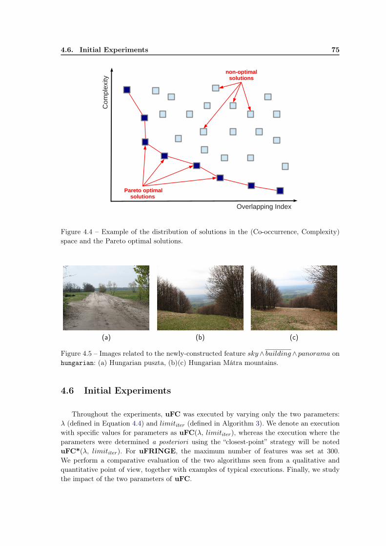
4.6. Initial Experiments 75
Overlapping Index
Co
mpl
exi
ty
non-optimalsolutions
Pareto optimalsolutions
Figure 4.4 – Example of the distribution of solutions in the (Co-occurrence, Complexity)space and the Pareto optimal solutions.
(a) (b) (c)
Figure 4.5 – Images related to the newly-constructed feature sky∧ building∧panorama onhungarian: (a) Hungarian puszta, (b)(c) Hungarian Mátra mountains.
4.6 Initial Experiments
Throughout the experiments, uFC was executed by varying only the two parameters:λ (defined in Equation 4.4) and limititer (defined in Algorithm 3). We denote an executionwith specific values for parameters as uFC(λ, limititer), whereas the execution where theparameters were determined a posteriori using the “closest-point” strategy will be noteduFC*(λ, limititer). For uFRINGE, the maximum number of features was set at 300.We perform a comparative evaluation of the two algorithms seen from a qualitative andquantitative point of view, together with examples of typical executions. Finally, we studythe impact of the two parameters of uFC.
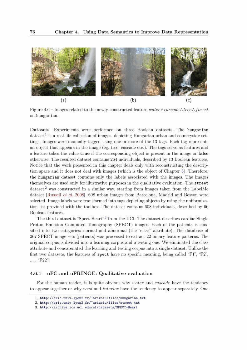
76 Chapter 4. Using Data Semantics to Improve Data Representation
(a) (b) (c)
Figure 4.6 – Images related to the newly-constructed feature water∧cascade∧tree∧foreston hungarian.
Datasets Experiments were performed on three Boolean datasets. The hungariandataset 1 is a real-life collection of images, depicting Hungarian urban and countryside set-tings. Images were manually tagged using one or more of the 13 tags. Each tag representsan object that appears in the image (eg. tree, cascade etc.). The tags serve as features anda feature takes the value true if the corresponding object is present in the image or falseotherwise. The resulted dataset contains 264 individuals, described by 13 Boolean features.Notice that the work presented in this chapter deals only with reconstructing the descrip-tion space and it does not deal with images (which is the object of Chapter 5). Therefore,the hungarian dataset contains only the labels associated with the images. The imagesthemselves are used only for illustrative purposes in the qualitative evaluation. The streetdataset 2 was constructed in a similar way, starting from images taken from the LabelMedataset [Russell et al. 2008]. 608 urban images from Barcelona, Madrid and Boston wereselected. Image labels were transformed into tags depicting objects by using the uniformiza-tion list provided with the toolbox. The dataset contains 608 individuals, described by 66Boolean features.
The third dataset is “Spect Heart” 3 from the UCI. The dataset describes cardiac SingleProton Emission Computed Tomography (SPECT) images. Each of the patients is clas-sified into two categories: normal and abnormal (the “class” attribute). The database of267 SPECT image sets (patients) was processed to extract 22 binary feature patterns. Theoriginal corpus is divided into a learning corpus and a testing one. We eliminated the classattribute and concatenated the learning and testing corpus into a single dataset. Unlike thefirst two datasets, the features of spect have no specific meaning, being called “F1”, “F2”,... , “F22”.
4.6.1 uFC and uFRINGE: Qualitative evaluation
For the human reader, it is quite obvious why water and cascade have the tendencyto appear together or why road and interior have the tendency to appear separately. One
1. http://eric.univ-lyon2.fr/~arizoiu/files/hungarian.txt2. http://eric.univ-lyon2.fr/~arizoiu/files/street.txt3. http://archive.ics.uci.edu/ml/datasets/SPECT+Heart
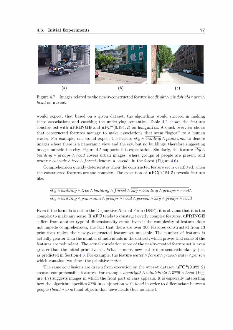
4.6. Initial Experiments 77
(a) (b) (c)
Figure 4.7 – Images related to the newly-constructed feature headlight∧windshield∧arm∧head on street.
would expect, that based on a given dataset, the algorithms would succeed in makingthese associations and catching the underlying semantics. Table 4.2 shows the featuresconstructed with uFRINGE and uFC*(0.194, 2) on hungarian. A quick overview showsthat constructed features manage to make associations that seem “logical” to a humanreader. For example, one would expect the feature sky ∧ building ∧ panorama to denoteimages where there is a panoramic view and the sky, but no buildings, therefore suggestingimages outside the city. Figure 4.5 supports this expectation. Similarly, the feature sky ∧building ∧ groups ∧ road covers urban images, where groups of people are present andwater ∧ cascade ∧ tree ∧ forest denotes a cascade in the forest (Figure 4.6).
Comprehension quickly deteriorates when the constructed feature set is overfitted, whenthe constructed features are too complex. The execution of uFC(0.184, 5) reveals featureslike:
sky ∧ building ∧ tree ∧ building ∧ forest ∧ sky ∧ building ∧ groups ∧ road∧
sky ∧ building ∧ panorama ∧ groups ∧ road ∧ person ∧ sky ∧ groups ∧ road
Even if the formula is not in the Disjunctive Normal Form (DNF), it is obvious that it is toocomplex to make any sense. If uFC tends to construct overly complex features, uFRINGEsuffers from another type of dimensionality curse. Even if the complexity of features doesnot impede comprehension, the fact that there are over 300 features constructed from 13primitives makes the newly-constructed feature set unusable. The number of features isactually greater than the number of individuals in the dataset, which proves that some of thefeatures are redundant. The actual correlation score of the newly-created feature set is evengreater than the initial primitive set. What is more, new features present redundancy, justas predicted in Section 4.3. For example, the feature water∧forest∧grass∧water∧personwhich contains two times the primitive water.
The same conclusions are drawn from execution on the street dataset. uFC*(0.322, 2)
creates comprehensible features. For example headlight ∧ windshield ∧ arm ∧ head (Fig-ure 4.7) suggests images in which the front part of cars appears. It is especially interestinghow the algorithm specifies arm in conjunction with head in order to differenciate betweenpeople (head ∧ arm) and objects that have heads (but no arms).
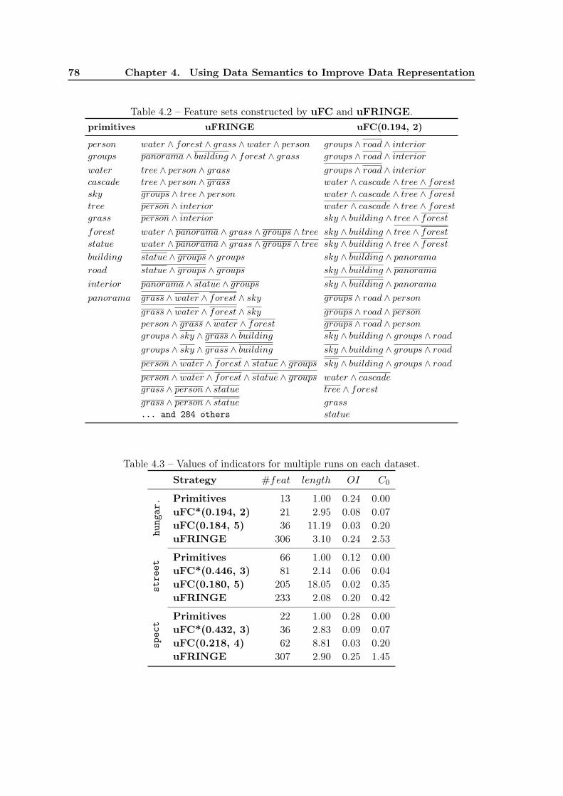
78 Chapter 4. Using Data Semantics to Improve Data Representation
Table 4.2 – Feature sets constructed by uFC and uFRINGE.primitives uFRINGE uFC(0.194, 2)
person water ∧ forest ∧ grass ∧ water ∧ person groups ∧ road ∧ interiorgroups panorama ∧ building ∧ forest ∧ grass groups ∧ road ∧ interiorwater tree ∧ person ∧ grass groups ∧ road ∧ interiorcascade tree ∧ person ∧ grass water ∧ cascade ∧ tree ∧ forestsky groups ∧ tree ∧ person water ∧ cascade ∧ tree ∧ foresttree person ∧ interior water ∧ cascade ∧ tree ∧ forestgrass person ∧ interior sky ∧ building ∧ tree ∧ forestforest water ∧ panorama ∧ grass ∧ groups ∧ tree sky ∧ building ∧ tree ∧ foreststatue water ∧ panorama ∧ grass ∧ groups ∧ tree sky ∧ building ∧ tree ∧ forestbuilding statue ∧ groups ∧ groups sky ∧ building ∧ panoramaroad statue ∧ groups ∧ groups sky ∧ building ∧ panoramainterior panorama ∧ statue ∧ groups sky ∧ building ∧ panoramapanorama grass ∧ water ∧ forest ∧ sky groups ∧ road ∧ person
grass ∧ water ∧ forest ∧ sky groups ∧ road ∧ personperson ∧ grass ∧ water ∧ forest groups ∧ road ∧ persongroups ∧ sky ∧ grass ∧ building sky ∧ building ∧ groups ∧ roadgroups ∧ sky ∧ grass ∧ building sky ∧ building ∧ groups ∧ roadperson ∧ water ∧ forest ∧ statue ∧ groups sky ∧ building ∧ groups ∧ roadperson ∧ water ∧ forest ∧ statue ∧ groups water ∧ cascadegrass ∧ person ∧ statue tree ∧ forestgrass ∧ person ∧ statue grass
... and 284 others statue
Table 4.3 – Values of indicators for multiple runs on each dataset.Strategy #feat length OI C0
hung
ar. Primitives 13 1.00 0.24 0.00
uFC*(0.194, 2) 21 2.95 0.08 0.07uFC(0.184, 5) 36 11.19 0.03 0.20uFRINGE 306 3.10 0.24 2.53
stre
et
Primitives 66 1.00 0.12 0.00uFC*(0.446, 3) 81 2.14 0.06 0.04uFC(0.180, 5) 205 18.05 0.02 0.35uFRINGE 233 2.08 0.20 0.42
spec
t
Primitives 22 1.00 0.28 0.00uFC*(0.432, 3) 36 2.83 0.09 0.07uFC(0.218, 4) 62 8.81 0.03 0.20uFRINGE 307 2.90 0.25 1.45
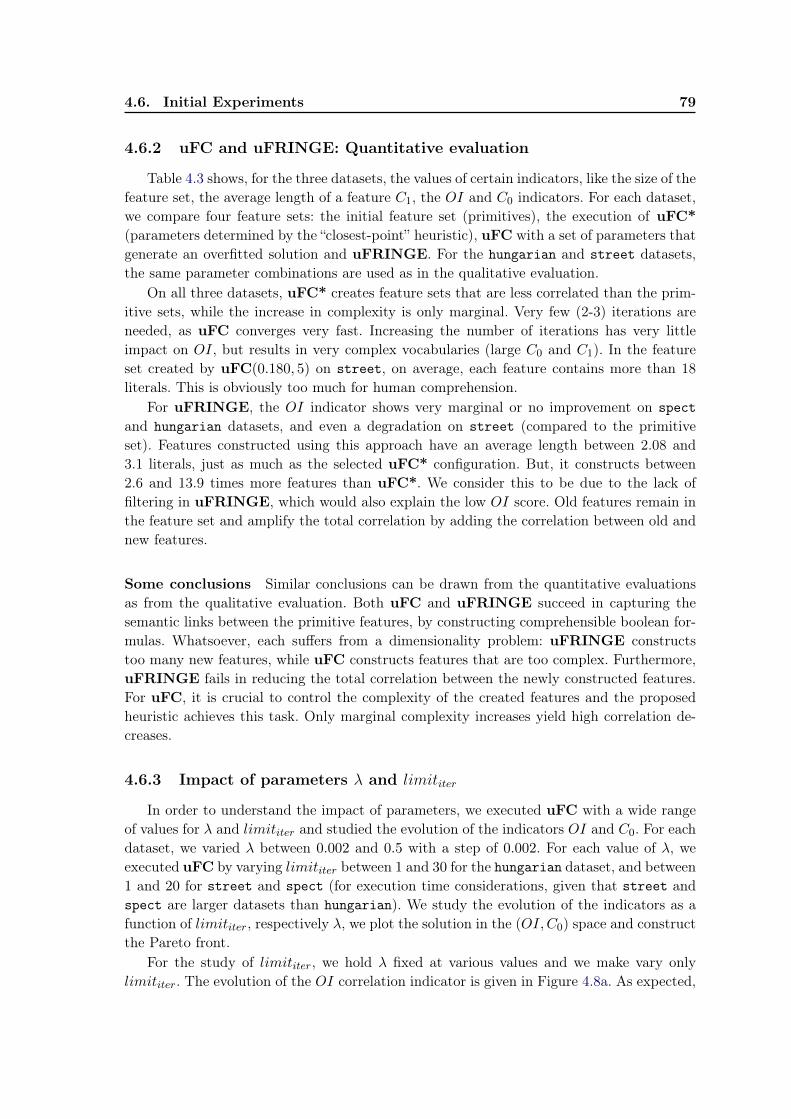
4.6. Initial Experiments 79
4.6.2 uFC and uFRINGE: Quantitative evaluation
Table 4.3 shows, for the three datasets, the values of certain indicators, like the size of thefeature set, the average length of a feature C1, the OI and C0 indicators. For each dataset,we compare four feature sets: the initial feature set (primitives), the execution of uFC*(parameters determined by the “closest-point” heuristic), uFC with a set of parameters thatgenerate an overfitted solution and uFRINGE. For the hungarian and street datasets,the same parameter combinations are used as in the qualitative evaluation.
On all three datasets, uFC* creates feature sets that are less correlated than the prim-itive sets, while the increase in complexity is only marginal. Very few (2-3) iterations areneeded, as uFC converges very fast. Increasing the number of iterations has very littleimpact on OI, but results in very complex vocabularies (large C0 and C1). In the featureset created by uFC(0.180, 5) on street, on average, each feature contains more than 18literals. This is obviously too much for human comprehension.
For uFRINGE, the OI indicator shows very marginal or no improvement on spectand hungarian datasets, and even a degradation on street (compared to the primitiveset). Features constructed using this approach have an average length between 2.08 and3.1 literals, just as much as the selected uFC* configuration. But, it constructs between2.6 and 13.9 times more features than uFC*. We consider this to be due to the lack offiltering in uFRINGE, which would also explain the low OI score. Old features remain inthe feature set and amplify the total correlation by adding the correlation between old andnew features.
Some conclusions Similar conclusions can be drawn from the quantitative evaluationsas from the qualitative evaluation. Both uFC and uFRINGE succeed in capturing thesemantic links between the primitive features, by constructing comprehensible boolean for-mulas. Whatsoever, each suffers from a dimensionality problem: uFRINGE constructstoo many new features, while uFC constructs features that are too complex. Furthermore,uFRINGE fails in reducing the total correlation between the newly constructed features.For uFC, it is crucial to control the complexity of the created features and the proposedheuristic achieves this task. Only marginal complexity increases yield high correlation de-creases.
4.6.3 Impact of parameters λ and limititer
In order to understand the impact of parameters, we executed uFC with a wide rangeof values for λ and limititer and studied the evolution of the indicators OI and C0. For eachdataset, we varied λ between 0.002 and 0.5 with a step of 0.002. For each value of λ, weexecuted uFC by varying limititer between 1 and 30 for the hungarian dataset, and between1 and 20 for street and spect (for execution time considerations, given that street andspect are larger datasets than hungarian). We study the evolution of the indicators as afunction of limititer, respectively λ, we plot the solution in the (OI,C0) space and constructthe Pareto front.
For the study of limititer, we hold λ fixed at various values and we make vary onlylimititer. The evolution of the OI correlation indicator is given in Figure 4.8a. As expected,
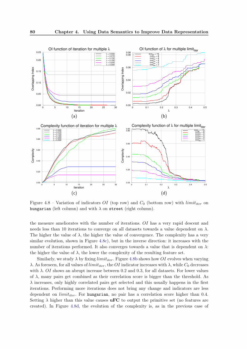
80 Chapter 4. Using Data Semantics to Improve Data Representation
0.00
0.05
0.10
0.15
0.20
0.23
0 5 10 15 20 25 30
Ove
rla
pp
ing
In
de
x
iteration
OI function of iteration for multiple λλ = 0.002λ = 0.070λ = 0.150λ = 0.190λ = 0.200λ = 0.300
(a)
0.00
0.02
0.04
0.06
0.08 0.08
0 0.1 0.2 0.3 0.4 0.5
Ove
rla
pp
ing
In
de
x
λ
OI function of λ for multiple limititerlimititer = 15
limititer = 8limititer = 4limititer = 3limititer = 2limititer = 1
(b)
0.00
0.20
0.40
0.60
0.80
0.99
0 5 10 15 20 25 30
Co
mp
lexity
iteration
Complexity function of iteration for multiple λλ = 0.002λ = 0.070λ = 0.150λ = 0.190λ = 0.200λ = 0.300
(c)
0.00
0.20
0.40
0.60
0.80 0.83
0 0.1 0.2 0.3 0.4 0.5
Co
mp
lexity
λ
Complexity function of λ for multiple limititerlimititer = 15
limititer = 8limititer = 4limititer = 3limititer = 2limititer = 1
(d)
Figure 4.8 – Variation of indicators OI (top row) and C0 (bottom row) with limititer onhungarian (left column) and with λ on street (right column).
the measure ameliorates with the number of iterations. OI has a very rapid descent andneeds less than 10 iterations to converge on all datasets towards a value dependent on λ.The higher the value of λ, the higher the value of convergence. The complexity has a verysimilar evolution, shown in Figure 4.8c), but in the inverse direction: it increases with thenumber of iterations performed. It also converges towards a value that is dependent on λ:the higher the value of λ, the lower the complexity of the resulting feature set.
Similarly, we study λ by fixing limititer. Figure 4.8b shows how OI evolves when varyingλ. As foreseen, for all values of limititer, theOI indicator increases with λ, while C0 decreaseswith λ. OI shows an abrupt increase between 0.2 and 0.3, for all datasets. For lower valuesof λ, many pairs get combined as their correlation score is bigger than the threshold. Asλ increases, only highly correlated pairs get selected and this usually happens in the firstiterations. Performing more iterations does not bring any change and indicators are lessdependent on limititer. For hungarian, no pair has a correlation score higher than 0.4.Setting λ higher than this value causes uFC to output the primitive set (no features arecreated). In Figure 4.8d, the evolution of the complexity is, as in the previous case of
4.6. Initial Experiments 81
0
0.1
0.2
0.3
0.4
0.5
0.6
0.7
0.8
0.9
0 0.05 0.1 0.15 0.2 0.25
Co
mp
lexity
Overlapping Index
The Pareto front
Pareto frontAll solutions
uFC*(0.432, 3)
(a)
0
0.05
0.1
0.15
0.2
0.25
0.3
0 0.05 0.1 0.15 0.2 0.25 0.3
Co
mp
lexity
Overlapping Index
The Pareto front (magnified)
Pareto frontAll solutions
uFC*(0.432, 3)
(b)
Figure 4.9 – The distribution of solutions, the Pareto front and the closest-point on spectdataset.
limititer very similar to the one of OI, but in the inverse direction. The complexity of theconstructed feature set descends with the increase of λ.
Pareto optimality To study Pareto optimality, we plot the generated solutions in the(OI, C0) space. Figure 4.9a presents the distribution of solutions, the Pareto front and thesolution chosen by the “closest-point” heuristic. The solutions generated by uFC with a widerange of parameter values are not dispersed in the solution space, but their distribution israther close together. This shows good algorithm stability. Even if not all the solutions arePareto optimal, none of them are too distant from the front and there are no outliers.
Most of the solutions densely populate the part of the curve corresponding to low OI
and high C0. As pointed out in the Section 4.5.2, the area of the front corresponding tohigh feature set complexity (high C0) represents the overfitting area. This confirms that thealgorithm converges fast, then enters overfitting. Most of the improvement in quality is donein the first 2-3 iterations, while further iterating improves quality only marginally with thecost of an explosion of complexity. The “closest-point” heuristic keeps the constructing outof overfitting, by stopping the algorithm at the point where the gain of co-occurence scoreand the loss in complexity are fairly equal. Figure 4.9b zooms to the region of the solutionspace corresponding for low numbers of iterations and both axis have equal scales.
4.6.4 Relation between number of features and feature length
Both the average length of a feature (C1) and the number of features (C0) increase withthe number of iterations. In Section 4.5.1 we have speculated that the two are correlated:C1 = f(C0). For each λ in the batch of tests, we create the C0 and C1 series dependingon the limititer. Figure 4.10 shows the series for λ ∈ [0.002, 0.07, 0.15, 0.19, 0.2, 0.3] (C1 isplotted on a logarithmic scale). We perform a statistical hypothesis test, using the Kendall
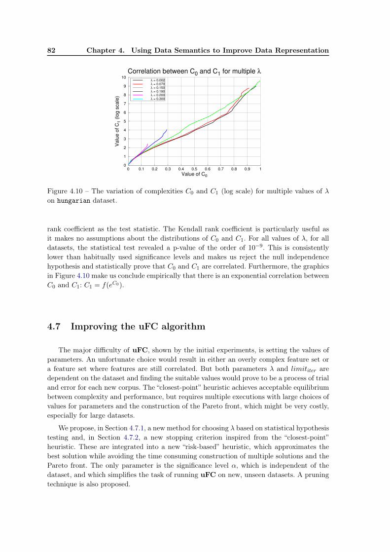
82 Chapter 4. Using Data Semantics to Improve Data Representation
0
1
2
3
4
5
6
7
8
9
10
0 0.1 0.2 0.3 0.4 0.5 0.6 0.7 0.8 0.9 1
Valu
e o
f C
1 (
log s
cale
)
Value of C0
Correlation between C0 and C1 for multiple λλ = 0.002λ = 0.070λ = 0.150λ = 0.190λ = 0.200λ = 0.300
Figure 4.10 – The variation of complexities C0 and C1 (log scale) for multiple values of λon hungarian dataset.
rank coefficient as the test statistic. The Kendall rank coefficient is particularly useful asit makes no assumptions about the distributions of C0 and C1. For all values of λ, for alldatasets, the statistical test revealed a p-value of the order of 10−9. This is consistentlylower than habitually used significance levels and makes us reject the null independencehypothesis and statistically prove that C0 and C1 are correlated. Furthermore, the graphicsin Figure 4.10 make us conclude empirically that there is an exponential correlation betweenC0 and C1: C1 = f(eC0).
4.7 Improving the uFC algorithm
The major difficulty of uFC, shown by the initial experiments, is setting the values ofparameters. An unfortunate choice would result in either an overly complex feature set ora feature set where features are still correlated. But both parameters λ and limititer aredependent on the dataset and finding the suitable values would prove to be a process of trialand error for each new corpus. The “closest-point” heuristic achieves acceptable equilibriumbetween complexity and performance, but requires multiple executions with large choices ofvalues for parameters and the construction of the Pareto front, which might be very costly,especially for large datasets.
We propose, in Section 4.7.1, a new method for choosing λ based on statistical hypothesistesting and, in Section 4.7.2, a new stopping criterion inspired from the “closest-point”heuristic. These are integrated into a new “risk-based” heuristic, which approximates thebest solution while avoiding the time consuming construction of multiple solutions and thePareto front. The only parameter is the significance level α, which is independent of thedataset, and which simplifies the task of running uFC on new, unseen datasets. A pruningtechnique is also proposed.
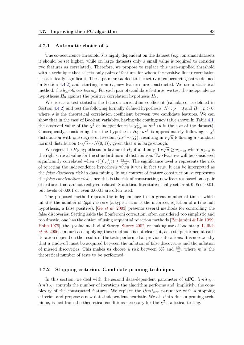
4.7. Improving the uFC algorithm 83
4.7.1 Automatic choice of λ
The co-occurrence threshold λ is highly dependent on the dataset (e.g., on small datasetsit should be set higher, while on large datasets only a small value is required to considertwo features as correlated). Therefore, we propose to replace this user-supplied thresholdwith a technique that selects only pairs of features for whom the positive linear correlationis statistically significant. These pairs are added to the set O of co-occurring pairs (definedin Section 4.4.2) and, starting from O, new features are constructed. We use a statisticalmethod: the hypothesis testing. For each pair of candidate features, we test the independencehypothesis H0 against the positive correlation hypothesis H1.
We use as a test statistic the Pearson correlation coefficient (calculated as defined inSection 4.4.2) and test the following formally defined hypothesis: H0 : ρ = 0 and H1 : ρ > 0,where ρ is the theoretical correlation coefficient between two candidate features. We canshow that in the case of Boolean variables, having the contingency table shown in Table 4.1,the observed value of the χ2 of independence is χ2
obs = nr2 (n is the size of the dataset).Consequently, considering true the hypothesis H0, nr2 is approximately following a χ2
distribution with one degree of freedom (nr2 ∼ χ21), resulting in r
√n following a standard
normal distribution (r√n ∼ N(0, 1)), given that n is large enough.
We reject the H0 hypothesis in favour of H1 if and only if r√n ≥ u1−α, where u1−α is
the right critical value for the standard normal distribution. Two features will be consideredsignificantly correlated when r((fi, fj)) ≥ u1−α√
n. The significance level α represents the risk
of rejecting the independence hypothesis when it was in fact true. It can be interpreted asthe false discovery risk in data mining. In our context of feature construction, α representsthe false construction risk, since this is the risk of constructing new features based on a pairof features that are not really correlated. Statistical literature usually sets α at 0.05 or 0.01,but levels of 0.001 or even 0.0001 are often used.
The proposed method repeats the independence test a great number of times, whichinflates the number of type I errors (a type I error is the incorrect rejection of a true nullhypothesis, a false positive). [Ge et al. 2003] presents several methods for controlling thefalse discoveries. Setting aside the Bonferroni correction, often considered too simplistic andtoo drastic, one has the option of using sequential rejection methods [Benjamini & Liu 1999,Holm 1979], the q-value method of Storey [Storey 2002] or making use of bootstrap [Lallichet al. 2006]. In our case, applying these methods is not clear-cut, as tests performed at eachiteration depend on the results of the tests performed at previous iterations. It is noteworthythat a trade-off must be acquired between the inflation of false discoveries and the inflationof missed discoveries. This makes us choose a risk between 5% and 5%
m , where m is thetheoretical number of tests to be performed.
4.7.2 Stopping criterion. Candidate pruning technique.
In this section, we deal with the second data-dependent parameter of uFC: limititer.limititer controls the number of iterations the algorithm performs and, implicitly, the com-plexity of the constructed features. We replace the limititer parameter with a stoppingcriterion and propose a new data-independent heuristic. We also introduce a pruning tech-nique, issued from the theoretical conditions necessary for the χ2 statistical testing.
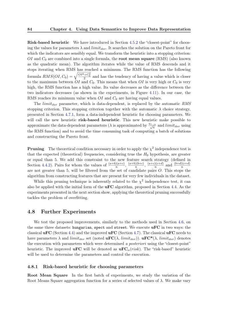
84 Chapter 4. Using Data Semantics to Improve Data Representation
Risk-based heuristic We have introduced in Section 4.5.2 the “closest-point” for choos-ing the values for parameters λ and limititer. It searches the solution on the Pareto front forwhich the indicators are sensibly equal. We transform the heuristic into a stopping criterion:OI and C0 are combined into a single formula, the root mean square (RMS) (also knownas the quadratic mean). The algorithm iterates while the value of RMS descends and itstops iterating when RMS has reached a minimum. The RMS function has the following
formula RMS(OI,C0) =
√OI2+C2
02 and has the tendency of having a value which is closer
to the maximum between OI and C0. This means that when OI is very high or C0 is veryhigh, the RMS function has a high value. Its value decreases as the difference between thetwo indicators decreases (as shown in the experiments, in Figure 4.11). In our case, theRMS reaches its minimum value when OI and C0 are having equal values.
The limititer parameter, which is data-dependent, is replaced by the automatic RMSstopping criterion. This stopping criterion together with the automatic λ choice strategy,presented in Section 4.7.1, form a data-independent heuristic for choosing parameters. Wewill call the new heuristic risk-based heuristic. This new heuristic make possible toapproximate the data-dependent parameters (λ is approximated by u1−α√
nand limititer using
the RMS function) and to avoid the time consuming task of computing a batch of solutionsand constructing the Pareto front.
Pruning The theoretical condition necessary in order to apply the χ2 independence test isthat the expected (theoretical) frequencies, considering true the H0 hypothesis, are greateror equal than 5. We add this constraint to the new feature search strategy (defined inSection 4.4.2). Pairs for whom the values of (a+b)(a+c)
n , (a+b)(b+c)n , (a+c)(c+d)
n and (b+d)(c+d)n
are not greater than 5, will be filtered from the set of candidate pairs O. This stops thealgorithm from constructing features that are present for very few individuals in the dataset.
While this pruning technique is inherently related to the χ2 independence test, it canalso be applied with the initial form of the uFC algorithm, proposed in Section 4.4. As theexperiments presented in the next section show, applying the theoretical pruning successfullytackles the problem of overfitting.
4.8 Further Experiments
We test the proposed improvements, similarly to the methods used in Section 4.6, onthe same three datasets: hungarian, spect and street. We execute uFC in two ways: theclassical uFC (Section 4.4) and the improved uFC (Section 4.7). The classical uFC needs tohave parameters λ and limititer set (noted uFC(λ, limititer)). uFC*(λ, limititer) denotesthe execution with parameters which were determined a posteriori using the “closest-point”heuristic. The improved uFC will be denoted as uFCα(risk). The “risk-based” heuristicwill be used to determine the parameters and control the execution.
4.8.1 Risk-based heuristic for choosing parameters
Root Mean Square In the first batch of experiments, we study the variation of theRoot Means Square aggregation function for a series of selected values of λ. We make vary
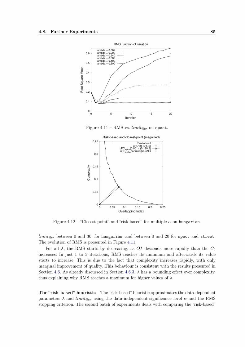
4.8. Further Experiments 85
0
0.1
0.2
0.3
0.4
0.5
0.6
0 5 10 15 20
Ro
ot
Sq
ua
re M
ea
n
iteration
RMS function of iteration
lambda = 0.002lambda = 0.200lambda = 0.240lambda = 0.300lambda = 0.400lambda = 0.500
Figure 4.11 – RMS vs. limititer on spect.
0
0.05
0.1
0.15
0.2
0.25
0 0.05 0.1 0.15 0.2 0.25
Co
mp
lexity
Overlapping Index
Risk-based and closest-point (magnified)
Pareto frontuFC*(0.194, 2)
uFCalpha(0.001): (0.190,2)uFCalpha for multiple risks
Figure 4.12 – “Closest-point” and “risk-based” for multiple α on hungarian.
limititer between 0 and 30, for hungarian, and between 0 and 20 for spect and street.The evolution of RMS is presented in Figure 4.11.
For all λ, the RMS starts by decreasing, as OI descends more rapidly than the C0
increases. In just 1 to 3 iterations, RMS reaches its minimum and afterwards its valuestarts to increase. This is due to the fact that complexity increases rapidly, with onlymarginal improvement of quality. This behaviour is consistent with the results presented inSection 4.6. As already discussed in Section 4.6.3, λ has a bounding effect over complexity,thus explaining why RMS reaches a maximum for higher values of λ.
The “risk-based” heuristic The “risk-based” heuristic approximates the data-dependentparameters λ and limititer using the data-independent significance level α and the RMSstopping criterion. The second batch of experiments deals with comparing the “risk-based”
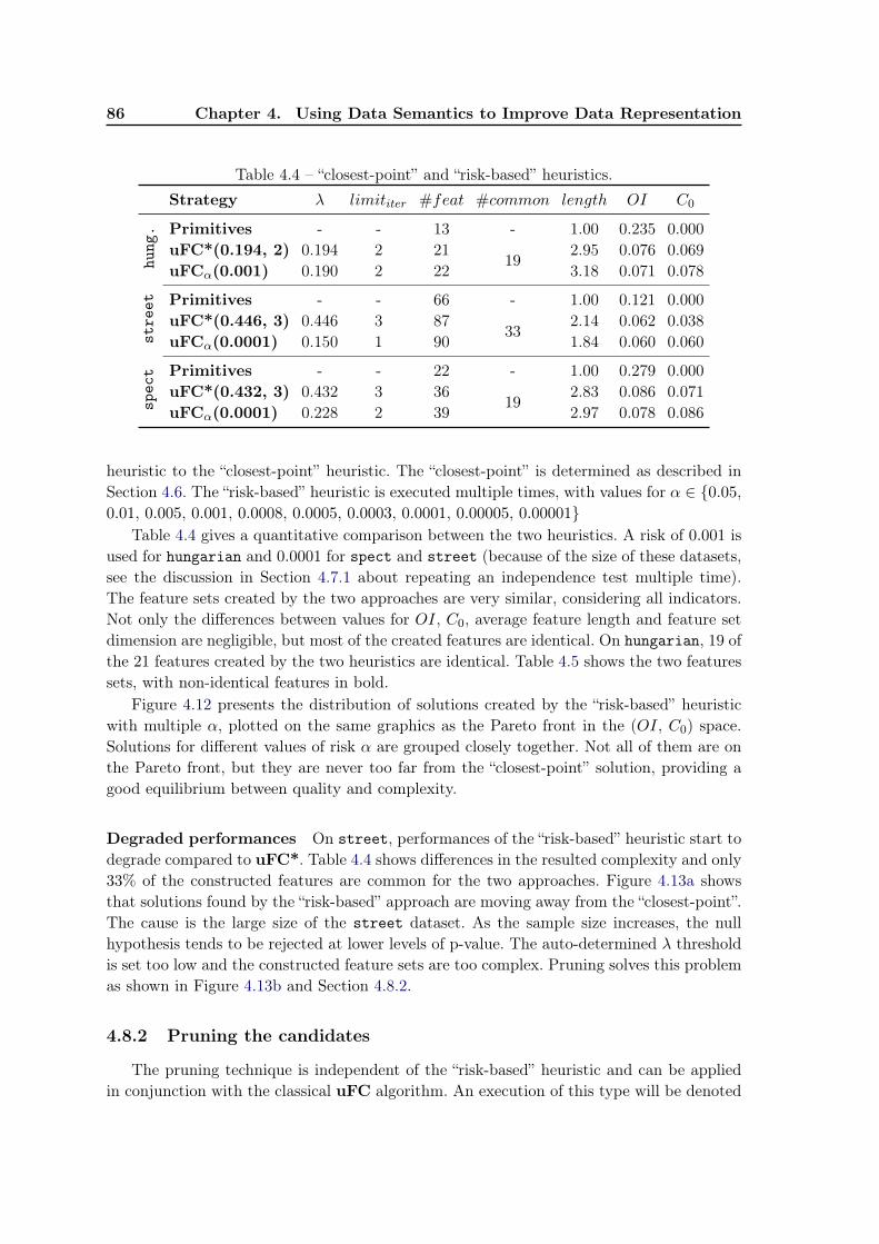
86 Chapter 4. Using Data Semantics to Improve Data Representation
Table 4.4 – “closest-point” and “risk-based” heuristics.Strategy λ limititer #feat #common length OI C0
hung
. Primitives - - 13 - 1.00 0.235 0.000uFC*(0.194, 2) 0.194 2 21
192.95 0.076 0.069
uFCα(0.001) 0.190 2 22 3.18 0.071 0.078
stre
et Primitives - - 66 - 1.00 0.121 0.000uFC*(0.446, 3) 0.446 3 87
332.14 0.062 0.038
uFCα(0.0001) 0.150 1 90 1.84 0.060 0.060
spec
t Primitives - - 22 - 1.00 0.279 0.000uFC*(0.432, 3) 0.432 3 36
192.83 0.086 0.071
uFCα(0.0001) 0.228 2 39 2.97 0.078 0.086
heuristic to the “closest-point” heuristic. The “closest-point” is determined as described inSection 4.6. The “risk-based” heuristic is executed multiple times, with values for α ∈ {0.05,0.01, 0.005, 0.001, 0.0008, 0.0005, 0.0003, 0.0001, 0.00005, 0.00001}
Table 4.4 gives a quantitative comparison between the two heuristics. A risk of 0.001 isused for hungarian and 0.0001 for spect and street (because of the size of these datasets,see the discussion in Section 4.7.1 about repeating an independence test multiple time).The feature sets created by the two approaches are very similar, considering all indicators.Not only the differences between values for OI, C0, average feature length and feature setdimension are negligible, but most of the created features are identical. On hungarian, 19 ofthe 21 features created by the two heuristics are identical. Table 4.5 shows the two featuressets, with non-identical features in bold.
Figure 4.12 presents the distribution of solutions created by the “risk-based” heuristicwith multiple α, plotted on the same graphics as the Pareto front in the (OI, C0) space.Solutions for different values of risk α are grouped closely together. Not all of them are onthe Pareto front, but they are never too far from the “closest-point” solution, providing agood equilibrium between quality and complexity.
Degraded performances On street, performances of the “risk-based” heuristic start todegrade compared to uFC*. Table 4.4 shows differences in the resulted complexity and only33% of the constructed features are common for the two approaches. Figure 4.13a showsthat solutions found by the “risk-based” approach are moving away from the “closest-point”.The cause is the large size of the street dataset. As the sample size increases, the nullhypothesis tends to be rejected at lower levels of p-value. The auto-determined λ thresholdis set too low and the constructed feature sets are too complex. Pruning solves this problemas shown in Figure 4.13b and Section 4.8.2.
4.8.2 Pruning the candidates
The pruning technique is independent of the “risk-based” heuristic and can be appliedin conjunction with the classical uFC algorithm. An execution of this type will be denoted
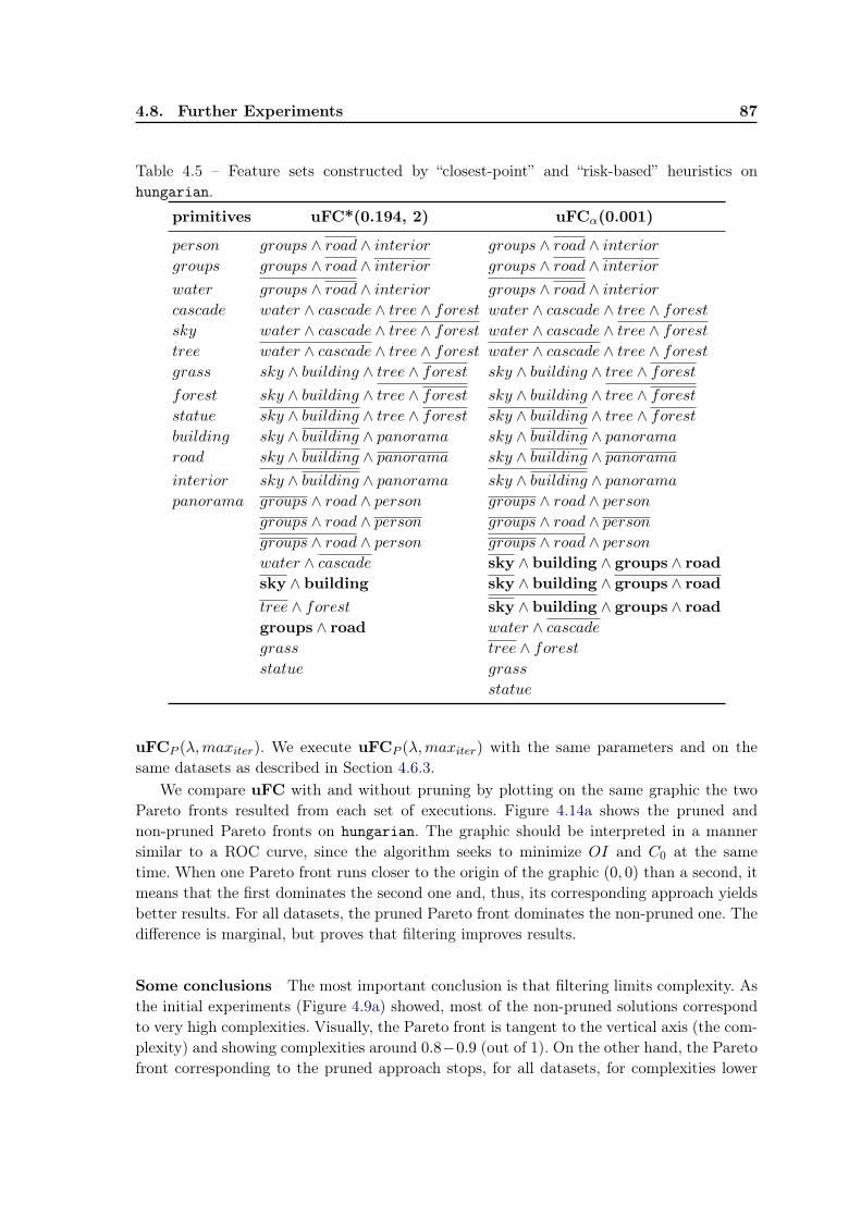
4.8. Further Experiments 87
Table 4.5 – Feature sets constructed by “closest-point” and “risk-based” heuristics onhungarian.
primitives uFC*(0.194, 2) uFCα(0.001)
person groups ∧ road ∧ interior groups ∧ road ∧ interiorgroups groups ∧ road ∧ interior groups ∧ road ∧ interiorwater groups ∧ road ∧ interior groups ∧ road ∧ interiorcascade water ∧ cascade ∧ tree ∧ forest water ∧ cascade ∧ tree ∧ forestsky water ∧ cascade ∧ tree ∧ forest water ∧ cascade ∧ tree ∧ foresttree water ∧ cascade ∧ tree ∧ forest water ∧ cascade ∧ tree ∧ forestgrass sky ∧ building ∧ tree ∧ forest sky ∧ building ∧ tree ∧ forestforest sky ∧ building ∧ tree ∧ forest sky ∧ building ∧ tree ∧ foreststatue sky ∧ building ∧ tree ∧ forest sky ∧ building ∧ tree ∧ forestbuilding sky ∧ building ∧ panorama sky ∧ building ∧ panoramaroad sky ∧ building ∧ panorama sky ∧ building ∧ panoramainterior sky ∧ building ∧ panorama sky ∧ building ∧ panoramapanorama groups ∧ road ∧ person groups ∧ road ∧ person
groups ∧ road ∧ person groups ∧ road ∧ persongroups ∧ road ∧ person groups ∧ road ∧ personwater ∧ cascade sky ∧ building ∧ groups ∧ road
sky ∧ building sky ∧ building ∧ groups ∧ road
tree ∧ forest sky ∧ building ∧ groups ∧ road
groups ∧ road water ∧ cascadegrass tree ∧ foreststatue grass
statue
uFCP (λ,maxiter). We execute uFCP (λ,maxiter) with the same parameters and on thesame datasets as described in Section 4.6.3.
We compare uFC with and without pruning by plotting on the same graphic the twoPareto fronts resulted from each set of executions. Figure 4.14a shows the pruned andnon-pruned Pareto fronts on hungarian. The graphic should be interpreted in a mannersimilar to a ROC curve, since the algorithm seeks to minimize OI and C0 at the sametime. When one Pareto front runs closer to the origin of the graphic (0, 0) than a second, itmeans that the first dominates the second one and, thus, its corresponding approach yieldsbetter results. For all datasets, the pruned Pareto front dominates the non-pruned one. Thedifference is marginal, but proves that filtering improves results.
Some conclusions The most important conclusion is that filtering limits complexity. Asthe initial experiments (Figure 4.9a) showed, most of the non-pruned solutions correspondto very high complexities. Visually, the Pareto front is tangent to the vertical axis (the com-plexity) and showing complexities around 0.8−0.9 (out of 1). On the other hand, the Paretofront corresponding to the pruned approach stops, for all datasets, for complexities lower
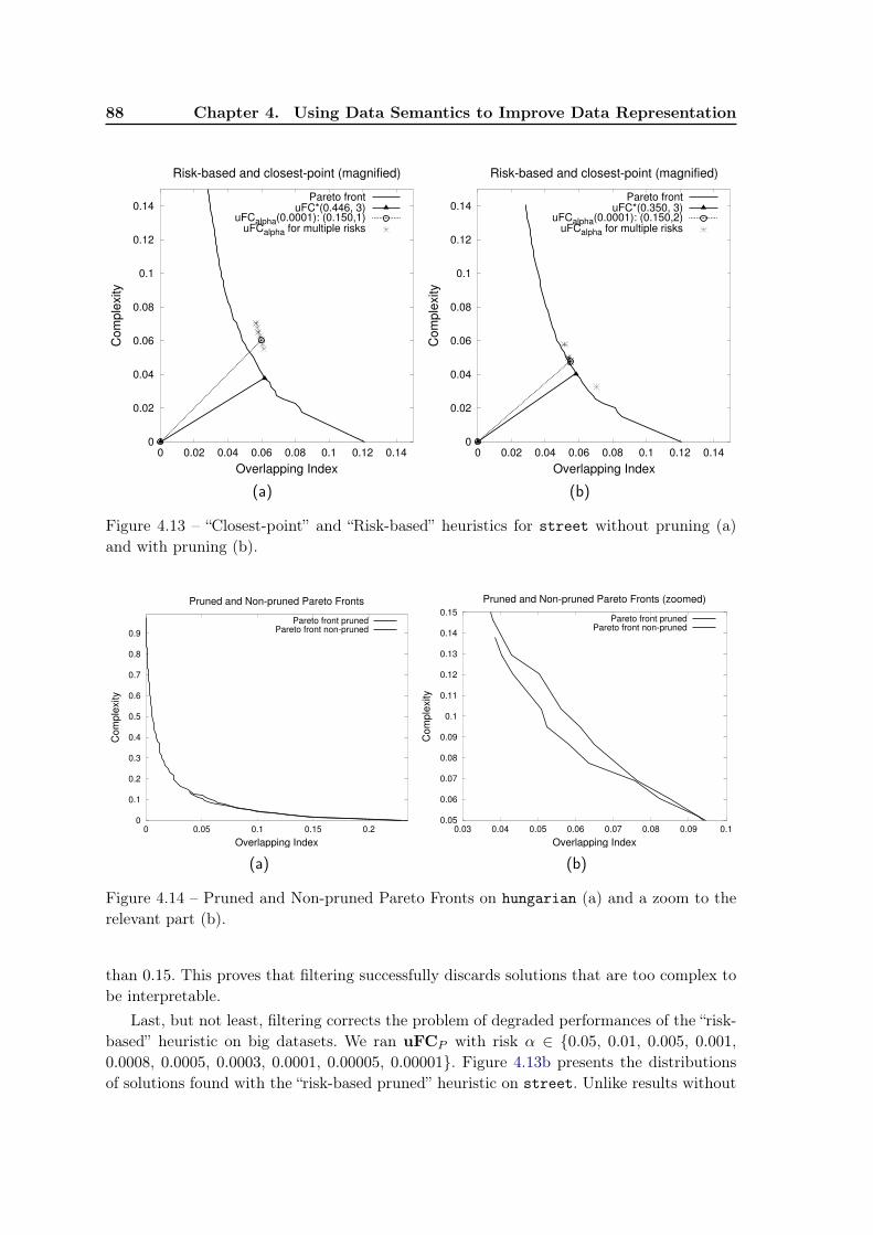
88 Chapter 4. Using Data Semantics to Improve Data Representation
0
0.02
0.04
0.06
0.08
0.1
0.12
0.14
0 0.02 0.04 0.06 0.08 0.1 0.12 0.14
Com
ple
xity
Overlapping Index
Risk-based and closest-point (magnified)
Pareto frontuFC*(0.446, 3)
uFCalpha(0.0001): (0.150,1)uFCalpha for multiple risks
(a)
0
0.02
0.04
0.06
0.08
0.1
0.12
0.14
0 0.02 0.04 0.06 0.08 0.1 0.12 0.14
Com
ple
xity
Overlapping Index
Risk-based and closest-point (magnified)
Pareto frontuFC*(0.350, 3)
uFCalpha(0.0001): (0.150,2)uFCalpha for multiple risks
(b)
Figure 4.13 – “Closest-point” and “Risk-based” heuristics for street without pruning (a)and with pruning (b).
0
0.1
0.2
0.3
0.4
0.5
0.6
0.7
0.8
0.9
0 0.05 0.1 0.15 0.2
Co
mp
lexity
Overlapping Index
Pruned and Non-pruned Pareto Fronts
Pareto front prunedPareto front non-pruned
(a)
0.05
0.06
0.07
0.08
0.09
0.1
0.11
0.12
0.13
0.14
0.15
0.03 0.04 0.05 0.06 0.07 0.08 0.09 0.1
Co
mp
lexity
Overlapping Index
Pruned and Non-pruned Pareto Fronts (zoomed)
Pareto front prunedPareto front non-pruned
(b)
Figure 4.14 – Pruned and Non-pruned Pareto Fronts on hungarian (a) and a zoom to therelevant part (b).
than 0.15. This proves that filtering successfully discards solutions that are too complex tobe interpretable.
Last, but not least, filtering corrects the problem of degraded performances of the “risk-based” heuristic on big datasets. We ran uFCP with risk α ∈ {0.05, 0.01, 0.005, 0.001,0.0008, 0.0005, 0.0003, 0.0001, 0.00005, 0.00001}. Figure 4.13b presents the distributionsof solutions found with the “risk-based pruned” heuristic on street. Unlike results without
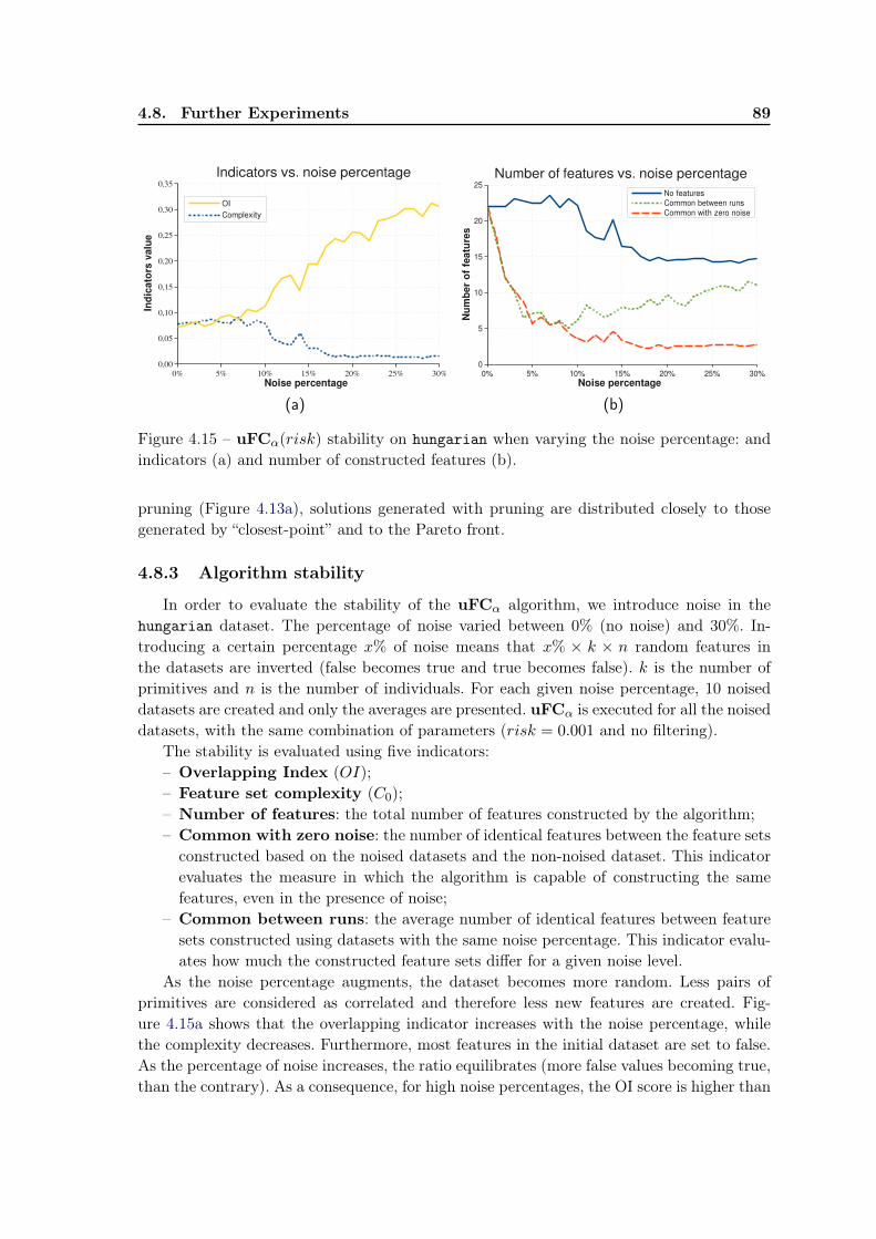
4.8. Further Experiments 89
0% 5% 10% 15% 20% 25% 30%
0,00
0,05
0,10
0,15
0,20
0,25
0,30
0,35
Indicators vs. noise percentage
OI
Complexity
Noise percentage
Indic
ato
rs v
alu
e
(a)
0% 5% 10% 15% 20% 25% 30%0
5
10
15
20
25
Number of features vs. noise percentage
No features
Common between runs
Common with zero noise
Noise percentage
Nu
mb
er
of
featu
res
(b)
Figure 4.15 – uFCα(risk) stability on hungarian when varying the noise percentage: andindicators (a) and number of constructed features (b).
pruning (Figure 4.13a), solutions generated with pruning are distributed closely to thosegenerated by “closest-point” and to the Pareto front.
4.8.3 Algorithm stability
In order to evaluate the stability of the uFCα algorithm, we introduce noise in thehungarian dataset. The percentage of noise varied between 0% (no noise) and 30%. In-troducing a certain percentage x% of noise means that x% × k × n random features inthe datasets are inverted (false becomes true and true becomes false). k is the number ofprimitives and n is the number of individuals. For each given noise percentage, 10 noiseddatasets are created and only the averages are presented. uFCα is executed for all the noiseddatasets, with the same combination of parameters (risk = 0.001 and no filtering).
The stability is evaluated using five indicators:– Overlapping Index (OI);– Feature set complexity (C0);– Number of features: the total number of features constructed by the algorithm;– Common with zero noise: the number of identical features between the feature sets
constructed based on the noised datasets and the non-noised dataset. This indicatorevaluates the measure in which the algorithm is capable of constructing the samefeatures, even in the presence of noise;
– Common between runs: the average number of identical features between featuresets constructed using datasets with the same noise percentage. This indicator evalu-ates how much the constructed feature sets differ for a given noise level.
As the noise percentage augments, the dataset becomes more random. Less pairs ofprimitives are considered as correlated and therefore less new features are created. Fig-ure 4.15a shows that the overlapping indicator increases with the noise percentage, whilethe complexity decreases. Furthermore, most features in the initial dataset are set to false.As the percentage of noise increases, the ratio equilibrates (more false values becoming true,than the contrary). As a consequence, for high noise percentages, the OI score is higher than
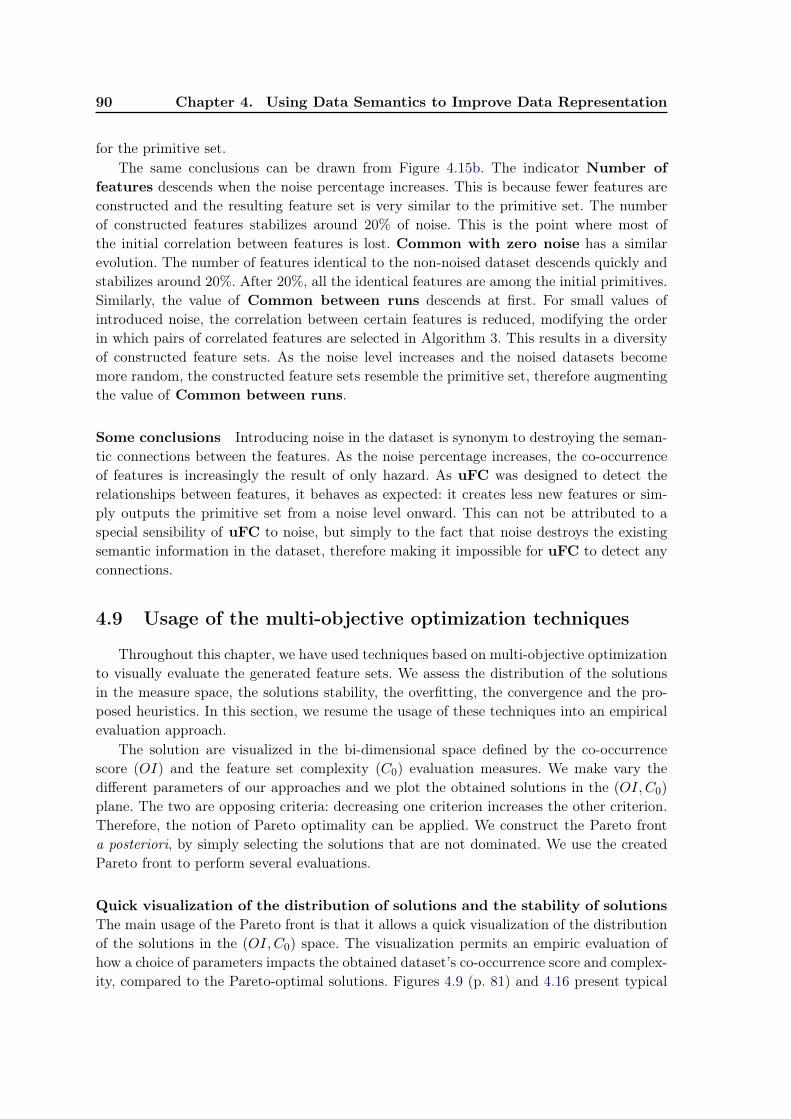
90 Chapter 4. Using Data Semantics to Improve Data Representation
for the primitive set.The same conclusions can be drawn from Figure 4.15b. The indicator Number of
features descends when the noise percentage increases. This is because fewer features areconstructed and the resulting feature set is very similar to the primitive set. The numberof constructed features stabilizes around 20% of noise. This is the point where most ofthe initial correlation between features is lost. Common with zero noise has a similarevolution. The number of features identical to the non-noised dataset descends quickly andstabilizes around 20%. After 20%, all the identical features are among the initial primitives.Similarly, the value of Common between runs descends at first. For small values ofintroduced noise, the correlation between certain features is reduced, modifying the orderin which pairs of correlated features are selected in Algorithm 3. This results in a diversityof constructed feature sets. As the noise level increases and the noised datasets becomemore random, the constructed feature sets resemble the primitive set, therefore augmentingthe value of Common between runs.
Some conclusions Introducing noise in the dataset is synonym to destroying the seman-tic connections between the features. As the noise percentage increases, the co-occurrenceof features is increasingly the result of only hazard. As uFC was designed to detect therelationships between features, it behaves as expected: it creates less new features or sim-ply outputs the primitive set from a noise level onward. This can not be attributed to aspecial sensibility of uFC to noise, but simply to the fact that noise destroys the existingsemantic information in the dataset, therefore making it impossible for uFC to detect anyconnections.
4.9 Usage of the multi-objective optimization techniques
Throughout this chapter, we have used techniques based on multi-objective optimizationto visually evaluate the generated feature sets. We assess the distribution of the solutionsin the measure space, the solutions stability, the overfitting, the convergence and the pro-posed heuristics. In this section, we resume the usage of these techniques into an empiricalevaluation approach.
The solution are visualized in the bi-dimensional space defined by the co-occurrencescore (OI) and the feature set complexity (C0) evaluation measures. We make vary thedifferent parameters of our approaches and we plot the obtained solutions in the (OI,C0)
plane. The two are opposing criteria: decreasing one criterion increases the other criterion.Therefore, the notion of Pareto optimality can be applied. We construct the Pareto fronta posteriori, by simply selecting the solutions that are not dominated. We use the createdPareto front to perform several evaluations.
Quick visualization of the distribution of solutions and the stability of solutionsThe main usage of the Pareto front is that it allows a quick visualization of the distributionof the solutions in the (OI,C0) space. The visualization permits an empiric evaluation ofhow a choice of parameters impacts the obtained dataset’s co-occurrence score and complex-ity, compared to the Pareto-optimal solutions. Figures 4.9 (p. 81) and 4.16 present typical
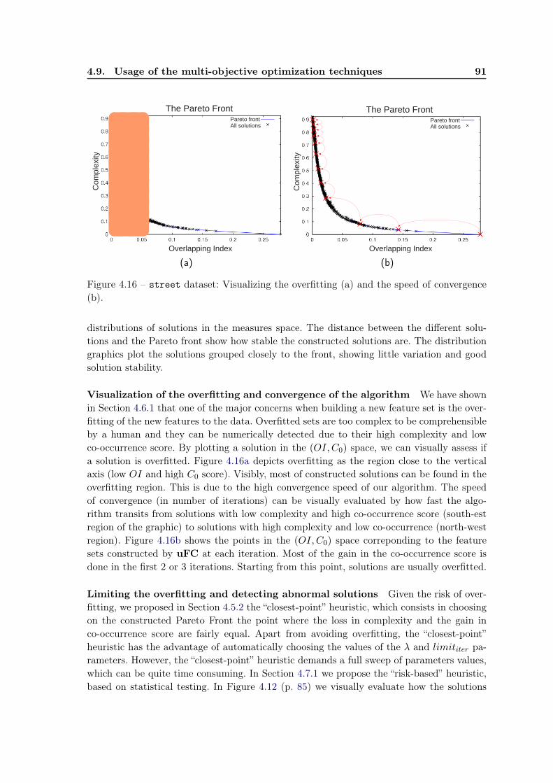
4.9. Usage of the multi-objective optimization techniques 91
The Pareto Front
Co
mp l
exi
ty
Overlapping Index
Pareto frontAll solutions
(a)
The Pareto Front
Co
mp l
exi
ty
Overlapping Index
Pareto frontAll solutions
(b)
Figure 4.16 – street dataset: Visualizing the overfitting (a) and the speed of convergence(b).
distributions of solutions in the measures space. The distance between the different solu-tions and the Pareto front show how stable the constructed solutions are. The distributiongraphics plot the solutions grouped closely to the front, showing little variation and goodsolution stability.
Visualization of the overfitting and convergence of the algorithm We have shownin Section 4.6.1 that one of the major concerns when building a new feature set is the over-fitting of the new features to the data. Overfitted sets are too complex to be comprehensibleby a human and they can be numerically detected due to their high complexity and lowco-occurrence score. By plotting a solution in the (OI,C0) space, we can visually assess ifa solution is overfitted. Figure 4.16a depicts overfitting as the region close to the verticalaxis (low OI and high C0 score). Visibly, most of constructed solutions can be found in theoverfitting region. This is due to the high convergence speed of our algorithm. The speedof convergence (in number of iterations) can be visually evaluated by how fast the algo-rithm transits from solutions with low complexity and high co-occurrence score (south-estregion of the graphic) to solutions with high complexity and low co-occurrence (north-westregion). Figure 4.16b shows the points in the (OI,C0) space correponding to the featuresets constructed by uFC at each iteration. Most of the gain in the co-occurrence score isdone in the first 2 or 3 iterations. Starting from this point, solutions are usually overfitted.
Limiting the overfitting and detecting abnormal solutions Given the risk of over-fitting, we proposed in Section 4.5.2 the “closest-point” heuristic, which consists in choosingon the constructed Pareto Front the point where the loss in complexity and the gain inco-occurrence score are fairly equal. Apart from avoiding overfitting, the “closest-point”heuristic has the advantage of automatically choosing the values of the λ and limititer pa-rameters. However, the “closest-point” heuristic demands a full sweep of parameters values,which can be quite time consuming. In Section 4.7.1 we propose the “risk-based” heuristic,based on statistical testing. In Figure 4.12 (p. 85) we visually evaluate how the solutions
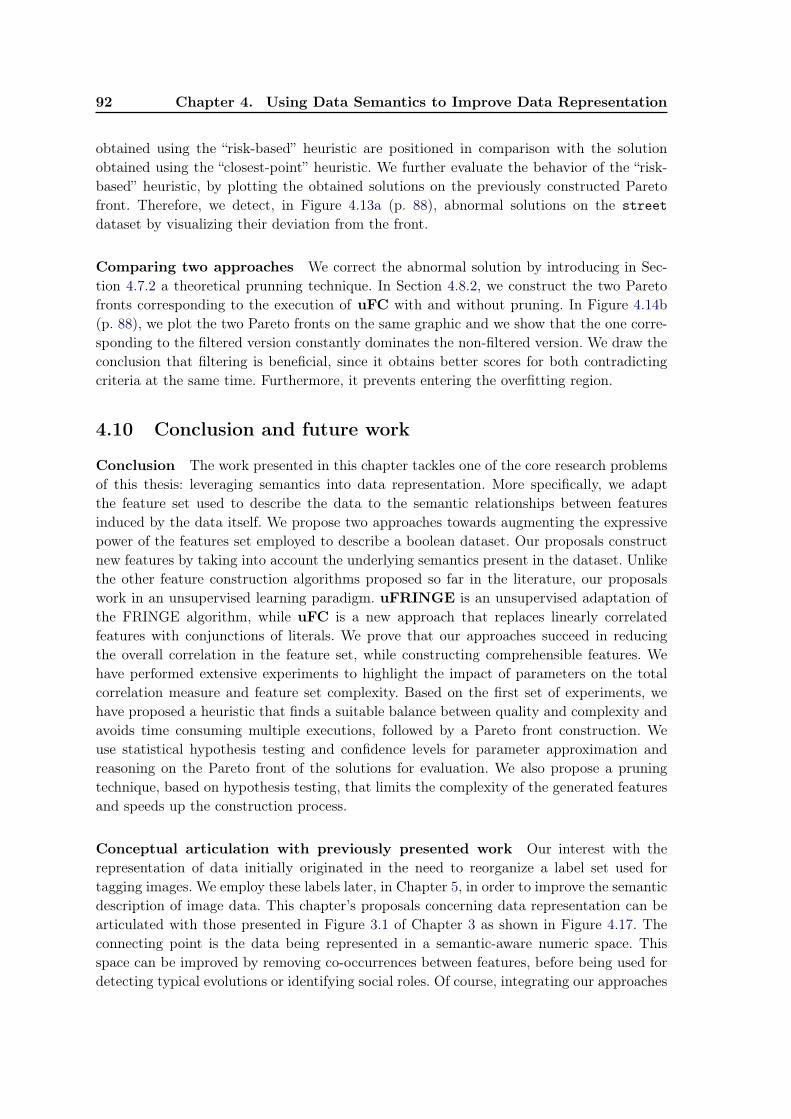
92 Chapter 4. Using Data Semantics to Improve Data Representation
obtained using the “risk-based” heuristic are positioned in comparison with the solutionobtained using the “closest-point” heuristic. We further evaluate the behavior of the “risk-based” heuristic, by plotting the obtained solutions on the previously constructed Paretofront. Therefore, we detect, in Figure 4.13a (p. 88), abnormal solutions on the streetdataset by visualizing their deviation from the front.
Comparing two approaches We correct the abnormal solution by introducing in Sec-tion 4.7.2 a theoretical prunning technique. In Section 4.8.2, we construct the two Paretofronts corresponding to the execution of uFC with and without pruning. In Figure 4.14b(p. 88), we plot the two Pareto fronts on the same graphic and we show that the one corre-sponding to the filtered version constantly dominates the non-filtered version. We draw theconclusion that filtering is beneficial, since it obtains better scores for both contradictingcriteria at the same time. Furthermore, it prevents entering the overfitting region.
4.10 Conclusion and future work
Conclusion The work presented in this chapter tackles one of the core research problemsof this thesis: leveraging semantics into data representation. More specifically, we adaptthe feature set used to describe the data to the semantic relationships between featuresinduced by the data itself. We propose two approaches towards augmenting the expressivepower of the features set employed to describe a boolean dataset. Our proposals constructnew features by taking into account the underlying semantics present in the dataset. Unlikethe other feature construction algorithms proposed so far in the literature, our proposalswork in an unsupervised learning paradigm. uFRINGE is an unsupervised adaptation ofthe FRINGE algorithm, while uFC is a new approach that replaces linearly correlatedfeatures with conjunctions of literals. We prove that our approaches succeed in reducingthe overall correlation in the feature set, while constructing comprehensible features. Wehave performed extensive experiments to highlight the impact of parameters on the totalcorrelation measure and feature set complexity. Based on the first set of experiments, wehave proposed a heuristic that finds a suitable balance between quality and complexity andavoids time consuming multiple executions, followed by a Pareto front construction. Weuse statistical hypothesis testing and confidence levels for parameter approximation andreasoning on the Pareto front of the solutions for evaluation. We also propose a pruningtechnique, based on hypothesis testing, that limits the complexity of the generated featuresand speeds up the construction process.
Conceptual articulation with previously presented work Our interest with therepresentation of data initially originated in the need to reorganize a label set used fortagging images. We employ these labels later, in Chapter 5, in order to improve the semanticdescription of image data. This chapter’s proposals concerning data representation can bearticulated with those presented in Figure 3.1 of Chapter 3 as shown in Figure 4.17. Theconnecting point is the data being represented in a semantic-aware numeric space. Thisspace can be improved by removing co-occurrences between features, before being used fordetecting typical evolutions or identifying social roles. Of course, integrating our approaches
4.10. Conclusion and future work 93
Figure 4.17 – Streamlined schema showing how the contributions in this chapter can beconceptually articulated with those in previous the chapters.
would require additional development, some of which is presented in the next paragraph.
Current work We have already undergoing work toward incorporating temporal informa-tion into the feature construction algorithm. This work will allow to simultaneously addressthe two major research problems of this thesis: the semantic representation and using thetemporal dimension of data.
The datasets presented in Section 4.6 have no temporal component. The building blockof the uFC algorithm is feature co-occurrence. For example, “manifestation” co-occurs with“urban” because usually manifestations take place in cities. With the introducing of the tem-poral information, the definition of the problem changes and the question of co-occurrencein a temporal context arises. Some features might co-occur, but not simultaneously. For ex-ample, the arrival of power of a socialist government and the increase of the country’s publicdeficit might be correlated, but with a time lag, as the macro-economic indicators have a biginertia. The purpose of this work is to detect such “correlations with a time lag” and createnew features like “socialist” and “public_deficit” co-occur at a time lag δ. This would allowto (i) improve the data representation by using the temporal dimension in addition to datasemantics (ii) detect hidden temporal correlations, which might prove to be causalities. Inaddition, the newly constructed temporal features can serve to create comprehensible labelsto temporal clusters extracted using TDCK-Means (proposed in Chapter 3).
We have extended the correlation coefficient defined in Equation 4.5 to calculate thecorrelation at with a given fixed lag δ. The experiments we performed so far show thatan “optimum” lag δ can be determined, that maximizes the temporal correlation. We arecurrently working on an extension of the and operator to the temporal case. The new
94 Chapter 4. Using Data Semantics to Improve Data Representation
features are no longer constructed as boolean expressions, but as temporal chains of theform fi
δ1−→ fjδ2−→ fk, meaning that fi precedes at at a time distance δ1, which fj precedes
fk at a time distance δ2.
Other future work A research direction we privilege is adapting our algorithms for dataof the Web 2.0 (e.g., automatic treatment of labels on the web). Several challenges arise,like very large label sets (it is common to have over 10 000 features), non-standard labelnames (see standardization preprocessing task that we have performed for the LabelMedataset in Section 4.6) and missing data. The problem of missing data is intimately linkedto the task of semantic-enriched numeric representation construction for images and theassumption of complete labeling that we have made at the beginning of this chapter. Incomplete labeling, if the label is not present, it therefore means that the object it denotes isabsent (in the case of object labeling in images). This assumption supposes binary labeling,where true means presence and false means absence. In the case of incomplete labeling,the absence of a label might also mean that the user forgot/chose not to label the givenimage/document. Therefore, a value of false is no longer a sure indicator for the absence ofthe given object. For example, when a user is labeling an image depicting a cascade andhas a choice between water, cascade or both, he/she might choose only cascade as it is themost specific. This adds new challenges for the feature construction algorithm, since theco-occurrence of water and cascade is no longer present. Similarly, created features whichare absent for all individuals can no longer be simply removed, since it is not sure if theobjects are really missing or simply their presence was not marked by the user.
Other planned developments include taking into account non-linear correlation betweenvariables by modifying the metric of the search and the co-occurrence measure. We alsoconsider converting generated features to the Disjunctive Normal Form for easier readingand suppressing features that have a low support in the dataset. This would reduce the sizeof the feature set by removing rare features, but would introduce new difficulties such asdetecting nuggets.
A related problem A somehow related class of problems is multi-label classifica-tion [Tsoumakas & Katakis 2007]. These algorithms work in another paradigm (supervisedlearning) and tackle another learning task (learning from a dataset with multiple class vari-ables, aiming to learn to differentiate between classes and be able to predict the class ofunseen examples). The connection with our learning problem is how these solutions tacklethe co-occurrence between the class variable (i.e., when an individual has two labels at-tached). In our work we do not relate or compare with these approaches, and we mentionthem here to completeness reasons.
Solutions to the problem of multi-label classification usually fall into two cate-gories [Tsoumakas & Katakis 2007]: (a) problem transformation methods and (b) algorithmadaptation methods. (a) Problem transformation methods are those methods that transformthe multi-label classification problem either into one or more single-label classification orregression problems. For example, protein classification using machine learning algorithmsis studied in [Diplaris et al. 2005]. For proteins that belong to several classes, they constructnew classes using boolean conjunctions: c′ = ci AND cj . (b) Algorithm adaptation methods
4.10. Conclusion and future work 95
are those methods that extend specific learning algorithms in order to handle multi-labeldata directly. For example, [Clare & King 2001] adapted the C4.5 algorithm for multi-label data. They modified the formula of entropy in order to take into account the relativefrequency of each class. They also allow multiple labels in the leaves of the tree.
While showing some success in the problem of predicting multiple label classification,this family of problems does not tackle the same task as the one stated in Section 4.1: theydo not deal with the co-occurrence in the description space. They are mostly interestingat the level of the chosen approach and their similarity towards the construction of newclass attributes/labels. Whatsoever, even this construction is limited in the case of multi-label classification: (a) negations cannot exist and, because of this fact, (b) not all booleanformulas can be created (the AND operator is not a complete operator set). Furthermore,(c) only very simple conjunctions of the initial labels can be created: they construct onlyconjunction of two initial labels, which are not evolved into a more complex formula.
Most of the work presented in this chapter was published in the international Journalof Intelligent Information Systems [Rizoiu et al. 2013a].


Chapter 5
Dealing with images: VisualVocabulary Construction
Contents5.1 Learning task and motivations . . . . . . . . . . . . . . . . . . . . . 97
5.1.1 An overview of our proposals . . . . . . . . . . . . . . . . . . . . . . . 995.1.2 Constructing a baseline “bag-of-features” image numerical description 100
5.2 Context and related work . . . . . . . . . . . . . . . . . . . . . . . . 1015.2.1 Sampling strategies and numerical description of image features . . . . 1025.2.2 Unsupervised visual vocabulary construction . . . . . . . . . . . . . . 1035.2.3 Leveraging additional information . . . . . . . . . . . . . . . . . . . . 103
5.3 Improving the BoF representation using semantic knowledge . . . 1065.3.1 Dedicated visual vocabulary generation . . . . . . . . . . . . . . . . . 1075.3.2 Filtering irrelevant features . . . . . . . . . . . . . . . . . . . . . . . . 108
5.4 Experiments and results . . . . . . . . . . . . . . . . . . . . . . . . . 1105.4.1 Experimental protocol . . . . . . . . . . . . . . . . . . . . . . . . . . . 1115.4.2 The learning task: content-based image classification . . . . . . . . . . 1125.4.3 Datasets . . . . . . . . . . . . . . . . . . . . . . . . . . . . . . . . . . . 1135.4.4 Qualitative evaluation . . . . . . . . . . . . . . . . . . . . . . . . . . . 1135.4.5 Quantitative evaluation . . . . . . . . . . . . . . . . . . . . . . . . . . 1145.4.6 Overfitting . . . . . . . . . . . . . . . . . . . . . . . . . . . . . . . . . 1195.4.7 Influence of parameter α . . . . . . . . . . . . . . . . . . . . . . . . . . 120
5.5 Conclusions and future work . . . . . . . . . . . . . . . . . . . . . . . 121
5.1 Learning task and motivations
In this chapter, we address one of our core research challenges: leveraging semanticswhen dealing with complex data. Images are one of the most widely encountered types ofcomplex data. Therefore, in this work we are interested in how to leverage external infor-mation in order to construct a semantic-aware numeric representation for images.The most prevalent learning task involving images is content-based image classification.This is a difficult task especially because the low-level features used to digitally describeimages usually capture little information about the semantics of the images. In our work,presented schematically in Figure 5.1, we tackle this difficulty by enriching the semantic con-tent of the image representation using external knowledge. The underlying hypothesis of ourwork is that creating a more semantically rich representation for images would yield higher
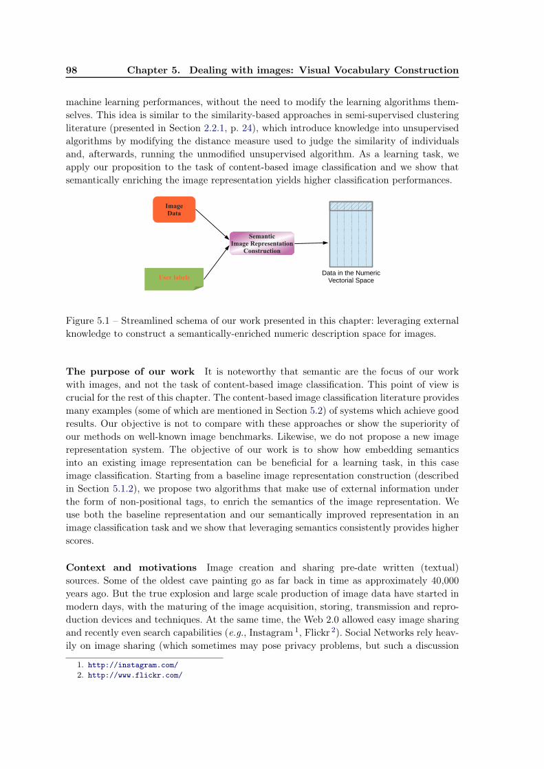
98 Chapter 5. Dealing with images: Visual Vocabulary Construction
machine learning performances, without the need to modify the learning algorithms them-selves. This idea is similar to the similarity-based approaches in semi-supervised clusteringliterature (presented in Section 2.2.1, p. 24), which introduce knowledge into unsupervisedalgorithms by modifying the distance measure used to judge the similarity of individualsand, afterwards, running the unmodified unsupervised algorithm. As a learning task, weapply our proposition to the task of content-based image classification and we show thatsemantically enriching the image representation yields higher classification performances.
Data in the Numeric Vectorial Space
SemanticImage Representation
Construction
User labels
ImageData
Figure 5.1 – Streamlined schema of our work presented in this chapter: leveraging externalknowledge to construct a semantically-enriched numeric description space for images.
The purpose of our work It is noteworthy that semantic are the focus of our workwith images, and not the task of content-based image classification. This point of view iscrucial for the rest of this chapter. The content-based image classification literature providesmany examples (some of which are mentioned in Section 5.2) of systems which achieve goodresults. Our objective is not to compare with these approaches or show the superiority ofour methods on well-known image benchmarks. Likewise, we do not propose a new imagerepresentation system. The objective of our work is to show how embedding semanticsinto an existing image representation can be beneficial for a learning task, in this caseimage classification. Starting from a baseline image representation construction (describedin Section 5.1.2), we propose two algorithms that make use of external information underthe form of non-positional tags, to enrich the semantics of the image representation. Weuse both the baseline representation and our semantically improved representation in animage classification task and we show that leveraging semantics consistently provides higherscores.
Context and motivations Image creation and sharing pre-date written (textual)sources. Some of the oldest cave painting go as far back in time as approximately 40,000years ago. But the true explosion and large scale production of image data have started inmodern days, with the maturing of the image acquisition, storing, transmission and repro-duction devices and techniques. At the same time, the Web 2.0 allowed easy image sharingand recently even search capabilities (e.g., Instagram 1, Flickr 2). Social Networks rely heav-ily on image sharing (which sometimes may pose privacy problems, but such a discussion
1. http://instagram.com/2. http://www.flickr.com/
5.1. Learning task and motivations 99
is out of the scope of this document). Because of the sheer volumes of created images,automatic summarization, search and classification methods are required.
The difficulty when analyzing images comes from the fact that digital image numericalformat does not embed the needed semantic information. For example, images acquiredusing a digital photo camera are most often stored in raster format, based on pixels. A pixelis an atomic image element, which has several characteristics the most important beingthe size (as small as possible) and its color. Other information can be color coding, alphachannel etc.. Therefore, an image is stored numerically as a matrix of pixels. The difficultyraises from the fact that low-level features, such as position and color of individual pixels,do not capture too much information about the semantic content of the image (e.g., shapes,objects). To address this issue, multiple representation paradigms have been proposed, someof which will be presented in Section 5.2. The one showing the most promising results is the“bag-of-features” representation, a representation inspired from the textual “bag-of-words”textual representation (detailed later in Section 6.2, p. 128).
The remainder of the chapter is structured as follows: the rest of this section presentsan overview of our proposals (in Section 5.1.1) and how to construct a baseline “bag-of-features” image description (in Section 5.1.2). In Section 5.2, we present a brief overview onconstructing a numerical image representation, concentrating on some of the state-of-the-art papers that relate to visual vocabulary construction and knowledge injection into imagerepresentation. Section 5.3 explains the two proposed approaches, followed, in Section 5.4,by the experiments that were performed. Some conclusions are drawn and future workperspectives are given in Section 5.5.
5.1.1 An overview of our proposals
The focus of our work is embedding semantic information into the construction of imagenumerical representation. The external information is under the form of non-positionallabels, which signal the presence in the image of an object (e.g., car, motorcycle) or giveinformation about the context of the image (e.g., holiday, evening), but do not give anyinformation about its position of the image (in the case of objects). Furthermore, the labelsare available only for a part of the image collection, therefore positioning our work in asemi-supervised learning context.
Our work is focused on the visual vocabulary construction (which is also referred in theliterature as codebook or model). In the “bag-of-features” (BoF ) representation, the visualwords serve a similar role as the real textual words do in the “bag-of-words” representation.We propose two novel contributions that leverage external semantic information and thatallow the visual vocabulary to capture more accurately the semantics behind a collectionof images. The first proposal deals with introducing the provided additional informationearly in the creation of the visual vocabulary. A dedicated visual vocabulary is constructedstarting from the visual features sampled from images labeled with a given label. Therefore,a dedicated vocabulary contains visual words adapted to describing the object denotedby the given label. In the end, the complete visual vocabulary is created by merging thededicated vocabularies. In the second proposal, we add a filtering phase as a pre-processingof the visual vocabulary construction. For any given image, we construct a known positiveset (images labeled with the same labels as the given image) and a known negative set
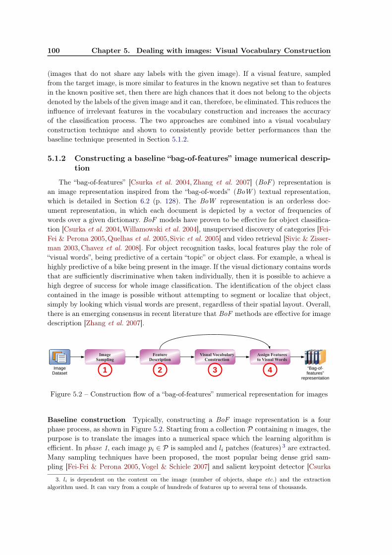
100 Chapter 5. Dealing with images: Visual Vocabulary Construction
(images that do not share any labels with the given image). If a visual feature, sampledfrom the target image, is more similar to features in the known negative set than to featuresin the known positive set, then there are high chances that it does not belong to the objectsdenoted by the labels of the given image and it can, therefore, be eliminated. This reduces theinfluence of irrelevant features in the vocabulary construction and increases the accuracyof the classification process. The two approaches are combined into a visual vocabularyconstruction technique and shown to consistently provide better performances than thebaseline technique presented in Section 5.1.2.
5.1.2 Constructing a baseline “bag-of-features” image numerical descrip-tion
The “bag-of-features” [Csurka et al. 2004, Zhang et al. 2007] (BoF ) representation isan image representation inspired from the “bag-of-words” (BoW ) textual representation,which is detailed in Section 6.2 (p. 128). The BoW representation is an orderless doc-ument representation, in which each document is depicted by a vector of frequencies ofwords over a given dictionary. BoF models have proven to be effective for object classifica-tion [Csurka et al. 2004,Willamowski et al. 2004], unsupervised discovery of categories [Fei-Fei & Perona 2005,Quelhas et al. 2005,Sivic et al. 2005] and video retrieval [Sivic & Zisser-man 2003,Chavez et al. 2008]. For object recognition tasks, local features play the role of“visual words”, being predictive of a certain “topic” or object class. For example, a wheal ishighly predictive of a bike being present in the image. If the visual dictionary contains wordsthat are sufficiently discriminative when taken individually, then it is possible to achieve ahigh degree of success for whole image classification. The identification of the object classcontained in the image is possible without attempting to segment or localize that object,simply by looking which visual words are present, regardless of their spatial layout. Overall,there is an emerging consensus in recent literature that BoF methods are effective for imagedescription [Zhang et al. 2007].
ImageSampling
FeatureDescription
Visual Vocabulary Construction
Assign Featuresto Visual Words
Image Dataset
“Bag-of-features”
representation
1 2 3 4
Figure 5.2 – Construction flow of a “bag-of-features” numerical representation for images
Baseline construction Typically, constructing a BoF image representation is a fourphase process, as shown in Figure 5.2. Starting from a collection P containing n images, thepurpose is to translate the images into a numerical space which the learning algorithm isefficient. In phase 1, each image pi ∈ P is sampled and li patches (features) 3 are extracted.Many sampling techniques have been proposed, the most popular being dense grid sam-pling [Fei-Fei & Perona 2005,Vogel & Schiele 2007] and salient keypoint detector [Csurka
3. li is dependent on the content on the image (number of objects, shape etc.) and the extractionalgorithm used. It can vary from a couple of hundreds of features up to several tens of thousands.
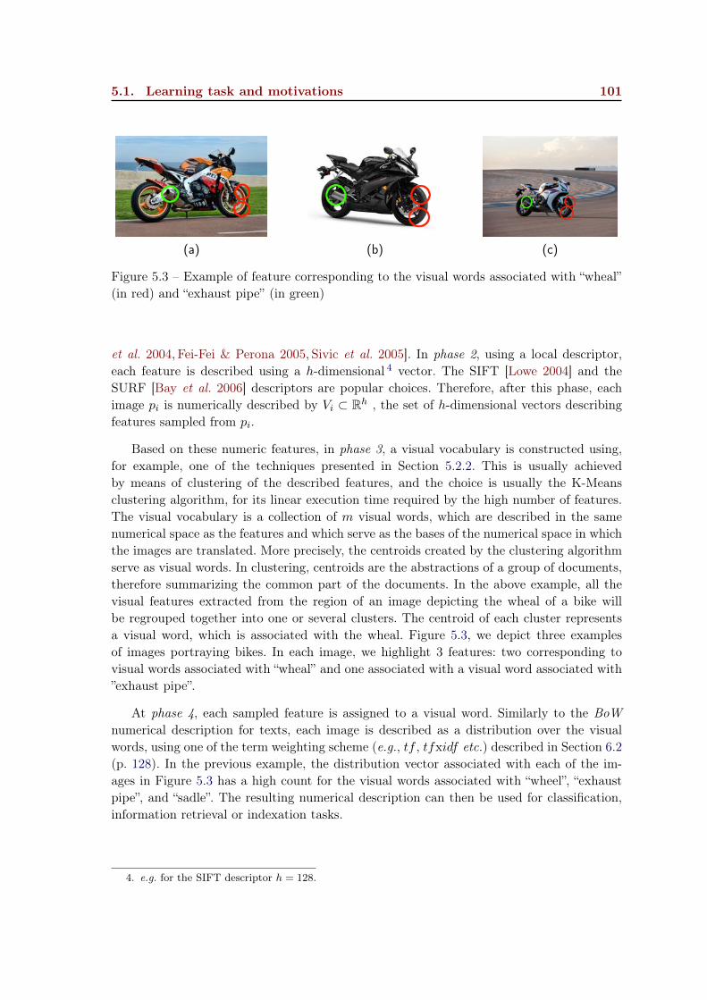
5.1. Learning task and motivations 101
(a) (b) (c)
Figure 5.3 – Example of feature corresponding to the visual words associated with “wheal”(in red) and “exhaust pipe” (in green)
et al. 2004, Fei-Fei & Perona 2005, Sivic et al. 2005]. In phase 2, using a local descriptor,each feature is described using a h-dimensional 4 vector. The SIFT [Lowe 2004] and theSURF [Bay et al. 2006] descriptors are popular choices. Therefore, after this phase, eachimage pi is numerically described by Vi ⊂ Rh , the set of h-dimensional vectors describingfeatures sampled from pi.
Based on these numeric features, in phase 3, a visual vocabulary is constructed using,for example, one of the techniques presented in Section 5.2.2. This is usually achievedby means of clustering of the described features, and the choice is usually the K-Meansclustering algorithm, for its linear execution time required by the high number of features.The visual vocabulary is a collection of m visual words, which are described in the samenumerical space as the features and which serve as the bases of the numerical space in whichthe images are translated. More precisely, the centroids created by the clustering algorithmserve as visual words. In clustering, centroids are the abstractions of a group of documents,therefore summarizing the common part of the documents. In the above example, all thevisual features extracted from the region of an image depicting the wheal of a bike willbe regrouped together into one or several clusters. The centroid of each cluster representsa visual word, which is associated with the wheal. Figure 5.3, we depict three examplesof images portraying bikes. In each image, we highlight 3 features: two corresponding tovisual words associated with “wheal” and one associated with a visual word associated with”exhaust pipe”.
At phase 4, each sampled feature is assigned to a visual word. Similarly to the BoWnumerical description for texts, each image is described as a distribution over the visualwords, using one of the term weighting scheme (e.g., tf , tfxidf etc.) described in Section 6.2(p. 128). In the previous example, the distribution vector associated with each of the im-ages in Figure 5.3 has a high count for the visual words associated with “wheel”, “exhaustpipe”, and “sadle”. The resulting numerical description can then be used for classification,information retrieval or indexation tasks.
4. e.g. for the SIFT descriptor h = 128.
102 Chapter 5. Dealing with images: Visual Vocabulary Construction
5.2 Context and related work
Over the past decades computer vision domain has seen a large interest from the re-search community. Its application are larger than image analysis and include augmentedreality, robotic vision, gesture recognition etc. Whatsoever, in the context of Internet-originating images, one of the prevailing task is content-based image classification. Someof the initial image classification systems used color histograms [Swain & Ballard 1991]for image representation. Such a representation does not retain any information aboutthe shapes of objects in images and obtains moderate results. Other systems [Haralick& Shanmugam 1973, de Medeiros Martins et al. 2002,Varma & Zisserman 2003, Lazebniket al. 2003b] rely on texture detection. Texture is characterized by the repetition of ba-sic elements or textons. For stochastic textures, it is the identity of the textons, not theirspatial arrangement, that matters. The BoF orderless representation has imposed itselfas the state-of-the-art in image representation, for classification and indexation purposes.The process of constructing the representation includes sampling the image (phase 1 inFigure 5.2), describing each features using an appearance-based descriptor (phase 2 ), con-structing a visual vocabulary (phase 3 ) and describing images as histograms over the visualwords (phase 4 ).
The remainder of this section presents a brief overview (i) of the sampling strategies andnumerical descriptors for image keypoints present in literature (in Section 5.2.1) and (ii) ofthe visual vocabulary construction techniques, concentrating on how external informationcan be used to improve the vocabularies representativity (in Section 5.2.2).
5.2.1 Sampling strategies and numerical description of image features
Image sampling methods Image sampling for the BoF representation is the process ofdeciding which regions of a given image should be numerically described. In Figure 5.2, itcorresponds to phase 1 of the construction of a BoF numerical representation. The out-put of feature detection is a set of patches, identified by their locations in the image andtheir corresponding scales and orientations. Multiple sampling methods exist [O’Hara &Draper 2011], including Interest Point Operators, Visual Saliency and random or densegrid sampling.
Interest Point Operators [Lowe 1999,Kadir & Brady 2001] search to find patches thatare stable under minor affine and photometric transformations. Interest point operatorsdetect locally discriminating features, such as corners, blob-like regions, or curves. A filteris used to detect these features, measuring the responses in a three dimensional space. Ex-treme values for the responses are considered as interest points. The popular choice is theHarris-Affine detector [Mikolajczyk & Schmid 2004], which uses a scale space representationwith oriented elliptical regions. Visual Saliency [Frintrop et al. 2010] feature detectors arebased on biomimetic computational models of the human visual attention system. Less usedby the BoF literature, these methods are concerned with finding locations in images thatare visually salient. In this case, fitness is often measured by how well the computationalmethods predict human eye fixations recorded by an eye tracker. There are research [Sivic& Zisserman 2003] that argue that interest point-based patch sampling, while useful forimage alignment, is not adapted for image classification tasks. Examples are city images,
5.2. Context and related work 103
for which the interest point detector does not consider relevant most of the concrete andasphalt surroundings, but which are good indicators of the images’ semantics. Some ap-proaches sample patches by using random sampling [Maree et al. 2005]. [Nowak et al. 2006]compare a random sampler with two interest point detectors: Laplacian of Gaussian [Linde-berg 1993] and Harris-Laplace [Lazebnik et al. 2003a]. They show that when using enoughsamples, random sampling exceeds the performance of interest point operators. Spatial Pyra-mid Matching is proposed in [Lazebnik et al. 2006]. Introduces spacial information in theorderless BoF representation by creating a pyramid representation, where each level dividesthe image in increasingly small regions. Feature histogram is calculated for each of theseregions. The distance between two images using this spatial pyramid representation is aweighted histogram intersection function, where weights are largest for the smallest regions.
Feature descriptors With the image sampled and a set of patches extracted, the nextquestions is how to numerically represent the neighborhood of pixels near a localized region.In Figure 5.2, this corresponds to phase 2 of the construction of a BoF numerical represen-tation. Initial feature descriptors simply used the pixel intensity values, scaled for the sizeof the region. The normalized pixel values have been shown [Fei-Fei & Perona 2005] to beoutperformed by more sophisticated feature descriptors, such as the SIFT descriptor. TheSIFT (Scale Invariant Feature Transform) [Lowe 2004] descriptor is today’s most widelyused descriptor. The responses to 8 gradient orientations at each of 16 cells of a 4x4 grid gen-erate the 128 components of the description vector. Alternative have been proposed, such asthe SURF (Speeded Up Robust Features) [Bay et al. 2006] descriptor. The SURF algorithmcontains both feature detection and description. It is designed to speed up the process ofcreating features similar to those produced by a SIFT descriptor on Hessian-Laplace interestpoints by using efficient approximations.
5.2.2 Unsupervised visual vocabulary construction
The visual vocabulary is a mid-level transition key between the low-level features and ahigh-level representation. It is a prototypic representation of features that are discriminativein a classification context.
The visual vocabulary is used to reduce dimensionality and to create a fixed length nu-merical representation for all images 5. Most BoF approaches use clustering to created thevisual vocabulary, usually the K-Means [Sivic & Zisserman 2003,Lazebnik et al. 2006,Jianget al. 2007] algorithm. K-Means is used for the fact that it produces centroids, which areprototypes of similar features in the same cluster. Its linear execution time is a plus consid-ering the high volume of individuals to be processed. Some authors [Jurie & Triggs 2005]argument that in K-Means, centroids are attracted by dense regions and under-representless denser, but equally informative regions. Therefore, methods were proposed for allocat-ing centers more uniformly, inspired by mean shift [Comaniciu & Meer 2002] and on-linefacility location [Meyerson 2001]. Other visual vocabulary construction techniques do notrely on K-Means. For example, [Moosmann et al. 2007] use an Extremely Randomized Clus-tering Forest, an ensemble of randomly created clustering trees. This technique provides
5. The number of extracted features can greatly vary depending on the image and the method used forsampling.
104 Chapter 5. Dealing with images: Visual Vocabulary Construction
good resistance to background clutter, but the main advantage over K-Means is the fastertraining time.
One of the most important parameters in the construction of the visual vocabularyis its dimension, which has a powerful impact on both performance and computationalcomplexity [Csurka et al. 2004, Jurie & Triggs 2005]. It has been shown [Jiang et al. 2007,López-Sastre et al. 2010,Nowak et al. 2006] that a large vocabulary may lead to overfittingfor construction techniques based on interest points detection. As our experiments show (inSection 5.4.6), even a random vocabulary (in a random vocabulary, a number of featuresare randomly chosen to serve as visual words) can lead to overfitting if its dimension is highenough.
5.2.3 Leveraging additional information
The BoF representation yields surprising results for image classification and indexing.This is because there is an intrinsic relation between the “quantity” of semantic informationcaptured by the description space and the performances of machine learning algorithms(e.g., in a classification task, the separability of individuals in the description space is cru-cial). Therefore, one direction to further improve results is to construct new representationsthat capture even more semantics from the raw image data. Another direction, the onethat we privilege in our work, is to use external information to further enrich the semanticcontent of the constructed representation. In the case of Internet-originating images, pre-cious information is given either by the textual context of images (e.g., titles, descriptionsetc.), or by labels attached to the images (e.g., on social networks websites, users have theoption to label the presence of their friends in images). Of course, the literature presentsapproaches that leverage other resources to semantically enrich enrich the image representa-tion (e.g., [Athanasiadis et al. 2005] propose a system that links low-level visual descriptorsto high-level, domain-specific concepts in an ontology). In Section 2.1.2 (p. 13), we havealready presented a number of learning tasks that can benefit from using image and textualdata simultaneously. In the following paragraphs, we detail some of the methods presentin the literature that address the use of additional information under the form of text orlabels in order to improve image classification results and we position our work relative tothese approaches.
Leveraging the image’s textual context In [Morsillo et al. 2009], the text that comesalongside the images is used to improve the visual query accuracy. A BoF representationfor images is created as shown in Section 5.1.2, with the exception that color information isalso added to the keypoint description. An 11-dimension vector coding the color informationof the sampled patches is added to the 128-dimension vector generated by the SIFT. Thetext that surrounds the images in the web pages is used to extract topics, using LDA [Bleiet al. 2003]. The inferred topics are, afterwards, used to describe the textual information(therefore functioning as a dimension reduction technique). The textual and the image dataare used together to estimate the parameters of a probabilistic graphical model, whichis trained using a small quantity of labeled data. Another approach that uses the textaccompanying images originating from the Internet is presented in [Wang et al. 2009]. Anauxiliary collection of Internet-originating images, with text attached, is used to create a
5.2. Context and related work 105
textual description of a target image. Images are described using three types of features: theSIFT features, the GIST features [Oliva & Torralba 2001] and local patch color information.For each test image, the K most similar images (in terms of visual features) are identified inthe auxiliary collection. The text associated with these near neighbor images is summarizedto build the text feature. The label of each image is considered as a unit (i.e., a whole phraseis considered as an item) and the text feature is constructed as a normalized histogramover labels. A text classifier and a visual classifier are trained and the outputs of the twoclassifiers are merged for a more accurate description of the photo. [Mooney et al. 2008] useco-training [Blum & Mitchell 1998] to construct a classifier starting from textual and visualdata. Text is described using a BoW representation, whereas images are described usingregion-based features. Each image is divided into a number of regions of fixed dimension(4-by-6 pixels), which are described using texture and color features. Co-training is a semi-supervised classification technique, which first learns a separate classifier for textual dataand image data, using any labeled examples. The most confident predictions of each classifieron the unlabeled data are then used to iteratively construct additional labeled training data,and the classifiers are re-trained.
Leveraging external semantic knowledge Other solutions rely on external expertknowledge in order to guide the visual vocabulary construction. This knowledge is mostoften expressed under the form of class/category annotations or labels (e.g. signaling thepresence of an object inside an image) or semantic resources, such as WordNet. [Zhanget al. 2009] uses an iterative boosting-like approach. Each iteration of boosting begins bylearning a visual vocabulary according to the weights assigned by the previous boostingiteration. The resulting visual vocabulary is then applied to encode the training examples,a new classifier is learned and new weights are computed. The visual vocabulary is learnedby clustering using K-Means a “learning” subset of image features. Features from imageswith high weights have more chances of being part of the learning subset. To classify a newexample, the AdaBoost [Freund & Schapire 1997] weighted voting scheme is used.
[Perronnin et al. 2006] construct both a generic vocabulary and a specific one foreach class. The generic vocabulary describes the content of all the considered classes ofimages, while the specific vocabularies are obtained through the adaptation of the universalvocabulary using class-specific data. Any given image can, afterwards, be described using thegeneric vocabulary or one of the class-specific vocabularies. A semi-supervised technique [Jiet al. 2010], based on Hidden Random Markov Fields, uses local features as ObservedFields and Semantic labels as Hidden Fields and employs WordNet to make correlations.Some works [Fulkerson et al. 2008, Hsu & Chang 2005, Lazebnik & Raginsky 2009,Winnet al. 2005] use mutual information between features and class labels in order to learn class-specific vocabularies, by merging or splitting initial visual words quantized by K-Means.Another work [Liu et al. 2009] presents an algorithm used for learning a generic visualvocabulary, while trying to preserve and use the semantic information in the form of apoint-wise mutual information vector. It uses the diffusion distance to measure intrinsicgeometric relations between features. Other approaches [Marszałek & Schmid 2006] makeuse of label positioning in the images to distinguish between foreground and backgroundfeatures. They use weights for features, higher for the ones corresponding to objects andlower for the background.
106 Chapter 5. Dealing with images: Visual Vocabulary Construction
Our positioning In the methods presented earlier, we identify several approaches to-wards improving the results of classification algorithms: (a) improving image representationsemantics by combining multiple types of visual features (e.g., SIFT, color, texture etc., noexternal information is leveraged), (b) modifying the classification algorithm to take intoaccount the text/label information (usually by training separate classifiers for (i) text andimage or (ii) based on each label), (c) training and using multiple vocabularies to describean image and (d) making use of positional labels to filter features unlikely to be relevant.Positional labels are labels in which the position of the objects in images are known, inaddition to their presence. This kind of labeling is usually more costly to perform thannon-positional labeling.
Our proposals deal with leveraging external information to enrich the semantics of theimage representation. The additional information is taken into account at the level of therepresentation construction. We do not modify the learning algorithm, therefore our pro-posals are compatible with existing classification algorithm. Our proposals can be classifiedunder the previous point (c), since we construct multiple dedicated visual vocabularies. Theoriginal contribution is that we propose a filtering algorithm that removes features unlikelyto be relevant for a given object using only non-positional labels.
5.3 Improving the BoF representation using semantic knowl-edge
In this section we present two novel methods that leverage external semantic information,under the form of non-positional object labels, into the visual vocabulary construction. Ourwork is positioned in a weakly supervised context, similar to the one defined by [Zhanget al. 2007]. Each label signals the presence of a given object in an image, but not its positionor boundaries. Our approaches use the semantic information to increase the relevancy of thevisual vocabulary. Our first approach follows an idea similar to some of the systems alreadypresented in Section 5.2.2. For each label, we construct a dedicated visual vocabulary, basedonly on the images with a certain label. Such approaches have been shown [Perronninet al. 2006, Jianjia & Limin 2011] to improve accuracy over a general purpose vocabulary,since specialized vocabularies contain visual words that more appropriately describe theobjects appearing in the image collection. In our second approach, we further improveaccuracy by proposing a novel pre-processing phase, which filters out features that areunlikely to belong to the respective object. Our filtering proposal follows the framework ofthe object recognition algorithm proposed in [Lowe 2004] and uses a positive and a negativeexample set, constructed based on the labels. The filtering pre-processing is combined withthe dedicated visual vocabulary construction, and we show in Section 5.4 that this approachconsistently achieves higher accuracy then both a dedicated vocabulary (with no filtering)and a general purpose vocabulary.
Including semantic knowledge The semantic knowledge is presented under the formof a collection T of k labels, T = {ti|i = 1, 2...k}. Each label is considered to denote anobject in the image (e.g., a car, a person, a tree), but no positional markers are available.We make the assumption that the objects denoted by labels do not overlap in the images
5.3. Improving the BoF representation using semantic knowledge 107
and their appearance in the dataset is not correlated (e.g., if a car appears, it does notnecessarily mean that there is a person next to it). While these are strong assumptions,we will discuss ways of relaxing them in Section 5.5. Furthermore, as the case of our workconcerning the unsupervised feature construction, we consider the labeling to be complete(i.e., if an image does not have a given label, than the object does not appear in the image).We discuss in further detail the effects of incomplete labeling after presenting our proposals,in Section 5.3.2 and in Chapter 8.
Only a fraction of the image dataset is labeled and we use both labeled and unlabeledimages to construct the semantic-aware representation, therefore positioning our work in thedomain of semi-supervised learning. We denote by P the input collection, having n images.n1 images are labeled, thus forming the labeled set (P1), while the remaining images haveno labels. The a priori label information is presented in the form of a boolean matrixY ∈ {0, 1}n1×k, having n1 lines and k columns so that
yi,j =
{1 if image pi ∈ P1 is labeled using tj ;0 otherwise.
5.3.1 Dedicated visual vocabulary generation
The idea behind the BoF representation is that the visual words are predictive for certainobjects (as seen in Section 5.1.2). The quality of the visual words (and their predictivepower) would be enhanced if they are constructed starting only from the features extractedfrom the respective objects. This would eliminate the background originated features andfeatures belonging to other objects. In a weakly supervised context, the object boundariesare unknown, but selecting only the images that contain a certain object increases therelevant/noise feature ratio. Consequently, the resulted visual words are more accuratedescriptions of the objects denoted by the labels. We propose to construct a dedicated visualvocabulary for each label ti ∈ T , starting only from features extracted from the imageslabeled with ti.
The proposed method is presented in Algorithm 4. We make no assumptions aboutthe number of visual words needed to describe each object and, therefore, visual wordsare distributed equally among objects. We construct k dedicated vocabularies, each onecontaining m/k visual words. Other division techniques can be imagined and make part ofthe perspectives of our work. Each dedicated vocabulary is created in the standard BoFapproach, shown in Section 5.1.2. For a given label ti, we create Ci, the collection of all thefeatures extracted from images labeled with ti. Formally:
Ci =
n1⋃j=1yj,i=1
Vj
where Vj is the set of numerically described features sampled from image pj . The func-tion choose_features_at_random is used to initialize the dedicated vocabulary Mi
with m/k features randomly picked from Ci. The function ameliorate_using_K-Meansevolves the visual vocabulary Mi by clustering the features in Ci around the visual words,using the K-Means algorithm. The Euclidean distance is used to measure the similarity of
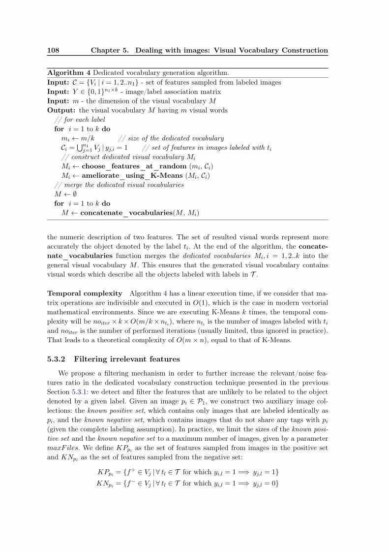
108 Chapter 5. Dealing with images: Visual Vocabulary Construction
Algorithm 4 Dedicated vocabulary generation algorithm.Input: C = {Vi | i = 1, 2..n1} - set of features sampled from labeled imagesInput: Y ∈ {0, 1}n1×k - image/label association matrixInput: m - the dimension of the visual vocabulary MOutput: the visual vocabulary M having m visual words// for each labelfor i = 1 to k domi ← m/k // size of the dedicated vocabularyCi =
⋃n1j=1 Vj | yj,i = 1 // set of features in images labeled with ti
// construct dedicated visual vocabulary Mi
Mi ← choose_features_at_random (mi, Ci)Mi ← ameliorate_using_K-Means (Mi, Ci)
// merge the dedicated visual vocabulariesM ← ∅for i = 1 to k doM ← concatenate_vocabularies(M , Mi)
the numeric description of two features. The set of resulted visual words represent moreaccurately the object denoted by the label ti. At the end of the algorithm, the concate-nate_vocabularies function merges the dedicated vocabularies Mi, i = 1, 2..k into thegeneral visual vocabulary M . This ensures that the generated visual vocabulary containsvisual words which describe all the objects labeled with labels in T .
Temporal complexity Algorithm 4 has a linear execution time, if we consider that ma-trix operations are indivisible and executed in O(1), which is the case in modern vectorialmathematical environments. Since we are executing K-Means k times, the temporal com-plexity will be noiter × k×O(m/k×nti), where nti is the number of images labeled with tiand noiter is the number of performed iterations (usually limited, thus ignored in practice).That leads to a theoretical complexity of O(m× n), equal to that of K-Means.
5.3.2 Filtering irrelevant features
We propose a filtering mechanism in order to further increase the relevant/noise fea-tures ratio in the dedicated vocabulary construction technique presented in the previousSection 5.3.1: we detect and filter the features that are unlikely to be related to the objectdenoted by a given label. Given an image pi ∈ P1, we construct two auxiliary image col-lections: the known positive set, which contains only images that are labeled identically aspi, and the known negative set, which contains images that do not share any tags with pi(given the complete labeling assumption). In practice, we limit the sizes of the known posi-tive set and the known negative set to a maximum number of images, given by a parametermaxFiles. We define KPpi as the set of features sampled from images in the positive setand KNpi as the set of features sampled from the negative set:
KPpi = {f+ ∈ Vj | ∀ tl ∈ T for which yi,l = 1 =⇒ yj,l = 1}KNpi = {f− ∈ Vj | ∀ tl ∈ T for which yi,l = 1 =⇒ yj,l = 0}
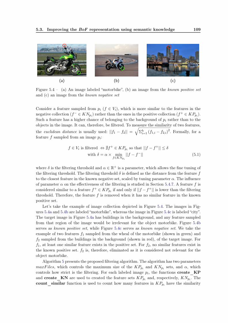
5.3. Improving the BoF representation using semantic knowledge 109
(a) (b) (c)
Figure 5.4 – (a) An image labeled “motorbike”, (b) an image from the known positive setand (c) an image from the known negative set
Consider a feature sampled from pi (f ∈ Vi), which is more similar to the features in thenegative collection (f− ∈ KNpi) rather than the ones in the positive collection (f+ ∈ KPpi).Such a feature has a higher chance of belonging to the background of pi rather than to theobjects in the image. It can, therefore, be filtered. To measure the similarity of two features,
the euclidean distance is usually used: ||f1 − f2|| =√
Σhi=1 (f1,i − f2,i)
2. Formally, for afeature f sampled from an image pi:
f ∈ Vi is filtered ⇔ @f+ ∈ KPpi so that ||f − f+|| ≤ δwith δ = α× min
f∈KNpi||f − f−|| (5.1)
where δ is the filtering threshold and α ∈ R+ is a parameter, which allows the fine tuning ofthe filtering threshold. The filtering threshold δ is defined as the distance from the feature fto the closest feature in the known negative set, scaled by tuning parameter α. The influenceof parameter α on the effectiveness of the filtering is studied in Section 5.4.7. A feature f isconsidered similar to a feature f+ ∈ KPpi if and only if ||f − f+|| is lower than the filteringthreshold. Therefore, the feature f is removed when it has no similar feature in the knownpositive set.
Let’s take the example of image collection depicted in Figure 5.4. The images in Fig-ures 5.4a and 5.4b are labeled “motorbike”, whereas the image in Figure 5.4c is labeled “city”.The target image in Figure 5.4a has buildings in the background, and any feature sampledfrom that region of the image would be irrelevant for the object motorbike. Figure 5.4bserves as known positive set, while Figure 5.4c serves as known negative set. We take theexample of two features f1 sampled from the wheal of the motorbike (shown in green) andf2 sampled from the buildings in the background (shown in red), of the target image. Forf1, at least one similar feature exists in the positive set. For f2, no similar features exist inthe known positive set. f2 is, therefore, eliminated as it is considered not relevant for theobject motorbike.
Algorithm 5 presents the proposed filtering algorithm. The algorithm has two parametersmaxFiles, which controls the maximum size of the KPpi and KNpi sets, and α, whichcontrols how strict is the filtering. For each labeled image pi, the functions create_KPand create_KN are used to created the feature sets KPpi and, respectively, KNpi . Thecount_similar function is used to count how many features in KPpi have the similarity
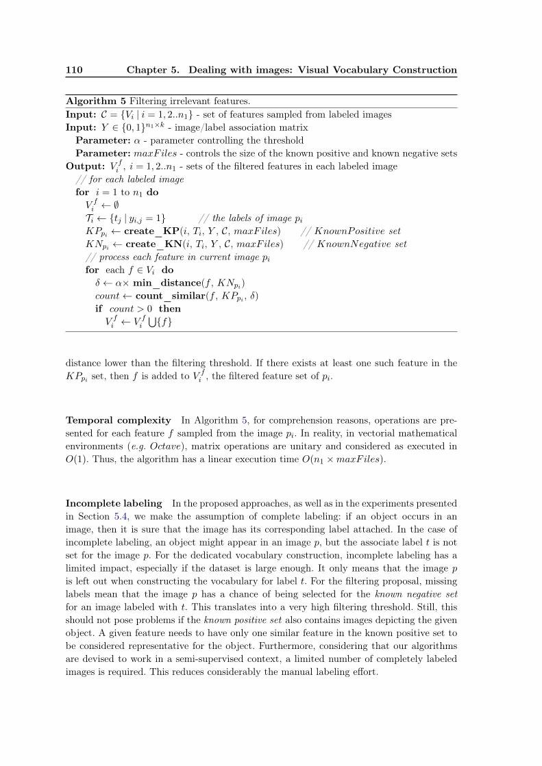
110 Chapter 5. Dealing with images: Visual Vocabulary Construction
Algorithm 5 Filtering irrelevant features.Input: C = {Vi | i = 1, 2..n1} - set of features sampled from labeled imagesInput: Y ∈ {0, 1}n1×k - image/label association matrixParameter: α - parameter controlling the thresholdParameter: maxFiles - controls the size of the known positive and known negative sets
Output: V fi , i = 1, 2..n1 - sets of the filtered features in each labeled image
// for each labeled imagefor i = 1 to n1 doV fi ← ∅Ti ← {tj | yi,j = 1} // the labels of image piKPpi ← create_KP(i, Ti, Y , C, maxFiles) // KnownPositive setKNpi ← create_KN(i, Ti, Y , C, maxFiles) // KnownNegative set// process each feature in current image pifor each f ∈ Vi doδ ← α× min_distance(f , KNpi)count← count_similar(f , KPpi , δ)if count > 0 thenV fi ← V f
i
⋃{f}
distance lower than the filtering threshold. If there exists at least one such feature in theKPpi set, then f is added to V f
i , the filtered feature set of pi.
Temporal complexity In Algorithm 5, for comprehension reasons, operations are pre-sented for each feature f sampled from the image pi. In reality, in vectorial mathematicalenvironments (e.g. Octave), matrix operations are unitary and considered as executed inO(1). Thus, the algorithm has a linear execution time O(n1 ×maxFiles).
Incomplete labeling In the proposed approaches, as well as in the experiments presentedin Section 5.4, we make the assumption of complete labeling: if an object occurs in animage, then it is sure that the image has its corresponding label attached. In the case ofincomplete labeling, an object might appear in an image p, but the associate label t is notset for the image p. For the dedicated vocabulary construction, incomplete labeling has alimited impact, especially if the dataset is large enough. It only means that the image pis left out when constructing the vocabulary for label t. For the filtering proposal, missinglabels mean that the image p has a chance of being selected for the known negative setfor an image labeled with t. This translates into a very high filtering threshold. Still, thisshould not pose problems if the known positive set also contains images depicting the givenobject. A given feature needs to have only one similar feature in the known positive set tobe considered representative for the object. Furthermore, considering that our algorithmsare devised to work in a semi-supervised context, a limited number of completely labeledimages is required. This reduces considerably the manual labeling effort.
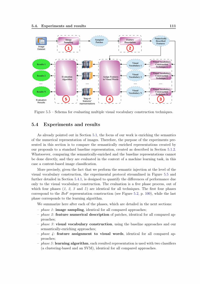
5.4. Experiments and results 111
Image Dataset
ImageSampling
1
SampledPatches
NumericallyDescribedFeatures
FeatureDescription
2
Visual Vocabulary ConstructionTechnique 1
Visual Vocabulary ConstructionTechnique 2
Visual Vocabulary ConstructionTechnique N
.....
3
VisualVocabulary 1
VisualVocabulary 2
VisualVocabulary N
.....
Assign Featuresto Visual Words
4
EvaluationAlgorithm
.....
Results 1
Results 2
Results N
.....
“Bag-of-features”
representations
EvaluationResults
5
Figure 5.5 – Schema for evaluating multiple visual vocabulary construction techniques.
5.4 Experiments and results
As already pointed out in Section 5.1, the focus of our work is enriching the semanticsof the numerical representation of images. Therefore, the purpose of the experiments pre-sented in this section is to compare the semantically enriched representations created byour proposals to a standard baseline representation, created as described in Section 5.1.2.Whatsoever, comparing the semantically-enriched and the baseline representations cannotbe done directly, and they are evaluated in the context of a machine learning task, in thiscase a content-based image classification.
More precisely, given the fact that we perform the semantic injection at the level of thevisual vocabulary construction, the experimental protocol streamlined in Figure 5.5 andfurther detailed in Section 5.4.1, is designed to quantify the differences of performance dueonly to the visual vocabulary construction. The evaluation is a five phase process, out ofwhich four phases (1, 2, 3 and 5 ) are identical for all techniques. The first four phasescorrespond to the BoF representation construction (see Figure 5.2, p. 100), while the lastphase corresponds to the learning algorithm.
We summarize here after each of the phases, which are detailed in the next sections:– phase 1 : image sampling, identical for all compared approaches;– phase 2 : feature numerical description of patches, identical for all compared ap-
proaches;– phase 3 : visual vocabulary construction, using the baseline approaches and our
semantically-enriching approaches;– phase 4 : feature assignment to visual words, identical for all compared ap-
proaches;– phase 5 : learning algorithm, each resulted representation is used with two classifiers
(a clustering-based and an SVM), identical for all compared approaches.
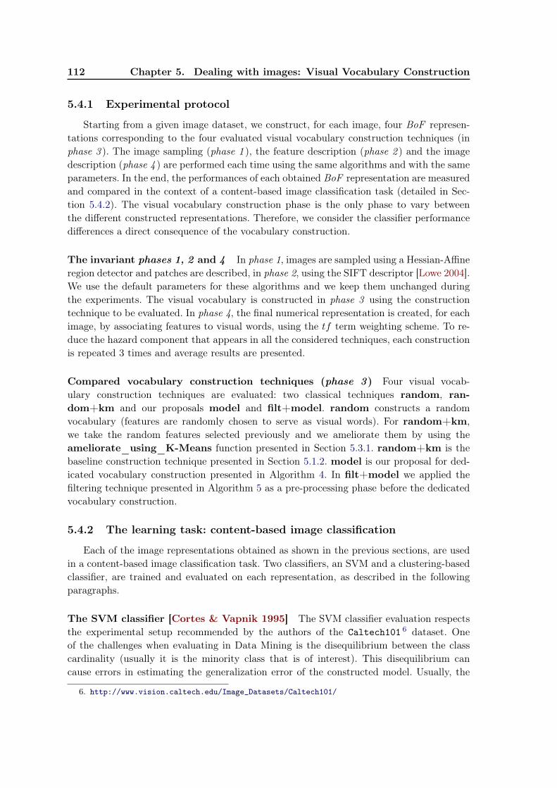
112 Chapter 5. Dealing with images: Visual Vocabulary Construction
5.4.1 Experimental protocol
Starting from a given image dataset, we construct, for each image, four BoF represen-tations corresponding to the four evaluated visual vocabulary construction techniques (inphase 3 ). The image sampling (phase 1 ), the feature description (phase 2 ) and the imagedescription (phase 4 ) are performed each time using the same algorithms and with the sameparameters. In the end, the performances of each obtained BoF representation are measuredand compared in the context of a content-based image classification task (detailed in Sec-tion 5.4.2). The visual vocabulary construction phase is the only phase to vary betweenthe different constructed representations. Therefore, we consider the classifier performancedifferences a direct consequence of the vocabulary construction.
The invariant phases 1, 2 and 4 In phase 1, images are sampled using a Hessian-Affineregion detector and patches are described, in phase 2, using the SIFT descriptor [Lowe 2004].We use the default parameters for these algorithms and we keep them unchanged duringthe experiments. The visual vocabulary is constructed in phase 3 using the constructiontechnique to be evaluated. In phase 4, the final numerical representation is created, for eachimage, by associating features to visual words, using the tf term weighting scheme. To re-duce the hazard component that appears in all the considered techniques, each constructionis repeated 3 times and average results are presented.
Compared vocabulary construction techniques (phase 3) Four visual vocab-ulary construction techniques are evaluated: two classical techniques random, ran-dom+km and our proposals model and filt+model. random constructs a randomvocabulary (features are randomly chosen to serve as visual words). For random+km,we take the random features selected previously and we ameliorate them by using theameliorate_using_K-Means function presented in Section 5.3.1. random+km is thebaseline construction technique presented in Section 5.1.2. model is our proposal for ded-icated vocabulary construction presented in Algorithm 4. In filt+model we applied thefiltering technique presented in Algorithm 5 as a pre-processing phase before the dedicatedvocabulary construction.
5.4.2 The learning task: content-based image classification
Each of the image representations obtained as shown in the previous sections, are usedin a content-based image classification task. Two classifiers, an SVM and a clustering-basedclassifier, are trained and evaluated on each representation, as described in the followingparagraphs.
The SVM classifier [Cortes & Vapnik 1995] The SVM classifier evaluation respectsthe experimental setup recommended by the authors of the Caltech101 6 dataset. Oneof the challenges when evaluating in Data Mining is the disequilibrium between the classcardinality (usually it is the minority class that is of interest). This disequilibrium cancause errors in estimating the generalization error of the constructed model. Usually, the
6. http://www.vision.caltech.edu/Image_Datasets/Caltech101/
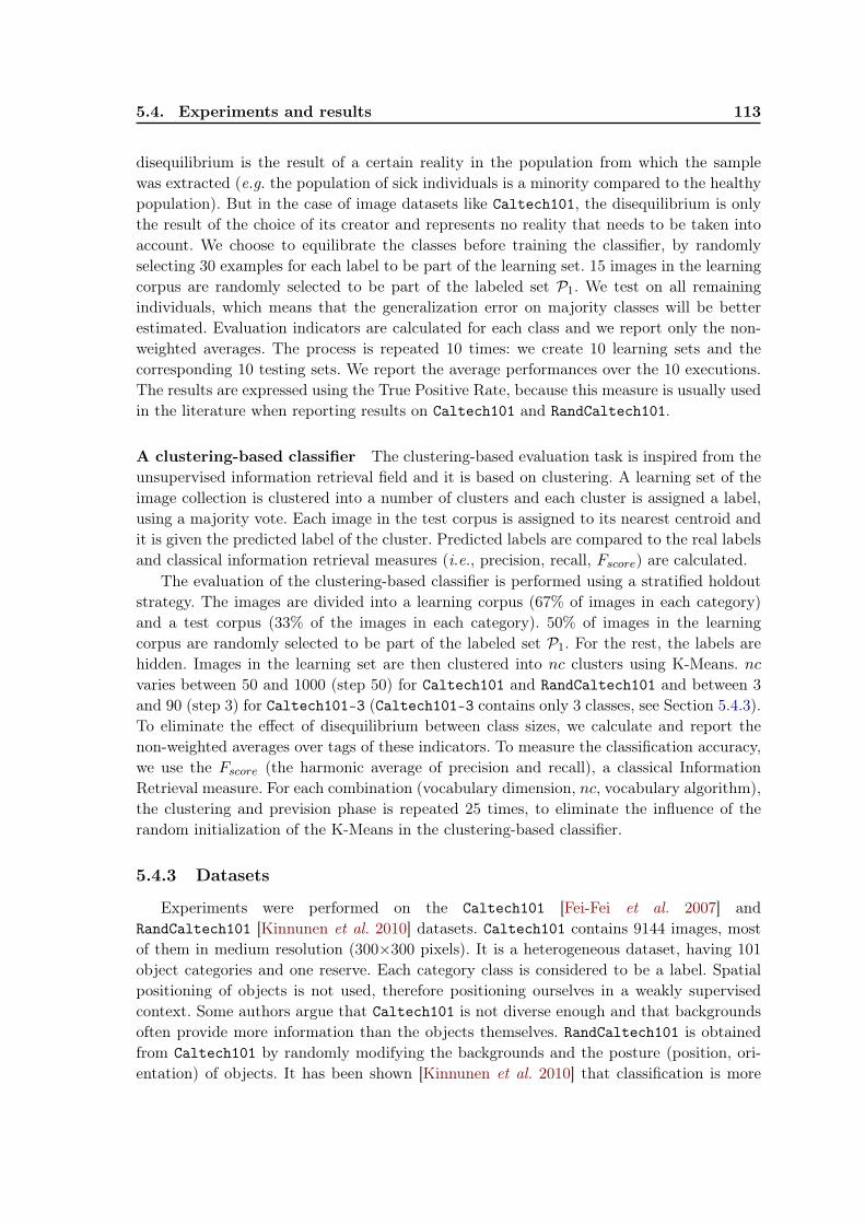
5.4. Experiments and results 113
disequilibrium is the result of a certain reality in the population from which the samplewas extracted (e.g. the population of sick individuals is a minority compared to the healthypopulation). But in the case of image datasets like Caltech101, the disequilibrium is onlythe result of the choice of its creator and represents no reality that needs to be taken intoaccount. We choose to equilibrate the classes before training the classifier, by randomlyselecting 30 examples for each label to be part of the learning set. 15 images in the learningcorpus are randomly selected to be part of the labeled set P1. We test on all remainingindividuals, which means that the generalization error on majority classes will be betterestimated. Evaluation indicators are calculated for each class and we report only the non-weighted averages. The process is repeated 10 times: we create 10 learning sets and thecorresponding 10 testing sets. We report the average performances over the 10 executions.The results are expressed using the True Positive Rate, because this measure is usually usedin the literature when reporting results on Caltech101 and RandCaltech101.
A clustering-based classifier The clustering-based evaluation task is inspired from theunsupervised information retrieval field and it is based on clustering. A learning set of theimage collection is clustered into a number of clusters and each cluster is assigned a label,using a majority vote. Each image in the test corpus is assigned to its nearest centroid andit is given the predicted label of the cluster. Predicted labels are compared to the real labelsand classical information retrieval measures (i.e., precision, recall, Fscore) are calculated.
The evaluation of the clustering-based classifier is performed using a stratified holdoutstrategy. The images are divided into a learning corpus (67% of images in each category)and a test corpus (33% of the images in each category). 50% of images in the learningcorpus are randomly selected to be part of the labeled set P1. For the rest, the labels arehidden. Images in the learning set are then clustered into nc clusters using K-Means. ncvaries between 50 and 1000 (step 50) for Caltech101 and RandCaltech101 and between 3and 90 (step 3) for Caltech101-3 (Caltech101-3 contains only 3 classes, see Section 5.4.3).To eliminate the effect of disequilibrium between class sizes, we calculate and report thenon-weighted averages over tags of these indicators. To measure the classification accuracy,we use the Fscore (the harmonic average of precision and recall), a classical InformationRetrieval measure. For each combination (vocabulary dimension, nc, vocabulary algorithm),the clustering and prevision phase is repeated 25 times, to eliminate the influence of therandom initialization of the K-Means in the clustering-based classifier.
5.4.3 Datasets
Experiments were performed on the Caltech101 [Fei-Fei et al. 2007] andRandCaltech101 [Kinnunen et al. 2010] datasets. Caltech101 contains 9144 images, mostof them in medium resolution (300×300 pixels). It is a heterogeneous dataset, having 101object categories and one reserve. Each category class is considered to be a label. Spatialpositioning of objects is not used, therefore positioning ourselves in a weakly supervisedcontext. Some authors argue that Caltech101 is not diverse enough and that backgroundsoften provide more information than the objects themselves. RandCaltech101 is obtainedfrom Caltech101 by randomly modifying the backgrounds and the posture (position, ori-entation) of objects. It has been shown [Kinnunen et al. 2010] that classification is more
114 Chapter 5. Dealing with images: Visual Vocabulary Construction
challenging on RandCaltech101 than on Caltech101.Because Caltech101 is an unbalanced dataset, with category sizes ranging from 31
to 800 images, we have taken 3 out of the biggest categories (airplanes, Motorbikes andFaces_easy) and created another corpus, denoted Caltech101-3. It contains 2033 images.The advantage of the new corpus is that it provides many examples for each category andit is balanced category-wise. This allows us to study how our propositions behave on bothbalanced and unbalanced datasets.
5.4.4 Qualitative evaluation
Figure 5.6 – Example of images from “easy” classes (top row) and “difficult” classes (bottomrow)
In a classification tasks, some classes are naturally easier to recognize than others. Thishappens when the numerical description is better adapted to translate them into a sepa-rable numerical space. On Caltech101, the best classification scores are almost invariablyobtained by the same categories, independent of the choice of visual construction algorithmsor parameters.
Figure 5.6 shows some examples of images belonging to “easy classes”, categories thatobtain good classification scores (on the upper row), and examples of “difficult classes”,categories that obtain low scores (on the bottom row). The objects belonging to the “easyclasses” either appear in the same posture in all examples or they have a specific colorpattern that makes them easily recognisable. Most of the examples of airplanes and garfieldappear with the same shape, size and orientation. Other categories like yin_yang, soc-cer_ball or dalmatian have a specific white-black alternation pattern, which makes themeasily recognizable even in the real world. By contrast, the objects depicted in picture of“difficult classes”, like seahorse or butterfly appear in different colors, multiple postures andsometimes hidden in the background.
We perform the same analysis on RandCaltech101. Table 5.1 presents a compar-ative view of “easy classes” and “difficult classes” constructed for Caltech101 andRandCaltech101, with the non-identical categories (between the two datasets) printed inboldface. We observe the high degree of overlapping of the constructed sets: most of the“easy classes” in Caltech101 also appear as “easily” recognizable for RandCaltech101. Sim-ilarly, difficult classes on Caltech101 remain difficult on RandCaltech101. In Table 5.1, theonly category that changes difficulty is metronome, which is an “easy class” in Caltech101
5.4. Experiments and results 115
Table 5.1 – “Easy” classes and “difficult” classes in Caltech101 and RandCaltech101
“Easy” classes “Difficult” classesCaltech101 RandCaltech101 Caltech101 RandCaltech101
airplanes accordion beaver basscar_side airplanes buddha binoculardalmatian car_side butterfly brontosaurusdollar_bill dalmatian ceiling_fan buddhaFaces_easy dollar_bill cougar_body butterflygarfield Faces_easy crab crab
grand_piano garfield crayfish crayfishLeopards laptop cup crocodilemetronome Motorbikes dragonfly cupMotorbikes panda ewer dragonfly
panda snoopy ferry ewerscissors soccer_ball flamingo flamingosnoopy stop_sign flamingo_head flamingo_head
soccer_ball watch ibis gerenukstop_sign windsor_chair kangaroo helicopter
tick yin_yang lamp ibiswatch lobster kangaroo
windsor_chair mandolin lampyin_yang mayfly lobster
minaret mandolinpigeon mayflyplatypus metronomepyramid minaretrhino okapi
saxophone pigeonschooner platypussea_horse saxophonestapler sea_horse
strawberry staplerwild_cat wrenchwrench
and a “difficult class” in RandCaltech101. This proves that the background randomizationperformed in order to create RandCaltech101, while it makes the dataset more challengingto classify as a whole, does not change the relative difficulty between categories. Cate-gories that obtain good classification scores for Caltech101 also obtain good scores forRandCaltech101.
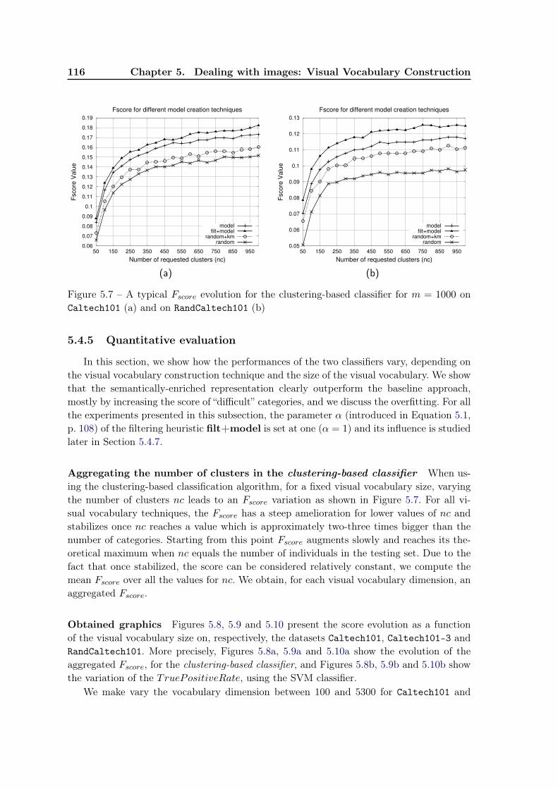
116 Chapter 5. Dealing with images: Visual Vocabulary Construction
0.06
0.07
0.08
0.09
0.1
0.11
0.12
0.13
0.14
0.15
0.16
0.17
0.18
0.19
50 150 250 350 450 550 650 750 850 950
Fscore
Valu
e
Number of requested clusters (nc)
Fscore for different model creation techniques
modelfilt+model
random+kmrandom
(a)
0.05
0.06
0.07
0.08
0.09
0.1
0.11
0.12
0.13
50 150 250 350 450 550 650 750 850 950
Fscore
Valu
e
Number of requested clusters (nc)
Fscore for different model creation techniques
modelfilt+model
random+kmrandom
(b)
Figure 5.7 – A typical Fscore evolution for the clustering-based classifier for m = 1000 onCaltech101 (a) and on RandCaltech101 (b)
5.4.5 Quantitative evaluation
In this section, we show how the performances of the two classifiers vary, depending onthe visual vocabulary construction technique and the size of the visual vocabulary. We showthat the semantically-enriched representation clearly outperform the baseline approach,mostly by increasing the score of “difficult” categories, and we discuss the overfitting. For allthe experiments presented in this subsection, the parameter α (introduced in Equation 5.1,p. 108) of the filtering heuristic filt+model is set at one (α = 1) and its influence is studiedlater in Section 5.4.7.
Aggregating the number of clusters in the clustering-based classifier When us-ing the clustering-based classification algorithm, for a fixed visual vocabulary size, varyingthe number of clusters nc leads to an Fscore variation as shown in Figure 5.7. For all vi-sual vocabulary techniques, the Fscore has a steep amelioration for lower values of nc andstabilizes once nc reaches a value which is approximately two-three times bigger than thenumber of categories. Starting from this point Fscore augments slowly and reaches its the-oretical maximum when nc equals the number of individuals in the testing set. Due to thefact that once stabilized, the score can be considered relatively constant, we compute themean Fscore over all the values for nc. We obtain, for each visual vocabulary dimension, anaggregated Fscore.
Obtained graphics Figures 5.8, 5.9 and 5.10 present the score evolution as a functionof the visual vocabulary size on, respectively, the datasets Caltech101, Caltech101-3 andRandCaltech101. More precisely, Figures 5.8a, 5.9a and 5.10a show the evolution of theaggregated Fscore, for the clustering-based classifier, and Figures 5.8b, 5.9b and 5.10b showthe variation of the TruePositiveRate, using the SVM classifier.
We make vary the vocabulary dimension between 100 and 5300 for Caltech101 and
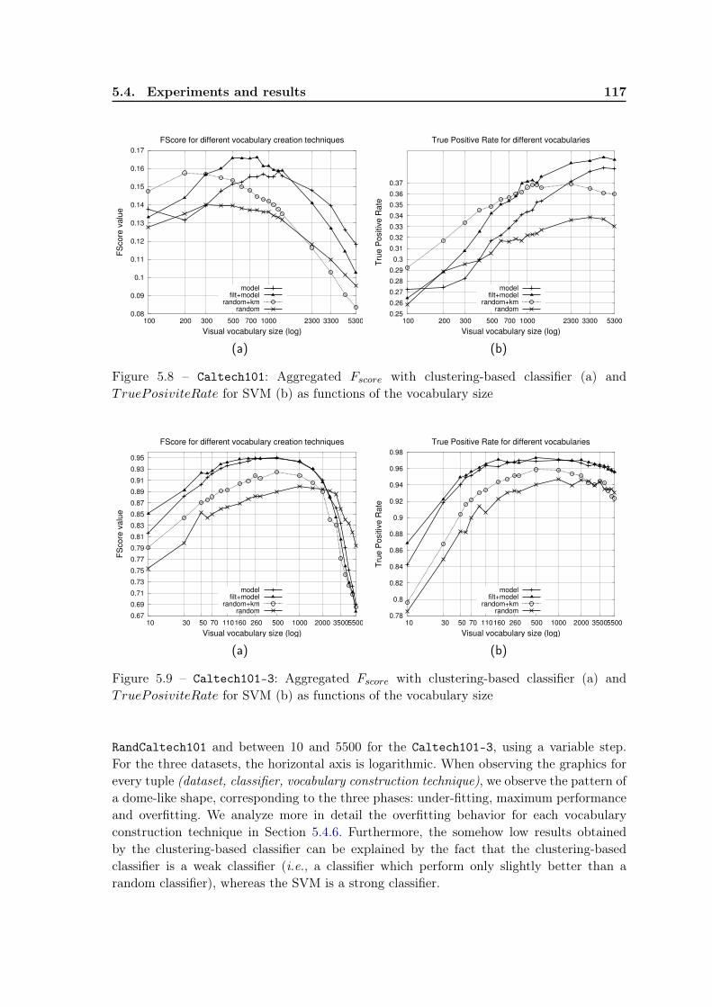
5.4. Experiments and results 117
0.08
0.09
0.1
0.11
0.12
0.13
0.14
0.15
0.16
0.17
100 200 300 500 700 1000 2300 3300 5300
FS
co
re v
alu
e
Visual vocabulary size (log)
FScore for different vocabulary creation techniques
modelfilt+model
random+kmrandom
(a)
0.25
0.26
0.27
0.28
0.29
0.3
0.31
0.32
0.33
0.34
0.35
0.36
0.37
100 200 300 500 700 1000 2300 3300 5300
Tru
e P
ositiv
e R
ate
Visual vocabulary size (log)
True Positive Rate for different vocabularies
modelfilt+model
random+kmrandom
(b)
Figure 5.8 – Caltech101: Aggregated Fscore with clustering-based classifier (a) andTruePosiviteRate for SVM (b) as functions of the vocabulary size
0.67
0.69
0.71
0.73
0.75
0.77
0.79
0.81
0.83
0.85
0.87
0.89
0.91
0.93
0.95
10 30 50 70 110 160 260 500 1000 2000 35005500
FS
co
re v
alu
e
Visual vocabulary size (log)
FScore for different vocabulary creation techniques
modelfilt+model
random+kmrandom
(a)
0.78
0.8
0.82
0.84
0.86
0.88
0.9
0.92
0.94
0.96
0.98
10 30 50 70 110 160 260 500 1000 2000 35005500
Tru
e P
ositiv
e R
ate
Visual vocabulary size (log)
True Positive Rate for different vocabularies
modelfilt+model
random+kmrandom
(b)
Figure 5.9 – Caltech101-3: Aggregated Fscore with clustering-based classifier (a) andTruePosiviteRate for SVM (b) as functions of the vocabulary size
RandCaltech101 and between 10 and 5500 for the Caltech101-3, using a variable step.For the three datasets, the horizontal axis is logarithmic. When observing the graphics forevery tuple (dataset, classifier, vocabulary construction technique), we observe the pattern ofa dome-like shape, corresponding to the three phases: under-fitting, maximum performanceand overfitting. We analyze more in detail the overfitting behavior for each vocabularyconstruction technique in Section 5.4.6. Furthermore, the somehow low results obtainedby the clustering-based classifier can be explained by the fact that the clustering-basedclassifier is a weak classifier (i.e., a classifier which perform only slightly better than arandom classifier), whereas the SVM is a strong classifier.
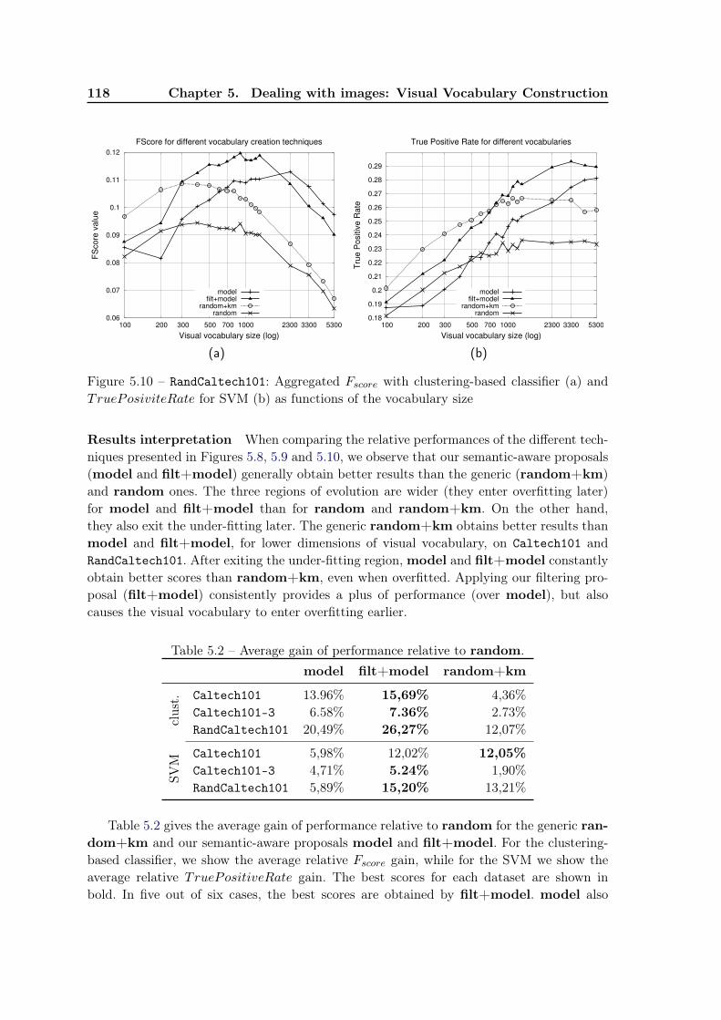
118 Chapter 5. Dealing with images: Visual Vocabulary Construction
0.06
0.07
0.08
0.09
0.1
0.11
0.12
100 200 300 500 700 1000 2300 3300 5300
FS
co
re v
alu
e
Visual vocabulary size (log)
FScore for different vocabulary creation techniques
modelfilt+model
random+kmrandom
(a)
0.18
0.19
0.2
0.21
0.22
0.23
0.24
0.25
0.26
0.27
0.28
0.29
100 200 300 500 700 1000 2300 3300 5300
Tru
e P
ositiv
e R
ate
Visual vocabulary size (log)
True Positive Rate for different vocabularies
modelfilt+model
random+kmrandom
(b)
Figure 5.10 – RandCaltech101: Aggregated Fscore with clustering-based classifier (a) andTruePosiviteRate for SVM (b) as functions of the vocabulary size
Results interpretation When comparing the relative performances of the different tech-niques presented in Figures 5.8, 5.9 and 5.10, we observe that our semantic-aware proposals(model and filt+model) generally obtain better results than the generic (random+km)and random ones. The three regions of evolution are wider (they enter overfitting later)for model and filt+model than for random and random+km. On the other hand,they also exit the under-fitting later. The generic random+km obtains better results thanmodel and filt+model, for lower dimensions of visual vocabulary, on Caltech101 andRandCaltech101. After exiting the under-fitting region, model and filt+model constantlyobtain better scores than random+km, even when overfitted. Applying our filtering pro-posal (filt+model) consistently provides a plus of performance (over model), but alsocauses the visual vocabulary to enter overfitting earlier.
Table 5.2 – Average gain of performance relative to random.model filt+model random+km
clust. Caltech101 13.96% 15,69% 4,36%
Caltech101-3 6.58% 7.36% 2.73%RandCaltech101 20,49% 26,27% 12,07%
SVM
Caltech101 5,98% 12,02% 12,05%Caltech101-3 4,71% 5.24% 1,90%RandCaltech101 5,89% 15,20% 13,21%
Table 5.2 gives the average gain of performance relative to random for the generic ran-dom+km and our semantic-aware proposals model and filt+model. For the clustering-based classifier, we show the average relative Fscore gain, while for the SVM we show theaverage relative TruePositiveRate gain. The best scores for each dataset are shown inbold. In five out of six cases, the best scores are obtained by filt+model. model also
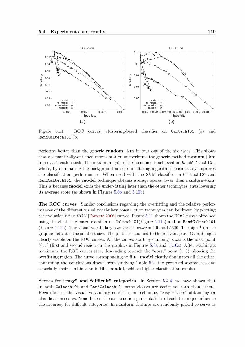
5.4. Experiments and results 119
0.08
0.09
0.1
0.11
0.12
0.13
0.14
0.15
0.0065 0.007 0.0075 0.008
Se
nsitiv
ity
1 - Specificity
ROC curve
modelfilt+model
random+kmrandom
(a)
0.07
0.08
0.09
0.1
0.11
0.007 0.0072 0.0074 0.0076 0.0078 0.008 0.0082 0.0084
Se
nsitiv
ity
1 - Specificity
ROC curve
modelfilt+model
random+kmrandom
(b)
Figure 5.11 – ROC curves: clustering-based classifier on Caltech101 (a) andRandCaltech101 (b)
performs better than the generic random+km in four out of the six cases. This showsthat a semantically-enriched representation outperforms the generic method random+kmin a classification task. The maximum gain of performance is achieved on RandCaltech101,where, by eliminating the background noise, our filtering algorithm considerably improvesthe classification performances. When used with the SVM classifier on Caltech101 andRandCaltech101, the model technique obtains average scores lower than random+km.This is because model exits the under-fitting later than the other techniques, thus loweringits average score (as shown in Figures 5.8b and 5.10b).
The ROC curves Similar conclusions regarding the overfitting and the relative perfor-mances of the different visual vocabulary construction techniques can be drawn by plottingthe evolution using ROC [Fawcett 2006] curves. Figure 5.11 shows the ROC curves obtainedusing the clustering-based classifier on Caltech101(Figure 5.11a) and on RandCaltech101(Figure 5.11b). The visual vocabulary size varied between 100 and 5300. The sign * on thegraphic indicates the smallest size. The plots are zoomed to the relevant part. Overfitting isclearly visible on the ROC curves. All the curves start by climbing towards the ideal point(0, 1) (first and second region on the graphics in Figures 5.8a and 5.10a). After reaching amaximum, the ROC curves start descending towards the “worst” point (1, 0), showing theoverfitting region. The curve corresponding to filt+model clearly dominates all the other,confirming the conclusions drawn from studying Table 5.2: the proposed approaches andespecially their combination in filt+model, achieve higher classification results.
Scores for “easy” and “difficult” categories In Section 5.4.4, we have shown thatin both Caltech101 and RandCaltech101 some classes are easier to learn than others.Regardless of the visual vocabulary construction technique, “easy classes” obtain higherclassification scores. Nonetheless, the construction particularities of each technique influencethe accuracy for difficult categories. In random, features are randomly picked to serve as
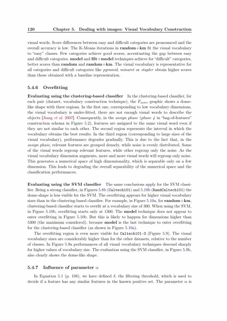
120 Chapter 5. Dealing with images: Visual Vocabulary Construction
visual words. Score differences between easy and difficult categories are pronounced and theoverall accuracy is low. The K-Means iterations in random+km fit the visual vocabularyto “easy” classes. Few categories achieve good scores, accentuating the gap between easyand difficult categories.model and filt+model techniques achieve for “difficult” categories,better scores than random and random+km. The visual vocabulary is representative forall categories and difficult categories like pyramid, minaret or stapler obtain higher scoresthan those obtained with a baseline representation.
5.4.6 Overfitting
Evaluating using the clustering-based classifier In the clustering-based classifier, foreach pair (dataset, vocabulary construction technique), the Fscore graphic shows a dome-like shape with three regions. In the first one, corresponding to low vocabulary dimensions,the visual vocabulary is under-fitted, there are not enough visual words to describe theobjects [Jiang et al. 2007]. Consequently, in the assign phase (phase 4 in “bag-of-features”construction schema in Figure 5.2), features are assigned to the same visual word even ifthey are not similar to each other. The second region represents the interval in which thevocabulary obtains the best results. In the third region (corresponding to large sizes of thevisual vocabulary), performance degrades gradually. This is due to the fact that, in theassign phase, relevant features are grouped densely, while noise is evenly distributed. Someof the visual words regroup relevant features, while other regroup only the noise. As thevisual vocabulary dimension augments, more and more visual words will regroup only noise.This generates a numerical space of high dimensionality, which is separable only on a fewdimension. This leads to degrading the overall separability of the numerical space and theclassification performances.
Evaluating using the SVM classifier The same conclusions apply for the SVM classi-fier. Being a strong classifier, in Figures 5.8b (Caltech101) and 5.10b (RandCaltech101) thedome-shape is less visible for the SVM. The overfitting appears for higher visual vocabularysizes than in the clustering-based classifier. For example, in Figure 5.10a, for random+km,clustering-based classifier starts to overfit at a vocabulary size of 300. When using the SVM,in Figure 5.10b, overfitting starts only at 1300. The model technique does not appear toenter overfitting in Figure 5.10b. But this is likely to happen for dimensions higher than5300 (the maximum considered), because model is the last technique to enter overfittingfor the clustering-based classifier (as shown in Figure 5.10a).
The overfitting region is even more visible for Caltech101-3 (Figure 5.9). The visualvocabulary sizes are considerably higher than for the other datasets, relative to the numberof classes. In Figure 5.9a performances of all visual vocabulary techniques descend sharplyfor higher values of vocabulary size. The evaluation using the SVM classifier, in Figure 5.9b,also clearly shows the dome-like shape.
5.4.7 Influence of parameter α
In Equation 5.1 (p. 108), we have defined δ, the filtering threshold, which is used todecide if a feature has any similar features in the known positive set. The parameter α is
5.4. Experiments and results 121
0.08
0.09
0.1
0.11
0.12
100 200 300 500 700 1000 2300 3300 5300
FS
co
re v
alu
e
Visual vocabulary size (log)
FScore curve for different values for alpha (filtering)
alpha = 0.8alpha = 1
alpha = 1.25alpha = 1.5
(a)
0.17
0.18
0.19
0.2
0.21
0.22
0.23
0.24
0.25
0.26
0.27
0.28
0.29
0.3
100 200 300 500 700 1000 2300 3300 5300
Tru
e P
ositiv
e R
ate
Visual vocabulary size (log)
True Positive Rate curve for different values for alpha (filtering)
alpha = 0.8alpha = 1
alpha = 1.25alpha = 1.5
(b)
Figure 5.12 – RandCaltech101: influence of parameter α on filt+model construction tech-nique in the clustering-based task (a) and the SVM classifier (b)
used to fine-tune this threshold. If α is set too low, only the features that are very close(in terms of Euclidean distance) are considered to be similar. Consequently, the filteringis very strict, lowering the number of false positives, with the risk of an inflation of falsenegatives. On the other hand, setting α too high allows distant features to be consideredas similar, causing a high number of false positives. In the previous experiments, we haveset the parameter α = 1. In this section, we study the influence of this parameter on theperformances obtained by the filt+model construction technique.
Figure 5.12 shows the evolution of the filt+model visual vocabulary construction tech-nique as a function of visual vocabulary size, when using α ∈ {0.8, 1, 1.25, 1.5}. Thehorizontal axis is logarithmic. A value for α = 0.8 is too strict and the high number of falsenegatives decreases classification performances. Augmenting α = 1 improves performances,both when using the clustering-based classifier (Figure 5.12a) and when using the SVMclassifier (Figure 5.12b).
If α is set too high, performances decrease again. Too many features are consideredsimilar and less features get filtered. Performances approach those obtained when no filteringis applied. α = 1.25 and α = 1.5 show similar performances, since both levels are alreadytoo high for filtering to be effective. For α ≥ 1.25 filt+model is equivalent to the modelvisual vocabulary construction technique. In Figure 5.12a, filt+model with α ∈ {1.25, 1.5}obtains, for high visual vocabulary sizes (m > 2000), better results than filt+model withα ∈ {0.8, 1}. This behaviour is similar with that already seen in Figure 5.10a, when modelenters overfitting later than filt+model and obtains better results for high vocabularysizes.
These initial experiments make us believe that α is dataset independent (a value of 1provided best results on all three datasets), but further experiments on other datasets arerequired in order to conclude this. Furthermore, a heuristic for automatically determiningits value is part of our future plans.
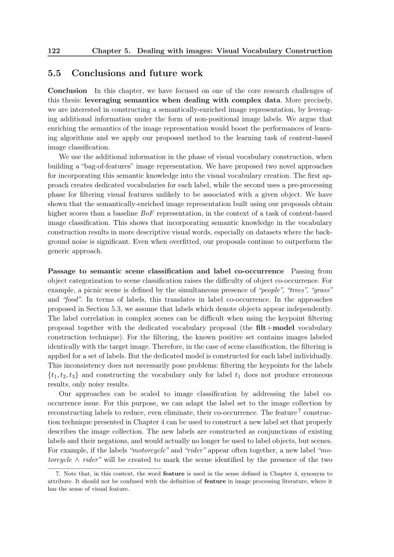
122 Chapter 5. Dealing with images: Visual Vocabulary Construction
5.5 Conclusions and future work
Conclusion In this chapter, we have focused on one of the core research challenges ofthis thesis: leveraging semantics when dealing with complex data. More precisely,we are interested in constructing a semantically-enriched image representation, by leverag-ing additional information under the form of non-positional image labels. We argue thatenriching the semantics of the image representation would boost the performances of learn-ing algorithms and we apply our proposed method to the learning task of content-basedimage classification.
We use the additional information in the phase of visual vocabulary construction, whenbuilding a “bag-of-features” image representation. We have proposed two novel approachesfor incorporating this semantic knowledge into the visual vocabulary creation. The first ap-proach creates dedicated vocabularies for each label, while the second uses a pre-processingphase for filtering visual features unlikely to be associated with a given object. We haveshown that the semantically-enriched image representation built using our proposals obtainhigher scores than a baseline BoF representation, in the context of a task of content-basedimage classification. This shows that incorporating semantic knowledge in the vocabularyconstruction results in more descriptive visual words, especially on datasets where the back-ground noise is significant. Even when overfitted, our proposals continue to outperform thegeneric approach.
Passage to semantic scene classification and label co-occurrence Passing fromobject categorization to scene classification raises the difficulty of object co-occurrence. Forexample, a picnic scene is defined by the simultaneous presence of “people”, “trees”, “grass”and “food”. In terms of labels, this translates in label co-occurrence. In the approachesproposed in Section 5.3, we assume that labels which denote objects appear independently.The label correlation in complex scenes can be difficult when using the keypoint filteringproposal together with the dedicated vocabulary proposal (the filt+model vocabularyconstruction technique). For the filtering, the known positive set contains images labeledidentically with the target image. Therefore, in the case of scene classification, the filtering isapplied for a set of labels. But the dedicated model is constructed for each label individually.This inconsistency does not necessarily pose problems: filtering the keypoints for the labels{t1, t2, t3} and constructing the vocabulary only for label t1 does not produce erroneousresults, only noisy results.
Our approaches can be scaled to image classification by addressing the label co-occurrence issue. For this purpose, we can adapt the label set to the image collection byreconstructing labels to reduce, even eliminate, their co-occurrence. The feature 7 construc-tion technique presented in Chapter 4 can be used to construct a new label set that properlydescribes the image collection. The new labels are constructed as conjunctions of existinglabels and their negations, and would actually no longer be used to label objects, but scenes.For example, if the labels “motorcycle” and “rider” appear often together, a new label “mo-torcycle ∧ rider” will be created to mark the scene identified by the presence of the two
7. Note that, in this context, the word feature is used in the sense defined in Chapter 4, synonym toattribute. It should not be confused with the definition of feature in image processing literature, where ithas the sense of visual feature.
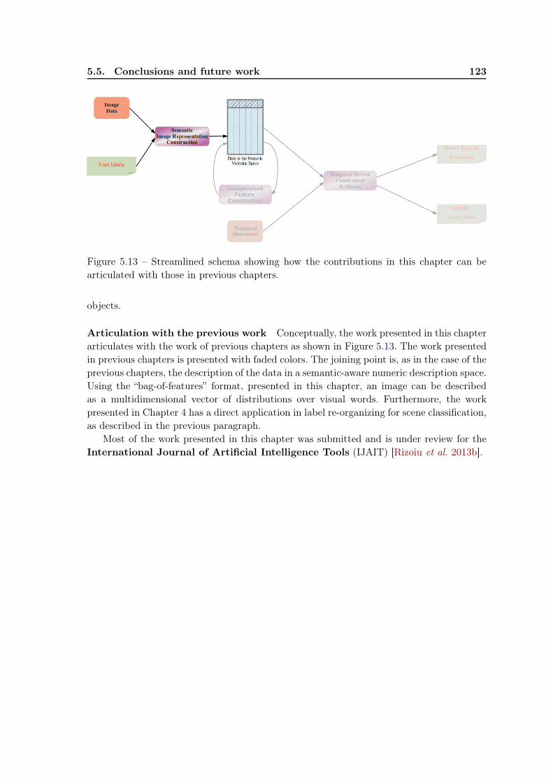
5.5. Conclusions and future work 123
Figure 5.13 – Streamlined schema showing how the contributions in this chapter can bearticulated with those in previous chapters.
objects.
Articulation with the previous work Conceptually, the work presented in this chapterarticulates with the work of previous chapters as shown in Figure 5.13. The work presentedin previous chapters is presented with faded colors. The joining point is, as in the case of theprevious chapters, the description of the data in a semantic-aware numeric description space.Using the “bag-of-features” format, presented in this chapter, an image can be describedas a multidimensional vector of distributions over visual words. Furthermore, the workpresented in Chapter 4 has a direct application in label re-organizing for scene classification,as described in the previous paragraph.
Most of the work presented in this chapter was submitted and is under review for theInternational Journal of Artificial Intelligence Tools (IJAIT) [Rizoiu et al. 2013b].

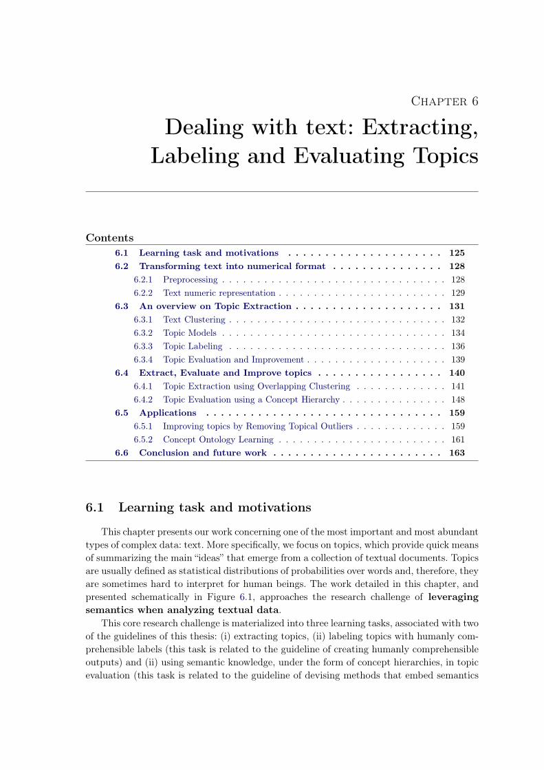
Chapter 6
Dealing with text: Extracting,Labeling and Evaluating Topics
Contents6.1 Learning task and motivations . . . . . . . . . . . . . . . . . . . . . 1256.2 Transforming text into numerical format . . . . . . . . . . . . . . . 128
6.2.1 Preprocessing . . . . . . . . . . . . . . . . . . . . . . . . . . . . . . . . 1286.2.2 Text numeric representation . . . . . . . . . . . . . . . . . . . . . . . . 129
6.3 An overview on Topic Extraction . . . . . . . . . . . . . . . . . . . . 1316.3.1 Text Clustering . . . . . . . . . . . . . . . . . . . . . . . . . . . . . . . 1326.3.2 Topic Models . . . . . . . . . . . . . . . . . . . . . . . . . . . . . . . . 1346.3.3 Topic Labeling . . . . . . . . . . . . . . . . . . . . . . . . . . . . . . . 1366.3.4 Topic Evaluation and Improvement . . . . . . . . . . . . . . . . . . . . 139
6.4 Extract, Evaluate and Improve topics . . . . . . . . . . . . . . . . . 1406.4.1 Topic Extraction using Overlapping Clustering . . . . . . . . . . . . . 1416.4.2 Topic Evaluation using a Concept Hierarchy . . . . . . . . . . . . . . . 148
6.5 Applications . . . . . . . . . . . . . . . . . . . . . . . . . . . . . . . . 1596.5.1 Improving topics by Removing Topical Outliers . . . . . . . . . . . . . 1596.5.2 Concept Ontology Learning . . . . . . . . . . . . . . . . . . . . . . . . 161
6.6 Conclusion and future work . . . . . . . . . . . . . . . . . . . . . . . 163
6.1 Learning task and motivations
This chapter presents our work concerning one of the most important and most abundanttypes of complex data: text. More specifically, we focus on topics, which provide quick meansof summarizing the main “ideas” that emerge from a collection of textual documents. Topicsare usually defined as statistical distributions of probabilities over words and, therefore, theyare sometimes hard to interpret for human beings. The work detailed in this chapter, andpresented schematically in Figure 6.1, approaches the research challenge of leveragingsemantics when analyzing textual data.
This core research challenge is materialized into three learning tasks, associated with twoof the guidelines of this thesis: (i) extracting topics, (ii) labeling topics with humanly com-prehensible labels (this task is related to the guideline of creating humanly comprehensibleoutputs) and (ii) using semantic knowledge, under the form of concept hierarchies, in topicevaluation (this task is related to the guideline of devising methods that embed semantics
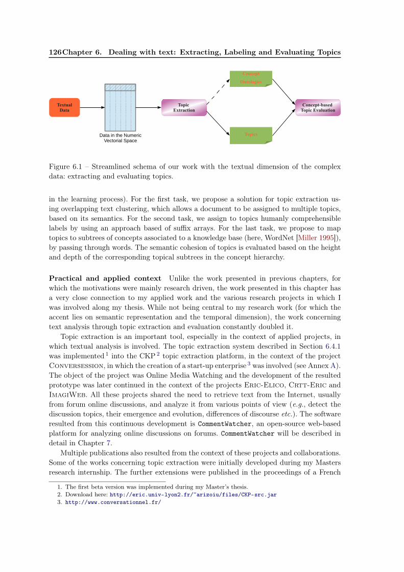
126Chapter 6. Dealing with text: Extracting, Labeling and Evaluating Topics
Data in the Numeric Vectorial Space
Topic Extraction
Concept-based Topic Evaluation
Concept
Ontologies
Topics
TextualData
Figure 6.1 – Streamlined schema of our work with the textual dimension of the complexdata: extracting and evaluating topics.
in the learning process). For the first task, we propose a solution for topic extraction us-ing overlapping text clustering, which allows a document to be assigned to multiple topics,based on its semantics. For the second task, we assign to topics humanly comprehensiblelabels by using an approach based of suffix arrays. For the last task, we propose to maptopics to subtrees of concepts associated to a knowledge base (here, WordNet [Miller 1995]),by passing through words. The semantic cohesion of topics is evaluated based on the heightand depth of the corresponding topical subtrees in the concept hierarchy.
Practical and applied context Unlike the work presented in previous chapters, forwhich the motivations were mainly research driven, the work presented in this chapter hasa very close connection to my applied work and the various research projects in which Iwas involved along my thesis. While not being central to my research work (for which theaccent lies on semantic representation and the temporal dimension), the work concerningtext analysis through topic extraction and evaluation constantly doubled it.
Topic extraction is an important tool, especially in the context of applied projects, inwhich textual analysis is involved. The topic extraction system described in Section 6.4.1was implemented 1 into the CKP 2 topic extraction platform, in the context of the projectConversession, in which the creation of a start-up enterprise 3 was involved (see Annex A).The object of the project was Online Media Watching and the development of the resultedprototype was later continued in the context of the projects Eric-Elico, Crtt-Eric andImagiWeb. All these projects shared the need to retrieve text from the Internet, usuallyfrom forum online discussions, and analyze it from various points of view (e.g., detect thediscussion topics, their emergence and evolution, differences of discourse etc.). The softwareresulted from this continuous development is CommentWatcher, an open-source web-basedplatform for analyzing online discussions on forums. CommentWatcher will be described indetail in Chapter 7.
Multiple publications also resulted from the context of these projects and collaborations.Some of the works concerning topic extraction were initially developed during my Mastersresearch internship. The further extensions were published in the proceedings of a French
1. The first beta version was implemented during my Master’s thesis.2. Download here: http://eric.univ-lyon2.fr/~arizoiu/files/CKP-src.jar3. http://www.conversationnel.fr/
6.1. Learning task and motivations 127
national conference [Rizoiu et al. 2010], while the application of topic extraction to ontologylearning was published in a book chapter [Rizoiu & Velcin 2011]. The topic evaluationmethodology was developed in collaboration with the Computer Science department of thePolytechnic University of Bucharest, and more precisely, the PhD research internship ofClaudiu Cristian Muşat at the ERIC laboratory. It was proposed in the proceedings of aninternational conference [Musat et al. 2011b]. The application of outlier detection was alsopublished in the proceedings of an international conference [Musat et al. 2011a].
Research context and motivations When automatically analyzing text, difficultiesarise, similar to those raised by image data. The textual native digital representation (whichhandles encoding at the level of character) usually captures little information about the se-mantics of the text. We define the semantics of a text as the information that is transmittedthough the text, its intent. To correctly structure text, most languages possess syntacticand morphological rules, which were employed by the Natural Language Processing researchcommunity to develop automatic language processing systems. These systems usually pro-vide good accuracy results, but they are costly to develop and maintain (due to the expertsupervised component), they are specialized on particular domains and often fail to capturethe subtleties of language (e.g., humor, irony, complex opinions). Other, more statistically-oriented approaches, were proposed. The most widely used textual representation employedby numeric systems, is the orderless “bag-of-words” representation, presented in detail inSection 6.2. Among these numeric approaches, topic extraction systems emerged as a re-sponse to the need to summarize large quantities of textual data and infer the main “ideas”behind a collection of textual documents.
The work presented in this chapter deals with leveraging semantic informationinto the tasks of topic extraction and topic evaluation. We also present some oftheir applications, such as ontology learning and topic improvement. We propose a topicextraction system that infers topics from text, by means of overlapping text clustering. Weaddress the problem of human comprehension of topics by assigning each cluster a “humanly-comprehensible” name, made out of a frequent complete expression. As one of the guidelinesof our work, we consider crucial to generate humanly-comprehensible outputs, since topicsdefined as distributions of probabilities over words are difficult to interpret for a humanbeing. For the topic evaluation task, the idea is to emulate the human judgment of topics.To this end, we use a semantic resource, such as a concept hierarchy (e.g. WordNet). Eachtopic is mapped to a subtree in the concept hierarchy and we redefine the specificity andcoverage of the subtree based on its height and depth in the concept hierarchy. We use thismeasures to evaluate the cohesion of topics.
The remainder of this chapter is structured as follows. In Section 6.2, we present how rawtext can be translated into a numerical format using the “bag-of-words” representation. Anoverview of research related to topic extraction, labeling and evaluation will be presentedin Section 6.3. In Section 6.4, we propose a topic extraction system and concept-basedtopic evaluation system. We continue in Section 6.5 by presenting two applications of ourproposals: topic extraction for ontology learning and the improvement of topic, based onconcepts, by removing the topic’s spurious words. We end with Section 6.6, in which wedraw the conclusions and plan some future work concerning the textual dimension of thecomplex data.
128Chapter 6. Dealing with text: Extracting, Labeling and Evaluating Topics
6.2 Transforming text into numerical format
One of the simplest text numerical representations is the “bag-of-words” representa-tion [Harris 1954,Harris 1968] (BoW ). This representation is extensively used in NaturalLanguage Processing and Information Retrieval tasks. Lately, this representation has alsobeen used in Image Processing, as shown in Chapter 5, under the form of “bag-of-features”representation. In the BoW model, text is represented as an unordered collection of words,disregarding grammar and even word order. Each word is assigned a score, calculated ac-cording to a term weighting scheme.
Documents(plain text)
Preprocessed documents
PreprocessingTranslation to
numericrepresentation
Data in the Numeric Vectorial Space
Figure 6.2 – Schema of transforming texts to a numerical representation.
Figure 6.2 shows the typical treatment chain that allows transforming textual data intothe tabular numeric format. In the Preprocessing phase, each document is preprocessed,as shown in Section 6.2.1. This usually includes (i) eliminating common words that donot bring any information about the thematic of the text and (ii) stemming or lemma-tizing inflected words, in order to increase their descriptive value. In the Translation tonumeric representation phase, the preprocessed documents are translated into the a nu-meric vectorial description space, as shown in Section 6.2.2, using one of the term weightingschemes (e.g., term frequency, TFxIDF etc.). At the end of this phase, the textual collec-tion can be represented as a term/document matrix. Each numeric feature (the columns)corresponds to a word in the vocabulary and each vector (the rows) defined in this multi-dimensional space corresponds to a textual document. We present in further detail each ofthese two phases over the next two subsections.
6.2.1 Preprocessing
The purpose of preprocessing is to augment the descriptive power of the terms andlimit the size of the vocabulary. There are typically two problems that arise when dealingwith natural language text using a BoW approach: inflected/derived words and stopwords.Therefore, the preprocessing is usually composed of two elements: stemming/lemmatizationand stopwords removal.
Stemming/Lemmatization Many languages apply inflections on words to express pos-session, verb tenses etc. For example, in English, the verb “to walk” may appear as “walk”,“walked”, “walks”, “walking”. The base form (i.e., “walk”), the infinitive for verbs, masculinesingular form for nouns, is called the lemma for the word. While crucial for the human com-prehension of the text, inflections can usually be ignored for many applications. When using
6.2. Transforming text into numerical format 129
the BoW representation, having different forms for the same base form leads to creatingmultiple bags for a single word and incorrectly evaluating the word’s score in the document.
Stemming is the process for reducing inflected words to their stem or root form, byremoving inflections, prefixes and/or suffixes. The stem of a word is not necessarily identicalto the word’s lemma and it may not even be a valid word or the morphological root of theword. It is sufficient that all inflected variants of a words map to the same stem. Stemmingis dependent on language, but algorithms have been developed for the majority of widelyused languages. For English, the stemmer mostly used is Porter’s stemmer [Porter 1980]and various initiatives (e.g., the CLEF Project 4) have proposed solutions for Europeanlanguages.
Lemmatization refers to determining the lemma for a given word. This process usuallyinvolves complex tasks such as understanding context and determining the part of speech ofa word in a sentence. Lemmatization is closely related to stemming. The difference is that astemmer operates on a single word without knowledge of the context, and therefore cannotdiscriminate between words which have different meanings depending on part of speech(e.g., “meeting” as a noun in “during our last meeting” or as a verb in “we are meeting againtomorrow”). Stemmers are typically easier to implement and run faster, while lemmatizationcan in principle select the appropriate lemma depending on the context.
Stopwords removal Stopwords are commonly used words, such as articles, prepositionsetc., that do not present any descriptive value, as they are not associated to a certain the-matic. When using a BoW representation, they increase the size of the dictionary and biasthe values of certain term weighting schemes (such as Term Frequency). Stopwords are typ-ically removed using stopword lists, which can contain short function words (e.g., the, is,at, which, on etc.), but any words judged unnecessary can also be included. Whatsoever,stopwords are important for the human reader (as shown in Section 6.4.1) and their removalmight render the results humanly-incomprehensible. Therefore, when results are shown tothe reader (e.g., cluster labels, search results), they typically include them. Our work con-cerning the topic labeling, presented in Section 6.4.1, uses complete expressions that alsoinclude stopwords.
6.2.2 Text numeric representation
Numerous textual representations exist in the Information Retrieval domain [Sing-hal 2001]. The Boolean Model compares True/False query statements with the word setthat describes a document. Such a system has the shortcoming that there is no inherentnotion of document ranking. The Probabilistic Model [Maron & Kuhns 1960] is based onthe general principle that documents in a collection should be ranked by decreasing proba-bility of their relevance to a query. In the Inference Network Model [Turtle & Croft 1989],document retrieval is modeled as an inference process in an inference network. A docu-ment instantiates a term with a certain strength, and the credit from multiple terms isaccumulated given a query to compute the equivalent of a numeric score for the document.
The Vector Space Model [Salton et al. 1975] is the representation most widely used inmodern text clustering algorithms and Information Retrieval tasks. Just as the BoW rep-
4. http://www.clef-campaign.org/
130Chapter 6. Dealing with text: Extracting, Labeling and Evaluating Topics
resentation, the Vector Space Model does not conserve the order of words or their semanticrelations. Each document is represented as a multidimensional vector in a space having asmany dimension as there are terms 5 in the considered dictionary and where each dimensionis associated to a term. The score on each dimension is directly proportional to the strengthof the relationship between the considered word and the document. The Vector Space Modelallows to define a distance between textual documents, which can be interpreted as the sim-ilarity between documents. It is usually calculated using the cosine distance of the twomultidimensional vectors:
||di − dj ||cos = 1− cos(~di, ~dj) = 1−∑|V|
k=1 di,k × dj,k√∑|V|k=1 d
2i,k
√∑|V|k=1 d
2j,k
(6.1)
where di and dj are two documents in the document collection D, V is the word vocabularyand di,k is the score of word wk ∈ V associated to the document di.
There are numerous methods for measuring the scores for words, also known as termweighting schemes [Salton & Buckley 1988], out of which we single out (i) the pres-ence/absence scheme, (ii) the term frequency scheme, (iii) the inverse document frequencyscheme and (iv) the TFxIDF scheme, detailed here after.
1. Presence/Absence is also known as binary weighting and it is the simplest wayto measure the belonging of a word to a document. Its formula is:
di,k = pa(di, wk) =
{1, if the word wk is found in document di0, otherwise
This weighting scheme can only show if a word is related to a document, but it doesnot measure the strength of the relationship [Dumais et al. 1998].
2. Term Frequency is also known as term count. It is defined as the number of times agiven word appears in a document. To avoid favoring longer documents, normalizationis usually used:
di,k = tf(di, wk) =ni,k∑|V|l=1 ni,l
where ni,k is the number of occurrences of the word wk in the document di and thedenominator is the total number of words in the document di.
3. Inverse Document Frequency is a measure of the general importance of a wordin the whole corpus. It favors rare words, giving a low score to words that appear inmany documents. IDF is defined as:
idf(wk) = log|D|
| {d |wk ∈ d , d ∈ D} |
where D is the collection of textual documents and | {d |wk ∈ d , d ∈ D} | is the totalnumber of documents in which the word wk appears. In practice, IDF is never usedalone, as it lacks the power to quantify the relationship between a word and a docu-ment and it favors very rare words, which often prove to be typographic errors. IDFis usually used in conjunction with TF in the TFxIDF weighting scheme.
5. A term is a word that has a certain semantic (i.e., most often a term refers to objects, ideas, events,states of affair etc.). All terms are words, but only some words are terms.
6.3. An overview on Topic Extraction 131
4. TFxIDF [Jones 1972] is the most used scheme in Information Retrieval. It is theproduct of Term Frequency and Inverse Document Frequency:
di,k = tfxidf(di, wk) = tf(di, wk)× idf(wk)
TFxIDF aims at balancing local and global occurrences of a word. It assigns a highscore to a word wk that appears multiple times in a document di (high Term Fre-quency), but which is scarce in the rest of the collection (high inverse documentfrequency).
Other term weighting schemes for the BoW representation exist, often variations of theclassical schemes. Okapi BM25 [Robertson et al. 1995] is a bag-of-words retrieval functionthat ranks a set of documents based on the query terms appearing in each document. It isbased on the probabilistic retrieval framework. Other weighting schemes search to includeadditional external information into the scoring function. For example [Karkali et al. 2012]propose tDF (temporal Document Frequency), which is a variation of the BM25 measure.It includes temporal information in order to “keep topics fresh”, by adding a decay factorunder the form of a temporal penalization function.
6.3 An overview on Topic Extraction
It is generally accepted that a topic represents an “idea” that emerges from a collectionof textual documents. But there is no widely accepted formal topic definition. Through-out the literature, a topic is considered to be (i) a cluster of documents that share athematic [Cleuziou 2008], (ii) a distribution of probabilities over words and over docu-ments [Blei et al. 2003] or (iii) an abstraction of the regrouped texts that needs a linguisticmaterialization: a word, a phrase or a sentence that summarizes the idea emerging from thetexts [Osinski 2003]. Plenty of applications can benefit greatly from topic inference fromtext, including information retrieval systems, database summarization, ontology learning,document clustering and querying large document collections.
We present an overview of topic extraction, focusing on flat clustering techniques,which create a partition of documents with a single level. These algorithms divide a col-lection of textual documents into groups, so that documents inside a group are similar interms of their topic (politics, economics, social etc.) and dissimilar with documents in othergroups. For each cluster, K-Means-based clustering algorithms present a centroid, which isan abstraction of the cluster and which summarizes the common part of the documents inthe cluster.
The centroid (a multidimensional vector or a distribution of probabilities) is not a realdocument and rarely makes any sense to a human. Therefore, it is convenient to choose acomprehensible name for it. There are a number of ways of labeling a topic [Roche 2004]:(i) choosing an arbitrary number of high rated words, (ii) selecting a document as repre-sentative, (iii) assigning a meaningful, human-readable expression or phrase etc. The wordproperty of polysemy is important when labeling topics. The same word can have differentmeanings, depending on the context. For example, the word “mining” has one meaning inthe expression “coal mining” and another in “data mining”.
132Chapter 6. Dealing with text: Extracting, Labeling and Evaluating Topics
Other topic extraction methods exist, most notably those issued from computationallinguistics [Ferret 2006] or graph-based methods [Ng et al. 2002]. In the following sectionswe concentrate only on statistical-based methods: we present text clustering based methods(in Section 6.3.1), probabilistic topic models (in Section 6.3.2). In Section 6.3.3, we addressthe issue of topic labeling, and we finish in Section 6.3.4 with a short overview of methodswhich deal with topic evaluation and improvement.
6.3.1 Text Clustering
We choose to divide text clustering algorithms into categories based on their ability tocreate overlapping groups. Other classifications are possible, some authors [Dermoucheet al. 2013] divide them into families of methods: (i) distance-based methods, (ii) matrixfactorization-based methods and (iii) probabilistic methods. Some of the solutions presentedbelow were designed specifically for text mining (like LDA), others are general purposeclustering algorithms. The latter can be used for text clustering by translating textualdocuments into the Vector Space Model (described in section 6.2.2).
Crisp solutions
Crisp clustering algorithms regroup a collection of documents into a partition of dis-jointed classess. K-Means [MacQueen 1967] is one of the most well-known crisp clusteringalgorithms. The algorithm iteratively optimizes an objective criterion, typically the distor-tion function. In the case of text mining and information retrieval, the cosine distance isused to calculate the similarity between texts. Bisecting K-Means [Steinbach et al. 2000]is a hierarchical variant of K-Means, which has been emphasized as more accurate thanK-Means for text clustering. It is a top-down algorithm that partitions, at each step, onecluster of documents into two crisp sub-clusters. At the first iteration, the collection is di-vided into two subsets according to multiple restarting 2-means. At the successive iterations,one subset is split into two and n+ 1 text clusters are obtained from n initial clusters. Theprocess is iterated until a stopping criterion is satisfied (e.g., a fixed number of clusters). Thefinal output of Bisecting K-Means can be seen as a truncated dendrogram. Hierarchicalagglomerative clustering (HAC) [Jain & Dubes 1988] is a hierarchical clustering tech-nique used more frequently in Information Retrieval. It constructs the hierarchy bottom-upand consists in merging at each step pairs of clusters. A single-level crisp partition can beobtained by cutting the dendogram at certain level, chosen using a given heuristic (e.g.,biggest gap between levels). Whatsoever, hierarchical clustering methods are ill adapted totreat the great volumes of data encountered in text mining.
Overlapping solutions
In overlapping clustering, documents are authorized to simultaneously be part of mul-tiple clusters. The result is no longer a strict partition of the document collection, sincegroups have non-empty intersections. Considering that longer texts have the tendency ofapproaching multiple subjects, it is only natural to allow them to be part of each of thecorresponding topics. (e.g., a text that talks about the “economical outcomes of a political
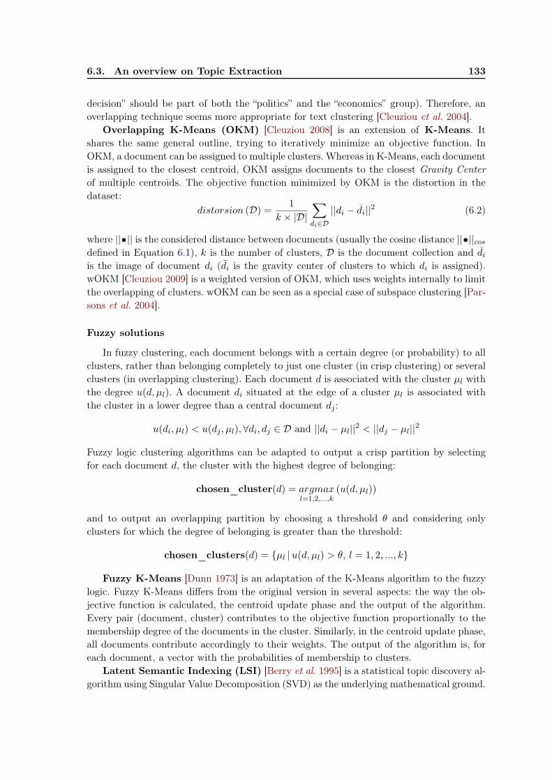
6.3. An overview on Topic Extraction 133
decision” should be part of both the “politics” and the “economics” group). Therefore, anoverlapping technique seems more appropriate for text clustering [Cleuziou et al. 2004].
Overlapping K-Means (OKM) [Cleuziou 2008] is an extension of K-Means. Itshares the same general outline, trying to iteratively minimize an objective function. InOKM, a document can be assigned to multiple clusters. Whereas in K-Means, each documentis assigned to the closest centroid, OKM assigns documents to the closest Gravity Centerof multiple centroids. The objective function minimized by OKM is the distortion in thedataset:
distorsion (D) =1
k × |D|∑di∈D||di − d̄i||2 (6.2)
where ||•|| is the considered distance between documents (usually the cosine distance ||•||cosdefined in Equation 6.1), k is the number of clusters, D is the document collection and d̄iis the image of document di (d̄i is the gravity center of clusters to which di is assigned).wOKM [Cleuziou 2009] is a weighted version of OKM, which uses weights internally to limitthe overlapping of clusters. wOKM can be seen as a special case of subspace clustering [Par-sons et al. 2004].
Fuzzy solutions
In fuzzy clustering, each document belongs with a certain degree (or probability) to allclusters, rather than belonging completely to just one cluster (in crisp clustering) or severalclusters (in overlapping clustering). Each document d is associated with the cluster µl withthe degree u(d, µl). A document di situated at the edge of a cluster µl is associated withthe cluster in a lower degree than a central document dj :
u(di, µl) < u(dj , µl), ∀di, dj ∈ D and ||di − µl||2 < ||dj − µl||2
Fuzzy logic clustering algorithms can be adapted to output a crisp partition by selectingfor each document d, the cluster with the highest degree of belonging:
chosen_cluster(d) = argmaxl=1,2,...,k
(u(d, µl))
and to output an overlapping partition by choosing a threshold θ and considering onlyclusters for which the degree of belonging is greater than the threshold:
chosen_clusters(d) = {µl |u(d, µl) > θ, l = 1, 2, ..., k}
Fuzzy K-Means [Dunn 1973] is an adaptation of the K-Means algorithm to the fuzzylogic. Fuzzy K-Means differs from the original version in several aspects: the way the ob-jective function is calculated, the centroid update phase and the output of the algorithm.Every pair (document, cluster) contributes to the objective function proportionally to themembership degree of the documents in the cluster. Similarly, in the centroid update phase,all documents contribute accordingly to their weights. The output of the algorithm is, foreach document, a vector with the probabilities of membership to clusters.
Latent Semantic Indexing (LSI) [Berry et al. 1995] is a statistical topic discovery al-gorithm using Singular Value Decomposition (SVD) as the underlying mathematical ground.
134Chapter 6. Dealing with text: Extracting, Labeling and Evaluating Topics
The algorithm decomposes the term/document matrix A in a product of three matrices:A = USV T . U and V are orthogonal matrices, containing the left and the right singularvectors of A. S is a diagonal matrix with the singular values of A ordered decreasingly.
LSI allows defining heuristics for reducing dimensionality and determining the numberof topics. Ak, the k-approximation of A (Ak = UkSkV
Tk ) is obtained by selecting the k
highest ranking singular values from S, alongside with the corresponding columns in U andthe lines in V . There exist heuristic for determining k, for example, (i) to order decreas-ingly the singular values of A and cut at the highest difference between two consecutivevalues [Osinski 2003] or (ii) the scree test [Cattell 1966]. The columns in U correspondingto the k highest singular values create an orthogonal basis for the document space. Anymultidimensional vector in this space can be expressed as a weighted sum of the elementsof the base:
di = α1µ1 + α2µ2 + . . . + αkµk ,
i ∈ 1, 2, . . . , |D| and l ∈ 1, 2, . . . , k
Considering the base elements µl as the centroids of clusters, documents are described in afuzzy logic: the document di has the probability αl of belonging to the cluster µl. LSI has theinconvenience that it can produce negative singular values, which can pose interpretabilityproblems [Lee & Seung 1999]. Non-negative Matrix Factorization [Lee & Seung 1999] (NMF)deals with this problem by finding a non-unique factorization of the non-negative matrix V ,so that V = WH. NMF-based methods have been shows efficient in topic extraction [Seung& Lee 2001,Xu et al. 2003].
6.3.2 Topic Models
Many concurrent solutions exist for topic extraction, some of which that fall in thecategory of text clustering have been presented in the Section 6.3.1. However, in recentyears, generative methods, and specifically topic models, imposed as the state-of-the-art.Starting from the assumption that observable data can be randomly generated following ana priori determined set of rules, topic models seek to detect the abstract “topics” that occurin a collection of documents.
Latent Dirichlet Allocation (LDA) [Blei et al. 2003] is probably the most well-knownprobabilistic generative model designed to extract topics from text corpora. It considersdocuments as “bags-of-words” and models each word in a document as a sample from amixture model. Each component of the mixture can be seen as a “topic”. Each word isgenerated from a single topic, but different words in a document are generally generatedfrom different topics. Each document is represented as a list of mixing proportions of thesemixture components and thereby reduced to a probability distribution on a fixed set oftopics.
LDA is highly related to probabilistic Latent Semantic Analysis [Hofmann 1999](pLSA), except that in LDA the topic distribution is assumed to have a Dirichlet prior. Thispoint is highly important because it permits to go beyond the often-criticized shortcomingof PLSA, namely that it is not a proper generative model for new documents and overfitting.More precisely, LDA is based on the hierarchical generative process illustrated in Figure 6.3.
6.3. An overview on Topic Extraction 135
Figure 6.3 – Schema of Latent Dirichlet Allocation.
The hyperparameters α and β are the basis of two Dirichlet distributions. The firstDirichlet distribution deals with the generation of the topic mixture for each of the |D|documents. The second Dirichlet distribution regards the generation of the word mixture foreach of the k topics. Each topic is then a distribution over the |W| words of the vocabulary.The generative process is the following: for each word wd,i of the corpus, draw a topic µdepending on the mixture θ associated to the document d and then draw a word from thetopic µ.
Note that words without special relevance, like articles and prepositions, will haveroughly even probability between classes (or they can be placed into a separate category). Aseach document is a mixture of different topics, in the clustering process, the same documentcan be placed into more than one group, though resulting in a (kind of)Overlapping Clus-tering Process. Learning the parameters θ and µ, and sometimes the hyper-parameters αand β, is rather difficult because the posterior p(θ, µ/D, α, β, k) cannot be fully calculated,because of an infinite sum in the denominator. Therefore various approximation algorithmsmust be used, such as variational EM, Monte-Carlo Markov processes, etc.
This probabilistic approach presents advantages and disadvantages:– The theoretical framework is well-known in bayesian statistics and well-grounded. It
has led to many fruitful researches (see below).– It is designed to make inferences on new documents: what are the associated top-
ics and with what proportions? What part of the document is associated to whichtopic? Depending on the likelihood p(d/Θ), does a new document describe an originalmixture of topics or a new, never seen before topic?
– LDA is a complex mathematical model, which considers each document as a com-bination of possibly many topics. While this may be interesting for describing thedocuments, in the case of clustering, it could lead to a situation where each documentbelongs, more or less, to many clusters (similar to a fuzzy approach). An issue is there-fore to be able to choose a finite (and hopefully short) list of topics to be associatedto the document, beyond setting a simple threshold parameter.
– This method does not present a center for each cluster, but a distribution of thetopics over the terms. This could make it difficult to associate a readable name to thecluster. Note that recent works relative to LDA are seeking to find useful names using
136Chapter 6. Dealing with text: Extracting, Labeling and Evaluating Topics
n-grams [Wang et al. 2007].– As in the other presented methods, this probabilistic approach does not solve the clas-
sical problem of finding the global optimum and choosing the number k of topics. Forthe latter, some methods are proposed inspired by the works in model selection [Ro-dríguez 2005].
Numerous works have followed the hierarchical generative model of LDA to deal with var-ious related issues: extracting topic trees (hLDA) [Blei et al. 2004], inducing a correlationstructure between topics [Blei & Lafferty 2006a], modeling topics through time [Blei &Lafferty 2006b,Wang et al. 2008], finding n-grams instead of single words to describe top-ics [Wang et al. 2007], social networks [Chang et al. 2009b], opinion mining [Mei et al. 2007a]etc.
6.3.3 Topic Labeling
Distributions of probabilities and multidimensional vectors are hardly comprehensiblefor a human reader. As shown in Section 6.3, there is no unanimously accepted method forpresenting topics. Most authors limit themselves to showing the top scoring words for eachtopic. While a list of words already gives a main idea of a topic, it is more interesting topresent the human reader a phrase to summarize the idea behind the group of documents.
To provide better topic descriptions, systems like Topical N-Grams [Wang et al. 2007]embed “spatial” connections between words in the topical learning process. Therefore, topicnames are inferred simultaneously with the topics. Topical N-Grams extracts topics as distri-bution over n-grams (sequences of multiple words which appear often together). Presentinghighly scored expressions is more comprehensible than a list of words [Wang et al. 2007].
Most topic labeling algorithms assign topic names in a post-processing phase of thetopic extraction. This type of approach is a two phase process: (i) the name candidates areextracted from the text corpus and (ii) the meaningfulness of each candidate is calculatedand the highest scoring one is chosen. [Mei et al. 2007b] address the labeling task as an opti-mization problem that aims at minimizing the Kullback-Leibler (KL) divergence [Kullback& Leibler 1951] between word distributions. In this case, the two compared distributionsare the topic itself and the name candidate’s word distribution. The obtained distance is anindicator of the name candidate’s meaningfulness to the analyzed topic. In [Osinski 2003],frequent keyphrases are extracted from web search snippets and assigned to topics, by usingthe cosine distance to calculate their similarity.
Phrase learning All algorithms that label topics in a post-processing phase share theneed for relevant and unambiguous phrases, which later serve as name candidates and areused to synthesize the idea of the group of documents associated to the topic. Compre-hensible topic names need to be complete phrases: they take into account the property ofpolysemy and they are humanly readable. As shown in Section 6.3, words can have differentmeanings, depending on the context. This is one of the reasons why single words rarelymake good topic names. Name candidates should be expressions which are precise enoughto specify the meaning of words (e.g., “data mining” compared to the single word “mining”).Humanly readable topic names contain words in their original textual form (not lemmatized,nor stemmed) and all the needed prepositions and articles (e.g., “the Ministry of Internal
6.3. An overview on Topic Extraction 137
Affairs”). Name candidates are also called keyphrases, sequences of one or multiple wordsthat are considered highly relevant as a whole.
Based on the learning paradigm, keyphase learning algorithms can be divided into con-structive algorithms and extractive algorithms [Hammouda et al. 2005]. Construct-ing keyphrases is usually a supervised learning task, often regarded as a more intelligentway of summarizing the text. These approaches make use of the external knowledge, underthe form of expert validation of the extracted phrases. The obtained results are usuallyless noisy, but involving human supervisor makes the extraction process slow, expensiveand biased towards the specific field (e.g., specialized to microbiology vocabulary). Theseapproaches do not scale to large datasets of general purpose texts. Examples of such sys-tems follow: ESATEC [Biskri et al. 2004], EXIT [Roche 2004], XTRACT [Smadja 1991].Extracting keyphrases is an unsupervised learning task, in which candidate names arediscovered using predefined patterns. This kind of approaches scale well to large datasets,but they have the drawback of almost exponential quantity of extracted keyphrases anda noisy output. Examples of such systems follow: CorePhrase [Hammouda et al. 2005],Armil [Geraci et al. 2006], SuffixTree Extraction [Osinski 2003].
According to the employed method, keyphrase learning algorithms can be divided into:linguistic approaches, statistical approaches and hybrid approaches [Roche 2004,Buitelaar et al. 2005,Cimiano et al. 2006].
Linguistic approaches
Linguistic approaches are issued from the domains of Terminology and Natural Lan-guage Processing. They employ linguistic processing, like phrase analysis or dependencystructure analysis. A part of speech tagger is usually employed for the morphological char-acterization of words (e.g., determine (i) if the word is a noun, adjective, verb or adverb,and (ii) its number, person, mode, time etc.). Words are further characterized with thesemantic information and their lemma (see Section 6.2.1). From the texts enriched withsyntactic and morphological information, keyphrases are extracted, most often using pre-defined patterns. TERMINO [Lauriston 1994] uses patterns like <Head> <PrepositionalGroup> <Adjectival Group> to discover keyphrases. LEXTER [Bourigault 1992] uses themorphological information to extract from the text nominal groups and then searches fordis-ambiguous maximal nominal groups. INTEX [Silberztein 1994, Ibekwe-SanJuan & San-Juan 2004] allows simple definition of morpho-syntactic rules to infer keyphrases. Such rulesare (i) a keyphrase can contain an adverb, one or multiple adjectives, a single prepositionand at least a noun, (ii) phrases made of preposition and determinant are excluded etc. Thekeyphrases extracted by INTEX can be further enriched [Ibekwe-SanJuan & SanJuan 2004]by adding variant phrases, using the FASTR system [Jacquemin 1999]. Variant phrasesare variations of initial phrases by altering the word order or inserting words (e.g., “onlinecustomer support” is a variant phrase of “online support”).
Keyphrase extraction methods based on linguistic approaches obtain less noisy outputthan purely statistical methods, but they are vulnerable to multilingual corpora, neolo-gisms and they have the tendency to adapt to stereotypical texts (texts from a specifiednarrow field) [Biskri et al. 2004]. Furthermore, the morphological and syntactic analyzersthey employ, as well as their predefined rules are sensible to the text quality. This makes
138Chapter 6. Dealing with text: Extracting, Labeling and Evaluating Topics
linguistic-based approached scale badly to internet-originated text, which usually writtenin an informal style (this is especially true for text on social networks and micro-blogging).Furthermore, they are costly to develop and maintain, due to the expert supervised task ofdefining patters, updating them etc.
Statistical approaches
Statistical keyphrase extraction algorithms are based on information retrieval techniquesfor term indexing [Salton & Buckley 1988]. The underlying assumption is that the senseof a word (see the property of polysemy) is given by its context (i.e. other words whichhave a strong relationship with the given word). Statistical measures are employed to de-tect keyphrases of strongly related words. A widely used measure which quantifies thedependency between two words in the binary collocation (also called bigram) is the MutualInformation, given by the formula:
mi(wi, wj) = p(wi, wj)× log(
p(wi, wj)
p(wi)× p(wj)
)where p(wi) and p(wj) are the probabilities with which the words wi and, respectively, wjappear in the text, while p(wi, wj) represents the probability of the words wi and wj ap-pearing together in a window of a specified length. In [Anaya-Sánchez et al. 2008], bigramsare detected using a window of dimension 11 (5 words before + considered word + 5 wordsafter). Other tools (e.g., EXIT [Roche 2004], ESATEC [Biskri et al. 2004]) rely on con-structing n-grams, by iteratively combining bigrams or increasing the length of a previouslydiscovered (n-1)gram. Longer collocations are obtained, with higher Mutual Informationscore.
Many other statistical measures have been proposed to calculate the strength of therelationship between two words. In [Anaya-Sánchez et al. 2008] a modified entropy functionis used to determine frequent bigrams from a set of frequent terms. LocalMaxs [da Silvaet al. 1999,Dias et al. 2000] uses the Symmetric Conditional Probability measure to extractcontinuous multiple word units and the Mutual Expectation measure for extracting non-continuous multiple word units. Some works study the impact of some of the most usedmeasures, judging their ability to identify lexically associated bigrams. The compared mea-sures are: t-score, Pearson’s χ-square test, log-likelihood ratio, pointwise mutual informationand mutual dependency [Thanopoulos et al. 2002].
There are other approaches that do not rely on bigram detection and n-gram construc-tion for keyphrase extraction. In CorePhrase [Hammouda et al. 2005] keyphrases are con-sidered to naturally lie at the intersection of textual documents in a cluster. The algorithmcompares every pair of documents to extract matching phrases. It employs a documentphrase indexing graph structure, the Document Index Graph. It constructs a cumulativegraph, representing currently processed documents. When introducing a new document, itsassociated subgraph is matched against the existing cumulative graph to extract the match-ing phrases between the new document and all previous documents. The graph maintains acomplete phrase structure identifying the containing document and phrase location, so cy-cles can be uniquely identified. Simultaneously, it calculates some predefined phrase featuresthat are used for later ranking. Suffix Array-based techniques [Osinski et al. 2004,Osinski
6.3. An overview on Topic Extraction 139
& Weiss 2004] can also used to discover keyphrases. Incomplete phrases (e.g., “PresidentBarack” instead of “President Barack Obama”), which are often meaningless, can be avoidedby using the notion of phrase completeness. A phrase is complete if and only if all of itscomponents appear together in all occurrences of the phrase. In the previous example, if thephrase “President Barack” is followed in all of its occurrences by the term “Obama”, then itis not a complete phrase. Starting from this definition, right and left completeness can bedefined (the example above is left complete, but not right complete). Using a Suffix Arraydata structure [Manber & Myers 1993], the complete phrases can be detected and the onesoccurring with a minimum frequency populate the topic label candidate set. More detailsabout a suffix array-based algorithm for keyphrase extraction can be found in Section 6.4.1.
Unlike linguistic approaches, statistical keyphrase extraction systems produce noisy re-sults [Biskri et al. 2004]. While extracted name candidates pass the frequency thresholdand get good statistical scores, many of them hardly capture any semantic meaning. Suchare the phrases which (i) are made out of common words, like articles, prepositions, certainverbs etc. (e.g., “he responded that”, “the biggest part of the”) and (ii) bring no informationto the topic. The advantage of statistical methods is that they scale well to big datasetsand they are virtually language independent.
Hybrid approaches
The advantages and inconveniences of linguistic and statistical approaches are com-plementary. Hybrid approaches aim at picking the best of the two worlds: scaling well tobig datasets and producing less noisy outputs. Hybrid systems usually add linguistic infor-mation to an essentially statistical system or add statistical information to an essentiallylinguistic system. For example, predefined keyphrase formats (e.g., <Subject> <Verb> or<Verb> <Adverb>) can be used to filter the output of statistical methods.
[Roche 2004] presents a review of hybrid approaches. For example, XTRACT[Smadja 1991] uses morphological and syntactic taggers as a final phase to filter out thenoise from the name candidate set resulted using statistical extraction. In the first phase,bigrams are extracted from a grammatically tagged corpus, using an 11-word window. Thesecond phase consists in extracting longer frequent phrases, called “rigid noun phrases”.The third phase is the linguistic phase. It consists in using statistic filtering based on thebigram’s frequency to associate a syntactic etiquette to extracted bigrams (e.g., <Noun>-<Verb>, <Adjective>-<Noun>). Longer phrases can be constructed based on the bigramsand filtered using predefined syntactic rules.
6.3.4 Topic Evaluation and Improvement
Topic extraction is an unsupervised machine learning task, meaning that no groundtruth exists to evaluate the results. This is a classical problem in clustering. Traditionalunsupervised tasks are usually evaluated using adapted statistical measures, which quantifythe fitness of the obtained results over a particular criterion. Evaluating topics adds anotherlevel of difficulty, since constructed topic must not only regroup similar documents, but asemantically coherent idea must also emerge from the topic. For example, topic extractionalgorithms based on text clustering can be evaluated using any traditional internal clustering
140Chapter 6. Dealing with text: Extracting, Labeling and Evaluating Topics
measure [Halkidi et al. 2001] (e.g., cluster variance). But applying such measures does notgive any semantic information about the fitness of topics. To take into account the semanticdimension, some authors [Cleuziou 2008, Rizoiu et al. 2010] use semantically annotateddatasets for evaluating topics. Each text in the dataset is labeled using one or multiplegiven tags (e.g., economics, oil). Techniques issued from the supervised learning literatureare used: topics are trained on a learning set and measures like precision and recall arecalculated on a previously unseen test set. We present such an evaluation technique inSection 6.4.1.
Generative topic modeling is today’s de facto state of the art in topic extraction. Tra-ditionally, these approaches have been evaluated qualitatively and quantitatively. From thequalitative point of view, a sample of topics is usually exhibited in order to convince thereader. Each exhibited topic is a short list of the first terms, ordered decreasingly from aprobability perspective. Most of the times, a topic label is manually assigned by the authors.A topic is considered to be good if most of its most probable words are semantically similar.Quantitatively, statistical measures, such as the perplexity [Wallach et al. 2009], are em-ployed to assess the ability of extracted topics to generalize on unseen data (either througha train set/test set approach or through cross-validation). Even though topic models showgood predictive power on new text, their weak point is their underlying assumption is thatthe latent space is semantically meaningful. In [Chang et al. 2009a], an extensive quanti-tative and qualitative evaluation of the interpretability of the latent space is performed. Itis shown that the human judgment does not always coincide with the statistical evaluationmeasures. Highly scoring topics are sometimes not humanly comprehensible, showing thatstatistic measures do not always achieve to capture the semantics of the dataset. [Newmanet al. 2010] addresses this lack of semantic comprehension by using external semantic re-sources (e.g., Wikipedia, Google) for the evaluation task and uses the topic coherence as anevaluation metric. Similarly, concept hierarchies (such as WordNet [Miller 1995]) are used fortopic evaluation purposes. In [Musat et al. 2011b,Musat 2011], we propose a topic-conceptmapping, in which each topic is assigned a topical subtree in the concept hierarchy. Themeasures of specificity and coverage are defined and used to evaluate topics. This methodwill be presented in detail in Section 6.4.2.
Many approaches have been proposed in recent years for improving topic extraction orfor adapting it to specific applications. Most often, the improvement techniques deal withembedding or leveraging external semantic information. In [Musat et al. 2011a,Musat 2011],we propose a technique for removing topic outliers (i.e., words unrelated to a certain topic).It uses the same topic-concept mapping presented earlier and it will be further detailed inSection 6.5.1. sLDA [Blei & McAuliffe 2008] introduces the semantic information underthe form of supervision of the topic modeling process. Other approaches adapt the topi-cal model to specific applications. Latent Dirichlet Allocation with WordNet [Boyd-Graber et al. 2007] is a topic model that uses semantic information (under the form ofWordNet) for word sense disambiguation. It is a version of LDA that considers the wordsenses as hidden variables and attempts to select the right sense when constructing topics.
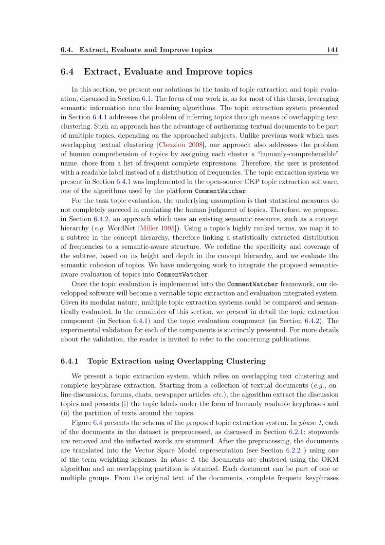
6.4. Extract, Evaluate and Improve topics 141
6.4 Extract, Evaluate and Improve topics
In this section, we present our solutions to the tasks of topic extraction and topic evalu-ation, discussed in Section 6.1. The focus of our work is, as for most of this thesis, leveragingsemantic information into the learning algorithms. The topic extraction system presentedin Section 6.4.1 addresses the problem of inferring topics through means of overlapping textclustering. Such an approach has the advantage of authorizing textual documents to be partof multiple topics, depending on the approached subjects. Unlike previous work which usesoverlapping textual clustering [Cleuziou 2008], our approach also addresses the problemof human comprehension of topics by assigning each cluster a “humanly-comprehensible”name, chose from a list of frequent complete expressions. Therefore, the user is presentedwith a readable label instead of a distribution of frequencies. The topic extraction system wepresent in Section 6.4.1 was implemented in the open-source CKP topic extraction software,one of the algorithms used by the platform CommentWatcher.
For the task topic evaluation, the underlying assumption is that statistical measures donot completely succeed in emulating the human judgment of topics. Therefore, we propose,in Section 6.4.2, an approach which uses an existing semantic resource, such as a concepthierarchy (e.g. WordNet [Miller 1995]). Using a topic’s highly ranked terms, we map it toa subtree in the concept hierarchy, therefore linking a statistically extracted distributionof frequencies to a semantic-aware structure. We redefine the specificity and coverage ofthe subtree, based on its height and depth in the concept hierarchy, and we evaluate thesemantic cohesion of topics. We have undergoing work to integrate the proposed semantic-aware evaluation of topics into CommentWatcher.
Once the topic evaluation is implemented into the CommentWatcher framework, our de-velopped software will become a veritable topic extraction and evaluation integrated system.Given its modular nature, multiple topic extraction systems could be compared and seman-tically evaluated. In the remainder of this section, we present in detail the topic extractioncomponent (in Section 6.4.1) and the topic evaluation component (in Section 6.4.2). Theexperimental validation for each of the components is succinctly presented. For more detailsabout the validation, the reader is invited to refer to the concerning publications.
6.4.1 Topic Extraction using Overlapping Clustering
We present a topic extraction system, which relies on overlapping text clustering andcomplete keyphrase extraction. Starting from a collection of textual documents (e.g., on-line discussions, forums, chats, newspaper articles etc.), the algorithm extract the discussiontopics and presents (i) the topic labels under the form of humanly readable keyphrases and(ii) the partition of texts around the topics.
Figure 6.4 presents the schema of the proposed topic extraction system. In phase 1, eachof the documents in the dataset is preprocessed, as discussed in Section 6.2.1: stopwordsare removed and the inflected words are stemmed. After the preprocessing, the documentsare translated into the Vector Space Model representation (see Section 6.2.2 ) using oneof the term weighting schemes. In phase 2, the documents are clustered using the OKMalgorithm and an overlapping partition is obtained. Each document can be part of one ormultiple groups. From the original text of the documents, complete frequent keyphrases
142Chapter 6. Dealing with text: Extracting, Labeling and Evaluating Topics
Documents(plain text)
Data in the Numeric Vectorial Space Overlapping
Partition
Pretreatmentand numeric
representation
TextualClustering
KeyphraseExtraction
Topic name candidates
Topic Labeling
Extractedtopics
1
2
3
4
Figure 6.4 – Schema of a topic extraction algorithm using overlapping text clustering.
are extracted, in phase 3, using a Suffix Array based algorithm. The extracted keyphrasesserve as topic label candidates. In phase 4, the topic label candidates are are reintroducedas pseudo-documents into the multidimensional space defined by Vector Space Model andthe cosine distance is used to chose the best name for each topic.
6.4.1.1 Phase 2 : Clustering
The text clustering is performed using OKM [Cleuziou 2008], which is a K-Means variantwhich authorizes documents to belong to more that one cluster. It inherits from K-Meansmost of its drawbacks (i.e., its powerful dependence on the initialization and the number ofclusters which must be set arbitrarily by the user) and its advantages (i.e., linear executiontime, exposing a centroid). Nonetheless, OKM is chosen for the text clustering task for itscapacity to create an overlapping partition of the dataset. This is especially important fortwo reasons: the property of polysemy of words and multi-topic documents. Words shouldbe allowed to be associated with multiple topics, given their corresponding senses. Similarly,documents that approach multiple thematics should authorized to be part of their multiplecorresponding topics.
OKM follows the general K-Means schema, of iteratively optimizing an objective func-tion by relocating the cluster centroids and re-assigning documents to clusters. In K-Means,each document is associated to only one centroid, the one closest in terms of the employeddistance. OKM assigns a document to multiple clusters by constructing a document imageas the gravity center of all the associated centroids. Lets take the example of a document dand centroids c1, c2 and c3. Without losing generality, we consider that
||d− c1||cos < ||d− c2||cos < ||d− c3||cos
where || • ||cos is the cosine distance defined in Equation 6.1. Let d̄ be the image of thedocument d and A be the set of centroids to which the document d is assigned. Initially,the document d is assigned to the closest centroid (A ← c1) and, therefore, d̄ = c1. Thesecond closest centroid (c2) is now considered and the new document image is computed asthe gravity center of c1 and c2 (d̄new = gravity(c1, c2)). If the new document image is closerto the document than the old image (||d − d̄new||cos < ||d − d̄old||cos) then the document dis also assigned to the cluster with the centroid c2 (A ← A ∪ c2 = {c1, c2}). The process
6.4. Extract, Evaluate and Improve topics 143
is continued with c3: d̄new = gravity(c1, c2, c3). If the new document image is not closer tod than the old image (||d − d̄new||cos ≥ ||d − d̄old||cos), then the process is finished and thedocument d is assigned to clusters with the centers c1 and c2.
In the centroid update step, each document di contributes to each associated centroid(each cj ∈ Ai). The contribution is inversely proportional with the number of clusters towhich the document belongs to: the more clusters the document is part of, the less influenceit has in the update of their respective centroids. The update formula for the centroids:
cj =1∑
di∈Cj1δ2i
×∑di∈Cj
d̂jiδ2i
(6.3)
where d̂ji = δidi − (δi − 1)d̄Ai\{cj}i . Notations:
– Ai is the set of centroids to which the document di is assigned;– δi = |Ai| is the number of centroids associated with document di;– Cj is the collection of documents associated to the centroid cj ;– d̄
Ai\{cj}i is the image of document d, excluding centroid cj (gravity center of the
centroids to which di is associated, except centroid cj);– cj is the centroid to be updated.Unlike K-Means, in OKM the update of a centroid (Equation 6.3) is dependent not only
on the documents under its cluster, but also on the other centroids (through the documentimage). The result is that centroids can continue to evolve in the multidimensional space,if the cluster composition stopped changing. In the process of topic labeling, topic namesare associated to each resulted cluster based on the similarity between the name candidateand the cluster’s centroid. Therefore, we modify the stopping criterion of the original OKMalgorithm proposed in [Cleuziou 2008] in order to allow the centroids to evolve until theyare fully adapted to the documents in the cluster. We define a threshold ε and we stop theclustering process when the variation of the objective function (see Equation 6.2, p. 133)between two iterations descends under the threshold. In practice, this means that the lastcouple of iterations of the clustering algorithm are performed only to refine the centroidsand adapt them to the documents in their respective clusters.
The clustering phase creates a data partition that regroups documents relative to theirtopic similarity. Simultaneously, this phase outputs the centroids of each class, which canbe regarded as abstract representations of the topics. These centroids are multimensionalvectors in the Vector Space Model, having a high scores for the words that are specific tothe cluster (i.e., the words that are characteristic for the specific topic).
6.4.1.2 Phase 3 : Keyphrase Extraction
In order to populate the topic label candidate set, we extract frequent keyphrases fromthe original text of the document. Common words (e.g., prepositions, articles), that weremoved in the preprocessing phase of the text clustering are necessary for the humancomprehension of topic labels. The topic labels need to be correctly formed expressions.Initial documents is usually correctly formed, therefore, it suffices to extract sequences ofwords from the initial text, which fulfill several conditions [Osinski 2003]:
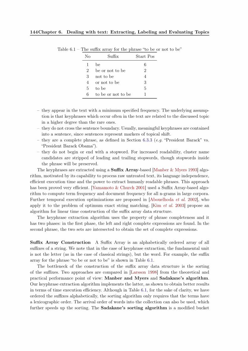
144Chapter 6. Dealing with text: Extracting, Labeling and Evaluating Topics
Table 6.1 – The suffix array for the phrase “to be or not to be”No Suffix Start Pos
1 be 62 be or not to be 23 not to be 44 or not to be 35 to be 56 to be or not to be 1
– they appear in the text with a minimum specified frequency. The underlying assump-tion is that keyphrases which occur often in the text are related to the discussed topicin a higher degree than the rare ones.
– they do not cross the sentence boundary. Usually, meaningful keyphrases are containedinto a sentence, since sentences represent markers of topical shift.
– they are a complete phrase, as defined in Section 6.3.3 (e.g. “President Barack” vs.“President Barack Obama”).
– they do not begin or end with a stopword. For increased readability, cluster namecandidates are stripped of leading and trailing stopwords, though stopwords insidethe phrase will be preserved.
The keyphrases are extracted using a Suffix Array-based [Manber & Myers 1993] algo-rithm, motivated by its capability to process raw untreated text, its language independence,efficient execution time and the power to extract humanly readable phrases. This approachhas been proved very efficient. [Yamamoto & Church 2001] used a Suffix Array-based algo-rithm to compute term frequency and document frequency for all n-grams in large corpora.Further temporal execution optimizations are proposed in [Abouelhoda et al. 2002], whoapply it to the problem of optimum exact string matching. [Kim et al. 2003] propose analgorithm for linear time construction of the suffix array data structure.
The keyphrase extraction algorithm uses the property of phrase completeness and ithas two phases: in the first phase, the left and right complete expressions are found. In thesecond phrase, the two sets are intersected to obtain the set of complete expressions.
Suffix Array Construction A Suffix Array is an alphabetically ordered array of allsuffixes of a string. We note that in the case of keyphrase extraction, the fundamental unitis not the letter (as in the case of classical strings), but the word. For example, the suffixarray for the phrase “to be or not to be” is shown in Table 6.1.
The bottleneck of the construction of the suffix array data structure is the sortingof the suffixes. Two approaches are compared in [Larsson 1998] from the theoretical andpractical performance point of view: Manber and Myers and Sadakane’s algorithm.Our keyphrase extraction algorithm implements the latter, as shown to obtain better resultsin terms of time execution efficiency. Although in Table 6.1, for the sake of clarity, we haveordered the suffixes alphabetically, the sorting algorithm only requires that the terms havea lexicographic order. The arrival order of words into the collection can also be used, whichfurther speeds up the sorting. The Sadakane’s sorting algorithm is a modified bucket
6.4. Extract, Evaluate and Improve topics 145
sorting, which takes into consideration the unequal dimensions of the suffixes. Consideringthat a keyphrase can not pass the boundary of a sentence, we modify the construction ofthe suffix array so that it is sentence-based. In practice, we build a suffix array for eachsentence and then we merge everything into a single structure. Therefore, the identificationof a suffix is given by the beginning of the suffix and the index of the its containing sentence.
Complete Phrase Discovery The right complete keyphrases are discovered by linearlyscanning the constructed suffix array in search for frequent prefixes and counting theirnumber of occurrences. Information about position and frequency is stored alongside theidentified prefixes. Discovering the left complete phrases is achieved by applying the samealgorithm to the inverse of the document. A version of the document which has the wordsin reverse order is created, right complete phrases are detected and the correct complete leftphrases are recovered by inverting the order of the extracted prefixes. Both left completeand right complete phrase sets are in lexicographic order, therefore they can be intersectedin linear time. Name candidates are returned along with their frequency.
The last phase is filtering the obtained phrase set using the minimum frequency conditionand the stripping of leading and trailing stopwords. Only phrases that appear in the textwith minimum frequency are kept, the rest are eliminated. [Osinski 2003] set the valueof this threshold between 2 and 5: the most frequent expressions are not necessarily themost expressive. They are usually frequent expressions made out of common words (e.g.“in order to”). In the end, leading and trailing stopwords are recursively eliminated fromthe phrases. This further filters the candidate set. Some of the most frequent candidatesdisappear completely (they are composed solely from stopwords). Others become duplicatesof existing phrases (e.g., “the president” and “president of”, both duplicate “president” whenthe leading “the” and the “trailing” of are stripped).
6.4.1.3 Phase 4 : Topic Labeling
The result of the text clustering space is a multidimensional space in which documentsare translated, the clusters that thematically regroup the documents and the centroids,which summarize each cluster. The keyphrase extraction phase generates a list of topiclabel candidates. In the last phase of the topic extraction, a suitable name is chosen amongthe name candidates to label each topics. This is done by introducing the name candidatesas “pseudo-documents” in the same vectorial space defined for the document collection.The keyphrases are extracted from natural language texts, so they may contain inflectedwords and stopwords. The same preprocessing (i.e., stopwords removal, stemming) andthe same term weighting scheme are used with the name candidates as with the originaldocuments. After translating into the Vector Space Model, the last step is to calculate thesimilarity between the “pseudo-documents” and the centroids of each class. The highestscoring candidate is chosen to serve as topic label.
Other that labeling topics, this approach can be used to filter semantically irrelevantexpressions from a phrase set. As centroids are abstractions of the documents in their re-spective classes, choosing phrases that are close in term of the considered distance, naturallyeliminates phrases that are too general or semantically irrelevant. This has a similar effectas adding linguistic filters to statistic methods (presented in Section 6.3.3), but without
146Chapter 6. Dealing with text: Extracting, Labeling and Evaluating Topics
their language and field dependency. For example, in a document group that talks mainlyabout politics, the highest scoring would naturally be “parliament”, “govern”, “president”,“party”, “politics” etc. When calculating the similarity between the group’s centroid and thephrase candidates, phrases like “presidential elections” would have a higher similarity thansemantically irrelevant phrases like “as a matter of fact”.
6.4.1.4 Experimental Validation
In this subsection, we briefly present some experiments and results that can be obtainedwith this topic extraction system. The performed experiments are still preliminary, beingperformed on small datasets. We have planned to perform a more complete batch of experi-ments and to compare to other topic extraction algorithm once we complete the integrationof the semantic-aware topic evaluation into CommentWatcher. We choose to present thesepreliminary experiments mostly from a qualitative point of view, to show the capabilitiesof the proposed system, and most notably the topic labeling part.
The experiments are performed on an English and a French dataset. The English datasetis a subset of the Reuters 6 corpus, composed of 262 documents. The writing style is journalarticle, each text contains between 21 and 1000 words. The French dataset 7 is issued outof a reader discussion forum attached to a news article, entitled Commemoration 8. It has aninformal writing style, it is composed of 272 documents, each one containing between 1 and713 words.
Qualitative evaluation Table 6.2 presents an example of three extracted topics from theReuters subset. The 10 highest rated words, 3 highest scoring documents and the chosentopic label are presented for each topic. Note that the highest rated words are in theirstemmed version, and, therefore, they are not always existing words. The first column showsthe extracted topic labels: “oil and gas company”, “tonnes of copper” and “united food andcommercial workers”. The second column presents the ten top scoring words associated witheach topic. The words are presented in their stemmed version. The next two columns indicatethe number of documents covered by each topic and three examples of documents from eachclusters. Let’s consider the example of the topic which covers the maximum number of texts:“oil and gas company”. The first two texts talk explicitly about the economical activitiesof companies that operate in the business of oil and natural gas (buying oil and naturalgas proprieties in the first case and estimating reserves in the second case). On the otherhand, the third document talks about the “food for oil” program between Brazil and Iraq.Unlike the first two documents, the text does not refer to an oil company. Whatsoever, thedocument is placed under the same topic, because it approaches the thematic of “oil andgas”. It also approaches with the thematic of food and this is why the document is alsofound under the topic “united food and commercial workers”. This emphasis the importanceof the overlapping property of the clustering algorithm.
6. http://mlr.cs.umass.edu/ml/datasets/Reuters-21578+Text+Categorization+Collection7. http://eric.univ-lyon2.fr/~arizoiu/files/commemoration.tar.bz28. http://www.liberation.fr/societe/0101220668-y-a-t-il-trop-de-commemorations-en-france
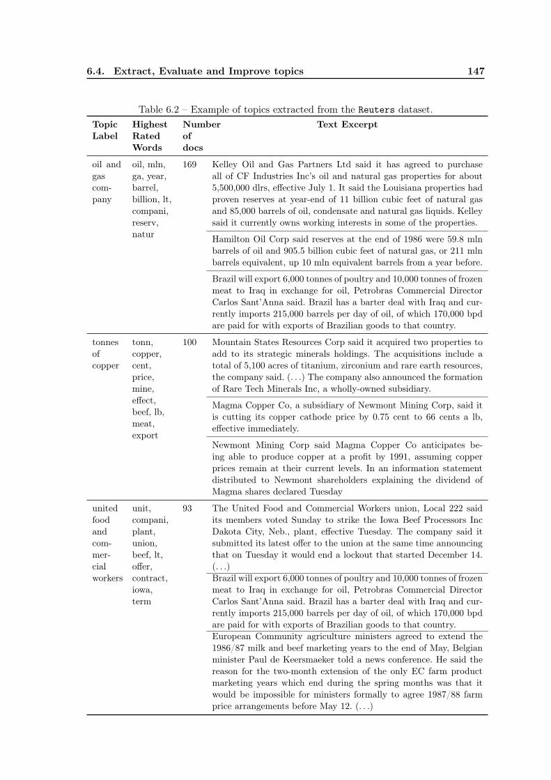
6.4. Extract, Evaluate and Improve topics 147
Table 6.2 – Example of topics extracted from the Reuters dataset.TopicLabel
HighestRatedWords
Numberofdocs
Text Excerpt
oil andgascom-pany
oil, mln,ga, year,barrel,billion, lt,compani,reserv,natur
169 Kelley Oil and Gas Partners Ltd said it has agreed to purchaseall of CF Industries Inc’s oil and natural gas properties for about5,500,000 dlrs, effective July 1. It said the Louisiana properties hadproven reserves at year-end of 11 billion cubic feet of natural gasand 85,000 barrels of oil, condensate and natural gas liquids. Kelleysaid it currently owns working interests in some of the properties.
Hamilton Oil Corp said reserves at the end of 1986 were 59.8 mlnbarrels of oil and 905.5 billion cubic feet of natural gas, or 211 mlnbarrels equivalent, up 10 mln equivalent barrels from a year before.
Brazil will export 6,000 tonnes of poultry and 10,000 tonnes of frozenmeat to Iraq in exchange for oil, Petrobras Commercial DirectorCarlos Sant’Anna said. Brazil has a barter deal with Iraq and cur-rently imports 215,000 barrels per day of oil, of which 170,000 bpdare paid for with exports of Brazilian goods to that country.
tonnesofcopper
tonn,copper,cent,price,mine,effect,beef, lb,meat,export
100 Mountain States Resources Corp said it acquired two properties toadd to its strategic minerals holdings. The acquisitions include atotal of 5,100 acres of titanium, zirconium and rare earth resources,the company said. (. . .) The company also announced the formationof Rare Tech Minerals Inc, a wholly-owned subsidiary.
Magma Copper Co, a subsidiary of Newmont Mining Corp, said itis cutting its copper cathode price by 0.75 cent to 66 cents a lb,effective immediately.
Newmont Mining Corp said Magma Copper Co anticipates be-ing able to produce copper at a profit by 1991, assuming copperprices remain at their current levels. In an information statementdistributed to Newmont shareholders explaining the dividend ofMagma shares declared Tuesday
unitedfoodandcom-mer-cialworkers
unit,compani,plant,union,beef, lt,offer,contract,iowa,term
93 The United Food and Commercial Workers union, Local 222 saidits members voted Sunday to strike the Iowa Beef Processors IncDakota City, Neb., plant, effective Tuesday. The company said itsubmitted its latest offer to the union at the same time announcingthat on Tuesday it would end a lockout that started December 14.(. . .)Brazil will export 6,000 tonnes of poultry and 10,000 tonnes of frozenmeat to Iraq in exchange for oil, Petrobras Commercial DirectorCarlos Sant’Anna said. Brazil has a barter deal with Iraq and cur-rently imports 215,000 barrels per day of oil, of which 170,000 bpdare paid for with exports of Brazilian goods to that country.European Community agriculture ministers agreed to extend the1986/87 milk and beef marketing years to the end of May, Belgianminister Paul de Keersmaeker told a news conference. He said thereason for the two-month extension of the only EC farm productmarketing years which end during the spring months was that itwould be impossible for ministers formally to agree 1987/88 farmprice arrangements before May 12. (. . .)
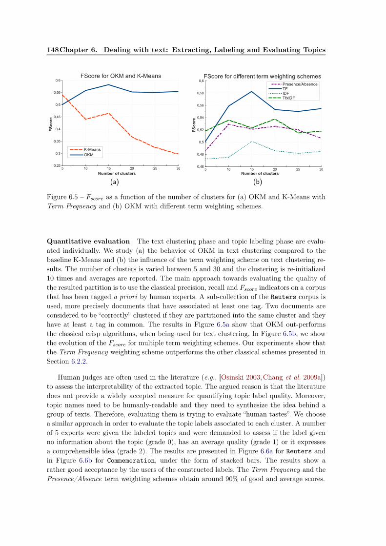
148Chapter 6. Dealing with text: Extracting, Labeling and Evaluating Topics
5 10 15 20 25 300,25
0,3
0,35
0,4
0,45
0,5
0,55
0,6FScore for OKM and K-Means
K-MeansOKM
Number of clusters
FS
co
re
(a)
5 10 15 20 25 300,46
0,48
0,5
0,52
0,54
0,56
0,58
0,6FScore for different term weighting schemes
Presence/AbsenceTFIDFTfxIDF
Number of clusters
FS
co
re
(b)
Figure 6.5 – Fscore as a function of the number of clusters for (a) OKM and K-Means withTerm Frequency and (b) OKM with different term weighting schemes.
Quantitative evaluation The text clustering phase and topic labeling phase are evalu-ated individually. We study (a) the behavior of OKM in text clustering compared to thebaseline K-Means and (b) the influence of the term weighting scheme on text clustering re-sults. The number of clusters is varied between 5 and 30 and the clustering is re-initialized10 times and averages are reported. The main approach towards evaluating the quality ofthe resulted partition is to use the classical precision, recall and Fscore indicators on a corpusthat has been tagged a priori by human experts. A sub-collection of the Reuters corpus isused, more precisely documents that have associated at least one tag. Two documents areconsidered to be “correctly” clustered if they are partitioned into the same cluster and theyhave at least a tag in common. The results in Figure 6.5a show that OKM out-performsthe classical crisp algorithms, when being used for text clustering. In Figure 6.5b, we showthe evolution of the Fscore for multiple term weighting schemes. Our experiments show thatthe Term Frequency weighting scheme outperforms the other classical schemes presented inSection 6.2.2.
Human judges are often used in the literature (e.g., [Osinski 2003,Chang et al. 2009a])to assess the interpretability of the extracted topic. The argued reason is that the literaturedoes not provide a widely accepted measure for quantifying topic label quality. Moreover,topic names need to be humanly-readable and they need to synthesize the idea behind agroup of texts. Therefore, evaluating them is trying to evaluate “human tastes”. We choosea similar approach in order to evaluate the topic labels associated to each cluster. A numberof 5 experts were given the labeled topics and were demanded to assess if the label givenno information about the topic (grade 0), has an average quality (grade 1) or it expressesa comprehensible idea (grade 2). The results are presented in Figure 6.6a for Reuters andin Figure 6.6b for Commemoration, under the form of stacked bars. The results show arather good acceptance by the users of the constructed labels. The Term Frequency and thePresence/Absence term weighting schemes obtain around 90% of good and average scores.
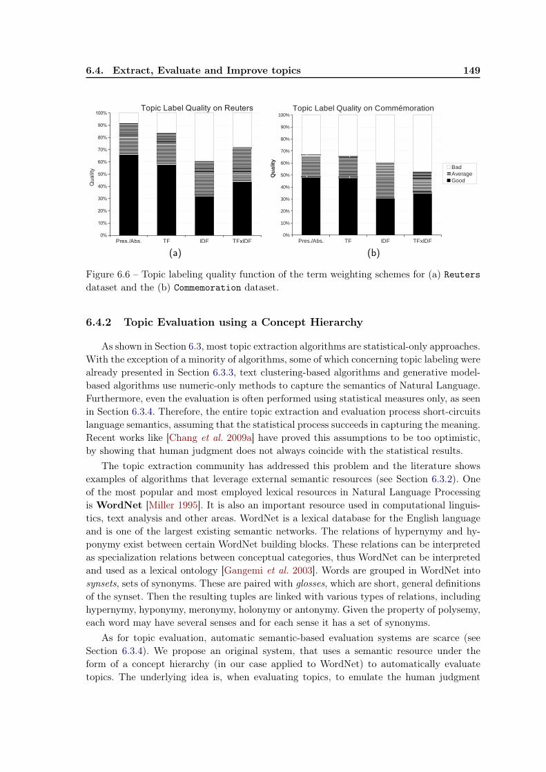
6.4. Extract, Evaluate and Improve topics 149
Pres./Abs. TF IDF TFxIDF0%
10%
20%
30%
40%
50%
60%
70%
80%
90%
100%Topic Label Quality on Reuters
Qu
alit
y
(a)Pres./Abs. TF IDF TFxIDF
0%
10%
20%
30%
40%
50%
60%
70%
80%
90%
100%Topic Label Quality on Commémoration
BadAverageGood
Qualit
y
(b)
Figure 6.6 – Topic labeling quality function of the term weighting schemes for (a) Reutersdataset and the (b) Commemoration dataset.
6.4.2 Topic Evaluation using a Concept Hierarchy
As shown in Section 6.3, most topic extraction algorithms are statistical-only approaches.With the exception of a minority of algorithms, some of which concerning topic labeling werealready presented in Section 6.3.3, text clustering-based algorithms and generative model-based algorithms use numeric-only methods to capture the semantics of Natural Language.Furthermore, even the evaluation is often performed using statistical measures only, as seenin Section 6.3.4. Therefore, the entire topic extraction and evaluation process short-circuitslanguage semantics, assuming that the statistical process succeeds in capturing the meaning.Recent works like [Chang et al. 2009a] have proved this assumptions to be too optimistic,by showing that human judgment does not always coincide with the statistical results.
The topic extraction community has addressed this problem and the literature showsexamples of algorithms that leverage external semantic resources (see Section 6.3.2). Oneof the most popular and most employed lexical resources in Natural Language Processingis WordNet [Miller 1995]. It is also an important resource used in computational linguis-tics, text analysis and other areas. WordNet is a lexical database for the English languageand is one of the largest existing semantic networks. The relations of hypernymy and hy-ponymy exist between certain WordNet building blocks. These relations can be interpretedas specialization relations between conceptual categories, thus WordNet can be interpretedand used as a lexical ontology [Gangemi et al. 2003]. Words are grouped in WordNet intosynsets, sets of synonyms. These are paired with glosses, which are short, general definitionsof the synset. Then the resulting tuples are linked with various types of relations, includinghypernymy, hyponymy, meronymy, holonymy or antonymy. Given the property of polysemy,each word may have several senses and for each sense it has a set of synonyms.
As for topic evaluation, automatic semantic-based evaluation systems are scarce (seeSection 6.3.4). We propose an original system, that uses a semantic resource under theform of a concept hierarchy (in our case applied to WordNet) to automatically evaluatetopics. The underlying idea is, when evaluating topics, to emulate the human judgment
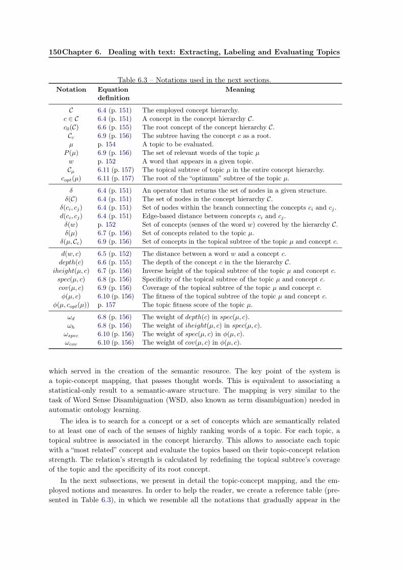
150Chapter 6. Dealing with text: Extracting, Labeling and Evaluating Topics
Table 6.3 – Notations used in the next sections.Notation Equation
definitionMeaning
C 6.4 (p. 151) The employed concept hierarchy.c ∈ C 6.4 (p. 151) A concept in the concept hierarchy C.c0(C) 6.6 (p. 155) The root concept of the concept hierarchy C.Cc 6.9 (p. 156) The subtree having the concept c as a root.µ p. 154 A topic to be evaluated.
P (µ) 6.9 (p. 156) The set of relevant words of the topic µw p. 152 A word that appears in a given topic.Cµ 6.11 (p. 157) The topical subtree of topic µ in the entire concept hierarchy.
copt(µ) 6.11 (p. 157) The root of the “optimum” subtree of the topic µ.
δ 6.4 (p. 151) An operator that returns the set of nodes in a given structure.δ(C) 6.4 (p. 151) The set of nodes in the concept hierarchy C.
δ(ci, cj) 6.4 (p. 151) Set of nodes within the branch connecting the concepts ci and cj .d(ci, cj) 6.4 (p. 151) Edge-based distance between concepts ci and cj .δ(w) p. 152 Set of concepts (senses of the word w) covered by the hierarchy C.δ(µ) 6.7 (p. 156) Set of concepts related to the topic µ.
δ(µ, Cc) 6.9 (p. 156) Set of concepts in the topical subtree of the topic µ and concept c.
d(w, c) 6.5 (p. 152) The distance between a word w and a concept c.depth(c) 6.6 (p. 155) The depth of the concept c in the the hierarchy C.
iheight(µ, c) 6.7 (p. 156) Inverse height of the topical subtree of the topic µ and concept c.spec(µ, c) 6.8 (p. 156) Specificity of the topical subtree of the topic µ and concept c.cov(µ, c) 6.9 (p. 156) Coverage of the topical subtree of the topic µ and concept c.φ(µ, c) 6.10 (p. 156) The fitness of the topical subtree of the topic µ and concept c.
φ(µ, copt(µ)) p. 157 The topic fitness score of the topic µ.
ωd 6.8 (p. 156) The weight of depth(c) in spec(µ, c).ωh 6.8 (p. 156) The weight of iheight(µ, c) in spec(µ, c).ωspec 6.10 (p. 156) The weight of spec(µ, c) in φ(µ, c).ωcov 6.10 (p. 156) The weight of cov(µ, c) in φ(µ, c).
which served in the creation of the semantic resource. The key point of the system isa topic-concept mapping, that passes thought words. This is equivalent to associating astatistical-only result to a semantic-aware structure. The mapping is very similar to thetask of Word Sense Disambiguation (WSD, also known as term disambiguation) needed inautomatic ontology learning.
The idea is to search for a concept or a set of concepts which are semantically relatedto at least one of each of the senses of highly ranking words of a topic. For each topic, atopical subtree is associated in the concept hierarchy. This allows to associate each topicwith a “most related” concept and evaluate the topics based on their topic-concept relationstrength. The relation’s strength is calculated by redefining the topical subtree’s coverageof the topic and the specificity of its root concept.
In the next subsections, we present in detail the topic-concept mapping, and the em-ployed notions and measures. In order to help the reader, we create a reference table (pre-sented in Table 6.3), in which we resemble all the notations that gradually appear in the
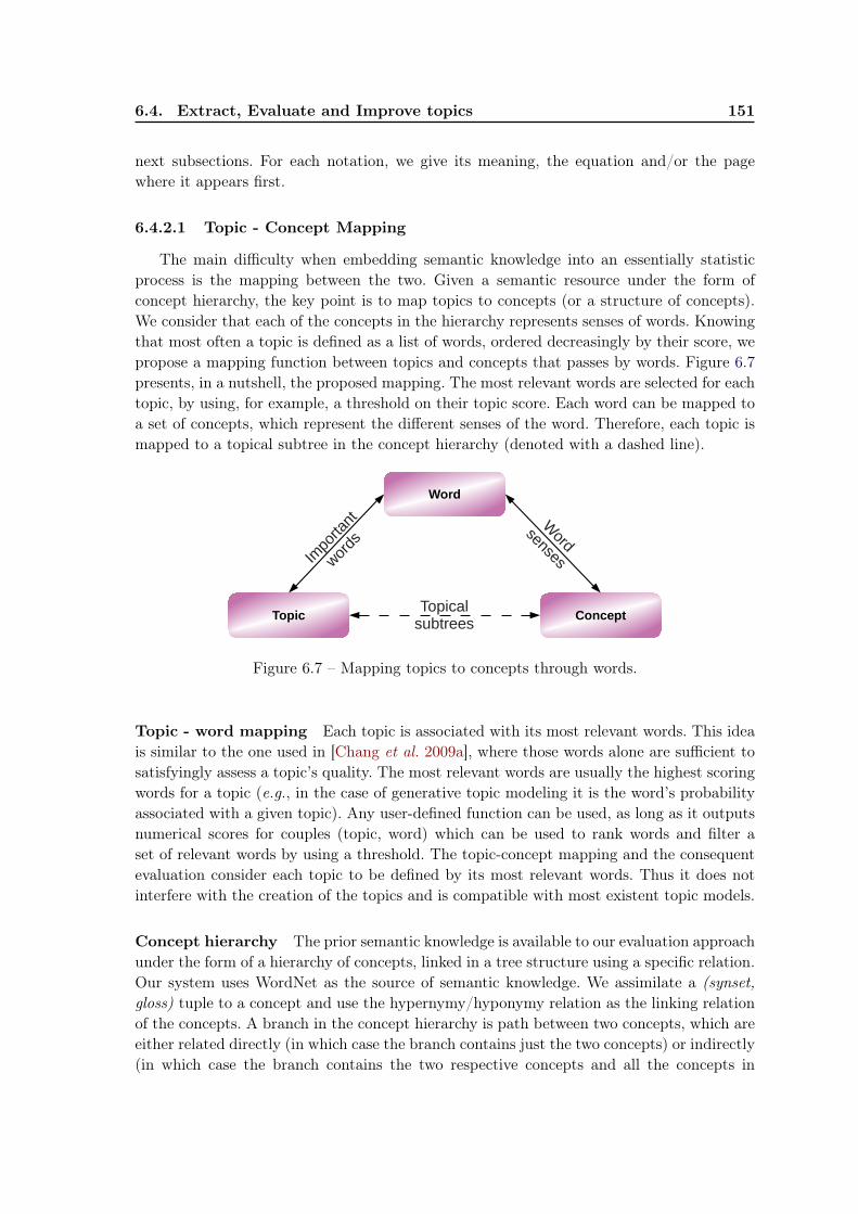
6.4. Extract, Evaluate and Improve topics 151
next subsections. For each notation, we give its meaning, the equation and/or the pagewhere it appears first.
6.4.2.1 Topic - Concept Mapping
The main difficulty when embedding semantic knowledge into an essentially statisticprocess is the mapping between the two. Given a semantic resource under the form ofconcept hierarchy, the key point is to map topics to concepts (or a structure of concepts).We consider that each of the concepts in the hierarchy represents senses of words. Knowingthat most often a topic is defined as a list of words, ordered decreasingly by their score, wepropose a mapping function between topics and concepts that passes by words. Figure 6.7presents, in a nutshell, the proposed mapping. The most relevant words are selected for eachtopic, by using, for example, a threshold on their topic score. Each word can be mapped toa set of concepts, which represent the different senses of the word. Therefore, each topic ismapped to a topical subtree in the concept hierarchy (denoted with a dashed line).
Topic Concept
Word
Impo
rtant
words
Word
senses
Topicalsubtrees
Figure 6.7 – Mapping topics to concepts through words.
Topic - word mapping Each topic is associated with its most relevant words. This ideais similar to the one used in [Chang et al. 2009a], where those words alone are sufficient tosatisfyingly assess a topic’s quality. The most relevant words are usually the highest scoringwords for a topic (e.g., in the case of generative topic modeling it is the word’s probabilityassociated with a given topic). Any user-defined function can be used, as long as it outputsnumerical scores for couples (topic, word) which can be used to rank words and filter aset of relevant words by using a threshold. The topic-concept mapping and the consequentevaluation consider each topic to be defined by its most relevant words. Thus it does notinterfere with the creation of the topics and is compatible with most existent topic models.
Concept hierarchy The prior semantic knowledge is available to our evaluation approachunder the form of a hierarchy of concepts, linked in a tree structure using a specific relation.Our system uses WordNet as the source of semantic knowledge. We assimilate a (synset,gloss) tuple to a concept and use the hypernymy/hyponymy relation as the linking relationof the concepts. A branch in the concept hierarchy is path between two concepts, which areeither related directly (in which case the branch contains just the two concepts) or indirectly(in which case the branch contains the two respective concepts and all the concepts in
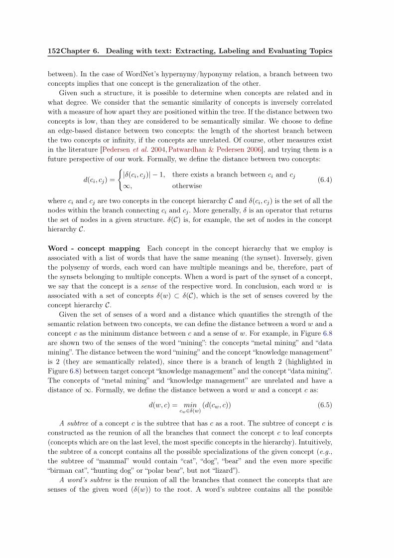
152Chapter 6. Dealing with text: Extracting, Labeling and Evaluating Topics
between). In the case of WordNet’s hypernymy/hyponymy relation, a branch between twoconcepts implies that one concept is the generalization of the other.
Given such a structure, it is possible to determine when concepts are related and inwhat degree. We consider that the semantic similarity of concepts is inversely correlatedwith a measure of how apart they are positioned within the tree. If the distance between twoconcepts is low, than they are considered to be semantically similar. We choose to definean edge-based distance between two concepts: the length of the shortest branch betweenthe two concepts or infinity, if the concepts are unrelated. Of course, other measures existin the literature [Pedersen et al. 2004,Patwardhan & Pedersen 2006], and trying them is afuture perspective of our work. Formally, we define the distance between two concepts:
d(ci, cj) =
{|δ(ci, cj)| − 1, there exists a branch between ci and cj∞, otherwise
(6.4)
where ci and cj are two concepts in the concept hierarchy C and δ(ci, cj) is the set of all thenodes within the branch connecting ci and cj . More generally, δ is an operator that returnsthe set of nodes in a given structure. δ(C) is, for example, the set of nodes in the concepthierarchy C.
Word - concept mapping Each concept in the concept hierarchy that we employ isassociated with a list of words that have the same meaning (the synset). Inversely, giventhe polysemy of words, each word can have multiple meanings and be, therefore, part ofthe synsets belonging to multiple concepts. When a word is part of the synset of a concept,we say that the concept is a sense of the respective word. In conclusion, each word w isassociated with a set of concepts δ(w) ⊂ δ(C), which is the set of senses covered by theconcept hierarchy C.
Given the set of senses of a word and a distance which quantifies the strength of thesemantic relation between two concepts, we can define the distance between a word w and aconcept c as the minimum distance between c and a sense of w. For example, in Figure 6.8are shown two of the senses of the word “mining”: the concepts “metal mining” and “datamining”. The distance between the word “mining” and the concept “knowledge management”is 2 (they are semantically related), since there is a branch of length 2 (highlighted inFigure 6.8) between target concept “knowledge management” and the concept “data mining”.The concepts of “metal mining” and “knowledge management” are unrelated and have adistance of ∞. Formally, we define the distance between a word w and a concept c as:
d(w, c) = mincw∈δ(w)
(d(cw, c)) (6.5)
A subtree of a concept c is the subtree that has c as a root. The subtree of concept c isconstructed as the reunion of all the branches that connect the concept c to leaf concepts(concepts which are on the last level, the most specific concepts in the hierarchy). Intuitively,the subtree of a concept contains all the possible specializations of the given concept (e.g.,the subtree of “mammal” would contain “cat”, “dog”, “bear” and the even more specific“birman cat”, “hunting dog” or “polar bear”, but not “lizard”).
A word’s subtree is the reunion of all the branches that connect the concepts that aresenses of the given word (δ(w)) to the root. A word’s subtree contains all the possible
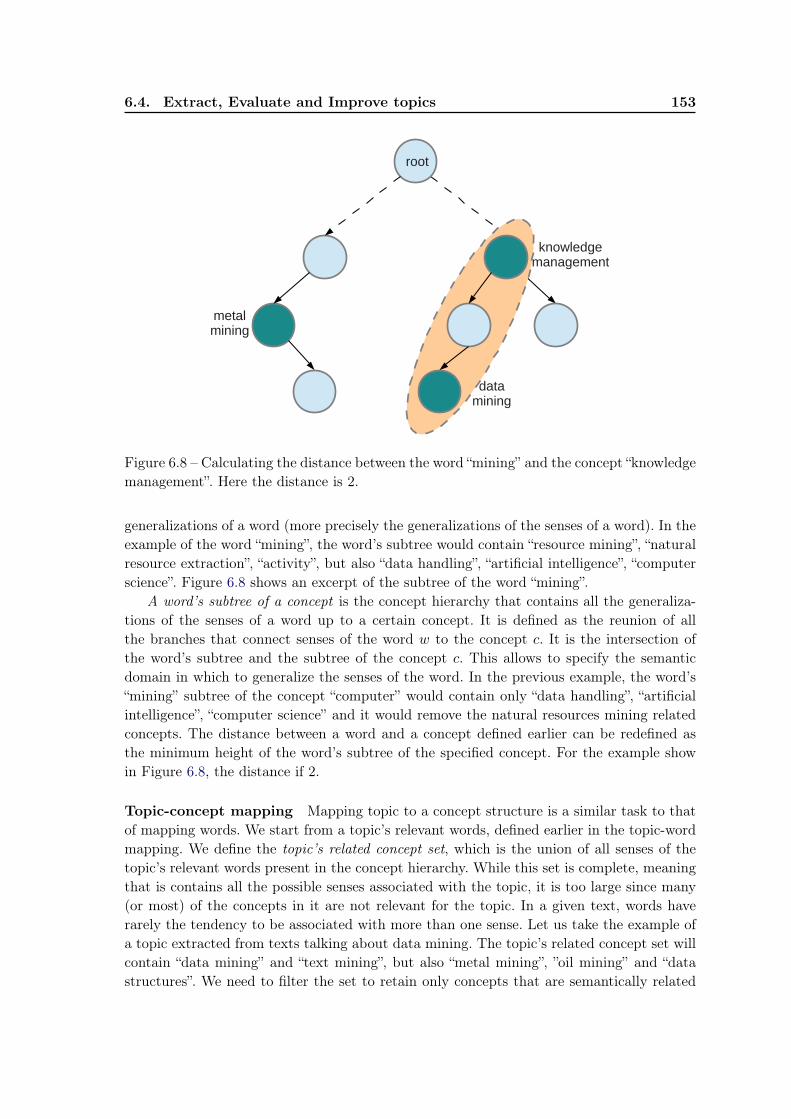
6.4. Extract, Evaluate and Improve topics 153
root
metalmining
datamining
knowledgemanagement
Figure 6.8 – Calculating the distance between the word “mining” and the concept “knowledgemanagement”. Here the distance is 2.
generalizations of a word (more precisely the generalizations of the senses of a word). In theexample of the word “mining”, the word’s subtree would contain “resource mining”, “naturalresource extraction”, “activity”, but also “data handling”, “artificial intelligence”, “computerscience”. Figure 6.8 shows an excerpt of the subtree of the word “mining”.
A word’s subtree of a concept is the concept hierarchy that contains all the generaliza-tions of the senses of a word up to a certain concept. It is defined as the reunion of allthe branches that connect senses of the word w to the concept c. It is the intersection ofthe word’s subtree and the subtree of the concept c. This allows to specify the semanticdomain in which to generalize the senses of the word. In the previous example, the word’s“mining” subtree of the concept “computer” would contain only “data handling”, “artificialintelligence”, “computer science” and it would remove the natural resources mining relatedconcepts. The distance between a word and a concept defined earlier can be redefined asthe minimum height of the word’s subtree of the specified concept. For the example showin Figure 6.8, the distance if 2.
Topic-concept mapping Mapping topic to a concept structure is a similar task to thatof mapping words. We start from a topic’s relevant words, defined earlier in the topic-wordmapping. We define the topic’s related concept set, which is the union of all senses of thetopic’s relevant words present in the concept hierarchy. While this set is complete, meaningthat is contains all the possible senses associated with the topic, it is too large since many(or most) of the concepts in it are not relevant for the topic. In a given text, words haverarely the tendency to be associated with more than one sense. Let us take the example ofa topic extracted from texts talking about data mining. The topic’s related concept set willcontain “data mining” and “text mining”, but also “metal mining”, ”oil mining” and “datastructures”. We need to filter the set to retain only concepts that are semantically related
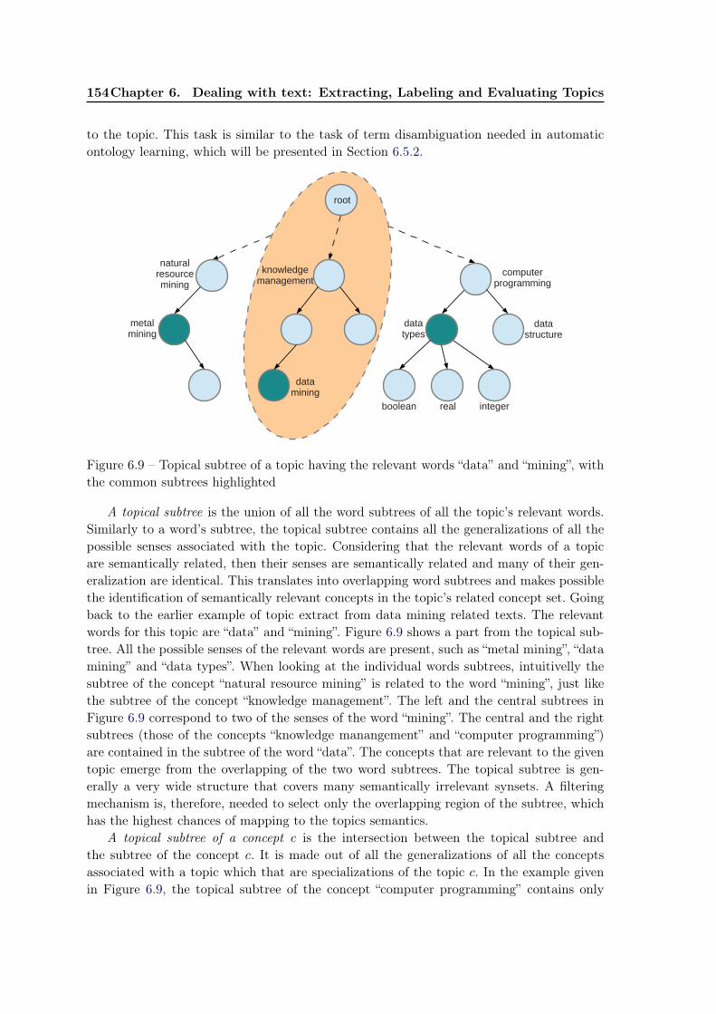
154Chapter 6. Dealing with text: Extracting, Labeling and Evaluating Topics
to the topic. This task is similar to the task of term disambiguation needed in automaticontology learning, which will be presented in Section 6.5.2.
root
metalmining
datamining
knowledgemanagement
datatypes
natural resourcemining
computerprogramming
integerboolean real
datastructure
Figure 6.9 – Topical subtree of a topic having the relevant words “data” and “mining”, withthe common subtrees highlighted
A topical subtree is the union of all the word subtrees of all the topic’s relevant words.Similarly to a word’s subtree, the topical subtree contains all the generalizations of all thepossible senses associated with the topic. Considering that the relevant words of a topicare semantically related, then their senses are semantically related and many of their gen-eralization are identical. This translates into overlapping word subtrees and makes possiblethe identification of semantically relevant concepts in the topic’s related concept set. Goingback to the earlier example of topic extract from data mining related texts. The relevantwords for this topic are “data” and “mining”. Figure 6.9 shows a part from the topical sub-tree. All the possible senses of the relevant words are present, such as “metal mining”, “datamining” and “data types”. When looking at the individual words subtrees, intuitivelly thesubtree of the concept “natural resource mining” is related to the word “mining”, just likethe subtree of the concept “knowledge management”. The left and the central subtrees inFigure 6.9 correspond to two of the senses of the word “mining”. The central and the rightsubtrees (those of the concepts “knowledge manangement” and “computer programming”)are contained in the subtree of the word “data”. The concepts that are relevant to the giventopic emerge from the overlapping of the two word subtrees. The topical subtree is gen-erally a very wide structure that covers many semantically irrelevant synsets. A filteringmechanism is, therefore, needed to select only the overlapping region of the subtree, whichhas the highest chances of mapping to the topics semantics.
A topical subtree of a concept c is the intersection between the topical subtree andthe subtree of the concept c. It is made out of all the generalizations of all the conceptsassociated with a topic which that are specializations of the topic c. In the example givenin Figure 6.9, the topical subtree of the concept “computer programming” contains only
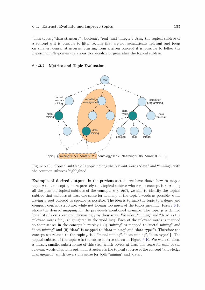
6.4. Extract, Evaluate and Improve topics 155
“data types”, “data structure”, “boolean”, “real” and “integer”. Using the topical subtree ofa concept c it is possible to filter regions that are not semantically relevant and focuson smaller, denser structures. Starting from a given concept it is possible to follow thehyperonymy/hyponymy relations to specialize or generalize the topical subtree.
6.4.2.2 Metrics and Topic Evaluation
root
metalmining
datamining
knowledgemanagement
datatypes
natural resourcemining
computerprogramming
integerboolean real
datastructure
Topic μ ( “mining” 0.53 , “data” 0.25 , “ontology” 0.12 , “learning” 0.06 , “error” 0.02 ... )
Figure 6.10 – Topical subtree of a topic having the relevant words “data” and “mining”, withthe common subtrees highlighted.
Example of desired output In the previous section, we have shown how to map atopic µ to a concept c, more precisely to a topical subtree whose root concept is c. Amongall the possible topical subtrees of the concepts ci ∈ δ(C), we aim to identify the topicalsubtree that includes at least one sense for as many of the topic’s words as possible, whilehaving a root concept as specific as possible. The idea is to map the topic to a dense andcompact concept structure, while not loosing too much of the topics meaning. Figure 6.10shows the desired mapping for the previously mentioned example. The topic µ is definedby a list of words, ordered decreasingly by their score. We select “mining” and “data” as therelevant words for µ (highlighted in the word list). Each of the relevant words is mappedto their senses in the concept hierarchy ( (i) “mining” is mapped to “metal mining” and“data mining” and (ii) “data” is mapped to “data mining” and “data types”). Therefore theconcept set related to the topic µ is { “metal mining”, “data mining”, “data types”}. Thetopical subtree of the topic µ is the entire subtree shown in Figure 6.10. We want to chosea denser, smaller substructure of this tree, which covers at least one sense for each of therelevant words of µ. This optimum structure is the topical subtree of the concept “knowledgemanagement” which covers one sense for both “mining” and “data”.
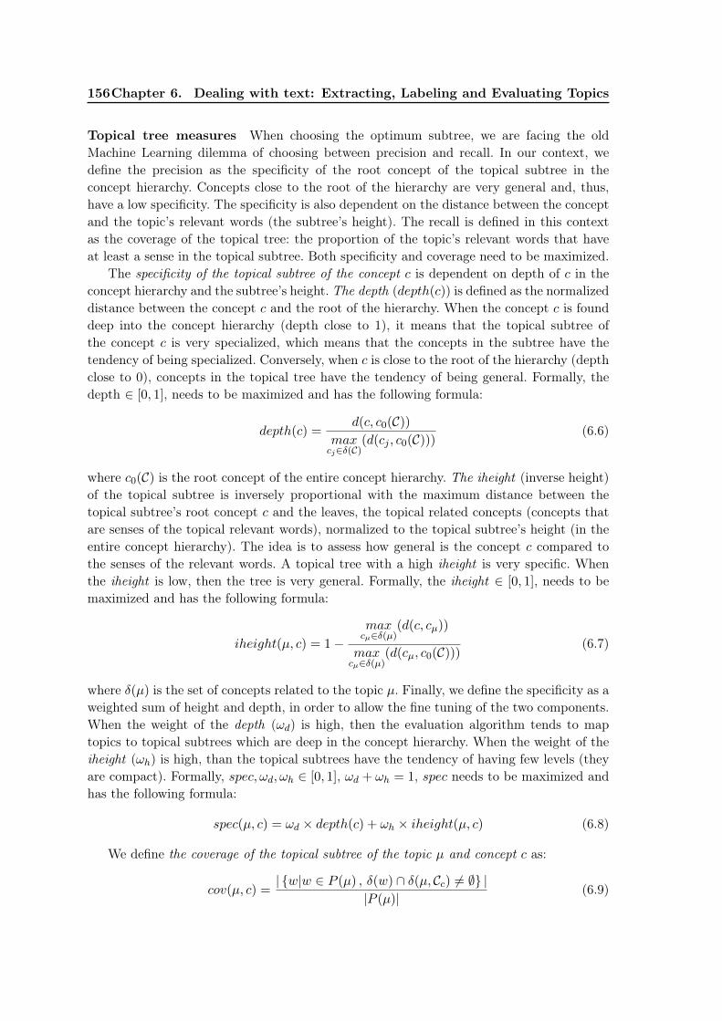
156Chapter 6. Dealing with text: Extracting, Labeling and Evaluating Topics
Topical tree measures When choosing the optimum subtree, we are facing the oldMachine Learning dilemma of choosing between precision and recall. In our context, wedefine the precision as the specificity of the root concept of the topical subtree in theconcept hierarchy. Concepts close to the root of the hierarchy are very general and, thus,have a low specificity. The specificity is also dependent on the distance between the conceptand the topic’s relevant words (the subtree’s height). The recall is defined in this contextas the coverage of the topical tree: the proportion of the topic’s relevant words that haveat least a sense in the topical subtree. Both specificity and coverage need to be maximized.
The specificity of the topical subtree of the concept c is dependent on depth of c in theconcept hierarchy and the subtree’s height. The depth (depth(c)) is defined as the normalizeddistance between the concept c and the root of the hierarchy. When the concept c is founddeep into the concept hierarchy (depth close to 1), it means that the topical subtree ofthe concept c is very specialized, which means that the concepts in the subtree have thetendency of being specialized. Conversely, when c is close to the root of the hierarchy (depthclose to 0), concepts in the topical tree have the tendency of being general. Formally, thedepth ∈ [0, 1], needs to be maximized and has the following formula:
depth(c) =d(c, c0(C))
maxcj∈δ(C)
(d(cj , c0(C)))(6.6)
where c0(C) is the root concept of the entire concept hierarchy. The iheight (inverse height)of the topical subtree is inversely proportional with the maximum distance between thetopical subtree’s root concept c and the leaves, the topical related concepts (concepts thatare senses of the topical relevant words), normalized to the topical subtree’s height (in theentire concept hierarchy). The idea is to assess how general is the concept c compared tothe senses of the relevant words. A topical tree with a high iheight is very specific. Whenthe iheight is low, then the tree is very general. Formally, the iheight ∈ [0, 1], needs to bemaximized and has the following formula:
iheight(µ, c) = 1−maxcµ∈δ(µ)
(d(c, cµ))
maxcµ∈δ(µ)
(d(cµ, c0(C)))(6.7)
where δ(µ) is the set of concepts related to the topic µ. Finally, we define the specificity as aweighted sum of height and depth, in order to allow the fine tuning of the two components.When the weight of the depth (ωd) is high, then the evaluation algorithm tends to maptopics to topical subtrees which are deep in the concept hierarchy. When the weight of theiheight (ωh) is high, than the topical subtrees have the tendency of having few levels (theyare compact). Formally, spec, ωd, ωh ∈ [0, 1], ωd + ωh = 1, spec needs to be maximized andhas the following formula:
spec(µ, c) = ωd × depth(c) + ωh × iheight(µ, c) (6.8)
We define the coverage of the topical subtree of the topic µ and concept c as:
cov(µ, c) =| {w|w ∈ P (µ) , δ(w) ∩ δ(µ, Cc) 6= ∅} |
|P (µ)|(6.9)
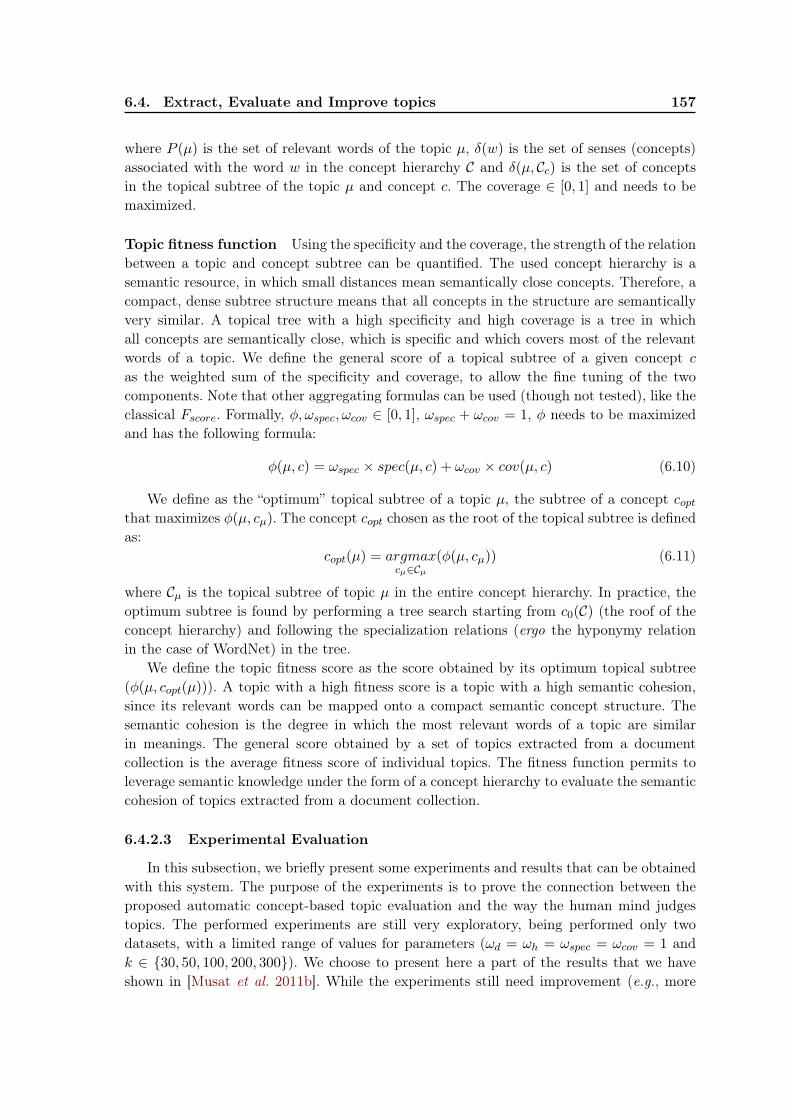
6.4. Extract, Evaluate and Improve topics 157
where P (µ) is the set of relevant words of the topic µ, δ(w) is the set of senses (concepts)associated with the word w in the concept hierarchy C and δ(µ, Cc) is the set of conceptsin the topical subtree of the topic µ and concept c. The coverage ∈ [0, 1] and needs to bemaximized.
Topic fitness function Using the specificity and the coverage, the strength of the relationbetween a topic and concept subtree can be quantified. The used concept hierarchy is asemantic resource, in which small distances mean semantically close concepts. Therefore, acompact, dense subtree structure means that all concepts in the structure are semanticallyvery similar. A topical tree with a high specificity and high coverage is a tree in whichall concepts are semantically close, which is specific and which covers most of the relevantwords of a topic. We define the general score of a topical subtree of a given concept cas the weighted sum of the specificity and coverage, to allow the fine tuning of the twocomponents. Note that other aggregating formulas can be used (though not tested), like theclassical Fscore. Formally, φ, ωspec, ωcov ∈ [0, 1], ωspec + ωcov = 1, φ needs to be maximizedand has the following formula:
φ(µ, c) = ωspec × spec(µ, c) + ωcov × cov(µ, c) (6.10)
We define as the “optimum” topical subtree of a topic µ, the subtree of a concept coptthat maximizes φ(µ, cµ). The concept copt chosen as the root of the topical subtree is definedas:
copt(µ) = argmaxcµ∈Cµ
(φ(µ, cµ)) (6.11)
where Cµ is the topical subtree of topic µ in the entire concept hierarchy. In practice, theoptimum subtree is found by performing a tree search starting from c0(C) (the roof of theconcept hierarchy) and following the specialization relations (ergo the hyponymy relationin the case of WordNet) in the tree.
We define the topic fitness score as the score obtained by its optimum topical subtree(φ(µ, copt(µ))). A topic with a high fitness score is a topic with a high semantic cohesion,since its relevant words can be mapped onto a compact semantic concept structure. Thesemantic cohesion is the degree in which the most relevant words of a topic are similarin meanings. The general score obtained by a set of topics extracted from a documentcollection is the average fitness score of individual topics. The fitness function permits toleverage semantic knowledge under the form of a concept hierarchy to evaluate the semanticcohesion of topics extracted from a document collection.
6.4.2.3 Experimental Evaluation
In this subsection, we briefly present some experiments and results that can be obtainedwith this system. The purpose of the experiments is to prove the connection between theproposed automatic concept-based topic evaluation and the way the human mind judgestopics. The performed experiments are still very exploratory, being performed only twodatasets, with a limited range of values for parameters (ωd = ωh = ωspec = ωcov = 1 andk ∈ {30, 50, 100, 200, 300}). We choose to present here a part of the results that we haveshown in [Musat et al. 2011b]. While the experiments still need improvement (e.g., more
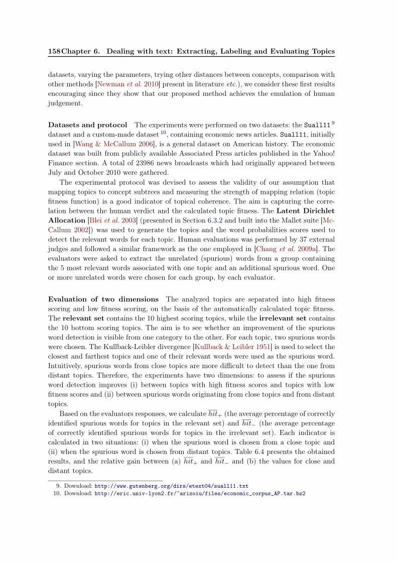
158Chapter 6. Dealing with text: Extracting, Labeling and Evaluating Topics
datasets, varying the parameters, trying other distances between concepts, comparison withother methods [Newman et al. 2010] present in literature etc.), we consider these first resultsencouraging since they show that our proposed method achieves the emulation of humanjudgement.
Datasets and protocol The experiments were performed on two datasets: the Suall11 9
dataset and a custom-made dataset 10, containing economic news articles. Suall11, initiallyused in [Wang & McCallum 2006], is a general dataset on American history. The economicdataset was built from publicly available Associated Press articles published in the Yahoo!Finance section. A total of 23986 news broadcasts which had originally appeared betweenJuly and October 2010 were gathered.
The experimental protocol was devised to assess the validity of our assumption thatmapping topics to concept subtrees and measuring the strength of mapping relation (topicfitness function) is a good indicator of topical coherence. The aim is capturing the corre-lation between the human verdict and the calculated topic fitness. The Latent DirichletAllocation [Blei et al. 2003] (presented in Section 6.3.2 and built into the Mallet suite [Mc-Callum 2002]) was used to generate the topics and the word probabilities scores used todetect the relevant words for each topic. Human evaluations was performed by 37 externaljudges and followed a similar framework as the one employed in [Chang et al. 2009a]. Theevaluators were asked to extract the unrelated (spurious) words from a group containingthe 5 most relevant words associated with one topic and an additional spurious word. Oneor more unrelated words were chosen for each group, by each evaluator.
Evaluation of two dimensions The analyzed topics are separated into high fitnessscoring and low fitness scoring, on the basis of the automatically calculated topic fitness.The relevant set contains the 10 highest scoring topics, while the irrelevant set containsthe 10 bottom scoring topics. The aim is to see whether an improvement of the spuriousword detection is visible from one category to the other. For each topic, two spurious wordswere chosen. The Kullback-Leibler divergence [Kullback & Leibler 1951] is used to select theclosest and farthest topics and one of their relevant words were used as the spurious word.Intuitively, spurious words from close topics are more difficult to detect than the one fromdistant topics. Therefore, the experiments have two dimensions: to assess if the spuriousword detection improves (i) between topics with high fitness scores and topics with lowfitness scores and (ii) between spurious words originating from close topics and from distanttopics.
Based on the evaluators responses, we calculate hit+ (the average percentage of correctlyidentified spurious words for topics in the relevant set) and hit− (the average percentageof correctly identified spurious words for topics in the irrelevant set). Each indicator iscalculated in two situations: (i) when the spurious word is chosen from a close topic and(ii) when the spurious word is chosen from distant topics. Table 6.4 presents the obtainedresults, and the relative gain between (a) hit+ and hit− and (b) the values for close anddistant topics.
9. Download: http://www.gutenberg.org/dirs/etext04/suall11.txt10. Download: http://eric.univ-lyon2.fr/~arizoiu/files/economic_corpus_AP.tar.bz2
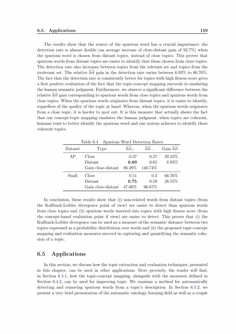
6.5. Applications 159
The results show that the source of the spurious word has a crucial importance: thedetection rate is almost double (an average increase of close-distant gain of 92.7%) whenthe spurious word is chosen from distant topics, instead of close topics. This proves thatspurious words from distant topics are easier to identify that those chosen from close topics.The detection rate also increases between topics from the relevant set and topics from theirrelevant set. The relative hit gain in the detection rate varies between 6.93% to 66.76%.The fact that the detection rate is consistently better for topics with high fitness score givesa first positive evaluation of the fact that the topic-concept mapping succeeds in emulatingthe human semantic judgment. Furthermore, we observe a significant difference between therelative hit gain corresponding to spurious words from close topics and spurious words fromclose topics. When the spurious words originates from distant topics, it is easier to identify,regardless of the quality of the topic at hand. Whereas, when the spurious words originatesfrom a close topic, it is harder to spot out. It is this measure that actually shows the factthat our concept-topic mapping emulates the human judgment: when topics are coherent,humans tend to better identify the spurious word and our system achieves to identify thesecoherent topics.
Table 6.4 – Spurious Word Detection Rates.Dataset Type hit+ hit− Gain hit
AP Close 0.37 0.27 39.33%Distant 0.69 0.65 6.93%Gain close-distant 86.49% 140.74%
Suall Close 0.51 0.3 66.76%Distant 0.75 0.59 28.55%Gain close-distant 47.06% 96.67%
In conclusion, these results show that (i) non-related words from distant topics (fromthe Kullback-Leibler divergence point of view) are easier to detect than spurious wordsfrom close topics and (ii) spurious words inserted into topics with high fitness score (fromthe concept-based evaluation point if view) are easier to detect. This proves that (i) theKullback-Leibler divergence can be used as a measure of the semantic distance between twotopics expressed as a probability distribution over words and (ii) the proposed topic-conceptmapping and evaluation measures succeed in capturing and quantifying the semantic cohe-sion of a topic.
6.5 Applications
In this section, we discuss how the topic extraction and evaluation techniques, presentedin this chapter, can be used in other applications. More precisely, the reader will find,in Section 6.5.1, how the topic-concept mapping, alongside with the measures defined inSection 6.4.2, can be used for improving topic. We examine a method for automaticallydetecting and removing spurious words from a topic’s description. In Section 6.5.2, wepresent a very brief presentation of the automatic ontology learning field as well as a couple

160Chapter 6. Dealing with text: Extracting, Labeling and Evaluating Topics
of hints of how topics extracted from a collection of documents can be used in ontologylearning.
6.5.1 Improving topics by Removing Topical Outliers
After presenting how topics can be created (in Sections 6.3.1, 6.3.2 and 6.4.1) andevaluated (in Section 6.3.4 and 6.4.2), a natural follow-up is topic improvement. We use thesame general framework which is described in Section 6.4.2 (p. 148). A semantic resourceunder the form of a concept hierarchy is used and a topic-concept mapping is created,passing through words. Topics are associated with topical subtrees, which contain all thegeneralizations of the senses of their most relevant words.
The idea of the topic improvement system is to create a projection of the topic as awhole onto the given ontology and decide which part of the topic, if any, is separated fromthe others. The underlying assumption is that the understandability of the given topic canbe improved by removing the parts which are unrelated from a human perspective. Thepresented system is designed to improve individual topics according to their semantic cohe-sion. We use an established simplified representation of topics, used in most of the literature,which is the list of most relevant words. To improve topic readability and meaningfulness,we prune the outliers from the related word set, using the concept hierarchy. Topical out-liers are the words that are unrelated to the other words from a semantic perspective. Afterthe pruning, the remaining relevant words are more inter-related as a set and confer moremeaning to the user. The core of this work is establishing the conceptual context of a singlegiven topic, as shown in Section 6.4.2. We detect which concepts from the used ontology arerelevant to the topic as a whole and choose the topical words unrelated to those conceptsas the outliers to be eliminated.
Methodology In order to detect the topical words that are unrelated to conceptual con-text created by the others, we must first identify the related concepts. In Section 6.4.2,we have shown that for any given topical, multiple topical subtrees of a specific conceptscan be constructed. Each of topical subtrees were assigned a general topical subtree score,given by Equation 6.10 (p. 156). In the evaluation process, we have selected the “optimum”topical subtree as the one having the highest topical subtree score. In order to detect topicaloutliers, we do not choose one “optimum” subtree (belonging to just one concept), but wechoose l ∈ N topical subtrees that have the highest scores. If we are to make a parallel,the highest ranking topical subtrees are like the axes in of Principal Component Analy-sis (PCA) [Dunteman 1989]. Just like PCA’s axes, the topical subtrees contain decreasingamounts of semantic information. Selecting the first few highest ranking subtrees permits tomap most of the semantic information contained in the topic. We define the topical outliersas the words not covered by the reunion of the l highest scoring topical subtrees for a giventhe topic µ. l is a parameter of the system.
In Figure 6.11, we present a simplified version of the topical subtree for the topicµ(“mining”, “data”, “error”, “ontology”, “learning”). For l = 2, the highest two scoring topicalsubtrees are those of concepts “knowledge management” and “semantic web” (highlightedin orange). The topical subtree of the concept “knowledge management” contains senses forthe words “mining” and “data”, whereas the topical subtree of the concept “semantic web”
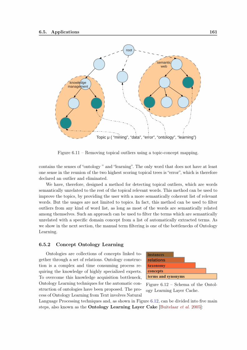
6.5. Applications 161
root
Topic μ ( “mining”, “data”, “error”, “ontology”, “learning”)
knowledgemanagement
semanticweb
Figure 6.11 – Removing topical outliers using a topic-concept mapping.
contains the senses of “ontology ” and “learning”. The only word that does not have at leastone sense in the reunion of the two highest scoring topical trees is “error”, which is thereforedeclared an outlier and eliminated.
We have, therefore, designed a method for detecting topical outliers, which are wordssemantically unrelated to the rest of the topical relevant words. This method can be used toimprove the topics, by providing the user with a more semantically coherent list of relevantwords. But the usages are not limited to topics. In fact, this method can be used to filteroutliers from any kind of word list, as long as most of the words are semantically relatedamong themselves. Such an approach can be used to filter the terms which are semanticallyunrelated with a specific domain concept from a list of automatically extracted terms. Aswe show in the next section, the manual term filtering is one of the bottlenecks of OntologyLearning.
6.5.2 Concept Ontology Learning
terms and synonymsconceptstaxonomyrelationsinstances
Figure 6.12 – Schema of the Ontol-ogy Learning Layer Cache.
Ontologies are collections of concepts linked to-gether through a set of relations. Ontology construc-tion is a complex and time consuming process re-quiring the knowledge of highly specialized experts.To overcome this knowledge acquisition bottleneck,Ontology Learning techniques for the automatic con-struction of ontologies have been proposed. The pro-cess of Ontology Learning from Text involves NaturalLanguage Processing techniques and, as shown in Figure 6.12, can be divided into five mainsteps, also known as the Ontology Learning Layer Cake [Buitelaar et al. 2005]:
162Chapter 6. Dealing with text: Extracting, Labeling and Evaluating Topics
1. extraction of domain terminology and synonyms from a corpus of documents (theterms and synonyms layer);
2. definition of main concepts on the basis of the detected relevant terms and the classesof synonyms (the concepts layer);
3. structuring of concepts into taxonomy (the taxonomy layer);
4. definition of non-taxonomic relations between concepts (the relations layer);
5. population of the ontology with concepts and relations instances (the instances layer).
An overview of the state-of-the-art of ontology learning and the proposed solutions for eachstep can be found in [Cimiano et al. 2006]. The main approach toward learning conceptsand their taxonomy (the hierarchical relations between concepts) is Conceptual cluster-ing [Michalski & Stepp 1983], an unsupervised machine learning technique closely connectedto unsupervised hierarchical clustering. Examples of algorithms developed for this purposeare the well-known COBWEB [Fisher 1987] and the more recent WebDCC [Godoy &Amandi 2006]. We take a look into alternative methods and discuss the usage of topic ex-traction at the two bottom layers of the ontology cache: the terms and synonyms layer andthe concepts layer.
Work at the terms and synonyms layer Topic extraction systems have already beenused at the terms and synonyms layer, where the challenges are (i) extracting relevant termsthat unambiguously refer to a domain-specific concept and (ii) dealing with disambiguation.The literature provides many examples of term extraction methods [Wong et al. 2008,Wonget al. 2009] that could be used as a first step in ontology learning from text, but theresulted list of relevant terms needs to be filtered by a domain expert [Cimiano et al. 2006].The topic-concept mapping presented in Section 6.4.2 and the topic improvement approachpresented in the Section 6.5.1 allow further automatization of this process. Semantic outlierscan be detected by using a general purpose semantic resource, such as WordNet, thereforesimplifying or completely eliminating the supervision of the field expert.
Disambiguation deals with choosing, considering the property of polysemy, the rightmeaning for a word in a given context. Most of today’s word sense disambiguation algo-rithms, like the one in [Lesk 1986], rely on usage of synonym sets. The literature presentstwo main approaches towards finding synonyms [Buitelaar et al. 2005]:
– algorithms that rely on readily available synonym sets such as WordNet [Miller 1995]or EuroWordNet 11 [Turcato et al. 2000,Kietz et al. 2000];
– algorithms that directly discover synonyms by means of clustering. These algorithmsare based on statistical measures mainly used in Information Retrieval and start fromthe hypothesis that terms are similar in meaning to the extent in which they sharesyntactic contexts [Harris 1968]. text clustering places documents which share thesame context into the same group, which in turn leads to synonyms being placedunder the same topic.
As terms have different meaning depending on the context, it is only natural to allowthem to be part of more than one group. In this case, the clustering algorithm can be used tofind synonyms, but also for term disambiguation (choosing between the different meanings).
11. http://www.illc.uva.nl/EuroWordNet/
6.6. Conclusion and future work 163
The crisp text clustering solutions presented in Section 6.3.1 have the inconvenient that theyoutput a crisp partition, where each document belong to only one group. These approachescan be used for regrouping synonyms, but they cannot be used for disambiguation. Anoverlapping solution, as the one presented in Section 6.4.1, would address the disambiguationproblem, allowing terms to be in more than one cluster. Terms with multiple meanings canbe regrouped together with their synonyms, for each of their meanings.
The concepts layer : evolving topics to concepts A topic is not a concept since itrepresents the abstraction of the idea behind a group of texts rather than a notion in itself.While the difference between the two is subtle, evolving a topic into a fully fledged conceptis still to be achieved. The literature does not provide any largely accepted solution. Ofcourse, the simplest way to do it is to have a human expert manually evolving the topicsinto concepts by adding relations and building the structure of the ontology. But in the longterm, the objective is to completely automatize the ontology building process. That is whyrelations need to be found in a human-independent way.
Some of the recent topic extraction algorithms already made the first steps towardsthis objective. hLDA [Blei et al. 2004] outputs an hierarchy of topics, which can pro-vide, to a certain extent, the hierarchical relation between concepts. Other algorithms, likecLDA [Blei & Lafferty 2006a], obtain a correlation structure between topics by using thelogistic normal distribution instead of the Dirichlet. Some authors consider that a hierarchyof topics can already be considered an ontology. [Yeh & Yang 2008] extract the topics fromthe text, using LSA, LDA or pLSA. Then they regroup them into super-topics, using ahierarchical agglomerative clustering using the cosine distance. They consider that “becausethe latent topics contain semantics, the clustering process is regarded as some kind of se-mantic clustering”. In the end, they obtain an ontology in OWL. Topic to concept passageis also related to other perspectives, such as reconciling the similarity-based dendrogramsbuilt by traditional Hierarchical Agglomerative Clustering and the concept hierarchies usedin Format Concept Analysis [Ganter & Wille 1999]. The recent work of [Estruch et al. 2008]proposes in this line an original framework to fill the gap between statistics and logic. InSection 6.4.2 (p. 148), we presented a method for mapping topics to a concept hierarchy.Such a mapping can be used as intermediary step from a general purpose semantic resource,such as WordNet, to a domain specific ontology by passing though topics.
6.6 Conclusion and future work
In this chapter, we have focused on one of the core research challenges of this thesis:leveraging semantics, and applied it to dealing with textual data. More precisely, we areinterested in the tasks of (i) topic extraction, (ii) topic labeling and (iii) topic evaluation. Forthe topic extraction task, we have proposed an overlapping text clustering-based solution,that authorizes textual documents to be associated with more than one topic, dependingon their approached subjects. For the topic labeling task, we associate to topics humanly-comprehensible labels, which are chosen from a candidate set of frequent complete phrases.For the topic evaluation task, we have proposed a system that aims at emulating the humanjudgment of topics by using an external concept hierarchy (e.g., WordNet).
164Chapter 6. Dealing with text: Extracting, Labeling and Evaluating Topics
Conclusion Topics are the central point of our work with the textual dimension. A topicis a general idea behind a group of similar documents. We have shown our reader an overviewof the different approaches present in the literature which extract and evaluate topics. Weargument that the property of polysemy of words and the fact that a single textual documentcan approach multiple topics are crucial in topic extraction. Therefore, we present two novelsystems, one for extracting topics and the other for evaluating topics. The topic extractionsystem is based on an overlapping clustering algorithm and assigns for each of the extractedtopics a humanly readable name using a suffix array-based keyphrase extraction algorithm.The topic evaluation system is based on an external semantic resource under the form of theconcept hierarchy. The core of the system is the topic-concept mapping, in which each topicis associated with a topical subtree of a certain concept c. This structure is a concept subtreehaving (i) c as its root and (ii) the senses of the most relevant words of the given topic asleaves. It contains, therefore, all the generalizations of the senses of relevant words whichare simultaneously specializations of the concept c. We search in the concept hierarchy forthe topical subtree which has the largest coverage (contains at least one sense for as manyas the possible of the topic’s relevant words) and is as specific as possible. We propose anevaluation measure which quantifies the semantic coherence of a topic. Towards the end ofthe chapter, we have presented two applications of the proposed systems: the detection ofoutliers from a list of words (outliers are the words semantically unrelated with the others)and the usage of topics in automatic Ontology Learning.
Practical and applied context Some of the work concerning topic extraction was ini-tially developed during my Masters research internship. The further extensions were pub-lished in the proceedings of a French national conference [Rizoiu et al. 2010], while theapplication of topic extraction to ontology learning was published in a book chapter [Rizoiu& Velcin 2011]. The topic evaluation methodology was developed in collaboration with theComputer Science department of the Polytechnic University of Bucharest, and more pre-cisely, the PhD research internship of Claudiu Cristian Muşat at the ERIC laboratory. Itwas proposed in the proceedings of an international conference [Musat et al. 2011b]. Theapplication of outlier detection was also published in the proceedings of an internationalconference [Musat et al. 2011a].
The work presented in this chapter has the particularity of being in close connectionwith the different research projects in which I was involved (as discussed in Section 6.1) andthe applied part of my work. The proposals discussed in Section 6.4 either are or they willsoon be integrated into CommentWatcher, our open-source web-based platform for analyzingonline discussions on forums. CommentWatcher will be described in detail next, in Chapter 7.
Future work We identify for our work with the textual dimension some developmenttracks. We consider applying the proposed topic-concept mapping to other fields of naturallanguage processing, such as (i) integrating semantic knowledge into the topic extractionalgorithm by using the proposed topic-concept mapping, (ii) automatic filtering of unrelatedterms at the terms and synonyms layer or (iii) word sense disambiguation in the OntologyLearning Layer Cache.
Given the intimate link between our work concerning text and our applied work (mostnotably CommentWatcher), many of our future perspectives are linked to practical aspects.
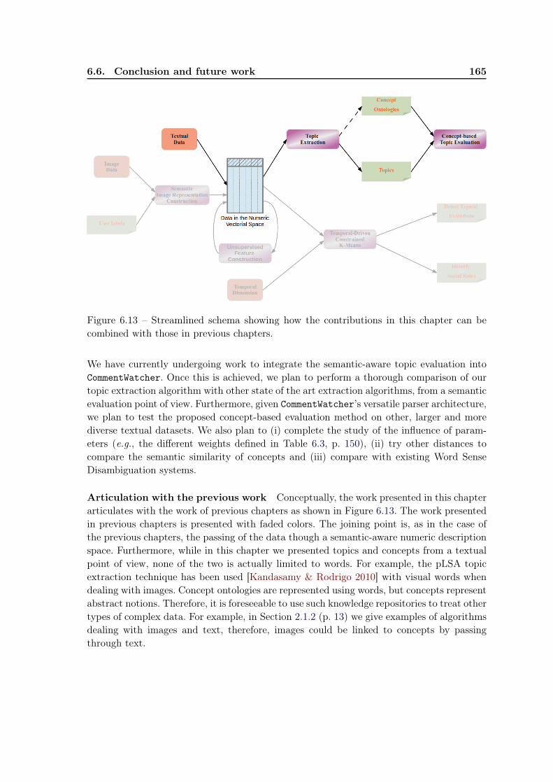
6.6. Conclusion and future work 165
Figure 6.13 – Streamlined schema showing how the contributions in this chapter can becombined with those in previous chapters.
We have currently undergoing work to integrate the semantic-aware topic evaluation intoCommentWatcher. Once this is achieved, we plan to perform a thorough comparison of ourtopic extraction algorithm with other state of the art extraction algorithms, from a semanticevaluation point of view. Furthermore, given CommentWatcher’s versatile parser architecture,we plan to test the proposed concept-based evaluation method on other, larger and morediverse textual datasets. We also plan to (i) complete the study of the influence of param-eters (e.g., the different weights defined in Table 6.3, p. 150), (ii) try other distances tocompare the semantic similarity of concepts and (iii) compare with existing Word SenseDisambiguation systems.
Articulation with the previous work Conceptually, the work presented in this chapterarticulates with the work of previous chapters as shown in Figure 6.13. The work presentedin previous chapters is presented with faded colors. The joining point is, as in the case ofthe previous chapters, the passing of the data though a semantic-aware numeric descriptionspace. Furthermore, while in this chapter we presented topics and concepts from a textualpoint of view, none of the two is actually limited to words. For example, the pLSA topicextraction technique has been used [Kandasamy & Rodrigo 2010] with visual words whendealing with images. Concept ontologies are represented using words, but concepts representabstract notions. Therefore, it is foreseeable to use such knowledge repositories to treat othertypes of complex data. For example, in Section 2.1.2 (p. 13) we give examples of algorithmsdealing with images and text, therefore, images could be linked to concepts by passingthrough text.

Chapter 7
Produced Prototypes and Software
Contents7.1 Introduction . . . . . . . . . . . . . . . . . . . . . . . . . . . . . . . . 1677.2 Discussion Forums . . . . . . . . . . . . . . . . . . . . . . . . . . . . . 169
7.2.1 Current limitations . . . . . . . . . . . . . . . . . . . . . . . . . . . . . 1697.2.2 Related works . . . . . . . . . . . . . . . . . . . . . . . . . . . . . . . . 1707.2.3 Introducing CommentWatcher . . . . . . . . . . . . . . . . . . . . . . 171
7.3 Platform Design . . . . . . . . . . . . . . . . . . . . . . . . . . . . . . 1717.3.1 Software technologies . . . . . . . . . . . . . . . . . . . . . . . . . . . 1717.3.2 Platform architecture . . . . . . . . . . . . . . . . . . . . . . . . . . . 1717.3.3 The fetching module . . . . . . . . . . . . . . . . . . . . . . . . . . . . 1727.3.4 Topic extraction and textual classification . . . . . . . . . . . . . . . . 1737.3.5 Visualization . . . . . . . . . . . . . . . . . . . . . . . . . . . . . . . . 173
7.4 License and source code . . . . . . . . . . . . . . . . . . . . . . . . . 1757.5 Conclusion and future work . . . . . . . . . . . . . . . . . . . . . . . 175
7.1 Introduction
As previously hinted, my theoretical research work was constantly doubled by an appliedresearch work. Scripts were developed for the experimental part of each of the approachespresented in previous chapters. These are usually just proofs-of-concept, written in scriptinglanguages (like Octave 1). CommentWatcher, the most prominent produced software and theone presented in this chapter, is an open source tool aimed at analyzing discussions on webforums. Constructed as a web platform, CommentWatcher features automatic fetching of theforums using a versatile parser architecture, topic extraction from a selection of texts anda temporal visualization of extracted topics and the underlying social network of users. Itis aimed at both the media watchers (it allows quick identification of important subjects inthe forums and user interest) and the researches in social media (who can use to constitutetemporal textual datasets). CommentWatcher is currently used in the Crtt-Eric researchproject to study the evolution of specialized discourse in the domain of nuclear medicine,while taking into account the temporal evolution and the different involved populations(e.g., doctors, nurses, patients). It is also planned to be used to construct a dataset forstudying the detection of behavioral roles by using temporal-driven constrained clustering(as seen in Section 3.6 (p. 52)).
1. http://www.gnu.org/software/octave/
168 Chapter 7. Produced Prototypes and Software
Features of CommentWatcher CommentWatcher answers to a series of limitations con-cerning online forum discussions (some of which are detailed in Section 7.2): (a) concerningdiscussion forum benchmark datasets and (b) concerning existing software solutions. (a)We identify the following limitations concerning discussion forum benchmark datasets: (i)scarcity of forum benchmarks, (ii) the existing forum benchmarks are issued from a singleforum website, therefore, it is not possible to study inter-website user behavior, (iii) thestructure of forum websites is continuously changing, rendering forum parsers useless and(iv) the copyright of forum data is unclear, therefore hindering the sharing in the researchcommunity. (b) The limitations concerning existing software solutions are that (i) they areproprietary solutions, unusable for research purposes and (ii) they do not deal with crawlingthe forum sources and need to be supplied directly with formatted data.
CommentWatcher addresses these limitations by featuring a modular parser architecture,capable of handling the ever-changing structure of websites. Furthermore, it is open source,meaning that it can be freely distributed. It can be used to solve the problem of contentcopyright, since only the tool is distributed and the forum benchmark can be easily recon-structed locally by each researcher. To our knowledge, CommentWatcher is the only solutiondedicated to online discussion forums that integrates (a) forum parsing, (b) topic extractionand visualization and (c) online social network inference and visualization.
Experimenting with CommentWatcher A public demo installation of CommentWatcher isavailable 2. The reader is able to interact with CommentWatcher in a normal browser window,through the tools web interface. The tool itself is hosted and executed on its dedicatedmachine, located at the ERIC laboratory. The reader can, first-hand, experience the toolscapabilities by (a) seeing how multiple discussion forums can be fetched by searching the webusing keywords, (b) applying topics extraction algorithms and tweaking their parameters,(c) visualizing the extracted topic as a expression cloud and their temporal evolution and(d) visualizing the social network constructed starting from the initial forums. A shortpresentation movie is also available 3, showing the main features of CommentWatcher.
CommentWatcher’s history The platform evolved from a simple prototype into a fully-fledged academic software, due to the needs and purposes of the different research projects(detailed in Appendix A) in which I was involved. It started in the context of the appliedresearch project Conversession, in which the creation of a start-up enterprise 4 was in-volved. The purpose of the project was Online Media Watching, and more precisely focusedon news discussion forums. The resulted prototype is called Discussion Analysis 5, a Javadesktop application that features (i) fetching of discussion forums from 2 French websites(www.liberation.fr and www.rue89.fr) and 2 English sites (www.huffingtonpost.comand forums.sun.com), (ii) textual preprocessing (as shown in Section 6.2.1 (p. 128)) and(iii) topic extraction using the system described in Section 6.4.1 (p. 141). The develop-ment of the prototype was continued in the context of projects Eric-Elico, Crtt-Ericand ImagiWeb. The interest for each of these projects was to constitute discussion forum
2. Online here: http://mediamining.univ-lyon2.fr:8080/CommentWatcher/3. Presentation website: http://mediamining.univ-lyon2.fr/commentwatcher4. http://www.conversationnel.fr/5. Download here: http://mediamining.univ-lyon2.fr/rizoiu/files/discussion-analysis.jar
7.2. Discussion Forums 169
datasets and to analyze the discussion topics. The platform evolved accordingly. The in-terface was migrated to a web-based interface to allow simultaneous work of multiple usersand a unified discussion database. A new discussion forum fetching module, described inSection 7.3.3 was implemented, which eliminates the dependency of the code base on thewebsite structure. Support for new topic extraction algorithms (details in Section 7.3.4) wasadded. The visualization module (described in Section 7.3.5) was added for temporal topicvisualization and social network visualization. The development of the platform continuesat this date: a force-directed graph drawing is being implemented, as well as a temporaltopic model system.
Planning of the chapter The remainder of this chapter is structured as follows. InSection 7.2, we present an overview of applied discussion forum analysis: the current lim-itations, some of the solutions existing in the literature and an overview of our proposedapproach. In Section 7.3, we present the general design and detail the different componentsof CommentWatcher. Section 7.4 gives the license under which CommentWatcher is releasedand describes how to obtain the software. We conclude in Section 7.5 and we present thework we are currently undertaking, and we plan future developments.
7.2 Discussion Forums
CommentWatcher’s vocation is to analyze online discussions. The Web 2.0 has changedthe way users discuss with other users. One of the preferred online discussion environmentsare the web forums. Users can react, post their opinions, discuss and debate any kindof subjects. The forums are usually thematic (e.g. Java programming forums 6) and newusers have access to the past discussion (e.g. solutions posted by other users to a specificproblem). Therefore the users become full collaborative participants in the informationcreation process. The subjects of discussion between readers are very dynamic and theoverall sum of reactions gives a snapshot of the general trends that emerge in the userpopulation. At the same time, the way users reply one to another suggests an underlyingsocial network structure. The forum’s “reply-to” structural relations can be used to addlinks between users. Other types of relations can be added, like the name and textualcitations [Forestier et al. 2011]. Furthermore, based on such social networks constructedfrom web forums, adapted graph measures can be used to detect user social roles [Anokhinet al. 2012]. In Section 3.6 (p. 52), we have shown how a temporal-driven constrainedclustering technique, that we proposed in Section 3.4 (p. 34), can be applied to detectbehavioral roles in such a social network constructed from web forums.
7.2.1 Current limitations
These forum data are still ill explored, even if they represent an important source ofknowledge. News articles analysis and micro blogging (e.g. Twitter) analysis receive a lot ofattention from the community. There are available tools that perform the analysis of newsmedia [Amer-Yahia et al. 2012], but without treating the social network aspect. Other tools
6. http://www.javaprogrammingforums.com/
170 Chapter 7. Produced Prototypes and Software
concentrate on analyzing and visualizing the social dynamics [Guille et al. 2013] or detectevents [Marcus et al. 2011] based on twitter data. To the best of our knowledge, there areno publicly available tools that treat forums, while inferring a social network structure.
Another limitation concerns the forum benchmarks. There are a multitude of generalpurpose information retrieval datasets (e.g. the ClueWeb12 dataset 7 of project Lemure)and of Twitter datasets (e.g. the infochimps collections 8). But dedicated web forumbenchmark datasets are scarce. Those that exist are usually issued from a single forum web-site (e.g. the boards.ie Forums Dataset 9 based on boards.ie website or the Ancestry.comForum Dataset 10, based on ancestry.com website). This is due to the diverse and everchanging structure of the websites hosting the discussions and copyright problems. Eachhost website has its own license on the user-produced data, which is not always clearlystipulated. This leads researchers to develop their own house-bred parsers and create theirown datasets. These datasets are rarely shared with the community, which poses problemswhen testing new proposals and comparing to existing approaches.
7.2.2 Related works
Several tools intending to extract knowledge from on-line discussions have been proposedin the recent years.
MAQSA [Amer-Yahia et al. 2012] is a system for social analytics on news that allows itsusers to define their own topic of interest, in order to gather related articles, identify relatedtopics, and extract the time-line and network of comments that show who commented whicharticle and when.
Eddi [Bernstein et al. 2010] offers visualizations such as time-lines and tag clouds oftopics extracted from tweets using a simple topic detection algorithm that uses a searchengine as an external knowledge base.
OpinionCrawl 11 is an on-line service that crawls various web-sources – such as blogs,news, forums and Twitter – searching for a user-defined topic and then presents key conceptsas a tag cloud, provides a visualization of the temporal dynamics of the topic and performsa sentiment analysis.
SONDY [Guille et al. 2013] is an open-source plateform for analyzing on-line social net-work data. It features a data import and pre-processing service, a topic detection and trendsanalysis service, as well as a service for the interactive exploration of the corresponding net-works (i.e., active authors for the considered topic(s)).
The aforementioned tools are limited for various reasons. They are either propri-etary softwares and thus can’t be extended for scientific purposes or can’t directly crawlweb sources and can only be used to analyze formatted datasets provided by the user.CommentWatcher intends to provide researchers with an open-source extendable tool thatpermits to crawl the web and build datasets that suit their needs.
7. http://lemurproject.org/clueweb12/specs.php8. http://www.infochimps.com/collections/twitter-census9. http://www.icwsm.org/2012/submitting/datasets/
10. http://www.cs.cmu.edu/~jelsas/data/ancestry.com/11. http://opinioncrawl.com
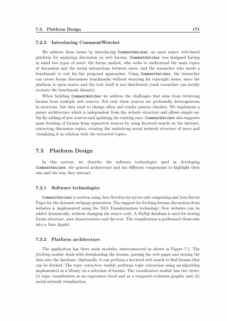
7.3. Platform Design 171
7.2.3 Introducing CommentWatcher
We address these issues by introducing CommentWatcher, an open source web-basedplatform for analyzing discussion on web forums. CommentWatcher was designed havingin mind two types of users: the forum analyst, who seeks to understand the main topicsof discussion and the social interactions between users, and the researcher who needs abenchmark to test his/her proposed approaches. Using CommentWatcher, the researchercan create forum discussions benchmarks without worrying for copyright issues, since theplatform is open source and the text itself is not distributed (each researcher can locallyrecreate the benchmark dataset).
When building CommentWatcher we address the challenges that arise from retrievingforums from multiple web sources. Not only these sources are profoundly heterogeneousin structure, but they tend to change often and render parsers obsolete. We implement aparser architecture which is independent from the website structure and allows simple on-the-fly adding of new sources and updating the existing ones. CommentWatcher also supportsmass fetching of forums from supported sources by using keyword search on the internet,extracting discussion topics, creating the underlying social network structure of users andvisualizing it in relation with the extracted topics.
7.3 Platform Design
In this section, we describe the software technologies used in developingCommentWatcher, the general architecture and the different components to highlight theiraim and the way they interact.
7.3.1 Software technologies
CommentWatcher is written using Java Servlets for server-side computing and Java ServerPages for the dynamic webpage generation. The support for fetching forums discussions fromwebsites is implemented using the XLS Transformation technology. New websites can beadded dynamically, without changing the source code. A MySql database is used for storingforum structure, user characteristics and the text. The visualization is performed client-sideinto a Java Applet.
7.3.2 Platform architecture
The application has three main modules, interconnected as shown in Figure 7.1. Thefetching module deals with downloading the forums, parsing the web pages and storing thedata into the database. Optionally, it can perform a keyword web search to find forums thatcan be fetched. The topic extraction module performs topic extraction using an algorithmimplemented as a library on a selection of forums. The visualization module has two views:(i) topic visualization as an expression cloud and as a temporal evolution graphic and (ii)social network visualization.
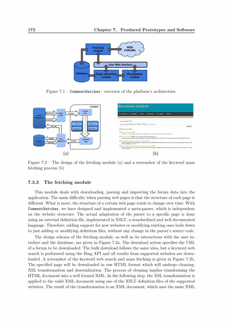
172 Chapter 7. Produced Prototypes and Software
Fetching module
Database
User Web Interface
Topic extraction module
WEB FORUMS
Visualization module
Figure 7.1 – CommentWatcher: overview of the platform’s architecture.
Chapter 2
Preprocessing articles and messages
2.1 Task Description
The task of the first team was to retrieve certain data (content, title, date, author etc.) of the website articles,as well as the data associated to comments to this articles. As a source of articles four different French websiteswere used, namely Liberation, LeMonde, LeFigaro and Rue89. All the retrieved data was to be cleaned andsaved in a database and provided further on to the other teams in order for them to achieve their tasks.
Typically an Internet discussion has a web page containing an article and additional web pages with com-ments. The challenge of our task is to gather data scattered around these several web pages. We had to developa mechanism of parsing HTML pages and extracting the data of our interest. The complication is that the websites have different layouts, and thus, we need to work with each web site separately. At the same time, it ispreferable to develop a mechanism that would allow adding new websites on the fly (i.e. without recompilingand redeploying the system).
2.2 Solution
For a similar task, one of the members of ERIC laboratory developed a website using Java Server Pages (JSP)technology. We worked on improving this existing website so that it could satisfy our requirements. Theweb application itself consists of three main parts, the user interface (JSP pages), the data gathering part(implemented as Java server code) and the data storage (MySQL database) as shown on the figure 2.1.
X
S
L
T
r
a
n
s
f
o
r
m
Storing
Retrieving
Bulk Download
Reading
Cleaning
VALID
XML
USER
INTERFACE
rue89.xsl
lemonde.xsl liberation.xsl
lefigaro.xsl
Showing
HTML
PAGE
UNIFIED
XML
JAVA
OBJECTS DATA
Download
Figure 2.1: Solution architecture diagram.
The user interface consists of the set of JSP pages (Discussion List, Classification, Xml Files, List of Feeds,List of Articles, Statistics). For a more detailed description of the UI see section 2.2.1.
6
(a) (b)
Figure 7.2 – The design of the fetching module (a) and a screenshot of the keyword massfetching process (b)
7.3.3 The fetching module
This module deals with downloading, parsing and importing the forum data into theapplication. The main difficulty when parsing web pages is that the structure of each page isdifferent. What is more, the structure of a certain web page tends to change over time. WithCommentWatcher, we have designed and implemented a meta-parser, which is independenton the website structure. The actual adaptation of the parser to a specific page is doneusing an external definition file, implemented in XSLT, a standardized and well documentedlanguage. Therefore, adding support for new websites or modifying existing ones boils downto just adding or modifying definition files, without any change in the parser’s source code.
The design schema of the fetching module, as well as its interactions with the user in-terface and the database, are given in Figure 7.2a. The download action specifies the URLof a forum to be downloaded. The bulk download follows the same idea, but a keyword websearch is performed using the Bing API and all results from supported websites are down-loaded. A screenshot of the keyword web search and mass fetching is given in Figure 7.2b.The specified page will be downloaded in raw HTML format which will undergo cleaning,XSL transformation and deserialization. The process of cleaning implies transforming theHTML document into a well formed XML. In the following step, the XSL transformation isapplied to the valid XML document using one of the XSLT definition files of the supportedwebsites. The result of the transformation is an XML document, which uses the same XML
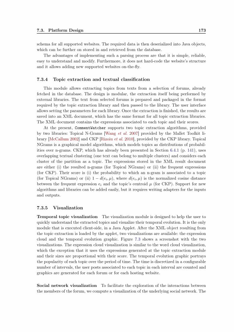
7.3. Platform Design 173
schema for all supported websites. The required data is then deserialized into Java objects,which can be further on stored in and retrieved from the database.
The advantages of implementing such a parsing process are that it is simple, reliable,easy to understand and modify. Furthermore, it does not hard-code the website’s structureand it allows adding new supported websites on-the-fly.
7.3.4 Topic extraction and textual classification
This module allows extracting topics from texts from a selection of forums, alreadyfetched in the database. The design is modular, the extraction itself being performed byexternal libraries. The text from selected forums is prepared and packaged in the formatrequired by the topic extraction library and then passed to the library. The user interfaceallows setting the parameters for each library. Once the extraction is finished, the results aresaved into an XML document, which has the same format for all topic extraction libraries.The XML document contains the expressions associated to each topic and their scores.
At the present, CommentWatcher supports two topic extraction algorithms, providedby two libraries: Topical N-Grams [Wang et al. 2007] provided by the Mallet Toolkit li-brary [McCallum 2002] and CKP [Rizoiu et al. 2010], provided by the CKP library. TopicalNGrams is a graphical model algorithms, which models topics as distributions of probabil-ities over n-grams. CKP, which has already been presented in Section 6.4.1 (p. 141), usesoverlapping textual clustering (one text can belong to multiple clusters) and considers eachcluster of the partition as a topic. The expressions stored in the XML result documentare either (i) the resulted n-grams (for Topical NGrams) or (ii) the frequent expressions(for CKP). Their score is (i) the probability to which an n-gram is associated to a topic(for Topical NGrams) or (ii) 1 − d(ei, µ), where d(ei, µ) is the normalized cosine distancebetween the frequent expression ei and the topic’s centroid µ (for CKP). Support for newalgorithms and libraries can be added easily, but it requires writing adapters for the inputsand outputs.
7.3.5 Visualization
Temporal topic visualization The visualization module is designed to help the user toquickly understand the extracted topics and visualize their temporal evolution. It is the onlymodule that is executed client-side, in a Java Applet. After the XML object resulting fromthe topic extraction is loaded by the applet, two visualizations are available: the expressioncloud and the temporal evolution graphic. Figure 7.3 shows a screenshot with the twovisualizations. The expression cloud visualization is similar to the word cloud visualization,which the exception that it uses the expressions generated at the topic extraction moduleand their sizes are proportional with their score. The temporal evolution graphic portraysthe popularity of each topic over the period of time. The time is discretized in a configurablenumber of intervals, the user posts associated to each topic in each interval are counted andgraphics are generated for each forum or for each hosting website.
Social network visualization To facilitate the exploration of the interactions betweenthe members of the forum, we compute a visualization of the underlying social network. The
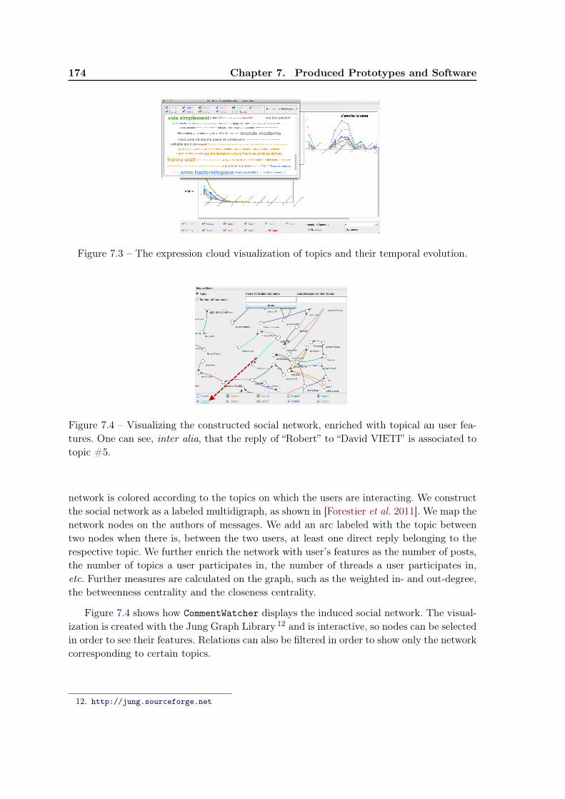
174 Chapter 7. Produced Prototypes and Software
Figure 7.3 – The expression cloud visualization of topics and their temporal evolution.
Figure 7.4 – Visualizing the constructed social network, enriched with topical an user fea-tures. One can see, inter alia, that the reply of “Robert” to “David VIETI” is associated totopic #5.
network is colored according to the topics on which the users are interacting. We constructthe social network as a labeled multidigraph, as shown in [Forestier et al. 2011]. We map thenetwork nodes on the authors of messages. We add an arc labeled with the topic betweentwo nodes when there is, between the two users, at least one direct reply belonging to therespective topic. We further enrich the network with user’s features as the number of posts,the number of topics a user participates in, the number of threads a user participates in,etc. Further measures are calculated on the graph, such as the weighted in- and out-degree,the betweenness centrality and the closeness centrality.
Figure 7.4 shows how CommentWatcher displays the induced social network. The visual-ization is created with the Jung Graph Library 12 and is interactive, so nodes can be selectedin order to see their features. Relations can also be filtered in order to show only the networkcorresponding to certain topics.
12. http://jung.sourceforge.net
7.4. License and source code 175
7.4 License and source code
CommentWatcher is released under the opensource license GNU General Public Li-cense version 3 (GNU GPL v3) 13. The individual topic extraction and textual cluster-ing software packages are the objects of their respective licenses. The present versionof CommentWatcher comes with two Natural Language Processing toolkits: the MalletToolkit [McCallum 2002] v2.0.7, released under the open source Common Public License,and CKP [Rizoiu et al. 2010] v0.2, released under the GNU GPL v3. The install files andthe source code of CommentWatcher is available through a public Mercurial repository 14.
7.5 Conclusion and future work
Conclusion This chapter presented CommentWatcher, an open source web-based platformfor analyzing discussions on web forums. Our tool is designed for both end-users, as well asfor researchers. End-users have at their disposal an easy to use, integrated tool that allowsretrieving forum discussion from multiple websites, performs topic extraction to identifythe main discussion topics and provides an expression cloud visualization to identify themost important expressions associated to each topic. The temporal popularity of topicscan be evaluated using an evolution graphic. CommentWatcher also features extracting theunderlying social network by using the direct citation links between users. The visualizationof the social network is interactive, features of nodes can be visualized and relations canbe filtered to show only the network corresponding to a certain topic. For researchers,CommentWatcher tackles the problem of creating multi source web forum datasets, thanksto its versatile parser which is independent of the structure of webpages. Support for newwebsites can be added on-the-fly. It can also solve the problem of copyright when sharingforum datasets, since no text is distributed and each researcher can easily recreate thedataset.
Current and future development With the beginning of the Crtt-Eric project,CommentWatcher has officially become one of the academic software supported by the DMD(Data Mining and Decision) team of the ERIC laboratory. It is currently the center pointof multiple student research and development internships and has recently acquired a dedi-cated machine. The objects of the ongoing development are (i) a better plotting of the socialnetwork, by using force-directed graph drawing, (ii) integrating a temporal topic model al-gorithm and (iii) importing external data into the discussion database, in order to be ableto treat other types of discussions (e.g., chat discussions). As future work, we intend toadd a credential mechanism and transform CommentWatcher into a multiuser tool and weconsider implementing a topic evaluation based on ontologies of concepts, as presented inSection 6.4.2 (p. 148).
13. http://www.gnu.org/licenses/14. http://eric.univ-lyon2.fr/~commentwatcher/cgi-bin/CommentWatcher.cgi/CommentWatcher/

Chapter 8
Conclusion and Perspectives
Contents8.1 Thesis outline . . . . . . . . . . . . . . . . . . . . . . . . . . . . . . . . 1778.2 Original contributions . . . . . . . . . . . . . . . . . . . . . . . . . . . 1798.3 General conclusions . . . . . . . . . . . . . . . . . . . . . . . . . . . . 1808.4 Current and Future work . . . . . . . . . . . . . . . . . . . . . . . . . 182
8.4.1 Current work . . . . . . . . . . . . . . . . . . . . . . . . . . . . . . . . 1838.4.2 Future work . . . . . . . . . . . . . . . . . . . . . . . . . . . . . . . . . 184
This final chapter of my thesis is dedicated to drawing some general conclusions, brieflypresenting the current work and outlining directions for future work. This chapter is struc-tured into four parts: summary of the work, original ideas, conclusions, and outline of futurework. In Section 8.1 we present, for each chapter, an outline of the original contributionsand their positioning relative to existing methods. The three most important original ideasin our work are singled out in Section 8.2 and shown in the context of the publications theygenerated. The conclusions follow in Section 8.3 and present a meta-view of our work, under-lining how the directive guidelines manifested in our work, the different transverse links thatappear between the different parts and their conceptual articulation. Finally, Section 8.4closes the chapter by detailing the ongoing work as well as the planned extensions of theresearch presented in this thesis.
8.1 Thesis outline
The purpose of this section is to present an overview of the work presented in this thesisand, most notably, to position our contributions relative to the current state of the art. Italso follows the logical flow of ideas throughout our work and creates a summary of thetasks and accomplishments.
All the work presented in this thesis lies at the intersection of Complex Data Analysisand Semi-Supervised Clustering. More specifically, we address two research challenges:(i) embedding semantics into data representation and machine learning algorithms and (ii)leveraging the temporal dimension. We investigate on how data of different natures can beanalyzed, while considering the temporal dimension and the additional information that maycome with the data. Given the great heterogeneity of complex data (e.g., different natures,temporal dimension) our work touches to many different aspects of Machine Learning. Ourresearch ranges from introducing partial supervision into clustering, to using ontologies fortopic evaluation and to extracting visual features from images. After a chapter in which wepresent an overview of the domain, we present our original research in four chapters, (a) one
178 Chapter 8. Conclusion and Perspectives
for the temporal dimension, (b) a second one dedicated to reconstructing a feature set, withdirect application in re-organizing user-supplied additional information under the form oflabels, and the last two of them corresponding to the considered natures of complex data( (c) text and (d) images). A fifth chapter is dedicated to CommentWatcher, an academicsoftware, result of the applied research and in close connection with the work on the textualdimension. Given the great diversity of the approached subjects, each chapter containsdedicated sections presenting the related work in the given field, the proposed contributionsand partial conclusions. Therefore, each of the five chapters can be seen as autonomous,while remaining connected by the general research topics and the transverse links betweenthem (some detailed in Section 8.3).
Chapter 1 starts by positioning our work and presenting the general context of thethesis. It is followed, in Chapter 2, by an overview of the two domains around which ourwork revolves: Complex Data Analysis and Semi-Supervised Clustering.
Chapter 3 addresses the task of leveraging the temporal dimension of complex data intoclustering. Relative to existing methods, the work proposed in this chapter introduces (a) anew temporal-aware dissimilarity measure, which combines the descriptive dimension withthe temporal dimension and allows the fine-tuning of their ratio; (b) a new penalty function,calculated using a function inspired from the Normal Distribution function, to ensure acontiguous segmentation of the observations belonging to an entity. Unlike existing solutions,which are basically a threshold function, our proposal inflict a high penalty for breakingthe constraints for observations close in time and a low penalty for distant observations; (c)a novel time-driven constrained clustering algorithm, called TDCK-Means, which createsa partition of coherent clusters, both in the multidimensional space and in the temporalspace; (d) a new measure (ShaP), to evaluate the contiguity of the segmentation of theseries of observations belonging to an entity and (e) a new method to infer social roles ina social network as a mixture of temporal behavioral roles. As far as we know, this is thefirst proposal to infer the social roles as a succession of temporal states, previous solutionsconcentrate on calculating a set of measures on the network’s graph.
Chapter 4 regroups our research concerning the task of semantic data representationreconstruction. In this chapter we address the problem of improving representation spaceof the data by using the underlying semantics of the dataset. Relative to existing meth-ods, the work proposed in this chapter introduces (a) two algorithms that construct thenew features as conjunctions of the initial features and their negations. The constructedfeatures are more appropriate for describing the dataset and, at the same time, are com-prehensible for a human user. The methods present so far in the literature either constructnon-comprehensible features (e.g., PCA, the kernel of SVM) or construct comprehensiblefeatures in a supervised way. As far as we know, this is the first solution for an unsuper-vised construction of comprehensible features. We also propose (b) a measure to quantifythe total co-occurrence of a feature set; (c) a method, based on statistical testing, for settingthe value of parameters; (d) a method, based on statistical considerations, for pruning thecandidate pairs of correlated features.
Chapter 5 presents our research concerning image data, and more specifically the taskof improving image representation using semi-supervised visual vocabulary construction. Weare interested in using expert knowledge, under the form of non-positional labels attachedto the images, in the process of creating the image numerical representation. Relative to
8.2. Original contributions 179
existing methods, the work proposed in this chapter introduces (a) a method for constructinga dedicated visual vocabulary starting from features sampled only from a subset of labeledimages. This ensures that the generated visual vocabulary has words adapted to describingeach of the objects appearing in the image collection; (b) a novel method for filtering featuresirrelevant to a given object, using non-positional labels. We show that that filtering approachconsistently improves the accuracy of a content-based image classification task.
Chapter 6 presents in detail our research concerning textual data, and more precisely,we interest in the task of topic extraction and evaluation. We make an in-depth review oftopic extraction and evaluation literature, while referencing methods related to our gen-eral domain of interest (e.g., incorporating the temporal dimension or external semanticknowledge). Relative to existing methods, the work proposed in this chapter introduces (a)a textual clustering-based topic extraction system; (b) a topic evaluation system. Most ofthe solutions present in the literature use statistical measures (e.g., the perplexity) to assesthe fitness of topics. Our solution uses an external semantic resource, such as WordNet, toevaluate the semantic cohesion of topics.
Chapter 7 presents the practical prototype production, most notably CommentWatcher,an open source tool for analyzing discussions on web forums. Most of the solutions presentin literature have the inconvenience of being either (a) proprietary (i.e., cannot be usedin scientific purposes) or (b) unable to crawl web sources and can be only used to ana-lyze formatted datasets provided by the user. CommentWatcher has the advantage of beingconstructed as a web platform, giving the possibility of being used collaboratively. It also al-lows to by-pass the problem of copyright issues: the platform is open-source and the forumbenchmark needs not to the distributed (each researcher can locally recreate the bench-mark). CommentWatcher features (i) automatic fetching of forums, using a versatile parserarchitecture, (ii) topic extraction from a selection of texts and (iii) a temporal visualizationof extracted topics and the underlying social network of users.
8.2 Original contributions
We summarize our work by presenting three of the most important ideas of our research.Most of the original proposals presented in this thesis are related to these ideas:
– taking into account both the temporal dimension and the descriptive dimension into aclustering framework (in Chapter 3). The resulted clusters are coherent from both thetemporal and the descriptive point of view. Constraints are added to ensure the entitysegmentation contiguity. This idea is presented in a paper in the proceedings of theInternational Conference on Tools with Artificial Intelligence (ICTAI ’12),paper which won the best student paper award [Rizoiu et al. 2012];
– unsupervised construction of a feature set based on the co-occurrences issued from thedataset (in Chapter 4). This allows adapting a feature set to the dataset’s semantics.The new features are constructed as conjunctions of the initial features and their nega-tions, which renders the result comprehensible for the human reader. This idea waspublished in an article with the international Journal of Intelligent InformationSystems (JIIS) [Rizoiu et al. 2013a];
– using non-positional user labels (denoting objects) to filter irrelevant visual features
180 Chapter 8. Conclusion and Perspectives
and to construct a semantically aware visual vocabulary for a “bag-of-feature” imagerepresentation (in Chapter 5). Even if the position of objects is unknown, we use theinformation about the presence of objects in images to detect and remove featuresunlikely to belong to the given object. Dedicated visual vocabularies are constructed,resulting in a numerical description which yields higher object categorization accuracy.This idea is presented in an article under review with the International Journal ofArtificial Intelligence Tools (IJAIT) [Rizoiu et al. 2013b].
Throughout this manuscript, multiple contributions were proposed, some of which areissued from the major ideas presented before. Others are related to the textual natureof complex data and the prototype production, and were published in the proceedings ofthe International Joint Conference on Artificial Intelligence (IJCAI ’11) [Musatet al. 2011b], the International Symposium on Methodologies for Intelligent Sys-tems (ISMIS ’11) [Musat et al. 2011a], the French national conference Extraction etGestion des Connaissances (EGC ’10) [Rizoiu et al. 2010] and a chapter in the bookOntology Learning and Knowledge Discovery Using the Web: Challenges andRecent Advances [Rizoiu & Velcin 2011]. A complete list of the publications issued fromthe research presented in this thesis can be found in Annex B.
8.3 General conclusions
There are two main research challenges that our work addresses: (i) embedding semanticsinto data representation and machine learning algorithms and (ii) leveraging the temporaldimension. The two challenges are linked to (a) the applications concerning the structuringof the immense quantities of complex data produced by the Web 2.0 and (b) the embeddingof semantics into webpages, which is the object of the Semantic Web. The general context mythesis lies at the intersection of Complex Data Analysis and Semi-Supervised Clus-tering. In our work concerning the semantic representation, we concentrate on leveragingadditional external information, under the form of expert-provided information (e.g., imagelabels in Chapter 5) and external semantic resources (e.g., concept ontologies in Chapter 6),while our work concerning the temporal dimension of data is presented in Chapter 3.
As mentioned earlier, our work is composed of four distinct, yet complementary parts.The four parts deal, respectively, with (a) the temporal dimension, (b) semantic data repre-sentation and the different natures of complex data, i.e., (c) image and (d) text. Each partis dealt with in an individual chapter, which contains an overview of the state of the art ofthe domain, the proposals, conclusions about the work and some plans for future work. Afifth chapter is dedicated to the my applied work. Therefore, each of the five chapters canbe seen as autonomous, while remaining connected the directive guidelines, the trans-verse links between them and the conceptual articulation. We detail in the followingparagraphs how each of the above were taken into account in our work.
Directive guidelines While the different aspects of our work are distinct, they are notindependent one from the other. Each deals with the different particularities of complexdata, while respecting the same directive guidelines: (i) human comprehension, (ii) trans-lating data of different natures into a semantic-aware description space and (iii) devising
8.3. General conclusions 181
algorithms and methods that embed semantics and the temporal component.We consider crucial to generate human comprehensible outputs and we have stressed
this aspect all along this thesis. Our proposal for feature construction, in Chapter 4, waspartly motivated by this need. Black-box approaches (i.e., the feature extraction and thefeature selection algorithms presented in Section 4.2, p. 63) exist and they can achieve wellthe reduction of co-occurrences in the feature set. But the new features are completely syn-thetic and make results difficult to interpret. Human comprehension is also central for topiclabeling, presented in Chapter 6. We argue that a complete expression is more meaningfulfor a human being than a probability distribution over words. Similarly, when generatingthe typical evolution phases in Chapter 3, human comprehension motivates the choice tosegment contiguously the observations corresponding to an entity.
As shown in Section 2.1 (p. 9), some of today’s challenges concerning complex data lie in(a) rendering the data into a common usable numeric format, which succeeds in capturingthe information present in the native format, and in (b) efficiently using external informa-tion for improving the numeric representation. The second directive guideline throughoutour work is translating data of different natures into a semantic-aware descriptionspace, which we call the Numeric Vectorial Space. Our work concerning images in Chap-ter 5 is specifically targeted at embedding semantic information in the image numericaldescription. Section 6.2 (p. 128) in Chapter 6 is dedicated to translating textual data intothe “bag-of-words” numerical representation. Finally, the purpose of the feature constructionalgorithm in Chapter 4 is to improve the representation of data, by adapting the featuresto the dataset they describe.
Finally, a central axis of our research is devising algorithms and methods thatembed semantics and the temporal component, based on unsupervised and semi-supervised techniques. Often additional information and knowledge is attached to the data,under the form of (a) user labels, (b) structure of interconnected documents or (c) exter-nal knowledge bases. We use this additional knowledge at multiple instances, usually usingsemi-supervised clustering techniques. We use such an approach when constructing a seman-tically improved image numeric representation, in Chapter 5. Dedicated visual vocabulariesare constructed starting from the provided labeled subset of images. But the entire im-age collection (labeled and unlabeled) is used to generate the actual image representation.Furthermore, our work with the text also deals with leveraging external semantic knowl-edge into the topic evaluation process. Similarly, in Chapter 3, we use semi-supervised softpair-wise constraints to model the temporal dependencies in the data.
Transverse links There are multiple transverse links between the different parts ofour work. (a) The feature construction algorithm, uFC, was initially motivated by theneed to re-organize the user user label set we use to create the semantic-enabled imagerepresentation. In Section 5.5 (p. 121), we discuss how the proposed semantic visual vocab-ulary construction can be adapted to scene classification (where the main problem is labelco-occurrence) by using the proposed feature construction algorithm. (b) Our work withtextual data is intimately linked with the software CommentWatcher. The text from onlinediscussion forums is retrieved, we extract topics from it and infer a social network using theforum’s reply-to relation. The social network is modeled and visualized as a multidigraph,in which links between nodes are associated to topics. (c) Furthermore, the temporal-driven
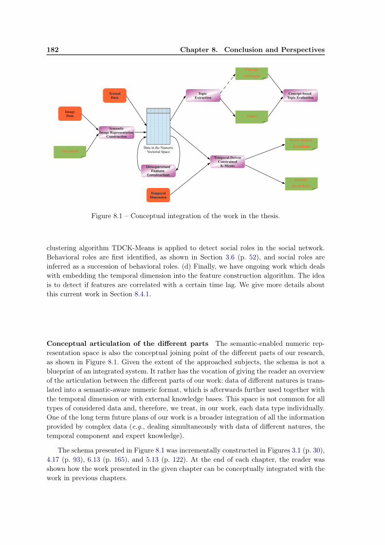
182 Chapter 8. Conclusion and Perspectives
Temporal-DrivenConstrained
K-Means
Detect Typical
Evolutions
Identify
Social Roles
TemporalDimension
UnsupervisedFeature
Construction
Topic Extraction
Concept-based Topic Evaluation
Concept
Ontologies
Topics
TextualData
Data in the Numeric Vectorial Space
SemanticImage Representation
Construction
User labels
ImageData
Figure 8.1 – Conceptual integration of the work in the thesis.
clustering algorithm TDCK-Means is applied to detect social roles in the social network.Behavioral roles are first identified, as shown in Section 3.6 (p. 52), and social roles areinferred as a succession of behavioral roles. (d) Finally, we have ongoing work which dealswith embedding the temporal dimension into the feature construction algorithm. The ideais to detect if features are correlated with a certain time lag. We give more details aboutthis current work in Section 8.4.1.
Conceptual articulation of the different parts The semantic-enabled numeric rep-resentation space is also the conceptual joining point of the different parts of our research,as shown in Figure 8.1. Given the extent of the approached subjects, the schema is not ablueprint of an integrated system. It rather has the vocation of giving the reader an overviewof the articulation between the different parts of our work: data of different natures is trans-lated into a semantic-aware numeric format, which is afterwards further used together withthe temporal dimension or with external knowledge bases. This space is not common for alltypes of considered data and, therefore, we treat, in our work, each data type individually.One of the long term future plans of our work is a broader integration of all the informationprovided by complex data (e.g., dealing simultaneously with data of different natures, thetemporal component and expert knowledge).
The schema presented in Figure 8.1 was incrementally constructed in Figures 3.1 (p. 30),4.17 (p. 93), 6.13 (p. 165), and 5.13 (p. 122). At the end of each chapter, the reader wasshown how the work presented in the given chapter can be conceptually integrated with thework in previous chapters.
8.4. Current and Future work 183
8.4 Current and Future work
The domain of this thesis is vast and plenty of work still remains. Future work for eachof the parts has already been planned in the corresponding chapters. The remainder of thissection will revisit some of them and present them in a broader context. We divide ourresearch plans into current work and future work, depending on their status of ongoing orplanned work. The order of presentation roughly represents the advancement of each of theideas, mostly for current work.
8.4.1 Current work
Detecting behavioral roles At present, we are simultaneously working on multipleextensions and applications of our work. One of the directions of our current work is toapply TDCK-Means to the detection of user social roles in social networks. This work isperformed in collaboration with the Technicolor Laboratories in Rennes, France, and it is inan advanced state: the submission of an article is already planned. The reader has alreadyseen a more detailed description of this current work in Section 3.6 (p. 52).
Our underlying hypothesis is that, when interacting in an online community, a user plays,during a given period of time, multiple roles. We assume that these roles are temporallycoherent (i.e., a user’s activity is uniformly similar when in a role) and he/she can changebetween roles. We call these roles behavioral roles and we construct a global social roleas a mixture of different behavioral roles, which incorporates the dynamics of behavioraltransitions. Therefore, we define the user social role as a succession of behavioral roles.
The social roles of users are constructed based on the social network inferred fromonline discussion forums. The used TWOP [Anokhin et al. 2012] dataset is constructed basedon Television Without Pity 1 forum website. We have briefly shown, in Chapter 7, how sucha social network can be constructed (when we presented CommentWatcher, our tool designedto analyze online discussion forums). The nodes of the graph are the users posting in theforums. A directed arc is added between users A and B when A replies to B. Social rolesare identified in a three-phase framework: (a) behavioral features are identified based on thestructure of the inferred social network, (b) behavioral roles are created using TDCK-Meansand (c) the user social roles are determined based in the transitions between behavioral roles.Section 3.6 (p. 52) describes more in detail this process, alongside with some preliminaryresults.
Inferring a graph structure for temporal clusters In Chapter 3, when we constructedour temporal clustering algorithm, TDCK-Means, we concentrated on the temporal anddescriptive coherence of clusters, as well as on the contiguous segmentation of observationsbelonging to an entity. We are currently working on an extension of TDCK-Means, whichalso organizes the resulted temporal clusters in a graph structure. This would be veryuseful for the human comprehension of the constructed evolution phases (see the discussionon the human comprehensibility guideline of our work, in Section 8.3). The trajectory of anindividual through an evolution graph is easier to follow and more informative towards therelations between phases.
1. http://www.televisionwithoutpity.com/
184 Chapter 8. Conclusion and Perspectives
We are working on (i) a temporal distance between clusters and (ii) a function thatquantifies the intersection of two clusters. We plan to extend the Objective Function de-fined in Equation 3.7 (p. 39) with these two functions, which quantify the relation betweentwo clusters. With these modifications, the graph’s adjacency matrix could be inferred si-multaneously with the temporal clusters.
Temporal feature construction Another research direction that we already startedundergoing is incorporating temporal information into the feature construction algorithm,presented in Chapter 4. From a research challenge point of view, this work will allow theintegration of our two research challenges, with which, for now, we deal individually.
This work is motivated by the fact that the introduction of the temporal informationchanges the problem definition. The datasets used in Chapter 4 have no temporal evolution.The building block of the uFC algorithm is feature co-occurrence. We have motivated thatthis co-occurrence is not the fruit of hazard, but has a semantic meaning. For example,“manifestation” co-occurs with “urban” because usually manifestations take place in cities.With the introduction of the temporal information, new questions arise and new semanticinformation can be induced. Such a question would be what means co-occurrence in a tempo-ral context? Some features might co-occur, but not simultaneously. For example, the arrivalto power of a socialist government and the increase of the country’s public deficit might becorrelated, but with a time lag, as the macro-economic indicators have a big inertia. Thepurpose of this work is to detect such “correlations at a time lag” and create new featureslike “socialist” and “public_deficit” co-occur at a time lag δ.
We have extended the correlation coefficient defined in Equation 4.5 (p. 70) to calculatethe correlation with a given fixed lag δ. The experiments we performed so far show thatan “optimum” lag δ can be determined, that maximizes the temporal correlation. We arecurrently working on an extension of the and operator to the temporal case. The newfeatures are no longer constructed as boolean expressions, but as temporal chains like fi
δ1−→fj
δ2−→ fk, meaning that fi precedes fj at a time distance δ1, which fj precedes fk at a timedistance δ2.
This approach allows us to improve our feature construction algorithm, so that it usesthe temporal dimension in addition to data semantics to improve data representation. Inaddition, the newly constructed temporal features can be used as easily comprehensiblelabels for the temporal clusters extracted using TDCK-Means.
8.4.2 Future work
One of our short term plans is devising a method for automatically setting the valuesof TDCK-Means’s parameters (α, β and δ), by using an approach inspired from multi-objective optimization using evolutionary algorithms [Zhang & Li 2007]. The idea is totransform the learning process into a multi-objective learning problem. Each of the additivecomponents of the objective function defined in Equation 3.7 (p. 39) becomes an objective(in the sense of multi-objective optimization). Multiple instances of TDCK-Means, withmultiple initial combinations of values for α, β and δ, will be launched simultaneously anda small seed set of solutions will be obtained. Using evolutionary algorithms, the seed set canbe evolved to approximate the Pareto front (in the space defined by the different objectives).
8.4. Current and Future work 185
In the end, it suffices to chose, on the generated Pareto front, a compromise solution, forexample using a technique similar to the one employed in Section 4.5.2 (p. 74). Such atechnique would eliminate the need to arbitrarily set the parameters and would guaranteean “optimum” (meaning Pareto non-dominated), given certain criteria.
Another planned extension venue is adapting the image representation constructionproposal to incomplete labeling. This boils down to adapting the feature constructionalgorithm to data issued from the internet (e.g., labels on an image sharing platform). Wehave made several assumptions about the feature set (in Chapter 4) and the label set (inChapter 5). For comprehensibility reasons, in the remainder of the discussion we considerthe two as being the same problem in two different contexts and we denote them as labels.Throughout Chapters 4 and 5, we considered the labeling to be complete: if the label wasnot present, it therefore means that the object is absent. This assumption supposes binarylabeling, where true means presence and false means absence. In the case of real worldlabeling, the absence of a label might also mean that the user forgot/chose not to labelthe given image/document. Therefore, a value of false is no longer a sure indicator forthe absence of the given object. For example, when a user is labeling an image depicting acascade and has a choice between water, cascade or both, he/she might choose only cascadeas it is the most specific. This adds new challenges for both (i) the feature constructionalgorithm (i.e., the co-occurrence of water and cascade is no longer present) and (ii) thefiltering algorithm for image representation construction (i.e., a keypoint belonging to acascade is not different from a keypoint belonging to water).
Our short term plans for the applied part of our work are closely related to the textualdata. We intend to implement the proposed topic evaluation using a concept hier-archy in CommentWatcher. This, alongside integrating other topic extraction algorithms,will allow performing a thorough comparative evaluation of topic models in the context ofinternet issued texts. Most of the extensions for CommentWatcher concern the visualizationmodule, and more specifically the generation of the social network based on the discussionforums. Other, longer term plans include extending (a) the natures of complex data thatcan be processed and (b) the knowledge that can be used as additional information (e.g.processing video, using knowledge from the semantic web etc.). In a foreseeable future, thetreatment of structured data of multiple natures will be integrated into CommentWatcherand it will become a veritable “media mining” platform, capable to retrieve and analyze textand images from discussion forums, online news media and other imaginable online sources.
The long term goal, for both the theoretical and the applied parts of our work, is abroader integration of all the information provided by complex data: text, image, video, au-dio, numerical measurements, temporal dimension, user labels and ontologies. Throughoutthis manuscript, we have shown our reader how to solve a number of different tasks (e.g.,how to take time into account, how to evaluate topics using external resources), but the realobjective is devising algorithms and data representation that are capable of taking profitfrom every available piece of information and construct a complete knowledge inferencesystem.

Appendix A
Participation in Research Projects
A.1 Participation in projects
Some of the learning tasks presented in Chapter 1 were partially motivated by thespecific problems and applications needed by the different research projects in which I wasinvolved. I present, in Table A.1, the list with these projects alongside with my contributionsto them.
A.2 The ImagiWeb project
On a daily basis, millions of people post their opinions on Web 2.0 and discuss aboutvarious topics such as the news, politics, the latest results of athletics, etc. These kinds ofpostings contribute to the production and dissemination of the image of different entities,such as that of politicians or companies. The image, as we specify it here, is a structuredand dynamic representation which can be seen in at least two ways: the representation thatan entity wishes to assign to itself, and the view that a person or a group of persons has ofthis entity. Thus, Internet seems to be privileged in its role as a contributor to disseminate,strengthen and impose representations and opinions, and as a place where the logic ofinfluence is present.
In this framework, the ImagiWeb project aims precisely at studying the image of entitiesof various kinds (companies, politicians, etc.) as this is diffused and viewed on the Internet.The study of these representations and their dynamics is considered today to be a realchallenge which, if it is resolved (even partially), will not only allow to respond to specificneeds, especially in the field of the press watching, but it will also answer to importantnowadays issues in the field of political sciences and sociology in general.
The project proposes two major novelties. The first is to address together a set of issuestreated so far separately (i.e., study of the opinions, taking context into account, the topicevolution, social network analysis, study of the topology of the Web) around a commonobject that is the image of entities (in the sense of the representation) that populate theWeb. Emphasis is given to the fact that one entity can be associated with several differentimages, and also to the underlying temporal aspect of the dynamics of the images.
The second novelty concerns the involvement in the project of Social Sciences and Hu-manities researchers. This is still quite rare in such computer science projects. Thus, the
1. https://research.technicolor.com/rennes/2. http://eric.univ-lyon2.fr/~jvelcin/imagiweb/3. http://recherche.univ-lyon2.fr/crtt/4. http://www.elico-recherche.eu/?lang=en5. http://www.conversationnel.fr/6. Download here: http://eric.univ-lyon2.fr/~arizoiu/files/discussion-analysis.jar
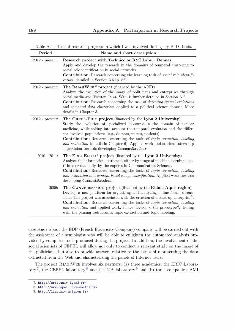
188 Appendix A. Participation in Research Projects
Table A.1 – List of research projects in which I was involved during my PhD thesis.Period Name and short description
2012 - present: Research project with Technicolor R&I Labs 1, RennesApply and develop the research in the domains of temporal clustering tosocial role identification in social networks.Contribution: Research concerning the learning task of social role identifi-cation, detailed in Section 3.6 (p. 52).
2012 - present: The ImagiWeb 2 project (financed by the ANR)Analyze the evolution of the image of politicians and enterprises throughsocial media and Twitter. ImagiWeb is further detailed in Section A.2.Contribution: Research concerning the task of detecting typical evolutionsand temporal data clustering, applied to a political science dataset. Moredetails in Chapter 3.
2012 - present: The Crtt 3-Eric project (financed by the Lyon 2 University)Study the evolution of specialized discourse in the domain of nuclearmedicine, while taking into account the temporal evolution and the differ-ent involved populations (e.g., doctors, nurses, patients).Contribution: Research concerning the tasks of topic extraction, labelingand evaluation (details in Chapter 6). Applied work and student internshipsupervision towards developing CommentWatcher.
2010 - 2011: The Eric-Elico 4 project (financed by the Lyon 2 University)Analyze the information extracted, either by usage of machine learning algo-rithms or manually, by the experts in Communication Sciences.Contribution: Research concerning the tasks of topic extraction, labelingand evaluation and content-based image classification. Applied work towardsdeveloping CommentWatcher.
2009: The Conversession project (financed by the Rhône-Alpes region)Develop a new platform for organizing and analyzing online forum discus-sions. The project was associated with the creation of a start-up enterprise 5.Contribution: Research concerning the tasks of topic extraction, labelingand evaluation and applied work: I have developed the prototype 6, dealingwith the parsing web forums, topic extraction and topic labeling.
case study about the EDF (French Electricity Company) company will be carried out withthe assistance of a semiologist who will be able to enlighten the automated analysis pro-vided by computer tools produced during the project. In addition, the involvement of thesocial scientists of CEPEL will allow not only to conduct a relevant study on the image ofthe politicians, but also to provide answers relative to the issues of representing the dataextracted from the Web and characterizing the panels of Internet users.
The project ImagiWeb involves six partners: (a) three academics: the ERIC Labora-tory 7, the CEPEL laboratory 8 and the LIA laboratory 9 and (b) three companies: AMI
7. http://eric.univ-lyon2.fr/8. http://www.cepel.univ-montp1.fr/9. http://lia.univ-avignon.fr/

A.2. The ImagiWeb project 189
Software 10, EDF 11 and XEROX 12. The ImagiWeb project is financed by the French Na-tional Research Agency (ANR).
10. http://www.amisw.com/en/11. http://innovation.edf.com/innovation-et-recherche-20.html12. http://www.xrce.xerox.com/

Appendix B
List of Publications
International journals
– Marian-Andrei Rizoiu, Julien Velcin and Stéphane Lallich. Unsupervised Feature Con-struction for Improving Data Representation and Semantics. Journal of IntelligentInformation Systems, vol. 40, no. 3, pages 501–527, 2013.
Proceedings of international conferences
– Marian-Andrei Rizoiu. Semi-Supervised Structuring of Complex Data. In DoctoralConsortium of International Joint Conference on Artificial Intelligence, Proceedingsof the Twenty-Third, IJCAI 2013. AAAI Press, November 2013.
– Marian-Andrei Rizoiu, Julien Velcin and Stéphane Lallich. Structuring typical evo-lutions using Temporal-Driven Constrained Clustering. In International Conferenceon Tools with Artificial Intelligence, Proceedings of the Twenty-Forth, ICTAI 2012,pages 610–617. IEEE, November 2012. Best Student Paper Award.
– Claudiu Musat, Julien Velcin, Stefan Trausan-Matu and Marian-Andrei Rizoiu. Im-proving topic evaluation using conceptual knowledge. In International Joint Conferenceon Artificial Intelligence, Proceedings of the Twenty-Second, volume 3 of IJCAI 2011,pages 1866–1871. AAAI Press, 2011.
– Claudiu Musat, Julien Velcin, Marian-Andrei Rizoiu and Stefan Trausan-Matu.Concept-based Topic Model Improvement. In International Symposium on Method-ologies for Intelligent Systems, volume 369 of ISMIS 2011, pages 133–142. Springer,June 2011.
National journals and proceedings of national conferences
– Marian-Andrei Rizoiu, Julien Velcin and Jean-Hugues Chauchat. Regrouper les don-nées textuelles et nommer les groupes à l’aide des classes recouvrantes. In Extractionet Gestion des Connaissances, (EGC 10) 10ème Conférence, volume E-19 of Revue desNouvelles Technologies de l’Information, pages 561–572. Cépaduès, January 2010.
– Claudiu Musat, Marian-Andrei Rizoiu and Stefan Trausan-Matu. An Intra and Inter-Topic Evaluation and Cleansing Method. Romanian Journal of Human-ComputerInteraction, vol. 3, no. 2, pages 81–96, 2010.
192 Appendix B. List of Publications
Book chapters
– Marian-Andrei Rizoiu and Julien Velcin. Topic Extraction for Ontology Learning. InWilson Wong, Wei Liu and Mohammed Bennamoun, editors, Ontology Learning andKnowledge Discovery Using the Web: Challenges and Recent Advances, chapter 3,pages 38–61. Hershey, PA: Information Science Reference, 2011.
Under review and submitted
– Marian-Andrei Rizoiu, Julien Velcin and Stéphane Lallich. Visual Vocabulary Con-struction for Image Classification in a Weakly Supervised Context. International Jour-nal of Artificial Intelligence Tools, 2012. Under review.
– Marian-Andrei Rizoiu, Julien Velcin and Stéphane Lallich. How to use Temporal-Driven Constrained Clustering to detect typical evolutions. International Journal ofArtificial Intelligence Tools, 2013. Submitted.
Bibliography
[Abouelhoda et al. 2002] Mohamed Abouelhoda, Enno Ohlebusch and Stefan Kurtz. Opti-mal exact string matching based on suffix arrays. In String Processing and Informa-tion Retrieval, pages 175–180. Springer, 2002. (Cited on page 143.)
[Aggarwal et al. 2003] Charu C. Aggarwal, Jiawei Han, Jianyong Wang and Philip S. Yu.A Framework for Clustering Evolving Data Streams. In Very large data bases, Pro-ceedings of the 29th International Conference On, pages 81–92, 2003. (Cited onpage 18.)
[Agrawal & Srikant 1995] Rakesh Agrawal and Ramakrishnan Srikant. Mining sequentialpatterns. In Data Engineering, 1995. Proceedings of the Eleventh International Con-ference on, pages 3–14. IEEE, 1995. (Cited on page 17.)
[Agrawal et al. 1993] Rakesh Agrawal, Tomasz Imieliński and Arun Swami. Mining asso-ciation rules between sets of items in large databases. In ACM SIGMOD Record,volume 22, pages 207–216. ACM, 1993. (Cited on page 17.)
[Agresti 2002] Alan Agresti. Categorical data analysis, volume 359. Wiley-interscience,2002. (Cited on page 63.)
[Amer-Yahia et al. 2012] Sihem Amer-Yahia, Samreen Anjum, Amira Ghenai, Aysha Sid-dique, Sofiane Abbar, Sam Madden, Adam Marcus and Mohammed El-Haddad.MAQSA: a system for social analytics on news. In Proceedings of the 2012 ACMSIGMOD International Conference on Management of Data, SIGMOD ’12, pages653–656, New York, NY, USA, 2012. ACM. (Cited on pages 169 and 170.)
[Anaya-Sánchez et al. 2008] Henry Anaya-Sánchez, Aurora Pons-Porrata and RafaelBerlanga-Llavori. A New Document Clustering Algorithm for Topic Discoveringand Labeling. In Iberoamerican congress on Pattern Recognition, Proceedings of the13th, CIARP ’08, pages 161–168, Berlin, Heidelberg, 2008. Springer-Verlag. (Citedon page 138.)
[Anokhin et al. 2012] Nikolay Anokhin, James Lanagan and Julien Velcin. Social Citation:Finding Roles in Social Networks. An Analysis of TV-Series Web Forums. In MiningCommunities and People Recommenders, The Second International Workshop on,pages 49–56, 2012. (Cited on pages 52, 53, 169 and 183.)
[Armingeon et al. 2011] Klaus Armingeon, David Weisstanner, Sarah Engler, Panajotis Po-tolidis, Marlène Gerber and Philipp Leimgruber. Comparative Political Data Set1960-2009. Institute of Political Science, University of Berne., 2011. (Cited onpages 31, 32 and 43.)
[Athanasiadis et al. 2005] Thanos Athanasiadis, Vassilis Tzouvaras, Kosmas Petridis, Fred-eric Precioso, Yannis Avrithis and Yiannis Kompatsiaris. Using a multimedia ontol-ogy infrastructure for semantic annotation of multimedia content. In InternationalWorkshop on Knowledge Markup and Semantic Annotation, collocated with Inter-national Semantic Web Conference (ISWC 2005), SemAnnot ’05, Galway, Ireland,November 2005. (Cited on page 104.)
194 Bibliography
[Bar-Hillel et al. 2003] Aharon Bar-Hillel, Tomer Hertz, Noam Shental and Daphna Wein-shall. Learning distance functions using equivalence relations. In Machine Learn-ing, International Workshop then conference, volume 20, page 11, 2003. (Cited onpage 25.)
[Barnard et al. 2003] Kobus Barnard, Pinar Duygulu, David Forsyth, Nando De Freitas,David M. Blei and Michael I. Jordan. Matching words and pictures. The Journal ofMachine Learning Research, vol. 3, pages 1107–1135, 2003. (Cited on page 16.)
[Basu et al. 2002] Sugato Basu, Arindam Banerjee and Raymond J. Mooney. Semi-supervised clustering by seeding. In International Conference on Machine Learning,pages 19–26, 2002. (Cited on page 27.)
[Basu et al. 2003] Sugato Basu, Mikhail Bilenko and Raymond J. Mooney. Comparing andUnifying Search-Based and Similarity-Based Approaches to Semi-Supervised Clus-tering. In Workshop on the Continuum from Labeled to Unlabeled Data in MachineLearning and Data Mining, Collocated with ICML ’03, ICML ’03, pages 42–49, 2003.(Cited on pages 23, 24, 26 and 27.)
[Bay et al. 2006] Herbert Bay, Tinne Tuytelaars and Luc Van Gool. Surf: Speeded up robustfeatures. Computer Vision–ECCV 2006, pages 404–417, 2006. (Cited on pages 100and 103.)
[Bekkerman & Jeon 2007] Ron Bekkerman and Jiwoon Jeon. Multi-modal clusteringfor multimedia collections. In Computer Vision and Pattern Recognition, 2007.CVPR’07. IEEE Conference on, pages 1–8. IEEE, 2007. (Cited on pages 14 and 15.)
[Bellman & Kalaba 1959] Richard Bellman and Robert Kalaba. On adaptive control pro-cesses. Automatic Control, IRE Transactions on, vol. 4, no. 2, pages 1–9, 1959.(Cited on page 19.)
[Benjamini & Liu 1999] Yoav Benjamini and Wei Liu. A step-down multiple hypothesestesting procedure that controls the false discovery rate under independence. Journalof Statistical Planning and Inference, vol. 82, no. 1-2, pages 163–170, 1999. (Citedon page 83.)
[Bernstein et al. 2010] Michael S. Bernstein, Bongwon Suh, Lichan Hong, Jilin Chen, San-jay Kairam and Ed H. Chi. Eddi: interactive topic-based browsing of social statusstreams. In UIST ’10, pages 303–312, 2010. (Cited on page 170.)
[Berry et al. 1995] Michael W. Berry, Susan T. Dumais and Gavin W. O’Brien. UsingLinear Algebra for Intelligent Information Retrieval. SIAM Review, vol. 37, no. 4,pages 573–595, 1995. (Cited on page 133.)
[Beyer et al. 1999] Kevin Beyer, Jonathan Goldstein, Raghu Ramakrishnan and Uri Shaft.When is “nearest neighbor” meaningful? Database Theory, Proceedings of the Inter-natioanal Conference on, vol. ICDT ’99, pages 217–235, 1999. (Cited on page 19.)
[Bilenko & Mooney 2003] Mikhail Bilenko and Raymond J. Mooney. Adaptive duplicatedetection using learnable string similarity measures. In Knowledge Discovery andData Mining, Proceedings of the ninth ACM SIGKDD international conference on,pages 39–48. ACM New York, NY, USA, 2003. (Cited on page 25.)
Bibliography 195
[Biskri et al. 2004] Ismaïl Biskri, Jean-Guy Meunier and Sylvain Joyal. L’extraction destermes complexes : une approche modulaire semiautomatique. In Gérard Purnelle,Cédrick Fairon and Anne Dister, editors, Analyse Statistique des Données Textuelles,Actes des 7èmes Journées Internationales de, volume 1, pages 192–201. Presses Uni-versitaires de Louvain, 2004. (Cited on pages 137 and 138.)
[Bizer et al. 2009] Christian Bizer, Jens Lehmann, Georgi Kobilarov, Sören. Auer, ChristianBecker, Richard Cyganiak and Sebastian Hellmann. DBpedia-A crystallization pointfor the Web of Data. Web Semantics: Science, Services and Agents on the WorldWide Web, vol. 7, no. 3, pages 154–165, 2009. (Cited on pages 2 and 10.)
[Blei & Lafferty 2006a] David M. Blei and John D. Lafferty. Correlated Topic Models. InAdvances in Neural Information Processing Systems, Proceedings of the 2005 Con-ference on, volume 18, page 147. MIT, 2006. (Cited on pages 136 and 162.)
[Blei & Lafferty 2006b] David M. Blei and John D. Lafferty. Dynamic topic models. InInternational Conference on Machine Learning, Proceedings of the 23rd, pages 113–120. ACM, 2006. (Cited on page 136.)
[Blei & McAuliffe 2008] David M. Blei and Jon D. McAuliffe. Supervised topic models.Advances in Neural Information Processing Systems, vol. 20, pages 121–128, 2008.(Cited on page 140.)
[Blei et al. 2003] David M. Blei, Andrew Y. Ng and Michael I. Jordan. Latent dirichletallocation. The Journal of Machine Learning Research, vol. 3, pages 993–1022, 2003.(Cited on pages 104, 131, 134 and 157.)
[Blei et al. 2004] David M. Blei, Thomas L. Griffiths, Michael I. Jordan and Joshua B.Tenenbaum. Hierarchical topic models and the nested Chinese restaurant process. InAdvances in Neural Information Processing Systems, Proceedings of the 18th AnnualConference on, volume 16, pages 106–123. MIT Press, 2004. (Cited on pages 136and 162.)
[Blockeel et al. 1998] Hendrik Blockeel, Luc De Raedt and Jan Ramon. Top-down inductionof clustering trees. In Proceedings of the 15th International Conference on MachineLearning, pages 55–63, 1998. (Cited on page 66.)
[Bloedorn & Michalski 1998] Eric Bloedorn and Ryszard S. Michalski. Data-driven con-structive induction. Intelligent Systems and their Applications, vol. 13, no. 2, pages30–37, 1998. (Cited on page 64.)
[Blum & Mitchell 1998] Avrim Blum and Tom Mitchell. Combining labeled and unla-beled data with co-training. In Computational Learning Theory, Proceedings of theeleventh annual conference on, COLT 9́8, pages 92–100. ACM, 1998. (Cited onpage 104.)
[Bourigault 1992] Didier Bourigault. Surface grammatical analysis for the extraction ofterminological noun phrases. In Computational Linguistics, Proceedings of the In-ternational Conference on, volume 92, pages 977–981, 1992. (Cited on page 137.)
[Boyd-Graber et al. 2007] Jordan Boyd-Graber, David M. Blei and Xiaojin Zhu. A topicmodel for word sense disambiguation. In Joint Conference on Empirical Methodsin Natural Language Processing and Computational Natural Language Learning,
196 Bibliography
Proceedings of the 2007, EMNLP-CoNLL 2007, pages 1024–1033, 2007. (Cited onpage 140.)
[Brillinger 2001] David R. Brillinger. Time series: data analysis and theory, volume 36.Society for Industrial Mathematics, 2001. (Cited on page 17.)
[Buitelaar et al. 2005] Paul Buitelaar, Philipp Cimiano and Bernardo Magnini. OntologyLearning from Texts: An Overview. In Paul Buitelaar, Philipp Cimiano and BernardoMagnini, editors, Ontology Learning from Text: Methods, Evaluation and Applica-tions, volume 123 of Frontiers in Artificial Intelligence and Applications. IOS Press,2005. (Cited on pages 137, 161 and 162.)
[Cai et al. 2004] Deng Cai, Xiaofei He, Zhiwei Li, Wei-Ying Ma and Ji-Rong Wen. Hi-erarchical clustering of WWW image search results using visual, textual and linkinformation. In International Conference on Multimedia, Proceedings of the 12thannual ACM, pages 952–959. ACM, 2004. (Cited on page 15.)
[Cattell 1966] Raymond B. Cattell. The Scree Test For The Number Of Factors. Multivari-ate Behavioral Research, vol. 1, no. 2, pages 245–276, 1966. (Cited on page 134.)
[Chang et al. 2009a] Jonathan Chang, Jonathan Boyd-Graber, Sean Gerrish, Chong Wangand David M. Blei. Reading Tea Leaves: How Humans Interpret Topic Models. InAdvances in Neural Information Processing Systems, Proceedings of the 23rd AnnualConference on, volume 31 of NIPS 2009, 2009. (Cited on pages 140, 148, 149, 150and 157.)
[Chang et al. 2009b] Jonathan Chang, Jordan Boyd-Graber and David M. Blei. Connec-tions between the lines: augmenting social networks with text. In International Con-ference on Knowledge Discovery and Data Mining, Proceedings of the 15th ACMSIGKDD, pages 169–178. ACM, 2009. (Cited on page 136.)
[Chang et al. 2010] Yin-Wen Chang, Cho-Jui Hsieh, Kai-Wei Chang, Michael Ringgaardand Chih-Jen Lin. Training and testing low-degree polynomial data mappings vialinear SVM. The Journal of Machine Learning Research, vol. 99, pages 1471–1490,2010. (Cited on page 20.)
[Chapelle et al. 2006] Olivier Chapelle, Bernhard Schölkopf and Alexander Zien. Semi-supervised learning, volume 2 of Adaptive Computation and Machine Learning. TheMIT Press, September 2006. (Cited on pages 2 and 21.)
[Chavez et al. 2008] Camara G. Chavez, Frederic Precioso, Matthieu Cord, Sylvie Phillip-Foliguet and A. de A. Araújo. An interactive video content-based retrieval system.In Systems, Signals and Image Processing, 15th International Conference on, IWS-SIP ’08, pages 133–136. IEEE, 2008. (Cited on page 100.)
[Chen et al. 2009] Shixi Chen, Haixun Wang and Shuigeng Zhou. Concept clustering ofevolving data. In Data Engineering, 2009. ICDE’09. IEEE 25th International Con-ference on, pages 1327–1330. IEEE, 2009. (Cited on page 34.)
[Christoudias et al. 2006] C. Mario Christoudias, Kate Saenko, Louis-Philippe Morency andTrevor Darrell. Co-adaptation of audio-visual speech and gesture classifiers. InProceedings of the 8th international conference on Multimodal interfaces, pages 84–91. ACM, 2006. (Cited on page 16.)
Bibliography 197
[Cimiano et al. 2006] Philipp Cimiano, Johanna Völker and Rudi Studer. Ontologies on De-mand? -A Description of the State-of-the-Art, Applications, Challenges and Trendsfor Ontology Learning from Text Information. Information, Wissenschaft und Praxis,vol. 57, no. 6-7, pages 315–320, 2006. (Cited on pages 137, 161 and 162.)
[Clare & King 2001] Amanda Clare and Ross D. King. Knowledge discovery in multi-labelphenotype data. In Principles of Data Mining and Knowledge Discovery, pages 42–53.Springer, 2001. (Cited on page 94.)
[Cleuziou et al. 2004] Guillaume Cleuziou, Lionel Martin and Christel Vrain. PoBOC: anOverlapping Clustering Algorithm. Application to Rule-Based Classification and Tex-tual Data. In R. López de Mántaras and L. Saitta, editors, European Conference onArtificial Intelligence, Proceedings of the 16th, ECAI ’04, pages 440–444, Valencia,Spain, August 2004. (Cited on page 133.)
[Cleuziou 2008] Guillaume Cleuziou. An extended version of the k-means method for over-lapping clustering. In Pattern Recognition, 2008. ICPR 2008. 19th InternationalConference on, pages 1–4. IEEE, 2008. (Cited on pages 131, 133, 139, 140, 142and 143.)
[Cleuziou 2009] Guillaume Cleuziou. OKMed et WOKM : deux variantes de OKM pour laclassification recouvrante. In Jean-Gabriel Ganascia and Pierre Gançarski, editors,Extraction et Gestion des Connaisances, volume RNTI-E-15 of EGC 2009, pages31–42. Cépaduès-Éditions, January 2009. (Cited on page 133.)
[Cohn et al. 2003] David Cohn, Rich Caruana and Andrew McCallum. Semi-supervisedclustering with user feedback. In Constrained Clustering: Advances in Algorithms,Theory, and Applications, volume 4, pages 17–32. Cornell University, 2003. (Citedon pages 22, 23 and 25.)
[Comaniciu & Meer 2002] Dorin Comaniciu and Peter Meer. Mean shift: A robust approachtoward feature space analysis. Pattern Analysis and Machine Intelligence, IEEETransactions on, vol. 24, no. 5, pages 603–619, 2002. (Cited on page 103.)
[Cortes & Vapnik 1995] Corrina Cortes and Vladimir Vapnik. Support-vector networks. Ma-chine learning, vol. 20, no. 3, pages 273–297, 1995. (Cited on pages 20, 21, 62, 64and 112.)
[Csurka et al. 2004] Gabriela Csurka, Christopher R. Dance, Lixin Fan, Jutta Willamowskiand Cédric Bray. Visual categorization with bags of keypoints. In Workshop onstatistical learning in computer vision, ECCV, volume 1, pages 1–22, 2004. (Citedon pages 100 and 103.)
[da Silva et al. 1999] Joaquim da Silva, Gaël Dias, Sylvie Guilloré and José Pereira Lopes.Using LocalMaxs Algorithm for the Extraction of Contiguous and Non-contiguousMultiword Lexical Units. Progress in Artificial Intelligence, page 849, 1999. (Citedon page 138.)
[Darrell & Pentland 1993] Trevor Darrell and Alexander Pentland. Space-time gestures.In Computer Vision and Pattern Recognition, Proceedings of the IEEE ComputerSociety Conference on, CVPR ’93, pages 335–340. IEEE, 1993. (Cited on page 17.)
198 Bibliography
[Davidson & Basu 2007] Ian Davidson and Sugato Basu. A survey of clustering with in-stance level constraints. ACM Transactions on Knowledge Discovery from Data,pages 1–41, 2007. (Cited on pages 2, 22 and 26.)
[Davidson & Ravi 2005] Ian Davidson and SS Ravi. Clustering with constraints: Feasibilityissues and the fc-means algorithm. In International Conference on Data Mining,Proceedings of the Fifth SIAM, volume 119, page 138. Society for Industrial Math-ematics, 2005. (Cited on page 23.)
[de Andrade Bresolin et al. 2008] Adriano de Andrade Bresolin, Adrião Duarte Dória Netoand Pablo Javier Alsina. Digit recognition using wavelet and SVM in Brazilian Por-tuguese. In Acoustics, Speech and Signal Processing, IEEE International Conferenceon, ICASSP ’08, pages 1545–1548, 2008. (Cited on page 13.)
[De la Torre & Agell 2007] Fernando De la Torre and Carlos Agell. Multimodal Diaries.In Multimedia and Expo, 2007 IEEE International Conference on, pages 839–842.IEEE, 2007. (Cited on page 34.)
[de Medeiros Martins et al. 2002] Allan de Medeiros Martins, Wedson Torres deAlmeida Filho, Agostinho Medeiros Brito Júnior and Adrião Duarte Dória Neto.A new method for multi-texture segmentation using neural networks. In NeuralNetworks, Proceedings of the 2002 International Joint Conference on, volume 3 ofIJCNN’02, pages 2064–2069. IEEE, 2002. (Cited on page 102.)
[Demiriz et al. 1999] Ayhan Demiriz, Kristin Bennett and Mark J. Embrechts. Semi-Supervised Clustering Using Genetic Algorithms. In Artificial Neural Networks inEngineering, pages 809–814. ASME Press, 1999. (Cited on page 26.)
[Dermouche et al. 2013] Mohamed Dermouche, Julien Velcin, Sabine Loudcher and LeilaKhouas. Une nouvelle mesure pour l’évaluation des méthodes d’extraction de théma-tiques: la Vraisemblance Généralisée. In Extraction et la Gestion des Connaissances,La 13ème Conférence Francophone sur, EGC ’13, pages 317–328. Revue des Nou-velles Technologies de l’Information, 2013. (Cited on page 132.)
[Dias et al. 2000] Gaël Dias, Sylvie Guilloré and José Pereira Lopes. Extraction automa-tique d’associations textuelles à partir de corpora non traités. In M. Rajman andJ. C. Chapelier, editors, Statistical Analysis of Textual Data, Proceedings of 5thInternational Conference on the, volume 2 of JADT 2000, pages 213–221, Lausanne,March 2000. Ecole Polytechnique Fédérale de Lausanne. (Cited on page 138.)
[Dietterich & Michalski 1985] Thomas G. Dietterich and Ryszard S. Michalski. Discoveringpatterns in sequences of events. Artificial Intelligence, vol. 25, no. 2, pages 187–232,1985. (Cited on page 17.)
[Diplaris et al. 2005] Sotiris Diplaris, Grigorios Tsoumakas, Pericles A. Mitkas and IoannisVlahavas. Protein classification with multiple algorithms. Advances in Informatics,pages 448–456, 2005. (Cited on page 94.)
[Dormont 1989] Brigitte Dormont. Petite apologie des données de panel. Économie &prévision, vol. 87, no. 1, pages 19–32, 1989. (Cited on page 43.)
[Dumais et al. 1998] Susan Dumais, John Platt, David Heckerman and Mehran Sahami.Inductive learning algorithms and representations for text categorization. In Con-
Bibliography 199
ference on Information and Knowledge Management, Proceedings of the SeventhInternational, CIKM ’98, pages 148–155. ACM, 1998. (Cited on page 130.)
[Dunn 1973] Joseph C. Dunn. A Fuzzy Relative of the ISODATA Process and Its Use inDetecting Compact Well-Separated Clusters. Journal of Cybernetics, vol. 3, no. 3,pages 32–57, 1973. (Cited on page 133.)
[Dunteman 1989] G. H. Dunteman. Principal components analysis, volume 69. SAGEpublications, Inc, 1989. (Cited on pages 20, 62, 64 and 160.)
[Egghe 2006] Leo Egghe. Theory and practise of the g-index. Scientometrics, vol. 69, no. 1,pages 131–152, 2006. (Cited on page 53.)
[Elomaa & Rousu 2004] Tapio Elomaa and Juho Rousu. Efficient multisplitting revisited:Optima-preserving elimination of partition candidates. Data Mining and KnowledgeDiscovery, vol. 8, no. 2, pages 97–126, 2004. (Cited on page 63.)
[Estruch et al. 2008] Vicent Estruch, J. H. Orallo and M. J. R. Quintana. Bridging the gapbetween distance and generalisation: Symbolic learning in metric spaces. PhD thesis,Universitat Politècnica de València, 2008. (Cited on page 163.)
[Farnstrom et al. 2000] Fredrik Farnstrom, James Lewis and Charles Elkan. Scalability forclustering algorithms revisited. ACM SIGKDD Explorations Newsletter, vol. 2, no. 1,pages 51–57, 2000. (Cited on page 18.)
[Fawcett 2006] Tom Fawcett. An introduction to ROC analysis. Pattern recognition letters,vol. 27, no. 8, pages 861–874, 2006. (Cited on page 118.)
[Fayyad & Irani 1993] Usama M. Fayyad and Keki B Irani. Multi-Interval Discretization ofContinuous-Valued Attributes for Classification Learning. In Ruzena Bajcsy, editor,International Joint Conference on Uncertainty in AI, Proceedings of the, volume 2,pages 1022–1027. Morgan Kaufmann, 1993. (Cited on page 63.)
[Fei-Fei & Perona 2005] Li Fei-Fei and Pietro Perona. A bayesian hierarchical model forlearning natural scene categories. In Computer Vision and Pattern Recognition,IEEE Computer Society Conference on, volume 2 of CVPR 2005, pages 524–531.IEEE, 2005. (Cited on pages 100 and 103.)
[Fei-Fei et al. 2007] Li Fei-Fei, Rob Fergus and Pietro Perona. Learning generative visualmodels from few training examples: An incremental bayesian approach tested on 101object categories. Computer Vision and Image Understanding, vol. 106, no. 1, pages59–70, 2007. (Cited on page 113.)
[Feller 1950] W. Feller. An introduction to probability theory and its applications. vol. i.Wiley, 1950. (Cited on page 71.)
[Ferret 2006] Olivier Ferret. Approches endogène et exogène pour améliorer la segmentationthématique de documents. Traitement Automatique des Langues, vol. 47, no. 2, pages111–135, 2006. (Cited on page 132.)
[Fisher 1987] Douglas H. Fisher. Knowledge Acquisition Via Incremental Conceptual Clus-tering. Machine Learning, vol. 2, no. 2, pages 139–172, 1987. (Cited on page 161.)
[Forestier et al. 2011] Mathilde Forestier, Julien Velcin and Djamel A. Zighed. Extractingsocial networks to understand interaction. In Advances in Social Networks Analysis
200 Bibliography
and Mining, International Conference on, ASONAM ’11, pages 213–219. IEEE, 2011.(Cited on pages 169 and 174.)
[Fournier-Viger et al. 2011] Philippe Fournier-Viger, Roger Nkambou and Vincent Shin-MuTseng. RuleGrowth: mining sequential rules common to several sequences by pattern-growth. In Proceedings of the 2011 ACM Symposium on Applied Computing, pages956–961. ACM, 2011. (Cited on page 17.)
[Francois et al. 2007] Damien Francois, Vincent Wertz and Michel Verleysen. The concen-tration of fractional distances. Knowledge and Data Engineering, IEEE Transactionson, vol. 19, no. 7, pages 873–886, 2007. (Cited on page 19.)
[Freund & Schapire 1997] Yoav Freund and Robert E. Schapire. A decision-theoretic gen-eralization of on-line learning and an application to boosting. Journal of computerand system sciences, vol. 55, no. 1, pages 119–139, 1997. (Cited on page 105.)
[Frintrop et al. 2010] Simone Frintrop, Erich Rome and Henrik I. Christensen. Compu-tational visual attention systems and their cognitive foundations: A survey. ACMTransactions on Applied Perception (TAP), vol. 7, no. 1, page 6, 2010. (Cited onpage 102.)
[Fulkerson et al. 2008] Brian Fulkerson, Andrea Vedaldi and Stefano Soatto. Localizingobjects with smart dictionaries. Computer Vision–ECCV 2008, pages 179–192, 2008.(Cited on page 105.)
[Gangemi et al. 2003] Aldo Gangemi, Roberto Navigli and Paola Velardi. The OntoWord-Net Project: extension and axiomatization of conceptual relations in WordNet. InInternational Conference on Ontologies, Databases and Applications of SEmantics,Proceedings of the, ODBASE’03, pages 820–838. Springer, 2003. (Cited on page 149.)
[Ganter & Wille 1999] Bernhard Ganter and Rudolf Wille. Formal concept analysis.Springer Berlin, 1999. (Cited on page 163.)
[Gao et al. 2006] Jing Gao, Pang-Ning Tan and Haibin Cheng. Semi-supervised clusteringwith partial background information. In In Proceedings of the Sixth SIAM Interna-tional Conference on Data Mining, 2006. (Cited on page 26.)
[Ge et al. 2003] Yongchao Ge, Sandrine Dudoit and Terence P. Speed. Resampling-basedmultiple testing for microarray data analysis. Test, vol. 12, no. 1, pages 1–77, 2003.(Cited on page 83.)
[Geraci et al. 2006] Filippo Geraci, Marco Pellegrini, Marco Maggini and Fabrizio Sebas-tiani. Cluster Generation and Cluster Labelling for Web Snippets: A Fast and Ac-curate Hierarchical Solution. In String Processing and Information Retrieval, pages25–36. Springer, 2006. (Cited on page 137.)
[Godoy & Amandi 2006] Daniela Godoy and Analía Amandi. Modeling user interests byconceptual clustering. Information System, vol. 31, no. 4-5, pages 247–265, 2006.(Cited on page 161.)
[Goemans et al. 2009] Hein E. Goemans, Kristian S. Gleditsch and Giacomo Chiozza. In-troducing Archigos: A dataset of political leaders. Journal of Peace Research, vol. 46,no. 2, pages 269–283, 2009. (Cited on page 31.)
Bibliography 201
[Gold et al. 2011] Bernard Gold, Nelson Morgan and Dan Ellis. Speech and audio signalprocessing. Wiley Online Library, 2011. (Cited on page 17.)
[Gomez & Morales 2002] Giovani Gomez and Eduardo Morales. Automatic feature con-struction and a simple rule induction algorithm for skin detection. In Proc. of theICML workshop on Machine Learning in Computer Vision, pages 31–38, 2002. (Citedon page 64.)
[Grira et al. 2005] Nizar Grira, Michel Crucianu and Nozha Boujemaa. Unsupervised andSemi-supervised Clustering: a Brief Survey. Technical report, A Review of MachineLearning Techniques for Processing Multimedia Content, Report of the MUSCLEEuropean Network of Excellence (FP6), 2005. (Cited on page 24.)
[Guille et al. 2013] Adrien Guille, Cécile Favre, Hakim Hacid and Djamel A. Zighed.SONDY: An Open Source Platform for Social Dynamics Mining and Analysis. InProceedings of the 2013 ACM SIGMOD International Conference on Managementof Data, SIGMOD ’13, 2013. (Cited on page 170.)
[Halkidi et al. 2001] Maria Halkidi, Yannis Batistakis and Michalis Vazirgiannis. On clus-tering validation techniques. Journal of Intelligent Information Systems, vol. 17,no. 2, pages 107–145, 2001. (Cited on pages 45 and 139.)
[Hammouda et al. 2005] Khaled M. Hammouda, Diego N. Matute and Mohamed S. Kamel.CorePhrase: Keyphrase Extraction for Document Clustering. Machine Learning andData Mining in Pattern Recognition, pages 265–274, 2005. (Cited on pages 136, 137and 138.)
[Haralick & Shanmugam 1973] R. M. Haralick and K. Shanmugam. Computer classificationof reservoir sandstones. Geoscience Electronics, IEEE Transactions on, vol. 11, no. 4,pages 171–177, 1973. (Cited on page 102.)
[Harris 1954] Zellig S. Harris. Distributional structure. Word, vol. 10, pages 146–162, 1954.(Cited on page 128.)
[Harris 1968] Zellig S. Harris. Mathematical structures of language. Wiley, 1968. (Cited onpages 128 and 162.)
[Hastie et al. 2005] Trevor Hastie, Robert Tibshirani, Jerome Friedman and JamesFranklin. The elements of statistical learning: data mining, inference and predic-tion. The Mathematical Intelligencer, vol. 27, no. 2, pages 83–85, 2005. (Cited onpage 17.)
[Hinneburg et al. 2000] Alexander Hinneburg, Charu C. Aggarwal and Daniel A. Keim.What is the nearest neighbor in high dimensional spaces? Bibliothek der UniversitätKonstanz, 2000. (Cited on page 19.)
[Hirsch 2005] Jorge E. Hirsch. An index to quantify an individual’s scientific research out-put. Proceedings of the National Academy of Sciences of the United states of Amer-ica, vol. 102, no. 46, page 16569, 2005. (Cited on page 53.)
[Hoffman et al. 2008] Forrest M. Hoffman, William W. Hargrove, Richard T. Mills, SalilMahajan, David J. Erickson and Robert J. Oglesby. Multivariate Spatio-TemporalClustering (MSTC) as a data mining tool for environmental applications. In In-ternational Congress on Environmental Modelling and Software, Proceedings of theiEMSs Fourth Biennial Meeting, 2008. (Cited on page 17.)
202 Bibliography
[Hofmann 1999] Thomas Hofmann. Probabilistic latent semantic indexing. In Research andDevelopment in Information Retrieval, Proceedings of the 22nd annual internationalACM SIGIR conference on, RDIR ’99, pages 50–57. ACM, 1999. (Cited on page 134.)
[Holm 1979] Sture Holm. A simple sequentially rejective multiple test procedure. Scandina-vian Journal of Statistics, vol. 6, no. 2, pages 65–70, 1979. (Cited on page 83.)
[Hong & Kwong 2009] Yi Hong and Sam Kwong. Learning assignment order of instancesfor the constrained k-means clustering algorithm. Systems, Man, and Cybernetics,Part B: Cybernetics, IEEE Transactions on, vol. 39, no. 2, pages 568–574, 2009.(Cited on page 26.)
[Houle et al. 2010] Michael E. Houle, Hans-Peter Kriegel, Peer Kröger, Erich Schubert andArthur Zimek. Can shared-neighbor distances defeat the curse of dimensionality?In Scientific and Statistical Database Management, pages 482–500. Springer, 2010.(Cited on page 19.)
[Hsu & Chang 2005] Winston Hsu and Shih-Fu Chang. Visual cue cluster construction viainformation bottleneck principle and kernel density estimation. Image and VideoRetrieval, pages 82–91, 2005. (Cited on page 105.)
[Huo et al. 2006] Xiaoming Huo, Xuelei S. Ni and Andrew K. Smith. A survey of manifold-based learning methods. In Mining of Enterprise Data, emerging nonparametricmethodology, chapter 1, pages 06–40. Springer, New York, 2006. (Cited on pages 20and 64.)
[Ibekwe-SanJuan & SanJuan 2004] Fidelia Ibekwe-SanJuan and Eric SanJuan. Mining tex-tual data through term variant clustering: the TermWatch system. Coupling ap-proaches, coupling media and coupling languages for information retrieval., pages487–503, 2004. (Cited on page 137.)
[Jacquemin 1999] Christian Jacquemin. Syntagmatic and paradigmatic representations ofterm variation. In Meeting of the Association for Computational Linguistics on Com-putational Linguistics, Proceedings of the 37th annual, pages 341–348. Associationfor Computational Linguistics, 1999. (Cited on page 137.)
[Jain & Dubes 1988] Anil K Jain and Richard C Dubes. Algorithms for clustering data.Prentice-Hall, Inc., 1988. (Cited on page 132.)
[Ji et al. 2010] Rongrong Ji, Hongxun Yao, Xiaoshuai Sun, Bineng Zhong and Wen Gao.Towards semantic embedding in visual vocabulary. In Computer Vision and PatternRecognition (CVPR), 2010 IEEE Conference on, pages 918–925, 2010. (Cited onpages 15 and 105.)
[Jiang et al. 2007] Yu-Gang Jiang, Chong-Wah Ngo and Jun Yang. Towards optimal bag-of-features for object categorization and semantic video retrieval. In Proceedings of the6th ACM International Conference on Image and Video Retrieval, pages 494–501.ACM, 2007. (Cited on pages 103 and 119.)
[Jianjia & Limin 2011] Zhang Jianjia and Luo Limin. Combined Category Visual Vocabu-lary: A new approach to visual vocabulary construction. In Image and Signal Pro-cessing, 4th International Congress on, volume 3 of CISP 2011, pages 1409–1415,October 2011. (Cited on page 106.)
Bibliography 203
[Jones 1972] Karen Sparck Jones. A statistical interpretation of term specificity and itsapplication in retrieval. Journal of documentation, vol. 28, no. 1, pages 11–21, 1972.(Cited on page 131.)
[Jurie & Triggs 2005] Frederic Jurie and Bill Triggs. Creating efficient codebooks for vi-sual recognition. In Computer Vision, 2005. ICCV 2005. Tenth IEEE InternationalConference on, volume 1, pages 604–610. IEEE, 2005. (Cited on page 103.)
[Kadir & Brady 2001] Timor Kadir and Michael Brady. Saliency, scale and image descrip-tion. International Journal of Computer Vision, vol. 45, no. 2, pages 83–105, 2001.(Cited on page 102.)
[Kandasamy & Rodrigo 2010] Kirthevasan Kandasamy and Ranga Rodrigo. Use of a visualword dictionary for topic discovery in images. In Information and Automation forSustainability (ICIAFs), 2010 5th International Conference on, pages 510–515, 2010.(Cited on page 164.)
[Karkali et al. 2012] Margarita Karkali, Vassilis Plachouras, Constantinos Stefanatos andMichalis Vazirgiannis. Keeping keywords fresh: a BM25 variation for personalizedkeyword extraction. In Proceedings of the 2nd Temporal Web Analytics Workshop,collocated with WWW’12, TempWeb ’12, pages 17–24, New York, NY, USA, 2012.ACM. (Cited on page 131.)
[Kietz et al. 2000] Joerg-Uwe Kietz, Alexander Maedche and Raphael Volz. A method forsemi-automatic ontology acquisition from a corporate intranet. In Workshop on On-tologies and Text, Collocated with EKAW ’2000, October 2000. (Cited on page 162.)
[Kim et al. 2003] Dong Kim, Jeong Sim, Heejin Park and Kunsoo Park. Linear-time con-struction of suffix arrays. In Combinatorial Pattern Matching, pages 186–199.Springer, 2003. (Cited on page 143.)
[Kinnunen et al. 2010] Teemu Kinnunen, Joni Kristian Kamarainen, Lasse Lensu, JukkaLankinen and Heikki Kälviäinen. Making Visual Object Categorization More Chal-lenging: Randomized Caltech-101 Data Set. In 2010 International Conference onPattern Recognition, pages 476–479. IEEE, 2010. (Cited on page 113.)
[Kisilevich et al. 2010] Slava Kisilevich, Florian Mansmann, Mirco Nanni and SalvatoreRinzivillo. Spatio-temporal clustering. Data mining and knowledge discovery hand-book, pages 855–874, 2010. (Cited on page 17.)
[Klein et al. 2002] Dan Klein, Sepandar D. Kamvar and Christopher D. Manning. Frominstance-level constraints to space-level constraints: Making the most of prior knowl-edge in data clustering. In International Conference on Machine Learning, pages307–314, 2002. (Cited on page 25.)
[Kotsiantis & Kanellopoulos 2006] Sotiris Kotsiantis and Dimitris Kanellopoulos. Dis-cretization techniques: A recent survey. GESTS International Transactions on Com-puter Science and Engineering, vol. 32, no. 1, pages 47–58, 2006. (Cited on page 63.)
[Kriegel et al. 2011] Hans-Peter Kriegel, Irene Ntoutsi, Myra Spiliopoulou, GrigorisTsoumakas and Arthur Zimek. Mining complex dynamic data. Tutorial atECML/PKDD 2011, September 2011. (Cited on page 18.)
204 Bibliography
[Kullback & Leibler 1951] Solomon Kullback and Richard A. Leibler. On information andsufficiency. The Annals of Mathematical Statistics, vol. 22, no. 1, pages 79–86, 1951.(Cited on pages 25, 136 and 158.)
[Lallich & Rakotomalala 2000] Stéphane Lallich and Ricco Rakotomalala. Fast feature se-lection using partial correlation for multi-valued attributes. In Djamel A. Zighed,J. Komorowski and J. M. Zytkow, editors, Proceedings of the 4th European Confer-ence on Principles of Data Mining and Knowledge Discovery, pages 221–231. LNAISpringer-Verlag, 2000. (Cited on pages 19 and 64.)
[Lallich et al. 2006] Stéphane Lallich, Olivier Teytaud and Elie Prudhomme. Statisticalinference and data mining: false discoveries control. In COMPSTAT: proceedingsin computational statistics: 17th symposium, page 325. Springer, 2006. (Cited onpage 83.)
[Larsson 1998] N. Jesper Larsson. Notes on Suffix Sorting. Technical Report LU-CS-TR:98-199, LUNDFD6/(NFCS-3130)/1–43/(1998), Department of Computer Science, LundUniversity, Sweden, June 1998. (Cited on page 144.)
[Lauriston 1994] Andy Lauriston. Automatic recognition of complex terms: Problems andthe TERMINO solution. Terminology, vol. 1, no. 1, pages 147–170, 1994. (Cited onpage 137.)
[Laxman & Sastry 2006] Srivatsan Laxman and P. Shanti Sastry. A survey of temporal datamining. Sadhana, vol. 31, no. 2, pages 173–198, 2006. (Cited on page 17.)
[Lazebnik & Raginsky 2009] Svetlana Lazebnik and Maxim Raginsky. Supervised learn-ing of quantizer codebooks by information loss minimization. Pattern Analysis andMachine Intelligence, IEEE Transactions on, vol. 31, no. 7, pages 1294–1309, 2009.(Cited on page 105.)
[Lazebnik et al. 2003a] Svetlana Lazebnik, Cordelia Schmid and Jean Ponce. Affine-invariant local descriptors and neighborhood statistics for texture recognition. InComputer Vision, 2003. Proceedings of the Ninth IEEE International Conferenceon, ICCV 2003, pages 649–655. IEEE, 2003. (Cited on page 102.)
[Lazebnik et al. 2003b] Svetlana Lazebnik, Cordelia Schmid and Jean Ponce. A sparse tex-ture representation using affine-invariant regions. In Computer Vision and PatternRecognition, 2003. Proceedings. 2003 IEEE Computer Society Conference on, vol-ume 2, pages II–319. IEEE, 2003. (Cited on page 102.)
[Lazebnik et al. 2006] Svetlana Lazebnik, Cordelia Schmid and Jean Ponce. Beyond bagsof features: Spatial pyramid matching for recognizing natural scene categories. InComputer Vision and Pattern Recognition, 2006 IEEE Computer Society Conferenceon, volume 2, pages 2169–2178. IEEE, 2006. (Cited on pages 102 and 103.)
[Lee & Seung 1999] Daniel D. Lee and H. Sebastian Seung. Learning the parts of objects bynon-negative matrix factorization. Nature, vol. 401, no. 6755, pages 788–791, 1999.(Cited on page 134.)
[Lesk 1986] Michael Lesk. Automatic sense disambiguation using machine readable dictio-naries: how to tell a pine cone from an ice cream cone. In SIGDOC ’86: Proceedingsof the 5th annual international conference on Systems documentation, pages 24–26,New York, NY, USA, 1986. ACM. (Cited on page 162.)
Bibliography 205
[Lesot et al. 2009] Marie-Jeanne Lesot, Maria Rifqi and Hamid Benhadda. Similarity mea-sures for binary and numerical data: a survey. International Journal of KnowledgeEngineering and Soft Data Paradigms, vol. 1, no. 1, pages 63–84, 2009. (Cited onpage 24.)
[Lin & Hauptmann 2006] Wei-Hao Lin and Er Hauptmann. Structuring continuous videorecordings of everyday life using time-constrained clustering. In IS&T/SPIE Sympo-sium on Electronic Imaging, 2006. (Cited on pages 26, 34, 37, 46 and 50.)
[Lindeberg 1993] Tony Lindeberg. Detecting salient blob-like image structures and theirscales with a scale-space primal sketch: a method for focus-of-attention. InternationalJournal of Computer Vision, vol. 11, no. 3, pages 283–318, 1993. (Cited on page 102.)
[Liu & Motoda 1998] Huan Liu and Hiroshi Motoda. Feature extraction, construction andselection: A data mining perspective. Springer, 1998. (Cited on page 63.)
[Liu et al. 2007] Ying Liu, Dengsheng Zhang, Guojun Lu and Wei-Ying Ma. A survey ofcontent-based image retrieval with high-level semantics. Pattern Recognition, vol. 40,no. 1, pages 262–282, 2007. (Cited on page 15.)
[Liu et al. 2009] Jingen Liu, Yang Yang and Mubarak Shah. Learning semantic visual vo-cabularies using diffusion distance. In Computer Vision and Pattern Recognition(CVPR), IEEE Conference on, pages 461–468. IEEE, 2009. (Cited on page 105.)
[Loeff et al. 2006] Nicolas Loeff, Cecilia Ovesdotter Alm and David A. Forsyth. Discrim-inating image senses by clustering with multimodal features. In Proceedings of theCOLING/ACL on Main conference poster sessions, pages 547–554. Association forComputational Linguistics, 2006. (Cited on page 15.)
[López-Sastre et al. 2010] RJ López-Sastre, T. Tuytelaars, FJ Acevedo-Rodríguez andS. Maldonado-Bascón. Towards a more discriminative and semantic visual vocab-ulary. Computer Vision and Image Understanding, vol. 115, no. 3, pages 415–425,November 2010. (Cited on page 103.)
[Lowe 1999] David G. Lowe. Object recognition from local scale-invariant features. In Com-puter Vision, The Proceedings of the Seventh IEEE International Conference on,volume 2 of ICCV 1999, pages 1150–1157. IEEE, 1999. (Cited on page 102.)
[Lowe 2004] David G. Lowe. Distinctive image features from scale-invariant keypoints. In-ternational Journal of Computer Vision, vol. 60, no. 2, pages 91–110, 2004. (Citedon pages 100, 103, 106 and 111.)
[Lu et al. 2009] Zhiwu Lu, Horace H. S. Ip and Qizhen He. Context-based multi-label imageannotation. In Conference on Image and Video Retrieval, Proceeding of the ACMInternational, CIVR ’09, pages 1–7. ACM, 2009. (Cited on page 16.)
[MacQueen 1967] James MacQueen. Some methods for classification and analysis of multi-variate observations. In L. M. Cam and J. Neyman, editors, Berkeley Symposium onMathematical Statistics and Probability, Proceedings of the Fifth, volume 1, pages281–297. University of California Press, 1967. (Cited on pages 34 and 132.)
[Manber & Myers 1993] Udi Manber and Gene Myers. Suffix arrays: A new method foron-line string searches. SIAM Journal on Computing, vol. 22, no. 5, pages 935–948,1993. (Cited on pages 138 and 143.)

206 Bibliography
[Mannila et al. 1997] Heikki Mannila, Hannu Toivonen and Inkeri A. Verkamo. Discovery offrequent episodes in event sequences. Data Mining and Knowledge Discovery, vol. 1,no. 3, pages 259–289, 1997. (Cited on page 17.)
[Marcus et al. 2011] Adam Marcus, Michael S. Bernstein, Osama Badar, David R. Karger,Samuel Madden and Robert C. Miller. Twitinfo: aggregating and visualizing mi-croblogs for event exploration. In Proceedings of the SIGCHI Conference on HumanFactors in Computing Systems, CHI ’11, pages 227–236, New York, NY, USA, 2011.ACM. (Cited on page 170.)
[Maree et al. 2005] Raphael Maree, Pierre Geurts, Justus Piater and Louis Wehenkel. Ran-dom subwindows for robust image classification. In Computer Vision and PatternRecognition, IEEE Computer Society Conference on, volume 1 of CVPR 2005, pages34–40. IEEE, 2005. (Cited on page 102.)
[Maron & Kuhns 1960] Melvin Earl Maron and John L. Kuhns. On relevance, probabilisticindexing and information retrieval. Journal of the ACM (JACM), vol. 7, no. 3, pages216–244, 1960. (Cited on page 129.)
[Marszałek & Schmid 2006] Marcin Marszałek and Cordelia Schmid. Spatial weighting forbag-of-features. In Computer Vision and Pattern Recognition, 2006 IEEE ComputerSociety Conference on, volume 2, pages 2118–2125. IEEE, 2006. (Cited on page 105.)
[Matheus 1990] Christopher John Matheus. Adding domain knowledge to SBL through fea-ture construction. In Proceedings of the Eighth National Conference on ArtificialIntelligence, pages 803–808, 1990. (Cited on page 65.)
[McCallum 2002] Andrew McCallum. Mallet: A machine learning for language toolkit.http://mallet.cs.umass.edu, 2002. (Cited on pages 157, 173 and 175.)
[Mei et al. 2007a] Qiaozhu Mei, Xu Ling, MatthewWondra, Hang Su and ChengXiang Zhai.Topic sentiment mixture: modeling facets and opinions in weblogs. In InternationalConference on World Wide Web, Proceedings of the 16th, pages 171–180. ACM,2007. (Cited on page 136.)
[Mei et al. 2007b] Qiaozhu Mei, Xuehua Shen and ChengXiang Zhai. Automatic labelingof multinomial topic models. In International Conference on Knowledge Discoveryand Data Mining, Proceedings of the 13th ACM SIGKDD, ICKDDM 2007, pages490–499. ACM, 2007. (Cited on page 136.)
[Meyerson 2001] Adam Meyerson. Online facility location. In Foundations of ComputerScience, Proceedings of the 42nd IEEE Symposium on, pages 426–431. IEEE, 2001.(Cited on page 103.)
[Michalski & Stepp 1983] Ryszard S. Michalski and Robert E. Stepp. Learning from obser-vation: Conceptual clustering. Machine Learning: An artificial intelligence approach,vol. 1, pages 331–363, 1983. (Cited on page 161.)
[Michalski 1983] Ryszard S. Michalski. A theory and methodology of inductive learning.Artificial Intelligence, vol. 20, no. 2, pages 111–161, 1983. (Cited on page 64.)
[Mikolajczyk & Schmid 2004] Krystian Mikolajczyk and Cordelia Schmid. Scale & affineinvariant interest point detectors. International Journal of Computer Vision, vol. 60,no. 1, pages 63–86, 2004. (Cited on page 102.)
Bibliography 207
[Miller 1995] George A. Miller. WordNet: a lexical database for English. Communications ofthe ACM, vol. 38, no. 11, pages 39–41, 1995. (Cited on pages 126, 140, 149 and 162.)
[Mo & Huang 2011] D. Mo and S. H. Huang. Feature selection based on inference corre-lation. Intelligent Data Analysis, vol. 15, no. 3, pages 375–398, 2011. (Cited onpages 19 and 64.)
[Mooney et al. 2008] Raymond J. Mooney, Sonal Gupta, Joohyun Kim and Kristen Grau-man. Watch, Listen & Learn: Co-training on Captioned Images and Videos. MachineLearning and Knowledge Discovery in Databases, pages 457–472, September 2008.(Cited on pages 15 and 104.)
[Moosmann et al. 2007] Frank Moosmann, Bill Triggs and Frederic Jurie. Fast discrim-inative visual codebooks using randomized clustering forests. Advances in neuralinformation processing systems, vol. 19, page 985, 2007. (Cited on page 103.)
[Morsillo et al. 2009] Nicholas Morsillo, Christopher Pal and Randal Nelson. Semi-supervised learning of visual classifiers from web images and text. In InternationalJoint Conference on Artificial Intelligence, Proceedings of the 21st, IJCAI 2009,pages 1169–1174. Morgan Kaufmann Publishers Inc., 2009. (Cited on page 104.)
[Motoda & Liu 2002] Hiroshi Motoda and Huan Liu. Feature selection, extraction and con-struction. Communication of IICM (Institute of Information and Computing Ma-chinery), vol. 5, pages 67–72, 2002. (Cited on page 64.)
[Murphy & Pazzani 1991] Patrick M. Murphy and Michael J. Pazzani. ID2-of-3: Construc-tive induction of M-of-N concepts for discriminators in decision trees. In Proceedingsof the Eighth International Workshop on Machine Learning, pages 183–187, 1991.(Cited on page 66.)
[Musat et al. 2011a] Claudiu Musat, Julien Velcin, Marian-Andrei Rizoiu and StefanTrausan-Matu. Concept-based Topic Model Improvement. In International Sym-posium on Methodologies for Intelligent Systems, volume 369 of ISMIS 2011, pages133–142. Springer, June 2011. (Cited on pages 127, 140, 164 and 180.)
[Musat et al. 2011b] Claudiu Musat, Julien Velcin, Stefan Trausan-Matu and Marian-Andrei Rizoiu. Improving topic evaluation using conceptual knowledge. In Interna-tional Joint Conference on Artificial Intelligence, Proceedings of the Twenty-Second,volume 3 of IJCAI 2011, pages 1866–1871. AAAI Press, 2011. (Cited on pages 127,140, 157, 164 and 180.)
[Musat 2011] Claudiu Musat. The Analysis of Implicit Opinions in Economic Texts and Re-lations between Them. PhD thesis, Polytechnic University of Bucharest, Bucharest,Romania, October 2011. (Cited on page 140.)
[Nanni & Pedreschi 2006] Mirco Nanni and Dino Pedreschi. Time-focused clustering of tra-jectories of moving objects. Journal of Intelligent Information Systems, vol. 27, no. 3,pages 267–289, 2006. (Cited on page 17.)
[Navarro 2001] Gonzalo Navarro. A guided tour to approximate string matching. ACMcomputing surveys (CSUR), vol. 33, no. 1, pages 31–88, 2001. (Cited on page 17.)
[Newman et al. 2010] David Newman, Jey Han Lau, Karl Grieser and Timothy Baldwin.Automatic evaluation of topic coherence. In North American Chapter of the As-sociation for Computational Linguistics, Human Language Technologies: The 2010
208 Bibliography
Annual Conference of the, pages 100–108. Association for Computational Linguistics,2010. (Cited on pages 140 and 157.)
[Ng et al. 2002] Andrew Y. Ng, Michael I. Jordan, Yair Weisset al. On spectral clustering:Analysis and an algorithm. Advances in Neural Information Processing Systems,vol. 2, pages 849–856, 2002. (Cited on page 132.)
[Norris 2008] Pippa Norris. Driving democracy: do power-sharing institutions work? Cam-bridge University Press New York, 2008. (Cited on page 31.)
[Nowak et al. 2006] Eric Nowak, Frederic Jurie and Bill Triggs. Sampling strategies for bag-of-features image classification. Computer Vision–ECCV 2006, pages 490–503, 2006.(Cited on pages 102 and 103.)
[O’Hara & Draper 2011] Stephen O’Hara and Bruce A Draper. Introduction to the bag offeatures paradigm for image classification and retrieval. Technical report, CornellUniversity Library, 2011. arXiv preprint arXiv:1101.3354. (Cited on page 102.)
[Oliva & Torralba 2001] Aude Oliva and Antonio Torralba. Modeling the shape of the scene:A holistic representation of the spatial envelope. International Journal of ComputerVision, vol. 42, no. 3, pages 145–175, 2001. (Cited on page 104.)
[Osato et al. 2002] Naoki Osato, Masayoshi Itoh, Hideaki Konno, Shinji Kondo, KazuhiroShibata, Piero Carninci, Toshiyuki Shiraki, Akira Shinagawa, Takahiro Arakawa andShoshi Kikuchi. A computer-based method of selecting clones for a full-length cDNAproject: simultaneous collection of negligibly redundant and variant cDNAs. Genomeresearch, vol. 12, no. 7, pages 1127–1134, 2002. (Cited on page 17.)
[O’Shaughnessy 2000] Douglas O’Shaughnessy. Speech communication: Human and ma-chine. IEEE Press, Piscataway, USA, 2nd ed. édition, 2000. (Cited on page 17.)
[Osinski & Weiss 2004] Stanislaw Osinski and Dawid Weiss. Conceptual Clustering UsingLingo Algorithm: Evaluation on Open Directory Project Data. In Intelligent Infor-mation Systems, pages 369–377, 2004. (Cited on page 138.)
[Osinski et al. 2004] Stanislaw Osinski, Jerzy Stefanowski and Dawid Weiss. Lingo: Searchresults clustering algorithm based on singular value decomposition. In Intelligentinformation processing and web mining, Proceedings of the International IIS, IIP-WM’04, page 359, 2004. (Cited on page 138.)
[Osinski 2003] Stanislaw Osinski. An algorithm for clustering of web search results. Master’sthesis, Poznań University of Technology, Poland, June 2003. (Cited on pages 131,134, 136, 137, 143, 144 and 148.)
[Pagallo & Haussler 1990] Giulia Pagallo and David Haussler. Boolean feature discovery inempirical learning. Machine learning, vol. 5, no. 1, pages 71–99, 1990. (Cited onpages 20, 65 and 66.)
[Parsons et al. 2004] Lance Parsons, Ehtesham Haque and Huan Liu. Subspace clusteringfor high dimensional data: a review. ACM SIGKDD Explorations Newsletter, vol. 6,no. 1, pages 90–105, 2004. (Cited on page 133.)
[Patwardhan & Pedersen 2006] Siddharth Patwardhan and Ted Pedersen. Using WordNet-based context vectors to estimate the semantic relatedness of concepts. In WorkshopMaking Sense of Sense-Bringing Computational Linguistics and Psycholinguistics
Bibliography 209
Together, Collocated with EACL 2006, volume 1501 of EACL ’06, pages 1–8, 2006.(Cited on page 151.)
[Pedersen et al. 2004] Ted Pedersen, Siddharth Patwardhan and Jason Michelizzi. Word-Net:: Similarity: measuring the relatedness of concepts. In Demonstration Track atNorth American Chapter of the Association for Computational Linguistics: HumanLanguage Technologies, HLT-NAACL ’04, pages 38–41. Association for Computa-tional Linguistics, 2004. (Cited on page 151.)
[Perronnin et al. 2006] Florent Perronnin, Christopher R. Dance, Gabriela Csurka andMarco Bressan. Adapted vocabularies for generic visual categorization. ComputerVision–ECCV 2006, pages 464–475, 2006. (Cited on pages 105 and 106.)
[Plamondon & Srihari 2000] Réjean Plamondon and Sargur N. Srihari. Online and off-linehandwriting recognition: a comprehensive survey. Pattern Analysis and MachineIntelligence, IEEE Transactions on, vol. 22, no. 1, pages 63–84, 2000. (Cited onpage 17.)
[Porter 1980] Martin F. Porter. An algorithm for suffix stripping. Program, vol. 14, no. 3,1980. (Cited on page 129.)
[Qamra et al. 2006] Arun Qamra, Belle Tseng and Edward Y. Chang. Mining blog sto-ries using community-based and temporal clustering. In Information and KnowledgeManagement, Proceedings of the 15th ACM international conference on, pages 58–67, New York, NY, USA, 2006. ACM. (Cited on page 34.)
[Quattoni et al. 2007] Ariadna Quattoni, Michael Collins and Trevor Darrell. Learning vi-sual representations using images with captions. In 2007 IEEE Conference on Com-puter Vision and Pattern Recognition, pages 1–8. IEEE, 2007. (Cited on page 15.)
[Quelhas et al. 2005] Pedro Quelhas, Florent Monay, J-M Odobez, Daniel Gatica-Perez,Tinne Tuytelaars and Luc Van Gool. Modeling scenes with local descriptors and la-tent aspects. In Computer Vision, Tenth IEEE International Conference on, volume 1of ICCV 2005, pages 883–890. IEEE, 2005. (Cited on page 100.)
[Quinlan 1986] John R. Quinlan. Induction of decision trees. Machine learning, vol. 1, no. 1,pages 81–106, 1986. (Cited on page 66.)
[Quinlan 1993] John R. Quinlan. C4.5: programs for machine learning. Morgan Kaufmann,1993. (Cited on page 66.)
[Rizoiu & Velcin 2011] Marian-Andrei Rizoiu and Julien Velcin. Topic Extraction for On-tology Learning. In Wilson Wong, Wei Liu and Mohammed Bennamoun, editors,Ontology Learning and Knowledge Discovery Using the Web: Challenges and Re-cent Advances, chapter 3, pages 38–61. Hershey, PA: Information Science Reference,2011. (Cited on pages 127, 164 and 180.)
[Rizoiu et al. 2010] Marian-Andrei Rizoiu, Julien Velcin and Jean-Hugues Chauchat. Re-grouper les données textuelles et nommer les groupes à l’aide des classes recouvrantes.In Extraction et Gestion des Connaissances, (EGC 10) 10ème Conférence, volume E-19 of Revue des Nouvelles Technologies de l’Information, pages 561–572. Cépaduès,January 2010. (Cited on pages 127, 139, 164, 173, 175 and 180.)
210 Bibliography
[Rizoiu et al. 2012] Marian-Andrei Rizoiu, Julien Velcin and Stéphane Lallich. Structuringtypical evolutions using Temporal-Driven Constrained Clustering. In InternationalConference on Tools with Artificial Intelligence, Proceedings of the Twenty-Forth,ICTAI 2012, pages 610–617. IEEE, November 2012. (Cited on pages 57 and 179.)
[Rizoiu et al. 2013a] Marian-Andrei Rizoiu, Julien Velcin and Stéphane Lallich. Unsuper-vised Feature Construction for Improving Data Representation and Semantics. Jour-nal of Intelligent Information Systems, vol. 40, no. 3, pages 501–527, 2013. (Citedon pages 95 and 179.)
[Rizoiu et al. 2013b] Marian-Andrei Rizoiu, Julien Velcin and Stéphane Lallich. VisualVocabulary Construction for Image Classification in a Weakly Supervised Context.International Journal of Artificial Intelligence Tools, 2013. (Cited on pages 123and 180.)
[Robertson et al. 1995] Stephen E. Robertson, Steve Walker, Susan Jones, Micheline M.Hancock-Beaulieu and Mike Gatford. Okapi at TREC-3. NIST Special PublicationSP, pages 109–109, 1995. (Cited on page 131.)
[Roche 2004] Mathieu Roche. Intégration de la construction de la terminologie de domainesspécialisés dans un processus global de fouille de textes. Thèse de doctorat universitéde paris 11, Université de Paris 11, December 2004. (Cited on pages 131, 137, 138and 139.)
[Rodríguez 2005] Carlos C. Rodríguez. The ABC of Model Selection: AIC, BIC and theNew CIC. In Bayesian Inference and Maximum Entropy Methods in Science andEngineering, volume 803, pages 80–87, 2005. (Cited on page 135.)
[Russell et al. 2008] Bryan C. Russell, Antonio Torralba, Kevin P. Murphy and William T.Freeman. LabelMe: a database and web-based tool for image annotation. InternationalJournal of Computer Vision, vol. 77, no. 1, pages 157–173, 2008. (Cited on page 76.)
[Salton & Buckley 1988] Gerard Salton and Christopher Buckley. Term-weighting ap-proaches in automatic text retrieval. Information Processing & Management, vol. 24,no. 5, pages 513–523, 1988. (Cited on pages 130 and 137.)
[Salton et al. 1975] Gerard Salton, Anita Wong and Chung-Shu Yang. A vector space modelfor automatic indexing. Communications of the ACM, vol. 18, no. 11, pages 613–620,November 1975. (Cited on page 129.)
[Sanders & Sukthankar 2001] Brandon C. S. Sanders and Rahul Sukthankar. Unsuperviseddiscovery of objects using temporal coherence. Technical report, CVPR TechnicalSketch, 2001. (Cited on page 34.)
[Sawaragi et al. 1985] Y. Sawaragi, H. Nakayama and T. Tanino. Theory of multiobjectiveoptimization, volume 176. Academic Press New York, 1985. (Cited on pages 63and 74.)
[Sethi et al. 2001] Ishwar K. Sethi, Ioana L. Coman and Daniela Stan. Mining associationrules between low-level image features and high-level concepts. In Aerospace/DefenseSensing, Simulation, and Controls, pages 279–290. International Society for Opticsand Photonics, 2001. (Cited on page 15.)
Bibliography 211
[Seung & Lee 2001] H. Sebastian Seung and Daniel D. Lee. Algorithms for non-negativematrix factorization. Advances in Neural Information Processing Systems, vol. 13,pages 556–562, 2001. (Cited on page 134.)
[Silberztein 1994] Max D. Silberztein. INTEX: a corpus processing system. In Computa-tional Linguistics, Proceedings of the 15th conference on, volume 1, pages 579–583.Association for Computational Linguistics, 1994. (Cited on page 137.)
[Singhal 2001] Amit Singhal. Modern information retrieval: A brief overview. IEEE DataEngineering Bulletin, vol. 24, no. 4, pages 35–43, 2001. (Cited on page 129.)
[Sivic & Zisserman 2003] Josef Sivic and Andrew Zisserman. Video Google: A text retrievalapproach to object matching in videos. In Computer Vision, Proceedings of the NinthIEEE International Conference on, ICCV 2003, pages 1470–1477. IEEE, 2003. (Citedon pages 100, 102 and 103.)
[Sivic et al. 2005] Josef Sivic, Bryan C. Russell, Alexei A. Efros, Andrew Zisserman andWilliam T. Freeman. Discovering objects and their location in images. In ComputerVision, Tenth IEEE International Conference on, volume 1 of ICCV 2005, pages370–377. IEEE, 2005. (Cited on page 100.)
[Smadja 1991] Frank A. Smadja. From N-grams to collocations: an evaluation of Xtract.In Association for Computational Linguistics, Proceedings of the 29th annual meet-ing on, pages 279–284, Morristown, NJ, USA, 1991. Association for ComputationalLinguistics. (Cited on pages 137 and 139.)
[Steinbach et al. 2000] Michael Steinbach, George Karypis and Vipin Kumar. A Compari-son of Document Clustering Techniques. In KDD Workshop on Text Mining, volume400, pages 525–526, 2000. (Cited on page 132.)
[Storey 2002] John D. Storey. A direct approach to false discovery rates. Journal of theRoyal Statistical Society: Series B (Statistical Methodology), vol. 64, no. 3, pages479–498, 2002. (Cited on page 83.)
[Swain & Ballard 1991] Michael J. Swain and Dana H. Ballard. Color indexing. Inter-national Journal of Computer Vision, vol. 7, no. 1, pages 11–32, 1991. (Cited onpage 102.)
[Talukdar et al. 2012] Partha Pratim Talukdar, Derry Wijaya and Tom Mitchell. Coupledtemporal scoping of relational facts. In Web Search and Data Mining, Proceedingsof the fifth ACM international conference on, pages 73–82. ACM, 2012. (Cited onpage 34.)
[Thanopoulos et al. 2002] Aristomenis Nikos Thanopoulos, Nikos Fakotakis and GeorgeKokkinakis. Comparative Evaluation of Collocation Extraction Metrics. In Lan-guage Resources Evaluation Conference, Proceedings of the 3rd, volume 2, pages620–625, 2002. (Cited on page 138.)
[Tsoumakas & Katakis 2007] Grigorios Tsoumakas and Ioannis Katakis. Multi-label clas-sification: An overview. International Journal of Data Warehousing and Mining(IJDWM), vol. 3, no. 3, pages 1–13, 2007. (Cited on page 94.)
[Turcato et al. 2000] Davide Turcato, Fred Popowich, Janine Toole, Dan Fass, DevlanNicholson and Gordon Tisher. Adapting a synonym database to specific domains.
212 Bibliography
In Workshop on Recent Advances in Natural Language Processing and Informa-tion Retrieval, collocated with ACL 2000, pages 1–11, Morristown, NJ, USA, 2000.Association for Computational Linguistics. (Cited on page 162.)
[Turtle & Croft 1989] Howard Turtle and W. Bruce Croft. Inference networks for documentretrieval. In Research and Development in Information Retrieval, Proceedings of the13th annual international ACM SIGIR conference on, pages 1–24. ACM, 1989. (Citedon page 129.)
[Varma & Zisserman 2003] Manik Varma and Andrew Zisserman. Texture classification:Are filter banks necessary? In Computer Vision and Pattern Recognition, Proceed-ings of the IEEE computer society conference on, volume 2 of CVPR 2003, pagesII–691. IEEE, 2003. (Cited on page 102.)
[Vogel & Schiele 2007] Julia Vogel and Bernt Schiele. Semantic modeling of natural scenesfor content-based image retrieval. International Journal of Computer Vision, vol. 72,no. 2, pages 133–157, 2007. (Cited on page 100.)
[Wagstaff & Cardie 2000] Kiri Wagstaff and Claire Cardie. Clustering with Instance-levelConstraints. In International Conference on Machine Learning, Proceedings of theSeventeenth, pages 1103–1110, 2000. (Cited on pages 22 and 26.)
[Wagstaff et al. 2001] Kiri Wagstaff, Claire Cardie, Seth Rogers and Stefan Schroedl. Con-strained K-means Clustering with Background Knowledge. In International Confer-ence on Machine Learning, Proceedings of the Eighteenth, pages 577–584. MorganKaufmann, 2001. (Cited on page 26.)
[Wallach et al. 2009] Hanna M. Wallach, Iain Murray, Ruslan Salakhutdinov and DavidMimno. Evaluation methods for topic models. In International Conference on Ma-chine Learning, Proceedings of the 26th Annual, pages 1105–1112. ACM, 2009.(Cited on page 139.)
[Wang & McCallum 2006] Xuerui Wang and Andrew McCallum. Topics over time: a non-Markov continuous-time model of topical trends. In Knowledge discovery and datamining, Proceedings of the 12th ACM SIGKDD international conference on, pages424–433. ACM, 2006. (Cited on page 157.)
[Wang et al. 2007] Xuerui Wang, Andrew McCallum and Xing Wei. Topical n-grams:Phrase and topic discovery, with an application to information retrieval. In In-ternational Conference on Data Mining, Proceedings of the 7th IEEE, ICDM 2007,pages 697–702. IEEE, 2007. (Cited on pages 135, 136 and 173.)
[Wang et al. 2008] Chong Wang, David M. Blei and David Heckerman. Continuous timedynamic topic models. In Conference on Uncertainty in Artificial Intelligence, Pro-ceedings of the 23rd, 2008. (Cited on page 136.)
[Wang et al. 2009] Gang Wang, Derek Hoiem and David Forsyth. Building text featuresfor object image classification. In Computer Vision and Pattern Recognition, 2009.CVPR 2009. IEEE Conference on, pages 1367–1374. IEEE, 2009. (Cited on pages 15and 104.)
[Webster & Burrough 1972] R. Webster and P. A. Burrough. Computer-based Soil Mappingof Small Areas from Sample Data: II. Classification Smoothing. Journal of SoilScience, vol. 23, no. 2, pages 222–234, 1972. (Cited on page 23.)
Bibliography 213
[Widmer & Ritschard 2009] Eric D. Widmer and Gilbert Ritschard. The de-standardizationof the life course: Are men and women equal? Advances in Life Course Research,vol. 14, no. 1-2, pages 28–39, 2009. (Cited on page 34.)
[Willamowski et al. 2004] Jutta Willamowski, Damian Arregui, Gabriela Csurka, Christo-pher R. Dance and Lixin Fan. Categorizing nine visual classes using local appearancedescriptors. In ICPR Workshop on Learning for Adaptable Visual Systems, 2004.(Cited on page 100.)
[Winn et al. 2005] J. Winn, A. Criminisi and T. Minka. Object categorization by learneduniversal visual dictionary. In Computer Vision, 2005. ICCV 2005. Tenth IEEEInternational Conference on, volume 2, pages 1800–1807. IEEE, 2005. (Cited onpage 105.)
[Wong et al. 2008] Wilson Wong, Wei Liu and Mohammed Bennamoun. Determination ofunithood and termhood for term recognition. Handbook of Research on Text andWeb Mining Technologies. IGI Global, 2008. (Cited on page 161.)
[Wong et al. 2009] Wilson Wong, Wei Liu and Mohammed Bennamoun. A probabilisticframework for automatic term recognition. Intelligent Data Analysis, vol. 13, no. 4,pages 499–539, 2009. (Cited on page 161.)
[Xing et al. 2002] Eric P. Xing, Andrew Y. Ng, Michael I. Jordan and Stuart Russell. Dis-tance Metric Learning with Application to Clustering with Side-Information. Ad-vances in Neural Information Processing Systems, vol. 15, pages 505–512, 2002.(Cited on page 25.)
[Xu et al. 2003] Wei Xu, Xin Liu and Yihong Gong. Document clustering based on non-negative matrix factorization. In Research and Development in Informaion Retrieval,Proceedings of the 26th international SIGIR conference on, pages 267–273. ACM,2003. (Cited on page 134.)
[Yamamoto & Church 2001] Mikio Yamamoto and Kenneth W. Church. Using suffix arraysto compute term frequency and document frequency for all substrings in a corpus.Computational Linguistics, vol. 27, no. 1, pages 1–30, 2001. (Cited on page 143.)
[Yang et al. 1991] Der-Shung Yang, Larry Rendell and Gunnar Blix. A scheme for featureconstruction and a comparison of empirical methods. In Proceedings of the TwelfthInternational Joint Conference on Artificial Intelligence, pages 699–704, 1991. (Citedon page 64.)
[Yang et al. 2010] Shuang Hong Yang, Jiang Bian and Hongyuan Zha. Hybrid Genera-tive/Discriminative Learning for Automatic Image Annotation. In Uncertainty inArtificial Intelligence, Proceedings of the 26th Conference on, UAI 2010, Catalina Is-land, California, 2010. Association for Uncertainty in Artificial Intelligence (AUAI).,AUAI Press. (Cited on page 16.)
[Yeh & Yang 2008] J. Yeh and N. Yang. Ontology Construction Based on Latent TopicExtraction in a Digital Library. Digital Libraries: Universal and Ubiquitous Accessto Information, pages 93–103, 2008. (Cited on page 162.)
[Zaiane et al. 2003] Osmar R. Zaiane, Simeon Simoff and Chabane Djeraba, editors. Miningmultimedia and complex data, volume 2797 of Lecture Notes in Computer Science.Springer, 2003. (Cited on pages 13 and 14.)
214 Bibliography
[Zhang & Li 2007] Qingfu Zhang and Hui Li. MOEA/D: A multiobjective evolutionaryalgorithm based on decomposition. Evolutionary Computation, IEEE Transactionson, vol. 11, no. 6, pages 712–731, 2007. (Cited on pages 51, 57 and 184.)
[Zhang et al. 2007] Jianguo Zhang, Marcin Marszałek, Svetlana Lazebnik and CordeliaSchmid. Local features and kernels for classification of texture and object categories:A comprehensive study. International Journal of Computer Vision, vol. 73, no. 2,pages 213–238, 2007. (Cited on pages 100 and 106.)
[Zhang et al. 2009] Wei Zhang, Akshat Surve, Xiaoli Fern and Thomas G. Dietterich.Learning non-redundant codebooks for classifying complex objects. In Proceedings ofthe 26th Annual International Conference on Machine Learning, pages 1241–1248.ACM, 2009. (Cited on page 105.)
[Zheng 1995] Zijian Zheng. Constructing nominal X-of-N attributes. In Proceedings ofInternational Joint Conference On Artificial Intelligence, volume 14, pages 1064–1070, 1995. (Cited on pages 64 and 66.)
[Zheng 1996] Zijian Zheng. A comparison of constructive induction with different types ofnew attribute. Technical report, School of Computing and Mathematics, DeakinUniversity, Geelong, 1996. (Cited on page 66.)
[Zheng 1998] Zijian Zheng. Constructing conjunctions using systematic search on decisiontrees. Knowledge-Based Systems, vol. 10, no. 7, pages 421–430, 1998. (Cited onpages 20 and 65.)
[Zhu 2005] Xiaojin Zhu. Semi-Supervised Learning Literature Survey. Technical Re-port 1530, Computer Sciences, University of Wisconsin-Madison, 2005. (Cited onpage 21.)
[Zhuang et al. 1999] Yueting Zhuang, Xiaoming Liu and Yunhe Pan. Apply semantic tem-plate to support content-based image retrieval. In Proceedings of the SPIE, Storageand Retrieval for Media Databases, volume 3972, pages 442–449, 1999. (Cited onpage 15.)
[Zighed et al. 2009] Djamel A. Zighed, Shusaku Tsumoto, Zbigniew W. Ras and HakimHacid, editors. Mining complex data, volume 165 of Studies in Computational In-telligence. Springer, 2009. (Cited on page 10.)


