Embed Size (px)
Citation preview

ARISTOTLE UNIVERSITY OF THESSALONIKI SCHOOL OF ENGINEERING – DEPARTMENT OF CIVIL ENGINEERING
DIVISION OF GEOTECHNICAL ENGINEERING
SOTIRIA T. KARAPETROU Civi l Engineer, MSc
SEISMIC VULNERABILITY OF REINFORCED CONCRETE
BUILDINGS CONSIDERING AGING AND SOIL-STRUCTURE
INTERACTION EFFECTS
DOCTORAL THESIS
THESSALONIKI 2015


SOTIRIA T. KARAPETROU
SEISMIC VULNERABILITY OF REINFORCED CONCRETE BUILDINGS
CONSIDERING AGING AND SOIL-STRUCTURE INTERACTION EFFECTS
DOCTORAL THESIS
Submitted to the Department of Civil Engineering, Division of Geotechnical Engineering,
Laboratory of Soil Mechanics, Foundations & Geotechnical Earthquake Engineering
Date of defense: 27 November 2015 Examining Committee: Prof. K. Pitilakis, Supervisor Prof. M. Dolce, Member of the Advisory Committee Assist. Prof. D. Pitilakis, Member of the Advisory Committee Prof. G. Manos, Examiner Prof. Dr. S. Parolai, Examiner Assoc. Prof. D. Raptakis, Examiner Assist. Prof. A. Anastasiadis, Examiner

© Sotiria T. Karapetrou © AUTh Seismic vulnerability of reinforced concrete buildings considering aging and soil-structure interaction effects ISBN
‘Acceptance of this Doctoral Thesis by the Department of Civil Engineering of Aristotle University Thessaloniki does not imply acceptance of the opinions of the author’ (Law 5343/1932, article 202, par. 2)

ACKNOWLEDGMENTS
This thesis owes its existence to the help, support and inspiration of several people. First and
foremost I would like to express my sincere gratitude to my supervisor Prof. Kyriazis Pitilakis,
for the continuous support and guidance of my Ph.D. study and related research. I would like
to thank him for providing me the opportunity to work with challenging topics with large
amounts of independence and initiative. I am also grateful he offered me the opportunity to
participate in large European research projects he was scientifically in charge of. This gave me
the privilege to meet and collaborate with important researchers in the field of earthquake
engineering and seismology.
I sincerely thank my advisory committee: Prof. Mauro Dolce for his interest in my work and his
insightful comments and suggestions raising important points which helped me to improve it;
Assist. Prof. Dimitris Pitilakis for the scientific guidance and for sharing his insights with me on
the different issues investigated in my thesis.
I would also like to thank my examiners: Prof. George Manos for taking the time to review this
thesis and for providing constructive and pointed comments; Prof. Stefano Parolai for very
thoroughly revising my work and for our instructive collaboration during these years in the
frame of significant European research projects; Assoc. Prof. Dimitris Raptakis for his interest
in my work and our many discussions over several scientific issues of engineering and
seismological interest; Assist. Prof. Anastasios Anastasiadis for carefully reading my
manuscript and for his support and encouragement.
The work described in this thesis was financially supported by the European research projects
REAKT (2011-2014) “Strategies and tools of Real Time Earthquake Risk Reduction” and NERA
(2012-2014) “Network of European Research Infrastructures for Earthquake Risk Assessment
and Mitigation”. This support is gratefully acknowledged. The additional one-year fund from
AUTh Research committee is also greatly appreciated.
Special thanks go to my friends and colleagues from AUTh: Dr. Stavroula Fotopoulou, Dr.
Maria Manakou, Dr. Grigorios Tsinidis, Dr. Zafeiria Roumelioti, Dr. Anna Karatzetzou, Dr. Evi

Riga, Dr. Sotiris Argyroudis, Dr. Achileas Pistolas, Stella Karafragka, Aggelos Tsinaris, Dr.
Kostas Trevlopoulos and Anastasia Argyroudi for their support and help during the last four
years. I also thank Argyro Fillipa, Despoina Lamprou, Sofia Kotsiri, Katerina Tsagdi, Kelly
Valaouri, Ioannis Thomaidis, Evaggelia Yfantidou, Dimitra Giannoula and Ioannis-Prodromos
Thomaidis for our cooperation during their Master Theses in the frame of the postgraduate
program in Earthquake Engineering and Seismic Design of Structures.
Last but not least I would like to express my heart-felt gratitude to my husband Yannis for his
endless support and encouragement during this journey. None of this would have been
possible without his love and patience. This thesis is dedicated to him.
Sotiria T. Karapetrou

SUMMARY
The reliable vulnerability assessment of existing structures and infrastructures is a
prerequisite for seismic loss estimation, risk mitigation and management. At present, the
seismic vulnerability assessment of reinforced concrete (RC) buildings is made
considering fixed base conditions; moreover, the mechanical properties of the building
remain intact in time. In this research it is investigated whether these two fundamental
hypotheses are sound as aging and soil-structure interaction (SSI) effects might play a
crucial role in the seismic fragility analysis of RC structures. Stemming from the general
lack of seismic vulnerability studies for RC buildings that take into consideration the
effects of progressive deterioration and soil-structure interaction, one of the most
significant challenges of the present research is the quantification of an analytical
methodology to estimate the seismic vulnerability of RC buildings considering aging and
SSI effects.
To demonstrate the methodology for the time-dependent vulnerability assessment,
seven RC moment resisting frames, designed according to different seismic code levels,
are selected as case studies. The consideration of aging is achieved by including
probabilistic models of chloride induced corrosion deterioration of the RC elements within
the vulnerability assessment framework. Different corrosion aspects are considered in the
analysis including the loss of reinforcement cross-sectional area, the degradation of
concrete cover and the reduction of steel ultimate deformation. Two-dimensional
incremental dynamic analysis (IDA) is performed to assess the seismic performance of
the initial uncorroded and corroded RC moment resisting frame structures. The time-
dependent fragility functions are derived in terms of the spectral acceleration at the
fundamental mode of the structure Sa(T1, 5%) for the immediate occupancy and collapse
prevention limit states. Results show an overall increase in seismic vulnerability over
time due to corrosion highlighting the important influence of deterioration due to aging
effects on the structural behavior.
A further challenge of the present thesis is to investigate whether SSI and site effects
may affect the seismic performance and vulnerability of RC moment resisting frame

buildings and consequently modify the fragility curves. SSI is modeled applying the direct
one-step approach considering either linear elastic or nonlinear soil behavior while site
effects are inherently accounted for. To further examine the contribution of site and SSI
effects, a two-step uncoupled approach is also applied, which takes into account site
effects on the response of the fixed base structure, but neglects SSI effects. Additional
analyses are performed investigating the influence of the soil depth and stratigraphy
under nonlinear soil behavior on the seismic response and fragility of RC buildings.
Fragility curves are derived as a function of rock outcropping peak ground acceleration
for the immediate occupancy and collapse prevention limit states for the fixed base and
SSI models based on the statistical exploitation of the results of incremental dynamic
analysis of the given structural systems. Results show the significant role of SSI and site
effects under linear or nonlinear soil behavior in altering the expected structural
performance and fragility of fixed base structures.
In the context of seismic vulnerability assessment of RC buildings, the use of field
monitoring data constitutes a significant tool for the representation of the actual
structural state, reducing uncertainties associated with the building configuration
properties as well as many non-physical parameters (age, maintenance, etc.), enhancing
thus the reliability in the risk assessment procedure. In the present thesis, the seismic
vulnerability of existing RC buildings is evaluated, combining through a comprehensive
methodology, the numerical analysis and field monitoring data. The proposed
methodology is highlighted through the derivation of “time-building specific” fragility
curves for an eight-storey RC structure (hospital building), built almost five decades ago,
that is composed by two adjacent units separated through a structural joint. The
assessment of the dynamic characteristics is performed using ambient noise
measurements. The modal identification results are used to update and better constrain
the initial finite element model of the building, which is based on the available design and
construction documentation plans. Three-dimensional incremental dynamic analysis is
performed to derive the fragility curves for the initial as built model (“building-specific”)
and for the real structures as they are nowadays (“time-building specific”). The initial
“building specific” curves are evaluated through their comparison with conventional
generic curves that are commonly used in risk assessment studies. Moreover, in order to
enhance the reliability of the obtained results, the “time-building specific” fragility curves,
are compared to time-dependent curves derived for the hospital units adopting an
appropriate for the specific case study corrosion scenario. Results derived from both
approaches indicate that the consideration of the actual state of structures may
significantly alter their expected seismic performance leading to higher vulnerability
values.

Sotiria Karapetrou – Doctoral Thesis
CONTENTS
Contents ................................................................................................... i List of Figures ....................................................................................... vii List of Tables ....................................................................................... xxv Chapter 1 ................................................................................................ 1
Introduction ............................................................................................. 1 1.1 Statement of the problem ................................................................. 1 1.2 Objectives and scope of the research .................................................. 3 1.3 Outline of the Thesis ........................................................................ 3 Chapter 2 ................................................................................................ 7
Literature review on the seismic vulnerability assessment of RC buildings ......... 7 2.1 Introduction .................................................................................... 7 2.2 Background ..................................................................................... 7 2.3 Prerequisites for the derivation of fragility functions ............................ 11
2.3.1 Taxonomy/typology/classification ............................................................... 11
2.3.2 Intensity measures ................................................................................... 16
2.3.3 Damage indicators and states .................................................................... 18
2.3.3.1. Local damage indices .................................................................... 21
2.3.3.2. Global damage indices .................................................................. 25
2.3.3.3. Damage measures ....................................................................... 28
2.3.3.4. Drift damage formulation .............................................................. 29
2.3.4 Treatment of uncertainties ......................................................................... 33
2.4 Methodologies for deriving seismic fragility functions ........................... 36
2.4.1 Derivation of fragility functions based on analytical methods ........................... 38
2.4.1.1. Capacity Spectrum Method (CSM) .................................................. 40
2.4.1.2. Nonlinear dynamic analysis ........................................................... 42
2.4.1.3. Factors affecting the reliability of analytical fragility functions ............. 44
2.5 Review of previous studies .............................................................. 45 2.6 SYNER-G: The fragility function manager .......................................... 48 2.7 Current challenges in seismic vulnerability assessment of RC buildings .. 51 2.8 Evolution of building vulnerability over time ....................................... 52
2.8.1 Mechanisms acting on structural performance during lifetime .......................... 52

CONTENTS ii
Sotiria Karapetrou – Doctoral Thesis
2.8.2 Aging effects: Corrosion of reinforcement .................................................... 53
2.8.2.1. Chloride induced corrosion mechanism ............................................ 53
2.8.2.2. Probabilistic modeling of chloride induced corrosion initiation .............. 56
2.8.2.3. Evaluation of corrosion rate ........................................................... 59
2.8.3 Effects of chloride induced corrosion on seismic performance and fragility of RC
buildings ................................................................................................. 61
2.9 Evaluation of soil-structure interaction and site effects on seismic vulnerability ........................................................................................... 66
2.9.1 Dynamic soil-structure interaction ............................................................... 66
2.9.2 Evaluation of soil-structure interaction and site effects on seismic structural
response and vulnerability ......................................................................... 67
2.10 Building-specific fragility curves using field monitoring data ............... 69 Chapter 3 .............................................................................................. 73
Reference buildings and vulnerability assessment methodology ..................... 73 3.1 Introduction .................................................................................. 73 3.2 Description of the methodological framework ..................................... 73 3.3 Selection of the reference fixed base - intact frame buildings ............... 75
3.3.1 MRF buildings designed with no seismic code provisions ................................. 75
3.3.2 MRF buildings designed with low seismic code provisions ................................ 77
3.3.3 MRF buildings designed with high seismic code provisions .............................. 79
3.4 Finite element modeling in OpenSees ................................................ 81
3.4.1 Infill modeling .......................................................................................... 84
3.5 Selection of the seismic input motion ................................................ 86 3.6 Incremental dynamic analysis IDA .................................................... 88
3.6.1 Performing IDA ........................................................................................ 88
3.6.2 Limit damage states ................................................................................. 93
3.7 Derivation of fragility functions ........................................................ 95
3.7.1 Fragility curves of the fixed base, bare frame structures ................................ 99
3.7.2 Comparison of infilled - bare frame structures ............................................ 102
3.8 Comparison of the derived fragility curves with literature curves .......... 104
3.8.1 Bare MRF buildings ................................................................................. 105
3.8.1.1. Bare MRFs with no seismic code provisions .................................... 105
3.8.1.2. Bare MRFs with low seismic code provisions ................................... 109
3.8.1.3. Bare MRFs with high seismic code provisions .................................. 113
3.8.2 Regularly and irregularly infilled MRF buildings ........................................... 119
3.8.2.1. Infilled MRFs with no seismic code provisions ................................. 119

CONTENTS iii
Sotiria Karapetrou – Doctoral Thesis
3.8.2.2. Infilled MRFs with low seismic code provisions ................................ 121
3.8.2.3. Infilled MRFs with high seismic code provisions ............................... 123
3.8.3 Discussion ............................................................................................. 125
Chapter 4 ............................................................................................ 127
Time-dependent fragility functions for RC buildings ..................................... 127 4.1 Introduction ................................................................................. 127 4.2 Aging effects: Chloride induced corrosion ......................................... 127
4.2.1 Corrosion initiation time .......................................................................... 128
4.2.2 Deterioration modeling due to corrosion .................................................... 130
4.3 Pushover analysis ......................................................................... 134 4.4 Comparative dynamic analysis ........................................................ 136 4.5 Incremental dynamic analysis ......................................................... 142 4.6 Definition of damage states ............................................................ 144 4.7 Time-dependent fragility curves ...................................................... 145
4.7.1 Fixed base bare frame structures .............................................................. 147
4.7.2 Fixed base infilled frame structures ........................................................... 152
4.8 Time-variant quadratic model for the fragility parameters ................... 154 4.9 Discussion and concluding remarks .................................................. 157 Chapter 5 ............................................................................................ 159
Seismic vulnerability assessment of RC buildings considering soil-structure interaction effects .................................................................................. 159 5.1 Introduction ................................................................................. 159 5.2 Description of the parametric investigation ....................................... 160
5.2.1 Selection of prototype buildings ................................................................ 160
5.2.2 Soil-structure interaction (SSI) modeling ................................................... 161
5.2.2.1. Soil constitutive model ................................................................ 166
5.2.3 Parametric study .................................................................................... 169
5.2.3.1. Effect of SSI and site effects under nonlinear soil behavior ............... 169
5.2.3.2. Effect of soil depth and stratigraphy under nonlinear soil behavior ..... 170
5.3 Comparative dynamic analysis ........................................................ 171 5.4 Derivation of fragility curves ........................................................... 183
5.4.1 Comparison of SSI - fixed based structures under linear soil behavior ............ 186
5.4.2 Effect of SSI and site effects under linear and nonlinear soil behavior ............ 187
5.4.3 Effect of soil depth and stratigraphy under nonlinear soil behavior ................. 189

CONTENTS iv
Sotiria Karapetrou – Doctoral Thesis
5.5 Time-dependent fragility curves under the consideration of both aging and SSI effects ............................................................................................ 190 5.6 Conclusions .................................................................................. 193 Chapter 6 ............................................................................................ 197
Time-building specific vulnerability assessment of RC buildings using field monitoring data ..................................................................................... 197 6.1 Introduction ................................................................................. 197 6.2 Application study: AHEPA hospital ................................................... 198
6.2.1 Structural description .............................................................................. 198
6.2.2 Instrumentation arrays ........................................................................... 205
6.2.2.1. Permanent array ........................................................................ 205
6.2.2.2. Temporary array ........................................................................ 207
6.3 Description of the methodological framework .................................... 209 6.4 Operational modal analysis (OMA) using field monitoring data ............. 210
6.4.1 Modal identification methods .................................................................... 210
6.4.2 Operational modal analysis using ambient noise measurements .................... 215
6.4.3 System identification and operational modal analysis using seismic recordings 223
6.5 Finite element model updating ........................................................ 228 6.6 Nonlinear finite element modeling ................................................... 233 6.7 Selection of the input motion .......................................................... 234 6.8 Incremental dynamic analysis (IDA) ................................................ 235 6.9 Derivation of fragility curves ........................................................... 238 6.10 Comparison with the time-dependent fragility curves of the hospital building units ........................................................................................ 241
6.10.1 Deterioration modeling due to corrosion ........................................ 241
6.10.2 Derivation of the time-dependent fragility curves and comparison with
“time-building specific” curves .................................................................. 243
6.11 Discussion and Conclusive remarks ............................................... 245 Chapter 7 ............................................................................................ 249
Conclusions – Limitations – Recommendations for future research ................ 249 7.1 Summary of findings and contributions ............................................ 249 7.2 Limitations and recommendations for future work .............................. 254 References .......................................................................................... 257

CONTENTS v
Sotiria Karapetrou – Doctoral Thesis
Annex A ............................................................................................... 285
Seismic input motion .............................................................................. 285
A.1 Seismic input motion .............................................................................. 285
Annex B ............................................................................................... 293
Modal identification results of AHEPA hospital using earthquake data ............. 293
B.1 Grid models in MACEC ............................................................................. 293
B.2 Seismic input motion .............................................................................. 296
B.3 Modal identification ................................................................................. 299
Annex C ............................................................................................... 305
Seismic input motion – AHEPA hospital ..................................................... 305
C.1 Seismic input motion .............................................................................. 305
Εκτενής Περίληψη ............................................................................... 317
I.1 Εισαγωγή ..................................................................................... 317 I.2 Μεθοδολογία αποτίμησης της τρωτότητας ......................................... 318
I.2.1 Περιγραφή των υπό μελέτη φορέων .......................................................... 319
I.2.2 Σεισμικές διεγέρσεις εισαγωγής ................................................................. 323
I.2.3 Μη γραμμικές ανελαστικές βήμα προς βήμα δυναμικές αναλύσεις ................... 325
I.2.4 Κατασκευή καμπυλών τρωτότητας ............................................................. 326
I.2.5 Αξιολόγηση των καμπυλών τρωτότητας ...................................................... 328
I.3 Χρονικά εξαρτώμενη σεισμική τρωτότητα κτηρίων Ο/Σ λαμβάνοντας υπόψη τη γήρανση των υλικών .......................................................................... 330 I.4 Επιρροή της δυναμικής αλληλεπίδρασης εδάφους – κατασκευής στην εκτίμηση της σεισμικής τρωτότητας κτηρίων Ο/Σ ......................................... 338 I.5 Αποτίμηση σεισμικής τρωτότητας κτηρίων Ο/Σ με βάση μετρήσεις πεδίου. Εφαρμογή στο κτήριο της νευρολογικής κλινικής και διοικητικών υπηρεσιών του νοσοκομείου ΑΧΕΠΑ στη Θεσσαλονίκη ....................................................... 347 I.6 Συμπεράσματα .............................................................................. 358 I.7 Βιβλιογραφικές αναφορές ............................................................... 359

CONTENTS vi
Sotiria Karapetrou – Doctoral Thesis

LIST OF FIGURES
Figure 2.1. Graphical presentation of an example fragility curve ................................ 9
Figure 2.2. Conditional probabilities of exceeding different damage states ................... 9
Figure 2.3. Conditional probabilities of exceeding different damage states ................. 10
Figure 2.4. Flow chart for a Reinforced Concrete, Moment Resisting Frame building class
according to SYNER-G ......................................................................................... 15
Figure 2.5. Pie chart presenting the percentages of different intensity measure types
used for the development of fragility functions for reinforced concrete buildings (Pitilakis
et al., 2014a) .................................................................................................... 17
Figure 2.6. Relationship between damage parameter (or damage variable) and damage
index (Kappos, 1997) ......................................................................................... 19
Figure 2.7. Limit states and damage states (Crowley et al., 2011) ........................... 20
Figure 2.8. Variation in fundamental period of a structure during an earthquake
(DiPasquale et al., 1990) ..................................................................................... 27
Figure 2.9. Typical structural performance and associated damage states (Ghobarah,
2004) ............................................................................................................... 30
Figure 2.10. Correlation between the interstorey drift factor and damage for a 3, 6, 9
and 12 storey MRFs (Ghobarah, 2004) .................................................................. 31
Figure 2.11. Pie chart presenting the percentages of different methodologies used for
the development of fragility functions for reinforced concrete buildings (Pitilakis et al.,
2014a) ............................................................................................................. 38
Figure 2.12. Flowchart to describe the components of the calculation of analytical
fragility curves (after Kwon and Elnashai, 2007) ..................................................... 39
Figure 2.13. HAZUS procedure for building damage estimation based on CSM (Pitilakis
et al., 2014a) .................................................................................................... 41
Figure 2.14. (a) IDA curves for the individual records and the estimation of the
associated limit-state capacities for CP limit state and (b) summarization of the 15 IDA
curves into their 16, 50 and 84 % fractiles ............................................................. 43
Figure 2.15. Sources of uncertainty associated with analytical fragility assessment
(adapted from D’Ayala and Meslem, 2013) ............................................................. 44
Figure 2.16. Fragility curves (in terms of PGA) for medium-rise infilled frames, low (left)
and high code design (Kappos et al., 2006) ............................................................ 47

viii Seismic vulnerability of reinforced concrete buildings considering aging and SSI effects
Figure 2.17. Sd-based fragility curves for medium-rise infilled R/C frames, low (left) and
high code design (Kappos et al., 2006) .................................................................. 47
Figure 2.18. Interface of the Fragility Function Manager (adapted from Silva et al., 2014
in Pitilakis et al., 2014a) ..................................................................................... 50
Figure 2.19. Mean curve for (a) limit state yielding curve and (b) limit state collapse
curve for reinforced concrete with moment resisting frame buildings, mid rise, seismically
designed model building type ............................................................................... 50
Figure 2.20. General description of the system remaining lifetime (Beushausen and
Alexander, 2010) ............................................................................................... 53
Figure 2.21. The electrochemical corrosion process (Malioka, 2009) ......................... 54
Figure 2.22. Left: Corrosion phases (adapted from Tuuti, 1982) of concrete structures.
Right: Effects on structural capacity and limit states (adapted from Malioka, 2009) ..... 55
Figure 2.23. Information required to determine the variables Cs and Cs,∆x (FIB-CEB TASK
GROUP 5.6, 2006) .............................................................................................. 58
Figure 2.24. Structural deterioration due to reinforcement corrosion ........................ 63
Figure 2.25. Izmit earthquake: (a) corrosion of reinforcement in columns and (b)
corrosion-induced loss of steel-concrete bond (Çağatay, 2005) ................................ 63
Figure 2.26. Capacity curves for the sound and corroded structure: achievement of the
Near Collapse (NC) limit state (Berto et al., 2012) .................................................. 64
Figure 2.27. Fragility curves of the different limit states for the initial and corroded
SDOF system (Yalciner et al., 2012) ...................................................................... 65
Figure 2.28. Fragility surfaces as a function of time and PGA for slight, moderate,
extensive and complete limit states considering chloride induced corroded buildings on
flexible foundations (Fotopoulou, 2012) ................................................................. 65
Figure 2.29. Schematic representation of the dynamical comparative approach:
complete inelastic finite element computations (SSI-FE) versus a two-step approach (T-
S) (Saez et al., 2011) ......................................................................................... 67
Figure 2.30. Fragility curves following both SSI-FE and T-S approaches. Parameters α
and β control the position and the slope of the curves. (Saez, 2009).......................... 68
Figure 2.31. Comparative plots of fragility curves for the fixed base and SSI models
(Rajeev and Tesfamariam, 2012) .......................................................................... 68
Figure 2.32. Structural health monitoring system architecture: (a) Monitored
constructions, (b) local server, (c) data transmission, (d) satellite communication and
seismic network, (e) master server (Rainieri, 2009) ................................................ 70

List of Figures ix
Figure 2.33. Methodological scheme for the estimation of the fragility curve
corresponding to the slight damage using the modal model given by the ambient
vibration experiment (Michel et al., 2012) .............................................................. 71
Figure 3.1. Methodological framework for the fragility analysis of the RC MRF buildings
....................................................................................................................... 74
Figure 3.2. Reference MRF model used for seismic vulnerability assessment: plan and
elevation view with geometrical properties and reinforcing details (diameters in inches) of
the Low rise-No code model (Bracci et al., 1992) ................................................. 76
Figure 3.3. Reference MRF model used for seismic vulnerability assessment: plan and
elevation view with geometrical properties and reinforcing details (diameters in mm) of
the Mid rise-No code model (Pinto et al., 2002) ................................................... 77
Figure 3.4. Reference MRF models used for seismic vulnerability assessment: plan and
elevation view with geometrical properties and reinforcing details (diameters in mm) of
the (a) Mid rise-Low code and (b) High rise–Low code models (Kappos et al., 2006,
personal communication Kappos A. and Panagopoulos G.) ........................................ 78
Figure 3.5. Reference MRF model used for seismic vulnerability assessment: plan and
elevation view with geometrical properties and reinforcing details of the Low rise-High
code (Greek) model (Gelagoti, 2010) .................................................................. 80
Figure 3.6. Reference MRF model used for seismic vulnerability assessment: plan and
elevation view with geometrical properties and reinforcing details of the Mid rise-High
code (Greek) model (Kappos et al., 2006) ........................................................... 80
Figure 3.7. Reference MRF model used for seismic vulnerability assessment: plan and
elevation view with geometrical properties and reinforcing details of the Mid rise-High
code (Portuguese) model (Abo El Ezz, 2008) ....................................................... 81
Figure 3.8. Fiber approach for the representation of the cross-sectional behavior along
an RC element ................................................................................................... 82
Figure 3.9. Material objects adopted in OpenSees for the representation of the uniaxial
stress-strain relationships of the concrete cover and core (left) and for the reinforcement
steel (right) ....................................................................................................... 83
Figure 3.10. Implemented infill panel model under horizontal loading. In-plane double-
single strut model .............................................................................................. 85
Figure 3.11. Normalized average elastic response spectrum of the input motions in
comparison with the corresponding reference spectrum proposed by Ambraseys et al.
(1996) .............................................................................................................. 88

x Seismic vulnerability of reinforced concrete buildings considering aging and SSI effects
Figure 3.12. IDA curves for the initial intact fixed base bare frame structures with no,
low and high seismic code provisions .................................................................... 90
Figure 3.13. IDA curves for the initial intact (regularly and irregularly) infilled structures
with no, low and high seismic code provisions ........................................................ 92
Figure 3.14. Definition of IO and CP limit states on the median IDA curve of the high
rise – low code MRF model .................................................................................. 94
Figure 3.15. Regression analysis for the computation of the median intensity measure
values for the high rise – low code model: (a) Sa (T1, 5%) - maxISD relationships (in
log-log scale) and (b) computation of the median IM values corresponding to the
Immediate Occupancy (IO) and Collapse Prevention (CP) limit states ........................ 96
Figure 3.16. Regression analysis for the intact fixed base bare frame structures with no,
low and high seismic code provisions .................................................................... 97
Figure 3.17. Regression analysis for the (regularly and irregularly) infilled structures
with no, low and high seismic code provisions ........................................................ 98
Figure 3.18. Seismic fragility curves of the High rise – Low code MRF model in terms of
Sa(T1, ξ=5%) for the Immediate Occupancy (IO) and Collapse Prevention (CP) damage
states ............................................................................................................... 99
Figure 3.19. Seismic fragility curves in terms of Sa(T1, ξ=5%) of the analyzed fixed-
base, bare frame structures for the Immediate Occupancy (IO) and Collapse prevention
(CP) states ...................................................................................................... 101
Figure 3.20. Comparative plots of the fragility curves in terms of Sa(T1, ξ=5%) of the
analyzed regularly infilled, irregularly infilled (pilotis) and bare frame structures for the
Immediate Occupancy (IO) and Collapse (CP) prevention states ............................. 103
Figure 3.21. Comparison of the harmonized derived fragility curves as a function of Sa
for low rise, non-seismically designed, RC frame building subjected to seismic ground
shaking with the corresponding curves provided by Borzi et al. (2007) for the same
building typologies ........................................................................................... 105
Figure 3.22. Comparison of the harmonized derived fragility curves as a function of Sa
for low rise, non-seismically designed, RC frame building subjected to seismic ground
shaking with the corresponding curves provided by Erberik (2008) for the same building
typologies ....................................................................................................... 106
Figure 3.23. Comparison of the harmonized derived fragility curves as a function of Sa
for low rise, non-seismically designed, RC frame building subjected to seismic ground
shaking with the corresponding curves provided by Kwon and Elnashai (2006) for the
same building typologies ................................................................................... 106

List of Figures xi
Figure 3.24. Comparison of the harmonized derived fragility curves as a function of Sa
for mid rise, non-seismically designed, RC frame building subjected to seismic ground
shaking with the corresponding curves provided by Ahmad et al. (2011) for the same
building typologies ........................................................................................... 107
Figure 3.25. Comparison of the harmonized derived fragility curves as a function of Sa
for mid rise, non-seismically designed, RC frame building subjected to seismic ground
shaking with the corresponding curves provided by Kircil and Polat (2006) for the same
building typologies ........................................................................................... 108
Figure 3.26. Comparison of the harmonized derived fragility curves as a function of Sa
for mid rise, non-seismically designed, RC frame building subjected to seismic ground
shaking with the corresponding curves provided by Borzi et al. (2007; 2008) for the
same building typologies ................................................................................... 108
Figure 3.27. Comparison of the harmonized derived fragility curves as a function of Sa
for mid-rise RC frame buildings with low seismic code provisions subjected to seismic
ground shaking with the corresponding curves provided by Borzi et al. (2007; 2008) for
the same building typologies .............................................................................. 109
Figure 3.28. Comparison of the harmonized derived fragility curves as a function of Sa
for mid-rise RC frame buildings with low seismic code provisions subjected to seismic
ground shaking with the corresponding curves provided by Rota et al. (2008) for the
same building typologies ................................................................................... 110
Figure 3.29. Comparison of the harmonized derived fragility curves as a function of Sa
for mid-rise RC frame buildings with low seismic code provisions subjected to seismic
ground shaking with the corresponding curves provided by Kappos et al. (2003) for the
same building typologies ................................................................................... 110
Figure 3.30. Comparison of the harmonized derived fragility curves as a function of Sa
for high-rise RC frame buildings with low seismic code provisions subjected to seismic
ground shaking with the corresponding curves provided by Kappos et al. (2003; 2006)
for the same building typologies ......................................................................... 111
Figure 3.31. Comparison of the harmonized derived fragility curves as a function of Sa
for high-rise RC frame buildings with low seismic code provisions subjected to seismic
ground shaking with the corresponding curves provided by RISK-UE (2003) for the same
building typologies ........................................................................................... 112
Figure 3.32. Comparison of the harmonized derived fragility curves as a function of Sa
for high-rise RC frame buildings with low seismic code provisions subjected to seismic
ground shaking with the corresponding curves provided by Tsionis et al. (2011) for the
same building typologies ................................................................................... 112

xii Seismic vulnerability of reinforced concrete buildings considering aging and SSI effects
Figure 3.33. Comparison of the harmonized derived fragility curves as a function of Sa
for low-rise RC frame buildings with high seismic code provisions subjected to seismic
ground shaking with the corresponding curves provided by Kappos et al. (2003) for the
same building typologies ................................................................................... 113
Figure 3.34. Comparison of the harmonized derived fragility curves as a function of Sa
for low-rise RC frame buildings with high seismic code provisions subjected to seismic
ground shaking with the corresponding curves provided by Kircil and Polat (2006) for the
same building typologies ................................................................................... 114
Figure 3.35. Comparison of the harmonized derived fragility curves as a function of Sa
for low-rise RC frame buildings with high seismic code provisions subjected to seismic
ground shaking with the corresponding curves provided by Tsionis et al. (2011) for the
same building typologies ................................................................................... 114
Figure 3.36. Comparison of the harmonized derived fragility curves as a function of Sa
for mid-rise RC frame buildings with high seismic code provisions subjected to seismic
ground shaking with the corresponding curves provided by Kappos et al. (2003) for the
same building typologies ................................................................................... 115
Figure 3.37. Comparison of the harmonized derived fragility curves as a function of Sa
for mid-rise RC frame buildings with high seismic code provisions subjected to seismic
ground shaking with the corresponding curves provided by RISKUE-IZIIS (2003) and
RISKUE-UTBC (2003) for the same building typologies .......................................... 116
Figure 3.38. Comparison of the harmonized derived fragility curves as a function of Sa
for mid-rise RC frame buildings with high seismic code provisions subjected to seismic
ground shaking with the corresponding curves provided by Tsionis et al., (2011) for the
same building typologies ................................................................................... 116
Figure 3.39. Comparison of the harmonized derived fragility curves as a function of Sa
for mid-rise RC frame buildings with high seismic code provisions subjected to seismic
ground shaking with the corresponding curves provided by Kappos et al. (2003) for the
same building typologies ................................................................................... 117
Figure 3.40. Comparison of the harmonized derived fragility curves as a function of Sa
for mid-rise RC frame buildings with high seismic code provisions subjected to seismic
ground shaking with the corresponding curves provided by Kircil and Polat (2006) for the
same building typologies ................................................................................... 118
Figure 3.41. Comparison of the harmonized derived fragility curves as a function of Sa
for mid-rise RC frame buildings with high seismic code provisions subjected to seismic
ground shaking with the corresponding curves provided by Tsionis et al., (2011) for the
same building typologies ................................................................................... 118

List of Figures xiii
Figure 3.42. Comparison of the harmonized derived fragility curves as a function of Sa
for low-rise regularly infilled RC frame buildings with no seismic code provisions
subjected to seismic ground shaking with the corresponding curves provided by Borzi et
al. (2008) for the same building typologies .......................................................... 119
Figure 3.43. Comparison of the harmonized derived fragility curves as a function of Sa
for low-rise regularly infilled RC frame buildings with no seismic code provisions
subjected to seismic ground shaking with the corresponding curves provided by Erberik
(2008) for the same building typologies ............................................................... 120
Figure 3.44. Comparison of the harmonized derived fragility curves as a function of Sa
for low-rise irregularly infilled RC frame buildings (pilotis) with no seismic code provisions
subjected to seismic ground shaking with the corresponding curves provided by Borzi et
al. (2008) for the same building typologies .......................................................... 120
Figure 3.45. Comparison of the harmonized derived fragility curves as a function of Sa
for low-rise irregularly infilled RC frame buildings (pilotis) with no seismic code provisions
subjected to seismic ground shaking with the corresponding curves provided by Tsionis et
al. (2008) for the same building typologies .......................................................... 121
Figure 3.46. Comparison of the harmonized derived fragility curves as a function of Sa
for high-rise regularly infilled RC frame buildings with low seismic code provisions
subjected to seismic ground shaking with the corresponding curves provided by Kappos
et al. (2003;2006) for the same building typologies .............................................. 122
Figure 3.47. Comparison of the harmonized derived fragility curves as a function of Sa
for high-rise irregularly infilled RC frame buildings (pilotis) with low seismic code
provisions subjected to seismic ground shaking with the corresponding curves provided
by Kappos et al., (2003;2006) for the same building typologies .............................. 122
Figure 3.48. Comparison of the harmonized derived fragility curves as a function of Sa
for mid-rise regularly infilled RC frame buildings with high seismic code provisions
subjected to seismic ground shaking with the corresponding curves provided by Kappos
et al. (2003;2006) for the same building typologies .............................................. 123
Figure 3.49. Comparison of the harmonized derived fragility curves as a function of Sa
for mid-rise regularly infilled RC frame buildings with high seismic code provisions
subjected to seismic ground shaking with the corresponding curves provided by Borzi et
al. (2008) for the same building typologies .......................................................... 124
Figure 3.50. Comparison of the harmonized derived fragility curves as a function of Sa
for mid-rise irregularly infilled RC frame buildings (pilotis) with high seismic code
provisions subjected to seismic ground shaking with the corresponding curves provided
by Kappos et al. (2003) for the same building typologies ....................................... 124

xiv Seismic vulnerability of reinforced concrete buildings considering aging and SSI effects
Figure 3.51. Comparison of the harmonized derived fragility curves as a function of Sa
for mid-rise irregularly infilled RC frame buildings (pilotis) with high seismic code
provisions subjected to seismic ground shaking with the corresponding curves provided
by Borzi et al. (2008) for the same building typologies .......................................... 125
Figure 4.1. Pushover curves for the initial (t=0 years) and corroded (t=25, 50 and 75
years) bare frame structures.............................................................................. 135
Figure 4.2. Pushover curves for the initial (t=0 years) and corroded (t=50 years) infilled
(regularly and infilled) high rise frame structure design with low seismic code provisions
..................................................................................................................... 136
Figure 4.3. Snapshots of floor displacements (left) and storey drifts (right) at the time
of maxISD occurrence for the different time scenarios (Friuli earthquake 0.3g) ......... 139
Figure 4.4. Snapshots of floor displacements (left) and storey drifts (right) at the time
of maxISD occurrence for the different time scenarios (Friuli earthquake 0.3g) for the
infilled (regularly and irregularly) high rise building with low seismic code provisions . 141
Figure 4.5. Indicative IDA curves for the initial (t=0 years) and 50-year corroded
structures with no, low and high seismic code provisions ....................................... 143
Figure 4.6. Indicative IDA curves for the initial (t=0 years) and 50-year corroded
(regularly and irregularly) infilled structures with low seismic code provisions ........... 144
Figure 4.7. Sa(T1, 5%) – maxISD relationships for the bare frame high rise structure
designed with low seismic code provisions for the initial (t=0 years) and corroded (t= 25,
50 and 75 years) scenario ................................................................................. 146
Figure 4.8. Sa(T1, 5%) – maxISD relationships for the regularly and irregularly infilled
high rise structure designed with low seismic code provisions for the initial (t=0 years)
and corroded (t= 50 years) scenario ................................................................... 147
Figure 4.9. Time-dependent fragility curves in terms of Sa(T1, 5%) for the analyzed
fixed base, bare frame structures ....................................................................... 149
Figure 4.10. Fragility surfaces as a function of time and Sa(T1, 5%) for the Immediate
Occupancy (left) and Collapse Prevention (right) damage states (fit: Linear Interpolant)
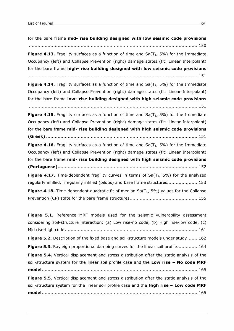
for the bare frame low- rise building designed with no seismic code provisions 150
Figure 4.11. Fragility surfaces as a function of time and Sa(T1, 5%) for the Immediate
Occupancy (left) and Collapse Prevention (right) damage states (fit: Linear Interpolant)
for the bare frame mid- rise building designed with no seismic code provisions 150
Figure 4.12. Fragility surfaces as a function of time and Sa(T1, 5%) for the Immediate
Occupancy (left) and Collapse Prevention (right) damage states (fit: Linear Interpolant)
List of Figures xv
for the bare frame mid- rise building designed with low seismic code provisions
..................................................................................................................... 150
Figure 4.13. Fragility surfaces as a function of time and Sa(T1, 5%) for the Immediate
Occupancy (left) and Collapse Prevention (right) damage states (fit: Linear Interpolant)
for the bare frame high- rise building designed with low seismic code provisions
..................................................................................................................... 151
Figure 4.14. Fragility surfaces as a function of time and Sa(T1, 5%) for the Immediate
Occupancy (left) and Collapse Prevention (right) damage states (fit: Linear Interpolant)
for the bare frame low- rise building designed with high seismic code provisions
..................................................................................................................... 151
Figure 4.15. Fragility surfaces as a function of time and Sa(T1, 5%) for the Immediate
Occupancy (left) and Collapse Prevention (right) damage states (fit: Linear Interpolant)
for the bare frame mid- rise building designed with high seismic code provisions
(Greek) ......................................................................................................... 151
Figure 4.16. Fragility surfaces as a function of time and Sa(T1, 5%) for the Immediate
Occupancy (left) and Collapse Prevention (right) damage states (fit: Linear Interpolant)
for the bare frame mid- rise building designed with high seismic code provisions
(Portuguese) ................................................................................................. 152
Figure 4.17. Time-dependent fragility curves in terms of Sa(T1, 5%) for the analyzed
regularly infilled, irregularly infilled (pilotis) and bare frame structures..................... 153
Figure 4.18. Time-dependent quadratic fit of median Sa(T1, 5%) values for the Collapse
Prevention (CP) state for the bare frame structures ............................................... 155
Figure 5.1. Reference MRF models used for the seismic vulnerability assessment
considering soil-structure interaction: (a) Low rise-no code, (b) High rise-low code, (c)
Mid rise-high code ............................................................................................ 161
Figure 5.2. Description of the fixed base and soil-structure models under study ....... 162
Figure 5.3. Rayleigh proportional damping curves for the linear soil profile .............. 164
Figure 5.4. Vertical displacement and stress distribution after the static analysis of the
soil-structure system for the linear soil profile case and the Low rise – No code MRF
model ............................................................................................................ 165
Figure 5.5. Vertical displacement and stress distribution after the static analysis of the
soil-structure system for the linear soil profile case and the High rise – Low code MRF
model ............................................................................................................ 165

xvi Seismic vulnerability of reinforced concrete buildings considering aging and SSI effects
Figure 5.6. Vertical displacement and stress distribution after the static analysis of the
soil-structure system for the linear soil profile case and the Mid rise – High code MRF
model ............................................................................................................ 166
Figure 5.7. Hyperbolic backbone curve for soil nonlinear shear stress-strain response
and piecewise-linear representation in multi-surface plasticity (after Prevost, 1985;
Stewart et al., 2008; Parra, 1996) ...................................................................... 167
Figure 5.8. Shear modulus reduction curve by Darendeli, 2001 for clay soil with
plasticity index PI=30 and atmospheric pressure p’0 = 1 atm, utilized for the calibration
of the soil constitutive model in OpenSees ........................................................... 168
Figure 5.9. Schematic view of the modeling approaches to assess the influence of SSI
and site effects under linear elastic or inelastic soil behavior for the high-rise, non ductile
MRF structure .................................................................................................. 170
Figure 5.10. Finite element model of the soil-structure systems in OpenSees in the case
of the high-rise, non ductile MRF structure ........................................................... 170
Figure 5.11. Schematic representation of the analyzed cases for the investigation of the
effect of (a) soil depth and (b) stratigraphy under nonlinear soil behavior ................. 171
Figure 5.12. Acceleration time histories at the base of the Low-rise, No code
structure for the fixed base and SSI configurations considering linear soil behavior
(outcrop input motion: Friuli, 6/5/1976, Mw=6.5, R=23km) .................................... 172
Figure 5.13. Snapshots of floor displacement (left) and storey drifts (right) of the Low-
rise, No code structure at the time corresponding to maxISD for linear soil behavior
(Friuli earthquake 0.3g) .................................................................................... 173
Figure 5.14. Acceleration time histories at the base of the Mid-rise, High code
structure for the fixed base and SSI configurations considering linear soil behavior
(outcrop input motion: Friuli, 6/5/1976, Mw=6.5, R=23km) .................................... 173
Figure 5.15. Snapshots of floor displacement (left) and storey drifts (right) of the Mid-
rise, High code structure at the time corresponding to maxISD for linear soil behavior
(Friuli earthquake 0.3g) .................................................................................... 173
Figure 5.16. Acceleration time histories at the base of the High-rise, Low code
structure for the different analyzed configurations considering or not SSI, site effects and
soil nonlinearity (outcrop input motion: Friuli, 6/5/1976, Mw=6.5, R=23km) ............. 175
Figure 5.17. Maximum interstorey drift ratio (%) for the different analyzed
configurations of the High-rise, Low code building considering or not SSI, site effects
and soil nonlinearity for Friuli earthquake ............................................................ 176

List of Figures xvii
Figure 5.18. Snapshots of floor displacement (left) and storey drifts (right) for the
different analyzed configurations of the High-rise, Low code building at the time
corresponding to maxISD for linear and nonlinear (NL) soil behavior (Friuli earthquake
0.3g) .............................................................................................................. 176
Figure 5.19. Acceleration time histories at the base of the structure for the different
analyzed nonlinear SSI cases with varying soil depth and stratigraphy ..................... 178
Figure 5.20. Stress-strain hysteretic loops at various depths for the 30m homogeneous
and layered soil profiles .................................................................................... 179
Figure 5.21. Stress-strain hysteretic loops at various depths for the 60m homogeneous
and layered soil profiles .................................................................................... 180
Figure 5.22. Maximum interstorey drift ratios (%) for the different analyzed
configurations with varying soil depth and stratigraphy .......................................... 182
Figure 5.23. Snapshots of floor displacement (left) and storey drifts (right) at the time
maxISD occurs for nonlinear soil behavior and varying soil depth and stratigraphy .... 182
Figure 5.24. IDA curves for the prototype fixed base models (Low-rise, No-code; High-
rise, Low-code; Mid-rise, High code) founded on rock ............................................ 184
Figure 5.25. PGA - maxISD relationships for the fixed base high-rise, low code model
founded on rock ............................................................................................... 185
Figure 5.26. Comparative PGA - maxISD relationships for the SSI and fixed base models
of the high-rise, low code structure under linear (left) and nonlinear (right) soil behavior
Figure 5.27. Fragility curves in terms of rock outcropping PGA for the fixed base
structure founded on rock in comparison with the SSI model under linear soil behavior for
the MRF structures under study .......................................................................... 186
Figure 5.28. Fragility curves for the fixed base structure founded on rock in comparison
with the SSI model under linear and nonlinear soil behavior (left) and with the
corresponding fixed base models, which consider site effects (right) ........................ 188
Figure 5.29. Fragility curves for the fixed base structure considering site effects and the
SSI configurations under linear (left) and nonlinear (right) soil behavior .................. 188
Figure 5.30. Fragility curves for different analyzed nonlinear SSI cases with varying soil
stratigraphy for the shallower (left) and the deeper (right) soil profile ...................... 189
Figure 5.31. Comparative PGA - maxISD relationships for the SSI configurations of the
high-rise, low-code MRF under linear (left) and nonlinear (right) soil behavior for the
initial (t=0 years) and the 50-year corrosion scenario (t=50 years) ......................... 190
Figure 5.32. Time-dependent fragility curves in terms of PGA for the analyzed fixed
base and SSI structural configurations ................................................................ 192

xviii Seismic vulnerability of reinforced concrete buildings considering aging and SSI effects
Figure 5.33. Time-dependent fragility curves in terms of PGA for the high rise, low code
building when considering fixed base and SSI structural configurations under linear and
nonlinear soil behavior ...................................................................................... 193
Figure 6.1. General view of the AHEPA hospital complex ....................................... 198
Figure 6.2. (a) Typical floor plan and middle floor with the structural joint and (b)
typical soil profile of AHEPA hospital building (dimension in m) ............................... 201
Figure 6.3. Geometrical properties of the element sections of UNIT 1 and UNIT 2
presented in section A-A’ along the longitudinal direction of the hospital building
(dimensions in m) ............................................................................................ 202
Figure 6.4. Reinforcement layout of UNIT 1 and UNIT 2: red and blue correspond to the
beam and column reinforcement respectively (diameters in mm) ............................ 202
Figure 6.5. Diameters and position of the column reinforced bars of the different floor
levels for both UNIT 1 and UNIT 2 (diameters and dimensions in mm) ..................... 203
Figure 6.6. Floor plans of the basement, 1st and 4th floors and the roof with the
permanent and temporary instrumentation. All SXXXX are accelerometers of the
permanent network, all RE-XX and T4D50 are seismometers of the temporary networks
operating for short period of time inside the hospital. Photos of the SOSEWIN stations at
the 4th floor near the structural joint (RE-39) and at roof (SB0F8) .......................... 206
Figure 6.7. Permanent network array of AHEPA hospital ....................................... 206
Figure 6.8. Earthquake data for the longitudinal (east-west, EW), transverse (north-
south, NS) and vertical (V) components recorded at SOSEWIN sensors at the 4th floor
and the roof from the 11.10.2013 Volvi Earthquake (Mw=4.7, R=10km) ................... 207
Figure 6.9. Sections A-A΄ and B-B΄ along the longitudinal and transverse direction of
the hospital building with the temporary instrumentation ....................................... 208
Figure 6.10. Synchronized ambient noise recordings for the longitudinal component. All
the records have the same amplitude scale (y-axis) .............................................. 209
Figure 6.11. Methodological framework adopted in the present study ..................... 210
Figure 6.12. Stochastic Output-Only Identification ............................................... 211
Figure 6.13. Frequency Domain Decomposition (FDD) method .............................. 212
Figure 6.14. Stochastic subspace identification (SSI) method ................................ 215
Figure 6.15. Visualization of the building’s geometry in MACEC 3.2 ........................ 216
Figure 6.16. Indicative auto-correlation PSDs+ for time series recorded at stations near
the joint, (a) station installed at the basement and (b) station installed at the top ..... 217

List of Figures xix
Figure 6.17. Indicative cross-correlation PSDs+ between time series recorded at
stations of the basement and roof (a) near the joint and (b) far from the joint .......... 217
Figure 6.18. Singular values of Covariance-driven SSI method in decreasing order of
magnitude ....................................................................................................... 218
Figure 6.19. Modal identification applying the Peak Picking (PP), Frequency Domain
Decomposition (FDD) and the reference-based covariance-driven Stochastic Subspace
Identification (SSI-cov) methods using ambient noise measurements ...................... 219
Figure 6.20. Mode shapes corresponding to the five first indentified frequencies for UNIT
1 ................................................................................................................... 221
Figure 6.21. Mode shapes corresponding to the five first identified frequencies for UNIT
2 ................................................................................................................... 221
Figure 6.22. Mode shapes corresponding to the five first indentified frequencies for
BUILDING ....................................................................................................... 222
Figure 6.23. Contribution of the lateral components in the first two modes in the
longitudinal and transverse direction for UNIT 1 .................................................... 222
Figure 6.24. Grid models of the different systems analyzed in MACEC for the earthquake
events: Limnos 2014 ........................................................................................ 224
Figure 6.25. Input acceleration in the longitudinal and transverse direction recorded at
the base of UNIT 1 and the corresponding elastic acceleration response spectra for
Limnos, 24.05.2014 event ................................................................................. 225
Figure 6.26. Modal identification applying the Frequency Domain Decomposition (FDD)
and the Stochastic Subspace Identification (SSI) methods using earthquake recordings of
Limnos, 24.05.2014 event ................................................................................. 225
Figure 6.27. Mode shapes of the identified modes of UNIT 1, UNIT 2 and BUILDING for
the earthquake event of Limnos, 24.05.2014 event. .............................................. 226
Figure 6.28. The different updating scenarios adopted within this study .................. 230
Figure 6.29. Normalized average elastic acceleration response spectrum of the input
motions compared with the corresponding reference spectrum adopted from SHARE for a
475 year return period (http://portal.share-eu.org:8080/jetspeed/portal/) ............... 235
Figure 6.30. Assignments of the immediate occupancy (IO) and collapse prevention
(CP) limit damage state points on the IDA curves for the updated units ................... 237
Figure 6.31. PGA-maxISD relationships for updated finite element models of UNIT 1 and
UNIT 2 ............................................................................................................ 240

xx Seismic vulnerability of reinforced concrete buildings considering aging and SSI effects
Figure 6.32. Comparative plots of the initial fragility curves derived for the two adjacent
building units with the corresponding fragility curves provided by Kappos et al.
(2003;2006).................................................................................................... 241
Figure 6.33. Comparative plot of the “building-specific” fragility curves derived for the
initial and updated models of UNIT 1 and UNIT 2 .................................................. 241
Figure 6.34. Assignments of the IO and CP limit damage state points on the IDA curves
for the corroded units ....................................................................................... 244
Figure 6.35. PGA-maxISD relationships for the corroded (t=45years) hospital buildings
UNIT 1 and UNIT 2 ........................................................................................... 244
Figure 6.36. Comparative plots of the fragility curves corresponding to the initial,
updated and corroded models of UNIT 1 and UNIT 2 ............................................. 245
Figure A.1. Accelerograms of the real seismic records used as input motion for the IDA.
Figure A.2. Normalized elastic response spectra of the seismic records in comparison to
the corresponding median predicted spectrum of Ambraseys et al., (1996). .............. 289
Figure B.1. Grid models of the different systems analyzed in MACEC for the earthquake
events: NW from Lake Langada 2013, West from Kassandra peninsula in Halkidiki 2014
..................................................................................................................... 294
Figure B.2. Grid models of the different systems analyzed in MACEC for the earthquake
events: Thessaloniki 2012 ................................................................................. 294
Figure B.3. Grid models of the different systems analyzed in MACEC for the earthquake
events: Thessaloniki 2013 ................................................................................. 294
Figure B.4. Grid models of the different systems analyzed in MACEC for the earthquake
events: Kalamaria 2014, Limnos 2014 ................................................................. 295
Figure B.5. Grid models of the different systems analyzed in MACEC for the earthquake
events: West from Kassandra peninsula in Halkidiki 2013 ...................................... 295
Figure B.6. Input acceleration in the longitudinal and transverse direction recorded at
the base of UNIT 1 and the corresponding elastic acceleration response spectra for the
NW from Lake Langada, 6.12.2013 event. ........................................................... 297
Figure B.7. Input acceleration in the longitudinal and transverse direction recorded at
the base of UNIT 1 and the corresponding elastic acceleration response spectra for
Limnos, 24.05.2014 event. ................................................................................ 297

List of Figures xxi
Figure B.8. Input acceleration in the longitudinal and transverse direction recorded at
the base of UNIT 1 and the corresponding elastic acceleration response spectra for the
Kalamaria, 16.7.2014 event. .............................................................................. 298
Figure B.9. Input acceleration in the longitudinal and transverse direction recorded at
the base of UNIT 1 and the corresponding elastic acceleration response spectra for the
West from Kassandra peninsula in Halkidiki, 22.8.2014 event. ................................ 298
Figure B.10. Modal identification applying the Frequency Domain Decomposition (FDD)
and the Stochastic Subspace Identification (SSI) methods using earthquake recordings of
the Thessaloniki, 2012 event. ............................................................................ 300
Figure B.11. Modal identification applying the Frequency Domain Decomposition (FDD)
and the Stochastic Subspace Identification (SSI) methods using earthquake recordings of
the Thessaloniki, 2013 event. ............................................................................ 300
Figure B.12. Modal identification applying the Frequency Domain Decomposition (FDD)
and the Stochastic Subspace Identification (SSI) methods using earthquake recordings of
N West from Kassandra peninsula in Halkidiki, 26.10.2013 event. ........................... 301
Figure B.13. Modal identification applying the Frequency Domain Decomposition (FDD)
and the Stochastic Subspace Identification (SSI) methods using earthquake recordings of
NW from Lake Langada, 6.12.2013 event. ........................................................... 301
Figure B.14. Modal identification applying the Frequency Domain Decomposition (FDD)
and the Stochastic Subspace Identification (SSI) methods using earthquake recordings of
Limnos, 24.05.2014 event. ................................................................................ 302
Figure B.15. Modal identification applying the Frequency Domain Decomposition (FDD)
and the Stochastic Subspace Identification (SSI) methods using earthquake recordings of
Kalamaria, 16.07.2014 event. ............................................................................ 302
Figure B.16. Modal identification applying the Frequency Domain Decomposition (FDD)
and the Stochastic Subspace Identification (SSI) methods using earthquake recordings of
the West from Kassandra peninsula in Halkidiki, 22.08.2014 event. ......................... 303
Figure C.1. Accelerograms of the real seismic records used as input motion for the IDA
(continued). .................................................................................................... 306
Figure C.2. Normalized elastic response spectra of the seismic records in comparison to
the corresponding reference normalized spectrum adopted from SHARE for a 475 year
return period. .................................................................................................. 311

xxii Seismic vulnerability of reinforced concrete buildings considering aging and SSI effects
Σχήμα I.1. ∆ιάγραμμα ροής της μεθοδολογίας για την αποτίμηση της σεισμικής
τρωτότητας κτηρίων οπλισμένου σκυροδέματος .................................................... 319
Σχήμα I.2. Σχηματική αναπαράσταση των γεωμετρικών (διατομές) και των
κατασκευαστικών (λεπτομέρειες όπλισης) χαρακτηριστικών των πακτωμένων φορέων . 320
Σχήμα I.3. Σύγκριση μέσου κανονικοποιημένου ελαστικού φάσματος καταγραφών με το
στοχευόμενο μέσο κανονικοποιημένο φάσμα των Ambraseys et al. (1996) ................ 324
Σχήμα I.4. Ορισμός των επιπέδων βλάβης «Άμεση Χρήση μετά το σεισμό ΑΧ» και
«Αποφυγή Κατάρρευσης ΑΚ» επάνω στη διάμεσο καμπύλη απόκρισης των βήμα προς βήμα
δυναμικών αναλύσεων για την περίπτωση του υψηλού κτηρίου σχεδιασμένου με βάση
χαμηλό επίπεδο αντισεισμικού κανονισμού ........................................................... 326
Σχήμα I.5. Ανάλυση παλινδρόμησης για τον υπολογισμό των διαμέσων τιμών του μέτρου
έντασης που αντιστοιχούν στις θεωρούμενες στάθμες βλάβης για την περίπτωση του
υψηλού κτηρίου σχεδιασμένου με βάση χαμηλό επίπεδο αντισεισμικό κανονισμό: (α)
Σχέσεις Sa (T1, 5%) – maxISD σε λογαριθμική κλίμακα και (β) υπολογισμός των διαμέσων
τιμών του μέτρου έντασης για τις ΑΧ και ΑΚ στάθμες βλάβης ................................... 327
Σχήμα I.6. Καμπύλες τρωτότητας του υψηλού κτηρίου σχεδιασμένου με βάση χαμηλού
επιπέδου κανονισμό σε όρους Sa(T1, ξ=5%) για τις στάθμες βλάβης που αντιστοιχούν
στην Άμεση Χρήση «ΑΧ» μετά το σεισμό και την Αποφυγή Κατάρρευσης «ΑΚ» ........... 328
Σχήμα I.7. Σύγκριση των εναρμονισμένων καμπυλών τρωτότητας σε όρους Sa για την
περίπτωση του υψηλού μη τοιχοπληρωμένου κτηρίου σχεδιασμένου βάσει χαμηλού
επιπέδου αντισεισμικό κανονισμό με τις αντίστοιχες καμπύλες των Kappos et al. (2003;
2006) που αντιστοιχούν στην ίδια τυπολογία φορέα ............................................... 329
Σχήμα I.8. Καμπύλες αντίστασης του «γυμνού» και τοιχοπληρωμένου (ομοιόμορφη καθ’
ύψος κατανομή, pilotis) υψηλού κτηρίου σχεδιασμένο με βάση χαμηλό επίπεδο
Κανονισμού για τα θεωρούμενα χρονικά σενάρια ................................................... 332
Σχήμα I.9.Χρονικά εξαρτώμενες καμπύλες τρωτότητας συναρτήσει του Sa(T1, 5%) για τα
πακτωμένα, μη τοιχοπληρωμένα πλαισιακά κτήρια ................................................. 334
Σχήμα I.10.Επιφάνειες τρωτότητας συναρτήσει του χρόνου και Sa(T1, 5%) για τις
στάθμες βλάβης που αντιστοιχούν στην «Άμεση Χρήση μετά το σεισμό» (αριστερά) και της
«Αποφυγή Κατάρρευσης» (δεξιά) για την περίπτωση του μη τοιχοπληρωμένου υψηλού
κτηρίου σχεδιασμένο με βάση χαμηλό επίπεδο αντισεισμικό κανονισμό ...................... 335
Σχήμα I.11.Χρονικά εξαρτώμενες καμπύλες τρωτότητας συναρτήσει του Sa(T1, 5%) για
τα πακτωμένα, τοιχοπληρωμένα πλαισιακά κτήρια (ομοιόμορφη καθ’ ύψος κατανομή και
pilotis) ............................................................................................................ 336
Σχήμα I.12. Αναπαράσταση της χρονικά εξαρτώμενης διαμέσου (σε όρους Sa(T1, 5%))
των καμπυλών με πολυώνυμο δευτέρου βαθμού για την περίπτωση βλαβών που

List of Figures xxiii
αντιστοιχούν στη στάθμη επιτελεστικότητας ΑΚ, για το μη τοιχοπληρωμένο υψηλό κτήριο
σχεδιασμένο βάσει χαμηλού επιπέδου κανονισμό ................................................... 337
Σχήμα I.13. Σχηματική απεικόνιση των εφαρμοσμένων προσομοιωμάτων για τη μελέτη
της επιμέρους επιρροής της ∆ΑΕΚ και των τοπικών εδαφικών συνθηκών για την
περίπτωση του υψηλού κτηρίου σχεδιασμένο βάσει χαμηλού επιπέδου κανονισμό ....... 339
Σχήμα I.14. Σχηματική απεικόνιση των υπό μελέτη περιπτώσεων που εξετάζουν την
επιρροή (α) του βάθους και (β) της διαστρωμάτωσης του εδαφικού προφίλ για ανελαστική
συμπεριφορά εδάφους για την περίπτωση του υψηλού κτηρίου σχεδιασμένο βάσει
χαμηλού επιπέδου κανονισμό ............................................................................. 339
Σχήμα I.15. Καμπύλες τρωτότητας των πακτωμένων προσομοιωμάτων θεμελιωμένων σε
βράχο σε σύγκριση με τα προσομοιώματα ∆ΑΕΚ για ελαστική συμπεριφορά εδάφους. Οι
καμπύλες τρωτότητας αναφέρονται και στα τρία υπό μελέτη πλαισιακά κτήρια και
εκφράζονται σε όρους μέγιστης εδαφικής επιτάχυνσης PGA σε συνθήκες «οιονεί» βράχου
..................................................................................................................... 342
Σχήμα I.16. Καμπύλες τρωτότητας του πακτωμένου υψηλού κτηρίου θεμελιωμένο σε
βράχο και των προσομοιωμάτων ∆ΑΕΚ (αριστερά) καθώς και των πακτωμένων
προσομοιωμάτων που λαμβάνουν υπόψη την ΕΤΕΣ (δεξιά) για ελαστικό και ανελαστικό
έδαφος ........................................................................................................... 343
Σχήμα I.17. Καμπύλες τρωτότητας του πακτωμένου μοντέλου λαμβάνοντας υπόψη την
ΕΤΕΣ και των μοντέλων ∆ΑΕΚ για ελαστικό (αριστερά) και ανελαστικό (δεξιά) έδαφος . 343
Σχήμα I.18. Καμπύλες τρωτότητας των υπό μελέτη συστημάτων ∆ΑΕΚ για ανελαστικό
έδαφος με διαστρωμάτωση μικρότερου (αριστερά) και μεγαλύτερου (δεξιά) βάθους .... 344
Σχήμα I.19. Χρονικά εξαρτώμενες καμπύλες τρωτότητας σε όρους PGA των υπό μελέτη
πακτωμένων φορέων και των αντίστοιχων συστημάτων εδάφους – κατασκευής που
λαμβάνουν υπόψη τη ∆ΑΕΚ για ελαστική συμπεριφορά του εδάφους ........................ 345
Σχήμα I.20. Χρονικά εξαρτώμενες καμπύλες τρωτότητας σε όρους PGA για το υψηλό
κτήριο σχεδιασμένο με βάση χαμηλού επιπέδου κανονισμό θεωρώντας συνθήκες
πάκτωσης στο βράχο καθώς και τη ∆ΑΕΚ για ελαστικό και μη γραμμικό έδαφος .......... 346
Σχήμα I.21. ∆ιάγραμμα ροής της μεθοδολογίας για την αποτίμηση της σεισμικής
τρωτότητας κτηρίων οπλισμένου σκυροδέματος με βάση μετρήσεις πεδίου ................ 348
Σχήμα I.22. Νευρολογική κλινική του νοσοκομείου ΑΧΕΠΑ: τυπικός όροφος και όροφος
μεσοπατώματος των δυο επιμέρους κτηρίων και η ένωσή τους μέσω του κατασκευαστικού
αρμού ............................................................................................................. 349
Σχήμα I.23. Τομές Α-Α’ και Β-Β’ κατά τη διαμήκη και εγκάρσια διεύθυνση του
νοσοκομειακού κτηρίου με τη διάταξη του προσωρινού δικτύου ............................... 350

xxiv Seismic vulnerability of reinforced concrete buildings considering aging and SSI effects
Σχήμα I.24. Αποτελέσματα ταυτοποίησης των υπό μελέτη συστημάτων με βάση τις
μεθόδους FDD και SSI χρησιμοποιώντας μετρήσεις θορύβου ................................... 351
Σχήμα I.25. Σύγκριση μέσου κανονικοποιημένου ελαστικού φάσματος απόκρισης
επιταχύνσεων των κινήσεων εισαγωγής με το αντίστοιχο κανονικοποιημένο φάσμα του
SHARE για περίοδο επαναφοράς τα 475 έτη (http://portal.share-
eu.org:8080/jetspeed/portal/) ........................................................................... 354
Σχήμα I.26. Ορισμός των οριακών τιμών ΑΧ και ΑΚ των αναπροσαρμοσμένων
προσομοιωμάτων βάσει των καμπυλών απόκρισης των δυναμικών βήμα προς βήμα
επαυξητικών αναλύσεων .................................................................................... 355
Σχήμα I.27. Συγκριτικά γραφήματα των καμπυλών τρωτότητας για τα αρχικά αριθμητικά
προσομοιώματα των δυο επιμέρους κτηρίων Γ και ∆ και των καμπυλών των Kappos et al.
(2003;2006) για την ίδια τυπολογία .................................................................... 356
Σχήμα I.28. Συγκριτικά γραφήματα των καμπυλών τρωτότητας των αρχικών και
αναπροσαρμοσμένων κτηρίων Γ και ∆ .................................................................. 357
Σχήμα I.29. Συγκριτικά γραφήματα των καμπυλών τρωτότητας των αρχικών,
αναπροσαρμοσμένων και διαβρωμένων προσομοιωμάτων των κτηρίων Γ και ∆ ........... 357

LIST OF TABLES
Table 2.1. SYNER-G taxonomy for buildings .......................................................... 12
Table 2.2.Comparison of existing damage scales with the HRC damage scale (adapted
from Rossetto and Elnashai, 2003) ....................................................................... 21
Table 2.3. Damage states (adapted from Rossetto and Elnashai, 2003) ................... 22
Table 2.4. Damage states (Park et al., 1984; Williams and Sexsmith, 1995) ............. 25
Table 2.5. Range of the proposed damage index for different damage states (Ghobarah
et al., 1999) ...................................................................................................... 27
Table 2.6. Compliance criteria for assessment of RC flexural member in Eurocode 8 –
Part 3 (Fardis 2014) ........................................................................................... 28
Table 2.7. Description of the discrete damage scales adopted in Crowley et al. (2004)
for RC frame structures ....................................................................................... 29
Table 2.8. Damage states for damage index based on interstorey drift (Algan, 1982) . 31
Table 2.9. Damage states for damage index based on interstorey drift for ductile MRFs
(Ghobarah, 2004) .............................................................................................. 32
Table 2.10. Drift ratio (%) limits associated with various damage levels (Ghobarah,
2004) ............................................................................................................... 32
Table 2.11. Limit state criteria adopted for the reference building structure in Ji et al.
(2007) .............................................................................................................. 32
Table 2.12. Sources of uncertainty in fragility functions as identified in FEMA461 (2007)
....................................................................................................................... 34
Table 2.13. Statistical quantification of parameters affecting chloride induced corrosion
according to FIB-CEB Task Group (2006) ............................................................... 59
Table 2.14.Classification of icorr based on laboratory test or measurements on real size
structures ......................................................................................................... 60
Table 2.15. Chloride-induced corrosion rates (icorr-20) for the different exposure
classes according to DuraCrete (1998) .................................................................. 60
Table 2.16. Suggested ranges of icorr for EN 206 exposure classes (Rodriguez et al.,
1994) ............................................................................................................... 61
Table 3.1. Characteristics of the reference studied buildings .................................... 75

xxvi Seismic vulnerability of reinforced concrete buildings considering aging and SSI effects
Table 3.2. Parameter values for the definition of the material object ‘Concrete01’ in
OpenSees (unconfined concrete) .......................................................................... 83
Table 3.3. Characteristics of the infilled studied buildings ........................................ 86
Table 3.4. Lists of records used for the IDA .......................................................... 88
Table 3.5. Description of Immediate Occupancy and Collapse Prevention performance
levels according to FEMA356 for concrete frames .................................................... 93
Table 3.6. CP limit state maxISD values defined on the IDA curve for the bare frame
fixed base intact structures .................................................................................. 94
Table 3.7. CP limit state maxISD values defined on the IDA curve for the infilled fixed
base, intact structures ........................................................................................ 94
Table 3.8. Seismic fragility parameters in terms of Sa(T1, ξ=5%) for fixed base, bare
frame structures .............................................................................................. 100
Table 3.9. Seismic fragility parameters in terms of Sa(T1, ξ=5%) for fixed base, bare
frame structures .............................................................................................. 102
Table 3.10. Main parameters of the fragility curves from the literature used for the
comparison with the Low rise – No code model ..................................................... 105
Table 3.11. Main parameters of the fragility curves from the literature used for the
comparison with the Mid rise – No code model ..................................................... 107
Table 3.12. Main parameters of the fragility curves from the literature used for the
comparison with the Mid rise – Low code model .................................................... 109
Table 3.13. Main parameters of the fragility curves from the literature used for the
comparison with the High rise – Low code model .................................................. 111
Table 3.14. Main parameters of the fragility curves from the literature used for the
comparison with the Low rise – High code model .................................................. 113
Table 3.15. Main parameters of the fragility curves from the literature used for the
comparison with the Mid rise – High code (Greek) model ....................................... 115
Table 3.16. Main parameters of the fragility curves from the literature used for the
comparison with the Mid rise – High code (Portuguese) model. ............................... 117
Table 3.17. Main parameters of the fragility curves from the literature used for the
comparison with the Low rise – No code (regularly and irregularly) infilled model ...... 119
Table 3.18. Main parameters of the fragility curves from the literature used for the
comparison with the High rise – Low code (regularly and irregularly) infilled model .... 121
Table 3.19. Main parameters of the fragility curves from the literature used for the
comparison with the Mid rise – High code (regularly and irregularly) infilled model .... 123

List of Tables xxvii
Table 4.1. Statistical characteristics of parameters affecting the chloride induced
corrosion of RC elements adopted in the present study .......................................... 130
Table 4.2. Loss in reinforcement (%) for the considered corrosion scenarios ............ 132
Table 4.3. Concrete cover strength reduction (%) for the considered corrosion scenarios
..................................................................................................................... 133
Table 4.4. Steel ultimate deformation reduction (%) for the considered corrosion
scenarios ........................................................................................................ 133
Table 4.5. Fundamental periods of the reference uncorroded (t=0 years) and corroded
(t=25, 50, 75 years) bare frame MRF structures ................................................... 133
Table 4.6. Fundamental periods of the uncorroded (t=0 years) and corroded (t=50
years) regularly and irregularly infilled MRF structures ........................................... 133
Table 4.7. CP limit state maxISD values defined on the IDA curve for the bare frame
structures over time ......................................................................................... 145
Table 4.8. CP limit state maxISD values defined on the IDA curve for the infilled
buildings for the initial and 50-year corrosion scenario ........................................... 145
Table 4.9. Time-dependent fragility parameters in terms of Sa(T1, 5%) for the fixed
base, bare frame structures ............................................................................... 148
Table 4.10. Time-dependent fragility parameters in terms of Sa(T1, 5%) for the bare,
regularly infilled and irregularly infilled (pilotis) frame buildings .............................. 154
Table 4.11. Coefficients of quadratic interpolation for the median IO and CP limit values
and the corresponding dispersion (in terms of log-standard deviation) ..................... 156
Table 5.1. Summary of parameters adopted for the linear soil profile case .............. 165
Table 5.2. Summary of parameters adopted for the pressure independent multi-yield
plasticity model ................................................................................................ 169
Table 5.3. Parameters of the fragility functions in terms of PGA for the fixed base
founded on rock models and for the SSI configurations under linear soil behavior ...... 187
Table 5.4. Parameters of the fragility functions in terms of PGA for the analyzed
structural configurations when considering or not SSI and site effects under linear or
nonlinear behavior for the case of the High rise – Low code building ........................ 188
Table 5.5. Parameters of the fragility functions in terms of PGA for the analyzed
structural configurations when considering the soil depth and stratigraphy under
nonlinear soil behavior ...................................................................................... 190
Table 5.6. Parameters of the fragility functions in terms of PGA for the considered
structural configurations and corrosion scenarios .................................................. 191

xxviii Seismic vulnerability of reinforced concrete buildings considering aging and SSI effects
Table 5.7. Time-dependent fragility parameters in terms of PGA for the high rise, low
code building considering fixed base and SSI (for linear or nonlinear soil behavior)
structural configurations .................................................................................... 193
Table 6.1. Main characteristics of the hospital building units (fc and fy represent the
strength of concrete and reinforcement steel respectively) ..................................... 200
Table 6.2. Serial number and position of all the stations used in the two-day ambient
noise experiment ............................................................................................. 208
Table 6.3. Modal identification results for UNIT 1, UNIT 2 and BUILDING estimated
using parametric and non-parametric identification techniques ............................... 219
Table 6.4. Earthquake events used for OMA of the hospital building ...................... 224
Table 6.5. Modal identification results for the recorded earthquake events compared to
the corresponding results for the noise measurements (FDD) ................................. 227
Table 6.6. Comparison of the updated finite element model of UNIT 1 with the initial
model and the experimental results (T: period, f: frequency) .................................. 232
Table 6.7. Comparison of the updated finite element model of UNIT 2 with the initial
model and the experimental results (T: period, f: frequency) .................................. 232
Table 6.8. List of records used for the IDA .......................................................... 235
Table 6.9. Statistical characteristics of parameters affecting the chloride induced
corrosion of RC elements adopted in the present study (according to the methodology of
Chapter 4) ...................................................................................................... 242
Table 6.10. Loss of reinforcement (%) and concrete cover strength reduction (%) for
the considered corrosion scenario (t=45 years) .................................................... 242
Table 6.11. Parameters of the derived fragility curves for the initial and updated finite
element models for UNIT 1 and UNIT 2 ............................................................... 245
Πίνακας I.1. Κύρια χαρακτηριστικά των πλαισιακών κτηριακών προσομοιωμάτων ...... 320
Πίνακας I.2. Κύρια χαρακτηριστικά των τοιχοπληρωμένων πλαισιακών κτηριακών
προσομοιωμάτων .............................................................................................. 323
Πίνακας I.3. Σεισμικές διεγέρσεις για τη διεξαγωγή των ανελαστικών δυναμικών
Πίνακας I.4. Οριακές τιμές της στάθμης βλάβης «Αποφυγή Κατάρρευσης» όπως έχουν
υπολογισθεί για τα «γυμνά» πλαίσια και τα θεωρούμενα χρονικά σενάρια .................. 332
Πίνακας I.5. Οριακές τιμές της στάθμης βλάβης «Αποφυγή Κατάρρευσης» όπως έχουν
υπολογισθεί για τα τοιχοπληρωμένα πλαίσια και τα θεωρούμενα χρονικά σενάρια ....... 333

List of Tables xxix
Πίνακας I.6. Κύρια χαρακτηριστικά των υπό μελέτη κτηρίων της νευρολογικής κλινικής
..................................................................................................................... 349
Πίνακας I.7. Αποτελέσματα ιδιομορφικών αναλύσεων με βάση την FDD και SSI
μεθοδολογία για το ΚΤΗΡΙΟ Γ, ΚΤΗΡΙΟ ∆ και ΕΝΙΑΙΟ ΚΤΗΡΙΟ .................................. 351
Πίνακας I.8. Σύγκριση του αναπροσαρμοσμένου προσομοιώματος του κτηρίου Γ με το
αντίστοιχο αρχικό και πειραματικό προσομοίωμα (T: ιδιοπερίοδος, f: ιδιοσυχνότητα) .. 353
Πίνακας I.9. Σύγκριση του αναπροσαρμοσμένου προσομοιώματος του κτηρίου ∆ με το
αντίστοιχο αρχικό και πειραματικό προσομοίωμα (T: ιδιοπερίοδος, f: ιδιοσυχνότητα) .. 353

xxx Seismic vulnerability of reinforced concrete buildings considering aging and SSI effects

Sotiria Karapetrou – Doctoral Thesis
CHAPTER 1
Introduction
1.1 Statement of the problem
In the last few decades, the significant increase in the social and economic losses caused
by earthquakes worldwide, has stimulated many studies on seismic risk of structures.
The disastrous effects of strong seismic events on social and economical scale, such as
the recent earthquakes of Japan (Tohoku, 2011) and New Zealand (Christchurch, 2011),
have emerged the need of developing operational tools in order to increase preparedness
and establish efficient mitigation and emergency management strategies. Thus scientific
research has been focused not only in the seismic design and analysis of new structures
but also on the assessment of the seismic performance of the existing ones. In order to
design efficient assessment tools that could be utilized by civil protection authorities,
decision makers in emergency management organizations, insurance companies,
engineers, seismologists etc., a reliable risk model for the region or for a specific
structure under consideration needs to be compiled in order to predict future losses due
to seismic events with a high accuracy level.
In this context, the reliable vulnerability assessment of existing structures and
infrastructures is a prerequisite for seismic loss estimation, risk mitigation and
management. Vulnerability is commonly expressed through fragility functions
representing the probability of exceeding a prescribed level of damage for a wide range
of ground motion intensities. There are numerous studies regarding the derivation of
fragility curves for reinforced concrete (RC) buildings (e.g. Rossetto and Elnashai, 2003;
Mosalam et al., 1997; Chryssanthopoulos et al., 2000; Kappos et al., 2006 etc.).
Traditionally, it is implicitly assumed that the structures are optimally maintained during
their lifetime and the impact of the progressive deterioration due to various time-
dependent mechanisms on structural performance is commonly neglected. Although
widely applied seismic vulnerability assessment methods (e.g. HAZUS methodology)
allow the integration of coefficients that depend on the maintenance condition or are
related to in-situ properties of building materials, such integration does not necessarily

CHAPTER 1: Introduction 2
Sotiria Karapetrou – Doctoral Thesis
increase the reliability of the results as the actual structural state may still not be
captured properly. Moreover the development of degradation phenomena in time is
generally neglected. On this basis deterioration of the material properties caused by
aggressive environmental attack is not accounted for. One of the primary sources of
structural degradation is the corrosion of RC members, generally associated to
carbonation process and chloride penetration, leading to the variation of the mechanical
properties of steel and concrete over time. Consequently, both safety and serviceability
of RC structures may be affected under the action of seismic (or even static) loading,
compromising the capability of the structures to withstand the loads for which they are
designed. Although there are a few studies devoted to the modeling and vulnerability
assessment of RC bridges that have undergone corrosion effects (Choe et al., 2008;
2009; 2010; Ghosh and Padgett, 2010; Simon et al., 2010), research on the fragility
analysis of RC buildings due to aging is still limited.
Besides aging effects the influence of soil conditions and SSI might also contribute to
the building’s seismic fragility. The general assumption that the structure is fixed to its
base ignoring the presence of the soil beneath its foundation may be realistic (or at least
conservative) when the structure is founded on rock or very stiff soil. However, in the
case of softer soil formations, SSI and local site effects may play an important role
modifying considerably the free field input motion as well as the dynamic characteristics
of the building and finally its response (Stewart et al., 1999). Although there are some
studies that take into account the local site effects by providing fragility curves for
buildings for different soil conditions (e.g. NIBS, 2004), the effect of SSI to the expected
structure’s performance has not received much attention. This may be due to the fact
that the incorporation of SSI phenomena in the analysis is generally considered beneficial
reducing the seismic demand and consequently the corresponding structural damage of
non-linear systems (Ciampoli and Pinto, 1995). Nevertheless, it has been shown that soil
deformability and SSI may modify the structural response and fragility leading to either
beneficial or unfavorable effects depending on the dynamic properties of the soil and the
structure as well as the characteristics (frequency content, amplitude, significant
duration) of the input motion (e.g. Dutta et al., 2004; Saez et al., 2011; Rajeev and
Tesfamariam, 2012).
In the context of building-specific vulnerability assessment, the use of conventional
generic fragility curves, although appropriate for assessing fragility and losses in a
regional/urban scale, may lead to inaccurate fragility and loss estimates in the case of
individual building assessment, which constitute crucial components in the framework of
decision making and risk mitigation strategies (e.g. seismic safety and rehabilitation
costs). This issue is crucial especially in the case of structures with strategic interest (e.g.

CHAPTER 1: Introduction 3
Sotiria Karapetrou – Doctoral Thesis
hospital buildings, harbor facilities, nuclear power plants etc.). The use of field
monitoring data for identifying the actual state of existing structures has recently drawn
attention in the civil engineering community for developing real time assessment tools
and reducing uncertainties involved within the risk assessment procedure (Gueguen et
al., 2007; Michel et al., 2008; 2012). Real-time monitoring of civil structures and
infrastructures provide valuable information to assess the structural health and identify
the actual state and vulnerability of the associated systems. Furthermore, it allows
monitoring the evolution of the structure’s safety during the earthquake crisis while it
constitutes the key component for rapid damage assessment or the preparation of
reliable damage scenarios. The integration of a comprehensive methodology for the
seismic vulnerability assessment of critical structures and infrastructures using
monitoring data, constitutes an efficient tool for reducing the uncertainties associated
with the risk assessment procedure improving seismic safety and allowing the
development of robust real time assessment tools and appropriate risk mitigation
strategies.
1.2 Objectives and scope of the research
The present thesis aims to propose and quantify an analytical methodology to assess the
seismic vulnerability of reinforced concrete buildings taking into account aging as well as
soil-structure interaction and site effects. Probabilistic fragility curves are proposed for
different structural typologies that might be used by scientists and practitioners for
efficient implementation within a probabilistic risk assessment framework on a regional
scale.
Moreover on a building-specific scale, an integrated methodology is proposed for the
derivation of seismic fragility functions using field monitoring data. The use of field
monitoring data constitutes a significant tool for the representation of the actual
structural state, reducing uncertainties associated with the building configuration
properties as well as many non-physical parameters (age, maintenance, etc.), enhancing
thus the reliability in the risk assessment procedure. The methodology is highlighted
through its application on a hospital building located in Thessaloniki, Greece.
1.3 Outline of the Thesis
The thesis is organized into seven chapters with the following contents:
In the present chapter (Chapter 1), the motivation and the main objectives of the
research are presented.

CHAPTER 1: Introduction 4
Sotiria Karapetrou – Doctoral Thesis
In Chapter 2 the main issues involved in the seismic vulnerability assessment of RC
buildings are discussed. More specifically the chapter is divided into two parts. The first
part outlines the main components, parameters and methods to derive fragility functions,
which are used in the seismic risk assessment of reinforced concrete buildings at urban
and regional scale. Its aim is to provide a mean of understanding the main factors
governing the current practice in seismic vulnerability assessment. The second part of
the chapter discusses the needs and challenges that have not been thoroughly studied up
to now and are investigated in the present thesis aiming at enhancing the reliability and
robustness of seismic vulnerability assessment procedures.
Chapter 3 focuses on the quantification of an analytical procedure to assess the
vulnerability of reinforced concrete (RC) structures subjected to seismic motion.
Vulnerability is expressed in terms of probabilistic fragility curves, which describe the
probability of exceeding a predefined level of damage under a seismic excitation of a
given intensity. Furthermore the reference RC buildings are presented, that have been
selected in the context of the present thesis for the seismic vulnerability assessment
considering aging and soil-structure interaction effects. Seven two-dimensional RC
moment resisting frame structures (MRF) have been adopted from the literature to
represent varying typologies designed with different seismic code levels. The structural
detailing, material properties as well as modeling issues and associated assumptions are
addressed in full detail. To illustrate the methodological framework of the seismic
vulnerability assessment, fragility curves are derived for the fixed base, intact frame
buildings. The effects of aging and soil-structure interaction are investigated in the
ensuing chapters. In terms of numerical computations, incremental dynamic analysis
(IDA) of the structural models is performed for the estimation of the fragility function
parameters. Finally the derived fragility curves for the fixed base, intact frame buildings
are compared with proposed curves from the literature to verify the validity of the
proposed methodology.
In Chapter 4 time-dependent fragility functions of the reference MRF buildings are
developed taking into account deterioration due to aging effects. The consideration of
aging is achieved including probabilistic models of chloride induced corrosion
deterioration of the RC elements within the vulnerability assessment framework
presented in detail in Chapter 3. The structural models are analyzed assuming fixed base
conditions for their uncorroded (t=0 years) and corroded (t=25, 50, 75 years) states. In
particular chloride induced corrosion is considered based on probabilistic modeling of
corrosion initiation time and corrosion rate. Different corrosion aspects are considered in
the analysis including the loss of reinforcement cross-sectional area, the degradation of
concrete cover and the reduction of steel ultimate deformation. Furthermore the relative

CHAPTER 1: Introduction 5
Sotiria Karapetrou – Doctoral Thesis
contribution of infill walls on the expected structural performance over time is also
assessed, analyzing both regularly and irregularly infilled (i.e. pilotis) moment resisting
frames and comparing their seismic behavior with the corresponding bare frames.
The aim of the research presented in Chapter 5 is to investigate whether soil-
structure interaction (SSI) and site effects may affect the seismic performance and
vulnerability of reinforced concrete moment resisting frame buildings and consequently
modify the fragility curves. The direct one-step approach is applied for the SSI modeling
under linear or nonlinear soil behavior while site effects are inherently accounted for. To
further examine the contribution of site and SSI effects, a two-step uncoupled approach
is also applied, which takes into account site effects on the response of the fixed base
structures, but neglects SSI effects. Additional analyses are performed investigating the
influence of the soil depth and stratigraphy under nonlinear soil behavior on the seismic
response and fragility of RC buildings. Finally time-dependent fragility functions of the RC
buildings are derived considering both SSI and aging effects. The chloride induced
corrosion model presented in Chapter 4 is adopted considering two time-scenarios (t=0
and 50 years).
In Chapter 6 the seismic vulnerability of existing RC buildings is evaluated combining
through a comprehensive methodology, the numerical analysis and field monitoring data.
Monitoring data of the building are exploited for the representation of the actual
structural state, reducing uncertainties associated with the building configuration
properties as well as many non-physical parameters (age, maintenance, etc.) increasing
thus the reliability of the derived fragility curves. The proposed methodology is
highlighted through the derivation of “time-building specific” fragility curves for an eight-
storey RC structure (hospital building), built almost five decades ago, that is composed
by two adjacent units connected with a structural joint. The assessment of the dynamic
characteristics is performed using ambient noise measurements recorded by a temporary
seismic network which was deployed inside the hospital. The modal identification results
are used to update and better constrain the initial finite element model of the building,
which is based on the available design and construction documentation plans. Three-
dimensional incremental dynamic analysis is performed to derive the fragility curves for
the initial as built model (“building-specific”) and for the real structures as they are
nowadays (“time-building specific”). The initial “building specific” curves are evaluated
through their comparison with conventional generic curves that are commonly used in
risk assessment studies. Moreover, in order to validate and enhance the reliability of the
obtained results, the “time-building specific” fragility curves, are compared to time-
dependent curves derived for the hospital units applying the analytical methodology

CHAPTER 1: Introduction 6
Sotiria Karapetrou – Doctoral Thesis
proposed in Chapter 4 adopting an appropriate for the specific case study corrosion
scenario.
Chapter 7 summarizes the main findings and contributions of the work providing also
recommendations and suggestions for future research.

Sotiria Karapetrou – Doctoral Thesis
CHAPTER 2
Literature review on the seismic vulnerability assessment of RC buildings
2.1 Introduction
The present chapter aims at providing a critical review of the main issues involved in the
seismic vulnerability assessment of reinforced concrete (RC) buildings. The first part
outlines the main components, parameters and methods to derive fragility functions,
which are used in the seismic risk assessment of RC buildings at urban and regional
scale. Its aim is to provide a mean of understanding the main factors governing the
current practice in seismic vulnerability assessment. The second part of the chapter
discusses the needs and challenges that have not been thoroughly investigated up to
now and are investigated in the present thesis aiming at enhancing the reliability and
robustness of seismic vulnerability assessment procedures.
2.2 Background
Seismic risk assessment can be defined as the estimation of the probability of expected
damages and losses due to seismic hazard. In the past decades the field of seismic risk
assessment has received significant attention (Calvi et al., 2006) due to the dramatic
increase in the losses caused by earthquakes, that has been observed worldwide. The
formulation of an earthquake loss model for a given region is a critical component not
only for predicting the economic impact of future seismic events but also for establishing
emergency preparedness and risk mitigation strategies by the national authorities. A
significant component of a loss model is the methodology to assess the vulnerability of
the built environment. The vulnerability of a structure is described in all engineering-
relevant approaches as vulnerability and/or fragility functions, which can be regarded as
a graphical representation of seismic risk. More specifically vulnerability functions provide
the probability of losses (social or economic) given the level of ground shacking whereas
fragility functions describe the probability of exceeding different limit states (usually

Chapter 2: Literature review on the seismic vulnerability assessment of RC buildings 8
Sotiria Karapetrou – Doctoral Thesis
expressed as physical damage) given the level of ground shaking. The former relates the
level of ground shaking with the mean damage ratio (e.g. ratio of cost of repair to cost of
replacement) and the latter relates the level of ground motion with the probability of
exceeding the limit states (Pitilakis et al., 2014a).
In structural performance evaluation, it is convenient to describe the system
performance in terms of demand and capacity. The demand can be defined in terms of
different response parameters (e.g. shear, bending moment, displacement, velocity,
acceleration, drift, ductility, energy dissipation etc.) in the system caused by the ground
excitation. The capacity of the system is the maximum forces or response that the
system can withstand without member or system failure. The assessment of vulnerability
is made for a particular characterization of ground motion, which represents the seismic
demand of the earthquake on the building. The selected parameter should correlate the
ground motion with the damage to the building. Thus the definition of two intermediate
variables is required, one describing the ground motion intensity measure (IM) and the
other describing the structural demand, also known as engineering demand parameter
(EDP).
Simply stated fragility defines the conditional probability P[∙] of the seismic demand
(D) placed upon the structure exceeding its capacity (C) for a given level of ground
motion intensity (IM), as shown in the following equation:
Fragility P D C IM (2.1)
Different mathematical procedures for developing fragility curves have been proposed
in the literature (e.g. ATC-13, 1985; Shinozuka et al., 2000; Cornell et al., 2002; NIBS,
2004; Nielson and DesRoches, 2007; Porter et al., 2007 etc.). However two-parameter
lognormal distribution functions are traditionally used due to their simple parametric form
(Shinozuka et al., 2000). Thus Equation 2.1 can be further represented through Equation
2.2, which gives the cumulative probability of exceeding a particular damage state dsi
conditioned on a measure of the seismic intensity IM.
[ ]itot mi
1 IMP ds ds IM Φ lnβ IM
(2.2)
where P[∙] denotes the probability of being at or exceeding a particular damage state dsi
for a given seismic intensity level defined by the earthquake intensity measure IM, Φ is
the standard normal cumulative distribution function, IMmi is the median threshold value
of the earthquake intensity measure IM required to cause the ith damage state and βtot is
the total standard deviation. According to Equation 2.2, to develop fragility curves the
definition of two parameters is required, namely IMmi and βtot.

Chapter 2: Literature review on the seismic vulnerability assessment of RC buildings 9
Sotiria Karapetrou – Doctoral Thesis
Figure 2.1 presents the graphical representation of a fragility curve. The conditional
probabilities P[ds=i/IM] for a structure experiencing a specific damage state dsi
illustrated in Figure 2.2, are estimated based on the probabilities of exceedance
P[ds≥i/IM]. For example if four damage states are adopted (i=0,1,2,3) then the
probabilities that a structure experiences the different damage states are calculated as:
P0(=no damage)=1.0-P(ds ≥ slight damage)
P1(=slight damage)= P(ds ≥ slight damage) – P(ds ≥ moderate damage)
P2(=moderate damage)= P(ds ≥ moderate damage) - P(ds ≥ extensive damage)
P3(=extensive damage)= P(ds ≥ extensive damage)
The total sum of these probabilities is equal to 1.
Figure 2.1. Graphical presentation of an example fragility curve
Figure 2.2. Conditional probabilities of exceeding different damage states

Chapter 2: Literature review on the seismic vulnerability assessment of RC buildings 10
Sotiria Karapetrou – Doctoral Thesis
The vulnerability curve can be generated based on the estimation of the mean
damage ratio MDR. In Figure 2.3 an example vulnerability curve is presented. The MDR is
a representative single statistics that can be calculated assuming a repair cost for each
damage level (Hancilar et al., 2014). It is mathematically expressed as:
[ ]i ids
MDR CDR P ds i IM (2.3)
where CDRi represents the central damage ratio which is the ratio of the average cost of
repair at each damage state to the cost for building replacement (Hwang et al., 1994).
Figure 2.3. Conditional probabilities of exceeding different damage states
HAZUS (NIBS, 2004) is the first comprehensive methodology that contains models for
estimating potential losses of buildings from earthquake hazards at an urban scale. Its
first edition was released in 1997 (HAZUS, 97); the current version is HAZUS-MH v2.0,
which estimates the risk due to earthquakes, floods and hurricanes. Fragility curves for
buildings, utility and transportation networks are provided in HAZUS methodology. In the
first editions, the majority of the fragility functions were relied on the methodology and
data that were presented in ATC-13 (ATC, 1985) and ATC-25 (ATC, 1991) reports
following an expert judgment approach. Analytical studies have been later considered for
bridges and buildings.
In Europe, the first initiative to establish a methodology for the seismic risk
assessment of buildings include the RISK-UE (2004) project followed by LESSLOSS
(2007) both funded by European Commission framework programs for Research and
Technological Development.
Several research efforts have been made at a national level in Europe, aiming to
propose adequate generic fragility curves for buildings. Representative examples include
the SRM-LIFE (2007) projects in Greece and the RELUIS projects in Italy. Finally,

Chapter 2: Literature review on the seismic vulnerability assessment of RC buildings 11
Sotiria Karapetrou – Doctoral Thesis
numerous other research efforts have been performed worldwide, developing fragility
functions and methods for the vulnerability assessment of different physical assets.
Among the latest developments is SYNER-G (2013) project. In the framework of the
project, a comprehensive review of existing fragility curves for the most important
elements at risk has been carried out, while new fragility curves have been developed
where necessary, considering the distinctive features of European elements (Kaynia,
2013). Moreover an integrated methodology has been developed for the systemic seismic
vulnerability and risk analysis of buildings, lifelines, infrastructures, transportation, utility
systems and critical facilities. The main goals of SYNER-G are summarized in the
following bullets:
to elaborate appropriate, in the European context, fragility relationships for the
vulnerability analysis and loss estimation of all elements at risk
to develop social and economic vulnerability relationships for quantifying the
impact of earthquakes
to develop a unified methodology and tools for systemic vulnerability assessment
accounting for all components exposed to seismic hazard, considering
interdependencies within a system unit and between systems
to validate the methodology and the proposed fragility functions in selected sites
(urban scale) and systems and to implement in an appropriate open source and
unrestricted access software tool.
The results of the studies carried out within the project can be found in Pitilakis et al.
(2014a).
2.3 Prerequisites for the derivation of fragility functions
The main parameters that are involved in the derivation of fragility functions, namely
taxonomy/typology/classification, intensity measures and damage states, are presented
in the following subsection. It should be noted herein that the main epistemic
uncertainties involved in the vulnerability assessment procedure are related to the
definition of the aforementioned parameters.
2.3.1 Taxonomy/typology/classification
The knowledge of the inventory of the general building stock in a region exposed to
seismic hazard and the capability to create uniform classes of building types are one of
the main challenges required to carry out a seismic risk assessment at an urban scale,
where it is practically impossible to perform the assessment at a building level. The
development of an efficient taxonomy able to adequately group different types of existing

Chapter 2: Literature review on the seismic vulnerability assessment of RC buildings 12
Sotiria Karapetrou – Doctoral Thesis
buildings from different countries in Europe and worldwide is the key component in the
vulnerability assessment procedure. The classification is made based on the assumption
that buildings with similar structural characteristics are expected to perform in the same
way under a seismic excitation. For buildings the geometry, material properties and
seismic design level are among the common typology parameters.
Several building typologies exist. Prominent among these are: ATC-13 (ATC, 1985);
EMS-98 (Grunthal, 1998); ATC-14 (ATC, 1987), which was used with modifications in
FEMA 154 (ATC, 2002), HAZUS-MH (FEMA, 2006), and other FEMA-funded efforts; the
World Housing Encylopedia (WHE, http://www.world-housing.net/); RISK-UE 2004
(Mouroux et al., 2004); PAGER (Jaiswal and Wald, 2008; Jaiswal et al., 2010,
http://pager.world-housing.net.) and the most recent developed SYNER-G (Pitilakis et
al., 2014a, http://www.syner-g.eu/) for typical European structures.
In SYNER-G a great effort was paid to create a comprehensive taxonomy from which
European typologies for the most important elements at risk are defined (Hancilar and
Taucer, 2013). A taxonomy of existing buildings should allow their classification in terms
of their seismic resistance and response. As shown in Table 2.1, different main categories
are identified to describe a building, such as the force resisting mechanism, material,
elevation, code design level, cladding, etc. A hierarchy is used for some categories where
additional information might or might not be available, largely depending on the scale of
the studied region. Figure 2.4 presents a representative flowchart to group reinforced
concrete (RC) with moment resisting frame (MRF) buildings, taking into account the
height level, the code level, the cladding and the detailing. It is noted that each column
represents a different level of detail.
Table 2.1. SYNER-G taxonomy for buildings
CATEGORY SUB-CATEGORY Force Resisting Mechanism (FRM1) Moment Resisting Frame (MRF) Structural Wall (W) Flat Slab (FS) Bearing Walls (BW) Precast (P) Confined Masonry (CM)
Force Resisting Mechanism (FRM2) Embedded beams (EB) Emergent beams (EGB)
FRM Material (FRMM1) Concrete (C) Masonry (M)
FRM Material (FRMM2) Reinforced Concrete (RC) Unreinforced Masonry (URM) Reinforced Masonry (RM) High strength concrete (>50MPa) (HSC) Average strength concrete (20-50 MPa)
(ASC) Low strength concrete (<20 MPa) (LSC) Adobe (A)

Chapter 2: Literature review on the seismic vulnerability assessment of RC buildings 13
Sotiria Karapetrou – Doctoral Thesis
CATEGORY SUB-CATEGORY Fired brick (FB) Hollow clay tile (HC) Stone (S) High yield strength reinforcing bars
(>300MPa) (HY) Low yield strength reinforcing bars
(<300MPa) (LY) Classification of reinforcing bars based on
EC2 (A,B,C) Lime mortar (LM) Cement mortar (CM) Mud mortar (MM) Smooth rebars (SB) Non-smooth rebars Concrete Masonry Unit (CMU) Autoclaved Aerated Concrete (AAC) High % of voids (H%) Low % of voids (L%) Regular Cut (Rc) Rubble (Ru)
Plan (P) Regular (R) Irregular (IR)
Elevation (E) Regular geometry (R) Irregular geometry (IR)
Cladding (C) Regular infill vertically (RI) Irregular infill vertically (IRI) Bare (B)
Cladding Characteristics (CM) Fired brick masonry (FB) High % voids (H%) Low % voids (L%) Autoclaved Aerated Concrete (AAC) Precast concrete (PC) Glazing (G) Single layer of cladding (SL) Double layer of cladding (DL) Open first floor (Pilotis) (P) Open upper floor (U)
Detailing (D) Ductile (D) Non-ductile (ND) With tie rods/beams (WTB) Without tie rods/beams (WoTB)
Floor System (FS) Rigid (R) Flexible (F)
Floor System Material (FSM) Reinforced concrete (RC) Steel (S) Timber (T)
Roof System (RS) Peaked (P) Flat (F) Gable End Walls (G)
Roof System Material (RSM) Timber (Ti) Thatch (Th) Corrugated Metal Sheet (CMS)
Height Level (HL) Number of stories (NS) [Here the number of stories is explicitly given,

Chapter 2: Literature review on the seismic vulnerability assessment of RC buildings 14
Sotiria Karapetrou – Doctoral Thesis
CATEGORY SUB-CATEGORY Low-rise (1-3) (L) Mid-rise (4-7) (M) High-rise (8-19) (H) Tall (20+)(Ta)
if known]
Code Level (CL) None (NC) Low (<0.1g) (LC) Moderate (0.1-0.3g) (MC) High (>0.3g) (HC)

Chapter 2: Literature review on the seismic vulnerability assessment of RC buildings 15
Sotiria Karapetrou – Doctoral Thesis
Figure 2.4. Flow chart for a Reinforced Concrete, Moment Resisting Frame building class according
to SYNER-G

Chapter 2: Literature review on the seismic vulnerability assessment of RC buildings 16
Sotiria Karapetrou – Doctoral Thesis
2.3.2 Intensity measures
The selection of an appropriate earthquake intensity measure (IM) that characterizes the
strong ground motion (e.g. amplitude, duration, frequency content, energy content) and
correlates well with the building response is of high importance for the derivation of
fragility curves. The optimal selection of IM can be supported by examining the following
qualities (Mackie and Stojadinovic, 2003;2005, Mehanny, 2009, Padgett et al., 2008):
practicality, sufficiency, effectiveness, efficiency, robustness and hazard computability.
Practicality refers to whether or not there is any direct correlation between an IM and the
demand placed on the structure. A further criterion for evaluating practicality is whether
the IM is readily described by available attenuation relationships or other sources of
hazard data. A sufficient IM is statistically independent of ground motion characteristics
(such as magnitude and epicentral distance), rendering a demand model that is
conditionally independent of the earthquake scenario. The effectiveness of an IM is
determined by its ability to evaluate, in a closed form, the mean annual frequency of a
decision variable exceeding a given limiting value. An efficient IM reduces the amount of
variation in the estimated demand for a given IM value. Robustness describes the
efficiency trends of an IM-EDP pair across different structures and therefore fundamental
period ranges. Hazard computability refers to the availability of estimates of the expected
IM from hazard studies.
In general, IMs are grouped into two general categories: the empirical intensity
measures (e.g. European macroseismic scale EMS) and the instrumental intensity
measures (e.g. peak ground acceleration PGA, peak ground velocity PGV, peak ground
displacement PGD etc.) (Pitilakis et al., 2014a). The instrumental intensity measures
have the advantage that the severity of the earthquake is no longer subjective as they
are expressed as an analytical value measured by an instrument or computed analyzing
the seismic recordings and therefore are considered more accurate and representative of
the seismic intensity characteristics.
For the assessment of buildings the strong motion parameters that are used almost
invariably to characterize earthquake shaking are the peak ground acceleration (PGA)
and response spectral ordinates for a linear-elastic lightly-damped (often 5%) single
degree of freedom (SDOF) system. Response spectral ordinate usually refers to spectral
acceleration Sa(Ty) (or pseudo-spectral acceleration) or spectral displacement Sd(Ty) at
the elastic natural period Ty of the structure and their advantage in comparison to PGA is
that they provide information also on the frequency content of earthquake shaking. In
the pie chart of Figure 2.5 the percentages regarding the different IMs used for the
vulnerability assessment of European buildings (Pitilakis et al., 2014a) are presented. In

Chapter 2: Literature review on the seismic vulnerability assessment of RC buildings 17
Sotiria Karapetrou – Doctoral Thesis
the reviewed studies, fragility functions have been derived in terms of macroseismic IMs
(Mercalli-Cancani-Sieberg Intensity Scale: MCS, Modified Mercalli Intensity Scale: MMI,
Medvedev-Sponheuer-Karnik Intensity Scale: MSK81, European Macroseismic Scale:
EMS98) and instrumental IMs (PGA, PGV, root mean square of the acceleration RMS,
Sa(Ty), Sd(Ty), spectral displacement at the inelastic period TLS corresponding to a specific
damage state: Sd(TLS), roof drift ratio). Sa(Ty), Sd(Ty), Sd(TLS) and roof drift ratio are
structure-dependent IMs as they are based on response parameters and thus require
structural information regarding the building typology. Figure 2.5 shows that PGA has
been the most commonly used intensity measure in the studied literature.
MMI 5%
MCS 2% MSK81
3%
PGA 38%
PGV5%Sa(Ty)
3%
Sd(Ty)15%
Sd(TLS)23%
RMS 3%
Roof Drift Ratio3%
Figure 2.5. Pie chart presenting the percentages of different intensity measure types used for the
development of fragility functions for reinforced concrete buildings (Pitilakis et al., 2014a)
One IM that has recently been shown to be useful in explaining structural response is
epsilon of Sa at a certain structural period Ty, which is defined as the normalized residual,
in terms of natural logarithms, between the observed and the predicted by a given GMPE
for Sa (Baker and Cornell, 2005). The reason why epsilon is a potentially useful IM is that
it is an indicator of peaks and troughs in response spectra scaled to a common Sa at a
given period: negative epsilon generally indicates a trough (hence a higher structural
response because it is influenced by neighboring higher Sa) and positive epsilon means a
peak (hence a lower structural response due to lower Sa at adjacent periods). The use of
epsilon for risk evaluation is possible if its value is known from hazard disaggregation or
by using probabilistic site-specific demand analysis but it is not a suitable parameter for
the construction of fragility functions unless it is combined with a fragility function using
Sa (e.g. Tothong and Luco, 2007).

Chapter 2: Literature review on the seismic vulnerability assessment of RC buildings 18
Sotiria Karapetrou – Doctoral Thesis
2.3.3 Damage indicators and states
In order to derive seismic fragility curves for different elements at risk, it is necessary to
define multiple damage states for the element exposed to seismic hazard. To accomplish
this, the first step is the establishment of a damage indicator or damage measure in
terms of engineering demand parameters that are able to adequately describe its
expected seismic performance.
Generally, damage indices or damage measures aim to quantify the damage level of
structures under earthquake loading. Damage indices are damage functions that are
commonly defined based on the results of a numerical analysis, on the measured
response of a structure during an earthquake or on a comparison of a structure’s
physical properties before and after an earthquake (Williams and Sexsmith, 1995).
Also empirical damage indices may be defined based on databases of damage data
collected following one or more earthquake events.
In general damage indices may consist of one or more damage measures and can be
classified based on deformation terms, stiffness degradation, hysteretic energy
dissipation, number of seismic cycles, engineering experience, observational data as well
as rehabilitation and reconstruction (or replacement) cost. The relationship between a
damage parameter (d) and a damage index (D) is illustrated in Figure 2.6 for the simple
case where D is expressed in terms of a single parameter d (Kappos, 1997). As shown in
Figure 2.6 for D=0 it is d=d0>0, which implies that below a threshold value of the
damage parameter no damage is detected and the structural behavior remains elastic.
On the other hand when d=du structural failure (or complete collapse) is considered and
therefore D=1. For d>dr repair of the structure is required to restore its initial
conditions. The description of the curve shape D=f(d) and the selection of appropriate
values for du and dr is not an easy task due to the lack of sufficient experimental data for
different structural types and the difficulty in the definition of common failure criteria
between the different research groups. A possible expression of the damage index
(Kappos, 1997) could be:
a
cal 0a
u 0
(d d )D
(d d )
(2.4)
where dcal is the value of the damage parameter value calculated from the analysis and a
is an exponent which may be considered equal to unity in the absence of experimental
data. The relationship damage index – damage parameter, as illustrated in Figure 2.6,
can be expressed not only in structural but also in economical terms. In this case the
economic damage index is expressed as the ratio of the required cost of repair to the
corresponding cost of replacement (or reconstruction).

Chapter 2: Literature review on the seismic vulnerability assessment of RC buildings 19
Sotiria Karapetrou – Doctoral Thesis
Numerous damage indices/measures are proposed in the scientific literature. They
may express analytically the comparison of a demand with a capacity quantity, or the
consequence of a mitigation action, or the assembled consequences of all damages (the
“impact”). In the case of reinforced concrete buildings subjected to earthquake loading,
the damage measures that are commonly used, are related to deformation quantities,
such as strain (compressive, tensile) and curvature, rotations at member ends, horizontal
storey displacements, relative displacements between two adjacent storeys (interstorey
drift) and/or fatigue loading terms. For indicators based on displacement or stiffness
degradation, the maximum seismic response of the structures is taken into consideration.
On the other hand, indicators related to degenerative behavior and/or cumulative
damage sustained under repeated load reversals depend on the amount of dissipated
hysteretic energy and take into account the effect of plastic cycles in the structural
response.
The parameters most widely used to evaluate structural damage are ductility and
plastic dissipated energy. In the case of ductility, collapse depends on a predefined
displacement value whilst, in the case of plastic dissipated energy, collapse of the
structure under cyclic loads depends on the amount of energy that can be plastically
dissipated. Indicators based on dynamic properties are used to quantify damage through
modal testing. This approach often includes vibration measurements of the structure due
to a particular excitation. In case of structural deterioration, changes in the measured
dynamic responses are expected. These changes are reflected in the modal properties of
the structure (natural frequencies, damping ratios, mode shapes), which can be
determined either experimentally or analytically. Indices developed on this basis may
provide information both on the extent of damage and its location.
Figure 2.6. Relationship between damage parameter (or damage variable) and damage index
(Kappos, 1997)

Chapter 2: Literature review on the seismic vulnerability assessment of RC buildings 20
Sotiria Karapetrou – Doctoral Thesis
Different schemes are proposed for the classification of damage indices (Kappos,
1997). For example some categorizations are defined based on whether they refer to a
single element or to the whole structure (local or global) or whether they are structural
or economic, on the mathematical approach for their determination (deterministic or
probabilistic) or the type of analysis for their estimation (no analysis, linear elastic,
inelastic). In the next subchapter the most commonly used global and local damage
indices based on structural properties are presented.
Based on performance indicators, damage thresholds may be defined, that are called
limit states. A limit state defines the threshold between different damage conditions,
whereas the damage states define the damage conditions themselves. For example, the
displacement capacity can be related to damage conditions that are identifiable through
limit states. In Figure 2.7 the difference between damage states and limit states is
presented (Crowley et al., 2011).
Figure 2.7. Limit states and damage states (Crowley et al., 2011)
Methods for deriving fragility curves generally model the damage on a discrete
damage scale. In empirical procedures, the scale is used in reconnaissance efforts to
produce post-earthquake damage statistics, whereas in analytical procedures the scale is
related to mechanical properties of the buildings.
The number of damage states (and consequently the number of limit states) depends
on the damage scale used and is related with the functionality of the components and/or
the repair duration and cost. Some of the most frequently damage scales used are: HCR
(Rossetto and Elnashai, 2003), HAZUS99 (FEMA, 1999), Vision2000 (SEAOC,1995),
EMS98 (Grunthal, 1998), ATC-13 (ATC,1985). A summary and qualitative comparison of
some of the damage scales applicable for RC buildings is presented in Table 2.2. It
should be noted that there are some studies that do not refer to any of the damage

Chapter 2: Literature review on the seismic vulnerability assessment of RC buildings 21
Sotiria Karapetrou – Doctoral Thesis
scales reported in Table 2.2 but they follow specific damage state scales developed by
the authors.
Depending on the methodology used to compute the fragility functions, different
scales with different limit states/damage states can be adopted. Limit states in reinforced
concrete structures should be correlated to the predominant damage mode. In this
respect, the corresponding damage index that best reflects a flexural limit state may not
correlate well with damage such as diagonal cracking due to shear, or bond splitting due
to lack of confinement (Williams and Sexsmith, 1995).
Table 2.2.Comparison of existing damage scales with the HRC damage scale (adapted from Rossetto and Elnashai, 2003)
HRC HAZUS99 Vision 2000 EMS98 ATC-13 None No damage
Slight
Slight damage
Fully operational Grade 1
Slight
Light Light
Operational Grade 2
Moderate
Moderate Moderate damage Grade 3
Life Safe Heavy
Extensive Extensive damage
Near Collapse Grade 4
Major Partial Collapse Collapse
Collapse Collapse
2.3.3.1. Local damage indices
Local indices may involve a single damage parameter, such as maximum deformation or
dissipated energy, or two or more parameters. Most local indices are cumulative in
nature, reflecting the dependence of damage on both the amplitude and the number of
cycles of loading. Local damage indices may be further categorized as cumulative and
non-cumulative damage indices. A non-cumulative damage index can only capture the
maximum damage value whereas a cumulative damage index takes into account the
damage accumulation reflecting the dependence of damage on both the amplitude and
the number of cycles of loading.
Non-cumulative damage indices
The non-cumulative damage indices are usually expressed in ductility, deformation or
stiffness terms. The earliest and simplest form of damage indices is ductility. The ductility
ratio can be defined in terms of rotation, curvature or displacement and by choosing it as
a damage measure it is assumed that structural collapse is expected for maximum plastic

Chapter 2: Literature review on the seismic vulnerability assessment of RC buildings 22
Sotiria Karapetrou – Doctoral Thesis
deformation, independent of the number of plastic cycles and the amount of dissipated
energy.
Banon et al. (1981) used the rotational ductility (μθ) at the end of a structural
member as its damage index:
m ymθ
y y
θ θθμ 1
θ θ (2.5)
where θm is the maximum rotation (including both elastic and plastic rotations) under
seismic loading and θy is the yield rotation, considering the member’s antisymmetric
double-curvature bending with the point of contraflexure in its mid-span.
An indicator based on kinematic or cyclic ductility was developed by Cosenza et al.
(1993). The proposed damage index is defined as:
u
μ 1Dμ 1
(2.6)
where μ is the kinematic or cyclic ductility of the structural element and μu the maximum
allowable ductility corresponding to the maximum displacement.
In Erduran and Yakut (2004) damage functions were developed for reinforced
concrete columns based on the drift ratio. More specifically the damage criterion used in
this study depends mainly on the ductility index which is the ratio of the given drift
divided by the yield drift, hence the yield drift. Different parameters that affect the
seismic behavior of a RC column were taken into account, namely the axial load level,
the slenderness, the amount and the yield strength of longitudinal reinforcement and the
amount of the transverse reinforcement. Moreover three ductility levels for the RC
column were considered (low, medium and high). Damage scores were assigned to
different levels of crack widths. The calibration of the corresponding damage states was
achieved based on the criterion suggested by the Japanese government. In Table 2.3 the
proposed limit values of the damage index (DI) corresponding to the different damage
state are summarized.
Table 2.3. Damage states (adapted from Rossetto and Elnashai, 2003)
Damage states Limit values of DI No damage DI < 0.005
Negligible 0.005 < DI < 0.075
Light 0.075 < DI < 0.30
Moderate 0.30 ≤ DI ≤ 0.90
Collapse 0.90 ≤ DI ≤1.00
In Jeong and Elnashai (2005) a damage index in terms of interstorey drift was
preferred to curvature demand, due to the fact that the former is easier to monitor and
accurate enough to estimate damage inflicted on critical columns. The demand-to-

Chapter 2: Literature review on the seismic vulnerability assessment of RC buildings 23
Sotiria Karapetrou – Doctoral Thesis
capacity ratio (DCR) of each column is expressed based on Equation 2.7 and accounts for
the bi-directional response of the structure:
22
x y
∆x ∆yDCR∆u ∆u
(2.7)
where ∆x and ∆y are the interstorey drift in the x direction and in the y direction
respectively while ∆ux and ∆uy the ultimate interstorey drift where the curvature of the
column reaches the ultimate value under average axial force.
Damage indicators based on stiffness and strength degradation have also been
proposed in the literature. Lybas and Sozen (1977) proposed an indicator based on the
stiffness degradation of the damaged component while Banon et al. (1981) defined the
flexural damage ratio (FDR) as an indicator based on stiffness and strength degradation
that occur under cyclic loading. Roufaiel and Meyer (1987a) on the other hand used a
modified version of the flexural damage ratio index, considering the increase in flexibility
at maximum deformation and at failure state.
Cumulative damage indices
Different damage indices are proposed in the literature to model cumulative damage
under cyclic loading. Cumulative indicators are usually defined based on a low-cycle
fatigue formulation, in which damage is considered as a function of either the
accumulated plastic deformation or the hysteretic energy absorbed during the loading.
Stephens and Yao (1987) developed a cumulative damage index based on
displacement ductility considering for its calculation the positive and negative
displacement increments during cyclic loading. Jeong and Iwan (1988) index quantified
damage under cyclic loading combining the effects of cyclic at different amplitudes. More
specifically the proposed index relates the number of cycles at a specific amplitude with
the number of cycles to failure at that same amplitude. It also measured the influence of
both duration and ductility of response.
Many cumulative damage indices are related to the hysteretic behavior of the
concrete member under study. Gosain et al. (1977) first adopted as damage measure a
simple cumulative energy ratio, which was defined based on the force corresponding to
the element displacement in relation to the force corresponding to the element yielding
displacement. Furthermore modification factors were proposed in order to account for the
effect of shear span ratio and axial load. The plastic dissipated energy was firstly
introduced as a damage measure considering cumulative energy absorption (Akiyama,
1985). Researchers have proposed different variations of this type of damage index

Chapter 2: Literature review on the seismic vulnerability assessment of RC buildings 24
Sotiria Karapetrou – Doctoral Thesis
including modification factors to account for the specific geometrical and loading
conditions of reinforced concrete elements.
Kratzig et al. (1989) developed a more complex index formulation based on the
definition of primary and follower half-cycles. A primary half-cycle (PHC) is defined as the
first half-cycle of loading at a given amplitude, with subsequent half-cycles termed as
followers unless they exceed the previous maximum amplitude. Thus, cumulative
damage caused by cyclic loading is taken into account even when no increase in
maximum deformation is noticed. The energy absorbed is considered to be equal to the
area of the hysteresis loops. The energy of each half – cycle may be assumed to be the
half of the complete cycle under the condition that the loops in the load – deformation
diagram are symmetrical.
Combined indices
Park and Ang (1985) damage indicator is a linear combination of maximum deformation
and hysteretic energy dissipation. The form of the Park-Ang index is:
Μe
u y u
dEδDI β
δ F δ (2.8)
where D is the damage index, δm is the maximum response deformation under an
earthquake, dE is the incremental dissipated hysteretic energy, δu is the ultimate
deformation capacity under monotonic loading, Fy is the yield strength of the longitudinal
reinforcement and βe is a nonnegative constant and is a factor which considers the effect
of cyclic loadings on structural damage. It is a function of shear span ratio, normalized
axial stress, longitudinal steel ratio and confinement steel ratio. The first term is the ratio
of maximum recorded deformation to the capacity deformation of a member under
monotonic loading conditions (ductility-based damage index) and the integral term is the
energy dissipation normalized by the product of the yield force and deformation capacity,
scaled by an empirical factor determined on the basis of a large number of test results.
Park et al. (1984) presented five damage levels based on observation of post-earthquake
damage of RC buildings. The suggested classification of limit states is presented in Table
2.4 (Williams and Sexsmith, 1995).
The modified Park-Ang index (Kunnath et al., 1992) slightly modifies Equation 2.8 to
consider only the permanent deformation in the first term. Also moment and curvature
are used instead of force and displacement:
m ye
u y y u
dEφ φDI β
φ φ M φ (2.9)

Chapter 2: Literature review on the seismic vulnerability assessment of RC buildings 25
Sotiria Karapetrou – Doctoral Thesis
where φm is the maximum curvature under seismic loading, φu is the ultimate curvature,
φy is the yielding curvature, βe is an empirical coefficient defined as a function of the
structural characteristics and My the yielding bending moment.
Table 2.4. Damage states (Park et al., 1984; Williams and Sexsmith, 1995)
Damage states Limit values of DI
No damage or localized minor cracking DI < 0.1
Minor damage (light cracking throughout)
0.1 ≤ DI < 0.25
Moderate damage (severe cracking, localized spalling)
0.25 < DI < 0.4
Severe damage (crushing of concrete, reinforcement exposed)
0.4 ≤ DI ≤ 1.0
Collapse (Total or partial collapse of building)
DI ≥1.0
2.3.3.2. Global damage indices
The global damage state of the overall structure depends on both the distribution and
severity of localized damages. The use of local damage indices identifies the weak or
vulnerable elements that should be rehabilitated. However using local damage indices it
is difficult to estimate the structural response to a given ground motion and to assess the
residual strength and safety of a damaged structure. Thus global damage indices are
required for post-earthquake evaluation of structures , reliability studies and applications
in the performance-based engineering approach (Ghobarah et al., 1999).
The approach widely used to obtain the global damage state is to take an average of
the local indices, weighted by the local energy absorption (Park et al., 1987; Chung et
al., 1990; Kunnath et al., 1992). Thus the damage index for a single storey of a
structure is defined as:
i istorey
i
D ED
E
(2.10)
where Di is the local damage index at location i and Ei is the energy absorbed at location
i.
Park and Ang's (1985) global damage index is used to represent the performance
of structural systems. It is defined as a weighted average of the local damage indices of
each element. The weighting function for each element is proportional to the energy
dissipated in the element. The global damage index is given by the following equation:
i iD λD (2.11)

Chapter 2: Literature review on the seismic vulnerability assessment of RC buildings 26
Sotiria Karapetrou – Doctoral Thesis
ii
i
Eλ
E
(2.12)
where Ei is energy dissipated at location i.
Bracci et al. (1989) presented a more generalized definition of the storey damage
index:
(b 1)
i istorey b
i i
w DD
w D
(2.13)
where b is an exponent giving greater emphasis on the most damage elements and wi is
the weights defined as the ratio of the gravity load supported by member i to the total
gravity load on the structure.
Damage causes changes in dynamic structural properties (natural
periods/frequencies, damping, mode shapes). Due to stiffness degradation and energy
dissipation usually an increase in the natural period and damping is expected respectively
(Dowell, 1979). Damping has been found to be too variable as a parameter to be a useful
damage indicator. Thus research has been focused on changes in period and more
specifically in fundamental period (or the fundamental frequency).
Newmark and Rosenblueth (1974) developed an indicator based on the fundamental
period from laboratory experiments on reinforced concrete elements. Modal damage
index, as expected, requires the identification of the natural frequencies of the structure
under study, which can be estimated from analytical processing of responses of the
structure to external vibrations. Then when structural damage occurs the changes in the
natural frequencies serve as damage indicators.
Roufaiel and Meyer (1987b) proposed a correlation for a simple global damage index
expressed in terms of deflections at roof level:
undy
damm yglobal
f y f y
f14.2δ 1
fδ δD
δ δ δ δ
(2.14)
where fund and fdam are respectively the fundamental frequencies of the structure before
and after being damaged and δf, δy are the ultimate and yielding deformation capacity
under monotonic loading respectively.
Softening indices (DiPasquale and Cakmak, 1987; 1989, DiPasquale et al., 1990)
were developed based on the combination of characteristic fundamental periods (or
frequencies) obtained at different states of the damage process. The maximum softening
Dms, the plastic softening Dps, the final softening Dfs, presented in the following equation
can be formulated in terms of the three periods indicated in Figure 2.8.

Chapter 2: Literature review on the seismic vulnerability assessment of RC buildings 27
Sotiria Karapetrou – Doctoral Thesis
2 2
und dam undms ps fs2 2
m m dam
T T TD 1 , D 1 , D 1
T T T (2.15)
where Tund and Tdam: the fundamental period of the structure before and after the
earthquake and Tm is the maximum period obtained during the earthquake.
Figure 2.8. Variation in fundamental period of a structure during an earthquake (DiPasquale et al.,
1990)
Ghobarah et al. (1999) recognizing the difficulties in the analytical calculation of the
change in period as a measure of damage, proposed an approach for determining the
change in stiffness of the structure. According to this approach, pushover analysis is
performed twice, once before the structure is subjected to the earthquake and once after
the structure has been subjected to the seismic loading. Relating the initial stiffness
before and after subjecting the structure to seismic ground motion, a global stiffness
damage index can be calculated for the ith as follows:
i
i finaliKinitial
KDI 1
K (2.16)
where Kiinitial and Ki
final are the initial slopes of the base shear-storey drift relationships of
the ith storey. One of the main advantage of this approach is that the proposed global
damage index can be obtained for each storey level separately as well as for the whole
frame, without the need for an averaging or weighting of local damage indices to
integrate the effect of the frame elements. The limit values corresponding to the different
damage states for the proposed damage index can be defined as listed in Table 2.5.
Table 2.5. Range of the proposed damage index for different damage states (Ghobarah et al., 1999)
Damage states Limit values of DI No or slight damage 0.0 < DI < 0.15
Moderate (reparable) 0.15 < DI < 0.30
Severe (irreparable) 0.30 < DI < 0.80
Collapse 0.80 < DI ≤1.00

Chapter 2: Literature review on the seismic vulnerability assessment of RC buildings 28
Sotiria Karapetrou – Doctoral Thesis
2.3.3.3. Damage measures
In many vulnerability assessment methods the use of damage measures over damage
indices is preferred. The most common damage measure that is used for the derivation
of fragility function for reinforced concrete buildings is the interstorey drift ratio. Other
damage measures that have also been used are the chord rotation and the material
strain.
Chord rotation
In Fardis et al. (2012) fragility curves were derived for RC frame and wall-frame
buildings designed to the EN-Eurocodes, using as damage measure the chord rotation at
the member end for two damage states: member yielding and ultimate condition in
flexure. Chord rotation at a member end is the angle between the normal to the member
section there and the chord connecting the two member ends in the deformed
configuration. In Part 3 of Eurocode 8 three performance levels/limit states are defined:
“Damage Limitation” (DL), similar to “Immediate Occupancy” in SEAOC 1995; ATC
1997; ASCE 2007
“Significant Damage” (SD), which corresponds to “Life Safety” in SEAOC 1995;
ATC 1997; ASCE 2007
“Near Collapse” (NC), similar to “Collapse Prevention” in SEAOC 1995; ATC 1997;
ASCE 2007
The limit states for flexural systems are defined in terms of chord rotations at the
member ends. At the “Damage Limitation” (DL) limit state, ductile mechanisms are
required to remain elastic (below yielding) while at other extreme, the “Near Collapse”
(NC) limit state, ductile elements are allowed to reach their ultimate deformation
capacity. At the “Significant Damage” (SD) limit state, the chord rotations at the member
ends of “ductile” elements are limited to 78% of the deformation limit in the “Near
Collapse” (NC) level. The ultimate chord rotation, θu, or plastic hinge rotation, θplu, under
cyclic loading is conventionally identified with a 20%-drop in moment resistance. Annex
A of Eurocode 8 Part 3 (CEN 2005a, 2009) gives expressions and rules for the calculation
of the mean value of the chord rotation at yielding θy or at ultimate θu,m. The compliance
criteria for the assessment of RC members in Eurocode 8 Part 3 are summarized on Table
2.6.
Table 2.6. Compliance criteria for assessment of RC flexural member in Eurocode 8 – Part 3 (Fardis 2014)
Mechanism Damage limitations (DL)
Significant damage (SD)
Near collapse (NC)
Flexure (ductile) θ ≤ θy θ ≤ 0.75θu,m θ ≤ θu,m

Chapter 2: Literature review on the seismic vulnerability assessment of RC buildings 29
Sotiria Karapetrou – Doctoral Thesis
Material strain
In Crowley et al. (2004) a probabilistic displacement-based vulnerability assessment
procedure was proposed for earthquake loss estimation. Structural damage was
described based on the mechanical material properties of RC members. Four discrete
scales of structural damage were defined: none to slight, moderate, extensive or
complete. A qualitative description of each damage level is given in Table 2.7 along with
quantitative suggestions for the mechanical material properties, namely steel strains (εs)
and concrete strains (εc) based on the work of Priestley (1997) and Calvi (1999). The
first structural limit state is defined as the yield point of the structure while the second
and third limit states are attained when the sectional steel and concrete strains reach the
suggested limits of Table 2.7. Two alternative ranges of strain limits are suggested for
the limit states “Extensive” and “Collapse” due to the fact that the ultimate strains that
can be reached depend on the level of structural members confinement.
Table 2.7. Description of the discrete damage scales adopted in Crowley et al. (2004) for RC frame structures
Damage states Description
None to slight
Linear elastic response, flexural or shear type hairline cracks (<1.0mm) in some members, no yielding in any critical section; hence
limit state to damage band is structural yield point Limit state 1: Steel bar yielding
Moderate Member flexural strengths achieved, limited ductility developed, crack
widths reach 1.0mm, initiation of concrete spalling Limit state 2: εs = 0.010-0.015 εc = 0.004-0.005
Extensive
Significant repair required to building, wide flexural or shear cracks, buckling of longitudinal reinforcement may occur
Limit state 3: Inadequately confined members: εs = 0.015-0.030 εc = 0.005-0.010 Adequately confined members: εs = 0.040-0.060 εc = 0.010-0.020
Complete Repair of building not feasible either physically or economically,
demolition after earthquake required, could be due to shear failure of vertical elements or excessive displacements
2.3.3.4. Drift damage formulation
Drift is widely used in seismic vulnerability assessment studies of RC buildings either as
damage measure or damage indicator. Ductility alone is not able to describe adequately
failure due to damage concentration on the floor levels. In these cases the use of
maximum inter-storey drift ratio (ISD) is more appropriate as it is found to correlate well
with structural damage and levels of inelastic behavior.
The drift of a structure is a function of different parameters like stiffness, strength,
ductility, the type of applied load. Experimental studies for example have shown that
increase of axial load increases the shear resistance of the structural member and
reduces lateral drift (Ghobarah, 2004). In Figure 2.9, the relationship between

Chapter 2: Literature review on the seismic vulnerability assessment of RC buildings 30
Sotiria Karapetrou – Doctoral Thesis
performance objectives and damage is illustrated based on the typical capacity curve in
terms of drift.
Figure 2.9. Typical structural performance and associated damage states (Ghobarah, 2004)
Roof drift is often used for damage assessment despite the fact that it cannot always
reflect the damage distribution along the structure’s height, which is important for soft
storey identification. Inter-storey drift, on the other hand, can be correlated well to
damage at each floor level. For example, in case of a moment resisting frame structure
with a soft storey, inter-storey drift of the soft storey would be a more reliable damage
indicator in comparison to the roof drift as it would allow capturing also the damage
distribution alone the structure’s height. Thus maximum interstorey drift of the soft
storey may indicate collapse while roof drift would possibly correspond to a lower
damage level. Therefore two parameters should be considered for the identification of
structural damage in a MRF: (a) the interstorey drift and (b) its distribution along the
height of the structure (Ghobarah, 2004).
Two sources are contributing to the ISD, the lateral translations by shear and flexural
deformation and the translations from rigid body motion due to lower storey rotation.
The first one relates structural deformations to member stress and strain resultants,
while the latter one does not contribute to structural demand.
Algan (1982) attempted an initial approach of estimating reinforced concrete building
damage based on inter-storey drift. In case of shear walls he proposed a damage
indicator for each storey defined as the difference of the drift index angle for that storey
and the joint rotation at the bottom floor level whilst in case of moment resisting

Chapter 2: Literature review on the seismic vulnerability assessment of RC buildings 31
Sotiria Karapetrou – Doctoral Thesis
frames, drift is used directly as the damage index. The scale of damage that was used to
estimate the damage condition of the buildings is presented in Table 2.8.
Table 2.8. Damage states for damage index based on interstorey drift (Algan, 1982) Damage states Limit values of DI None (no repair) 0.0 < DI < 0.05
Minor (minor or no repair) 0.05 ≤ DI < 0.35
Moderate (some repair) 0.35 ≤ DI < 0.55
Substantial (a lot of repair) 0.55 ≤ DI <0.75
Major (demolition and rebuilding) 0.75 ≤ DI ≤1.00
Ghobarah (2004) defined for reinforced concrete moment resisting frames the storey
drift factor (SDF), an indicator based on the inter-storey drift and its distribution along
the height of the structure, which correlates quite well with damage in moment resisting
frames with soft storey. A value of the SDF=0 indicates equal interstorey drift along the
height whereas a value close to 1 represents the case where the overall drift is caused by
few storeys (e.g. soft storey). The SDF for a number of ductile, well-designed MRFs is
correlated with damage as shown in Figure 2.10. The damage index that is used in this
study is the final softening damage index, which represents the effect of stiffness
degradation following the loading history and can be related to damage at the element
and storey levels (Table 2.9).
Although Algan (1982) and Ghobarah (2004) used interstorey drift for the formulation
of a damage indicator, most vulnerability assessment studies are using maximum
interstorey drift as a damage measure for the derivation of fragility curves. Ghobarah
(2004) associated the different damage levels for RC buildings also with maximum
interstorey drift limits as presented in Table 2.10.
Figure 2.10. Correlation between the interstorey drift factor and damage for a 3, 6, 9 and 12
storey MRFs (Ghobarah, 2004)

Chapter 2: Literature review on the seismic vulnerability assessment of RC buildings 32
Sotiria Karapetrou – Doctoral Thesis
Table 2.9. Damage states for damage index based on interstorey drift for ductile MRFs (Ghobarah, 2004)
Damage states Element Storey Global
No damage <0.2 <0.15 <0.1
Repairable damage (a) Light <0.3 <0.2 <0.15
(b) Moderate <0.4 <0.3 <0.2
Irreparable damage (>yield) >0.4 >0.3 >0.2
Severe damage – Life safe – Partial collapse 0.6-0.8 0.5-0.7 0.4-0.6
Collapse >0.8 >0.7 >0.6
Table 2.10. Drift ratio (%) limits associated with various damage levels (Ghobarah, 2004)
Damage states Ductile MRF
Nonductile MRF
MRF with infills
Ductile walls
Squat walls
No damage <0.2 <0.1 <0.1 <0.2 <0.1
Repairable damage (a) Light 0.4 0.2 0.2 0.4 0.2
(b) Moderate <1.0 <0.5 <0.4 <0.8 <0.4
Irreparable damage (>yield) >1.0 >0.5 >0.4 >0.8 >0.4
Severe damage – Life safe – Partial collapse 1.8 0.8 0.7 1.5 0.7
Collapse >3.0 >1.0 >0.8 >2.5 >0.8
According to Ji et al. (2007) for high-rise buildings, it is insufficient to use traditional
definitions of inter-storey drift ratio for damage measure of the structural performance.
There are two significant sources that contribute to the ISD: (1) the lateral translations
by shear and flexural deformation on one hand, which relates the structural deformations
to member stress and strain resultants and (2) the translations from rigid body motion
due to lower storey rotation, which does not contribute to structural demand. To this
aim, a new measure was proposed called inter-storey pure translation ratio (ISPT), which
can be calculated from post-processed deformation data by removing the rigid body
component. In Table 2.11 the proposed limit states criteria that are adopted in this study
are summarized for both maximum ISD and maximum ISPT respectively.
Table 2.11. Limit state criteria adopted for the reference building structure in Ji et al. (2007)
Level Limit State ISDmax (%) ISPTmax (%)
Limit State 1 (LS1) Serviceability 0.20 0.035
Limit State 2 (LS2) Damage Control 0.52 0.147
Limit State 3 (LS3) Collapse Prevention 1.10 0.265
Many previous studies and design standards have adopted drift limits for damage
assessment of reinforced concrete buildings (FEMA-356; HAZUS; Rossetto and Elnashai,
2003; Ghobarah, 2004; Akkar et al., 2005 etc.). Damage states have been defined based

Chapter 2: Literature review on the seismic vulnerability assessment of RC buildings 33
Sotiria Karapetrou – Doctoral Thesis
on the drift for ductile, non-ductile, infilled and bare-frame reinforced concrete moment
resisting frames as well as shear walls. In general the damage scales that are used in
the different studies can be quite heterogeneous. In Hill and Rossetto (2008)
correspondences between the different scales are well detailed.
2.3.4 Treatment of uncertainties
Several sources of uncertainties are introduced in the assessment process and
accordingly impact the ensuing technical, economic and social decision. Therefore the key
point is to incorporate the uncertainties in a way that the information and the knowledge
relevant to the problem are presented in the most faithful manner (Aven and Zio, 2011).
The uncertainties are usually categorized in aleatory and epistemic. Aleatory
uncertainties stem from the intrinsic randomness of a phenomenon (e.g. earthquake
occurrence on a known fault) while epistemic uncertainties arise from the lack of
knowledge, ignorance or modeling (e.g. two dimensional idealization of buildings for
structural analysis). Apparently random observations due to: unknown factors; known
factors which are not modeled and pragmatic simplifications of reality, are generally
considered to be a result of aleatory uncertainties (Strasser et al., 2009). It may appear
that the characterization of any given uncertainty as aleatory or epistemic is self-evident,
but in fact the aleatory/epistemic quality is not an absolute attribute of uncertainty.
Rather, it depends on the deterministic or stochastic representation of the phenomenon.
Uncertainty that is explicitly recognized by a stochastic model is aleatory. Uncertainty on
the model itself and its parameters is epistemic. Hence the aleatory/epistemic split of the
total uncertainty is model-dependent (Wen et al., 2003). In contrast to aleatory
uncertainties, the knowledge based (or epistemic) uncertainties depend on the quality of
the analysis and supporting databases, and generally can be reduced, at the expense of
more comprehensive (and costly) analysis (Ellingwood and Wen, 2005). Thus although
the distinction between aleatory and epistemic uncertainties depends on the problem that
is investigated, uncertainties should be treated as aleatory or epistemic depending on
whether they are reducible or not (DerKiureghian and Ditlevsen, 2009).
Sources of epistemic uncertainties in a fragility assessment study are associated with
small databases of poor quality, biased sampling techniques, inability to account for the
complete characteristics of ground shaking in the selection of IMs, the nonlinear models
for the variety of structural materials and components, imposed loading distribution to
identify critical response, effects of using monotonic response to represent capacity when
actual earthquake demand is cyclic in nature, differences in analytical programs etc.
Limitations in knowledge and ability to model the hazard and its demand on the system,
the response of the system to specific demands, the ensuing state of the system and

Chapter 2: Literature review on the seismic vulnerability assessment of RC buildings 34
Sotiria Karapetrou – Doctoral Thesis
damage and the relation of costs to limit or damage states give further rise to epistemic
uncertainties. On the other hand sources of aleatory uncertainty include the natural
variation in earthquakes and their resulting ground shaking, the variability in material
properties for both structural strength and stiffness, construction errors etc.
Table 2.12 provides seven sources of uncertainty present in the development of
fragility functions from experimental data as defined in FEMA 461 (2007). As noted in
FEMA 461, the first four uncertainties (epistemic) can be reduced by careful planning of
the experimental program while the last two are simply denoted as randomness
(aleatory) uncertainty which can be directly considered using the experimental data.
In general the uncertainty in fragility is estimated through the standard deviation βtot
that describes the total variability associated with each fragility curve. Although many
researchers investigate the propagation of the uncertainties based on the aforementioned
categorization (e.g. Baker and Cornell, 2008; Bradley, 2010), aleatory and epistemic
uncertainties are often not separated.
In the simplest case, where only the uncertainties in seismic demand (βD) and
structural capacity (βC) are considered, the total variability βtot is determined assuming
that they are stochastically independent and lognormally distributed random variables
based on the following equation:
2 2tot D Cβ β β (2.17)
Table 2.12. Sources of uncertainty in fragility functions as identified in FEMA461 (2007)
N Description Classification
1 Testing a component isolated from its in-situ conditions such as electrical conduits, piping, or supported floor slabs Epistemic
2 Imperfect simulation of boundary conditions Epistemic
3 Extrapolation to in-situ conditions not fully simulated in the test Epistemic
4 Variability in configuration Epistemic
5 Employment of a loading history that cannot precisely replicate the loading experienced by components in a real building responding to
earthquake shaking Epistemic
6 Uncertainty in the definition of the several damage states, and the input loading at which they initiate Aleatory
7 Variability in material properties and fabrication/construction methods and details Aleatory
Based however on the categorization of the uncertainties into aleatory and epistemic,
the previous equation can be expressed as:
2 2 2 2tot DU DR CU CRβ β β β β (2.18)

Chapter 2: Literature review on the seismic vulnerability assessment of RC buildings 35
Sotiria Karapetrou – Doctoral Thesis
where βDU and βDR are the aleatory and epistemic uncertainty in seismic demand
respectively while βCU and βCR are respectively the aleatory and epistemic uncertainty in
structural capacity.
It should be noted herein that capacity uncertainty reflects the variability of structural
properties as well as the fact that the modeling procedures are not perfect. Demand
uncertainty reflects the fact that IM is not exactly sufficient, so different records of
ground motion with equal IM may have different effects on the same structure (Selva et
al., 2013). Kwon and Elnashai (2006) investigated the effects of the uncertainties
associated with ground motion input and material variability on the fragility of a three-
storey reinforced concrete structure. Results produced based on Monte Carlo analysis,
showed that material properties contribute to the variability in structural response, but
the resulting variability is much smaller than that due to ground motion variability. In
Celik and Ellingwood (2010) the sensitivity of the response statistics of gravity load
designed reinforced concrete frames to the uncertainties in material and structural
properties and modeling parameters was investigated at various levels of earthquake
hazard. Damping, concrete strength, and joint cracking strain were found to have the
greatest impact on the response statistics. However, the uncertainty in ground motion
dominated the overall uncertainty in structural response, which is in line also with the
results of Kwon and Elnashai (2006).
In a general framework of seismic vulnerability assessment however three primary
sources of uncertainty are usually considered. Besides the uncertainties in capacity and
demand, which were previously described, also the definition of damage states, βDS, is
taken into account. In particular, damage state definition uncertainties are due to the
fact that the thresholds of the damage indices or parameters used to define damage
states are not known (Selva et al., 2013). In this case, the total variability is modeled by
the combination of the three contributors, assuming that they are stochastically
independent and lognormally distributed random variables and the equivalent expression
of Equation 2.17 can be expressed according to HAZUS prescriptions (FEMA, 2008) as:
( [ ])2 2tot C D DSβ CONV β β β (2.19)
The convolution procedure between βC and βD is extensively described in Gencturk
(2007). The HAZUS manual advocates βDS for all damage states. Recommendations are
also provided for the variability in the capacity: βC=0.25 for code compliant element and
βC=0.30 for pre-code constructions.

Chapter 2: Literature review on the seismic vulnerability assessment of RC buildings 36
Sotiria Karapetrou – Doctoral Thesis
2.4 Methodologies for deriving seismic fragility functions
Several methods are available in the literature to derive fragility functions for RC
buildings. Conventionally, they are classified into four generic groups: empirical, expert
judgment, analytical and hybrid based on whether the damage data used for their
generation are derived from post earthquake surveys, expert opinion, analytical
simulations or combinations of these respectively (Rossetto and Elnashai, 2003; Pitilakis
et al, 2014a).
Empirical fragility curves for buildings (Spence et al., 1992; Sabetta et al., 1998;
Rossetto and Elnashai, 2003) are derived based on post-earthquake surveys and
observations of actual damage of the exposed stock. The main advantage of the
empirical method is the use of real observed data considering alongside the variability in
the structural capacity, site effects, soil-structure interaction, the path and source
characteristics. However this may be also a drawback as the severe limitations in their
application potential arise from the fact that empirical fragility curves are derived for a
given area and remain thus highly specific to the particular seismo-tectonic, geotechnical
and built-environment. Furthermore the observational data used for the curve generation
are scarce and usually based on low-magnitude events and therefore tend to be clustered
in the low-damage range. This leads to significant uncertainties associated with their
reliable use in the case of large magnitude events.
Judgment-based fragility curves are developed based on expert opinion. Probability
distribution functions are fit to the experts predictions to represent the range of damage
estimates at each intensity level. These methods have the advantage of not being
affected by the lack of extensive damage data (empirical curves) and since the experts
can provide damage estimates for any structural type, the curves include all factors
affecting the response of different structures. Their main weakness however remains the
difficulty to extrapolate their results in other countries with different construction
practices. The reliability of judgment-based curves is questionable as the results rely on
the individual experience of the expert consulted. To properly elicit expert opinion on
uncertain quantities, it is required to clear definitions, biases, assumption and expert
qualifications (Porter et al., 2007). Expert opinion is used by most rehabilitation codes in
the United States of America (ATC 1985; ATC 1996) while a recent effort to revive the
judgment-based methods has been carried out within the Global Earthquake Model
(www.globalquakemodel.org).
Analytical fragility curves (e.g. Mosalam et al., 1997; Chryssanthopoulos, 2000;
Reinhorn, 2001 etc) are based on the estimation of damage distributions through the
numerical analysis of structural models subjected to seismic loading. Analytical methods

Chapter 2: Literature review on the seismic vulnerability assessment of RC buildings 37
Sotiria Karapetrou – Doctoral Thesis
may reduce the bias of the derived curves and increase the reliability of the vulnerability
estimates for different structures in comparison to expert opinion. In the past their use
might not be the common practice due to the significant computational effort involved
and the limitations in the modeling capabilities. Architectural assets are not taken into
account, the infill modeling remains a challenge, effects of soil-structure interaction such
as rocking and uplifting are not considered while many computational environments
present difficulties in converging when structural models are subjected to large demands
resulting to numerical failures which may precede the actual structural collapse. However
due to recent developments in the analysis techniques and solution algorithms, the
numerical approaches have become a very attractive technique for the estimation of
structures’ fragilities in terms of ease and efficiency. A detailed description of the
analytical methods will be presented in next section of this chapter.
Hybrid fragility curves (Singhal and Kiremidjian, 1998; Kappos et al., 2006) are
derived based on the combination of methods to compensate for the lack of observational
data, subjectivity of expert judgment and deficiencies of analytical procedures. For
buildings, hybrid fragility functions usually focus on the combination of empirical and
analytical data. In this case analytical fragility curves are combined with available
damage data from previous earthquakes to enhance their robustness. One rare example
of hybridization between analytical, empirical and expert opinion has been attempted
within the PAGER project (Jaiswal and Wald, 2010).
The pie chart of Figure 2.11 shows the percentages of the different methodologies
used among 50 studies/publications for reinforced concrete buildings in Europe, that
have been reviewed in the framework of SYNER-G (Pitilakis et al., 2014a). Figure 2.11
shows the popularity of analytical methods for the derivation of fragility functions for
European buildings. The “unknown” class in the chart refers to the cases where it was not
clear which method has been used.

Chapter 2: Literature review on the seismic vulnerability assessment of RC buildings 38
Sotiria Karapetrou – Doctoral Thesis
Empirical 14%
Expert-opinion based
3%
Analytical 69%
Hybrid 11%
Unknown 3%
Figure 2.11. Pie chart presenting the percentages of different methodologies used for the development of fragility functions for reinforced concrete buildings (Pitilakis et al., 2014a)
2.4.1 Derivation of fragility functions based on analytical methods
The main issues that are involved in the analytical derivation of fragility functions are the
following:
definition of seismic hazard
numerical modeling of the reference structure
selection of intensity measure
analysis method that is performed for the calculation of the response parameters
selection of appropriate damage measure/indicator and the definition of the
corresponding damage states
quantification of the uncertainties considering the variability in seismic demand,
structural capacity, definition of damage states etc.
The different components of the analytical vulnerability analysis are illustrated in
Figure 2.12. The seismic hazard that is used as an input to a structure should be defined
taking into account the seismic nature of the region where the derived fragility curves will
be applied. Depending on the analysis method, the seismic input can be represented by a
response spectrum (static methods) or an acceleration time-history (dynamic methods).
The generation of the numerical models of the reference structures has to be made
taking into account not only the accuracy of the representation of the nonlinear behavior
but also the robustness and cost-efficiency of the model. The finite element modeling of a
structure can be coarse or detailed depending on the objective of the study. For the
assessment of seismic vulnerability at regional/urban scale, usually simplified models of
the common building typologies are employed. On the other hand in case of building-

Chapter 2: Literature review on the seismic vulnerability assessment of RC buildings 39
Sotiria Karapetrou – Doctoral Thesis
specific fragility assessment probably a detailed three-dimensional model may be
required depending on the structural configuration. The nonlinear behavior of reinforced
concrete buildings may be represented using the concentrated or distributed plasticity
concept. In the first case plastic hinges are employed to represent the nonlinear behavior
of the critical reinforced concrete member sections based on moment-curvature
relationships. In the second case on the other hand, the fiber based approach using
constitutive material laws to represent the nonlinear behavior of concrete (confined or
unconfined) and reinforcement steel.
Figure 2.12. Flowchart to describe the components of the calculation of analytical fragility curves (after Kwon and Elnashai, 2007)
The analysis methods can be divided into two main categories: the nonlinear static and
dynamic approach respectively. In the pie chart of Figure 2.11, the total percentage
corresponding to the analytical method for deriving fragility functions (69%) is
presented, which can be further analyzed to the percentages showing the popularity of
each approach. More specifically, from the studies that use analytical methods for the
vulnerability assessment, 40% used the nonlinear dynamic approach and 29% the
nonlinear static approach. Continuously the most popular analysis methods are shortly
described, namely the Capacity Spectrum method and the general Dynamic Analysis.
Inelastic analyses, either static (pushover) or dynamic (time-history) are the most
appropriate approach to investigate the deformation capacity of the structure and to
provide estimate of their seismic vulnerability. The use of time-history analyses,
however, requires several assumptions regarding the selection of the suite of earthquake
ground motions and is also generally time-consuming because of the high number of
calculations involved. On the other hand pushover analysis is based on static loading and

Chapter 2: Literature review on the seismic vulnerability assessment of RC buildings 40
Sotiria Karapetrou – Doctoral Thesis
cannot represent dynamic phenomena with a high degree of accuracy. Therefore it is
approximate in nature as inelastic dynamic response may differ significantly from
pushover analysis predictions particularly if higher mode effects become important. As a
general remark, the method that is followed for the derivation of analytical fragility
curves is related to the nature of each element at risk, the availability of resources (such
as expertise, advanced computational tools etc.) and the reliability of the analytical tools.
Continuously the most popular analysis methods are shortly described, namely the
Capacity Spectrum method and the general Dynamic Analysis.
2.4.1.1. Capacity Spectrum Method (CSM)
In recent years, there has been an increasing attention to simplified Nonlinear Static
Procedures. For instance, the ATC-40 (ATC, 1996) and FEMA 273 (FEMA, 1997)
guidelines presented performance-based engineering methods that rely on nonlinear
static analysis procedures, a move that was then followed by other similar documents
and codes (e.g. CEN, 2005). In all these procedures, pushover analysis is employed to
predict the inelastic force-deformation behavior of the structure, the different methods
then differing in the technique used to calculate the inelastic displacement demand for a
given ground motion.
The Capacity Spectrum method was first introduced in the 1970s as a rapid
evaluation procedure in a pilot project for assessing seismic vulnerability of buildings
(Freeman et al., 1975). In the 1980s, it was used as a procedure to find a correlation
between earthquake ground motion and building performance (ATC, 1982). The method
compares the capacity of a structure with the demands of the earthquake ground motion
on the structure. The capacity of the structure is represented by a force-displacement
curve which is obtained based on non-linear static (pushover) analysis. The base shear
forces and roof displacements are converted to the spectral accelerations and spectral
displacements of an equivalent Single-Degree-Of-Freedom (SDOF) system, respectively.
These spectral values define the capacity spectrum. The demands of the earthquake
ground motion are represented in the form of response spectra with different levels of
viscous damping (e.g. 5%, 10%, 15%, 20% and sometimes 30% to approximate the
reduction in structural response due to the increasing levels of damage). The
Acceleration-Displacement Response Spectrum (ADRS) format (Mahaney et al., 1993) is
used, in which spectral accelerations are plotted against spectral displacements, with the
periods represented by radial lines. The intersection of the capacity spectrum and the
demand spectrum provides an estimate of the inelastic acceleration (strength) and
displacement demand.

Chapter 2: Literature review on the seismic vulnerability assessment of RC buildings 41
Sotiria Karapetrou – Doctoral Thesis
The capacity spectrum method has been also adapted as analysis procedure for the
fragility curve generation for RC buildings by HAZUS. For different levels of seismic code
(pre-code, low-, moderate- and high-level code) and for each building typology, the
HAZUS methodology defines bilinear capacity curves based on two control points: the
yield (Dy, Ay), and the ultimate capacity (Du, Au). Yield capacity represents the true
lateral strength of the building, whereas ultimate capacity represents the maximum
strength of the building when the global structural system has reached a fully plastic
state. The capacity curves, expressed in the spectral acceleration – spectral displacement
(Sa-Sd) format, are used to obtain the performance point of the structural element
(depending on the seismic response spectrum) and to deduce the spectral displacement,
which corresponds to a given damage level. The HAZUS methodology for the building
damage estimation based on the CSM is represented schematically in Figure 2.13.
Figure 2.13. HAZUS procedure for building damage estimation based on CSM (Pitilakis et al., 2014a)

Chapter 2: Literature review on the seismic vulnerability assessment of RC buildings 42
Sotiria Karapetrou – Doctoral Thesis
2.4.1.2. Nonlinear dynamic analysis
Despite the relatively large computational efforts involved, the fragility functions
developed by means of nonlinear dynamic analyses are able to reproduce most
accurately in most cases the seismic response of typical civil engineering structures. This
analytical approach aims at the estimation of seismic demand on structural models based
on numerous nonlinear dynamic analyses with a series of acceleration time-histories. The
demand model can be formulated using two analysis methods: Probabilistic Seismic
Demand Analysis (PSDA) and Incremental Dynamic Analysis (IDA). The first method
(e.g. cloud analysis) attempts to represent seismicity through a wide selection of many
ground motions, grouped into bins. The latter method achieves the same by stepwise
increment of a few ground motion records.
The selection of the ground motion records that are used as input for the dynamic
analyses is of paramount importance for the reliable evaluation of the seismic response.
The quantity and the distribution of intensity measures in the sample of records have
indeed a great influence on the fragility parameters (both the standard deviation and the
median). The studied typology is usually restricted to a given geographical area, which
allows adequate time-histories based on specified intervals of magnitude, source-to-site
distance and possibly other scenario characteristics, such as focal depth and mechanism
to be selected (e.g. Bommer and Acevedo, 2004). Special software and strong ground
motion recordings from European and international databases can be used for this
purpose, as for example REXEL (Iervolino et al., 2010) and REXEL-DISP (Smerzini et al.,
2012). In the record selection and analysis processes it is important to consider records
with possible special features, such as near-source directivity pulses. Such records must
be appropriately accounted for, since the results can be significantly different than those
for records further from the source. When soil foundation- structure interaction (SSI) is
taken into consideration, modeling both soil and structure in a coupled system, the input
motion is normally introduced at the seismic bedrock and therefore it should refer to rock
conditions, as the SSI model directly captures site effects.
Incremental Dynamic Analysis (IDA)
Incremental dynamic analysis (IDA) is a promising computer-intensive method, which is
used for the evaluation of the seismic performance of structures. IDA procedure involves
the performing of a series of nonlinear dynamic analyses under a suite of multiple scaled
ground motion records whose intensities should be ideally selected to cover the whole
range from elasticity to global dynamic instability (Vamvatsikos and Cornell, 2002). IDA
curves of the structural response, which provide a relationship between a damage
measure quantity (i.e. engineering demand parameter EDP) and an intensity measure

Chapter 2: Literature review on the seismic vulnerability assessment of RC buildings 43
Sotiria Karapetrou – Doctoral Thesis
(IM) of the applied scaled accelerograms, are then constructed by interpolating the
resulting EDP-IM discrete points. The reliability of the procedure generally relies primarily
on the proper formation of the nonlinear structural model, the compilation of a suite of
records, as well as on the selection of efficient EDPs and IMs. A representative set of
input ground motions should consist of approximately 15–30 ordinary records assuming
that a relatively efficient IM, like Sa(T1,5 %), is used and that peculiar features in the
records (e.g. ground motions containing pulses due to effects such as forward-directivity,
fling step, basin effects and site effects) that could potentially bias structural response
are eliminated. In addition, care should be taken in the selection of the scaling levels for
each record and in the post processing of the IDA analysis results. The scaling of the
records may provide good estimates of the distribution of EDP given IM provided that
their statistical relationship is effectively independent of magnitude M and source-to-site
distance R in the range of interest. An advanced tracing algorithm, such as the hunt & fill
(Vamvatsikos and Cornell, 2002; 2004), which ensures that the records are properly
scaled with the minimum required computational effort, is recommended to perform the
IDA. The engineering demand parameter EDP is an observable response parameter that
can be extracted from IDA. A typically adopted EDP is the maximum interstorey drift
ratio, θmax, which is known to relate well to dynamic instability and structural damage.
Limit-states (e.g. collapse prevention CP) can be defined on the IDA curve and the
corresponding capacities can be calculated. Figure 2.14(a) presents indicative plots of 15
continuous IDA curves derived by interpolation of the Sa(T1,5 %) θmax pairs for each
individual record and the associated CP limit-state capacities for a nine-story reinforced
concrete moment resisting frame building whereas Figure 2.14(b) illustrates the
corresponding summarized across all records IDA curves at 16, 50 and 84 % fractiles.
Figure 2.14. (a) IDA curves for the individual records and the estimation of the associated limit-state
capacities for CP limit state and (b) summarization of the 15 IDA curves into their 16, 50 and 84 % fractiles

Chapter 2: Literature review on the seismic vulnerability assessment of RC buildings 44
Sotiria Karapetrou – Doctoral Thesis
2.4.1.3. Factors affecting the reliability of analytical fragility functions
Analytical fragility curves can be derived using a variety of approaches that employ
diverse structural modeling and analysis techniques, damage models and damage scales.
Thus the identification of the uncertainty sources in the capacity, demand and damage
thresholds and their quantification in the fragility function are fundamental for the
derivation of reliable fragility curves. Figure 2.15 presents the different sources of
uncertainties associated with analytical fragility assessment (D’Ayala and Meslem, 2013).
Uncertainties in the demand are associated with the record-to-record variability
reflecting the variability in the mechanism of the seismic source, path attenuation and
site effects of the seismic event as well as with the selection of intensity measure for the
efficient characterization of the strong ground motion. Uncertainties in the capacity are
introduced through geometrical, mechanical, structural and modeling parameters and
may be accounted for by randomizing the different involved parameters (such as
material parameters, mass, damping etc) adopting usually a normal or lognormal
probabilistic distribution or by analyzing a large number of real buildings defining thus a
median and standard deviation of the sample (e.g. D’Ayala, 2005; Vacareanu et al.,
2007). Uncertainties in the definition of damage thresholds are often neglected in
vulnerability assessment studies found in the literature. However in several studies
damage state thresholds are treated as aleatory uncertainty adopting a probability
(usually lognormal) distribution (e.g. Kappos et al., 2006; Shahzada et al., 2011; Uma et
al., 2011) while Aslani and Miranda (2004) consider also the epistemic uncertainty in the
mean value of this distribution.
Figure 2.15. Sources of uncertainty associated with analytical fragility assessment (adapted from
D’Ayala and Meslem, 2013)

Chapter 2: Literature review on the seismic vulnerability assessment of RC buildings 45
Sotiria Karapetrou – Doctoral Thesis
2.5 Review of previous studies
The last twenty years many studies have been carried out regarding the derivation of
seismic fragility functions for reinforced concrete buildings based on different assessment
methods. Some of these studies based on analytical or hybrid methods are presented in
the following paragraphs.
Singhal and Kiremidjian (1995) derived fragility curves and damage probability
matrices for three sample building classes (low-, mid- and high rise RC frames) designed
according to SEAOC (1990) recommendations. Park and Ang’s (1985) index was used to
represent structural damage while as intensity measures the Spectral acceleration at the
structural period range of interest was selected. Nonlinear dynamic analysis was
performed using artificial records and the Monte Carlo simulation approach was used to
estimate the probabilities of damage conditional on different ground motion levels.
In Mosalam et al. (1997) fragility analyses for bare and infilled low-rise lightly
reinforced concrete frames were performed. Nonlinear static (pushover) analysis was
conducted considering the variability in reinforced concrete and masonry material based
on experimental data, in order to obtain trilinear capacity curves. Nonlinear analysis of
the trilinear SDOF systems was performed using synthetic accelerograms and the Monte
Carlo technique was employed to sample 200 capacity curves for each accelerogram. The
maximum interstorey drift was used as damage measure while the fragility curves were
derived in terms of PGA. Comparison of the obtained fragility curves showed good
agreement with those based on ATC-13 data and indicate that adding masonry infill walls
to low-rise frames produces substantial reduction in the likelihood of seismic damage.
Dumova-Jovanoska (2000) performed nonlinear dynamic analyses using synthetic
accelerograms to develop fragility functions and damage probability matrices for sample
reinforced concrete frame structures lower (6-storey building) and higher (16-storey
building) than 10 storeys. A modified Park and Ang damage model was chosen as a
measure of the structures’ response to earthquake excitation. Fragility curves were
derived in terms of Modified Mercalli Intensity to represent through this measure the
available data of occurred seismic events.
Erberik and Elnashai (2004) focused on the derivation of fragility curves for a mid-rise
flat slab building with masonry infills designed according to current US seismic codes to
resist both gravity and earthquake loadings. Nonlinear dynamic analysis was performed
employing real earthquake records that were selected to be compatible with the code
design spectrum. The variability in concrete compressive strength and steel yield
strength was taken into account through the Latin Hypercube Sampling (LHS) method.
Damage limit states were defined considering as damage measure the interstorey drift

Chapter 2: Literature review on the seismic vulnerability assessment of RC buildings 46
Sotiria Karapetrou – Doctoral Thesis
ratio and fragility functions were developed in terms of spectral displacement. The
comparison between the derived curves for the flat-slab structure with the corresponding
curves for a moment resisting building indicated that using the fragility curves of the
latter to assess the seismic damage of the former may lead to non-conservative results.
In Akkar et al. (2005) fragility functions were determined for low- and mid-rise
concrete buildings with low level of seismic design, representing the most vulnerable
construction type in Turkey. A hybrid approach was employed where building capacities
were obtained from field data while their dynamic responses were calculated based on
time history analyses. The stiffness, strength and deformation capacities of the 32
sample buildings used, were determined by pushover analyses while their inelastic
dynamic structural characteristics were represented by equivalent single-degree-of-
freedom systems for which nonlinear dynamic analyses were performed to estimate their
seismic deformation demands. Drift ratio limits were defined for three performance
levels, namely the Immediate Occupancy, the Life Safety and the Collapse Prevention.
Fragility functions in terms of peak ground velocity (PGV) were derived separately for
buildings with different number of storeys (2,3,4 and 5-storey buildings).
In Rossetto and Elnashai (2005) fragility curves are derived for low-rise infilled
reinforced concrete frames of inadequate seismic design. Adaptive pushover analysis was
employed within a capacity spectrum framework to determine the structural performance
under increasing ground motion intensity. The Homogeneous Reinforced Concrete (HRC)
damage scale was used to determine the damage state of the building at the
performance point in terms of maximum interstorey drift. The derived fragility curves in
terms of spectral displacement, which are appropriate for use within a displacement-
based assessment framework, were compared with observational data and empirical
curves showing that the proposed methodology is capable of yielding analytical
vulnerability curves that provide reasonable predictions of observed post-earthquake
damage.
Kircil and Polat (2006) developed fragility functions for mid-rise reinforced concrete
frame buildings designed according to the 1975 Turkish seismic code. Incremental
dynamic analyses were performed for the sample 3, 5 and 7- storey buildings employing
artificial ground motions. Maximum interstorey drift was used as damage measure to
represent the structural response and define the damage limit states. Fragility curves
were derived in terms of elastic pseudo spectral acceleration, peak ground acceleration
and elastic spectral displacement for yielding and collapse damage levels with lognormal
distribution. Furthermore simple equations between the number of storeys and mean and
standard deviation of the curves were established that may be used for the preliminary
evaluation of mid-rise RC frame structures designed according to the 1975 Turkish code.

Chapter 2: Literature review on the seismic vulnerability assessment of RC buildings 47
Sotiria Karapetrou – Doctoral Thesis
Kappos et al. (2006) developed fragility functions for RC frame and wall-frame
buildings, representative of structures in South European countries, according to a hybrid
method developed at Aristotle University of Thessaloniki (AUTh). This method combines
statistical data with appropriately processed results from non-linear dynamic or static
analyses, that permit extrapolation of statistical data to PGAs and/or spectral
displacements for which no data are available. Low-rise, mid-rise and high-rise buildings
were analyzed; each one was assumed to have three different configurations (bare,
regularly infilled and soft ground storey building). Four classes of seismic design were
considered: no code, low code, moderate code and high code. The damage was
expressed in economical terms and was defined as the ratio of repair cost to replacement
cost (i.e. direct loss index). Fragility curves were derived in terms of PGA (e.g. Figure
2.16), as well as spectral displacement Sd (e.g. Figure 2.17).
Figure 2.16. Fragility curves (in terms of PGA) for medium-rise infilled frames, low (left) and high
code design (Kappos et al., 2006)
Figure 2.17. Sd-based fragility curves for medium-rise infilled R/C frames, low (left) and high code
design (Kappos et al., 2006)
Polese et al. (2008) studied RC frame buildings constructed in Naples designed only
for gravity loading. The bilinear capacity curves of 400 RC frame buildings, with 1, 4 and
7 storeys and varying plan dimensions were obtained based on pushover analyses.
Sample buildings were generated by Monte Carlo simulation and the properties of their
capacity curves were obtained from the database of the 400 buildings. The capacity

Chapter 2: Literature review on the seismic vulnerability assessment of RC buildings 48
Sotiria Karapetrou – Doctoral Thesis
spectrum method was applied for the EC8 spectrum with increasing values of peak
ground acceleration. Following the criteria suggested in HAZUS to relate component
deformation to average inter-storey drift ratio, the four significant damage thresholds of
slight, moderate, extensive and complete damage were detected along each push-over
curve in terms of roof displacement. Fragility curves were derived in terms of elastic
spectral displacement and it was shown that dispersions of geometrical configuration and
material properties have comparatively less influence on the vulnerability for all classes
investigated.
In Fardis et al. (2012) fragility curves were derived for regular RC frame and wall-
frame buildings designed according to EC2 and EC8. The aim of this study was to use the
seismic performance assessment methods and criteria of EC8 for existing buildings to
evaluate if the performance goals were also achieved for new European buildings.
Different building typologies were analyzed considering the following parameters: the
number of storeys, the level of seismic design, for the in-wall frame system the fraction
of the seismic base shear that is taken by the walls and for the frame systems with a
mixture of flexible and stiffer frames the ratio of the number of flexible frames to stiffer
ones. Two damage states were considered, namely the yielding and ultimate condition of
a member in flexure, and are defined in terms of chord rotation at the member end. For
the member ultimate condition in shear, the shear force outside or inside the plastic
hinge was considered. Fragility curves were derived in terms of PGA and it was shown
that the EC8 seismic performance goals for new RC buildings were met for all building
types considered except for the walls of medium ductility class, which appeared to fail
earlier in shear despite their design to EC8.
2.6 SYNER-G: The fragility function manager
The Fragility Function Manager (FFM) has been developed in the framework of SYNER-G
project, to store, visualize and manage a large number of fragility function sets not only
for buildings but also for bridges and other elements at risk. The FFM has been created
such that users can easily obtain standardized sets of available fragility functions from
the literature, that contain all the parameters required for their use in seismic risk
calculations. Each fragility function is accompanied by metadata to allow the user to
compare and select the functions of interest. Within the SYNER-G project, a large effort
was made to compile and upload European fragility functions for buildings to the FFM
(e.g. Ahmad et al., 2011; Akkar et al., 2005; Borzi et al., 2008a; Dumova-Jovanoska
2000; Erberik and Elnashai, 2004; Hancilar et al., 2006; Jeong and Elnashai, 2007;
Kappos et al., 2006; Kircil and Polat, 2006; Kostov et al., 2004; Kwon and Elnashai,
2006; Liel and Lynch, 2009; Ozmen et al., 2010; Polese et al., 2008; Rossetto and

Chapter 2: Literature review on the seismic vulnerability assessment of RC buildings 49
Sotiria Karapetrou – Doctoral Thesis
Elnashai, 2003;2005; Tsionis et al, 2011 etc.). The general metadata provided for each
study includes the reference papers, the region of applicability, the building typology, the
SYNERG-taxonomy, the methodology used to develop the fragility functions, the intensity
measure types and the damage scales. The interface of the Fragility Function Manager
for buildings is illustrated in Figure 2.18.
The main features of the FFM tool are the following:
Uploading and viewing fragility functions: in order to add a set of fragility curves
to the FFM, the taxonomy, metadata and the input of the fragility parameter need
to be provided.
Harmonizing Intensity Measures types (IMTs): in order to directly compare
fragility functions from different studies, the various intensity measure types are
converted to a common target IMTs, namely PGA, PGV and Sa(T), using
appropriate conversion equation (Silva et al., 2014).
Harmonizing limit states: to directly compare fragility functions from different
authors, the limit states are harmonized into two thresholds, damage limitation or
yielding and collapse.
Comparison of fragility functions: once the user has harmonized the fragility
functions in terms of IMTs and limit states a number of features are available to
allow the functions to be compared. It is also possible to compare the damage
distributions from different sets using the “bar chart” feature.
A detailed description of the FFM tool and its features can be found in Silva et al. (2014).
Figure 2.19 shows the variability that can be observed in the harmonized fragility
functions for a user-selected class of buildings at the yield and collapse limit states.
Provided the same sources of uncertainty have been modeled in the derivation of each
fragility function, the variability between the functions can be considered epistemic
uncertainty. If we consider, however, that these fragility functions originally had the
same IMT and limit state and are all lognormal distributions, then we can estimate the
epistemic uncertainty and model it using the mean and standard deviation of the
parameters of the fragility functions (which each have a median and dispersion), as well
as the correlation between these parameters (Silva et al., 2014).

Chapter 2: Literature review on the seismic vulnerability assessment of RC buildings 50
Sotiria Karapetrou – Doctoral Thesis
Figure 2.18. Interface of the Fragility Function Manager (adapted from Silva et al., 2014 in Pitilakis et al., 2014a)
Figure 2.19. Mean curve for (a) limit state yielding curve and (b) limit state collapse curve for reinforced concrete with moment resisting frame buildings, mid rise, seismically designed model
building type

Chapter 2: Literature review on the seismic vulnerability assessment of RC buildings 51
Sotiria Karapetrou – Doctoral Thesis
2.7 Current challenges in seismic vulnerability assessment of RC buildings
As discussed in the previous chapters, significant efforts have been made in the context
of the most recent research projects (e.g. SYNER-G, GEM) to synthesize the available
vulnerability studies and to provide standard guidelines for the future development of
fragility functions. However many important issues have remained unsolved and need
further investigation. Among them the following are investigated in the present thesis:
Traditionally, in seismic vulnerability assessment, it is implicitly assumed that
structures are optimally maintained during their lifetime, thus neglecting any
deterioration mechanism that may adversely affect their structural performance.
On this basis, the impact of progressive deterioration of the material properties
caused by aggressive environmental conditions, as for example the corrosion due
to chloride penetration leading to the variation of the mechanical properties of
steel and concrete over time, is not accounted for. The safety and serviceability of
RC structures may then be affected under the action of seismic loading,
compromising the ability of the structures to withstand the loads they are
designed for. Consequently, fragility functions are not constant in time and should
account for aging effects introducing the time-dependent vulnerability
assessment.
The effects of soil-structure interaction (SSI) in the derivation of fragility functions
for RC buildings are not explicitly taken into account so far in any of the currently
available sets of fragility functions. In several cases however, these SSI effects
may modify considerably and sometimes in a detrimental way the analytical
fragility functions.
Uncertainties associated with the construction systems, material, mass and
geometry properties that are pronounced particularly in the case of existing
buildings may not be properly captured using generic fragility curves. Moreover
the structure may have suffered previous earthquakes without proper retrofitting
and strengthening and the structural system has several “weak” points
depredating its initial strength. This is practically impossible to be identified
without rigorous field monitoring.
Field monitoring is an excellent tool to improve the quality and credibility of the
vulnerability assessment; it can be used for traditional structural health
monitoring, to identify the actual structural state and hence to derive building-
specific fragility functions allowing the development of robust real time
assessment tools and appropriate risk mitigation strategies, which is of primary

Chapter 2: Literature review on the seismic vulnerability assessment of RC buildings 52
Sotiria Karapetrou – Doctoral Thesis
importance in the case of structures, critical facilities, important public buildings
(e.g. schools, hospitals) and infrastructures of strategic interest.
Although their consideration in the assessment procedure enhances the reliability and
robustness of the results, up to date there are only few research studies dealing with
these issues. In the following sections the aforementioned topics are further discussed.
2.8 Evolution of building vulnerability over time
2.8.1 Mechanisms acting on structural performance during lifetime
Two different sources of deterioration, which cause damage to accumulate with time are
generally recognized: one has substantially slow, progressive effects and is usually linked
to environmental and operating conditions (e.g. aging, Pitilakis et al., 2014b); the other
has effects that are superposed occasionally to the first effects, and are usually related to
external sudden changes in the structural capacity (e.g. due to cumulative earthquake
damage, Réveillère et al., 2012; Iervolino et al., 2013).
Aging of structures can be defined as partial or total loss of their capacity via a slow,
progressive and irreversible process that occurs over a period of time. The aging process
affects directly structures by changing the characteristics of the materials of which they
are made leading to a loss in their resistance capacity. Common problems to concrete
material may include alkali-aggregate reaction, freezing and thawing, leaching, sulphate
attack, cracking due volume changes led by temperature variation, corrosion of concrete,
debonding of steel. Cracking, splitting, spalling and disintegration, loss of mortar and
stones are common defects occurring in masonry structures due to aging (Valliappan and
Chee, 2008). Aging effects as a consequence of chemical, physical and environmental
attacks (e.g. corrosion, erosion, fatigue) may lead to continuous stiffness and strength
degradation of materials, affecting the expected seismic performance and the
predominant damage mechanisms of structural systems. For building and strategic
infrastructures (such as bridges, tunnels and nuclear power plants) subjected to
aggressive environmental conditions, aging effects are associated to a significant
reduction of their safety and serviceability, potentially leading to unexpected failures
(e.g. Saydam and Frangopol, 2011). Thus, the ability of the structural system to
withstand various challenges from operation, environment and natural events may be
reduced. Once the structural capacity falls below a given performance threshold, the
structure may be intervened, leading to a new initial capacity, diminishing progressively
over time the ability to withstand future operating conditions (Figure 2.20).

Chapter 2: Literature review on the seismic vulnerability assessment of RC buildings 53
Sotiria Karapetrou – Doctoral Thesis
Figure 2.20. General description of the system remaining lifetime (Beushausen and Alexander,
2010)
In all this, the economic aspects play a decisive role. The costs of adequate
prevention carried out at the design and execution phases are minimal compared to the
costs of rehabilitation/repairing interventions performed during the service life. Thus,
maximization of the utility combined with minimization of the costs is the target of the
engineering decision-making process. In order to support decision makers with a better
comprehension of the matter of safety assessment and its impacts, the concept of risk
management has recently become of great concern also in civil engineering (e.g.
Almusallam et al., 1996), being already popular in other disciplines (Mohammed et al.,
2004).
2.8.2 Aging effects: Corrosion of reinforcement
2.8.2.1. Chloride induced corrosion mechanism
For reinforced concrete buildings corrosion of the reinforcement is considered the most
serious deterioration mechanism. The high alkalinity of the concrete cover (pH
approximately equal to 13) theoretically protects reinforcement, forming an oxide layer
on the steel surface, the so called passive layer, that prevents the corrosion of
reinforcement. However there are two processes that may break down this passive layer,
namely the ingress of chlorides, producing the so called pitting corrosion, and carbon
dioxides, usually causing a more uniform corrosion pattern. The alkalinity of the concrete
mass is due to the Ca(OH)2 which is produced during the cement hydration, that is the
reaction of the cement with water. Depassivation of the protective layer occurs either
when chloride ions diffuse in the pore water and reach the reinforced bars or when the
pH value of the concrete surrounding the bars falls below 9 due to diffusion of
atmospheric CO2 and its reaction with Ca(OH)2 of the concrete mass (Apostolopoulos and
Papadakis, 2008). Environmental pollution, especially in urban and industrial
environments, results to a significant concentration of carbon dioxides and therefore
carbonation initiated corrosion prevails. On the other hand chloride induced corrosion,

Chapter 2: Literature review on the seismic vulnerability assessment of RC buildings 54
Sotiria Karapetrou – Doctoral Thesis
which is reportedly considered as the most serious corrosion mechanism (fib, 1999),
predominates in marine environments, in coastal areas and when deicing salts come in
contact with concrete surface (Apostolopoulos and Papadakis, 2008; Berto et al., 2009).
Figure 2.21 illustrates the general corrosion process of steel in concrete, in which
steel loses its ions at the anode by the oxidation reaction (Fe Fe++ +2e-). The electrons
are released and transported to the cathode for the reduction of oxygen (O2 + 2H2O +
4e- 4OH-). The flow of ions through the concrete pore solution and electrons forms an
electrical current for the reactions to proceed. As a result, the electrical resistivity of
concrete, availability of oxygen and chemistry of the pore solution are the determining
factors for the corrosion kinetics of the carbon steel in a concrete medium (Tuutti, 1982).
The result of this procedure is the formation of hydrated ferric oxide (2Fe(OH)3
Fe2O3∙H2O + 2H2O) which is known as rust.
Figure 2.21. The electrochemical corrosion process (Malioka, 2009)
The identification of the corrosion phases is important as each phase is associated
with individual characteristics which not only affect the structural performance but also
the decision process in terms of time and maintenance actions (Malioka, 2009). There
are two main phases as illustrated in Figure 2.22: the initiation and the propagation
phase. During the initiation phase there is no weakening of the structural materials but
the passive layer protecting the reinforcement is destabilized under the effect
mainly of chlorides and carbon dioxides. At the end of the initiation phase the passive
layer of the outer reinforcement layer is de-passivated signifying that corrosion has
initiated. Corrosion initiates at the first layer of reinforcement when the
concentration of chlorides or carbon dioxides exceeds a critical value. In the
propagation phase due to the corrosion’s chemical reactions, pits form at the
anode areas i.e. the cross section of the steel decreases. Corrosion products
(rust) built up on the surface of the reinforcement and as the volume of rust
increases, expansive stresses are set up in the concrete surrounding the steel. Cracks are

Chapter 2: Literature review on the seismic vulnerability assessment of RC buildings 55
Sotiria Karapetrou – Doctoral Thesis
then appearing at the concrete cover and after some time the corrosion products may
disperse through the cracks and become visible on the surface of the structure. That is
then a strong indication not only of corrosion initiation but of progressed corrosion.
Spalling will eventually occur if corrosion products continue to build up and these effects
will result to significant damage to the structure leading eventually to the reduction of
the structure’s serviceability and load carrying capacity beyond acceptable levels and
finally to failure. The duration of both corrosion phases will vary based on the
concrete characteristics e.g. strength, on the concrete cover depth as well as the
exposure conditions.
Figure 2.22. Left: Corrosion phases (adapted from Tuuti, 1982) of concrete structures. Right: Effects on structural capacity and limit states (adapted from Malioka, 2009)
The parameters that affect the evolution of chloride induced corrosion are related on
one hand to the structural design and construction (design and execution phase
parameters), and on the other hand to the environmental conditions (environmental
parameters). The design and execution phase parameters are the following:
Concrete cover depth: provides physical protection of the reinforcement and
affects significantly the corrosion initiation time.
Water to cement (w/c) ratio: controls the workability, strength and permeability of
concrete. High values of w/c ratio increase the concrete permeability and in
relation to the volume of the pores may accelerate the corrosion process. Typical
values of w/c ratio range between 0.35-0.40.
Cement content and type: high percent of cement content generally makes
concrete less permeable in the penetration of harmful substances. However the
influence of this parameter should be examined in combination with other factors,
such as w/c ratio.

Chapter 2: Literature review on the seismic vulnerability assessment of RC buildings 56
Sotiria Karapetrou – Doctoral Thesis
Curing and compaction: two other parameters affecting the concrete permeability.
Poor compaction results to a reduction of concrete strength and a more porous
concrete increasing the permeability. The curing process provides the concrete
with the necessary strength and impermeability and poor curing affects mostly the
surface zone that protects the reinforcement in the concrete. Curing time is
affected by the w/c ratio, the cement type and content.
Regarding the environmental factors there are two parameters that are affecting in
principle the corrosion mechanism, namely oxygen and water (moisture). A structure
that is exposed to steady environmental (dry) conditions will face low risk of corrosion
damage. On the contrary under constantly changing conditions the risk of corrosion
increases as the concrete absorbs more water than it actually looses. The influence of the
environmental conditions however should be investigated also in combination with the
mechanism that will initiate corrosion. For chloride induced corrosion it is critical to
identify the source of chlorides as its occurrence is related to the level of chlorides at the
depth of the reinforcement. The period of exposure and the interaction with other
environmental parameters will define the time of corrosion initiation, depending also on
the design and execution parameters.
2.8.2.2. Probabilistic modeling of chloride induced corrosion initiation
The need to identify and take into account the different uncertainties in corrosion
modeling requires the investigation of the corrosion mechanism and its effects on
structural response within a probabilistic framework. Recognizing the importance of this
issue, several probabilistic models have been proposed for the quantification of corrosion
in the design, construction, fragility analysis and maintenance of RC structures. A
summary of these models can be found in DuraCrete (2000). The DuraCrete project,
started in 1996 and was funded by the European Union with main aim to develop a
methodology for a durability based design approach for reinforced concrete structures
using probabilistic models that could take sufficiently into account the factors affecting
the structural performance. According to DuraCrete two exposure conditions are
considered of main concern particularly for chloride induced corrosion, namely the marine
and road environment (use of de-icing salts). Four different zones are further indentified
for the marine environment based on the water level: the atmospheric, the splash, the
tidal and the submerged zone.
A full probabilistic design approach has been adopted by FIB-CEB Task Group 5.6
(2006) for the modeling of chloride induced corrosion in uncracked concrete, which has
been developed in DuraCrete and has been slightly revised in the research project DARTS
(revised DuraCrete model), also funded by the European Union. The model is based on

Chapter 2: Literature review on the seismic vulnerability assessment of RC buildings 57
Sotiria Karapetrou – Doctoral Thesis
Fick’s second law of diffusion (Collepardi et al., 1972) as according to most observations,
the transport of chlorides in concrete is diffusion controlled. This is however not valid for
the convection zone (i.e. the zone on the surface exposed to a frequent change of
wetting and subsequent evaporation), where the approach of Fick’s second law of
diffusion yields no satisfactory approximation for the chloride penetration. In this case
the data of the convection zone is neglected and Fick’s second law of diffusion is applied
starting at depth ∆x (which marks the depth of the convection zone) with a substitute
surface concentration Cs,∆x. With this simplifications Fick’s second law of diffusion yields a
good approximation of chloride distribution at a depth x≥ ∆x (FIB-CEB Task Group 5.6
2006). According to the proposed model, the prediction of time- and depth- dependent
critical chloride content is expressed through the following equation:
0 , 0
,
( , ) 12
crit s x
app C
a xC C x t C C C erf
D t
(2.20)
where Ccrit is the critical chloride content [wt.-%/c], C(x,t) is the chloride content in the
concrete at a depth x (structure surface: x=0 m) and at time t [wt.-%/c], C0 is the initial
chloride content of the concrete [wt.-%/c], Cs,∆x is the chloride content at a depth ∆x and
a certain point in time t [wt.-%/c], x is the depth with a corresponding content of
chlorides C(x,t) [mm], α is the concrete cover [mm], ∆x is the depth of the convection
zone (concrete layer, up to which the process of chloride penetration differs from Fick’s
second law of diffusion [mm], Dapp,C is the apparent chloride diffusion coefficient in
concrete [mm2/years], t is the time [years] and erf is an error function.
According to FIB-CEP Task Group 5.6 (2006), the critical chloride content is defined
as the total chloride content which leads to the depassivation of the reinforcement
surface and initiation of iron dissolution, irrespective of whether it leads to visible
corrosion damage on the concrete surface. The chloride content in the concrete is not
only caused by chloride ingress from the surface, but can also be due to chloride
contaminated aggregates, cements or water used for the concrete production. Especially
when building in marine environment, the chloride content of fine and coarse aggregates
and water can be considerable. The initial chloride content C0 is taken into account in
Equation 2.20. In contrast to the chloride profiles resulting from chloride ingress from the
surface, the distribution of the initial chloride content can be assumed to be uniform over
the whole cross section. The chloride content Cs at the concrete surface (x=0) as well as
the substitute surface content Cs,∆x at a depth ∆x are variables that depend on material
properties and on geometrical and environmental conditions. The information that are
required to determine Cs and Cs,∆x are presented in the flowchart of Figure 2.23.

Chapter 2: Literature review on the seismic vulnerability assessment of RC buildings 58
Sotiria Karapetrou – Doctoral Thesis
Figure 2.23. Information required to determine the variables Cs and Cs,∆x (FIB-CEB TASK GROUP
5.6, 2006)
The apparent chloride diffusion coefficient in concrete Dapp,C is subjected to
considerable scatter and tends to reduce with increasing exposure time. Dapp,C can be
determined by means of the following Equation:
, ,0( ) ( )app C e RCM tD t k D k A t (2.21)
where DRCM,0 is the chloride migration coefficient [mm2/a], ke is the environmental
transfer variable, kt is the transfer parameter (constant, value: 1) and A(t) is the aging
function with:
0( )n
tA t
t
(2.22)
where t0 is the reference point in time [years] and n is the age component which varies
significantly according to the cement type and the type of exposure. The reference point
of time has been chosen to correspond to 28 days thus t0=0.0767. It should be noted
herein that the chloride migration coefficient DRCM,0 is one of the governing parameters
for the description of the material properties in the model and varies significantly in
dependence on the water/cement ratio and the type of binder. Suitable data for the
estimation of DRCM,0 may be obtained from literature to be used as starting variables in a
service life design calculation or in a vulnerability assessment study. The environmental
transfer variable ke has been introduced in order to take into account the influence of the
temperature of the structural element and can be estimated as:
1 1expe e
ref real
k bT T
(2.23)

Chapter 2: Literature review on the seismic vulnerability assessment of RC buildings 59
Sotiria Karapetrou – Doctoral Thesis
where be is a regression variable [K], Tref is the standard test temperature [K] and Treal is
the temperature of the structural element or the ambient air [K]. The standard test
temperature is defined as 293 K (=20°C) and can be considered constant.
The statistical quantification of the different parameters according to FIB-CEB Task
Group 5.6 (2006) that are not considered constant, are summarized in Table 2.13.
Regarding the concrete cover α, it is chosen during the design phase. Depending on the
construction practices the actual concrete cover varies and therefore it is recommended
to considered it as a stochastic variable rather than a constant value. Different
distribution may be applied, such as normal, beta, Weibull, lognormal and Neville
distribution. For a statistic description of low concrete covers however (e.g. αnom=20 mm)
the lognormal, Neville and beta-distribution are considered to be appropriate (FIB-CEB
Task Group 5.6 2006).
Table 2.13. Statistical quantification of parameters affecting chloride induced corrosion according to FIB-CEB Task Group (2006)
Parameter Distribution Mean Standard deviation
Chloride migration coefficient DRCM,0 Normal m → Table B2-1 (cement type; w/c) s=0.2m
Aging exponent α Beta m → Table B2-2
(cement type; w/c) s, a, b → Table B2-2 (cement type; w/c)
Environmental transfer
variable ke
Regression variable be Normal m=4800 s=700
Temperature Treal Normal Evaluated weather station data
Evaluated weather station data
Critical chloride content CCrit Beta m=0.6 s=0.15; a=0.2; b=2.0
Based on Equation 2.20 and assuming that the chloride concentration near the
surface is constant, the corrosion initiation time can be estimated as:
12 12
1
,0 0
14
n
critini n
se t RCM
CaT erf
Ck k D t
(2.24)
2.8.2.3. Evaluation of corrosion rate
A fundamental parameter of the corrosion propagation phase is the corrosion rate icorr,
which is also required for the quantification of the corrosion effects on structural
performance. Corrosion rates are highly variable and dependent on concrete grade, cover
and environment (Stewart et al., 2011) and are generally measured as corrosion current
density (μA/cm2) which gives the quantity of metal that transforms into oxides by unit of
reinforcement surface and time (in mm/year). In recent years a number of formulations
have been proposed in the literature to calculate the corrosion rate, varying from
deterministic to fully probabilistic approaches (e.g. Val and Melchers, 1997; Stewart,
2004; Marsh and Frangopol, 2008; Sudret et al., 2008). Table 2.14 summarizes typical

Chapter 2: Literature review on the seismic vulnerability assessment of RC buildings 60
Sotiria Karapetrou – Doctoral Thesis
values of icorr obtained in laboratory or measured on real size structures as suggested by
different authors. Based on the British Standard BS 6349-1 the mean corrosion rate for
the atmospheric zone is 0.04mm/year (3.45μΑ/cm2), 0.08mm/year (6.9 μΑ/cm2) for the
splash zone and 0.04mm/year (3.45μΑ/cm2) for the tidal zone. The corrosion rates
recommended by DuraCrete (1998), which take into account the concrete grades
suggested for the different exposure classes, are shown in Table 2.15. It is seen that the
recommended values do not differ significantly from those suggested in BS 6349-1.
Table 2.14.Classification of icorr based on laboratory test or measurements on real size structures
Corrosion risk Dhir et al.,
1994 (μA/cm2)
BRITE/EURAM (μA/cm2)
Middleton and Hogg, 1998 (μA/cm2)
Rodriguez and Andrade, 2001
(μA/cm2)
Negligible - <0.1 - < 0.1 – 0.2
Low 0.1 0.1 – 0.5 0.1-0.2 0.2 – 0.5
Moderate 1.0 0.5 – 1.0 0.2-1.0 0.5 – 1.0
High > 10.0 > 1.0 > 1.0 > 1.0
Table 2.15. Chloride-induced corrosion rates (icorr-20) for the different exposure classes
according to DuraCrete (1998)
Exposure class Mean (μA/cm2)
Standard deviation (μA/cm2) Distribution
Cl1 – Wet-rarely dry 0.345 0.259 Lognormal
Cl2 – Cyclic wet-dry 2.586 1.724 Lognormal
Cl3 – Airborne sea water 2.586 1.724 Lognormal
Cl4 - Submerged - - Lognormal
Cl5 – Tidal zone 6.035 3.448 Lognormal
Vu and Stewart (2000) proposed a mathematical expression for the calculation of the
corrosion rate at the beginning of corrosion propagation in terms of w/c ratio and the
thickness of the concrete cover α:
1.64
,0
37.8 1 /corr
w ci
a
(2.25)
Moreover they developed also an expression for the computation of the time-varying
corrosion rate as a function of propagation time:
0.29,0 0.85corr p corr pi t i t (2.26)
According to the above equation, the corrosion rate diminishes with time as corrosion
products formed around the reinforced bars impede the diffusion of iron ions. In most
research studies however a constant corrosion rate is usually considered during the
propagation period.

Chapter 2: Literature review on the seismic vulnerability assessment of RC buildings 61
Sotiria Karapetrou – Doctoral Thesis
Rodriguez et al. (1994) have associated a range of representative corrosion rates to
the different exposure classes according to EN 206. Table 2.16 summarizes the proposed
chloride induced corrosion rates, which have been obtained by averaging the
instantaneous recorded values of icorr.
In Simioni (2009) the corrosion rate that was considered for the case studies under
investigation, has been evaluated on the basis of the climatic characteristics of the site
and the average concrete strength.
Table 2.16. Suggested ranges of icorr for EN 206 exposure classes (Rodriguez et al., 1994)
Exposure class icorr (μA/cm2)
D1 – Moderate humidity 0.1 – 0.2
D2 – Wet-rarely dry 0.1 – 0.5
D3 – Cyclic wet-dry 0.5 - 5
S1 – Airborne sea water 0.5 - 5
S2 - Submerged 0.1 - 1
S3 – Tidal zone 1 - 10
2.8.3 Effects of chloride induced corrosion on seismic performance and
fragility of RC buildings
The corrosion of rebars may cause significant effects on the behavior of RC structures
affecting not only the reinforcing steel and the surrounding concrete separately, but also
the interaction between the two materials resulting to a degradation of the bond
strength. These effects can be summarized as follows (Berto et al., 2009):
Reduction of steel cross-section which may lead to the degradation of the
structural resistance and bearing capacity (e.g. Ghosh and Padgett, 2010).
Modification of the mechanical characteristics of reinforced bars, such as reduction
of steel ultimate elongation which may result to loss of steel ductility (e.g.
Almusallam, 2001; Rodriguez and Andrade, 2001; Kobayashi, 2006).
Development of tensile stresses in the concrete surrounding the rebars which may
exceed the tensile strength of the material. This may be induced due to the
internal pressure generated by the increasing volume of corrosion products that
are formed along the steel bar surface. This may lead to cover cracking,
delamination of the outer concrete layers which together with the loss of bond
between steel and concrete may result to rebar slippage and finally to total loss of
anchorage (e.g. Coronelli and Gambarova, 2004; Simioni, 2009).

Chapter 2: Literature review on the seismic vulnerability assessment of RC buildings 62
Sotiria Karapetrou – Doctoral Thesis
Loss of steel-concrete bond which is caused either by the reduction of the
confinement level of the rebars due to the longitudinal cracks that are developed
in the surrounding concrete or by the deterioration of the interface between the
two materials (e.g. formation of a rust layer around the steel bars) (e.g. Al-
Sulaimani et al., 1990; El Maaddawy et al., 2005; Berto et al., 2008)
All these effects may result to the reduction of the resistance and load bearing
capacity of the structure and to the variation of the failure mechanism from ductile to a
more fragility type (e.g. Saetta et al., 2008; Mohammed et al., 2011; Yalciner et al.,
2012; Rodriquez et al., 1997; Berto et al., 2009). Figures 2.24 and 2.25 present typical
structural failures as a result of reinforcement corrosion.
Under the aforementioned considerations, a reliable evaluation of the structural
performance usually requires to take into account degradation mechanisms such as rebar
corrosion as they may affect both the safety and serviceability of RC structures,
compromising their ability to withstand the loads they are designed for. When combined
with the earthquake loading, the effects may be even more detrimental. Recognizing the
importance of this issue, several probabilistic models have recently been introduced into
the time-variant vulnerability assessment of corroded RC structures (e.g. Ghosh and
Padgett, 2010; Choe et al. 2010). Although there are few studies devoted to the
modeling and vulnerability assessment of RC bridges that have undergone corrosion of
reinforcement (Choe et al., 2008; 2009; 2010; Ghosh and Padgett, 2010; Simon et al.,
2010), research on the fragility analysis of RC buildings due to aging effects is still
limited. There are few studies that have investigated the effects of reinforcement
corrosion on the seismic response of typical low and/or mid rise RC buildings in terms of
capacity curves estimating the residual load bearing capacity for the adopted degradation
scenarios by means of inelastic static analysis (Berto et al., 2009; Celarec et al., 2011).

Chapter 2: Literature review on the seismic vulnerability assessment of RC buildings 63
Sotiria Karapetrou – Doctoral Thesis
(a) Uniform corrosion (b) Localized corrosion
(c) Corrosion of RC columns
Figure 2.24. Structural deterioration due to reinforcement corrosion
(a)
(b) Figure 2.25. Izmit earthquake: (a) corrosion of reinforcement in columns and (b) corrosion-
induced loss of steel-concrete bond (Çağatay, 2005)

Chapter 2: Literature review on the seismic vulnerability assessment of RC buildings 64
Sotiria Karapetrou – Doctoral Thesis
Figure 2.26 presents the seismic capacity curves of the initial (intact) and the
corresponding corroded building provided by Berto et al. (2012). The curves reveal a
reduction of the load bearing capacity and particularly a significant reduction of the
ductility of the corroded building with respect to the undamaged one.
Figure 2.26. Capacity curves for the sound and corroded structure: achievement of the Near Collapse (NC) limit state (Berto et al., 2012)
On the other hand, the time-dependent fragility curves proposed by Yalciner et al.
(2012) taking into account the effect of reinforcement corrosion refer to a simple SDOF
system that may not be considered representative of the existing building typology. The
derived fragility curves of Figure 2.27 corresponding to different limit states, present a
shift to the left indicating an increase in the structure’s vulnerability with time.
Fotopoulou (2012) developed fragility curves for low-rise RC buildings exposed to
earthquake-induced landslide damage at different points in time considering chloride
induced corrosion. A 3D illustration of the fragility estimates over time (fragility surface)
was also shown (Figure 2.28) in order to obtain a better view of the evolution of
vulnerability with time. An increase of the structure’s fragility was observed with time
due to corrosion which was much more pronounced for higher damage levels.

Chapter 2: Literature review on the seismic vulnerability assessment of RC buildings 65
Sotiria Karapetrou – Doctoral Thesis
(a) Immediate Occupancy (IO) (b) Life Safety (LS)
(c) Collapse Prevention (CP)
Figure 2.27. Fragility curves of the different limit states for the initial and corroded SDOF system (Yalciner et al., 2012)
Figure 2.28. Fragility surfaces as a function of time and PGA for slight, moderate, extensive and complete limit states considering chloride induced corroded buildings on flexible foundations
(Fotopoulou, 2012)

Chapter 2: Literature review on the seismic vulnerability assessment of RC buildings 66
Sotiria Karapetrou – Doctoral Thesis
2.9 Evaluation of soil-structure interaction and site effects on seismic vulnerability
2.9.1 Dynamic soil-structure interaction
The common practice in seismic performance assessment assumes that structures are
fixed to their base, which may be a realistic hypothesis only when these are founded on
relatively solid rock or very stiff soil. The seismic response of a structure resting on
deformable soil however may differ significantly compared to the fixed base assumption
(Clough, 1955; Mylonakis and Gazetas, 2000). Soil-structure interaction (SSI) and local
site effects are generally shown to be more pronounced in the case of soft soil formations
and high rise structures modifying considerably the free field input motion as well as the
dynamic characteristics of the building and finally its response (Stewart et al., 1999).
The consideration of SSI is usually achieved by taking into account inertial and
kinematic interaction schemes resulting to an elongation of the natural period of the soil-
structure system and an increase of system damping due to the energy dissipation at the
soil-foundation level compared to the fixed base case (Veletsos and Meek, 1974).
Kinematic interaction affects the real Foundation Input Motion (FIM) due to the actual
stiffness of the foundation elements and the soil. In general, it deviates from free-field
motions as a result of ground-motion incoherence, wave inclination or foundation
embedment (Stewart et al., 1999). On the other hand, the inertial interaction causes
further deformation in the soil due to the inertial forces transmitted to the soil from the
oscillating mass of the super-structure. There are two main approaches that are
commonly used for the analysis of the SSI phenomenon: the direct approach and the
substructure approach. In the direct method, soil, foundation and structure are modeled
and analyzed as one single system while in the substructure approach (e.g. Wolf, 1985)
SSI is analyzed as two separate systems where the coupling of the interacting
subdomains is achieved through the concept of impedance functions (e.g. Gazetas,
1991).
Numerous studies have highlighted the effects of elastic dynamic soil-structure
interaction on elastic and inelastic structural response (for example: Ciampoli and Pinto,
1995; Rodriguez and Montes, 2000; Gazetas and Mylonakis, 2001; Aviles and Pirez-
Rocha, 2003); however there are only few studies investigating SSI and site effects on
structures under nonlinear soil behavior (Iida, 1998; Saez, 2009; Saez et al., 2013;
Pitilakis D. et al., 2013). The incorporation of SSI phenomena in the analysis of elastic
systems is generally believed to be beneficial. Nevertheless, research up to date has
resulted in rather contradictory findings especially when nonlinear structural behavior is
considered (Moghaddasi et al., 2011). SSI effects tend to reduce force demands on the

Chapter 2: Literature review on the seismic vulnerability assessment of RC buildings 67
Sotiria Karapetrou – Doctoral Thesis
structure. However, in nonlinear soil-structure systems additional translation and rotation
effects may be introduced increasing the displacement demands of the structure
(Krammer, 1996).
2.9.2 Evaluation of soil-structure interaction and site effects on seismic
structural response and vulnerability
Soil conditions and soil-structure interaction, which affect the foundation compliance,
have not been thoroughly investigated within the framework of structural vulnerability
assessment. Although there are some studies that take into account the local site effects
by providing fragility curves for buildings for different soil conditions (e.g. NIBS, 2004),
the effect of SSI to the expected structure’s performance has not received much
attention. A summary of the few reported studies incorporating SSI in fragility analysis of
buildings is briefly discussed herein. Saez et al. (2011) investigated the effects of the
inelastic dynamic SSI on the seismic vulnerability assessment of buildings performing a
comparative dynamic analysis between a complete inelastic soil-structure system that
takes into account all nonlinearities of soil, superstructure and interface associated to the
SSI phenomenon and a two-step modeling approach that neglects radiation damping but
includes the nonlinear soil behavior modifying the imposed input motion to the fixed base
superstructure (Figure 2.29). Fragility curves were derived in terms of Arias Intensity
(AI) for the slight and moderate damage states (Figure 2.30). The authors showed that
soil deformability and SSI may modify the response and fragility of non-linear structures
leading to either beneficial or unfavorable effects depending on the dynamic properties of
the soil and the structure as well as the characteristics (frequency content, amplitude,
significant duration) of the input motion.
Figure 2.29. Schematic representation of the dynamical comparative approach: complete inelastic finite element computations (SSI-FE) versus a two-step approach (T-S) (Saez et al., 2011)

Chapter 2: Literature review on the seismic vulnerability assessment of RC buildings 68
Sotiria Karapetrou – Doctoral Thesis
(a) Slight damage (b) Moderate damage
Figure 2.30. Fragility curves following both SSI-FE and T-S approaches. Parameters α and β control the position and the slope of the curves. (Saez, 2009)
Rajeev and Tesfamariam (2012) studied the effects of SSI on seismic fragilities of
non-ductile concrete frames highlighting the influence of the uncertainties in soil
properties, foundation geometrical parameters and ground motion characteristics. To
model the interaction between the adopted shallow foundation and soil interface, the
Beam on Nonlinear Winkler Foundation (BNWF) model was used, which is capable of
capturing the rocking and sliding effects as well as the permanent settlement of the
footing for both linear and nonlinear soil behavior. Fragility curves were developed in
terms of spectral acceleration at the fundamental period of the structures for the
Immediate Occupancy (IO), Life Safety (LS) and Collapse Prevention (CP) damage states
(Figure 2.31). It was shown that fragilities of the fixed base models may differ from the
SSI models depending on the type of the structure while the uncertainty in ground
motion was found to be the dominating parameter influencing the structural response of
the SSI models.
Figure 2.31. Comparative plots of fragility curves for the fixed base and SSI models (Rajeev and
Tesfamariam, 2012)

Chapter 2: Literature review on the seismic vulnerability assessment of RC buildings 69
Sotiria Karapetrou – Doctoral Thesis
2.10 Building-specific fragility curves using field monitoring data
The devastating impacts from past seismic events have shown that prevention and
preparedness are key tools for improving the seismic safety and resilience to earthquake
disasters. Risk and vulnerability of urban sites to earthquake hazard lead to an emerging
need for developing operational frameworks that can be used by the authorities (e.g. civil
protection authorities, end users) in pre-crises situation to establish decision making
procedures and risk mitigation strategies (Dolce and Di Bucci, 2015). In this context, the
reliable vulnerability assessment of existing structures and infrastructures is a
prerequisite for seismic loss estimation, risk mitigation and management. Recent studies
investigated the effects of degradation phenomena on the structural response and
fragility under dynamic loading namely aging (progressive deterioration of material
properties) and cumulative earthquake damage (structural modifications or existing
damages from previous events) proving that conventional generic fragility curves
(Pitilakis et al., 2014a) may not accurately represent the actual state of existing
structural systems but need to be updated in order to reflect their real condition.
Moreover uncertainties associated with the construction systems, material, mass and
geometry properties that are pronounced particularly in the case of existing buildings
may not be properly captured using generic fragility curves. Although widely applied
seismic vulnerability assessment methods (e.g. HAZUS methodology) allow the
integration of coefficients that depend on the maintenance condition or are related to in-
situ properties of building materials (by means of destructive and non-destructive tests),
such integration does not necessarily increase the reliability of the results as the actual
structural state may still not be captured properly. Moreover the development of
degradation phenomena in time is generally neglected.
The use of field monitoring data for identifying the actual state of existing structures
has recently drawn attention in civil engineering community for developing real time
assessment tools and reducing uncertainties involved within the risk assessment
procedure (Gueguen et al., 2007; Michel et al., 2008; 2012). Real-time monitoring of
civil structures and infrastructures provide valuable information to assess the structural
health and identify the actual state and vulnerability of the associated systems.
Furthermore, it allows monitoring the evolution of the structure’s safety during the
earthquake crisis while it constitutes the key component for rapid damage assessment or
the preparation of reliable damage scenarios. In Rainieri et al. (2009; 2012) an approach
for robust evaluation and monitoring of instrumented buildings is proposed in the context
of rapid post-earthquake emergency management and structural health monitoring
(Figure 2.32).

Chapter 2: Literature review on the seismic vulnerability assessment of RC buildings 70
Sotiria Karapetrou – Doctoral Thesis
Figure 2.32. Structural health monitoring system architecture: (a) Monitored constructions, (b) local server, (c) data transmission, (d) satellite communication and seismic network, (e) master
server (Rainieri, 2009)
In Michel et al. (2012), the main aim is to show how the experimental model
extracted from ambient vibration measurements may contribute in the framework of
seismic vulnerability assessment of existing buildings in moderate seismic-prone regions.
The proposed method (Figure 2.33) aimed at improving seismic vulnerability assessment
by reducing the epistemic uncertainties due to the lack of knowledge in building models.
Ambient vibration-based methods were used to adjust the building model to realities in
the field. The experimental modal model was adapted to the recent definition of seismic
hazard and full waveform or response spectra were employed to estimate whether or not
the building may suffer from damage by the end of shaking. However the method is
based on ambient vibrations, thus the model is relevant only for slight damage which
was considered as the end of the linear building response.

Chapter 2: Literature review on the seismic vulnerability assessment of RC buildings 71
Sotiria Karapetrou – Doctoral Thesis
Figure 2.33. Methodological scheme for the estimation of the fragility curve corresponding to the slight damage using the modal model given by the ambient vibration experiment (Michel et al.,
2012)
The interest of scientific research as well as civil protection in the development of
integrated suites of tools and methodologies to rapidly extract, collect and integrate
information on the exposure of the urban environment seismic risk is growing constantly
not only in Europe but also worldwide. Currently research is concentrating on issues such
as rapid damage detection of single important structures, rapid and reliable damage
scenario preparation and early earthquake warning. On a building specific scale a
permanent instrumentation array installed inside the building (especially in the case of
structures/infrastructures with strategic interest) allows the development of a building-
specific alert procedure suitable for performing an automated building tagging and the
establishment of decision making strategies which will allow the Civil protection
authorities to act efficiently in real (or near real-time) and after the event. The main goal
is the fast assessment of structural health conditions in the early post- earthquake
phase. The key issue for the implementation of an advanced seismic protection system
requires reduction of the computational effort and the reaction time (Rainieri et al.,
2011). Automated identification procedures (Rainieri and Fabbrocino, 2010; Rainieri et
al., 2011; Magalhaes et al., 2008; 2009) may contribute significantly in this direction
allowing a fast evaluation of health conditions of a structure after an earthquake or
during a seismic sequence. One of the advantages of the wireless units with embedded
computing power is that they can be rapidly installed inside a building during a seismic
sequence and, later, collect the data from outside through the wifi connection. An
example is given in Picozzi et al. (2011), where the Navelli city hall was damaged by the
l’Aquila earthquake and later monitored with SOSEWIN instruments during the
aftershocks sequence. Since the units have computing power, that is they can process
the data and communicate the outcomes, software for damage detection or for
evaluating the residual capacity/vulnerability after a given number of shocks can be
installed in the firmware.

Chapter 2: Literature review on the seismic vulnerability assessment of RC buildings 72
Sotiria Karapetrou – Doctoral Thesis
In this context, dynamic characterization of civil engineering structures (natural
frequencies, damping ratios, mode shapes) using monitoring data becomes increasingly
important in a wide range of research and application fields, such as dynamic response
prediction (e.g. Manos et al., 1996; Asmussen et al., 1996; Brownjohn, 2003; Fabbrocino
et al., 2010; Manos et al., 2014; Di Cesare et al., 2014), finite element model updating
(e.g. Teughels, 2003; Jaishi and Ren, 2005; Zarate and Caicedo, 2008; Savoia et al.,
2013; Ventura et al., 2002; Aras at al., 2011; Antonacci et al., 2012), structural health
monitoring (De Stefano, 2007; Spina et al., 2011) and damage detection (Peeters,
2000; Farrar et al., 2001; Ramos et al., 2010; Goulet et al., 2014). In order to predict or
modify the response of a structure, an accurate well-known mathematical model is
required that represents the dynamics of the structure, the so-called modal model
(Parloo, 2003). Rapid development of data acquisition and processing capabilities has
given rise to major advances in the experimental operational studies and more
specifically in the estimation of modal parameters of vibrating systems. A modal model of
an artificially excited structure can be obtained based on Experimental Modal Analysis
(EMA) by measuring the forces and vibrational structural responses (Ewins 1984;
Allemang 1994; Heylen et al., 1995). For large-scale applications however (e.g. civil
engineering structures) Operational Modal Analysis (OMA) is generally preferred to forced
vibration measurements due to the fact that the same modal parameters can be obtained
from vibration data in operational rather than laboratory conditions (Reynders, 2012).
Ambient vibration measurements are usually used to perform OMA and indentify the
modal parameters of a structure.
In order to derive ” building specific” fragility curves based on field monitoring data,
that represents the actual state and vulnerability of a structure, the measured modal
parameters can be used to improve the finite element models to better reflect the
measured data than the initial ones. The lack of correlation between the numerical
structural models and experimental observations may be attributed to poorly known
boundary conditions and material properties or modeling simplifications. Due to these
uncertainties the predicted analytical dynamics of an “as built” structure based on the
initial design plans, may differ from the measured dynamics of the real structure.

Sotiria Karapetrou – Doctoral Thesis
CHAPTER 3
Reference buildings and vulnerability assessment methodology
3.1 Introduction
In the present chapter the reference reinforced concrete (RC) buildings are presented,
that have been selected in the context of this thesis for the seismic vulnerability
assessment considering aging and soil-structure interaction effects. Vulnerability is
described in terms of probabilistic fragility functions representing the probability of
exceeding a predefined level of damage under a seismic excitation of a given intensity.
The analytical methodology that is applied for the derivation of the fragility curves is also
described.
The reference buildings are two-dimensional RC moment resisting frame structures
that have been adopted from the literature to represent varying typologies designed with
different seismic code levels. To illustrate the methodological framework of the
vulnerability assessment in this chapter, fragility curves are derived for the fixed base –
intact frame buildings. The effects of aging and soil-structure interaction are investigated
in the ensuing chapters. The derived fragility curves are compared with proposed curves
from the literature to verify the validity of the proposed methodology.
3.2 Description of the methodological framework
Figure 3.1 presents a schematic flowchart of the proposed framework adopted to assess
the seismic vulnerability of RC frame buildings. In order to derive generic fragility curves
and increase the reliability of the results, different building configurations are considered
through the selection of RC moment resisting frame (MRF) buildings of varying typologies
designed according to different seismic code levels. The analytical simulation of the
structural capacity is based on the structural detailing, the material properties and the
plasticity modeling. Aging and soil-structure interaction effects are incorporated in the
assessment methodology performed and are discussed in the ensuing Chapters 4 and 5.

Chapter 3: Reference buildings and vulnerability assessment methodology 74
Sotiria Karapetrou – Doctoral Thesis
The earthquake demand is defined based on the selection of real earthquake records so
as the seismic input motion is characterized by different characteristics in terms of
frequency content and duration. Two-dimensional Incremental Dynamic Analyses (IDA)
are conducted to assess the seismic performance of the structural systems. The damage
states are defined in terms of maximum interstorey drift (maxISD) for the Immediate
Occupancy (IO) and Collapse Prevention (CP) damage states. The fragility curves are
derived in terms of either the spectral acceleration at the fundamental elastic period of
the structure Sa(T1, ξ%) or the peak ground acceleration (PGA) based on the statistical
exploitation of the results of the IDA. In the probabilistic approach proposed herein,
several uncertainties are involved with respect to the capacity of the buildings, the
seismic demand and the definition of the damage states. The capacity uncertainty
reflects the variability of the structural properties and the fact that the modeling
procedures are not perfect. Demand uncertainty is associated with the randomness in the
ground motions and the record-to-record variability. Finally the uncertainties in the
definition of the damage states are due to the fact that the thresholds of the damage
indices or parameters used to define the damage states are generally not known.
Building configurations - selection of RC moment resisting frame buildings designed according to dif ferent code levels
Capacity of buildings- structural detailing - material properties - plasticity modeling
Earthquake demand- selection of seismic input motion
Incremental dynamic analysis- response parameter: maximum interstorey drift- failure mechanisms
Definition of limit damage states- def ined in terms of maximum interstorey drift Methodology for fragility
curve generation- statistical analysis- incorporation of uncertainties in seismic demand, structural capacity, def inition of damage states
Derivation of fragility functions -in terms of spectral acceleration corresponding to the fundamental period of the structures-in terms of peak ground acceleration
Figure 3.1. Methodological framework for the fragility analysis of the RC MRF buildings

Chapter 3: Reference buildings and vulnerability assessment methodology 75
Sotiria Karapetrou – Doctoral Thesis
3.3 Selection of the reference fixed base - intact frame buildings
Seven different reinforced concrete (RC) moment resisting frames (MRFs) have been
selected as reference structures. They have been designed according to different seismic
code levels in order to capture the different periods of construction. The SYNER-G
(www.syner-g.eu) taxonomy for RC structures is used to describe the different building
typologies (e.g. Crowley et al., 2011). Among the seven reference structures addressed,
two have been designed for gravity loads only with no seismic provisions (No code), two
have been designed with low level of seismic design according to the 1959 Greek seismic
code (‘Royal Decree’ of 1959) (Low code) whereas the remaining three have been
designed following the provisions of the Greek (EAK, 2000) and Portuguese modern
seismic codes (High code). Table 3.1 summarizes the main characteristics of the
reference models, namely the total mass, the fundamental elastic period, the concrete
and steel strength (characteristic values). Also the base shear coefficients for all
structural models are presented normalized to the gravitational acceleration
(g=9.81m/sec2). In the following paragraphs a more detailed description of the selected
typologies is presented. The assumptions associated with the design criteria of each
structural model adopted may be found in the corresponding references.
Table 3.1. Characteristics of the reference studied buildings
RC building Total mass [t]
Initial fundamental period T1 [sec]
fc [MPa]
fy [MPa]
Base shear
coefficient Low rise – No code 207 0.98 24 276 -
Mid rise – No code 198 0.66 16 343 -
Mid rise – Low code 135 0.58 14 400 0.06
High rise – Low code 334 0.89 14 400 0.06
Low rise – High code 35 0.40 20 500 0.26
Mid rise – High code (Greek) 130 0.66 20 400 0.08
Mid rise – High code (Portuguese) 266 0.48 28 460 0.14
3.3.1 MRF buildings designed with no seismic code provisions
The frame models with no seismic provisions have both been originally designed for the
purpose of experimental studies. The first one is a three storey – three bay frame model
(Bracci et al., 1992) representative of low rise buildings (Low rise – No code) with storey
height and bay width equal to approximately 3.7m and 5.5m respectively. The total
building height is 11m. It is designed for gravity loads and is non-seismically detailed.
The provisions of ACI 318-89 (ACI, 1989) code, with Grade 40 steel (fy=276MPa) and
ordinary Portland cement (fc=24MPa) is employed. More details regarding the design
information may be found in Bracci et al., (1992). The plan and elevation layouts of the

Chapter 3: Reference buildings and vulnerability assessment methodology 76
Sotiria Karapetrou – Doctoral Thesis
building are illustrated in Figure 3.2 including the section geometries and reinforcing
details. As shown in Table 3.1, the fundamental period of the structure presents higher
values for the particular building (Low rise – No code) than for the other structural
models. Even the total mass and the compressive concrete strength are relatively high.
This may be attributed to the fact that these properties have been specified in
accordance with the design and construction common practice more than 50 years ago,
making the building more flexible in comparison to the other ones. Moreover in Figure
3.2 it is seen that also the geometrical characteristics contribute to the high flexibility of
the structure as the floor height and the bay width of the model are relatively large
compared to the rest of the adopted buildings. As stated in Bracci et al. (1992), the
relative dimensions adapted for the frame members of the idealized prototype structure
were based on a survey of typical construction practices in the eastern United States
conducted by El-Attar et al. (1991a; 1991b) at Cornell University and Lao (1990) at State
University of New York (SUNY) at Buffalo.
Figure 3.2. Reference MRF model used for seismic vulnerability assessment: plan and elevation
view with geometrical properties and reinforcing details (diameters in inches) of the Low rise-No code model (Bracci et al., 1992)
The second model has been designed also for vertical loads only and is representative
of old construction practice of Southern Europe in the 1950s. The particular RC building
model is referred to as ICONS Project frame which was tested at European Laboratory for
Structural Assessment (ELSA) of the Joint Research Center (JRC) in Ispra, Italy (Pinho
and Elnashai 2001; Pinto et al., 2002). It is a four storey – three bay frame model with
storey height equal to 2.7m and is considered representative of mid-rise MRF structures

Chapter 3: Reference buildings and vulnerability assessment methodology 77
Sotiria Karapetrou – Doctoral Thesis
with no seismic code provisions. The first two bays have a width equal to 5m while the
third one is 2.5m wide. The material properties considered in the design phase are a low
strength concrete (fc=16MPa) and smooth longitudinal reinforcing steel of class Fe B22k
with nominal yield strength equal to fy=215MPa. However the mechanical properties of
steel obtained from non-destructive experimental tests (Pinto et al., 2002) differed
considerably from the nominal values, estimating the average yielding strength much
higher, approximately equal to fy=343MPa. The plan and elevation views of the model
with the geometric characteristics and the reinforcement are shown in Figure 3.3. More
information regarding the reinforcement detailing and material properties is provided in
Pinto et al. (2002).
Figure 3.3. Reference MRF model used for seismic vulnerability assessment: plan and elevation view with geometrical properties and reinforcing details (diameters in mm) of the Mid rise-No code model
(Pinto et al., 2002)
3.3.2 MRF buildings designed with low seismic code provisions
The buildings with low level of seismic design are a four storey and a nine storey – three
bay frame structures (Kappos et al., 2006) that are considered typical of mid (Mid rise –
Low code) and high rise (High rise-Low code) buildings respectively designed according
to the 1959 Greek seismic code (‘Royal Decree’ of 1959). In the latter regulations, the
ductility and the dynamic features of the constructions are completely ignored. According
to the code’s prescription the base shear coefficient, which is required for the
computation of the seismic base shear forces, is considered equal to the seismic
coefficient which varies for the different seismic zones defined for Greece and the type of

Chapter 3: Reference buildings and vulnerability assessment methodology 78
Sotiria Karapetrou – Doctoral Thesis
(a)
(b)
Figure 3.4. Reference MRF models used for seismic vulnerability assessment: plan and elevation view with geometrical properties and reinforcing details (diameters in mm) of the (a) Mid rise-Low code and (b) High rise–Low code models (Kappos et al., 2006, personal communication Kappos A. and
Panagopoulos G.)

Chapter 3: Reference buildings and vulnerability assessment methodology 79
Sotiria Karapetrou – Doctoral Thesis
the soil. For the buildings under study seismic zone II (seismic coefficient α=0.06) and
soil type A corresponding to rock soil conditions are considered.
Figure 3.4 shows the plan and elevation views for both models with their geometrical
and reinforcement layouts. The storey height for both models is 3m except for the 1st
storey which has a height equal to 4.5m. The total height for the mid- and high-rise
structures is 13.5m and 28.5m respectively. The length of both buildings is equal to 16m
with the length of the end bays being equal both to 6m and the mid-bay to 4m. The
material properties considered for the low-code designed structures are concrete and
steel strength equal to fc=14MPa and fy=400MPa respectively.
3.3.3 MRF buildings designed with high seismic code provisions
The frame structures designed based on modern seismic code provisions are considered
representative of low- and mid-rise buildings. In particular a two storey – one bay (Low
rise – High code) (Gelagoti, 2010) and a four storey – three bay frame model (Mid rise –
High code) (Kappos et al., 2006) have been selected, both designed according to the
provisions of Greek modern seismic code (EAK 2000). This code is characterized by
enhanced level of seismic design and ductile seismic detailing of RC members according
to the new generation of seismic codes (similar to Eurocode 8). The base shear
coefficient according to the Greek modern code is calculated for the low rise building
considering seismic zone III (seismic coefficient α=0.36) and rock soil conditions while
for the mid-rise building zone II was considered (α=0.16). Furthermore, a mid-rise frame
structure with three bays (Abo El Ezz, 2008) designed according to the Portuguese
modern seismic code (Romao, 2002) (Mid rise-High code) is studied. The frame is
designed following the capacity design rules that insure beam hinging side-sway pattern.
The base shear coefficient according to the latter regulations is calculated considering a
seismic zone A and rock soil conditions. The reference seismic coefficient depends on the
nature of the soil and the dynamic characteristics of the structure and is calculated equal
to 0.25.
The total height and length of the low-rise building is 7m and 5m respectively. The
height of the first storey is equal to 4m while in the second floor it decreases to 3m. The
concrete and steel strength are considered 20MPa and 500MPa respectively. The mid-rise
frame model designed with the modern Greek seismic code has a total height equal to
13.5m while its length is 16m, similarly to the mid rise – low code model of Figure 3.4.
The height of the first storey is 4.5m whereas the other storeys have a regular storey
height equal to 3m. The compressive concrete strength is considered equal to 20MPa and
the steel tensile strength equal to 400MPa. The frame model designed with the modern
Portuguese seismic code is a four-storey structure with regular storey height (3m). The

Chapter 3: Reference buildings and vulnerability assessment methodology 80
Sotiria Karapetrou – Doctoral Thesis
total height and length of the building are equal to 12m and 9m respectively. The
material properties for the particular frame model are concrete strength equal to 28MPa
and steel yielding strength equal to 460MPa.
The plan and elevation layouts as well as the geometrical properties and reinforcing
details of the three moment resisting frame models designed with high seismic code
provisions presented above are shown in Figures 3.5, 3.6 and 3.7 respectively.
Figure 3.5. Reference MRF model used for seismic vulnerability assessment: plan and elevation view with geometrical properties and reinforcing details of the Low rise-High code (Greek) model
(Gelagoti, 2010)
Figure 3.6. Reference MRF model used for seismic vulnerability assessment: plan and elevation view with geometrical properties and reinforcing details of the Mid rise-High code (Greek)
model (Kappos et al., 2006)

Chapter 3: Reference buildings and vulnerability assessment methodology 81
Sotiria Karapetrou – Doctoral Thesis
Figure 3.7. Reference MRF model used for seismic vulnerability assessment: plan and elevation view with geometrical properties and reinforcing details of the Mid rise-High code (Portuguese)
model (Abo El Ezz, 2008)
3.4 Finite element modeling in OpenSees
The numerical analyses are conducted using OpenSees (Mazzoni et al., 2009), a platform
designed around an object-oriented architecture facilitating the use of existing features
and the development of new components and modulus, making it particularly attractive
to model complex structural or geotechnical systems subjected to static or dynamic
loads. An extensive library of material models is provided, supporting also a wide range
of solution procedures and computation models.
Inelastic force-based formulations are employed for the simulation of the nonlinear
two-dimensional with three degrees of freedom beam-column frame elements, that are
subjected to both axial compression and bending, considering four Gauss-Lobatto
(Neuenhofer and Filippou, 1997) integration points along each member’s length. The
applied formulations allow both geometric (P-delta and large displacements/rotation
effects) and material nonlinearities to be captured.
Distributed material plasticity along the element length is considered for the beam-
column elements based on the fiber approach to represent the cross-sectional behavior
(Spacone et al., 1996). Each fiber is associated with a uniaxial stress-strain relationship;

Chapter 3: Reference buildings and vulnerability assessment methodology 82
Sotiria Karapetrou – Doctoral Thesis
the sectional stress-strain state of the beam-column elements is obtained through the
integration of the nonlinear uniaxial stress-strain response of the individual fibers in
which the section is subdivided (Figure 3.8).
RC Section UnconfinedConcrete Fibers(cover patch)
ConfinedConcrete Fibers
(core patch)
Steel Fibers(steel layer)
Beam – Column element
Fiber section
σ
ε
σ
ε
σ
ε
Figure 3.8. Fiber approach for the representation of the cross-sectional behavior along an RC
element
The modified Kent and Park model (Scott et al., 1982) is used to define the behavior
of the concrete fibers, yet different material parameters are adopted for the confined
(core) and the unconfined (cover) concrete. The uniaxial ‘Concrete01’ material is used to
construct a uniaxial Kent-Scott-Park concrete material object with degraded linear
unloading/reloading stiffness according to the work of Karsan-Jirsa (Karsan and Jirsa,
1969) with zero tensile strength. The steel reinforcement is modeled using the uniaxial
‘Steel01’ material to represent a uniaxial bilinear steel material with kinematic hardening
described by a nonlinear evolution equation. The material objects used for the
representation of the stress-strain relationships for concrete (cover and core) and
reinforcement steel are shown in Figure 3.9.

Chapter 3: Reference buildings and vulnerability assessment methodology 83
Sotiria Karapetrou – Doctoral Thesis
Figure 3.9. Material objects adopted in OpenSees for the representation of the uniaxial stress-strain
relationships of the concrete cover and core (left) and for the reinforcement steel (right)
The parameters involved in the definition of the concrete material objects are the
following: the maximum concrete compressive strength fpc, the concrete strain at
maximum stress epsc0, the concrete crushing strength fpcu and the strain at ultimate
stress epsU. The confinement factor (i.e. the ratio of confined to unconfined concrete
strength) is taken equal to 1 for the buildings designed with no or low seismic code
provisions (i.e. no confinement is considered) and 1.2 for the structures designed with
high seismic design code level. For the cases where the confinement of the section is
taken into account, the strain epsU corresponding to the ultimate stress, is considered
equal to the 20% of the confined concrete compressive strength. Table 3.2 summarizes
the parameter values of the unconfined concrete material object adopted for the different
building configurations. The table presents the characteristic values for the concrete
material, which are considered in the analyses.
Table 3.2. Parameter values for the definition of the material object ‘Concrete01’ in OpenSees (unconfined concrete)
RC building fpc [MPa] epsc0 fpcu [MPa] epscU unconfined
Low rise – No code 24 0.002 4.9 0.012
Mid rise – No code 16 0.002 3.2 0.008
Mid rise – Low code 14 0.002 2.8 0.0098
High rise – Low code 14 0.002 2.8 0.0098
Low rise – High code 20 0.002 4.0 0.007
Mid rise – High code (Greek) 20 0.002 4.0 0.007
Mid rise – High code (Portuguese) 28 0.002 5.6 0.005
For the steel material object the main parameters that are required are the steel yield
stress Fy, the initial elastic tangent modulus of steel E0 and the strain-hardening ratio b
(i.e. the ratio between post-yield tangent and initial elastic tangent). In this study the

Chapter 3: Reference buildings and vulnerability assessment methodology 84
Sotiria Karapetrou – Doctoral Thesis
steel modulus and the strain-hardening ratio are taken equal to 200GPa and 0.005
respectively. The yield stress values for the different structural typologies are
summarized in Table 3.1 (fy values).
Hysteretic damping, which is usually responsible for the dissipation of the majority of
energy introduced by the earthquake action, is implicitly taken into account within the
nonlinear fiber model formulation of the inelastic frame elements. Additionally, to
account for the non-hysteretic viscous type of damping that is mobilized during the
dynamic response of the analyzed systems (e.g. internal friction in the structural
materials, connections, non-structural components etc.) tangent stiffness – proportional
damping is assigned with a damping ratio of 3%. In this case the stiffness coefficient is
recomputed each time the stiffness changes and on this basis the damping matrix is
reformed, assuming that the damping ratios in the specified modes do not change
regardless of the modal frequency (Charney, 2008). It has been shown (Priestley and
Grant, 2005) that tangent-stiffness proportional damping is more appropriate for
modeling elastic viscous damping in inelastic time-history analyses resulting to a more
realistic computation of the elastic damping forces and more reliable estimates of the
displacement responses.
3.4.1 Infill modeling
Masonry infill walls are widely used as interior partitions and external walls in RC
buildings and are generally treated as non-structural elements and are therefore not
considered in the design process. Nevertheless, post-earthquake damage observation,
experimental and numerical research have shown that their presence may have a
significant impact on the seismic response of RC frame buildings providing a considerable
increase in terms of strength, stiffness and energy dissipation (Smyrou et al., 2011;
Ricci, 2010). However their post-peak response is characterized by brittle mechanisms
associated to wall failure and wall-frame interaction. Moreover the variability in their
mechanical properties of the materials and the construction details as well as the
different possible collapse modes in-plane and out-of plane introduce many uncertainties
affecting the evaluation and prediction of their behavior. Generally infills have a
beneficial effect on structural seismic response, provided that they are placed regularly
throughout the building and that they don’t cause shear failures of the columns (Dolšek
and Fajfar, 2001).
For the modeling of the masonry infills a double strut model has been adopted
(Holmes, 1963; Stafford-Smith, 1962; 1966; Thiruvengadam, 1985; Chrysostomou,
1991; Hashemi and Mosalam, 2007). The in-plane behavior of the infill panel is simulated
in OpenSees considering a pair of diagonal compression struts that carry the axial loads

Chapter 3: Reference buildings and vulnerability assessment methodology 85
Sotiria Karapetrou – Doctoral Thesis
across two opposite corners, as illustrated in Figure 3.10. It should be noted that the
adopted infill model does not take shear failure into account.
Figure 3.10. Implemented infill panel model under horizontal loading. In-plane double-single strut
model
Inelastic struts are used to represent infill walls because they have sufficient accuracy
to capture key characteristics of force-displacement response. Each strut is assigned an
elasto-plastic force displacement relationship representing initial stiffness, peak strength
and post-peak behavior of the masonry. The thickness of the struts is considered equal
to the actual infill thickness. The equivalent strut width dw, is computed according to
Holmes (1961) as:
ww
db
3 (3.1)
where dw the diagonal length of the infill panel computed based on the infill length (Linf)
and height (hinf) whereas bw is the width of strut under compression. The expected
modulus of elasticity Em of the infill is computed based on its compressive strength fm.
Based on the values of these parameters, the stiffness of the equivalent strut, Kinf, is
calculated as:
w w m
infw
b t EK
d (3.2)
The axial strength of the equivalent infill strut for pure in-plane loading is determined
by transforming the expected infill shear strength, Vine, that is computed as:
ine me nV ν A (3.3)

Chapter 3: Reference buildings and vulnerability assessment methodology 86
Sotiria Karapetrou – Doctoral Thesis
where An is the area of the net mortared/grouted horizontal section across the infill panel
and vme is the expected masonry shear strength. Then the axial strength of the diagonal
member is obtained as follows:
ineN0
VP
cosθ (3.4)
where θ is the angle whose tangent is the infill height to length aspect ratio i.e.
tanθ=hinf/Linf
Dividing this value by the axial stiffness Kinf, the axial deflection at yield can be
produced as:
N0Αy0
inf
P∆
K (3.5)
To gain insight of the impact of infill panels on the response of RC frames of different
height and code design classes subjected to seismic action, the following models are
addressed: the low rise – no code, the high rise – low code and the mid rise – high code
(Portuguese) buildings. All frame models are analyzed considering both regular and
irregular infill distribution in elevation (pilotis). Table 3.3 summarizes the main
characteristics of the infilled models, namely the fundamental periods for regularly and
irregularly infilled frames as well as the adopted values of compressive and shear
strengths and the modulus of Elasticity. The consideration of infill walls provides a
significant increase in terms of stiffness leading thus to a decrease of the initial
fundamental period of the corresponding bare-frame buildings.
Table 3.3. Characteristics of the infilled studied buildings
RC building
Fundamental period
irregularly infilled (pilotis)
Tpil [sec]
Fundamental period
regularly infilled Tinf [sec]
Compressive Strength fm [MPa]
Shear Strength
vme [MPa]
Modulus of
Elasticity Em
[MPa] Low rise – No code 0.69 0.25 1.2 0.62 660
High rise – Low code 0.48 0.33 3 1 3000
Mid rise – High code
(Portuguese) 0.23 0.15 3 1 3000
3.5 Selection of the seismic input motion
A representative set of accelerograms is selected that will subsequently be used for non-
linear incremental dynamic analysis and will provide the necessary response statistics for
the fragility analysis. The selected scenario earthquake consists of a set of 15 real ground
motion records obtained from the European Strong-Motion Database

Chapter 3: Reference buildings and vulnerability assessment methodology 87
Sotiria Karapetrou – Doctoral Thesis
(http://www.isesd.hi.is) (Table 3.4). They are all referring to outcrop conditions recorded
at sites classified as rock according to EC8 (soil type A) with moment magnitude (Mw)
and epicentral distance (R) that range between 5.8<Mw<7.2 and 0<R<45km
respectively. Outcropping records are selected to avoid uncertainties related to soil
effects. Additionally in order to eliminate potential source of bias in structural response,
the selection of pulse-like records has been avoided. The primary selection criterion is
the average acceleration spectra of the set to be of minimal “epsilon” (Baker and Cornell,
2005) at the period range of 0.00<T<2.00sec with respect to a reference spectra defined
based on the ground motion prediction equation (GMPE) proposed by Ambraseys et al.
(1996) corresponding to the median of the Mw and R selection bin. Epsilon is computed
by subtracking the mean predicted logarithmic spectral acceleration that corresponds to
the fundamental structural period lnSa(T1) from the record’s lnSa(T1) and dividing it by
the logarithmic standard deviation as estimated by the prediction equation (Baker and
Cornell, 2005). In order to achieve minimal “epsilon”, the set mean spectrum is
constrained to match the mean Sa prediction with a tolerance dependent on
corresponding variance of Sa. The optimization procedure is performed by making use of
the REXEL software. REXEL is a freely available software that can be downloaded from
the website of the Italian network of earthquake engineering University labs
(http://www.reluis.it/index.php?lang=en), which allows to search for suites of waveforms
from the European Strong-motion Database, compatible to reference spectra, either
user-defined or automatically generated to EC8 (CEN-European Committee for
Standardization, 2003) or the Italian seismic code (Iervolino et al., 2010). The selected
records cover a wide range of seismic motions in terms of amplitude, frequency content
and significant duration. Figure 3.11 depicts the mean normalized elastic response
spectrum of the records in comparison to the corresponding median predicted spectrum
of Ambraseys et al. (1996). As shown in the figure, a good match between the two
spectra is achieved.
Before applying the selected outcropping records, the real seismic records are first
subjected to baseline correction and filtering. In particular, a Butterworth bandpass 4th
order filter type in the frequency range from f1=0.25 Hz to f2=10 Hz and a linear type
baseline correction were applied to all records using Seismosignal software (Seismosoft,
Seismosignal 2011). ANNEX A summarizes the acceleration time histories as well as the
elastic acceleration response spectra of the seismic records used as input motion.

Chapter 3: Reference buildings and vulnerability assessment methodology 88
Sotiria Karapetrou – Doctoral Thesis
Table 3.4. Lists of records used for the IDA
Earthquake Name Station ID Date Mw R (km) PGA (m/s2)
Waveform code
Friuli ST20 6/5/1976 6.5 23 3.499 000055xa
Montenegro ST64 15/4/1979 6.9 21 1.774 000198xa
Montenegro (aftershock) ST68 24/5/1979 6.2 30 0.667 000234xa
Valnerina ST225 19/9/1979 5.8 5 1.51 000242xa
Valnerina ST61 19/9/1979 5.8 22 0.6 000246xa
Campano Lucano ST93 23/11/1980 6.9 23 1.363 000287xa
Lazio Abruzzo ST140 7/5/1984 5.9 5 0.985 000365xa
Lazio Abruzzo ST143 7/5/1984 5.9 22 0.628 000368xa
Golbasi ST161 5/5/1986 6 29 0.538 000410ya
Golbasi ST161 6/6/1986 5.8 34 0.167 000412xa
Izmit (aftershock) ST575 13/9/1999 5.8 15 0.714 001243xa
Mt. Vatnafjoll ST2483 25/5/1987 6 42 0.131 005271ya
Kozani ST1320 13/5/1995 6.5 17 1.396 006115ya
South Iceland ST2497 17/6/2000 6.5 34 0.386 006269xa
Firuzabad ST3293 20/6/1994 5.9 39 0.216 007158xa
Figure 3.11. Normalized average elastic response spectrum of the input motions in comparison
with the corresponding reference spectrum proposed by Ambraseys et al. (1996)
3.6 Incremental dynamic analysis IDA
3.6.1 Performing IDA
The IDA procedure is used to determine the seismic performance and finally to assess
the seismic vulnerability of the selected reference buildings. IDA is an emerging analysis
method which involves performing a series of nonlinear dynamic analyses under a suite
of multiply scaled ground motion records whose intensities should be ideally selected to
cover the whole range from elasticity to global dynamic instability (Vamvatsikos and
Cornell, 2002). IDA curves of the structural response, which provide a relationship

Chapter 3: Reference buildings and vulnerability assessment methodology 89
Sotiria Karapetrou – Doctoral Thesis
between a damage measure quantity (i.e. engineering demand parameter EDP) and a
scalable intensity measure (IM) of the applied scaled accelerograms, are then
constructed by interpolating the resulting EDP-IM discrete points.
Within the framework of this thesis, the damage measure is expressed in terms of
maximum interstorey drift ratio, maxISD, which is known to relate well to dynamic
instability and structural damage of frame buildings. For the fixed-base (bare and infilled)
structures the intensity measure is described by the 5%-damped spectral acceleration at
the fundamental period of the structure [Sa(T1,ξ=5%)]. The latter is generally found to
be both efficient and sufficient for first-mode dominated, moderate period structures
(Shome and Cornell, 1999). 5% is used as damping value despite of the models’
damping due to the fact that hazard curves are usually produced for Sa(T1,5%).
IDA for the structural models is conducted by applying the 15 progressively scaled
records to cover the entire range of structural response, from elasticity to yielding, and
finally global instability. An advanced tracing algorithm, namely the hunt & fill
(Vamvatsikos and Cornell, 2002; 2004), which ensures that the records are properly
scaled with the minimum required computational effort, is used to perform the IDA for
the fixed-base structures. Analyses are performed at rapidly increasing levels of the
selected IM until numerical non-convergence is achieved, indicating global dynamic
instability. Additional analyses are performed at intermediate IM levels to sufficiently
capture the global collapse and increase the accuracy at lower IMs (Vamvatsikos and
Cornell, 2004). In particular a maximum of 12 runs is allowed for each record with an
initial step of 0.1g, a step increment of 0.05g and a first elastic run at 0.005g and 0.01g
for the no/low and high code structures respectively.
By interpolating the derived pairs of Sa(T1,5%)) and maxISD for each individual
record we get 15 continuous IDA curves for each structural model. Figures 3.12 and 3.13
present the derived IDA curves for each record in terms of Sa(T1,ξ=5%) and the
corresponding summarized across all records IDA curves at 16%, 50% and 84% fractiles
for the fixed base-intact, bare and infilled buildings respectively. IDA is record and
structural model specific; when a model is subjected to different ground motions, it will
often produce quite dissimilar responses that are difficult to be predicted a priori
(Vamvatsikos and Cornell, 2002).

Chapter 3: Reference buildings and vulnerability assessment methodology 90
Sotiria Karapetrou – Doctoral Thesis
Figure 3.12. IDA curves for the initial intact fixed base bare frame structures with no, low and high seismic code provisions

Chapter 3: Reference buildings and vulnerability assessment methodology 91
Sotiria Karapetrou – Doctoral Thesis
Figure 3.12. (Continued) - IDA curves for the initial intact fixed base bare frame structures with no, low and high seismic code provisions
It is observed that the IDA curves of individual time-histories in many cases display a
twisting pattern that corresponds to sequential segments of “softening” and “hardening”
with the local slope or stiffness decreasing and increasing respectively with higher IM.
The excessive “hardening” leads a system that showed high response at a given intensity
level, to exhibit the same or even lower response when subjected to higher seismic
intensities. This could be attributed to the fact that as the accelerogram is scaled up, the
structure may yield in an early cycle thus altering its properties and becoming less
responsive in later stronger cycles. This means that the structures may experience
acceleration or deceleration of the EDP accumulation rate, thus locally pulling the IDA
curve to relatively lower EDPs resulting to a non-monotonic function of the IM
(Vamvatsikos and Cornell, 2002).
Despite the fact that Sa(T1,5%) is proven to be an efficient IM, it is observed that IDA
curves still display a considerable record-to-record variability with dispersion in the order
of 20%-50% close to the flatline depending on the structural characteristics. Thus, once
the structures deform into the nonlinear range and become progressively more damaged,
the optimal period may move away from the first-mode elastic period T1 as witnessed by
the increased variability of the IDA curves close to global collapse. However, the a priori
selection of the appropriate periods before the end of the dynamic analysis is not an easy
task (e.g. Vamvatsikos and Cornell, 2005) which lies beyond the scope of this thesis.

Chapter 3: Reference buildings and vulnerability assessment methodology 92
Sotiria Karapetrou – Doctoral Thesis
Figure 3.13. IDA curves for the initial intact (regularly and irregularly) infilled structures with no, low and high seismic code provisions

Chapter 3: Reference buildings and vulnerability assessment methodology 93
Sotiria Karapetrou – Doctoral Thesis
3.6.2 Limit damage states
The selection of well-defined and realistic damage (or performance) states is a key issue
in the development of seismic fragility curves. Two limit states are defined in terms of
maximum interstorey drift ratio, maxISD, representing the Immediate Occupancy (IO)
and Collapse, or near Collapse Prevention (CP) performance levels. In the Immediate
Occupancy state the structure is characterized essentially by elastic behavior by limiting
structural damage (e.g. yielding of steel, significant cracking of concrete, non-structural
damage) whereas in the Collapse Prevention state there is a small risk of partial or
complete building collapse by limiting structural deformations and forces to the onset of
significant strength and stiffness degradation. Table 3.5 presents the definition of the two
performance levels according to FEMA356.
Table 3.5. Description of Immediate Occupancy and Collapse Prevention performance levels according to FEMA356 for concrete frames
Element: Concrete Frames Immediate Occupancy Level Collapse Prevention Level
Primary
Minor hairline cracking. Limited yielding possible at a few
locations. No crushing (strains below 0.003)
Extensive cracking and hinge formation in ductile elements. Limited cracking and/or splice
failure in some non-ductile columns. Severe damage in
short columns.
Secondary
Minor spalling in a few places in ductile columns and beams.
Flexural cracking in beams and columns.
Extensive spalling in columns and beams. Severe joint
damage. Some reinforcing buckled.
The first limit state is defined at 0.5% and 0.1% according to HAZUS prescriptions
(NIBS, 2004) for RC bare and infilled moment resisting frame structures, whereas the
second is assigned on the median (50%-fractile) IDA curve derived in terms of Sa(T1,
ξ%). In Figure 3.14 an example of the limit state definition for the bare frame high rise –
low code building is shown. The main idea is to place the CP limit state at a point where
the IDA curve is softening towards the flat line but at low enough values of maxISD so
that we still trust the structural model (Vamvatsitkos and Cornell, 2004). Tables 3.6 and
3.7 summarize the CP limit state values adopted for the bare and infilled frame structural
models respectively. It is observed that rather low CP limit values are obtained for the
regularly infilled building cases. This can be attributed to the elasto-plastic model that
has been adopted for the simulation of the nonlinear behavior of the infill panels, which
does not capture the post-peak behavior of the masonry and thus building collapse is
considered when the first softening occurs although after the infill failure the residual
strength remains stable until the collapse of the structural elements.

Chapter 3: Reference buildings and vulnerability assessment methodology 94
Sotiria Karapetrou – Doctoral Thesis
IO CP
Figure 3.14. Definition of IO and CP limit states on the median IDA curve of the high rise – low code MRF model
Table 3.6. CP limit state maxISD values defined on the IDA curve for the bare frame fixed base
intact structures
Low rise MRF-no
code
Mid rise MRF-no
code
Mid rise MRF-low
code
High rise MRF-low
code
Low rise MRF-high
code
Mid rise MRF-high code(Portuguese)
Mid rise MRF-high code (Greek)
0.028 0.014 0.013 0.0225 0.049 0.025 0.039
Table 3.7. CP limit state maxISD values defined on the IDA curve for the infilled fixed base, intact structures
Low rise MRF-no code-
regularly infilled
Low rise MRF-no code- pilotis
High rise MRF-low
code- regularly infilled
High rise MRF-low
code- pilotis
Mid rise MRF-high code(Portuguese)- regularly infilled
Mid rise MRF-high code(Portuguese)-
pilotis
0.005 0.019 0.005 0.023 0.003 0.03

Chapter 3: Reference buildings and vulnerability assessment methodology 95
Sotiria Karapetrou – Doctoral Thesis
3.7 Derivation of fragility functions
A fragility curve represents a graphical relationship of the probability of exceeding a
predefined level of damage (e.g. IO, CP) under a seismic excitation of a given intensity.
The results of the IDA (Sa(T1,5%)- maxISD values) are used to derive the fragility curves
expressed as two-parameter lognormal distribution functions:
ln IM ln IM
P DS / IM Φβ
(3.6)
where, Φ is the standard normal cumulative distribution function, IM is the intensity
measure of the earthquake expressed both in terms of Sa(T1,5%) (in units of g), IM and
β are the median values (in units of g) and log-standard deviations respectively of the
building fragilities and DS is the damage state.
The median values of Sa(T1,5%) corresponding to the prescribed performance levels
are determined based on a regression analysis of the nonlinear IDA results (Sa(T1,5%) –
maxISD pairs) for each structural model. More specifically, in accordance to previous
studies (e.g. Cornell et al., 2002), a linear regression fit of the logarithms of the
Sa(T1,5%) - maxISD data which minimizes the regression residuals is adopted in all
analysis cases. In Figure 3.15 an example of the computation of the median values of the
selected IM is illustrated for the bare frame high rise – low code building and for the
considered damage states: Immediate Occupancy and Collapse prevention. In Figure
3.15(a), the Sa(T1,5%) – maxISD pairs derived from the incremental dynamic analyses,
are presented in the log-log scale as well as the IO and CP performance levels. The fitting
line corresponding to the simulated data and the computation of the median intensity
measure values corresponding to IO and CP limit states are shown in Figure 3.15(b).
Figures 3.16 and 3.17 present the Sa (T1, 5%) - maxISD relationships (in log-log scale),
which are used to extract the IM values for the bare and infilled structural models
respectively.
The various uncertainties are taken into account through the log-standard deviation
parameter β, which describes the total dispersion related to each fragility curve. Three
primary sources of uncertainty contribute to the total variability for any given damage
state (NIBS, 2004), namely the variability associated with the definition of the limit state
value, the capacity of each structural type and the seismic demand. The uncertainty in
the definition of limit states is assumed to be equal to 0.4 while the variability of the
capacity is assumed to be 0.25 and 0.3 for the high and no/low code structures
respectively (NIBS, 2004). The third source of uncertainty associated with the demand,
is taken into consideration by calculating the dispersion of the logarithms of Sa(T1,5%) -

Chapter 3: Reference buildings and vulnerability assessment methodology 96
Sotiria Karapetrou – Doctoral Thesis
maxISD simulated data with respect to the regression fit. Under the assumption that
these three variability components are statistically independent, the total variability is
estimated as the root of the sum of the squares of the component dispersions. The
herein computed log-standard deviation β values of the curves vary from 0.57 to 0.72
and from 0.54 to 0.77 for the bare and infilled (regularly and pilotis) frame models
respectively.
ΙΟΙΜ CPΙΜ
(a) (b)
Figure 3.15. Regression analysis for the computation of the median intensity measure values for the high rise – low code model: (a) Sa (T1, 5%) - maxISD relationships (in log-log scale) and (b)
computation of the median IM values corresponding to the Immediate Occupancy (IO) and Collapse Prevention (CP) limit states

Chapter 3: Reference buildings and vulnerability assessment methodology 97
Sotiria Karapetrou – Doctoral Thesis
Figure 3.16. Regression analysis for the intact fixed base bare frame structures with no, low and high seismic code provisions

Chapter 3: Reference buildings and vulnerability assessment methodology 98
Sotiria Karapetrou – Doctoral Thesis
Figure 3.17. Regression analysis for the (regularly and irregularly) infilled structures with no, low and
high seismic code provisions

Chapter 3: Reference buildings and vulnerability assessment methodology 99
Sotiria Karapetrou – Doctoral Thesis
3.7.1 Fragility curves of the fixed base, bare frame structures
Figure 3.18 presents the seismic fragility curves derived for the High rise – Low code
moment resisting frame model in terms of Sa(T1,5%) for the IO and CP damage states. It
is seen that for a specific intensity level, for example 0.4g, the probability of exceeding
the IO and CP states are 97% and 20% respectively. For the same intensity value, the
probability of the structure suffering no damage, being thus in the fully operational state
when subjected to a seismic event is computed equal to 3%. On the other hand the
corresponding probabilities of the building experiencing the IO and CP states are 77%
and 20% respectively.
PCP
PIO
Figure 3.18. Seismic fragility curves of the High rise – Low code MRF model in terms of Sa(T1, ξ=5%) for the Immediate Occupancy (IO) and Collapse Prevention (CP) damage states
Figure 3.19 illustrates the graphs of fragility curves also for the rest of the analyzed
structures whereas Table 3.8 summarizes the lognormal distributed fragility parameters
(median and log-standard deviation) in terms of Sa(T1,5%) for all intact, bare frame
buildings when considering fixed base conditions. As expected the highest fragility values
are observed for the buildings with no seismic code provisions. Even when compared with
the models designed with low seismic code level the median values of the latter are
considerably higher being thus less vulnerable. The probability of exceeding especially
the Collapse Prevention state decreases significantly when the buildings are designed
with high seismic code provisions. However based on the results presented in Figure 3.19
and Table 3.8, buildings (i.e. mid rise – high code models) with the same classification
may present differences regarding their seismic performance and vulnerability. For the
mid- rise models designed with high code provisions (Greek and Portuguese) it is
observed that the percentage differences in the median intensity values may be even up

Chapter 3: Reference buildings and vulnerability assessment methodology 100
Sotiria Karapetrou – Doctoral Thesis
to 35%. This is attributed mainly to the different applied seismic criteria applied for the
design of two models. For the IO limit state which basically defines the end of the
building linear behavior, the geometric characteristics and the material properties of the
models exert greater influence on the seismic response and vulnerability. Therefore the
mid-rise building designed based on the Portuguese code, which is more regular from a
geometrical point of view (equal heights and bay widths) and for which the concrete and
steel strength values are higher presents lower vulnerability values. On the other hand
for the CP damage state, the median IM of the mid-rise building designed in accordance
with the Greek code regulations is higher, which can be attributed to the fact that its
reinforcement layout consists of a larger number of rebars of larger diameters.
Table 3.8. Seismic fragility parameters in terms of Sa(T1, ξ=5%) for fixed base, bare frame structures
RC building Median Sa(T1, ξ=5%) (g)
Dispersion IO CP
Low rise MRF-no code 0.08 0.56 0.62
Mid rise MRF-no code 0.15 0.43 0.62
Mid rise MRF-low code 0.27 0.77 0.60
High rise MRF-low code 0.13 0.64 0.57
Low rise MRF-high code 0.26 3.92 0.61
Mid rise MRF-high code (Greek) 0.20 1.73 0.67
Mid rise MRF-high code (Portuguese) 0.27 1.31 0.72

Chapter 3: Reference buildings and vulnerability assessment methodology 101
Sotiria Karapetrou – Doctoral Thesis
Figure 3.19. Seismic fragility curves in terms of Sa(T1, ξ=5%) of the analyzed fixed-base, bare frame structures for the Immediate Occupancy (IO) and Collapse prevention (CP) states

Chapter 3: Reference buildings and vulnerability assessment methodology 102
Sotiria Karapetrou – Doctoral Thesis
3.7.2 Comparison of infilled - bare frame structures
Table 3.9 summarizes the estimated fragility parameters for the different damage states
(e.g. IO, CP) as a function of Sa(T1,5%) for all the considered structural typologies.
Figure 3.20 presents comparative plots of fragility curves derived in terms of Sa(T1,5%)
for three representative bare, regularly infilled and irregularly infilled (pilotis) frames. It
is seen that the seismically designed bare frames are more vulnerable for both damage
states compared to the infilled ones as the presence of the infill walls significantly
increases the strength and stiffness of the structures. In particular, the regularly infilled
buildings present lower vulnerability values with respect to the ones with a pilotis. Thus,
as expected, the presence of the soft ground storey has a less favorable effect on the
overall capacity of the structures due to the localization of inelastic displacement demand
at the bottom bare storey. This observation is generally consistent with previous studies
(e.g. Kappos et al., 2003; 2006; D'Ayala et al., 2012) enforcing the validity of the
results. On the other hand, as far as the low rise building designed only for gravity loads
is concerned, the irregularly infilled frame sustains the greatest damage (for the CP
damage state) following by the corresponding bare frame whereas the fully infilled frame
shows the lower vulnerability values.
Table 3.9. Seismic fragility parameters in terms of Sa(T1, ξ=5%) for fixed base, bare frame structures
RC building Structural typology Median Sa(T1, ξ=5%) (g)
Dispersion IO CP
Low rise -no code
Bare frame 0.08 0.56 0.62 Regularly infilled 0.16 1.42 0.61
Pilotis 0.06 0.51 0.63
High rise -low code
Bare frame 0.13 0.64 0.57
Regularly infilled 0.22 1.74 0.69
Pilotis 0.15 1.43 0.73
Mid rise -high code (Portuguese)
Bare frame 0.27 1.31 0.72
Regularly infilled 0.70 2.06 0.54
Pilotis 0.30 1.65 0.77

Chapter 3: Reference buildings and vulnerability assessment methodology 103
Sotiria Karapetrou – Doctoral Thesis
Figure 3.20. Comparative plots of the fragility curves in terms of Sa(T1, ξ=5%) of the analyzed regularly infilled, irregularly infilled (pilotis) and bare frame structures for the Immediate
Occupancy (IO) and Collapse (CP) prevention states

Chapter 3: Reference buildings and vulnerability assessment methodology 104
Sotiria Karapetrou – Doctoral Thesis
3.8 Comparison of the derived fragility curves with literature curves
The comparison of the derived fragility curves of the different RC frame typologies
subjected to seismic loading with the curves available in the literature is of particular
interest not only for the validation of the applied methodology but also for the
investigation of the potential variability between the curves referring to the same building
class. The fragility function manager tool, developed in the framework of SYNER-G
project (Silva et al., 2014), is used for the comparison of the curves through their
harmonization in terms of intensity measure and damage scale/states. A detailed
description of the tool can be found in Chapter 2 of the present thesis (Section 2.6
“SYNER-G: The fragility function manager”).
The fragility curves selected from the literature, are derived based on empirical,
analytical and hybrid methods in terms of different intensity measures and damage
scales. The harmonization of the selected curves in terms of intensity measure (i.e. PGA,
PGV, Sd(TLS)), is performed using the spectral acceleration at the fundamental elastic
period Sa(T1) of the models analyzed in this study as the target intensity measure using
appropriate conversion equations. More specifically for the conversion of PGA to Sa(T1)
the standardized response spectrum of IBC-2006 (ICC, 2006) is utilized while PGV is
converted to Sa(T1) using the correlations proposed by Bommer and Alacorn (2006) in
combination with the response spectrum of IBC-2006. The conversion of the spectral
displacement Sd(TLS) corresponding to the inelastic period and a specific limit state TLS,
is achieved considering the target natural frequency of interest. The harmonization in
terms of limit states is conducted considering two different limit states, namely yielding
and collapse. Using these particular two limit states is the simplest way of harmonizing
limit states for a large number of fragility curves, as nearly all sets have these two
thresholds available, allowing thus a straightforward comparison. Yielding almost always
corresponds to either the first or the second curve whilst the collapse limit state usually
reflects the last curve in the set. More details regarding the harmonization procedures
available in the fragility function manager tool can be found in Silva et al. (2014).
In the following paragraphs the fragility curves of the different analyzed bare and
infilled frame models are compared with curves corresponding to the same building
typologies from the literature. The ensuing tables summarize the selected references and
the main assumptions associated with the proposed curves while the figures illustrate
comparative plots between the proposed curves for the yielding and collapse limit states
and the harmonized literature seismic fragility curves.

Chapter 3: Reference buildings and vulnerability assessment methodology 105
Sotiria Karapetrou – Doctoral Thesis
3.8.1 Bare MRF buildings
3.8.1.1. Bare MRFs with no seismic code provisions
The fragility curves of the low- and mid- rise bare frame models with no seismic code
provisions are compared with curves selected from the literature that correspond to the
same typology designed with no or low seismic code provisions. Tables 3.10 and 3.11
summarize the corresponding references and Figures 3.21 to 3.23 and 3.24 to 3.26
present the comparative plots for the low- and mid- rise buildings respectively.
Low rise – No code
Table 3.10. Main parameters of the fragility curves from the literature used for the comparison
with the Low rise – No code model
Reference Region of applicability Methodology Intensity measure
Cumulative distribution
function
Borzi et al., 2007 RC buildings non-
seismically designed in Italy
Analytical – Nonlinear static PGA Lognormal
Erberik, 2008 RC structures with
low seismic code level in Turkey
Analytical – Nonlinear dynamic PGV Lognormal
Kwon and Elnashai, 2006
RC buildings with no seismic design provisions
in central northern Europe and USA
Analytical – Nonlinear dynamic PGA Lognormal
Figure 3.21. Comparison of the harmonized derived fragility curves as a function of Sa for low rise, non-seismically designed, RC frame building subjected to seismic ground shaking with the
corresponding curves provided by Borzi et al. (2007) for the same building typologies

Chapter 3: Reference buildings and vulnerability assessment methodology 106
Sotiria Karapetrou – Doctoral Thesis
Figure 3.22. Comparison of the harmonized derived fragility curves as a function of Sa for low rise, non-seismically designed, RC frame building subjected to seismic ground shaking with the
corresponding curves provided by Erberik (2008) for the same building typologies
Figure 3.23. Comparison of the harmonized derived fragility curves as a function of Sa for low rise, non-seismically designed, RC frame building subjected to seismic ground shaking with the corresponding curves provided by Kwon and Elnashai (2006) for the same building typologies

Chapter 3: Reference buildings and vulnerability assessment methodology 107
Sotiria Karapetrou – Doctoral Thesis
Mid rise – No code
Table 3.11. Main parameters of the fragility curves from the literature used for the comparison
with the Mid rise – No code model
Reference Region of applicability Methodology Intensity
measure
Cumulative distribution
function
Ahmad et al., 2011 RC bare irregular non-ductile MRF in Euro-
Mediterranean regions
Analytical – Nonlinear static PGA Lognormal
Borzi et al., 2007 RC buildings non-
seismically designed in Italy
Analytical – Nonlinear static PGA Lognormal
Borzi et al., 2008 RC buildings non-
seismically designed in Italy
Analytical – Nonlinear static PGA Lognormal
Kircil and Polat, 2006 RC buildings designed with the 1975 Turkish seismic design code
Analytical – Nonlinear dynamic Sa(T1) Lognormal
Figure 3.24. Comparison of the harmonized derived fragility curves as a function of Sa for mid rise, non-seismically designed, RC frame building subjected to seismic ground shaking with the
corresponding curves provided by Ahmad et al. (2011) for the same building typologies

Chapter 3: Reference buildings and vulnerability assessment methodology 108
Sotiria Karapetrou – Doctoral Thesis
Figure 3.25. Comparison of the harmonized derived fragility curves as a function of Sa for mid rise, non-seismically designed, RC frame building subjected to seismic ground shaking with the
corresponding curves provided by Kircil and Polat (2006) for the same building typologies
Figure 3.26. Comparison of the harmonized derived fragility curves as a function of Sa for mid rise, non-seismically designed, RC frame building subjected to seismic ground shaking with the
corresponding curves provided by Borzi et al. (2007; 2008) for the same building typologies

Chapter 3: Reference buildings and vulnerability assessment methodology 109
Sotiria Karapetrou – Doctoral Thesis
3.8.1.2. Bare MRFs with low seismic code provisions
The fragility curves of the mid- and high- rise bare frame models with low seismic code
provisions are compared with curves selected from the literature that correspond to the
same typology designed based on low seismic code level. Tables 3.12 and 3.13
summarize the corresponding references and Figures 3.27 to 3.29 and 3.30 to 3.32
present the comparative plots for the mid- and high- rise buildings respectively.
Mid rise – Low code
Table 3.12. Main parameters of the fragility curves from the literature used for the comparison
with the Mid rise – Low code model
Reference Region of applicability Methodology Intensity
measure
Cumulative distribution
function
Borzi et al., 2007 RC buildings non-
seismically designed in Italy
Analytical – Nonlinear static PGA Lognormal
Borzi et al., 2008 RC buildings non-
seismically designed in Italy
Analytical – Nonlinear static PGA Lognormal
Rota et al., 2008 RC structures in Italy Empirical PGA Lognormal
Kappos et al., 2003 RC MRF with low
seismic code provisions in Greece
Hybrid (statistical data and analytical
methods)
PGA Lognormal
Figure 3.27. Comparison of the harmonized derived fragility curves as a function of Sa for mid-rise RC frame buildings with low seismic code provisions subjected to seismic ground shaking with the corresponding curves provided by Borzi et al. (2007; 2008) for the same building typologies

Chapter 3: Reference buildings and vulnerability assessment methodology 110
Sotiria Karapetrou – Doctoral Thesis
Figure 3.28. Comparison of the harmonized derived fragility curves as a function of Sa for mid-rise RC frame buildings with low seismic code provisions subjected to seismic ground shaking with
the corresponding curves provided by Rota et al. (2008) for the same building typologies
Figure 3.29. Comparison of the harmonized derived fragility curves as a function of Sa for mid-rise RC frame buildings with low seismic code provisions subjected to seismic ground shaking with
the corresponding curves provided by Kappos et al. (2003) for the same building typologies

Chapter 3: Reference buildings and vulnerability assessment methodology 111
Sotiria Karapetrou – Doctoral Thesis
High rise – Low code
Table 3.13. Main parameters of the fragility curves from the literature used for the comparison
with the High rise – Low code model
Reference Region of applicability Methodology Intensity
measure
Cumulative distribution
function
Kappos et al., 2003 RC MRF with low
seismic code provisions in Greece
Hybrid (statistical data and analytical
methods)
PGA Lognormal
Kappos et al., 2006 RC MRF with low
seismic code provisions in Greece
Hybrid (statistical data and analytical
methods)
PGA Lognormal
RISK-UE, 2003 RC MRF with low
seismic code provisions in Europe
Analytical – Nonlinear static
(UTCB approach) Sd(TLS) Normal
Tsionis et al., 2011
RC MRF with low seismic code
provisions in Euro-Mediterranean
Regions
Analytical – Nonlinear dynamic PGA Lognormal
Figure 3.30. Comparison of the harmonized derived fragility curves as a function of Sa for high-rise RC frame buildings with low seismic code provisions subjected to seismic ground shaking with the corresponding curves provided by Kappos et al. (2003; 2006) for the same building typologies

Chapter 3: Reference buildings and vulnerability assessment methodology 112
Sotiria Karapetrou – Doctoral Thesis
Figure 3.31. Comparison of the harmonized derived fragility curves as a function of Sa for high-rise RC frame buildings with low seismic code provisions subjected to seismic ground shaking with
the corresponding curves provided by RISK-UE (2003) for the same building typologies
Figure 3.32. Comparison of the harmonized derived fragility curves as a function of Sa for high-rise RC frame buildings with low seismic code provisions subjected to seismic ground shaking with
the corresponding curves provided by Tsionis et al. (2011) for the same building typologies

Chapter 3: Reference buildings and vulnerability assessment methodology 113
Sotiria Karapetrou – Doctoral Thesis
3.8.1.3. Bare MRFs with high seismic code provisions
The fragility curves of the low- and mid- rise bare frame models with low seismic code
provisions are compared with curves selected from the literature that correspond to the
same typology designed based on high seismic code level. Table 3.14 and Figures 3.33 to
3.35 present the corresponding references and the comparative plots for the low-rise
building respectively. Tables 3.15 and 3.16 summarize the corresponding references and
Figures 3.36 to 3.38 and 3.39 to 3.41 depict the comparative plots for the mid-rise
buildings designed with the Greek and the Portuguese seismic codes respectively.
Low rise – High code
Table 3.14. Main parameters of the fragility curves from the literature used for the comparison
with the Low rise – High code model
Reference Region of applicability Methodology Intensity
measure
Cumulative distribution
function
Kappos et al., 2003 RC MRF with high
seismic code provisions in Greece
Hybrid (statistical data and analytical
methods)
PGA Lognormal
Kircil and Polat, 2006 RC buildings designed with the 1975 Turkish seismic design code
Analytical – Nonlinear dynamic Sa(T1) Lognormal
Tsionis et al., 2011
RC MRF with high seismic code
provisions in Euro-Mediterranean
Regions
Analytical – Nonlinear dynamic PGA Lognormal
Figure 3.33. Comparison of the harmonized derived fragility curves as a function of Sa for low-rise RC frame buildings with high seismic code provisions subjected to seismic ground shaking
with the corresponding curves provided by Kappos et al. (2003) for the same building typologies

Chapter 3: Reference buildings and vulnerability assessment methodology 114
Sotiria Karapetrou – Doctoral Thesis
Figure 3.34. Comparison of the harmonized derived fragility curves as a function of Sa for low-rise RC frame buildings with high seismic code provisions subjected to seismic ground shaking
with the corresponding curves provided by Kircil and Polat (2006) for the same building typologies
Figure 3.35. Comparison of the harmonized derived fragility curves as a function of Sa for low-rise RC frame buildings with high seismic code provisions subjected to seismic ground shaking
with the corresponding curves provided by Tsionis et al. (2011) for the same building typologies

Chapter 3: Reference buildings and vulnerability assessment methodology 115
Sotiria Karapetrou – Doctoral Thesis
Mid rise – High code (Greek)
Table 3.15. Main parameters of the fragility curves from the literature used for the comparison
with the Mid rise – High code (Greek) model
Reference Region of applicability Methodology Intensity
measure
Cumulative distribution
function
Kappos et al., 2003 RC MRF with high
seismic code provisions in Greece
Hybrid (statistical data and analytical
methods)
PGA Lognormal
RISK-UE, 2003
RC MRF with high seismic code
provisions in Fyrom
Analytical – Nonlinear dynamic (IZIIS approach)
Sd(TLS) Lognormal
RC MRF with high seismic code
provisions in Europe
Hybrid (IZIIS approach)
Sd(TLS) Lognormal
RC MRF with high seismic code
provisions in Europe
Hybrid (UTCB approach)
Sd(TLS) Lognormal
Tsionis et al., 2011
RC MRF with high seismic code
provisions in Euro-Mediterranean
Regions
Analytical – Nonlinear dynamic PGA Lognormal
Figure 3.36. Comparison of the harmonized derived fragility curves as a function of Sa for mid-rise RC frame buildings with high seismic code provisions subjected to seismic ground shaking
with the corresponding curves provided by Kappos et al. (2003) for the same building typologies

Chapter 3: Reference buildings and vulnerability assessment methodology 116
Sotiria Karapetrou – Doctoral Thesis
Figure 3.37. Comparison of the harmonized derived fragility curves as a function of Sa for mid-rise RC frame buildings with high seismic code provisions subjected to seismic ground shaking
with the corresponding curves provided by RISKUE-IZIIS (2003) and RISKUE-UTBC (2003) for the same building typologies
Figure 3.38. Comparison of the harmonized derived fragility curves as a function of Sa for mid-rise RC frame buildings with high seismic code provisions subjected to seismic ground shaking
with the corresponding curves provided by Tsionis et al., (2011) for the same building typologies

Chapter 3: Reference buildings and vulnerability assessment methodology 117
Sotiria Karapetrou – Doctoral Thesis
Mid rise – High code (Portuguese)
Table 3.16. Main parameters of the fragility curves from the literature used for the comparison
with the Mid rise – High code (Portuguese) model.
Reference Region of applicability Methodology Intensity
measure
Cumulative distribution
function
Kappos et al., 2003 RC MRF with high
seismic code provisions in Greece
Hybrid (statistical data and analytical methods)
PGA Lognormal
Kircil and Polat, 2006 RC buildings designed with the 1975 Turkish seismic design code
Analytical – Nonlinear dynamic Sa(T1) Lognormal
Tsionis et al., 2011
RC MRF with high seismic code
provisions in Euro-Mediterranean
Regions
Analytical – Nonlinear dynamic PGA Lognormal
Figure 3.39. Comparison of the harmonized derived fragility curves as a function of Sa for mid-rise RC frame buildings with high seismic code provisions subjected to seismic ground shaking
with the corresponding curves provided by Kappos et al. (2003) for the same building typologies

Chapter 3: Reference buildings and vulnerability assessment methodology 118
Sotiria Karapetrou – Doctoral Thesis
Figure 3.40. Comparison of the harmonized derived fragility curves as a function of Sa for mid-rise RC frame buildings with high seismic code provisions subjected to seismic ground shaking
with the corresponding curves provided by Kircil and Polat (2006) for the same building typologies
Figure 3.41. Comparison of the harmonized derived fragility curves as a function of Sa for mid-rise RC frame buildings with high seismic code provisions subjected to seismic ground shaking
with the corresponding curves provided by Tsionis et al., (2011) for the same building typologies

Chapter 3: Reference buildings and vulnerability assessment methodology 119
Sotiria Karapetrou – Doctoral Thesis
3.8.2 Regularly and irregularly infilled MRF buildings
3.8.2.1. Infilled MRFs with no seismic code provisions
The fragility curves of the low-rise (regularly and irregularly) infilled frame models with
no seismic code provisions are compared with curves selected from the literature that
correspond to the same typology designed with no or low seismic code provisions. Table
3.17 summarizes the corresponding references while Figures 3.42 to 3.43 and 3.44 to
3.45 present the comparative plots for the regularly and irregularly infilled models
respectively.
Low rise – No code
Table 3.17. Main parameters of the fragility curves from the literature used for the comparison
with the Low rise – No code (regularly and irregularly) infilled model
Reference Region of applicability Methodology Intensity
measure
Cumulative distribution
function
Borzi et al., 2008 RC buildings non-
seismically designed in Italy
Analytical – Nonlinear static PGA Lognormal
Erberik, 2008 RC structures with
low seismic code level in Turkey
Analytical – Nonlinear dynamic PGV Lognormal
Tsionis et al., 2011
RC MRF with no seismic code
provisions in Euro-Mediterranean
Regions
Analytical – Nonlinear dynamic PGA Lognormal
Figure 3.42. Comparison of the harmonized derived fragility curves as a function of Sa for low-rise regularly infilled RC frame buildings with no seismic code provisions subjected to seismic ground shaking with the corresponding curves provided by Borzi et al. (2008) for the same
building typologies

Chapter 3: Reference buildings and vulnerability assessment methodology 120
Sotiria Karapetrou – Doctoral Thesis
Figure 3.43. Comparison of the harmonized derived fragility curves as a function of Sa for low-rise regularly infilled RC frame buildings with no seismic code provisions subjected to seismic
ground shaking with the corresponding curves provided by Erberik (2008) for the same building typologies
Figure 3.44. Comparison of the harmonized derived fragility curves as a function of Sa for low-rise irregularly infilled RC frame buildings (pilotis) with no seismic code provisions subjected to seismic ground shaking with the corresponding curves provided by Borzi et al. (2008) for the
same building typologies

Chapter 3: Reference buildings and vulnerability assessment methodology 121
Sotiria Karapetrou – Doctoral Thesis
Figure 3.45. Comparison of the harmonized derived fragility curves as a function of Sa for low-rise irregularly infilled RC frame buildings (pilotis) with no seismic code provisions subjected to seismic ground shaking with the corresponding curves provided by Tsionis et al. (2008) for the
same building typologies
3.8.2.2. Infilled MRFs with low seismic code provisions
The fragility curves of the high-rise (regularly and irregularly) infilled frame models with
low seismic code provisions are compared with curves selected from the literature that
correspond to the same typology designed with low seismic code provisions. Table 3.18
summarizes the corresponding references while Figures 3.46 and 3.47 present the
comparative plots for the regularly and irregularly infilled models respectively.
High rise – Low code
Table 3.18. Main parameters of the fragility curves from the literature used for the comparison
with the High rise – Low code (regularly and irregularly) infilled model
Reference Region of applicability Methodology Intensity
measure
Cumulative distribution
function
Kappos et al., 2003 RC MRF with low
seismic code provisions in Greece
Hybrid (statistical data and analytical
methods)
PGA Lognormal
Kappos et al., 2006 RC MRF with low
seismic code provisions in Greece
Hybrid (statistical data and analytical
methods)
PGA Lognormal

Chapter 3: Reference buildings and vulnerability assessment methodology 122
Sotiria Karapetrou – Doctoral Thesis
Figure 3.46. Comparison of the harmonized derived fragility curves as a function of Sa for high-rise regularly infilled RC frame buildings with low seismic code provisions subjected to seismic ground shaking with the corresponding curves provided by Kappos et al. (2003;2006) for the
same building typologies
Figure 3.47. Comparison of the harmonized derived fragility curves as a function of Sa for high-rise irregularly infilled RC frame buildings (pilotis) with low seismic code provisions subjected to
seismic ground shaking with the corresponding curves provided by Kappos et al., (2003;2006) for the same building typologies

Chapter 3: Reference buildings and vulnerability assessment methodology 123
Sotiria Karapetrou – Doctoral Thesis
3.8.2.3. Infilled MRFs with high seismic code provisions
The fragility curves of the mid- rise (regularly and irregularly) infilled frame models with
high seismic code provisions (Portuguese code) are compared with curves selected from
the literature that correspond to the same typology designed with high seismic code
provisions. Table 3.19 summarizes the corresponding references while Figures 3.48 to
3.49 and 3.50 to 3.51 present the comparative plots for the regularly and irregularly
infilled models respectively.
Mid rise – High code (Portuguese)
Table 3.19. Main parameters of the fragility curves from the literature used for the comparison
with the Mid rise – High code (regularly and irregularly) infilled model
Reference Region of applicability Methodology Intensity
measure
Cumulative distribution
function
Borzi et al., 2008 RC buildings
seismically designed in Italy
Analytical – Nonlinear static PGA Lognormal
Kappos et al., 2003 RC MRF with low
seismic code provisions in Greece
Hybrid (statistical data and analytical
methods)
PGA Lognormal
Kappos et al., 2006 RC MRF with low
seismic code provisions in Greece
Hybrid (statistical data and analytical
methods)
PGA Lognormal
Figure 3.48. Comparison of the harmonized derived fragility curves as a function of Sa for mid-rise regularly infilled RC frame buildings with high seismic code provisions subjected to seismic ground shaking with the corresponding curves provided by Kappos et al. (2003;2006) for the
same building typologies

Chapter 3: Reference buildings and vulnerability assessment methodology 124
Sotiria Karapetrou – Doctoral Thesis
Figure 3.49. Comparison of the harmonized derived fragility curves as a function of Sa for mid-rise regularly infilled RC frame buildings with high seismic code provisions subjected to seismic
ground shaking with the corresponding curves provided by Borzi et al. (2008) for the same building typologies
Figure 3.50. Comparison of the harmonized derived fragility curves as a function of Sa for mid-rise irregularly infilled RC frame buildings (pilotis) with high seismic code provisions subjected to seismic ground shaking with the corresponding curves provided by Kappos et al. (2003) for the
same building typologies

Chapter 3: Reference buildings and vulnerability assessment methodology 125
Sotiria Karapetrou – Doctoral Thesis
Figure 3.51. Comparison of the harmonized derived fragility curves as a function of Sa for mid-rise irregularly infilled RC frame buildings (pilotis) with high seismic code provisions subjected to
seismic ground shaking with the corresponding curves provided by Borzi et al. (2008) for the same building typologies
3.8.3 Discussion
In general the comparison of the derived fragility curves for the different building
typologies subjected to seismic loading with the literature curves is judged satisfactory.
It should be noted herein that the bare frame buildings, for which seismic fragility
analyses have been already carried out in past studies, a very good agreement between
the literature and the current curves is observed (i.e. Low rise – No code and Kwon and
Elnashai, 2006; High rise – Low code and Kappos et al., 2006; Mid rise – High code and
Kappos et al., 2003 etc.) verifying the reliability of the proposed fragility curves.
It should be noticed that the scatter observed between the proposed and the
literature curves reveal the high aleatory and epistemic uncertainties associated with the
different fragility curves found in the literature. The scatter between the curves
corresponding to the yielding limit state is shown in most cases to be smaller in
comparison to the collapse limit state which can be attributed to the fact that the
structural behavior near collapse is highly nonlinear and depends significantly on the
modeling assumptions and analysis methods that have been adopted in each study. For
example the comparison of the fragility curves of the High rise – Low code bare frame
model with the curves proposed by Tsionis et al. (2011), show a very good match for the
yielding damage state. For the collapse state however significant differences are
observed in the shape of the curves. More specifically the curve of Tsionis et al. (2011)
corresponding to the collapse state results to higher fragility values in comparison to the

Chapter 3: Reference buildings and vulnerability assessment methodology 126
Sotiria Karapetrou – Doctoral Thesis
corresponding yielding state for intensity levels lower than 0.1g. This can be attributed to
the fact that the structure is characterized as non-ductile expecting potential shear
failures of the vertical structural elements to occur leading thus to brittle failure
mechanisms. In the analyses conducted in the present thesis, the potential of shear
failures is not taken into account in the modeling phase and this is the reason the two
studies present such different fragility curve shape for the collapse state. Furthermore
the variability between the curves corresponding to the two damage states is expected to
be higher for the infilled structures. The modeling techniques adopted for the simulation
of the infill panels and the definition of their material properties may vary significantly
between the different studies affecting thus the vulnerability results.
Finally it should be noted that the simplified typologies that are used for the fragility
analyses in the present thesis as well as the fragility curves proposed in the literature
which are derived analyzing single degrees of freedom systems or simplified two-
dimensional structures, are developed to be used as generalized curves for seismic risk
assessment at regional or urban scale. Thus although the conventional generic fragility
curves are considered appropriate for assessing fragility and losses in a regional/urban
scale, their use may lead to inaccurate fragility and loss estimates in the case of
individual building assessment. This becomes particularly evident through the significant
variability observed between the different sets of derived curves referring to the same
building typology. This issue constitutes a crucial component in the framework of decision
making and risk mitigation strategies (e.g. seismic safety and rehabilitation costs) on a
building-specific scale and will be discussed in more detail in Chapter 6 of the thesis
where field monitoring data are used for the seismic vulnerability assessment of existing
structures.

Sotiria Karapetrou – Doctoral Thesis
CHAPTER 4
Time-dependent fragility functions for RC buildings
4.1 Introduction
The aim of the present chapter is the development of time-dependent fragility functions
taking into account deterioration due to aging effects. To demonstrate the methodology
for the time-dependent vulnerability assessment, the seven RC moment resisting frames,
presented previously in Chapter 3, are used as case studies. All seven models are
analyzed assuming fixed base conditions for their un-corroded (t=0 years) and corroded
state (t=25, 50, 75 years). The consideration of aging is achieved by including
probabilistic models of chloride induced corrosion deterioration of the RC elements within
the vulnerability assessment framework presented in detail in previous Chapter 3. Among
the various aging processes, chloride-induced corrosion is considered based on
probabilistic modeling of corrosion initiation time and corrosion rate. Different corrosion
aspects are considered in the analysis including the loss of reinforcement cross-sectional
area, the degradation of concrete cover and the reduction of steel ultimate deformation.
The relative contribution of infill walls on the expected structural performance over time
is also assessed, analyzing both regularly and irregularly infilled (i.e. pilotis) moment
resisting frames and comparing their seismic behavior with the corresponding bare
frames. Part of this research has been published in Bulletin of Earthquake Engineering
scientific journal (Pitilakis et al., 2014b).
4.2 Aging effects: Chloride induced corrosion
The impact of deterioration of the material properties caused by aggressive
environmental attack (such as e.g. corrosion, temperature variations, sulphate attack,
fatigue) is investigated. Among the most common environmental deterioration factors,
reinforcement corrosion, generally associated to carbonation and chloride ingress, is
considered the most significant degradation mechanism, leading to the adverse variation

Chapter 4: Time-dependent fragility functions for RC buildings 128
Sotiria Karapetrou – Doctoral Thesis
of the mechanical properties of steel and concrete over time (Saetta et al., 2008). The
deterioration related to the corrosion of reinforcement steel bars in concrete structures is
basically a two-phase process consisting of the initiation and the propagation phase. As
soon as the concentration of chlorides or carbon dioxides exceeds a critical value, the so
called “passive layer” protecting the outer reinforcement is destroyed signifying the
initiation of corrosion. Then the corrosion is gradually propagating causing the formation
of corrosion products (rust), leading progressively to concrete cracking and spalling as
the volume of rust increases and finally resulting to significant structural damage. The
parameters that affect the corrosion initiation and its progress in time may be
categorized based on whether they are associated with the design and execution phase
(e.g. concrete cover depth, water/cement ratio) or with the environmental exposure
(humidity, temperature, carbon dioxide or chlorides concentration) (e.g. Malioka, 2009).
Thus, corrosion may affect a RC structure in a variety of ways, including, among other,
cover spalling, degradation of concrete cover, loss of steel-concrete bond strength and
loss of steel cross-sectional area. In this respect, in case of significant loss of ductility
due to high corrosion levels, a reduction in the load-carrying capacity of the structure, as
well as a shift to more brittle failure mechanisms is expected (e.g. Rodriquez et al.,
1997; Berto et al., 2009; Mohammed et al., 2011; Yalciner et al., 2012). Under these
considerations, a reliable evaluation of the structural performance usually requires to
take into account degradation mechanisms such as rebar corrosion as they may affect
both the safety and serviceability of RC structures, compromising their ability to
withstand the loads they are designed for. When combined with the earthquake loading,
the effects may be even more detrimental. In the present research the corrosion of
reinforcing bars due to the ingress of chlorides is considered, as it is reportedly one of
the most serious and widespread deterioration mechanisms of RC structures. In the
following Sections 4.2.1 and 4.2.2 the chloride induced corrosion model adopted herein is
presented in detail.
4.2.1 Corrosion initiation time
The severe uncertainties involved in corrosion phenomena point out the need for a
probabilistic approach to predict degradation phenomena (DuraCrete, 2000). Recognizing
the importance of this issue, several probabilistic models have recently been introduced
into the time-variant vulnerability assessment of corroded bridges and RC frame
buildings (e.g. Ghosh and Padgett, 2010; Choe et al., 2010; Fotopoulou et al., 2012;
Karapetrou et al., 2013a; Karapetrou et al., 2013b; Karapetrou et al., 2013c; Pitilakis et
al., 2014b). The models have been proposed to quantify and account for corrosion in the
design, construction, fragility analysis and maintenance of RC structures. A summary of

Chapter 4: Time-dependent fragility functions for RC buildings 129
Sotiria Karapetrou – Doctoral Thesis
these models can be found e.g. in DuraCrete (1998). The probabilistic model proposed by
FIB-CEB Task Group 5.6 (2006) is adopted herein to model corrosion initiation time due
to chloride ingress that is expressed as:
12 12
1
0 0
14 ,
ncrit
ini nse t RCM
CT erf
Ck k D t
(4.1)
where Tini=corrosion initiation time (years), α=cover depth (mm), Ccrit.=critical chloride
content expressed as a percentage by weight of cement (wt % cement), Cs = the
equilibrium chloride concentration at the concrete surface expressed as a percentage by
weight of cement (wt % cement), t0= reference point of time (years), DRCM,0=Chloride
migration Coefficient (m2/s), ke=environmental function, kt=transfer variable defined
deterministically according to Choe et al. (2008) equal to 0.832, erf=Gaussian error
function and n=aging exponent.
The statistical quantification of the model parameters describing the chloride induced
corrosion adopted for the present study is given in Table 4.1 in accordance with FIB-CEB
Task Group 5.6 (2006) prescriptions and the available literature (e.g. Choe et al., 2009;
Ghosh and Padgett, 2010). An atmospheric exposure environment (e.g. ke=0.67, Choe et
al., 2009) with water-to cement ratio of the concrete material equal to 0.5 is assumed for
the considered chloride induced deterioration scenario. It is noted that the adopted
corrosion rate implies a relatively high corrosion level (Stewart, 2004). The rate of
corrosion is considered to be constant on average along the service life of the structures
(Ghosh and Padgett, 2010).
First Order Second Moment (FOSM) reliability analysis is conducted using Rt software
(Mahsuli and Haukaas, 2013) to assess Tini that varies for the different models under
study, depending on their structural characteristics and more specifically on the cover
depth considered for each case (see Table 4.1). The seven RC moment resisting frames
that are used as case studies are presented in detail in Chapter 3. Based on the applied
probabilistic model, mean values for Tini are estimated as 7.01 and 14.11 years
respectively for the structural models designed with no or low seismic provisions (cover
depth a=20mm, Table 4.1) in the first case and with modern seismic code in the second
one (cover depth a=25mm, Table 4.1).

Chapter 4: Time-dependent fragility functions for RC buildings 130
Sotiria Karapetrou – Doctoral Thesis
Table 4.1. Statistical characteristics of parameters affecting the chloride induced corrosion of RC elements adopted in the present study
Parameter Mean Coefficient of variation (cov) Distribution
Cover Depth (mm) α 20/25 0.40/0.32 Lognormal
Environmental function ke 0.67 0.17 Normal
Chloride migration Coefficient (DRCM,0) (m2/s) 1.58E-11 0.20 Normal
Aging exponent n 0.362 cov=0.677 , a=0.0, b=0.98 Beta
Critical Chloride Concentration (Ccrit) wt % cement
0.6 cov=0.25, a= 0.2, b=2.0 Beta
Surface Chloride Concentration (Cs) wt % cement
1.283 0.20 Normal
Rate of Corrosion (icorr) mA/cm2 2 0.25 Normal
4.2.2 Deterioration modeling due to corrosion
The effects of corrosion are assumed to be distributed uniformly around the perimeter
and along the concrete members. Furthermore it should be noted that uniform
parameters are considered for all the structural elements without further distinction
between internal and external environment. Once the protective passive film around the
reinforcement dissolves due to continued chloride ingress, corrosion initiates and the
time-dependent loss of reinforcement cross-sectional area can be expressed as (e.g.
Ghosh and Padgett, 2010):
2
2
4
4
for t( )
for t
i ini
ini
n D TA t
n D t T
(4.2)
where n=number of reinforcement bars, Di=initial diameter of steel reinforcement,
t=elapsed time in years and D(t)=reinforcement diameter at the end of (t – Tini) years,
which can be defined as:
( ) ( )i corr iniD t D i t T (4.3)
where icorr=rate of corrosion (mA/cm2), κ=corrosion penetration (μm/year)
(κ=11.6μm/year uniform corrosion penetration for generalized corrosion, Stewart, 2004).
The effect of loss of reinforcement is more pronounced for smaller diameters, thus higher
steel area losses are expected with decreasing bar diameters (Stewart, 2004).
Due to the radial pressure developed along the steel bar surfaces, caused by the
increasing volume of the corrosion products, the tensile stresses in the concrete
surrounding the rebars may exceed the tensile strength leading thus to the cracking of
the concrete cover. The cracking and spalling of the cover concrete are taken into

Chapter 4: Time-dependent fragility functions for RC buildings 131
Sotiria Karapetrou – Doctoral Thesis
account by reducing the concrete cover strength according to the model proposed by
Coronelli and Gambarova (2004) and applied latter in Simioni (2009):
11
* cc
co
ff
K
(4.4)
where K is a coefficient related to bar diameter and roughness (K=0.1 for medium-
diameter ribbed bars), εco is the strain at the peak compressive stress fc, ε1 is the
average tensile strain in the cracked concrete calculated as:
1f o
o
b bb
(4.5)
where bo is the section width in the virgin state before corrosion cracking while bf
corresponds to the increased section width due to corrosion cracking and rust expansion.
An approximation of the width increase is given by:
f o bars crb b n w (4.6)
where nbars is the number of the bars in the layer under compression, wcr is the total
crack width for a given corrosion level:
2 1, ( )cr i corr rsi
w u X (4.7)
where νrs is the ratio of volumetric expansion of the rust products with respect to the
virgin material, X is the depth of the corrosion attack equal to the reduction in bar radius
and ui,corr is the opening of each single corrosion cracks. In the present study νrs is
assumed equal to 2 as proposed in Simioni (2009). The most influential parameters for
the reduction of concrete cover strength are the depth of corrosion attack X, the number
of the reinforcement bars nbars and the section width in its virgin state bo. In particular
higher values of bar radius reduction due to corrosion cracks lead to higher concrete
cover strength reduction, which is also expected with increasing number of reinforced
bars and/or decreasing width of the section. However the latter two parameters have
significantly higher effect on the reduction of concrete cover strength in comparison to
the first one.
Regarding the effects of corrosion on steel mechanical properties the loss of steel
ductility is taken into account through the reduction of steel elongation at maximum load.
Thus, the reduction of the steel ultimate deformation εsu is calculated based on linear
interpolation of the experimental results by Rodriguez and Andrade (2001), where the
reduction reaches values of 30% and 50% for losses of reinforcement cross-sectional
area of 15% and 28% respectively.

Chapter 4: Time-dependent fragility functions for RC buildings 132
Sotiria Karapetrou – Doctoral Thesis
The distribution of the loss of reinforcement area as well as the reduction in concrete
cover strength due to corrosion of the RC elements for the considered corrosion scenarios
(t=25, 50 and 75 years) are calculated as a function of the corrosion rate and the
corrosion initiation time variables. Tables 4.2, 4.3 and 4.4 summarize respectively the
mean percentages (%) of reinforcement area loss, cover concrete strength and steel
ultimate deformation reduction due to corrosion within the elapsed time (t-Tini). The
estimated covs vary from 0.05 to 0.10 and from 0.25 to 0.50 for the loss of
reinforcement and cover strength reduction variables respectively. For the purpose of the
present research, the mean values of the corrosion modeling parameters are adopted for
the analysis of the degraded structural models in OpenSees. Overall, for a given
corrosion scenario, beams are shown to be more affected compared to columns since
their reinforcement layout include steel bars of lower diameters. An increase of the initial
fundamental period of the fixed base bare and infilled frame structures (Tables 4.5 and
4.6 respectively) is expected since corrosion effects cause progressive stiffness
degradation as well. The bare frame structural models under study present a percentage
increase in the natural period that varies between 4-14% for the transition from 0 years
to 25 years, 3-8% from 25 to 50 years and 2-5% from 50 to 75 years, depending on the
characteristics of the initial and corroded structures. In the case of regularly distributed
infills the percentage decrease in natural period varies between 63-74% and 65-77% for
the uncorroded (t=0years) and corroded structures (t=50years) respectively depending
on the different structural characteristics. Similarly for the models with pilotis the
percentage decrease in relation to the initial bare frame ones varies between 30-52%
and 30-48% for their uncorroded and corroded state respectively. Finally the increase of
the fundamental period of the infilled models due to corrosion for the 50-year time
scenario is estimated equal to 3-7% and 4-35% for the regularly and irregularly infilled
systems respectively.
Table 4.2. Loss in reinforcement (%) for the considered corrosion scenarios
Steel area loss (%)
t (years)
Structural element
Low rise-No
code
Mid rise -No code
Mid rise -Low code
High rise-Low code
Low rise -High code
Mid rise -high code
(Portuguese)
Mid-rise/High
code (Greek)
25 Beam 5 6 6 6 3 4 4
Column 5 6 5 5 3 4 3
50 Beam 12 14 14 14 11 14 11
Column 11 15 12 11 8 12 9
75 Beam 18 21 22 21 18 23 19
Column 16 23 18 18 14 20 15

Chapter 4: Time-dependent fragility functions for RC buildings 133
Sotiria Karapetrou – Doctoral Thesis
Table 4.3. Concrete cover strength reduction (%) for the considered corrosion scenarios
Cover strength reduction (%)
t (years)
Structural element
Low rise-No
code
Mid rise -No code
Mid rise -Low code
High rise-Low
code
Low rise -High code
Mid rise -High code
(Portuguese)
Mid rise-High code
(Greek)
25 Beam 54 58 50 53 33 40 41
Column 40 40 33 33 23 21 28
50 Beam 74 77 70 73 62 69 70
Column 61 61 53 54 50 47 56
75 Beam 82 84 79 81 73 79 80
Column 71 71 64 65 63 60 68 Table 4.4. Steel ultimate deformation reduction (%) for the considered corrosion scenarios
Steel ultimate deformation reduction (%)
t (years)
Low rise-No code
Mid rise-No code
Mid rise – Low code
High rise-Low code
Low rise -High code
Mid rise – High code
(Portuguese)
Mid rise-High code (Greek)
25 9 12 11 10 6 9 6
50 20 27 25 24 20 27 20
75 33 42 39 35 33 41 33
Table 4.5. Fundamental periods of the reference uncorroded (t=0 years) and corroded (t=25, 50,
75 years) bare frame MRF structures
Fundamental Period (sec)
t (years)
Low rise-No
code
Mid rise -No code
Mid rise -Low code
High rise-Low code
Low rise-high code
Mid rise - High code
(Portuguese)
Mid rise- High code (Greek)
0 0.98 0.66 0.58 0.89 0.40 0.48 0.67
25 1.06 0.77 0.62 0.94 0.42 0.50 0.70
50 1.12 0.84 0.64 0.97 0.44 0.53 0.75
75 1.15 0.88 0.66 0.99 0.46 0.55 0.78
Table 4.6. Fundamental periods of the uncorroded (t=0 years) and corroded (t=50 years)
regularly and irregularly infilled MRF structures
RC building Time scenario
Fundamental period
irregularly infilled (pilotis)
Tpil [sec]
Fundamental period
regularly infilled
Tinf [sec]
Low rise – No code 0 0.69 0.25 50 0.78 0.26
High rise – Low code 0 0.48 0.33 50 0.50 0.34
Mid rise – High code (Portuguese) 0 0.23 0.15 50 0.31 0.16

Chapter 4: Time-dependent fragility functions for RC buildings 134
Sotiria Karapetrou – Doctoral Thesis
4.3 Pushover analysis
The seismic performance of the intact and the corroded structures is first assessed by
means of a nonlinear static procedure, commonly known as pushover analysis, using
OpenSees software platform. The pushover procedure allows tracing the sequence of
yielding and failure on the member and structure level, as well as the progress of the
overall capacity curve of the structure. The method has been widely used for the seismic
assessment of buildings mainly due to its conceptual simplicity and computational
efficiency with respect to the fully nonlinear dynamic analysis. Although pushover
analysis provides crucial information on response parameters that cannot be obtained
with conventional elastic methods (either static or dynamic), it is not exempt from some
limitations such as the inability to account for the characteristics of earthquake records
and the variation in applied seismic demand with increasing structural degradation as
well as the poor representation of the deformed shape of structures that do not respond
predominantly in the first mode (e.g. Krawinkler and Seneviratna, 1998; Fajfar, 2000).
In this research the derived nonlinear structural models are displaced to a predefined
roof displacement and the resulting internal deformations and forces are determined. As
already described previously, the nonlinear behavior of the beams and columns is
represented using the distributed plasticity concept whereas lumped plasticity approach
is considered for the infill walls. A triangular lateral load pattern with a displacement
control integration scheme is adopted and the intensity of the load is monotonically
increased until either the limit displacement at the control node (located at the highest
floor) is reached or structural collapse is detected. The limit displacement is selected to
represent a very large displacement which forces the structure to reach collapse. The
latter ensures that the full capacity of the structure is developed. Figure 4.1 shows the
derived pushover curves in terms of normalized base shear V/W (base shear V divided by
the total weight W in kN) against peak roof drift ratio θroof for the initial (t=0 years) and
corroded (t= 25, 50 and 75 years) bare frame structures under study whereas Figure 4.2
presents indicatively the capacity curves for the high-rise building with regularly and
irregularly (pilotis) distributed infills for its uncorroded (t=0 years) and corroded (t=50
years) states. Regarding the effects of the infill panels, the comparison of the bare frame
high-rise building with the corresponding (regularly and irregularly) infilled models shows
that the contribution of the infills increases significantly the stiffness of the structure
leading as expected to higher base shear values and smaller yield roof drifts.
Furthermore the maximum roof drift of the infill models is significantly smaller compared
to the bare frame building. This could be attributed to the fact that building collapse
occurs with the masonry infill failure since the applied model for the nonlinear response
of the masonry panels does not capture the post-peak behavior of the infills.

Chapter 4: Time-dependent fragility functions for RC buildings 135
Sotiria Karapetrou – Doctoral Thesis
Figure 4.1. Pushover curves for the initial (t=0 years) and corroded (t=25, 50 and 75 years) bare
frame structures

Chapter 4: Time-dependent fragility functions for RC buildings 136
Sotiria Karapetrou – Doctoral Thesis
Figure 4.2. Pushover curves for the initial (t=0 years) and corroded (t=50 years) infilled (regularly and infilled) high rise frame structure design with low seismic code provisions
Regarding the effects of aging it can be clearly seen from the figures that the
structures undergo a progressive strength and stiffness degradation as well as a loss of
ductility over time due to corrosion.
4.4 Comparative dynamic analysis
To illustrate the influence of corrosion effects on the seismic performance of the selected
building typologies, a preliminary comparative analysis of the structural models is carried
out at different points in time for a test ground motion. More specifically, dynamic
analyses are conducted using Friuli earthquake record (waveform code 000055xa, see
Table 3.4 of Chapter 3 and ANNEX A) as input motion scaled to a PGA level equal to
0.3g.
The results are presented in terms of displacement response and maximum
interstorey drift ratios maxISD(%). More specifically to investigate the structural
behavior of the considered building (bare frame) typologies under seismic loading for the
adopted time scenarios (t=0, 25, 50, 75 years), the distribution of floor displacements
and storey drifts with the structures’ height is illustrated in Figure 4.3, corresponding to
the time of maximum interstorey drift occurrence (maxISD). Similar graphs are
presented also for the high-rise MRF structure designed with low seismic code provisions
including regularly and irregularly distributed infills in Figure 4.4.
The low-rise building with no seismic code provisions is characterized by a global
sidesway mechanism. The expected performance of this type of no ductile frame
designed only for gravity loads is a soft storey mechanism due to the presents of strong-
stiff beams and weak-flexible columns in terms of both strength and stiffness. Maximum
interstorey drift (maxISD) and the resulting storey mechanisms occur in different floor

Chapter 4: Time-dependent fragility functions for RC buildings 137
Sotiria Karapetrou – Doctoral Thesis
levels for the different time scenarios. In particular for the uncorroded structure, maxISD
occurs in the third floor whereas for the 25-, 50- and 75- year scenarios variation of the
sidesway mechanism is observed with the maxISD being detected systematically at the
second floor. Although the maximum interstorey drift is not increasing significantly with
time for the specific analyzed case, it is observed that the maximum roof displacement of
the building increases up to 35% for the transition from 0 years to 75 years.
Regarding the dynamic response of the mid-rise building with no seismic code
provisions, maxISD occurs for all time scenarios in the second floor of the building. The
building is characterized by a sidesway mechanism while soft storeys are identified at the
second and third floors. The roof displacement and masxISD are increasing with time up
to 20% and 28% respectively from the transition from t=0 years to t=75 years.
For the mid-rise MRF with low seismic code provisions, maxISD is located for the
initial and 25-year corrosion scenarios in the first floor of the building whereas for the 50-
and 75- year scenarios maxISD is located in the third floor. An increase of the maxISD
and the roof displacement at the time maxISD occurs is observed with time up to 13%
and 16% respectively for the 75-year corroded building compared to its initial intact
state.
The high-rise building designed with low seismic code provisions is of particular
interest as the effect of higher modes is expected to be pronounced on the seismic
response of the structure. Thus although maxISD occurs for all scenarios in the eighth
floor of the building, a decrease of both maxISD and roof displacement is observed with
time presenting however much more significant contribution of the higher modes. In
particular it is noticed that for the corroded structural states (mainly for t=50 and 75
years) the contribution of the second mode to the response is more pronounced in
relation to the initial uncorroded state of the building influencing the inelastic behavior of
the structure and resulting to the modification of the sidesway mechanism increasing the
displacement demands at the lower strorey levels.
The predicted mechanism for the structures designed according to high seismic code
provisions is a beam hinging pattern according to the design of the frame with capacity
design principle of strong columns and week beams. For the low-rise building designed
based on a high seismic code level, maxISD occurs for all cases in the second floor
presenting a percentage increase up to 41% with time. On the contrary roof
displacement is increasing with time only for the 50-year corroded building in relation to
the intact uncorroded one whereas a decrease of the roof displacement is observed for
the 25- and 75- time scenarios. This may be attributed to the variation of the sidesway
mechanisms that is observed for the latter scenarios, where although roof displacement
decreases, a significant increase in the interstorey drift of the second floor in relation to

Chapter 4: Time-dependent fragility functions for RC buildings 138
Sotiria Karapetrou – Doctoral Thesis
the ground floor is observed. The percentage increase of the interstorey drift of the
second floor is estimated up to 69% and 80% in comparison to the first floor for t=25
and t=50 years respectively when this increase is limited to 32% and 26% for the initial
and 50- years corrosion scenario respectively.
As far as the mid-rise building is concerned that is designed with high code level
according to the Portuguese provisions, maxISD occurs for all non- and corroded systems
in the third floor. Although the roof displacement does not increase significantly with time
(2-7%), the increase in the maxISD value is much higher (12-30%) in relation to the
initial uncorroded scenario (t=0 years). On the other hand for the mid-rise building
designed according the Greek seismic code standards (high code level), maxISD is
located for all time scenarios at the first floor of the structure. Roof displacement at the
time maxISD occurs and maximum interstorey drift increase with time 5-8% and 5-20%
respectively for the considered corrosion scenarios in relation to the initial uncorroded
state of the building.
Regarding the contribution of the infills, the dynamic response of the regularly and
irregularly infilled high-rise building with low seismic code provisions is investigated. As it
clearly seen in Figure 4.4 the predicted behavior of both infilled models (fully infilled and
pilotis) constitutes by the formation of a first soft storey mechanism while in the case of
the bare frame model, storey mechanisms were detected at the eighth floor. Lower roof
displacements and maxISD values are developed for both fully infilled structure and the
model with pilotis compared to the bare frame building. Finally an increase of the roof
displacement at the time of maxISD and of the maximum interstorey drift is observed for
the transition from t=0 years and t=50 years due to corrosion.
Based on the above results it is seen that on a global scale, corrosion effects may
result to the reduction of the resistance and load bearing capacity of the structure and to
the variation of the failure mechanisms. It should be noted however that the results
presented herein refer to the specific test ground motion (Friuli 1976, Mw=6.5, R=23 km)
aiming to provide insight on the impact of aging on the variation of the global structural
response in terms of displacement demands. The ground motion characteristics
(frequency content, duration) in relation to the dynamic properties of the buildings may
lead to modifications of the structural response without however affecting the general
conclusions of this part.

Chapter 4: Time-dependent fragility functions for RC buildings 139
Sotiria Karapetrou – Doctoral Thesis
Figure 4.3. Snapshots of floor displacements (left) and storey drifts (right) at the time of maxISD occurrence for the different time scenarios (Friuli earthquake 0.3g)

Chapter 4: Time-dependent fragility functions for RC buildings 140
Sotiria Karapetrou – Doctoral Thesis
Figure 4.3. (Continued) - Snapshots of floor displacements (left) and storey drifts (right) at the time of maxISD occurrence for the different time scenarios (Friuli earthquake 0.3g)

Chapter 4: Time-dependent fragility functions for RC buildings 141
Sotiria Karapetrou – Doctoral Thesis
Figure 4.3. (Continued) - Snapshots of floor displacements (left) and storey drifts (right) at the time of maxISD occurrence for the different time scenarios (Friuli earthquake 0.3g)
Figure 4.4. Snapshots of floor displacements (left) and storey drifts (right) at the time of maxISD occurrence for the different time scenarios (Friuli earthquake 0.3g) for the infilled (regularly and
irregularly) high rise building with low seismic code provisions

Chapter 4: Time-dependent fragility functions for RC buildings 142
Sotiria Karapetrou – Doctoral Thesis
4.5 Incremental dynamic analysis
The IDA procedure is used to determine the seismic performance and to assess the time-
dependent seismic vulnerability of the given structures under the influence of aging. IDA
is performed for all structural systems and for all time scenarios according to the
procedure described in detail in Chapter 3. The 15 selected seismic records (Table 3.4 of
Chapter 3 and ANNEX A) are progressively scaled until global dynamic instability of the
structural models is achieved for the considered time periods t=0, 25, 50 and 75 years.
By interpolating the derived pairs of Sa(T1,5%) and maxISD for each individual record 15
continuous IDA curves are derived for each structural model and time scenario. Figures
4.5 and 4.6 present indicative graphs of the derived IDA curves for each record in terms
of Sa(T1,5%) and the corresponding summarized across all records IDA curves at 16%,
50% and 84% fractiles for three representative bare frame structures and for one
representative (regularly and irregularly) infilled building, for their initial state (t=0
years) and for the 50-year corrosion scenario.

Chapter 4: Time-dependent fragility functions for RC buildings 143
Sotiria Karapetrou – Doctoral Thesis
Figure 4.5. Indicative IDA curves for the initial (t=0 years) and 50-year corroded structures with no, low and high seismic code provisions

Chapter 4: Time-dependent fragility functions for RC buildings 144
Sotiria Karapetrou – Doctoral Thesis
Figure 4.6. Indicative IDA curves for the initial (t=0 years) and 50-year corroded (regularly and irregularly) infilled structures with low seismic code provisions
4.6 Definition of damage states
The definition of the two considered damage states, namely the Immediate Occupancy
(IO) and the Collapse Prevention (CP) states are described in Chapter 3. The first limit
state is defined at 0.5% and 0.1% according to HAZUS prescriptions (NIBS, 2004) for RC
bare and infilled moment resisting frame structures respectively, whereas the second is
assigned on the median (50%-fractile) IDA curve derived in terms of Sa(T1, 5%). Tables
4.7 and 4.8 summarize the time-variant CP limit state values adopted for the bare and
infilled frame structural models respectively. The bare frame structural models under
study present a percentage decrease as expected in the CP limit value that varies
between 0-12 % for the transition from 0 years to 25 years, 4-21% from 25 to 50 years
and 5-18% from 50 to 75 years, depending on the characteristics of the initial and
corroded structures. Similarly for the buildings with regularly and irregularly distributed
infills, the percentage decrease from 0 to 50 years is varying between 10-17% and 2-8%
respectively, depending on the structural typology and characteristics.

Chapter 4: Time-dependent fragility functions for RC buildings 145
Sotiria Karapetrou – Doctoral Thesis
Table 4.7. CP limit state maxISD values defined on the IDA curve for the bare frame structures over time
Time scenario (years)
Low rise
MRF-no code
Mid rise MRF-no
code
Mid rise MRF-low
code
High rise MRF-low
code
Low rise
MRF-high code
Mid rise MRF-high code(Portuguese)
Mid rise MRF-high
code (Greek)
0 0.028 0.014 0.013 0.0225 0.049 0.025 0.039
25 0.025 0.014 0.012 0.021 0.046 0.022 0.037
50 0.024 0.011 0.011 0.02 0.043 0.02 0.033
75 0.021 0.009 0.0095 0.017 0.037 0.019 0.03
Table 4.8. CP limit state maxISD values defined on the IDA curve for the infilled buildings for the
initial and 50-year corrosion scenario
Time scenario (years)
Low rise MRF-no code-
regularly infilled
Low rise MRF-no code- pilotis
High rise MRF-low
code- regularly infilled
High rise
MRF-low code- pilotis
Mid rise MRF-high code(Portuguese)- regularly infilled
Mid rise MRF-high code(Portuguese)-
pilotis
0 0.005 0.019 0.005 0.023 0.003 0.03
50 0.0045 0.0175 0.0045 0.0225 0.0025 0.028
4.7 Time-dependent fragility curves
The results of the IDA (Sa(T1,5%)- maxISD) are used to derive time-dependent (or
aging-dependent) fragility curves expressed as the two-parameter time-variant
lognormal distribution function based on the Equation 3.6 described in Chapter 3, Section
3.7:
ln ln/
IM IM tP DS IM
t
(4.8)
where the median values (in units of g) IM t and log-standard deviations β(t) of the
fragility functions are the time-varying parameters which are defined at different points
in time along the buildings’ lifetime.
The median values of Sa(T1,5%) corresponding to the prescribed performance levels
are determined based on a regression analysis of the nonlinear IDA results (Sa(T1,5%) –
maxISD) for each structural model and time scenario. A linear regression fit of the
logarithms of the Sa(T1,5%) - maxISD data which minimizes the regression residuals is
adopted in all analysis cases. Figure 4.7 presents representative Sa(T1, 5%) - maxISD
relationships (in log-log scale) for the bare frame high rise, low-code designed structure
for the initial (t=0 years) and corroded scenarios (t=25, 50 and 75 years). Similar plots

Chapter 4: Time-dependent fragility functions for RC buildings 146
Sotiria Karapetrou – Doctoral Thesis
in terms of Sa(T1, 5%) - maxISD are also shown in Figure 4.8 for the same structural
typology including regularly and irregularly distributed infills, for the initial and 50-year
corrosion scenarios.
The various uncertainties are taken into account through the log-standard deviation
parameter β(t), which describes the total dispersion related to each fragility curve and is
defined according to Section 3.7 of Chapter 3.
Figure 4.7. Sa(T1, 5%) – maxISD relationships for the bare frame high rise structure designed with low seismic code provisions for the initial (t=0 years) and corroded (t= 25, 50 and 75 years)
scenario

Chapter 4: Time-dependent fragility functions for RC buildings 147
Sotiria Karapetrou – Doctoral Thesis
Figure 4.8. Sa(T1, 5%) – maxISD relationships for the regularly and irregularly infilled high rise structure designed with low seismic code provisions for the initial (t=0 years) and corroded (t=
50 years) scenario
4.7.1 Fixed base bare frame structures
Table 4.9 presents the lognormal distributed fragility parameters (median and log-
standard deviation) in terms of Sa(T1,5%) for the initial (t=0 years) and corroded (t=25,
50 and 75 years) bare frame buildings whereas Figure 4.9 illustrates the corresponding
graphs of fragility curves. In Figures 4.10 to 4.16 a 3D illustration of the fragility
estimates over time (fragility surface) is also shown in order to obtain a better view of
the evolution of vulnerability with time.

Chapter 4: Time-dependent fragility functions for RC buildings 148
Sotiria Karapetrou – Doctoral Thesis
As it can be seen, the vulnerability of the structures increases over time due to
corrosion. This increase is generally more noticeable for the CP limit state. In particular,
the change in the median Sa(T1,5%) value for the IO and CP limit states after 75 years is
in the order of 20% and 40% respectively for most of the analyzed structures. The
greater and lower increase in fragility is expected for the mid rise - no code structure and
for the mid rise - high code structure designed with the modern seismic code of Greece
respectively. The scatter in the time-dependent medians of the fragility functions could
be probably attributed to the different structural typologies and code design criteria
adopted as well as to the different corrosion initiation time calculated for the no/low and
high code structures.
Table 4.9. Time-dependent fragility parameters in terms of Sa(T1, 5%) for the fixed base, bare
frame structures
RC building Time scenario (years)
Median Sa(T1,5%) (g) Dispersion β(t)
IO CP
Low rise MRF-no code
0 0.08 0.56 0.62 25 0.07 0.41 0.59 50 0.07 0.39 0.59 75 0.06 0.33 0.6
Mid rise MRF-no code
0 0.15 0.43 0.62 25 0.12 0.33 0.63 50 0.10 0.23 0.60 75 0.10 0.19 0.59
Mid rise MRF-low code
0 0.27 0.77 0.6 25 0.25 0.67 0.62 50 0.24 0.57 0.62 75 0.22 0.45 0.61
High rise MRF-low code
0 0.13 0.64 0.57 25 0.12 0.53 0.58 50 0.11 0.48 0.58 75 0.11 0.39 0.59
Low rise MRF-high code
0 0.26 3.92 0.61 25 0.24 3.27 0.64 50 0.2 2.68 0.62 75 0.2 2.18 0.64
Mid rise MRF-high code (Portuguese)
0 0.27 1.31 0.72 25 0.25 1.13 0.69 50 0.24 0.96 0.64 75 0.24 0.90 0.66
Mid rise MRF-high code (Greek)
0 0.2 1.73 0.67 25 0.18 1.56 0.66 50 0.15 1.24 0.69 75 0.14 1.14 0.67

Chapter 4: Time-dependent fragility functions for RC buildings 149
Sotiria Karapetrou – Doctoral Thesis
Figure 4.9. Time-dependent fragility curves in terms of Sa(T1, 5%) for the analyzed fixed base, bare frame structures

Chapter 4: Time-dependent fragility functions for RC buildings 150
Sotiria Karapetrou – Doctoral Thesis
Figure 4.10. Fragility surfaces as a function of time and Sa(T1, 5%) for the Immediate Occupancy
(left) and Collapse Prevention (right) damage states (fit: Linear Interpolant) for the bare frame low- rise building designed with no seismic code provisions
Figure 4.11. Fragility surfaces as a function of time and Sa(T1, 5%) for the Immediate Occupancy
(left) and Collapse Prevention (right) damage states (fit: Linear Interpolant) for the bare frame mid- rise building designed with no seismic code provisions
Figure 4.12. Fragility surfaces as a function of time and Sa(T1, 5%) for the Immediate Occupancy
(left) and Collapse Prevention (right) damage states (fit: Linear Interpolant) for the bare frame mid- rise building designed with low seismic code provisions

Chapter 4: Time-dependent fragility functions for RC buildings 151
Sotiria Karapetrou – Doctoral Thesis
Figure 4.13. Fragility surfaces as a function of time and Sa(T1, 5%) for the Immediate Occupancy
(left) and Collapse Prevention (right) damage states (fit: Linear Interpolant) for the bare frame high- rise building designed with low seismic code provisions
Figure 4.14. Fragility surfaces as a function of time and Sa(T1, 5%) for the Immediate Occupancy
(left) and Collapse Prevention (right) damage states (fit: Linear Interpolant) for the bare frame low- rise building designed with high seismic code provisions
Figure 4.15. Fragility surfaces as a function of time and Sa(T1, 5%) for the Immediate Occupancy
(left) and Collapse Prevention (right) damage states (fit: Linear Interpolant) for the bare frame mid- rise building designed with high seismic code provisions (Greek)

Chapter 4: Time-dependent fragility functions for RC buildings 152
Sotiria Karapetrou – Doctoral Thesis
Figure 4.16. Fragility surfaces as a function of time and Sa(T1, 5%) for the Immediate Occupancy
(left) and Collapse Prevention (right) damage states (fit: Linear Interpolant) for the bare frame mid- rise building designed with high seismic code provisions (Portuguese)
4.7.2 Fixed base infilled frame structures
Table 4.10 summarizes the estimated fragility parameters for the different damage states
(e.g. IO, CP) as a function of Sa(T1,5%) for all the considered structural typologies and
time scenarios. Figure 4.17 presents comparative plots of fragility curves derived in
terms of Sa(T1,5%) for three representative bare, regularly infilled and irregularly infilled
(pilotis) frames for the initial and 50-year corrosion scenario. It is seen that the
seismically designed bare frames are more vulnerable for both damage states compared
to the infilled ones as the presence of the infill walls significantly increases the strength
and stiffness of the structures. In particular, the regularly infilled buildings present lower
vulnerability values with respect to the ones with a pilotis. Thus, as expected, the
presence of the soft ground storey has a less favorable effect on the overall capacity of
the structures due to the localization of inelastic displacement demand at the bottom
bare storey. This observation is generally consistent with previous studies (e.g. Kappos
et al., 2003; 2006; D'Ayala et al., 2012) enforcing the validity of our results. On the
other hand, as far as the low-rise building designed only for gravity loads is concerned,
the irregularly infilled frame sustains the greatest damage following by the corresponding
bare frame whereas the fully infilled frame shows the lower vulnerability values. The
above observations are generally noticeable for the different analyzed time scenarios (0
and 50 years).
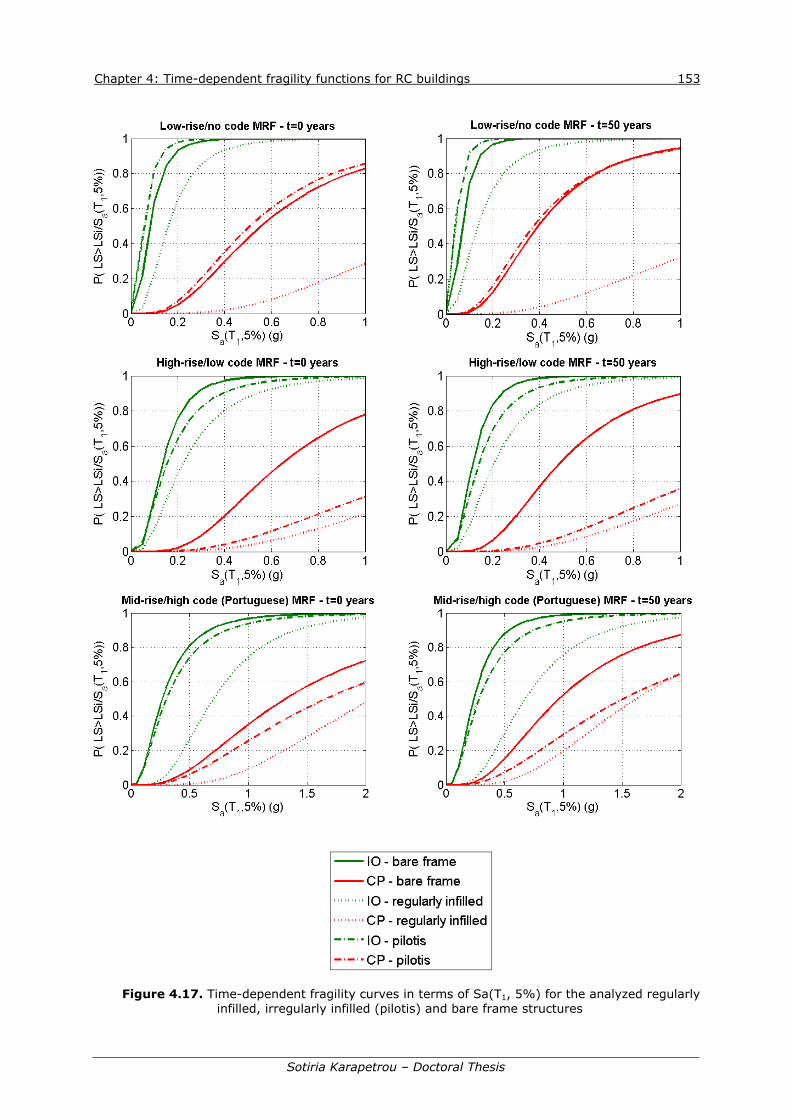
Chapter 4: Time-dependent fragility functions for RC buildings 153
Sotiria Karapetrou – Doctoral Thesis
Figure 4.17. Time-dependent fragility curves in terms of Sa(T1, 5%) for the analyzed regularly infilled, irregularly infilled (pilotis) and bare frame structures

Chapter 4: Time-dependent fragility functions for RC buildings 154
Sotiria Karapetrou – Doctoral Thesis
Table 4.10. Time-dependent fragility parameters in terms of Sa(T1, 5%) for the bare, regularly infilled and irregularly infilled (pilotis) frame buildings
RC building Structural typology
Time scenario (years)
Median Sa(T1, 5%) (g) Dispersion β(t)
IO CP
Low rise MRF-no code
Bare frame 0 0.08 0.56 0.62 50 0.07 0.39 0.59
Regularly infilled 0 0.16 1.42 0.61 50 0.13 1.39 0.72
Pilotis 0 0.06 0.51 0.63 50 0.04 0.37 0.63
High rise MRF-low
code
Bare frame 0 0.13 0.64 0.57 50 0.11 0.48 0.58
Regularly infilled 0 0.22 1.74 0.69 50 0.20 1.52 0.68
Pilotis 0 0.15 1.43 0.73 50 0.14 1.29 0.70
Mid rise MRF-high
code (Portuguese)
Bare frame 0 0.27 1.31 0.72 50 0.24 0.96 0.64
Regularly infilled 0 0.7 2.06 0.54 50 0.67 1.62 0.57
Pilotis 0 0.3 1.65 0.77 50 0.28 1.51 0.76
4.8 Time-variant quadratic model for the fragility parameters
To continuously evaluate and predict the seismic vulnerability of the structures with time,
fragility parameters at different points in time along their service life are required.
Analytical functions representing time-dependent fragility models constitute an efficient
tool for estimating the fragility parameters at any point in time for the given structural
typology and corrosion parameters without the need to conduct complete fragility
analysis. Based on Gosh and Padgett (2010) a quadratic model of the form
parameter(t)=p1t2+p2t+p3, is found to best fit the time-dependent variation in fragility
parameters, where parameter(t) is either the median m(t) or dispersion β(t) at t years
and p1, p2, p3 the quadratic coefficients from regression analysis. Figure 4.18 shows the
quadratic coefficients estimated for the time-dependent median of the bare frame
structures corresponding to the Collapse Prevention (CP) damage state. Table 4.11
summarizes the coefficients of the quadratic equations for the fragility parameters for the
two defined damage states and for the different structural typologies considered. These
coefficients can be then used in Equation 4.8 to evaluate the building fragilities at any
point in time as:
2
1 2 3
21 2 3
_ _ _
_ _ _
ln ln/ m m mIM p t p t p
P DS IM tp t p t p
(4.9)
where the subscripts on the coefficients indicate median m or dispersion β.

Chapter 4: Time-dependent fragility functions for RC buildings 155
Sotiria Karapetrou – Doctoral Thesis
Figure 4.18. Time-dependent quadratic fit of median Sa(T1, 5%) values for the Collapse
Prevention (CP) state for the bare frame structures

Chapter 4: Time-dependent fragility functions for RC buildings 156
Sotiria Karapetrou – Doctoral Thesis
Figure 4.18. (Continued) - Time-dependent quadratic fit of median Sa(T1, 5%) values for the
Collapse Prevention (CP) state for the bare frame structures
Table 4.11. Coefficients of quadratic interpolation for the median IO and CP limit values and the corresponding dispersion (in terms of log-standard deviation)
RC MRF Quadratic coefficients Median IO Median CP Dispersion
Low-rise No code p1mIO p2mIO p3mIO p1mCP p2mCP p3mCP p1β p2β p3β
Mid-rise No code 2e-06 0.00 0.08 3e-05 -0.005 0.547 2e-05 -0.001 0.619
Mid-rise Low code 1e-05 -0.001 0.148 2e-05 -0.004 0.429 -0.005 0.023 0.597
High-rise Low code -1e-06 0.0 0.271 -6e-06 -0.003 0.764 -0.008 0.061 0.512
Low-rise High code 5e-06 0.0 0.133 8e-06 -0.003 0.637 0.002 -0.010 0.585
Mid-rise High code (Greek)
2e-06 -0.001 0.199 3e-05 -0.010 1.749 -0.001 0.017 0.634
Mid-rise High code
(Portuguese) 8e-06 -0.001 0.262 7e-05 -0.028 3.931 -0.004 0.040 0.550

Chapter 4: Time-dependent fragility functions for RC buildings 157
Sotiria Karapetrou – Doctoral Thesis
4.9 Discussion and concluding remarks
The seismic vulnerability of RC frame buildings has been assessed taking into
account the aging of RC buildings due to rebar corrosion. Three main aspects for
corrosion have been included in the analysis namely the loss of reinforcement cross-
sectional area, the degradation of concrete cover and the reduction of steel ultimate
deformation. Seven MRF structures corresponding to different code design levels and
described according to the SYNER-G taxonomy, have been analyzed for four time periods
(t=0, 25, 50 and 75 years) by employing 2D incremental dynamic analysis (IDA). The
relative contribution of infill walls on the seismic performance and fragility of selected
representative buildings is also assessed. Both regularly infilled and irregularly infilled
(pilotis) frames are analyzed for the initial and 50-year corrosion scenario.
Time-dependent probabilistic fragility functions have been derived for the IO and CP
limit states and different periods in time in terms of Sa(T1,5%). A significant increase in
the seismic fragility of the structures is observed over time due to corrosion, highlighting
the importance of considering the deterioration effects due to aging on the seismic
vulnerability of structures. It should be stressed however that the results have been
produced under the assumption of uniform corrosion effects for all structural elements
(external and internal) adopting external environmental conditions. The potential of
pitting corrosion or the consideration of a different corrosion scenario for the internal and
external structural elements was not investigated in the context of the present thesis.
The consideration of regularly infilled walls is shown to yield a substantial decrease in
fragility of the initial as-built and corroded bare frame structures. However, the
irregularly infilled frames may have either a favorable or detrimental effect in fragility of
the reference bare frames depending on the structural typology and code design level
(e.g. seismically or non-seismically designed frames).
By exploiting the available fragility data of the bare frame buildings at different points
in time, simple quadratic functions are introduced for the efficient assessment of the
time-dependent shift in the fragility parameters (median and dispersion) for each
damage state due to corrosion. The advantage of such time-dependent models is that the
fragility parameters can be estimated at any point in time without conducting complete
fragility analyses.
Overall, the present research provides a further insight on the seismic vulnerability of
typical RC frame buildings by proposing time (or aging)-dependent fragility functions
applicable to a variety of RC typologies exposed to aging. Validation of the suggested
time-dependent fragility curves with field post earthquake surveys and adequate field
experiments and large scale laboratory tests in prototype structures or building

Chapter 4: Time-dependent fragility functions for RC buildings 158
Sotiria Karapetrou – Doctoral Thesis
components is certainly warranted to enhance their reliability and robustness and finally
to ensure their efficient implementation in seismic vulnerability assessment studies.

Sotiria Karapetrou – Doctoral Thesis
CHAPTER 5
Seismic vulnerability assessment of RC buildings considering soil-structure
interaction effects
5.1 Introduction
Besides aging the influence of soil conditions and soil-structure interaction (SSI) might
also contribute to the building’s seismic fragility. Although there are some studies that
take into account the local site effects by providing fragility curves for buildings for
different soil conditions, the effect of SSI to the expected structure’s performance has
not received much attention. This may be due to the fact that the incorporation of SSI
phenomena in the analysis is generally considered beneficial reducing the seismic
demand and consequently the corresponding structural damage of non-linear systems
(Ciampoli and Pinto, 1995). Nevertheless, it has been shown that soil deformability and
SSI may modify the structural response and fragility leading to either beneficial or
detrimental effects depending on the dynamic properties of the soil and the structure as
well as the characteristics (frequency content, amplitude, significant duration) of the
input motion (e.g. Dutta et al., 2004; Saez et al., 2011).
The objective of the research presented in Chapter 5 is to study whether soil structure
interaction and site effects may affect the seismic performance and vulnerability of
reinforced concrete moment resisting frame buildings and consequently modify the
fragility curves. SSI is modeled applying the direct one-step approach considering either
linear elastic or nonlinear soil behavior while site effects are inherently accounted for. To
further examine the contribution of site and SSI effects, a two-step uncoupled approach
is also applied, which takes into account site effects on the response of the fixed base
structures, but neglects SSI effects. Additional analyses are performed investigating the
influence of the soil depth and stratigraphy under nonlinear soil behavior on the seismic
response and fragility of RC buildings. Finally time-dependent fragility functions are
derived of the RC buildings considering both SSI and aging effects. The chloride induced

Chapter 5: Seismic vulnerability assessment of RC buildings considering SSI effects 160
Sotiria Karapetrou – Doctoral Thesis
corrosion model presented in Chapter 4 is adopted considering two time-scenarios (t=0
and 50 years). Fragility curves are derived as a function of rock outcropping peak ground
acceleration for the Immediate Occupancy and Collapse Prevention limit states for the
fixed base and SSI models based on the methodology described in detail in Chapter 3.
Results show the significant role of SSI and site effects under linear or nonlinear soil
behavior in altering the expected structural performance and fragility of fixed base
structures. Moreover an overall increase in seismic vulnerability over time due to
corrosion is observed highlighting the important influence of deterioration due to aging
effects on the structural behavior. The research presented in this chapter has been
published in Bulletin of Earthquake Engineering (Pitilakis et al., 2014b) and Soil
Dynamics and Earthquake Engineering (Karapetrou et al., 2015) scientific journals.
5.2 Description of the parametric investigation
5.2.1 Selection of prototype buildings
In this study SSI is considered for three representative bare frames designed according
to different seismic code levels and height classes. More specifically the low rise - no
code (Bracci et al., 1992), the high rise - low code (Kappos et al., 2006) and the mid rise
- high code (Greek) (Kappos et al., 2006) buildings, which are described in detail in
Chapter 3, are adopted as reference structures. The selected fixed base reference
structures are presented in Figure 5.1. The numerical modeling of the nonlinear
structural models is conducted in OpenSees (Mazzoni et al., 2009) as described in
Chapter 3.

Chapter 5: Seismic vulnerability assessment of RC buildings considering SSI effects 161
Sotiria Karapetrou – Doctoral Thesis
Figure 5.1. Reference MRF models used for the seismic vulnerability assessment considering soil-
structure interaction: (a) Low rise-no code, (b) High rise-low code, (c) Mid rise-high code
5.2.2 Soil-structure interaction (SSI) modeling
The consideration of SSI is usually achieved by taking into account inertial and kinematic
interaction schemes resulting to an elongation of the natural period of the SSI system
and an increase of system damping due to the energy dissipation at the soil-foundation
level (Veletsos and Meek, 1974). The general assumption that the structure is fixed to its
base ignoring the presence of the soil beneath its foundation may be realistic (or at least
conservative) when the structure is founded on rock or very stiff soil. However, in the
case of softer soil formations, SSI and local site effects may play an important role
modifying considerably the free field input motion as well as the dynamic characteristics
of the building and finally its response (Stewart et al., 1999).
The dynamic analyses of the fixed base and SSI configurations are conducted using
OpenSees software. Figure 5.2 illustrates a general schematic view of the reference
structural models in the case of fixed base and SSI configurations. The soil is modeled in
two-dimensions with two degrees-of-freedom using the plane strain formulation of
the quad element. To account for the finite rigidity of the underlying half-space, a
Lysmer-Kuhlemeyer (Lysmer and Kuhlemeyer, 1969) dashpot is incorporated at the base
of the soil profile. The soil profile is excited at the base by a horizontal force time history,
which is proportional to the known velocity time history of the ground motion (Joyner

Chapter 5: Seismic vulnerability assessment of RC buildings considering SSI effects 162
Sotiria Karapetrou – Doctoral Thesis
and Chen, 1975; Lysmer, 1978). It is noted that due to the consideration of an elastic
half-space it was possible to directly apply the outcropping rock motion at the base of the
soil model (Kwok et al., 2007). A sensitivity analysis is conducted to identify the
appropriate dimensions of the considered soil grid so as to assure free field and “quasi
transparent” conditions at the boundaries. Thus, the grid adopted for the low and mid-
rise structures has a total length of 120m with a depth of 30m that includes
approximately 3600 four-node quadrilateral elements, whereas for the high rise model
the total length and the number of quadrilateral elements increase to 220m and 6600
respectively. The geometry of the mesh is based upon the concept of resolving the
propagation of the shear waves at or below a particular frequency allowing an adequate
number of elements to fit within the wavelength of the chosen shear wave. This ensures
that the mesh is refined enough to capture satisfactorily the propagating waves.
Considering that the maximum frequency of interest is set to 10Hz a relatively dense
discretization is adopted with quadratic elements of 1.0m x 1.0m.
(a)
Outcrop
Elastic bedrock
Fixed base modelSSI-FE model
Free field
Soil profile Vs0,30
(b)
Input Motion
Rigid beam-column element
Free Field
Lysmer-Kuhlemeyer (1969)dashpot
120.0m
30
.0m
Elastic Bedrock
Vso,30
Figure 5.2. Description of the fixed base and soil-structure models under study

Chapter 5: Seismic vulnerability assessment of RC buildings considering SSI effects 163
Sotiria Karapetrou – Doctoral Thesis
Even though soil material nonlinearity can be incorporated in the direct approach, first
an elastic soil profile is considered with an average shear wave velocity Vs,30 equal to
200m/sec corresponding to ground type C of the Eurocode 8 soil classification system. A
very soft soil has been specifically selected in order to amplify the effects of the SSI.
Moreover, to gain further insight into the influence of SSI and site effects on the seismic
fragility analysis, the SSI effect considering soil nonlinearity is investigated for the high-
rise building designed with low seismic code provisions, for which SSI effects are
expected to be much more pronounced in comparison to the rest of the adopted
structures. The soil constitutive model utilized in OpenSees is described in the following
subsection.
Viscous damping is employed in the frequency-dependent Rayleigh form (Rayleigh
and Lindsay, 1945). Although, the damping of the soil materials is normally of hysteretic
type and frequency independent, this damping form facilitates the dynamic analysis, as
the damping matrix is built as a linear combination of the mass and stiffness matrices
(Chopra, 2001):
C a M K (5.1)
where α is the mass proportional damping constant, and β is the stiffness proportional
damping constant. Figure 5.3 illustrates schematically the damping as a function of the
frequency corresponding to the adopted soil profile. The selection of the frequencies f1
and f2 (ω1 and ω2) is made, in order the resulting damping curve to simulate an almost
constant damping at the frequency range of interest. In particular the frequency range of
interest is defined based on the predominant frequencies of the soil deposit, f1 and f2=5f1
Hz (e.g. Kwok et al., 2007). This range includes the model’s natural frequencies and the
predominant frequencies of the input motions. Assuming constant frequency for both
modes ξ, the damping parameters are finally given by the following expressions:
1 2
1 2 1 2
12 , 2
(5.2)
where ω1 and ω2 are the natural (cyclic) frequencies of the modes. A small amount of
mass and stiffness proportional Rayleigh damping (ξ=5% for the soil material) is
assigned to account for energy dissipation during seismic loading for the linear soil profile
cases.
The elastic bedrock (Vs,bedrock=900m/sec) lies at 30m beneath the ground surface. The
Lysmer-Kuhlemeyer (Lysmer and Kuhlemeyer, 1969) dashpot is defined based on the
viscous uniaxial material model and the ‘zeroLength’ element formulation at the same
location, to connect the two previously defined dashpot nodes. This material model
requires a single input, the dashpot coefficient c that is defined according to Joyner and

Chapter 5: Seismic vulnerability assessment of RC buildings considering SSI effects 164
Sotiria Karapetrou – Doctoral Thesis
Chen (1975) as the product of the mass density and shear wave velocity of the
underlying bedrock including also the base area of the soil profile in order to maintain
proportional results for any horizontal element size. The nodes at the lateral boundaries
corresponding to each depth level are tied together in order to achieve a simple shear
deformation pattern of the soil profile. Full contact between the soil and structures’ nodes
is assumed forbidding thus any relative movement between the structure and the soil
(i.e. no detachment or sliding are allowed). The connection of the soil with the structure
is achieved by applying common nodes and appropriate constrains (to ensure equal
displacement) for both the soil and the structure’s foundation. A continuous raft
foundation is considered modeled as an elastic beam-column element of infinite rigidity.
Rigid foundation was considered for sake of simplicity. In case of flexible or isolated
footings As expected, the consideration of SSI causes an elongation of the fundamental
period of the soil-structure models compared to the corresponding fixed based cases
leading to a much more flexible system. More specifically, the low-strain fundamental
period of the SSI systems increases for the low-rise, no code structure from 0.98s, which
corresponds to the fundamental period of the fixed base model presented in Chapter 3,
to 1.28s, for the high-rise, low code model from 0.89s to 1.46s and for the mid-rise, high
code building from 0.66s to 0.91s. Table 5.1 summarizes the parameters of the soil
material properties adopted. Figures 5.4, 5.5 and 5.6 illustrate contour plots of the
vertical displacements and stress distribution developed at the soil profile after the static
analysis of the soil-structure systems. The contour plots are derived using the GiD post-
processor tool (CIMNE, 2013)
Figure 5.3. Rayleigh proportional damping curves for the linear soil profile

Chapter 5: Seismic vulnerability assessment of RC buildings considering SSI effects 165
Sotiria Karapetrou – Doctoral Thesis
Table 5.1. Summary of parameters adopted for the linear soil profile case
Parameter Description Value adopted
Vs,30 of the soil deposit (m/sec) Shear wave velocity 200 Vs,b of the bedrock (m/sec) Shear wave velocity 900
ρo,s (Mg/m3) Mass density of the soil 1.8 ρo,b (Mg/m3) Mass density of the bedrock 2.2
G (kPa) Shear Modulus 72000 nu Poisson’s ratio of soil 0.3
E (kPa) Soil Elasticity Modulus 187200
Figure 5.4. Vertical displacement and stress distribution after the static analysis of the soil-structure system for the linear soil profile case and the Low rise – No code MRF model
Figure 5.5. Vertical displacement and stress distribution after the static analysis of the soil-structure system for the linear soil profile case and the High rise – Low code MRF model

Chapter 5: Seismic vulnerability assessment of RC buildings considering SSI effects 166
Sotiria Karapetrou – Doctoral Thesis
Figure 5.6. Vertical displacement and stress distribution after the static analysis of the soil-structure system for the linear soil profile case and the Mid rise – High code MRF model
5.2.2.1. Soil constitutive model
For the high-rise non-ductile frame structure, where SSI effects are expected to be much
more pronounced, soil-structure interaction is investigated for both linear elastic and
nonlinear soil behavior. For the simulation of the nonlinear soil behavior, the soil profile is
considered as a homogenous cohesive medium with an average shear wave velocity Vs,ave
and an undrained shear strength Cu. For the nonlinear soil profile Vs,ave is considered
equal to 300m/sec in order to reach approximately the same levels of the corresponding
shear wave velocity for the linear soil profile (Vs=200m/sec) at the end of the time-
history analysis and allow for direct comparison. To achieve this preliminary iterative
nonlinear dynamic analyses of the systems were performed considering the records
scaled at a PGA level equal to 0.3g. Soil nonlinearity is described based on an advanced
constitutive model, which follows the concept of multi-yield surface (nested-surface)
plasticity (Iwan, 1967; Prevost, 1985; Mroz, 1967; Yang, 2000) where each yield
surface is defined in the deviatoric stress space as (Elgamal, 1992; Gu et al., 2009):
1
230
2:f K
(5.3)
where τ= the deviatoric stress tensor; α= the back-stress tensor referring to the center
of the yield surface f=0 and K= the size of the yield surface defining the region of
constant plastic shear modulus. For non-pressure sensitive cohesive soil material the
yield surfaces are of the Von Mises type.
The nonlinear shear stress-strain response of the soil is described by the hyperbolic
backbone curve (Gu et al., 2009) as:

Chapter 5: Seismic vulnerability assessment of RC buildings considering SSI effects 167
Sotiria Karapetrou – Doctoral Thesis
1
r
G
(5.4)
where τ= the octahedral shear stress; γ= the octahedral shear strain; G= the low-strain
shear modulus and γr= a reference shear strain defined as:
max max
max maxr G
(5.5)
where τmax is the shear strength corresponding to the shear strain γmax.
Within the multi-surface plasticity framework the yield surfaces define regions of
constant shear moduli in the stress space and are utilized to represent the hyperbolic
backbone curve through a piecewise linear representation. As depicted in Figure 5.7 each
linear segment represents the domain of a yield surface fm with shear modulus Hm for
m=1,2,...NYS with NYS denoting the total number of yield surfaces (Stewart et al.,
2008). The outermost yield surface fNYS, which corresponds to the peak shear strength
τmax, represents the failure surface and corresponds to zero shear modulus HNYS.
The yield surface, the hardening law and the flow rule constitute the key components
of the applied pressure-independent multi yield surface incremental plasticity model
(Kramer and Elgamal, 2001; Parra, 1996; Yang and Elgamal, 2008). During the static
analysis phase the material behavior is linear elastic. In the subsequent dynamic (fast
rate) loading phase, the stress-strain response is turned to elastic-plastic following the
multi-surface plasticity concept, with Von Mises yield surfaces, an associative flow rule
and a kinematic hardening law (Prevost, 1985) employed to capture the Masing
hysteretic cyclic response behavior (Masing, 1926).
τ
γ
τmax
1
fmfNYS f1 γm γmax
Deviatoric plane
Hyperbolic backbone curve
Hm/2τm
Figure 5.7. Hyperbolic backbone curve for soil nonlinear shear stress-strain response and
piecewise-linear representation in multi-surface plasticity (after Prevost, 1985; Stewart et al., 2008; Parra, 1996)

Chapter 5: Seismic vulnerability assessment of RC buildings considering SSI effects 168
Sotiria Karapetrou – Doctoral Thesis
A user-defined backbone curve is defined where the parameters controlling the shear
behavior of the constitutive model are calibrated to yield the shear modulus reduction
curve provided by Darendeli (2001) for clay soil with plasticity index PI=30 and
atmospheric pressure p’0 = 1 atm, which is presented in Figure 5.8. The backbone curve
is appropriately adjusted to render the undrained shear strength Cu using the following
equation (Yang and Elgamal, 2008):
3
2m
uC
(5.6)
where σm is the product of the last modulus and strain pair in the defined modulus
reduction curve. Since the model considers elastoplastic soil behavior, a considerable
amount of hysteretic energy dissipation is represented by the multi-yield function
considering that extensive plastic deformation is expected to occur during ground
shaking. A small amount of mass and stiffness proportional Rayleigh damping ξ=1.2%
(α=0.314, β=0.000255) is assigned to account for the energy dissipation during the
elastic part of the cyclic response, which corresponds to the small-strain damping ratio
defined based on the damping ratio curve for clay soil proposed by Darendeli (2001) with
plasticity index PI=30 and atmospheric pressure p’0 = 1 atm. The parameters of the soil
material properties adopted are summarized in Table 5.2.
Figure 5.8. Shear modulus reduction curve by Darendeli, 2001 for clay soil with plasticity index PI=30 and atmospheric pressure p’0 = 1 atm, utilized for the calibration of the soil constitutive
model in OpenSees

Chapter 5: Seismic vulnerability assessment of RC buildings considering SSI effects 169
Sotiria Karapetrou – Doctoral Thesis
Table 5.2. Summary of parameters adopted for the pressure independent multi-yield plasticity model
Parameter Description Value adopted/Data sources
Vs,ave (m/sec) Low-strain shear wave velocity 300 ρo (Mg/m3) Mass density 1.8
p'r (atm) Reference pressure 1.0
d Pressure dependent coefficient 0.0 Gr (kPa) Shear Modulus at p'
r 162000 nu Poisson’s ratio of soil 0.3
E (kPa) Soil Elasticity Modulus 421200 Br (kPa) Bulk Modulus at p'
r 351000 φ Friction angle 0.0
Cu (kPa) Undrained shear strength 110.0
G/Gmax or γmax Modulus reduction curve or shear strain at failure
Darendeli (2001) for clay soil with plasticity index PI=30 and atmospheric
pressure p’0 = 1 atm
5.2.3 Parametric study
The three representative MRF buildings which are selected for the investigation of the SSI
and site effects in their seismic vulnerability are analyzed considering at first linear soil
behavior. The applied modeling approaches in the case of fixed base and SSI
configurations are schematically described in Figure 5.2. The fixed base models are
assumed to be founded on rock and are analyzed by imposing outcropping bedrock input
motions. On the other hand SSI is modeled applying the direct method based on the
one-step approach where the entire soil-foundation-structure system is analyzed in a
single step. For the high-rise non-ductile RC frame structure, for which SSI effects are
expected to be much more pronounced, further sensitivity analyses are conducted to
investigate on an extensive basis the influence of SSI and site effects considering soil
nonlinearity, which are described in the following subsections.
5.2.3.1. Effect of SSI and site effects under nonlinear soil behavior
Figure 5.9 represents schematically for the high-rise, non-ductile structure the applied
modeling approaches. A first series of analyses is conducted for the fixed base structure
founded on rock by imposing outcropping bedrock input motions. The influence of SSI
and site effects on the seismic response and fragility of the building is investigated for
both linear elastic and nonlinear soil behavior considering a depth for the finite element
model of Figure 5.10 equal to H=30m. Additionally, a two-step uncoupled approach is
also applied using OpenSees in which a 1D seismic response analysis of the given (elastic
or inelastic) soil profile is first performed and then the obtained free field motion is
imposed as input ground motion to the fixed base structural model. It is noted that the
1D soil profile is composed of four-node quadrilateral elements using the same vertical
discretization as the one used for complete 2D SSI model. This approach takes into

Chapter 5: Seismic vulnerability assessment of RC buildings considering SSI effects 170
Sotiria Karapetrou – Doctoral Thesis
account site effects including (or not) soil nonlinearity, but neglects SSI effects. Thus, it
allows gaining further insight into the relative contribution of site and SSI effects in
fragility analysis.
Fixed base model
Outcrop
Elastic bedrock
SSI-FE model
Free field
Elastic or inelastic soil profile
Two-step modelingapproach
Figure 5.9. Schematic view of the modeling approaches to assess the influence of SSI and site effects under linear elastic or inelastic soil behavior for the high-rise, non ductile MRF structure
Input Motion
Rigid beam‐column element
Free Field
Elastic Bedrock
Vs,ave
Lysmer‐Kuhlemeyer (1969) dashpot
Figure 5.10. Finite element model of the soil-structure systems in OpenSees in the case of the high-
rise, non ductile MRF structure
5.2.3.2. Effect of soil depth and stratigraphy under nonlinear soil behavior
To further examine the importance of site effects and inelastic SSI on the seismic
performance and vulnerability of RC buildings, additional analyses are performed
investigating the influence of the soil depth and stratigraphy under nonlinear soil
behavior. Figure 5.11 presents schematically the analyzed cases. To study the effect of
soil stratigraphy an additional layered soil medium is considered where the low-strain
shear wave velocity of the profile increases with depth H. More specifically, the adopted
soil profile consists of three layers with an average low-strain shear wave velocity Vs,ave
equal to 300m/sec to allow for direct comparison with the homogeneous nonlinear soil

Chapter 5: Seismic vulnerability assessment of RC buildings considering SSI effects 171
Sotiria Karapetrou – Doctoral Thesis
medium considered previously. The average value Vs,ave is computed based on the shear
wave velocity and thickness of each layer as:
31 2
1 2 3
,s avei
si s s s
H HVH HH HV V V V
(5.7)
where Vs1, Vs2, Vs3 and H1, H2, H3 are the shear wave velocities and thicknesses of the
surface, intermediate and bottom layers respectively.
Furthermore to study the effect of the soil depth H in the fragility analysis, the
inelastic soil-structure systems for both homogeneous and layered soil profiles are
analyzed for varying soil depth. In particular, two soil profiles are considered, the H=30m
profile which corresponds to the shallow soil medium with fundamental elastic period
equal to TH=30=0.4sec and a deeper one where the depth and fundamental period
increase to H=60m and TH=60=0.8sec respectively.
Vs,ave=300m/sec H=30m,60m
Bedrock (a)
Vs1=250m/sec
Vs2=290m/sec
Vs3=350m/sec
H1=H/6
H2=H/2
H3=H/3
Bedrock (b)
Figure 5.11. Schematic representation of the analyzed cases for the investigation of the effect of (a) soil depth and (b) stratigraphy under nonlinear soil behavior
5.3 Comparative dynamic analysis
To illustrate the relative influence of SSI and site effects on the seismic response under
linear or nonlinear soil behavior of the structural typologies under study, a preliminary
comparative dynamic analysis is carried out for the different considered modeling
approaches (i.e. SSI coupled and fixed base-site effects analysis cases considering or not
soil nonlinearity) for a test ground motion. More specifically, dynamic analyses are
conducted using Friuli earthquake record (waveform code 000055xa, see Table 3.4 of
Chapter 3 and ANNEX A) as input motion scaled to a PGA level equal to 0.3g. At this level
of shaking the soil is normally expected to exhibit yielding and nonlinear cyclic
deformations. The analyzed nonlinear models can accommodate these effects, which
however cannot be captured by the corresponding linear elastic models. The results are

Chapter 5: Seismic vulnerability assessment of RC buildings considering SSI effects 172
Sotiria Karapetrou – Doctoral Thesis
presented in terms of acceleration time histories at the base of the structure at first for
the soil-structure systems for which only linear soil behavior is considered in comparison
with the reference free field outcropping motion directly imposed to the fixed base
structure founded on rock. The arias intensity (Ia) values for each case are also shown.
Furthermore the distribution of floor displacements and storey drifts along the structures’
height are also presented which correspond to the time of maximum interstorey drift
occurrence maxISD. It should be noted herein that for the SSI configurations, only the
deformation component that causes structural distortion is considered. Thus, the
horizontal displacement and the rocking motion of the foundation are not included in the
presented results as the particular components may not contribute to the structural
distortion.
Figures 5.12 and 5.14 show that the amplitude, in acceleration terms, is amplified
with respect to the free field outcropping motion for the soil-structure systems, which
consider linear elastic soil behavior for both the low-rise, no code and the mid-rise, high-
code MRF structures. Figures 5.13 and 5.15 show that for both soil-structure systems
considering linear soil behavior, maxISD values are higher in comparison to the
corresponding fixed base models. The systems are characterized by a global plastic
sidesway mechanism and the maximum interstorey drift occurs in the same storey where
the corresponding fixed base models presented their maximum values. More specifically
for the low-rise, no-code building, maxISD is located in the third floor (top floor) whereas
for the mid-rise, high-code MRF, maxISD occurs in the ground floor.
Figure 5.12. Acceleration time histories at the base of the Low-rise, No code structure for the fixed base and SSI configurations considering linear soil behavior (outcrop input motion:
Friuli, 6/5/1976, Mw=6.5, R=23km)

Chapter 5: Seismic vulnerability assessment of RC buildings considering SSI effects 173
Sotiria Karapetrou – Doctoral Thesis
Figure 5.13. Snapshots of floor displacement (left) and storey drifts (right) of the Low-rise, No code structure at the time corresponding to maxISD for linear soil behavior (Friuli earthquake
0.3g)
Figure 5.14. Acceleration time histories at the base of the Mid-rise, High code structure for the fixed base and SSI configurations considering linear soil behavior (outcrop input motion:
Friuli, 6/5/1976, Mw=6.5, R=23km)
Figure 5.15. Snapshots of floor displacement (left) and storey drifts (right) of the Mid-rise,
High code structure at the time corresponding to maxISD for linear soil behavior (Friuli earthquake 0.3g)

Chapter 5: Seismic vulnerability assessment of RC buildings considering SSI effects 174
Sotiria Karapetrou – Doctoral Thesis
Similar results are presented continuously for the different analyzed models for the
high-rise non-ductile MRF structure. It can be noticed in Figure 5.16 that the amplitude,
in acceleration terms, is amplified with respect to the free field outcropping motion for
the soil-structure system, which considers linear elastic soil behavior. This amplification is
even more noticeable for the corresponding fixed base model where site effects are taken
into account. On the contrary, when considering soil nonlinearity, the derived seismic
response at the base of the structure is decreased compared to the free field outcropping
motion. This could be attributed to the effect of hysteretic damping in nonlinear systems,
which generally tends to reduce acceleration values at the ground surface as the level of
shear strain increases. A further deamplification of the response is expected for the
nonlinear SSI system compared to the corresponding fixed base model that considers
site effects. The latter could be justified considering that SSI introduces additional
damping to the system due to the energy dissipation at the soil-foundation interface.
Figure 5.17 displays the maximum calculated interstorey drift ratios maxISD (%) for
the different analyzed configurations of the high-rise, low code building for a selected
input motion i.e. Friuli 1976. The highest drift values are shown for the fixed base linear
model, which considers soil conditions (site effects), whereas the lowest ones are
presented for the fixed base structural configuration without considering any site effects,
i.e. the building receives directly the outcrop input motion. It is seen that for the
nonlinear cases the derived drift demands of the structure do not increase proportionally
to the acceleration values. In particular, while the amplitude of the acceleration time
histories is deamplified for the nonlinear systems with respect to the free field
outcropping motion, the corresponding drift values are higher for the models, which
consider soil nonlinearity. This trend is more pronounced for the nonlinear SSI coupled
system compared to the corresponding fixed base case, probably due to the increased
deformation demand introduced at the soil-foundation interface. A better correlation with
drift demand is shown when using Ia as a metric of the seismic intensity. This is
reasonable considering that Ia characterizes not only the seismic intensity (as PGA) but
also the total energy content of the seismic excitation. To further investigate the
structural behavior of the different systems under seismic loading, the distribution of
floor displacements and storey drifts with the structure’s height is illustrated in Figure
5.18, corresponding to the time of maximum interstorey drift occurrence maxISD. The
systems are characterized by a global plastic sidesway mechanism and the maximum
interstorey drift occurs for all cases in the 8th floor of the building. Based on the
deformed shapes of Figure 5.18, it becomes clear that for the fixed base model founded
on rock the contribution of higher modes is not significant. However for the soil-structure
systems as well as for the fixed base models accounting for site effects it is seen that the
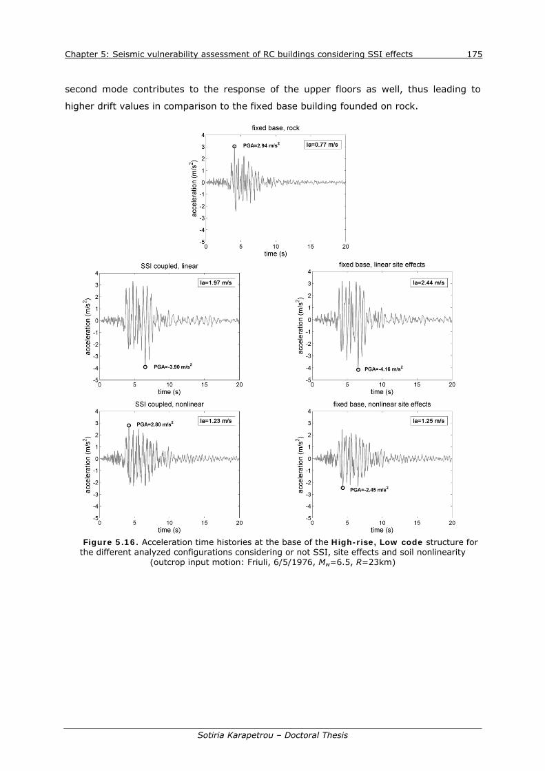
Chapter 5: Seismic vulnerability assessment of RC buildings considering SSI effects 175
Sotiria Karapetrou – Doctoral Thesis
second mode contributes to the response of the upper floors as well, thus leading to
higher drift values in comparison to the fixed base building founded on rock.
Figure 5.16. Acceleration time histories at the base of the High-rise, Low code structure for
the different analyzed configurations considering or not SSI, site effects and soil nonlinearity (outcrop input motion: Friuli, 6/5/1976, Mw=6.5, R=23km)

Chapter 5: Seismic vulnerability assessment of RC buildings considering SSI effects 176
Sotiria Karapetrou – Doctoral Thesis
Figure 5.17. Maximum interstorey drift ratio (%) for the different analyzed configurations of
the High-rise, Low code building considering or not SSI, site effects and soil nonlinearity for Friuli earthquake
Figure 5.18. Snapshots of floor displacement (left) and storey drifts (right) for the different analyzed configurations of the High-rise, Low code building at the time corresponding to
maxISD for linear and nonlinear (NL) soil behavior (Friuli earthquake 0.3g)
Preliminary dynamic analyses are also conducted to demonstrate the effect of soil
depth and layering on the nonlinear seismic response of the SSI coupled models Two

Chapter 5: Seismic vulnerability assessment of RC buildings considering SSI effects 177
Sotiria Karapetrou – Doctoral Thesis
different earthquake records are used in this case as input accelerations, scaled at PGA
equal to 0.3g, i.e. Campano Lucano (23/11/1980, Mw=6.9, R=23km) and Kozani
(13/5/1995, Mw=6.5, R=17km) records with waveform codes 000287xa and 006115ya
(Table 3.4 of Chapter 3 and ANNEX A) respectively. These records are characterized by
quite different characteristics in terms of both frequency content and duration. The
Campano Lucano record is associated with a longer significant duration and a rather low
frequency content whereas Kozani record represents a low-duration, high frequency
motion. Thus, for the SSI system increased nonlinearity is expected and consequently
increased drift demands on the structure for the former rather than for the latter motion.
Figure 5.19 depicts the derived acceleration time histories at the base of the structure
(the Ia values are also shown) for the different analyzed nonlinear SSI cases with varying
soil depth and stratigraphy for the two selected acceleration scenarios. It is readily seen
that the acceleration values are generally amplified for the 3-layer soil profile compared
to the corresponding values of the homogeneous soil profile. This could be attributed to
the increased trapping of seismic waves in the thinner upper layer of the layered soil
profile due to the impedance contrast between the sublayers and the underlying bedrock.
The soil depth may also affect the response at the base of the structure. In particular,
the 60m soil profile shows reduced acceleration values compared to the respective 30m
profile. This is evident for both considered representative records and is mainly
associated to the attenuation of the seismic motion with the distance from the bedrock
(i.e. radiation damping) that is increased for the deeper soil profile.
Figures 5.20 and 5.21 present stress-strain hysteretic loops at various depths
(corresponding to soil elements at the middle of each sublayer of the 3-layer profile) for
the homogeneous and the layered 30m and 60m soil profiles respectively. In general
larger loops are observed and thus increased energy dissipation and damping of the
system from the surface layer to the deeper ones as the shear wave velocity of the layer
decreases. Shear modulus degradation is also shown with increasing shear strain that is
more pronounced for the deeper layers. These trends are much more obvious for the
long-duration, low frequency Campano Lucano earthquake motion highlighting the
significant role of the ground motion characteristics in altering the nonlinear seismic
response. In the surface layer, where the shear wave velocity (Vs) of the layered soil
profile is lower compared to the corresponding homogeneous profile (Vs =250m/sec and
300m/sec respectively), the average secant shear modulus of the curve is decreased for
the layered profile that is indicative of the lower stiffness of the layer. This trend is
reversed for the deeper layer where the Vs of the layered soil profile shows greater shear
modulus values compared to the corresponding homogeneous profile (Vs= 350m/sec and
300m/sec respectively). Finally, in the intermediate layer, where the Vs values of the

Chapter 5: Seismic vulnerability assessment of RC buildings considering SSI effects 178
Sotiria Karapetrou – Doctoral Thesis
homogeneous and layered soil profiles are quite close (Vs= 300m/sec and 290m/sec
respectively), the equivalent shear modulus (and thus the average slope) of the curves
are almost identical while the loop is relatively larger for the layered soil profile.
Figure 5.19. Acceleration time histories at the base of the structure for the different analyzed
nonlinear SSI cases with varying soil depth and stratigraphy

Chapter 5: Seismic vulnerability assessment of RC buildings considering SSI effects 179
Sotiria Karapetrou – Doctoral Thesis
Figure 5.20. Stress-strain hysteretic loops at various depths for the 30m homogeneous and layered soil profiles

Chapter 5: Seismic vulnerability assessment of RC buildings considering SSI effects 180
Sotiria Karapetrou – Doctoral Thesis
Figure 5.21. Stress-strain hysteretic loops at various depths for the 60m homogeneous and layered soil profiles

Chapter 5: Seismic vulnerability assessment of RC buildings considering SSI effects 181
Sotiria Karapetrou – Doctoral Thesis
Figure 5.22 illustrates the maximum calculated interstorey drift ratios (%) for the
analyzed SSI coupled configurations with varying soil depth and stratigraphy for the two
representative ground motions. It is observed that the SSI models associated with the
homogeneous soil profiles show lower drift ratios compared to the corresponding models
with the layered soil profiles. In addition, as expected, higher drift values are presented
for the long-duration, low frequency Campano Lucano earthquake motion (000287xa)
than for the low-duration, high frequency Kozani earthquake (006115ya) for all analysis
cases. This is in line with the low-strain fundamental period of the SSI system (TSSI=1.46
sec), which is shown to be closer to the predominant periods of the Campano Lucano
earthquake motion allowing further amplifications in drift demands due to possible
resonance phenomena. These trends are consistent with the estimated Ia values (shown
in Figure 5.19) indicating good correlations with the drift demand. Figure 5.23 presents
snapshots of the floor displacement and storey drift distribution along the building’s
height at the time maxISD occurs, indicating that the depth of the considered soil
medium may affect significantly the seismic behavior of the structure. This becomes
particularly evident for the Kozani earthquake event. While for the 30m-soil profile the
higher mode effects influence the inelastic behavior of the structure, when the depth of
the soil medium increases to 60m, the contribution of these effects seems to be less
important. Furthermore the estimated maximum drift ratios (Figure 5.23) for the Kozani
earthquake are shown to be higher for the shallower (homogeneous and layered) profiles
(30m) in comparison to the deeper soil mediums (60m). This is to be expected as it has
been previously shown that the deeper soil profile reduces the response values at the
base of the structure due to higher attenuation. Moreover Kozani earthquake spectrum is
mostly amplified in periods around 0.3sec, which is closer to the predominant elastic
period of the 30m profile (0.4sec) than the 60m (0.8sec) one resulting to higher drift
ratios for the shallower than for the deeper soil medium. On the contrary for the
Campano Lucano earthquake there is not a clear trend for the homogeneous and layered
soil profiles. In particular, while the increase of the soil depth results to lower drift ratio
values of the structure for the homogeneous case, greater drift values are shown for the
stratified deeper profile compared to the corresponding shallower one. The lower drift
values observed for the homogeneous deeper soil profile in comparison to the
corresponding shallower one are mainly associated with the increased attenuation of the
deeper soil profile. On the other hand, the greater drift values shown for the stratified
deeper profile could be related to the nonlinear behavior of the SSI system which effects
seem to be more pronounced for the stratified deeper soil medium, thus resulting to
larger structural deformations yielding finally higher drift demands close to global
dynamic instability (Vamvatsikos and Cornell, 2004).

Chapter 5: Seismic vulnerability assessment of RC buildings considering SSI effects 182
Sotiria Karapetrou – Doctoral Thesis
Figure 5.22. Maximum interstorey drift ratios (%) for the different analyzed configurations
with varying soil depth and stratigraphy
Figure 5.23. Snapshots of floor displacement (left) and storey drifts (right) at the time maxISD occurs for nonlinear soil behavior and varying soil depth and stratigraphy

Chapter 5: Seismic vulnerability assessment of RC buildings considering SSI effects 183
Sotiria Karapetrou – Doctoral Thesis
5.4 Derivation of fragility curves
The IDA procedure is used to determine the seismic performance and finally assess the
seismic vulnerability of the given structure under the influence of SSI and site effects.
The damage measure is expressed in terms of maximum interstorey drift ratio (maxISD),
which is known to relate well to dynamic instability and structural damage of frame
buildings. The seismic intensity is described using the peak ground acceleration (PGA)
recorded on rock outcropping conditions or soil type A according to EC8. PGA recorded on
rock conditions, and not on the corresponding free field considering site effects, is
selected as an IM for the derivation of fragility curves. In that way, the uncertainties
associated with local soil conditions and surface geology are directly included in the
analysis. Moreover, the use of outcropping PGA allows comparison of all analyzed models
with the reference fixed based structure founded on rock. Although other IMs (e.g. the
5%-damped first-mode spectral acceleration, Sa(T1, 5%)) appear preferable to PGA
producing lower dispersion in the IDA results (e.g. Vamvatsikos and Cornell, 2005) or
being more stable and significant when dealing with different earthquakes (e.g. Housner
Intensity (HI) and Effective Peak Acceleration (EPA)), within the framework of this study
PGA is considered a more appropriate IM mainly due to its simplicity, taking also into
account the uncertainties in estimating the period lengthening of the non-linear SSI
systems. Besides, a structure-independent IM such as PGA is more practical allowing
generalization of the results and permitting direct comparison with currently available
seismic fragility curves (Pitilakis et al., 2014a).
IDA for the different analyzed models is conducted by applying the 15 progressively
scaled records as described in detail in Chapter 3. The hunt & fill tracing algorithm
(Vamvatsikos and Cornell 2002; 2004) which ensures that the records are properly
scaled with the minimum required computational effort, is used to perform the IDA for
the fixed base model founded on rock. A maximum of 12 runs for each record is allowed
while the tracing algorithm was configured to use in terms of PGA, an initial step of 0.1g,
a step increment of 0.01g and a first elastic run designated at 0.005g. Similarly a
stepping algorithm is used for the models including SSI and site effects to perform the
IDA comprising first an elastic run at 0.005g and an initial step of 0.1. It should be noted
that for certain records it was necessary to reduce the step size of the algorithm to
increase the accuracy close to the flatline of the IDA curve. To reach the standards of the
hunt and fill algorithm the minimum number of converging runs is allowed to vary from 8
to 12 per record depending on the characteristics of each record itself.
By interpolating the derived pairs of PGA and maxISD for each individual record, 15
continuous IDA curves are derived for each structural model. Figure 5.24 presents the

Chapter 5: Seismic vulnerability assessment of RC buildings considering SSI effects 184
Sotiria Karapetrou – Doctoral Thesis
derived IDA curves for each record in terms of PGA and the corresponding summarized
across all records IDA curves at 16%, 50% and 84% fractiles for the reference fixed base
structures founded on rock adopted in the present research.
Figure 5.24. IDA curves for the prototype fixed base models (Low-rise, No-code; High-rise, Low-
code; Mid-rise, High code) founded on rock
The limit values of the damage states are defined for the fixed base structures founded
on rock and have already been presented in Chapter 3 of the present thesis. The
Immediate Occupancy damage state is defined according to HAZUS equal to 0.5%
whereas the limit values corresponding to the Collapse Prevention (CP) state are defined
on the IDA curves and are calculated equal to 2.8% for the low-rise MRF designed with
no seismic code provisions, 2.25% for the high-rise frame building designed with low
seismic code provisions and 3.9% for the mid-rise building with high seismic design code
level.
The median PGA values corresponding to the prescribed performance levels are
determined based on a regression analysis of the nonlinear IDA results (PGA- maxISD
pairs) for each structural model. More specifically, a linear regression fit of the logarithms
of the PGA - maxISD data respectively which minimizes the regression residuals is
adopted in all analysis cases. Figure 5.25 illustrates representative PGA - maxISD
relationships for the high-rise low-code fixed base structural model founded on rock when

Chapter 5: Seismic vulnerability assessment of RC buildings considering SSI effects 185
Sotiria Karapetrou – Doctoral Thesis
outcrop ground motions are imposed while Figure 5.26 presents comparative PGA -
maxISD diagrams of the structure considering SSI and fixed base models under linear
and nonlinear soil conditions respectively. It is worth noting that while for the linear
elastic soil behavior the fixed base model tends to yield higher interstorey drift ratios
compared to the SSI model for PGA level lower than approximately 0.5g, when soil
nonlinearity is considered these results are reversed with the nonlinear SSI model
presenting higher drift values for the entire PGA level range.
The various uncertainties are taken into account through the log-standard deviation
parameter β as described in detail in Chapter 3. The herein computed log-standard
deviation β values of the curves vary from 0.64 to 0.78 for all structural models.
Figure 5.25. PGA - maxISD relationships for the fixed base high-rise, low code model founded on
rock
Figure 5.26. Comparative PGA - maxISD relationships for the SSI and fixed base models of
the high-rise, low code structure under linear (left) and nonlinear (right) soil behavior

Chapter 5: Seismic vulnerability assessment of RC buildings considering SSI effects 186
Sotiria Karapetrou – Doctoral Thesis
5.4.1 Comparison of SSI - fixed based structures under linear soil behavior
Figure 5.27 depicts comparative plots of fragility curves for the three representative
buildings derived as a function of PGA for the fixed-base and SSI models. A great
increase in fragility is observed for the SSI models with respect to the fixed base
structures founded on rock outcropping conditions. This trend is more pronounced for the
high-rise structure designed with low seismic code provisions. In particular, the median
PGA values for the IO and CP limit states decrease by 50% and 59% respectively for the
high-rise, low-code structure due to the consideration of site and SSI effects. In general
it is observed that when investigating the effects of SSI and the soil conditions on the
vulnerability the number of stories prevail the seismic code design level.
The results show that the soil properties and SSI effects may play a crucial role in the
expected structural damage, as it is expressed in terms of the maximum interstorey drift
ratio, and therefore they should not be neglected for assessment purposes. Table 5.3
summarizes the estimated median and β values of the different damage states (e.g. IO,
CP) as a function of PGA for all the considered building configurations.
Figure 5.27. Fragility curves in terms of rock outcropping PGA for the fixed base structure founded on rock in comparison with the SSI model under linear soil behavior for the MRF structures
under study

Chapter 5: Seismic vulnerability assessment of RC buildings considering SSI effects 187
Sotiria Karapetrou – Doctoral Thesis
Table 5.3. Parameters of the fragility functions in terms of PGA for the fixed base founded on rock models and for the SSI configurations under linear soil behavior
RC building Foundation conditions
Median PGA (g) Dispersion
IO CP
Low rise – No coed MRF
Fixed base – outcropping rock 0.10 0.73 0.74
SSI models- Vs=200 m/sec 0.06 0.44 0.65
High rise – Low code MRF
Fixed base - outcropping rock 0.14 0.68 0.65
SSI models- Vs=200 m/sec 0.07 0.28 0.68
Mid rise – High code (Greek) MRF
Fixed base - outcropping rock 0.10 1.31 0.78
SSI models- Vs=200 m/sec 0.08 0.75 0.64
5.4.2 Effect of SSI and site effects under linear and nonlinear soil behavior
For the high-rise MRF designed with low seismic code provisions, in which SSI is found to
dominate the structural response, the consideration of soil nonlinearity in SSI is also
investigated as well as the relative contribution of SSI and site effects under linear and
nonlinear soil behavior. Table 5.4 presents the lognormal distributed fragility parameters
(median and log-standard deviation) in terms of rock outcropping PGA for the building
considering or not SSI and site effects under linear or nonlinear soil behavior. Figure 5.28
depicts comparative plots of fragility curves for the different SSI or fixed base models
which consider site effects compared to the reference fixed base model without modifying
the ground motion due to site effects. It is shown that the SSI model, which considers
soil nonlinearity is less vulnerable compared to the SSI system where linear elastic soil
behavior is taken into account. This observation is more noticeable for the CP damage
limit state. These trends are even more pronounced for the corresponding fixed base
models, which consider site effects. Nevertheless, a significant overall increase of the
building’s fragility with respect to the fixed base model founded on rock is clearly shown
in all analysis cases. Thus, local soil properties and SSI effects may play a crucial role in
the expected structural damage, as it is expressed in terms of the maximum interstorey
drift ratio, and therefore they should not be neglected for assessment purposes.
In Figure 5.29 the fragility curves for the different coupled SSI cases and fixed base
models are compared considering linear elastic and inelastic soil behavior. An important
difference between the linear elastic and non-linear case is observed. When soil behavior
is assumed linear elastic, the coupled approach, where SSI and site effects are
considered inherently, has practically no difference with the uncoupled fixed base model
where site effects are taken into account. On the other hand, when soil non-linearity is
taken into consideration then the coupled case of SSI and site effects leads to a

Chapter 5: Seismic vulnerability assessment of RC buildings considering SSI effects 188
Sotiria Karapetrou – Doctoral Thesis
significant increase of the vulnerability compared to the fixed base case where site
effects are simply taken into account through the 1D analysis modifying in that way the
bedrock input motion. Thus, while both nonlinear models (SSI and fixed base) are
associated with the presence of higher attenuation and larger shear strains, SSI also
introduces additional translation and rotation effects at the soil-structure interface
resulting to increased displacement demands to the structure.
Table 5.4. Parameters of the fragility functions in terms of PGA for the analyzed structural configurations when considering or not SSI and site effects under linear or nonlinear behavior for
the case of the High rise – Low code building
RC building/soil-structure system Median PGA (g)
Dispersion β IO CP
Fixed base, rock 0.14 0.68 0.65 SSI linear, coupled 0.07 0.28 0.68
Fixed base, linear site effects 0.06 0.28 0.65 SSI nonlinear, coupled 0.07 0.36 0.64
Fixed base, nonlinear, site effects 0.089 0.50 0.75
Figure 5.28. Fragility curves for the fixed base structure founded on rock in comparison with the
SSI model under linear and nonlinear soil behavior (left) and with the corresponding fixed base models, which consider site effects (right)
Figure 5.29. Fragility curves for the fixed base structure considering site effects and the SSI
configurations under linear (left) and nonlinear (right) soil behavior

Chapter 5: Seismic vulnerability assessment of RC buildings considering SSI effects 189
Sotiria Karapetrou – Doctoral Thesis
5.4.3 Effect of soil depth and stratigraphy under nonlinear soil behavior
Table 5.5 summarizes the lognormal distributed fragility parameters (median and log-
standard deviation) in terms of PGA for the high-rise, low-code MRF considering SSI and
site effects under nonlinear soil behavior for varying soil depth and stratigraphy while
Figure 5.30 represents the corresponding fragility curves. It is seen that for both the
shallower (H=30m) and deeper (H=60m) soil medium cases, the consideration of a more
detailed stratigraphy amplifies the nonlinearities of the soil-structure systems leading
thus to higher vulnerability values. This was to be expected as it has been shown that
the layered soil profiles produce higher amplification, compared to the homogeneous
cases, in seismic response in acceleration terms at the base of the structure. The
increase in fragility of the building due to the consideration of the stratigraphy is much
more prominent for the CP limit state for both soil depth cases but is generally more
pronounced for the deeper soil medium. Regarding the influence of the soil depth,
comparing the median values of Table 5.5 as well as the fragility plots of Figure 5.30, it is
seen that the deeper soil medium (for both layered and homogeneous profiles) decreases
the vulnerability of the structure compared to the shallower one. Although for specific
earthquake cases (i.e. Campano Lucano record) the stratified deeper soil medium may
lead to higher structural drift demands due to the complex nonlinear behavior of the SSI
system, the general trend is that the increase of soil depth reduces the response and
finally the fragilities of the structure for both the homogeneous and layered soil profiles.
This may be attributed to the increased attenuation in the case of the deeper soil profile,
which reduces the seismic response at the base of the structure generally resulting to
lower drift demands in comparison to the respective shallower profile.
Figure 5.30. Fragility curves for different analyzed nonlinear SSI cases with varying soil stratigraphy for the shallower (left) and the deeper (right) soil profile
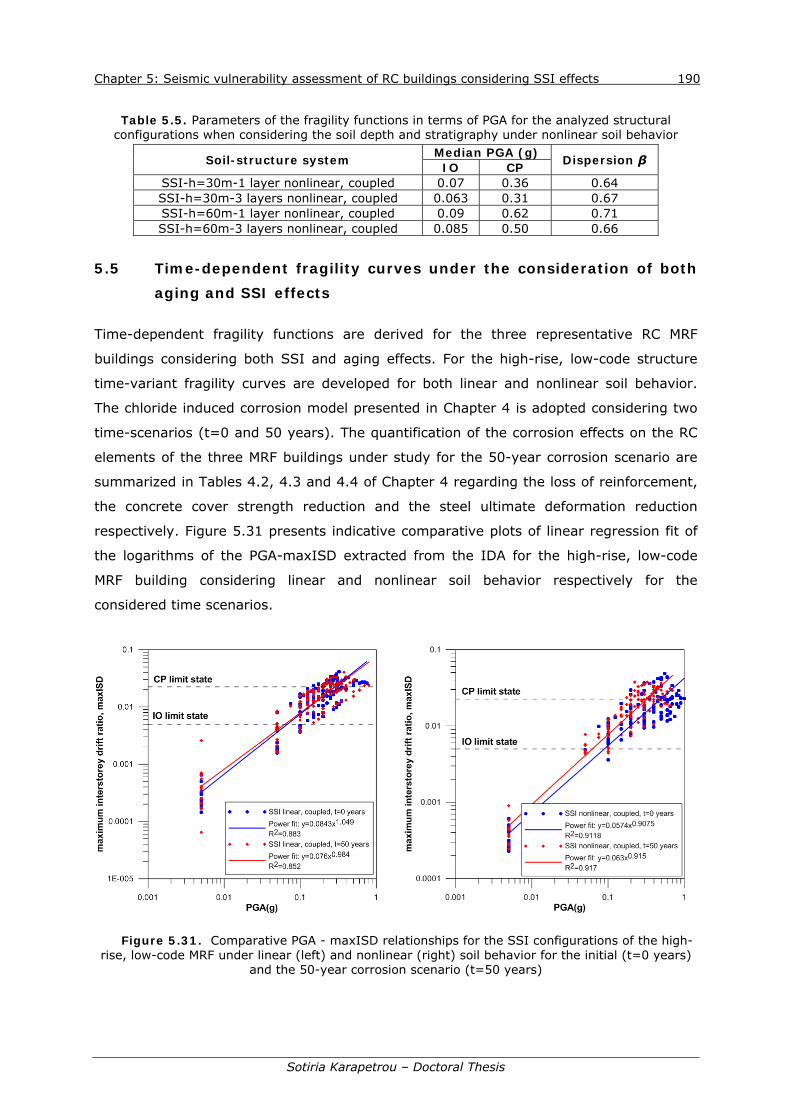
Chapter 5: Seismic vulnerability assessment of RC buildings considering SSI effects 190
Sotiria Karapetrou – Doctoral Thesis
Table 5.5. Parameters of the fragility functions in terms of PGA for the analyzed structural configurations when considering the soil depth and stratigraphy under nonlinear soil behavior
Soil-structure system Median PGA (g) Dispersion β IO CP SSI-h=30m-1 layer nonlinear, coupled 0.07 0.36 0.64 SSI-h=30m-3 layers nonlinear, coupled 0.063 0.31 0.67 SSI-h=60m-1 layer nonlinear, coupled 0.09 0.62 0.71 SSI-h=60m-3 layers nonlinear, coupled 0.085 0.50 0.66
5.5 Time-dependent fragility curves under the consideration of both aging and SSI effects
Time-dependent fragility functions are derived for the three representative RC MRF
buildings considering both SSI and aging effects. For the high-rise, low-code structure
time-variant fragility curves are developed for both linear and nonlinear soil behavior.
The chloride induced corrosion model presented in Chapter 4 is adopted considering two
time-scenarios (t=0 and 50 years). The quantification of the corrosion effects on the RC
elements of the three MRF buildings under study for the 50-year corrosion scenario are
summarized in Tables 4.2, 4.3 and 4.4 of Chapter 4 regarding the loss of reinforcement,
the concrete cover strength reduction and the steel ultimate deformation reduction
respectively. Figure 5.31 presents indicative comparative plots of linear regression fit of
the logarithms of the PGA-maxISD extracted from the IDA for the high-rise, low-code
MRF building considering linear and nonlinear soil behavior respectively for the
considered time scenarios.
Figure 5.31. Comparative PGA - maxISD relationships for the SSI configurations of the high-rise, low-code MRF under linear (left) and nonlinear (right) soil behavior for the initial (t=0 years)
and the 50-year corrosion scenario (t=50 years)

Chapter 5: Seismic vulnerability assessment of RC buildings considering SSI effects 191
Sotiria Karapetrou – Doctoral Thesis
Figure 5.32 depicts comparative plots of fragility curves for the three representative
buildings derived as a function of PGA for the fixed-base and SSI models always for the
different corrosion scenarios. A great increase in fragility is observed for the SSI models
with respect to the fixed base structures founded on rock. This trend holds true for both
the initial and 50-year corroded structures with the latter showing higher vulnerability. In
addition, for the high-rise building designed with low seismic code provisions, Figure 5.33
shows the derived graphs of time-dependent fragility functions for the SSI configurations
in the light of linear and nonlinear soil behavior respectively in comparison with the fixed
based structure for the initial and corroded scenario. It is shown that the SSI model,
which considers soil nonlinearity is less vulnerable compared to the SSI system where
linear elastic soil behavior is taken into account. This observation is more noticeable for
the CP damage limit state and for the initial time scenario (t=0 years).
Table 5.6 summarizes the estimated median and β(t) values of the different damage
states (e.g. IO, CP) as a function of PGA for all the considered building configurations and
time scenarios. Finally, Table 5.7 presents the time variant fragility parameters for the
different considered SSI configurations of the analyzed high rise, low code building.
Table 5.6. Parameters of the fragility functions in terms of PGA for the considered structural
configurations and corrosion scenarios
RC building Foundation conditions
Time scenario (years)
Median PGA (g) Dispersion
IO CP
Low rise MRF-no code
Fixed base –outcropping rock
0 0.10 0.73 0.74
50 0.09 0.59 0.73
SSI models- Vs=200 m/sec
0 0.06 0.44 0.65
50 0.05 0.37 0.67
High rise MRF-low code
Fixed base - outcropping rock
0 0.14 0.68 0.65
50 0.13 0.59 0.65
SSI models- Vs=200 m/sec
0 0.07 0.28 0.68
50 0.06 0.26 0.71
Mid rise MRF-high code (Greek)
Fixed base - outcropping rock
0 0.10 1.31 0.78
50 0.10 1.13 0.77
SSI models- Vs=200 m/sec
0 0.08 0.75 0.64
50 0.08 0.67 0.64

Chapter 5: Seismic vulnerability assessment of RC buildings considering SSI effects 192
Sotiria Karapetrou – Doctoral Thesis
Figure 5.32. Time-dependent fragility curves in terms of PGA for the analyzed fixed base and
SSI structural configurations

Chapter 5: Seismic vulnerability assessment of RC buildings considering SSI effects 193
Sotiria Karapetrou – Doctoral Thesis
Table 5.7. Time-dependent fragility parameters in terms of PGA for the high rise, low code building considering fixed base and SSI (for linear or nonlinear soil behavior) structural
configurations
RC building Foundation conditions
Time scenario (years)
Median PGA (g) Dispersion
IO CP
High rise MRF-low
code
Fixed base - outcropping rock
0 0.14 0.68 0.65
50 0.13 0.59 0.65
SSI models- Vs=200 m/sec
0 0.07 0.28 0.68
50 0.06 0.26 0.71
Fully nonlinear SSI model- Vs=300 m/sec
0 0.07 0.36 0.64
50 0.06 0.28 0.62
Figure 5.33. Time-dependent fragility curves in terms of PGA for the high rise, low code building when considering fixed base and SSI structural configurations under linear and nonlinear
soil behavior
5.6 Conclusions
The seismic vulnerability of three representative RC frame buildings designed according
to different seismic code levels, has been assessed taking into account SSI effects.
Consideration of SSI has been achieved by applying the direct one-step coupled
approach, which accounts simultaneously for inertial and kinematic interaction schemes.
The different soil-structure systems have been analyzed considering at first linear soil
behavior. For the high-rise building designed with low seismic code provisions, for which
soil-structure interaction was more pronounced, both linear elastic and nonlinear soil
behavior have been considered to gain further insight into the influence of SSI and site
effects on fragility analysis. Soil nonlinearity has been introduced through the use of a
pressure-independent multi yield surface incremental plasticity model. A two-step
uncoupled approach has been also applied which considers the modification of ground
motion due to site effects on the response of the fixed base structure. In this way, the

Chapter 5: Seismic vulnerability assessment of RC buildings considering SSI effects 194
Sotiria Karapetrou – Doctoral Thesis
importance and relevant contribution of site and SSI effects have been investigated.
Moreover, to examine more thoroughly the effect of SSI on the seismic performance and
fragility of the building under nonlinear soil behavior, the coupled soil-structure systems
have been further analyzed for varying soil depth and stratigraphy. Finally, time-
dependent fragility functions were derived for all three MRF structures considering both
SSI and chloride induced corrosion effects for a 50-year time scenario.
Comparative dynamic analyses were conducted for the fixed base models (considering
or not site effects) and the soil-structure systems under linear and nonlinear soil
behavior for selected test earthquake records to demonstrate the influence of SSI and
site effects on the seismic response and vulnerability. Results in terms of acceleration
time histories at the base of the structure, interstorey drifts and stress-strain hysteretic
loops at various soil depths for the nonlinear soil-structure configurations highlighted the
significant role of SSI and site effects in modifying the ground motion imposed at the
base of the structure and finally its structural dynamic response. The level of this
modification depends on the ground motion characteristics (frequency content, duration),
the dynamic properties of the soil and the structure itself.
IDA was performed by applying 15 multiply scaled input motions for all considered
models. Finally, probabilistic fragility functions have been derived in terms of rock
outcropping PGA for the IO and CP limit states. It was shown that the consideration of
SSI and site effects under both linear and nonlinear soil behavior may significantly affect
the structural performance increasing considerably the structure’s seismic vulnerability
compared to the reference case where the structure is assumed as fixed base and no SSI
or site effects are taken into account. When soil nonlinearity is introduced these effects
are generally expected to have lower impact on structure’s fragilities for higher levels of
seismic loading. When the soil behavior is assumed linear elastic the fragility curves
derived for the coupled SSI approach have practically no difference with the uncoupled
fixed base model where site effects are taken into account. On the other hand, nonlinear
SSI leads to an increase of the structure’s vulnerability compared to the corresponding
fixed base model. The latter could be attributed to the complex nonlinear behavior of the
underlying soil that may introduce additional translation and rotation effects to the
structure yielding to higher drift demands. Overall, among the analyzed cases, the
uncoupled fixed based model where site effects are linearly modeled shows the highest
vulnerability. Thus, while avoiding the computational cost introduced by the coupled SSI
models, the use of the fragility curves for the fixed based model where site effects are
modeled linearly would lead to conservative results. However, this is valid only for the
analyzed cases and should not be regarded as a general conclusion.

Chapter 5: Seismic vulnerability assessment of RC buildings considering SSI effects 195
Sotiria Karapetrou – Doctoral Thesis
Furthermore, nonlinear SSI leads to an increase in fragility of structure when the
stratigraphy of the soil profile is taken into account, as the step-like layered soil medium
may amplify the imposed input motion at the base of the structure in comparison to the
homogeneous soil cases. On the other hand, it is seen that nonlinear SSI may decrease
the seismic vulnerability of the structure for deeper homogeneous and layered soil
profiles. This may be attributed to the increase of attenuation levels. However it
generally depends on the considered soil depth and stratigraphy as well as on the
characteristics of the input motions in relation to the dynamic properties of the soil and
the structure itself.
Regarding the consideration of aging effects on the seismic vulnerability of the soil-
structure systems, as expected based on the results of Chapter 4, chloride induced
corrosion leads to an overall increase of the seismic fragilities with time.
Overall, the aim of the present study is to prove that the conventional way of
calculating building fragility with the hypothesis of fixed base structure may lead to
unconservative results. SSI and site effects are very important to be ignored. The work
presented herein provides an insight into the influence of SSI and site effects on the
seismic performance and vulnerability of RC frame buildings under linear and nonlinear
soil behavior. Based on the results of this study and in order to enhance the reliability in
seismic vulnerability assessment studies, further research is necessary for the
development of generalized fragility functions applicable to a variety of RC building
typologies which would take into account SSI and site effects for a variety of soil
conditions. Moreover vulnerability functions derived for the same building should be
related to varying subsoil conditions and different Intensity Measures.

Chapter 5: Seismic vulnerability assessment of RC buildings considering SSI effects 196
Sotiria Karapetrou – Doctoral Thesis

Sotiria Karapetrou – Doctoral Thesis
CHAPTER 6
Time-building specific vulnerability assessment of RC buildings using field
monitoring data
6.1 Introduction
In the context of seismic vulnerability assessment of reinforced concrete (RC) buildings,
the use of field monitoring data constitutes a significant tool for the representation of the
actual structural state, reducing uncertainties associated with the building configuration
properties as well as many non-physical parameters (age, maintenance, etc.), enhancing
thus the reliability in the risk assessment procedure. In the present chapter, the seismic
vulnerability of existing RC buildings is evaluated combining through a comprehensive
methodology, the numerical analysis and field monitoring data. The proposed
methodology is highlighted through the derivation of “time-building specific” fragility
curves for an eight-storey RC structure (hospital building), built almost five decades ago,
that is composed by two adjacent units separated through a structural joint. The
assessment of the dynamic characteristics is performed using ambient noise
measurements recorded by a temporary seismic network which was deployed inside the
hospital. The modal identification results are used to update and better constrain the
initial finite element model of the building, which is based on the available design and
construction documentation plans. Three-dimensional incremental dynamic analysis is
performed to derive the fragility curves for the initial as built model (“building-specific”)
and for the real structures as they are nowadays (“time-building specific”). The initial
“building specific” curves are evaluated through their comparison with conventional
generic curves that are commonly used in risk assessment studies. Moreover, in order to
validate and enhance the reliability of the obtained results, the “time-building specific”
fragility curves, are compared to time-dependent curves derived for the hospital units
applying the analytical methodology proposed in Chapter 4 adopting an appropriate for
the specific case study corrosion scenario. Results derived from both approaches indicate

Chapter 6: Time-building specific vulnerability assessment of RC buildings using monitoring data198
Sotiria Karapetrou – Doctoral Thesis
that the consideration of the actual state of structures may significantly alter their
expected seismic performance leading to higher vulnerability values. Part of the research
presented in this chapter has been published in Bulletin of Earthquake Engineering (Bindi
et al., 2014a) scientific journal.
6.2 Application study: AHEPA hospital
6.2.1 Structural description
The AHEPA general hospital in Thessaloniki is one of the largest hospitals in northern
Greece located in the campus of Aristotle University. It is a major teaching and research
hospital and part of the National Healthcare System of Greece. It covers all possible
specializations of a large-scale major hospital (surgical, pathology, psychiatry etc.). The
hospital complex (illustrated in Figure 6.1) consists of 40 buildings of various functions
and typologies, 2 electrical substations, a gas distribution network and an underground
water supply system. Many of these buildings were built before 1985 and are classified
as low seismic code structures. In case of an emergency its central location in the city of
Thessaloniki makes it one of the most important medical care centers for an efficient
crisis management.
Figure 6.1. General view of the AHEPA hospital complex

Chapter 6: Time-building specific vulnerability assessment of RC buildings using monitoring data199
Sotiria Karapetrou – Doctoral Thesis
The target building hosts both administration and hospitalization activities. It was
constructed in 1971 and is considered representative of structures that have been
designed according to the old 1959 Greek seismic code (‘Royal Decree’ of 1959), where
the ductility and the dynamic features of the constructions are ignored. During the 1978
Thessaloniki earthquake (M=6.5, R=26.7km, Papazachos et al., 1979; Soufleris et al.,
1982), which generally caused extensive damages and the collapse of one high-rise
residence structure, the hospital building suffered only slight damage. It is an eight
storey infilled structure and its special feature is that it is composed of two adjacent tall
building units that are separated through a structural joint as illustrated in Figure 6.2(a).
The separation gap is approximately equal to 5cm and potential pounding phenomena
(hammering effects) between the to units may occur during a strong earthquake event.
UNIT 1 covers a rectangular area of 29m by 16m while UNIT 2 has a trapezoidal cross
section of 21m by 27m by 16m. The total height of the building with respect to the
foundation level is 28.6m with a constant inter-storey height of 3.4m except for the
second floor where the height increases to 4.8m due to the presence of a middle floor
level which covers only a part of the typical floor plan (Figure 6.2(a)). From the structural
point of view the building’s force resisting mechanism comprises longitudinal and
externally transverse reinforced concrete moment resisting frames. The columns have
variable dimensions along the height of the building starting from 0.45m x 0.70m at the
lowest level (basement) and resulting to 0.35m x 0.35m at the upper floor. In the
longitudinal direction the outer and inner columns are connected by beams with cross-
section of 0.20m x 0.60m and 0.35m x 0.40m respectively. In the transverse direction
on the other hand only the exterior columns are connected by beams with dimensions of
0.20m x 0.95m. The presence of beam to beam connections at all floor levels near the
staircases and elevator shafts, constitute a complex structural system which is
particularly evident in the middle floor where the RC beams are inverted. Reinforced
concrete walls are present in both building units, surrounding partially the staircases and
the lift shafts; they are not specially detailed for seismic performance. More specifically
there are two walls in the transverse and one in the longitudinal direction of UNIT 1 and
only one wall in the transverse direction of UNIT 2. The RC walls are 0.20m thick while
their length is decreasing significantly along the structure’s height. Moreover a perimeter
reinforced concrete wall with dimensions of 0.20m x 3.00m has been constructed at top
of the building. Figures 6.3 and 6.4 present the geometrical properties of the sections
and the reinforcement details of the structural elements respectively. Moreover Figure
6.5 illustrates the diameters and position of the reinforced bars of walls and columns for
the different floor levels. It is observed that the reinforcement of the second and upper
floor columns is greater than for the first floor elements probably due to the presence of

Chapter 6: Time-building specific vulnerability assessment of RC buildings using monitoring data200
Sotiria Karapetrou – Doctoral Thesis
the middle floor which leads also to an increase of the height of the second floor. In-situ
testing on materials, structural details and non-structural components were not possible
to be conducted. The material properties and the structural details used for the numerical
modeling of the building units, are defined based on the information of the available
blueprints. More specifically concrete B225 (fc=14MPa) is used for all beams and columns
while two steel classes StIII (fy=500MPa) and StI (fy=220MPa) are utilized for the
reinforced bars. Steel class StI is used for the reinforcement of all beams (longitudinal
and transverse) and for most column elements. In Figure 6.5, it can be seen for which
cases StIII is utilized. The mass properties are deduced from the available blueprints
based on the structural elements and the prescriptions of the national loading standards.
Table 6.1 summarizes the main characteristics of the two building units according to the
design and construction plans, namely the mass, the characteristic strength values of
concrete (fc) and reinforcement steel (fy). The two building units do not have common
foundation. The foundation system of UNIT 1 consists of simple footings of variable
geometries without tie-beams whereas in UNIT 2 the footings are combined partially with
a raft foundation. Figure 6.2(b) represents a typical cross-section of the hospital with the
foundation soil profile and the average shear wave velocities Vs,ave estimated from cross-
hole and down-hole tests (Raptakis et al., 1994). The soil consist of a stiff clay with
average Vs,ave of about 400-450m/sec. The rock basement (schist) is found at 30 to 35m
depth having Vs velocities greater than 750m/sec. The foundation soil at the hospital
building can be characterized as soil type B according to EC8 soil classification.
Regarding the non-structural components, besides the three existent elevators, an
electricity generator is also installed in the basement of UNIT 1, which in case of a
general shut down (e.g. due to a strong earthquake event) constitutes the only source of
electricity supply for the entire hospital. Finally it should be noted that no significant
interventions or retrofitting works have been carried out over the years according to the
Technical service of the hospital, that would allow deviations from the available design
and construction plans.
Using the SYNER-G taxonomy (Pitilakis et al., 2014a) for RC structures to describe
the typology of the hospital building, it may be considered typical of high-rise infilled
moment resisting frame buildings designed with low seismic code level.
Table 6.1. Main characteristics of the hospital building units (fc and fy represent the strength of concrete and reinforcement steel respectively)
RC building Total mass (t) fc (MPa) fy (MPa)
UNIT 1 3804.0 14.0 220.0 and 500.0
UNIT 2 3144.0 14.0 220.0 and 500.0

Chapter 6: Time-building specific vulnerability assessment of RC buildings using monitoring data201
Sotiria Karapetrou – Doctoral Thesis
(a)
(b)
Figure 6.2. (a) Typical floor plan and middle floor with the structural joint and (b) typical soil profile of AHEPA hospital building (dimension in m)

Chapter 6: Time-building specific vulnerability assessment of RC buildings using monitoring data202
Sotiria Karapetrou – Doctoral Thesis
Figure 6.3. Geometrical properties of the element sections of UNIT 1 and UNIT 2 presented in
section A-A’ along the longitudinal direction of the hospital building (dimensions in m)
Figure 6.4. Reinforcement layout of UNIT 1 and UNIT 2: red and blue correspond to the beam and column reinforcement respectively (diameters in mm)

Chapter 6: Time-building specific vulnerability assessment of RC buildings using monitoring data203
Sotiria Karapetrou – Doctoral Thesis
Basement 1st floor
2nd floor 3rd floor
Figure 6.5. Diameters and position of the column reinforced bars of the different floor levels for both UNIT 1 and UNIT 2 (diameters and dimensions in mm)

Chapter 6: Time-building specific vulnerability assessment of RC buildings using monitoring data204
Sotiria Karapetrou – Doctoral Thesis
4th floor 5th floor
6th floor 7th floor
Figure 6.5. (Continued) - Diameters and position of the column reinforced bars of the different floor
levels for both UNIT 1 and UNIT 2 (diameters and dimensions in mm)

Chapter 6: Time-building specific vulnerability assessment of RC buildings using monitoring data205
Sotiria Karapetrou – Doctoral Thesis
6.2.2 Instrumentation arrays
Permanent and temporary instrumentation arrays (Figure 6.6) have been implemented
under the responsibility of the Soil Dynamics and Geotechnical Earthquake Engineering of
the Aristotle University of Thessaloniki (SDGEE-AUTH) and in close cooperation with
Helmholtz Centre Potsdam, German Centre for Geosciences (GFZ). The permanent
accelerometric array (SOSEWIN network) operates in AHEPA hospital since May 2012. In
addition to the SOSEWIN network, various temporary networks have been deployed
inside the hospital to evaluate the risk of the building for various earthquake scenarios.
The permanent network is installed for the long term building monitoring. It is composed
by sensing units where the building motion is measured in real time through MEMS
sensors. It is mainly intended to monitor the building response to earthquakes.
Furthermore the earthquake recordings from the permanent instrumentation array are
used to develop an operational framework for Early Earthquake Warning (EEW) and rapid
post-earthquake damage assessment. Ambient noise measurements on the other hand
are used for the dynamic characterization of the building deploying a denser network of
stations equipped with velocimeters, which have a better amplitude resolution and a
lower internal noise than the MEMS. The description of both permanent and temporary
network provides a complete view of the instrumentation arrays that have been installed
in the hospital building.
6.2.2.1. Permanent array
The SOSEWIN network constitutes of 13 triaxial accelerometers (MEMS ADXL203 chip)
installed in the basement (S02FC), the first (SB4D4) and the fourth (SB6C4, SB688,
SB5E8, SB27C) floor (SB6C4, SB688, SB5E8, SB27C) and the roof (SB0F8, SB22C,
SB260, SB278, SB110, SB6BC, SB11C) as presented schematically in Figure 6.6. One
more accelerometer is installed on the roof of a nearby building and used as bridge node
for the data transmission to the two gateways installed outside of the SDGEE-AUTH as
illustrated in Figure 6.7. Several earthquake events have already been recorded and the
instrumentation array continues to transfer data streams to the Seiscomp3 server
installed at SDGEE-AUTH premises. In Figure 6.8 SOSEWIN recordings for a local
earthquake (Volvi Earthquake 11.10.2013, Mw=4.7, R=10km) are shown.

Chapter 6: Time-building specific vulnerability assessment of RC buildings using monitoring data206
Sotiria Karapetrou – Doctoral Thesis
Figure 6.6. Floor plans of the basement, 1st and 4th floors and the roof with the permanent and temporary instrumentation. All SXXXX are accelerometers of the permanent network, all RE-XX
and T4D50 are seismometers of the temporary networks operating for short period of time inside the hospital. Photos of the SOSEWIN stations at the 4th floor near the structural joint (RE-39) and
at roof (SB0F8)
Target-13 sensors
Bridge node1 sensor
Data centerGateway nodes
Figure 6.7. Permanent network array of AHEPA hospital

Chapter 6: Time-building specific vulnerability assessment of RC buildings using monitoring data207
Sotiria Karapetrou – Doctoral Thesis
Figure 6.8. Earthquake data for the longitudinal (east-west, EW), transverse (north-south, NS) and
vertical (V) components recorded at SOSEWIN sensors at the 4th floor and the roof from the 11.10.2013 Volvi Earthquake (Mw=4.7, R=10km)
6.2.2.2. Temporary array
In February 2013 a two-day ambient noise experiment was conducted in the hospital
building in cooperation with GFZ Potsdam. During the first day, a temporary array of 39
triaxial seismometers was deployed in the two building units. In order to capture the
translational and torsional modes of the building, the sensors were installed in every floor
with the configuration illustrated in Figures 6.6 and 6.9. Each floor was instrumented
with four stations, which were installed along the middle corridor of the building near and
far the structural joint (Figure 6.9). The instruments were Mark Products short-period
seismometers (L4C-3D, 1Hz natural frequency) coupled to EarthData recorders EDL
(PR6-24). The seismic sensors are passive seismic sensors with 1Hz corner frequency,
connected to 24bit digitizers. Even in the free field, the internal noise of such equipment
allow to record ambient noise to about 0.2Hz (e.g. Strollo et al., 2008a; 2008b). At four
locations, a second station equipped with Güralp broadband seismometers (CMG-40T,
30sec natural period) coupled to Reftek recorders (DAS-130) was also deployed for
instrumental comparison purposes. GPS antennas guaranteed the time synchronizations
among all instruments. The sensors recorded along the two orthogonal horizontal and
along the vertical directions (three components). The two horizontal components are
oriented along the longitudinal and transversal direction of the building. Ambient noise
was recorded simultaneously for about 4 hours in all stations with a sampling rate of 500
Hz and gain 10. In the second day, 51 stations were used (44 EDL and 7 Reftek), adding
one station at certain floors. Table 6.2 summarizes the serial codes and locations of the
employed instruments for both days of experiment. As illustrated in Figure 6.10 the
amplitude of the time series is increasing as the noise waveforms are propagating from
the basement to the roof of the building.

Chapter 6: Time-building specific vulnerability assessment of RC buildings using monitoring data208
Sotiria Karapetrou – Doctoral Thesis
Figure 6.9. Sections A-A΄ and B-B΄ along the longitudinal and transverse direction of the hospital building with the temporary instrumentation
Table 6.2. Serial number and position of all the stations used in the two-day ambient noise experiment
1st day 2nd day Station position UNIT 1 UNIT 2 UNIT 1 UNIT 2
Basement RE-07, RE-03 RE-30, RE-02 RE-38, T4K21*, RE-05, RE-02 RE-10, RE-31
1st floor RE-29, RE-41 RE-01, RE-10 RE-01, RE-43 RE-09, RE-21
2nd floor RE-09, RE-31 RE-38, RE-05 RE-07, RE-11, RE-03 RE-28, RE-36
3rd floor RE-22, RE-25 RE-18, RE-14 RE-25, T4D50*, RE-18, RE-16 RE-14, RE-22
4th floor RE-45,RE-39 T4D50* RE-34, RE-12 RE-39, RE-45
T4D50, T4K19* RE-12, RE-34
5th floor RE-15, RE-44 RE-26,RE-35, T4K20*
RE-26, RE-35 T4K20*, RE-37 RE-15, RE-44
6th floor RE-17, RE-20 RE-08,RE-33, T4D78*
RE-17, RE-33, RE-41
RE-20,RE-08, T4D78*
7th floor RE-27, RE-23 RE-32,RE-42, T4D49*
RE-42, RE-27, RE-29
RE-23,RE-32 T4D49*
Roof RE-06, RE-24, RE-13 RE-04, RE-40 RE-13, RE-27,
RE-06 RE-19, RE-24,
RE-40 *: broad-band seismometers (CMG-40T)

Chapter 6: Time-building specific vulnerability assessment of RC buildings using monitoring data209
Sotiria Karapetrou – Doctoral Thesis
Figure 6.10. Synchronized ambient noise recordings for the longitudinal component. All the
records have the same amplitude scale (y-axis)
6.3 Description of the methodological framework
A schematic flowchart of the proposed methodological framework that has been adopted
for the derivation of the ”time-building specific” fragility curves of the hospital building
units based on field monitoring data is presented in Figure 6.11. Ambient noise
measurements are used to derive the experimental modal model of the hospital building
and identify its modal properties based on operational modal analysis (OMA). The modal
identification results are used to update and better constrain the initial finite element
model of the building, which is based on the design and construction documentation
plans. In the absence of any structural geometry modification since 1971 when the
building was constructed, only the variation in the material properties is taken into
account in the present study. An eigenvalue sensitivity analysis of the elastic numerical
modal models is performed to identify the most sensitive parameters influencing the
structural modes of interest which are used in the manual updating process to define the
optimal analytical models that reflect the experimental results. The selection of the best
updated finite element (FE) model for the two building units is made by evaluating an
appropriate response correlation function between experimental and numerical results.
Three-dimensional incremental dynamic analyses (IDA) (Vamvatsikos and Cornell, 2002)
of the nonlinear updated models are performed using real ground motion accelerograms
that are selected based on the regional seismic hazard, to derive the “time-building
specific” fragility curves that correspond to the actual state of the hospital building units.

Chapter 6: Time-building specific vulnerability assessment of RC buildings using monitoring data210
Sotiria Karapetrou – Doctoral Thesis
Monitoring dataExperimental modal model
(Operational Modal Analysis)
Design and construction plansInitial FE model
Building-time specific vulnerability assessment using field monitoring data
Nonlinear analytical simulation of the updated models: Material inelasticityGeometrical nonlinearity
Building-time specific fragility curves generation
3D nonlinear incremental dynamic analysisEDP: maximum interstory drift
Earthquake demand:Regional seismic hazard (SHARE)
Methodology for fragility curve generation:Incorporation of uncertainties in limit state definition, capacity and demand
Manual updating process
Comparison between experimental and numerical modal model: evaluation of response function
Eigenvalue sensitivity analysis
Sensitivity in material properties
Selection of the “best” updated FE model
Figure 6.11. Methodological framework adopted in the present study
6.4 Operational modal analysis (OMA) using field monitoring data
6.4.1 Modal identification methods
System identification is the process of building a mathematical model of a physical
system based on experimental data (Ljung, 1999). From an engineering point of view the
goal of system identification is to predict the physical quantities of a system based on its
mathematical model (Kim, 2011). Research on linear system identification evolved in the
late 1960s on the basis of control engineering (Gevers, 2006).
The typical scheme of the identification process for a linear time-invariant vibrating
structure is presented in Figure 6.12. Based on the knowledge of the system’s
experimental response (output data) to an excitation source (input data) a parametric
modal model can be derived that is defined by a set of modal parameters
(eigenfrequencies, mode shapes, damping ratios). There are several deterministic or
stochastic techniques developed over the past years that can be used to build the
mathematical model of the dynamic structural systems in frequency or time domain
based on measured data. A modal model of an artificially excited structure can be
obtained based on Experimental Modal Analysis (EMA); however in case of real scale civil
structures applying an artificial excitation might be difficult from technical and

Chapter 6: Time-building specific vulnerability assessment of RC buildings using monitoring data211
Sotiria Karapetrou – Doctoral Thesis
economical point of view. Therefore, Operational Modal Analysis (OMA) is generally
preferred to forced vibration measurements since the same modal parameters can be
obtained from vibration data in operational rather than laboratory conditions by modeling
the interaction between the structure and its environment (e.g. wind, traffic, etc).
Ambient vibration measurements are usually used to perform OMA and indentify the
modal parameters of a structure. In contrast to Experimental Modal Analysis, the
properties of ambient excitation in Operational or Output- Only Modal Analysis are
difficult or impossible to be measured. Therefore stochastic identification techniques
have been developed by the assumption that the response is a realization of a stochastic
process with unknown white Gaussian noise as input (Figure 6.12) characterized by a flat
spectrum in the frequency range of interest. Based on this assumption the excitation
input is considered to have the same energy level at all frequencies implying that all
modes are excited equally (Van Overschee and De Moor, 1996; Peeters, 2000).
Figure 6.12. Stochastic Output-Only Identification
There are different stochastic identification techniques to extract the modal
parameters of a structural system, namely the parametric and non-parametric methods.
In non-parametric methods the modal parameters are estimated directly by post-
processing the measured data whereas in the parametric methods the dynamic
characteristics are extracted based on a parametric model that is updated to fit the
recorded data. The two methods are described in more detail in the following paragraphs.
Non-parametric algorithms are traditionally associated with the Discrete Fourier
Transform and the computation of auto and cross power spectra. They are widely used
due to their simplicity and intuitiveness. Two of the most commonly used non-parametric
methods for the modal parameters estimation of the identified system are (a) the Basic
Frequency Domain or the Peak Picking (PP) method (Bendat and Piersol, 1993) and (b)
the Frequency Domain Decomposition (FDD) (Brincker et al., 2000). Both methods are
based on correlations of the power spectra between the outputs and the reference
outputs and on decomposition of the stochastic power spectral density (PSD). In the first
method the frequency peaks from the average spectra are selected that are derived
based on the output recordings of the sensors. The FDD method is considered to be an
improved version of the PP method and consists of decomposing the system’s power
spectral density into its singular values. It is shown that taking the Singular Value
Decomposition SVD of the spectral matrix, the latter is decomposed into a set of auto

Chapter 6: Time-building specific vulnerability assessment of RC buildings using monitoring data212
Sotiria Karapetrou – Doctoral Thesis
spectral density functions each corresponding to a single degree of freedom (SDOF)
system (Brincker et al., 2000).
The output PSD, Gyy(jω), at discrete frequencies is decomposed by taking the Singular
Value Decomposition SVD of the matrix:
Hyy i i iG ( j ) U S U (6.1)
where Ui=[ui1, ui2,….., uim] is a unitary matrix including the singular vectors uij and Si is a
diagonal matrix including the scalar singular values sij. If only one mode is dominating
close to the peak then the first singular vector is an estimate of the mode shape. If two
modes are dominating at this frequency peak then the two first singular vectors are
estimates of the corresponding mode shapes (Figure 6.13).
These results are exact under the following conditions:
the loading is white noise
the structure is lightly damped and
the mode shapes of close modes are geometrically orthogonal.
Disadvantages of the nonparametric methods are the subjective selection of the
eigenfrequencies, the lack of accurate damping estimates and the determination of
operational deflections shapes instead of mode shapes since no modal model is fitted to
the data (Peeters and De Roeck, 1999).
Figure 6.13. Frequency Domain Decomposition (FDD) method
Stochastic subspace identification SSI (Van Overschee and De Moor, 1991) works in
time domain and is one of the most commonly applied parametric identification methods.
The SSI techniques involve the selection of a mathematical model whose parameters are
adjusted to the model so that it fits to the measured data. The goal of this model
calibration is to minimize the deviation between the predicted and measured system
response. The number of the parameters plays a significant role in the identification
process. In case a too small number is defined, the modal parameters may be not
modeled statistically correctly. On the other hand, if the number is defined to be too
high, then the model becomes over-specified resulting in unnecessary high statistical
uncertainties of the model parameters. An advantage of the parametric over the non-

Chapter 6: Time-building specific vulnerability assessment of RC buildings using monitoring data213
Sotiria Karapetrou – Doctoral Thesis
parametric techniques is the direct estimation of the system’s damping ratio from the
identification process.
SSI is based on a state space description of the dynamic problem. In fact, the second
order dynamic problem, expressed through the differential equation of motion, is
converted into two first order problems, namely the “state equation” and “observation
equation”. The stochastic state-space model of a discrete–time, linear, time invariant
system is mathematically described by the following set of equations (Ewins, 1984;
Peeters and De Roeck, 1999):
k 1 k kx Ax w (6.2)
k k ky Cx v (6.3)
with
p T Tq q pqT
p
w Q SE w u
u S R
(6.4)
where yk l is the measurement vector at time instant k of the l outputs; kx n is the
state vector at discrete time instant k and contains the numerical values of n states; vk l and wk
n are unmeasurable vector signals that are assumed to be zero mean,
stationary, white noise vector sequences; A n n is the state matrix that describes the
dynamics of the system by its eigenvalues whereas C l n is the output matrix. The
matrices Q n n , S n l and R l l are the covariance matrices of the noise sequence wk
and vk. The matrix pair A, C is assumed to be observable, which means that all modes
of the system can be observed in the output yk and can thus be identified. E is the
expected value operator and δpq is the Kronecker delta. During the stochastic
identification the parametric model is defined to determine the following parameters:
the order n of the unknown system
the system matrices A and C as well as Q, S and R so that the
predicted and the measured output of the model are equal.
The output measurements are gathered and rearranged in a block Hankel (data
driven SSI) or Toeplitz (covariance driven SSI) matrix as past (reference) and future
blocks. The Hankel or Toeplitz matrix is a matrix where each antidiagonal or diagonal
consists of the repetition of the same element respectively. More specifically for the
predicted output response time series expressed as a discrete data matrix the block
Hankel and Toeplitz matrices are defined accordingly as:

Chapter 6: Time-building specific vulnerability assessment of RC buildings using monitoring data214
Sotiria Karapetrou – Doctoral Thesis
Hankel matrix Toeplitz matrix
1 2 n 2s
2 3 n 2s 1
ps s 1 n s 1
s 1 s 2 n s f
s 2 n s 1
2s 2s 1 n
y y y
y y y
Hy y yH
y y y Hy y
y y y
Tf pT H H
s s 1 1
s 1 s 2
2s 1 2s 2 s
R R R
R R RT
R R R
(6.5)
where H 2sl ( n 2s ) and T ls ls , s is the number of block rows and n-2s the number of
block columns. The subscripts p and f stand for past and future and the matrices Hp and
Hf are defined by splitting the Hankel matrix into two parts of s blocks. Rs are the
covariance matrices between all outputs and references and are defined as T
k s kRs E y y . The key step of SSI is the projection of the row space of the future
outputs into the row space of the past outputs (Van Overschee and De Moor, 1996). The
idea behind the projection is that it retains all the information in the past that is useful to
predict the future resulting to a data order reduction. The main theorem of SSI (Van
Overschee and De Moor, 1996) states that the projection can be factorized as the
product of the observability matrix (that is based on the matrix pair A, C) and the
Kalman filter state sequence. The aim of the Kalman filter (Van Overschee and De Moor,
1996; Peeters and De Roeck, 1999; Ljung, 1987; Juang, 1994) is to produce an optimal
prediction for the state vector xk+1 by making use of the observations of the outputs up
to time k and the system matrices combined with the noise covariances. Introducing a
QR-factorization to the Hankel or Toeplitz matrix the projection matrix can be computed.
Continuously the projection matrix is decomposed into its singular values (Singular Value
Decomposition SVD) revealing the order of the system. Finally based on the estimated
system order, the observability matrices and the Kalman filter state sequences, the
system matrices can be calculated. Knowing the outputs, the system order and the
system matrices the identification problem is solved and the modal parameters can be
extracted (Figure 6.14).

Chapter 6: Time-building specific vulnerability assessment of RC buildings using monitoring data215
Sotiria Karapetrou – Doctoral Thesis
Figure 6.14. Stochastic subspace identification (SSI) method
6.4.2 Operational modal analysis using ambient noise measurements
To evaluate the dynamic characteristics of the hospital building, namely the natural
frequencies and mode shapes, system identification and Operational Modal Analysis were
performed using MACEC 3.2 software (Reynders et al., 2011) for the two adjacent
building units separately (UNIT 1 and UNIT 2) as well as for the entire hospital building
complex, analyzed as a single building taking into account the interaction of the two
building units due to their connection with the structural joint (BUILDING). MACEC 3.2 is
a Matlab based code that offers extensive functionalities for the visualization and
processing of the data, the identification of system models and the determination and
visualization of the structural modal parameters. Operational modal analysis consists of
three distinct steps which are: (1) the collection of the data and preprocessing, (2)
system identification and (3) the determination of the modal parameters from the
identified system model. Thus the term “modal analysis” can be defined at two different
levels: (i) the whole procedure of obtaining modal parameters from measurements (steps
1, 2 and 3) and (ii) the determination of the modal parameters from the identified
system model (step 3). MACEC toolbox clearly differentiates between system
identification and modal analysis of level (ii).
The geometrical characteristics of the models introduced and analyzed in MACEC 3.2
are illustrated in Figure 6.15. Operational modal analysis is performed considering only
the horizontal components of the measurements. The grid of the models is built so that
the defined nodes correspond to nodes that have been actually measured. The sensors
that were used for the identification process are illustrated in Figure 6.9. A total duration
of 1800 sec (30min) is used for OMA as tests for stability of the results showed that 30
minutes are enough to get reliable results. Before identification the data were decimated
with a factor of 10 and filtered with a low-pass anti-aliasing filter with a cut-off frequency
of 25Hz and re-sampled at 50Hz reducing thus the number of data from 900000 to

Chapter 6: Time-building specific vulnerability assessment of RC buildings using monitoring data216
Sotiria Karapetrou – Doctoral Thesis
90000 points avoiding thus unnecessary computational burden in the modal analysis
where the frequencies of interest are smaller than 25Hz.
UNIT 1 UNIT 2 BUILDING
Figure 6.15. Visualization of the building’s geometry in MACEC 3.2
In order to verify and enhance the modal identification results for the different
systems under study (UNIT 1, UNIT 2 and BUILDING), analyses have been conducted
using both non-parametric and parametric identification techniques. More specifically the
stochastic (or output-only) system identification methods that have been applied in
MACEC 3.2 are the following:
nonparametric PSD+ estimation using the correlogram method in frequency
domain
reference-based covariance-driven stochastic subspace identification in time
domain.
In the non-parametric methods, system identification is based on the calculation of
the Positive Power Spectral Density (PSD+) matrix at discrete frequency lines. For the
PSD+ estimation of the measured outputs collected from all channels, the correlogram
method was applied. In the correlogram approach, the auto and cross-PSDs of one or
two quasi-stationary ergodic sequences is estimated as the Laplace transform of the auto
or cross correlation functions respectively (Reynders, 2012). In Figures 6.16 and 6.17
indicative plots of estimated auto and cross correlation PSDs are illustrated
corresponding to stations installed at the basement and the top of the hospital building
near and far from the structural joint.
Modal analysis of the identified non-parametric models has been conducted based on
the Peak Picking (PP) and Frequency Domain Decomposition (FDD) methods. In the PP
method the averaged normalized power spectral density (ANPSD) is computed and the
well separated modes are estimated by picking the peaks in the ANPSD. In the FDD

Chapter 6: Time-building specific vulnerability assessment of RC buildings using monitoring data217
Sotiria Karapetrou – Doctoral Thesis
method, the singular values are obtained from the decomposition of the PSD matrix and
the modal parameters are estimated by picking the peaks of the first singular value.
(a) (b)
Figure 6.16. Indicative auto-correlation PSDs+ for time series recorded at stations near the joint, (a) station installed at the basement and (b) station installed at the top
(a) (b)
Figure 6.17. Indicative cross-correlation PSDs+ between time series recorded at stations of the basement and roof (a) near the joint and (b) far from the joint
Modal identification based on parametric methods was conducted by applying the
reference-based covariance-driven stochastic subspace method. The number of block
rows in Toeplitz matrix was selected as 2x(expected system order)/number of outputs).
After the QR and singular value decomposition step of the SSI algorithm (Figure 6.14),
the real system order was estimated based on the singular values (Figure 6.18). For
noiseless data, the system order equals the number of nonzero singular values while for
noisy data the noise causes some singular values to be different of zero. Due to the fact
that the noise is present in the recorded ambient vibration data, the identified system
description contains both system and noise dynamics. A common approach in modal
analysis is then to over-specify the model order (Peeters et al., 1999) such that the true
system modes (physical modes) are separated from the noise modes (mathematical
modes) (Reynders et al., 2011). In general the selection of the model order for the

Chapter 6: Time-building specific vulnerability assessment of RC buildings using monitoring data218
Sotiria Karapetrou – Doctoral Thesis
construction of the stabilization diagrams for the SSI method depends on the number of
modes of interest as well as the number of sensors. For the construction of the
stabilization diagrams a model order range from 2 to 150 in steps of 2 was selected for
UNIT 1 and UNIT 2, whereas for BUILDING the upper limit of the model order was
increased to 200. The increase of the model order for BUILDING was required due to the
analysis of a much larger data set as data from 36 stations were used for the
identification analysis in contrast to UNIT 1 and UNIT 2 where data from only 18 sensors
were used. The aim is to use the stabilization diagrams to detect the columns of stable
modes that satisfy the defined stabilization criteria and continuously select a
representative mode from each column.
Figure 6.18. Singular values of Covariance-driven SSI method in decreasing order of
magnitude
The results of the nonparametric and parametric analyses for the two adjacent
buildings analyzed separately (UNIT 1 and UNIT 2) and as one single building
(BUILDING) are presented in Figure 6.19. In Table 6.3 the eigenfrequencies computed
with the different system identification methods are summarized. It should be noted
herein that potential effects of the non-structural components did not influence the
identification results. The electricity generator was not operating during the experiment
while other non structural elements, such as elevators and medical devices, are
operating in high frequencies (f>10Hz) and are not affecting thus the frequency range of
interest (f<10Hz).

Chapter 6: Time-building specific vulnerability assessment of RC buildings using monitoring data219
Sotiria Karapetrou – Doctoral Thesis
UNIT 1-PP
UNIT 2-PP
BUILDING-PP
UNIT 1 - FDD
UNIT 2 - FDD
BUILDING - FDD
UNIT 1 - SSI/COV
UNIT 2 - SSI/COV
BUILDING - SSI/COV
Figure 6.19. Modal identification applying the Peak Picking (PP), Frequency Domain Decomposition (FDD) and the reference-based covariance-driven Stochastic Subspace Identification (SSI-cov)
methods using ambient noise measurements
Table 6.3. Modal identification results for UNIT 1, UNIT 2 and BUILDING estimated using
parametric and non-parametric identification techniques
Mode type UNIT 1 UNIT 2 BUILDING
PP(Hz)/ FDD (Hz)
SSI (Hz, ξ %)
PP(Hz)/ FDD (Hz)
SSI (Hz, ξ %)
PP(Hz)/ FDD(Hz)
SSI (Hz, ξ %)
Mode1: Coupled
translational 1.65/1.65 1.65 0.8 1.65/1.65 1.65 0.9 1.65/1.65 1.65 0.8
Mode 2: Coupled
translational 1.91/1.90 1.91 1.3 1.91/1.91 1.91 1.1 1.91/1.91 1.91 0.8
Mode 3: Torsional 2.33/2.33 2.33 3.6 2.35/2.35 2.33 3.5 2.35/2.35 2.33 3.2
Mode 4: 1st
Longitudinal 3.50/3.50 3.47 5.4 3.58/3.58 3.52 5.8 3.54/3.58 3.51 6.4
Mode 5: 2nd
Longitudinal 5.20/5.20 5.15 3.0 5.20/5.22 5.16 1.1 5.20/5.20 5.15 2.1

Chapter 6: Time-building specific vulnerability assessment of RC buildings using monitoring data220
Sotiria Karapetrou – Doctoral Thesis
Comparing the results between the different techniques, it is observed that the
estimated frequency values for the five well separated modes are very close to each
other (practically the same for the first three modes) for the two identification methods
applied as well as for the different system models identified. Similar orders and shape
types of the modes are estimated for the different system models (UNIT 1, UNIT 2 and
BUILDING) implying that the dynamic characteristics of the complex hospital building are
possible to be captured by monitoring and analyzing the two adjacent building units
separately. The mode shapes corresponding to the identified modes are presented in
Figures 6.20, 6.21 and 6.22. The building is exhibiting coupled sway and torsional modes
in the frequency range of interest, which are expected in case of geometric and structural
irregularities or eccentricities between the center of mass and center of rigidity. The
highly coupled obtained mode shapes confirm the complex vibrational characteristics of
the building especially for the first two identified frequencies. Figure 6.23 represents
indicatively for UNIT 1 the contribution of the transverse, longitudinal and torsional
motion in the first two modes.
The resonant frequencies of the two adjacent units are very close which may be
attributed to their similar mass and stiffness properties. In order to gain insight of the
modal behavior of the two units and to investigate the correlation between their mode
shapes, the modal assurance criterion (Allemang and Brown, 1982) for the identified
modes is quantified as:
Tj Ei
ij T Tj i Ej Ei
MAC
(6.6)
where φj is the eigenvector j from the experimental modal model of UNIT 1 and φEi the
eigenvector i from the experimental modal model of UNIT 2. MAC values are calculated
higher than 0.8 for the first, third and the fourth modes, approximately equal to 0.60 for
the fifth mode while for the second mode MAC value is found to be lower than 0.60.
Based on the MAC results, it is seen that mode shapes for the two building units are
identical for the first, third and fourth modes. For the second and fifth modes which
correspond to the same frequencies for both units, the mode shapes are not identical for
the UNIT 1 and UNIT 2 although being of similar type. This may be attributed to the
different geometrical and structural configurations of the two units. An interesting aspect
is also the fact that mode 3 is identified for both units as torsional, however the mode
shapes for the two structures are out of phase. Based on the above considerations the
two units cannot be considered as an entire monolithic building neglecting the influence
of the structural joint as they do not present a common modal behavior. In fact the
identified mode shapes reveal a coupling of the two building units under low vibration

Chapter 6: Time-building specific vulnerability assessment of RC buildings using monitoring data221
Sotiria Karapetrou – Doctoral Thesis
(operational conditions). The first and second mode shapes are identified as coupled
translational modes mainly in the transverse direction. The difference between the two
first modes is the fact that for both units the torsional component in the second mode
shape is much more pronounced in comparison to the first one (Figure 6.23). Under no
interaction, the second mode shape would be expected to be a coupled translational
mode mainly in the longitudinal direction. Under strong ground motion however, due to
the strong nonlinearities which the systems are expected to experience and taking into
account the fact that the two units do not have common foundation, the interaction
between the two units may be completely different affecting consequently their seismic
response. For the above reasons the seismic vulnerability assessment is performed
considering the two units separately. The aim of the updating procedure presented
continuously is to calibrate the numerical models in order to reflect the elastic modal
behavior of the two separate structural units as identified through the analysis of the
noise measurements. Damping values are not considered in the implemented updating
formula as their computation includes high levels of uncertainties and are presented
herein only for the sake of completeness.
1st mode: 2nd mode: 3rd mode: 4th mode: 5th mode: Coupled
translational Coupled
translational Torsional 1st Longitudinal 2nd Longitudinal
Figure 6.20. Mode shapes corresponding to the five first indentified frequencies for UNIT 1
1st mode: 2nd mode: 3rd mode: 4th mode: 5th mode: Coupled
translational Coupled
translational Torsional 1st Longitudinal 2nd Longitudinal
Figure 6.21. Mode shapes corresponding to the five first identified frequencies for UNIT 2

Chapter 6: Time-building specific vulnerability assessment of RC buildings using monitoring data222
Sotiria Karapetrou – Doctoral Thesis
1st mode: 2nd mode: 3rd mode: 4th mode: 5th mode: Coupled
translational Coupled
translational Torsional 1st Longitudinal 2nd Longitudinal
Figure 6.22. Mode shapes corresponding to the five first indentified frequencies for BUILDING
Mode shape 1 Mode shape 2
Figure 6.23. Contribution of the lateral components in the first two modes in the longitudinal and transverse direction for UNIT 1

Chapter 6: Time-building specific vulnerability assessment of RC buildings using monitoring data223
Sotiria Karapetrou – Doctoral Thesis
6.4.3 System identification and operational modal analysis using seismic
recordings
Operational modal analysis has been performed using besides the ambient noise
measurements, also the earthquake events recorded by the permanent accelerometric
network. The seismic events recorded since the SOSEWIN network started to operate in
May 2012, which have been used for the analyses, are presented in Table 6.4. It should
be noted herein that no significant earthquake, in terms of damage potential, has
occurred within the time frame of the operating period.
The grid of the systems analyzed in MACEC varies depending on the earthquake and
more specifically on the sensors of the two building units that actually recorded the
seismic events. Only these sensors are used for the identification process and the modal
analysis for each earthquake. In Figures 6.24, 6.26 and 6.27 the grid models and the
modal identification results are presented indicatively for the Limnos earthquake case
(Limnos 24/5/2014, M=6.2, R=12.8km) based on both FDD and SSI methods. In ANNEX
B the grid models and analyses results of all earthquake events are summarized. For
specific seismic events (NW from Lake Langada 6/12/2013, Limnos 24/5/2014,
Kalamaria 16/7/2014, West from Kassandra peninsula in Halkidiki 22/8/2014) a broad
band seismometer was operating on the ground floor of UNIT 1 recording thus the input
motion. For these cases the corresponding input accelerograms and response spectra are
also presented (Figure 6.25 for the Limnos earthquake event 24/5/2014). Table 6.5
summarizes the modal identification results in terms of resonance frequencies for all
recorded earthquake events which are also compared to the corresponding results using
the noise measurements (FDD method). Results show that using the earthquake data it
is not possible to capture all frequencies of the structural systems. For almost all seismic
events, only the first, second and third modes are systematically identified. It is also
noticed that for most cases the frequencies are found slightly smaller in relation to the
identification results using noise measurements. It should be noted however that
ambient noise measurements were conducted at the building deploying a denser network
of stations equipped with velocimeters, which have a better amplitude resolution and a
lower internal noise than the MEMS, providing thus more accurate results regarding the
dynamic characterization of the building. In order to derive reliable results and determine
how the characteristics of real ground motion recordings (frequency content, duration)
affect the dynamic behavior of the monitored structural systems, more earthquake data
need to be collected and analyzed.

Chapter 6: Time-building specific vulnerability assessment of RC buildings using monitoring data224
Sotiria Karapetrou – Doctoral Thesis
Table 6.4. Earthquake events used for OMA of the hospital building
Date Event Time Lateral Longitudinal Depth (km)
Magnitude (M
L)
12.5.2012 Thessaloniki 22:48:12.8 40.564 22.841 7.4 4
11.10.2013 Volvi, Thessaloniki 8:15:48 40.689 23.410 10 4.7
26.10.2013 West from Kassandra peninsula in Halkidiki 17:07:14:30 40.227 23.102 8.1 3.6
6.12.2013 NW from Lake Langada 17:00:52:2 40.799 22.938 9.5 2.6
24.5.2014 Limnos 09:25:02:1 40.286 25.375 12.8 6.2
16.7.2014 Kalamaria 16:14:58:0 40.569 22.948 12.2 3
22.8.2014 West from Kassandra peninsula in Halkidiki 4:27:54 39.935 23.431 13.5 5
UNIT 1 UNIT 2 BUILDING
Figure 6.24. Grid models of the different systems analyzed in MACEC for the earthquake events: Limnos 2014

Chapter 6: Time-building specific vulnerability assessment of RC buildings using monitoring data225
Sotiria Karapetrou – Doctoral Thesis
Figure 6.25. Input acceleration in the longitudinal and transverse direction recorded at the
base of UNIT 1 and the corresponding elastic acceleration response spectra for Limnos, 24.05.2014 event
Figure 6.26. Modal identification applying the Frequency Domain Decomposition (FDD) and the Stochastic Subspace Identification (SSI) methods using earthquake recordings of Limnos, 24.05.2014
event

Chapter 6: Time-building specific vulnerability assessment of RC buildings using monitoring data226
Sotiria Karapetrou – Doctoral Thesis
UNIT 1 UNIT 2 BUILDING
f1=1.60Hz f1=1.60Hz f1=1.60Hz
f2=1.88Hz f2=1.88Hz f2=1.88Hz
f5=5.15 f5=5.12 f5=5.12
Figure 6.27. Mode shapes of the identified modes of UNIT 1, UNIT 2 and BUILDING for the earthquake event of Limnos, 24.05.2014 event.

Chapter 6: Time-building specific vulnerability assessment of RC buildings using monitoring data 227
Sotiria Karapetrou – Doctoral Thesis
Table 6.5. Modal identification results for the recorded earthquake events compared to the corresponding results for the noise measurements (FDD)
EQ Thessaloniki 12/5/2012
Volvi, Thessaloniki 11/10/2013
West from Kassandra peninsula in Halkidiki
26/10/2013
NW from Lake Langada 6/12/2013
(Hz) UNIT 1 UNIT 2 BUILDING UNIT 1 UNIT 2 BUILDING UNIT 1 UNIT 2 BUILDING UNIT 1 UNIT 2 BUILDING
f1 1.60 1.61 1.61 1.60 1.60 1.60 1.60 1.60 1.60 1.64 1.64 1.64
f2 - - - 1.80 1.80 1.80 1.92 - 1.92 1.92 1.92 1.92
f3 - - - - - - - - - - - -
f4 - - - - - - - - - - - -
f5 5.10 5.10 5.09 5.08 5.10 5.10 5.10 5.08 5.08 5.04 5.04 5.04
EQ Limnos 24/5/2014
Kalamaria 16/7/2014
West from Kassandra peninsula in Halkidiki
22/8/2014 Noise measurements
(Hz) UNIT 1 UNIT 2 BUILDING UNIT 1 UNIT 2 BUILDING UNIT 1 UNIT 2 BUILDING UNIT 1 UNIT 2 BUILDING
f1 1.60 1.60 1.60 1.64 1.64 1.64 1.64 1.64 1.64 1.65 1.65 1.65
f2 1.88 1.88 1.88 - - - 1.96 1.96 1.96 1.90 1.91 1.91
f3 - - - - - - - - - 2.33 2.35 2.35
f4 - - - - - - - - 4.20 3.50 3.58 3.58
f5 5.15 5.12 5.12 5.7 5.7 5.7 5.16 5.16 5.16 5.20 5.22 5.20

Chapter 6: Time-building specific vulnerability assessment of RC buildings using monitoring data228
Sotiria Karapetrou – Doctoral Thesis
6.5 Finite element model updating
Model updating aims at the “correction” or “update” of the initial finite element model
based on data processing, obtained from measurements conducted on the test structure
(Mottershead and Friswell, 1993). The main purpose is to modify iteratively updating
parameters to result in structural models that better reflect the measured data than the
initial ones. One of the key issues during the updating process is the selection of the
appropriate updating parameter. In general, if not serious geometrical modifications are
identified, as in the present test case, structural features, such as material or mass
properties, are likely to be selected as updating parameters in order to increase the
correlation between the observed dynamic response of the structure and the predicted
from the numerical modal model (Scodeggio et al., 2012). Other parameters such as soil-
structure interaction, condition and aging of the foundations after a strong earthquake,
the connection between structural elements which influence the modal properties, may
contribute in the updating process, however include high uncertainty levels and
additional tests may be required for their determination (e.g. non-destructive tests). For
the AHEPA case study, soil-structure interaction effects are not expected to be
pronounced as the soil is characterized as stiff clay with an average shear wave velocity
over the upper 30-35m equal to 450m/s (Figure 6.2). Besides, for the extracted modes
(particularly for the three first modes) that are used in the updating procedure, the
modal displacements extracted from the ambient vibration measurements corresponding
to the basement nodes are much smaller in comparison to the top floor nodes for both
buildings allowing the fixed base assumption. On the other hand the evaluation of the
condition and aging of the foundations after the Thessaloniki earthquake or the quality of
the connections between structural elements is not indicated as limited information is
provided by the blueprints and data from non-destructive tests are not available. An
extensive parametric study of the hospital buildings considering the variation in structural
parameters (e.g. modulus of elasticity) is conducted, investigating the sensitivity of the
model to material properties, and how the latter may affect the overall stiffness of the
structure. A manual updating scheme is applied considering only a limited number of
parameters, which however allows a good observation of the process in order to gain
complete insight on the effects of the sensitivity parameters on the structural behavior.
The initial numerical modal model of the buildings under study is based on the design
and construction documentation plans. The numerical modeling is conducted for the two
adjacent units separately using OpenSees finite element platform (Mazzoni et al., 2009).
Elastic beam-column and truss elements are employed to model the linear RC elements
(beams and columns) and masonry infills respectively. For the linear modeling of the

Chapter 6: Time-building specific vulnerability assessment of RC buildings using monitoring data229
Sotiria Karapetrou – Doctoral Thesis
masonry infills a double strut model is adopted to represent the in-plane behavior of the
infill panel. Fixed base conditions are assumed for both structural models.
The updating procedure is performed not only to improve the frequencies of the
considered modes of the initial numerical model presented in Tables 6.6 and 6.7, but also
to calibrate the numerical mode shapes in order to fit the experimental data. Only the
third mode of the numerical modal model was identical to the respective experimental
one for both units. One the other hand the mode shapes of the first and second modes
needed to be updated in order to capture the coupled sway modes reflecting thus the
experimental results preserving at the same time the torsional mode shape of the third
mode. As sensitivity parameter for the updating procedure, the compressive strength of
the masonry infill, fm, is selected to take into account the uncertainties of the material
behavior as well as the possible heterogeneity between the material properties of the
different infill parts. Besides the masonry strength of the infills, also the sensitivity in the
concrete strength has been investigated as well as the combination of both parameters.
The updating procedure using the concrete strength showed that frequencies and mode
shapes were not affected significantly. Thus it was preferred to use only one sensitivity
parameter, namely the compressive strength of the infill panels, in order to avoid
complicated updating schemes and allow a better observation of the updating procedure.
The selection of the particular parameter is made as its definition includes high
uncertainty levels due to the fact that no data were available from the design and
constructions plans. A suite of numerical modal models is generated assuming a normal
distribution for fm and defining possible scenarios adopting different infill masonry
compressive strength values and configurations (Scodeggio et al., 2012). The random
properties of the masonry compressive strength, namely the mean value μ=3MPa and its
covariance COV=20% are defined according to Mosalam et al. (1997). For the initial
finite element models the compressive masonry strength is considered equal to the mean
value μ=3MPa. The different values of compressive strength for the considered updating
scenarios are subsequently computed based on the mean and standard deviation σ
according to the adopted normal distribution considering a limit range for the mean value
of μ-3≤ fm≤ μ+3 Then the elastic modulus in compression, Em, which is used as input
parameter to simulate the masonry infills, is estimated based on the adopted mean value
for the compressive strength according to the relation Em= 1000fm (Paulay and Priestley,
1992).
To take into account the heterogeneity of the masonry mechanical properties as well
as the possible variation between the material properties and the modulus of elasticity of
the different parts, several updating scenarios are investigated. In particular five
different scenarios are defined based on the variation in fm (or Em) and the considered

Chapter 6: Time-building specific vulnerability assessment of RC buildings using monitoring data230
Sotiria Karapetrou – Doctoral Thesis
configurations of the masonry infills for the selection of the best model as illustrated in
Figure 6.28.
- Scenario 1: single value of elastic modulus for all the perimeter of the two buildings
Em
- Scenario 2: different values of elastic modulus for (a) the longitudinal Emlong and (b)
the transverse Emtransv infills
- Scenario 3: different values of elastic modulus for (a) the longitudinal infills
depending their location Emlong1 and Emlong2, (b) the transverse infills far from the joint
Emtransv1 and (c) the transverse infills close to the joint Emtransv2
- Scenario 4: different values of elastic modulus for (a) the longitudinal and (b) the
transverse infills building by building (UNIT1: Emlong1, Emtransv1 / UNIT2: Emlong2, Emtransv2).
- Scenario 5: different values of elastic modulus for all infills along the perimeter
regardless their location (Emlong1, Emlong2, Emlong3, Emlong4, Emtransv1, Emtransv2, Emtransv3,
Emtransv4).
Scenario 1 Scenario 2 Scenario 3
Em Em
Em
EmEm
Em Em Em
Emlong
Emtransv
Emlong
Emlong Emlong
Emtransv Emtransv
Emtransv
Emlong1
Emtransv1
Emlong1
Emlong2 Emlong2
Emtransv2 Emtransv2
Emtransv1
Scenario 4 Scenario 5
Emlong1
Emtransv1
Emlong2
Emlong1 Emlong2
Emtransv1 Emtransv2
Emtransv2
Emlong1
Emtransv1
Emlong2
Emlong3 Emlong4
Emtransv2 Emtransv3
Emtransv4
Figure 6.28. The different updating scenarios adopted within this study
Modal analyses for all the derived numerical modal models are performed in
OpenSees for the three dimensional elastic linear finite element models of the two
adjacent buildings separately (UNIT 1 and UNIT 2). Only one among them is considered
as the best model representing the measured dynamic response. The selection of the
best model is based on the evaluation of the Modal Assurance Criterion-MAC defined
according to Equation 6.6, where φj is the eigenvector j from numerical modal model and
φEi the eigenvector i from field monitoring test. The computation of the MAC values and
the correlation of the responses between the experimental and numerical modal models
are made at 18 nodes (2 nodes per floor corresponding to the sensor locations) for each
building unit. A good correlation between the two tested modes is considered to be

Chapter 6: Time-building specific vulnerability assessment of RC buildings using monitoring data231
Sotiria Karapetrou – Doctoral Thesis
achieved for MAC values greater than 0.8. The scenario that represents most accurately
the experimental results for the modes under investigation is found to be the one
corresponding to the updating scenario 3. The elastic moduli in compression of masonry
infills adopted for this scenario were the following: Emlong1=3GPa (fm=μ=3MPa),
Emlong2=1.8GPa (fm=μ-2σ=1.8MPa), Emtransv1=3GPa (fm=μ=3MPa) and Emtransv2=4.8GPa
(fm=μ+3σ=4.8MPa).
Due to the complexity of the structure under study only the first three modes are
considered in the updating process, which represent the fundamental deformation modes
of the structure and activate approximately 80% of the total mass of the building units.
In Tables 6.6 and 6.7 the results of the updating methodology for UNIT 1 and UNIT 2 are
presented respectively. The eigenfrequencies and mode shapes of the updated finite
element models are compared to the initial ones as well as to the experimental results. It
is seen that for UNIT 1 the updated finite element model correlates well with the
experimental results for all the modes under investigation (MAC>0.8). For UNIT 2 on the
other hand, MAC values are high for the 1st and 3rd mode, indicating the satisfactory
correlation between analytically and experimentally calculated modal parameters,
whereas for the 2nd mode it was not possible to achieve MAC values greater than 0.8.
This may be attributed to the fact that the structural configuration of UNIT 2 (trapezoidal
plan section) did not allow to capture the 2nd mode shape and probably another
sensitivity parameter related not only to the structural stiffness (such as the masonry
compressive strength) but also to the storey mass or a combination of several
parameters related to both stiffness and mass, would be more appropriate. Given
however the difficulties in proper asserting the mass properties of the complex hospital
building (e.g. distribution of mass along height and floor), this parameter is not used in
the updating procedure as the associated uncertainties may reduce the accuracy of the
results.

Chapter 6: Time-building specific vulnerability assessment of RC buildings using monitoring data232
Sotiria Karapetrou – Doctoral Thesis
Table 6.6. Comparison of the updated finite element model of UNIT 1 with the initial model and the experimental results (T: period, f: frequency)
Initial FEM T (sec)/f(Hz)
Mode shape of updated FEM T (sec)/f(Hz)
Mode shape of experimental model T(sec)/f(Hz) MAC
Coupled translational T1=0.69sec/f1=1.46Hz
0.96
T1=0.64sec/f1=1.56Hz T1=0.61sec/f1=1.65Hz
Coupled translational T2=0.48sec/f2=2.06Hz
0.94
T2=0.53sec/f2=1.89Hz T2=0.52sec/f2=1.91Hz
Torsional T3=0.37sec/f3=2.70Hz
0.97
T3=0.37sec/f3=2.70Hz T3=0.43sec/f3=2.33Hz
Table 6.7. Comparison of the updated finite element model of UNIT 2 with the initial model and the experimental results (T: period, f: frequency)
Initial FEM T (sec)/f(Hz)
Mode shape of updated FEM T (sec)/f(Hz)
Mode shape of experimental model
T(sec)/f(Hz) MAC
Coupled translational T1=0.67sec/f1=1.50Hz
0.98
T1=0.65sec/f1=1.54Hz T1=0.61sec/f1=1.65Hz
Coupled translational T2=0.49sec/f2=2.05Hz
<0.8 due to the particular structural
configuration T2=0.53sec/f2=1.89Hz T2=0.52sec/f2=1.91Hz
Torsional T3=0.36sec/f3=2.77Hz
0.94
T3=0.35sec/f3=2.86Hz T3=0.43sec/f3=2.33Hz

Chapter 6: Time-building specific vulnerability assessment of RC buildings using monitoring data233
Sotiria Karapetrou – Doctoral Thesis
6.6 Nonlinear finite element modeling
The nonlinear numerical modeling of the initial and updated structure is conducted using
OpenSees finite element platform (Mazzoni et al., 2009). Inelastic force-based
formulations are employed for the simulation of the nonlinear three-dimensional, with six
degrees of freedom, beam-column frame elements. The applied formulations allow both
geometric and material nonlinearities to be captured. Distributed material plasticity along
the element length is considered based on the fiber approach to represent the cross-
sectional behavior. Each fiber is associated with a uniaxial stress-strain relationship; the
sectional stress-strain state of the beam-column elements is obtained through the
integration of the nonlinear uniaxial stress-strain response of the individual fibers in
which the section is subdivided. For both initial and updated units, the material strength
properties for concrete and steel summarized in Table 6.1, are used for the definition of
the stress-strain relationship. It should be noted that the consideration of the characteristic
strength values of the concrete and steel materials for the analyses may lead to conservative results.
However since in-situ tests were not conducted in order to extract reliable mean values of the
materials’ strength and as the main goal was to identify the material properties (concrete and
masonry) through the updating procedure, it was decided to proceed the analyses considering the
characteristic strength values. The Popovics concrete model (Popovics, 1973) is used to
define the behavior of the concrete fibers, yet different material parameters are adopted
for the confined (core) and the unconfined (cover) concrete. Due to the fact that the
building units are designed according to low seismic code provisions with non sufficient
transverse reinforcement, the element sections are considered to be unconfined. The
uniaxial ‘Concrete04’ material is used to construct a uniaxial Popovics concrete material object
with degraded linear unloading/reloading stiffness according to the work of Karsan and
Jirsa (Karsan and Jirsa, 1969) with zero tensile strength. The steel reinforcement is
modeled using the uniaxial ‘Steel01’ material to represent a uniaxial bilinear steel
material with kinematic hardening described by a nonlinear evolution equation. For the
nonlinear modeling of the masonry infills inelastic struts are used to represent infill walls
as they provide sufficient accuracy to capture key characteristics of the force-
displacement response. The nonlinear behavior of the infill panels is reflected by assigned
axial load hinges on the diagonal struts whose characteristics are determined as given in
FEMA-356 (FEMA, 2000). Each strut is assigned an elasto-plastic force displacement
relationship representing initial stiffness and peak strength behavior of the masonry. The
infill material strength for the initial models is taken equal to the mean value adopted for
the updating procedure (μ=3MPa) while for the updated models the masonry strength is
defined based on the selected updated scenario described in the previous section. The
structural models do not include any contribution from non-structural components or

Chapter 6: Time-building specific vulnerability assessment of RC buildings using monitoring data234
Sotiria Karapetrou – Doctoral Thesis
from gravity-load resisting structural elements that are not part of the lateral resisting
system. Since non-destructive tests were not possible to be conducted and details for the
formation of the beam-column joints were not available from the blueprints, rigid
connection is considered for the modeling of the joints between beam and column. To
take into account the rigidity against the in-plane deformation of the floor slabs,
diaphragm constraint is employed. For both structural models fixed base conditions are
assumed.
6.7 Selection of the input motion
A representative set of accelerograms is selected to perform the non-linear incremental
dynamic analysis. The selected earthquake scenario consists of a set of 15 real ground
motion records (Table 6.8) obtained from the European Strong-Motion Database
(http://www.isesd.hi.is). They are all referring to stiff soil conditions classified as soil type B
according to EC8 (CEN, 2004) with moment magnitude (Mw) and epicentral distance (R)
that range between 5.8<Mw<7.2 and 0<R<45km respectively. Soil type B is the soil
category of the foundation soil according to a detailed geotechnical survey performed in
the site (Anastasiadis et al., 2001). In order to eliminate potential source of bias in
structural response, the selection of pulse-like records is avoided. The primary selection
criterion was the average acceleration spectra of the set to be of minimal “epsilon”
(Baker and Cornell, 2005) at the period range of 0<T<2sec with respect to the regional
acceleration spectrum adopted from SHARE for a 475 year return period
(http://portal.share-eu.org:8080/jetspeed/portal/). The optimization procedure was performed
making use of the REXEL software (Iervolino et al., 2010). The mean normalized elastic
response spectrum of the records is illustrated in Figure 6.29 in comparison with the
corresponding reference spectrum adopted from SHARE. It is observed that a good fit
between the two spectra is achieved. Before applying the selected records, the real
seismic records are first subjected to baseline correction and filtering. In particular, a
Butterworth bandpass 4th order filter type in the frequency range from f1=0.25 Hz to
f2=10 Hz and a linear type baseline correction were applied to all records using
Seismosignal software (Seismosoft, Seismosignal 2011). ANNEX C summarizes the
acceleration time histories as well as the elastic acceleration response spectra of the
seismic records used as input motion.

Chapter 6: Time-building specific vulnerability assessment of RC buildings using monitoring data235
Sotiria Karapetrou – Doctoral Thesis
Figure 6.29. Normalized average elastic acceleration response spectrum of the input motions
compared with the corresponding reference spectrum adopted from SHARE for a 475 year return period (http://portal.share-eu.org:8080/jetspeed/portal/)
Table 6.8. List of records used for the IDA
Earthquake Name Station ID Date Mw R
[km] PGA_X [m/s2]
PGA_Y [m/s2]
Waveform ID
Friuli (aftershock) ST28 15/9/1976 6.0 14 1.3841 2.3189 000147 Izmit
(aftershock) ST3265 13/9/1999 5.8 23 1.8983 1.2837 006959
Montenegro (aftershock) ST76 24/5/1979 6.2 21 1.6273 1.3034 000231
South Iceland ST2488 17/6/2000 6.5 17 3.9202 2.3852 004676 Kalamata ST164 13/9/1986 5.9 10 2.1082 2.9095 000413
Izmir ST162 6/11/1992 6.0 41 0.6527 0.8007 000549 Potenza ST99 3/2/1998 5.8 36 0.7848 0.8544 000944
Ano Liosia ST1101 7/9/1999 6.0 17 1.171 1.0661 001314 Tithorea ST166 18/11/1992 5.9 25 0.3709 0.2744 000550
Ano Liosia ST1258 7/9/1999 6.0 14 2.3842 2.1588 001714 South Aegean ST1310 23/5/1994 6.1 45 0.5976 0.4023 001881
Ano Liosia ST1255 7/9/1999 6.0 20 0.8549 0.7604 001711 Valnerina ST83 19/9/1979 5.8 39 0.3855 0.2303 000244
Friuli (aftershock) ST35 15/9/1976 6.0 21 4.6466 4.9562 000126 Duzce 1 ST3134 12/11/1999 7.2 11 1.0914 0.7137 006494
6.8 Incremental dynamic analysis (IDA)
The IDA procedure (Vamvatsikos and Cornell, 2002) is used to determine the seismic
performance and assess the seismic vulnerability of the initial and updated finite element
models of UNIT 1 and UNIT 2. Within this study the damage measure is expressed in
terms of maximum interstorey drift ratio, which is generally used as engineering demand
parameter in assessment studies of frame buildings as it relates well to dynamic
instability and structural damage (Rossetto and Elnashai, 2003). More specifically, the
maximum peak SRSS drift, maxISD (i.e. the maximum over all stories of the peak of the
square-root-sum-of-squares of each storey’s drift) in the two principal directions is
selected (Wen and Song, 2002). The seismic intensity is described using peak ground

Chapter 6: Time-building specific vulnerability assessment of RC buildings using monitoring data236
Sotiria Karapetrou – Doctoral Thesis
acceleration (PGA) recorded on soil type B according to EC8 (CEN, 2004). PGA is selected
as intensity measure due to the fact that the derived curves are incorporated in an
operational tool for Early Earthquake Warning and rapid post-event damage assessment
that will be used by the civil protection authority of the hospital. In this context, PGA is
considered appropriate due to its simple computation in real-time and its efficient use by
the authorities.
IDA is conducted for the structural models by applying the 15 progressively scaled
records of Table 6.8. In particular, a PGA-stepping tracing algorithm is applied for each
record with an initial step of 0.1g, a step increment of 0.1g and a first elastic run at
0.05g. For certain records it was necessary to reduce the step size of the algorithm to
increase the accuracy close to the flatline of the IDA curve. The minimum number of
converging runs is allowed to vary from 10 to 15 per record depending on the
characteristics of the structure and the record itself.
The fiber based approach that has been adopted for the nonlinear modeling of the
structures simulates sidesway collapse associated with strength and stiffness degradation
along the total length of beams and columns. The section and reinforcement details
presented in Figures 6.3 and 6.4 reveal stronger columns – weaker beam formations.
The analysis model does not directly capture column shear failure as the columns in this
study are expected to yield first in flexure rather than experiencing direct shear failure,
as in the case of squat non-ductile RC columns. Collapse modes for the particular building
units are related to column flexural failures in the lower storeys which are defined for
each ground motion based on the intensity (peak ground acceleration) of the input
ground motion that results in structural collapse, identified in the analysis by excessive
interstorey drifts.
By interpolating the derived pairs of PGA and maxISD for each individual record 15
continuous IDA curves for each structural model are derived. Figure 6.30(b) illustrates
representative IDA curves for each record in terms of PGA for the updated finite element
models of UNIT 1 and UNIT 2. For the purpose of the present study, two limit states are
defined in terms of interstorey drift ratio, representing the immediate occupancy (IO)
and collapse or near collapse prevention (CP) performance levels. The first limit state,
namely the Immediate Occupancy corresponds to the yielding point where the elastic
branch gives place to the post-elastic branch. The second limit state is assigned at a
point where the IDA curve is softening towards the flat line, but at low enough values of
maxISD so that we still trust the structural model (Vamvatsikos and Cornell, 2004). Thus
different IO and CP limit state values are chosen on the IDA curves for the same
structure depending on the reference finite element model (initial or updated) and the
individual record. For both initial and updated models of UNIT 1 and UNIT 2 the median

Chapter 6: Time-building specific vulnerability assessment of RC buildings using monitoring data237
Sotiria Karapetrou – Doctoral Thesis
of the first limit state is found equal to 0.1%, which is in line also with the proposed limit
value of HAZUS for moment resisting infilled frame buildings. The median of the defined
CP limit states in terms of SRSS interstorey drift (maxISD) is used to define the CP limit
state of the structure, which for both structures is found to be equal to 1.4% and 1.1%
for the initial and updated models respectively. The assignments of the IO and CP limit
state points on the IDA curves of the updated units are presented in Figures 6.30(a) and
(b). The dispersion that is observed in the definition of the collapse prevention limit value
may be attributed on one hand to the record-to-record variability in terms of frequency
content and duration and on the other hand to the fact that PGA is used as intensity
measure as in this case the seismic response and vulnerability depends on the input
ground motion sets (Kwon and Elnashai, 2007).
(a)
(b)
Figure 6.30. Assignments of the immediate occupancy (IO) and collapse prevention (CP) limit damage state points on the IDA curves for the updated units

Chapter 6: Time-building specific vulnerability assessment of RC buildings using monitoring data238
Sotiria Karapetrou – Doctoral Thesis
6.9 Derivation of fragility curves
The results of the IDA (PGA - maxISD values) are used to derive the fragility curves for
both analyzed buildings, expressed as a two-parameter lognormal distribution functions.
Equation 6.7 represents the cumulative probability of exceeding a damage state DS
conditioned on a measure of the seismic intensity IM:
ln ln
/IM IM
P DS IM
(6.7)
where, Φ is the standard normal cumulative distribution function, IM is the intensity
measure of the earthquake expressed in terms of PGA (in units of g), IM and β are the
median values (in units of g) and log-standard deviations respectively of the building
fragilities and DS is the damage state. The median values of PGA corresponding to the
prescribed performance levels are determined based on a regression analysis of the
nonlinear IDA results (PGA – maxISD pairs) for both building units. More specifically a
linear regression fit of the logarithms of the PGA – maxISD data which minimizes the
regression residuals is adopted in the analysis cases. Figure 6.31 presents the PGA -
maxISD relationships for the updated models of both UNIT 1 and UNIT 2, where it is
noticed that the results show similar distribution and curve fitting.
Three primary sources of uncertainties are generally taken into account for the
estimation of the total variability associated to each damage state for conventionally
derived fragility curves, namely the variability associated with the definition of the
damage states, the capacity of the structure and the seismic demand. Demand
uncertainties are associated to the effects of ground motion record-to-record variability
on building response. Capacity uncertainty reflects the variability of structural properties
as well as the fact that the modeling procedures are not perfect. Damage state definition
uncertainties are due to the fact that the thresholds of the damage indices or parameters
used to define damage states are not known (Selva et al., 2013). In the present study
the uncertainty associated with the demand is taken into consideration by calculating the
dispersion of the logarithms of PGA – maxISD simulated data with respect to the
regression fit. The log-standard deviation value in the capacity is assumed to be 0.3 for
the low code structures following the HAZUS prescriptions (NIBS, 2004). Uncertainties in
how well the nonlinear simulation model represents the behavior of the real building as
well as the highly nonlinear structural behavior near collapse are incorporated in the
collapse assessment and are reflected in the fragility curves through the consideration of
the capacity uncertainty. As far as the uncertainty in the definition of the damage states
is concerned, the damage limit values are defined on the IDA curves and since they are

Chapter 6: Time-building specific vulnerability assessment of RC buildings using monitoring data239
Sotiria Karapetrou – Doctoral Thesis
considered building-specific, the additional uncertainty related to the definition of the
damage states is not taken into consideration. Based on the above considerations, the
definition of the limit state values is implicitly related to the material properties and
structural modeling and is therefore incorporated in the uncertainty associated with the
capacity. As discussed in (Michel et al., 2012) and (Perrault et al., 2013) in-situ tests and
vibration measurements may improve the knowledge of the building’s response and its
seismic behavior reducing thus the epistemic uncertainties associated with the capacity.
In the present study the use of ambient noise measurements to improve the knowledge
regarding the elastic behavior of the structure may reduce the epistemic uncertainties for
the IO limit state, however for the definition of the CP state, there are significant
underlying uncertainties which cannot be neglected as nonlinear behavior of structures
under strong ground motion introduces variations of the modal parameters and
influences their seismic response. Therefore the uncertainty in the capacity is not further
reduced. Under the assumption that the log-standard deviation components of demand
and capacity are statistically independent, the total log-standard deviation is estimated
as the root of the sum of the squares of the component dispersions. The herein
computed log-standard deviation β values of the curves vary from 0.6 to 0.68 for the
considered finite element models of the adjacent building units.
Fragility curves are derived for the initial and updated finite element models of UNIT 1
and UNIT 2. The initial as built numerical models are based on the available design plans
and correspond to the initial state of the structures (“building-specific”), whereas the
updated models reflect the measured responses and therefore represent their actual
state (“time-building specific”).
The calculated “building-specific” fragility curves of UNIT 1 and UNIT 2 that
correspond to their initial state are evaluated through their comparison with conventional
curves from the literature (Pitilakis et al., 2014a) that are derived for representative
models of the same typology (high-rise, regularly infilled, moment resisting frame
structures designed with low seismic provisions). More specifically, in Figure 6.32 the
derived curves are compared with the generic curves proposed by Kappos et al. (2003;
2006) for the specific typology. It is noted that most of the work presented in Kappos et
al. (2003) was carried out by the same authors within the framework of the RISK-UE
project. The differences between the results (given in terms of fragility functions) of
Kappos et al. (2003) and Kappos et al. (2006), are probably due to slight geometric
differences adopted for the studied RC building typologies. A good match between the
curves is observed for the IO limit state as both generic curve sets are very close to the
calculated ones. However for the CP state it is seen that the “building-specific” curves
corresponding to the as-built state of the hospital case study are comparable only with

Chapter 6: Time-building specific vulnerability assessment of RC buildings using monitoring data240
Sotiria Karapetrou – Doctoral Thesis
the curves of Kappos et al. (2003) and differs significantly with the respective curves of
Kappos et al. (2006), which is indicative of the non negligible variability that may be
observed between generic fragility curves.
The initial fragility curves are further validated through the computation of the
expected damage probability of the hospital building for the 1978 destructive earthquake
in Thessaloniki (Penelis et al., 1988) as they are considered to better reflect the state of
the structure at the time of the event which occurred quite soon after their construction
(in 1971). For a representative intensity value for the specific seismic event equal to 0.3g
the probabilities of slight damage (IO state) and collapse (CP state) according to Figure
6.32 are approximately estimated to 99% and 1% respectively. These probabilities are
consistent with the actual reports of that time that no considerable earthquake damage
was observed for the specific building.
In Figure 6.33 the updated numerical models are compared with the initial ones for
both building units. The updated curves present a shift to the left in comparison to the
initial ones, indicating an increase in the structures’ vulnerability which is more
noticeable for the CP limit state and for higher intensities. Since this difference in the
fragility between the initial and updated models is not attributed to geometrical
modifications but to the variation and distribution of material properties, it could be
assumed that the increase in the buildings’ fragility is in fact an evidence of potential
degradation of the structure over time. As no significant damages have been reported for
the specific building during past earthquake events, the structural deterioration may be
related to aging effects, which are further analyzed in the following section.
Figure 6.31. PGA-maxISD relationships for updated finite element models of UNIT 1 and UNIT 2

Chapter 6: Time-building specific vulnerability assessment of RC buildings using monitoring data241
Sotiria Karapetrou – Doctoral Thesis
Figure 6.32. Comparative plots of the initial fragility curves derived for the two adjacent building units with the corresponding fragility curves provided by Kappos et al. (2003;2006)
Figure 6.33. Comparative plot of the “building-specific” fragility curves derived for the initial and updated models of UNIT 1 and UNIT 2
6.10 Comparison with the time-dependent fragility curves of the hospital building units
6.10.1 Deterioration modeling due to corrosion
Time-dependent fragility curves are derived for both hospital units considering aging
effects due to rebar corrosion following the analytical methodology presented in Chapter
4. Corrosion may affect an RC structure in a variety of ways (e.g. cover spalling, loss of
steel-concrete bond strength, loss of steel cross sectional area) resulting to loss of
ductility, reduction of load bearing capacity and finally to more brittle failure
mechanisms. The aim of the present application is twofold: to apply the proposed
methodology on a real building case and to compare the “time-building specific” fragility
curves derived in the previous section with the time-dependent curves increasing the
reliability of the methodologies and results.

Chapter 6: Time-building specific vulnerability assessment of RC buildings using monitoring data242
Sotiria Karapetrou – Doctoral Thesis
The probabilistic model proposed by FIB- CEB Task Group 5.6 (2006) is adopted for
the computation of the corrosion initiation time, Tini, due to chloride ingress. The
statistical characteristics of the parameters involved in the computation of Tini (Table
6.9), adopted in the corrosion model of Chapter 4 for a relatively high corrosion scenario
are considered appropriate also for the coastal city of Thessaloniki. For a cover depth
equal to 20mm, the mean value of Tini is estimated approximately equal to 7 years.
Table 6.9. Statistical characteristics of parameters affecting the chloride induced corrosion of RC elements adopted in the present study (according to the methodology of Chapter 4)
Parameter Mean Coefficient of variation (cov) Distribution
Cover Depth (mm) α 20 0.40/0.32 Lognormal Environmental function ke 0.67 0.17 Normal
Chloride migration Coefficient (DRCM,0) (m2/s) 1.58E-11 0.20 Normal Aging exponent n 0.362 cov=0.677 , a=0.0, b=0.98 Beta
Critical Chloride Concentration (Ccrit) wt % cement 0.6 cov=0.25, a= 0.2, b=2.0 Beta
Surface Chloride Concentration (Cs) wt % cement 1.283 0.20 Normal
Rate of Corrosion (icorr) mA/cm2 2 0.25 Normal
A 45-year corrosion scenario is adopted, which is considered representative of the
current state of the hospital building units. The chloride induced corrosion effects that are
taken into account, are the section area loss of reinforced bars (Ghosh and Padgett,
2010) and the concrete cover strength reduction (Coronelli and Gambarova, 2004;
Simioni, 2009). The effects of corrosion are assumed to be distributed uniformly around
the perimeter and along the concrete members. Table 6.10 summarizes the mean
percentages (%) of reinforcement area loss and cover concrete strength reduction due to
corrosion for the different RC elements of the structures under study within the elapsed
time (t-Tini). Results show that beams seem to be more affected regarding the steel area
loss in comparison to columns. On the other hand similar concrete cover reduction values
are observed for both beams and column elements.
Table 6.10. Loss of reinforcement (%) and concrete cover strength reduction (%) for the considered corrosion scenario (t=45 years)
UNIT 1 UNIT 2
Steel area loss (%) Concrete cover reduction (%) Steel area loss (%) Concrete cover
reduction (%)
Beam 14 59 13 59
Column 8 59 8 56

Chapter 6: Time-building specific vulnerability assessment of RC buildings using monitoring data243
Sotiria Karapetrou – Doctoral Thesis
6.10.2 Derivation of the time-dependent fragility curves and comparison with
“time-building specific” curves
Using the seismic records of Table 6.8, IDA analysis is performed for the corroded
building units following the same procedure as described in Chapter 3, Section 3.6 for the
initial and updated models. The median IO limit value is defined based on the IDA results
and is found equal to 0.1% for UNIT 1 and UNIT 2 respectively. The median of the
defined CP values is estimated equal to 1.0% for both corroded units, which is a slightly
lower value compared to the 1.1% estimated for the updated models. The assignments
of the IO and CP limit state points on the IDA curves of the corroded units are presented
in Figure 6.34. The median PGA values for the two damage states are computed based
on the regression analysis of Figure 6.35 while the standard deviation is calculated
accounting for the variability associated with the definition of the limit state value, the
capacity of each structural type and the seismic demand.
The fragility curves of the initial, updated and corroded models of both UNIT 1 and
UNIT 2 are compared in Figure 6.36, while the fragility parameters (median and log-
standard deviation) of the different cases are summarized in Table 6.11. As it can be
seen, the vulnerability of the structures increases over time due to corrosion, as
expected. This increase is more noticeable for the CP limit state. Comparing the fragility
between corroded and updated models, it is seen that for the IO limit state, no significant
difference between the curves is observed. For the CP state however, the curves
corresponding to the corroded models present a greater shift to the left in comparison to
the respective curves of the updated models indicating that the analytical procedure
considering aging effects results to higher fragility. In particular the difference in the
median PGA values corresponding to the CP state for the corroded models in relation to
the updated ones is in the order of 8-13% for UNIT 1 and UNIT 2. The 1978 Thessaloniki
event is used again for the evaluation of the damage probabilities for the different cases
that are investigated. For the IO state (slight damage level), no significant differences
are observed in comparison to the initial state of the building as the probability is high for
all cases (approximately 95%). For the CP state however the probability of occurrence is
increased compared to the as built state of the structure from 1% to 3% and 5%
respectively for the updated and corroded case.

Chapter 6: Time-building specific vulnerability assessment of RC buildings using monitoring data244
Sotiria Karapetrou – Doctoral Thesis
a).
b). Figure 6.34. Assignments of the IO and CP limit damage state points on the IDA curves for
the corroded units
Figure 6.35. PGA-maxISD relationships for the corroded (t=45years) hospital buildings UNIT 1 and UNIT 2

Chapter 6: Time-building specific vulnerability assessment of RC buildings using monitoring data245
Sotiria Karapetrou – Doctoral Thesis
Figure 6.36. Comparative plots of the fragility curves corresponding to the initial, updated and corroded models of UNIT 1 and UNIT 2
Table 6.11. Parameters of the derived fragility curves for the initial and updated finite element models for UNIT 1 and UNIT 2
RC building Finite Element Model Median PGA (g)
Dispersion IO CP
UNIT 1 Initial 0.059 1.49 0.67
Updated 0.057 1.21 0.64 Corroded 0.050 1.11 0.61
UNIT 2 Initial 0.074 1.35 0.68
Updated 0.065 0.99 0.6 Corroded 0.073 0.86 0.63
6.11 Discussion and Conclusive remarks
The “time-building specific” or actual seismic vulnerability of one of the main buildings of
the most important hospital in Thessaloniki (AHEPA) has been assessed based on
ambient noise field monitoring data. The special feature of the target building is that it is
composed of two adjacent tall units that are connected with a structural joint. Ambient
noise measurements were used to derive the experimental modal model of the two
adjacent buildings first separately, and then for the entire building analyzed as one,
taking into account the interaction of the two building units and identify their modal
properties based on system identification and OMA respectively. The identified modal
parameters were found very close for the different identification methods (non-
parametric and parametric) applied as well as for the different system models analyzed,
implying that the dynamic characteristics of the hospital building analyzed as one are
possible to be captured by monitoring and analyzing the two adjacent buildings
separately.
The modal identification results based on ambient noise measurements were used to
update and better constrain the initial finite element models of the two adjacent units,
which were based on the design and construction documentation plans provided by the
Technical Service of the hospital. A sensitivity parameter related to the structural

Chapter 6: Time-building specific vulnerability assessment of RC buildings using monitoring data246
Sotiria Karapetrou – Doctoral Thesis
stiffness was adopted for the updating procedure, namely the compressive masonry infill
strength. In general a good correlation with the experimental results was achieved for
both building units.
Incremental dynamic analysis was performed for the initial and updated structural
models to evaluate the seismic performance of the building units when their actual state
is taken into account. The fragility functions were derived for the IO and CP limit states in
terms of PGA for both units. It was shown that the use of conventional generic fragility
curves, although appropriate for assessing fragility and losses in a regional/urban scale,
may lead to inaccurate fragility and loss estimates in the case of individual building
assessment, which constitute crucial components in the framework of decision making
and risk mitigation strategies (e.g. seismic safety and rehabilitation costs). Moreover, an
overall increase in the structures’ fragility for the updated models is observed in
comparison to the ones corresponding to their initial state, which is attributed to
deterioration phenomena affecting progressively the building over time. In order to
increase the reliability of the derived results, the updated “time-building specific” fragility
curves are compared with the time-dependent curves where aging effects due to rebar
corrosion are taken into account through the analytical simulation of steel area loss and
concrete cover strength reduction for a 45-year corrosion scenario adopting the
methodology presented in detail in Chapter 4. Although the applied methodologies are
quite different approaches for assessing the actual structural condition, both result to an
increase of the seismic vulnerability in comparison to the initial, “as built” state of the
hospital building. In general, a good correlation between the “time-building specific” and
time-dependent fragility curves is observed. The fact that for the CP state, the structures’
fragilities appear to be higher for the corroded case may be attributed to the relatively
high rate of corrosion that was considered indicating that a conservative corrosion
scenario/model was adopted for the hospital building case. Combining the analytical
methodology with in-situ visual inspections would allow a more realistic quantification of
the corrosion effects on the different elements instead of considering these effects to be
uniformly distributed. For example a distinction between the external and the internal
elements should be accounted for as the latter are much less exposed to corrosion
phenomena. In any case, results indicate that potential degradation mechanisms that
may affect the structural condition over time should not be ignored especially in the case
of buildings with strategic interest (e.g. hospital) as this may lead to an underestimation
of their real vulnerability.
Overall the study presented in this chapter, provides further insight on the
assessment of the “time-building specific” seismic vulnerability of typical RC buildings
using ambient noise field monitoring data, presenting an integrated methodology where

Chapter 6: Time-building specific vulnerability assessment of RC buildings using monitoring data247
Sotiria Karapetrou – Doctoral Thesis
the actual state of the structure is taken into account (degradation due to time, possible
pre-existing damages, changes in geometry and mass distribution etc). Thus the
presented methodology can be used to yield more reliable structural models with respect
to their real conditions in terms of structural detailing, mass distribution and material
properties. However the analysis results of monitoring data (e.g. ambient noise
measurements) should be used with caution when trying to extract information for the
instrumented building such as the dynamic properties.
It should be noted herein that ambient vibration measurements may provide
information regarding the impact of degradation phenomena (such as corrosion) on the
global behavior by tracking changes in modal parameters (frequencies, mode shapes)
with time. In order to quantify locally aging (corrosion) effects on the RC elements, also
non-destructive tests are required in order to gain insight regarding the effects on a
component level. Furthermore the proposed methodology should be extended for “real-
time” risk assessment and post-seismic fragility updating. As an example, by exploiting
the computing power of the strong motion sensing units installed in AHEPA, the “time-
building specific” fragility curves derived in this study allow the implementation of
building-customized alerting procedure suitable for performing an automatic building
tagging (Bindi et al., 2015b; Parolai et al., 2015). In this context, the use of field
monitoring data will contribute in reducing the uncertainties associated with the risk
assessment procedure improving seismic safety and allowing the development of robust
real time assessment tools and appropriate risk mitigation strategies.

Chapter 6: Time-building specific vulnerability assessment of RC buildings using monitoring data248
Sotiria Karapetrou – Doctoral Thesis

Sotiria Karapetrou – Doctoral Thesis
CHAPTER 7
Conclusions – Limitations – Recommendations for future research
7.1 Summary of findings and contributions
An efficient seismic risk assessment tool that could be utilized by decision makers, civil
protection authorities and scientists in order to establish emergency plans and mitigation
strategies on a regional or site-specific scale, requires the reliable vulnerability
assessment of the structures. However, in most of the existing studies assessing the
vulnerability of reinforced concrete (RC) buildings, it is assumed that the structures are
optimally maintained during their lifetime neglecting the impact of progressive
deterioration due to various time-dependent mechanisms. Moreover RC buildings are
considered fixed to their base ignoring the presence of the soil beneath their foundation,
which may be realistic only when the structure is founded on rock or very stiff soil. A
better understanding on the effects of deterioration mechanisms acting during the
structure’s lifetime as well as the influence of the base conditions on the structural
performance, is therefore essential to reduce a great deal of uncertainty associated with
the seismic vulnerability assessment of RC buildings. The probabilistic treatment of these
uncertainties through the use of the so-called fragility (or vulnerability) curves allows the
efficient integration of the physical vulnerability components to the risk assessment
study. In this context the use of field monitoring data for identifying the actual state and
vulnerability of existing structures becomes an attractive tool for reducing uncertainties
involved within the risk assessment procedures and rapid damage assessment
frameworks.
Stemming from the general lack of seismic vulnerability assessment studies for RC
buildings that take into consideration the effects of progressive deterioration and soil-
structure interaction (see Chapter 2), one of the most significant contributions of the
present research is the proposition and quantification of an analytical methodology to
estimate the physical vulnerability of RC frame buildings subjected to seismic motion

CHAPTER 7:Conclusions – Limitations – Recommendations for future research 250
Sotiria Karapetrou – Doctoral Thesis
taking into account aging (Chapter 4) and SSI effects (Chapter 5). Overall, more than
10,000 nonlinear dynamic analyses were performed for the different structural
configurations and time scenarios.
Aging and SSI effects are incorporated in the analytical vulnerability assessment
methodology of RC buildings described in Chapter 3. In order to derive generic fragility
curves and increase the reliability of the results, seven RC moment resisting frame
buildings were selected of varying typologies designed to different seismic code levels.
The proposed methodological framework for the fragility curve generation was
highlighted analyzing the intact, fixed base reference frame buildings. Moreover in order
to investigate the impact of infill panels on the response of RC frames, representative
models of different height and code design classes were analyzed considering regularly
and irregularly contributed infills along the height of the structures. The derived fragility
curves showed that the highest fragility values were observed for the buildings with no
seismic code provisions. Even when compared with the models designed with low seismic
code level the median values of the latter were considerably higher being thus less
vulnerable. The probability of exceeding especially the collapse prevention state
decreases significantly when the buildings are designed with high seismic code
provisions. It is also seen that the seismically designed bare frames are more vulnerable
for both damage states compared to the infilled ones as the presence of the infill walls
significantly increases the strength and stiffness of the structures. In particular, the
regularly infilled buildings present lower vulnerability values with respect to the ones with
a pilotis. Thus, as expected, the presence of the soft ground storey has a less favorable
effect on the overall capacity of the structures due to the localization of inelastic
displacement demand at the bottom bare storey. However, the irregularly infilled frames
may have either a favorable or detrimental effect in fragility of reference bare frames
depending on the structural typology and code design level (e.g. seismically or non-
seismically designed frames). The derived fragility curves of the bare frame and infilled
structures were validated through their comparison with literature curves for the same
building typologies. In general the comparison between the proposed and the literature
curves is judged satisfactory. The scatter observed between the curves reveal the high
aleatory and epistemic uncertainties associated with the different fragility curves found in
the literature. The high scatter of the curves corresponding to the collapse prevention
damage state can be attributed to the fact that the structural behavior near collapse is
highly nonlinear and depends significantly on the modeling assumptions and analysis
methods that have been adopted in each study. Furthermore the variability between the
curves corresponding to the adopted damage states is noticed to be higher for the infilled
structures as the modeling techniques adopted for the simulation of the infill panels and

CHAPTER 7:Conclusions – Limitations – Recommendations for future research 251
Sotiria Karapetrou – Doctoral Thesis
the definition of their material properties may vary significantly between the different
studies affecting thus the vulnerability results. Based on the previous findings it becomes
evident that although conventional generic fragility curves, derived usually for simplified
finite element models, may be appropriate for seismic fragility and loss assessment on a
regional/urban scale, their use in the case of individual building assessment may not
always lead to reliable fragility and loss estimates, which have significant impact on the
seismic safety and rehabilitation costs especially for buildings with strategic interest.
Traditionally the structural vulnerability implicitly refers to the intact, as-built state of
the structures assuming an optimum plan of maintenance. However different time-
dependent mechanisms acting on the structures during their lifetime, may lead to
significant deterioration levels when they are not subjected to the required interventions.
This issues become even more crucial in the presence of seismic hazard. In Chapter 4,
time-dependent probabilistic fragility functions were derived considering chloride induced
corrosion effects. Three main aspects for corrosion were included in the analysis, namely
the loss of reinforcement cross-sectional area, the degradation of concrete cover and the
reduction of steel ultimate deformation. Different corrosion initiation times were
estimated depending on the structural characteristics. Thus, it was seen that corrosion
starts to affect the buildings designed with no or low seismic code provisions much earlier
(Tini7years) compared to the structures designed with high seismic code levels
(Tini14years). It was shown that for the given corrosion scenario, beams were more
affected compared to the columns as their reinforcement layout included steel bars of
lower diameters. In general the consideration of corrosion effects led to an increase the
fundamental period of the structures with time implying decreasing progressively the
stiffness of the systems. Pushover analyses that were conducted for the different
structures and time scenarios under study, showed that due to effects of aging, the
structures undergo a progressive strength and stiffness degradation as well as a loss of
ductility over time. Moreover the comparative dynamic analysis that was performed for
the structural models at different points in time, showed that that corrosion effects may
result to the variation of the failure mechanisms over time reducing the resistance and
loading bearing capacity of the structures. Furthermore the definition of the collapse
prevention limit state based on the IDA results for the considered time scenarios
revealed a decrease of the CP limit values over time for the different structures analyzed.
Overall, a significant increase in the seismic fragility of the structures was observed over
time due to corrosion for both bare frame and infilled buildings, highlighting the
importance of considering the deterioration effects due to aging on the seismic
vulnerability of structures. Results show that the increase in the structures’ fragility is
much more pronounced for the bare frame models and the CP limit state resulting to an

CHAPTER 7:Conclusions – Limitations – Recommendations for future research 252
Sotiria Karapetrou – Doctoral Thesis
average decrease of the corresponding median intensity measure value (Sa(T1, ξ%)) up
to 40% after 75 years due to corrosion. Buildings designed only for gravity loads are
expected to experience greater increase in fragility over time in comparison to the
structures which have been designed according to seismic code provisions. The
consideration of regularly infilled walls was shown to yield a substantial decrease in
fragility of both the initial as-built and corroded bare frame structures. Finally for the
bare frame models, simple time-dependent models were introduced for the efficient
assessment of the time-dependent shift in the fragility parameters for each damage state
due to corrosion, allowing the estimation of the fragility parameters at any point in time
without conducting complete fragility analyses.
Besides aging, other important effects that can significantly contribute to the
building’s seismic fragility are the soil condition affecting the foundation compliance and
the soil-structure interaction. Due to the fact that the incorporation of SSI phenomena in
the analysis is generally believed to reduce the seismic demand and consequently the
corresponding structural damage, their effects in fragility modeling is generally
neglected. In Chapter 5, probabilistic fragility functions were derived considering SSI
and site effects for both linear and nonlinear soil behavior. In general, it was shown that
the conventional way of calculating building fragility with the hypothesis of fixed base
structure may lead to unconservative results. In particular the consideration of SSI and
site effects under both linear and nonlinear soil behavior may significantly affect the
structural performance increasing considerably the structure’s seismic vulnerability
compared to the reference case where the structure is assumed as fixed base and no SSI
or site effects are taken into account. When soil nonlinearity is introduced these effects
are generally expected to have lower impact on the structure’s fragilities for higher levels
of seismic loading. Moreover it was shown that for linear soil behavior, the fragility
curves derived for the coupled SSI approach have practically no difference with the
uncoupled fixed base model where site effects are taken into account. On the other hand,
nonlinear SSI leads to an increase of the structure’s vulnerability compared to the
corresponding fixed base model. The latter could be attributed to the complex nonlinear
behavior of the underlying soil that may introduce additional translation and rotation
effects to the structure yielding higher drift demands. Overall, among the analyzed cases,
the uncoupled fixed based model where site effects are linearly modeled shows the
highest vulnerability. Thus, while avoiding the computational cost introduced by the
coupled SSI models, the use of the fragility curves for the fixed based model where site
effects are modeled linearly would lead to conservative results. However, this is valid
only for the analyzed cases and should not be regarded as a general conclusion.
Furthermore, nonlinear SSI leads to an increase in fragility of structure when the

CHAPTER 7:Conclusions – Limitations – Recommendations for future research 253
Sotiria Karapetrou – Doctoral Thesis
stratigraphy of the soil profile is taken into account, as the step-like layered soil medium
may amplify the imposed input motion at the base of the structure in comparison to the
homogeneous soil cases. On the other hand, it is seen that nonlinear SSI may decrease
the seismic vulnerability of the structure for deeper homogeneous and layered soil
profiles. This may be attributed to the increase of attenuation levels. However it
generally depends on the considered soil depth and stratigraphy as well as on the
characteristics of the input motions in relation to the dynamic properties of the soil and
the structure itself. Regarding the consideration of aging effects on the seismic
vulnerability of the soil-structure systems, as expected chloride induced corrosion leads
to an overall increase of the seismic fragilities with time, resulting to an average
decrease of the median intensity value (PGA) corresponding to the collapse prevention
state up to 14% after 50 years.
In the context of seismic vulnerability assessment of reinforced concrete (RC)
buildings, the use of field monitoring data constitutes a significant tool for the
representation of the actual structural state, reducing uncertainties associated with the
building configuration properties as well as many non-physical parameters (age,
maintenance, etc.), enhancing thus the reliability in the risk assessment procedure. In
Chapter 6 a comprehensive methodology was proposed for the evaluation of the seismic
vulnerability of existing buildings combining the numerical analysis and field monitoring
data. The proposed methodology was highlighted through the derivation of “time-building
specific” fragility curves for a high-rise hospital building designed according to low
seismic code provisions using ambient noise measurement. The special feature of the
target building is that it is composed of two adjacent tall units that are separated through
a structural joint. Operational modal analysis was conducted to identify the experimental
modal models. The identified modal parameters were found very close for the different
identification methods (non-parametric and parametric) applied as well as for the
different system models analyzed, implying that the dynamic characteristics of the
hospital building analyzed as one are possible to be captured by monitoring and
analyzing the two adjacent buildings separately. The modal identification results reveal a
coupling of the two building units under operational conditions. However it was decided
to perform the vulnerability assessment study separately for the two units due to the fact
that under strong ground motion, their interaction may be completely different due to the
severe nonlinearities that are expected to be experienced by the systems affecting
consequently their seismic response. The modal identification results based on ambient
noise measurements were used to update and better constrain the initial finite element
models of the two adjacent units, which were based on the design and construction
documentation plans provided by the Technical Services of the hospital. A sensitivity

CHAPTER 7:Conclusions – Limitations – Recommendations for future research 254
Sotiria Karapetrou – Doctoral Thesis
parameter related to the structural stiffness was adopted for the updating procedure. In
general a good correlation with the experimental results was achieved for both building
units. Three-dimensional incremental dynamic analyses were conducted to assess the
seismic performance of the two building units and derive the fragility curves for the initial
(“building-specific”) and for the updated (“time-building specific”) models. It was shown
that the use of conventional generic fragility curves, although appropriate for assessing
fragility and losses in a regional/urban scale, may lead to inaccurate fragility and loss
estimates in the case of individual building assessment, which constitute crucial
components in the framework of decision making and risk mitigation strategies (e.g.
seismic safety and rehabilitation costs). Moreover, an overall increase in structures
fragility for the updated models was observed in comparison to the ones corresponding
to their initial state, which was attributed to deterioration phenomena affecting
progressively the building over time. In order to increase the reliability of the derived
results, the updated “time-building specific” fragility curves were compared with the
time-dependent curves where aging effects due to rebar corrosion were taken into
account through the analytical simulation of steel area loss and concrete cover strength
reduction for a 45-year corrosion scenario adopting the methodology presented in detail
in Chapter 4. Although the applied methodologies are quite different approaches for
assessing the actual structural condition, both resulted to an increase of the seismic
vulnerability in comparison to the initial, “as built” state of the hospital building. Results
indicate that potential degradation mechanisms that may affect the structural condition
over time should not be ignored especially in the case of buildings with strategic interest
(e.g. hospital) as this may lead to an underestimation of their real vulnerability.
7.2 Limitations and recommendations for future work
The work of the present thesis has certain limitations and should be extended through
additional research in the following areas:
Future study should aim at the validation of the proposed time-dependent fragility
curves with field post earthquake surveys and adequate field experiments while
large scale laboratory tests in prototype structures or building components is
certainly warranted to enhance their reliability and robustness and finally to
ensure their efficient implementation in seismic vulnerability assessment studies.
The proposed vulnerability assessment method considering SSI and site effects
and the corresponding fragility curves are appropriate for predicting the structural
damage of the soil-structure systems assuming rigid foundation and full contact
between the soil and structures’ nodes forbidding thus any relative movement
between the structure and the soil. Further research should be addressed

CHAPTER 7:Conclusions – Limitations – Recommendations for future research 255
Sotiria Karapetrou – Doctoral Thesis
investigating the influence of a compliant foundation where detachment and
sliding is allowed.
Significant effort should be devoted for the development of generalized fragility
functions applicable to a variety of RC building typologies which would take into
account SSI and site effects for a variety of soil conditions.
It is also suggested to increase the applicability band of the proposed
methodological framework through the development of supplementary fragility
curves considering aging and SSI effects for other structural typologies (e.g. for
dual RC buildings)
The proposed updating procedure that is used for the calibration of the numerical
models in order to match the experimental results extracted analyzing field
monitoring data, should be further developed in order to yield more reliable
models with respect to their real conditions in terms of structural detailing, mass
distribution and material properties.
The methodology proposed for the seismic vulnerability assessment of RC
buildings using filed monitoring data, should be extended for “real-time” risk
assessment and post-seismic fragility updating. As an example, by exploiting the
computing power of the strong motion sensing units installed in AHEPA, the “time-
building specific” fragility curves derived in this study allow the implementation of
building-customized alerting procedure suitable for performing an automatic
building tagging (Bindi et al., 2015b; Parolai et al., 2015). In this context, the use
of field monitoring data will contribute in reducing the uncertainties associated
with the risk assessment procedure improving seismic safety and allowing the
development of robust real time assessment tools and appropriate risk mitigation
strategies.

CHAPTER 7:Conclusions – Limitations – Recommendations for future research 256
Sotiria Karapetrou – Doctoral Thesis

Sotiria Karapetrou – Doctoral Thesis
REFERENCES
Abo El Ezz A. (2008), “Deformation and strength based assessment of seismic failure
mechanisms for existing RC frame buildings”, Master’s dissertation, ROSE School,
Italy.
ACI (1989), “Building code requirements for structural concrete and commentary (318-
89)”, American Concrete Institute, Detroit, Michigan.
Ahmad N., Crowley H., Pinho R. (2011), “Analytical Fragility Functions for Reinforced
Concrete and Masonry Buildings and Buildings Aggregates of Euro-Mediterranean
Regions – UPAV methodology”, Internal Report, Syner-G Project 2009/2012.
Akiyama H. (1985), “Earthquake resistant limit-state design for buildings”, Tokyo:
University of Tokyo Press.
Akkar S., Sucuoglu H., Yakut A. (2005), “Displacement-based fragility functions for low-
and mid-rise ordinary concrete buildings”, Earthquake Spectra, vol. 21, no. 4, pp.
901-927.
Algan B. (1982), “Drift and Damage Considerations in Earthquake-Resistant Design of
Reinforced Concrete Buildings”, PhD thesis, Department of Civil Engineering,
University of Illinois at Urbana Champaign.
Allemang R.J., Brown D.L. (1982), “A correlation coefficient for modal vector analysis”, In
Proceedings of the 1st international modal analysis conference, vol. 1, pp. 110-116,
SEM, Orlando.
Allemang R.J., Brown D.L., Fladung W. (1994), “Modal parameter estimation: a unified
matrix polynomial approach”, In Proceedings-Spie the International Society for
Optical Engineering (pp. 501-501). Spie International Society For Optical.
Almusallam A.A. (2001), “Effect of degree of corrosion on the properties of reinforcing
steel bars”, Construction and Building Materials, vol. 15, no. 8, pp. 361–368.
Almusallam A.A., Al-Gahtani A.S., Aziz A.R., Dakhil F.H., Rasheeduzzafar (1996), “Effect
of reinforcement corrosion on flexural behavior of concrete slabs”, Journal of Materials
in Civil Engineering, vol. 8, no. 3, pp. 123–127.
Al-Sulaimani G.J., Kaleemullah M., Basunbul I.A. (1990), “Influence of corrosion and
cracking on bond behavior and strength of reinforced concrete members”, ACI
Structural Journal, vol. 87, no. 2, pp. 220–231.

REFERENCES 258
Sotiria Karapetrou – Doctoral Thesis
Ambrasseys N.N., Simpson K.A., Bommer J.J. (1996), “Prediction of horizontal response
spectra in Europe”, Earthquake Engineering and Structural Dynamics, vol. 25, pp.
371-400.
Anastasiadis A., Raptakis D., Pitilakis K. (2001), “Thessaloniki’s detailed microzoning:
subsurface structure as basis for site response analysis”, Pure and Applied Geophysics
vol. 158, pp. 2597-2633.
Antonacci E., De Stefano A., Gattulli V., Lepidi M., Matta E. (2012), “Comparative study
of vibration-based parametric identification techniques for a three-dimensional frame
structure”, Structural Control and Health Monitoring, vol. 19, pp. 579-608.
Apostolopoulos C.A., Papadakis V.G. (2008), “Consequences of steel corrosion on the
ductility properties of reinforcement bar”, Construction and Building Materials, vol.
22, no. 12, pp. 2316-2324.
Applied Technology Council (ATC) 1997. NEHRP guidelines for the seismic retrofitting of
buildings. Report No. FEMA-273, Washington, DC, USA.
Aras F, Krstevska L, Altay G, Tashkov L. (2011), “Experimental and numerical modal
analyses of a historical masonry palace”, Construction and Building Materials, vol. 25,
pp. 81-91.
ASCE/SEI 41/06 (2007), “Seismic rehabilitation of existing buildings”, American Society
of Civil Engineers, Reston.
Aslani H., Miranda E. (2004), “Component-level and system-level sensitivity study for
earthquake loss estimation”, In: Proceedings of the thirteenth world conference on
earthquake engineering structure, Vancouver, BC, Canada.
Asmussen J.C., Andersen P., Brincker R., Manos G.C. (1996), “Identification of the EURO-
SEIS Test Structure”, Department of Building Technology and Structural Engineering,
Aalborg University.
ATC (1982), “An Investigation of the Correlation between Earthquake Ground Motion and
Building Performance”, Report ATC-10, Applied Technology Council, Redwood City,
California, U.S.A.
ATC (1987), “ATC-14, Evaluation of the Seismic Resistance of Existing Buildings”,
Redwood City, CA, pp. 370.
ATC (Applied Technology Council) (1991), “Seismic Vulnerability and Impact of
Disruption of Lifelines in the Conterminous United States”, Redwood City, California,
Applied Technology Council Report ATC-25, pp. 440.
ATC (1996), “Seismic Evaluation and Retrofit of Concrete Buildings”, Products 1.2 and
1.3 of the Proposition 122 Seismic Retrofit Practices Improvement Program, California

REFERENCES 259
Sotiria Karapetrou – Doctoral Thesis
Seismic Safety Commission, Report No. SSC 96-01, ATC-40, Applied Technology
Council, Redwood City, California.
ATC (2002), “FEMA 154, Rapid Visual Screening of Buildings for Potential Seismic
Hazards”, A Handbook, Second Edition, Federal Emergency Management Agency,
Washington, D.C.
ATC-13 (1985), “Earthquake Damage Evaluation Data for California”, Applied Technology
Council.
Aven T., Zio E. (2011), “Some considerations on the treatment of uncertainties in risk
assessment for practical decision making”, Journal of Reliability Engineering and
System Safety, vol. 96, pp. 64–74.
Aviles J., Pérez-Rocha L.E. (2003), “Soil–structure interaction in yielding systems”,
Earthquake Engineering and Structural Dynamics, vol. 32, no. 11, pp. 1749–1771.
Baker J.W., Cornell C.A. (2005), “A Vector-Valued Ground Motion Intensity Measure
Consisting of Spectral Acceleration and Epsilon”, Earthquake Engineering and
Structural Dynamics, vol. 34, no. 10, pp. 1193-1217.
Baker J.W., Cornell C.A. (2008), “Uncertainty propagation in probabilistic seismic loss
estimation”, Structural Safety, vol. 30, no. 3, pp. 236-252.
Banon H., Biggs J.M., Irvine H.M. (1981), “Seismic damage in reinforced concrete
frames”, Journal of Structural Engineering, ASCE, vol. 107, no. 9, pp. 1713–1729.
Bendat J.S., Piersol A.G. (1993), “Engineering Applications of Correlation and Spectral
Analysis”, John Wiley & Sons.
Berto L., Saetta A., Simioni P. (2012), “Structural risk assessment of corroding RC
structures under seismic excitation”, Construction and Building Materials, vol. 30, pp.
803-813.
Berto L., Simioni P., Saetta A. (2008), “Numerical modeling of bond behavior in RC
structures affected by reinforcement corrosion,” Engineering Structures, vol. 3, no. 5,
pp. 1375–1385.
Berto L., Vitaliani R., Saetta A., Simioni P. (2009), “Seismic assessment of existing RC
structures affected by degradation phenomena”, Structural Safety, vol. 31, pp. 284-
297.
Bindi D., Petrovic B., Karapetrou S., Manakou M., Boxberger T., Raptakis D., Pitilakis K.,
Parolai S. (2015a), “Seismic response of an 8-story RC-building from ambient
vibration analysis”, Bulletin of Earthquake Engineering, Vol. 13, no. 7, pp. 2095-2120.

REFERENCES 260
Sotiria Karapetrou – Doctoral Thesis
Bindi D., Boxberger T., Orunbaev S., Pilz M., Stankiewicz J., Pittore M., Iervolino I.,
Ellguth E., Parolai S. (2015b), “On-site early-warning system for Bishkek
(Kyrgyzstan)”, Annals of Geophysics, 2015, in press.
Bommer J. J., Acevedo A.B. (2004), “The use of real earthquake accelerograms as input
to dynamic analysis”, Journal of Earthquake Engineering, vol. 8(spec01), pp. 43-91.
Bommer J.J., Alacorn J.E. (2006), “The prediction and use of peak ground velocity”,
Journal of Earthquake Engineering, vol. 10, pp. 1-31.
Borzi B., Crowley H., Pinho R. (2008), “The influence of infill panels on vulnerability
curves for RC buildings”, Proceedings of the 14th World Conference on Earthquake
Engineering, Beijing, China.
Borzi B., Pinho R., Crowley H. (2007), “SP-BELA: un metodo meccanico per la definizione
della vulnerabilità basato su analisi pushover semplificate”, ANIDIS, Pisa (in italian).
Borzi B., Pinho R., Crowley H. (2008a), “Simplified pushover-based analysis for large-
scale assessment of RC buildings”, Engineering Structures, vol. 30, pp. 804-820.
Bracci J., Reinhorn A., Mander J., Kunnath S. (1989), “Deterministic model for seismic
damage evaluation of RC structures”, Technical Report NVEER-89-0033, National
Center for Earthquake Engineering Research, State University of New York, Buffalo
NY.
Bracci J.M., Reinhorn A.M., Mander J.B. (1992), “Seismic resistance of reinforced
concrete frame structures designed only for gravity-loads: Part I – Design and
properties of a third-scale model structure”, NCEER Technical Report 92-0027, State
University of New-York, Buffalo, NY.
Bradley B. (2010), “Epistemic uncertainties in component fragility functions”, Earthquake
Spectra, vol. 26, no. 1, pp. 41-62.
Brincker R., Zhang L., Andersen P. (2000), “Modal Identification from Ambient Responses
using Frequency Domain Decomposition”, Proceedings Of the 18th International Modal
analysis Conference, San Antonio, Texas.
BRITE/EURAM. The residual service life of reinforced concrete structures, Final Technical
Report, Report No. BRUE-CT92-0591, 1995.
Brownjohn J.M.W. (2003), “Ambient vibration studies for system identification of tall
buildings”, Earthquake Engineering and Structural Dynamics, vol. 32, pp. 71-95.
BS 6349-1:2000. Maritime structures. Part 1: code of practice for general criteria. British
Standard.
Çağatay İ.H. (2005), “Experimental evaluation of buildings damaged in recent
earthquakes in Turkey”, Engineering Failure Analysis, vol. 12, no. 3, pp. 440-452.

REFERENCES 261
Sotiria Karapetrou – Doctoral Thesis
Calvi G.M. (1999), “A displacement-based approach for vulnerability evaluation of classes
of buildings”, Journal of Earthquake Engineering, vol. 3, no. 3, pp. 411–438.
Calvi G.M., Pinho R., Magenes G., Bommer J.J., Restrepo-Vélez L.F., Crowley H. (2006),
“Development of seismic vulnerability assessment methodologies over the past 30
years”, ISET journal of Earthquake Technology, vol. 43, no. 3, pp. 75-104.
Celarec D., Vamavatsikos D., Dolšek M. (2011), “Simplified estimation of seismic risk for
reinforced concrete buildings with consideration of corrosion over time”, Bulletin of
Earthquake Engineering, vol. 9, pp. 1137-1155.
Celik O., Ellingwood B. (2010), “Seismic Fragilities for Non-Ductile Reinforced Concrete
Frames – Role of Aleatoric and Epistemic Uncertainties”, Structural Safety, vol. 32,
no. 1, pp. 1–12.
CEN (2004), “Eurocode 8: Design of structures for earthquake resistance - Part 1:
general rules, seismic actions and rules for buildings”, EN 1998-1:2004, European
Committee for Standardization, Brussels.
CEN (2005), “European standard EN 1998-3:2005: Eurocode 8 – design of structures for
earthquake resistance – part 3: assessment and retrofitting of buildings”, Comite
Europeen de Normalisation, Brussels.
CEN (2009), “European standard EN 1998-3:2005: Eurocode 8 – design of structures for
earthquake resistance – part 3: assessment and retrofitting of buildings”, Comite
Europeen de Normalisation, Brussels.
CEN-European Committee for Standardization (2003), “p.rENV 1998-1 – Eurocode 8:
Design of structures for earthquake resistance. Part 1: General rules, seismic actions
and rules for buildings”, Draft No. 4, Brussels, Belgium.
Charney F.A. (2008), “Unintended consequences of modeling damping in structures”,
Journal of Structural Engineering, vol. 134, no. 4, pp. 581-592.
Choe D.-E., Gardoni P., Rosowsky D. (2010), “Fragility Increment Functions for
Deteriorating Reinforced Concrete Bridge Columns”, Journal of Engineering Mechanics,
vol. 136, no. 8, pp. 969- 978.
Choe D.E., Gardoni P., Rosowsky D., Haukaas T. (2008), “Probabilistic capacity models
and seismic fragility estimates for RC columns subject to corrosion”, Reliability
Engineering and System Safety, vol. 93, no. 3, pp. 383-393.
Choe D.-E., Gardoni P., Rosowsky D., Haukaas T. (2009), “Seismic fragility estimates for
reinforced concrete bridges subject to corrosion”, Structural Safety, vol. 31, pp. 275–
283.

REFERENCES 262
Sotiria Karapetrou – Doctoral Thesis
Chopra A.K. (2001), “Dynamics of Structures: Theory and Applications to Earthquake
Engineering” , Prentice Hall: New Jersey.
Chrysostomou C.Z. (1991), “Effects of degrading infill walls on the non-linear seismic
response of two-dimensional steel frames”, PhD thesis, Cornell, United States.
Chryssanthopoulos M.K., Dymiotis C., Kappos A.J. (2000), “Probabilistic evaluation of
behaviour factors in EC8-designed R/C frames” , Engineering Structures, vol. 22, no.
8, pp. 1028-1041.
Chung, K. L., Williams, R. J., & Williams, R. J. (1990). Introduction to stochastic
integration (Vol. 2). Boston: Birkhäuser.
Ciampoli M., Pinto P. (1995), “Effects of soil-structure interaction on inelastic seismic
response of bridge piers”, Journal of Structural Engineering, vol. 121, no. 5, pp. 806–
14.
CIMNE (2013), “GiD 11 Reference Manual, Pre and post processing system for numerical
simulations”, International Center For Numerical Methods In Engineering, Available
online: http://gid.cimne.upc.es/, 2013.
Clough R.W. (1955), “On the importance of higher modes of vibration in the earthquake
response of a tall building”, Bulletin of the Seismological Society of America, vol. 45,
pp. 289-301
Collepardi M., Marcialis A., Turriziani R. (1972), “Penetration of Chloride Ions into
Cement Pastes and Concretes”, Journal of the American Ceramic Society, Vol.55, 534-
535
Concrete research Institute, Stockholm, Sweden.
Cornell C.A., Jalayer F., Hamburger R.O., Foutch D.A. (2002), “Probabilistic basis for
2000 SAC/FEMA steel moment frame guidelines”, Journal of Structural Engineering,
vol. 128, no. 4, pp. 526–533.
Coronelli D., Gambarova P. (2004), “Structural assessment of corroded reinforced
concrete beams: modeling guidelines”, Journal of Structural Engineering, vol. 130, no.
8, pp. 1214-1224.
Cosenza E., Manfredi G., Ramasco R. (1993), “The use of damage functionals in
earthquake engineering: a comparison between different methods”, Earthquake
Engineering and Structural Dynamics, vol. 22, no. 10, pp. 855-868.
Crowley H., Colombi M., Silva M., Ahmad N., Fardis, M., Tsionis G., Papailia A., Taucer F.,
Hancilar U., Yakut F., Erberik M.A. (2011), “D3.1 - Fragility functions for common RC
building types in Europe”, WP3: Fragility Functions of Elements at Risk, Seventh

REFERENCES 263
Sotiria Karapetrou – Doctoral Thesis
Framework Program (FP7): SYNER-G: Systemic Seismic Vulnerability and Risk
Analysis for Buildings, Lifeline Networks and Infrastructures Safety Gain 2009/2012.
Crowley H., Pinho R., Bommer J.J. (2004), “A probabilistic displacement-based
vulnerability assessment procedure for earthquake loss estimation”, Bulletin of
Earthquake Engineering, vol. 2, no. 2, pp. 173-219
D’Ayala D. (2005), “Force and displacement based vulnerability assessment for
traditional buildings”, Bulletin of Earthquake Engineering, vol. 3, no. 3, pp. 235–265.
D’Ayala D., Meslem A. (2013), “Guide for Selection of existing analytical fragility curves
and compilation of the database”, GEM technical report 2013-X, GEM Foundation,
Pavia, Italy
Darendeli M. (2001),”Development of a new family of normalized modulus reduction and
material damping curves”, PhD Thesis, University of Texas.
D'Ayala D.F., Kappos A., Crowley H., Antoniadis P., Colombi M., Kishali E., Panagopoulos
E., Silva V. (2012), “Providing building vulnerability data and analytical fragility
functions for PAGER”, Final technical report EERI.
De Stefano A. (2007), “Structural identification and health monitoring on the historical
architectural heritage”, Key Engineering Materials, vol. 347, no. 1, pp. 37-54.
DerKiureghian A., Ditlevsen O. (2009), “Aleatory or epistemic? Does it matter?”
Structural Safety, vol. 31, pp. 105–112
Dhir R.K., Jones M.R., McCarthy M.J. (1994), “PFA concrete: chloride-induced
reinforcement corrosion”, Magazine of Concrete Research, vol. 46, no. 169, pp. 269–
277.
Di Cesare A., Ponzo F.C., Vona M., Dolce M., Masi A., Gallipoli M.R., Mucciarelli M.
(2014), “Identification of the structural model and analysis of the global seismic
behavior of a RC damaged building”, Soil Dynamics and Earthquake Engineering, vol.
65, pp. 131-141.
DiPasquale E., Cakmak A.S. (1987), “Detection and assessment of seismic structural
damage”, Technical Report NCEER-87-0015.
DiPasquale E., Cakmak A.S. (1989). “On the relation between local and global damage
indices”, National Center for Earthquake Engineering Research.
DiPasquale E., Ju J.-W., Askar A., Cakmak A. (1990), “Relation between global
damage indices and local stiffness degradation”, Journal of Structural Engineering,
vol. 116, no. 5, pp. 1440–1456.
Dolce M., Di Bucci D. (2015), “Civil Protection Achievements and Critical Issues in
Seismology and Earthquake Engineering Research”, In Perspectives on European

REFERENCES 264
Sotiria Karapetrou – Doctoral Thesis
Earthquake Engineering and Seismology, pp. 21-58, Springer International
Publishing.
Dolšek M., Fajfar P. (2001), “Soft storey effects in uniformly infilled reinforced concrete
frames”, Journal of Earthquake Engineering, vol. 5, no. 1, pp.1-12.
Dowell E.H. (1979), “On some general properties of combined dynamical systems”,
Journal of Applied Mechanics, vol. 46, no. 1, pp. 206-209.
Dumova-Jovanoska E. (2000), “Fragility curves for reinforced concrete structures in
Skopje (Macedonia) region”, Soil Dynamics and Earthquake Engineering, vol. 19, no.
6, pp. 455-466.
DuraCrete (1998), “Modeling of degradation. DuraCrete—probabilistic performance based
durability design of concrete structures”, EU—brite EuRam III. Contract BRPR-CT95-
0132. Project BE95-1347/R4-5, pp. 174.
DuraCrete (2000), “Probabilistic Performance Based Durability Design of Concrete
Structures: Statistical Quantification of the Variables in the Limit State Functions”,
Report No.: BE 95-1347.
Dutta S.C., Bhattacharya K., Roy R. (2004), “Response of low-rise buildings under
seismic ground excitation incorporating soil–structure interaction”, Soil Dynamics and
Earthquake Engineering, vol. 24, pp. 893–914.
EAK2000 (2000), “Greek Seismic Code”, Organization of Seismic Planning and Protection.
El-Attar A.G., White R.N., Gergely P. (1991a), “Shaking Table Test of a 1/6 Scale Two-
Story Lightly Reinforced Concrete Building”, Technical Report NCEER-91-0017,
National Center for Earthquake Engineering Research, SUNY/Buffalo.
El-Attar A.G., White R.N., Gergely P. (1991b), “Shaking Table Test of a 1/8 Scale Three-
Story Lightly Reinforced Concrete Building”, Technical Report NCEER-91-0018,
National Center for Earthquake Engineering Research, SUNY/Buffalo.
El Maaddawy T., Soudki K., Topper T. (2005), “Analytical model to predict nonlinear
flexural behavior of corroded reinforced concrete beams”, ACI Structural Journal, vol.
102, no. 4, pp. 550–559.
Elgamal A. (1992), “Three dimensional seismic analysis of La Villita dam”, ASCE Journal
of the Geotechnical Engineering Division, vol. 118 (GT12), pp. 1937–1958.
Ellingwood B., Wen Y. (2005), “Risk-benefit based design decisions for low
probability/high consequence earthquake events in Mid-America”, Progress In
Structural Engineering and Material, vol. 7, no. 2, pp. 56–70.
Erberik M.A. (2008), “Fragility-based assessment of typical mid-rise and low-rise RC
buildings in Turkey”, Engineering Structures, vol. 30, no. 5, pp. 1360-1374.

REFERENCES 265
Sotiria Karapetrou – Doctoral Thesis
Erberik M.A., Elnashai A.S. (2004), “Vulnerability analysis of flat slab structures”, 13th
World Conference on Earthquake Engineering.
Erduran E., Yakut A. (2004), “Drift based damage functions for reinforced concrete
columns”, Computers and Structures, vol. 82, no. 2-3, pp. 121–130.
Ewins D. (1984), “Modal Testing: Theory and Practice”, John Wiley and Sons, Inc., New
York, pp. 269.
Fabbrocino G., Ranieri C., Laorenza C., Di Carluccio A., Dolce M., Manfredi G. (2010),
“Post-earthquake experimental dynamic identification and structural assessment of a
public steel building in L’Aquila”, In 4th int. conf. on steel & composite structures, vol.
2123.
Fajfar P. (2000), “A Nonlinear Analysis Method for Performance‐Based Seismic Design”,
Earthquake Spectra, vol. 16, no. 3, pp. 573-592.
Fardis M. (2014), “From Performance- and Displacement-Based Assessment of Existing
Buildings per EN1998-3 to Design of New Concrete Structures in fib MC2010”, chapter
7 in Perspectives on European Earthquake Engineering and Seismology, Volume 1
(ed) A. Ansal, Geotechnical, Geological and Earthquake Engineering, vol. 34, DOI
10.1007/978-3-319-07118-3_7
Fardis M., Papailia A., Tsionis G. (2012), “Seismic fragility of RC framed and wall-frame
buildings designed to the EN-Eurocodes”, Bulletin of Earthquake Engineering, vol. 10,
pp. 1767-1793.
Farrar C., Doebling S., Nix D. (2001), “Vibration-based structural damage identification”,
Philosophical Transactions of the Royal Society of London Series A-Mathematical,
Physical and Engineering Sciences, vol. 359, no. 1778, pp. 1674-1684.
Federal Emergency Management Agency (FEMA) (2000), “Prestandard and Commentary
for Seismic Rehabilitation of Buildings”, Rep. FEMA-356, Washington, D.C.
Fédération international du béton (1999), “Corrosion protection of reinforcing steel”, fib
1999.
FEMA (1999), “HAZUS-99: Earthquake Loss Estimation Methodology” developed by the
Federal Emergency Management Agency with the National Institute of Building
Sciences.
FEMA (2006), “HAZUS-MH MR2 Technical Manual”, http://www.fema.
gov/plan/prevent/hazus/hz_manuals.shtm, Federal Emergency Management Agency,
Washington, D.C.,

REFERENCES 266
Sotiria Karapetrou – Doctoral Thesis
FEMA (2007), “ Interim Protocols for Determining Seismic Performance Characteristics of
Structural and Nonstructural Components Through Laboratory Testing,” FEMA 461
Draft document, Federal Emergency Management Agency.
FEMA (2008), “HAZUS MH Estimated Annualized Earthquake Losses for the United
States”, FEMA: Washington, D.C.
FEMA (1997), “NEHRP Guidelines for the Seismic Rehabilitation of Buildings”, developed
by the Building Seismic Safety Council for the Federal Emergency Management
Agency (Report No. FEMA 273), Washington, D.C.
FEMA HAZUS97 (1997), “Technical Manual”, Federal Emergency Management Agency,
Washington, D.C.
FIB-CEB Task Group 5.6 (2006) Model for Service Life Design, fédération internationale
du béton (fib).
Fotopoulou S. (2012), “Seismic vulnerability of reinforced concrete buildings in sliding
slopes”, Doctoral thesis, Aristotle University of Thessaloniki.
Fotopoulou S.D., Karapetrou S.T., Pitilakis, K.D. (2012), “Seismic vulnerability of RC
buildings considering SSI and aging effects”, Proceedings of the 15WCEE International
Conference, Lisboa.
Freeman S.A., Nicoletti J.P., Tyrell J.V. (1975), “Evaluations of Existing Buildings for
Seismic Risk - A Case Study of Puget Sound Naval Shipyard, Bremerton,
Washington”, Proceedings of U.S. National Conference on Earthquake Engineering,
Berkeley, U.S.A., pp. 113-122.
Gazetas G. (1991), “Formulas and charts for impedance of surface and embedded
foundations”, Journal of Geotechnical Engineering, ASCE, vol. 117, no. 9, pp. 1363-
1381.
Gazetas G., Mylonakis G. (2001), “Soil structure interaction effects on elastic and
inelastic structures”, Proceedings of the 4th international conference on recent
advances in geotechnical earthquake engineering and soil dynamics; paper no.SOAP –
2, San Diego.CA.
Gelagoti F. (2010), “Metaplastic Response and Collapse of frame-foundation systems,
and the concept of rocking isolation”, Ph.D. Dissertation, National technical University
of Athens
Gencturk B.E. (2007), “Fragility relationships for populations of buildings based on
inelastic response”, MS thesis, Department of Civil and Environmental Engineering,
University of Illinois at Urbana-Champaign, Urbana

REFERENCES 267
Sotiria Karapetrou – Doctoral Thesis
Gevers M. (2006), “A personal view of the development of System Identification”, IEEE
Control Systems Magazine, vol. 26, pp. 93–105.
Ghobarah A. (2004), “On drift limits with different damage levels”, Proceeding of
International Workshop on Performance-based seismic design concepts and
implementation, Bled , Slovenia, June 28th – July 1st.
Ghobarah A., Biddah A., Abou-Elfath H. (1999), “Response-based damage assessment of
structures”, Earthquake Engineering and Structural Dynamics, vol. 28, no. 1, pp. 79–
104.
Ghosh J., Padgett J.E. (2010), “Aging considerations in the development of time-
dependent seismic fragility curves”, Journal of Structural Engineering, vol. 136, no.
12, pp. 1497-1511.
Gosain N.K., Brown R.H., Jirsa J.O. (1977), “Shear requirements for load reversals on RC
members”, Journal of Structural Engineering, ASCE, vol. 103, no. 7, pp. 1461-1476.
Goulet J.A., Michel C, Der Kiureghian A. (2014), “Data-driven post-earthquake rapid
structural safety assessment”, Earthquake Engineering and Structural Dynamics, vol.
44, no. 4, pp.549-562.
Grunthal G. (ed.) (1998), “European Macroseismic Scale 1998 (EMS-98)”, Cahiers du
Centre Europeen de Geodynamique et de Seismologie 15, Centre Europeen de
Geodynamique et de Seismologie, Luxembourg
Gu Q., Conte J.P., Elgamal A., Yang Z. (2009), “Finite element response sensitivity
analysis of multi-yield-surface J2 plasticity model by direct differentiation method”,
Computer Methods in Applied Mechanics and Engineering, vol. 198, no. 30-32, pp.
2272-2285.
Guéguen P., Michel C, Le Corre L. (2007), “A Simplified Approach for Vulnerability
Assessment in Moderate-to-low seismic hazard Regions: Application to Grenoble
(France)”, Bulletin of Earthquake Engineering, vol. 5, pp. 467–490.
Hancilar U., Çaktı E., Erdik M., Franco G.E., Deodatis G. (2014), “Earthquake
vulnerability of school buildings: Probabilistic structural fragility analyses”, Soil
Dynamics and Earthquake Engineering, vol. 67, pp. 169-178.
Hancilar U., Durukal E., Franco G., Deodatis G., Erdik M., Smyth A. (2006), “Probabilistic
Vulnerability Analysis: An Application to A Typical School Building in Istanbul”, 1st
European Conference on Earthquake Engineering and Seismology (1st ECEES),
Geneva, Switzerland, 3-8 September, Paper Number: 889.
Hancilar U., Taucer F. (eds) (2013), “Guidelines for typology definition of European
physical assets for earthquake risk assessment”, SYNER-G Reference Report 2,
Publications Office of the European Union, ISBN 978-92-79-28973-6

REFERENCES 268
Sotiria Karapetrou – Doctoral Thesis
Hashemi S.A., Mosalam K.M. (2007), “Seismic evaluation of reinforced concrete buildings
including effects of infill masonry walls”, Pacific Earthquake Engineering Research
Center, PEER 2007/100.
HAZUS (1999), “Earthquake loss estimation methodology”, Technical and user manuals,
vol 1–3. Federal Emergency Management Agency (FEMA), National Institute of
Building Sciences, Washington, DC
Heylen W., Lammens S., Sas P. (1995), “Modal Analysis Theory and Testing”, Katholieke
Universiteit Leuven, Department of Mechanical Engineering
Hill M., Rossetto T. (2008), “Comparison of building damage scales and damage
descriptions for use in earthquake loss modeling in Europe”, Bulletin of Earthquake
Engineering, vol. 6, pp. 335-365.
Holmes M. (1961), “Steel frames with brickwork and concrete infilling”, Proceedings of
the Institution of Civil Engineers, vol. 19, pp. 473-478.
Holmes M. (1963), “Combined loading on infilled frames.” Proceeding Of The Institution
Of Civil Engineers, vol. 25, pp. 31-38.
Hwang H.M., Xu M., Huo J-R. (1994), “Estimation of seismic damage and repair cost of
the University of Memphis buildings”, Center for Earthquake Research and
Information, the University of Memphis, Tennessee
Iervolino I., Galasso C., Cosenza E. (2010), “REXEL: computer aided record selection
for code-based seismic structural analysis”, Bulletin of Earthquake Engineering, vol.
8, no. 2, pp. 339-362.
Iervolino I., Giorgio M., Chioccarelli E. (2013), “Closed-form aftershock reliability of
damage-cumulating elastic-perfectly-plastic systems”, Earthquake Engineering and
Structural Dynamics, vol. 43, no. 4, pp. 613-625.
Iida M. (1998), “Three-dimensional non-linear soil–building interaction analysis in the
lakebed zone of Mexico City during the hypothetical Guerrero Earthquake” Earthquake
Engineering and Structural Dynamics, vol. 27, no. 12, pp. 1483–502.
International Code Council ICC (2006), “2006 International Building Code (IBC-2006)”,
United States
Iwan W.D. (1967), “On a class of models for the yielding behavior of continuous and
composite systems”, Journal of Applied Mechanics, Trans. ASCE 1967; 34 (E3): 612–
617.
Jaishi B., Ren W.X. (2005), “Structural finite element model updating using ambient
vibration test results” Journal of Structural Engineering, vol. 131, pp. 617-628.

REFERENCES 269
Sotiria Karapetrou – Doctoral Thesis
Jaiswal K.S., Wald D.J. (2008), “Creating a global building inventory for earthquake loss
assessment and risk management”, U.S. Geological Survey, Open File Report 2008-
1160, USGS, pp. 109.
Jaiswal K., Wald D.J. (2010), “Development of a semi-empirical loss model within the
USGS Prompt Assessment of Global Earthquake for Response (PAGER) system”, In:
Proceedings of the 9th U.S. and 10th Canadian conference on earthquake
engineering: reaching beyond borders, 25–29 July, Toronto, ON, Canada, Paper No.
1095.
Jaiswal K.S., Wald D.J., Porter K. (2010), “A global building inventory for earthquake loss
estimation and risk management”, Earthquake Spectra, vol.26, no. 3, pp. 731-748.
Jeong G.D., Iwan W.D. (1988), “Effect of earthquake duration on the damage of
structures”, Earthquake Engineering and Structural Dynamics, vol. 16, no. 8, pp.
1201-1211.
Jeong S.H., Elnashai A. (2005), “Analytical assessment of an irregular RC frame for full-
scale 3d pseudo-dynamic testing PartI: analytical model verification”, Journal of
Earthquake Engineering, vol. 9, no. 1, pp. 95–128.
Jeong S.H., Elnashai A.S. (2007), “Probabilistic fragility analysis parameterized by
fundamental response quantities”, Engineering Structures, vol. 29, no. 6, pp. 1238-
1251.
Ji J., Elnashai A.S., Kuchma D.A. (2007), “Seismic fragility assessment for reinforced
concrete, high-rise buildings”, Mid-America Earthquake Center, University of Illinois at
Urbana-Champaign, CD Release 07-14, September.
Joyner W.B., Chen A.T.F. (1975), “Calculation of nonlinear ground response in
earthquakes”, Bulletin of the Seismological Society of America, vol. 65, no. 5, pp.
1315-1336.
Juang J.N. (1994), “Applied system identification.” Prentice-Hall, Inc. Upper Saddle River,
NJ, USA©1994 ISBN: 0-13-079211-X.
Kappos A.J. (1997), “Seismic damage index for RC buildings: evaluation of concepts and
procedures”, Progress in Structural Engineering and Materials, vol. 1, no. 1.
Kappos A.J., Panagiotopoulos C., Panagopoulos G., Panagopoulos E.l. (2003), “WP4-
Reinforced concrete buildings (Level I and II analysis)”, RISK-UE: An advanced
approach to earthquake risk scenarios with applications to different European towns.
Kappos A.J., Panagopoulos G., Panagiotopoulos C., Penelis G. (2006), “A hybrid method
for the vulnerability assessment of R/C and URM buildings” Bulletin of Earthquake
Engineering, vol. 4, no. 4, pp. 391-413.

REFERENCES 270
Sotiria Karapetrou – Doctoral Thesis
Karapetrou S., Filippa A., Fotopoulou S., Pitilakis K. (2013a), “Time-Dependent
Vulnerability Assessment Of RC Buildings Considering SSI and Aging Effects”,
COMPDYN 2013, 4rth International Conference on Computational Methods in
Structural Dynamics and Earthquake Engineering, 12-14 June, Kos, Greece.
Karapetrou S., Fotopoulou S., Pitilakis K. (2013b), “Consideration of aging and SSI on
the time-variant seismic vulnerability assessment of R/C buildings”, 11th International
Conference on Structural Safety & Reliability (ICOSSAR 2013), June 16-20, Columbia
University, New York.
Karapetrou S., Fotopoulou S., Pitilakis K. (2013c), “Consideration of aging effects on the
time-dependent seismic vulnerability assessment of RC buildings”, Vienna Congress
on Recent Advances in Earthquake Engineering and Structural Dynamics (VEESD
2013), C. Adam, R. Heuer, W. Lenhardt & C. Schranz (eds), 28-30 August 2013,
Vienna, Austria.
Karapetrou S.T., Fotopoulou S.D., Pitilakis K.D. (2015), “Seismic vulnerability
assessment of high-rise non-ductile RC buildings considering soil–structure interaction
effects”, Soil Dynamics and Earthquake Engineering, vol. 73, pp. 42-57.
Karsan I., Jirsa J. (1969), “Behavior of Concrete under Compressive Loadings”,
Journal of the Structural Division, ASCE, vol. 95, pp. 2543-2563.
Kaynia A.M. (ed) (2013), “Guidelines for deriving seismic fragility functions of elements
at risk: buildings, lifelines, transportation networks and critical facilities”, SYNER-G
Reference Report 4, Publications Office of the European Union. ISBN 978-92-79-
28966-8.
Kim J. (2011), “System Identification of Civil Engineering Structures through Wireless
Structural Monitoring and Subspace System Identification Methods”, PhD Dissertation,
The University of Michigan.
Kirçil M.S., Polat Z. (2006), “Fragility analysis of mid-rise R/C frame buildings”,
Engineering Structures, vol. 28, no. 9, pp. 1335-1345.
Kobayashi K., (2006), “The seismic behavior of RC members suffering from chloride
induced corrosion”, FIB 2th International Congress. Naples, Italy; 2006.
Kostov M., Vaseva E., Kaneva A., Koleva N., Varbanov G., Stefanov D., Darvarova E.,
Solakov D., Simeonova S., Cristoskov L. (2004), “Application to Sofia”, RISK-UE
WP13.
Kramer S.L. (1996), “Geotechnical Earthquake Engineering”, Prentice-Hall Inc., Upper
Saddle River, New Jersey.

REFERENCES 271
Sotiria Karapetrou – Doctoral Thesis
Kramer S.L., Elgamal A.W. (2001), “Modeling soil liquefaction hazards for performance
based earthquake engineering”, PEER Report 2001/13, Pacific Earthquake Engineering
Research Center, Richmond, California.
Kratzig W.B., Meyer I.F., Meskouris K. (1989), “Damage evolution in reinforced concrete
members under cyclic loading”, Proc. 5th Int. Conf. on Structural Safety and Reliability
(ICOSSAR 89), San Francisco CA, vol. 2, pp. 795-802.
Krawinkler H., Seneviratna, G.D.P.K. (1998), “Pros and Cons of a pushover analysis of
seismic performance evaluation”, Engineering Structures, vol. 20, no. 4-6, pp. 452-
464.
Kunnath S.K., Reinhorn A.M., Lobo R.F. (1992), “IDARC version 3.0: a program for the
inelastic damage analysis of reinforced concrete structures”.
Kwok A.O.L., Stewart J.P., Hashash Y.M., Matasovic N., Pyke R., Wang Z., Yang Z.
(2007), “Use of exact solutions of wave propagation problems to guide
implementation of nonlinear seismic ground response analysis procedures”, Journal of
Geotechnical Engineering, vol. 133, no. 11, pp. 1385-1398.
Kwon O.S., Elnashai A. (2006), “The effect of material and ground motion uncertainty on
the seismic vulnerability curves of RC structures”, Engineering Structures, vol. 28, no.
2, pp. 289–303.
Kwon O.S., Elnashai A.S. (2007), “Probabilistic seismic assessment of structure,
foundation and soil interacting systems”, NSEL Report NSEL-004, Department of Civil
and Environmental Engineering, University of Illinois, Urbana-Champaign, IL.
Lao L.F. (1990), “The effect of detailing on the seismic performance of gravity load
dominated reinforced concrete frames”, MS Thesis, State University of New York at
Buffalo.
LessLoss (2007), “Risk mitigation for earthquakes and landslides”, Research project,
European Commission, GOCE-CT-2003-505448
Liel A.B., Lynch K.P. (2009), “Vulnerability of reinforced concrete frame buildings and
their occupants in the 2009 L’Aquila, Italy earthquake”, University of Colorado,
Natural Hazards Center.
Ljung L. (1987), “System Identification: Theory for the User”, 1st edition, Prentice-Hall,
Englewood Cliffs.
Ljung L. (1999), “System identification: Theory for the User”, 2nd edition. Prentice Hall,
Upper Saddle River, 1999.
Lybas L., Sozen M.A. (1977), “Effect of beam strength & stiffness on dynamic behavior of
reinforced concrete structures”, Report SRS, No. 444, University of Illinois, Urbana.

REFERENCES 272
Sotiria Karapetrou – Doctoral Thesis
Lysmer J. (1978), “Analytical procedures in soil dynamics”, University of California at
Berkeley, Earthquake Engineering Research Center, Richmond, Report No. UCB/EERC-
78/29, 1978, CA.
Lysmer J., Kuhlemeyer R.L. (1969), “Finite dynamic model for infinite media”,
Engineering Mechanics, vol. 95, pp. 859-877.
Mackie K., Stojadinovic B. (2003), “Seismic demands for performance-based design of
bridges” PEER Report 2003/16, Pacific Earthquake Engineering Research Center,
University of California, Berkeley, CA.
Mackie K., Stojadinovic B. (2005), “Fragility basis for California highway overpass bridge
seismic decision making”, PEER Report 2005/12, Pacific Earthquake Engineering
Research Center, University of California, Berkeley, CA.
Magalhaes F., Cunha A., Caetano E. (2008), “Dynamic monitoring of a long span arch
bridge”, Engineering Structures, vol. 30, pp. 3034-3044.
Magalhaes F., Cunha A., Caetano E. (2009), “Online automatic identification of the modal
parameters of a long span arch bridge”, Mechanical Systems and Signal Processing,
vol. 23, pp. 316-329.
Mahaney J.A., Freeman S.A., Paret T.F., Kehoe B.E. (1993), “The capacity spectrum
method for evaluating structural response during the Loma Prieta earthquake”,
Proceedings of National Earthquake Conference, Memphis, 1993, pp. 501-510.
Malioka V. (2009), “Condition indicators for the assessment of local and spatial
deterioration of concrete structures Swiss federal institute of technology”, PhD thesis,
Zurich.
Manos G.C., Triamataki M., Yasin B., Skalkos P., Thaumpta J., Demosthenous M. (1996),
“Prediction of the dynamic characteristics of a 5-story R.C. building at the Volvi EURO-
SEISTEST site, utilizing low-intensity vibrations”, Structural Dynamics, EURODYN'96.,
2, pp. 877-884.
Manos G.C., Pitilakis K.D., Sextos A.G., Kourtides V., Soulis V., Thauampteh J. (2014),
“Field experiments for monitoring the dynamic soil–structure–foundation response of
a bridge-pier model structure at a test site”, Journal of Structural Engineering, vol.
141, no. 1, pp. D4014012.
Marsh P.S., Frangopol D.M. (2008), “Reinforced concrete bridge deck reliability model
incorporating temporal and spatial variations of probabilistic corrosion rate sensor
data”, Reliability Engineering and System Safety, vol. 93, pp. 394–409.
Masing G. (1926), “Eigenspannungen and verfertigung beim messing”. Procedures of the
2nd International Congress on Applied Mechanics.

REFERENCES 273
Sotiria Karapetrou – Doctoral Thesis
Mahsuli M., Haukaas T. (2013), “Computer program for multimodel reliability and
optimization analysis”, Journal of Computing in Civil Engineering, vol. 27, no. 1, pp.
87–98 (DOI).
Mazzoni S., McKenna F., Scott M.H., Fenves G.L. (2009), “Open System for Earthquake
Engineering Simulation User Command-Language Manual”, Pacific Earthquake
Engineering Research Center, Berkeley, California.
Mazzoni S., McKenna F., Scott M.H., Fenves G.L. (2009), “Open System for Earthquake
Engineering Simulation User Command-Language Manual”, Pacific Earthquake
Engineering Research Center, Berkeley, California.
Mehanny S.S.F. (2009), “A broad-range power-law form scalar-based seismic intensity
measure”, Engineering Structures, vol. 31, pp. 1354–1368.
Michel C., Guéguen P., Causse M. (2012), “Seismic Vulnerability Assessment to Slight
Damage based on Experimental Modal Parameters”, Earthquake Engineering and
structural dynamics, vol. 41, pp. 81-98.
Michel C., Guéguen P., Bard P.Y. (2008), “Dynamic parameters of structures extracted
from ambient vibration measurements: An aid for the seismic vulnerability
assessment of existing buildings in moderate seismic hazard regions”, Soil Dynamics
and Earthquake Engineering, vol. 28, no. 8, pp. 593-604.
Middleton C.R., Hogg V. (1998), “Review of deterioration models used to predict
corrosion in reinforced concrete structures”, CUED/D – STRUCT/TR.173. Cambridge
University.
Moghaddasi M., Cubrinovski M., Chase J.G., Pampanin S., Carr A. (2011), “Probabilistic
evaluation of soil–foundation–structure interaction effects on seismic structural
response”, Earthquake Engineering and Structural Dynamics, vol. 40, no. 2, pp. 135-
154.
Mohammed A.M., Almansour H.H., Martín-Pérez B. (2011), “Combined effect of
reinforcement corrosion and seismic loads on RC bridge columns : modeling”, 2nd
International Engineering Mechanics and Materials Specialty Conference, Ottawa,
Ontario, June 14-17, pp. 1-10.
Mohammed T.U., Hamada H., Yamaji T. (2004), “Concrete after 30 years of exposure –
Part II: Chloride ingress and corrosion of steel bars”, ACI Material Journal, vol. 101,
no. 1, pp. 13–18.
Mosalam K.M., Ayala G., White R.N., Roth C. (1997), “Seismic fragility of LRC frames
with and without masonry infill walls”, Journal of Earthquake Engineering, vol. 1, no.
4, pp. 693–719.

REFERENCES 274
Sotiria Karapetrou – Doctoral Thesis
Mosalam K.M., White R.N., Gergely P. (1997), “Static Response of Infilled Frames Using
Quasi-Static Experimentation”, Journal of Structural Engineering ASCE, vol. 123.
Mottershead J.E., Friswell M.I. (1993), “Model Updating in Structural Dynamics: A
Survey”, Journal of Sound and Vibration, vol. 167.
Mouroux P., Bertrand E., Bour M., Le Brun B., Depinois S., Masure P. (2004), “The
European RISK-UE project: an advanced approach to earthquake risk scenarios”,
Proceedings of the 13th World Conference on Earthquake Engineering, Vancouver,
BC, Canada, paper 3329 (CD-Rom).
Mroz A. (1967), “On the description of anisotropic workhardening”, Journal of the
Mechanics and Physics of Solids, vol. 15, no. 3, pp. 163–175.
Mylonakis G., Gazetas G. (2000), “Seismic soil-structure interaction: beneficial or
detrimental”, Journal of Earthquake Engineering, vol. 4, no. 3, pp. 277-301.
National Institute of Building Sciences NIBS (2004), “Direct physical damage – General
building stock”, HAZUS-MH Technical manual, Chapter 5. Federal Emergency
Management Agency, Washington, D.C.
Neuenhofer A., Filippou F.C. (1997), “Evaluation of nonlinear frame finite-element
models”, Journal of Structural Engineering, vol. 123, no. 7, pp. 958-966, July.
Newmark N.M., Rosenblueth E. (1974), “Fundamentals of Earthquake Engineering”,
Prentice Hall.
Nielson B.G., DesRoches R. (2007), “Analytical seismic fragility curves for typical bridges
in the central and southeastern United States”, Earthquake Spectra, vol. 23, no. 3,
pp. 615-633.
Ozmen H.B., Inel M., Meral E., Bucakli M. (2010), “Vulnerability of Low and Mid-Rise
Reinforced Concrete Buildings in Turkey”, 14ECEE, Ohrid.
Padgett J.E., Nielson B.G., DesRoches R. (2008), “Selection of optimal intensity measures
in probabilistic seismic demand models of highway bridge portfolios”, Earthquake
Engineering and Structural Dynamics, vol. 37, pp. 711–725.
Papazachos B., Mountrakis D., Psilovikos A., Leventakis G. (1979), “Surface fault traces
and fault plane solutions of the May-June 1978 shocks in the Thessaloniki area, North
Greece”, Tectonophysics, vol. 53, pp. 171 – 183.
Park Y.J., Ang A.H.S. (1985), “Mechanistic seismic damage model for reinforced
concrete”, Journal of Structural Engineering, vol. 111, no. 4, pp. 722–739.
Park Y.J., Ang A.H-S., Wen Y. K. (1984), “Seismic damage analysis and damage-limiting
design of RC buildings”, University of Illinois Engineering Experiment Station, College

REFERENCES 275
Sotiria Karapetrou – Doctoral Thesis
of Engineering Experiment Station, College of Engineering, University of Illinois at
Urbana-Champaign.
Park Y.J., Ang A.H., Wen Y.K. (1987), “Damage-limiting aseismic design of buildings”,
Earthquake spectra, vol. 3, no. 1, pp. 1-26.
Parloo E. (2003), “Application of Frequency Domain System Identification Techniques in
the Field of Operational Modal Analysis”, PhD Dissertation, VRIJE Universiteit, Brussel.
Parolai S., Bindi D., Boxberger T., Milkereit C., Fleming K., Pittore M. (2015), “On-Site
Early Warning and rapid damage forecasting using 1 single stations: outcomes from
the REAKT project”, Seismological Research Letters (under revision).
Parra E. (1996), “Numerical modeling of liquefaction and lateral ground deformation
including cyclic mobility and dilation response in soil systems”, PhD Thesis,
Department of Civil Engineering, Rensselaer Polytechnic Institute, Troy, NY 1996.
Paulay T., Priestley M. (1992), “Seismic Design of Reinforced Concrete and Masonry
Buildings”, New York.
Peeters B. (2000), “System identification and damage detection in Civil Engineering”,
PhD thesis, Department of Civil Engineering, K.U.Leuven.
Peeters B., De Roeck G. (1999), “Reference-based Stochastic Sub-space Iidentification
for Output-Only Modal Analysis”, Mechanical Systems Signal Processing, vol. 13, pp.
855–878.
Peeters B., De Roeck, G., Andersen, P. (1999), “Stochastic system identification:
uncertainty of the estimated modal parameters”, Proceedings of IMAC 17, Kissimmee,
FL, USA. pp. 231-237.
Penelis G.G., Sarigiannis D., Stavrakakis E., Stylianidis K.C. (1988), “A statistical
evaluation of damage to buildings in the Thessaloniki, Greece, earthquake of June,
20, 1978”, Proceedings of 9th World Conference on Earthquake Engineering, Tokyo-
Kyoto, Japan, August 1988.
Perrault M., Gueguen P., Aldea A., Demetriu S. (2013), “Using experimental data to
reduce the single-building sigma of fragility curves: case study of the BRD tower in
Bucharest, Romania”, Earthquake Engineering and Engineering Vibration, vol. 12, pp.
643-658.
Picozzi M., Parolai S., Mucciarelli M., Milkereit C., Bindi D., Ditommaso R., Vona M.,
Gallipoli M.R., Zschau J. (2011), “Interferometric Analysis of Strong Ground Motion
for Structural Health Monitoring: The Example of the L’Aquila, Italy, Seismic Sequence
of 2009”, Bulletin of the Seismological Society of America, vol. 101, pp. 635-651.

REFERENCES 276
Sotiria Karapetrou – Doctoral Thesis
Pinho R., Elnashai A.S. (2001), “Dynamic collapse testing of a full-scale four story RC
frame,” ISET Journal of Earthquake Technology, vol. 37, Special Issue no. 4, pp. 143-
163.
Pinto A., Verzeletti G., Molina J., Varum H., Pinho R., Coelho E. (2002), “Pseudo-
dynamic tests on non-seismic resisting RC-frames (bare and selective retrofit
frames)”, JCR Report EUR-20244-EN, Ispra, Italy.
Pitilakis D., Moderessi-Farahmand-Razavi A., Clouteau D. (2013), “Equivalent-Linear
Dynamic Impedance Functions of Surface Foundations”, Journal of Geotechnical and
Geoenvironmental Engineering, vol. 139, no. 7, pp. 1130-1139. doi:
10.1061/(ASCE)GT.1943-5606.0000829.
Pitilakis K., Crowley H., Kaynia A. (Eds.). (2014a), “SYNER-G: Typology Definition and
Fragility Functions for Physical Elements at Seismic Risk. Buildings, Lifelines,
Transportation Networks and Critical Facilities”, Series title: Geotechnical, Geological
and Earthquake Engineering, series vol. 27. DOI: 10.1007/978-94-007-7872-6
Pitilakis K.D., Karapetrou S.T., Fotopoulou S.D. (2014b), “Consideration of aging and SSI
effects on seismic vulnerability assessment of RC buildings”, Bulletin of Earthquake
engineering, vol.12, no. 4, pp. 1755-1776
Polese M., Verderame G.M., Mariniello C., Iervolino I., Manfredi G. (2008), “Vulnerability
analysis for gravity load designed RC buildings in Naples – Italy”, Journal of
Earthquake Engineering, vol. 12, no. S2, pp. 234-245.
Popovics S. (1973), “A Numerical Approach to the Complete Stress Strain Curve for
Concrete”, Cement and concrete research, vol. 3, no. 5, pp. 583-599.
Porter K., Kennedy R., Bachman R. (2007), “Creating fragility functions for performance-
based earthquake engineering”, Earthquake Spectra, vol. 23, no. 2, pp. 471–489.
Prévost J.H. (1985), “A simple plasticity theory for frictional cohesionless soils”, Soil
Dynamics and Earthquake Engineering, vol. 4, pp. 9–17.
Priestley M.J.N. (1997), “Displacement-based seismic assessment of reinforced concrete
buildings”, Journal of Earthquake Engineering, vol. 1, no. 1, pp. 157–192.
Priestley M.J.N., Grant D.N. (2005), “Viscous damping in seismic design and analysis”,
Journal of Earthquake Engineering, vol. 9, Special Issue, pp. 229-255
Rainieri C. (2009), “Operational modal analysis for seismic protection of structures”, PhD
thesis, University of Naples “Federico II”.
Rainieri C., Fabbrocino G. (2010), “Automated output-only dynamic identification of civil
engineering structures”, Mechanical Systems and Signal Processing, vol. 24, no. 3,
pp. 678-695, doi:10.1016/j.ymssp.2009.10.003.

REFERENCES 277
Sotiria Karapetrou – Doctoral Thesis
Rainieri C., Fabbrocino G., Cosenza E. (2011), “Near real-time tracking of dynamic
properties for standalone structural health monitoring systems”, Mechanical Systems
and Signal Processing, vol. 25, pp. 3010-3026.
Rainieri C., Fabbrocino G., Manfredi G., Dolce M. (2012), “Robust output-only modal
identification and monitoring of buildings in the presence of dynamic interactions for
rapid post-earthquake emergency management”, Engineering Structures, vol. 34, pp.
436-446.
Rajeev P., Tesfamariam S. (2012), “Seismic fragilities of non-ductile reinforced concrete
frames with consideration of soil structure interaction”, Soil Dynamics and Earthquake
Engineering, vol. 40, pp. 78–86.
Ramos L.F., Marques L., Lourenco P.B., De Roeck G., Campos-Costa A., Roque J. (2010),
“Monitoring historical masonry structures with operational modal analysis: Two case
studies”, Mechanical Systems and Signal Processing, vol. 24, pp. 1291-1305.
Raptakis D.G., Anastasiadis A.J., Pitilakis K.D., Lontzetidis K. (1994), “Shear wave
velocities and damping of Greek natural soils”, Proceeding of the 10th Conference on
Earthquake Engineering, vol. 1, pp. 477-482.
Rayleigh J.W.S., Lindsay R.B. (1945), “The theory of sound”, Dover Publications, New
York.
Reinhorn A.M., Barron-Corvera R., Ayala A.G. (2001), “Spectral evaluation of seismic
fragility of structures”, Structural safety and reliability, (ICOSSAR 2001)RELUIS
(2003–2013) Retedei Laboratori Universitaridi Ingegneria Sismica.
http://www.reluis.it/
Réveillère A., Gehl P., Seyedi D., Modaressi H. (2012), “Development of seismic fragility
curves for mainshock-damaged reinforced-concrete structures”, Proceeding of the 15
WCEE, Lisboa, September.
Reynders E. (2012), “System Identification Methods for (Operational) Modal Analysis:
Review and Comparison”, Archives of Computational Methods in Engineering”, vol. 19,
pp. 51-124.
Reynders E., Schevenels M., De Roeck G. (2011), “MACEC 3.2: A Matlab toolbox for
experimental and operational modal analysis-User's manual”, Katholieke Universiteit,
Leuven.
Ricci P. (2010), “Seismic vulnerability of existing RC buildings”, PhD Thesis. Department
of Structural Engineering, University of Naples Federico II.
RISK-UE (2001-2004), “An Advanced approach to earthquake risk scenarios with
applications to different European towns. WP4: Vulnerability of current buildings”.

REFERENCES 278
Sotiria Karapetrou – Doctoral Thesis
RISK-UE (2003), “An Advanced approach to earthquake risk scenarios with applications
to different European towns”, WP4: Vulnerability of current buildings Risk-UE - IZIIS
Approach.
RISK-UE (2003), “An Advanced approach to earthquake risk scenarios with applications
to different European towns”, WP4: Vulnerability of current buildings Risk-UE - UTCB
Approach.
Rodriguez J., Andrade C. (2001), “CONTECVET - A validated users manual for assessing
the residual service life of concrete structures”, DG Enterprise, CEC, GEOCISA,
Madrid.
Rodriguez J., Ortega L.M., Casal J. (1994), “Corrosion of reinforcing bars and service life
of reinforced concrete structures: corrosion and bond deterioration”, International
Conference ‘Concrete across Borders’, Odense, Denmark.
Rodriguez J., Ortega L.M., Casal J. (1997), “Load carrying capacity of concrete structures
with corroded reinforcement”, Construction and Building Materials, vol. 11, no. 4, pp.
239-248.
Rodriguez M.E., Montes R. (2000), “Seismic response and damage analysis of buildings
supported on flexible soils”, Earthquake Engineering and Structural Dynamics, vol. 29,
no. 5, pp. 647–665.
Rodriquez J., Andrade, C. (2001), “CONTECVET – A validated user’s manual for assessing
the residual service life of concrete structures”, GEOCISA. Madrid, Spain.
Romao X. (2002), “Novos modelos de dimensionamiento sismico de estruturas”, Master’s
dissertation, Universidade do Porto, Portugal.
Rossetto T., Elnashai A. (2003), “Derivation of vulnerability functions for European-type
RC structures based on observational data”, Engineering Structures, vol. 25, no. 10,
pp. 1241-1263.
Rossetto T., Elnashai A. (2005), “A new analytical procedure for the derivation of
displacement-based vulnerability curves for populations of RC structures”,
Engineering Structures, vol. 27, no. 3, pp. 397-409.
Rota M., Penna A., Strobbia G. (2008), “Processing Italian damage data to derive
typological fragility curves”, Soil Dynamics and Earthquake Engineering, vol. 28, pp.
933-947.
Roufaiel M. S., Meyer C. (1987b), “Reliability of concrete frames damaged by
earthquakes”, Journal of Structural Engineering, vol. 113, no. 3, pp. 445-457.
Roufaiel M.S.L., Meyer C. (1987a), “Analytical modeling of hysteretic behavior of WC
frames”, Journal of Structural Engineering (ASCE), vol. 113, no. 3, pp. 429-444.

REFERENCES 279
Sotiria Karapetrou – Doctoral Thesis
Sabetta F., Goretti A., Lucantoni A. (1998), “Empirical fragility curves from damage
surveys and estimated strong ground-motion”, In: 11th European conference on
earthquake engineering, Paris, France.
Saetta A., Simioni P., Berto L., Vitaliani R. (2008), “Seismic response of corroded RC
structures”, International fib Symposium, May 19th - 22nd, Amsterdam, the
Netherlands
Saez E., Lopez-Caballero F., Modaressi-Farahmand-Razavi A. (2011), “Effect of the
inelastic dynamic soil-structure interaction on the seismic vulnerability assessment”,
Structural Safety, vol. 33, pp. 51-63.
Saez E., Lopez-Caballo F., Modaressi-Farahmand-Razavi A. (2013), “Inelastic dynamic
soil–structure interaction effects on moment-resisting frame buildings”, Engineering
Structures, vol. 51, pp. 166-177.
Saez E.R. (2009), “Dynamic nonlinear soil-structure interaction”, PhD Thesis, Ecole
Central, Paris.
Savoia M., Vincenzi L., Bassoli E., Gambarelli P., Betti R., Testa R. (2013), “Identification
of the Manhattan bridge dynamic properties for fatigue assessment”, Safety,
Reliability, Risk and Life-Cycle Performance of Structure & Infrastructure, Edited by
George Deodatis , Bruce R . Ellingwood and Dan M . Frangopol, CRC Press 2014, pp.
4667–4674, Print ISBN: 978-1-138-00086-5, eBook ISBN: 978-1-315-88488-2, DOI:
10.1201/b16387-675
Saydam D., Frangopol D.M. (2011), “Time-dependent performance indicators of
damaged bridge superstructures”, Engineering Structures, vol. 33, no. 9, pp. 2458-
2471.
Scodeggio A., Monteiro R., Daccaro F., Crowley H., Pinho R. (2012), “Finite Element
Model Updating of Buildings using Dynamic Identification Measurements”, Proceedings
of 15WCEE, Lisboa.
Scott B.D., Park R., Priestley M.J.N. (1982), "Stress-strain behavior of concrete confined
by overlapping hoops at low and high strain rates." Journal of the American Concrete
Institute, vol. 79, pp. 13-27.
SEAOC (1995). "Vision 2000 - A Framework for Performance Based Earthquake
Engineering." vol. 1, January.
SEAOC (1990), “Recommended lateral force requirements and tentative commentary”,
Seismology Committee, Structural Engineers Association of California, San Francisco,
California.
SeismoSoft, SeismoSignal (2011), “A computer program for signal processing of
strongmotion data”, Available from URL: www.seismosoft.com.

REFERENCES 280
Sotiria Karapetrou – Doctoral Thesis
Selva J., Argyroudis S., Pitilakis K. (2013), “Impact on loss/risk assessments of inter-
model variability in vulnerability analysis”, Natural Hazards, vol. 67, no. 2, pp. 723–
746. doi:10.1007/s11069-013-0616-z
Shahzada K., Gencturk B., Khan A.N., Naseer A., Javed M., Fahad M. (2011),
“Vulnerability assessment of typical buildings in Pakistan”, International Journal of
Earth Science, vol. 4, pp. 208–211.
Shinozuka M., Feng M.Q., Lee J., Naganuma T. (2000), “Statistical analysis of fragility
curves”, Journal of Engineering Mechanics, vol. 126, no. 12, pp. 1224-1231.
Shome N., Cornell C.A. (1999), “Probabilistic seismic demand analysis of nonlinear
structures”, RMS Report-35, Reliability of Marine Structures Group, Stanford
University, Stanford.
Silva V., Crowley H., Colombi M. (2014), “Fragility Function Manager Tool” In: Pitilakis
K., Crowley H. and Kaynia, A.M. (Eds.) Buildings, Lifelines, Transportation Networks
and Critical Facilities. Geotechnical, Geological and Earthquake Engineering, series
vol. 27.
Simioni P. (2009), “Seismic response of reinforced concrete structures affected by
reinforcement corrosion”, PhD thesis. Faculty of Architecture, Civil Engineering and
Environmental Sciences University of Braunschweig—Institute of Technology and the
Faculty of Engineering University of Florence.
Simon J., Bracci J.M., Gardoni P. (2010), “Seismic response and fragility of deteriorated
reinforced concrete bridges”, Structural Engineering, vol. 136, no. 10, pp. 1273-1281.
Singhal A., Kiremidjian A. (1995), “Method for developing motion damage relationships
for reinforced concrete frames”, Technical report NCEER-95-0008.
Singhal A., Kiremedjian A.S. (1998), “Bayesian updating of fragilities with application to
RC frames”, Journal of Structural Engineering, 124(8):922–929
Smerzini C., Galasso C., Iervolino I., Paolucci R. (2012), “ Engineering ground motion
selection based on displacement-spectrum compatibility”, Proceedings of 15WCEE,
Lisboa, PT. Paper, (2354).
Smyrou E., Priestley M.J.N., Carr A.J. (2011), “Modeling of elastic damping in nonlinear
time-history analyses of cantilever RC walls”, Bulletin of Earthquake Engineering, vol.
9, pp. 1559-1578 (DOI: 10.1007/s10518-011-9286-y).
Soufleris C., Jackson J.A., King G.C.P., Spencer C.P., Scholz C.H. (1982), “The 1978
earthquake sequence near Thessaloniki (northern Greece)”, Geophysical Journal of
the Royal Astonomical Society, vol. 68, pp. 429 – 458.

REFERENCES 281
Sotiria Karapetrou – Doctoral Thesis
Spacone E., Filippou F.C., Taucer F.F. (1996), “Fibre beam-column element for nonlinear
analysis of R/C frames, Part I: Formulation”, Earthquake Engineering and Structural
Dynamics, vol. 25, pp. 711-725.
Spence R.J.S., Coburn A.W., Pomonis A. (1992), “Correlation of ground motion with
building damage: the definition of a new damage-based seismic intensity scale”, In:
Proceedings of 10th world conference on earthquake engineering structure, Balkema,
Rotterdam.
Spina D., Lamonaca B.G., Nicoletti M., Dolce M. (2011), “Structural monitoring by the
Italian Department of Civil Protection and the case of 2009 Abruzzo seismic
sequence”, Bulletin of Earthquake Engineering, vol. 9, no. 1, pp. 325-346.
Stafford-Smith B. (1962), “Lateral stiffness of infilled frames”, Journal of the Structural
Division, 88, Vol. 6, pp. 183–199.
Stafford-Smith B. (1966), “Behavior of square infilled frames”, ASCE Journal of Structural
Division, vol. 92, no. ST1, pp. 381-403.
Stephens J.E., Yao J.T.P. (1987), “Damage Assessment Using Response Measurement”,
Journal of Structural Engineering, ASCE, vol. 113, no. 4, pp. 787-801.
Stewart J.P., Fenves G.L., Seed R.B. (1999), “Seismic soil-structure-interaction in
buildings I: Analytical methods”, ASCE Journal of Geotechnical and Geoenvironmental
Engineering, vol. 125, no. 1, pp. 26-37.
Stewart J.P., Kwok A., Hashash Y., Matasovic N., Pyke R., Wang Z., Yang A., (2008),
“Benchmarking of nonlinear geotechnical ground response analysis procedures”,
Pacific Earthquake Engineering Research Center, PEER Report 2008/04.
Stewart M. (2004), “Spatial variability of pitting corrosion and its influence on
structural fragility and reliability of RC beams in flexure”, Structural Safety, vol. 26,
pp. 453-470.
Stewart M.G., Wang X., Nguyen M.N. (2011), “Climate change impact and risks of
concrete infrastructure deterioration”, Engineering Structures, vol. 33, no. 4, pp.
1326-1337.
Strasser F., Abrahamson N., Bommer J. (2009), “Sigma: Issues, insights, and
challenges”, Seismological Research Letters, vol. 80, pp. 40–56.
Strollo A., Bindi D., Parolai S., Jaeckel K.H. (2008b), “On the suitability of 1 s geophone
for ambient noise measurements in the 0.1–20Hz frequency range: experimental
outcomes”, Bulletin of Earthquake Engineering, vol. 6, no. 1, pp. 141-147.

REFERENCES 282
Sotiria Karapetrou – Doctoral Thesis
Strollo A., Parolai S., Jaeckel K.H., Marzorati S., Bindi D. (2008a), “Suitability of short-
period sensors for retrieving reliable H/V peaks for frequencies less than 1 Hz”,
Bulletin of the Seismological Society of America, vol. 98, no. 2, pp. 671-681.
Structural Engineers Association of California SEAOC (1990), “Recommended lateral force
requirements and commentary”, Blue Book, 5th edition, SEAOC, Sacramento, CA
Structural Engineers Association of California SEAOC (1995). “Vision 2000: A framework
for performance based engineering of buildings”, Structural Engineers Association of
California, Sacramento, CA.
Sudret B., Defaux G., Pendola M. (2008), “Probabilistic models for the extent of damage
in degrading reinforced concrete structures” Reliability Engineering and System
Safety, vol. 93, pp. 410–422.
Teughels A. (2003), “Inverse modeling of civil engineering structures based on
operational modal data”, PhD thesis, Katholieke Universiteit of Leuven.
Thiruvengadam H. (1985), “On the natural frequencies of infilled frames”, Journal of
Earthquake Engineering and Structural Dynamics, vol. 13, pp. 401-419.
Tothong P., Luco N. (2007), “Probabilistic seismic demand analysis using advanced
ground motion intensity measures”, Earthquake Engineering and Structural Dynamics,
vol. 36: 1837-1860. DOI: 10.1002/eqe.696.
Tsionis G., Papailia A., Fardis M.N. (2011), “Analytical Fragility Functions for Reinforced
Concrete Buildings and Buildings Aggregates of Euro-Mediterranean Regions – UPAT
methodology”, Internal Report, Syner-G Project 2009/2012.
Tuutti K. (1982), “Corrosion of steel in Concrete”, Report no 4, Swedish Cement and
Uma S.R., Ryu H., Luco N., Liel A.B., Raghunandan M. (2011), “Comparison of main-
shock and aftershock fragility curves developed for New Zealand and US buildings”,
In: Proceedings of the ninth pacific conference on earthquake engineering structure
building and Earthquake- Resilient Society, Auckland, New Zealand, 14–16 April.
Vacareanu R., Chesca A.B., Georgescu B., Seki M. (2007), “Case study on the expected
seismic losses of soft and weak ground floor buildings”, International symposium on
strong vrancea earthquake and risk mitigation, Bucharest, Romania, October.
Val D.V., Melchers R. (1997), “Reliability of Deteriorating RC slab bridges”, Journal of
Structural Engineering, ASCE, vol. 128, no. 2, pp. 1638-1644.
Valliappan S., Chee C.K. (2008), “Aging degradation of mechanical structures”, Journal of
mechanics of materials and structures, vol. 3, no. 10, pp. 1923–1938.
Vamvatsikos D., Cornell C.A. (2002), “Incremental dynamic analysis”, Earthquake
Engineering and Structural Dynamics, vol. 31, no. 3, pp. 491-514.

REFERENCES 283
Sotiria Karapetrou – Doctoral Thesis
Vamvatsikos D., Cornell C.A. (2004), “Applied incremental dynamic analysis”, Earthquake
Spectra, vol. 20, no. 2, pp. 523–553.
Vamvatsikos D., Cornell C.A. (2005), “Developing efficient scalar and vector intensity
measures for IDA capacity estimation by incorporating elastic spectral shape
information”, Earthquake Engineering and Structural Dynamics, vol. 34, no. 13, pp.
1573–1600.
Vamvatsikos D., Cornell C.A. (2005), “Direct estimation of the seismic demand and
capacity of MDOF systems through Incremental Dynamic Analysis of an SDOF
Approximation”, ASCE Journal of Structural Engineering, vol. 131, no. 4, pp. 589-599.
Van Overschee P., De Moor B. (1991), “Subspace Algorithm for the Stochastic
Identification Problem” In: Proceedings of the 30th IEEE conference on decision and
control, Brighton, UK, December, pp. 1321–1326.
Van Overschee P., De Moor B. (1996), “Subspace Identification for Linear Systems:
Theory-Implemantation-Applications”, K.U.Leuven Academic Publishers.
Veletsos A.S., Meek J.W. (1974), “Dynamic behavior of building foundation systems”,
Earthquake Engineering and Structural Dynamics, vol. 3, no. 2, pp. 121-138.
Ventura C.E., Lord J.F., Simpson R.D. (2002), "Effective use of Ambient Vibration
Measurements for Modal Updating of a 48 Storey Building in Vancouver”, Proceedings
of the 3rd International Conference on Structural Dynamics Modeling - Test, Analysis,
Correlation and Validation - Madeira Island, Portugal.
Vu K.A.T., Stewart M.G. (2000), “Structural reliability of concrete bridges including
improved chloride-induced corrosion models”, Structural Safety, vol. 22, pp. 313–
333.
Wen Y., Ellingwood B., Veneziano D., Bracci J. (2003), “Uncertainty modeling in
earthquake engineering”, Urbana, IL, Mid-America Earthquake Center.
Wen Y.K., Song S.H. (2002), “Structural reliability/redundancy under earthquakes”,
Journal of Structural Engineering ASCE, vol. 129, pp. 56–67.
Williams M.S., Sexsmith R.G. (1995), “Seismic damage indices for concrete structures: a
state-of-the-art review”, Earthquake Spectra, vol. 11, no. 2, pp. 319-349.
Wolf J.P. (1985), “Dynamic Soil–Structure Interaction”, Prentice-Hall: New Jersey.
Yalciner H., Sensoy S., Eren O. (2012), “Time-dependent seismic performance
assessment of a single-degree-of-freedom frame subject to corrosion, Engineering
Failure Analysis, vol. 19, pp. 109–122.

REFERENCES 284
Sotiria Karapetrou – Doctoral Thesis
Yang Z. (2000), “Numerical Modeling of Earthquake Site Response Including Dilation and
Liquefaction”, PhD Thesis, Department of Civil Engineering and Engineering
Mechanics, Columbia University, NY, New York.
Yang Z., Lu J., Elgamal A. (2008), “OpenSees Soil Models and Solid- Fluid Fully Coupled
Elements”, User’s Manual, ver. 1.0. University of California, San Diego, 2008.
Zarate B.A., Caicedo J.M. (2008), “Finite element model updating: multiple alternatives”,
Engineering structures, vol. 30, no. 12, pp. 3724-3730.

Sotiria Karapetrou – Doctoral Thesis
ANNEX A
Seismic input motion
A.1 Seismic input motion
The acceleration records and response spectra of the earthquake events which have been
used for the seismic vulnerability assessment of RC buildings considering aging and soil-
structure interaction effects. The response spectrum of each record is compared to the
reference spectrum of Ambraseys et al., 1996.

ANNEX A: Seismic input motion 286
Sotiria Karapetrou – Doctoral Thesis
Figure A.1. Accelerograms of the real seismic records used as input motion for the IDA

ANNEX A: Seismic input motion 287
Sotiria Karapetrou – Doctoral Thesis
Figure A.1. Accelerograms of the real seismic records used as input motion for the IDA (continued)

ANNEX A: Seismic input motion 288
Sotiria Karapetrou – Doctoral Thesis
Figure A.1. Accelerograms of the real seismic records used as input motion for the IDA (continued)

ANNEX A: Seismic input motion 289
Sotiria Karapetrou – Doctoral Thesis
Figure A.2. Normalized elastic response spectra of the seismic records in comparison to the corresponding median predicted spectrum of Ambraseys et al., (1996)

ANNEX A: Seismic input motion 290
Sotiria Karapetrou – Doctoral Thesis
Figure A.2. Normalized elastic response spectra of the seismic records in comparison to the corresponding median predicted spectrum of Ambraseys et al., (1996) (continued)

ANNEX A: Seismic input motion 291
Sotiria Karapetrou – Doctoral Thesis
Figure A.2. Normalized elastic response spectra of the seismic records in comparison to the corresponding median predicted spectrum of Ambraseys et al., (1996) (continued)

ANNEX A: Seismic input motion 292
Sotiria Karapetrou – Doctoral Thesis

Sotiria Karapetrou – Doctoral Thesis
ANNEX B
Modal identification results of AHEPA hospital using earthquake data
B.1 Grid models in MACEC
The grid of the systems analyzed in MACEC varies depending on the earthquake and
more specifically on the sensors of the two building units that actually recorded the
seismic events. Only these sensors are used for the identification process and the modal
analysis for each earthquake. ANNEX C summarizes all grid models that have been
introduced for the identification analysis in MACEC for all recorded earthquake cases.

ANNEX B: Modal identification results of AHEPA hospital using earthquake data 294
Sotiria Karapetrou – Doctoral Thesis
UNIT 1 UNIT 2 BUILDING
Figure B.1. Grid models of the different systems analyzed in MACEC for the earthquake events: NW from Lake Langada 2013, West from Kassandra peninsula in Halkidiki 2014
UNIT 1 UNIT 2 BUILDING
Figure B.2. Grid models of the different systems analyzed in MACEC for the earthquake events: Thessaloniki 2012
UNIT 1 UNIT 2 BUILDING
Figure B.3. Grid models of the different systems analyzed in MACEC for the earthquake events:
Thessaloniki 2013

ANNEX B: Modal identification results of AHEPA hospital using earthquake data 295
Sotiria Karapetrou – Doctoral Thesis
UNIT 1 UNIT 2 BUILDING
Figure B.4. Grid models of the different systems analyzed in MACEC for the earthquake events:
Kalamaria 2014, Limnos 2014
UNIT 1 UNIT 2 BUILDING
Figure B.5. Grid models of the different systems analyzed in MACEC for the earthquake events:
West from Kassandra peninsula in Halkidiki 2013

ANNEX B: Modal identification results of AHEPA hospital using earthquake data 296
Sotiria Karapetrou – Doctoral Thesis
B.2 Seismic input motion
For specific seismic events (NW from Lake Langada 6/12/2013, Limnos 24/5/2014,
Kalamaria 16/7/2014, West from Kassandra peninsula in Halkidiki 22/8/2014) a broad
band seismometer was operating on the ground floor of UNIT 1 during the earthquake
occurrence, recording thus the input motion. For these cases the corresponding input
accelerograms and response spectra are also summarized in the present ANNEX.

ANNEX B: Modal identification results of AHEPA hospital using earthquake data 297
Sotiria Karapetrou – Doctoral Thesis
Figure B.6. Input acceleration in the longitudinal and transverse direction recorded at the
base of UNIT 1 and the corresponding elastic acceleration response spectra for the NW from Lake Langada, 6.12.2013 event
Figure B.7. Input acceleration in the longitudinal and transverse direction recorded at the base of UNIT 1 and the corresponding elastic acceleration response spectra for Limnos,
24.05.2014 event

ANNEX B: Modal identification results of AHEPA hospital using earthquake data 298
Sotiria Karapetrou – Doctoral Thesis
Figure B.8. Input acceleration in the longitudinal and transverse direction recorded at the
base of UNIT 1 and the corresponding elastic acceleration response spectra for the Kalamaria, 16.7.2014 event
Figure B.9. Input acceleration in the longitudinal and transverse direction recorded at the
base of UNIT 1 and the corresponding elastic acceleration response spectra for the West from Kassandra peninsula in Halkidiki, 22.8.2014 event

ANNEX B: Modal identification results of AHEPA hospital using earthquake data 299
Sotiria Karapetrou – Doctoral Thesis
B.3 Modal identification
In the following figures the modal identification of the different analyzed systems is
presented based on both Frequency Domain Decomposition (FDD) and Stochastic
Subspace Identification (SSI) methods for all earthquake cases.

ANNEX B: Modal identification results of AHEPA hospital using earthquake data 300
Sotiria Karapetrou – Doctoral Thesis
Figure B.10. Modal identification applying the Frequency Domain Decomposition (FDD) and the Stochastic Subspace Identification (SSI) methods using earthquake recordings of the Thessaloniki,
2012 event
Figure B.11. Modal identification applying the Frequency Domain Decomposition (FDD) and the Stochastic Subspace Identification (SSI) methods using earthquake recordings of the Thessaloniki,
2013 event

ANNEX B: Modal identification results of AHEPA hospital using earthquake data 301
Sotiria Karapetrou – Doctoral Thesis
Figure B.12. Modal identification applying the Frequency Domain Decomposition (FDD) and the Stochastic Subspace Identification (SSI) methods using earthquake recordings of N West from
Kassandra peninsula in Halkidiki, 26.10.2013 event
Figure B.13. Modal identification applying the Frequency Domain Decomposition (FDD) and the Stochastic Subspace Identification (SSI) methods using earthquake recordings of NW from Lake
Langada, 6.12.2013 event

ANNEX B: Modal identification results of AHEPA hospital using earthquake data 302
Sotiria Karapetrou – Doctoral Thesis
Figure B.14. Modal identification applying the Frequency Domain Decomposition (FDD) and the Stochastic Subspace Identification (SSI) methods using earthquake recordings of Limnos, 24.05.2014
event
Figure B.15. Modal identification applying the Frequency Domain Decomposition (FDD) and the Stochastic Subspace Identification (SSI) methods using earthquake recordings of Kalamaria,
16.07.2014 event

ANNEX B: Modal identification results of AHEPA hospital using earthquake data 303
Sotiria Karapetrou – Doctoral Thesis
Figure B.16. Modal identification applying the Frequency Domain Decomposition (FDD) and the Stochastic Subspace Identification (SSI) methods using earthquake recordings of the West from
Kassandra peninsula in Halkidiki, 22.08.2014 event

ANNEX B: Modal identification results of AHEPA hospital using earthquake data 304
Sotiria Karapetrou – Doctoral Thesis

Sotiria Karapetrou – Doctoral Thesis
ANNEX C
Seismic input motion – AHEPA hospital
C.1 Seismic input motion
ANNEX B summarizes the acceleration records and response spectra of the earthquake
events that have been used for the seismic vulnerability assessment of the AHEPA
hospital building units. The response spectrum of each record is compared to the
reference spectrum adopted from SHARE for a 475 year return period
(http://portal.share-eu.org:8080/jetspeed/portal/).

ANNEX C: Seismic input motion – AHEPA hospital 306
Sotiria Karapetrou – Doctoral Thesis
Figure C.1. Accelerograms of the real seismic records used as input motion for the IDA

ANNEX C: Seismic input motion – AHEPA hospital 307
Sotiria Karapetrou – Doctoral Thesis
Figure C.1. Accelerograms of the real seismic records used as input motion for the IDA (continued)

ANNEX C: Seismic input motion – AHEPA hospital 308
Sotiria Karapetrou – Doctoral Thesis
Figure C.1. Accelerograms of the real seismic records used as input motion for the IDA (continued)

ANNEX C: Seismic input motion – AHEPA hospital 309
Sotiria Karapetrou – Doctoral Thesis
Figure C.1. Accelerograms of the real seismic records used as input motion for the IDA (continued)

ANNEX C: Seismic input motion – AHEPA hospital 310
Sotiria Karapetrou – Doctoral Thesis
Figure C.1. Accelerograms of the real seismic records used as input motion for the IDA (continued)

ANNEX C: Seismic input motion – AHEPA hospital 311
Sotiria Karapetrou – Doctoral Thesis
Figure C.2. Normalized elastic response spectra of the seismic records in comparison to the corresponding reference normalized spectrum adopted from SHARE for a 475 year return period

ANNEX C: Seismic input motion – AHEPA hospital 312
Sotiria Karapetrou – Doctoral Thesis
Figure C.2. Normalized elastic response spectra of the seismic records in comparison to the corresponding reference normalized spectrum adopted from SHARE for a 475 year return period
(continued)

ANNEX C: Seismic input motion – AHEPA hospital 313
Sotiria Karapetrou – Doctoral Thesis
Figure C.2. Normalized elastic response spectra of the seismic records in comparison to the corresponding reference normalized spectrum adopted from SHARE for a 475 year return period
(continued)

ANNEX C: Seismic input motion – AHEPA hospital 314
Sotiria Karapetrou – Doctoral Thesis
Figure C.2. Normalized elastic response spectra of the seismic records in comparison to the corresponding reference normalized spectrum adopted from SHARE for a 475 year return period
(continued)

ANNEX C: Seismic input motion – AHEPA hospital 315
Sotiria Karapetrou – Doctoral Thesis
Figure C.2. Normalized elastic response spectra of the seismic records in comparison to the corresponding reference normalized spectrum adopted from SHARE for a 475 year return period
(continued)

ANNEX C: Seismic input motion – AHEPA hospital 316
Sotiria Karapetrou – Doctoral Thesis

Σωτηρία Καραπέτρου – ∆ιδακτορική ∆ιατριβή
ΕΚΤΕΝΗΣ ΠΕΡΙΛΗΨΗ
I.1 Εισαγωγή
Τις τελευταίες δεκαετίες το ενδιαφέρον της επιστημονικής κοινότητας των μηχανικών
επικεντρώνεται όχι μόνο στην ανάλυση και το σχεδιασμό νέων κατασκευών αλλά κυρίως
στην αποτίμηση της συμπεριφοράς των υφισταμένων. Οι καταστρεπτικές συνέπειες
ισχυρών σεισμών σε κοινωνικό αλλά και οικονομικό επίπεδο, όπως στις πρόσφατες
περιπτώσεις της Ιαπωνίας (Tohokou, 2011) και της Ν. Ζηλανδίας (Christchurch, 2011)
έχουν καταστήσει επιτακτική την ανάγκη της διεξαγωγής όλο και περισσότερων
προσεισμικών ελέγχων και μελετών εκτίμησης των αναμενόμενων απωλειών λόγω
σεισμού κυρίως για έργα υψηλής σπουδαιότητας, όπως νοσοκομεία, σχολεία, λιμενικές
εγκαταστάσεις κτλ. Σε χώρες υψηλής σεισμικής επικινδυνότητας (όπως η Ελλάδα)
ενδέχεται κατά τη διάρκεια ενός ισχυρού σεισμού να εμφανιστούν σοβαρές βλάβες σε
κτηριακές και όχι μόνο δομές, οι οποίες ιδιαίτερα στην περίπτωση κτηρίων υψηλής
σπουδαιότητας μπορεί να οδηγήσουν σε σημαντικές απώλειες τόσο σε κοινωνικό αλλά και
σε οικονομικό επίπεδο. Στο πλαίσιο της μείωσης της σεισμικής διακινδύνευσης, η έρευνα
διεθνώς επικεντρώνεται τόσο στο αντικείμενο της σεισμικής διακινδύνευσης όσο και της
δομικής τρωτότητας καθώς και της σύζευξης αυτών.
∆εδομένου του σημαντικού οικονομικού και κοινωνικού διακυβεύματος, πολλές
επιστημονικές μελέτες έχουν επικεντρωθεί στην ανάπτυξη μεθοδολογιών για την
αποτίμηση της σεισμικής τρωτότητας κτηρίων. Η συνήθης πρακτική κατά την αποτίμηση
της σεισμικής τρωτότητας των κατασκευών είναι η θεώρηση της πλήρους πάκτωσης
αγνοώντας ταυτόχρονα οποιοδήποτε φαινόμενο γήρανσης. Έτσι δε λαμβάνονται υπόψη
παράγοντες που σχετίζονται με τις συνθήκες του περιβάλλοντος των κατασκευών οι οποίοι
ωστόσο είναι δυνατόν να προκαλέσουν σημαντικές φθορές σε αυτές με αποτέλεσμα τη
μείωση της λειτουργικότητας και της αντοχής τους. Ένας από τους πιο σημαντικούς
παράγοντες της κατηγορίας αυτής αποτελεί η διάβρωση του σκυροδέματος, ένα φαινόμενο
που οφείλεται στη διείσδυση των χλωριόντων της ατμόσφαιρας (Ghosh and Padgett,
2010). Επίσης σημαντική επίδραση στη σεισμική τρωτότητα των κτηρίων ασκεί και το

Εκτενής Περίληψη 318
Σωτηρία Καραπέτρου – ∆ιδακτορική ∆ιατριβή
φαινόμενο της αλληλεπίδρασης εδάφους – κατασκευής. Η επίδραση του φαινομένου
μπορεί να είναι άλλοτε θετική και άλλοτε αρνητική καθώς εξαρτάται τόσο από τα δυναμικά
χαρακτηριστικά του εδάφους και του υπό μελέτη συστήματος όσο και από τα
χαρακτηριστικά (συχνοτικό περιεχόμενο, πλάτος, διάρκεια) της σεισμικής διέγερσης (Sαez
et al., 2011). Κατά την αποτίμηση υφισταμένων κτηρίων απαιτείται επίσης να λαμβάνονται
υπόψη διάφορες παράμετροι οι οποίες μπορεί να οδηγήσουν σε απομείωση της
δυσκαμψίας στο χρόνο και να επηρεάσουν τη σεισμική συμπεριφορά τους. Τέτοιες
παράμετροι μπορεί να είναι η φθορά των κατασκευών λόγω φαινομένων γήρανσης καθώς
και πιθανές προϋπάρχουσες βλάβες λόγω προηγούμενων ισχυρών σεισμών. Σε αυτές τις
περιπτώσεις η ενοργάνωση των κτηρίων και η χρήση των μετρήσεων πεδίου μπορεί να
αποτελέσει ένα σημαντικό εργαλείο για την εκτίμηση της πραγματικής δυναμικής
συμπεριφοράς και σεισμικής τρωτότητας των κατασκευών.
Στόχος της παρούσας διατριβής είναι η διερεύνηση όλων των ανωτέρω επιμέρους
θεμάτων προτάσσοντας μια ολοκληρωμένη μεθοδολογία βελτιωμένης αξιοπιστίας για την
αποτίμηση της σεισμικής τρωτότητας κτηρίων οπλισμένου σκυροδέματος στην οποία θα
συνεκτιμώνται φαινόμενα τα οποία μέχρι τώρα έχουν αντιμετωπιστεί μόνο επιμεριστικά,
όπως η γήρανση των υλικών, η αλληλεπίδραση εδάφους – κατασκευής και η συνεκτίμηση
της δυναμικής συμπεριφοράς βάσει μετρήσεων πεδίου. Μια συνοπτική περιγραφή των
μεθοδολογιών που έχουν εφαρμοστεί καθώς και των αποτελεσμάτων/συμπερασμάτων που
έχουν εξαχθεί παρουσιάζεται στις ενότητες που ακολουθούν.
I.2 Μεθοδολογία αποτίμησης της τρωτότητας
Η διδακτορική διατριβή επικεντρώνεται στην αποτίμηση της τρωτότητας κτηρίων
οπλισμένου σκυροδέματος (Ο/Σ) που υπόκεινται σε σεισμικές διεγέρσεις λαμβάνοντας
υπόψη τη γήρανση των υλικών και την αλληλεπίδραση εδάφους-κατασκευής. Η
τρωτότητα εκφράζεται μέσω αθροιστικών λογαριθμοκανονικών συναρτήσεων τρωτότητας
που περιγράφουν την πιθανότητα υπέρβασης της κάθε οριζόμενης στάθμης βλάβης
συναρτήσει μιας η περισσότερων παραμέτρων που χαρακτηρίζουν την ένταση του
πιθανού σεισμού. Το Σχήμα I.1 απεικονίζει το γενικό πλαίσιο της προτεινόμενης
μεθοδολογίας. Για την κατασκευή των καμπυλών τρωτότητας λαμβάνοντας υπόψη τη
γήρανση των υλικών και τη δυναμική αλληλεπίδραση εδάφους-κατασκευής, μελετήθηκαν
διδιάστατα πλαισιακά κτηριακά προσομοιώματα διαφορετικής γεωμετρίας και δυσκαμψίας,
σχεδιασμένα βάσει διαφορετικών επιπέδων αντισεισμικών κανονισμών τα οποία
περιγράφονται στην αμέσως επόμενη υποενότητα. Η «ικανότητα» της κατασκευής ορίζεται
από την τυπολογία του κτηρίου (γεωμετρία, δυσκαμψία), τις ιδιότητες των υλικών και την
προσομοίωση της πλαστικότητας των μελών. Η γήρανση και η αλληλεπίδραση εδάφους-
κατασκευής ενσωματώνονται στη μεθοδολογία της αποτίμησης όπως περιγράφεται στο

Εκτενής Περίληψη 319
Σωτηρία Καραπέτρου – ∆ιδακτορική ∆ιατριβή
Σχήμα I.1 και περιγράφονται στις ενότητες Ι.3 και Ι.4 αντίστοιχα. Η σεισμική απαίτηση
ορίζεται βάσει πραγματικών σεισμικών καταγραφών που χρησιμοποιούνται ως κινήσεις
εισαγωγής για τη διεξαγωγή των βήμα προς βήμα επαυξητικών δυναμικών αναλύσεων με
διαφορετικά χαρακτηριστικά ως προς το συχνοτικό περιεχόμενο και τη διάρκεια κίνησης. Η
παράμετρος απόκρισης η οποία μελετάται και βάσει της οποίας ορίζονται οι στάθμες
βλάβης (ή επιτελεστικότητας) είναι το μέγιστο σχετικό βέλος ορόφου. Ορίζονται δύο
αντιπροσωπευτικές στάθμες επιτελεστικότητας, της άμεσης χρήσης μετά το σεισμό (ΑΧ)
και της αποφυγής κατάρρευσης (ΑΚ). Κατασκευάζονται διαφορετικά σετ καμπυλών
τρωτότητας, τα οποία εκφράζονται συνερτήσει είτε της φασματικής επιτάχυνσης που
αντιστοιχεί στη θεμελιώδη ιδιοπερίοδο των κατασκευών είτε της μέγιστης εδαφικής
επιτάχυνσης.
Κτηριακά προσομοιώματα- πλαισιακά κτήρια Ο/Σ σχεδιασμένα με βάση διαφορετικών επιπέδων κανονισμών.
Αναλυτική προσομοίωση των φορέων- γεωμετρία και δυσκαμψία- ιδιότητες υλικού- προσομοίωση πλαστικότητας
Σεισμική απαίτηση- επιλογή σεισμικών κινήσεων εισαγωγής
Επαυξητικές δυναμικές αναλύσεις- παράμετρος απόκρισης: μέγιστο σχετικό βέλος ορόφου- μηχανισμός αστοχίαςΟρισμός σταθμών
βλάβης- σε όρους μέγιστου σχετικού βέλους ορόφου Μεθοδολογία κατασκευής
καμπυλών τρωτότητας- στατιστική ανάλυση- αβεβαιότητες στη σεισμική απαίτηση, τη διαθέσιμη απόκριση, τον ορισμό σταθμών βλάβης
Κατασκευή καμπυλών τρωτότητας-σε όρους φασματικής επιτάχυνσης που αντιστοιχεί στη θεμελιώδη ιδιοπερίοδο περίοδο των κατασκευών- σε όρους μέγιστης εδαφικής επιτάχυνσης
Σχήμα I.1. ∆ιάγραμμα ροής της μεθοδολογίας για την αποτίμηση της σεισμικής τρωτότητας κτηρίων οπλισμένου σκυροδέματος
I.2.1 Περιγραφή των υπό μελέτη φορέων
Στα πλαίσια της παρούσας διατριβής, επιλέχθηκαν επτά κτήρια Ο/Σ αμιγούς πλαισιακής
λειτουργίας, τα οποία έχουν σχεδιασθεί με βάση διαφορετικά επίπεδα αντισεισμικών
κανονισμών. Η περιγραφή και η ταξινόμηση των διαφορετικών κτηριακών τυπολογιών
έγινε βάσει του πλαισίου ταξινόμησης κατά SYNER-G (www.syner-g.eu) (e.g. Crowley et
al., 2011). Έτσι επιλέχθηκαν δύο αντιπροσωπευτικά κτήρια χαμηλού και μέσου ύψους, τα
οποία έχουν σχεδιασθεί μόνο για να παραλαμβάνουν κατακόρυφα φορτία βαρύτητας,
χωρίς αντισεισμική προστασία (Χαμηλό κτήριο – Χωρίς Κανονισμό; Μέσου ύψους κτήριο –
Χωρίς Κανονισμό). Επίσης επιλέχθηκαν δυο πλαισιακά συστήματα, συγκεκριμένα ένα

Εκτενής Περίληψη 320
Σωτηρία Καραπέτρου – ∆ιδακτορική ∆ιατριβή
μέσου ύψους και ένα υψηλό κτήριο, σχεδιασμένα με βάση τον Ελληνικό Αντισεισμικό
Κανονισμό του 1959 (Μέσου ύψους κτήριο – Χαμηλό επίπεδο Κανονισμό; Υψηλό κτήριο –
Χαμηλό επίπεδο Κανονισμού). Τέλος χρησιμοποιήθηκαν για τις αναλύσεις τρία κτήρια
αμιγούς πλαισιακής λειτουργίας σχεδιασμένα βάσει σύγχρονων Αντισεισμικών
Κανονισμών. Συγκεκριμένα επιλέχθηκαν δύο κτήρια χαμηλού και μέσου ύψους
σχεδιασμένα με βάση τον Ελληνικό Αντισεισμικό Κανονισμό ΕΑΚ (Χαμηλό κτήριο – Υψηλό
επίπεδο Κανονισμού; Μέσου ύψους κτήριο – Υψηλό επίπεδο Κανονισμού Ελλάδας) καθώς
και ένα επιπλέον κτήριο μέσου ύψους το οποίο έχει σχεδιασθεί βάσει των σύγχρονων
αντισεισμικών διατάξεων του Κανονισμού της Πορτογαλίας (Μέσου ύψους κτήριο – Υψηλό
επίπεδο Κανονισμού Πορτογαλίας). Ο Πίνακας I.1 παρουσιάζει συγκεντρωτικά βασικά
χαρακτηριστικά των φορέων σε όρους μάζας, αρχικής θεμελιώδους ιδιοπεριόδου Τ1,
αντοχής σκυροδέματος fc και χάλυβα fy. Στο Σχήμα I. παρουσιάζονται τα γεωμετρικά
χαρακτηριστικά καθώς και οι λεπτομέρειες όπλισης των υπό μελέτη πακτωμένων
κατασκευών.
Πίνακας I.1. Κύρια χαρακτηριστικά των κτηριακών προσομοιωμάτων πλαισιακής λειτουργίας
Κτήριο Ο/Σ Συνολική Μάζα [t]
Αρχική θεμελιώδης ιδιοπερίοδος T1 [sec] fc [MPa] fy [MPa]
Χαμηλό κτήριο – Χωρίς Κανονισμό 207 0.98 24 276
Μέσου ύψος κτήριο - Χωρίς Κανονισμό 198 0.66 16 343
Μέσου ύψος κτήριο – Χαμηλό επίπεδο Κανονισμού 135 0.58 14 400
Υψηλό κτήριο – Χαμηλό επίπεδο Κανονισμού 334 0.89 14 400
Χαμηλό κτήριο – Υψηλό επίπεδο Κανονισμού 35 0.40 20 500
Μέσου ύψος κτήριο – Υψηλό επίπεδο Κανονισμού (Ελλάδας) 130 0.66 20 400
Μέσου ύψος κτήριο – Υψηλό επίπεδο Κανονισμού (Πορτογαλίας) 266 0.48 28 460
Σχήμα I.2. Σχηματική αναπαράσταση των γεωμετρικών (διατομές) και των κατασκευαστικών (λεπτομέρειες όπλισης) χαρακτηριστικών των πακτωμένων φορέων

Εκτενής Περίληψη 321
Σωτηρία Καραπέτρου – ∆ιδακτορική ∆ιατριβή
Σχήμα I.2. (Συνέχεια)-Σχηματική αναπαράσταση των γεωμετρικών (διατομές) και των κατασκευαστικών (λεπτομέρειες όπλισης) χαρακτηριστικών των πακτωμένων φορέων

Εκτενής Περίληψη 322
Σωτηρία Καραπέτρου – ∆ιδακτορική ∆ιατριβή
Σχήμα I.2. (Συνέχεια)-Σχηματική αναπαράσταση των γεωμετρικών (διατομές) και των κατασκευαστικών (λεπτομέρειες όπλισης) χαρακτηριστικών των πακτωμένων φορέων
Η αριθμητική προσομοίωση των φορέων έγινε στο πρόγραμμα πεπερασμένων
στοιχείων OpenSees (Mazzoni et al., 2009). H ανελαστική προσομοίωση των δοκών και
των υποστυλωμάτων έγινε χρησιμοποιώντας στοιχεία δοκού-υποστυλώματος με βάση τη
μέθοδο των δυνάμεων. Η πλαστικότητα προσομοιώνεται ως κατανεμημένη σε όλο το
μήκος των δομικών στοιχείων μέσω ινών που περιγράφουν τη συμπεριφορά των διατομών
του κάθε μέλους βάσει μη-γραμμικών νόμων τάσεων – παραμορφώσεων. Για την
περιγραφή της συμπεριφοράς του σκυροδέματος σε θλίψη χρησιμοποιήθηκε το μοντέλο
των Kent and Park (Scott et al., 1982) με γραμμική μείωση της δυσκαμψίας υπό
ανακυκλιζόμενη φόρτιση και μηδενική εφελκυστική αντοχή (‘Concrete01’), με
διαφοροποίηση αντοχής και παραμορφωσιμότητας για το περισφιγμένο και το
απερίσφιγκτο σκυρόδεμα. Για την προσομοίωση του χάλυβα θεωρήθηκε διγραμμικός

Εκτενής Περίληψη 323
Σωτηρία Καραπέτρου – ∆ιδακτορική ∆ιατριβή
ελαστοπλαστικός νόμος με κινηματική κράτυνση (‘Steel01’). Η μάζα θεωρείται
ομοιόμορφα κατανεμημένη κατά μήκος των δομικών στοιχείων.
Τα κτηριακά προσομοιώματα μελετώνται αρχικά ως «γυμνά» πλαισιακά συστήματα. Για
τη μελέτη της επιρροής τοιχοπληρώσεων στη σεισμική απόκριση και τρωτότητα των
φορέων, επιλέχθηκαν τρία αντιπροσωπευτικά προσομοιώματα, τα οποία αναλύθηκαν και
για την περίπτωση πλαισιακών τοιχοπληρωμένων συστημάτων (Χαμηλό κτήριο – Χωρίς
Κανονισμό; Υψηλό κτήριο – Χαμηλό επίπεδο Κανονισμού; Μέσου ύψους – Υψηλό επίπεδο
Κανονισμού). Η προσομοίωση της τοιχοποιίας στο OpenSees πραγματοποιείται βάσει του
μοντέλου του διπλού θλιπτήρα (Holmes, 1963; Stafford-Smith, 1962; 1966;
Thiruvengadam, 1985; Chrysostomou, 1991; Hashemi and Mosalam, 2007) που αποτελεί
ικανοποιητική προσέγγιση της αλληλεπίδρασης της τοιχοπλήρωσης με το περιβάλλον
πλαισιακό σύστημα και ως προς την πολυπλοκότητα του προσομοιώματος και ως προς το
υπολογιστικό κόστος (απαιτούμενος χρόνος ανάλυσης). Τα τοιχοπληρωμένα πλαίσια
μελετήθηκαν για την περιπτώσεις ομοιόμορφης καθ’ ύψος κατανομής της τοιχοποιίας
καθώς και για την περίπτωση ύπαρξης pilotis. Στον Πίνακα I.2 παρουσιάζονται
συγκεντρωμένα τα κύρια χαρακτηριστικά των τοιχοπληρωμένων πλαισίων.
Πίνακας I.2. Κύρια χαρακτηριστικά των τοιχοπληρωμένων πλαισιακών κτηριακών προσομοιωμάτων
Κτήριο Ο/Σ
Θεμελιώδης ιδιοπερίοδος
τοιχοπληρωμένων πλαισίων-pilotis
Tpil [sec]
Θεμελιώδης ιδιοπερίοδος ομοιόμορφης καθ’ ύψος
τοιχοπλήρωσης Tinf [sec]
Θλιπτική αντοχή
fm [MPa]
∆ιατμητική αντοχή
vme [MPa]
Μέτρο Ελαστικότητας
Em [MPa]
Χαμηλό κτήριο – Χωρίς Κανονισμό
0.69 0.25 1.2 0.62 660
Υψηλό κτήριο – Χαμηλό επίπεδο Κανονισμού
0.48 0.33 3 1 3000
Μέσου ύψος κτήριο – Υψηλό
επίπεδο Κανονισμού
(Πορτογαλίας)
0.23 0.15 3 1 3000
I.2.2 Σεισμικές διεγέρσεις εισαγωγής
Για τη διεξαγωγή των μη γραμμικών δυναμικών αναλύσεων επελέγησαν 15 πραγματικές
σεισμικές καταγραφές από την ευρωπαϊκή βάση δεδομένων ισχυρής εδαφικής κίνησης
(“European Strong-Motion Database” http://www.isesd.hi.is) (Πίνακας I.3). Οι
επιλεγείσες διεγέρσεις είναι στο σύνολό τους καταγραφές σε επιφανειακή έξαρση βράχου
και αντιστοιχούν σε κατηγορία εδάφους Α σύμφωνα με τον Ευρωκώδικα 8 με μέγεθος
(Mw) και επικεντρική απόσταση (R) που κυμαίνονται μεταξύ των 5.8<Mw<7.2 και
0<R<45km αντίστοιχα. Το βασικό κριτήριο επιλογής ήταν το μέσο φάσμα επιταχύνσεων

Εκτενής Περίληψη 324
Σωτηρία Καραπέτρου – ∆ιδακτορική ∆ιατριβή
των καταγραφών για ένα εύρος περιόδου 0.00<T<2.00sec να προσεγγίζει κατά το
δυνατόν το στοχευόμενο φάσμα αναφοράς (Ambraseys et al., 1996) χρησιμοποιώντας τις
μέσες τιμές των Mw και R για τα ορισθέντα παραπάνω όρια. Η παραπάνω διαδικασία για
την επιλογή των διεγέρσεων πραγματοποιήθηκε με τη βοήθεια του προγράμματος REXEL
(Iervolino et al., 2010). Στο Σχήμα I.3 απεικονίζονται συγκριτικά το μέσο
κανονικοποιημένο φάσμα των καταγραφών σε σχέση με το στοχευόμενο μέσο
κανονικοποιημένο φάσμα του Ambraseys et al. (1996) όπου παρατηρείται πολύ καλή
σύγκλιση.
Πίνακας I.3. Σεισμικές διεγέρσεις για τη διεξαγωγή των ανελαστικών δυναμικών αναλύσεων
Σεισμός Σταθμός Ημερομηνία Mw R (km) PGA (m/s2) Κωδικός Friuli ST20 6/5/1976 6.5 23 3.499 000055xa
Montenegro ST64 15/4/1979 6.9 21 1.774 000198xa
Montenegro (aftershock) ST68 24/5/1979 6.2 30 0.667 000234xa
Valnerina ST225 19/9/1979 5.8 5 1.51 000242xa
Valnerina ST61 19/9/1979 5.8 22 0.6 000246xa
Campano Lucano ST93 23/11/1980 6.9 23 1.363 000287xa
Lazio Abruzzo ST140 7/5/1984 5.9 5 0.985 000365xa
Lazio Abruzzo ST143 7/5/1984 5.9 22 0.628 000368xa
Golbasi ST161 5/5/1986 6 29 0.538 000410ya
Golbasi ST161 6/6/1986 5.8 34 0.167 000412xa
Izmit (aftershock) ST575 13/9/1999 5.8 15 0.714 001243xa
Mt. Vatnafjoll ST2483 25/5/1987 6 42 0.131 005271ya
Kozani ST1320 13/5/1995 6.5 17 1.396 006115ya
South Iceland ST2497 17/6/2000 6.5 34 0.386 006269xa
Firuzabad ST3293 20/6/1994 5.9 39 0.216 007158xa
Σχήμα I.3. Σύγκριση μέσου κανονικοποιημένου ελαστικού φάσματος καταγραφών με το
στοχευόμενο μέσο κανονικοποιημένο φάσμα των Ambraseys et al. (1996)

Εκτενής Περίληψη 325
Σωτηρία Καραπέτρου – ∆ιδακτορική ∆ιατριβή
I.2.3 Μη γραμμικές ανελαστικές βήμα προς βήμα δυναμικές αναλύσεις
∆ιεξάγονται μη γραμμικές ανελαστικές βήμα προς βήμα δυναμικές αναλύσεις όπου τα υπό
μελέτη συστήματα υποβάλλονται σε µία (ή περισσότερες) καταγραφές εδαφικής
κίνησης, η καθεµία από τις οποίες κλιµακώνεται σε διάφορα επίπεδα έντασης
καλύπτοντας το εύρος από την ελαστικότητα μέχρι και τη δυναμική αστάθεια της
κατασκευής (Vamvatsikos and Cornell, 2002). Παράγονται έτσι µία (ή περισσότερες)
καµπύλες απόκρισης του κάθε συστήματος που εκφράζουν τη σχέση μεταξύ της
παραμέτρου βλάβης και του επιπέδου έντασης. Στα πλαίσια της παρούσας εργασίας ως
παράμετρος βλάβης επιλέγεται το μέγιστο σχετικό βέλος ορόφου maxISD ενώ ως μέτρο
έντασης η φασματική επιτάχυνση που αντιστοιχεί στην αρχική θεμελιώδη ιδιοπερίοδο των
φορέων Sa(T1,5%).
Οι βήμα προς βήμα επαυξητικές δυναμικές αναλύσεις διεξήχθησαν για όλα τα
προσομοιώματα για τις 15 προοδευτικά κλιμακούμενες σεισμικές διεγέρσεις. Η κλιμάκωση
των καταγραφών έγινε εφαρμόζοντας κατάλληλο αλγόριθμο έτσι ώστε για κάθε
καταγραφή να επιτρέπεται μέγιστος αριθμός 12 αναλύσεων με αρχικό βήμα ίσο με 0.01g,
επαυξητικό βήμα ίσο με 0.05g και μια πρώτη ελαστική ανάλυση για 0.005g και 0.01g για
τα κτήρια σχεδιασμένα χωρίς ή με χαμηλό επίπεδο αντισεισμικού Κανονισμού και για τα
κτήρια σχεδιασμένα με βάσει σύγχρονο αντισεισμικό κανονισμό αντίστοιχα.
Τα ζεύγη Sa(T1,5%)-maxISD για κάθε καταγραφή χρησιμοποιήθηκαν για τη κατασκευή
των καμπυλών απόκρισης με παρεμβολή των ενδιάμεσων σημείων. Στο Σχήμα I.4
φαίνονται οι 15 παραχθείσες καμπύλες απόκρισης καθώς και οι ποσοστιαίες καμπύλες
16%, 50% (διάμεσος) και 84% για τον πακτωμένο υψηλό κτήριο Ο/Σ σχεδιασμένο με
βάση χαμηλού επιπέδου αντισεισμικό κανονισμό.
Το επόμενο βήμα για την κατασκευή των καμπυλών τρωτότητας είναι ο ορισμός των
σταθμών βλάβης. Επιλέγονται δυο οριακές τιμές του μέγιστου σχετικού βέλους ορόφου
maxISD αντιπροσωπευτικές των σταθμών επιτελεστικότητας που αντιστοιχούν στη άμεση
χρήση (ΑΧ) μετά το σεισμό και της αποφυγής κατάρρευσης (ΑΚ). Η πρώτη τιμή ορίζεται
σύμφωνα με τις προδιαγραφές κατά HAZUS (NIBS, 2004), ενώ η δεύτερη ορίζεται πάνω
στη διάμεσο (50% ποσοστημόριο) καμπύλη απόκρισης του κάθε φορέα. Για τον αξιόπιστο
ορισμό της οριακής τιμής ΑΚ επιλέγεται ένα σημείο στο τμήμα “χαλάρωσης” πριν το πλατό
της καμπύλης που σηματοδοτεί την έναρξη της δυναμικής αστάθειας της κατασκευής
(Vamvatsitkos and Cornell, 2004). Ενδεικτικά παρουσιάζεται στο Σχήμα I.4 ο ορισμός των
σταθμών βλάβης ΑΧ και ΑΚ επάνω στη διάμεσο καμπύλη απόκρισης που έχει εξαχθεί για
την περίπτωση του υψηλού κτηρίου σχεδιασμένο με βάση αντισεισμικό κανονισμό.

Εκτενής Περίληψη 326
Σωτηρία Καραπέτρου – ∆ιδακτορική ∆ιατριβή
Σχήμα I.4. Ορισμός των επιπέδων βλάβης «Άμεση Χρήση μετά το σεισμό ΑΧ» και «Αποφυγή Κατάρρευσης ΑΚ» επάνω στη διάμεσο καμπύλη απόκρισης των βήμα προς βήμα δυναμικών αναλύσεων για την περίπτωση του υψηλού κτηρίου σχεδιασμένου με βάση χαμηλό επίπεδο
αντισεισμικού κανονισμού
I.2.4 Κατασκευή καμπυλών τρωτότητας
Οι καμπύλες τρωτότητας περιγράφουν την πιθανότητα για δεδομένη σεισμική ένταση, η
βλάβη μιας κατασκευής να είναι ίση ή μεγαλύτερη από ένα ορισμένο επίπεδο. Τα
αποτελέσματα των βήμα προς βήμα δυναμικών αναλύσεων (Sa(T1,5%)-maxISD ή PGA-
maxISD) χρησιμοποιούνται για την κατασκευή των καμπυλών τρωτότητας που
περιγράφουν την κατανομή της πιθανότητας υπέρβασης της κάθε στάθμης βλάβης και
εκφράζονται βάσει της ακόλουθης κανονικής λογαριθμικής κατανομής:
In IM In IM
P DS IM
/ Φ
(I.1)
όπου Φ: η τυπική κανονική αθροιστική συνάρτηση, DS: η στάθμη βλάβης, ΙΜ: το μέτρο
έντασης που στην παρούσα εργασία εκφράζεται σε όρους μέγιστης εδαφικής επιτάχυνσης,
IM και β: η διάμεσος (εκφρασμένη σε g) και η λογαριθμοκανονική τυπική απόκλιση των
καμπυλών τρωτότητας αντίστοιχα. Οι τιμές των διαμέσων τιμών Sa(T1,5%) ή PGA που
αντιστοιχούν στις στάθμες επιτελεστικότητας ΑΧ και ΑΚ, υπολογίζονται με ανάλυση
παλινδρόμησης των αποτελεσμάτων των βήμα προς βήμα δυναμικών αναλύσεων (ζεύγη
Sa(T1,5%)-maxISD, PGA-maxISD). Στο Σχήμα I.5 παρουσιάζεται ενδεικτικά ο
υπολογισμός των διαμέσων τιμών του μέτρου έντασης Sa(T1,5%) που αντιστοιχούν στα
επίπεδα βλάβης ΑΧ και ΑΚ για την περίπτωση του υψηλού κτηρίου σχεδιασμένου με
χαμηλό επίπεδο κανονισμού.

Εκτενής Περίληψη 327
Σωτηρία Καραπέτρου – ∆ιδακτορική ∆ιατριβή
AXSa AKSa
(α) (β)
Σχήμα I.5. Ανάλυση παλινδρόμησης για τον υπολογισμό των διαμέσων τιμών του μέτρου έντασης που αντιστοιχούν στις θεωρούμενες στάθμες βλάβης για την περίπτωση του υψηλού κτηρίου σχεδιασμένου με βάση χαμηλό επίπεδο αντισεισμικό κανονισμό: (α) Σχέσεις Sa (T1, 5%) – maxISD σε λογαριθμική κλίμακα και (β) υπολογισμός των διαμέσων τιμών του μέτρου έντασης για τις ΑΧ και ΑΚ στάθμες
βλάβης
Οι αβεβαιότητες που υπεισέρχονται στον υπολογισμό της τρωτότητας, εκφράζονται
μέσω της διασποράς της λογαριθμοκανονικής κατανομής β, η οποία αποτελείται από
τρεις επιμέρους όρους που εκφράζουν την αβεβαιότητα που αφορά στη σεισμική
απαίτηση, στη διαθέσιμη απόκριση και στον ορισμό των σταθμών βλαβών. Η
αβεβαιότητα στη σεισμική απαίτηση υπολογίζεται από τη διασπορά των αποτελεσμάτων
Sa(T1,5%)-maxISD ή PGA-maxISD των βήμα προς βήμα δυναμικών αναλύσεων ενώ για
τις άλλες πηγές αβεβαιοτήτων υιοθετήθηκαν οι προτεινόμενες τιμές κατά HAZUS (NIBS,
2004) ίσες με 0.25/0.3 (υψηλού/χαμηλού επίπεδου αντισεισμικός κανονισμός) και 0.40
αντίστοιχα. Η συνολική διασπορά υπολογίζεται ως το άθροισμα των τετραγώνων των
επιμέρους αβεβαιοτήτων.
Στο Σχήμα I.6 παρουσιάζονται οι καμπύλες τρωτότητας για το υψηλό κτήριο
σχεδιασμένο με βάση χαμηλό επίπεδο αντισεισμικού κανονισμού σε όρους Sa(T1,5%) για
τις στάθμες βλάβες που αντιστοιχούν στην Άμεση Χρήση μετά το σεισμό «ΑΧ» και την
Αποφυγή Κατάρρευσης «ΑΚ». Βάσει των καμπυλών υπολογίζεται για ένα επίπεδο έντασης,
π.χ. 0.4g, η πιθανότητα υπέρβασης των επιπέδων βλάβης ΑΧ και ΑΚ ίση με 97% και 20%
αντίστοιχα. Για το ίδιο επίπεδο έντασης, η πιθανότητα το κτήριο να μην εμφανίσει βλάβες
είναι ίση με 2%. Οι πιθανότητες όμως ο φορέας να παρουσιάσει βλάβες που να
αντιστοιχούν στις στάθμες επιτελεστικότητας ΑΧ και ΑΚ είναι 77% και 20% αντίστοιχα.

Εκτενής Περίληψη 328
Σωτηρία Καραπέτρου – ∆ιδακτορική ∆ιατριβή
PAK
PAX
Σχήμα I.6. Καμπύλες τρωτότητας του υψηλού κτηρίου σχεδιασμένου με βάση χαμηλού επιπέδου κανονισμό σε όρους Sa(T1, ξ=5%) για τις στάθμες βλάβης που αντιστοιχούν στην Άμεση Χρήση «ΑΧ»
μετά το σεισμό και την Αποφυγή Κατάρρευσης «ΑΚ»
I.2.5 Αξιολόγηση των καμπυλών τρωτότητας
Στόχος αυτής της ενότητας είναι η επαλήθευση της αξιοπιστίας των καμπυλών τρωτότητας
που έχουν εξαχθεί με βάση την παραπάνω μεθοδολογία για τα θεωρούμενα πακτωμένα
πλαισιακά κτήρια. Για το σκοπό αυτό πραγματοποιήθηκαν συγκρίσεις των καμπυλών με
αντίστοιχες καμπύλες της βιβλιογραφίας για τις υπό μελέτη τυπολογίες κτηρίων Ο/Σ με τη
βοήθεια κατάλληλου υπολογιστικού εργαλείου που αναπτύχθηκε στα πλαίσια του
ερευνητικού προγράμματος Syner-G (http://www.vce.at/SYNER-G/), όπου σημαντικό
κομμάτι των εργασιών επικεντρώθηκε στον εντοπισμό των κύριων τυπολογιών κτηρίων
στην Ευρώπη και στη συγκέντρωση των αντίστοιχων καμπυλών τρωτότητας (κτήρια από
οπλισμένο σκυρόδεμα και τοιχοποιία). Επιχειρήθηκε η εναρμόνιση των καμπυλών με
τέτοιο τρόπο ώστε να αναφέρονται στις μεταξύ τους συγκρίσεις σε ίδια μορφή έντασης,
επιπέδων βλαβών και τυπολογίας κτηρίων. Αυτό επιτυγχάνεται βάσει σχέσεων της
διεθνούς βιβλιογραφίας, οι οποίες έχουν συμπεριληφθεί σε κατάλληλο λογισμικό το οποίο
εκτελεί αυτομάτως τις απαιτούμενες μετατροπές (Fragility Function Manager). Για τις
ανάγκες της παρούσας διατριβής η εναρμόνιση ως προς την ένταση επιτελείται θεωρώντας
την φασματική επιτάχυνση που αντιστοιχεί στη θεμελιωμένη ιδιοπερίοδο της κατασκευής
ενώ ως προς τις στάθμες βλάβης, η εναρμόνιση διεξάγεται για δύο στάθμες βλάβης: της
διαρροής και της ολικής κατάρρευσης.
Στο Σχήμα I.7 παρατίθενται ενδεικτικά συγκριτικά διαγράμματα των εναρμονισμένων
καμπυλών με τις αντίστοιχες σεισμικές καμπύλες τρωτότητας της βιβλιογραφίας για το
υψηλό κτήριο σχεδιασμένο με βάση χαμηλό επίπεδο κανονισμού. Συνολικά, οι
προσεγγιστικές αυτές συγκρίσεις θεωρούνται αρκετά ικανοποιητικές. Φανερώνουν,

Εκτενής Περίληψη 329
Σωτηρία Καραπέτρου – ∆ιδακτορική ∆ιατριβή
ωστόσο, τη μεγάλη αβεβαιότητα που σχετίζεται με τις διαφορετικές καμπύλες τρωτότητας
που συναντώνται στη βιβλιογραφία.
Σχήμα I.7. Σύγκριση των εναρμονισμένων καμπυλών τρωτότητας σε όρους Sa για την περίπτωση του υψηλού μη τοιχοπληρωμένου κτηρίου σχεδιασμένου βάσει χαμηλού επιπέδου αντισεισμικό
κανονισμό με τις αντίστοιχες καμπύλες των Kappos et al. (2003; 2006) που αντιστοιχούν στην ίδια τυπολογία φορέα

Εκτενής Περίληψη 330
Σωτηρία Καραπέτρου – ∆ιδακτορική ∆ιατριβή
I.3 Χρονικά εξαρτώμενη σεισμική τρωτότητα κτηρίων Ο/Σ λαμβάνοντας υπόψη τη γήρανση των υλικών
Η συνήθης πρακτική των μεθοδολογιών αποτίμησης είναι η θεώρηση της τρωτότητας ως
«αμετάβλητης» στο χρόνο αγνοώντας οποιοδήποτε φαινόμενο γήρανσης. Έτσι δε
λαμβάνονται υπόψη παράγοντες που σχετίζονται με τις συνθήκες του περιβάλλοντος των
κατασκευών οι οποίοι ωστόσο είναι δυνατόν να προκαλέσουν σημαντικές φθορές σε αυτές
με αποτέλεσμα τη μείωση της λειτουργικότητας και της αντοχής τους. Παρά τις
προσπάθειες κάποιων ερευνητών να ενσωματώσουν την παράμετρο του χρόνου ως βασική
συνιστώσα στη μεθοδολογία της αποτίμησης γεφυρών και κτηρίων Ο/Σ (π.χ. Ghosh and
Padgett, 2010; Choe et al., 2010; Yalciner et al., 2012; Fotopoulou et al., 2012), η
χρήση χρονικά εξαρτώμενων συναρτήσεων τρωτότητας δεν είναι αρκετά διαδεδομένη έως
σήμερα.
Ένας από τους πιο σημαντικούς παράγοντες της κατηγορίας αυτής αποτελεί η
διάβρωση του σκυροδέματος που μπορεί να οδηγήσει σε σημαντική μείωση της αντοχής
και της λειτουργικότητας της κατασκευής. Οι παράγοντες που την επηρεάζουν είναι είτε
φυσικοί (κλιματολογικές συνθήκες περιβάλλοντος, τοπογραφία) είτε εξωγενείς (κακός
σχεδιασμός). Κύριες αιτίες που την προκαλούν είναι η ενανθράκωση του σκυροδέματος
και η διείσδυση χλωριόντων, διαδικασίες που δεν είναι τελείως ανεξάρτητες μεταξύ τους.
Στην παρούσα διατριβή η γήρανση των υλικών κτηρίων Ο/Σ λαμβάνεται υπόψη
ενσωματώνοντας στη μεθοδολογία της αποτίμησης πιθανοτικά προσομοιώματα
υπολογισμού της χρονικής στιγμής έναρξης της διάβρωσης του οπλισμού λόγω της
διείσδυσης χλωριόντων. Συγκεκριμένα υιοθετείται το πιθανοτικό προσομοίωμα κατά FIB-
CEB Task Group 5.6 (2006) με βασικές παραμέτρους τη συγκέντρωση των χλωριόντων
και την επικάλυψη του σκυροδέματος. Η μεθοδολογία εφαρμόσθηκε και για τα επτά
πλαισιακά κτήρια Ο/Σ που παρουσιάστηκαν στην προηγούμενη ενότητα εξετάζοντας ένα
δυσμενές διαβρωτικό περιβάλλον με ένα σχετικά υψηλό ρυθμό διάβρωσης (Stewart,
2004), ο οποίος θωρείται σταθερός κατά τη διάρκεια ζωής των κατασκευών (Ghosh and
Padgett, 2010). Ο χρόνος έναρξης της διάβρωσης υπολογίστηκε ίσος με 7.01 χρόνια για
τα κτήρια που έχουν σχεδιασθεί χωρίς ή με βάση χαμηλού επιπέδου αντισεισμικό
κανονισμό (πάχος επικάλυψης 20mm) ενώ για τα κτήρια σχεδιασμένα με βάση σύγχρονο
κανονισμό ο χρόνος έναρξης της διάβρωσης προσδιορίστηκε στα 14.11 χρόνια (πάχος
επικάλυψης 25mm).
Κατά τη φάση έναρξης της διάβρωσης δεν παρατηρείται αμέσως απομείωση της
αντοχής των υλικών, αρχίζει όμως να αποσταθεροποιείται η υπάρχουσα προστατευτική
μεμβράνη λόγω της διείσδυσης των χλωριόντων και του διοξειδίου του άνθρακα της
ατμόσφαιρας. Όταν η συγκέντρωση των χλωριόντων ή του διοξειδίου του άνθρακα

Εκτενής Περίληψη 331
Σωτηρία Καραπέτρου – ∆ιδακτορική ∆ιατριβή
υπερβεί μία κρίσιμη τιμή η μεμβράνη αδρανοποιείται σημαίνοντας την έναρξη του
φαινομένου. Ως επιπτώσεις της διάβρωσης στην κατασκευή θεωρηθήκαν η μείωση της
διατομής των ράβδων οπλισμού (Ghosh and Padgett, 2010), η μείωση της αντοχής του
σκυροδέματος της επικάλυψης (Coronelli and Gambarova, 2004) και η μείωση της
μέγιστης εφελκυστικής παραμόρφωσης του χάλυβα (Rodriguez and Andrade, 2001) και
υπολογίστηκαν για κάθε κτήριο συναρτήσει του ρυθμού και του χρόνου έναρξης της
διάβρωσης. Τα «γυμνά» μη τοιχοπληρωμένα πλαίσια μελετήθηκαν για τέσσερα χρονικά
σενάρια t=0, 25, 50 και 75 χρόνια ενώ τα τοιχοπληρωμένα κτήρια για τα χρονικά σενάρια,
t=0 και 50 χρόνια. Σε κάθε περίπτωση οι επιπτώσεις της διάβρωσης φαίνεται να είναι
σημαντικότερες για τις δοκούς σε σύγκριση με τους στύλους που αποδίδεται στο γεγονός
πως αποτελούνται από μικρότερης διαμέτρου οπλισμούς. Παρατηρείται επίσης αύξηση της
ιδιοπεριόδου των «γυμνών» και τοιχοπληρωμένων (ομοιόμορφα καθ’ ύψος και pilotis)
πλαισίων με τον χρόνο, καθώς οι επιπτώσεις της διάβρωσης οδηγούν σε σταδιακή
απομείωση της δυσκαμψίας.
Η επιρροή της γήρανσης στη δυναμική απόκριση των κτηρίων μελετήθηκε αρχικά
εφαρμόζοντας ανελαστικές στατικές υπερωθητικές αναλύσεις των προσομοιωμάτων για τα
θεωρούμενα χρονικά σενάρια. Στο Σχήμα I.8 παρουσιάζονται ενδεικτικά αποτελέσματα
καμπυλών αντίστασης όπως έχουν προκύψει από τη στατική υπερωθητική ανάλυση του
υψηλού κτηρίου σχεδιασμένο με βάση χαμηλό αντισεισμικό Κανονισμό για τις περιπτώσεις
«γυμνού» και τοιχοπληρωμένου πλαισίου και για τα διάφορα χρονικά σενάρια. Το
τοιχοπληρωμένο (ομοιόμορφη κατανομή καθ’ ύψος και pilotis) σε σύγκριση με το «γυμνό»
πλαισιακό σύστημα παρουσιάζει σημαντικά αυξημένη δυσκαμψία και χαρακτηρίζεται από
υψηλότερες τέμνουσες βάσης και μικρότερες μετακινήσεις οροφής. Σε όλες τις
περιπτώσεις όμως λόγω των φαινομένων της γήρανσης τα κτήρια (τοιχοπληρωμένα και
μη) παρουσιάζουν μείωση της αντοχής και της δυσκαμψίας καθώς και απώλεια της
πλαστιμότητας στο χρόνο.
Για τα πλαισιακά συστήματα (τοιχοπληρωμένα και μη) διεξήχθησαν μη γραμμικές
ανελαστικές βήμα προς βήμα δυναμικές αναλύσεις για την κατασκευή των χρονικά
εξαρτώμενων λογαριθμοκανονικών καμπυλών και επιφανειών τρωτότητας. Κρίσιμο βήμα
αποτελεί ο ορισμός των επιπέδων βλάβης. Η οριακή τιμή της πρώτης στάθμης βλάβης που
αντιστοιχεί στην «Άμεση Χρήση μετά το σεισμό» (ΑΧ) ορίζεται ίση με 0.5% και 0.1%
ακολουθώντας τις οδηγίες κατά HAZUS (NIBS, 2004). Η δεύτερη στάθμη βλάβης
αντιστοιχεί στην «Αποφυγή Κατάρρευσης» (ΑΚ) η οριακή τιμή της οποίας ορίζεται βάσει
των αποτελεσμάτων των δυναμικών αναλύσεων. Οι Πίνακες I.4 και I.5 παρουσιάζουν
συγκεντρωμένες τις χρονικά μεταβαλλόμενες οριακές τιμές ΑΚ για τα θεωρούμενα πλαίσια
(τοιχοπληρωμένα και μη αντίστοιχα).

Εκτενής Περίληψη 332
Σωτηρία Καραπέτρου – ∆ιδακτορική ∆ιατριβή
Σχήμα I.8. Καμπύλες αντίστασης του «γυμνού» και τοιχοπληρωμένου (ομοιόμορφη καθ’ ύψος κατανομή, pilotis) υψηλού κτηρίου σχεδιασμένο με βάση χαμηλό επίπεδο Κανονισμού για τα
θεωρούμενα χρονικά σενάρια
Πίνακας I.4. Οριακές τιμές της στάθμης βλάβης «Αποφυγή Κατάρρευσης» όπως έχουν υπολογισθεί
για τα «γυμνά» πλαίσια και τα θεωρούμενα χρονικά σενάρια
Χρονικό σενάριο
(έτη)
Χαμηλό κτήριο – Χωρίς
Κανονισμό
Μέσου ύψος κτήριο - Χωρίς
Κανονισμό
Μέσου ύψος
κτήριο – Χαμηλό επίπεδο
Κανονισμού
Υψηλό κτήριο – Χαμηλό επίπεδο
Κανονισμού
Χαμηλό κτήριο – Υψηλό επίπεδο
Κανονισμού
Μέσου ύψος κτήριο – Υψηλό επίπεδο
Κανονισμού (Πορτογαλίας)
Μέσου ύψος
κτήριο – Υψηλό επίπεδο
Κανονισμού (Ελλάδας)
0 0.028 0.014 0.013 0.0225 0.049 0.025 0.039
25 0.025 0.014 0.012 0.021 0.046 0.022 0.037
50 0.024 0.011 0.011 0.02 0.043 0.02 0.033
75 0.021 0.009 0.0095 0.017 0.037 0.019 0.03

Εκτενής Περίληψη 333
Σωτηρία Καραπέτρου – ∆ιδακτορική ∆ιατριβή
Πίνακας I.5. Οριακές τιμές της στάθμης βλάβης «Αποφυγή Κατάρρευσης» όπως έχουν υπολογισθεί για τα τοιχοπληρωμένα πλαίσια και τα θεωρούμενα χρονικά σενάρια
Χρονικό σενάριο
(έτη)
Χαμηλό κτήριο – Χωρίς Κανονισμό
Υψηλό κτήριο – Χαμηλό επίπεδο Κανονισμού
Μέσου ύψος κτήριο – Υψηλό επίπεδο Κανονισμού
(Πορτογαλίας) ομοιόμορφη κατανομή καθ’ ύψος
pilotis ομοιόμορφη κατανομή καθ’
ύψος pilotis
ομοιόμορφη κατανομή καθ’
ύψος pilotis
0 0.005 0.019 0.005 0.023 0.003 0.03
50 0.0045 0.0175 0.0045 0.0225 0.0025 0.028
Στο Σχήμα I.9 παρουσιάζονται συγκεντρωτικά για τα επτά μη τοιχοπληρωμένα
πλαισιακά συστήματα οι χρονικά εξαρτώμενες καμπύλες τρωτότητας συναρτήσει της
φασματικής επιτάχυνσης που αντιστοιχεί στη θεμελιώδη ιδιοπερίοδο των κτηρίων. Στο
Σχήμα I.10 δίνονται επιπλέον τυπικά αποτελέσματα υπό τη μορφή χρονικά
μεταβαλλόμενων επιφανειών τρωτότητας συναρτήσει της Sa(T1,5%) για το υψηλό κτήριο
σχεδιασμένο με βάση χαμηλού επιπέδου αντισεισμικό κανονισμού.

Εκτενής Περίληψη 334
Σωτηρία Καραπέτρου – ∆ιδακτορική ∆ιατριβή
Σχήμα I.9.Χρονικά εξαρτώμενες καμπύλες τρωτότητας συναρτήσει του Sa(T1, 5%) για τα πακτωμένα, μη τοιχοπληρωμένα πλαισιακά κτήρια

Εκτενής Περίληψη 335
Σωτηρία Καραπέτρου – ∆ιδακτορική ∆ιατριβή
Σχήμα I.10.Επιφάνειες τρωτότητας συναρτήσει του χρόνου και Sa(T1, 5%) για τις στάθμες βλάβης που αντιστοιχούν στην «Άμεση Χρήση μετά το σεισμό» (αριστερά) και της «Αποφυγή Κατάρρευσης» (δεξιά) για την περίπτωση του μη τοιχοπληρωμένου υψηλού κτηρίου σχεδιασμένο με βάση χαμηλό επίπεδο
αντισεισμικό κανονισμό
Τα αποτελέσματα φανερώνουν γενικά μια αύξηση της σεισμικής τρωτότητας με τον
χρόνο. Η αύξηση αυτή φαίνεται να είναι πιο έντονη για το επίπεδο βλάβης που αντιστοιχεί
στην «Αποφυγή Κατάρρευσης». Πιο συγκεκριμένα η αύξηση της διαμέσου Sa(T1,5%) για
τα επίπεδα βλάβης «Άμεση Χρήση μετά το σεισμό» και «Αποφυγή Κατάρρευσης»
υπολογίζεται σε 20% και 40% αντίστοιχα για σχεδόν όλα τα υπό μελέτη κτήρια. Πάντως η
μεγαλύτερη και μικρότερη αύξηση αναμένεται για τα προσομοιώματα «Μέσου ύψους
κτήριο - Χωρίς Κανονισμό» και «Μέσου ύψους κτήριο – Υψηλό επίπεδο Κανονισμού
(Ελλάδας)» αντίστοιχα.
Το Σχήμα I.11 συγκεντρώνει τις αντίστοιχες χρονικά εξαρτώμενες καμπύλες
τρωτότητας για τα τοιχοπληρωμένα πλαίσια με ομοιόμορφη κατανομή τοιχοποιίας καθ’
ύψος και με pilotis. Σε σύγκριση με τα «γυμνά» πλαισιακά κτήρια Ο/Σ, τα τοιχοπληρωμένα
πλαίσια φαίνεται να είναι λιγότερο τρωτά ειδικά για τις περιπτώσεις εκείνες που τα κτήρια
έχουν σχεδιασθεί με υψηλό επίπεδο αντισεισμικού κανονισμού. Πιο συγκεκριμένα τα
πλήρως τοιχοπληρωμένα κτήρια με ομοιόμορφη κατανομή της τοιχοποιίας καθ’ ύψος
παρουσιάζουν τη μικρότερη τρωτότητα όλων των υπό μελέτη τύπων («γυμνά» πλαίσια,
πλήρως τοιχοπληρωμένα, pilotis) με τα κτήρια με pilotis να ακολουθούν. Σε αυτή την
περίπτωση τα «γυμνά» πλαίσια είναι τα πιο τρωτά συστήματα τα οποία υπό ισχυρή
σεισμική διέγερση αναμένεται να παρουσιάσουν τις μεγαλύτερες βλάβες. Ωστόσο όσον
αφορά στο χαμηλό κτήριο σχεδιασμένο χωρίς αντισεισμικό κανονισμό, τη μεγαλύτερη
τρωτότητα παρουσιάζει το προσομοίωμα με pilotis ενώ το λιγότερο τρωτό σύστημα είναι
εκείνο του πλήρους τοιχοπληρωμένου προσομοιώματος. Τα συμπεράσματα αυτά ισχύουν
και για το αρχικό σενάριο (t=0 έτη) καθώς και για το χρονικό σενάριο των 50 ετών.

Εκτενής Περίληψη 336
Σωτηρία Καραπέτρου – ∆ιδακτορική ∆ιατριβή
Σχήμα I.11.Χρονικά εξαρτώμενες καμπύλες τρωτότητας συναρτήσει του Sa(T1, 5%) για τα πακτωμένα, τοιχοπληρωμένα πλαισιακά κτήρια (ομοιόμορφη καθ’ ύψος κατανομή και pilotis)

Εκτενής Περίληψη 337
Σωτηρία Καραπέτρου – ∆ιδακτορική ∆ιατριβή
Για την περίπτωση των «γυμνών» πλαισιακών φορέων, που έχουν μελετηθεί για
περισσότερα των δύο χρονικών σεναρίων, η χρονικά εξαρτώμενη διάμεσος των καμπυλών
μπορεί να αναπαρασταθεί επαρκώς με μια πολυωνυμική συνάρτηση δευτέρου βαθμού. Στο
Σχήμα I.12 παρουσιάζεται ενδεικτικά η χρονικά εξαρτώμενη διάμεσος σε όρους Sa(T1,
5%) για την περίπτωση του μη τοιχοπληρωμένου υψηλού κτηρίου σχεδιασμένο με
χαμηλού επιπέδου κανονισμό και για τη στάθμη βλάβης ΑΚ. Με τον ίδιο τρόπο μπορούν να
αναπαρασταθούν και οι αντίστοιχες τυπικές αποκλίσεις. Έτσι αναπαριστώντας τις βασικές
παραμέτρους των καμπυλών τρωτότητας μέσω απλών σχέσεων, δίνεται η δυνατότητα της
άμεσης εκτίμησης της τρωτότητας του δεδομένου κτηρίου και για το συγκεκριμένο
σενάριο διάβρωσης για οποιαδήποτε στιγμή στο χρόνο, εφόσον είναι γνωστή η
τρωτότητας της κατασκευής στην αρχική της κατάσταση (t=0 έτη).
Υψηλό κτήριο –Χαμηλό επίπεδο Κανονισμού
Σχήμα I.12. Αναπαράσταση της χρονικά εξαρτώμενης διαμέσου (σε όρους Sa(T1, 5%)) των καμπυλών με πολυώνυμο δευτέρου βαθμού για την περίπτωση βλαβών που αντιστοιχούν στη
στάθμη επιτελεστικότητας ΑΚ, για το μη τοιχοπληρωμένο υψηλό κτήριο σχεδιασμένο βάσει χαμηλού επιπέδου κανονισμό

Εκτενής Περίληψη 338
Σωτηρία Καραπέτρου – ∆ιδακτορική ∆ιατριβή
I.4 Επιρροή της δυναμικής αλληλεπίδρασης εδάφους – κατασκευής στην εκτίμηση της σεισμικής τρωτότητας κτηρίων Ο/Σ
Η συνήθης πρακτική κατά την αποτίμηση της σεισμικής τρωτότητας των κατασκευών
οπλισμένου σκυροδέματος (Ο/Σ) είναι η θεώρηση πλήρους πάκτωσης αγνοώντας το
φαινόμενο της δυναμικής αλληλεπίδρασης εδάφους-κατασκευής (∆ΑΕΚ). Πρόσφατες
μελέτες ωστόσο έχουν δείξει πως η επίδραση του φαινομένου μπορεί να παίξει
καθοριστικό ρόλο στη σεισμική απόκριση και τρωτότητα κτηρίων Ο/Σ. Η ∆ΑΕΚ αφορά στην
αμοιβαία αλληλεπίδραση του εδάφους και της κατασκευής με αποτέλεσμα τη
διαφοροποίηση της απόκρισης του συστήματος σε δυναμική φόρτιση. Για τα συνήθη
κτήρια αναμένεται γενικά μείωση των σεισμικών δράσεων. Ωστόσο είναι δυνατόν να
σημειωθεί σημαντική επαύξηση των μετακινήσεων λόγω ενδεχόμενης ενίσχυσης
δευτερογενών καταπονήσεων (π.χ. φαινόμενα P-delta) και των επιπρόσθετων
παραμορφώσεων που εισάγουν (Kramer, 1996). Παρόλο που υπάρχουν διαθέσιμες
καμπύλες τρωτότητας για κτήρια που λαμβάνουν υπόψη την επιρροή των τοπικών
εδαφικών συνθηκών (ΕΤΕΣ) για διάφορους εδαφικούς σχηματισμούς (NIBS, 2004), δεν
συμβαίνει το ίδιο για τη ∆ΑΕΚ που γενικά θεωρείται πως δρα ευνοϊκά μειώνοντας τη
σεισμική δράση των γραμμικών ελαστικών συστημάτων. Ωστόσο η ενδοσιμότητα του
εδάφους σε συνδυασμό με τη ∆ΑΕΚ για μη γραμμικά ανελαστικά συστήματα μπορεί να έχει
άλλοτε θετική και άλλοτε αρνητική επίδραση καθώς εξαρτάται τόσο από τα δυναμικά
χαρακτηριστικά του εδάφους και του υπό μελέτη συστήματος όσο και από τα
χαρακτηριστικά (συχνοτικό περιεχόμενο, πλάτος, διάρκεια) της σεισμικής διέγερσης (Sαez
et al, 2011).
Στόχος της παρούσας διατριβής αποτελεί η περεταίρω διερεύνηση της ∆ΑΕΚ στην
αποτίμηση της σεισμικής τρωτότητας πλαισιακών κτηρίων Ο/Σ. Για το σκοπό αυτό
επιλέγονται τρία αντιπροσωπευτικά πλαίσια σχεδιασμένα με διαφορετικά επίπεδα
αντισεισμικού κανονισμού, που αναλύθηκαν και ως πακτωμένα συστήματα λαμβάνοντας
υπόψη φαινόμενα γήρανσης όπως περιγράφηκε στην προηγούμενη ενότητα. Συγκριμένα
επιλέγονται τα ακόλουθα προσομοιώματα: Χαμηλό κτήριο – Χωρίς Κανονισμό, Υψηλό
κτήριο – Χαμηλό επίπεδο Κανονισμού, Μέσου ύψους κτήριο – Υψηλό επίπεδο Κανονισμού
(Ελλάδας). Για την προσομοίωση του φαινομένου της ∆ΑΕΚ εφαρμόζεται η άμεση μέθοδος
όπου η ανάλυση των υπό μελέτη συστημάτων πραγματοποιείται σε ένα υπολογιστικό βήμα
για ελαστική συμπεριφορά εδάφους. Με αυτόν τον τρόπο λαμβάνονται υπόψη και η
αδρανειακή και η κινηματική αλληλεπίδραση.
Για το υψηλό κτήριο Ο/Σ σχεδιασμένο με βάση παλιό αντισεισμικό κανονισμό, όπου
αναμένεται το φαινόμενο της αλληλεπίδρασης να είναι πιο έντονο, η ∆ΑΕΚ ερευνάται
εκτός από ελαστική και για ανελαστική συμπεριφορά του εδάφους. Επιπλέον διερευνάται

Εκτενής Περίληψη 339
Σωτηρία Καραπέτρου – ∆ιδακτορική ∆ιατριβή
και η επιμέρους επιρροή των τοπικών εδαφικών συνθηκών (ΕΤΕΣ) και της ∆ΑΕΚ
εφαρμόζοντας την προσέγγιση των αποσυζευγμένων συστημάτων όπου λαμβάνεται υπόψη
μόνο η ΕΤΕΣ στη δυναμική απόκριση του πακτωμένου φορέα ενώ αγνοείται το φαινόμενο
της αλληλεπίδρασης. Τέλος για την περίπτωση ανελαστικής συμπεριφοράς εδάφους,
πραγματοποιούνται αναλύσεις ευαισθησίας ως προς την επιρροή του βάθους και της
διαστρωμάτωσης του εδάφους στη σεισμική τρωτότητα του συστήματος εδάφους –
κατασκευής. Τα διάφορα προσομοιώματα απεικονίζονται στα Σχήματα I.13 και I.14.
Πακτωμένο μοντέλο, βράχος
Επιφανειακήεμφάνιση βράχου
Ελαστικό υπόβαθρο
Μοντέλο ∆ΑΕΚ
Ελεύθερο πεδίο
Ελαστικό ή ανελαστικόεδαφικό προφίλ
Μοντέλο 2 βημάτων
Σχήμα I.13. Σχηματική απεικόνιση των εφαρμοσμένων προσομοιωμάτων για τη μελέτη της
επιμέρους επιρροής της ∆ΑΕΚ και των τοπικών εδαφικών συνθηκών για την περίπτωση του υψηλού κτηρίου σχεδιασμένο βάσει χαμηλού επιπέδου κανονισμό
Vs,ave=300m/sec H=30m,60m
Βραχώδες υπόβαθρο (α)
Vs1=250m/sec
Vs2=290m/sec
Vs3=350m/sec
H1=H/6
H2=H/2
H3=H/3
Βραχώδες υπόβαθρο (β)
Σχήμα I.14. Σχηματική απεικόνιση των υπό μελέτη περιπτώσεων που εξετάζουν την επιρροή (α) του βάθους και (β) της διαστρωμάτωσης του εδαφικού προφίλ για ανελαστική συμπεριφορά
εδάφους για την περίπτωση του υψηλού κτηρίου σχεδιασμένο βάσει χαμηλού επιπέδου κανονισμό
Το έδαφος προσομοιώθηκε με επιφανειακά τετράκομβα πεπερασμένα στοιχεία επίπεδης
παραμόρφωσης. Το πλάτος και το μήκος του εδαφικού προφίλ για τα προσομοιώματα
«Χαμηλό κτήριο – Χωρίς Κανονισμό» και «Μέσου ύψους κτήριο – Υψηλό επίπεδο
Κανονισμού» θεωρήθηκαν 30m και 120m ενώ για το «Υψηλό κτήριο – Χαμηλό επίπεδο

Εκτενής Περίληψη 340
Σωτηρία Καραπέτρου – ∆ιδακτορική ∆ιατριβή
Κανονισμού» το μήκος του προφίλ αυξήθηκε σε 220 ώστε να εξασφαλιστούν στα άκρα
του συνθήκες ελευθέρου πεδίου. Για όλες τις περιπτώσεις υιοθετήθηκε πυκνή
διακριτοποίηση βάσει της συχνότητας ενδιαφέροντος (10Hz) με τετράπλευρα στοιχεία
1m×1m. Το ελαστικό υπόβαθρο (Vs,bedrock=900m/sec) βρίσκεται σε βάθος 30m. Για την
αποφυγή της ανάκλασης των σεισμικών κυμάτων στη βάση του καννάβου εφαρμόσθηκε
κατάλληλος ιξώδης αποσβεστήρας για την προσομοίωση της απόσβεσης ακτινοβολίας.
Αρχικά διεξήχθησαν αναλύσεις για τους πακτωμένους φορείς θεμελιωμένους σε βράχο
για τις σεισμικές διεγέρσεις σε συνθήκες ‘οιονεί’ βράχου. Στη συνέχεια ακολούθησαν
αναλύσεις των υπό μελέτη συστημάτων εδάφους-κατασκευής που λαμβάνουν υπόψη τη
∆ΑΕΚ για ελαστικό έδαφος. Για το ελαστικό εδαφικό προφίλ θεωρήθηκε μια μέση ταχύτητα
διατμητικών κυμάτων Vs,30 ίση με 200m/sec ώστε να αντιστοιχεί σε έδαφος τύπου C
σύμφωνα με τις κατηγορίες εδάφους που προτείνονται στον Ευρωκώδικα 8.
Για το υψηλό πλαισιακό κτήριο, για το οποίο μελετήθηκε η ∆ΑΕΚ καθώς και η ΕΤΕΣ για
ελαστικό και ανελαστικό έδαφος, η μη γραμμική ανελαστική συμπεριφορά του εδάφους
προσομοιώθηκε με σύνθετο μη-γραμμικό καταστατικό νόμο (Yang et al., 2008).
Συγκεκριμένα, κατά τη διάρκεια της στατικής ανάλυσης η συμπεριφορά του εδάφους
θεωρείται γραμμική ελαστική ενώ κατά τη δυναμική ανάλυση μετατρέπεται σε
ελαστοπλαστική όπου η σχέση τάσεων-παραμορφώσεων εκφράζεται μέσω ενός
καταστατικού προσομοιώματος που συνδυάζει κινηματική κράτυνση με συσχετισμένο νόμο
πλαστικής ροής, με το κριτήριο διαρροής Von Mises και πολλαπλές επιφάνειες διαρροής.
Έτσι λαμβάνεται υπόψη η διάχυση της υστερητικής ενέργειας καθώς και η δημιουργία
πλαστικών παραμορφώσεων κατά τη διάρκεια της ισχυρής εδαφικής κίνησης. Η σκελετική,
μη γραμμική καμπύλη περιγράφεται βάσει του μοντέλου Masing για τη βαθμονόμηση του
οποίου χρησιμοποιούνται οι καμπύλες G-γ-D του Darendeli (2001) για αργιλικό έδαφος με
δείκτη πλαστικότητας PI=30 και ατμοσφαιρική πίεση p’0=1atm. Το έδαφος θεωρήθηκε
ομογενές συνεκτικό με αστράγγιστη διατμητική αντοχή Cu=110kPa.
Τέλος για τη διερεύνηση της επιμέρους ΕΤΕΣ και της ∆ΑΕΚ διεξάγονται αναλύσεις των
αποσυζευγμένων υποσυστημάτων εδάφους και κατασκευής. Αρχικά πραγματοποιούνται
αναλύσεις ξεχωριστά για το θεωρούμενο (ελαστικό και ανελαστικό) εδαφικό προσoμοίωμα
και η απόκριση που υπολογίζεται στην επιφάνειά του (ελεύθερο πεδίο) χρησιμοποιείται
ακολούθως ως κίνηση εισαγωγής για τη δυναμική ανάλυση του πακτωμένου φορέα. Έτσι
λαμβάνεται υπόψη μόνο η ΕΤΕΣ στη διαφοροποίηση των χρονοϊστοριών και κατ’ επέκταση
στη δυναμική απόκριση της κατασκευής αγνοώντας το φαινόμενο της αλληλεπίδρασης.
Οι δυναμικές αναλύσεις των υπό μελέτη συστημάτων εδάφους - κατασκευής
διεξάγονται με το πρόγραμμα OpenSees. Ως παράμετρος βλάβης επιλέγεται το μέγιστο
σχετικό βέλος ορόφου maxISD ενώ ως μέτρο έντασης η μέγιστη εδαφική επιτάχυνση PGA
σε συνθήκες «οιονεί» βράχου ή για έδαφος Α σύμφωνα με τον Ευρωκώδικα 8. Για τη

Εκτενής Περίληψη 341
Σωτηρία Καραπέτρου – ∆ιδακτορική ∆ιατριβή
διεξαγωγή των μη γραμμικών ανελαστικών βήμα προς βήμα δυναμικών αναλύσεων
χρησιμοποιούνται οι σεισμικές διεγέρσεις του Πίνακα I.3. Τα αποτελέσματα των δυναμικών
αναλύσεων, συγκεκριμένα τα ζεύγη PGA-maxISD για κάθε καταγραφή, χρησιμοποιήθηκαν
για την κατασκευή των καμπυλών απόκρισης με παρεμβολή των ενδιάμεσων σημείων. Για
τον ορισμό των επιπέδων βλάβης, επιλέγονται δυο οριακές τιμές του μέγιστου σχετικού
βέλους ορόφου maxISD, αντιπροσωπευτικές των σταθμών επιτελεστικότητας που
αντιστοιχούν στην άμεση χρήση μετά το σεισμό «ΑΧ» και στην αποφυγή κατάρρευσης
«ΑΚ». Η πρώτη τιμή ορίζεται 0.5% σύμφωνα με τις προδιαγραφές κατά HAZUS (NIBS,
2004) ενώ η δεύτερη ορίζεται επάνω στη διάμεσο καμπύλη απόκρισης των πακτωμένων
φορέων όπως περιγράφηκε στην ενότητα Ι.3. Οι οριακές τιμές «ΑΚ» για τα υπό μελέτη
συστήματα αυτής της ενότητας, αντιστοιχούν στις τιμές maxISD του Πίνακα I.4 για το
χρονικό σενάριο των t=0 ετών.
Τα αποτελέσματα των βήμα προς βήμα δυναμικών αναλύσεων (PGA-maxISD)
χρησιμοποιούνται για την κατασκευή των καμπυλών τρωτότητας. Στο Σχήμα I.15
παρουσιάζονται συγκριτικά οι καμπύλες τρωτότητας των τριών πλαισιακών φορέων σε
όρους PGA για συνθήκες «οιονεί» βράχου, για την περίπτωση των πακτωμένων
συστημάτων θεμελιωμένων σε βράχο και για τα αντίστοιχα προσομοιώματα που
λαμβάνουν υπόψη τη ∆ΑΕΚ. Παρατηρείται σημαντική αύξηση της σεισμικής τρωτότητας
όταν λαμβάνονται υπόψη τα φαινόμενα της αλληλεπίδρασης εδάφους-κατασκευής. Όπως
αναμενόταν, η αύξηση αυτή φαίνεται να είναι μεγαλύτερη για το υψηλό κτήριο.
Συγκεκριμένα για το κτήριο αυτό υπολογίζεται αύξηση των διαμέσων τιμών PGA
υπολογίζεται κατά 52% και 57% για τις στάθμες βλάβης «ΑΧ» και «ΑΚ» αντίστοιχα. Σε
κάθε περίπτωση τα αποτελέσματα αναδεικνύουν τη σημαντική επίδραση των φαινομένων
∆ΑΕΚ στη δυναμική συμπεριφορά και τρωτότητα των κατασκευών, καθιστώντας
απαραίτητη τη θεώρησή τους στις μεθοδολογίες αποτίμησης.
Για την περίπτωση του υψηλού πλαισιακού φορέα σχεδιασμένο με χαμηλό επίπεδο
αντισεισμικού κανονισμού, όπου η επιρροή των φαινομένων της ∆ΑΕΚ ήταν πιο έντονα σε
σύγκριση με τα υπόλοιπα κτήρια, πραγματοποιήθηκαν επιπλέον αναλύσεις διερευνώντας
την επιμέρους επιρροή της ∆ΑΕΚ και των τοπικών εδαφικών συνθηκών υπό ελαστική και
ανελαστική συμπεριφορά εδάφους. Στο Σχήμα I.16 φαίνονται συγκριτικά οι καμπύλες
τρωτότητας του πακτωμένου υψηλού κτηρίου θεμελιωμένο σε βράχο με τις αντίστοιχες
καμπύλες των προσομοιωμάτων αλληλεπίδρασης εδάφους-κατασκευής (αριστερά) και των
πακτωμένων φορέων που λαμβάνουν υπόψη την επιρροή των τοπικών εδαφικών
συνθηκών (δεξιά). Όταν το έδαφος θεωρείται ανελαστικό η τρωτότητα του συστήματος
εδάφους-κατασκευής μειώνεται σε σύγκριση με τη θεώρηση ελαστικού εδάφους ιδιαίτερα
για την οριακή κατάσταση ΑΚ. Η μείωση αυτή είναι ακόμη πιο έντονη για την περίπτωση
του πακτωμένου φορέα που λαμβάνει υπόψη την ΕΤΕΣ. Σε κάθε περίπτωση όμως η ∆ΑΕΚ

Εκτενής Περίληψη 342
Σωτηρία Καραπέτρου – ∆ιδακτορική ∆ιατριβή
καθώς και η ΕΤΕΣ οδηγούν σε σημαντική αύξηση της σεισμικής τρωτότητας σε σχέση με
τον πακτωμένο φορέα θεμελιωμένο σε βράχο. Η επιρροή επομένως της ∆ΑΕΚ καθώς και
των τοπικών εδαφικών συνθηκών είναι σημαντική και πρέπει να λαμβάνεται υπόψη κατά
την αποτίμηση της σεισμικής συμπεριφοράς της κατασκευής.
Στο Σχήμα I.17 από την άλλη συγκρίνονται οι καμπύλες τρωτότητας του μοντέλου
αλληλεπίδρασης εδάφους-κατασκευής και του πακτωμένου μοντέλου που λαμβάνει υπόψη
την ΕΤΕΣ για ελαστική και ανελαστική συμπεριφορά του εδάφους όπου τα αποτελέσματα
φαίνεται να διαφοροποιούνται σημαντικά. Πιο συγκεκριμένα όταν το έδαφος θεωρείται
ελαστικό το μοντέλο δυναμικής αλληλεπίδρασης εδάφους-κατασκευής φαίνεται πρακτικά
να έχει την ίδια τρωτότητα με το πακτωμένο μοντέλο. Αντίθετα, όταν το έδαφος
προσομοιώνεται ως μη γραμμικό ανελαστικό, τότε η τρωτότητα του μοντέλου
αλληλεπίδρασης εδάφους-κατασκευής παρουσιάζεται σημαντικά αυξημένη σε σύγκριση με
τον πακτωμένο φορέα. Το αποτέλεσμα αυτό πιθανόν να οφείλεται στο γεγονός ότι η
ανελαστική συμπεριφορά του εδάφους είναι δυνατό να εισάγει επιπρόσθετες
παραμορφώσεις που οδηγούν σε επαύξηση της απαίτησης μετακινήσεων στην κατασκευή.
Σχήμα I.15. Καμπύλες τρωτότητας των πακτωμένων προσομοιωμάτων θεμελιωμένων σε βράχο σε σύγκριση με τα προσομοιώματα ∆ΑΕΚ για ελαστική συμπεριφορά εδάφους. Οι καμπύλες τρωτότητας αναφέρονται και στα τρία υπό μελέτη πλαισιακά κτήρια και εκφράζονται σε όρους
μέγιστης εδαφικής επιτάχυνσης PGA σε συνθήκες «οιονεί» βράχου

Εκτενής Περίληψη 343
Σωτηρία Καραπέτρου – ∆ιδακτορική ∆ιατριβή
Σχήμα I.16. Καμπύλες τρωτότητας του πακτωμένου υψηλού κτηρίου θεμελιωμένο σε βράχο και των προσομοιωμάτων ∆ΑΕΚ (αριστερά) καθώς και των πακτωμένων προσομοιωμάτων που
λαμβάνουν υπόψη την ΕΤΕΣ (δεξιά) για ελαστικό και ανελαστικό έδαφος
Σχήμα I.17. Καμπύλες τρωτότητας του πακτωμένου μοντέλου λαμβάνοντας υπόψη την ΕΤΕΣ και
των μοντέλων ∆ΑΕΚ για ελαστικό (αριστερά) και ανελαστικό (δεξιά) έδαφος
Στο Σχήμα I.18 παρουσιάζονται τα γραφήματα των καμπυλών τρωτότητας σε όρους
PGA για το υψηλό κτήριο σχεδιασμένο με χαμηλό επίπεδο κανονισμού, λαμβάνοντας
υπόψη τη ∆ΑΕΚ και την ΕΤΕΣ για ανελαστικό, μη γραμμικό έδαφος, καθώς και την
επιρροή του βάθους και της διαστρωμάτωσης του εδαφικού προφίλ. Παρατηρείται πως για
τις περιπτώσεις του μικρότερου (Η=30m) αλλά και του μεγαλύτερου βάθους (Η=60m)
εδαφικό προφίλ, η θεώρηση μιας πιο λεπτομερούς διαστρωμάτωσης οδηγεί σε ενίσχυση
των μη-γραμμικοτήτων των συστημάτων εδάφους-κατασκευής αυξάνοντας τη σεισμική
τρωτότητα. Η παρατήρηση αυτή αποδίδεται στο γεγονός πως ένα εδαφικό προφίλ με
πολλαπλές στρώσεις έχει ως αποτέλεσμα να προκληθούν μεγαλύτερες ενισχύσεις των

Εκτενής Περίληψη 344
Σωτηρία Καραπέτρου – ∆ιδακτορική ∆ιατριβή
επιταχύνσεων στη βάση της κατασκευής, σε σύγκριση με ένα αντίστοιχο ομογενές έδαφος.
Η αύξηση της τρωτότητας λόγω της θεώρησης εδαφικού προφίλ με διαστρωμάτωση
φαίνεται να είναι περισσότερο αισθητή για τη στάθμη βλάβης «ΑΚ». Αυτό ισχύει για το
μικρότερου (Η=30m) αλλά και για το μεγαλύτερου βάθους έδαφος (Η=60m) με την
τελευταία περίπτωση να εμφανίζει την αύξηση αυτή ακόμη πιο έντονη. Αναφορικά με την
επιρροή του βάθους, τα συγκριτικά γραφήματα των καμπυλών τρωτότητας του Σχήματος
I.18 αποδεικνύουν πως για τα συστήματα εδάφους – κατασκευής με βαθύτερα εδαφικά
προφίλ η τρωτότητα μειώνεται. Η μείωση αυτή οφείλεται πιθανώς στα μεγαλύτερα επίπεδα
απόσβεσης που παρατηρούνται στα εδάφη μεγάλου βάθους, τα οποία οδηγούν σε μείωση
της σεισμικής απόκρισης στη βάση της κατασκευής με αποτέλεσμα τη μείωση της
απαίτησης των μετακινήσεων των κατασκευών, σε σύγκριση με μικρότερου βάθους
προφίλ
Σχήμα I.18. Καμπύλες τρωτότητας των υπό μελέτη συστημάτων ∆ΑΕΚ για ανελαστικό έδαφος με διαστρωμάτωση μικρότερου (αριστερά) και μεγαλύτερου (δεξιά) βάθους
Υιοθετώντας το σενάριο διάβρωσης της προηγούμενης ενότητας, διεξήχθησαν επιπλέον
αναλύσεις για την κατασκευή χρονικά εξαρτώμενων καμπυλών τρωτότητας λαμβάνοντας
υπόψη και την αλληλεπίδραση εδάφους-κατασκευής. Το Σχήμα I.19 αναπαριστά
συγκριτικά γραφήματα των καμπυλών τρωτότητας για τα τρία επιλεγμένα πλαισιακά
κτήρια για ελαστική συμπεριφορά εδάφους. Συγκεκριμένα οι καμπύλες του πακτωμένου
κτηρίου συγκρίνονται με τις καμπύλες που έχουν προκύψει για τα αντίστοιχα συστήματα
εδάφους – κατασκευής για τα δυο υπό μελέτη χρονικά σενάρια, t=0 και 50 ετών. Για τα
αρχικά αλλά και για τα διαβρωμένα κτήρια παρατηρείται σημαντική αύξηση της
τρωτότητας όταν λαμβάνονται υπόψη τα φαινόμενα αλληλεπίδρασης εδάφους –
κατασκευής ιδιαίτερα για τη στάθμη βλάβης που αντιστοιχεί στην «Αποφυγή
Κατάρρευσης».

Εκτενής Περίληψη 345
Σωτηρία Καραπέτρου – ∆ιδακτορική ∆ιατριβή
Σχήμα I.19. Χρονικά εξαρτώμενες καμπύλες τρωτότητας σε όρους PGA των υπό μελέτη πακτωμένων φορέων και των αντίστοιχων συστημάτων εδάφους – κατασκευής που λαμβάνουν
υπόψη τη ∆ΑΕΚ για ελαστική συμπεριφορά του εδάφους

Εκτενής Περίληψη 346
Σωτηρία Καραπέτρου – ∆ιδακτορική ∆ιατριβή
Επιπρόσθετα για το υψηλό κτήριο σχεδιασμένο με βάση χαμηλό επίπεδο αντισεισμικού
κανονισμού παρουσιάζονται στο Σχήμα I.20 συγκριτικά χρονικά εξαρτώμενες καμπύλες
τρωτότητας λαμβάνοντας υπόψη τα φαινόμενα ∆ΑΕΚ για ελαστικό και ανελαστικό έδαφος.
Τα γραφήματα δείχνουν πως το προσομοίωμα ∆ΑΕΚ για ανελαστικό έδαφος είναι λιγότερο
τρωτό σε σύγκριση με το αντίστοιχο προσομοίωμα θεωρώντας ελαστική συμπεριφορά
εδάφους. Η μείωση αυτή της τρωτότητας γίνεται πιο αισθητή για τη στάθμη βλάβης «ΑΚ»
και για το αρχικό χρονικό σενάριο (t=0 έτη) που ουσιαστικά δε λαμβάνει υπόψη τη
γήρανση.
Σχήμα I.20. Χρονικά εξαρτώμενες καμπύλες τρωτότητας σε όρους PGA για το υψηλό κτήριο σχεδιασμένο με βάση χαμηλού επιπέδου κανονισμό θεωρώντας συνθήκες πάκτωσης στο βράχο
καθώς και τη ∆ΑΕΚ για ελαστικό και μη γραμμικό έδαφος

Εκτενής Περίληψη 347
Σωτηρία Καραπέτρου – ∆ιδακτορική ∆ιατριβή
I.5 Αποτίμηση σεισμικής τρωτότητας κτηρίων Ο/Σ με βάση μετρήσεις πεδίου. Εφαρμογή στο κτήριο της νευρολογικής κλινικής και διοικητικών υπηρεσιών του νοσοκομείου ΑΧΕΠΑ στη Θεσσαλονίκη
Στόχος του κεφαλαίου αυτού είναι η αποτίμηση της σεισμικής τρωτότητας κτηρίων
οπλισμένου σκυροδέματος με βάση μετρήσεις πεδίου. Κατά την αποτίμηση υφισταμένων
κτηρίων απαιτείται να λαμβάνονται υπόψη διάφορες παράμετροι οι οποίες μπορεί να
οδηγήσουν σε απομείωση της δυσκαμψίας στο χρόνο και να επηρεάσουν τη σεισμική
συμπεριφορά τους. Τέτοιες παράμετροι μπορεί να είναι η φθορά των κατασκευών λόγω
φαινομένων γήρανσης καθώς και πιθανές προϋπάρχουσες βλάβες λόγω προηγούμενων
ισχυρών σεισμών. Η συνήθης πρακτική που προτείνουν οι αντισεισμικοί κανονισμοί και
που εφαρμόζονται μέχρι και σήμερα είναι η ανάλυση των κτηρίων θεωρώντας
απομειωμένες τις παραμέτρους στιβαρότητας των δομικών στοιχείων. Από την άλλη,
υπάρχουσες οδηγίες για την αποτίμηση της σεισμικής τρωτότητας κτηρίων Ο/Σ (π.χ.
HAZUS) σε αυτές τις περιπτώσεις προβλέπουν την ενσωμάτωση συντελεστών που
συσχετίζονται είτε με τις συνθήκες συντήρησης των κτηρίων είτε με επί τόπου δοκιμές των
υλικών των δομικών στοιχείων. Οι ανωτέρω μέθοδοι παρόλο που αναγνωρίζουν την
ανάγκη να ληφθούν υπόψη φαινόμενα που οδηγούν σε υποβάθμιση των κατασκευών με
την πάροδο του χρόνου, δεν εξασφαλίζουν απαραίτητα τον αξιόπιστο προσδιορισμό της
πραγματικής κατάστασης των κατασκευών τη δεδομένη χρονική στιγμή της αποτίμησής
τους. Επιπλέον αυξάνεται όλο και περισσότερο το ενδιαφέρον τόσο σε ερευνητικό όσο και
σε επίπεδο εφαρμογής, η ανάπτυξη κατάλληλων εύχρηστων υπολογιστικών εργαλείων
αποτίμησης των κτηρίων σε πραγματικό χρόνο με σκοπό την άμεση εφαρμογή
στρατηγικών διαχείρισης σεισμικών κρίσεων και τη μείωση του σεισμικού κινδύνου. Η
ενόργανη παρακολούθηση της δυναμικής απόκρισης κατασκευών μπορεί να συμβάλλει
καθοριστικά στο πλαίσιο αυτό, αφού οι καταγραφές των δικτύων ενοργάνωσης μπορούν
να χρησιμοποιηθούν για τη δυναμική ταυτοποίηση των κτηρίων που περιλαμβάνει την
εκτίμηση των ιδιομορφικών χαρακτηριστικών (ιδιοπερίοδοι, ιδιομορφές, απόσβεση) σε
κατάσταση λειτουργίας τους (Operational Modal Analysis). Μεθοδολογίες
ταυτοποίησης/αναγνώρισης των δυναμικών χαρακτηριστικών των ενοργανωμένων
κτηρίων με βάση τις καταγραφές μόνιμων ή προσωρινών δικτύων επιτρέπουν έναν πιο
ακριβή προσδιορισμό της δυναμικής συμπεριφοράς των υφιστάμενων κατασκευών.
Τέτοιου τύπου μεθοδολογίες έχουν ένα ευρύ πεδίο εφαρμογής όπως την πρόβλεψη της
δυναμικής συμπεριφοράς (Brownjohn, 2003), την αναπροσαρμογή αριθμητικών
προσομοιωμάτων (Teughels, 2003; Jaishi and Ren, 2005; Zarate and Caicedo, 2008;
Savoia et al., 2013), την παρακολούθηση της δομικής υγείας των κατασκευών και τον
εντοπισμό βλαβών (Peeters, 2000; Farrar et al., 2001; Ramos et al., 2010; Goulet et al.,
2014), στην άμεση αποτίμηση τω βλαβών μετά από μια ισχυρή σεισμική διέγερση (Rainieri

Εκτενής Περίληψη 348
Σωτηρία Καραπέτρου – ∆ιδακτορική ∆ιατριβή
et al., 2012) και τη χρήση πειραματικών προσομοιωμάτων βάσει μετρήσεων θορύβου στα
πλαίσια της αποτίμησης της σεισμικής τρωτότητας υφιστάμενων κατασκευών (Michel et
al., 2012).
Για την αποτίμηση της σεισμικής τρωτότητας χρησιμοποιώντας μετρήσεις πεδίου, τα
πειραματικά αποτελέσματα σε όρους ιδιομορφικών χαρακτηριστικών χρησιμοποιούνται για
την αναπροσαρμογή του αρχικού αριθμητικού προσομοιώματος του κτηρίου που έχει
προκύψει με βάση τα διαθέσιμα αρχιτεκτονικά σχέδια και ξυλοτύπους. Στη συνέχεια
πραγματοποιούνται αναλύσεις ευαισθησίας για τη βαθμονόμηση του αριθμητικού
προσομοιώματος ώστε να προσεγγίζει τα πειραματικά αποτελέσματα. Η επιλογή του
«βέλτιστου» αναπροσαρμοσμένου προσομοιώματος χρησιμοποιείται τελικά για τη
διεξαγωγή των αναλύσεων με σκοπό την κατασκευή των καμπυλών τρωτότητας. Στο
Σχήμα I.21 παρουσιάζεται η προτεινόμενη μεθοδολογία για την αποτίμηση της σεισμικής
τρωτότητας ενοργανωμένων κτηρίων με βάση μετρήσεις πεδίου.
Καταγραφές δικτύων παρακολούθησης ενοργανωμένου κτηρίου
(Πειραματικό προσομοίωμα)
Αρχιτεκτονικά σχέδια και ξυλότυποι κτηρίου(Αρχικό αριθμητικό προσομοίωμα)
Αποτίμηση σεισμική τρωτότητας κτηρίων βάσει μετρήσεων πεδίων
3∆μη γραμμική επαυξητική δυναμική ανάλυσηΠαράμετρος απόκρισης:μέγιστο σχετικό βέλος ορόφου
Μη γραμμική προσομοίωση των αναπροσαρμοσμένων προσομοιωμάτων:- Κατανεμημένη πλαστικότητα- Γεωμετρικές μη γραμμικότητες
Κατασκευή των καμπυλών τρωτότητας
Σεισμική απαίτηση:Επιλογή πραγματικών σεισμικών καταγραφών
Μεθοδολογία κατασκευής καμπυλών:Αβεβαιότητες στη σεισμική απαίτηση και στη διαθέσιμη απόκριση
Αναπροσαρμογή αριθμητικού προσομοιώματος
Σύγκριση πειραματικού και αρχικού αριθμητικού προσομοιώματος:Αξιολόγηση συνάρτησης απόκρισης
Ιδιομορφική ανάλυσηΑνάλυση ευαισθησίας στα υλικά
Επιλογή του «βέλτιστου» αναπροσαρμοσμένου αριθμητικού προσομοιώματος
Σχήμα I.21. ∆ιάγραμμα ροής της μεθοδολογίας για την αποτίμηση της σεισμικής τρωτότητας κτηρίων οπλισμένου σκυροδέματος με βάση μετρήσεις πεδίου
Στην παρούσα διατριβή η μεθοδολογία αυτή εφαρμόσθηκε για το κτήριο της
νευρολογικής κλινικής του νοσοκομείου ΑΧΕΠΑ της Θεσσαλονίκης. Το υπό μελέτη κτήριο
(ΕΝΙΑΙΟ ΚΤΗΡΙΟ) έχει κατασκευαστεί το 1971 και αποτελείται από δύο επιμέρους κτήρια

Εκτενής Περίληψη 349
Σωτηρία Καραπέτρου – ∆ιδακτορική ∆ιατριβή
(ΚΤΗΡΙΟ Γ και ΚΤΗΡΙΟ ∆) που ενώνονται μεταξύ τους μέσω κατασκευαστικού αρμού
(Σχήμα I.22). Πρόκειται για δύο υψηλά πλαισιακά συστήματα οκτώ ορόφων από
οπλισμένο σκυρόδεμα με περιμετρική τοιχοποιία που έχουν σχεδιασθεί με βάση χαμηλού
επιπέδου αντισεισμικό κανονισμό (Βασιλικό ∆ιάταγμα ’59). Έτσι παρόλο που σε στατικό
επίπεδο θεωρείται πως λειτουργούν ανεξάρτητα, σε επίπεδο δυναμικής συμπεριφοράς υπό
ισχυρή σεισμική διέγερση αναμένεται η μεταξύ τους αλληλεπίδραση λόγω της σύνδεσής
τους μέσω του αρμού. Το ύψος των ορόφων παραμένει σταθερό και ίσο με 3.4m και για
τα δυο κτήρια με εξαίρεση τον δεύτερο όροφο όπου το ύψος του ορόφου αυξάνεται στα
4.8m λόγω της ύπαρξης μεσοπατώματος. Η θεμελίωση του κτηρίου Γ αποτελείται από
μεμονωμένα πέδιλα ενώ για την περίπτωση του κτηρίου ∆ τα πέδιλα συνδέονται μερικώς
με κοιτόστρωση. Ο Πίνακας I.6 παρουσιάζει συγκεντρωμένα τα βασικά χαρακτηριστικά
των κτηρίων σε όρους μάζας, και αντοχής των υλικών σκυροδέματος fc και χάλυβα fy.
ΚΤΗΡΙΟ Γ ΚΤΗΡΙΟ Δ
ΚΤΗΡΙΟ Γ ΚΤΗΡΙΟ Δ
Κατασκευαστικός αρμός
Σχήμα I.22. Νευρολογική κλινική του νοσοκομείου ΑΧΕΠΑ: τυπικός όροφος και όροφος μεσοπατώματος των δυο επιμέρους κτηρίων και η ένωσή τους μέσω του κατασκευαστικού αρμού
Πίνακας I.6. Κύρια χαρακτηριστικά των υπό μελέτη κτηρίων της νευρολογικής κλινικής
Κτήριο Συνολική μάζα (t) fc (MPa) fy (MPa)
ΚΤΗΡΙΟ Γ 3804.0 14.0 220.0 and 500.0
ΚΤΗΡΙΟ ∆ 3144.0 14.0 220.0 and 500.0
Στα πλαίσια του ερευνητικού προγράμματος REAKT (http://www.reaktproject.eu/),
διεξήχθη τον Φεβρουάριο 2013 στο υπό μελέτη κτήριο πείραμα μετρήσεων θορύβου
εγκαθιστώντας ένα προσωρινό δίκτυο 36 σεισμογράφων υπό την επίβλεψη του
Εργαστηρίου Γεωτεχνικής Σεισμικής Μηχανικής ΑΠΘ σε συνεργασία με το GFZ Potsdam
(http://www.gfz-potsdam.de/en/home/). Οι μετρήσεις θορύβου διήρκησαν 4-6 ώρες και η
διάταξη των οργάνων ήταν τέτοια ώστε να είναι δυνατή η εκτίμηση των μεταφορικών και
στρεπτικών ιδιομορφών των κτηρίων με τη μεγαλύτερη δυνατή ακρίβεια. Συγκεκριμένα σε

Εκτενής Περίληψη 350
Σωτηρία Καραπέτρου – ∆ιδακτορική ∆ιατριβή
κάθε όροφο των επιμέρους κτηρίων εγκαταστάθηκαν τέσσερα όργανα κατά μήκος του
κεντρικού διαδρόμου όπως φαίνεται στις τομές του Σχήματος I.23. Ο ρυθμός
δειγματοληψίας ορίστηκε στα 500Hz.
Σχήμα I.23. Τομές Α-Α’ και Β-Β’ κατά τη διαμήκη και εγκάρσια διεύθυνση του νοσοκομειακού κτηρίου με τη διάταξη του προσωρινού δικτύου
Μετά από κατάλληλη επεξεργασία οι καταγραφές χρησιμοποιήθηκαν για την
ιδιομορφική ανάλυση του κτηρίου υπό συνθήκες λειτουργίας του (Operational Modal
Analysis) ώστε να εκτιμηθούν τα πραγματικά δυναμικά τους χαρακτηριστικά. Η
ιδιομορφική ανάλυση των επιμέρους κτηρίων (ΚΤΗΡΙΟ Γ και ΚΤΗΡΙΟ ∆) αλλά και του
ενιαίου κτηρίου (ΕΝΙΑΙΟ ΚΤΗΡΙΟ) πραγματοποιήθηκε με το πρόγραμμα MACEC3.2 το
οποίο λειτουργεί σε περιβάλλον Matlab (Reynders et al., 2011). Ο κάνναβος των
πειραματικών προσομοιωμάτων ορίστηκε έτσι ώστε οι κόμβοι του μοντέλου να
αντιστοιχούν στις θέσεις των οργάνων (Σχήμα I.23). Η ιδιομορφική ανάλυση των
θεωρούμενων συστημάτων έγινε με βάσει παραμετρικών (Stochastic Subspace
Identification SSI Van Overschee and De Moor, 1996) και μη παραμετρικών
μεθοδολογιών (Frequency Domain Decomposition FDD Brincker et al., 2000). Τα
αποτελέσματα των FDD και SSI μεθοδολογιών σε όρους ιδιάζουσων τιμών και
διαγραμμάτων σταθεροποίησης αντιστοίχως, παρουσιάζονται στο Σχήμα I.24. Στον Πίνακα
I.7 παρουσιάζονται συγκεντρωμένα τα αποτελέσματα της ιδιομορφικής ανάλυσης σε όρους
ιδιοσυχνοτήτων και αποσβέσεων (για την SSI μέθοδο).

Εκτενής Περίληψη 351
Σωτηρία Καραπέτρου – ∆ιδακτορική ∆ιατριβή
ΚΤΗΡΙΟ Γ - FDD ΚΤΗΡΙΟ ∆- FDD ΕΝΙΑΙΟ ΚΤΗΡΙΟ- FDD
ΚΤΗΡΙΟ Γ - SSI ΚΤΗΡΙΟ ∆ - SSI ΕΝΙΑΙΟ ΚΤΗΡΙΟ - SSI
Σχήμα I.24. Αποτελέσματα ταυτοποίησης των υπό μελέτη συστημάτων με βάση τις μεθόδους FDD και SSI
χρησιμοποιώντας μετρήσεις θορύβου
Πίνακας I.7. Αποτελέσματα ιδιομορφικών αναλύσεων με βάση την FDD και SSI μεθοδολογία για το
ΚΤΗΡΙΟ Γ, ΚΤΗΡΙΟ ∆ και ΕΝΙΑΙΟ ΚΤΗΡΙΟ
Ιδιομορφές ΚΤΗΡΙΟ Γ ΚΤΗΡΙΟ ∆ ΕΝΙΑΙΟ ΚΤΗΡΙΟ
FDD (Hz) SSI (Hz, ξ %) FDD (Hz) SSI
(Hz, ξ %) FDD(Hz) SSI (Hz, ξ %)
1η: Συζευγμένη μεταφορική 1.65 1.65 0.8 1.65 1.65 0.9 1.65 1.65 0.8
2η: Συζευγμένη μεταφορική 1.90 1.91 1.3 1.91 1.91 1.1 1.91 1.91 0.8
3η: Στρεπτική 2.33 2.33 3.6 2.35 2.33 3.5 2.35 2.33 3.2 4η: 1η μεταφορική κατά τη διαμήκη διεύθυνση
3.50 3.47 5.4 3.58 3.52 5.8 3.58 3.51 6.4
5η: 2η μεταφορική κατά τη διαμήκη διεύθυνση
5.20 5.15 3.0 5.22 5.16 1.1 5.20 5.15 2.1
Με βάση τα αποτελέσματα της ιδιομορφικής ανάλυσης των πειραματικών
προσομοιωμάτων των μεμονωμένων κτηρίων επιχειρήθηκε η αναπροσαρμογή των
αντίστοιχων αριθμητικών προσομοιωμάτων με στόχο την όσο το δυνατόν καλύτερη
προσέγγιση των πειραματικών αποτελεσμάτων. Για το σκοπό αυτό διεξήχθησαν αναλύσεις
ευαισθησίας στο πρόγραμμα OpenSees με σκοπό τη σύγκλιση των ιδιομορφικών
χαρακτηριστικών των αριθμητικών με τα αντίστοιχα πειραματικά προσομοιώματα. Ως
παράμετρος ευαισθησίας θεωρήθηκε η θλιπτική αντοχή της εξωτερικής περιμετρικής
τοιχοποιίας. Κατά τη διαδικασία της αναπροσαρμογής των αριθμητικών προσομοιωμάτων
των μεμονωμένων κτιρίων εξετάστηκαν πέντε διαφορετικά σενάρια θεωρώντας

Εκτενής Περίληψη 352
Σωτηρία Καραπέτρου – ∆ιδακτορική ∆ιατριβή
διαφορετική τιμή της εξεταζόμενης παραμέτρου ευαισθησίας ανάλογα με τη θέση των
τοιχοπληρώσεων στην κάτοψη του κτηρίου. Η επιλογή του βέλτιστου σεναρίου βασίστηκε
στην εκτίμηση του συντελεστή MAC (Modal Assurance Criterion, Allemang and Brown,
1982) μέσω του οποίου πραγματοποιήθηκε η συσχέτιση των ιδιομορφών μεταξύ των
πειραματικών και αναλυτικών προσομοιωμάτων. Η σύγκλιση θεωρείται ικανοποιητική για
τιμές του συντελεστή MAC μεγαλύτερες του 0.8. Στους Πίνακες I.8 και I.9 παρουσιάζονται
τα αποτελέσματα της αναπροσαρμογής των κτηρίων Γ και ∆ αντίστοιχα. Μέσω αυτής της
διαδικασίας, επιτεύχθηκε ικανοποιητική σύγκλιση των ιδιομορφών και για τα δυο κτήρια Γ
και ∆ με εξαίρεση τη δεύτερη ιδιομορφή του κτιρίου ∆ όπου ο συντελεστής MAC προέκυψε
ιδιαίτερα χαμηλός, πιθανόν λόγω της ιδιαίτερης μορφολογίας του κτηρίου αυτού. Σε αυτή
την περίπτωση πιθανώς μια άλλη παράμετρος που θα συσχετίζεται εκτός από η δυσκαμψία
και με τη μάζα του κτηρίου να ήταν καταλληλότερη. Ο λόγος που δεν επιλέχθηκε μια
τέτοια παράμετρος οφείλεται στην πολυπλοκότητα και στη δυσκολία ελέγχου των
αποτελεσμάτων καθώς και στη σημαντική αβεβαιότητα που περικλείει ο ορισμός της μάζας
για ένα τέτοιου τύπου κτήριο (π.χ. κατανομή καθ’ ύψος και όροφο).
Στη συνέχεια πραγματοποιήθηκε μια σειρά μη γραμμικών βήμα προς βήμα δυναμικών
αναλύσεων για τα μη γραμμικά αναπροσαρμοσμένα προσομοιώματα πεπερασμένων
στοιχείων των δύο κτηρίων καλύπτοντας ένα ευρύ φάσμα σεισμικών εντάσεων από την
ελαστικότητα έως τη γενικευμένη δυναμική αστάθεια των κτηρίων (Vamvatsikos and
Cornell, 2002). Για το σκοπό αυτό επιλέχθηκαν 15 πραγματικές σεισμικές καταγραφές από
τη βάση δεδομένων ESMD (http://www.isesd.hi.is) που αντιστοιχούν σε έδαφος
κατηγορίας Β σύμφωνα με τον Ευρωκώδικα 8. Η επιλογή των καταγραφών έγινε με βάση
το μέγεθος σεισμικής ροπής (5.8<Mw<7.2), την επικεντρική απόσταση (0<R<45km)
καθώς και την ελαχιστοποίηση της απόκλισης του προκύπτοντος μέσου
κανονικοποιημένου φάσματος επιταχύνσεων από το αντίστοιχο φάσμα για την περιοχή του
υπό μελέτη κτιρίου (όπως ελήφθη από το SHARE) για τιμές ιδιοπεριόδων 0<Τ<2.0sec
(Σχήμα I.25).

Εκτενής Περίληψη 353
Σωτηρία Καραπέτρου – ∆ιδακτορική ∆ιατριβή
Πίνακας I.8. Σύγκριση του αναπροσαρμοσμένου προσομοιώματος του κτηρίου Γ με το αντίστοιχο αρχικό και πειραματικό προσομοίωμα (T: ιδιοπερίοδος, f: ιδιοσυχνότητα)
Αρχικό αριθμητικό προσομοίωμα T (sec)/f(Hz)
Αναπροσαρμοσμένο αριθμητικό προσομοίωμα
T (sec)/f(Hz)
Πειραματικό προσομοίωμα T(sec)/f(Hz) MAC
Συζευγμένη μεταφορική T1=0.69sec/f1=1.46Hz
0.96
T1=0.64sec/f1=1.56Hz T1=0.61sec/f1=1.65Hz
Συζευγμένη μεταφορική T2=0.48sec/f2=2.06Hz
0.94
T2=0.53sec/f2=1.89Hz T2=0.52sec/f2=1.91Hz
Στρεπτική T3=0.37sec/f3=2.70Hz
0.97
T3=0.37sec/f3=2.70Hz T3=0.43sec/f3=2.33Hz Πίνακας I.9. Σύγκριση του αναπροσαρμοσμένου προσομοιώματος του κτηρίου ∆ με το αντίστοιχο
αρχικό και πειραματικό προσομοίωμα (T: ιδιοπερίοδος, f: ιδιοσυχνότητα) Αρχικό αριθμητικό προσομοίωμα T (sec)/f(Hz)
Αναπροσαρμοσμένο αριθμητικό προσομοίωμα
T (sec)/f(Hz)
Πειραματικό προσομοίωμα T(sec)/f(Hz)
MAC
Συζευγμένη μεταφορική T1=0.67sec/f1=1.50Hz
0.98
T1=0.65sec/f1=1.54Hz T1=0.61sec/f1=1.65Hz
Συζευγμένη μεταφορική T2=0.49sec/f2=2.05Hz
<0.8 Λόγω της ιδιαίτερης μορφολογίας
T2=0.53sec/f2=1.89Hz T2=0.52sec/f2=1.91Hz
Στρεπτική T3=0.36sec/f3=2.77Hz
0.94
T3=0.35sec/f3=2.86Hz T3=0.43sec/f3=2.33Hz

Εκτενής Περίληψη 354
Σωτηρία Καραπέτρου – ∆ιδακτορική ∆ιατριβή
Σχήμα I.25. Σύγκριση μέσου κανονικοποιημένου ελαστικού φάσματος απόκρισης επιταχύνσεων των κινήσεων εισαγωγής με το αντίστοιχο κανονικοποιημένο φάσμα του SHARE για περίοδο επαναφοράς
τα 475 έτη (http://portal.share-eu.org:8080/jetspeed/portal/)
Πραγματοποιήθηκαν μη γραμμικές βήμα προς βήμα επαυξητικές δυναμικές αναλύσεις
για την κατασκευή των καμπυλών τρωτότητας των αρχικών καθώς και των
αναπροσαρμοσμένων αριθμητικών προσομοιωμάτων των δύο μεμονωμένων κτηρίων. Ως
παράμετρος βλάβης επιλέχθηκε το μέγιστο σχετικό βέλος ορόφων maxISD, καθώς
θεωρείται ότι αντιπροσωπεύει ικανοποιητικά τη δυναμική αστάθεια πλαισιακών κτηρίων.
∆εδομένου ότι οι σεισμικές διεγέρσεις εφαρμόστηκαν σε δύο διευθύνσεις, το μέγιστο
σχετικό βέλος ορόφων maxISD υπολογίστηκε ως η τετραγωνική ρίζα του αθροίσματος
των τετραγώνων των σχετικών βελών ορόφου κάθε διεύθυνσης. Ως μέτρο σεισμικής
έντασης επιλέχθηκε η μέγιστη εδαφική επιτάχυνση (PGA) λόγω της απλότητάς της. Με
βάση τα ζεύγη PGA και maxISD όπως προέκυψαν από κάθε δυναμική ανάλυση,
κατασκευάστηκαν οι καμπύλες απόκρισης των βήμα προς βήμα δυναμικών αναλύσεων
αυξανόμενης έντασης για κάθε κτήριο. Για τις ανάγκες της παρούσας εργασίας ορίστηκαν
δύο στάθμες βλάβης: της άμεσης χρήσης μετά το σεισμό «ΑΧ» και της αποφυγής
κατάρρευσης «ΑΚ», οι οριακές τιμές των οποίων υπολογίστηκαν με βάση τα αποτελέσματα
των δυναμικών αναλύσεων για κάθε κτήριο ξεχωριστά. Με τη λογική αυτή υπολογίστηκε
κοινή οριακή τιμή για τη στάθμη βλάβης ΑΧ ίση με 0.1% για τα αρχικά και τα
αναπροσαρμοσμένα προσομοιώματα ενώ η οριακή τιμή για τη στάθμη βλάβης ΑΚ
υπολογίστηκε ίση με 1.4% και 1.1% για τα αρχικά και αναπροσαρμοσμένα
προσομοιώματα αντίστοιχα (Σχήμα I.26).

Εκτενής Περίληψη 355
Σωτηρία Καραπέτρου – ∆ιδακτορική ∆ιατριβή
(a)
(b) Σχήμα I.26. Ορισμός των οριακών τιμών ΑΧ και ΑΚ των αναπροσαρμοσμένων προσομοιωμάτων βάσει
των καμπυλών απόκρισης των δυναμικών βήμα προς βήμα επαυξητικών αναλύσεων
Στο Σχήμα I.27 παρουσιάζονται συγκριτικά οι καμπύλες τρωτότητας του αρχικού
αριθμητικού προσομοιώματος και της βιβλιογραφίας για τη συγκεκριμένη τυπολογία
κτηρίου. Συγκεκριμένα για τη σύγκριση επιλέχθηκαν οι καμπύλες των Kappos et al.
(2003;2006) για πλαισιακά τοιχοπληρωμένα υψηλά κτήρια Ο/Σ σχεδιασμένα με βάση
χαμηλού επιπέδου κανονισμό. Και για τα δυο κτήρια παρατηρείται γενικά καλή σύγκλιση
μεταξύ των καμπυλών που αντιστοιχούν στη στάθμη βλάβης ΑΧ. Για τη στάθμη βλάβης ΑΚ
παρατηρείται πως οι καμπύλες των Kappos et al. (2003) είναι πολύ πιο κοντά με τις
καμπύλες των κτηρίων Γ και ∆ σε σχέση με τις καμπύλες των Kappos et al. (2006). Η
διαφορά αυτή είναι ενδεικτική της μεγάλης διασποράς που μπορεί να εμφανίσουν μεταξύ
τους οι καμπύλες τρωτότητας γενικευμένου τύπου που αναφέρονται στις ίδιες τυπολογίες
κτηρίων. Να σημειωθεί πως η διαφοροποίηση μεταξύ των καμπυλών των Kappos et al.,
(2003) και Kappos et al. (2006) αποδίδεται σε διαφορετικά γεωμετρικά χαρακτηριστικά
των προσομοιωμάτων που αναλύθηκαν για την κατασκευή των καμπυλών αυτών.

Εκτενής Περίληψη 356
Σωτηρία Καραπέτρου – ∆ιδακτορική ∆ιατριβή
Σχήμα I.27. Συγκριτικά γραφήματα των καμπυλών τρωτότητας για τα αρχικά αριθμητικά προσομοιώματα των δυο επιμέρους κτηρίων Γ και ∆ και των καμπυλών των Kappos et al. (2003;2006)
για την ίδια τυπολογία
Οι αρχικές καμπύλες τρωτότητας χρησιμοποιούνται για την εκτίμηση του επιπέδου
βλάβης για το σεισμό της Θεσσαλονίκης του 1978. Για την αξιολόγηση των βλαβών λόγω
του συγκεκριμένου σεισμού χρησιμοποιούνται οι αρχικές καμπύλες τρωτότητας αφού
αυτές πλησιάζουν περισσότερο στην πραγματική κατάσταση των κτηρίων την εποχή
εκείνη. Θεωρώντας ένα επίπεδο έντασης ίσο με 0.3g, οι πιθανότητες για μικρές βλάβες και
πλήρη κατάρρευση ισοδυναμούν με 98% και 2% αντίστοιχα, ποσοστά που είναι συμβατά
με τα υπάρχοντα αρχεία καταγραφής βλαβών για τον συγκεκριμένο σεισμό, για τον οποίο
δεν είχαν καταγραφεί σημαντικές βλάβες για το συγκεκριμένο κτήριο.
Στο Σχήμα I.28 οι καμπύλες τρωτότητας των αναπροσαρμοσμένων αριθμητικών
προσομοιωμάτων των δυο κτηρίων Γ και ∆ συγκρίνονται με αυτές των αρχικών.
Παρατηρείται πως η τρωτότητα των αναπροσαρμοσμένων προσομοιωμάτων είναι
μεγαλύτερη σε σύγκριση με τα αρχικά ιδιαίτερα για τη στάθμη βλάβης που αντιστοιχεί
στην αποφυγή κατάρρευσης ΑΚ. Από τη στιγμή που η αύξηση αυτή δεν αποδίδεται σε
γεωμετρικές παρεκκλίσεις αλλά σε διαφοροποίηση των υλικών (σε όρους τιμών και
κατανομών), θα μπορούσε να υποτεθεί πως τα κτήρια έχουν υποστεί φθορά στο χρόνο,
όπως για παράδειγμα λόγω φαινομένων γήρανσης.
Βάσει των παραπάνω παρατηρήσεων, για τα δυο επιμέρους κτήρια της νευρολογικής
κλινικής κατασκευάστηκαν χρονικά εξαρτώμενες καμπύλες τρωτότητας λαμβάνοντας
υπόψη τη διάβρωση του οπλισμού λόγω της διείσδυσης χλωριόντων εφαρμόζοντας το
μοντέλο της ενότητας Ι.3. Για το ίδιο σενάριο διάβρωσης και για ένα χρονικό σενάριο 45
ετών (που αντιστοιχεί στην ηλικία των κτηρίων), πραγματοποιήθηκαν μη γραμμικές βήμα
προς βήμα αναλύσεις. Οι οριακές τιμές των σταθμών βλάβης υπολογίστηκαν βάσει των
καμπυλών απόκρισης ίσες με 0.1% για την ΑΧ και 1% για την ΑΚ. Στο Σχήμα I.29
παρουσιάζονται συγκεντρωμένες οι καμπύλες τρωτότητας όλων των προσομοιωμάτων που

Εκτενής Περίληψη 357
Σωτηρία Καραπέτρου – ∆ιδακτορική ∆ιατριβή
θεωρήθηκαν στα πλαίσια αυτής της μελέτης, δηλαδή των αρχικών, των
αναπροσαρμοσμένων και των διαβρωμένων φορέων.
Σχήμα I.28. Συγκριτικά γραφήματα των καμπυλών τρωτότητας των αρχικών και αναπροσαρμοσμένων κτηρίων Γ και ∆
Σχήμα I.29. Συγκριτικά γραφήματα των καμπυλών τρωτότητας των αρχικών, αναπροσαρμοσμένων και διαβρωμένων προσομοιωμάτων των κτηρίων Γ και ∆

Εκτενής Περίληψη 358
Σωτηρία Καραπέτρου – ∆ιδακτορική ∆ιατριβή
I.6 Συμπεράσματα
Οι καταστρεπτικές συνέπειες των ισχυρών σεισμών σε κτήρια, υποδομές αλλά και σε
ανθρώπινες ζωές, καθιστούν επιτακτική την ανάγκη ανάπτυξης μεθοδολογιών
βελτιωμένης αξιοπιστίας για την αποτελεσματική αποτίμηση και μείωση της σεισμικής
διακινδύνευσης. Ωστόσο η ποσοτική εκτίμηση της σεισμικής διακινδύνευσης εμπεριέχει
πλήθος αβεβαιοτήτων που παρεμποδίζουν τον αντικειμενικό προσδιορισμό της. Μια από τις
πιο σημαντικές συνιστώσες, που εμπεριέχει σημαντικά επίπεδα αβεβαιοτήτων, αποτελεί η
αποτίμηση της σεισμικής τρωτότητας των κατασκευών που υπόκεινται στον κίνδυνο
σεισμικής διέγερσης. Στο πλαίσιο αυτό, ένα εκ των βασικότερων επιτευγμάτων της
συγκεκριμένης διδακτορικής διατριβής αποτελεί η διατύπωση ολοκληρωμένης
μεθοδολογίας βελτιωμένης αξιοπιστίας για την αποτίμηση της σεισμικής τρωτότητας
κτηρίων οπλισμένου σκυροδέματος με την συνεκτίμηση φαινομένων, τα οποία μέχρι τώρα
έχουν αντιμετωπιστεί μόνο επιμεριστικά, όπως η γήρανση των υλικών, η αλληλεπίδραση
εδάφους – κατασκευής και η συνεκτίμηση της δυναμικής συμπεριφοράς βάσει μετρήσεων
πεδίου. Η αξιοπιστία της γενικής αναλυτικής μεθοδολογία αποτίμησης της σεισμικής
τρωτότητας κτηρίων Ο/Σ επιβεβαιώθηκε μέσω της ικανοποιητικής σύγκρισης των
εξαχθέντων καμπυλών τρωτότητας με διαθέσιμες από τη βιβλιογραφία καμπύλες για
διάφορες τυπολογίες κτηρίων. Ένας από τους πρωταρχικούς στόχους της διατριβής ήταν η
μελέτη επιρροής του χρόνου ως βασική συνιστώσα της σεισμικής τρωτότητας
προτείνοντας χρονικά εξαρτώμενες καμπύλες και επιφάνειες τρωτότητας για κτήρια Ο/Σ
διαφόρων τυπολογιών σχεδιασμένα με διαφορετικά επίπεδα αντισεισμικού κανονισμού.
Όταν λαμβάνεται υπόψη η επιρροή της γήρανσης των υλικών και πιο συγκεκριμένα η
διάβρωση του οπλισμού λόγω διείσδυσης χλωριόντων, παρατηρείται σημαντική αύξηση
της σεισμικής τρωτότητας. Πέρα από την επιρροή της γήρανσης, προτάθηκαν επίσης
καμπύλες τρωτότητας κτηρίων Ο/Σ λαμβάνοντας υπόψη την επιρροή φαινομένων
αλληλεπίδρασης εδάφους-κατασκευής και των τοπικών εδαφικών συνθηκών.
Παρατηρείται ότι η δυναμική αλληλεπίδραση εδάφους-κατασκευής σε συνδυασμό με τις
τοπικές εδαφικές συνθήκες επηρεάζουν σημαντικά τη σεισμική απόκριση κτηρίων Ο/Σ
θεμελιωμένα σε μαλακά εδάφη, αυξάνοντας την τρωτότητά τους σε σύγκριση με τις
πακτωμένες κατασκευές εδραζόμενες σε βράχο όπου τα φαινόμενα αυτά αγνοούνται.
Όταν λαμβάνεται υπόψη η μη γραμμικότητα του εδάφους, η επίδραση των φαινομένων
αυτών αναμένεται να είναι απομειωμένη σε σχέση με την περίπτωση θεώρησης ελαστικού
γραμμικού εδάφους. Γενικά ωστόσο, η δυναμική αλληλεπίδραση εδάφους-κατασκευής υπό
τη θεώρηση είτε ελαστικού είτε ανελαστικού εδάφους αυξάνει τη σεισμική τρωτότητα της
πακτωμένης κατασκευής θεμελιωμένης σε βράχο. Το συζευγμένο σύστημα έδαφος-
κατασκευή για την περίπτωση θεώρησης ελαστικού εδάφους ουσιαστικά δεν παρουσιάζει
διαφοροποιήσεις σε σχέση με το αντίστοιχο πακτωμένο μοντέλο που συνυπολογίζει την

Εκτενής Περίληψη 359
Σωτηρία Καραπέτρου – ∆ιδακτορική ∆ιατριβή
επιρροή των τοπικών εδαφικών συνθηκών. Αντίθετα όταν η συμπεριφορά του εδάφους
είναι ανελαστική η ∆ΑΕΚ οδηγεί σε αύξηση της τρωτότητας σε σύγκριση με τον αντίστοιχο
πακτωμένο φορέα λόγω της πολύπλοκης, μη γραμμικής συμπεριφοράς του υποκείμενου
εδάφους που εισάγει στην κατασκευή επιπρόσθετες παραμορφώσεις και αυξάνει την
απαίτηση σε μετακινήσεις. Τέλος σημαντική είναι η συμβολή της διατριβής στην αποτίμηση
της σεισμικής τρωτότητας κτηρίων βάσει μετρήσεων πεδίου. Η προταθείσα μεθοδολογία
χρησιμοποιεί κατά βάση μετρήσεις θορύβου (υπό προϋποθέσεις και σεισμικές καταγραφές
χαμηλής έντασης) για την εκτίμηση της δυναμικής συμπεριφοράς του κτηρίου τη
δεδομένη στιγμή μελέτης του. Με αυτόν τον τρόπο λαμβάνονται υπόψη όλα τα πιθανά
φαινόμενα φθοράς (λόγω γήρανσης ή προϋπαρχόντων σεισμικών βλαβών) που θα
μπορούσαν να διαφοροποιήσουν τη σεισμική απόκριση των υφισταμένων κτηρίων και να
υποτιμήσουν σημαντικά τη σεισμική τρωτότητά τους.
I.7 Βιβλιογραφικές αναφορές
Allemang R.J., Brown D.L. (1982), “A Correlation Coefficient for Modal Vector Analysis”
In: Proc of the 1st Intl Modal Anal Conf:01–18.
Ambrasseys N.N., Simpson K.A., Bommer J.J. (1996), “Prediction of horizontal response
spectra in Europe”, Earthquake Engineering and Structural Dynamics, vol. 25, pp.
371-400.
Brincker R., Zhang L., Andersen P. (2000), “Modal Identification from Ambient Responses
using Frequency Domain Decomposition”, Proceedings Of the 18th International Modal
analysis Conference, San Antonio, Texas.
Brownjohn J.M.W. (2003), “Ambient vibration studies for system identification of tall
buildings”, Earthquake Engineering and Structural Dynamics, vol. 32, pp. 71-95.
Choe D.-E., Gardoni P., Rosowsky D. (2010), “Fragility Increment Functions for
Deteriorating Reinforced Concrete Bridge Columns”, Journal of Engineering Mechanics,
vol. 136, no. 8, pp. 969- 978.
Chrysostomou C.Z. (1991), “Effects of degrading infill walls on the non-linear seismic
response of two-dimensional steel frames”, PhD thesis, Cornell, United States.
Coronelli D., Gambarova P. (2004), “Structural assessment of corroded reinforced
concrete beams: modeling guidelines”, Journal of Structural Engineering, vol. 130, no.
8, pp. 1214-1224.
Crowley H., Colombi M., Silva M., Ahmad N., Fardis, M., Tsionis G., Papailia A., Taucer F.,
Hancilar U., Yakut F., Erberik M.A. (2011), “D3.1 - Fragility functions for common RC
building types in Europe”, WP3: Fragility Functions of Elements at Risk, Seventh

Εκτενής Περίληψη 360
Σωτηρία Καραπέτρου – ∆ιδακτορική ∆ιατριβή
Framework Program (FP7): SYNER-G: Systemic Seismic Vulnerability and Risk
Analysis for Buildings, Lifeline Networks and Infrastructures Safety Gain 2009/2012.
Darendeli M. (2001),”Development of a new family of normalized modulus reduction and
material damping curves”, PhD Thesis, University of Texas.
Farrar C., Doebling S., Nix D. (2001), “Vibration-based structural damage identification”,
Philosophical Transactions of the Royal Society of London Series A-Mathematical,
Physical and Engineering Sciences, vol. 359, no. 1778, pp. 1674-1684.
FIB-CEB Task Group 5.6 (2006) Model for Service Life Design, fédération internationale
du béton (fib).
Fotopoulou S.D., Karapetrou S.T., Pitilakis, K.D. (2012), “Seismic vulnerability of RC
buildings considering SSI and aging effects”, Proceedings of the 15WCEE International
Conference, Lisboa.
Ghosh J., Padgett J.E. (2010), “Aging considerations in the development of time-
dependent seismic fragility curves”, Journal of Structural Engineering, vol. 136, no.
12, pp. 1497-1511.
Goulet J.A., Michel C, Der Kiureghian A. (2014), “Data-driven post-earthquake rapid
structural safety assessment”, Earthquake Engineering and Structural Dynamics, vol.
44, no. 4, pp.549-562.
Hashemi S.A., Mosalam K.M. (2007), “Seismic evaluation of reinforced concrete buildings
including effects of infill masonry walls”, Pacific Earthquake Engineering Research
Center, PEER 2007/100.
Holmes M. (1963), “Combined loading on infilled frames.” Proceeding Of The Institution
Of Civil Engineers, vol. 25, pp. 31-38.
Iervolino I., Galasso C., Cosenza E. (2010), “REXEL: computer aided record selection
for code-based seismic structural analysis”, Bulletin of Earthquake Engineering, vol.
8, no. 2, pp. 339-362.
Jaishi B., Ren W.X. (2005), “Structural finite element model updating using ambient
vibration test results” Journal of Structural Engineering, vol. 131, pp. 617-628.
Kappos A.J., Panagiotopoulos C., Panagopoulos G., Panagopoulos E.l. (2003), “WP4-
Reinforced concrete buildings (Level I and II analysis)”, RISK-UE: An advanced
approach to earthquake risk scenarios with applications to different European towns.
Kappos A.J., Panagopoulos G., Panagiotopoulos C., Penelis G. (2006), “A hybrid method
for the vulnerability assessment of R/C and URM buildings” Bulletin of Earthquake
Engineering, vol. 4, no. 4, pp. 391-413.
Kramer S.L. (1996), “Geotechnical Earthquake Engineering”, Prentice-Hall Inc., Upper
Saddle River, New Jersey.

Εκτενής Περίληψη 361
Σωτηρία Καραπέτρου – ∆ιδακτορική ∆ιατριβή
Mazzoni S., McKenna F., Scott M.H., Fenves G.L. (2009), “Open System for Earthquake
Engineering Simulation User Command-Language Manual”, Pacific Earthquake
Engineering Research Center, Berkeley, California.
Michel C., Guéguen P., Causse M. (2012), “Seismic Vulnerability Assessment to Slight
Damage based on Experimental Modal Parameters”, Earthquake Engineering and
structural dynamics, vol. 41, pp. 81-98.
National Institute of Building Sciences NIBS (2004), “Direct physical damage – General
building stock”, HAZUS-MH Technical manual, Chapter 5. Federal Emergency
Management Agency, Washington, D.C.
Peeters B. (2000), “System identification and damage detection in Civil Engineering”,
PhD thesis, Department of Civil Engineering, K.U.Leuven.
Rainieri C., Fabbrocino G., Manfredi G., Dolce M. (2012), “Robust output-only modal
identification and monitoring of buildings in the presence of dynamic interactions for
rapid post-earthquake emergency management”, Engineering Structures, vol. 34, pp.
436-446.
Ramos L.F., Marques L., Lourenco P.B., De Roeck G., Campos-Costa A., Roque J. (2010),
“Monitoring historical masonry structures with operational modal analysis: Two case
studies”, Mechanical Systems and Signal Processing, vol. 24, pp. 1291-1305.
Reynders E., Schevenels M., De Roeck G. (2011), “MACEC 3.2: A Matlab toolbox for
experimental and operational modal analysis-User's manual”, Katholieke Universiteit,
Leuven.
Rodriguez J., Andrade C. (2001), “CONTECVET - A validated users manual for assessing
the residual service life of concrete structures”, DG Enterprise, CEC, GEOCISA,
Madrid.
Saez E., Lopez-Caballero F., Modaressi-Farahmand-Razavi A. (2011), “Effect of the
inelastic dynamic soil-structure interaction on the seismic vulnerability assessment”,
Structural Safety, vol. 33, pp. 51-63.
Savoia M., Vincenzi L., Bassoli E., Gambarelli P., Betti R., Testa R. (2013), “Identification
of the Manhattan bridge dynamic properties for fatigue assessment”, Safety,
Reliability, Risk and Life-Cycle Performance of Structure & Infrastructure, Edited by
George Deodatis , Bruce R . Ellingwood and Dan M . Frangopol, CRC Press 2014, pp.
4667–4674, Print ISBN: 978-1-138-00086-5, eBook ISBN: 978-1-315-88488-2, DOI:
10.1201/b16387-675
Scott B.D., Park R., Priestley M.J.N. (1982), "Stress-strain behavior of concrete confined
by overlapping hoops at low and high strain rates." Journal of the American Concrete
Institute, vol. 79, pp. 13-27.

Εκτενής Περίληψη 362
Σωτηρία Καραπέτρου – ∆ιδακτορική ∆ιατριβή
Stafford-Smith B. (1962), “Lateral stiffness of infilled frames”, Journal of the Structural
Division, 88, Vol. 6, pp. 183–199.
Stafford-Smith B. (1966), “Behavior of square infilled frames”, ASCE Journal of Structural
Division, vol. 92, no. ST1, pp. 381-403.
Stewart M. (2004), “Spatial variability of pitting corrosion and its influence on
structural fragility and reliability of RC beams in flexure”, Structural Safety, vol. 26,
pp. 453-470.
Teughels A. (2003), “Inverse modeling of civil engineering structures based on
operational modal data”, PhD thesis, Katholieke Universiteit of Leuven.
Thiruvengadam H. (1985), “On the natural frequencies of infilled frames”, Journal of
Earthquake Engineering and Structural Dynamics, vol. 13, pp. 401-419.
Vamvatsikos D., Cornell C.A. (2002), “Incremental dynamic analysis”, Earthquake
Engineering and Structural Dynamics, vol. 31, no. 3, pp. 491-514.
Vamvatsikos D., Cornell C.A. (2004), “Applied incremental dynamic analysis”, Earthquake
Spectra, vol. 20, no. 2, pp. 523–553.
Van Overschee P., De Moor B. (1996), “Subspace Identification for Linear Systems:
Theory-Implemantation-Applications”, K.U.Leuven Academic Publishers.
Yalciner H., Sensoy S., Eren O. (2012), “Time-dependent seismic performance
assessment of a single-degree-of-freedom frame subject to corrosion, Engineering
Failure Analysis, vol. 19, pp. 109–122.
Yang Z., Lu J., Elgamal A. (2008), “OpenSees Soil Models and Solid- Fluid Fully Coupled
Elements”, User’s Manual, ver. 1.0. University of California, San Diego, 2008.
Zarate B.A., Caicedo J.M. (2008), “Finite element model updating: multiple alternatives”,
Engineering structures, vol. 30, no. 12, pp. 3724-3730.


