Embed Size (px)
Citation preview

SAS Enterprise Miner and SAS Text Miner Procedures Reference for SAS 9.3
SAS® Documentation

The correct bibliographic citation for this manual is as follows: SAS Institute Inc 2012. SAS Enterprise Miner and SAS Text Miner Procedures Reference for SAS 9.3®. Cary, NC: SAS Institute Inc.
SAS Enterprise Miner and SAS Text Miner Procedures Reference for SAS 9.3®
Copyright © 2012, SAS Institute Inc., Cary, NC, USA
All rights reserved. Produced in the United States of America.
For a hardcopy book: No part of this publication may be reproduced, stored in a retrieval system, or transmitted, in any form or by any means, electronic, mechanical, photocopying, or otherwise, without the prior written permission of the publisher, SAS Institute Inc.
For a Web download or e-book:Your use of this publication shall be governed by the terms established by the vendor at the time you acquire this publication.
U.S. Government Restricted Rights Notice: Use, duplication, or disclosure of this software and related documentation by the U.S. government is subject to the Agreement with SAS Institute and the restrictions set forth in FAR 52.227–19 Commercial Computer Software-Restricted Rights (June 1987).
SAS Institute Inc., SAS Campus Drive, Cary, North Carolina 27513.
1st electronic book, July 2012
SAS® Publishing provides a complete selection of books and electronic products to help customers use SAS software to its fullest potential. For more information about our e-books, e-learning products, CDs, and hard-copy books, visit the SAS Publishing Web site at support.sas.com/publishing or call 1-800-727-3228.
SAS® and all other SAS Institute Inc. product or service names are registered trademarks or trademarks of SAS Institute Inc. in the USA and other countries. ® indicates USA registration.
Other brand and product names are registered trademarks or trademarks of their respective companies.
Contents
PART 1 Enterprise Miner Procedures 1
Chapter 1 • The ARBOR Procedure . . . . . . . . . . . . . . . . . . . . . . . . . . . . . . . . . . . . . . . . . . . . . . . . . 3Overview . . . . . . . . . . . . . . . . . . . . . . . . . . . . . . . . . . . . . . . . . . . . . . . . . . . . . . . . . . . . . . 4Syntax . . . . . . . . . . . . . . . . . . . . . . . . . . . . . . . . . . . . . . . . . . . . . . . . . . . . . . . . . . . . . . . . 7Details: The ARBOR Procedure . . . . . . . . . . . . . . . . . . . . . . . . . . . . . . . . . . . . . . . . . . . 32Examples . . . . . . . . . . . . . . . . . . . . . . . . . . . . . . . . . . . . . . . . . . . . . . . . . . . . . . . . . . . . . 64
Chapter 2 • The ASSOC Procedure . . . . . . . . . . . . . . . . . . . . . . . . . . . . . . . . . . . . . . . . . . . . . . . . . 67Overview . . . . . . . . . . . . . . . . . . . . . . . . . . . . . . . . . . . . . . . . . . . . . . . . . . . . . . . . . . . . . 67Syntax . . . . . . . . . . . . . . . . . . . . . . . . . . . . . . . . . . . . . . . . . . . . . . . . . . . . . . . . . . . . . . . 68Details . . . . . . . . . . . . . . . . . . . . . . . . . . . . . . . . . . . . . . . . . . . . . . . . . . . . . . . . . . . . . . . 70Further Reading . . . . . . . . . . . . . . . . . . . . . . . . . . . . . . . . . . . . . . . . . . . . . . . . . . . . . . . 70
Chapter 3 • The DECIDE Procedure . . . . . . . . . . . . . . . . . . . . . . . . . . . . . . . . . . . . . . . . . . . . . . . . 73Overview . . . . . . . . . . . . . . . . . . . . . . . . . . . . . . . . . . . . . . . . . . . . . . . . . . . . . . . . . . . . . 73Syntax . . . . . . . . . . . . . . . . . . . . . . . . . . . . . . . . . . . . . . . . . . . . . . . . . . . . . . . . . . . . . . . 74Examples . . . . . . . . . . . . . . . . . . . . . . . . . . . . . . . . . . . . . . . . . . . . . . . . . . . . . . . . . . . . . 79Further Reading . . . . . . . . . . . . . . . . . . . . . . . . . . . . . . . . . . . . . . . . . . . . . . . . . . . . . . . 81
Chapter 4 • The DMDB Procedure . . . . . . . . . . . . . . . . . . . . . . . . . . . . . . . . . . . . . . . . . . . . . . . . . . 83Overview . . . . . . . . . . . . . . . . . . . . . . . . . . . . . . . . . . . . . . . . . . . . . . . . . . . . . . . . . . . . . 83Syntax . . . . . . . . . . . . . . . . . . . . . . . . . . . . . . . . . . . . . . . . . . . . . . . . . . . . . . . . . . . . . . . 84Details . . . . . . . . . . . . . . . . . . . . . . . . . . . . . . . . . . . . . . . . . . . . . . . . . . . . . . . . . . . . . . . 88Examples . . . . . . . . . . . . . . . . . . . . . . . . . . . . . . . . . . . . . . . . . . . . . . . . . . . . . . . . . . . . . 88
Chapter 5 • The DMINE Procedure . . . . . . . . . . . . . . . . . . . . . . . . . . . . . . . . . . . . . . . . . . . . . . . . . 91Overview . . . . . . . . . . . . . . . . . . . . . . . . . . . . . . . . . . . . . . . . . . . . . . . . . . . . . . . . . . . . . 91Syntax . . . . . . . . . . . . . . . . . . . . . . . . . . . . . . . . . . . . . . . . . . . . . . . . . . . . . . . . . . . . . . . 92Details . . . . . . . . . . . . . . . . . . . . . . . . . . . . . . . . . . . . . . . . . . . . . . . . . . . . . . . . . . . . . . . 96Examples . . . . . . . . . . . . . . . . . . . . . . . . . . . . . . . . . . . . . . . . . . . . . . . . . . . . . . . . . . . . . 97
Chapter 6 • The DMNEURL Procedure . . . . . . . . . . . . . . . . . . . . . . . . . . . . . . . . . . . . . . . . . . . . . 101Overview . . . . . . . . . . . . . . . . . . . . . . . . . . . . . . . . . . . . . . . . . . . . . . . . . . . . . . . . . . . . 101Syntax . . . . . . . . . . . . . . . . . . . . . . . . . . . . . . . . . . . . . . . . . . . . . . . . . . . . . . . . . . . . . . 102Details . . . . . . . . . . . . . . . . . . . . . . . . . . . . . . . . . . . . . . . . . . . . . . . . . . . . . . . . . . . . . . 112Examples . . . . . . . . . . . . . . . . . . . . . . . . . . . . . . . . . . . . . . . . . . . . . . . . . . . . . . . . . . . . 113
Chapter 7 • The DMREG Procedure . . . . . . . . . . . . . . . . . . . . . . . . . . . . . . . . . . . . . . . . . . . . . . . 117Overview . . . . . . . . . . . . . . . . . . . . . . . . . . . . . . . . . . . . . . . . . . . . . . . . . . . . . . . . . . . . 117Syntax . . . . . . . . . . . . . . . . . . . . . . . . . . . . . . . . . . . . . . . . . . . . . . . . . . . . . . . . . . . . . . 118Details . . . . . . . . . . . . . . . . . . . . . . . . . . . . . . . . . . . . . . . . . . . . . . . . . . . . . . . . . . . . . . 135Examples . . . . . . . . . . . . . . . . . . . . . . . . . . . . . . . . . . . . . . . . . . . . . . . . . . . . . . . . . . . . 139Further Reading . . . . . . . . . . . . . . . . . . . . . . . . . . . . . . . . . . . . . . . . . . . . . . . . . . . . . . 146
Chapter 8 • The DMSPLIT Procedure . . . . . . . . . . . . . . . . . . . . . . . . . . . . . . . . . . . . . . . . . . . . . . 147Overview . . . . . . . . . . . . . . . . . . . . . . . . . . . . . . . . . . . . . . . . . . . . . . . . . . . . . . . . . . . . 147Syntax . . . . . . . . . . . . . . . . . . . . . . . . . . . . . . . . . . . . . . . . . . . . . . . . . . . . . . . . . . . . . . 148Examples . . . . . . . . . . . . . . . . . . . . . . . . . . . . . . . . . . . . . . . . . . . . . . . . . . . . . . . . . . . . 150
Chapter 9 • The DMVQ Procedure . . . . . . . . . . . . . . . . . . . . . . . . . . . . . . . . . . . . . . . . . . . . . . . . . 153Overview . . . . . . . . . . . . . . . . . . . . . . . . . . . . . . . . . . . . . . . . . . . . . . . . . . . . . . . . . . . . 153Syntax . . . . . . . . . . . . . . . . . . . . . . . . . . . . . . . . . . . . . . . . . . . . . . . . . . . . . . . . . . . . . . 154Further Reading . . . . . . . . . . . . . . . . . . . . . . . . . . . . . . . . . . . . . . . . . . . . . . . . . . . . . . 168
Chapter 10 • The DMZIP Procedure . . . . . . . . . . . . . . . . . . . . . . . . . . . . . . . . . . . . . . . . . . . . . . . 169Overview . . . . . . . . . . . . . . . . . . . . . . . . . . . . . . . . . . . . . . . . . . . . . . . . . . . . . . . . . . . . 169Syntax . . . . . . . . . . . . . . . . . . . . . . . . . . . . . . . . . . . . . . . . . . . . . . . . . . . . . . . . . . . . . . 170Examples . . . . . . . . . . . . . . . . . . . . . . . . . . . . . . . . . . . . . . . . . . . . . . . . . . . . . . . . . . . . 176
Chapter 11 • The NEURAL Procedure . . . . . . . . . . . . . . . . . . . . . . . . . . . . . . . . . . . . . . . . . . . . . 179Overview . . . . . . . . . . . . . . . . . . . . . . . . . . . . . . . . . . . . . . . . . . . . . . . . . . . . . . . . . . . . 180Syntax . . . . . . . . . . . . . . . . . . . . . . . . . . . . . . . . . . . . . . . . . . . . . . . . . . . . . . . . . . . . . . 182Details . . . . . . . . . . . . . . . . . . . . . . . . . . . . . . . . . . . . . . . . . . . . . . . . . . . . . . . . . . . . . . 210Examples . . . . . . . . . . . . . . . . . . . . . . . . . . . . . . . . . . . . . . . . . . . . . . . . . . . . . . . . . . . . 217Further Reading . . . . . . . . . . . . . . . . . . . . . . . . . . . . . . . . . . . . . . . . . . . . . . . . . . . . . . 222
Chapter 12 • The PATH Procedure . . . . . . . . . . . . . . . . . . . . . . . . . . . . . . . . . . . . . . . . . . . . . . . . 223Overview . . . . . . . . . . . . . . . . . . . . . . . . . . . . . . . . . . . . . . . . . . . . . . . . . . . . . . . . . . . . 223Syntax . . . . . . . . . . . . . . . . . . . . . . . . . . . . . . . . . . . . . . . . . . . . . . . . . . . . . . . . . . . . . . 224Details . . . . . . . . . . . . . . . . . . . . . . . . . . . . . . . . . . . . . . . . . . . . . . . . . . . . . . . . . . . . . . 231
Chapter 13 • The PMBR Procedure . . . . . . . . . . . . . . . . . . . . . . . . . . . . . . . . . . . . . . . . . . . . . . . . 235Overview . . . . . . . . . . . . . . . . . . . . . . . . . . . . . . . . . . . . . . . . . . . . . . . . . . . . . . . . . . . . 235Syntax . . . . . . . . . . . . . . . . . . . . . . . . . . . . . . . . . . . . . . . . . . . . . . . . . . . . . . . . . . . . . . 236Details . . . . . . . . . . . . . . . . . . . . . . . . . . . . . . . . . . . . . . . . . . . . . . . . . . . . . . . . . . . . . . 240Examples . . . . . . . . . . . . . . . . . . . . . . . . . . . . . . . . . . . . . . . . . . . . . . . . . . . . . . . . . . . . 242
Chapter 14 • The RULEGEN Procedure . . . . . . . . . . . . . . . . . . . . . . . . . . . . . . . . . . . . . . . . . . . . 245Overview . . . . . . . . . . . . . . . . . . . . . . . . . . . . . . . . . . . . . . . . . . . . . . . . . . . . . . . . . . . . 245Syntax . . . . . . . . . . . . . . . . . . . . . . . . . . . . . . . . . . . . . . . . . . . . . . . . . . . . . . . . . . . . . . 245Examples . . . . . . . . . . . . . . . . . . . . . . . . . . . . . . . . . . . . . . . . . . . . . . . . . . . . . . . . . . . . 247
Chapter 15 • The SEQUENCE Procedure . . . . . . . . . . . . . . . . . . . . . . . . . . . . . . . . . . . . . . . . . . . 249Overview . . . . . . . . . . . . . . . . . . . . . . . . . . . . . . . . . . . . . . . . . . . . . . . . . . . . . . . . . . . . 249Syntax . . . . . . . . . . . . . . . . . . . . . . . . . . . . . . . . . . . . . . . . . . . . . . . . . . . . . . . . . . . . . . 250Examples . . . . . . . . . . . . . . . . . . . . . . . . . . . . . . . . . . . . . . . . . . . . . . . . . . . . . . . . . . . . 252Further Reading . . . . . . . . . . . . . . . . . . . . . . . . . . . . . . . . . . . . . . . . . . . . . . . . . . . . . . 254
Chapter 16 • The SPLIT Procedure . . . . . . . . . . . . . . . . . . . . . . . . . . . . . . . . . . . . . . . . . . . . . . . . 255Overview . . . . . . . . . . . . . . . . . . . . . . . . . . . . . . . . . . . . . . . . . . . . . . . . . . . . . . . . . . . . 255Syntax . . . . . . . . . . . . . . . . . . . . . . . . . . . . . . . . . . . . . . . . . . . . . . . . . . . . . . . . . . . . . . 256Details . . . . . . . . . . . . . . . . . . . . . . . . . . . . . . . . . . . . . . . . . . . . . . . . . . . . . . . . . . . . . . 264Examples . . . . . . . . . . . . . . . . . . . . . . . . . . . . . . . . . . . . . . . . . . . . . . . . . . . . . . . . . . . . 271Further Reading . . . . . . . . . . . . . . . . . . . . . . . . . . . . . . . . . . . . . . . . . . . . . . . . . . . . . . 274
Chapter 17 • The SVM Procedure . . . . . . . . . . . . . . . . . . . . . . . . . . . . . . . . . . . . . . . . . . . . . . . . . 275Overview . . . . . . . . . . . . . . . . . . . . . . . . . . . . . . . . . . . . . . . . . . . . . . . . . . . . . . . . . . . . 275Syntax . . . . . . . . . . . . . . . . . . . . . . . . . . . . . . . . . . . . . . . . . . . . . . . . . . . . . . . . . . . . . . 276Details . . . . . . . . . . . . . . . . . . . . . . . . . . . . . . . . . . . . . . . . . . . . . . . . . . . . . . . . . . . . . . 281Examples . . . . . . . . . . . . . . . . . . . . . . . . . . . . . . . . . . . . . . . . . . . . . . . . . . . . . . . . . . . . 282Further Reading . . . . . . . . . . . . . . . . . . . . . . . . . . . . . . . . . . . . . . . . . . . . . . . . . . . . . . 283
Chapter 18 • The TAXONOMY Procedure . . . . . . . . . . . . . . . . . . . . . . . . . . . . . . . . . . . . . . . . . . . 285Overview . . . . . . . . . . . . . . . . . . . . . . . . . . . . . . . . . . . . . . . . . . . . . . . . . . . . . . . . . . . . 285Syntax . . . . . . . . . . . . . . . . . . . . . . . . . . . . . . . . . . . . . . . . . . . . . . . . . . . . . . . . . . . . . . 286
iv Contents

Examples . . . . . . . . . . . . . . . . . . . . . . . . . . . . . . . . . . . . . . . . . . . . . . . . . . . . . . . . . . . . 289
Chapter 19 • The TREEBOOST Procedure . . . . . . . . . . . . . . . . . . . . . . . . . . . . . . . . . . . . . . . . . . 293Overview . . . . . . . . . . . . . . . . . . . . . . . . . . . . . . . . . . . . . . . . . . . . . . . . . . . . . . . . . . . . 293Syntax . . . . . . . . . . . . . . . . . . . . . . . . . . . . . . . . . . . . . . . . . . . . . . . . . . . . . . . . . . . . . . 295Details . . . . . . . . . . . . . . . . . . . . . . . . . . . . . . . . . . . . . . . . . . . . . . . . . . . . . . . . . . . . . . 308
PART 2 Text Miner Procedures 327
Chapter 20 • The DOCPARSE Procedure . . . . . . . . . . . . . . . . . . . . . . . . . . . . . . . . . . . . . . . . . . . 329Overview . . . . . . . . . . . . . . . . . . . . . . . . . . . . . . . . . . . . . . . . . . . . . . . . . . . . . . . . . . . . 329Syntax . . . . . . . . . . . . . . . . . . . . . . . . . . . . . . . . . . . . . . . . . . . . . . . . . . . . . . . . . . . . . . 330Examples . . . . . . . . . . . . . . . . . . . . . . . . . . . . . . . . . . . . . . . . . . . . . . . . . . . . . . . . . . . . 336
Chapter 21 • The EMCLUS Procedure . . . . . . . . . . . . . . . . . . . . . . . . . . . . . . . . . . . . . . . . . . . . . 341Overview . . . . . . . . . . . . . . . . . . . . . . . . . . . . . . . . . . . . . . . . . . . . . . . . . . . . . . . . . . . . 341Syntax . . . . . . . . . . . . . . . . . . . . . . . . . . . . . . . . . . . . . . . . . . . . . . . . . . . . . . . . . . . . . . 342Details . . . . . . . . . . . . . . . . . . . . . . . . . . . . . . . . . . . . . . . . . . . . . . . . . . . . . . . . . . . . . . 346Examples . . . . . . . . . . . . . . . . . . . . . . . . . . . . . . . . . . . . . . . . . . . . . . . . . . . . . . . . . . . . 349
Chapter 22 • The SPSVD Procedure . . . . . . . . . . . . . . . . . . . . . . . . . . . . . . . . . . . . . . . . . . . . . . . 351Overview . . . . . . . . . . . . . . . . . . . . . . . . . . . . . . . . . . . . . . . . . . . . . . . . . . . . . . . . . . . . 351Syntax . . . . . . . . . . . . . . . . . . . . . . . . . . . . . . . . . . . . . . . . . . . . . . . . . . . . . . . . . . . . . . 353Examples . . . . . . . . . . . . . . . . . . . . . . . . . . . . . . . . . . . . . . . . . . . . . . . . . . . . . . . . . . . . 358Further Reading . . . . . . . . . . . . . . . . . . . . . . . . . . . . . . . . . . . . . . . . . . . . . . . . . . . . . . 360
Chapter 23 • The TMBELIEF Procedure . . . . . . . . . . . . . . . . . . . . . . . . . . . . . . . . . . . . . . . . . . . . 361Overview . . . . . . . . . . . . . . . . . . . . . . . . . . . . . . . . . . . . . . . . . . . . . . . . . . . . . . . . . . . . 361Syntax . . . . . . . . . . . . . . . . . . . . . . . . . . . . . . . . . . . . . . . . . . . . . . . . . . . . . . . . . . . . . . 362Details . . . . . . . . . . . . . . . . . . . . . . . . . . . . . . . . . . . . . . . . . . . . . . . . . . . . . . . . . . . . . . 368Examples . . . . . . . . . . . . . . . . . . . . . . . . . . . . . . . . . . . . . . . . . . . . . . . . . . . . . . . . . . . . 371Further Reading . . . . . . . . . . . . . . . . . . . . . . . . . . . . . . . . . . . . . . . . . . . . . . . . . . . . . . 377
Chapter 24 • The TMFACTOR Procedure . . . . . . . . . . . . . . . . . . . . . . . . . . . . . . . . . . . . . . . . . . . 379Overview . . . . . . . . . . . . . . . . . . . . . . . . . . . . . . . . . . . . . . . . . . . . . . . . . . . . . . . . . . . . 379Syntax . . . . . . . . . . . . . . . . . . . . . . . . . . . . . . . . . . . . . . . . . . . . . . . . . . . . . . . . . . . . . . 380Details . . . . . . . . . . . . . . . . . . . . . . . . . . . . . . . . . . . . . . . . . . . . . . . . . . . . . . . . . . . . . . 384Examples . . . . . . . . . . . . . . . . . . . . . . . . . . . . . . . . . . . . . . . . . . . . . . . . . . . . . . . . . . . . 385Further Reading . . . . . . . . . . . . . . . . . . . . . . . . . . . . . . . . . . . . . . . . . . . . . . . . . . . . . . 389
Chapter 25 • The TMSPELL Procedure . . . . . . . . . . . . . . . . . . . . . . . . . . . . . . . . . . . . . . . . . . . . . 391Overview . . . . . . . . . . . . . . . . . . . . . . . . . . . . . . . . . . . . . . . . . . . . . . . . . . . . . . . . . . . . 391Syntax . . . . . . . . . . . . . . . . . . . . . . . . . . . . . . . . . . . . . . . . . . . . . . . . . . . . . . . . . . . . . . 392Details . . . . . . . . . . . . . . . . . . . . . . . . . . . . . . . . . . . . . . . . . . . . . . . . . . . . . . . . . . . . . . 393Examples . . . . . . . . . . . . . . . . . . . . . . . . . . . . . . . . . . . . . . . . . . . . . . . . . . . . . . . . . . . . 393
Chapter 26 • The TMUTIL Procedure . . . . . . . . . . . . . . . . . . . . . . . . . . . . . . . . . . . . . . . . . . . . . . 399Overview . . . . . . . . . . . . . . . . . . . . . . . . . . . . . . . . . . . . . . . . . . . . . . . . . . . . . . . . . . . . 399Syntax . . . . . . . . . . . . . . . . . . . . . . . . . . . . . . . . . . . . . . . . . . . . . . . . . . . . . . . . . . . . . . 400Examples . . . . . . . . . . . . . . . . . . . . . . . . . . . . . . . . . . . . . . . . . . . . . . . . . . . . . . . . . . . . 410
Contents v

PART 3 Additional Procedures 419
Chapter 27 • The TGFILTER Procedure . . . . . . . . . . . . . . . . . . . . . . . . . . . . . . . . . . . . . . . . . . . . 421Overview . . . . . . . . . . . . . . . . . . . . . . . . . . . . . . . . . . . . . . . . . . . . . . . . . . . . . . . . . . . . 421Syntax . . . . . . . . . . . . . . . . . . . . . . . . . . . . . . . . . . . . . . . . . . . . . . . . . . . . . . . . . . . . . . 421
Chapter 28 • The TGPARSE Procedure . . . . . . . . . . . . . . . . . . . . . . . . . . . . . . . . . . . . . . . . . . . . 425Overview . . . . . . . . . . . . . . . . . . . . . . . . . . . . . . . . . . . . . . . . . . . . . . . . . . . . . . . . . . . . 425Syntax . . . . . . . . . . . . . . . . . . . . . . . . . . . . . . . . . . . . . . . . . . . . . . . . . . . . . . . . . . . . . . 426Examples . . . . . . . . . . . . . . . . . . . . . . . . . . . . . . . . . . . . . . . . . . . . . . . . . . . . . . . . . . . . 440
vi Contents
Part 1
Enterprise Miner Procedures
Chapter 1The ARBOR Procedure . . . . . . . . . . . . . . . . . . . . . . . . . . . . . . . . . . . . . . . . . . . 3
Chapter 2The ASSOC Procedure . . . . . . . . . . . . . . . . . . . . . . . . . . . . . . . . . . . . . . . . . . . 67
Chapter 3The DECIDE Procedure . . . . . . . . . . . . . . . . . . . . . . . . . . . . . . . . . . . . . . . . . . 73
Chapter 4The DMDB Procedure . . . . . . . . . . . . . . . . . . . . . . . . . . . . . . . . . . . . . . . . . . . . 83
Chapter 5The DMINE Procedure . . . . . . . . . . . . . . . . . . . . . . . . . . . . . . . . . . . . . . . . . . . 91
Chapter 6The DMNEURL Procedure . . . . . . . . . . . . . . . . . . . . . . . . . . . . . . . . . . . . . . . 101
Chapter 7The DMREG Procedure . . . . . . . . . . . . . . . . . . . . . . . . . . . . . . . . . . . . . . . . . 117
Chapter 8The DMSPLIT Procedure . . . . . . . . . . . . . . . . . . . . . . . . . . . . . . . . . . . . . . . . 147
Chapter 9The DMVQ Procedure . . . . . . . . . . . . . . . . . . . . . . . . . . . . . . . . . . . . . . . . . . . 153
Chapter 10The DMZIP Procedure . . . . . . . . . . . . . . . . . . . . . . . . . . . . . . . . . . . . . . . . . . 169
Chapter 11The NEURAL Procedure . . . . . . . . . . . . . . . . . . . . . . . . . . . . . . . . . . . . . . . . 179
Chapter 12The PATH Procedure . . . . . . . . . . . . . . . . . . . . . . . . . . . . . . . . . . . . . . . . . . . 223
Chapter 13The PMBR Procedure . . . . . . . . . . . . . . . . . . . . . . . . . . . . . . . . . . . . . . . . . . . 235
Chapter 14
1

The RULEGEN Procedure . . . . . . . . . . . . . . . . . . . . . . . . . . . . . . . . . . . . . . . 245
Chapter 15The SEQUENCE Procedure . . . . . . . . . . . . . . . . . . . . . . . . . . . . . . . . . . . . . 249
Chapter 16The SPLIT Procedure . . . . . . . . . . . . . . . . . . . . . . . . . . . . . . . . . . . . . . . . . . . 255
Chapter 17The SVM Procedure . . . . . . . . . . . . . . . . . . . . . . . . . . . . . . . . . . . . . . . . . . . . 275
Chapter 18The TAXONOMY Procedure . . . . . . . . . . . . . . . . . . . . . . . . . . . . . . . . . . . . . 285
Chapter 19The TREEBOOST Procedure . . . . . . . . . . . . . . . . . . . . . . . . . . . . . . . . . . . . 293
2
Chapter 1
The ARBOR Procedure
Overview . . . . . . . . . . . . . . . . . . . . . . . . . . . . . . . . . . . . . . . . . . . . . . . . . . . . . . . . . . . . . 4The ARBOR Procedure . . . . . . . . . . . . . . . . . . . . . . . . . . . . . . . . . . . . . . . . . . . . . . . 4Terminology . . . . . . . . . . . . . . . . . . . . . . . . . . . . . . . . . . . . . . . . . . . . . . . . . . . . . . . . 5Basic Features . . . . . . . . . . . . . . . . . . . . . . . . . . . . . . . . . . . . . . . . . . . . . . . . . . . . . . . 6
Syntax . . . . . . . . . . . . . . . . . . . . . . . . . . . . . . . . . . . . . . . . . . . . . . . . . . . . . . . . . . . . . . . . 7The ARBOR Procedure . . . . . . . . . . . . . . . . . . . . . . . . . . . . . . . . . . . . . . . . . . . . . . . 7PROC ARBOR Statement . . . . . . . . . . . . . . . . . . . . . . . . . . . . . . . . . . . . . . . . . . . . . 8ASSESS Statement . . . . . . . . . . . . . . . . . . . . . . . . . . . . . . . . . . . . . . . . . . . . . . . . . . 13BRANCH Statement . . . . . . . . . . . . . . . . . . . . . . . . . . . . . . . . . . . . . . . . . . . . . . . . . 15CODE Statement . . . . . . . . . . . . . . . . . . . . . . . . . . . . . . . . . . . . . . . . . . . . . . . . . . . 15DECISION Statement . . . . . . . . . . . . . . . . . . . . . . . . . . . . . . . . . . . . . . . . . . . . . . . . 16DESCRIBE Statement . . . . . . . . . . . . . . . . . . . . . . . . . . . . . . . . . . . . . . . . . . . . . . . 18FREQ Statement . . . . . . . . . . . . . . . . . . . . . . . . . . . . . . . . . . . . . . . . . . . . . . . . . . . . 18IMPORTANCE Statement . . . . . . . . . . . . . . . . . . . . . . . . . . . . . . . . . . . . . . . . . . . . 18INPUT Statement . . . . . . . . . . . . . . . . . . . . . . . . . . . . . . . . . . . . . . . . . . . . . . . . . . . 19INTERACT Statement . . . . . . . . . . . . . . . . . . . . . . . . . . . . . . . . . . . . . . . . . . . . . . . 22MAKEMACRO Statement . . . . . . . . . . . . . . . . . . . . . . . . . . . . . . . . . . . . . . . . . . . . 22PERFORMANCE Statement . . . . . . . . . . . . . . . . . . . . . . . . . . . . . . . . . . . . . . . . . . 22PRUNE Statement . . . . . . . . . . . . . . . . . . . . . . . . . . . . . . . . . . . . . . . . . . . . . . . . . . 23REDO Statement . . . . . . . . . . . . . . . . . . . . . . . . . . . . . . . . . . . . . . . . . . . . . . . . . . . 23SAVE Statement . . . . . . . . . . . . . . . . . . . . . . . . . . . . . . . . . . . . . . . . . . . . . . . . . . . . 24SCORE Statement . . . . . . . . . . . . . . . . . . . . . . . . . . . . . . . . . . . . . . . . . . . . . . . . . . 24SEARCH Statement . . . . . . . . . . . . . . . . . . . . . . . . . . . . . . . . . . . . . . . . . . . . . . . . . 25SETRULE Statement . . . . . . . . . . . . . . . . . . . . . . . . . . . . . . . . . . . . . . . . . . . . . . . . 25SPLIT Statement . . . . . . . . . . . . . . . . . . . . . . . . . . . . . . . . . . . . . . . . . . . . . . . . . . . . 27SUBMODEL Statement . . . . . . . . . . . . . . . . . . . . . . . . . . . . . . . . . . . . . . . . . . . . . . 28TARGET Statement . . . . . . . . . . . . . . . . . . . . . . . . . . . . . . . . . . . . . . . . . . . . . . . . . 28TRAIN Statement . . . . . . . . . . . . . . . . . . . . . . . . . . . . . . . . . . . . . . . . . . . . . . . . . . . 29UNDO Statement . . . . . . . . . . . . . . . . . . . . . . . . . . . . . . . . . . . . . . . . . . . . . . . . . . . 32
Details: The ARBOR Procedure . . . . . . . . . . . . . . . . . . . . . . . . . . . . . . . . . . . . . . . . . 32Tree Assessment and the Subtree Sequence . . . . . . . . . . . . . . . . . . . . . . . . . . . . . . . 32Retrospective Pruning . . . . . . . . . . . . . . . . . . . . . . . . . . . . . . . . . . . . . . . . . . . . . . . . 32Formulas for Assessment Measures . . . . . . . . . . . . . . . . . . . . . . . . . . . . . . . . . . . . . 33Cross-Validation . . . . . . . . . . . . . . . . . . . . . . . . . . . . . . . . . . . . . . . . . . . . . . . . . . . . 35Within Node Probabilities . . . . . . . . . . . . . . . . . . . . . . . . . . . . . . . . . . . . . . . . . . . . 37Form of a Splitting Rule . . . . . . . . . . . . . . . . . . . . . . . . . . . . . . . . . . . . . . . . . . . . . . 38Splitting Criteria . . . . . . . . . . . . . . . . . . . . . . . . . . . . . . . . . . . . . . . . . . . . . . . . . . . . 39Split Search Algorithm . . . . . . . . . . . . . . . . . . . . . . . . . . . . . . . . . . . . . . . . . . . . . . . 45Surrogate Splitting Rules . . . . . . . . . . . . . . . . . . . . . . . . . . . . . . . . . . . . . . . . . . . . . 46Missing Values . . . . . . . . . . . . . . . . . . . . . . . . . . . . . . . . . . . . . . . . . . . . . . . . . . . . . 47
3
Unseen Categorical Values . . . . . . . . . . . . . . . . . . . . . . . . . . . . . . . . . . . . . . . . . . . . 48Within Node Training Sample . . . . . . . . . . . . . . . . . . . . . . . . . . . . . . . . . . . . . . . . . 48Similarity and Dissimilarity of Pairs of Inputs . . . . . . . . . . . . . . . . . . . . . . . . . . . . . 49Variable Importance . . . . . . . . . . . . . . . . . . . . . . . . . . . . . . . . . . . . . . . . . . . . . . . . . 49Partial Dependency Functions . . . . . . . . . . . . . . . . . . . . . . . . . . . . . . . . . . . . . . . . . 53NODESTATS Output Data Set . . . . . . . . . . . . . . . . . . . . . . . . . . . . . . . . . . . . . . . . 55PATH Output Data Set . . . . . . . . . . . . . . . . . . . . . . . . . . . . . . . . . . . . . . . . . . . . . . . 56RULES Output Data Set . . . . . . . . . . . . . . . . . . . . . . . . . . . . . . . . . . . . . . . . . . . . . . 57The SCORE Statement Output Data Set . . . . . . . . . . . . . . . . . . . . . . . . . . . . . . . . . 59The SCORE Statement Fit Statistics Data Set . . . . . . . . . . . . . . . . . . . . . . . . . . . . . 61SEQUENCE Output Data Set . . . . . . . . . . . . . . . . . . . . . . . . . . . . . . . . . . . . . . . . . . 62Performance Considerations . . . . . . . . . . . . . . . . . . . . . . . . . . . . . . . . . . . . . . . . . . . 62
Examples . . . . . . . . . . . . . . . . . . . . . . . . . . . . . . . . . . . . . . . . . . . . . . . . . . . . . . . . . . . . 64Example 1: Basic Usage . . . . . . . . . . . . . . . . . . . . . . . . . . . . . . . . . . . . . . . . . . . . . . 64Example 2: Selecting a Subtree . . . . . . . . . . . . . . . . . . . . . . . . . . . . . . . . . . . . . . . . 64Example 3: Changing a Splitting Rule . . . . . . . . . . . . . . . . . . . . . . . . . . . . . . . . . . . 65
Overview
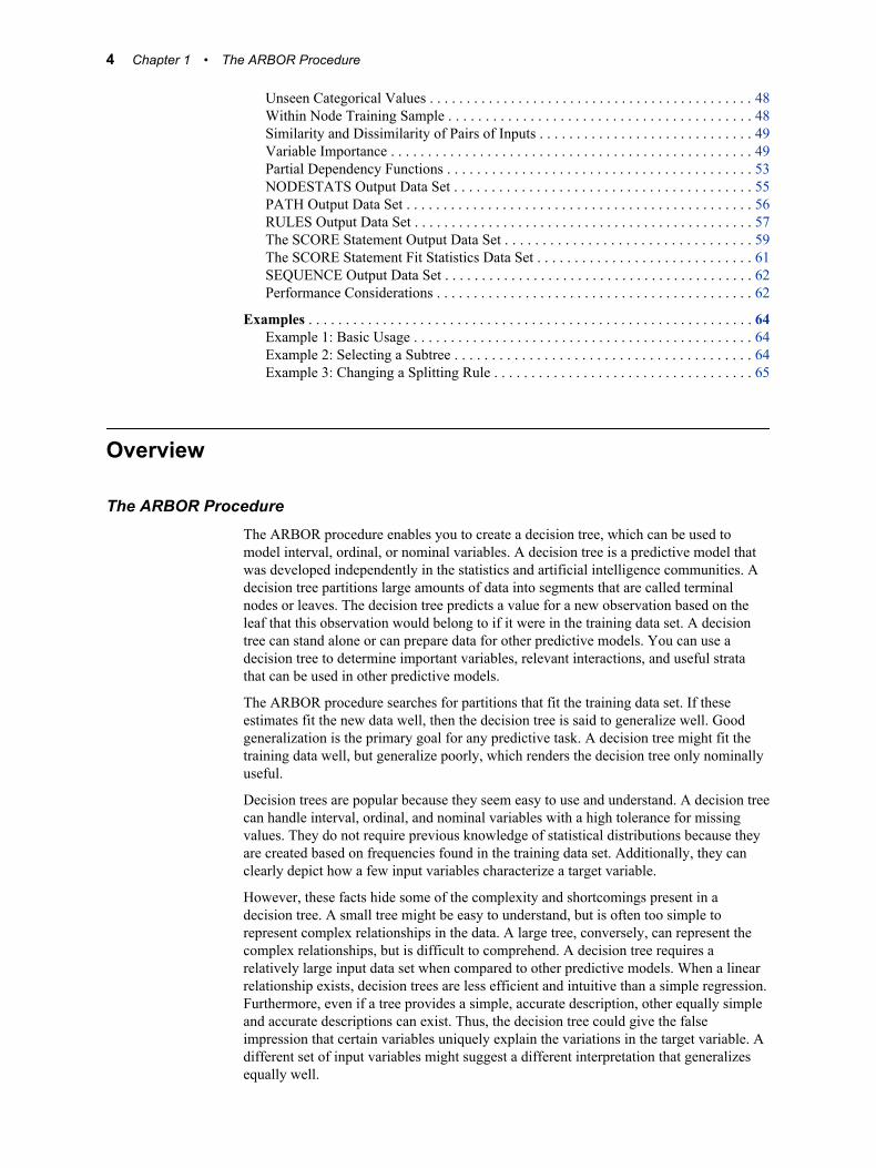
The ARBOR ProcedureThe ARBOR procedure enables you to create a decision tree, which can be used to model interval, ordinal, or nominal variables. A decision tree is a predictive model that was developed independently in the statistics and artificial intelligence communities. A decision tree partitions large amounts of data into segments that are called terminal nodes or leaves. The decision tree predicts a value for a new observation based on the leaf that this observation would belong to if it were in the training data set. A decision tree can stand alone or can prepare data for other predictive models. You can use a decision tree to determine important variables, relevant interactions, and useful strata that can be used in other predictive models.
The ARBOR procedure searches for partitions that fit the training data set. If these estimates fit the new data well, then the decision tree is said to generalize well. Good generalization is the primary goal for any predictive task. A decision tree might fit the training data well, but generalize poorly, which renders the decision tree only nominally useful.
Decision trees are popular because they seem easy to use and understand. A decision tree can handle interval, ordinal, and nominal variables with a high tolerance for missing values. They do not require previous knowledge of statistical distributions because they are created based on frequencies found in the training data set. Additionally, they can clearly depict how a few input variables characterize a target variable.
However, these facts hide some of the complexity and shortcomings present in a decision tree. A small tree might be easy to understand, but is often too simple to represent complex relationships in the data. A large tree, conversely, can represent the complex relationships, but is difficult to comprehend. A decision tree requires a relatively large input data set when compared to other predictive models. When a linear relationship exists, decision trees are less efficient and intuitive than a simple regression. Furthermore, even if a tree provides a simple, accurate description, other equally simple and accurate descriptions can exist. Thus, the decision tree could give the false impression that certain variables uniquely explain the variations in the target variable. A different set of input variables might suggest a different interpretation that generalizes equally well.
4 Chapter 1 • The ARBOR Procedure

The WHERE statement for PROC ARBOR applies only to data sets that are open when the WHERE statement is parsed. In other words, it should apply to data sets in preceding statements that have not yet been executed, but it should not apply to data sets in subsequent statements.
Terminology
General TermsIn order to avoid confusion with common definitions, certain terms are defined in the context of this document. When a branch is assigned to an observation, this act is called a decision, hence the term decision tree. Unfortunately, the terms decision and decision tree have different meanings in the closely related field of decision theory. In decision theory, a decision refers to the decision alternative whose utility or profit function is the maximum value for a given distribution of outcomes. The ARBOR procedure adopts this definition of decision and assigns a decision to each observation, when decision alternatives and a profit or loss function are specified.
To avoid confusion, a term must be used to describe when a branch is assigned to an observation. That term is splitting rule. Sometimes, it is called the primary splitting rule when used to discuss alternative partitions of the same node. A competing rule refers to a partition that is considered for an input variable other than the one that is used for the primary splitting rule. A leaf has no primary or competing rules, but might have a candidate rule that is ready to use if the leaf is split. A surrogate rule is one that is chosen to emulate a primary rule and is used only when the primary rule cannot be used. Surrogate rules are used most often when an observation lacks a value for the primary input variable.
Variable Roles and Measurement LevelsThe ARBOR procedure accepts variables with nominal, ordinal, and interval measurement levels. A nominal variable is a number or character categorical variable in which the categories are unordered. An ordinal variable is a number or character categorical variable in which the categories are ordered. An interval variable is a numeric variable where the differences of the values are informative.
The ARBOR procedure uses normalized, formatted values of categorical variables and considers two categorical values the same if the normalized values are identical. Normalization removes any leading blank spaces from a value, converts lowercase characters to uppercase, and truncates all values to 32 bytes. Documentation on the FORMAT procedure, in the Base SAS Procedures Guide, explains how to define a format. A FORMAT statement in the current run of a procedure or in the DATA step that created the data associates a format with a variable. By default, numeric variables use the BEST12 format, and the formatted values of character variables are the same as their unformatted values.
Data, Prior, and Posterior ProbabilitiesThe data that is available to the ARBOR procedure can be divided into multiple sets with different roles. The training data is used to find the partitions and construct a family of models. The validation data is used to make unbiased estimates and select one model from the family. The test data is used to evaluate the results. This division is prudent because the ARBOR procedure tends to overfit the models. To overfit is to fit the model with spurious features of the training data that do not appear in the score data.
For a categorical target, the proportions of the target values influence the model strongly. If the proportions in the training data differ noticeably from those in the scored data, then the model will generalize poorly. To correct this, the ARBOR procedure accepts
Overview 5

prior probabilities that specify what proportions to expect in the score data. The posterior probability of a target category for a particular observation is the probability that the observation has the target value, according to the model. The ARBOR procedure incorporates prior probabilities when it computes posterior probabilities. The procedure also incorporates the prior probabilities in the search for partitions if and only if the user requests this behavior.
Recursive PartitioningRecursive partitioning partitions the data into subsets and then partitions each of the subsets, and so on. The original data is the root node, the final, unpartitioned subsets are terminal nodes or leaves, and partitioned subsets are sometimes called internal nodes. Decision tree terminology also includes terms from genealogy, which provides the terms descendant and ancestor nodes. A branch of a node consists of a child node and its descendants.
Basic FeaturesThe ARBOR procedure enables you to mix tree construction strategies as advocated by Kass (CHAID) and by Breiman, et al. to match the needs of the situation. It extends the p-value adjustments of Kass and the retrospective pruning and misclassification costs of Breiman, et al.
The basic features of the ARBOR procedure include the following:
• Support for nominal, ordinal, and interval variables as both inputs and targets
• Multiple splitting criteria:
• Variance reduction for interval targets
• F test for interval targets
• Gini or entropy reduction (Information Gain) for categorical targets
• CHAID for nominal targets
• Binary or n-ary splits, for fixed or unspecified n
• Multiple missing value policies:
• Use missing values in the split search
• Assign missing values to the most correlated branch
• Distribute missing observations over all branches
• Surrogate rules for missing values and variable importance
• Cost-complexity pruning and reduced-error pruning with validation data
• Prior probabilities used in training or assessment
• Misclassification cost matrix that incorporates novel, alternative decisions
• Incorporation of a nominal decision matrix in the split criterion
• Interactive training mode to specify splits and nodes to prune
• Variable importance is computed separately with training and validation data
• Generation of SAS DATA step code with an indicator variable for each leaf.
• Generation of PMML
6 Chapter 1 • The ARBOR Procedure
Syntax
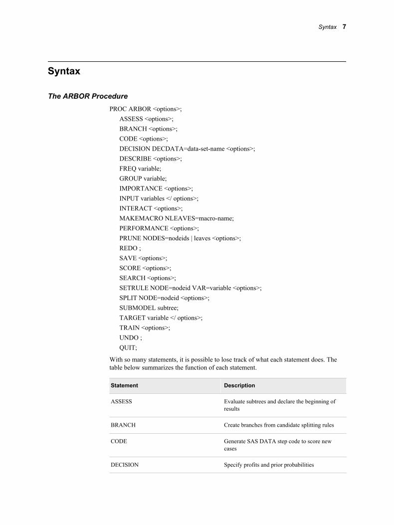
The ARBOR ProcedurePROC ARBOR <options>;
ASSESS <options>;BRANCH <options>;CODE <options>;DECISION DECDATA=data-set-name <options>;DESCRIBE <options>;FREQ variable;GROUP variable;IMPORTANCE <options>;INPUT variables </ options>;INTERACT <options>;MAKEMACRO NLEAVES=macro-name;PERFORMANCE <options>;PRUNE NODES=nodeids | leaves <options>;REDO ;SAVE <options>;SCORE <options>;SEARCH <options>;SETRULE NODE=nodeid VAR=variable <options>;SPLIT NODE=nodeid <options>;SUBMODEL subtree;TARGET variable </ options>;TRAIN <options>;UNDO ;QUIT;
With so many statements, it is possible to lose track of what each statement does. The table below summarizes the function of each statement.
Statement Description
ASSESS Evaluate subtrees and declare the beginning of results
BRANCH Create branches from candidate splitting rules
CODE Generate SAS DATA step code to score new cases
DECISION Specify profits and prior probabilities
Syntax 7
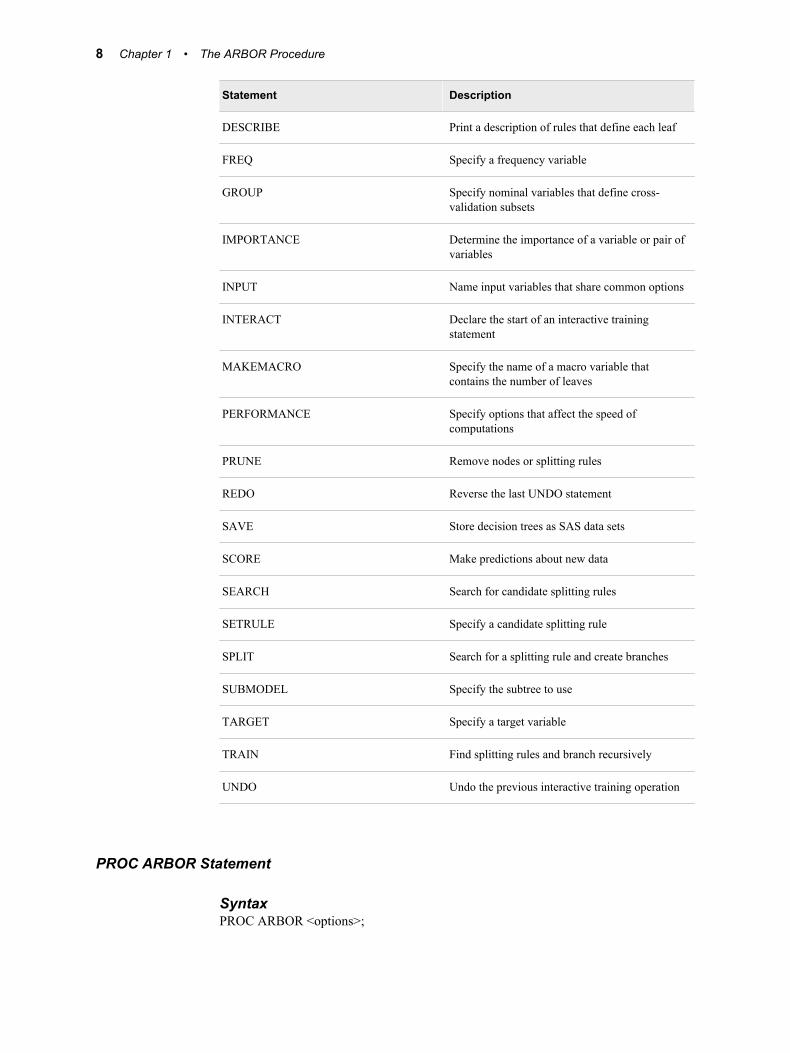
Statement Description
DESCRIBE Print a description of rules that define each leaf
FREQ Specify a frequency variable
GROUP Specify nominal variables that define cross-validation subsets
IMPORTANCE Determine the importance of a variable or pair of variables
INPUT Name input variables that share common options
INTERACT Declare the start of an interactive training statement
MAKEMACRO Specify the name of a macro variable that contains the number of leaves
PERFORMANCE Specify options that affect the speed of computations
PRUNE Remove nodes or splitting rules
REDO Reverse the last UNDO statement
SAVE Store decision trees as SAS data sets
SCORE Make predictions about new data
SEARCH Search for candidate splitting rules
SETRULE Specify a candidate splitting rule
SPLIT Search for a splitting rule and create branches
SUBMODEL Specify the subtree to use
TARGET Specify a target variable
TRAIN Find splitting rules and branch recursively
UNDO Undo the previous interactive training operation
PROC ARBOR Statement
SyntaxPROC ARBOR <options>;
8 Chapter 1 • The ARBOR Procedure
Optional ArgumentsALPHA=number
This option specifies a threshold p-value (number) for the significance level of a candidate splitting rule. This option is used with the PROBF and PROBCHISQ splitting criteria. The default value is 0.20.
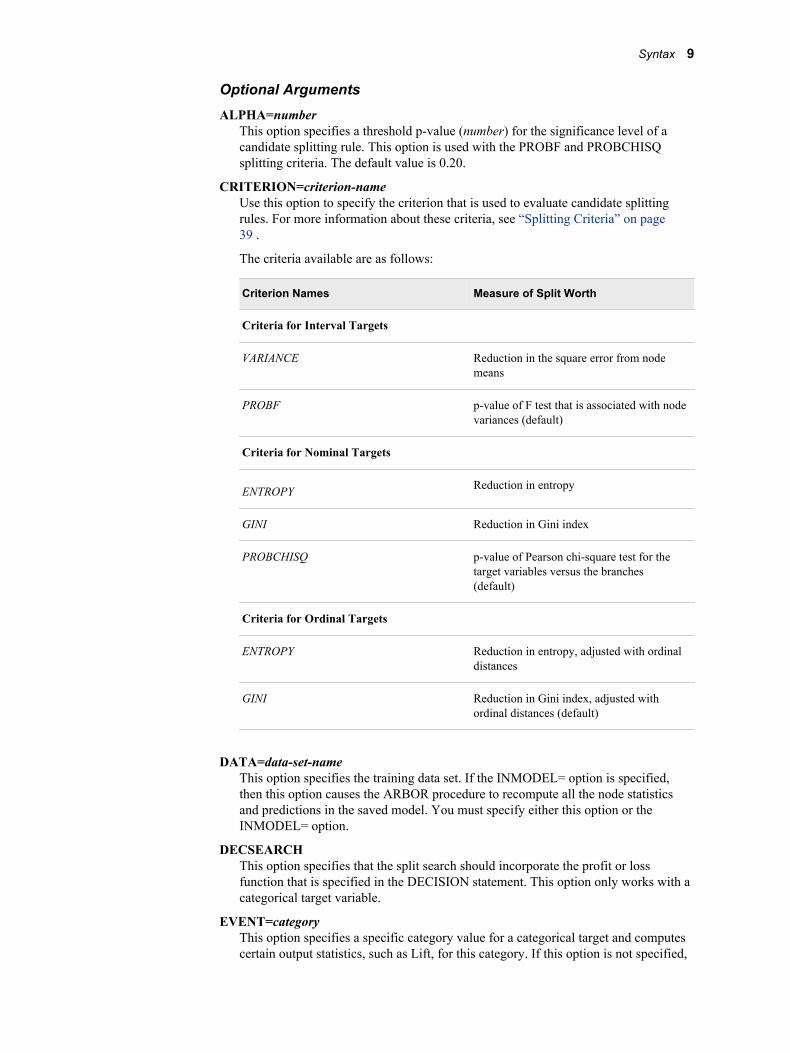
CRITERION=criterion-nameUse this option to specify the criterion that is used to evaluate candidate splitting rules. For more information about these criteria, see “Splitting Criteria” on page 39 .
The criteria available are as follows:
Criterion Names Measure of Split Worth
Criteria for Interval Targets
VARIANCE Reduction in the square error from node means
PROBF p-value of F test that is associated with node variances (default)
Criteria for Nominal Targets
ENTROPY Reduction in entropy
GINI Reduction in Gini index
PROBCHISQ p-value of Pearson chi-square test for the target variables versus the branches (default)
Criteria for Ordinal Targets
ENTROPY Reduction in entropy, adjusted with ordinal distances
GINI Reduction in Gini index, adjusted with ordinal distances (default)
DATA=data-set-nameThis option specifies the training data set. If the INMODEL= option is specified, then this option causes the ARBOR procedure to recompute all the node statistics and predictions in the saved model. You must specify either this option or the INMODEL= option.
DECSEARCHThis option specifies that the split search should incorporate the profit or loss function that is specified in the DECISION statement. This option only works with a categorical target variable.
EVENT=categoryThis option specifies a specific category value for a categorical target and computes certain output statistics, such as Lift, for this category. If this option is not specified,
Syntax 9
but is needed, then the least frequent target value is used. This option is ignored when an interval target is specified.
EXHAUSTIVE=numberThis option specifies the maximum number of splits that are allowed in a complete enumeration of all possible splits. An exhaustive split search examines all possible splits to determine whether there are more splits possible than number. If there are more splits possible than number, then a heuristic search is done. Both search methods apply only to multiway splits and binary splits on nominal targets with more than two values. For more information, see “Split Search Algorithm” on page 45 . The default value is 5000 splits.
INMODEL=data-set-nameThis option specifies a data set that was created with the MODEL argument in the SAVE statement. This option is used to save the computational costs of retraining a saved model. This data set contains the name of the training and validation data sets and will not train the decision tree if the training data set is still valid. Either this option or the DATA option must be specified.
INTERVALBINS=numberThis option specifies the preliminary number of bins to create for the input interval values. The width of each interval is (MAX — MIN)/number, where MAX and MIN are the maximum and minimum of the input variable values in the current node. The width is computed separately for each input and each node. The INTERVALDECIMALS= option specifies the precision of the split values, which might mean that less than number bins are necessary. This argument might indirectly modify the p-value adjustments. The search algorithm ignores this option if the number of distinct input values in the node is smaller than number.
INTERVALDECIMALS=number | MAXThis option specifies the precision, in decimals, of the split point for an interval input variable. When the ARBOR procedure searches for a split on an interval input value x, the partitioning procedure combines all observations that are identical to x when rounded to number decimal places. The value of number can be an integer from 0 to 8 and the MAX option does not round observations.
LEAFFRACTION=numberThis option determines the minimum number of observations necessary to form a new branch. This option specifies that number as a proportion of all observations in the branch to all available training observations. The value of number must be a real number between 0 and 1 and defaults to 0.001.
LEAFSIZE=numberThis option specifies the minimum number of observations that is necessary to form a new branch. Unlike the LEAFFRACTION= option, this argument specifies an exact number of observations. The value of number must be a positive integer.
MAXBRANCH=numberThis option specifies the maximum number of subsets that a splitting rule can produce. For example, if you set number equal to 2, then only binary splits will occur at each level. If you set number equal to 3, then binary or ternary splits are possible at each level.
MAXDEPTH=number | MAXThis option determines the maximum depth of a node on the decision tree. The depth of a node is the number of splitting rules that is necessary to get to that node. The root node has a depth of zero, while its immediate children have a depth of one, and so on. The ARBOR procedure will continue to search for new splitting rules as long as the depth of the current node is less than number. The default value for number is 6 and the MAX option sets this value to 50.
10 Chapter 1 • The ARBOR Procedure
MAXRULES=number | ALLThis option determines the maximum number of splitting rules that are saved for each node. The primary splitting rule is always saved, and up to number–1 additional competing rules are saved. The ALL option saves all available splitting rules for every node. You can output these rules with the RULES option in the SAVE statement. The amount of memory necessary to store these rules might be several megabytes.
A valid splitting rule might not exist for some input variables in some nodes. A common explanation is that none of the feasible rules meet the threshold of worth specified in the ALPHA= argument. Another less common cause is that the value of MINCATSIZE=, LEAFFRACTION=, or LEAFSIZE= is too large for the data set.
MAXSURROGATES | MAXSURRS=numberThis option specifies the maximum number of surrogate rules to find for each primary splitting rule. A surrogate rule is a backup rule to the primary splitting rule. The primary splitting rule might not apply to some observations because the value of the splitting variable might be missing or a categorical value that the rule does not recognize. In these cases, the surrogate rule is considered. By default, no surrogates are searched for because this search requires an extra pass through the data. For more information, see “Missing Values” on page 47 and “Variable Importance” on page 49 .
MINCATSIZE=numberIn order to create a splitting rule for a particular value of a nominal variable, there must be number observations of that value. If a value is observed fewer than number times, then it is treated as a missing value. You can still use these values if you specify the option MISSING=USEINSEARCH (see below). The policy to assign infrequent observations to a branch is the same policy that is used to assign missing values to a branch. The default value for number is 5. For more information, see “Missing Values” on page 47 .
MINWORTH=numberThe worth value for a candidate rule must be greater than number in order for the rule to be considered. This option is ignored in favor of the ALPHA= option when the CRITERION= option is set to either PROBCHISQ or PROBF. The default value for number is 0.
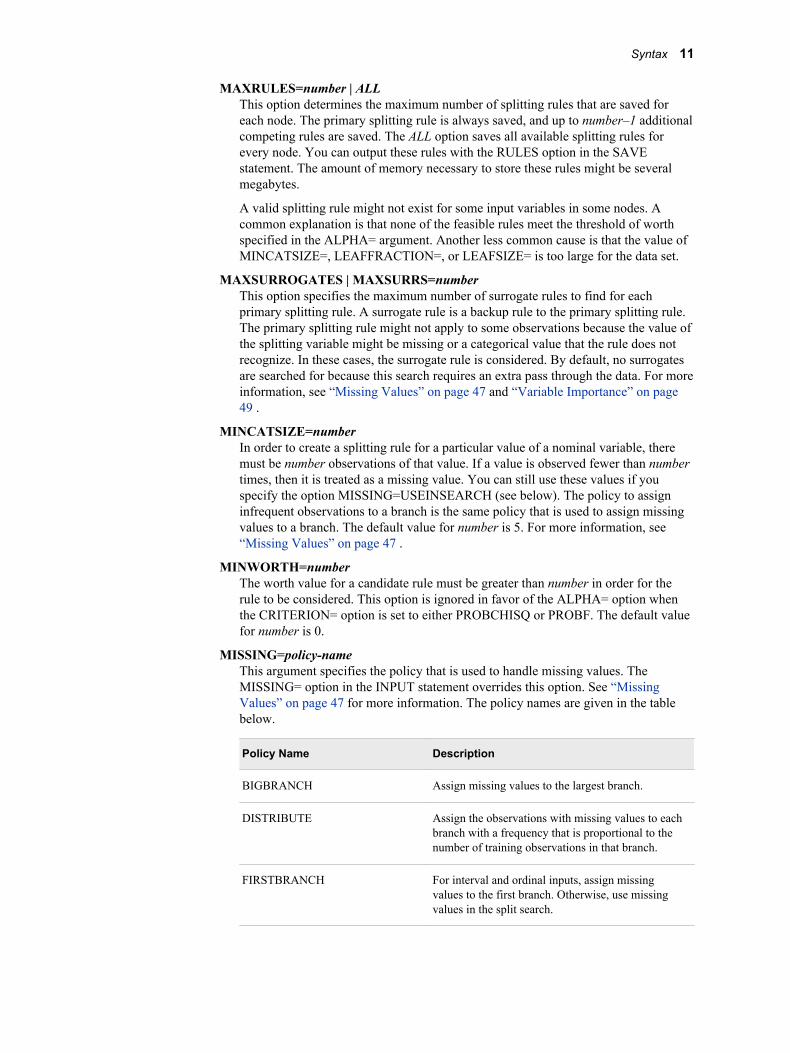
MISSING=policy-nameThis argument specifies the policy that is used to handle missing values. The MISSING= option in the INPUT statement overrides this option. See “Missing Values” on page 47 for more information. The policy names are given in the table below.
Policy Name Description
BIGBRANCH Assign missing values to the largest branch.
DISTRIBUTE Assign the observations with missing values to each branch with a frequency that is proportional to the number of training observations in that branch.
FIRSTBRANCH For interval and ordinal inputs, assign missing values to the first branch. Otherwise, use missing values in the split search.
Syntax 11
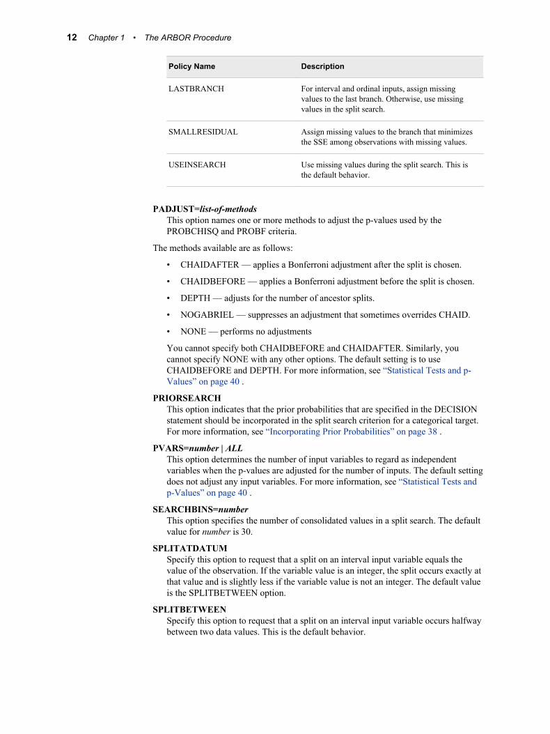
Policy Name Description
LASTBRANCH For interval and ordinal inputs, assign missing values to the last branch. Otherwise, use missing values in the split search.
SMALLRESIDUAL Assign missing values to the branch that minimizes the SSE among observations with missing values.
USEINSEARCH Use missing values during the split search. This is the default behavior.
PADJUST=list-of-methodsThis option names one or more methods to adjust the p-values used by the PROBCHISQ and PROBF criteria.
The methods available are as follows:
• CHAIDAFTER — applies a Bonferroni adjustment after the split is chosen.
• CHAIDBEFORE — applies a Bonferroni adjustment before the split is chosen.
• DEPTH — adjusts for the number of ancestor splits.
• NOGABRIEL — suppresses an adjustment that sometimes overrides CHAID.
• NONE — performs no adjustments
You cannot specify both CHAIDBEFORE and CHAIDAFTER. Similarly, you cannot specify NONE with any other options. The default setting is to use CHAIDBEFORE and DEPTH. For more information, see “Statistical Tests and p-Values” on page 40 .
PRIORSEARCHThis option indicates that the prior probabilities that are specified in the DECISION statement should be incorporated in the split search criterion for a categorical target. For more information, see “Incorporating Prior Probabilities” on page 38 .
PVARS=number | ALLThis option determines the number of input variables to regard as independent variables when the p-values are adjusted for the number of inputs. The default setting does not adjust any input variables. For more information, see “Statistical Tests and p-Values” on page 40 .
SEARCHBINS=numberThis option specifies the number of consolidated values in a split search. The default value for number is 30.
SPLITATDATUMSpecify this option to request that a split on an interval input variable equals the value of the observation. If the variable value is an integer, the split occurs exactly at that value and is slightly less if the variable value is not an integer. The default value is the SPLITBETWEEN option.
SPLITBETWEENSpecify this option to request that a split on an interval input variable occurs halfway between two data values. This is the default behavior.
12 Chapter 1 • The ARBOR Procedure
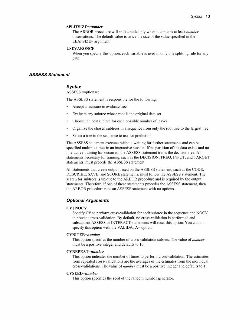
SPLITSIZE=numberThe ARBOR procedure will split a node only when it contains at least number observations. The default value is twice the size of the value specified in the LEAFSIZE= argument.
USEVARONCEWhen you specify this option, each variable is used in only one splitting rule for any path.
ASSESS Statement
SyntaxASSESS <options>;
The ASSESS statement is responsible for the following:
• Accept a measure to evaluate trees
• Evaluate any subtree whose root is the original data set
• Choose the best subtree for each possible number of leaves
• Organize the chosen subtrees in a sequence from only the root tree to the largest tree
• Select a tree in the sequence to use for prediction
The ASSESS statement executes without waiting for further statements and can be specified multiple times in an interactive session. If no partition of the data exists and no interactive training has occurred, the ASSESS statement trains the decision tree. All statements necessary for training, such as the DECISION, FREQ, INPUT, and TARGET statements, must precede the ASSESS statement.
All statements that create output based on the ASSESS statement, such as the CODE, DESCRIBE, SAVE, and SCORE statements, must follow the ASSESS statement. The search for subtrees is unique to the ARBOR procedure and is required by the output statements. Therefore, if one of these statements precedes the ASSESS statement, then the ARBOR procedure runs an ASSESS statement with no options.
Optional ArgumentsCV | NOCV
Specify CV to perform cross-validation for each subtree in the sequence and NOCV to prevent cross-validation. By default, no cross-validation is performed and subsequent ASSESS or INTERACT statements will reset this option. You cannot specify this option with the VALIDATA= option.
CVNITER=numberThis option specifies the number of cross-validation subsets. The value of number must be a positive integer and defaults to 10.
CVREPEAT=numberThis option indicates the number of times to perform cross-validation. The estimates from repeated cross-validations are the averages of the estimates from the individual cross-validations. The value of number must be a positive integer and defaults to 1.
CVSEED=numberThis option specifies the seed of the random number generator.
Syntax 13
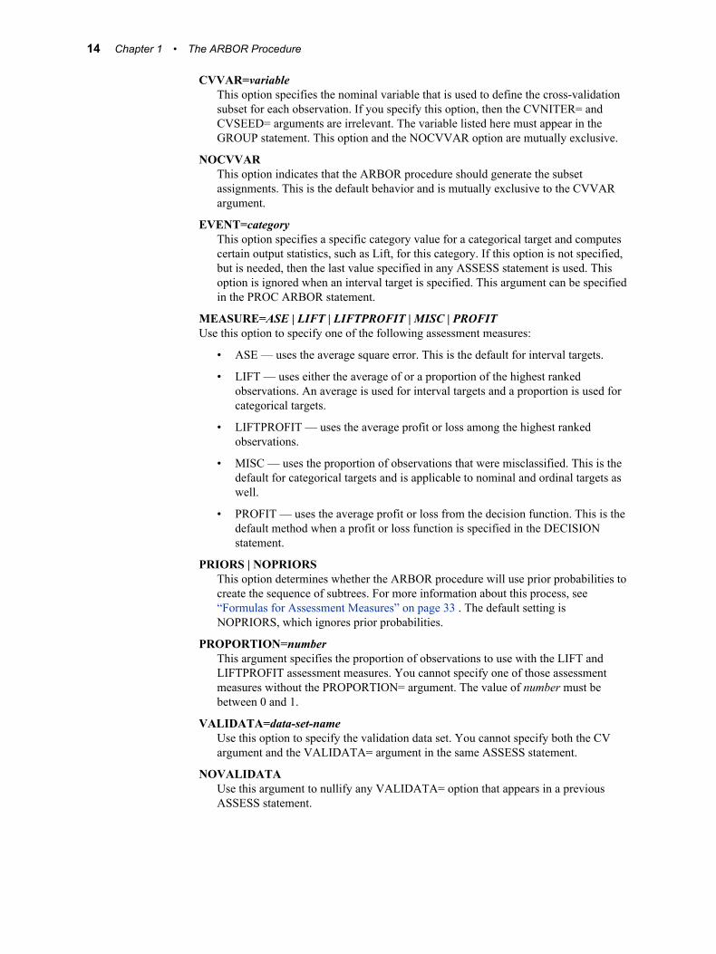
CVVAR=variableThis option specifies the nominal variable that is used to define the cross-validation subset for each observation. If you specify this option, then the CVNITER= and CVSEED= arguments are irrelevant. The variable listed here must appear in the GROUP statement. This option and the NOCVVAR option are mutually exclusive.
NOCVVARThis option indicates that the ARBOR procedure should generate the subset assignments. This is the default behavior and is mutually exclusive to the CVVAR argument.
EVENT=categoryThis option specifies a specific category value for a categorical target and computes certain output statistics, such as Lift, for this category. If this option is not specified, but is needed, then the last value specified in any ASSESS statement is used. This option is ignored when an interval target is specified. This argument can be specified in the PROC ARBOR statement.
MEASURE=ASE | LIFT | LIFTPROFIT | MISC | PROFITUse this option to specify one of the following assessment measures:
• ASE — uses the average square error. This is the default for interval targets.
• LIFT — uses either the average of or a proportion of the highest ranked observations. An average is used for interval targets and a proportion is used for categorical targets.
• LIFTPROFIT — uses the average profit or loss among the highest ranked observations.
• MISC — uses the proportion of observations that were misclassified. This is the default for categorical targets and is applicable to nominal and ordinal targets as well.
• PROFIT — uses the average profit or loss from the decision function. This is the default method when a profit or loss function is specified in the DECISION statement.
PRIORS | NOPRIORSThis option determines whether the ARBOR procedure will use prior probabilities to create the sequence of subtrees. For more information about this process, see “Formulas for Assessment Measures” on page 33 . The default setting is NOPRIORS, which ignores prior probabilities.
PROPORTION=numberThis argument specifies the proportion of observations to use with the LIFT and LIFTPROFIT assessment measures. You cannot specify one of those assessment measures without the PROPORTION= argument. The value of number must be between 0 and 1.
VALIDATA=data-set-nameUse this option to specify the validation data set. You cannot specify both the CV argument and the VALIDATA= argument in the same ASSESS statement.
NOVALIDATAUse this argument to nullify any VALIDATA= option that appears in a previous ASSESS statement.
14 Chapter 1 • The ARBOR Procedure
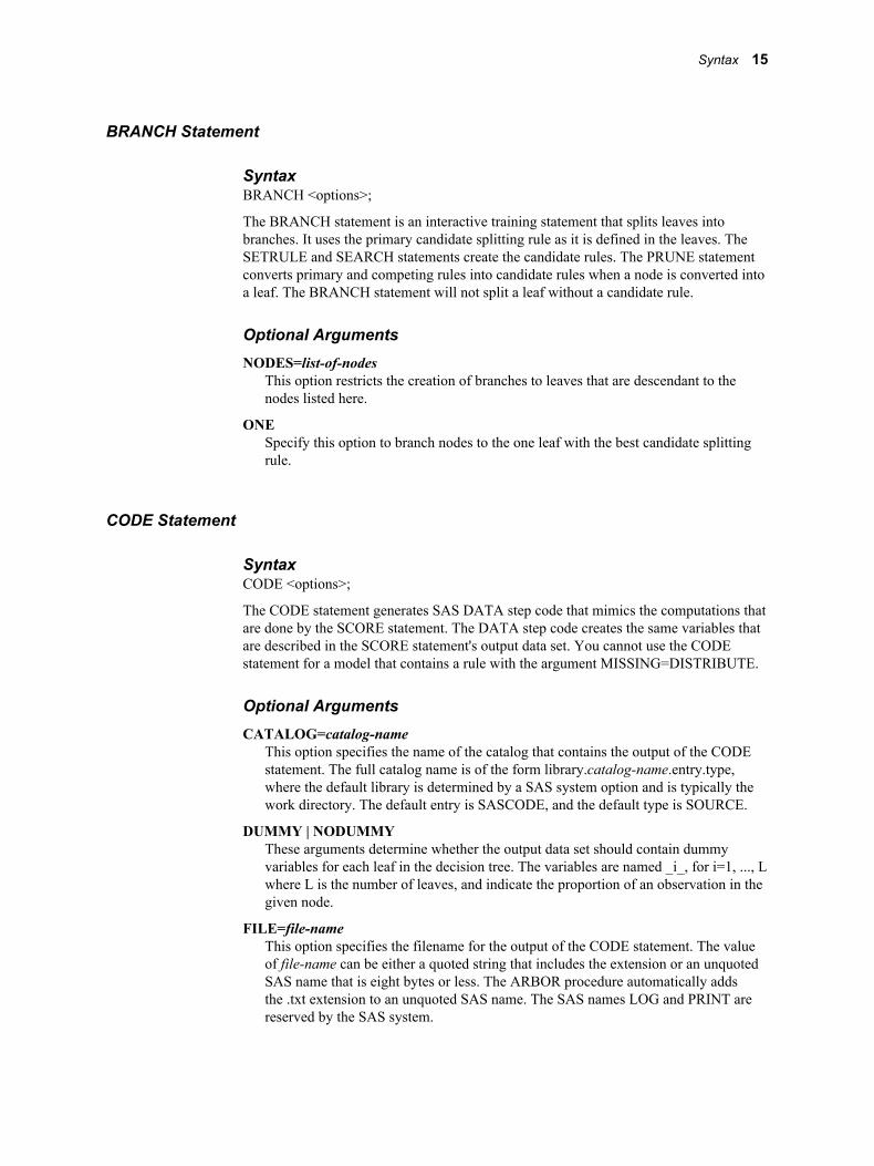
BRANCH Statement
SyntaxBRANCH <options>;
The BRANCH statement is an interactive training statement that splits leaves into branches. It uses the primary candidate splitting rule as it is defined in the leaves. The SETRULE and SEARCH statements create the candidate rules. The PRUNE statement converts primary and competing rules into candidate rules when a node is converted into a leaf. The BRANCH statement will not split a leaf without a candidate rule.
Optional ArgumentsNODES=list-of-nodes
This option restricts the creation of branches to leaves that are descendant to the nodes listed here.
ONESpecify this option to branch nodes to the one leaf with the best candidate splitting rule.
CODE Statement
SyntaxCODE <options>;
The CODE statement generates SAS DATA step code that mimics the computations that are done by the SCORE statement. The DATA step code creates the same variables that are described in the SCORE statement's output data set. You cannot use the CODE statement for a model that contains a rule with the argument MISSING=DISTRIBUTE.
Optional ArgumentsCATALOG=catalog-name
This option specifies the name of the catalog that contains the output of the CODE statement. The full catalog name is of the form library.catalog-name.entry.type, where the default library is determined by a SAS system option and is typically the work directory. The default entry is SASCODE, and the default type is SOURCE.
DUMMY | NODUMMYThese arguments determine whether the output data set should contain dummy variables for each leaf in the decision tree. The variables are named _i_, for i=1, ..., L where L is the number of leaves, and indicate the proportion of an observation in the given node.
FILE=file-nameThis option specifies the filename for the output of the CODE statement. The value of file-name can be either a quoted string that includes the extension or an unquoted SAS name that is eight bytes or less. The ARBOR procedure automatically adds the .txt extension to an unquoted SAS name. The SAS names LOG and PRINT are reserved by the SAS system.
Syntax 15
FORMAT=formatThis option indicates the format to use for numeric values that do not have a format from the input data set. The default is BEST20.
LEAFID | NOLEAFIDThese arguments control the creation of the _NODE_ and _LEAF_ variables that contain the node and leaf identification numbers for each observation. By default, these variables are created.
LINESIZE | LS=numberThis option determines the length of each line in the generated code. The value of number must be a positive integer between 64 and 254, with a default value of 72.
PMML | XMLSpecify this option to produce scoring code in Predictive Modeling Markup Language, an XML-based standard to represent data mining results. For more information, see the PMML help section in the Enterprise Miner help documents.
PREDICTION | NOPREDICTIONThese arguments control the computation of predicted values. By default, predicted values are computed.
RESIDUAL | NORESIDUALThese arguments control the computation of residuals, which require a target variable. For more information, see “The SCORE Statement Output Data Set” on page 59 . You can use this option without a target variable, but the output will contain confusing notes and warnings. By default, no residuals are computed.
DECISION Statement
SyntaxDECISION DECDATA=data-set-name <options>;
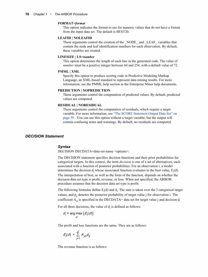
The DECISION statement specifies decision functions and their prior probabilities for categorical targets. In this context, the term decision is one of a set of alternatives, each associated with a function of posterior probabilities. For an observation i, a model determines the decision di whose associated function evaluates to the best value, Ei(d). The interpretation of best, as well as the form of the function, depends on whether the decision data set type is profit, revenue, or loss. When not specified, the ARBOR procedure assumes that the decision data set type is profit.
The following formulas define Ei(d) and di. The sum is taken over the J categorical target values, and pij denotes the posterior probability of target value j for observation i. The coefficient Ajd is specified in the DECDATA= data set for target value j and decision d.
For all three decisions, the value of di is defined as follows:
di = arg maxd
(Ei(d))
The profit and loss functions are the same. They are as follows:
Ei(d) = ∑j=1
JA jd pij
The revenue function is as follows:
16 Chapter 1 • The ARBOR Procedure
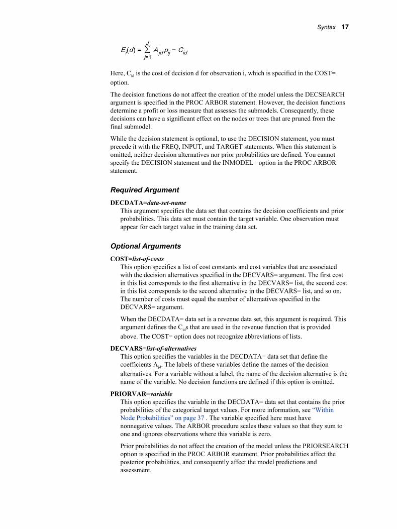
Ei(d) = ∑j=1
JA jd pij − Cid
Here, Cid is the cost of decision d for observation i, which is specified in the COST= option.
The decision functions do not affect the creation of the model unless the DECSEARCH argument is specified in the PROC ARBOR statement. However, the decision functions determine a profit or loss measure that assesses the submodels. Consequently, these decisions can have a significant effect on the nodes or trees that are pruned from the final submodel.
While the decision statement is optional, to use the DECISION statement, you must precede it with the FREQ, INPUT, and TARGET statements. When this statement is omitted, neither decision alternatives nor prior probabilities are defined. You cannot specify the DECISION statement and the INMODEL= option in the PROC ARBOR statement.
Required ArgumentDECDATA=data-set-name
This argument specifies the data set that contains the decision coefficients and prior probabilities. This data set must contain the target variable. One observation must appear for each target value in the training data set.
Optional ArgumentsCOST=list-of-costs
This option specifies a list of cost constants and cost variables that are associated with the decision alternatives specified in the DECVARS= argument. The first cost in this list corresponds to the first alternative in the DECVARS= list, the second cost in this list corresponds to the second alternative in the DECVARS= list, and so on. The number of costs must equal the number of alternatives specified in the DECVARS= argument.
When the DECDATA= data set is a revenue data set, this argument is required. This argument defines the Cids that are used in the revenue function that is provided above. The COST= option does not recognize abbreviations of lists.
DECVARS=list-of-alternativesThis option specifies the variables in the DECDATA= data set that define the coefficients Ajd. The labels of these variables define the names of the decision alternatives. For a variable without a label, the name of the decision alternative is the name of the variable. No decision functions are defined if this option is omitted.
PRIORVAR=variableThis option specifies the variable in the DECDATA= data set that contains the prior probabilities of the categorical target values. For more information, see “Within Node Probabilities” on page 37 . The variable specified here must have nonnegative values. The ARBOR procedure scales these values so that they sum to one and ignores observations where this variable is zero.
Prior probabilities do not affect the creation of the model unless the PRIORSEARCH option is specified in the PROC ARBOR statement. Prior probabilities affect the posterior probabilities, and consequently affect the model predictions and assessment.
Syntax 17
DESCRIBE Statement
SyntaxDESCRIBE <options>;
The DESCRIBE statement causes the ARBOR procedure to output a simple description of the rules and some statistics associated with each leaf. This information is typically more readable than the information that is output by the CODE statement.
Optional ArgumentsCATALOG=catalog-name
Use this option to specify the name of the output catalog.
FILE=file-nameUse this option to specify the name of the output file.
FORMAT=format-nameUse this option to specify the format to use for numeric values that do not have a specified format in the input data set.
LINESIZE | LS=numberUse this option to determine the line size for the output file. The value of number must be an integer between 64 and 254 and defaults to 72.
FREQ Statement
SyntaxFREQ variable;
Optional Argumentvariable
The FREQ statement identifies a variable that contains the frequency of occurrence for each observation. The ARBOR procedure treats each observation as if it appears N times, where N is the value of the FREQ variable for the observation. The value of N can be fractional to indicate partial observations. If the value of N is close to zero, negative, or missing, then the observation is ignored. When the FREQ statement is not specified, each observation is assigned a frequency of 1.
IMPORTANCE Statement
SyntaxIMPORTANCE <options>;
The IMPORTANCE statement uses an observation-based approach to evaluate the importance of a variable or a pair of variables to the predictions of the model. For each observation, the IMPORTANCE statement outputs the prediction once with the actual variable value and once with an uninformative variable value. For information about uninformative variable values, see “Variable Importance” on page 49 . The differences for all the observations can be plotted against the actual variable value or observation number to explore where the dependence is stronger or weaker.
18 Chapter 1 • The ARBOR Procedure
The ARBOR procedure also computes goodness-of-fit statistics with both the original and the uninformative variable values. A comparison of these statistics will reveal the dependence of the statistics on the variable. If you evaluate several variables, their statistics can be ranked to reveal the relative observation-based importance of the variables.
Optional ArgumentsDATA=data-set-name
This option specifies the input data set. If this option is absent, then the procedure uses the training data set.
N2WAY=m nUse this option to request that the best m variables are paired with the best n variables. Here, best refers to the split-based variable importance rankings that were computed in the IMPORTANCE= option of the SAVE statement. The values of m and n are positive integers, and n is set to m if it is not specified. Each variable is also computed individually, as if it were specified in the VAR= argument.
NVARS=numberThis argument instructs the ARBOR procedure to evaluate the best number variables as ranked by their split-based importance. If N2WAY=, NVARS=, and VAR= are absent, then this value is assumed to be 5.
OUT=data-set-nameThis option specifies an output data set. If you do not specify this option, then the IMPORTANCE statement will automatically create an output data set. You can suppress this data set altogether if you specify OUT=_NULL_.
This data set contains the same variables as the output data set in the SCORE statement, plus one or two more variables. These variables contain the names of the uninformative variables. The number of observations in this data set equals the number of variables and variable pairs that are evaluated plus the number of observations in the input data set. For more information, see “The SCORE Statement Output Data Set” on page 59 .
OUTFIT=data-set-nameThis data set contains the goodness-of-fit statistics. The number of observations in this data set is the number of variables plus the number of pairs of variables plus one. This data set contains the same variables as the output data set in the SCORE statement, plus one or two more variables. These variables contain the names of the uninformative variables.
VAR=(list-of-variables)This argument specifies the variables and variable pairs to evaluate. An asterisk between two variables indicates a variable pair; square brackets are used as grouping symbols. You cannot nest square brackets. You must enclose the list in parentheses. If you specify a pair of variables, then each variable is also evaluated individually.
Consider the statement VAR=(A B*C [D E]*[E C]). The IMPORTANCE statement would evaluate the variables A, B, C, D, and E individually. Furthermore, it would also evaluate the variable pairs B-C, D-E, D-C, and E-C.
INPUT Statement
SyntaxINPUT variables </ options>;
Syntax 19
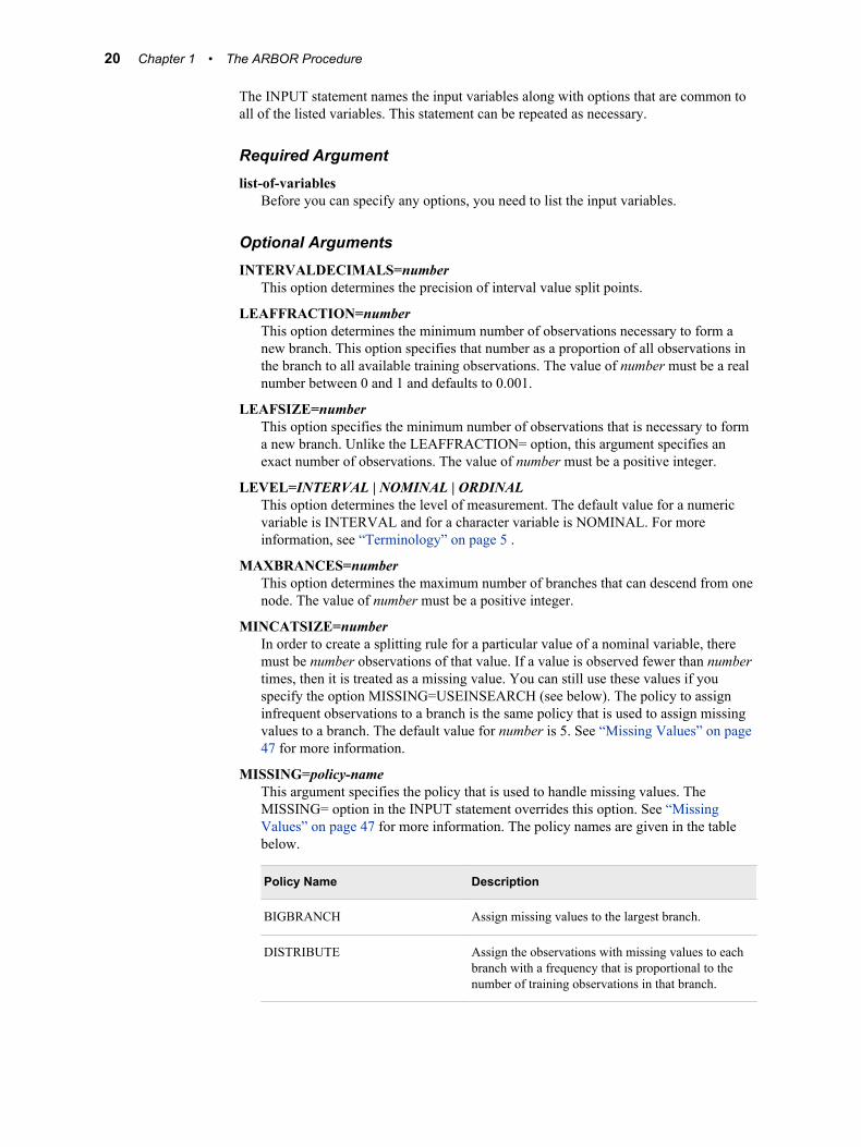
The INPUT statement names the input variables along with options that are common to all of the listed variables. This statement can be repeated as necessary.
Required Argumentlist-of-variables
Before you can specify any options, you need to list the input variables.
Optional ArgumentsINTERVALDECIMALS=number
This option determines the precision of interval value split points.
LEAFFRACTION=numberThis option determines the minimum number of observations necessary to form a new branch. This option specifies that number as a proportion of all observations in the branch to all available training observations. The value of number must be a real number between 0 and 1 and defaults to 0.001.
LEAFSIZE=numberThis option specifies the minimum number of observations that is necessary to form a new branch. Unlike the LEAFFRACTION= option, this argument specifies an exact number of observations. The value of number must be a positive integer.
LEVEL=INTERVAL | NOMINAL | ORDINALThis option determines the level of measurement. The default value for a numeric variable is INTERVAL and for a character variable is NOMINAL. For more information, see “Terminology” on page 5 .
MAXBRANCES=numberThis option determines the maximum number of branches that can descend from one node. The value of number must be a positive integer.
MINCATSIZE=numberIn order to create a splitting rule for a particular value of a nominal variable, there must be number observations of that value. If a value is observed fewer than number times, then it is treated as a missing value. You can still use these values if you specify the option MISSING=USEINSEARCH (see below). The policy to assign infrequent observations to a branch is the same policy that is used to assign missing values to a branch. The default value for number is 5. See “Missing Values” on page 47 for more information.
MISSING=policy-nameThis argument specifies the policy that is used to handle missing values. The MISSING= option in the INPUT statement overrides this option. See “Missing Values” on page 47 for more information. The policy names are given in the table below.
Policy Name Description
BIGBRANCH Assign missing values to the largest branch.
DISTRIBUTE Assign the observations with missing values to each branch with a frequency that is proportional to the number of training observations in that branch.
20 Chapter 1 • The ARBOR Procedure
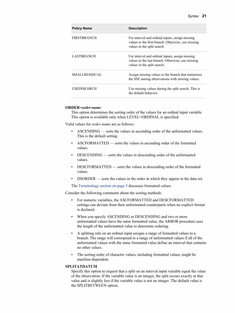
Policy Name Description
FIRSTBRANCH For interval and ordinal inputs, assign missing values to the first branch. Otherwise, use missing values in the split search.
LASTBRANCH For interval and ordinal inputs, assign missing values to the last branch. Otherwise, use missing values in the split search.
SMALLRESIDUAL Assign missing values to the branch that minimizes the SSE among observations with missing values.
USEINSEARCH Use missing values during the split search. This is the default behavior.
ORDER=order-nameThis option determines the sorting order of the values for an ordinal input variable. This option is available only when LEVEL=ORDINAL is specified.
Valid values for order-name are as follows:
• ASCENDING — sorts the values in ascending order of the unformatted values. This is the default setting.
• ASCFORMATTED — sorts the values in ascending order of the formatted values.
• DESCENDING — sorts the values in descending order of the unformatted values.
• DESCFORMATTED — sorts the values in descending order of the formatted values.
• DSORDER — sorts the values in the order in which they appear in the data set.
The Terminology section on page 5 discusses formatted values.
Consider the following comments about the sorting methods:
• For numeric variables, the ASCFORMATTED and DESCFORMATTED settings can deviate from their unformatted counterparts when no explicit format is declared.
• When you specify ASCENDING or DESCENDING and two or more unformatted values have the same formatted value, the ARBOR procedure uses the length of the unformatted value to determine ordering.
• A splitting rule on an ordinal input assigns a range of formatted values to a branch. The range will correspond to a range of unformatted values if all of the unformatted values with the same formatted value define an interval that contains no other values.
• The sorting order of character values, including formatted values, might be machine-dependent.
SPLITATDATUMSpecify this option to request that a split on an interval input variable equal the value of the observation. If the variable value is an integer, the split occurs exactly at that value and is slightly less if the variable value is not an integer. The default value is the SPLITBETWEEN option.
Syntax 21
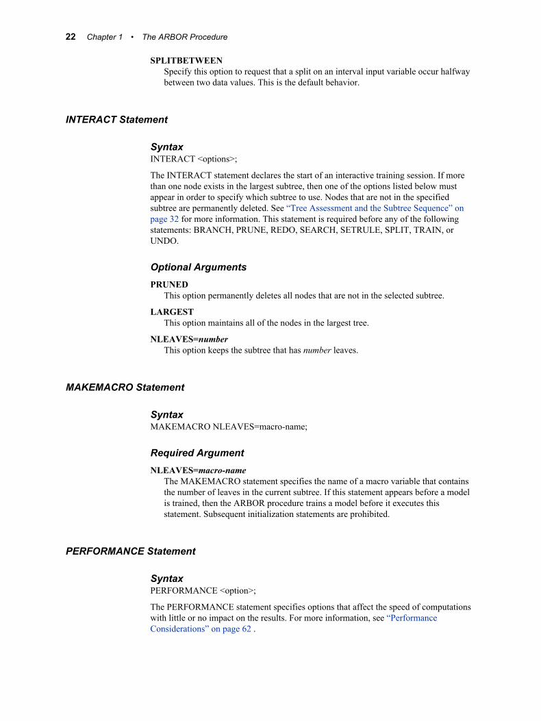
SPLITBETWEENSpecify this option to request that a split on an interval input variable occur halfway between two data values. This is the default behavior.
INTERACT Statement
SyntaxINTERACT <options>;
The INTERACT statement declares the start of an interactive training session. If more than one node exists in the largest subtree, then one of the options listed below must appear in order to specify which subtree to use. Nodes that are not in the specified subtree are permanently deleted. See “Tree Assessment and the Subtree Sequence” on page 32 for more information. This statement is required before any of the following statements: BRANCH, PRUNE, REDO, SEARCH, SETRULE, SPLIT, TRAIN, or UNDO.
Optional ArgumentsPRUNED
This option permanently deletes all nodes that are not in the selected subtree.
LARGESTThis option maintains all of the nodes in the largest tree.
NLEAVES=numberThis option keeps the subtree that has number leaves.
MAKEMACRO Statement
SyntaxMAKEMACRO NLEAVES=macro-name;
Required ArgumentNLEAVES=macro-name
The MAKEMACRO statement specifies the name of a macro variable that contains the number of leaves in the current subtree. If this statement appears before a model is trained, then the ARBOR procedure trains a model before it executes this statement. Subsequent initialization statements are prohibited.
PERFORMANCE Statement
SyntaxPERFORMANCE <option>;
The PERFORMANCE statement specifies options that affect the speed of computations with little or no impact on the results. For more information, see “Performance Considerations” on page 62 .
22 Chapter 1 • The ARBOR Procedure
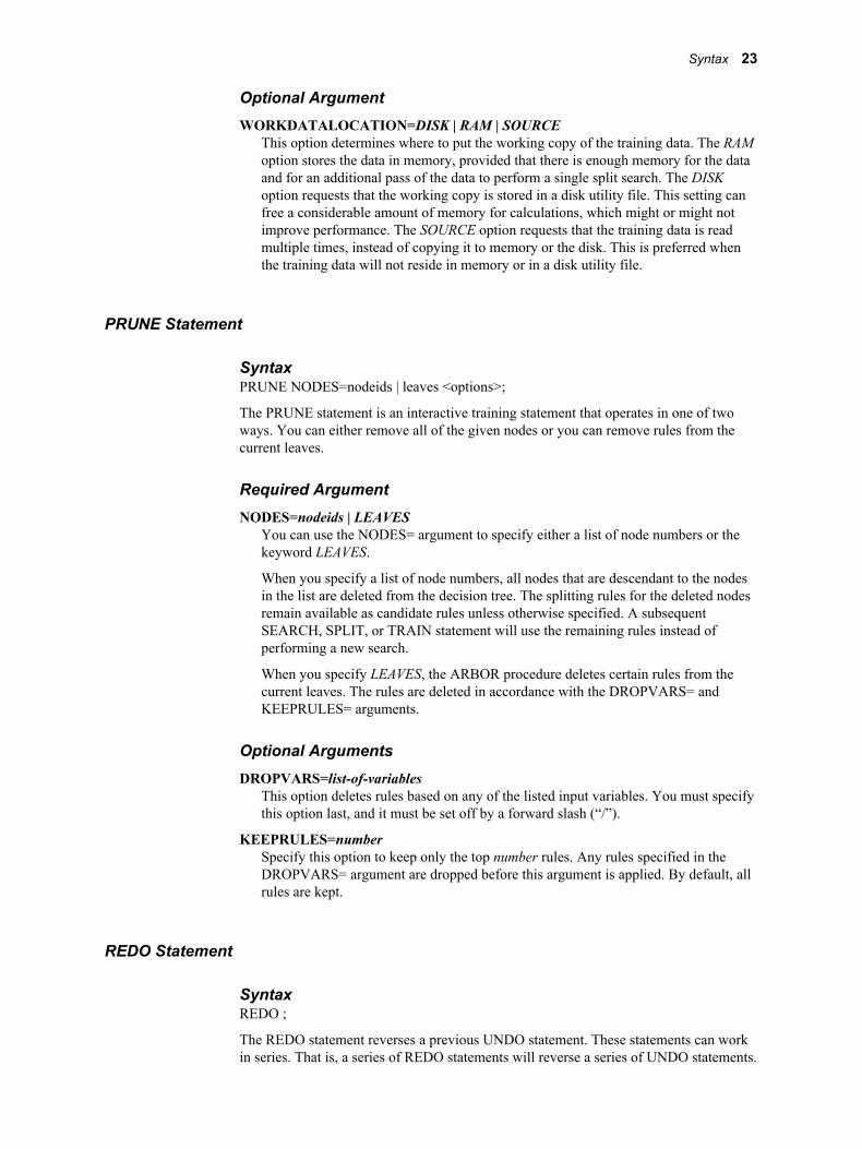
Optional ArgumentWORKDATALOCATION=DISK | RAM | SOURCE
This option determines where to put the working copy of the training data. The RAM option stores the data in memory, provided that there is enough memory for the data and for an additional pass of the data to perform a single split search. The DISK option requests that the working copy is stored in a disk utility file. This setting can free a considerable amount of memory for calculations, which might or might not improve performance. The SOURCE option requests that the training data is read multiple times, instead of copying it to memory or the disk. This is preferred when the training data will not reside in memory or in a disk utility file.
PRUNE Statement
SyntaxPRUNE NODES=nodeids | leaves <options>;
The PRUNE statement is an interactive training statement that operates in one of two ways. You can either remove all of the given nodes or you can remove rules from the current leaves.
Required ArgumentNODES=nodeids | LEAVES
You can use the NODES= argument to specify either a list of node numbers or the keyword LEAVES.
When you specify a list of node numbers, all nodes that are descendant to the nodes in the list are deleted from the decision tree. The splitting rules for the deleted nodes remain available as candidate rules unless otherwise specified. A subsequent SEARCH, SPLIT, or TRAIN statement will use the remaining rules instead of performing a new search.
When you specify LEAVES, the ARBOR procedure deletes certain rules from the current leaves. The rules are deleted in accordance with the DROPVARS= and KEEPRULES= arguments.
Optional ArgumentsDROPVARS=list-of-variables
This option deletes rules based on any of the listed input variables. You must specify this option last, and it must be set off by a forward slash (“/”).
KEEPRULES=numberSpecify this option to keep only the top number rules. Any rules specified in the DROPVARS= argument are dropped before this argument is applied. By default, all rules are kept.
REDO Statement
SyntaxREDO ;
The REDO statement reverses a previous UNDO statement. These statements can work in series. That is, a series of REDO statements will reverse a series of UNDO statements.
Syntax 23
If an UNDO statement is followed by any statement other than an UNDO or REDO statement, then the REDO statement does nothing.
SAVE Statement
SyntaxSAVE <options>;
The SAVE statement outputs decision tree information into SAS data sets. Unless otherwise stated, the information describes a subtree, selected in the ASSESS or SUBMODEL statement, that might omit nodes from the largest tree in the sequence.
Optional ArgumentsIMPORTANCE=data-set-name
This data set contains the split-based variable importance. For more information, see “Variable Importance” on page 49 .
MODEL=data-set-nameThis data set encodes the information necessary to use the INMODEL= option in subsequent calls to the ARBOR procedure.
NODES=list-of-nodesWhen this option is specified, only the nodes listed here are used for the NODESTATS=, PATH=, and RULES= data set.
NODESTATS=data-set-nameThis data set contains information about all of the nodes. For more information, see “NODESTATS Output Data Set” on page 55 .
PATH=data-set-nameThis data set describes the paths to each node. For more information, see “PATH Output Data Set” on page 56 .
RULES=data-set-nameThis data set describes the splitting rules. For more information, see “RULES Output Data Set” on page 57 .
SEQUENCE=data-set-nameThis data set contains the fit statistics for every tree in the sequence of decision trees.
SUMMARY=data-set-nameThis data set contains the summary statistics. For categorical targets, the summary statistics consist of the counts and proportions of observations that are correctly classified. For interval targets, the summary statistics include the average square error and R-squared measure.
SCORE Statement
SyntaxSCORE <options>;
The SCORE statement is used to calculate predictions, residuals, decisions, and leaf assignments.
24 Chapter 1 • The ARBOR Procedure
Optional ArgumentsDATA=data-set-name
This option indicates the input data set. If this option is absent, then the ARBOR procedure uses the training data set.
DUMMY | NODUMMYThese arguments determine whether the output data set should contain dummy variables for each leaf in the decision tree. The variables are named _i_, for i=1, ..., L, where L is the number of leaves, and indicate the proportion of an observation in the given node.
LEAFID | NOLEAFIDThese arguments control the creation of the _NODE_ and _LEAF_ variables that contain the node and leaf identification numbers for each observation. By default, these variables are created.
NODES=list-of-nodesUse this option to list the nodes that you want to score. If an observation is not assigned to any node in this list, then it does not contribute to the fit statistics and is not included in the output data set.
OUT=data-set-nameThis data set contains the scored data. An output data set is automatically created if this argument is not included. To suppress this data set completely, specify OUT=_NULL_. For more information about this data set, see “The SCORE Statement Fit Statistics Data Set” on page 61 .
OUTFIT=data-set-nameThis data set contains the fit statistics that were computed by the ARBOR procedure.
PREDICTION | NOPREDICTIONThese arguments control the computation of predicted values. By default, predicted values are computed.
ROLE=SCORE | TEST | TRAIN | VALIDThis option determines the role of the input data set and determines the fit statistics to compute. Only the SCORE setting includes observations without a target value.
SEARCH Statement
SyntaxSEARCH <options>;
The SEARCH statement is an interactive training statement that searches for splitting rules in leaves. It behaves like the TRAIN statement, except no branches are formed. The options for the SEARCH statement are identical to those in the “TRAIN Statement” on page 29 .
SETRULE Statement
SyntaxSETRULE NODE=node-id VAR=variable <options>;
The SETRULE statement is an interactive training statement that specifies the primary splitting rule for a leaf.
Syntax 25
Required ArgumentsNODE=node-id
The SETRULE statement assigns the primary splitting rule for the node whose node number is node-id. If the node already has a candidate rule for the specified variable, then the candidate rule for that variable is set to the primary splitting rule for the node.
VAR=variableThis argument indicates the variable that is used for the primary splitting rule.
Optional Argumentsmissing-policy
This option determines how to assign observations with missing values for the specified variable.
Valid values for missing-policy are as follows:
• MISSBRANCH=b — indicates that branch b should contain all of the missing values. If b is greater than the number of branches implied by the var-values option, then the last branch specified is used for missing values.
• MISSDISTRIBUTE — specifies that observations with missing values should be distributed over all branches. You cannot use this option and the CODE statement simultaneously.
• MISSFIRST — assigns all observations with missing values to the first branch. This is valid only for input variables that are interval or ordinal variables.
• MISSLAST — assigns all observations with missing values to the last branch. This is valid only for input variables that are interval or ordinal variables.
• MISSONLY — reserves the last branch exclusively for missing values. This branch is added to the branches specified in the var-values option. If that option is omitted, then a binary split is created with missing values on one branch and nonmissing values on the other.
This option is ignored if the var-values option is absent. If this option is absent, then the ARBOR procedure will honor the MISSING= option in the INPUT statement.
var-valuesThis option must be preceded by a forward slash. This option specifies a list of values of the specified variable. The list of variables must assume a separate form for each measurement level.
• Nominal — You must specify all values, with commas to separate each branch. Specify formatted values in quotation marks. All categories that appear before the first comma are assigned to the first branch.
• Ordinal — You must specify the minimum branch values in increasing order. Specify formatted values in quotation marks. Specify the smallest value for each branch, except for the first branch. Only one value should appear for a binary split. Commas are prohibited.
• Interval — You must specify the splitting values in increasing order. A single value specifies a binary split. Observations with values less than the first number are assigned to the first branch. Observations equal to the first number are assigned to the second branch.
This option and the missing-policy option override the MAXBRANCH= setting in the TRAIN statement. If this option is not provided, then a split is made on the
26 Chapter 1 • The ARBOR Procedure
candidate rule that is stored in the leaf. If no candidate rule exists, then the ARBOR procedure will search for one and create the branches if a rule is found.
SPLIT Statement
SyntaxSPLIT NODE=nodeid <options>;
The SPLIT statement is an interactive training statement that specifies how to split a leaf node.
Required ArgumentNODE=node-id
The SPLIT statement assigns the primary splitting rule for the node whose node number is node-id. If the node already has a candidate rule for the specified variable, then the candidate rule for that variable is set to the primary splitting rule for the node.
Optional ArgumentsVAR=variable
This argument indicates the variable that is used for the primary splitting rule.
missing-policyThis option determines how to assign observations with missing values for the specified variable.
Valid values for missing-policy are as follows:
• MISSBRANCH=b — indicates that branch b should contain all of the missing values. If b is greater than the number of branches implied by the var-values option, then the last branch specified is used for missing values.
• MISSDISTRIBUTE — specifies that observations with missing values should be distributed over all branches. You cannot use this option and the CODE statement simultaneously.
• MISSFIRST — assigns all observations with missing values to the first branch. This is valid only for input variables that are interval or ordinal variables.
• MISSLAST — assigns all observations with missing values to the last branch. This is valid only for input variables that are interval or ordinal variables.
• MISSONLY — reserves the last branch exclusively for missing values. This branch is added to the branches specified in the var-values option. If that option is omitted, then a binary split is created with missing values on one branch and nonmissing values on the other.
This option is ignored if the var-values option is absent. If this option is absent, then the ARBOR procedure will honor the MISSING= option in the INPUT statement.
NEWNODE=numberThis option specifies the node ID number of the first branch specified by the var-values list.
Syntax 27
var-valuesThis option must be preceded by a forward slash. This option specifies a list of values of the specified variable. The list of variables must assume a separate form for each measurement level.
• Nominal — You must specify all values, with commas to separate each branch. Specify formatted values in quotation marks. All categories that appear before the first comma are assigned to the first branch.
• Ordinal — You must specify the minimum branch values in increasing order. Specify formatted values in quotation marks. Specify the smallest value for each branch, except for the first branch. Only one value should appear for a binary split. Commas are prohibited.
• Interval — You must specify the splitting values in increasing order. A single value specifies a binary split. Observations with values less than the first number are assigned to the first branch. Observations equal to the first number are assigned to the second branch.
This option and the missing-policy option override the MAXBRANCH= setting in the TRAIN statement. If this option is not provided, then a split is made on the candidate rule that is stored in the leaf. If no candidate rule exists, then the ARBOR procedure will search for one and create the branches if a rule is found.
SUBMODEL Statement
SyntaxSUBMODEL subtree;
The SUBMODEL statement selects a subtree from the sequence of subtrees. For more information, see “Tree Assessment and the Subtree Sequence” on page 32 .
Required ArgumentBEST | LARGEST | NLEAVES=number
If you specify the BEST argument, then the ARBOR procedure selects the smallest subtree with the best assessment value. The LARGEST argument selects the subtree that contains all of the nodes. The NLEAVES=number argument selects the largest subtree with no more than number leaves.
TARGET Statement
SyntaxTARGET variable </ options>;
Required Argumentvariable
This is the variable that the decision tree model attempts to predict.
28 Chapter 1 • The ARBOR Procedure
Optional ArgumentsLEVEL=BINARY | INTERVAL | NOMINAL | ORDINAL
This argument specifies the level of measurement for the target variable. The default for a numeric variable is INTERVAL and is NOMINAL for a character variable.
ORDER=ASCENDING | ASCFORMATTED | DESCENDING | DESCFORMATTED | DSORDER
This option specifies how the values of an ordinal target variable are ordered. This option is available only when LEVEL=ORDINAL is specified and has no impact with a target variable that has only two values. This option is the same as the ORDINAL option in the INPUT statement.
TRAIN Statement
SyntaxTRAIN <options>;
The TRAIN statement searches for splitting rules, applies these rules to create branches, and repeats these two steps in newly formed leaves to grow the decision tree. Most options from previous SEARCH, SPLIT, and TRAIN statements are still active for the current call to the TRAIN statement. The exceptions are MAXNEWDEPTH= and NODES=.
Optional ArgumentsALPHA=number
This option specifies a threshold p-value (number) for the significance level of a candidate splitting rule. This option is used with the PROBF and PROBCHISQ splitting criteria. The default value is 0.20.
CRITERION=criterion-nameUse this option to specify the criterion that is used to evaluate candidate splitting rules. For more information about the splitting criteria, see “Splitting Criteria” on page 39 .
The criteria available are as follows:
Criterion Names Measure of Split Worth
Criteria for Interval Targets
VARIANCE Reduction in the square error from node means
PROBF p-value of F test that is associated with node variances (default)
Criteria for Nominal Targets
ENTROPY Reduction in entropy
GINI Reduction in Gini index
Syntax 29
Criterion Names Measure of Split Worth
PROBCHISQ p-value of Pearson chi-square test for the target variables versus the branches (default)
Criteria for Ordinal Targets
ENTROPY Reduction in entropy, adjusted with ordinal distances
GINI Reduction in Gini index, adjusted with ordinal distances (default)
EXHAUSTIVE=numberThis option specifies the maximum number of splits that are allowed in a complete enumeration of all possible splits. An exhaustive split search examines all possible splits to determine whether there are more splits possible than number. If there are more splits possible than number, then a heuristic search is done. Both search methods apply only to multiway splits and binary splits on nominal targets with more than two values. See “Split Search Algorithm” on page 45 . The default value is 5000 splits.
INTERVALBINS=numberThis option specifies the preliminary number of bins to create for the input interval values. The width of each interval is (MAX — MIN)/number, where MAX and MIN are the maximum and minimum of the input variable values in the current node. The width is computed separately for each input and each node. The INTERVALDECIMALS= option specifies the precision of the split values, which might mean that fewer than number bins are necessary. This argument might indirectly modify the p-value adjustments. The search algorithm ignores this option if the number of distinct input values in the node is smaller than number.
INTERVALDECIMALS=number | MAXThis option specifies the precision, in decimals, of the split point for an interval input variable. When the ARBOR procedure searches for a split on an interval input x, the partitioning procedure combines all observations that are identical to x when rounded to number decimal places. The value of number can be an integer from 0 to 8; the MAX option does not round observations.
LEAFFRACTION=numberThis option determines the minimum number of observations necessary to form a new branch. This option specifies that number as a proportion of all observations in the branch to all available training observations. The value of number must be a real number between 0 and 1 and defaults to 0.001.
LEAFSIZE=numberThis option specifies the minimum number of observations that is necessary to form a new branch. Unlike the LEAFFRACTION= option, this argument specifies an exact number of observations. The value of number must be a positive integer.
MAXBRANCH=numberThis option specifies the maximum number of subsets that a splitting rule can produce. For example, if you set number equal to 2, then only binary splits will occur at each level. If you set number equal to 3, then binary or ternary splits are possible at each level.
30 Chapter 1 • The ARBOR Procedure
MAXDEPTH=number | MAXThis option determines the maximum depth of a node on the decision tree. The depth of a node is equivalent to the number of splitting rules that is necessary to get to that node. The root node has a depth of zero, while its immediate children have a depth of one, and so on. The ARBOR procedure will continue to search for new splitting rules as long as the depth of the current node is less than number. The default value for number is 6; the MAX option sets this value to 50.
MAXNEWDEPTH=number | MAXThis option specifies the maximum number of new generations of nodes that are created from a leaf. You can specify MAXNEWDEPTHS=0 to specify other options, but prevent a search for splitting rules. The value of MAX, which is also the default value, is 50. This option is reset each time you call the TRAIN statement.
MAXRULES=number | ALLThis option determines the maximum number of splitting rules that are saved for each node. The primary splitting rule is always saved, and up to number–1 additional competing rules are saved. The ALL option saves all available splitting rules for every node. You can output these rules with the RULES= option in the SAVE statement. The amount of memory necessary to store these rules might be several megabytes.
A valid splitting rule might not exist for some input variables in some nodes. A common explanation is that none of the feasible rules meet the threshold of worth specified in the ALPHA= argument. Another less common cause is that the value of MINCATSIZE=, LEAFFRACTION=, or LEAFSIZE= is too large for the data set.
MAXSURROGATES | MAXSURRS=numberThis option specifies the maximum number of surrogate rules to find for each primary splitting rule. A surrogate rule is a backup rule to the primary splitting rule. The primary splitting rule might not apply to some observations because the value of the splitting variable might be missing or be a categorical value that the rule does not recognize. In these cases, the surrogate rule is considered. By default, no surrogates are searched for because this search requires an extra pass through the data. For more information, see “Missing Values” on page 47 and “Variable Importance” on page 49 .
MINCATSIZE=numberIn order to create a splitting rule for a particular value of a nominal variable, there must be number observations of that value. If a value is observed fewer than number times, then it is treated as a missing value. You can still use these values if you specify the option MISSING=USEINSEARCH (see below). The policy to assign infrequent observations to a branch is the same policy that is used to assign missing values to a branch. The default value for number is 5. See “Missing Values” on page 47 .
MINWORTH=numberThe worth value for a candidate rule must be greater than number in order for the rule to be considered. This option is ignored in favor of the ALPHA= option when the CRITERION= option is set to either PROBCHISQ or PROBF. The default value for number is 0.
NODES=list-of-nodesThis option specifies that training should proceed from all leaves that are descendant from the nodes listed here.
SEARCHBINS=numberThis option specifies the number of consolidated values in a split search. The default value for number is 30.
Syntax 31
SPLITSIZE=numberThe ARBOR procedure will split a node only when it contains at least number observations. The default value is twice the size of the value specified in the LEAFSIZE= argument.
USEVARONCEWhen you specify this option, each variable is used in only one splitting rule for any path.
UNDO Statement
SyntaxUNDO ;
The UNDO statement reverses the effects of the most recent PRUNE, SETRULE, SPLIT, or TRAIN statement. This statement can be reversed by the REDO statement.
Details: The ARBOR Procedure
Tree Assessment and the Subtree SequenceThe ASSESS statement declares an assessment measure that is used to evaluate decision trees. The ARBOR procedure anticipates that it will create more nodes than are worthwhile. Therefore, a subtree is obtained when the ARBOR procedure chooses some nodes to be leaves and deletes their descendants. For every feasible number of leaves, the procedure chooses a subtree with the best sequencing assessment measure; thus there is a subtree for every feasible number of leaves. These subtrees are arranged into a sequence. The sequence begins with the subtree that consists of only the original root node and ends with the decision tree that contains all of the nodes.
The sequencing assessment measure is the same as the assessment measure in the ASSESS statement except when the latter is LIFT or LIFTPROFIT. In these cases, the sequencing measure are ASE or PROFIT, respectively. The ARBOR procedure only uses the sequencing measure to create the sequence of subtrees.
Retrospective PruningThe ASSESS statement and the SUBTREE statement select one subtree in the sequence. Tree results that are output by the CODE, DESCRIBE, SAVE, and SCORE statements reflect the selected subtree and ignore any nodes that are not in the subtree.
The strategy of intentionally creating more nodes than is used is referred to as retrospective pruning. The objective is to find a subtree that generalizes well: that is, a subtree that predicts better on new data than a tree that contains all of the nodes. The primary purpose of a predictive model is to make a prediction on an observation where the target value is not already known. Predicting validation data is worthwhile to estimate how well the model will do when it predicts an unknown target value. But, predicting validation data is not an important objective because the target values in the validation data are already known.
Splitting rules are usually more effective on the training data than on new data. Target values of training data are more homogeneous within a branch and more heterogeneous between branches than the target values of validation data. Consider the plot of the
32 Chapter 1 • The ARBOR Procedure
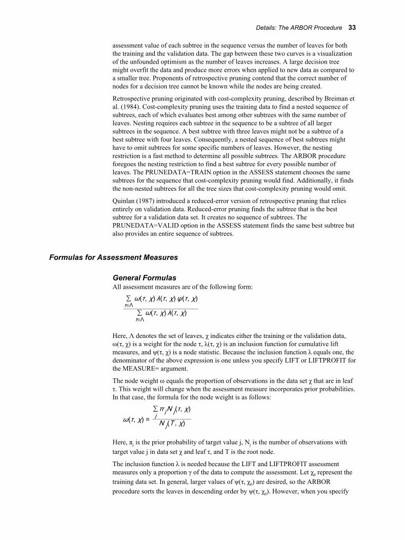
assessment value of each subtree in the sequence versus the number of leaves for both the training and the validation data. The gap between these two curves is a visualization of the unfounded optimism as the number of leaves increases. A large decision tree might overfit the data and produce more errors when applied to new data as compared to a smaller tree. Proponents of retrospective pruning contend that the correct number of nodes for a decision tree cannot be known while the nodes are being created.
Retrospective pruning originated with cost-complexity pruning, described by Breiman et al. (1984). Cost-complexity pruning uses the training data to find a nested sequence of subtrees, each of which evaluates best among other subtrees with the same number of leaves. Nesting requires each subtree in the sequence to be a subtree of all larger subtrees in the sequence. A best subtree with three leaves might not be a subtree of a best subtree with four leaves. Consequently, a nested sequence of best subtrees might have to omit subtrees for some specific numbers of leaves. However, the nesting restriction is a fast method to determine all possible subtrees. The ARBOR procedure foregoes the nesting restriction to find a best subtree for every possible number of leaves. The PRUNEDATA=TRAIN option in the ASSESS statement chooses the same subtrees for the sequence that cost-complexity pruning would find. Additionally, it finds the non-nested subtrees for all the tree sizes that cost-complexity pruning would omit.
Quinlan (1987) introduced a reduced-error version of retrospective pruning that relies entirely on validation data. Reduced-error pruning finds the subtree that is the best subtree for a validation data set. It creates no sequence of subtrees. The PRUNEDATA=VALID option in the ASSESS statement finds the same best subtree but also provides an entire sequence of subtrees.
Formulas for Assessment Measures
General FormulasAll assessment measures are of the following form:
∑τ∈Λ
ω(τ, χ) λ(τ, χ) ψ(τ, χ)
∑τ∈Λ
ω(τ, χ) λ(τ, χ)
Here, Λ denotes the set of leaves, χ indicates either the training or the validation data, ω(τ, χ) is a weight for the node τ, λ(τ, χ) is an inclusion function for cumulative lift measures, and ψ(τ, χ) is a node statistic. Because the inclusion function λ equals one, the denominator of the above expression is one unless you specify LIFT or LIFTPROFIT for the MEASURE= argument.
The node weight ω equals the proportion of observations in the data set χ that are in leaf τ. This weight will change when the assessment measure incorporates prior probabilities. In that case, the formula for the node weight is as follows:
ω(τ, χ) =∑jπ jN j(τ, χ)
N j(T , χ)
Here, πj is the prior probability of target value j, Nj is the number of observations with target value j in data set χ and leaf τ, and T is the root node.
The inclusion function λ is needed because the LIFT and LIFTPROFIT assessment measures only a proportion γ of the data to compute the assessment. Let χ0 represent the training data set. In general, larger values of ψ(τ, χ0) are desired, so the ARBOR procedure sorts the leaves in descending order by ψ(τ, χ0). However, when you specify
Details: The ARBOR Procedure 33
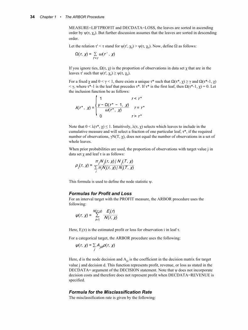
MEASURE=LIFTPROFIT and DECDATA=LOSS, the leaves are sorted in ascending order by ψ(τ, χ0). But further discussion assumes that the leaves are sorted in descending order.
Let the relation τ' < τ stand for ψ(τ', χ0) > ψ(τ, χ0). Now, define Ω as follows:
Ω(τ, χ) = ∑τ′<τ
ω(τ ′ , χ)
If you ignore ties, Ω(τ, χ) is the proportion of observations in data set χ that are in the leaves τ' such that ψ(τ', χ0) ≥ ψ(τ, χ0).
For a fixed χ and 0 < γ < 1, there exists a unique τ* such that Ω(τ*, χ) ≥ γ and Ω(τ*-1, χ) < γ, where τ*-1 is the leaf that precedes τ*. If τ* is the first leaf, then Ω(τ*-1, χ) = 0. Let the inclusion function be as follows:
λ(τ * , χ) = { 1 τ < τ *γ − Ω(τ * − 1, χ)
ω(τ * , χ) τ = τ *
0 τ > τ *
Note that 0 < λ(τ*, χ) ≤ 1. Intuitively, λ(τ, χ) selects which leaves to include in the cumulative measure and will select a fraction of one particular leaf, τ*, if the required number of observations, γN(T, χ), does not equal the number of observations in a set of whole leaves.
When prior probabilities are used, the proportion of observations with target value j in data set χ and leaf τ is as follows:
ρ j(τ, χ) =π jN j(τ, χ) / N j(T , χ)∑iπiN i(τ, χ) / N i(T , χ)
This formula is used to define the node statistic ψ.
Formulas for Profit and LossFor an interval target with the PROFIT measure, the ARBOR procedure uses the following:
ψ(τ, χ) = ∑i=1
N(τ,χ) Ei(τ)N (τ, χ)
Here, Ei(τ) is the estimated profit or loss for observation i in leaf τ.
For a categorical target, the ARBOR procedure uses the following:
ψ(τ, χ) = ∑jA jdρ(τ, χ)
Here, d is the node decision and Ajd is the coefficient in the decision matrix for target value j and decision d. This function represents profit, revenue, or loss as stated in the DECDATA= argument of the DECISION statement. Note that ψ does not incorporate decision costs and therefore does not represent profit when DECDATA=REVENUE is specified.
Formula for the Misclassification RateThe misclassification rate is given by the following:
34 Chapter 1 • The ARBOR Procedure
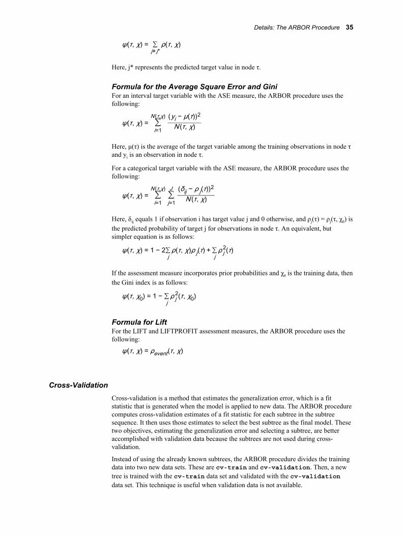
ψ(τ, χ) = ∑j≠ j*
ρ(τ, χ)
Here, j* represents the predicted target value in node τ.
Formula for the Average Square Error and GiniFor an interval target variable with the ASE measure, the ARBOR procedure uses the following:
ψ(τ, χ) = ∑i=1
N(τ,χ) (yi − μ(τ))2N (τ, χ)
Here, μ(τ) is the average of the target variable among the training observations in node τ and yi is an observation in node τ.
For a categorical target variable with the ASE measure, the ARBOR procedure uses the following:
ψ(τ, χ) = ∑i=1
N(τ,χ)∑j=1
J (δij − ρ j(τ))2N (τ, χ)
Here, δij equals 1 if observation i has target value j and 0 otherwise, and ρj(τ) = ρj(τ, χ0) is the predicted probability of target j for observations in node τ. An equivalent, but simpler equation is as follows:
ψ(τ, χ) = 1 − 2∑jρ(τ, χ)ρ j(τ) + ∑j
ρ j2(τ)
If the assessment measure incorporates prior probabilities and χ0 is the training data, then the Gini index is as follows:
ψ(τ, χ0) = 1 − ∑jρ j2(τ, χ0)
Formula for LiftFor the LIFT and LIFTPROFIT assessment measures, the ARBOR procedure uses the following:
ψ(τ, χ) = ρevent(τ, χ)
Cross-ValidationCross-validation is a method that estimates the generalization error, which is a fit statistic that is generated when the model is applied to new data. The ARBOR procedure computes cross-validation estimates of a fit statistic for each subtree in the subtree sequence. It then uses those estimates to select the best subtree as the final model. These two objectives, estimating the generalization error and selecting a subtree, are better accomplished with validation data because the subtrees are not used during cross-validation.
Instead of using the already known subtrees, the ARBOR procedure divides the training data into two new data sets. These are cv-train and cv-validation. Then, a new tree is trained with the cv-train data set and validated with the cv-validation data set. This technique is useful when validation data is not available.
Details: The ARBOR Procedure 35
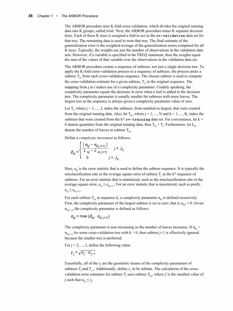
The ARBOR procedure uses K-fold cross-validation, which divides the original training data into K groups, called folds. Next, the ARBOR procedure trains K separate decision trees. Each of these K trees is assigned a fold to act as the cv-validation data set for that tree. The remaining data is used to train that tree. The final estimate of the generalization error is the weighted average of the generalization errors computed for all K trees. Typically, the weights are just the number of observations in the validation data sets. However, if a variable is specified in the FREQ statement, then the weights equal the sum of the values of that variable over the observations in the validation data set.
The ARBOR procedure creates a sequence of subtrees, not just a single decision tree. To apply the K-fold cross-validation process to a sequence of subtrees, the process picks a subtree Tki from each cross-validation sequence. The chosen subtree is used to compute the cross-validation estimate for a given subtree, Tj, in the original sequence. The mapping from j to i makes use of a complexity parameter. Crudely speaking, the complexity parameter equals the decrease in error when a leaf is added to the decision tree. The complexity parameter is usually smaller for subtrees with more leaves. The largest tree in the sequence is always given a complexity parameter value of zero.
Let Tj, where j = 1, ..., J, index the subtrees, from smallest to largest, that were created from the original training data. Also, let Tkj, where j = 1, ..., N and k = 1, ..., K, index the subtrees that were created from the kth cv-training data set. For convenience, let k = 0 denote quantities from the original training data, thus T0j = Tj. Furthermore, let Lkj
denote the number of leaves in subtree Tkj.
Define a complexity increment as follows:
βkj = { | ekj − ek ( j+1) |L kj − L k ( j+1)j < Jk
0 j = Jk
Here, ekj is the error statistic that is used to define the subtree sequence. It is typically the misclassification rate or the average square error of subtree Tj in the kth sequence of subtrees. For an error statistic that is minimized, such as the misclassification rate or the average square error, ekj ≥ ek(j+1). For an error statistic that is maximized, such as profit, ekj ≤ ek(j+1).
For each subtree Tkj in sequence k, a complexity parameter αkj is defined recursively. First, the complexity parameter of the largest subtree is set to zero, that is αkN = 0. Given αk(j+1), the complexity parameter is defined as follows:
αkj = max (βkj, αk ( j+1))
The complexity parameter is non-increasing as the number of leaves increases. If αkj = αk(j+1) for some cross-validation tree with k > 0, then subtree j+1 is effectively ignored because the smaller tree is preferred.
For j = 2, ..., J, define the following value:
γ j = α j ⋅ α j−1
Essentially, all of the γj are the geometric means of the complexity parameters of subtrees Tj and Tj-1. Additionally, define γ1 to be infinite. The calculation of the cross-validation error estimates for subtree Tj uses subtree Tkj', where j' is the smallest value of j such that αkj ≤ γj.
36 Chapter 1 • The ARBOR Procedure
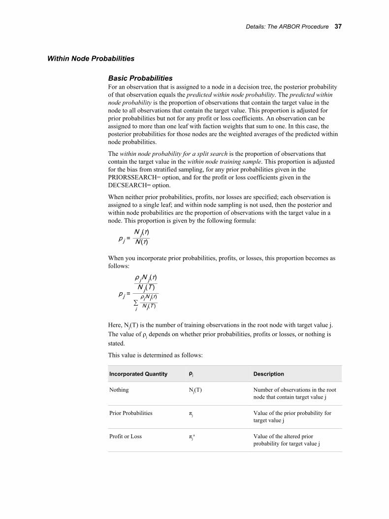
Within Node Probabilities
Basic ProbabilitiesFor an observation that is assigned to a node in a decision tree, the posterior probability of that observation equals the predicted within node probability. The predicted within node probability is the proportion of observations that contain the target value in the node to all observations that contain the target value. This proportion is adjusted for prior probabilities but not for any profit or loss coefficients. An observation can be assigned to more than one leaf with faction weights that sum to one. In this case, the posterior probabilities for those nodes are the weighted averages of the predicted within node probabilities.
The within node probability for a split search is the proportion of observations that contain the target value in the within node training sample. This proportion is adjusted for the bias from stratified sampling, for any prior probabilities given in the PRIORSSEARCH= option, and for the profit or loss coefficients given in the DECSEARCH= option.
When neither prior probabilities, profits, nor losses are specified; each observation is assigned to a single leaf; and within node sampling is not used, then the posterior and within node probabilities are the proportion of observations with the target value in a node. This proportion is given by the following formula:
p j =N j(τ)N (τ)
When you incorporate prior probabilities, profits, or losses, this proportion becomes as follows:
p j =
ρ jN j(τ)N j(T )
∑i
ρiNi(τ)Ni(T )
Here, Nj(T) is the number of training observations in the root node with target value j. The value of ρj depends on whether prior probabilities, profits or losses, or nothing is stated.
This value is determined as follows:
Incorporated Quantity ρj Description
Nothing Nj(T) Number of observations in the root node that contain target value j
Prior Probabilities πj Value of the prior probability for target value j
Profit or Loss πja Value of the altered prior
probability for target value j
Details: The ARBOR Procedure 37
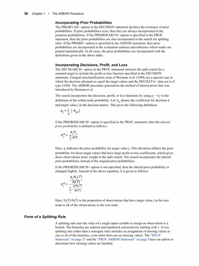
Incorporating Prior ProbabilitiesThe PRIORVAR= option in the DECISION statement declares the existence of prior probabilities. If prior probabilities exist, then they are always incorporated in the posterior probabilities. If the PRIORSEARCH= option is specified in the PROC statement, then the prior probabilities are also incorporated in the search for splitting rules. If the PRIORS= option is specified in the ASSESS statement, then prior probabilities are incorporated in the evaluation subtrees and influence which nodes are pruned automatically. In all cases, the prior probabilities are incorporated with the definitions given in the above table.
Incorporating Decisions, Profit, and LossThe DECSEARCH= option in the PROC statement instructs the split search for a nominal target to include the profit or loss function specified in the DECISION statement. Unequal misclassification costs of Breiman et al. (1984) are a special case in which the decision alternatives equal the target values and the DECDATA= data set is of type LOSS. The ARBOR procedure generalizes the method of altered priors that was introduced by Breiman et al.
The search incorporates the decisions, profit, or loss functions by using ρj = πja in the
definition of the within node probability. Let Ajd denote the coefficient for decision d and target value j in the decision matrix. This gives the following definition:
a j = ∑d| A jd |
If the PRIORSSEARCH= option is specified in the PROC statement, then the altered prior probability is defined as follows:
π ja =
a jπ j∑iaiπi
Here, πj indicates the prior probability for target value j. This alteration inflates the prior probability for those target values that have large profit or loss coefficients, which gives those observations more weight in the split search. The search incorporates the altered prior probabilities instead of the original prior probabilities.
If the PRIORSSEARCH= option is not specified, then the altered prior probability is changed slightly. Instead of the above equation, it is given as follows:
π ja =
a jN j(T )N (T )
∑i
aiNi(T )N (T )
Here, Nj(T)/N(T) is the proportion of observations that have target value j in the root node to all of the observations in the root node.
Form of a Splitting RuleA splitting rule uses the value of a single input variable to assign an observation to a branch. The branches are ordered and numbered consecutively starting with 1. Every splitting rule (other than a surrogate rule) includes an assignment of missing values to one or all of the branches, even when there are no missing values. The “SPLIT Statement” on page 27 and the “PROC ARBOR Statement” on page 8 have an option to determine how missing values are handled.
38 Chapter 1 • The ARBOR Procedure
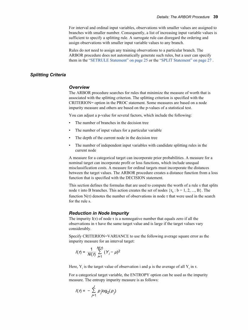
For interval and ordinal input variables, observations with smaller values are assigned to branches with smaller number. Consequently, a list of increasing input variable values is sufficient to specify a splitting rule. A surrogate rule can disregard the ordering and assign observations with smaller input variable values to any branch.
Rules do not need to assign any training observations to a particular branch. The ARBOR procedure does not automatically generate such rules, but a user can specify them in the “SETRULE Statement” on page 25 or the “SPLIT Statement” on page 27 .
Splitting Criteria
OverviewThe ARBOR procedure searches for rules that minimize the measure of worth that is associated with the splitting criterion. The splitting criterion is specified with the CRITERION= option in the PROC statement. Some measures are based on a node impurity measure and others are based on the p-values of a statistical test.
You can adjust a p-value for several factors, which include the following:
• The number of branches in the decision tree
• The number of input values for a particular variable
• The depth of the current node in the decision tree
• The number of independent input variables with candidate splitting rules in the current node
A measure for a categorical target can incorporate prior probabilities. A measure for a nominal target can incorporate profit or loss functions, which include unequal misclassification costs. A measure for ordinal targets must incorporate the distances between the target values. The ARBOR procedure creates a distance function from a loss function that is specified with the DECISION statement.
This section defines the formulas that are used to compute the worth of a rule s that splits node τ into B branches. This action creates the set of nodes {τb : b = 1, 2, ..., B}. The function N(τ) denotes the number of observations in node τ that were used in the search for the rule s.
Reduction in Node ImpurityThe impurity I(τ) of node τ is a nonnegative number that equals zero if all the observations in τ have the same target value and is large if the target values vary considerably.
Specify CRITERION=VARIANCE to use the following average square error as the impurity measure for an interval target:
I (τ) = 1N (τ) ∑i=1
N(τ)(Y i − μ)2
Here, Yi is the target value of observation i and μ is the average of all Yi in τ.
For a categorical target variable, the ENTROPY option can be used as the impurity measure. The entropy impurity measure is as follows:
I (τ) = − ∑j=1
Jp jlog2(p j)
Details: The ARBOR Procedure 39
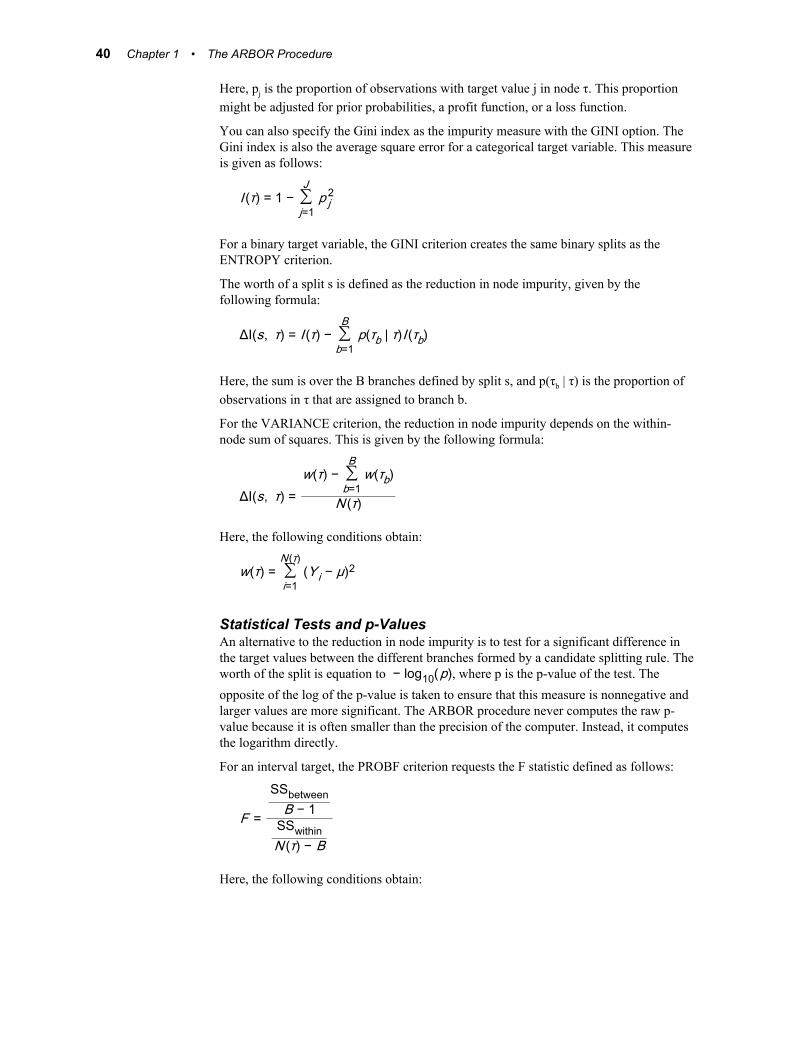
Here, pj is the proportion of observations with target value j in node τ. This proportion might be adjusted for prior probabilities, a profit function, or a loss function.
You can also specify the Gini index as the impurity measure with the GINI option. The Gini index is also the average square error for a categorical target variable. This measure is given as follows:
I (τ) = 1 − ∑j=1
Jp j2
For a binary target variable, the GINI criterion creates the same binary splits as the ENTROPY criterion.
The worth of a split s is defined as the reduction in node impurity, given by the following formula:
ΔI(s, τ) = I (τ) − ∑b=1
Bp(τb | τ)I (τb)
Here, the sum is over the B branches defined by split s, and p(τb | τ) is the proportion of observations in τ that are assigned to branch b.
For the VARIANCE criterion, the reduction in node impurity depends on the within-node sum of squares. This is given by the following formula:
ΔI(s, τ) =w(τ) − ∑
b=1
Bw(τb)
N (τ)
Here, the following conditions obtain:
w(τ) = ∑i=1
N(τ)(Y i − μ)2
Statistical Tests and p-ValuesAn alternative to the reduction in node impurity is to test for a significant difference in the target values between the different branches formed by a candidate splitting rule. The worth of the split is equation to − log10(p), where p is the p-value of the test. The opposite of the log of the p-value is taken to ensure that this measure is nonnegative and larger values are more significant. The ARBOR procedure never computes the raw p-value because it is often smaller than the precision of the computer. Instead, it computes the logarithm directly.
For an interval target, the PROBF criterion requests the F statistic defined as follows:
F =
SSbetweenB − 1SSwithinN (τ) − B
Here, the following conditions obtain:
40 Chapter 1 • The ARBOR Procedure
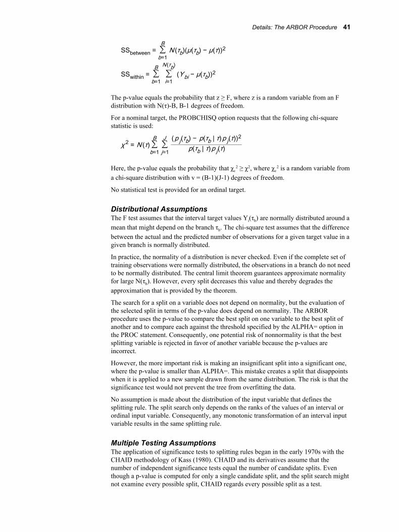
SSbetween = ∑b=1
BN (τb)(μ(τb) − μ(τ))2
SSwithin = ∑b=1
B∑i=1
N(τb)(Ybi − μ(τb))2
The p-value equals the probability that z ≥ F, where z is a random variable from an F distribution with N(τ)-B, B-1 degrees of freedom.
For a nominal target, the PROBCHISQ option requests that the following chi-square statistic is used:
χ 2 = N (τ)∑b=1
B∑j=1
J (p j(τb) − p(τb | τ)p j(τ))2p(τb | τ)p j(τ)
Here, the p-value equals the probability that χv2 ≥ χ2, where χv
2 is a random variable from a chi-square distribution with v = (B-1)(J-1) degrees of freedom.
No statistical test is provided for an ordinal target.
Distributional AssumptionsThe F test assumes that the interval target values Yi(τb) are normally distributed around a mean that might depend on the branch τb. The chi-square test assumes that the difference between the actual and the predicted number of observations for a given target value in a given branch is normally distributed.
In practice, the normality of a distribution is never checked. Even if the complete set of training observations were normally distributed, the observations in a branch do not need to be normally distributed. The central limit theorem guarantees approximate normality for large N(τb). However, every split decreases this value and thereby degrades the approximation that is provided by the theorem.
The search for a split on a variable does not depend on normality, but the evaluation of the selected split in terms of the p-value does depend on normality. The ARBOR procedure uses the p-value to compare the best split on one variable to the best split of another and to compare each against the threshold specified by the ALPHA= option in the PROC statement. Consequently, one potential risk of nonnormality is that the best splitting variable is rejected in favor of another variable because the p-values are incorrect.
However, the more important risk is making an insignificant split into a significant one, where the p-value is smaller than ALPHA=. This mistake creates a split that disappoints when it is applied to a new sample drawn from the same distribution. The risk is that the significance test would not prevent the tree from overfitting the data.
No assumption is made about the distribution of the input variable that defines the splitting rule. The split search only depends on the ranks of the values of an interval or ordinal input variable. Consequently, any monotonic transformation of an interval input variable results in the same splitting rule.
Multiple Testing AssumptionsThe application of significance tests to splitting rules began in the early 1970s with the CHAID methodology of Kass (1980). CHAID and its derivatives assume that the number of independent significance tests equal the number of candidate splits. Even though a p-value is computed for only a single candidate split, and the split search might not examine every possible split, CHAID regards every possible split as a test.
Details: The ARBOR Procedure 41
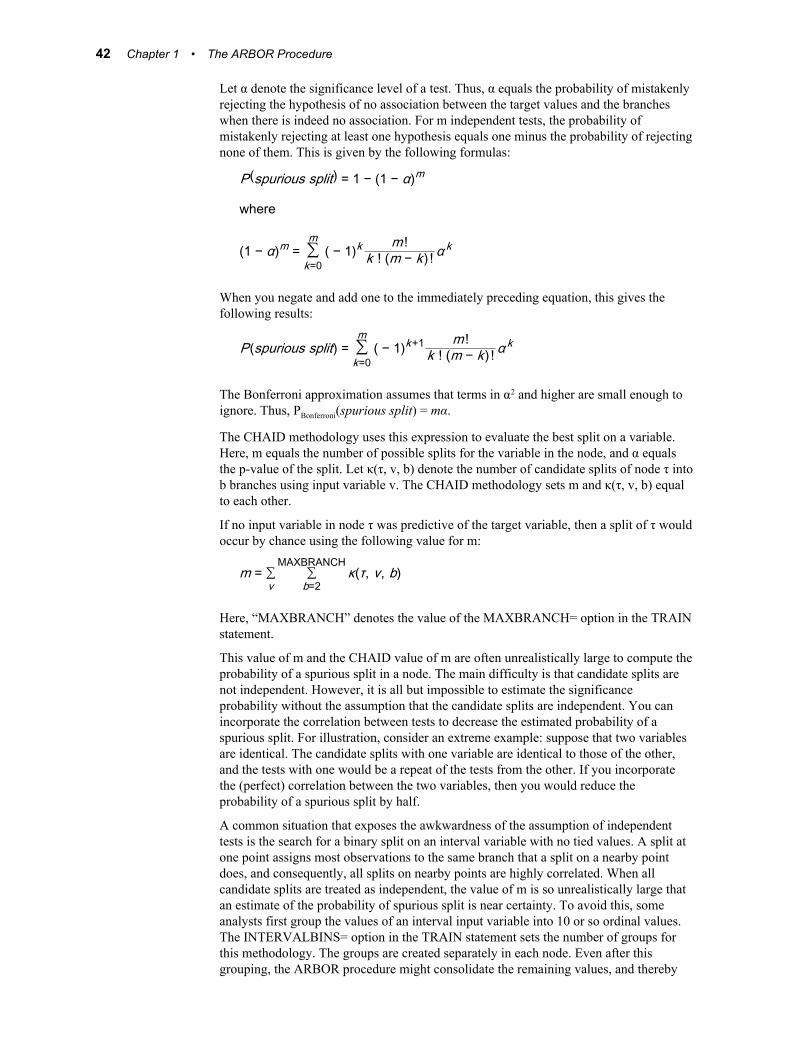
Let α denote the significance level of a test. Thus, α equals the probability of mistakenly rejecting the hypothesis of no association between the target values and the branches when there is indeed no association. For m independent tests, the probability of mistakenly rejecting at least one hypothesis equals one minus the probability of rejecting none of them. This is given by the following formulas:
P(spurious split) = 1 − (1 − α)m
where
(1 − α)m = ∑k=0
m( − 1)k m!
k ! (m − k) ! αk
When you negate and add one to the immediately preceding equation, this gives the following results:
P(spurious split) = ∑k=0
m( − 1)k+1 m!
k ! (m − k) ! αk
The Bonferroni approximation assumes that terms in α2 and higher are small enough to ignore. Thus, PBonferroni(spurious split) = mα.
The CHAID methodology uses this expression to evaluate the best split on a variable. Here, m equals the number of possible splits for the variable in the node, and α equals the p-value of the split. Let κ(τ, v, b) denote the number of candidate splits of node τ into b branches using input variable v. The CHAID methodology sets m and κ(τ, v, b) equal to each other.
If no input variable in node τ was predictive of the target variable, then a split of τ would occur by chance using the following value for m:
m = ∑v
∑b=2
MAXBRANCHκ(τ, v, b)
Here, “MAXBRANCH” denotes the value of the MAXBRANCH= option in the TRAIN statement.
This value of m and the CHAID value of m are often unrealistically large to compute the probability of a spurious split in a node. The main difficulty is that candidate splits are not independent. However, it is all but impossible to estimate the significance probability without the assumption that the candidate splits are independent. You can incorporate the correlation between tests to decrease the estimated probability of a spurious split. For illustration, consider an extreme example: suppose that two variables are identical. The candidate splits with one variable are identical to those of the other, and the tests with one would be a repeat of the tests from the other. If you incorporate the (perfect) correlation between the two variables, then you would reduce the probability of a spurious split by half.
A common situation that exposes the awkwardness of the assumption of independent tests is the search for a binary split on an interval variable with no tied values. A split at one point assigns most observations to the same branch that a split on a nearby point does, and consequently, all splits on nearby points are highly correlated. When all candidate splits are treated as independent, the value of m is so unrealistically large that an estimate of the probability of spurious split is near certainty. To avoid this, some analysts first group the values of an interval input variable into 10 or so ordinal values. The INTERVALBINS= option in the TRAIN statement sets the number of groups for this methodology. The groups are created separately in each node. Even after this grouping, the ARBOR procedure might consolidate the remaining values, and thereby
42 Chapter 1 • The ARBOR Procedure
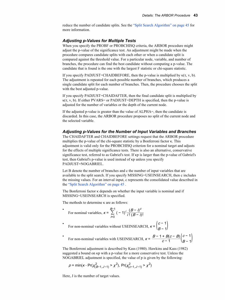
reduce the number of candidate splits. See the “Split Search Algorithm” on page 45 for more information.
Adjusting p-Values for Multiple TestsWhen you specify the PROBF or PROBCHISQ criteria, the ARBOR procedure might adjust the p-value of the significance test. An adjustment might be made when the procedure compares candidate splits with each other or when a candidate split is compared against the threshold value. For a particular node, variable, and number of branches, the procedure can find the best candidate without computing a p-value. The candidate that is found is the one with the largest F statistic or chi-square statistic.
If you specify PADJUST=CHAIDBEFORE, then the p-value is multiplied by κ(τ, v, b). The adjustment is repeated for each possible number of branches, which produces a single candidate split for each number of branches. Then, the procedure chooses the split with the best adjusted p-value.
If you specify PADJUST=CHAIDAFTER, then the final candidate split is multiplied by κ(τ, v, b). If either PVARS= or PADJUST=DEPTH is specified, then the p-value is adjusted for the number of variables or the depth of the current node.
If the adjusted p-value is greater than the value of ALPHA=, then the candidate is discarded. In this case, the ARBOR procedure proposes no split of the current node and the selected variable.
Adjusting p-Values for the Number of Input Variables and BranchesThe CHAIDAFTER and CHAIDBEFORE settings request that the ARBOR procedure multiplies the p-value of the chi-square statistic by a Bonferroni factor κ. This adjustment is valid only for the PROBCHISQ criterion for a nominal target and adjusts for the effects of multiple significance tests. There is also an alternative, conservative significance test, referred to as Gabriel's test. If κp is larger than the p-value of Gabriel's test, then Gabriel's p-value is used instead of κp unless you specify PADJUST=NOGABRIEL.
Let B denote the number of branches and c the number of input variables that are available to the split search. If you specify MISSING=USEINSEARCH, then c includes the missing values. For an interval input, c represents the consolidated value described in the “Split Search Algorithm” on page 45 .
The Bonferroni factor κ depends on whether the input variable is nominal and if MISSING=USEINSEARCH is specified.
The methods to determine κ are as follows:
•For nominal variables, κ = ∑
i=0
B−1( − 1)i (B − i)c
i ! (B − i) !
•For non-nominal variables without USEINSEARCH, κ = (c − 1B − 1)
•For non-nominal variables with USEINSEARCH, κ = B − 1 + B(c − B)
c − 1 (c − 1B − 1)The Bonferroni adjustment is described by Kass (1980). Hawkins and Kass (1982) suggested a bound on κp with a p-value for a more conservative test. Unless the NOGABRIEL adjustment is specified, the value of p is given by the following:
p = min(κ ⋅ Pr(χ(B−1,J −1)2 > χ 2), Pr(χ(c−1,J −1)
2 > χ 2)
Here, J is the number of target values.
Details: The ARBOR Procedure 43
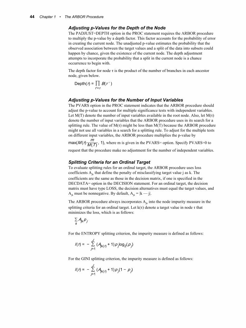
Adjusting p-Values for the Depth of the NodeThe PADJUST=DEPTH option in the PROC statement requires the ARBOR procedure to multiply the p-value by a depth factor. This factor accounts for the probability of error in creating the current node. The unadjusted p-value estimates the probability that the observed association between the target values and a split of the data into subsets could happen by chance, given the existence of the current node. The depth adjustment attempts to incorporate the probability that a split in the current node is a chance occurrence to begin with.
The depth factor for node τ is the product of the number of branches in each ancestor node, given below.
Depth(τ) = ∏τ′<τ
B(τ ′ )
Adjusting p-Values for the Number of Input VariablesThe PVARS option in the PROC statement indicates that the ARBOR procedure should adjust the p-value to account for multiple significance tests with independent variables. Let M(T) denote the number of input variables available in the root node. Also, let M(τ) denote the number of input variables that the ARBOR procedure uses in its search for a splitting rule. The value of M(τ) might be less than M(T) because the ARBOR procedure might not use all variables in a search for a splitting rule. To adjust for the multiple tests on different input variables, the ARBOR procedure multiplies the p-value by
max(M (τ) mM (T ) , 1), where m is given in the PVARS= option. Specify PVARS=0 to
request that the procedure make no adjustment for the number of independent variables.
Splitting Criteria for an Ordinal TargetTo evaluate splitting rules for an ordinal target, the ARBOR procedure uses loss coefficients Ajk that define the penalty of misclassifying target value j as k. The coefficients are the same as those in the decision matrix, if one is specified in the DECDATA= option in the DECISION statement. For an ordinal target, the decision matrix must have type LOSS, the decision alternatives must equal the target values, and Ajk must be nonnegative. By default, Ajk = |k — j|.
The ARBOR procedure always incorporates Ajk into the node impurity measure in the splitting criteria for an ordinal target. Let k(τ) denote a target value in node τ that minimizes the loss, which is as follows:
∑kAjkp j
For the ENTROPY splitting criterion, the impurity measure is defined as follows:
I (τ) = − ∑j=1
J(Ajk(τ) + 1)p jlog2(p j)
For the GINI splitting criterion, the impurity measure is defined as follows:
I (τ) = − ∑j=1
J(Ajk(τ) + 1)p j(1 − p j)
44 Chapter 1 • The ARBOR Procedure
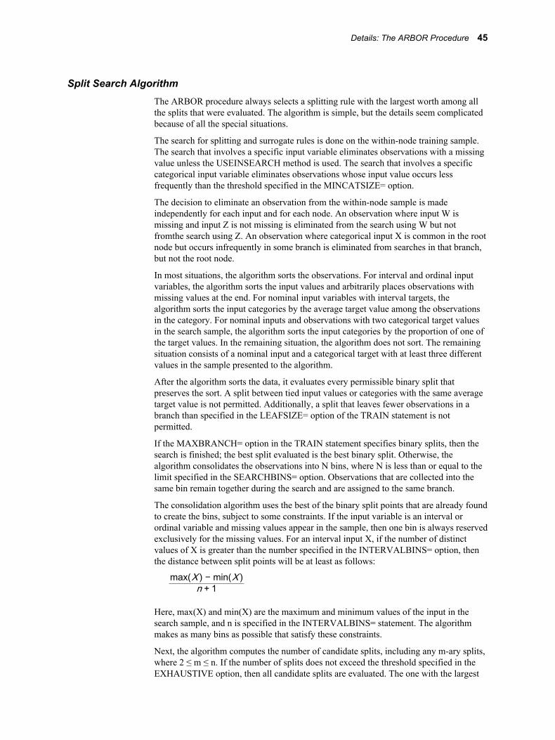
Split Search AlgorithmThe ARBOR procedure always selects a splitting rule with the largest worth among all the splits that were evaluated. The algorithm is simple, but the details seem complicated because of all the special situations.
The search for splitting and surrogate rules is done on the within-node training sample. The search that involves a specific input variable eliminates observations with a missing value unless the USEINSEARCH method is used. The search that involves a specific categorical input variable eliminates observations whose input value occurs less frequently than the threshold specified in the MINCATSIZE= option.
The decision to eliminate an observation from the within-node sample is made independently for each input and for each node. An observation where input W is missing and input Z is not missing is eliminated from the search using W but not fromthe search using Z. An observation where categorical input X is common in the root node but occurs infrequently in some branch is eliminated from searches in that branch, but not the root node.
In most situations, the algorithm sorts the observations. For interval and ordinal input variables, the algorithm sorts the input values and arbitrarily places observations with missing values at the end. For nominal input variables with interval targets, the algorithm sorts the input categories by the average target value among the observations in the category. For nominal inputs and observations with two categorical target values in the search sample, the algorithm sorts the input categories by the proportion of one of the target values. In the remaining situation, the algorithm does not sort. The remaining situation consists of a nominal input and a categorical target with at least three different values in the sample presented to the algorithm.
After the algorithm sorts the data, it evaluates every permissible binary split that preserves the sort. A split between tied input values or categories with the same average target value is not permitted. Additionally, a split that leaves fewer observations in a branch than specified in the LEAFSIZE= option of the TRAIN statement is not permitted.
If the MAXBRANCH= option in the TRAIN statement specifies binary splits, then the search is finished; the best split evaluated is the best binary split. Otherwise, the algorithm consolidates the observations into N bins, where N is less than or equal to the limit specified in the SEARCHBINS= option. Observations that are collected into the same bin remain together during the search and are assigned to the same branch.
The consolidation algorithm uses the best of the binary split points that are already found to create the bins, subject to some constraints. If the input variable is an interval or ordinal variable and missing values appear in the sample, then one bin is always reserved exclusively for the missing values. For an interval input X, if the number of distinct values of X is greater than the number specified in the INTERVALBINS= option, then the distance between split points will be at least as follows:
max(X ) − min(X )n + 1
Here, max(X) and min(X) are the maximum and minimum values of the input in the search sample, and n is specified in the INTERVALBINS= statement. The algorithm makes as many bins as possible that satisfy these constraints.
Next, the algorithm computes the number of candidate splits, including any m-ary splits, where 2 ≤ m ≤ n. If the number of splits does not exceed the threshold specified in the EXHAUSTIVE option, then all candidate splits are evaluated. The one with the largest
Details: The ARBOR Procedure 45
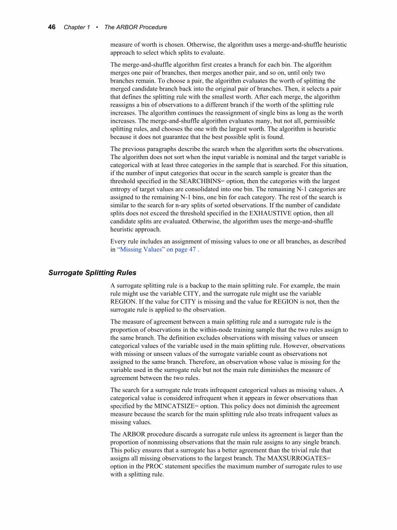
measure of worth is chosen. Otherwise, the algorithm uses a merge-and-shuffle heuristic approach to select which splits to evaluate.
The merge-and-shuffle algorithm first creates a branch for each bin. The algorithm merges one pair of branches, then merges another pair, and so on, until only two branches remain. To choose a pair, the algorithm evaluates the worth of splitting the merged candidate branch back into the original pair of branches. Then, it selects a pair that defines the splitting rule with the smallest worth. After each merge, the algorithm reassigns a bin of observations to a different branch if the worth of the splitting rule increases. The algorithm continues the reassignment of single bins as long as the worth increases. The merge-and-shuffle algorithm evaluates many, but not all, permissible splitting rules, and chooses the one with the largest worth. The algorithm is heuristic because it does not guarantee that the best possible split is found.
The previous paragraphs describe the search when the algorithm sorts the observations. The algorithm does not sort when the input variable is nominal and the target variable is categorical with at least three categories in the sample that is searched. For this situation, if the number of input categories that occur in the search sample is greater than the threshold specified in the SEARCHBINS= option, then the categories with the largest entropy of target values are consolidated into one bin. The remaining N-1 categories are assigned to the remaining N-1 bins, one bin for each category. The rest of the search is similar to the search for n-ary splits of sorted observations. If the number of candidate splits does not exceed the threshold specified in the EXHAUSTIVE option, then all candidate splits are evaluated. Otherwise, the algorithm uses the merge-and-shuffle heuristic approach.
Every rule includes an assignment of missing values to one or all branches, as described in “Missing Values” on page 47 .
Surrogate Splitting RulesA surrogate splitting rule is a backup to the main splitting rule. For example, the main rule might use the variable CITY, and the surrogate rule might use the variable REGION. If the value for CITY is missing and the value for REGION is not, then the surrogate rule is applied to the observation.
The measure of agreement between a main splitting rule and a surrogate rule is the proportion of observations in the within-node training sample that the two rules assign to the same branch. The definition excludes observations with missing values or unseen categorical values of the variable used in the main splitting rule. However, observations with missing or unseen values of the surrogate variable count as observations not assigned to the same branch. Therefore, an observation whose value is missing for the variable used in the surrogate rule but not the main rule diminishes the measure of agreement between the two rules.
The search for a surrogate rule treats infrequent categorical values as missing values. A categorical value is considered infrequent when it appears in fewer observations than specified by the MINCATSIZE= option. This policy does not diminish the agreement measure because the search for the main splitting rule also treats infrequent values as missing values.
The ARBOR procedure discards a surrogate rule unless its agreement is larger than the proportion of nonmissing observations that the main rule assigns to any single branch. This policy ensures that a surrogate has a better agreement than the trivial rule that assigns all missing observations to the largest branch. The MAXSURROGATES= option in the PROC statement specifies the maximum number of surrogate rules to use with a splitting rule.
46 Chapter 1 • The ARBOR Procedure
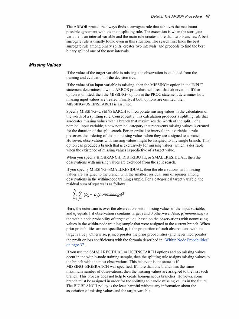
The ARBOR procedure always finds a surrogate rule that achieves the maximum possible agreement with the main splitting rule. The exception is when the surrogate variable is an interval variable and the main rule creates more than two branches. A best surrogate rule is usually found even in this situation. The search first finds the best surrogate rule among binary splits, creates two intervals, and proceeds to find the best binary split of one of the new intervals.
Missing ValuesIf the value of the target variable is missing, the observation is excluded from the training and evaluation of the decision tree.
If the value of an input variable is missing, then the MISSING= option in the INPUT statement determines how the ARBOR procedure will treat that observation. If that option is omitted, then the MISSING= option in the PROC statement determines how missing input values are treated. Finally, if both options are omitted, then MISSING=USEINSEARCH is assumed.
Specify MISSING=USEINSEARCH to incorporate missing values in the calculation of the worth of a splitting rule. Consequently, this calculation produces a splitting rule that associates missing values with a branch that maximizes the worth of the split. For a nominal input variable, a new nominal category that represents missing values is created for the duration of the split search. For an ordinal or interval input variable, a rule preserves the ordering of the nonmissing values when they are assigned to a branch. However, observations with missing values might be assigned to any single branch. This option can produce a branch that is exclusively for missing values, which is desirable when the existence of missing values is predictive of a target value.
When you specify BIGBRANCH, DISTRIBUTE, or SMALLRESIDUAL, then the observations with missing values are excluded from the split search.
If you specify MISSING=SMALLRESIDUAL, then the observations with missing values are assigned to the branch with the smallest residual sum of squares among observations in the within-node training sample. For a categorical target variable, the residual sum of squares is as follows:
∑i=1
N∑j=1
J(δij − p j(nonmissing))2
Here, the outer sum is over the observations with missing values of the input variable; and δij equals 1 if observation i contains target j and 0 otherwise. Also, pj(nonmissing) is the within node probability of target value j, based on the observations with nonmissing values in the within-node training sample that were assigned to the current branch. When prior probabilities are not specified, pj is the proportion of such observations with the target value j. Otherwise, pj incorporates the prior probabilities (and never incorporates the profit or loss coefficients) with the formula described in “Within Node Probabilities” on page 37 .
If you use the SMALLRESIDUAL or USEINSEARCH options and no missing values occur in the within-node training sample, then the splitting rule assigns missing values to the branch with the most observations. This behavior is the same as if MISSING=BIGBRANCH was specified. If more than one branch has the same maximum number of observations, then the missing values are assigned to the first such branch. This process does not help to create homogeneous branches. However, some branch must be assigned in order for the splitting to handle missing values in the future. The BIGBRANCH policy is the least harmful without any information about the association of missing values and the target variable.
Details: The ARBOR Procedure 47
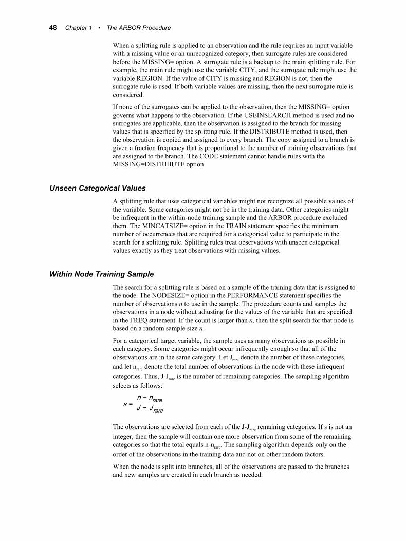
When a splitting rule is applied to an observation and the rule requires an input variable with a missing value or an unrecognized category, then surrogate rules are considered before the MISSING= option. A surrogate rule is a backup to the main splitting rule. For example, the main rule might use the variable CITY, and the surrogate rule might use the variable REGION. If the value of CITY is missing and REGION is not, then the surrogate rule is used. If both variable values are missing, then the next surrogate rule is considered.
If none of the surrogates can be applied to the observation, then the MISSING= option governs what happens to the observation. If the USEINSEARCH method is used and no surrogates are applicable, then the observation is assigned to the branch for missing values that is specified by the splitting rule. If the DISTRIBUTE method is used, then the observation is copied and assigned to every branch. The copy assigned to a branch is given a fraction frequency that is proportional to the number of training observations that are assigned to the branch. The CODE statement cannot handle rules with the MISSING=DISTRIBUTE option.
Unseen Categorical ValuesA splitting rule that uses categorical variables might not recognize all possible values of the variable. Some categories might not be in the training data. Other categories might be infrequent in the within-node training sample and the ARBOR procedure excluded them. The MINCATSIZE= option in the TRAIN statement specifies the minimum number of occurrences that are required for a categorical value to participate in the search for a splitting rule. Splitting rules treat observations with unseen categorical values exactly as they treat observations with missing values.
Within Node Training SampleThe search for a splitting rule is based on a sample of the training data that is assigned to the node. The NODESIZE= option in the PERFORMANCE statement specifies the number of observations n to use in the sample. The procedure counts and samples the observations in a node without adjusting for the values of the variable that are specified in the FREQ statement. If the count is larger than n, then the split search for that node is based on a random sample size n.
For a categorical target variable, the sample uses as many observations as possible in each category. Some categories might occur infrequently enough so that all of the observations are in the same category. Let Jrare denote the number of these categories, and let nrare denote the total number of observations in the node with these infrequent categories. Thus, J-Jrare is the number of remaining categories. The sampling algorithm selects as follows:
s =n − nrareJ − J rare
The observations are selected from each of the J-Jrare remaining categories. If s is not an integer, then the sample will contain one more observation from some of the remaining categories so that the total equals n-nrare. The sampling algorithm depends only on the order of the observations in the training data and not on other random factors.
When the node is split into branches, all of the observations are passed to the branches and new samples are created in each branch as needed.
48 Chapter 1 • The ARBOR Procedure
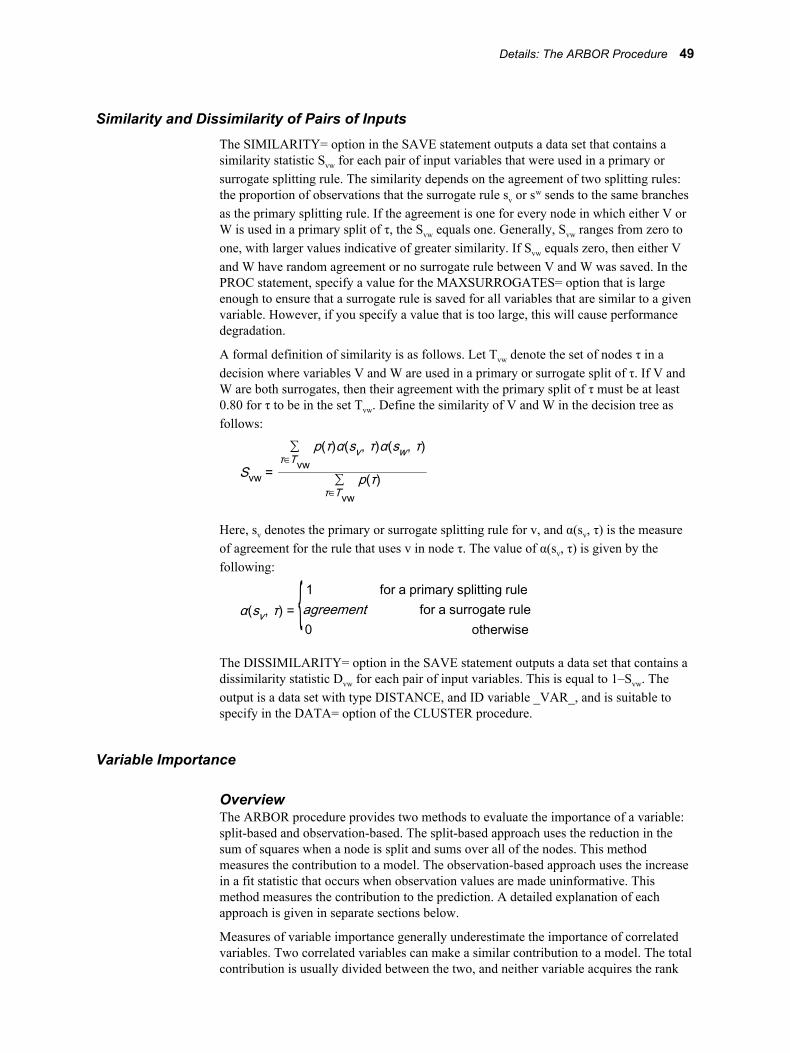
Similarity and Dissimilarity of Pairs of InputsThe SIMILARITY= option in the SAVE statement outputs a data set that contains a similarity statistic Svw for each pair of input variables that were used in a primary or surrogate splitting rule. The similarity depends on the agreement of two splitting rules: the proportion of observations that the surrogate rule sv or sw sends to the same branches as the primary splitting rule. If the agreement is one for every node in which either V or W is used in a primary split of τ, the Svw equals one. Generally, Svw ranges from zero to one, with larger values indicative of greater similarity. If Svw equals zero, then either V and W have random agreement or no surrogate rule between V and W was saved. In the PROC statement, specify a value for the MAXSURROGATES= option that is large enough to ensure that a surrogate rule is saved for all variables that are similar to a given variable. However, if you specify a value that is too large, this will cause performance degradation.
A formal definition of similarity is as follows. Let Tvw denote the set of nodes τ in a decision where variables V and W are used in a primary or surrogate split of τ. If V and W are both surrogates, then their agreement with the primary split of τ must be at least 0.80 for τ to be in the set Tvw. Define the similarity of V and W in the decision tree as follows:
Svw =
∑τ∈Tvw
p(τ)α(sv, τ)α(sw, τ)
∑τ∈Tvw
p(τ)
Here, sv denotes the primary or surrogate splitting rule for v, and α(sv, τ) is the measure of agreement for the rule that uses v in node τ. The value of α(sv, τ) is given by the following:
α(sv, τ) = { 1 for a primary splitting ruleagreement for a surrogate rule0 otherwise
The DISSIMILARITY= option in the SAVE statement outputs a data set that contains a dissimilarity statistic Dvw for each pair of input variables. This is equal to 1–Svw. The output is a data set with type DISTANCE, and ID variable _VAR_, and is suitable to specify in the DATA= option of the CLUSTER procedure.
Variable Importance
OverviewThe ARBOR procedure provides two methods to evaluate the importance of a variable: split-based and observation-based. The split-based approach uses the reduction in the sum of squares when a node is split and sums over all of the nodes. This method measures the contribution to a model. The observation-based approach uses the increase in a fit statistic that occurs when observation values are made uninformative. This method measures the contribution to the prediction. A detailed explanation of each approach is given in separate sections below.
Measures of variable importance generally underestimate the importance of correlated variables. Two correlated variables can make a similar contribution to a model. The total contribution is usually divided between the two, and neither variable acquires the rank
Details: The ARBOR Procedure 49
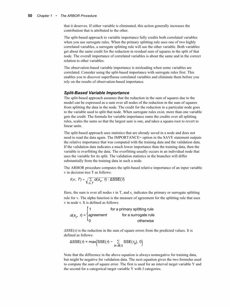
that it deserves. If either variable is eliminated, this action generally increases the contribution that is attributed to the other.
The split-based approach to variable importance fully credits both correlated variables when you use surrogate rules. When the primary splitting rule uses one of two highly correlated variables, a surrogate splitting rule will use the other variable. Both variables get about the same credit for the reduction in residual sum of squares in the split of that node. The overall importance of correlated variables is about the same and in the correct relation to other variables.
The observation-based variable importance is misleading when some variables are correlated. Consider using the split-based importance with surrogate rules first. This enables you to discover superfluous correlated variables and eliminate them before you rely on the results of observation-based importance.
Split-Based Variable ImportanceThe split-based approach assumes that the reduction in the sum of squares due to the model can be expressed as a sum over all nodes of the reduction in the sum of squares from splitting the data in the node. The credit for the reduction in a particular node goes to the variable used to split that node. When surrogate rules exist, more than one variable gets the credit. The formula for variable importance sums the credits over all splitting rules, scales the sums so that the largest sum is one, and takes a square-root to revert to linear units.
The split-based approach uses statistics that are already saved in a node and does not need to read the data again. The IMPORTANCE= option in the SAVE statement outputs the relative importance that was computed with the training data and the validation data. If the validation data indicates a much lower importance than the training data, then the variable is overfitting the data. The overfitting usually occurs in an individual node that uses the variable for its split. The validation statistics in the branches will differ substantially from the training data in such a node.
The ARBOR procedure computes the split-based relative importance of an input variable v in decision tree T as follows:
I (v, T ) ∝ ∑τ∈T
α(sv, τ) ⋅ ΔSSE(τ)
Here, the sum is over all nodes τ in T, and sv indicates the primary or surrogate splitting rule for v. The alpha function is the measure of agreement for the splitting rule that uses v in node τ. It is defined as follows:
α(sv, τ) = { 1 for a primary splitting ruleagreement for a surrogate rule0 otherwise
ΔSSE(τ) is the reduction in the sum of square errors from the predicted values. It is defined as follows:
ΔSSE(τ) = max(SSE(τ) − ∑b∈B(τ)
SSE(τb), 0)Note that the difference in the above equation is always nonnegative for training data, but might be negative for validation data. The next equation gives the two formulas used to compute the sum of square error. The first is used for an interval target variable Y and the second for a categorical target variable Y with J categories.
50 Chapter 1 • The ARBOR Procedure

SSE(τ) = { ∑i=1
N(τ)(Y i − μ(τ))2
∑i=1
N(τ)∑j=1
J(δij − ρi(τ))2
The following definitions are used in the equations above:
• B(τ) is the set of branches from node τ
• τb is the child node of τ in branch b
• N(τ) is the number of observations in τ
• μ(τ) is the average of the target variables in the training data in node τ
• δij is 1 if Yi = j and 0 otherwise
• ρi(τ) is the average δij in the training data in node τ
For a categorical target variable, the formula for SSE(τ) is reduced to the formula below. The first equation is for training data, and the second is for validation data.
SSE(τ) = { N (1 − ∑j=1
Jρ j2)
N (1 − ∑j=1
J(2p j − ρ j)ρ j
Here, pj is the proportion of the validation data with target value j, and N, pj, and ρj are evaluated in node τ.
SAVE Statement IMPORTANCE Output Data SetThe IMPORTANCE= option in the SAVE statement specifies the output data set that contains the split-based measure of relative importance for each input variable in the selected subtree. The ASSESS and SUBTREE statements determine which subtree is selected. Each observation describes an input variable. The observations are in order of decreasing importance as computed with the training data.
The variables in this data set are as follows:
• NAME — The name of the input variable
• LABEL — The label of the input variable
• NRULES — The number of splitting rules that use this variable
• NSURROGATES — The number of surrogate rules that use this variable
• IMPORTANCE — The relative importance of this variable as computed with the training data
• V_IMPORTANCE — The relative importance of this variable as computed with the validation data
• RATIO — the ratio of V_IMPORTANCE to IMPORTANCE, or empty if IMPORTANCE is less than 0.0001.
The NSURROGATES variable is omitted unless surrogate rules are requested in the MAXSURROGATES= option in the TRAIN statement. The V_IMPORTANCE and RATIO variables are omitted unless the VALIDATA= option appears in the ASSESS statement.
Details: The ARBOR Procedure 51
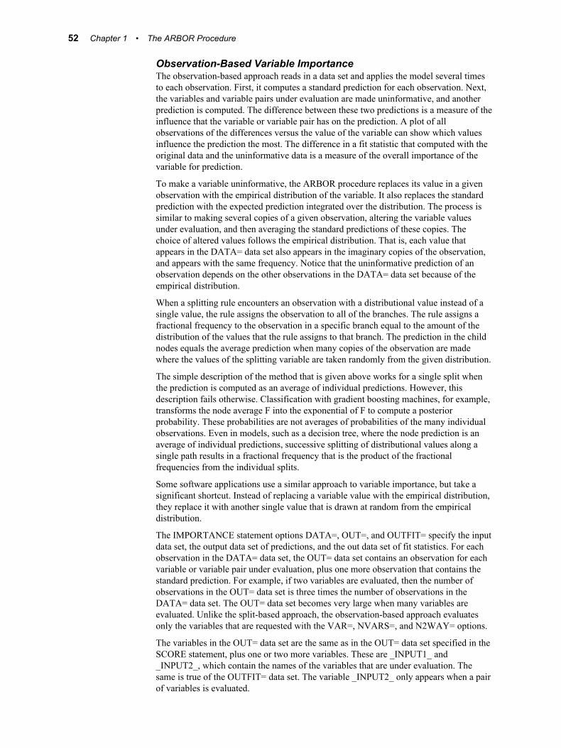
Observation-Based Variable ImportanceThe observation-based approach reads in a data set and applies the model several times to each observation. First, it computes a standard prediction for each observation. Next, the variables and variable pairs under evaluation are made uninformative, and another prediction is computed. The difference between these two predictions is a measure of the influence that the variable or variable pair has on the prediction. A plot of all observations of the differences versus the value of the variable can show which values influence the prediction the most. The difference in a fit statistic that computed with the original data and the uninformative data is a measure of the overall importance of the variable for prediction.
To make a variable uninformative, the ARBOR procedure replaces its value in a given observation with the empirical distribution of the variable. It also replaces the standard prediction with the expected prediction integrated over the distribution. The process is similar to making several copies of a given observation, altering the variable values under evaluation, and then averaging the standard predictions of these copies. The choice of altered values follows the empirical distribution. That is, each value that appears in the DATA= data set also appears in the imaginary copies of the observation, and appears with the same frequency. Notice that the uninformative prediction of an observation depends on the other observations in the DATA= data set because of the empirical distribution.
When a splitting rule encounters an observation with a distributional value instead of a single value, the rule assigns the observation to all of the branches. The rule assigns a fractional frequency to the observation in a specific branch equal to the amount of the distribution of the values that the rule assigns to that branch. The prediction in the child nodes equals the average prediction when many copies of the observation are made where the values of the splitting variable are taken randomly from the given distribution.
The simple description of the method that is given above works for a single split when the prediction is computed as an average of individual predictions. However, this description fails otherwise. Classification with gradient boosting machines, for example, transforms the node average F into the exponential of F to compute a posterior probability. These probabilities are not averages of probabilities of the many individual observations. Even in models, such as a decision tree, where the node prediction is an average of individual predictions, successive splitting of distributional values along a single path results in a fractional frequency that is the product of the fractional frequencies from the individual splits.
Some software applications use a similar approach to variable importance, but take a significant shortcut. Instead of replacing a variable value with the empirical distribution, they replace it with another single value that is drawn at random from the empirical distribution.
The IMPORTANCE statement options DATA=, OUT=, and OUTFIT= specify the input data set, the output data set of predictions, and the out data set of fit statistics. For each observation in the DATA= data set, the OUT= data set contains an observation for each variable or variable pair under evaluation, plus one more observation that contains the standard prediction. For example, if two variables are evaluated, then the number of observations in the OUT= data set is three times the number of observations in the DATA= data set. The OUT= data set becomes very large when many variables are evaluated. Unlike the split-based approach, the observation-based approach evaluates only the variables that are requested with the VAR=, NVARS=, and N2WAY= options.
The variables in the OUT= data set are the same as in the OUT= data set specified in the SCORE statement, plus one or two more variables. These are _INPUT1_ and _INPUT2_, which contain the names of the variables that are under evaluation. The same is true of the OUTFIT= data set. The variable _INPUT2_ only appears when a pair of variables is evaluated.
52 Chapter 1 • The ARBOR Procedure
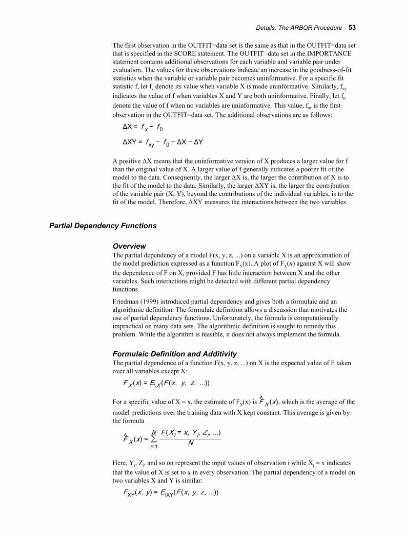
The first observation in the OUTFIT=data set is the same as that in the OUTFIT=data set that is specified in the SCORE statement. The OUTFIT=data set in the IMPORTANCE statement contains additional observations for each variable and variable pair under evaluation. The values for these observations indicate an increase in the goodness-of-fit statistics when the variable or variable pair becomes uninformative. For a specific fit statistic f, let fx denote its value when variable X is made uninformative. Similarly, fxy
indicates the value of f when variables X and Y are both uninformative. Finally, let f0
denote the value of f when no variables are uninformative. This value, f0, is the first observation in the OUTFIT=data set. The additional observations are as follows:
ΔX = f x − f 0
ΔXY = f xy − f 0 − ΔX − ΔY
A positive ΔX means that the uninformative version of X produces a larger value for f than the original value of X. A larger value of f generally indicates a poorer fit of the model to the data. Consequently, the larger ΔX is, the larger the contribution of X is to the fit of the model to the data. Similarly, the larger ΔXY is, the larger the contribution of the variable pair (X, Y), beyond the contributions of the individual variables, is to the fit of the model. Therefore, ΔXY measures the interactions between the two variables.
Partial Dependency Functions
OverviewThe partial dependency of a model F(x, y, z, ...) on a variable X is an approximation of the model prediction expressed as a function FX(x). A plot of FX(x) against X will show the dependence of F on X, provided F has little interaction between X and the other variables. Such interactions might be detected with different partial dependency functions.
Friedman (1999) introduced partial dependency and gives both a formulaic and an algorithmic definition. The formulaic definition allows a discussion that motivates the use of partial dependency functions. Unfortunately, the formula is computationally impractical on many data sets. The algorithmic definition is sought to remedy this problem. While the algorithm is feasible, it does not always implement the formula.
Formulaic Definition and AdditivityThe partial dependence of a function F(x, y, z, ...) on X is the expected value of F taken over all variables except X:
FX (x) = E\X (F (x, y, z, ...))
For a specific value of X = x, the estimate of FX(x) is F X (x), which is the average of the model predictions over the training data with X kept constant. This average is given by the formula
F X (x) = ∑i=1
N F(X i = x, Y i, Zi, ...)N
Here, Yi, Zi, and so on represent the input values of observation i while Xi = x indicates that the value of X is set to x in every observation. The partial dependency of a model on two variables X and Y is similar:
FXY(x, y) = E\XY(F (x, y, z, ...))
Details: The ARBOR Procedure 53
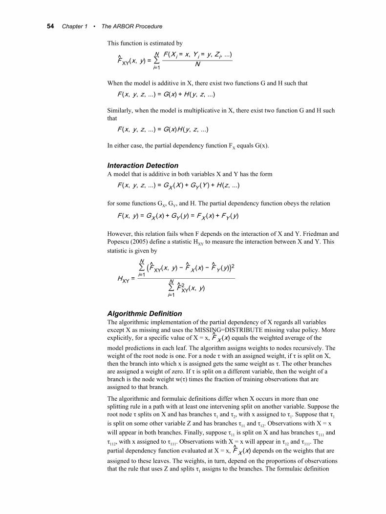
This function is estimated by
FXY(x, y) = ∑i=1
N F(X i = x, Y i = y, Zi, ...)N
When the model is additive in X, there exist two functions G and H such that
F(x, y, z, ...) = G(x) + H (y, z, ...)
Similarly, when the model is multiplicative in X, there exist two function G and H such that
F(x, y, z, ...) = G(x)H (y, z, ...)
In either case, the partial dependency function FX equals G(x).
Interaction DetectionA model that is additive in both variables X and Y has the form
F(x, y, z, ...) = GX (X ) + GY (Y ) + H (z, ...)
for some functions GX, GY, and H. The partial dependency function obeys the relation
F(x, y) = GX (x) + GY (y) = FX (x) + FY (y)
However, this relation fails when F depends on the interaction of X and Y. Friedman and Popescu (2005) define a statistic HXY to measure the interaction between X and Y. This statistic is given by
HXY =∑i=1
N(FXY(x, y) − F X (x) − FY (y))2
∑i=1
NFXY2 (x, y)
Algorithmic DefinitionThe algorithmic implementation of the partial dependency of X regards all variables except X as missing and uses the MISSING=DISTRIBUTE missing value policy. More explicitly, for a specific value of X = x, F X (x) equals the weighted average of the model predictions in each leaf. The algorithm assigns weights to nodes recursively. The weight of the root node is one. For a node τ with an assigned weight, if τ is split on X, then the branch into which x is assigned gets the same weight as τ. The other branches are assigned a weight of zero. If τ is split on a different variable, then the weight of a branch is the node weight w(τ) times the fraction of training observations that are assigned to that branch.
The algorithmic and formulaic definitions differ when X occurs in more than one splitting rule in a path with at least one intervening split on another variable. Suppose the root node τ splits on X and has branches τ1 and τ2, with x assigned to τ1. Suppose that τ1
is split on some other variable Z and has branches τ11 and τ12. Observations with X = x will appear in both branches. Finally, suppose τ11 is split on X and has branches τ111 and τ112, with x assigned to τ111. Observations with X = x will appear in τ12 and τ111. The partial dependency function evaluated at X = x, F X (x) depends on the weights that are assigned to these leaves. The weights, in turn, depend on the proportions of observations that the rule that uses Z and splits τ1 assigns to the branches. The formulaic definition
54 Chapter 1 • The ARBOR Procedure
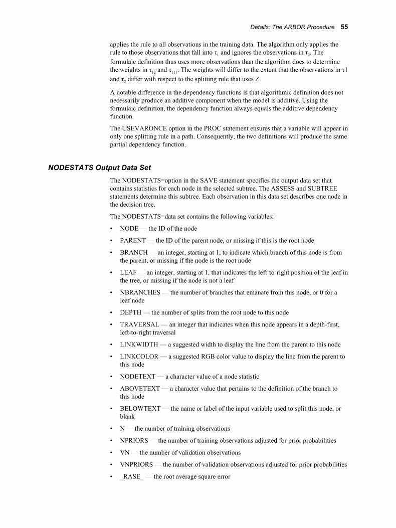
applies the rule to all observations in the training data. The algorithm only applies the rule to those observations that fall into τ1 and ignores the observations in τ2. The formulaic definition thus uses more observations than the algorithm does to determine the weights in τ12 and τ111. The weights will differ to the extent that the observations in τ1 and τ2 differ with respect to the splitting rule that uses Z.
A notable difference in the dependency functions is that algorithmic definition does not necessarily produce an additive component when the model is additive. Using the formulaic definition, the dependency function always equals the additive dependency function.
The USEVARONCE option in the PROC statement ensures that a variable will appear in only one splitting rule in a path. Consequently, the two definitions will produce the same partial dependency function.
NODESTATS Output Data SetThe NODESTATS=option in the SAVE statement specifies the output data set that contains statistics for each node in the selected subtree. The ASSESS and SUBTREE statements determine this subtree. Each observation in this data set describes one node in the decision tree.
The NODESTATS=data set contains the following variables:
• NODE — the ID of the node
• PARENT — the ID of the parent node, or missing if this is the root node
• BRANCH — an integer, starting at 1, to indicate which branch of this node is from the parent, or missing if the node is the root node
• LEAF — an integer, starting at 1, that indicates the left-to-right position of the leaf in the tree, or missing if the node is not a leaf
• NBRANCHES — the number of branches that emanate from this node, or 0 for a leaf node
• DEPTH — the number of splits from the root node to this node
• TRAVERSAL — an integer that indicates when this node appears in a depth-first, left-to-right traversal
• LINKWIDTH — a suggested width to display the line from the parent to this node
• LINKCOLOR — a suggested RGB color value to display the line from the parent to this node
• NODETEXT — a character value of a node statistic
• ABOVETEXT — a character value that pertains to the definition of the branch to this node
• BELOWTEXT — the name or label of the input variable used to split this node, or blank
• N — the number of training observations
• NPRIORS — the number of training observations adjusted for prior probabilities
• VN — the number of validation observations
• VNPRIORS — the number of validation observations adjusted for prior probabilities
• _RASE_ — the root average square error
Details: The ARBOR Procedure 55
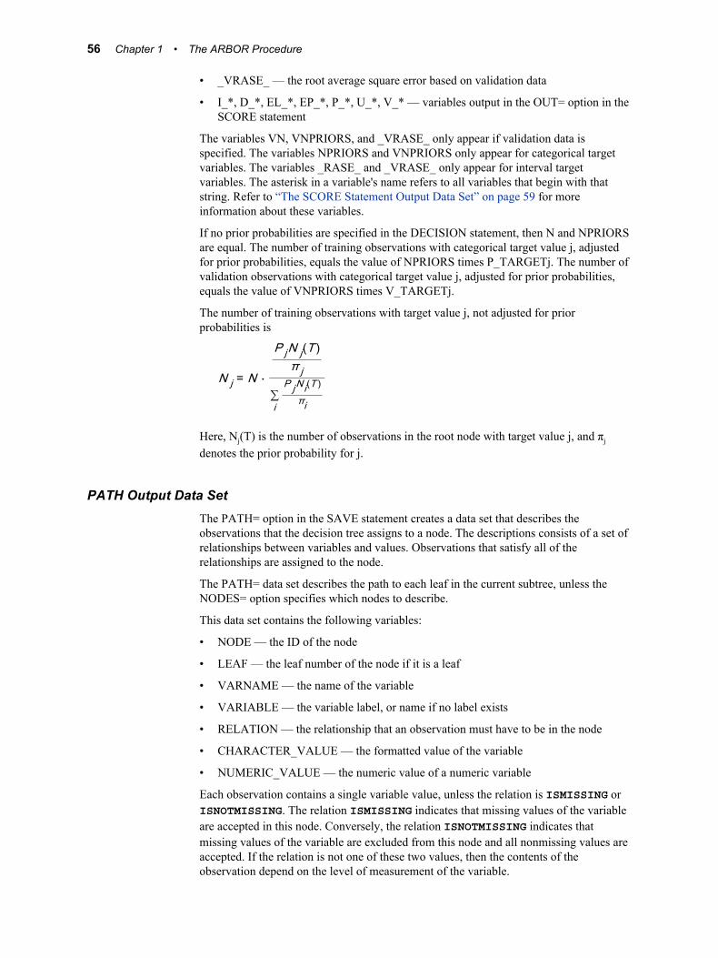
• _VRASE_ — the root average square error based on validation data
• I_*, D_*, EL_*, EP_*, P_*, U_*, V_* — variables output in the OUT= option in the SCORE statement
The variables VN, VNPRIORS, and _VRASE_ only appear if validation data is specified. The variables NPRIORS and VNPRIORS only appear for categorical target variables. The variables _RASE_ and _VRASE_ only appear for interval target variables. The asterisk in a variable's name refers to all variables that begin with that string. Refer to “The SCORE Statement Output Data Set” on page 59 for more information about these variables.
If no prior probabilities are specified in the DECISION statement, then N and NPRIORS are equal. The number of training observations with categorical target value j, adjusted for prior probabilities, equals the value of NPRIORS times P_TARGETj. The number of validation observations with categorical target value j, adjusted for prior probabilities, equals the value of VNPRIORS times V_TARGETj.
The number of training observations with target value j, not adjusted for prior probabilities is
N j = N ⋅
P jN j(T )π j
∑i
P jNi(T )πi
Here, Nj(T) is the number of observations in the root node with target value j, and πj
denotes the prior probability for j.
PATH Output Data SetThe PATH= option in the SAVE statement creates a data set that describes the observations that the decision tree assigns to a node. The descriptions consists of a set of relationships between variables and values. Observations that satisfy all of the relationships are assigned to the node.
The PATH= data set describes the path to each leaf in the current subtree, unless the NODES= option specifies which nodes to describe.
This data set contains the following variables:
• NODE — the ID of the node
• LEAF — the leaf number of the node if it is a leaf
• VARNAME — the name of the variable
• VARIABLE — the variable label, or name if no label exists
• RELATION — the relationship that an observation must have to be in the node
• CHARACTER_VALUE — the formatted value of the variable
• NUMERIC_VALUE — the numeric value of a numeric variable
Each observation contains a single variable value, unless the relation is ISMISSING or ISNOTMISSING. The relation ISMISSING indicates that missing values of the variable are accepted in this node. Conversely, the relation ISNOTMISSING indicates that missing values of the variable are excluded from this node and all nonmissing values are accepted. If the relation is not one of these two values, then the contents of the observation depend on the level of measurement of the variable.
56 Chapter 1 • The ARBOR Procedure
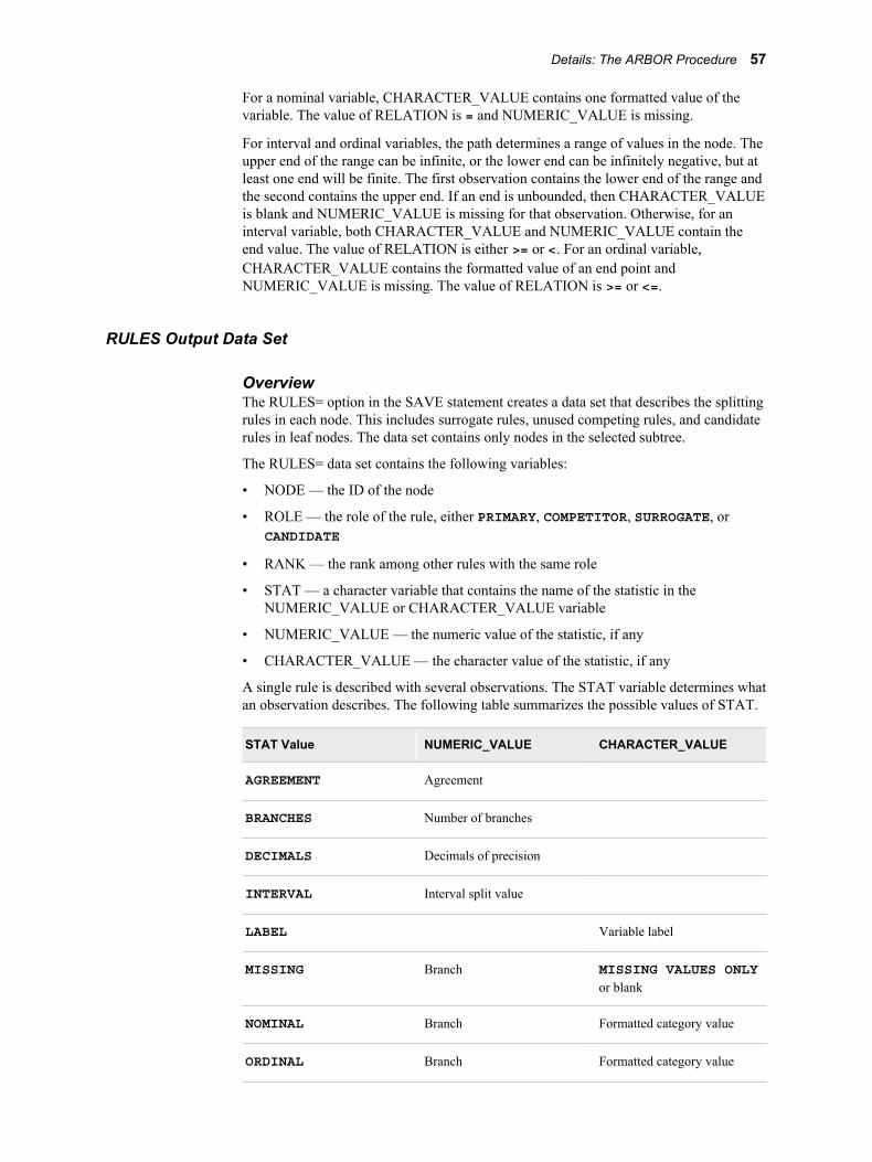
For a nominal variable, CHARACTER_VALUE contains one formatted value of the variable. The value of RELATION is = and NUMERIC_VALUE is missing.
For interval and ordinal variables, the path determines a range of values in the node. The upper end of the range can be infinite, or the lower end can be infinitely negative, but at least one end will be finite. The first observation contains the lower end of the range and the second contains the upper end. If an end is unbounded, then CHARACTER_VALUE is blank and NUMERIC_VALUE is missing for that observation. Otherwise, for an interval variable, both CHARACTER_VALUE and NUMERIC_VALUE contain the end value. The value of RELATION is either >= or <. For an ordinal variable, CHARACTER_VALUE contains the formatted value of an end point and NUMERIC_VALUE is missing. The value of RELATION is >= or <=.
RULES Output Data Set
OverviewThe RULES= option in the SAVE statement creates a data set that describes the splitting rules in each node. This includes surrogate rules, unused competing rules, and candidate rules in leaf nodes. The data set contains only nodes in the selected subtree.
The RULES= data set contains the following variables:
• NODE — the ID of the node
• ROLE — the role of the rule, either PRIMARY, COMPETITOR, SURROGATE, or CANDIDATE
• RANK — the rank among other rules with the same role
• STAT — a character variable that contains the name of the statistic in the NUMERIC_VALUE or CHARACTER_VALUE variable
• NUMERIC_VALUE — the numeric value of the statistic, if any
• CHARACTER_VALUE — the character value of the statistic, if any
A single rule is described with several observations. The STAT variable determines what an observation describes. The following table summarizes the possible values of STAT.
STAT Value NUMERIC_VALUE CHARACTER_VALUE
AGREEMENT Agreement
BRANCHES Number of branches
DECIMALS Decimals of precision
INTERVAL Interval split value
LABEL Variable label
MISSING Branch MISSING VALUES ONLY or blank
NOMINAL Branch Formatted category value
ORDINAL Branch Formatted category value
Details: The ARBOR Procedure 57
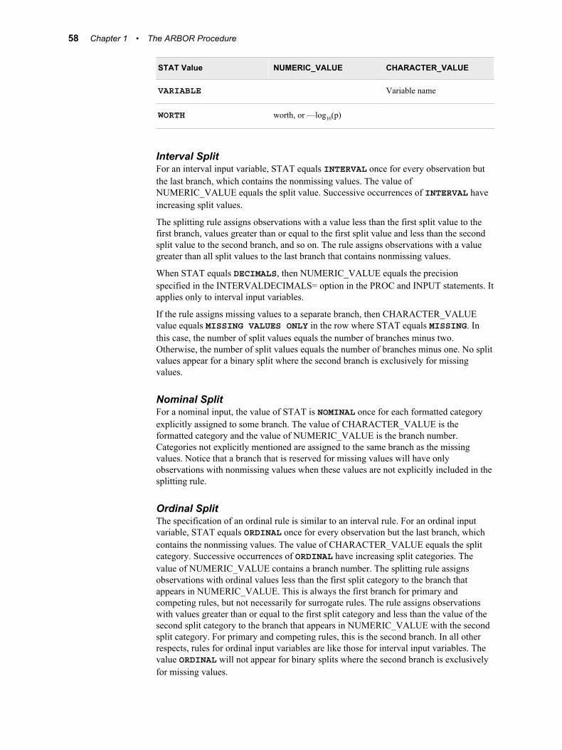
STAT Value NUMERIC_VALUE CHARACTER_VALUE
VARIABLE Variable name
WORTH worth, or —log10(p)
Interval SplitFor an interval input variable, STAT equals INTERVAL once for every observation but the last branch, which contains the nonmissing values. The value of NUMERIC_VALUE equals the split value. Successive occurrences of INTERVAL have increasing split values.
The splitting rule assigns observations with a value less than the first split value to the first branch, values greater than or equal to the first split value and less than the second split value to the second branch, and so on. The rule assigns observations with a value greater than all split values to the last branch that contains nonmissing values.
When STAT equals DECIMALS, then NUMERIC_VALUE equals the precision specified in the INTERVALDECIMALS= option in the PROC and INPUT statements. It applies only to interval input variables.
If the rule assigns missing values to a separate branch, then CHARACTER_VALUE value equals MISSING VALUES ONLY in the row where STAT equals MISSING. In this case, the number of split values equals the number of branches minus two. Otherwise, the number of split values equals the number of branches minus one. No split values appear for a binary split where the second branch is exclusively for missing values.
Nominal SplitFor a nominal input, the value of STAT is NOMINAL once for each formatted category explicitly assigned to some branch. The value of CHARACTER_VALUE is the formatted category and the value of NUMERIC_VALUE is the branch number. Categories not explicitly mentioned are assigned to the same branch as the missing values. Notice that a branch that is reserved for missing values will have only observations with nonmissing values when these values are not explicitly included in the splitting rule.
Ordinal SplitThe specification of an ordinal rule is similar to an interval rule. For an ordinal input variable, STAT equals ORDINAL once for every observation but the last branch, which contains the nonmissing values. The value of CHARACTER_VALUE equals the split category. Successive occurrences of ORDINAL have increasing split categories. The value of NUMERIC_VALUE contains a branch number. The splitting rule assigns observations with ordinal values less than the first split category to the branch that appears in NUMERIC_VALUE. This is always the first branch for primary and competing rules, but not necessarily for surrogate rules. The rule assigns observations with values greater than or equal to the first split category and less than the value of the second split category to the branch that appears in NUMERIC_VALUE with the second split category. For primary and competing rules, this is the second branch. In all other respects, rules for ordinal input variables are like those for interval input variables. The value ORDINAL will not appear for binary splits where the second branch is exclusively for missing values.
58 Chapter 1 • The ARBOR Procedure
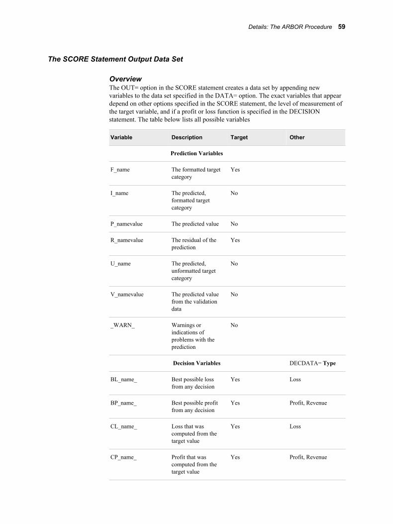
The SCORE Statement Output Data Set
OverviewThe OUT= option in the SCORE statement creates a data set by appending new variables to the data set specified in the DATA= option. The exact variables that appear depend on other options specified in the SCORE statement, the level of measurement of the target variable, and if a profit or loss function is specified in the DECISION statement. The table below lists all possible variables
Variable Description Target Other
Prediction Variables
F_name The formatted target category
Yes
I_name The predicted, formatted target category
No
P_namevalue The predicted value No
R_namevalue The residual of the prediction
Yes
U_name The predicted, unformatted target category
No
V_namevalue The predicted value from the validation data
No
_WARN_ Warnings or indications of problems with the prediction
No
Decision Variables DECDATA= Type
BL_name_ Best possible loss from any decision
Yes Loss
BP_name_ Best possible profit from any decision
Yes Profit, Revenue
CL_name_ Loss that was computed from the target value
Yes Loss
CP_name_ Profit that was computed from the target value
Yes Profit, Revenue
Details: The ARBOR Procedure 59
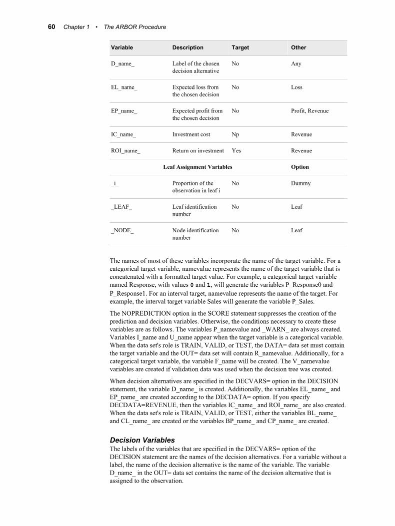
Variable Description Target Other
D_name_ Label of the chosen decision alternative
No Any
EL_name_ Expected loss from the chosen decision
No Loss
EP_name_ Expected profit from the chosen decision
No Profit, Revenue
IC_name_ Investment cost Np Revenue
ROI_name_ Return on investment Yes Revenue
Leaf Assignment Variables Option
_i_ Proportion of the observation in leaf i
No Dummy
_LEAF_ Leaf identification number
No Leaf
_NODE_ Node identification number
No Leaf
The names of most of these variables incorporate the name of the target variable. For a categorical target variable, namevalue represents the name of the target variable that is concatenated with a formatted target value. For example, a categorical target variable named Response, with values 0 and 1, will generate the variables P_Response0 and P_Response1. For an interval target, namevalue represents the name of the target. For example, the interval target variable Sales will generate the variable P_Sales.
The NOPREDICTION option in the SCORE statement suppresses the creation of the prediction and decision variables. Otherwise, the conditions necessary to create these variables are as follows. The variables P_namevalue and _WARN_ are always created. Variables I_name and U_name appear when the target variable is a categorical variable. When the data set's role is TRAIN, VALID, or TEST, the DATA= data set must contain the target variable and the OUT= data set will contain R_namevalue. Additionally, for a categorical target variable, the variable F_name will be created. The V_namevalue variables are created if validation data was used when the decision tree was created.
When decision alternatives are specified in the DECVARS= option in the DECISION statement, the variable D_name_ is created. Additionally, the variables EL_name_ and EP_name_ are created according to the DECDATA= option. If you specify DECDATA=REVENUE, then the variables IC_name_ and ROI_name_ are also created. When the data set's role is TRAIN, VALID, or TEST, either the variables BL_name_and CL_name_ are created or the variables BP_name_ and CP_name_ are created.
Decision VariablesThe labels of the variables that are specified in the DECVARS= option of the DECISION statement are the names of the decision alternatives. For a variable without a label, the name of the decision alternative is the name of the variable. The variable D_name_ in the OUT= data set contains the name of the decision alternative that is assigned to the observation.
60 Chapter 1 • The ARBOR Procedure
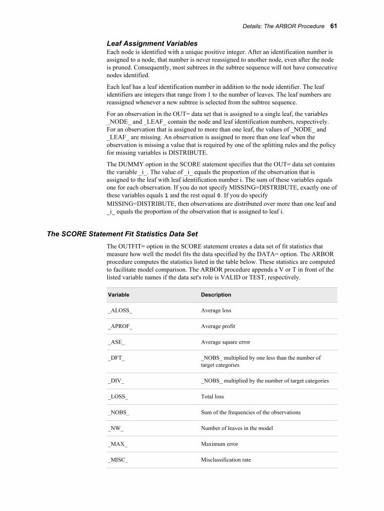
Leaf Assignment VariablesEach node is identified with a unique positive integer. After an identification number is assigned to a node, that number is never reassigned to another node, even after the node is pruned. Consequently, most subtrees in the subtree sequence will not have consecutive nodes identified.
Each leaf has a leaf identification number in addition to the node identifier. The leaf identifiers are integers that range from 1 to the number of leaves. The leaf numbers are reassigned whenever a new subtree is selected from the subtree sequence.
For an observation in the OUT= data set that is assigned to a single leaf, the variables _NODE_ and _LEAF_ contain the node and leaf identification numbers, respectively. For an observation that is assigned to more than one leaf, the values of _NODE_ and _LEAF_ are missing. An observation is assigned to more than one leaf when the observation is missing a value that is required by one of the splitting rules and the policy for missing variables is DISTRIBUTE.
The DUMMY option in the SCORE statement specifies that the OUT= data set contains the variable _i_. The value of _i_ equals the proportion of the observation that is assigned to the leaf with leaf identification number i. The sum of these variables equals one for each observation. If you do not specify MISSING=DISTRIBUTE, exactly one of these variables equals 1 and the rest equal 0. If you do specify MISSING=DISTRIBUTE, then observations are distributed over more than one leaf and _i_ equals the proportion of the observation that is assigned to leaf i.
The SCORE Statement Fit Statistics Data SetThe OUTFIT= option in the SCORE statement creates a data set of fit statistics that measure how well the model fits the data specified by the DATA= option. The ARBOR procedure computes the statistics listed in the table below. These statistics are computed to facilitate model comparison. The ARBOR procedure appends a V or T in front of the listed variable names if the data set's role is VALID or TEST, respectively.
Variable Description
_ALOSS_ Average loss
_APROF_ Average profit
_ASE_ Average square error
_DFT_ _NOBS_ multiplied by one less than the number of target categories
_DIV_ _NOBS_ multiplied by the number of target categories
_LOSS_ Total loss
_NOBS_ Sum of the frequencies of the observations
_NW_ Number of leaves in the model
_MAX_ Maximum error
_MISC_ Misclassification rate
Details: The ARBOR Procedure 61
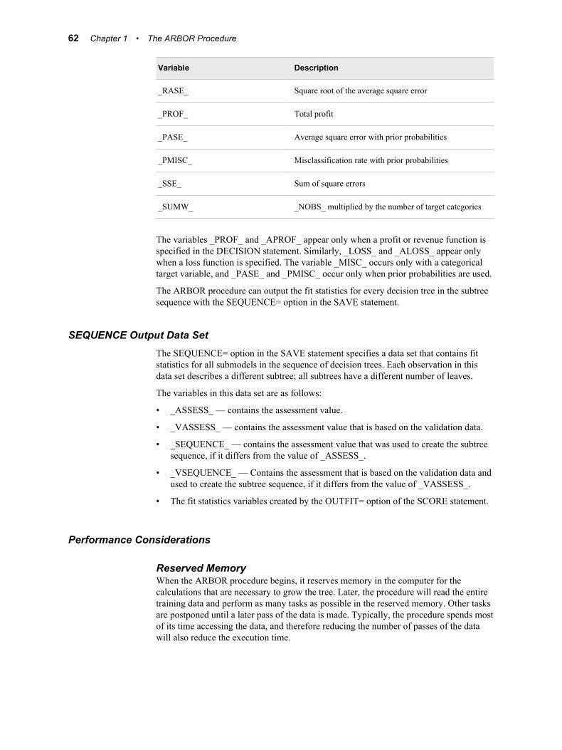
Variable Description
_RASE_ Square root of the average square error
_PROF_ Total profit
_PASE_ Average square error with prior probabilities
_PMISC_ Misclassification rate with prior probabilities
_SSE_ Sum of square errors
_SUMW_ _NOBS_ multiplied by the number of target categories
The variables _PROF_ and _APROF_ appear only when a profit or revenue function is specified in the DECISION statement. Similarly, _LOSS_ and _ALOSS_ appear only when a loss function is specified. The variable _MISC_ occurs only with a categorical target variable, and _PASE_ and _PMISC_ occur only when prior probabilities are used.
The ARBOR procedure can output the fit statistics for every decision tree in the subtree sequence with the SEQUENCE= option in the SAVE statement.
SEQUENCE Output Data SetThe SEQUENCE= option in the SAVE statement specifies a data set that contains fit statistics for all submodels in the sequence of decision trees. Each observation in this data set describes a different subtree; all subtrees have a different number of leaves.
The variables in this data set are as follows:
• _ASSESS_ — contains the assessment value.
• _VASSESS_ — contains the assessment value that is based on the validation data.
• _SEQUENCE_ — contains the assessment value that was used to create the subtree sequence, if it differs from the value of _ASSESS_.
• _VSEQUENCE_ — Contains the assessment that is based on the validation data and used to create the subtree sequence, if it differs from the value of _VASSESS_.
• The fit statistics variables created by the OUTFIT= option of the SCORE statement.
Performance Considerations
Reserved MemoryWhen the ARBOR procedure begins, it reserves memory in the computer for the calculations that are necessary to grow the tree. Later, the procedure will read the entire training data and perform as many tasks as possible in the reserved memory. Other tasks are postponed until a later pass of the data is made. Typically, the procedure spends most of its time accessing the data, and therefore reducing the number of passes of the data will also reduce the execution time.
62 Chapter 1 • The ARBOR Procedure
Passes of the DataEach of the following tasks for a node requires a pass of the entire training data:
• Compute the node statistics
• Search for a split on an input variable
• Determine a rule for missing values for a specified split
• Search for a surrogate rule on an input variable
If only one task were done per pass of the data, the number of passes would equal approximately the number of nodes times the number of input variables. Surrogate splits would require more passes. The number of additional passes equals the number of inputs minus one. The actual number is typically less for three reasons. First, if no split on an input variable is found in a node, then no search is attempted on that variable in any descendant node. See the description of the MAXRULES= option in the “TRAIN Statement” on page 29 for some situations where no split exists on an input variable. Second, the ARBOR procedure does not search for any splits in nodes at the depths specified in the MAXDEPTH= option of the TRAIN statement. Third, given sufficient memory, the procedure can perform several tasks during the same pass of the data.
The ARBOR procedure computes node statistics before it begins a split search in that node. Consequently, to create a node and find a split requires at least two passes of the data. The procedure will search for a split in a node on every input variable in one pass of the data if enough memory is available. The search for surrogate rules begins after the primary rules are established. Thus, to create a node, find a split, and find a surrogate split require at least three passes of the data. A separate search for a rule to handle missing values is necessary only for splits that do not define a rule to handle missing values. If the rule for missing values is present in the SPLIT statement, then no pass is needed for a split search in the node for any input variable.
The number of bytes needed for each search task approximately equals the within-node sample size specified in the NODESIZE= option of the PERFORMANCE statement, multiplied by 3, multiply by the number of bytes in a double word (typically 8).
Memory ConsiderationsReserving more memory can reduce the number of data passes, but cannot reduce the execution time if a large proportion of the memory is virtual memory that is swapped to the disk. A computer operating system allocates more memory to the running software programs than is physically available. When the operating system detects that no program is using an allocated section the physical memory, the system copies the contents of that section to the disk. The newly freed memory is assigned to another program or task. The common name for this action is swapping-out. When the program that created the original data (now on the disk) tries to access it, the operating system swaps out a different section of memory with the original data. Thus, the programs appear to have more memory available than physically exists. The apparent amount of memory is called virtual memory.
By default, the ARBOR procedure estimates the amount of memory that it will need to construct the decision tree, asks the operating system how much physical memory is available, and then allocates enough to memory to perform its tasks or reserves all of the memory, whichever is smaller. The estimate of the amount of memory assumes that all split searches in a node are done in the same pass. The MEMSIZE= option in the PERFORMANCE statement overrides the default process. The SAS MEMSIZE= option sets limits on the amount of physical memory that is available to the tasks.
Details: The ARBOR Procedure 63
Examples
Example 1: Basic UsageThis example introduces the ARBOR procedure with a minimum number of statements and options. The ARBOR procedure creates a sequence of increasingly complicated subtrees that are designed to overfit the input data. First, create a sequence of subtrees with the SASHELP.SHOES data set.
proc arbor data=sashelp.shoes; target sales; input region subsidiary product stores; save summary=sum1 sequence=seq1 model=tree1 rules=rule1 path=path1; assess cv;quit;
The SHOES data set contains sales information about various brands of shoes in different stores and regions. This call to the ARBOR statement creates a sequence of subtrees to predict what factors influence total sales.
The SAVE statement specifies five separate output data sets. The data set sum1 includes summary statistics for the best subtree, as chosen by the ARBOR procedure. The Log notes that this was the subtree with 31 nodes and 16 leaves. The data set seq1 contains several statistics for all 16 subtrees in the sequence. Notice that the subtree with 16 leaves had the smallest maximum absolute error, sum of squared error, average square error, and root average square error. The data set tree1 contains information about the sequence of subtrees so that you can reuse this information later. The data set rule1 contains a description of all the primary and competitor rules for each node. Finally, path1 details the path that was created from the observed value of NODE to LEAF.
The ASSESS statement is included to perform cross validation on the sequence of subtrees. If you read the Log, you will notice that cross validation confirmed that the subtree with 31 nodes and 16 leaves generalized the best. Thus, it was chosen as the champion subtree once again. You can specify different cross validation measures and options to affect the champion subtree.
Example 2: Selecting a SubtreeNote: This example assumes that you have completed “Example 1: Basic Usage” on
page 64 .
Suppose that you wanted to manually select a specific subtree and analyze the summary statistics for that subtree. The SUBTREE statement enables this action. In order to save time, you can use the INMODEL= option in the PROC statement, which imports the computed subtrees from Example 1.
proc arbor inmodel=tree1; subtree nleaves=5; save summary=sum2 nodestats=nodes2 rules=rule2;quit;
64 Chapter 1 • The ARBOR Procedure
This code selects the subtree with 5 leaves and saves certain information about this decision tree.
The data set sum2 contains summary statistics for this decision tree. Notice that the r-squared value for this decision is tree 0.501..., which is less than the 0.571... indicated for the subtree with 16 leaves. This indicates that the larger subtree is a better fit.
The data set nodes2 contains information about the nodes in the selected subtree. Additionally, rule2 indicates the primary and competitor rules for each node in the selected subtree.
Example 3: Changing a Splitting RuleNote: This example assumes that you have completed “Example 1: Basic Usage” on
page 64 .
In this example, you will alter the definition of one of the rules that was created in Example 1. The rule change will assign both men's dress shoes and men's casual shoes to the same node. In Example 1, only men's casual shoes were assigned to node 7. However, the code below changes this assignment.
proc arbor data=sashelp.shoes inmodel=tree1; interact pruned; prune node=7; split node=7 var=product / "Men's Casual" "Men's Dress", "Women's Casual" "Women's Dress"; save summary=sum3 node=7 rules=rule3;quit;
First, this code prunes node 7 from the decision tree and then replaces it with a new node with a slightly different splitting rule. Here, node 7 is split into two branches. The first contains casual and dress shoes for men and the second contains casual and dress shoes for women.
The data set sum3 includes summary statistics about the new decision tree that was created when node 7 was altered. You can compare these statistics to sum1 and sum2 to determine which decision tree is a better fit to the data. However, rule3 includes information about the primary and competitor rules for only node 7, not the entire decision tree. This data set highlights the changes to this node when compared to the relevant observations in rule1 and rule2.
Examples 65

66 Chapter 1 • The ARBOR Procedure
Chapter 2
The ASSOC Procedure
Overview . . . . . . . . . . . . . . . . . . . . . . . . . . . . . . . . . . . . . . . . . . . . . . . . . . . . . . . . . . . . 67The ASSOC Procedure . . . . . . . . . . . . . . . . . . . . . . . . . . . . . . . . . . . . . . . . . . . . . . . 67
Syntax . . . . . . . . . . . . . . . . . . . . . . . . . . . . . . . . . . . . . . . . . . . . . . . . . . . . . . . . . . . . . . . 68The ASSOC Procedure . . . . . . . . . . . . . . . . . . . . . . . . . . . . . . . . . . . . . . . . . . . . . . . 68PROC ASSOC Statement . . . . . . . . . . . . . . . . . . . . . . . . . . . . . . . . . . . . . . . . . . . . . 68CUSTOMER Statement . . . . . . . . . . . . . . . . . . . . . . . . . . . . . . . . . . . . . . . . . . . . . . 69TARGET Statement . . . . . . . . . . . . . . . . . . . . . . . . . . . . . . . . . . . . . . . . . . . . . . . . . 69
Details . . . . . . . . . . . . . . . . . . . . . . . . . . . . . . . . . . . . . . . . . . . . . . . . . . . . . . . . . . . . . . . 70The ASSOC Procedure . . . . . . . . . . . . . . . . . . . . . . . . . . . . . . . . . . . . . . . . . . . . . . . 70Output Processing . . . . . . . . . . . . . . . . . . . . . . . . . . . . . . . . . . . . . . . . . . . . . . . . . . . 70
Further Reading . . . . . . . . . . . . . . . . . . . . . . . . . . . . . . . . . . . . . . . . . . . . . . . . . . . . . . 70
Overview
The ASSOC ProcedureAssociation discovery is the identification of items that occur together in a given event or record. This technique is also known as market basket analysis. Online transaction processing systems often provide the data sources for association discovery. Association rules are based on frequency counts of the number of times items occur alone and in combination in the database. The rules are expressed as “if item A is part of an event, then item B is also part of the event X percent of the time.” The rules should not be interpreted as a direct causation but as an association between two or more items. Identifying creditable associations can help the business technologist make decisions such as when to distribute coupons, when to put a product on sale, or how to lay out items in a store.
Hypothetical association discovery rules include:
• If a customer buys shoes, then 10% of the time he or she also buys socks.
• A grocery chain might find that 80% of all shoppers are apt to buy a jar of salsa when they also purchase a bag of tortilla chips.
• When “do-it-yourselfers” buy latex paint, they also buy rollers 85% of the time.
• Forty percent of investors holding an equity index fund will have a growth fund in their portfolio.
67
An association rule has a left side (antecedent) and a right side (consequent). Both sides of the rule can contain more than one item. The confidence factor, level of support, and lift are three important evaluation criteria of association discovery. The strength of an association is defined by its confidence factor, which is the percentage of cases in which a consequent appears with a given antecedent. The level of support is how frequently the combination occurs in the market basket (database). Lift is equal to the confidence factor divided by the expected confidence. A credible rule has a large relative confidence factor, a relatively large level of support, and a value of lift greater than 1. Rules with a high level of confidence but little support should be interpreted with caution.
The maximum number of items in an association determines the maximum size of the item set to be considered. For example, the default of four items indicates that up to 4-way associations are performed.
This procedure is required before you can run either the RULEGEN or the SEQUENCE procedure.
Syntax
The ASSOC ProcedurePROC ASSOC DATA=data-set-name <options>;
CUSTOMER list-of-variables;TARGET variable;
PROC ASSOC Statement
SyntaxPROC ASSOC DATA=data-set-name <options>;
Required ArgumentsDATA=data-set-name
This argument identifies the input data set. To perform association discovery, the input data set must have a separate observation for each product that was purchased by each customer. You must also assign the model role ID to a variable and the model role TARGET to another variable. This data set can be the output from the DMDB procedure, but if it is, then you must specify the option DMDB.
DMDBCAT=catalog-nameThis option specified the metadata catalog for the input data source. For more information about this database, see the documentation on the DMDB procedure.
OUT=data-set-nameThis argument specified the output data set, which contains the variables SET_SIZE, COUNT, ITEM1, ITEM2, ..., ITEMn. Here, n is the maximum number of items in the association rule. A brief description of each variable is given below, but a more detailed description is given in “Output Processing” on page 70 .
68 Chapter 2 • The ASSOC Procedure
Optional ArgumentsDMDB
You must specify this option if your input data set is the output data set from the DMDB procedure.
ITEMS=numberThis option specifies the maximum number of events or transactions to associate together. The value of number must be a positive integer.
PCTSUP=numberThis option specifies the minimum level of support that is needed to claim that the items are associated. The support percentage figure that you specify refers to the proportion of the largest single item frequency, and not the end support. The value of number must be a real number between 0 and 100.
SUPPORT=numberThis option specifies the minimum number of transactions that must occur in order to accept a rule. Rules that do not meet this support level are rejected. The level of support represents how frequently the combination occurs in the input data set. The value of number must be a positive integer and defaults to 5% of the greatest item frequency count.
For example, if the most popular item in a data set was purchased 600 times, then 5% of 600 is 30. This means that only rules with at least 30 customers will be considered by the ASSOC procedure.
CUSTOMER Statement
SyntaxCUSTOMER list-of-variables;
Required Argumentlist-of-variables
The CUSTOMER statement specifies one or more variables that identify the customers that are analyzed.
TARGET Statement
SyntaxTARGET variable;
Required Argumentvariable
The TARGET statement identifies a nominal variable that contains the purchased items and is usually ordered by customers.
Note: By default, this variable is normalized, left-justified, truncated to NORMLEN= characters, and converted to uppercase. For example, the items “Blue Socks,” “blue socks,” and “blue SOCKS” are all mapped to the normalized item “BLUE SOCKS.”
Syntax 69
Details
The ASSOC ProcedureThe input to the ASSOC procedure must have a variable with the role of ID and another with the role of TARGET. All records with the same ID values form a transaction. Every transaction has a unique ID value and one or more TARGET values.
You can have more than one ID variable. However, associations analysis can be performed on only one target variable at a time. When there are multiple ID variables, the ASSOC procedure concatenates them into a single identifier value during computation.
For numeric target variables, missing values constitute a separate item or target level and show up in the rules as a period. For character target variables, completely blank values constitute a separate target level and show up in the rules as a period. All records with missing ID values are considered a single valid transaction.
Output ProcessingThe ASSOC procedure makes a pass through the data and obtains transaction counts for each item. It outputs these counts with a value of 1 for the variable SET_SIZE and the items are listed under ITEM1. Items that do not meet the support level are discarded. By default, the support level is set to 5% of the largest item count.
The ASSOC procedure then generates all potential 2–item sets, makes a pass through the data, and obtains transaction counts for each of the 2–item sets. The sets that meet the support level are output with SET_SIZE value of 2 and items listed under ITEM1 and ITEM2.
The entire process is repeated for up to n-item sets. The output from the ASSOC procedure is saved in multiple SAS data sets. The data sets enable you to define your own evaluation criteria and/or reports.
Note that the order of the items within an n-item set is not important. Any individual transaction, where each of the n items occurs in any order, qualifies for that particular set. The support level, once set, remains constant throughout the process.
The theoretical potential number of item sets can grow very quickly. For example, with 50 different items, you have 1225 potential 2–item sets and 19,600 3–item sets. With 5,000 items, you have over 12 million of the 2–item sets. You may run out of memory if you attempt to process that many association sets. However, you can reduce the item sets to a more manageable number when you specify a higher level of support.
Further ReadingIf you are interested in more information about the ASSOC procedure, consider the following resources:
• R. Agrawal, T. Imielinki, and A. Swami. 1993. “Mining Association Rules between Sets of Items in Large Databases.” Proceedings, ACM SIGMOID Conference on Management of Data, 207–216. Washington, D.C.
70 Chapter 2 • The ASSOC Procedure

• M.J.A Berry and G. Linoff, Data Mining Techniques for Marketing, Sales, and Customer Support. (New York, NY: John Wiley and Sons, Inc., 1997)
Further Reading 71

72 Chapter 2 • The ASSOC Procedure
Chapter 3
The DECIDE Procedure
Overview . . . . . . . . . . . . . . . . . . . . . . . . . . . . . . . . . . . . . . . . . . . . . . . . . . . . . . . . . . . . 73The DECIDE Procedure . . . . . . . . . . . . . . . . . . . . . . . . . . . . . . . . . . . . . . . . . . . . . . 73
Syntax . . . . . . . . . . . . . . . . . . . . . . . . . . . . . . . . . . . . . . . . . . . . . . . . . . . . . . . . . . . . . . . 74The DECIDE Procedure . . . . . . . . . . . . . . . . . . . . . . . . . . . . . . . . . . . . . . . . . . . . . . 74PROC DECIDE Statement . . . . . . . . . . . . . . . . . . . . . . . . . . . . . . . . . . . . . . . . . . . . 74CODE Statement . . . . . . . . . . . . . . . . . . . . . . . . . . . . . . . . . . . . . . . . . . . . . . . . . . . 75DECISION Statement . . . . . . . . . . . . . . . . . . . . . . . . . . . . . . . . . . . . . . . . . . . . . . . . 76FREQ Statement . . . . . . . . . . . . . . . . . . . . . . . . . . . . . . . . . . . . . . . . . . . . . . . . . . . . 77POSTERIORS Statement . . . . . . . . . . . . . . . . . . . . . . . . . . . . . . . . . . . . . . . . . . . . . 78PREDICTED Statement . . . . . . . . . . . . . . . . . . . . . . . . . . . . . . . . . . . . . . . . . . . . . . 78TARGET Statement . . . . . . . . . . . . . . . . . . . . . . . . . . . . . . . . . . . . . . . . . . . . . . . . . 78
Examples . . . . . . . . . . . . . . . . . . . . . . . . . . . . . . . . . . . . . . . . . . . . . . . . . . . . . . . . . . . . 79Example 1: Preprocessing the Data and Basic Usage . . . . . . . . . . . . . . . . . . . . . . . 79
Further Reading . . . . . . . . . . . . . . . . . . . . . . . . . . . . . . . . . . . . . . . . . . . . . . . . . . . . . . 81
Overview
The DECIDE ProcedureThe DECIDE procedure creates optimal decisions based on a user-supplied decision matrix, prior probabilities, and output from a modeling procedure. This output can be either posterior probabilities for a categorical target variable or predicted values for an interval target variable. The DECIDE procedure can also adjust the posterior probabilities for changes in the prior probabilities.
The decision matrix contains columns (decision variables) and rows (observations). Columns correspond to each decision. Rows correspond to target values. The values of the decision variables represent target-specific consequences such as profit, loss, or revenue. These consequences are the same for all cases that are scored.
A categorical target variable should have one row for each category. Each entry dij in the decision matrix indicates the consequence of selecting target value i for variable j.
For an interval target variable, each row defines a knot in a piecewise linear spline function. The consequence of making a decision is an interpolation in the corresponding column of the decision matrix. If the predicted target value is outside of the range of knots in the decision matrix, then the consequence is computed by linear extrapolation.
73
For each decision, there can be either a cost variable or a numeric constant. The values of this variable represent case-specific consequences, which are always costs. These consequences do not depend on the target values of the cases that are scored. The costs
are used to compute the return on investment as revenue − cost
cost .
Cost variables can be specified only if the decision data set contains revenue variables, but not profit or loss variables. If revenues and costs are specified, then profits are computed as revenue minus costs. If revenues are specified without costs, then the costs are assumed to be zero. The interpretation of consequences as profits, losses, revenues, and costs is needed only to compute the return on investment. You can specify values in the decision data set that are target-specific consequences but that can have some practical interpretation other than costs. If the revenue or cost interpretation is not applicable, the values that were computed for return on investment might not be meaningful.
The DECIDE procedure will choose the optimal decision for each observation. If the decision data set is of type PROFIT or REVENUE, the decision that produces the maximum expected or estimated profit is chosen. If the decision data is of type LOSS, then the decision that produces the minimum expected or estimated loss is chosen.
If the actual value of the target variable is known, then the DECIDE procedure will calculate the following:
• the consequence of the chosen decision for the actual target value for each case
• the best possible consequence for each case
• summary statistics that give the total and average profit or loss
Some modeling procedures assume that the prior probabilities for categorical variable levels are either all equal or proportional to the relative frequency of the corresponding response level in the data set. The DECIDE procedure enables you to specify other prior probabilities. Thus, you can conduct a sensitivity analysis without rerunning the modeling procedure.
Syntax
The DECIDE ProcedurePROC DECIDE DATA=data-set-name <options>;
CODE <options>;DECISION DECDATA=data-set-name <options>;FREQ variable;POSTERIORS list-of-variables;PREDICTED variable;TARGET variable;RUN;
PROC DECIDE Statement
SyntaxPROC DECIDE DATA=data-set-name <options>;
74 Chapter 3 • The DECIDE Procedure
Required ArgumentDATA=data-set-name
This argument specifies the input data set, which is the output from a modeling procedure.
Note: Strictly speaking, this argument is not required. If you omit this argument, then the DECIDE procedure will use the most recently created data set.
Optional ArgumentsOUT=data-set-nameThis option specifies the output data set, which contains the following information:
• the variables from the input data set
• the chosen decision with a prefix of “D_”
• the expected consequence of the chosen decision with a prefix of either “EL_” or “EP_”
If the target value is in the input data set, then the output data set also contains the following variables:
• the consequence of the chosen decision computed from the target value with a prefix of either “CL_” or “CP_”
• the consequence of the best possible decision knowing the target value with a prefix of either “BL_” or “BP_”
Moreover, if the PRIORVAR= and OLDPRIORVAR= variables are specified, then this data set will contain the recalculated posterior probabilities. The default name for this data set is data_n, where n is the smallest integer not already used to name a data set.
OUTFIT=data-set-nameThis option specifies an output data set that contains fit statistics. These statistics include the total and average profit or loss. You cannot specify this option with a data set of type SCORE. By default, this data set is not created.
ROLE=TRAIN | VALID | VALIDATION | TEST | SCOREThis option specifies the role of the data set. This option affects the variables that are created in the OUTFIT= data set. The default value is TEST.
CODE Statement
SyntaxCODE <options>;
This statement generates SAS DATA step code that is used to score data sets. If neither FILE= nor METABASE= are specified, then the SAS code is written to the SAS log. You can specify both of these options to write the code to both locations.
Optional ArgumentsFILE=filename
This option specifies a path to an external file that will contain the SAS score code. For example, you can specify FILE='C:\mydir\scorecode.sas'.
Syntax 75
FORMAT=formatThis option specifies the format that is used to print numeric constants. The default value is BEST12.
GROUP=group-nameThis option specifies a group identifier (up to 16 bytes) for group processing.
METABASE=catalog-specThis option specifies a catalog entry that will contain the SAS score code. For example, you can specify METABASE=myLibrary.myCatalog.catalog-entry.
RESIDUALSpecify this option to compute the variables that depend on the target variable in the score code.
DECISION Statement
SyntaxDECISION DECDATA=data-set-name <options>;
Required ArgumentDECDATA=data-set-name
This argument specifies the input data set that contains the decision matrix, the prior probabilities, or both. This data set might contain decision variables that are specified with the DECVARS= option. Also, it might contain prior probability variables that are specified with the PRIORVAR= option, the OLDPRIORVAR= option, or both.
This data set must contain the target variable, which is specified in the TARGET statement.
For a categorical target variable, there should be one observation for each class. Each entry dij in the decision matrix indicates the consequence of selecting target value i for variable j. If any class appears twice or more in this data set, an error message is printed and the procedure terminates. Any class value in the input data set that is not found in this data set is treated as a missing class value. Note that the classes in this data set must correspond exactly with the variables in the POSTERIORS statement.
For an interval target variable, each row defines a knot in a piecewise linear spline function. The consequence of making a decision is computed by interpolating in the corresponding column of the decision matrix. If the predicted target value is outside the range of knots in the decision matrix, the consequence is computed by linear extrapolation. If the target values are monotonically increasing or decreasing, any interior target value is allowed to appear twice in the data set. This enables you to specify discontinuities in the data. The end points, which are the minimum and maximum data points, cannot appear more than once. No target value is allowed to appear more than twice. If the target values are not monotonic, then they are sorted by the procedure and are not allowed to appear more than once.
T I P The DECDATA= data set can be of type LOSS, PROFIT, or REVENUE. PROFIT is assumed by default. TYPE is a data set option that is specified in parentheses after the data set name when the data set is created or used.
76 Chapter 3 • The DECIDE Procedure
Optional ArgumentsDECVARS=list-of-variables
This option specifies the numeric decision variables in the DECDATA= data set that contain the target-specific consequences for each decision. The decision variables cannot contain any missing values.
COST=list-of-costsThis option specifies one of the following:
• numeric constants that give the cost of a decision
• numeric variables in the input data set that contain case-specific costs
• any combination of constants and variables
There must be the same number of cost constants and variables as there are decision variables in the DECVARS= option. In this option, you cannot use abbreviated variable lists. For any case where a cost variable is missing, the results for that case are considered missing. By default, all costs are assumed to be zero. Furthermore, this option can be used only when the DECDATA= data set is of type REVENUE.
PRIORVAR=variableThis option specifies the numeric variable in the DECDATA= data set that contains the prior probabilities that are used to make decisions. Prior probabilities are also used to adjust the total and average profit or loss. Prior probabilities cannot be missing or negative, and there must be at least one positive prior probability. The prior probabilities are not required to sum one. But, if they do not sum to one, then they are scaled by some constant so that they do sum to one. If this option is not specified, then no adjustment for prior probabilities is applied to the posterior probabilities.
OLDPRIORVAR=variableThis option specifies the numeric variable in the DECDATA= data set that contains the prior probabilities that were used the first time the model was fit. If you specify this option, then you must also specify PRIORVAR=.
FREQ Statement
SyntaxFREQ variable;
Required Argumentvariable
This option specifies a single numeric variable whose value represents the frequency of each observation. If you use the FREQ statement, the DECIDE procedure treats the data set as if each observation appeared n times, where n is the value of the FREQ variable. The FREQ variable has no effect on decisions for the adjustment for prior probabilities. It only affects the summary statistics in the OUTFIT= data set. If a value of the FREQ variable is not an integer, then the fractional part is not truncated. If a value of the FREQ variable is less than or equal to zero, then the observation does not contribute to the summary statistics. However, all of the variables in the OUT= data set are processed as if the FREQ variable were positive.
Syntax 77
POSTERIORS Statement
SyntaxPOSTERIORS list-of-variables;
The POSTERIORS statement can be specified only with a categorical target variable. You cannot use both the POSTERIORS statement and the PREDICTED statement.
Required Argumentlist-of-variables
Specify the numeric variables in the input data set that contain the estimated posterior probabilities that correspond to the categories of the target variable. If one of a few certain conditions are met, then a case is set to missing and the variable _WARN_ contains the flag P.
These conditions are as follows:
• The posterior probability is missing, negative, or greater than 1.
• There is a nonzero posterior that corresponds to a zero posterior.
• There is not at least one valid positive posterior probability.
Note that the order of the variables in this list must correspond exactly to the order of the classes in the DECDATA= data set.
PREDICTED Statement
SyntaxPREDICTED variable;
The PREDICTED statement can be specified only with an interval target variable. You cannot use both the POSTERIORS statement and the PREDICTED statement.
Required Argumentvariable
This option specifies the numeric variable in the input data set that contains the predicted values of an interval target variable.
TARGET Statement
SyntaxTARGET variable;
The TARGET statement specifies the variable in the DECDATA= data set that is the target variable. The DECIDE procedure will search for a target variable with the same name in the input data set. If that variable is not found, then the DECIDE procedure assumes that the actual target values are unknown. For a categorical variable, the target variables in the DATA= and DECDATA= data sets do not need to be the same type. This is because only the formatted values are used for comparisons. For an interval target, both variables must be numeric. If scoring code is generated by the CODE
78 Chapter 3 • The DECIDE Procedure
statement, the code will format the target variable with the format and length from the DATA= data set.
This statement is required.
Required Argumentvariable
This variable must be in the DECDATA= data set and is the target variable.
Examples
Example 1: Preprocessing the Data and Basic UsageThis extended fictitious example illustrates how to adjust prior probabilities and make decisions with a revenue matrix and cost constants. This example considers a population of men who consult urologists for prostate problems. In this population, 70% of the men have benign enlargement of the prostate, 25% have an infection, and 5% have cancer. A sample of 100 men is taken and two new diagnostic measures, X and Y, are made on each patient. The training data set also includes the diagnosis made by reliable, conventional methods.
For each patient, three treatments are available. First, the urologist could prescribe antibiotics, which are effective against infection, but might have moderately bad side effects. Antibiotics have no effect on benign enlargement or cancer. Second, the urologist could recommend surgery, which is effective for all diseases, but has potentially severe side effects, such as impotence. Finally, the urologist and patient could decide against both antibiotics and surgery, thereby doing nothing.
The first step is to create the sample of 100 men. To simulate the measurements of diagnostics X and Y, this example employs the SAS random number generator. Because you specify the initial seed to the random number generator, all of your results will be identical to those presented in this example.
data Prostate; length dx $14; dx='Benign'; mx=30; sx=10; my=30; sy=10; n=70; link generate;
dx='Infection'; mx=70; sx=20; my=35; sy=15; n=25; link generate;
dx='Cancer'; mx=50; sx=10; my=50; sy=15; n=5; link generate; stop;
Examples 79
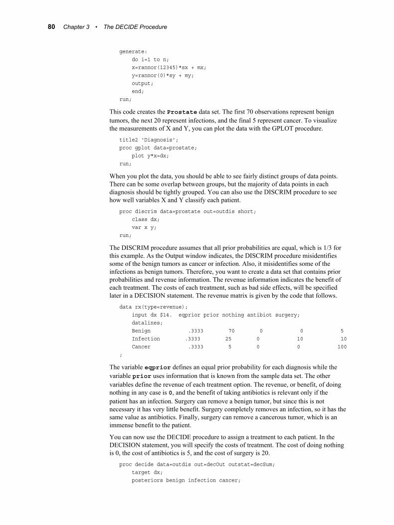
generate: do i=1 to n; x=rannor(12345)*sx + mx; y=rannor(0)*sy + my; output; end;run;
This code creates the Prostate data set. The first 70 observations represent benign tumors, the next 20 represent infections, and the final 5 represent cancer. To visualize the measurements of X and Y, you can plot the data with the GPLOT procedure.
title2 'Diagnosis';proc gplot data=prostate; plot y*x=dx;run;
When you plot the data, you should be able to see fairly distinct groups of data points. There can be some overlap between groups, but the majority of data points in each diagnosis should be tightly grouped. You can also use the DISCRIM procedure to see how well variables X and Y classify each patient.
proc discrim data=prostate out=outdis short; class dx; var x y;run;
The DISCRIM procedure assumes that all prior probabilities are equal, which is 1/3 for this example. As the Output window indicates, the DISCRIM procedure misidentifies some of the benign tumors as cancer or infection. Also, it misidentifies some of the infections as benign tumors. Therefore, you want to create a data set that contains prior probabilities and revenue information. The revenue information indicates the benefit of each treatment. The costs of each treatment, such as bad side effects, will be specified later in a DECISION statement. The revenue matrix is given by the code that follows.
data rx(type=revenue); input dx $14. eqprior prior nothing antibiot surgery; datalines; Benign .3333 70 0 0 5 Infection .3333 25 0 10 10 Cancer .3333 5 0 0 100;
The variable eqprior defines an equal prior probability for each diagnosis while the variable prior uses information that is known from the sample data set. The other variables define the revenue of each treatment option. The revenue, or benefit, of doing nothing in any case is 0, and the benefit of taking antibiotics is relevant only if the patient has an infection. Surgery can remove a benign tumor, but since this is not necessary it has very little benefit. Surgery completely removes an infection, so it has the same value as antibiotics. Finally, surgery can remove a cancerous tumor, which is an immense benefit to the patient.
You can now use the DECIDE procedure to assign a treatment to each patient. In the DECISION statement, you will specify the costs of treatment. The cost of doing nothing is 0, the cost of antibiotics is 5, and the cost of surgery is 20.
proc decide data=outdis out=decOut outstat=decSum; target dx; posteriors benign infection cancer;
80 Chapter 3 • The DECIDE Procedure
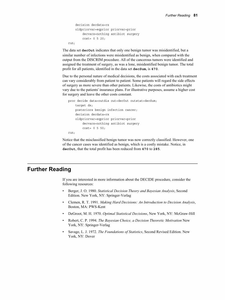
decision decdata=rx oldpriorvar=eqprior priorvar=prior decvars=nothing antibiot surgery cost= 0 5 20;run;
The data set decOut indicates that only one benign tumor was misidentified, but a similar number of infections were misidentified as benign, when compared with the output from the DISCRIM procedure. All of the cancerous tumors were identified and assigned the treatment of surgery, as was a lone, misidentified benign tumor. The total profit for all patients, identified in the data set decSum, is 470.
Due to the personal nature of medical decisions, the costs associated with each treatment can vary considerably from patient to patient. Some patients will regard the side effects of surgery as more severe than other patients. Likewise, the costs of antibiotics might vary due to the patients' insurance plans. For illustrative purposes, assume a higher cost for surgery and leave the other costs constant.
proc decide data=outdis out=decOut outstat=decSum; target dx; posteriors benign infection cancer; decision decdata=rx oldpriorvar=eqprior priorvar=prior decvars=nothing antibiot surgery cost= 0 5 50;run;
Notice that the misclassified benign tumor was now correctly classified. However, one of the cancer cases was identified as benign, which is a costly mistake. Notice, in decOut, that the total profit has been reduced from 470 to 285.
Further ReadingIf you are interested in more information about the DECIDE procedure, consider the following resources:
• Berger, J. O. 1980. Statistical Decision Theory and Bayesian Analysis, Second Edition. New York, NY: Springer-Verlag
• Clemen, R. T. 1991. Making Hard Decisions: An Introduction to Decision Analysis, Boston, MA: PWS-Kent
• DeGroot, M. H. 1970. Optimal Statistical Decisions, New York, NY: McGraw-Hill
• Robert, C. P. 1994. The Bayesian Choice, a Decision Theoretic Motivation New York, NY: Springer-Verlag
• Savage, L. J. 1972. The Foundations of Statistics, Second Revised Edition. New York, NY: Dover
Further Reading 81

82 Chapter 3 • The DECIDE Procedure
Chapter 4
The DMDB Procedure
Overview . . . . . . . . . . . . . . . . . . . . . . . . . . . . . . . . . . . . . . . . . . . . . . . . . . . . . . . . . . . . 83The DMDB Procedure . . . . . . . . . . . . . . . . . . . . . . . . . . . . . . . . . . . . . . . . . . . . . . . 83
Syntax . . . . . . . . . . . . . . . . . . . . . . . . . . . . . . . . . . . . . . . . . . . . . . . . . . . . . . . . . . . . . . . 84The DMDB Procedure . . . . . . . . . . . . . . . . . . . . . . . . . . . . . . . . . . . . . . . . . . . . . . . 84PROC DMDB Statement . . . . . . . . . . . . . . . . . . . . . . . . . . . . . . . . . . . . . . . . . . . . . 84CLASS Statement . . . . . . . . . . . . . . . . . . . . . . . . . . . . . . . . . . . . . . . . . . . . . . . . . . . 86FREQ Statement . . . . . . . . . . . . . . . . . . . . . . . . . . . . . . . . . . . . . . . . . . . . . . . . . . . . 87ID Statement . . . . . . . . . . . . . . . . . . . . . . . . . . . . . . . . . . . . . . . . . . . . . . . . . . . . . . . 87TARGET Statement . . . . . . . . . . . . . . . . . . . . . . . . . . . . . . . . . . . . . . . . . . . . . . . . . 87VAR Statement . . . . . . . . . . . . . . . . . . . . . . . . . . . . . . . . . . . . . . . . . . . . . . . . . . . . . 87
Details . . . . . . . . . . . . . . . . . . . . . . . . . . . . . . . . . . . . . . . . . . . . . . . . . . . . . . . . . . . . . . . 88The Data Mining Database . . . . . . . . . . . . . . . . . . . . . . . . . . . . . . . . . . . . . . . . . . . . 88
Examples . . . . . . . . . . . . . . . . . . . . . . . . . . . . . . . . . . . . . . . . . . . . . . . . . . . . . . . . . . . . 88Example 1: Basic Usage . . . . . . . . . . . . . . . . . . . . . . . . . . . . . . . . . . . . . . . . . . . . . . 88
Overview
The DMDB ProcedureSAS Enterprise Miner architecture is based on the creation of a data mining database (DMDB) that is a snapshot of the original data. The DMDB procedure creates this DMDB from the input data source. It also compiles and computes metadata information about the input data that is based on variable roles. This data is stored in a metadata catalog. The DMDB and metadata catalog facilitate subsequent data mining activities. These catalogs are designed to efficiently process and store large amounts of data.
The ASSOC, DMINE, DMNEURAL, DMSPLIT, DMREG, DMVQ, PMBR, NEURAL, SEQUENCE, and SVM procedures all depend on the catalogs that are created by the DMDB procedure. The DMDB catalog is optional in the SPLIT procedure and not valid in the ARBOR, RULEGEN, and TAXONOMY procedures.
83
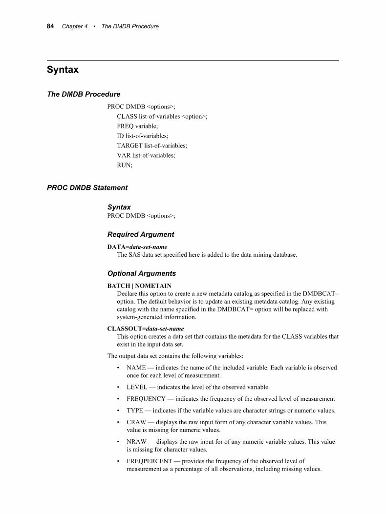
Syntax
The DMDB ProcedurePROC DMDB <options>;
CLASS list-of-variables <option>;FREQ variable;ID list-of-variables;TARGET list-of-variables;VAR list-of-variables;RUN;
PROC DMDB Statement
SyntaxPROC DMDB <options>;
Required ArgumentDATA=data-set-name
The SAS data set specified here is added to the data mining database.
Optional ArgumentsBATCH | NOMETAIN
Declare this option to create a new metadata catalog as specified in the DMDBCAT= option. The default behavior is to update an existing metadata catalog. Any existing catalog with the name specified in the DMDBCAT= option will be replaced with system-generated information.
CLASSOUT=data-set-nameThis option creates a data set that contains the metadata for the CLASS variables that exist in the input data set.
The output data set contains the following variables:
• NAME — indicates the name of the included variable. Each variable is observed once for each level of measurement.
• LEVEL — indicates the level of the observed variable.
• FREQUENCY — indicates the frequency of the observed level of measurement
• TYPE — indicates if the variable values are character strings or numeric values.
• CRAW — displays the raw input form of any character variable values. This value is missing for numeric values.
• NRAW — displays the raw input for of any numeric variable values. This value is missing for character values.
• FREQPERCENT — provides the frequency of the observed level of measurement as a percentage of all observations, including missing values.
84 Chapter 4 • The DMDB Procedure
• NMISSPERCENT — provides the frequency of the observed level of measurement as a percentage of observations without missing values.
MISSINGONLYSpecify this option to obtain frequencies and other applicable statistics that are based solely on the distinction between missing and nonmissing values.
MAXLEVEL=numberThis option specifies the maximum number of class levels to process. The default value of number is the largest machine integer available. The value of number must be an integer greater than or equal to 3.
MAXOBS=numberThis option specifies the max number of database records that are processed. Often, the total number of records in a database is not known. This option prevents the excessive download of data into SAS by limiting the imported data to number rows. If in-database processing is used, then this option is ignored.
NONORMInclude this option to generate class level values without normalization. A normalized value is left-justified, truncated to NORMLEN= length, and in uppercase. By default, the DMDB procedure generates metadata with normalized class levels. Normalization helps with unclean or inconsistent data. For example, the values “Yes”, “YES”, and “yes” all share the same normalized form “YES”. Also note that class levels need to be unique within the default NORMLEN= length of 32 bytes. For example, the values “ABC Department store, nylon socks, blue” and “ABC Department store, nylon socks, black” would both share the normalized form “ABC DEPARMENT STORE, NYLON SOCKS” even though they are different values.
NORMLEN=numberThis option specifies the normalized length of categorical variable values. The value of number must be an integer and defaults to 32.
OUT=data-set-nameUse this option to name the DMDB. The DMDB contains each of the ID, VAR, and FREQ variables, copied as is from the input data set. The DMDB also converts each of the CLASS variables to a corresponding integer class level value.
PMMLSpecify this option to create PMML score code. The DMDB procedure produces the DataDictionary component of a PMML document. For more information about PMML, see the PMML Support in Enterprise Miner section in the Enterprise Miner help documentation.
VARDEF=DF | numberThis option indicates the divisor that is used when the DMDB procedure calculates variance and standard deviation. You can specify DF to use the degrees of freedom and number to specify the number of observations. The default value is the degrees of freedom.
VAROUT=data-set-nameThis option creates a data set that contains the metadata for the VAR variables that exist in the input data set.
The output data set contains the following variables:
• NAME — indicates the name of the included variable. Each variable is observed once for each level of measurement.
• NMISS — indicates the number of missing values for the observed variable.
Syntax 85
• N — indicates the total number of observations for the observed variable, not including missing values.
• MIN — provides the smallest observed value.
• MAX — provides the largest observed value.
• MEAN — provides the average of the variables values, not including any missing values.
• STD — provides the standard deviation of the variable values, not including any missing values.
• SKEWNESS — indicates the skewness of the variable values, not including any missing values.
• KURTOSIS — indicates the kurtosis of the variable values, not including any missing values.
CLASS Statement
SyntaxCLASS list-of-variables <(option)>;
Required Argumentlist-of-variables
This option specifies a list of categorical variables that are used in later analysis. For each variable listed here, the metadata contains information on its class level value, its frequency, and its ordering information. The variables listed here can be character or numeric. These variables cannot be stated in the ID or VAR statements.
Optional ArgumentsSORTING-ORDER
This option determines how each variable is sorted. For an example on how to use this option, see “Example 1: Basic Usage” on page 88 .
Valid values of SORTING-ORDER are as follows:
• ASC | ASCENDING — Class levels are arranged from lowest to highest order of unformatted values. This is the default value.
• DESC | DESCENDING — Class levels are arranged from highest to lowest order of unformatted values.
• ASCFMT | ASCFORMATTED — Class levels are arranged from lowest to highest order of formatted values.
• DESFMT | DESFORMATTED — Class levels are arranged from highest to lowest order of formatted values.
• DATA | DSORDER — Class levels are arranged according to their order in the input data set.
86 Chapter 4 • The DMDB Procedure
FREQ Statement
SyntaxFREQ variable;
Required Argumentvariable
This argument specifies a numeric variable whose value represents the frequency of the observation. If you specify this statement, then this variable is used by all other Enterprise Miner procedures in the current data mining project. If the variable value is 0 or missing, then the observation is omitted in the DMDB and is not included in statistical calculations.
ID Statement
SyntaxID list-of-variables;
Required Argumentlist-of-variables
Use the ID statement to specify a list of variables that contain unique identifiers for each observation in the input data set. These variables can be either character or numeric.
TARGET Statement
SyntaxTARGET list-of-variables;
Required Argumentlist-of-variables
The variables listed here are the target variables in the data set. These variables must be specified in either the VAR or the CLASS statements. These variables can be character or numeric variables.
VAR Statement
SyntaxVAR list-of-variables;
Syntax 87
Required Argumentlist-of-variables
Use the VAR statement to list any numeric analysis variables. These variables will appear in the output data set in the same order that you specify them here. If you omit this statement, then the DMDB procedure analyzes all numeric variables that are not listed in any other statement.
Details
The Data Mining DatabaseThe DMDB is maintained as a SAS data set. The metadata information that is associated with the DMDB is maintained in a SAS catalog. Metadata includes overall data set information as well as statistical information for the variables according to their roles. For each CLASS variable, the metadata contains information on class level values, frequencies, and ordering information. In the DMDB, the CLASS variables are stored as integers that are mapped to different class level values.
The statistics stored for VAR variables are as follows:
• The number of observations with nonmissing values
• The number of observations with missing values
• The minimum observed value
• The maximum observed value
• The sum of all nonmissing values
• The corrected sum of squares
• The uncorrected sum of squares
• The standard deviation
• A measure of the skewness of the data
• A measure of the kurtosis of the data
Data mining databases are created only for training data and should not be used for validation or testing data.
Examples
Example 1: Basic UsageThis example demonstrates how to create a DMDB data set and catalog. The example uses the SAMPSIO.HMEQ data set, which includes information about 5960 fictitious mortgages. Each case represents an applicant for a home equity loan, and all applicants have an existing mortgage. The binary target variable BAD indicates whether an applicant eventually defaulted or was ever seriously delinquent. There are 10 numeric input variables and two class input variables. The code below creates the DMDB data set and catalog for the HMEQ data set.
88 Chapter 4 • The DMDB Procedure

proc dmdb batch data=sampsio.hmeq out=DMhmeq dmdbcat=CAThmeq; var loan derog mortdue value yoi delinq clage ninq clno debtinc; class bad(desc) reason(ascending) job; target bad;run;
The data set DMhmeq contains the DMDB data set, and CAThmeq contains the DMDB catalog. Both should be found in your Work directory. The numeric variables are specified in the VAR statement and the categorical variables are specified in the CLASS statement. You cannot specify a variable in both of these statements. Note that this data set does not contain an ID or a FREQ variable. The TARGET statement is used to identify the variable BAD as the target variable.
Notice that the variable BAD is sorted in descending order while REASON is sorted in ascending order. You can specify different sorting methods for each of the variables in the CLASS statement. Because nothing is specified for JOB, it is automatically sorted in ascending order.
Examples 89

90 Chapter 4 • The DMDB Procedure
Chapter 5
The DMINE Procedure
Overview . . . . . . . . . . . . . . . . . . . . . . . . . . . . . . . . . . . . . . . . . . . . . . . . . . . . . . . . . . . . 91The DMINE Procedure . . . . . . . . . . . . . . . . . . . . . . . . . . . . . . . . . . . . . . . . . . . . . . . 91
Syntax . . . . . . . . . . . . . . . . . . . . . . . . . . . . . . . . . . . . . . . . . . . . . . . . . . . . . . . . . . . . . . . 92The DMINE Procedure . . . . . . . . . . . . . . . . . . . . . . . . . . . . . . . . . . . . . . . . . . . . . . . 92PROC DMINE Statement . . . . . . . . . . . . . . . . . . . . . . . . . . . . . . . . . . . . . . . . . . . . . 92CODE Statement . . . . . . . . . . . . . . . . . . . . . . . . . . . . . . . . . . . . . . . . . . . . . . . . . . . 94FREQ Statement . . . . . . . . . . . . . . . . . . . . . . . . . . . . . . . . . . . . . . . . . . . . . . . . . . . . 95TARGET Statement . . . . . . . . . . . . . . . . . . . . . . . . . . . . . . . . . . . . . . . . . . . . . . . . . 95VARIABLES Statement . . . . . . . . . . . . . . . . . . . . . . . . . . . . . . . . . . . . . . . . . . . . . . 95WEIGHT Statement . . . . . . . . . . . . . . . . . . . . . . . . . . . . . . . . . . . . . . . . . . . . . . . . . 95
Details . . . . . . . . . . . . . . . . . . . . . . . . . . . . . . . . . . . . . . . . . . . . . . . . . . . . . . . . . . . . . . . 96The DMINE Procedure . . . . . . . . . . . . . . . . . . . . . . . . . . . . . . . . . . . . . . . . . . . . . . . 96Missing Values . . . . . . . . . . . . . . . . . . . . . . . . . . . . . . . . . . . . . . . . . . . . . . . . . . . . . 96
Examples . . . . . . . . . . . . . . . . . . . . . . . . . . . . . . . . . . . . . . . . . . . . . . . . . . . . . . . . . . . . 97Example 1: Preprocessing the Data and Basic Usage . . . . . . . . . . . . . . . . . . . . . . . 97Example 2: Including the AOV16 and Grouping Variables . . . . . . . . . . . . . . . . . . . 99Example 3: Modeling a Binary Target . . . . . . . . . . . . . . . . . . . . . . . . . . . . . . . . . . . 99
Overview
The DMINE ProcedureMany data mining databases have hundreds of potential model inputs (independent variables). The DMINE procedure enables you to identify the input variables that are useful for predicting the target variables based on a linear models framework. The procedure facilitates ordinary least squares or logistic regression methods. Logistic regression is a form of regression analysis where the response variable is either binary or ordinal. The DMINE procedure and the DMSPLIT procedure are the underlying procedures for the Variable Selection node.
91
Syntax
The DMINE ProcedurePROC DMINE DATA=data-set-name DMDBCAT=catalog-name <options>;
CODE <options>;FREQ variable;TARGET variable;VARIABLES list-of-variables;WEIGHT variable;
PROC DMINE Statement
SyntaxPROC DMINE DATA=data-set-name DMDBCAT=catalog-name <options>;
Required ArgumentsDATA=data-set-name
This argument specifies the input data set.
DMDBCAT=catalog-nameThis argument identifies the metadata catalog that was created by the DMDB procedure for the input data set. For more information about this catalog, see the documentation for the DMDB procedure.
Optional ArgumentsMAXROWS=n
This option specifies the upper bound for the number of independent variables that are selected for the model. This is an upper bound for the number of rows and columns of the X'X matrix of the regression problem.
The value of n must be a positive integer and default to 3000. This means that for most models the MINR2= and STOPR2= settings will determine the number of independent variables that are selected. The X'X matrix used for the stepwise
regression requires n( n + 12 ) double precision values of storage in RAM. For the
default value of 3000, this results in 3000*1500*8 bytes, or about 36 megabytes, of memory that is required.
MINR2=numberThis option specifies the lower bound for the individual R-square value of a variable for that variable to be eligible for the model selection process. Variables with R-square values greater than or equal to number are included in the selection process. The value of number must be a real, positive number and defaults to 0.00001.
NOAOV16Specify this option to suppress the creation of the AOV16 variables. By default, the DMINE procedure creates the AOV16 variables, calculates their R-square values, and uses the remaining significant variables in the forward stepwise selection
92 Chapter 5 • The DMINE Procedure
process. The interval scaled variables are grouped into categories to create the AOV16 variables. The range of interval scaled variables can be divided into 16 equal categories, and each observation of the variable is mapped into one of these categories. Note that the R-square value is calculated for each AOV16 variable even if you specify this option.
NOINTERSpecify this option to ignore the interactions between the categories, known as two-way interactions, of categorical variables during the process of variable selection. A two-way interaction measures the effect of a classification input variable across the levels of another classification variable. For example, credit worthiness might not be consistent across job classifications. The lack of uniformity in the response might signify a credit worthiness by job classification interaction.
By default, two-way interactions between categorical variables are considered in the variable selection process. Note that the two-way interactions can dramatically increase the processing time of the DMINE procedure.
NOMONITORSpecify this option to suppress the output of the status monitor that indicates the progress made in the computations. By default, this information is displayed.
NOPRINTSpecify this option to suppress all printed output in the Output window.
OUTEFFECT=data-set-nameSpecify OUTEFFECT= to save a copy of selected effects and their properties to the specified data set.
OUTRSQUARE=data-set-nameSpecify OUTRSQUARE= to save the initial r-square value to the specified data set.
OUTEST=data-set-nameThis option specifies the name of an output data set that contains the estimation and fit statistics.
OUTGROUP=data-set-nameThe data set specified here contains information on the following:
• AOV16 interval variables to show individual bin values for the interval variables
• Group class variables to show group numbers for individual class levels of the variables.
• Two-way interactions between the levels of two class variables
The OUTGROUP= data set can be used to interpret the parts of the generated DATA step source code that were created in the CODE statement.
PSHORTSpecify this option to print a minimal amount of information in the output window or list file.
STOPR2=numberThis option specifies a lower bound for the incremental model R-square value where the variable selection process is stopped. The value of number must be a real, positive number and default to 0.00005.
THREADS=number <FORCE>This argument specifies the number of computational threads to use. If used with the FORCE option, then exactly number threads are used. If FORCE is not specified, then number is used as a suggestion. The actual number is chosen based on various
Syntax 93
factors such as the size of the problem, the number of computers available, the amount of available memory, and so on.
The DMINE procedure also uses threads to read partitioned data sets that are created by the SPD Engine and to perform preliminary computations. However, this is not controlled by the THREADS= option.
USEGROUPSBy default, the DMINE procedure tries to reduce the levels of each class variable to a group variable based on the relationship with the target. By doing so, observations of class variables with many categories (for example, ZIP codes) can be mapped into groups of fewer categories. If you specify the USEGROUPS option, and a class variable can be reduced to a group variable, then only the group variable is considered in the model. If you omit this option, then both group variables and the original class variables are allowed in the model.
CODE Statement
SyntaxCODE <options>;
Optional ArgumentsCATALOG | CAT=library.catalog.entry.type
This option specifies where to write the output SAS DATA step code. The default library is determined by the SAS system option USER and is usually set to the WORK folder. The default entry is SASCODE and the default type is SOURCE.
You can specify both CATALOG= and FILE= in the same CODE statement. If you specify neither, then the code is written to the SAS log, unless the PMML option is specified.
FILE=file-nameThis option specifies the file that is used for the output SAS DATA step code. You can specify this as a quoted string that provides the full path to the external file or a SAS filename of no more than eight bytes. If the filename is assigned as a fileref in a FILENAME statement, the specified file is opened. The special filerefs LOG and PRINT are always reserved by the SAS system. If the specified name is not assigned a fileref, then the specified name value is concatenated with a .txt extension and then opened. If the specified filename is more than eight bytes, then an error message is printed.
LINESIZE | LS=numberThis option specifies the line size for the generated code. The value of number must be a positive integer between 64 and 254 and default to 72.
PMML | XMLSpecify this option to enable the creation of Predictive Modeling Markup Language scoring code. PMML is an XML-based standard to represent data mining results. For more information, see the PMML Support in the Enterprise Miner section in the Enterprise Miner Help.
PREDICTSpecify this option to generate score code to compute predicted target values.
94 Chapter 5 • The DMINE Procedure
RESIDUAL | NORESIDUALSpecify RESIDUAL to generate residual values for many variables. If you request code for residuals and then score a data set that does not contain target values, the residuals will have missing values. By default, no residuals are generated.
FREQ Statement
SyntaxFREQ variable;
You can specify the FREQ variable in either the DMDB procedure or the DMINE procedure. Specify this variable in the DMDB procedure so that the information is saved in the DMDB catalog and it is automatically used by the DMINE procedure. This also ensures that the FREQ variable is automatically used by all other Enterprise Miner procedures.
Required Argumentvariable
This argument specifies one numeric variable that contains the frequency of each observation. If this variable differs from the one specified in the DMDB statement, then no FREQ variable is used.
TARGET Statement
SyntaxTARGET variable;
Required Argumentvariable
This argument specifies the response variable.
VARIABLES Statement
SyntaxVARIABLES | VAR list-of-variables;
Required Argumentlist-of-variables
This argument specifies all of the independent variables that can be used to predict or model the target variable.
WEIGHT Statement
SyntaxWEIGHT variable;
Syntax 95
You can specify the WEIGHT variable in the DMDB procedure so that the information is save in the DMDB catalog. This variable is used automatically as the WEIGHT variable in the DMINE procedure.
Required Argumentvariable
This argument specifies one numeric variable that is used to weight the input variables.
Details
The DMINE ProcedureThe DMINE procedure performs two tasks.
• The DMINE procedure computes a forward stepwise least squares regression. In each step, an independent variable is selected, which contributes maximally to the model R-square value. Two parameters, MINR2= and STOPR2=, can be specified to guide the variable selection process.
• If a variable has an individual R-square value smaller than MINR2=, then the variable is not considered for the model.
• In the stepwise process, the variable with the largest contribution to the model R-square value is added to the model. After this change, if the global R-square value changes by less than the STOPR2= value, then the stepwise regression is terminated.
• For a binary target, a fast algorithm for an approximate logistic regression is computed in the second part of the DMINE procedure. The independent variable is the prediction from the former least squares regression. Since only one regression variable is used for the logistic regression, only two parameters are estimated, the intercept and the slope. The range of predicted values is divided into a number of equidistant intervals, called knots, where the logistic function is interpolated.
• If NOPRINT is not specified, a table is printed that indicates the accuracy of the logistic model.
Missing ValuesMissing values are handled differently for each variable type. For categorical variables, a new category is created to represent missing values. For other variables, missing values are replaced by the mean of that variable. Observations with missing target values are dropped from the data.
96 Chapter 5 • The DMINE Procedure
Examples
Example 1: Preprocessing the Data and Basic Usage
CodeThe data set SAMPSIO.BASEBALL contains statistics and salary information for 322 Major League Baseball players in the 1986 season. The goal of this example is to identify the variables that best predict each player's salary. There are 18 input variables and one target variable. The interval target variable indicates the base salary in thousands of dollars, given in 1987 dollars, unadjusted for inflation. There are also two more variables for the player's league and division that will serve as input variables for this example, but as target values in “Example 3: Modeling a Binary Target” on page 99 .
The first step is to create the data mining database from the input data set. Because you will use the variables LEAGUE and DIVISON as target variables later on, you must specify them in the TARGET statement now.
/* Create the DMDB */proc dmdb batch data=sampsio.baseball out=baseOut dmdbcat=catBASE; var no_atbat no_hits no_home no_runs no_rbi no_bb yr_major cr_atbat cr_hits cr_home cr_runs cr_rbi cr_bb no_outs no_assts no_error salary; class team league division position; target salary league division;run;
Now, you can call the DMINE procedure with the data created by the DMDB procedure.
/* Run the DMINE Procedure */proc dmine data=baseOut dmdbcat=catBASE minr2=0.02 stopr2=0.005 noaov16 nointer; var no_atbat no_hits no_home no_runs no_rbi no_bb yr_major cr_atbat cr_hits cr_home cr_runs cr_rbi cr_bb no_outs no_assts no_error team league division position; target salary;run;
When you invoke the DMINE procedure, the Dmine Status Monitor window appears. This window monitors the execution time of the procedure. To suppress the display of this window, specify the NOMONITOR option in the PROC DMINE statement.
R-Squares for Target Variable: SALARYThe first table in the Output window provides the R-square values for all of the input variables, class variables, group variables, and AOV16 variables. Effects that have an R-square value less than the MINR2= cutoff value are not chosen for the model. These effects are labeled as “R2 < MINR2” in the table. The remaining significant variables are analyzed in a subsequent forward selection regression.
Examples 97

There are four types of model effects:
• Class effects are estimated for each class variable and all possible two-factor interactions. The R–square statistic is calculated for each class effect using a one-way analysis of variance. Two-factor interaction effects are constructed by combining all possible levels of each class variable into one term. Because the NOINTER option was specified, the two-factor interactions are not used in the final forward stepwise regression. The degrees of freedom for a class effect are equal to the number of unique factor levels minus 1. For two-factor interactions, the degrees of freedom is equal to the number of levels in factor A multiplied by the number of levels in factor B minus 1.
• Group effects are created by reducing each class effect through an analysis of means. The degrees of freedom for each group effect are equal to the number of levels.
• Var effects are estimated from interval variables as standard regression inputs. A simple linear regression is performed to determine the R2 statistic for interval inputs. The degrees of freedom are always equal to 1.
• AOV16 effects are calculated as a result of grouping numeric variables into a maximum of 16 equally spaced buckets. AOV16 effects might account for possible non-linearity in the target variable SALARY. The degrees of freedom are calculated as the number of groups. Because the NOAOV16 option was specified, the AOV16 variables are not used in the final forward stepwise regression.
Note that the class effect TEAM*POSITION has the largest R-square value with the target variable. There are several AOV16 effects with relatively large R-square values, but these are not included in the final forward stepwise regression.
Effects Chosen for Target: SALARYThe next table in the Output window indicates the effects that were chosen for the model. This table indicates the degrees of freedom, R-square value, F-value, p-value, and sum of squares for the selected input variables. Notice that only the Var and Class effects were chosen for this model.
Note: The AOV16, GROUP, and two-way class interaction effects are not considered in the forward stepwise regression. Including these effects can produce a better model, but it will also increase the execution time of the DMINE procedure. To learn how to include these effects into the analysis, see “Example 2: Including the AOV16 and Grouping Variables” on page 99 .
The Final ANOVA Table for Target: SALARYNext in the Output window, you will find the Final ANOVA Table for Target: SALARY. The ANOVA table is divided into four columns:
• Effect labels the source of the variation as Model, Error, or Total.
• DF lists the degrees of freedom for each source of variation.
• R-Square is the model R-square value, which is the ratio of the model sum of squares to the total sum of squares. In this example, the model explains about 2/3 of the variation in the target variable.
• Sum of Squares partitions the total target variation into portions that can be attributed to the model inputs and to error.
98 Chapter 5 • The DMINE Procedure
Effects Not Chosen for Target: SALARYThe final table lists the sum of squares and the R-square values for the effects that are not chosen in the final model. Notice that these effects have very small R-square values and large p-values.
Example 2: Including the AOV16 and Grouping VariablesNote: This example assumes that you have completed “Example 1: Preprocessing the
Data and Basic Usage” on page 97 .
This example expands on the previous example and includes the AOV16, group, and two-way class interaction effects into the final forward stepwise analysis. The addition of these effects can produce a better model, but will increase the execution time of the DMINE procedure. The code that follows is identical to the code in Example 1 except that the options NOAOV16 and NOINTER have been removed.
proc dmine data=baseOut dmdbcat=catBASE minr2=0.02 stopr2=0.005; var no_atbat no_hits no_home no_runs no_rbi no_bb yr_major cr_atbat cr_hits cr_home cr_runs cr_rbi cr_bb no_outs no_assts no_error team league division position; target salary;run;
In the Output window, find the Effects Chosen for Target: SALARY table and the Final ANOVA Table for Target: SALARY table. Notice in the first table that only three effects were chosen, one of them a two-way class interaction and the other two were AOV16 effects. The ANOVA table indicates that over 99% of the total variance can be explained in the model with these effects. This is an improvement over the results in Example 1.
Notice, though, that this example took more than four times as long to process as Example 1. For such a small example, this difference was not large. But, as your problems grow in size and complexity, the time difference can become significant.
Example 3: Modeling a Binary TargetNote: This example assumes that you have completed “Example 1: Preprocessing the
Data and Basic Usage” on page 97 .
The DMDB that you created in Example 1will be sufficient for this example. However, in this example, you will attempt to predict the league each player was in based on much of the same information as the first two examples. This example does not include the variable TEAM because this variable would completely determine the value of LEAGUE. This call to the DMINE procedure uses the same information, except where noted above, as in Example 1.
/* Run the DMINE Procedure */proc dmine data=baseOut dmdbcat=catBASE minr2=0.02 stopr2=0.005 noaov16 nointer; var no_atbat no_hits no_home no_runs no_rbi no_bb yr_major cr_atbat cr_hits cr_home cr_runs cr_rbi cr_bb no_outs no_assts no_error salary division position;
Examples 99

target league;run;
The output for this call to the DMINE procedure begins with the same information as the previous examples. However, after the Effects not Chosen table, you will find more information that is specific to binary target values. When the target is binary, predicted values are computed from the forward stepwise regression. The predicted values are then grouped into 256 equally spaced intervals, which are used as the independent variable in a final logistic regression analysis. The logistic regression helps you decide the cutoff of the binary response. Since there is one input, only two parameters are estimated, the intercept and the slope.
The first new table is the Estimating logistic table, which indicates the computed estimates for the intercept (alpha) and the slope (beta) for the approximate logistic regression.
The next table, titled The DMINE Procedure, contains the predicted values, which are bucketed into the 256 equally sized sub-intervals. This table contains information about each of the 256 sub-intervals. For each sub-interval, the column N0 indicates the number of observations in the American League, N1 indicates the number in the National League, and Nmiss indicates the number of observations with missing values. Additionally, X represents the center value of the sub-interval and P represents the predicted value for X.
Finally, you will find the Classification Table for CUTOFF = 0.5000. This classification table indicates the number of observations that were correctly and incorrectly identified as being in the American League or National league. This table indicates that the model was accurate 62.73% of the time.
100 Chapter 5 • The DMINE Procedure
Chapter 6
The DMNEURL Procedure
Overview . . . . . . . . . . . . . . . . . . . . . . . . . . . . . . . . . . . . . . . . . . . . . . . . . . . . . . . . . . . 101The DMNEURL Procedure . . . . . . . . . . . . . . . . . . . . . . . . . . . . . . . . . . . . . . . . . . 101
Syntax . . . . . . . . . . . . . . . . . . . . . . . . . . . . . . . . . . . . . . . . . . . . . . . . . . . . . . . . . . . . . . 102The DMNEURL Procedure . . . . . . . . . . . . . . . . . . . . . . . . . . . . . . . . . . . . . . . . . . 102PROC DMNEURL Statement . . . . . . . . . . . . . . . . . . . . . . . . . . . . . . . . . . . . . . . . 103DECISION Statement . . . . . . . . . . . . . . . . . . . . . . . . . . . . . . . . . . . . . . . . . . . . . . . 108FREQ Statement . . . . . . . . . . . . . . . . . . . . . . . . . . . . . . . . . . . . . . . . . . . . . . . . . . . 109FUNCTION Statement . . . . . . . . . . . . . . . . . . . . . . . . . . . . . . . . . . . . . . . . . . . . . . 110LINK Statement . . . . . . . . . . . . . . . . . . . . . . . . . . . . . . . . . . . . . . . . . . . . . . . . . . . 110TARGET Statement . . . . . . . . . . . . . . . . . . . . . . . . . . . . . . . . . . . . . . . . . . . . . . . . 111VAR Statement . . . . . . . . . . . . . . . . . . . . . . . . . . . . . . . . . . . . . . . . . . . . . . . . . . . . 111WEIGHT Statement . . . . . . . . . . . . . . . . . . . . . . . . . . . . . . . . . . . . . . . . . . . . . . . . 111
Details . . . . . . . . . . . . . . . . . . . . . . . . . . . . . . . . . . . . . . . . . . . . . . . . . . . . . . . . . . . . . . 112Scoring the Model with the OUTEST Data Set . . . . . . . . . . . . . . . . . . . . . . . . . . . 112
Examples . . . . . . . . . . . . . . . . . . . . . . . . . . . . . . . . . . . . . . . . . . . . . . . . . . . . . . . . . . . 113Example 1: Preprocessing the Data and a Binary Target . . . . . . . . . . . . . . . . . . . . 113Example 2: Preprocessing the Data and an Interval Target . . . . . . . . . . . . . . . . . . 114
Overview
The DMNEURL ProcedureThe DMNEURL procedure tries to establish a nonlinear model for the prediction of a binary or interval scaled target variable. The algorithm used in the DMNEURL procedure was developed to overcome some problems that exist when the NEURAL procedure is used for data mining purposes. These problems are exacerbated when the data set contains many highly collinear variables.
Some of the problems are as follows:
1. The nonlinear estimation problem in common neural networks is seriously under-determined, which yields highly rank-deficient Hessian matrices. In turn, this situation leads to extremely slow convergence (close to linear) of nonlinear optimization algorithms. The solution is to use a full-rank estimation of the Hessian matrix.
2. Each call to the NEURAL procedure corresponds to a single run through the entire training data set. Normally, many function calls are needed for convergent nonlinear
101
optimization with rank-deficient Hessian matrices. The DMNEURL procedure requires significantly fewer passes of the data to reach convergence.
3. The Hessian matrix has many eigenvalues λ=0 that correspond to long, flat valleys in the shape of the objective function. The traditional approach has serious problems with such objective functions because it cannot decide when an estimate is close enough to an appropriate solution and the optimization process can be terminated. The algorithm implemented by the DMNEURL procedure features quadratic convergence, and helps to solve this issue.
4. Also due to the eigenvalue λ=0, the common neural network algorithms tend to find local solutions, rather than global one. Thus, the optimization results are very sensitive with respect to the starting point of the optimization. The DMNEURL procedure is able to determine good starting points for the optimization problem.
The DMNEURL procedure is built to deal with specific optimization problems. These problems should have full-rank Hessian matrices, a small number of parameters, and good starting points that are identifiable. The convergence of the nonlinear optimizer is normally very fast; typically convergence happens in less than 10 iterations per optimization.
The function and derivative calls during optimization do not require any passes through the data set. However, the search for good starting points and the final evaluations for the solutions need several passes through the data. These two processes also perform a number of preliminary tasks.
With the DMNEURL procedure, you can determine multiple activation functions and select the best result. Because the optimization process for one activation function does not depend on any other functions, processing time is further reduced with parallel processing.
Expect when the NEURAL procedure tends to favor local solutions over the global solution, the DMNEURL procedure is not expected to outperform, in terms of precision, the NEURAL procedure. However, the results of the DMNEURL procedure are very close to those of the NEURAL procedure. For a very large data set, the DMNEURL procedure is faster than the NEURAL procedure. For a small data set, the NEURAL procedure can be much faster than the DMNEURL procedure, especially for an interval target variable. The DMNEURL procedure is most efficient for the analysis of a binary target variable without FREQ and WEIGHT statements and without cost variables in the input data set.
Syntax
The DMNEURL ProcedurePROC DMNEURL DATA=data-set-name DMDBCAT=catalog-name <options>;
DECISION DECDATA=data-set-name <options>;FREQ variable;FUNCTION function-name;LINK function-name;TARGET variable;VAR list-of-variables;WEIGHT variable;
102 Chapter 6 • The DMNEURL Procedure
PROC DMNEURL Statement
SyntaxPROC DMNEURL DATA=data-set-name DMDBCAT=catalog-name <options>;
Required ArgumentsDATA=data-set-name
This argument specifies the input data set.
DMDBCAT=catalog-nameThis argument specifies the DMDB catalog created by the DMDB procedure. For more information about this catalog, see the documentation for the DMDB procedure.
Optional ArgumentsABSGCONV | ABSGTOL=number
This argument specifies the absolute gradient convergence criterion for the default optimization process. The value of number must be a real, positive number and the default value is 0.0005 in general and 0.001 when you specify the exponential activation function.
CORRDFThis argument ensures that the correct number of degrees of freedom to use for the values of the variables RMSE, AIC, and SBC. If you do not specify this option, then the degrees of freedom are computed as the sum of the weights minus the number of parameters. When you specify this option, the degrees of free are computed as the sum of the weights minus the rank of the joint Jacobian matrix.
COVSpecify this option to use the covariance matrix when the DMNEURL procedure computes eigenvalues and eigenvectors that are compatible with the PRINCOMP procedure. This option is valid only when you specify an OUTSTAT= data set. If neither COV nor CORR are specified, then the DMNEURL procedure computes eigenvalues and eigenvectors from the cross product matrix XTX.
CORRSpecify this option to use the correlation matrix when the DMNEURL procedure computes eigenvalues and eigenvectors that are compatible with the PRINCOMP procedure. This option is valid only when you specify an OUTSTAT= data set. If neither COV nor CORR are specified, then the DMNEURL procedure computes eigenvalues and eigenvectors from the cross product matrix XTX.
CRITWGT=numberThis option specifies a weight for a weighted least squares fit. This option can be used only with a binary target variable. If you specify a value greater than 1, this will enforce a better fit of the (1, 1) entry in the accuracy table, which might be useful for fitting rare events. However, values much greater than 1 will significantly reduce the fit quality of the remaining entries. Values between 0 and 1 will enforce a better fit of the (0, 0) entry in the accuracy table. The value of number must be a real, positive number. However, recommended values are 0.5 < number < 1 and 1 < number < 2.
CUTOFF=numberThis option specifies a cutoff threshold to decide when a predicted value of a binary response is classified as 0 or 1. If the value of the posterior for observation j is
Syntax 103
smaller than the specified cutoff value, the observation is considered a 0. If the value of the posterior is greater than or equal to the specified cutoff value, then the observation is considered a 1. This option is not used for nonbinary target variables. The value of number must be a real number between 0 and 1 and default to 0.5.
FCRITSpecify this option to use the probability of the F test for the selection of principal components, instead of the R-square criterion.
GCONV | GTOL=numberUse this option to specify a relative gradient convergence criterion for the optimization process. The value of number must be a nonnegative, real number and default to 10–7.
MAXCOMP=mThis argument specifies an upper bound for the number of components that are selected to predict the target variable in each stage. The value of m must be an integer between 2 and 8, with values between 3 and 5 as the best. Note that the compute time and memory required increase superlinearly for values larger than 5.
There is one memory allocation that takes nm long integer values, where n comes from the NPOINT= option and m from the MAXCOMP= option. Thus, the memory requirements will grow exponentially as you increase the value of m. If more precision is required, it is better to increase the value of the MAXSTAGE= option.
MAXFUNC=numberThis option specifies an upper bound for the number of function calls in each optimization. Normally, the default number of functions calls is sufficient to reach convergence. Larger values can be used if the iteration history indicates that the optimization process was close to a promising solution, but needed more calls to converge. Smaller values can be used when a faster, but less optimal, solution is sufficient. The value of number must be a positive integer and default to 500.
MAXITER=numberThis option specifies an upper bound for the number of iterations in each optimization. Normally, the default number of iterations is sufficient to reach convergence. Larger values can be used if the iteration history indicates that the optimization process was close to a promising solution, but needed more iterations to converge. Smaller values can be used when a faster, but less optimal, solution is sufficient. The value of number must be a positive integer and default to 200.
MAXROWS=NThis option specifies an upper bound for the number of independent variables selected for the model. Specifically, this is the upper bound for the rows and columns of the XTX matrix of the regression problem. Note that this regression requires
N ( N + 12 ) double precision values stored in memory. For the default value of N,
this amounts to approximately 36 megabytes of memory. The value of N must be a positive integer and default to 3000.
MAXSTAGE=numberThis option specifies an upper bound for the number of stages of estimation. You can specify this option with or without a value for number. If you do not specify number, then the estimation process terminates if either the sum of squares residual changes by less than 1% or 100 stages are processed. This behavior is different than when you do not specify this option altogether. Large values of number might result in numerical problems such as a large discretization error and a worsening fit criterion. In such a case, the stagewise process is terminated with the last good stage. The value of number must be a positive integer and default to 5.
104 Chapter 6 • The DMNEURL Procedure
MAXSTPT=numberThis option specifies the number of values of the objective function that are inspected for the start of the optimization process. Values larger than the default value can improve the result of the optimization process, especially when more than three components are used. The value of number must be a positive integer and default to 250.
MAXVECT=numberThis option specifies an upper bound for the number of eigenvectors that are available for selection. Values smaller than the default should be used only if there is limited memory available to store the eigenvectors. The value specified here cannot be less than the value specified in the MINCOMP= option nor greater than the value specified in the MAXROWS= option. The value of number must be a positive integer and default to 400.
MEMSIZ=numberFor interval targets and in a multiple stage process, some memory consuming operations are performed. For very large data sets, the computations performed can vary based on the amount of memory that is available. This option determines the amount of memory, in megabytes, that is available to perform these computations. Because other operations need additional memory, not more than 25% of the total memory should be specified here. You can reduce the amount of memory specified here if the DMNEURL procedure fails due to a lack of memory. The value of number must be a positive integer and default to 8.
MINCOMP=numberThis option specifies a lower bound for the number of components that are selected to predict the target variable in each stage. This value can permit the selection of components that otherwise would be rejected by the STOPR2= option. The DMNEURL procedure can override that value when the rank of the XTX matrix is less than the specified value. The value of number must be an integer between 2 and 8 and default to 2.
NOMONITORSpecify this option to suppress the output of the status monitor that indicates the progress of the DMNEURL procedure.
NOPRINTSpecify this option to suppress all of the output that would normally appear in the Output window.
NPOINT=numberThis option specifies the number of discretization points. By default, this value is determined based on the values of MINCOMP= and MAXCOMP=. The value of number must be an integer between 5 and 19, ideally even.
OPTCRIT=SSE | ACC | WSSEThis option specifies the criterion to use for the optimization phase. Specify SSE to use the sum of squares error. Specify ACC to maximize a measure of the accuracy rate. For interval targets, the Goodman and Kruskal's lambda is applied on a frequency table defined by deciles of the actual target value. Specify WSSE to minimize the weighted sum of squares. To use this option, you must specify the CRITWGT= option and use a binary target variable.
OUT=data-set-nameThis option specifies an output data set that contains the predicted values (posteriors) and residuals for all observations in the input data set. This data set contains the values of all ID variables, the name of the target value, the number of the stage, the predicted value, and the residual. If a DECISION statement is used, then this data set
Syntax 105
also contains the best decision, the consequences of the decision, the expected profit or cost, and the expected value for all decision variables.
OUTCLASS=data-set-nameThis option specifies an output data set that contains the mapping between compound variable names and the names of the variables and categories of the categorical variables. The compound names are used to denote dummy variables that are created for each category of a variable with more than two categories. Because the compound names of dummy variables are used for the variable names in other data sets, you must know how these correspond to the original names. This data set contains only the compound variable name, the original variable name, and the name of the original level of measurement. If there are no categorical variables in the input data set, then this data set is empty.
OUTEST=data-set-nameThis argument specifies an output data set that contains all of the model information necessary to score additional cases or data sets. This data set contains the name of the target variable, the type of observation, the name of the observation, the number of the stage, and the actual variables. The first variables presented are the categorical variables, followed by the interval variables. Note that a set of binary dummy variables is created for each nonbinary categorical variable.
Additionally, each observation includes the variables _MEAN_ and _STDEV_, whose values are based on the type of observation.
• If the type of observation is _V_MAP_ or _C_MAP_, then the observation contains the mapping indices between the variables used in the model and the number of the variable in the data set. The value of _MEAN_ is the number of index mappings. For _V_MAP_, the value of _STDEV_ is the index of the target variable. For _C_MAP_, the value of _STDEV_ is the category number of the categorical target variable.
• If the type of observation is _EIGVAL_, then the observation contains the sorted eigenvalues of the XTX matrix. Here, the value of _MEAN_ is the number of model variables. The value of _STDEV_ is the number of model components.
• At each stage of the estimation process, two groups of observations are written to the OUTEST= data set.
• Observations of type _EIGVEC_ contain a set of c principal components that are used as predictor variables for the estimation of the original target value or the stage j residual. Here, the variable _MEAN_ contains the criterion used to include the component into the model, normally the R-square value. The variable _STDEV_ contains the eigenvalue number of the corresponding eigenvector. The best activation function is also reported.
• Observations of type _PARMS_ contain the total number of parameter estimates for each activation function. Here, the variable _MEAN_ contains the value of the optimization criterion, and _STDEV_ contains the accuracy value of the prediction.
OUTFIT=data-set-nameThis option specifies an output data set that contains fit indices for each stage and for the final model estimates. For a binary target variable, it also contains the frequencies of the 2x2 accuracy table of the best fit at the final stage. The same information is provided if a TESTDATA= input data set is specified.
The variables in this data set are as follows:
• _TARGET_ — identifies the name of the target value.
106 Chapter 6 • The DMNEURL Procedure
• _DATA_ — identifies the data set that contains the fit criteria. This can be the training data, test data, fit indices data, or the accuracy table data.
• _STAGE_ — indicates the number of stages in the estimation process.
• _SSE_ — contains the sum of squares error of the solution.
• _RMSE_ — contains the root mean square error of the solution.
• _ACCU_ — indicates the accuracy of the prediction for categorical targets.
• _AIC_ — is the Akaike information criterion.
• _SBC_ — is the Schwarz information criterion.
If a DECISION statement is specified, this data set also includes information about the profit, loss, and return on investment.
OUTSTAT=data-set-nameThis option specifies an output data set that contains all eigenvalues and eigenvectors of the XTX matrix. When this option is specified, no other computations are performed and the procedure terminates after saving this data set. This data set contains each of the variables in the model and two additional variables.
• _TYPE_ — provides the type of the observation.
• _EIGVAL_ — contains different numeric information.
The first three observations in this data set contain the mapping indices between the model's variables and the variable numbers of the input variables. The next observations contain the sorted eigenvalues of the XTX matrix. The final observations contain a set of eigenvectors of the XTX matrix. For these observations, the value of _EIGVAL_ corresponds to the appropriate eigvenvalue.
PALLSpecify this option to print summary information for the optimization history and the accuracy tables. Additionally, if OUTSTAT= is specified, then this also prints some simple statistics and the eigenvalues.
PMATRIXSpecify this option to print the XTX matrix. You can specify only this option if the OUTSTAT= option is also specified.
POPTHISSpecify this option to print the detailed histories of the optimization processes.
PSHORTSpecify this option to print a shorted form of the information found in the PALL option.
PTABLESpecify this option to print the accuracy tables.
SELCRIT=ACC | SSE | WSSEThis argument specified the criterion used to select the best result among all of the activation functions. Specify SSE to select the solution with the smallest sum of squared error. Specify ACC to select the solution with the greatest accuracy rate. For interval targets, the Goodman and Kruskal's lambda is applied on a frequency table defined by deciles of the actual target value. Specify WSSE to minimize the weighted sum of squares. To use this option, you must specify the CRITWGT= option and use a binary target variable.
SINGULAR=numberThis option specifies the criterion for the singularity test. The value of number must be a real, positive number and default to 10–7.
Syntax 107
STOPR2=numberThis argument specifies a lower bound for the incremental model R-square value where the variable selection process is stopped. This criterion is used only for the R-square values of the components that are selected in the range specified by MINCOMP= and MAXCOMP=. The value of number must be a real, positive number and default to 0.00005.
TESTDATA=data-set-nameThis argument specifies an input data set that is used to test the model created by the DMNEURL procedure. This data set must contain all of the variables in the input data set.
TESTDMDBThis option enables you to use a data set generated by the DMDB procedure as the TESTDATA= data set.
TESTOUT=data-set-nameThis output data set contains the same information as the OUT= data set, only computed for the TESTDATA= data set.
DECISION Statement
SyntaxDECISION DECDATA=data-set-name <options>;
Required ArgumentDECDATA=data-set-name
This argument specifies the input data set that contains the decision matrix, the prior probabilities, or both. This data set might contain decision variables that are specified with the DECVARS= option. Also, it might contain prior probability variables that are specified with the PRIORVAR= option, the OLDPRIORVAR= option, or both.
This data set must contain the target variable, which is specified in the TARGET statement.
For a categorical target variable, there should be one observation for each class. Each entry dij in the decision matrix indicates the consequence of selecting target value i for variable j. If any class appears twice or more in this data set, an error message is printed and the procedure terminates. Any class value in the input data set that is not found in this data set is treated as a missing class value. Note that the classes in this data set must correspond exactly with the variables in the POSTERIORS statement.
For an interval target variable, each row defines a knot in a piecewise linear spline function. The consequence of making a decision is computed by interpolating in the corresponding column of the decision matrix. If the predicted target value is outside the range of knots in the decision matrix, the consequence is computed by linear extrapolation. If the target values are monotonically increasing or decreasing, any interior target value is allowed to appear twice in data set. This allows you to specify discontinuities in the data. The end points, which are the minimum and maximum data points, might not appear more than once. No target value is allowed to appear more than twice. If the target values are not monotonic, then they are sorted by the procedure and are not allowed to appear more than once.
108 Chapter 6 • The DMNEURL Procedure
T I P The DECDATA= data set can be of type LOSS, PROFIT, or REVENUE. PROFIT is assumed by default. TYPE is a data set option that is specified in parentheses after the data set name when the data set is created or used.
Optional ArgumentsDECVARS=list-of-variables
This option specifies the numeric decision variables in the DECDATA= data set that contain the target-specific consequences for each decision. The decision variables cannot contain any missing values.
COST=list-of-costsThis option specifies one of the following:
• numeric constants that give the cost of a decision
• numeric variables in the input data set that contain case-specific costs
• any combination of constants and variables
There must be the same number of cost constants and variables as there are decision variables in the DECVARS= option. In this option, you cannot use abbreviated variable lists. For any case where a cost variable is missing, the results for that case are considered missing. By default all costs are assumed to be 0. Furthermore, this option can be used only when the DECDATA= data set is of type REVENUE.
PRIORVAR=variableThis option specifies the number variable in the DECDATA= data set that contains the prior probabilities that are used to make decisions. Prior probabilities are also used to adjust the total and average profit or loss. Prior probabilities cannot be missing or negative, and there must be at least one positive prior probability. The prior probabilities are not required to sum 1. But, if they do not sum to 1, then they are scaled by some constant so that they do sum to 1. If this option is not specified, then no adjustment for prior probabilities is applied to the posterior probabilities.
OLDPRIORVAR=variableThis option specifies the numeric variable in the DECDATA= data set that contains the prior probabilities that were used the first time the model was fit. If you specify this option, then you must also specify PRIORVAR=.
FREQ Statement
SyntaxFREQ variable;
Required Argumentvariable
The FREQ statement specifies a variable that contains the frequency of each observation in the input data set. You should specify this information in the DMDB procedure, because then it will be used automatically in the DMNEURL and other procedures.
Syntax 109
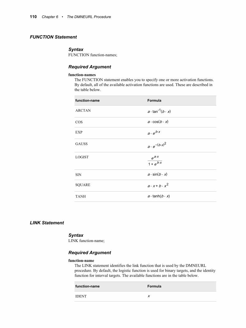
FUNCTION Statement
SyntaxFUNCTION function-names;
Required Argumentfunction-names
The FUNCTION statement enables you to specify one or more activation functions. By default, all of the available activation functions are used. These are described in the table below.
function-name Formula
ARCTAN a ⋅ tan-1(b ⋅ x)
COS a ⋅ cos(b ⋅ x)
EXP a ⋅ e b⋅x
GAUSSa ⋅ e −(b⋅x)
2
LOGIST e a⋅x
1 + e b⋅x
SIN a ⋅ sin(b ⋅ x)
SQUARE a ⋅ x + b ⋅ x 2
TANH a ⋅ tanh(b ⋅ x)
LINK Statement
SyntaxLINK function-name;
Required Argumentfunction-name
The LINK statement identifies the link function that is used by the DMNEURL procedure. By default, the logistic function is used for binary targets, and the identity function for interval targets. The available functions are in the table below.
function-name Formula
IDENT x
110 Chapter 6 • The DMNEURL Procedure
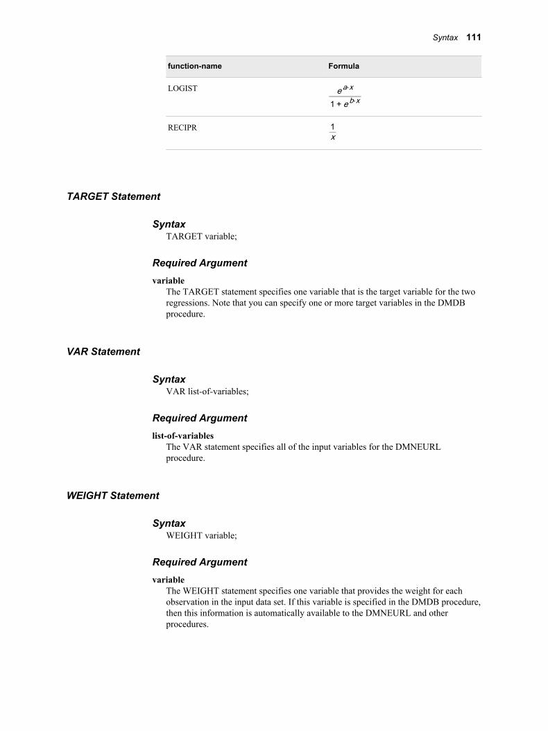
function-name Formula
LOGIST e a⋅x
1 + e b⋅x
RECIPR 1x
TARGET Statement
SyntaxTARGET variable;
Required Argumentvariable
The TARGET statement specifies one variable that is the target variable for the two regressions. Note that you can specify one or more target variables in the DMDB procedure.
VAR Statement
SyntaxVAR list-of-variables;
Required Argumentlist-of-variables
The VAR statement specifies all of the input variables for the DMNEURL procedure.
WEIGHT Statement
SyntaxWEIGHT variable;
Required Argumentvariable
The WEIGHT statement specifies one variable that provides the weight for each observation in the input data set. If this variable is specified in the DMDB procedure, then this information is automatically available to the DMNEURL and other procedures.
Syntax 111
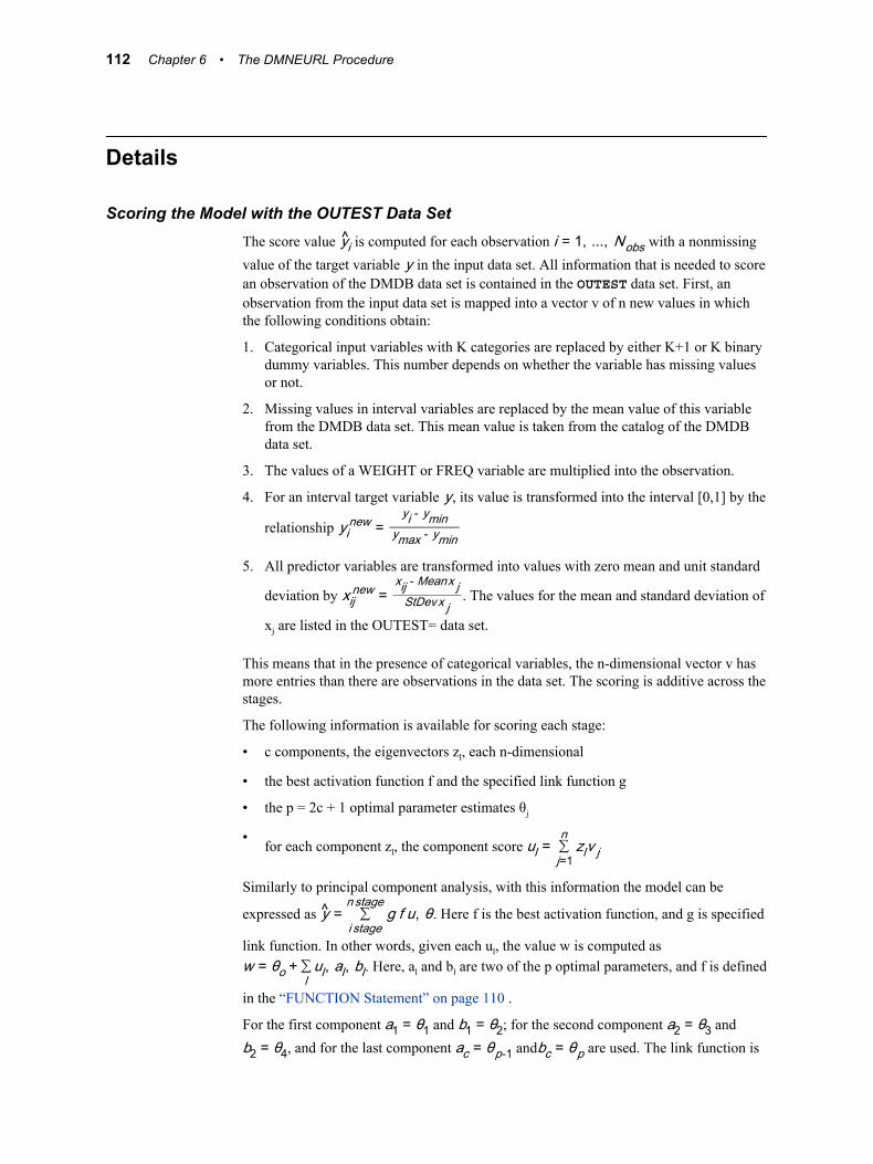
Details
Scoring the Model with the OUTEST Data SetThe score value yi is computed for each observation i = 1, ..., Nobs with a nonmissing value of the target variable y in the input data set. All information that is needed to score an observation of the DMDB data set is contained in the OUTEST data set. First, an observation from the input data set is mapped into a vector v of n new values in which the following conditions obtain:
1. Categorical input variables with K categories are replaced by either K+1 or K binary dummy variables. This number depends on whether the variable has missing values or not.
2. Missing values in interval variables are replaced by the mean value of this variable from the DMDB data set. This mean value is taken from the catalog of the DMDB data set.
3. The values of a WEIGHT or FREQ variable are multiplied into the observation.
4. For an interval target variable y, its value is transformed into the interval [0,1] by the
relationship yinew =
yi - yminymax - ymin
5. All predictor variables are transformed into values with zero mean and unit standard
deviation by xijnew =
xij - Meanx jStDevx j
. The values for the mean and standard deviation of
xj are listed in the OUTEST= data set.
This means that in the presence of categorical variables, the n-dimensional vector v has more entries than there are observations in the data set. The scoring is additive across the stages.
The following information is available for scoring each stage:
• c components, the eigenvectors zl, each n-dimensional
• the best activation function f and the specified link function g
• the p = 2c + 1 optimal parameter estimates θj
• for each component zl, the component score ul = ∑j=1
nzlv j
Similarly to principal component analysis, with this information the model can be
expressed as y = ∑i stage
nstageg f u, θ. Here f is the best activation function, and g is specified
link function. In other words, given each ul, the value w is computed as w = θo + ∑l
ul, al, bl . Here, al and bl are two of the p optimal parameters, and f is defined
in the “FUNCTION Statement” on page 110 .
For the first component a1 = θ1 and b1 = θ2; for the second component a2 = θ3 and b2 = θ4, and for the last component ac = θp-1 andbc = θp are used. The link function is
112 Chapter 6 • The DMNEURL Procedure
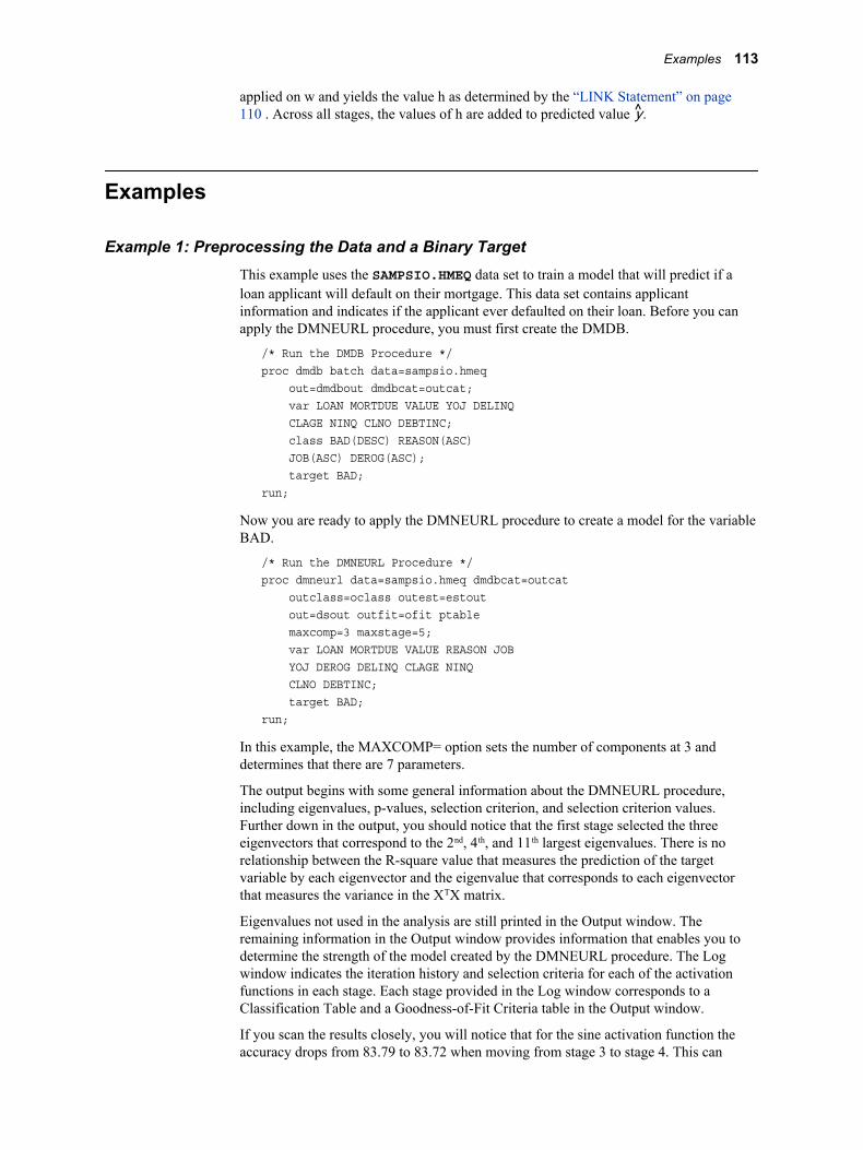
applied on w and yields the value h as determined by the “LINK Statement” on page 110 . Across all stages, the values of h are added to predicted value y.
Examples
Example 1: Preprocessing the Data and a Binary TargetThis example uses the SAMPSIO.HMEQ data set to train a model that will predict if a loan applicant will default on their mortgage. This data set contains applicant information and indicates if the applicant ever defaulted on their loan. Before you can apply the DMNEURL procedure, you must first create the DMDB.
/* Run the DMDB Procedure */proc dmdb batch data=sampsio.hmeq out=dmdbout dmdbcat=outcat; var LOAN MORTDUE VALUE YOJ DELINQ CLAGE NINQ CLNO DEBTINC; class BAD(DESC) REASON(ASC) JOB(ASC) DEROG(ASC); target BAD;run;
Now you are ready to apply the DMNEURL procedure to create a model for the variable BAD.
/* Run the DMNEURL Procedure */proc dmneurl data=sampsio.hmeq dmdbcat=outcat outclass=oclass outest=estout out=dsout outfit=ofit ptable maxcomp=3 maxstage=5; var LOAN MORTDUE VALUE REASON JOB YOJ DEROG DELINQ CLAGE NINQ CLNO DEBTINC; target BAD;run;
In this example, the MAXCOMP= option sets the number of components at 3 and determines that there are 7 parameters.
The output begins with some general information about the DMNEURL procedure, including eigenvalues, p-values, selection criterion, and selection criterion values. Further down in the output, you should notice that the first stage selected the three eigenvectors that correspond to the 2nd, 4th, and 11th largest eigenvalues. There is no relationship between the R-square value that measures the prediction of the target variable by each eigenvector and the eigenvalue that corresponds to each eigenvector that measures the variance in the XTX matrix.
Eigenvalues not used in the analysis are still printed in the Output window. The remaining information in the Output window provides information that enables you to determine the strength of the model created by the DMNEURL procedure. The Log window indicates the iteration history and selection criteria for each of the activation functions in each stage. Each stage provided in the Log window corresponds to a Classification Table and a Goodness-of-Fit Criteria table in the Output window.
If you scan the results closely, you will notice that for the sine activation function the accuracy drops from 83.79 to 83.72 when moving from stage 3 to stage 4. This can
Examples 113
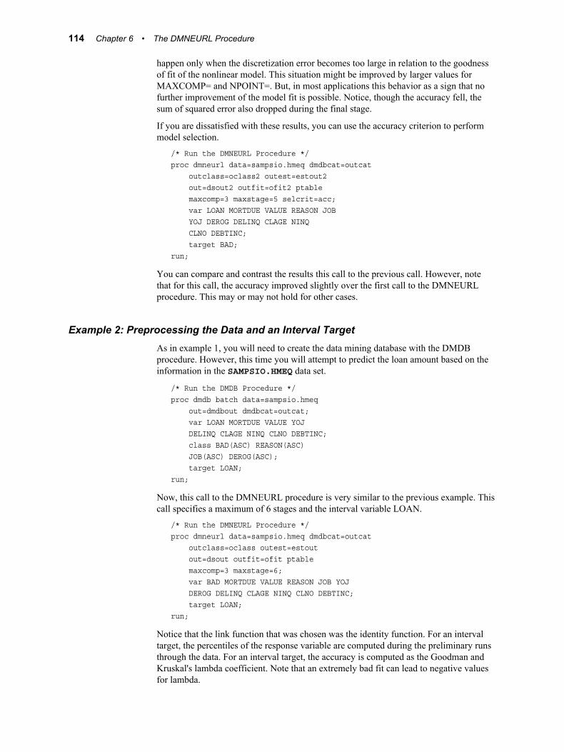
happen only when the discretization error becomes too large in relation to the goodness of fit of the nonlinear model. This situation might be improved by larger values for MAXCOMP= and NPOINT=. But, in most applications this behavior as a sign that no further improvement of the model fit is possible. Notice, though the accuracy fell, the sum of squared error also dropped during the final stage.
If you are dissatisfied with these results, you can use the accuracy criterion to perform model selection.
/* Run the DMNEURL Procedure */proc dmneurl data=sampsio.hmeq dmdbcat=outcat outclass=oclass2 outest=estout2 out=dsout2 outfit=ofit2 ptable maxcomp=3 maxstage=5 selcrit=acc; var LOAN MORTDUE VALUE REASON JOB YOJ DEROG DELINQ CLAGE NINQ CLNO DEBTINC; target BAD;run;
You can compare and contrast the results this call to the previous call. However, note that for this call, the accuracy improved slightly over the first call to the DMNEURL procedure. This may or may not hold for other cases.
Example 2: Preprocessing the Data and an Interval TargetAs in example 1, you will need to create the data mining database with the DMDB procedure. However, this time you will attempt to predict the loan amount based on the information in the SAMPSIO.HMEQ data set.
/* Run the DMDB Procedure */proc dmdb batch data=sampsio.hmeq out=dmdbout dmdbcat=outcat; var LOAN MORTDUE VALUE YOJ DELINQ CLAGE NINQ CLNO DEBTINC; class BAD(ASC) REASON(ASC) JOB(ASC) DEROG(ASC); target LOAN;run;
Now, this call to the DMNEURL procedure is very similar to the previous example. This call specifies a maximum of 6 stages and the interval variable LOAN.
/* Run the DMNEURL Procedure */proc dmneurl data=sampsio.hmeq dmdbcat=outcat outclass=oclass outest=estout out=dsout outfit=ofit ptable maxcomp=3 maxstage=6; var BAD MORTDUE VALUE REASON JOB YOJ DEROG DELINQ CLAGE NINQ CLNO DEBTINC; target LOAN;run;
Notice that the link function that was chosen was the identity function. For an interval target, the percentiles of the response variable are computed during the preliminary runs through the data. For an interval target, the accuracy is computed as the Goodman and Kruskal's lambda coefficient. Note that an extremely bad fit can lead to negative values for lambda.
114 Chapter 6 • The DMNEURL Procedure

If you examine the output, you will see that there were six stages and 48 objective function optimizations, each with 7 parameters. The DMNEURL procedure made 33 passes through the data. On average, the computation of each objective function took 4 iterations and needed 7 function calls. The most accurate prediction after stage 5 was the square activation function and identity link function at 47.33%.
Examples 115

116 Chapter 6 • The DMNEURL Procedure
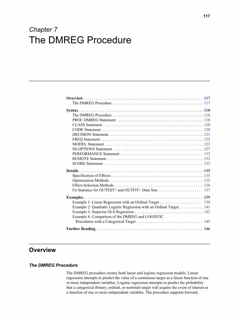
Chapter 7
The DMREG Procedure
Overview . . . . . . . . . . . . . . . . . . . . . . . . . . . . . . . . . . . . . . . . . . . . . . . . . . . . . . . . . . . 117The DMREG Procedure . . . . . . . . . . . . . . . . . . . . . . . . . . . . . . . . . . . . . . . . . . . . . 117
Syntax . . . . . . . . . . . . . . . . . . . . . . . . . . . . . . . . . . . . . . . . . . . . . . . . . . . . . . . . . . . . . . 118The DMREG Procedure . . . . . . . . . . . . . . . . . . . . . . . . . . . . . . . . . . . . . . . . . . . . . 118PROC DMREG Statement . . . . . . . . . . . . . . . . . . . . . . . . . . . . . . . . . . . . . . . . . . . 118CLASS Statement . . . . . . . . . . . . . . . . . . . . . . . . . . . . . . . . . . . . . . . . . . . . . . . . . . 120CODE Statement . . . . . . . . . . . . . . . . . . . . . . . . . . . . . . . . . . . . . . . . . . . . . . . . . . 120DECISION Statement . . . . . . . . . . . . . . . . . . . . . . . . . . . . . . . . . . . . . . . . . . . . . . . 121FREQ Statement . . . . . . . . . . . . . . . . . . . . . . . . . . . . . . . . . . . . . . . . . . . . . . . . . . . 122MODEL Statement . . . . . . . . . . . . . . . . . . . . . . . . . . . . . . . . . . . . . . . . . . . . . . . . . 123NLOPTIONS Statement . . . . . . . . . . . . . . . . . . . . . . . . . . . . . . . . . . . . . . . . . . . . . 127PERFORMANCE Statement . . . . . . . . . . . . . . . . . . . . . . . . . . . . . . . . . . . . . . . . . 132REMOTE Statement . . . . . . . . . . . . . . . . . . . . . . . . . . . . . . . . . . . . . . . . . . . . . . . . 132SCORE Statement . . . . . . . . . . . . . . . . . . . . . . . . . . . . . . . . . . . . . . . . . . . . . . . . . 133
Details . . . . . . . . . . . . . . . . . . . . . . . . . . . . . . . . . . . . . . . . . . . . . . . . . . . . . . . . . . . . . . 135Specification of Effects . . . . . . . . . . . . . . . . . . . . . . . . . . . . . . . . . . . . . . . . . . . . . . 135Optimization Methods . . . . . . . . . . . . . . . . . . . . . . . . . . . . . . . . . . . . . . . . . . . . . . 135Effect-Selection Methods . . . . . . . . . . . . . . . . . . . . . . . . . . . . . . . . . . . . . . . . . . . . 136Fit Statistics for OUTEST= and OUTFIT= Data Sets . . . . . . . . . . . . . . . . . . . . . . 137
Examples . . . . . . . . . . . . . . . . . . . . . . . . . . . . . . . . . . . . . . . . . . . . . . . . . . . . . . . . . . . 139Example 1: Linear Regression with an Ordinal Target . . . . . . . . . . . . . . . . . . . . . 139Example 2: Quadratic Logistic Regression with an Ordinal Target . . . . . . . . . . . . 141Example 3: Stepwise OLS Regression . . . . . . . . . . . . . . . . . . . . . . . . . . . . . . . . . . 142Example 4: Comparison of the DMREG and LOGISTIC
Procedures with a Categorical Target . . . . . . . . . . . . . . . . . . . . . . . . . . . . . . . . . 145
Further Reading . . . . . . . . . . . . . . . . . . . . . . . . . . . . . . . . . . . . . . . . . . . . . . . . . . . . . 146
Overview
The DMREG ProcedureThe DMREG procedure creates both linear and logistic regression models. Linear regression attempts to predict the value of a continuous target as a linear function of one or more independent variables. Logistic regression attempts to predict the probability that a categorical (binary, ordinal, or nominal) target will acquire the event of interest as a function of one or more independent variables. The procedure supports forward,
117
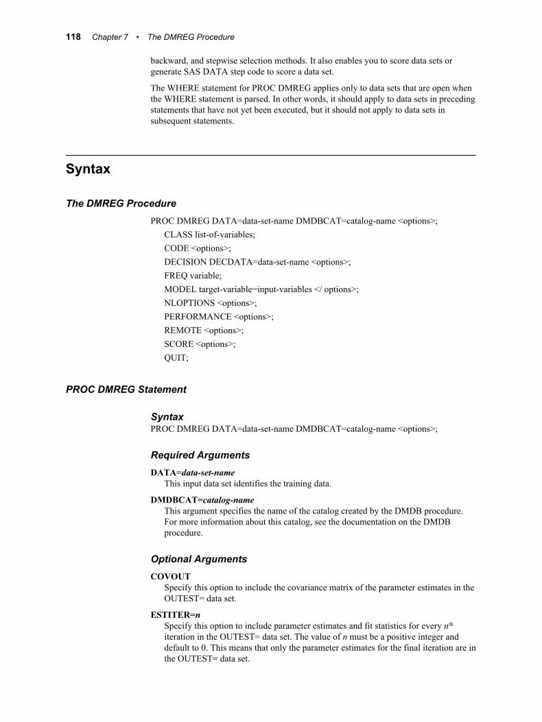
backward, and stepwise selection methods. It also enables you to score data sets or generate SAS DATA step code to score a data set.
The WHERE statement for PROC DMREG applies only to data sets that are open when the WHERE statement is parsed. In other words, it should apply to data sets in preceding statements that have not yet been executed, but it should not apply to data sets in subsequent statements.
Syntax
The DMREG ProcedurePROC DMREG DATA=data-set-name DMDBCAT=catalog-name <options>;
CLASS list-of-variables;CODE <options>;DECISION DECDATA=data-set-name <options>;FREQ variable;MODEL target-variable=input-variables </ options>;NLOPTIONS <options>;PERFORMANCE <options>;REMOTE <options>;SCORE <options>;QUIT;
PROC DMREG Statement
SyntaxPROC DMREG DATA=data-set-name DMDBCAT=catalog-name <options>;
Required ArgumentsDATA=data-set-name
This input data set identifies the training data.
DMDBCAT=catalog-nameThis argument specifies the name of the catalog created by the DMDB procedure. For more information about this catalog, see the documentation on the DMDB procedure.
Optional ArgumentsCOVOUT
Specify this option to include the covariance matrix of the parameter estimates in the OUTEST= data set.
ESTITER=nSpecify this option to include parameter estimates and fit statistics for every nth
iteration in the OUTEST= data set. The value of n must be a positive integer and default to 0. This means that only the parameter estimates for the final iteration are in the OUTEST= data set.
118 Chapter 7 • The DMREG Procedure
INEST=data-set-nameThis argument specifies an input data set that contains the initial estimates.
MINIMALSpecify this option to minimize the resources that are used when the DMREG procedure finds the logistic regression model. The conjugate gradient technique is used and standard errors for the regression parameters are not computed. Memory for the Hessian matrix is not needed. Model selection is disabled when this option is specified. The MINIMAL option does not apply to normal error regression models.
NAMELEN=numberThis argument specifies the length of effect names in the printed output. The effect names are limited to number characters, where number is an integer between 20 and 200 and default to 20.
NOPRINTSpecify this option to suppress all printed output.
OUTMAP=data-set-nameThis option specifies the output data set that contains the variable mappings for each of the parameter names. There is a variable for each model parameter. In addition, the data set contains the character variables _TYPE_ and _NAME_. The value for _NAME_ can be either INPUT, which identifies the input variables that the parameters are associated with, or CODE, which identifies the equivalent variables in the scoring code.
OUTEST=data-set-nameThis option specifies an output data set that contains the estimation and fit statistics.
OUTTERM=data-set-nameThis option specifies an output data set that contains the estimated coefficients, the corresponding t-statistics, and the p-values.
This data contains the following variables:
• Term — is a numeric value that represents the parameter number, starting at 0. Observations that have the same value for Term correspond to the same parameter.
• Variable — is a character value that represents the name of the input variables that the parameter is associated with.
• ClassLevel — is a character value that represents the categorical level of the corresponding input variable. This value is blank for interval variables.
• Coefficient — represents the estimated regression coefficient.
• tValue — represents the t-statistics.
• pValue — represents the p-value.
Note: The values of Variable and ClassLevel identify a parameter, but it can take more than one observation to do so. In this case, the value of Term for these observations is identical.
SIMPLESpecify this option to print simple descriptive statistics for the input variables.
TESTDATA=data-set-nameThis option specifies the test data set.
VALIDATA=data-set-nameThis option specifies the validation data set.
Syntax 119
CLASS Statement
SyntaxCLASS list-of-variables;
Required Argumentlist-of-variables
This CLASS statement specifies a list of categorical variables that are used in the analysis. If the target variable is a categorical variable, then it must be specified in the CLASS statement.
CODE Statement
SyntaxCODE <options>;
If you want to score a data set, you can use the CODE statement to write SAS DATA step code to a file or catalog entry. You can include this code in a DATA step that uses a SET statement to read the scored data set. Alternatively, you can use the PMML option to produce XML scoring code for a database engine. You can specify this statement multiple times in the same call to the DMREG procedure.
Optional ArgumentsCATALOG | CAT | C=libaray.catalog.entry.type
This option specifies where to write the output SAS DATA step code. The default value for library is determined by the SAS system option USER= and is usually WORK. The default entry is SASCODE and the default type is SOURCE.
You cannot specify both FILE= and CATALOG= in the same CODE statement. If you specify neither, the code is written to the SAS log unless the PMML option is specified.
DUMMIES | NODUMMIESSpecify DUMMIES to keep dummy variables, standardized variables, and other transformed variables in the data set. By default, these variables are dropped.
ERROR | NOERRORSpecify ERROR to compute the error function.
FILE=file-nameThe SAS DATA step code is saved in the file specified here. You can either specify the full pathname in a quoted string or provide an unquoted SAS filename or eight bytes or less. If the filename is an assigned fileref in a FILENAME statement, that file is used. The filerefs LOG and PRINT are reserved for the SAS system. If the specified name is not an assigned fileref, then file-name is saved as file-name.txt.
FORMAT=formatUse this option to format weights and other numeric values that do not have a format specified in the input data set. The default value for format is BEST20.
120 Chapter 7 • The DMREG Procedure
GROUP=group-identifierUse this option to specify the group identifier that is used for group processing. The group identifier should be a valid SAS name, 32 bytes or less. The group identifier is used to construct array names and statement labels in the generated code.
LINESIZE | LS=numberThis option specifies the line size for generated code. The value of number must be an integer between 64 and 254 and default to 72.
PMML | XMLSpecify this option to create scoring code in the Predictive Modeling Markup Language, an XML-based standard to represent data mining results. You must specify an ODS PMML destination before you invoke the DMREG procedure, such as
ods pmml file=’foo.xml’;proc dmreg; model y=x; code pmml; run;ods pmml close;
For more information, see the PMML Support in Enterprise Miner section in the Enterprise Miner help.
RESIDUAL | NORESIDUALSpecify RESIDUAL to compute the residual values for the variables R_*, F_*, CL_*, CP_*, BL_*, BP_*, and ROI_*. By default, the residuals are not computed. If you request code for residuals and then score a data set that does not contain target values, the residuals will have missing values.
DECISION Statement
SyntaxDECISION DECDATA=data-set-name <options>;
Required ArgumentDECDATA=data-set-name
This argument specifies the input data set that contains the decision matrix, the prior probabilities, or both. This data set might contain decision variables that are specified with the DECVARS= option. Also, it may contain prior probability variables that are specified with the PRIORVAR option.
This data set must contain the target variable, which is specified in the TARGET statement.
For a categorical target variable, there should be one observation for each class. Each entry dij in the decision matrix indicates the consequence of selecting target value i for variable j. If any class appears twice or more in this data set, an error message is printed and the procedure terminates. Any class value in the input data set that is not found in this data set is treated as a missing class value.
For an interval target variable, each row defines a knot in a piecewise linear spline function. The consequence of making a decision is computed by interpolating in the corresponding column of the decision matrix. If the predicted target value is outside the range of knots in the decision matrix, the consequence is computed by linear extrapolation. If the target values are monotonically increasing or decreasing, any
Syntax 121
interior target value is allowed to appear twice in data set. This enables you to specify discontinuities in the data. The end points, which are the minimum and maximum data points, might not appear more than once. No target value is allowed to appear more than twice. If the target values are not monotonic, then they are sorted by the procedure and are not allowed to appear more than once.
T I P The DECDATA= data set can be of type LOSS, PROFIT, or REVENUE. PROFIT is assumed by default. TYPE is a data set option that is specified in parentheses after the data set name when the data set is created or used.
Optional ArgumentsDECVARS=list-of-variables
This option specifies the numeric decision variables in the DECDATA= data set that contain the target-specific consequences for each decision. The decision variables cannot contain any missing values.
COST=list-of-costsThis option specifies one of the following:
• numeric constants that give the cost of a decision
• numeric variables in the input data set that contain case-specific costs
• any combination of constants and variables
There must be the same number of cost constants and variables as there are decision variables in the DECVARS= option. In this option, you cannot use abbreviated variable lists. For any case where a cost variable is missing, the results for that case are considered missing. By default all costs are assumed to be 0. Furthermore, this option can be used only when the DECDATA= data set is of type REVENUE.
PRIORVAR=varaibleThis option specifies the number variable in the DECDATA= data set that contains the prior probabilities that are used to make decisions. Prior probabilities are also used to adjust the total and average profit or loss. Prior probabilities cannot be missing or negative, and there must be at least one positive prior probability. The prior probabilities are not required to sum 1. But, if they do not sum to 1, then they are scaled by some constant so that they do sum to 1. If this option is not specified, then no adjustment for prior probabilities is applied to the posterior probabilities.
FREQ Statement
SyntaxFREQ variable;
Required Argumentvariable
The FREQ statement specifies the frequency variable. This variable contains the frequency value for each observation in the input data set. If you do not use the FREQ statement in the DMREG procedure, then the frequency variable in the DMDB catalog is used. If you specify the FREQ statement but not a variable name, then each observation is assigned a frequency of 1.
If the DMDB contains a frequency variable, you should not use the FREQ statement in the DMREG procedure to specify a different variable. If you specify a different variable, it can contain invalid frequency values (for example, zero or negative
122 Chapter 7 • The DMREG Procedure
values) for observations in the training data. These observations are ignored and thus improperly excluded from the data mining analysis.
MODEL Statement
SyntaxMODEL target-variable=input-variables </ options>;
The model statement is used to specify a single target variable and several input variables. The options listed below are grouped according to the features that they affect, but can be specified in any order.
Required Argumenttarget-variable=input-variables
Use the model statement to define the target variable in terms of the input variables.
Display OptionsCORRB
Specify this option to print the correlation matrix in the output.
COVBSpecify this option to print the covariance matrix in the output.
DETAILSSpecify this option to print the details for each step of the variable selection process in the output.
NODESIGNPRINT | NODPThis option suppresses the class variable input coding display in the output.
SHORTThis option suppresses printing the results of the intermediate models that the DMREG procedure fits during the variable selection process. When you specify the SHORT model option, the output prints only the variable selection summary and the results of the chosen model. The SHORT option has no effect if the SELECTION= option is not specified.
FITTING OptionsMISCCONV=number
This option specifies the critical misclassification rate for the convergence criterion that is based on misclassification rates. If the MISCCONV= value is greater than 0, the optimization phase terminates and declares convergence when the misclassification rate is less than or equal to the MISCCONV= value. The value of number must be a real number between 0 and 1 and default to 0.
STARTMISC=numberThis option specifies the number of iterations that are processed before checking the misclassification rate. The default value for the number of iterations depends on the optimization method that is specified in the TECHNIQUE= option of the NLOPTIONS statement.
Possible cases are as follows:
• When the TECHNIQUE= option specifies NEWRAP (Newton-Raphson Optimization with Line Search), NRRIDG (Newton-Raphson Ridge
Syntax 123
Optimization), or TRUREG (Trust Region Optimization), then the default value for STARTMISC= is 3.
• When the TECHNIQUE= option specifies QUANEW (Quasi-Newton Optimization) or DBLDOG (Double Dogleg Optimization), then the default value for STARTMISC= is 5.
• When the TECHNIQUE= option specifies CONGRA (Conjugate Gradient Optimization), then the default value for STARTMISC= is 10.
The value of number must be a positive integer.
Confidence Interval OptionsALPHA=number
This option specifies the significance level for confidence interval regression parameters. The value of number must be between 0 and 1 and default to 0.05
CLPARMSpecify this option to compute and include confidence intervals for regression parameters in the output.
Selection OptionsCHOOSE=criterion
The DMREG procedure will choose the model that yields the best value of the criterion that is specified here at each step of model construction. If the optimal value of the specified criterion occurs for models at more than one step, then the model with the smallest number of parameters is chosen.
The following criteria are available for choosing the model:
• AIC — chooses the model that has the smallest Akaike Information Criterion value.
• NONE — chooses the model at the final step of the selection process.
• SBC — chooses the model that has the smallest Schwarz Bayesian Criterion value.
• TDECDATA — chooses the model that has the largest total profit or smallest total loss for the training data.
• VDECDATA — chooses the model that has the largest total profit or smallest total loss from the validation data.
• VERROR — chooses the model that has the smallest error rate for the validation data. The error rate for a least-squares regression model is the sum of squared error. The error rate for a logistic regression model is the negative log-likelihood.
• VMISC — chooses the model that has the smallest misclassification rate for the validation data.
• XDECDATA — chooses the model according to the total profit or loss from cross-validation of the training data. The model with the largest profit or smallest loss is chosen.
• XERROR — chooses the model that has the smallest error rate from cross-validation of the training data. The error rate for a least squares regression model is the sum of squared error. The error rate for a logistic regression model is the negative log-likelihood.
124 Chapter 7 • The DMREG Procedure
• XMISC — chooses the model with the smallest misclassification rate from the cross-validation of the training data.
The default value is VERROR if you specify a VALIDATA= data set. The default value is TDECDATA if you use decision processing (that is, you specify the DECISION statement). Otherwise, the default value is NONE.
HIERARCHY= numberThis option specifies the variable inclusion rule that is used to determine variable selection for the model.
The following variable inclusion rules are available:
• ALL — uses all independent variables that meet hierarchical requirements. This is the default value.
• CLASS — uses only the class variables that meet hierarchical requirements.
INCLUDE=numberIncludes the first number effects in the model. The value of number must be a positive integer and default to 0.
MAXSTEP=numberThis option specifies the maximum number of steps permitted when you use the STEPWISE variable selection method. The value of number must be a positive integer. The default value is twice the number of effects that are specified in the MODEL statement.
RULE=MULTIPLE | NONE | SINGLEThis option specifies the effects selection rule that you want to use when you specify SELECTION= as FORWARD, BACKWARD, or STEPWISE in the MODEL statement.
The available effects selection rules are as follows:
• MULTIPLE — One or more effects are considered for entry or removal at the same time, so long as the hierarchical rule is observed. Consider the case where main effects A and B are not in the model and the interaction A*B is not in the model. The effects considered for entry in a single step are just A, just B, A then B, and A*B.
• NONE — Effects are included or excluded one at a time, without preservation of any hierarchical order. This is the default setting.
• SINGLE — A single effect is considered for entry into the model only if its lower order effects are already in the model. A single effect is considered for removal from the model only if its higher order effects are not in the model.
SELECTION=BACKWARD | FORWARD | NONE | STEPWISEThis option specifies the method used to select effects for the selecting process. For more information about these methods, see “Effect-Selection Methods” on page 136 .
• BACKWARD — specifies backward elimination. This method starts with all effects in the model and deletes effects.
• FORWARD — specifies forward selection. This method starts with no effects in the model and adds effects.
• NONE — specifies no model selection. The complete specifications in the MODEL statement are used to fit the model. This is the default method.
Syntax 125
• STEPWISE — specifies stepwise regression. This is similar to the FORWARD method, except that the effects already in the model do not necessarily stay in the model as time progresses.
SEQUENTIALWhen you specify this option, the DMREG procedure adds or deletes input variables and effects sequentially, as specified in the MODEL statement.
SLENTRY=numberThis option specifies the significance level that is used as a threshold criterion to add input variables. Variables that have p-values less than or equal to number are added as inputs. The value of number must be a real number greater than 0 and default to 0.05.
SLSTAY=numberThis option specifies the significance level that is used as a threshold criterion to remove variables. Variables that have p-values greater than number are removed from the list of input variables. The value of number must be a real number greater than 0 and default to 0.05.
START=numberSpecify this option to include the first number effects in the starting model.
• For models that use the FORWARD or STEPWISE selection methods, the default value for the START= option is 0.
• For models that use the BACKWARD selection method, the default value for the START= option is the total number of effects in the MODEL statement.
STOP=numberThe effects selection process terminates after number effects have been either added (using the FORWARD method) or removed (using the BACKWARD method) from the model. The STOP= option has no effect when the model effect selection method is set to NONE or STEPWISE. The value of number is an integer value that ranges from 0 to the total number of effects in the MODEL statement. The default value of number is the total number of effects for FORWARD selection and 0 for BACKWARD selection.
Specification OptionsCODING=DEVIATION | GLM
This option specifies the coding method that you want to use for class input variables. Specify DEVIATION to use deviation from the mean coding, also known as effect coding. This is the default setting. Specify GLM to use non-full rank generalized linear model coding, as performed by the GLM procedure.
ERROR=MBERNOULLI | NORMALThis option specifies the error distribution. MBERNOULLI specifies a multinomial distribution with one trial, and NORMAL specifies a normal distribution. MBERNOULLI includes the binomial distribution with one trial and is not available for interval targets, but is the default for all other targets. You cannot use NORMAL with nominal measurements, but it is the default value for interval targets.
LEVEL=INTERVAL | NOMINAL | ORDINALThis option specifies the measurement level of the target variable. The default value for a categorical target is ORDINAL and for a numeric target is INTERVAL.
LINK=CLOGLOG | IDENTITY | LOGIT | PROBITThis option specifies the link function that represents the expected values of the target to the linear predictors.
126 Chapter 7 • The DMREG Procedure
• CLOGLOG — specifies the complementary log-log function, which is the inverse of the extreme value distribution function. The CLOGLOG function is available for ordinal and binary targets.
• IDENTITY — specifies the identity function. This link function can be used only with linear regression analysis. This is the default setting when you specify ERROR=NORMAL.
• LOGIT — specifies the logit function, which is the inverse of the logistic distribution function. This function is available for nominal, ordinal, or binary targets. This is the default setting when you specify ERROR=MBERNOULLI.
• PROBIT — specifies the probit function, which is the inverse of the standard normal distribution function. This function is available for ordinal or binary targets.
The CLOGLOG, LOGIT, and PROBIT functions are used for a logistic regression analysis.
NOINTSpecify this option to suppress the intercept for the binary target model or the normal error for the linear regression model.
SINGULAR=numberThis option specifies the tolerance level when the DMREG procedure tests for singular matrices. The value of number must be a real, positive number and default to 0.000001.
NLOPTIONS Statement
SyntaxNLOPTIONS <options>;
The NLOPTIONS statement specifies options for the nonlinear optimization. These options only apply when the logistic regression model is fit. Let β be the parameter vector of interest. You want to maximize the log-likelihood objective function l(B). Let g(β) denote the gradient vector of β and H(β) the Hessian matrix for β. The gradient with respect to the ith parameter is denoted as gi(β). Superscripts in parentheses indicate the iteration count. Thus, g(k) = g(β(k)) is the gradient vector at iteration k, H(k) = H(β(k)) is the Hessian matrix at iteration k, and Hi,i
(k) is the ith diagonal element of H(k).
Optional ArgumentsABSCONV=number
This option specifies an absolute function convergence criterion. Termination requires l(β(k)) ≥ number. The value of number must be a real, positive number and default to 0.001 times the log-likelihood of the intercept only model.
ABSFCONV=numberThis option specifies an absolute function convergence criterion. Termination requires a small change of the log-likelihood in successive iterations, that is, |l(β(k+1)) - l(β(k))| ≤ number. The value of number must be a real, positive number and default to 0.00001.
Syntax 127
ABSGCONV=numberThis option specifies the absolute gradient convergence criterion. Termination requires max
j| gi(β (k )) | ≤ number. The value of number must be a real, positive
number and default to 0.00001.
ABSXCONV=numberThis option specifies the absolute parameter convergence criterion. Termination requires β k − β (k−1)
2 ≤ number. The value of number must be a real, positive number and default to 10–8.
DAMPSTEP=numberThis option specifies the initial step size for each line search used by the QUANEW, CONGRA, and NEWRAP techniques. The step size cannot be larger than the product of number and the step size used in the previous iteration. The value of number must be a real, positive number and default to 2.
DIAHESSpecify this option to force the TRUREG, NEWRAP, and NRRIDG optimization algorithms to take advantage of the diagonality of the Hessian matrix.
FCONV=numberThis option specifies a function convergence criterion. Termination requires
| l(β (k )) − l(β (k−1)) |max( | l(β (k−1)) | , FSIZE) ≤ number, where FSIZE is defined in the FSIZE=
option. The value of number must be a real, positive number and default to 10–FDIGITS, where FDIGITS is provided by the FDIGITS= option.
FCONV2=numberThis argument specifies another function convergence criterion. Termination requires a small predicted reduction: l(β (k )) − l(β (k ) − H (k ) −1 ⋅ g (0) k ) ≤ number. The value of number must be a real, positive number and default to 10–4.
FDIGITS=numberThis option specifies the number of accurate digits when the objective function is evaluated. The value of number must be a real, positive number and default to -log(M), where M is the machine precision.
FSIZE=numberThis option specifies the parameter of the relative function and relative gradient termination criteria. The value of number must be a nonnegative real number and default to 0.
GCONV=numberThis option specifies the relative gradient convergence criterion. Except for the CONGRA technique, termination requires that the normalized predicted function
reduction is small: g (k ) ′ H (k ) −1g (k )
max( | l(β (k )) | , FSIZE) ≤ number. Here, FSIZE is defined in
the FSIZE= option. For the CONGRA technique, termination requires g (k )
22 ⋅ s(β (k )) 2
g (k ) − g (k−1)2 ⋅ max( | l(β(k )) | , FSIZE)
≤ number, where s(β(k)) is the
step increment at iteration k. The value of number must be a real, positive number and default to 10–6.
128 Chapter 7 • The DMREG Procedure
GCONV2=numberThis option specifies another relative gradient convergence criterion. Termination
requires maxi
| gi(β (k ))l(β (k )) ⋅ H i,i
(k ) | . The value of number must be a real, positive
number and default to 0.
HESCAL=0 | 1 | 2 | 3This option specifies the scaling version of the Hessian or cross-product Jacobian matrix that is used for NRRIDG, TRUREG, LEVMAR, NEWRAP, or DBLDOG optimization. If HESCAL is not equal to 0, the first iteration and each restart iteration set the diagonal scaling matrix D (0) = diag(di(0)), where
di(0) = max( | H i,i
(0) | , M ) and Hi,i(0) are the diagonal elements of the Hessian or
cross-product Jacobian matrix. In every other iteration, the diagonal scaling matrix D(0) is updated based on the HESCAL= option.
• Specify 0 to indicate that no scaling should be done.
• Specify 1 to do the More (1978) scaling update: di(k+1) = max(di(k ), max( | H i,i
(k ) | , M )).• Specify 2 to do the Dennis, Gay, and Welsch (1981) scaling update:
di(k+1) = max(0.6 ⋅ di(k ), max( | H i,i
(k ) | , M )).• Specify 3 to reset di in each iteration: di
(k+1) = max( | H i ,i(k ) | , M ).
In each scaling update, epsilon is the relative machine precision. The default value is HESCAL=1 for the LEVMAR minimization technique and 0 for all others. Scaling of the Hessian can be time consuming when general linear constraints are active.
INHESSIAN=numberThis option specifies how the initial estimate of the approximate Hessian is defined for the quasi-Newton techniques QUANEW and DBLDOG. The initial estimate of the approximate Hessian is set to number times the matrix. If the value of number is 0, then the initial estimate is computed from the magnitude of the initial gradient. The value of number must be a nonnegative real number and default to H(0), the Hessian at the initial estimate β(0).
INSTEP=numberThis option specifies the radius of the trust region used in the TRUREG, DBLDOG, and LEVMAR algorithms. The value of number , must be a real, positive number and default to 1.
LINESEARCH=numberThis option specifies the line-search method for the CONGRA, QUANEW, and NEWRAP optimization techniques. The value of number must be between 1 and 8, inclusive, and default to 2.
LSPRECISION=numberThis option specifies the degree of accuracy that should be obtained by the second and third line-sear algorithms. The default value varies based on technique and update method.
Technique Update Method Default Value
QUANEW DBFGS, BFGS 0.4
Syntax 129
Technique Update Method Default Value
QUANEW DDFP, DFP 0.06
CONGRA All Methods 0.1
NEWRAP No Update Method 0.9
The value of number must be a real, positive number.
MAXFUNC=numberThis option specifies the maximum number of function calls in the optimization process. The objective function that is minimized is the negative log-likelihood function. The value of number must be a real, positive number. The default value is 125 for the TRUREG, NRRIDG, and NEWRAP methods; 500 for the QUANEW and DBLDOG methods; and 1000 for the CONGRA method.
MAXITER=numberThis option specifies the maximum number of iterations in the optimization process. The value of number must be a real, positive number. The default value is 50 for the TRUREG, NRRIDG, and NEWRAP methods; 200 for the QUANEW and DBLDOG methods; and 400 for the CONGRA method.
MAXSTEP=numberThis option specifies the upper bound for the step length of the line-search algorithms. The value of number must be a real, positive number and default to the largest double precision value.
MAXTIME=numberThis option specifies the upper limit of CPU time that is used for the optimization process. The value of number is given in seconds and must be a real, positive value. The default value is 604800 seconds, which is 7 days.
NPRINTSpecify this option to suppress all printed outputs except for errors, warnings, and notes in the log file.
PALLSpecify this option to print all optional output except the output generated by the PSTDERR, LIST, or LISTCODE options.
PHISTORYSpecify this option to print the optimization history. If PSUMMARY or NOPRINT are not specified, then PHISTORY is set automatically. The iteration history is printed by default.
PSUMMARYSpecify this option to print a short form of the iteration history, errors, warnings, and notes.
RESTART=numberThis option specifies that the QUANEW or CONGRA algorithm is restarted with the direction of steepest descent (or ascent) after number iterations are completed. The value of number must be a positive integer. The default value is the largest integer available for the QUANEW technique. The default value is the number of parameters for the CONGRA technique when the update method is not PB. This option is not used when the update method is PB.
130 Chapter 7 • The DMREG Procedure
SINGULAR=numberThis option determines the singularity criterion for the computation of the inertia of the Hessian matrix, cross-product Jacobian matrix, and their projected forms. The value of number must be a real, positive number and default to 10–8.
TECHNIQUE=methodThe value of method can be one of the following:
• CONGRA — specifies the conjugate gradient optimization technique. This is the default method when the number of convergence parameters is greater than or equal to 400.
• DBLDOG — specifies the double-dogleg optimization technique.
• NEWRAP — specifies the Newton-Raphson with line-search optimization technique.
• NONE — specifies that no optimization is performed.
• NRRIDG — specifies the Newton-Raphson with ridging optimization technique. This is the default when the number of parameters is less than or equal to 40.
• QUANEW — specifies the quasi-Newton optimization technique. This is the default when the number of parameters is between 40 and 400, exclusive.
• TRUREG — specifies the trust-region optimization technique.
UPDATE=methodThe value of method can be one of the following:
• BFGS — specifies the Broyden-Fletcher-Goldfarb-Shanno update of the Cholesky factor of the Hessian matrix. This is used for the quasi-Newton technique.
• CD — specifies the conjugate descent update for the conjugate gradient method.
• DBFGS — specifies a dual BFGS update of the Cholesky factor of the Hessian matrix. This is the default technique, and works only for the double dogleg and quasi-Newton methods.
• DDFP — specifies a dual DFP update of the Cholesky factor of the Hessian matrix. This technique works only for the double dogleg and quasi-Newton methods..
• DFP — specifies the Davidson-Fletcher-Powell update of the inverse Hessian matrix. This is used for the quasi-Newton technique.
• FR — specifies the Fletcher-Reeves update with the conjugate gradient method.
• PB — specifies the automatic restart update method of Powell and Beale. This is the default technique, and works only for the conjugate gradient method.
• PR — specifies the Polak-Ribiere update for the conjugate gradient method.
VERSION=1 | 2 | 3This option specifies the version of the hybrid quasi-Newton optimization technique or the quasi-Newton technique with nonlinear constraints. The default version is 2.
XCONV=numberThis option specifies the relative parameter convergence criterion. Termination requires a small relative parameter change in successive iterations:
max(βi(k ) − βi(k−1))max(βi(k ), βi(k−1), XSIZE)
≤ number. Here, XSIZE is defined in the XSIZE=
option. The value of number must be a real, positive number and default to 10–8.
Syntax 131
XSIZE=numberThis option specifies the number of successive iterations for which the criterion must be satisfied before the optimization process can be terminated. The value of number must be a positive integer and default to 0.
PERFORMANCE Statement
SyntaxPERFORMANCE <options>;
The PERFORMANCE statement is used to change the options that affect the performance of the DMREG procedure. Additionally, the PERFORMANCE statement requests detailed information about the active performance options and the amount of time the procedure ran. Threaded code can be used only for binary target models.
Optional ArgumentsCPUCOUNT=ACTUAL | number
This option specifies the number of processors that you want the DMREG to use for multithreaded processing. Specify ACTUAL to use the number of physical processors available. Note that this can be less than the number of actual processors if the SAS process has been restricted by system administration tools. The value of number must be a positive integer between 1 and 1024, inclusive. If you specify more than the actual number of available processors, then you might see reduced performance.
Note: This option overrides the SAS system option CPUCOUNT=. If CPUCOUNT=1 is specified, then NOTHREADS is in effect. Normally, multithreading is not performed on a single processor.
DETAILSSpecify this option to include additional details in the PERFORMANCE statement output. These details include a performance settings table that summarizes the selected options and timing table that displays a broad breakdown of the time used by each step of the DMREG procedure.
THREADS | NOTHREADSSpecify THREADS to enable multithreaded computations and NOTHREADS to disable multithreaded computations when the DMREG procedure fits a binary target model. This option overrides the SAS system option THREADS | NOTHREADS.
REMOTE Statement
SyntaxREMOTE <options>;
The REMOTE statement is used to communicate with an MFC monitor (an external process on a Windows client) to observe the progress of the iterative algorithm or to interrupt the iterative process. You can invoke the monitor at any time with a chosen port number. After the socket connection is made, you can see the iteration history of the ongoing optimization.
The monitor has a Graph tab and a Status tab. The Graph tab displays the iteration history: the objective function versus the iteration number and the maximum absolute gradient versus the iteration number. Click the Stop Current or Stop all button to stop the
132 Chapter 7 • The DMREG Procedure
current or all optimization processes, respectively. The Status tab displays the objective function and the maximum absolute element of the gradient vectors for each iteration.
Optional ArgumentsPLOTFILE=file-name
This option specifies the external file that contains the iteration history. This history includes the iteration number, the objective function, and the maximum absolute gradient. You can specify either the full path to the external file in a quoted string or use the FILENAME statement to specify a file reference. This option is obsolete if you can take advantage of the SOCKET= option.
SOCKET=socket-referenceThis option establishes a TCP/IP socket connection to an MFC monitor. The socket reference contains the IP address and the port number. It can be identified with a FILENAME statement, such as this one: FILENAME socket-reference SOCKET 'ip-address:portNum';. Here, ip-address is the IP address of the Windows client and portNum is the socket port number. The socket port number can be any number that you want to use to invoke the MFC monitor.
STOPFILE=file-nameThis option specifies an external file such that the iterative process will be terminated if this file exists. This is useful when you run a project with a large data set. To stop the process, you must create the external file. The DMREG procedure stops the iterative process when it detects this file. The file does not need to have any content. You can specify the full path to the external file in a quoted string or use the LIBNAME statement to specify a file reference. This option is obsolete if you can take advantage of the SOCKET= option.
SCORE Statement
SyntaxSCORE <options>;
Optional ArgumentsADDITIONALRESIDUALS | ADDRES | AR
Specify this option to include additional residuals in the OUT= data set.
ALPHA=numberThis option specifies the significance level p for the construction of the 100(1–p)% confidence interval for the posterior probabilities. The value of number must be a real number between 0 and 1 and default to 0.05.
CLPSpecify this option to indicate that the OUT= data set should contain the confidence limits for the posterior probabilities. The significance level is determined by the ALPHA= option.
DATA=data-set-nameThis option specifies the input data set that contains the input variables and can contain target variables. If no data set is specified, this is assumed to be the DATA= data set in the PROC DMREG statement.
Syntax 133
OUT=data-set-nameThis option specifies the output data set when the DATA= data set is scored. If you do not specify this option, then a data set will be created name DATAn, where n is the smallest unused integer.
Names for computed variables are normally taken from the data dictionary. If necessary, names for these variables are generated by adding a prefix to the name of the corresponding target variable. In the tables below, targetname refers to the name of the target variable.
The prefixes for normal error regression are as follows:
Name Label
P_targetname Predicted: targetname
E_targetname Error Function: targetname
R_targetname Residuals: targetname
RD_targetname Deviance Residuals: targetname
F_targetname From: targetname
I_targetname Into: targetname
RS_targetname Standardized Residuals: targetname
RT_targetname Studentized Residuals: targetname
RDS_targetname Standardized Deviance Residuals: targetname
RDT_targetname Studentized Deviance Residuals: targetname
The prefixes for binomial or multinomial regression are as follows:
Name Label
P_targetname_value Predicted: targetname=value
F_targetname From: targetname
I_targetname Into: targetname
E_targetname Error Function: targetname
R_targetname_value Residuals: targetname=value
If the ADDITIONALRESIDUALS option is specified, then the OUT= data set contains the standardized residual for each target value.
OUTFIT=data-set-nameThis option specifies an output data set that contains the fit statistics.
134 Chapter 7 • The DMREG Procedure
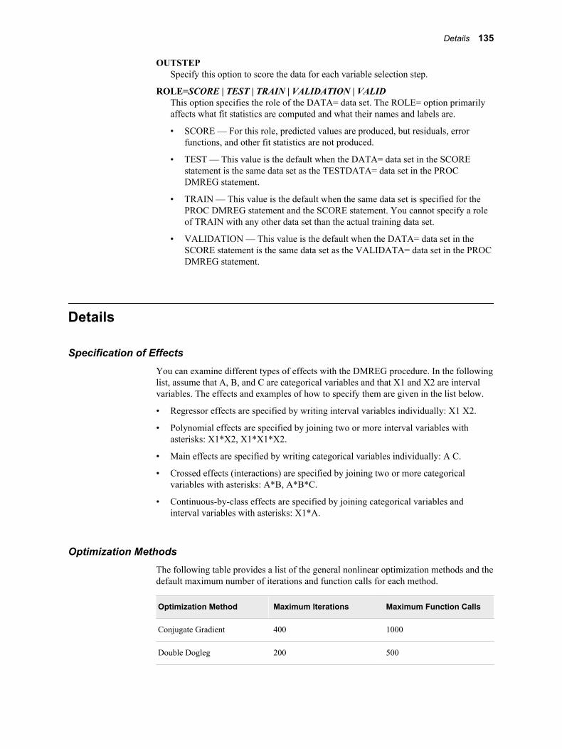
OUTSTEPSpecify this option to score the data for each variable selection step.
ROLE=SCORE | TEST | TRAIN | VALIDATION | VALIDThis option specifies the role of the DATA= data set. The ROLE= option primarily affects what fit statistics are computed and what their names and labels are.
• SCORE — For this role, predicted values are produced, but residuals, error functions, and other fit statistics are not produced.
• TEST — This value is the default when the DATA= data set in the SCORE statement is the same data set as the TESTDATA= data set in the PROC DMREG statement.
• TRAIN — This value is the default when the same data set is specified for the PROC DMREG statement and the SCORE statement. You cannot specify a role of TRAIN with any other data set than the actual training data set.
• VALIDATION — This value is the default when the DATA= data set in the SCORE statement is the same data set as the VALIDATA= data set in the PROC DMREG statement.
Details
Specification of EffectsYou can examine different types of effects with the DMREG procedure. In the following list, assume that A, B, and C are categorical variables and that X1 and X2 are interval variables. The effects and examples of how to specify them are given in the list below.
• Regressor effects are specified by writing interval variables individually: X1 X2.
• Polynomial effects are specified by joining two or more interval variables with asterisks: X1*X2, X1*X1*X2.
• Main effects are specified by writing categorical variables individually: A C.
• Crossed effects (interactions) are specified by joining two or more categorical variables with asterisks: A*B, A*B*C.
• Continuous-by-class effects are specified by joining categorical variables and interval variables with asterisks: X1*A.
Optimization MethodsThe following table provides a list of the general nonlinear optimization methods and the default maximum number of iterations and function calls for each method.
Optimization Method Maximum Iterations Maximum Function Calls
Conjugate Gradient 400 1000
Double Dogleg 200 500
Details 135

Optimization Method Maximum Iterations Maximum Function Calls
Newton-Raphson with Line Search
50 125
Newton-Raphson with Ridging
50 125
Quasi-Newton 200 500
Trust-Region 50 125
You should set the optimization method based on the size of the data mining problem as follows:
1. Small-to-medium problems — The Trust-Region, Newton-Raphson with Ridging, and Newton-Raphson with Line Search methods are appropriate for small and medium sized optimization problems (40 or fewer model parameters) where the Hessian matrix is easy and cheap to compute. Sometimes, Newton-Raphson with Ridging can be faster than Trust-Region, but Trust-Region is numerically more stable. If the Hessian matrix is not singular at the optimum, then the Newton-Raphson with Line Search can be a very competitive method.
2. Medium Problems — The quasi-Newton and Double Dogleg methods are appropriate for medium optimization problems (up to 400 model parameters) where the objective function and the gradient are much faster to compute than the Hessian. Quasi-Newton and Double Dogleg require more iterations than the Trust-Region or the Newton-Raphson methods, but each iteration is much faster.
3. Large Problems — The Conjugate Gradient method is appropriate for large data mining problems (more than 400 model parameters) where the objective function and the gradient are much faster to compute than the Hessian matrix, and where they need too much memory to store the approximate Hessian matrix.
Note: To learn more about these optimization methods, see “The NLP Procedure” in the SAS/OR User's Guide: Mathematical Programming.
The default optimization method depends on the number of parameters in the model. If the number of parameters is less than or equal to 40, then the default method is Newton-Raphson with Ridging. If the number of parameters is greater than 40 and less than 400, then the default method is quasi-Newton. If the number of parameters is greater than 400, then Conjugate Gradient is the default method.
Effect-Selection MethodsFour effect-selection methods are available by specifying the SELECTION= option in the MODEL statement. The simplest method (and the default) is SELECTION=NONE. This method instructs the DMREG procedure to fit the complete model as specified in the MODEL statement. The other three methods are FORWARD for forward selection, BACKWARD for backward elimination, and STEPWISE for stepwise selection. Intercept parameters are forced to stay in the model unless the NOINT option is specified.
When SELECTION=FORWARD is specified, the DMREG procedure first estimates parameters for effects forced into the model. These effects are the intercepts and the first n explanatory effects in the MODEL statement, where n is the number specified by the START= or INCLUDE= option in the MODEL statement (n is zero by default). Next,
136 Chapter 7 • The DMREG Procedure
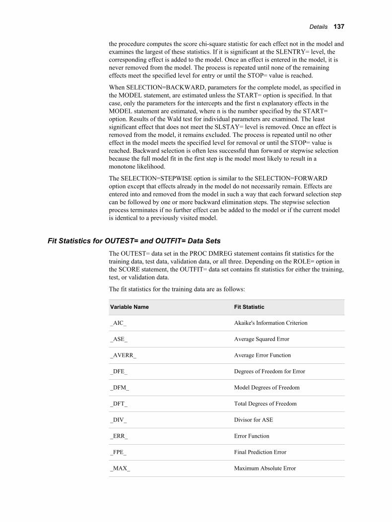
the procedure computes the score chi-square statistic for each effect not in the model and examines the largest of these statistics. If it is significant at the SLENTRY= level, the corresponding effect is added to the model. Once an effect is entered in the model, it is never removed from the model. The process is repeated until none of the remaining effects meet the specified level for entry or until the STOP= value is reached.
When SELECTION=BACKWARD, parameters for the complete model, as specified in the MODEL statement, are estimated unless the START= option is specified. In that case, only the parameters for the intercepts and the first n explanatory effects in the MODEL statement are estimated, where n is the number specified by the START= option. Results of the Wald test for individual parameters are examined. The least significant effect that does not meet the SLSTAY= level is removed. Once an effect is removed from the model, it remains excluded. The process is repeated until no other effect in the model meets the specified level for removal or until the STOP= value is reached. Backward selection is often less successful than forward or stepwise selection because the full model fit in the first step is the model most likely to result in a monotone likelihood.
The SELECTION=STEPWISE option is similar to the SELECTION=FORWARD option except that effects already in the model do not necessarily remain. Effects are entered into and removed from the model in such a way that each forward selection step can be followed by one or more backward elimination steps. The stepwise selection process terminates if no further effect can be added to the model or if the current model is identical to a previously visited model.
Fit Statistics for OUTEST= and OUTFIT= Data SetsThe OUTEST= data set in the PROC DMREG statement contains fit statistics for the training data, test data, validation data, or all three. Depending on the ROLE= option in the SCORE statement, the OUTFIT= data set contains fit statistics for either the training, test, or validation data.
The fit statistics for the training data are as follows:
Variable Name Fit Statistic
_AIC_ Akaike's Information Criterion
_ASE_ Average Squared Error
_AVERR_ Average Error Function
_DFE_ Degrees of Freedom for Error
_DFM_ Model Degrees of Freedom
_DFT_ Total Degrees of Freedom
_DIV_ Divisor for ASE
_ERR_ Error Function
_FPE_ Final Prediction Error
_MAX_ Maximum Absolute Error
Details 137
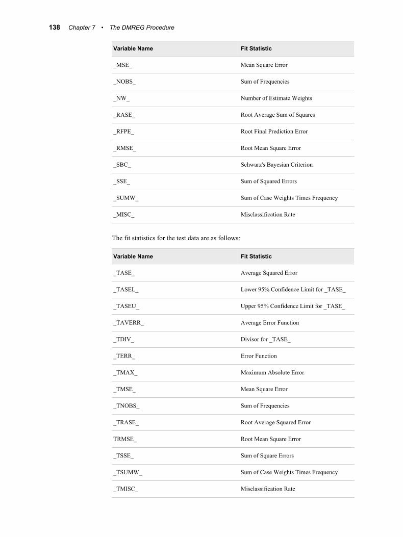
Variable Name Fit Statistic
_MSE_ Mean Square Error
_NOBS_ Sum of Frequencies
_NW_ Number of Estimate Weights
_RASE_ Root Average Sum of Squares
_RFPE_ Root Final Prediction Error
_RMSE_ Root Mean Square Error
_SBC_ Schwarz's Bayesian Criterion
_SSE_ Sum of Squared Errors
_SUMW_ Sum of Case Weights Times Frequency
_MISC_ Misclassification Rate
The fit statistics for the test data are as follows:
Variable Name Fit Statistic
_TASE_ Average Squared Error
_TASEL_ Lower 95% Confidence Limit for _TASE_
_TASEU_ Upper 95% Confidence Limit for _TASE_
_TAVERR_ Average Error Function
_TDIV_ Divisor for _TASE_
_TERR_ Error Function
_TMAX_ Maximum Absolute Error
_TMSE_ Mean Square Error
_TNOBS_ Sum of Frequencies
_TRASE_ Root Average Squared Error
TRMSE_ Root Mean Square Error
_TSSE_ Sum of Square Errors
_TSUMW_ Sum of Case Weights Times Frequency
_TMISC_ Misclassification Rate
138 Chapter 7 • The DMREG Procedure
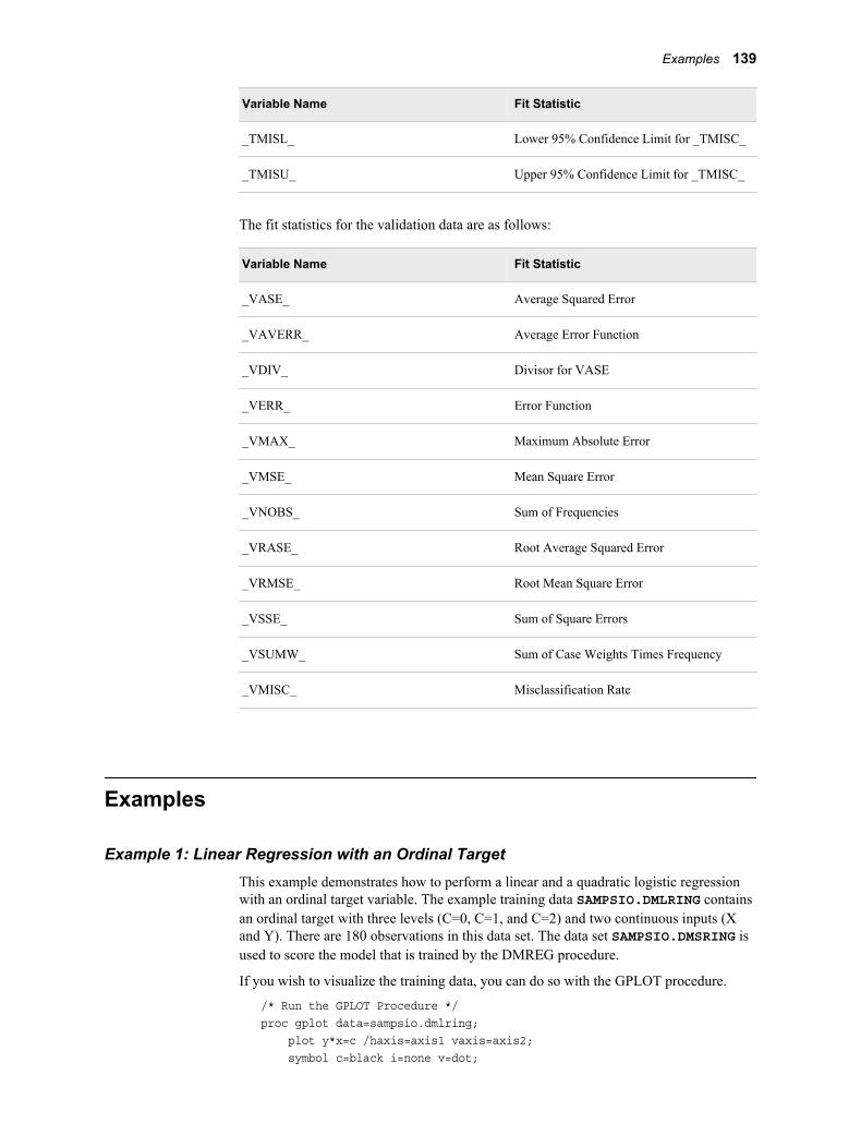
Variable Name Fit Statistic
_TMISL_ Lower 95% Confidence Limit for _TMISC_
_TMISU_ Upper 95% Confidence Limit for _TMISC_
The fit statistics for the validation data are as follows:
Variable Name Fit Statistic
_VASE_ Average Squared Error
_VAVERR_ Average Error Function
_VDIV_ Divisor for VASE
_VERR_ Error Function
_VMAX_ Maximum Absolute Error
_VMSE_ Mean Square Error
_VNOBS_ Sum of Frequencies
_VRASE_ Root Average Squared Error
_VRMSE_ Root Mean Square Error
_VSSE_ Sum of Square Errors
_VSUMW_ Sum of Case Weights Times Frequency
_VMISC_ Misclassification Rate
Examples
Example 1: Linear Regression with an Ordinal TargetThis example demonstrates how to perform a linear and a quadratic logistic regression with an ordinal target variable. The example training data SAMPSIO.DMLRING contains an ordinal target with three levels (C=0, C=1, and C=2) and two continuous inputs (X and Y). There are 180 observations in this data set. The data set SAMPSIO.DMSRING is used to score the model that is trained by the DMREG procedure.
If you wish to visualize the training data, you can do so with the GPLOT procedure.
/* Run the GPLOT Procedure */proc gplot data=sampsio.dmlring; plot y*x=c /haxis=axis1 vaxis=axis2; symbol c=black i=none v=dot;
Examples 139
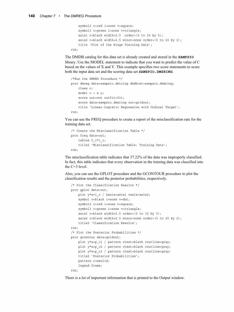
symbol2 c=red i=none v=square; symbol3 c=green i=none v=triangle; axis1 c=black width=2.5 order=(0 to 30 by 5); axis2 c=black width=2.5 minor=none order=(0 to 20 by 2); title 'Plot of the Rings Training Data';run;
The DMDB catalog for this data set is already created and stored in the SAMPSIO library. Use the MODEL statement to indicate that you want to predict the value of C based on the values of X and Y. This example specifies two score statements to score both the input data set and the scoring data set SAMSPIO.DMSRING.
/*Run the DMREG Procedure */proc dmreg data=sampsio.dmlring dmdbcat=sampsio.dmdring; class c; model c = x y; score out=out outfit=fit; score data=sampsio.dmsring out=gridout; title 'Linear-Logistic Regression with Ordinal Target';run;
You can use the FREQ procedure to create a report of the misclassification rate for the training data set.
/* Create the Misclassification Table */proc freq data=out; tables f_c*i_c; title2 ’Misclassification Table: Training Data’;run;
The misclassification table indicates that 37.22% of the data was improperly classified. In fact, this table indicates that every observation in the training data was classified into the C=3 level.
Also, you can use the GPLOT procedure and the GCONTOUR procedure to plot the classification results and the posterior probabilities, respectively.
/* Plot the Classification Results */proc gplot data=out; plot y*x=i_c / haxis=axis1 vaxis=axis2; symbol c=black i=none v=dot; symbol2 c=red i=none v=square; symbol3 c=green i=none v=triangle; axis1 c=black width=2.5 order=(0 to 30 by 5); axis2 c=black width=2.5 minor=none order=(0 to 20 by 2); title2 'Classification Results';run;/* Plot the Posterior Probabilities */proc gcontour data=gridout; plot y*x=p_c1 / pattern ctext=black coutline=gray; plot y*x=p_c2 / pattern ctext=black coutline=gray; plot y*x=p_c3 / pattern ctext=black coutline=gray; title2 ’Posterior Probabilities’; pattern v=msolid; legend frame;run;
There is a lot of important information that is printed to the Output window.
140 Chapter 7 • The DMREG Procedure
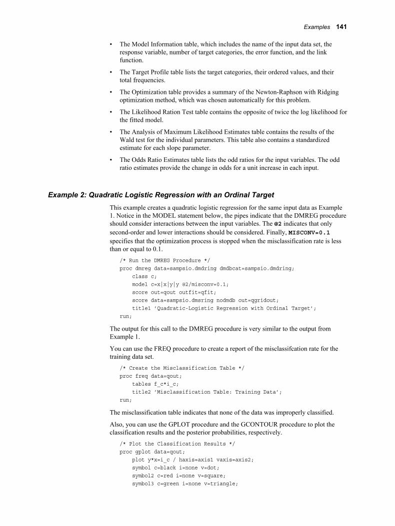
• The Model Information table, which includes the name of the input data set, the response variable, number of target categories, the error function, and the link function.
• The Target Profile table lists the target categories, their ordered values, and their total frequencies.
• The Optimization table provides a summary of the Newton-Raphson with Ridging optimization method, which was chosen automatically for this problem.
• The Likelihood Ration Test table contains the opposite of twice the log likelihood for the fitted model.
• The Analysis of Maximum Likelihood Estimates table contains the results of the Wald test for the individual parameters. This table also contains a standardized estimate for each slope parameter.
• The Odds Ratio Estimates table lists the odd ratios for the input variables. The odd ratio estimates provide the change in odds for a unit increase in each input.
Example 2: Quadratic Logistic Regression with an Ordinal TargetThis example creates a quadratic logistic regression for the same input data as Example 1. Notice in the MODEL statement below, the pipes indicate that the DMREG procedure should consider interactions between the input variables. The @2 indicates that only second-order and lower interactions should be considered. Finally, MISCONV=0.1 specifies that the optimization process is stopped when the misclassification rate is less than or equal to 0.1.
/* Run the DMREG Procedure */proc dmreg data=sampsio.dmdring dmdbcat=sampsio.dmdring; class c; model c=x|x|y|y @2/misconv=0.1; score out=qout outfit=qfit; score data=sampsio.dmsring nodmdb out=qgridout; title1 ’Quadratic-Logistic Regression with Ordinal Target’;run;
The output for this call to the DMREG procedure is very similar to the output from Example 1.
You can use the FREQ procedure to create a report of the misclassifcation rate for the training data set.
/* Create the Misclassification Table */proc freq data=qout; tables f_c*i_c; title2 ’Misclassification Table: Training Data’;run;
The misclassification table indicates that none of the data was improperly classified.
Also, you can use the GPLOT procedure and the GCONTOUR procedure to plot the classification results and the posterior probabilities, respectively.
/* Plot the Classification Results */proc gplot data=qout; plot y*x=i_c / haxis=axis1 vaxis=axis2; symbol c=black i=none v=dot; symbol2 c=red i=none v=square; symbol3 c=green i=none v=triangle;
Examples 141
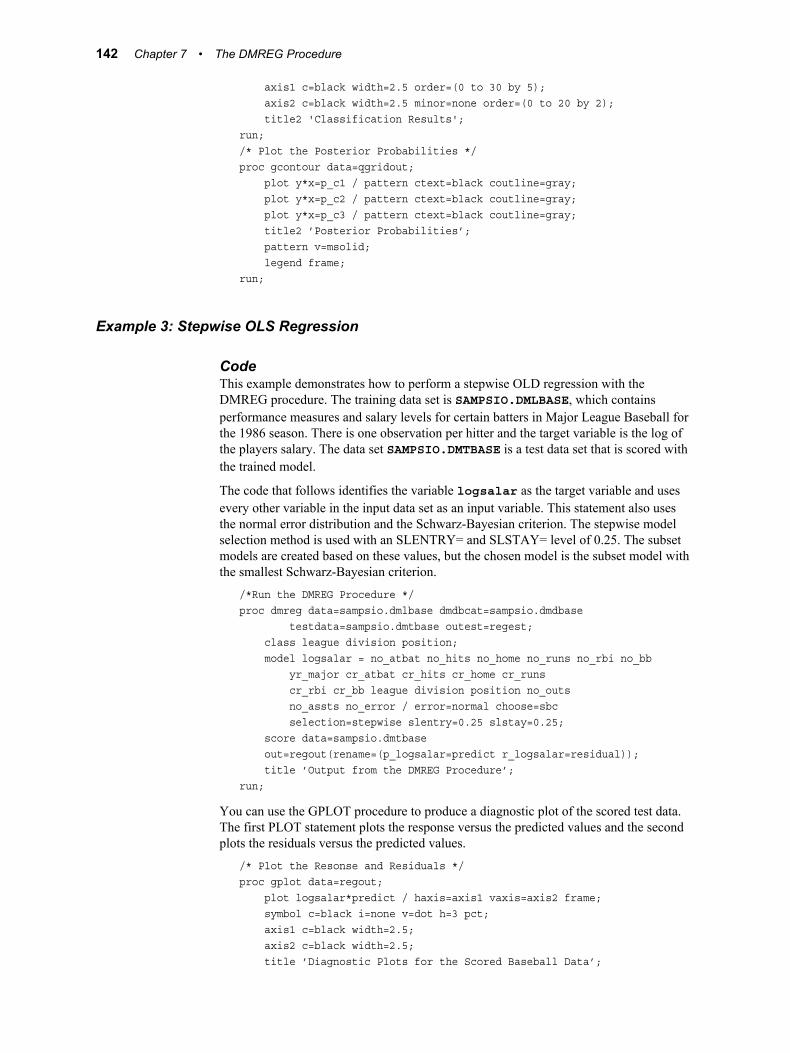
axis1 c=black width=2.5 order=(0 to 30 by 5); axis2 c=black width=2.5 minor=none order=(0 to 20 by 2); title2 'Classification Results';run;/* Plot the Posterior Probabilities */proc gcontour data=qgridout; plot y*x=p_c1 / pattern ctext=black coutline=gray; plot y*x=p_c2 / pattern ctext=black coutline=gray; plot y*x=p_c3 / pattern ctext=black coutline=gray; title2 ’Posterior Probabilities’; pattern v=msolid; legend frame;run;
Example 3: Stepwise OLS Regression
CodeThis example demonstrates how to perform a stepwise OLD regression with the DMREG procedure. The training data set is SAMPSIO.DMLBASE, which contains performance measures and salary levels for certain batters in Major League Baseball for the 1986 season. There is one observation per hitter and the target variable is the log of the players salary. The data set SAMPSIO.DMTBASE is a test data set that is scored with the trained model.
The code that follows identifies the variable logsalar as the target variable and uses every other variable in the input data set as an input variable. This statement also uses the normal error distribution and the Schwarz-Bayesian criterion. The stepwise model selection method is used with an SLENTRY= and SLSTAY= level of 0.25. The subset models are created based on these values, but the chosen model is the subset model with the smallest Schwarz-Bayesian criterion.
/*Run the DMREG Procedure */proc dmreg data=sampsio.dmlbase dmdbcat=sampsio.dmdbase testdata=sampsio.dmtbase outest=regest; class league division position; model logsalar = no_atbat no_hits no_home no_runs no_rbi no_bb yr_major cr_atbat cr_hits cr_home cr_runs cr_rbi cr_bb league division position no_outs no_assts no_error / error=normal choose=sbc selection=stepwise slentry=0.25 slstay=0.25; score data=sampsio.dmtbase out=regout(rename=(p_logsalar=predict r_logsalar=residual)); title ’Output from the DMREG Procedure’;run;
You can use the GPLOT procedure to produce a diagnostic plot of the scored test data. The first PLOT statement plots the response versus the predicted values and the second plots the residuals versus the predicted values.
/* Plot the Resonse and Residuals */proc gplot data=regout; plot logsalar*predict / haxis=axis1 vaxis=axis2 frame; symbol c=black i=none v=dot h=3 pct; axis1 c=black width=2.5; axis2 c=black width=2.5; title ’Diagnostic Plots for the Scored Baseball Data’;
142 Chapter 7 • The DMREG Procedure
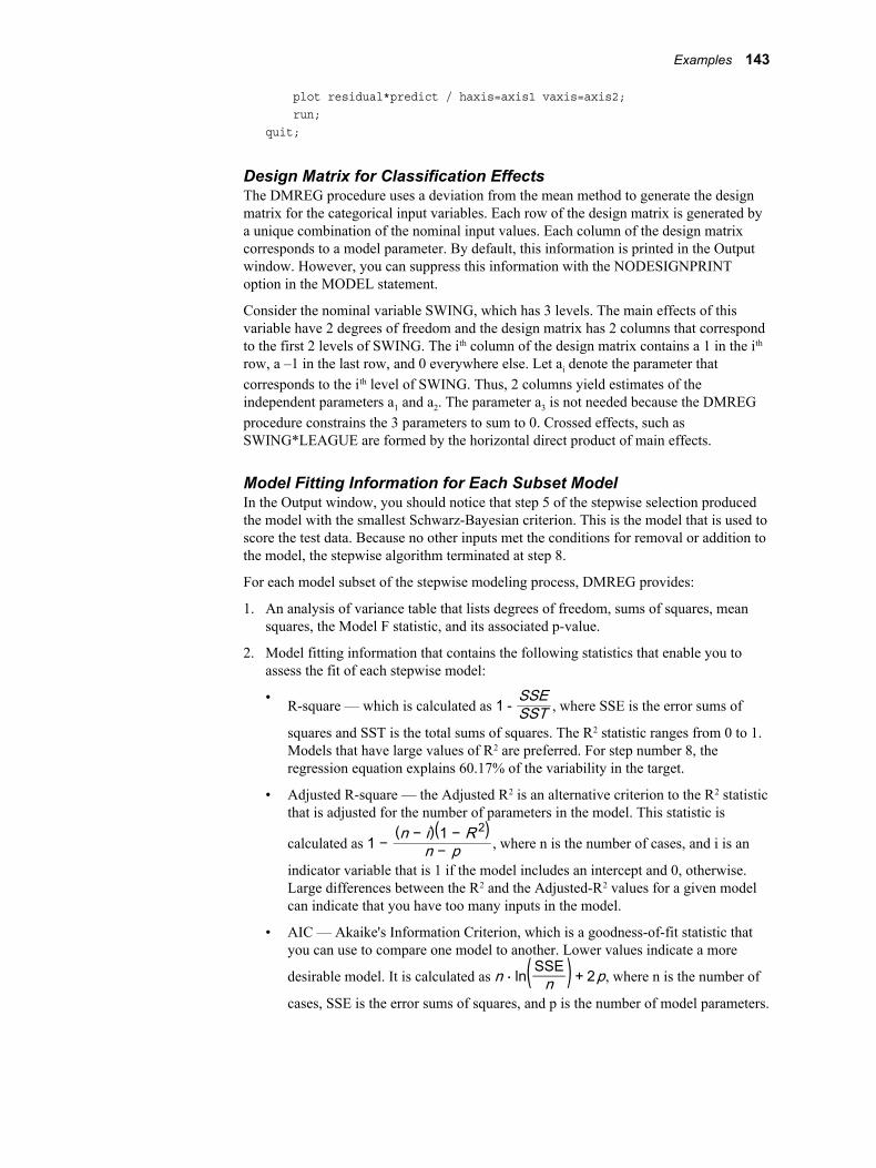
plot residual*predict / haxis=axis1 vaxis=axis2; run;quit;
Design Matrix for Classification EffectsThe DMREG procedure uses a deviation from the mean method to generate the design matrix for the categorical input variables. Each row of the design matrix is generated by a unique combination of the nominal input values. Each column of the design matrix corresponds to a model parameter. By default, this information is printed in the Output window. However, you can suppress this information with the NODESIGNPRINT option in the MODEL statement.
Consider the nominal variable SWING, which has 3 levels. The main effects of this variable have 2 degrees of freedom and the design matrix has 2 columns that correspond to the first 2 levels of SWING. The ith column of the design matrix contains a 1 in the ith
row, a –1 in the last row, and 0 everywhere else. Let ai denote the parameter that corresponds to the ith level of SWING. Thus, 2 columns yield estimates of the independent parameters a1 and a2. The parameter a3 is not needed because the DMREG procedure constrains the 3 parameters to sum to 0. Crossed effects, such as SWING*LEAGUE are formed by the horizontal direct product of main effects.
Model Fitting Information for Each Subset ModelIn the Output window, you should notice that step 5 of the stepwise selection produced the model with the smallest Schwarz-Bayesian criterion. This is the model that is used to score the test data. Because no other inputs met the conditions for removal or addition to the model, the stepwise algorithm terminated at step 8.
For each model subset of the stepwise modeling process, DMREG provides:
1. An analysis of variance table that lists degrees of freedom, sums of squares, mean squares, the Model F statistic, and its associated p-value.
2. Model fitting information that contains the following statistics that enable you to assess the fit of each stepwise model:
• R-square — which is calculated as 1 - SSESST , where SSE is the error sums of
squares and SST is the total sums of squares. The R2 statistic ranges from 0 to 1. Models that have large values of R2 are preferred. For step number 8, the regression equation explains 60.17% of the variability in the target.
• Adjusted R-square — the Adjusted R2 is an alternative criterion to the R2 statistic that is adjusted for the number of parameters in the model. This statistic is
calculated as 1 −(n − i)(1 − R 2)
n − p , where n is the number of cases, and i is an
indicator variable that is 1 if the model includes an intercept and 0, otherwise. Large differences between the R2 and the Adjusted-R2 values for a given model can indicate that you have too many inputs in the model.
• AIC — Akaike's Information Criterion, which is a goodness-of-fit statistic that you can use to compare one model to another. Lower values indicate a more
desirable model. It is calculated as n ⋅ ln( SSEn ) + 2p, where n is the number of
cases, SSE is the error sums of squares, and p is the number of model parameters.
Examples 143
• BIC — Bayesian Information Criterion is another goodness-of-fit statistic that is
calculated as n ⋅ ln( SSEn ) + 2q(p + 2) − 2q 2, where q = MSESSEn
(MSE is
obtained from the full model). Smaller BIC values are preferred.
• SBC — Schwarz's Bayesian Criterion is another goodness-of-fit statistic that is
calculated as n ⋅ ln( SSEn ) + p ⋅ ln(n). Models that have small SBC values are
preferred. Because the CHOOSE=SBC option was specified, the DMREG procedure selects the model that has the smallest SBC value.
• C(p) — Mallow's C(p) Statistic enables you to determine whether your model is
under or overspecified. This statistic is calculated as SSE(p)MSE - (n - 2p). Here,
SSE(p) is the error sums of squares for the subset model with p parameters including the intercept, MSE is the error mean square for the full model, and n is the number of cases. For any subset model C(p) > p, there is evidence of bias due to an incompletely specified model (your model might not contain enough inputs). However, if there are values of C(p) < p, the full model is said to be overspecified. When the right model is chosen, the parameter estimates are unbiased, and this is reflected in C(p) < p or at least near p.
3. A listing of the analysis of effects and parameter estimates that contains the effect, degrees of freedom, parameter estimate, standard error, type 3 sums of squares, F value, and the corresponding p-value.
The Stepwise Selection ProcessThe Summary of Stepwise Selection table provides an explanation of the inputs added to or removed from the model at each step. It also provides the F statistic and corresponding p-value on which the entry or removal of the input is based. For this example, 8 of the 19 input variables met the 0.25 entry and stay probability values.
Selected Variables from the OUTEST= Data SetYou can use the PRINT procedure to create a report of selected variables in the OUTEST= data set
/* Create a Report of Selected Variables */proc print data=regest noobs label; var _step_ _chosen_ _sbc_ _mse_ _averr_ _tmse_ _taverr_; where _type_ = 'PARMS'; title 'Partial Listing of the OUTEST= Data Set';run;
This report lists certain fit statistics from the training and test data sets. The default OUTEST= data set contains three observations for each step number. These observations are distinguished by their value in the _TYPE_ variable.
• PARMS — contains parameter estimates and the fit statistics.
• T — contains the t-values for the parameter estimates.
• P — contains the p-values for the parameter estimates.
Because the WHERE statement specified _TYPE_='PARMS', this report contains only one observation per step number. An additional observation is displayed that identifies the model that is chosen based on the Schwarz-Bayesian criterion.
144 Chapter 7 • The DMREG Procedure
Example 4: Comparison of the DMREG and LOGISTIC Procedures with a Categorical Target
The DMREG and LOGISTIC procedures fit the same models for a categorical target. Both procedures have the CLASS statement to specify categorical input variables and both use the deviation from the mean coding as the default parameterization for a CLASS input variable.
However, there are many differences between the two procedures, both in syntax and in features. For example, to specify the GLM parameterization of CLASS variables, you specify the MODEL statement option CODING= GLM in the DMREG procedure. But, in the LOGISTIC procedure , you specify the CLASS statement option PARAM= GLM. You are required to specify a DMDB catalog of input data in the DMREG procedure, but not in the LOGISTIC procedure. The DMREG procedure produces DATA step scoring code, but the LOGISTIC procedure does not.
In terms of training a model, you might expect the estimates from both procedures to be identical. Often the estimates between the two procedures are very close but not necessarily identical for a number of reasons. The DMREG and LOGISTIC procedures do not use the same routines to carry out the optimization, and the convergence criterion and optimization technique used might not be the same. However, discrepancies of the parameter estimates between the two procedures would not make any difference in prediction. Consider the data set SAMPSIO.HMEQ, which contains fictitious mortgage data where each case represents an applicant for a home equity loan. The binary target BAD represents whether an applicant eventually defaults the loan (BAD=1 for delinquent and BAD=0 otherwise). For illustration, one interval input variable (DEBTINC) and one categorical input variable (JOB) are used to predict the target BAD.
To model the probability of BAD= 1 in the LOGISTIC procedure, you can use the DESCENDING option in the PROC LOGISTIC statement (to model the last level of the binary target instead of the first level).
/* Run the LOGISTIC Procedure */proc logistic data=sampsio.hmeq descending; class bad job; model bad=job debtinc; score data=sampsio.hmeq(where=(job^=' ' and debtinc^=.)) out=logitout; title 'LOGISTIC Analysis of Home Equity Data';run;
To train the same model using the DMREG procedure, you need the DMDB catalog, which is created in the DMDB procedure:
/* Run the DMDB procedure */proc dmdb batch data=sampsio.hmeq dmdbcat=dm_cat; var debtinc; class bad(desc) job; target bad;run;
Because the order of target BAD was set to descending in the DMDB catalog, DMREG also models the probability that BAD=1.
/* Run the DMREG Procedure */proc dmreg data=sampsio.hmeq dmdbcat=dm_cat; class bad job; model bad=job debtinc;
Examples 145
score data=sampsio.hmeq(where=(job^=' ' and debtinc^=.)) out=dmregout; title 'DMREG Analysis of Home Equity Data';run;
PROC LOGISTIC does not score observations with missing inputs, but PROC DMREG does. The SCORE statement is used in each procedure to score the subset of the training data that does not have missing values in the input variables. The COMPARE procedure is used to compare the predicted probabilities computed by the two procedures.
/* Compare the Predictions */proc compare data=dmregout compare=logitout criterion=1e-4; var P_BAD1 P_BAD0;run;
You should notice that the discrepancies in the estimates occur in the fourth decimal places. Furthermore, the two models should give nearly identical scoring results. For the training data, the COMPARE procedure found no differences in the predicted probabilities from the scoring results between the two procedures.
Further ReadingIf you are interested in learning more about the statistics behind the DMREG procedure, you should consider the following resources:
• M.J.A. Berry and G. Linoff, Data Mining Techniques for Marketing, Sales, and Customer Support. (New York, NY: John Wiley and Sons, Inc., 1997)
• D.R. Cox and E.J. Snell, The Analysis of Binary Data, 2nd Edition, (London: Chapman and Hall, 1989)
• J. E. Dennis and H.H.W. Mei, “Two New Unconstrained Optimization Algorithms that Use Function and Gradient Values,” Journal of Optimal Theory Application 28 (1979), 453–482.
• N. Draper and H. Smith, Applied Regression Analysis, 2nd Edition, (New York, NY: John Wiley and Sons, Inc., 1981)
• R.J.A. Little and D.B. Rubin, Statistical Analysis with Missing Data, (New York, NY: John Wiley and Sons, Inc., 1987)
• R.J.A. Little, “Regression with Missing X's: A Review,” Journal of the American Statistical Associate, 87 (1992), 1227–1237.
• P. McCullagh and J.A. Nelder, Generalized Linear Models, 2nd Edition, (New York, NY: Chapman and Hall, 1989)
• J.J. More, “The Levenberg-Marquardt Algorithm: Implementation and Theory,” in: G.A. Watson (ed.) Lecture Notes in Mathematics 630, (Berlin-Heidelber-New York: Springer Verlag, 1978)
• J.O. Rawlings, Applied Regression Analysis: A Research Tool, (Pacific Grove, CA: Wadsworth and Brooks/Cole Advanced Books and Software, 1988).
• SAS Institute, Inc., Logistic Regression Examples Using the SAS System, Version 6, 1st Edition, (Cary, NC: SAS Institute, Inc., 1995)
• SAS Institute, Inc., SAS/OR Users's Guide: Mathematical Programming, in: SAS OnlineDoc 9.1
• SAS Institute, Inc., SAS/STAT Users's Guide, in: SAS OnlineDoc 9.1
146 Chapter 7 • The DMREG Procedure
Chapter 8
The DMSPLIT Procedure
Overview . . . . . . . . . . . . . . . . . . . . . . . . . . . . . . . . . . . . . . . . . . . . . . . . . . . . . . . . . . . 147The DMSPLIT Procedure . . . . . . . . . . . . . . . . . . . . . . . . . . . . . . . . . . . . . . . . . . . . 147
Syntax . . . . . . . . . . . . . . . . . . . . . . . . . . . . . . . . . . . . . . . . . . . . . . . . . . . . . . . . . . . . . . 148The DMSPLIT Procedure . . . . . . . . . . . . . . . . . . . . . . . . . . . . . . . . . . . . . . . . . . . . 148PROC DMSPLIT Statement . . . . . . . . . . . . . . . . . . . . . . . . . . . . . . . . . . . . . . . . . . 148FREQ Statement . . . . . . . . . . . . . . . . . . . . . . . . . . . . . . . . . . . . . . . . . . . . . . . . . . . 149TARGET Statement . . . . . . . . . . . . . . . . . . . . . . . . . . . . . . . . . . . . . . . . . . . . . . . . 149VARIABLE Statement . . . . . . . . . . . . . . . . . . . . . . . . . . . . . . . . . . . . . . . . . . . . . . 149WEIGHT Statement . . . . . . . . . . . . . . . . . . . . . . . . . . . . . . . . . . . . . . . . . . . . . . . . 149
Examples . . . . . . . . . . . . . . . . . . . . . . . . . . . . . . . . . . . . . . . . . . . . . . . . . . . . . . . . . . . 150Example 1: Preprocessing the Data and Basic Usage . . . . . . . . . . . . . . . . . . . . . . 150
Overview
The DMSPLIT ProcedureThe DMSPLIT procedure performs variable selection using binary variable splits that maximize the chi-square value of a 2x2 frequency table. The cutoff threshold is chosen so that the chi-square value of the table is maximized. In Enterprise Miner, the DMSPLIT procedure and the DMINE procedure are the underlying procedures for the Variable Selection node.
For numeric variables, missing values are replaced by the weighted mean of that variable. For categorical variables, missing values are considered an additional category.
147
Syntax
The DMSPLIT ProcedurePROC DMSPLIT DATA=data-set-name DMDBCAT=catalog-name <options>;
FREQ variable;TARGET variable;VARIABLE list-of-variables;WEIGHT variable;RUN;
PROC DMSPLIT Statement
SyntaxPROC DMSPLIT DATA=data-set-name DMDBCAT=catalog-name <options>;
Required ArgumentsDATA=data-set-name
This argument specifies the input data set that contains the training data.
DMDBCAT=catalog-nameThis argument specifies the metadata catalog that was created by the DMDB procedure for the input data set. The catalog contains important information that enables the DMSPLIT procedure to operate efficiently.
Optional ArgumentsBINS=number
This option specifies the number of categories that are used to partition the interval variables. Valid values of number are positive integers and the default value is 100.
CHISQ=numberThis option specifies the lower bound for the chi-square values that are still eligible for variable splits. The value of number governs the number of splits that are performed. As the value of number increases, the number of splits and passes of the input data decreases. The value of number must be a positive real number and the default value is 0.
OUTVARS=data-set-nameThis data set contains the most of the output table information for the splits.
PASSES=numberThis option specifies the maximum allowable number of passes through the input data set when the DMSPLIT procedure performs binary splits. The value of number must be a positive integer and defaults to 12.
PRINT | NOPRINTSpecify the PRINT option to write output information to the Output window. The default behavior does not print any information to the Output window.
148 Chapter 8 • The DMSPLIT Procedure
FREQ Statement
SyntaxFREQ variable;
Required Argumentvariable
This option specifies a numeric variable that indicates the frequency of each observation. You should also specify this variable in the DMDB procedure so that any information about this variable is saved in the DMDB catalog. Additionally, the variable specified in the DMDB procedure will automatically be used as the frequency variable in the DMSPLIT procedure, and any other Enterprise Miner procedure.
If the variable specified here is different from the variable specified in the DMDB procedure, then no frequency variable is used.
TARGET Statement
SyntaxTARGET variable;
Required Argumentvariable
Use the TARGET statement to specify the target variable in the input data set. If you already specified a target variable in the DMDB procedure, you cannot also specify that variable in the DMSPLIT procedure.
VARIABLE Statement
SyntaxVARIABLE list-of-variables;
Required Argumentlist-of-variables
Use the VARIABLE statement to specify all variables (numeric and categorical) that can be used as independent variables in the model of the target variable.
WEIGHT Statement
SyntaxWEIGHT variable;
Syntax 149
Required Argumentvariable
The WEIGHT statement identifies an interval variable that is used to weight the input variables. You can also specify this variable in the DMDB procedure to save important information about this variable.
Examples
Example 1: Preprocessing the Data and Basic UsageIn this extended example, you assume the role of a loan officer at a bank. The SAMPSIO.HMEQ data set contains information about 5960 loans. The variable BAD indicates if the loan ever went into default or was seriously delinquent. The goal of this example is to create a model that will predict if a loan will go into default or serious delinquency. Additionally, you select a sample of the loans in order to score the training data.
Before you can analyze the data with the DMSPLIT procedure, you must create the DMDB catalog that contains the metadata for the HMEQ data set. That is done with a call to the DMDB procedure. In this step, you also create the scoring data set, named score, with a DATA step. Ideally, you would create two mutually exclusive data sets to train and then score the data, but this will suffice.
/* Create the DMDB */proc dmdb batch data=sampsio.hmeq dmdbcat=catHMEQ; var loan mortdue value yoj derog delinq clage ninq clno debtinc; class bad reason job; target bad;run;/* Create the Scoring Data Set */data score(drop=ran); set sampsio.hmeq; ran=ranuni(12345); if ran lt 0.08;run;
With the DMDB created, you are now ready to run the DMSPLIT procedure. Here, you specify all of the input variables in the VAR statement and identify the target variable BAD with the TARGET statement
proc dmsplit data=sampsio.hmeq dmdbcat=catHMEQ bins=30 chisq=2 passes=20 outvars=varOut; var loan mortdue value yoj derog delinq clage ninq clno debtinc reason job; target bad;run;
The next step is to import the new decision tree into the SPLIT procedure. The SPLIT procedure analyzes the decision tree created by the DMSPLIT procedure and computes several fit statistics. The input for the SPLIT procedure is the output from the DMSPLIT procedure, indicated by the INDMSPLIT argument.
150 Chapter 8 • The DMSPLIT Procedure
proc split dmdbcat=catHMEQ indmsplit outmatrix=treeStats outleaf=leafData outtree=treeData;run;
The data set treeStats consists of the classification counts and proportions for the loans, both good and bad. The first row of this data set indicates that only 8 of the 4771 good loans were misclassified as bad loans. The second row indicates that 73 of the bad loans were misclassified as good loans. Once you have passed the training data to the SPLIT procedure, you can now use the scoring data. This will determine how well the decision tree fits the input data.
proc split intree=treeData; score data=score nodmdb outfit=tFit out=tOut;run;
Note that the misclassification rate, given in tFit, is nearly zero for the scored data set. If you develop more than one model, you can compare the statistics in this data set with the other candidate models. Smaller values for these statistics are preferred. The final step of the analysis used the FREQ procedure to create a misclassification table for the scored data set.
proc freq data=tOut; tables f_bad*i_bad; title2 'Scored Data'; title3 'Misclassification Table';run;
You can view the misclassification table in the Output window. The table indicates that of the 396 loans where the value of BAD was 0 all of them were classified correctly. Of the 93 loans where the value of BAD was 1, 88 were classified correctly and 5 were misclassified. This would indicate that the decision tree accurately classified the data set.
Examples 151

152 Chapter 8 • The DMSPLIT Procedure
Chapter 9
The DMVQ Procedure
Overview . . . . . . . . . . . . . . . . . . . . . . . . . . . . . . . . . . . . . . . . . . . . . . . . . . . . . . . . . . . 153The DMVQ Procedure . . . . . . . . . . . . . . . . . . . . . . . . . . . . . . . . . . . . . . . . . . . . . . 153
Syntax . . . . . . . . . . . . . . . . . . . . . . . . . . . . . . . . . . . . . . . . . . . . . . . . . . . . . . . . . . . . . . 154The DMVQ Procedure . . . . . . . . . . . . . . . . . . . . . . . . . . . . . . . . . . . . . . . . . . . . . . 154PROC DMVQ Statement . . . . . . . . . . . . . . . . . . . . . . . . . . . . . . . . . . . . . . . . . . . . 154CODE Statement . . . . . . . . . . . . . . . . . . . . . . . . . . . . . . . . . . . . . . . . . . . . . . . . . . 156INITIAL Statement . . . . . . . . . . . . . . . . . . . . . . . . . . . . . . . . . . . . . . . . . . . . . . . . . 157INPUT Statement . . . . . . . . . . . . . . . . . . . . . . . . . . . . . . . . . . . . . . . . . . . . . . . . . . 158MAKE Statement . . . . . . . . . . . . . . . . . . . . . . . . . . . . . . . . . . . . . . . . . . . . . . . . . . 163SOM Statement . . . . . . . . . . . . . . . . . . . . . . . . . . . . . . . . . . . . . . . . . . . . . . . . . . . . 163TARGET Statement . . . . . . . . . . . . . . . . . . . . . . . . . . . . . . . . . . . . . . . . . . . . . . . . 164TRAIN Statement . . . . . . . . . . . . . . . . . . . . . . . . . . . . . . . . . . . . . . . . . . . . . . . . . . 165VQ Statement . . . . . . . . . . . . . . . . . . . . . . . . . . . . . . . . . . . . . . . . . . . . . . . . . . . . . 168
Further Reading . . . . . . . . . . . . . . . . . . . . . . . . . . . . . . . . . . . . . . . . . . . . . . . . . . . . . 168
Overview
The DMVQ ProcedureThe DMVQ procedure performs data mining vector quantization. Data mining vector quantization is used to form disjoint clusters of observations based on specified criteria. The DMVQ procedure is an interactive procedure and executes each statement when it is submitted. Thus, the order in which you submit your statements is important.
The procedure is typically used in the following manner:
1. Submit the PROC DMVQ statement.
2. Submit one or more INPUT or TARGET statements.
3. Submit either a VQ or a SOM statement.
4. Optionally, submit an INITIAL statement.
5. Optionally, submit a TRAIN statement.
6. Optionally, submit any number of SAVE, SCORE, or CODE statements.
7. Issue the QUIT command.
153
Syntax
The DMVQ ProcedurePROC DMVQ DMDBCAT=catalog-name <options>;
CODE FILE=file-name <options>;INITIAL <options>;INPUT list-of-variables </options>;MAKE <options>;SCORE <options>;SOM <options>;TARGET list-of-variables </options>;TRAIN <options>;VQ <options>;QUIT;
PROC DMVQ Statement
SyntaxPROC DMVQ DMDBCAT=catalog-name <options>;
Required ArgumentDMDBCAT=catalog-name
This argument specifies the data mining database that was created by the DMDB procedure for the input data set. The DMDB catalog contains several summary statistics and important computations of the input data set.
Optional ArgumentsDATA=data-set-name
This argument specifies the input data set that contains the training data.
MESSAGE | MSG=SILENT | TERSE | VERBOSEThe option specifies the amount of information that is written to the SAS log. The setting SILENT, abbreviated S, writes no process information to the SAS log. The setting TERSE, abbreviated T, writes a subset of the available process information to the SAS log. The setting VERBOSE, abbreviated V, writes all available process information to the SAS log.
MINMAX | NOMINMAXSpecify MINMAX to request that the minimum and maximum values of each variable in each cluster are included in the OUTSTAT= data set. NOMINMAX saves memory because this argument does not compute these statistics. The default setting is MINMAX.
154 Chapter 9 • The DMVQ Procedure
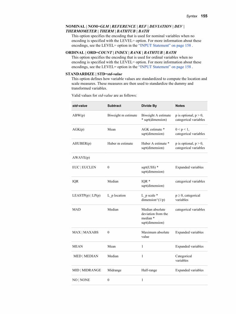
NOMINAL | NOM=GLM | REFERENCE | REF | DEVIATION | DEV | THERMOMETER | THERM | BATHTUB | BATH
This option specifies the encoding that is used for nominal variables when no encoding is specified with the LEVEL= option. For more information about these encodings, see the LEVEL= option in the “INPUT Statement” on page 158 .
ORDINAL | ORD=COUNT | INDEX | RANK | BATHTUB | BATHThis option specifies the encoding that is used for ordinal variables when no encoding is specified with the LEVEL= option. For more information about these encodings, see the LEVEL= option in the “INPUT Statement” on page 158 .
STANDARDIZE | STD=std-valueThis option defines how variable values are standardized to compute the location and scale measures. These measures are then used to standardize the dummy and transformed variables.
Valid values for std-value are as follows:
std-value Subtract Divide By Notes
ABW(p) Biweight m estimate Biweight A estimate * sqrt(dimension)
p is optional, p > 0, categorical variables
AGK(p) Mean AGK estimate * sqrt(dimension)
0 < p < 1, categorical variables
AHUBER(p) Huber m estimate Huber A estimate * sqrt(dimension)
p is optional, p > 0, categorical variables
AWAVE(p)
EUC | EUCLEN 0 sqrt(USS) * sqrt(dimension)
Expanded variables
IQR Median IQR * sqrt(dimension)
categorical variables
LEASTP(p) | LP(p) L_p location L_p scale * dimension^(1/p)
p ≥ 0, categorical variables
MAD Median Median absolute deviation from the median * sqrt(dimension)
categorical variables
MAX | MAXABS 0 Maximum absolute value
Expanded variables
MEAN Mean 1 Expanded variables
MED | MEDIAN Median 1 Categorical variables
MID | MIDRANGE Midrange Half-range Expanded variables
NO | NONE 0 1
Syntax 155
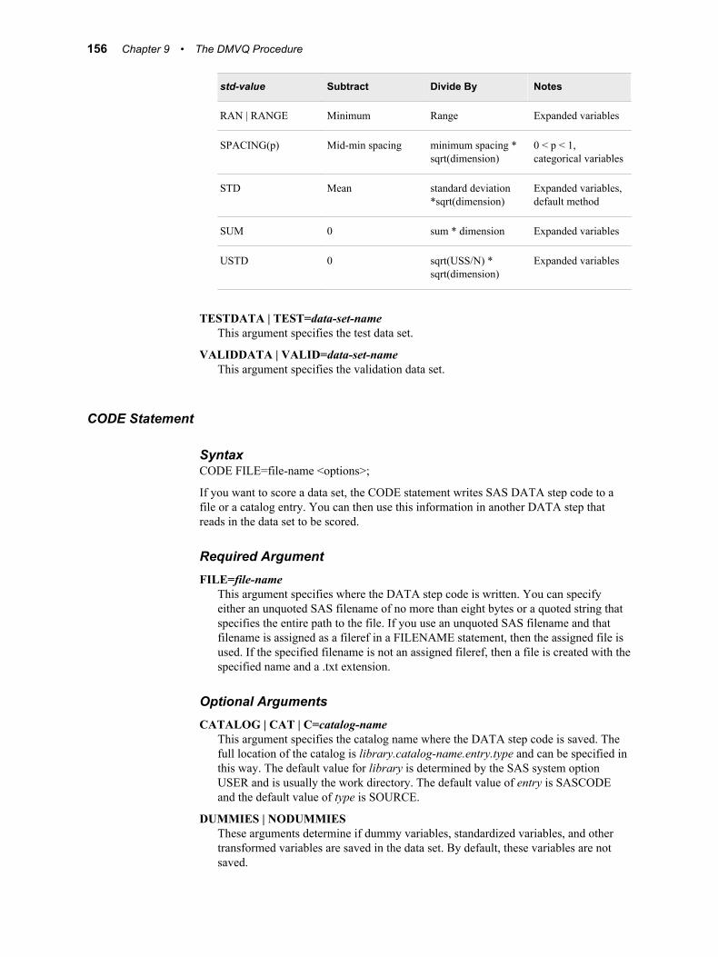
std-value Subtract Divide By Notes
RAN | RANGE Minimum Range Expanded variables
SPACING(p) Mid-min spacing minimum spacing * sqrt(dimension)
0 < p < 1, categorical variables
STD Mean standard deviation *sqrt(dimension)
Expanded variables, default method
SUM 0 sum * dimension Expanded variables
USTD 0 sqrt(USS/N) * sqrt(dimension)
Expanded variables
TESTDATA | TEST=data-set-nameThis argument specifies the test data set.
VALIDDATA | VALID=data-set-nameThis argument specifies the validation data set.
CODE Statement
SyntaxCODE FILE=file-name <options>;
If you want to score a data set, the CODE statement writes SAS DATA step code to a file or a catalog entry. You can then use this information in another DATA step that reads in the data set to be scored.
Required ArgumentFILE=file-name
This argument specifies where the DATA step code is written. You can specify either an unquoted SAS filename of no more than eight bytes or a quoted string that specifies the entire path to the file. If you use an unquoted SAS filename and that filename is assigned as a fileref in a FILENAME statement, then the assigned file is used. If the specified filename is not an assigned fileref, then a file is created with the specified name and a .txt extension.
Optional ArgumentsCATALOG | CAT | C=catalog-name
This argument specifies the catalog name where the DATA step code is saved. The full location of the catalog is library.catalog-name.entry.type and can be specified in this way. The default value for library is determined by the SAS system option USER and is usually the work directory. The default value of entry is SASCODE and the default value of type is SOURCE.
DUMMIES | NODUMMIESThese arguments determine if dummy variables, standardized variables, and other transformed variables are saved in the data set. By default, these variables are not saved.
156 Chapter 9 • The DMVQ Procedure

ERROR | NOERRORThese arguments determine if the error function is computed or not.
FORMAT=formatUse the FORMAT= option to format the weights and other numeric values that do not have a format specified in the input data set. The default value of format is BEST20.
GROUP=group-identifierThis option specifies the group identifier for group processing. The value of group-identifier should be a valid SAS name of 32 bytes or less. This name is used to construct array names and statement labels in the generated code.
LS | LINESIZE=numberThis argument specifies the line size for generated code. The value of number must be an integer between 64 and 254, with a default value of 72.
LOOKUP=algorithmThis argument specifies the algorithm that is used to look up CLASS variables' levels.
The following are valid values for algorithm:
• SELECT — uses a select statement to perform lookups. This method can be slow if there are many categories.
• LINEAR — uses a linear search with IF statements where the categories are in the order specified in the DMDB catalog. This process is slow if there are many categories.
• LINFREQ — uses a linear search with IF statements with the categories in descending order of frequency. This process is fast if the distribution of class frequencies is highly uneven, but slow if the class frequencies are relatively uniform.
• BINARY — uses a binary search. Although fast, this process can produce incorrect results based on the character-encoding system of your machine. Because some characters collate differently in ASCII and EBCDIC, results will be incorrect when switching between the two.
• AUTO — selects the fastest method for each variable that is portable across both ASCII and EBCDIC.
PMML | XMLSpecify this argument to produce scoring code in the Predictive Modeling Markup Language. PMML is an XML-based standard to represent data mining results. For more information about PMML, see the PMML Support in the SAS Enterprise Miner section in the SAS Enterprise Miner help documentation.
RESIDUAL | NORESIDUALSpecify RESIDUAL to generate residual values for certain variables. If you request code that contains the residuals and then score a data set that does contain target values, the residuals will have missing values. The default setting is to not compute the residuals.
INITIAL Statement
SyntaxINITIAL <options>;
Syntax 157
The INITIAL statement provides options that control the initial seed selection.
Optional ArgumentsINITIAL | INIT=selection-method
This argument specifies how the initial cluster-seed selection is performed. From the SOM statement, let r be the value specified in the ROWS= option and c be the value specified in the COLUMNS= option. Additionally, let s = r*c be the number of seeds needed for a self-organizing map.
The following are valid values for selection-method:
• FIRST — select the first s complete cases as initial seeds.
• MACQUEEN — uses the MacQueens' k-means algorithm to compute the initial seeds.
• SEPARATE — selects initial seeds that are well-separated using the partial replacement FASTCLUS algorithm.
• OUTLIER — selects initial seeds that are very well-separated using the full replacement FASTCLUS algorithm.
• PRINCOMP — selects initial seeds on an evenly spaced grid in the plane of the first two principal components. If r ≤ c, then the first principal component is oriented to vary with the column number and the second will vary with the row number. Otherwise, the first principal component will vary with the row number and the second will vary with the column number. The maximum absolute value in the grid, along with each component, is the square root of the corresponding eigenvalue. If you specify the VQ statement, instead of the SOM statement, the initial seeds are evenly spaced along the first principal component.
INSTAT=data-set-nameThis input data set must be a data set that was created by the OUTSTAT= option in a previous call to the DMVQ procedure.
OUT=data-set-nameThis output data set contains the original information plus cluster membership and distance variables.
OUTMEAN=data-set-nameThis output data set contains the means of the expanded (imputed and dummy) variables.
OUTSTAT=data-set-nameThis output data set contains all of the statistics that are computed by the analysis phase of the DMVQ procedure.
RADIUS | R=numberThis argument specifies the initial seed radius. The value of number must be a nonnegative real number.
INPUT Statement
SyntaxINPUT list-of-variables </options>;
158 Chapter 9 • The DMVQ Procedure
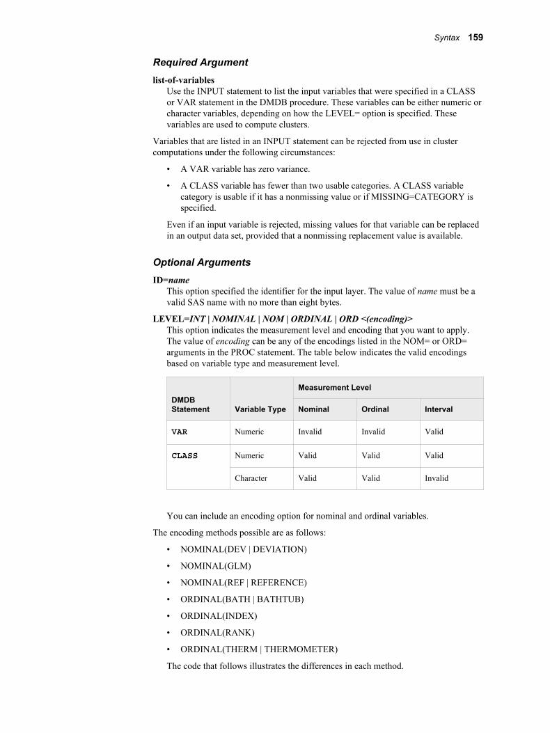
Required Argumentlist-of-variables
Use the INPUT statement to list the input variables that were specified in a CLASS or VAR statement in the DMDB procedure. These variables can be either numeric or character variables, depending on how the LEVEL= option is specified. These variables are used to compute clusters.
Variables that are listed in an INPUT statement can be rejected from use in cluster computations under the following circumstances:
• A VAR variable has zero variance.
• A CLASS variable has fewer than two usable categories. A CLASS variable category is usable if it has a nonmissing value or if MISSING=CATEGORY is specified.
Even if an input variable is rejected, missing values for that variable can be replaced in an output data set, provided that a nonmissing replacement value is available.
Optional ArgumentsID=name
This option specified the identifier for the input layer. The value of name must be a valid SAS name with no more than eight bytes.
LEVEL=INT | NOMINAL | NOM | ORDINAL | ORD <(encoding)>This option indicates the measurement level and encoding that you want to apply. The value of encoding can be any of the encodings listed in the NOM= or ORD= arguments in the PROC statement. The table below indicates the valid encodings based on variable type and measurement level.
DMDB Statement Variable Type
Measurement Level
Nominal Ordinal Interval
VAR Numeric Invalid Invalid Valid
CLASS Numeric Valid Valid Valid
Character Valid Valid Invalid
You can include an encoding option for nominal and ordinal variables.
The encoding methods possible are as follows:
• NOMINAL(DEV | DEVIATION)
• NOMINAL(GLM)
• NOMINAL(REF | REFERENCE)
• ORDINAL(BATH | BATHTUB)
• ORDINAL(INDEX)
• ORDINAL(RANK)
• ORDINAL(THERM | THERMOMETER)
The code that follows illustrates the differences in each method.
Syntax 159
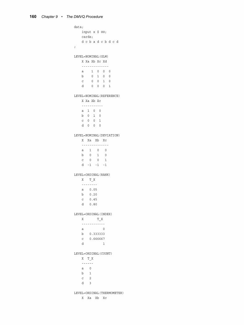
data; input x $ @@; cards; d c b a d c b d c d;
LEVEL=NOMINAL(GLM) X Xa Xb Xc Xd -------------- a 1 0 0 0 b 0 1 0 0 c 0 0 1 0 d 0 0 0 1
LEVEL=NOMINAL(REFERENCE) X Xa Xb Xc ----------- a 1 0 0 b 0 1 0 c 0 0 1 d 0 0 0
LEVEL=NOMINAL(DEVIATION) X Xa Xb Xc -------------- a 1 0 0 b 0 1 0 c 0 0 1 d -1 -1 -1
LEVEL=ORDINAL(RANK) X T_X -------- a 0.05 b 0.20 c 0.45 d 0.80
LEVEL=ORDINAL(INDEX) X T_X ------------ a 0 b 0.333333 c 0.666667 d 1
LEVEL=ORDINAL(COUNT) X T_X ------ a 0 b 1 c 2 d 3
LEVEL=ORDINAL(THERMOMETER) X Xa Xb Xc
160 Chapter 9 • The DMVQ Procedure
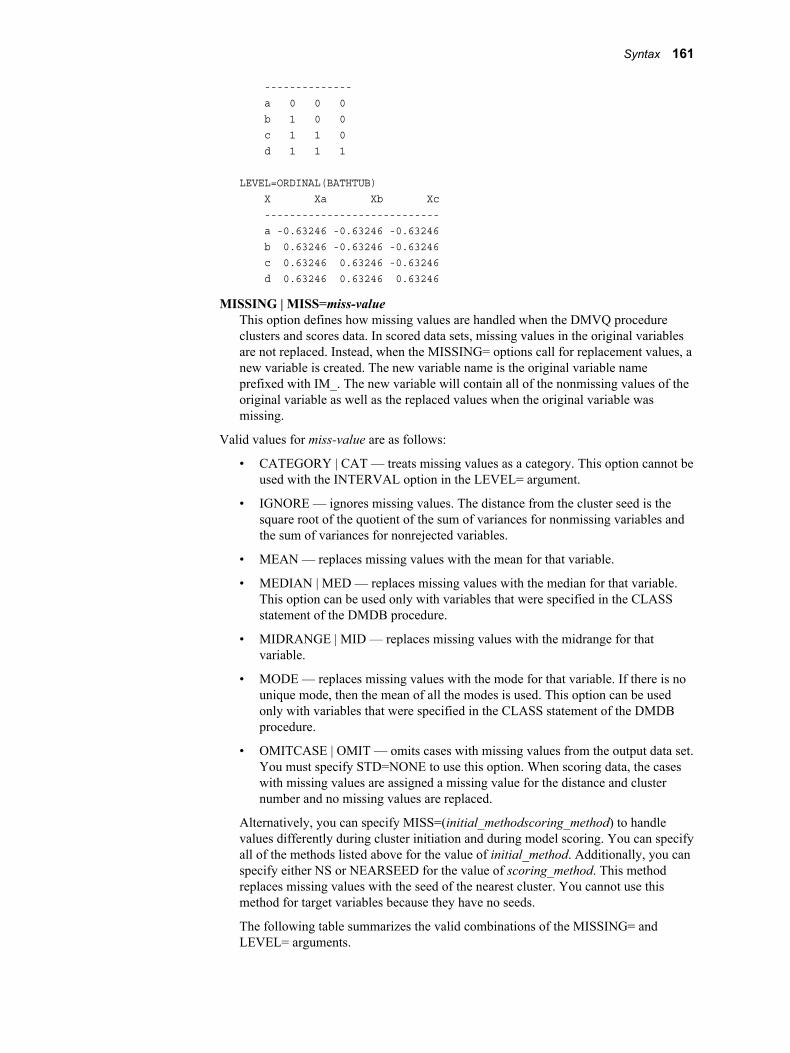
-------------- a 0 0 0 b 1 0 0 c 1 1 0 d 1 1 1
LEVEL=ORDINAL(BATHTUB) X Xa Xb Xc ---------------------------- a -0.63246 -0.63246 -0.63246 b 0.63246 -0.63246 -0.63246 c 0.63246 0.63246 -0.63246 d 0.63246 0.63246 0.63246
MISSING | MISS=miss-valueThis option defines how missing values are handled when the DMVQ procedure clusters and scores data. In scored data sets, missing values in the original variables are not replaced. Instead, when the MISSING= options call for replacement values, a new variable is created. The new variable name is the original variable name prefixed with IM_. The new variable will contain all of the nonmissing values of the original variable as well as the replaced values when the original variable was missing.
Valid values for miss-value are as follows:
• CATEGORY | CAT — treats missing values as a category. This option cannot be used with the INTERVAL option in the LEVEL= argument.
• IGNORE — ignores missing values. The distance from the cluster seed is the square root of the quotient of the sum of variances for nonmissing variables and the sum of variances for nonrejected variables.
• MEAN — replaces missing values with the mean for that variable.
• MEDIAN | MED — replaces missing values with the median for that variable. This option can be used only with variables that were specified in the CLASS statement of the DMDB procedure.
• MIDRANGE | MID — replaces missing values with the midrange for that variable.
• MODE — replaces missing values with the mode for that variable. If there is no unique mode, then the mean of all the modes is used. This option can be used only with variables that were specified in the CLASS statement of the DMDB procedure.
• OMITCASE | OMIT — omits cases with missing values from the output data set. You must specify STD=NONE to use this option. When scoring data, the cases with missing values are assigned a missing value for the distance and cluster number and no missing values are replaced.
Alternatively, you can specify MISS=(initial_methodscoring_method) to handle values differently during cluster initiation and during model scoring. You can specify all of the methods listed above for the value of initial_method. Additionally, you can specify either NS or NEARSEED for the value of scoring_method. This method replaces missing values with the seed of the nearest cluster. You cannot use this method for target variables because they have no seeds.
The following table summarizes the valid combinations of the MISSING= and LEVEL= arguments.
Syntax 161
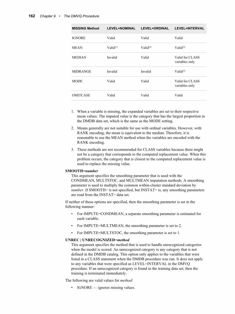
MISSING Method LEVEL=NOMINAL LEVEL=ORDINAL LEVEL=INTERVAL
IGNORE Valid Valid Valid
MEAN Valid[1] Valid[2] Valid[3]
MEDIAN Invalid Valid Valid for CLASS variables only
MIDRANGE Invalid Invalid Valid[3]
MODE Valid Valid Valid for CLASS variables only
OMITCASE Valid Valid Valid
1. When a variable is missing, the expanded variables are set to their respective mean values. The imputed value is the category that has the largest proportion in the DMDB data set, which is the same as the MODE setting.
2. Means generally are not suitable for use with ordinal variables. However, with RANK encoding, the mean is equivalent to the median. Therefore, it is reasonable to use the MEAN method when the variables are encoded with the RANK encoding.
3. These methods are not recommended for CLASS variables because there might not be a category that corresponds to the computed replacement value. When this problem occurs, the category that is closest to the computed replacement value is used to replace the missing value.
SMOOTH=numberThis argument specifies the smoothing parameter that is used with the CONDMEAN, MULTSTOC, and MULTMEAN imputation methods. A smoothing parameter is used to multiply the common within-cluster standard deviation by number. If SMOOTH= is not specified, but INSTAT= is, any smoothing parameters are read from the INSTAT= data set.
If neither of these options are specified, then the smoothing parameter is set in the following manner:
• For IMPUTE=CONDMEAN, a separate smoothing parameter is estimated for each variable.
• For IMPUTE=MULTMEAN, the smoothing parameter is set to 2.
• For IMPUTE=MULTSTOC, the smoothing parameter is set to 1.
UNREC | UNRECOGNIZED=methodThis argument specifies the method that is used to handle unrecognized categories when the model is scored. An unrecognized category is any category that is not defined in the DMDB catalog. This option only applies to the variables that were listed in a CLASS statement when the DMDB procedure was run. It does not apply to any variables that were specified as LEVEL=INTERVAL in the DMVQ procedure. If an unrecognized category is found in the training data set, then the training is terminated immediately.
The following are valid values for method:
• IGNORE — ignores missing values.
162 Chapter 9 • The DMVQ Procedure
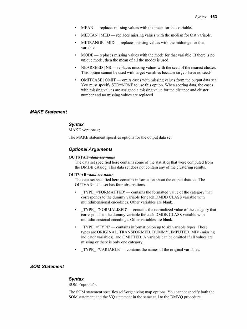
• MEAN — replaces missing values with the mean for that variable.
• MEDIAN | MED — replaces missing values with the median for that variable.
• MIDRANGE | MID — replaces missing values with the midrange for that variable.
• MODE — replaces missing values with the mode for that variable. If there is no unique mode, then the mean of all the modes is used.
• NEARSEED | NS — replaces missing values with the seed of the nearest cluster. This option cannot be used with target variables because targets have no seeds.
• OMITCASE | OMIT — omits cases with missing values from the output data set. You must specify STD=NONE to use this option. When scoring data, the cases with missing values are assigned a missing value for the distance and cluster number and no missing values are replaced.
MAKE Statement
SyntaxMAKE <options>;
The MAKE statement specifies options for the output data set.
Optional ArgumentsOUTSTAT=data-set-name
The data set specified here contains some of the statistics that were computed from the DMDB catalog. This data set does not contain any of the clustering results.
OUTVAR=data-set-nameThe data set specified here contains information about the output data set. The OUTVAR= data set has four observations.
• _TYPE_='FORMATTED' — contains the formatted value of the category that corresponds to the dummy variable for each DMDB CLASS variable with multidimensional encodings. Other variables are blank.
• _TYPE_='NORMALIZED' — contains the normalized value of the category that corresponds to the dummy variable for each DMDB CLASS variable with multidimensional encodings. Other variables are blank.
• _TYPE_='TYPE' — contains information on up to six variable types. These types are ORIGINAL, TRANSFORMED, DUMMY, IMPUTED, MIV (missing indicator variables), and OMITTED. A variable can be omitted if all values are missing or there is only one category.
• _TYPE_='VARIABLE' — contains the names of the original variables.
SOM Statement
SyntaxSOM <options>;
The SOM statement specifies self-organizing map options. You cannot specify both the SOM statement and the VQ statement in the same call to the DMVQ procedure.
Syntax 163
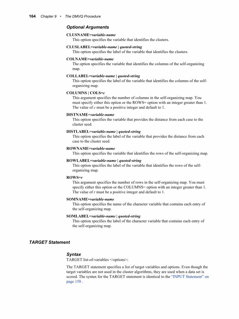
Optional ArgumentsCLUSNAME=variable-name
This option specifies the variable that identifies the clusters.
CLUSLABEL=variable-name | quoted-stringThis option specifies the label of the variable that identifies the clusters.
COLNAME=variable-nameThe option specifies the variable that identifies the columns of the self-organizing map.
COLLABEL=variable-name | quoted-stringThis option specifies the label of the variable that identifies the columns of the self-organizing map.
COLUMNS | COLS=cThis argument specifies the number of columns in the self-organizing map. You must specify either this option or the ROWS= option with an integer greater than 1. The value of c must be a positive integer and default to 1.
DISTNAME=variable-nameThis option specifies the variable that provides the distance from each case to the cluster seed.
DISTLABEL=variable-name | quoted-stringThis option specifies the label of the variable that provides the distance from each case to the cluster seed.
ROWNAME=variable-nameThis option specifies the variable that identifies the rows of the self-organizing map.
ROWLABEL=variable-name | quoted-stringThis option specifies the label of the variable that identifies the rows of the self-organizing map.
ROWS=rThis argument specifies the number of rows in the self-organizing map. You must specify either this option or the COLUMNS= option with an integer greater than 1. The value of r must be a positive integer and default to 1.
SOMNAME=variable-nameThis option specifies the name of the character variable that contains each entry of the self-organizing map.
SOMLABEL=variable-name | quoted-stringThis option specifies the label of the character variable that contains each entry of the self-organizing map.
TARGET Statement
SyntaxTARGET list-of-variables </options>;
The TARGET statement specifies a list of target variables and options. Even though the target variables are not used in the cluster algorithms, they are used when a data set is scored. The syntax for the TARGET statement is identical to the “INPUT Statement” on page 158 .
164 Chapter 9 • The DMVQ Procedure
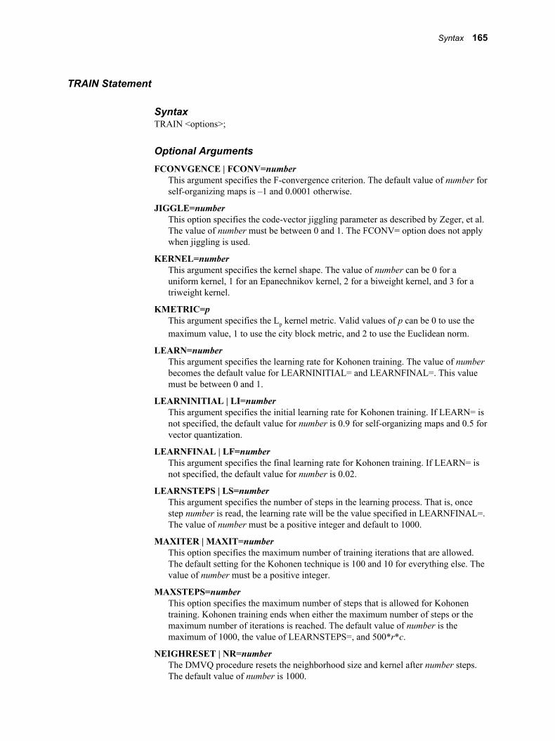
TRAIN Statement
SyntaxTRAIN <options>;
Optional ArgumentsFCONVGENCE | FCONV=number
This argument specifies the F-convergence criterion. The default value of number for self-organizing maps is –1 and 0.0001 otherwise.
JIGGLE=numberThis option specifies the code-vector jiggling parameter as described by Zeger, et al. The value of number must be between 0 and 1. The FCONV= option does not apply when jiggling is used.
KERNEL=numberThis argument specifies the kernel shape. The value of number can be 0 for a uniform kernel, 1 for an Epanechnikov kernel, 2 for a biweight kernel, and 3 for a triweight kernel.
KMETRIC=pThis argument specifies the Lp kernel metric. Valid values of p can be 0 to use the maximum value, 1 to use the city block metric, and 2 to use the Euclidean norm.
LEARN=numberThis argument specifies the learning rate for Kohonen training. The value of number becomes the default value for LEARNINITIAL= and LEARNFINAL=. This value must be between 0 and 1.
LEARNINITIAL | LI=numberThis argument specifies the initial learning rate for Kohonen training. If LEARN= is not specified, the default value for number is 0.9 for self-organizing maps and 0.5 for vector quantization.
LEARNFINAL | LF=numberThis argument specifies the final learning rate for Kohonen training. If LEARN= is not specified, the default value for number is 0.02.
LEARNSTEPS | LS=numberThis argument specifies the number of steps in the learning process. That is, once step number is read, the learning rate will be the value specified in LEARNFINAL=. The value of number must be a positive integer and default to 1000.
MAXITER | MAXIT=numberThis option specifies the maximum number of training iterations that are allowed. The default setting for the Kohonen technique is 100 and 10 for everything else. The value of number must be a positive integer.
MAXSTEPS=numberThis option specifies the maximum number of steps that is allowed for Kohonen training. Kohonen training ends when either the maximum number of steps or the maximum number of iterations is reached. The default value of number is the maximum of 1000, the value of LEARNSTEPS=, and 500*r*c.
NEIGHRESET | NR=numberThe DMVQ procedure resets the neighborhood size and kernel after number steps. The default value of number is 1000.
Syntax 165
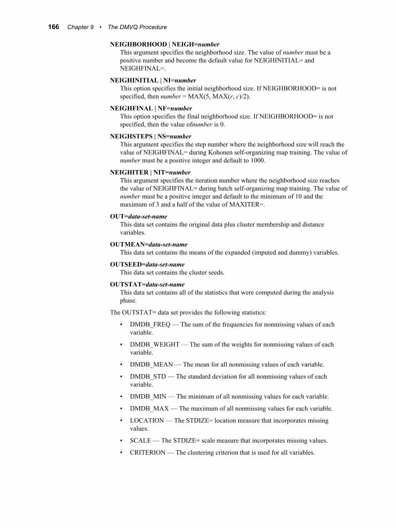
NEIGHBORHOOD | NEIGH=numberThis argument specifies the neighborhood size. The value of number must be a positive number and become the default value for NEIGHINITIAL= and NEIGHFINAL=.
NEIGHINITIAL | NI=numberThis option specifies the initial neighborhood size. If NEIGHBORHOOD= is not specified, then number = MAX(5, MAX(r, c)/2).
NEIGHFINAL | NF=numberThis option specifies the final neighborhood size. If NEIGHBORHOOD= is not specified, then the value ofnumber is 0.
NEIGHSTEPS | NS=numberThis argument specifies the step number where the neighborhood size will reach the value of NEIGHFINAL= during Kohonen self-organizing map training. The value of number must be a positive integer and default to 1000.
NEIGHITER | NIT=numberThis argument specifies the iteration number where the neighborhood size reaches the value of NEIGHFINAL= during batch self-organizing map training. The value of number must be a positive integer and default to the minimum of 10 and the maximum of 3 and a half of the value of MAXITER=.
OUT=data-set-nameThis data set contains the original data plus cluster membership and distance variables.
OUTMEAN=data-set-nameThis data set contains the means of the expanded (imputed and dummy) variables.
OUTSEED=data-set-nameThis data set contains the cluster seeds.
OUTSTAT=data-set-nameThis data set contains all of the statistics that were computed during the analysis phase.
The OUTSTAT= data set provides the following statistics:
• DMDB_FREQ — The sum of the frequencies for nonmissing values of each variable.
• DMDB_WEIGHT — The sum of the weights for nonmissing values of each variable.
• DMDB_MEAN — The mean for all nonmissing values of each variable.
• DMDB_STD — The standard deviation for all nonmissing values of each variable.
• DMDB_MIN — The minimum of all nonmissing values for each variable.
• DMDB_MAX — The maximum of all nonmissing values for each variable.
• LOCATION — The STDIZE= location measure that incorporates missing values.
• SCALE — The STDIZE= scale measure that incorporates missing values.
• CRITERION — The clustering criterion that is used for all variables.
166 Chapter 9 • The DMVQ Procedure
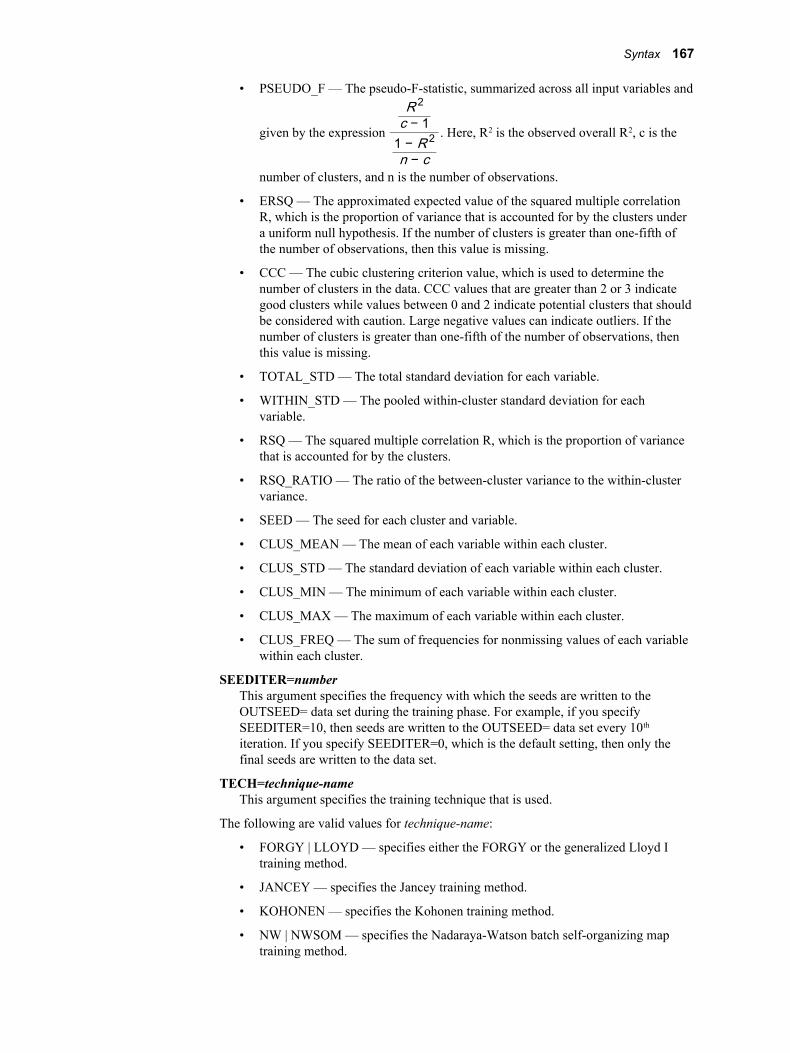
• PSEUDO_F — The pseudo-F-statistic, summarized across all input variables and
given by the expression
R 2
c − 11 − R 2
n − c
. Here, R2 is the observed overall R2, c is the
number of clusters, and n is the number of observations.
• ERSQ — The approximated expected value of the squared multiple correlation R, which is the proportion of variance that is accounted for by the clusters under a uniform null hypothesis. If the number of clusters is greater than one-fifth of the number of observations, then this value is missing.
• CCC — The cubic clustering criterion value, which is used to determine the number of clusters in the data. CCC values that are greater than 2 or 3 indicate good clusters while values between 0 and 2 indicate potential clusters that should be considered with caution. Large negative values can indicate outliers. If the number of clusters is greater than one-fifth of the number of observations, then this value is missing.
• TOTAL_STD — The total standard deviation for each variable.
• WITHIN_STD — The pooled within-cluster standard deviation for each variable.
• RSQ — The squared multiple correlation R, which is the proportion of variance that is accounted for by the clusters.
• RSQ_RATIO — The ratio of the between-cluster variance to the within-cluster variance.
• SEED — The seed for each cluster and variable.
• CLUS_MEAN — The mean of each variable within each cluster.
• CLUS_STD — The standard deviation of each variable within each cluster.
• CLUS_MIN — The minimum of each variable within each cluster.
• CLUS_MAX — The maximum of each variable within each cluster.
• CLUS_FREQ — The sum of frequencies for nonmissing values of each variable within each cluster.
SEEDITER=numberThis argument specifies the frequency with which the seeds are written to the OUTSEED= data set during the training phase. For example, if you specify SEEDITER=10, then seeds are written to the OUTSEED= data set every 10th
iteration. If you specify SEEDITER=0, which is the default setting, then only the final seeds are written to the data set.
TECH=technique-nameThis argument specifies the training technique that is used.
The following are valid values for technique-name:
• FORGY | LLOYD — specifies either the FORGY or the generalized Lloyd I training method.
• JANCEY — specifies the Jancey training method.
• KOHONEN — specifies the Kohonen training method.
• NW | NWSOM — specifies the Nadaraya-Watson batch self-organizing map training method.
Syntax 167

• LL | LLSOM — specifies the local-linear batch self-organizing map training method.
XCONVERGE | XCONV=numberThis argument specifies the X-convergence criterion. The value of number must be a nonnegative real number and default to 0.0001.
VQ Statement
SyntaxVQ <options>;
The VQ statement specifies vector quantization options. You cannot specify both the VQ statement and the SOM statement in the same call to the DMVQ procedure.
Optional ArgumentsCLUSNAME=variable-name
This option specifies the name of the variable that is used to identify clusters.
CLUSLABEL=variable-name | quoted-stringThis option specifies the label of the variable that is used to identify clusters.
DISTNAME=variable-nameThis option specifies the name of the variable that gives the distance from each case to the cluster seed.
DISTLABEL=variable-name | quoted-stringThe option specifies the label of the variable that gives the distance from each case to the cluster seed.
MAXCLUSTERS | MAXCLUS | MAXC | MAX=numberThis option specifies the maximum number of clusters. The value of number must be a positive integer.
Further ReadingThe following resource provides more information about the topics discussed above:
• K. Zeger, J. Vaisey, and A. Gersho. “Globally Optimal Vector Quantizer Design by Stochastic Relaxation,” IEEE Transactions on Signal Processing, 40 (1992): 310–322.
168 Chapter 9 • The DMVQ Procedure
Chapter 10
The DMZIP Procedure
Overview . . . . . . . . . . . . . . . . . . . . . . . . . . . . . . . . . . . . . . . . . . . . . . . . . . . . . . . . . . . 169The DMZIP Procedure . . . . . . . . . . . . . . . . . . . . . . . . . . . . . . . . . . . . . . . . . . . . . . 169
Syntax . . . . . . . . . . . . . . . . . . . . . . . . . . . . . . . . . . . . . . . . . . . . . . . . . . . . . . . . . . . . . . 170The DMZIP Procedure . . . . . . . . . . . . . . . . . . . . . . . . . . . . . . . . . . . . . . . . . . . . . . 170PROC DMZIP Statement . . . . . . . . . . . . . . . . . . . . . . . . . . . . . . . . . . . . . . . . . . . . 170CODE Statement . . . . . . . . . . . . . . . . . . . . . . . . . . . . . . . . . . . . . . . . . . . . . . . . . . 170INPUT Statement . . . . . . . . . . . . . . . . . . . . . . . . . . . . . . . . . . . . . . . . . . . . . . . . . . 171MAKE Statement . . . . . . . . . . . . . . . . . . . . . . . . . . . . . . . . . . . . . . . . . . . . . . . . . . 175SCORE Statement . . . . . . . . . . . . . . . . . . . . . . . . . . . . . . . . . . . . . . . . . . . . . . . . . 176
Examples . . . . . . . . . . . . . . . . . . . . . . . . . . . . . . . . . . . . . . . . . . . . . . . . . . . . . . . . . . . 176Example 1: Preprocessing the Data and Basic Usage . . . . . . . . . . . . . . . . . . . . . . 176Example 2: INPUT Statement Options . . . . . . . . . . . . . . . . . . . . . . . . . . . . . . . . . . 177
Overview
The DMZIP ProcedureThe DMZIP procedure computes new variables including standardized interval variables and encoded categorical variables. Using the SCORE statement, PROC DMZIP copies a DMDB-encoded input data set to an output data set and creates the new variables in the output data set. Using the CODE statement, PROC DMZIP generates SAS code to compute the new variables.
The new variables can be:
• standardized variables computed from interval variables using any of a variety of standardization methods.
• dummy variables computed from nominal or ordinal variables using any of a variety of encoding methods.
PROC DMZIP also offers several options for handling missing values and unrecognized categories.
You must run PROC DMDB to create a DMDB catalog before running PROC DMZIP.
169
Syntax
The DMZIP ProcedurePROC DMZIP DATA=data-set-name DMDBCAT=data-set-name <options>;
CODE <options>;INPUT variables </options>;MAKE <option>;SCORE <options>;QUIT;
PROC DMZIP Statement
SyntaxPROC DMZIP DATA=data-set-name DMDBCAT=data-set-name <options>;
Required ArgumentsDATA=data-set-name
Use this argument to specify the DMDB-encoded input data set. You may also specify this data set with the DATA= argument in the “SCORE Statement” on page 176 .
DMDBCAT=catalog-nameUse this option to specify the location of the DMDB catalog.
Optional ArgumentsNOMINAL | NOM = DEVIATION | DEV | GLM | REFERENCE | REF
This option specifies the encoding that is used for nominal variables. This argument is applied only if the encoding is not specified in the LEVEL= argument of the INPUT statement.
ORDINAL | ORD = BATHTUB | BATH | COUNT | INDEX | RANK | THERMOMETER | THERM
This option specifies the encoding that is used for ordinal variables. This argument is applied only if the encoding is not specified in the LEVEL= argument of the INPUT statement.
CODE Statement
SyntaxCODE <options>;
The CODE statement generates SAS code that mimics the computations in the SCORE statement.
170 Chapter 10 • The DMZIP Procedure
Optional ArgumentsCATALOG=catalog-name
Use this option to specify the catalog where the SAS code is written. The full catalog name is of the form library.catalog-name.entry.type. The default library is determined by the SAS system option USER and is usually the WORK directory. The default entry is SASCODE and the default type is SOURCE.
FILE=file-nameUse this option to specify the file name for SAS code. This can either be a quoted string that contains the filename and extension or an unquoted SAS name of eight bytes or less. If the unquoted SAS name was assigned in a FILENAME statement, the file specified in that statement is opened. If the unquoted SAS name was not assigned in a FILENAME statement then the .txt extension is added to this name. The SAS names LOG and PRINT are reserved by the system.
FORMAT=formatUse this option to specify the format for numeric values that do not have a format specified in the input data set. The default value is BEST20.
GROUP=group-nameUse this option to support group processing. This name should be a valid SAS name of no more than 32 bytes. It is used to construct array names and statement labels in the generated code.
LINESIZE | LS= numberThis option specifies the length of each line in the generated code. The value of number must be an integer between 64 and 254 and defaults to 72.
LOOKUP=AUTO | BINARY | LINEAR | LINFREQ | SELECTThis argument specifies the algorithm that is used to look up class levels.
The methods are as follows:
• AUTO — selects the fastest method available for each variable that is portable across ASCII and EBCDIC.
• BINARY — uses a binary search. This process is fast, but can produce incorrect results if you generate the code on an ASCII machine and execute the code on an EBCDIC machine, or vice versa. The CSCORE procedure is unable to translate this code.
• LINEAR — uses a linear search with IF statements. Categories are in the order specified by the DMDB catalog. This process is slow if there are many categories.
• LINFREQ — uses a linear search with IF statements. Categories are in descending order of frequency as given in the DMDB catalog. This process is fast if the distribution of class frequencies is highly uneven, but is slow if there are many categories with approximately equal frequencies.
• SELECT — uses a SELECT statement
INPUT Statement
SyntaxINPUT variables </options>;
Syntax 171
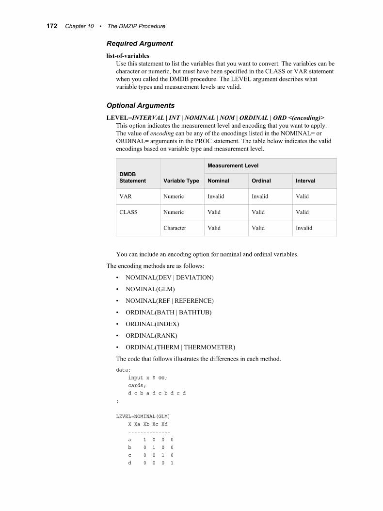
Required Argumentlist-of-variables
Use this statement to list the variables that you want to convert. The variables can be character or numeric, but must have been specified in the CLASS or VAR statement when you called the DMDB procedure. The LEVEL argument describes what variable types and measurement levels are valid.
Optional ArgumentsLEVEL=INTERVAL | INT | NOMINAL | NOM | ORDINAL | ORD <(encoding)>
This option indicates the measurement level and encoding that you want to apply. The value of encoding can be any of the encodings listed in the NOMINAL= or ORDINAL= arguments in the PROC statement. The table below indicates the valid encodings based on variable type and measurement level.
DMDB Statement Variable Type
Measurement Level
Nominal Ordinal Interval
VAR Numeric Invalid Invalid Valid
CLASS Numeric Valid Valid Valid
Character Valid Valid Invalid
You can include an encoding option for nominal and ordinal variables.
The encoding methods are as follows:
• NOMINAL(DEV | DEVIATION)
• NOMINAL(GLM)
• NOMINAL(REF | REFERENCE)
• ORDINAL(BATH | BATHTUB)
• ORDINAL(INDEX)
• ORDINAL(RANK)
• ORDINAL(THERM | THERMOMETER)
The code that follows illustrates the differences in each method.
data; input x $ @@; cards; d c b a d c b d c d;
LEVEL=NOMINAL(GLM) X Xa Xb Xc Xd -------------- a 1 0 0 0 b 0 1 0 0 c 0 0 1 0 d 0 0 0 1
172 Chapter 10 • The DMZIP Procedure
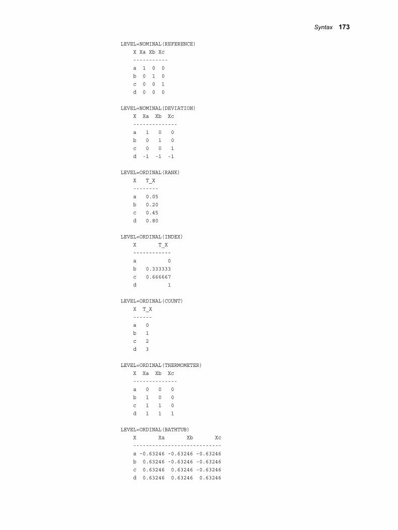
LEVEL=NOMINAL(REFERENCE) X Xa Xb Xc ----------- a 1 0 0 b 0 1 0 c 0 0 1 d 0 0 0
LEVEL=NOMINAL(DEVIATION) X Xa Xb Xc -------------- a 1 0 0 b 0 1 0 c 0 0 1 d -1 -1 -1
LEVEL=ORDINAL(RANK) X T_X -------- a 0.05 b 0.20 c 0.45 d 0.80
LEVEL=ORDINAL(INDEX) X T_X ------------ a 0 b 0.333333 c 0.666667 d 1
LEVEL=ORDINAL(COUNT) X T_X ------ a 0 b 1 c 2 d 3
LEVEL=ORDINAL(THERMOMETER) X Xa Xb Xc -------------- a 0 0 0 b 1 0 0 c 1 1 0 d 1 1 1
LEVEL=ORDINAL(BATHTUB) X Xa Xb Xc ---------------------------- a -0.63246 -0.63246 -0.63246 b 0.63246 -0.63246 -0.63246 c 0.63246 0.63246 -0.63246 d 0.63246 0.63246 0.63246
Syntax 173
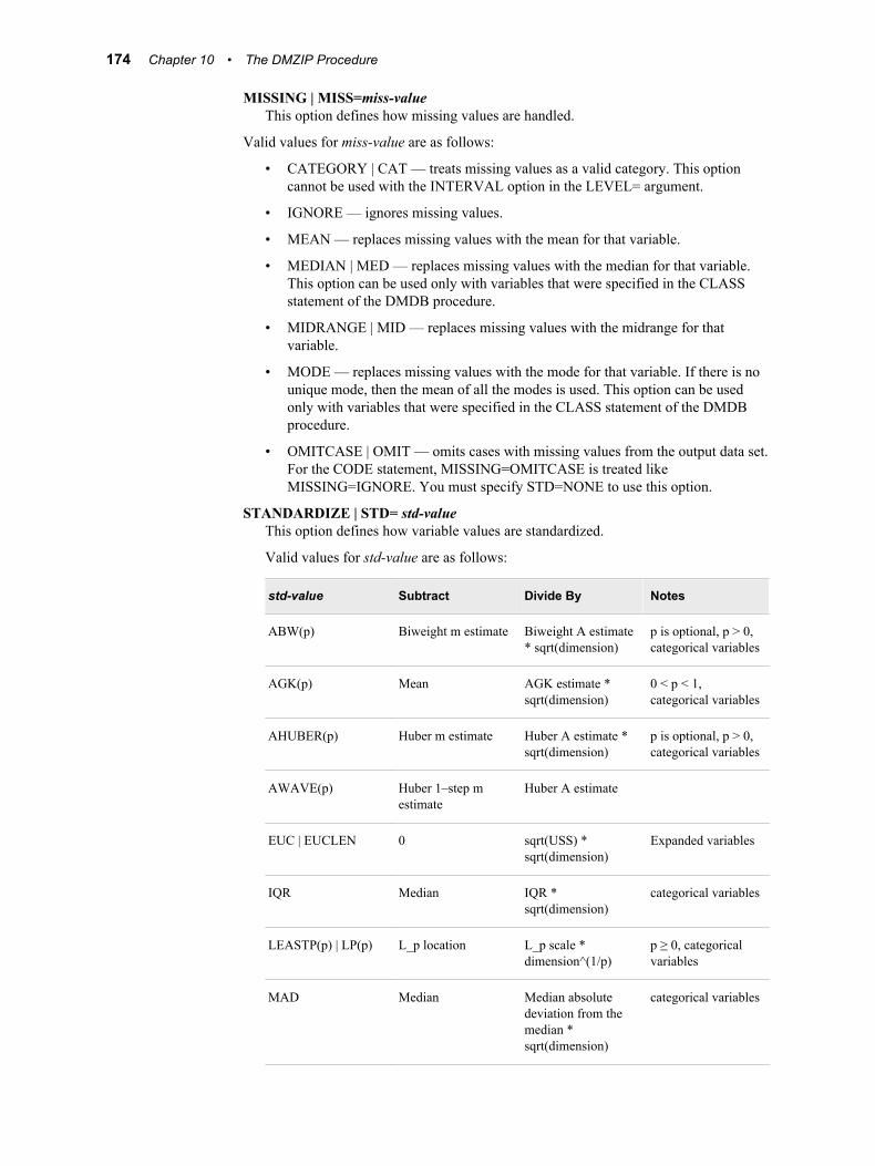
MISSING | MISS=miss-valueThis option defines how missing values are handled.
Valid values for miss-value are as follows:
• CATEGORY | CAT — treats missing values as a valid category. This option cannot be used with the INTERVAL option in the LEVEL= argument.
• IGNORE — ignores missing values.
• MEAN — replaces missing values with the mean for that variable.
• MEDIAN | MED — replaces missing values with the median for that variable. This option can be used only with variables that were specified in the CLASS statement of the DMDB procedure.
• MIDRANGE | MID — replaces missing values with the midrange for that variable.
• MODE — replaces missing values with the mode for that variable. If there is no unique mode, then the mean of all the modes is used. This option can be used only with variables that were specified in the CLASS statement of the DMDB procedure.
• OMITCASE | OMIT — omits cases with missing values from the output data set. For the CODE statement, MISSING=OMITCASE is treated like MISSING=IGNORE. You must specify STD=NONE to use this option.
STANDARDIZE | STD= std-valueThis option defines how variable values are standardized.
Valid values for std-value are as follows:
std-value Subtract Divide By Notes
ABW(p) Biweight m estimate Biweight A estimate * sqrt(dimension)
p is optional, p > 0, categorical variables
AGK(p) Mean AGK estimate * sqrt(dimension)
0 < p < 1, categorical variables
AHUBER(p) Huber m estimate Huber A estimate * sqrt(dimension)
p is optional, p > 0, categorical variables
AWAVE(p) Huber 1–step m estimate
Huber A estimate
EUC | EUCLEN 0 sqrt(USS) * sqrt(dimension)
Expanded variables
IQR Median IQR * sqrt(dimension)
categorical variables
LEASTP(p) | LP(p) L_p location L_p scale * dimension^(1/p)
p ≥ 0, categorical variables
MAD Median Median absolute deviation from the median * sqrt(dimension)
categorical variables
174 Chapter 10 • The DMZIP Procedure
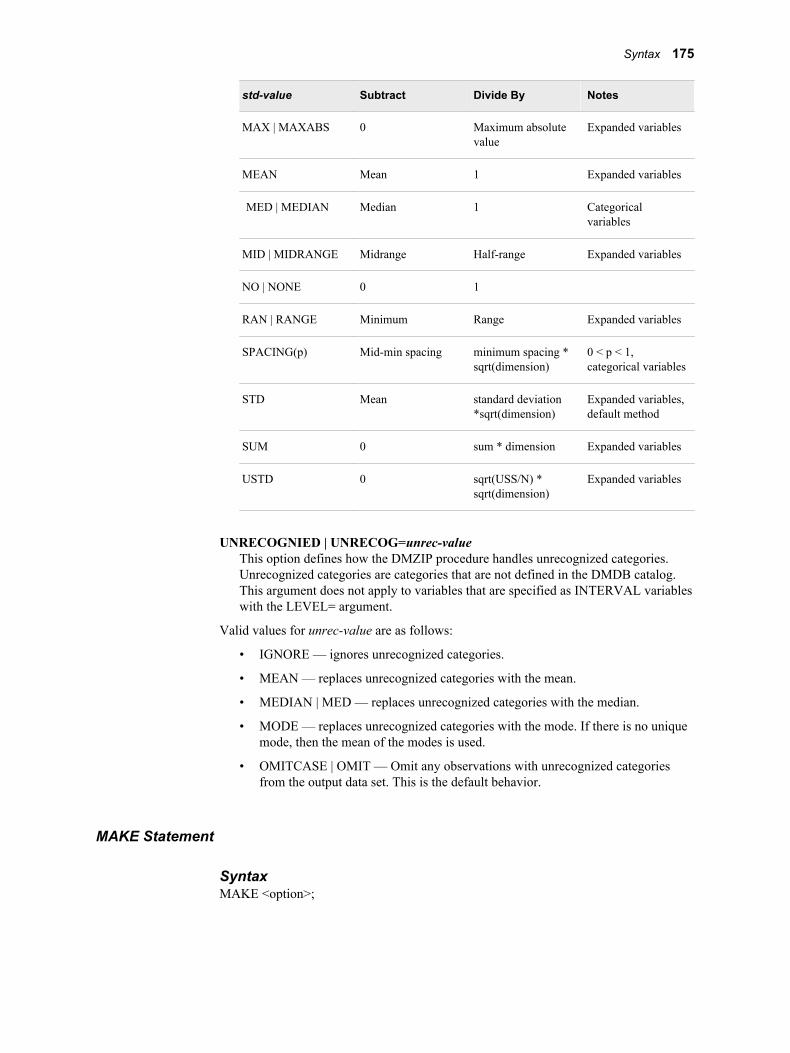
std-value Subtract Divide By Notes
MAX | MAXABS 0 Maximum absolute value
Expanded variables
MEAN Mean 1 Expanded variables
MED | MEDIAN Median 1 Categorical variables
MID | MIDRANGE Midrange Half-range Expanded variables
NO | NONE 0 1
RAN | RANGE Minimum Range Expanded variables
SPACING(p) Mid-min spacing minimum spacing * sqrt(dimension)
0 < p < 1, categorical variables
STD Mean standard deviation *sqrt(dimension)
Expanded variables, default method
SUM 0 sum * dimension Expanded variables
USTD 0 sqrt(USS/N) * sqrt(dimension)
Expanded variables
UNRECOGNIED | UNRECOG=unrec-valueThis option defines how the DMZIP procedure handles unrecognized categories. Unrecognized categories are categories that are not defined in the DMDB catalog. This argument does not apply to variables that are specified as INTERVAL variables with the LEVEL= argument.
Valid values for unrec-value are as follows:
• IGNORE — ignores unrecognized categories.
• MEAN — replaces unrecognized categories with the mean.
• MEDIAN | MED — replaces unrecognized categories with the median.
• MODE — replaces unrecognized categories with the mode. If there is no unique mode, then the mean of the modes is used.
• OMITCASE | OMIT — Omit any observations with unrecognized categories from the output data set. This is the default behavior.
MAKE Statement
SyntaxMAKE <option>;
Syntax 175
Optional ArgumentOUTVAR=data-set-name
This data set contains the variable _TYPE_ and all of the expanded variables, which are character variables. There are three observations in this data set.
• _TYPE_=VARIABLE — contains the name of the original variable that corresponds to the expanded variable.
• _TYPE_=FORMATTED — contains the formatted value of the category that corresponds to the expanded variable for categorical variables with multidimensional encodings. This value is blank for categorical variables with one-dimensional encodings and for interval variables.
• _TYPE_=NORMALIZED — contains the normalized value of the category that corresponds to the expanded variable for categorical variables with multidimensional encodings. This value is blank for categorical variables with one-dimensional encodings and for interval variables.
SCORE Statement
SyntaxSCORE <options>;
Optional ArgumentsDATA=data-set-name
Use this option to specify the input data set, if you did not specify this data set in the PROC statement.
OUT=data-set-nameThis is the output data set, which contains the original data plus dummy variables, standardized variables, and transformed variables.
For the GLM, reference, deviation, thermometer, and bathtub encodings, dummy variables are created for each dimension and named by concatenating the original variable name with the category. Standardization and missing-value replacement are done in accordance with the STDIZE= and MISSING= options.
For any other variable that is standardized, one transformed variable is created and named by concatenating S_ with the original variable name. Missing-value replacement is done in accordance with the MISSING= option.
For the rank and index encodings and for variables in which missing values are replaced, one transformed variable is created and named by concatenating T_ with the original variable name. Missing-value replacement is done in accordance with the MISSING= option.
Examples
Example 1: Preprocessing the Data and Basic UsageBecause the data sets in the SAMPSIO library are relatively large, it may be hard to understand what the DMZIP procedure does with these data sets. Therefore, you will
176 Chapter 10 • The DMZIP Procedure
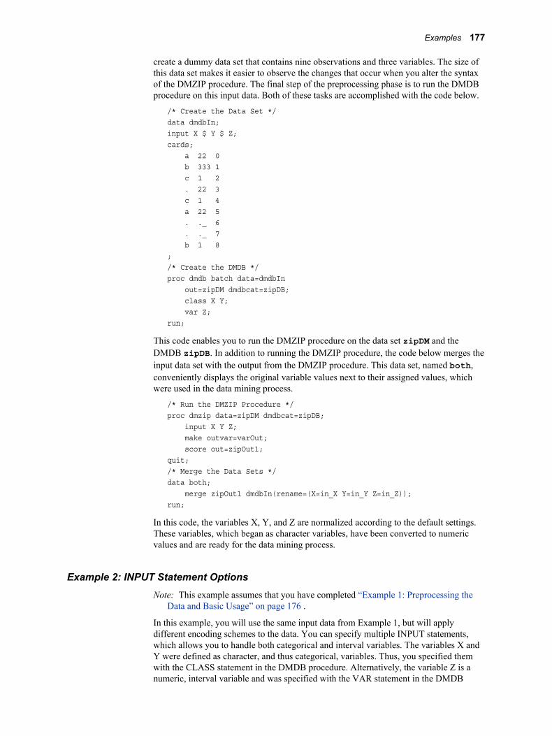
create a dummy data set that contains nine observations and three variables. The size of this data set makes it easier to observe the changes that occur when you alter the syntax of the DMZIP procedure. The final step of the preprocessing phase is to run the DMDB procedure on this input data. Both of these tasks are accomplished with the code below.
/* Create the Data Set */data dmdbIn;input X $ Y $ Z;cards; a 22 0 b 333 1 c 1 2 . 22 3 c 1 4 a 22 5 . ._ 6 . ._ 7 b 1 8;/* Create the DMDB */proc dmdb batch data=dmdbIn out=zipDM dmdbcat=zipDB; class X Y; var Z;run;
This code enables you to run the DMZIP procedure on the data set zipDM and the DMDB zipDB. In addition to running the DMZIP procedure, the code below merges the input data set with the output from the DMZIP procedure. This data set, named both, conveniently displays the original variable values next to their assigned values, which were used in the data mining process.
/* Run the DMZIP Procedure */proc dmzip data=zipDM dmdbcat=zipDB; input X Y Z; make outvar=varOut; score out=zipOut1;quit;/* Merge the Data Sets */data both; merge zipOut1 dmdbIn(rename=(X=in_X Y=in_Y Z=in_Z));run;
In this code, the variables X, Y, and Z are normalized according to the default settings. These variables, which began as character variables, have been converted to numeric values and are ready for the data mining process.
Example 2: INPUT Statement OptionsNote: This example assumes that you have completed “Example 1: Preprocessing the
Data and Basic Usage” on page 176 .
In this example, you will use the same input data from Example 1, but will apply different encoding schemes to the data. You can specify multiple INPUT statements, which allows you to handle both categorical and interval variables. The variables X and Y were defined as character, and thus categorical, variables. Thus, you specified them with the CLASS statement in the DMDB procedure. Alternatively, the variable Z is a numeric, interval variable and was specified with the VAR statement in the DMDB
Examples 177
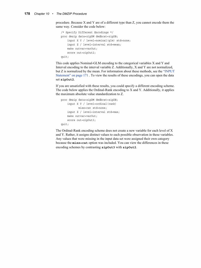
procedure. Because X and Y are of a different type than Z, you cannot encode them the same way. Consider the code below:
/* Specify Different Encodings */proc dmzip data=zipDM dmdbcat=zipDB; input X Y / level=nominal(glm) std=none; input Z / level=interval std=mean; make outvar=varOut; score out=zipOut2;quit;
This code applies Nominal-GLM encoding to the categorical variables X and Y and Interval encoding to the interval variable Z. Additionally, X and Y are not normalized, but Z is normalized by the mean. For information about these methods, see the “INPUT Statement” on page 171 . To view the results of these encodings, you can open the data set zipOut2.
If you are unsatisfied with these results, you could specify a different encoding scheme. The code below applies the Ordinal-Rank encoding to X and Y. Additionally, it applies the maximum absolute value standardization to Z.
proc dmzip data=zipDM dmdbcat=zipDB; input X Y / level=ordinal(rank) miss=cat std=none; input Z / level=interval std=max; make outvar=varOut; score out=zipOut3;quit;
The Ordinal-Rank encoding scheme does not create a new variable for each level of X and Y. Rather, it assigns distinct values to each possible observation in these variables. Any values that were missing in the input data set were assigned their own category because the miss=cat option was included. You can view the differences in these encoding schemes by contrasting zipOut3 with zipOut2.
178 Chapter 10 • The DMZIP Procedure
Chapter 11
The NEURAL Procedure
Overview . . . . . . . . . . . . . . . . . . . . . . . . . . . . . . . . . . . . . . . . . . . . . . . . . . . . . . . . . . . 180The NEURAL Procedure . . . . . . . . . . . . . . . . . . . . . . . . . . . . . . . . . . . . . . . . . . . . 180Terminology and Architectural Description . . . . . . . . . . . . . . . . . . . . . . . . . . . . . . 180Running the Neural Procedure . . . . . . . . . . . . . . . . . . . . . . . . . . . . . . . . . . . . . . . . 180
Syntax . . . . . . . . . . . . . . . . . . . . . . . . . . . . . . . . . . . . . . . . . . . . . . . . . . . . . . . . . . . . . . 182The NEURAL Procedure . . . . . . . . . . . . . . . . . . . . . . . . . . . . . . . . . . . . . . . . . . . . 182PROC NEURAL Statement . . . . . . . . . . . . . . . . . . . . . . . . . . . . . . . . . . . . . . . . . . 182ARCHITECTURE Statement . . . . . . . . . . . . . . . . . . . . . . . . . . . . . . . . . . . . . . . . . 183CODE Statement . . . . . . . . . . . . . . . . . . . . . . . . . . . . . . . . . . . . . . . . . . . . . . . . . . 186CONNECT Statement . . . . . . . . . . . . . . . . . . . . . . . . . . . . . . . . . . . . . . . . . . . . . . 188CUT Statement . . . . . . . . . . . . . . . . . . . . . . . . . . . . . . . . . . . . . . . . . . . . . . . . . . . . 189DECISION Statement . . . . . . . . . . . . . . . . . . . . . . . . . . . . . . . . . . . . . . . . . . . . . . . 189DELETE Statement . . . . . . . . . . . . . . . . . . . . . . . . . . . . . . . . . . . . . . . . . . . . . . . . 190FREEZE Statement . . . . . . . . . . . . . . . . . . . . . . . . . . . . . . . . . . . . . . . . . . . . . . . . . 190FREQ Statement . . . . . . . . . . . . . . . . . . . . . . . . . . . . . . . . . . . . . . . . . . . . . . . . . . . 191HIDDEN Statement . . . . . . . . . . . . . . . . . . . . . . . . . . . . . . . . . . . . . . . . . . . . . . . . 191INITIAL Statement . . . . . . . . . . . . . . . . . . . . . . . . . . . . . . . . . . . . . . . . . . . . . . . . . 192INPUT Statement . . . . . . . . . . . . . . . . . . . . . . . . . . . . . . . . . . . . . . . . . . . . . . . . . . 193NETOPTIONS Statement . . . . . . . . . . . . . . . . . . . . . . . . . . . . . . . . . . . . . . . . . . . . 194NLOPTIONALS . . . . . . . . . . . . . . . . . . . . . . . . . . . . . . . . . . . . . . . . . . . . . . . . . . . 195PERFORMANCE Statement . . . . . . . . . . . . . . . . . . . . . . . . . . . . . . . . . . . . . . . . . 199PERTURB Statement . . . . . . . . . . . . . . . . . . . . . . . . . . . . . . . . . . . . . . . . . . . . . . . 200PRELIM Statement . . . . . . . . . . . . . . . . . . . . . . . . . . . . . . . . . . . . . . . . . . . . . . . . . 201RANOPTIONS Statement . . . . . . . . . . . . . . . . . . . . . . . . . . . . . . . . . . . . . . . . . . . 203SAVE Statement . . . . . . . . . . . . . . . . . . . . . . . . . . . . . . . . . . . . . . . . . . . . . . . . . . . 204SCORE Statement . . . . . . . . . . . . . . . . . . . . . . . . . . . . . . . . . . . . . . . . . . . . . . . . . 204SET Statement . . . . . . . . . . . . . . . . . . . . . . . . . . . . . . . . . . . . . . . . . . . . . . . . . . . . 205SHOW Statement . . . . . . . . . . . . . . . . . . . . . . . . . . . . . . . . . . . . . . . . . . . . . . . . . . 205TARGET Statement . . . . . . . . . . . . . . . . . . . . . . . . . . . . . . . . . . . . . . . . . . . . . . . . 205THAW Statement . . . . . . . . . . . . . . . . . . . . . . . . . . . . . . . . . . . . . . . . . . . . . . . . . . 207TRAIN Statement . . . . . . . . . . . . . . . . . . . . . . . . . . . . . . . . . . . . . . . . . . . . . . . . . . 208USE Statement . . . . . . . . . . . . . . . . . . . . . . . . . . . . . . . . . . . . . . . . . . . . . . . . . . . . 210
Details . . . . . . . . . . . . . . . . . . . . . . . . . . . . . . . . . . . . . . . . . . . . . . . . . . . . . . . . . . . . . . 210Activation Functions . . . . . . . . . . . . . . . . . . . . . . . . . . . . . . . . . . . . . . . . . . . . . . . . 210Combination Functions . . . . . . . . . . . . . . . . . . . . . . . . . . . . . . . . . . . . . . . . . . . . . . 211The BPROP, RPROP, and QPROP Algorithms . . . . . . . . . . . . . . . . . . . . . . . . . . . 212
Examples . . . . . . . . . . . . . . . . . . . . . . . . . . . . . . . . . . . . . . . . . . . . . . . . . . . . . . . . . . . 217Example 1: Develop a Simple Multilayer Perceptron . . . . . . . . . . . . . . . . . . . . . . 217Example 2: Developing a Neural Network for a Continuous Target . . . . . . . . . . . 218Example 3: The Hill and Plateau Data with 3 Hidden Units . . . . . . . . . . . . . . . . . 220
179
Example 4: The Hill and Plateau Data with 30 Hidden Units . . . . . . . . . . . . . . . . 221
Further Reading . . . . . . . . . . . . . . . . . . . . . . . . . . . . . . . . . . . . . . . . . . . . . . . . . . . . . 222
Overview
The NEURAL ProcedureThe NEURAL procedure trains a wide variety of feed-forward neural networks using proven statistical methods and numerical algorithms. Before referring to this document, you should be familiar with the chapters “Introduction to Predictive Modeling” and “Neural Network Node: Reference” in the Enterprise Miner help. These chapters provide background information and details needed to understand the current NEURAL procedure.
The WHERE statement for PROC NEURAL applies only to data sets that are open when the WHERE statement is parsed. In other words, it should apply to data sets in preceding statements that have not yet been executed, but it should not apply to data sets in subsequent statements.
Terminology and Architectural DescriptionEach INPUT, HIDDEN, and TARGET statement defines a layer. For the INPUT statement, a layer is a convenient grouping of variables that serve as inputs to the network and have common values for LEVEL= and STD=. Similarly, for the TARGET statement, a layer is a convenient grouping of variables that serve as outputs of the network and have common values for LEVEL=, STD=, ACTIVATION=, COMBINATION=, and other arguments. Each layer consists of units, which is synonymous with the term neuron in the literature about neural networks. It is the smallest computational entity in the network.
The INPUT and TARGET statements require a list of variables. If the variables are interval variables, then there is one unit that corresponds to each variable. If the variables are nominal or ordinal variables, then there is one unit for each level of every variable. The HIDDEN statement requires you to input a number that determines the number of units in the associated layer. This layer is a grouping of units that have common values for ACTIVATION=, COMBINATION=, and other arguments.
Each INPUT statement produces an input layer. Because multiple INPUT statements are allowed, a network can have multiple input layers. However, connections from multiple input layers must be parallel; there cannot be serial connections between input layers. Similarly, multiple TARGET statements generate multiple output layers. The connections to multiple output layers must be in parallel; there cannot be serial connections between output layers. Hidden layers can be connected in series or in parallel.
Running the Neural ProcedureBefore you run the NEURAL procedure, you must run the DMDB procedure to create a DMDB catalog entry.
A typical call to the NEURAL procedure uses the following statements:
• A PROC NEURAL statement to specify the training set, DMDB catalog, and random number seed. If you specify a 0 or a negative seed, the system clock is used
180 Chapter 11 • The NEURAL Procedure
to obtain a seed. In this case, the seed will be unavailable if it is ever necessary to reproduce the initial weights.
• One or more INPUT statements to specify an input layer, which includes the input variables and other layer characteristics.
• One or more HIDDEN statements to specify a hidden layer, which includes the number of hidden units and other characteristics.
• One or more TARGET statements to specify a target layer, which includes the target variables and other characteristics.
• An ID= argument within the INPUT, HIDDEN, or TARGET statements. If not specified, then a default ID is used. This default is I1, I2, ... for input layers; H1, H2, ... for hidden layers; and O1, O2, ... for output layers.
• One or more CONNECT statements to connect layers in the network if the default serial connections are not appropriate.
• A PRELIM statement to do preliminary training in order to avoid bad local optimizations.
• A TRAIN statement to train the neural network.
• One or more SCORE statements to create output data sets.
Two types of statements are used with the NEURAL procedure. All of the statements in the list above are action statements; they directly affect the network or directly produce output. There are also option statements, such as NETOPTIONS, NLOPTIONS, and RANOPTIONS, that set options for future use. Options specified in an action statement apply only to that statement and do not affect subsequent statements. For example, the default technique for least squares training is Levenberg-Marquardt (TECH=LEVMAR). If you execute a TRAIN statement with the option TECH=CONGRA, conjugate gradient training will be used for that particular training run. If you then execute another TRAIN statement without the TECH= option, the technique will revert to the default value of TECH=LEVMAR. But if you submit an NLOPTIONS statement with TECH=CONGRA, conjugate gradient training will be used for all subsequent TRAIN statements until you explicitly specify a different technique.
Each layer in the network has an identifier specified by the ID= option in the INPUT, HIDDEN, or TARGET statements. An identifier can be any SAS name, but to avoid confusion, you should not use the name of a variable in the training set. Layer identifiers are used in various statements, such as CONNECT, to specify previously defined layers.
Each unit in the network has a name. For units that correspond to interval variables in input or output layers, the name of the unit is the same as the name of the variable. For units that correspond to dummy variables for categorical variables, the name of each unit is constructed by concatenating the name of the variable with the value of the category. Names are truncated as necessary to make the length of the name eight characters or less. For hidden units, the names are constructed by concatenating the layer ID with an integer.
Overview 181
Syntax
The NEURAL ProcedurePROC NEURAL DATA=data-set-name DMDBCAT=catalog-name <options>;
ARCHITECTURE architecture-name <options>;CODE FILE=file-name <options>;CONNECT list-of-ids </options>;CUT list-of-ids | ALL;DECISION DECDATA=data-set-name <options>;DELETE list-of-ids | ALL;FREEZE list-of-weights </options>;FREQ variable;HIDDEN number / ID=name</options>;INITIAL <options>;INPUT list-of-variables / ID=name<options>;NETOPTIONS <options>;NLOPTIONS <options>;PERFORMANCE <options>;PERTURB list-of-weights </options>;PRELIM number <options>;REMOTE <options>;RANOPTIONS list-of-connections </options>;SAVE <options>;SCORE OUT=data-set-name <options>;SET list-of-weights number;SHOW STATEMENTS WEIGHTS;TARGET list-of-variables / ID=name <options>;THAW list-of-weights;TRAIN <options>;USE data-set-name;QUIT;
PROC NEURAL Statement
SyntaxPROC NEURAL DATA=data-set-name DMDBCAT=catalog-name <options>;
Required ArgumentsDATA=data-set-name
This argument specifies the input data set that contains the training data.
182 Chapter 11 • The NEURAL Procedure
DMDBCAT=catalog-nameThis argument specifies the DMDB catalog that was created by the DMDB procedure.
Optional ArgumentsNETWORK=screen-spec
This option constructs a network according to a description that was saved by the SAVE statement during a previous execution of the NEURAL procedure. The value of screen-spec is the catalog entry that was specified in the SAVE statement.
RANDOM=numberThis option specifies the seed for the random number generated that is used for network weight initialization. The value of number must be a positive integer and default to 12345.
If you specify 0 or a negative number, then the NEURAL procedure will use the system clock as the value of number. In this case, the NEURAL procedure will not disclose this value and you will be unable to repeat the initialization process with the same values. Thus, the final weights will differ, and predicted outputs for the input information will differ as well.
STOPFILE='file-name'This option enables you to stop the NEURAL procedure when you are in the middle of a large job. Before you invoke the NEURAL procedure, specify a filename (for example, STOPFILE= 'c:\mydir\haltneural'). Initially, this file should not exist. The NEURAL procedure checks for the existence of this file between iterations in the training process. When you want to stop the job, create the specified file, and the NEURAL procedure will halt the training at the current iteration. The file does not have to contain any contents.
TESTDATA=data-set-nameThis option specifies a data set that is used to compute the test average error during the training phase. At selected iterations (controlled by ESTITER=), the information in data-set-name is scored with the current network weight values and the error is computed. The average test error is output to the OUTEST= data set. Because the data is scored, data-set-name must contain all of the input and target variables.
VALIDATA=data-set-nameThis option specifies the data set that is used to compute the validation average error during the training phase. At selected iterations (controlled by ESTITER=), each observation in data-set-name is scored with the current network weight values and the error is computed. The average validation error is then output to the OUTEST= data set. Because this data is scored, data-set-name must contain all of the input and target variables.
ARCHITECTURE Statement
SyntaxARCHITECTURE architecture-name <options>;
You cannot override the hidden unit options ACT= and COMBINE= that are implied by the ARCHITECTURE statement because these define the architecture. You can override all other values that are set by the ARCHITECTURE statement with an INPUT, HIDDEN, TARGET, or RANOPTIONS statement.
Syntax 183
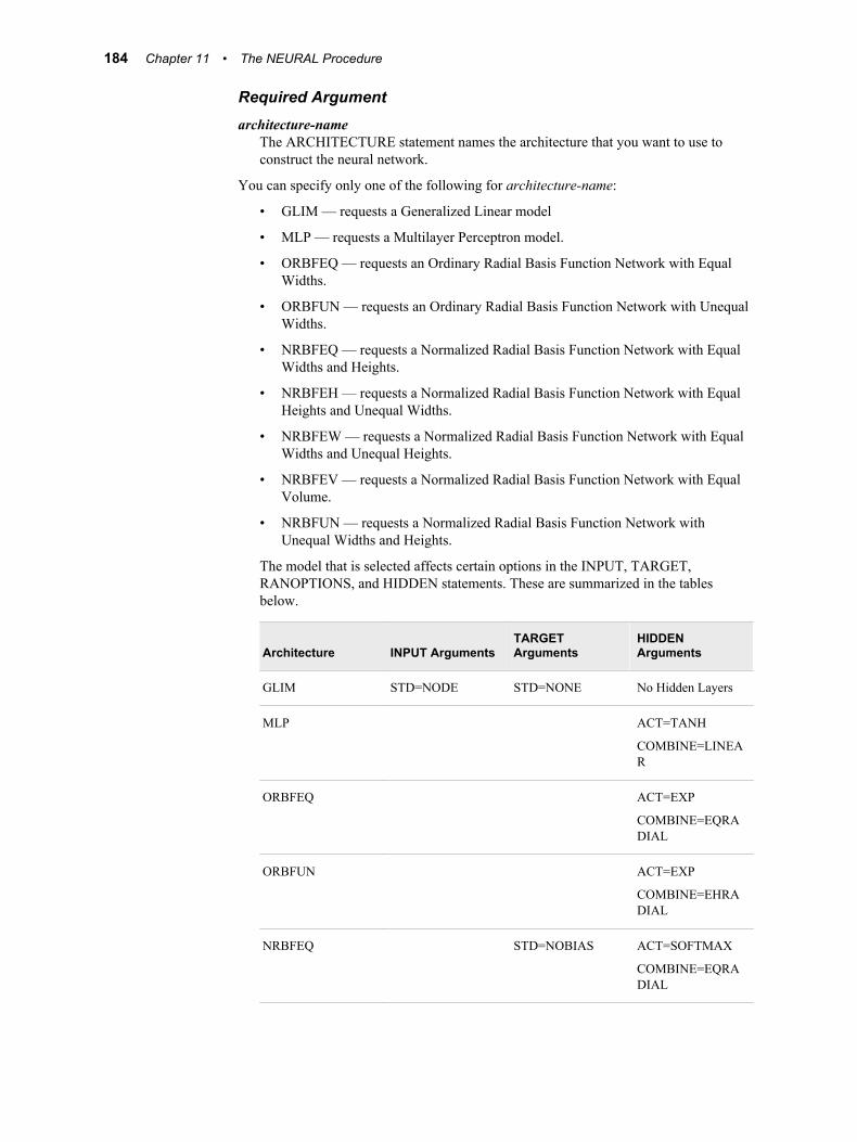
Required Argumentarchitecture-name
The ARCHITECTURE statement names the architecture that you want to use to construct the neural network.
You can specify only one of the following for architecture-name:
• GLIM — requests a Generalized Linear model
• MLP — requests a Multilayer Perceptron model.
• ORBFEQ — requests an Ordinary Radial Basis Function Network with Equal Widths.
• ORBFUN — requests an Ordinary Radial Basis Function Network with Unequal Widths.
• NRBFEQ — requests a Normalized Radial Basis Function Network with Equal Widths and Heights.
• NRBFEH — requests a Normalized Radial Basis Function Network with Equal Heights and Unequal Widths.
• NRBFEW — requests a Normalized Radial Basis Function Network with Equal Widths and Unequal Heights.
• NRBFEV — requests a Normalized Radial Basis Function Network with Equal Volume.
• NRBFUN — requests a Normalized Radial Basis Function Network with Unequal Widths and Heights.
The model that is selected affects certain options in the INPUT, TARGET, RANOPTIONS, and HIDDEN statements. These are summarized in the tables below.
Architecture INPUT ArgumentsTARGET Arguments
HIDDEN Arguments
GLIM STD=NODE STD=NONE No Hidden Layers
MLP ACT=TANH
COMBINE=LINEAR
ORBFEQ ACT=EXP
COMBINE=EQRADIAL
ORBFUN ACT=EXP
COMBINE=EHRADIAL
NRBFEQ STD=NOBIAS ACT=SOFTMAX
COMBINE=EQRADIAL
184 Chapter 11 • The NEURAL Procedure
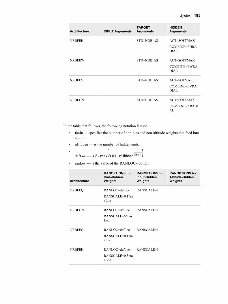
Architecture INPUT ArgumentsTARGET Arguments
HIDDEN Arguments
NRBFEH STD=NOBIAS ACT=SOFTMAX
COMBINE=EHRADIAL
NRBFEW STD=NOBIAS ACT=SOFTMAX
COMBINE=EWRADIAL
NRBFEV STD=NOBIAS ACT=SOFMAX
COMBINE=EVRADIAL
NRBFUN STD=NOBIAS ACT=SOFTMAX
COMBINE=XRADIAL
In the table that follows, the following notation is used:
• fanIn — specifies the number of non-bias and non-altitude weights that feed into a unit
• nHidden — is the number of hidden units.
•defLoc — is 2 ⋅ max(0.01, nHidden 1
fanIn )• ranLoc — is the value of the RANLOC= option.
Architecture
RANOPTIONS for Bias-Hidden Weights
RANOPTIONS for Input-Hidden Weights
RANOPTIONS for Altitude-Hidden Weights
ORBFEQ RANLOC=defLoc
RANSCALE=0.1*ranLoc
RANSCALE=1
ORBFUN RANLOC=defLoc
RANSCALE=5*ranLoc
RANSCALE=1
NRBFEQ RANLOC=defLoc
RANSCALE=0.1*ranLoc
RANSCALE=1
NRBFEH RANLOC=defLoc
RANSCALE=0.5*ranLoc
RANSCALE=1
Syntax 185
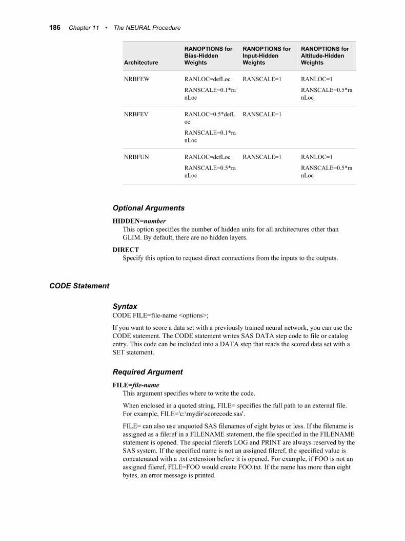
Architecture
RANOPTIONS for Bias-Hidden Weights
RANOPTIONS for Input-Hidden Weights
RANOPTIONS for Altitude-Hidden Weights
NRBFEW RANLOC=defLoc
RANSCALE=0.1*ranLoc
RANSCALE=1 RANLOC=1
RANSCALE=0.5*ranLoc
NRBFEV RANLOC=0.5*defLoc
RANSCALE=0.1*ranLoc
RANSCALE=1
NRBFUN RANLOC=defLoc
RANSCALE=0.5*ranLoc
RANSCALE=1 RANLOC=1
RANSCALE=0.5*ranLoc
Optional ArgumentsHIDDEN=number
This option specifies the number of hidden units for all architectures other than GLIM. By default, there are no hidden layers.
DIRECTSpecify this option to request direct connections from the inputs to the outputs.
CODE Statement
SyntaxCODE FILE=file-name <options>;
If you want to score a data set with a previously trained neural network, you can use the CODE statement. The CODE statement writes SAS DATA step code to file or catalog entry. This code can be included into a DATA step that reads the scored data set with a SET statement.
Required ArgumentFILE=file-name
This argument specifies where to write the code.
When enclosed in a quoted string, FILE= specifies the full path to an external file. For example, FILE='c:\mydir\scorecode.sas'.
FILE= can also use unquoted SAS filenames of eight bytes or less. If the filename is assigned as a fileref in a FILENAME statement, the file specified in the FILENAME statement is opened. The special filerefs LOG and PRINT are always reserved by the SAS system. If the specified name is not an assigned fileref, the specified value is concatenated with a .txt extension before it is opened. For example, if FOO is not an assigned fileref, FILE=FOO would create FOO.txt. If the name has more than eight bytes, an error message is printed.
186 Chapter 11 • The NEURAL Procedure
Optional ArgumentCATALOG | CAT | C=library.catalog.entry.type
This option determines where to write the code in the form of library.catalog.entry.type. The compound name can have from one to four levels. The default library is determined by the SAS system option USER=, and is usually the Work directory. The default entry is SASCODE, and the default type is SOURCE.
DUMMIES | NODUMMIESSpecify DUMMIES to keep dummy variables, standardized variables, or other transformed variables in the data set. By default, these variables are dropped from the data.
ERROR | NOERRORSpecify ERROR to compute error function, given by the variable E_*. By default, no error function is calculated.
FORMAT=formatUse FORMAT= to format weights or other numeric values that don't have a format from the input data set. The default value is BEST20.
GROUP=group-identifierUse GROUP= to specify the group identifier that is used for group processing. This should be a valid SAS name of 16 bytes or less, which is used to construct array names and statement labels in the generated code.
LINESIZE | LS=numberUse LINESIZE= to specify the line size for generated code. The permissible range for number is 64 to 254 and defaults to 72.
LOOKUP=AUTO | BINARY | LINEAR | LINFREQ | SELECTUse LOOKUP= to specify the algorithm that is used to look up CLASS levels.
• AUTO — selects the fastest method for each variable that is portable across ASCII/EBCDIC. This is the default method.
• BINARY — uses a binary search. This is fast, but might produce incorrect results if you generate the code on an ASCII machine and execute the code on an EBCDIC machine or vice versa, and the normalized category values contain characters that collate in different orders on ASCII and EBCDIC. PROC CSCORE is unable to translate this code.
• LINEAR — uses a linear search with IF statements. Categories are in the order specified in the DMDB catalog. This is slow if there are many categories.
• LINFREQ — uses a linear search with IF statements. Categories are in descending order of frequency as given by the DMDB catalog. This is fast if the distribution of class frequencies is highly uneven, but is slow if there are many categories with approximately equal frequencies.
• SELECT — uses a SELECT statement. This method may be slow if there are many categories.
You cannot specify both FILE= and CATALOG=. If you specify neither, the code is written to the SAS log.
PMML | XMLSpecify PMML to produce scoring code in Predictive Modeling Markup Language, an XML-based standard for representing data mining results. For more information, see the PMML Support in Enterprise Miner section in the Enterprise Miner 5.3 Java Help.
Syntax 187
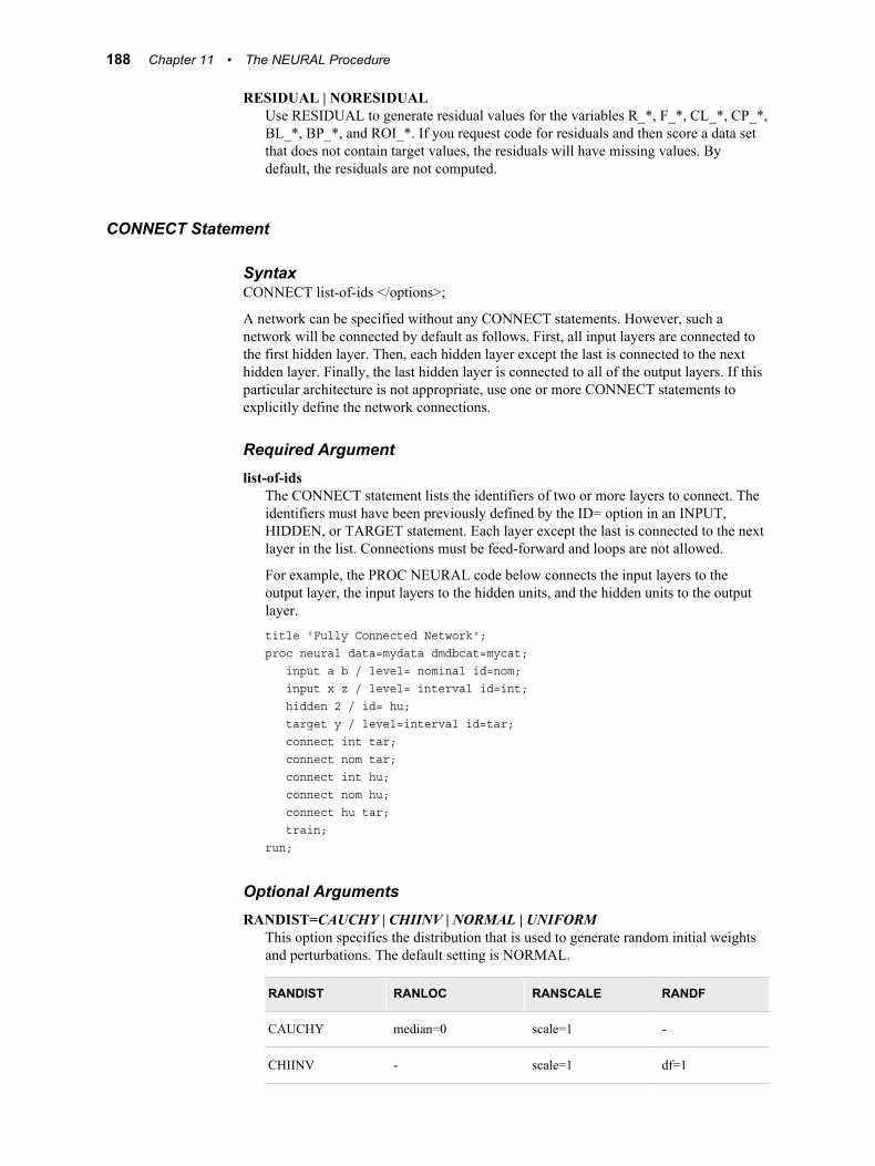
RESIDUAL | NORESIDUALUse RESIDUAL to generate residual values for the variables R_*, F_*, CL_*, CP_*, BL_*, BP_*, and ROI_*. If you request code for residuals and then score a data set that does not contain target values, the residuals will have missing values. By default, the residuals are not computed.
CONNECT Statement
SyntaxCONNECT list-of-ids </options>;
A network can be specified without any CONNECT statements. However, such a network will be connected by default as follows. First, all input layers are connected to the first hidden layer. Then, each hidden layer except the last is connected to the next hidden layer. Finally, the last hidden layer is connected to all of the output layers. If this particular architecture is not appropriate, use one or more CONNECT statements to explicitly define the network connections.
Required Argumentlist-of-ids
The CONNECT statement lists the identifiers of two or more layers to connect. The identifiers must have been previously defined by the ID= option in an INPUT, HIDDEN, or TARGET statement. Each layer except the last is connected to the next layer in the list. Connections must be feed-forward and loops are not allowed.
For example, the PROC NEURAL code below connects the input layers to the output layer, the input layers to the hidden units, and the hidden units to the output layer.
title 'Fully Connected Network';proc neural data=mydata dmdbcat=mycat; input a b / level= nominal id=nom; input x z / level= interval id=int; hidden 2 / id= hu; target y / level=interval id=tar; connect int tar; connect nom tar; connect int hu; connect nom hu; connect hu tar; train;run;
Optional ArgumentsRANDIST=CAUCHY | CHIINV | NORMAL | UNIFORM
This option specifies the distribution that is used to generate random initial weights and perturbations. The default setting is NORMAL.
RANDIST RANLOC RANSCALE RANDF
CAUCHY median=0 scale=1 -
CHIINV - scale=1 df=1
188 Chapter 11 • The NEURAL Procedure
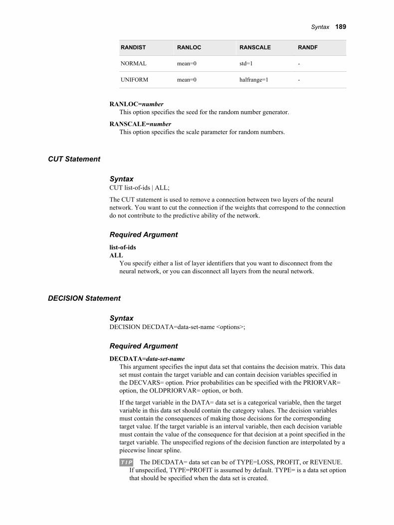
RANDIST RANLOC RANSCALE RANDF
NORMAL mean=0 std=1 -
UNIFORM mean=0 halfrange=1 -
RANLOC=numberThis option specifies the seed for the random number generator.
RANSCALE=numberThis option specifies the scale parameter for random numbers.
CUT Statement
SyntaxCUT list-of-ids | ALL;
The CUT statement is used to remove a connection between two layers of the neural network. You want to cut the connection if the weights that correspond to the connection do not contribute to the predictive ability of the network.
Required Argumentlist-of-idsALL
You specify either a list of layer identifiers that you want to disconnect from the neural network, or you can disconnect all layers from the neural network.
DECISION Statement
SyntaxDECISION DECDATA=data-set-name <options>;
Required ArgumentDECDATA=data-set-name
This argument specifies the input data set that contains the decision matrix. This data set must contain the target variable and can contain decision variables specified in the DECVARS= option. Prior probabilities can be specified with the PRIORVAR= option, the OLDPRIORVAR= option, or both.
If the target variable in the DATA= data set is a categorical variable, then the target variable in this data set should contain the category values. The decision variables must contain the consequences of making those decisions for the corresponding target value. If the target variable is an interval variable, then each decision variable must contain the value of the consequence for that decision at a point specified in the target variable. The unspecified regions of the decision function are interpolated by a piecewise linear spline.
T I P The DECDATA= data set can be of TYPE=LOSS, PROFIT, or REVENUE. If unspecified, TYPE=PROFIT is assumed by default. TYPE= is a data set option that should be specified when the data set is created.
Syntax 189
Optional ArgumentsCOST=list-of-costs
Use this option to specify numeric constants that give the cost of a decision, to list variables in the DATA= data set that contain case-specific costs, or a combination of both. There must be the same total number of cost constants and variables as there are decision variables in the DECVARS= option. In the COST= option, you cannot use abbreviated variable lists. If you do not specify this option, then all costs are assumed to be 0.
Note: You can specify this option only when the DECDATA= data set is of type REVENUE.
DECVARS=list-of-variablesUse this option to specify the decision variables in the DECDATA= data set. These variables contain the target-specific consequences for each decision.
OLDPRIORVAR=variableThis option specifies the variable in the DECDATA= data set that contains the prior probabilities that were used the first time the model was created. If you specify OLDPRIORVAR=, then you must specify PRIORVAR=.
PRIORVAR=variableThis option specifies the variable in the DECDATA= data set that contains the prior probabilities that are used to make decisions.
DELETE Statement
SyntaxDELETE list-of-ids;
The DELETE statement removes a layer from the neural network and all associated weights. While the CUT statement is used to remove connections between layers, the DELETE statement completely removes a layer.
Required Argumentlist-of-ids
Specify a list of layer identifiers that you want to remove from the neural network.
FREEZE Statement
SyntaxFREEZE list-of-weights </options>;
Normally, all weights are updated during the training phase. If you freeze one or more weights, those weights will retain their frozen value until a corresponding THAW statement is executed. When you freeze weights, training will be quicker and less memory is used.
190 Chapter 11 • The NEURAL Procedure
Required Argumentlist-of-weights
Use the FREEZE statement to specify a list of weights to freeze. The list of weights must be in the form wName —> wName2. wName is either a unit name, a layer identifier, BIAS, or ALTITUDE. wName2 is either a unit name or a layer identifier.
Optional ArgumentsVALUE=number
Specify the VALUE= option to freeze all the specified weights at the given value number. You cannot specify both VALUE= and EST=.
EST=data-set-nameSpecify the EST= option to freeze all the specified weights to the values given in data-set-name.
FREQ Statement
SyntaxFREQ variable;
Required Argumentvariable
Use the FREQ statement to specify a variable that contains the frequency of each observation. Noninteger values are truncated to the nearest integer.
The variable specified here is not required in the input data set because the NEURAL procedure will search for the FREQ variable in the DATA=, VALIDATA=, and TESTDATA= data set. If it does not appear in any of these data sets, then the procedure issues a warning but continues processing. For any data set that does not contain the FREQ variable, the NEURAL procedure assumes a frequency of 1 for every observation.
HIDDEN Statement
SyntaxHIDDEN number / ID=name<options>;
The HIDDEN statement is used to specify the hidden layers of the neural network. You can specify as many HIDDEN statements as you want, limited only by computer memory, time, and disk space. The hidden layers can be connected in any feed-forward pattern via CONNECT statements.
Required Argumentsnumber
The value specified here represents the number of units in the hidden layer.
ID=nameUse the ID= statement to specify the identifier for the layer.
Syntax 191
Optional ArgumentsACT=activation-function
This option specifies the activation that is used by the hidden layer. For a complete list of the activation functions, see “Activation Functions” on page 210 .
For hidden units, the default activation function depends on the combination function and the number of units in the layer.
• For COMBINE=ADD, the default activation is IDENTITY.
• For COMBINE=LINEAR or EQSLOPES, the default activation function is TANH.
• For COMBINE=EHRADIAL, EQRADIAL, EVRADIAL, WERADIAL, or XRADIAL, the default activation function is EXP if there is one hidden unit and SOFTMAX if there are more.
BIAS | NOBIASThis option specifies whether to use bias in the hidden layer. By default, bias is used.
COMBINE=combination-functionThis option specifies the combination function that is used by the hidden layer. For a complete list of combination functions, see “Combination Functions” on page 211 .
INITIAL Statement
SyntaxINITIAL <options>;
After the input variables, hidden layers, and output layers of a network are defined, the NEURAL procedure assigns initial values to the weights and biases in the network. By default, the NEURAL procedure supplies appropriate random or computed values for these quantities.
Optional ArgumentsBIADJUST=NONE | SUM | USS
This option specifies how to adjust the random biases for units with the LINEAR combination function. A random bias is adjusted by multiplying it by the specified weight function and dividing by the scale, set in RANSCALE=, of the distribution.
• NONE — performs no bias adjustment. This is the default behavior.
• SUM — adjusts random initial biases for the sum of the absolute connection weights that lead into the unit. Typically, this adjustment is used with STD=MIDRANGE for input variables and RANDIST=UNIFORM.
• USS — adjusts random initial biases for the square root of the sum of squared connection weights that lead into the unit. Typically, this adjustment is used with STD=STD for input variables and RANDIST=NORMAL.
INEST=data-set-nameThis option specifies an input data set that contains some or all of the weights. Any observations in data-set-name with missing values are assigned values based on RANDOM=, RANDOUT, RANDBIAS, and relevant options in the RANDOM statement. An INEST= data set is typically an OUTEST= data set from the SAVE or TRAIN statement in a previous call to the NEURAL procedure.
192 Chapter 11 • The NEURAL Procedure
INFAN=numberSpecify this option to indicate that random connection weights should be divided by fanInnumber. Here, fanIn is the number of other units that feed into that unit, not adjusted for bias or altitude. The default value of number is 0 for radial combination functions and 0.5 for all others. The value of number must be a real number between 0 and 1.
OUTEST=data-set-nameThis output data set contains the initial weights.
RANDBIAS | NORANDBIASThis option determines if the output biases are randomized or not. By default, output biases are not randomized; instead they are set to the inverse activation function of the target mean. This option overrides the option in the RANOPTIONS statement.
RANDOM=numberThe RANDOM= option is used to specify the initial seed for the random number generator. The value of number must be a positive integer and default to 12345.
RANDOUT | NORANDOUTThis option determines if the output connection weights are randomized or not. By default, output connection weights are not randomized, instead they are set to 0. This option overrides the option in the RANOPTIONS statement.
RANDSCALE | NORANDSCALEThis option determines if the target scale estimates are randomized or not. By default, target scale estimates are not randomized; instead they are set to the standard deviation of the corresponding target variable. This option overrides the option in the RANOPTIONS statement.
INPUT Statement
SyntaxINPUT list-of-variables / ID=name<options>;
The INPUT statement enables you to group input variables that have common levels and standardizations. You can specify as many INPUT statements as you want, given the limits imposed by computer memory, time, and disk space. The input layers can be connected to hidden or output layers via the CONNECT statement.
Required Argumentslist-of-variables
The first argument in the INPUT statement must be the list of input variables.
ID=nameUse the ID argument to specify an identifier for the layer.
Optional ArgumentsLEVEL=INTERVAL | INT | NOMINAL | NOM | ORDINAL | ORD
This option specifies the measurement level of the input variables. The default level for variables specified in the VAR statement in the DMDB procedure is INTERVAL. The default level for variables specified in a CLASS statement in the DMDB procedure is NOMINAL.
STD=methodThis option determines how each variable is standardized.
Syntax 193
Valid values for method are as follows:
• MIDRANGE | MID — Variables are scaled such that their midrange is 0 and the half-range is 1. That is, the variables have a minimum of –1 and a maximum of 1.
• NONE | NO — Variables are not altered.
• RANGE | RAN — Variables are scaled such that their minimum is 0 and the range is 1. This standardization is not recommended for input variables.
• STD — Variables are scaled such that their mean is 0 and the standard deviation is 1. This is the default standardization.
NETOPTIONS Statement
SyntaxNETOPTIONS <options>;
Optional ArgumentsDECAY=number
This option specifies the weight decay. The DECAY option does not affect the Softmax output weights because the adjustment to the error is very small. The function AdjustForDecay() explicitly excludes target biases from the adjustment term. The value of number must be a nonnegative real number. The default value for the QPROP optimization technique is 0.0001 and 0 for all other techniques.
INVALIDTARGET | INVTAR=OMITCASE | OMIT | STOPThis option determines the action to take if an invalid target value is found. If you specify OMITCASE or OMIT, then a warning is given, the observation is not used, and training continues. If you specify STOP, then an error is issued and the training is terminated immediately. The default setting is STOP.
OBJECT=DEV | LIKE | MESTThis option determines the objective function that is used by the NEURAL procedure. Specify DEV to use the deviance as the objective function. For ERROR=NORMAL this is equivalent to least squares. Specify LIKE to use the negative log-likelihood function. Specify MEST to use the M-estimation function.
The default value depends on the error function that is used by the NEURAL procedure. The table below indicates Yes if you can use an error function or objective function pair and No if you cannot. From left to right, the first column with a Yes indicates the default objective function for that error function.
ERRORS DEV LIKE MEST
Normal Yes Yes No
Cauchy No Yes No
Logistic No Yes No
Huber No No Yes
Biweight No No Yes
Wave No No Yes
194 Chapter 11 • The NEURAL Procedure
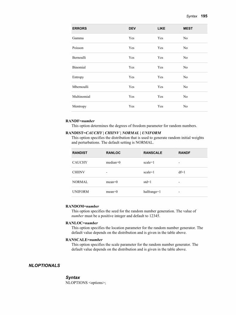
ERRORS DEV LIKE MEST
Gamma Yes Yes No
Poisson Yes Yes No
Bernoulli Yes Yes No
Binomial Yes Yes No
Entropy Yes Yes No
Mbernoulli Yes Yes No
Multinomial Yes Yes No
Mentropy Yes Yes No
RANDF=numberThis option determines the degrees of freedom parameter for random numbers.
RANDIST=CAUCHY | CHIINV | NORMAL | UNIFORMThis option specifies the distribution that is used to generate random initial weights and perturbations. The default setting is NORMAL.
RANDIST RANLOC RANSCALE RANDF
CAUCHY median=0 scale=1 -
CHIINV - scale=1 df=1
NORMAL mean=0 std=1 -
UNIFORM mean=0 halfrange=1 -
RANDOM=numberThis option specifies the seed for the random number generation. The value of number must be a positive integer and default to 12345.
RANLOC=numberThis option specifies the location parameter for the random number generator. The default value depends on the distribution and is given in the table above.
RANSCALE=numberThis option specifies the scale parameter for the random number generator. The default value depends on the distribution and is given in the table above.
NLOPTIONALS
SyntaxNLOPTIONS <options>;
Syntax 195
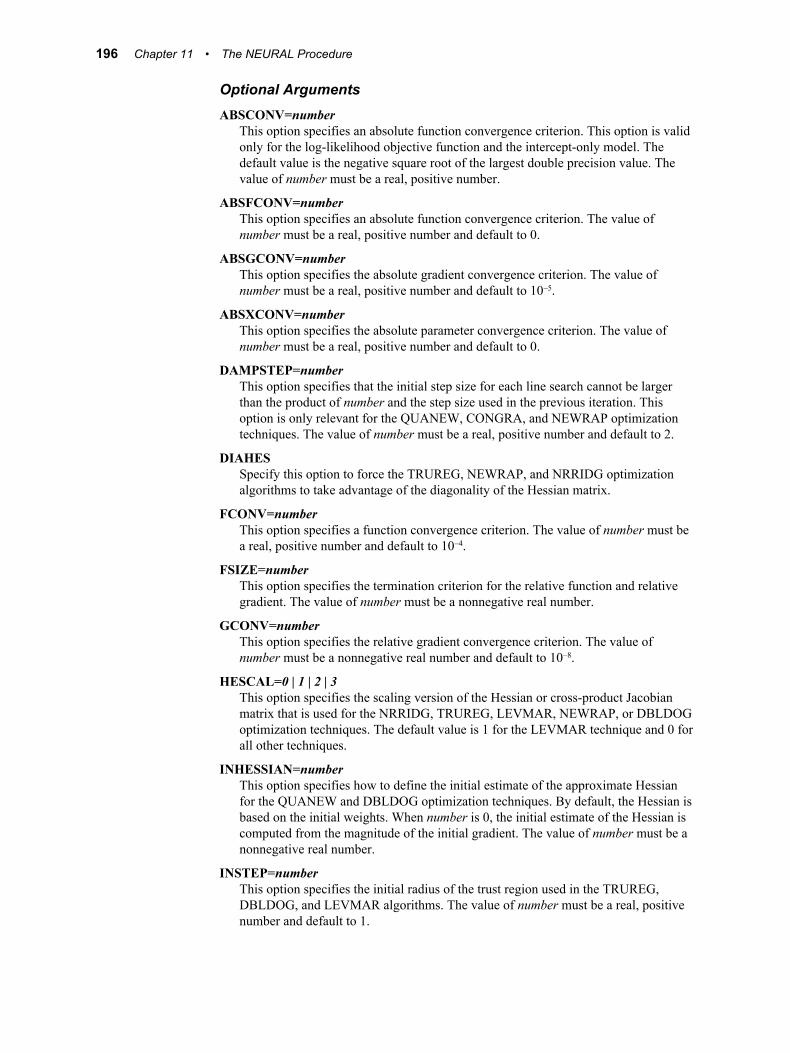
Optional ArgumentsABSCONV=number
This option specifies an absolute function convergence criterion. This option is valid only for the log-likelihood objective function and the intercept-only model. The default value is the negative square root of the largest double precision value. The value of number must be a real, positive number.
ABSFCONV=numberThis option specifies an absolute function convergence criterion. The value of number must be a real, positive number and default to 0.
ABSGCONV=numberThis option specifies the absolute gradient convergence criterion. The value of number must be a real, positive number and default to 10–5.
ABSXCONV=numberThis option specifies the absolute parameter convergence criterion. The value of number must be a real, positive number and default to 0.
DAMPSTEP=numberThis option specifies that the initial step size for each line search cannot be larger than the product of number and the step size used in the previous iteration. This option is only relevant for the QUANEW, CONGRA, and NEWRAP optimization techniques. The value of number must be a real, positive number and default to 2.
DIAHESSpecify this option to force the TRUREG, NEWRAP, and NRRIDG optimization algorithms to take advantage of the diagonality of the Hessian matrix.
FCONV=numberThis option specifies a function convergence criterion. The value of number must be a real, positive number and default to 10–4.
FSIZE=numberThis option specifies the termination criterion for the relative function and relative gradient. The value of number must be a nonnegative real number.
GCONV=numberThis option specifies the relative gradient convergence criterion. The value of number must be a nonnegative real number and default to 10–8.
HESCAL=0 | 1 | 2 | 3This option specifies the scaling version of the Hessian or cross-product Jacobian matrix that is used for the NRRIDG, TRUREG, LEVMAR, NEWRAP, or DBLDOG optimization techniques. The default value is 1 for the LEVMAR technique and 0 for all other techniques.
INHESSIAN=numberThis option specifies how to define the initial estimate of the approximate Hessian for the QUANEW and DBLDOG optimization techniques. By default, the Hessian is based on the initial weights. When number is 0, the initial estimate of the Hessian is computed from the magnitude of the initial gradient. The value of number must be a nonnegative real number.
INSTEP=numberThis option specifies the initial radius of the trust region used in the TRUREG, DBLDOG, and LEVMAR algorithms. The value of number must be a real, positive number and default to 1.
196 Chapter 11 • The NEURAL Procedure
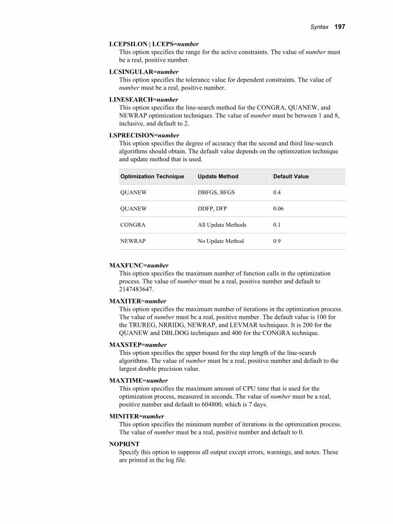
LCEPSILON | LCEPS=numberThis option specifies the range for the active constraints. The value of number must be a real, positive number.
LCSINGULAR=numberThis option specifies the tolerance value for dependent constraints. The value of number must be a real, positive number.
LINESEARCH=numberThis option specifies the line-search method for the CONGRA, QUANEW, and NEWRAP optimization techniques. The value of number must be between 1 and 8, inclusive, and default to 2.
LSPRECISION=numberThis option specifies the degree of accuracy that the second and third line-search algorithms should obtain. The default value depends on the optimization technique and update method that is used.
Optimization Technique Update Method Default Value
QUANEW DBFGS, BFGS 0.4
QUANEW DDFP, DFP 0.06
CONGRA All Update Methods 0.1
NEWRAP No Update Method 0.9
MAXFUNC=numberThis option specifies the maximum number of function calls in the optimization process. The value of number must be a real, positive number and default to 2147483647.
MAXITER=numberThis option specifies the maximum number of iterations in the optimization process. The value of number must be a real, positive number. The default value is 100 for the TRUREG, NRRIDG, NEWRAP, and LEVMAR techniques. It is 200 for the QUANEW and DBLDOG techniques and 400 for the CONGRA technique.
MAXSTEP=numberThis option specifies the upper bound for the step length of the line-search algorithms. The value of number must be a real, positive number and default to the largest double precision value.
MAXTIME=numberThis option specifies the maximum amount of CPU time that is used for the optimization process, measured in seconds. The value of number must be a real, positive number and default to 604800, which is 7 days.
MINITER=numberThis option specifies the minimum number of iterations in the optimization process. The value of number must be a real, positive number and default to 0.
NOPRINTSpecify this option to suppress all output except errors, warnings, and notes. These are printed in the log file.
Syntax 197
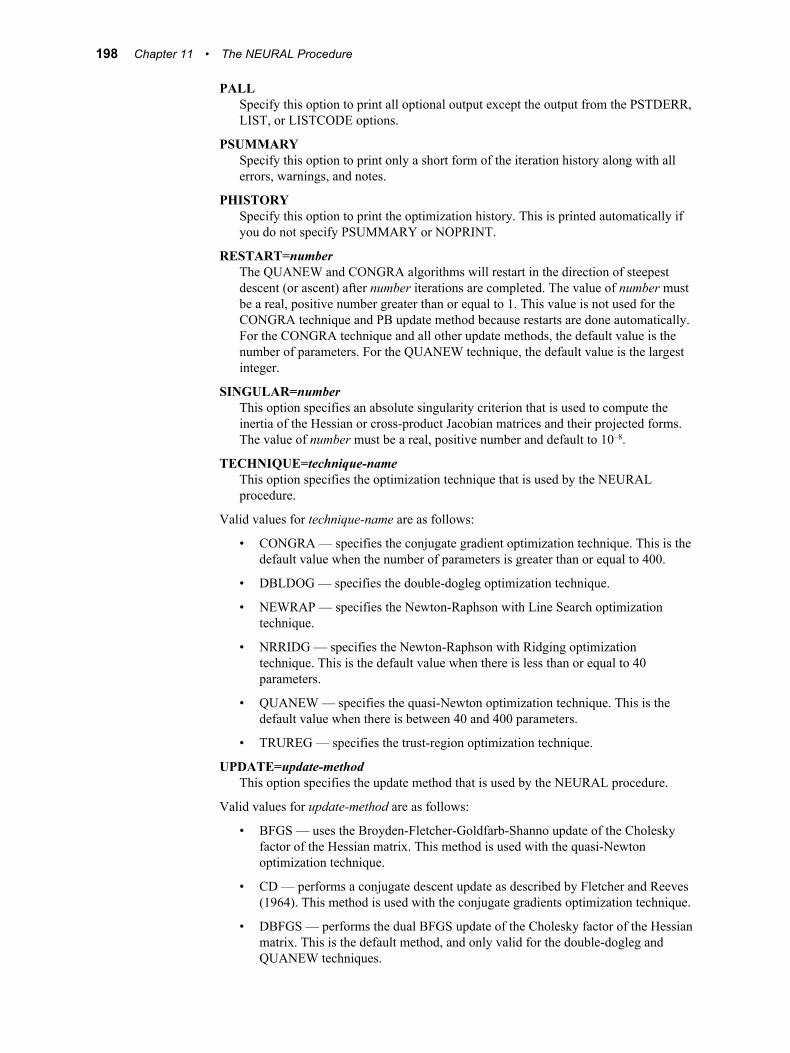
PALLSpecify this option to print all optional output except the output from the PSTDERR, LIST, or LISTCODE options.
PSUMMARYSpecify this option to print only a short form of the iteration history along with all errors, warnings, and notes.
PHISTORYSpecify this option to print the optimization history. This is printed automatically if you do not specify PSUMMARY or NOPRINT.
RESTART=numberThe QUANEW and CONGRA algorithms will restart in the direction of steepest descent (or ascent) after number iterations are completed. The value of number must be a real, positive number greater than or equal to 1. This value is not used for the CONGRA technique and PB update method because restarts are done automatically. For the CONGRA technique and all other update methods, the default value is the number of parameters. For the QUANEW technique, the default value is the largest integer.
SINGULAR=numberThis option specifies an absolute singularity criterion that is used to compute the inertia of the Hessian or cross-product Jacobian matrices and their projected forms. The value of number must be a real, positive number and default to 10–8.
TECHNIQUE=technique-nameThis option specifies the optimization technique that is used by the NEURAL procedure.
Valid values for technique-name are as follows:
• CONGRA — specifies the conjugate gradient optimization technique. This is the default value when the number of parameters is greater than or equal to 400.
• DBLDOG — specifies the double-dogleg optimization technique.
• NEWRAP — specifies the Newton-Raphson with Line Search optimization technique.
• NRRIDG — specifies the Newton-Raphson with Ridging optimization technique. This is the default value when there is less than or equal to 40 parameters.
• QUANEW — specifies the quasi-Newton optimization technique. This is the default value when there is between 40 and 400 parameters.
• TRUREG — specifies the trust-region optimization technique.
UPDATE=update-methodThis option specifies the update method that is used by the NEURAL procedure.
Valid values for update-method are as follows:
• BFGS — uses the Broyden-Fletcher-Goldfarb-Shanno update of the Cholesky factor of the Hessian matrix. This method is used with the quasi-Newton optimization technique.
• CD — performs a conjugate descent update as described by Fletcher and Reeves (1964). This method is used with the conjugate gradients optimization technique.
• DBFGS — performs the dual BFGS update of the Cholesky factor of the Hessian matrix. This is the default method, and only valid for the double-dogleg and QUANEW techniques.
198 Chapter 11 • The NEURAL Procedure
• DDFP — performs the dual DFP update of the Cholesky factor of the Hessian matrix. This technique is only valid for the double-dogleg and QUANEW techniques.
• DFP — uses the Davidson-Fletcher-Powell update of the inverse Hessian matrix. This method is used with the QUANEW technique.
• FR — uses the Fletcher-Reeves update for the conjugate gradient technique.
• PB — performs the automatic restart update method of Powell and Beale. This is the default method, and only valid for the conjugate gradient technique.
• PR — uses the Polak-Ribiere update for the conjugate gradient technique.
VERSION=1 | 2 | 3This option specifies the version of the hybrid quasi-Newton optimization technique or the version of the quasi-Newton optimization technique with nonlinear constraints. The default value is 2.
XCONV=numberThis option specifies the relative parameter convergence criterion. The value of number must be a real, positive number and default to 0.
XSIZE=numberThis option specifies the number of successive iterations for which the criterion must be satisfied before the optimization process can be terminated. The value of number must be a real, positive number and default to 0.
PERFORMANCE Statement
SyntaxPERFORMANCE <options>;
Optional ArgumentsCOMPILE | NOCOMPILE
The COMPILE option requests that code is generated and compiled for a specific network. The compiled code is then used in the network computation. For large, complex networks, the time saved during network computation with compiled code offsets the time required to generate the compiled code. The NOCOMPILE option ensures that compiled code is not created.
CPUCOUNT=numberThis option specifies the number of processors that PROC NEURAL assumes is available for multithreaded network computation. Specify CPUCOUNT=ACTUAL to use all of the physical processors that are available. The actual number of processors available can be less than the physical number of processors if the SAS process has been restricted your system administrator. You might experience performance degradations if the value of number is greater than the actual number of available processors.
This option overrides the SAS system option CPUCOUNT=. When you specify CPUCOUNT=1, you tacitly specify NOTHREADS as well.
MULTIPASS | NOUTILFILEThe MULTIPASS option instructs the NEURAL procedure to not write a utility file for the training data set. MULTIPASS and NOUTILFILE specify the same behavior.
Syntax 199
Training a neural network can require that the training data set is read multiple times (at least once per iteration). Various flags that are associated with the input and target values must be computed for each observation. Typically, computation time decreases when the training data set is read once, the flags are computed, and the results are written to an internal utility file. Consequently, specifying MULTIPASS can increase the amount of time needed to train a network.
THREADS<=YES | NO> | NOTHREADSSpecify THREADS (or THREADS=YES) to enable multithreaded network computation. Specify NOTHREADS (or THREADS=NO), which is the default action, to disable multithreaded network computation. This option overrides the SAS system option THREADS | NOTHREADS.
Because this option requires compiled code, the NEURAL procedure will ignore this option when the NOCOMPILE argument is also specified. Furthermore, the NEURAL procedure cannot process multithreaded network computations for the incremental backprop method. This method will always use singly threaded network computation code.
PERTURB Statement
SyntaxPERTURB list-of-weights </options>;
The PERTURB statement is used to perturb weights, which sometimes allows you to escape a local minimum.
Required Argumentlist-of-weights
This argument is used to list the weights that you want to perturb. The list of weights must be in the form wName —> wName2. wName is either a unit name, a layer identifier, BIAS, or ALTITUDE. wName2 is either a unit name or a layer identifier.
Optional ArgumentsOUTEST=data-set-name
This option specifies the output data set that contains all of the weights.
RANDF=numberThis option specifies the degrees of freedom that are used to generate random numbers.
RANDIST=CAUCHY | CHIINV | NORMAL | UNIFORMThis option specifies the distribution that is used to generate random initial weights and perturbations. The default setting is NORMAL.
RANDIST RANLOC RANSCALE RANDF
CAUCHY median=0 scale=1 -
CHIINV - scale=1 df=1
NORMAL mean=0 std=1 -
UNIFORM mean=0 halfrange=1 -
200 Chapter 11 • The NEURAL Procedure
RANDOM=numberThis option specifies the seed for the random number generation. The value of number must be a positive integer and default to 12345.
RANLOC=numberThis option specifies the location parameter for the random number generator. The default value depends on the distribution and is given in the table above.
RANSCALE=numberThis option specifies the scale parameter for the random number generator. The default value depends on the distribution and is given in the table above.
PRELIM Statement
SyntaxPRELIM number <options>;
The PRELIM statement performs preliminary training in order to reduce the risk of bad local optima. The final weights and biases in a trained network depend on the initial values. The PRELIM statement repeatedly trains a network for a small number of iterations (10 by default) with different initializations. The final weights of the best trained network are then used to initialize a subsequent TRAIN statement.
Required Argumentnumber
This argument specifies the number of preliminary optimizations. The value of number must be a positive integer.
Optional ArgumentsACCELERATE | ACCEL=number
This option specifies the rate of increase in learning for the RPROP optimization technique. The value of number must be a real number greater than 1 and default to 1.2.
DECELERATE | DECEL=numberThis option specifies the rate of decrease in learning for the RPROP optimization technique. The value of number must be a real number between 0 and 1 and default to 0.5.
INEST=data-set-nameThis option specifies an input data set that contains some or all of the weights. Any weights in this data set that have missing values are assigned values according to the RANDOM=, RANDOUT, and RANDBIAS options in addition to the options specified in the RANDOM statement.
LEARN=numberThis option specifies the learning rate for BPROP or the initial learning rate for QPROP and RPROP. The value of number must be a real, positive number and default to 0.1.
MAXLEARN=numberThis option specifies the maximum learning rate for RPROP. The value of number must be a real, positive number. The default value is the reciprocal of the square root of the machine epsilon.
Syntax 201
MAXMOMENTUM | MAXMOM=numberThis option specifies the maximum momentum for BPROP. The value of number must be a real, positive number and default to 1.75.
MINLEARN=numberThis option specifies the minimum learning rate for RPROP. The value of number must be a real, positive number. The default value is the reciprocal of the square root of the machine epsilon.
MOMENTUM | MOM=numberThis option specifies the momentum for BPROP. The value of number must be a real number between 0 and 1. The default value is 0.9 for BPROP and is 0.1 for RPROP.
OUTEST=data-set-nameThis output data set contains all of the weights.
PREITER=numberThis option specifies the maximum number of iterations in each preliminary optimization. The value of number must be a positive integer and default to 10.
PRETECH | TECHNIQUE=technique-nameThis option specifies the optimization technique that is used by the PRELIM statement.
Valid values for technique-name are as follows:
• CONGRA — specifies the conjugate gradient optimization technique. This is the default value when the number of parameters is greater than or equal to 400.
• DBLDOG — specifies the double-dogleg optimization technique.
• NEWRAP — specifies the Newton-Raphson with Line Search optimization technique.
• NRRIDG — specifies the Newton-Raphson with Ridging optimization technique. This is the default value when there is less than or equal to 40 parameters.
• QUANEW — specifies the quasi-Newton optimization technique. This is the default value when there are between 40 and 400 parameters.
• TRUREG — specifies the trust-region optimization technique.
PRETIME=numberThis option specifies the amount of time until training stops.
RANDBIAS | NORANDBIASThis option determines whether output biases are randomized. By default, the output biases are not randomized; they are set to the inverse activation function of the target mean. This option overrides anything that you specify in the RANDOM statement.
RANDOM=numberThis option specifies the seed for the random number generator. The value of number must be a positive integer and default to 12345.
RANDOUT | NORANDOUTThis option determines whether output connection weights are randomized. By default, the output connection weights are all set to 0. This option overrides anything that you specify in the RANDOM statement.
202 Chapter 11 • The NEURAL Procedure
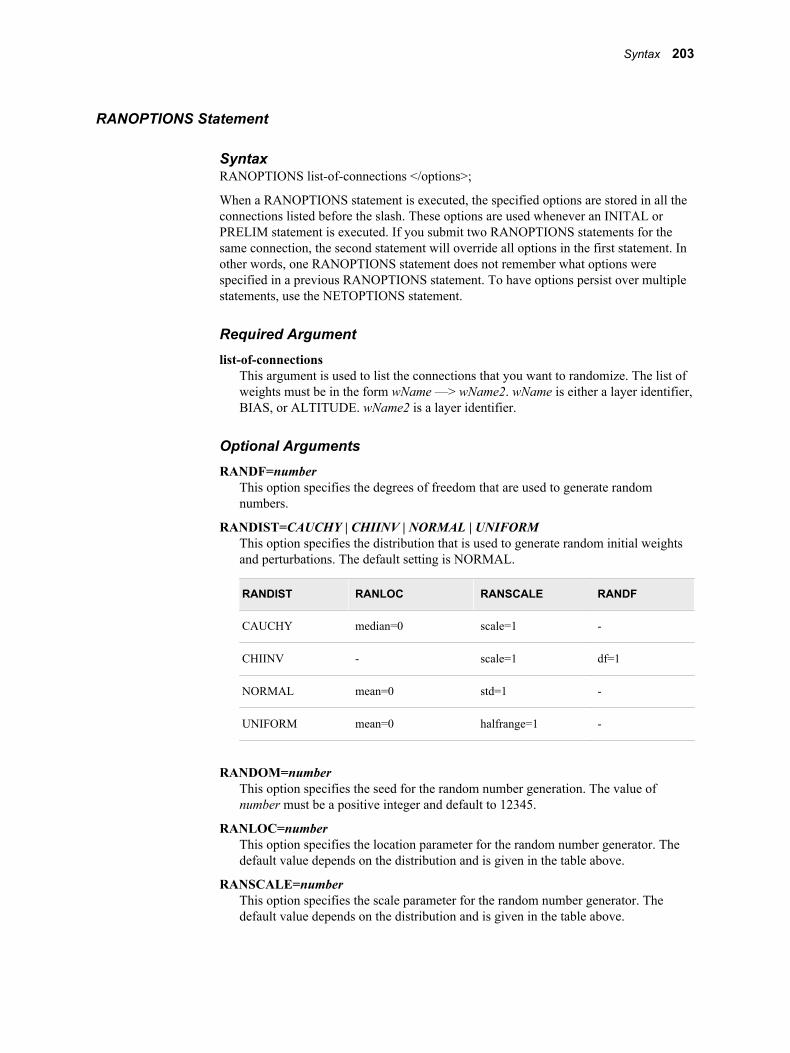
RANOPTIONS Statement
SyntaxRANOPTIONS list-of-connections </options>;
When a RANOPTIONS statement is executed, the specified options are stored in all the connections listed before the slash. These options are used whenever an INITAL or PRELIM statement is executed. If you submit two RANOPTIONS statements for the same connection, the second statement will override all options in the first statement. In other words, one RANOPTIONS statement does not remember what options were specified in a previous RANOPTIONS statement. To have options persist over multiple statements, use the NETOPTIONS statement.
Required Argumentlist-of-connections
This argument is used to list the connections that you want to randomize. The list of weights must be in the form wName —> wName2. wName is either a layer identifier, BIAS, or ALTITUDE. wName2 is a layer identifier.
Optional ArgumentsRANDF=number
This option specifies the degrees of freedom that are used to generate random numbers.
RANDIST=CAUCHY | CHIINV | NORMAL | UNIFORMThis option specifies the distribution that is used to generate random initial weights and perturbations. The default setting is NORMAL.
RANDIST RANLOC RANSCALE RANDF
CAUCHY median=0 scale=1 -
CHIINV - scale=1 df=1
NORMAL mean=0 std=1 -
UNIFORM mean=0 halfrange=1 -
RANDOM=numberThis option specifies the seed for the random number generation. The value of number must be a positive integer and default to 12345.
RANLOC=numberThis option specifies the location parameter for the random number generator. The default value depends on the distribution and is given in the table above.
RANSCALE=numberThis option specifies the scale parameter for the random number generator. The default value depends on the distribution and is given in the table above.
Syntax 203
SAVE Statement
SyntaxSAVE <options>;
Optional ArgumentsNote: At least one of these two arguments must be specified.
NETWORK=catalog-entryThis option saves the definition of the entire network.
OUTEST=data-set-nameThis option saves the network weights in a data set.
SCORE Statement
SyntaxSCORE OUT=data-set-name <options>;
The SCORE statement creates an output data set that contains the predicted values and other results such as residuals, classifications, decisions, and assessment values.
Required ArgumentOUT=data-set-name
This option specifies an output data set that contains the outputs.
Optional ArgumentsDATA=data-set-name
This option specifies the input data set that you want to score. This data set must contain all of the input variables and can contain the target variables. If you do not specify this option, then the training data set from the PROC NEURAL statement is used.
DUMMIES | NODUMMIESThis option determines whether dummy variables are written to the OUT= data set. By default, these variables are not written to the output data set.
OUTFIT=data-set-nameThis option specifies the output data set that contains the fit statistics.
ROLE=SCORE | TEST | TRAIN | VALIDATION | VALIDThis option specifies the role of the DATA= data set. This option primarily affects the fit statistics that are computed. If you specify TRAIN, VALID, or TEST, then the data set must contain the target variable. If you specify SCORE, then residuals, error functions, and fit statistics are not computed.
The default role is TEST unless the follow conditions are met:
• The DATA= data set in the SCORE statement is the same as the DATA= data set in the PROC statement. In this case, the role is TRAIN. You cannot specify this role with any other data set but the training data set.
204 Chapter 11 • The NEURAL Procedure
• The DATA= data set in the SCORE statement is the same as the VALIDATA= data set in the PROC statement. In this case, the role is VALID.
SET Statement
SyntaxSET list-of-weights number;
The SET statement is used to set the value of one or more weights to a specified number. The SET statement does not freeze weights, so subsequent training can alter the values that you assign with the SET statement.
Required Argumentslist-of-weights
This argument specifies the weights that you want to change.
numberThe weights that are given in the previous argument are all set to number.
SHOW Statement
SyntaxSHOW STATEMENTS WEIGHTS;
The SHOW statement prints information about the neural network.
Required ArgumentNote: At least one of these two arguments must be specified.
STATEMENTSSpecify STATEMENTS to print statements that can be used with the NEURAL procedure in order to reproduce the network.
WEIGHTSSpecify WEIGHTS to print the network weights.
TARGET Statement
SyntaxTARGET list-of-variables / ID=name <options>;
The TARGET statement is used to create an output layer in the neural network.
Required Argumentslist-of-variables
The first argument in the TARGET statement is the list of target variables.
ID=nameUse the ID statement to assign a unique label to the output layer.
Syntax 205

Optional ArgumentsACT=activation-function
This option specifies the activation function. For the full list of functions, see “Activation Functions” on page 210 . The default activation function for interval variables is the identity function. The default activation function for ordinal variables is the logistic function. The default activation function for nominal variables is MLOGISTIC. The MLOGISTIC function is the only activation function available when the error function is MBERNOULLI, MENTROPY, or MULTINOMIAL.
BIAS | NOBIASUse this option to specify if you want to use bias or do not want to use bias. By default, bias is used.
COMBINE=combination-functionThis option specifies the combination function. For the full list of functions, see “Combination Functions” on page 211 .
ERROR=error-functionThis option specifies the error function. For interval variables, the default error function is NORMAL and is MBERNOULLI for all others. The available functions are given in the table below.
error-function
Acceptable Target Values Description
Functions with a scale parameter:
BIWEIGHT any Biweight M estimator
CAUCHY any Cauchy distribution
GAMMA >0 Gamma distribution
HUBER any Huber M estimator
LOGISTIC any Logistic distribution
NORMAL any Normal distribution
POISSON ≥0 Poisson distribution
WAVE any Wave M estimator
Functions without a scale parameter:
BERNOULLI 0,1 Bernoulli distribution (binomial with one trial)
BINOMIAL ≥0 Binomial distribution
ENTROPY 0-1 Cross or relative entropy for independent targets
MBERNOULLI
0,1 Multiple Bernoulli (multinomial with one trial)
206 Chapter 11 • The NEURAL Procedure
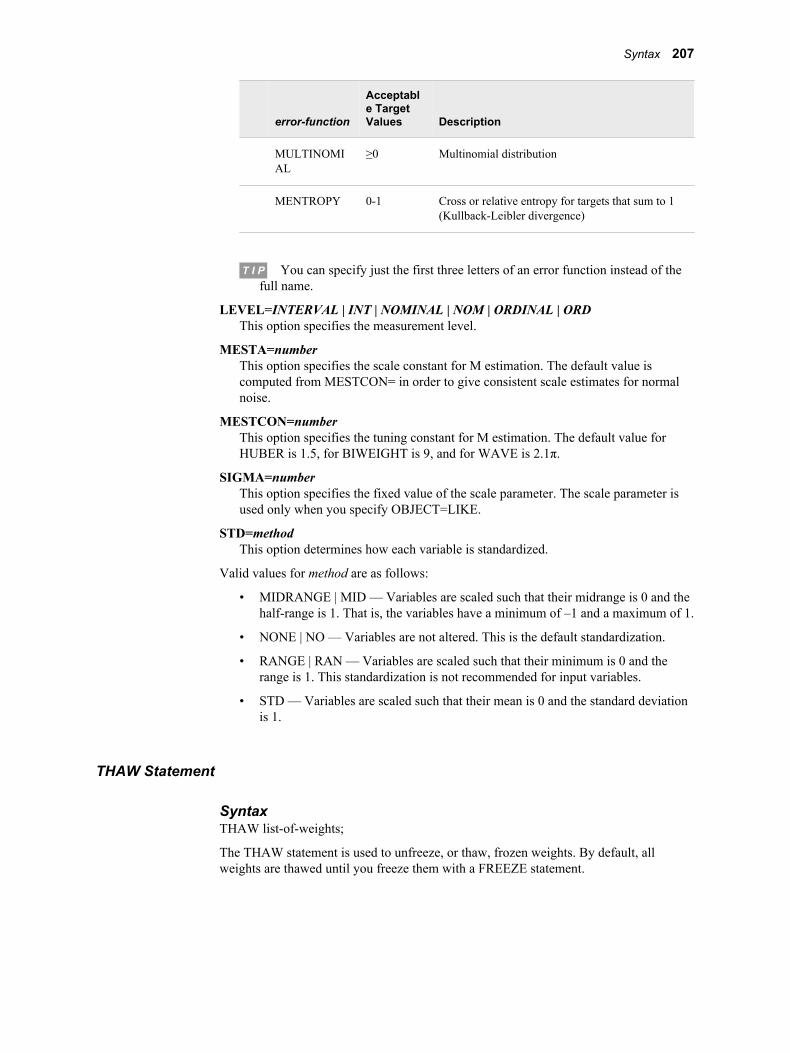
error-function
Acceptable Target Values Description
MULTINOMIAL
≥0 Multinomial distribution
MENTROPY 0-1 Cross or relative entropy for targets that sum to 1 (Kullback-Leibler divergence)
T I P You can specify just the first three letters of an error function instead of the full name.
LEVEL=INTERVAL | INT | NOMINAL | NOM | ORDINAL | ORDThis option specifies the measurement level.
MESTA=numberThis option specifies the scale constant for M estimation. The default value is computed from MESTCON= in order to give consistent scale estimates for normal noise.
MESTCON=numberThis option specifies the tuning constant for M estimation. The default value for HUBER is 1.5, for BIWEIGHT is 9, and for WAVE is 2.1π.
SIGMA=numberThis option specifies the fixed value of the scale parameter. The scale parameter is used only when you specify OBJECT=LIKE.
STD=methodThis option determines how each variable is standardized.
Valid values for method are as follows:
• MIDRANGE | MID — Variables are scaled such that their midrange is 0 and the half-range is 1. That is, the variables have a minimum of –1 and a maximum of 1.
• NONE | NO — Variables are not altered. This is the default standardization.
• RANGE | RAN — Variables are scaled such that their minimum is 0 and the range is 1. This standardization is not recommended for input variables.
• STD — Variables are scaled such that their mean is 0 and the standard deviation is 1.
THAW Statement
SyntaxTHAW list-of-weights;
The THAW statement is used to unfreeze, or thaw, frozen weights. By default, all weights are thawed until you freeze them with a FREEZE statement.
Syntax 207
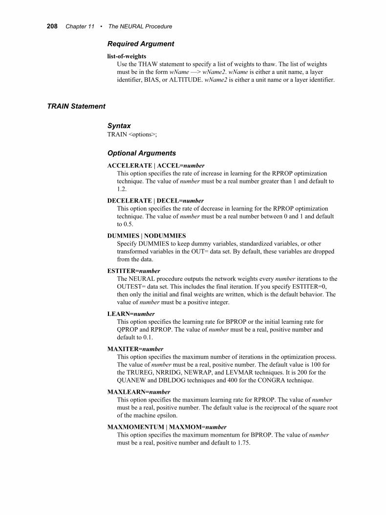
Required Argumentlist-of-weights
Use the THAW statement to specify a list of weights to thaw. The list of weights must be in the form wName —> wName2. wName is either a unit name, a layer identifier, BIAS, or ALTITUDE. wName2 is either a unit name or a layer identifier.
TRAIN Statement
SyntaxTRAIN <options>;
Optional ArgumentsACCELERATE | ACCEL=number
This option specifies the rate of increase in learning for the RPROP optimization technique. The value of number must be a real number greater than 1 and default to 1.2.
DECELERATE | DECEL=numberThis option specifies the rate of decrease in learning for the RPROP optimization technique. The value of number must be a real number between 0 and 1 and default to 0.5.
DUMMIES | NODUMMIESSpecify DUMMIES to keep dummy variables, standardized variables, or other transformed variables in the OUT= data set. By default, these variables are dropped from the data.
ESTITER=numberThe NEURAL procedure outputs the network weights every number iterations to the OUTEST= data set. This includes the final iteration. If you specify ESTITER=0, then only the initial and final weights are written, which is the default behavior. The value of number must be a positive integer.
LEARN=numberThis option specifies the learning rate for BPROP or the initial learning rate for QPROP and RPROP. The value of number must be a real, positive number and default to 0.1.
MAXITER=numberThis option specifies the maximum number of iterations in the optimization process. The value of number must be a real, positive number. The default value is 100 for the TRUREG, NRRIDG, NEWRAP, and LEVMAR techniques. It is 200 for the QUANEW and DBLDOG techniques and 400 for the CONGRA technique.
MAXLEARN=numberThis option specifies the maximum learning rate for RPROP. The value of number must be a real, positive number. The default value is the reciprocal of the square root of the machine epsilon.
MAXMOMENTUM | MAXMOM=numberThis option specifies the maximum momentum for BPROP. The value of number must be a real, positive number and default to 1.75.
208 Chapter 11 • The NEURAL Procedure
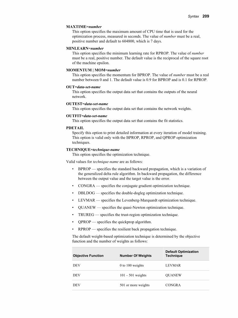
MAXTIME=numberThis option specifies the maximum amount of CPU time that is used for the optimization process, measured in seconds. The value of number must be a real, positive number and default to 604800, which is 7 days.
MINLEARN=numberThis option specifies the minimum learning rate for RPROP. The value of number must be a real, positive number. The default value is the reciprocal of the square root of the machine epsilon.
MOMENTUM | MOM=numberThis option specifies the momentum for BPROP. The value of number must be a real number between 0 and 1. The default value is 0.9 for BPROP and is 0.1 for RPROP.
OUT=data-set-nameThis option specifies the output data set that contains the outputs of the neural network.
OUTEST=data-set-nameThis option specifies the output data set that contains the network weights.
OUTFIT=data-set-nameThis option specifies the output data set that contains the fit statistics.
PDETAILSpecify this option to print detailed information at every iteration of model training. This option is valid only with the BPROP, RPROP, and QPROP optimization techniques.
TECHNIQUE=technique-nameThis option specifies the optimization technique.
Valid values for technique-name are as follows:
• BPROP — specifies the standard backward propagation, which is a variation of the generalized delta rule algorithm. In backward propagation, the difference between the output value and the target value is the error.
• CONGRA — specifies the conjugate gradient optimization technique.
• DBLDOG — specifies the double-dogleg optimization technique.
• LEVMAR — specifies the Levenberg-Marquardt optimization technique.
• QUANEW — specifies the quasi-Newton optimization technique.
• TRUREG — specifies the trust-region optimization technique.
• QPROP — specifies the quickprop algorithm.
• RPROP — specifies the resilient back propagation technique.
The default weight-based optimization technique is determined by the objective function and the number of weights as follows:
Objective Function Number Of WeightsDefault Optimization Technique
DEV 0 to 100 weights LEVMAR
DEV 101 – 501 weights QUANEW
DEV 501 or more weights CONGRA
Syntax 209
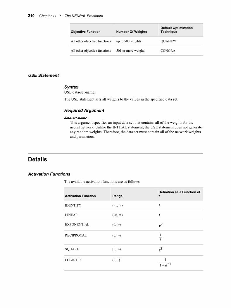
Objective Function Number Of WeightsDefault Optimization Technique
All other objective functions up to 500 weights QUANEW
All other objective functions 501 or more weights CONGRA
USE Statement
SyntaxUSE data-set-name;
The USE statement sets all weights to the values in the specified data set.
Required Argumentdata-set-name
This argument specifies an input data set that contains all of the weights for the neural network. Unlike the INITIAL statement, the USE statement does not generate any random weights. Therefore, the data set must contain all of the network weights and parameters.
Details
Activation FunctionsThe available activation functions are as follows:
Activation Function RangeDefinition as a Function of t
IDENTITY (-∞, ∞) t
LINEAR (-∞, ∞) t
EXPONENTIAL (0, ∞) e t
RECIPROCAL (0, ∞) 1t
SQUARE [0, ∞) t 2
LOGISTIC (0, 1) 11 + e −1
210 Chapter 11 • The NEURAL Procedure
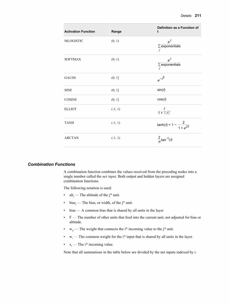
Activation Function RangeDefinition as a Function of t
MLOGISTIC (0, 1) e t∑jexponentials
SOFTMAX (0, 1) e t∑jexponentials
GAUSS (0, 1]e −t
2
SINE (0, 1] sin(t)
COSINE (0, 1] cos(t)
ELLIOT (-1, 1) t1 + | t |
TANH (-1, 1) tanh(t) = 1 − 21 + e 2t
ARCTAN (-1, 1) 2π tan-1(t)
Combination FunctionsA combination function combines the values received from the preceding nodes into a single number called the net input. Both output and hidden layers are assigned combination functions.
The following notation is used:
• altj — The altitude of the jth unit.
• biasj — The bias, or width, of the jth unit.
• bias — A common bias that is shared by all units in the layer
• F — The number of other units that feed into the current unit, not adjusted for bias or altitude.
• wij — The weight that connects the ith incoming value to the jth unit.
• wi — The common weight for the ith input that is shared by all units in the layer.
• xi — The ith incoming value.
Note that all summations in the table below are divided by the net inputs indexed by i.
Details 211
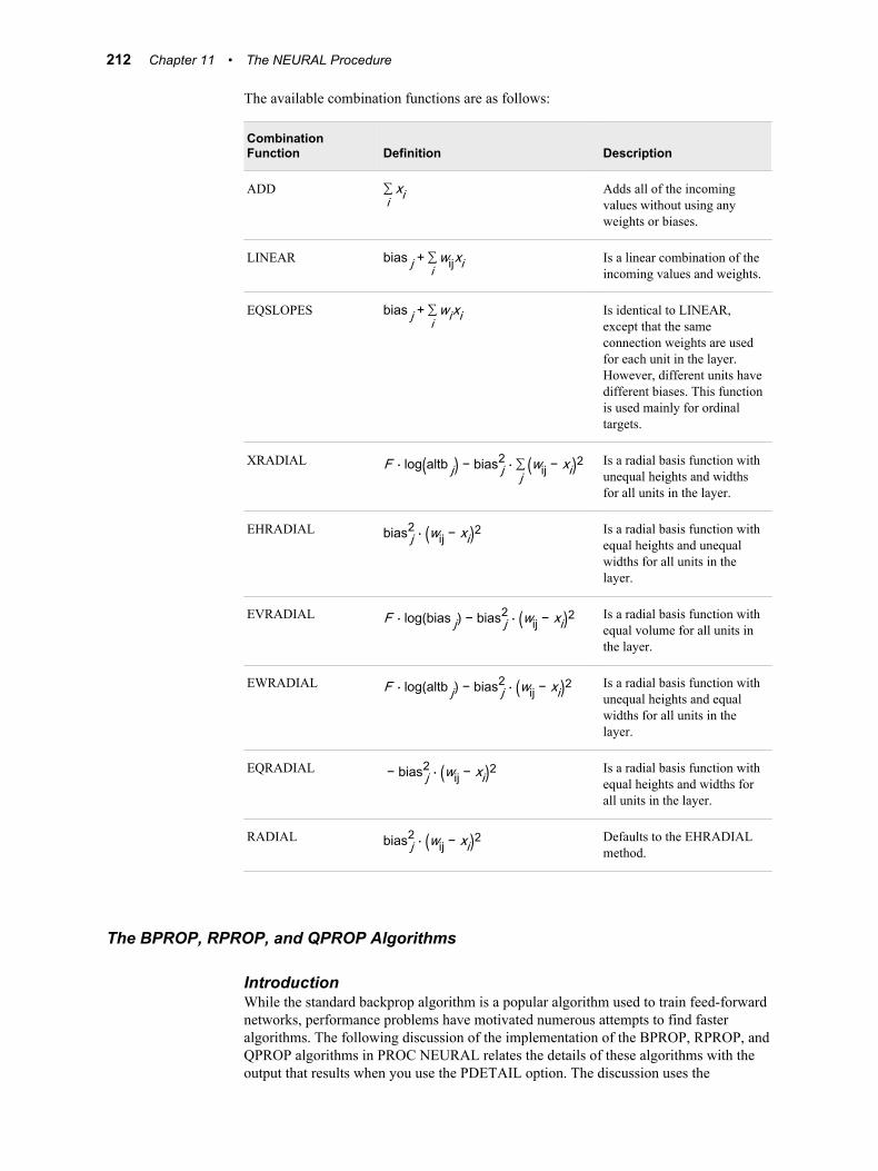
The available combination functions are as follows:
Combination Function Definition Description
ADD ∑ixi Adds all of the incoming
values without using any weights or biases.
LINEAR bias j + ∑iwijxi Is a linear combination of the
incoming values and weights.
EQSLOPES bias j + ∑iwixi Is identical to LINEAR,
except that the same connection weights are used for each unit in the layer. However, different units have different biases. This function is used mainly for ordinal targets.
XRADIAL F ⋅ log(altb j) − bias j2 ⋅ ∑j (wij − xi)2 Is a radial basis function with
unequal heights and widths for all units in the layer.
EHRADIAL bias j2 ⋅ (wij − xi)2 Is a radial basis function with
equal heights and unequal widths for all units in the layer.
EVRADIAL F ⋅ log(bias j) − bias j2 ⋅ (wij − xi)2 Is a radial basis function with
equal volume for all units in the layer.
EWRADIAL F ⋅ log(altb j) − bias j2 ⋅ (wij − xi)2 Is a radial basis function with
unequal heights and equal widths for all units in the layer.
EQRADIAL − bias j2 ⋅ (wij − xi)2 Is a radial basis function with
equal heights and widths for all units in the layer.
RADIAL bias j2 ⋅ (wij − xi)2 Defaults to the EHRADIAL
method.
The BPROP, RPROP, and QPROP Algorithms
IntroductionWhile the standard backprop algorithm is a popular algorithm used to train feed-forward networks, performance problems have motivated numerous attempts to find faster algorithms. The following discussion of the implementation of the BPROP, RPROP, and QPROP algorithms in PROC NEURAL relates the details of these algorithms with the output that results when you use the PDETAIL option. The discussion uses the
212 Chapter 11 • The NEURAL Procedure

algorithmic description and notation in Schiffmann, Joost, and Werner (1994) as well as the Neural Net FAQ available at: ftp://ftp.sas.com/pub/neural/FAQ.html.
There is an important distinction between the back propagation of errors technique, referred to as backprop, and the backpropagation algorithm. The backprop technique is an efficient computational technique to compute the derivative of the error function with respect to the weights and biases of the network. This derivative, more commonly known as the error gradient, is needed for any first order nonlinear optimization method. The standard backpropagation algorithm is a method to update the model with weights that are based on the gradient. It is a variation of the simple delta rule approach. See the section “What is backprop?” in part 2 of the Neural Net FAQ for more details and references on standard backprop, RPROP, and Quickprop.
With any of the propagation algorithms, PROC NEURAL enables you to print detailed information about each iteration. When you specify the PDETAIL option in the TRAIN statement, every quantity involved in the algorithm for each weight in the network is printed. This option should be used with caution as it can result in voluminous output. However, if you restrict the number of iterations and number of non-frozen weights, a manageable amount of information is produced. The PDETAIL option enables you to follow the nonlinear optimization of the error function for each of the network weights. For any particular propagation method, as described below, all quantities used to compute an updated weight are printed.
In the standard backprop algorithm, a learning rate that is too low causes the network to learn very slowly. A learning rate that is too low causes the weights and error function to diverge quickly, so there is no learning at all. If the error function is quadratic, as in linear models, you can compute good learning rates from the Hessian matrix. If the error function has many local and global optima, as in typical feed-forward neural networks with hidden units, the optimal learning rate can change dramatically during the training process. These changes occur because the Hessian matrix also changes dramatically. Trying to train a neural network with a constant learning rate is usually a tedious process that requires much trial and error.
Many other variants of backprop have been invented, but most suffer from the same theoretical flaw as standard backprop. This error is that the magnitude of the change in the weights (the step size) is a function of the magnitude of the gradient. In some regions of the weight space, the gradient is small and you need a large step size; this happens when you initialize a network with small random weights. In other regions of the weight space, the gradient is small and you need a small step size; this happens when you are close to a local minimum. Likewise, a large gradient might call for either a small step or a large step. Many algorithms try to adapt the learning rate. But, any algorithm that multiplies the learning rate by the gradient to compute the change in the weights is likely to produce erratic behavior when the gradient changes abruptly.
With batch training, there is no need to use a constant learning rate. In fact, there is no reason to use the standard backprop technique, because the QPROP and RPROP techniques implement more efficient, reliable, and convenient batch training algorithms. The great advantage of QPROPR and RPROP is that they do not emphasize the magnitude of the gradient as much as BPROP. Conventional optimization algorithms use the gradient and either a second-order derivative or a line search (or some combination thereof) to obtain a good step size.
Mathematical NotationThe following notation will be used to discuss the NEURAL procedure:
• n — represents the iteration number.
• ωij(n) — is the weight that is associated with the connection between the ith unit in the current layer and the jth unit in the previous layer.
Details 213
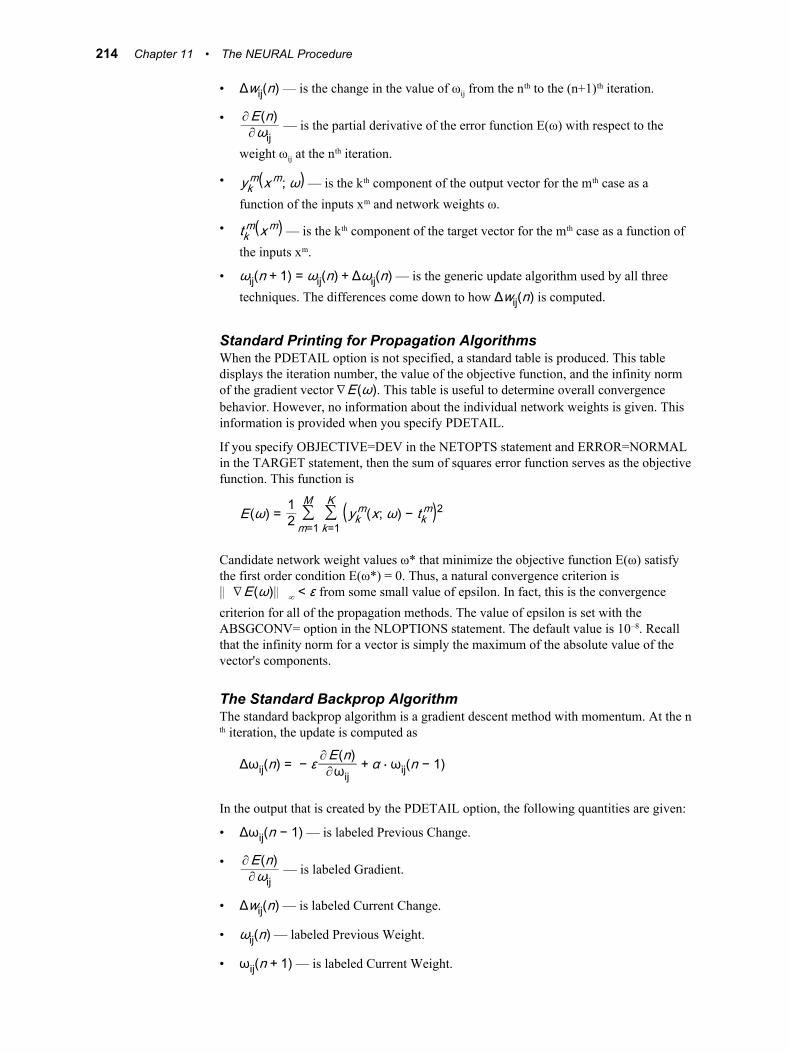
• Δwij(n) — is the change in the value of ωij from the nth to the (n+1)th iteration.
• ∂E(n)∂ωij
— is the partial derivative of the error function E(ω) with respect to the
weight ωij at the nth iteration.
• ykm(xm; ω) — is the kth component of the output vector for the mth case as a
function of the inputs xm and network weights ω.
• tkm(xm) — is the kth component of the target vector for the mth case as a function of
the inputs xm.
• ωij(n + 1) = ωij(n) + Δωij(n) — is the generic update algorithm used by all three techniques. The differences come down to how Δwij(n) is computed.
Standard Printing for Propagation AlgorithmsWhen the PDETAIL option is not specified, a standard table is produced. This table displays the iteration number, the value of the objective function, and the infinity norm of the gradient vector ∇E(ω). This table is useful to determine overall convergence behavior. However, no information about the individual network weights is given. This information is provided when you specify PDETAIL.
If you specify OBJECTIVE=DEV in the NETOPTS statement and ERROR=NORMAL in the TARGET statement, then the sum of squares error function serves as the objective function. This function is
E(ω) = 12 ∑m=1
M∑k=1
K (ykm(x; ω) − tkm)2
Candidate network weight values ω* that minimize the objective function E(ω) satisfy the first order condition E(ω*) = 0. Thus, a natural convergence criterion is ∇E(ω) ∞ < ε from some small value of epsilon. In fact, this is the convergence
criterion for all of the propagation methods. The value of epsilon is set with the ABSGCONV= option in the NLOPTIONS statement. The default value is 10–8. Recall that the infinity norm for a vector is simply the maximum of the absolute value of the vector's components.
The Standard Backprop AlgorithmThe standard backprop algorithm is a gradient descent method with momentum. At the nth iteration, the update is computed as
Δωij(n) = − ε ∂E(n)∂ωij+ α ⋅ ωij(n − 1)
In the output that is created by the PDETAIL option, the following quantities are given:
• Δωij(n − 1) — is labeled Previous Change.
• ∂E(n)∂ωij
— is labeled Gradient.
• Δwij(n) — is labeled Current Change.
• ωij(n) — labeled Previous Weight.
• ωij(n + 1) — is labeled Current Weight.
214 Chapter 11 • The NEURAL Procedure
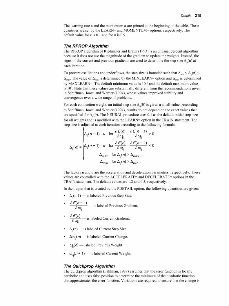
The learning rate ε and the momentum α are printed at the beginning of the table. These quantities are set by the LEARN= and MOMENTUM= options, respectively. The default value for ε is 0.1 and for α is 0.9.
The RPROP AlgorithmThe RPROP algorithm of Riedmiller and Braun (1993) is an unusual descent algorithm because it does not use the magnitude of the gradient to update the weights. Instead, the signs of the current and previous gradients are used to determine the step size Δij(n) at each iteration.
To prevent oscillations and underflows, the step size is bounded such that Δmin ≤ Δij(n) ≤ Δmax. The value of Δmin is determined by the MINLEARN= option and Δmax is determined by MAXLEARN=. The default minimum value is 10–7 and the default maximum value is 107. Note that these values are substantially different from the recommendations given in Schiffman, Joost, and Werner (1994), whose values improved stability and convergence over a wide range of problems.
For each connection weight, an initial step size Δij(0) is given a small value. According to Schiffman, Joost, and Werner (1994), results do not depend on the exact values that are specified for Δij(0). The NEURAL procedure uses 0.1 as the default initial step size for all weights and is modified with the LEARN= option in the TRAIN statement. The step size is adjusted at each iteration according to the following formula:
Δij(n) = {Δij(n − 1) ⋅ u for ∂E(n)∂ωij⋅ ∂E(n − 1)∂ωij
> 0
Δij(n − 1) ⋅ d for ∂E(n)∂ωij⋅ ∂E(n − 1)∂ωij
< 0
Δmax for Δij(n) > ΔmaxΔmin for Δij(n) > Δmin
The factors u and d are the acceleration and deceleration parameters, respectively. These values are controlled with the ACCELERATE= and DECELERATE= options in the TRAIN statement. The default values are 1.2 and 0.5, respectively.
In the output that is created by the PDETAIL option, the following quantities are given:
• Δij(n-1) — is labeled Previous Step Size.
• ∂E(n − 1)∂ωij
— is labeled Previous Gradient.
• ∂E(n)∂ωij
— is labeled Current Gradient.
• Δij(n) — is labeled Current Step Size.
• Δwij(n) — is labeled Current Change.
• ωij(n) — labeled Previous Weight.
• ωij(n + 1) — is labeled Current Weight.
The Quickprop AlgorithmThe quickprop algorithm (Fahlman, 1989) assumes that the error function is locally parabolic and uses false position to determine the minimum of the quadratic function that approximates the error function. Variations are required to ensure that the change is
Details 215
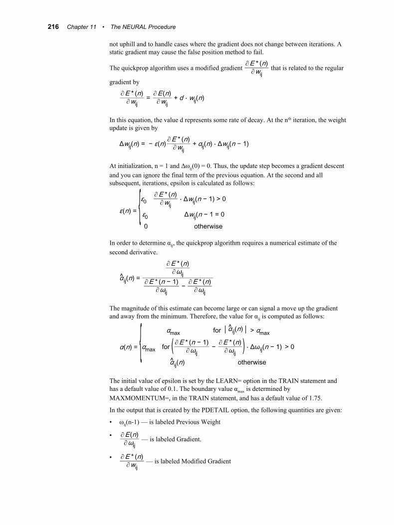
not uphill and to handle cases where the gradient does not change between iterations. A static gradient may cause the false position method to fail.
The quickprop algorithm uses a modified gradient ∂E * (n)∂wij
that is related to the regular
gradient by
∂E * (n)∂wij
= ∂E(n)∂wij
+ d ⋅ wij(n)
In this equation, the value d represents some rate of decay. At the nth iteration, the weight update is given by
Δwij(n) = − ε(n) ∂E * (n)∂wij
+ αij(n) ⋅ Δwij(n − 1)
At initialization, n = 1 and Δωij(0) = 0. Thus, the update step becomes a gradient descent and you can ignore the final term of the previous equation. At the second and all subsequent, iterations, epsilon is calculated as follows:
ε(n) = {ε0 ∂E * (n)∂wij
⋅ Δwij(n − 1) > 0
ε0 Δwij(n − 1 = 00 otherwise
In order to determine αij, the quickprop algorithm requires a numerical estimate of the second derivative.
α ij(n) =
∂E * (n)∂ωij
∂E * (n − 1)∂ωij
− ∂E * (n)∂ωij
The magnitude of this estimate can become large or can signal a move up the gradient and away from the minimum. Therefore, the value for αij is computed as follows:
α(n) = { αmax for | α ij(n) | > αmaxαmax for ( ∂E * (n − 1)
∂ωij− ∂E * (n)
∂ωij) ⋅ Δωij(n − 1) > 0
α ij(n) otherwise
The initial value of epsilon is set by the LEARN= option in the TRAIN statement and has a default value of 0.1. The boundary value αmax is determined by MAXMOMENTUM=, in the TRAIN statement, and has a default value of 1.75.
In the output that is created by the PDETAIL option, the following quantities are given:
• ωij(n-1) — is labeled Previous Weight
• ∂E(n)∂ωij
— is labeled Gradient.
• ∂E * (n)∂wij
— is labeled Modified Gradient
216 Chapter 11 • The NEURAL Procedure
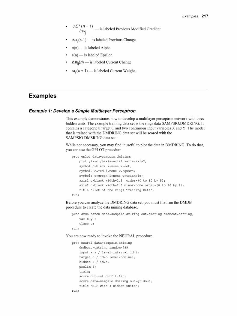
• ∂E * (n − 1)∂wij
— is labeled Previous Modified Gradient
• Δωij(n-1) — is labeled Previous Change
• α(n) — is labeled Alpha
• ε(n) — is labeled Epsilon
• Δwij(n) — is labeled Current Change.
• ωij(n + 1) — is labeled Current Weight.
Examples
Example 1: Develop a Simple Multilayer PerceptronThis example demonstrates how to develop a multilayer perceptron network with three hidden units. The example training data set is the rings data SAMPSIO.DMDRING. It contains a categorical target C and two continuous input variables X and Y. The model that is trained with the DMDRING data set will be scored with the SAMPSIO.DMSRING data set.
While not necessary, you may find it useful to plot the data in DMDRING. To do that, you can use the GPLOT procedure.
proc gplot data=sampsio.dmlring; plot y*x=c /haxis=axis1 vaxis=axis2; symbol c=black i=none v=dot; symbol2 c=red i=none v=square; symbol3 c=green i=none v=triangle; axis1 c=black width=2.5 order=(0 to 30 by 5); axis2 c=black width=2.5 minor=none order=(0 to 20 by 2); title 'Plot of the Rings Training Data';run;
Before you can analyze the DMDRING data set, you must first run the DMDB procedure to create the data mining database.
proc dmdb batch data=sampsio.dmlring out=dmdring dmdbcat=catring; var x y ; class c;run;
You are now ready to invoke the NEURAL procedure.
proc neural data=sampsio.dmlring dmdbcat=catring random=789; input x y / level=interval id=i; target c / id=o level=nominal; hidden 3 / id=h; prelim 5; train; score out=out outfit=fit; score data=sampsio.dmsring out=gridout; title 'MLP with 3 Hidden Units';run;
Examples 217
Use the INPUT statement to create an input layer that uses the variables X and Y. Additionally, you will create an output layer with the TARGET statement and a hidden layer with three units using the HIDDEN statement. By default, the two input layers are each connected to all three hidden layers. This code uses a PRELIM statement to search for the best starting weights before the NEURAL procedure fully trains the model. Finally, two SCORE statements were specified first, to save the output data sets and second, to score the DMSRING data set.
The first section in the Output window describes the preliminary training phase. The preliminary run number, initial random seed, and objective function are all included in this section. Additionally, the initial parameter estimates are listed in this section of the output. Because the target variable is nominal, the error function is the MBERNOULLI function and the objective function is the log-likelihood function.
At the start of optimization, the procedure lists the number of active constraints, the current value of the objective function, the maximum gradient element, and the radius. The iteration history includes the number of restarts, the value of the objective function, the change in the objective function, and the infinity norm of the gradient. Final parameter estimates are also reported in the Output window.
You can use the PRINT procedure to print selected information about the fit statistics for the training data set.
proc print data=fit noobs label; var _aic_ _ase_ _max_ _rfpe_ _misc_ _wrong_; where _name_ = 'OVERALL'; title2 'Fits Statistics for the Training Data Set';run;
The PROC PRINT report provides selected fit statistics for the training data. By default, the OUTFIT= data set contains two observations; however, this call to PROC PRINT only selects one of those variables. This report shows that the NEURAL procedure correctly classified every observation.
Similarly, you can use the FREQ procedure to create a misclassification table for the training data. The variable F_C is the actual target value for each case and I_C is the predicted target variable for each case.
proc freq data=out; tables f_c*i_c; title2 'Misclassification Table';run;
In the misclassification table, you should notice that every observation was correctly identified.
Example 2: Developing a Neural Network for a Continuous TargetThis example demonstrates how to create a neural network for a continuous target variable. A simple multilayer perceptron architecture is used with one hidden unit and direct connections. The example data set SAMPSIO.DMBASE contains performance measures and salary levels for several batters in Major League Baseball for the 1986 season. The continuous target variable is the log of each player's salary.
A preliminary run of the DMREG procedure is used to reduce the number of model inputs. The input set from the model with the smallest Schwarz's Bayesian Criterion is used as input to the network. This call to the DMREG procedure is based on the third example in the PROC DMREG chapter.
218 Chapter 11 • The NEURAL Procedure
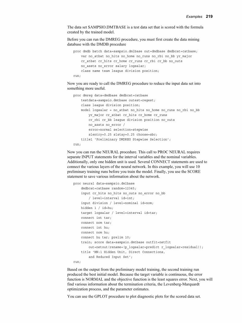
The data set SAMPSIO.DMTBASE is a test data set that is scored with the formula created by the trained model.
Before you can run the DMREG procedure, you must first create the data mining database with the DMDB procedure
proc dmdb batch data=sampsio.dmlbase out=dmdbase dmdbcat=catbase; var no_atbat no_hits no_home no_runs no_rbi no_bb yr_major cr_atbat cr_hits cr_home cr_runs cr_rbi cr_bb no_outs no_assts no_error salary logsalar; class name team league division position;run;
Now you are ready to call the DMREG procedure to reduce the input data set into something more useful.
proc dmreg data=dmdbase dmdbcat=catbase testdata=sampsio.dmtbase outest=regest; class league division position; model logsalar = no_atbat no_hits no_home no_runs no_rbi no_bb yr_major cr_atbat cr_hits cr_home cr_runs cr_rbi cr_bb league division position no_outs no_assts no_error / error=normal selection=stepwise slentry=0.25 slstay=0.25 choose=sbc; title1 'Preliminary DMDREG Stepwise Selection';run;
Now you can run the NEURAL procedure. This call to PROC NEURAL requires separate INPUT statements for the interval variables and the nominal variables. Additionally, only one hidden unit is used. Several CONNECT statements are used to connect the various layers of the neural network. In this example, you will use 10 preliminary training runs before you train the model. Finally, you use the SCORE statement to save various information about the network.
proc neural data=sampsio.dmlbase dmdbcat=catbase random=12345; input cr_hits no_hits no_outs no_error no_bb / level=interval id=int; input division / level=nominal id=nom; hidden 1 / id=hu; target logsalar / level=interval id=tar; connect int tar; connect nom tar; connect int hu; connect nom hu; connect hu tar; prelim 10; train; score data=sampsio.dmtbase outfit=netfit out=netout(rename=(p_logsalar=predict r_logsalar=residual)); title 'NN:1 Hidden Unit, Direct Connections, and Reduced Input Set';run;
Based on the output from the preliminary model training, the second training run produced the best initial model. Because the target variable is continuous, the error function is NORMAL and the objective function is the least squares error. Next, you will find various information about the termination criteria, the Levenberg-Marquardt optimization process, and the parameter estimates.
You can use the GPLOT procedure to plot diagnostic plots for the scored data set.
Examples 219
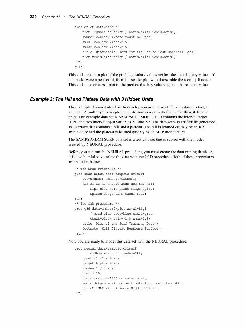
proc gplot data=netout; plot logsalar*predict / haxis=axis1 vaxis=axis2; symbol c=black i=none v=dot h=3 pct; axis1 c=black width=2.5; axis2 c=black width=2.5; title 'Diagnostic Plots for the Scored Test Baseball Data'; plot residual*predict / haxis=axis1 vaxis=axis2;run;quit;
This code creates a plot of the predicted salary values against the actual salary values. If the model were a perfect fit, then this scatter plot would resemble the identity function. This code also creates a plot of the predicted salary values against the residual values.
Example 3: The Hill and Plateau Data with 3 Hidden UnitsThis example demonstrates how to develop a neural network for a continuous target variable. A multilayer perceptron architecture is used with first 3 and then 30 hidden units. The example data set is SAMPSIO.DMDSURF. It contains the interval target HIPL and two interval input variables X1 and X2. The data set was artificially generated as a surface that contains a hill and a plateau. The hill is learned quickly by an RBF architecture and the plateau is learned quickly by an MLP architecture.
The SAMPSIO.DMTSURF data set is a test data set that is scored with the model created by NEURAL procedure.
Before you can run the NEURAL procedure, you must create the data mining database. It is also helpful to visualize the data with the G3D procedure. Both of these procedures are included below.
/* The DMDB Procedure */proc dmdb batch data=sampsio.dmlsurf out=dmdsurf dmdbcat=catsurf; var x1 x2 d2 d addd adds ces hat hill hipl hiva mult plane ridge spiral splash steps tanh tanh3 flat;run;/* The G3D procedure */proc g3d data=dmdsurf;plot x2*x1=hipl / grid side ctop=blue caxis=green ctext=black zmin=-1.5 zmax=1.5; title 'Plot of the Surf Training Data'; footnote 'Hill Plateau Response Surface'; run;
Now you are ready to model this data set with the NEURAL procedure.
proc neural data=sampsio.dmlsurf dmdbcat=catsurf random=789; input x1 x2 / id=i; target hipl / id=o; hidden 3 / id=h; prelim 10; train maxiter=1000 outest=mlpest; score data=sampsio.dmtsurf out=mlpout outfit=mlpfit; title2 'MLP with &hidden Hidden Units';run;
220 Chapter 11 • The NEURAL Procedure
Finally, you can use the GCONTOUR and G3D procedures to plot the output of the NEURAL procedure. This output indicates that the neural network significantly underfits the data.
/* The GCONTOUR Procedure */proc gcontour data=mlpout; plot x2*x1=p_hipl / pattern ctext=black coutline=gray; pattern v=msolid; legend frame; title3 'Predicted Values'; footnote;run;/* The G3D Procedure */proc g3d data=mlpout; plot x2*x1=p_hipl / grid side ctop=blue caxis=green ctext=black zmin=-1.5 zmax=1.5;run;
Example 4: The Hill and Plateau Data with 30 Hidden UnitsThis example is a continuation of the previous example and relies on the data mining database that is created in “Example 3: The Hill and Plateau Data with 3 Hidden Units” on page 220 . However, for this example, you will use a hidden unit that has 30 units. Each of your input layers is connected to every hidden unit and there are 10 preliminary training runs.
proc neural data=sampsio.dmlsurf dmdbcat=catsurf random=789; input x1 x2 / id=i; target hipl / id=o; hidden 30 / id=h; prelim 10; train maxiter=1000 outest=mlpest2; score data=sampsio.dmtsurf out=mlpout2 outfit=mlpfit2; title2 'MLP with &hidden Hidden Units';run;
Again, use the GCONTOUR and G3D procedures to visualize the output of this training session.
/* The GCONTOUR Procedure */proc gcontour data=mlpout2; plot x2*x1=p_hipl / pattern ctext=black coutline=gray; pattern v=msolid; legend frame; title3 'Predicted Values'; footnote;run;/* The G3D Procedure */proc g3d data=mlpout2; plot x2*x1=p_hipl / grid side ctop=blue caxis=green ctext=black zmin=-1.5 zmax=1.5;run;
Note that with 30 hidden units and 121 weights in the neural network, there are clear discrepancies between the previous examples. However, there are also clear
Examples 221
discrepancies between this model and the actual target values. It would take a neural network with about 50 hidden units to model the hill and plateau without visual discrepancies.
Further ReadingThe following materials contain helpful information about neural networks:
• M.J.A. Berry and G. Linoff, Data Mining Techniques for Marketing, Sales, and Customer Support, (New York, NY: John Wiley and Sons, Inc. 1997)
• C.M. Bishop, Neural Networks for Pattern Recognition, (New York, NY: Oxford University Press, 1995)
• J.P. Bigus, Data Mining with Neural Networks: Solving Business Problems — from Application Development to Decision Support, (New York, NY: McGraw-Hill, 1996)
• Collier Books, The 1987 Baseball Encyclopedia Update, (New York, NY: Macmillan Publishing Company, 1987)
• S.E Fahlman, “Faster-Learning Variations on Back-Propagation: An Empirical Study,” in D. Touretsky, et al., eds, Proceedings of the 1998 Connectionist Models Summer School, (San Mateo, CA: Morgan Kaufmann, 1989)
• R. Fletcher and C. M. Reeves, “Function Minimization by Conjugate Gradients,” Computer Journal 7 (1964), 149–154.
• D. Michie, D.J. Spiegalhalter, and C.C. Taylor, Machine Learning, Neural and Statistical Classification, (New York, NY: Ellis Horwood, 1994)
• M. Riedmiller and H. Braun, “A Direct Adaptive Method for Faster Backpropagation Learning: The RPROP Algorithm,” Proceedings of the IEEE International Conference on Neural Networks 1993, (San Francisco, CA: IEEE, 1993)
• B.D. Ripley, Pattern Recognition and Neural Networks, (New York, NY: Cambridge University Press, 1996)
• W.S. Sarle, “Neural Networks and Statistical Models,” Proceedings of the Nineteenth Annual SAS Users Group International Conference, (Cary, NC: SAS Institute Inc., 1994a): 1538–1550.
• W.S. Sarle, “Neural Network Implementation in SAS Software,” Proceedings of the Nineteenth Annual SAS Users Group International Conference, (Cary, NC: SAS Institute Inc., 1994b): 1550–1573.
• W. Schiffmann, M. Joost, and R. Werner, “Optimization of the Backpropagation Algorithm for Training Multilayer Perceptrons” (1994).
• M. Smith, Neural Networks for Statistical Modeling, (New York, NY: Van Nostrand Reinhold, 1993)
• S.M. Weiss and C.A. Kulikowski, Computer Systems that Learn: Classification and Prediction Methods from Statistics, Neural Nets, Machine Learning, and Expert Systems, (San Mateo, CA: Morgan Kaufmann, 1991)
222 Chapter 11 • The NEURAL Procedure
Chapter 12
The PATH Procedure
Overview . . . . . . . . . . . . . . . . . . . . . . . . . . . . . . . . . . . . . . . . . . . . . . . . . . . . . . . . . . . 223The PATH Procedure . . . . . . . . . . . . . . . . . . . . . . . . . . . . . . . . . . . . . . . . . . . . . . . 223
Syntax . . . . . . . . . . . . . . . . . . . . . . . . . . . . . . . . . . . . . . . . . . . . . . . . . . . . . . . . . . . . . . 224The PATH Procedure . . . . . . . . . . . . . . . . . . . . . . . . . . . . . . . . . . . . . . . . . . . . . . . 224PROC PATH Statement . . . . . . . . . . . . . . . . . . . . . . . . . . . . . . . . . . . . . . . . . . . . . 224CUSTOMER Statement . . . . . . . . . . . . . . . . . . . . . . . . . . . . . . . . . . . . . . . . . . . . . 225FUNNEL Statement . . . . . . . . . . . . . . . . . . . . . . . . . . . . . . . . . . . . . . . . . . . . . . . . 225RECOUNT Statement . . . . . . . . . . . . . . . . . . . . . . . . . . . . . . . . . . . . . . . . . . . . . . 225REFERRER Statement . . . . . . . . . . . . . . . . . . . . . . . . . . . . . . . . . . . . . . . . . . . . . . 226RESTRICT Statement . . . . . . . . . . . . . . . . . . . . . . . . . . . . . . . . . . . . . . . . . . . . . . 227SCORE Statement . . . . . . . . . . . . . . . . . . . . . . . . . . . . . . . . . . . . . . . . . . . . . . . . . 228SEQUENCE Statement . . . . . . . . . . . . . . . . . . . . . . . . . . . . . . . . . . . . . . . . . . . . . 229TARGET Statement . . . . . . . . . . . . . . . . . . . . . . . . . . . . . . . . . . . . . . . . . . . . . . . . 229TRANSITION Statement . . . . . . . . . . . . . . . . . . . . . . . . . . . . . . . . . . . . . . . . . . . . 230
Details . . . . . . . . . . . . . . . . . . . . . . . . . . . . . . . . . . . . . . . . . . . . . . . . . . . . . . . . . . . . . . 231Path Completion . . . . . . . . . . . . . . . . . . . . . . . . . . . . . . . . . . . . . . . . . . . . . . . . . . . 231Path Break Detection . . . . . . . . . . . . . . . . . . . . . . . . . . . . . . . . . . . . . . . . . . . . . . . 232Maximal Paths . . . . . . . . . . . . . . . . . . . . . . . . . . . . . . . . . . . . . . . . . . . . . . . . . . . . 233
Overview
The PATH ProcedureThe PATH procedure performs analyses of visitor path sequences on click stream data commonly seen in Web applications.
The PATH procedure uses preprocessed click stream data to perform the following tasks:
• mine the most frequently navigated paths on a Web site
• identify visitors who satisfy the most popular paths (with or without the final click) with scoring data
• identify changes in visitor usage patterns over time
• calculate the entry-exit probabilities for specific paths in a path
• identify drop-offs in the number of visitors along a given path
• analyze visitor patterns on specific, infrequent paths
223
Syntax
The PATH ProcedurePROC PATH DATA=data-set-name OUT=data-set-name <options>;
CUSTOMER | ID list-of-variables;FUNNEL OUT=data-set-name <option>;RECOUNT OUT=data-set-name RULES=data-set-name;REFERRER variable </options>;RESTRICT OUT=data-set-name PATTERNS=data-set-name <option>;SCORE OUT=data-set-name <options>;SEQUENCE | CLICK variable </options>;TARGET variable </options>;TRANSITION OUT=data-set-name <options>;RUN;
PROC PATH Statement
SyntaxPROC PATH DATA=data-set-name OUT=data-set-name <options>;
Required ArgumentsDATA=data-set-name
This argument specifies the input data set that contains the training data.
OUT=data-set-nameThis argument specifies the main output data set that contains information about the frequent paths.
Optional ArgumentsFREQOUT=data-set-name
This option specifies the frequency count data set.
ITEM=numberUse this option to specify the maximum length of the sequence rules that are generated.
RESTRICT=data-set-nameThis option specifies the data set that contains the RESTRICT statement's pattern matching specifications.
SUPPORT=numberThis option identifies the minimum support level by count. The value of number must be a positive integer.
PCTSUP=numberThis option identifies the minimum support level as a percentage of the total number of visitor sequences. The value of number must be a real number between 0 and 1.
224 Chapter 12 • The PATH Procedure
CUSTOMER Statement
SyntaxCUSTOMER | ID list-of-variables;
Required Argumentlist-of-variables
If a single variable is listed, then that variable must contain the customer names or unique customer IDs. If more than one variable is listed, then the combination of values determines a unique customer or session.
FUNNEL Statement
SyntaxFUNNEL OUT=data-set-name <option>;
The FUNNEL statement is used to perform funnel counts. Funnel counts show the drop off in the number of visitors along a particular path of interest. Funnel counts can show patterns of visitor attrition that identify the biggest drop-off points. For example, the path A ð B ð C ð D might have the output <1002, 899, 300, 40>. This output means that 1002 visitors went to A, 899 continued to B, 300 of those visitors proceeded to C, and only 40 of the original visitors made it to D. This statement is optional.
Required ArgumentOUT=data-set-name
This argument specifies the funnel output data set.
Optional ArgumentRULE=data-set-name
This option specifies a set of rules that determine paths of interest.
Such a data set must be one of the following:
• An output data set that was produced by a previous run of the PATH procedure.
• A user-created data set that mimics the format of an output data set from the PATH procedure.
• A user-created data set that contains only the target items and no other variables. The variables in this data set can have arbitrary names, but they must be in the same order as the items in the rule.
RECOUNT Statement
SyntaxRECOUNT OUT=data-set-name RULES=data-set-name;
The RECOUNT statement provides performance metrics (such as support and confidence) for frequent paths of interest. The input for this statement is the output data
Syntax 225
set from a previous run of the PATH procedure. The differences between old and new performance metrics indicate how visitor usage patterns are changing. This statement is optional.
This functionality is used to identify changes in visitor usage over time.
Required ArgumentsOUT=data-set-name
This argument specifies the Recount Paths output data set.
RULES=data-set-nameThis option specifies a set of rules that determine paths of interest.
Such a data set must be one of the following:
• An output data set that was produced by a previous run of the PATH procedure.
• A user-created data set that mimics the format of an output data set from the PATH procedure.
• A user-created data set that contains only the target items and no other variables. The variables in this data set can have arbitrary names, but they must be in the same order as the items in the rule.
If you use a previously generated output data set, both the old and the new performance metrics are written to the output data set specified in the RECOUNT statement. Otherwise, only the new performance metrics are saved.
REFERRER Statement
SyntaxREFERRER variable </options>;
For more information about the REFERRER statement, see “Path Completion” on page 231 . This statement is optional.
Required Argumentvariable
This argument specifies the referrer variable. The referrer variable is required to perform path completion tasks during path mining. A referring Web page is the name of the active Web page when the click was made to advance to the next page in the path.
Optional ArgumentsBACKUP_LIMIT=number
This option specifies the maximum number of previous page requests to search in order to perform path completion. For more information, see “Path Completion” on page 231 .
MAXIMALSpecify this option to perform maximal path detection, which can be used only when path completion is enabled.
The PATH procedure can infer maximal paths from a user session, but this is an optional feature. Maximal paths are generated in two steps. The first step is to perform path completion as described in “Path Completion” on page 231 . The next
226 Chapter 12 • The PATH Procedure
step considers each subset of requests that is created with only forward references as a separate path. The example in the Path Completion section would generate four maximal paths.
RESTRICT Statement
SyntaxRESTRICT OUT=data-set-name PATTERNS=data-set-name <option>;
The RESTRICT statement limits path mining analysis to specific paths or specific path patterns. This statement is used to analyze a particular path, such as visitors who view the page ReturnPolicy.html and then subsequently abandon their shopping cart. This statement is optional.
The patterns that are matched are subject to the following matching logic:
• If a beginning (ending) item is not specified, then the complete sequence that ends (begins) with the specified item is matched up to the maximum length constraint. For example, if the pattern <A, .> needs to be matched, then the complete sequence A ð B ð C ð ... ð M ð N is matched.
• The pattern matching within a sequence stops with the first successful match. For example, the pattern <A, N> matches the first A and the first N in the sequence A ð B ð C ð A ð ... ð N ð M ð N. This means that even if two separate paths satisfy a restriction pattern, only the first path that satisfies the restriction pattern will be counted.
Required ArgumentsOUT=data-set-name
This argument specifies the output data set for the RESTRICT statement's pattern.
PATTERNS=data-set-nameThis argument specifies the input data set that contains the criteria for the RESTRICT statement's pattern.
This data set must meet the following criteria:
• It must contain the variables BGN_ITEM, END_ITEM, MAX_LEN, and MIN_LEN. These variables can appear in any order.
• If the above variables are not found, then the data set format must be <MINLENGTH, MAXLENGTH, BEGIN, END>, in that order. That is, the first variable is assumed to be MINLENGTH, the next MAXLENGTH, and so on. The variable names will not matter, and any additional variables will be ignored.
Note: The RESTRICT statement's patterns are specified by the four values beginning, ending, minimum length, and maximum length. Either the beginning or ending value can be unspecified and both the minimum and maximum length can be unspecified.
Optional ArgumentEXACT
This option indicates that the beginning page, the ending page, or both pages in the RESTRICT statement's pattern must match the corresponding page request in your sequence in order to be considered.
Syntax 227
Note: The metrics that are generated from the RESTRICT statement's patterns are created for each pattern. If you submit more than one pattern in a single data set, metrics are provided per pattern. Metrics for multiple patterns that are not contained in a single data set are not combined.
SCORE Statement
SyntaxSCORE OUT=data-set-name <options>;
Path scoring associates path sequences with visitor IDs, which are useful in follow-up marketing campaigns. There are two types of path scoring. Basic scoring matches the entire rule with the visitor's session. If the visitor's session contains a specified rule sequence, then that visitor ID and rule ID are saved in the scoring output data set. Basic scoring identifies visitors who satisfy the most popular paths and is the default scoring method. NORHS scoring identifies visitors who match a specified rule sequence, except for the last page or click.
In this case, the visitor ID and rule ID are saved if and only if both of the following conditions are met:
• The visitor's session satisfies all but the last item of a rule sequence.
• The visitor moves to a page not in the rule sequence or terminates their session.
With NORHS scoring, two additional variables are included in the scoring output data set. These are RULE_RHS, which shows the right hand side of the rule, and TARGET, which shows what the customer actually clicked on. If the customer terminated their session, then the value of TARGET is blank.
By default, the SCORE statement outputs only the visitor IDs that satisfy the rule sequences as described above. If you submit the INCLUDE option, then only complete paths will be included in the output data set. If a visitor's path does not satisfy any of the sequences that are scored, then the rule ID is missing for that visitor ID, unless INCLUDE ALL_ID is specified.
This statement is optional.
Required ArgumentOUT=data-set-name
This argument specifies the output data set for the SCORE statement.
Optional ArgumentsINCLUDE ALL_ID | ALL_CUST
Use this option to output information about every customer in the input data set. The arguments ALL_ID and ALL_CUST are interchangeable and produce identical results.
NORHS | NO_RHSSpecify this argument to use NORHS scoring instead of basic scoring.
NUMRULES=numberThis option specifies the maximum number of rule paths that are scored. The value of number must be a positive integer and default to 100.
RULES=data-set-nameThis option specifies a set of rules that determine paths of interest.
228 Chapter 12 • The PATH Procedure
Such a data set must be one of the following:
• An output data set that was produced by a previous run of the PATH procedure.
• A user-created data set that mimics the format of an output data set from the PATH procedure.
• A user-created data set that contains only the target items and no other variables. The variables in this data set can have arbitrary names, but they must be in the same order as the items in the rule.
SORTBY CONF | SUPPORTThis option determines if the results are sorted by confidence or by support level of the rules in the RULES= data set.
SEQUENCE Statement
SyntaxSEQUENCE | CLICK variable </options>;
Required Argumentvariable
This variable contains the sequence or time-stamp information. This variable must be a class variable.
Optional ArgumentsMIN=number
This option specifies the minimum length of a visitor sequence to be considered for analysis. You can specify just the MIN= option, or both the MIN= and MAX= options. The default value is 2.
MAX=numberThis option specifies the maximum length of a visitor sequence to be considered for analysis. You can specify just the MAX= option, or both the MIN= and MAX= options. The default value is 1000.
If a sequence is shorter than or longer than the range specified by the above options, then it is not considered for analysis.
TARGET Statement
SyntaxTARGET variable </options>;
Required Argumentvariable
Use the TARGET statement to specify the target variable. This variable must be a class variable.
Syntax 229
Optional ArgumentsKEEP_RELOAD
Specify this option to track the Web client page reload requests in the input data set, which is used for path mining.
Every time that a customer clicks Reload in their browser window, this common action creates a new request at the Web server. By default, the PATH procedure ignores any page reload requests that are in the input data set. In the absence of a referrer variable, if there are consecutive requests for the same Web page, all but the first request will be treated as page reload requests. However, if a referrer variable is specified, consecutive requests for the same page are treated as reload requests only if the referrer page is the same as the requested page.
LONGEST_ONLYSpecify this option to generate results for only the longest paths in the input data set that meet the minimum support requirement. For example, assume that the paths A ð B ð C and A ð B ð C ð D both meet the minimum support requirement. With the LONGEST_ONLY option specified, only the path A ð B ð C ð D is of interest because this path implies the path A ð B ð C.
TRANSITION Statement
SyntaxTRANSITION OUT=data-set-name <options>;
The TRANSITION statement identifies the entry-exit probabilities. You specify a list of pages that interest you, and the TRANSITION statement determines the pages that most visitors enter from and leave for. This statement is optional.
Required ArgumentOUT=data-set-name
This option specifies the transition rules output data set. The output consists of the top entry pages with the counts and percentages of all entry page counts. Additionally, the top exit pages are included with the counts and percentages of all exit page counts.
Optional ArgumentNUMITEMS=number
If the TARGETS= data set is not specified, then the currently accessed pages are sorted by their frequency, and the top number items are used for reporting.
NUMRANK=numberThis option specifies the number of exit points to consider. The value of number must be a positive integer.
TARGETS=data-set-nameThe data set specified here must contain the list of pages or nodes that interest you. For each target node, the output contains a report for the top entry points and exit points. This data set must be a list of target pages or target values. If it is not specified, then the current, most accessed pages are chosen by default.
230 Chapter 12 • The PATH Procedure
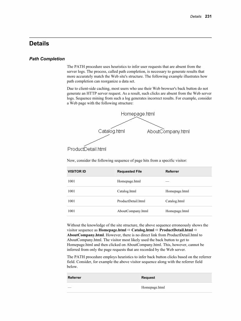
Details
Path CompletionThe PATH procedure uses heuristics to infer user requests that are absent from the server logs. The process, called path completion, is necessary to generate results that more accurately match the Web site's structure. The following example illustrates how path completion can reorganize a data set.
Due to client-side caching, most users who use their Web browser's back button do not generate an HTTP server request. As a result, such clicks are absent from the Web server logs. Sequence mining from such a log generates incorrect results. For example, consider a Web page with the following structure:
Now, consider the following sequence of page hits from a specific visitor:
VISITOR ID Requested File Referrer
1001 Homepage.html —
1001 Catalog.html Homepage.html
1001 ProductDetail.html Catalog.html
1001 AboutCompany.html Homepage.html
Without the knowledge of the site structure, the above sequence erroneously shows the visitor sequence as Homepage.html ð Catalog.html ð ProductDetail.html ð AboutCompany.html. However, there is no direct link from ProductDetail.html to AboutCompany.html. The visitor most likely used the back button to get to Homepage.html and then clicked on AboutCompany.html. This, however, cannot be inferred from only the page requests that are recorded by the Web server.
The PATH procedure employs heuristics to infer back button clicks based on the referrer field. Consider, for example the above visitor sequence along with the referrer field below.
Referrer Request
— Homepage.html
Details 231
Referrer Request
Homepage.html Catalog.html
Catalog.html ProductDetail.html
Homepage.html AboutCompany.html
By matching the requests with the referrer, the PATH procedure completes the above path as Homepage.html ð Catalog.html ð ProductDetail.html ð Catalog.html ð Homepage.html ð AboutCompany.html.
A user option called BACKUP_LIMIT= controls how far back the requests are searched for path completion. In the above example, if the BACKUP_LIMIT= is set to 1, no path completion is performed.
Path completion is attempted only if a referrer variable is specified. Optionally, the user can turn off path completion by omitting the referrer specification.
Path Break Detection
DetailsThis feature detects any breaks in the consecutive browsing pattern based on the referrer field. These types of breaks can happen when a visitor leaves a Web site but comes back within the time-out period or if a visitor follows a bookmarked link within the site. If a break in the path is detected, the subsequences are considered separate sequences for that visitor and are counted separately.
Now consider the following sequence of page views from a specific visitor:
Referrer Request
— Homepage.html
Homepage.html Catalog.html
Catalog.html ProductDetail.html
— AboutCompany.html
Because the Referrer field for the AboutCompany.html page is empty, this request belongs to a separate sequence for this visitor.
Even when the visitor navigates to a page after a series of back button clicks, it will be considered a page break if the value of BACKUP_LIMIT= is smaller than the number of back button clicks.
SyntaxPath completion is enabled by specifying a referrer variable. A template for the syntax is given below.
PROC PATH <options>; CUSTOMER variables; TARGET variable;
232 Chapter 12 • The PATH Procedure
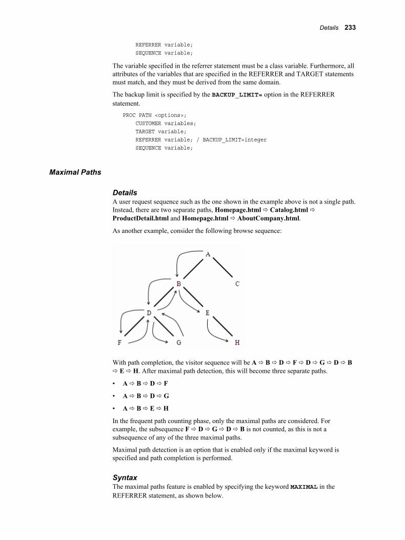
REFERRER variable; SEQUENCE variable;
The variable specified in the referrer statement must be a class variable. Furthermore, all attributes of the variables that are specified in the REFERRER and TARGET statements must match, and they must be derived from the same domain.
The backup limit is specified by the BACKUP_LIMIT= option in the REFERRER statement.
PROC PATH <options>; CUSTOMER variables; TARGET variable; REFERRER variable; / BACKUP_LIMIT=integer SEQUENCE variable;
Maximal Paths
DetailsA user request sequence such as the one shown in the example above is not a single path. Instead, there are two separate paths, Homepage.html ð Catalog.html ð ProductDetail.html and Homepage.html ð AboutCompany.html.
As another example, consider the following browse sequence:
With path completion, the visitor sequence will be A ð B ð D ð F ð D ð G ð D ð B ð E ð H. After maximal path detection, this will become three separate paths.
• A ð B ð D ð F
• A ð B ð D ð G
• A ð B ð E ð H
In the frequent path counting phase, only the maximal paths are considered. For example, the subsequence F ð D ð G ð D ð B is not counted, as this is not a subsequence of any of the three maximal paths.
Maximal path detection is an option that is enabled only if the maximal keyword is specified and path completion is performed.
SyntaxThe maximal paths feature is enabled by specifying the keyword MAXIMAL in the REFERRER statement, as shown below.
Details 233

PROC PATH <options>; CUSTOMER variables; TARGET variable; REFERRER variable / MAXIMAL; SEQUENCE variable;
234 Chapter 12 • The PATH Procedure
Chapter 13
The PMBR Procedure
Overview . . . . . . . . . . . . . . . . . . . . . . . . . . . . . . . . . . . . . . . . . . . . . . . . . . . . . . . . . . . 235The PMBR Procedure . . . . . . . . . . . . . . . . . . . . . . . . . . . . . . . . . . . . . . . . . . . . . . . 235
Syntax . . . . . . . . . . . . . . . . . . . . . . . . . . . . . . . . . . . . . . . . . . . . . . . . . . . . . . . . . . . . . . 236The PMBR Procedure . . . . . . . . . . . . . . . . . . . . . . . . . . . . . . . . . . . . . . . . . . . . . . . 236PROC PMBR Statement . . . . . . . . . . . . . . . . . . . . . . . . . . . . . . . . . . . . . . . . . . . . . 236DECISION Statement . . . . . . . . . . . . . . . . . . . . . . . . . . . . . . . . . . . . . . . . . . . . . . . 238ID Statement . . . . . . . . . . . . . . . . . . . . . . . . . . . . . . . . . . . . . . . . . . . . . . . . . . . . . . 239SCORE Statement . . . . . . . . . . . . . . . . . . . . . . . . . . . . . . . . . . . . . . . . . . . . . . . . . 239TARGET Statement . . . . . . . . . . . . . . . . . . . . . . . . . . . . . . . . . . . . . . . . . . . . . . . . 240VAR Statement . . . . . . . . . . . . . . . . . . . . . . . . . . . . . . . . . . . . . . . . . . . . . . . . . . . . 240
Details . . . . . . . . . . . . . . . . . . . . . . . . . . . . . . . . . . . . . . . . . . . . . . . . . . . . . . . . . . . . . . 240The PMBR Procedure . . . . . . . . . . . . . . . . . . . . . . . . . . . . . . . . . . . . . . . . . . . . . . . 240Nearest Neighbors . . . . . . . . . . . . . . . . . . . . . . . . . . . . . . . . . . . . . . . . . . . . . . . . . 241
Examples . . . . . . . . . . . . . . . . . . . . . . . . . . . . . . . . . . . . . . . . . . . . . . . . . . . . . . . . . . . 242Example 1: Preprocessing the Data and Basic Usage . . . . . . . . . . . . . . . . . . . . . . 242Example 2: Different Values of K . . . . . . . . . . . . . . . . . . . . . . . . . . . . . . . . . . . . . 242Example 3: The SCAN Method . . . . . . . . . . . . . . . . . . . . . . . . . . . . . . . . . . . . . . . 243
Overview
The PMBR ProcedureThe PMBR procedure is a predictive modeling tool that is presented as an alternative to the other predictive modeling tools. Unlike the other predictive modeling tools, the PMBR procedure does not create a set of rules based on the training data. Instead, it categorizes an observation in the scoring data set based on that observation's nearest neighbors in the training data set. The posterior probability for the scored observation is the probability that is determined by the nearest neighbors. For more information about how this probability is determined, see “Details” on page 240 . This method is supported only for binary, interval, and nominal targets; however, you can model ordinal targets as interval targets and apply the PMBR procedure.
235
Syntax
The PMBR ProcedurePROC PMBR DATA=data-set-name DMDBCAT=data-set-name <options>;
DECISION <options>;ID <variable>;SCORE DATA=data-set-name <options>;TARGET variable;VAR <variables>;RUN;
PROC PMBR Statement
SyntaxPROC PMBR DATA=data-set-name DMDBCAT=data-set-name <options>;
Required ArgumentsDATA=data-set-name
This argument specifies the training data set.
Note: Strictly speaking, this argument is not required, but should be included. If the DATA= argument is omitted, then the most recently created data set is used for analysis.
DMDBCAT=catalog-nameThis argument specifies the name of the DMDB catalog for the training data set.
Optional ArgumentsBUCKET=number
Use this option to specify the number of buckets that a leaf node is allowed to grow before it splits into a branch with two new leaves. The value of number must be an integer greater than or equal to 2. This option only applies to the RDTREE method.
EPSILON=numberThe value of number is the minimum allowable distance for a scoring observation to a training observation. For example, if number is greater than 0, then a training observation that is identical to the scored observation will not be considered a neighbor because it is too close. The value of number must be a nonnegative number and default to 0.0. This option only applies to the RDTREE method.
K=numberThis option specifies the number of neighbors to retrieve for each scored observation. The value of number must be a positive integer and default to 1.
METHOD=SCAN | RDTREEThis option determines the data representation that is used to store the training data set and determine the nearest neighbors.
236 Chapter 13 • The PMBR Procedure
The two methods available are:
• RDTREE — stores the training data set observations in a reduced dimensionality tree. This method creates a binary tree by repeatedly partitioning the data set into subsets such that the number of observations in each of the subsets is small. The RDTREE method splits a node along some dimension, usually the one with the greatest variation. The split generally occurs at the median value of the node. This method is typically quicker when there are fewer than 100 dimensions. This is the default method.
• SCAN — scans every observation in the training data set to calculate its distance to the scored observation.
NEIGHBORSIf you specify this option, then the nearest neighbors are printed in the output data set. This option adds the variables _N1, ..., _NK to the output data set, where the value of K is specified with the K= argument. The values in these variables are either the values of the ID variable (if it was specified) or positive integers that correspond to the observations in the input data set.
Note: If an ID variable was not specified and the input data set is sorted, then the values of these variables are not valid.
OPTIMIZEKUse this option to let the PMBR procedure determine the optimal value for K. If you specify this argument and the K= argument, then the value given there is considered the maximum acceptable value for K. When you specify this option, a note is printed to the log that indicates the optimal value for K.
For an interval target, the optimal value is the smallest number of neighbors that corresponds to the largest correlation between the actual target variable and the predicted target variable in the training data set. For a categorical target, the optimal value of K is the smallest number of neighbors that corresponds to the largest sum of posterior probabilities at the level of the target variable in the training data set.
OUT=data-set-nameThis option specifies the output data set. This data set contains the information in the input data set and the calculated posterior probabilities. The exact variables that are included are determined by the type of the target variable. You can use the options NEIGHBORS and SHOWNODES to include additional variables in this data set. If you specify this data set in the “SCORE Statement” on page 239 , then it will override this argument.
Note: The PMBR procedure will always create an output data set when you score a data set. If this option is omitted, then the PMBR procedure will create the data set DATAn, where n is the smallest integer not already used by the PMBR procedure.
OUTEST=data-set-nameThe data set specified here contains the estimated weights and fit statistics for the training, validation, and test data sets.
SCORE=data-set-nameThis option specifies the data set that you want to score. This data set does not need to contain the target variable and can be the same data set as the training data set. You can also use the “SCORE Statement” on page 239 to specify this data set.
SHOWNODESWhen you specify this option, the output data set contains a variable that identifies the number of nodes that were analyzed to determine the nearest neighbors.
Syntax 237
TESTDATA=data-set-nameThis option specifies the name of the test data set. This data set should be raw data, not a DMDB encoded data set. This data set must contain all the input variables and the target variable.
THREADS | NOTHREADSThis option controls the behavior of the multi-threaded search for a scored observation's nearest neighbors. Use THREADS to let the system determine the optimal number of threads to spawn and use NOTHREADS to disable this feature. This option is not supported with the RDTREE method. The default setting is THREADS.
THREADS=numberAs an alternative, you can set the number of threads with the THREADS=number statement. The PMBR procedure will use exactly number threads, where number is a positive integer greater than 1. This option is not supported with the RDTREE method.
VALIDATA=data-set-nameThis option specifies the name of the test data set. This data set should be raw data, not a DMDB encoded data set. This data set must contain all the input variables and the target variable.
WEIGHTEDWhen you specify this option, the input variables are weighted by the absolute value of their correlation to the target variable. This option is ignored if the target is a class variable with more than two levels. In this case, a note is printed to the log that indicates the option was ignored.
DECISION Statement
SyntaxDECISION <options>;
Optional ArgumentsCOST=list-of-numbers
Use this option to specify a list of constants that represent the cost associated with each decision.
COSTVAR=list-of-variablesUse this option to specify a list of variables that contain the cost associated with each decision. These variables must appear in the scoring data set.
DECISIONDATA | DECDATA=data-set-nameThis data set contains the decision matrix and prior probabilities.
DECVAR=variable-namessThis option specifies the decision variables in the DECDATA= data set.
PRIORVAR=variable-nameThis option specifies the prior probabilities in the DECDATA= data set.
238 Chapter 13 • The PMBR Procedure
ID Statement
SyntaxID <variable>;
Optional Argumentvariable
Use this option to specify what variable, if any, contains a unique identifier for each observation in the input data set.
SCORE Statement
SyntaxSCORE DATA=data-set-name <options>;
Note: You can use the “PROC PMBR Statement” on page 236 to specify the scoring data set and the output data set with the SCORE= and OUT= arguments, respectively. However, anything declared in the SCORE statement will override the declarations in the PROC statement.
Required ArgumentDATA=data-set-name
This option specifies the scoring data set. This data set does not need to contain the target variable and can be the same data set as the training data set.
Optional ArgumentsOUT=data-set-name
This option specifies the output data set. This data set contains the information in the input data set and the calculated posterior probabilities. The exact variables that are included are determined by the type of the target variable. You can use the options NEIGHBORS and SHOWNODES, available in the PROC statement, to include additional variables in this data set.
Note: The PMBR procedure will always create an output data set when you score a data set. If this option is omitted, then the PMBR procedure will create the data set DATAn, where n is the smallest integer not already used by the PMBR procedure.
OUTFIT=data-set-nameThe data set specified here contains the fit statistics for the scoring data set.
ROLE=TRAIN | VALID | TEST | SCOREThis option specifies the type of fit statistics to compute for the OUTFIT= data set. You cannot use the OUTFIT= argument and the SCORE role simultaneously. Also, if the TRAIN role is used, then the scoring data set must be the same as the input data set.
Syntax 239
TARGET Statement
SyntaxTARGET variable;
Required Argumentvariable
This statement indicates what variable in the input data set is the target variable. The TARGET statement is required.
VAR Statement
SyntaxVAR <list-of-variables>;
Optional Argumentlist-of-variables
Specify all variables that you want to treat as dimensions for the nearest neighbor search. For best results, these variables should be standardized and orthogonal. If no VAR statement is specified, then all variables in the data set are used for analysis.
Details
The PMBR ProcedureThe PMBR procedure is a memory-based learning approach that implements the k-nearest neighbors algorithm. This approach does not use a training step to generate a set of rules that are used for future prediction. Instead, this method stores the training data set in memory and classifies each scored observation based on its k-nearest neighbors. These k neighbors determine the posterior probability that is assigned to the scored observation with a majority vote. A brief example of the voting process is given in the next section.
To determine the nearest neighbors, the PMBR calculates the Euclidean distance between each scored observation and relevant observations in the training data set. Relevant observations are all observations in the training data set when the SCAN method is used. However, the RDTREE method presents a more efficient solution. With the RDTREE method, the training data is divided into buckets based on the variable with the highest variance. Each scored observation is only compared against the observations in the bucket that best describes that observation.
Unless otherwise specified, each variable in the training data represents a unique dimension when the distance is calculated. Therefore, the PMBR procedure assumes that the variables are standardized and orthogonal to each other. If your input data is not standardized and orthogonal, you need to precede the PMBR procedure with one that will create orthogonal, standardized variables. The following procedures will accomplish this task: CORRESP, DMNEURAL, PRINCOMP, PRINQUAL, and SPSVD. If a
240 Chapter 13 • The PMBR Procedure
variable value is missing, then that value is replaced by the mean of that variable, which is stored in the DMDB catalog.
Nearest NeighborsThis section presents an example to illustrate how the PMBR procedure determines the posterior probability for a scored observation. Let a scored observation be denoted by S. The table below lists the five nearest observations to S from a fictitious training data set.
Observation ID Target ValueDistance Rank (1: Closest, 5: Farthest)
7 N 3
12 Y 2
35 N 5
108 Y 1
334 N 4
This table lists observation 108 as the nearest neighbor to S and observation 35 as the farthest neighbor to S. You can use the value of k to determine the number of neighbors that contribute to the posterior probability for S. The table below calculates the posterior probability five values of k.
kIDs of Nearest Neighbors
Target Value of Nearest Neighbors
Posterior Probabilities for S
1 108 Y Prob(Y) = 1.0, Prob(N) = 0.0
2 108, 12 Y, Y Prob(Y) = 1.0, Prob(N) = 0.0
3 108, 12, 7 Y, Y, N Prob(Y) = 0.667, Prob(N) = 0.333
4 108, 12, 7, 334 Y, Y, N, N Prob(Y) = 0.5, Prob(N) = 0.5
5 108, 12, 7, 334, 35 Y, Y, N, N, N Prob(Y) = 0.4, Prob(N) = 0.6
In this example, if 1–, 2–, or 3–nearest neighbors are used for the search, then S is assigned a posterior probability of Y. When 5–nearest neighbors are used , S is assigned a posterior probability of N. When 4–nearest neighbors are used, this method results in a tie between Y and N. An easy generalization to make from this example is that when you have a binary target, an odd value for k will prevent tied votes.
If the target is an interval variable, then the average of the target values for the k-nearest neighbors is calculated and reported for the value of S.
Details 241
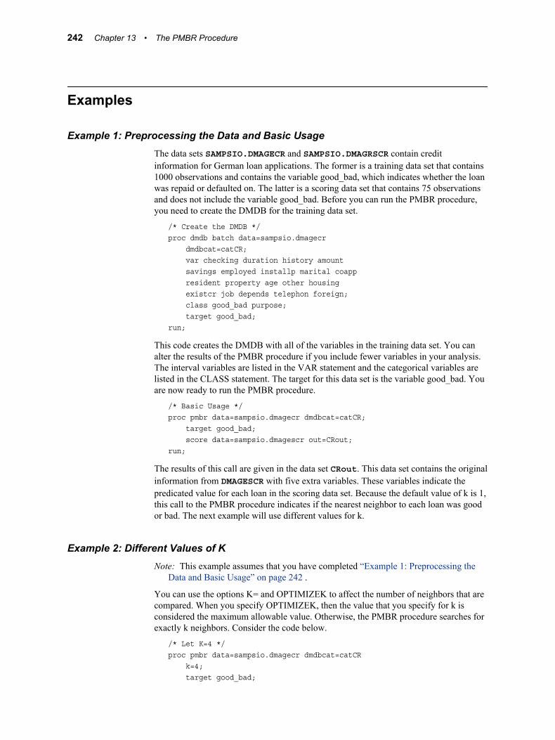
Examples
Example 1: Preprocessing the Data and Basic UsageThe data sets SAMPSIO.DMAGECR and SAMPSIO.DMAGRSCR contain credit information for German loan applications. The former is a training data set that contains 1000 observations and contains the variable good_bad, which indicates whether the loan was repaid or defaulted on. The latter is a scoring data set that contains 75 observations and does not include the variable good_bad. Before you can run the PMBR procedure, you need to create the DMDB for the training data set.
/* Create the DMDB */proc dmdb batch data=sampsio.dmagecr dmdbcat=catCR; var checking duration history amount savings employed installp marital coapp resident property age other housing existcr job depends telephon foreign; class good_bad purpose; target good_bad;run;
This code creates the DMDB with all of the variables in the training data set. You can alter the results of the PMBR procedure if you include fewer variables in your analysis. The interval variables are listed in the VAR statement and the categorical variables are listed in the CLASS statement. The target for this data set is the variable good_bad. You are now ready to run the PMBR procedure.
/* Basic Usage */proc pmbr data=sampsio.dmagecr dmdbcat=catCR; target good_bad; score data=sampsio.dmagescr out=CRout;run;
The results of this call are given in the data set CRout. This data set contains the original information from DMAGESCR with five extra variables. These variables indicate the predicated value for each loan in the scoring data set. Because the default value of k is 1, this call to the PMBR procedure indicates if the nearest neighbor to each loan was good or bad. The next example will use different values for k.
Example 2: Different Values of KNote: This example assumes that you have completed “Example 1: Preprocessing the
Data and Basic Usage” on page 242 .
You can use the options K= and OPTIMIZEK to affect the number of neighbors that are compared. When you specify OPTIMIZEK, then the value that you specify for k is considered the maximum allowable value. Otherwise, the PMBR procedure searches for exactly k neighbors. Consider the code below.
/* Let K=4 */proc pmbr data=sampsio.dmagecr dmdbcat=catCR k=4; target good_bad;
242 Chapter 13 • The PMBR Procedure
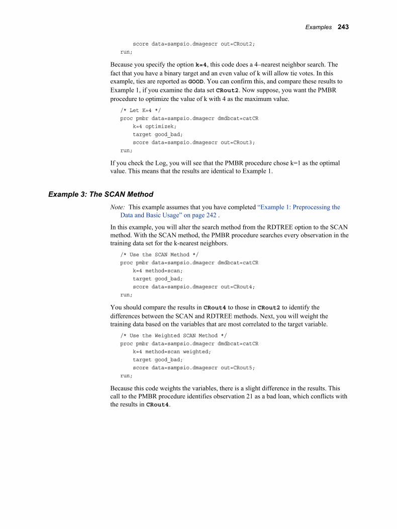
score data=sampsio.dmagescr out=CRout2;run;
Because you specify the option k=4, this code does a 4–nearest neighbor search. The fact that you have a binary target and an even value of k will allow tie votes. In this example, ties are reported as GOOD. You can confirm this, and compare these results to Example 1, if you examine the data set CRout2. Now suppose, you want the PMBR procedure to optimize the value of k with 4 as the maximum value.
/* Let K=4 */proc pmbr data=sampsio.dmagecr dmdbcat=catCR k=4 optimizek; target good_bad; score data=sampsio.dmagescr out=CRout3;run;
If you check the Log, you will see that the PMBR procedure chose k=1 as the optimal value. This means that the results are identical to Example 1.
Example 3: The SCAN MethodNote: This example assumes that you have completed “Example 1: Preprocessing the
Data and Basic Usage” on page 242 .
In this example, you will alter the search method from the RDTREE option to the SCAN method. With the SCAN method, the PMBR procedure searches every observation in the training data set for the k-nearest neighbors.
/* Use the SCAN Method */proc pmbr data=sampsio.dmagecr dmdbcat=catCR k=4 method=scan; target good_bad; score data=sampsio.dmagescr out=CRout4;run;
You should compare the results in CRout4 to those in CRout2 to identify the differences between the SCAN and RDTREE methods. Next, you will weight the training data based on the variables that are most correlated to the target variable.
/* Use the Weighted SCAN Method */proc pmbr data=sampsio.dmagecr dmdbcat=catCR k=4 method=scan weighted; target good_bad; score data=sampsio.dmagescr out=CRout5;run;
Because this code weights the variables, there is a slight difference in the results. This call to the PMBR procedure identifies observation 21 as a bad loan, which conflicts with the results in CRout4.
Examples 243

244 Chapter 13 • The PMBR Procedure
Chapter 14
The RULEGEN Procedure
Overview . . . . . . . . . . . . . . . . . . . . . . . . . . . . . . . . . . . . . . . . . . . . . . . . . . . . . . . . . . . 245The RULEGEN Procedure . . . . . . . . . . . . . . . . . . . . . . . . . . . . . . . . . . . . . . . . . . . 245
Syntax . . . . . . . . . . . . . . . . . . . . . . . . . . . . . . . . . . . . . . . . . . . . . . . . . . . . . . . . . . . . . . 245The RULEGEN Procedure . . . . . . . . . . . . . . . . . . . . . . . . . . . . . . . . . . . . . . . . . . . 245PROC RULEGEN Statement . . . . . . . . . . . . . . . . . . . . . . . . . . . . . . . . . . . . . . . . . 245
Examples . . . . . . . . . . . . . . . . . . . . . . . . . . . . . . . . . . . . . . . . . . . . . . . . . . . . . . . . . . . 247Example 1: The RULEGEN Procedure . . . . . . . . . . . . . . . . . . . . . . . . . . . . . . . . . 247
Overview
The RULEGEN ProcedureThe RULEGEN procedure generates association rules based on the output of the ASSOC procedure. Additionally, the RULEGEN procedure computes statistics, such as confidence and lift, for these rules. While the ASSOC procedure identifies sets of items that are related, the RULEGEN procedure discovers the rules that govern these associations. The output is saved as a SAS data set so that you can review the results and, if necessary, adjust the input arguments.
Syntax
The RULEGEN ProcedurePROC RULEGEN IN=data-set-name OUT=data-set-name <options>;
RUN;
PROC RULEGEN Statement
SyntaxPROC RULEGEN IN=data-set-name OUT=data-set-name <options>;
245
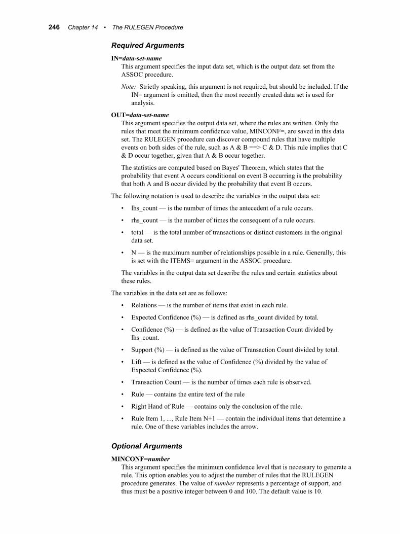
Required ArgumentsIN=data-set-name
This argument specifies the input data set, which is the output data set from the ASSOC procedure.
Note: Strictly speaking, this argument is not required, but should be included. If the IN= argument is omitted, then the most recently created data set is used for analysis.
OUT=data-set-nameThis argument specifies the output data set, where the rules are written. Only the rules that meet the minimum confidence value, MINCONF=, are saved in this data set. The RULEGEN procedure can discover compound rules that have multiple events on both sides of the rule, such as A & B ==> C & D. This rule implies that C & D occur together, given that A & B occur together.
The statistics are computed based on Bayes' Theorem, which states that the probability that event A occurs conditional on event B occurring is the probability that both A and B occur divided by the probability that event B occurs.
The following notation is used to describe the variables in the output data set:
• lhs_count — is the number of times the antecedent of a rule occurs.
• rhs_count — is the number of times the consequent of a rule occurs.
• total — is the total number of transactions or distinct customers in the original data set.
• N — is the maximum number of relationships possible in a rule. Generally, this is set with the ITEMS= argument in the ASSOC procedure.
The variables in the output data set describe the rules and certain statistics about these rules.
The variables in the data set are as follows:
• Relations — is the number of items that exist in each rule.
• Expected Confidence (%) — is defined as rhs_count divided by total.
• Confidence (%) — is defined as the value of Transaction Count divided by lhs_count.
• Support (%) — is defined as the value of Transaction Count divided by total.
• Lift — is defined as the value of Confidence (%) divided by the value of Expected Confidence (%).
• Transaction Count — is the number of times each rule is observed.
• Rule — contains the entire text of the rule
• Right Hand of Rule — contains only the conclusion of the rule.
• Rule Item 1, ..., Rule Item N+1 — contain the individual items that determine a rule. One of these variables includes the arrow.
Optional ArgumentsMINCONF=number
This argument specifies the minimum confidence level that is necessary to generate a rule. This option enables you to adjust the number of rules that the RULEGEN procedure generates. The value of number represents a percentage of support, and thus must be a positive integer between 0 and 100. The default value is 10.
246 Chapter 14 • The RULEGEN Procedure
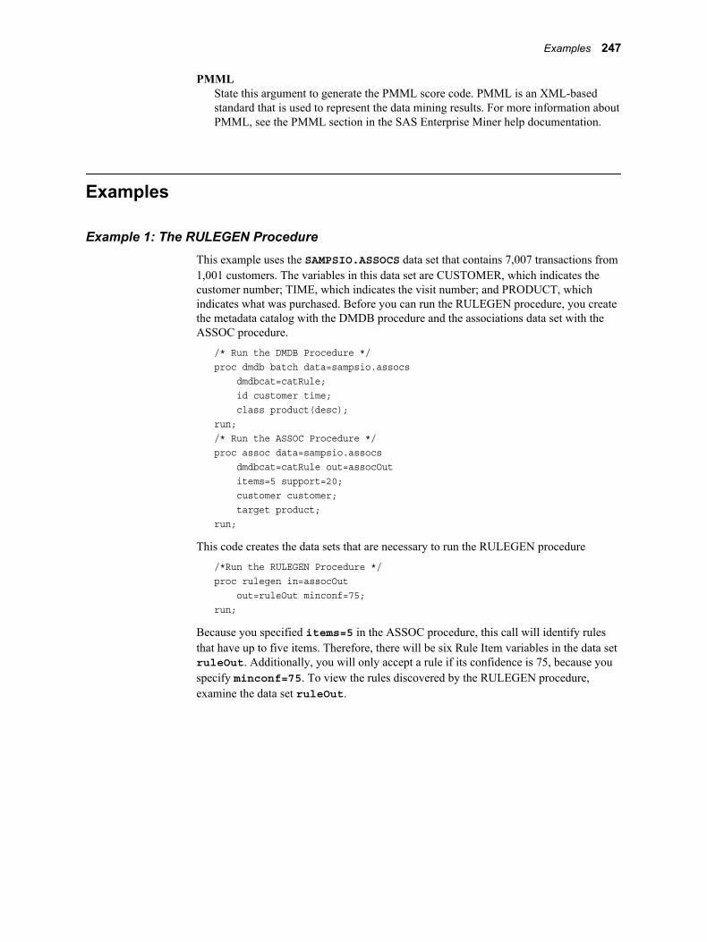
PMMLState this argument to generate the PMML score code. PMML is an XML-based standard that is used to represent the data mining results. For more information about PMML, see the PMML section in the SAS Enterprise Miner help documentation.
Examples
Example 1: The RULEGEN ProcedureThis example uses the SAMPSIO.ASSOCS data set that contains 7,007 transactions from 1,001 customers. The variables in this data set are CUSTOMER, which indicates the customer number; TIME, which indicates the visit number; and PRODUCT, which indicates what was purchased. Before you can run the RULEGEN procedure, you create the metadata catalog with the DMDB procedure and the associations data set with the ASSOC procedure.
/* Run the DMDB Procedure */proc dmdb batch data=sampsio.assocs dmdbcat=catRule; id customer time; class product(desc);run;/* Run the ASSOC Procedure */proc assoc data=sampsio.assocs dmdbcat=catRule out=assocOut items=5 support=20; customer customer; target product;run;
This code creates the data sets that are necessary to run the RULEGEN procedure
/*Run the RULEGEN Procedure */proc rulegen in=assocOut out=ruleOut minconf=75;run;
Because you specified items=5 in the ASSOC procedure, this call will identify rules that have up to five items. Therefore, there will be six Rule Item variables in the data set ruleOut. Additionally, you will only accept a rule if its confidence is 75, because you specify minconf=75. To view the rules discovered by the RULEGEN procedure, examine the data set ruleOut.
Examples 247

248 Chapter 14 • The RULEGEN Procedure
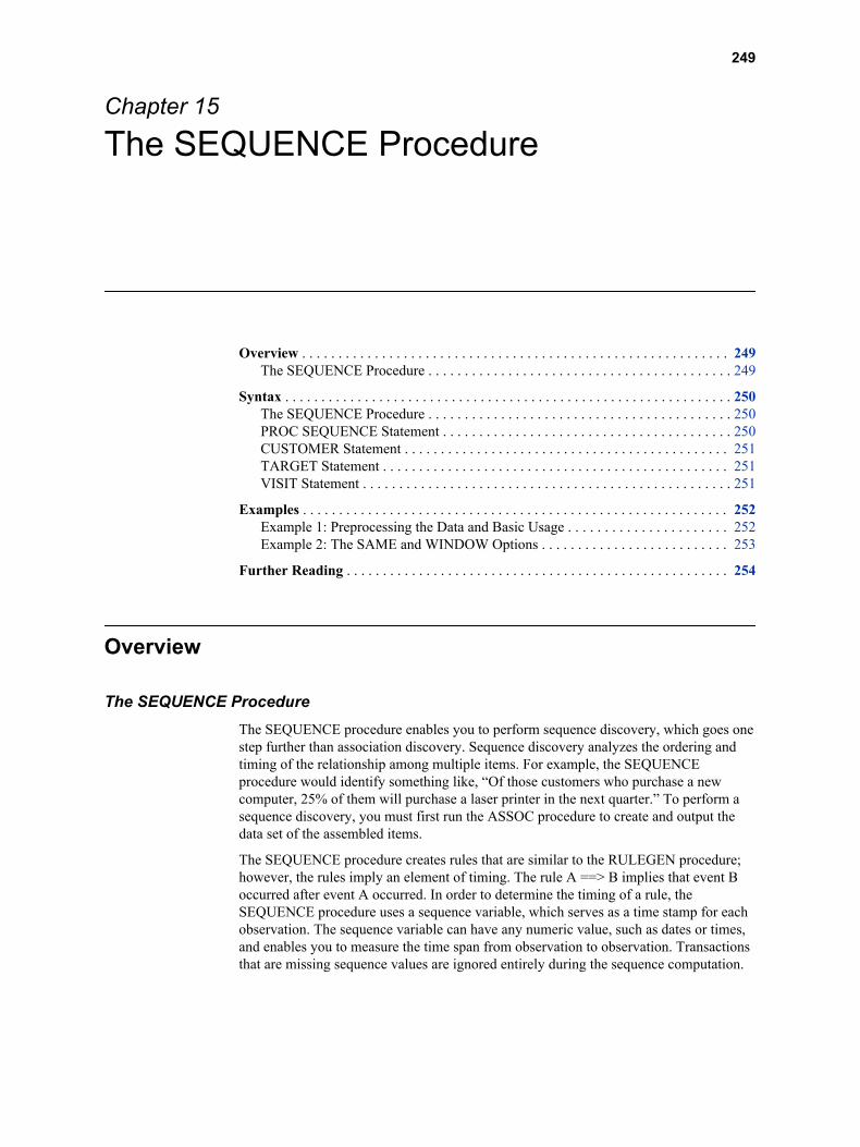
Chapter 15
The SEQUENCE Procedure
Overview . . . . . . . . . . . . . . . . . . . . . . . . . . . . . . . . . . . . . . . . . . . . . . . . . . . . . . . . . . . 249The SEQUENCE Procedure . . . . . . . . . . . . . . . . . . . . . . . . . . . . . . . . . . . . . . . . . . 249
Syntax . . . . . . . . . . . . . . . . . . . . . . . . . . . . . . . . . . . . . . . . . . . . . . . . . . . . . . . . . . . . . . 250The SEQUENCE Procedure . . . . . . . . . . . . . . . . . . . . . . . . . . . . . . . . . . . . . . . . . . 250PROC SEQUENCE Statement . . . . . . . . . . . . . . . . . . . . . . . . . . . . . . . . . . . . . . . . 250CUSTOMER Statement . . . . . . . . . . . . . . . . . . . . . . . . . . . . . . . . . . . . . . . . . . . . . 251TARGET Statement . . . . . . . . . . . . . . . . . . . . . . . . . . . . . . . . . . . . . . . . . . . . . . . . 251VISIT Statement . . . . . . . . . . . . . . . . . . . . . . . . . . . . . . . . . . . . . . . . . . . . . . . . . . . 251
Examples . . . . . . . . . . . . . . . . . . . . . . . . . . . . . . . . . . . . . . . . . . . . . . . . . . . . . . . . . . . 252Example 1: Preprocessing the Data and Basic Usage . . . . . . . . . . . . . . . . . . . . . . 252Example 2: The SAME and WINDOW Options . . . . . . . . . . . . . . . . . . . . . . . . . . 253
Further Reading . . . . . . . . . . . . . . . . . . . . . . . . . . . . . . . . . . . . . . . . . . . . . . . . . . . . . 254
Overview
The SEQUENCE ProcedureThe SEQUENCE procedure enables you to perform sequence discovery, which goes one step further than association discovery. Sequence discovery analyzes the ordering and timing of the relationship among multiple items. For example, the SEQUENCE procedure would identify something like, “Of those customers who purchase a new computer, 25% of them will purchase a laser printer in the next quarter.” To perform a sequence discovery, you must first run the ASSOC procedure to create and output the data set of the assembled items.
The SEQUENCE procedure creates rules that are similar to the RULEGEN procedure; however, the rules imply an element of timing. The rule A ==> B implies that event B occurred after event A occurred. In order to determine the timing of a rule, the SEQUENCE procedure uses a sequence variable, which serves as a time stamp for each observation. The sequence variable can have any numeric value, such as dates or times, and enables you to measure the time span from observation to observation. Transactions that are missing sequence values are ignored entirely during the sequence computation.
249
Syntax
The SEQUENCE ProcedurePROC SEQUENCE ASSOC=data-set-name DATA=data-set-nameDMDBCAT=catalog-name <options>;
CUSTOMER variable;TARGET variable;VISIT variable</options>;RUN;
PROC SEQUENCE Statement
SyntaxPROC SEQUENCE ASSOC=data-set-name DATA=data-set-nameDMDBCAT=catalog-name <options>;
Required ArgumentsASSOC=data-set-name
The data set provided here is the output data set from the ASSOC procedure. This is one of the input data sets for the SEQUENCE procedure.
DATA=data-set-nameThis argument identifies the input data source. To perform sequence discovery, the input data set must have a separate observation for each product that was purchased by each customer. In this data set, you must assign a customer variable, a target variable, and a sequence with the CUSTOMER, TARGET, and VISIT statements, respectively.
DMDBCAT=catalog-nameThis option identifies the metadata catalog that is associated with the input data source.
Optional ArgumentsNITEMS=number
This option specifies the maximum number of events that are possible for each rule. The value of number must be a positive integer. If you request rules with more than two events, then number-2 additional passes through the input data set are required. The default value is 2.
OUT=data-set-nameThis option specifies the output data set, where the discovered relationships are stored.
The variables in this data set are as follows:
• Chain Length — contains the length of the rule.
• Transaction Count — contains the number of transactions or distinct customers that meet the rule's criteria.
250 Chapter 15 • The SEQUENCE Procedure
• Support (%) — contains the percentage of customers that meet the rule's criteria. That is, it is the value of Transaction Count divided by the total number of transactions.
• Confidence (%) — contains the confidence value for each rule. For the rule A & B ==> C, this value would be the value of Transaction Count divided by the number of times the hypothesis, A & B, occurs. This value is the conditional probability of the rule, given that the antecedent A & B occurs.
• Rule — contains the rule text. For example, A & B ==> C.
• Chain Item 1, ..., Chain Item N — contain, in order, the events that form the rule. The SEQUENCE procedure can detect multiple events that occur at the same time and will report them as rules in the form A & B ==> C & D. This means that events A and B occurred simultaneously and were followed by the simultaneous occurrence of C and D.
SUPPORT=numberThis option specifies the minimum number of transactions that must occur for a rule to be accepted. Rules that occur less than number times are rejected. Note that this is in addition to the SUPPORT= argument in the ASSOC procedure. The value of number must be a positive integer. If not specified, then this value is 2% of the total transaction count.
CUSTOMER Statement
SyntaxCUSTOMER variable;
Required Argumentvariable
The variable identified here must be in the input data set and identify the customer that will be analyzed.
TARGET Statement
SyntaxTARGET variable;
Required Argumentvariable
The variable identified here must be in the input data set and identify the name of the product that will be analyzed.
VISIT Statement
SyntaxVISIT variable</options>;
Syntax 251
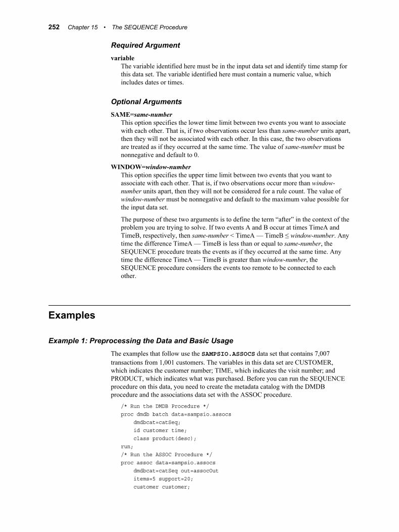
Required Argumentvariable
The variable identified here must be in the input data set and identify time stamp for this data set. The variable identified here must contain a numeric value, which includes dates or times.
Optional ArgumentsSAME=same-number
This option specifies the lower time limit between two events you want to associate with each other. That is, if two observations occur less than same-number units apart, then they will not be associated with each other. In this case, the two observations are treated as if they occurred at the same time. The value of same-number must be nonnegative and default to 0.
WINDOW=window-numberThis option specifies the upper time limit between two events that you want to associate with each other. That is, if two observations occur more than window-number units apart, then they will not be considered for a rule count. The value of window-number must be nonnegative and default to the maximum value possible for the input data set.
The purpose of these two arguments is to define the term “after” in the context of the problem you are trying to solve. If two events A and B occur at times TimeA and TimeB, respectively, then same-number < TimeA — TimeB ≤ window-number. Any time the difference TimeA — TimeB is less than or equal to same-number, the SEQUENCE procedure treats the events as if they occurred at the same time. Any time the difference TimeA — TimeB is greater than window-number, the SEQUENCE procedure considers the events too remote to be connected to each other.
Examples
Example 1: Preprocessing the Data and Basic UsageThe examples that follow use the SAMPSIO.ASSOCS data set that contains 7,007 transactions from 1,001 customers. The variables in this data set are CUSTOMER, which indicates the customer number; TIME, which indicates the visit number; and PRODUCT, which indicates what was purchased. Before you can run the SEQUENCE procedure on this data, you need to create the metadata catalog with the DMDB procedure and the associations data set with the ASSOC procedure.
/* Run the DMDB Procedure */proc dmdb batch data=sampsio.assocs dmdbcat=catSeq; id customer time; class product(desc);run;/* Run the ASSOC Procedure */proc assoc data=sampsio.assocs dmdbcat=catSeq out=assocOut items=5 support=20; customer customer;
252 Chapter 15 • The SEQUENCE Procedure
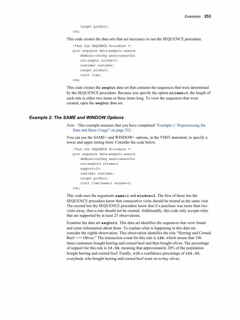
target product;run;
This code creates the data sets that are necessary to run the SEQUENCE procedure.
/*Run the SEQUENCE Procedure */proc sequence data=sampsio.assocs dmdbcat=catSeq assoc=assocOut out=seqOut nitems=3; customer customer; target product; visit time;run;
This code creates the seqOut data set that contains the sequences that were determined by the SEQUENCE procedure. Because you specify the option nitems=3, the length of each rule is either two items or three items long. To view the sequences that were created, open the seqOut data set.
Example 2: The SAME and WINDOW OptionsNote: This example assumes that you have completed “Example 1: Preprocessing the
Data and Basic Usage” on page 252 .
You can use the SAME= and WINDOW= options, in the VISIT statement, to specify a lower and upper timing limit. Consider the code below.
/*Run the SEQUENCE Procedure */proc sequence data=sampsio.assocs dmdbcat=catSeq assoc=assocOut out=seqOut2 nitems=2 support=25; customer customer; target product; visit time/same=1 window=2;run;
This code uses the arguments same=1 and window=2. The first of these lets the SEQUENCE procedure know that consecutive visits should be treated as the same visit. The second lets the SEQUENCE procedure know that if a purchase was more than two visits away, then a rule should not be created. Additionally, this code only accepts rules that are supported by at least 25 observations.
Examine the data set seqOut2. This data set identifies the sequences that were found and some information about them. To explain what is happening in this data set, consider the eighth observation. This observation identifies the rule “Herring and Corned Beef ==> Olives.” The transaction count for this rule is 196, which means that 196 times customers bought herring and corned beef and then bought olives. The percentage of support for this rule is 19.58, meaning that approximately 20% of the population bought herring and corned beef. Finally, with a confidence percentage of 100.00, everybody who bought herring and corned beef went on to buy olives.
Examples 253

Further ReadingFor more information about the methods used by the SEQUENCE procedure, consider the following sources:
• R. Agrawal, T. Imielinksi, and A. Swami. 1993. “Mining Associate Rules Between Sets of Items in Large Databases.” Proceedings, ACM SIGMOID Conference on Management of Data, 207–216. Washington, D.C.
• M. Berry and G. Linoff, Data Mining Techniques for Marketing, Sales, and Customer Support (New York, NY: John Wiley and Sons, Inc, 1997)
254 Chapter 15 • The SEQUENCE Procedure
Chapter 16
The SPLIT Procedure
Overview . . . . . . . . . . . . . . . . . . . . . . . . . . . . . . . . . . . . . . . . . . . . . . . . . . . . . . . . . . . 255The SPLIT Procedure . . . . . . . . . . . . . . . . . . . . . . . . . . . . . . . . . . . . . . . . . . . . . . . 255
Syntax . . . . . . . . . . . . . . . . . . . . . . . . . . . . . . . . . . . . . . . . . . . . . . . . . . . . . . . . . . . . . . 256The SPLIT Procedure . . . . . . . . . . . . . . . . . . . . . . . . . . . . . . . . . . . . . . . . . . . . . . . 256PROC SPLIT Statement . . . . . . . . . . . . . . . . . . . . . . . . . . . . . . . . . . . . . . . . . . . . . 256CODE Statement . . . . . . . . . . . . . . . . . . . . . . . . . . . . . . . . . . . . . . . . . . . . . . . . . . 260DESCRIBE Statement . . . . . . . . . . . . . . . . . . . . . . . . . . . . . . . . . . . . . . . . . . . . . . 261FREQ Statement . . . . . . . . . . . . . . . . . . . . . . . . . . . . . . . . . . . . . . . . . . . . . . . . . . . 261INPUT Statement . . . . . . . . . . . . . . . . . . . . . . . . . . . . . . . . . . . . . . . . . . . . . . . . . . 261PRIORS Statement . . . . . . . . . . . . . . . . . . . . . . . . . . . . . . . . . . . . . . . . . . . . . . . . . 262PRUNE Statement . . . . . . . . . . . . . . . . . . . . . . . . . . . . . . . . . . . . . . . . . . . . . . . . . 262SCORE Statement . . . . . . . . . . . . . . . . . . . . . . . . . . . . . . . . . . . . . . . . . . . . . . . . . 263TARGET Statement . . . . . . . . . . . . . . . . . . . . . . . . . . . . . . . . . . . . . . . . . . . . . . . . 264
Details . . . . . . . . . . . . . . . . . . . . . . . . . . . . . . . . . . . . . . . . . . . . . . . . . . . . . . . . . . . . . . 264Missing Values . . . . . . . . . . . . . . . . . . . . . . . . . . . . . . . . . . . . . . . . . . . . . . . . . . . . 264Method of Split Search . . . . . . . . . . . . . . . . . . . . . . . . . . . . . . . . . . . . . . . . . . . . . . 265Automatic Pruning and Subtree Selection . . . . . . . . . . . . . . . . . . . . . . . . . . . . . . . 266CHAID . . . . . . . . . . . . . . . . . . . . . . . . . . . . . . . . . . . . . . . . . . . . . . . . . . . . . . . . . . 267Classification and Regression Trees . . . . . . . . . . . . . . . . . . . . . . . . . . . . . . . . . . . . 268C4.5 and C5.0 . . . . . . . . . . . . . . . . . . . . . . . . . . . . . . . . . . . . . . . . . . . . . . . . . . . . . 269
Examples . . . . . . . . . . . . . . . . . . . . . . . . . . . . . . . . . . . . . . . . . . . . . . . . . . . . . . . . . . . 271Example 1: Preprocessing the Data and Basic Usage . . . . . . . . . . . . . . . . . . . . . . 271Example 2: Score the Decision Tree . . . . . . . . . . . . . . . . . . . . . . . . . . . . . . . . . . . 272Example 3: Create a Decision Tree with an Interval Target . . . . . . . . . . . . . . . . . 273
Further Reading . . . . . . . . . . . . . . . . . . . . . . . . . . . . . . . . . . . . . . . . . . . . . . . . . . . . . 274
Overview
The SPLIT ProcedureAn empirical decision tree segments an input data set with a series of simple rules. Each rule assigns an observation to a segment based on the value of one input variable. A series of rules is applied, which results in a hierarchy of segments within each segment. The hierarchy is called a tree and each segment is called a node. The original segment contains the entire data set and is called the root node of the tree. A node and all of its successors form a branch of the node that created it. The final nodes, which are not
255
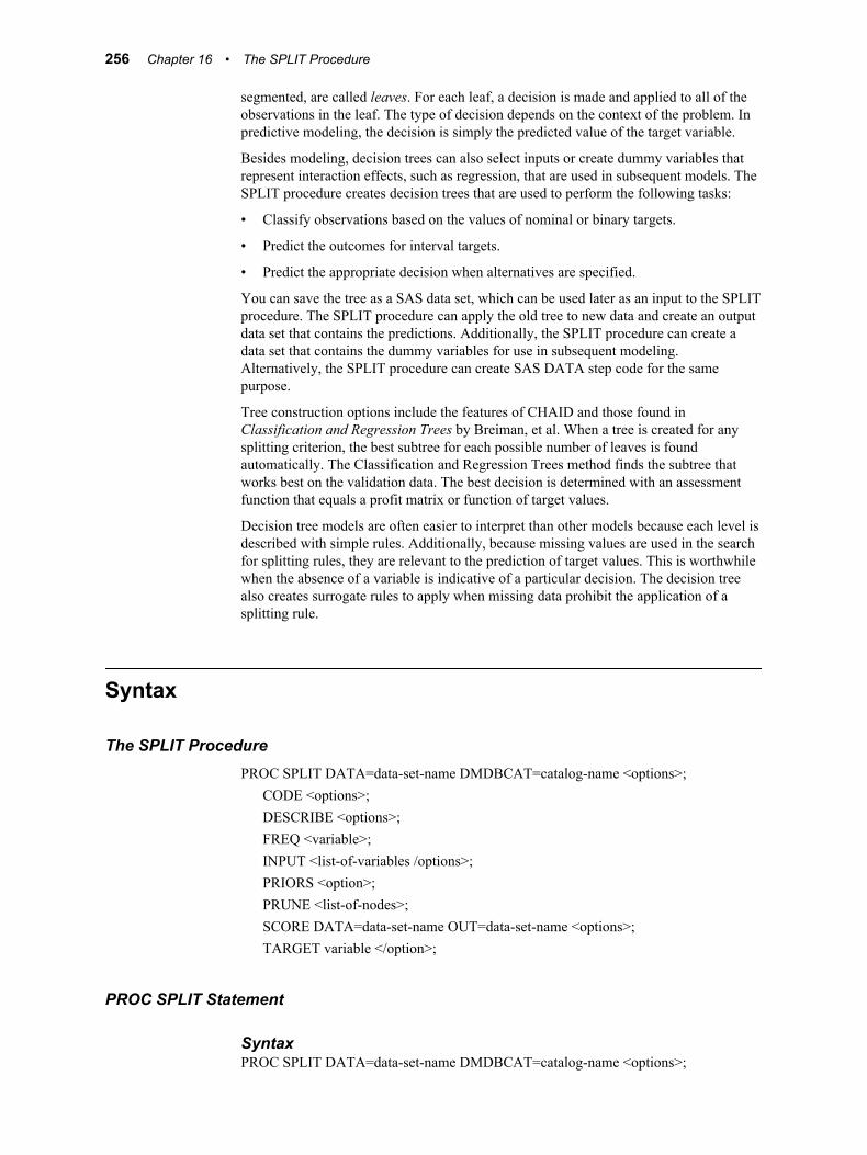
segmented, are called leaves. For each leaf, a decision is made and applied to all of the observations in the leaf. The type of decision depends on the context of the problem. In predictive modeling, the decision is simply the predicted value of the target variable.
Besides modeling, decision trees can also select inputs or create dummy variables that represent interaction effects, such as regression, that are used in subsequent models. The SPLIT procedure creates decision trees that are used to perform the following tasks:
• Classify observations based on the values of nominal or binary targets.
• Predict the outcomes for interval targets.
• Predict the appropriate decision when alternatives are specified.
You can save the tree as a SAS data set, which can be used later as an input to the SPLIT procedure. The SPLIT procedure can apply the old tree to new data and create an output data set that contains the predictions. Additionally, the SPLIT procedure can create a data set that contains the dummy variables for use in subsequent modeling. Alternatively, the SPLIT procedure can create SAS DATA step code for the same purpose.
Tree construction options include the features of CHAID and those found in Classification and Regression Trees by Breiman, et al. When a tree is created for any splitting criterion, the best subtree for each possible number of leaves is found automatically. The Classification and Regression Trees method finds the subtree that works best on the validation data. The best decision is determined with an assessment function that equals a profit matrix or function of target values.
Decision tree models are often easier to interpret than other models because each level is described with simple rules. Additionally, because missing values are used in the search for splitting rules, they are relevant to the prediction of target values. This is worthwhile when the absence of a variable is indicative of a particular decision. The decision tree also creates surrogate rules to apply when missing data prohibit the application of a splitting rule.
Syntax
The SPLIT ProcedurePROC SPLIT DATA=data-set-name DMDBCAT=catalog-name <options>;
CODE <options>;DESCRIBE <options>;FREQ <variable>;INPUT <list-of-variables /options>;PRIORS <option>;PRUNE <list-of-nodes>;SCORE DATA=data-set-name OUT=data-set-name <options>;TARGET variable </option>;
PROC SPLIT Statement
SyntaxPROC SPLIT DATA=data-set-name DMDBCAT=catalog-name <options>;
256 Chapter 16 • The SPLIT Procedure
Required ArgumentsDATA=data-set-name
This argument specifies the input data set that is used to create the decision tree. The variables named in the FREQ, INPUT, and TARGET statements must be in this data set.
DMDBCAT=catalog-nameUse this argument to specify the DMDB that was created for the input data set with the DMDB procedure.
Optional ArgumentsASSESS=IMPURITY | LIFT | PROFIT | STATISTIC
This option determines how to evaluate a decision tree and construct the sequence subtrees. Each method is described below.
• IMPURITY — uses the total leaf impurity, either the Gini index or the average squared error. Impurity for interval target variables is measured with the average squared error, and impurity for categorical targets uses the Gini index. The impurity measure produces a finer separation of leaves than a classification rate and is preferable for lift charts. This method implements class probability trees as described in Breiman et al.
• LIFT — uses the average assessment in the highest ranked observations. For categorical targets, this method first generates the sequence of subtrees with the IMPURITY method and then prunes those results. Similarly, for interval targets, this method generates the subtrees with either the PROFIT or STATISTIC method and then prunes those results. The LIFTDEPTH option specifies the proportion of observations to use.
• PROFIT — uses the average profit or loss from the decision function. This is the default method when a decision function is provided.
• STATISTIC — uses the nominal classification rate for categorical targets or the average squared error for interval targets. This is the default method when no decision function is provided.
COSTSPLITSpecify this option to use the decision matrix in the split search criteria. To use this option, you must specify either CRITERION=ENTROPY or CRITERION=GINI (see below), and the DECDATA= data set must be either PROFIT or LOSS. This argument is unnecessary for ordinal targets because the decision matrix is always incorporated into the split search criterion.
CRITERION=methodThis argument specifies the method that is used to search for and evaluate candidate splitting rules. Possible methods depend on the level of measurement appropriate for the target variable. The methods available for binary or nominal targets are given below.
• CHISQ — uses the Pearson chi-square statistic for target versus segments.
• ENTROPY — uses the reduction in the entropy measure of node impurity.
• ERATIO — uses the reduction in the entropy of split.
• GINI — uses the reduction in the Gini measure of node impurity.
• PROBCHISQ — uses the p-value of the Pearson chi-square statistic for target versus segments. This is the default method.
Syntax 257
The methods available for interval targets are as follows:
• F — uses the F statistic that is associated with node variance.
• PROBF — uses the p-value of the F test associated with node variance. This is the default method for interval variables.
• VARIANCE — uses the reduction in squared error from node means.
EXCLUDEMISSSpecify this option to exclude missing values during the search for splitting criteria.
EXHAUSTIVE=numberThis argument specifies the most number of candidate splits to find in an exhaustive search. If more candidates need to be considered, then a heuristic search is used instead. This option applies to multi-way splits and for binary splits on nominal targets with more than two values. The value of number must be a positive integer and default to 5000.
INDMSPLITUse this option to specify that a decision tree created by the DMSPLIT procedure will be the input to the SPLIT procedure. This decision tree is expected in the DMDBCAT= catalog and is input with the INTREE= option.
INTREE=data-set-nameUse this option to import an output data set from either the SPLIT procedure or the DMSPLIT procedure.
Note: If you specify this option, then you cannot use the DECISION, FREQ, INPUT, PRIORS, or TARGET statements.
LEAFSIZE=numberThis option determines the smallest number of training observations allowed in each node. The value of number must be a positive integer and default to MAX(5, MIN(5000, N/1000)) where N is the total number of observations.
LIFTDEPTH=numberThis option specifies the proportion of observations to use with the LIFT assessment measure. The value of number must be between 0 and 1.
MAXBRANCH=numberThis argument restricts the number of subsets that a splitting rule can produce to number or fewer. For example, if you specify MAXBRANCH=2, then this defines a tree with only binary splits. The value of number must be an integer between 2 and 100, inclusive.
MAXDEPTH=numberThis option specifies the maximum depth of the decision tree. The root node has a depth of 0, all of its children have a depth of 1, and so on. The SPLIT procedure will only split a node if its depth is strictly less than number. The value of number must be a positive integer and default to 6.
NODESAMPLE=numberThis argument specifies the within node sample size that is used to find splits. If the number of training observations in a node is larger than number, then the split search for that node is based on a random sample of size number. The value of number must be a positive integer between 1 and 32767, inclusive, and default to 5000.
NRULES=numberThis argument specifies how many splitting rules are saved with each node, even though tree only uses one rule. The remaining rules are saved for comparison. Based on the criterion that you selected, you can see how well the selected rule and every competitor rule would split the data.
258 Chapter 16 • The SPLIT Procedure
NSURRS=numberThis option specifies the number of surrogate rules that are found in each node that is not a leaf. A surrogate rule is a backup to the main splitting rule. When the main splitting rule depends on an input value that is missing, the first surrogate rule is used. For more information, see “Missing Values” on page 264 . The value of number must be a positive integer and default to 0.
OUTAFDS=data-set-nameThis output data set contains a description of the tree that is suitable as input data for SAS/AF widgets such as ORGCHART and TREERING.
Note: A SAS/AF widget is a visible part of a window, which can be treated as a separate, isolated entity. For example, a SAS/AF widget can be a scroll bar, a text field, or a push button. It is an individual component of the user interface.
OUTLEAF=data-set-nameThis output data set contains summary statistics for each leaf node.
OUTMATRIX=data-set-nameThis output data set contains summary statistics for the entire decision tree. For nominal targets, the summary statistics contain the counts and proportions of observations that are correctly classified. For interval targets, the summary statistics include the average squared prediction error and the R2 value, which equals
1 − average squared prediction errorsum of squares from the average .
OUTSEQ=data-set-nameThis output data set contains summary statistics for each subtree in the sequence of subtrees.
OUTTREE=data-set-nameThis output data sets contains all of the decision tree information. You can reuse this information with the INTREE= argument.
PADJUST=methodThis option names the method used to adjust the p-values when you use the PROBCHISQ or PROBFTEST criterion.
Valid values of method are as follows:
• DEPTH — adjusts for the number of ancestor splits.
• DEVILLE — adjusts independently of the number of branches in a split.
• KASSAFTER — performs a Bonferroni adjustment after the split is chosen.
• KASSBEFORE — performs a Bonferroni adjustment before the split is chosen.
• NOGABRIEL — prevents an adjustment that sometimes overrides the KASS adjustments.
• NONE — does not adjust the p-values.
PVARS=numberThis option specifies the number of inputs to consider uncorrelated when the p-values are adjusted for the number of inputs. The value of number must be a positive integer.
SPLITSIZE=numberThis option specifies the smallest number of training observations in a node for the SPLIT procedure to consider splitting that node. The value of number must be a positive integer between 2 and 32767 and default to twice the value of LEAFSIZE=.
Syntax 259
SUBTREE=ASSESSMENT | LARGEST | numberThis option determines the selection method that is used to determine the best subtree. The ASSESSMENT method uses the best assessment value and is the default method. The LARGEST method uses the largest subtree in the sequence. Also, you can specify SUBTREE=number to select the largest subtree with no more than number leaves.
USEVARONCEIf you specify this option, then when a variable is used to split a node, none of that node's children will be split on the same variable.
VALIDATA=data-set-nameThis option names the data set that contains the validation data.
WORTH=numberThis argument specifies a threshold p-value for the worth of a candidate splitting rule. The measure of worth depends on the selected value of CRITERION=. For a method based on p-values, the threshold is a maximum acceptable p-value. For other criteria, the threshold is the minimal acceptable increase in the measure of worth. The default value of p-value methods is 0.20 and 0 for other methods.
CODE Statement
SyntaxCODE <options>;
The CODE statement generates SAS DATA step code that mimics the computations done by the SCORE statement.
Optional ArgumentsDUMMY
Specify this option to create a dummy variable for each leaf node. The value of the dummy variable is 1 for each observation in the leaf and 0 for all other observations.
FILE=file-nameThis argument specifies the file that contains the code. The value of file-name must be a quoted string that provides the full path to the desired file.
FORMAT=formatUse this argument to specify the format for all numeric values that do not have a format from the input data set.
NOLEAFIDSpecify this option to suppress the creation of the _NODE_ variable that contains the numeric ID of the leaf that contains the observation.
NOPREDSpecify this option to suppress the creation of the predicted variables.
RESIDUALSpecify this option to request code that assumes the existence of a target variable. By default, the code contains no reference to the target variable, because this avoids confusing notes or warnings. With this option, the CODE statement computes values that depend on the target variable.
260 Chapter 16 • The SPLIT Procedure
DESCRIBE Statement
SyntaxDESCRIBE <options>;
The DESCRIBE statement generates a simple description of the rules that define each leaf and some statistics for each leaf. This information is easier to understand than the equivalent information from the CODE statement.
Optional ArgumentsFILE=file-name
This argument specifies the file that contains the code. The value of file-name must be a quoted string that provides the full path to the desired file.
FORMAT=formatUse this argument to specify the format for all numeric values that do not have a format from the input data set.
FREQ Statement
SyntaxFREQ <variable>;
Optional Argumentsvariable
The FREQ statement names a variable that provides frequencies for each observation in the DATA= data set. If the value of this variable is missing or less than 0, then the observation is not used in the analysis. The values of this variable are never truncated.
INPUT Statement
SyntaxINPUT <list-of-variables /options>;
The input statement names input variables with common options. You can specify multiple INPUT statements to identify multiple groups of variables, each of a different level and sorting order.
Optional Argumentslist-of-variables
Use this argument to list the variables with the same level of measurement and desired sorting order.
LEVEL=INTERVAL | NOMINAL | ORDINALThis option identifies the level of measurement of the listed variables. The default value is INTERVAL.
Syntax 261
ORDER=ASCENDING | DESCENDING | ASCFORMATTED | DESFORMATTED | DSORDER
This option identifies the desired sorting order for the listed variables and is allowed only for ordinal variables. The default value is ASCENDING. Ordinal variables can be sorted by their formatted value, unformatted value, or their order of appearance in the training data. The unformatted value can be either numeric or character values. When you sort the unformatted values, the smallest unformatted value for a given formatted value represents that formatted value.
PRIORS Statement
SyntaxPRIORS <option>;
The PRIORS statement specifies the prior probabilities for the values of a nominal or ordinal target variable. For each target variable value, a prior probability is the proportion of that value in the data set that will be applied to the decision tree.
This statement is not allowed if the DECISION statement is used; instead use the PRIORVAR= option in the DECISION statement. The PRIORS statement is not valid for an interval target variable.
Optional ArgumentPROPORTIONAL | PROPEQUAL'value_1'=prob_1 ... 'value_N'=prob_N
There are three mutually exclusive ways to identify the prior probabilities.
• PROPORTIONAL — Specify this argument to indicate that the prior probabilities are the same as in the training data. This is the default method.
• EQUAL — Specify this argument to indicate that all prior probabilities are equal.
• 'value_1'=prob_1 ... 'value_N'=prob_N — With this method, you specify each formatted value of the target variable and a desired prior probability. All nonmissing values of the target variable must be included. The values of prob_1 through prob_N must be real numbers between 0 and 1, and they must all sum to 1.
PRUNE Statement
SyntaxPRUNE <list-of-nodes>;
The PRUNE statement deletes all nodes that descend from the specified nodes. This statement requires the INTREE= or INDMSPLIT argument option in the PROC SPLIT statement.
Optional Argumentlist-of-nodes
The children of the nodes identified here will be deleted. The values identified here must be node numbers assigned by the SPLIT procedure when the decision tree was built.
262 Chapter 16 • The SPLIT Procedure
SCORE Statement
SyntaxSCORE DATA=data-set-name OUT=data-set-name <options>;
Required ArgumentsDATA=data-set-name
This argument specifies the data set that you want to score. This data set must contain all of the input variables in the training data set and, optionally, can contain the target variable.
OUT=data-set-nameThis argument specifies the output data set for the scored data.
Optional ArgumentsDUMMY
Specify this option to include a dummy variable for each node to indicate if an observation is in the node or not.
NODES=list-of-nodesThis argument specifies a list of node identifiers such that only those nodes are used to score the observations. If an observation does not fall into any node in this list, then it does not contribute to the statistics and is not included in the output. If an observation occurs in more than one node, it contributes multiple times to the statistics and is output once for each node in which it occurs.
You must specify this option last, and it must be set off from the other options by a forward slash. The NODES= argument requires either the INTREE= or INDMSPLIT argument in the PROC SPLIT statement.
By default, this is the list of leaf nodes. If you omit this option, then the decisions, utilities, and leaf assignments are output for all observations in the scoring data set.
NOLEAFIDSpecify this option to omit leaf identifiers or node numbers from the output data set.
NOPREDSpecify this option to omit predicted values from the output data set.
OUTFIT=data-set-nameThis data set contains several fit statistics for the scored data set.
ROLE=SCORE | TEST | TRAIN | VALIDThis argument specifies the role of the DATA= data set. This option primarily affects which fit statistics are computed and what their names and labels are. Each role is described below.
• SCORE — does not compute residuals, profit, and fit statistics.
• TEST — is the default role when the SCORE statement's input data set is not the same as the PROC SPLIT statement's input data set.
• TRAIN — is the default role when the SCORE statement's input data set is the same as the PROC SPLIT statement's input data set.
• VALID — is the default role when the SCORE statement's input data set is the same as the PROC SPLIT statement's VALIDATA= data set.
Syntax 263
TARGET Statement
SyntaxTARGET variable </option>;
Required Argumentvariable
This argument specifies the variable that the decision tree attempts to predict.
Optional ArgumentLEVEL=BINARY | INTERVAL | NOMINAL | ORDINAL
This argument specifies the level of measurement for the target variable. The default value is INTERVAL.
Details
Missing ValuesThe SPLIT procedure will handle missing values differently depending on the circumstances. Observations that are missing the target value are ignored when training or validating the decision tree. If EXCLUDEMISS is specified, then observations with missing values are excluded from the search for a splitting rule. After a split is chosen, the rule is amended to assign missing values to the largest branch. If EXCLUDEMISS is not specified, then missing values are considered an acceptable, informative value and used in the search for a split. All observations with missing values are assigned to the same branch.
A branch that contains observations with missing values may or may not contain other observations. The branch chosen is the one that maximizes the split worth. For splits on a categorical variable, this treats the missing values as a separate category. For numerical variables, this treats all missing values as the same unknown nonmissing value.
One advantage of using missing data in the split search is that the worth of a split is computed with the same number of observations for each input variable. Another advantage is that an association of the missing values with the target values can contribute to the predictive ability of the split. One disadvantage is that the missing values could unjustifiably dominate the choice of a split.
Surrogate splitting rules are backup rules to the main splitting rules. Surrogate splitting rules exist to handle observations with missing values. Surrogate rules are checked before an observation is assigned to the branch for missing values. For example, if a main splitting rule uses the value of COUNTY, a surrogate rule might use the value of REGION. If the value of COUNTY is missing but the value of REGION is present, then the surrogate rule is used. When several surrogate rules exist, each is checked in sequence until one is suitable for the observation. If none can be applied, then the main rule applies the observation to the branch for missing values.
Surrogate rules are considered in the order of their agreement with the main splitting rule. The agreement is measured as the proportion of training observations that the surrogate and the main rule apply to the same branch. This measure excludes the
264 Chapter 16 • The SPLIT Procedure
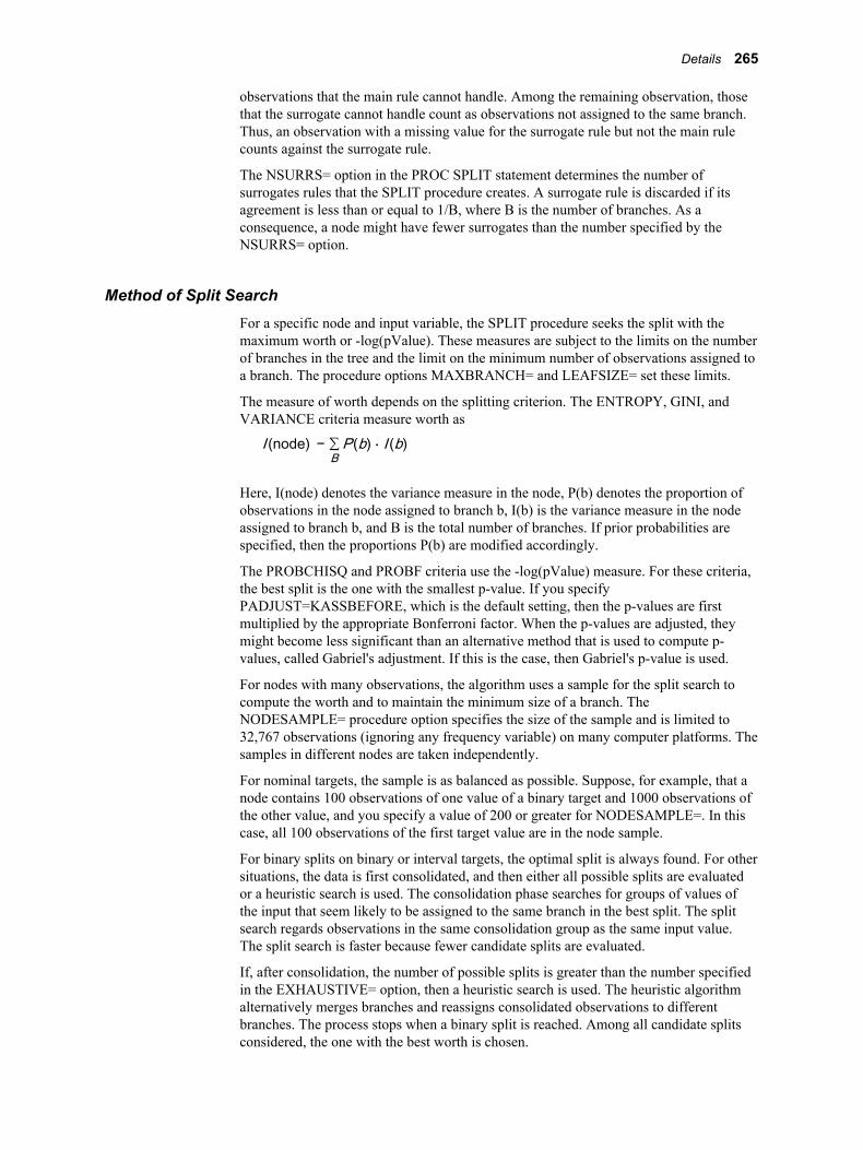
observations that the main rule cannot handle. Among the remaining observation, those that the surrogate cannot handle count as observations not assigned to the same branch. Thus, an observation with a missing value for the surrogate rule but not the main rule counts against the surrogate rule.
The NSURRS= option in the PROC SPLIT statement determines the number of surrogates rules that the SPLIT procedure creates. A surrogate rule is discarded if its agreement is less than or equal to 1/B, where B is the number of branches. As a consequence, a node might have fewer surrogates than the number specified by the NSURRS= option.
Method of Split SearchFor a specific node and input variable, the SPLIT procedure seeks the split with the maximum worth or -log(pValue). These measures are subject to the limits on the number of branches in the tree and the limit on the minimum number of observations assigned to a branch. The procedure options MAXBRANCH= and LEAFSIZE= set these limits.
The measure of worth depends on the splitting criterion. The ENTROPY, GINI, and VARIANCE criteria measure worth as
I (node) − ∑BP(b) ⋅ I (b)
Here, I(node) denotes the variance measure in the node, P(b) denotes the proportion of observations in the node assigned to branch b, I(b) is the variance measure in the node assigned to branch b, and B is the total number of branches. If prior probabilities are specified, then the proportions P(b) are modified accordingly.
The PROBCHISQ and PROBF criteria use the -log(pValue) measure. For these criteria, the best split is the one with the smallest p-value. If you specify PADJUST=KASSBEFORE, which is the default setting, then the p-values are first multiplied by the appropriate Bonferroni factor. When the p-values are adjusted, they might become less significant than an alternative method that is used to compute p-values, called Gabriel's adjustment. If this is the case, then Gabriel's p-value is used.
For nodes with many observations, the algorithm uses a sample for the split search to compute the worth and to maintain the minimum size of a branch. The NODESAMPLE= procedure option specifies the size of the sample and is limited to 32,767 observations (ignoring any frequency variable) on many computer platforms. The samples in different nodes are taken independently.
For nominal targets, the sample is as balanced as possible. Suppose, for example, that a node contains 100 observations of one value of a binary target and 1000 observations of the other value, and you specify a value of 200 or greater for NODESAMPLE=. In this case, all 100 observations of the first target value are in the node sample.
For binary splits on binary or interval targets, the optimal split is always found. For other situations, the data is first consolidated, and then either all possible splits are evaluated or a heuristic search is used. The consolidation phase searches for groups of values of the input that seem likely to be assigned to the same branch in the best split. The split search regards observations in the same consolidation group as the same input value. The split search is faster because fewer candidate splits are evaluated.
If, after consolidation, the number of possible splits is greater than the number specified in the EXHAUSTIVE= option, then a heuristic search is used. The heuristic algorithm alternatively merges branches and reassigns consolidated observations to different branches. The process stops when a binary split is reached. Among all candidate splits considered, the one with the best worth is chosen.
Details 265
The heuristic algorithm initially assigns each consolidated group of observations to a different branch, even if the number of such branches is more than the total number allowed. At each merge step, the two branches that are merged are the two branches that have the least impact on the worth of the partition. After two branches are merged, the algorithm considered reassigning consolidated groups of observations to different branches. Each consolidated group is considered in turn, and the process stops when no group is reassigned.
With the PROBCHISQ and PROBF criteria, the p-value of the selected split on an input is subjected to more adjustments. These adjustments are KASSAFTER, DEPTH, DEVILLE, and INPUTS. If the adjusted p-value is greater than or equal to the WORTH= procedure option, then the split is rejected.
Automatic Pruning and Subtree SelectionAfter a node is split, the newly created nodes are considered for splitting. The SPLIT procedure ends when no node can be split.
The reasons that a node will not split are as follows:
• The node contains too few observations, as specified in the SPLITSIZE= procedure option.
• The number of nodes in the path between the root node and the given node equals the number specified in the MAXDEPTH= procedure option.
• No split exceeds the threshold worth requirement specified in the WORTH= procedure option.
The last reason is the most informative. Either all of the observations in the node contain nearly the same target value, or no input is sufficiently predictive in the node.
A tree adapts itself to the training data and generally does not fit as well when applied to new data. Trees that fit the training data too well often predict too poorly to use on new data.
When SPLITSIZE=, MAXDEPTH=, and WORTH= are set to extreme values, PADJUST=NODE. When you use either the PROCHISQ or PROBF criterion, the tree is apt to grow until all observations in a leaf contain the same target value. Such trees typically overfit the training data and will predict new data poorly.
A primary consideration when you develop a tree for prediction is deciding how large to grow the tree or, equivalently, what nodes to prune from the tree. The CHAID method of tree construction specifies a significance level of a chi-square test to stop tree growth. The authors of C4.5 and Classification and Regression Trees argue that the right thresholds to stop tree construction are not knowable in advance. Thus, they recommend that you grow your tree too large and prune nodes from the decision tree.
The SPLIT procedure allows you both to determine the size of the tree and to prune excessive nodes from a tree. The WORTH= option affects the significance level used in CHAID. After tree construction stops, the SPLIT procedure creates a sequence of subtrees of the original tree, one subtree for each possible number of leaves. For example, the subtree that is chosen with three leaves has the best assessment value of all candidate subtrees with three leaves.
After the sequence of subtrees is established, the SPLIT procedure uses one of three methods to select which subtree to use for prediction. The SUBTREE= procedure option specifies this method.
266 Chapter 16 • The SPLIT Procedure
• The ASSESSMENT method uses the best assessment value and is the default method. This method is based on the validation data when available, which differs from the construction of the subtree sequence that only uses the training data.
• The LARGEST method uses the largest subtree in the sequence, after pruning, that does not increase the assessment based on the training data. For a nominal target, the largest subtree in the sequence might be much smaller than the original, unpruned tree. This happens when a splitting rule has a good split worth, but does not increase the number of observations correctly classified.
• Also, you can specify SUBTREE=number to select the largest subtree with no more than number leaves.
CHAID
DescriptionIn the CHAID method, the input variables are either nominal or ordinal. Many software applications accept interval inputs and automatically group the values into ranges before growing the tree.
The splitting criteria are based on p-values from the F distribution for interval targets and the chi-square distribution for nominal targets. The p-values are adjusted to accommodate multiple testing.
A missing value might be treated as a separate value. For nominal inputs, a missing value constitutes a new category. For ordinal inputs, a missing value is free of any order restrictions.
The split search proceeds stepwise. Initially, a branch is allocated for each value of the input. Branches are alternately merged and split again as seems warranted by the p-values. The original CHAID algorithm by Kass stops when no merge or re-split creates an adequate p-value. At this point, the final split is adopted. A common alternative, sometimes called the exhaustive method, continues merging to a binary split, and then adopts the split with the most favorable p-value among all splits that the algorithm considered.
After a split is adopted for an input, its p-value is adjusted, and the input with the best adjusted p-value is selected as the splitting variable. If the adjusted p-value is smaller than a threshold, specified by the user, then the node is split. Tree construction ends when all the adjusted p-values of the splitting variable in the unsplit nodes are above the user-specified threshold.
Relation to the SPLIT ProcedureThe CHAID algorithm differs from the SPLIT procedure in a number of ways. First, the SPLIT procedure seeks the split that minimizes the adjusted p-value, while the original CHAID algorithm does not. The CHAID exhaustive method is similar to the SPLIT procedure's heuristic method, except that the exhaustive method “re-splits” and the heuristic method “reassigns.” Also, CHAID software discretizes interval inputs, while the SPLIT procedure sometimes consolidates observations into groups. The SPLIT procedure searches on a within-node sample, unlike the CHAID algorithm.
Using the SPLIT Procedure to Approximate CHAIDIn order to approximate the CHAID algorithm with the SPLIT procedure, you can specify certain options. These options are detailed below.
• For nominal targets, specify the options below.
Details 267
• CRITERION=PROBCHISQ
• SUBTREE=LARGEST (to avoid automatic pruning)
• For interval targets, specify the options below.
• CRITERION=PROBF
• SUBTREE=LARGEST (to avoid automatic pruning)
• For any type of target, specify the options below.
• EXHAUSTIVE=0 (forces a heuristic search)
• MAXBRANCH=maximum number of categorical values in an input
• NODESAMPLE=size of the data set (up to 32,000)
• NSURRS=0
• PADJUST=KASSAFTER
• WORTH=0.05 (or another appropriate significance level)
Classification and Regression Trees
DescriptionThe book Classification and Regression Trees (written by Breiman, Friedman, Olshen, and Stone) describes the BFOS methodology of tree creation. In such a tree, the inputs are either nominal or interval and ordinal inputs are treated as interval inputs. The available splitting criteria vary by target variables. For interval targets, you can use reduction in variance and reduction in least absolute deviation. For nominal targets, you can use the reduction in Gini impurity or the twoing method. Ordinal targets allow for the use of ordered twoing. For binary targets, Gini, twoing, and ordered twoing all create the same splits. Breiman, et al. discuss twoing and ordered twoing infrequently throughout their book.
The BFOS method does an exhaustive search for the best binary split. Linear combination splits are also available. In a linear combination split, an observation is assigned to the “left” branch when a linear combination of interval inputs is less than some constant. The coefficients and the constant define the split. The BFOS method excludes missing values during a split search. The BFOS method that is used to find linear combination splits is heuristic and might not find the best linear combination.
The BFOS method omits observations with missing values when a split is created. Surrogate splits are also created and used to assign the observations with missing values. If missing values prevent the use of primary and surrogate splitting rules, then the observation is assigned to the largest branch, based on the within-node training sample.
When a node has many training observations, a sample is taken and used for the split search. The samples in different nodes are independent.
For nominal targets, prior probabilities and misclassification costs are recognized. Additionally, class probability trees are an alternative to classification trees. Trees are grown to produce distinct distributions of class probabilities in the leaves. Trees are evaluated in terms of an overall Gini index. Neither misclassification costs nor rates are used.
The BFOS method intentionally grows the tree to overfit the data. A sequence of subtrees is formed with the cost-complexity measure. The subtree with the best fit to validation data is selected. Cross-validation is available when validation data is not.
268 Chapter 16 • The SPLIT Procedure
Using the SPLIT Procedure to Approximate the BFOS MethodTypically, trees grown with the SPLIT procedure will be similar to those grown with the BFOS method. However, the SPLIT procedure does not have the linear combination, twoing, or ordered twoing splitting criteria. Additionally, the SPLIT procedure implements a loss matrix into the split search differently than the BFOS method. Therefore, splits in the presence of misclassification costs might differ. Finally, the SPLIT procedure handles ordinal target variables differently than the BFOS method.
The BFOS method recommends that you use validation data unless the data set contains too few observations. The SPLIT procedure is intended for large data sets, so you can divide the input data into a training data set and a validation data set. In order to approximate the BFOS method with the SPLIT procedure, you must specify certain options, which are detailed below.
• For nominal targets, specify the option below.
• CRITERION=GINI
• For interval targets, specify the option below
• CRITERION=VARIANCE
• For any type of target, specify the options below.
• ASSESS=STATISTIC
• EXCLUDEMISS
• EXHAUSTIVE=50000 (This must be large enough to enumerate all possible splits.)
• MAXBRANCH=2
• NODESAMPLE=1000 (Or another value as recommended by BFOS)
• NSURRS=5 (This is not exact)
• SUBTREE=ASSESSMENT or ASSESS=IMPURITY (For class probability trees)
• VALIDATA=validation-data-set
C4.5 and C5.0
DescriptionJ. Ross Quinlan, in the book C4.5: Programs for Machine Learning, establishes another means of decision tree creation. The C4.5 method uses a nominal target variable with nominal and interval input variables. The recommended splitting criterion is Gain Ration, defined as the reduction in entropy divided by the entropy of a split. The entropy of a split is defined as the entropy function applied to the set {P(b) | b= 1...B}. Here, P(b) is the proportion of training observations assigned to branch b, and B is the total number of branches.
For interval inputs, the C4.5 method finds the best binary split. For nominal inputs, a branch is created for every value, and then, optionally, the branches are merged until the splitting measure does not improve. Merging is performed stepwise, and each step will merge the two branches that most improve the splitting measure.
When a split is created, observations with missing values are discarded when the reduction in entropy is computed. The entropy of a split is computed as if the split makes an additional branch exclusively for the missing values.
Details 269
When a splitting rule is applied to an observation with missing values, that observation is replaced by B observations, one for each branch. Each new observation is assigned a weight equal to the proportion of observations in its assigned branch. The posterior probabilities of the original observation equal the weighted sum of the probabilities for the split observations.
The tree is grown to overfit the training data. In each node, an upper confidence limit of the number of misclassified observations is estimated with a binomial distribution around the observed number of misclassifications. The C4.5 method seeks a subtree that minimizes the sum of the upper confidences in each leaf.
The C4.5 method can convert a tree into a rule set, which is a set of rules that assigns most observations to the same class that the tree does. Generally, the rule set contains fewer rules than needed to describe all root-leaf paths and is consequently more intelligible than the decision tree.
The C4.5 method can create fuzzy splits on interval input variables. First, the tree is constructed without fuzzy splits. If an interval input variable has a value near the splitting value, then the observation is effectively replaced by two observations. Each of these new observations are weighted by their proximity to the splitting value. The posterior probabilities of the original observation equal the weighted sum of probabilities for the two new observations.
The Web site http://www.rulequest.com contains some information about C5.0, which is an updated version of C4.5. The updates include the branch merging option for nominal splits as default, user-specified misclassification costs, and the implementation of tree boosting and cross-validation.
Using the SPLIT Procedure to Approximate the C4.5 MethodThe decision tree created by the SPLIT procedure will vary from the tree created with the C4.5 method for several reasons. First, the two methods implement different algorithms to create rule sets from the decision tree. Next, the C4.5 method creates binary splits on interval inputs and multiway splits on nominal inputs, which favors nominal inputs. The SPLIT procedure treats interval and nominal inputs identically when it creates splits. Also, the C4.5 method uses a pruning method that is designed to avoid the use of validation data sets. The SPLIT procedure expects validation data and does not offer the pessimistic pruning algorithm of the C4.5 method.
In order to approximate the C4.5 method with the SPLIT procedure, you must specify certain options, which are detailed below.
• For any type of target, specify the options below.
• CRITERION=ERATIO
• EXHAUSTIVE=0 (This forces a heuristic search.)
• MAXBRANCH=maximum number of nominal values in an input (The maximum value is 100.)
• NODESAMPLE=size of the data set (Up to 32,000)
• NSURRS=0
• SUBTREE=ASSESSMENT
• VALIDATA=validation-data-set
270 Chapter 16 • The SPLIT Procedure
Examples
Example 1: Preprocessing the Data and Basic UsageThis example demonstrates how to create a decision tree with a categorical target variable. The ENTROPY splitting criterion is used to search for and evaluate the candidate splitting rules.
This example uses the data set SAMPSIO.DMDRING, which contains categorical targets with three levels, C=0, C=1, and C=2. There are two interval input variables, X and Y, and 180 observations in the training data set. The data set is scored with the scoring formula from the trained model.
Note that the DMDB procedure reassigns the target values based on the order in which they appear in the data set. The reassignments can be confusing because the target levels get renamed to C=1, C=2, and C=3. The original target value C=0 is reassigned to C=3, the original target value C=1 is reassigned to C=2, and the original target value C=2 is reassigned to C=1.
The first step is to plot the data so that you can see the data set you will work with.
/* Give a title, specify options, and plot the data set */title ’SPLIT Example: RINGS Data’;title2 ’Plot of the Rings Training Data’;goptions gunit=pct ftext=swiss ftitle=swissb htitle=4 htext=3;proc gplot data=sampsio.dmdring; plot y*x=c /haxis=axis1 vaxis=axis2; symbol c=black i=none v=dot; symbol2 c=red i=none v=square; symbol3 c=green i=none v=triangle; axis1 c=black width=2.5 order=(0 to 30 by 5); axis2 c=black width=2.5 minor=none order=(0 to 20 by 2);run;
Next, you want to invoke the SPLIT procedure. You need to specify the input data set, the DMDB catalog, and some other options. Namely, you will set the splitting criterion to ENTROPY, the minimum number of observations in each new node, and the maximum number of branches at each level.
/* Run the SPLIT Procedure */proc split data=sampsio.dmdring dmdbcat=sampsio.dmdring criterion=entropy splitsize=2 maxbranch=3 outtree=Tree; input x y; target c / level=nominal; score out=Out outfit=Fit;run;
The data set Fit contains several fit statistics for the training data. You can use the FREQ procedure to print a misclassification table from the Out data set.
/* Print the Misclassification Table */proc freq data=out;
Examples 271
tables f_c*i_c; title3 ’Misclassification Table’;run;
This misclassification table indicates that every observation was correctly classified. Alternatively, you could plot these results with the GPLOT procedure
/* Plot the Classification Results */proc gplot data=out;plot y*x=i_c / haxis=axis1 vaxis=axis2; symbol c=black i=none v=dot; symbol2 c=red i=none v=square; symbol3 c=green i=none v=triangle; axis1 c=black width=2.5 order=(0 to 30 by 5); axis2 c=black width=2.5 minor=none order=(0 to 20 by 2); title3 ’Classification Results’;run;
Example 2: Score the Decision TreeNote: This example assumes that you have completed “Example 1: Preprocessing the
Data and Basic Usage” on page 271 .
The INTREE option allows you to import a previously created decision tree. This example will use the decision tree created in the first example. This enables you to use the SCORE statement to score a data set.
/* Score the Data */proc split intree=Tree; score data=sampsio.dmsring nodmdb role=score out=gridOut;run;
This code scores the data set SAMPSIO.DMSRING with the decision trained in Example 1. The data set gridOut provides an idea of how well the decision tree predicted the scoring data.
Finally, you can use the GCONTOUR procedure to create a contour plot of the posterior probabilities and the GPLOT procedure to plot the leaf nodes.
/* Contour Plot of the Probabilities */proc gcontour data=gridout; plot y*x=p_c1 / pattern ctext=black coutline=gray; plot y*x=p_c2 / pattern ctext=black coutline=gray; plot y*x=p_c3 / pattern ctext=black coutline=gray; title2 'Posterior Probabilities'; pattern v=msolid; legend frame; title3 'Posterior Probabilities';run;/* Scatter Plot of the Leaf Nodes */proc gplot data=gridout; plot y*x=_node_;; symbol c=blue i=none v=dot; symbol2 c=red i=none v=square; symbol3 c=green i=none v=triangle; symbol4 c=black i=none v=star; symbol5 c=orange i=none v=plus; symbol6 c=brown i=none v=circle;
272 Chapter 16 • The SPLIT Procedure
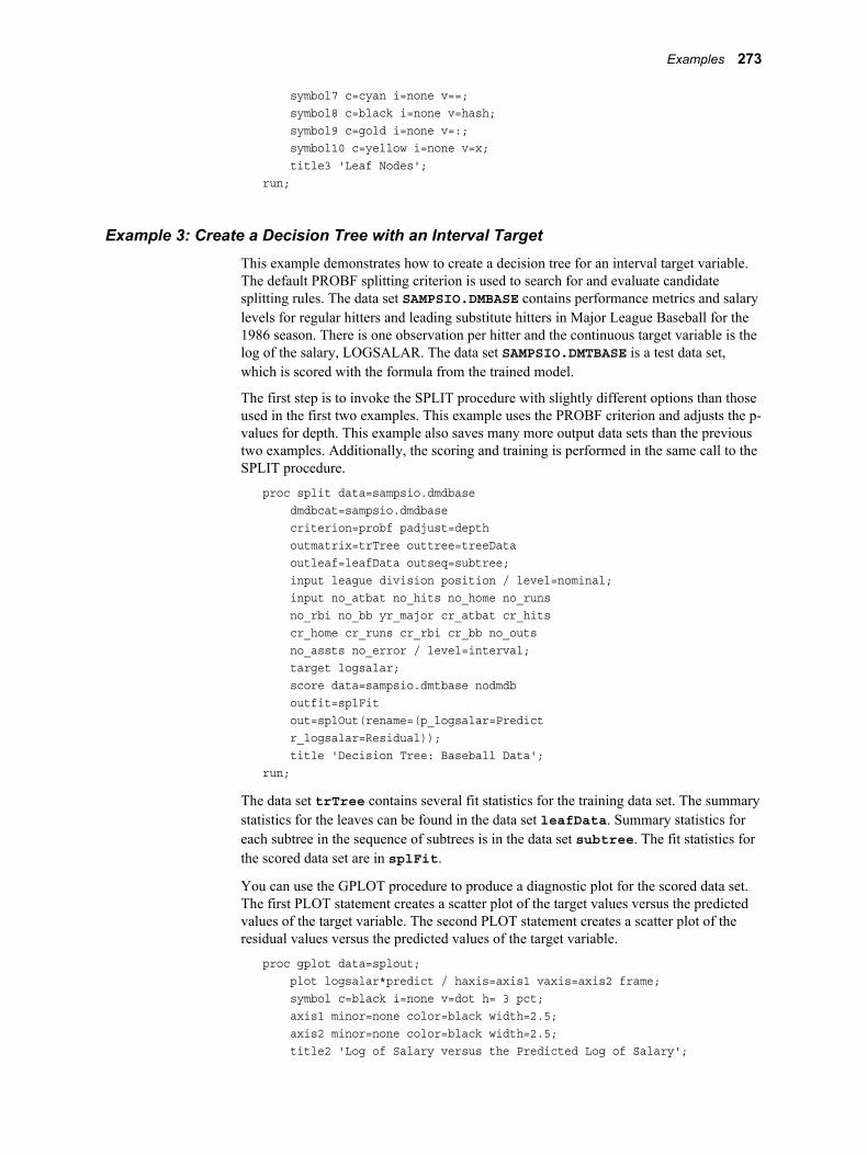
symbol7 c=cyan i=none v==; symbol8 c=black i=none v=hash; symbol9 c=gold i=none v=:; symbol10 c=yellow i=none v=x; title3 'Leaf Nodes';run;
Example 3: Create a Decision Tree with an Interval TargetThis example demonstrates how to create a decision tree for an interval target variable. The default PROBF splitting criterion is used to search for and evaluate candidate splitting rules. The data set SAMPSIO.DMBASE contains performance metrics and salary levels for regular hitters and leading substitute hitters in Major League Baseball for the 1986 season. There is one observation per hitter and the continuous target variable is the log of the salary, LOGSALAR. The data set SAMPSIO.DMTBASE is a test data set, which is scored with the formula from the trained model.
The first step is to invoke the SPLIT procedure with slightly different options than those used in the first two examples. This example uses the PROBF criterion and adjusts the p-values for depth. This example also saves many more output data sets than the previous two examples. Additionally, the scoring and training is performed in the same call to the SPLIT procedure.
proc split data=sampsio.dmdbase dmdbcat=sampsio.dmdbase criterion=probf padjust=depth outmatrix=trTree outtree=treeData outleaf=leafData outseq=subtree; input league division position / level=nominal; input no_atbat no_hits no_home no_runs no_rbi no_bb yr_major cr_atbat cr_hits cr_home cr_runs cr_rbi cr_bb no_outs no_assts no_error / level=interval; target logsalar; score data=sampsio.dmtbase nodmdb outfit=splFit out=splOut(rename=(p_logsalar=Predict r_logsalar=Residual)); title 'Decision Tree: Baseball Data';run;
The data set trTree contains several fit statistics for the training data set. The summary statistics for the leaves can be found in the data set leafData. Summary statistics for each subtree in the sequence of subtrees is in the data set subtree. The fit statistics for the scored data set are in splFit.
You can use the GPLOT procedure to produce a diagnostic plot for the scored data set. The first PLOT statement creates a scatter plot of the target values versus the predicted values of the target variable. The second PLOT statement creates a scatter plot of the residual values versus the predicted values of the target variable.
proc gplot data=splout; plot logsalar*predict / haxis=axis1 vaxis=axis2 frame; symbol c=black i=none v=dot h= 3 pct; axis1 minor=none color=black width=2.5; axis2 minor=none color=black width=2.5; title2 'Log of Salary versus the Predicted Log of Salary';
Examples 273
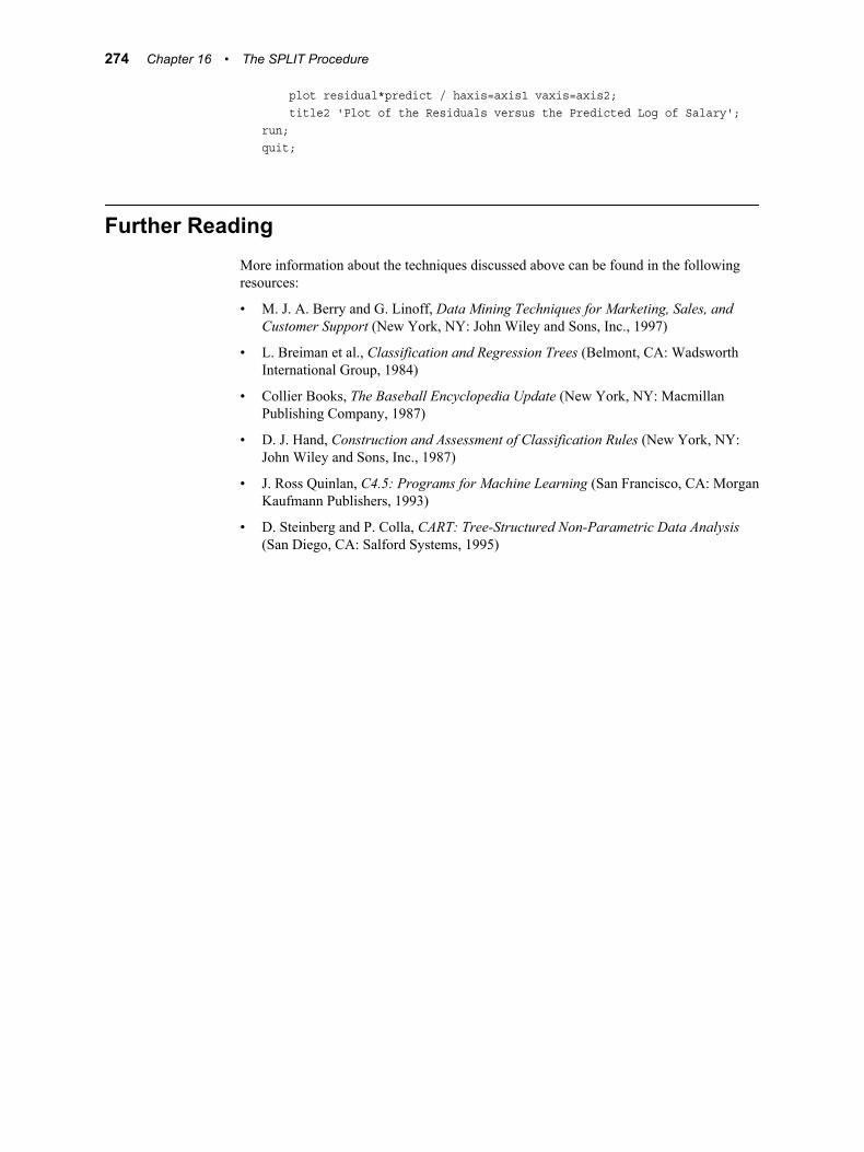
plot residual*predict / haxis=axis1 vaxis=axis2; title2 'Plot of the Residuals versus the Predicted Log of Salary';run;quit;
Further ReadingMore information about the techniques discussed above can be found in the following resources:
• M. J. A. Berry and G. Linoff, Data Mining Techniques for Marketing, Sales, and Customer Support (New York, NY: John Wiley and Sons, Inc., 1997)
• L. Breiman et al., Classification and Regression Trees (Belmont, CA: Wadsworth International Group, 1984)
• Collier Books, The Baseball Encyclopedia Update (New York, NY: Macmillan Publishing Company, 1987)
• D. J. Hand, Construction and Assessment of Classification Rules (New York, NY: John Wiley and Sons, Inc., 1987)
• J. Ross Quinlan, C4.5: Programs for Machine Learning (San Francisco, CA: Morgan Kaufmann Publishers, 1993)
• D. Steinberg and P. Colla, CART: Tree-Structured Non-Parametric Data Analysis (San Diego, CA: Salford Systems, 1995)
274 Chapter 16 • The SPLIT Procedure
Chapter 17
The SVM Procedure
Overview . . . . . . . . . . . . . . . . . . . . . . . . . . . . . . . . . . . . . . . . . . . . . . . . . . . . . . . . . . . 275The SVM Procedure . . . . . . . . . . . . . . . . . . . . . . . . . . . . . . . . . . . . . . . . . . . . . . . . 275
Syntax . . . . . . . . . . . . . . . . . . . . . . . . . . . . . . . . . . . . . . . . . . . . . . . . . . . . . . . . . . . . . . 276The SVM Procedure . . . . . . . . . . . . . . . . . . . . . . . . . . . . . . . . . . . . . . . . . . . . . . . . 276PROC SVM Statement . . . . . . . . . . . . . . . . . . . . . . . . . . . . . . . . . . . . . . . . . . . . . . 276C Statement . . . . . . . . . . . . . . . . . . . . . . . . . . . . . . . . . . . . . . . . . . . . . . . . . . . . . . . 280TARGET Statement . . . . . . . . . . . . . . . . . . . . . . . . . . . . . . . . . . . . . . . . . . . . . . . . 280VAR Statement . . . . . . . . . . . . . . . . . . . . . . . . . . . . . . . . . . . . . . . . . . . . . . . . . . . . 280
Details . . . . . . . . . . . . . . . . . . . . . . . . . . . . . . . . . . . . . . . . . . . . . . . . . . . . . . . . . . . . . . 281The Binary Classification Problem . . . . . . . . . . . . . . . . . . . . . . . . . . . . . . . . . . . . . 281Separable Problem for a Linear Kernel . . . . . . . . . . . . . . . . . . . . . . . . . . . . . . . . . 281Inseparable Problem for a Linear Kernel . . . . . . . . . . . . . . . . . . . . . . . . . . . . . . . . 281Dual Estimation Problem . . . . . . . . . . . . . . . . . . . . . . . . . . . . . . . . . . . . . . . . . . . . 282
Examples . . . . . . . . . . . . . . . . . . . . . . . . . . . . . . . . . . . . . . . . . . . . . . . . . . . . . . . . . . . 282Example 1: Preprocessing the Data and Basic Usage . . . . . . . . . . . . . . . . . . . . . . 282
Further Reading . . . . . . . . . . . . . . . . . . . . . . . . . . . . . . . . . . . . . . . . . . . . . . . . . . . . . 283
Overview
The SVM ProcedureSupport vector machines (SVMs) are used to classify multidimensional data sets that contain a binary target variable. An SVM attempts to establish a hyperplane that maximally separates the observations that contain one target value from those that contain the other target value. If such a hyperplane exists, then it is called the maximum-margin hyperplane, and any suitable hyperplane is called a linear classifier. The margin is the distance between a linear classifier and a data point. A margin classifier is the nearest data point to the linear classifier on that side of the hyperplane. Thus, an SVM creates the maximum-margin hyperplane by maximizing the distance from the linear classifier to both margin classifiers.
275
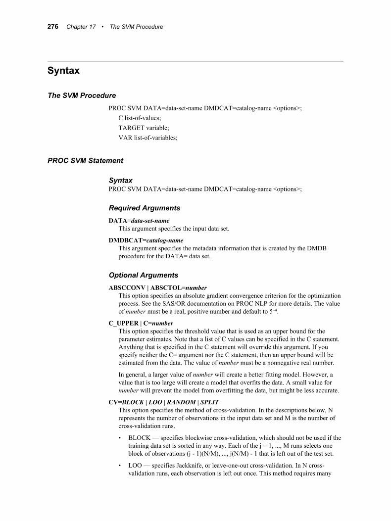
Syntax
The SVM ProcedurePROC SVM DATA=data-set-name DMDCAT=catalog-name <options>;
C list-of-values;TARGET variable;VAR list-of-variables;
PROC SVM Statement
SyntaxPROC SVM DATA=data-set-name DMDCAT=catalog-name <options>;
Required ArgumentsDATA=data-set-name
This argument specifies the input data set.
DMDBCAT=catalog-nameThis argument specifies the metadata information that is created by the DMDB procedure for the DATA= data set.
Optional ArgumentsABSCCONV | ABSCTOL=number
This option specifies an absolute gradient convergence criterion for the optimization process. See the SAS/OR documentation on PROC NLP for more details. The value of number must be a real, positive number and default to 5–4.
C_UPPER | C=numberThis option specifies the threshold value that is used as an upper bound for the parameter estimates. Note that a list of C values can be specified in the C statement. Anything that is specified in the C statement will override this argument. If you specify neither the C= argument nor the C statement, then an upper bound will be estimated from the data. The value of number must be a nonnegative real number.
In general, a larger value of number will create a better fitting model. However, a value that is too large will create a model that overfits the data. A small value for number will prevent the model from overfitting the data, but might be less accurate.
CV=BLOCK | LOO | RANDOM | SPLITThis option specifies the method of cross-validation. In the descriptions below, N represents the number of observations in the input data set and M is the number of cross-validation runs.
• BLOCK — specifies blockwise cross-validation, which should not be used if the training data set is sorted in any way. Each of the j = 1, ..., M runs selects one block of observations (j - 1)(N/M), ..., j(N/M) - 1 that is left out of the test set.
• LOO — specifies Jackknife, or leave-one-out cross-validation. In N cross-validation runs, each observation is left out once. This method requires many
276 Chapter 17 • The SVM Procedure
training runs, but can be fast when the estimation method makes good use of optimal initial values.
• RANDOM — specifies random cross-validation. This method randomly selects N/M observations that are left out of the cross-validation data set.
• SPLIT — specifies split cross-validation. Each of the j = 1, ..., M runs removes the observations j, j + M, ..., N/M from the cross-validation data set.
GCONV | GTOL=numberThis option specifies a relative gradient convergence criterion for the optimization process. The value of number must be a real, positive number and default to 10–8.
MAXFUNC=numberThis option specifies an upper bound for the number of function calls that are allowed in each optimization. Normally, the default number of function class is sufficient to reach convergence. Use larger values if the iteration history indicates that the optimization process was close to a promising solution, but needed a few more function calls. Use smaller values when a faster, but suboptimal, solution is sufficient. The value of number must be a positive integer and default to 500.
MAXITER=numberThis option specifies an upper bound for the number of iterations in each optimization. Normally, the default number of iterations is sufficient to reach convergence. Use larger values if the iteration history indicates that the optimization process was close to a promising solution, but needed a few more iterations. Use smaller values when a faster, but suboptimal, solution is sufficient. The value of number must be a positive integer and default to 200.
Note: If the optimization subroutine cannot complete the iteration, a message is printed in the form: ERROR: xxx Optimization cannot be completed. If you want to replace this error with a warning, use the following code: options debug='nlpitermsg=2';.
MEMSIZE=numberThis option specifies the amount of RAM that should be used for the SVM procedure. For large data sets, the computations can depend on how much RAM is available for those computations. Because other operations also need memory, you should not specify more than 25% of the available system memory. The value of number must be a nonnegative real number, given in megabytes, and default to 8 megabytes.
METHOD=LSVMThis option specifies the Lagrangian SVM method that is similar to that of Mangasarian and Musicant (2001).
NOPRINTSpecify this option to suppress all printed output in the Output window.
NOSCALESpecify this option to suppress the default scaling and override the XSCALE option.
OUT=data-set-nameThis option creates an output data set that contains the predicted values (posteriors) and residuals for all observations in the DATA= data set.
The variables in this data set are as follows:
• idvarnami — gives the values of all the ID variables.
• _TARGET_ — provides the name of the target value.
• _Y_ — is the observed value of the target variable.
Syntax 277
• _P_ — is the predicted value of the target variable.
• _R_ — is the residual.
• _ALPHA_ — gives certain model parameters.
• _BESTDEC_ — provides the best decision available. This variable is only present when the DECISION statement is used.
• _CONSEQ_ — states the consequences of the decision. This variable is only present when the DECISION statement is used.
• _EVALUE_ — is the expected profit or cost. This variable is only present when the DECISION statement is used.
• decvari — is the expected value for all decision variables.
OUTCLASS=data-set-nameThis option specifies an output data set that contains the mapping between compound variable names and the names of variables and categories that are used in the model. The compound variable names are used to denote dummy variables, which are created for each category of a CLASS variable with more than two categories. Because the compound names of dummy variables are used for variable names in other data sets, you must know to which category each compound name corresponds. This data set contains the compound variable name, the original variable name, and the level name of the variable.
OUTEST=data-set-nameThis output data set contains various statistics about the DATA= data set.
The variables in this data set are as follows:
• idvarnami — gives the values of all the ID variables.
• _TARGET_ — provides the name of the target value.
• _TYPE_ — is the type of the observation.
• _NAME_ — is the name of the observation.
• _MEAN_ — contains different information based on the variable _TYPE_.
• _STDEV_ — contains different information based on the variable _TYPE_.
• _effects_ — names the effects of the input variables.
The following information is written to this data set:
• _TYPE_=_V_MAP_ — provides mapping information for continuous variables with effects.
• _TYPE_=_C_MAP_ — provides mapping information for categorical variables with effects.
• _TYPE_=_MEAN_ — gives the means of the effects.
• _TYPE_=_V_STDEV_ — gives the standard deviation of the effects.
• _TYPE_=_PARMS_ — is used only for linear kernels. The effect variables contain the coefficients (weights) of the linear classifier. Two different estimates of the regression constant (the intercept) are written to the _MEAN_ and _STDEV_ variables.
For a linear kernel, the _TYPE_ = _PARMS_ observation can be used to score a data set. That is, it can be used to compute the predicted values of the linear model.
278 Chapter 17 • The SVM Procedure

OUTFIT=data-set-nameThis output data set contains a number of fit statistics. For SVM classification, this data set contains the classification tables for the training and test data sets.
OUTL=numberThis option is only valid when you specify CV=LOO. In addition to the slightly modified LOO cross-validatiaon, a table is printed that contains the numbers of observations that contribute most to the fit criteria. This information can be used to manually train the model.
PALLSpecify this option to print the maximum amount of information in the Output window.
PINITIALSpecify this option to print simple statistics for effects in the Output window. This is not included in the PALL option because the amount of output can be overwhelming.
POPTHISSpecify this option to print a detailed history of the optimization process in the Output window. This is included in the PALL option.
PPARMSpecify this option to print the parameter vector in the Output window. This is not included in the PALL option because the amount of output can be overwhelming.
PPLANSpecify this option to print the parameter vector w in the Output window. This is not included in the PALL option because the amount of output can be overwhelming.
PPREDSpecify this option to print observation statistics in the Output window. This is not included in the PALL option because the amount of output can be overwhelming.
PSHORTSpecify this option to print a short form of the output in the Output window.
RANDOM=numberThis option specifies the initial seed for the random number generator. The value of number must be a real, positive number and default to the time of day.
RIDGE=numberThis option specifies a positive ridge value for the kernel matrix. The value of number must be a nonnegative real number and the default value varies based on the optimization method.
SINGULAR=numberThis option specifies the tolerance level for the singularity test of the kernel matrix. The value of number must be a real, positive number and default to 10–8.
TESTDATA=data-set-nameThis option specifies a second input data set that contains all of the variables in the DATA= data set.
TESTOUT=data-set-nameThis output data set contains the same information as the OUT= data set, but uses the TESTDATA= data set.
XSCALESpecify this option to scale the predictor variables before they are used in analysis.
Syntax 279
C Statement
SyntaxC list-of-values;
Use the C statement to specify a list of C values. For each positive C value, ordered from smallest to largest, the SVM training is performed. At the end, the model with the best fit is scored. If cross-validation or a test data set is specified, the goodness-of-fit is evaluated on the test data. If neither cross-validation nor a test data set is specified, then the fit is evaluated on the training data. Therefore, the best result will normally correspond to the largest C value. If this value is too large, then the model is probably overfit. Note that anything that you specify in the C statement will override the C= option in the PROC SVM statement.
Required Argumentlist-of-values
The values listed here must be arranged in order from smallest to largest. Values specified here must be nonnegative real numbers. You can use the keywords TO and BY in the list of values.
TARGET Statement
SyntaxTARGET variable;
Required Argumentvariable
Use the TARGET statement to specify the target variable in the input data set.
VAR Statement
SyntaxVAR list-of-variables;
Required Argumentlist-of-variables
Use the VAR statement to specify all of the input variables. You must specify every variable, numeric or categorical, that you want to include in the SVM model.
280 Chapter 17 • The SVM Procedure
Details
The Binary Classification ProblemThe binary classification problem is to find a parametric function for a hyperplane that separates two sets of points in m-dimensional real space, Rm. This hyperplane can be linear or nonlinear, depending on the kernel specification.
Separable Problem for a Linear KernelConsider a data set that has N observations and the predictors xi = xi1, ..., xim. Each of these predictors expresses cluster, also called group, membership. For mathematical convenience, the target values are represented as –1 and +1 rather than as 0 and +1. If the two clusters are linearly separable, then there exists three planes.
• The separating hyperplane H0: y = wTx - b = 0. This is the linear classifier that separates the two groups of observations.
• The right hyperplane H1: y = wTx - b = 1. This plane contains at least one x with the target value +1 that is a margin classifier, which means that it is the closest point to H0.
• The left hyperplane H1: y = wTx - b = –1. This plane contains at least one x with the target value –1 that is a margin classifier, which means that it is the closest point to H0.
The points on either side of the linear classifier are called support vectors. The orientation of the plane H0 is chosen so that the distance between H1 and H2 is maximized. Ideally, there will be no points between H1 and H2.
The distance from one point on H0 to H1 is given by w T x − bw Tw
= 1w Tw
. In order to
maximize the distance between H1 and H2, you need to minimize the value of wTw. This minimization is done over m+1 unknowns w = w1, ..., wm and a scalar b. The minimization is subject to the constraints that no point is between H1 and H2, wTx - b ≥ 1 or y = 1, and wTx - b ≤ –1 for y = –1. The final two constraints can be combined into one inequality: ywTx - b ≥ 1.
Therefore, the primal separable problem contains m + 1 variables to estimate
min( 12 w Tw). The constraint is ywTx - b ≥ 1. Note that the parameter estimates w and b
are defined only by the points on H1 and H2. You can move the other points arbitrarily without altering the optimization result.
Inseparable Problem for a Linear KernelIn practical applications, data is seldom geometrically separable. For inseparable data, the problem considered above will have no feasible solution. Therefore, the optimization problem must allow the existence of points between H1 and H2. These points must also be allowed to reside on the wrong side of H0, but should not be penalized for doing so.
Details 281
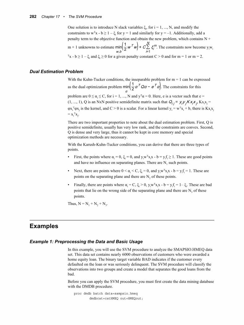
One solution is to introduce N slack variables ξi, for i = 1, ..., N, and modify the constraints to wTx - b ≥ 1 – ξi for y = 1 and similarly for y = –1. Additionally, add a penalty term to the objective function and obtain the new problem, which contains N +
m + 1 unknowns to estimate minw,b
( 12 w Tw) + C∑i=1
Nξim. The constraints now become yiwi
Tx - b ≥ 1 – ξi and ξi ≥ 0 for a given penalty constant C > 0 and for m = 1 or m = 2.
Dual Estimation ProblemWith the Kuhn-Tucker conditions, the inseparable problem for m = 1 can be expressed
as the dual optimization problem minα( 12 α TQα − e Tα). The constraints for this
problem are 0 ≤ αi ≤ C, for i = 1, ..., N and yTα = 0. Here, e is a vector such that e = (1, ..., 1), Q is an NxN positive semidefinite matrix such that Qi j = yiy jK xix j, Kxixj = φxi
Tφxj is the kernel, and C > 0 is a scalar. For a linear kernel yi = wTxi + b, there is Kxixj
= xiTxj.
There are two important properties to note about the dual estimation problem. First, Q is positive semidefinite, usually has very low rank, and the constraints are convex. Second, Q is dense and very large, thus it cannot be kept in core memory and special optimization methods are necessary.
With the Karush-Kuhn-Tucker conditions, you can derive that there are three types of points.
• First, the points where αi = 0, ξi = 0, and yiwTxix - b = yifi ≥ 1. These are good points and have no influence on separating planes. There are N1 such points.
• Next, there are points where 0 < αi < C, ξi = 0, and yiwTxix - b = yifi = 1. These are points on the separating plane and there are N2 of these points.
• Finally, there are points where αi = C, ξi > 0, yiwTxix - b = yifi = 1– ξi. These are bad points that lie on the wrong side of the separating plane and there are N3 of these points.
Thus, N = N1 + N2 + N3.
Examples
Example 1: Preprocessing the Data and Basic UsageIn this example, you will use the SVM procedure to analyze the SMAPSIO.HMEQ data set. This data set contains nearly 6000 observations of customers who were awarded a home equity loan. The binary target variable BAD indicates if the customer every defaulted on the loan or was seriously delinquent. The SVM procedure will classify the observations into two groups and create a model that separates the good loans from the bad.
Before you can apply the SVM procedure, you must first create the data mining database with the DMDB procedure.
proc dmdb batch data=sampsio.hmeq dmdbcat=catHMEQ out=HMEQout;
282 Chapter 17 • The SVM Procedure
var CLAGE CLNO DEBTINC DELINQ DEROG LOAN MORTDUE NINQ VALUE YOJ; class BAD; target BAD;run;
Now that you have created the DMDB, you are ready to run the SVM procedure.
proc svm data=HMEQout dmdbcat=catHMEQ out=sOut1 outest=sEst1 method=LSVM xscale; var CLAGE CLNO DEBTINC DELINQ DEROG LOAN MORTDUE NINQ VALUE YOJ; target BAD; C 0.1 to 0.2 by 0.01;run;
This call to PROC SVM uses all of the available variables as inputs, scales the input values, and searches for the best C between 0.1 and 0.2. In the output window, the classification table indicates that 924 bad loans were predicted to be good and 73 good loans were predicted to be bad. This means that the SVM for this data set was correct 83.27% of the time.
Further ReadingFor more information about support vector machines, see the following resources:
• N. Cristianni and J. Shawe-Taylor, Support Vector Machines and Other Kernel-Based Learning Methods, (Cambridge, England: Cambridge University Press, 2000).
• G. Fung and O.L. Mangasarian, “Proximal Support Vector Machines,” Technical Report 01–02, Data Mining Institute, (Madison, WI: University of Wisconsin, 2000).
• O.L. Mangasarian and D.R. Musicant, “Lagrangian Support Vector Machines,” Technical Report 00–06, Data Mining Institute, (Madison, WI: University of Wisconsin, 2001). Also in Journal of Machine Learning Research, 1 , March 2001, 161–177.
Further Reading 283

284 Chapter 17 • The SVM Procedure
Chapter 18
The TAXONOMY Procedure
Overview . . . . . . . . . . . . . . . . . . . . . . . . . . . . . . . . . . . . . . . . . . . . . . . . . . . . . . . . . . . 285The TAXONOMY Procedure . . . . . . . . . . . . . . . . . . . . . . . . . . . . . . . . . . . . . . . . . 285
Syntax . . . . . . . . . . . . . . . . . . . . . . . . . . . . . . . . . . . . . . . . . . . . . . . . . . . . . . . . . . . . . . 286The TAXONOMY Procedure . . . . . . . . . . . . . . . . . . . . . . . . . . . . . . . . . . . . . . . . . 286PROC TAXONOMY Statement . . . . . . . . . . . . . . . . . . . . . . . . . . . . . . . . . . . . . . . 286CUSTOMER Statement . . . . . . . . . . . . . . . . . . . . . . . . . . . . . . . . . . . . . . . . . . . . . 288HIERARCHY Statement . . . . . . . . . . . . . . . . . . . . . . . . . . . . . . . . . . . . . . . . . . . . 288TARGET Statement . . . . . . . . . . . . . . . . . . . . . . . . . . . . . . . . . . . . . . . . . . . . . . . . 289
Examples . . . . . . . . . . . . . . . . . . . . . . . . . . . . . . . . . . . . . . . . . . . . . . . . . . . . . . . . . . . 289Example 1: Preprocessing the Data and Basic Usage . . . . . . . . . . . . . . . . . . . . . . 289Example 2: Using Item Taxonomies . . . . . . . . . . . . . . . . . . . . . . . . . . . . . . . . . . . 291
Overview
The TAXONOMY ProcedureThe TAXONOMY procedure performs association rule mining over transaction data in conjunction with an item taxonomy. This procedure is an extension of the market basket analysis capability that is available in SAS Enterprise Miner. Market basket analysis is useful in retail marketing scenarios that involve tens of thousands of distinct items that are grouped in a hierarchy. An item taxonomy is the hierarchical group of these items. The TAXONOMY procedure uses the taxonomy data and generates rules at multiple levels, which are known as generalized association rules. These rules solve some of the problems, which are described below, that arise in simple market basket analysis.
Market basket analysis that is performed over the transaction or point-of-sale data might miss potentially useful and significant associations. For example, consider a supermarket that sells different types of breads and a wide selection of wines. Furthermore, assume that a large number of customers buy some type of bread with some type of wine. However, market basket analysis performed with the ASSOC procedure might fail to spot a rule that links bread and wine at the transaction level. This procedure computes the support for specific types of breads to specific types of wines, none of which might be large enough to generate a rule. On the other hand, the TAXONOMY procedure combines the item taxonomy with the transaction data and computes the support for any type of bread to any type of wine. The TAXONOMY procedure also computes the specific rules.
285
Additionally, simple association mining is prone to create a large number of obvious and uninteresting rules along with the useful rules. Thus, the solution to the previous problem is not to reduce the support, which would only exacerbate this problem. In practice, this fact is one of the major drawbacks of association mining. If the support is set high, fewer rules are generated, but more of them are obvious and thus useless (such as “Cereal ==> Milk”). Furthermore, if the support is set low, too many rules are generated and the domain experts must evaluate the rules to determine what rules are useful. One solution to this problem is generalized association rule mining.
Generalized association rule mining provides the ability to generate an interestingness measure, called “support lift.” This measure is based on the deviation of a rule's support from its estimated support, which is computed based on the support of the ancestors of the rule's items. Objectively, greater deviation indicates greater surprise, which indicates that a rule is more likely to be interesting. To give a different perspective, an item taxonomy represents a limited form of domain knowledge, which is used by the TAXONOMY procedure, to generate more interesting rules. Generalized associations also enable the use of focused, interactive mining. For example, you might consider only the rules at the top of the item taxonomy, where there are fewer, more understandable rules. Subsequently, you can refine these rules as you move to progressively lower levels of the taxonomy to generate specific, actionable rules.
The TAXONOMY procedure does not limit rules to items that are on the same level of the item taxonomy. Often, the overall frequency of an item determines how far up the taxonomy it is generalized. If no item taxonomy is specified, then the TAXONOMY procedure generates simple association rules.
Syntax
The TAXONOMY ProcedurePROC TAXONOMY DATA=data-set-name <options>;
CUSTOMER | ID variables;HIERARCHY <option>;TARGET variable <[options]>;RUN;
PROC TAXONOMY Statement
SyntaxPROC TAXONOMY DATA=data-set-name <options>;
Required ArgumentDATA=data-set-name
This data set specifies the input data, which is typically from a transactional system. The data set must contain the variables specified in the CUSTOMER and the TARGET statements. The data must be sorted by the variables in the CUSTOMER statement.
286 Chapter 18 • The TAXONOMY Procedure
Optional ArgumentsCONF=number
This option determines the minimum confidence for the rules. The value of number must be a real number between 0 and 100.
ITEMS=numberThis option specifies the number of items in a rule. The value of number must be an integer between 1 and 100. The default value is 2 when either OUT= or OUTRULE= is specified and 1 otherwise.
LIFT=numberThis option determines the minimum lift value necessary to generate a rule. The value of number must be a positive, real number.
MAXBSKTSZ=numberA basket is a group of all the target items grouped by the customer ID. This option specifies a maximum basket size, such that baskets larger than number are rejected from analysis. The value of number must be a positive integer.
MAXRULES=numberThis option determines the maximum number of rules that are generated by the TAXONOMY procedure. The TAXONOMY procedure may generate fewer than number rules. After number rules have been generated, the TAXONOMY procedure exits. The value of number must be a positive integer.
MINBSKTSZ=numberA basket is a group of all the target items grouped by the customer ID. This option specifies a minimum basket size, such that baskets smaller than number are rejected from analysis. The value of number must be a positive integer.
MAXCANDS=numberThis option determines the maximum number of candidate sets to consider. If the number of candidates exceeds this value, the TAXONOMY procedure exits with an error message. In this case, you can usually increase the value of SUPPORT to successfully run the TAXONOMY procedure.
NORMSpecify this option to normalize the values of the target variable and the items in the taxonomy.
NUMRULES=numberThis option determines the exact number of rules to output in the OUTRULE= data set. By default, the TAXONOMY procedure outputs all rules to this data set. This argument has no effect if the number of generated rules is less than number.
OUT=data-set-nameThis output data set contains general information about the rules that were generated. This includes variables that identify the count, support, and individual items.
OUTFREQ=data-set-nameThis output data set contains information about the items' frequencies.
OUTRULE=data-set-nameThis output data set contains detailed information about the rules that were generated. This includes, but is not limited to, variables that identify the left hand side, right hand side, support, and lift.
Note: At least one of the preceding three output data sets must be specified.
Syntax 287
PCTSUP=numberThis option determines the minimum level of support for a rule as a percentage of the number of baskets in the input data set. The value of number must be a real number between 0 and 100.
SORTBY CONF | SUPPORT | LHSSZ | LIFT | RHSSZ | SUP_LIFT | SIZEUse this option to specify how the OUTRULE data set is sorted. By default, this data set is sorted by the support value.
SUPPORT=numberThis option determines the minimum level of support for a rule. The value of number must be an integer and represent the minimum allowable frequency for a rule. SUPPORT= takes precedence over PCTSUP=.
SUP_LIFT=numberThis option determines the minimum “support lift” necessary to generate a rule. The value of number must be a positive, real number.
CUSTOMER Statement
SyntaxCUSTOMER | ID variables;
Required Argumentlist-of-variables
The CUSTOMER statement enables you to specify one or more variables that are used to group the target variable into baskets. If even one of the variables listed here is not present in the data set, then the TAXONOMY procedure ends with an error.
HIERARCHY Statement
SyntaxHIERARCHY <option>;
There are several points to note about the HIERARCHY statement.
• This statement is optional. If it is not specified, then the TAXONOMY procedure will perform simple association analysis on the input data without the hierarchy.
• Each distinct item in the input data set must have a parent in the lowest level of the hierarchy. The levels of the hierarchy must be specified in ascending order, with the lowest level specified first.
• Multiple parents are not supported. If multiple parents are specified for a child at any level, only the last parent is used for analysis.
• Rugged hierarchy is not supported. That is, at any level, if a parent exists for an item, then the item must appear in the level immediately below the parent.
Optional ArgumentDATA=list-of-data-sets
Use this argument to specify a preexisting item taxonomy that is in the form of flattened data sets. The data sets contain the values of the child and parent items at each level of the hierarchy, starting with the lowest level. Each data set must contain
288 Chapter 18 • The TAXONOMY Procedure
at least two variables such that the first variable is the child and the second variable is the parent. See “Example 2: Using Item Taxonomies” on page 291 for an example of how to use this option.
TARGET Statement
SyntaxTARGET variable <(ASC) / NOMISS>;
Required Argumentvariable
The TARGET statement enables you to specify a single nominal variable to use as the target variable. If this variable is not present in the data set, then the TAXONOMY procedure exits with an error.
Optional ArgumentsASCENDING | ASC
Specify this option, enclosed in parentheses, to sort the OUTFREQ data set by the target variable.
NOMISSSpecify this option to ignore any observations with missing values. Otherwise, they are treated as a separate items in the taxonomy.
Examples
Example 1: Preprocessing the Data and Basic UsageBecause the data sets in the SAMPSIO library are fairly large, you will create a small sample data set to understand how the TAXONOMY procedure handles data. This data set contains information about products available at a grocery store and information about three customers' purchases. First, create the items and their categories.
/* Items (Children) and Categories (Parents) */data work.Category;length Item $20 Category $20; Item='Whole Milk'; Category='Milk'; output; Item='2% Fat Milk'; Category='Milk'; output; Item='Skim Milk'; Category='Milk'; output; Item='Feta Cheese'; Category='Cheese'; output; Item='Edam Cheese'; Category='Cheese'; output; Item='Waffles'; Category='Breakfast'; output; Item='Pancakes'; Category='Breakfast'; output; Item='Pizza'; Category='Dinner'; output; Item='Ice Cream'; Category='Dessert'; output; Item='Cake'; Category='Dessert'; output; Item='Milk'; Category='Dairy Products'; output; Item='Cheese'; Category='Dairy Products'; output; Item='Breakfast'; Category='Frozen Foods'; output;
Examples 289
Item='Dinner'; Category='Frozen Foods'; output; Item='Dessert'; Category='Frozen Foods'; output;run;
This data set identifies 15 common grocery store items and assigns them a broad category. In this example the variable Item represents the child and Category is the parent. The next code block assigns departments to each of the categories to create another layer of the item hierarchy.
/* Grocery Store Departments (Parents) */data work.Dept;length Category $20 Department $20; Category='Milk'; Department='Dairy Products'; output; Category='Cheese'; Department='Dairy Products'; output; Category='Breakfast'; Department='Frozen Foods'; output; Category='Dinner'; Department='Frozen Foods'; output; Category='Dessert'; Department='Frozen Foods'; output;run;
Here, each Category represents the child and Department is the parent. These first two data sets will not be used in this example, however. They will be used in “Example 2: Using Item Taxonomies” on page 291 . Finally, you want to create a data set that contains the purchases of three customers.
/* Customer Purchases */data work.Basket;length Customer $ 10 Item $ 20 ;retain Customer;Customer='Brian'; Item='2% Fat Milk'; output; Item='Feta Cheese'; output; Item='Cake'; output; Item='Pizza'; output; Item='Ice Cream'; output; Item='Pancakes'; output;Customer='Ikea'; Item='2% Fat Milk'; output; Item='Edam Cheese'; output; Item='Pizza'; output; Item='Ice Cream'; output;Customer='Juan's; Item='Skim Milk'; output; Item='Edam Cheese'; output; Item='Ice Cream'; output; Item='Cake'; output;run;
The next code block runs the TAXONOMY procedure with slightly more than the minimally required arguments. Additionally, this call uses the ID notation to differentiate between the CUSTOMER statement and the variable Customer.
/* Run the TAXONOMY Procedure */proc taxonomy data=Basket out=out1 outfreq=freq1 outrule=rule1; id customer; target item;run;
290 Chapter 18 • The TAXONOMY Procedure
This uses the Basket data set to determine rules about which items are related based on which items are purchased together. The data set freq1 indicates that there were 8 unique items purchased and the variable Support (%) indicates the percentage of customers that purchased an item. The data sets out1 and rule1 both contain information about different sets of rules that were generated by the TAXONOMY procedure.
Example 2: Using Item TaxonomiesNote: This example assumes that you have completed “Example 1: Preprocessing the
Data and Basic Usage” on page 289 .
Because you did not specify the preexisting item taxonomy, you did not take full advantage of the TAXONOMY procedure. To perform an analysis that considers the category and department that an item belongs to, you must specify the HIERARCHY statement. This statement allows the TAXONOMY procedure to create the item taxonomy.
/* Run the TAXONOMY Procedure */proc taxonomy data=Basket out=out2 outfreq=freq2 outrule=rule2; id customer; target item; hierarchy data=Category Dept;run;
This code creates the rules in out2 and rule2 based on the entire item taxonomy, instead of just the purchases. Therefore, you should notice that these two data sets are considerably larger than their counterparts from Example 1. However, some of these rules are uninformative, such as “Ice Cream ==> Dairy Products”. To compensate for this fact, you can use some of the options in the PROC TAXONOMY statement to clean the output data sets.
/* Run the TAXONOMY Procedure */proc taxonomy data=Basket out=out3 outfreq=freq3 outrule=rule3 lift=1.5 sortby sup_lift; id customer; target item; hierarchy data=Category Dept;run;
This code removes all of the rules that have a lift of 1 and sorts the data set rule3 by the support lift value. Remember that this value is the indicator of how surprising a rule is. If you view the data set rule3, the first two entries indicate the rules “Pancakes ==> Feta Cheese” and “Breakfast ==> Feta Cheese”. While you might expect that pancakes and breakfast are related (observation 35), you might have missed their connection to feta cheese. The high value of Support Lift indicates that these connections were probably not expected.
Examples 291

292 Chapter 18 • The TAXONOMY Procedure
Chapter 19
The TREEBOOST Procedure
Overview . . . . . . . . . . . . . . . . . . . . . . . . . . . . . . . . . . . . . . . . . . . . . . . . . . . . . . . . . . . 293The TREEBOOST Procedure . . . . . . . . . . . . . . . . . . . . . . . . . . . . . . . . . . . . . . . . . 293Terminology . . . . . . . . . . . . . . . . . . . . . . . . . . . . . . . . . . . . . . . . . . . . . . . . . . . . . . 294
Syntax . . . . . . . . . . . . . . . . . . . . . . . . . . . . . . . . . . . . . . . . . . . . . . . . . . . . . . . . . . . . . . 295The TREEBOOST Procedure . . . . . . . . . . . . . . . . . . . . . . . . . . . . . . . . . . . . . . . . . 295PROC TREEBOOST Procedure . . . . . . . . . . . . . . . . . . . . . . . . . . . . . . . . . . . . . . . 296ASSESS Statement . . . . . . . . . . . . . . . . . . . . . . . . . . . . . . . . . . . . . . . . . . . . . . . . . 299CODE Statement . . . . . . . . . . . . . . . . . . . . . . . . . . . . . . . . . . . . . . . . . . . . . . . . . . 299DECISION Statement . . . . . . . . . . . . . . . . . . . . . . . . . . . . . . . . . . . . . . . . . . . . . . . 300FREQ Statement . . . . . . . . . . . . . . . . . . . . . . . . . . . . . . . . . . . . . . . . . . . . . . . . . . . 302IMPORTANCE Statement . . . . . . . . . . . . . . . . . . . . . . . . . . . . . . . . . . . . . . . . . . . 302INPUT Statement . . . . . . . . . . . . . . . . . . . . . . . . . . . . . . . . . . . . . . . . . . . . . . . . . . 303MAKEMACRO Statement . . . . . . . . . . . . . . . . . . . . . . . . . . . . . . . . . . . . . . . . . . . 305PERFORMANCE Statement . . . . . . . . . . . . . . . . . . . . . . . . . . . . . . . . . . . . . . . . . 305SAVE Statement . . . . . . . . . . . . . . . . . . . . . . . . . . . . . . . . . . . . . . . . . . . . . . . . . . . 306SCORE Statement . . . . . . . . . . . . . . . . . . . . . . . . . . . . . . . . . . . . . . . . . . . . . . . . . 307SUBSERIES Statement . . . . . . . . . . . . . . . . . . . . . . . . . . . . . . . . . . . . . . . . . . . . . 307TARGET Statement . . . . . . . . . . . . . . . . . . . . . . . . . . . . . . . . . . . . . . . . . . . . . . . . 308
Details . . . . . . . . . . . . . . . . . . . . . . . . . . . . . . . . . . . . . . . . . . . . . . . . . . . . . . . . . . . . . . 308Split Search Algorithm . . . . . . . . . . . . . . . . . . . . . . . . . . . . . . . . . . . . . . . . . . . . . . 308Formulas for Assessment Measures . . . . . . . . . . . . . . . . . . . . . . . . . . . . . . . . . . . . 309Within-Node Probabilities . . . . . . . . . . . . . . . . . . . . . . . . . . . . . . . . . . . . . . . . . . . 312Within-Node Training Sample . . . . . . . . . . . . . . . . . . . . . . . . . . . . . . . . . . . . . . . . 313Missing Values . . . . . . . . . . . . . . . . . . . . . . . . . . . . . . . . . . . . . . . . . . . . . . . . . . . . 314Unseen Categorical Values . . . . . . . . . . . . . . . . . . . . . . . . . . . . . . . . . . . . . . . . . . . 315Variable Importance . . . . . . . . . . . . . . . . . . . . . . . . . . . . . . . . . . . . . . . . . . . . . . . . 315NODESTATS Output Data Set . . . . . . . . . . . . . . . . . . . . . . . . . . . . . . . . . . . . . . . 319RULES Output Data Set . . . . . . . . . . . . . . . . . . . . . . . . . . . . . . . . . . . . . . . . . . . . . 320The SCORE Statement Output Data Set . . . . . . . . . . . . . . . . . . . . . . . . . . . . . . . . 322Performance Considerations . . . . . . . . . . . . . . . . . . . . . . . . . . . . . . . . . . . . . . . . . . 324
Overview
The TREEBOOST ProcedureThe TREEBOOST procedure creates a series of decision trees that together form a single predictive model. A tree in the series is fit to the residual of the prediction from the
293
earlier trees in the series. The residual is defined in terms of the derivatives of a loss function. For square error loss with an interval target, the residual is the target value minus the predicted value. This process is defined for binary, nominal, and interval target variables. The TREEBOOST procedure implements the algorithms that are described in the research papers “A Gradient Boosting Machine” (1999) and “Stochastic Gradient Boosting” (1999) by Jerome Friedman.
Like decision trees, tree boosting makes no assumptions about the distribution of the data. For an interval input, the model depends only on the ranks of the values. For an interval target, the influence of an extreme value depends on the loss function. The TREEBOOST procedure offers a Huber M-estimate loss that reduces the influence of extreme target values. Boosting is less prone to overfit the data than a single decision tree, and if a decision tree fits the data fairly well, then boosting often improves the fit.
Terminology
General TermsIn order to avoid confusion with common definitions, certain terms are defined in the context of this document. When a branch is assigned to an observation, this act is called a decision, hence the term decision tree. Unfortunately, the terms decision and decision tree have different meanings in the closely related field of decision theory. In decision theory, a decision refers to the decision alternative whose utility or profit function is the maximum value for a given distribution of outcomes. The TREEBOOST procedure adopts this definition of decision and assigns a decision to each observation, when decision alternatives and a profit or loss function are specified.
To avoid confusion, a term must be used to describe when a branch is assigned to an observation. That term is splitting rule. Sometimes, it is called the primary splitting rule when used to discuss alternative partitions of the same node. A competing rule refers to a partition that is considered for an input variable other than the one that is used for the primary splitting rule. A leaf has no primary or competing rules, but might have a candidate rule that is ready to use if the leaf is split. A surrogate rule is one that is chosen to emulate a primary rule and is used only when the primary rule cannot be used. Surrogate rules are used most often when an observation lacks a value for the primary input variable.
Variable Roles and Measurement LevelsThe TREEBOOST procedure accepts variables with nominal, ordinal, and interval measurement levels. A nominal variable is a number or character categorical variable in which the categories are unordered. An ordinal variable is a number or character categorical variable in which the categories are ordered. An interval variable is a numeric variable where the differences of the values are informative.
The TREEBOOST procedure uses normalized, formatted values of categorical variables and considers two categorical values the same if the normalized values are identical. Normalization removes any leading blank spaces from a value, converts lowercase characters to uppercase, and truncates all values to 32 characters. Documentation on the FORMAT procedure, in the Base SAS Procedures Guide, explains how to define a format. A FORMAT statement in the current run of a procedure or in the DATA step that created the data associates a format with a variable. By default, numeric variables use the BEST12 format and the formatted values of character variables are the same as their unformatted values.
294 Chapter 19 • The TREEBOOST Procedure
Data, Prior, and Posterior ProbabilitiesThe data that is available to the TREEBOOST procedure can be divided into multiple sets with different roles. The training data is used to find the partitions and construct a family of models. The validation data is used to make unbiased estimates and select one model from the family. The test data is used to evaluate the results. This division is prudent because the TREEBOOST procedure tends to overfit the models. To overfit is to fit the model with spurious features of the training data that do not appear in the score data.
For a categorical target, the proportions of the target values influence the model strongly. If the proportions in the training data differ noticeably from those in the scored data, then the model will generalize poorly. To correct this, the TREEBOOST procedure accepts prior probabilities that specify what proportions to expect in the score data. The posterior probability of a target category for a particular observation is the probability that the observation has the target value, according to the model. The TREEBOOST procedure incorporates prior probabilities when it computes posterior probabilities. The procedure also incorporates the prior probabilities in the search for partitions if and only if the user requests this behavior.
Recursive PartitioningRecursive partitioning partitions the data into subsets and then partitions each of the subsets, and so on. The original data is the root node, the final, unpartitioned subsets are terminal nodes or leaves, and partitioned subsets are sometimes called internal nodes. Decision tree terminology also includes terms from genealogy, which provides the terms descendant and ancestor nodes. A branch of a node consists of a child node and its descendants.
Syntax
The TREEBOOST ProcedurePROC TREEBOOST <options>;
ASSESS <options>;CODE <options>;DECISION DECDATA=data-set-name <options>;FREQ variable;IMPORTANCE <options>;INPUT list-of-variables </options>;MAKEMACRO NTREES=macro-name;PERFORMANCE <options>;SAVE <options>;SCORE <options>;SUBSERIES <options>;TARGET variable </options>;RUN;
Syntax 295
PROC TREEBOOST Procedure
SyntaxPROC TREEBOOST <options>;
Optional ArgumentsCATEGORICALBINS=number
This option specifies the number of preliminary bins that are used to collect categorical input values just before the search for a split. If an input variable has more than number categories in the node, then the split search uses the most frequent number - 1 categories and places the remaining categories into one bin. The count of categories is done separately in each node. The value of number must be a positive integer and the default value is 15 if MAXBRANCHES= is specified and 30 otherwise.
DATA=data-set-nameThis option specifies the training data set. If the INMODEL= option is specified, then this option causes the TREEBOOST procedure to recompute all the node statistics and predictions in the saved model. You must specify either this option or the INMODEL= option.
EVENT=categoryThis option specifies a specific category value for a categorical target and computes certain output statistics, such as Lift, for this category. If this option is not specified, but is needed, then the least frequent target value is used. This option is ignored when an interval target is specified.
EXHAUSTIVE=numberThis option specifies the maximum number of splits that are allowed in a complete enumeration of all possible splits. An exhaustive split search examines all possible splits to determine whether there are more splits possible than number. If there are more splits possible than number, then a heuristic search is done. Both search methods only apply to multiway splits and binary splits on nominal targets with more than two values. For more information, see “Split Search Algorithm” on page 308 . The default value is 5000 splits.
HUBER=number | NOSpecify this option to use the Huber M-regression loss function, instead of the square error loss, with an interval target variable. The Huber loss function is less sensitive to extreme target values. The value of number must be between 0.6 and 1. If you specify HUBER=NO, then the TREEBOOST procedure uses the square error loss function. This option is ignored when the target is not an interval variable.
INMODEL=data-set-nameThis option specifies a data set that was created with the MODEL= argument in the SAVE statement. This option is used to save the computational costs of retraining a saved model. This data set contains the name of the training and validation data sets and will not train the decision tree if the training data set is still valid. Either this option or the DATA= option must be specified.
INTERVALBINS=numberThis option specifies the preliminary number of bins to create for the input interval values. The width of each interval is (MAX — MIN)/number, where MAX and MIN are the maximum and minimum of the input variable values in the current node. The width is computed separately for each input and each node. The
296 Chapter 19 • The TREEBOOST Procedure
INTERVALDECIMALS= option specifies the precision of the split values, which might mean that less than number bins are necessary. This argument might indirectly modify the p-value adjustments. The search algorithm ignores this option if the number of distinct input values in the node is smaller than number.
INTERVALDECIMALS=number | MAXThis option specifies the precision, in decimals, of the split point for an interval input variable. When the TREEBOOST procedure searches for a split on an interval input value x, the partitioning procedure combines all observations that are identical to x when rounded to number decimal places. The value of number can be an integer from 0 to 8 and the MAX option does not round observations.
ITERATIONS=numberThis option specifies the number of terms in the boosting series. For interval and binary targets, the number of iterations equals the number of trees. For a nominal target, a separate tree is created for each target category in each iteration, which results in number*J trees, where J is the number of target values. The value of number must be an integer between 1 and 1000 and default to 50 for interval and binary targets and 50/J for nominal targets.
LEAFFRACTION=numberThis option determines the minimum number of observations necessary to form a new branch. This option specifies that number as a proportion of all observations in the branch to all available training observations. The value of number must be a real number between 0 and 1 and default to 0.001.
LEAFSIZE=numberThis option specifies the minimum number of observations that is necessary to form a new branch. Unlike the LEAFFRACTION= option, this argument specifies an exact number of observations. The value of number must be a positive integer.
MAXBRANCH=numberThis option specifies the maximum number of subsets that a splitting rule can produce. For example, if you set number equal to 2, then only binary splits will occur at each level. If you set number equal to 3, then binary or ternary splits are possible at each level.
MAXDEPTH=number | MAXThis option determines the maximum depth of a node on the decision tree. The depth of a node is the number of splitting rules that are necessary to get to that node. The root node has a depth of zero, while its immediate children have a depth of one, and so on. The TREEBOOST procedure will continue to search for new splitting rules as long as the depth of the current node is less than number. The default value for number is 6 and the MAX option sets this value to 50.
MINCATSIZE=numberIn order to create a splitting rule for a particular value of a nominal variable, there must be number observations of that value. If a value is observed fewer than number times, then it is treated as a missing value. You can still use these values if you specify the option MISSING=USEINSEARCH (see below). The policy to assign infrequent observations to a branch is the same policy that is used to assign missing values to a branch. The default value for number is 5. For more information, see “Missing Values” on page 314 .
MISSING=policy-nameThis argument specifies the policy that is used to handle missing values. The MISSING= option in the INPUT statement overrides this option. See “Missing Values” on page 314 for more information. The policy names are given in the table below.
Syntax 297
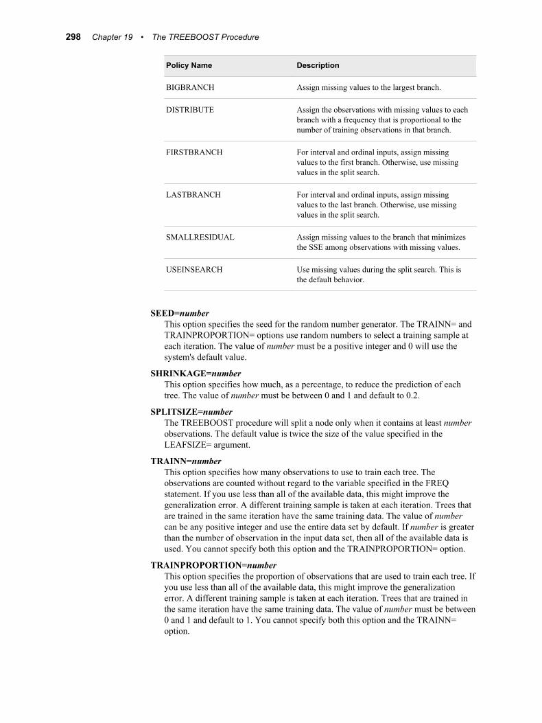
Policy Name Description
BIGBRANCH Assign missing values to the largest branch.
DISTRIBUTE Assign the observations with missing values to each branch with a frequency that is proportional to the number of training observations in that branch.
FIRSTBRANCH For interval and ordinal inputs, assign missing values to the first branch. Otherwise, use missing values in the split search.
LASTBRANCH For interval and ordinal inputs, assign missing values to the last branch. Otherwise, use missing values in the split search.
SMALLRESIDUAL Assign missing values to the branch that minimizes the SSE among observations with missing values.
USEINSEARCH Use missing values during the split search. This is the default behavior.
SEED=numberThis option specifies the seed for the random number generator. The TRAINN= and TRAINPROPORTION= options use random numbers to select a training sample at each iteration. The value of number must be a positive integer and 0 will use the system's default value.
SHRINKAGE=numberThis option specifies how much, as a percentage, to reduce the prediction of each tree. The value of number must be between 0 and 1 and default to 0.2.
SPLITSIZE=numberThe TREEBOOST procedure will split a node only when it contains at least number observations. The default value is twice the size of the value specified in the LEAFSIZE= argument.
TRAINN=numberThis option specifies how many observations to use to train each tree. The observations are counted without regard to the variable specified in the FREQ statement. If you use less than all of the available data, this might improve the generalization error. A different training sample is taken at each iteration. Trees that are trained in the same iteration have the same training data. The value of number can be any positive integer and use the entire data set by default. If number is greater than the number of observation in the input data set, then all of the available data is used. You cannot specify both this option and the TRAINPROPORTION= option.
TRAINPROPORTION=numberThis option specifies the proportion of observations that are used to train each tree. If you use less than all of the available data, this might improve the generalization error. A different training sample is taken at each iteration. Trees that are trained in the same iteration have the same training data. The value of number must be between 0 and 1 and default to 1. You cannot specify both this option and the TRAINN= option.
298 Chapter 19 • The TREEBOOST Procedure

ASSESS Statement
SyntaxASSESS <options>;
The ASSESS statement accepts an assessment measure, uses it to evaluate each subset of trees, and selects the best subset as the model to use for prediction.
Optional ArgumentsMEASURE=ASE | LIFT | LIFTPROFIT | MISC | PROFITUse this option to specify one of the following assessment measures:
• ASE — uses the average square error. This is the default for interval targets.
• LIFT — uses either the average of or a proportion of the highest ranked observations. An average is used for interval targets and a proportion is used for categorical targets.
• LIFTPROFIT — uses the average profit or loss among the highest ranked observations.
• MISC — uses the proportion of observations that were misclassified. This is the default for categorical targets and is applicable to nominal and ordinal targets as well.
• PROFIT — uses the average profit or loss from the decision function. This is the default method when a profit or loss function is specified in the DECISION statement.
PRIORS | NOPRIORSThis option determines whether the TREEBOOST procedure will use prior probabilities to create the sequence of subtrees. For more information about this process, see “Formulas for Assessment Measures” on page 309 . The default setting is NOPRIORS, which ignores prior probabilities.
VALIDATA=data-set-nameUse this option to specify the validation data set. You cannot specify both the CV argument and the VALIDATA= argument in the same ASSESS statement.
NOVALIDATAUse this argument to nullify any VALIDATA= option that appears in a previous ASSESS statement.
CODE Statement
SyntaxCODE <options>;
The CODE statement generates SAS DATA step code that mimics the computations done by the SCORE statement.
Syntax 299
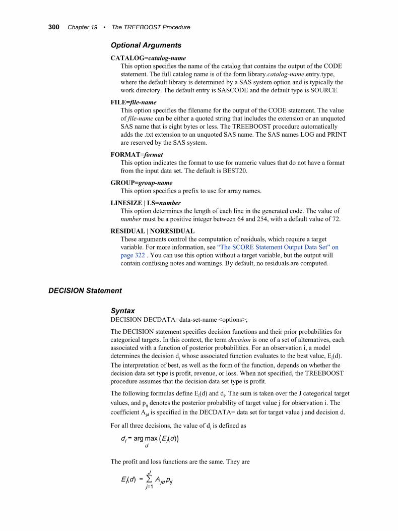
Optional ArgumentsCATALOG=catalog-name
This option specifies the name of the catalog that contains the output of the CODE statement. The full catalog name is of the form library.catalog-name.entry.type, where the default library is determined by a SAS system option and is typically the work directory. The default entry is SASCODE and the default type is SOURCE.
FILE=file-nameThis option specifies the filename for the output of the CODE statement. The value of file-name can be either a quoted string that includes the extension or an unquoted SAS name that is eight bytes or less. The TREEBOOST procedure automatically adds the .txt extension to an unquoted SAS name. The SAS names LOG and PRINT are reserved by the SAS system.
FORMAT=formatThis option indicates the format to use for numeric values that do not have a format from the input data set. The default is BEST20.
GROUP=group-nameThis option specifies a prefix to use for array names.
LINESIZE | LS=numberThis option determines the length of each line in the generated code. The value of number must be a positive integer between 64 and 254, with a default value of 72.
RESIDUAL | NORESIDUALThese arguments control the computation of residuals, which require a target variable. For more information, see “The SCORE Statement Output Data Set” on page 322 . You can use this option without a target variable, but the output will contain confusing notes and warnings. By default, no residuals are computed.
DECISION Statement
SyntaxDECISION DECDATA=data-set-name <options>;
The DECISION statement specifies decision functions and their prior probabilities for categorical targets. In this context, the term decision is one of a set of alternatives, each associated with a function of posterior probabilities. For an observation i, a model determines the decision di whose associated function evaluates to the best value, Ei(d). The interpretation of best, as well as the form of the function, depends on whether the decision data set type is profit, revenue, or loss. When not specified, the TREEBOOST procedure assumes that the decision data set type is profit.
The following formulas define Ei(d) and di. The sum is taken over the J categorical target values, and pij denotes the posterior probability of target value j for observation i. The coefficient Ajd is specified in the DECDATA= data set for target value j and decision d.
For all three decisions, the value of di is defined as
di = arg maxd
(Ei(d))
The profit and loss functions are the same. They are
Ei(d) = ∑j=1
JA jd pij
300 Chapter 19 • The TREEBOOST Procedure
The revenue function is
Ei(d) = ∑j=1
JA jd pij − Cid
Here, Cid is the cost of decision d for observation i, which is specified in the COST= option.
The decision functions do not affect the creation of the model unless the DECSEARCH= argument is specified in the PROC TREEBOOST statement. However, the decision functions determine a profit or loss measure that assesses the submodels. Consequently, these decisions might have a significant effect on the nodes or trees that are pruned from the final submodel.
While the decision statement is optional, to use the DECISION statement, it must be preceded by the FREQ, INPUT, and TARGET statements. When this statement is omitted, neither decision alternatives nor prior probabilities are defined. You cannot specify the DECISION statement and the INMODEL= option in the PROC TREEBOOST statement.
Required ArgumentsDECDATA=data-set-name
This argument specifies the data set that contains the decision coefficients and prior probabilities. This data set must contain the target variable. One observation must appear for each target value in the training data set.
Optional ArgumentsCOST=list-of-costs
This option specifies a list of cost constants and cost variables that are associated with the decision alternatives specified in the DECVARS= argument. The first cost in this list corresponds to the first alternative in the DECVARS= list, the second cost in this list corresponds to the second alternative in the DECVARS= list, and so on. The number of costs must equal the number of alternatives specified in the DECVARS= argument.
When the DECDATA= data set is a revenue data set, this argument is required. This argument defines the Cids that are used in the revenue function that is provided above. The COST= option does not recognize abbreviations of lists.
DECVARS=list-of-alternativesThis option specifies the variables in the DECDATA= data set that define the coefficients Ajd. The labels of these variables define the names of the decision alternatives. For a variable without a label, the name of the decision alternative is the name of the variable. No decision functions are defined if this option is omitted.
PRIORVAR=variableThis option specifies the variable in the DECDATA= data set that contains the prior probabilities of the categorical target values. For more information, see “Within-Node Probabilities” on page 312 . The variable specified here must have nonnegative values. The TREEBOOST procedure scales these values so that they sum to one and ignores observations where this variable is zero.
Prior probabilities do not affect the creation of the model. Prior probabilities affect the posterior probabilities, and consequently affect the model predictions and assessment.
Syntax 301
FREQ Statement
SyntaxFREQ variable;
Required Argumentvariable
The FREQ statement identifies a variable that contains the frequency of occurrence for each observation. The TREEBOOST procedure treats each observation as if it appears n times, where n is the value of the FREQ variable for the observation. The value of n can be fractional to indicate partial observations. If the value of n is close to zero, negative, or missing, then the observation is ignored. When the FREQ statement is not specified, each observation is assigned a frequency of 1.
IMPORTANCE Statement
SyntaxIMPORTANCE <options>;
The IMPORTANCE statement uses an observation-based approach to evaluate the importance of a variable or a pair of variables to the predictions of the model. For each observation, the IMPORTANCE statement outputs the prediction once with the actual variable value and once with an uninformative variable value. For information about uninformative variable values, see “Variable Importance” on page 315 . The differences for all the observations can be plotted against the actual variable value or observation number to explore where the dependence is stronger or weaker.
The TREEBOOST procedure also computes goodness-of-fit statistics with both the original and the uninformative variable values. A comparison of these statistics will reveal the dependence of the statistics on the variable. If you evaluate several variables, their statistics can be ranked to reveal the relative observation-based importance of the variables.
Optional ArgumentsDATA=data-set-name
This option specifies the input data set. If this option is absent, then the procedure uses the training data set.
N2WAY=m nUse this option to request that the best m variables are paired with the best n variables. Here, best refers to the split-based variable importance rankings that were computed in the IMPORTANCE= option of the SAVE statement. The values of m and n are positive integers, and n is set to m if it is not specified. Each variable is also computed individually, as if it were specified in the VAR= argument.
NVARS=numberThis argument instructs the TREEBOOST procedure to evaluate the best number variables as ranked by their split-based importance. If N2WAY=, NVARS=, and VAR= are absent, then this value is assumed to be 5.
302 Chapter 19 • The TREEBOOST Procedure
OUT=data-set-nameThis option specifies an output data set. If you do not specify this option, then the IMPORTANCE statement will automatically create an output data set. You can suppress this data set altogether if you specify OUT=_NULL_.
This data set contains the same variables as the output data set in the SCORE statement, plus one or two more variables. These variables contain the names of the uninformative variables. The number of observations in this data set equals the number of variables and variable pairs that are evaluated plus the number of observations in the input data set. For more information, see “The SCORE Statement Output Data Set” on page 322 .
OUTFIT=data-set-nameThis data set contains the goodness-of-fit statistics. The number of observations in this data set is the number of variables plus the number of pairs of variables plus one. This data set contains the same variables as the output data set in the SCORE statement, plus one or two more variables. These variables contain the names of the uninformative variables.
VAR=(list-of-variables)This argument specifies the variables and variable pairs to evaluate. An asterisk between two variables indicates a variable pair, and square brackets are used as grouping symbols. You cannot nest square brackets. You must enclose the list in parentheses. If you specify a pair of variables, then each variable is also evaluated individually.
Consider the statement VAR=(A B*C [D E]*[E C]). The IMPORTANCE statement would evaluate the variables A, B, C, D, and E individually. Furthermore, it would also evaluate the variable pairs B-C, D-E, D-C, and E-C.
INPUT Statement
SyntaxINPUT variables </ options>;
The INPUT statement names the input variables along with options that are common to all of the listed variables. This statement can be repeated as necessary.
Required Argumentlist-of-variables
Before you can specify any options, you need to list the input variables.
Optional ArgumentsINTERVALDECIMALS=number
This option determines the precision of interval value split points.
LEVEL=INTERVAL | NOMINAL | ORDINALThis option determines the level of measurement. The default value for a numeric variable is INTERVAL and for a character variable is NOMINAL. For more information, see “Terminology” on page 294 .
MAXBRANCES=numberThis option determines the maximum number of branches that can descend from one node. The value of number must be a positive integer.
Syntax 303
MINCATSIZE=numberIn order to create a splitting rule for a particular value of a nominal variable, there must be number observations of that value. If a value is observed fewer than number times, then it is treated as a missing value. You can still use these values if you specify the option MISSING=USEINSEARCH (see below). The policy to assign infrequent observations to a branch is the same policy that is used to assign missing values to a branch. The default value for number is 5. See “Missing Values” on page 314 for more information.
MISSING=policy-nameThis argument specifies the policy that is used to handle missing values. The MISSING= option in the INPUT statement overrides this option. See “Missing Values” on page 314 for more information. The policy names are given in the table below.
Policy Name Description
BIGBRANCH Assign missing values to the largest branch.
DISTRIBUTE Assign the observations with missing values to each branch with a frequency that is proportional to the number of training observations in that branch.
FIRSTBRANCH For interval and ordinal inputs, assign missing values to the first branch. Otherwise, use missing values in the split search.
LASTBRANCH For interval and ordinal inputs, assign missing values to the last branch. Otherwise, use missing values in the split search.
SMALLRESIDUAL Assign missing values to the branch that minimizes the SSE among observations with missing values.
USEINSEARCH Use missing values during the split search. This is the default behavior.
ORDER=order-nameThis option determines the sorting order of the values for an ordinal input variable. This option is available only when LEVEL=ORDINAL is specified.
Valid values for order-name are as follows:
• ASCENDING — sorts the values in ascending order of the unformatted values. This is the default setting.
• ASCFORMATTED — sorts the values in ascending order of the formatted values.
• DESCENDING — sorts the values in descending order of the unformatted values.
• DESCFORMATTED — sorts the values in descending order of the formatted values.
• DSORDER — sorts the values in the order in which they appear in the data set.
The Terminology Section on page 294 discusses formatted values.
304 Chapter 19 • The TREEBOOST Procedure
Consider the following comments about the sorting methods:
• For numeric variables, the ASCFORMATTED and DESFORMATTED settings can deviate from their unformatted counterparts when no explicit format is declared.
• When you specify ASCENDING or DESCENDING and two or more unformatted values have the same formatted value, the TREEBOOST procedure uses the length of the unformatted value to determine ordering.
• A splitting rule on an ordinal input assigns a range of formatted values to a branch. The range will correspond to a range of unformatted values if all of the unformatted values with the same formatted value define an interval that contains no other values.
• The sorting order of character values, including formatted values, might be machine-dependent.
SPLITATDATUMSpecify this option to request that a split on an interval input variable equals the value of the observation. If the variable value is an integer, the split occurs exactly at that value and is slightly less if the variable value is not an integer. The default value is the SPLITBETWEEN option.
SPLITBETWEENSpecify this option to request that a split on an interval input variable occurs halfway between two data values. This is the default behavior.
MAKEMACRO Statement
SyntaxMAKEMACRO NTREES=macro-name;
Required ArgumentNTREES=macro-name
The MAKEMACRO statement specifies the name of a macro variable that contains the number of terms in the current subseries of trees. If this statement appears before a model is trained, then the TREEBOOST procedure trains a model before it executes this statement. Subsequent initialization statements are prohibited.
PERFORMANCE Statement
SyntaxPERFORMANCE <options>;
The PERFORMANCE statement specifies options that affect the speed of computations with little or no impact on the results. For more information, see “Performance Considerations” on page 324 .
Optional ArgumentsMEMSIZE=number<B | K | M | G>
This argument specifies the maximum amount of memory to allocate for the computations and the working copy of the training data. The optional suffixes B, K,
Syntax 305
M, and G stand for bytes, kilobytes, megabytes, and gigabytes, respectively. With a suffice, the TREEBOOST procedure assumes bytes. The value of number can be any positive number and is limited by the SAS MEMSIZE system option. The default value depends on the computer.
NODESIZE=number | ALLThis option specifies the number of training observations to use when the TREEBOOST procedure searches for a splitting rule. Specify NODESIZE=ALL to use all of the observations available. For larger data sets, a large within-node sample might require more passes of the data, which results in slower overall performance.
The PATH procedure counts the number of training observations in a node without adjusting the number for the frequency variable specified in the FREQ statement. If the count is larger than number, then the split search for that node is based on a random sample of size number. For categorical targets, the sample uses as many observations with less frequent target values as possible. The acceptable range, on most machines, for number is from two to two billion. For more information, see “Within-Node Training Sample” on page 313 .
WORKDATALOCATION=DISK | RAM | SOURCEThis option determines where to put the working copy of the training data. The RAM option stores the data in memory, provided that there is enough memory for the data and for an additional pass of the data to perform a single split search. The DISK option requests that the working copy is stored in a disk utility file. This setting can free a considerable amount of memory for calculations, which may or may not improve performance. The SOURCE option requests that the training data is read multiple times, instead of copying it to memory or the disk. This is preferred when the training data will not fitin memory or a disk utility file.
SAVE Statement
SyntaxSAVE <options>;
The SAVE statement outputs decision tree information into SAS data sets.
Optional ArgumentsFIT=data-set-name
This option specifies a data set that contains the fit statistics for each iteration. The data set contains one observation for each iteration.
IMPORTANCE=data-set-nameThis data set contains the split-based variable importance. For more information, see “Variable Importance” on page 315 .
MODEL=data-set-nameThis data set encodes the information necessary to use the INMODEL= option in subsequent calls to the TREEBOOST procedure.
NODESTATS=data-set-nameThis data set contains information about all of the nodes. For more information, see “NODESTATS Output Data Set” on page 319 .
RULES=data-set-nameThis data set describes the splitting rules. For more information, see “RULES Output Data Set” on page 320 .
306 Chapter 19 • The TREEBOOST Procedure
SCORE Statement
SyntaxSCORE <options>;
The SCORE statement is used to calculate predictions, residuals, decisions, and leaf assignments.
Optional ArgumentsDATA=data-set-name
This option indicates the input data set. If this option is absent, then the TREEBOOST procedure uses the training data set.
OUT=data-set-nameThis data set contains the scored data. An output data set is automatically created if this argument is not included. To suppress this data set completely, specify OUT=_NULL_. For more information about this data set, see “The SCORE Statement Output Data Set” on page 322 .
OUTFIT=data-set-nameThis data set contains the fit statistics that were computed by the TREEBOOST procedure.
PREDICTION | NOPREDICTIONThese arguments control the computation of predicted values. By default, predicted values are computed.
ROLE=SCORE | TEST | TRAIN | VALIDThis option determines the role of the input data set and determines the fit statistics to compute. Only the SCORE setting can include observations without a target value.
SUBSERIES Statement
SyntaxSUBSERIES <options>;
The SUBSERIES statement specifies how many iterations in the series to use in the model. For a binary or interval target, the number of iterations is the number of trees in the series. For a nominal target with k categories, k > 2, each iteration contains k trees. The following options are mutually exclusive.
Optional ArgumentsBESTLONGESTITERATIONS=number
The BEST argument selects the smallest subseries with the best assessment value. The LONGEST argument selects the complete series of decision trees. The ITERATIONS= argument selects the subseries that contains number iterations.
Syntax 307
TARGET Statement
SyntaxTARGET variable </ options>;
Required Argumentvariable
This is the variable that the decision tree model attempts to predict.
Optional ArgumentsLEVEL=BINARY | INTERVAL | NOMINAL | ORDINAL
This argument specifies the level of measurement for the target variable. The default for a numeric variable is INTERVAL and is NOMINAL for a character variable.
Details
Split Search AlgorithmThe TREEBOOST procedure always selects a splitting rule with the largest worth among all the splits that were evaluated. The algorithm is simple, but the details seem complicated because of all the special situations.
The search for splitting and surrogate rules is done on the within-node training sample. The search that involves a specific input variable eliminates observations with a missing value unless the USEINSEARCH= method is used. The search that involves a specific categorical input variable eliminates observations whose input value occurs less frequently than the threshold specified in the MINCATSIZE= option.
The decision to eliminate an observation from the within-node sample is made independently for each input and for each node. An observation where input W is missing and input Z is not missing is eliminated from the search using W but the search using Z. An observation where categorical input X is common in the root node but occurs infrequently in some branch is eliminated from searches in that branch, but not the root node.
In most situations, the algorithm sorts the observations. For interval and ordinal input variables, the algorithm sorts the input values and arbitrarily places observations with missing values at the end. For nominal input variables with interval targets, the algorithm sorts the input categories by the average target value among the observations in the category. For nominal inputs and observations with two categorical target values in the search sample, the algorithm sorts the input categories by the proportion of one of the target values. In the remaining situation, the algorithm does not sort. The remaining situation consists of a nominal input and a categorical target with at least three different values in the sample presented to the algorithm.
After the algorithm sorts the data, it evaluates every permissible binary split that preserves the sort. A split between tied input values or categories with the same average target value is not permitted. Additionally, a split that leaves fewer observations in a branch than specified in the LEAFSIZE= option of the TRAIN statement is not permitted.
308 Chapter 19 • The TREEBOOST Procedure
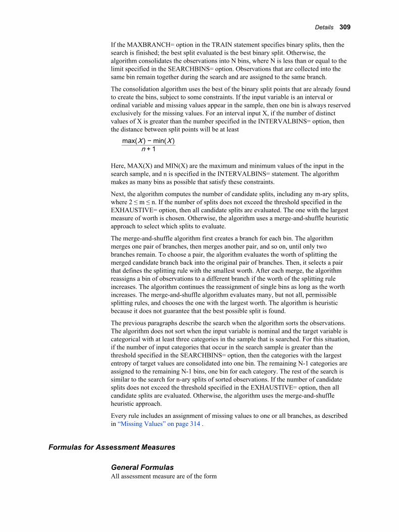
If the MAXBRANCH= option in the TRAIN statement specifies binary splits, then the search is finished; the best split evaluated is the best binary split. Otherwise, the algorithm consolidates the observations into N bins, where N is less than or equal to the limit specified in the SEARCHBINS= option. Observations that are collected into the same bin remain together during the search and are assigned to the same branch.
The consolidation algorithm uses the best of the binary split points that are already found to create the bins, subject to some constraints. If the input variable is an interval or ordinal variable and missing values appear in the sample, then one bin is always reserved exclusively for the missing values. For an interval input X, if the number of distinct values of X is greater than the number specified in the INTERVALBINS= option, then the distance between split points will be at least
max(X ) − min(X )n + 1
Here, MAX(X) and MIN(X) are the maximum and minimum values of the input in the search sample, and n is specified in the INTERVALBINS= statement. The algorithm makes as many bins as possible that satisfy these constraints.
Next, the algorithm computes the number of candidate splits, including any m-ary splits, where 2 ≤ m ≤ n. If the number of splits does not exceed the threshold specified in the EXHAUSTIVE= option, then all candidate splits are evaluated. The one with the largest measure of worth is chosen. Otherwise, the algorithm uses a merge-and-shuffle heuristic approach to select which splits to evaluate.
The merge-and-shuffle algorithm first creates a branch for each bin. The algorithm merges one pair of branches, then merges another pair, and so on, until only two branches remain. To choose a pair, the algorithm evaluates the worth of splitting the merged candidate branch back into the original pair of branches. Then, it selects a pair that defines the splitting rule with the smallest worth. After each merge, the algorithm reassigns a bin of observations to a different branch if the worth of the splitting rule increases. The algorithm continues the reassignment of single bins as long as the worth increases. The merge-and-shuffle algorithm evaluates many, but not all, permissible splitting rules, and chooses the one with the largest worth. The algorithm is heuristic because it does not guarantee that the best possible split is found.
The previous paragraphs describe the search when the algorithm sorts the observations. The algorithm does not sort when the input variable is nominal and the target variable is categorical with at least three categories in the sample that is searched. For this situation, if the number of input categories that occur in the search sample is greater than the threshold specified in the SEARCHBINS= option, then the categories with the largest entropy of target values are consolidated into one bin. The remaining N-1 categories are assigned to the remaining N-1 bins, one bin for each category. The rest of the search is similar to the search for n-ary splits of sorted observations. If the number of candidate splits does not exceed the threshold specified in the EXHAUSTIVE= option, then all candidate splits are evaluated. Otherwise, the algorithm uses the merge-and-shuffle heuristic approach.
Every rule includes an assignment of missing values to one or all branches, as described in “Missing Values” on page 314 .
Formulas for Assessment Measures
General FormulasAll assessment measure are of the form
Details 309
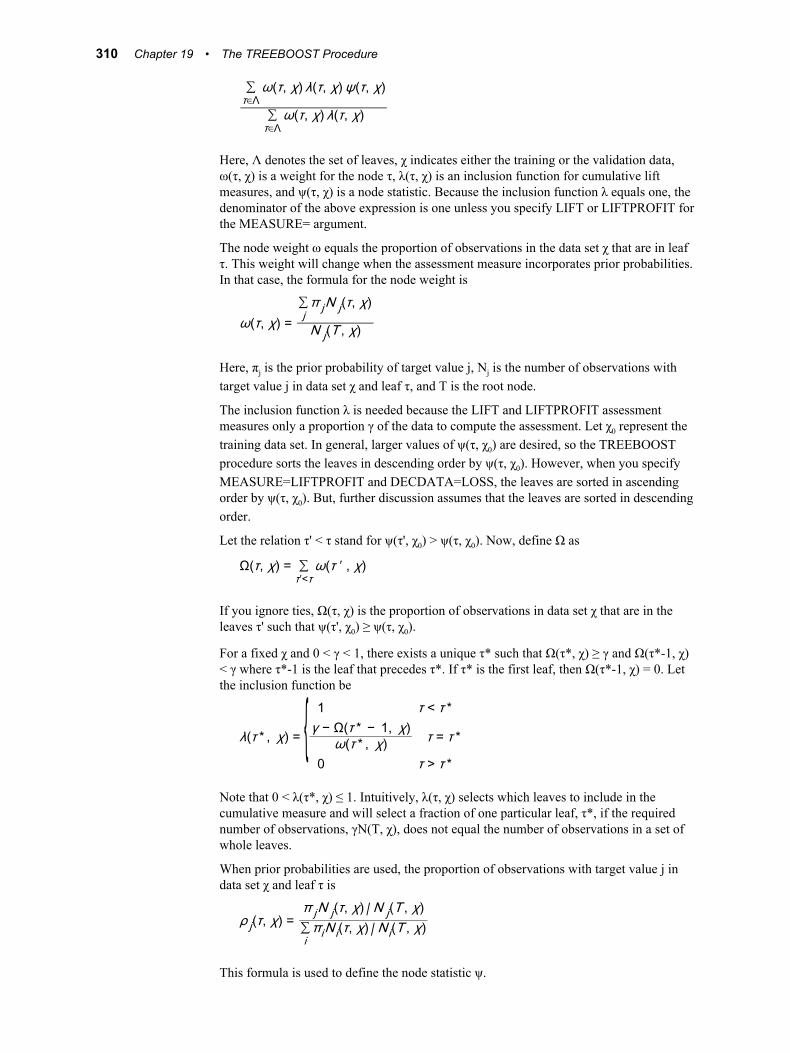
∑τ∈Λ
ω(τ, χ) λ(τ, χ) ψ(τ, χ)
∑τ∈Λ
ω(τ, χ) λ(τ, χ)
Here, Λ denotes the set of leaves, χ indicates either the training or the validation data, ω(τ, χ) is a weight for the node τ, λ(τ, χ) is an inclusion function for cumulative lift measures, and ψ(τ, χ) is a node statistic. Because the inclusion function λ equals one, the denominator of the above expression is one unless you specify LIFT or LIFTPROFIT for the MEASURE= argument.
The node weight ω equals the proportion of observations in the data set χ that are in leaf τ. This weight will change when the assessment measure incorporates prior probabilities. In that case, the formula for the node weight is
ω(τ, χ) =∑jπ jN j(τ, χ)
N j(T , χ)
Here, πj is the prior probability of target value j, Nj is the number of observations with target value j in data set χ and leaf τ, and T is the root node.
The inclusion function λ is needed because the LIFT and LIFTPROFIT assessment measures only a proportion γ of the data to compute the assessment. Let χ0 represent the training data set. In general, larger values of ψ(τ, χ0) are desired, so the TREEBOOST procedure sorts the leaves in descending order by ψ(τ, χ0). However, when you specify MEASURE=LIFTPROFIT and DECDATA=LOSS, the leaves are sorted in ascending order by ψ(τ, χ0). But, further discussion assumes that the leaves are sorted in descending order.
Let the relation τ' < τ stand for ψ(τ', χ0) > ψ(τ, χ0). Now, define Ω as
Ω(τ, χ) = ∑τ′<τ
ω(τ ′ , χ)
If you ignore ties, Ω(τ, χ) is the proportion of observations in data set χ that are in the leaves τ' such that ψ(τ', χ0) ≥ ψ(τ, χ0).
For a fixed χ and 0 < γ < 1, there exists a unique τ* such that Ω(τ*, χ) ≥ γ and Ω(τ*-1, χ) < γ where τ*-1 is the leaf that precedes τ*. If τ* is the first leaf, then Ω(τ*-1, χ) = 0. Let the inclusion function be
λ(τ * , χ) = { 1 τ < τ *γ − Ω(τ * − 1, χ)
ω(τ * , χ) τ = τ *
0 τ > τ *
Note that 0 < λ(τ*, χ) ≤ 1. Intuitively, λ(τ, χ) selects which leaves to include in the cumulative measure and will select a fraction of one particular leaf, τ*, if the required number of observations, γN(T, χ), does not equal the number of observations in a set of whole leaves.
When prior probabilities are used, the proportion of observations with target value j in data set χ and leaf τ is
ρ j(τ, χ) =π jN j(τ, χ) / N j(T , χ)∑iπiN i(τ, χ) / N i(T , χ)
This formula is used to define the node statistic ψ.
310 Chapter 19 • The TREEBOOST Procedure
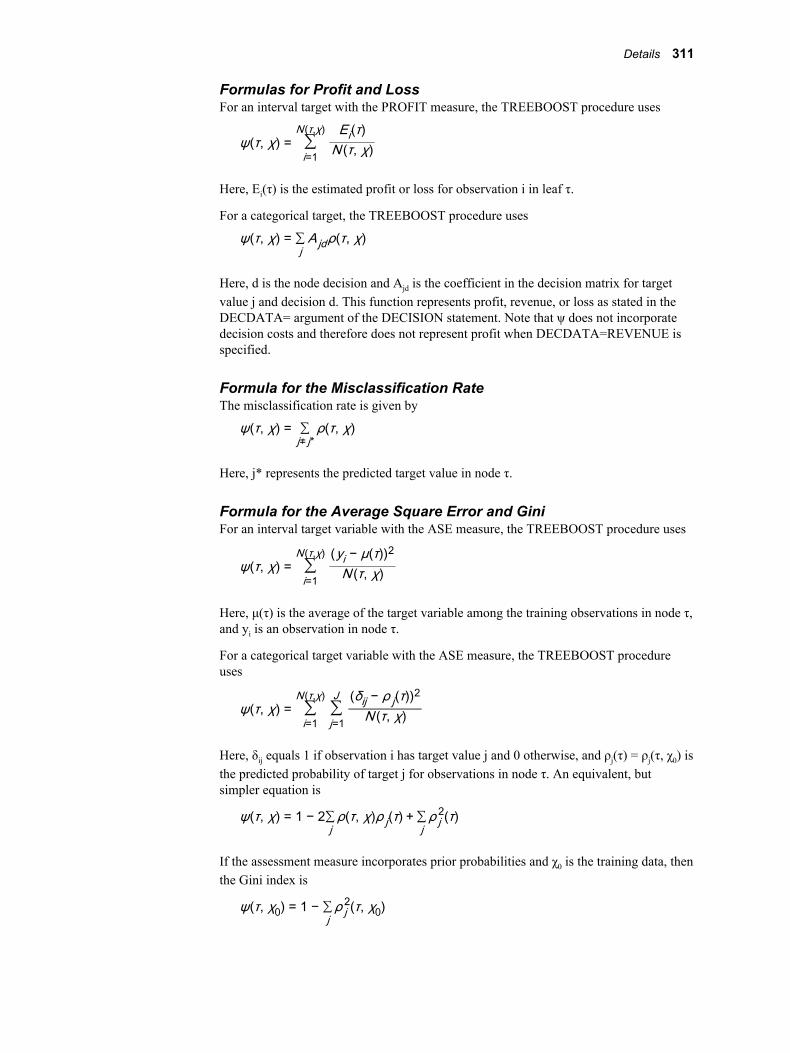
Formulas for Profit and LossFor an interval target with the PROFIT measure, the TREEBOOST procedure uses
ψ(τ, χ) = ∑i=1
N(τ,χ) Ei(τ)N (τ, χ)
Here, Ei(τ) is the estimated profit or loss for observation i in leaf τ.
For a categorical target, the TREEBOOST procedure uses
ψ(τ, χ) = ∑jA jdρ(τ, χ)
Here, d is the node decision and Ajd is the coefficient in the decision matrix for target value j and decision d. This function represents profit, revenue, or loss as stated in the DECDATA= argument of the DECISION statement. Note that ψ does not incorporate decision costs and therefore does not represent profit when DECDATA=REVENUE is specified.
Formula for the Misclassification RateThe misclassification rate is given by
ψ(τ, χ) = ∑j≠ j*
ρ(τ, χ)
Here, j* represents the predicted target value in node τ.
Formula for the Average Square Error and GiniFor an interval target variable with the ASE measure, the TREEBOOST procedure uses
ψ(τ, χ) = ∑i=1
N(τ,χ) (yi − μ(τ))2N (τ, χ)
Here, μ(τ) is the average of the target variable among the training observations in node τ, and yi is an observation in node τ.
For a categorical target variable with the ASE measure, the TREEBOOST procedure uses
ψ(τ, χ) = ∑i=1
N(τ,χ)∑j=1
J (δij − ρ j(τ))2N (τ, χ)
Here, δij equals 1 if observation i has target value j and 0 otherwise, and ρj(τ) = ρj(τ, χ0) is the predicted probability of target j for observations in node τ. An equivalent, but simpler equation is
ψ(τ, χ) = 1 − 2∑jρ(τ, χ)ρ j(τ) + ∑j
ρ j2(τ)
If the assessment measure incorporates prior probabilities and χ0 is the training data, then the Gini index is
ψ(τ, χ0) = 1 − ∑jρ j2(τ, χ0)
Details 311
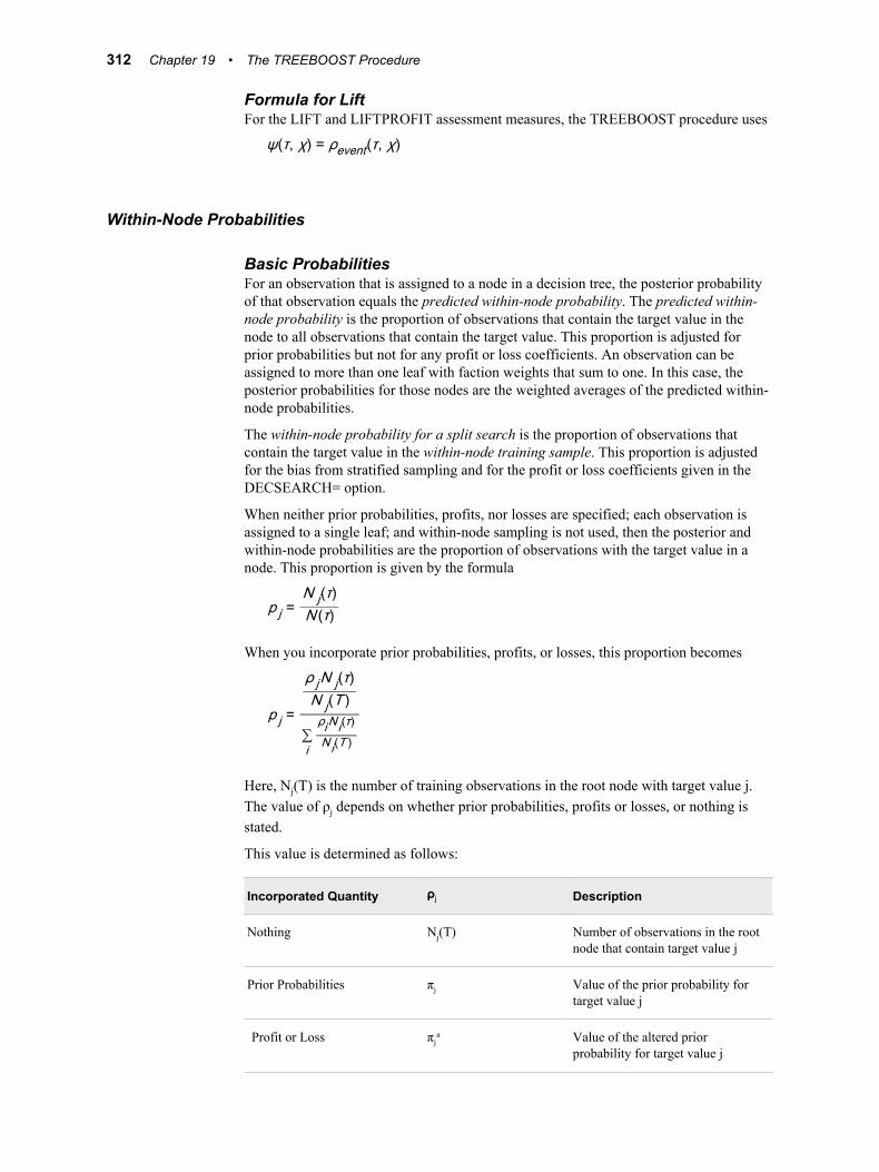
Formula for LiftFor the LIFT and LIFTPROFIT assessment measures, the TREEBOOST procedure uses
ψ(τ, χ) = ρevent(τ, χ)
Within-Node Probabilities
Basic ProbabilitiesFor an observation that is assigned to a node in a decision tree, the posterior probability of that observation equals the predicted within-node probability. The predicted within-node probability is the proportion of observations that contain the target value in the node to all observations that contain the target value. This proportion is adjusted for prior probabilities but not for any profit or loss coefficients. An observation can be assigned to more than one leaf with faction weights that sum to one. In this case, the posterior probabilities for those nodes are the weighted averages of the predicted within-node probabilities.
The within-node probability for a split search is the proportion of observations that contain the target value in the within-node training sample. This proportion is adjusted for the bias from stratified sampling and for the profit or loss coefficients given in the DECSEARCH= option.
When neither prior probabilities, profits, nor losses are specified; each observation is assigned to a single leaf; and within-node sampling is not used, then the posterior and within-node probabilities are the proportion of observations with the target value in a node. This proportion is given by the formula
p j =N j(τ)N (τ)
When you incorporate prior probabilities, profits, or losses, this proportion becomes
p j =
ρ jN j(τ)N j(T )
∑i
ρiNi(τ)Ni(T )
Here, Nj(T) is the number of training observations in the root node with target value j. The value of ρj depends on whether prior probabilities, profits or losses, or nothing is stated.
This value is determined as follows:
Incorporated Quantity ρj Description
Nothing Nj(T) Number of observations in the root node that contain target value j
Prior Probabilities πj Value of the prior probability for target value j
Profit or Loss πja Value of the altered prior
probability for target value j
312 Chapter 19 • The TREEBOOST Procedure
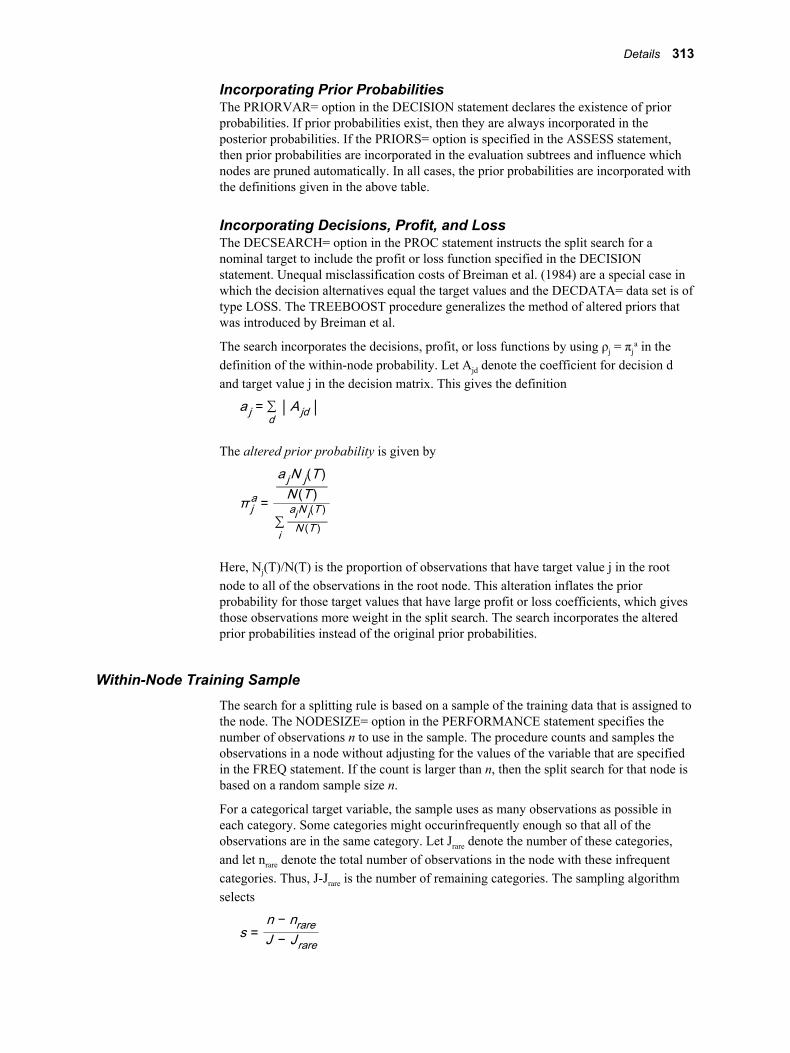
Incorporating Prior ProbabilitiesThe PRIORVAR= option in the DECISION statement declares the existence of prior probabilities. If prior probabilities exist, then they are always incorporated in the posterior probabilities. If the PRIORS= option is specified in the ASSESS statement, then prior probabilities are incorporated in the evaluation subtrees and influence which nodes are pruned automatically. In all cases, the prior probabilities are incorporated with the definitions given in the above table.
Incorporating Decisions, Profit, and LossThe DECSEARCH= option in the PROC statement instructs the split search for a nominal target to include the profit or loss function specified in the DECISION statement. Unequal misclassification costs of Breiman et al. (1984) are a special case in which the decision alternatives equal the target values and the DECDATA= data set is of type LOSS. The TREEBOOST procedure generalizes the method of altered priors that was introduced by Breiman et al.
The search incorporates the decisions, profit, or loss functions by using ρj = πja in the
definition of the within-node probability. Let Ajd denote the coefficient for decision d and target value j in the decision matrix. This gives the definition
a j = ∑d| A jd |
The altered prior probability is given by
π ja =
a jN j(T )N (T )
∑i
aiNi(T )N (T )
Here, Nj(T)/N(T) is the proportion of observations that have target value j in the root node to all of the observations in the root node. This alteration inflates the prior probability for those target values that have large profit or loss coefficients, which gives those observations more weight in the split search. The search incorporates the altered prior probabilities instead of the original prior probabilities.
Within-Node Training SampleThe search for a splitting rule is based on a sample of the training data that is assigned to the node. The NODESIZE= option in the PERFORMANCE statement specifies the number of observations n to use in the sample. The procedure counts and samples the observations in a node without adjusting for the values of the variable that are specified in the FREQ statement. If the count is larger than n, then the split search for that node is based on a random sample size n.
For a categorical target variable, the sample uses as many observations as possible in each category. Some categories might occurinfrequently enough so that all of the observations are in the same category. Let Jrare denote the number of these categories, and let nrare denote the total number of observations in the node with these infrequent categories. Thus, J-Jrare is the number of remaining categories. The sampling algorithm selects
s =n − nrareJ − J rare
Details 313
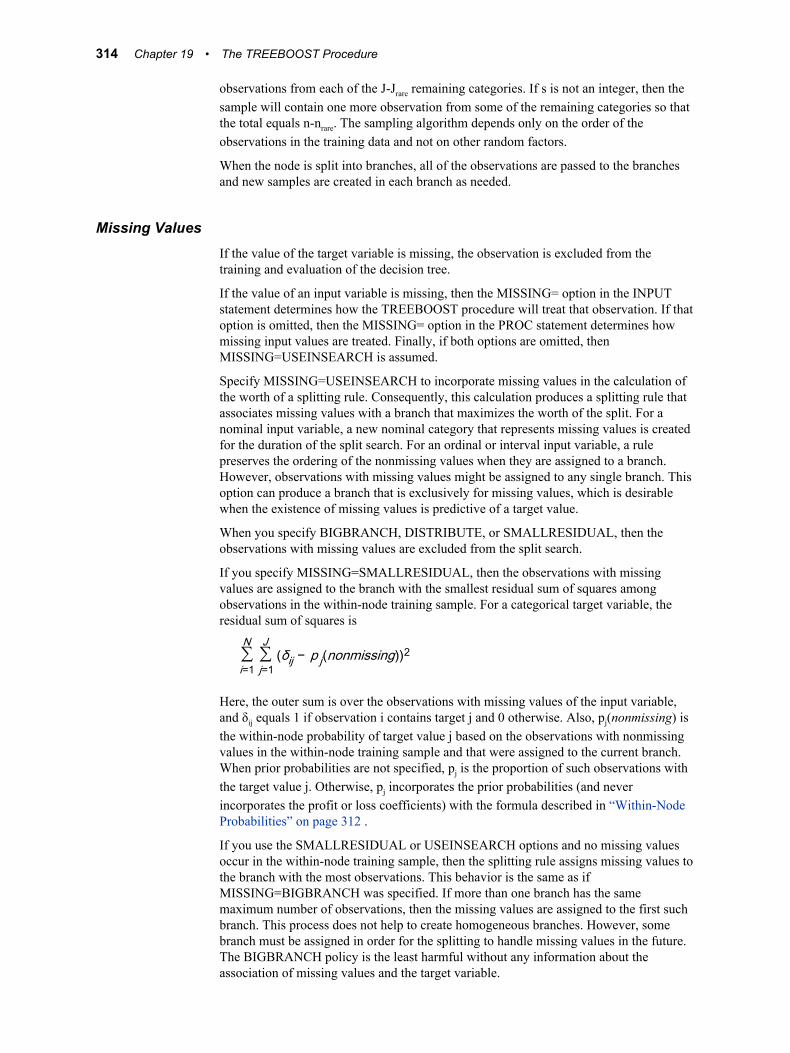
observations from each of the J-Jrare remaining categories. If s is not an integer, then the sample will contain one more observation from some of the remaining categories so that the total equals n-nrare. The sampling algorithm depends only on the order of the observations in the training data and not on other random factors.
When the node is split into branches, all of the observations are passed to the branches and new samples are created in each branch as needed.
Missing ValuesIf the value of the target variable is missing, the observation is excluded from the training and evaluation of the decision tree.
If the value of an input variable is missing, then the MISSING= option in the INPUT statement determines how the TREEBOOST procedure will treat that observation. If that option is omitted, then the MISSING= option in the PROC statement determines how missing input values are treated. Finally, if both options are omitted, then MISSING=USEINSEARCH is assumed.
Specify MISSING=USEINSEARCH to incorporate missing values in the calculation of the worth of a splitting rule. Consequently, this calculation produces a splitting rule that associates missing values with a branch that maximizes the worth of the split. For a nominal input variable, a new nominal category that represents missing values is created for the duration of the split search. For an ordinal or interval input variable, a rule preserves the ordering of the nonmissing values when they are assigned to a branch. However, observations with missing values might be assigned to any single branch. This option can produce a branch that is exclusively for missing values, which is desirable when the existence of missing values is predictive of a target value.
When you specify BIGBRANCH, DISTRIBUTE, or SMALLRESIDUAL, then the observations with missing values are excluded from the split search.
If you specify MISSING=SMALLRESIDUAL, then the observations with missing values are assigned to the branch with the smallest residual sum of squares among observations in the within-node training sample. For a categorical target variable, the residual sum of squares is
∑i=1
N∑j=1
J(δij − p j(nonmissing))2
Here, the outer sum is over the observations with missing values of the input variable, and δij equals 1 if observation i contains target j and 0 otherwise. Also, pj(nonmissing) is the within-node probability of target value j based on the observations with nonmissing values in the within-node training sample and that were assigned to the current branch. When prior probabilities are not specified, pj is the proportion of such observations with the target value j. Otherwise, pj incorporates the prior probabilities (and never incorporates the profit or loss coefficients) with the formula described in “Within-Node Probabilities” on page 312 .
If you use the SMALLRESIDUAL or USEINSEARCH options and no missing values occur in the within-node training sample, then the splitting rule assigns missing values to the branch with the most observations. This behavior is the same as if MISSING=BIGBRANCH was specified. If more than one branch has the same maximum number of observations, then the missing values are assigned to the first such branch. This process does not help to create homogeneous branches. However, some branch must be assigned in order for the splitting to handle missing values in the future. The BIGBRANCH policy is the least harmful without any information about the association of missing values and the target variable.
314 Chapter 19 • The TREEBOOST Procedure
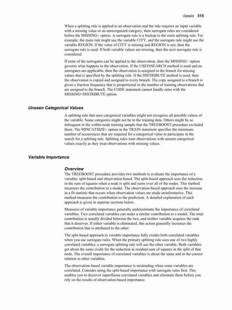
When a splitting rule is applied to an observation and the rule requires an input variable with a missing value or an unrecognized category, then surrogate rules are considered before the MISSING= option. A surrogate rule is a backup to the main splitting rule. For example, the main rule might use the variable CITY, and the surrogate rule might use the variable REGION. If the value of CITY is missing and REGION is not, then the surrogate rule is used. If both variable values are missing, then the next surrogate rule is considered.
If none of the surrogates can be applied to the observation, then the MISSING= option governs what happens to the observation. If the USEINSEARCH method is used and no surrogates are applicable, then the observation is assigned to the branch for missing values that is specified by the splitting rule. If the DISTRIBUTE method is used, then the observation is copied and assigned to every branch. The copy assigned to a branch is given a fraction frequency that is proportional to the number of training observations that are assigned to the branch. The CODE statement cannot handle rules with the MISSING=DISTRIBUTE option.
Unseen Categorical ValuesA splitting rule that uses categorical variables might not recognize all possible values of the variable. Some categories might not be in the training data. Others might be so infrequent in the within-node training sample that the TREEBOOST procedure excluded them. The MINCATSIZE= option in the TRAIN statement specifies the minimum number of occurrences that are required for a categorical value to participate in the search for a splitting rule. Splitting rules treat observations with unseen categorical values exactly as they treat observations with missing values.
Variable Importance
OverviewThe TREEBOOST procedure provides two methods to evaluate the importance of a variable: split-based and observation-based. The split-based approach uses the reduction in the sum of squares when a node is split and sums over all of the nodes. This method measures the contribution to a model. The observation-based approach uses the increase in a fit statistic that occurs when observation values are made uninformative. This method measures the contribution to the prediction. A detailed explanation of each approach is given in separate sections below.
Measures of variable importance generally underestimate the importance of correlated variables. Two correlated variables can make a similar contribution to a model. The total contribution is usually divided between the two, and neither variable acquires the rank that it deserves. If either variable is eliminated, this action generally increases the contribution that is attributed to the other.
The split-based approach to variable importance fully credits both correlated variables when you use surrogate rules. When the primary splitting rule uses one of two highly correlated variables, a surrogate splitting rule will use the other variable. Both variables get about the same credit for the reduction in residual sum of squares in the split of that node. The overall importance of correlated variables is about the same and in the correct relation to other variables.
The observation-based variable importance is misleading when some variables are correlated. Consider using the split-based importance with surrogate rules first. This enables you to discover superfluous correlated variables and eliminate them before you rely on the results of observation-based importance.
Details 315
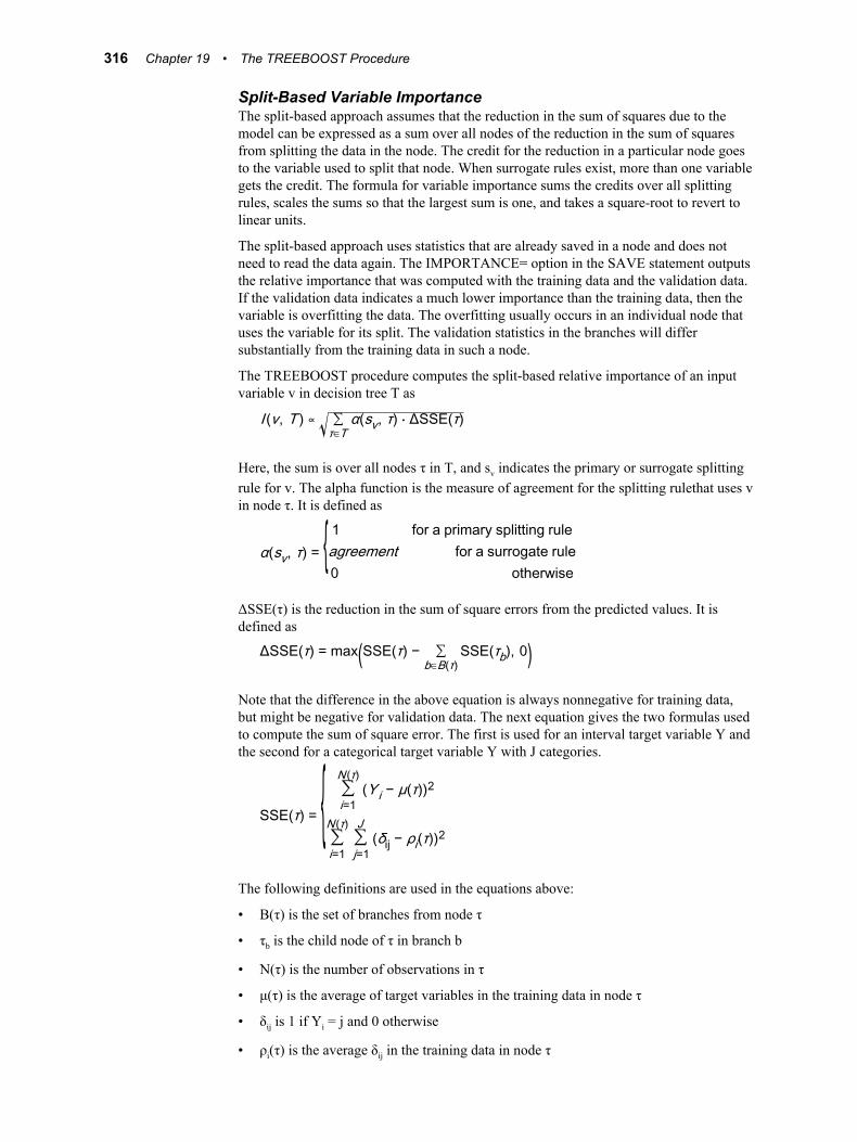
Split-Based Variable ImportanceThe split-based approach assumes that the reduction in the sum of squares due to the model can be expressed as a sum over all nodes of the reduction in the sum of squares from splitting the data in the node. The credit for the reduction in a particular node goes to the variable used to split that node. When surrogate rules exist, more than one variable gets the credit. The formula for variable importance sums the credits over all splitting rules, scales the sums so that the largest sum is one, and takes a square-root to revert to linear units.
The split-based approach uses statistics that are already saved in a node and does not need to read the data again. The IMPORTANCE= option in the SAVE statement outputs the relative importance that was computed with the training data and the validation data. If the validation data indicates a much lower importance than the training data, then the variable is overfitting the data. The overfitting usually occurs in an individual node that uses the variable for its split. The validation statistics in the branches will differ substantially from the training data in such a node.
The TREEBOOST procedure computes the split-based relative importance of an input variable v in decision tree T as
I (v, T ) ∝ ∑τ∈T
α(sv, τ) ⋅ ΔSSE(τ)
Here, the sum is over all nodes τ in T, and sv indicates the primary or surrogate splitting rule for v. The alpha function is the measure of agreement for the splitting rulethat uses v in node τ. It is defined as
α(sv, τ) = { 1 for a primary splitting ruleagreement for a surrogate rule0 otherwise
ΔSSE(τ) is the reduction in the sum of square errors from the predicted values. It is defined as
ΔSSE(τ) = max(SSE(τ) − ∑b∈B(τ)
SSE(τb), 0)Note that the difference in the above equation is always nonnegative for training data, but might be negative for validation data. The next equation gives the two formulas used to compute the sum of square error. The first is used for an interval target variable Y and the second for a categorical target variable Y with J categories.
SSE(τ) = { ∑i=1
N(τ)(Y i − μ(τ))2
∑i=1
N(τ)∑j=1
J(δij − ρi(τ))2
The following definitions are used in the equations above:
• B(τ) is the set of branches from node τ
• τb is the child node of τ in branch b
• N(τ) is the number of observations in τ
• μ(τ) is the average of target variables in the training data in node τ
• δij is 1 if Yi = j and 0 otherwise
• ρi(τ) is the average δij in the training data in node τ
316 Chapter 19 • The TREEBOOST Procedure
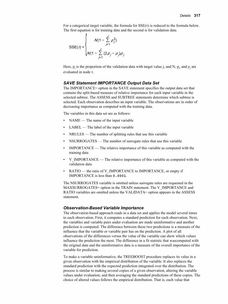
For a categorical target variable, the formula for SSE(τ) is reduced to the formula below. The first equation is for training data and the second is for validation data.
SSE(τ) = { N (1 − ∑j=1
Jρ j2)
N (1 − ∑j=1
J(2p j − ρ j)ρ j
Here, pj is the proportion of the validation data with target value j, and N, pj, and ρj are evaluated in node τ.
SAVE Statement IMPORTANCE Output Data SetThe IMPORTANCE= option in the SAVE statement specifies the output data set that contains the split-based measure of relative importance for each input variable in the selected subtree. The ASSESS and SUBTREE statements determine which subtree is selected. Each observation describes an input variable. The observations are in order of decreasing importance as computed with the training data.
The variables in this data set are as follows:
• NAME — The name of the input variable
• LABEL — The label of the input variable
• NRULES — The number of splitting rules that use this variable
• NSURROGATES — The number of surrogate rules that use this variable
• IMPORTANCE — The relative importance of this variable as computed with the training data
• V_IMPORTANCE — The relative importance of this variable as computed with the validation data
• RATIO — the ratio of V_IMPORTANCE to IMPORTANCE, or empty if IMPORTANCE is less than 0.0001.
The NSURROGATES variable is omitted unless surrogate rules are requested in the MAXSURROGATES= option in the TRAIN statement. The V_IMPORTANCE and RATIO variables are omitted unless the VALIDATA= option appears in the ASSESS statement.
Observation-Based Variable ImportanceThe observation-based approach reads in a data set and applies the model several times to each observation. First, it computes a standard prediction for each observation. Next, the variables and variable pairs under evaluation are made uninformative and another prediction is computed. The difference between these two predictions is a measure of the influence that the variable or variable pair has on the prediction. A plot of all observations of the differences versus the value of the variable can show which values influence the prediction the most. The difference in a fit statistic that wascomputed with the original data and the uninformative data is a measure of the overall importance of the variable for prediction.
To make a variable uninformative, the TREEBOOST procedure replaces its value in a given observation with the empirical distribution of the variable. It also replaces the standard prediction with the expected prediction integrated over the distribution. The process is similar to making several copies of a given observation, altering the variable values under evaluation, and then averaging the standard predictions of these copies. The choice of altered values follows the empirical distribution. That is, each value that
Details 317
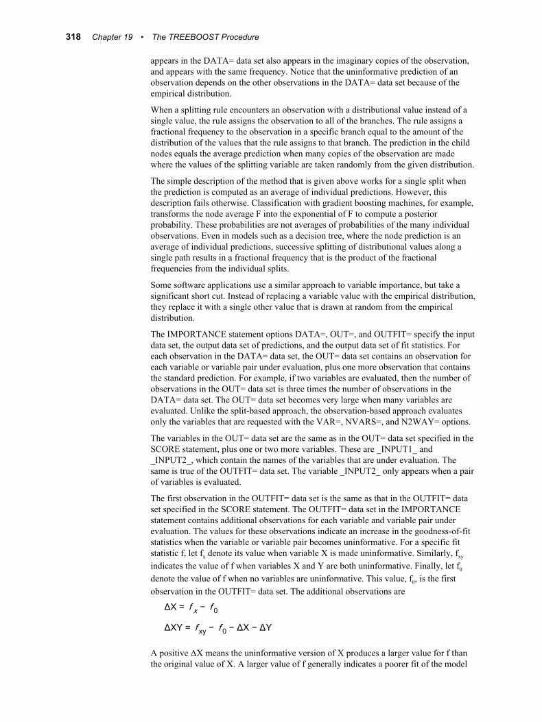
appears in the DATA= data set also appears in the imaginary copies of the observation, and appears with the same frequency. Notice that the uninformative prediction of an observation depends on the other observations in the DATA= data set because of the empirical distribution.
When a splitting rule encounters an observation with a distributional value instead of a single value, the rule assigns the observation to all of the branches. The rule assigns a fractional frequency to the observation in a specific branch equal to the amount of the distribution of the values that the rule assigns to that branch. The prediction in the child nodes equals the average prediction when many copies of the observation are made where the values of the splitting variable are taken randomly from the given distribution.
The simple description of the method that is given above works for a single split when the prediction is computed as an average of individual predictions. However, this description fails otherwise. Classification with gradient boosting machines, for example, transforms the node average F into the exponential of F to compute a posterior probability. These probabilities are not averages of probabilities of the many individual observations. Even in models such as a decision tree, where the node prediction is an average of individual predictions, successive splitting of distributional values along a single path results in a fractional frequency that is the product of the fractional frequencies from the individual splits.
Some software applications use a similar approach to variable importance, but take a significant short cut. Instead of replacing a variable value with the empirical distribution, they replace it with a single other value that is drawn at random from the empirical distribution.
The IMPORTANCE statement options DATA=, OUT=, and OUTFIT= specify the input data set, the output data set of predictions, and the output data set of fit statistics. For each observation in the DATA= data set, the OUT= data set contains an observation for each variable or variable pair under evaluation, plus one more observation that contains the standard prediction. For example, if two variables are evaluated, then the number of observations in the OUT= data set is three times the number of observations in the DATA= data set. The OUT= data set becomes very large when many variables are evaluated. Unlike the split-based approach, the observation-based approach evaluates only the variables that are requested with the VAR=, NVARS=, and N2WAY= options.
The variables in the OUT= data set are the same as in the OUT= data set specified in the SCORE statement, plus one or two more variables. These are _INPUT1_ and _INPUT2_, which contain the names of the variables that are under evaluation. The same is true of the OUTFIT= data set. The variable _INPUT2_ only appears when a pair of variables is evaluated.
The first observation in the OUTFIT= data set is the same as that in the OUTFIT= data set specified in the SCORE statement. The OUTFIT= data set in the IMPORTANCE statement contains additional observations for each variable and variable pair under evaluation. The values for these observations indicate an increase in the goodness-of-fit statistics when the variable or variable pair becomes uninformative. For a specific fit statistic f, let fx denote its value when variable X is made uninformative. Similarly, fxy
indicates the value of f when variables X and Y are both uninformative. Finally, let f0
denote the value of f when no variables are uninformative. This value, f0, is the first observation in the OUTFIT= data set. The additional observations are
ΔX = f x − f 0
ΔXY = f xy − f 0 − ΔX − ΔY
A positive ΔX means the uninformative version of X produces a larger value for f than the original value of X. A larger value of f generally indicates a poorer fit of the model
318 Chapter 19 • The TREEBOOST Procedure
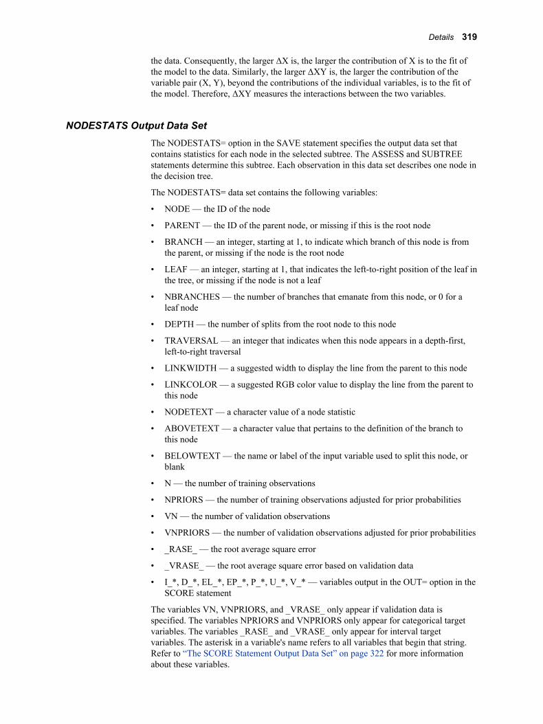
the data. Consequently, the larger ΔX is, the larger the contribution of X is to the fit of the model to the data. Similarly, the larger ΔXY is, the larger the contribution of the variable pair (X, Y), beyond the contributions of the individual variables, is to the fit of the model. Therefore, ΔXY measures the interactions between the two variables.
NODESTATS Output Data SetThe NODESTATS= option in the SAVE statement specifies the output data set that contains statistics for each node in the selected subtree. The ASSESS and SUBTREE statements determine this subtree. Each observation in this data set describes one node in the decision tree.
The NODESTATS= data set contains the following variables:
• NODE — the ID of the node
• PARENT — the ID of the parent node, or missing if this is the root node
• BRANCH — an integer, starting at 1, to indicate which branch of this node is from the parent, or missing if the node is the root node
• LEAF — an integer, starting at 1, that indicates the left-to-right position of the leaf in the tree, or missing if the node is not a leaf
• NBRANCHES — the number of branches that emanate from this node, or 0 for a leaf node
• DEPTH — the number of splits from the root node to this node
• TRAVERSAL — an integer that indicates when this node appears in a depth-first, left-to-right traversal
• LINKWIDTH — a suggested width to display the line from the parent to this node
• LINKCOLOR — a suggested RGB color value to display the line from the parent to this node
• NODETEXT — a character value of a node statistic
• ABOVETEXT — a character value that pertains to the definition of the branch to this node
• BELOWTEXT — the name or label of the input variable used to split this node, or blank
• N — the number of training observations
• NPRIORS — the number of training observations adjusted for prior probabilities
• VN — the number of validation observations
• VNPRIORS — the number of validation observations adjusted for prior probabilities
• _RASE_ — the root average square error
• _VRASE_ — the root average square error based on validation data
• I_*, D_*, EL_*, EP_*, P_*, U_*, V_* — variables output in the OUT= option in the SCORE statement
The variables VN, VNPRIORS, and _VRASE_ only appear if validation data is specified. The variables NPRIORS and VNPRIORS only appear for categorical target variables. The variables _RASE_ and _VRASE_ only appear for interval target variables. The asterisk in a variable's name refers to all variables that begin that string. Refer to “The SCORE Statement Output Data Set” on page 322 for more information about these variables.
Details 319
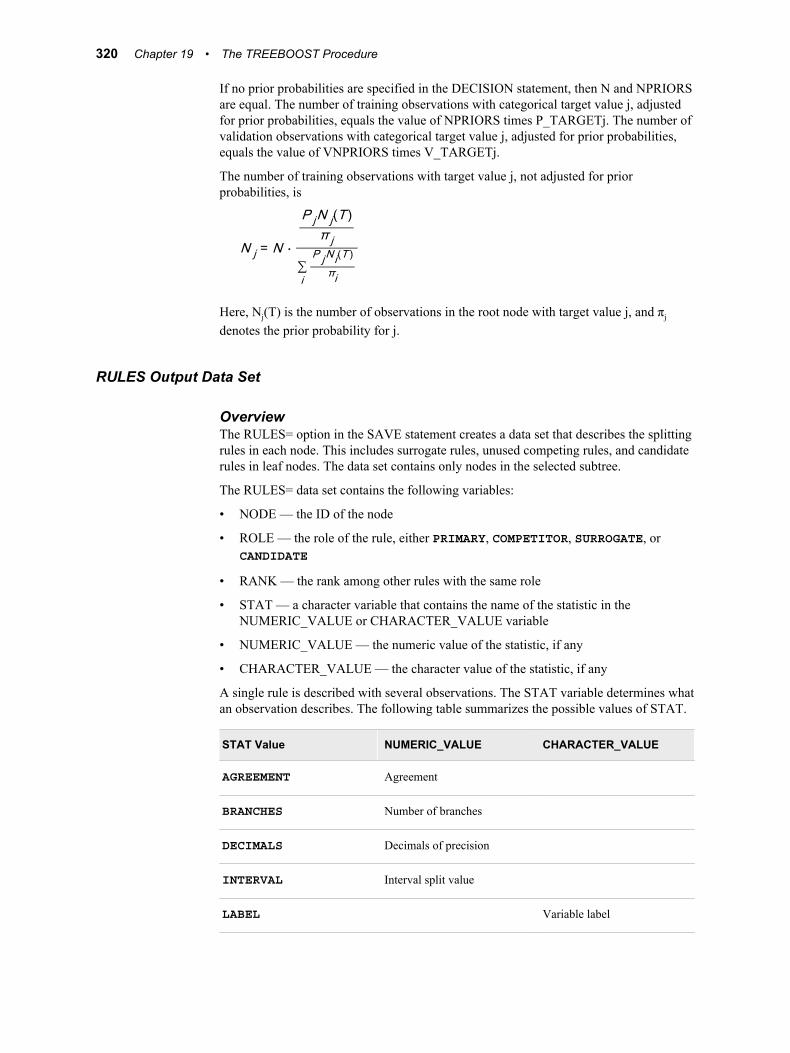
If no prior probabilities are specified in the DECISION statement, then N and NPRIORS are equal. The number of training observations with categorical target value j, adjusted for prior probabilities, equals the value of NPRIORS times P_TARGETj. The number of validation observations with categorical target value j, adjusted for prior probabilities, equals the value of VNPRIORS times V_TARGETj.
The number of training observations with target value j, not adjusted for prior probabilities, is
N j = N ⋅
P jN j(T )π j
∑i
P jNi(T )πi
Here, Nj(T) is the number of observations in the root node with target value j, and πj
denotes the prior probability for j.
RULES Output Data Set
OverviewThe RULES= option in the SAVE statement creates a data set that describes the splitting rules in each node. This includes surrogate rules, unused competing rules, and candidate rules in leaf nodes. The data set contains only nodes in the selected subtree.
The RULES= data set contains the following variables:
• NODE — the ID of the node
• ROLE — the role of the rule, either PRIMARY, COMPETITOR, SURROGATE, or CANDIDATE
• RANK — the rank among other rules with the same role
• STAT — a character variable that contains the name of the statistic in the NUMERIC_VALUE or CHARACTER_VALUE variable
• NUMERIC_VALUE — the numeric value of the statistic, if any
• CHARACTER_VALUE — the character value of the statistic, if any
A single rule is described with several observations. The STAT variable determines what an observation describes. The following table summarizes the possible values of STAT.
STAT Value NUMERIC_VALUE CHARACTER_VALUE
AGREEMENT Agreement
BRANCHES Number of branches
DECIMALS Decimals of precision
INTERVAL Interval split value
LABEL Variable label
320 Chapter 19 • The TREEBOOST Procedure
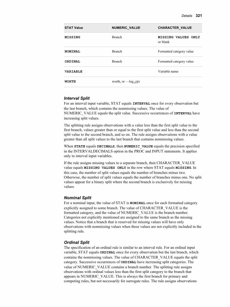
STAT Value NUMERIC_VALUE CHARACTER_VALUE
MISSING Branch MISSING VALUES ONLY or blank
NOMINAL Branch Formatted category value
ORDINAL Branch Formatted category value
VARIABLE Variable name
WORTH worth, or —log10(p)
Interval SplitFor an interval input variable, STAT equals INTERVAL once for every observation but the last branch, which contains the nonmissing values. The value of NUMERIC_VALUE equals the split value. Successive occurrences of INTERVAL have increasing split values.
The splitting rule assigns observations with a value less than the first split value to the first branch, values greater than or equal to the first split value and less than the second split value to the second branch, and so on. The rule assigns observations with a value greater than all split values to the last branch that contains nonmissing values.
When STATE equals DECIMALS, then NUMERIC_VALUE equals the precision specified in the INTERVALDECIMALS option in the PROC and INPUT statements. It applies only to interval input variables.
If the rule assigns missing values to a separate branch, then CHARACTER_VALUE value equals MISSING VALUES ONLY in the row where STAT equals MISSING. In this case, the number of split values equals the number of branches minus two. Otherwise, the number of split values equals the number of branches minus one. No split values appear for a binary split where the second branch is exclusively for missing values.
Nominal SplitFor a nominal input, the value of STAT is NOMINAL once for each formatted category explicitly assigned to some branch. The value of CHARACTER_VALUE is the formatted category, and the value of NUMERIC_VALUE is the branch number. Categories not explicitly mentioned are assigned to the same branch as the missing values. Notice that a branch that is reserved for missing values will have only observations with nonmissing values when these values are not explicitly included in the splitting rule.
Ordinal SplitThe specification of an ordinal rule is similar to an interval rule. For an ordinal input variable, STAT equals ORDINAL once for every observation but the last branch, which contains the nonmissing values. The value of CHARACTER_VALUE equals the split category. Successive occurrences of ORDINAL have increasing split categories. The value of NUMERIC_VALUE contains a branch number. The splitting rule assigns observations with ordinal values less than the first split category to the branch that appears in NUMERIC_VALUE. This is always the first branch for primary and competing rules, but not necessarily for surrogate rules. The rule assigns observations
Details 321
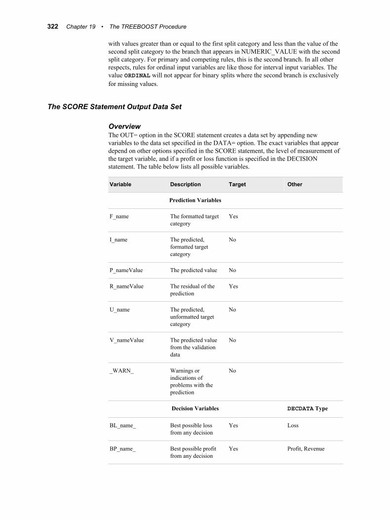
with values greater than or equal to the first split category and less than the value of the second split category to the branch that appears in NUMERIC_VALUE with the second split category. For primary and competing rules, this is the second branch. In all other respects, rules for ordinal input variables are like those for interval input variables. The value ORDINAL will not appear for binary splits where the second branch is exclusively for missing values.
The SCORE Statement Output Data Set
OverviewThe OUT= option in the SCORE statement creates a data set by appending new variables to the data set specified in the DATA= option. The exact variables that appear depend on other options specified in the SCORE statement, the level of measurement of the target variable, and if a profit or loss function is specified in the DECISION statement. The table below lists all possible variables.
Variable Description Target Other
Prediction Variables
F_name The formatted target category
Yes
I_name The predicted, formatted target category
No
P_nameValue The predicted value No
R_nameValue The residual of the prediction
Yes
U_name The predicted, unformatted target category
No
V_nameValue The predicted value from the validation data
No
_WARN_ Warnings or indications of problems with the prediction
No
Decision Variables DECDATA Type
BL_name_ Best possible loss from any decision
Yes Loss
BP_name_ Best possible profit from any decision
Yes Profit, Revenue
322 Chapter 19 • The TREEBOOST Procedure
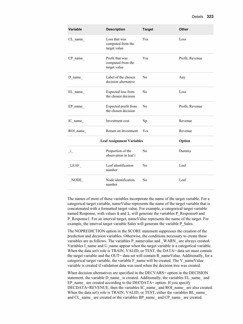
Variable Description Target Other
CL_name_ Loss that was computed from the target value
Yes Loss
CP_name_ Profit that was computed from the target value
Yes Profit, Revenue
D_name_ Label of the chosen decision alternative
No Any
EL_name_ Expected loss from the chosen decision
No Loss
EP_name_ Expected profit from the chosen decision
No Profit, Revenue
IC_name_ Investment cost Np Revenue
ROI_name_ Return on investment Yes Revenue
Leaf Assignment Variables Option
_i_ Proportion of the observation in leaf i
No Dummy
_LEAF_ Leaf identification number
No Leaf
_NODE_ Node identification number
No Leaf
The names of most of these variables incorporate the name of the target variable. For a categorical target variable, nameValue represents the name of the target variable that is concatenated with a formatted target value. For example, a categorical target variable named Response, with values 0 and 1, will generate the variables P_Response0 and P_Response1. For an interval target, nameValue represents the name of the target. For example, the interval target variable Sales will generate the variable P_Sales.
The NOPREDICTION option in the SCORE statement suppresses the creation of the prediction and decision variables. Otherwise, the conditions necessary to create these variables are as follows. The variables P_namevalue and _WARN_ are always created. Variables I_name and U_name appear when the target variable is a categorical variable. When the data set's role is TRAIN, VALID, or TEST, the DATA= data set must contain the target variable and the OUT= data set will contain R_nameValue. Additionally, for a categorical target variable, the variable F_name will be created. The V_nameValue variable is created if validation data was used when the decision tree was created.
When decision alternatives are specified in the DECVARS= option in the DECISION statement, the variable D_name_ is created. Additionally, the variables EL_name_ and EP_name_ are created according to the DECDATA= option. If you specify DECDATA=REVENUE, then the variables IC_name_ and ROI_name_ are also created. When the data set's role is TRAIN, VALID, or TEST, either the variables BL_name_and CL_name_ are created or the variables BP_name_ and CP_name_ are created.
Details 323
Decision VariablesThe labels of the variables that are specified in the DECVARS= option of the DECISION statement are the names of the decision alternatives. For a variable without a label, the name of the decision alternative is the name of the variable. The variable D_name_ in the OUT= data set contains the name of the decision alternative that is assigned to the observation.
Leaf Assignment VariablesEach node is identified with a unique positive integer. Once an identification number is assigned to a node, that number is never reassigned to another node, even after the node is pruned. Consequently, most subtrees in the subtree sequence will not have consecutive node identified.
Each leaf has a leaf identification number in addition to the node identifier. The leaf identifiers are integers that range from 1 to the number of leaves. The leaf numbers are reassigned whenever a new subtree is selected from the subtree sequence.
For an observation in the OUT= data set that is assigned to a single leaf, the variables _NODE_ and _LEAF_ contain the node and leaf identification numbers, respectively. For an observation that is assigned to more than one leaf, the values of _NODE_ and _LEAF_ are missing. An observation is assigned to more than one leaf when the observation is missing a value that is required by one of the splitting rules and the policy for missing variables is DISTRIBUTE.
The DUMMY option in the SCORE statement specifies that the OUT= data set contains the variable _i_. The value of _i_ equals the proportion of the observation that is assigned to the leaf with leaf identification number i. The sum of these variables equals one for each observation. If you do not specify MISSING=DISTRIBUTE, exactly one of these variables equals 1 and the rest equal 0. If you do specify MISSING=DISTRIBUTE, then observations are distributed over more than one leaf and _i_ equals the proportion of the observation that is assigned to leaf i.
Performance Considerations
Reserved MemoryWhen the TREEBOOST procedure begins, it reserves memory in the computer for the calculations that are necessary to grow the tree. Later, the procedure will read the entire training data and perform as many tasks as possible in the reserved memory. Other tasks are postponed until a later pass of the data is made. Typically, the procedure spends most of its time accessing the data, and therefore reducing the number of passes of the data will also reduce the execution time.
Passes of the DataEach of the following tasks for a node requires a pass of the entire training data:
• Compute the node statistics
• Search for a split on an input variable
• Determine a rule for missing values for a specified split
• Search for a surrogate rule on an input variable
If only one task were done per pass of the data, the number of passes would equal approximately the number of nodes times the number of input variables. Surrogate splits would require more passes. The number of additional passes equals the number of inputs minus one. The actual number is typically less for three reasons. First, if no split on an
324 Chapter 19 • The TREEBOOST Procedure
input variable is found in a node, then no search is attempted on that variable in any descendant node. Second, the TREEBOOST procedure does not search for any splits in nodes at the depths specified in the MAXDEPTH= option of the TRAIN statement. Third, given sufficient memory, the procedure can perform several tasks during the same pass of the data.
The TREEBOOST procedure computes node statistics before it begins a split search in that node. Consequently, to create a node and find a split requires at least two passes of the data. The procedure will search for a split in a node on every input variable in one pass of the data if enough memory is available. The search for surrogate rules begins after the primary rules are established. Thus, to create a node, find a split, and find a surrogate split require at least three passes of the data. A separate search for a rule to handle missing values is necessary only for splits that do not define a rule to handle missing values. If the rule for missing values is present in the SPLIT statement, then no pass is needed for a split search in the node for any input variable.
The number of bytes needed for each search task approximately equals the within-node sample size specified in the NODESIZE= option of the PERFORMANCE statement, multiplied by 3, multiplied by the number of bytes in a double word (typically 8).
Memory ConsiderationsReserving more memory can reduce the number of data passes, but cannot reduce the execution time if a large proportion of the memory is virtual memory that is swapped to the disk. A computer operating system allocates more memory to the running software programs than is physically available. When the operating system detects that no program is using an allocated section of the physical memory, the system copies the contents of that section to the disk. The newly freed memory is assigned to another program or task. The common name for this action is swapping-out. When the program that created the original data (now on the disk) tries to access it, the operating system swaps-out a different section of memory with the original data. Thus, the programs appear to have more memory available than physically exists. The apparent amount of memory is called virtual memory.
By default, the TREEBOOST procedure estimates the amount of memory that it will need to construct the decision tree, asks the operating system how much physical memory is available, and then allocates enough to memory to perform its tasks or reserves all of the memory, whichever is smaller. The estimate of the amount of memory assumes that all split searches in a node are done in the same pass. The MEMSIZE= option in the PERFORMANCE statement overrides the default process. The SAS MEMSIZE= option sets limits on the amount of physical memory that is available to the tasks.
Details 325

326 Chapter 19 • The TREEBOOST Procedure

Part 2
Text Miner Procedures
Chapter 20The DOCPARSE Procedure . . . . . . . . . . . . . . . . . . . . . . . . . . . . . . . . . . . . . 329
Chapter 21The EMCLUS Procedure . . . . . . . . . . . . . . . . . . . . . . . . . . . . . . . . . . . . . . . . 341
Chapter 22The SPSVD Procedure . . . . . . . . . . . . . . . . . . . . . . . . . . . . . . . . . . . . . . . . . . 351
Chapter 23The TMBELIEF Procedure . . . . . . . . . . . . . . . . . . . . . . . . . . . . . . . . . . . . . . . 361
Chapter 24The TMFACTOR Procedure . . . . . . . . . . . . . . . . . . . . . . . . . . . . . . . . . . . . . 379
Chapter 25The TMSPELL Procedure . . . . . . . . . . . . . . . . . . . . . . . . . . . . . . . . . . . . . . . 391
Chapter 26The TMUTIL Procedure . . . . . . . . . . . . . . . . . . . . . . . . . . . . . . . . . . . . . . . . . 399
327

328
Chapter 20
The DOCPARSE Procedure
Overview . . . . . . . . . . . . . . . . . . . . . . . . . . . . . . . . . . . . . . . . . . . . . . . . . . . . . . . . . . . 329The DOCPARSE Procedure . . . . . . . . . . . . . . . . . . . . . . . . . . . . . . . . . . . . . . . . . . 329
Syntax . . . . . . . . . . . . . . . . . . . . . . . . . . . . . . . . . . . . . . . . . . . . . . . . . . . . . . . . . . . . . . 330The DOCPARSE Procedure . . . . . . . . . . . . . . . . . . . . . . . . . . . . . . . . . . . . . . . . . . 330PROC DOCPARSE Statement . . . . . . . . . . . . . . . . . . . . . . . . . . . . . . . . . . . . . . . . 330SELECT Statement . . . . . . . . . . . . . . . . . . . . . . . . . . . . . . . . . . . . . . . . . . . . . . . . . 334VAR Statement . . . . . . . . . . . . . . . . . . . . . . . . . . . . . . . . . . . . . . . . . . . . . . . . . . . . 335
Examples . . . . . . . . . . . . . . . . . . . . . . . . . . . . . . . . . . . . . . . . . . . . . . . . . . . . . . . . . . . 336Example 1: Sample Data and Basic Usage . . . . . . . . . . . . . . . . . . . . . . . . . . . . . . . 336Example 2: Stemming and Tagging . . . . . . . . . . . . . . . . . . . . . . . . . . . . . . . . . . . . 336Example 3: Entities and Noun Groups . . . . . . . . . . . . . . . . . . . . . . . . . . . . . . . . . . 337Example 4: Iterative Parsing . . . . . . . . . . . . . . . . . . . . . . . . . . . . . . . . . . . . . . . . . . 338Example 5: The SELECT Statement . . . . . . . . . . . . . . . . . . . . . . . . . . . . . . . . . . . 338
Overview
The DOCPARSE ProcedureThe DOCPARSE procedure processes text documents to reveal information about the terms in those documents. The DOCPARSE procedure is capable of reading documents in various languages and file formats. The information is stored in two data sets, the KEY data set and the OUT data set. The KEY data set contains summary information about each term, such as frequency, keep status, and part of speech. The OUT data set is a compressed representation of the term-by-document matrix. Both of these are used in later steps of the text mining process.
329
Syntax
The DOCPARSE ProcedurePROC DOCPARSE DATA=data-set-name OUT=data-set-name KEY=data-set-name <options>;
SELECT <options>;VAR variable;RUN;
PROC DOCPARSE Statement
SyntaxPROC DOCPARSE DATA=data-set-name OUT=data-set-name KEY=data-set-name <options>;
Required ArgumentsDATA=data-set-name
This data set contains either the documents or references to the documents that are parsed.
Note: Strictly speaking, this argument is not required, but should be included. If the DATA= argument is omitted, then the most recently created data set is used for analysis.
KEY=data-set-nameThis data set is the summary information about the terms in the document collection.
The variables in this data set are as follows:
• Term — A lowercase version of the term.
• Role — The term's part of speech. This variable is empty if tagging is off or not specified.
• Attribute — An indication of the characters that compose the term. Possible attributes are Alpha, only alphabetic characters; Mixed, a combination of attributes; Num, only numbers; Punct, punctuation characters; and Entity, an identified entity.
• Freq — The frequency of a term in the entire document collection.
• numdocs — The number of documents that contain the term.
• Keep — The keep status of the term. A Y indicates that the term is kept for analysis, and an N indicates that the term is dropped from analysis.
• Key — The assigned term number. Each unique term has a unique Key value.
• Parent — The Key value of the term's parent or a period. If a term has a parent, then this variable gives the term number of that parent. If a term does not have a parent, then this value is a period. When the values of Key, Parent, and Parent_id are identical, the observation indicates that the parent occurs as itself. When the values of Parent and Parent_id are identical but differ from Key, the observation is a child.
330 Chapter 20 • The DOCPARSE Procedure
• Parent_id — Another description of the term's parent. While Parent only gives the parent's term number if a term is a child, Parent_id gives this value for all terms.
• _ispar — An indication of term's status as a parent, child, or neither. A + (plus sign) indicates that the term is a parent. A . (period) indicates that the term is a child. A missing value indicates that the term is neither a parent nor a child.
Note: When either stemming or a synonym list is used, children are assigned to parents with the Parent and Parent_id variables. Thus, parents might appear in the KEY= data set twice. One entry indicates how often the term appeared as itself, and the other indicates the totals for a parent and all its children. The variables Parent, Parent_id, and _ispar indicate this information in slightly different ways.
OUT=data-set-nameThis data set is the compressed term-by-document matrix.
The variables in this data set are as follows:
• _TERMNUM_ — A positive integer that uniquely defines each term (or term-role pair when tagging is on).
• _DOCUMENT_ — A positive integer that uniquely defines each document.
• _COUNT_ — A positive integer that indicates the frequency of the observed term-document pair.
Optional ArgumentsCONFIG=data-set-name
This data set contains configuration information. If you specify this option and data-set-name does not exist, then the DOCPARSE procedure will create it from the information provided in the current call to the DOCPARSE procedure. Statements in the DOCPARSE procedure take precedence over statements in this data set.
The variables in this data set are as follows:
• namedfile — indicates if the parsed variable was in an external file or the input data set.
• language — indicates the source language of the documents.
• encoding — indicates the encoding of the documents.
• plugin — indicates the plugin used to parse the document collection.
• stemming — indicates Y if stemming is used and N if it is not.
• tagging — indicates Y if tagging is used and N if it is not.
• NG — indicates how noun groups are processed.
• entities — indicates if entities are used or not.
• entList — indicates the entities that are kept.
• attributes — indicates if attributes are kept or dropped.
• attrList — indicates the attributes that are kept or dropped.
• pos — indicates if parts of speech are kept or dropped
• posList — indicates the parts of speech that are kept or dropped.
• multiterm — indicates if mutli-word terms are kept or dropped.
Syntax 331
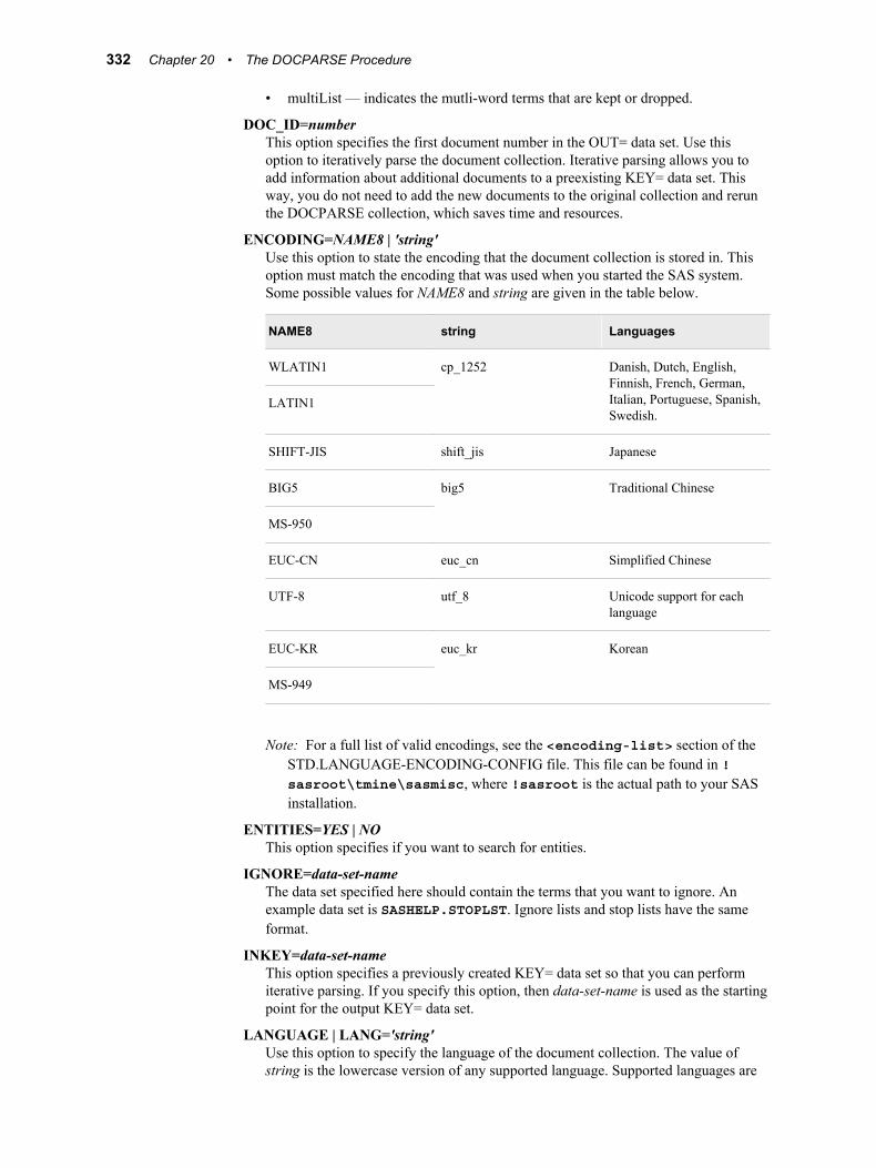
• multiList — indicates the mutli-word terms that are kept or dropped.
DOC_ID=numberThis option specifies the first document number in the OUT= data set. Use this option to iteratively parse the document collection. Iterative parsing allows you to add information about additional documents to a preexisting KEY= data set. This way, you do not need to add the new documents to the original collection and rerun the DOCPARSE collection, which saves time and resources.
ENCODING=NAME8 | 'string'Use this option to state the encoding that the document collection is stored in. This option must match the encoding that was used when you started the SAS system. Some possible values for NAME8 and string are given in the table below.
NAME8 string Languages
WLATIN1 cp_1252 Danish, Dutch, English, Finnish, French, German, Italian, Portuguese, Spanish, Swedish.
LATIN1
SHIFT-JIS shift_jis Japanese
BIG5 big5 Traditional Chinese
MS-950
EUC-CN euc_cn Simplified Chinese
UTF-8 utf_8 Unicode support for each language
EUC-KR euc_kr Korean
MS-949
Note: For a full list of valid encodings, see the <encoding-list> section of the STD.LANGUAGE-ENCODING-CONFIG file. This file can be found in !sasroot\tmine\sasmisc, where !sasroot is the actual path to your SAS installation.
ENTITIES=YES | NOThis option specifies if you want to search for entities.
IGNORE=data-set-nameThe data set specified here should contain the terms that you want to ignore. An example data set is SASHELP.STOPLST. Ignore lists and stop lists have the same format.
INKEY=data-set-nameThis option specifies a previously created KEY= data set so that you can perform iterative parsing. If you specify this option, then data-set-name is used as the starting point for the output KEY= data set.
LANGUAGE | LANG='string'Use this option to specify the language of the document collection. The value of string is the lowercase version of any supported language. Supported languages are
332 Chapter 20 • The DOCPARSE Procedure
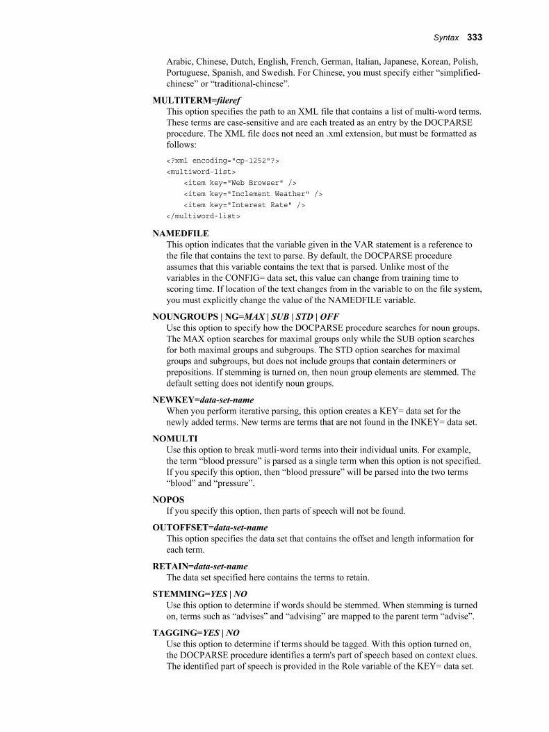
Arabic, Chinese, Dutch, English, French, German, Italian, Japanese, Korean, Polish, Portuguese, Spanish, and Swedish. For Chinese, you must specify either “simplified-chinese” or “traditional-chinese”.
MULTITERM=filerefThis option specifies the path to an XML file that contains a list of multi-word terms. These terms are case-sensitive and are each treated as an entry by the DOCPARSE procedure. The XML file does not need an .xml extension, but must be formatted as follows:
<?xml encoding="cp-1252"?><multiword-list> <item key="Web Browser" /> <item key="Inclement Weather" /> <item key="Interest Rate" /></multiword-list>
NAMEDFILEThis option indicates that the variable given in the VAR statement is a reference to the file that contains the text to parse. By default, the DOCPARSE procedure assumes that this variable contains the text that is parsed. Unlike most of the variables in the CONFIG= data set, this value can change from training time to scoring time. If location of the text changes from in the variable to on the file system, you must explicitly change the value of the NAMEDFILE variable.
NOUNGROUPS | NG=MAX | SUB | STD | OFFUse this option to specify how the DOCPARSE procedure searches for noun groups. The MAX option searches for maximal groups only while the SUB option searches for both maximal groups and subgroups. The STD option searches for maximal groups and subgroups, but does not include groups that contain determiners or prepositions. If stemming is turned on, then noun group elements are stemmed. The default setting does not identify noun groups.
NEWKEY=data-set-nameWhen you perform iterative parsing, this option creates a KEY= data set for the newly added terms. New terms are terms that are not found in the INKEY= data set.
NOMULTIUse this option to break mutli-word terms into their individual units. For example, the term “blood pressure” is parsed as a single term when this option is not specified. If you specify this option, then “blood pressure” will be parsed into the two terms “blood” and “pressure”.
NOPOSIf you specify this option, then parts of speech will not be found.
OUTOFFSET=data-set-nameThis option specifies the data set that contains the offset and length information for each term.
RETAIN=data-set-nameThe data set specified here contains the terms to retain.
STEMMING=YES | NOUse this option to determine if words should be stemmed. When stemming is turned on, terms such as “advises” and “advising” are mapped to the parent term “advise”.
TAGGING=YES | NOUse this option to determine if terms should be tagged. With this option turned on, the DOCPARSE procedure identifies a term's part of speech based on context clues. The identified part of speech is provided in the Role variable of the KEY= data set.
Syntax 333
START=data-set-nameThe data set specified here contains the terms to include in your analysis. The keep status of a term in a start list is always Y.
STOP=data-set-nameThe data set specified here contains the terms to exclude from your analysis. These terms are displayed in the KEY= data set with a keep status of N. They are not identified as parents or children.
SYN=data-set-nameThe data set specified here contains parent-child relationships. This data set must have the three variables TERM, PARENT, and CATEGORY or the four variables TERM, PARENT, TERMROLE, and PARENTROLE. You can use this option with or without stemming, but this list overrides any relationships that are identified when terms are stemmed.
SELECT Statement
SyntaxSELECT <options>;
The SELECT statement enables you to specify the parts of speech or attributes that you want to include in or exclude from your analysis. You can use the SELECT statement to keep specified entities, but not to drop them. For an example of how to apply this statement, see “Example 5: The SELECT Statement” on page 338 .
Optional Arguments“pos1” ... “posN” / <GROUP=“ENTITIES” | “ATTRIBUTES”> keep | drop
With the SELECT statement, you identify a group of parts of speech, a group of entities, or a group of attributes and state whether they are dropped from or kept in your analysis. The labels pos1, ..., posN can be parts of speech, entities, or attributes. If they are entities or attributes, you need to specify the corresponding GROUP argument. You do not need to specify the GROUP argument if the labels are parts of speech. Finally, specify if you want to keep or drop the identified labels.
The parts of speech that you can use are as follows:
• ABBR — abbreviations
• ADJ — adjectives
• ADV — adverbs
• AUX — auxiliary or modal terms
• CONJ — conjunctions
• DET — determiners
• INTERJ — interjections
• NOUN — nouns
• NUM — numbers or numeric expressions
• PART — infinitive markers, negative participles, or possessive markers
• PREF — prefixes
• PREP — prepositions
334 Chapter 20 • The DOCPARSE Procedure
• PRON — pronouns
• PROP — proper nouns
• PUNCT — punctuation
• VERB — verbs
• VERBADJ — verb adjectives
The entities that you can use are as follows:
• ADDRESS — postal address or number and street name
• COMPANY — company name
• CURRENCY — currency or currency expression
• DATE — date, day, month, or year
• INTERNET — e-mail address or URL
• LOCATION — city, county, state, political or geographical place or region,
• MEASURE — measurement or measurement expression
• ORGANIZATION — government, legal, or service agency
• PERCENT — percentage or percentage expression
• PERSON — person's name
• PHONE — phone number
• PROP_MISC — proper noun with an ambiguous classification
• TIME — time or time expression
• TIME_PERIOD — measure of time expressions
• TITLE — person's title or position
• VEHICLE — motor vehicle, including color, year, make, and model
The attributes that you can use are as follows:
• ALPHA — only letters
• NUM — only numbers
• PUNCT — punctuation characters
• MIXED — combination of letters, numbers, and punctuation
VAR Statement
SyntaxVAR variable;
Required Argumentvariable
This argument specifies the variable that contains the text that you want to process.
Syntax 335
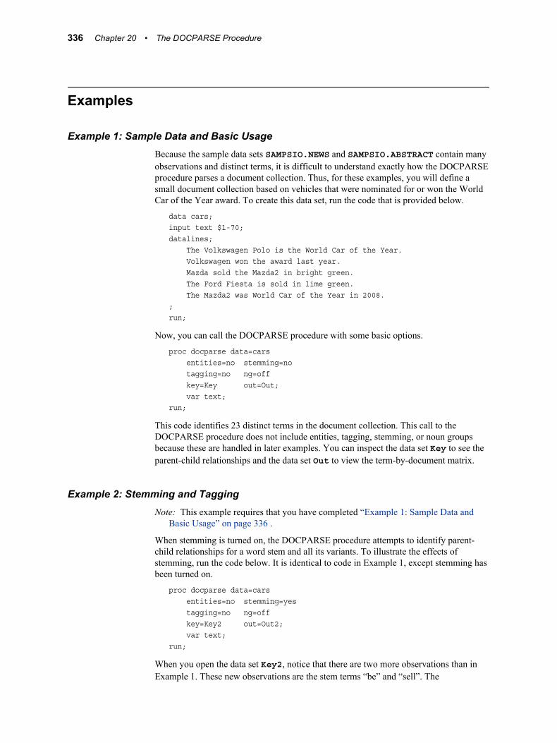
Examples
Example 1: Sample Data and Basic UsageBecause the sample data sets SAMPSIO.NEWS and SAMPSIO.ABSTRACT contain many observations and distinct terms, it is difficult to understand exactly how the DOCPARSE procedure parses a document collection. Thus, for these examples, you will define a small document collection based on vehicles that were nominated for or won the World Car of the Year award. To create this data set, run the code that is provided below.
data cars;input text $1-70;datalines; The Volkswagen Polo is the World Car of the Year. Volkswagen won the award last year. Mazda sold the Mazda2 in bright green. The Ford Fiesta is sold in lime green. The Mazda2 was World Car of the Year in 2008.;run;
Now, you can call the DOCPARSE procedure with some basic options.
proc docparse data=cars entities=no stemming=no tagging=no ng=off key=Key out=Out; var text;run;
This code identifies 23 distinct terms in the document collection. This call to the DOCPARSE procedure does not include entities, tagging, stemming, or noun groups because these are handled in later examples. You can inspect the data set Key to see the parent-child relationships and the data set Out to view the term-by-document matrix.
Example 2: Stemming and TaggingNote: This example requires that you have completed “Example 1: Sample Data and
Basic Usage” on page 336 .
When stemming is turned on, the DOCPARSE procedure attempts to identify parent-child relationships for a word stem and all its variants. To illustrate the effects of stemming, run the code below. It is identical to code in Example 1, except stemming has been turned on.
proc docparse data=cars entities=no stemming=yes tagging=no ng=off key=Key2 out=Out2; var text;run;
When you open the data set Key2, notice that there are two more observations than in Example 1. These new observations are the stem terms “be” and “sell”. The
336 Chapter 20 • The DOCPARSE Procedure
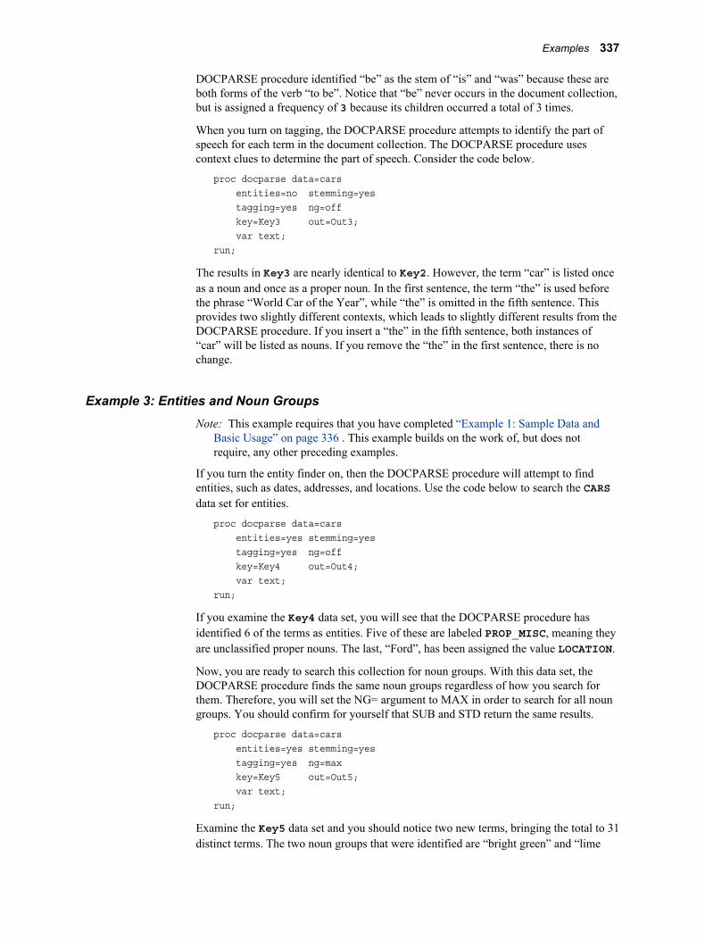
DOCPARSE procedure identified “be” as the stem of “is” and “was” because these are both forms of the verb “to be”. Notice that “be” never occurs in the document collection, but is assigned a frequency of 3 because its children occurred a total of 3 times.
When you turn on tagging, the DOCPARSE procedure attempts to identify the part of speech for each term in the document collection. The DOCPARSE procedure uses context clues to determine the part of speech. Consider the code below.
proc docparse data=cars entities=no stemming=yes tagging=yes ng=off key=Key3 out=Out3; var text;run;
The results in Key3 are nearly identical to Key2. However, the term “car” is listed once as a noun and once as a proper noun. In the first sentence, the term “the” is used before the phrase “World Car of the Year”, while “the” is omitted in the fifth sentence. This provides two slightly different contexts, which leads to slightly different results from the DOCPARSE procedure. If you insert a “the” in the fifth sentence, both instances of “car” will be listed as nouns. If you remove the “the” in the first sentence, there is no change.
Example 3: Entities and Noun GroupsNote: This example requires that you have completed “Example 1: Sample Data and
Basic Usage” on page 336 . This example builds on the work of, but does not require, any other preceding examples.
If you turn the entity finder on, then the DOCPARSE procedure will attempt to find entities, such as dates, addresses, and locations. Use the code below to search the CARS data set for entities.
proc docparse data=cars entities=yes stemming=yes tagging=yes ng=off key=Key4 out=Out4; var text;run;
If you examine the Key4 data set, you will see that the DOCPARSE procedure has identified 6 of the terms as entities. Five of these are labeled PROP_MISC, meaning they are unclassified proper nouns. The last, “Ford”, has been assigned the value LOCATION.
Now, you are ready to search this collection for noun groups. With this data set, the DOCPARSE procedure finds the same noun groups regardless of how you search for them. Therefore, you will set the NG= argument to MAX in order to search for all noun groups. You should confirm for yourself that SUB and STD return the same results.
proc docparse data=cars entities=yes stemming=yes tagging=yes ng=max key=Key5 out=Out5; var text;run;
Examine the Key5 data set and you should notice two new terms, bringing the total to 31 distinct terms. The two noun groups that were identified are “bright green” and “lime
Examples 337
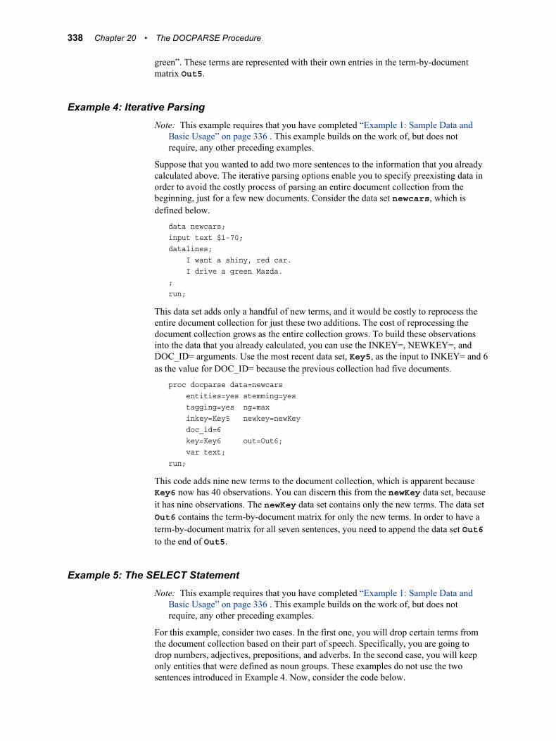
green”. These terms are represented with their own entries in the term-by-document matrix Out5.
Example 4: Iterative ParsingNote: This example requires that you have completed “Example 1: Sample Data and
Basic Usage” on page 336 . This example builds on the work of, but does not require, any other preceding examples.
Suppose that you wanted to add two more sentences to the information that you already calculated above. The iterative parsing options enable you to specify preexisting data in order to avoid the costly process of parsing an entire document collection from the beginning, just for a few new documents. Consider the data set newcars, which is defined below.
data newcars;input text $1-70;datalines; I want a shiny, red car. I drive a green Mazda.;run;
This data set adds only a handful of new terms, and it would be costly to reprocess the entire document collection for just these two additions. The cost of reprocessing the document collection grows as the entire collection grows. To build these observations into the data that you already calculated, you can use the INKEY=, NEWKEY=, and DOC_ID= arguments. Use the most recent data set, Key5, as the input to INKEY= and 6 as the value for DOC_ID= because the previous collection had five documents.
proc docparse data=newcars entities=yes stemming=yes tagging=yes ng=max inkey=Key5 newkey=newKey doc_id=6 key=Key6 out=Out6; var text;run;
This code adds nine new terms to the document collection, which is apparent because Key6 now has 40 observations. You can discern this from the newKey data set, because it has nine observations. The newKey data set contains only the new terms. The data set Out6 contains the term-by-document matrix for only the new terms. In order to have a term-by-document matrix for all seven sentences, you need to append the data set Out6 to the end of Out5.
Example 5: The SELECT StatementNote: This example requires that you have completed “Example 1: Sample Data and
Basic Usage” on page 336 . This example builds on the work of, but does not require, any other preceding examples.
For this example, consider two cases. In the first one, you will drop certain terms from the document collection based on their part of speech. Specifically, you are going to drop numbers, adjectives, prepositions, and adverbs. In the second case, you will keep only entities that were defined as noun groups. These examples do not use the two sentences introduced in Example 4. Now, consider the code below.
338 Chapter 20 • The DOCPARSE Procedure
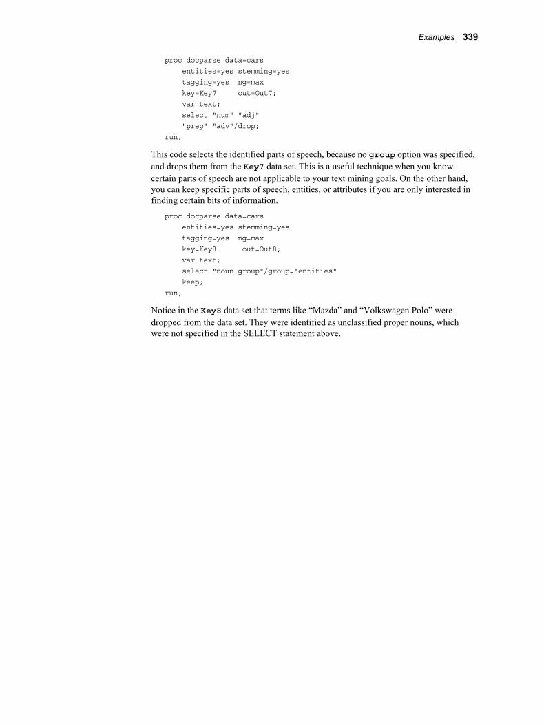
proc docparse data=cars entities=yes stemming=yes tagging=yes ng=max key=Key7 out=Out7; var text; select "num" "adj" "prep" "adv"/drop;run;
This code selects the identified parts of speech, because no group option was specified, and drops them from the Key7 data set. This is a useful technique when you know certain parts of speech are not applicable to your text mining goals. On the other hand, you can keep specific parts of speech, entities, or attributes if you are only interested in finding certain bits of information.
proc docparse data=cars entities=yes stemming=yes tagging=yes ng=max key=Key8 out=Out8; var text; select "noun_group"/group="entities" keep;run;
Notice in the Key8 data set that terms like “Mazda” and “Volkswagen Polo” were dropped from the data set. They were identified as unclassified proper nouns, which were not specified in the SELECT statement above.
Examples 339

340 Chapter 20 • The DOCPARSE Procedure
Chapter 21
The EMCLUS Procedure
Overview . . . . . . . . . . . . . . . . . . . . . . . . . . . . . . . . . . . . . . . . . . . . . . . . . . . . . . . . . . . 341The EMCLUS Procedure . . . . . . . . . . . . . . . . . . . . . . . . . . . . . . . . . . . . . . . . . . . . 341
Syntax . . . . . . . . . . . . . . . . . . . . . . . . . . . . . . . . . . . . . . . . . . . . . . . . . . . . . . . . . . . . . . 342The EMCLUS Procedure . . . . . . . . . . . . . . . . . . . . . . . . . . . . . . . . . . . . . . . . . . . . 342PROC EMCLUS Statement . . . . . . . . . . . . . . . . . . . . . . . . . . . . . . . . . . . . . . . . . . 342CODE Statement . . . . . . . . . . . . . . . . . . . . . . . . . . . . . . . . . . . . . . . . . . . . . . . . . . 344INITCLUS Statement . . . . . . . . . . . . . . . . . . . . . . . . . . . . . . . . . . . . . . . . . . . . . . . 346VAR Statement . . . . . . . . . . . . . . . . . . . . . . . . . . . . . . . . . . . . . . . . . . . . . . . . . . . . 346
Details . . . . . . . . . . . . . . . . . . . . . . . . . . . . . . . . . . . . . . . . . . . . . . . . . . . . . . . . . . . . . . 346The EMCLUS Procedure . . . . . . . . . . . . . . . . . . . . . . . . . . . . . . . . . . . . . . . . . . . . 346Data Summarization Phases . . . . . . . . . . . . . . . . . . . . . . . . . . . . . . . . . . . . . . . . . . 347Output . . . . . . . . . . . . . . . . . . . . . . . . . . . . . . . . . . . . . . . . . . . . . . . . . . . . . . . . . . . 348Removing Outliers from Clusters . . . . . . . . . . . . . . . . . . . . . . . . . . . . . . . . . . . . . . 348
Examples . . . . . . . . . . . . . . . . . . . . . . . . . . . . . . . . . . . . . . . . . . . . . . . . . . . . . . . . . . . 349Example 1: Basic Usage . . . . . . . . . . . . . . . . . . . . . . . . . . . . . . . . . . . . . . . . . . . . . 349Example 2: The Scaled EM Algorithm . . . . . . . . . . . . . . . . . . . . . . . . . . . . . . . . . 349Example 3: Dealing with Outliers . . . . . . . . . . . . . . . . . . . . . . . . . . . . . . . . . . . . . 350
Overview
The EMCLUS ProcedureThe EMCLUS procedure clusters a data set with either the Expectation-Maximum (standard EM) algorithm or a scalable version of the EM algorithm (scaled EM). The standard EM algorithm will run without issue if the entire input data set fits in memory. The scaled EM algorithm runs when the input data set does not fit in memory. The scaled EM algorithm was designed for very large data sets and requires a random sample to return valid results. The effectiveness of the EMCLUS procedure depends on the initial parameter estimates. Because good inputs result in faster convergence and better results, you can refine your initial estimates with repeated calls to the EMCLUS procedure.
341
Syntax
The EMCLUS ProcedurePROC EMCLUS DATA=data-set-name CLUSTERS=number <options>;
CODE <options>;INITCLUS <list-of-integers>;VAR <variables>;RUN;
PROC EMCLUS Statement
SyntaxPROC EMCLUS DATA=data-set-name CLUSTERS=number <options>;
Required ArgumentsDATA | IN=data-set-name
This argument specifies the name of the input data set. All variables in this data set must be numeric and missing data is ignored.
Note: Strictly speaking, this argument is not required, but should be included. If the DATA= argument is omitted, then the most recently created data set is used for analysis.
CLUSTERS=numberThis argument specifies the number of primary clusters.
Optional ArgumentsCLEAR=number
After number iterations, the EMCLUS procedure will delete any observations that remain in memory after the secondary summarization phase. The value of number can be any nonnegative integer. The default value of zero does not delete any observations from memory. You must specify METHOD=SCALED to use this option.
COV=DIAG | ONEDIAG | FULL | ONEFULLThis option specifies the type of covariance matrix that is used to model the primary clusters. The DIAG and FULL options use a different covariance matrix to model each primary cluster. The ONEDIAG and ONEFULL options use the same covariance matrix to model every primary cluster. The default value is DIAG.
DECVAR=numberThis option specifies the proportion to decrease the initial variances by when you use the option OUTLIERS=CLUSTER. The value of number must be between 0 and 1. For more information about how outliers are handled, see “Removing Outliers from Clusters” on page 348 .
DIST=numberThe value of number is the minimum distance that is allowed between initial clusters when you use random initial estimates. This value is also used as the minimum
342 Chapter 21 • The EMCLUS Procedure
distance between the initial cluster means in the secondary summarization phase. The value of number must be a nonnegative number. The default value is the square root of the average of the sample variances that are obtained during the first iteration.
EPS=numberUse this option to specify the tolerance. The EMCLUS procedure terminates when two successive iterations differ by less than the value of number. The default value is 10-6.
INIT=RANDOM | FASCLUS | EMCLUSUse this option to specify how the initial estimates are obtained. If either the FASTCLUS or EMCLUS option is used, then the SEEDS= option must also be specified. The FASTCLUS option requires the OUTSEEDS= data set from the FASTCLUS procedure. The EMCLUS option requires the OUTSTAT= data set from the EMCLUS procedure. The default is RANDOM.
INITSTD=numberThis option specifies the maximum standard deviation of the initial clusters. This option does not affect the last primary cluster when you cluster the outliers. The value of number must be positive. The default value is determined from a sample of the data that is obtained during the first iteration.
ITER=numberThe EMCLUS procedure updates the model parameters every number iterations. The value of number must be a positive integer. The default value is 50.
MAXITER=numberThe EMCLUS procedure will run at most number iterations before it quits. This option should be used only with the scaled EM algorithm. The value of number must be a positive integer. The default value is the largest integer available to the machine.
METHOD=STANDARD | SCALEDUse this option to select either the standard EM algorithm or the scaled EM algorithm.
MIN=numberThis option specifies the minimum number of observations allowed in each primary cluster. This value must be a nonnegative integer. At any iteration, if the total number of observations in a cluster is less than number, then the cluster becomes inactive. A cluster can be reseeded at a more appropriate point, if one exists. This option should only be used with the scaled EM algorithm. The default value is 3.
NOBS=numberThis option specifies how many observations are used for each iteration. The value of number must be a positive integer. This option should only be used with the scaled EM algorithm. The default value is all observations in the data set. But, if this value cannot be determined, then the EMCLUS procedure uses 500 observations.
OUT=data-set-nameThis data set contains the original information along with the probability that each observation will be in a given cluster. Let k be the number of clusters and h=1...k. This data set contains the k variables PROB_h, which is the probability that an observation is in cluster h. The default name for this data set is data_n, where n is the smallest integer not already used to name a data set.
OUTLIERS=CLUSTER | IGNORE | KEEPThis option specifies how the EMCLUS procedure treats outliers. The CLUSTER option creates a large initial cluster that contains all the outliers. With the IGNORE option, observations that are not in the 99th percentile of any estimated primary cluster are weighted less. If the KEEP option is used, these observations are treated
Syntax 343
like every other observation. For more information about outliers, see “Removing Outliers from Clusters” on page 348 .
OUTSTAT=data-set-nameThis option specifies the output data set. This data set contains five more columns than there are variables in the input data set. The extra columns provide the cluster number, cluster type, cluster frequency, estimate of the weight parameter, and type of statistic (mean or variance). The final columns contain either the mean or the variance for each of the original variables.
P=numberThe value of number specifies the radius around each cluster mean. Any point that lies inside of this radius is summarized by that cluster. The value of number must be between 0 and 1. This option should be used only with the scaled EM algorithm. The default value is 0.5.
PRINT=ALL | LAST | NONEUse this option to control the output of the EMCLUS procedure. The ALL option prints every iteration to the output window. The LAST option, which is the default setting, prints only the last iteration to the output window. The NONE option does not print any iterations to the output window.
ROLE=TRAIN | SCOREThis option specifies the role of the input data set. Use the TRAIN option to cluster the data set and the SCORE option to compute the probabilities that each observation is in each primary cluster. When the SCORE option is used, the SEED= argument must specify the OUTSTAT= data set that was created when the original data was clustered. Also, when you score a data set, you must use the same setting in the COV argument as when you trained the data. The default behavior uses the TRAIN option.
SECCLUS=numberThis option specifies the number of secondary clusters that the algorithm will search for during the secondary data summarization phase. The value of number must be nonnegative. If this option is set to 0, then there is no secondary data summarization phase. This option should be used only with the scaled EM algorithm. The default value is twice the number of primary clusters.
SECSTD=numberIf a subset of observations wants to be a secondary cluster, then the maximum allowable standard deviation of any variable in that subset is number. This option should only be used with the scaled EM algorithm. The default value is the smallest sample standard deviation that was obtained during the first iteration.
SEED=data-set-nameThis data set specifies the initial parameter estimates. This argument must be used when either the FASTCLUS or the EMCLUS option is specified in the INIT= argument. Suitable data sets are created by the OUTSEEDS= option in the FASTCLUS procedure or the OUTSTAT= option in the EMCLUS procedure.
CODE Statement
SyntaxCODE <options>;
344 Chapter 21 • The EMCLUS Procedure
Optional ArgumentsCATALOG=catalog-name
This option indicates the catalog where the EMCLUS procedure writes its code. The complete path for the EMCLUS catalog is library.catalog-name.entry.type. The default library is determined by the SAS system, but is usually the WORK library. The default entry is SASCODE and the default type is SOURCE.
DUMMIES | NODUMMIESThis option determines whether dummy variables, standardized variables, and other transformed variables should be kept or dropped.
ERRORSpecify this option to compute the error function, given by the variable E_*.
FILE=file-nameThe EMCLUS procedure will write the code that it generates to the external file specified here. The value of file-name is either a quoted string or an unquoted SAS name.
If you specify a SAS name, there are several things to keep in mind. First, a SAS name is at most eight bytes long. The EMCLUS procedure will print an error if the SAS name is longer than eight bytes. Next, if the name was assigned as a fileref in a FILENAME statement, then the file specified in that statement is opened. If the name is not an assigned fileref, the specified name is concatenated with the .txt extension. The names “LOG” and “PRINT” are reserved by the SAS system.
FORMAT=numberThis option specifies the format for all values that do not have a specified format in the input data set. The value of number must be a positive integer. The default value is BEST20.
GROUP=group-nameThis option specifies the identifier that is used for group processing. The value of group-name must be shorter than 32 bytes.
LINESIZE | LS=numberThis option specifies the length of each line in the generated code. This value must be an integer between 64 and 254. The default value is 72.
LOOKUP=AUTO | BINARY | LINEAR | LINFREQ | SELECTThis option specifies the algorithm that is used to look up CLASS levels.
• AUTO — selects the fastest method that is portable across ASCII and EBCDIC machines for each variable.
• BINARY — uses a binary search. This method is fast, but can produce errors if you generate the code on an ASCII machine and execute the code on an EBCDIC machine, or vice versa. The normalized category values contain characters that collate in different orders on ASCII and EBCDIC machines. The SCORE procedure is unable to translate this code.
• LINEAR — uses a linear search with IF statements. The categories are in the order specified in the DMDB catalog. This method can be slow if there are many categories.
• LINFREQ — uses a linear search with IF statements. However, the categories are in descending order of frequency. This can be faster if the distribution of class frequencies is highly uneven, but slow if there are many categories with nearly equal frequencies.
• SELECT — uses a select statement. This method can be slow if there are many categories.
Syntax 345
RESIDUALSpecify this option to compute the variables that depend on the target variable.
INITCLUS Statement
SyntaxINITCLUS list-of-integers;
Required Argumentlist-of-integers
This option specifies the clusters that are used as initial estimates for the EMCLUS procedure. For example, if you want to use clusters 2, 4–8, and 10 as initial seeds, you can use the statement INITCLUS 2, 4 to 8, 10;. The number of clusters here should not exceed the number of clusters specified with the CLUSTERS= option in the PROC EMCLUS statement. The default value uses all of the clusters when EMCLUS is specified in the INIT argument and the highest frequency clusters when FASTCLUS is specified.
VAR Statement
SyntaxVAR variables;
Required Argumentvariables
Use this option to specify the variables that you want to cluster. If this statement is omitted, then all of the variables in the input data set are used.
Details
The EMCLUS ProcedureThe EMCLUS procedure runs either a full or scaled version of the Expectation-Maximum (EM) algorithm, which groups a data set into a given number of clusters. The scaled EM algorithm requires a primary and a secondary data summarization phase, which are described in the next section. The full version runs the normal EM algorithm, without data summarization. Both algorithms assume that the probability distribution function is f (u, V ) = ∑
kwk ⋅ g(x | u, V ). In this equation, g(x | u, V) is a multivariate
normal distribution with mean u and covariance matrix V, w is some weight, and k is the number of clusters.
The initial parameter estimates have a strong influence on the effectiveness of the EMCLUS procedure. Because the EM algorithm is an iterative scheme, there is no guarantee that the likelihood function will converge. But, good initial estimates will converge to a local maximum of the likelihood function. The EMCLUS procedure can start with either precalculated or random estimates. The precalculated estimates are
346 Chapter 21 • The EMCLUS Procedure
obtained from either the FASTCLUS procedure or the EMCLUS procedure. Initial estimates obtained from the EMCLUS procedure are used to refine the primary clusters.
Both the standard and the scaled EM algorithm can be slow to converge because there are several factors that influence convergence. You can expedite convergence by reducing the value of ITER=, increasing the value of P=, increasing the value of EPS=, or using the CLEAR argument. However, these changes might alter the parameter estimates.
Note: If the variance of a cluster is less than the square root of the tolerance, then a generalized inverse will be used for the inverse of the covariance matrix. In this case, it is not guaranteed that the likelihood function will increase at each iteration of the standard EM algorithm.
Data Summarization PhasesThe scaled EM algorithm was designed for very large data sets and is not a true EM algorithm. As such, the scaled algorithm requires a random sample of the data set. A nonrandom sample will result in very poor results.
The general outline of the scaled EM algorithm is:
1. Read in a sample of the data set.
2. Estimate the model parameters using an algorithm similar to EM.
3. Summarize the data in the primary phase.
4. Summarize the data in the secondary phase.
5. Repeat steps 1–4 until a stopping criterion is met.
The scaled EM algorithm stops if every observation is read, the system is out of memory, a likelihood condition is satisfied, or the maximum number of iterations is reached.
The primary data summarization phase summarizes the observations near each of the primary cluster means and then deletes the summarized observations from memory. For a specified value p0, this phase summarizes all observations within 100*p0% of the volume of the multivariate normal distribution with mean u and covariance matrix V. After this step, the clusters are checked to see if they contain fewer than a given minimum number of observations. A cluster with fewer than the minimum number of observations is deemed inactive and is not used to update the parameter estimates.
An inactive cluster will remain inactive until one of the following conditions occurs:
• The inactive cluster gets reseeded as a secondary cluster that contains the minimum number of observations.
• The inactive cluster gets reseeded because the standard deviation for a variable in an active cluster is too large.
The secondary summarization phase is performed on the observations that exist in memory. This phase uses the k-means clustering algorithm to identify secondary clusters, followed by a hierarchical agglomerative clustering algorithm to combine similar clusters. At the end of the k-means algorithm, each of the secondary clusters are tested to ensure that the standard deviation for each variable is small enough. If it is, then the cluster becomes a secondary cluster.
Note: A secondary cluster is formed from a group of observations only if the memory required to summarize the observations is less than the memory required to keep the
Details 347
observations. Thus, the minimum number of observations in a secondary cluster will vary by platform and data sets.
If you set the option SECCLUS=0, then you will bypass the secondary data summarization phase. However, if you run the scaled EM algorithm, it is not recommended that you skip this phase. The secondary phase acts as a backup method that finds primary clusters when the initial estimates are poor. If there are many outliers in the data set, then a large number of secondary clusters will increase the likelihood that you find clusters. A secondary cluster is disjoint from all other secondary clusters and all primary clusters.
OutputThe output data set contains information about the initial parameter estimates, calculated parameter estimates, sample means, and sample variances for the active primary clusters. The inactive clusters are shown as missing values. The sample means and variances are calculated from the observations summarized by the primary clusters.
The cluster summary table contains the following statistics:
• Current Frequency — This is the number of observations that are summarized in a cluster during the current iteration.
• Total Frequency — This is the cumulative sum of the current frequencies for each cluster.
• Proportion of Data Summarized — This is the total frequency divided by the number of observations.
• Nearest Cluster — This is the closest primary cluster based on the Euclidean distance between the estimated means.
• Distance — This is the Euclidean distance to the nearest cluster.
The iteration summary table contains the following information:
• Log-likelihood — This is the average log-likelihood over all of the observations that are read in.
• Obs read in this iteration — This is the number of observations that are read in at the current iteration.
• Obs read in — This is the cumulative sum of the observations that have been read in.
• Current Summarized — This is the sum of the current frequencies across the primary clusters.
• Total Summarized — This is the sum of the total frequencies across the primary clusters.
• Proportion Summarize — This is the total summarized divided by the number of observations.
If there are secondary clusters, then the sample mean, sample variance, and number of observations for these clusters are displayed after the iteration summary table.
Removing Outliers from ClustersThe argument OUTLIERS=CLUSTER assigns all outliers to the final cluster. This way, they do not interfere with the rest of the clusters. When you use this option, ensure that the variances in the initial clusters are small enough to identify outliers. Otherwise, the
348 Chapter 21 • The EMCLUS Procedure
final cluster will be empty. Inversely, if the variances are too small, the last cluster will contain all of the observations.
Some ways to reduce the initial cluster variance are:
• Specify a value for the INITSTD= option in the PROC EMCLUS statement.
• Choose a larger value for MAXLCUSTERS= argument in the FASTCLUS procedure.
• Choose a value for DECVAR= in the PROC EMCLUS statement
Additionally, you can choose to ignore outliers completely with the OUTLIERS=IGNORE argument. However, when you use this option, you should use the FASTCLUS procedure to obtain the initial estimates. In the call to the FASTCLUS procedure, you need to specify a larger value for MAXCLUSTERS= than you will specify in the CLUSTERS= argument of the EMCLUS procedure.
Examples
Example 1: Basic UsageThe EMCLUS procedure partitions a data set into a defined number of clusters. Minimally, you must provide the EMCLUS procedure with the data set you want to cluster and the number of clusters that you desire. You can choose to seed the clusters with either random seed values or with information learned in a previous call to the EMCLUS procedure. First, run the EMCLUS procedure with random seeds. Because this is the default setting, you do not need to specify the INIT= option.
/* Basic Usage */proc emclus data=sampsio.hmeq out=clusOut clusters=10 outstat=statOut;run;
This call to the EMCLUS procedure creates a data set, clusOut, that contains the original information in SAMPSIO.HMEQ plus new variables. These new variables indicate the probability that each observation is in a given cluster. The OUTSTAT= argument creates the data set that is necessary to seed the EMCLUS procedure with previous information.
/* Run with EMCLUS Seeds */proc emclus data=sampsio.hmeq init=emclus seed=statOut out=seedOut clusters=5; initclus 1 3 5 7 9;run;
In this call, you specify the initial seeds in three places. First, the INIT= argument indicates that the seeds were generated by the EMCLUS procedure. Second, the SEED= argument identifies the data set that contains the seed information. Third, the INITCLUS statement identifies the odd clusters as the only relevant clusters.
Example 2: The Scaled EM AlgorithmBy default, the EMCLUS algorithm performs the full Expectation-Maximum algorithm. However, this algorithm can consume a large amount of system resources. Thus, it may be preferable to use the scaled EM algorithm. With the scaled EM algorithm, there are a number of different options that you can specify. This example only illustrates a few of
Examples 349
these options. First, run the scaled EM algorithm with all observations read in at each iteration.
/* Run the Scaled EM Algorithm */proc emclus data=sampsio.hmeq out=scaleOut method=scaled clusters=10 nobs=5960;run;
This code clusters the HMEQ data set into 10 clusters using the scaled EM algorithm. The results are found in the data set scaleOut and should be similar to those from clusOut in Example 1. In the Log, you will find the values that were used for various options. The code below alters some of these settings.
/* Run the Scaled EM Algorithm */proc emclus data=sampsio.hmeq out=scaleOut2 method=scaled clusters=10 nobs=5960 iter=100 secclus=25 min=50 p=0.3;run;
Here, you raise the maximum number of iterations from 50 to 100, increase the number of secondary clusters from 20 to 25, and require that each cluster contains at least 50 observations. Additionally, you reduce the value of p from 0.5 to 0.3, which affects the number of observations in each cluster. The value of p defines a radius around each cluster mean. An observation must fall inside of this radius to be summarized by that cluster. With a smaller radius, fewer observations are identified into each cluster. Also notice that clusters 1 and 7 did not contain at least 50 observations, and thus were made inactive.
Example 3: Dealing with OutliersThe EMCLUS procedure provides some options that determine how to handle outliers. You can either ignore them entirely, create a cluster for the outliers, or keep them as normal observations. The default setting treats outliers as normal observations, but this example will create a cluster specifically for the outliers.
/* Cluster the Outliers */proc emclus data=sampsio.hmeq out=Outliers clusters=5 outliers=cluster decvar=0.1 method=scaled nobs=5960 iter=200;run;
Here, you create five clusters with the scaled EM algorithm. The fifth cluster is reserved for outliers because the option OUTLIERS=CLUSTER is specified. Additionally, the initial variance is decreased by 10%, because the option DECVAR=0.1 is specified.
350 Chapter 21 • The EMCLUS Procedure
Chapter 22
The SPSVD Procedure
Overview . . . . . . . . . . . . . . . . . . . . . . . . . . . . . . . . . . . . . . . . . . . . . . . . . . . . . . . . . . . 351The SPSVD Procedure . . . . . . . . . . . . . . . . . . . . . . . . . . . . . . . . . . . . . . . . . . . . . . 351Applications in Text Mining . . . . . . . . . . . . . . . . . . . . . . . . . . . . . . . . . . . . . . . . . . 352
Syntax . . . . . . . . . . . . . . . . . . . . . . . . . . . . . . . . . . . . . . . . . . . . . . . . . . . . . . . . . . . . . . 353The SPSVD Procedure . . . . . . . . . . . . . . . . . . . . . . . . . . . . . . . . . . . . . . . . . . . . . . 353PROC SPSVD Statement . . . . . . . . . . . . . . . . . . . . . . . . . . . . . . . . . . . . . . . . . . . . 353COL Statement . . . . . . . . . . . . . . . . . . . . . . . . . . . . . . . . . . . . . . . . . . . . . . . . . . . . 355ENTRY Statement . . . . . . . . . . . . . . . . . . . . . . . . . . . . . . . . . . . . . . . . . . . . . . . . . 356OUTPUT Statement . . . . . . . . . . . . . . . . . . . . . . . . . . . . . . . . . . . . . . . . . . . . . . . . 356ROW Statement . . . . . . . . . . . . . . . . . . . . . . . . . . . . . . . . . . . . . . . . . . . . . . . . . . . 357SAMPLE Statement . . . . . . . . . . . . . . . . . . . . . . . . . . . . . . . . . . . . . . . . . . . . . . . . 358
Examples . . . . . . . . . . . . . . . . . . . . . . . . . . . . . . . . . . . . . . . . . . . . . . . . . . . . . . . . . . . 358Example 1: Compute the Singular Value Decomposition . . . . . . . . . . . . . . . . . . . 358Example 2: Projecting on the Singular Value Decomposition . . . . . . . . . . . . . . . . 359
Further Reading . . . . . . . . . . . . . . . . . . . . . . . . . . . . . . . . . . . . . . . . . . . . . . . . . . . . . 360
Overview
The SPSVD ProcedureThe SPSVD procedure has two main functions. The first is to calculate a truncated singular value decomposition of a large, sparse matrix. The second is to project the rows or columns of a sparse matrix onto the columns of a dense matrix. For input, the SPSVD procedure requires at least a compressed representation of the sparse term-by-document matrix, such as the one created by the DOCPARSE procedure and then reformulated by the TMUTIL procedure. The output of the SPSVD procedure is a truncated singular value decomposition of the input matrix. A truncated singular value decomposition only calculates the first k columns of the singular value decomposition, where k is specified by the user. A singular value decomposition is used to reduce the dimension of the term-by-document matrix, which reveals themes that are present in the document collection.
In general, the value of k must be large enough to capture the meaning of the document collection, yet small enough to ignore the noise. This value can be specified explicitly or recommended by the SPSVD procedure. For information about how the SPSVD procedure recommends the value of k, see the “PROC SPSVD Statement” on page 353 . A value that is between 50 and 200 should work well for a document collection that contains thousands of documents.
351
The SPSVD procedure computes a truncated singular value decomposition of a sparse matrix that is represented as a compressed matrix. The singular value decomposition of a sparse matrix A factors A into three matrices such that A = UΣVT. Additionally, the singular value decomposition requires that the columns of U and V are orthogonal and Σ is a real-valued, diagonal matrix with monotonically decreasing, nonnegative entries. The entries of Σ are called singular values. This structure provides many interesting and important qualities that are discussed in the next section. A truncated singular value decomposition calculates only the first k columns for each matrix U, Σ, and V.
To construct a singular value decomposition, you need to determine the eigenvalues and eigenvectors of both AAT and ATA. The eigenvectors of AAT determine the columns of U and the eigenvectors of ATA determine the columns of V. It can be shown that the eigenvalues of AAT and ATA are identical, and thus only one set needs to be calculated. The square root of the eigenvalues provides the singular values for the matrix Σ. The implementation of such a scheme is more complicated due to the complexities involved in the general calculation of eigenvectors and eigenvalues.
Applications in Text MiningAn important purpose of a singular value decomposition is to reduce a high dimension term-by-document matrix into a low dimension representation that reveals information about the document collection. In general, the columns of the term-by-document matrix Amxn form the coordinates for the document space and the rows form the coordinates of the term space. Each document in the collection is represented as a vector in m-dimensional space and each term as a vector in n-dimensional space. The singular value decomposition captures this same information with a smaller number of basis vectors than would be necessary if you were to analyze A directly.
For example, consider the columns of A, which represent the document space. By construction, the columns of U also reside in m-dimensional space. If U has only one column, the line between that vector and the origin would form the best fit line, in a least squares sense, to the original document space. If U has two columns, then these columns would form the best fit plane to the original document space. In general, the first k columns of U form the best fit k-dimensional subspace for the document space. Thus, you can project the columns of A onto the first k columns of U in order to optimally reduce the dimension of the document space from m to k.
The projection of a document d (one column of A) onto U results in k real numbers defined by the inner product d with each column of U. That is, pi = dTui. With this representation, each document forms a k-dimensional vector that can be considered a theme in the document collection. You can then calculate the Euclidean distance between each document and each column of U to determine the documents that are described by this theme.
In a similar fashion, you can repeat the above procedure with the rows of A and the first k columns of V. This generates a best fit k-dimensional subspace for the term space. This representation is used to group terms into similar clusters. These clusters also represent concepts that are prevalent in the document collection. Thus, the singular value decomposition can be used to cluster both the terms and documents into meaningful representations of the entire document collection.
352 Chapter 22 • The SPSVD Procedure
Syntax
The SPSVD ProcedurePROC SPSVD DATA=data-set-name<options>;
COL variable;ENTRY variable;OUTPUT <options>;ROW variable;SAMPLE <options>;RUN;
PROC SPSVD Statement
SyntaxPROC SPSVD DATA=data-set-name<options>;
Required ArgumentDATA=data-set-name
This argument indicates the primary input data set. This data set must contain the compressed term-by-document matrix, such as the output from the DOCPARSE procedure that has been reformulated by the TMUTIL procedure.
Note: Strictly speaking, this argument is not required, but should be included. If the DATA= argument is omitted, then the most recently created data set is used for analysis.
Optional ArgumentsYou can use the next two arguments to weight the document collection before you conduct the singular value decomposition. For the purposes of these two arguments, let fij be the entry in row i, column j of the term-by-document matrix. The global term weight of term i will be wi and the local cell weight is the function g(x). Thus, the weighted frequency of each term is given by wi*g(fij).
The following notation will be used:
• di is the number of documents term i appears in.
• gi is the global term frequency for term i.
• n is the number of documents in the document collection.
•pij =
f ijgi
GLOBAL=NORMAL | GFIDF | IDF | ENTROPYUse this option to specify a global term weight, wi, to apply to each entry of the input matrix. You can save the weighted matrix with the WGT= option and the global
Syntax 353
weights with the GWGT= option, both in the OUTPUT statement. If the GLOBAL= option is not stated, then the term weight is set to 1.
The available weights are:
• NORMAL — wi =1∑jf ij2
•GFIDF (Global Frequency Inverse Document Frequency) — wi =
gidi
• IDF (Inverse Document Frequency) — wi = log 2( ndi ) + 1•
ENTROPY — wi = 1 + ∑j
pij ⋅ log2(pij)log2(n)
LOCAL=BINARY | LOG | NONESpecify this option to apply the requested cell weight.
The available cell weights are as follows:
•BINARY — g(x) = {1 if f ij ≠ 0
0 if f ij = 0} You can use this option to completely
remove the influence of high frequency terms. With this option, every term in a document is assigned the same count value, regardless of frequency.
• LOG — g(x) = log 2( f ij + 1) This option reduces, but does not eliminate, the influence of high frequency terms by applying the log function.
• NONE — No cell weight function is applied.
IN_GLOBAL=data-set-nameUse this option as an alternative to the GLOBAL= option. Here, you specify a SAS data set that contains the global weights. Typically, this option is used in conjunction with the GWGT= option in the OUTPUT statement. This approach enables you to apply the same global weights to multiple data sets.
IN_U=data-set-nameThis option specifies the U matrix that is used for a column projection. If this option is used, then the singular value decomposition of the input matrix is not calculated.
IN_S=data-set-nameThis option specifies the Σ matrix that is used for a projection. If this option is used, then the singular value decomposition of the input matrix is not calculated.
IN_V=data-set-nameThis option specifies the V matrix that is used for a row projection. If this option is used, then the singular value decomposition of the input matrix is not calculated.
k=numberThe value of number is the number of columns in the matrices U, V, and Σ. This value is the number of dimensions of the data set after the singular value decomposition is performed. If the value of number is too large for your application, then the SPSVD procedure will run for an unnecessarily long time. This argument is not necessary if either IN_U= or IN_V= is specified. You cannot use this option and MAX_k= at the same time.
MAX_k=numberThe value of number is the maximum value that the SPSVD procedure should return as the recommended value of k. If you use the RES= argument to recommend the
354 Chapter 22 • The SPSVD Procedure
value of k, this option will limit that value to at most number. The SPSVD procedure will attempt to calculate (as opposed to recommend) number dimensions when it performs a singular value decomposition. You cannot use this option and k= at the same time.
p=numberThis option specifies the number of iterations, beyond k, to complete before the procedure restarts. The value of number must be a positive integer. Because the SPSVD procedure uses an iterative factorization method, the amount of memory used and the calculations required by the procedure can grow large enough to slow the procedure. Thus, if the desired results are not calculated to an acceptable accuracy within k+p iterations, the procedure will restart. The SPSVD procedure restarts with much of the same information that it learned in the first k+p iterations.
If you set the value of p too low, then the SPSVD procedure will use less memory, but will restart frequently. Because it takes time to restart the procedure, this might reduce overall performance. Conversely, if the value of p is too large, the procedure will begin to slow due to the number of calculations that are required. If this option is not specified, the default value is the MIN(k, 75).
RES=LOW | MED | HIGHUse this option to specify the recommended number of dimensions (resolution) for the singular value decomposition. A low resolution singular value decomposition will have fewer dimensions than a high resolution singular value decomposition. The second column of the output data set for Σ (entitled KEEP) indicates the recommended number of dimensions because there is a 1 in the rows that are kept.
This option recommends the value of k heuristically based on the amount of variance that is explained by the value of MAX_k= that you specify. Let the value of MAX_k= be N and a singular value decomposition with N dimensions accounts for R% of the total variance. The option HIGH always recommends the maximum number of dimensions; here that is N. The option MED recommends the number of dimensions that will explain (5/6)*R% of the total variance. The option LOW recommends the number of dimensions that will explain (2/3)*R% of the total variance.
TOL=numberThis option specifies the maximum allowable tolerance for the eigenvalues of ATA. Suppose that θ is an eigenvalue estimate and γ is an eigenvector estimate. The SPSVD procedure will terminate when all k sets of θ and γ satisfy ||ATAγ — γθ||2 ≤ number. The default value is 10-6, which is more than adequate for most text mining problems.
COL Statement
SyntaxCOL variable;
Required Argumentvariable
This argument specifies the name of the variable in the input data set that contains the column variable for the compressed term-by-document matrix. If the name of the variable is COL, then this statement is not required. For Text Miner, this variable corresponds to the document index.
Syntax 355
ENTRY Statement
SyntaxENTRY variable;
Required Argumentvaraible
This argument specifies the name of the variable in the input data set that contains the term frequencies for the compressed term-by-document matrix. If the name of the variable is ENTRY, then this statement is not required. For Text Miner, this variable corresponds to the frequency of the term in the document.
OUTPUT Statement
SyntaxOUTPUT <options>;
Optional ArgumentsBIGPRO
Specify this option to indicate that the ROWPRO= and COLPRO= projections should use as much disk space as possible. The default behavior attempts to form these projections in memory. This option enables you to handle the projections for very large input data sets. This option is used in conjunction with either the ROWPRO= option or the COLPRO= option, but not both. When you use this option, the ROWPRO= option requires that the data is sorted by the row variable and the COLPRO= option requires that the data is sorted by the column variable. Two calls must be with the BIGPRO= option in order to get both sets of projections.
U=data-set-nameThis option specifies where to save the calculated U matrix. You cannot use this option if the IN_U= option is also specified.
S=data-set-nameThis option specifies where to save the calculated Σ matrix. You cannot use this option if the IN_S= option is also specified.
V=data-set-nameThis option specifies where to save the calculated V matrix. You cannot use this option if the IN_V= option is also specified.
COLPRO | DOCPRO=data-set-nameThis option specifies the data set that contains the projections of the columns of the input matrix onto the columns of U. If the IN_U= option is used, then that matrix will be used for the projection. Otherwise, U will be calculated from the input data set.
NORMCOL | NORMDOCUse this option to normalize the Euclidean length of the observations in the data set specified by the COLPRO= argument. With the output produced by this option, similarity can be measured with the Euclidean distance instead of the angle between two vectors.
356 Chapter 22 • The SPSVD Procedure
SCALECOL | SCALEDOCSpecify this option to scale the observations in the data set specified by the COLPRO= argument by the inverse of the singular values.
ROWPRO | WORDPRO=data-set-nameThis option specifies the data set that contains the projection of the rows of the input matrix onto the rows of V. If the IN_V= option is used, then that matrix will be used for the projection. Otherwise, V will be calculated from the input data set.
NORMROW | NORMWORDUse this option to normalize the Euclidean length of the observations in the data set specified by the ROWPRO= argument. With the output produced by this option, similarity can be measured with the Euclidean distance instead of the angle between two vectors.
SCALEROW | SCALEWORDSpecify this option to scale the observations in the data set specified by the ROWPRO argument by the inverse of the singular values.
NORMALLUse this option to normalize the observations in both of the data sets specified by COLPRO= and ROWPRO=. Similarity between term or document vectors is usually measured with the angle between the vectors. But, once normalized, the Euclidean distance can be used to compare the similarity of two vectors.
SCALEALLSpecify this option to scale the observations in both of the data sets specified by COLPRO= and ROWPRO=. Let pij be the ith coordinate of the projected image of the jth document. Thus pij = aT
j∙vi. If the observations are scaled, pij = aTj ∙ vi ∙ σi, where σi
is the ith singular value (the ith diagonal entry of Σ).
There are two reasons to scale the singular value decomposition. First, when the singular value decomposition is scaled, more weight is given to the uncommon themes that are present in the document collection. Second, if either the terms or the documents, but not both, are scaled and both are placed in the same space, then the terms and documents that are highly correlated are more likely to be near each other.
WGT=data-set-nameThis option specifies the name of the weighted term-by-document matrix that is generated when either of the LOCAL= or GLOBAL= arguments are used. You can specify those arguments without the WGT= option, but the weighted matrix will not be saved. If the WGT= option is specified and COLPRO=, ROWPRO=, U=, S=, and V= are not specified, then the weighted matrix is written and no other calculations are performed.
GWGT=data-set-nameThis option specifies the data set that contains the calculated global weights. You can apply these weights to other data sets with the IN_GLOBAL= argument. This option must be used in conjunction with the GLOBAL= option.
ROW Statement
SyntaxROW variable;
Syntax 357
Required Argumentvariable
This argument specifies the name of the variable in the input data set that contains the row variable for the compressed term-by-document matrix. If the name of the variable is ROW, then this statement is not required. For Text Miner, this variable corresponds to the term index.
SAMPLE Statement
SyntaxSAMPLE <options>;
Optional ArgumentsALLOW
For very large problems or in low memory conditions, this option indicates that the SPSVD procedure can take a sample of documents in the input data set. In these situations, a sample might be necessary in order for the computation to succeed. When a sample is taken, a note is written to the log that indicates the percent of the documents that were chosen for the computation. The selection is done by a random sample of all input documents.
NOIf you specify this option, then the SPSVD procedure is not allowed to take a sample of the data. This is the default behavior when the SAMPLE statement is not specified.
RATE=numberWhen used in conjunction with the ALLOW option, this option indicates the sampling rate that is used by the SPSVD procedure. The value of number must be between 0 and 1.
SEED=numberThis option indicates the initial seed for the random number generator. When this option is not used, the seed is chosen from the system clock and reported to the log.
Examples
Example 1: Compute the Singular Value DecompositionFor the examples in this chapter, you will compute the singular value decomposition on the term-by-document matrix for the SAMPSIO.ABSTRACT data set. This data set contains the titles and abstracts for over 1200 research papers. Before you can calculate the singular value decomposition, you need to generate the compressed term-by-document matrix with the DOCPARSE procedure. You can use the following code to generate this matrix.
/* Parse the document collection */proc docparse data=sampsio.abstract out=parseOut key=parseKey stemming=yes tagging=no entities=no ng=std
358 Chapter 22 • The SPSVD Procedure
stop=sashelp.engstop buildindex=yes; var text; select "aux" "conj" "det" "interj" "part" "prep" "pron" "Newline" "Num" "Punct"/drop;run;
Once the ABSTRACT data set has been parsed, it is almost ready for the SPSVD procedure. The TMUTIL procedure reformulates the OUT data set from the DOCPARSE procedure. It removes the child occurrences and attributes their frequencies to their parent terms. It also correctly sorts the data set for the SPSVD procedure.
/* Run the TMUTIL Procedure */proc tmutil data=parseOut key=parseKey; control init release; output out=spsvdIn;run;
Now you are ready to compute the singular value decomposition on the data set spsvdTrain. In the code below, you will apply entropy-binary weighting to the term-by-document matrix. Also, this code specifies a maximum value of 75 for k and a value of 50 for p. Because the DOCPARSE procedure does not use the variable names ROW, COL, and ENTRY, you need to specify the ROW, COL, and ENTRY statements. As output, this code saves the singular value decomposition in U=, S=, and V=; the weighted term-by-document matrix in weights; and the global weights in gWeight.
/* Compute the SVD */proc spsvd data=spsvdIn global=entropy local=binary max_k=75 res=med p=50; row _termnum_; col _document_; entry _count_; output U=U S=S V=V WGT=weights GWGT=gWeight;run;
You are now ready to project the information in the ABSTRACT data set onto the singular value decomposition.
Example 2: Projecting on the Singular Value DecompositionNote: This example assumes that you have completed “Example 1: Compute the
Singular Value Decomposition” on page 358 .
With the data sets that you calculated in Example 1, you are ready to compute the row and column projections. Because you saved the weighted term-by-document matrix, you can submit that matrix in the DATA= argument. This way, you do not need to recalculate the local or global weights, which saves time. Also, this matrix has the proper variable names, so you do not need to include the ROW, COL, or ENTRY statements. The code below provides the SPSVD procedure with the weighted term-by-document matrix, U matrix, S matrix, and V matrix that were computed in the previous example.
/*Project onto the Data */proc spsvd data=weights IN_U=U IN_S=S IN_V=V; output normall colpro=docProj
Examples 359
rowpro=termProj;run;
The data sets docProj and termProj contain the normalized column and row projections, respectively, for the weighted term-by-document matrix. You can use the information in these projections to extract knowledge about the most important terms and documents in the collection.
Further ReadingIf you are interested in learning more about the statistics behind the SPSVD procedure, you should consider the following resources:
• M.W. Berry and M. Browne, Understanding Search Engines: Mathematical Modeling and Text Retrieval (Philadelphia, PA: SIAM, 1999)
• S. Deerwester et al., “Indexing by Latent Semantic Analysis,” Journal of the American Society for Information Science 41(6) (1990): 391–407.
• L.N. Trefethen and D. Bau, Numerical Linear Algebra (Philadelphia, PA: SIAM, 1997)
• D.S. Watkins, Fundamentals of Matrix Computations (New York, NY: John Wiley and Sons, 1991)
360 Chapter 22 • The SPSVD Procedure
Chapter 23
The TMBELIEF Procedure
Overview . . . . . . . . . . . . . . . . . . . . . . . . . . . . . . . . . . . . . . . . . . . . . . . . . . . . . . . . . . . 361The TMBELIEF Procedure . . . . . . . . . . . . . . . . . . . . . . . . . . . . . . . . . . . . . . . . . . 361
Syntax . . . . . . . . . . . . . . . . . . . . . . . . . . . . . . . . . . . . . . . . . . . . . . . . . . . . . . . . . . . . . . 362The TMBELIEF Procedure . . . . . . . . . . . . . . . . . . . . . . . . . . . . . . . . . . . . . . . . . . 362PROC TMBELIEF Statement . . . . . . . . . . . . . . . . . . . . . . . . . . . . . . . . . . . . . . . . 362APPLYPRIOR Statement . . . . . . . . . . . . . . . . . . . . . . . . . . . . . . . . . . . . . . . . . . . . 363CLASS Statement . . . . . . . . . . . . . . . . . . . . . . . . . . . . . . . . . . . . . . . . . . . . . . . . . . 363OPTS Statement . . . . . . . . . . . . . . . . . . . . . . . . . . . . . . . . . . . . . . . . . . . . . . . . . . . 364SAVE Statement . . . . . . . . . . . . . . . . . . . . . . . . . . . . . . . . . . . . . . . . . . . . . . . . . . . 367VAR Statement . . . . . . . . . . . . . . . . . . . . . . . . . . . . . . . . . . . . . . . . . . . . . . . . . . . . 367VARHIER Statement . . . . . . . . . . . . . . . . . . . . . . . . . . . . . . . . . . . . . . . . . . . . . . . 368
Details . . . . . . . . . . . . . . . . . . . . . . . . . . . . . . . . . . . . . . . . . . . . . . . . . . . . . . . . . . . . . . 368The TMBELIEF Procedure . . . . . . . . . . . . . . . . . . . . . . . . . . . . . . . . . . . . . . . . . . 368Belief Propagation Models . . . . . . . . . . . . . . . . . . . . . . . . . . . . . . . . . . . . . . . . . . . 369Reparameterized Belief Propagation . . . . . . . . . . . . . . . . . . . . . . . . . . . . . . . . . . . 369Modified Belief Propagation . . . . . . . . . . . . . . . . . . . . . . . . . . . . . . . . . . . . . . . . . 370Optimal Prior Distribution . . . . . . . . . . . . . . . . . . . . . . . . . . . . . . . . . . . . . . . . . . . 370
Examples . . . . . . . . . . . . . . . . . . . . . . . . . . . . . . . . . . . . . . . . . . . . . . . . . . . . . . . . . . . 371Example 1: Preprocessing the Data and Basic Usage . . . . . . . . . . . . . . . . . . . . . . 371Example 2: Incorporating Prior Distributions . . . . . . . . . . . . . . . . . . . . . . . . . . . . 373Example 3: Variable Hierarchies . . . . . . . . . . . . . . . . . . . . . . . . . . . . . . . . . . . . . . 375
Further Reading . . . . . . . . . . . . . . . . . . . . . . . . . . . . . . . . . . . . . . . . . . . . . . . . . . . . . 377
Overview
The TMBELIEF ProcedureThe TMBELIEF procedure uses a hierarchical Bayesian model to analyze a body of documents in the same manner that a human might compose a document. The hierarchical Bayesian model encodes a conditional independence structure among syntactical constructs (terms, sentences, paragraphs, sections, and so on) at the lower levels and among user-assigned categories (author, locale, publisher, and so on) at the higher levels. This approach goes beyond the standard “bag of words” assumption to incorporate distribution and proximity of terms across a document. The hierarchical Bayesian model allows for efficient computation of marginal distributions via the well-known belief propagation algorithm, thus permitting analysis of very large document
361
collections. Additional functionality of the TMBELIEF procedure builds on the underlying model and the marginalization engine to provide further insight into the document set.
Model training and optimization is effectively achieved with the TMBELIEF procedure. The hierarchical model can be automatically pruned to rapidly discover Boolean rules and term associations, called variable hierarchies, indicative of particular documents or higher level groups of documents. The variable hierarchies can be combined with document term probabilities (computed via belief propagation) to arrive at new features that are easier to understand than the standard singular vector-based features. Should a topic warrant closer inspection, Boolean rules can be seeded and grown to further refine and investigate term groups of interest. Also, by allowing flexible incorporation of prior distributions, the TMBELIEF procedure can better refine a document collection. In the empirical Bayes paradigm, optimal priors can be automatically computed from the data, which enhances the discrimination between different categories and reduces the appearance of noise terms.
This functionality is all available inside an interactive procedure. The interactive environment permits efficient refinement of the text mining analysis through rapid feedback on the effects of modifying any of a number of options associated with each argument.
Syntax
The TMBELIEF ProcedurePROC TMBELIEF DATA=data-set-name <options>;
CLASS variables;VAR variable;APPLYPRIOR variables;VARHIER variables <->;SAVE <options>;OPTS <options>;QUIT ;
PROC TMBELIEF Statement
SyntaxPROC TMBELIEF DATA=data-set-name <options>;
See “Example 1: Preprocessing the Data and Basic Usage” on page 371 for an introduction to the PROC TMBELIEF statement.
Required ArgumentDATA=data-set-name
This argument indicates the primary input data set. This data set must contain the variables in the VAR and CLASS statements. Any other variables will be ignored. Each distinct occurrence of a VAR value should appear on a separate line. This means that terms should not be rolled-up to their document counts when analyzing text data. Rows should be sorted by the variables in the CLASS statement.
362 Chapter 23 • The TMBELIEF Procedure
Optional ArgumentsINIT=number
The value given for INIT= scales the degree of parent-child coupling in upward belief propagation. At each upward propagation step, a few iterations of Newton's method are carried out to adjust the ratio of maximum to minimum belief to INIT=. This value given for number should be in the open interval (0, 1). If the input is 0, then it is perturbed slightly to avoid numerical errors. If the input is 1, then it is possible for all terms to be trimmed. The default value is 0.1.
MAXLVL | MAX=numberThis is the maximum level of the Bayesian hierarchy that is of interest. Results for this node level and below will be written to memory. After upward belief propagation, data for nodes beyond this level is immediately discarded. To retain only the root, set MAXLVL=0 or omit the option. Set MAXLVL=1 to save down to the level of the first variable in the CLASS statement. The default value is 0.
Note: In most cases, this option should be specified, but is not necessary.
OUT=data-set-nameThis data set will contain a complete record of the beliefs and any requested variable hierarchies of all the nodes in the Bayesian hierarchy in memory down to the level specified in MAXLVL=. Results are written according to the most recently registered options at the time of exit from the interactive procedure.
RACC=numberThe number provided here is the convergence tolerance for the Newton iterations that are carried out at each upward propagation to adjust the ratio of the maximum to minimum belief to the value given in INIT=. The default value of 1e-4 is acceptable for most applications.
APPLYPRIOR Statement
SyntaxAPPLYPRIOR variables;
Required Argumentlist-of-variables
Use this statement to apply any prior distributions directly to nodes at the levels corresponding to the variables given in the CLASS statement when you compute the final belief. If a node is located at a level included in the APPLYPRIOR statement, then its descendant information is multiplied by the prior distribution to compute the beliefs. This is instead of the default behavior of multiplying by the ancestor information. For more information, see “Modified Belief Propagation” on page 370and “Example 2: Incorporating Prior Distributions” on page 373 .
CLASS Statement
SyntaxCLASS variables;
Note: The CLASS statement is required before any SAVE or QUIT statements are issued.
Syntax 363
Required Argumentlist-of-variables
Here is where you list the variables from the input data set that define the levels of the Bayesian hierarchy. Each variable must be listed separately and in the order in which it appears in the data set. For more information, see “Example 1: Preprocessing the Data and Basic Usage” on page 371 .
OPTS Statement
SyntaxOPTS <options>;
The options listed below are sorted based on which aspect of the procedure they affect. While not required, it is useful to organize the dynamic options in this manner when using the TMBELIEF procedure. However, all options can be specified in any order without affecting the performance of the OPTS statement or the TMBELIEF procedure.
Belief Propagation OptionsThese options affect the operation of the core belief propagation algorithm.
EPS=numberThis option specifies a belief tolerance. Values that are within number of the non-observed value belief are approximated by the non-observed value belief. These values are then trimmed from the node indices.
EXPDOWN=ALL | DESCONLY | ANCONLYThis option controls the downward belief propagation that is performed before writing results. If set to ALL, the final value indices written are formed by merging the parent index with the current index. This can result in large belief value lists. If set to DESCONLY, the beliefs are computed for only those VAR values observed in descendants of the current node. They are not trimmed due to being within the EPS= tolerance in the upward propagation phase. If set to ANCONLY, the beliefs are computed in the current index for only the VAR values in its parent index. The default setting is DESCONLY.
Prior Distribution OptionsThese options permit the specification of manual prior distribution and control the computation of optimal priors that are computed automatically. For an example of how to apply a prior distribution, see “Example 2: Incorporating Prior Distributions” on page 373 .
CLEARPRIUse this option to reset the current prior distribution to a uniform distribution.
KPRIOR=numberUse this option to specify the non-observed prior value. This value is used for any VAR value that is not listed in the PRIOR= data set. The default value for this option is 1.
OPTPRIORWhen this option is included, the TMBELIEF procedure will compute an optimal prior distribution for separating the highest level children in the Bayesian hierarchy. For more information, see “Optimal Prior Distribution” on page 370 .
364 Chapter 23 • The TMBELIEF Procedure
OPTPRIORREG=numberThis option controls the degree to which the prior distribution deviates from a uniform distribution. Valid values for this option are real numbers from 0 to 1. A value of 1 corresponds to full regularization where the optimal solution will be a uniform prior distribution. A value of 0 corresponds to no regularization of the prior distribution. The default value for this option is 0.5.
OPTPRIORTERMS=numberUse this option to determine the maximum number of distinct VAR values used in formulating the optimization problem for computing the prior distribution. The OPTPRIORTERMS values with the highest belief at the root of the Bayesian hierarchy are considered under a nominal uniform prior. The default value is 500.
PRIOR=data-set-nameUse this option to specify the manual prior distribution. The data set should include the variable in the VAR statement to list select terms. Also, it must include the variable PRIOR that gives the value of the prior distribution for those terms. The prior distribution does not need to be normalized.
Variable Hierarchy OptionsThese options affect the construction of variable hierarchies. For an example of how to construct variable hierarchies, see “Example 3: Variable Hierarchies” on page 375 .
ALLOWSEEDSUBS | TOGALLOWSEEDSUBSWhen a SEED= data set is specified, the default behavior is to subset children on the basis of all non-empty VAR values in each row. If this option is included, then the TMBELIEF procedure will try to seed with subsets of the row when variable hierarchy growth is unsuccessful using the entire row. This is a toggle option, which means that each time the token is encountered the previous state is reversed. In the original state, subsets of a row are not allowed.
ALLOWVHREP | TOGALLOWVHREPBy default, the TMBELIEF procedure checks new branches of variable hierarchies to make sure they are not permutations of existing branches. By specifying this option, permutation checking will be disabled, which will save some memory. This is a toggle option, which means that each time the token is encountered the previous state is reversed. In the original state, permutations of existing branches are not allowed.
CLEARVHSThis option will clear any variable hierarchy seed data sets and seed subsequent variable hierarchies with top belief VAR values.
SEED=data-set-nameThis option enables you to specify variable hierarchy seeds for the current node instead of taking the top belief VAR values. The data set specified must have one or more variables that match the format and length of the variable specified in the VAR statement. The variables specified do not need to have the same name. The TMBELIEF procedure will seed a new variable hierarchy with all non-empty VAR values in each row of the data set.
VHMAXCHILD | VHMAXC=numberThis option specifies the number of values with the highest belief that are used at each level of the variable hierarchy to subset the children for the next generation. The default value is 5.
VHMAXLVL | VHMAX=numberThis option specifies the maximum depth of the variable hierarchy. The time and memory requirements of the computations grow exponentially as VHMAXLVL=
Syntax 365

grows linearly. Because of this, avoid selecting a VHMAXLVL= value that is too large. The default value is 2.
VHMINSUP=numberThis is the minimum support required for continued growth of a variable hierarchy. It is expressed as a fraction of the total number of children. For example, if VHMINSUP=0.25, then at least one-quarter of the children of the current node must contain the proposed VAR value for growing the hierarchy. Otherwise, the current branch is terminated. The default value is 0.
VHMINTCHILD | VHMINTC=numberThis option provides another approach to terminating the growth of a variable hierarchy. VHMINTCHILD= specifies the minimum number of children that must contain the proposed VAR value in order to continue growth of the hierarchy. The default value is 2.
Note: If both VHMINSUP= and VHMINTCHILD= are specified, then both criteria must be met to continue the hierarchy.
VHRTMAXCHILD | VHRTMAXC=numberThis option sets a different value for VHMAXCHILD= at the root of the variable hierarchy. Sometimes, it is convenient to use a large number for VHRTMAXCHILD= to seed the variable hierarchy but use a smaller value of VHMAXCHILD= for growth beyond the root. The default value is 5.
Writing OptionsUse these options to control some of the aspects of the way results are written to the output data sets. For an example of how to apply these options, see “Example 3: Variable Hierarchies” on page 375 .
WRITELIMIT | WLIM=numberUse this option to limit the number of VAR values that are written to the output data set for the current node. If specified, then only the WRITELIMIT= values with the highest belief at the current node are written. To resume the default behavior, which is to write all observed values to the data set, specify WRITELIMIT=0.
NOWRITECONST | TOGWRITECONSTBy default, the TMBELIEF procedure writes the belief for all non-observed values at the current node below that node's list of observed belief values. This includes a missing value for the VAR value. Include this option to omit this row. This is a toggle option, which means that each time this token is encountered the previous state is reversed. In the original state, the non-observed value belief is written.
NOWRITEVHBRANCH | TOGWRITEVHBRANCHWhen constructing a variable, the TMBELIEF procedure will include term beliefs after each new VAR value is added to a branch. To disable this behavior, specify this option. For example, the default behavior will return beliefs associated with child subsets that correspond to 'a', 'a,b', and 'a,b,c' for the branch 'a,b,c'. When this option is disabled, only beliefs associated with upward propagation of those children that contain 'a,b,c' are written. This option might be considered when only the VAR values in the variable hierarchy are of interest. This is a toggle option, which means that each time the token is encountered the previous state is reversed. In the original state, the complete variable hierarchy is written.
366 Chapter 23 • The TMBELIEF Procedure
SAVE Statement
SyntaxSAVE <options>;
The SAVE statement is designed to allow for immediate inspection of the beliefs or variable hierarchies at select nodes of interest within an interactive session. This argument is used to request the Bayesian hierarchy nodes through the LVL= and NODES= arguments and to provide an output data set. For examples on how to apply the save statement, see “Example 2: Incorporating Prior Distributions” on page 373 and “Example 3: Variable Hierarchies” on page 375 .
Optional ArgumentsDESCINFO
When this argument is included, only the descendant information (without multiplying by the ancestor or prior distribution) will be applied to the VAR value. When this argument is omitted, descendant information is combined with either the ancestor information or the prior distribution when the VAR value is written.
LVL=numberThis is the Bayesian hierarchy level at which the requested node resides.
NODES=data-set-nameThis data set contains the identifiers for the requested nodes. It should have variables that match those listed in the CLASS statement. The lengths of the text variables also need to match those in the CLASS statement. The data set must have as many variables in it as is requested by the LVL= argument. For example, if LVL=2, then the data set specified in NODES= must have at least the first two variables in the CLASS statement.
Note: If the OUT= data set is specified, then the LVL= argument is required. If the value of LVL= is greater than 0, then the NODES= argument is required.
OUT=data-set-nameThis is the data set where the results are written.
OUTKPRIOR=data-set-nameThe data set specified here will contain the current value of the prior distribution for all VAR values not explicitly listed in the prior distribution data set.
OUTPRIOR=data-set-nameThe data set specified here will contain the current prior distribution so that it can be retrieved for later use.
VAR Statement
SyntaxVAR variable;
Note: The VAR statement is required before any SAVE or QUIT statements are issued.
Syntax 367
Required Argumentvariable
This is the single variable for which marginal probabilities (beliefs) will be computed. Distinct values of this variable are referred to throughout the document as VAR values.
VARHIER Statement
SyntaxVARHIER variables<->;
Required Argumentlist-of-variables
Use this argument to request variable hierarchies. Variable hierarchies can be requested only at the levels specified by the first MAXLVL= variables listed in the CLASS statement. For more information, see “Modified Belief Propagation” on page 370 and “Example 3: Variable Hierarchies” on page 375 .
Optional Argument—
Include a single hyphen in the list of VARHIER variables to request a variable hierarchy at the root of the Bayesian tree.
Details
The TMBELIEF ProcedureThe TMBELIEF procedure uses a novel hierarchical Bayesian model to analyze occurrences of categorical data. The model was developed primarily with textual data in mind, and individual category levels are often referred to as terms. The typical approach to text mining uses the bag-of-words approach. This method creates a large term-by-document matrix and then performs a singular value decomposition to obtain a lower dimensional topic space that summarizes the data. However, the TMBELIEF procedure goes beyond this approach and attempts to create topics and analyze a document set based on the way that a person might create a document.
Typically, a document is composed by first selecting a general topic that will guide the rest of the writing. With this overarching theme in mind, most writers will select smaller, supportive topics for each chapter or paragraph. These subtopics are used to guide the diction and word choice for individual sentences. Because a writer wants to make specific arguments, the location and choice of words is deliberate and can be a valuable tool in document analysis.
The TMBELIEF procedure attempts to capture the idea of hierarchical composition, exploit co-localization of terms, and inspect word order to produce results that are easy to interpret. The Belief Propagation model organizes the document terms into successively coarser groups (also called nodes) that are typically determined by punctuation. More general document categories are used to determine higher level groups. This allows parent-child relationships to be defined explicitly. For example, a
368 Chapter 23 • The TMBELIEF Procedure
single paragraph, which determines a parent node, might contain several sentences, which are the children of that node. Each group is then summarized by a single term.
Belief Propagation ModelsThe parent-child dependence model is given as follows:
Pt | τij (u | ν) = { β ij if u = ν
1 − β ij
N − 1 if u ≠ ν
Here, t is the child node summary term, τ is the parent node summary term, u and ν are terms in the vocabulary set V, and N ≡ |V| is the cardinality of the vocabulary set. The coupling parameter βij depends on the parent j of a sibling group in the Bayesian hierarchy (the same value for all children of a single parent) and the order of child i with respect to its siblings (varies for different children of the same parent). A reasonable method to determine βij is provided in “Reparameterized Belief Propagation” on page 369 , but you can assume that it is given for now. Note that βij is in [1/N, 1], where the lower bound corresponds to independence of the parent and child summary terms and the upper bound corresponds to equality of the summary terms with probability 1.
The next step is to develop the belief propagation equations that are applied to the parent-child dependence model. While the general belief propagation framework is left in Pearl (1988), some of his notation is adopted. The information from descendants of a node is λ, and information from its ancestors is π (not to be confused with the prior probabilities). In an effort to avoid messy node indexing, denote the summary term of the current node with t (argument u) and its parent with τ (argument ν). Parent-child messages are subscripted, so that λτ(ν) represents an upward message from a node to its parents about the belief that the parent summary term τ is ν. Similarly, πti(u) is a downward message from a parent node to its ith child about the belief that the child summary term ti is u.
The general belief propagation equations are as follows:
λ(u) = α∏iλti(u)
λτ(ν) = ∑u=1
Nλ(u)Pt |τ(u | ν)
The product on the first line over all the children of the current node and α is an arbitrary scaling constant. The computation complexity associated with these can be reduced drastically with the concept of an observed term. A term u is observed at a given node if there is at least one leaf L descended from the node with PL(u) = 1. That is, u is the summary term of L. It can be shown that descendant information from a given is constant across all non-observed terms. This result means that only local vocabularies that consist of observed terms are maintained.
Reparameterized Belief PropagationThis section develops an illuminating reparameterization of the belief propagation equations. It can be shown that an equivalent representation of the upward and downward belief propagation equations is given as follows:
Details 369
λτ(ν) = (1 − αiα j) + αiα jλ(ν)∑uλ(u)
π(u) = (1 − αiα j) + αiα jπt(u)∑νπt(ν)
Here, both sums are taken over all N terms in the vocabulary. The reparameterization is as follows:
αiα j = 1 −1 − β ij
β ij(N − 1)
This parameterization is convenient because it accomplishes two things. It separates the order dependence part αi and reveals the computation as a simple convex combination between a constant and the fractional value of the corresponding term belief. The order dependence can be chosen directly subject to the constraint that αi ≥ 0 for all children in a sibling group and ∑
iαi is equal to the number of children in the sibling group. Each
scale parameter αj is chosen during the upward propagation phase for each sibling group.
Modified Belief PropagationThe TMBELIEF procedure permits two modifications to the process of belief propagation. The first modification is to allow the substitution of a prior distribution for the ancestor information when summary terms beliefs are computed. This is allowed at any level of the Bayesian hierarchy. Normally, any specified prior distribution is used only to compute the beliefs at the root of the Bayesian hierarchy. Depending on how far down the hierarchy a requested node is, the prior distribution might be diluted to the point where it has a marginal impact on that node. The effect of the prior distribution is significantly stronger when substituted for the ancestor information. Prior distributions are used to help overcome the strong likelihood of noise terms in text data. For information about using a prior distribution, see the “APPLYPRIOR Statement” on page 363 .
The other useful modification allows the children of a node to be pruned in the upward belief propagation phase. This is done with a defined index set I that corresponds to only a subset of the children of the current node. The upward belief propagation is computed only for the children that are elements of i, instead of all of the children, which is the default behavior.
λ(u) = α∏i∈I
λti(u)
This set can be defined by considering only those children with term descendant values exceeding some threshold value for all of the terms in some larger set (possibly the entire document collection). This is implemented with a recursive algorithm that is called when the VARHIER statement is used. The VARHIER variables produced on the output data set correspond to the subset of the children and are considered the defined index set. For more information, see the “VARHIER Statement” on page 368 .
Optimal Prior DistributionIn the presence of noise terms, it is useful to automatically determine a prior distribution that will minimize their importance as summary terms. Normally a prior distribution represents known information rather than information that is obtained by recent
370 Chapter 23 • The TMBELIEF Procedure
estimation. However, it is possible to compute a prior distribution directly from the data in the empirical Bayes paradigm. The approach used in the TMBELIEF procedure separates the beliefs of the root children, which is achieved by minimizing the cosine measure between the root children. This method not only reduces the importance of noise terms, but it also aids in the classification problem when the different root children represent distinct document categories.
Consider the distribution of summary term beliefs as a vector in N dimensional space that represents each root child. A commonly used similarity metric in information retrieval is the cosine measure, which is just the cosine of the angle between two vectors. The desired prior distribution is one that maximizes the average dissimilarity between root child belief vectors, which is equivalent to minimizing the average cosine measure. Nominally, you can assume the non-informative uniform distribution and regularize the optimization by penalizing the negative entropy. This results in the following convex optimization problem:
minπ∈Φ
(1 − λ)Z1∑ua(u)π(u)2 + λZ2∑u
π(u)log (π(u))
Here, Φ represents the probability simplex {x ∈ ℜN | 0 ≽ x ≽ 1, ∑ux(u) = 1}, Z1 and
Z2 are normalization constants to make both terms sum to 1, and λ ∈ 0, 1 is the prior regularization coefficient used to control the effect of the negative entropy penalty. The coefficients a(u) represent the average value of the cosine measure between root children and descendant information.
a(u) ≡ ∑i≠ j
λ i(u)λ j(u)λ i λ j
It can be shown that this is equivalent to the average cosine measure between root children beliefs, if you assume that the prior distribution is applied directly to the root children instead of the ancestor information.
It is often enough to consider distinct values of the optimal prior distribution over only the top Nw terms at the root node. This reduces the dimensionality of the problem and allows for quicker computation of the distribution. The optimization is solved numerically via Newton's method when the OPTPRIOR statement is used. For more information, see the prior distribution options in “OPTS Statement” on page 364 .
Examples
Example 1: Preprocessing the Data and Basic UsageThe TMBELIEF procedure is designed primarily for text analysis; however, it can be used with any categorical or binned interval data. The following examples will illustrate how to use the TMBELIEF procedure with the NEWS data set from the SAMPSIO library. This data set contains news articles about computer graphics, hockey, and medicine. The first step is to parse the document collection with the DOCPARSE procedure.
/* Parse the Document Collection */proc docparse data=sampsio.news key=key out=out stemming=yes tagging=no entities=no ng=off stop=sashelp.engstop
Examples 371
addsentence addparent addoffset; var text; select "aux" "conj" "det" "interj" "part" "prep" "pron" "Newline" "Num" "Punct"/drop;run;
The ADDSENTENCE option in the DOCPARSE procedure uses the sentence tokenizer to add another layer to the Bayesian hierarchy. The ADDOFFSET option ensures that individual term tokens are listed separately, rather than tabulating counts for the number of times a term appears in a given document. The ADDPARENT option is included for illustrative purposes.
The next step uses the SQL procedure to create a data set that is suitable for the TMBELIEF procedure.
/* Merge Higher Level Grouping Variables (graphics) and Sort */proc sql; create table tmbelIn(drop=_offset_) as select graphics, b._document_, _sentence_, _parent_, _offset_ from (select graphics, monotonic() as _document_ from sampsio.news) a, out b where a._document_=b._document_ order by graphics , _document_, _sentence_, _offset_;quit;
The above code merges in the variable graphics from the original data set for higher level grouping of the documents. Essentially, this divides the articles into those about computer graphics and those not about computer graphics. Then, it sorts the data set in a manner appropriate for the TMBELIEF procedure.
Now you are ready to implement the TMBELIEF procedure. The following code contains a simple call to the TMBELIEF procedure.
/* Basic Usage of the TMBELIEF Procedure */proc tmbelief data=tmbelIn out=tmbelOut maxlvl=2; class graphics _document_ _sentence_; var _parent_;quit;
The first two lines of code specify the input and output data sets. The next line states how far down the Bayesian hierarchy will be saved. In this example, the Bayesian tree is saved down to the _document_ level because maxlvl=2 is specified and _document_ is the second variable in the CLASS statement. Also, note that the variables listed in the CLASS statement are in the same order here as they were in the preceding call to the SQL procedure.
Note: Specifying _parent_ in the VAR statement is useful for illustrative purposes. However, it is not as memory efficient as analyzing the _termnum_ output of the DOCPARSE procedure.
If you peruse the tmbelOut data set, you will find that the term beliefs are sorted in descending order for each node in the hierarchy down to the _document_ level. This means that the first group of observations contain missing values for the variables, graphics, and _document_. Further down the data set, you will find the nodes where graphics=0 but _document_ is still missing. This pattern continues as the nodes are sorted in ascending order first by graphics and then by _document_.
372 Chapter 23 • The TMBELIEF Procedure
Notice that the value for _parent_ of the lowest belief term is blank. This value represents the belief of all non-observed terms. That is, this is the belief value of all terms not appearing in any descendants at the current node. The non-observed term belief value is very close to 0.1 because the default value of the INIT= option is 0.1. You can suppress the writing of non-observed term belief values using the NOWRITECONST option.
Another option you might want to experiment with is the EPS option. If you run the TMBELIEF procedure above with eps=0.02 , then you will find fewer terms remaining for each node. The higher value of EPS= pulls more terms with lower beliefs into the noise. Once the terms are considered noise, they are trimmed from the data set. Notice that there are far fewer terms for each node.
Note: This is not equivalent to just setting a threshold on the previous beliefs. By specifying the EPS= option, the noise trimming is done internally each time a group of children is rolled up to a parent.
Example 2: Incorporating Prior DistributionsNote: This example assumes that you have completed “Example 1: Preprocessing the
Data and Basic Usage” on page 371 .
Noise terms are individual terms that contain little or no information value in the analysis of the document collection. In the previous example, you probably observed that there were many noise terms that were assigned a high belief value. Some examples of the noise terms are “be”, “do”, “have”, and “not”. These terms do not provide much insight into the meaning of the document collection. Therefore, they should be either discarded or deemphasized during the analysis. The TMBELIEF procedure provides a means to accomplish this task when you specify a prior distribution. You can specify a prior distribution either manually or automatically, and the following code blocks will illustrate both of these approaches.
This example introduces the interactive analysis capabilities of the TMBELIEF procedure. This means that results are written with the save statement immediately after making changes to the options. However, to save individual nodes below the root level of the Bayesian hierarchy, you need a data set such as the one shown below. The following code accomplishes this task.
/* Use this step to save individual nodes */data nodes; graphics=0; _document_=201; output; graphics=1; _document_=1; output;run;
Based on the observations from the previous example, a useful prior data set would be one that assigns zero probability to the noise terms. The code below creates such a data set.
/* Create a prior probabilities data set */data prior; length _parent_ $48; _parent_='have'; prior=0; output; _parent_='be'; output; _parent_='do'; output; _parent_='not'; output;run;
Now that you have defined prior probabilities for some noise terms, you are ready to start an interactive session of the TMBELIEF procedure. While you are in the interactive
Examples 373
session, you should not enter any other procedure code or DATA steps, because these will terminate the interactive session.
First, you will need to call the TMBELIEF procedure with some basic options.
/* Interactive Usage with Prior Probabilities */proc tmbelief data=tmbelIn maxlvl=3; class graphics _document_ _sentence_; var _parent_; save lvl=1 nodes=nodes out=out1;
This call to the TMBELIEF procedure uses many of the same settings that were used in Example 1. However, you should notice that the nodes=nodes statement restricts your analysis to only those nodes that were specified above. In this example, that is all nodes where graphics=0 or graphics=1, because of the lvl=1 statement. Notice that the term beliefs in the out1 data set match the corresponding observations from the tmbelOut data set.
This occurred because you did not specify a prior probability data set. To implement the prior probabilities that you set earlier, use this code.
/* Include the prior data set from above */ opts prior=prior; save lvl=1 nodes=nodes out=out2;
This code instructs the TMBELIEF procedure to apply a prior probability of zero to the noise terms that were identified earlier. In the data set out2, you will see the noise terms appear at the bottom of the node term lists with a Belief value of 0.
While this prior probability data set works for this example, it is often tedious to manually create your own prior probability data set. The TMBELIEF procedure has the ability to produce an optimal set of prior probabilities. This data set filters out noise terms that commonly occur across different nodes in the Bayesian hierarchy. The following code uses a regularization coefficient of 0.7, which will produce a data set that is close to uniform.
/* Generate an optimal prior data set and save at two levels */ opts optprior optpriorreg=0.7; save lvl=0 out=out3 outprior=optpri outkprior=optkpri; save lvl=1 nodes=nodes out=out4
The output data sets out3 and out4 illustrate the effects of the prior probabilities at the document collection level and the graphics level, respectively. The optimal prior data set is written to optpri, and non-observed terms are written to optkpri.
Notice that the noise term be is still the most probable term for both the graphics=0 and the graphics=1 nodes in the out4 data set. This term persisted even though it was assigned a low prior probability. This is because the prior probability is applied only at the first level of the Bayesian hierarchy and then filtered down through the rest of the nodes. If a term has a sufficiently high likelihood at a given node, then it can override the prior probability. This becomes increasingly evident the farther down the hierarchy that you travel.
To combat this unwanted behavior, you can use the APPLYPRIOR statement to apply the prior probability at a given level. This is accomplished with the following code.
/* Strengthen the optimal prior by direct application */ applyprior graphics _document_; opts prior=optpri kprior=8.32645e-5;
374 Chapter 23 • The TMBELIEF Procedure
save lvl=1 nodes=nodes out=out5; save lvl=2 nodes=nodes out=out6
In this code, the TMBELIEF procedure resets the previously saved optimal prior probabilities and saves the results for two different levels of the Bayesian hierarchy. When the prior probabilities are directly applied, the noise terms are effectively deemphasized. In the following image, notice that hockey-related terms are prominent when graphics=0 and computer graphics-related terms are prominent when graphics=1.
The final step in this example is to clear the prior probabilities data set and save the data once more.
/* Reset to a Uniform Prior */ opts clearpri; save lvl=0 out=out7;quit;
The data stored in out7 should match the document collection level belief values in the tmbelOut data set. Finally, the quit; command terminates the current interactive session.
Example 3: Variable HierarchiesNote: This example assumes that you have completed “Example 1: Preprocessing the
Data and Basic Usage” on page 371 and “Example 2: Incorporating Prior Distributions” on page 373 .
The previous examples illustrated the capability of the TMBELIEF procedure to rate the importance of individual terms at different nodes in the Bayesian hierarchy. However, it is possible to create strings of related terms by pruning the children of a given node to contain only selected, observed terms. After the children are pruned, the TMBELIEF procedure recomputes the belief propagation with only the remaining children. This creates a distinct structural hierarchy that is created from the children of the current node that contain certain instances of the VAR value. The terms selected for building the strings (also called variable hierarchies) are usually the top belief terms, but the variable hierarchies can be seeded by the user.
Before you begin this example, you need to create a seed data set.
/* Variable Hierarchy Seed Data Set */data vhseed; length t1 t2 $48; t1='pittsburgh'; t2='banks'; output; t1='science'; t2=''; output; t1='algorithm'; output;run;
Now, start an interactive session of the TMBELIEF procedure with the code below. The first part of the code defines the input data source and a prior probabilities data set like those that were created in the previous examples.
/* Construction of Variable Hierarchies */proc tmbelief data=tmbelIn maxlvl=1; prior=optpri; kprior=8.32645e-5; class graphics _document_ _sentence_; var _parent_; applyprior graphics;
Examples 375
/* Request basic variable hierarchies on graphics level */ varhier graphics; save lvl=1 nodes=nodes out=vout1;
The VARHIER statement creates a variable hierarchy at the graphics level. Because no options are given, the hierarchies are produced with the default settings. In the data set vout1, you will see the belief values printed before the variable hierarchy for each node. The default settings prune children sets to the five terms with the highest belief values at each node. These sets are then pruned again to the five terms that have the highest belief values. The values of the VarHier columns indicate the terms that were used to partition the children. The columns VarHier1Sup and VarHier2Sup give the fraction of the total number of children that were retained for belief propagation.
Now, you want to modify the way that variable hierarchies are created. To do this, you will specify different depths for the variable hierarchies.
/* Modify some varhier options */ opts vhmax=5 vhmaxc=1 vhrtmaxc=10 writelimit=1 nowriteconst; save lvl=1 nodes=nodes out=vout2;
The first option, vhmax=5, sets the depth of the variable hierarchy at five levels deep. The next option, vhmaxc=1, indicates that only one child term will be used to partition the children of the next level of the variable hierarchy. The vhrtmaxc=10 option seeds each variable hierarchy with ten values. The final two options cause only the term with the highest belief to be written to the output data set.
The next two lines of code introduce two additional options: NOWRITEVHBRANCH and ALLOWVHREP. The first option instructs the TMBELIEF procedure to write only the longest branch in a variable hierarchy. The second option permits redundant variable hierarchies because the TMBELIEF procedure no longer checks for permutations.
/* Allow repeated permutations */ opts nowritevhbranch allowvhrep vhmaxc=1 vhrtmaxc=10 writelimit=1 nowriteconst; save lvl=1 nodes=nodes out=vout3;
Consider the two data sets vout2 and vout3. Notice that the first full-length variable hierarchy in vout2 occurs at row six. The next two places this happens are rows 11 and 17. These three rows correspond to rows three, six, and nine in the data set vout3. The incomplete variable hierarchies that are present in vout2 have been truncated in vout3. However, you should also notice that rows five and seven (along with others) in vout3 represent essentially the same variable hierarchy. This is because permutation checking was turned off in the above code.
The next bit of code will take the term seeds that you created earlier and use these to start the variable hierarchies. This enables you to discover term associations that are interesting to you.
/* Seed variable hierarchies, turn off repeats */ opts seed=vhseed nowritevhbranch vhmaxc=1 vhrtmaxc=10 writelimit=1 nowriteconst; save lvl=1 nodes=nodes out=vout4;
The option seed=vhseed sets the variable hierarchy seeds to only those terms listed in the vhseed data set. Notice that all of the variable hierarchies built in vout4 begin with the terms in vhseed.
Finally, you will clear all variable hierarchies, reset the write limits, and save the results again.
376 Chapter 23 • The TMBELIEF Procedure
/* Clear variable hierarchy requests */ varhier; opts wlim=0; save lvl=1 nodes=nodes out=vout5;quit;
The purpose of saving the data once again is to check that everything was cleared as expected. The data sets vout5 and out5, from the previous example, should be identical. This concludes example three.
Further ReadingIf you are interested in learning more about the statistics behind the TMBELIEF procedure, you should consider the following resources:
• J. Pearl, Probabilistic Reasoning in Intelligent Systems: Networks of Plausible Inference. (San Francisco, CA: Morgan Kaufmann, 1988)
• C.D. Manning and H. Schutze, Foundations of Statistical Natural Language Processing (Cambridge, MA: The MIT Press, 2001)
• J. Pearl, Causality: Models, Reasoning, and Inference (Cambridge, UK: Cambridge University Press, 2000)
• K. Jones, “A Statistical Interpretation of Term Specificity and its Application in Retrieval,” Journal of Documentation 28 (1972): 11–21.
Further Reading 377

378 Chapter 23 • The TMBELIEF Procedure
Chapter 24
The TMFACTOR Procedure
Overview . . . . . . . . . . . . . . . . . . . . . . . . . . . . . . . . . . . . . . . . . . . . . . . . . . . . . . . . . . . 379The TMFACTOR Procedure . . . . . . . . . . . . . . . . . . . . . . . . . . . . . . . . . . . . . . . . . 379
Syntax . . . . . . . . . . . . . . . . . . . . . . . . . . . . . . . . . . . . . . . . . . . . . . . . . . . . . . . . . . . . . . 380The TMFACTOR Procedure . . . . . . . . . . . . . . . . . . . . . . . . . . . . . . . . . . . . . . . . . 380PROC TMFACTOR Statement . . . . . . . . . . . . . . . . . . . . . . . . . . . . . . . . . . . . . . . 380INITIAL Statement . . . . . . . . . . . . . . . . . . . . . . . . . . . . . . . . . . . . . . . . . . . . . . . . . 381ITERATE Statement . . . . . . . . . . . . . . . . . . . . . . . . . . . . . . . . . . . . . . . . . . . . . . . . 382PERTURB Statement . . . . . . . . . . . . . . . . . . . . . . . . . . . . . . . . . . . . . . . . . . . . . . . 383SAVE Statement . . . . . . . . . . . . . . . . . . . . . . . . . . . . . . . . . . . . . . . . . . . . . . . . . . . 383Random Options . . . . . . . . . . . . . . . . . . . . . . . . . . . . . . . . . . . . . . . . . . . . . . . . . . . 383
Details . . . . . . . . . . . . . . . . . . . . . . . . . . . . . . . . . . . . . . . . . . . . . . . . . . . . . . . . . . . . . . 384The TMFACTOR Procedure . . . . . . . . . . . . . . . . . . . . . . . . . . . . . . . . . . . . . . . . . 384Metric Spaces . . . . . . . . . . . . . . . . . . . . . . . . . . . . . . . . . . . . . . . . . . . . . . . . . . . . . 384Nonnegative Matrix Factorization . . . . . . . . . . . . . . . . . . . . . . . . . . . . . . . . . . . . . 385
Examples . . . . . . . . . . . . . . . . . . . . . . . . . . . . . . . . . . . . . . . . . . . . . . . . . . . . . . . . . . . 385Example 1: Preprocessing the Data and Basic Usage . . . . . . . . . . . . . . . . . . . . . . 385Example 2: The Initial and Perturb Statements . . . . . . . . . . . . . . . . . . . . . . . . . . . 387Example 3: Penalty Terms and the Symmetric Matrix . . . . . . . . . . . . . . . . . . . . . . 388
Further Reading . . . . . . . . . . . . . . . . . . . . . . . . . . . . . . . . . . . . . . . . . . . . . . . . . . . . . 389
Overview
The TMFACTOR ProcedureIn most text mining tasks, there is a dimensionality reducing step that represents a high dimension term-by-document matrix as the product of two or more low dimension matrices. This process creates a set of basis vectors that are used to represent all of the data in the document collection. However, standard techniques place no restraints on the individual values of the basis vectors. In text mining, these values represent term counts and negative components have no physical meaning. This problem is not unique to text mining. In order to create realistic models of physical systems, a new technique, nonnegative matrix factorization, was created.
The TMFACTOR procedure computes a nonnegative matrix factorization to obtain information about a document collection. When applied to text mining, the nonnegative matrix factorization of a term-by-document matrix creates basis vectors that correspond to semantic categories. Semantic categories can be viewed as groups of similar words
379
within a document collection, which identify a theme. Furthermore, the nonnegative matrix factorization can place one term in multiple categories, thus distinguishing between homonyms.
The TMFACTOR procedure implements four different nonnegative matrix factorization algorithms. The methods implemented are a multiplicative update method, an alternating least squares method, a combination of the first two, and an efficient quasi-Newton method. Additionally, there are a number of required and optional arguments that can be used to customize the results of the TMFACTOR procedure. Finally, this is all available in an interactive procedure that provides rapid feedback on the effects of modifying an argument.
Syntax
The TMFACTOR ProcedurePROC TMFACTOR DATA=data-set-name <options>;
INITIAL <options>;ITERATE <options>;SAVE <options>;PERTURB <options>;QUIT ;
PROC TMFACTOR Statement
SyntaxPROC TMFACTOR DATA=data-set-name <options>;
See “Example 1: Preprocessing the Data and Basic Usage” on page 385 for an introduction to the usage of the PROC TMFACTOR statement.
Required ArgumentDATA=data-set-name
This argument indicates the primary input data set. This data set must contain the sparse input matrix Y. Each observation must contain the ROW=, COL=, and VALUE= variables. Otherwise, you need to specify the names of the variables. The default names for these variables are row, col, and value respectively.
Note: Strictly speaking, this argument is not required, but should be included. If the DATA= argument is omitted, then the most recently created data set is used for analysis.
Optional ArgumentsCOL=variable-name
This option specifies the name of the variable that contains the column information.
COST=EUCLIDIAN | DIVERGENCEThis option sets the cost function to either the Euclidean distance or the divergence measure. For more information, see “Metric Spaces” on page 384 .
380 Chapter 24 • The TMFACTOR Procedure
FACTORS=numberThis argument specifies the number of columns of the matrix L. The default value is 10.
LPENALTY=numberThis option is the penalty value that is applied to the objective function for the L matrix.
PRINT=NONE | DESCRIPTION | HISTORY | ALLUse this argument to specify the default print action for the procedure. When this option is set to NONE, then only the technique name will be printed to the system output. If this option is set to ALL, then the objective function is computed at every iteration, the objective function results are printed at every iteration, and a description of the factorization is printed. When this option is set to HISTORY, the results of the objective function are printed at every iteration. If you use the DESCRIPTION setting, then the description information is printed, but the objective function might not be computed at every iteration. The computation of the objective function depends on the options specified in the “ITERATE Statement” on page 382 .
ROW=variable-nameThis option specifies the name of the variable that contains the row information.
RPENALTY=numberThis option is the penalty value that is applied to the objective function for the R matrix.
SEED=numberUse this option to specify the seed used for the random number generator. If this option is omitted, then the system clock is used and a note is written to the log giving the value that was used.
SORT=ASCENDING | DESCENDING | NOSORTThis option determines the method used to sort the columns of L and rows of R. By default, no sorting is applied to these matrices.
VALUE=variable-nameThis option specifies the name of the variable that contains the value information.
INITIAL Statement
SyntaxINITIAL <options>;
Optional ArgumentsIN_LEFT=data-set-name
This option uses the specified data set to initialize the left matrix. If this data set is not sufficient to initialize the matrix completely, then the TMFACTOR procedure initializes the remaining coefficients by randomization.
IN_RIGHT=data-set-nameThis option uses the specified data set to initialize the right matrix. If this data set is not sufficient to initialize the matrix completely, then the TMFACTOR procedure initializes the remaining coefficients by randomization.
Syntax 381
L(random-options)This argument controls the random number generator options that are used to create the left matrix. For a list of random number options, see “Random Options” on page 383 .
R(random-options)This argument controls the random number generator options that are used to create the right matrix. For a list of random number options, see “Random Options” on page 383 .
ITERATE Statement
SyntaxITERATE <options>;
Optional ArgumentsFTOL=number
This option specifies the convergence in the objective function.
GTOL=numberThis option specifies the convergence of the gradient.
ITPRINT=numberThis option prints the iteration history every number of iterations. In this case, if the objective function is not needed at every iteration, then the TMFACTOR procedure does not compute the objective function. The default state of this argument is adopted from the PROC statement.
Note: The LBFGS technique requires that the objective function and gradient are computed at every iteration.
MAXITER=numberThis option specifies the maximum number of iterations.
NOPRINTIf this option is included, then the iteration history will not print to the screen. In this case, certain algorithms save unnecessary, but expensive, evaluations of the objective function.
TECH=technique-nameThis argument selects the update method that is used to produce the nonnegative matrix factorization.
The value of technique-name can be one of the following:
• Leeandseung — This option uses the multiplicative update method.
• ALSQ — This option uses the alternating least squares method.
• GDCLS — This option uses the gradient descent with constrained least squares method.
• LBFGS — This option uses an efficient quasi-Newton update method.
For more information about these methods, see the references in “Further Reading” on page 389 .
Note: You cannot use the alternating least squares method or the gradient descent method with the divergence measure.
382 Chapter 24 • The TMFACTOR Procedure
TURNS=numberThis option specifies the number of consecutive increases in the objective function.
XTOL=numberThis option specifies the convergence in the parameter space.
PERTURB Statement
SyntaxPERTURB <options>;
Optional ArgumentsL(random-options)
This argument controls the random number generator options that are used for the perturbation of the current values of the left matrix. For a list of random number options, see “Random Options” on page 383 .
R(random-options)This argument controls the random number generator options that are used for the perturbation of the current values of the right matrix. For a list of random number options, see “Random Options” on page 383 .
SAVE Statement
SyntaxSAVE <options>;
Optional ArgumentsOUT_LEFT=data-set-name
This is the output data set for the left matrix.
OUT_RIGHT=data-set-nameThis is the output data set for the right matrix.
SIM_LEFT=data-set-nameThis is the output data set for the similarity matrix of L, which is the dot product of each column of L with every other column of L.
SIM_RIGHT=data-set-nameThis is the output data set for the similarity matrix of R, which is the dot product of each row of R with every other row of R.
Random OptionsThe following arguments can be used as the random-options for the “INITIAL Statement” on page 381 and the “PERTURB Statement” on page 383 .
DISTRIBUTION=UNIFORM | NORMALThis option specifies the distribution that is used to generate the random numbers.
LOCATION=numberThe value of number must be strictly greater than 0.
Syntax 383
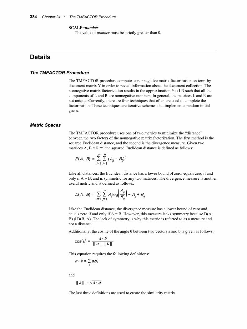
SCALE=numberThe value of number must be strictly greater than 0.
Details
The TMFACTOR ProcedureThe TMFACTOR procedure computes a nonnegative matrix factorization on term-by-document matrix Y in order to reveal information about the document collection. The nonnegative matrix factorization results in the approximation Y ≈ LR such that all the components of L and R are nonnegative numbers. In general, the matrices L and R are not unique. Currently, there are four techniques that often are used to complete the factorization. These techniques are iterative schemes that implement a random initial guess.
Metric SpacesThe TMFACTOR procedure uses one of two metrics to minimize the “distance” between the two factors of the nonnegative matrix factorization. The first method is the squared Euclidean distance, and the second is the divergence measure. Given two matrices A, B ∈ ℝmxn, the squared Euclidean distance is defined as follows:
E(A, B) = ∑i=1
m∑j=1
n(Aij − Bij)2
Like all distances, the Euclidean distance has a lower bound of zero, equals zero if and only if A = B, and is symmetric for any two matrices. The divergence measure is another useful metric and is defined as follows:
D(A, B) = ∑i=1
m∑j=1
nAijlog( AijBij ) − Aij + Bij
Like the Euclidean distance, the divergence measure has a lower bound of zero and equals zero if and only if A = B. However, this measure lacks symmetry because D(A, B) ≠ D(B, A). The lack of symmetry is why this metric is referred to as a measure and not a distance.
Additionally, the cosine of the angle θ between two vectors a and b is given as follows:
cos(θ) = a ⋅ b|| a || || b ||
This equation requires the following definitions:
a ⋅ b = ∑iaibi
and
|| a || = a ⋅ a
The last three definitions are used to create the similarity matrix.
384 Chapter 24 • The TMFACTOR Procedure
Nonnegative Matrix FactorizationA nonnegative matrix factorization is an attempt to find low dimension representation of some data set that contains only nonnegative values. More formally, given a nonnegative matrix Y ∈ ℝmxn and some positive integer k < min(m, n), find two nonnegative matrices L ∈ ℝmxk and R ∈ ℝkxn such that Y ≈ LR and the chosen metric is minimized. In general, the value of k that is chosen is significantly smaller than either m or n.
The nonnegative matrix factorization results in an approximation of the original matrix Y that is not unique. Indeed, the product LR can be rewritten as LDD-1R for any nonsingular matrix D such that LD and D-1R are both nonnegative. For example, D can be a permutation matrix. Because the solution is not unique, penalty functions J1(L) and J2(R) can be applied with weights λL > 0 and λR > 0. These constraints enforce a desired characteristic or enhance the smoothness of the solution.
The solution to such a problem is computed iteratively on both L and R until convergence or the maximum number of iterations is reached. The four methods that the TMFACTOR procedure uses are multiplicative update, alternating least squares, gradient descent, and quasi-Newton. The multiplicative update method initializes L and R with random, nonnegative values and updates alternating rows of L and R sequentially until convergence is reached. The alternating least squares method initializes the matrix L, solves the least squares problem LTLR = LTY for R, sets all negative values in R to zero, and then reverses the roles of L and R. This is repeated until convergence. The gradient descent method initializes L and R with random, nonnegative values and updates their values based on the partial derivatives of L and R. The quasi-Newton method is an implementation of the limited-memory Broyden–Fletcher–Goldfarb–Shanno method.
The reason to compute a nonnegative matrix factorization is to determine information about the document collection under analysis. The k columns, or basis vectors, of L represent the topics in the document collection. There are n columns in the data set R, and these represent the n documents in the original collection. These columns have k elements, each one indicating the weight of the corresponding topic to that document. The largest weight determines which topic is assigned to each document.
Examples
Example 1: Preprocessing the Data and Basic UsageThe TMFACTOR procedure works with any sparse array of nonnegative numbers; however, the following examples will use a term-by-document matrix from the NEWS data set of the SAMPSIO library. This data set contains news articles about computer graphics, hockey, and medicine. The first step is to parse the document collection with the DOCPARSE procedure.
/* Parse the document collection */proc docparse data=sampsio.news out=work.parseOut key=work.parseKey stemming=yes tagging=no entities=no ng=std stop=sashelp.engstop addparent; var text; select "aux" "conj" "det" "interj"
Examples 385
"part" "prep" "pron" "Newline" "Num" "Punct"/drop;run;
This code creates the data sets parseOut and parseKey, which contain information about the document collection. Each row of the parseOut data set indicates the frequency for the given term number and document number. The ADDPARENT line of code includes the parent term for each term number and is used solely for illustrative purposes. Before factoring the term-by-document matrix, you will weight the term frequencies with the following code.
/* Load the data into memory, Weight the term-document frequency table let f_ij be the (i,j)th entry of term-doc freq matrix, w_i be the TERM weight of term i, g() be the cell weight function; then w_i *g(f_ij) = the weighted frequency of the ijth entry */proc tmutil data=work.parseOut key=work.parseKey; control init memloc="here"; weight termwgt=entropy cellwgt=log;run;proc tmutil; control memloc="here" release; output reindex key=work.utilKey out=work.utilOut doc=work.utilDoc keyformat=simple;run;/* Sort the data set */proc sort data=work.utilOut; by _termnum_ _document_;run;
The utilOut data set is a compact representation of the weighted term-by-document matrix. Notice that the _PARENT_ column has been removed from this data set. The following code computes a nonnegative matrix factorization for this term-by-document matrix.
/* Basic Usage */proc tmfactor data=work.utilOut row=_termnum_ col=_document_ value=_count_ seed=12345 print=all; iterate tech=leeandseung maxiter=20 itprint=1; save out_left=work.left out_right=work.right;quit;
In this code, the multiplicate update method of Lee and Seung is used with only twenty iterations. The itprint=1 prints the value of the objective function at every iteration to the output window. Here, the seed=12345 statement ensures that the results are identical from one run to the next. If the system clock was used, then different initial matrices would be generated, which would lead to slightly different results for the
386 Chapter 24 • The TMFACTOR Procedure
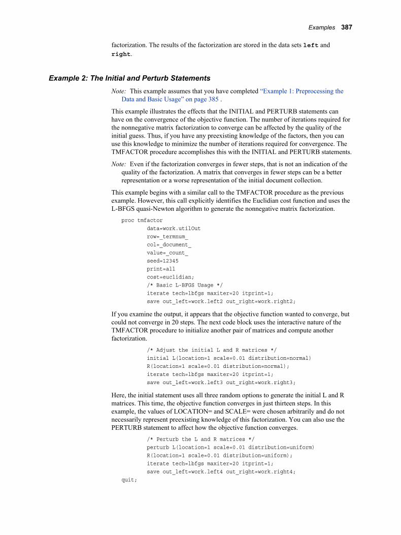
factorization. The results of the factorization are stored in the data sets left and right.
Example 2: The Initial and Perturb StatementsNote: This example assumes that you have completed “Example 1: Preprocessing the
Data and Basic Usage” on page 385 .
This example illustrates the effects that the INITIAL and PERTURB statements can have on the convergence of the objective function. The number of iterations required for the nonnegative matrix factorization to converge can be affected by the quality of the initial guess. Thus, if you have any preexisting knowledge of the factors, then you can use this knowledge to minimize the number of iterations required for convergence. The TMFACTOR procedure accomplishes this with the INITIAL and PERTURB statements.
Note: Even if the factorization converges in fewer steps, that is not an indication of the quality of the factorization. A matrix that converges in fewer steps can be a better representation or a worse representation of the initial document collection.
This example begins with a similar call to the TMFACTOR procedure as the previous example. However, this call explicitly identifies the Euclidian cost function and uses the L-BFGS quasi-Newton algorithm to generate the nonnegative matrix factorization.
proc tmfactor data=work.utilOut row=_termnum_ col=_document_ value=_count_ seed=12345 print=all cost=euclidian; /* Basic L-BFGS Usage */ iterate tech=lbfgs maxiter=20 itprint=1; save out_left=work.left2 out_right=work.right2;
If you examine the output, it appears that the objective function wanted to converge, but could not converge in 20 steps. The next code block uses the interactive nature of the TMFACTOR procedure to initialize another pair of matrices and compute another factorization.
/* Adjust the initial L and R matrices */ initial L(location=1 scale=0.01 distribution=normal) R(location=1 scale=0.01 distribution=normal); iterate tech=lbfgs maxiter=20 itprint=1; save out_left=work.left3 out_right=work.right3;
Here, the initial statement uses all three random options to generate the initial L and R matrices. This time, the objective function converges in just thirteen steps. In this example, the values of LOCATION= and SCALE= were chosen arbitrarily and do not necessarily represent preexisting knowledge of this factorization. You can also use the PERTURB statement to affect how the objective function converges.
/* Perturb the L and R matrices */ perturb L(location=1 scale=0.01 distribution=uniform) R(location=1 scale=0.01 distribution=uniform); iterate tech=lbfgs maxiter=20 itprint=1; save out_left=work.left4 out_right=work.right4;quit;
Examples 387
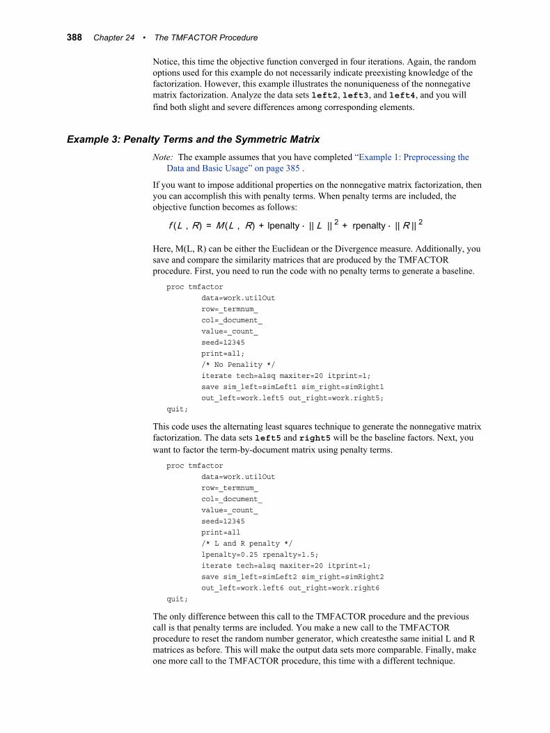
Notice, this time the objective function converged in four iterations. Again, the random options used for this example do not necessarily indicate preexisting knowledge of the factorization. However, this example illustrates the nonuniqueness of the nonnegative matrix factorization. Analyze the data sets left2, left3, and left4, and you will find both slight and severe differences among corresponding elements.
Example 3: Penalty Terms and the Symmetric MatrixNote: The example assumes that you have completed “Example 1: Preprocessing the
Data and Basic Usage” on page 385 .
If you want to impose additional properties on the nonnegative matrix factorization, then you can accomplish this with penalty terms. When penalty terms are included, the objective function becomes as follows:
f (L , R) = M (L , R) + lpenalty ⋅ || L || 2 + rpenalty ⋅ || R || 2
Here, M(L, R) can be either the Euclidean or the Divergence measure. Additionally, you save and compare the similarity matrices that are produced by the TMFACTOR procedure. First, you need to run the code with no penalty terms to generate a baseline.
proc tmfactor data=work.utilOut row=_termnum_ col=_document_ value=_count_ seed=12345 print=all; /* No Penality */ iterate tech=alsq maxiter=20 itprint=1; save sim_left=simLeft1 sim_right=simRight1 out_left=work.left5 out_right=work.right5;quit;
This code uses the alternating least squares technique to generate the nonnegative matrix factorization. The data sets left5 and right5 will be the baseline factors. Next, you want to factor the term-by-document matrix using penalty terms.
proc tmfactor data=work.utilOut row=_termnum_ col=_document_ value=_count_ seed=12345 print=all /* L and R penalty */ lpenalty=0.25 rpenalty=1.5; iterate tech=alsq maxiter=20 itprint=1; save sim_left=simLeft2 sim_right=simRight2 out_left=work.left6 out_right=work.right6quit;
The only difference between this call to the TMFACTOR procedure and the previous call is that penalty terms are included. You make a new call to the TMFACTOR procedure to reset the random number generator, which createsthe same initial L and R matrices as before. This will make the output data sets more comparable. Finally, make one more call to the TMFACTOR procedure, this time with a different technique.
388 Chapter 24 • The TMFACTOR Procedure
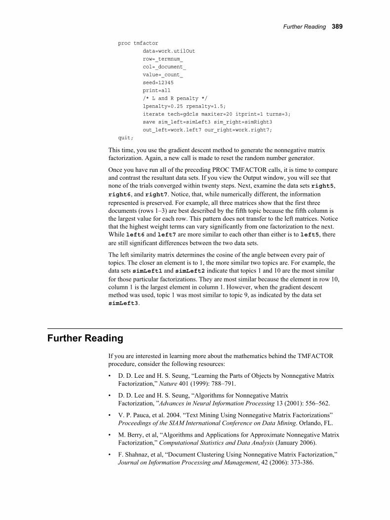
proc tmfactor data=work.utilOut row=_termnum_ col=_document_ value=_count_ seed=12345 print=all /* L and R penalty */ lpenalty=0.25 rpenalty=1.5; iterate tech=gdcls maxiter=20 itprint=1 turns=3; save sim_left=simLeft3 sim_right=simRight3 out_left=work.left7 our_right=work.right7;quit;
This time, you use the gradient descent method to generate the nonnegative matrix factorization. Again, a new call is made to reset the random number generator.
Once you have run all of the preceding PROC TMFACTOR calls, it is time to compare and contrast the resultant data sets. If you view the Output window, you will see that none of the trials converged within twenty steps. Next, examine the data sets right5, right6, and right7. Notice, that, while numerically different, the information represented is preserved. For example, all three matrices show that the first three documents (rows 1–3) are best described by the fifth topic because the fifth column is the largest value for each row. This pattern does not transfer to the left matrices. Notice that the highest weight terms can vary significantly from one factorization to the next. While left6 and left7 are more similar to each other than either is to left5, there are still significant differences between the two data sets.
The left similarity matrix determines the cosine of the angle between every pair of topics. The closer an element is to 1, the more similar two topics are. For example, the data sets simLeft1 and simLeft2 indicate that topics 1 and 10 are the most similar for those particular factorizations. They are most similar because the element in row 10, column 1 is the largest element in column 1. However, when the gradient descent method was used, topic 1 was most similar to topic 9, as indicated by the data set simLeft3.
Further ReadingIf you are interested in learning more about the mathematics behind the TMFACTOR procedure, consider the following resources:
• D. D. Lee and H. S. Seung, “Learning the Parts of Objects by Nonnegative Matrix Factorization,” Nature 401 (1999): 788–791.
• D. D. Lee and H. S. Seung, “Algorithms for Nonnegative Matrix Factorization, ”Advances in Neural Information Processing 13 (2001): 556–562.
• V. P. Pauca, et al. 2004. “Text Mining Using Nonnegative Matrix Factorizations” Proceedings of the SIAM International Conference on Data Mining. Orlando, FL.
• M. Berry, et al, “Algorithms and Applications for Approximate Nonnegative Matrix Factorization,” Computational Statistics and Data Analysis (January 2006).
• F. Shahnaz, et al, “Document Clustering Using Nonnegative Matrix Factorization,” Journal on Information Processing and Management, 42 (2006): 373-386.
Further Reading 389

• R. H. Byrd, et al. “A Limited Memory Algorithm for Bound Constrained Optimization,” SIAM Journal on Scientific Computing 16 (1995): 1190–1208.
390 Chapter 24 • The TMFACTOR Procedure
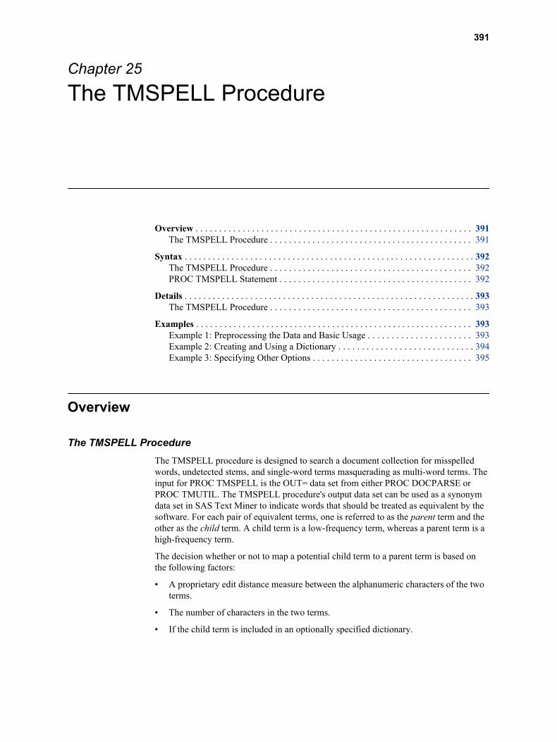
Chapter 25
The TMSPELL Procedure
Overview . . . . . . . . . . . . . . . . . . . . . . . . . . . . . . . . . . . . . . . . . . . . . . . . . . . . . . . . . . . 391The TMSPELL Procedure . . . . . . . . . . . . . . . . . . . . . . . . . . . . . . . . . . . . . . . . . . . 391
Syntax . . . . . . . . . . . . . . . . . . . . . . . . . . . . . . . . . . . . . . . . . . . . . . . . . . . . . . . . . . . . . . 392The TMSPELL Procedure . . . . . . . . . . . . . . . . . . . . . . . . . . . . . . . . . . . . . . . . . . . 392PROC TMSPELL Statement . . . . . . . . . . . . . . . . . . . . . . . . . . . . . . . . . . . . . . . . . 392
Details . . . . . . . . . . . . . . . . . . . . . . . . . . . . . . . . . . . . . . . . . . . . . . . . . . . . . . . . . . . . . . 393The TMSPELL Procedure . . . . . . . . . . . . . . . . . . . . . . . . . . . . . . . . . . . . . . . . . . . 393
Examples . . . . . . . . . . . . . . . . . . . . . . . . . . . . . . . . . . . . . . . . . . . . . . . . . . . . . . . . . . . 393Example 1: Preprocessing the Data and Basic Usage . . . . . . . . . . . . . . . . . . . . . . 393Example 2: Creating and Using a Dictionary . . . . . . . . . . . . . . . . . . . . . . . . . . . . . 394Example 3: Specifying Other Options . . . . . . . . . . . . . . . . . . . . . . . . . . . . . . . . . . 395
Overview
The TMSPELL ProcedureThe TMSPELL procedure is designed to search a document collection for misspelled words, undetected stems, and single-word terms masquerading as multi-word terms. The input for PROC TMSPELL is the OUT= data set from either PROC DOCPARSE or PROC TMUTIL. The TMSPELL procedure's output data set can be used as a synonym data set in SAS Text Miner to indicate words that should be treated as equivalent by the software. For each pair of equivalent terms, one is referred to as the parent term and the other as the child term. A child term is a low-frequency term, whereas a parent term is a high-frequency term.
The decision whether or not to map a potential child term to a parent term is based on the following factors:
• A proprietary edit distance measure between the alphanumeric characters of the two terms.
• The number of characters in the two terms.
• If the child term is included in an optionally specified dictionary.
391
Syntax
The TMSPELL ProcedurePROC TMSPELL DATA=data-set-name OUT=data-set-name <options>;
RUN;
PROC TMSPELL Statement
SyntaxPROC TMSPELL DATA=data-set-name OUT=data-set-name <options>;
See “Example 1: Preprocessing the Data and Basic Usage” on page 393 for an introduction to the usage of the PROC TMSPELL statement.
Required ArgumentsDATA=data-set-name
This argument indicates the input data set. This data set must contain the variables term, role, key, _ispar, parent, and numdocs.
OUT=data-set-nameThis argument specifies the synonym data set that is created by the TMSPELL procedure. This data set contains the variables numdocs, term, childndocs, parent, minsped, and dict. If the diffrole option is specified, then the data set includes the variables termrole and parentrole. If the diffrole option is not specified, then the data set contains the variable category.
The variable term indicates a child term, and the variable parent indicates the identified parent term. The value of numdocs indicates how many documents contained the parent term. Similarly, childndocs indicates how many documents contain the child term. The minimum distance between the two terms is given by minsped. The value of dict is Y if the parent term was found in the specified dictionary, N if it was not found, and blank if no dictionary was specified. The variables category and parentrole identify the part of speech of the parent. Likewise, termrole identifies the part of speech of the child.
Optional ArgumentsDICT=data-set-name
This argument specifies the data set to use as a dictionary. The TMSPELL procedure assumes that all terms in data-set-name are spelled correctly. This data set must contain the variable term. The number of false positives can be significantly reduced when a dictionary data set is used.
DICTPEN=numberThis argument specifies the penalty that is applied when a child term is found in the dictionary data set. The default value is 2.
DIFFERENTROLE | DIFFERENT ROLE | DIFFROLEBy default, terms are compared only if they have the same part of speech. If this option is specified, then terms with different parts of speech will be compared.
392 Chapter 25 • The TMSPELL Procedure
Consider the term “left,” which can be a noun, adjective, or verb. If the adjective “left” and the noun “left” appear in fewer than MAXCHILDREN= documents and the verb “left” appears in more than MINPARENTS= documents, then the TMSPELL procedure will identify all instances of “left” as a verb. This specific example is covered in “Example 3: Specifying Other Options” on page 395 .
MAXCHILDREN=numberThis argument specifies the maximum number of documents that a term can appear in to be considered a child. The default value is 6.
MAXSPEDIS=numberThis argument specifies the maximum allowable distance between a parent and a child. Because the proprietary distance is asymmetric, both distances are calculated and the shorter of the two is returned. The default value is 15.
MINPARENTS=numberThis argument specifies the minimum number of documents that a term must appear in to be considered as a parent. The default value is 3.
MULTIPEN=numberThis argument specifies the penalty that is applied when either a child or a parent is a multi-word term. The value of number is multiplied by the value that was returned by the proprietary distance function. The default value is 2.
Details
The TMSPELL ProcedureThe TMSPELL procedure divides the term bank into two sets in order to identify misspellings in the document collection. First, the list of candidate children is created from all terms that appear in less than MAXCHILDREN= documents. Then, the list of possible parents is created from all the terms that appear in more than MINPARENTS= documents. If a dictionary is specified, then all of the terms in the dictionary are added to the list of possible parents. Next, the TMSPELL procedure finds the minimum distance from each candidate child c to every parent p that starts with the same letter as c. Because the proprietary distance function is not symmetric, the distance is computed in both directions and then divided by the length of the shorter of the two terms. If either the parent or child is a multi-word term, then the distance is multiplied by MULTIPEN=. Likewise, if the child is found in the dictionary, then the distance is multiplied by DICTPEN=. Finally, if the distance between the child and parent is less than MAXSPEDIS=, then the two terms are identified as synonyms.
Examples
Example 1: Preprocessing the Data and Basic UsageThe TMSPELL procedure works with the output data set from the DOCPARSE procedure, the Text Miner node, or the Text Parsing node. For this example, you will use the NEWS data set from the SAMPSIO library. This data set contains news articles about computer graphics, hockey, and medicine. First, you need to parse the document collection.
Examples 393
/* Parse the document collection */proc docparse data=sampsio.news out=Out key=Key stemming=yes tagging=yes entities=no ng=std stop=sashelp.engstop; var text; select "aux" "det" "interj" "num" "part" "prep" "pron" "prop" "punct"/drop;run;
The data set Key could be used as the input to the TMSPELL procedure; however, it contains the terms that are in the stop list sashelp.engstop. These terms are identified in the Key data set by their keep status of N. The following code removes the terms in the stop list, reorders the variables, removes unnecessary variables, and sorts the data set in alphabetical order.
/* Reorder the input term set */proc sql;create table spellIn(drop=keep) as select term, role, key, _ispar, parent, numdocs, keep from work.key where keep="Y" order by term, role;quit;
The data set spellIn contains only the variables necessary for the TMSPELL procedure. Next, you will run the TMSPELL procedure on this data set with the default settings.
/* Basic Usage */proc tmspell data=spellIn out=synonyms;run;
This code checks the low-frequency words against more common terms to identify misspellings. If you browse the data set synonyms, then you will see that there are many false positives. For example, the term “swell” is identified as a misspelling of “sell,” and “noise” is identified as a misspelling of “nose.” To address this problem, you can specify a dictionary data set.
Example 2: Creating and Using a DictionaryNote: This example assumes that you have completed “Example 1: Preprocessing the
Data and Basic Usage” on page 393 .
A dictionary data set is used to reduce the number of false positives that are identified by the TMSPELL procedure. Every term in the dictionary data set is considered correct. This data set must contain a variable named TERM that contains the dictionary entities. There are several free dictionary sources that you can use with a SAS DATA step to create a dictionary data set that you can use with the TMSPELL procedure. For example, OpenOffice.org has links to dictionaries for over 96 languages that you can download for free from http://wiki.services.openoffice.org/wiki/Dictionaries.
To create an English dictionary for this example, save this English language dictionary from Open Office to your local machine. When the download is complete, unzip the file and note the location of the file en_US.dic. The following code will create a dictionary data set for use with the TMSPELL procedure.
394 Chapter 25 • The TMSPELL Procedure
/* Create an English dictionary */data dict (keep=term pos); length inputterm term $32; infile '<fileLocation>en_US.dic' truncover; input linetxt $80.;i=1; do until (inputterm = ' '); inputterm = scan(linetxt, i, ' '); if inputterm ne ' ' then do; location=index(inputterm,'/'); if location gt 0 then term = substr(inputterm,1,location-1); if location eq 0 then term = inputterm; if lowcase(term) ne term then pos = 'Prop'; term = lowcase(term); output; end; i=i+1; end;run;
Now, you can use the data set dict as a dictionary for the TMSPELL procedure.
/* Usage with a Dictionary */proc tmspell data=spellIn out=synonyms2 dict=dict dictpen=3 ;run;
This code uses a penalty value of 3 when a child is in the dictionary. A penalty reduces the likelihood that a term in the dictionary, which is assumed to be correct, is identified as a misspelling. The variable dict in synonyms2 is Y if the child was found in the dictionary and N if it was not. If you run the above code with dictpen=2, there are more terms from the dictionary that are identified as misspellings than when dictpen=3. This does not imply that a greater penalty value is better because some misspellings are correctly spelling words. For example, the words “silver” and “sliver” are both correctly spelled, but either could be a misspelling of the other, depending on the context of the problem.
Example 3: Specifying Other OptionsNote: This example assumes that you have completed “Example 1: Preprocessing the
Data and Basic Usage” on page 393 and “Example 2: Creating and Using a Dictionary” on page 394 .
You can use the MINPARENTS= and MAXCHILDREN= options to determine what terms are considered parents and children, respectively. Consider the code below.
proc tmspell data=spellIn out=synonyms3 minparents=10 maxchildren=8 dict=dict dictpen=3
Examples 395
;run;
There are two changes to note in this code. First, the value of MINPARENTS= is increased from the default value of 3 to the new value of 10. Thus, fewer terms from the document collection are considered parents (the dictionary terms are not affected by this change). In general, as MINPARENTS= increases, the number of parents identified decreases and vice versa. Second, the value of MAXCHILDREN= is increased from the default value of 6 to the new value of 8. The result of this change is that more terms are considered children. In general, as MAXCHILDREN= increases, the number of children identified also increases. The inverse of this statement is also true.
You can use the value of MAXSPEDIS= to control how close two words must be in order to be treated as synonyms. The MULTIPEN= option controls the penalty that is applied to mutli-word terms.
proc tmspell data=spellIn out=synonyms4 minparents=10 maxchildren=8 maxspedis=8 multipen=4 dict=dict dictpen=3 ;run;
In this code, the value of MAXSPEDIS= is reduced to 8, nearly half of the default value (15). This change significantly reduces the number of misspellings that are identified by the TMSPELL procedure. Indeed, if you compare the data sets synonyms3 and synonyms4, you should notice that synonyms4 fails to identify many of the misspelled terms that were caught in synonyms3. A good value for MAXSPEDIS= will vary by document collection, but when this value is too low the TMSPELL procedure will miss many misspelled terms.
The line multipen=4 increases the penalty for multi-word terms from the default value of 3 to a new value of 4. The effect of MUTLIPEN= is similar to that of DICTPEN=. That is, whenever a multi-word term is found, the proprietary distance value is multiplied by the value of MULTIPEN=. When this value is increased, the likelihood that a multi-word term is considered a misspelling is decreased.
Finally, you can choose to compare terms even if they are considered different parts of speech. By default, only terms that have the same part of speech are compared. However, if you specify the DIFFROLE option, then terms will be compared regardless of their part of speech. For example, the term “left” is an adjective, a noun, and a verb. The following code treats these three forms as identical terms.
proc tmspell data=spellIn out=synonyms5 minparents=10 maxchildren=10 maxspedis=15 multipen=4 dict=dict dictpen=2 diffrole ;run;
In the data set synonyms5, the noun “left” and the adjective “left” have both been identified as children. The parent for both of these terms is the verb “left” because it is
396 Chapter 25 • The TMSPELL Procedure

the only instance of “left” that appears in more than 10 documents. The DIFFROLE option greatly increases the likelihood that homonyms are falsely identified as misspellings.
Examples 397

398 Chapter 25 • The TMSPELL Procedure
Chapter 26
The TMUTIL Procedure
Overview . . . . . . . . . . . . . . . . . . . . . . . . . . . . . . . . . . . . . . . . . . . . . . . . . . . . . . . . . . . 399The TMUTIL Procedure . . . . . . . . . . . . . . . . . . . . . . . . . . . . . . . . . . . . . . . . . . . . . 399
Syntax . . . . . . . . . . . . . . . . . . . . . . . . . . . . . . . . . . . . . . . . . . . . . . . . . . . . . . . . . . . . . . 400The TMUTIL Procedure . . . . . . . . . . . . . . . . . . . . . . . . . . . . . . . . . . . . . . . . . . . . . 400PROC TMUTIL Statement . . . . . . . . . . . . . . . . . . . . . . . . . . . . . . . . . . . . . . . . . . . 400CONTROL Statement . . . . . . . . . . . . . . . . . . . . . . . . . . . . . . . . . . . . . . . . . . . . . . 402FILTER Statement . . . . . . . . . . . . . . . . . . . . . . . . . . . . . . . . . . . . . . . . . . . . . . . . . 402OUTPUT Statement . . . . . . . . . . . . . . . . . . . . . . . . . . . . . . . . . . . . . . . . . . . . . . . . 404SEARCH Statement . . . . . . . . . . . . . . . . . . . . . . . . . . . . . . . . . . . . . . . . . . . . . . . . 405SELECT Statement . . . . . . . . . . . . . . . . . . . . . . . . . . . . . . . . . . . . . . . . . . . . . . . . . 407SYN Statement . . . . . . . . . . . . . . . . . . . . . . . . . . . . . . . . . . . . . . . . . . . . . . . . . . . . 408WEIGHT Statement . . . . . . . . . . . . . . . . . . . . . . . . . . . . . . . . . . . . . . . . . . . . . . . . 409
Examples . . . . . . . . . . . . . . . . . . . . . . . . . . . . . . . . . . . . . . . . . . . . . . . . . . . . . . . . . . . 410Example 1: Basic Usage . . . . . . . . . . . . . . . . . . . . . . . . . . . . . . . . . . . . . . . . . . . . . 410Example 2: The CONTROL Statement . . . . . . . . . . . . . . . . . . . . . . . . . . . . . . . . . 411Example 3: The OUTPUT Statement . . . . . . . . . . . . . . . . . . . . . . . . . . . . . . . . . . . 412Example 4: The WEIGHT Statement . . . . . . . . . . . . . . . . . . . . . . . . . . . . . . . . . . . 413Example 5: The SYN Statement . . . . . . . . . . . . . . . . . . . . . . . . . . . . . . . . . . . . . . . 413Example 6: The FILTER Statement . . . . . . . . . . . . . . . . . . . . . . . . . . . . . . . . . . . . 414Example 7: The SELECT Statement . . . . . . . . . . . . . . . . . . . . . . . . . . . . . . . . . . . 416Example 8: The SEARCH Statement . . . . . . . . . . . . . . . . . . . . . . . . . . . . . . . . . . . 416
Overview
The TMUTIL ProcedureThe TMUTIL procedure is designed to support the text mining nodes found in Enterprise Miner, but is also available for users to build custom text mining solutions. Its primary input source is the output from the DOCPARSE procedure. The TMUTIL procedure uses an efficient internal representation of the output from the DOCPARSE procedure called an inverted index. The inverted index can be stored in memory as long as the user desires. This enables the user to manipulate the data with several TMUTIL calls without having to reload potentially very large data sets each time.
The procedure has several important functions:
• Maintain the inverted index structure that represents the document collection.
399
• Alter the inverted index structure based on interactive input (such as setting synonyms, dropping terms, and filtering).
• Apply transformations to the data via weightings and factorizations.
• Write out various data set representations of the inverted index structure.
• Load the Teragram search engine index and query the document collection.
Note: The TMUTIL procedure relies on resources that are provided by Teragram. For the TMUTIL procedure to function properly in Windows environments, the location of the Teragram resources must be added to your path environment variable. For details about this process, see the Text Miner post-installation notes.
Syntax
The TMUTIL ProcedurePROC TMUTIL <options>;
CONTROL <options>;FILTER <options>;OUTPUT <options>;SEARCH <options>;SELECT <options>;SYN <options>;WEIGHT <options>;RUN ;
PROC TMUTIL Statement
SyntaxPROC TMUTIL <options>;
Optional ArgumentsDATA=data-set-name
The input data set to the TMUTIL procedure is the output data set from the DOCPARSE procedure or the terms, doc, and train data sets from either the Text Parsing or Text Filter node. This data set is a compressed representation of the sparse term-by-document frequency matrix.
The three variables that are required in this data set are the following:
• _TERMNUM_ — Contains the indices that correspond to the value of the variable KEY in the KEY data set produced by the DOCPARSE procedure. These values are positive integers that uniquely identify each term.
• _DOCUMENT_ — Contains the indices that correspond to the document indices in the DOC= data set. These values are positive integers that uniquely identify each document.
• _COUNT_ — A nonnegative integer that specifies the number of times that the observed _TERMNUM_ occurred in the given document.
400 Chapter 26 • The TMUTIL Procedure
Note: The DATA= option must be used in combination with the INIT option in the CONTROL statement.
DOCUMENTS | DOC=data-set-nameThis is the input DOCUMENT data set.
While the TMUTIL procedure does not store document text, it can use and store the contents of the following two variables:
• _DOCUMENT_ — A positive integer that uniquely identifies each document. If this variable is not specified, then the _DOCUMENT_ entry will be generated sequentially, beginning with 1.
• Target Variable — Any nominal or ordinal variable that is identified with the TARGET= option. This variable is used when calculating the categorical weightings.
KEY | TERMS=data-set-nameThis data set contains information about the terms in a document collection and is typically the output KEY= data set created by the DOCPARSE procedure. This data set is essential if synonyms, stems, start lists, or stop lists were applied when the DOCPARSE data sets were generated. If this option is not specified, then every term in the OUT= data set of the DOCPARSE procedure will be kept, and there will be no parents or synonyms assigned.
The following is a list of variables that can be in the KEY= data set and used by the TMUTIL procedure:
• _TERMNUM_ | KEY | INDEX — the index of the term. This variable is required if the KEY= data set is used. This value must be a positive integer.
• FREQ — the frequency of a term in the document collection. If this variable is omitted, then the TMUTIL procedure will compute it from the DATA= data set and write this value to the output KEY= data sets.
• NUMDOCS — the number of documents that contain the term. If this variable is omitted, then the TMUTIL procedure will compute it from the DATA= data set and write this value to the output KEY= data sets.
• KEEP — either Y if the term is kept or N if the term is dropped. If this variable does not exist, then all terms are kept and output KEY= data sets will indicate this decision.
• PARENT — a positive integer if the term has a parent and blank otherwise. This value indicates the KEY of the parent that represents this term. When the value is missing, the term has no parent. It is possible for the value of KEY and PARENT to be the same. In this case, the values of NUMDOCS and FREQ refer to the parent, independent of its children. The variable _ISPAR is required when the variable PARENT is used.
• _ISPAR — a character that indicates whether the term is a parent, child, or neither. This variable is required whenever there are parent-child relationships in the input KEY= data set. This variable is a + (a plus sign) if the term is a parent, a . (a period) if the term is a child, and a space character if the term is neither.
• FILTER — the level where a term will be filtered. A value of 0 indicates that the term is not filtered. If this variable is missing, then every term is assigned a FILTER value of 0, which means that everything is unfiltered. For more information about filters, see the “FILTER Statement” on page 402 .
Syntax 401
TARGET=variableThis option indicates the target variable in the DOC= data set, which will be weighted. This setting is used when a category-specific weighting is requested. For information about the available weightings, see the “WEIGHT Statement” on page 409 .
CONTROL Statement
SyntaxCONTROL <options>;
The TMUTIL procedure is unusual because the data that it uses persists in memory until the user explicitly clears it or the SAS session is terminated. After the initial call to the TMUTIL procedure, subsequent calls are made without the expensive overhead of reading in a list of documents and terms. When the TMUTIL procedure is called again, it reconnects to the data that was stored in memory during the initial call.
The CONTROL statement has options that tell the TMUTIL procedure if this is the first call or the last call to the memory. There is also an option that indicates the name of the SAS macro variable that holds the location of the memory. When memory is tight, you might want to release the memory used by the TMUTIL procedure in order to perform other tasks. If you want to start the TMUTIL procedure with the same data at a later time, include the KEY= and OUT= options in the OUTPUT statement. Later, you can initialize the TMUTIL procedure with these data sets. You can save more memory if you use the RENUMBER option in the OUTPUT statement.
Optional ArgumentsINITIAL | INIT
Specify this option to indicate that this is the first time the TMUTIL procedure is called. When this option is specified, the TMUTIL procedure allocates the memory necessary to store the input data. If this option is used, then the DATA= option must be specified in the PROC TMUTIL statement.
MEMLOC='string'The string provided here is used as the macro variable name that holds the location in memory of the stored data. Subsequent calls to the TMUTIL procedure will access the allocated memory via this macro variable name. If several instances of the TMUTIL procedure are run simultaneously, a different string should be used for each instance of the TMUTIL procedure. This argument is required on all calls to the TMUTIL procedure unless both INIT and RELEASE are used.
RELEASESpecify this option to release all allocated memory upon completion of the TMUTIL procedure. If this option is not specified, then the memory is not released. You should issue the RELEASE option on the final call to the TMUTIL procedure; otherwise, system memory will not be freed until the SAS session is terminated.
FILTER Statement
SyntaxFILTER <options>;
402 Chapter 26 • The TMUTIL Procedure
The FILTER statement is used to subset the document collection in order to identify the terms or documents that should be used in future analysis. The terms and documents on a filter list are temporarily excluded from any analysis performed by the TMUTIL procedure. Unlike a SELECT statement, a FILTER statement can be reversed with the UNDO or the UNDOALL option. This enables you to quickly examine a subset of the document collection, and gives you the ability to return to the original document collection when finished.
Optional ArgumentsCOMPLEMENT | COMP
Specify this option to reverse the behavior of the filter. That is, when this option is specified, the information about a filter list is filtered out rather than filtered in. This option is used in combination with TERMDATA=, TERMLIST=, DOCDATA=, or DOCLIST=.
DOCDATA=data-set-nameThis data set specifies the documents to use in the analysis. All other documents are filtered out. The data set requires a single variable named either _DOCUMENT_, KEY, or INDEX. The values of this variable are positive integers that correspond to the documents that you want to keep for analysis. Documents not specified in this data set are removed from the analysis, and corresponding term counts are updated accordingly. If this COMP option is used, then the documents listed here are removed from analysis.
DOCLIST=list-of-integersThis is an alternative method to the DOCDATA= option. This approach accepts a list of positive integers on the SAS command line that are filtered in. If the COMP option is used, then these documents are filtered out.
INDOCSThis option indicates that the documents that contain any of the terms in the TERMDATA= or TERMLIST= inputs are to be filtered in. Thus, if this option is specified, then either the TERMDATA= or TERMLIST= option must also be specified. The COMP option can be used to filter out the documents that contain the given terms.
REDUCEF=numberThis option removes terms that are not in at least number documents. The value of number must be a positive integer. This option can be used in conjunction with the REDUCEW= option.
REDUCEW=numberThis option removes all terms that have a weight less than number, which must be a real, positive value. This option can be used in conjunction with the REDUCEF= option.
REDUCEN=numberThis option keeps the number highest weighted terms. The value of number must be a positive integer. If there are fewer than number kept terms, then this option has no effect. This option cannot be used with REDUCEW= or REDUCEF=.
REDUCEP=numberThis option removes terms that occur in more than number% of the documents. The value of number can be any real value between 0 and 100. This option is used to remove terms that occur too frequently in your document collection.
TERMDATA=data-set-nameThis option specifies a data set that indicates the term numbers to filter in. This data set requires a single variable named _TERMNUM_, KEY, or INDEX. The values of
Syntax 403
this variable are positive integers that correspond to the terms that you want to filter in. If the COMP is used, then these terms are removed from the analysis.
TERMLIST=list-of-integersSimilar to DOCLIST=, this option accepts a list of positive integers from the SAS command line, which indicates the terms that are kept. When the COMP option is used, then these terms are filtered out.
UNDOSpecify this option to undo the most recent filter, whether it was a document filter or a term filter.
UNDOALLSpecify this option to undo all preceding filters.
OUTPUT Statement
SyntaxOUTPUT <options>;
The OUTPUT statement specifies the data sets that are saved and the options that control how they are saved. In general, you manipulate the input from the KEY= and OUT= data sets with FILTER, SELECT, KEEP, and DROP statements. These manipulations alter the output KEY=, OUT=, and DOC= data sets, and the OUTPUT statement enables you to request updated copies of these data sets. Also, you can save the current version of the stop list or synonyms list.
Optional ArgumentsDOC=data-set-name
This option specifies the output data set for the documents. This data set contains the variable _DOCUMENT_, which identifies the document numbers that match the current filter or search results. This data set can contain other variables depending on how the TMUTIL procedure is used. For example, when the SEARCH statement is used, this data set contains a snippet of the text and a relevance score for each document.
KEY=data-set-nameThis option outputs the current KEY= data set. For more information about the variables in this data set, see the “PROC TMUTIL Statement” on page 400 .
KEEPONLYSpecify this option to include only the kept terms in the output KEY= data set.
KEYFORMAT=DEFAULT | SIMPLE | TMSCOREThis option controls the variables and contents that are saved in the KEY data set.
• DEFAULT — includes the variables that Text Miner requires in the data set.
• SIMPLE — uses the variables PFREQ and PNUMDUC to indicate the frequencies that correspond to when a term is used as a parent versus when it occurs as itself. In addition, only the kept terms are written to the KEY= data set
• TMSCORE — includes only the variables necessary for scoring with the DOCSCORE function. Only the kept terms are included, and frequencies and document counts are removed because they are not necessary to score a new data set.
404 Chapter 26 • The TMUTIL Procedure
OUT=data-set-nameThis data set includes the same variables as the input DATA= data set, but the term counts can be weighted, if requested. This option saves only the kept, representative terms, where the child frequencies are attributed to the corresponding parent. In order to get information about the children, use the OUTCHILD= option.
OUTCHILD=data-set-nameThis option outputs the same variables as the OUT= option with additional entries for the children, which are listed separately rather than summarized by the counts associated with their parents.
REINDEXWhen this option is included, the kept terms are renumbered sequentially. The option can be used only when no filters are applied, an OUT= data set is specified, an output KEY= data set is specified, and the RELEASE option is used. To save memory, you can specify this option and then make a new call to the TMUTIL procedure with the reindexed data. This option can only be used when an INIT and RELEASE call are used together.
STOP=data-set-nameUse this option to output all terms that have a keep status of No. The one variable in this data set, _TERMNUM_, indicates the term number of the dropped terms. This data set, when merged with the actual terms, can be used as a stop list in Text Miner.
SYN=data-set-nameThis data set will contain all the synonyms that exist in the document collection. This data set contains the variables _TERMNUM_, which is the term number for the child, and PARENT, which is the term number of the parent. Once merged with the actual terms, this data set can be used as a synonym list in Text Miner.
UNWEIGHTEDWhen this option is specified, the term frequencies are not weighted on the output OUT= data set.
SEARCH Statement
SyntaxSEARCH <options>;
The SEARCH statement enables the TMUTIL procedure to search a document collection that has been processed by the DOCPARSE procedure. The SEARCH statement specifies how to load and query the document collection. An implicit document filter is applied to the internal representation of the document collection, and the query results are written to the output DOC= data set. As a result of the query, this data set contains two added variables. The first is a relevance score, valued between 0 and 1, that is useful for ranking the results. The second is a snippet of text that provides a context for the query match.
Optional ArgumentsCOMP
Include the COMP option to return the complement of the set that matches your query. This option can be used only with the STOBSEARCH= option.
FROM=numberUse this option to specify the first result that is returned, where the results are ordered by their relevance score. The default value for this option is 1.
Syntax 405
INDEXNAME='string'This option indicates the prefix for the name of the index files. The default prefix is the string “tgindex”.
INDEXPATH=path-nameUse this option to set the location of the index files. If this option is not used, then the INDEXPATH= is assumed to be the SAS Work directory.
LANGUAGE | LANG='Arabic | Chinese | Danish | Dutch | English | Finnish | French | German | Italian | Japanese | Korean | Norwegian | Polish | Portuguese | Spanish | Swedish'
This option sets the language that is used to perform a search. This option is necessary because queries are processed with language-specific techniques. The default setting is English.
LOADThis option indicates that the TMUTIL procedure needs to load the index necessary to search the document collection. This index is built when the BUILDINDEX option is specified in the DOCPARSE procedure. By default, this index resides in the SAS Work directory, but can be specified with the INDEXPATH= option.
QUERYDATA=data-set-nameThis option provides an alternative method to using the SAS command line in order to input query data. This data set must contain only one variable, named either SSEARCH or STOBSEARCH, which indicates the search method that is performed. See the documentation on the SSEARCH= and STOBSEARCH options for more information.
SSEARCH='query string'Use this option to perform a simple search, which uses a fast, intuitive query syntax. With this method, you place several terms in the query string, and the results are the top N matches for your search. The value of N derives from the FROM= and TO= options. The SSEARCH= option is not designed to return all matches for a query; this is the function of STOBSEARCH=.
The following reserved characters have special meaning in a simple search:
• The minus sign (-) — When used in front of a term, all documents that contain that term are excluded from the results.
• The plus sign (+) — When used in front of a term, only documents that contain that term are included in the results.
• Quotations (“multi-word term”) — Use quotations to indicate that the multi-word term is treated as a phrase and that the individual terms should exist sequentially in the document to get the highest match.
• The asterisk (*) — The asterisk is similar to a regular expression matching character that indicates that a wildcard expansion should occur. For example, a search for “col*r” would match both “color” and “colour”.
STOBSEARCH='query string'A STOBSEARCH= automatically converts the simple search to an appropriate Boolean search. This search is designed to return all documents that are relevant to a query. The STOBSEARCH= option uses the same set of reserved characters as the SSEARCH= option.
TO=numberUse this option to specify the last result that is returned. When the SSEARCH= option is used, the default value is 100, and when the STOBSEARCH= is used the default value is the number of documents in the collection.
406 Chapter 26 • The TMUTIL Procedure
UNDOThis option removes the most recent filter that was created by a search. If the UNDO option is not used after a search, then later searches will be performed only on the results of the previous search.
UNDOALLThis option removes all active search filters.
SELECT Statement
SyntaxSELECT <options>;
The SELECT statement enables you to alter the keep status of terms. The SELECT statement is similar to the FILTER statement. However, you cannot reverse results with an UNDO option. In order to reverse results, you must resubmit the term numbers with the opposite option. For example, if you dropped a term with the DROP= option, the only way to undo this action is to state that term in the KEEP= option.
Optional ArgumentsDROPDATA=data-set-name
Use this option to change the keep status of all of the term numbers specified in data-set-name to N. The required variable for this data set is either _TERMNUM_, KEY, or INDEX. This option has no effect on terms that are already dropped or filtered out.
DROPLIST | DROP=list-of-integersThis is an alternative method to the DROPDATA= option. This approach accepts a list of integers on the SAS command line and sets the keep status of those term numbers to N.
KEEPDATA=data-set-nameUse this option to change the keep status of all the term numbers specified in data-set-name to Y. The required variable for this data set is either _TERMNUM_, KEY, or INDEX. This option has no effect on terms that are already kept or filtered in.
KEEPLIST | KEEP=list-of-integersThis is an alternative method to the KEEPDATA= option. This approach accepts a list of integers on the SAS command line and sets the keep status of those term numbers to Y.
REDUCEF=numberSpecify this option to keep only the terms that occur in at least number documents. The value of number must be a positive integer. This option can be used in conjunction with REDUCEW=.
REDUCEW=numberUse this option to keep only the terms that are weighted greater than or equal to number. The value of number is a real, positive number. This option can be used in combination with the REDUCEF= option.
REDUCEN=numberThis option keeps only the number highest weighted terms. You can use this option to control exactly how many terms are kept. This option has no effect if there are fewer than number kept terms in the document collection. This option cannot be used with either the REDUCEW= or REDUCEF= options.
Syntax 407
REDUCENSQR=numberThis option keeps only the number highest adjusted weight terms. The adjusted weight of a term is the product of the weight of the term and the square root of the number of documents that contain the term. This option seeks a balance between the highly weighted terms and the terms that occur frequently enough to be useful. This option has no effect if there are fewer than number kept terms in the document collection. This option cannot be used with either the REDUCEW= or REDUCEF= options.
REDUCEP=numberUse this option to drop terms that appear in more than number% of the documents. The value of number must be a real, positive number between 0 and 100. You can use this option to remove terms that occur too frequently in your document collection.
SYN Statement
SyntaxSYN <options>;
The SYN statement is used to create and remove relationships between equivalent terms. The input KEY= data set contains synonym relationships that were identified by the DOCPARSE procedure. The SYN statement enables you to edit these relationships, create new relationships, and delete preexisting relationships.
Optional ArgumentsCHILDLIST | TERMLIST=list-of-integers
This option specifies a list of positive integers that are the term numbers that will become children. This option must be used in combination with the PARENT= option. The default behavior assigns the children listed here to the parent given in the PARENT= option. The synonym relationship is broken if the UNSET option is also specified.
PARENT | PARENTID=numberThe positive integer number specifies the term number of the desired parent. This option must be used in combination with the CHILDLIST= option. With these options, only one equivalent group can be set at a time. Use the UNSET option to break any relationships currently assigned to the specified term.
SYNDATA=data-set-nameThe data set specified here must contain the two variables _TERMNUM_ and PARENT. Acceptable values for both variables are positive integers, which correspond to term numbers. Use this option set or break multiple synonym relationships at the same time. Do not use this option with the CHILDLIST= and PARENT= options.
UNSETSpecify this option to reverse the default behavior of the SYN statement and break synonym relationships. If you specify a parent and the child is missing, then all children of that parent are removed as synonyms. If you provide a child and the parent is missing, then the term is removed as a child of its parent.
408 Chapter 26 • The TMUTIL Procedure
WEIGHT Statement
SyntaxWEIGHT <options>;
The weight statement enables you to weight the frequencies in the compressed term-by-document matrix. There are two types of weights, term weights and cell weights. The term weight is a positive number assigned to each term based on the distribution of that term in the document collection. This weight can be interpreted as an indication of the importance of that term to the document collection. The cell weight is a function that is applied to every entry in the term-by-document matrix. It is a function that moderates the effect of a term that is repeated within a document.
For the purposes of this section, let fij be the entry in row i, column j, of the term-by-document matrix. The term weight of term i will be wi, and the cell weight is the function g(x). Thus, the weighted frequency of each term is given by wi*g(fij).
Optional ArgumentsCELLWGT=BINARY | LOG | NONE
Specify this option to apply the requested cell weight.
The available cell weights are as follows:
•BINARY — g(x) = {1 if f ij ≠ 0
0 if f ij = 0} You can use this option to completely
remove the influence of high frequency terms. With this option, every term in a document is assigned the same count value, regardless of frequency.
• LOG — g(x) = log 2( f ij + 1) This option reduces, but does not eliminate, the influence of high frequency terms by applying the log function.
• NONE — No cell weight function is applied.
TERMWGT=NORMAL | GFIDF | IDF | ENTROPY | MI | IG | CHI | NONESpecify this option to apply the requested term weight.
The following notation will be used:
• di is the number of documents term i appears in.
• gi is the global term frequency for term i.
• n is the number of documents in the document collection.
•pij =
f ijgi
• ti represents term i.
• t i indicates the absences of the term ti.
•P(ti) =
din
• Ck is the set of documents that belong to category k.
• P(Ck) is the percentage of documents that belong to category k.
Syntax 409
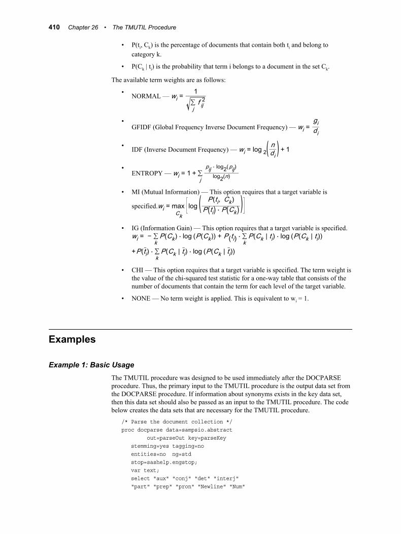
• P(ti, Ck) is the percentage of documents that contain both ti and belong to category k.
• P(Ck | ti) is the probability that term i belongs to a document in the set Ck.
The available term weights are as follows:
• NORMAL — wi =1∑jf ij2
•GFIDF (Global Frequency Inverse Document Frequency) — wi =
gidi
• IDF (Inverse Document Frequency) — wi = log 2( ndi ) + 1•
ENTROPY — wi = 1 + ∑j
pij ⋅ log2(pij)log2(n)
• MI (Mutual Information) — This option requires that a target variable is
specified.wi = maxCk
log ( P(ti, Ck )P(ti) ⋅ P(Ck ) )
• IG (Information Gain) — This option requires that a target variable is specified.wi = − ∑
kP(Ck ) ⋅ log (P(Ck )) + P(ti) ⋅ ∑k
P(Ck | ti) ⋅ log (P(Ck | ti))
+P(ti) ⋅ ∑kP(Ck | ti) ⋅ log (P(Ck | ti))
• CHI — This option requires that a target variable is specified. The term weight is the value of the chi-squared test statistic for a one-way table that consists of the number of documents that contain the term for each level of the target variable.
• NONE — No term weight is applied. This is equivalent to wi = 1.
Examples
Example 1: Basic UsageThe TMUTIL procedure was designed to be used immediately after the DOCPARSE procedure. Thus, the primary input to the TMUTIL procedure is the output data set from the DOCPARSE procedure. If information about synonyms exists in the key data set, then this data set should also be passed as an input to the TMUTIL procedure. The code below creates the data sets that are necessary for the TMUTIL procedure.
/* Parse the document collection */proc docparse data=sampsio.abstract out=parseOut key=parseKey stemming=yes tagging=no entities=no ng=std stop=sashelp.engstop; var text; select "aux" "conj" "det" "interj" "part" "prep" "pron" "Newline" "Num"
410 Chapter 26 • The TMUTIL Procedure
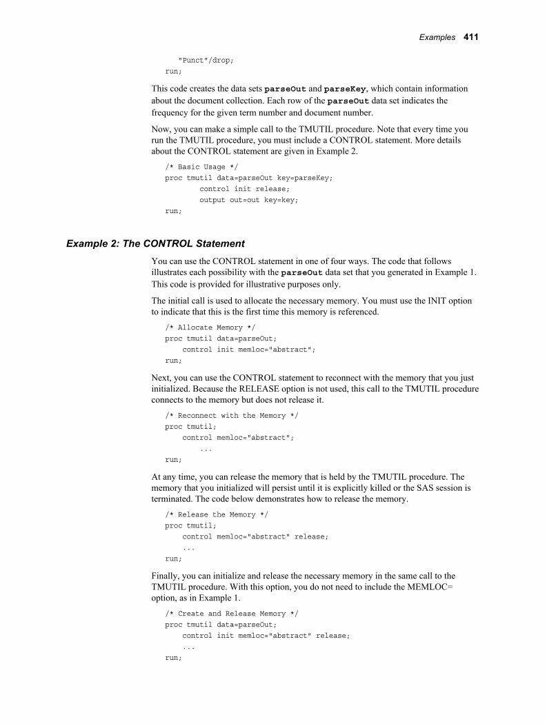
"Punct"/drop;run;
This code creates the data sets parseOut and parseKey, which contain information about the document collection. Each row of the parseOut data set indicates the frequency for the given term number and document number.
Now, you can make a simple call to the TMUTIL procedure. Note that every time you run the TMUTIL procedure, you must include a CONTROL statement. More details about the CONTROL statement are given in Example 2.
/* Basic Usage */proc tmutil data=parseOut key=parseKey; control init release; output out=out key=key;run;
Example 2: The CONTROL StatementYou can use the CONTROL statement in one of four ways. The code that follows illustrates each possibility with the parseOut data set that you generated in Example 1. This code is provided for illustrative purposes only.
The initial call is used to allocate the necessary memory. You must use the INIT option to indicate that this is the first time this memory is referenced.
/* Allocate Memory */proc tmutil data=parseOut; control init memloc="abstract";run;
Next, you can use the CONTROL statement to reconnect with the memory that you just initialized. Because the RELEASE option is not used, this call to the TMUTIL procedure connects to the memory but does not release it.
/* Reconnect with the Memory */proc tmutil; control memloc="abstract"; ...run;
At any time, you can release the memory that is held by the TMUTIL procedure. The memory that you initialized will persist until it is explicitly killed or the SAS session is terminated. The code below demonstrates how to release the memory.
/* Release the Memory */proc tmutil; control memloc="abstract" release; ...run;
Finally, you can initialize and release the necessary memory in the same call to the TMUTIL procedure. With this option, you do not need to include the MEMLOC= option, as in Example 1.
/* Create and Release Memory */proc tmutil data=parseOut; control init memloc="abstract" release; ...run;
Examples 411
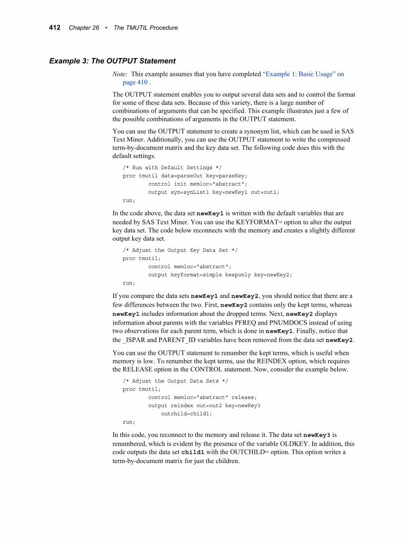
Example 3: The OUTPUT StatementNote: This example assumes that you have completed “Example 1: Basic Usage” on
page 410 .
The OUTPUT statement enables you to output several data sets and to control the format for some of these data sets. Because of this variety, there is a large number of combinations of arguments that can be specified. This example illustrates just a few of the possible combinations of arguments in the OUTPUT statement.
You can use the OUTPUT statement to create a synonym list, which can be used in SAS Text Miner. Additionally, you can use the OUTPUT statement to write the compressed term-by-document matrix and the key data set. The following code does this with the default settings.
/* Run with Default Settings */proc tmutil data=parseOut key=parseKey; control init memloc="abstract"; output syn=synList1 key=newKey1 out=out1;run;
In the code above, the data set newKey1 is written with the default variables that are needed by SAS Text Miner. You can use the KEYFORMAT= option to alter the output key data set. The code below reconnects with the memory and creates a slightly different output key data set.
/* Adjust the Output Key Data Set */proc tmutil; control memloc="abstract"; output keyformat=simple keeponly key=newKey2;run;
If you compare the data sets newKey1 and newKey2, you should notice that there are a few differences between the two. First, newKey2 contains only the kept terms, whereas newKey1 includes information about the dropped terms. Next, newKey2 displays information about parents with the variables PFREQ and PNUMDOCS instead of using two observations for each parent term, which is done in newKey1. Finally, notice that the _ISPAR and PARENT_ID variables have been removed from the data set newKey2.
You can use the OUTPUT statement to renumber the kept terms, which is useful when memory is low. To renumber the kept terms, use the REINDEX option, which requires the RELEASE option in the CONTROL statement. Now, consider the example below.
/* Adjust the Output Data Sets */proc tmutil; control memloc="abstract" release; output reindex out=out2 key=newKey3 outchild=child1;run;
In this code, you reconnect to the memory and release it. The data set newKey3 is renumbered, which is evident by the presence of the variable OLDKEY. In addition, this code outputs the data set child1 with the OUTCHILD= option. This option writes a term-by-document matrix for just the children.
412 Chapter 26 • The TMUTIL Procedure
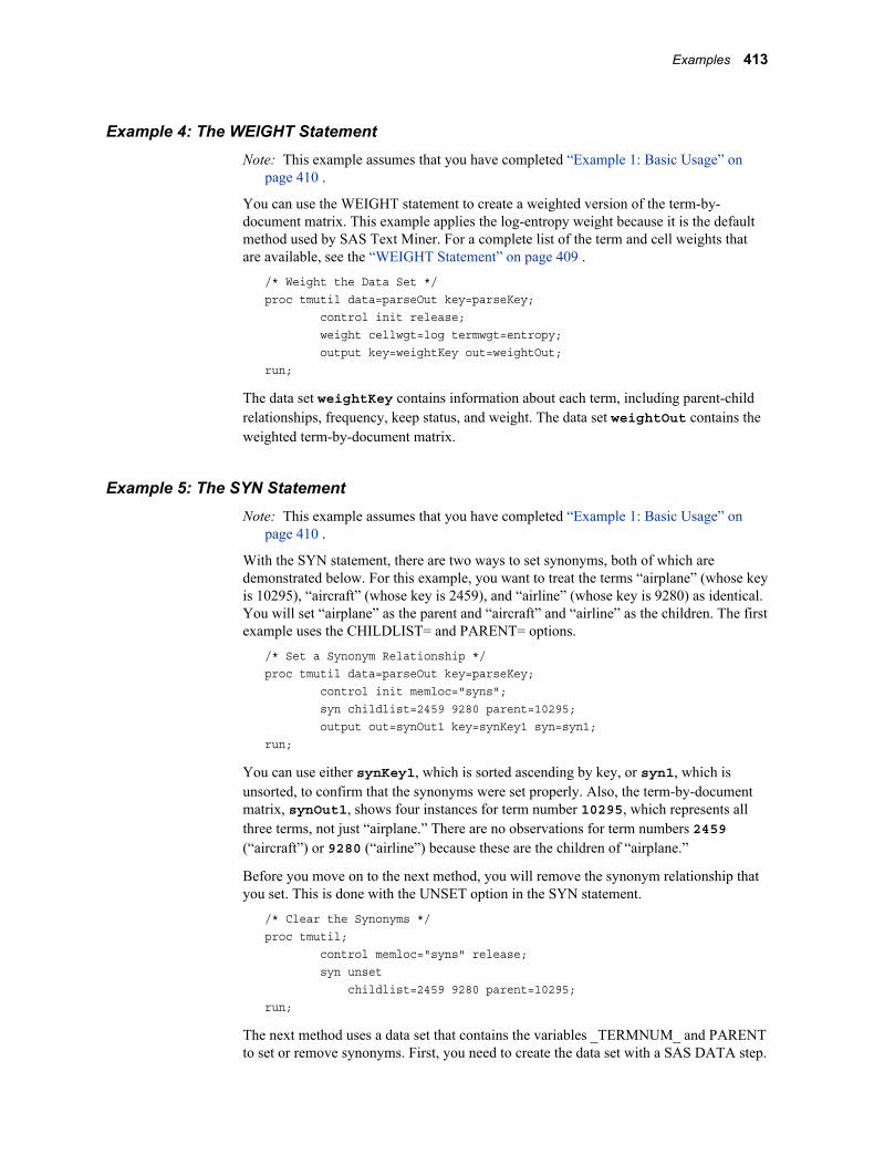
Example 4: The WEIGHT StatementNote: This example assumes that you have completed “Example 1: Basic Usage” on
page 410 .
You can use the WEIGHT statement to create a weighted version of the term-by-document matrix. This example applies the log-entropy weight because it is the default method used by SAS Text Miner. For a complete list of the term and cell weights that are available, see the “WEIGHT Statement” on page 409 .
/* Weight the Data Set */proc tmutil data=parseOut key=parseKey; control init release; weight cellwgt=log termwgt=entropy; output key=weightKey out=weightOut;run;
The data set weightKey contains information about each term, including parent-child relationships, frequency, keep status, and weight. The data set weightOut contains the weighted term-by-document matrix.
Example 5: The SYN StatementNote: This example assumes that you have completed “Example 1: Basic Usage” on
page 410 .
With the SYN statement, there are two ways to set synonyms, both of which are demonstrated below. For this example, you want to treat the terms “airplane” (whose key is 10295), “aircraft” (whose key is 2459), and “airline” (whose key is 9280) as identical. You will set “airplane” as the parent and “aircraft” and “airline” as the children. The first example uses the CHILDLIST= and PARENT= options.
/* Set a Synonym Relationship */proc tmutil data=parseOut key=parseKey; control init memloc="syns"; syn childlist=2459 9280 parent=10295; output out=synOut1 key=synKey1 syn=syn1;run;
You can use either synKey1, which is sorted ascending by key, or syn1, which is unsorted, to confirm that the synonyms were set properly. Also, the term-by-document matrix, synOut1, shows four instances for term number 10295, which represents all three terms, not just “airplane.” There are no observations for term numbers 2459 (“aircraft”) or 9280 (“airline”) because these are the children of “airplane.”
Before you move on to the next method, you will remove the synonym relationship that you set. This is done with the UNSET option in the SYN statement.
/* Clear the Synonyms */proc tmutil; control memloc="syns" release; syn unset childlist=2459 9280 parent=10295;run;
The next method uses a data set that contains the variables _TERMNUM_ and PARENT to set or remove synonyms. First, you need to create the data set with a SAS DATA step.
Examples 413
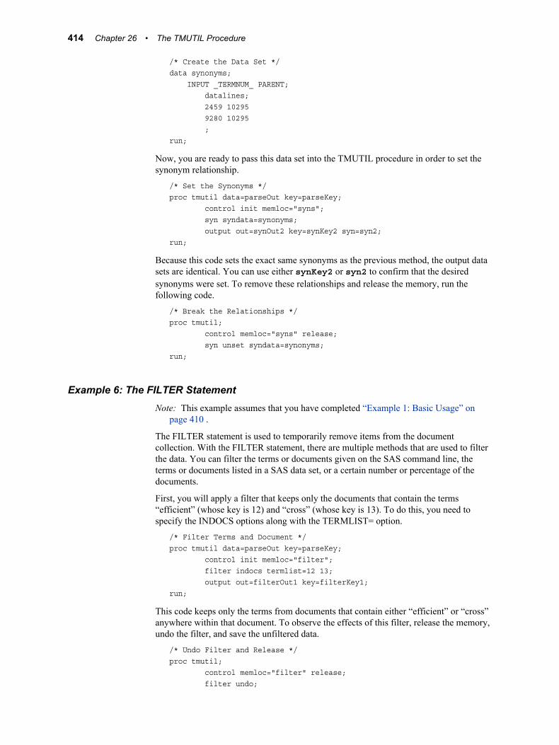
/* Create the Data Set */data synonyms; INPUT _TERMNUM_ PARENT; datalines; 2459 10295 9280 10295 ;run;
Now, you are ready to pass this data set into the TMUTIL procedure in order to set the synonym relationship.
/* Set the Synonyms */proc tmutil data=parseOut key=parseKey; control init memloc="syns"; syn syndata=synonyms; output out=synOut2 key=synKey2 syn=syn2;run;
Because this code sets the exact same synonyms as the previous method, the output data sets are identical. You can use either synKey2 or syn2 to confirm that the desired synonyms were set. To remove these relationships and release the memory, run the following code.
/* Break the Relationships */proc tmutil; control memloc="syns" release; syn unset syndata=synonyms;run;
Example 6: The FILTER StatementNote: This example assumes that you have completed “Example 1: Basic Usage” on
page 410 .
The FILTER statement is used to temporarily remove items from the document collection. With the FILTER statement, there are multiple methods that are used to filter the data. You can filter the terms or documents given on the SAS command line, the terms or documents listed in a SAS data set, or a certain number or percentage of the documents.
First, you will apply a filter that keeps only the documents that contain the terms “efficient” (whose key is 12) and “cross” (whose key is 13). To do this, you need to specify the INDOCS options along with the TERMLIST= option.
/* Filter Terms and Document */proc tmutil data=parseOut key=parseKey; control init memloc="filter"; filter indocs termlist=12 13; output out=filterOut1 key=filterKey1;run;
This code keeps only the terms from documents that contain either “efficient” or “cross” anywhere within that document. To observe the effects of this filter, release the memory, undo the filter, and save the unfiltered data.
/* Undo Filter and Release */proc tmutil; control memloc="filter" release; filter undo;
414 Chapter 26 • The TMUTIL Procedure
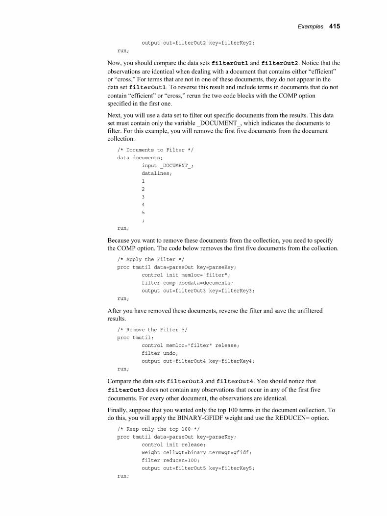
output out=filterOut2 key=filterKey2;run;
Now, you should compare the data sets filterOut1 and filterOut2. Notice that the observations are identical when dealing with a document that contains either “efficient” or “cross.” For terms that are not in one of these documents, they do not appear in the data set filterOut1. To reverse this result and include terms in documents that do not contain “efficient” or “cross,” rerun the two code blocks with the COMP option specified in the first one.
Next, you will use a data set to filter out specific documents from the results. This data set must contain only the variable _DOCUMENT_, which indicates the documents to filter. For this example, you will remove the first five documents from the document collection.
/* Documents to Filter */data documents; input _DOCUMENT_; datalines; 1 2 3 4 5 ;run;
Because you want to remove these documents from the collection, you need to specify the COMP option. The code below removes the first five documents from the collection.
/* Apply the Filter */proc tmutil data=parseOut key=parseKey; control init memloc="filter"; filter comp docdata=documents; output out=filterOut3 key=filterKey3;run;
After you have removed these documents, reverse the filter and save the unfiltered results.
/* Remove the Filter */proc tmutil; control memloc="filter" release; filter undo; output out=filterOut4 key=filterKey4;run;
Compare the data sets filterOut3 and filterOut4. You should notice that filterOut3 does not contain any observations that occur in any of the first five documents. For every other document, the observations are identical.
Finally, suppose that you wanted only the top 100 terms in the document collection. To do this, you will apply the BINARY-GFIDF weight and use the REDUCEN= option.
/* Keep only the top 100 */proc tmutil data=parseOut key=parseKey; control init release; weight cellwgt=binary termwgt=gfidf; filter reducen=100; output out=filterOut5 key=filterKey5;run;
Examples 415
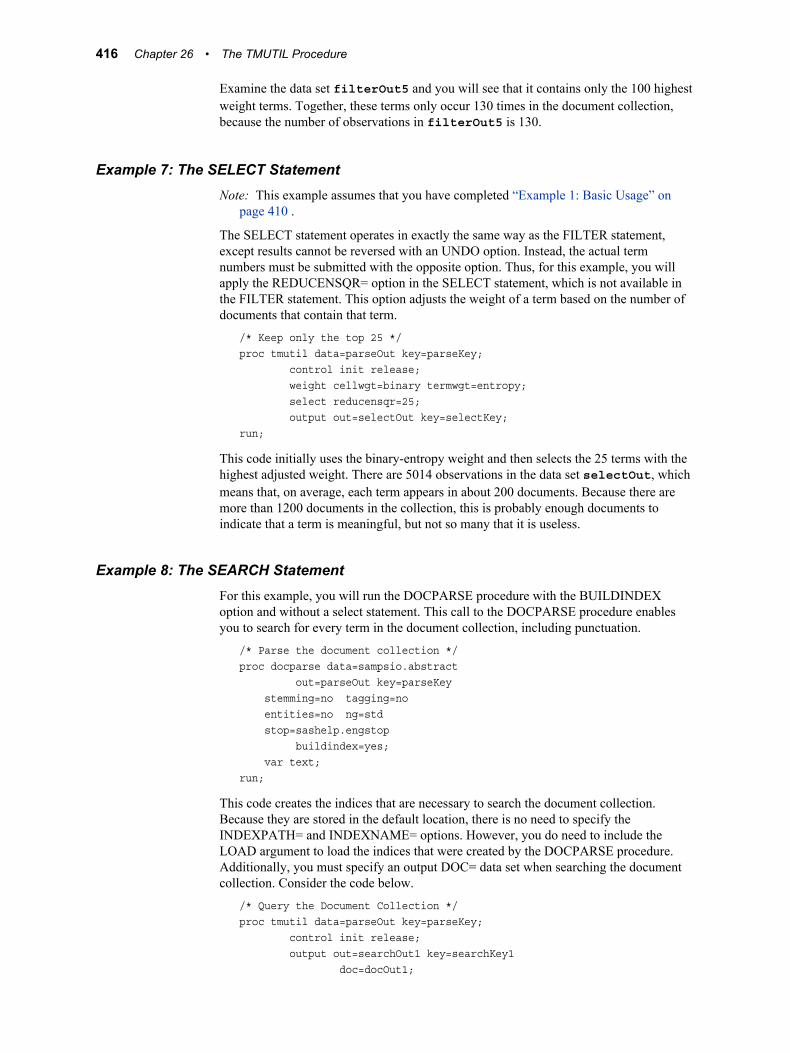
Examine the data set filterOut5 and you will see that it contains only the 100 highest weight terms. Together, these terms only occur 130 times in the document collection, because the number of observations in filterOut5 is 130.
Example 7: The SELECT StatementNote: This example assumes that you have completed “Example 1: Basic Usage” on
page 410 .
The SELECT statement operates in exactly the same way as the FILTER statement, except results cannot be reversed with an UNDO option. Instead, the actual term numbers must be submitted with the opposite option. Thus, for this example, you will apply the REDUCENSQR= option in the SELECT statement, which is not available in the FILTER statement. This option adjusts the weight of a term based on the number of documents that contain that term.
/* Keep only the top 25 */proc tmutil data=parseOut key=parseKey; control init release; weight cellwgt=binary termwgt=entropy; select reducensqr=25; output out=selectOut key=selectKey;run;
This code initially uses the binary-entropy weight and then selects the 25 terms with the highest adjusted weight. There are 5014 observations in the data set selectOut, which means that, on average, each term appears in about 200 documents. Because there are more than 1200 documents in the collection, this is probably enough documents to indicate that a term is meaningful, but not so many that it is useless.
Example 8: The SEARCH StatementFor this example, you will run the DOCPARSE procedure with the BUILDINDEX option and without a select statement. This call to the DOCPARSE procedure enables you to search for every term in the document collection, including punctuation.
/* Parse the document collection */proc docparse data=sampsio.abstract out=parseOut key=parseKey stemming=no tagging=no entities=no ng=std stop=sashelp.engstop buildindex=yes; var text;run;
This code creates the indices that are necessary to search the document collection. Because they are stored in the default location, there is no need to specify the INDEXPATH= and INDEXNAME= options. However, you do need to include the LOAD argument to load the indices that were created by the DOCPARSE procedure. Additionally, you must specify an output DOC= data set when searching the document collection. Consider the code below.
/* Query the Document Collection */proc tmutil data=parseOut key=parseKey; control init release; output out=searchOut1 key=searchKey1 doc=docOut1;
416 Chapter 26 • The TMUTIL Procedure
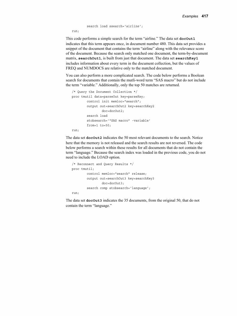
search load ssearch='airline';run;
This code performs a simple search for the term “airline.” The data set docOut1 indicates that this term appears once, in document number 480. This data set provides a snippet of the document that contains the term “airline” along with the relevance score of the document. Because the search only matched one document, the term-by-document matrix, searchOut1, is built from just that document. The data set searchKey1 includes information about every term in the document collection, but the values of FREQ and NUMDOCS are relative only to the matched document.
You can also perform a more complicated search. The code below performs a Boolean search for documents that contain the mutli-word term “SAS macro” but do not include the term “variable.” Additionally, only the top 50 matches are returned.
/* Query the Document Collection */proc tmutil data=parseOut key=parseKey; control init memloc="search"; output out=searchOut2 key=searchKey2 doc=docOut2; search load stobsearch='"SAS macro" -variable' from=1 to=50;run;
The data set docOut2 indicates the 50 most relevant documents to the search. Notice here that the memory is not released and the search results are not reversed. The code below performs a search within these results for all documents that do not contain the term “language.” Because the search index was loaded in the previous code, you do not need to include the LOAD option.
/* Reconnect and Query Results */proc tmutil; control memloc="search" release; output out=searchOut3 key=searchKey3 doc=docOut3; search comp stobsearch='language';run;
The data set docOut3 indicates the 35 documents, from the original 50, that do not contain the term “language.”
Examples 417

418 Chapter 26 • The TMUTIL Procedure

Part 3
Additional Procedures
Chapter 27The TGFILTER Procedure . . . . . . . . . . . . . . . . . . . . . . . . . . . . . . . . . . . . . . . 421
Chapter 28The TGPARSE Procedure . . . . . . . . . . . . . . . . . . . . . . . . . . . . . . . . . . . . . . . 425
419

420
Chapter 27
The TGFILTER Procedure
Overview . . . . . . . . . . . . . . . . . . . . . . . . . . . . . . . . . . . . . . . . . . . . . . . . . . . . . . . . . . . 421The TGFILTER Procedure . . . . . . . . . . . . . . . . . . . . . . . . . . . . . . . . . . . . . . . . . . . 421
Syntax . . . . . . . . . . . . . . . . . . . . . . . . . . . . . . . . . . . . . . . . . . . . . . . . . . . . . . . . . . . . . . 421The TGFILTER Procedure . . . . . . . . . . . . . . . . . . . . . . . . . . . . . . . . . . . . . . . . . . . 421PROC TGFILTER Statement . . . . . . . . . . . . . . . . . . . . . . . . . . . . . . . . . . . . . . . . . 421
Overview
The TGFILTER ProcedureNote: Support for each language must be licensed individually.
The TGFILTER procedure extracts plain text from a collection of documents, which can be stored in various formats, such as Word or PDF. The TGFILTER procedure creates an output data set that contains the plain text and can store the input documents in a user-specified directory. Additionally, PROC TGFILTER can identify the language and other information about the input documents. The TGFILTER procedure works with SAS Document Converter. See the SAS Document Conversion: Developer's Guide for more information.
Syntax
The TGFILTER ProcedurePROC TGFILTER <options>;
RUN;
PROC TGFILTER Statement
SyntaxPROC TGFILER <options>;
421
Required ArgumentsOUT=data-set-name
This argument specifies the SAS data set that contains information about the data processing.
This data set contains the following variables:
• TEXT — A snippet of text from the input document. You can determine the length of this column via the NUMCHAR= option.
• URI — The full path of the input file.
• NAME — The input file name.
• FILTERED — The output file name.
• TRUNCATED — A flag that indicates if the TEXT variable is truncated. The value of TRUNCATED is 0 if the text is not truncated and 1 if it is truncated.
• OMITTED — A flag that indicates if the document was processed. The value of OMITTED is 0 if the document was not omitted and 1 if it was omitted.
• LANGUAGE — The language of the document, as identified by PROC TGFILTER.
• EXTENSION — The extension of the input file.
• CREATED — The date the input file was created.
• ACCESSED — The last time the input file was accessed.
• MODIFIED — The last time the input file was modified.
• SIZE — The size in bytes of the input file.
• FILTEREDSIZE — The size in bytes of the output file.
SRCDIR=file-nameThis option specifies either an unquoted file reference or a quoted string. In either case, the value of file-name points to the directory that contains the input documents.
Optional ArgumentsDESTDIR=file-name
This option specifies a file reference or a quoted string that specifies the directory where PROC TGFILTER will place the output documents.
EXTLIST=“quoted-string”This option specifies the list of extensions that the TGFILTER procedure considers.
FORCESpecify this option to delete the contents of the destination directory. By default, the TGFILTER procedure will not run if there are any files in the DESTDIR= directory.
LANGUAGE | LANG=“quoted-string”The LANGUAGE= option narrows the language choices for PROC TGFILTER to those specified here. Use this option only when you know what language or languages are used in the document collection.
NUMCHARS=numberThis option specifies the number of characters that PROC TGFILTER uses in the text variable out of the OUT= data set. The value of number must be a positive integer between 1 and 32KB, and the default value is 60.
422 Chapter 27 • The TGFILTER Procedure

TGSERVICE=(options)The TGSERVICE= option specifies options for the server. Valid options are as follows:
PORT==numberThis option specifies the port number.
HOSTNAME | HOST=“quoted-string”This option specifies the host name for your service.
Syntax 423

424 Chapter 27 • The TGFILTER Procedure
Chapter 28
The TGPARSE Procedure
Overview . . . . . . . . . . . . . . . . . . . . . . . . . . . . . . . . . . . . . . . . . . . . . . . . . . . . . . . . . . . 425The TGPARSE Procedure . . . . . . . . . . . . . . . . . . . . . . . . . . . . . . . . . . . . . . . . . . . 425
Syntax . . . . . . . . . . . . . . . . . . . . . . . . . . . . . . . . . . . . . . . . . . . . . . . . . . . . . . . . . . . . . . 426The TGPARSE Procedure . . . . . . . . . . . . . . . . . . . . . . . . . . . . . . . . . . . . . . . . . . . 426PROC TGPARSE Statement . . . . . . . . . . . . . . . . . . . . . . . . . . . . . . . . . . . . . . . . . 426SELECT Statement . . . . . . . . . . . . . . . . . . . . . . . . . . . . . . . . . . . . . . . . . . . . . . . . . 434VAR Statement . . . . . . . . . . . . . . . . . . . . . . . . . . . . . . . . . . . . . . . . . . . . . . . . . . . . 435List of Entities . . . . . . . . . . . . . . . . . . . . . . . . . . . . . . . . . . . . . . . . . . . . . . . . . . . . . 435
Examples . . . . . . . . . . . . . . . . . . . . . . . . . . . . . . . . . . . . . . . . . . . . . . . . . . . . . . . . . . . 440Example 1: Sample Data and Basic Usage . . . . . . . . . . . . . . . . . . . . . . . . . . . . . . . 440Example 2: Stemming . . . . . . . . . . . . . . . . . . . . . . . . . . . . . . . . . . . . . . . . . . . . . . . 440Example 3: Entities and Noun Groups . . . . . . . . . . . . . . . . . . . . . . . . . . . . . . . . . . 441Example 4: Tagging . . . . . . . . . . . . . . . . . . . . . . . . . . . . . . . . . . . . . . . . . . . . . . . . 442Example 5: Iterative Parsing . . . . . . . . . . . . . . . . . . . . . . . . . . . . . . . . . . . . . . . . . . 442Example 6: The SELECT Statement . . . . . . . . . . . . . . . . . . . . . . . . . . . . . . . . . . . 443
Overview
The TGPARSE ProcedureNote: Support for each language must be licensed individually.
The TGPARSE procedure processes text documents to reveal information about the terms in those documents. The TGPARSE procedure is capable of reading documents in various languages and file formats. The information is stored in two data sets, the KEY data set and the OUT data set. The KEY data set contains summary information about each term, such as frequency, keep status, and part of speech. The OUT data set is a compressed representation of the term-by-document matrix. Both of these data sets are used in later steps of the text mining process.
425
Syntax
The TGPARSE ProcedurePROC TGPARSE DATA=data-set-name OUT=data-set-name KEY=data-set-name <options>;
SELECT <options>;VAR variable;RUN;
PROC TGPARSE Statement
SyntaxPROC TGPARSE DATA=data-set-name OUT=data-set-name KEY=data-set-name <options>;
Required ArgumentsDATA=data-set-name
This data set contains either the documents or references to the documents that are parsed.
Note: Strictly speaking, this argument is not required, but should be included. If the DATA= argument is omitted, then the most recently created data set is used for analysis.
KEY=data-set-nameThis data set is the summary information about the terms in the document collection.
The variables in this data set are as follows:
• Term — A lowercase version of the term.
• Role — The term's part of speech. This variable is empty if tagging is off or not specified.
• Attribute — An indication of the characters that compose the term. Possible attributes are Alpha, only alphabetic characters; Mixed, a combination of attributes; Num, only numbers; Punct, punctuation characters; and Entity, an identified entity.
• Freq — The frequency of a term in the entire document collection.
• numdocs — The number of documents that contain the term.
• Keep — The keep status of the term. A Y indicates that the term is kept for analysis and an N indicates that the term should be dropped in later stages of analysis.
• Key — The assigned term number. Each unique term in the parsed documents and each unique parent term has a unique Key value.
• Parent — The Key value of the term's parent or a period. If a term has a parent, then this variable gives the term number of that parent. If a term does not have a parent then this value is a period. When the values of Key, Parent, and Parent_id are identical, the observation indicates that the parent occurs as itself. When the
426 Chapter 28 • The TGPARSE Procedure
values of Parent and Parent_id are identical but differ from Key, the observation is a child.
• Parent_id — Another description of the term's parent. While Parent only gives the parent's term number if a term is a child, Parent_id gives this value for all terms.
• _ispar — An indication of a term's status as a parent, child, or neither. A + (plus sign) indicates that the term is a parent. A . (period) indicates that the term is a child. A missing value indicates that the term is neither a parent nor a child.
Note: When either stemming or a synonym list is used, children are assigned to parents with the Parent and Parent_id variables. Thus, parents might appear in the KEY= data set twice. One entry indicates how often the term appeared as itself and the other indicates the totals for a parent and all its children. The variables Parent, Parent_id, and _ispar indicate this information in slightly different ways.
OUT=data-set-nameThis data set is the compressed term-by-document matrix. The OUT= data set contains all of the terms included in every document, not the parent or stemmed terms. The TGPARSE procedure is typically a precursor to the TGSCORE procedure and you can remove the superfluous child terms with either PROC TMUTIL or SQL code.
The variables in this data set are as follows:
• _TERMNUM_ — A positive integer that uniquely defines each term (or term-role pair when tagging is on).
• _DOCUMENT_ — A positive integer that uniquely defines each document.
• _COUNT_ — A positive integer that indicates the frequency of the observed term-document pair.
Optional ArgumentsCONFIG=data-set-name
The CONFIG= data set is a SAS data set that contains predefined PROC TGPARSE run option settings. In other words, it contains the configuration settings for the procedure. The primary purpose of this data set is to relay the configuration information from the TGPARSE procedure to the TGSCORE procedure. Thus, the TGSCORE procedure is forced to use options that are consistent with the TGPARSE procedure.
Alternatively, you can use the CONFIG= data set to predefine options for PROC TGPARSE. If data-set-name exists, then the procedure will run with the settings that are specified there. If there are discrepancies between the CONFIG= data set and an argument specified in the proc statement, then the specified argument will take precedence. Additionally, the CONFIG= data set will be updated to reflect the specified argument.
If data-set-name does not exists, then this data set will be created. You can update this data set as you would any other SAS data set.
Configuration information in this data set is as follows:
• namedfile — indicates if the parsed variable was in an external file or the input data set.
• language — indicates the source language of the documents.
• encoding — indicates the encoding of the documents.
Syntax 427
• plugin — indicates the plugin used to parse the document collection.
• stemming — indicates Y if stemming is used and N if it is not.
• tagging — indicates Y if tagging is used and N if it is not.
• NG — indicates how noun groups are processed.
• entities — indicates if entities are used or not.
• entList — indicates the entities that are kept.
• attributes — indicates if attributes are kept or dropped.
• attrList — indicates the attributes that are kept or dropped.
• pos — indicates if parts of speech are kept or dropped
• posList — indicates the parts of speech that are kept or dropped.
• multiterm — specifies the path to the multiterm list.
• litiList — indicates the path to your custom entities. These custom entities are contained in .li files that are called liti lists. You can create as many .li files as you need to specify and run customized entities through PROC TGPARSE.
DOC_ID=numberThis option specifies the first document number in the OUT= data set. Use this option to iteratively parse the document collection. Iterative parsing allows you to add information about additional documents to a preexisting KEY= data set. This way, you do not need to add the new documents to the original collection and rerun the TGPARSE collection, which saves time and resources.
ENTITIES=YES | NOUse this option to determine whether the entity extractor should use the standard list of entities or not. There are two types of entity extraction, standard and custom. The ENTITIES= option applies to both standard and custom entity extraction. Standard entities are used when ENTITIES=YES and the LITILIST= option is not used. Custom entities are used when ENTITIES=YES and a user supplied LITI file is referenced in the LITILIST= option. When standard entities are used, terms such as "Wiley E. Coyote" are recognized as an entity and given the corresponding entity role and attribute. For this example, the entity role is PERSON and the attribute is Entity. While the entity is treated as the single term "wiley e. coyoyte", the individual tokens "wiley", "e", and "coyote" are also included.
Note: The following languages do not support the standard entity list for the entity extractor and therefore cannot use the ENTITIES= option: Czech, Danish, Finnish, Greek, Hebrew, Hungarian, Indonesian, Norwegian, Romanian, Russian, Slovak, Thai, Turkish, and Vietnamese. The LITILIST= option allows you to use the custom entities. Please see the LITILIST=option for details.
IGNORE=data-set-nameThis data set should contain the terms that you want to ignore. An example data set is SASHELP.STOPLST. Ignore lists and stop lists have the same format.
INKEY=data-set-nameThis option specifies a previously created KEY= data set so that you can perform iterative parsing. If you specify this option, then data-set-name is used as the starting point for the output KEY= data set.
LANGUAGE | LANG='string'Use this option to specify the language of the document collection. The value of string is the lowercase version of any supported language. Supported languages are Arabic, Chinese, Czech, Danish, Dutch, English, Finnish, French, German, Greek,
428 Chapter 28 • The TGPARSE Procedure
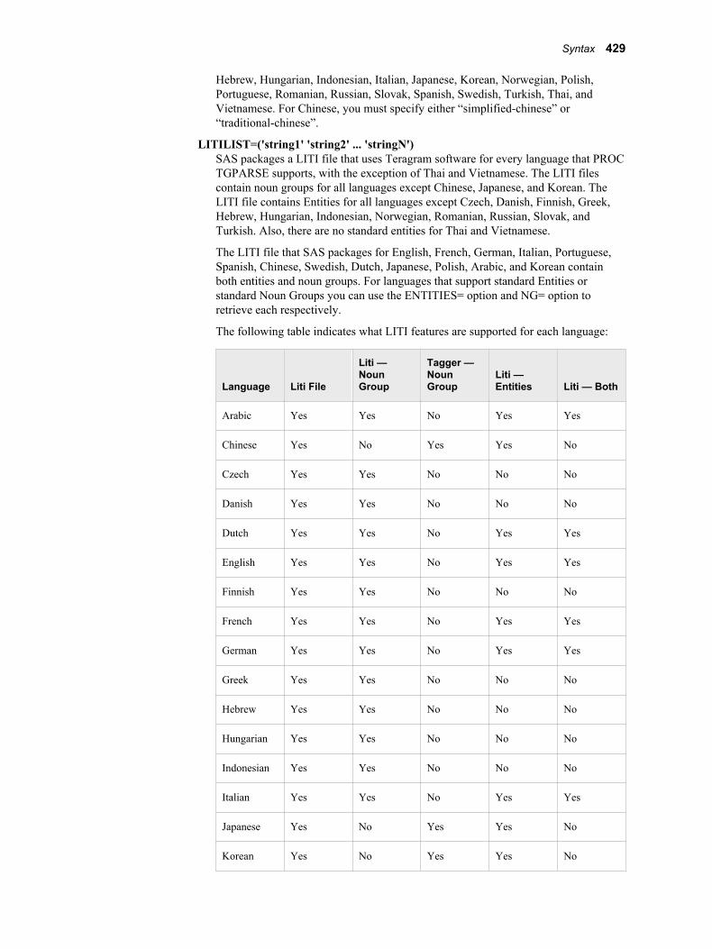
Hebrew, Hungarian, Indonesian, Italian, Japanese, Korean, Norwegian, Polish, Portuguese, Romanian, Russian, Slovak, Spanish, Swedish, Turkish, Thai, and Vietnamese. For Chinese, you must specify either “simplified-chinese” or “traditional-chinese”.
LITILIST=('string1' 'string2' ... 'stringN')SAS packages a LITI file that uses Teragram software for every language that PROC TGPARSE supports, with the exception of Thai and Vietnamese. The LITI files contain noun groups for all languages except Chinese, Japanese, and Korean. The LITI file contains Entities for all languages except Czech, Danish, Finnish, Greek, Hebrew, Hungarian, Indonesian, Norwegian, Romanian, Russian, Slovak, and Turkish. Also, there are no standard entities for Thai and Vietnamese.
The LITI file that SAS packages for English, French, German, Italian, Portuguese, Spanish, Chinese, Swedish, Dutch, Japanese, Polish, Arabic, and Korean contain both entities and noun groups. For languages that support standard Entities or standard Noun Groups you can use the ENTITIES= option and NG= option to retrieve each respectively.
The following table indicates what LITI features are supported for each language:
Language Liti File
Liti — Noun Group
Tagger — Noun Group
Liti — Entities Liti — Both
Arabic Yes Yes No Yes Yes
Chinese Yes No Yes Yes No
Czech Yes Yes No No No
Danish Yes Yes No No No
Dutch Yes Yes No Yes Yes
English Yes Yes No Yes Yes
Finnish Yes Yes No No No
French Yes Yes No Yes Yes
German Yes Yes No Yes Yes
Greek Yes Yes No No No
Hebrew Yes Yes No No No
Hungarian Yes Yes No No No
Indonesian Yes Yes No No No
Italian Yes Yes No Yes Yes
Japanese Yes No Yes Yes No
Korean Yes No Yes Yes No
Syntax 429
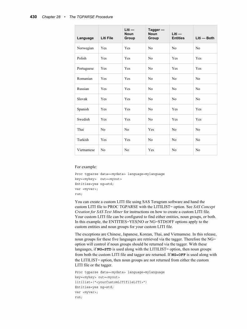
Language Liti File
Liti — Noun Group
Tagger — Noun Group
Liti — Entities Liti — Both
Norwegian Yes Yes No No No
Polish Yes Yes No Yes Yes
Portuguese Yes Yes No Yes Yes
Romanian Yes Yes No No No
Russian Yes Yes No No No
Slovak Yes Yes No No No
Spanish Yes Yes No Yes Yes
Swedish Yes Yes No Yes Yes
Thai No No Yes No No
Turkish Yes Yes No No No
Vietnamese No No Yes No No
For example:
Proc tgparse data=<mydata> language=mylanguagekey=<mykey> out=<myout>Entities=yes ng=std;var <myvar>;run;
You can create a custom LITI file using SAS Teragram software and hand the custom LITI file to PROC TGPARSE with the LITILIST= option. See SAS Concept Creation for SAS Text Miner for instructions on how to create a custom LITI file. Your custom LITI file can be configured to find either entities, noun groups, or both. In this example, the ENTITIES=YES|NO or NG=STD|OFF options apply to the custom entities and noun groups for your custom LITI file.
The exceptions are Chinese, Japanese, Korean, Thai, and Vietnamese. In this release, noun groups for these five languages are retrieved via the tagger. Therefore the NG= option will control if noun groups should be returned via the tagger. With these languages, if NG=STD is used along with the LITILIST= option, then noun groups from both the custom LITI file and tagger are returned. If NG=OFF is used along with the LITILIST= option, then noun groups are not returned from either the custom LITI file or the tagger.
Proc tgparse data=<mydata> language=mylanguagekey=<mykey> out=<myout>litilist=("<yourCustomLITIfileLITI>")Entities=yes ng=std;var <myvar>;run;
430 Chapter 28 • The TGPARSE Procedure
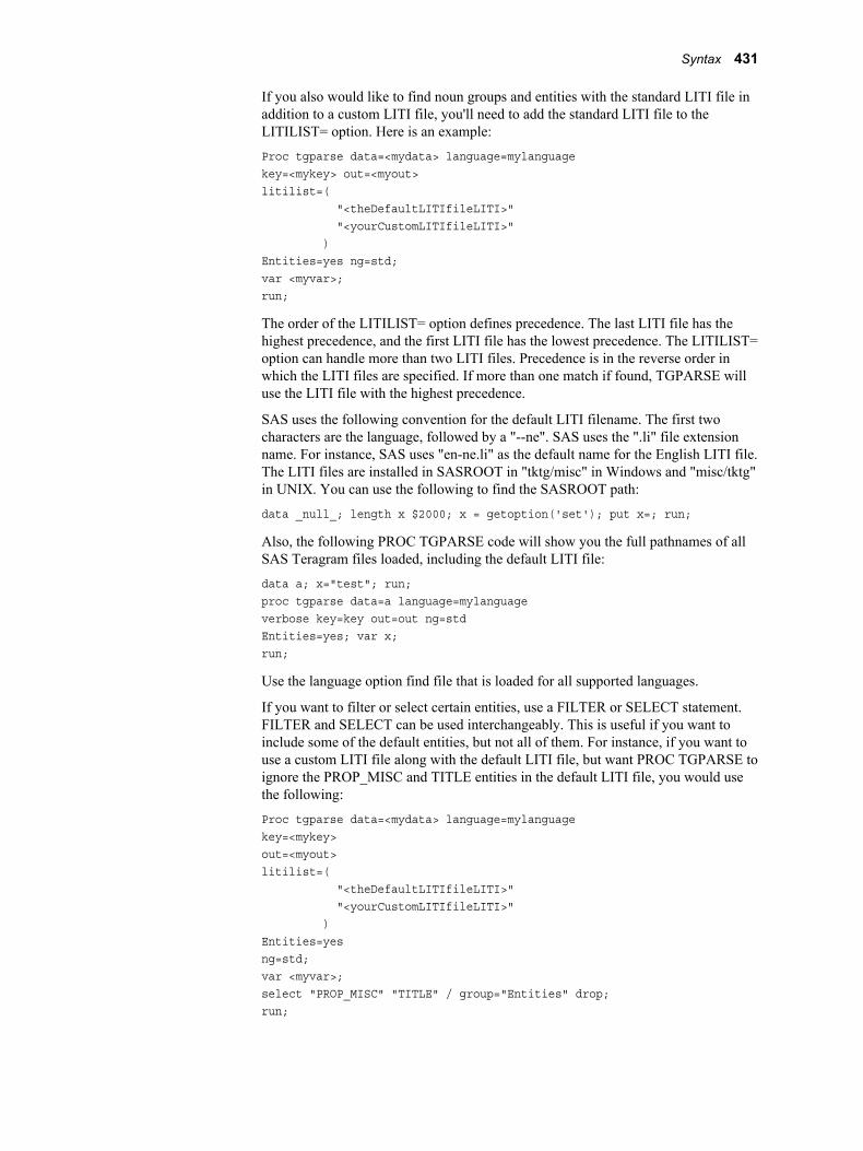
If you also would like to find noun groups and entities with the standard LITI file in addition to a custom LITI file, you'll need to add the standard LITI file to the LITILIST= option. Here is an example:
Proc tgparse data=<mydata> language=mylanguagekey=<mykey> out=<myout>litilist=( "<theDefaultLITIfileLITI>" "<yourCustomLITIfileLITI>" )Entities=yes ng=std;var <myvar>;run;
The order of the LITILIST= option defines precedence. The last LITI file has the highest precedence, and the first LITI file has the lowest precedence. The LITILIST= option can handle more than two LITI files. Precedence is in the reverse order in which the LITI files are specified. If more than one match if found, TGPARSE will use the LITI file with the highest precedence.
SAS uses the following convention for the default LITI filename. The first two characters are the language, followed by a "--ne". SAS uses the ".li" file extension name. For instance, SAS uses "en-ne.li" as the default name for the English LITI file. The LITI files are installed in SASROOT in "tktg/misc" in Windows and "misc/tktg" in UNIX. You can use the following to find the SASROOT path:
data _null_; length x $2000; x = getoption('set'); put x=; run;
Also, the following PROC TGPARSE code will show you the full pathnames of all SAS Teragram files loaded, including the default LITI file:
data a; x="test"; run;proc tgparse data=a language=mylanguageverbose key=key out=out ng=stdEntities=yes; var x;run;
Use the language option find file that is loaded for all supported languages.
If you want to filter or select certain entities, use a FILTER or SELECT statement. FILTER and SELECT can be used interchangeably. This is useful if you want to include some of the default entities, but not all of them. For instance, if you want to use a custom LITI file along with the default LITI file, but want PROC TGPARSE to ignore the PROP_MISC and TITLE entities in the default LITI file, you would use the following:
Proc tgparse data=<mydata> language=mylanguagekey=<mykey>out=<myout>litilist=( "<theDefaultLITIfileLITI>" "<yourCustomLITIfileLITI>" )Entities=yesng=std;var <myvar>;select "PROP_MISC" "TITLE" / group="Entities" drop;run;
Syntax 431
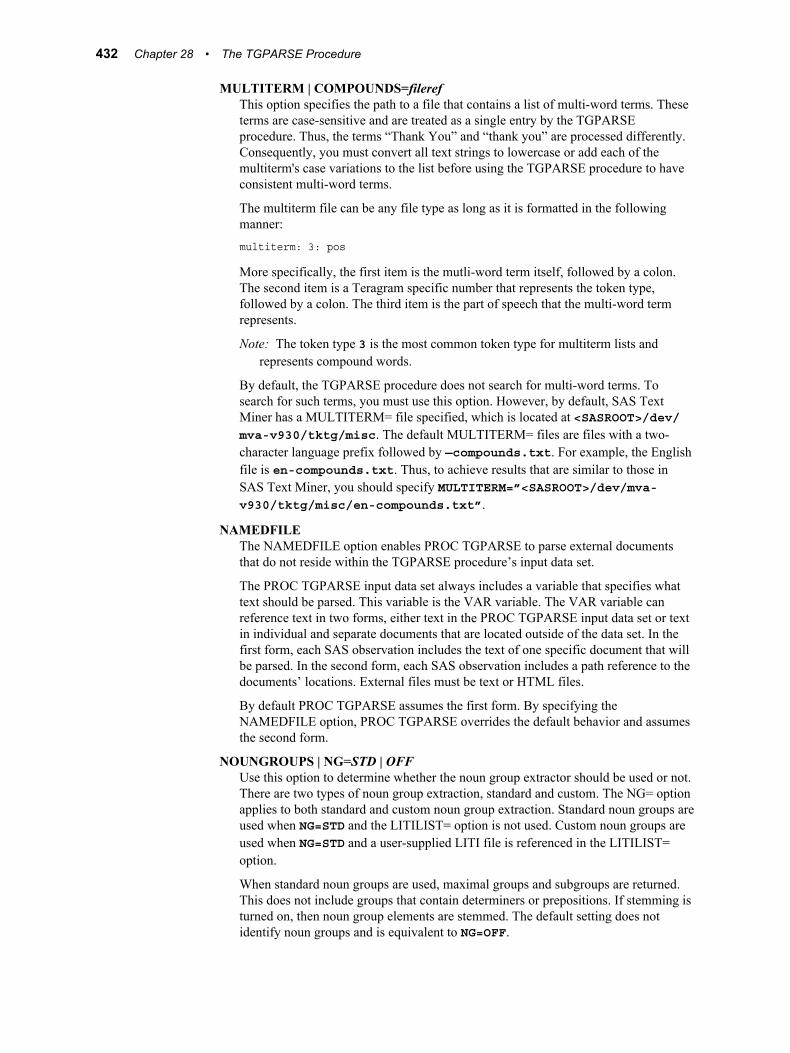
MULTITERM | COMPOUNDS=filerefThis option specifies the path to a file that contains a list of multi-word terms. These terms are case-sensitive and are treated as a single entry by the TGPARSE procedure. Thus, the terms “Thank You” and “thank you” are processed differently. Consequently, you must convert all text strings to lowercase or add each of the multiterm's case variations to the list before using the TGPARSE procedure to have consistent multi-word terms.
The multiterm file can be any file type as long as it is formatted in the following manner:
multiterm: 3: pos
More specifically, the first item is the mutli-word term itself, followed by a colon. The second item is a Teragram specific number that represents the token type, followed by a colon. The third item is the part of speech that the multi-word term represents.
Note: The token type 3 is the most common token type for multiterm lists and represents compound words.
By default, the TGPARSE procedure does not search for multi-word terms. To search for such terms, you must use this option. However, by default, SAS Text Miner has a MULTITERM= file specified, which is located at <SASROOT>/dev/mva-v930/tktg/misc. The default MULTITERM= files are files with a two-character language prefix followed by —compounds.txt. For example, the English file is en-compounds.txt. Thus, to achieve results that are similar to those in SAS Text Miner, you should specify MULTITERM=”<SASROOT>/dev/mva-v930/tktg/misc/en-compounds.txt”.
NAMEDFILEThe NAMEDFILE option enables PROC TGPARSE to parse external documents that do not reside within the TGPARSE procedure’s input data set.
The PROC TGPARSE input data set always includes a variable that specifies what text should be parsed. This variable is the VAR variable. The VAR variable can reference text in two forms, either text in the PROC TGPARSE input data set or text in individual and separate documents that are located outside of the data set. In the first form, each SAS observation includes the text of one specific document that will be parsed. In the second form, each SAS observation includes a path reference to the documents’ locations. External files must be text or HTML files.
By default PROC TGPARSE assumes the first form. By specifying the NAMEDFILE option, PROC TGPARSE overrides the default behavior and assumes the second form.
NOUNGROUPS | NG=STD | OFFUse this option to determine whether the noun group extractor should be used or not. There are two types of noun group extraction, standard and custom. The NG= option applies to both standard and custom noun group extraction. Standard noun groups are used when NG=STD and the LITILIST= option is not used. Custom noun groups are used when NG=STD and a user-supplied LITI file is referenced in the LITILIST= option.
When standard noun groups are used, maximal groups and subgroups are returned. This does not include groups that contain determiners or prepositions. If stemming is turned on, then noun group elements are stemmed. The default setting does not identify noun groups and is equivalent to NG=OFF.
432 Chapter 28 • The TGPARSE Procedure
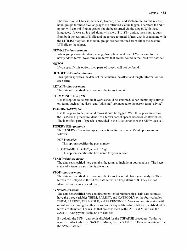
The exception is Chinese, Japanese, Korean, Thai, and Vietnamese. In this release, noun groups for these five languages are retrieved via the tagger. Therefore the NG= option will control if noun groups should be returned via the tagger. With these languages, if NG=STD is used along with the LITILIST= option, then noun groups from both the custom LITI file and tagger are returned. If NG=OFF is used along with the LITILIST= option, then noun groups are not returned from either the custom LITI file or the tagger.
NEWKEY=data-set-nameWhen you perform iterative parsing, this option creates a KEY= data set for the newly added terms. New terms are terms that are not found in the INKEY= data set.
NOPOSIf you specify this option, then parts of speech will not be found.
OUTOFFSET=data-set-nameThis option specifies the data set that contains the offset and length information for each term.
RETAIN=data-set-nameThe data set specified here contains the terms to retain.
STEMMING=YES | NOUse this option to determine if words should be stemmed. When stemming is turned on, terms such as “advises” and “advising” are mapped to the parent term “advise”.
TAGGING=YES | NOUse this option to determine if terms should be tagged. With this option turned on, the TGPARSE procedure identifies a term's part of speech based on context clues. The identified part of speech is provided in the Role variable of the KEY= data set.
TGSERVICE=(options)The TGSERVICE= option specifies options for the server. Valid options are as follows:
PORT=numberThis option specifies the port number.
HOSTNAME | HOST=“quoted-string”This option specifies the host name for your service.
START=data-set-nameThe data set specified here contains the terms to include in your analysis. The keep status of a term in a start list is always Y.
STOP=data-set-nameThe data set specified here contains the terms to exclude from your analysis. These terms are displayed in the KEY= data set with a keep status of N. They are not identified as parents or children.
SYN=data-set-nameThe data set specified here contains parent-child relationships. This data set must have the three variables TERM, PARENT, and CATEGORY or the four variables TERM, PARENT, TERMROLE, and PARENTROLE. You can use this option with or without stemming, but this list overrides any relationships that are identified when terms are stemmed. For results that are consistent with SAS Text Miner, use the SASHELP.Engsynms as the SYN= data set.
By default, the SYN= data set is disabled for the TGPARSE procedure. To derive results similar to those in SAS Text Miner, use the SASHELP.Engsynms data set for the SYN= data set.
Syntax 433
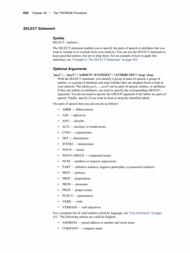
SELECT Statement
SyntaxSELECT <options>;
The SELECT statement enables you to specify the parts of speech or attributes that you want to include in or exclude from your analysis. You can use the SELECT statement to keep specified entities, but not to drop them. For an example of how to apply this statement, see “Example 6: The SELECT Statement” on page 443 .
Optional Arguments“pos1” ... “posN” / <GROUP=“ENTITIES” | “ATTRIBUTES”> keep | drop
With the SELECT statement, you identify a group of parts of speech, a group of entities, or a group of attributes and state whether they are dropped from or kept in your analysis. The labels pos1, ..., posN can be parts of speech, entities, or attributes. If they are entities or attributes, you need to specify the corresponding GROUP= argument. You do not need to specify the GROUP argument if the labels are parts of speech. Finally, specify if you want to keep or drop the identified labels.
The parts of speech that you can use are as follows:
• ABBR — abbreviations
• ADJ — adjectives
• ADV — adverbs
• AUX — auxiliary or modal terms
• CONJ — conjunctions
• DET — determiners
• INTERJ — interjections
• NOUN — nouns
• NOUN_GROUP — compound nouns
• NUM — numbers or numeric expressions
• PART — infinitive markers, negative participles, or possessive markers
• PREF — prefixes
• PREP — prepositions
• PRON — pronouns
• PROP — proper nouns
• PUNCT — punctuation
• VERB — verbs
• VERBADJ — verb adjectives
For a complete list of valid entities sorted by language, see “List of Entities” on page 435 . The following entities are valid for English:
• ADDRESS — postal address or number and street name
• COMPANY — company name
434 Chapter 28 • The TGPARSE Procedure
• CURRENCY — currency or currency expression
• DATE — date, day, month, or year
• INTERNET — e-mail address or URL
• LOCATION — city, county, state, political or geographical place or region,
• MEASURE — measurement or measurement expression
• NOUN_GROUP — phrases that contain multiple words
• ORGANIZATION — government, legal, or service agency
• PERCENT — percentage or percentage expression
• PERSON — person's name
• PHONE — phone number
• PROP_MISC — proper noun with an ambiguous classification
• SSN — social security number
• TIME — time or time expression
• TIME_PERIOD — measure of time expressions
• TITLE — person's title or position
• VEHICLE — motor vehicle, including color, year, make, and model
The attributes that you can use are as follows:
• ALPHA — only letters
• ENTITIES — only entities
• NUM — only numbers
• PUNCT — punctuation characters
• MIXED — combination of letters, numbers, and punctuation
VAR Statement
SyntaxVAR variable;
Required Argumentvariable
This argument specifies the variable that contains the text that you want to process.
List of EntitiesNot all entities are supported for every language that is supported by PROC TGPARSE. The list that follows indicates which languages are supported for each entity.
The following tables indicate the languages that are available for each entity. Here, Y indicates that the language-entity pair is available, and N specifies that it is not available.
Syntax 435

Tabl
e 28
.1S
uppo
rted
lang
uage
-ent
ity p
airs
Add
ress
Com
pany
Cur
renc
yD
ate
Inte
rnet
Loca
tion
Mea
sure
Nou
n_G
roup
Num
ber
Ord
num
ber
Ara
bic
YN
YY
YY
YY
YN
Chi
nese
YN
YY
YY
YY
NN
Cze
chN
NN
NN
NN
YN
N
Dan
ish
YY
YY
YY
YY
NN
Dut
chY
YY
YY
YY
YN
N
Engl
ish
YY
YY
YY
YY
NN
Fini
shN
NN
NN
NN
YN
N
Fren
chY
YY
YY
YY
YN
N
Ger
man
YY
YY
YY
YY
NN
Gre
ekN
NN
NN
NN
YN
N
Heb
rew
NN
NN
NN
NY
NN
Hun
garia
nN
NN
NN
NN
YN
N
Indo
nesi
anN
NN
NN
NN
YN
N
Italia
nY
YY
YY
YY
YN
N
Japa
nese
YN
YY
YY
YY
NN
Kor
ean
YY
YY
YY
YY
YY
Nor
weg
ian
NN
NN
NN
NY
NN
436 Chapter 28 • The TGPARSE Procedure
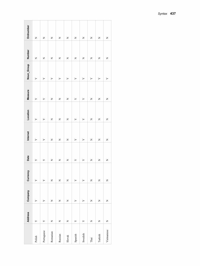
Add
ress
Com
pany
Cur
renc
yD
ate
Inte
rnet
Loca
tion
Mea
sure
Nou
n_G
roup
Num
ber
Ord
num
ber
Polis
hY
YY
YY
YY
YN
N
Portu
gues
eY
YY
YY
YY
YN
N
Rom
ania
nN
NN
NN
NN
YN
N
Rus
sian
NN
NN
NN
NY
NN
Slov
akN
NN
NN
NN
YN
N
Span
ish
YY
YY
YY
YY
NN
Swed
ish
YY
YY
YY
YY
NN
Thai
NN
NN
NN
NY
NN
Turk
ish
NN
NN
NN
NY
NN
Vie
tnam
ese
NN
NN
NN
NY
NN
Syntax 437
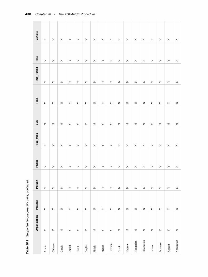
Tabl
e 28
.2S
uppo
rted
lang
uage
-ent
ity p
airs
, con
tinue
d
Org
aniz
atio
nPe
rcen
tPe
rson
Phon
ePr
op_M
isc
SSN
Tim
eTi
me_
Perio
dTi
tleVe
hcile
Ara
bic
YY
YY
NN
YY
YN
Chi
nese
YY
YY
YN
YY
YN
Cze
chN
NN
NN
NN
NN
N
Dan
ish
YY
YY
YY
YY
YY
Dut
chY
YY
YY
YY
YY
Y
Engl
ish
YY
YY
YY
YY
YY
Fini
shN
NN
NN
NN
NN
N
Fren
chY
YY
YY
YY
YY
N
Ger
man
YY
YY
YY
YY
NN
Gre
ekN
NN
NN
NN
NN
N
Heb
rew
NN
NN
NN
NN
NN
Hun
garia
nN
NN
NN
NN
NN
N
Indo
nesi
anN
NN
NN
NN
NN
N
Italia
nN
YY
YY
YY
YY
N
Japa
nese
YY
YY
NN
YY
YN
Kor
ean
YY
YY
NN
YY
YN
Nor
weg
ian
NN
NN
NN
NN
NN
438 Chapter 28 • The TGPARSE Procedure
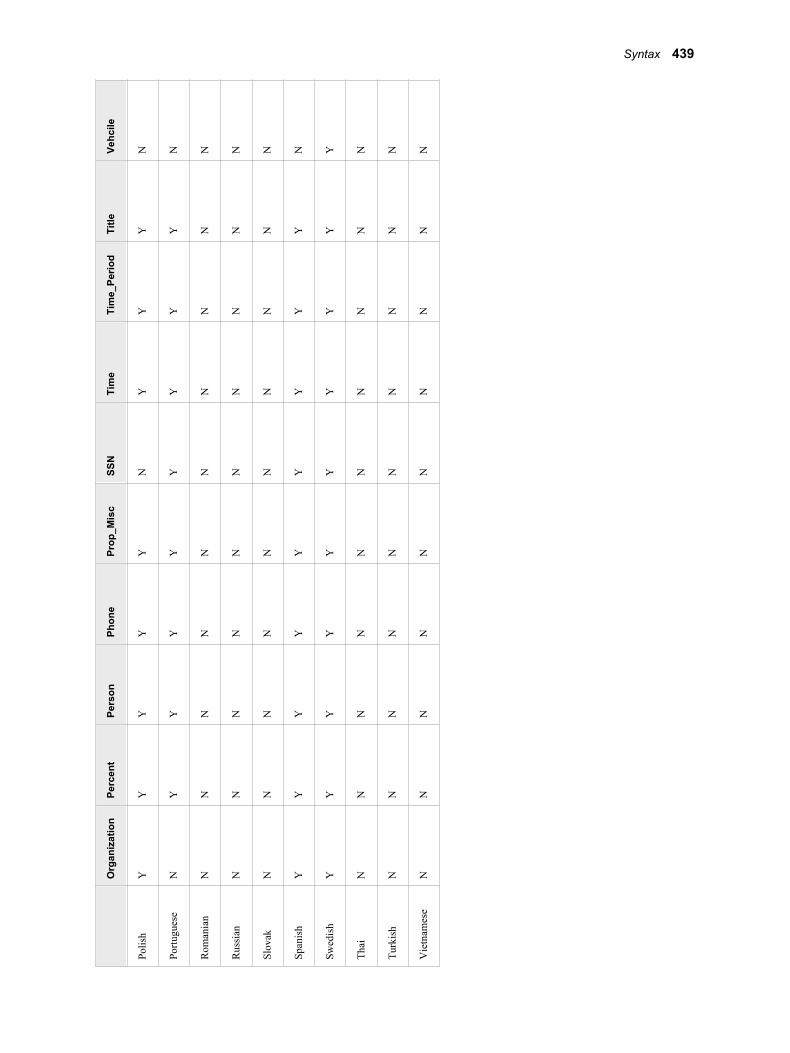
Org
aniz
atio
nPe
rcen
tPe
rson
Phon
ePr
op_M
isc
SSN
Tim
eTi
me_
Perio
dTi
tleVe
hcile
Polis
hY
YY
YY
NY
YY
N
Portu
gues
eN
YY
YY
YY
YY
N
Rom
ania
nN
NN
NN
NN
NN
N
Rus
sian
NN
NN
NN
NN
NN
Slov
akN
NN
NN
NN
NN
N
Span
ish
YY
YY
YY
YY
YN
Swed
ish
YY
YY
YY
YY
YY
Thai
NN
NN
NN
NN
NN
Turk
ish
NN
NN
NN
NN
NN
Vie
tnam
ese
NN
NN
NN
NN
NN
Syntax 439
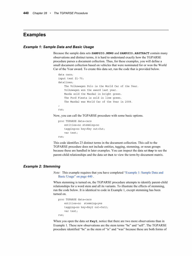
Examples
Example 1: Sample Data and Basic UsageBecause the sample data sets SAMPSIO.NEWS and SAMPSIO.ABSTRACT contain many observations and distinct terms, it is hard to understand exactly how the TGPARSE procedure parses a document collection. Thus, for these examples, you will define a small document collection based on vehicles that were nominated for or won the World Car of the Year award. To create this data set, run the code that is provided below.
data cars;input text $1-70;datalines; The Volkswagen Polo is the World Car of the Year. Volkswagen won the award last year. Mazda sold the Mazda2 in bright green. The Ford Fiesta is sold in lime green. The Mazda2 was World Car of the Year in 2008.;run;
Now, you can call the TGPARSE procedure with some basic options.
proc TGPARSE data=cars entities=no stemming=no tagging=no key=Key out=Out; var text;run;
This code identifies 23 distinct terms in the document collection. This call to the TGPARSE procedure does not include entities, tagging, stemming, or noun groups because these are handled in later examples. You can inspect the data set Key to see the parent-child relationships and the data set Out to view the term-by-document matrix.
Example 2: StemmingNote: This example requires that you have completed “Example 1: Sample Data and
Basic Usage” on page 440 .
When stemming is turned on, the TGPARSE procedure attempts to identify parent-child relationships for a word stem and all its variants. To illustrate the effects of stemming, run the code below. It is identical to code in Example 1, except stemming has been turned on.
proc TGPARSE data=cars entities=no stemming=yes tagging=no key=Key2 out=Out2; var text;run;
When you open the data set Key2, notice that there are two more observations than in Example 1. These new observations are the stem terms “be” and “sell”. The TGPARSE procedure identified “be” as the stem of “is” and “was” because these are both forms of
440 Chapter 28 • The TGPARSE Procedure
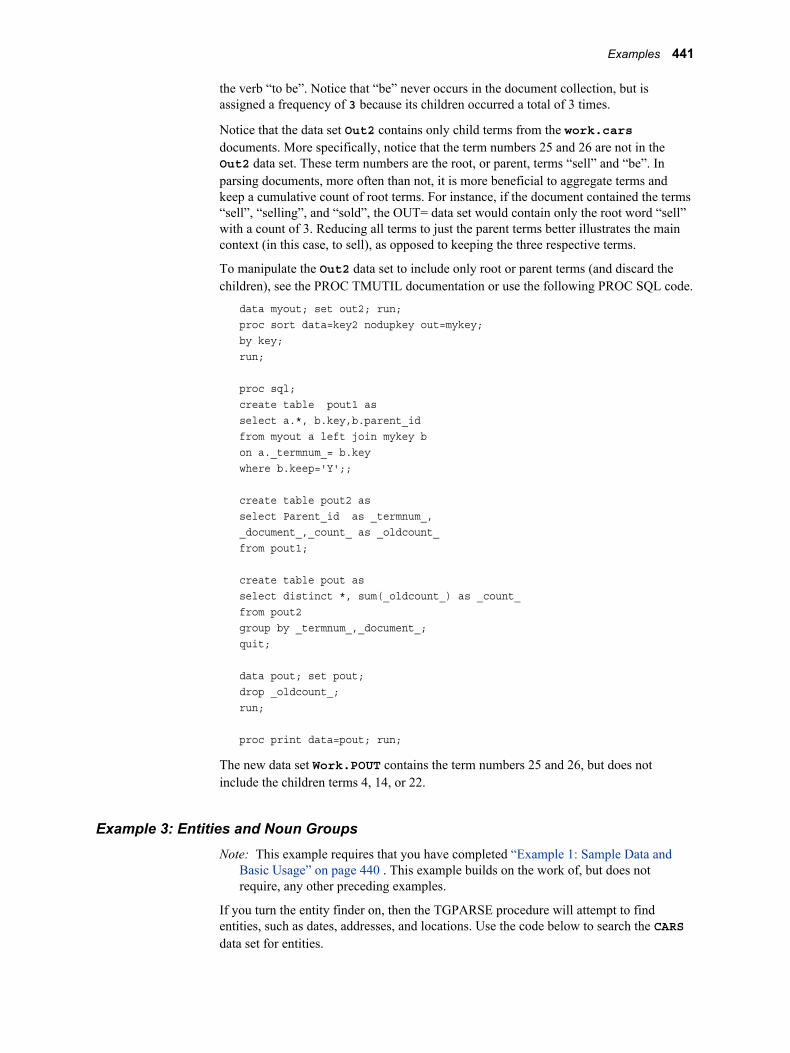
the verb “to be”. Notice that “be” never occurs in the document collection, but is assigned a frequency of 3 because its children occurred a total of 3 times.
Notice that the data set Out2 contains only child terms from the work.cars documents. More specifically, notice that the term numbers 25 and 26 are not in the Out2 data set. These term numbers are the root, or parent, terms “sell” and “be”. In parsing documents, more often than not, it is more beneficial to aggregate terms and keep a cumulative count of root terms. For instance, if the document contained the terms “sell”, “selling”, and “sold”, the OUT= data set would contain only the root word “sell” with a count of 3. Reducing all terms to just the parent terms better illustrates the main context (in this case, to sell), as opposed to keeping the three respective terms.
To manipulate the Out2 data set to include only root or parent terms (and discard the children), see the PROC TMUTIL documentation or use the following PROC SQL code.
data myout; set out2; run;proc sort data=key2 nodupkey out=mykey;by key;run;
proc sql;create table pout1 as select a.*, b.key,b.parent_idfrom myout a left join mykey bon a._termnum_= b.keywhere b.keep='Y';;
create table pout2 as select Parent_id as _termnum_,_document_,_count_ as _oldcount_from pout1;
create table pout asselect distinct *, sum(_oldcount_) as _count_from pout2group by _termnum_,_document_;quit;
data pout; set pout;drop _oldcount_;run;
proc print data=pout; run;
The new data set Work.POUT contains the term numbers 25 and 26, but does not include the children terms 4, 14, or 22.
Example 3: Entities and Noun GroupsNote: This example requires that you have completed “Example 1: Sample Data and
Basic Usage” on page 440 . This example builds on the work of, but does not require, any other preceding examples.
If you turn the entity finder on, then the TGPARSE procedure will attempt to find entities, such as dates, addresses, and locations. Use the code below to search the CARS data set for entities.
Examples 441
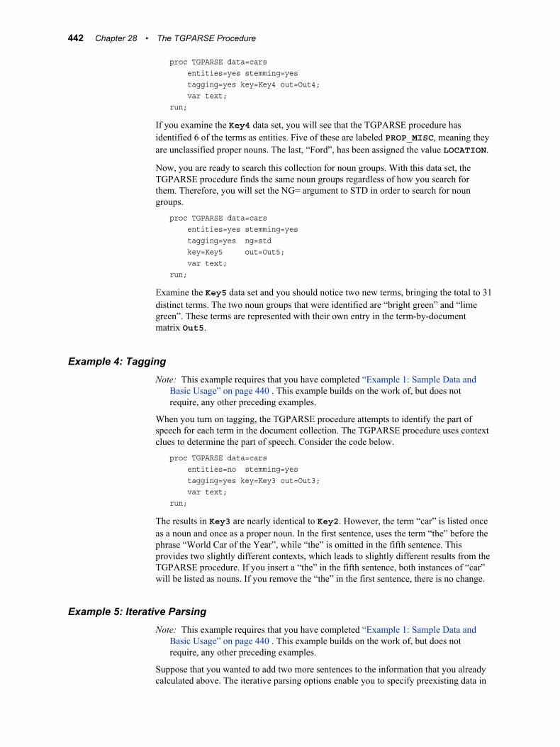
proc TGPARSE data=cars entities=yes stemming=yes tagging=yes key=Key4 out=Out4; var text;run;
If you examine the Key4 data set, you will see that the TGPARSE procedure has identified 6 of the terms as entities. Five of these are labeled PROP_MISC, meaning they are unclassified proper nouns. The last, “Ford”, has been assigned the value LOCATION.
Now, you are ready to search this collection for noun groups. With this data set, the TGPARSE procedure finds the same noun groups regardless of how you search for them. Therefore, you will set the NG= argument to STD in order to search for noun groups.
proc TGPARSE data=cars entities=yes stemming=yes tagging=yes ng=std key=Key5 out=Out5; var text;run;
Examine the Key5 data set and you should notice two new terms, bringing the total to 31 distinct terms. The two noun groups that were identified are “bright green” and “lime green”. These terms are represented with their own entry in the term-by-document matrix Out5.
Example 4: TaggingNote: This example requires that you have completed “Example 1: Sample Data and
Basic Usage” on page 440 . This example builds on the work of, but does not require, any other preceding examples.
When you turn on tagging, the TGPARSE procedure attempts to identify the part of speech for each term in the document collection. The TGPARSE procedure uses context clues to determine the part of speech. Consider the code below.
proc TGPARSE data=cars entities=no stemming=yes tagging=yes key=Key3 out=Out3; var text;run;
The results in Key3 are nearly identical to Key2. However, the term “car” is listed once as a noun and once as a proper noun. In the first sentence, uses the term “the” before the phrase “World Car of the Year”, while “the” is omitted in the fifth sentence. This provides two slightly different contexts, which leads to slightly different results from the TGPARSE procedure. If you insert a “the” in the fifth sentence, both instances of “car” will be listed as nouns. If you remove the “the” in the first sentence, there is no change.
Example 5: Iterative ParsingNote: This example requires that you have completed “Example 1: Sample Data and
Basic Usage” on page 440 . This example builds on the work of, but does not require, any other preceding examples.
Suppose that you wanted to add two more sentences to the information that you already calculated above. The iterative parsing options enable you to specify preexisting data in
442 Chapter 28 • The TGPARSE Procedure
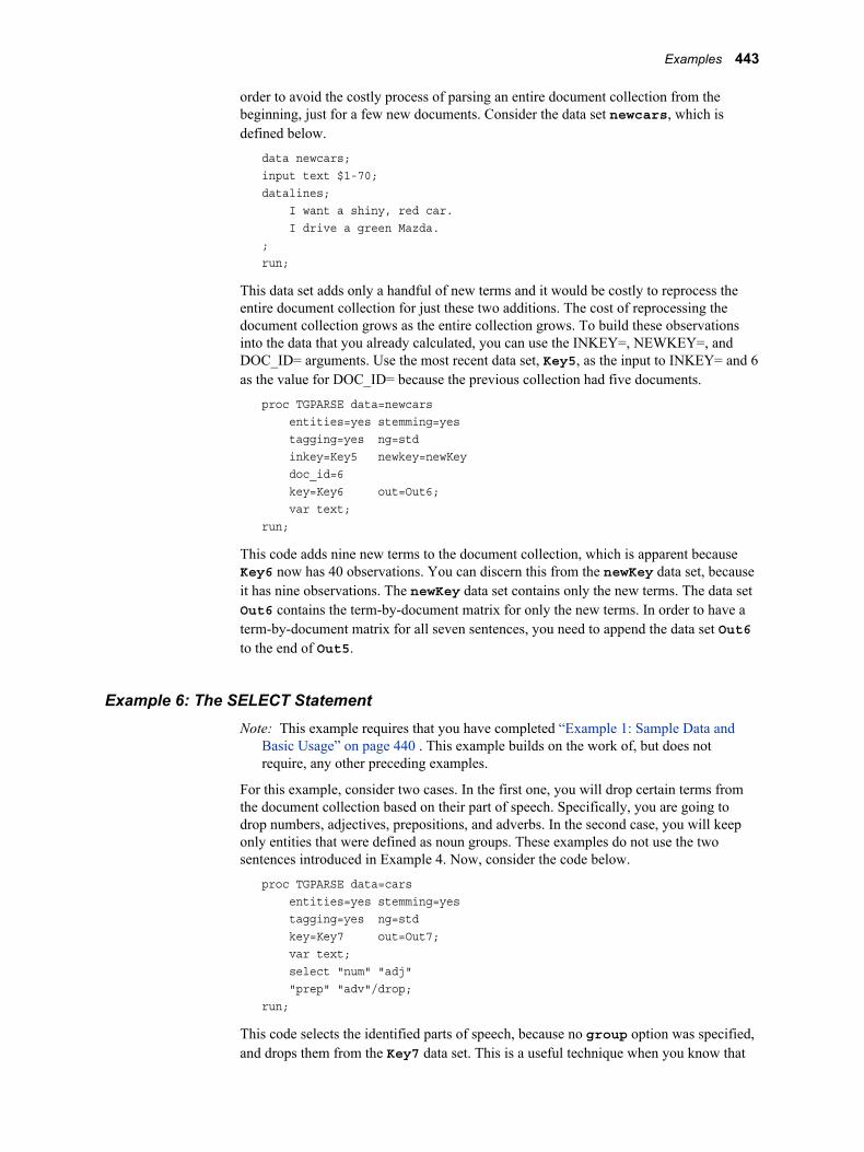
order to avoid the costly process of parsing an entire document collection from the beginning, just for a few new documents. Consider the data set newcars, which is defined below.
data newcars;input text $1-70;datalines; I want a shiny, red car. I drive a green Mazda.;run;
This data set adds only a handful of new terms and it would be costly to reprocess the entire document collection for just these two additions. The cost of reprocessing the document collection grows as the entire collection grows. To build these observations into the data that you already calculated, you can use the INKEY=, NEWKEY=, and DOC_ID= arguments. Use the most recent data set, Key5, as the input to INKEY= and 6 as the value for DOC_ID= because the previous collection had five documents.
proc TGPARSE data=newcars entities=yes stemming=yes tagging=yes ng=std inkey=Key5 newkey=newKey doc_id=6 key=Key6 out=Out6; var text;run;
This code adds nine new terms to the document collection, which is apparent because Key6 now has 40 observations. You can discern this from the newKey data set, because it has nine observations. The newKey data set contains only the new terms. The data set Out6 contains the term-by-document matrix for only the new terms. In order to have a term-by-document matrix for all seven sentences, you need to append the data set Out6 to the end of Out5.
Example 6: The SELECT StatementNote: This example requires that you have completed “Example 1: Sample Data and
Basic Usage” on page 440 . This example builds on the work of, but does not require, any other preceding examples.
For this example, consider two cases. In the first one, you will drop certain terms from the document collection based on their part of speech. Specifically, you are going to drop numbers, adjectives, prepositions, and adverbs. In the second case, you will keep only entities that were defined as noun groups. These examples do not use the two sentences introduced in Example 4. Now, consider the code below.
proc TGPARSE data=cars entities=yes stemming=yes tagging=yes ng=std key=Key7 out=Out7; var text; select "num" "adj" "prep" "adv"/drop;run;
This code selects the identified parts of speech, because no group option was specified, and drops them from the Key7 data set. This is a useful technique when you know that
Examples 443

certain parts of speech are not applicable to your text mining goals. On the other hand, you can keep specific parts of speech, entities, or attributes if you are only interested in finding certain bits of information.
proc TGPARSE data=cars entities=yes stemming=yes tagging=yes ng=std key=Key8 out=Out8; var text; select "noun_group"/group="entities" keep;run;
Notice in the Key8 data set that terms like “Mazda” and “Volkswagen Polo” were dropped from the data set. They were identified as unclassified proper nouns, which were not specified in the SELECT statement above.
444 Chapter 28 • The TGPARSE Procedure