Process Mining with the HeuristicsMinerAlgorithm

A.J.M.M. Weijters, W.M.P. van der Aalst, and A.K. Alves de Medeiros

Department of Technology Management, Eindhoven University of TechnologyP.O. Box 513, NL-5600 MB, Eindhoven, The Netherlands.

{w.m.p.v.d.aalst,a.k.medeiros,a.j.m.m.weijters}@tm.tue.nl

Abstract. The basic idea of process mining is to extract knowledgefrom event logs recorded by an information system. Until recently, theinformation in these event logs was rarely used to analyze the underly-ing processes. Process mining aims at improving this by providing tech-niques and tools for discovering process, organizational, social, and per-formance information from event logs. Fuelled by the omnipresence ofevent logs in transactional information systems (cf. WFM, ERP, CRM,SCM, and B2B systems), process mining has become a vivid researcharea [1, 2]. In this paper we introduce the challenging process miningdomain and discuss a heuristics driven process mining algorithm; theso-called “HeuristicsMiner” in detail. HeuristicsMiner is a practical ap-plicable mining algorithm that can deal with noise, and can be used toexpress the main behavior (i.e. not all details and exceptions) registeredin an event log. In the experimental section of this paper we introducebenchmark material (12.000 different event logs) and measurements bywhich the performance of process mining algorithms can be measured.

Keywords: Knowledge Discovering, Process Mining, process mining benchmark, Busi-

ness Process Intelligence.

1 Process Mining

Within organizations there has been a shift from data orientation to processorientation. By process we mean the way an organization arranges there workand recourses, for instance the order in which tasks are performed and whichgroup of people are allowed to perform specific tasks. Sometimes, organizationshave very explicit process descriptions of the way the work is organized andthis description is supported by a process aware information system like, forinstance, a workflow management system (WFM). But even if there are explicitdescriptions of the way the work should be done, the practical way of workingcan differ considerably from the prescribed way of working. Other times, thereis no, or only a very immature process description available. However, in manysituations it is possible to gather information about the processes as they takeplace. For instance, in many hospitals, information about the different treatmentsof a patient are registered (date, time, treatment, medical staff) for, reasons like

financial administration. However, this kind of information in combination withsome mining techniques can also be used to get more insight in the health careprocess [6]. Any information system using transactional systems such as ERP,CRM, or workflow management systems will offer this information in some form.Note that we do not assume the presence of a workflow management system.The only assumption we make, is that it is possible to construct event logswith event data. These event logs are used to construct a process specification,which adequately models the behavior registered. We use the term process miningfor the method of distilling a structured process description from a set of realexecutions.

As mentioned, the goal of process mining is to extract information aboutprocesses from transaction logs [1]. We assume that it is possible to record eventssuch that (i) each event refers to an activity (i.e., a well-defined step in theprocess), (ii) each event refers to a case (i.e., a process instance), (iii) eachevent can have a performer also referred to as originator (the person executingor initiating the activity), and (iv) events have a time stamp and are totallyordered. Table 1 shows an example of a log involving 19 events, 5 activities, and6 originators. In addition to the information shown in this table, some eventlogs contain more information on the case itself, i.e., data elements referring toproperties of the case (i.e. in an hospital information system, age, sex, diagnose,etc. of a patient).

Event logs such as the one shown in Table 1 are used as the starting point formining. We distinguish three different perspectives: (1) the process perspective,(2) the organizational perspective and (3) the case perspective. The process per-spective focuses on the control-flow, i.e., the ordering of activities. The goal ofmining this perspective is to find a good characterization of all possible paths,expressed in terms of, for instance, a Petri net [9]. The organizational perspectivefocuses on the originator field, i.e., which performers are involved in performingthe activities and how they are related. The goal is to either structure the or-ganization by classifying people in terms of roles and organizational units or toshow relations between individual performers (i.e., build a social network [10]).The case perspective focuses on properties of cases. Cases can be characterizedby their path in the process or by the originators working on a case. However,cases can also be characterized by the values of the corresponding data elements.For example, if a case represents a specific treatment of patients in a hospital itme be interesting to know the differences in throughput times between smokersand non-smokers.

To illustrate the first perspective consider Figure 1. The log shown in Table 1contains information about five cases (i.e., process instances). The log shows thatfor four cases (1, 2, 3, and 4) the activities A, B, C, and D have been executed.For the fifth case only three activities have been executed: activities A, E, andD. Each case starts with the execution of A and ends with the execution of D.If activity B is executed, then also activity C is executed. However, for somecases activity C is executed before activity B. Based on the information shownin Table 1 and by making some assumptions about the completeness of the log

2

case id activity id originator time stamp

case 1 activity A John 9-3-2004:15.01case 2 activity A John 9-3-2004:15.12case 3 activity A Sue 9-3-2004:16.03case 3 activity B Carol 9-3-2004:16.07case 1 activity B Mike 9-3-2004:18.25case 1 activity C John 10-3-2004:9.23case 2 activity C Mike 10-3-2004:10.34case 4 activity A Sue 10-3-2004:10.35case 2 activity B John 10-3-2004:12.34case 2 activity D Pete 10-3-2004:12.50case 5 activity A Sue 10-3-2004:13.05case 4 activity C Carol 11-3-2004:10.12case 1 activity D Pete 11-3-2004:10.14case 3 activity C Sue 11-3-2004:10.44case 3 activity D Pete 11-3-2004:11.03case 4 activity B Sue 11-3-2004:11.18case 5 activity E Clare 11-3-2004:12.22case 5 activity D Clare 11-3-2004:14.34case 4 activity D Pete 11-3-2004:15.56

Table 1. An event log.

A

AND -split

B

C

AND -join

D

E

(a) The control-flow structure expressed in terms of a Petri net.

(b) The organizational structure expressed in terms of an activity-role-performer diagram.

John Sue Mike Carol Pete Clare

role X role Y role Z

John Sue

Mike

Carol Pete

Clare

(c) A sociogram based on transfer of work.

Fig. 1. Some mining results for the process perspective (a) and organizational (b andc) perspective based on the event log shown in Table 1.

3

(i.e., assuming that the cases are representative and a sufficient large subset ofpossible behaviors has been observed), we can deduce the process model shown inFigure 1(a). The model is represented in terms of a Petri net. The Petri net startswith activity A and finishes with activity D. These activities are represented bytransitions. After executing A there is a choice between either executing B andC concurrently (i.e., in parallel or in any order) or just executing activity E. Toexecute B and C in parallel two non-observable activities (AND-split and AND-join) have been added. These activities have been added for routing purposesonly and are not present in the event log. Note that for this example we assumethat two activities are concurrent if they appear in any order.

Figure 1(a) does not show any information about the organization, i.e., it doesnot use any information concerning the people executing activities. Informationabout performers of activities however, is included in Table 1. For example, fromthe log we can deduce that (i) activity A is executed by either John or Sue, (ii)activity B is executed by John, Sue, Mike or Carol, (iii) C is executed by John,Sue, Mike or Carol, (iv) D is executed by Pete or Clare, and (v) E is executed byClare. We could indicate this information in Figure 1(a). The information couldalso be used to “guess” or “discover” organizational structures. For example, aguess could be that there are three roles: X, Y, and Z. For the execution of A roleX is required and John and Sue have this role. For the execution of B and C roleY is required and John, Sue, Mike and Carol have this role. For the executionof D and E role Z is required and Pete and Clare have this role. For five casesthese choices may seem arbitrary but for larger data sets such inferences capturethe dominant roles in an organization. The resulting “activity-role-performerdiagram” is shown in Figure 1(b). The three “discovered” roles link activitiesto performers. Figure 1(c) shows another view on the organization based onthe transfer of work from one individual to another, i.e., not focussing on therelation between the process and individuals but on relations among individuals(or groups of individuals). Consider for example Table 1. Although Carol andMike can execute the same activities (B and C), Mike is always working withJohn (cases 1 and 2) and Carol is always working with Sue (cases 3 and 4).Probably Carol and Mike have the same role but based on the small sampleshown in Table 1 it seems that John isn’t working with Carol and Sue isn’tworking with Carol.1 These examples show that the event log can be used toderive relations between performers of activities, thus resulting in a sociogram.For example, it is possible to generate a sociogram based on the transfers of workfrom one individual to another as is shown in Figure 1(c). Each node representsone of the six performers and each arc represents that there has been a transferof work from one individual to another. The definition of “transfer of work fromR1 to R2” is based on whether, in the same case, an activity executed by R1 isdirectly followed by an activity executed by R2. For example, both in case 1 and2 there is a transfer from John to Mike. Figure 1(c) does not show frequencies.However, for analysis purposes these frequencies can added. The arc from John

1 Clearly the number of events in Table 1 is too small to establish these assumptionsaccurately. However, real event logs will contain thousands or more events.

4

to Mike would then have weight 2. Typically, we do not use absolute frequenciesbut weighted frequencies to get relative values between 0 and 1. Figure 1(c) showsthat work is transferred to Pete but not vice versa. Mike only interacts with Johnand Carol only interacts with Sue. Clare is the only person transferring work toherself.

Focusing on the third perspective (i.e. the case perspective) is more inter-esting when also data elements are logged but these are not listed in Table 1.The case perspective looks at the case as a whole and tries to establish rela-tions between the various properties of a case. Note that some of the propertiesmay refer to the activities being executed, the performers working on the case,and the values of various data elements linked to the case. Using traditionaldata mining algorithms it would for example be possible to search for rules thatpredict the handling time of cases.

Orthogonal to the three perspectives (process, organization, and case), theresult of a mining effort may refer to logical issues and/or performance issues.For example, process mining can focus on the logical structure of the processmodel (e.g., the Petri net shown in Figure 1(a)) or on performance issues suchas flow time. For mining the organizational perspective, the emphasis can be onthe roles or the social network (cf. Figure 1(b) and (c)) or on the utilizationof performers or execution frequencies. To address the three perspectives andthe logical and performance issues a set of plug-ins has been developed for theProMframework [5] These plug-ins share a common XML format. For moredetails about the ProMframework, its plug-ins, and the common XML-format,we refer to www.processmining.org.

In this paper we focus on the process perspective. In fact, we consider a spe-cific algorithm: the HeuristicsMiner-algorithm. In the next section (Section 2)we present the details of the HeuristicsMiner-algorithm. Section 3 is the exper-imental section in which we describe the benchmark material (12.000 differentevent logs), process and event log characteristics, and measurements by whichthe performance of process mining algorithms can be measured.

2 Process mining with the HeuristicsMiner algorithm

The HeuristicsMiner Plug-in mines the control-flow perspective of a processmodel. To do so, it only considers the order of the events within a case. Inother words, the order of events among cases isn’t important. For instance forthe log in Tabletablog only the fields case id, time stamp and activity are con-sidered during the mining. The timestamp of an activity is used to calculatethese ordening. In Table 1 it is important that for case 1 activity A is followedby B within the context of case 1 and not that activity A of case 1 is followedby activity A of case 2. Therefore, we define an event log as follows. Let T be aset of activities. σ ∈ T ∗ is an event trace, i.e., an arbitrary sequence of activityidentifiers. W ⊆ T ∗ is an event log, i.e., a multiset (bag) of event traces. Notethat since W is a multiset, every event trace can appear more than once in alog. In practical mining tools frequencies become important. If we use this nota-

5

tion to describe the log shown in Table 1 we obtain the multiset W = [ABCD,ABCD, ACBD, ACBD, AED].

To find a process model on the basis of an event log, the log should beanalyzed for causal dependencies, e.g., if an activity is always followed by anotheractivity it is likely that there is a dependency relation between both activities.To analyze these relations we introduce the following notations. Let W be anevent log over T , i.e., W ⊆ T ∗. Let a, b ∈ T :

1. a >W b iff there is a trace σ = t1t2t3 . . . tn and i ∈ {1, . . . , n− 1} such thatσ ∈ W and ti = a and ti+1 = b,

2. a →W b iff a >W b and b 6>W a,3. a#W b iff a 6>W b and b 6>W a, and4. a‖W b iff a >W b and b >W a,5. a >>W b iff there is a trace σ = t1t2t3 . . . tn and i ∈ {1, . . . , n− 2} such that

σ ∈ W and ti = a and ti+1 = b and ti + 2 = a,6. a >>>W b iff there is a trace σ = t1t2t3 . . . tn and i < j and i, j ∈ {1, . . . , n}

such that σ ∈ W and ti = a and tj = b.

Consider the event log W = {ABCD, ABCD, ACBD, ACBD, AED} (i.e.,the log shown in Table 1). The first relation >W describes which activities ap-peared in sequence (one directly following the other). Clearly, A >W B, A >W C,A >W E, B >W C, B >W D, C >W B, C >W D, and E >W D. Relation →W

can be computed from >W and is referred to as the (direct) dependecy relationderived from event log W . A →W B, A →W C, A →W E, B →W D, C →W D,and E →W D. Note that B 6→W C because C >W B. Relation ‖W suggestsconcurrent behavior, i.e., potential parallelism. For log W activities B and Cseem to be in parallel, i.e., B‖W C and C‖W B. If two activities can follow eachother directly in any order, then all possible interleavings are present 2 andtherefore they are likely to be in parallel. Relation #W gives pairs of transitionsthat never follow each other directly. This means that there are no direct depen-decy relations and parallelism is unlikely. In a formal mining approach (i.e. theα algorithm [3] these three basic relations (i.e., A →W B, A#W B, or A‖W B)are directly used for the construction of a Petri net. An advantage of the for-mal approach is that we can characterize the class of nets that can be minedcorrectly. It turns out that assuming a weak notion of completeness (i.e., if oneactivity can be followed by another this should happen at least once in the log),any so-called SWF-net without short loops and implicit places can be minedcorrectly. SWF-nets are Petri nets with a single source and sink place satisfyingsome additional syntactical requirements such as the free-choice property. In thispaper, we will not elaborate on formal characterizations of the class of processesthat can be successfully mined. For the details we refer to [3].

The formal approach presupposes perfect information: (i) the log must becomplete (i.e., if an activity can follow another activity directly, the log shouldcontain an example of this behavior) and (ii) there is no noise in the log (i.e.,

2 If, for instance 10 activities are in parallel this can be a practical problem (10!possible patrons).

6

everything that is registered in the log is correct). Furthermore, the α-algorithmdoes not consider the frequency of traces in the log. However, in practical situ-ations logs are rarely complete and/or noise free. Especially the differentiationbetween errors, low frequent activities, low frequent activity sequences, and ex-ceptions is problematic. Therefore, in practice, it becomes more difficult to decideif between two activities (say A and B), one of the three derived relations (i.e.,A →W B, A#W B, or A‖W B) holds. For instance, the dependency relation asused in the α-algorithm (A →W B) only holds if and only if in the log there isa trace in which A is directly followed by B (i.e., the relation A >W B holds)and there is no trace in which B is directly followed by A (i.e., not B >W A).However, in a noisy situation one erroneous example can completely mess up thederivation of a right conclusion. Even if we have thousands of log traces in whichA is directly followed by B, then one B >W A example based on an incorrectregistration, will prevent a correct conclusion. As noted before, frequency infor-mation isn’t used in the formal approach. For this reason in the HeuristicsMinerwe use techniques which are less sensitive to noise and the incompleteness of logs.The main idea is to take the frequency of the following relations into accountwhile inferring the derived ones (i.e., A →W B, A#W B, or A‖W B)

2.1 Step 1: mining of the dependency graph

The starting point of the HeuristicsMiner is the construction of a so called de-pendency graph. A frequency based metric is used to indicate how certain we arethat there is truly a dependency relation between two events A and B (notationA ⇒W B). The calculated ⇒W values between the events of an event log areused in a heuristic search for the correct dependency relations.

Let W be an event log over T , and a, b ∈ T . Then |a >W b| is the number oftimes a >W b occurs in W , and

a ⇒W b =( |a >W b| − |b >W a||a >W b|+ |b >W a|+ 1

)(1)

First, remark that the value of a ⇒W b is always between -1 and 1. Somesimple examples demonstrate the rationale behind this definition. If we use thisdefinition in the situation that, in 5 traces, activity A is directly followed byactivity B but the other way around never occurs, the value of A ⇒W B = 5/6 =0.833 indicating that we are not completely sure of the dependency relation (only5 observations possibly caused by noise). However if there are 50 traces in whichA is directly followed by B but the other way around never occurs, the value ofA ⇒W B = 50/51 = 0.980 indicates that we are pretty sure of the dependencyrelation. If there are 50 traces in which activity A is directly followed by B andnoise caused B to follow A once, the value of A ⇒W B is 49/52 = 0.94 indicatingthat we are pretty sure of a dependency relation.

A high A ⇒W B value strongly suggests that there is a dependency relationbetween activity A and B. But what is a high value, what is a good thresholdto take the decision that B truly depends on A (i.e. A →W B holds)? The

7

threshold appears sensitive for the amount of noise, the degree of concurrencyin the underlying process, and the frequency of the involved activities.

However, for many dependency relations it seems unnecessary to use alwaysa threshold value. After all, we know that each non-initial activity must haveat least one other activity that is its cause, and each non-final activity musthave at least one dependent activity. Using this information in the so called all-activities-connected heuristic, we can take the best candidate (with the highestA ⇒W B score). This simple heuristic helps us enormously in finding reliablecausality relations even if the event log contains noise. As an example we haveapplied the heuristic to an event log from the Petri net of Figure 1 but withnoise in it. Thirty event traces are used (nine for each of the three possibletraces and three incorrect traces: ABCED, AECBD, AD) resulting in the eventlog W = [ABCD9, ACBD,AED9, ABCED, AECBD,AD]. We first calculatethe ⇒-values for all possible activity combinations. The result is displayed inthe matrix below.

⇒W A B C D EA 0.0 0.909 0.900 0.500 0.909B 0.0 0.0 0.0 0.909 0.0C 0.0 0.0 0.0 0.900 0.0D -0.500 -0.909 -0.909 0.0 -0.909E 0.0 0.0 0.0 0.909 0.0

We now apply the all-activities-connected heuristic on this matrix. We can rec-ognize the initial activity A, it is the activity without a positive value in theA-column. For the dependent activity of A we search for the highest value inrow A of the matrix. Both B and E are high (0.909). We arbitrarily choose B.If we use the matrix to search for the cause for B (the highest value of the Bcolumn) we will again find A as the cause for B. D is the depending activityof B (D is the highest value of the B row). The result of applying the sameprocedure on activity B, C, and E is presented in Figure 2; remark that onlythe causal relations are depicted in a so called dependency graph. The numbersin the activity boxes indicate the frequency of the activity, the numbers on thearcs indicate the reliability of each causal relation and the numbers on the nodesthe frequencies. In spite of the noise, the causal relations are correctly mined.

In this example we know the process model that is used for generating theevent log and we know the traces with noise (i.e. ABCED, AECBD, AD). How-ever, in a practical situation we never know if for instance the trace AD is reallynoise or if it is a low frequent pattern. To handle this, three threshold parame-ters are available in the HeuristicsMiner: (i) the Dependency threshold, (ii) thePositive observations threshold, (iii) the Relative to best threshold. With thesethreshold we can indicate that we will also accept dependency relations betweenactivities that have (i) a dependency measure above the value of the Depen-dency threshold, and (ii) have a frequency higher than the value of the Positiveobservations threshold, and (iii) have a dependency measure for which the dif-ference with the ”best” dependency measure is lower than the value of Relative

8

A30

B20

0,909/20

C20

0,900/20

E11

0,909/11

D30

0,909/20 0,900/20 0,909/11

Fig. 2. A dependency graph resulting from applying the heuristic approach to a noisylog from the Petri-net of Figure 1.

to best threshold. In our example the following parameter setting will result ina dependency graph in which also the low frequent behavior AD is modelled:Dependency threshold = 0.45, Positive observations threshold = 1, Relative tobest threshold = 0.4 In practical situations (with event logs with thousands oftraces, low frequent traces and some noise) these parameters are very useful toget insight in the main behavior and/or the details of processes.

However, the basic algorithm as presented above is far from complete. Itcan’t handle short loops, the type of the dependency relations (AND/XOR-split/join) isn’t represented in the dependency graph, there are problems withnon-observable activities, and it can’t handle long distance dependencies.

Short loops In a process, it may be possible to execute the same activitymultiple times. If this happens, this typically refers to a loop in the correspondingmodel. Long distance loops (e.g. ...ABCABCABC...) are no problem for theHeuristicsMiner presented so far (the values of A ⇒W B, B ⇒W C, and C ⇒W

A are useful to indicate dependency relations). However, for length-one loops(i.e. traces like ACB, ACCB, ACCCB, ... are possible) and loops of length two(i.e. traces like ACDB, ACDCDB, ACDCDCDB, ... are possible) the value ofC ⇒W C and C ⇒W D is always very low. However, it appears very simple todefine the dependency measure for loops of length one and length two. Let Wbe an event log over T , and a, b ∈ T . Then |a >W a| is the number of timesa >W a occurs in W , and |a >>W a| is the number of times a >>W b occurs inW .

a ⇒W a =( |a >W a||a >W a|+ 1

)(2)

a ⇒2 W b =( |a >>W b|+ |b >>W a||a >>W b|+ |b >>W a|+ 1

)(3)

9

During the construction of the dependency graph loops of length one are treatedin the same way as other activities (they need an external cause and a dependentactivity). Loops of length-two need a special treatment while applying the all-activities-connected heuristic. They form a pair and as a pair they need only onecause and one depending activity. 3

2.2 AND/XOR-split/join and non-observable tasks

The process model for the event log W = [ABCD, ABCD, ACBD, ACBD,AED] shown in Figure 1(a) is a Petri net. Activities are represented by tran-sitions. After executing of the first task A, there is a choice between eitherexecuting B and C concurrently (i.e., in parallel or in any order) or just exe-cuting activity E. To execute B and C in parallel two non-observable activities(AND-split and AND-join) have been added. Mining of these non-observableactivities is difficult, because they are not present in the event log. To avoidthe explicit modelling of invisible activities, in the HeuristicsMiner we don’t usePetri nets for the representation of process models, but so called Causal Ma-trix. The translation of a Petri net to a Causal Matrix is straightforward [8]. Asan example we show the translation of the Petri net of Figure 1 to the CausalMatrix representation.

ACTIVITY INPUT OUTPUT

A ∅ (B ∨ E) ∧ (C ∨ E)

B A D

C A D

D (B ∨ E) ∧ (C ∨ E) ∅E A D

Table 2. The translation of the Petri net of Figure 1(a) to a Causal Matrix.

Each activity has an input and output expression. Because A is the startactivity the input expression is empty and activity A is enabled. After the firingof A the output (B ∨ E) ∧ (C ∨ E) is activated (i.e. (B ∨ E) is activated and(C ∨ E) is activated). We now look if activity B is enabled. Because the inputexpression of B is only A, we have to look if all B’s are active in the outputexpression of A. This is the case. But because the ∨ in (B ∨ E) is an exclusiveor, the (B ∨ E) isn’t longer activated but the (C ∨ E) expression still is. We

3 A length-one loop C in combination with a concurrent process A can easily producepatterns like CAC. To prevent the HeuristicsMiner for this trap a length-two depen-dency relation (A ⇒2 W C) between A and C only holds if A and C are not lengthone loops. In short, we first calculate equation (2) and then (3). This way we captureall tasks in a length-one loop construct before searching for length-two loops.

10

now look if activity E is enabled. Because the input expression of E is onlyA, we have to look if all E’s are active in the output expression of A. This isthe not case because (B ∨ E) is no more activated. However, activity B is stillenabled (all relevant expressions are still activated). This is exactly the behaviorwe like to model. For more details about the semantics of Causal Matrices werefer to [7]. The same paper gives detailed information about the translation ofa Causal Matrix to a Petri net. This translation is a little more complex becauseappropriate hidden activities must be introduced. We will now concentrate onthe heuristics for mining the correct logical expressions.

The underlying idea is relative simple. Let we start with a simple example.The dependency graph of (Figure 2) already gives the information that activitiesB,C and E are in the output expression of activity A (as sown in Table 2). If twoactivities (e.g. B and E) are in the AND-relation, the pattern ...BE... can appearin the event log. If two activities (e.g. B and C) are in the XOR relation thepattern ...BC... isn’t possible. The following measurement is defined to expressthe above formulated idea. Let W be an event log over T , a, b, c ∈ T , and b andc are in depending relation with a. Then

a ⇒W b ∧ c =( |b >W c|+ |c >W b||a >W b|+ |a >W c|+ 1

)(4)

The |a >W b| + |a >W c| indicates the number of positive observations and|b >W c|+ |c >W b| indicates the number of times b and c appear directly aftereach other. Given the event log with noise (i.e. W = [ABCD9, ACBD9, AED9,ABCED, AECBD, AED]) the value of A ⇒W B ∧ C = (10+10/10+9+1) =1.0 indicating that B and C are in a AND-relation. The value of A ⇒W B ∧ E= (0/10+11+1) = 0.00 and the value of A ⇒W C ∧ E = (1+1/9+11+1) =0.09 indicating that B,E and C,E are both in a XOR-relation. During all ourexperiments a default value of 0.1 for the a ⇒W b∧c-parameter is used. Given theinput and output set of each activity in the Dependency graph in combinationwith the a ⇒W b ∧ c measure the construction of the AND/XOR-split/joins isstraight forward. As an illustration we follow the construction of the output-expression of activity A (e.g. Aoutput). Because there are dependency relationsfrom A to B,C, and E the basic material is the set {B, C,E}. We will start withthe first element in BCE (e.g. Aoutput = ((B)). The next element is C. The valueof A ⇒W B∧C = 1.00 (e.g. B and C are in a AND-relation, and the new value ofAoutput = ((B)∧ (C)). In the next step we use the values of A ⇒W B∧E = 0.00and A ⇒W C ∧E = 0.09. If both values were above the ∧-threshold value of 0.1then the new Aoutput-expression would be ((B)∧(C)∧(E)). But both calculatedvalues are below the ∧-threshold resulting in Aoutput = ((B∨E)∧(C∨E)).4 Theresult of applying the HeuristicsMiner as defined so far on the example event logwith noise will result in the HeuristicNet as presented in Table 2.

4 If we start the procedure above with activity E the result would be ((E ∨ B) ∧ C).Therefore an extra loop is performed in which we check for all of the ∨-groups if thisgroup can be extended with any of the available activities.

11

2.3 Step 3: Mining long distance dependencies

B

D

E

C F

A G

Fig. 3. A process model with a non-free-choice construct.

In some process models the choice between two activities isn’t determinedinside some node in the process model but may depend on choices made inother parts of the process model. Figure 3 shows a long distance dependencyconstruct. After executing activity D there is a choice between activity E andactivity F. However, the choice between E and F is “controlled” by the earlierchoice between B and C. Clearly, such non-local behavior is difficult to mine formining approaches primarily based on binary information (a >W b). Only a fewprocess mining algorithms [4, 11] are able to mine them successfully. Mining anevent log generated by the process model of Figure 3 with the HeuristicsMiner aspresented so far, will result in a dependency graph without the B to E and C to Fconnection. However, the a >>>W b-relation as given in Section 2 will stronglyindicate that B is always followed by E and C by F. (e.g. if |B| is the frequency ofactivity B, then B ⇒l

W E = |B >>>W E|/|B|+1 value close to 1.0). But manyhigh ⇒l

W -values are already sound with process model. For instance, if we lookin the process model of Figure 3 then the value of A ⇒l

W D will be close to 1.0but no extra dependency relation is necessary. We can check this by looking atthe process model mined so far and test out if it is possible to go from A to theend activity (G) without visiting activity D. Only if this is possible the processmodel is updated with the extra dependency relation from A to D and the logicalinput and output expressions of the Causal Matrix are updated in line with thisnew connection. The pseudo code for the “long-distance-dependency-heuristic”is given in the Appendix (Table 4).

3 Experimental results

In this experimental section we will introduce our benchmark material, some rele-vant measurements for this material, measurements by which the performance ofprocess mining algorithms can be assessed, and finally the performance measure-ments of the HeuristicsMiner for the benchmark material. But, as an intermezzowe will first illustrate the HeuristicsMiner on low frequent behavior and noise.

12

3.1 An Illustration

As a first illustration the process model in Figure 4 is used for generating eventlogs. All examples in an event log are, in principle, positive examples; nega-tive examples are not available or it isn’t clear which traces are wrong. Thisstarting-point is an extra handicap during mining; specially the combination oflow frequent patterns and noise is problematic. The loop from activity J to C andthe direct connection from activity D to K are used to exemplify the behavior ofthe HeuristicsMiner algorithm in case of exceptions (low frequent behavior) andnoise. One noise free event log with 1000 random traces is generated. Remarkthat activities D1, D2 and D3 are not present in the event log (i.e. they areinvisible tasks). One other event log with 1000 traces is generated where 5% oftraces contains noise. To incorporate noise in our event logs we define five differ-ent types of noise generating operations: (i) delete the head of a trace, (ii) deletethe tail of a trace, (iii) delete a part of the body, (iv) remove one event, and fi-nally (v) interchange two random chosen events. During the deletion-operationsat least one event, and no more than one third of the trace is deleted. To incor-porate 5% noise the traces of a noise free event log are randomly selected andthen one of the five above described noise generating operations is applied (eachnoise generation operation with an equal probability of 1/5).

A

K

D

D2

D3

I

D1

B

E

H

G

J C

F

Exception

Exception

Fig. 4. The process model used for generating event logs (with and without noise).

Using the default parameter setting of the HeuristicsMiner (relative to bestthreshold=0.05, positive observations=3, dependency threshold=0.9 and AND-threshold=0.1) mining of the noise free example results in the dependency graphof Figure 5. To save space, the logical behavior of the splits and joins is depictedin the dependency graph (using the & and ∨ symbols). Remark that only themain behavior (not the low frequent behavior) is reflected in the graph.

If we change the parameter setting a bit so that less reliable dependencymeasures are also accepted, for instance, using relative to best threshold = 0.05,

13

A 1000

B 1000

C 1025

D 497

E 503

0.99/1000

F 477

G 503

H 980

I 2047

J 1025

K 1000

0.99/1000

0.99/1025

0.99/1022

0.99/1025

0.99/477

0.99/1000

0.99/1000

0.99/1000

0.99/533

0.99/477

0.99/980

0.99/1000

&

V

&

V

Fig. 5. The result of HeuristicsMiner with default parameter setting and without noise(relative to best threshold=0.05, positive observations=3, dependency threshold=0.9and AND-threshold=0.1). Note that the two low frequent dependency relations from(from D to K and from J to C) are not in the model.

positive observations = 3, dependency threshold=0.9 and AND-threshold = 0.1,the model depicted in Figure 6 is mined. Note that this model also contains thelow frequent dependency relations that are not in the model in Figure 5.

A 1000

B 1000

C 1025

D 497

E 503

0.99/1000

F 477

G 503

H 980

I 2047

J 1025

K 1000

0.99/1000

0.99/1025

0.99/1022

0.99/1025

0.99/477

0.99/1000

0.99/1000

0.99/1000

0.99/533

0.99/477

0.99/980

0.99/1000

&

V

&

0.90/25

0.86/20

Fig. 6. The result of HeuristicsMiner with updated parameter setting and withoutnoise (relative to best threshold = 0.20, dependency threshold = 0.85, without noise).Note that low-frequent dependency relations (from D to K and from J to C) are catchedwith this setting, but were not when using the default parameters (i.e. Figure 5).

14

The two low frequent dependency relations are now correctly mined. Lookingat the numbers in 6 shows that the first relation from J to C is only used 25times (i.e. that the pattern J...C appears 25 times in the event log). Becausethere is concurrency, the situation in which J is directly followed by C only canbe lower. The frequency for the D...K pattern is even lower, 20 times. If we usethe default parameter setting to mine the event log with 5% noise the minedprocess model is exactly the same model as the model in Figure 5 (only the thedependency values between activities are in general a little bit lower). If we minethe event log with noise in combination with a parameter setting such that alsoless reliable dependency measures are accepted (i.e. the setting used above: rel-ative to best threshold=0.20, dependency threshold=0.8) the two low frequentdependency relations are correctly mined. However, also an extra dependencyrelation (value 0.8, frequency 7) between A and I is found. Because we knowthe correct model, it is simple to choose the parameter setting in such a waythat exactly the correct model is mined (e.g. relative to best threshold=0.20,dependency threshold=0.85). However, in a realistic setting one doesn’t know ifregistered behavior in the event log is low frequent behavior or noise. The pa-rameters of the HeuristicsMiner can be use to catch only high frequent behavioror also low frequent behavior. But mining for also the low frequent behavior hasalways the risk to catch also noise.

Some remarks about the parameters of the HeuristicsMiner seems relevant.First, during the construction of the basic process model the all-activities-con-nected heuristic is used. During applying this heuristic the values of the differentparameters are ignored; simply one ingoing and outgoing connection with thehighest dependency value is accepted. For instance, in the B1 Petri net (Figure7 of the Appendix) all the connections of the net are accepted on the basis ofthe all-activities-connected heuristic. If we know that we have a noise free log,we can simply use an extraordinary intolerant parameter setting (e.g. positiveobservations threshold = 1000, dependency threshold = 1.0, and relative to bestthreshold = 0.00); with this setting, the constructed B1-model will always haveexactly the right connections 5. The main function of the parameters is the ex-tension of the model on the basis of low frequent behavior. Extra connections areonly accepted if (i) the positive observations are above the threshold and if (ii)the dependency value is above the threshold and if (iii) the difference betweenthe new dependency value and the first accepted one is less than the relative tobest threshold. Finally, there is a strong correlation between the positive obser-vation threshold and the dependency threshold. For instance, choosing a depen-dency threshold of 0.9 means that we need more than 10 positive observation ofA directly followed B to accept an dependency between A and B. After all, if|A >W B| = 10 and there is no noise, then A ⇒W B = |A >W B| − |B >W A|/ |A >W B|+ |B >W A|+ 1 = 10/10+1 = 0.909. That means that our defaultpositive observation threshold of 3 is a relative low. Changing only the value of

5 This does not hold for the other models in the appendix B2, B3, and B4; if we onlyuse the all-activities-connected heuristic, some connections are missing.

15

the positive observation threshold to a higher value but equal or lower than 10will never result in the mining of the (extra) connections.

In above experimental setting - where we know the process model used forgenerating event logs - we can easily check to what degree mined models arecomparable with the original models. However, in a practical setting it is onlypossible to search for an optimal process model in the sense that is in accor-dance with the information in the event log. Testing if all traces can be parsedcorrectly by the mined process model is one possibility to check the quality ofa model. The ParsingMeasure (PM) is defined as the number of correct parsedtraces divided by the number of traces in the event log. The PM-values for thefour mined models discussed above (i.e. (i) default parameters, without noise;(ii) updated parameters without noise; (iii) default parameters, with noise; (iv)updated parameters with noise) are given in the PM-column of Table 3. Thevalues (0.96, 1.00, 0.91 and 0.95) seems in accordance with the discussed miningresults. For instance, the PM-value (0.96) of mining with default parametersand a noise free event log does not model the low frequent behavior in 45 traces(from D to K and from J to C), resulting in a PM of 0.96.

Experiment PM CPM

(i) no noise, default parameters 0.96 0.997

(ii) no noise, updated parameters 1.00 1.000

(iii) 5% noise, default parameters 0.91 0.990

(iv) 5% noise, updated parameters 0.95 0.995

Table 3. Mining performance results for the four experiments in the illustrative exam-ple (e.i. (i) default parameters, without noise; (ii) updated parameters without noise;(iii) default parameters, with noise; (iv) updated parameters with noise). PM is thenaive Parsing Measure; after an error the parsing stops. CPM is the Continuous ParsingMeasure; after an error the error is recorded and the parsing goes on.

However, this PM fitness measure seems to naive. First of all, if for oneprocess model the parsing get stuck at many places of a trace and in an otherprocess model there is only one error at the end of the trace we prefer thesecond model. The ContinuesParsingMeasure (CPM) is a quality measure thattakes this element into account. During the calculation of the CPM we don’tstop the parsing of a trace if an error occurs. Instead the error is recordedand the parsing goes on. That means that this quality measure is based onthe number of successfully parsed events instead of the number of parsed traces(1000). Moreover, we like proper completion of the parsing process (i.e. if theend event is parsed there are no hanging active logical expressions in the processmodel). Both, missing active expressions during parsing and hanging activatedexpressions after parsing have a negative influence on the quality of the processmodel. The following measurement is defined to express the above formulated

16

idee. Let W be an event log with e events, m is the total number of missingactivated input expressions , and r the number of remaining activated outputexpressions. Then the CPM is

CPM =12

(e−m)e

+12

(e− r)e

(5)

The CPM-values for the four mined models discussed above are given in theCPM-column of Table 3. All CPM-values are close to one indicating that in allthe process models most activities are correctly modelled (i.e. dependencies andlogical expressions are correct).

Up to here an illustration of the process mining performance of the Heuristic-sMiner on an example. In contrast with the machine learning research domain,general used process mining benchmarking material is missing. For that reasonwe started a collection of four sets of event logs for benchmarking process dis-covery algorithms. In the next section (section 3.2) we first describe the fourbenchmark sets and their characteristics. In section 3.3 we explain our miningperformance measurements. Finally, the performance results for the Heuristic-sMiner are given (Section 3.4).

3.2 Benchmark material

Starting point for the benchmark material are the Petri nets as given in theAppendix. Petri net B1 (cf. Figure 7) contains 16 activities and AND/XOR-split/joins, but no loops. Petri net B2 (cf. Figure 8) is an extension of net B1with different types of loops (i.e. a long loop, a length two loop and recursion).Petri net B3 (Figure 9) is an extension of B2 with extra parallel behavior in eightextra activities. In the event logs of Petri net B2 and B3 there are non-observable(or dummy) tasks (DUM1, DUM2, and DUM3). They are registered in the eventlogs of the B2 (Dum1) and B3 (DUM1, DUM2, and DUM3) material. In the B4experiments the non-observable (or dummy) tasks are not registered in the log.Mining of the event logs without information about non-observable activities ismore difficult then mining with this information. Besides the differences in thePetri net models the following variations are used.

The amount of imbalance in execution prioritiesIn the Petri net used for generating the benchmark material each activity hasan execution priority between 0 and 2. If during the generation of an event-tracemore than one activity is enabled, the priority value is used to calculate thechance that a specific activity is chosen. Suppose that in the Petri net B1 (cf.Figure 7), the priority of activity B is 0.5 and the priority of activity C is 1.5.Then, after executing activity A (i.e. an AND-split) the chance that the nextactivity is B is 25% and the chance that the next activity is C is 75% (i.e.there is a higher chance for the A,C,B,... pattern as for the A,B,C,..). Supposethat in the same Petri net B1, the priority of activity F is 0.5 and the priorityof activity G is 1.5. Than, after executing activity C (i.e. an XOR-split) thechance for the F, I, M track is 25% and the chance for the G, J-track is 75%.

17

Our hypothesis is that extreme imbalance will negatively affect the rediscoveryprocess; low frequent, but possible behaviors is not or hardly registered in the log.

Completeness of the event logThe quality of mining results are strongly affected by the completeness of theevent log. Only if a representative and a sufficient large subset of possible be-haviors is registered in the log, successful mining is possible. It is clear that anextensive log with extreme imbalances can be incomplete. In the formal approachin [3], we characterize the class of nets that can be mined correctly. It turns outthat assuming a weak notion of completeness (i.e., if one activity can be followedby another this should happen at least once in the log), any so-called SWF-netwithout short loops and implicit places can be mined correctly. Notwithstandingin the HeuristicsMiner a stronger completeness notation is needed 6 we will usethis weak completeness notation to indicate the completeness of an event log.For instance, in the Petri net B2 181 directly following relations are possible(183 after adding an artificial begin- and end-task). It may be that in a smallor very imbalanced event log only 172 different following relations are registeredin the event log. It is clear that both the size of an event log and the imbalancecan influence the completeness of the log.

NoiseAs stated before, we distinguish five different types noise generating operations:(i) delete the head of a event sequence, (ii) delete the tail of a sequence, (iii)delete a part of the body (iv) remove one randomly chosen event, and (v) inter-change two randomly chosen events. For each type of Petri net, we distinguishsix different amounts of imbalance: 01, 02, 05, 10, 20, 50. In the 01 situation thepriority value of an activity has a value between 0.01=0+0.01 and 1.99=2-0.01(i.e. a very high imbalance). In the 50 situation the priority value of an activitiehas a value between 0.50 and 1.50 (i.e. a low imbalance). For each imbalancevalue 10 different imbalance distributions are randomly generated and for eachimbalanced Petri net 10 event logs with 1000 traces are generated. For eachPetri net this will result in 600 different noise free event logs. We will use thenotation B1P05 09 01 X00 to indicate an event log based on Petri-net B1 withan imbalance of 0.05 to 1.95 (P05) and random event log number 9 (09). TheX00 indicates that there is no noise in the event log. Starting with this noisefree material we generated event logs with a mix 7 of the five different noisetypes (each noise type has an equal chance to appear) and with six different

6 A stronger completeness notation is needed because we use thresholds. For instanceby using a positive observation threshold of 3 at least three observations are needed.A second reason is the use of measurements not only based on the directly followingrelation (i.e. a >>W b and a >>>W b Definition 2).

7 Event logs with only a specific noise type (i.e (H(head), T(tail), W(waist),O(one), I(interchange), M(mix)) are available. Starting with the noise free logB1P05 09 01 X00 we will use the event log name B1P0509I05 to indicate 5% noiseinterchange noise (I05). In this paper only the experimental results for the mixednoise are reported.

18

noise-levels (1%, 2%, 5%, 10%, 20% and 50% noise). For each noise free eventlog this results in 6 new event logs with noise. Starting with the noise free logB1P0509X00 we will use the event log name B1P05 09 01 M05 to indicate 5%noise mixed noise (M05). The event log B1 is the event log with 1000 traces ofthe original Petri net with the same structure but without imbalance.

Before we present the mining results of the HeuristicsMiner on the describedbenchmark material we discuss the different measurements we have used to getan impression of the process mining performance of one mining experiment.

3.3 Event log and performance measurements

In a typical process mining experiment without noise an event log (e.g. B1P05 09 -01 X00) is used as mining material. After mining the discovered model the sameevent log (i.e. B1P05 09 01 X00) is first parsed by the mined model and thenthe B1 event log (i.e. a complete event log from the original, balanced Petrinet). Table 3.3 shows the different measurements as registered for one miningexperiment.

We can distinguish four groups of properties/measurements: (i) propertiesof the event log, (ii) properties of the mined model, (iii) results of parsing themined event log, (iv) results of parsing an balanced-version of the mined eventlog. Both, a > b(130) and a > b ≥ b ≥ are event log measurements that indicatethe weak completeness of the log. a > b(130) = 124 indicates that 124 from thepossible 130 direct following relations (i.e. a >W b) are really one or more timesregistered in the event log and a > b ≥ 3 = 116 indicates that 116 from themappears more than three times. It is very well possible to calculate more andother event log properties like the standard deviation from the different activityfrequency. A closer look at the mining results shows that the mined model hasone extra connection (i.e. #conn (20) = 21 and not 20) from activity O to B.This seems strange, but a closer inspection of the event log B1P05 09 01 X00displays 601 registrations of event O directly followed by B and 18 registrationsthe other way around. Strong imbalance in the original Petri net B1P0 09 seemsthe cause for this unexpected behavior: the chance of activity B appears verylow 0.11 on a scale of 0.05 to 1.95. The time the HeuristicMiner require for theconstruction of the process model is 7 mili seconds (mining time = 0:07) If weuse the mined model to parse the mined event log (i.e. (iii) results of parsingthe mined event log), the extra connection creates errors: only 399 out of 1000traces (#correctT1 = 399) are completely correct parsed (i.e. no missing or leftactivities). The performance on an event level appears better: 14764 out of 15365events are correctly parsed. There are only missing activations (#missingA1 =601), no left activations (#leftA1 = 0). The resulting CPM-fitness value formined event log is 0.980 (fitness1 = 0.980). The lowest part of Table 4 displaysthe parsing results for the traces in the event log B1 (i.e. a balanced versionof Petri net B1). It is surprising that the results on this event log are slightlybetter: 983 correct parsed traces (#correctT1= 399), only 62 missing activities(#missingA2 = 62), and a CPM-fitness very close to one (fitness2 = 0.998).

19

Item Example Clarification

Event log properties

event log B1P05 09 01 X00 mined event log,imbalance P05 (between 0.05 and 1.95) no noise

(a > b) ≥ 3 116 116 from the 124 direct following relations(i.e. a >W b) appear three times or more

(a > b) (130) 124 124 from the 130 possible direct following relations(i.e. a >W b) are really in the event log

Results of mining event log B1P05 09 01 X00

#conn (20) 21 the number of mined connections(20 for the original B1 model)

correct 0 1 model is correct, 0 the model has errorsMining time 0.08 sec time needed to construct the process model

Results of parsing log B1P05 09 01 X00 with the mined model

#correctE1 14764 number of correct parsed events#E1 15365 number of events#correctT1 399 number of correct parsed traces#T1 1000 number of traces (1000 for all experiments)#missingA1 601 number of missing activations#leftA1 0 left activationsfitness1 0.980 fitness of the mined event logparsing time 0.08 sec time needed to parse the event log

Results of parsing B1 with the mined model

#correctE2 15451 number of correct parsed events of B1#E2 15513 number of events in log B1#correctT2 938 number of correct parsed traces#T2 1000 number of traces (1000 for all experiments)#missingA2 62 number of missing activations#leftA2 0 left activationsfitness2 0.998 fitness of the B1 event logparsing time 0.08 time needed to parse the extra event log

Table 4. Example of the registered data during mining of one noise free event log.

20

3.4 HeuristicsMiner benchmark results

Below we present the HeuristicsMiner process mining benchmark results on thematerial as described in subsection 3.2. We first focus on the influence of theamount of incompleteness in the event logs. After that the focus is on the influ-ence of the amount of noise.

Tables 5, 6, 7, and 8 display the mining performance results for 2400 eventlogs; 600 for every Petri net (B1, B2, B3 and B4) and with different imbalances(P01, P02, P05, P10, P20, P50), but all noise free. The imbalance strongly influ-ence the completeness of the event logs. To save space only the most informativemeasurements of the measurements discussed above are displayed in the tables.For instance, there is a strong relation between the number of correct parsedevent, missing and left activities and the fitness measurement. For this reasononly the fitness is reported. Because the time needed for the mining of the eventlogs and for parsing an event log is about the same (≈ 0.10 seconds) for all logsin the same benchmark set, this information is also not presented in the tables.

However, a short general remark about the memory and time complexity ofthe HeuristicsMiner algorithm seems relevant. Given an event log W , with k dif-ferent events and t traces, the first step in the mining algorithm is the calculationof the values of basic relations (i.e. |a >W b|, |a >>W b|, and |a >>>W b|). Thetraces can be loaded trace by trace, and the information is stored in three k× karrays. The time complexity of this part of the algorithm is linear to the numberof traces and k2 to the number of different activities. After the calculation ofthe values of the basic relations, only these values are used for the constructionof theprocess model. This time complexity of this part of the algorithm is againk2. The HeuristicsMiner is implemented Java in the ProM framework [5] and ina stand alone version in Delphi. Using the Delphi implementation on a standardnotebook (Dell Latitude D800) the mining of an event log from B1, B2, B3 en B4benchmark sets takes in average respectively 0.08, 0.14, 0.16, and 0.12 seconds.Parsing of an event log takes in average respectively 0.08, 0.12, 0.12, and 0.12seconds.

B1 material: Average results (6 x 10 x 10 experiments)

measure P01 P02 P05 P10 P20 P50a > b ≥ 3 119.3 117.0 121.2 124.3 126.1 128.9a > b (max 130) 125.7 125.4 127.1 128.2 128.8 129.8Avg. connections (20) 20.5 20.8 20.4 20 20 20#correct models 55 60 62 100 100 100Avg. fitness .986 .984 .992 1.0 1.0 1.0Avg. fitness B1 .991 .990 .996 1.0 1.0 1.0Avg. missing 273 285 119 0 0 0Avg. left 10 29 0 0 0 0

Table 5. Process mining performance results for the 6 x 10 x 10 B1 experiments(imbalance and incompleteness).

21

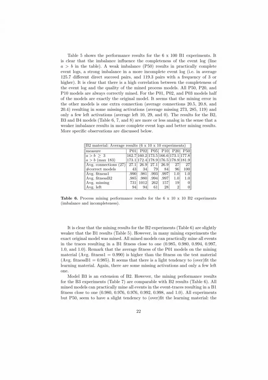
Table 5 shows the performance results for the 6 x 100 B1 experiments. Itis clear that the imbalance influence the completeness of the event log (linea > b in the table). A weak imbalance (P50) results in practically completeevent logs, a strong imbalance in a more incomplete event log (i.e. in average125.7 different direct succeed pairs, and 119.3 pairs with a frequency of 3 orhigher). It is clear that there is a high correlation between the completeness ofthe event log and the quality of the mined process models. All P50, P20, andP10 models are always correctly mined. For the P01, P02, and P03 models halfof the models are exactly the original model. It seems that the mining error inthe other models is one extra connection (average connections 20.5, 20.8, and20.4) resulting in some missing activations (average missing 273, 285, 119) andonly a few left activations (average left 10, 29, and 0). The results for the B2,B3 and B4 models (Table 6, 7, and 8) are more or less analog in the sense that aweaker imbalance results in more complete event logs and better mining results.More specific observations are discussed below.

B2 material: Average results (6 x 10 x 10 experiments)

measure P01 P02 P05 P10 P20 P50a > b ≥ 3 162.7 160.2 173.5 166.6 173.1 177.8a > b (max 183) 173.1 172.4 178.9 176.5 178.9 181.9Avg. connections (27) 27.1 26.9 27.1 26.9 27 27#correct models 43 34 79 84 96 100Avg. fitness1 .990 .981 .993 .997 1.0 1.0Avg. fitnessB2 .985 .980 .994 .997 1.0 1.0Avg. missing 731 1012 262 157 19 0Avg. left 94 94 61 28 2 0

Table 6. Process mining performance results for the 6 x 10 x 10 B2 experiments(imbalance and incompleteness).

It is clear that the mining results for the B2 experiments (Table 6) are slightlyweaker that the B1 results (Table 5). However, in many mining experiments theexact original model was mined. All mined models can practically mine all eventsin the traces resulting in a B1 fitness close to one (0.985, 0.980, 0.994, 0.997,1.0, and 1.0). Remark that the average fitness of the P01 models on the miningmaterial (Avg. fitness1 = 0.990) is higher than the fitness on the test material(Avg. fitnessB1 = 0.985). It seems that there is a light tendency to (over)fit thelearning material. Again, there are some missing activations and only a few leftone.

Model B3 is an extension of B2. However, the mining performance resultsfor the B3 experiments (Table 7) are comparable with B2 results (Table 6). Allmined models can practically mine all events in the event-traces resulting in a B1fitness close to one (0.980, 0.976, 0.976, 0.992, 0.998, and 1.0). All experimentsbut P50, seem to have a slight tendency to (over)fit the learning material: the

22

B3 material: Average results (6 x 10 x 10 experiments)

measure P01 P02 P05 P10 P20 P50a > b ≥ 3 273.2 247.7 273.6 289.2 304.9 316.0a > b (max 339) 303.0 286.6 308.3 313.6 321.0 327.9Avg. connections 37.3 37.1 37.3 36.8 37.0 37.0#correct models 31 24 31 57 91 100Avg. fitness1 .984 .978 .979 .993 .999 1.0Avg. fitnessB3 .980 .976 .976 .992 .998 1.0Avg. missing 954 1212 1280 86 86 0Avg. left 179 167 107 10 10 0

Table 7. Process mining performance results for the 6 x 10 x 10 B3 experiments(imbalance and incompleteness).

average fitness of the mined models on the mining material (Avg. fitness1) ishigher that the fitness on the test material (fitnessB1). Again, there are somemissing activations and only a few left one. Apart from that it is surprising thataverage completeness of the P02 material is relatively low (a > b = 286.6). Alsothe average fitness1 and fitnessB3 of the mined models is low (0.978 and 0.976)indicating that there is a high correlation between the completeness of a eventlog on the mining results.

B4 material: Average results (6 x 100 experiments)

measure P01 P02 P05 P10 P20 P50a > b ≥ 3 232.8 214.3 233.0 246.3 257.4 265.9a > b (max 274) 253.7 243.7 258.4 262.8 267.5 271.2Avg. connections (34) 34.1 34.0 34.1 33.8 34.0 34.0#correct models 6 10 20 39 62 94Avg. fitness1 0.952 0.950 0.968 0.980 0.987 0.998Avg. fitnessB4 0.949 0.952 0.961 0.980 0.988 0.999Avg. missing 2284 2214 1851 938 539 60Avg. left 365 306 196 124 60 9

Table 8. Process mining performance results for the 6 x 100 B4 experiments (imbalanceand incompleteness).

In the event log of the B4 experiments (Table 8) the hidden activities (DUM1,DUM2, and DUM3) are removed out of the B3 event logs. Mining the B4 materialseems more difficult then mining of the B3 material (Table 7). This is in line withfitness results of the B3 and B4 experiments (0.980 vs. 0.949, 0.976 vs. 0.952,0.976 vs. 0.961, 0.992 vs. 0.980, 0.998 vs. 0.988, and 1.0 vs. 0.999). However,specially for the experiments with only a weak imbalance the differences areminimal. Because the B4 material is the B3 material with the hidden activities

23

removed, the average completeness of the P02 material is relatively low (a > b= 243.7). However, the drop in the average fitness1 and fitnessB4 of the P02experiments isn’t so distinctly as in the B3 experiments. So far the mining resultsof event logs without noise.

Tables 9, 10, 11, and 13 displays the mining performance results for 4 x 3600= 14400 event logs; 6 x 6 x 10 x 10 = 3600 for every Petri net (B1, B2, B3and B4), 10 x 10 event logs with different imbalances (P01, P02, P05, P10, P20,P50), and with different noise levels (1%, 2%, 5%, 10%, 20%, and 50% noise). Thepresence of noise is reflected in the average amount of available direct succeedrelations (the a > b-line in the tables). Remark that the number of different a > brelations in a event log with noise can be higher than the maximum number ofdifferent a > b patterns in a noise free event log. The general observation isthat 1%, 2%, 5%, and 10% hardly influence the mining performance results (theaverage number of correct mined models, average fitness measurements, andthe average missing and left activations). For instance, in the B1 experiments(Table 9) with a high imbalance (the P01 column) the sum of the correct minedmodels drops from 55 (no noise, Table 5) to respectively 55 (1% noise), 54 (2%noise), 55 (5% noise), 57 (10% noise), 48 (20% noise), and 36 (50% noise). Thefitness for the B1 materials (fitness3) drops from 0.991 (no noise, Table 5) torespectively 0.991 (1% noise), 0.991 (2%), 0.990 (5%), 0.989 (10%), 0.986 (20%),and 0.974 (50% noise). The missing/left activations are respectively 273/10 (0%noise, Table 5), 277/10 (1%), 277/18 (2%), 291/18 (5%), 302/39 (10%), 330/99(20%), and 751/53 (50% noise). In all four Tables (9, 10, 11, 13) the influence of1% to 20% noise is slight; with 50% the decrease in mining performance is moredistinctly, but the HeuristicsMiner is still able to construct a process model witha relatively high fitness on learning and test material.

4 Conclusion

In this paper, we first introduced the challenging problem of process mining. Wedistinguish three different perspectives: (1) the process perspective, (2) the or-ganizational perspective and (3) the case perspective. We focused on the processperspective. Hereafter, we presented the details of the three steps of the Heuris-ticsMiner algorithm: Step (1) the construction of the dependency graph, Step (2)for each activity, the construction the input- and output expressions and Step(3) the search for long distance dependency relations. Simultaneously we intro-duced a new process modelling language (e.g. Causal Matrices) and we illustratethe advantages of Causal Matrices during the mining of hidden activities. In theexperimental session we showed how the HeuristicsMiner can deal with noise andlow frequent behavior. In practical situation (i.e. with event log with thousandsof traces, low frequent behavior and some noise) the HeuristicsMiner can focuson all behavior in the event log, or only the main behavior.

In this paper we first introduced the challenging process mining domain.Hereafter, we presented the details of the three steps of the HeuristicsMineralgorithm: Step (1) the construction of the dependency graph, Step (2) for each

24

B1 material: Average results (6 x 6 x 10 x 10 experiments)

Noise level 1% P01 P02 P05 P10 P20 P50Avg of a > b ≥ 3 119.4 117.1 121.3 124.5 126.3 129.0Avg of a > b (max 130) 135.1 135.1 136.3 137.1 138.2 137.8Avg of conn 20.5 20.8 20.4 20.0 20.0 20.0Sum of correct 55 60 61 100 100 100Avg of fitness 0.985 0.983 0.991 0.999 0.999 0.999Avg of fitness2 0.986 0.984 0.992 1.000 1.000 1.000Avg of fitness3 0.991 0.989 0.996 1.000 1.000 1.000Avg of missing3 277.3 292.6 124.5 0.0 0.0 0.0Avg of left3 9.9 34.5 0.0 0.0 0.0 0.0Noise level 2% P01 P02 P05 P10 P20 P50Avg of a > b ≥ 3 119.9 117.6 121.8 125.0 126.6 129.4Avg of a > b (max 130) 142.1 141.7 144.0 145.0 145.2 146.5Avg of conn 20.5 20.8 20.4 20.0 20.0 20.0Sum of correct 54 60 61 100 100 100Avg of fitness 0.984 0.982 0.990 0.998 0.998 0.998Avg of fitness2 0.986 0.984 0.992 1.000 1.000 1.000Avg of fitness3 0.991 0.989 0.996 1.000 1.000 1.000Avg of missing3 276.7 288.4 120.0 0.0 0.0 0.0Avg of left3 18.0 37.5 0.0 0.0 0.0 0.0Noise level 5% P01 P02 P05 P10 P20 P50Avg of a > b ≥ 3 122.9 121.1 125.1 127.7 129.7 132.1Avg of a > b (max 130) 159.2 161.2 160.2 161.7 162.7 164.6Avg of conn 20.5 20.8 20.4 20.0 20.0 20.0Sum of correct 55 60 62 100 100 100Avg of fitness 0.980 0.980 0.987 0.994 0.994 0.994Avg of fitness2 0.986 0.985 0.992 1.000 1.000 1.000Avg of fitness3 0.990 0.989 0.996 1.000 1.000 1.000Avg of missing3 291.1 276.0 119.4 0.0 0.0 0.0Avg of left3 18.0 57.6 0.0 0.0 0.0 0.0Noise level 10% P01 P02 P05 P10 P20 P50Avg of a > b ≥ 3 131.3 128.7 132.8 135.1 136.6 139.2Avg of a > b (max 130) 179.6 177.8 180.3 181.9 182.5 183.0Avg of conn 20.5 20.8 20.4 20.0 20.0 20.0Sum of correct 57 61 60 100 100 100Avg of fitness 0.975 0.973 0.981 0.989 0.989 0.989Avg of fitness2 0.986 0.984 0.992 1.000 1.000 1.000Avg of fitness3 0.989 0.986 0.996 1.000 1.000 1.000Sum of correct 57 61 60 100 100 100Avg of missing3 301.7 340.3 125.1 0.0 0.0 0.0Avg of left3 39.3 83.6 0.0 0.0 0.0 0.0Noise level 20% P01 P02 P05 P10 P20 P50Avg of a > b ≥ 3 144.7 142.8 145.5 149.2 151.0 153.1Avg of a > b (max 130) 201.8 202.0 203.6 206.2 206.4 208.1Avg of conn 20.7 20.9 20.6 20.2 20.1 20.1Sum of correct 49 58 62 98 100 100Avg of fitness 0.965 0.963 0.970 0.977 0.977 0.977Avg of fitness2 0.986 0.985 0.991 1.000 1.000 1.000Avg of fitness3 0.986 0.984 0.996 1.000 1.000 1.000Avg of missing3 330.0 347.4 109.7 10.4 0.0 0.0Avg of left3 99.6 133.8 19.2 0.0 0.0 0.0Noise level 50% P01 P02 P05 P10 P20 P50Avg of a > b ≥ 3 178.7 175.1 179.4 184.0 184.7 186.9Avg of a > b (max 130) 232.9 231.5 233.3 235.6 236.2 237.8Avg of conn 27.4 27.6 27.4 26.4 26.6 26.7Sum of correct 36 40 45 69 73 61Avg of fitness 0.927 0.930 0.937 0.941 0.942 0.938Avg of fitness2 0.974 0.975 0.982 0.990 0.991 0.987Avg of fitness3 0.974 0.970 0.984 0.990 0.990 0.987Avg of missing3 750.9 718.7 415.5 290.4 280.0 360.0Avg of left3 53.0 209.0 81.6 30.8 15.1 40.5

Table 9. Performance results for the 6 x 6 x 10 x 10 B1 experiments (imbalance,incompleteness and noise).

25

B2 material: Average results (6 x 6 x 10 x 10 experiments)

Noise level 1% P01 P02 P05 P10 P20 P50Avg of a > b ≥ 3 162.8 160.1 173.5 166.7 173.2 177.9Avg of a > b (max 183) 181.2 182.6 187.6 186.2 188.4 191.2Avg of conn 27.1 26.9 27.1 26.9 27.0 27.0Sum of correct 43 34 79 84 96 100Avg of fitness 0.990 0.981 0.993 0.997 0.999 0.999Avg of fitness2 0.990 0.981 0.993 0.997 1.000 1.000Avg of fitness3 0.985 0.980 0.994 0.997 1.000 1.000Avg of missing3 728.2 1000.8 262.3 157.2 19.0 0.0Avg of left3 95.1 93.9 61.2 28.4 2.2 0.0Noise level 2% P01 P02 P05 P10 P20 P50Avg of a > b ≥ 3 163.0 160.3 173.7 167.0 173.5 178.1Avg of a > b (max 183) 190.3 190.5 196.1 194.1 196.5 198.0Avg of conn 27.1 26.9 27.1 26.9 27.0 27.0Sum of correct 43.0 34.0 79.0 84.0 96.0 100.0Avg of fitness 1 1 1 1 1 1Avg of fitness2 0.990 0.982 0.993 0.997 1.000 1.000Avg of fitness3 0.985 0.981 0.994 0.997 1.000 1.000Avg of missing3 736.780 981.530 262.280 157.150 18.990 0.000Avg of left3 93.7 97.3 61.2 28.4 2.2 0.0Noise level 5% P01 P02 P05 P10 P20 P50Avg of a > b ≥ 3 165.4 162.9 176.0 169.3 175.5 180.3Avg of a > b (max 183) 208.4 209.9 215.5 213.2 215.5 217.6Avg of conn 27.1 26.9 27.0 26.9 27.0 27.0Sum of correct 42 35 78 84 96 100Avg of fitness 0.986 0.979 0.991 0.994 0.997 0.997Avg of fitness2 0.989 0.981 0.993 0.997 1.000 1.000Avg of fitness3 0.984 0.981 0.994 0.997 1.000 1.000Avg of missing3 804.1 986.6 251.1 157.2 19.0 0.0Avg of left3 103.0 96.7 63.4 28.4 2.2 0.0Noise level 10% P01 P02 P05 P10 P20 P50Avg of a > b ≥ 3 172.8 171.4 183.3 176.5 182.7 186.9Avg of a > b (max 183) 230.0 230.6 236.8 234.6 237.9 239.6Avg of conn 27.1 26.8 27.0 26.9 27.0 27.0Sum of correct 42 31 78 81 96 100Avg of fitness 0.983 0.978 0.988 0.991 0.993 0.994Avg of fitness2 0.989 0.982 0.994 0.997 1.000 1.000Avg of fitness3 0.984 0.980 0.995 0.996 1.000 1.000Avg of missing3 809.1 973.5 241.1 167.4 19.0 0.0Avg of left3 107.5 117.4 63.4 29.8 2.2 0.0Noise level 20% P01 P02 P05 P10 P20 P50Avg of a > b ≥ 3 187.9 189.1 199.0 192.2 198.3 202.3Avg of a > b (max 183) 256.3 255.5 264.1 261.7 266.1 269.1Avg of conn 27.3 26.9 27.0 26.9 27.0 27.0Sum of correct 44 31 80 80 94 99Avg of fitness 0.978 0.972 0.983 0.985 0.986 0.988Avg of fitness2 0.989 0.981 0.994 0.998 1.000 1.000Avg of fitness3 0.984 0.980 0.995 0.996 0.999 1.000Avg of missing3 769.5 1018.6 219.1 163.9 32.5 2.2Avg of left3 115.5 118.2 59.3 34.9 2.2 2.2Noise level 50% P01 P02 P05 P10 P20 P50Avg of a > b ≥ 3 221.6 222.6 235.6 228.3 235.5 238.5Avg of a > b (max 183) 294.7 286.4 301.4 299.0 306.0 308.2Avg of conn 31.2 29.4 29.8 30.6 30.4 30.2Sum of correct 39 29 78 73 95 94Avg of fitness 0.965 0.961 0.969 0.968 0.970 0.970Avg of fitness2 0.990 0.980 0.994 0.996 1.000 0.999Avg of fitness3 0.982 0.976 0.995 0.995 0.999 0.999Avg of missing3 874.6 1155.3 209.8 244.4 31.2 45.7Avg of left3 116.2 194.7 80.2 56.1 4.4 7.5

Table 10. Performance results for the 6 x 6 x 10 x 10 B2 experiments (imbalance,incompleteness and noise).

26

B3 material: Average results (6 x 6 x 10 x 10 experiments)

Noise level 1% P01 P02 P05 P10 P20 P50Average of a > b ≥ 3 273.3 247.8 273.6 289.3 304.9 316.1Average of a > b (max 339) 311.8 296.4 317.5 322.5 330.1 337.3Average of conn 37.2 37.1 37.3 36.8 37.0 37.0Sum of correct 31 24 31 55 91 100Average of fitness 0.983 0.978 0.978 0.992 0.998 0.999Average of fitness2 0.984 0.978 0.979 0.992 0.999 1.000Average of fitness3 0.980 0.976 0.976 0.991 0.998 1.000Average of missing3 964.2 1211.5 1263.1 424.4 86.4 0.0Average of left3 178.9 166.5 99.3 79.6 9.7 0.0Noise level 2% P01 P02 P05 P10 P20 P50Average of a > b ≥ 3 273.6 248.0 273.7 289.5 305.2 316.3Average of a > b (max 339) 320.9 303.7 326.0 331.4 338.6 344.6Average of conn 37.2 37.1 37.2 36.8 37.0 37.0Sum of correct 31 24 32 57 90 100Average of fitness 0.950 0.950 0.966 0.979 0.985 0.997Average of fitness2 0.984 0.978 0.979 0.993 0.999 1.000Average of fitness3 0.980 0.975 0.976 0.992 0.998 1.000Average of missing3 948.7 1229.0 1237.4 399.8 87.8 0.0Average of left3 184.0 168.0 99.9 77.8 11.0 0.0Noise level 5% P01 P02 P05 P10 P20 P50Average of a > b ≥ 3 275.7 250.2 275.6 291.7 307.0 317.9Average of a > b (max 339) 341.0 324.2 345.5 351.1 358.8 364.9Average of conn 37.2 37.1 37.3 36.8 37.0 37.0Sum of correct 30 24 31 56 89 100Average of fitness 0.982 0.975 0.976 0.990 0.996 0.997Average of fitness2 0.984 0.978 0.979 0.993 0.999 1.000Average of fitness3 0.980 0.975 0.976 0.992 0.998 1.000Average of missing3 945.5 1251.6 1276.2 401.1 89.1 0.0Average of left3 184.4 169.1 99.6 79.2 12.3 0.0Noise level 10% P01 P02 P05 P10 P20 P50Average of a > b ≥ 3 283.3 257.2 282.1 297.0 313.6 324.2Average of a > b (max 339) 366.2 349.5 369.1 374.4 383.9 389.9Average of conn 37.2 37.1 37.2 36.8 37.0 37.0Sum of correct 29 25 32 55 90 98Average of fitness 0.978 0.973 0.974 0.985 0.992 0.994Average of fitness2 0.983 0.978 0.980 0.991 0.998 1.000Average of fitness3 0.979 0.976 0.976 0.990 0.998 1.000Average of missing3 993.0 1212.9 1229.1 495.5 109.7 2.7Average of left3 185.5 171.9 104.3 83.3 10.6 2.7Noise level 20% P01 P02 P05 P10 P20 P50Average of a > b ≥ 3 299.0 272.7 297.3 312.7 328.5 338.8Average of a > b (max 339) 397.7 380.7 404.6 407.7 414.5 423.9Average of conn 37.1 37.1 37.2 36.8 37.0 37.0Sum of correct 30 23 28 54 88 100Average of fitness 0.972 0.966 0.966 0.979 0.986 0.988Average of fitness2 0.983 0.977 0.978 0.991 0.998 1.000Average of fitness3 0.977 0.974 0.975 0.990 0.998 1.000Average of missing3 1107.4 1289.6 1327.6 486.7 102.1 0.0Average of left3 199.4 178.2 103.7 86.9 12.8 0.0Noise level 50% P01 P02 P05 P10 P20 P50Average of a > b ≥ 3 335.3 310.6 335.2 349.3 366.2 377.4Average of a > b (max 339) 448.0 429.7 455.4 460.2 467.8 474.3Average of conn 40.1 39.8 39.4 38.8 39.1 38.7Sum of correct 17 12 25 47 63 87Average of fitness 0.953 0.954 0.947 0.960 0.964 0.970Average of fitness2 0.980 0.981 0.977 0.990 0.994 0.999Average of fitness3 0.972 0.975 0.973 0.989 0.994 0.999Average of missing3 1377.3 1182.3 1375.0 525.5 313.2 68.0Average of left3 185.5 250.7 138.9 112.7 37.1 7.5

Table 11. Performance results for the 6 x 6 x 10 x 10 B3 experiments (imbalance,incompleteness and noise).

27

B4 material: Average results (6 x 6 x 10 x 10 experiments)

Noise level 1% P01 P02 P05 P10 P20 P50Average of a > b ≥ 3 232.9 214.4 233.1 246.4 257.4 266.0Average of a > b (max 274) 262.4 252.6 267.1 271.7 275.7 279.5Average of conn 34.1 34.0 34.1 33.8 34.0 34.0Sum of correct 6 10 20 40 62 94Average of fitness 0.951 0.951 0.967 0.980 0.986 0.998Average of fitness2 0.952 0.952 0.968 0.980 0.987 0.998Average of fitness3 0.949 0.953 0.961 0.980 0.988 0.999Average of missing3 2303.0 2126.6 1849.5 910.8 539.5 60.4Average of left3 364.8 304.6 197.5 124.5 59.6 9.4Noise level 2% P01 P02 P05 P10 P20 P50Average of a > b ≥ 3 233.1 214.8 233.3 246.6 257.6 266.3Average of a > b (max 274) 271.0 260.0 275.0 279.5 284.2 287.7Average of conn 34.1 34.0 34.1 33.8 34.0 34.0Sum of correct 6.0 9.0 20.0 37.0 61.0 93.0Average of fitness 1 1 1 1 1 1Average of fitness2 0.952 0.951 0.967 0.980 0.987 0.998Average of fitness3 0.949 0.952 0.960 0.980 0.989 0.998Average of missing3 2316.2 2170.9 1890.4 930.2 534.4 70.4Average of left3 345.1 305.2 196.1 126.5 59.5 11.0Noise level 5% P01 P02 P05 P10 P20 P50Average of a > b ≥ 3 236.0 217.3 236.0 248.8 259.6 268.2Average of a > b (max 274) 289.3 279.5 293.5 296.1 301.3 305.4Average of conn 34.1 34.0 34.1 33.8 34.0 34.0Sum of correct 6 9 18 38 61 90Average of fitness 0.949 0.947 0.961 0.976 0.983 0.994Average of fitness2 0.952 0.950 0.964 0.979 0.986 0.998Average of fitness3 0.948 0.951 0.957 0.979 0.988 0.998Average of missing3 2329.8 2215.1 2022.4 954.5 573.8 82.0Average of left3 354.0 315.7 194.9 126.2 66.4 18.9Noise level 10% P01 P02 P05 P10 P20 P50Average of a > b ≥ 3 243.4 224.8 242.2 256.0 266.3 274.7Average of a > b/130 310.6 300.3 313.8 318.0 322.8 326.5Average of conn 34.1 34.0 34.0 33.8 34.0 34.0Sum of correct 5 8 19 39 56 93Average of fitness 0.946 0.943 0.961 0.973 0.978 0.991Average of fitness2 0.953 0.949 0.967 0.980 0.985 0.998Average of fitness3 0.949 0.952 0.960 0.980 0.986 0.998Average of missing3 2280.8 2200.0 1874.1 939.9 630.6 70.6Average of left3 372.3 313.6 210.8 126.5 74.5 11.0Noise level 20% P01 P02 P05 P10 P20 P50Average of a > b ≥ 3 258.4 239.8 257.6 270.4 281.8 290.1Average of a > b (max 274) 336.1 324.3 340.4 343.0 349.2 351.9Average of conn 34.0 34.0 34.0 33.8 34.0 34.0Sum of correct 4 7 15 33 56 84Average of fitness 0.942 0.938 0.952 0.964 0.972 0.982Average of fitness2 0.955 0.950 0.966 0.978 0.986 0.996Average of fitness3 0.948 0.951 0.959 0.977 0.987 0.996Average of missing3 2306.8 2205.3 1929.3 1041.9 587.2 161.6Average of left3 387.9 339.0 219.9 147.6 70.7 33.1Noise level 50% P01 P02 P05 P10 P20 P50Average of a > b ≥ 3 291.9 272.9 291.8 303.5 315.2 322.9Average of a > b (max 274) 377.2 364.1 380.1 381.5 388.2 389.4Average of conn 37.8 37.3 37.0 36.9 36.9 36.7Sum of correct 3 1 18 29 41 78Average of fitness 0.927 0.922 0.932 0.945 0.953 0.964Average of fitness2 0.956 0.951 0.963 0.978 0.986 0.997Average of fitness3 0.946 0.949 0.956 0.977 0.986 0.996Average of missing3 2449.3 2283.8 2025.0 1056.5 593.5 142.8Average of left3 382.9 353.4 245.6 139.0 120.5 41.9

Table 12. Performance results for the 6 x 6 x 10 x 10 B4 experiments (imbalance,incompleteness and noise).

28

activity, the construction the input- and output expressions and Step (3) thesearch for long distance dependency relations. Simultaneously we introduced anew process modelling language (e.g. Causal Matrices) and we illustrate theadvantages of Causal Matrices during the mining of hidden activities. In theexperimental session we first illustrate how the HeuristicsMiner can deal withnoise and low frequent behavior. In practical situation (i.e. with event log withthousands of traces, low frequent behavior and some noise) the HeuristicsMinercan focus on all behavior in the event log, or only the main behavior. After that,we introduced material (12.000 different event logs) and measurements by whichthe performance of process mining algorithms can be measured. Finally, thebenchmark material and the measurements are used for measuring the miningperformance of the HeuristicsMiner. The most striking results is the robustnessof the HeuristicsMiner for noise.

Although our approach is based on Causal Matrices, it can be applied toother models with executable semantics, e.g., formalizations of Petri nets, EPCs,BPMN, or UML activity diagrams. In our future work, we would like to extendthe benchmark with more realistic material (i.e. from real processes) so thatit becomes possible to benchmark also the other process mining perspectives:the organizational, social, performance, and the case perspective. Besides this,research for better process performance measurements remains challenging (refxxx BPM 06). An other priority is to apply process mining in a wide variety ofpractical situations.

References

1. W.M.P. van der Aalst, B.F. van Dongen, J. Herbst, L. Maruster, G. Schimm, andA.J.M.M. Weijters. Workflow Mining: A Survey of Issues and Approaches. Dataand Knowledge Engineering, 47(2):237–267, 2003.

2. W.M.P. van der Aalst and A.J.M.M. Weijters, editors. Process Mining, SpecialIssue of Computers in Industry, Volume 53, Number 3. Elsevier Science Publishers,Amsterdam, 2004.

3. W.M.P. van der Aalst, A.J.M.M. Weijters, and L. Maruster. Workflow Mining:Discovering Process Models from Event Logs. IEEE Transactions on Knowledgeand Data Engineering, 16(9):1128–1142, 2004.

4. A.K. Alves de Medeiros. Genetic Process Mining. PhD thesis, Eindhoven, Univer-sity of Technology, Eindhoven, The Netherlands, 2006.

5. B. van Dongen, A.K. Alves de Medeiros, H.M.W. Verbeek, A.J.M.M. Weijters, andW.M.P. van der Aalst. The ProM framework: A New Era in Process Mining ToolSupport. In G. Ciardo and P. Darondeau, editors, Application and Theory of PetriNets 2005, volume 3536 of Lecture Notes in Computer Science, pages 444–454.Springer-Verlag, Berlin, 2005.

6. L. Maruster, W.M.P. van der Aalst, A.J.M.M. Weijters, A. van den Bosch, andW. Daelemans. Automated Discovery of Workflow Models from Hospital Data.In C. Dousson, F. Hoppner, and R. Quiniou, editors, Proceedings of the ECAIWorkshop on Knowledge Discovery and Spatial Data, pages 32–36, 2002.

7. A.K.A. de Medeiros, A.J.M.M. Weijters, and W.M.P. van der Aalst. Using Ge-netic Algorithms to Mine Process Models: Representation, Operators and Results.

29

BETA Working Paper Series, WP 124, Eindhoven University of Technology, Eind-hoven, 2004.

8. A.K.A. de Medeiros, A.J.M.M. Weijters, and W.M.P. van der Aalst. Genetic Pro-cess Mining: A Basic Approach and its Challenges. In C. Bussler et al., editor,BPM 2005 Workshops (Workshop on Business Process Intelligence), volume 3812of Lecture Notes in Computer Science, pages 203–215. Springer-Verlag, Berlin,2006.

9. W. Reisig and G. Rozenberg, editors. Lectures on Petri Nets I: Basic Models,volume 1491 of Lecture Notes in Computer Science. Springer-Verlag, Berlin, 1998.

10. J. Scott. Social Network Analysis. Sage, Newbury Park CA, 1992.11. L. Wen, J. Wang, and J.Sun. Detecting implicit dependencies between tasks from

event logs. In X. Zhou, J. Li, H.T. Shen, M. Kitsuregawa, and Y. Zhang, editors,Proc. of the APWeb conference, volume 3841 of LNCS, pages 591–603. SpringerVerlag, 2006.

30

Appendix

A

P1 P2

B

P3 P4

C

P5

D

P6

E

P9

F

P7 G

P11H

P8

I

P10

J

P14

K

P12

L

P13

M

N

P15

O

P16

P

PE

PB

Fig. 7. Petri net B1 with 16 tasks, without loops.

A

P1 P2

B

P3 P4

C

P5

D

P6 E

P9

F

P7

G

P11

H

P8

I

P10 J

P14

K

P12

L

P13

M

N

P15

O

P16

P

PE

Q

R

DUM1

PB

Fig. 8. Petri net B2. It is an extension of net b1 with different types of loops (i.e. along loop, a length two loop and recursion.

A

P1 P2

B

P3 P4

C

P5

D

P6 E

P9

F

P7

G

P11

H

P8

I

P10 J

P14

K

P12

L

P13

M

N

P15

O

P16

P

PE

Q

R

S

P19

T

P20

U

P21

V

P22

W

P23

X

P24

DUM1

DUM2

P17 P18

DUM3

PB

Fig. 9. Petri net B3 (and B4) is an extension of b2 with extra parallel behavior. In theevent logs of the b3 experiments the non-observable tasks (DUM1, DUM2, and DUM3)are recorded in the event log, in the B4 experiments this tasks are not registered in thelog.

Procedure LongDistanceDependency;

var i,j: Integer;

Score, HNC: Real;

begin

For i:=N_events downto 1 do

begin

For j:=N_events downto 1 do

begin

LongDistanceDependecy := (|Event[i]>>>Event[j]|/

|Event[i]|+1) - (|||Event[i]| - |Event[j]|||/|Event[i]|);

If (|Event[i]>>>Event[j]|>=AbsUseThres) and (LongDistanceDependecy>=AbsThres)) then

begin

If EscapeToEndPossible(Event[i],Event[j],[]) then

addConnection(Event[i],Event[j]);

end;

end;

end;

end;

Function EscapeToEndPossibleF(Event[x], Event[y]: ActivityT; VisitedS: IntSetT): Boolean;

var i,j: Integer;

Max, Min, MinHulp: Real;

begin

If ((x in VisitedS) or (x==y) or (Event[y]==EndActivity)) then

begin

EscapeToEndPossibleF:=False; Exit;

end;

With Event[x] do

begin

If (Card(OutOrCluster[1], N_events) = 0) then

// X is eEe event

begin

EscapeToEndPossibleF := True; Exit;

end;

// iteration over the OR-subsets

For i:=1 to N_output_clusters do

begin

// Test if output set i has at least one eEe-escape!

OutOrEscapePossible := False;

For j:=1 to N_Events do

begin

If (j in OutOrCluster[i]) then

begin

if EscapeToEndPossibleF(Event[j], Event[y], VisitedS + [Event[x]]) then

OrSetEscapePossible := True;

end;

end;

// If there is not a eEe-escape for i

If (Not OrSetEscapePossible) then

begin

EscapeToEndPossibleF:=False; Exit;

end;

end;

// For all i-OR sets escaping is possible

EscapeToEndPossibleF:=True;

end; // EndWith

end;

Table 13. Pseudo code for the “long-distance-dependency-heuristic”.