Embed Size (px)
Citation preview
Rheograms of Filled Polymer Melts from Melt-Flow
A. V. SHENOY, D . R. SAINI, a n d V . M. NADKARNI
Polymer Science and Engineering Group Chemical Engineering Division National Chemical Laborato y
Pune 411 008, India
Polymers filled with extending fillers, such as calcium car- bonate or talc, or with reinforcing fillers, such as glass fibers or mica, are increasingly being used in a number of applica- tions. The addition of fillers to a polymer changes the melt rheological behavior of the polymer. A knowledge of the vis- cosity US. shear-rate flow curves of the filled systems at various temperatures and as a function of filler parameters (such as filler type, shape, size, and amount) is necessary for process design, optimization, and trouble shooting. The gener- ation of such rheological data is expensive and cumbersome in view of the broad range of fillers and the large number of filler parameters. In the present article, a unifying approach is pro- posed that coalesces the flow curves of filled systems of a polymer at various temperatures into a master curve that is in- dependent of the filler parameters. An effective method is pre- sented to estimate the rheograms of filled systems with the use of a master curve, characteristic of a genetic resin type, know- ing the melt-flow index and glass-transition temperature of the system. Master curves have been reported for filled systems of low-density polyethylene, high-density polyethylene, poly- propylene polystyrene, nylons, poly(ethy1ene terephthalate), and polycarbonate.
INTRODUCTION olymers are derived from petrochemical feed-
Pstocks. As the cost of crude oil is escalating, the cost- effectiveness of polymeric materials vis-a-vis conven- tional materials (such as metals, ceramics, and wood) is reduced. The use of low-cost fillers is one way to ex- tend the cost-effectiveness of polymers. A comparison of the prices of common polymeric resins and fillers shows that the prices of fillers are considerably more stable than the resins. Filled polymeric materials are, therefore, being increasingly used in a number of products.
A wide variety of fillers has been used, not only for cost reduction, but also as reinforcing agents; these are listed in Table 1. In general, the particulate-type fillers, such as wood, flour, calcium carbonate, clay, and sand, are used as extenders. Whereas fibrous fillers (such as wollastonite, glass fibers, Franklin fiber) and plate-like fillers (such as mica) represent re- inforcing additions that improve the mechanical prop- erties of the base matrix. The physical and thermal properties of filled polymers are determined, not only by the type of the filler, but also by its size, shape, size distribution and amount. A key factor in the use of fillers without adversely affecting the material proper- ties is the stress transfer at the filler-matrix interface.
The interfacial adhesion can be substantially enhanced via a coupling agent that adheres well to both the matrix and the filler particles. The most commonly used cou- pling agents are silanes and organo-titanates; the various surface treatment agents are listed in Table 2 . The type and amount of the surface treatment are thus additional parameters affecting properties of filled polymeric systems.
Material systems manifesting a broad spectrum of properties can thus be obtained with filled polymers by playing with the filler shape, filler amount, particle size, matrix polymer, and the amount of surface modi- fier. As a result, filled polymers have been success- fully used in a number of consumer and engineering applications. The myriad products made from glass-fiber-reinforced plastics in electrical, marine, au- tomotive, and chemical industrial applications are quite well-known. The array of products made from poly(vi- nyl chloride) compounds, which represent a family of the commercially most exploited filled polymer sys- tems, are numerous. Recent examples include heater hijusings and fan blades of mica-filled polypropylene, fluid pump parts and battery heat shields of talc-filled polypropylene, high-voltage switch backs of mica- filled poly(buty1ene terephthalate), and dishware made of wollastonite-filled polysulfone.
POLYMER COMPOSITES, IANUARY, 1983, Vol. 4, No. 1 53
A. V. Shenoy, D . R . Saini, and V . M . Nadkarni
...
. . .......... v,
. . 0 . 0 . 0 . .
...
The processes involved in the manufacture of these composite products include compounding operations to prepare a well-dispersed filled system and conversion processes, such as injection molding, profile extrusion, compression molding, and sheet extrusion, followed by stamping or thermoforming. A knowledge of the com- plete melt flow curve or rheogram of the filled poly- mer, depicting the variation of the viscosity with shear rate, is necessary for proper equipment design, process optimization, and troubleshooting. For example, the mechanical properties of composite materials are af- fected by the level of dispersion of the filler in the ma- trix. In order to obtain uniform wetting and dispersion of the filler particles, compounding is generally carried out under conditions of temperature and shear rates corresponding to the region of shear-thinning vis- cosity behavior of the melt. Therefore, the rheograms of the melt are necessary in specifying optimum com- pounding conditions.
The necessary rheological data are generated on so- phisticated scientific instruments such as the Weissen- berg rheogonimeter (low shear data up to lo2 s-', Instron Capillary rheometer (shear rates, 10 to 10' s-'), mechanical spectrometer, etc. These instruments are very expensive and require trained operators. The use of such instruments for obtaining the rheological data is beyond the financial and technical capabilities of plas- tics processors. As an alternative, the melt flow in- dexer, which is a relatively inexpensive apparatus, can be used for elucidating the flow behavior of the mate- rial. The melt-flow index, however, is a single-point measurement under conditions of relatively low shear rates and temperature, as specified by ASTM 1238-73. Although MFI is a good indicator of the most suitable end use for which a particular system can be used, it is not a fundamental polymer property. It does not corre- late directly with the flow behavior during processing, wherein the values of temperature and shear rate are substantially different from those employed during a MFI test. However, the MFI value is easily available to the processor, either from the material supplier or through measurement on a standard melt-flow indexer (see Appendix I).
The purpose of the present article is to unify the avail- able rheological data on filled polymer melts, which are dependent on a large number of variables (such as filler type, shape, size, amount, surface-modifier type, and amount, as well as the polymer grade). Such a unifying procedure would also eliminate the need for cumbersome and expensive investigations to elucidate the influence of the large number of variables on the viscosity of the filled polymeric materials.
BACKGROUND There is considerable literature on the rheological
properties of filled systems, and most of it is summa- rized in White, et aE. (2). In all such investigations, the emphasis is on getting rheograms for various filled sys- tems in which the variables are the matrix type, filler type, and amount, and the type and amount of the cou- pling agent. Menges, et al. (3), have proposed a different
Rheogrums of Filled Polymer Melts from Melt-Flow Index
Azidosilane Titanates
Table 2. List of Different Types of Surface Modifiers
Some typical examples Trade name Manufacturer Surface modifier type
Chrome Complexes Methacrylate chromic chloride Volan Dupont Silanes Vinyltrimethoxy silane A-1 50 Union Carbide
Union Carbide Vinyl tri(2-methoxyethoxy)siIane y-Methacryloxypropyl-trimethoxy silane A-1 74/2-6030 Dow Corning y-Glycidoxypropyltrimethoxy silane A-187/2-6040 Dow Corning y-Aminopropyl triethoxy silane A-1 100 Union Carbide N-&(Aminoethyl)-y-amino-propyltrimethoxysilane A-1 120/2-6020 Union CarbideiDow Corning
Isopropyl, triisotearoyl titanate TTS Kenrich Petrochemical
Isopropyl, tricumyl phenyl titanate 34 s Pet roc hem ical Isopropyl, tri(diocty1pyrophosphato)titanate Petrochemical Tetra(2,P-diallyloxy methyl-1-buteneoxy 5 s Petrochemical titanium di(di-tridenyl) phosphite Titanium di(cumy1 phenolate) oxyacetate 134 S Petrochemical Titanium di(di-tridecyl) phosphite 138 S Petrochemical
Organopolysiloxane Glass Resin GR 100 Owens-Illinois Polymeric Esters w-900 Byk-Mallinckrodt
w-910 Byk-Mallinckrodt W-980 Byk-Mallinckrodt
Chlorinated Paraffins Chlorez-700 Dover Chemical Chlorez-760 Dover Chemical
Vinyltriethoxy silane A-151 2-6082 Union Carbide/Dow Corning
S-3076 Hercules
approach by providing a method for converting the vis- cosity curves for filled systems into those for the unfilled base polymer by a shift factor under a constant shear stress. Though their viscosity function is tempera- ture and concentration invarient, their approach re- quires a knowledge of the shift factor in the case of each system.
Shenoy, et al. (4), have proposed a method for gen- erating the flow curves of unfilled polymer melts by the use of master curves, knowing only the melt-flow index and glass-transition temperature of the polymer. They have successfully applied the unifying approach to a wide range of unfilled polymers (4, 5) covering three categories of polymers.
Long-chain, flexible addition polymers, such as low-density polyethylene, high-density poly- ethylene, polypropylene, and polystyrene. Short-chain, flexible condensation polymers, such as nylons, polyacetals, and poly(ethy1ene terephthalate). Shortchain, rigid condensation polymers, such as polycarbonate and polysulfone.
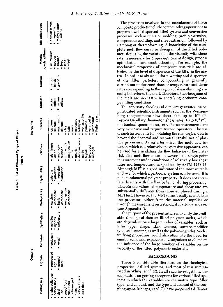
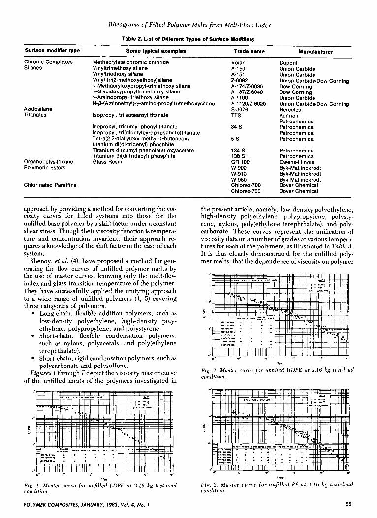
Figures 1 through 7 depict the viscosity master curve of the unfilled melts of the polymers investigated in
the present article; namely, low-density polyethylene, high-density polyethylene, polypropylene, polysty- rene, nylons, poly(ethy1ene terephthalate), and poly- carbonate. These curves represent the unification of viscosity data on a number of grades at various tempera- tures for each of the polymers, as illustrated in Table 3 . It is thus clearly demonstrated for the unfilled poly- mer melts, that the dependence of viscosity on polymer
*lW,
Fig. 2. Muster curve for unfilled H D P E ut 2.16 kg test-loud condition.
t luFt
Fig. 3 . Muster curve f o r unfilled P P nt 2 .16 kg test-loud condition.
POLYMER COMPOSITES, JANUARY, 1983, Voi. 4, No. J 55
A. V. Shenoy, D . R. Saini, and V. M . Nadkami
rlwl
Fig. 4 . Muster curve f o r unfilled PS ut 5 kg test-loud condition.
t d
I d d t/Wl
Fig. 5 . Muster curve for unfilled Nylon at 2.16 kg test-loud condition.
10'
t r
40'
t l M F I
Fig. 6. Muster curve f o r unfilled PET at 2.16 kg test-loud condition
k I
m'L I I I I l l i l l I I I111111 I I I1!1111 1 I I 1 1 1 1 1 1 I I I l l l l u 4 0 9 I00 10' 3 . 9 10' d
TfMFl
Fig. 7. Muster curve f o r unfilled PC nt 1 . 2 kg t es t - loud condition.
grade and temperature can be coalesced with the use of MFI.
In an unfilled system, for a given generic polymer type, flow properties are governed by molecular pa- rameters, such as number average molecular weight, molecular weight distribtion, and degree of branching. In filled systems, there are a number of additional pa- rameters influencing flow properties, as mentioned earlier. Thus, besides eliminating the dependence of the rheograms on polymer grade and temperature, in the present article, an attempt is made to make the flow curves invariant of filler type, amount, size, shape, filler, and the amount and type of surface modifier governing filler-matrix interaction.
DATA COLLECTION Viscosity us. shear-rate data on filled polymer melts
were collected on the polymers mentioned earlier. The filled polymer systems analyzed in the present study are summarized in Table 4 . The viscosity data include the effect of seven filler types; namely, carbon black, titanium dioxide, quartz powder, calcium carbonate, talc, mica, and glass fibers. These fillers represent a range of particle sizes. Carbon-black particles are gen- erally very fine, with the median particle size in the range of 0.02 to 0.08 p. The median particle size of talc and calcium carbonate varies from 1 to 10 p, depending on the method of preparation, whereas mica and quartz particles are relatively large, with the median size rang- ing from 10 to 80 p. A number of filler particle shapes are also represented, including particulate, plate-like, and fibrous. The various filler parameters influencing viscosity and their ranges, covered in the data analyzed in the present work, are summarized in Table 5 . Unifi- cation of the viscosity data influenced by such a range of varied parameters would prove the general validity of the proposed approach.
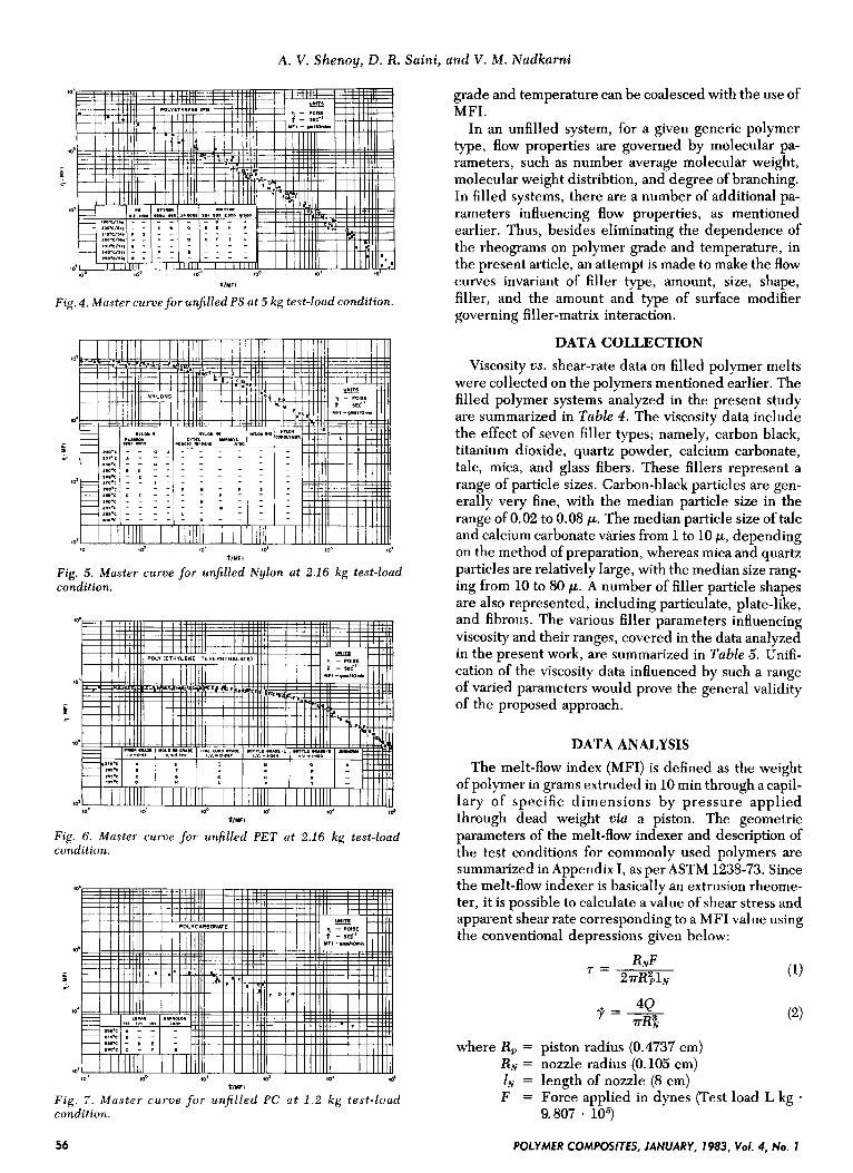
DATA ANALYSIS The melt-flow index (MFI) is defined as the weight
of polymer in grams extruded in 10 min through a capil- lary of specific dimensions by pressure applied through dead weight via a piston. The geometric parameters of the melt-flow indexer and description of the test conditions for commonly used polymers are summarized in Appendix I, as per ASTM 1238-73. Since the melt-flow indexer is basically an extrusion rheome- ter, it is possible to calculate a value of shear stress and apparent shear rate corresponding to a MFI value using the conventional depressions given below:
where R, = piston radius (0.4737 cm) RN = nozzle radius (0.105 cm) I N = length of nozzle (8 cm) F = Force applied in dynes (Test load L kg *
9.807 . 105)
56 POLYMER COMPOSITES, JANUARY, 1983, Vol. 4, No. 1
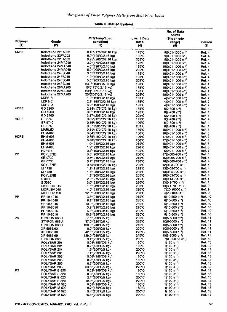
Rheogrums of Filled Polymer Melts from Melt-Flow lndex
Table 3. Unfilled Systems
No. of Data points
MFI(Temp/Load 7) vs. 7 Data (Shear rate Polymer Grade condition) temp. range) Source
(1 1 (2) (3) (4) (5) (6)
HDPE
HDPE
HDPE
PP
PP
PS
PS
LDPE In dot hene 22FA002 lndothene 22FA002 lndothene 22FA002 lndothene 24MA040 lndothene 24MA040 lndothene 24MA040 lndothene 24FS040 lndothene 24F5040 lndothene 24FS040 lndothene 24FS040 lndothene 26MA200 lndothene 22MA200 lndothene 22MA200 LDPE-8 LDPE-C LDPE-D GD 6260 GD 6260 GD 6260 GF 5740 GF 5740 GF 5740 MARLEX EHM-606 EHM-606 EHM-606 EHM-606 EHM-606 HDPE 4 KOY LE N E EB 0730 EB 0730 KOYLENE M 1730 M 1730 KOYLENE S 3030 S 3030 MOPLEN 01 5 MOPLEN 040 MOPLEN 120 PP 10-1046 PP 10-1046 PP 10-1046 PP 10-6016 PP 10-6016 PP 10-6016 STYRON 666U STYRON 666U STYRON 66611 XP 6065.00 XP 6065.00 XP 6065.00 STYRON 666 POLYSAR 201 POLYSAR 201 POLYSAR 201 POLYSAR 201 POLYSAR 205 POLYSAR 205 POLYSAR 205 POLYSAR 205 POLYSAR E 520 POLYSAR E 520 POLYSAR E 520 POLYSAR E 520 POLYSAR M 520 POLYSAR M 520 POLYSAR M 520 POLYSAR M 520
0.16a(l 75OV2.16 kg) 0.2b(l 90W2.16 kg) 0.25a(2050C/2.1 6 kg) 3.0a(l 75OW2.16 kg) 4.0b(l 90W2.16 kg) 5.0a(205"C/2.1 6 kg) 3.0a(175"C/2.16 kg) 4.0b(l 90W2.16 kg) 5.Oa(2O5"C/2.16 kg)
23.0b(l 9O0C/5.O0 kg) 16a(1750C/2.16 kg) 20b(190"C/2.16 kg) 25a(2050C/2.1 6 kg)
1 .2b(l 90W2.16 kg) 2.1 b( 1 90°C//2. 1 6 kg ) 6.gb(l 90w2.16 kg) 2.34a(179'C/2.1 6 kg) 3.0b(l 90W2.16 kg) 3.17a(205"C/2.16 kg) 0.35a(l 75OW2.16 kg) 0.45a(l 9OoC/2.1 6 kg) 0.57a(2050C/2.16 kg) 0.54a(1700C/2.1 6 kg) 0.64a(1800C/2.1 6 kg) 0.75b(1900C/2.1 6 kg) 0.88a(200"C/2.1 6 kg) 1 .0a(21 O"W2.16 kg) 1 .2b(2200C/2.1 6 kg) O.ab(l 90W2.16 kg) 0.3a(200"C/2.1 6 kg) 0.5a(21 5OW2.16 kg) 0.7b(2300C/2.1 6 kg) 0. 75a(2000C/2. 1 6 kg ) 1 .2a(2150C/2.16 kg) 1 .7b(230"C/2.16 kg) 1 .3a(2000C/2.1 6 kg) 2.0a(21 5W2.16 kg) 3.0b(2300C/2.1 6 kg) 1 .5b(2300C/2.16 kg) 4.Ob(23OoC/2.1 6 kg)
12.0b(2300C/2.1 6 kg) 3.7a(2100C/2.16 kg) 6.3b(2300C/2.1 6 kg)
10.0a(250"C/2.16 kg) 3.9=(21 OW2.16 kg) 6Sb(23OoC/2.16 kg)
1 0.3a(2500C/2.1 6 kg) 7Sb(20OoC/5 kg)
37.0a(220"C/5 kg) 1 30.0a(240"C/5 kg)
8.0b(2000C/5 kg) 42.0a(2200C/5 kg)
1 39.0a(240"C/5 kg) 9.4b(2000C/5 kg) O.Ola(l 60"C/5 kg) 0.2a(1 80°C/5 kg) 1 .5b(2000C/5 kg) 7.4a(2200C/5 kg) 0.05a(l 60°C/5 kg) O.Qa(l 80°C/5 kg) 6.8b(2000C/5 kg)
33.5a(220"C/5 kg) 0.02a(l 60°C/5 kg) 0.3a(l 80W5 kg) 2.4b(2000C/5 kg)
1 2.0a(220"C/5 kg) 0.04a(1600C/5 kg) 0.7a(1800C/5 kg) 5.4b(2000C/5 kg)
26.5a(2200C/5 kg)
POLYMER COMPOSITES, JANUARY, 1983, Val. 4, No. 1
175°C 190°C 205°C 175°C 190°C 205°C 175°C 190°C 205°C 190°C 175°C 190°C 205°C 190°C 175°C 190°C 175°C 190°C 205°C 175°C 190°C 205°C 170°C 180°C 190°C 200°C 21 0°C 220°C 190°C 200°C 21 5°C 230°C 200°C 21 5°C 230°C 200°C 21 5°C 230°C 230°C 230°C 230°C 21 0°C 230°C 250°C 21 0°C 230°C 250°C 200°C 220°C 240°C 200°C 220°C 240°C 200°C 160°C 180°C 200°C 220°C 160°C 180°C 200°C 220°C 160°C 180°C 200°C 220°C 160°C 180°C 200°C 220°C
9(0.01-1000 s-1)
9(0.01-1000 s-1)
9(0.01-1000 s-1)
lO(O.01-1000 s-1)
lO(O.01-1000 s-1)
1 O(O.01-1000 s-1)
lO(O.01-1000 s-1)
1 O(O.01-1000 s-1)
lO(O.01-1000 s-1)
1 O(O.01-1000 s-1)
lO(O.01-1000 s-1)
10(0.01-1000 s-1) lO(O.01-1000 s-1)
4(0.01-1000 s-') 4(0.01-1000 s-') 4(0.01-1000 s-') 6(2-700 s-') 6(2-700 s-') 6(2-700 s-') 6(2-700 s-') 6(2-700 s-') 6(2-700 s-')
18(0.01-1000 s-1)
1 qo.01-1000 s-1)
1qo.01-1000 s-1)
18(0.01-1000 s-1)
17(0.01-1000 s-') 17(0.01-1000 s-')
ki(O.01-1000 s-') 17(0.005-700 9') 16(0.005-700 s-') 16(0.005-700 s-') 12(0.03-700 s-') 13(0.05-700 s-') 13(0.05-700 s-') 16(0.03-700 s-') 13(0.14-700 s-') 13(0.1-700 s-') 13(0.1-700 s-') 7(20-10000 s-') 4(20-1000 s-') 6( 10-500 s-') 6( 10-500 s-') 6( 10-500 s-') 6( 10-500 s-') 6( 10-500 S-I) 6( 10-500 s-')
1 O(5-5000 s-') 1 O(5-5000 s-') 1 O(5-5OOO s-') 1 O(5-5000 s-') 1 O(5-5000 S-') 1 O(5-5000 S-I)
7(0.01-0.55 s-') l(lO0 s-1)
1 (1 00 s-1)
l(100 s-1)
l(100 s-1) l(100 s-1) l(100 s-1) 1 (1 00 s-1)
l(100 s-1) l(lO0 s-1)
1 (1 00 s-1)
1 (1 00 s-1) l(100 s-1) l(100 s-1) l(100 s-1)
l(100 s-1)
l(100 s-1)
Ref. 4 Ref. 4 Ref. 4 Ref. 4 Ref. 4 Ref. 4 Ref. 4 Ref. 4 Ref. 4 Ref. 4 Ref. 4 Ref. 4 Ref. 4 Ref. 7 Ref. 7 Ref. 7 Ref. 4 Ref. 4 Ref. 4 Ref. 4 Ref. 4 Ref. 4 Ref. 8 Ref. 8 Ref. 8 Ref. 8 Ref. 8 Ref. 8 Ref. 7 Ref. 4 Ref. 4 Ref. 4 Ref. 4 Ref. 4 Ref. 4 Ref. 4 Ref. 4 Ref. 4 Ref. 9 Ref. 9 Ref. 9 Ref. 10 Ref. 10 Ref. 10 Ref. 10 Ref. 10 Ref. 10 Ref. 11 Ref. 11 Ref. 11 Ref. 11 Ref. 11 Ref. 11 Ref. 12 Ref. 13 Ref. 13 Ref. 13 Ref. 13 Ref. 13 Ref. 13 Ref. 13 Ref. 13 Ref. 13 Ref. 13 Ref. 13 Ref. 13 Ref. 13 Ref. 13 Ref. 13 Ref. 13
57
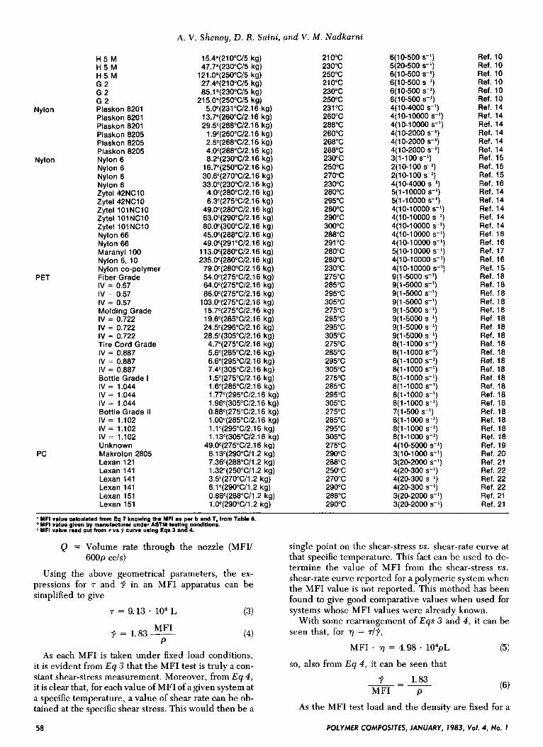
A. V. Shenoy, D. R. Saini, and V. M . Nudkami
Nylon
Nylon
PET
PC
H 5 M H 5 M H 5 M G 2 G 2 G 2 Plaskon 8201 Plaskon 8201 Plaskon 8201 Plaskon 8205 Plaskon 8205 Plaskon 8205 Nylon 6 Nylon 6 Nylon 6 Nylon 6 Zytel 42NClD Zytel 42NC10 Zytel 101 NC10 Zytel 101 NC10 Zytel 101 NClO Nylon 66 Nylon 66 Maranyl 100 Nylon 6, 10 Nylon co-polymer Fiber Grade IV = 0.57 IV = 0.57 IV = 0.57 Molding Grade IV = 0.722 IV = 0.722 IV = 0.722 Tire Cord Grade IV = 0.887 IV = 0.887 IV = 0.887
IV = 1.044 IV = 1.044 IV = 1.044 Bottle Grade II IV = 1.102 IV = 1.102 IV = 1.102 Unknown Makrolon 2805 Lexan 121 Lexan 141 Lexan 141 Lexan 141 Lexan 151 Lexan 151
Bottle Grade I
15.4a(2100C/5 kg) 47.7a(230aC/5 kg)
121 .Oa(25OoC/5 kg) 27.4a(2100C/5 kg) 85.1 "(23OoC/5 kg)
21 5.Oa(25OoC/5 kg) 5.0e(231"C/2.1 6 kg)
1 3. 7e( 260°C/2. 1 6 kg) 29.5'(288"C/2.16 kg) 1 .9c(2600C/2.16 kg) 2SC(268"C/2.1 6 kg) 4.OC(288"C/2.1 6 kg) 8.2c(2300C/2.1 6 kg)
16.7c(2500C/2.1 6 kg) 3O.6'(27O0C/2.1 6 kg) 33.0e(230"C/2.1 6 kg) 4.OC(28O0C/2.1 6 kg) 6.3c(2750C/2. 1 6 kg)
49.OC(28O0C/2.1 6 kg) 63.OC(29O0C/2.1 6 kg) 80.Oc(3OO0C/2.16 kg) 45.OC(288"C/2.1 6 kg) 49.Oc(29loC/2.16 kg)
1 13.OC(280"C/2.1 6 kg) 235.OC(28O0C/2.1 6 kg)
79.0e(28O0C/2.1 6 kg) 54.OC(275"C/2.1 6 kg) 64.OC(275"C/2.1 6 kg) 86.OC(275"C/2.1 6 kg)
1O3.Oc(275"C/2.1 6 kg) 1 5.7c(2750C/2.16 kg) 1 9.6e(2850C/2.1 6 kg) 24.5c(2950C/2.16 kg) 28.5c(3050C/2.1 6 kg) 4.7c(275"C/2.16 kg) 5.6c(2850C/2.1 6 kg) 6.6c(2950C/2.1 6 kg) 7.4c(305"C/2.1 6 kg) 1 .5c(2750C/2.1 6 kg) 1.6c(2850C/2.1 6 kg) 1 .77c(2950C/2.1 6 kg) 1 .96e(3050C/2.1 6 kg) 0.88c(2750C/2.1 6 kg) 1 .OOc(285"C/2.1 6 kg) 1 .lc(295"C/2.16 kg) 1 .13c(305"C/2.16 kg)
49.W(275"C/2.16 kg) 6.13c(290"C/1 .2 kg) 7.36c(2880C/l .2 kg) 1 .32c(250"C/1 .2 kg) 3.5c(2700C/l .2 kg) 6.lC(290"C/l .2 kg) 0.86c(288"C/1 .2 kg) 1 .OC(290"C/1 .2 kg)
21 0°C 230°C 250°C 21 0°C 230°C 250°C 231 "C 260°C 288°C 260°C 268°C 288°C 230°C 250°C 270°C 230°C 280°C 295°C 280°C 290°C 300°C 288°C 291°C 280°C 280°C 230°C 275°C 285°C 295°C 305°C 275°C 285°C 295°C 305°C 275°C 285°C 295°C 305°C 275°C 285°C 295°C 305°C 275°C 285°C 295°C 305°C 275°C 290°C 288°C 250°C 270°C 290°C 288°C 290°C
6(10-500 s-') 5(20-500 s-') 6(10-500 s-') 6(10-500 s-') 6( 10-500 s-') 6( 10-500 S-') 4( 10-4000 S-') 4( 10-1 0000 S-') 4(10-10000 S-') 4( 10-2000 s-') 4(10-2000 s-') 4( 10-2000 S-') 3(1-100 s-') 2(10-100 s-1)
2(10-100 9') 4(10-4000 s-') 5(1-10000 s-') 5(1-10000 s-') 4(10-10000 s-') 4(10-10000 S-l) 4(10-10000 s-') 4(10-10000 s-') 4( 10-1 0000 s-') 5( 10-1 0000 s-l) 4( 10-1 0000 s-1)
4(10-10000 s-') 9(1-5000 s-') 9( 1-5000 s-') 9( 1-5000 s-') 9(1-5000 s-') 9(1-5000 s-') 9(1-5000 s-') 9( 1-5000 s-') 9( 1-5000 S-')
8( 1-1 000 s-') 8(1-1000 s-1)
8(1-1000 s-1) 8(1-1000 s-1) 8(1-1000 s-1) 8(1-1000 s-1)
8(1-1000 s-1) 8(1-1000 s-1)
8(1-1000 s-1)
8(1-1000 s-1)
8( 1-1 000 s-1)
7( 1-500 s-')
4( 10-5000 s-') 3( 10-1 000 s-') 3(20-2000 S-') 4(20-300 s-') 4(20-300 S-') 4(20-300 S-') 3(20-2000 s-') 3(20-2000 s-')
Ref. 10 Ref. 10 Ref. 10 Ref. 10 Ref. 10 Ref. 10 Ref. 14 Ref. 14 Ref. 14 Ref. 14 Ref. 14 Ref. 14 Ref. 15 Ref. 15 Ref. 15 Ref. 16 Ref. 14 Ref. 14 Ref. 14 Ref. 14 Ref. 14 Ref. 16 Ref. 16 Ref. 17 Ref. 16 Ref. 15 Ref. 18 Ref. 18 Ref. 18 Ref. 18 Ref. 18 Ref. 18 Ref. 18 Ref. 18 Ref. 18 Ref. 18 Ref. 18 Ref. 18 Ref. 18 Ref. 18 Ref. 18 Ref. 18 Ref. 18 Ref. 18 Ref. 18 Ref. 18 Ref. 19 Ref. 20 Ref. 21 Ref. 22 Ref. 22 Ref. 22 Ref. 21 Ref. 21
YFI value calculated fmm Eq 7 knowlng the MFI as per b and T. from Table 6. MFI value given by manutacturer under ASTM testln condltlons. MFI value read out from T vs p curve urlng Eqs 3 an8 4.
Q = Volume rate through the nozzle (MFII
Using the above geometrical parameters, the ex- pressions for r and 7 in an MFI apparatus can be simplified to give
7 = 9.13 * 104 L
600p ccls)
(3)
M FI P
7 = 1.83 - (4)
As each MFI is taken under fixed load conditions, it is evident from E q 3 that the MFI test is truly a con- stant shear-stress measurement. Moreover, from E 9 4, it is clear that, for each value of MFI of a given system at a specific temperature, a value of shear rate can be ob- tained at the specific shear stress. This would then be a
58
single point on the shear-stress us. shear-rate curve at that specific temperature. This fact can be used to de- termine the value of MFI from the shear-stress us. shear-rate curve reported for a polymeric system when the MFI value is not reported. This method has been found to give good comparative values when used for systems whose MFI values were already known.
With some rearrangement of E q s 3 and 4 , it can be seen that, for 9 = r ly,
MFI . 7) = 4.98 - 1 0 4 ~ ~ (5) so, also from E q 4, it can be seen that
7 - 1.83 M FI P
As the MFI test load and the density are fixed for a
POLYMER COMPOSITES, JANUARY, 1983, Vol. 4, No. 1
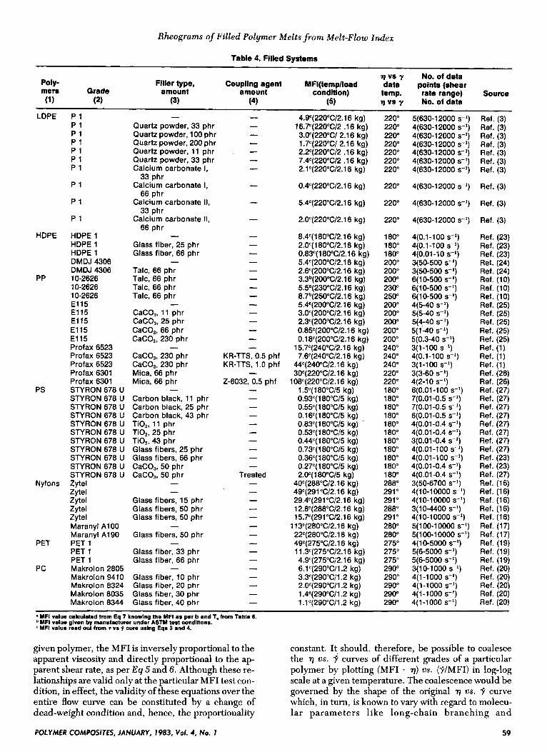
Rheogrums of Filled Polymer Melts from Melt-Flow Index
Table 4. Filled Systems
q vs y No. of data Poly- Filler type, Coupling agent MFl(temp/load data points (shear mers Grade amount amount condition) temp. rate range) Source (1) (2) (3) (4) (5) q vs y No. of data
LDPE P 1 P 1 P 1 P 1 P 1 P 1 P 1
P 1
P 1
P 1
HDPE HDPEl HDPE 1 HDPE 1 DMDJ 4306 DMDJ 4306
PP 10-2626 10-2626 10-2626 El15 El15 El15 El15 El15 Profax 6523 Profax 6523 Profax 6523 Profax 6301 Profax 6301
PS STYRON 678 U STY RON 678 U STYRON 678 U STYRON 678 U STYRON 678 U STYRON 678 U STYRON 678 U STY RON 678 U STYRON 678 U STYRON 678 U STYRON 678 U
Nylons Zytel Zytel Zytel Zytel Zytel Maranyl A1 00 Maranyl A190
PET PET1 PET 1 PET 1
PC Makrolon 2805 Makrolon 9410 Makrolon 8324 Makrolon 8035 Makrolon 8344
4.9'( 220°C/2. 1 6 kg ) Quartz powder, 33 phr - 1 6.7'(220°C/2 .16 kg) Quartz powder, 100 phr - 3.OC(22O0C/ 2.16 kg) Quartz Dowder. 200 Dhr - 1 .7c(220"C/ 2.16 kg)
2.2"1220"C/2 .16 ka)
- -
- Quartz powder; 11 phr Quartz powder, 33 phr Calcium carbonate I,
Calcium carbonate I,
Calcium carbonate II,
Calcium carbonate It,
33 phr
66 phr
33 phr
66 phr - Glass fiber, 25 phr Glass fiber, 66 phr
Talc, 66 phr Talc, 66 phr Talc, 66 phr Talc, 66 phr
CaCO,, 11 phr CaCO,, 25 phr CaCO,, 66 phr CaCO,, 230 phr
CaCO,, 230 phr CaCO,, 230 phr Mica, 66 phr Mica, 66 phr
Carbon black, 11 phr Carbon black, 25 phr Carbon black, 43 phr Ti02, 11 phr TiO,, 25 phr TiO,, 43 phr Glass fibers, 25 phr Glass fibers, 66 phr CaCO,, 50 phr CaCO,, 50 phr
Glass fibers, 15 phr Glass fibers, 50 phr Glass fibers, 50 phr
Glass fibers, 50 phr
Glass fiber, 33 phr Glass fiber, 66 phr
Glass fiber, 10 phr Glass fiber, 20 phr Glass fiber, 30 phr Glass fiber, 40 phr
-
-
-
-
- -
-
-
-
- - -
KR-TTS, 0.5 phf KR-TTS, 1 .O phf
2-6032, 0.5 phf - - - - - -
* MFI value cakulated from Eq 7 knowlng the MFI as per b and 1. from Table 6. MFI value given by manufacturer under ASTM test condltlons. MFI value resd out from T va 9 cure using Eqs 3 and 4.
given polymer, the MFI is inversely proportional to the apparent viscosity and directly proportional to the ap- parent shear rate, as per E 9 5 and 6. Although these re- lationships are valid only at the particular MFI test con- dition, in effect, the validity of these equations over the entire flow curve can be constituted by a change of dead-weight condition and, hence, the proportionality
7.4'i220°C/2 .16 k i j 2.lC(220"C/2.1 6 kg)
0.4c(2200C/2.1 6 kg)
5.4c(220"C/2.1 6 kg)
2. Oc( 220°C/2. 1 6 kg )
8.4'(1 8OoC/2.1 6 kg) 2.Oe(l8O0C/2.16 kg) 0.83c(1800C/2.1 6 kg) 5.4c(2000C/2.1 6 kg) 2.6'(2OO0C/2.1 6 kg) 3.3b(2000C/2.1 6 kg) 5.5a(230"C/2.1 6 kg) 8.7b(2500C/2. 1 6 kg) 5.4c(2000C/2.1 6 kg) 3.OC(200"C/2.1 6 kg) 2.3c(2000C/2. 1 6 kg) 0.85c(2000C/2.1 6 kg) 0.1 8c(2000C/2.1 6 kg)
1 5.7c(2400C/2.1 6 kg) 7.6c(240"C/2.1 6 kg)
44c(2400C/2.1 6 kg) 3OC(22O0C/2.1 6 kg)
108c(2200C/2.1 6 kg) 1 .!jC(1 80°C/5 kg) 0.93c(l 80"C/5 kg) 0.55"(1 80°C/5 kg) 0.16c(180"C/5 kg) 0.83c(1800C/5 kg) . 0.53'(1 8OoC/5 kg) 0.44'( 180°C/5 kg) 0.73c(l 80°C/5 kg) 0.36c(180"C/5 kg) 0.27c(l 80W5 kg) 2.07 1 80°C/5 kg)
4OC(288"C/2.1 6 kg) 4gC(291 W2.16 kg) 29.4c(2910C/2.1 6 kg) 1 2.8c(2880C/2.1 6 kg) 15.7c(2910C/2.1 6 kg)
1 13c(280"C/2.16 kg) 22'(280"C/2.1 6 kg) 49'(275"C/2.16 kg) 11.3c(2750C/2.1 6 kg) 4.9'(275"C/2.16 kg) 6.lC(29O0C/1 .2 kg) 3.3'(290"C/1.2 kg) 2.OC(290"C/1 .2 kg) 1 .4c(290"C/1 .2 kg) 1.1 c(290"C/1 .2 kg)
220" 220" 220" 220" 220" 220" 220"
220"
220"
220"
180" 180" 180" 200" 200" 200" 230" 250" 200" 200" 200" 200" 200" 240" 240" 240" 220" 220" 180" 180" 180" 180" 180" 180" 180" 180" 180" 180" 180" 288" 291' 291 O
288" 291" 280" 280" 275" 275" 275" 290" 290" 290" 290" 290"
5(630-12000 S-') 4(630-12000 S-') 4(630-12000 S-') 4(630-12000 S-') 4(630-12000 S-I) 4(630-12000 s-') 4(630-12000 S-')
4(630-12000 S - ' )
4(630-12000 S-')
4(630-12000 S-')
4(0.1-100 s-') 4(0.1-100 S-') 4(0.01-10 S-') 3(50-500 S-') 3(50-500 s-') 6(10-500 s-') 6(10-500 s-') 6( 10-500 S-') 4(5-40 s-') 5(5-40 s-') 5(4-40 S-' ) 5(1-40 S-') 5(0.3-40 S-' ) 3(1-100 S-') 4(0.1-100 s-') 3(1-100 s-') 3(3-60 S-') 4(2-10 s-') 6(0.01-100 s-') 7(0.01-0.5 S-') 7(0.01-0.5 s-') 6(0.01-0.5 s-') 4(0.01-0.4 S-') 4(0.01-0.4 S-') 3(0.01-0.4 S-I)
4(0.01-100 s-') 4(0.01-100 S-' ) 4(0.01-0.4 s-') 4(0.01-0.4 S-') 3(50-6700 s-I) 4( 10-1 0000 S-') 4( 10-1 0000 S-' ) 3(10-4400 s-') 4(10-10000 s-') 5(100-10000 s-') 5(100-10000 S-') 4( 10-5000 s-') 5(6-5000 S-') 5(6-5000 s-') 3(10-1000 S-') 4(1-1000 s-') 4(1-1000 S-') 4( 1 - 1 000 S-') 4(1-1000 S- ' )
Ref. (3) Ref. (3) Ref. (3) Ref. (3) Ref. (3) Ref. (3) Ref. (3)
Ref. (3)
Ref. (3)
Ref. (3)
Ref. (23) Ref. (23) Ref. (23) Ref. (24) Ref. (24) Ref. (10) Ref. (10) Ref. (10) Ref. (25) Ref. (25) Ref. (25) Ref. (25) Ref. (25) Ref. (1) Ref. (1) Ref. (1) Ref. (26) Ref. (26) Ref. (27) Ref. (27) Ref. (27) Ref. (27) Ref. (27) Ref. (27) Ref. (27) Ref. (27) Ref. (23) Ref. (23) Ref. (27) Ref. (16) Ref. (16) Ref. (16) Ref. (16) Ref. (16) Ref. (17) Ref. (17) Ref. (19) Ref. (19) Ref. (19) Ref. (20) Ref. (20) Ref. (20) Ref. (20) Ref. (20)
constant. It should, therefore, be possible to coalesce the q vs. 9 curves of different grades of a particular polymer by plotting (MFI * q) vs. (T/MFI) in log-log scale at a given temperature. The coalescence would be governed by the shape of the original 7) vs. 7 curve which, in turn, is known to vary with regard to molecu- lar parameters like long-chain branching and
POLYMER COMPOSITES, JANUARY, 1983, Vol. 4. No. I 59
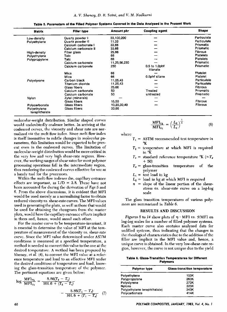
A. V. Shenoy, D. R . Saini, und V. M . Nudkami
Table 5 . Parameters of the Filled Polymer Systems Covered in the Data Analysed In the Present Work
Matrix Filler type Amount phr Coupllng agent Shape
Low-density Polyethylene
High-density Polyethylene Polypropylene
Polystyrene
Nylon
Polycarbonate Polyethylene
terephthalate
Quartz powder I Quartz powder II Calcium carbonate I Calcium carbonate II Fiber glass Talc Talc Calcium carbonate Calcium carbonate
Mica Mica Carbon black Titanium dioxide Glass fibers Calcium carbonate Calcium carbonate Zytel (minerals) Glass fibers Glass fibers Glass fibers
33,100,200 11,33 33,66 33,66 25,66 66 66 11,25,66,230 230
66 66 11,25,43 11,25,43 25,66 50 50
15.50 10,20,30,40 33.66
-
- - - - - - - -
0.5 to l.0phf titanate
0.5phf silane -
- - -
Treated untreated -
- -
Particulate Particulate Prismatic Prismatic Fibrous Platelets Platelets Prismatic Prismatic
Platelet Platelet Particulate Particulate Fibrous Prismatic Prismatic
Fibrous Fibrous
-
molecular-weight distribution. Similar shaped curves would undoubtedly coalesce better. In arriving at the coalesced curves, the viscosity and shear rate are nor- malized via the melt flow index. Since melt flow index is itself insensitive to subtle changes in molecular pa- rameters, this limitation would be expected to be pres- ent even in the coalesced curves. The limitation of molecular-weight distribution would be more critical in the very low and very high shear-rate regions. How- ever, the working ranges of shear rates for most polymer processing operations fall in the intermediate region, thus rendering the coalesced curves effective for use as a handy tool for the processors.
Within the melt-flow indexer die, capillary entrance effects are important, as WD = 3.8. These have not been accounted for during the derivation of Eqs 5 and 6. From the above discussions, it is evident that MFI would be used merely as a normalising factor to obtain reduced viscosity vs. shear-rate curves. The MFI values used in generating the plots, as well as those that would be used for obtaining the rheograms from the master plots, would have the capillary entrance effects implicit in them and, hence, would annul each other.
For the master curve to be temperature-invariant, it is essential to determine the value of MFI at the tem- perature of measurement of the viscosity US. shear-rate curve. Since the MFI value determined under ASTM conditions is Measured at a specified temperature, a method is needed to convert this value to the one at the desired temperature. A method has been proposed by Shenoy, et al. (4), to convert the MFI value at a refer- ence temperature and load to an effective MFI under the desired conditions of temperature and load, know- ing the glass-transition temperature of the polymer. The pertinent equations are given below:
M F I T ~ - 8.86(T2 - T,) log -
101.6 + (T2 - T,)
(7) - 8.86(T1 - T,)
101.6 + (TI - T,)
where T1 = ASTM recommended test temperature in
O K
T2 = temperature at which MFI is required in O K
T, = standard reference temperature "K ( = T g + 50)
Tg = glass-transition temperature of the polymer
L, = test load in kg L2 = load in kg at which MFI is required n = slope of the linear portion of the shear-
stress us. shear-rate curve on a log-log scale
The glass transition temperatures of various poly- mers are summarized in Table 6 .
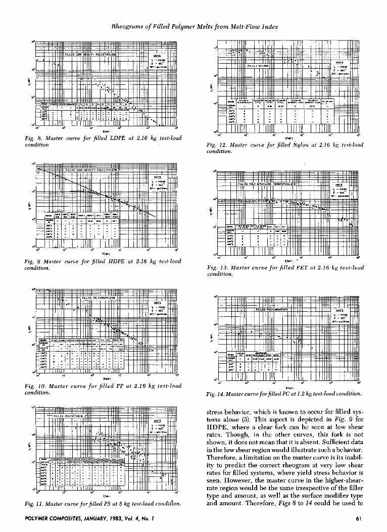
RESULTS AND DISCUSSION Figures 8 to 14 show plots of 7 * MFI vs. ?/MFI on
log-log scales for a number of filled polymer systems. Each master curve also contains analyzed data for unfilled systems, thus indicating that the changes in the rheological characteristics due to the addition of the filler are implicit in the MFI value and, hence, a unique curve is obtained. In the very low-shear-rate re- gion, however, the curve is not unique due to the yield
Table 6. Glass-Transition Temperatures for Different Polymers
Polymer type Glass-transition temperature
Polyethylene 153K Polypropylene 263K Polystyrene 373K Nylons 323K Poly(ethy1ene terephthalate) 343K Polycarbonate 41 4K
60 POLYMER COMPOSITES, JANUARY, 1983, Vol. 4, No. 1
Rheogrums of Filled Polymer Melts from Melt-Flow lndex
m'
5 c
to' 16' 0'
l M F l
Fig. 8. Muster curue f o r filled LDPE ut 2.16 kg test-loud condition
t /YF I
Fig. 9 Muster curve f o r filled HDPE at 2.16 kg test-loud condition.
YMFl
Fig. 11. Muster curve forfi l led PS at 5 kg test-loud condidon.
l Y F l
Fig. 12. Muster curve f o r filled Nylon (it 2.16 kg test-loud condition.
5 r
$04 I11111111 1 I l l l l l l l I I l l l l l l l I I l l l l l l i I I l l l U U
F i g . 13 . Muster curue f o r f i l led PET u t 2.16 kg test-loud condition.
d $ 0 3 Id 0' 0' Id tIW -
*/urn
Fig. 14. Muster curve forfilled PC ut 1.2 kg test-loud condition.
stress behavior, which is known to occur for filled sys- tems alone (3). This aspect is depicted in Fig. 9 for HDPE, where a clear fork can be seen at low shear rates. Though, in the other curves, this fork is not shown, it does not mean that it is absent. Sufficient data in the low shear region would illustrate such a behavior. Therefore, a limitation on the master curve is its inabil- ity to predict the correct rheogram at very low shear rates for filled systems, where yield stress behavior is seen. However, the master curve in the higher-shear- rate region would be the same irrespective of the filler type and amount, as well as the surface modifier type and amount. Therefore, Figs 8 to 14 could be used to
POLYMER COMPOSITES, JANUARY, 1983, Voi. 4, No. 1 61
A. V. Shenoy, D. R . Suini, und V. M . Nudkumi
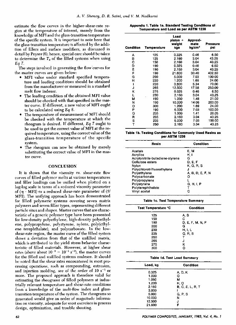
estimate the flow curves in the higher-shear-rate re- gion at the temperature of interest, merely from the knowledge of M FI and the glass-transition temperature of the specific system. It is important to note here that the glass-transition temperature is affected by the addi- tion of fillers and surface modifiers, as discussed in detail by Peyser (6); hence, special care should be taken to determine the Tg of the filled systems when using E 9 7.
The steps involved in generating the flow'curves for the master curves are eiven below:
.2
MFI value under standard specified tempera- ture and loading conditions should be obtained from the manufacturer or measured in a standard melt flow indexer. The loading condition of the obtained MFI value should be checked with that specified in the mas- ter curve. If different, a new value of MFI ought to be calculated using E q 8. The temperature of measurement of MFI should be checked with the temperature at which the rheogram is desired. If different, E q 7 ought to be used to get the correct value of MFI at the re- quired temperature, using the correct value of the glass-transition temperature of the specific system. The rheogram can now be obtained by merely substituting the correct value of MFI in the mas- ter curve.
CONCLUSION is shown that the viscosity vs. shear-rate flow
curves of filled polymer melts at various temperatures and filler loadings can be unified when plotted on a log-log scale in terms of a reduced viscosity parameter of (r) * MFI) us a reduced shear-rate parameter of (p/ MFI). The unifying approach has been demonstrated for filled polymeric systems covering seven matrix polymers and seven filler types, representing different particle sizes and shapes. Master curves that are charac- teristic of a generic polymer type have been presented for low-density polyethylene, high-density polyethyl- ene, polypropylene, polystyrene, nylons, poly(ethy1- ene terephthalate), and polycarbonate. In the low- shear-rate region, the master curve of the filled system shows a deviation from that of the unfilled matrix, which is attributed to the yield stress behavior charac- teristic of filled materials. However, at higher shear rates (above about lo-' - 10-1 s-l), the master curves for the filled and unfilled systems coalesce. I t should be noted that the shear rates encountered in most pro- cessing operations, such as compounding, extrusion, and injection molding, are of the order of 10 s-l or more. The proposed approach is therefore valid for estimating the rheograms of filled polymers at indus- trially relevant temperature and shear-rate conditions from a knowledge of the melt-flow index and glass- transition temperature of the system. The rheograms SO
generated would give an order of magnitude informa- tion on viscosity, adequate for most exercises in process design, optimization, and trouble shooting.
Appendix 1. Table la. Standard Testing Conditions of Temperature and Load as per ASTM 1238
Load
weight mate Pressure piston + Approxi-
Condition Temperature kgs kglcm' psi
A 6 C D E F G H
I J K L M N 0 P Q R S T
125 125 1 50 190 190 190 200 230 230 265 275 230 190 190 300 190 235 235 235 250
0.325 2.160 2.160 0.325 2.160
21.600 5.000 1.200 3.800
12.500 0.325 2.1 60 1.050
10.000 1.200 5.000 1 .ooo 2.160 5.000 2.160
0.46 3.04 3.04 0.46 3.04
30.40 7.03 1.69 5.34
17.58 0.46 3.04 1.48
14.06 1.69 7.03 1.41 3.04 7.03 3.04
6.50 43.25 43.25 6.50
43.25 432.50 100.00 24.00 70.00
250.00 6.50
43.25 21 .oo
200.00 24.00
100.00 20.05 43.25
100.00 43.25
Table 1 b. Testing Conditions for Commonly Used Resins as per ASTM 1238
Resin Condition
Acetals Acrylics Acrylonitrile-butadiene-styrene Cel I u lose esters Nylon Polychlorotrifluorethylene Polyethylene Polycarbonate Polypropylene Polystyrene Polyterephthalate Vinyl acetal
~~~ ~~
Table lc. Test Temperature Summary
Test Temperature "C Condition
125 150 190 200 230 235 250 265 275 300
Table Id. Test Load Summary
Load, kg Condition
0.325 1 .ooo 1.050 1.200 2.160 3.800 5.000
10.000 12.500 21.600
62 POLYMER COMPOSITES, JANUARY, 1983, Vol. 4, No. 1
Rheogrums of Filled Polymer Melts from Melt-Flow Index
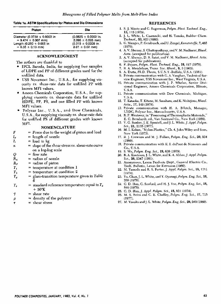
Table le . ASTM Specifications for Piston and Die Dimensions
Piston Die ~
Diameter (0.3730 2 0.0003 in = 9.474 2 0.007 mm)
Length (0.250 ? 0.005 in = 6.35 r 0.13 mrn)
(0.0825 f 0.0002 in. 2.095 2 0.005 mm) (0.315 2 0.0008 in. 8.01 * 0.02 mm)
ACKNOWLEDGMENT The authors are thankful to
IPCL Baroda, India, for supplying free samples of LDPE and PP of different grades used for the unfilled data. USS Novamont Inc., U.S.A., for supplying vis- cosity us. shear-rate data for unfilled PP with known MFI values. Amoco Chemicals Corporation, U.S.A., for sup- plying viscosity as. shear-rate data for unfilled HDPE, PP, PS, and one filled PP with known MFI values. Polysar Inc. , U.S.A., and Dow Chemicals, U. S. A., for supplying viscosity vs. shear-rate data for unfilled PS of different grades with known MFI.
NOMENCLATURE = Force due to the weight of piston and load = length of nozzle = load in kg = slope of the shear stress us. shear-rate curve
= flow rate = radius of nozzle = radius of piston = temperature at condition 1 = temperature at condition 2 = glass-transition temperature given in Table
6 = standard reference temperature equal to To
+ 50°K = shear rate = density of the polymer = shear stress
on a log-log scale
REFERENCES 1. S. J. Monte and G. Sugerman, Polym. Plust. Technol. Eng.,
2. J. L. White, L. Czarnecki, and H. Tanaka, Rubber Chem.
3. G . Menges, P. Geisbusch, and U. Zingel,Kunststoffe, 7,485
4. A. V. Shenoy, S. Chattopadhyay, and V. M. Nadkarni, Rheol.
5. A. V. Shenoy, D. R. Saini, and V. M. Nadkarni, Rheol. Actu.
6. P. Peyser, Polym. Plast. Technol. Eng., 10, 117 (1978). 7. H. A. Mendelson, Truns. Soc. Rheol., 9, 3 (1965). 8. A. Dutta, Ph.D. Thesis, S.U.N.Y.-BuffXo, U.S.A. (1981). 9. Private communication with G. A. Vaughan, Technical Ser-
vice Engineer, USS Novamont Inc., West Virginia, U.S.A. 10. Private communication with J. P. Whelan, Senior Divi-
sional Engineer, Amoco Chemicals Corporation, Illinois, U.S.A.
11. Private communication with Dow Chemicals, Michigan, U.S.A.
12. T. Kataoka, T. Kitano, M. Sasahara, and K. Nishijima, RheoI. Actu., 17, 149 (1978).
13. Private communication with H. A. Biletch, Manager, LTDC, Polysar Inc., Massachusetts, U.S.A.
14. R. F. Westover, in “ProcessingofThermoplastic Materials,” E. C. Bernhardt, ed., Van Nostrand Co., New York (1959).
15. V. G. Banker, J. E. Spruiell, and J. L. White,]. Appl. Polym. Sci., 21, 2135 (1977).
16. M. I. Kohan, “Nylon Plastics,” Ch. 4, John Wiley and Sons, New York (1973).
17. R. J. Crowson and M. J. Folkes, Polym. Eng. Sci., 20, 934 (1980).
18. Private communication with E. I. duPont de Nemours and Co., U.S.A.
19. S. Wu, Polym. Eng. Sci., 19,638 (1979). 20. B. A. Knutsson, J. L. White, and K. A. Alhas,]. Appl. Polym.
21. Anonymous, Lexan Products Dept., General Electric Co.,
22. M. Yamada and R. S. Porter, J. Appl. Polym. Sci., 18, 1711
23. Yu. Chan, J. L. White, and Y. Oyanagi, Polym. Eng. Sci., 18,
24. C. D. Han, C. Sanford, and H. J . Yoo, Polym. Eng. Sci., 18,
25. C. D. Han, /. Appl. Polym. Sci., 18, 821 (1974). 26. M. S . Boira and C. E. Chaffey, Polym. Eng. Sci., 17, 715
27. M. Tanaka and J. L. White, Polym. Eng. Sci., 20,949 (1980).
13, 115 (1979).
Technol., 53,823 (1980).
(1979).
Actu. (accepted for publication).
(accepted for publication).
Sci., 26, 2347 (1981).
Tech. Bulletin, Lexan for Extrusion (1980).
(1974).
268 (1978).
849 (1978).
(1977).
POLYMER COMPOSITES, JANUARY, 1983, Vol. 4, No. 1 63


