Journal of Non-Crystalline Solids 358 (2012) 474–483

Contents lists available at SciVerse ScienceDirect

Journal of Non-Crystalline Solids

j ourna l homepage: www.e lsev ie r .com/ locate / jnoncryso l

Free induction decays in entangled polymer melts

Konstantin Fenchenko143409 Moscow Region, Krasnogorsk, Lenin Str. 44, 320, Russia

E-mail address: kfench@yandex.ru.

0022-3093/$ – see front matter © 2011 Elsevier B.V. Alldoi:10.1016/j.jnoncrysol.2011.10.036

a b s t r a c t

a r t i c l e i n f o

Article history:Received 11 July 2011Received in revised form 22 October 2011Available online 25 November 2011

Keywords:NMR transverse relaxation;Entanglements;Chain dynamics;Polymer melts;Kuhn segment

The relaxation of the transverse magnetization components caused by both dipolar interactions between thespins of different polymer chains and the dipolar coupling between CH-protons on an isolated Kuhn segmentalong a single polymer chain have been calculated. Explicit expressions for the transverse relaxation functionare given in terms of the absolute mean squared displacement of the Kuhn segment during melt gr(t), thetangent vector dynamical correlation function ⟨bn(t)b(0)⟩, the segmental relaxation time τs, the Kuhn seg-ment length b, the bond length a0, the internuclear distance d, and the spin number density ρs. It is shownthat the functional dependence of the intramolecular relaxation function on ⟨bn(t)b(0)⟩ is fairly weak. Thetime-dependence of the intramolecular contribution to the transverse relaxation function is dominated bythe probability density distribution function of the end-to-end vector of the Kuhn segment. The long-timedecay of the intramolecular contribution to the transverse relaxation function is found to scale as t−3/2 forτsbb tbbτmax, where τmaxis the maximum relaxation time of polymer chains in melts. For times much lessthan the spin–spin relaxation time, T2≈10−3−10−2s, we show that the intermolecular contribution tothe relaxation function is given by the following expression: exp(−λ1(b, τs, ρs)t2/gr3/2(t)). Both the numericalcoefficient and the functional dependence of λ1on b, τs and ρs reproduce the expression obtained from thefrequently used second cumulant approximation. For longer times (T2≤ tbbτmax), the intermolecular contri-bution is determined by the following relation: exp(−λ2(b, τs, ρs, t)gr(t)). We show that λ2 increases loga-rithmically with t. The molecular mass independence of λ1and λ2 shows that, in polymer melts withmolecular masses Mw far above the critical value Mc, the relevant experimental window for the decay ofthe intermolecular relaxation function is connected with the anomalous diffusion regime. Comparison withthe experimental data suggests that the intermolecular contribution plays a significant role in the NMR relax-ation process in polymer systems close to the melting point.

© 2011 Elsevier B.V. All rights reserved.

1. Introduction

One of the fundamental problems of magnetic resonance in poly-mer systems is the calculation of the transverse relaxation function.Currently, detailed theories of free induction decay (FID) are only de-veloped for systems with very short or very long local field modula-tion correlation times δτсbb1 or δτс>>1, where δ is the width ofan absorption line. The first case is typical of simple liquids; the sec-ond one occurs in crystal lattices. For the intermediate correlationtimes δτc~1 that occur in melts with molecular masses Mw farabove the critical value Mc, the general expression for the transverserelaxation function has not yet been obtained.

Magnetic relaxation in melts of low molecular mass polymers(MwbbMc) is well described with the Bloch–Redfield–Wangsness ap-proach [1–7]. According to this method, the diffusion processes areassumed to be very fast relative to the experimentally relevant timescale; thus, the magnetization decay is very slow. For fast modula-tions δτсbb1, Gaussian stochastic processes lead to the motional

rights reserved.

narrowing limit, in which the Bloch–Redfield–Wangsness theory isapplicable.

Entangled polymer melts (Mw>>Mc) have been successfully trea-ted by the method of cumulants [8–16]. For Gaussian stochastic pro-cesses, the cumulant expansion holds whether fast or slow motionis assumed. For relatively long correlation times, the magnetic reso-nance line shape has been found to be very similar to that of a Gauss-ian function.

Another facet of the problem is the consideration of intra- andintermolecular contributions to magnetic relaxation in polymer sys-tems. Generally, spin-spin interactions within a single Kuhn segment(intramolecular interactions) are expected to dominate in relaxationprocesses because the intermolecular dipole-dipole interactions de-crease with r, exhibiting an r−3 dependence. Nevertheless, recent ex-perimental research [17,18] has shown that for low resonancefrequencies, ν~102−108Hz, intermolecular contributions can begreater than intramolecular contributions. This result is also sup-ported by the theoretical estimate of the spin–lattice relaxation ratefor low frequencies [19,20]: (1/T1)int ra~ν−1/3 and (1/T1)int er~ν−1/2,where τmax

−1 bνbτs−1. Here, τs=10−10−10−9s is a typical value ofthe Kuhn segment relaxation time at room temperature,

475K. Fenchenko / Journal of Non-Crystalline Solids 358 (2012) 474–483

τmax≈τsN3÷3.4 is the maximum relaxation time of polymer chains inmelts, and N is the number of Kuhn segments per polymer chain.

Based on the reptation model [21] and the twice renormalizedRouse model [22], Fenchenko [16] derived the relations for the sec-ond ( ~M2 tð Þ) and fourth ( ~M4 tð Þ) cumulants, considering both the in-tramolecular and intermolecular contributions. The results provedto be in a good agreement with experimental data in the time interval0b tbT2 for molecular masses Mw>>Mc. A reasonable estimate forthe spin–spin relaxation time in polymer melts with molecularmasses Mw>>Mc is T2≈10−3−10−2s. However, the theoreticalvalues of the transverse relaxation function within the relevant ex-perimental window T2b tbτmax differ from the experimental data bya factor greater than ten.

Using the stochastic trajectory method, Brereton [23–25] calculat-ed the transverse relaxation function for an isolated spin pair that isrigidly connected to a monomer of a polymer chain. Although thismethod allows both short (tbT2) and long (t>T2) times to be consid-ered, it only takes into account intramolecular interactions and ne-glects intermolecular ones.

All perturbation theories address the first few orders of expansion.For polymer melts, the stochastic effects are not assumed to be strongcompared to the constant Zeeman interaction. However, this assump-tion is only valid in the case of either intramolecular (“internal”) re-laxation or short-time (tbT2) intermolecular effects. A theoreticaldescription of slow stochastic processes may require additionalterms in the expansion series; thus, the regime of relatively slow mo-tion (δτc~1) is still beyond the scope of perturbation theory.

In this paper, we present a new perturbation technique for the in-vestigation of the transverse relaxation characterized by intermediatetimes τs≪ t≪τmax. In the given approach, both the intramolecularand intermolecular contributions are considered. We argue that theprobability distribution of the end-to-end vector of the Kuhn segmentis manifested in the contribution of intramolecular interactions to therelaxation processes. Using the method described by Alexandrov–Karamjan [26] for the case of intermolecular (“external”) relaxationin a system with a diffusion-modulated interaction, it is shown thatthe intermolecular contribution to the transverse relaxation functionin polymer melts is described by a stretched exponential law. Thetheoretical results are in a good agreement with the experimentalresults.

2. Mathematical formulation of the problem

2.1. The intermolecular contribution

Initially, we consider the case of a frozen intra-group and segmen-tal motion. In this case, the free induction decay can be treated by themethod of moments [27,28] or the modified method of moment [29],e.g., by the methods commonly used for describing FID in solids.

The secular part of the magnetic dipole–dipole interaction Hamil-tonian can be written in the following form:

H ¼ ℏ α þ β� �

α ¼ 12N0ℏ

∑j≠k

АjkIjIk

β ¼ 12N0ℏ

∑j≠k

BjkIzjIzk

Bjk ¼ −3γ2ℏ2

2r3jk3 cos2θjk−1� �

;Ajk ¼ −13Bjk

ð1Þ

Here, Ix is the x component of the total moment operator, θjk is theangle between an external magnetic field B0 and the vector rjk con-necting the j-th and k-th spins, γ is the magnetogyric ratio, and N0

is the total number of spins in the volume sample V. Note that α ; Ix½ � ¼0 and β ; Ix

h i≠0.

The expansion of the transverse relaxation function in a power

series of the commutator α ; βh i

leads to the following expression

for FID in solids when I=1/2 [29]:

Fsolids tð Þ ¼ Usolids tð ÞSsolids tð ÞUsolids tð Þ ¼ ∏j′ cos Bjkt= 2ℏð Þ

� �Ssolids tð Þ ¼ 1−1

6t2ℏ

� �2 1N0

∑j≠k≠m

(Bjktg

Bjkt2ℏ

� �� �Bjmtg

Bjmt2ℏ

� �� �−

− BjktgBjkt2ℏ

� �� �Bkmtg

Bjmt2ℏ

� �� �)þ 19

t2ℏ

� �3 1N0

∑j≠k≠m

f2B2jkBkm−

−B2jkBjm−BjkBjmBkm

)tg

Bkmt2ℏ

� �− 1

12t2ℏ

� �4 1N0

∑j≠k≠m

B2jkB

2km−B2

jkBkmBjm

n oþ O B4

n o� �

ð2Þ

{B4} indicates that the series was cut off at the fourth order terms. The

Usolids(t) function that is connected with the β- component of themagnetic dipole-dipole interaction Hamiltonian presents directquantum-mechanical transitions, which are defined in terms of thesecond order term of the perturbation expansion for FID. The Ssolids(t) function describes the three spin processes induced by the com-

mutator of α (the scalar exchange interactions) and β components.Crystals demonstrate the best agreement between Eq. 2 and the ex-perimental data [28,29].

Now, let the segmental motions in the polymer melts be switchedon, i.e., the spin system fluctuates in a spatial position with a rate ofτc−1~δ. For the sake of convenience, we introduce a procedure forthe numeration of the spins in polymer melts. The vectorsrαnΨ;βkΩ tð Þ connecting the spins Ψ and Ω (which belong to the nthand kth Kuhn segments of macromolecules α and β, respectively) atmoment t are assumed to be random functions. We consider the sys-tem of spins coupled by dipole–dipole intermolecular interactions inwhich each Kuhn segment bears two spin−1

2= nuclei. AveragingEq. 2 over all possible values of the random functions rαjΨ;βkΩ tð Þ andexpanding tg(BαnΨ, βkΩt/(2ℏ)) in a power series to the first order,we obtain

F tð Þ ≈ ⟨U inter tð ÞU intra tð ÞS tð Þ⟩t ≈ ⟨U inter tð Þ⟩t⟨U intra tð Þ⟩t⟨S tð Þ⟩tF inter tð Þ ≡ ⟨U inter tð Þ⟩t ¼⟨∏

nM

β¼2∏N

n;kcos ∫

t

0

dτB1n1;βk1 τð Þ= 2ℏð Þ !

⟩tF intra tð Þ ≡ ⟨U intra tð Þ⟩t ¼⟨cos ∫

t

0

dτBαn1;αn2 τð Þ= 2ℏð Þ !

⟩t

⟨S tð Þ⟩t ¼ 1− 136

~S1 tð Þ−~S2 tð Þ� �

þ O B4n o� �

~S1 tð Þ≡ 12ℏð Þ4 T∫

t

0

dt1∫t

0

dt2∫t

0

dt3∫t

0

dt41N0 ⟨ ∑

A≠C≠DBAC t1ð ÞBAC t2ð ÞBAD t3ð ÞBAD t4ð Þ⟩t

~S2 tð Þ≡ 12ℏð Þ4 T∫

t

0

dt1∫t

0

dt2∫t

0

dt3∫t

0

dt41N0 ⟨ ∑

A≠C≠DBAC t1ð ÞBAC t2ð ÞBCD t3ð ÞBAD t4ð Þ⟩t

ð3Þ

where ⟨…⟩t is the average over rαnΨ;βkΩ tð Þ; nMis the number of mac-romolecules in the melt; A, C, and D are complex indexes that de-scribe all combinations of a number triple (α, n, Ψ); and T is thetime ordering operator. Bαn1, αn2(t)=−(3γ2ℏ2/2d3)(3 cos 2θαn1, αn2

(t)−1) is the coordinate part of the intrasegmental dipolar couplingsat moment t, and d is the internuclear distance (for example, the dis-tance between the protons in a CH2 group is d≈1:8A0). B1n1, βk1(t)=−(3γ2ℏ2/2r1n1, βk13 (t))(3 cos 2θ1n1, βk1(t)−1) is the coordinate part ofthe intermolecular dipolar couplings modulated by the relative mo-tions of macromolecules. Note that the second-order terms in expan-sions (2) and (3) are zero because of the commutation rules ofmoment operators; in addition, the stochastic independence of therelative motions of the protons on different chains and the Brownianrotation motions of the Kuhn segment are assumed. Here, the Fint er(t)

476 K. Fenchenko / Journal of Non-Crystalline Solids 358 (2012) 474–483

and Fint ra(t) functions are zero-order terms in expansion (3) that cor-respond to the intermolecular and intramolecular contributions,respectively.

The rest of this Section is devoted to the calculation of the Fint er(t)function. For the sake of simplicity, we omit the indexes A, C, and D.

We define the joint probability P({r(Ñ)}, t(Ñ) ;…{r(0)}, t(0)) suchthat the random function r ¼ r tð Þ has the value r

~Nð Þ at time t(Ñ),r

~N−1ð Þ at moment t(Ñ−1), r~N−2ð Þ at moment t(Ñ−2), and so on. Sup-

pose the relative motions of the pair of macromolecules are statisti-cally independent. Then, the characteristic function of the 2nMN-foldrandom processes rðtÞf g ¼ r1 tð Þ;…; r~α tð Þ;…; r2nMN tð Þ�

is factoredas follows:

P rð~N Þn o

; t~Nð Þ;… rð0Þ

n o; t 0ð Þ� �

¼ ∏2nMN

~α¼1P r~α ð ~N Þ

; t~Nð Þ;…; r~α ð0Þ

; t 0ð Þ� �ð4Þ

where t(0)b t(1)b…b t(Ñ) is the sequence of time points.Without loss of generality, we can assume that the relative motion

of the pair of spins is a Markovian random process. Therefore, the dis-tribution function can be written in the following form:

P r~Nð Þ; t ~Nð Þ;…; r 0ð Þ

; t 0ð Þ� �¼ G r ~N ; t

~Nð Þ; r ~N−1ð Þ; t ~N−1ð Þ� ��

�G r~N−1ð Þ; t ~N−1ð Þ; r ~N−2ð Þ; t ~N−2ð Þ� �

�…

� G r 1ð Þ; t 1ð Þ; r 0ð Þ

; t 0ð Þ� �P rð0Þ; t0� � ð5Þ

where G r ~N ; t~Nð Þ; r ~N−1ð Þ; t ~N−1ð Þ� �

is the conditional probability thatthe radius-vector connecting two spins has the value r

~Nð Þ at timet(Ñ) provided that the vector is already known to have the valuer

~N−1ð Þ at moment t(Ñ−1) and that P r0; t0ð Þ is the distribution functionof the initial condition. Here, the index ~α is omitted.

Because the propagator for the relative motions of macromole-cules is the same as that for the corresponding system of beads oftorn polymer chains, we can define the conditional probability as fol-lows:

G r kð Þ; t kð Þ; r k−1ð Þ ; t k−1ð Þ� �

¼ 2πσ3

gr t kð Þ−t k−1ð Þ� �� �−3=2�

� exp −3 r kð Þ−r k−1ð Þ� �22σgr t kð Þ−t k−1ð Þ �

264375 ð6Þ

where gr(t) is the absolute mean-square displacement of the Kuhnsegment, which depends on the details of the polymer dynamics. Bydefinition, σ is the correlation coefficient connecting the relativemean-square displacement ⟨rrel

2 (t)⟩ of two segments from differentchains with their absolute mean-square displacement (⟨rrel2 (t)⟩≈σgr(t)). For completely uncorrelated motion, σ=2, and in the case ofcorrelated motion, σ≈1.

Assuming no correlation in the stochastic motion of different mac-romolecules, we obtain the following expression:

F inter tð Þ ¼ limN0→∞V→∞

Re UV tð Þð Þ½ �N0

UV tð Þ≡⟨ exp − i2∫t

0

dτB r τð Þð Þ !

⟩t ¼ ∫dr0drP r0; t0ð ÞQ r; t; r0; t0ð Þ

ð7Þ

B r tð Þð ÞÞ ¼ 3γ2ℏ2r3 tð Þ 3 cos2θ tð Þ−1

� �ð8Þ

where r(t) is the distance between two spins at time t, θ(t) is theangle between B0 and the radius-vector rðtÞ connecting two spins,N0=2nMN, and P r0; t0ð Þ≈1=V . The function Q r; t; r0; t0ð Þ is definedby the following relations:

Q r; t; r0; t0ð Þ ¼ lim~N→∞Δtk→0

∫dr~N−1ð Þ…dr 1ð Þ exp −i

Xk¼1 ~N

12B r kð Þ� �

Δtk

24 35G ~Nþ1

Δtk ¼ t kð Þ−t k−1ð Þ

t ¼ t~Nð Þ; r tð Þ ¼ r

~Nð Þ and t0 ¼ t 0ð Þ; r0 ¼ r 0ð Þ

ð9Þ

and

Q r; t; r0; t0ð Þ ¼ lim~N→∞Δtk→0

∫dr ~Nð Þ…dr 2ð Þ exp −iXk¼1 ~N

12B r kð Þ� �

Δtk

24 35G ~Nþ1

Δtk ¼ t kþ1ð Þ−t kð Þ

t ¼ t~Nþ1ð Þ; r tð Þ ¼ r

~Nþ1ð Þ and t0 ¼ t 1ð Þ; r0 ¼ r 1ð Þ

ð10Þ

Here, G ~Nþ1 r; t; r~N−1ð Þ; t ~N−1ð Þ;…; r 1ð Þ; t 1ð Þ; r0; t0

� �is the Ñ+1-fold

conditional probability that the radius-vector connecting two spinshas the values r; r

~N−1ð Þ…r 1ð Þ at times t, t(Ñ−1),.. t(1) provided that itis already known to have the value r0 at momentt0.

Differentiating Eqs. (9)–(10) with respect to t and using thepseudo-Markovian approximation, we obtain the following:

∂Q r; t; r0 ;0 �

∂t ¼ − i2B rð ÞQ þ σ

3∫t

0

dτv τð Þv 0ð Þ∇2rQ r; t−τ; r0;0ð Þ ð11Þ

where

⟨v tð Þv 0ð Þ⟩ ¼ 12d2gr tð Þdt2

The conjugated equation can be written in the form

−∂Q r; t; r0 ;0 �

∂t ¼ i2B rð ÞQ þ σ

3∫t

0

dτv tð Þv 0ð Þ∇2rQ r; t−τ; r0;0ð Þ ð12Þ

In Eqs. (11)-(12), it is assumed that t0=0 and that v tð Þv 0ð Þ is thevelocity autocorrelation function. Corresponding to Eqs. (11)-(12),the boundary condition

gradQ Σ ¼ 0�� ð13Þ

indicates the absence of motion through the surface Σ that defines thelimit of the volume V. The initial condition can be written as

Q r; t0; r0; t0ð Þ ¼ δ r−r0ð Þ ð14Þ

We show below that the two limiting cases of the Fint er(t) functionmay be obtained.

2.1.1. Evaluation of the Fint er(t)function in the short-time regiontbT2

In the short-time region, Eq. (11) can be resolved using the itera-tion method. Using the Fourier transform,

a q; t;q0ð Þ ¼ ∫drdr0e−i qrþq0r0ð ÞQ r; t; r0ð Þ

477K. Fenchenko / Journal of Non-Crystalline Solids 358 (2012) 474–483

and combining Eqs. (11) and (7)–(8) with the accuracy of squareterms in γ2ℏr−3(3 cos 2θ−1), we obtain:

F inter tð Þ ¼ exp

− ρs

2πð Þ3 ∫t

0

dτ∫τ

0

d~τ∫dq1U q1ð ÞU� q1ð Þ �

� exp −σq216

gr τð Þ−gr ~τð Þ½ �( )!

U qð Þ ¼ −∫dre−iqr 3iγ2ℏ

4r33 cos2θ−1� �

ð15Þ

where ρs=N0/V is the spin number density and the symbol * repre-sents complex conjugation.

The Fint er(t)function is evaluated for a particular choice of gr(t)=b2(t/τs)1/2 if tbτe and gr(t)=b2(t/τs)1/3 if τebb tbbτmax. This choiceor an alternative similar choice is appropriate for long chain polymermelts that are Rouse-type (i.e., gr~ t1/2) at short times. The systemcrosses over to entangled dynamics at a crossover time, τe, whichis independent of the molecular weight. The Kuhn segment lengthis represented by b. Taking into account the expression

⟨r2 τð Þ⟩−⟨r2 ~τð Þ⟩≈⟨r2 τ−~τð Þ⟩, we finally obtain the following:

F inter tð Þ≈ exp −A0γ4ℏ2ρst

2

σ3=2g3=2r

( )τsbb tbb T2

ð16Þ

The numerical coefficient A0 is 8.3 if gr(t)~ t1/2 and 3.5 if gr(t)~ t1/3.Result (16) reproduces the expression obtained with the second

cumulant approximation [16]. The results from both approaches aresimilar because both consider the two-spin quantum mechanicalprocesses.

2.1.2. Calculation of the Fint er(t)t function in the long-time regionT2btbbτmax

To eliminate the angular variables in Eqs. (11)-(12), we introducethe following pre-averaging procedure:

⟨3 cos2θ tð Þ−1⟩preav≡

∫dΩ 3 cos2θ tð Þ−1� �2

4π

0B@1CA

1=2

≈ 1 ð17Þ

Introducing the dimensionless variables ~r ¼ r=b and ~t ¼ t=τs, wecan rewrite Eqs. (11)-(12) in the following form:

∂Q∂~t

¼ σ∫0~t

dτv τð Þv 0ð Þ∇~r

2

Q ~r;~t−τ; ~r0 �

−34iγ2ℏτs=b

3

~r3Q ð18Þ

−∂Q∂~t

¼ σ∫0~t

dτv τð Þv 0ð Þ∇~r02

Q ~r ;~t−τ; ~r0 �þ 3

4iγ2ℏτs=b

3

~r30Q ð19Þ

After performing the Laplace transformation, Eqs. (18) and (19)become

pQ ~r ; p; ~r0ð Þ−δ r−r0ð Þ ¼¼ −34iγ2ℏτs=b

3

~r3Q þ σD pð Þ∇2

~rQ ð20Þ

− pQ ~r ;p; ~r0ð Þ−δ r−r0ð Þ� �

¼¼ 34iγ2ℏτs=b

3

~r30Q þ σD pð Þ∇2

~r0Q ð21Þ

where

Q ~r ;p; ~r0ð Þ ¼ ∫∞

0

d~te−p~t Q ~r ;~t ; ~r0 �

D pð Þ ¼ ∫∞

0

d~te−p~tv 0ð Þv ~t �

The solution of Eqs. (20)-(21) has the following form:

Q ~r ;р; ~r0ð Þ ¼ ψk ~rð Þ~ψk ~r0ð Þ ð22Þ

where ψk ~rð Þ, ~ψk ~rð Þ are eigenvectors of the following equations:

Aψ ~rð Þ ¼ k2ψ ~rð ÞA� ~ψ ~rð Þ ¼ ~k2 ~ψ ~rð ÞA ¼ −∇2

~r þ34iγ2ℏτs=b

3

σ D pð Þ~r3

A� ¼ −∇2~r−

34iγ2ℏτs=b

3

σD pð Þ~r3k2 ¼ − p

σD pð Þ; ~k2 ¼ p

σ D pð Þ

ð23Þ

Now, we determine the solution of Eq. (23) with an isotropic po-tential of the form

ψk rð Þ ¼ Rnl rð ÞYml θ;ϕð Þ

where r; θ and ϕ are the spherical coordinates. We can observe fromEq. (7) that the evaluation of FV(t)involves no functions other thanl=m=0, provided that the pre-average approximation is accepted.The corresponding radial functions Rk0=Rk and ~R~k0 ¼ ~R~k (we dropthe second subscript because only the case l=0 is of interest) obeythe equations:

−k2Rk ~rð Þ ¼ −34iγ2ℏτs=b

3

σ D pð Þ~r3Rk ~rð Þþ

þ R′′k þ 2~rRk

′� � ð24Þ

−~k2~R~k ~rð Þ ¼ 34iγ2ℏτs=b

3

σ D pð Þ~r3~R~k ~rð Þ þ þ R~k

00þ 2~rR~k

0� �ð25Þ

Choosing the surface Σ in (13) to be a sphere with radius r0, thefollowing boundary conditions can be defined:

dRdr

r¼r0

¼ d~Rdr r¼r0

¼ 0����

������ ð26Þ

In full analogy with the Schrödinger equation (Eqs. (24)–(25) witha real potential), all roots of Eqs. (24)–(25) can be divided into twogroups. First, an infinite set of eigenvalues k2(p) always exists thatform a quasicontinuous spectrum. Second, a set of discrete rootsalso exists. Alexandrov and Karamjan [26] proved that the eigen-values of the discrete spectrum do not contribute to Fint er(t) in thesub-diffusion regime tbτmax. In melts with molecular massesMw>>Mc, the experimental window of interest (10−3b tb1s) isalways within the sub-diffusion regime (τsbb tbbτmax). In meltswith long chain polymers, the maximum relaxation time is muchmore thanT2(τmax=1÷10s). Thus, the time-dependence of themean-square segment displacement over times on the order of T2 isstill “anomalous”. Therefore, we focus on the quasicontinuous roots.

478 K. Fenchenko / Journal of Non-Crystalline Solids 358 (2012) 474–483

Now, we note some essential points for further calculations:

1. The corresponding eigenfunctions Rk at r0→∞ transfer to the solutionsof Eqs. (24) and (25) in unrestricted space and are normalized to the δ-function of k−k ':

2πδ k2−k1ð Þ ¼ limr0→∞

b3 ∫r0=b

0

d~r~r2Rk1~rð ÞRk2

~rð Þ ð27Þ

2. The sum over the quasicontinuum may be changed into the inte-gral over p:

∑k→∫dp

3. For the full set of functions ψk, we write

b−3δ ~r2−~r1ð Þ ¼ 12πi

∫þi∞þс

−i∞þс

dpψk ~r1ð Þ~ψk ~r2ð Þ ð28Þ

which is caused by initial condition (14).

It is clear from the scattering theory at low energy [30] that for theisotropic interaction ω(r) that vanishes faster than r−3, the scatteringlength λ does not depend on the wave vector k. For the interactionω(r)~r−3, the dispersion of the scattering length is logarithmic, thatis, λ(k)~ ln(const/k). Indeed, the analogues of the scattering length(see values J and ~J in Appendix A) contain the logarithm of thewave vector.

Considering the asymptotic solution of Eqs. (24)-(25) for k~rbb1(see the detailed calculation in Appendix A), we obtain the Fint er(t)function as follows:

lnF inter tð Þ ≈ −4:6γ4ℏ2σρsτsgr tð Þ

b2�

�"5:6−2:2 ln 2:8

γ2ℏτsb3σ3=2

!1=2g3=4r tð Þb3=2

!

þ2:2 ln2 ln 2:8γ2ℏτsb3σ3=2

!1=2g3=4r tð Þb3=2

!# ð29Þ

if gr(t)~ t1/3 (entangled dynamics), and

lnF inter tð Þ ≈ −5:3γ4ℏ2σρsτsgr tð Þ

b2�

�"3:7−0:02 ln 2:8

γ2ℏτsb3σ3=2

!1=2g1=4r tð Þb1=2

!

þ1:4 ln2 ln 2:8γ2ℏτsb3σ3=2

!1=2g1=4r tð Þb1=2

!# ð30Þ

if gr(t)~ t1/2 (Rouse-type dynamics)

T2b t bb τmax

2.2. The intramolecular contribution

The simplest theoretical model of the intramolecular relaxation inpolymer molecules consists of two spins equal to - 1

2= , separated by adistance d and fixed to a single bond in a chain of identical bonds. Thedipolar interactions between this spin pair are considered, while theinteractions with spin pairs on other bonds are neglected. The spatialconfiguration and dynamical behavior of the bonds carrying theNMR-active spins will, at the local level, be determined by the atomicdetails of the particular polymer. This level of detail would precludeany analytic treatment and is in general not necessary, especially for

long chains, for which the concept of scale invariance plays an impor-tant role [31]. This idea has already been adapted to the NMR case in aseries of papers by Cohen-Addad [8–12].

The atomic bond carrying the NMR spin pair is considered alongwith the neighboring bonds aif g to be part of a larger submolecule(the Kuhn segment) that is the free-joined chain. The dipole interac-tion energy is given by

ε ¼ ℏ~B φð Þ ~B φð Þ ¼ 3γ2ℏ2d3

3 cos2φ−1� �

ð31Þ

where γ is the gyromagnetic ratio andφ is the angle between the dipoleand the magnetic field B. The dipole energy given by (31) is averagedover all configurations of the submolecule under consideration andsubject only to the constraint that the end-to-end vector ∑ai(or thetangent vector) has a given value r, i.e., the rescaled interaction ε* asso-ciated with the Kuhn segment is given as [8]

ε� ¼ ℏ~B� rð Þ~B� rð Þ ≈ 3γ2ℏ

2d33a20r

2

5b4

!3 cosθr−1ð Þ ¼

¼ 3γ2ℏ2d3

3a205b4

!2z2−x2−y2� � ð32Þ

where θris the angle between the vector r and the magnetic field B; x,y,and z are the Cartesian coordinates of the tangent vector r of the n-thsubmolecule; a0is the single bond length; and ⟨r2⟩1/2=b is the averageend-to-end distance (or the Kuhn segment length).

The effective interaction energy ε� rð Þ is similar in form to the orig-inal expression (31), but instead of a microscopic dynamical quantity,such as φ, it contains coarse-grained dynamical quantities, which arethe components and length of a vector that connects the ends of theKuhn segment. All real microscopic details are contained in the pa-rameter a02/(d3b4).

Brereton [23] calculated the transverse relaxation function withthe interaction energy given by Eq. (32) in the frozen chain limit. Inthis limit, the tangent vector becomes time independent. The authorderived an expression for the transverse relaxation function withthe following limiting behavior: [Fint ra(t)]frozen∝ t−3/2 for t→∞.There is a strong temptation to suggest that the shape of the intramo-lecular relaxation function is unaffected by the slow segmental mo-tion with the correlation time δτc~1 that occurs in entangledpolymer melts (Mw>>Mc). This hypothesis must be treated basedon the theory of stochastic processes.

A discontinuous stochastic process is a stochastic process in whichthe coordinate r changes in instantaneous jumps and is keptunchanged between two successive jumps. If such a process is a Mar-kov process, the conditional probability G r; r0; tð Þ satisfies theKolmogorov-Feller equation [32]:

∂G r; r0; tð Þ∂t ¼ −ν r; tð ÞGþ ∫f r; r0; t

�ν r0; t �

G r0; r0; t �

dr0 ð33Þ

Here,G r; r0; tð Þ is the conditional probability that the radius-vectorconnecting two ends of the Kuhn segment has the value r at momentt, provided that it is already known to have r0 at moment t=0;ν r; tð Þdt describes the probability that a variable r is changed withinthe interval (t, t+dt); and f r; r0; tð Þ is the probability that a changeof the radius-vector from r0 to r occurs during the jump.

Corresponding to Eqs. (11) and (12), the general equation for theQ r;r0; tð Þ function, which is defined by Eqs. (9)–(10), can be writtenin the following way:

∂Q∂t ¼ −ν r; tð ÞQ þ ∫f r; r0; t

�ν r0; t �

Q r; r0; t �

dr0− i2~B� rð ÞQ ð34Þ

479K. Fenchenko / Journal of Non-Crystalline Solids 358 (2012) 474–483

Now, we consider some particular situations. Suppose that anychange of the variable r occurs equally often such that theν r; tð Þ func-tion does not depend on the variable r: ν r; tð Þ ¼ ν tð Þ. Additionally,suppose that the f r; r0; tð Þ function does not depend on the coordi-nates of the radius-vector before the jump: f r; r0; tð Þ ¼ P r; tð Þ. This fur-ther suggests that the random process is the stationary randomprocess such that P r; tð Þ ¼ P rð Þ. Then, the P rð Þ function is assumedto be the probability distribution of the Kuhn segment length. Forthe case of Gaussian random variables, we have:

P rð Þ ¼ 32πb2

� �3=2exp

−3r2

2b2

!ð35Þ

For the purpose of definiteness, we consider the variable r0 to befixed. One can then rewrite Eq. (34) in the followed simplified form:

∂Q r; tð Þ∂t ¼ −ν tð Þ Q r; tð Þ−P rð ÞF intra tð Þ½ �− i

2~B� rð ÞQ r; tð Þ ð36Þ

where

F intra tð Þ ¼ ∫drQ r; tð Þ

Integrating Eq. (36) in t, we obtain

F intra tð Þ ¼ exp −∫t

0

dτν τð Þ !½Q r; 0ð Þ exp −i

~B� rð Þt2

!þ

þP rð Þ∫t

0

dτν τð Þ exp ∫τ

0

dτ1ν τ1ð Þ !

exp −it−τð Þ~B� rð Þ

2

!F intra τð Þ�

ð37Þ

The solution Q r; tð Þ satisfies the initial condition

Q r;0ð Þ ¼ P rð ÞF intra 0ð Þ

Integrating Eq. (37) in r, we get

F intra tð Þ ¼ exp −∫t

0

dτν τð Þ !

~D tð Þ þ ∫t

0

dτ ~D t−τð Þν τð Þ exp ∫τ

0

dτ1ν τ1ð Þ !

F intra τð Þ" #

ð38Þ

where

~D tð Þ≡∫P rð Þ exp −i~B� rð Þt2

!dr

Combining Eqs. (32) and (35), we obtain

~D tð Þ ¼ ∫P rð Þ exp −32iΔ0tb2

2z2−x2−y2� � �

dr ¼

¼ 11þ 2iΔ0tð Þ1=2 1−iΔ0tð Þ

ð39Þ

where

Δ0 ¼ 3γ2ℏa2010d3b2

The unknown ν(t) function can be determined in the followingway: we introduce the joint probability density function for theend-to-end vector of the Kuhn segment to have the value r at time t

if it has the value r0 at time t=0; using the Fourier representation,an expression for the W r; r0; tð Þ function can be written in the form

W r; r0; tð Þ ¼ ∫ dk1

2πð Þ3dk2

2πð Þ3 exp i k1rþ k2r0ð Þf g�

�⟨ exp −i k1bn tð Þ þ k2bn 0ð Þð Þf g⟩ð40Þ

where the brackets ⟨…⟩ denote the averaging over the initial equilib-rium distribution and over all stochastic trajectories. Using the Gauss-ian approximation, Eq. (40) can be evaluated as follows:

W r; r0; tð Þ ¼ ∫ dk1

2πð Þ3dk2

2πð Þ3 exp i k1rþ k2r0ð Þf g�

� exp −16

k21 þ k22� �

b2 þ 2k1k2bn tð Þbn 0ð Þ� � � ð41Þ

where ⟨bn tð Þbn 0ð Þ⟩ is the tangent vector dynamical correlation func-tion, which depends on the details of the polymer dynamics model.

Integrating Eq. (41) in k1 and k2, we obtain:

W r; r0; tð Þ ¼ 3

2π b4−bn 0ð Þbn tð Þ2 �1=2 !3

�

� exp −34

rþ r0ð Þ2b2 þ bn 0ð Þbn tð Þ �( )

exp −34

r−r0ð Þ2b2−bn 0ð Þbn tð Þ �( )

Using a relation connecting the W r; r0; tð Þ and G r; r0; tð Þ functions

G r; r0; tð Þ ¼ W r; r0; tð Þ=P r0ð Þ

and differentiating the latter equation in t, we obtain

∂G r; r0; tð Þ∂t ¼ −ν tð ÞG r; r0; tð Þ−

−32G r; r0; tð Þ ∂∂t

b2 r2 þ r20� �

−2rr0bn tð Þbn 0ð Þb4−bn 0ð Þbn tð Þ2 �

24 35 ð42Þ

where

ν tð Þ ¼ − 32 b4−bn 0ð Þbn tð Þ2 � ∂bn tð Þbn 0ð Þ2

∂t

The first term on the right-hand side of Eq. (42) can be identifiedwith that of Eq. (33). This relation determines the ν(t)function. Notethat the typical time dependence of the tangent vector dynamical cor-relation function for intermediate times (τsbb tbbτmax) in entangledpolymer melts (Mw>>Mc) scales as follows: bn tð Þbn 0ð Þ∝t−κ , where0bκb1/2. One can then see that the ν(t)function is positive.

It is easy to prove that, for a fast decaying function, D(t)∝ t− ε

(ε>1), the asymptotic solution of Eq. (38) can be written as follows:

F intra tð Þ ≈ Re ~D tð Þh i

exp −∫t

0

dτν τð Þ !

≈

≈ Re ~D tð Þh i

exp32bn tð Þbn 0ð Þ2

b4

!τs bb t bb τmax

ð43Þ

This expression can be manipulated into an algebraic form withthe following limiting behavior:

F intra tð Þ ≈ 12

1Δ0tð Þ3=2 1þ 3

2bn tð Þbn 0ð Þ2

b4

" #as t→τmax ≈ 1 as t→τs

ð44Þ

0 2 4 6 8 10 12 14 16 18 2010-2

10-1

100

T2

~t-1.4

F(t

), F

intr

a(t)

t,(ms)

F(t): 100% PEOH 438000Fintra(t): 15.2% PEOH 438000 in 84.8% PEOD 460000

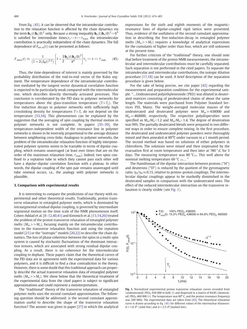
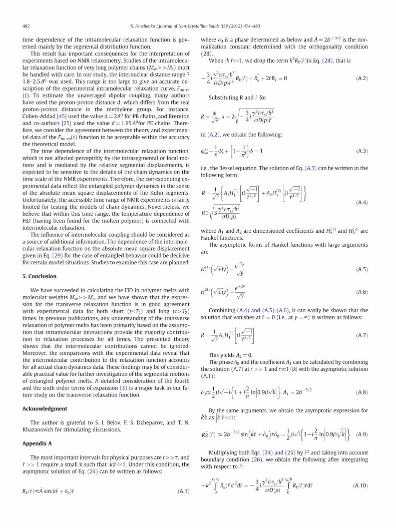
Fig. 1. Normalized experimental proton transverse relaxation curves recorded from(undeuterated) PEOH 438 000 in bulk (▪) and dispersed in a matrix of 84.8% (deuterat-ed) PEOD 460 000 (•). The temperature was 800 C, and the proton resonance frequencywas 200 MHz. The experimental data are taken from [42]. The theoretical relaxationcurve is drawn according to Eq. (45) for different values of the internuclear distances:d=1.8 A0 (solid line) and d=2.5 A0(dashed line).

480 K. Fenchenko / Journal of Non-Crystalline Solids 358 (2012) 474–483

From Eq. (43), it can be observed that the intramolecular contribu-tion to the relaxation function is affected by the chain dynamics viathe term bn tð Þbn 0ð Þ2 only. Because a strong inequality bn tð Þbn 0ð Þ2bbb4is satisfied for intermediate times,τsbb tbbτmax, the intramolecularcontribution is practically independent of the chain dynamics. The fulldependence of Fint ra(t) can be presented as follows:

F intra tð Þ ≈ 11þ 2 Δ0tð Þ3=2 � 1þ 3

2bn tð Þbn 0ð Þ2

b4

" #τs bb t bb τmax ð45Þ

Thus, the time-dependence of interest is mainly governed by theprobability distribution of the end-to-end vector of the Kuhn seg-ment. The temperature dependence of the intramolecular contribu-tion mediated by the tangent vector dynamical correlation functionis expected to be particularly weak compared with the intermolecularone, which describes directly thermally activated processes. Thisconclusion is corroborated by the FID data in polymer networks fortemperatures above the glass-transition temperature (T>Tc). Thefree induction decays in polymer networks with sufficiently highcrosslinking density for temperatures T>Tc do not depend on thetemperature [33,34]. This phenomenon can be explained by thesuggestion that the averaging of spin coupling by thermal motion inpolymer networks is not complete. In papers [35–39], thetemperature-independent width of the resonance line in polymernetworks is shown to be inversely proportional to the average distancebetween neighboring cross-links. Analogous to polymer networks, theproblem of the intramolecular relaxation function of highly interpene-trated polymer systems seems to be tractable in terms of dipolar cou-pling, which remains unaveraged (at least over times that are on theorder of the maximum relaxation time, τmax). Indeed, two spins con-fined to a reptation tube in which they cannot pass each other willhave a dipolar–dipolar correlation function with a plateau. In otherwords, the dipolar coupling of the spin pair remains unaveraged untiltube renewal occurs, i.e., the analogy with polymer networks isplausible.

3. Comparison with experimental results

It is interesting to compare the predictions of our theory with ex-perimental and other theoretical results. Traditionally, proton trans-verse relaxation in entangled polymer melts, which is dominated byintrasegmental residual dipolar coupling, is governed by intermediatesegmental motion on the time scale of the NMR phenomenon itself.Cohen-Addad et al. [8–12,40,41] and Kimmich et al. [13,14,20] treatedthe problem of the proton transverse relaxation of entangled polymermelts (Mw>>Mc), focusing mainly on the intramolecular contribu-tion to the transverse relaxation function and using the reptationmodel [21] or the “isotropic”models [20,22] to describe the chain dy-namics. The loss of phase coherence between the spins in a multi-spinsystem is caused by stochastic fluctuations of the dominant interac-tion tensors, which are associated with strong residual dipolar cou-pling. As a result, there is no coherence for the intermolecularcoupling to dephase. These papers claim that the theoretical curves ofthe FID data are in agreement with the experimental data for variouspolymers, and it is difficult to find a clear contradiction in the theory.However, there is somedoubt that this traditional approach can proper-ly describe the actual transverse relaxation data of entangled polymermelts (Mw>>Mc). We show below that the theoretical treatment ofthe experimental data from the cited papers is subject to significantapproximations and could represent a misinterpretation.

The “traditional” theory of the transverse relaxation of entangledpolymer melts uses the second cumulant approximation. The follow-ing question should be addressed: is the second cumulant approxi-mation useful to describe the shape of the transverse relaxationfunction? The answer was given in paper [27] in which the analytical

expressions for the sixth and eighth moments of the magnetic-resonance lines of dipolar-coupled rigid lattice were presented.Thus, evidence of the usefulness of the second cumulant approxima-tion in describing the free-induction-decay in entangled polymermelts (Mw>>Mc) requires a knowledge of analytical expressionsfor the cumulants of higher order than four, which are still unknownat the present time.

For further criticism of the “traditional” theory, one should notethat before treatment of the proton NMRmeasurements, the intramo-lecular and intermolecular contributions must be carefully separated.Such separation is not performed in the cited papers. To separate theintramolecular and intermolecular contributions, the isotopic dilutionprocedure [17,18] can be used. A brief description of the separationprocedure is given below.

For the sake of being precise, we cite paper [42] regarding themeasurement and preparation conditions for the experimental sam-ple. “…Undeuterated polyethyleneoxide (PEO) was diluted in deuter-ated matrices consisting of perdeuterated chains of about the samelength. The materials were purchased from Polymer Standard Ser-vices PSS, Mainz. The weight-averaged molecular masses of theundeuterated and deuterated polymer were Mw=438000 andMw=460000, respectively. The respective polydispersities werespecified as Mw/Mnb1.2 and Mw/Mnb1.4. The degree of deuterationwas 99%. The partially deuterated blends were prepared in two differ-ent ways in order to ensure complete mixing. In the first procedure,the deuterated and undeuterated polymer powders were thoroughlymixed and then annealed at 800C under vacuum in a 1 month period.The second method was based on solutions of either polymers inchloroform. The solutions were mixed and then inspissated by theevacuation first at room temperature and then later at ?80 °?C for 3days. The measuring temperature was 80 °C??. This well above thenominal melting temperature 60 °C ??… ”

The Hamiltonian of the dipolar interaction between protons (“H”)and deuterons (“D”) is reduced by the quotient of the gyromagneticratio, γD/γH≈0.15, relative to proton–proton couplings. The intermo-lecular dipolar couplings appear to be markedly diminished in thedeuterated samples in comparison with the undeuterated ones. Theeffect of the reduced intermolecular interaction on the transverse re-laxation is clearly visible (see Fig. 1).

0 2 4 6 8 10 12 14 16 18 2010-2

10-1

100

t>T2 regime

t<T2 regime

T2

Rouse-type dynamics

Entangled dynamics

F(t

), F

inte

r(t)

t,(ms)

F(t): Finter(t)=F(t)/Fintra(t)

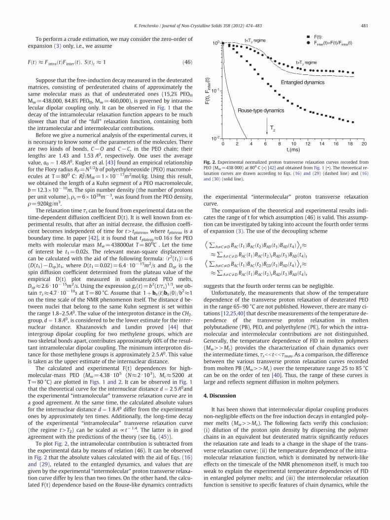
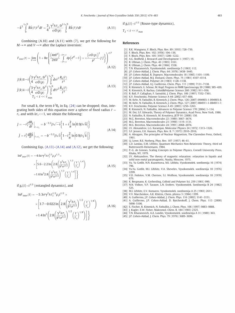
Fig. 2. Experimental normalized proton transverse relaxation curves recorded fromPEO (Mw=438 000) at 800 C (▪) [42] and obtained from Fig. 1 (•). The theoretical re-laxation curves are drawn according to Eqs. (16) and (29) (dashed line) and (16)and (30) (solid line).

481K. Fenchenko / Journal of Non-Crystalline Solids 358 (2012) 474–483

To perform a crude estimation, we may consider the zero-order ofexpansion (3) only, i.e., we assume

F tð Þ ≈ F intra tð ÞF inter tð Þ; S tð Þt ≈ 1 ð46Þ

Suppose that the free-induction decay measured in the deuteratedmatrices, consisting of perdeuterated chains of approximately thesame molecular mass as that of undeuterated ones (15,2% PEOH

Mw=438,000, 84.8% PEOD, Mw=460,000), is governed by intramo-lecular dipolar coupling only. It can be observed in Fig. 1 that thedecay of the intramolecular relaxation function appears to be muchslower than that of the “full” relaxation function, containing boththe intramolecular and intermolecular contributions.

Before we give a numerical analysis of the experimental curves, itis necessary to know some of the parameters of the molecules. Thereare two kinds of bonds, C−O and C−C, in the PEO chain; theirlengths are 1.43 and 1.53 A0, respectively. One uses the averagevalue, a0 ¼ 1:48A0. Kugler et al. [43] found an empirical relationshipfor the Flory radius RF=N1/2b of polyethyleneoxide (PEO) macromol-ecules at T=800 C: RF

2/MW=1×10−17m2mol/kg. Using this result,we obtained the length of a Kuhn segment of a PEO macromolecule,b=12.3×10−10m. The spin number density (the number of protonsper unit volume), ρs=6×1028m−3, was found from the PEO density,ρ=920kg/m3.

The relaxation time τs can be found from experimental data on thetime-dependent diffusion coefficient D(t). It is well known from ex-perimental results, that after an initial decrease, the diffusion coeffi-cient becomes independent of time for t> tplateau, where tplateau is aboundary time. In paper [42], it is found that tplateau≈0:16 s for PEOmelts with molecular mass Mw=438000at T=800C . Let the timeof interest be t1=0.02s. The relevant mean-square displacementcan be calculated with the aid of the following formula: ⟨r2(t1)⟩=6(D(t1)−Dsp)t1, where D(t1=0.02)=6.4 ⋅10−15m2/s and Dsp is thespin diffusion coefficient determined from the plateau value of theempirical D(t) plot measured in undeuterated PEO melts,Dsp≈2.6⋅10−15m2/s. Using the expression gr(t)=b2(t/τs)1/3, we ob-tain τs≈4.7 ⋅10−10s at T=80 °C. Assume that 1þ bn tð Þbn 0ð Þ=b2≈1on the time scale of the NMR phenomenon itself. The distance d be-tween nuclei that belong to the same Kuhn segment is set withinthe range 1.8–2.5A0. The value of the interproton distance in the CH2-

group, d ¼ 1:8A0, is considered to be the lower estimate for the inter-nuclear distance. Khazanovich and Lundin proved [44] thatintergroup dipolar coupling for two methylene groups, which aretwo skeletal bonds apart, contributes approximately 60% of the resul-tant intramolecular dipolar coupling. The minimum interproton dis-tance for those methylene groups is approximately 2:5A0. This valueis taken as the upper estimate of the internuclear distance.

The calculated and experimental F(t) dependences for high-molecular-mass PEO (Mw=4.38⋅105 (N≈2⋅103), Mc≈5200 atT=80 °C) are plotted in Figs. 1 and 2. It can be observed in Fig. 1that the theoretical curve for the internuclear distance d ¼ 2:5A0andthe experimental “intramolecular” transverse relaxation curve are ina good agreement. At the same time, the calculated absolute valuesfor the internuclear distance d ¼ 1:8A0 differ from the experimentalones by approximately ten times. Additionally, the long-time decayof the experimental “intramolecular” transverse relaxation curve(the regime t>T2) can be scaled as ∝ t−1.4. The latter is in goodagreement with the predictions of the theory (see Eq. (45)).

To plot Fig. 2, the intramolecular contribution is subtracted fromthe experimental data by means of relation (46). It can be observedin Fig. 2 that the absolute values calculated with the aid of Eqs. (16)and (29), related to the entangled dynamics, and values that aregiven by the experimental “intermolecular” proton transverse relaxa-tion curve differ by less than two times. On the other hand, the calcu-lated F(t) dependence based on the Rouse-like dynamics contradicts

the experimental “intermolecular” proton transverse relaxationcurve.

The comparison of the theoretical and experimental results indi-cates the range of t for which assumption (46) is valid. This assump-tion can be investigated by taking into account the fourth order termsof expansion (3). The use of the decoupling scheme

⟨∑A≠C≠D BAC t1ð ÞBAC t2ð ÞBAD t3ð ÞBAD t4ð Þ⟩t≈≈∑A≠C≠D BAC t1ð ÞBAC t2ð ÞtBAD t3ð ÞBAD t4ð Þt

⟨∑A≠C≠D BAC t1ð ÞBAC t2ð ÞBCD t3ð ÞBAD t4ð Þ⟩t≈≈∑A≠C≠D BAC t1ð ÞBAC t2ð ÞtBAD t3ð ÞBAD t4ð Þt

suggests that the fourth order terms can be negligible.Unfortunately, the measurements that show of the temperature

dependence of the transverse proton relaxation of deuterated PEOin the range 65–90 °C are not published. However, there are many ci-tations [12,25,40] that describe measurements of the temperature de-pendence of the transverse proton relaxation in moltenpolybutadiene (PB), PEO, and polyethylene (PE), for which the intra-molecular and intermolecular contributions are not distinguished.Generally, the temperature dependence of FID in molten polymers(Mw>>Mc) provides the characterization of chain dynamics overthe intermediate times, τsbb tbbτmax. As a comparison, the differencebetween the various transverse proton relaxation curves recordedfrom molten PB (Mw>>Mc) over the temperature range 25 to 85 °Ccan be on the order of ten [40]. Thus, the range of these curves islarge and reflects segment diffusion in molten polymers.

4. Discussion

It has been shown that intermolecular dipolar coupling producesnon-negligible effects on the free induction decays in entangled poly-mer melts (Mw>>Mc). The following facts verify this conclusion:(i) dilution of the proton spin density by dispersing the polymerchains in an equivalent but deuterated matrix significantly reducesthe relaxation rate and leads to a change in the shape of the trans-verse relaxation curve; (ii) the temperature dependence of the intra-molecular relaxation function, which is dominated by network-likeeffects on the timescale of the NMR phenomenon itself, is much tooweak to explain the experimental temperature dependencies of FIDin entangled polymer melts; and (iii) the intermolecular relaxationfunction is sensitive to specific features of chain dynamics, while the

482 K. Fenchenko / Journal of Non-Crystalline Solids 358 (2012) 474–483

time dependence of the intramolecular relaxation function is gov-erned mainly by the segmental distribution function.

This result has important consequences for the interpretation ofexperiments based on NMR relaxometry. Studies of the intramolecu-lar relaxation function of very long polymer chains (Mw>>Mc) mustbe handled with care. In our study, the internuclear distance range ?1.8–2.5 A0 was used. This range is too large to give an accurate de-scription of the experimental intramolecular relaxation curve, Fint ra(t). To estimate the unaveraged dipolar coupling, many authorshave used the proton-proton distance d, which differs from the realproton-proton distance in the methylene group. For instance,Cohen-Addad [45] used the value d=2A0 for PB chains, and Breretonand co-authors [25] used the value d=1.95 A0for PE chains. There-fore, we consider the agreement between the theory and experimen-tal data of the Fint ra(t) function to be acceptable within the accuracythe theoretical model.

The time dependence of the intermolecular relaxation function,which is not affected perceptibly by the intrasegmental or local mo-tions and is mediated by the relative segmental displacements, isexpected to be sensitive to the details of the chain dynamics on thetime scale of the NMR experiments. Therefore, the corresponding ex-perimental data reflect the entangled polymer dynamics in the senseof the absolute mean square displacements of the Kuhn segments.Unfortunately, the accessible time range of NMR experiments is fairlylimited for testing the models of chain dynamics. Nevertheless, webelieve that within this time range, the temperature dependence ofFID (having been found for the molten polymer) is connected withintermolecular relaxation.

The influence of intermolecular coupling should be considered asa source of additional information. The dependence of the intermole-cular relaxation function on the absolute mean square displacementgiven in Eq. (29) for the case of entangled behavior could be decisivefor certain model situations. Studies to examine this case are planned.

5. Conclusion

We have succeeded in calculating the FID in polymer melts withmolecular weights Mw>>Mc, and we have shown that the expres-sion for the transverse relaxation function is in good agreementwith experimental data for both short (tbT2) and long (t>T2)times. In previous publications, any understanding of the transverserelaxation of polymer melts has been primarily based on the assump-tion that intramolecular interactions provide the majority contribu-tion to relaxation processes for all times. The presented theoryshows that the intermolecular contributions cannot be ignored.Moreover, the comparisons with the experimental data reveal thatthe intermolecular contribution to the relaxation function accountsfor all actual chain dynamics data. These findings may be of consider-able practical value for further investigation of the segmental motionsof entangled polymer melts. A detailed consideration of the fourthand the sixth order terms of expansion (3) is a major task in our fu-ture study on the transverse relaxation function.

Acknowledgment

The author is grateful to S. I. Belov, F. S. Dzheparov, and T. N.Khazanovich for stimulating discussions.

Appendix A

The most important intervals for physical purposes are t>>τs and~r >> 1 require a small k such that kj j~rbb1. Under this condition, theasymptotic solution of Eq. (24) can be written as follows:

Rk ~rð Þ≈~A sin k~r þ δ0ð Þ~r ðA:1Þ

where δ0 is a phase determined as below and Ã=2b−3/2 is the nor-malization constant determined with the orthogonality condition(28).

When kj j~rbb1, we drop the term k2Rk ~rð Þin Eq. (24), that is

−34iγ2ℏτs=b

3

σ D pð Þ~r3Rk ~rð Þ þ R

00

k þ 2~rR0

k ¼ 0 ðA:2Þ

Substituting R and ~r for

R ¼ ϕffiffiffi~r

p ; x ¼ 2

ffiffiffiffiffiffiffiffiffiffiffiffiffiffiffiffiffiffiffiffiffiffiffiffiffiffiffiffiffiffiffi−3

4iγ2ℏτs=b

3

σD pð Þ~r

s

in (A.2), we obtain the following:

ϕxx′′þ1xϕx′þ 1− 1

x2

� �ϕ ¼ 1 ðA:3Þ

i.e., the Bessel equation. The solution of Eq. (A.3) can be written in thefollowing form:

R ¼ 1ffiffiffi~r

p A1H1ð Þ1 β

ffiffiffiffiffiffi−i

p

~r1=2

" #þ A2H

2ð Þ1 β

ffiffiffiffiffiffi−i

p

~r1=2

" #( )

β≡ffiffiffiffiffiffiffiffiffiffiffiffiffiffiffiffiffiffiffiffiffiffiffiffi3γ2ℏτs=b

3

σD pð Þ

s ðA:4Þ

where А1 and А2 are dimensioned coefficients and Нλ(1) and Нλ

(2) areHankel functions.

The asymptotic forms of Hankel functions with large argumentsare

Н 1ð Þ1

ffiffiffiffiffiffi�i

py

� � e e�2yffiffiffiy

p ðA:5Þ

Н 2ð Þ1

ffiffiffiffiffiffi�i

py

� � e e∓2yffiffiffiy

p ðA:6Þ

Combining (A.4) and (A.5)-(A.6), it can easily be shown that thesolution that vanishes at ~r ¼ 0 (i.e., at y=∞) is written as follows:

R ¼ 1ffiffiffi~r

p A1H1ð Þ1 β

ffiffiffiffiffiffi−i

p

~r1=2

" #ðA:7Þ

This yields А2=0.The phase δ0 and the coefficient A1 can be calculated by combining

the solution (A.7) at ~r >> 1 and ~r≈1= kj jwith the asymptotic solution(A.1):

δ0≈12βffiffiffiffiffiffi−i

p1þ i

2πln 0:9β

ffiffiffik

p��� ��� �;A1 ¼ 2b−3=2 ðA:8Þ

By the same arguments, we obtain the asymptotic expression for~R~k as ~k

��� ���~rbb1:~R~k ~rð Þ ≈ 2b−3=2 sin ~k~r þ ~δ0

� �~r~δ0 ¼ 1

2βffiffii

p1−i

2πln 0:9β

ffiffiffi~k

q���� ���� �ðA:9Þ

Multiplying both Eqs. (24) and (25) by ~r2 and taking into accountboundary condition (26), we obtain the following after integratingwith respect to ~r:

−k2 ∫r0=b

0

Rk ~rð Þ~r2d~r ¼ −34iγ2ℏτs=b

3

σ D pð Þ ∫r0=b

0

Rk ~rð Þ~rd~r ðA:10Þ

483K. Fenchenko / Journal of Non-Crystalline Solids 358 (2012) 474–483

−~k2 ∫r0=b

0

~R~k ~rð Þ~r2d~r ¼ 34iγ2ℏτs=b

3

σD pð Þ ∫r0=b

0

~R~k ~rð Þ~rd~r ðA:11Þ

Combining (A.10) and (A.11) with (7), we get the following forΜ→∞ and V→∞ after the Laplace inversion:

F inter tð Þ ¼ limV→∞

1þ Re4πb6� �2πiV

∫þi∞þc

−i∞þс

dp ep~t−1

� ���

σ D pð Þ� �2

p2J⋅~J)8><>:1CA

ρsV0B@

ðA:12Þ

J kð Þ≡−i34γ2ℏτs=b

3

σ D pð Þ

!∫

r0=b

0

~dr~r2Rk ~rð Þ~r3

~J kð Þ≡−i34γ2ℏτs=b

3

σ D pð Þ

!∫

r0=b

0

d~r~r2~Rk ~rð Þ~r3

T2 b t bb τmax

ðA:13Þ

For small k, the term k2Rk in Eq. (24) can be dropped; thus, inte-grating both sides of this equation over a sphere of fixed radius ~r ¼r1 and with kr1bb1, we obtain the following:

J ¼ −r21dRk

d~r j~r¼r1

¼ b−3=2βffiffiffiffiffiffi−i

p1þ i

2πln 0:9β

ffiffiffik

p��� ��� �

~J ¼ r21d~R~kd~r ~r¼r1

¼ −b−3=2βffiffii

p1−i

2πln 0:9β

ffiffiffi~k

q���� ���� �����ðA:14Þ

Combining Eqs. (A.13)–(A.14) and (A.12), we get the following:

lnF inter tð Þ ¼ −4:6σγ2ℏτ2=3s ρst1=3�

�"5:6−2:2 ln 2:8

γ2ℏτsb3σ3=2

!1=2tτs

� �1=4 !

þ1:6 ln22:8γ2ℏτsb3σ3=2

!1=2tτs

� �1=4#) ðA:15Þ

if gr(t)~ t1/3 (entangled dynamics), and

lnF inter tð Þ ¼ −5:3σγ2ℏτ1=2s ρst1=2 �

�"3:7−0:022 ln 2:8

γ2ℏτsb3σ3=2

!1=2tτs

� �1=8 !

þ1:4 ln2 2:8γ2ℏτsb3σ3=2

!1=2tτs

� �1=8 !#) ðA:16Þ

if gr(t)~ t1/2 (Rouse-type dynamics),

T2 b t bb τmax

References

[1] R.K. Wangness, F. Bloch, Phys. Rev. 89 (1953) 728–739.[2] F. Bloch, Phys. Rev. 102 (1956) 104–136.[3] F. Bloch, Phys. Rev. 105 (1957) 1206–1222.[4] A.G. Redfield, J. Research and Development 1 (1957) 19.[5] R. Ullman, J. Chem. Phys. 43 (1965) 3161.[6] R. Ullman, J. Chem. Phys. 44 (1966) 1558.[7] T.N. Khazanovich, Vysokomolek. soedinenija 5 (1963) 112.[8] J.P. Cohen-Addad, J. Chem. Phys. 64 (1976) 3438–3445.[9] J.P. Cohen-Addad, R. Dupeyre, Macromolecules 18 (1985) 1101–1109.

[10] J.P. Cohen-Addad, M.J. Domard, Chem. Phys. 75 (1981) 4107–4114.[11] J.P. Cohen-Addad, Polymer 24 (1983) 1128–1138.[12] J.P. Cohen-Addad, A.J. Guillermo, Chem. Phys. 111 (1999) 7131–7138.[13] R. Kimmich, G. Schnur, M. Kopf, Progress in NMR Spectroscopy 20 (1988) 385–420.[14] R. Kimmich, R. Bachus, Coloid&Polymer Science 260 (1982) 911–936.[15] R. Ball, P. Callaghan, F. Samulski, J. Chem. Phys. 106 (1997) 7352–7361.[16] K.V. Fenchenko, Polymer Science A 44 (2002) 657–666.[17] M. Kehr, N. Fatkullin, R. Kimmich, J. Chem. Phys. 126 (2007) 094903-1-094903-8.[18] M. Kehr, N. Fatkullin, R. Kimmich, J. Chem. Phys. 127 (2007) 084911-1-084911-7.[19] K.V. Fenchenko, Polymer Science A 45 (2003) 1250–1263.[20] R. Kimmich, N. Fatkullin, Advances in Polymer Science 170 (2004) 1–114.[21] M. Doi, S.F. Edwards, Theory of Polymer Dynamics, Acad Press, New York, 1986.[22] N. Fatkullin, R. Kimmich, M. Kroutieva, JETP 91 (2000) 150.[23] M.G. Brereton, Macromolecules 22 (1989) 3667–3674.[24] M.G. Brereton, Macromolecules 23 (1990) 1119–1131.[25] M.G. Brereton, Macromolecules 24 (1991) 2068–2074.[26] I.V. Alexandrov, L.G. Karamjan, Molecular Physics 24 (1972) 1313–1326.[27] S.F. Jensen, E.K. Hansen, Phys. Rev. B. 7 (1973) 2910–2916.[28] A. Abragam, The principles of Nuclear Magnetism, The Clarendon Press, Oxford,

1961.[29] I.J. Lowe, R.E. Norberg, Phys. Rev. 107 (1957) 46–61.[30] L.D. Landau, E.M. Lifshitz, Quantum Mechanics Non-Relativistic Theory, third ed

Butterworth-Heinemann, 1984.[31] P.-G. de Gennes, Scaling Concepts in Polymer Physics, Cornell University Press,

Ithaka, NY, 1979.[32] I.V. Aleksandrov, The theory of magnetic relaxation: relaxation in liquids and

solid non-metal paramagnetic, Nauka, Moscow, 1975.[33] Yu. Ya Gotlib, N.N. Kuznetsova, M.I. Lifshitz, Vysokomolek. soedinenija 16 (1974)

796.[34] Yu.Ya. Gotlib, M.I. Lifshitz, V.A. Shevelev, Vysokomolek. soedinenija 18 (1976)

2299.[35] V.D. Fedotov, V.M. Chernov, S.I. Wolfson, Vysokomolek. soedinenija 18 (1978)

679.[36] K. Bergmann, K. Gerberding, Colloid and Polymer Sci. 259 (1981) 990.[37] N.N. Volkov, V.P. Tarasov, L.N. Erofeev, Vysokomolek. Soedinenija B 24 (1982)

525.[38] M.I. Lifshitz, E.V. Komarov, Vysokomolek. soedinenija A 25 (1983) 2611.[39] V.V. Marchenkov, A.K. Khitrin, Chem. phisica 3 (1984) 1399.[40] A. Guillermo, J.P. Cohen-Addad, J. Chem. Phys. 116 (2002) 3141–3151.[41] A. Guillermo, J.P. Cohen-Addad, D. Bytchenkoff, J. Chem. Phys. 113 (2000)

5098–5106.[42] E. Fischer, R. Kimmich, N. Fatkullin, J. Chem. Phys. 106 (1997) 9883–9888.[43] J. Kugler, E.W. Fisher, Makromol. Chem. B. 184 (1983) 2325.[44] T.N. Khazanovich, A.A. Lundin, Vysokomolek. soedinenija A 31 (1989) 363.[45] J.P. Cohen-Addad, J. Chem. Phys. 79 (1976) 3689–3696.