Revealing the WebsInsights from the Exploitation of Complementary Informationfrom various Magnetic Resonance Imaging related Connectivity Methods

Dissertationzur Erlangung des Grades einesDoktors der Naturwissenschaften(Dr. rer. nat.)der Mathematisch-Naturwissenschaftlichen Fakultatundder Medizinischen Fakultatder Eberhard Karls Universitat Tubingenvorgelegt von

Dipl.-Psych. Balint Varkuti

aus Budapest, Ungarn

TubingenAugust, 2011

Tag der mundlichen Prufung: 13.10.2011

Dekan der Math.-Nat. Fakulat: Prof. Dr. Wolfgang RosenstielDekan der Medizinischen Fakulat: Prof. Dr. I. B. Autenrieth

1. Berichterstatter: Prof. Dr. Niels Birbaumer2. Berichterstatter: Prof. Dr. Martin Hautzinger

Prufungskomission: Prof. Dr. Kamil UludagProf. Dr. Christoph Braun

Declaration

I hereby declare that I have produced the work entitled: ”Revealing the Webs”, submitted forthe award of a doctorate, on my own (without external help), have used only the sources and aidsindicated and have marked passages included from other works, whether verbatim or in content,as such. I swear upon oath that these statements are true and that I have not concealed anything.I am aware that making a false declaration under oath is punishable by a term of imprisonmentof up to three years or by a fine.

Tubingen, den 14.8.2011 . . . . . . . . . . . . . . . . . . . . . . . . . . . . . . . . . . . . . . . . . . . . .

Acknowledgments

I would like to thank Professor Niels Birbaumer for giving me the opportunity to work in his

lab, for his patience and for always bringing me back down to earth when it was necessary.

I would also like to thank the other members of my supervisory board for their support and

advice during so many questions and lively debates.

I want to especially thank Ranganatha Sitaram for being my supervisor and close colleague

over the years, for supporting me and for patiently reading through tons of my half-baked ideas.

I want to thank my colleagues and collaborators at the Institute of Medical Psychology and

Behavioral Neurobiology for all their help and a great time.

Most of all I would like to thank my mother Iren and my father Geza for always supporting

me no matter what I did, and for being there for me during this time. And I want to thank my

friends who kept me sane throughout these years, and thank a certain foggy place in Freiburg

where I had my best ideas.

And last but not least, I want to thank my wonderful wife Jessica who did not run away from

the crazy brain scientist, but came with me and changed ours lives to the better.

We shall not cease from exploration. And the end of all our exploring

will be to arrive where we started and know the place for the first time.

T.S. Eliot

Contents

1 Introduction 2

1.1 Current Connectivity concepts and terminology . . . . . . . . . . . . . . . . . . . . 10

1.2 Localizationism, disconnection syndromes and systems neuroscience . . . . . . . . 13

1.3 Employed methodology . . . . . . . . . . . . . . . . . . . . . . . . . . . . . . . . . 17

2 Motivation, hypotheses and approach 20

3 Methodical developments and innovations 22

4 Short summary of results 24

5 Discussion 25

5.1 Implications of our findings . . . . . . . . . . . . . . . . . . . . . . . . . . . . . . . 25

5.2 Supporting evidence from the field of developmental neurobiology . . . . . . . . . . 27

5.3 Implications for stroke research . . . . . . . . . . . . . . . . . . . . . . . . . . . . . 28

5.4 Implications for BCI research . . . . . . . . . . . . . . . . . . . . . . . . . . . . . . 30

6 Outlook 33

7 Publications, manuscripts and contributions 45

7.1 Chapter 1 - The link between Anatomical Connectivity, Perfusion and regional

Cerebral Blood Flow . . . . . . . . . . . . . . . . . . . . . . . . . . . . . . . . . . . 47

7.2 Chapter 2 - A taxonomy of Functional Connectivity Networks and the influence of

regional brain properties on network formation . . . . . . . . . . . . . . . . . . . . 97

7.3 Chapter 3 - Functional Connectivity Network alterations as an effect of stroke re-

habilitation . . . . . . . . . . . . . . . . . . . . . . . . . . . . . . . . . . . . . . . . 162

7.4 Chapter 4 - On the relationship of Brain-Computer Interface aptitude and Anatom-

ical Connectivity . . . . . . . . . . . . . . . . . . . . . . . . . . . . . . . . . . . . . 188

1

1 Introduction

Information processing, memory storage or the adaptation of behavior do not occur solely within

single specialized computational units of the human brain such as the single neuron, but require

the ordered interplay of many such computational units. Although the physical manifestation of

behavior can be caused by volitional control of a single neuron (Fetz, 2007), even in this case other

neurons and entire neuronal ensembles play a central role in the conditioning processes involved

with gaining volitional control over the spike trains of the target neuron. Consequentially, when we

refer to any brain function we implicitly refer to phenomena generated by the ordered cooperation

of neural computational units within neural networks.

When moving up the spatial scale, the first microscopic level of such interplay - if we ignore the role

of astrocytes for now (Schummers et al., 2008) - is the ordered interaction of multiple neighboring

neurons via synapses, followed by the interaction of larger neuronal ensembles in mesoscale struc-

tures such as cortical columns and finally the interaction of multiple neuronal ensembles across

larger distances - and via white matter fibre bundles - in macroscale neuronal networks.

Beyond the spatial scale such interactions can be sorted along the temporal dimension as well,

starting with the quasi-simultaneous firing of single neurons or neuron groups leading to strength-

ened associations between them based on Hebbian learning (Abbott and Nelson, 2000), followed

by more sequential constellations of causally interdependent neuronal excitations - as in the case

of neural avalanches (Beggs and Plenz, 2003) - or inhibitions and finally the more delayed forms of

interactions, where the complex intra-modular interplay of a neural ensemble triggers the eventual

intra-modular interplay of another distant neural ensemble, a constellation where distinct neural

events can become distinguishable.

Clearly the healthy brain at large is practically never in a state of communicatory silence. The

concept of such neural events does not refer to bursts of neural firing that break states of neural

rest, but rather refers to temporally delimitable and spatially localized changes in the patterns

of neurotransmission. Such changes can be causally linked in sequences, feedforward- or feedback

loops, but might appear synchronous to an observer if for example the temporal resolution of the

measurement method is too low.

Such distinctions strongly depend on the spatial and temporal scale of the measurement method

and on how indirectly the measured metric is linked to the actual neuronal processing itself. In the

case of Blood Oxygen Level-Dependent (BOLD) functional Magnetic Resonance Imaging (fMRI)

the spatial scale is in the range of millimeters, the temporal scale is usually on the order of seconds

2

and the measured metric, namely the local ratio of oxygenated versus deoxygenated hemoglobin,

represents a - not always unambiguous - delayed metabolic echo of macroscale neural processes

(Logothetis, 2008). These limitations of our insight into in-vivo neural processes shape the ap-

pearance of neural networks to us (illustrated in Figure 1).

Neural networks on the macro- or mesoscale can appear to us in an fMRI analysis as one clump

of synchronously activating points in the brain (e.g. the V1 area) which we then can associate

with the assumed trigger event or the independent variable that we manipulated experimentally

(e.g. the display of a checkerboard on the screen). But they can also appear as multi-site events,

where synchronous neural activation or de-activation is detected at multiple distant sites but at

the same time.

These formations of temporally coherent changes in activity are what we usually refer to as

Functional Connectivity Network (FCN). Examples of such networks are the Default Brain Mode

network (Raichle et al., 2001) which we associate with resting behavior, or the prefrontal executive

control network which is associated with volitionally executed complex tasks (Seeley et al., 2007a).

With other methods, such as electrophysiology, which measure neural activity more directly via

the electromagnetic distortions that macroscale neural processes cause, FCNs appear mainly as

statistical interactions between sensors (Micheloyannis et al., 2006). Although the temporal res-

olution of these methods is magnitudes higher than that of hemodynamics based methods such

as fMRI, the spatial characterization, of where the functional interactions, that correspond to the

changes in the electromagnetic field, occur exactly in the brain remains challenging (Wendel et al.,

2009).

But irrespective of which method of study and which emphasis in analysis is chosen, it is clear that

the underlying neural processes we try to gather when studying FCNs are not entirely understood

with respect to how and why they form in their specific spatial and temporal configurations.

Beyond studying which stimuli, contexts or tasks elicit how much activity in which neural net-

work, a second perspective on networks has co-evolved alongside classical experimentation (Van

Dijk et al., 2010). This discipline is trying to answer such questions as how these networks are

formed (Bullmore and Sporns, 2009), why we observe exactly this limited set of networks and

not others or how the boundaries of the underlying static system these dynamic networks form

within influence them (Honey et al., 2009), and vice versa. As such we have begun to study the

complexity of the interaction of systems in the brain itself, rather than reducing our efforts to

focusing merely on the complexity of single parts, scales or levels (Barabasi, 2012). To deepen our

3

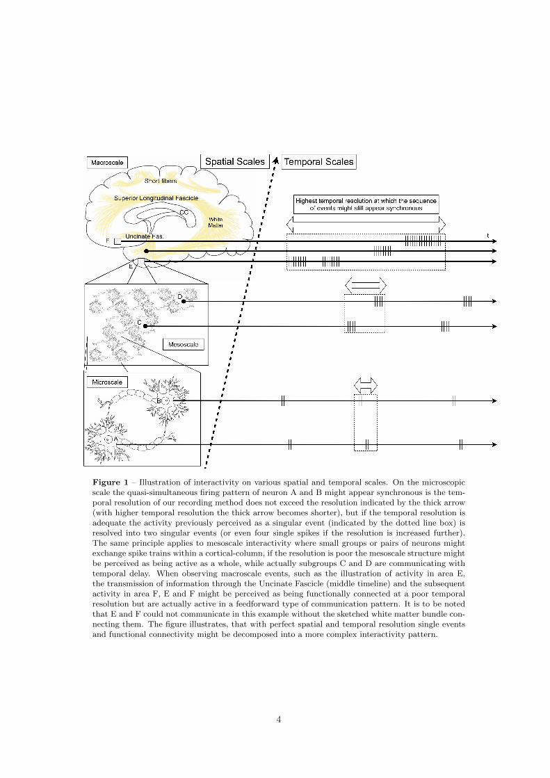
Figure 1 – Illustration of interactivity on various spatial and temporal scales. On the microscopicscale the quasi-simultaneous firing pattern of neuron A and B might appear synchronous is the tem-poral resolution of our recording method does not exceed the resolution indicated by the thick arrow(with higher temporal resolution the thick arrow becomes shorter), but if the temporal resolution isadequate the activity previously perceived as a singular event (indicated by the dotted line box) isresolved into two singular events (or even four single spikes if the resolution is increased further).The same principle applies to mesoscale interactivity where small groups or pairs of neurons mightexchange spike trains within a cortical-column, if the resolution is poor the mesoscale structure mightbe perceived as being active as a whole, while actually subgroups C and D are communicating withtemporal delay. When observing macroscale events, such as the illustration of activity in area E,the transmission of information through the Uncinate Fascicle (middle timeline) and the subsequentactivity in area F, E and F might be perceived as being functionally connected at a poor temporalresolution but are actually active in a feedforward type of communication pattern. It is to be notedthat E and F could not communicate in this example without the sketched white matter bundle con-necting them. The figure illustrates, that with perfect spatial and temporal resolution single eventsand functional connectivity might be decomposed into a more complex interactivity pattern.

4

understanding of these links is relevant for basic research with healthy individuals, but even more

so in the clinical context (Lawrie et al., 2008).

Neural networks in the brain change over time due to learning (Tamas Kincses et al., 2008), matu-

ration (Dosenbach et al., 2010; Casey et al., 2005) or degradation (Greicius et al., 2004; Wu et al.,

2011) but do this within the boundaries that are set by structure/function relationships. One re-

gion of the brain might for example not be able to provide all the neurocomputational processing

or the right neuronal assemblies required for the successful execution of a certain behavior, so a

second region is recruited that complements the processing of the first region. With more and

more training, the interplay between these regions usually changes and becomes more fine-tuned

and economical (Voss et al., 2011; Lee et al., 2011), but if the direct structural link between these

regions is severed and no poly-synaptic neural detour is at disposal, the shape, capacity and be-

havioral significance of this neural network will be massively altered - one drastic example of how

structure can restrict function.

But the brain can not simply add more and more neuronal ensembles to a neural process like

a computer might activate more and more processors to solve a given problem quickly. Not all

neuronal ensembles are capable of performing all neurocomputational processing tasks but quite

the contrary. There are certain basic restrictions in the functional roles brain regions can assume,

and because not each brain region can assume any functional role, the ensembles in which brain

regions are associated in FCNs do not form arbitrarily but in a manner depending very specifically

on the task at hand.

The restrictions that define the functional roles brain regions can assume are reflected in our disso-

ciation of brain regions into primary sensory, primary motor, subcortical, secondary or association

cortex regions. These regions differ with regard to multiple traits, such as their physical position

in the brain, their anatomical connectivity via white matter fiber bundles, their local vasculature

and relative perfusion, the range and type of neurons contained within such a region, the ordering

of cortical layers, the integrity and Gray Matter Volume (GMV) in general, the intra-modular

wiring pattern, neurotransmitter availability and many other factors. As such each region can be

described as a point in a multi-dimensional feature space, where each feature in question is one

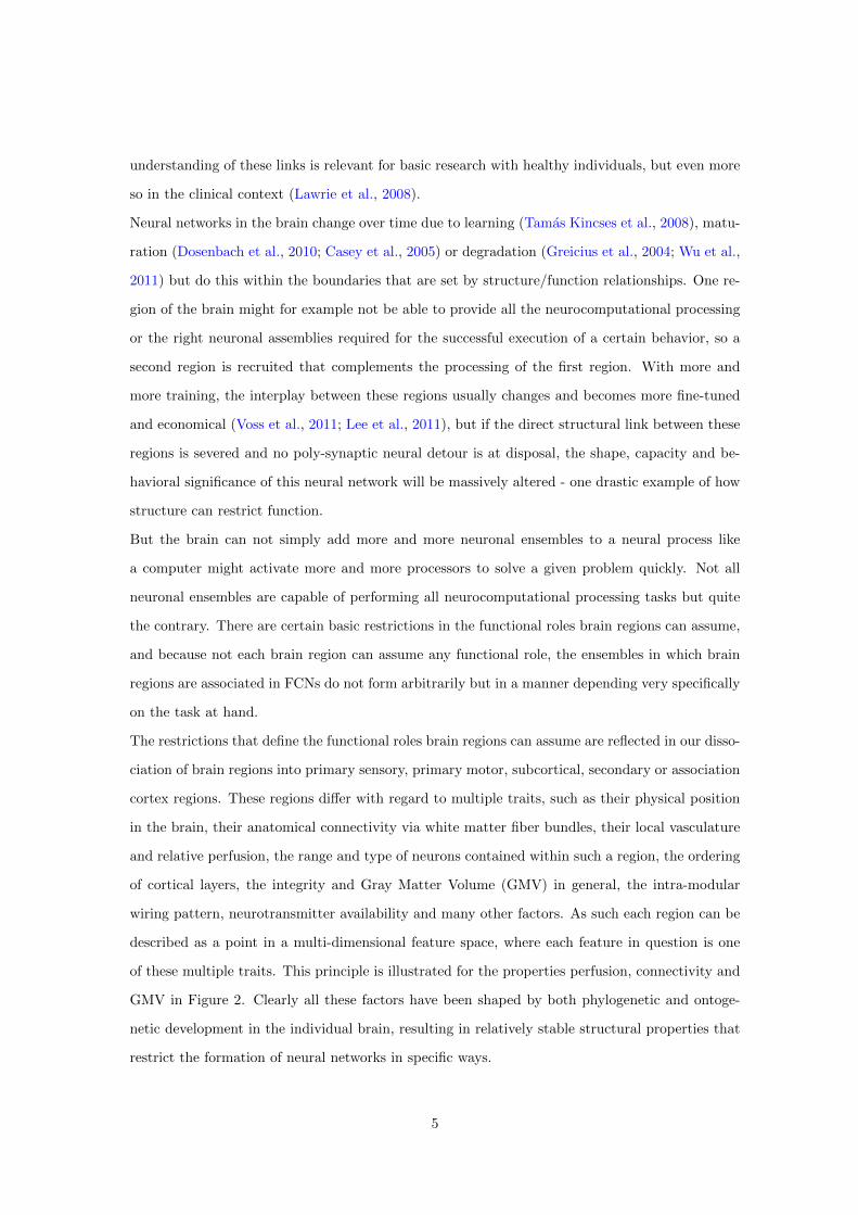
of these multiple traits. This principle is illustrated for the properties perfusion, connectivity and

GMV in Figure 2. Clearly all these factors have been shaped by both phylogenetic and ontoge-

netic development in the individual brain, resulting in relatively stable structural properties that

restrict the formation of neural networks in specific ways.

5

Figure 2 – Illustration of general principle, Regions 1 and 2 engage in both FCNs A (red) and B(green), but Regions 3 and 4 only engage in one network, either network A (Region 4) or B (Region 3)- a look at the regional properties shows that regions engaging in multiple networks differ from thosethat are only member of one network (marked by red asterisks), these regions have higher GMV,Perfusion and Connectivity than regions which are only members of one network and that these alsohave a more balanced perfusion and GMV ratio (Ratio P/GMV), the illustrated concept motivatedone of our studies (Varkuti et al., 2011) which can be found in Chapter 1.

Multiple phenomena in neurological and psychiatric practice are related to restrictions or alter-

ations of the brains’ ability to form or maintain adaptive and economical neural networks (Lawrie

et al., 2008; Whitfield-Gabrieli et al., 2009; Demirci et al., 2009; Rubinov et al., 2009; Jafri et al.,

2008; Lynall et al., 2010; Whitford et al., 2010; Begre et al., 2003; Cammoun et al., 2009). This

is reflected in findings on the biomarkers of disease, where structural differences in the brain can

successfully be correlated with pathology.

Such biomarkers are being successively narrowed down for phenomena such as Amyotrophic Lateral

Sclerosis (ALS) (Senda et al., 2011; Woolley et al., 2011; Filippini et al., 2010), autism spectrum

disorders (Eigsti and Shapiro, 2003) or ageing and dementia (Head et al., 2004). Some of the

structural changes that are identified as biomarkers might have co-evolved with the pathology,

6

some might have preceded or even caused the outbreak of a disease, while others might be the

result of compensatory or other after-effects of certain functional abnormalities. Such changes

can be rather sudden in terms of onset and effect, such as for example the paralysis due to dis-

connection of the motor system and the periphery after stroke, while others might emerge much

slower such as for example cortical atrophy, disconnection and hypoperfusion in certain forms of

neurodegenerative disease such as dementia (Grundman et al., 2002; Fellgiebel et al., 2004; Stam

et al., 2007; Devanand et al., 2007; Stam et al., 2009; Chao et al., 2010; Seeley et al., 2009a; Bottino

et al., 2002; Sugihara et al., 2004) or manifest in a contra-intuitive form (Madhavan et al., 2010).

Local structural traits are properties of a brain region that only change slowly, such as for example

anatomical connectivity, tissue volume or vascularization. These traits either enable or restrict

brain function in a specific way or can change themselves as a result of brain activity (e.g. the way

extensive practice of a musical instrument can change the cortical representation of the hands).

In the case of disease we often can identify biomarkers which are structural traits, because these

have been either altered by the disease or played a role in the etiology, or both. From these cases

we infer structure/function relationships that try to summarize our findings and allow for the

deduction of new hypotheses.

In this sense, structure/function relationships are essentially formulated as rules, which are based

on empirical evidence either from (quasi-)experimental (e.g. does structural similarity of monozy-

gotic twins predict functional similarities?) or correlative studies (e.g. does anatomical connec-

tivity predict the likelihood of functional connectivity between a pair of regions?).

Such rules can be very simple, such as that there can be no neural activity where metabolic

prerequisites such as a supply of oxygen and glucose are not given. But these rules can as well

be more complex, such as that functional connectivity on a specific timescale (e.g. milliseconds)

between a group of regions is only possible if these regions are directly anatomically connected

through white matter fibre bundles with intact myelinisation and hence good electrical conduction

properties. Such rules can incorporate additional pathogenic factors, such as predictions where

neural communication is expected to be macroscopically distorted for example as a function of

amyloid plaque concentration in the brain (Ross and Poirier, 2004; Wu et al., 2011; Stam et al.,

2009).

If we understand how the the entirety and interplay of local brain traits - further referred to

7

as the underlying system - generates neural networks in the absence of external stimuli (such as

the Default Brain Mode network) or for example as a result of repeated activity patterns - which is

the case in learning and training - we would be able to formulate rules by which structure restricts

or enables function, or by which function alters structure over time. If we are able to broaden our

understanding of these rules, our ability to predict and influence the progression of diseases would

improve dramatically.

One example with which this can be illustrated are atlases and more generally brain parcellation

schemes. The parcellation and functional description of brain regions did not evolve much further

than uniting the early cytoarchitectonic distinction (Brodmann, 1909) of regions with long lists

of functional observations detailing which experimental contexts led to localized activity in which

brain region. Even when it became apparent that functional networks do span across cytoarchi-

tectonic boundaries, only minimal changes to the standard parcellation schemes were made.

These parcellation schemes or atlases are closely based on neurological experience (lesion and

stimulation studies) and experimental evidence (neuroimaging data) but primarily contain a list

of cerebral landmark positions and the associated functions. As such, these descriptions have to

remain on a qualitative level of distinction, as long as the rules that govern the emergence of

functional from structural properties are not understood, and vice versa.

In essence, atlases contain information that is based on a simple rule - if the position A in the

brain is defined by the following x,y and z coordinates, predictable alterations of activity in that

spot A are expected in healthy/patient populations in a given context that we thus associate with

that position. This context is defined by the presented stimuli, circumstantial factors and the task

at hand. For example if we ask a participant to perform a fingertapping task with the right hand

we expect directly an increase in activity in a landmark we termed the left primary motor cortex.

By understanding the rules that govern the emergence of functional properties on a deeper level,

the qualitative component of such a rule (the landmark part so to speak) can be replaced. Pre-

dictable alterations of activity are expected as a result of for example a fingertapping task in all

areas of the brain that fulfill a set of criteria, such as direct connectivity to the motor pathways,

the existence of pyramidal neurons in that region, no hypoperfusion, no cortical atrophy, the pres-

ence of the relevant motor assemblies on the mesoscale etc. Measures that describe these criteria

can be acquired using measurement methods from multiple modalities whose combined data will

thus allow us to predict where in the brain activity will be altered.

At first, such an approach might appear unnecessarily complex when compared with the classical

8

atlases, but it is the collection of such rules that delineate the transformation of atlases, away from

being a combination of landmarks and function lists (or lists of lesions and their consequences),

to becoming bottom-up generated models, where the emergence of certain brain states can be

predicted from measuring a multitude of relevant local and global traits. Violations to the rule

either call for an update or extension of the rule (a classical case where we mistook correlation for

causality) or hint at pathological changes (e.g. no activity in the contralateral motor cortex after

fingertapping in a fully connected and intact motor cortex is a sign that something is not right).

Such rules are what transforms data into an interpretable form and allow us to understand why

the lines we have been drawing for centuries to parcellate the human brain are exactly where they

are.

Clearly this example is a crude simplification, but it is such rule sets and the predictions we gen-

erate based on them that are the implicit products of empirical neuroscience, even if we might

seldom formulate them so naively.

In order to understand the rules that govern structure/function relationships with respect to

the emergence of FCNs it is important to understand how the constituents of the underlying sys-

tem are linked with one another, and how all the constituents act together in the formation or

restoration of these neural networks.

In the present work we tried to understand how cerebral perfusion, macroscale anatomical con-

nectivity through white matter fibre bundles and gray matter tissue volume are interrelated and

how they influence certain local properties of the brain, which are essential for the formation of

FCNs.

To do this, a comprehensive set of FCNs was characterized using fMRI in order to create a tax-

onomy of these networks and to study how network formation is related to properties of the

underlying system. Following the main research focus of our institute, the results are finally ap-

plied to understand the effect of the underlying anatomy on particular electrophysiological features

related to Brain-Computer Interface (BCI) aptitude, and the effects of training on pathologically

altered FCNs after stroke.

9

1.1 Current Connectivity concepts and terminology

The three most relevant connectivity concepts in use in present days neuroimaging are anatomical

connectivity, functional connectivity and effective connectivity (Sporns, 2007).

These concepts embody the notion that connectivity can either refer to a physical link between

two areas, or to some kind of statistical association of their activity profile over time.

Although a multitude of physical links can exist between regions in the brain - they might share

the same blood supply structure, be linked by the same ventricle, might by separated by the same

type of cells - the term macroscopic anatomical connectivity is mostly understood as a measure

reflecting the amount and quality of axonal connections (converging in fibre bundles) between two

regions.

Notions of functional and effective connectivity on the other hand strongly rely on the temporal

resolution with which brain activity is measured.

Functional connectivity - defined as temporally synchronous activity in at least two spatially re-

mote regions - can dissolve into its underlying effective connectivity - defined as the directed

influence that parts of a system exert onto one another - patterns when temporal resolution is

increased (see Figure 1).

Unfortunately in the case of fMRI, increasing the temporal resolution of BOLD imaging is only of

limited use, since we can not gain more direct information on neural activity by merely measuring

a time delayed indirect indicator - the hemodynamic response - more precisely.

The three types of connectivity are systematically linked (van den Heuvel et al., 2009), since

anatomical connectivity defines the temporal boundaries for communication between parts of the

system - for example conduction delay times, path length in terms of direct vs. indirect con-

nections - which in turn shapes global communicational hierarchies (e.g. association cortex vs.

primary sensory cortex regions), the possibility of local feedback loops, information exchange rate

and speed in the form of up- and downstream patterns and the extent of local information con-

vergence and dispersion.

In effect, the hardwired and relatively (Lebel and Beaulieu, 2011) static system of white matter

connections in the adult brain defines the boundaries within which patterns of neural interaction

can emerge (Horwitz et al., 2005; Fonteijn et al., 2008). Effective connectivity patterns - essen-

tially causally linked sequences of neural events - can only occur within these boundaries, and the

coherent metabolic activity of entire networks, as observed with hemodynamics based functional

connectivity methods, is often only the blurred reflection of many such fast neural event sequences.

10

In that context, neural events can occur on all scales (the micro-, meso- and macroscale), but it

is mainly fast causal interactivity on smaller scales (the interaction of single neurons on the mi-

croscale e.g. within a neural column), that eventually produces patterns of activity on larger scales

that have slower state transitions (such as the activity of cortical columns on the mesoscale or the

activity of interregional networks on the macroscale, see Figure 1).

It is to be noted that univariate analysis methods that have dominated fMRI data analysis do not

necessarily stand in opposition to connectivity analysis. A localized area of adjacent voxels that

is more active in one condition than another is merely a FCN of adjacent voxels, whose common

hemodynamic response reflects the metabolic demands originating from the sequence of neural

events occurring within that brain region.

Neural functional connectivity though, in the true sense of the concept, can not directly be mea-

sured with hemodynamics based methods, as this type of connectivity is conceptually a measure

of neural synchronization (Varela et al., 2001). Non-invasive electrophysiological methods such as

the Electroencephalogram (EEG) or Magnetoencephalography (MEG) and invasive methods such

as Electrocorticography (ECoG) are far better suited to resolve such relations due to their superior

temporal resolution and the fact that neuroelectrical activity is a more direct measure of neuronal

activation than the traces of indirectly related local metabolism, which we traditionally measure

with methods like functional Near Infared Spectroscopy (fNIRS), Positron Emission Tomography

(PET) or fMRI.

On this level, empirical studies and simulations have shown that neural synchronization is hap-

pening in predictable and ordered patterns in the human brain, pointing towards the existence

of spatial and temporal restrictions for interactivity, imposed by a more static underlying sys-

tem (Kitzbichler et al., 2009). It stands to reason, that this underlying system is defined by

the anatomical traits of the brain, such as anatomical connectivity, type and conduction speed of

fibers, relative spatial position and distance of brain regions to another, local and global metabolic

supply characteristics, local neurocomputational capabilities of brain regions, local number and

composition of certain neuron types, local neurotransmitter concentrations and availability and

many more.

It is to be noted that although the spatial resolution of fMRI images is quite low, the small dif-

ferences in spatial frequency in the underlying neural activity could have a summative effect on

the macroscopic scale, especially when analyzed with sensitive techniques such as multivariate

pattern analysis. Thus, in a surprising finding Kamitani and Tong (2005) have shown that minute

11

differences in neural activations pertaining to visual orientation gratings could be decoded from

fMRI signals.

But if fMRI is mainly a macroscopic measure reflecting relatively slowly changing summation ef-

fects, then why study functional connectivity with hemodynamic methods at all?

Although fMRI FCNs are only an indirect and macroscopic measure of the underlying neural

processes, these FCNs are of high diagnostic value. Every healthy human of a particular age

group has a number of FCNs that can be termed the canonical FCNs (Beckmann et al., 2005;

Dosenbach et al., 2007).

Some of these are related to normal motor function, execution and attention (Seeley et al., 2007b),

others to consciousness, working memory or spatial orientation. If none of the measured FCNs

correspond to the canonical FCNs or those observed are deformed, that is a clear indicator of

severe brain dysfunction (Greicius et al., 2004) and probably underlying structural damage. Sim-

ilarly FCNs that change over time have to correspond to effects of either structural plasticity,

functional reorganization or both (see Chapter 3).

Among the entirety of fMRI observable FCNs the number of those which are actually observed

represent only a minimal fraction of those networks that would theoretically be observable based

on the number of parts in the system. If we assume 116 distinct brain regions - on the basis of the

Automated Anatomical Labeling (AAL) atlas - we could theoretically observe any network with at

minimum 2 and maximum 116 parts, leading to the astronomical number of 8.3077 * 1034 possible

distinct networks. If we allow for a maximum of 8 network members (based on our findings in our

taxonomy work in Chapter 2) this number is - with 6.8506 * 1011 - still much higher than any

reported number of empirically observed distinct networks. Even if we do not follow the network

stereotyping method proposed in our taxonomy paper (identifying 172 stereotypical networks), or

assume that the initial value of 5812 networks represents the true value of plausible networks in

the sample (please see Chapter 2 for details) in any way the identified (by us and others) variety

of canonical networks represent only a minimal fraction, in any case less than 10−8 the number of

the theoretically possible networks. This can be attributed to the fact that FCNs do neither form

randomly nor form in just any theoretically possible configuration, but are an emergent property

of the underlying system which sets the boundaries for FCN formation and maintenance (Honey

et al., 2009).

Evidently the relationship of properties of the underlying system and FCNs needs to be studied

12

on a deeper level, to advance our understanding of to what extent FCN changes trigger plasticity

processes and changes of the underlying structure or to which extent training and learning influ-

ence structure, and vice versa (Takeuchi et al., 2010). In that sense, the object of study are the

rules with which we express observed structure/function relationships and that also define the pos-

sibility space for FCN formation in the human brain. But how did FCNs and structure/function

relationships enter the focus of the neuroscientific community?

1.2 Localizationism, disconnection syndromes and systems neuroscience

Localizationism was a dominating paradigm in neuroscience in the 19th century, when experiments

utilizing electrical stimulation of the animal cortex demonstrated that one organizational principle

of the brain is anatomically segregated functional specialization.1

The excitation of specific areas of the cortex produces direct and clear behavioral responses, lead-

ing up to an idea essentially formulating the existence of distinct neural “organs”on the cortex,

the concept for which Franz Joseph Gall coined the term cortical organs (Frackowiak, 2004).

Around the transition of the 19th and 20th century Theodore Meynerts work - the detailed neu-

roanatomical study of white matter bundles - influenced Karl Wernicke into formulating his doc-

trine of the associationist school and into interpreting observations of patients with specific -

particularly white matter - brain lesions and specific symptomes (e.g. conduction aphasia) as

disconnection syndromes (Catani and Ffytche, 2005).

This new school of thought envisioned that certain psychological phenomena can only emerge if

the association pathways in the brain are uninterrupted and the brain can puzzle together per-

ceptual inputs and motoric outputs with consciousness - much like a mosaic. The idea was born

that multiple parts of the system needed to cooperate to provide certain functions.

Soon after that, the observation of dysfunction in brain areas distant but connected to a lesion site

that could not be explained by the spread of structural damage delivered further evidence that

opposed simple localizationism, leading to the term and concept of diaschisis in the early 20th

century (coined by Constantin von Monakow in 1914).

The rise of refined anatomical methods - namely Alfred Walter Campbell’s and Korbinian Brod-

man’s cytoarchitectonic division of the cortex - and the culmination of observation data from brain

lesion patients into cortical mappings of higher brain function (as by Karl Kleist in 1934) weak-

1Historical recapitulation closely based on the review work by Catani and Ffytche

13

ened the associacionist perspective and triggered at the same time a counter-movement opposed to

localizationism or associationism, namely the holistic perspective that was present in neuroscience

until Norman Geschwind.

Geschwind’s work - particularly on callosal sections in animals and epilepsy patients - in the 70s

on the concept of disconnection syndromes and the relevance of the association cortex revived

the connectivity perspective. But it was his incorporation of Paul Flechsig’s work on the associ-

ation cortex as a relay station between lower order systems that marks an essential cesura in our

perspective on brain parts (Catani and Ffytche, 2005).

In Wernicke’s view, lesions of the connections - the edges in a network graph - produced syn-

dromes such as conduction aphasia, but now the thought started to form that both - the damage

to the edges in the graph and damage to important strongly interconnected nodes in the graph

such as the association cortices - could produce complex syndromes.

The idea of relay stations in the brain itself entered a systems view into neuroscience that triggered

the idea of novel functional roles of brain regions and changed the way we think about information

flow in the brain. It was this shift in thinking that would later stimulate graph theoretical analyses

of functional and anatomical brain connectivity and find a theoretical framework to relate their

results to behavioral phenomena.

From here, further efforts were invested into understanding syndromes originating from lesions of

the brain as syndromes originating from damaging parts of networks. The brain was not anymore

regarded as one network - essentially the holistic view - but was constantly empirically and theo-

retically dis- and reassembled into one entity comprised of a multitude of interrelated subnetworks.

The rise of neuroimaging methods such as PET, Single Photon Emission Tomography (SPECT)

and fMRI and of non-invasive in vivo connection tractography methods such as Diffusion Tensor

Imaging (DTI) extended our perspective from mere disconnection syndromes (subcortical white

matter lesions) to other alterations of connectivity such as hyperconnectivity in autism or state-

dependent dynamic diaschisis. (Catani and Ffytche, 2005)

Today we know that while some basic processes - particularly those associated with basic affer-

ent input into or efferent output from the brain - show a relatively invariant structure/function

mapping and strengthen a localizationistic view, particularly in areas in which projection fibers

originate or terminate such as the primary auditory cortex or the hand area in the motor cortex.

But it is clear that many neural processes of higher order involve the association cortices and the

interaction of multiple brain areas via short- and long-distance callosal and association fibers.

14

The dynamics - and complexity - of this perspective on functionally relevant networks was en-

riched after the 90s by neuroimaging methods with a temporal resolution of (or even below) a

single second. Additionally to a spatial dimension - where spatially remote nodes of a network

are the constituting parts - a temporal dimension was introduced. Context-dependent networks

were observed to dynamically form and decompose as a reaction to stimuli and tasks and a limited

number of canonical networks were beginning to be observed, such as the Default Brain Mode

Network, (Raichle et al., 2001) that seemed to reflect traits of the underlying system (Achard

et al., 2006).

In this form of network research, the notion that specialized cortical regions exist is neither dis-

counted nor is it in any way functionally more or less relevant to the emergence of adaptive

behavior. The proper functioning of each of these centers individually is as important as their

ability to adaptively form functional networks to deal with the tasks presented to the brain. In

that sense one can feel reminded of the idea of subagents coined by Marvin Minsky in the era of

the Artificial Intelligence research boom in the 60s (Minsky, 1988), that hypothesized that one

mechanism to reach effective processing is the distribution of one problem to a plurality of spe-

cialized subagents, which each complete a part of the task at hand and whose results are finally

assembled into one output - which in the case of the brain is behavior. Extending that thought

in the light of how anatomical and functional networks in the brain are structured on the macro-,

meso- and micro-level (Bassett et al., 2006) it appears as if each task or function is again and again

disassembled and distributed to ever smaller subagents, from the large-scale functional network to

the mesoscale columns within the participating brain regions and all the way down to the single

neuron, and that this is done in a similar fashion across all scales. Nevertheless the question

remains open where and how the results are organized, since the functional network is certainly

not the highest entity but a subagent itself. Interestingly in the human brain, subagents within

functional networks are recruited from systems that have originated in different stages of human

phylogenetic development, probably contributing to the uniqueness of human behavior.

When functional networks moved further into the focus of the neuroscience community, this hap-

pened mainly as a mere substitute for the earlier univariate voxel-by-voxel perspective that had

dominated neuroimaging data analysis for decades. Now it is not anymore the association of

voxel-by-voxel-activity with behavior, but the association of network activity with behavior. But

in essence the bottom-up definition of multi-voxel entities (networks) does not serve us with funda-

15

mentally new information on brain function if we do not go further. Unfortunately until recently

only little effort had been invested into understanding what the underlying rules are that govern

the emergence of functional networks (Bullmore and Sporns, 2009).

Parallel to and potentially inspired by the rise of connectivity studies a trend towards multi-

modal studies could be observed. Until recently multi-modal studies utilizing multiple methods -

EEG, MEG, DTI, Arterial Spin Labeling (ASL), fMRI, MRI etc. - on the same subjects and at

the sime time were rare and small sample size studies were very common, particularly in the field

of fMRI.

It is this new exceeding flood of information within which we are now starting to look for sys-

tematic relations between systems in the brain (e.g. are anatomical connectivity hubs functional

connectivity hubs?), rather than only for relations within systems (e.g. which is the largest and

which is the smallest anatomical connectivity hub?) or only the association of system properties

or functions with behavior (e.g. does white matter fibre bundle myelination predict certain apti-

tudes?).

The trend to layer information from multiple methods into qualitatively new models can as well

be observed in general radiological practice. The combination of static Computer Tomography

(CT) or Magnetic Resonance (MR) and PET images for the detection of tumor candidates (An-

toch et al., 2003) and visualization of their tissue metabolism is only one example of how the

combination of imaging methods is being leveraged in present day radiology.

It is now that, for example, the association cortices can be described at such a structural detail

- regarding cell types, anatomical connections, metabolic supply and demand - that these models

from multi-modal data might be used to explain why particularly this combination of features

makes one particular area of tissue the area that is capable of serving that specific range of func-

tions - functions such as functional integration. More precisely, we are beginning to understand

which properties of the underlying system lay the trait-level framework for the emergence of state-

dependent functional properties - such as integration, specialization or even dysfunction. It is

certain, that in the coming years as the radiological state of the art progresses into integrating

diagnostic information on properties of the anatomical system (e.g. DTI or anatomical MR im-

ages) with our understanding of how functional networks emerge, this will radically alter and

individualize areas such as image guided patient-specific surgical path planning in neurosurgery

or neurooncology and radiotherapy.

16

The present problem with this flood of data is that we can describe the brain of each subject

with an exceedingly long vector of values describing a multitude of features, but it is not clear how

to deal with that amount of information and how to identify which features are relevant. The mul-

tiple comparisons problem makes hypothesis-free mining for relevant features statistically highly

complicated, which is as well the reason why many researchers (and clinicians) refrain from using

all the information they can obtain from the measurements in a combined model. In a study with

for example two groups of 20 subjects, a structural description of each individual brain on the lev-

els of tissue volume anatomy and anatomical connectivity can result in up to many hundred values

per person, already allowing the spurious statistical identification of group-differentiating features

due to purely random variations. It is exactly this challenge to adapt our analysis paradigms

to the sheer volume of data we can record that is currently marking the merge of data-mining

methods and modern neuroimaging.

The rise of machine learning and data-mining methods in neuroimaging, and more generally in

radiology and diagnostics, will enable the clinician to utilize information that could earlier only

be obtained from these advanced scientific methods by analysis experts. These methods will im-

prove clinical practice dramatically by offering analysis results and image-enrichment for better

clinical decision making that result from harvesting information which can not be obtained by vi-

sual inspection (as it is common clinical practice amongst radiologists today with for example CT

images) but only by a deeper computational analysis of imaging information (Whitfield-Gabrieli

et al., 2009) using automated diagnostics. The key to the future application of scientific insights

from this field of study is to find a way to communicate such results in an understandable and

time-efficient manner to the practicing clinician.

1.3 Employed methodology

In 1736, Leonhard Euler published his paper on the “Seven Bridges of Konigsberg”, the first sci-

entific proposition of a topological problem, namely how to cross each bridge over the river Pregel

exactly once on a round trip over the islands, using graph theoretical methods (Euler, 1986).

For this he depicted the bridges and islands of Konigsberg as a graph, consisting of edges for the

bridges and nodes for the islands. On this simplified map he simulated the possible walks leading

from one node to another and derived equations to describe them in terms of path length (How

many bridges are there to cross?) and visitation frequency (How often can we visit a specific island

17

if we want to pass each bridge only once?).

Since that first prelude of graph theory, numerous researchers have advanced the field and its ap-

plication (Sporns, 2010), so that today graph theory is applied in many areas (Barnes, 1969) such

as the study of social graphs, financial systems (Boss et al., 2004) or complex biological phenomena

like genetic expression (Xu et al., 2002), protein interactivity (Bolser et al., 2003), intracellular

messaging cascades (Barabasi and Oltvai, 2004) or predator-prey-networks and food-webs (Dunne

et al., 2002).

The discipline is - amongst other topics - dedicated to the understanding of the emergence of

certain global and local properties of a given system from the distribution of pairwise relations of

parts of that system (e.g. if many parts have one connection to another single part, the sum of

these connections make the latter the hub of the system).

In the present work, the graph theoretical perspective is one of the ways with which we seek to

describe the brain in order to understand certain pathologies like stroke and more generally to

understand the lines along which structure-function relationships form.

Towards this end DTI based probabilistic tractography is employed as a computational framework

for graph theoretical analysis of structural brain connectivity (Gigandet et al., 2008). DTI based

tractography can be used to characterize the quality and number of possible white matter tracks

between two regions in the brain and allow for an estimation of connection probability (Kreher

et al., 2008). For this purpose, probability density maps can be formed from the repeated prop-

agation of curves (random walks) through the DTI based tensor field, which is representing local

white matter orientation. From the resulting probability of inter-regional connectivity, network

edges can be formed which are representing the direct macroscopic connectivity via white matter

fiberbundles (Iturria-Medina et al., 2008). This map, is nothing less than a roadmap of the indi-

vidual brain representing whole-brain anatomical connectivity.

The resulting brain connectivity graphs (also termed white matter network connectomes) can then

be analyzed to identify the hubs of the system (e.g. the Posterior Cingulate or Precuneus) and to

advance the understanding of the overall organization of connectivity (e.g. are parallel or strictly

sequential pathways dominating?).

Continuing from this point, we try to understand the influence of anatomical connectivity on the

emergence of functional traits (e.g. resting state FCNs) and states (the task dependent interac-

tivity of regions).

Advanced MR methods are used such as Voxel-Based Morphometry (Mechelli et al., 2005) for

18

the quantification of volumetric differences of the brain based on anatomical MR images and this

structural information of certain brain traits (e.g. local GMV) is combined (Varkuti et al., 2011)

with functional information from methods like perfusion weighted imaging in order to deepen the

understanding on the interplay of structural and functional local traits (e.g. larger GMV and high

resting state perfusion) with connectivity (e.g. hub characteristics).

A simple analogy can be used to describe this approach more comprehensively. When trying to

understand which regions of for example Europe are of central relevance, one can look at structure

(Where are more buildings and which type of buildings?), local supply (Which regions receive more

fuel, electricity etc.?), communication (Which regions communicate a lot with other regions?) and

physical connectedness (How many streets link a city on short distance? ; How many roads and

highways link cities on medium distance and how many long distance connections connect it to

other airports?). It is clear that all of these measures are interrelated - in important cities (e.g.

London) there is a dense, partially modern, functional architecture, a vast network of roads, streets

and a big airport which is at a central position in the network of flight connections, with intense

communication within and between the city over a plurality of channels and a strong supply of all

kinds of material (e.g. fuel, gas, electricity).

While a city might look different to a rural area in all of these aspects, the basic relations or rules

are always the same. Larger structures require more supplies, larger structures host more single

entities and hence there is generally more communication within and between structures. Trans-

portation hubs for example, are usually places with larger structures with more supplies coming

in and a higher amount of communication.

In this analogy, each city has a number of within-connections (streets) and medium-distance con-

nections (highways to other cities). The number and direction of the incoming and outgoing flights

from its airport on the other hand represent the long-distance connections and constitute its po-

sition within the air-traffic network. A large city has a large international airport, but there are

some airports - such as in London - that are different in terms of its network position to a less

significant airport - such as Stuttgart.

The network position of an airport (its centrality in the network) shapes the amount and type of

needed buildings (towers, terminals etc.), just as it shapes the infrastructure necessary to maintain

normal function (personnel, fuel, electricity etc.) and the amount and type of communication to

other airports (e.g. collaborative air traffic control). All these features are of relevance to describe

the state and capability of that particular region (e.g. lack of supplies precedes overall deteriora-

19

tion).

If the balance of these features is violated (e.g. if no more supplies are reaching London) the

effects are immediate. Functionality is interrupted, communication patterns are changed or lost,

flight connections are decreased and if the problem is not solved on the long run structures will

start to deteriorate.

The effects of changes in one property translate to changes in other properties over time following

certain predictable patterns, which are the rules by which these properties are inherently linked.

Eventually these changes on the ground will affect function (communication and traffic) in a spe-

cific way. While a power shortage will stop functioning of the airport immediately, cutting off

both airport and city from fuel and electricity gradually will manifest in slower changes and reor-

ganization.

In the very same manner, a brain region can be described by its network position in the white

matter network (Gong et al., 2009), the local GMV (Chen et al., 2008), the regional Cerebral

Blood Flow (rCBF) and the extent of functional connectivity with other brain regions in vivo

using non-invasive imaging methods (Cohen et al., 2008). An extensive description each each

region in terms of these structural and functional properties can help us understand how and why

communication between brain regions and within FCNs changes or ceases as a result of structural

changes in the underlying system. This data enables us to characterize individual brains and brain

regions on a new level of information depth and to understand the connectivity rules by which

communication networks (FCNs) in the brain emerge and collapse as a consequence of properties

of the underlying system.

2 Motivation, hypotheses and approach

To understand the rules of influence of the underlying system onto FCN emergence is crucial for

understanding the mechanisms of pathological processes that result in cognitive decline, as well

as for optimizing interventions that target the maintenance of canonical FCNs to fight neurode-

generative disease (Seeley et al., 2009b) or even the creation of new adaptive networks within an

altered set of system-boundaries as in post-stroke neurorehabilitation.

In the light of these concepts the following basic hypotheses and subgoals were defined:

20

Basic and application oriented hypotheses:

1. Regional system properties (GMV, anatomical connectivity and local perfusion) are system-

atically linked across the brain, naturally reflecting supply-demand relationships, so that

highly anatomically connected regions of the brain (the hubs) show higher resting state

perfusion. This demonstrates how structural properties of the underlying system are sys-

tematically linked.

2. fMRI measured FCNs of neural origin can be dissociated from false positive FCNs originating

from non-neural sources (physiological noise, algorithm error) using Independent Component

Analysis (ICA) for the detection of FCN candidates and Independent Component (IC) fin-

gerprinting methods. With this method stereotypical neural communication patterns can be

extracted from the data in a data-driven fashion.

3. A taxonomy of FCNs of neural origin can be derived, consequentially observed FCNs are not

only similar across individuals or experimental contexts (canonical FCNs) but can be grouped

under a subset of stereotypical networks which is significantly smaller than the entirety of

all observed FCNs. As such each of the stereotypical networks represents a distinct area of

increased occupation/population density both in the FCNs IC fingerprints feature space and

the basic possibility space for FCN formation. These clusters in IC fingerprint feature space

represent classes, into which the observed stereotypical neural communication patterns can

be sorted.

4. The underlying system (with respect to the local properties of GMV, anatomical connectivity

and local perfusion) allows systematic predictions on the observation of FCNs of neural

origin. Larger and more connected brain regions with higher resting state perfusion should

participate in more FCNs of neural origin. This hypothesis links observations of stereotypical

communication patterns with the trait-level properties of the underlying system.

5. The results of the FCN taxonomy can be applied to data from patient populations to identify

FCNs of interest.

6. Behavioral changes due to training in stroke patients can be related to changes within such

identified FCNs over time. The extent of FCN reorganization (connectivity increase) reflects

beneficial behavioral changes.

21

7. Properties of the underlying system such as anatomical connectivity influence electrophysio-

logical phenomena as well, supposedly via alteration of inter-regional conduction properties,

which affects phenomena which are relevant for example for BCI aptitude.

By empirically testing the first set of hypotheses (1 to 4) we were trying to answer some basic

questions that can be counted into the domain of fundamental research and systems neuroscience.

So in order to better understand rules which are substantiated in commonly observable struc-

ture/function relationships first a model was developed that unified information from multiple

modalities into a comprehensive description of global and regional brain structure and perfusion

dynamics to characterize the underlying system. Systematic relations of system properties were

assessed (Hypothesis 1).

Secondly, a taxonomy of observable FCNs was created from a multitude of fMRI studies to build

a bottom up catalogue of canonical FCNs. In order to obtain this goal, first a denoising system

had to be created that dissociates FCNs of neural from FCNs of non-neural origin, to admit only

the FCNs of interest into such a catalogue (relevant for Hypotheses 2 and 3).

The model of the underlying system (data from multiple subjects on brain perfusion, GMV and

anatomical connectivity) was unified with the FCN taxonomy so that the hypotheses on system-

atic relations could be confirmed (Hypothesis 4).

In the second part of our work (Hypotheses 5 to 7) we focussed on the application of the gained

models to more practical research questions of direct relevance to patient populations. The in-

formation from the taxonomy was applied to identify interesting FCNs in stroke survivors that

had undergone an extensive rehabilitation training, and pre-post changes within these FCNs were

quantified and related to behavioral changes (Hypotheses 5 and 6). Furthermore the white matter

connectivity analysis methods were applied to study the link between anatomical connectivity and

BCI control (Hypothesis 7).

3 Methodical developments and innovations

In order to test Hypotheses 1 and 4, we needed to derive individual macroscopic anatomical con-

nectomes. For that purpose, a probabilistic tractography based pipeline for the automated analysis

of DTI data had to be implemented (which did not exist in a publicly available format at the time),

where the resulting white matter connectivity adjacency matrix was automatically analyzed with

graph theoretical methods for each subject. For more details regarding the challenges and the

22

presently implemented system please see (Varkuti et al., 2011). Secondly, analysis methods had

to be developed to process results from volumetric analysis - based on Voxel Based Morphometry

(VBM) - and perfusion measurements (rCBF results from ASL) in one model and to control for

critical factors.

The development of an IC fingerprinting based denoising system (relevant for Hypothesis 2) is

illustrated in Chapter 2. The concept of data-driven clustering of high-dimensional IC fingerprint-

ing feature data using Self-Organizing Feature Maps in combination with the Clusot toolbox, and

the elimination of implausible IC clusters for the substantiation of denoising were implemented

and tested in the course of this thesis. This system can theoretically be used outside the present

context as a preprocessing tool to remove ICs not of interest from fMRI timeseries.

Furthermore a system for automated sorting and organization of FCN features had to be derived

that allowed the bottom-up construction of useful taxonomy categories in order to test Hypothesis

3.

A paradigm for the unification of the taxonomy results with the multi-modal data from the first

study had to be found, in order to test the influence of perfusion, GMV and anatomical connec-

tivity on the features of FCNs (Hypothesis 4).

An analysis pipeline for the reliable identification of FCN changes over time had to be developed

that took account of the structural differences in stroke subjects (Hypotheses 5 and 6) and that

incorporated a cross-validation method to safeguard against false-positive results. The presently

implemented multiple-regression with leave-one out cross-validation approach that was used to

identify changes in FCNs that correspond to behavioral changes in stroke patients needed to be

programmed as an extension of the standard Multiple Regression Implementation in the Statistical

Parametric Mapping Software Package, Version 8 (SPM8).

To test Hypothesis 7, the DTI data from healthy EEG-BCI users were processed to derive Frac-

tional Anisotropy (FA) images for each participant. FA is a measure of the microstructural in-

tegrity of white matter which is based on information from DTI data. In order to transfer the

ICBM DTI atlas images into DTI native space to extract regionwise statistics on FA, a procedure

of normalization and parameter inversion analogous to the method described in Gong et al. (2009)

23

needed to be adapted for the International Consortium for Brain Mapping (ICBM) atlas and the

particularities of FA images.

4 Short summary of results

For a more detailed summary of the results please see Chapters 1 to 4 containing the original

research work.

1. The structure of the macroscopic white matter anatomical connectivity network in the human

brain and resting state perfusion show a significant degree of covariation. This could be

shown for two independent samples of subjects and with different measurement schemes for

a total of 23 healthy participants. As such the structural basis of neural cooperation and the

resting state blood supply in healthy participants are linked systematically on a macroscopic

level.

2. Based on a large body of data from 90 participants, FCNs of non-neural origin can be

separated from FCNs of neural origin using a combination of IC fingerprinting features.

More than 25 % of all identified ICs can be regarded as FCNs of non-neural origin and

discarded.

3. The previously derived set of FCNs cleared from FCNs of non-neural origin can be organized

into subgroups according to their spatial overlap, resulting in 172 stereotypical networks

which represent the most frequently observable network types in the present sample (the

sample-specific canonical brain networks).

4. By combining the FCN results and our results regarding Hypothesis 1 it can be shown that

FCNs emerge preferably along direct anatomical connections. This finding is not restricted

to resting state networks, nor is it solely based on experimental data from one single experi-

mental paradigm, but proves this relationship for the first time for a high number of distinct

FCNs from various contexts. Regions of the brain with high GMV, resting state perfusion

and a high number of anatomical connections are more likely to participate in a high num-

ber of distinct functional connectivity networks and serving a number of distinct functions

within these than brain regions with low GMV, perfusion and anatomical connectivity.

5. The distinction rules derived from IC fingerprinting and FCN clustering can be applied to

other datasets (stroke dataset) to be used for denoising.

24

6. It could be shown in the analysis of a separate study, that if the correct canonical FCNs of

neural origin are chosen, the extent of motor recovery in stroke survivors participating in an

EEG-based motor rehabilitation program is positively correlated with the degree of resting

state functional connectivity increase in certain (even extra-motorical) networks.

7. It could be shown in the analysis of a further study, that anatomical connectivity (opera-

tionalized as the FA of certain white matter systems) predicts EEG-BCI aptitude in healthy

subjects.

5 Discussion

We successfully retrieved data from multiple-imaging modalities (MR, DTI, ASL) to construct

a healthy-sample based model of system properties and analyzed their statistical interactions

(covariation of connectivity and perfusion, Chapter 1). By subsequently extracting a range of

basic neural communication patterns from a large sample of fMRI data (see Chapter 2), we were

finally able to link local trait-level properties of the underlying system with the our observations

on neural communication patterns of brain regions. High gray matter tissue volume, perfusion and

a particular hub-like pattern of anatomical connectivity are those features that are statistically

associated with participation in a higher number of distinguishable neural communication patterns.

Our prediction model in Chapter 2 provides a quantifiable and testable manifestation of this

structure/function relationship. For a more detailed discussion of the specific results please see

Chapters 1 to 4 containing the original research work.

5.1 Implications of our findings

The presented results regarding Hypotheses 1, 3 and 4 allow us the formulation of new experi-

mentally testable hypotheses, which to the best of our knowledge have not yet been systematically

tested before. If the supply of metabolites is disturbed by diseases related to globally abnormal

cerebral perfusion, the impact should be more dramatic at anatomical connectivity hubs and on

FCNs that involve them. From this it follows that, if cerebrovascular fitness improves the ratio

of perfusion and anatomical connectivity (or GMV) testable differences to subjects with low cere-

brovascular fitness should be observable, specifically regarding functions that rely on the FCNs

that involve anatomical connectivity hubs.

Regarding the observed interdependency of direct anatomical connectivity and FCN formation

25

we can assume, that the limited duration disruption of an anatomical connection should directly

deform or disrupt the FCN which supposedly transmits information through it. If reversible

functional disruption of specific fiber bundles (possibly by future developments in the field of

optogenetics, Fenno et al. (2010)) should become a viable experimental tool, this would enable

us to study the various functional roles anatomically segregated members of a FCN assume and

potentially allow us to understand which information is transmitted via which fiber bundles.

Consequentially, some anatomical connections should be relevant for a higher total number of

FCNs than others due to their physical position, conduction properties etc.. A comprehensive

mapping of the roles of each white matter connection could lead to a ranked list of the most

relevant connections. It is an interesting question, to which extent such experimentally proven

relevancy of white matter bundles would be identical to our present notions of edge vulnerability

(see Chapter 1) in white matter connectomes.

A deeper analysis of local properties (potentially including further methods such as Magnetic

Resonance Spectroscopy) could reveal why the 172 stereotypical networks form in the observed

ways and why a certain set of networks (e.g. FCNs that compromise more than 10 AAL re-

gions) are never observed (Chapter 2). Why the observed FCNs are limited with respect to the

maximum number of participating brain regions is a question of considerable interest, since the

observed numbers might mark the natural coordination maximum of the brain. If this number is

meaningful, we should be able to observe alterations of the maximum number of FCN members

in certain forms of developmental disorders.

Another experimental tool to study FCN formation and a potential future intervention method

might be the artificial induction of functional connectivity in identified target areas which should

be beneficial for recovery for example in patients suffering from subcortical stroke (see Chapter

3). Such artificial induction of functional connectivity would require the precisely timed induction

of activity in one region, as a reaction to activity in another region. One potential method to

obtain this would be the triggering of neuronal activity in genetically manipulated neural tissue

using fiberoptics (Fenno et al., 2010), by coupling the activity triggering to an implanted or sur-

face electrode at the distant site of initial natural activity. The right timing of this artificially

induced co-activation would be critical, in order to induce the right (Hebbian) processes. To which

extent methods related to classical conditioning can be applied to such interventions, and what

role augmentation methods based on brain stimulation transcranial Direct Current Stimulation

26

(tDCS) or medication (potentially targeting N-Methyl-D-aspartic acid receptors) might play, will

be an interesting area of future research.

If our findings (Chapter 2) are correct and FCN formation is depending on direct anatomical

connectivity, probably the inverse relation can be utilized for intervention purposes. If functional

connectivity inducing trainings could target strengthening inter-hemispheric communication, this

might increase white matter microstructural integrity in some target areas (e.g. Corpus Callo-

sum). Based on our findings (Chapter 4) this could increase EEG-BCI aptitude and performance.

Further implications are discussed extensively in the appended manuscripts, with a more compre-

hensive discussion of these issues in Chapter 2.

5.2 Supporting evidence from the field of developmental neurobiology

Considerable empirical evidence from neurobiological studies (Bocker-Meffert et al., 2002; Ruhrberg

et al., 2008; Merrill and Oldfield, 2005; Jin et al., 2002; Sondell et al., 1999) strengthens the pro-

posed link between neural connectivity and the vascular system (see Chapter 1).

For some central nervous projections the axon-growth cones migrate during development along the

vascular structure and some factors that are distinctive for vascular growth - such as the Vascular

Endothelial Growth Factor (VEGF) - are known to act as chemoattractants guiding that axonal

growth.

Factors like VEGF have been shown to be neurotrophic in vitro and in vivo (Brockington et al.,

2010) and lack of these factors is associated with developmental disorders affecting neuronal cir-

cuitry and more generally with neurodegeneration in the adult brain.

It is presently not possible to determine, whether areas of the brain have more axonal connec-

tions because they are stronger vascularised and that in turn attracts more axons - or whether

the strong interconnectedness of certain areas lead to heightened neural activity and metabolic

demand, which in turn activate vascular growth factors via hypoxia-inducible factors triggered by

that heightened demand.

Another aspect to consider is the possibility that in areas containing a high number of axons, the

supporting glial cells release signaling factors triggered by heightened metabolic demand. Further-

more not all types of tissue are equally permissive (for vascular structures or axons) so that highly

permissive areas of the brain might simply allow for more vascularization and axonal connections.

In summary, it is likely that all of these links play some role in the crosstalk between the nervous

27

and the vascular system on a microscopic level.

Although such bidirectional interactions may play a role during the development of the nervous

system, it is unclear whether these highly localized effects add up over time (the span of neural

development and maturation) and space to influence brain structure and function on the macro-

scopically observable level of capillaries and fiber bundles.

Future experiments might resolve this question by manipulating genetic expression so that for

example VEGF-production- or axon-growth cone VEGF-sensitivity-relevant genes are downreg-

ulated either early in ontogenetic neural development or in the adult animal and macroscopic

neural connectivity and cerebral perfusion is assessed using DTI and ALS. It is to be expected

that early disruption of such natural nervous- and vascular-system crosstalk might lead to severe

impairments as the regulation of adequate metabolic supply is inhibited. It is to be expected that

the natural resting state functional connectivity and common anatomical connectivity networks

are deformed.

Present research into triggering localized vascular growth (Kusaka et al., 2005) in the adult brain

might open a new possibility for intervention in cases where the local metabolic demand is not

met anymore by adequate supply (hypoperfusion).

If the effects of neurobiological intervention methods can significantly overcome effects from either

natural (such as e.g. atherosclerosis, hypoglycemia, hypotension) or aggravated causes (e.g. vas-

cular dementia) for hypoperfusion in the adult brain our methods from the field of macroscopic

neuroimaging could serve in future to guide such localized interventions to those spots in the adult

brain where the connectivity/perfusion ratio is out of balance and where the cognitive deficits ob-

served in neurodegenerative diseases arise.

5.3 Implications for stroke research

The impact of neurogenesis, synaptogenesis and axonal regrowth in post-stroke regeneration is

subject to intense debate (Jin et al., 2006; Cramer, 2008), but the regeneration-hostile glial and

extracellular environment in the adult brain and specifically the pathologically altered neuro-

chemical environment after the stroke strongly limit the potential for regeneration in the sense

of large-scale structural reconstruction/regrowth or adaptive macroscopic redesign of the system.

Empirical evidence rather suggests degeneration of white matter connections and atrophy of tis-

sue even beyond the perilesional regions of the brain in ischaemic stroke survivors and possibly

28

even months after the subacute phase of regeneration. As such, one proposed main mechanism of

regeneration is functional adaptation substantiated by long-term potentiation (LTP) or long-term

depression (LTD) within the limits of the underlying system that remained intact post-stroke

(Albensi, 2001; Johansson, 2000). This functional adaptation does not occur under normal cir-

cumstances, as the neurochemical environment is altered specifically in the perilesional region

immediately after the stroke and during the timewindow critical for rehabilitation. This is par-

ticularly apparent for alterations of the γ-aminobutyric acid (GABA) system that is known to be

involved in motor-learning behavior (Stagg et al., 2011).

Only after the change of function are ”the boundaries of the system pushed from within” (func-

tional changes due to training do trigger structural changes) and the connections and tissue

changed structurally on a macroscopic level as an effect of that. This is reflected in some limited

evidence (Gauthier et al., 2008), suggesting that certain forms of therapy induce bilateral gray

matter structural brain changes in motor and sensory regions, but only in specific training groups.

Our results point towards an association of functional connectivity increase and motor rehabil-

itation outcome. Presently it can not be clearly answered, whether these results indicate that

generally greater plasticity of a patient (in the sense of a resource, e.g. a more learning-friendly

GABAergic system) lead to a stronger neural reorganization and to better motor outcome or

whether these pre-post differences in resting state functional connectivity mirror variations in the

effect size of the training intervention across patients.

It is noteworthy that increases in functional connectivity and not decreases were identified as being

statistically associated with motor rehabilitation (Chapter 3). Increased functional connectivity

indicates stronger neural cooperation within these networks, possibly reflecting an extension or

change of the functional role of certain brain regions.

The outcome of optimal motor rehabilitation is mediated by pre-lesion brain connectivity, extent

and impact of the lesion (particularly how much of the motor function relevant tissue is affected),

effectivity of post-stroke training and general usage (or disuse) of the impaired limbs. As such the

pre-lesion macroscopic anatomical connectome and the post-stroke vascular system might have a

considerable influence on the effectivity of motor rehabilitation.

Stimulated by these results, we are currently gathering information on anatomy, perfusion and rest-

ing state functional connectivity from a number of stroke survivors to better understand whether

a greater number of parallel anatomical connections post-stroke broaden the limits for and fascil-

itate functional reorganization (reflected in the global efficiency metric for the post-stroke white

29

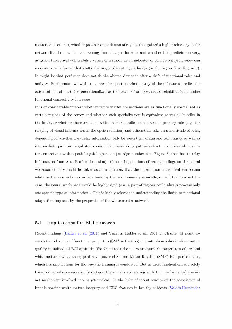
matter connectome), whether post-stroke perfusion of regions that gained a higher relevancy in the

network fits the new demands arising from changed function and whether this predicts recovery,

as graph theoretical vulnerability values of a region as an indicator of connectivity/relevancy can

increase after a lesion that shifts the usage of existing pathways (as for region X in Figure 3).

It might be that perfusion does not fit the altered demands after a shift of functional roles and

activity. Furthermore we wish to answer the question whether any of these features predict the

extent of neural plasticity, operationalized as the extent of pre-post motor rehabilitation training

functional connectivity increases.

It is of considerable interest whether white matter connections are as functionally specialized as

certain regions of the cortex and whether such specialization is equivalent across all bundles in

the brain, or whether there are some white matter bundles that have one primary role (e.g. the

relaying of visual information in the optic radiation) and others that take on a multitude of roles,

depending on whether they relay information only between their origin and terminus or as well as

intermediate piece in long-distance communications along pathways that encompass white mat-

ter connections with a path length higher one (as edge number 4 in Figure 3, that has to relay

information from A to B after the lesion). Certain implications of recent findings on the neural

workspace theory might be taken as an indication, that the information transferred via certain

white matter connections can be altered by the brain more dynamically, since if that was not the

case, the neural workspace would be highly rigid (e.g. a pair of regions could always process only

one specific type of information). This is highly relevant in understanding the limits to functional

adaptation imposed by the properties of the white matter network.

5.4 Implications for BCI research

Recent findings (Halder et al. (2011) and Varkuti, Halder et al., 2011 in Chapter 4) point to-

wards the relevancy of functional properties (SMA activation) and inter-hemispheric white matter

quality in individual BCI aptitude. We found that the microstructural characteristics of cerebral

white matter have a strong predictive power of Sensori-Motor-Rhythm (SMR) BCI performance,

which has implications for the way the training is conducted. But as these implications are solely

based on correlative research (structural brain traits correlating with BCI performance) the ex-

act mechanism involved here is yet unclear. In the light of recent studies on the association of

bundle specific white matter integrity and EEG features in healthy subjects (Valdes-Hernandez

30

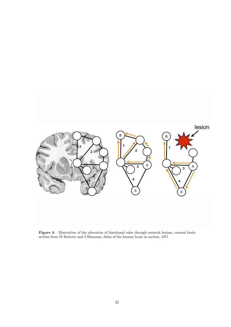
Figure 3 – Illustration of the alteration of functional roles through network lesions, coronal brainsection from M Roberts and J Hanaway, Atlas of the human brain in section, 1971

31

et al., 2010), the link of interhemispheric white matter connectivity with EEG frontal coherence

(Teipel et al., 2009) and the relation of interhemispheric transfer time to DTI derived measures

of white matter integrity, it is apparent that the conduction properties (e.g. conduction velocity,

myelination and local fiber density) of the brain are determined by the underlying white matter

network and that these properties might in turn significantly influence EEG features on both the

trait and state level. Specifically, the dynamics of the resting state alpha rhythm appear to be

connected to white matter architecture (Valdes-Hernandez et al., 2010).

One of the central purposes for BCIs is their potential to enable communication in patients suf-

fering from progressive degeneration of the motor system in ALS. While ALS was long considered

a disease with mainly motor system specific cerebral involvement, this notion is changing in the

light of recent findings on the involvement of extra-motoric white matter structures such as the

Corpus Callosum (Filippini et al., 2010), Cingulum (Woolley et al., 2011), Uncinate Fasciculus

(Sato et al., 2010) or in regions such as the Insula, Hippocampal Formation, the ventrolateral

Premotor Cortex, Parietal Cortex and bilateral Frontal Cortex (Senda et al., 2011). Based on

these findings, it can be assumed that the pathology in ALS is spreading in later stages to multi-

ple white matter regions, which can be considered critical for the control of those EEG features

that are presently used in most BCI applications (e.g. P300, SMR), hence probably impairing the

ability of the patients to utilize present BCIs.

We need to deepen our understanding of the impact of white matter myelination on the timing of

macroscopic neural communication, as it is possible that learning is impaired in patients suffering

from white matter degeneration due to the disturbed timing of classical or operant conditioning

processes by the pathological alteration of white matter conduction delays. Unfortunately, the im-

pact of white matter connectivity on conditioning processes in general, is a heavily understudied

field in modern neuroscience.

Based on our findings on the relevancy of direct anatomical connections for the formation of

FCNs, it can be assumed that patients suffering from degradation of white matter microstructure

will show systematically altered canonical and task-induced FCNs. But currently we have no

experimental means to reversibly manipulate the conduction properties of selected white matter

connections in vivo, which would be necessary to quantify the strength of causal links between

anatomical and functional connectivity.

However the results of this work lead to a set of hypotheses that can be tested in future experiments

to understand this problem better. On the level of correlative research, patients with inadequate

32

perfusion of anatomical connectivity hubs should show impaired FCNs and in turn altered EEG

features and potentially impaired BCI aptitude and healthy low- and high-aptitude BCI users

should as well differ in the functional connectivity of their canonical brain networks. For the level

of experimental research, we can assume that the identified white matter traits will not change

due to a single session of BCI training. Our findings indicate that the best way of improving BCI

performance of healthy low aptitude users is by conducting a long term BCI training program

consisting of multiple sessions that do not only target to increase proficiency in BCI usage for

communication and control but attempts to incorporate interventions that increase or stabilize

the microstructural integrity of BCI-critical central white matter.

Fortunately, the notion that white matter microstructure and connectivity are unalterable in the

adult brain had to be corrected in the light of present findings on the effectiveness of interventions

such as meditation (Tang et al., 2010), training of working memory (Takeuchi et al., 2010) or jug-

gling training (Scholz et al., 2009) in increasing local FA (a measure of white matter microstructure

integrity) in certain motoric and extra-motoric structures. As such these findings suggest that the

breakdown of white matter connections and the breakdown of functional networks could strongly

contribute to the difficulties in BCI communication in later stages of neurodegenerative disease

and should and can be the main focus of interventions targeting BCI aptitude. If training effects

on microstructural cerebral white matter properties can be observed (e.g. by using an EEG con-

nectivty BCI neurofeedback paradigm as described in Outlook) this method could be used as an

intervention that optimizes or stabilizes the structural conditions in the brain for late-stage BCI

communication.

If beneficial effects of such training on white matter structures relevant to the modulation of SMR

BCI-EEG features are observed, these training methods possibly in combination with tDCS based

augmentation could as well be promising for stroke survivors as it is known that this patient group

benefits from SMR BCI training (Pichiorri et al., 2011).

6 Outlook

Currently we are developing two new neurofeedback BCI systems to offer new intervention options

to patients suffering from localized hypoperfusion and functional disconnection syndromes. The

first system is an ALS based real time BCI that allows the real time feedback of rCBF to the

participant, enabling the person to learn upregulation techniques that target the reperfusion of

33

areas. Utilizing our knowledge on the macroscopic anatomical connectome, this intervention can

be targeted precisely at those brain regions, which require perfusion the most and which are

necessary to reinstate certain cognitive functions (e.g. the anatomical connectivity hubs).

The second system is an implementation for real time graph property feedback of functional

networks measured with electrophysiological methods. Using fast algorithms for the calculation of

real time EEG channel-to-channel coupling, the resulting adjacency matrices are analyzed using

graph theoretical methods and real time feedback of graph features becomes possible. Utilizing

these methods in combination with appropriate learning paradigms enables us to train a patient to

not only learn to activate a single brain region or a network of brain regions anymore, but to learn

how to shape the functional networks in his brain into a more efficient form and thus indirectly

manipulate the underlying white matter structures.

It is an area of ongoing studies at our institute how FCNs can be formed, altered or modulated in

their activity through the means of self-regulation (e.g. the role of the frontal cortex in patients

suffering from Attention Deficit Disorder), and with real-time feedback of EEG-connectivity graph

properties we hope to offer a new neurofeedback tool for this purpose.

To this day it remains to be proven, whether learning to directly manipulate such abstract graph

features of brain networks in real-time is possible at all, but if it is, this method promises to

become a highly relevant tool for neurofeedback based interventions for treatment and secondary

prevention.

References

Abbott, L. F. and Nelson, S. B. (2000). Synaptic plasticity: taming the beast. Nature neuroscience,

3 Suppl(november):1178–83.

Achard, S., Salvador, R., Whitcher, B., Suckling, J., and Bullmore, E. (2006). A resilient, low-

frequency, small-world human brain functional network with highly connected association cor-

tical hubs. The Journal of neuroscience : the official journal of the Society for Neuroscience,

26(1):63–72.

Albensi, B. C. (2001). Models of brain injury and alterations in synaptic plasticity. Journal of

Neuroscience Research, 65(4):279–283.

Antoch, G., Vogt, F. M., Freudenberg, L. S., Nazaradeh, F., Goehde, S. C., Barkhausen, J.,

Dahmen, G., Bockisch, A., Debatin, J. F., and Ruehm, S. G. (2003). Whole-body dual-modality

34

PET/CT and whole-body MRI for tumor staging in oncology. JAMA : the journal of the

American Medical Association, 290(24):3199–206.

Barabasi, A.-l. (2012). The network takeover. Nature Physics, 8(January):8–10.

Barabasi, A.-L. and Oltvai, Z. N. (2004). Network biology: understanding the cell’s functional

organization. Nature reviews. Genetics, 5(2):101–13.

Barnes, J. A. (1969). Graph Theory and Social Networks: A Technical Comment on Connectedness

and Connectivity. Sociology, 3(2):215–232.

Bassett, D. S., Meyer-Lindenberg, A., Achard, S., Duke, T., and Bullmore, E. (2006). Adaptive

reconfiguration of fractal small-world human brain functional networks. Proceedings of the

National Academy of Sciences of the United States of America, 103(51):19518–23.

Beckmann, C. F., DeLuca, M., Devlin, J. T., and Smith, S. M. (2005). Investigations into resting-

state connectivity using independent component analysis. Philosophical transactions of the

Royal Society of London. Series B, Biological sciences, 360(1457):1001–13.

Beggs, J. M. and Plenz, D. (2003). Neuronal Avalanches in Neocortical Circuits. J. Neurosci.,

23(35):11167–11177.

Begre, S., Federspiel, A., Kiefer, C., Schroth, G., Dierks, T., and Strik, W. K. (2003). Reduced

hippocampal anisotropy related to anteriorization of alpha EEG in schizophrenia. Neuroreport,

14(5):739.

Bocker-Meffert, S., Rosenstiel, P., Rohl, C., Warneke, N., Held-Feindt, J., Sievers, J., and Lucius,

R. (2002). Erythropoietin and VEGF Promote Neural Outgrowth from Retinal Explants in

Postnatal Rats. Invest. Ophthalmol. Vis. Sci., 43(6):2021–2026.

Bolser, D., Dafas, P., Harrington, R., Park, J., and Schroeder, M. (2003). Visualisation and

graph-theoretic analysis of a large-scale protein structural interactome. BMC bioinformatics,

4(1):45.

Boss, M., Elsinger, H., Summer, M., and Thurner, S. (2004). Network topology of the interbank

market. Quantitative Finance, 4(6):677–684.

Bottino, C. M. C., Castro, C. C., Gomes, R. L. E., Buchpiguel, C. A., Marchetti, R. L., and Neto,

M. R. L. a. (2002). Volumetric MRI Measurements Can Differentiate Alzheimer’s Disease, Mild

Cognitive Impairment, and Normal Aging. International Psychogeriatrics, 14(01):59–72.

35

Brockington, A., Heath, P. R., Holden, H., Kasher, P., Bender, F. L. P., Claes, F., Lambrechts, D.,

Sendtner, M., Carmeliet, P., and Shaw, P. J. (2010). Downregulation of genes with a function

in axon outgrowth and synapse formation in motor neurones of the VEGFdelta/delta mouse

model of amyotrophic lateral sclerosis. BMC genomics, 11:203.

Brodmann, K. (1909). Vergleichende Lokalisationslehre der Grosshirnrinde in ihren Prinzipien

dargestellt auf Grund des Zellenbaues, volume 13. Barth.

Bullmore, E. and Sporns, O. (2009). Complex brain networks: graph theoretical analysis of

structural and functional systems. Nature reviews. Neuroscience, 10(3):186–98.

Cammoun, L., Gigandet, X., Sporns, O., Thiran, J. P., Maeder, P., Meuli, R., Hagmann, P., Bovet,

P., and Do, K. Q. (2009). Connectome alterations in schizophrenia. NeuroImage, 47:S157.

Casey, B. J., Galvan, A., and Hare, T. a. (2005). Changes in cerebral functional organization

during cognitive development. Current opinion in neurobiology, 15(2):239–44.

Catani, M. and Ffytche, D. H. (2005). The rises and falls of disconnection syndromes. Brain : a

journal of neurology, 128(Pt 10):2224–39.

Chao, L. L., Buckley, S. T., Kornak, J., Schuff, N., Madison, C., Yaffe, K., Miller, B. L., Kramer,

J. H., and Weiner, M. W. (2010). ASL Perfusion MRI Predicts Cognitive Decline and Conversion

From MCI to Dementia. Alzheimer Disease & Associated Disorders, 24(1):19–27.

Chen, Z. J., He, Y., Rosa-Neto, P., Germann, J., and Evans, A. C. (2008). Revealing modular ar-

chitecture of human brain structural networks by using cortical thickness from {MRI}. Cerebral

cortex, 18(10):2374.

Cohen, A. L., Fair, D. a., Dosenbach, N. U. F., Miezin, F. M., Dierker, D., Van Essen, D. C.,

Schlaggar, B. L., and Petersen, S. E. (2008). Defining functional areas in individual human

brains using resting functional connectivity MRI. NeuroImage, 41(1):45–57.

Cramer, S. C. (2008). Repairing the human brain after stroke: I. Mechanisms of spontaneous

recovery. Annals of neurology, 63(3):272–87.

Demirci, O., Stevens, M. C., Andreasen, N. C., Michael, A., Liu, J., White, T., Pearlson, G. D.,

Clark, V. P., and Calhoun, V. D. (2009). Investigation of relationships between fMRI brain

networks in the spectral domain using ICA and Granger causality reveals distinct differences

between schizophrenia patients and healthy controls. NeuroImage, 46(2):419–31.

36

Devanand, D. P., Pradhaban, G., Liu, X., Khandji, A., De Santi, S., Segal, S., Rusinek, H.,

Pelton, G. H., Honig, L. S., Mayeux, R., Stern, Y., Tabert, M. H., and de Leon, M. J. (2007).

Hippocampal and entorhinal atrophy in mild cognitive impairment: Prediction of Alzheimer

disease. Neurology, 68(11):828–836.

Dosenbach, N., Nardos, B., and Cohen, A. (2010). Prediction of individual brain maturity using

fMRI. Science.

Dosenbach, N. U. F., Fair, D. a., Miezin, F. M., Cohen, A. L., Wenger, K. K., Dosenbach, R. a. T.,

Fox, M. D., Snyder, A. Z., Vincent, J. L., Raichle, M. E., Schlaggar, B. L., and Petersen, S. E.

(2007). Distinct brain networks for adaptive and stable task control in humans. Proceedings of

the National Academy of Sciences of the United States of America, 104(26):11073–8.

Dunne, J. A., Williams, R. J., and Martinez, N. D. (2002). Food-web structure and network

theory: The role of connectance and size. Proceedings of the National Academy of Sciences of

the United States of America, 99(20):12917–22.

Eigsti, I.-M. and Shapiro, T. (2003). A systems neuroscience approach to autism: biological,

cognitive, and clinical perspectives. Mental retardation and developmental disabilities research

reviews, 9(3):205–15.

Euler, L. (1986). Das Konigsberger Bruckenproblem. . . . Graphen. Mit einer Abhandlung von L.

Euler. Teubner- . . . .

Fellgiebel, A., Wille, P., Müller, M. J., Winterer, G., Scheurich, A., Vucurevic, G., Schmidt,

L. G., and Stoeter, P. (2004). Ultrastructural Hippocampal and White Matter Alterations

in Mild Cognitive Impairment: A Diffusion Tensor Imaging Study. Dementia and Geriatric

Cognitive Disorders, 18(1):101–108.

Fenno, L., Yizhar, O., and Deisseroth, K. (2010). The Development and Application of Optoge-

netics. Annual Review of Neuroscience, 34(1):110301101035033.

Fetz, E. E. (2007). Volitional control of neural activity: implications for brain-computer interfaces.

The Journal of physiology, 579(Pt 3):571–9.

Filippini, N., Douaud, G., Mackay, C. E., Knight, S., Talbot, K., and Turner, M. R. (2010).

Corpus callosum involvement is a consistent feature of amyotrophic lateral sclerosis. Neurology,

75(18):1645–52.

37

Fonteijn, H. M. J., Norris, D. G., and Verstraten, F. a. J. (2008). Exploring the anatomical basis

of effective connectivity models with DTI-based fiber tractography. International journal of

biomedical imaging, 2008:423192.

Frackowiak, R. (2004). Human brain function.

Gauthier, L. V., Taub, E., Perkins, C., Ortmann, M., Mark, V. W., and Uswatte, G. (2008).

Remodeling the brain: plastic structural brain changes produced by different motor therapies

after stroke. Stroke; a journal of cerebral circulation, 39(5):1520–5.

Gigandet, X., Hagmann, P., Kurant, M., Cammoun, L., Meuli, R., and Thiran, J.-P. (2008).

Estimating the confidence level of white matter connections obtained with MRI tractography.

PloS one, 3(12):e4006.

Gong, G., He, Y., Concha, L., Lebel, C., Gross, D. W., Evans, A. C., and Beaulieu, C. (2009).

Mapping anatomical connectivity patterns of human cerebral cortex using in vivo diffusion

tensor imaging tractography. Cerebral cortex (New York, N.Y. : 1991), 19(3):524–36.

Greicius, M. D., Srivastava, G., Reiss, A. L., and Menon, V. (2004). Default-mode network activity

distinguishes Alzheimer’s disease from healthy aging: evidence from functional MRI. Proceedings

of the National Academy of Sciences of the United States of America, 101(13):4637–42.

Grundman, M., Sencakova, D., Jack, C. R., Petersen, R. C., Kim, H. T., Schultz, A., Weiner,

M. F., DeCarli, C., DeKosky, S. T., Dyck, C., Thomas, R. G., Thal, L. J., and the Alzheimer’s

Disease Cooperative Study (2002). Brain MRI hippocampal volume and prediction of clinical

status in a mild cognitive impairment trial. Journal of Molecular Neuroscience, 19(1-2):23–27.

Halder, S., Agorastos, D., Veit, R., Hammer, E. M., Lee, S., Varkuti, B., Bogdan, M., Rosenstiel,

W., Birbaumer, N., and Kubler, a. (2011). Neural mechanisms of brain-computer interface

control. NeuroImage.

Head, D., Buckner, R. L., Shimony, J. S., Williams, L. E., Akbudak, E., Conturo, T. E., McAvoy,

M., Morris, J. C., and Snyder, A. Z. (2004). Differential Vulnerability of Anterior White Matter

in Nondemented Aging with Minimal Acceleration in Dementia of the Alzheimer Type: Evidence

from Diffusion Tensor Imaging. Cereb. Cortex, 14(4):410–423.

Honey, C. J., Sporns, O., Cammoun, L., Gigandet, X., Thiran, J. P., Meuli, R., and Hagmann,

P. (2009). Predicting human resting-state functional connectivity from structural connectivity.

Proceedings of the National Academy of Sciences, 106(6):2035.

38

Horwitz, B., Warner, B., Fitzer, J., Tagamets, M.-a., Husain, F. T., and Long, T. W. (2005).

Investigating the neural basis for functional and effective connectivity. Application to fMRI.

Philosophical transactions of the Royal Society of London. Series B, Biological sciences,

360(1457):1093–108.

Iturria-Medina, Y., Sotero, R. C., Canales-Rodrıguez, E. J., Aleman-Gomez, Y., and Melie-Garcıa,

L. (2008). Studying the human brain anatomical network via diffusion-weighted MRI and Graph

Theory. NeuroImage, 40(3):1064–76.

Jafri, M. J., Pearlson, G. D., Stevens, M., and Calhoun, V. D. (2008). A method for functional

network connectivity among spatially independent resting-state components in schizophrenia.

NeuroImage, 39(4):1666–81.

Jin, K., Wang, X., Xie, L., Mao, X. O., Zhu, W., Wang, Y., Shen, J., Mao, Y., Banwait, S.,

and Greenberg, D. A. (2006). Evidence for stroke-induced neurogenesis in the human brain.

Proceedings of the National Academy of Sciences of the United States of America, 103(35):13198–

202.

Jin, K., Zhu, Y., Sun, Y., Mao, X. O., Xie, L., and Greenberg, D. A. (2002). Vascular endothelial

growth factor (VEGF) stimulates neurogenesis in vitro and in vivo. Proceedings of the National

Academy of Sciences of the United States of America, 99(18):11946–50.

Johansson, B. B. (2000). Brain Plasticity and Stroke Rehabilitation : The Willis Lecture. Stroke,

31(1):223–230.

Kamitani, Y. and Tong, F. (2005). Decoding the visual and subjective contents of the human

brain. Nature neuroscience, 8(5):679–85.

Kitzbichler, M. G., Smith, M. L., Christensen, S. r. R., and Bullmore, E. (2009). Broadband

criticality of human brain network synchronization. PLoS computational biology, 5(3):e1000314.

Kreher, B. W., Schnell, S., Mader, I., Il’yasov, K. A., Hennig, J., Kiselev, V. G., and Saur, D.

(2008). Connecting and merging fibres: Pathway extraction by combining probability maps.

NeuroImage, 43(1):81–89.

Kusaka, N., Sugiu, K., Tokunaga, K., Katsumata, A., Nishida, A., Namba, K., Hamada, H.,

Nakashima, H., and Date, I. (2005). Enhanced brain angiogenesis in chronic cerebral hypoper-

fusion after administration of plasmid human vascular endothelial growth factor in combination

with indirect vasoreconstructive surgery. Journal of neurosurgery, 103(5):882–90.

39

Lawrie, S. M., McIntosh, A. M., Hall, J., Owens, D. G. C., and Johnstone, E. C. (2008). Brain

structure and function changes during the development of schizophrenia: the evidence from

studies of subjects at increased genetic risk. Schizophrenia bulletin, 34(2):330–40.

Lebel, C. and Beaulieu, C. (2011). Longitudinal Development of Human Brain Wiring Continues

from Childhood into Adulthood. Journal of Neuroscience, 31(30):10937–10947.

Lee, S., Ruiz, S., Caria, A., Veit, R., Birbaumer, N., and Sitaram, R. (2011). Detection of cerebral

reorganization induced by real-time fMRI feedback training of insula activation: a multivariate

investigation. Neurorehabilitation and neural repair, 25(3):259–67.

Logothetis, N. K. (2008). What we can do and what we cannot do with fMRI. Nature,

453(7197):869–78.

Lynall, M.-E., Bassett, D. S., Kerwin, R., McKenna, P. J., Kitzbichler, M., Muller, U., and

Bullmore, E. (2010). Functional Connectivity and Brain Networks in Schizophrenia. The Journal

of neuroscience : the official journal of the Society for Neuroscience, 30(28):9477–9487.

Madhavan, S., Rogers, L. M., and Stinear, J. W. (2010). A paradox: after stroke, the non-

lesioned lower limb motor cortex may be maladaptive. The European journal of neuroscience,

32(6):1032–9.

Mechelli, A., Price, C. J., Friston, K. J., and Ashburner, J. (2005). Voxel-based morphometry of

the human brain: methods and applications. Current Medical Imaging Reviews, 1(2):105–113.

Merrill, M. J. and Oldfield, E. H. (2005). A reassessment of vascular endothelial growth factor in

central nervous system pathology. Journal of neurosurgery, 103(5):853–68.

Micheloyannis, S., Pachou, E., Stam, C. J., Vourkas, M., Erimaki, S., and Tsirka, V. (2006). Using

graph theoretical analysis of multi channel EEG to evaluate the neural efficiency hypothesis.

Neuroscience letters, 402(3):273–7.

Minsky, M. (1988). The society of mind.

Pichiorri, F., De Vico Fallani, F., Cincotti, F., Babiloni, F., Molinari, M., Kleih, S. C., Neuper, C.,

Kubler, A., and Mattia, D. (2011). Sensorimotor rhythm-based brain-computer interface train-

ing: the impact on motor cortical responsiveness. Journal of neural engineering, 8(2):025020.

40

Raichle, M. E., MacLeod, A. M., Snyder, A. Z., Powers, W. J., Gusnard, D. A., and Shulman,

G. L. (2001). A default mode of brain function. Proceedings of the National Academy of Sciences

of the United States of America, 98(2):676.

Ross, C. A. and Poirier, M. A. (2004). Protein aggregation and neurodegenerative disease. Neu-

rodegeneration, (July).

Rubinov, M., Knock, S. a., Stam, C. J., Micheloyannis, S., Harris, A. W. F., Williams, L. M.,

and Breakspear, M. (2009). Small-world properties of nonlinear brain activity in schizophrenia.

Human brain mapping, 30(2):403–16.

Ruhrberg, C., Rosenstein, J. M., and Krum, J. M. (2008). VEGF in Development. Springer New

York, New York, NY.

Sato, K., Aoki, S., Iwata, N. K., Masutani, Y., Watadani, T., Nakata, Y., Yoshida, M., Terao,

Y., Abe, O., Ohtomo, K., and Tsuji, S. (2010). Diffusion tensor tract-specific analysis of the

uncinate fasciculus in patients with amyotrophic lateral sclerosis. Neuroradiology, 52(8):729–33.

Scholz, J., Klein, M. C., Behrens, T. E. J., and Johansen-Berg, H. (2009). Training induces

changes in white-matter architecture. Nature neuroscience, 12(11):1370–1.

Schummers, J., Yu, H., and Sur, M. (2008). Tuned responses of astrocytes and their influence on

hemodynamic signals in the visual cortex. Science (New York, N.Y.), 320(5883):1638–43.

Seeley, W. W., Crawford, R. K., Zhou, J., Miller, B. L., and Greicius, M. D. (2009a). Neurode-

generative diseases target large-scale human brain networks. Neuron, 62(1):42–52.

Seeley, W. W., Crawford, R. K., Zhou, J., Miller, B. L., and Greicius, M. D. (2009b). Neurode-

generative diseases target large-scale human brain networks. Neuron, 62(1):42–52.

Seeley, W. W., Menon, V., Schatzberg, A. F., Keller, J., Glover, G. H., Kenna, H., Reiss, A. L.,

and Greicius, M. D. (2007a). Dissociable intrinsic connectivity networks for salience processing

and executive control. The Journal of neuroscience : the official journal of the Society for

Neuroscience, 27(9):2349–56.

Seeley, W. W., Menon, V., Schatzberg, A. F., Keller, J., Glover, G. H., Kenna, H., Reiss, A. L.,

and Greicius, M. D. (2007b). Dissociable intrinsic connectivity networks for salience processing

and executive control. The Journal of neuroscience : the official journal of the Society for

Neuroscience, 27(9):2349–56.

41

Senda, J., Kato, S., Kaga, T., Ito, M., Atsuta, N., Nakamura, T., Watanabe, H., Tanaka, F.,

Naganawa, S., and Sobue, G. (2011). Progressive and widespread brain damage in ALS: MRI

voxel-based morphometry and diffusion tensor imaging study. Amyotrophic lateral sclerosis

: official publication of the World Federation of Neurology Research Group on Motor Neuron

Diseases, 12(1):59–69.

Sondell, M., Lundborg, G., and Kanje, M. (1999). Vascular endothelial growth factor has neu-

rotrophic activity and stimulates axonal outgrowth, enhancing cell survival and Schwann cell

proliferation in the peripheral nervous system. The Journal of neuroscience : the official journal

of the Society for Neuroscience, 19(14):5731–40.

Sporns, O. (2007). Brain connectivity. Scholarpedia, 2(10):4695.

Sporns, O. (2010). Networks of the Brain. The MIT Press.

Stagg, C. J., Bachtiar, V., and Johansen-Berg, H. (2011). The role of GABA in human motor

learning. Current biology : CB, 21(6):480–4.

Stam, C. J., de Haan, W., Daffertshofer, a., Jones, B. F., Manshanden, I., van Cappellen van

Walsum, a. M., Montez, T., Verbunt, J. P. a., de Munck, J. C., van Dijk, B. W., Berendse, H. W.,

and Scheltens, P. (2009). Graph theoretical analysis of magnetoencephalographic functional

connectivity in Alzheimer’s disease. Brain : a journal of neurology, 132(Pt 1):213–24.

Stam, C. J., Jones, B. F., Nolte, G., Breakspear, M., and Scheltens, P. (2007). Small-world

networks and functional connectivity in Alzheimer’s disease. Cerebral cortex (New York, N.Y.

: 1991), 17(1):92–9.

Sugihara, S., Kinoshita, T., Matsusue, E., Fujii, S., and Ogawa, T. (2004). Usefulness of Diffusion

Tensor Imaging of White Matter in Alzheimer Disease and Vascular Dementia. Acta Radiologica,

45(6):658–663.

Takeuchi, H., Sekiguchi, A., Taki, Y., Yokoyama, S., Yomogida, Y., Komuro, N., Yamanouchi,

T., Suzuki, S., and Kawashima, R. (2010). Training of working memory impacts structural

connectivity. The Journal of neuroscience : the official journal of the Society for Neuroscience,

30(9):3297–3303.

Tamas Kincses, Z., Johansen-Berg, H., Tomassini, V., Bosnell, R., Matthews, P. M., and Beck-

mann, C. F. (2008). Model-free characterization of brain functional networks for motor sequence

learning using fMRI. NeuroImage, 39(4):1950–8.

42

Tang, Y.-Y., Lu, Q., Geng, X., Stein, E. A., Yang, Y., and Posner, M. I. (2010). Short-term

meditation induces white matter changes in the anterior cingulate. Proceedings of the National

Academy of Sciences of the United States of America, 107(35):15649–15652.

Teipel, S. J., Pogarell, O., Meindl, T., Dietrich, O., Sydykova, D., Hunklinger, U., Georgii, B.,

Mulert, C., Reiser, M. F., Moller, H.-J., and Hampel, H. (2009). Regional networks underlying

interhemispheric connectivity: an EEG and DTI study in healthy ageing and amnestic mild

cognitive impairment. Hum Brain Mapp, 30(7):2098–2119.

Valdes-Hernandez, P. a., Ojeda-Gonzalez, A., Martınez-Montes, E., Lage-Castellanos, A., Virues-

Alba, T., Valdes-Urrutia, L., and Valdes-Sosa, P. a. (2010). White matter architecture rather

than cortical surface area correlates with the EEG alpha rhythm. NeuroImage, 49(3):2328–39.

van den Heuvel, M. P., Mandl, R. C. W., Kahn, R. S., and Hulshoff Pol, H. E. (2009). Functionally

linked resting-state networks reflect the underlying structural connectivity architecture of the

human brain. Human brain mapping, 30(10):3127–41.

Van Dijk, K. R. a., Hedden, T., Venkataraman, A., Evans, K. C., Lazar, S. W., and Buckner, R. L.

(2010). Intrinsic functional connectivity as a tool for human connectomics: theory, properties,

and optimization. Journal of neurophysiology, 103(1):297–321.

Varela, F., Lachaux, J. P., Rodriguez, E., and Martinerie, J. (2001). The brainweb: phase syn-

chronization and large-scale integration. Nature reviews. Neuroscience, 2(4):229–39.

Varkuti, B., Cavusoglu, M., Kullik, A., Schiffler, B., Veit, R., Yilmaz, O., Rosenstiel, W., Braun,

C., Uludag, K., Birbaumer, N., and Sitaram, R. (2011). Quantifying the link between anatomical

connectivity, gray matter volume and regional cerebral blood flow: an integrative MRI study.

PloS one, 6(4):e14801.

Voss, M. W., Prakash, R. S., Erickson, K. I., Boot, W. R., Basak, C., Neider, M. B., Simons, D. J.,

Fabiani, M., Gratton, G., and Kramer, A. F. (2011). Effects of training strategies implemented

in a complex videogame on functional connectivity of attentional networks. NeuroImage.

Wendel, K., Vaisanen, O., Malmivuo, J., Gencer, N. G., Vanrumste, B., Durka, P., Magjarevic, R.,

Supek, S., Pascu, M. L., Fontenelle, H., and Grave de Peralta Menendez, R. (2009). EEG/MEG

source imaging: methods, challenges, and open issues. Computational intelligence and neuro-

science, 2009:656092.

43

Whitfield-Gabrieli, S., Thermenos, H. W., Milanovic, S., Tsuang, M. T., Faraone, S. V., McCarley,

R. W., Shenton, M. E., Green, A. I., Nieto-Castanon, A., LaViolette, P., Wojcik, J., Gabrieli, J.

D. E., and Seidman, L. J. (2009). Hyperactivity and hyperconnectivity of the default network

in schizophrenia and in first-degree relatives of persons with schizophrenia. Proceedings of the

National Academy of Sciences of the United States of America, 106(4):1279–84.

Whitford, T. J., Kubicki, M., Ghorashi, S., Schneiderman, J. S., Hawley, K. J., McCarley, R. W.,

Shenton, M. E., and Spencer, K. M. (2010). Predicting inter-hemispheric transfer time from the

diffusion properties of the corpus callosum in healthy individuals and schizophrenia patients: A

combined ERP and DTI study. NeuroImage, 54(3):2318–2329.

Woolley, S. C., Zhang, Y., Schuff, N., Weiner, M. W., and Katz, J. S. (2011). Neuroanatomical

correlates of apathy in ALS using 4 Tesla diffusion tensor MRI. Amyotrophic lateral sclerosis

: official publication of the World Federation of Neurology Research Group on Motor Neuron

Diseases, 12(1):52–8.

Wu, X., Li, R., Fleisher, A. S., Reiman, E. M., Guan, X., Zhang, Y., Chen, K., and Yao, L. (2011).

Altered default mode network connectivity in alzheimer’s disease-A resting functional MRI and

bayesian network study. Human brain mapping, 00(November 2009).

Xu, Y., Olman, V., and Xu, D. (2002). Clustering gene expression data using a graph-theoretic

approach: an application of minimum spanning trees. Bioinformatics, 18(4):536–545.

44

7 Publications, manuscripts and contributions

45

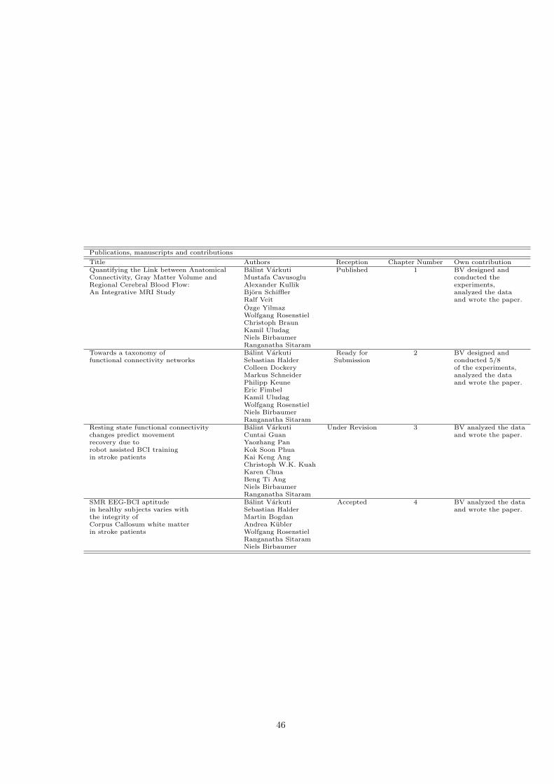
Publications, manuscripts and contributions

Title Authors Reception Chapter Number Own contributionQuantifying the Link between Anatomical Balint Varkuti Published 1 BV designed andConnectivity, Gray Matter Volume and Mustafa Cavusoglu conducted theRegional Cerebral Blood Flow: Alexander Kullik experiments,An Integrative MRI Study Bjorn Schiffler analyzed the data

Ralf Veit and wrote the paper.

Ozge YilmazWolfgang RosenstielChristoph BraunKamil UludagNiels BirbaumerRanganatha Sitaram

Towards a taxonomy of Balint Varkuti Ready for 2 BV designed andfunctional connectivity networks Sebastian Halder Submission conducted 5/8

Colleen Dockery of the experiments,Markus Schneider analyzed the dataPhilipp Keune and wrote the paper.Eric FimbelKamil UludagWolfgang RosenstielNiels BirbaumerRanganatha Sitaram

Resting state functional connectivity Balint Varkuti Under Revision 3 BV analyzed the datachanges predict movement Cuntai Guan and wrote the paper.recovery due to Yaozhang Panrobot assisted BCI training Kok Soon Phuain stroke patients Kai Keng Ang

Christoph W.K. KuahKaren ChuaBeng Ti AngNiels BirbaumerRanganatha Sitaram

SMR EEG-BCI aptitude Balint Varkuti Accepted 4 BV analyzed the datain healthy subjects varies with Sebastian Halder and wrote the paper.the integrity of Martin BogdanCorpus Callosum white matter Andrea Kublerin stroke patients Wolfgang Rosenstiel

Ranganatha SitaramNiels Birbaumer

46

7.1 Chapter 1 - The link between Anatomical Connectivity, Perfusion

and regional Cerebral Blood Flow

47

1

Quantifying the link between Anatomical Connectivity, Gray Matter

Volume and regional Cerebral Blood Flow – an integrative MRI study Author list and affiliation:

Bálint Várkuti1,2

Mustafa Cavusoglu3

Alexander Kullik4

Björn Schiffler7

Ralf Veit1

Özge Yilmaz1

Wolfgang Rosenstiel4

Christoph Braun1,5

Kamil Uludag3

Niels Birbaumer1,6

Ranganatha Sitaram1

1 Institute of Medical Psychology and Behavioral Neurobiology, University of Tübingen, Tübingen,

Baden-Württemberg, Germany

2 Graduate Training Centre of Neuroscience, International Max Planck Research School, Tübingen,

Baden-Württemberg, Germany

3 Max Planck Institute for Biological Cybernetics, Tübingen, Baden-Württemberg, Germany

4 Wilhelm-Schickard Institute for Computer Engineering, University of Tübingen, Tübingen,

Baden-Württemberg, Germany

5 CIMeC - Centro interdipartimentale Mente/Cervello, Rovereto, Trento, Italy

6 Ospedale San Camillo, Istituto di Ricovero e Cura a Carattere Scientifico, Venezia, Veneto, Italy

7 Institute of Psychology, Albert-Ludwigs-University, Freiburg im Breisgau, Baden-Württemberg,

Germany

2

Abstract

Background:

In the graph theoretical analysis of anatomical brain connectivity, the white matter connections between

regions of the brain are identified and serve as basis for the assessment of regional connectivity profiles, to

e.g. locate the hubs of the brain. But regions of the brain can be characterised further with respect to their

gray matter volume or resting state perfusion. Local anatomical connectivity, gray matter volume and

perfusion are traits of each brain region that are likely to be interdependent, however particular patterns of

systematic covariation have not yet been identified.

Methodology/Principal Findings:

We quantified the covariation of these traits by conducting an integrative MRI study on 23 subjects,

utilising a combination of Diffusion Tensor Imaging, Arterial Spin Labeling and anatomical imaging. Based

on our hypothesis that local connectivity, gray matter volume and perfusion are linked, we correlated these

measures and particularly isolated the covariation of connectivity and perfusion by statistically controlling

for gray matter volume. We found significant levels of covariation on the group- and regionwise level,

particularly in regions of the Default Brain Mode Network.

Conclusions/Significance:

Connectivity and perfusion are systematically linked throughout a number of brain regions, thus we discuss

these results as a starting point for further research on the role of homology in the formation of functional

connectivity networks and on how structure/function relationships can manifest in the form of such trait

interdependency.

Introduction

Recent findings are beginning to shed light on the organisational principles behind the structure of the

brain [1]. Instead of studying the brain merely as an agglomeration of individual regions with their very

specific functions and structural idiosyncrasies, this research, with its new and more systemic perspective, is

trying to understand the fundamental lines along which structure/function relationships form [2-5].

Such principles are identified by studying the parts (e.g. brain regions) and analysing the global properties

of the entire system that emerge from links between the parts (e.g. white matter connections). The network

of white matter connections in the brain seems to adhere to a small-world organisation principle, defined by

short path lengths for reaching any part from any other part, while providing high clustering and highly

efficient wiring.

Once such a property is established, relations to properties of other systems can be analysed.

The shared small-world properties of interregional gray matter structural similarity [6-7] and white matter

connectivity, and the small-world properties of functional brain networks as assessed with

3

electroencephalography [8], are recent examples that certain common principles of organisation can be found

in a multitude of brain systems and on a number of scales [9].

As some of these traits, such as number of synapses, cell body population, perfusion and type and quantity

of neural fiber bundles have proven to be examinable using advanced imaging methods of spectroscopy,

perfusion, structural or diffusion MRI, brain regions can now be characterised regarding multiple traits at

once. In certain cases the relationship between different structural properties is formed in a systematic way,

e.g. larger brain regions tend to have more connections than smaller brain regions. In other cases, structural

and functional traits are also systematically coupled, e.g. the neural computations that take place in a

particular brain region are partially shaped by the quantity, quality and usage of the in- and outgoing

connections of that region. In turn the principle of functional (computational) segregation - as reflected in

the typology of unimodal motor and sensory or heteromodal association areas of the cortex - is known to be

mirrored both in the macroscopic white matter network topology [10] and in functional connectivity

networks [11]. The afferent and efferent white matter connections of the motor system, the ascending

pathways of the primary sensory cortices and the rich interconnectivity of the association areas are not

uncoupled from the function of these areas, but rather allow us to formulate hypotheses on their functional

roles.

Mounting evidence suggests [12-15] that certain functional traits - such as the activity profile of a brain

region arising from its function and its metabolic demand as reflected e.g. by local capillary density - are

closely coupled [16, 17]. Local metabolic demand and perfusion are directly linked in the healthy brain, thus

allowing the indirect assessment of metabolism through means of perfusion weighted imaging.

If local white matter connectivity shapes neurocomputational processes, and these processes influence local

function and therefore metabolic demand, one could hypothesise that local white matter connectivity and

local perfusion might be coupled throughout the brain as well. If this were the case, such coupling would

constitute the manifestation of a supply-and-demand-principle - the metabolic demand being shaped by

connectivity - in the formation of a previously undocumented structure/function relationship.

In order to quantify the outlined traits of perfusion and white matter connectivity we conducted an

integrative MRI study on 23 healthy subjects (divided into two groups of 11 and 12 participants), utilising a

combination of Diffusion Tensor Imaging (DTI), Arterial Spin Labeling (ASL) and anatomical imaging.

DTI and ASL are methods to non-invasively characterise white matter structure and gray matter function

of the brain, respectively [18-19]. While DTI allows for the estimation of anatomical connectivity between

regions of the brain, ASL represents a MRI method for the quantification of global and regional Cerebral

Blood Flow (rCBF).

DTI based tractography can be used to characterise the amount and integrity of white matter tracks

between two regions and allows for an estimation of connection probability. For this purpose, probability

density maps can be formed from the repeated propagation of curves through the DTI-based tensor field,

which is representing local white matter orientation. Currently, DTI data are integrated into graph

4

representations [20, 21] of the white matter network in order to analyse the relation of network topology to

function [22] and its impairment [23]. This type of network modelling has originated from the broader

discipline of graph theory [24], which is dedicated to the understanding of the emergence of certain global

and local properties of a given system from the distribution of pairwise relations of parts of that system (e.g.

if many nodes have one connection to another single node, the sum of these connections or edges make that

node the hub of the system).

This approach allows for the quantification of node specific traits (e.g. the number of edges connecting one

node to others nodes, termed degree), edge specific traits (e.g. how severely a network is affected by the

removal of an edge) and general graph properties (e.g. how efficient is the information transfer from any

point A to any point B in general).

ASL [25, 26] on the other hand has proven to be a sensitive and reliable method for the quantification of

gray matter perfusion, defined as the volume of arterial blood delivered to the capillary bed per unit volume

of brain tissue per unit time. It has been utilised to study brain function following neuronal activation, as

well as for the detection of changes of perfusion occurring during brain pathology, maturation and aging [27,

28]. This is done by assessing the inflow of magnetically labelled arterial water spins into an imaging slice.

For quantitative measurement of rCBF, ASL constructs images following a tagging of inflowing arterial

blood by a 180° radiofrequency inversion pulse and, in an interleaved fashion, acquiring control images

without prior tagging, so that the subtraction of these two images (control-tag) only leaves magnetisation

proportional to the blood flow.

So far, only limited attention has been paid to possible synergies from the combined use of these two

imaging modalities. As a result, the link between white matter network connectivity and rCBF has not yet

been systematically addressed. Currently, there are a few studies focusing on rCBF alterations and changes

in white matter integrity (e.g. level of myelinisation, orientation of fibers) as markers of Alzheimer´s disease

(AD) and mild cognitive impairment [29], but the number of systematic studies using state of the art

imaging of both modalities in the same sample is low. White matter lesions in the frontal lobe were found

[30] to be correlated with a lower CBF in the elderly. [31] reported that rCBF reductions in the parietal

cortex are correlated with white matter integrity reductions in the Posterior Cingulum in a healthy sample.

However, evidence for a systematic relationship between white matter network topology and rCBF has yet

to be established.

Following our hypothesis that local metabolic demands are largely determined by the connectivity profile of

a brain region, we assumed that local perfusion and local connectivity measures of gray matter regions are

to be correlated. In order to take into account the properties of the gray matter regions themselves (e.g. a

region with larger volume might show higher perfusion and higher degree), we integrated a Voxel-based

Morphometry (VBM) analysis into our design. VBM is an established method [32, 33] for the quantification

of volumetric differences for the entire brain and its subparts based on anatomical MRI images.

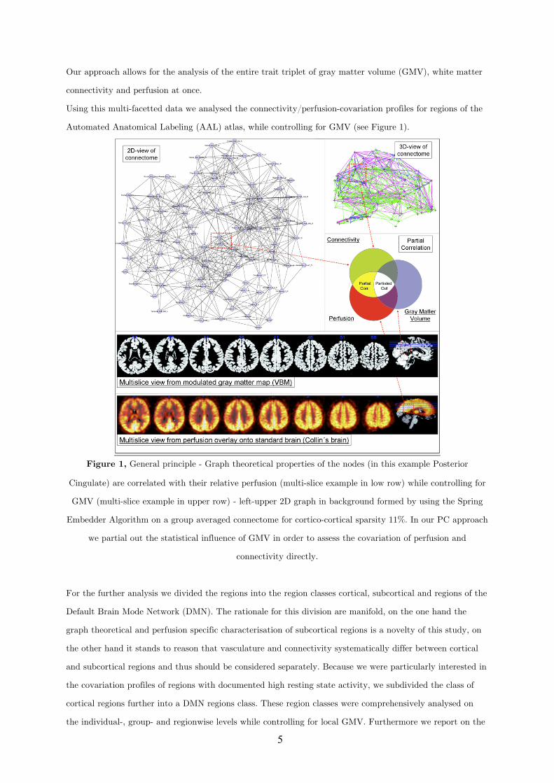
5

Our approach allows for the analysis of the entire trait triplet of gray matter volume (GMV), white matter

connectivity and perfusion at once.

Using this multi-facetted data we analysed the connectivity/perfusion-covariation profiles for regions of the

Automated Anatomical Labeling (AAL) atlas, while controlling for GMV (see Figure 1).

Figure 1, General principle - Graph theoretical properties of the nodes (in this example Posterior

Cingulate) are correlated with their relative perfusion (multi-slice example in low row) while controlling for

GMV (multi-slice example in upper row) - left-upper 2D graph in background formed by using the Spring

Embedder Algorithm on a group averaged connectome for cortico-cortical sparsity 11%. In our PC approach

we partial out the statistical influence of GMV in order to assess the covariation of perfusion and

connectivity directly.

For the further analysis we divided the regions into the region classes cortical, subcortical and regions of the

Default Brain Mode Network (DMN). The rationale for this division are manifold, on the one hand the

graph theoretical and perfusion specific characterisation of subcortical regions is a novelty of this study, on

the other hand it stands to reason that vasculature and connectivity systematically differ between cortical

and subcortical regions and thus should be considered separately. Because we were particularly interested in

the covariation profiles of regions with documented high resting state activity, we subdivided the class of

cortical regions further into a DMN regions class. These region classes were comprehensively analysed on

the individual-, group- and regionwise levels while controlling for local GMV. Furthermore we report on the

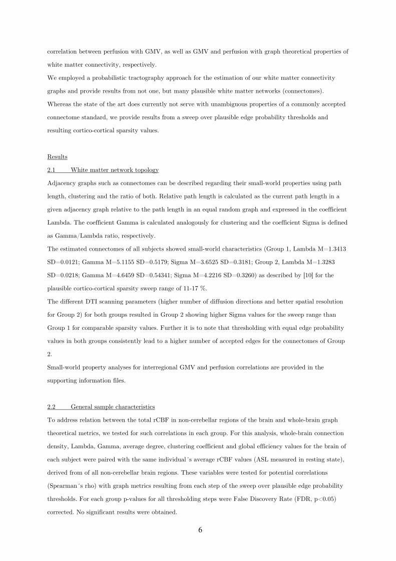
6

correlation between perfusion with GMV, as well as GMV and perfusion with graph theoretical properties of

white matter connectivity, respectively.

We employed a probabilistic tractography approach for the estimation of our white matter connectivity

graphs and provide results from not one, but many plausible white matter networks (connectomes).

Whereas the state of the art does currently not serve with unambiguous properties of a commonly accepted

connectome standard, we provide results from a sweep over plausible edge probability thresholds and

resulting cortico-cortical sparsity values.

Results

2.1 White matter network topology

Adjacency graphs such as connectomes can be described regarding their small-world properties using path

length, clustering and the ratio of both. Relative path length is calculated as the current path length in a

given adjacency graph relative to the path length in an equal random graph and expressed in the coefficient

Lambda. The coefficient Gamma is calculated analogously for clustering and the coefficient Sigma is defined

as Gamma/Lambda ratio, respectively.

The estimated connectomes of all subjects showed small-world characteristics (Group 1, Lambda M=1.3413

SD=0.0121; Gamma M=5.1155 SD=0.5179; Sigma M=3.6525 SD=0.3181; Group 2, Lambda M=1.3283

SD=0.0218; Gamma M=4.6459 SD=0.54341; Sigma M=4.2216 SD=0.3260) as described by [10] for the

plausible cortico-cortical sparsity sweep range of 11-17 %.

The different DTI scanning parameters (higher number of diffusion directions and better spatial resolution

for Group 2) for both groups resulted in Group 2 showing higher Sigma values for the sweep range than

Group 1 for comparable sparsity values. Further it is to note that thresholding with equal edge probability

values in both groups consistently lead to a higher number of accepted edges for the connectomes of Group

2.

Small-world property analyses for interregional GMV and perfusion correlations are provided in the

supporting information files.

2.2 General sample characteristics

To address relation between the total rCBF in non-cerebellar regions of the brain and whole-brain graph

theoretical metrics, we tested for such correlations in each group. For this analysis, whole-brain connection

density, Lambda, Gamma, average degree, clustering coefficient and global efficiency values for the brain of

each subject were paired with the same individual´s average rCBF values (ASL measured in resting state),

derived from of all non-cerebellar brain regions. These variables were tested for potential correlations

(Spearman´s rho) with graph metrics resulting from each step of the sweep over plausible edge probability

thresholds. For each group p-values for all thresholding steps were False Discovery Rate (FDR, p<0.05)

corrected. No significant results were obtained.

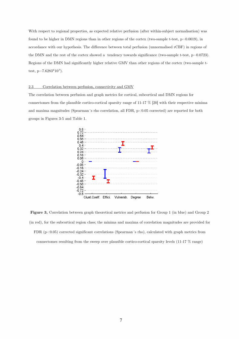
7

With respect to regional properties, as expected relative perfusion (after within-subject normalisation) was

found to be higher in DMN regions than in other regions of the cortex (two-sample t-test, p=0.0019), in

accordance with our hypothesis. The difference between total perfusion (unnormalised rCBF) in regions of

the DMN and the rest of the cortex showed a tendency towards significance (two-sample t-test, p=0.0723).

Regions of the DMN had significantly higher relative GMV than other regions of the cortex (two-sample t-

test, p=7.6283*10-8).

2.3 Correlation between perfusion, connectivity and GMV

The correlation between perfusion and graph metrics for cortical, subcortical and DMN regions for

connectomes from the plausible cortico-cortical sparsity range of 11-17 % [20] with their respective minima

and maxima magnitudes (Spearman´s rho correlation, all FDR, p<0.05 corrected) are reported for both

groups in Figures 3-5 and Table 1.

Figure 3, Correlation between graph theoretical metrics and perfusion for Group 1 (in blue) and Group 2

(in red), for the subcortical region class; the minima and maxima of correlation magnitudes are provided for

FDR (p<0.05) corrected significant correlations (Spearman´s rho), calculated with graph metrics from

connectomes resulting from the sweep over plausible cortico-cortical sparsity levels (11-17 % range)

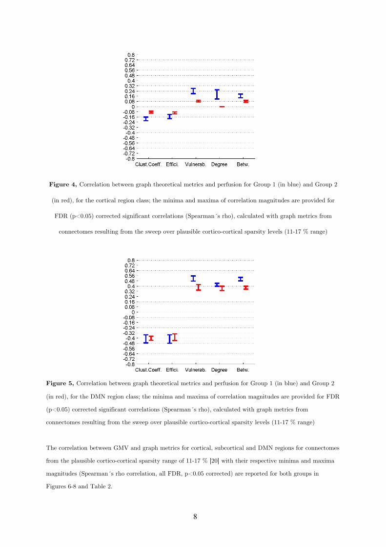
8

Figure 4, Correlation between graph theoretical metrics and perfusion for Group 1 (in blue) and Group 2

(in red), for the cortical region class; the minima and maxima of correlation magnitudes are provided for

FDR (p<0.05) corrected significant correlations (Spearman´s rho), calculated with graph metrics from

connectomes resulting from the sweep over plausible cortico-cortical sparsity levels (11-17 % range)

Figure 5, Correlation between graph theoretical metrics and perfusion for Group 1 (in blue) and Group 2

(in red), for the DMN region class; the minima and maxima of correlation magnitudes are provided for FDR

(p<0.05) corrected significant correlations (Spearman´s rho), calculated with graph metrics from

connectomes resulting from the sweep over plausible cortico-cortical sparsity levels (11-17 % range)

The correlation between GMV and graph metrics for cortical, subcortical and DMN regions for connectomes

from the plausible cortico-cortical sparsity range of 11-17 % [20] with their respective minima and maxima

magnitudes (Spearman´s rho correlation, all FDR, p<0.05 corrected) are reported for both groups in

Figures 6-8 and Table 2.

9

Figure 6, Correlation between graph theoretical metrics and GMV for Group 1 (in blue) and Group 2 (in

red), for the subcortical region class; the minima and maxima of correlation magnitudes are provided for

FDR (p<0.05) corrected significant correlations (Spearman´s rho), calculated with graph metrics from

connectomes resulting from the sweep over plausible cortico-cortical sparsity levels (11-17 % range)

Figure 7, Correlation between graph theoretical metrics and GMV for Group 1 (in blue) and Group 2 (in

red), for the cortical region class; the minima and maxima of correlation magnitudes are provided for FDR

(p<0.05) corrected significant correlations (Spearman´s rho), calculated with graph metrics from

connectomes resulting from the sweep over plausible cortico-cortical sparsity levels (11-17 % range)

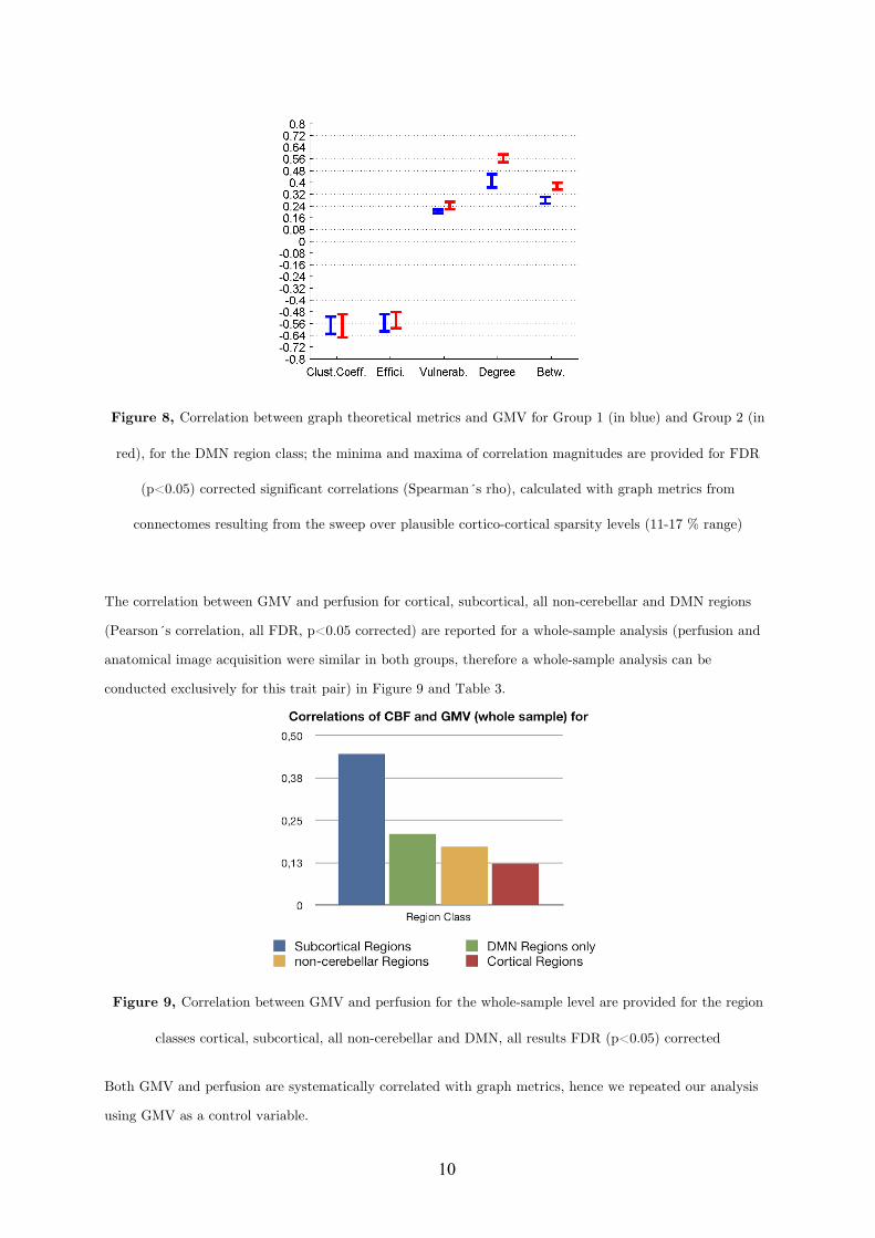
10

Figure 8, Correlation between graph theoretical metrics and GMV for Group 1 (in blue) and Group 2 (in

red), for the DMN region class; the minima and maxima of correlation magnitudes are provided for FDR

(p<0.05) corrected significant correlations (Spearman´s rho), calculated with graph metrics from

connectomes resulting from the sweep over plausible cortico-cortical sparsity levels (11-17 % range)

The correlation between GMV and perfusion for cortical, subcortical, all non-cerebellar and DMN regions

(Pearson´s correlation, all FDR, p<0.05 corrected) are reported for a whole-sample analysis (perfusion and

anatomical image acquisition were similar in both groups, therefore a whole-sample analysis can be

conducted exclusively for this trait pair) in Figure 9 and Table 3.

Figure 9, Correlation between GMV and perfusion for the whole-sample level are provided for the region

classes cortical, subcortical, all non-cerebellar and DMN, all results FDR (p<0.05) corrected

Both GMV and perfusion are systematically correlated with graph metrics, hence we repeated our analysis

using GMV as a control variable.

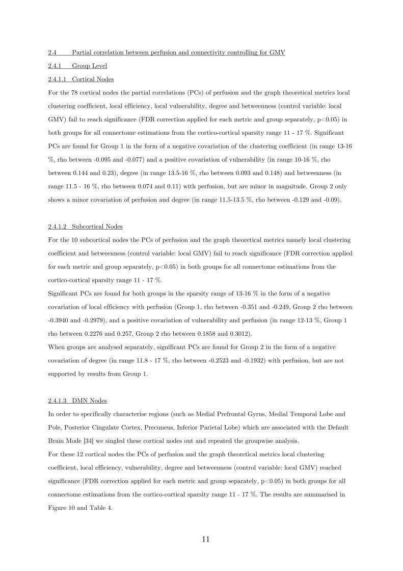
11

2.4 Partial correlation between perfusion and connectivity controlling for GMV

2.4.1 Group Level

2.4.1.1 Cortical Nodes

For the 78 cortical nodes the partial correlations (PCs) of perfusion and the graph theoretical metrics local

clustering coefficient, local efficiency, local vulnerability, degree and betweenness (control variable: local

GMV) fail to reach significance (FDR correction applied for each metric and group separately, p<0.05) in

both groups for all connectome estimations from the cortico-cortical sparsity range 11 - 17 %. Significant

PCs are found for Group 1 in the form of a negative covariation of the clustering coefficient (in range 13-16

%, rho between -0.095 and -0.077) and a positive covariation of vulnerability (in range 10-16 %, rho

between 0.144 and 0.23), degree (in range 13.5-16 %, rho between 0.093 and 0.148) and betweenness (in

range 11.5 - 16 %, rho between 0.074 and 0.11) with perfusion, but are minor in magnitude. Group 2 only

shows a minor covariation of perfusion and degree (in range 11.5-13.5 %, rho between -0.129 and -0.09).

2.4.1.2 Subcortical Nodes

For the 10 subcortical nodes the PCs of perfusion and the graph theoretical metrics namely local clustering

coefficient and betweenness (control variable: local GMV) fail to reach significance (FDR correction applied

for each metric and group separately, p<0.05) in both groups for all connectome estimations from the

cortico-cortical sparsity range 11 - 17 %.

Significant PCs are found for both groups in the sparsity range of 13-16 % in the form of a negative

covariation of local efficiency with perfusion (Group 1, rho between -0.351 and -0.249, Group 2 rho between

-0.3940 and -0.2979), and a positive covariation of vulnerability and perfusion (in range 12-13 %, Group 1

rho between 0.2276 and 0.257, Group 2 rho between 0.1858 and 0.3012).

When groups are analysed separately, significant PCs are found for Group 2 in the form of a negative

covariation of degree (in range 11.8 - 17 %, rho between -0.2523 and -0.1932) with perfusion, but are not

supported by results from Group 1.

2.4.1.3 DMN Nodes

In order to specifically characterise regions (such as Medial Prefrontal Gyrus, Medial Temporal Lobe and

Pole, Posterior Cingulate Cortex, Precuneus, Inferior Parietal Lobe) which are associated with the Default

Brain Mode [34] we singled these cortical nodes out and repeated the groupwise analysis.

For these 12 cortical nodes the PCs of perfusion and the graph theoretical metrics local clustering

coefficient, local efficiency, vulnerability, degree and betweenness (control variable: local GMV) reached

significance (FDR correction applied for each metric and group separately, p<0.05) in both groups for all

connectome estimations from the cortico-cortical sparsity range 11 - 17 %. The results are summarised in

Figure 10 and Table 4.

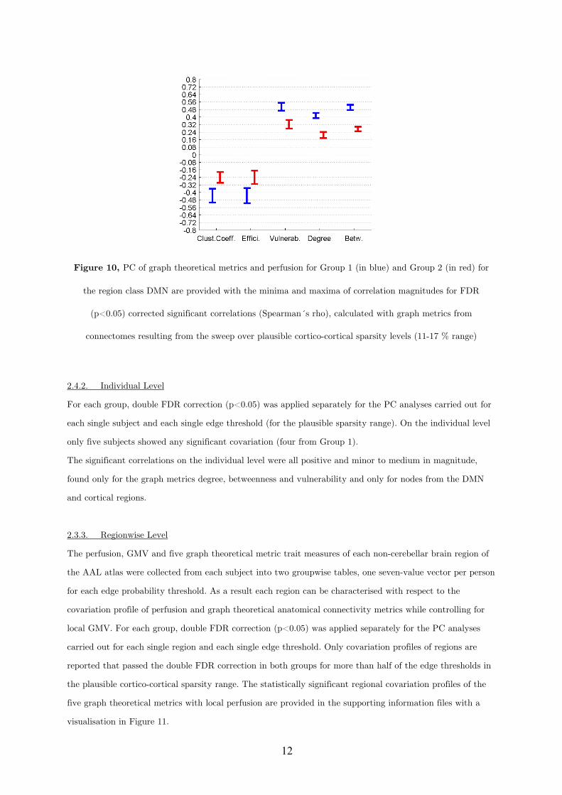
12

Figure 10, PC of graph theoretical metrics and perfusion for Group 1 (in blue) and Group 2 (in red) for

the region class DMN are provided with the minima and maxima of correlation magnitudes for FDR

(p<0.05) corrected significant correlations (Spearman´s rho), calculated with graph metrics from

connectomes resulting from the sweep over plausible cortico-cortical sparsity levels (11-17 % range)

2.4.2. Individual Level

For each group, double FDR correction (p<0.05) was applied separately for the PC analyses carried out for

each single subject and each single edge threshold (for the plausible sparsity range). On the individual level

only five subjects showed any significant covariation (four from Group 1).

The significant correlations on the individual level were all positive and minor to medium in magnitude,

found only for the graph metrics degree, betweenness and vulnerability and only for nodes from the DMN

and cortical regions.

2.3.3. Regionwise Level

The perfusion, GMV and five graph theoretical metric trait measures of each non-cerebellar brain region of

the AAL atlas were collected from each subject into two groupwise tables, one seven-value vector per person

for each edge probability threshold. As a result each region can be characterised with respect to the

covariation profile of perfusion and graph theoretical anatomical connectivity metrics while controlling for

local GMV. For each group, double FDR correction (p<0.05) was applied separately for the PC analyses

carried out for each single region and each single edge threshold. Only covariation profiles of regions are

reported that passed the double FDR correction in both groups for more than half of the edge thresholds in

the plausible cortico-cortical sparsity range. The statistically significant regional covariation profiles of the

five graph theoretical metrics with local perfusion are provided in the supporting information files with a

visualisation in Figure 11.

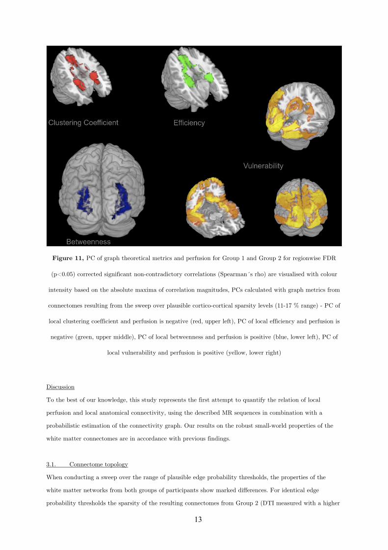
13

Figure 11, PC of graph theoretical metrics and perfusion for Group 1 and Group 2 for regionwise FDR

(p<0.05) corrected significant non-contradictory correlations (Spearman´s rho) are visualised with colour

intensity based on the absolute maxima of correlation magnitudes, PCs calculated with graph metrics from

connectomes resulting from the sweep over plausible cortico-cortical sparsity levels (11-17 % range) - PC of

local clustering coefficient and perfusion is negative (red, upper left), PC of local efficiency and perfusion is

negative (green, upper middle), PC of local betweenness and perfusion is positive (blue, lower left), PC of

local vulnerability and perfusion is positive (yellow, lower right)

Discussion

To the best of our knowledge, this study represents the first attempt to quantify the relation of local

perfusion and local anatomical connectivity, using the described MR sequences in combination with a

probabilistic estimation of the connectivity graph. Our results on the robust small-world properties of the

white matter connectomes are in accordance with previous findings.

3.1. Connectome topology

When conducting a sweep over the range of plausible edge probability thresholds, the properties of the

white matter networks from both groups of participants show marked differences. For identical edge

probability thresholds the sparsity of the resulting connectomes from Group 2 (DTI measured with a higher

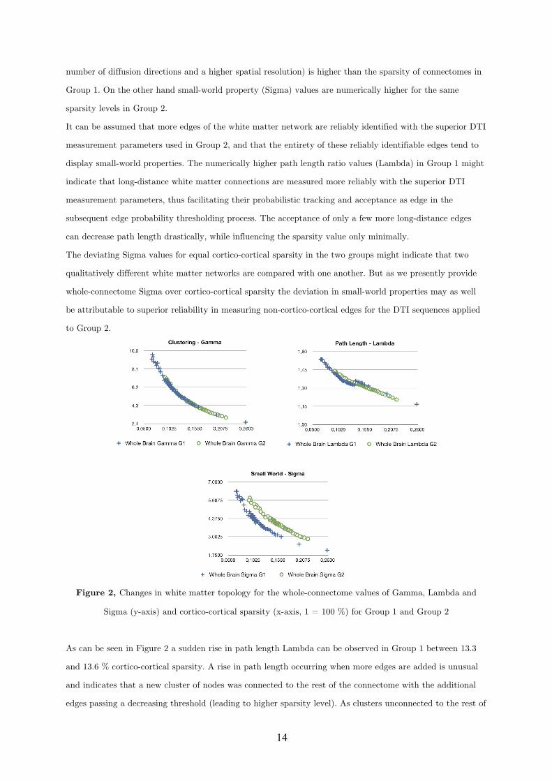
14

number of diffusion directions and a higher spatial resolution) is higher than the sparsity of connectomes in

Group 1. On the other hand small-world property (Sigma) values are numerically higher for the same

sparsity levels in Group 2.

It can be assumed that more edges of the white matter network are reliably identified with the superior DTI

measurement parameters used in Group 2, and that the entirety of these reliably identifiable edges tend to

display small-world properties. The numerically higher path length ratio values (Lambda) in Group 1 might

indicate that long-distance white matter connections are measured more reliably with the superior DTI

measurement parameters, thus facilitating their probabilistic tracking and acceptance as edge in the

subsequent edge probability thresholding process. The acceptance of only a few more long-distance edges

can decrease path length drastically, while influencing the sparsity value only minimally.

The deviating Sigma values for equal cortico-cortical sparsity in the two groups might indicate that two

qualitatively different white matter networks are compared with one another. But as we presently provide

whole-connectome Sigma over cortico-cortical sparsity the deviation in small-world properties may as well

be attributable to superior reliability in measuring non-cortico-cortical edges for the DTI sequences applied

to Group 2.

Figure 2, Changes in white matter topology for the whole-connectome values of Gamma, Lambda and

Sigma (y-axis) and cortico-cortical sparsity (x-axis, 1 = 100 %) for Group 1 and Group 2

As can be seen in Figure 2 a sudden rise in path length Lambda can be observed in Group 1 between 13.3

and 13.6 % cortico-cortical sparsity. A rise in path length occurring when more edges are added is unusual

and indicates that a new cluster of nodes was connected to the rest of the connectome with the additional

edges passing a decreasing threshold (leading to higher sparsity level). As clusters unconnected to the rest of

15

the connectome are unlikely, this might be an indication that the true level of cortico-cortical sparsity might

be in a range above 13.6 %.

3.2. General sample characteristics

The lack of any significant relation of whole-brain graph metrics and average perfusion values indicates that

there is no relation of overall absolute perfusion and overall connectivity in our healthy sample.

3.3. Correlation between perfusion, connectivity and GMV

Both local GMV and local perfusion show a pattern of significant covariation with local graph theoretical

metrics in both groups and for all three described region classes. This pattern of covariation indicates that

higher perfusion and higher GMV are more likely to be found in hub-like regions of the brain, with high

degree, betweenness and vulnerability, thus with low clustering coefficient and local efficiency.

GMV and perfusion show a marked covariation profile on the whole-sample level, with the strongest

correlation for subcortical regions, followed by regions of the DMN and finally non-cerebellar regions in

general and cortical regions. The marked correlations of perfusion and GMV could theoretically be a

confound due the fact that relatively larger regions contain more large vessels and have a superior ASL

Signal-to-Noise ratio (SNR) when compared with smaller regions. Alternatively the correlations could

indicate a genuine association of average perfusion and relative GMV.

3.4 Covariation of perfusion and connectivity

Cortical and subcortical nodes were characterised with respect to their graph theoretical properties, which

were further correlated with measures of perfusion, while controlling for local GMV.

3.4.1 Group Level

The covariations found on a group level, analysing the trait correlations of all cortical nodes, were only

minor (<0.25) in magnitude and inconclusive in terms of cross-group stability. The covariation profile of

traits from subcortical nodes on the other hand shows a negative covariation of local efficiency and a

positive covariation of vulnerability with perfusion in a minor to medium (<0.6) range of magnitude.

For regions associated with the DMN we observe similar patterns of covariation, but complemented by a

positive covariation of degree and betweenness and a negative covariation of the clustering coefficient with

perfusion, in a range of minor to medium magnitude.

For all three classes of nodes, the magnitude of covariation observed in Group 1 exceeds the magnitude of

covariations in Group 2.

3.4.2. Individual Level

16

On the individual level correlations for all cortical, subcortical and DMN regions largely fail to reach

significance in a stable pattern.

3.4.3. Regionwise Level

On a regionwise level, frontal, cingular and hippocampal regions show a negative covariation of perfusion

with the clustering coefficient and local efficiency, while mainly posterior portions of the brain show a

positive covariation particularly with vulnerability. All covariations remain minor to medium in magnitude

and have the same sign in both groups, except for the Frontal Inferior Cortex (pars triangularis and

orbitalis), the Frontal Superior Medial Gyrus, the Supplementary Motor Area, the Olfactory Cortex and the

Rolandic Operculum, where the signs of covariation are contradictory.

3.5. General covariation pattern

The present results do not allow for a clear and global falsification of a perfusion/connectivity-covariation in

the brain. Rather the results on group- and regionwise levels point towards a positive covariation of rCBF

with degree, betweenness and vulnerability and a negative covariation of rCBF with the clustering

coefficient and efficiency for some particular regions of the brain.

The correlation results for the covariation of GMV, perfusion and connectivity (no statistical control of

GMV) point into the same direction, thus could be influenced by the issues indicated in the methods

section.

This might indicate that for some areas of the brain an increased rCBF is more likely to be found in

regions, which have a central position in the white matter network and possess hub-like properties, but have

poor local clustering and number of parallel pathways to any other node (local efficiency). This might be the

manifestation of a structural organisation principle, which strives to minimise the potential of metabolic

deficiencies in central nodes, which are part of a rather sequential connection architecture.

The failure of the correlations to reach significance on the individual level could be attributed to the low

statistical power, since for the DMN twelve and for the subcortical regions merely ten pairs of values are

correlated for each participant, further decreasing the degrees of freedom by using PC and using

conservative multiple comparison correction. The same holds for results on the regionwise level (the number

of value pairs correlated for each region is equal to the number of subjects in that group, which are eleven

and twelve, respectively), which might offer one explanation for the contradictory findings in some regions.

The most stable results are obtained for regions of the DMN on a group- and regionwise level. Regions of

the DMN are known to possess hub-like properties in terms of both anatomical and functional connectivity

[4]. Possibly the present results point towards an exclusive realisation of an observable linear supply-and-

demand-principle of perfusion and connectivity in these regions, although it can not be excluded that

regions show possibly non-linear relations, which we did not test for in this present study.

17

3.6. Implications

These results might have implications on our understanding of resting state networks in general, not only

those exclusively involving nodes of the DMN network [34-39].

The finding that DMN regions (e.g. Posterior Cingulate) might play a role as bottlenecks in a potentially

task-negative default mode of macroscopic neural traffic might be underlined by past [34] [40] and present

results on the coincidence of heightened resting state perfusion and hub characteristics (marked by high

degree and vulnerability) in DMN regions. Just like the hubs of any traffic network can form bottlenecks

where traffic might dam up, some nodes with a central position within the white matter network might

show heightened activity during distinct global states, such as rest. But whether the apparent functional

connectivity of these hubs can be attributed to genuine joint information processing in a functionally

relevant network or merely to similar activity arising from e.g. coincidentally relaying traversing neural

signals, or parts of both, can currently not be conclusively answered.

It is possible that the common traits (high perfusion, hub-like connectivity, large relative GMV) and the

strong covariation of these traits contribute either causally to the formation, or confoundingly to our

awareness of resting state networks. Similar Blood Oxygen Level Dependent (BOLD) activity profiles might

in principle be caused by node interactivity in a functionally relevant information processing network or

alternatively by mere similarity of isolated neural processes in individual nodes [3]. It is unclear, to what

extent the coincidence of high resting state perfusion and hub-like connectivity can distort estimations of

functional connectivity between such nodes, by influencing the BOLD signal from these nodes generally with

their mutually high perfusion and the underlying activity in these nodes with their common hub-like

connectivity.

Understanding the link between local function and local connectivity better, might help understand the

apparent link between functional and anatomical connectivity networks [4] [5] and resolve the role of mere

homology in our perception of resting state networks.

It is a further open question of interest, whether there is any causal neurobiological link between a regional

perfusion profile and the emergence of hub characteristics or vice versa.

3.7. Conclusion

The method described might hold potential for the diagnosis of various diseases, as the identified

dependency of perfusion and connectivity might reflect the balance resulting from organisational principles

inherent to the structural architecture of the healthy brain. Although the identified coefficients from the

present healthy sample are only minor to medium in magnitude, it is to note that two traits might be only

rudimentarily related in the healthy brain, but might show stronger links in the pathologically altered brain

(e.g. hypoperfusion preceding gray matter atrophy).

18

However, to better understand the relevance of the identified relationships and to explore changes of the

derived coefficients due to ageing or disease future studies have to be performed on the respective

populations.

3.8. Potential confounds

It can be assumed that during our resting state ASL measurement, the regions of the DMN showed their -

by definition - heightened resting state activity and metabolic demand and it is possible that our

measurements were therefore systematically biased. If the metabolic profile of a region is best assessed when

this region shows a stable amount of activity over time, the metabolic demand of the resting state active

brain regions (the DMN) was eventually captured more clearly by our resting state experiment, than the

metabolic demand profile of a less resting state involved region such as e.g. the Fusiform Gyrus. This issue

touches on the general question whether stimulus-free measurements constitute a reliable baseline

measurement for the whole brain, or only for regions active under stimulus-free conditions.

Thus it can not be excluded that covariations of the present form could be identified more conclusively for

others regions of the brain as well. For such experiments, these regions would need to be consistently

activated for a prolonged amount of time (e.g. by presentation of a series of faces for characterisation of the

Fusiform Gyrus), what might allow us to assess their metabolic demand during activity better.

It might be argued that the prospect of such studies might be limited, as brain regions do not merely show

a straightforward type of homogeneous functional specialisation, but are rather able to perform

heterogenous functions that depend on the task-specific network(s) they are integrated in at a point of time.

Nevertheless it should be possible to capture the range of metabolic demand spanned by the conditions of

activity and rest for each region of the brain, as any computational process is likely to influence metabolic

demand in a specific way.

Studies on the relation of functional and anatomical connectivity networks in general might be influenced by

a similar aspect. The definition of functional connectivity is always limited to the state of the brain the

connectivity is observed in, therefore the definition of network nodes is not state-independent (the stable

association of the nodes with a network is one but not the only defining trait of the nodes) and thus

probably not one-by-one mappable onto other data, e.g. to adequately assess the underlying anatomical

connectivity network.

It stands to reason that both the range of metabolic demand states, local connectivity and GMV, and the

probability ranking of affiliations to functional connectivity networks of a brain region might be related in

some manner to the shape of the Hemodynamic Response Function in that region.

Alternatively to a direct causal interpretation, the co-variation of perfusion and connectivity could as well

be caused by a confounding third, presently unregarded variable other than GMV. Our initial hypothesis on

the link between local connectivity and local neural computations, neural computations and neural activity,

19

and neural activity and metabolic demand involves a series of dependencies, making the influence of

intermediary variables highly likely.

A more comprehensive model, including more potentially intermediate variables beyond merely GMV, could

be used in future studies to investigate the relations of local computational processes (e.g. using

electroencephalographic methods), neural circuitry (e.g. by utilising information on local cell body types),

neurotransmitter concentrations (e.g. by using Magnetic Resonance Spectroscopy), metabolism and

connectivity at once. With such a larger and more comprehensive dataset it is likely that the particular

perfusion/connectivity balance profile of each region could be resolved further.

3.9. Methodological issues

Several methodological issues need to be addressed. Although we employed a probabilistic tracking

approach with a high number of random walks and conservative thresholding, presently it is not possible to

ensure the validity of one singular estimated connectome with complete certainty due to the methodological

difficulty of proper edge falsification and the strong dependency of the results upon the chosen brain

parcellation scheme (the AAL atlas in this case). For a more precise estimation, the methodology has to be

refined by extending it to more sophisticated graph estimation methods e.g. based on Q-ball imaging data

[41] or diffusion tensor studies utilising multi b-value imaging - and by combining these advanced

measurements with advanced brain function atlases, derived from large databases of functional connectivity

data, since the optimal anatomical connectivity network nodes stem from the parcellation of the brain into

those regions, which eventually form a multitude of functional cooperations with others but always do this

as a whole [4].

The combination of multiple methods (DTI based connectivity estimation, VBM, ASL) allows for

quantifying and describing brain regions with a high number of measures, both on a global as well as on a

regional scale. The proper interpretation of this multifaceted data, with respect to the multiple comparisons

problem and open questions on the combination of non-gaussian measures with classical statistical

approaches, needs to be advanced in an integrative manner.

Further as the present findings are based on cross-sectional data from small samples, the results could be

influenced by potential cohort or small sample size effects. A longitudinal study design with a higher

number of subjects is necessary to broaden our understanding of the link of these structural and functional

brain properties.

It is to note that many different methods with their individual assumptions and errors are combined in an

integrative study, and that any of the modules (probabilistic tractography, graph theoretical analysis,

anatomical image segmentation, perfusion measurement, artefact control, normalisation etc.) could clearly

be improved on their own. Our approach is merely intended as a starting point for the combination of the

provided measures.

20

Therefore the present findings are of a preliminary nature, as for the integration of information about local

perfusion, connectivity and gray matter properties, the issues of natural variability versus the distribution of

measurement error have to be further resolved. Other quantification approaches for measuring integrity or

impairment of gray matter such as spectroscopy of synaptic density or recently introduced Positron

Emission Tomography methods [42] focussing on the quantification of plaques and tangles in AD might

complement the present approach in the future [4].

Methods

4.1. Subjects and data acquisition

Eleven participants (5 females) were recruited for Group 1 from a student sample (average age=25.4 years,

SD=3.4 years, Range: 21-32). After an update of scanner software twelve further participants (7 females)

were recruited, referred to as Group 2 (average age=36.7 years, SD=10.7 years, Range: 23-57). Participants

of both groups gave written informed consent. All participants were right handed (as confirmed by the

Edinburgh Handedness Questionnaire) and both physically (confirmed by extensive health questionnaire)

and mentally healthy (confirmed by the german ICD-10-Symptomrating questionnaire). The experiments

were approved by the local ethics committee. All MR data were acquired on a 3T Siemens MAGNETOM

Trio TIM (Erlangen, Germany) scanner using a 12-channel head coil. The head of each subject was bedded

in a deflatable pillow so as to minimise head motion artefacts.

4.2. Anatomical data acquisition and processing

Anatomical images were acquired using a T1 weighted sequence using a 3D MP-RAGE (magnetisation

prepared - rapid acquisition gradient echo) sequence (1x1x1 mm voxels, TR=7.92, TE=2.48, Flip

Angle=16°, FoV=256*256, 192 transversal slices, Group 1 - 1x1x1.1 mm voxels, TR=2.3, TE=2.98, Flip

Angle=9°, FoV=230*256, 160 sagittal slices, Group 2). The brain was extracted from the raw image using

the robust iterative estimation function (Fractional intensity threshold=0.5) of the Brain Extraction Tool

and subsequently segmented into gray and white matter ([43], distributed within the FMRIB's Software

Toolbox - FSL 4.0; http://www.fmrib.ox.ac.uk/fsl).

4.3. DTI data acquisition

Each subject in Group 1 participated in a DTI measurement (1.3x2.4x2.4 mm voxels, no gap, TR=8.83 sec,

TE=98 ms, FoV=1360*1360, Flip Angle=90°, 50 transversal slices, 12 diffusion directions, two averages, b-

value=1000 s/mm2) with the field of view (FoV) comprising the full cerebrum and parts of the rostral

cerebellum like the Uvula and Tuber of Vermis, Flocculus and Crus Cerebelli (dependent on individual

overall brain size).

Each subject in Group 2 participated in a DTI measurement (1.8x1.8x2.2 mm voxels, no gap, TR=6.8 sec,

TE=93 ms, FoV=1782*1840, Flip Angle=90°, 50 transversal slices, 64 diffusion directions, two averages, b-

21

value=1000 s/mm2) with the FoV comprising the full cerebrum and parts of the rostral cerebellum. The

DTI data were processed using the DTI and Fibertools Software Package [44] as described in the section

Network Edge Definition.

4.4. Connectome construction and edge calculation

For an overview on data flow for each participant and employed analysis schemes please see Figure S1 and

Figure S2.

4.4.1. Network node definition

In order to define the network nodes, gray matter areas were labelled for each subject individually based on

the AAL atlas [45], resulting in 116 nodes (80 cortical, 10 subcortical, 26 cerebellar) by using the procedure

of normalisation and parameter inversion analogous to the method described in [20].

In order to transfer the images into DTI native space, T1 weighted structural images were coregistered with

the B0 (non-diffusion) image and then normalised to the Montreal Neurological Institute (MNI) space. The

resulting transformation was inverted to warp the AAL template from MNI space to the DTI space. The

discrete labeling values were preserved by using a nearest neighbour interpolation method. Normalisation

and inverse transformation were implemented using the SPM8 package.

All available subcortical (Caudate, Putamen, Pallidum, Hippocampus and Thalamus) and cerebellar areas,

which were within the individual DTI FoV were included as nodes in order to round out the validity of the

individual connectivity graph estimation.

4.4.2 Network edge tracking

Using in-house code, the white matter voxels, which were neighbouring the gray matter of each network

node, were defined as seed voxels of that area.

Only voxels with a Fractional Anisotropy (FA) value above 0.3 (gray matter FA can reach values up to

∼0.2, [46]) were admitted to this procedure. In addition, these voxels also had to be labelled as white matter

by the segmentation step and reside within the brain outline mask resulting from the iterative Brain

Extraction Step.

Probabilistic tracking from the seed points was realised by using the PiCo [47] approach. The number of

random walks was adjusted to the number of voxels within the white matter tracking area for each single

seed point.

The algorithms implemented in the DTI and Fibertools Software Package [44] allow for creating extended

visitation maps for the tracking from each seed set (all seed voxels of an AAL area) separately, based on the

curves originating from the seed points and being propagated through the tensor field (number of curves

equalling the number of random walks) and combine this information with statistical estimates on the

plausibility of confluence of two white matter tracts anywhere in the brain. Please see [44] for more precise

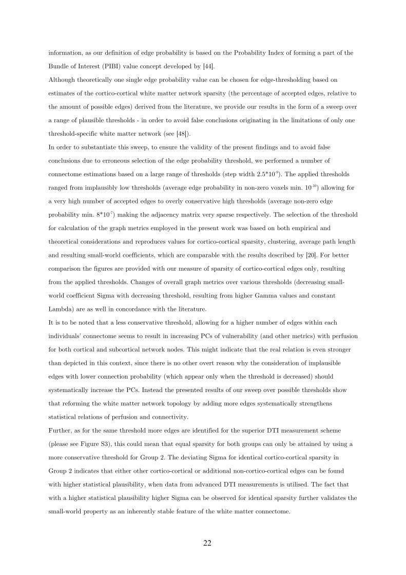
22

information, as our definition of edge probability is based on the Probability Index of forming a part of the

Bundle of Interest (PIBI) value concept developed by [44].

Although theoretically one single edge probability value can be chosen for edge-thresholding based on

estimates of the cortico-cortical white matter network sparsity (the percentage of accepted edges, relative to

the amount of possible edges) derived from the literature, we provide our results in the form of a sweep over

a range of plausible thresholds - in order to avoid false conclusions originating in the limitations of only one

threshold-specific white matter network (see [48]).

In order to substantiate this sweep, to ensure the validity of the present findings and to avoid false

conclusions due to erroneous selection of the edge probability threshold, we performed a number of

connectome estimations based on a large range of thresholds (step width 2.5*10-9). The applied thresholds

ranged from implausibly low thresholds (average edge probability in non-zero voxels min. 10-10) allowing for

a very high number of accepted edges to overly conservative high thresholds (average non-zero edge

probability min. 8*10-7) making the adjacency matrix very sparse respectively. The selection of the threshold

for calculation of the graph metrics employed in the present work was based on both empirical and

theoretical considerations and reproduces values for cortico-cortical sparsity, clustering, average path length

and resulting small-world coefficients, which are comparable with the results described by [20]. For better

comparison the figures are provided with our measure of sparsity of cortico-cortical edges only, resulting

from the applied thresholds. Changes of overall graph metrics over various thresholds (decreasing small-

world coefficient Sigma with decreasing threshold, resulting from higher Gamma values and constant

Lambda) are as well in concordance with the literature.

It is to be noted that a less conservative threshold, allowing for a higher number of edges within each

individuals’ connectome seems to result in increasing PCs of vulnerability (and other metrics) with perfusion

for both cortical and subcortical network nodes. This might indicate that the real relation is even stronger

than depicted in this context, since there is no other overt reason why the consideration of implausible

edges with lower connection probability (which appear only when the threshold is decreased) should

systematically increase the PCs. Instead the presented results of our sweep over possible thresholds show

that reforming the white matter network topology by adding more edges systematically strengthens

statistical relations of perfusion and connectivity.

Further, as for the same threshold more edges are identified for the superior DTI measurement scheme

(please see Figure S3), this could mean that equal sparsity for both groups can only be attained by using a

more conservative threshold for Group 2. The deviating Sigma for identical cortico-cortical sparsity in

Group 2 indicates that either other cortico-cortical or additional non-cortico-cortical edges can be found

with higher statistical plausibility, when data from advanced DTI measurements is utilised. The fact that

with a higher statistical plausibility higher Sigma can be observed for identical sparsity further validates the

small-world property as an inherently stable feature of the white matter connectome.

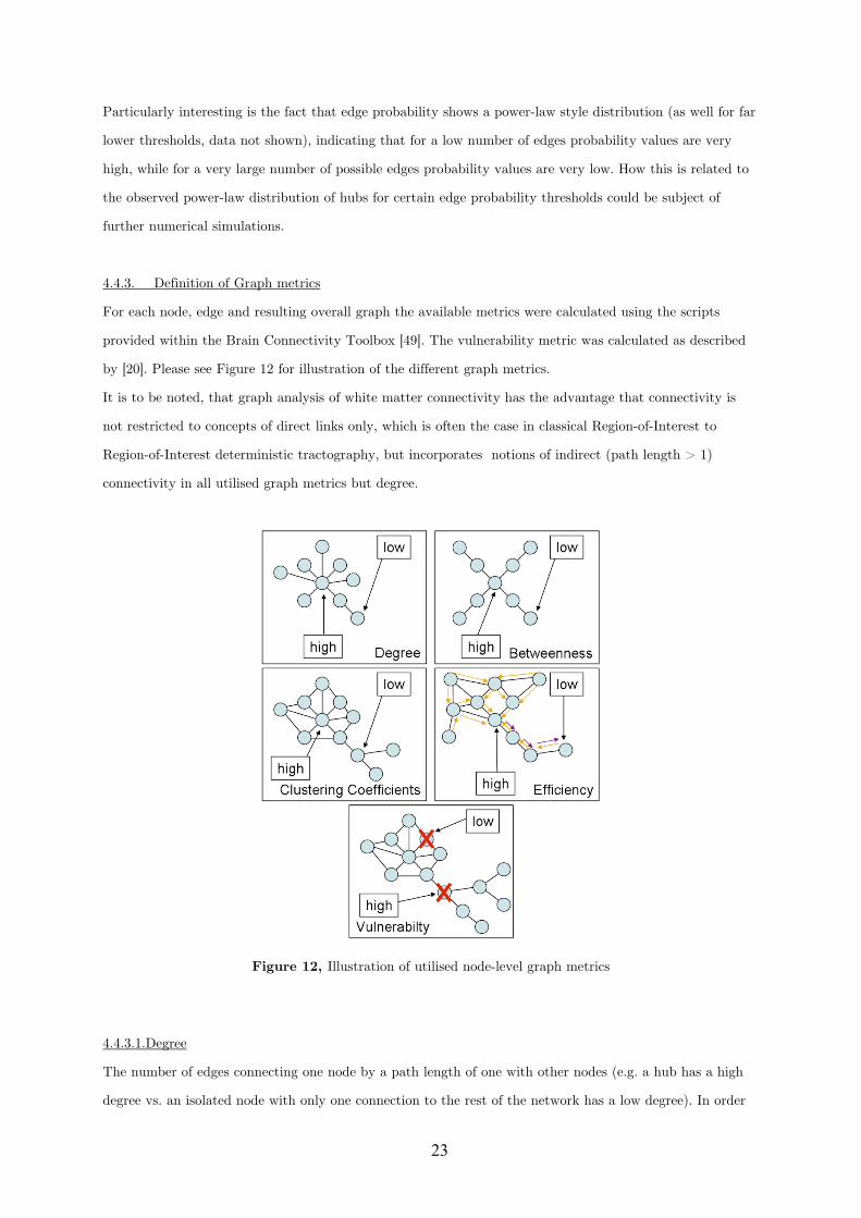
23

Particularly interesting is the fact that edge probability shows a power-law style distribution (as well for far

lower thresholds, data not shown), indicating that for a low number of edges probability values are very

high, while for a very large number of possible edges probability values are very low. How this is related to

the observed power-law distribution of hubs for certain edge probability thresholds could be subject of

further numerical simulations.

4.4.3. Definition of Graph metrics

For each node, edge and resulting overall graph the available metrics were calculated using the scripts

provided within the Brain Connectivity Toolbox [49]. The vulnerability metric was calculated as described

by [20]. Please see Figure 12 for illustration of the different graph metrics.

It is to be noted, that graph analysis of white matter connectivity has the advantage that connectivity is

not restricted to concepts of direct links only, which is often the case in classical Region-of-Interest to

Region-of-Interest deterministic tractography, but incorporates notions of indirect (path length > 1)

connectivity in all utilised graph metrics but degree.

Figure 12, Illustration of utilised node-level graph metrics

4.4.3.1.Degree

The number of edges connecting one node by a path length of one with other nodes (e.g. a hub has a high

degree vs. an isolated node with only one connection to the rest of the network has a low degree). In order

24

to normalise local degree values to make them comparable across graphs, the values are divided by the sum

of all node degree values.

4.4.3.2. Betweenness

A node with high betweenness is at a central position of the network, meaning that many of the paths

connecting any node A and any node B traverse that node (e.g. while a central hub has high betweenness, a

node forming a cul-de-sac has the lowest betweenness). Betweenness is calculated as the fraction of all

shortest paths in the network, which traverse a given edge/node. In order to normalise local betweenness

values to make them comparable across graphs, the values are divided by the sum of all node betweenness

values within the graph.

4.4.3.3. Clustering coefficient

If the nearest neighbours (path length = 1) of a node are also directly connected to each other they form a

cluster (e.g. when an individual´s friends are also friends with one another). The clustering coefficient

quantifies the number of connections that exist between the nearest neighbours of a node as a proportion of

the maximum number of possible connections amongst them. This normalisation allows comparing the

clustering coefficient of two nodes directly, irrespective of their individual degree.

4.4.3.4. Efficiency

Efficiency is inversely related to minimum path length (shortest) and quantifies how easily one node can be

reached from any other node. Nodes with a high efficiency have many interconnected neighbours and are

thus more easily reachable via a number of (parallel) direct paths from any other node. Local efficiency of a

node is therefore calculated as the harmonic mean for neighbour-neighbour distances.

4.4.3.5. Vulnerability

This metric describes how strongly the average shortest path lengths (the mean distance to get from any

node A to any node B) in a network grow if a node is removed. If a node with high betweenness, high

degree, low efficiency and low clustering coefficient is removed, a central hub is eliminated leading to

insufficient cost-effective (short) detours for reconnecting severed nodes and high node vulnerability. If a

network is fully connected (all nodes are connected to all other nodes) degree, efficiency and clustering

coefficient might be high for all nodes, but vulnerability might be low, as the removal of one node would not

affect the average distance of any pair of nodes significantly, due to the high number of parallel connecting

paths / cost-effective detours.

4.5. ASL data acquisition

25

ASL data were acquired with a FAIR-QUIPSSII PASL encoding scheme with echo-planar imaging (EPI)

readout. A total of 201 alternating tag and control images were obtained in each run (total scan time 10

min, TI1=700 ms, TI2=1100 ms, TE=20ms, TR=3000 ms, voxel size=3.5x3.5x10mm). For ASL

measurements of Group 2 the number of slices was increased from ten to eleven (TI2 was changed to 1400

respectively). In order to determine the equilibrium magnetisation for absolute CBF quantification, the

same parameters as above were used except that the TR and TI2 were 10000ms and 4000ms, respectively

[50]. For analysing the ASL data, FSL software (http://www.fmrib.ox.ac.uk/fsl), self-written MATLAB

(The Mathworks, Natick, MA, USA) and Linux shell script routines were used. Time courses of all voxels

were motion-corrected utilising the MCFLIRT module of FSL using the mean volume of the corresponding

run as reference. CBF time series were created by calculating control-tag difference images using surround

subtraction (i.e., computing the difference between each image and the average of its two nearest

neighbors), thereby reducing BOLD signal contamination of the CBF time course [50].

For the ASL resting state data acquisition subjects were instructed to relax with closed eyes while staying

awake. The ASL values for the nodes were extracted by averaging the absolute CBF (in ml/100g-min) from

the voxels within each network node Volume of interest (VOI) for each subject.

Regional absolute and within-subject normalised rCBF values are provided for all non-cerebellar regions of

the AAL atlas in the Figure S4.

4.6. Gray matter characterisation through Voxel-Based Morphometry

In order to address the relation between gray matter characteristics, graph theoretical measures and resting

state perfusion, we performed a VBM Analysis of the T1 weighted anatomical scans so as to derive

descriptives regarding the relative volume of each AAL region. As described in the section Network Node

Definition, each anatomical image was skull stripped and the Voxel-based Morphometry Toolbox (VBM5.1,

v.1.15, by Christian Gaser) was used subsequently for estimation of the individual modulated and

unmodulated segmentation outputs. As the modulated outputs can be corrected for non-linear warping only

and therefore make any further correction for different brain size redundant, these images can be used

directly for volume estimations.

For the unified segmentation approach (repeated segmentation, bias correction and warping iterations as

described in [51]) used in this study the tissue probability maps provided within the SPM5 template set

were used since the subjects were drawn from the appropriate population. We applied the thorough clean-up

option of the VBM toolbox and made use of a medium Hidden Markov Random Field model for an optimal

denoising of the T1 image.

A check of sample homogeneity of the modulated images (using the standard deviation approach within

VBM5.1) revealed that the VBM results of the images were all within a tolerable range.

So as to optimise the validity of our GMV estimation, we performed a voxel-wise multiplication of each

modulated gray matter image with the coregistered corresponding perfusion image (containing absolute

26

CBF information). Although perfusion imaging of white matter regions of the brain is possible in principle

[52], with many sequences estimation accuracy is limited due to the longer transit delay time (the travelling

time of blood from labelling region to reach the tissue) of white matter. As perfusion in gray matter is

higher, such a multiplication significantly sharpens the gray matter image histogram, thus facilitating the

valid estimation of GMV. In order to smooth the image histogram we applied a three dimensional Gaussian

smoothing kernel (FWHM=3 mm, being significantly below the rounded down cubic root of the volume of

the smallest AAL-region in equal voxel-space). For each AAL region (network node) the number of gray

matter voxels within the atlas derived volumes of interest was counted - equalling the regional volume as

relative to the entire individual brain. Naturally these volume values are strongly correlated across our

healthy sample as they all measure brain part volumes for identical regions.

Regional GMV values are provided for all non-cerebellar regions of the AAL atlas in Figure S5.

4.7. Employed data level and artefact control

As a univariate factor analysis revealed significant interindividual variability of rCBF values and an effect

of gender, the analysis was performed using within-subject z-scored rCBF values. Following this approach,

graph metrics and the GMV of nodes were all normalised (z-scored) on a within-subject level. The

normalisation was performed separately for cortical and subcortical nodes.

Cortical or subcortical regions for which no connections could be found (due to a tracking failure) or for

which no perfusion data could be obtained (due to localisation outside of the ASL imaging FoV) were

excluded pairwise from the analysis (in Group 1 seven missing values in different regions, in Group 2 four

missing values in two different regions). Cerebellar regions were not considered for correlation analysis, as

for 30.94 % of cerebellar regions rCBF could not be measured.

VOI specific artefacts in the estimation of rCBF can not be fully eliminated, due to the generally increased

SNR ratio of the ASL signal and the higher chance of intravascular artefacts in larger VOIs, which

naturally contain more large arteries and veins that distort rCBF estimations. Also imperfect slice profiles,

remaining magnetisation transfer effects and blood tissue water exchange time are factors, which cause

artefacts on rCBF estimation. In order to decrease the impact of VOI size on the estimation of relations, we

included GMV estimations from VBM as a control variable into our analysis and restricted the presented

results to the significant PCs calculated with Spearman's rho.

The data derived from the entirety of these measures constitute for each member of the sample a

subjectwise region-by-trait table, with the columns representing local perfusion, local GMV and five graph

theoretical metrics of local white matter connectivity, and with 116 rows - one for each region of the AAL

atlas.

In order to interpret such multifaceted data one can take various perspectives. The data can be sorted and

the trait measurements can be correlated on an individual subjectwise level, to answer the question, whether

there is a significant PC - controlling for local GMV - between local perfusion and local connectivity for all

27

the 116 regions of the AAL atlas in the brain of a given subject. Alternatively the data can be normalised

on a within-subject level and integrated with data from all other subjects into a group table, to answer the

question whether the previously outlined PC is significant in an analysis of pooled data as well. As a second

alternative approach, the data can be sorted by region, so as to answer the question whether in pooled

group data local perfusion and local connectivity of some regions shows stronger correlation than others

(e.g. the left Precentral Gyrus displays a stronger PC, than the same two traits of the right Precentral

Gyrus). Figures of dataflow and analaysis schemes are depicted in Figure S1 and Figure S2.

Results are presented for white matter connectomes that show plausible cortico-cortical sparsity (between

11 and 17 %).

Acknowledgements

The authors would like to thank Dr. Andrea Caria, Dr. Karsten Rauss, Linda van der Heiden and Sarah

Wyckoff for their constant help and support. We would also especially like to thank the developers of the

DTI and Fibertools Software Package from the Department of Radiology, Medical Physics, University

Hospital Freiburg Dr. Björn Kreher, Dr. Marco Reisert, Susanne Schnell and Dr. Kamil Il'yasov for allowing

us to use their software package.

References:

1. Bassett DS, Bullmore E (2006) Small-world brain networks. The neuroscientist 12: 512. 2. Greicius MD, Supekar K, Menon V, Dougherty RF (2008) Resting-state functional connectivity reflects

structural connectivity in the default mode network. Cerebral Cortex. 3. van den Heuvel M, Mandl R, Luigjes J, Hulshoff Pol H (2008) Microstructural organization of the

cingulum tract and the level of default mode functional connectivity. Journal of Neuroscience 28: 10844.

4. Buckner RL, Sepulcre J, Talukdar T, Krienen FM, Liu H, et al. (2009) Cortical hubs revealed by

intrinsic functional connectivity: mapping, assessment of stability, and relation to Alzheimer's disease. Journal of Neuroscience 29: 1860.

5. Honey CJ, Sporns O, Cammoun L, Gigandet X, Thiran JP, et al. (2009) Predicting human resting-state functional connectivity from structural connectivity. Proceedings of the National Academy of Sciences 106: 2035.

6. He Y, Chen ZJ, Evans AC (2007) Small-world anatomical networks in the human brain revealed by

cortical thickness from MRI. Cerebral Cortex 17: 2407. 7. Chen ZJ, He Y, Rosa-Neto P, Germann J, Evans AC (2008) Revealing modular architecture of human

brain structural networks by using cortical thickness from MRI. Cerebral cortex 18: 2374. 8. Stam C, Jones B, Nolte G, Breakspear M, Scheltens P (2007) Small-World Networks and Functional

Connectivity in Alzheimer's Disease. Cerebral Cortex, 17(1), 92 -99.

28

9. Sporns O (2006) Small-world connectivity, motif composition, and complexity of fractal neuronal connections. Biosystems 85: 55–64.

10. Sporns O, Zwi JD (2004) The small world of the cerebral cortex. Neuroinformatics 2: 145–162. 11. Achard S, Salvador R, Whitcher B, Suckling J, Bullmore E (2006) A resilient, low-frequency, small-

world human brain functional network with highly connected association cortical hubs. Journal of Neuroscience 26: 63.

12. Kuschinsky W (1991) Coupling of function, metabolism, and blood flow in the brain. Neurosurgical

review 14: 163–168. 13. Farkas E, Luiten PG (2001) Cerebral microvascular pathology in aging and Alzheimer's disease.

Progress in Neurobiology 64: 575–611. 14. Arthurs OJ, Boniface S (2002) How well do we understand the neural origins of the fMRI BOLD

signal? TRENDS in Neurosciences 25: 27–31. 15. Magistretti PJ (2006) Neuron-glia metabolic coupling and plasticity. Journal of Experimental Biology

209: 2304. 16. Gjedde A, Diemer NH (1985) Double-tracer study of the fine regional blood-brain glucose transfer in

the rat by computer-assisted autoradiography. Journal of cerebral blood flow and metabolism: official journal of the International Society of Cerebral Blood Flow and Metabolism 5: 282.

17. Klein B, Kuschinsky W, Schrock H, Vetterlein F (1986) Interdependency of local capillary density,

blood flow, and metabolism in rat brains. American Journal of Physiology- Heart and Circulatory Physiology 251: H1333.

18. Detre JA, Wang J, Wang Z, Rao H (2009) Arterial spin-labeled perfusion MRI in basic and clinical

neuroscience. Current opinion in neurology 22: 348. 19. Jellison BJ, Field AS, Medow J, Lazar M, Salamat MS, et al. (2004) Diffusion tensor imaging of

cerebral white matter: a pictorial review of physics, fiber tract anatomy, and tumor imaging patterns. American Journal of Neuroradiology 25: 356.

20. Gong G, He Y, Concha L, Lebel C, Gross DW, et al. (2009) Mapping anatomical connectivity patterns

of human cerebral cortex using in vivo diffusion tensor imaging tractography. Cerebral Cortex 19: 524.

21. Bullmore E, Sporns O (2009) Complex brain networks: graph theoretical analysis of structural and

functional systems. Nature Reviews Neuroscience 10: 186–198. 22. Li Y, Liu Y, Li J, Qin W, Li K, et al. (2009) Brain anatomical network and intelligence. PLoS Comput

Biol 5: e1000395. 23. Cammoun L, Gigandet X, Sporns O, Thiran JP, Maeder P, et al. (2009) Connectome alterations in

schizophrenia. NeuroImage 47: S157. 24. Barabási AL, Crandall RE (2003) Linked: The new science of networks. American journal of Physics

71: 409. 25. Williams DS, Detre JA, Leigh JS, Koretsky AP (1992) Magnetic resonance imaging of perfusion using

spin inversion of arterial water. Proceedings of the National Academy of Sciences of the United States

29

of America 89: 212. 26. Wong EC, Buxton RB, Frank LR (1997) Implementation of quantitative perfusion imaging techniques

for functional brain mapping using pulsed arterial spin labeling. NMR in Biomedicine 10: 237–249. 27. Parkes LM, Rashid W, Chard DT, Tofts PS (2004) Normal cerebral perfusion measurements using

arterial spin labeling: reproducibility, stability, and age and gender effects. Magnetic Resonance in Medicine 51: 736–743.

28. Biagi L, Abbruzzese A, Bianchi MC, Alsop DC, Del Guerra A, et al. (2007) Age dependence of cerebral

perfusion assessed by magnetic resonance continuous arterial spin labeling. Journal of Magnetic Resonance Imaging 25: 696–702.

29. Schuff N, Zhu XP (2007) Imaging of mild cognitive impairment and early dementia. British Journal of

Radiology 80: S109. 30. Kawamura J, Meyer JS, Ichijo M, Kobari M, Terayama Y, et al. (1993) Correlations of leuko-araiosis

with cerebral atrophy and perfusion in elderly normal subjects and demented patients. British Medical Journal 56: 182.

31. Jahng G, Schuff N, Du A, Zhang Y, Mueller S, et al. (2007) Age-related Reductions of Cerebral Blood

Flow and White Matter Integrity by High-Field Perfusion and Diffusion MRI. World Congress on Medical Physics and Biomedical Engineering 2006. S. 1380–1383.

32. Ashburner J, Friston KJ (2001) Why voxel-based morphometry should be used. Neuroimage 14: 1238–

1243. 33. Mechelli A, Price CJ, Friston KJ, Ashburner J (2005) Voxel-based morphometry of the human brain:

methods and applications. Current Medical Imaging Reviews 1: 105–113. 34. Raichle ME, MacLeod AM, Snyder AZ, Powers WJ, Gusnard DA, et al. (2001) A default mode of brain

function. Proceedings of the National Academy of Sciences of the United States of America 98: 676. 35. Gusnard DA, Raichle ME (2001) Searching for a baseline: functional imaging and the resting human

brain. Nature Reviews Neuroscience 2: 685–694. 36. Calhoun VD, Adali T, Hansen LK, Larsen J, Pekar JJ (2003) ICA of functional MRI data: an

overview. in Proceedings of the International Workshop on Independent Component Analysis and Blind Signal Separation.

37. Jafri MJ, Pearlson GD, Stevens M, Calhoun VD (2008) A method for functional network connectivity

among spatially independent resting-state components in schizophrenia. Neuroimage 39: 1666–1681. 38. Fair DA, Cohen AL, Dosenbach NU, Church JA, Miezin FM, et al. (2008) The maturing architecture

of the brain's default network. Proceedings of the National Academy of Sciences 105: 4028. 39. Buckner RL, Vincent JL (2007) Unrest at rest: default activity and spontaneous network correlations.

Neuroimage 37: 1091–1096. 40. van den Heuvel MP, Mandl RC, Kahn RS, Hulshoff Pol HE (2009) Functionally linked resting-state

networks reflect the underlying structural connectivity architecture of the human brain. Human brain mapping 30: 3127–3141.

41. Sotiropoulos SN, Bai L, Morgan PS, Constantinescu CS, Tench CR (2010) Brain tractography using Q-

30

ball imaging and graph theory: Improved connectivities through fibre crossings via a model-based approach. NeuroImage 49: 2444–2456.

42. Nordberg A (2010) Amyloid Imaging in Early Detection of Alzheimer’s Disease. Neurodegenerative

Diseases 7: 136–138. 43. Smith SM (2002) Fast robust automated brain extraction. Human Brain Mapping 17: 143–155. 44. Kreher BW, Schnell S, Mader I, Il'yasov KA, Hennig J, et al. (2008) Connecting and merging fibres:

Pathway extraction by combining probability maps. NeuroImage 43: 81–89. 45. Tzourio-Mazoyer N, Landeau B, Papathanassiou D, Crivello F, Etard O, et al. (2002) Automated

anatomical labeling of activations in SPM using a macroscopic anatomical parcellation of the MNI MRI single-subject brain. Neuroimage 15: 273–289.

46. Le Bihan D, Mangin JF, Poupon C, Clark CA, Pappata S, et al. (2001) Diffusion tensor imaging:

concepts and applications. Journal of magnetic resonance imaging 13: 534–546. 47. Parker GJ, Haroon HA, Wheeler-Kingshott CA (2003) A framework for a streamline-based

probabilistic index of connectivity (PICo) using a structural interpretation of MRI diffusion measurements. Journal of Magnetic Resonance Imaging 18: 242–254.

48. Sporns O, Tononi G, Kotter R (2005) The human connectome: a structural description of the human

brain. PLoS Comput Biol 1: e42. 49. Rubinov M, Sporns O (2009) Complex network measures of brain connectivity: uses and

interpretations. Neuroimage. 50. Cavusoglu M, Pfeuffer J, Ugurbil K, Uludag K (2009) Comparison of pulsed arterial spin labeling

encoding schemes and absolute perfusion quantification. Magnetic resonance imaging 27: 1039–1045. 51. Ashburner J, Friston KJ (2005) Unified segmentation. Neuroimage 26: 839–851. 52. van Osch MJ, Teeuwisse WM, van Walderveen MA, Hendrikse J, Kies DA, et al. (2009) Can arterial

spin labeling detect white matter perfusion signal? Magnetic Resonance in Medicine 62: 165–173.

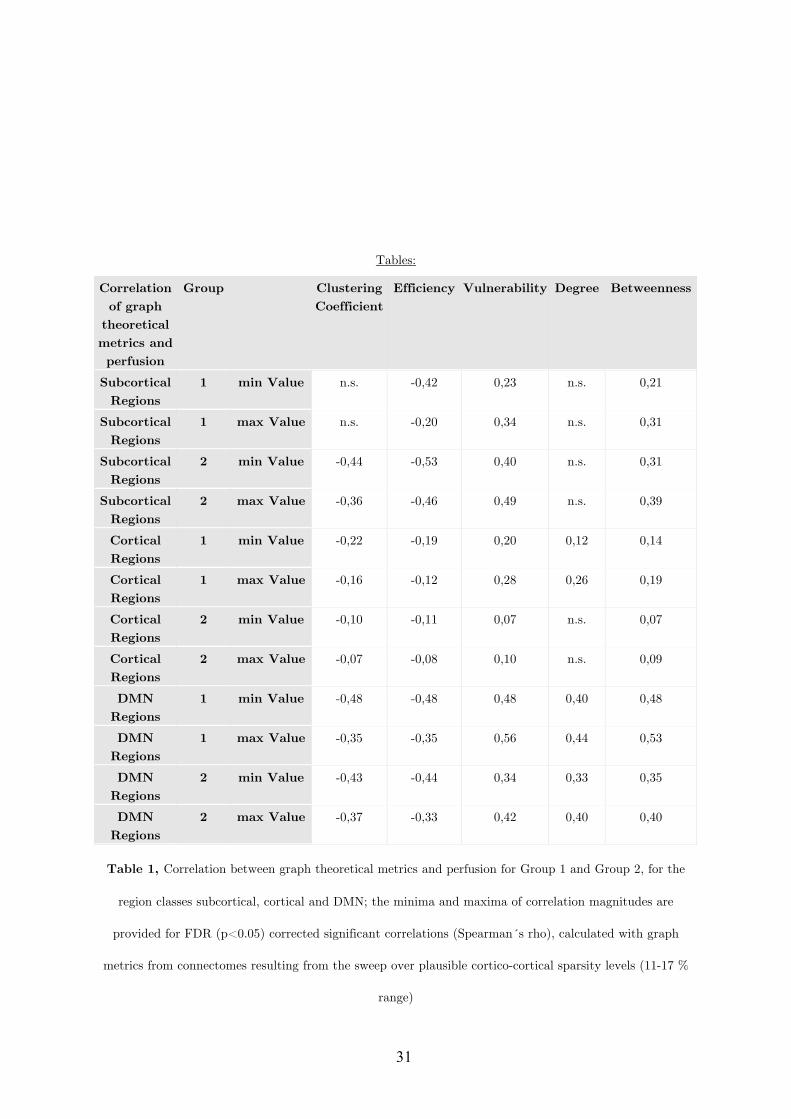
31

Tables:

Correlation of graph

theoretical metrics and perfusion

Group Clustering Coefficient

Efficiency Vulnerability Degree Betweenness

Subcortical Regions

1 min Value n.s. -0,42 0,23 n.s. 0,21

Subcortical Regions

1 max Value n.s. -0,20 0,34 n.s. 0,31

Subcortical Regions

2 min Value -0,44 -0,53 0,40 n.s. 0,31

Subcortical Regions

2 max Value -0,36 -0,46 0,49 n.s. 0,39

Cortical Regions

1 min Value -0,22 -0,19 0,20 0,12 0,14

Cortical Regions

1 max Value -0,16 -0,12 0,28 0,26 0,19

Cortical Regions

2 min Value -0,10 -0,11 0,07 n.s. 0,07

Cortical Regions

2 max Value -0,07 -0,08 0,10 n.s. 0,09

DMN Regions

1 min Value -0,48 -0,48 0,48 0,40 0,48

DMN Regions

1 max Value -0,35 -0,35 0,56 0,44 0,53

DMN Regions

2 min Value -0,43 -0,44 0,34 0,33 0,35

DMN Regions

2 max Value -0,37 -0,33 0,42 0,40 0,40

Table 1, Correlation between graph theoretical metrics and perfusion for Group 1 and Group 2, for the

region classes subcortical, cortical and DMN; the minima and maxima of correlation magnitudes are

provided for FDR (p<0.05) corrected significant correlations (Spearman´s rho), calculated with graph

metrics from connectomes resulting from the sweep over plausible cortico-cortical sparsity levels (11-17 %

range)

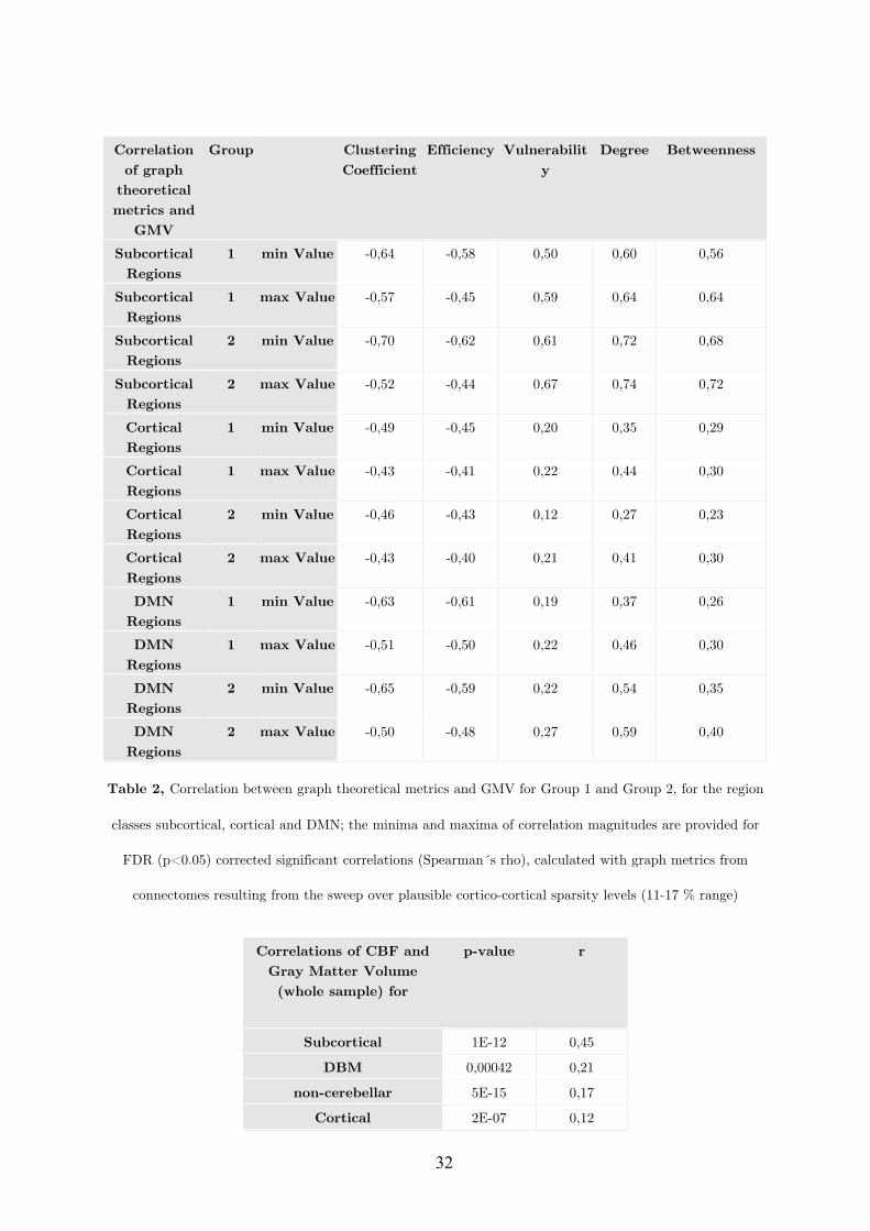
32

Correlation

of graph theoretical metrics and

GMV

Group Clustering Coefficient

Efficiency Vulnerability

Degree Betweenness

Subcortical Regions

1 min Value -0,64 -0,58 0,50 0,60 0,56

Subcortical Regions

1 max Value -0,57 -0,45 0,59 0,64 0,64

Subcortical Regions

2 min Value -0,70 -0,62 0,61 0,72 0,68

Subcortical Regions

2 max Value -0,52 -0,44 0,67 0,74 0,72

Cortical Regions

1 min Value -0,49 -0,45 0,20 0,35 0,29

Cortical Regions

1 max Value -0,43 -0,41 0,22 0,44 0,30

Cortical Regions

2 min Value -0,46 -0,43 0,12 0,27 0,23

Cortical Regions

2 max Value -0,43 -0,40 0,21 0,41 0,30

DMN Regions

1 min Value -0,63 -0,61 0,19 0,37 0,26

DMN Regions

1 max Value -0,51 -0,50 0,22 0,46 0,30

DMN Regions

2 min Value -0,65 -0,59 0,22 0,54 0,35

DMN Regions

2 max Value -0,50 -0,48 0,27 0,59 0,40

Table 2, Correlation between graph theoretical metrics and GMV for Group 1 and Group 2, for the region

classes subcortical, cortical and DMN; the minima and maxima of correlation magnitudes are provided for

FDR (p<0.05) corrected significant correlations (Spearman´s rho), calculated with graph metrics from

connectomes resulting from the sweep over plausible cortico-cortical sparsity levels (11-17 % range)

Correlations of CBF and

Gray Matter Volume (whole sample) for

p-value r

Subcortical 1E-12 0,45

DBM 0,00042 0,21

non-cerebellar 5E-15 0,17

Cortical 2E-07 0,12

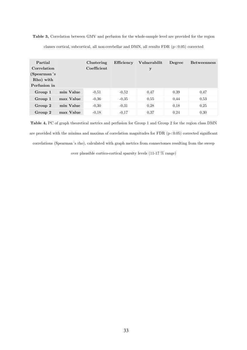
33

Table 3, Correlation between GMV and perfusion for the whole-sample level are provided for the region

classes cortical, subcortical, all non-cerebellar and DMN, all results FDR (p<0.05) corrected

Partial

Correlation (Spearman´s Rho) with

Perfusion in

Clustering Coefficient

Efficiency Vulnerability

Degree Betweenness

Group 1 min Value -0,51 -0,52 0,47 0,39 0,47 Group 1 max Value -0,36 -0,35 0,55 0,44 0,53 Group 2 min Value -0,30 -0,31 0,28 0,18 0,25 Group 2 max Value -0,18 -0,17 0,37 0,24 0,30

Table 4, PC of graph theoretical metrics and perfusion for Group 1 and Group 2 for the region class DMN

are provided with the minima and maxima of correlation magnitudes for FDR (p<0.05) corrected significant

correlations (Spearman´s rho), calculated with graph metrics from connectomes resulting from the sweep

over plausible cortico-cortical sparsity levels (11-17 % range)

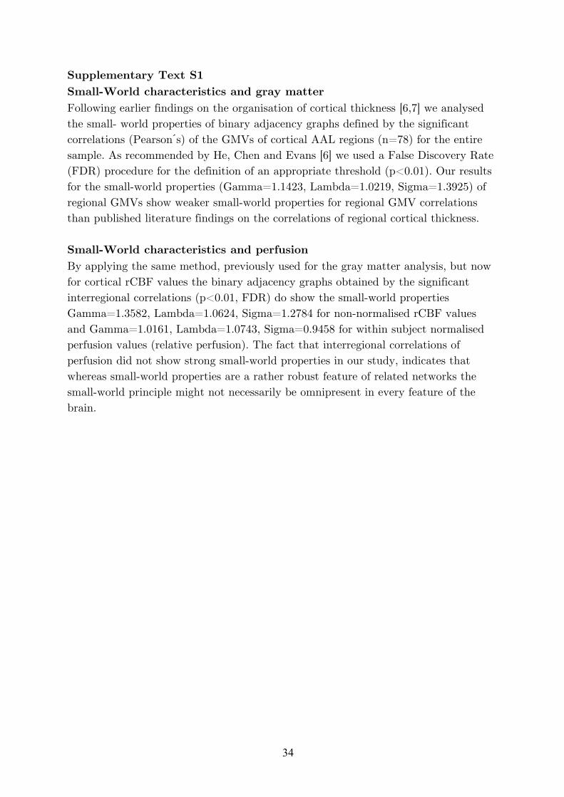
34

Supplementary Text S1 Small-World characteristics and gray matter Following earlier findings on the organisation of cortical thickness [6,7] we analysed the small- world properties of binary adjacency graphs defined by the significant correlations (Pearson s) of the GMVs of cortical AAL regions (n=78) for the entire sample. As recommended by He, Chen and Evans [6] we used a False Discovery Rate (FDR) procedure for the definition of an appropriate threshold (p<0.01). Our results for the small-world properties (Gamma=1.1423, Lambda=1.0219, Sigma=1.3925) of regional GMVs show weaker small-world properties for regional GMV correlations than published literature findings on the correlations of regional cortical thickness. Small-World characteristics and perfusion By applying the same method, previously used for the gray matter analysis, but now for cortical rCBF values the binary adjacency graphs obtained by the significant interregional correlations (p<0.01, FDR) do show the small-world properties Gamma=1.3582, Lambda=1.0624, Sigma=1.2784 for non-normalised rCBF values and Gamma=1.0161, Lambda=1.0743, Sigma=0.9458 for within subject normalised perfusion values (relative perfusion). The fact that interregional correlations of perfusion did not show strong small-world properties in our study, indicates that whereas small-world properties are a rather robust feature of related networks the small-world principle might not necessarily be omnipresent in every feature of the brain.

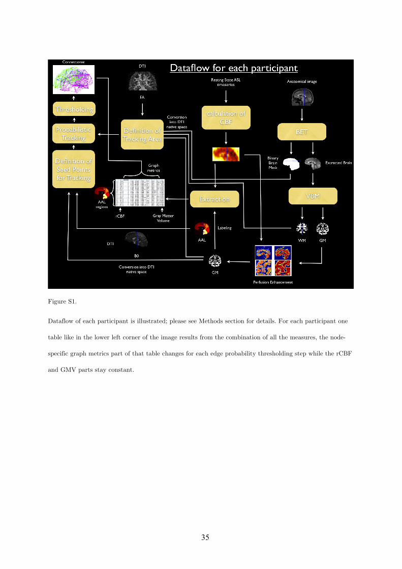
35

Figure S1.

Dataflow of each participant is illustrated; please see Methods section for details. For each participant one

table like in the lower left corner of the image results from the combination of all the measures, the node-

specific graph metrics part of that table changes for each edge probability thresholding step while the rCBF

and GMV parts stay constant.

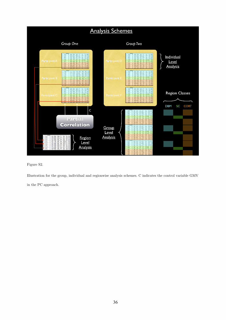
36

Figure S2.

Illustration for the group, individual and regionwise analysis schemes. C indicates the control variable GMV

in the PC approach.

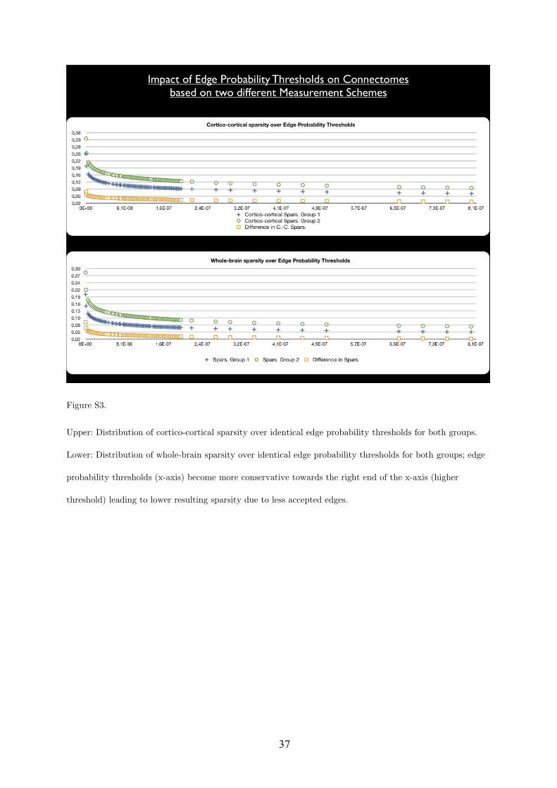
37

Figure S3.

Upper: Distribution of cortico-cortical sparsity over identical edge probability thresholds for both groups.

Lower: Distribution of whole-brain sparsity over identical edge probability thresholds for both groups; edge

probability thresholds (x-axis) become more conservative towards the right end of the x-axis (higher

threshold) leading to lower resulting sparsity due to less accepted edges.

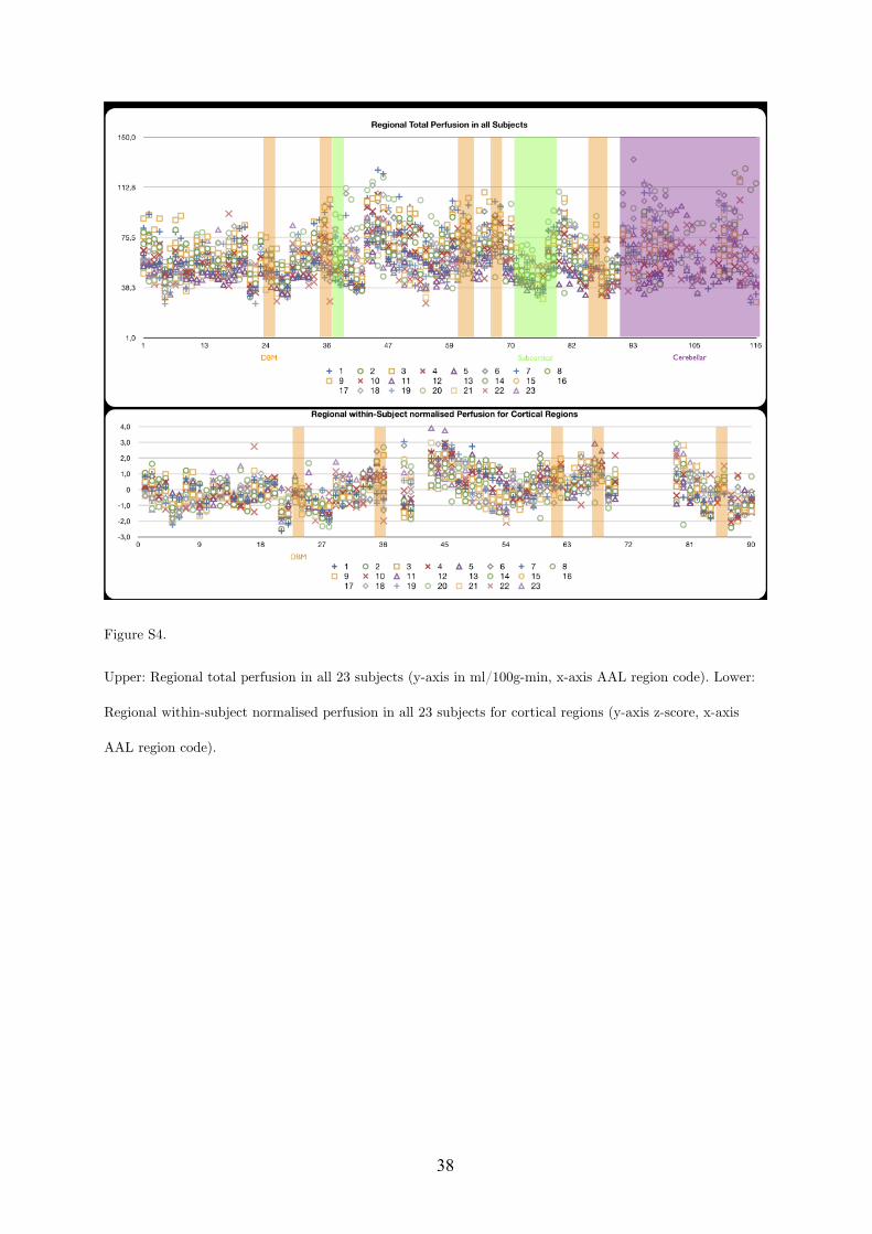
38

Figure S4.

Upper: Regional total perfusion in all 23 subjects (y-axis in ml/100g-min, x-axis AAL region code). Lower:

Regional within-subject normalised perfusion in all 23 subjects for cortical regions (y-axis z-score, x-axis

AAL region code).

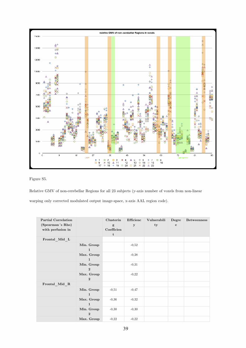
39

Figure S5.

Relative GMV of non-cerebellar Regions for all 23 subjects (y-axis number of voxels from non-linear

warping only corrected modulated output image-space, x-axis AAL region code).

Partial Correlation (Spearman´s Rho) with perfusion in

Clustering

Coefficient

Efficiency

Vulnerability

Degree

Betweenness

Frontal_Mid_L Min. Group

1 -0,52

Max. Group 1

-0,38

Min. Group 2

-0,31

Max. Group 2

-0,22

Frontal_Mid_R Min. Group

1 -0,51 -0,47

Max. Group 1

-0,36 -0,32

Min. Group 2

-0,30 -0,30

Max. Group -0,22 -0,22

40

2 Frontal_Inf_Tri_L

Min. Group 1

-0,24

Max. Group 1

-0,16

Min. Group 2

0,14

Max. Group 2

0,23

Frontal_Inf_Tri_R Min. Group

1 -0,26 -0,24

Max. Group 1

-0,17 -0,15

Min. Group 2

0,15 0,15

Max. Group 2

0,25 0,25

Frontal_Inf_Orb_L Min. Group

1 -0,23

Max. Group 1

-0,14

Min. Group 2

0,20

Max. Group 2

0,29

Frontal_Inf_Orb_R

Min. Group 1

-0,27 -0,21

Max. Group 1

-0,18 -0,13

Min. Group 2

0,21 0,19

Max. Group 2

0,31 0,31

Rolandic_Oper_L Min. Group

1 -0,27 -0,22

Max. Group 1

-0,18 -0,13

Min. Group 2

0,16 0,14

Max. Group 2

0,27 0,27

Rolandic_Oper_R Min. Group

1 -0,27 -0,22

Max. Group 1

-0,20 -0,16

Min. Group 2

0,14 0,13

Max. Group 2

0,26 0,24

Supp_Motor_Area_L

Min. Group -0,29 -0,23

41

1 Max. Group

1 -0,22 -0,17

Min. Group 2

0,13 0,12

Max. Group 2

0,23 0,21

Supp_Motor_Area_R

Min. Group 1

-0,30 -0,25

Max. Group 1

-0,23 -0,18

Min. Group 2

0,10 0,09

Max. Group 2

0,19 0,18

Olfactory_L Min. Group

1 -0,21

Max. Group 1

-0,14

Min. Group 2

0,12

Max. Group 2

0,21

Frontal_Sup_Medial_L

Min. Group 1

-0,17

Max. Group 1

-0,09

Min. Group 2

0,10

Max. Group 2

0,18

Frontal_Sup_Medial_R

Min. Group 1

-0,17

Max. Group 1

-0,08

Min. Group 2

0,09

Max. Group 2

0,19

Frontal_Mid_Orb_R

Min. Group 1

-0,17

Max. Group 1

-0,08

Min. Group 2

0,10

Max. Group 2

0,19

Rectus_L Min. Group

1 -0,18

42

Max. Group 1

-0,10

Min. Group 2

0,07

Max. Group 2

0,16

Insula_R Min. Group

1 -0,23

Max. Group 1

-0,10

Min. Group 2

-0,14

Max. Group 2

-0,04

Cingulum_Post_L Min. Group

1 -0,19 -0,15

Max. Group 1

-0,13 -0,11

Min. Group 2

-0,14 -0,14

Max. Group 2

-0,10 -0,10

Cingulum_Post_R Min. Group

1 -0,20 -0,16

Max. Group 1

-0,13 -0,10

Min. Group 2

-0,15 -0,14

Max. Group 2

-0,09 -0,10

Hippocampus_L Min. Group

1 -0,18 -0,14

Max. Group 1

-0,11 -0,09

Min. Group 2

-0,19 -0,18

Max. Group 2

-0,12 -0,14

Hippocampus_R Min. Group

1 -0,17 -0,13

Max. Group 1

-0,11 -0,08

Min. Group 2

-0,21 -0,20

Max. Group 2

-0,14 -0,15

ParaHippocampal_L Min. Group

1 -0,14

Max. Group 1

-0,09

Min. Group 2

-0,19

Max. Group -0,10

43

2 ParaHippocampal_

R

Min. Group 1

-0,14

Max. Group 1

-0,10

Min. Group 2

-0,18

Max. Group 2

-0,09

Calcarine_R Min. Group

1 0,07

Max. Group 1

0,14

Min. Group 2

0,15

Max. Group 2

0,20

Cuneus_L Min. Group

1 0,09

Max. Group 1

0,15

Min. Group 2

0,17

Max. Group 2

0,21

Cuneus_R Min. Group

1 0,10

Max. Group 1

0,16

Min. Group 2

0,18

Max. Group 2

0,21

Lingual_L Min. Group

1 0,11

Max. Group 1

0,17

Min. Group 2

0,20

Max. Group 2

0,23

Lingual_R Min. Group

1 0,11

Max. Group 1

0,17

Min. Group 2

0,21

Max. Group 2

0,25

Occipital_Sup_L Min. Group

1 0,13

44

Max. Group 1

0,18

Min. Group 2

0,22

Max. Group 2

0,25

Occipital_Sup_R Min. Group

1 0,14

Max. Group 1

0,20

Min. Group 2

0,21

Max. Group 2

0,25

Occipital_Mid_L Min. Group

1 0,16 0,10

Max. Group 1

0,21 0,18

Min. Group 2

0,20 0,13

Max. Group 2

0,23 0,16

Occipital_Mid_R Min. Group

1 0,16 0,09

Max. Group 1

0,21 0,18

Min. Group 2

0,18 0,12

Max. Group 2

0,22 0,16

Occipital_Inf_L Min. Group

1 0,15

Max. Group 1

0,20

Min. Group 2

0,18

Max. Group 2

0,22

Occipital_Inf_R Min. Group

1 0,15

Max. Group 1

0,20

Min. Group 2

0,18

Max. Group 2

0,22

Fusiform_L Min. Group

1 0,14

Max. Group 1

0,19

Min. Group 2

0,18

Max. Group 0,22

45

2 Fusiform_R

Min. Group 1

0,13

Max. Group 1

0,18

Min. Group 2

0,18

Max. Group 2

0,21

Postcentral_L Min. Group

1 0,14

Max. Group 1

0,19

Min. Group 2

0,18

Max. Group 2

0,21

Postcentral_R Min. Group

1 0,14

Max. Group 1

0,19

Min. Group 2

0,18

Max. Group 2

0,21

Parietal_Sup_L Min. Group

1 0,14

Max. Group 1

0,19

Min. Group 2

0,17

Max. Group 2

0,20

Parietal_Sup_R Min. Group

1 0,14

Max. Group 1

0,19

Min. Group 2

0,17

Max. Group 2

0,20

Parietal_Inf_L Min. Group

1 0,14

Max. Group 1

0,19

Min. Group 2

0,16

Max. Group 2

0,19

Parietal_Inf_R Min. Group

1 0,11

Max. Group 0,16

46

1 Min. Group

2 0,14

Max. Group 2

0,17

SupraMarginal_L Min. Group

1 0,10

Max. Group 1

0,16

Min. Group 2

0,13

Max. Group 2

0,15

SupraMarginal_R Min. Group

1 0,10

Max. Group 1

0,15

Min. Group 2

0,11

Max. Group 2

0,14

Angular_L Min. Group

1 0,08

Max. Group 1

0,13

Min. Group 2

0,09

Max. Group 2

0,12

Angular_R Min. Group

1 0,08

Max. Group 1

0,13

Min. Group 2

0,09

Max. Group 2

0,11

Precuneus_L Min. Group

1 0,09

Max. Group 1

0,14

Min. Group 2

0,10

Max. Group 2

0,13

Precuneus_R Min. Group

1 0,10

Max. Group 1

0,15

Min. Group 2

0,11

Max. Group 2

0,14

47

Paracentral_Lobule_L

Min. Group 1

0,10

Max. Group 1

0,15

Min. Group 2

0,11

Max. Group 2

0,14

Paracentral_Lobule_R

Min. Group 1

0,10

Max. Group 1

0,15

Min. Group 2

0,10

Max. Group 2

0,14

Caudate_L Min. Group

1 0,08

Max. Group 1

0,14

Min. Group 2

0,09

Max. Group 2

0,13

Caudate_R Min. Group

1 0,07

Max. Group 1

0,12

Min. Group 2

0,08

Max. Group 2

0,13

Putamen_L Min. Group

1 0,06

Max. Group 1

0,11

Min. Group 2

0,08

Max. Group 2

0,12

Pallidum_L Min. Group

1 0,05

Max. Group 1

0,11

Min. Group 2

0,08

Max. Group 2

0,12

Pallidum_R Min. Group

1 0,06

48

Max. Group 1

0,11

Min. Group 2

0,08

Max. Group 2

0,13

Thalamus_L Min. Group

1 0,05

Max. Group 1

0,11

Min. Group 2

0,09

Max. Group 2

0,14

Thalamus_R Min. Group

1 0,06

Max. Group 1

0,11

Min. Group 2

0,11

Max. Group 2

0,15

Heschl_L Min. Group

1 0,05

Max. Group 1

0,10

Min. Group 2

0,09

Max. Group 2

0,12

Temporal_Pole_Mid_R

Min. Group 1

0,06

Max. Group 1

0,11

Min. Group 2

0,06

Max. Group 2

0,08

Temporal_Inf_L Min. Group

1 0,06

Max. Group 1

0,11

Min. Group 2

0,06

Max. Group 2

0,08

Temporal_Inf_R Min. Group

1 0,06

Max. Group 1

0,11

Min. Group 2

0,06

49

Max. Group 2

0,08

Table S1.

Results of the regionwise PC analysis (graph theoretical metrics with perfusion, controlling for local GMV),

presented for statistically significant (FDR corrected, p<0.05) regions only provided with minima and

maxima of correlation magnitudes for Group 1 and Group 2.

7.2 Chapter 2 - A taxonomy of Functional Connectivity Networks and

the influence of regional brain properties on network formation

97

Towards a taxonomy of Functional Connectivity Networks

Author list and affiliation:

Balint Varkuti1

Sebastian Halder1,2

Colleen A. Dockery1

Markus Schneider1

Philipp M. Keune3

Eric Fimbel4

Kamil Uludag5

Wolfgang Rosenstiel2

Niels Birbaumer1,6

Ranganatha Sitaram1

1 Institute of Medical Psychology and Behavioral Neurobiology, University of Tubingen, Tubingen,

Baden-Wurttemberg, Germany

2 Wilhelm-Schickard Institute for Computer Science, University of Tubingen, Tubingen,

Baden-Wurttemberg, Germany

3 Institute of Psychology, Department of Clinical and Developmental Psychology, University of Tubingen,

Tubingen, Baden-Wurttemberg, Germany

4 Fatronik Tecnalia, Donostia - San Sebastian, Gipuzkoa, Spain

5 Department of Cognitive Neuroscience, Maastricht University, Maastricht, Limburg, Netherlands

6 Ospedale San Camillo, Istituto di Ricovero e Cura a Carattere Scientifico,

Laboratorio di Neuroscience comportamentale, Venezia, Italy

1

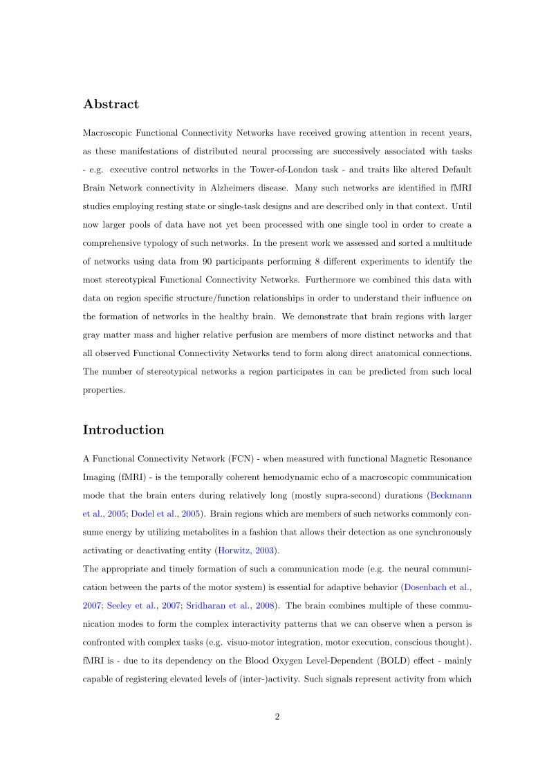
Abstract

Macroscopic Functional Connectivity Networks have received growing attention in recent years,

as these manifestations of distributed neural processing are successively associated with tasks

- e.g. executive control networks in the Tower-of-London task - and traits like altered Default

Brain Network connectivity in Alzheimers disease. Many such networks are identified in fMRI

studies employing resting state or single-task designs and are described only in that context. Until

now larger pools of data have not yet been processed with one single tool in order to create a

comprehensive typology of such networks. In the present work we assessed and sorted a multitude

of networks using data from 90 participants performing 8 different experiments to identify the

most stereotypical Functional Connectivity Networks. Furthermore we combined this data with

data on region specific structure/function relationships in order to understand their influence on

the formation of networks in the healthy brain. We demonstrate that brain regions with larger

gray matter mass and higher relative perfusion are members of more distinct networks and that

all observed Functional Connectivity Networks tend to form along direct anatomical connections.

The number of stereotypical networks a region participates in can be predicted from such local

properties.

Introduction

A Functional Connectivity Network (FCN) - when measured with functional Magnetic Resonance

Imaging (fMRI) - is the temporally coherent hemodynamic echo of a macroscopic communication

mode that the brain enters during relatively long (mostly supra-second) durations (Beckmann

et al., 2005; Dodel et al., 2005). Brain regions which are members of such networks commonly con-

sume energy by utilizing metabolites in a fashion that allows their detection as one synchronously

activating or deactivating entity (Horwitz, 2003).

The appropriate and timely formation of such a communication mode (e.g. the neural communi-

cation between the parts of the motor system) is essential for adaptive behavior (Dosenbach et al.,

2007; Seeley et al., 2007; Sridharan et al., 2008). The brain combines multiple of these commu-

nication modes to form the complex interactivity patterns that we can observe when a person is

confronted with complex tasks (e.g. visuo-motor integration, motor execution, conscious thought).

fMRI is - due to its dependency on the Blood Oxygen Level-Dependent (BOLD) effect - mainly

capable of registering elevated levels of (inter-)activity. Such signals represent activity from which

2

the information that is exchanged within a network can not be directly extracted (Logothetis,

2008). Therefore using fMRI alone, neural communication can not be comprehensively tapped.

Despite these strong limitations of fMRI, large-scale events like the coherent activation of an entire

neural mass or even the synchronous co-activation of two activation centers in a network can be

detected (e.g. bilateral activations of V1 and V2 as a reaction to visual stimuli). Although we are

presently only able to indirectly infer what information is communicated within such an activation

network, such activations and co-activation patterns are of a high diagnostic value, as they may

allow the experimenter to investigate the responsiveness and overall integrity of the communica-

tion modes the brain is capable of establishing.

Not all of these communication modes are task-dependent (Beckmann et al., 2005) and many

can be observed in a task-free resting state. Some of these networks have been noted to undergo

change over the course of maturation (Fair et al., 2008), and to vanish or be disrupted in certain

disorders. One example for the latter is the association of loss of consciousness with impaired

Default Brain Mode (DBM) activity (Raichle et al., 2001; Greicius et al., 2004).

Furthermore, not all detected FCNs necessarily represent patterns of macroscopic neural cooper-

ation and communication, but are in some cases confounds which are observed due to vasomotor

oscillations, temporally coherent pollution of the BOLD signal with physiological noise or other

reasons (McKeown et al., 1998; McKeown, 2003; Perlbarg et al., 2007). Other FCNs extracted

from activation data might be false-positives originating in a similar appearance of local activation

patterns over time in parts of the brain (homology), but without any information exchange within

these false-positive FCNs.

The creation of an extensive taxonomy of FCNs would serve us with a reference system that allows

us to classify newly observed networks into distinct classes, facilitate the interpretation of network

phenomena and aid the detection of network abnormalities in patient data. This approach is

already beginning to spread into clinical practice (Dosenbach et al., 2010).

Furthermore, such data could be mined with a multitude of methods to answer presently unre-

solved questions on network formation and network properties. Functional hubs which belong to

many networks have mostly been characterized using data from single sites and single experiments

(Achard et al., 2006; Bassett et al., 2006; Cohen et al., 2008; Bullmore and Sporns, 2009a; Demirci

et al., 2009; van den Heuvel et al., 2009; Van Dijk et al., 2010) but only seldom by unifying larger

amounts of data to identify global relationships between regional properties and local functional

network connectivity (Honey et al., 2009). Presently there are no comprehensive lists yet, which

3

would list all networks observed with fMRI, and allow us to answer the question, of how networks

in the human brain are generally constituted. Such a list of observed networks could be used to

identify families of spatially and functionally similar networks, and not only answer which are the

canonical brain networks that each healthy brain should be capable of establishing, but as well

answer how many families of similar networks there are in the healthy human brain.

To assure that only FCNs of neural origin are used for the formation of such a taxonomy, FCNs

as observed using fMRI have to be dissociated into networks of interest (networks representing

neural communication patterns) and networks not of interest (noise based confounds, phenomena

occurring due to homology and so on).

In order to dissociate the observed FCNs into these three basic types, the networks can be exten-

sively fingerprinted (Sporns et al., 2004; Smolders et al., 2007; Sui et al., 2009) by recording their

features (spatial extent, fractionality, spectral properties, interactivity patterns and correlations

with noise) and by clustering the FCNs based on their individual profile in such a multi-dimensional

feature space. We hypothesized that certain types of networks should form interpretable types of

clusters and allow us to label these clusters as network classes that contain FCNs of neural-origin

or otherwise. For example, physiological noise in the form of ventricular pulsations does occur

more in Cerebro-spinal fluid (CSF) than in gray matter (GM) and this ratio can be quantified for

each single FCN candidate and used for sorting.

Finally, the remaining networks of presumably neural origin can be clustered again based on their

spatial profile (regions of the brain involved) and characterized using their feature fingerprint (e.g.

networks containing the left and right temporal lobe always have low correlations of their activity

with ventricular pulsations). The technical problem at hand - with such a comprehensive list of

component features - is the appropriate clustering of this high-dimensional data into meaningful

classes and the proper interpretation of subspace clusters.

We decided to use Independent Component Analysis (ICA) to organize and extract the functional

connectivity data of 90 participants performing 8 different experiments over a total of 175 sessions

in a data-driven way, and to characterize each Independent Component (IC) with respect to its

IC fingerprint features. The data was organized using Self-Organizing Feature Maps (SOFM)

(Kohonen, 1990) and this bottom-up organized feature space was further organized with the Clu-

sot (Bogdan and Rosenstiel, 1999; Bogdan et al., 1999) software package by clustering the FCN

fingerprint feature maps. This latter cycle of SOFM organization and Clusot sorting is repeated

step by step first for spatial and subsequently for noise features in order to dissociate noise compo-

4

nents (confounds) from components representing networks of neural origin. These latter networks

were further organized with respect to their spatial extent in order to derive the most prominent

stereotypes of FCNs, equalling the taxonomy class centroids. This set of resulting - presumably

canonical - networks and the regions which were members of each respective network were further

characterized in terms of their anatomical connectivity, perfusion and regional tissue volume using

data from an earlier study (Varkuti et al., 2011). By combining these datasets, we were able to

study the most common properties of observed networks and aid our understanding of why the

observed networks form in the manner they were observed.

Such a dataset could be organized, clustered and mined with other methods, which is why we

supply the entire FCN x feature data in the online Supplementary Material and invite the reader

to conduct his own preferred type of analysis.

Materials and Methods

Experiments

All experiments were approved by the Internal Review Board of the Medical Faculty, University

of Tubingen. All participants provided written informed consent and all investigation was con-

ducted according to the principles expressed in the Declaration of Helsinki. Participants had no

history of neurological diseases, were mostly right handed and German native speakers. All MRI

measurements were performed in one Siemens Magneton Trio Tim 3T whole body scanner using

a standard 12 channel head coil.

Experiment 1 - Tower of London

Sixteen healthy subjects (7 male, average age 24.9 SD 3.9) participated in a training session prior

to the experiment where they were presented with 30 Tower of London (ToL) (Baker et al., 1996)

problems with different difficulty levels (number of necessary moves ranging from 1 to 5). For each

problem, two possible solutions were presented and subjects had to select the correct solution by

button press. Subjects were admitted to the fMRI experiment (EPI TR=1.3 sec, 3x3x3.2 mm

voxels, gap=1 mm, 21 transversal slices, TE 30ms, descending acquisition, 90 ◦ flip angle) as soon

as they were able to complete all training problems correctly. Once placed in the scanner, subjects

completed a pseudo-randomized sequence of 50 new ToL problems (within the allowed time of 20

seconds), with 10 problems per difficulty level.

5

Experiment 2 - Tracking task with a joystick

Eight healthy participants (3 male, average age 25 SD 3.1) were trained inside the scanner (EPI

TR=1.84 sec, 3x3x4 mm voxels, gap=1 mm, 30 transversal slices, TE 30ms, descending acquisition,

74 ◦ flip angle) to steer a dot through an animated landscape that consisted of two sine waves, one

placed above the other. The participant had to steer the dot through the cave of the sine waves

using a MR-safe joystick without touching the boundaries or leaving the cave. If the participant

crossed the boundaries, the dot turned red. The dot could only be moved along the vertical axis.

In the subsequent actual task, the participant had to master the task with changing precision

demands (distance of the boundaries was closer or further apart), disturbances (random wind)

and switches of the joystick direction polarity.

Experiment 3 - Tapping task with a button box

Nine healthy participants (6 male, average age 24.1 SD 1.6) were trained inside the scanner (EPI

TR=1.84 sec, 3x3x4 mm voxels, gap=1 mm, 30 transversal slices, TE 30ms, descending acquisition,

74 ◦ flip angle) to respond to an animated task of four circles, falling down and flipping back after

one another. The participant had to press the appropriate button for each circle exactly when

the circle hit the lowest point. If the participant did not press the right button in time, the circle

turned red. In the subsequent actual task, the participant had to master the task with changing

precision demands (error tolerance for timing imprecision of button press was varied), disturbances

(circles did not fall in a particular order but randomly) and switches of the control device polarity

(e.g. outer left circle was not represented anymore by outer left button, but by outer right button).

Experiment 4 - Detection of deception

Fifteen healthy volunteers (6 male, average age 26 SD 4.7) participated in a thief role-play and

were subsequently interrogated using a video questioning and visual depiction of objects setup

within the scanner (EPI TR=1.5 sec, 3x3x3.5 mm voxels, gap=1 mm, 21 transversal slices, TE

30ms, descending acquisition, 90 ◦ flip angle). Participants responded to the questions by the

video interrogator by pressing a button for yes or no and by doing so, heard their own prerecorded

voice over MR safe headphones, giving the answer. Participants tried to conceal their involvement

in the deed by giving untruthful answers with respect to recognizing presented objects from the

thief-role play room (Concealed Information Test).

6

Experiment 5-7 - Motor imagination, observation and execution

17 healthy participants (10 male, average age 23.47 SD 2.72) participated in three fMRI experi-

ments (EPI TR=2 sec, 3x3x3.5 mm voxels, gap=1 mm, 32 transversal slices, TE 30ms, descending

acquisition, 90 ◦ flip angle). Each participant performed a motor imagery, observation and execu-

tion experiment in the fMRI. Each experiment - as reported earlier in (Halder et al., 2011) - was

repeated once, resulting in a total of six measurements (two of each task) per participant. One

of the experiments consisted of seven blocks of 30 seconds in which participants were required to

perform motor tasks such as execution of left hand, right hand or foot (preferred side) movements

according to arrows displayed on the screen pointing to the left, right or down. Since each ex-

periment was repeated there were in total 14 blocks per motor task. Each motor task block was

followed by a 30 s resting period. In the observation condition, participants were instructed to

attend to videos of ten seconds length. Videos showed either left or right hand squeezing of a

ball, or feet moving their toes (recorded from a first person’s perspective). The participants were

instructed to mentally imitate the observed movement from a first person’s perspective as opposed

to a distanced, evaluative observation of the displayed movement from a third person perspective

(Zentgraf et al., 2005). Finally, in the imagery condition, participants were asked to imagine

movement according to certain displayed cues. The participants were specifically instructed to use

kinesthetic and not visual movement imagery (Neuper and Scherer, 2005). The feeling one has

when moving feet in sand was provided as an example of kinesthetic imagery to all participants.

It was emphasized that the focus of the imagery should be kinesthetic sensation. The length of

trial and pause were the same as during movement execution.

Experiment 8 - Resting state

Twenty-five subjects participated in a resting state (eyes closed) fMRI measurement (duration 10

min 20 s, 9 male, average age 41.3 SD 11,4, EPI TR=1.53 sec, 3x3x3 mm voxels, gap=1 mm, 25

transversal slices, TE 30ms, descending acquisition, 90 ◦ flip angle). Twelve of the participants

were a subset of participants reported on in an earlier study (Keune et al., 2011) and had been

diagnosed with repeated episodes of Major Depressive Disorder in the past but were in remission

and symptom free at the time of measurement (as evaluated with ICD 10 Symptom Questionnaire

which covers a time of up to two weeks before the time of measurement).

7

Data flow

fMRI data preprocessing

All fMRI image series were preprocessed session-wise using SPM8 (Wellcome Trust Centre for

Neuroimaging, London). Functional images were realigned (4th degree B-Spline interpolation)

to the mean image, slice timing corrected to the middle slice, normalized (4th degree B-Spline

interpolation) into 3x3x3 mm MNI-space and smoothed using an 8-mm Full Width Half Maximum

kernel.

Group ICA details

Each of the 8 experiment datasets (a total of 90 subjects distributed over five single-session and

three two-session experiments resulting in a total of 175 sessions) was analyzed with one Group

ICA (Correa et al., 2007) separately for each experiment using the 1.3d version of the GIFT-

ICA toolbox (Calhoun, 2004). The optimal number of ICs was calculated for each Group ICA

using the ICASSO (Himberg and Hyvarinen, 2003) approach (run 20 times, with both ’randinit’

and ’bootstrap’). Each ICA was run with the Infomax algorithm (Bell and Sejnowski, 1995),

back-reconstruction was performed using the GICA3 implementation (Erhardt et al., 2010), data-

preprocessing was done by removing the mean per time point, PCA options were standard (double

precision, selective eigen solver, maximum number of reduction steps was two, batch estimation,

Minimum Description Length estimation option mean, number of principle components to reduce

each subject down to at reduction step one was 20, at two 16) and results were scaled to z-scores.

All further analysis such as IC image analysis, feature computations and listing of results were

realized on the lowest level of abstraction - namely the subject-session image-level instead of the

group-experiment mean images-level. The ICASSO results were further used to select only highly

stable components for further processing, so that the component list was filtered and components

with an ICASSO component stability value (how stably a component is extracted repeatedly by

the partially stochastic ICA process from the data) below 0.9 were removed (from 7705 initial

components, 847 equalling 10.9 % of all resulting components were removed due to low stability).

A total of 7705 initial components in the list equal an average of 44 detected ICs per session.

Binary-coding of IC images

IC images were binary-coded for the calculation of spatial features by thresholding the z-scored

output images at a cutoff value of 1.75. Although IC images contain negative values as well,

8

indicating parts of the IC whose activity is generally anti-correlated with the ICs positive value

marked regions, we only used the IC image voxels above our positive threshold in this approach to

characterize the components spatial features. The rationale for this is, that although a component

is logically made up of two anti-correlated parts both of which contribute to the raw BOLD signal,

a functional network of neural origin is most clearly defined as a region that coherently activates

and deactivates together as one network, rather than two regions or networks whose activity

patterns are opposing.

Feature Computation

Spatial Features

The T1 images of all participants were processed using the SPM VBM5 software package (Ash-

burner and Friston, 2001; Mechelli et al., 2005) and the individual GM, white matter (WM)

and CSF modulated and unmodulated segmentation outputs were estimated. We used the tissue

probability maps provided within the SPM5 template set since the subjects were drawn from the

appropriate population. We applied the thorough clean-up option of the VBM toolbox and made

use of a medium Hidden Markov Random Field model for an optimal denoising of the T1 image.

As the modulated outputs can be corrected for non-linear warping only and therefore make any

further correction for different brain size redundant, we created a study specific template by aver-

aging all modulated segmentation outputs into a GM, WM and CSF template, respectively. These

templates were resliced into the appropriate voxel space of the IC output images and the portion

of each components spatial extent that resided in GM, WM, CSF or outside of all these three

(termed Out-of-Brain (OFB)) was calculated as a percentage output (Features 1-4). Furthermore,

we calculated the total number of voxels belonging to an IC (Feature 5) as well as the spatial

fractionality/smoothness of the component (Feature 6) by calculating the number of neighbouring

IC voxels (using a 3D 26-neighbours model) over the amount of total IC voxels (components scat-

tered widely over the brain would get a lower value than e.g. components compromised of a single

adjacent voxel mass). Each binary-coded component’s percentage overlap with regions of the AAL

atlas (Tzourio-Mazoyer et al., 2002) was calculated (with a separate calculation of overlap with a

DBM regions mask) and saved for the first 90 cerebral regions of the atlas (see Attachment A).

9

Noise Features

We extracted and averaged the raw BOLD values from the preprocessed fMRI images of each

session from the voxels within the CSF-template mask (see spatial features), an accordingly resliced

ventricle mask (all ventricles, template from the WFU PickAtlas (Maldjian and Laurienti, 2003),

dilated by 1 voxel) and the total volume (all voxels per image). The component timecourses

were then correlated with the respective noise timecourses (p=0.05) and the correlation values

were squared (Features 7-9). The six movement regressors (three translational, three rotational)

derived for each session from the realignment-preprocessing step in SPM8 were used as predictors

in a multiple regression to predict each component’s timecourse. For components corresponding

to head movements the multiple regression is significant and results in a high R2 (Feature 10).

Spectral Features

The Power Spectral Density (PSD) plot for each component per session was calculated using a

discrete Fast Fourier Transform, with the normalized and detrended component timecourse as

input. The resulting PSD plot was characterized with respect to kurtosis, skewness and peak.

As the lowest sampling frequency in the dataset was 0.5 Hz (TR=2 seconds) only information

for the frequencies up to 0.25 Hz was utilized (Features 11-13). In analogy to the frequency bin

power feature calculation function within GIFT (Spectral Group compare), we further calculated

the power in the frequency bins 0-0.04, 0.04-0.08, 0.08-0.12, 0.12-0.16, 0.16-0.2, 0.2-0.24 Hz with

a dynamic adaptation of bin width depending on session-specific frequency resolution/sampling

rate (Features 14-19).

Interactivity features

Brain networks are known to interact with one another and such interactivity patterns can contain

significant information on the underlying neural processes (Demirci et al., 2009). We calculated

the Granger Causality interactions (time-domain) for all components of a session using their

normalized and detrended back-reconstructed component timecourses as input for a multivariate

Granger Causality implementation (Seth, 2005, 2010). In order to account for the variable TRs, the

optimal model order was calculated using the Aikake Information Criterion (order range: 2-3) and

time-delayed component interactivity was assessed using a Bonferroni-corrected p-value threshold

of 0.05. The resulting component interactivity graphs were transformed into Granger Causal

outflow, inflow, total flow, weighted outflow and weighted inflow metrics for each component per

10

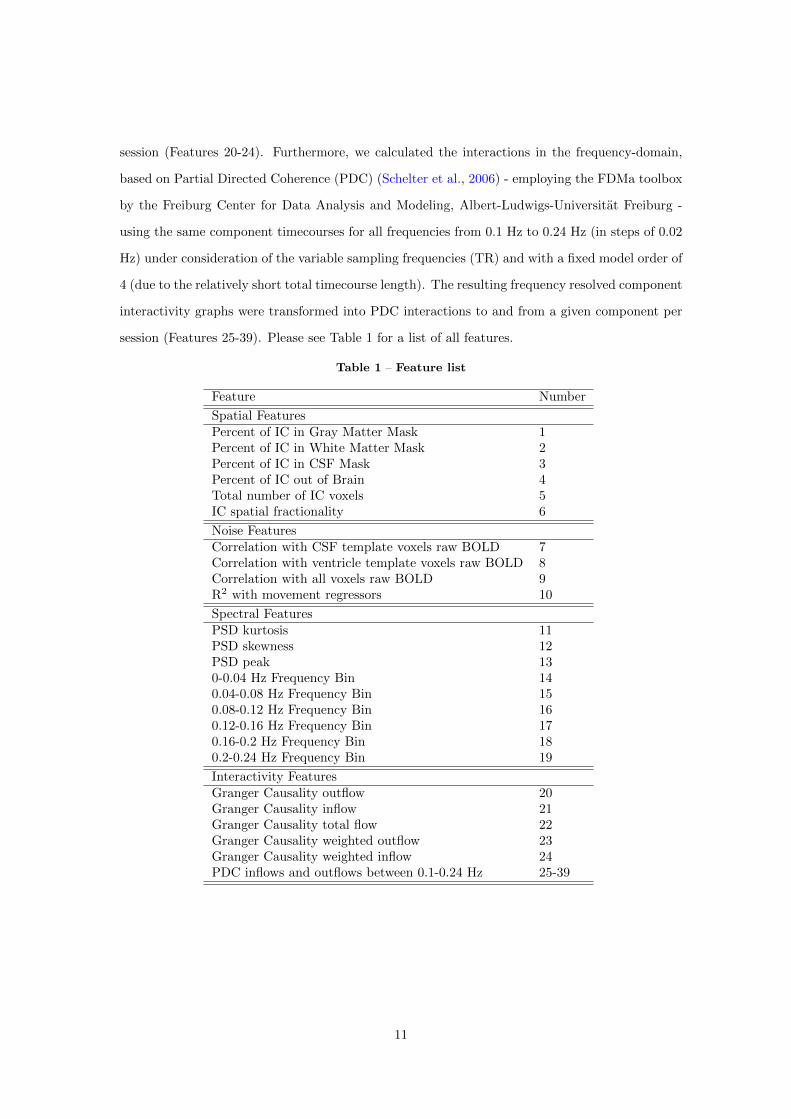
session (Features 20-24). Furthermore, we calculated the interactions in the frequency-domain,

based on Partial Directed Coherence (PDC) (Schelter et al., 2006) - employing the FDMa toolbox

by the Freiburg Center for Data Analysis and Modeling, Albert-Ludwigs-Universitat Freiburg -

using the same component timecourses for all frequencies from 0.1 Hz to 0.24 Hz (in steps of 0.02

Hz) under consideration of the variable sampling frequencies (TR) and with a fixed model order of

4 (due to the relatively short total timecourse length). The resulting frequency resolved component

interactivity graphs were transformed into PDC interactions to and from a given component per

session (Features 25-39). Please see Table 1 for a list of all features.

Table 1 – Feature list

Feature Number

Spatial FeaturesPercent of IC in Gray Matter Mask 1Percent of IC in White Matter Mask 2Percent of IC in CSF Mask 3Percent of IC out of Brain 4Total number of IC voxels 5IC spatial fractionality 6

Noise FeaturesCorrelation with CSF template voxels raw BOLD 7Correlation with ventricle template voxels raw BOLD 8Correlation with all voxels raw BOLD 9R2 with movement regressors 10

Spectral FeaturesPSD kurtosis 11PSD skewness 12PSD peak 130-0.04 Hz Frequency Bin 140.04-0.08 Hz Frequency Bin 150.08-0.12 Hz Frequency Bin 160.12-0.16 Hz Frequency Bin 170.16-0.2 Hz Frequency Bin 180.2-0.24 Hz Frequency Bin 19

Interactivity FeaturesGranger Causality outflow 20Granger Causality inflow 21Granger Causality total flow 22Granger Causality weighted outflow 23Granger Causality weighted inflow 24PDC inflows and outflows between 0.1-0.24 Hz 25-39

11

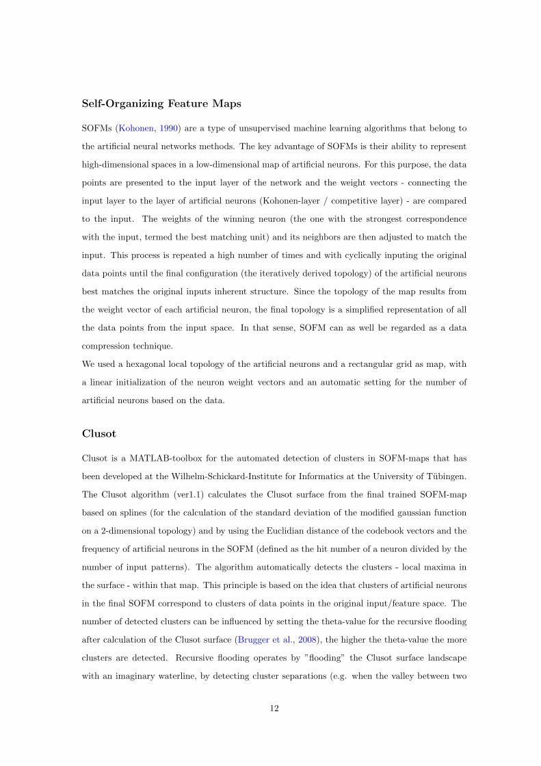
Self-Organizing Feature Maps

SOFMs (Kohonen, 1990) are a type of unsupervised machine learning algorithms that belong to

the artificial neural networks methods. The key advantage of SOFMs is their ability to represent

high-dimensional spaces in a low-dimensional map of artificial neurons. For this purpose, the data

points are presented to the input layer of the network and the weight vectors - connecting the

input layer to the layer of artificial neurons (Kohonen-layer / competitive layer) - are compared

to the input. The weights of the winning neuron (the one with the strongest correspondence

with the input, termed the best matching unit) and its neighbors are then adjusted to match the

input. This process is repeated a high number of times and with cyclically inputing the original

data points until the final configuration (the iteratively derived topology) of the artificial neurons

best matches the original inputs inherent structure. Since the topology of the map results from

the weight vector of each artificial neuron, the final topology is a simplified representation of all

the data points from the input space. In that sense, SOFM can as well be regarded as a data

compression technique.

We used a hexagonal local topology of the artificial neurons and a rectangular grid as map, with

a linear initialization of the neuron weight vectors and an automatic setting for the number of

artificial neurons based on the data.

Clusot

Clusot is a MATLAB-toolbox for the automated detection of clusters in SOFM-maps that has

been developed at the Wilhelm-Schickard-Institute for Informatics at the University of Tubingen.

The Clusot algorithm (ver1.1) calculates the Clusot surface from the final trained SOFM-map

based on splines (for the calculation of the standard deviation of the modified gaussian function

on a 2-dimensional topology) and by using the Euclidian distance of the codebook vectors and the

frequency of artificial neurons in the SOFM (defined as the hit number of a neuron divided by the

number of input patterns). The algorithm automatically detects the clusters - local maxima in

the surface - within that map. This principle is based on the idea that clusters of artificial neurons

in the final SOFM correspond to clusters of data points in the original input/feature space. The

number of detected clusters can be influenced by setting the theta-value for the recursive flooding

after calculation of the Clusot surface (Brugger et al., 2008), the higher the theta-value the more

clusters are detected. Recursive flooding operates by ”flooding” the Clusot surface landscape

with an imaginary waterline, by detecting cluster separations (e.g. when the valley between two

12

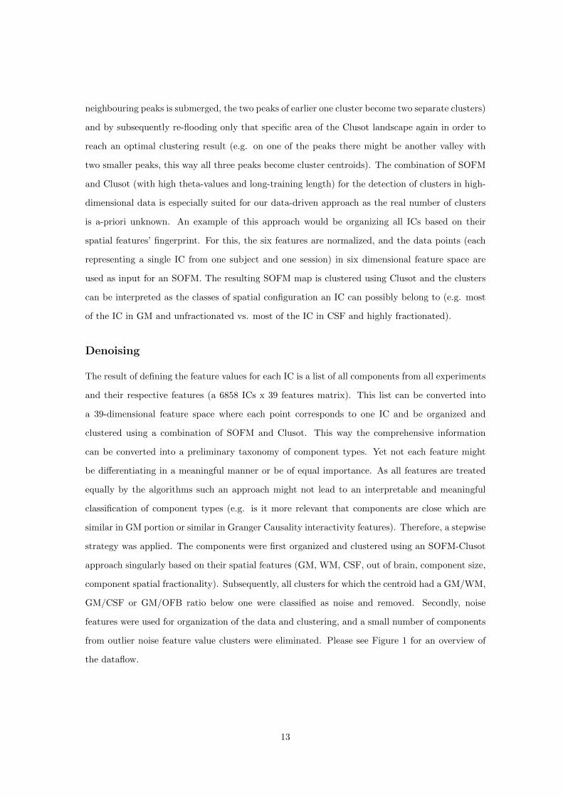
neighbouring peaks is submerged, the two peaks of earlier one cluster become two separate clusters)

and by subsequently re-flooding only that specific area of the Clusot landscape again in order to

reach an optimal clustering result (e.g. on one of the peaks there might be another valley with

two smaller peaks, this way all three peaks become cluster centroids). The combination of SOFM

and Clusot (with high theta-values and long-training length) for the detection of clusters in high-

dimensional data is especially suited for our data-driven approach as the real number of clusters

is a-priori unknown. An example of this approach would be organizing all ICs based on their

spatial features’ fingerprint. For this, the six features are normalized, and the data points (each

representing a single IC from one subject and one session) in six dimensional feature space are

used as input for an SOFM. The resulting SOFM map is clustered using Clusot and the clusters

can be interpreted as the classes of spatial configuration an IC can possibly belong to (e.g. most

of the IC in GM and unfractionated vs. most of the IC in CSF and highly fractionated).

Denoising

The result of defining the feature values for each IC is a list of all components from all experiments

and their respective features (a 6858 ICs x 39 features matrix). This list can be converted into

a 39-dimensional feature space where each point corresponds to one IC and be organized and

clustered using a combination of SOFM and Clusot. This way the comprehensive information

can be converted into a preliminary taxonomy of component types. Yet not each feature might

be differentiating in a meaningful manner or be of equal importance. As all features are treated

equally by the algorithms such an approach might not lead to an interpretable and meaningful

classification of component types (e.g. is it more relevant that components are close which are

similar in GM portion or similar in Granger Causality interactivity features). Therefore, a stepwise

strategy was applied. The components were first organized and clustered using an SOFM-Clusot

approach singularly based on their spatial features (GM, WM, CSF, out of brain, component size,

component spatial fractionality). Subsequently, all clusters for which the centroid had a GM/WM,

GM/CSF or GM/OFB ratio below one were classified as noise and removed. Secondly, noise

features were used for organization of the data and clustering, and a small number of components

from outlier noise feature value clusters were eliminated. Please see Figure 1 for an overview of

the dataflow.

13

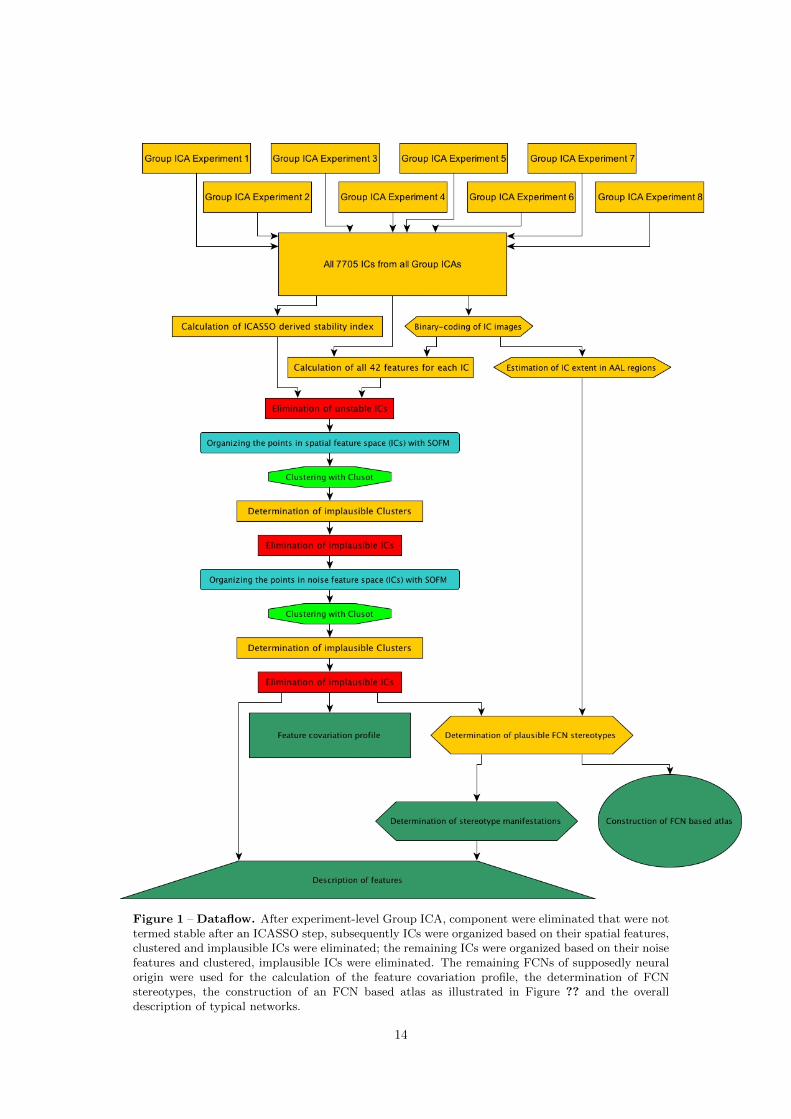
Figure 1 – Dataflow. After experiment-level Group ICA, component were eliminated that were nottermed stable after an ICASSO step, subsequently ICs were organized based on their spatial features,clustered and implausible ICs were eliminated; the remaining ICs were organized based on their noisefeatures and clustered, implausible ICs were eliminated. The remaining FCNs of supposedly neuralorigin were used for the calculation of the feature covariation profile, the determination of FCNstereotypes, the construction of an FCN based atlas as illustrated in Figure ?? and the overalldescription of typical networks.

14

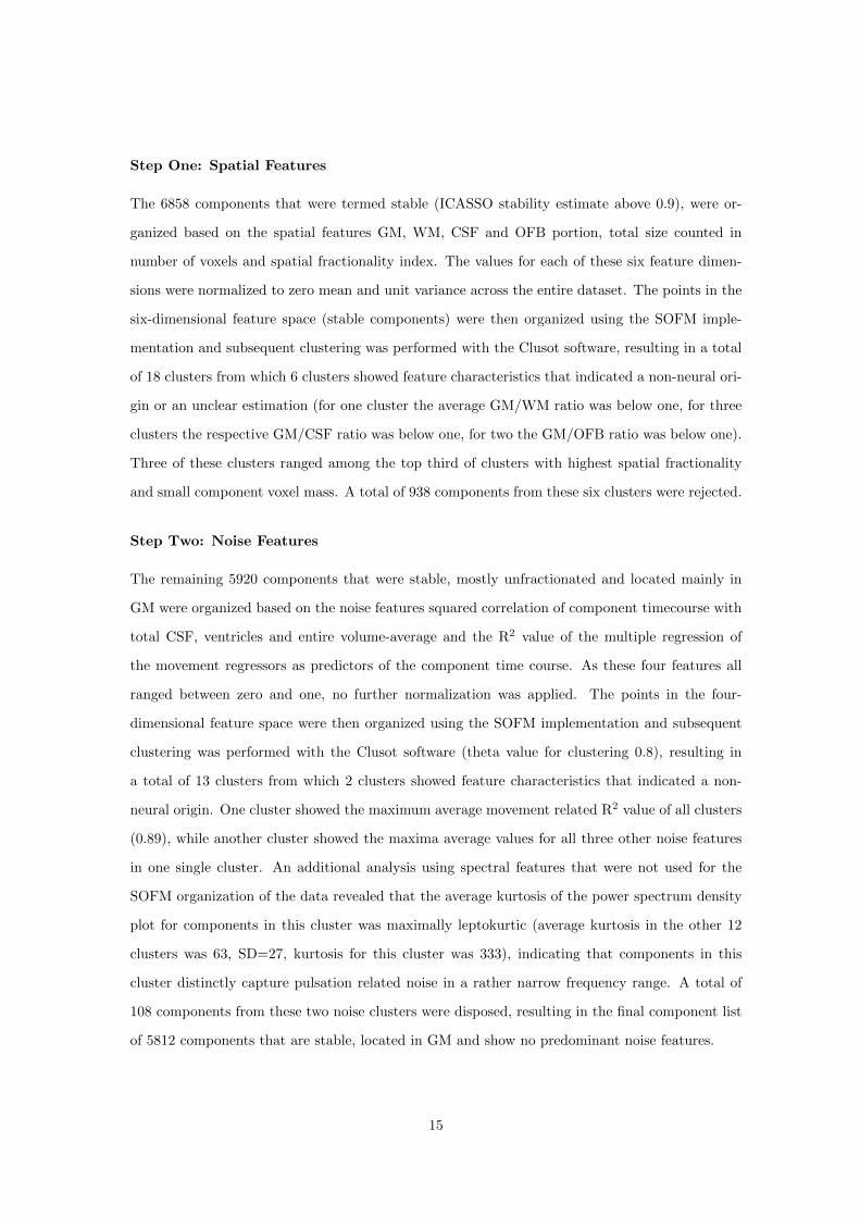
Step One: Spatial Features

The 6858 components that were termed stable (ICASSO stability estimate above 0.9), were or-

ganized based on the spatial features GM, WM, CSF and OFB portion, total size counted in

number of voxels and spatial fractionality index. The values for each of these six feature dimen-

sions were normalized to zero mean and unit variance across the entire dataset. The points in the

six-dimensional feature space (stable components) were then organized using the SOFM imple-

mentation and subsequent clustering was performed with the Clusot software, resulting in a total

of 18 clusters from which 6 clusters showed feature characteristics that indicated a non-neural ori-

gin or an unclear estimation (for one cluster the average GM/WM ratio was below one, for three

clusters the respective GM/CSF ratio was below one, for two the GM/OFB ratio was below one).

Three of these clusters ranged among the top third of clusters with highest spatial fractionality

and small component voxel mass. A total of 938 components from these six clusters were rejected.

Step Two: Noise Features

The remaining 5920 components that were stable, mostly unfractionated and located mainly in

GM were organized based on the noise features squared correlation of component timecourse with

total CSF, ventricles and entire volume-average and the R2 value of the multiple regression of

the movement regressors as predictors of the component time course. As these four features all

ranged between zero and one, no further normalization was applied. The points in the four-

dimensional feature space were then organized using the SOFM implementation and subsequent

clustering was performed with the Clusot software (theta value for clustering 0.8), resulting in

a total of 13 clusters from which 2 clusters showed feature characteristics that indicated a non-

neural origin. One cluster showed the maximum average movement related R2 value of all clusters

(0.89), while another cluster showed the maxima average values for all three other noise features

in one single cluster. An additional analysis using spectral features that were not used for the

SOFM organization of the data revealed that the average kurtosis of the power spectrum density

plot for components in this cluster was maximally leptokurtic (average kurtosis in the other 12

clusters was 63, SD=27, kurtosis for this cluster was 333), indicating that components in this

cluster distinctly capture pulsation related noise in a rather narrow frequency range. A total of

108 components from these two noise clusters were disposed, resulting in the final component list

of 5812 components that are stable, located in GM and show no predominant noise features.

15

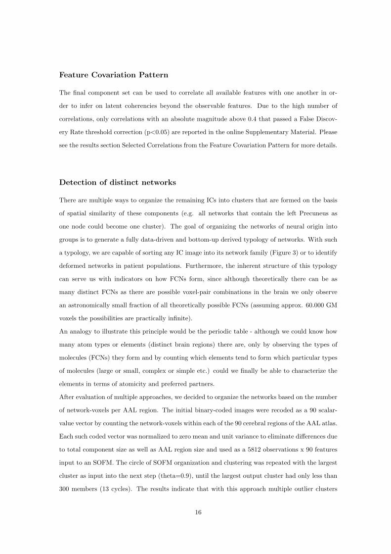
Feature Covariation Pattern

The final component set can be used to correlate all available features with one another in or-

der to infer on latent coherencies beyond the observable features. Due to the high number of

correlations, only correlations with an absolute magnitude above 0.4 that passed a False Discov-

ery Rate threshold correction (p<0.05) are reported in the online Supplementary Material. Please

see the results section Selected Correlations from the Feature Covariation Pattern for more details.

Detection of distinct networks

There are multiple ways to organize the remaining ICs into clusters that are formed on the basis

of spatial similarity of these components (e.g. all networks that contain the left Precuneus as

one node could become one cluster). The goal of organizing the networks of neural origin into

groups is to generate a fully data-driven and bottom-up derived typology of networks. With such

a typology, we are capable of sorting any IC image into its network family (Figure 3) or to identify

deformed networks in patient populations. Furthermore, the inherent structure of this typology

can serve us with indicators on how FCNs form, since although theoretically there can be as

many distinct FCNs as there are possible voxel-pair combinations in the brain we only observe

an astronomically small fraction of all theoretically possible FCNs (assuming approx. 60.000 GM

voxels the possibilities are practically infinite).

An analogy to illustrate this principle would be the periodic table - although we could know how

many atom types or elements (distinct brain regions) there are, only by observing the types of

molecules (FCNs) they form and by counting which elements tend to form which particular types

of molecules (large or small, complex or simple etc.) could we finally be able to characterize the

elements in terms of atomicity and preferred partners.

After evaluation of multiple approaches, we decided to organize the networks based on the number

of network-voxels per AAL region. The initial binary-coded images were recoded as a 90 scalar-

value vector by counting the network-voxels within each of the 90 cerebral regions of the AAL atlas.

Each such coded vector was normalized to zero mean and unit variance to eliminate differences due

to total component size as well as AAL region size and used as a 5812 observations x 90 features

input to an SOFM. The circle of SOFM organization and clustering was repeated with the largest

cluster as input into the next step (theta=0.9), until the largest output cluster had only less than

300 members (13 cycles). The results indicate that with this approach multiple outlier clusters

16

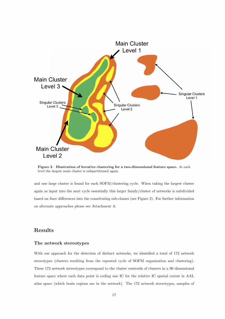
Figure 2 – Illustration of iterative clustering for a two-dimensional feature space. At eachlevel the largest main cluster is subpartitioned again.

and one large cluster is found for each SOFM/clustering cycle. When taking the largest cluster

again as input into the next cycle essentially this larger family/cluster of networks is subdivided

based on finer differences into the constituting sub-classes (see Figure 2). For further information

on alternate approaches please see Attachment A.

Results

The network stereotypes

With our approach for the detection of distinct networks, we identified a total of 172 network

stereotypes (clusters resulting from the repeated cycle of SOFM organization and clustering).

These 172 network stereotypes correspond to the cluster centroids of clusters in a 90 dimensional

feature space where each data point is coding one IC for the relative IC spatial extent in AAL

atlas space (which brain regions are in the network). The 172 network stereotypes, samples of

17

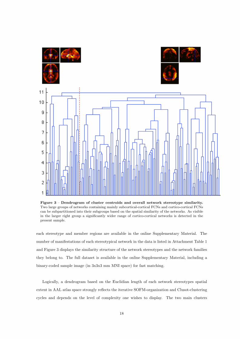
Figure 3 – Dendrogram of cluster centroids and overall network stereotype similarity.Two large groups of networks containing mainly subcortical-cortical FCNs and cortico-cortical FCNscan be subpartitioned into their subgroups based on the spatial similarity of the networks. As visiblein the larger right group a significantly wider range of cortico-cortical networks is detected in thepresent sample.

each stereotype and member regions are available in the online Supplementary Material. The

number of manifestations of each stereotypical network in the data is listed in Attachment Table 1

and Figure 3 displays the similarity structure of the network stereotypes and the network families

they belong to. The full dataset is available in the online Supplementary Material, including a

binary-coded sample image (in 3x3x3 mm MNI space) for fast matching.

Logically, a dendrogram based on the Euclidian length of each network stereotypes spatial

extent in AAL atlas space strongly reflects the iterative SOFM-organization and Clusot-clustering

cycles and depends on the level of complexity one wishes to display. The two main clusters

18

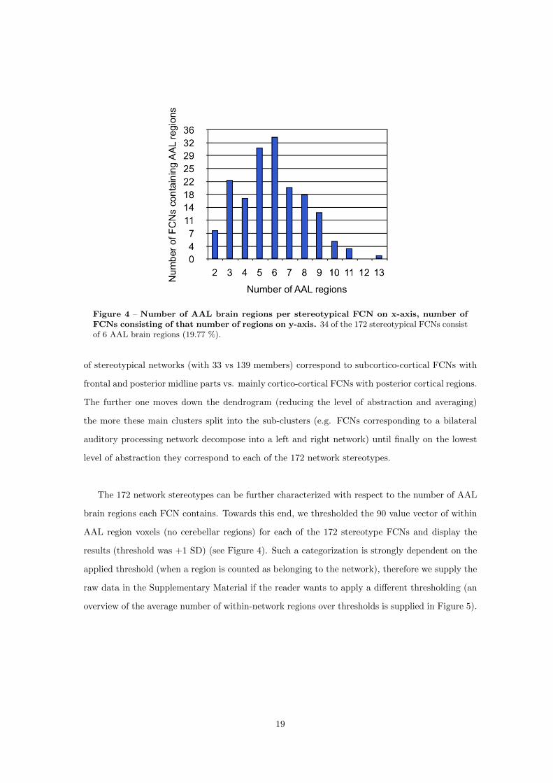
Figure 4 – Number of AAL brain regions per stereotypical FCN on x-axis, number ofFCNs consisting of that number of regions on y-axis. 34 of the 172 stereotypical FCNs consistof 6 AAL brain regions (19.77 %).

of stereotypical networks (with 33 vs 139 members) correspond to subcortico-cortical FCNs with

frontal and posterior midline parts vs. mainly cortico-cortical FCNs with posterior cortical regions.

The further one moves down the dendrogram (reducing the level of abstraction and averaging)

the more these main clusters split into the sub-clusters (e.g. FCNs corresponding to a bilateral

auditory processing network decompose into a left and right network) until finally on the lowest

level of abstraction they correspond to each of the 172 network stereotypes.

The 172 network stereotypes can be further characterized with respect to the number of AAL

brain regions each FCN contains. Towards this end, we thresholded the 90 value vector of within

AAL region voxels (no cerebellar regions) for each of the 172 stereotype FCNs and display the

results (threshold was +1 SD) (see Figure 4). Such a categorization is strongly dependent on the

applied threshold (when a region is counted as belonging to the network), therefore we supply the

raw data in the Supplementary Material if the reader wants to apply a different thresholding (an

overview of the average number of within-network regions over thresholds is supplied in Figure 5).

19

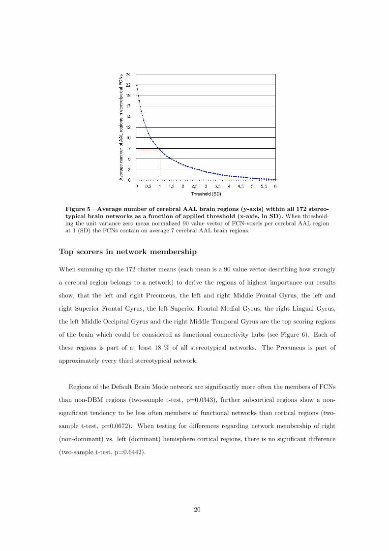
Figure 5 – Average number of cerebral AAL brain regions (y-axis) within all 172 stereo-typical brain networks as a function of applied threshold (x-axis, in SD). When threshold-ing the unit variance zero mean normalized 90 value vector of FCN-voxels per cerebral AAL regionat 1 (SD) the FCNs contain on average 7 cerebral AAL brain regions.

Top scorers in network membership

When summing up the 172 cluster means (each mean is a 90 value vector describing how strongly

a cerebral region belongs to a network) to derive the regions of highest importance our results

show, that the left and right Precuneus, the left and right Middle Frontal Gyrus, the left and

right Superior Frontal Gyrus, the left Superior Frontal Medial Gyrus, the right Lingual Gyrus,

the left Middle Occipital Gyrus and the right Middle Temporal Gyrus are the top scoring regions

of the brain which could be considered as functional connectivity hubs (see Figure 6). Each of

these regions is part of at least 18 % of all stereotypical networks. The Precuneus is part of

approximately every third stereotypical network.

Regions of the Default Brain Mode network are significantly more often the members of FCNs

than non-DBM regions (two-sample t-test, p=0.0343), further subcortical regions show a non-

significant tendency to be less often members of functional networks than cortical regions (two-

sample t-test, p=0.0672). When testing for differences regarding network membership of right

(non-dominant) vs. left (dominant) hemisphere cortical regions, there is no significant difference

(two-sample t-test, p=0.6442).

20

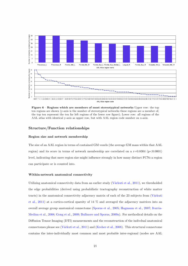
Figure 6 – Regions which are members of most stereotypical networks Upper row: the topten regions are shown (y-axis is the number of stereotypical networks these regions are a member of,the top ten represent the ten far left regions of the lower row figure); Lower row: all regions of theAAL atlas with identical y-axis as upper row, but with AAL region code number on x-axis.

Structure/Function relationships

Region size and network membership

The size of an AAL region in terms of contained GM voxels (the average GM mass within that AAL

region) and its score in terms of network membership are correlated on a r=0.8304 (p<0.0001)

level, indicating that mere region size might influence strongly in how many distinct FCNs a region

can participate or is counted into.

Within-network anatomical connectivity

Utilizing anatomical connectivity data from an earlier study (Varkuti et al., 2011), we thresholded

the edge probabilities (derived using probabilistic tractography reconstruction of white matter

tracts) in the anatomical connectivity adjacency matrix of each of the 23 subjects from (Varkuti

et al., 2011) at a cortico-cortical sparsity of 14 % and averaged the adjacency matrices into an

overall average group anatomical connectome (Sporns et al., 2005; Hagmann et al., 2007; Iturria-

Medina et al., 2008; Gong et al., 2009; Bullmore and Sporns, 2009a). For methodical details on the

Diffusion Tensor Imaging (DTI) measurements and the reconstruction of the indivdual anatomical

connectomes please see (Varkuti et al., 2011) and (Kreher et al., 2008). This structural connectome

contains the inter-individually most common and most probable inter-regional (nodes are AAL

21

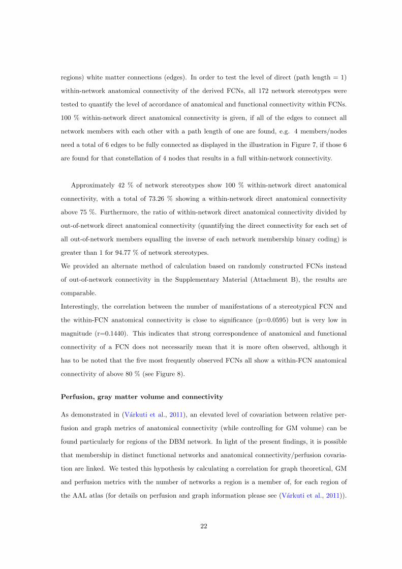
regions) white matter connections (edges). In order to test the level of direct (path length = 1)

within-network anatomical connectivity of the derived FCNs, all 172 network stereotypes were

tested to quantify the level of accordance of anatomical and functional connectivity within FCNs.

100 % within-network direct anatomical connectivity is given, if all of the edges to connect all

network members with each other with a path length of one are found, e.g. 4 members/nodes

need a total of 6 edges to be fully connected as displayed in the illustration in Figure 7, if those 6

are found for that constellation of 4 nodes that results in a full within-network connectivity.

Approximately 42 % of network stereotypes show 100 % within-network direct anatomical

connectivity, with a total of 73.26 % showing a within-network direct anatomical connectivity

above 75 %. Furthermore, the ratio of within-network direct anatomical connectivity divided by

out-of-network direct anatomical connectivity (quantifying the direct connectivity for each set of

all out-of-network members equalling the inverse of each network membership binary coding) is

greater than 1 for 94.77 % of network stereotypes.

We provided an alternate method of calculation based on randomly constructed FCNs instead

of out-of-network connectivity in the Supplementary Material (Attachment B), the results are

comparable.

Interestingly, the correlation between the number of manifestations of a stereotypical FCN and

the within-FCN anatomical connectivity is close to significance (p=0.0595) but is very low in

magnitude (r=0.1440). This indicates that strong correspondence of anatomical and functional

connectivity of a FCN does not necessarily mean that it is more often observed, although it

has to be noted that the five most frequently observed FCNs all show a within-FCN anatomical

connectivity of above 80 % (see Figure 8).

Perfusion, gray matter volume and connectivity

As demonstrated in (Varkuti et al., 2011), an elevated level of covariation between relative per-

fusion and graph metrics of anatomical connectivity (while controlling for GM volume) can be

found particularly for regions of the DBM network. In light of the present findings, it is possible

that membership in distinct functional networks and anatomical connectivity/perfusion covaria-

tion are linked. We tested this hypothesis by calculating a correlation for graph theoretical, GM

and perfusion metrics with the number of networks a region is a member of, for each region of

the AAL atlas (for details on perfusion and graph information please see (Varkuti et al., 2011)).

22

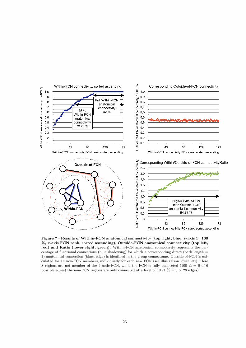
Figure 7 – Results of Within-FCN anatomical connectivity (top right, blue, y-axis 1=100%, x-axis FCN rank, sorted ascending), Outside-FCN anatomical connectivity (top left,red) and Ratio (lower right, green). Within-FCN anatomical connectivity represents the per-centage of functional connections (blue shadowing) for which a corresponding direct (path length =1) anatomical connection (black edge) is identified in the group connectome. Outside-of-FCN is cal-culated for all non-FCN members, individually for each new FCN (see illustration lower left). Here8 regions are not member of the 4-node-FCN, while the FCN is fully connected (100 % = 6 of 6possible edges) the non-FCN regions are only connected at a level of 10.71 % = 3 of 28 edges).

23

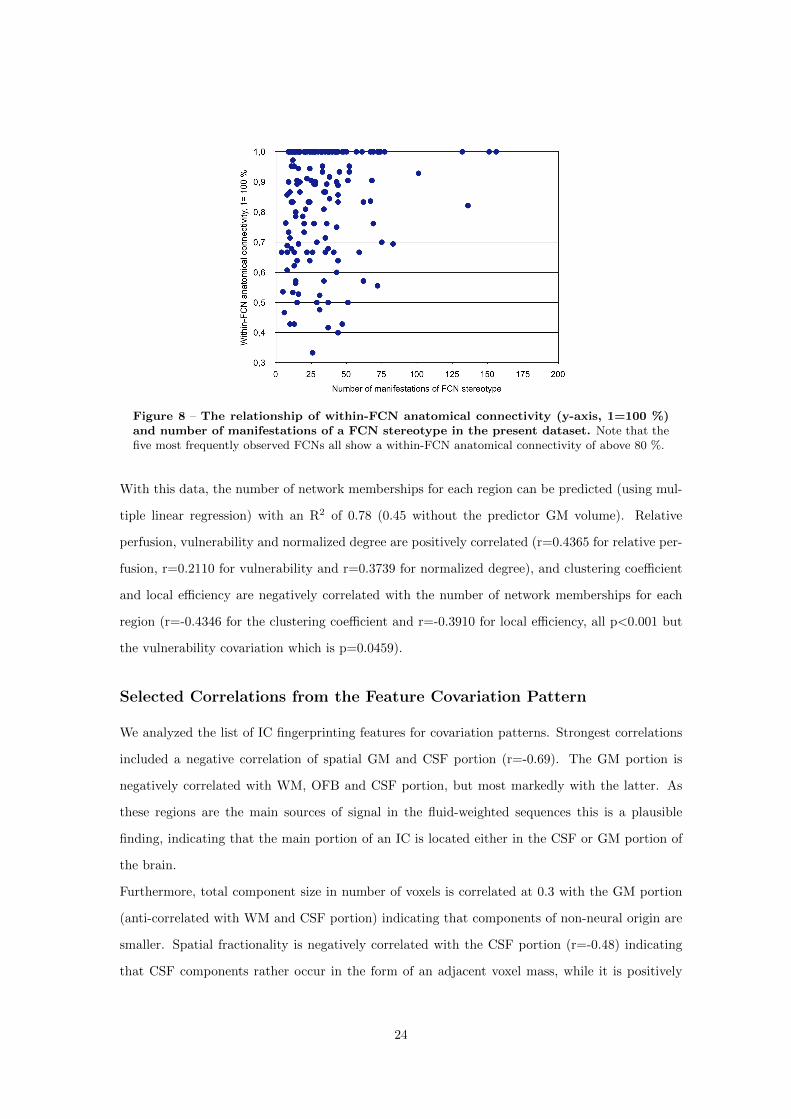
Figure 8 – The relationship of within-FCN anatomical connectivity (y-axis, 1=100 %)and number of manifestations of a FCN stereotype in the present dataset. Note that thefive most frequently observed FCNs all show a within-FCN anatomical connectivity of above 80 %.

With this data, the number of network memberships for each region can be predicted (using mul-

tiple linear regression) with an R2 of 0.78 (0.45 without the predictor GM volume). Relative

perfusion, vulnerability and normalized degree are positively correlated (r=0.4365 for relative per-

fusion, r=0.2110 for vulnerability and r=0.3739 for normalized degree), and clustering coefficient

and local efficiency are negatively correlated with the number of network memberships for each

region (r=-0.4346 for the clustering coefficient and r=-0.3910 for local efficiency, all p<0.001 but

the vulnerability covariation which is p=0.0459).

Selected Correlations from the Feature Covariation Pattern

We analyzed the list of IC fingerprinting features for covariation patterns. Strongest correlations

included a negative correlation of spatial GM and CSF portion (r=-0.69). The GM portion is

negatively correlated with WM, OFB and CSF portion, but most markedly with the latter. As

these regions are the main sources of signal in the fluid-weighted sequences this is a plausible

finding, indicating that the main portion of an IC is located either in the CSF or GM portion of

the brain.

Furthermore, total component size in number of voxels is correlated at 0.3 with the GM portion

(anti-correlated with WM and CSF portion) indicating that components of non-neural origin are

smaller. Spatial fractionality is negatively correlated with the CSF portion (r=-0.48) indicating

that CSF components rather occur in the form of an adjacent voxel mass, while it is positively

24

correlated with the OFB portion, indicating that OFB types of noise are rather scattered over the

image.

A negative correlation of spatial WM portion and OFB regions (r=-0.40), a positive correlation of

PSD kurtosis and skewness (r=0.95), a series of high correlations that show positive covariation

of Partially Directed Coherence features across several frequency bins (r between 0.94 and 0.93)

and high correlations of noise features with one another and with spectral features (r>0.82) are

observed. The squared correlation of component timecourse with total CSF, ventricles and entire

volume-average are all highly intercorrelated indicating one underlying main factor for all three

noise features.

PSD kurtosis and skewness are correlated at r=0.95, indicating that the more leptokurtic the spec-

tral profile of a component is, the more the peak is located in the lower frequency range. Given the

insufficient frequency resolution of fMRI for frequencies above 0.25 Hz, this is a plausible finding.

Furthermore, both are correlated with the R2 of the head movement regressors (based on the

realignment preprocessing step), which is plausible as this regression method best captures slow

head movements. Component size (number of network-voxels) is anti-correlated around r=-0.3

with PSD skewness and kurtosis, indicating that larger components have rather platykurtic and

higher peaking PSD profiles.

Discussion

Noise and networks of interest

The data-driven dissociation of networks of neural origin and networks not of interest allowed

for the preclusion of significant portion of ICs from further processing steps. Although such

exclusion of ICs based on IC-fingerprinting was mostly successful in our case, the approach can

be refined with respect to the included features and the exclusion criteria. For such a system

to be applied more broadly (e.g. in the automated denoising of images) the minimization of

false-positive detections of confound ICs has to be of highest relevance, in order to avoid any

elimination of valuable information. While, for our purposes, the ICs originating from scanner or

physiological noise could mostly be excluded, the differentiation between FCNs of neural origin

and FCNs detected due to homology can only be accomplished by the systematic experimental

manipulation of network parts. FCNs of neural origin within which information is communicated,

25

will be disrupted or altered as a whole by the experimental suppression or activation of one isolated

network node, while other FCNs detected due to homology should not be significantly affected by

the manipulation of one single part.

Feature Covariation Patterns

The observed covariation patterns of features describe mostly intuitive general relationships be-

tween IC properties that can aid our understanding on the properties and sources of the fMRI

signal (e.g GM or CSF). An enlargement of the available data would increase the number of ICs

in specific subgroups and clusters which result from the SOFM and Clusot cycle, so that Feature

Covariation Patterns could be calculated for each specific subgroup/family of ICs. Most likely such

calculations would result in deviating covariation patterns (e.g. between spectral and noise fea-

tures) for example of ICs originating from various types of physiological noise. The exact amount of

useful information for FCN characterization that can be mined from Feature Covariation Patterns

remains to be assessed in future work.

Detectability of networks

Our finding that regional GM volume is a strong predictor of network membership for a brain

region could be interpreted in various ways. First of all, it could indicate that GM mass is largest

in multimodal association areas of the brain that engage in a multitude of neurocomputational

tasks. Secondly, it could indicate that our current fMRI measurement scheme (approx. 3x3x3

mm voxels and supra-second TRs) is most sensitive to the detection of macroscopic FCNs that

emerge slowly (on broad timescales), with a large spatial extent and mainly in regions of the brain

with relatively similar hemodynamic response functions. This could as well explain why there is

a tendency for subcortical regions to less frequently be members of observed networks.

It is therefore not unlikely that there remains an entire universe of fast emerging and decomposing

FCNs that contain only a small set of voxels which are presently invisible to us with fMRI. Faster,

multiplexed EPIs (Feinberg et al., 2010) provide subsecond temporal resolution with whole brain

coverage and high spatial resolution that may help unravel subcortical and rapidly transitioning

FCNs. The systematic detection and recording of FCNs using electrophysiological methods and

their projection onto the cortical surface could be used to significantly itemize the present taxon-

omy and answer a series of central questions. It can be hypothesized that there is a systematic

relation between FCNs derived with electrophysiological methods and FCNs measured with hemo-

26

dynamics based methods. The relationship of brain activity captured by the hemodynamics of

networks must restrict the state space within which electrophysiologically measured states can

occur. If so, there should only be a limited number of electrophysiologically detectable networks

while a FCN is considered coherently active in terms of hemodynamics, as the neural processes

leaving their traces on these two timescales would have to be coupled and restricting each other

in some systematic way - an issue presently mainly addressed by joint/parallel ICA approaches

(Brown et al., 2010; Mantini et al., 2010; Lei et al., 2010; Edwards et al., 2011; Bullmore and

Sporns, 2009b). Furthermore, there is growing evidence that properties of all of these networks

(structural and functional) are tightly linked, irrespective of the applied measurement modalities

(Teipel et al., 2009; Whitford et al., 2010; Valdes-Hernandez et al., 2010).

Network Stereotypes and diagnostics

The list of 172 network stereotypes and their feature properties and similarity corresponds to

the intended taxonomy (please see Figure 9 for exemplary stereotypes). These 172 networks

correspond to the canonical brain networks observed in our data and can theoretically be used for

diagnostic purposes. Evidently one does not need to test a person with tasks for all of the 172

networks but can as well test for a smaller number of main networks, by for example activating

the FCNs that correspond to the most basic networks (are higher up in the network family tree,

Figure 3).

It has to be noted that this detection of distinct networks is occurring on the atlas-level of

abstraction, where each functional network is regarded as an entity which is dispersed over a

limited set of regions. For a deeper analysis distinct networks could as well be identified directly

on the level of voxelwise binary-coded IC images, but this would result in a much higher number

of original functional networks, as already components that only differ in one single voxel (or any

arbitrary number) might have to be regarded as two distinct networks. Furthermore, the use

of this approach on the voxel-level would result in approx. 60.000-dimensional data (as many

dimensions as non-empty voxels) which is computationally unfeasible.

This taxonomy can be validated in future studies by a multitude of methods, such as regenerating

it with the same method from new datasets, analyzing the split-half reliability, actively impairing

or facilitating the formation of certain network types by means of brain stimulation (e.g. TMS,

tDCS) or by observing pathological populations. A clear prediction of this taxonomy is that

27

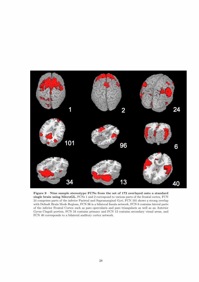
Figure 9 – Nine sample stereotype FCNs from the set of 172 overlayed onto a standardsingle brain using MicroGL. FCNs 1 and 2 correspond to various parts of the frontal cortex, FCN24 comprises parts of the inferior Parietal and Supramarginal Gyri, FCN 101 shows a strong overlapwith Default Brain Mode Regions, FCN 96 is a bilateral Insula network, FCN 6 contains lateral partsof the inferior Frontal Cortex such as pars opercularis and pars triangularis as well as an AnteriorGyrus Cinguli portion, FCN 34 contains primary and FCN 13 contains secondary visual areas, andFCN 40 corresponds to a bilateral auditory cortex network.

28

patients with mostly intact anatomy but functional impairments should first loose the ability to

establish some of the network stereotypes on the lowest level of abstraction (the level of the 172

stereotypes, e.g. loss of a specific frontal executive network) while patients with more progressed or

more severe diseases should be unable to generate the FCNs of an entire subgroup (e.g. disability to

form any network with frontal involvement) until in most severe cases observable function should

break down at the most global level (e.g. disability to generate subcortical-cortical or cortico-

cortical FCNs). Thus, this taxonomy and methodology opens a new diagnostic potential for the

classification of brain damage severity and functional abnormality. An example of such a diagnostic

kit would be a diagnosis based on the elicited activity of 15 canonical FCNs, each belonging to

one of the main network families (e.g. around level 9 in Figure 3). Abnormal properties of one

network or the inability to establish any of the main networks could be associated with certain

types of pathology. The combination of multiple such task-free (e.g. DTI analysis of the individual

anatomical connectome or resting state functional measurements) and task-based methods with

sophisticated data analysis approaches seems to hold great potential for the development of new

diagnostic tools and is currently a strongly studied subject (Greicius et al., 2004; Lawrie et al.,

2008; Stam et al., 2009; Whitfield-Gabrieli et al., 2009; Rubinov et al., 2009; Seeley et al., 2009;

Dosenbach et al., 2010; Van Dijk et al., 2010; Wu et al., 2011; Bullmore and Sporns, 2009b).

The fact that the DBM regions are significantly more often members of FCNs than non-DBM

regions suggests the possible interpretation of resting-state elevated DBM activity as a form of

idling state, from which the DBM regions break away into task-dependent associations with other

FCNs. If this hypothesis is true, disruption of normal DBM functional connectivity should impair

the subsequent formation of certain FCNs. The documented uncoupling effects of anesthetics on

DBM activity and the decrease of adaptive behavior with increasing anesthesia depth could be

a first indicator. Nevertheless, if the presented taxonomy and the idling hypothesis are correct

at least 54 stereotypical networks that do not contain DBM members should be less affected by

experimental DBM activity manipulations. This hypothesis remains to be tested in future work.

The role of regional properties in the formation of Functional Connec-

tivity Networks

Our results clearly underline that the observed stereotypical FCNs tend to form along direct

anatomical connections. Nevertheless, the existence of a multitude of FCNs that form between

regions that are not directly connected by macroscopic WM bundles can not be excluded based

29

on these findings. The present data only indicates, that networks which form for longer (supra-

second) durations and between brain areas with a high GM mass generally rely on direct WM

connections.

The documented covariations of perfusion, GM volume and graph theoretical indices of anatomical

connectivity with the number of networks a region of the brain is observed to be a member of, can

be interpreted either causally or as an isolated statistical coherence. Regions of the brain with

high resting state perfusion, strong anatomical interconnectedness and high relevance (but not

necessarily high damage resilience in terms of lesions to the anatomical connectome) apparently

form networks more often. By the same token hypoperfusion, cortical atrophy and disconnection

(e.g. in aging) might contribute in a major way to the decline of the brains ability to establish

large-scale FCNs in an adaptive manner. If this assumption is correct, a series of hypotheses

can be derived from this: Natural or experimental manipulation of anatomical connectivity, GM

volume and relative perfusion should influence the ability of a brain region to engage in FCNs.

While this has been clear to the scientific and clinical community on a qualitative basis, the data

from our present study allow the creation of quantitative models and the formation of predictions

on the basis of our multiple regression results. The successful prediction of the number of network

memberships of a region from data on the regional properties of that region represents the quan-

titative formulation of an implicated balance in such structure/function relationships.

The top scoring regions in network membership mostly correspond to regions of the association

cortex, many of them along the midline of the cerebrum and known anatomical connectivity hubs

(Gong et al., 2009). These findings strengthen the concept of a strong association of regional

properties and functional roles (association cortex, primary- or secondary motor/sensory cortex)

of brain regions.

Further links between anatomical connectivity and the regional properties of brain regions have re-

cently been documented by other groups (Chen et al., 2008; Cohen et al., 2008; Honey et al., 2009;

van den Heuvel et al., 2009), such as for example the successful association of the covariation pro-

files of local cortical thickness with the underlying anatomical connectivity between brain regions

(Gong et al., 2011). On a longitudinal level, engaging in a high number of FCNs might influence

the properties of a brain region either on the phylogenetic level in terms of an evolutionary push

to increase resting state perfusion, GM volume, cortical thickness and anatomical connectivity or

on a rather ontogenetic level in terms of an association of functional and anatomical properties of

a brain region in terms of co-maturation. Whether changes in the activity profile (participation

30

in FCNs) precedes a shift of regional properties during development or vice versa remains to be

tested in future work, possibly by manipulating either the formation of regional properties by

influencing local axon guidance and perfusion or by altering the functional connectivity profile of

a region.

Impact and implications

We’ve demonstrated a data-driven system for the denoising of fMRI time series and for the sorting

and analysis of Group ICA derived ICs. The derived cluster boundaries for the denoising steps can

(after a cross-validation, that was not the scope of the present study) be directly utilized for noise

vs. non-noise classification of ICs derived from newly measured data. Furthermore, we provide

a rich description of multiple thousand ICs using a multitude of state of the art features and

describe covariation patterns such as the covariation of Granger Causality features and spectral

properties. While this dataset can be mined by the scientific community with alternate methods,

we provide a taxonomy and list of stereotypical/canonical brain networks that remains to be

refined by the integration of larger data bodies and to be validated experimentally by observing

functional connectivity in patient populations. Data from new ICA analyses can be directly

annotated with the information provided in our data set, including the display of parent-child

relationships (e.g. the observed network of fronto-parietal regions belongs to the network family

of networks forming along the cerebral midline). Furthermore, in Attachment C we provide a

new functional parcellation scheme for the individual (or group) inspired by the concept of a

chronoarchitectural analysis of brain activity (Bartels and Zeki, 2005) that is based on the idea,

that the smallest macroscopic functional unit of the brain is the one that might participate in a

multitude of networks but always does this as a whole.

The functional hubs of the brain are those regions with largest GM mass, relative perfusion and

anatomical connectivity and evidently these regions form a multitude of different networks but

with a clear tendency to follow direct and therefore short anatomical connections (path length =

1). In that sense, not only are the anatomical connectome and the functional connectome strongly

overlapping, but are regional GM mass and resting state perfusion as well part of an equation

that describes the healthy brain in terms of the harmonic interplay of its functional and structural

parts.

Based on this finding, the decay of anatomical connectivity in aging and in certain disorders can

clearly be related to systematic alterations in functional connectivity by using one comprehensive

31

model that encompasses all relevant parts. A major challenge of our future work will be the

exploration of the question, whether these group level results derived from large data bodies can

be reliably translated onto the single subject/case level for diagnostic use.

As illustrated in Figure 5, the detected networks take on specific formations in terms of the number

of regions that participate. It is possible that these numbers represent the limits of network

formation and maintenance in the healthy brain and that specifically these numbers might change

due to certain forms of disease, so that the maximum number of nodes in the functional networks

of such patients might decrease along with the brain’s ability to maintain complex interactions.

Methodical limitations

We want to point out that it is possible that some regions of the brain do not show sufficient BOLD

activity or do not show such a hemodynamic response sufficiently in sync with other regions, for

them to appear as part of a network in fMRI studies. Due to the large and heterogenic data

sample this is unlikely, but possible. Although the brain is extensively studied in the MR-scanner

with a variety of stimuli and tasks, it is evident that certain types of networks and activations

that the healthy brain is capable of producing will probably never be recorded in the artificial

setting of the scanner environment. This environment restricts subjects in a way that makes real

natural vision, movement through a scenery or e.g. complex prolonged social interactions very

difficult. Therefore, the development of more accurate stimulation schemes and less restrictive

scanner environments might lead to the discovery of yet undocumented functional networks in

the future - as already addressed in (Bartels and Zeki, 2004). Furthermore, our results are based

on one spatial parcellation scheme for the sorting of FCNs into clusters and the identification

of stereotypical networks, namely the AAL atlas. It is possible that the use of different atlases

might alter the results (Wang et al., 2009), but we do not expect any dramatic alteration as the

AAL atlas offers a parcellation of both cortical and subcortical regions into a high number of

functionally sound and well established brain areas.

Conclusions

This approach is merely a first step to form a taxonomy of FCNs on a purely data-driven basis that

has been realized at one single center. Being scalable, the method can be transposed into cloud

computing or other solutions for the high-throughput analysis of publicly shared functional data.

Future experiments on the active manipulation of network formation, regional brain properties

32

and local activity suppression remain to be conducted and integrated in order to test the validity

of the raised hypotheses on network formation.

Acknowledgements

This paper reflects the authors’ views only and funding agencies are not liable for any use that

may be made of the information contained herein. The funders had no role in study design, data

collection and analysis, decision to publish, or preparation of the manuscript. This work was par-

tially supported by the Deutsche Forschungsgemeinschaft (DFG), the 7th Framework Programme

(FP7) of the European Commission and the Werner Reichardt Centre for Integrative Neuroscience

(CIN) at the University Tubingen, Germany. The authors would like to thank Markus Schurholz,

Bjorn Schiffler, Jana Kneslova and Jessica Rajandran for their contributions.

References

References

Achard, S., Salvador, R., Whitcher, B., Suckling, J., and Bullmore, E. (2006). A resilient, low-

frequency, small-world human brain functional network with highly connected association cor-

tical hubs. The Journal of neuroscience : the official journal of the Society for Neuroscience,

26(1):63–72.

Ashburner, J. and Friston, K. J. (2001). Why voxel-based morphometry should be used. Neu-

roimage, 14(6):1238–1243.

Baker, S., Rogers, R., and Owen, A. (1996). Neural systems engaged by planning: a PET study

of the Tower of London task. Neuropsychologia.

Bartels, A. and Zeki, S. (2004). Functional brain mapping during free viewing of natural scenes.

Human brain mapping, 21(2):75–85.

Bartels, A. and Zeki, S. (2005). The chronoarchitecture of the cerebral cortex. Philosophical

transactions of the Royal Society of London. Series B, Biological sciences, 360(1456):733–50.

Bassett, D. S., Meyer-Lindenberg, A., Achard, S., Duke, T., and Bullmore, E. (2006). Adaptive

33

reconfiguration of fractal small-world human brain functional networks. Proceedings of the

National Academy of Sciences of the United States of America, 103(51):19518–23.

Beckmann, C. F., DeLuca, M., Devlin, J. T., and Smith, S. M. (2005). Investigations into resting-

state connectivity using independent component analysis. Philosophical transactions of the

Royal Society of London. Series B, Biological sciences, 360(1457):1001–13.

Bell, A. J. and Sejnowski, T. J. (1995). An Information-Maximization Approach to Blind Separa-

tion and Blind Deconvolution. Neural Computation, 7(6):1129–1159.

Bogdan, M. and Rosenstiel, W. (1999). Application of Artificial Neural Networks for Different

Engineering Problems. Esprit, pages 277–294.

Bogdan, M., Rosenstiel, W., Pavelka, J., Tel, G., and Bartosek, M. (1999). SOFSEM’99: Theory

and Practice of Informatics, volume 1725 of Lecture Notes in Computer Science. Springer Berlin

Heidelberg, Berlin, Heidelberg.

Brown, K. S., Ortigue, S., Grafton, S. T., and Carlson, J. M. (2010). Improving human brain map-

ping via joint inversion of brain electrodynamics and the BOLD signal. NeuroImage, 49(3):2401–

15.

Brugger, D., Bogdan, M., and Rosenstiel, W. (2008). Automatic cluster detection in Kohonen’s

SOM. IEEE transactions on neural networks / a publication of the IEEE Neural Networks

Council, 19(3):442–59.

Bullmore, E. and Sporns, O. (2009a). Complex brain networks: graph theoretical analysis of

structural and functional systems. Nature reviews. Neuroscience, 10(3):186–98.

Bullmore, E. and Sporns, O. (2009b). Complex brain networks: graph theoretical analysis of

structural and functional systems. Nat Rev Neurosci.

Calhoun, V. (2004). Group ICA of fMRI toolbox (GIFT). Online at http://icatb. sourceforge. net.

Chen, Z. J., He, Y., Rosa-Neto, P., Germann, J., and Evans, A. C. (2008). Revealing modular ar-

chitecture of human brain structural networks by using cortical thickness from {MRI}. Cerebral

cortex, 18(10):2374.

Cohen, A. L., Fair, D. a., Dosenbach, N. U. F., Miezin, F. M., Dierker, D., Van Essen, D. C.,

Schlaggar, B. L., and Petersen, S. E. (2008). Defining functional areas in individual human

brains using resting functional connectivity MRI. NeuroImage, 41(1):45–57.

34

Correa, N., Adali, T., and Calhoun, V. D. (2007). Performance of blind source separation algo-

rithms for fMRI analysis using a group ICA method. Magnetic resonance imaging, 25(5):684–94.

Demirci, O., Stevens, M. C., Andreasen, N. C., Michael, A., Liu, J., White, T., Pearlson, G. D.,

Clark, V. P., and Calhoun, V. D. (2009). Investigation of relationships between fMRI brain

networks in the spectral domain using ICA and Granger causality reveals distinct differences

between schizophrenia patients and healthy controls. NeuroImage, 46(2):419–31.

Dodel, S., Golestani, N., Pallier, C., Elkouby, V., Le Bihan, D., and Poline, J.-B. (2005). Condition-

dependent functional connectivity: syntax networks in bilinguals. Philosophical transactions of

the Royal Society of London. Series B, Biological sciences, 360(1457):921–35.

Dosenbach, N., Nardos, B., and Cohen, A. (2010). Prediction of individual brain maturity using

fMRI. Science.

Dosenbach, N. U. F., Fair, D. a., Miezin, F. M., Cohen, A. L., Wenger, K. K., Dosenbach, R. a. T.,

Fox, M. D., Snyder, A. Z., Vincent, J. L., Raichle, M. E., Schlaggar, B. L., and Petersen, S. E.

(2007). Distinct brain networks for adaptive and stable task control in humans. Proceedings of

the National Academy of Sciences of the United States of America, 104(26):11073–8.

Edwards, B. G., Calhoun, V. D., and Kiehl, K. A. (2011). Joint ICA of ERP and fMRI during

Error-Monitoring. NeuroImage.

Erhardt, E. B., Rachakonda, S., Bedrick, E. J., Allen, E. A., Adali, T., and Calhoun, V. D. (2010).

Comparison of multi-subject ICA methods for analysis of fMRI data. Human brain mapping.

Fair, D. A., Cohen, A. L., Dosenbach, N. U. F., Church, J. A., Miezin, F. M., Barch, D. M.,

Raichle, M. E., Petersen, S. E., and Schlaggar, B. L. (2008). The maturing architecture of the

brain’s default network. Proceedings of the National Academy of Sciences, 105(10):4028.

Feinberg, D., Moeller, S., and Smith, S. (2010). Multiplexed Echo Planar Imaging for Sub-Second

Whole Brain FMRI and Fast Diffusion Imaging. PloS one.

Gong, G., He, Y., Chen, Z. J., and Evans, A. C. (2011). Convergence and Divergence of Thickness

Correlations with Diffusion Connections across the Human Cerebral Cortex. NeuroImage.

Gong, G., He, Y., Concha, L., Lebel, C., Gross, D. W., Evans, A. C., and Beaulieu, C. (2009).

Mapping anatomical connectivity patterns of human cerebral cortex using in vivo diffusion

tensor imaging tractography. Cerebral Cortex, 19(3):524.

35

Greicius, M. D., Srivastava, G., Reiss, A. L., and Menon, V. (2004). Default-mode network activity

distinguishes Alzheimer’s disease from healthy aging: evidence from functional MRI. Proceedings

of the National Academy of Sciences of the United States of America, 101(13):4637–42.

Hagmann, P., Kurant, M., Gigandet, X., Thiran, P., Wedeen, V. J., Meuli, R., and Thiran, J.-

P. (2007). Mapping human whole-brain structural networks with diffusion MRI. PloS one,

2(7):e597.

Halder, S., Agorastos, D., Veit, R., Hammer, E. M., Lee, S., Varkuti, B., Bogdan, M., Rosenstiel,

W., Birbaumer, N., and Kubler, a. (2011). Neural mechanisms of brain-computer interface

control. NeuroImage.

Himberg, J. and Hyvarinen, A. (2003). Icasso: software for investigating the reliability of ICA

estimates by clustering and visualization. In 2003 IEEE XIII Workshop on Neural Networks

for Signal Processing (IEEE Cat. No.03TH8718), pages 259–268. IEEE.

Honey, C. J., Sporns, O., Cammoun, L., Gigandet, X., Thiran, J. P., Meuli, R., and Hagmann,

P. (2009). Predicting human resting-state functional connectivity from structural connectivity.

Proceedings of the National Academy of Sciences, 106(6):2035.

Horwitz, B. (2003). The elusive concept of brain connectivity. NeuroImage, 19(2):466–470.

Iturria-Medina, Y., Sotero, R. C., Canales-Rodrıguez, E. J., Aleman-Gomez, Y., and Melie-Garcıa,

L. (2008). Studying the human brain anatomical network via diffusion-weighted MRI and Graph

Theory. NeuroImage, 40(3):1064–76.

Keune, P. M., Bostanov, V., Hautzinger, M., and Kotchoubey, B. (2011). Mindfulness-based

cognitive therapy (MBCT), cognitive style, and the temporal dynamics of frontal EEG alpha

asymmetry in recurrently depressed patients. Biological psychology.

Kohonen, T. (1990). The self-organizing map. Proceedings of the IEEE.

Kreher, B. W., Schnell, S., Mader, I., Il’yasov, K. a., Hennig, J., Kiselev, V. G., and Saur, D.

(2008). Connecting and merging fibres: pathway extraction by combining probability maps.

NeuroImage, 43(1):81–9.

Lawrie, S. M., McIntosh, A. M., Hall, J., Owens, D. G. C., and Johnstone, E. C. (2008). Brain

structure and function changes during the development of schizophrenia: the evidence from

studies of subjects at increased genetic risk. Schizophrenia bulletin, 34(2):330–40.

36

Lei, X., Qiu, C., Xu, P., and Yao, D. (2010). A parallel framework for simultaneous EEG/fMRI

analysis: methodology and simulation. NeuroImage, 52(3):1123–34.

Logothetis, N. K. (2008). What we can do and what we cannot do with fMRI. Nature,

453(7197):869–78.

Maldjian, J. and Laurienti, P. (2003). An automated method for neuroanatomic and cytoarchi-

tectonic atlas-based interrogation of fMRI data sets. Neuroimage.

Mantini, D., Marzetti, L., Corbetta, M., Romani, G. L., and Del Gratta, C. (2010). Multimodal

integration of fMRI and EEG data for high spatial and temporal resolution analysis of brain

networks. Brain topography, 23(2):150–8.

McKeown, M. (2003). Independent component analysis of functional MRI: what is signal and

what is noise? Current Opinion in Neurobiology, 13(5):620–629.

McKeown, M. J., Makeig, S., Brown, G. G., Jung, T. P., Kindermann, S. S., Bell, a. J., and

Sejnowski, T. J. (1998). Analysis of fMRI data by blind separation into independent spatial

components. Human brain mapping, 6(3):160–88.

Mechelli, A., Price, C. J., Friston, K. J., and Ashburner, J. (2005). Voxel-based morphometry of

the human brain: methods and applications. Current Medical Imaging Reviews, 1(2):105–113.

Neuper, C. and Scherer, R. (2005). Imagery of motor actions: differential effects of kinesthetic

and visual-motor mode of imagery in single-trial EEG. Cognitive Brain Research.

Perlbarg, V., Bellec, P., Anton, J.-L., Pelegrini-Issac, M., Doyon, J., and Benali, H. (2007). COR-

SICA: correction of structured noise in fMRI by automatic identification of ICA components.

Magnetic resonance imaging, 25(1):35–46.

Raichle, M. E., MacLeod, A. M., Snyder, A. Z., Powers, W. J., Gusnard, D. A., and Shulman,

G. L. (2001). A default mode of brain function. Proceedings of the National Academy of Sciences

of the United States of America, 98(2):676.

Rubinov, M., Knock, S. a., Stam, C. J., Micheloyannis, S., Harris, A. W. F., Williams, L. M.,

and Breakspear, M. (2009). Small-world properties of nonlinear brain activity in schizophrenia.

Human brain mapping, 30(2):403–16.

37

Schelter, B., Winterhalder, M., Eichler, M., Peifer, M., Hellwig, B., Guschlbauer, B., Lucking,

C. H., Dahlhaus, R., and Timmer, J. (2006). Testing for directed influences among neural

signals using partial directed coherence. Journal of neuroscience methods, 152(1-2):210–9.

Seeley, W. W., Crawford, R. K., Zhou, J., Miller, B. L., and Greicius, M. D. (2009). Neurodegen-

erative diseases target large-scale human brain networks. Neuron, 62(1):42–52.

Seeley, W. W., Menon, V., Schatzberg, A. F., Keller, J., Glover, G. H., Kenna, H., Reiss, A. L.,

and Greicius, M. D. (2007). Dissociable intrinsic connectivity networks for salience processing

and executive control. The Journal of neuroscience : the official journal of the Society for

Neuroscience, 27(9):2349–56.

Seth, A. (2010). A MATLAB toolbox for Granger causal connectivity analysis. Journal of neuro-

science methods.

Seth, A. K. (2005). Causal connectivity of evolved neural networks during behavior. Network:

Computation in Neural Systems, 16(1):35–54.

Smolders, A., De Martino, F., Staeren, N., Scheunders, P., Sijbers, J., Goebel, R., and Formisano,

E. (2007). Dissecting cognitive stages with time-resolved fMRI data: a comparison of fuzzy

clustering and independent component analysis. Magnetic resonance imaging, 25(6):860–8.

Sporns, O., Chialvo, D. R., Kaiser, M., and Hilgetag, C. C. (2004). Organization, development

and function of complex brain networks. Trends in cognitive sciences, 8(9):418–25.

Sporns, O., Tononi, G., and Kotter, R. (2005). The human connectome: A structural description

of the human brain. PLoS computational biology, 1(4):e42.

Sridharan, D., Levitin, D. J., and Menon, V. (2008). A critical role for the right fronto-insular

cortex in switching between central-executive and default-mode networks. Proceedings of the

National Academy of Sciences of the United States of America, 105(34):12569–74.

Stam, C. J., de Haan, W., Daffertshofer, a., Jones, B. F., Manshanden, I., van Cappellen van

Walsum, a. M., Montez, T., Verbunt, J. P. a., de Munck, J. C., van Dijk, B. W., Berendse, H. W.,

and Scheltens, P. (2009). Graph theoretical analysis of magnetoencephalographic functional

connectivity in Alzheimer’s disease. Brain : a journal of neurology, 132(Pt 1):213–24.

38

Sui, J., Adali, T., Pearlson, G. D., and Calhoun, V. D. (2009). An ICA-based method for the

identification of optimal FMRI features and components using combined group-discriminative

techniques. NeuroImage, 46(1):73–86.

Teipel, S. J., Pogarell, O., Meindl, T., Dietrich, O., Sydykova, D., Hunklinger, U., Georgii, B.,

Mulert, C., Reiser, M. F., Moller, H.-J., and Hampel, H. (2009). Regional networks underlying

interhemispheric connectivity: an EEG and DTI study in healthy ageing and amnestic mild

cognitive impairment. Hum Brain Mapp, 30(7):2098–2119.

Tzourio-Mazoyer, N., Landeau, B., Papathanassiou, D., Crivello, F., Etard, O., Delcroix, N., Ma-

zoyer, B., and Joliot, M. (2002). Automated anatomical labeling of activations in {SPM} using

a macroscopic anatomical parcellation of the {MNI} {MRI} single-subject brain. Neuroimage,

15(1):273–289.

Valdes-Hernandez, P. a., Ojeda-Gonzalez, A., Martınez-Montes, E., Lage-Castellanos, A., Virues-

Alba, T., Valdes-Urrutia, L., and Valdes-Sosa, P. a. (2010). White matter architecture rather

than cortical surface area correlates with the EEG alpha rhythm. NeuroImage, 49(3):2328–39.

van den Heuvel, M. P., Mandl, R. C. W., Kahn, R. S., and Hulshoff Pol, H. E. (2009). Functionally

linked resting-state networks reflect the underlying structural connectivity architecture of the

human brain. Human brain mapping, 30(10):3127–41.

Van Dijk, K. R. a., Hedden, T., Venkataraman, A., Evans, K. C., Lazar, S. W., and Buckner, R. L.

(2010). Intrinsic functional connectivity as a tool for human connectomics: theory, properties,

and optimization. Journal of neurophysiology, 103(1):297–321.

Varkuti, B., Cavusoglu, M., Kullik, A., Schiffler, B., Veit, R., Yilmaz, O., Rosenstiel, W., Braun,

C., Uludag, K., Birbaumer, N., and Sitaram, R. (2011). Quantifying the link between anatomical

connectivity, gray matter volume and regional cerebral blood flow: an integrative MRI study.

PloS one, 6(4):e14801.

Wang, J., Wang, L., Zang, Y., Yang, H., Tang, H., Gong, Q., Chen, Z., Zhu, C., and He, Y.

(2009). Parcellation-dependent small-world brain functional networks: a resting-state fMRI

study. Human brain mapping, 30(5):1511–23.

Whitfield-Gabrieli, S., Thermenos, H. W., Milanovic, S., Tsuang, M. T., Faraone, S. V., McCarley,

R. W., Shenton, M. E., Green, A. I., Nieto-Castanon, A., LaViolette, P., Wojcik, J., Gabrieli, J.

39

D. E., and Seidman, L. J. (2009). Hyperactivity and hyperconnectivity of the default network

in schizophrenia and in first-degree relatives of persons with schizophrenia. Proceedings of the

National Academy of Sciences of the United States of America, 106(4):1279–84.

Whitford, T. J., Kubicki, M., Ghorashi, S., Schneiderman, J. S., Hawley, K. J., McCarley, R. W.,

Shenton, M. E., and Spencer, K. M. (2010). Predicting inter-hemispheric transfer time from the

diffusion properties of the corpus callosum in healthy individuals and schizophrenia patients: A

combined ERP and DTI study. NeuroImage, 54(3):2318–2329.

Wu, X., Li, R., Fleisher, A. S., Reiman, E. M., Guan, X., Zhang, Y., Chen, K., and Yao, L. (2011).

Altered default mode network connectivity in alzheimer’s disease-A resting functional MRI and

bayesian network study. Human brain mapping, 00(November 2009).

Zentgraf, K., Stark, R., and Reiser, M. (2005). Differential activation of pre-SMA and SMA proper

during action observation: Effects of instructions. Neuroimage.

40

1

Attachments

Attachment A: Percentage-threshold method

Duplicate networks were removed from the final set of components by first binarizing the component-onto-

AAL percentage vectors with a percentage threshold and second marking and eliminating all duplicates.

A percentage threshold of e.g. 5 percent binary-codes this vector in a way, that only regions of the AAL

atlas that contain more than 5 percent of the components spatial extent will be set to one. The higher

the threshold is, the less regions are added to the network and accordingly the total number of regions

that are never part of a single- or multi-region component grows.

In order to account for that fact, we performed a sweep over plausible thresholds (starting with 4.9 per-

cent, the threshold were no region is never considered part of a network) and selected a threshold from

the plateau most likely representing the captured network dynamics most accurately.

The optimal percentage threshold can be derived from an analysis of the binary-coded component images.

When thresholding all Independent Component (IC) images using a cluster-extent threshold, every image

contains at least one cluster if the cluster-threshold has a size of 225 voxels (equalling 2,025 cm3). Fifty

percent of the components from the final list are single-cluster components, 28.39 % are two-cluster com-

ponents, 14.38 % three-, 5.49 % four- and 1.45 % five-cluster components. Six-, seven- and eight-cluster

components can be found as well but make for only less than 1 % of all components. Such clusters of

adjacent voxels can lie within one single AAL region or on the boundary of two or multiple such regions.

The optimal percentage threshold (5.14 %) is identified by performing a sweep over thresholds and cor-

relating the number of found AAL regions in the network with the number of distinct clusters above

225 voxels in the image. The percentage threshold that maximizes this correlation best captures each

networks extension in AAL atlas space.

An alternative method would be to use the number of manifestations, as it is highly unlikely that a

distinct functional network can be found more than 175 times in a dataset composed of 175 sessions

(that would mean instances of it are found several times within one session). Formally this is possible

as spatially similar networks can be found with variable spectral properties. We calculated the mean

variability of the spectral properties among the manifestations of one distinct functional network for

each percentage threshold (so for each level of distinction). While for higher percentages the variability

is rising as more and more fundamentally different networks are considered as one since they overlap

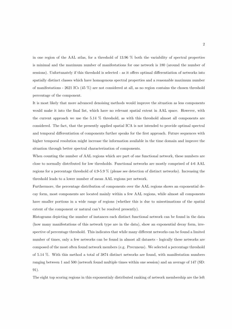
2

in one region of the AAL atlas, for a threshold of 13.96 % both the variability of spectral properties

is minimal and the maximum number of manifestations for one network is 180 (around the number of

sessions). Unfortunately if this threshold is selected - as it offers optimal differentiation of networks into

spatially distinct classes which have homogenous spectral properties and a reasonable maximum number

of manifestations - 2621 ICs (45 %) are not considered at all, as no region contains the chosen threshold

percentage of the component.

It is most likely that more advanced denoising methods would improve the situation as less components

would make it into the final list, which have no relevant spatial extent in AAL space. However, with

the current approach we use the 5.14 % threshold, as with this threshold almost all components are

considered. The fact, that the presently applied spatial ICA is not intended to provide optimal spectral

and temporal differentiation of components further speaks for the first approach. Future sequences with

higher temporal resolution might increase the information available in the time domain and improve the

situation through better spectral characterization of components.

When counting the number of AAL regions which are part of one functional network, these numbers are

close to normally distributed for low thresholds. Functional networks are mostly comprised of 4-6 AAL

regions for a percentage threshold of 4.9-5.9 % (please see detection of distinct networks). Increasing the

threshold leads to a lower number of mean AAL regions per network.

Furthermore, the percentage distribution of components over the AAL regions shows an exponential de-

cay form, most components are located mainly within a few AAL regions, while almost all components

have smaller portions in a wide range of regions (whether this is due to misestimations of the spatial

extent of the component or natural can’t be resolved presently).

Histograms depicting the number of instances each distinct functional network can be found in the data

(how many manifestations of this network type are in the data), show an exponential decay form, irre-

spective of percentage threshold. This indicates that while many different networks can be found a limited

number of times, only a few networks can be found in almost all datasets - logically these networks are

composed of the most often found network members (e.g. Precuneus). We selected a percentage threshold

of 5.14 %. With this method a total of 3874 distinct networks are found, with manifestation numbers

ranging between 1 and 500 (network found multiple times within one session) and an average of 147 (SD:

91).

The eight top scoring regions in this exponentialy distributed ranking of network membership are the left

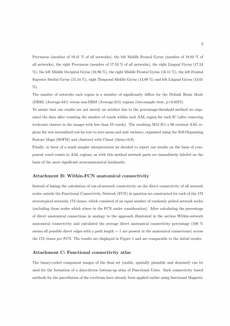
3

Precuneus (member of 19.41 % of all networks), the left Middle Frontal Gyrus (member of 18.02 % of

all networks), the right Precuneus (member of 17.53 % of all networks), the right Lingual Gyrus (17.53

%), the left Middle Occipital Gyrus (16.96 %), the right Middle Frontal Gyrus (16.11 %), the left Frontal

Superior Medial Gyrus (15.44 %), right Temporal Middle Gyrus (13.89 %) and left Lingual Gyrus (13.01

%).

The number of networks each region is a member of significantly differs for the Default Brain Mode

(DBM) (Average:341) versus non-DBM (Average:215) regions (two-sample ttest, p<0.0375).

To assure that our results are not merely an artefact due to the percentage-threshold method we orga-

nized the data after counting the number of voxels within each AAL region for each IC (after removing

irrelevant clusters in the images with less than 10 voxels). The resulting 5812 ICs x 90 cerebral AAL re-

gions list was normalized row-by-row to zero mean and unit variance, organized using the Self-Organizing

Feature Maps (SOFM) and clustered with Clusot (theta=0.9).

Finally, in favor of a much simpler interpretation we decided to report our results on the basis of com-

ponent voxel-counts in AAL regions, as with this method network parts are immediately labeled on the

basis of the most significant neuroanatomical landmarks.

Attachment B: Within-FCN anatomical connectivity

Instead of basing the calculation of out-of-network connectivity on the direct connectivity of all network

nodes outside the Functional Connectivity Network (FCN) in question we constructed for each of the 172

stereotypical networks 172 clones, which consisted of an equal number of randomly picked network nodes

(excluding those nodes which where in the FCN under consideration). After calculating the percentage

of direct anatomical connections in analogy to the approach illustrated in the section Within-network

anatomical connectivity and calculated the average direct anatomical connectivity percentage (100 %

means all possible direct edges with a path length = 1 are present in the anatomical connectome) across

the 172 clones per FCN. The results are displayed in Figure 1 and are comparable to the initial results.

Attachment C: Functional connectivity atlas

The binary-coded component images of the final set (stable, spatially plausible and denoised) can be

used for the formation of a data-driven bottom-up atlas of Functional Units. Such connectivity based

methods for the parcellation of the cerebrum have already been applied earlier using functional Magnetic

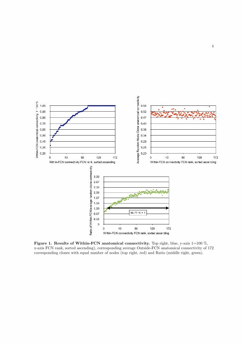
4

Figure 1. Results of Within-FCN anatomical connectivity. Top right, blue, y-axis 1=100 %,x-axis FCN rank, sorted ascending), corresponding average Outside-FCN anatomical connectivity of 172corresponding clones with equal number of nodes (top right, red) and Ratio (middle right, green).

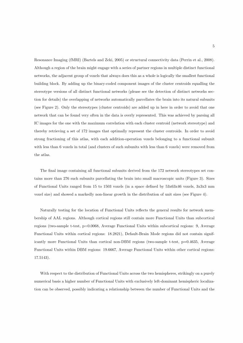
5

Resonance Imaging (fMRI) (Bartels and Zeki, 2005) or structural connectivity data (Perrin et al., 2008).

Although a region of the brain might engage with a series of partner regions in multiple distinct functional

networks, the adjacent group of voxels that always does this as a whole is logically the smallest functional

building block. By adding up the binary-coded component images of the cluster centroids equalling the

stereotype versions of all distinct functional networks (please see the detection of distinct networks sec-

tion for details) the overlapping of networks automatically parcellates the brain into its natural subunits

(see Figure 2). Only the stereotypes (cluster centroids) are added up in here in order to avoid that one

network that can be found very often in the data is overly represented. This was achieved by parsing all

IC images for the one with the maximum correlation with each cluster centroid (network stereotype) and

thereby retrieving a set of 172 images that optimally represent the cluster centroids. In order to avoid

strong fractioning of this atlas, with each addition-operation voxels belonging to a functional subunit

with less than 6 voxels in total (and clusters of such subunits with less than 6 voxels) were removed from

the atlas.

The final image containing all functional subunits derived from the 172 network stereotypes set con-

tains more than 276 such subunits parcellating the brain into small macroscopic units (Figure 3). Sizes

of Functional Units ranged from 15 to 1503 voxels (in a space defined by 53x63x46 voxels, 3x3x3 mm

voxel size) and showed a markedly non-linear growth in the distribution of unit sizes (see Figure 4).

Naturally testing for the location of Functional Units reflects the general results for network mem-

bership of AAL regions. Although cortical regions still contain more Functional Units than subcortical

regions (two-sample t-test, p=0.0068, Average Functional Units within subcortical regions: 9, Average

Functional Units within cortical regions: 18.2821), Default-Brain Mode regions did not contain signif-

icantly more Functional Units than cortical non-DBM regions (two-sample t-test, p=0.4635, Average

Functional Units within DBM regions: 19.6667, Average Functional Units within other cortical regions:

17.5143).

With respect to the distribution of Functional Units across the two hemispheres, strikingly on a purely

numerical basis a higher number of Functional Units with exclusively left-dominant hemispheric localiza-

tion can be observed, possibly indicating a relationship between the number of Functional Units and the

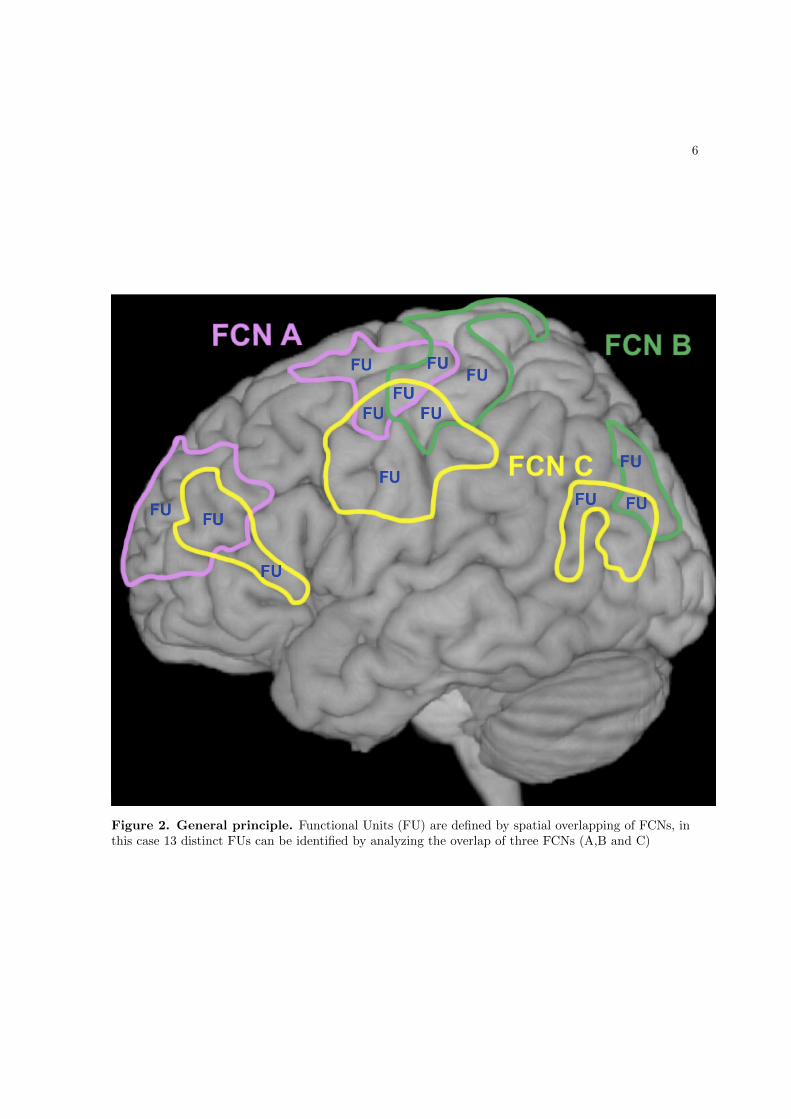
6

Figure 2. General principle. Functional Units (FU) are defined by spatial overlapping of FCNs, inthis case 13 distinct FUs can be identified by analyzing the overlap of three FCNs (A,B and C)

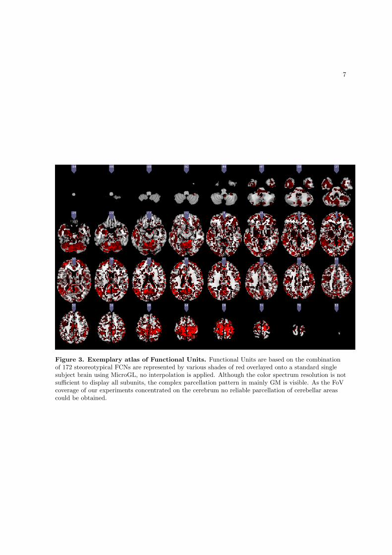
7

Figure 3. Exemplary atlas of Functional Units. Functional Units are based on the combinationof 172 steoreotypical FCNs are represented by various shades of red overlayed onto a standard singlesubject brain using MicroGL, no interpolation is applied. Although the color spectrum resolution is notsufficient to display all subunits, the complex parcellation pattern in mainly GM is visible. As the FoVcoverage of our experiments concentrated on the cerebrum no reliable parcellation of cerebellar areascould be obtained.

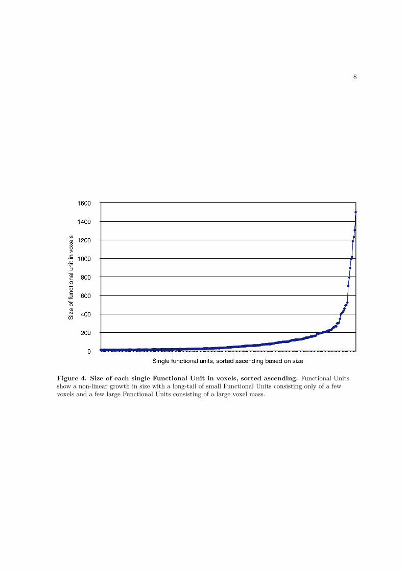
8

Figure 4. Size of each single Functional Unit in voxels, sorted ascending. Functional Unitsshow a non-linear growth in size with a long-tail of small Functional Units consisting only of a fewvoxels and a few large Functional Units consisting of a large voxel mass.

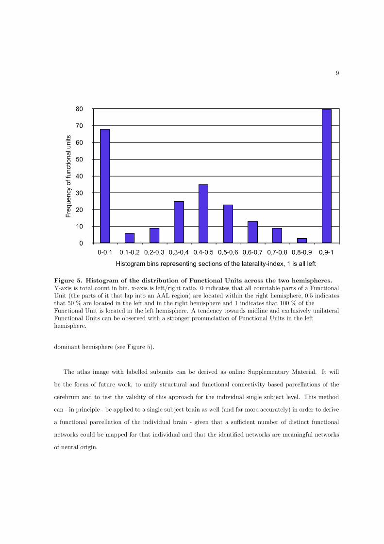
9

Figure 5. Histogram of the distribution of Functional Units across the two hemispheres.Y-axis is total count in bin, x-axis is left/right ratio. 0 indicates that all countable parts of a FunctionalUnit (the parts of it that lap into an AAL region) are located within the right hemisphere, 0.5 indicatesthat 50 % are located in the left and in the right hemisphere and 1 indicates that 100 % of theFunctional Unit is located in the left hemisphere. A tendency towards midline and exclusively unilateralFunctional Units can be observed with a stronger pronunciation of Functional Units in the lefthemisphere.

dominant hemisphere (see Figure 5).

The atlas image with labelled subunits can be derived as online Supplementary Material. It will

be the focus of future work, to unify structural and functional connectivity based parcellations of the

cerebrum and to test the validity of this approach for the individual single subject level. This method

can - in principle - be applied to a single subject brain as well (and far more accurately) in order to derive

a functional parcellation of the individual brain - given that a sufficient number of distinct functional

networks could be mapped for that individual and that the identified networks are meaningful networks

of neural origin.

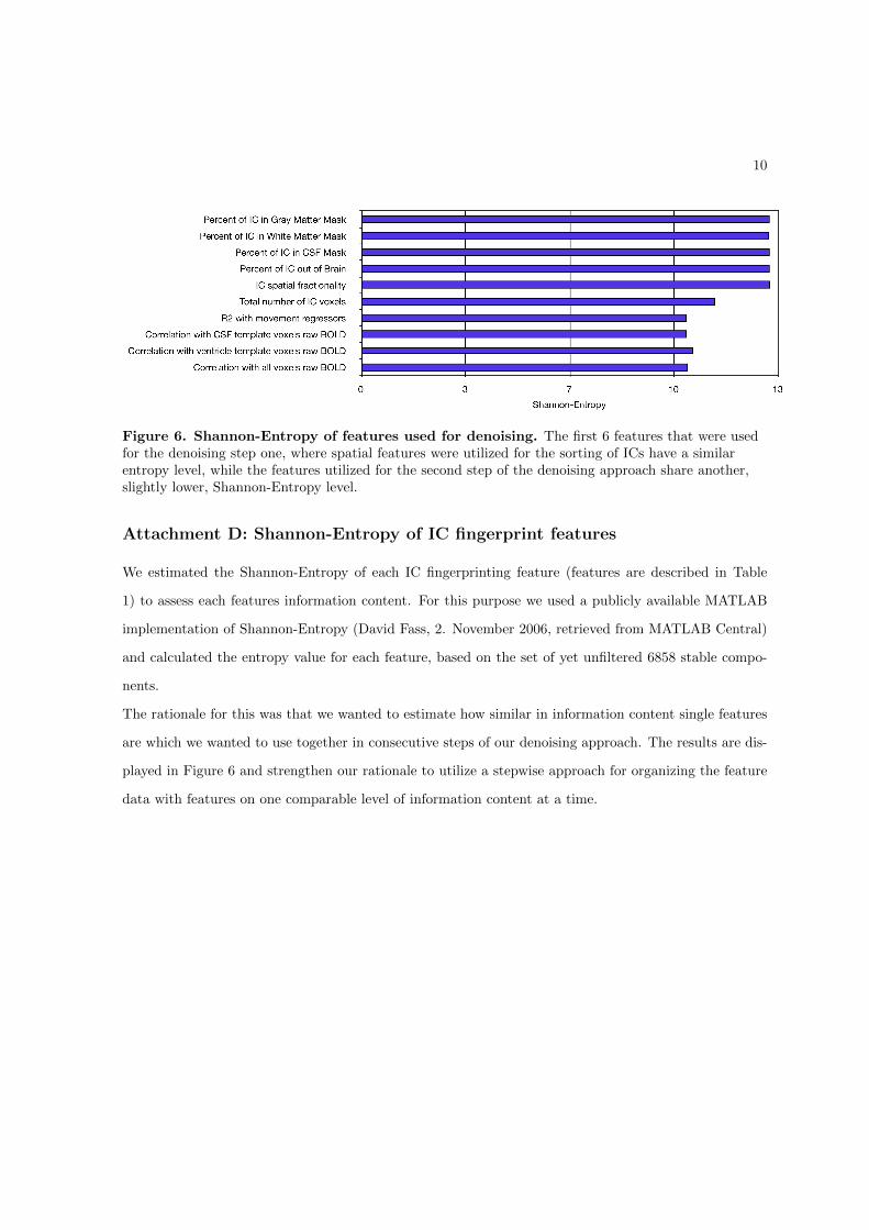
10

Figure 6. Shannon-Entropy of features used for denoising. The first 6 features that were usedfor the denoising step one, where spatial features were utilized for the sorting of ICs have a similarentropy level, while the features utilized for the second step of the denoising approach share another,slightly lower, Shannon-Entropy level.

Attachment D: Shannon-Entropy of IC fingerprint features

We estimated the Shannon-Entropy of each IC fingerprinting feature (features are described in Table

1) to assess each features information content. For this purpose we used a publicly available MATLAB

implementation of Shannon-Entropy (David Fass, 2. November 2006, retrieved from MATLAB Central)

and calculated the entropy value for each feature, based on the set of yet unfiltered 6858 stable compo-

nents.

The rationale for this was that we wanted to estimate how similar in information content single features

are which we wanted to use together in consecutive steps of our denoising approach. The results are dis-

played in Figure 6 and strengthen our rationale to utilize a stepwise approach for organizing the feature

data with features on one comparable level of information content at a time.

11

Supplementary References

References

Bartels A, Zeki S. 2005. The chronoarchitecture of the cerebral cortex. Philosophical transactions of the

Royal Society of London Series B, Biological sciences. 360:733–50.

Perrin M, Cointepas Y, Cachia A, Poupon C, Thirion B, Riviere D, Cathier P, El Kouby V, Constantinesco

A, Le Bihan D, Mangin JF. 2008. Connectivity-Based Parcellation of the Cortical Mantle Using q-Ball

Diffusion Imaging. International Journal of Biomedical Imaging. 2008:1–19.

12

Attachment Table 1

Included are all 172 network stereotypes with the AAL regions they contain and the number of manifes-

tations (column Found), reflecting how often each of these networks is found in the data. The data is

sorted according to the number of manifestations, so that the most prominent networks are on top.

FoundCalcarine_L

Calcarine_R

Cuneus_L

Cuneus_R

Lingual_L Lingual_R

156

Precuneus_L

Precuneus_R

151

Calcarine_L

Lingual_L Lingual_R

Fusiform_L

Fusiform_R

Precuneus_L

Precuneus_R

Temporal_Inf_R

136

Frontal_Sup_L

Frontal_Sup_R

Frontal_Mid_L

Frontal_Mid_R

Supp_Motor_Area_L

Supp_Motor_Area_R

Frontal_Sup_Medial_L

Frontal_Sup_Medial_R

132

Calcarine_L

Calcarine_R

Lingual_L Lingual_R

Occipital_Mid_L

Occipital_Mid_R

Occipital_Inf_L

Occipital_Inf_R

101

Precentral_L

Precentral_R

Frontal_Mid_L

Frontal_Mid_R

Frontal_Inf_Oper_L

Frontal_Inf_Oper_R

Frontal_Inf_Tri_L

Frontal_Inf_Tri_R

Frontal_Sup_Medial_L

83

Frontal_Sup_L

Frontal_Sup_Medial_L

Frontal_Sup_Medial_R

Frontal_Mid_Orb_L

Frontal_Mid_Orb_R

Cingulum_Ant_L

Cingulum_Ant_R

77

Rolandic_Oper_R

Temporal_Sup_L

Temporal_Sup_R

Temporal_Mid_L

Temporal_Mid_R

75

Cuneus_L

Cuneus_R

Occipital_Sup_L

Occipital_Sup_R

Occipital_Mid_L

Occipital_Mid_R

Precuneus_L

Precuneus_R

74

Frontal_Sup_L

Frontal_Sup_R

Frontal_Mid_L

Frontal_Mid_R

Frontal_Inf_Tri_L

Frontal_Inf_Tri_R

73

Calcarine_L

Calcarine_R

Cuneus_L

Cuneus_R

Lingual_L Lingual_R

Occipital_Sup_L

Occipital_Sup_R

Occipital_Mid_L

73

Calcarine_L

Cuneus_L

Cuneus_R

Occipital_Sup_L

Occipital_Sup_R

Precuneus_L

Precuneus_R

72

Frontal_Sup_L

Frontal_Sup_R

Frontal_Mid_L

Frontal_Mid_R

Frontal_Sup_Medial_L

Frontal_Sup_Medial_R

Occipital_Mid_L

Occipital_Mid_R

Temporal_Mid_R

72

Precentral_R

Supp_Motor_Area_R

Postcentral_L

Postcentral_R

Parietal_Sup_L

Parietal_Sup_R

Precuneus_L

Precuneus_R

Paracentral_Lobule_L

Paracentral_Lobule_R

69

Hippocampus_L

Hippocampus_R

ParaHippocampal_L

ParaHippocampal_R

Lingual_L Lingual_R

Temporal_Sup_L

69

FoundPrecentral_R

Supp_Motor_Area_R

Postcentral_L

Postcentral_R

Parietal_Sup_L

Parietal_Sup_R

Precuneus_L

Precuneus_R

Paracentral_Lobule_L

Paracentral_Lobule_R

69

Calcarine_L

Lingual_L Lingual_R

Precuneus_L

Precuneus_R

Thalamus_L

Thalamus_R

68

Precentral_L

Postcentral_L

Parietal_Sup_L

Parietal_Inf_L

67

Occipital_Sup_L

Occipital_Sup_R

Occipital_Mid_L

Occipital_Mid_R

Occipital_Inf_L

Occipital_Inf_R

Fusiform_L

Fusiform_R

Parietal_Sup_L

Parietal_Sup_R

Temporal_Inf_R

67

Frontal_Sup_L

Frontal_Sup_R

Frontal_Mid_L

Frontal_Mid_R

Frontal_Sup_Medial_L

Frontal_Sup_Medial_R

Cingulum_Ant_L

Cingulum_Mid_L

Cingulum_Mid_R

67

Precentral_R

Rolandic_Oper_R

Postcentral_L

Postcentral_R

62

Rolandic_Oper_L

Rolandic_Oper_R

Insula_R Postcentral_L

Postcentral_R

SupraMarginal_R

Temporal_Sup_L

Temporal_Sup_R

62

Cingulum_Mid_L

Cingulum_Mid_R

Precuneus_L

Precuneus_R

61

Frontal_Mid_L

Frontal_Sup_Medial_L

Frontal_Sup_Medial_R

Cingulum_Ant_L

Cingulum_Ant_R

Temporal_Sup_R

59

Parietal_Sup_L

Parietal_Sup_R

Precuneus_L

Precuneus_R

57

Precentral_L

Frontal_Sup_L

Frontal_Sup_R

Frontal_Mid_L

Frontal_Mid_R

Supp_Motor_Area_L

Supp_Motor_Area_R

52

Precentral_R

Frontal_Mid_R

Frontal_Inf_Oper_R

Frontal_Inf_Tri_R

Postcentral_R

Temporal_Sup_R

52

Precentral_L

Frontal_Mid_L

Frontal_Inf_Oper_L

Frontal_Inf_Tri_L

Occipital_Mid_L

Postcentral_L

Parietal_Inf_L

51

Rolandic_Oper_L

Rolandic_Oper_R

Insula_R Temporal_Sup_L

Temporal_Sup_R

51

Precentral_R

Frontal_Sup_R

Frontal_Mid_R

Postcentral_R

Parietal_Sup_R

Parietal_Inf_R

SupraMarginal_R

50

FoundCalcarine_L

Cuneus_L

Cuneus_R

Occipital_Sup_L

Occipital_Sup_R

Precuneus_L

Precuneus_R

48

Frontal_Sup_L

Frontal_Sup_R

Frontal_Mid_L

Frontal_Mid_R

Frontal_Sup_Medial_L

Frontal_Sup_Medial_R

47

Frontal_Inf_Orb_L

Insula_L Insula_R Temporal_Sup_L

Temporal_Sup_R

Temporal_Pole_Sup_L

Temporal_Pole_Sup_R

47

Angular_R

Precuneus_L

Precuneus_R

Temporal_Sup_R

Temporal_Mid_L

Temporal_Mid_R

45

Precentral_R

Postcentral_L

Postcentral_R

SupraMarginal_R

44

Frontal_Sup_L

Frontal_Sup_Medial_L

Frontal_Sup_Medial_R

Calcarine_L

Occipital_Mid_L

Angular_R

Precuneus_L

Precuneus_R

Temporal_Mid_R

44

Parietal_Inf_L

Parietal_Inf_R

SupraMarginal_L

SupraMarginal_R

Temporal_Sup_L

44

Cingulum_Ant_L

Hippocampus_L

Lingual_L Lingual_R

Precuneus_L

Precuneus_R

Thalamus_L

Thalamus_R

44

Precentral_R

Frontal_Sup_R

Frontal_Mid_R

Frontal_Inf_Oper_R

Frontal_Inf_Tri_R

Frontal_Sup_Medial_R

Parietal_Sup_R

Parietal_Inf_R

Angular_R

Temporal_Mid_R

44

Caudate_L

Caudate_R

Thalamus_L

Thalamus_R

44

Parietal_Sup_L

Parietal_Sup_R

Precuneus_L

Precuneus_R

43

Precentral_L

Precentral_R

Frontal_Sup_L

Frontal_Sup_R

Supp_Motor_Area_L

Supp_Motor_Area_R

43

Precentral_R

Frontal_Sup_L

Frontal_Sup_R

Frontal_Mid_L

Frontal_Mid_R

43

Frontal_Sup_L

Frontal_Mid_L

Frontal_Sup_Medial_L

Occipital_Mid_L

Parietal_Inf_L

Parietal_Inf_R

Angular_L

Angular_R

Precuneus_L

Temporal_Mid_L

43

FoundRolandic_Oper_R

Supp_Motor_Area_L

Supp_Motor_Area_R

Insula_L Insula_R Cingulum_Mid_L

Cingulum_Mid_R

SupraMarginal_L

SupraMarginal_R

43

Cingulum_Post_L

Calcarine_L

Cuneus_L

Cuneus_R

Precuneus_L

Precuneus_R

42

Cingulum_Mid_R

Cuneus_L

Cuneus_R

Precuneus_L

Precuneus_R

42

Lingual_L Lingual_R

Fusiform_R

41

Precentral_L

Frontal_Sup_L

Frontal_Mid_L

Postcentral_L

Parietal_Sup_L

Parietal_Inf_L

40

Parietal_Sup_L

Parietal_Sup_R

Precuneus_L

Precuneus_R

40

Calcarine_L

Calcarine_R

Lingual_L Lingual_R

Precuneus_L

Precuneus_R

40

Frontal_Sup_L

Frontal_Sup_R

Frontal_Mid_L

Frontal_Mid_R

Frontal_Inf_Tri_L

40

Caudate_L

Caudate_R

Thalamus_L

Thalamus_R

38

Precentral_L

Precentral_R

Frontal_Sup_L

Frontal_Sup_R

Frontal_Mid_L

Frontal_Mid_R

Supp_Motor_Area_L

Supp_Motor_Area_R

Frontal_Sup_Medial_L

38

Frontal_Sup_Medial_L

Caudate_L

Caudate_R

Thalamus_L

Thalamus_R

38

Frontal_Mid_R

Occipital_Mid_R

Postcentral_R

Parietal_Sup_R

Parietal_Inf_L

Parietal_Inf_R

SupraMarginal_R

Angular_R

Precuneus_R

Temporal_Mid_R

38

Hippocampus_L

Hippocampus_R

ParaHippocampal_L

ParaHippocampal_R

Lingual_L Lingual_R

Fusiform_L

Fusiform_R

37

Frontal_Inf_Orb_L

Olfactory_L

Frontal_Mid_Orb_L

Frontal_Mid_Orb_R

Cingulum_Ant_L

Cingulum_Ant_R

Caudate_L

37

Frontal_Inf_Orb_L

Frontal_Inf_Orb_R

Insula_L Insula_R Temporal_Sup_L

Temporal_Sup_R

Temporal_Pole_Sup_L

Temporal_Pole_Sup_R

Temporal_Mid_R

37

FoundFrontal_Sup_L

Frontal_Sup_R

Frontal_Mid_L

Frontal_Mid_R

Frontal_Sup_Medial_L

Frontal_Sup_Medial_R

37

Precentral_L

Supp_Motor_Area_L

Supp_Motor_Area_R

Frontal_Sup_Medial_L

Cingulum_Mid_L

Cingulum_Mid_R

37

Insula_L Insula_R Temporal_Sup_L

Temporal_Sup_R

37

Frontal_Sup_L

Supp_Motor_Area_R

Frontal_Sup_Medial_L

Lingual_R

Precuneus_L

Precuneus_R

Temporal_Sup_R

36

Frontal_Sup_Medial_L

Cingulum_Post_L

Calcarine_L

Calcarine_R

Cuneus_L

Occipital_Mid_L

Precuneus_L

Precuneus_R

36

Occipital_Sup_L

Occipital_Sup_R

Occipital_Mid_L

Occipital_Mid_R

Parietal_Sup_L

Parietal_Sup_R

Temporal_Mid_R

35

Precentral_R

Supp_Motor_Area_R

Postcentral_R

Parietal_Sup_R

Parietal_Inf_R

35

Frontal_Sup_L

Frontal_Sup_R

Frontal_Mid_L

Frontal_Mid_R

Frontal_Inf_Tri_L

35

Frontal_Inf_Oper_L

Frontal_Inf_Tri_L

Frontal_Inf_Orb_L

Insula_L Temporal_Sup_L

Temporal_Mid_L

35

Temporal_Sup_R

Temporal_Mid_L

Temporal_Mid_R

35

Frontal_Sup_R

Frontal_Mid_R

Parietal_Inf_R

SupraMarginal_R

Angular_L

Angular_R

Temporal_Mid_R

35

Precentral_R

Postcentral_R

Parietal_Sup_L

Parietal_Sup_R

Parietal_Inf_L

Parietal_Inf_R

SupraMarginal_R

34

Frontal_Inf_Orb_R

Calcarine_L

Lingual_R

Fusiform_L

Fusiform_R

Temporal_Mid_R

Temporal_Inf_R

34

Insula_L Caudate_L

Caudate_R

Thalamus_L

Thalamus_R

Temporal_Sup_L

34

Insula_L Caudate_R

Putamen_L

Putamen_R

Thalamus_L

Thalamus_R

33

FoundInsula_L Caudate_

LCaudate_R

Putamen_L

Putamen_R

Thalamus_L

Thalamus_R

33

Caudate_L

Caudate_R

Putamen_L

33

Frontal_Sup_L

Frontal_Mid_L

Parietal_Sup_L

Parietal_Inf_L

Angular_L

Precuneus_L

32

Cuneus_R

Parietal_Sup_L

Parietal_Sup_R

Precuneus_L

Precuneus_R

32

Precentral_R

Supp_Motor_Area_L

Supp_Motor_Area_R

Postcentral_L

Postcentral_R

Parietal_Sup_R

Precuneus_L

Precuneus_R

Paracentral_Lobule_L

Paracentral_Lobule_R

32

Insula_L Insula_R ParaHippocampal_R

Temporal_Sup_L

Temporal_Sup_R

Temporal_Pole_Sup_L

Temporal_Pole_Sup_R

31

Insula_L Insula_R Lingual_R

Temporal_Sup_L

Temporal_Sup_R

Temporal_Pole_Sup_L

Temporal_Mid_L

31

Calcarine_L

Calcarine_R

Lingual_L Lingual_R

Occipital_Sup_L

Occipital_Mid_L

Occipital_Inf_L

30

Calcarine_L

Lingual_L Lingual_R

Fusiform_L

Fusiform_R

29

ParaHippocampal_R

Lingual_L Lingual_R

Caudate_L

Thalamus_R

29

Cingulum_Mid_L

Cingulum_Mid_R

Precuneus_L

Precuneus_R

28

Precentral_L

Precentral_R

Postcentral_L

Postcentral_R

Parietal_Inf_L

28

Calcarine_L

Calcarine_R

Cuneus_R

Occipital_Sup_L

Occipital_Sup_R

Occipital_Mid_L

Occipital_Mid_R

28

Frontal_Sup_R

Frontal_Mid_R

Occipital_Mid_R

Parietal_Sup_R

Parietal_Inf_R

Angular_R

Precuneus_R

Temporal_Mid_R

28

Caudate_L

Caudate_R

Thalamus_L

Thalamus_R

27

FoundFrontal_Mid_L

Frontal_Inf_Oper_L

Frontal_Inf_Tri_L

Frontal_Inf_Orb_L

Supp_Motor_Area_L

Frontal_Sup_Medial_L

Insula_L Temporal_Mid_L

27

Frontal_Sup_L

Frontal_Mid_L

Calcarine_L

Precuneus_L

Precuneus_R

Temporal_Sup_L

Temporal_Sup_R

27

Caudate_L

Caudate_R

Thalamus_L

Thalamus_R

27

ParaHippocampal_L

ParaHippocampal_R

Temporal_Pole_Sup_L

Temporal_Pole_Sup_R

26

Precentral_L

Precentral_R

Supp_Motor_Area_L

Supp_Motor_Area_R

Postcentral_L

Postcentral_R

Parietal_Sup_L

Parietal_Sup_R

Precuneus_L

Precuneus_R

Paracentral_Lobule_L

Paracentral_Lobule_R

26

Rolandic_Oper_L

Rolandic_Oper_R

Insula_L Insula_R Cingulum_Mid_L

Cingulum_Mid_R

SupraMarginal_R

Temporal_Sup_L

Temporal_Sup_R

26

Frontal_Inf_Orb_L

Frontal_Mid_Orb_L

Frontal_Mid_Orb_R

Cingulum_Ant_L

Cingulum_Ant_R

Caudate_L

25

SupraMarginal_R

Angular_R

Precuneus_L

Precuneus_R

Temporal_Sup_R

Temporal_Mid_L

Temporal_Mid_R

25

Cuneus_L

Cuneus_R

Occipital_Sup_L

Occipital_Sup_R

Occipital_Mid_L

Occipital_Mid_R

24

Frontal_Sup_L

Frontal_Sup_R

Frontal_Mid_L

Frontal_Mid_R

Frontal_Sup_Medial_L

Frontal_Sup_Medial_R

24

Hippocampus_L

Hippocampus_R

ParaHippocampal_R

Lingual_L Lingual_R

Fusiform_R

Precuneus_R

Thalamus_L

Thalamus_R

24

Frontal_Sup_R

Frontal_Mid_L

Frontal_Mid_R

Calcarine_L

Occipital_Mid_L

Occipital_Mid_R

Precuneus_L

Precuneus_R

Temporal_Mid_R

24

Caudate_L

Caudate_R

Thalamus_L

Thalamus_R

24

Cingulum_Post_L

Cingulum_Post_R

Calcarine_L

Lingual_L Lingual_R

Precuneus_L

Precuneus_R

Thalamus_L

Thalamus_R

24

Occipital_Mid_L

Temporal_Sup_L

Temporal_Mid_L

Temporal_Mid_R

23

FoundFrontal_Sup_L

Frontal_Sup_R

Frontal_Mid_L

Frontal_Mid_R

22

Temporal_Sup_R

Temporal_Mid_L

Temporal_Mid_R

22

Calcarine_L

Calcarine_R

Lingual_L Lingual_R

Occipital_Sup_L

Occipital_Mid_L

Occipital_Mid_R

Occipital_Inf_L

Occipital_Inf_R

Temporal_Mid_R

22

Occipital_Sup_L

Occipital_Mid_L

Parietal_Sup_L

Parietal_Inf_L

Angular_L

Precuneus_L

21

Frontal_Sup_L

Frontal_Sup_R

Frontal_Mid_L

Frontal_Mid_R

Supp_Motor_Area_L

Supp_Motor_Area_R

Frontal_Sup_Medial_L

Frontal_Sup_Medial_R

21

Precentral_L

Frontal_Mid_L

Frontal_Inf_Tri_L

Occipital_Mid_L

Parietal_Sup_L

Parietal_Inf_L

Precuneus_L

21

Frontal_Sup_L

Frontal_Sup_R

Frontal_Mid_L

Frontal_Mid_R

Frontal_Sup_Medial_L

Frontal_Sup_Medial_R

Cingulum_Ant_L

21

Parietal_Sup_L

Parietal_Sup_R

Precuneus_L

Precuneus_R

20

Frontal_Sup_L

Frontal_Sup_R

Frontal_Mid_L

Frontal_Mid_R

Frontal_Mid_Orb_L

Frontal_Inf_Tri_L

20

Frontal_Mid_L

Calcarine_L

Cuneus_L

Occipital_Sup_L

Occipital_Mid_L

Occipital_Mid_R

Parietal_Inf_L

SupraMarginal_R

Precuneus_L

Precuneus_R

20

Frontal_Mid_L

Occipital_Sup_L

Occipital_Mid_L

Occipital_Mid_R

Precuneus_L

Precuneus_R

Temporal_Mid_R

20

Precentral_R

Supp_Motor_Area_L

Supp_Motor_Area_R

Cingulum_Mid_L

Cingulum_Mid_R

SupraMarginal_R

Temporal_Sup_L

Temporal_Sup_R

19

Precuneus_L

Precuneus_R

Temporal_Sup_R

Temporal_Mid_L

Temporal_Mid_R

17

Frontal_Sup_L

Frontal_Sup_Orb_L

Frontal_Mid_L

Frontal_Sup_Medial_L

Frontal_Sup_Medial_R

Frontal_Mid_Orb_L

Frontal_Mid_Orb_R

Cingulum_Ant_L

17

Frontal_Sup_L

Frontal_Mid_L

Frontal_Mid_R

Frontal_Inf_Tri_L

Frontal_Sup_Medial_L

Precuneus_L

17

FoundPrecentral_L

Precentral_R

Postcentral_L

Postcentral_R

Parietal_Sup_L

Parietal_Sup_R

Precuneus_L

Precuneus_R

Paracentral_Lobule_L

Paracentral_Lobule_R

17

Precentral_R

Frontal_Sup_R

Frontal_Mid_R

Postcentral_R

Parietal_Sup_R

Parietal_Inf_R

SupraMarginal_R

17

Precentral_L

Precentral_R

Supp_Motor_Area_L

Supp_Motor_Area_R

Cingulum_Mid_L

Cingulum_Mid_R

Postcentral_L

Postcentral_R

Parietal_Sup_L

Parietal_Sup_R

Precuneus_L

Precuneus_R

Paracentral_Lobule_L

Paracentral_Lobule_R

17

Caudate_L

Caudate_R

Thalamus_L

Thalamus_R

16

Frontal_Sup_L

Frontal_Sup_R

Frontal_Mid_L

Frontal_Mid_R

Frontal_Sup_Medial_L

Frontal_Sup_Medial_R

Cingulum_Ant_L

Cingulum_Ant_R

Caudate_L

Caudate_R

16

Precentral_L

Frontal_Sup_L

Frontal_Sup_R

Frontal_Mid_L

Frontal_Mid_R

Supp_Motor_Area_L

Supp_Motor_Area_R

Frontal_Sup_Medial_L

Frontal_Sup_Medial_R

16

Precentral_L

Precentral_R

Frontal_Mid_R

Occipital_Mid_R

Postcentral_R

SupraMarginal_R

Temporal_Sup_R

Temporal_Mid_L

Temporal_Mid_R

16

Insula_L Insula_R ParaHippocampal_R

Lingual_L Lingual_R

Thalamus_L

Thalamus_R

Temporal_Sup_L

Temporal_Pole_Sup_L

16

Frontal_Sup_R

Frontal_Mid_R

Occipital_Mid_R

Parietal_Sup_R

Parietal_Inf_R

Angular_R

Temporal_Mid_R

15

Postcentral_R

Parietal_Inf_L

Parietal_Inf_R

SupraMarginal_L

SupraMarginal_R

15

Occipital_Mid_L

SupraMarginal_R

Angular_R

Precuneus_L

Precuneus_R

Temporal_Sup_R

Temporal_Mid_L

Temporal_Mid_R

15

Frontal_Mid_R

Frontal_Inf_Tri_L

Frontal_Inf_Tri_R

Occipital_Mid_R

Postcentral_R

SupraMarginal_R

Temporal_Sup_R

Temporal_Mid_L

Temporal_Mid_R

15

Calcarine_L

Calcarine_R

Lingual_L Lingual_R

Precuneus_L

Precuneus_R

15

Cingulum_Mid_R

Cingulum_Post_L

Cuneus_L

Cuneus_R

Precuneus_L

Precuneus_R

14

Precentral_L

Frontal_Mid_L

Frontal_Mid_R

Frontal_Inf_Tri_L

Frontal_Inf_Tri_R

Occipital_Mid_L

Postcentral_L

SupraMarginal_L

Temporal_Sup_R

Temporal_Mid_L

Temporal_Mid_R

14

FoundFrontal_Sup_L

Frontal_Mid_L

Frontal_Mid_R

Frontal_Inf_Tri_L

Rolandic_Oper_L

Rolandic_Oper_R

Frontal_Sup_Medial_L

Insula_R Cingulum_Ant_L

Caudate_L

Caudate_R

14

Occipital_Mid_L

SupraMarginal_L

Angular_L

Temporal_Sup_L

Temporal_Mid_L

Temporal_Mid_R

14

Frontal_Inf_Orb_L

Occipital_Mid_L

Occipital_Inf_L

Fusiform_L

Temporal_Sup_L

Temporal_Pole_Sup_L

Temporal_Mid_L

Temporal_Inf_L

14

Frontal_Sup_L

Frontal_Sup_R

Frontal_Sup_Medial_L

Frontal_Sup_Medial_R

Frontal_Mid_Orb_L

Cingulum_Ant_L

Cingulum_Ant_R

14

ParaHippocampal_L

ParaHippocampal_R

Fusiform_L

Temporal_Pole_Sup_L

Temporal_Pole_Sup_R

Temporal_Mid_L

Temporal_Pole_Mid_L

Temporal_Inf_L

14

Precentral_L

Precentral_R

Supp_Motor_Area_L

Supp_Motor_Area_R

Postcentral_L

Postcentral_R

Parietal_Sup_L

Parietal_Sup_R

Precuneus_L

Precuneus_R

Paracentral_Lobule_L

Paracentral_Lobule_R

13

Frontal_Sup_Medial_L

Cingulum_Ant_L

Cingulum_Ant_R

Cingulum_Mid_L

Cingulum_Mid_R

Cingulum_Post_L

13

Insula_L ParaHippocampal_L

ParaHippocampal_R

Lingual_L Lingual_R

Caudate_L

Temporal_Pole_Sup_L

Temporal_Pole_Sup_R

13

Precentral_L

Precentral_R

Postcentral_L

Postcentral_R

Parietal_Sup_L

Parietal_Sup_R

Parietal_Inf_L

13

Frontal_Mid_R

Frontal_Inf_Tri_L

Frontal_Inf_Tri_R

Frontal_Inf_Orb_R

Rolandic_Oper_R

Insula_R Occipital_Mid_L

Temporal_Sup_R

Temporal_Pole_Sup_R

Temporal_Mid_R

13

ParaHippocampal_R

Lingual_L Lingual_R

Fusiform_R

13

Precuneus_R

Temporal_Sup_R

Temporal_Mid_L

Temporal_Mid_R

12

Frontal_Sup_L

Frontal_Sup_R

Frontal_Mid_L

Frontal_Mid_R

Frontal_Inf_Oper_R

Frontal_Inf_Tri_L

Frontal_Inf_Tri_R

Frontal_Sup_Medial_L

Frontal_Sup_Medial_R

12

FoundOccipital_Mid_L

Occipital_Inf_L

Temporal_Mid_L

12

Occipital_Mid_L

Angular_L

Temporal_Mid_L

12

Lingual_L Lingual_R

Fusiform_L

Caudate_L

Thalamus_L

Thalamus_R

12

Calcarine_L

Calcarine_R

Cuneus_R

Lingual_L Lingual_R

Occipital_Sup_L

Occipital_Sup_R

Occipital_Mid_L

Occipital_Mid_R

Occipital_Inf_L

11

Precentral_L

Frontal_Mid_L

Frontal_Mid_R

Supp_Motor_Area_L

Frontal_Sup_Medial_L

Cingulum_Mid_L

Cingulum_Mid_R

11

Frontal_Sup_L

Frontal_Sup_R

Frontal_Mid_L

Frontal_Mid_R

Frontal_Inf_Tri_L

Frontal_Sup_Medial_L

Frontal_Sup_Medial_R

Caudate_L

Temporal_Sup_R

11

Frontal_Sup_Medial_L

Frontal_Sup_Medial_R

Calcarine_L

Lingual_R

Occipital_Mid_L

Precuneus_L

Precuneus_R

Temporal_Mid_R

11

Precentral_L

Precentral_R

Rolandic_Oper_R

Postcentral_L

Postcentral_R

SupraMarginal_R

Temporal_Sup_R

10

Calcarine_L

Cuneus_L

Occipital_Mid_L

Precuneus_L

Precuneus_R

10

Calcarine_L

Cuneus_L

Lingual_L Lingual_R

Precuneus_L

Precuneus_R

10

Frontal_Sup_R

Frontal_Mid_L

Frontal_Mid_R

Frontal_Inf_Tri_L

Frontal_Inf_Tri_R

Frontal_Inf_Orb_R

10

Frontal_Inf_Orb_L

ParaHippocampal_L

ParaHippocampal_R

Lingual_L Lingual_R

Fusiform_L

Temporal_Pole_Sup_L

10

Precentral_L

Precentral_R

Postcentral_L

Postcentral_R

Parietal_Inf_L

9

Precentral_L

Precentral_R

Supp_Motor_Area_R

Postcentral_L

Postcentral_R

Parietal_Sup_L

Parietal_Sup_R

Precuneus_L

Precuneus_R

Paracentral_Lobule_L

Paracentral_Lobule_R

9

Frontal_Sup_L

Frontal_Mid_L

Frontal_Mid_R

Frontal_Sup_Medial_L

9

FoundCalcarine_L

Lingual_R

Caudate_L

Caudate_R

Thalamus_L

Thalamus_R

9

Precentral_L

Precentral_R

Supp_Motor_Area_L

Supp_Motor_Area_R

Postcentral_L

Postcentral_R

Parietal_Sup_L

Parietal_Sup_R

Precuneus_L

Precuneus_R

Paracentral_Lobule_L

Paracentral_Lobule_R

9

Occipital_Mid_L

Temporal_Mid_L

Temporal_Mid_R

8

Frontal_Sup_Medial_L

Cingulum_Mid_L

Cingulum_Mid_R

Calcarine_L

Lingual_R

Precuneus_L

Precuneus_R

8

Frontal_Sup_Medial_L

Insula_L Insula_R Calcarine_L

Lingual_L Lingual_R

Precuneus_R

Thalamus_R

Temporal_Sup_L

Temporal_Sup_R

8

Precentral_R

Frontal_Sup_L

Frontal_Sup_Medial_L

Lingual_R

Angular_R

Caudate_L

Caudate_R

Temporal_Sup_L

8

Precentral_L

Precentral_R

Frontal_Sup_L

Frontal_Sup_R

Frontal_Mid_L

Frontal_Mid_R

Postcentral_R

Parietal_Sup_R

Parietal_Inf_R

Angular_R

Precuneus_L

7

Insula_L Insula_R Temporal_Sup_L

Temporal_Sup_R

Temporal_Pole_Sup_L

Temporal_Pole_Sup_R

6

Frontal_Mid_L

Supp_Motor_Area_L

Frontal_Sup_Medial_L

Calcarine_L

Precuneus_R

Temporal_Sup_R

Temporal_Mid_R

Temporal_Inf_R

5

Precentral_L

Frontal_Sup_L

Frontal_Mid_L

Frontal_Mid_R

Frontal_Inf_Tri_L

Frontal_Inf_Orb_L

Temporal_Mid_R

4

7.3 Chapter 3 - Functional Connectivity Network alterations as an ef-

fect of stroke rehabilitation

162

Resting state functional connectivity changes predict movement

recovery due to robot assisted BCI training in stroke patients Author list and affiliations:

Bálint Várkuti1,2,3

Cuntai Guan3

Yaozhang Pan 3

Kok Soon Phua 3

Kai Keng Ang 3

Christopher Wee Keong Kuah 4

Karen Chua4

Beng Ti Ang5

Niels Birbaumer1

Sitaram Ranganathan1,6

1 Institute of Medical Psychology and Behavioral Neurobiology, University of Tübingen,

Gartenstr. 29, 72074 Tübingen, Germany

2 Graduate Training Centre of Neuroscience, International Max Planck Research School,

University of Tübingen, Österbergstr. 3, 72074 Tübingen, Germany

3 Institute for Infocomm Research, 1 Fusionopolis Way, #21-01 Connexis (South Tower),

138632 Singapore

4 Department of Rehabilitation Medicine, Tan Tock Seng Hospital, TTSH rehabilitation

centre, 17 Ang Mo Kio Ave 9, 569766, Singapore.

5 National Neuroscience Institute, 11 Jalan Tan Tock Seng, 308433, Singapore

6 Sri Chitra Tirunal Institute of Medical Sciences and Technology, Thiruvananthapuram, 695

011, Kerala, India

Abstract

Background and Purpose—

We compared the effectiveness of standard robotic rehabilitation (MANUS) and a robotic

rehabilitation paradigm involving Electroencephalography-based Brain Computer Interfaces

and Motor Imagery (MI EEG-BCI) in a large population of stroke survivors. In order to

assess changes in brain function due to the rehabilitation we conducted a resting state

functional Magnetic Resonance Imaging (rs-fMRI) study with a subgroup of participants

before and after the training.

Methods—

A total of 9 adults with upper extremity paresis were trained over a 4 week period with a

MANUS (3) and a MI EEG-BCI (6) robotic rehabilitation paradigm. Pretraining and

posttraining, rs-fMRI measurements and upper extremity assessments using Fugl-Meyer

upper extremity Test (FM) were conducted for each participant. Functional connectivity

networks of the motor system were identified using an Independent Component Analysis

approach.

Results—

The individual gain in upper extremity function (FM) over a 12 week period could be

predicted from pre-post functional connectivity changes (FCC). FCC of the Supplementary

Motor Area, the contra- and ipsilesional Motor Cortex and parts of the Visuospatial System

with regions in the Superior Medial Gyrus, Anterior Cingulate Cortex, Superior and Middle

Temporal Gyrus, Inferior Parietal Lobe, Precuneus, Middle Orbital Gyrus and Cerebellum

predicted individual upper extremity function improvement.

Conclusions—

Certain FCC predict the steepness of individual recovery in our sample. Following these

lines, future training and rehabilitation methods might therefore focuss on inducing beneficial

increases in functional connectivity such as those observed in this study through means of

direct connectivity-neurofeedback. Exploratory treatment group comparison indicates that

MI is a potential fascilitator of such beneficial neuroplasticity.

Key words:

rehabilitation, stroke, brain imaging, hemiparesis, neuroplasticity

1. Introduction

Stroke is known to be one of the leading causes of death and impairment in the industrialized

world 1 – leaving not only the stroke survivors themselves severely affected, but impacting as

well their families and work environment. 2-3

Thus it is essential to identify the factors that contribute to optimal post-stroke motor

recovery and to develop new methods that target beneficial effects on brain plasticity.

Electroencephalography-based Brain Computer Interfaces (EEG-BCIs) – particularly with

paradigms including motor imagery (MI) - have recently been proposed as potentially

successful therapeutic interventions.4-5 Such approaches target the integrity and connectivity

of the brain systems involved in the successfull execution of a movement that have been

severed by the stroke.6

Instead of allowing the patient to use compensatory movement strategies to complete a given

movement task, patients using EEG-BCIs volitionally generate patterns of brain activity that

are detected by the BCI and translated into movement of the paretic limb by external

effectors, thereby bridging the disconnection between intention to move and execution.

Hereby neural processes are stimulated that are intended to recombine the willfull intention

of the patient to move a paretic limb and the perceived afferent sensory input. That sensory

input is generated by a robot orthosis moving that limb. The reconnection of the severed

parts of the motor system is to take place by learning processes induced by a combination of

operant (the translation of the patients intention into a movement is a reward) and classical

conditioning (the coincidence of volition and relevant afference). Thus the rationale behind

such a BCI training is to restore neural cooperation within the motor system by means of

conditioning the neuronal ensembles back into a functioning motor network and to generally

stimulate adaptive processes.

In order to assure a close temporal association of the intention to move and the movement

executed by a robot, EEG-BCI systems such as those utilized in this study adapt a two stage

strategy.7-8 In the first step the system is calibrated by asking the patient to imagine the

movement and by saving the associated patterns of activation. In a second step – the actual

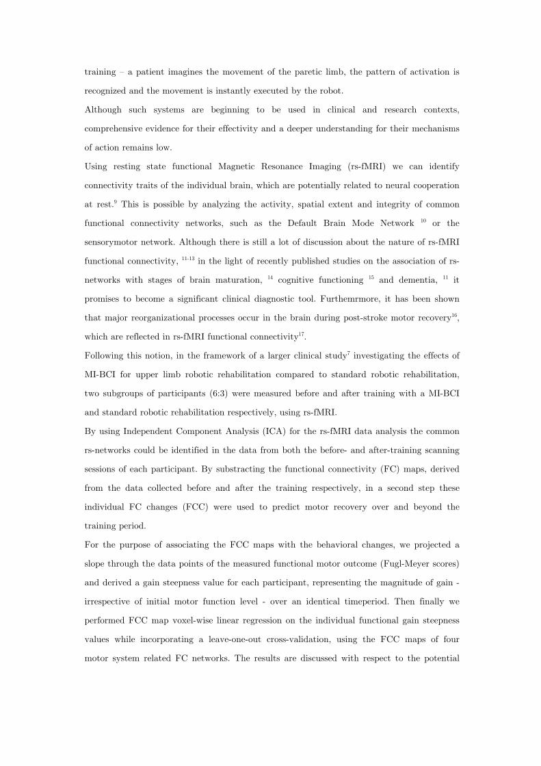
training – a patient imagines the movement of the paretic limb, the pattern of activation is

recognized and the movement is instantly executed by the robot.

Although such systems are beginning to be used in clinical and research contexts,

comprehensive evidence for their effectivity and a deeper understanding for their mechanisms

of action remains low.

Using resting state functional Magnetic Resonance Imaging (rs-fMRI) we can identify

connectivity traits of the individual brain, which are potentially related to neural cooperation

at rest.9 This is possible by analyzing the activity, spatial extent and integrity of common

functional connectivity networks, such as the Default Brain Mode Network 10 or the

sensorymotor network. Although there is still a lot of discussion about the nature of rs-fMRI

functional connectivity, 11-13 in the light of recently published studies on the association of rs-

networks with stages of brain maturation, 14 cognitive functioning 15 and dementia, 11 it

promises to become a significant clinical diagnostic tool. Furthemrmore, it has been shown

that major reorganizational processes occur in the brain during post-stroke motor recovery16,

which are reflected in rs-fMRI functional connectivity17.

Following this notion, in the framework of a larger clinical study7 investigating the effects of

MI-BCI for upper limb robotic rehabilitation compared to standard robotic rehabilitation,

two subgroups of participants (6:3) were measured before and after training with a MI-BCI

and standard robotic rehabilitation respectively, using rs-fMRI.

By using Independent Component Analysis (ICA) for the rs-fMRI data analysis the common

rs-networks could be identified in the data from both the before- and after-training scanning

sessions of each participant. By substracting the functional connectivity (FC) maps, derived

from the data collected before and after the training respectively, in a second step these

individual FC changes (FCC) were used to predict motor recovery over and beyond the

training period.

For the purpose of associating the FCC maps with the behavioral changes, we projected a

slope through the data points of the measured functional motor outcome (Fugl-Meyer scores)

and derived a gain steepness value for each participant, representing the magnitude of gain -

irrespective of initial motor function level - over an identical timeperiod. Then finally we

performed FCC map voxel-wise linear regression on the individual functional gain steepness

values while incorporating a leave-one-out cross-validation, using the FCC maps of four

motor system related FC networks. The results are discussed with respect to the potential

effect of MI-BCI motor rehabilitations and future approaches for FC enhancing real-time

fMRI trainings.

2. Methods

2.1 Sample Group

Participants were included into the study if they met the following criteria: first ever

ischaemic or haemorhagic stroke diagnosed by CT or MRI brain imaging within 6 hours of

ictus who were more than 1 month post stroke onset, aged between 21 to 65 years, with a

Fugly-Meyer Motor Assessment score of the affected upper limb from 0-45 at the Screening

Evaluation. Abbreviated Mental Test score had to be >6/10, participants had to have the

ability to maintain attention and sit supportedly for 1 hour continuously. In addition, resting

brain states were detected during BCI screening using EEG based MI and successful subjects

required at least 80% accuracy for participation.

Orthoslice views of each participants' T1 image (centered on the main lesion location,

normalized and intensity corrected using the Voxel Based Morphometry 8 Toolbox) can be

found in Supplementary Figure 1.

Exclusion criteria were severe aphasia, cognitive or behavioural impairment or uncontrolled

psychiatric conditions like depression, medical instability including postural hypotension,

unresolved sepsis, epilepsy, end stage renal failure and terminal illness, hemispatial neglect

detected using the line bisection test or severe visual impairment despite visual orthotics,

cranial defects or neurosurgical procedures. In addition, subjects were excluded if they had

the following local arm factors such as upper limb spasticity with Modified Ashworth scale:

>2 in any shoulder, elbow or wrist or finger region, shoulder pain with visual analogue scale

>4/10, fixed joint contractures, impaired skin integrity or infections which could potentially

be worsened by robotic shell or prolonged EEG cap usage.

From the initially scanned 11 participants (participant details are provided in Table 1) two

had to be excluded due to failure to comply with the protocol (one participant was sleeping

most of the time) and a significantly deviating lesion severity and location (massive cortical

involvement), leaving 9 participants that were included in the analysis (3 in the MANUS

group, 6 in the MI-BCI group). The study was approved by the local ethics committee.

Stroke location in the sample encompassed mainly subcortical sites around the basal ganglia,

with minimal thalamic involvement.

2.2 Training details for standard robotic rehabilitation (MANUS) and MI-BCI

groups

Studies have shown that movement therapy delivered from robots can be effective for stroke

rehabilitation.18 Further, recent advances in machine learning and signal processing have

enabled the use of EEG-based MI-BCI for neurorehabilitation. In this study, stroke patients

were divided into two groups for different rehabilitation protocols. One group of patients

carried out the clinically proven MANUS robotic rehabilitation.19 Another group (MI-BCI

group) of patients used a rehabilitation protocol exploiting synergy effects from the

combination of an EEG-based MI-BCI with a MANUS robot.7-8

Stroke patients in the MANUS-only group used the MANUS robot for upper limb

rehabilitation. During the training, the patient was required to move the impaired limb

towards the goal displayed on the video screen in form of a video game, with their impaired

limb being strapped to the robot end-effector.19

If a member of the MANUS group could not perform the motor task according to the

recommended MANUS protocol due to weakness in their stroke-affected limb, the robot

assisted to move the member’s limb after a pre-defined period of 2 seconds after the onset of

the visual cue. If a member could perform the motor task, the robot did not assist the

training movements for the member of the MANUS group.20 Patients in the MANUS-only

group were not instructed to imagine movements.

In the MI-BCI group, the MANUS robot was coupled with an EEG-based MI-BCI. Here the

training contained two phases: a calibration phase and a rehabilitation phase, as illustrated

in Fig. 1.

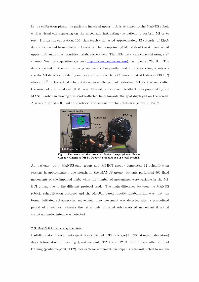
In the calibration phase, the patient's impaired upper limb is strapped to the MANUS robot,

with a visual cue appearing on the screen and instructing the patient to perform MI or to

rest. During the calibration, 160 trials (each trial lasted approximately 12 seconds) of EEG-

data are collected from a total of 4 sessions, that comprised 80 MI trials of the stroke-affected

upper limb and 80 rest condition trials, respectively. The EEG data were collected using a 27

channel Nuamps acquisition system (http://www.neuroscan.com), sampled at 250 Hz. The

data collected in the calibration phase were subsequently used for constructing a subject-

specific MI detection model by employing the Filter Bank Common Spatial Pattern (FBCSP)

algorithm.21 In the actual rehabilitation phase, the patient performed MI for 4 seconds after

the onset of the visual cue. If MI was detected, a movement feedback was provided by the

MANUS robot in moving the stroke-affected limb towards the goal displayed on the screen.

A setup of the MI-BCI with the robotic feedback neurorehabilitation is shown in Fig. 2.

All patients (both MANUS-only group and MI-BCI group) completed 12 rehabilitation

sessions in approximately one month. In the MANUS group patients performed 960 fixed

movements of the impaired limb, while the number of movements were variable in the MI-

BCI group, due to the different protocol used. The main difference between the MANUS

robotic rehabilitation protocol and the MI-BCI based robotic rehabilitation was that the

former initiated robot-assisted movement if no movement was detected after a pre-defined

period of 2 seconds, whereas the latter only initiated robot-assisted movement if actual

voluntary motor intent was detected.

2.3 Rs-fMRI data acquisition

Rs-fMRI data of each participant was collected 6.33 (average) 6.98 (standard deviation)

days before start of training (pre-timepoint, TP1) and 12.33 6.10 days after stop of

training (post-timepoint, TP2). For each measurement participants were instructed to remain

relaxed and awake with their eyes closed and not to engage in any specific activity. Each rs-

fMRI session consisted of a 10 min block (400 volumes, 28 slices, 3x3x4 mm voxels, 0.4 mm

slice gap, TR=1.5 secs, TE=30 ms, interleaved-ascending acquisition) and was performed in

the same Siemens Magnetom Trio Tim syngo MR B15 scanner.

2.4 Calculation of functional motor gain from behavioral data

Fugl-Meyer (FM) scores were recorded for each participant at 0, 2, 4 and 12 weeks after

beginning of training by a trained occupational therapist. By fitting a slope to the FM data

of each participant an indicator of individual gain steepness was derived, by using the incline

of each participants' functional outcome gain slope (see Figure 3). It is to note that by

incorporating a 8 week post-training follow-up measurement (12 weeks after beginning), out-

of-lab effects are part of the behavioral assessment thus reflecting the steepness of general

recovery during and after treatment. The individual gain values were used as criteria in the

subsequent regressions.

Table 1, Participant data - including Oxford classification of stroke

(BG=basal ganlia/thalamic, CR=Corona Radiata, MCA=Middle Cerebral

Artey), Month is calculated as (Date1-Date2/30days).   Time to therapy is the

number of months that elapse between the stroke onset and week 0. Screening

to therapy (month) is the number of months that elapse between the screening

and week 0.

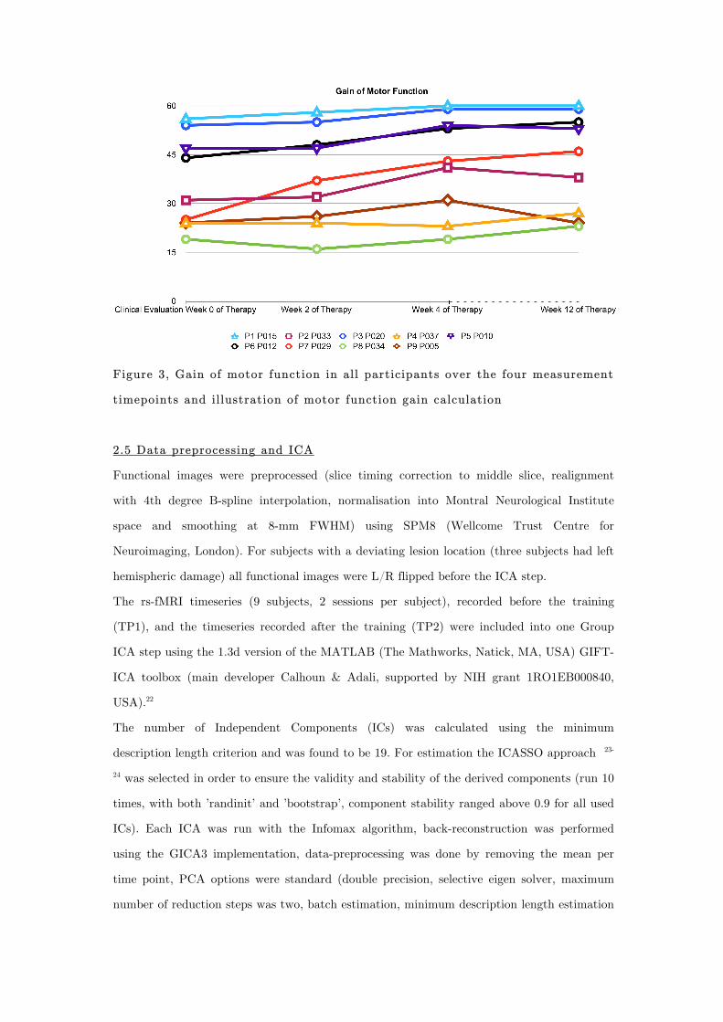
Figure 3, Gain of motor function in all participants over the four measurement

timepoints and illustration of motor function gain calculation

2.5 Data preprocessing and ICA

Functional images were preprocessed (slice timing correction to middle slice, realignment

with 4th degree B-spline interpolation, normalisation into Montral Neurological Institute

space and smoothing at 8-mm FWHM) using SPM8 (Wellcome Trust Centre for

Neuroimaging, London). For subjects with a deviating lesion location (three subjects had left

hemispheric damage) all functional images were L/R flipped before the ICA step.

The rs-fMRI timeseries (9 subjects, 2 sessions per subject), recorded before the training

(TP1), and the timeseries recorded after the training (TP2) were included into one Group

ICA step using the 1.3d version of the MATLAB (The Mathworks, Natick, MA, USA) GIFT-

ICA toolbox (main developer Calhoun & Adali, supported by NIH grant 1RO1EB000840,

USA).22

The number of Independent Components (ICs) was calculated using the minimum

description length criterion and was found to be 19. For estimation the ICASSO approach 23-

24 was selected in order to ensure the validity and stability of the derived components (run 10

times, with both ’randinit’ and ’bootstrap’, component stability ranged above 0.9 for all used

ICs). Each ICA was run with the Infomax algorithm, back-reconstruction was performed

using the GICA3 implementation, data-preprocessing was done by removing the mean per

time point, PCA options were standard (double precision, selective eigen solver, maximum

number of reduction steps was two, batch estimation, minimum description length estimation

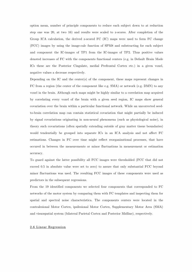
option mean, number of principle components to reduce each subject down to at reduction

step one was 20, at two 16) and results were scaled to z-scores. After completion of the

Group ICA calculation, the derived z-scored FC (IC) maps were used to form FC change

(FCC) images by using the image-calc function of SPM8 and substracting for each subject

and component the IC-images of TP1 from the IC-images of TP2. Thus positive values

denoted increases of FC with the components functional centers (e.g. in Default Brain Mode

ICs these are the Posterior Cingulate, medial Prefrontal Cortex etc.) in a given voxel,

negative values a decrease respectively.

Depending on the IC and the center(s) of the component, these maps represent changes in

FC from a region (the center of the component like e.g. SMA) or network (e.g. DMN) to any

voxel in the brain. Although such maps might be highly similar to a correlation map acquired

by correlating every voxel of the brain with a given seed region, IC maps show general

covariation over the brain within a particular functional network. While an uncorrected seed-

to-brain correlation map can contain statistical covariation that might partially be induced

by signal covariations originating in non-neural phenomena (such as physiological noise), in

theory such covariations (often spatially extending outside of gray matter tissue boundaries)

would tendentially be grouped into separate ICs in an ICA analysis and not affect FC

estimations. Changes in FC over time might reflect reorganizational processes, that have

occured in between the measurements or minor fluctuations in measurement or estimation

accuracy.

To guard against the latter possibility all FCC images were thresholded (FCC that did not

exceed 0.5 in absolute value were set to zero) to assure that only substantial FCC beyond

minor fluctuations was used. The resulting FCC images of these components were used as

predictors in the subsequent regressions.

From the 19 identified components we selected four components that corresponded to FC

networks of the motor system by comparing them with FC templates and inspecting them for

spatial and spectral noise characteristica. The components centers were located in the

contralesional Motor Cortex, ipsilesional Motor Cortex, Supplementary Motor Area (SMA)

and visuospatial system (bilateral Parietal Cortex and Posterior Midline), respectively.

2.6 Linear Regression

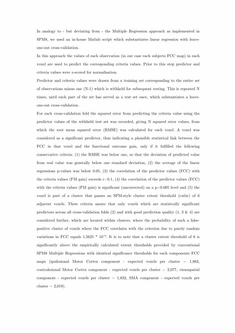
In analogy to - but deviating from - the Multiple Regression approach as implemented in

SPM8, we used an in-house Matlab script which substantiates linear regression with leave-

one-out cross-validation.

In this approach the values of each observation (in our case each subjects FCC map) in each

voxel are used to predict the corresponding criteria values. Prior to this step predictor and

criteria values were z-scored for normalisation.

Predictor and criteria values were drawn from a training set corresponding to the entire set

of observations minus one (N-1) which is withheld for subsequent testing. This is repeated N

times, until each part of the set has served as a test set once, which substantiates a leave-

one-out cross-validation.

For each cross-validation fold the squared error from predicting the criteria value using the

predictor values of the withheld test set was recorded, giving N squared error values, from

which the root mean squared error (RMSE) was calculated for each voxel. A voxel was

considered as a significant predictor, thus indicating a plausible statistical link between the

FCC in that voxel and the functional outcome gain, only if it fulfilled the following

conservative criteria: (1) the RMSE was below one, so that the deviation of predicted value

from real value was generally below one standard deviation, (2) the average of the linear

regressions p-values was below 0.05, (3) the correlation of the predictor values (FCC) with

the criteria values (FM gain) exceeds r=0.1, (4) the correlation of the predictor values (FCC)

with the criteria values (FM gain) is significant (uncorrected) on a p=0.005 level and (5) the

voxel is part of a cluster that passes an SPM-style cluster extent threshold (cubic) of 6

adjacent voxels. These criteria assure that only voxels which are statistcally significant

predictors across all cross-validation folds (2) and with good prediction quality (1, 3 & 4) are

considered further, which are located within clusters, where the probability of such a false-

positive cluster of voxels where the FCC correlates with the criterion due to purely random

variations in FCC equals 1,5625 * 10-14. It is to note that a cluster extent threshold of 6 is

significantly above the empirically calculated extent thresholds provided by conventional

SPM8 Multiple Regressions with identical significance thresholds for each components FCC

maps (ipsilesional Motor Cortex component - expected voxels per cluster = 1,863,

contralesional Motor Cortex component - expected voxels per cluster = 2,077, visuospatial

component - expected voxels per cluster = 1,833, SMA component - expected voxels per

cluster = 2,019).

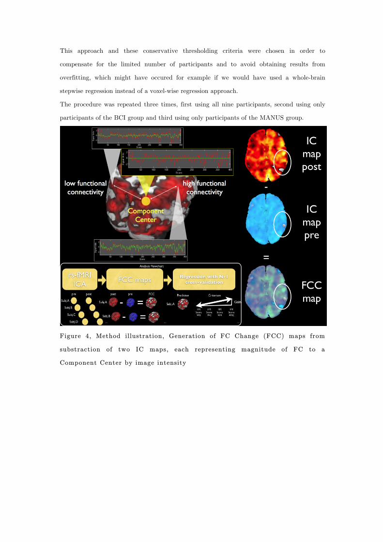
This approach and these conservative thresholding criteria were chosen in order to

compensate for the limited number of participants and to avoid obtaining results from

overfitting, which might have occured for example if we would have used a whole-brain

stepwise regression instead of a voxel-wise regression approach.

The procedure was repeated three times, first using all nine participants, second using only

participants of the BCI group and third using only participants of the MANUS group.

Figure 4, Method illustration, Generation of FC Change (FCC) maps from

substraction of two IC maps, each representing magnitude of FC to a

Component Center by image intensity

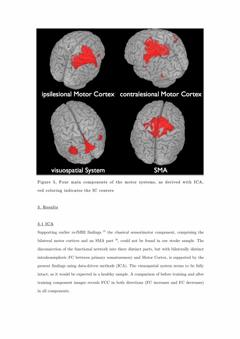
Figure 5, Four main components of the motor systems, as derived with ICA,

red coloring indicates the IC centers

3. Results

3.1 ICA

Supporting earlier rs-fMRI findings 25 the classical sensorimotor component, comprising the

bilateral motor cortices and an SMA part 26, could not be found in our stroke sample. The

disconnection of the functional network into three distinct parts, but with bilaterally distinct

intrahemispheric FC between primary somatosensory and Motor Cortex, is supported by the

present findings using data-driven methods (ICA). The visuospatial system seems to be fully

intact, as it would be expected in a healthy sample. A comparison of before training and after

training component images reveals FCC in both directions (FC increases and FC decreases)

in all components.

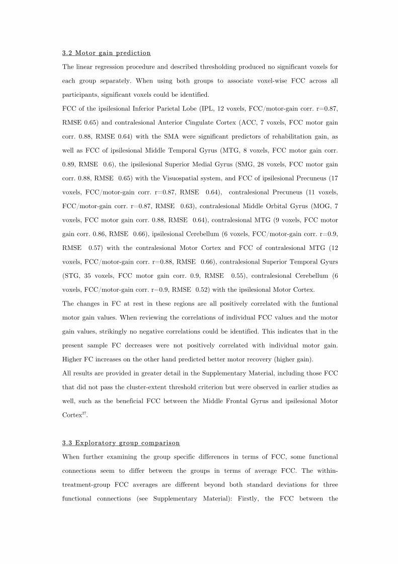
3.2 Motor gain prediction

The linear regression procedure and described thresholding produced no significant voxels for

each group separately. When using both groups to associate voxel-wise FCC across all

participants, significant voxels could be identified.

FCC of the ipsilesional Inferior Parietal Lobe (IPL, 12 voxels, FCC/motor-gain corr. r=0.87,

RMSE 0.65) and contralesional Anterior Cingulate Cortex (ACC, 7 voxels, FCC motor gain

corr. 0.88, RMSE 0.64) with the SMA were significant predictors of rehabilitation gain, as

well as FCC of ipsilesional Middle Temporal Gyrus (MTG, 8 voxels, FCC motor gain corr.

0.89, RMSE 0.6), the ipsilesional Superior Medial Gyrus (SMG, 28 voxels, FCC motor gain

corr. 0.88, RMSE 0.65) with the Visuospatial system, and FCC of ipsilesional Precuneus (17

voxels, FCC/motor-gain corr. r=0.87, RMSE 0.64), contralesional Precuneus (11 voxels,

FCC/motor-gain corr. r=0.87, RMSE 0.63), contralesional Middle Orbital Gyrus (MOG, 7

voxels, FCC motor gain corr. 0.88, RMSE 0.64), contralesional MTG (9 voxels, FCC motor

gain corr. 0.86, RMSE 0.66), ipsilesional Cerebellum (6 voxels, FCC/motor-gain corr. r=0.9,

RMSE 0.57) with the contralesional Motor Cortex and FCC of contralesional MTG (12

voxels, FCC/motor-gain corr. r=0.88, RMSE 0.66), contralesional Superior Temporal Gyurs

(STG, 35 voxels, FCC motor gain corr. 0.9, RMSE 0.55), contralesional Cerebellum (6

voxels, FCC/motor-gain corr. r=0.9, RMSE 0.52) with the ipsilesional Motor Cortex.

The changes in FC at rest in these regions are all positively correlated with the funtional

motor gain values. When reviewing the correlations of individual FCC values and the motor

gain values, strikingly no negative correlations could be identified. This indicates that in the

present sample FC decreases were not positively correlated with individual motor gain.

Higher FC increases on the other hand predicted better motor recovery (higher gain).

All results are provided in greater detail in the Supplementary Material, including those FCC

that did not pass the cluster-extent threshold criterion but were observed in earlier studies as

well, such as the beneficial FCC between the Middle Frontal Gyrus and ipsilesional Motor

Cortex27.

3.3 Exploratory group comparison

When further examining the group specific differences in terms of FCC, some functional

connections seem to differ between the groups in terms of average FCC. The within-

treatment-group FCC averages are different beyond both standard deviations for three

functional connections (see Supplementary Material): Firstly, the FCC between the

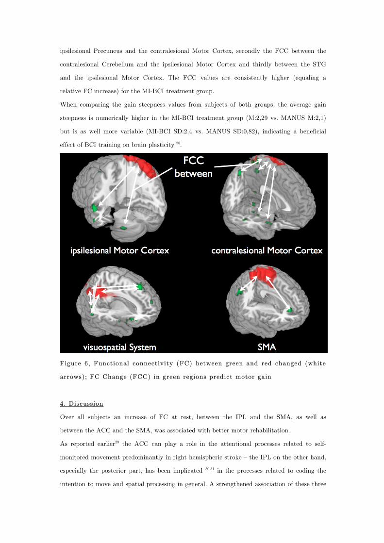
ipsilesional Precuneus and the contralesional Motor Cortex, secondly the FCC between the

contralesional Cerebellum and the ipsilesional Motor Cortex and thirdly between the STG

and the ipsilesional Motor Cortex. The FCC values are consistently higher (equaling a

relative FC increase) for the MI-BCI treatment group.

When comparing the gain steepness values from subjects of both groups, the average gain

steepness is numerically higher in the MI-BCI treatment group (M:2,29 vs. MANUS M:2,1)

but is as well more variable (MI-BCI SD:2,4 vs. MANUS SD:0,82), indicating a beneficial

effect of BCI training on brain plasticity  28.

Figure 6, Functional connectivity (FC) between green and red changed (white

arrows); FC Change (FCC) in green regions predict motor gain

4. Discussion

Over all subjects an increase of FC at rest, between the IPL and the SMA, as well as

between the ACC and the SMA, was associated with better motor rehabilitation.

As reported earlier29 the ACC can play a role in the attentional processes related to self-

monitored movement predominantly in right hemispheric stroke – the IPL on the other hand,

especially the posterior part, has been implicated 30,31 in the processes related to coding the

intention to move and spatial processing in general. A strengthened association of these three

systems, namely the IPL, ACC and the SMA in a functional network could be beneficial for

motor recovery, as it might constitute an adapted functional network for processing motor

attention, cueing and movement initiation.

The visuospatial system has been associated with representing the world around us, as well

as with processing visuo-spatial cues.26 The FC increases with the ipsilesional MTG and

Frontal Cortex (SMG), might indicate a strengthening of systems related to spatial

awareness and spatial processing, which both have been associated with the Medial Gyrus

and Temporal Lobe.32 Especially the MTG has been associated with spatial mental imagery 33, which is a function that is targeted in the MI-BCI treatment.

The observed - supposedly beneficial - strengthening of functional connections between

fronto-parietal regions which are known to play a key role in top-down processes and the

visuospatial system and SMA, might be adaptations thate are counter-acting the deficits in

the connectivity of these systems following stroke that have been described in resting-state

studies earlier34.

The functonal connectivity increases between the contralesional MTG, Precuneus, MOG and

ipsilesional Cerebellum with the contralesional Motor Cortex, as well as the changes in FC

between the contralesional MTG, STG, Cerebellum and the ipsilesional Motor Cortex, might

reflect adaptive processes that occur during the reorganization of motor control and reflect

increased recruitment of regions disconnected by the stroke35 and have recently been

described by other groups as well36.

It has long been argued whether control from ipsilesional or contralesional Motor Cortex

should be targeted as means of functional rehabilitation especially in subcortical stroke.37-45

Our results indicate, that the process might be more complex than the idea of a mere role

change for one single motor system and the silencing of another. It is possible that the

contralesional Motor Cortex assumes only a temporary role in adaptive motor control,

predominantly in the early stages of stroke recovery.46

We clearly recognize the limitations of our study, such as the limited group size and the

short time between the two rs-fMRI sessions. It is possible that these results represent only a

snapshot of the adaptive processes occuring in the recovering brain. Specifically in the light

of recent findings on the link between perfusion, white matter connectivity47 and FC future

longitudinal studies need to evaluate the role of post-stroke changes in cerebral perfusion and

tissue integrity in peri-lesional white matter bundles and gray matter structures48 as potential

mediators of FCC.

It might be an interesting experimental strategy, to form new trainings that target a

strengthening of FC between the described regions, for example by means of real-time fMRI

based neurofeedback training. In such a training the feedback could consist of not one single

signal from one single region, merely giving the classical real time neurofeedback of activity,

but rather consist directly of the correlation value itself, which could be derived from the

voxel-to-voxel correlations calculated with a moving window and signals from multiple

targeted sites (e.g. ACC and SMA). Such a neurofeedback could be used to directly train FC

increases, rather than an activation of single sites.

4.1 Treatment group comparison

In an exploratory attempt we compared average FCC between the two treatment groups for

all identified sites where the relation of FCC and motor recovery was significant.

Participants in the MI-BCI group showed stronger FC increases between the contralesional

Cerebellum and the ipsilesional Motor Cortex, the contralesional STG and the ipsilesional

Motor Cortex and the ipsilesional Precuneus and the contralesional Motor Cortex.

As these connections are known to be involved in MI performance, it might be hypothesized

that the value of the MI-BCI treatment might not only be a numerically higher gain in upper

limb motor function, but as well a strengthening of those functional networks which

contribute to neural processing of MI. Good MI involving the paretic limb can not occur

entirely outside of systems, that contain somatosensory and motoric memories of moving that

limb, as it is unlikely that post-stroke MI involving the paretic limb is based on a re-creation

of imagery, or any kind of mental content related to the limb, entirely from scratch. It is

therefore not unlikely, that MI-BCI training strengthens the re-association of neural

representations of the paretic limb and the experienced afference, and that this leads to

better MI and better recovery.

5. Conclusions

Increases in rs-fMRI FC within parts of the motor system, and between motor regions and

higher-order association cortices significantly predict better functional motor recovery. The

increased FC at rest could be interpreted to reflect an after-effect of strenghtening neural

connections within these networks. The fact that the extent of this FC increase is directly

correlated with functional motor gain suggests a fascilatory effect of such connection

strengthening on motor recovery, possibly implicating an increase in inter-regional

macroscopic neural cooperation as an explanation for this effect. Studies on larger

populations and with sham-BCI-treament or control groups have to be conducted in order to

clarify the stability of these results and to investigate the question, whether higher overall

brain plasticity or only the strengthening of specific connections is beneficial for motor

recovery.

Acknowledgments:

The authors thank the participants and the entire Singapore research team,

recruiters, trainers, testers and nurses in the Tan Tock Seng Hospital

rehabilitation center, as well as everybody involved in the data acquisition

process. We would as well like to thank Prof. Chee for his help with the

revision process and scanning.

Declaration of Conflicting Interests:

None.

Funding:

Author BV was partially funded by the European Union (HUMOUR 231724).

We are thankful to the The Enterprise Challenge Grant, Singapore and Agency

for Science, Technology and Research, Singapore for their funding support.

References:

1 McGinnis JM, Foege WH. Actual causes of death in the United States. Jama.

1993;270(18):2207.

2 Anderson CS, Linto J, Stewart-Wynne EG. A population-based assessment of the

impact and burden of caregiving for long-term stroke survivors. Stroke.

1995;26(5):843.

3 Vestling M, Tufvesson B, Iwarsson S. Indicators for return to work after stroke and

the importance of work for subjective well-being and life satisfaction. Journal of

Rehabilitation Medicine. 2003;35(3):127–131.

4 Birbaumer N. Breaking the silence: brain–computer interfaces (BCI) for

communication and motor control. Psychophysiology. 2006;43(6):517–532.

5 Buch E, Weber C, Cohen LG, et al. Think to move: a neuromagnetic brain-computer

interface (BCI) system for chronic stroke. Stroke. 2008;39(3):910.

6 Grefkes C, Nowak DA, Eickhoff SB, et al. Cortical connectivity after subcortical

stroke assessed with functional magnetic resonance imaging. Annals of neurology.

2008;63(2):236–246.

7 Ang KK, Guan C, Chua KSI et al. Clinical study of neurorehabilitation in stroke

using eeg-based motor imagery brain-computer interface with robotic feedback. In:

32nd Annual International Conference of the IEEE Engineering in Medicine and

Biology Society (EMBC), Buenos Aires, Argentina, 31 August - 4 September 2010.

8 Ang KK, Guan C, Chua SG, et al. A clinical study of motor imagery-based brain-

computer interface for upper limb robotic rehabilitation. In: Engineering in Medicine

and Biology Society, 2009. EMBC 2009. Annual International Conference of the

IEEE.; 2009:5981–5984.

9 De Luca M, Beckmann CF, De Stefano N, Matthews PM, Smith SM. fMRI resting

state networks define distinct modes of long-distance interactions in the human brain.

Neuroimage. 2006;29(4):1359–1367.

10 Greicius MD, Srivastava G, Reiss AL, Menon V. Default-mode network activity

distinguishes Alzheimer's disease from healthy aging: evidence from functional MRI.

Proceedings of the National Academy of Sciences of the United States of America.

2004;101(13):4637.

11 Greicius MD, Krasnow B, Reiss AL, Menon V. Functional connectivity in the resting

brain: a network analysis of the default mode hypothesis. Proceedings of the National

Academy of Sciences of the United States of America. 2003;100(1):253.

12 Fransson P. Spontaneous low-frequency BOLD signal fluctuations: an fMRI

investigation of the resting-state default mode of brain function hypothesis. Human

brain mapping. 2005;26(1):15–29.

13 "Cordes D, Haughton VM, Arfanakis K, et al. Frequencies contributing to functional

connectivity in the cerebral cortex in"" resting-state"" data. American Journal of

Neuroradiology. 2001;22(7):1326. "

14 Dosenbach NU, Nardos B, Cohen AL, et al. Prediction of Individual Brain Maturity

Using fMRI. Science. 2010;329(5997):1358.

15 Ystad M, Eichele T, Lundervold AJ, Lundervold A. Subcortical functional

connectivity and verbal episodic memory in healthy elderly–A resting state fMRI

study. NeuroImage. 2010;52(1):379–388.

16 Grefkes C, Fink GR. Reorganization of cerebral networks after stroke: new insights

from neuroimaging with connectivity approaches. Brain : a journal of neurology.

2011;134(Pt 5):1264-76. Available at:

http://www.pubmedcentral.nih.gov/articlerender.fcgi?artid=3097886&tool=pmcentre

z&rendertype=abstract. Accessed August 6, 2011.

17 Westlake KP, Nagarajan SS. Functional connectivity in relation to motor

performance and recovery after stroke. Frontiers in systems neuroscience.

2011;5(March):8. Available at:

http://www.pubmedcentral.nih.gov/articlerender.fcgi?artid=3060711&tool=pmcentre

z&rendertype=abstract. Accessed June 17, 2011.

18 Krebs HI, Hogan N. Therapeutic robotics: A technology push. Proceedings of the

IEEE. 2006;94(9):1727–1738.

19 Krebs HI, Hogan N, Aisen ML, Volpe BT. Robot-aided neurorehabilitation. IEEE

Transactions on Rehabilitation Engineering. 1998;6(1):75–87.

20 Krebs HI, Palazzolo JJ, Dipietro L, et al. Rehabilitation robotics: Performance-based

progressive robot-assisted therapy. Autonomous Robots. 2003;15(1):7–20.

21 Ang KK, Chin ZY, Zhang H, Guan C. Filter bank common spatial pattern (FBCSP)

in brain-computer interface. In: Neural Networks, 2008. IJCNN 2008.(IEEE World

Congress on Computational Intelligence). IEEE International Joint Conference on.;

2008:2390–2397.

22 Calhoun VD, Liu J, AdalI T. A review of group ICA for fMRI data and ICA for joint

inference of imaging, genetic, and ERP data. Neuroimage. 2009;45(1):S163–S172.

23 Himberg J, Hyvarinen A. Icasso: software for investigating the reliability of ICA

estimates by clustering and visualization. In: Neural Networks for Signal Processing,

2003. NNSP'03. 2003 IEEE 13th Workshop on.; 2004:259–268.

24 Correa N, Adali T, Calhoun VD. Performance of blind source separation algorithms

for fMRI analysis using a group ICA method. Magnetic resonance imaging.

2007;25(5):684–694.

25 van Meer M, van der Marel K, Wang K, et al. Recovery of sensorimotor function

after experimental stroke correlates with restoration of resting-state interhemispheric

functional connectivity. Journal of Neuroscience. 2010;30(11):3964.

26 Beckmann CF, DeLuca M, Devlin JT, Smith SM. Investigations into resting-state

connectivity using independent component analysis. Philosophical Transactions of the

Royal Society B: Biological Sciences. 2005;360(1457):1001.

27 Park C-hyun, Chang WH, Ohn SH, et al. Longitudinal changes of resting-state

functional connectivity during motor recovery after stroke. Stroke; a journal of

cerebral circulation. 2011;42(5):1357-62. Available at:

http://www.ncbi.nlm.nih.gov/pubmed/21441147. Accessed June 19, 2011.

28 Caria A, Weber C, Brötz D, et al. Chronic stroke recovery after combined BCI

training and physiotherapy: a case report. Psychophysiology. 2011;48(4):578-82.

Available at: http://www.ncbi.nlm.nih.gov/pubmed/20718931. Accessed September

26, 2011.

29 Hanlon CA, Buffington AL, McKeown MJ. New brain networks are active after right

MCA stroke when moving the ipsilesional arm. Neurology. 2005;64(1):114.

30 Ruiz S, Lee S, Schneider C, et al. Multivariate prediction of movement intention in

the human fronto-parietal cortex. (submitted)

31 Desmurget M, Reilly KT, Richard N, et al. Movement intention after parietal cortex

stimulation in humans. science. 2009;324(5928):811.

32 Karnath HO, Ferber S, Himmelbach M. Spatial awareness is a function of the

temporal not the posterior parietal lobe. Nature. 2001;411(6840):950–953.

33 Mellet E, Tzourio N, Crivello F, et al. Functional anatomy of spatial mental imagery

generated from verbal instructions. Journal of Neuroscience. 1996;16(20):6504.

34 Inman CS, James GA, Hamann S, et al. Altered resting-state effective connectivity of

fronto-parietal motor control systems on the primary motor network following stroke.

NeuroImage. 2011;59(1):227-237. Available at:

http://www.ncbi.nlm.nih.gov/pubmed/21839174. Accessed September 23, 2011.

35 Bosnell R a, Kincses T, Stagg CJ, et al. Motor practice promotes increased activity in

brain regions structurally disconnected after subcortical stroke. Neurorehabilitation

and neural repair. 2011;25(7):607-16. Available at:

http://www.ncbi.nlm.nih.gov/pubmed/21646444. Accessed September 24, 2011.

36 Wang L, Yu C, Chen H, et al. Dynamic functional reorganization of the motor

execution network after stroke. Brain : a journal of neurology. 2010;133(Pt 4):1224-

38. Available at: http://www.ncbi.nlm.nih.gov/pubmed/20354002. Accessed July 18,

2011.

37 Calautti C, Baron JC. Functional neuroimaging studies of motor recovery after stroke

in adults: a review. Stroke. 2003;34(6):1553.

38 Calautti C, Jones PS, Naccarato M, et al. The relationship between motor deficit and

primary motor cortex hemispheric activation balance after stroke: longitudinal fMRI

study. British Medical Journal. 2010.

39 Calautti C, Leroy F, Guincestre JY, Marié RM, Baron JC. Sequential activation

brain mapping after subcortical stroke: changes in hemispheric balance and recovery.

Neuroreport. 2001;12(18):3883.

40 Ward NS, Newton JM, Swayne OB, et al. Motor system activation after subcortical

stroke depends on corticospinal system integrity. Brain. 2006;129(3):809.

41 Ward NS. Mechanisms underlying recovery of motor function after stroke. British

Medical Journal. 2005;81(958):510.

42 Ward NS, Brown MM, Thompson AJ, Frackowiak RSJ. Neural correlates of motor

recovery after stroke: a longitudinal fMRI study. Brain. 2003;126(11):2476.

43 Fridman EA, Hanakawa T, Chung M, et al. Reorganization of the human ipsilesional

premotor cortex after stroke. Brain. 2004;127(4):747.

44 Tombari D, Loubinoux I, Pariente J, et al. A longitudinal fMRI study: in recovering

and then in clinically stable sub-cortical stroke patients. Neuroimage. 2004;23(3):827–

839.

45 Loubinoux I, Carel C, Pariente J, et al. Correlation between cerebral reorganization

and motor recovery after subcortical infarcts. Neuroimage. 2003;20(4):2166–2180.

46 Rehme AK, Fink GR, von Cramon DY, Grefkes C. The Role of the Contralesional

Motor Cortex for Motor Recovery in the Early Days after Stroke Assessed with

Longitudinal fMRI. Cerebral Cortex. 2010.

47 Aslan S, Huang H, Uh J, et al. White matter cerebral blood flow is inversely

correlated with structural and functional connectivity in the human brain.

NeuroImage. 2011;56(3):1145-53. Available at:

http://www.pubmedcentral.nih.gov/articlerender.fcgi?artid=3085605&tool=pmcentre

z&rendertype=abstract. Accessed August 17, 2011.

48 Várkuti B, Cavusoglu M, Kullik A, et al. Quantifying the link between anatomical

connectivity, gray matter volume and regional cerebral blood flow: an integrative

MRI study. Sporns O, ed. PloS one. 2011;6(4):e14801. Available at:

http://dx.plos.org/10.1371/journal.pone.0014801. Accessed June 23, 2011.

Supplementary Table

Results of multiple regression analysis for all included components, green and orange colors mark

particularly strong FCC differences between treatment groups

186

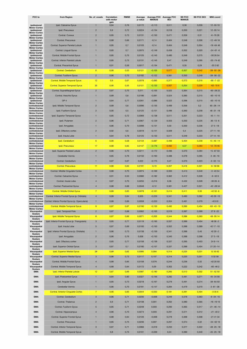
FCC to from Region No_of_voxels Correlation with motor

gain

RMSE Average p-value

Average FCC MANUS

Average FCC BCI

SD FCC MANUS

SD FCC BCI MNI coord

ipsilesional Motor Cortexipsilesional

Motor Cortexipsilesional

Motor Cortexipsilesional

Motor Cortexipsilesional

Motor Cortexipsilesional

Motor Cortexipsilesional

Motor Cortexipsilesional

Motor Cortexipsilesional

Motor Cortexipsilesional

Motor Cortexipsilesional

Motor Cortexipsilesional

Motor Cortexipsilesional

Motor Cortexipsilesional

Motor Cortexipsilesional

Motor Cortexipsilesional

Motor Cortexcontralesional Motor Cortexcontralesional Motor Cortexcontralesional Motor Cortexcontralesional Motor Cortexcontralesional Motor Cortexcontralesional Motor Cortexcontralesional Motor Cortexcontralesional Motor Cortexcontralesional Motor Cortexcontralesional Motor Cortexcontralesional Motor Cortexcontralesional Motor Cortexcontralesional Motor Cortexcontralesional Motor Cortexcontralesional Motor Cortexcontralesional Motor Cortexcontralesional Motor Cortexcontralesional Motor Cortexcontralesional Motor Cortexcontralesional Motor Cortexcontralesional Motor CortexVisuospatial

SystemVisuospatial

SystemVisuospatial

SystemVisuospatial

SystemVisuospatial

SystemVisuospatial

SystemVisuospatial

SystemVisuospatial

SystemVisuospatial

SystemVisuospatial

SystemVisuospatial

SystemVisuospatial

SystemSMA

SMA

SMA

SMA

SMA

SMA

SMA

SMA

SMA

SMA

SMA

SMA

SMA

Ipsil. Calcarine Gyrus 1 0,84 0,76 0,0172 -0,113 0,511 0,36 0,226 12 -55 10

Ipsil. Precuneus 2 0,9 0,72 0,0224 -0,134 0,518 0,350 0,221 12 -55 14

Contral. Cuneus 2 0,85 0,73 0,0131 -0,150 0,471 0,359 0,31 -6 -76 26

Contral. Precuneus 3 0,88 0,66 0,0171 -0,14 0,464 0,348 0,306 -12 -49 18

Contral. Superior Parietal Lobule 1 0,85 0,7 0,0103 -0,14 0,464 0,349 0,304 -18 -64 46

Contral. Lingual Gyrus 1 0,85 0,7 0,0075 -0,149 0,459 0,352 0,320 -24 -61 -6

Contral. Middle Frontal Gyrus 1 0,85 0,75 0,0125 -0,145 0,480 0,349 0,275 -30 26 54

Contral. Inferior Parietal Lobule 1 0,85 0,73 0,0131 -0,145 0,47 0,349 0,295 -33 -74 42

Contral. Precentral Gyrus 1 0,91 0,59 0,0017 -0,134 0,471 0,35 0,29 -33 2 62

Contral. Cerebellum 6 0,90 0,53 0,0121 -0,105 0,577 0,357 0,242 -39 -55 -26

Contral. Fusiform Gyrus 2 0,86 0,70 0,0182 -0,122 0,581 0,350 0,249 -39 -58 -22

Contral. Middle Temporal Gyrus 12 0,9 0,67 0,0078 -0,085 0,377 0,373 0,316 -60 -7 -22

Contral. Superior Temporal Gyrus 35 0,90 0,55 0,0121 -0,133 0,507 0,354 0,229 -63 -10 6

Contral. SupraMarginal Gyrus 2 0,87 0,70 0,011 -0,105 0,522 0,364 0,215 -60 -28 22

Contral. Heschls Gyrus 1 0,89 0,6 0,0186 -0,091 0,524 0,385 0,215 -60 -10 10

OP 4 1 0,84 0,77 0,0261 -0,086 0,522 0,396 0,215 -63 -10 10

Ipsil. Middle Temporal Gyrus 2 0,89 0,6 0,0096 -0,135 0,499 0,356 0,2 60 -28 -14

Ipsil. Fusiform Gyrus 2 0,90 0,5 0,0125 -0,151 0,496 0,360 0,258 48 -31 -18

Ipsil. Superior Temporal Gyrus 1 0,85 0,72 0,0069 -0,138 0,511 0,351 0,223 45 -1 -14

Ipsil. Putamen 2 0,86 0,71 0,0067 -0,129 0,503 0,350 0,235 36 -13 -6

Ipsil. Amygdala 1 0,86 0,70 0,0098 -0,131 0,50 0,350 0,236 27 5 -18

Ipsil. Olfactory cortex 2 0,92 0,6 0,0019 -0,141 0,509 0,4 0,225 27 11 -18

Ipsil. Insula Lobe 1 0,84 0,78 0,0125 -0,133 0,511 0,349 0,223 27 14 -18

Ipsil. Cerebellum 6 0,90 0,58 0,0134 -0,087 0,499 0,404 0,239 15 -40 -14

Ipsil. Precuneus 17 0,88 0,65 0,0137 -0,176 0,492 0,37 0,283 12 -70 46

Ipsil. Superior Parietal Lobule 2 0,86 0,70 0,0211 -0,172 0,496 0,370 0,284 15 -67 50

Cerebellar Vermis 1 0,85 0,76 0,0150 -0,160 0,488 0,378 0,285 3 -46 -10

Contral. Cerebellum 1 0,87 0,67 0,022 -0,175 0,47 0,370 0,323 -3 -52 -14

Contral. Precuneus 11 0,88 0,63 0,0191 -0,19 0,357 0,416 0,331 -6 -58 66

Contral. Middle Cingulate Cortex 1 0,88 0,70 0,0074 -0,169 0,350 0,413 0,340 -3 -43 54

Contral. Calcarine Gyrus 1 0,91 0,53 0,0080 -0,182 0,362 0,412 0,328 -6 -52 6

Contral. Insula Lobe 4 0,87 0,70 0,0255 -0,216 0,36 0,432 0,328 -30 26 -6

Contral. Postcentral Gyrus 4 0,88 0,68 0,0048 -0,12 0,381 0,427 0,321 -42 -28 54

Contral. Middle Orbital Gyrus 7 0,89 0,65 0,0078 -0,161 0,414 0,411 0,30 -42 50 -6

Contral. Inferior Frontal Gyrus (p. Orbitalis) 4 0,89 0,64 0,005 -0,229 0,341 0,480 0,392 -45 29 -10

Contral. Inferior Frontal Gyrus (p. Opercularis) 1 0,88 0,66 0,0058 -0,220 0,354 0,481 0,379 -45 8 6

Contral. Middle Temporal Gyrus 9 0,87 0,67 0,0190 -0,133 0,492 0,390 0,454 -63 -43 -10

Ipsil. Temporal Pole 2 0,87 0,68 0,0062 -0,105 0,519 0,387 0,399 27 8 -22

Ipsil. Middle Temporal Gyrus 8 0,87 0,69 0,0071 -0,205 0,344 0,386 0,393 48 -55 14

Ipsil. Inferior Frontal Gyrus (p. Triangularis) 3 0,85 0,77 0,0119 -0,195 0,337 0,389 0,404 48 38 -2

Ipsil. Insula Lobe 5 0,87 0,69 0,0100 -0,150 0,352 0,388 0,389 42 17 -10

Ipsil. Inferior Frontal Gyrus (p. Orbitalis) 1 0,86 0,73 0,0138 -0,159 0,341 0,388 0,40 42 29 -2

Ipsil. Amygdala 2 0,86 0,76 0,006 -0,150 0,340 0,388 0,398 27 5 -18

Ipsil. Olfactory cortex 2 0,85 0,77 0,0158 -0,138 0,337 0,395 0,403 24 8 -14

Ipsil. Superior Orbital Gyrus 3 0,87 0,7 0,0180 -0,157 0,337 0,388 0,404 21 20 -14

Ipsil. Superior Medial Gyrus 28 0,89 0,62 0,0085 0,084 0,314 0,225 0,231 12 35 62

Contral. Superior Medial Gyrus 3 0,86 0,73 0,0117 0,107 0,314 0,220 0,251 0 32 58

Contral. Middle Frontal Gyrus 4 0,88 0,65 0,0158 0,076 0,244 0,236 0,32 -42 20 50

Contral. Middle Temporal Gyrus 4 0,88 0,64 0,0172 0,09 0,302 0,222 0,242 -60 -46 2

Ipsil. Inferior Parietal Lobule 12 0,87 0,69 0,0087 -0,180 0,265 0,513 0,302 51 -52 50

Ipsil. Postcentral Gyrus 1 0,84 0,80 0,0327 -0,156 0,282 0,481 0,271 45 -34 58

Ipsil. Angular Gyrus 1 0,85 0,73 0,0218 -0,167 0,279 0,491 0,274 39 -64 50

Cerebellar Vermis 1 0,86 0,70 0,0181 -0,147 0,284 0,479 0,270 3 -61 -38

Contral. Anterior Cingulate Cortex 7 0,90 0,65 0,0044 -0,033 0,181 0,391 0,404 -3 35 6

Contral. Cerebellum 3 0,86 0,71 0,0230 -0,008 0,249 0,378 0,363 -9 -34 -10

Contral. Thalamus 2 0,9 0,71 0,0138 0,001 0,262 0,380 0,365 -18 -19 10

Contral. Fusiform Gyrus 5 0,85 0,71 0,0248 0,003 0,290 0,365 0,317 -21 -46 -14

Contral. Hippocampus 4 0,86 0,70 0,0274 0,003 0,291 0,371 0,312 -21 -40 2

Contral. Superior Frontal Gyrus 1 0,88 0,64 0,0126 -0,008 0,278 0,368 0,308 -21 41 34

Contral. Precuneus 1 0,85 0,75 0,0236 0,007 0,297 0,374 0,32 -24 -52 10

Contral. Inferior Temporal Gyrus 3 0,87 0,71 0,0066 -0,018 0,250 0,377 0,322 -48 -25 -18

Contral. Middle Temporal Gyrus 1 0,8 0,73 0,0101 -0,039 0,24 0,380 0,340 -45 -25 -18

7.4 Chapter 4 - On the relationship of Brain-Computer Interface apti-

tude and Anatomical Connectivity

188

SMR EEG-BCI aptitude in healthy subjects varies with the

integrity of Corpus Callosum white matter

Author list and affiliation:

Balint Varkuti1

Sebastian Halder1,2

Martin Bogdan2,3

Andrea Kubler4

Wolfgang Rosenstiel2

Ranganatha Sitaram1

Niels Birbaumer1,5

1 Institute of Medical Psychology and Behavioral Neurobiology, University of Tubingen, Tubingen,

Baden-Wurttemberg, Germany

2 Wilhelm-Schickard Institute for Computer Science, University of Tubingen, Tubingen,

Baden-Wurttemberg, Germany

3 Computer Engineering, University of Leipzig, Johannisgasse 26, 04103 Leipzig, Germany

4 Department of Psychology I, University of Wurzburg, Marcusstr. 9-11, 97070 Wurzburg, Germany

5 Ospedale San Camillo, Istituto di Ricovero e Cura a Carattere Scientifico,

Laboratorio di Neuroscience comportamentale, Venezia, Italy

1

Abstract

Healthy subjects differ in terms of their ability to control EEG based BCIs, but the reasons

for this remain unclear. Deviating from the classical perspective of analyzing psychological

intermediary variables we investigated whether the structural trait of inter-hemispheric white

matter integrity differs between subjects that can be classified as low and high aptitude users.

For this purpose 17 healthy subjects participated in a Diffusion Tensor Imaging measurement

as well as in a SMR EEG-BCI session. We extracted the individual Corpus Callosum (CC)

Fractional Anisotropy (FA) values from each subject and compared them across the two user

groups. The difference is significant (two-sample t-test, p=0.0187) and the values differ in

the expected direction (CC mean FA low aptitude users 0.53 vs. high aptitude users 0.58).

We conclude that individual inter-hemispheric connectivity traits might influence our ability

to optimally master SMR EEG-BCI control.

1 Introduction

The use of some EEG based BCIs depends critically on an individuals ability to voluntarily alter

the own brain activity in a directed manner and with relatively precise timing. Psychological

variables such as attention, training and the right mental strategy or technique, equipment related

variables such as sufficient Signal-to-Noise-Ratio (SNR) during the EEG recording and adequate

processing as well as functional variables such as individual neural plasticity and normality of the

EEG features (spectral properties, modulability of BCI-critical features) are relevant to successful

BCI control.

The link between the individual anatomy and these features becomes most apparent in patients

with severe lesions (e.g. due to stroke) or neurodegenerative disease, who show altered EEG fea-

tures, reduced neural plasticity, locally altered SNR and altered neuropsychological properties,

all of which are strongly influencing their EEG-BCI capability. But how does this relate to the

considerable variability in the BCI aptitude of healthy users with normal brain anatomy ?

Recent studies Valdes-Hernandez et al. (2010a) have indicated a critical role of central white mat-

ter for the spectral properties of an individuals EEG, underlining the significance of certain fiber

bundles for appropriate inter-regional conduction velocity in intra-cerebral neural signaling. The

relative equivalency of this conduction velocity across individuals is critical in assuring that cogni-

tive processes are running on comparable timescales. But there is as well considerable variability in

2

the integrity of fiber bundles between subjects. While the fiber bundles in the healthy brain form

always some standard connections (the connectome core so to speak), there are connections that

vary and which are an individual trademark of our brain - just like a fingerprint. While most of

these connections are intra-hemispheric and located within diverse association fiber bundles (e.g.

Superior Longitudinal Fascicle, Capsula Externa) that spread over each hemispheres cerebral white

matter, roughly more than one third of all macroscopic inter-regional anatomical connections in

the brain are inter-hemispheric and traverse through a few localized commissural structures such

as the Corpus Callosum, which could be termed the bottlenecks of inter-hemispheric connectivity.

SMR modulation through means of motor imagery is known to be a complex task, involving

multiple cortical and subcortical structures and the timely integration of their respective neural

computations into a coherent and continuous mental construct accessible to consciousness and

voluntary control. The overall integration and the time-critical signaling processes within this

bi-hemispheric task-dependent neural network must therefore strongly rely on commissural con-

nections.

We tested the hypothesis that the structural substrate of inter-hemispheric anatomical connectiv-

ity has an influence on individual BCI aptitude, by splitting a group of SMR EEG-BCI users into a

high and a low aptitude group and comparing the structural properties of their main commissural

connection (namely the Fractional Anisotropy of the Corpus Callosum).

2 Methods

2.1 Participants

Twenty healthy participants (seven female and 13 male, mean age 24.5 years SD 3.7, range 19-36)

took part in the study which was approved by the Internal Review Board of the Medical Faculty,

University of Tu?bingen. All participants had no prior experience with SMR BCIs , had no history

of neurological diseases and were German native speakers. The data from three subjects had to

be excluded due to image and scanner artifacts. A detailed overview of EEG BCI performance,

performed imagery tasks and demographic data of all participants can be found in Halder et al.

(2011).

3

2.2 EEG-BCI setup and definition of low and high aptitude users

The EEG recording was performed using four 32 channel Brainamp DC amplifiers manufactured

by Brainproducts, Munich, Germany. A 128 channel cap manufactured by Easy Cap, Munich,

Germany was used. Of these 119 were used for EEG recording and positioned according to the

extended 10-20 system Sharbrough et al. (1991), referenced to the nasion and grounded to an

electrode between Fz and Fpz. The EEG was recorded at 1000 Hz, band-pass filtered between

0.05 Hz to 200 Hz and notch filtered at 50 Hz. Electromyogram (EMG) artifacts were monitored

with bipolar electrodes on both forearms and the participants preferred leg. Electrooculogram

(EOG) artifacts were recorded with electrodes placed above and below the right eye for vertical

EOG (superior and inferior orbital fossa), and for horizontal EOG with electrodes placed at the

outer canthi of the eyes. This data was used to exclude artifact contaminated trials. Each of

the participants performed a single EEG BCI session. This included measurements in which the

participant had to perform motor execution, observation and imagery. Three imagery measure-

ments which totaled 75 trials of three classes (left hand, right hand, foot) were used to calibrate

the feedback parameters. The calibration trials had a duration of 8 seconds, in 4 of which the

participant performed the task. After calibration three feedback measurements were performed

in which the participant had to use the two classes which showed the highest discriminability in

the calibration data to control a cursor Blankertz et al. (2010b). Feedback trials had a length of 9

seconds, 4 of which were feedback. The additional second is used to indicate which class is to be

performed in the current trial. In total 300 feedback trials were performed (150 per class). The

accuracy of the participants achieved in these 300 trials was used to categorize them into high and

low aptitude SMR BCI users by a median split.

2.3 MRI recording

The MRI measurements were performed in a Siemens Magneton Trio Tim 3T whole body scanner

using a standard 12 channel head coil. Each subject participated in a DTI measurement (1.8 x

1.8 x 6.5 mm voxels, 5 mm gap, TR=3 sec, TE=93 ms, FoV=1150*1150, Flip Angle=90?, 20

transversal slices, 128x128 voxels per slice, 20 diffusion directions, b-value=1000 s/mm2) with the

field of view (FoV) comprising the full cerebrum.

4

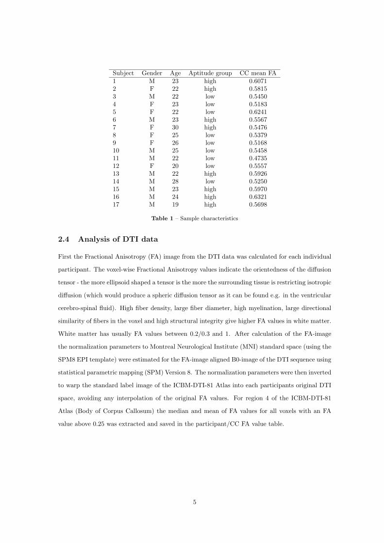
Subject Gender Age Aptitude group CC mean FA1 M 23 high 0.60712 F 22 high 0.58153 M 22 low 0.54504 F 23 low 0.51835 F 22 low 0.62416 M 23 high 0.55677 F 30 high 0.54768 F 25 low 0.53799 F 26 low 0.516810 M 25 low 0.545811 M 22 low 0.473512 F 20 low 0.555713 M 22 high 0.592614 M 28 low 0.525015 M 23 high 0.597016 M 24 high 0.632117 M 19 high 0.5698

Table 1 – Sample characteristics

2.4 Analysis of DTI data

First the Fractional Anisotropy (FA) image from the DTI data was calculated for each individual

participant. The voxel-wise Fractional Anisotropy values indicate the orientedness of the diffusion

tensor - the more ellipsoid shaped a tensor is the more the surrounding tissue is restricting isotropic

diffusion (which would produce a spheric diffusion tensor as it can be found e.g. in the ventricular

cerebro-spinal fluid). High fiber density, large fiber diameter, high myelination, large directional

similarity of fibers in the voxel and high structural integrity give higher FA values in white matter.

White matter has usually FA values between 0.2/0.3 and 1. After calculation of the FA-image

the normalization parameters to Montreal Neurological Institute (MNI) standard space (using the

SPM8 EPI template) were estimated for the FA-image aligned B0-image of the DTI sequence using

statistical parametric mapping (SPM) Version 8. The normalization parameters were then inverted

to warp the standard label image of the ICBM-DTI-81 Atlas into each participants original DTI

space, avoiding any interpolation of the original FA values. For region 4 of the ICBM-DTI-81

Atlas (Body of Corpus Callosum) the median and mean of FA values for all voxels with an FA

value above 0.25 was extracted and saved in the participant/CC FA value table.

5

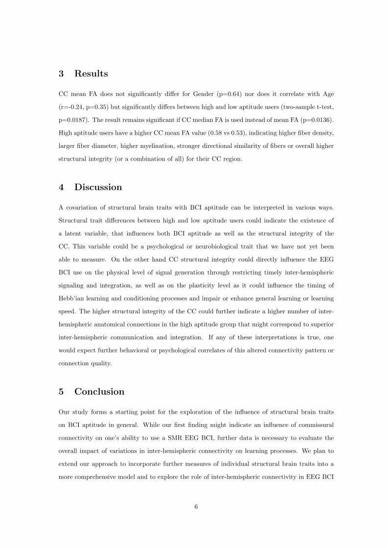
3 Results

CC mean FA does not significantly differ for Gender (p=0.64) nor does it correlate with Age

(r=-0.24, p=0.35) but significantly differs between high and low aptitude users (two-sample t-test,

p=0.0187). The result remains significant if CC median FA is used instead of mean FA (p=0.0136).

High aptitude users have a higher CC mean FA value (0.58 vs 0.53), indicating higher fiber density,

larger fiber diameter, higher myelination, stronger directional similarity of fibers or overall higher

structural integrity (or a combination of all) for their CC region.

4 Discussion

A covariation of structural brain traits with BCI aptitude can be interpreted in various ways.

Structural trait differences between high and low aptitude users could indicate the existence of

a latent variable, that influences both BCI aptitude as well as the structural integrity of the

CC. This variable could be a psychological or neurobiological trait that we have not yet been

able to measure. On the other hand CC structural integrity could directly influence the EEG

BCI use on the physical level of signal generation through restricting timely inter-hemispheric

signaling and integration, as well as on the plasticity level as it could influence the timing of

Hebb’ian learning and conditioning processes and impair or enhance general learning or learning

speed. The higher structural integrity of the CC could further indicate a higher number of inter-

hemispheric anatomical connections in the high aptitude group that might correspond to superior

inter-hemispheric communication and integration. If any of these interpretations is true, one

would expect further behavioral or psychological correlates of this altered connectivity pattern or

connection quality.

5 Conclusion

Our study forms a starting point for the exploration of the influence of structural brain traits

on BCI aptitude in general. While our first finding might indicate an influence of commissural

connectivity on one’s ability to use a SMR EEG BCI, further data is necessary to evaluate the

overall impact of variations in inter-hemispheric connectivity on learning processes. We plan to

extend our approach to incorporate further measures of individual structural brain traits into a

more comprehensive model and to explore the role of inter-hemispheric connectivity in EEG BCI

6

use.

References

Allison, B. Z., McFarland, D. J., Schalk, G., Zheng, S. D., Jackson, M. M., and Wolpaw, J. R.

(2008). Towards an independent brain-computer interface using steady state visual evoked

potentials. Clin Neurophysiol, 119(2):399–408.

Ashburner, J. and Friston, K. J. (2005). Unified segmentation. NeuroImage, 26(3):839–51.

Berger, H. (1929). Uber das elektrenkephalogramm des menschen. Arch Psychiatr Nervenkr, pages

527–570.

Birbaumer, N., Elbert, T., Canavan, A. G., and Rockstroh, B. (1990). Slow potentials of the

cerebral cortex and behavior. Physiol Rev, 70(1):1–41.

Birbaumer, N., Ghanayim, N., Hinterberger, T., Iversen, I., Kotchoubey, B., Kubler, A., Perel-

mouter, J., Taub, E., and Flor, H. (1999). A spelling device for the paralysed. Nature,

398(6725):297–298.

Birbaumer, N., Murguialday, A. R., and Cohen, L. (2008). Brain-computer interface in paralysis.

Curr Opin Neurol, 21(6):634–638.

Blankertz, B., Lemm, S., Treder, M., Haufe, S., and Muller, K.-R. (2010a). Single-trial analysis

and classification of ERP components - A tutorial. Neuroimage.

Blankertz, B., Losch, F., Krauledat, M., Dornhege, G., Curio, G., and Muller, K.-R. (2008). The

Berlin Brain–Computer Interface: accurate performance from first-session in {BCI}-na{ı}ve

subjects. IEEE Trans Biomed Eng, 55(10):2452–2462.

Blankertz, B., Sannelli, C., \textbfHalder, S., Hammer, E. M., Kubler, A., Muller, K.-R., Curio,

G., and Dickhaus, T. (2010b). Neurophysiological predictor of {SMR}-based {BCI} perfor-

mance. Neuroimage, 51(4):1303–1309.

Farwell, L. A. and Donchin, E. (1988). Talking off the top of your head: toward a mental prosthesis

utilizing even-related brain potentials. Electroencephalogr Clin Neurophysiol, 70:510–523.

Filippini, N., Douaud, G., Mackay, C. E., Knight, S., Talbot, K., and Turner, M. R. (2010).

Corpus callosum involvement is a consistent feature of amyotrophic lateral sclerosis. Neurology,

75(18):1645–52.

7

Grosse-Wentrup, M., Scholkopf, B., and Hill, J. (2010). Causal influence of gamma oscillations on

the sensorimotor rhythm. Neuroimage.

Guger, C., Daban, S., Sellers, E., Holzner, C., Krausz, G., Carabalona, R., Gramatica, F., and

Edlinger, G. (2009). How many people are able to control a P300-based brain-computer interface

(BCI)? Neurosci Lett, 462(1):94–98.

Halder, S., Agorastos, D., Veit, R., Hammer, E. M., Lee, S., Varkuti, B., Bogdan, M., Rosenstiel,

W., Birbaumer, N., and Kubler, A. (2011). Neural mechanisms of brain-computer interface

control. Neuroimage.

Hammer, E. M., \textbfHalder, S., Blankertz, B., Sannelli, C., Dickhaus, T., Kleih, S., Muller,

K.-R., and Kubler, A. (subm). Psychological predictors of {SMR-BCI} performance. Biol

Psychol.

Hari, R. and Salmelin, R. (1997). Human cortical oscillations: a neuromagnetic view through the

skull. Trends Neurosci, 20(1):44–49.

Hochberg, L. R., Serruya, M. D., Friehs, G. M., Mukand, J. A., Saleh, M., Caplan, A. H., Branner,

A., Chen, D., Penn, R. D., and Donoghue, J. P. (2006). Neuronal ensemble control of prosthetic

devices by a human with tetraplegia. Nature, 442(7099):164–171.

Kubler, A. and Neumann, N. (2005). Brain-computer interfaces–the key for the conscious brain

locked into a paralyzed body. Prog Brain Res, 150:513–525.

Kubler, A., Neumann, N., Kaiser, J., Kotchoubey, B., Hinterberger, T., and Birbaumer, N. P.

(2001). Brain-computer communication: self-regulation of slow cortical potentials for verbal

communication. Arch Phys Med Rehabil, 82(11):1533–1539.

Kubler, A., Neumann, N., Wilhelm, B., Hinterberger, T., and Birbaumer, N. (2004). Brain-

computer predictability of brain-computer communication. Journal of Psychophysiology, 18(2-

3):121–129.

Kubler, A., Nijboer, F., Mellinger, J., Vaughan, T. M., Pawelzik, H., Schalk, G., McFarland, D. J.,

Birbaumer, N., and Wolpaw, J. R. (2005). Patients with {ALS} can use sensorimotor rhythms

to operate a brain-computer interface. Neurology, 64(10):1775–1777.

Kuhlman, W. N. (1978). Functional topography of the human {Mu} rhythm. Electroencephalogr

Clin Neurophysiol, 44(1):83–93.

8

Mellinger, J., Schalk, G., Braun, C., Preissl, H., Rosenstiel, W., Birbaumer, N., and Kubler, A.

(2007). An {MEG}-based brain-computer interface ({BCI}). Neuroimage, 36(3):581–593.

Middendorf, M., McMillan, G., Calhoun, G., and Jones, K. S. (2000). Brain-computer interfaces

based on the steady-state visual-evoked response. IEEE Trans Rehabil Eng, 8(2):211–214.

Monti, M. M., Vanhaudenhuyse, A., Coleman, M. R., Boly, M., Pickard, J. D., Tshibanda, L.,

Owen, A. M., and Laureys, S. (2010). Willful modulation of brain activity in disorders of

consciousness. N Engl J Med, 362(7):579–589.

Neuper, C., Muller, G. R., Kubler, A., Birbaumer, N., and Pfurtscheller, G. (2003). Clinical

application of an {EEG}-based brain-computer interface: a case study in a patient with severe

motor impairment. Clin Neurophysiol, 114(3):399–409.

Neuper, C., Scherer, R., Wriessnegger, S., and Pfurtscheller, G. (2009). Motor imagery and

action observation: modulation of sensorimotor brain rhythms during mental control of a brain-

computer interface. Clin Neurophysiol, 120(2):239–247.

Nijboer, F., Furdea, A., Gunst, I., Mellinger, J., McFarland, D. J., Birbaumer, N., and Kubler,

A. (2008a). An auditory brain-computer interface ({BCI}). J Neurosci Methods, 167(1):43–50.

Nijboer, F., Sellers, E. W., Mellinger, J., Jordan, M. A., Matuz, T., Furdea, A., \textbfHalder, S.,

Mochty, U., Krusienski, D. J., Vaughan, T. M., Wolpaw, J. R., Birbaumer, N., and Kubler, A.

(2008b). A {P300}-based brain-computer interface for people with amyotrophic lateral sclerosis.

Clin Neurophysiol, 119(8):1909–1916.

Pfurtscheller, G. (1981). Central beta rhythm during sensorimotor activities in man. Electroen-

cephalogr Clin Neurophysiol, 51(3):253–264.

Pfurtscheller, G., Allison, B. Z., Brunner, C., Bauernfeind, G., Solis-Escalante, T., Scherer, R.,

Zander, T. O., Mueller-Putz, G., Neuper, C., and Birbaumer, N. (2010). The hybrid BCI. Front

Neurosci, 4:30.

Pfurtscheller, G. and da Silva, F. H. (1999). Event-related {EEG}/{MEG} synchronization and

desynchronization: basic principles. Clin Neurophysiol, 110(11):1842–1857.

Pfurtscheller, G., Neuper, C., Andrew, C., and Edlinger, G. (1997). Foot and hand area mu

rhythms. Int J Psychophysiol, 26(1-3):121–135.

9

Pistohl, T., Ball, T., Schulze-Bonhage, A., Aertsen, A., and Mehring, C. (2008). Prediction of arm

movement trajectories from {ECoG}-recordings in humans. J Neurosci Methods, 167(1):105–

114.

Polich, J. (2007). Updating {P300}: an integrative theory of {P3a} and {P3b}. Clin Neurophysiol,

118(10):2128–2148.

Raven, J., Raven, J. C., and Court, J. H. (2003). Manual for {Raven}’s Progressive Matrices and

Vocabulary Scales. {S}ection {I}: General overview. Harcourt Assessment.

Regan, D. (1977). Steady-state evoked potentials. J Opt Soc Am, 67(11):1475–1489.

Sato, K., Aoki, S., Iwata, N. K., Masutani, Y., Watadani, T., Nakata, Y., Yoshida, M., Terao,

Y., Abe, O., Ohtomo, K., and Tsuji, S. (2010). Diffusion tensor tract-specific analysis of the

uncinate fasciculus in patients with amyotrophic lateral sclerosis. Neuroradiology, 52(8):729–33.

Schafer, J. and Strimmer, K. (2005). A shrinkage approach to large-scale covariance matrix

estimation and implications for functional genomics. Stat Appl Genet Mol Biol, 4:Article32.

Scholz, J., Klein, M. C., Behrens, T. E. J., and Johansen-Berg, H. (2009). Training induces

changes in white-matter architecture. Nature neuroscience, 12(11):1370–1.

Senda, J., Kato, S., Kaga, T., Ito, M., Atsuta, N., Nakamura, T., Watanabe, H., Tanaka, F.,

Naganawa, S., and Sobue, G. (2011). Progressive and widespread brain damage in ALS: MRI

voxel-based morphometry and diffusion tensor imaging study. Amyotrophic lateral sclerosis

: official publication of the World Federation of Neurology Research Group on Motor Neuron

Diseases, 12(1):59–69.

Sharbrough, F. W., Chatrian, G.-E., Lesser, R. P., Luders, H., Nuwer, M., and Picton, T. W.

(1991). American Electroencephalographic Society guidelines for standard electrode position

nomenclature. J Clin Neurophysiol, 8(2):200–202.

Silvoni, S., Volpato, C., Cavinato, M., Marchetti, M., Priftis, K., Merico, A., Tonin, P., Koutsikos,

K., Beverina, F., and Piccione, F. (2009). P300-Based Brain-Computer Interface Communica-

tion: Evaluation and Follow-up in Amyotrophic Lateral Sclerosis. Front Neurosci, 3:60.

Sitaram, R., Caria, A., Veit, R., Gaber, T., Rota, G., Kubler, A., and Birbaumer, N. (2007).

{FMRI} brain-computer interface: a tool for neuroscientific research and treatment. Comput

Intell Neurosci, page 25487.

10

Sorger, B., Dahmen, B., Reithler, J., Gosseries, O., Maudoux, A., Laureys, S., and Goebel, R.

(2009). Another kind of ’BOLD Response’: answering multiple-choice questions via online

decoded single-trial brain signals. Prog Brain Res, 177:275–292.

Takeuchi, H., Sekiguchi, A., Taki, Y., Yokoyama, S., Yomogida, Y., Komuro, N., Yamanouchi,

T., Suzuki, S., and Kawashima, R. (2010). Training of working memory impacts structural

connectivity. The Journal of neuroscience : the official journal of the Society for Neuroscience,

30(9):3297–303.

Tang, Y.-Y., Lu, Q., Geng, X., Stein, E. A., Yang, Y., and Posner, M. I. (2010). Short-term

meditation induces white matter changes in the anterior cingulate. Proceedings of the National

Academy of Sciences of the United States of America, 107(35):15649–15652.

Teipel, S. J., Pogarell, O., Meindl, T., Dietrich, O., Sydykova, D., Hunklinger, U., Georgii, B.,

Mulert, C., Reiser, M. F., Moller, H.-J., and Hampel, H. (2009a). Regional networks underlying

interhemispheric connectivity: an EEG and DTI study in healthy ageing and amnestic mild

cognitive impairment. Hum Brain Mapp, 30(7):2098–2119.

Teipel, S. J., Pogarell, O., Meindl, T., Dietrich, O., Sydykova, D., Hunklinger, U., Georgii, B.,

Mulert, C., Reiser, M. F., Moller, H.-J., and Hampel, H. (2009b). Regional networks underlying

interhemispheric connectivity: an EEG and DTI study in healthy ageing and amnestic mild

cognitive impairment. Human brain mapping, 30(7):2098–119.

Valdes-Hernandez, P. A., Ojeda-Gonzalez, A., Martınez-Montes, E., Lage-Castellanos, A., Virues-

Alba, T., Valdes-Urrutia, L., and Valdes-Sosa, P. A. (2010a). White matter architecture rather

than cortical surface area correlates with the EEG alpha rhythm. Neuroimage, 49(3):2328–2339.

Valdes-Hernandez, P. a., Ojeda-Gonzalez, A., Martınez-Montes, E., Lage-Castellanos, A., Virues-

Alba, T., Valdes-Urrutia, L., and Valdes-Sosa, P. a. (2010b). White matter architecture rather

than cortical surface area correlates with the EEG alpha rhythm. NeuroImage, 49(3):2328–39.

Whitford, T. J., Kubicki, M., Ghorashi, S., Schneiderman, J. S., Hawley, K. J., McCarley, R. W.,

Shenton, M. E., and Spencer, K. M. (2010). Predicting inter-hemispheric transfer time from the

diffusion properties of the corpus callosum in healthy individuals and schizophrenia patients: A

combined ERP and DTI study. NeuroImage, 54(3):2318–2329.

Woolley, S. C., Zhang, Y., Schuff, N., Weiner, M. W., and Katz, J. S. (2011). Neuroanatomical

correlates of apathy in ALS using 4 Tesla diffusion tensor MRI. Amyotrophic lateral sclerosis

11

: official publication of the World Federation of Neurology Research Group on Motor Neuron

Diseases, 12(1):52–8.

Wriessnegger, S. C., Kurzmann, J., and Neuper, C. (2008). Spatio-temporal differences in brain

oxygenation between movement execution and imagery: a multichannel near-infrared spec-

troscopy study. Int J Psychophysiol, 67(1):54–63.

12