Island Biogeography of Food Webs - Claire Jacquet

CHAPTER FOUR

Island Biogeographyof Food WebsF.Massol*,1, M. Dubart†,{, V. Calcagno§, K. Cazelles¶,||,#, C. Jacquet¶,||,#,S. K!efi{, D. Gravel¶,||,***CNRS, Universit!e de Lille, UMR 8198 Evo-Eco-Paleo, SPICI Group, Lille, France†CNRS, Universit!e de Lille-Sciences et Technologies, UMR 8198 Evo-Eco-Paleo, SPICI Group, Villeneuved’Ascq, France{Institut des Sciences de l’!Evolution, Universit!e de Montpellier, CNRS, IRD, EPHE, CC065, Montpellier,France§Universit!e Cote d’Azur, CNRS, INRA, ISA, France¶Universit!e du Qu!ebec a Rimouski, Rimouski, QC, CanadajjQuebec Center for Biodiversity Science, Montr!eal, QC, Canada#UMR MARBEC (MARine Biodiversity, Exploitation and Conservation), Universit!e de Montpellier,Montpellier, France**Facult!e des Sciences, Universit!e de Sherbrooke, Sherbrooke, QC, Canada1Corresponding author: e-mail address: [email protected]

Contents

1. Introduction 1841.1 Island Biogeography 1841.2 Spatial Food Webs 1891.3 Invasions in Food Webs, Eco-evolutionary Perspectives 1931.4 Invasions in Other Spatially Structured Networks 195

2. Island Biogeography of Food Webs 1982.1 The Model 1982.2 Simple Insights 2102.3 Interpretation in Terms of Food Web Transitions 214

3. Effects of Mainland Food Web Properties on Community Assembly 2193.1 Simulating the Model 2203.2 Results Obtained When Controlling Mainland Food Web Richness,

Connectance, Degree Distribution and the Proportion of Primary Producers 2283.3 Results Obtained Using the SBM to Generate Mainland Food Web 237

4. Discussion 2394.1 Legacies of Island Biogeography Theory 2394.2 The Future of Island Biogeography Theory 2404.3 Using the TTIB to Model Species Distribution 2474.4 From Theory to Data 248

Acknowledgements 249Appendix. Breadth-First Directing of the Links in the Generated Network 249References 252

Advances in Ecological Research, Volume 56 # 2017 Elsevier LtdISSN 0065-2504 All rights reserved.http://dx.doi.org/10.1016/bs.aecr.2016.10.004

183

Abstract

To understand why and how species invade ecosystems, ecologists have made heavyuse of observations of species colonization on islands. The theory of island biogeogra-phy, developed in the 1960s by R.H. MacArthur and E.O. Wilson, has had a tremendousimpact on how ecologists understand the link between species diversity and character-istics of the habitat such as isolation and size. Recent developments have described howthe inclusion of information on trophic interactions can further inform our understand-ing of island biogeography dynamics. Here, we extend the trophic theory of island bio-geography to assess whether certain food web properties on the mainland affectcolonization/extinction dynamics of species on islands. Our results highlight that bothfood web connectance and size on the mainland increase species diversity on islands.We also highlight that more heavily tailed degree distributions in the mainland foodweb correlate with less frequent but potentially more important extinction cascadeson islands. The average shortest path to a basal species on islands follows a hump-shaped curve as a function of realized species richness, with food chains slightly longerthan on the mainland at intermediate species richness. More modular mainland websare also less persistent on islands. We discuss our results in the context of global changesand from the viewpoint of community assembly rules, aiming at pinpointing furthertheoretical developments needed to make the trophic theory of island biogeographyeven more useful for fundamental and applied ecology.

1. INTRODUCTION1.1 Island Biogeography

Islands have always fascinated ecologists. Since the earliest stages of ecology

as a scientific discipline, the fauna and flora of islands have been considered

as objects worthy of study because they capture the essence of colonization-

extinction and ecoevolutionary dynamics shaping natural systems (Whittaker

and Fernandez-Palacios, 2007). Among the iconic rules of ecology, the “island

rule” (Lomolino, 1985) suggests that the span of body sizes found on islands is

much narrower than on continents, reflecting the remarkable examples of

gigantism in small herbivores/granivores and of dwarfism in predators

observed. Simple, general theoretical models of faunal build-up on islands

were proposed some 50 years ago (Levins and Heatwole, 1963; MacArthur

andWilson, 1963).More recently, extensions and applications of thesemodels

have beenmade, constituting what has been dubbed “eco-evolutionary island

biogeography” which incorporates trophic, functional and local adaptation

information into the island biogeography framework (Farkas et al., 2015;

Gravel et al., 2011b). Empirically, islands have provided ecologists with a

184 F. Massol et al.

playground to understand community assembly (Piechnik et al., 2008;

Simberloff, 1976; Simberloff and Abele, 1976), species diversity (Condit

et al., 2002; Ricklefs and Renner, 2012; Volkov et al., 2003) and

metapopulation dynamics (Hanski, 1999; Ojanen et al., 2013).

The historical “theory of island biogeography” (TIB), presented inde-

pendently by Levins and Heatwole (1963) and MacArthur and Wilson

(1963), and summarized in the well-known book of the same name by

MacArthur andWilson (1967), is based on the idea that the ecological com-

munities found on islands are a sample of those found on continents. The size

of this “sample” results from two opposing processes: island colonization by

external species and their local extinction on the island (see also Preston,

1962). The original formulation of the model by MacArthur and Wilson

(1963) takes the form of a master equation linking the probability PS(t) that

the focal island has exactly S species (from the original T total number of

species found on the mainland) at time t to the rate of colonization by a

new species (λS) and the rate of species extinction (μS):

dPSdt

¼ λS"1PS"1 + μS+1PS+1" λS + μSð ÞPS (1)

Adding the assumption of constant colonization and extinction rates (i.e.

λS ¼ T "Sð Þc and μS ¼ Se, where c is the species colonization rate and e,

their extinction rate), this naturally leads to the following equation on the

expected species richness !S at time t:

d!S

dt¼X

S

SdPSdt

¼ c T " !Sð Þ" e!S (2)

Solved at equilibrium, Eq. (2) yields the expected number of species on

the island at any given time:

!S*¼Tc

c + e(3)

Eq. (3) lends itself to the interpretation of species–area and species–distancecurves (i.e. curves linking the number of species present on an island to the

area of the island or its distance from the continent) as the log-derivative of

Eq. (3) with respect to e/c yields:

d log !S*d e=cð Þ ¼" 1

1+ e=c(4)

185Island Biogeography of Food Webs

For large e/c, Eq. (4) reads approximately as:

d log !S*d e=cð Þ #$1 (5)

As long as e and c are supposed to be monotonic functions of area and dis-

tance, with the intuitive slopes (i.e. c increases with area and decreases with

distance, and the opposite relationships hold for e) from the continent

respectively, Eq. (5) yields species–area and species–distance curves compat-

ible with observed patterns (MacArthur and Wilson, 1963, 1967).

The TIB is a cornerstone of invasion biology for several reasons. First, it

is very likely that colonization by external species is a strong component of

the forces shaping community composition on long time scales for islands,

whereas for mainland communities random species extinction and larger

population sizes make coevolution more likely to be the dominant factor

structuring communities on the same time scales. In a sense, remote islands

can be seen as complete population sinks for all species (i.e. black-hole sinks

or nearly so) and, as such, have very little to no impact on the overall coevo-

lutionary patterns observed in species (Holt et al., 2003; Kawecki, 2004;

Massol and Cheptou, 2011; Rousset, 1999), except for island endemics.

From an other point of view, islands can also be considered as natural exper-

iments for understanding biological invasions. The dynamics of successive

species colonization from the mainland to the island constitutes an

“accelerated” version of what could happen in other less extinction-prone

habitats. Understanding how waves of colonization events can take place

on an island, depending on island and mainland community characteristics,

will give information on the conditions favouring the invasibility of habitats

by exotic species—be they habitat characteristics or species traits. In the case

of the TIB, colonizing species are not assumed to be fundamentally different

in terms of their ability to invade an island; thus, the variability in diversity

on islands predicted by the TIB boils down to variability in colonization and

extinction parameters among islands, which in turn is assumed to only

depend on island remoteness and area (MacArthur andWilson, 1963, 1967).

Predictions from the TIB can be tested in different ways. First, the

species–area curves can be fitted to infer underlying extinction-to-

colonization ratios and/or to test whether such ratios are indeed constant

across different areas, during a given period or among taxa (Cameron

et al., 2013; Guilhaumon et al., 2008; Triantis et al., 2012). While this

approach has produced some success in the past, it is not a strong test per


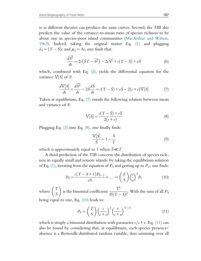
se as different theories can produce the same curves. Second, the TIB also

predicts the value of the variance-to-mean ratio of species richness to be

about one in species-poor island communities (MacArthur and Wilson,

1963). Indeed, taking the original master Eq. (1) and plugging

λS ¼ T "Sð Þc and μS ¼ Se, one finds that:

dS2

dt¼ 2c !ST "S2

! ""2eS2 + c T " !Sð Þ+ e!S (6)

which, combined with Eq. (2), yields the differential equation for the

variance V S½ & of S:

dV S½ &dt

¼ dS2

dt"2!S

d!S

dt¼ c T " !Sð Þ+ e!S"2 c + eð ÞV S½ & (7)

Taken at equilibrium, Eq. (7) entails the following relation between mean

and variance of S:

V S½ & ¼ c T " !Sð Þ+ e!S

2 c + eð Þ(8)

Plugging Eq. (3) into Eq. (8), one finally finds:

V S½ &!S

¼ 1"!S

T(9)

which is approximately equal to 1 when !S≪T .

A third prediction of the TIB concerns the distribution of species rich-

ness in equally small and remote islands: by taking the equilibrium solution

of Eq. (1), iterating from the equation of P0 and getting up to PT, one finds:

PS ¼c T "S+1ð ÞPS"1

eS¼…¼ T

S

# $c

e

% &S

P0 (10)

whereTS

# $is the binomial coefficient

T !

S! T "Sð Þ!. With the sum of all PS

being equal to one, Eq. (10) leads to:

PS ¼TS

# $c

c + e

% &S e

c + e

% &T"S

(11)

which is simply a binomial distribution with parameter c=c + e. Eq. (11) can

also be found by considering that, at equilibrium, each species presence/

absence is a Bernoulli-distributed random variable, thus summing over all


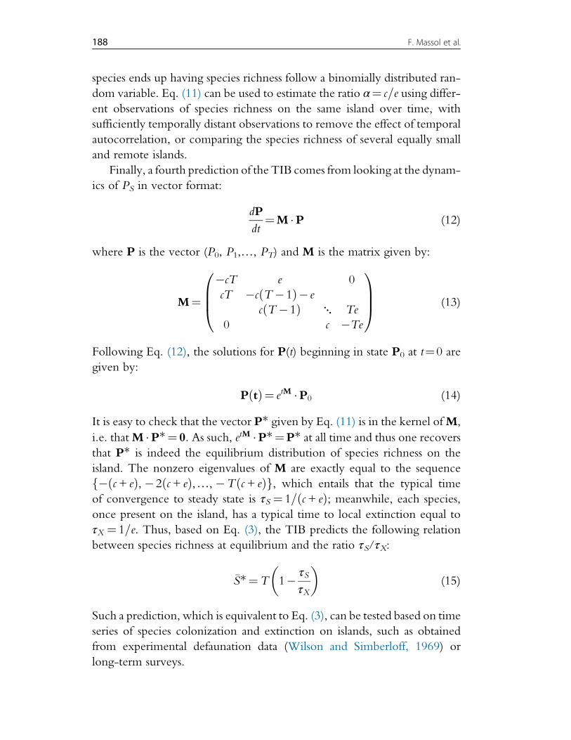
species ends up having species richness follow a binomially distributed ran-

dom variable. Eq. (11) can be used to estimate the ratio α¼ c=e using differ-ent observations of species richness on the same island over time, with

sufficiently temporally distant observations to remove the effect of temporal

autocorrelation, or comparing the species richness of several equally small

and remote islands.

Finally, a fourth prediction of the TIB comes from looking at the dynam-

ics of PS in vector format:

dP

dt¼M "P (12)

where P is the vector (P0, P1,…, PT) and M is the matrix given by:

M¼

#cT e 0cT #c T #1ð Þ# e

c T #1ð Þ ⋱ Te0 c #Te

0

BB@

1

CCA (13)

Following Eq. (12), the solutions for P(t) beginning in state P0 at t¼0 are

given by:

P tð Þ¼ etM "P0 (14)

It is easy to check that the vector P* given by Eq. (11) is in the kernel ofM,

i.e. thatM "P*¼ 0. As such, etM "P*¼P* at all time and thus one recovers

that P* is indeed the equilibrium distribution of species richness on the

island. The nonzero eigenvalues of M are exactly equal to the sequence

# c + eð Þ,#2 c + eð Þ,…, #T c + eð Þf g, which entails that the typical time

of convergence to steady state is τS ¼ 1= c + eð Þ; meanwhile, each species,

once present on the island, has a typical time to local extinction equal to

τX ¼ 1=e. Thus, based on Eq. (3), the TIB predicts the following relation

between species richness at equilibrium and the ratio τS/τX:

!S*¼T 1# τSτX

! "(15)

Such a prediction, which is equivalent to Eq. (3), can be tested based on time

series of species colonization and extinction on islands, such as obtained

from experimental defaunation data (Wilson and Simberloff, 1969) or

long-term surveys.


Thus, as initially envisaged by its first proponents (Levins and Heatwole,

1963; MacArthur andWilson, 1963, 1967), the TIB tries to explain species–area and species–distance curves on islands using a simple theory that assumes

species accumulate due to colonization from the mainland and die out on

islands at a constant rate. Although precisely formalized in mathematical

terms, the TIB is not a mechanistic model per se as it assumes that extinction

decreases with island area and that colonization decreases with distance

between island and mainland. While these assumptions seem justified in

general, the underlying mechanisms generating these relationships are omit-

ted from the TIB. In particular, the links between island area, its underlying

habitat heterogeneity (and hence its diversity in terms of potential species

niches) and species carrying capacities (and thus extinction probabilities)

have opposite effects on extinction rate, because habitat heterogeneity trades

off with habitat size in an island of limited size (Allouche et al., 2012). More-

over, the TIB does not take species interactions into account in the sense

that colonization and extinction rates are independent from current species

composition on the island. Species are considered equivalent, but the model

differs from neutral theory in that there is no competitive interaction

(Hubbell’s model assumes very strong preemptive competition). As a con-

sequence, the TIB cannot predict any aspect of community structure based

on species-specific attributes, such as the dominance by generalists, func-

tional composition or successional sequence. Gravel et al. (2011b) therefore

introduced an extension to the classic TIB called the trophic theory of island

biogeography (TTIB) with the aim of predicting the variation in food web

structure with area and isolation. When trying to model empirical data akin

to mainland-islands datasets such as Havens’ (1992), they found that the

TTIB performs significantly better (in terms of statistical goodness-of-fit

indicators) without introducing any new parameter into the TIB.

1.2 Spatial Food WebsTo understand how species coexist, it is necessary to understand how they

interact. At the simplest level, species can be considered as competing under

limiting factors (resources, predators, etc.). Competition need not be as

simple as scramble resource competition. Indirect interactions through

shared natural enemies (Holt, 1977; Leibold, 1996) or more generally any

other species’ abundances or occurrences (e.g. species recycling nutrients

from detritus; Daufresne and Hedin, 2005) can also be experienced as lim-

iting factors and result in “apparent” competition sensu lato. Competition is


the only kind of interaction taken into account in most metacommunity

models (Hubbell, 2001; Leibold et al., 2004; Massol et al., 2011). In general,

however, species interactions are not only competitive. Food webs, i.e. net-

works of species that feed on one another, represent antagonistic trophic

interactions among species and, as such, have to be taken into account as

a structuring force behind coexistence patterns within communities. While

other types of ecological interaction networks do exist (e.g. mutualistic tro-

phic networks between plants, fungus and soil microbes, or antagonistic

nontrophic networks among antibiotic-producing bacteria), food webs

are ubiquitous and their complexity seems to be tightly associated with

species richness, abundances, functioning and dynamics of communities

(Chase et al., 2000; Cohen and Briand, 1984; Cohen and Łuczak, 1992;

Downing and Leibold, 2002; Dunne et al., 2004; K!efi et al., 2012; Pimm

et al., 1991; Post et al., 2000).

Inspired by the work of Huffaker, recent work on the subject of food

web dynamics has emphasized the necessity to consider food webs as

spatialized entities (Duggins et al., 1989; Estes and Duggins, 1995; Estes

et al., 1998; Huffaker, 1958; Huffaker et al., 1963; Polis and Hurd, 1995;

Polis et al., 2004) in order to understand patterns such as species turnover,

species richness, food chain length or nutrient recycling dynamics (Calcagno

et al., 2011; Gravel et al., 2011a; Massol et al., 2011; McCann et al., 2005;

Pillai et al., 2010, 2011; Takimoto et al., 2012). Considering food webs only

as local, spatially disconnected entities may lead to misunderstanding, e.g.

not recognizing population sinks because populations are maintained by

the dispersal of detritus among habitat patches (Gravel et al., 2010). How-

ever, all species do not perceive space with the same grain, with habitat pat-

ches for one species not being the same as for another species at a different

trophic level (Massol et al., 2011;McCann et al., 2005). Taking into account

the spatial aspect of food webs is thus a necessity that requires understanding

the complexity of spatial scales of species interactions. Acknowledging this

spatial component of food webs is also a prerequisite to fully grasp the con-

cept of limiting factors (Gravel et al., 2010; Haegeman and Loreau, 2014;

Massol et al., 2011): when species and abiotic nutrients move from habitat

patch to habitat patch, the effective “limitation” of species growth by an

environmental factor depends not only on the local conditions but also

on conditions in nearby patches contributing to influxes of organisms and

nutrients into the focal patch. For these reasons, considering the spatial

aspect of food webs is an important issue worthy of both theoretical and

empirical development.


When considering food webs as spatialized entities, the fluxes of organ-

isms and abiotic material between different locations present a duality of per-

spective of ecological fluxes (Massol and Petit, 2013; Massol et al., 2011): on

the one hand, these fluxes contribute to the demographics of all species

present in the different locations under study through immigration and emi-

gration; more generally, such fluxes participate in the shaping of species and

abiotic material stocks through source-sink dynamics (Loreau et al., 2013),

while, on the other hand, the movement of plants, animals or simply abiotic

material can be translated in fluxes of energy and nutrients that, together

with other energy/nutrient fluxes due to local species interactions, represent

the dynamics of nutrients and energy at large scales, flowing through trophic

levels and between spatially distinct locations (in a manner rather reminis-

cent of Ulanowicz’ ascendant perspective; Ulanowicz, 1997). Under this

second perspective, there are common currencies (energy, carbon, nitrogen,

phosphorus, etc.) behind each and every flux of organisms across the spatial

food web that must comply with basic conservation laws (mass balance), thus

constraining the possibilities of source-sink patterns among trophic levels

(Loreau and Holt, 2004). Coupled with a consideration of species stoichio-

metric needs in terms of C:N:P ratios, such a perspective can potentially help

us understand the spatial dynamics of nutrient enrichment through, for

example death, reproduction, excretion and the foraging of organisms in

different habitats (Hannan et al., 2007; Helfield and Naiman, 2002;

Jefferies et al., 2004; Nakano and Murakami, 2001).

In the case of the TIB, the necessity of taking into account the spatial

aspects of food webs has been construed as mandating the use of food

web information in TIB models. The first model bridging food web theory

and TIB was named the TTIB and makes use of trophic information for

which species preys on what to correct effective colonization and extinction

rates (Cazelles et al., 2015b; Cirtwill and Stouffer, 2016; Gravel et al.,

2011b). In this first model, this correction takes a very simple form: species

cannot colonize an island when they have no prey on the island, and the

extinction of the prey species of a colonizer will also extirpate it from the

island (Holt, 2002). More generally, this framework can be extended to

account for arbitrary changes in colonization and extinction probabilities

that depend on the presence or absence of other species on the island

(Cazelles et al., 2015b). Thus, the TTIB can represent a complex picture

of rates of transitions from one community state (i.e. the set of species occur-

ring on the island) to another, through species colonization and extinction

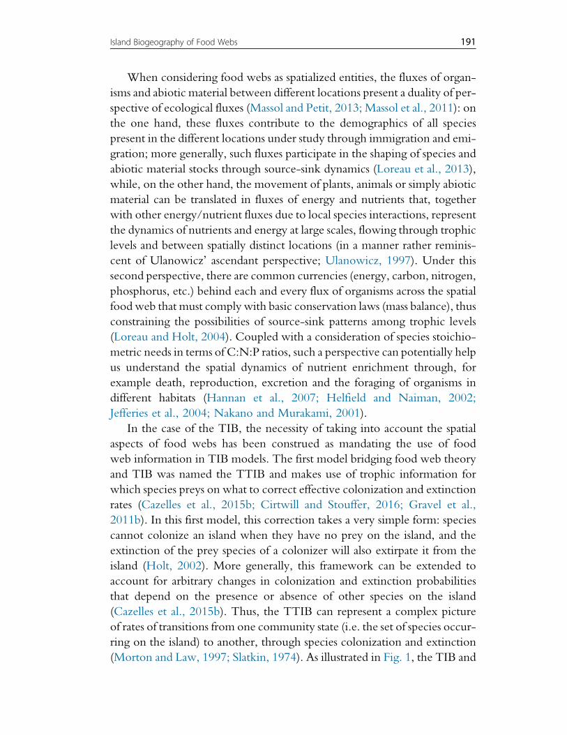
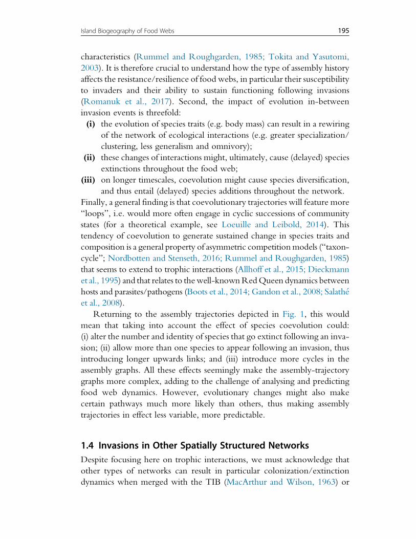
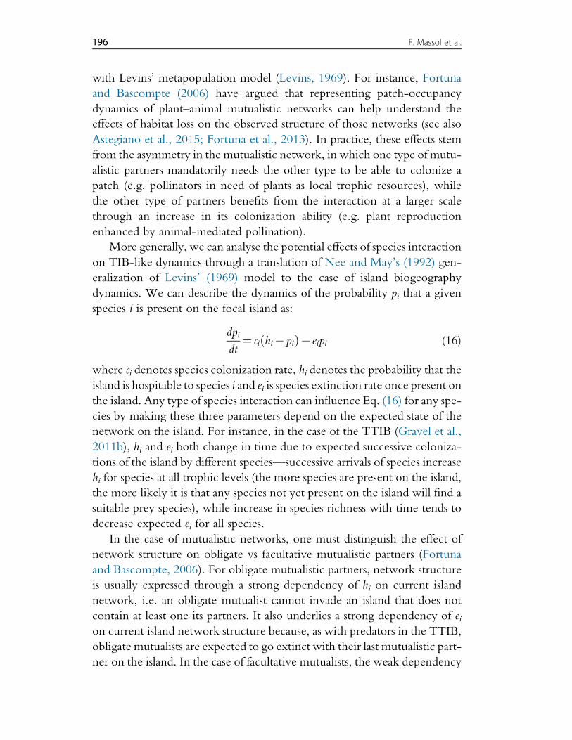
(Morton and Law, 1997; Slatkin, 1974). As illustrated in Fig. 1, the TIB and


BD

CE

CE

CE

B C

D

C

D

CE

BD

C

BD

B

E

D

BD E

B

D E

B CE

BD

CE

CE

CE

B C

D E

D

C

D

CE

BD

C

B CE

BD

B

E

BD

BD E

(a)

(b)

Fig.

1Re

presen

tatio

nsof

(a)the

TIBan

d(b)the

TTIBinterm

sof

possibletran

sitio

nsam

ongcommun

ities,followingthefram

eworkof

Morton

andLaw(199

7).The

totalcom

mun

ity(w

ithspeciesB

,C,D

andE)isrepresen

tedatthetopof

both

panels,whiletheem

ptycommun

ityisatthe

bottom

.Arrow

srepresen

teith

ercolonizatio

n(upw

ards)o

rextinction(dow

nwards)e

vents.In

thecase

oftheTIB(a),alltransition

sarerevers-

iblean

dspeciesrichn

essd

oesn

ot“le

apba

ckwards”a

sspe

cies

areloston

eby

one.Inthecase

oftheTTIB(b),certaincommun

ities

(ingrey

with

dotted

borders)areim

possible

becausethey

violatetheprincipleof

atleaston

eprey

speciessustaining

apred

ator

species;moreo

ver,the

extin

ctionof

asing

lespeciescanlead

tolosing

morethan

onespecies,e.g.speciesCge

ttingextin

cten

tails

losing

both

speciesCan

dB,an

dthus

thereisapo

ssibletran

sitio

nbe

tweenthetotalcom

mun

itytowards

the(D,E)com

mun

ity.W

hilethissche

mehigh

lightstheconcep

tual

diffe

rences

arisingfrom

taking

into

accoun

ttheprincipleof

sequ

entia

l,bo

ttom

-up,

food

web

assembly,morefle

xibleap

proa

ches

canbe

develope

d,e.g.by

allowingpred

ator

speciesto

sustainthem

selves

intheab

senceof

preys(albeitw

ithmoredifficulty

)ora

llowingpred

ator

speciesto

invade

thecommun

ity“in

advance”

oftheirprey

(Cazelleset

al.,20

15b).

TTIB are extremes of a continuum of approaches that weight differently

transitions among possible community states.

1.3 Invasions in Food Webs, Eco-evolutionary PerspectivesCommunity assembly, broadly envisioned as the accumulation of species

diversity over time in a novel habitat, has been modeled, classically, as an

ecological process driven by sequential colonizations of species from a

regional pool. This approach effectively considers species as having fixed

characteristics and traits (e.g. prey range, feeding preferences, antipredator

defences, etc.). This form of community assembly produces what are often

called “invasion-structured” food webs (Rummel andRoughgarden, 1985).

Invasion-structured food webs may be an adequate concept for ecosystems

that are well connected to mainland, in which immigration events and inva-

sions occur at a frequent pace. However, when considering more isolated

areas, such as remote islands characterized by a very low colonization rate

(low c value in the TIB framework), species may undergo a significant

amount of evolutionary change in the interval of time between successive

species arrivals. In such conditions, it is no longer legitimate to consider

community assembly as a purely ecological process, and one needs to con-

sider the effect of species evolution as well. The process of community

assembly should thus be considered as involving three different timescales:

(i) a rapid ecological timescale corresponding to community dynamics

following species invasion;

(ii) a slow immigration timescale corresponding to the arrival of individ-

uals from the main source of species;

(iii) a slow timescale corresponding to species (co)evolution in-between

immigration events.

The relative speed of the last two timescales will be contingent on the level

of isolation of the focal community directly through the rate of species col-

onization and indirectly through the amount of gene flow (slowing down

local adaptation in the colonized community) and local selective pressures.

We can consider two extreme cases of community assembly: (i) where

immigration events are common enough to completely outpace the effects

of in situ coevolution, we recover the classic “invasion-structured” food

webs; and, (ii) where evolution has plenty of time to proceed in-between

invasion events, we may obtain “adaptive radiations”, i.e. the in situ forma-

tion of new species by evolution (see also Vanoverbeke et al., 2016). This

second extreme case is sometimes called “evolutionary community


assembly” (Bonsall et al., 2004; Br€annstr€om et al., 2012; Doebeli and

Dieckmann, 2000; HilleRisLambers et al., 2012; Loeuille and Leibold,

2014; Pillai and Guichard, 2012; Tokita and Yasutomi, 2003). Evolutionary

community assembly has been mostly applied to competitive communities,

but some studies have considered evolutionary diversification in the context of

food webs. Doebeli and Dieckmann (2000) have shown how coevolution

could yield diversification and greater specialization in predator–prey interac-tions. In the same vein, Loeuille and Leibold (2008) explored how the

evolution of specific vs nonspecific (but costly) plant defences affects the

topology of plant-herbivore food web modules. While these approaches

treated trophic positions as fixed, and evolution occurred within trophic

levels, more general approaches have also been employed. Rossberg et al.

(2006) considered the coevolution of foraging and vulnerability traits in an

abstract set of species and could reproduce interaction matrices similar to that

of natural food webs (see also Drossel et al., 2004 for similar approaches).

Loeuille and Loreau (2005) and Allhoff et al. (2015), using dynamical models

of trophic interactions based on body mass, have studied how the level of

trophic structuring and a number of trophic levels emerge from single ancestor

species. In the case of mutualistic networks, Nuismer et al. (2013) assessed

how the coevolution of mutualistic partners along a phenotypic trait con-

tinuum that governs both local adaptation and partner match/mismatch

affected the topology of the mutualistic network.

Although studying the two extreme cases of community assembly is useful,

it should be kept in mind that most natural food webs are likely not assembled

by only invasions or only evolution, but probably by a combination of the two

forces. Hence most ecosystems should harbour “coevolution-structured”

food webs, using the terminology coined by Rummel and Roughgarden

(1985). Unfortunately, comparatively few studies have examined the simul-

taneous action of sequential invasions and in situ coevolution on the dynamics

of community assembly. Moreover, these studies have either only considered

generalized Lotka–Volterra (or replicator) equations (Tokita and Yasutomi,

2003) or competitive interactions (Rummel and Roughgarden, 1985) and

not trophic interactions. To some extent, predictions from models of

asymmetric competitive interactions might be extrapolated to trophic inter-

actions, but more work is needed to explore the interaction of invasion and

coevolution (both directional evolution and diversification) in assembling

food webs.

A few general conclusions can nevertheless be drawn. First, invasion-

and coevolution-assembled communities can possess very different


characteristics (Rummel and Roughgarden, 1985; Tokita and Yasutomi,

2003). It is therefore crucial to understand how the type of assembly history

affects the resistance/resilience of food webs, in particular their susceptibility

to invaders and their ability to sustain functioning following invasions

(Romanuk et al., 2017). Second, the impact of evolution in-between

invasion events is threefold:

(i) the evolution of species traits (e.g. body mass) can result in a rewiring

of the network of ecological interactions (e.g. greater specialization/

clustering, less generalism and omnivory);

(ii) these changes of interactions might, ultimately, cause (delayed) species

extinctions throughout the food web;

(iii) on longer timescales, coevolution might cause species diversification,

and thus entail (delayed) species additions throughout the network.

Finally, a general finding is that coevolutionary trajectories will feature more

“loops”, i.e. would more often engage in cyclic successions of community

states (for a theoretical example, see Loeuille and Leibold, 2014). This

tendency of coevolution to generate sustained change in species traits and

composition is a general property of asymmetric competitionmodels (“taxon-

cycle”; Nordbotten and Stenseth, 2016; Rummel and Roughgarden, 1985)

that seems to extend to trophic interactions (Allhoff et al., 2015; Dieckmann

et al., 1995) and that relates to thewell-knownRedQueen dynamics between

hosts and parasites/pathogens (Boots et al., 2014; Gandon et al., 2008; Salath!eet al., 2008).

Returning to the assembly trajectories depicted in Fig. 1, this would

mean that taking into account the effect of species coevolution could:

(i) alter the number and identity of species that go extinct following an inva-

sion; (ii) allow more than one species to appear following an invasion, thus

introducing longer upwards links; and (iii) introduce more cycles in the

assembly graphs. All these effects seemingly make the assembly-trajectory

graphs more complex, adding to the challenge of analysing and predicting

food web dynamics. However, evolutionary changes might also make

certain pathways much more likely than others, thus making assembly

trajectories in effect less variable, more predictable.

1.4 Invasions in Other Spatially Structured NetworksDespite focusing here on trophic interactions, we must acknowledge that

other types of networks can result in particular colonization/extinction

dynamics when merged with the TIB (MacArthur and Wilson, 1963) or


with Levins’ metapopulation model (Levins, 1969). For instance, Fortuna

and Bascompte (2006) have argued that representing patch-occupancy

dynamics of plant–animal mutualistic networks can help understand the

effects of habitat loss on the observed structure of those networks (see also

Astegiano et al., 2015; Fortuna et al., 2013). In practice, these effects stem

from the asymmetry in the mutualistic network, in which one type of mutu-

alistic partners mandatorily needs the other type to be able to colonize a

patch (e.g. pollinators in need of plants as local trophic resources), while

the other type of partners benefits from the interaction at a larger scale

through an increase in its colonization ability (e.g. plant reproduction

enhanced by animal-mediated pollination).

More generally, we can analyse the potential effects of species interaction

on TIB-like dynamics through a translation of Nee and May’s (1992) gen-

eralization of Levins’ (1969) model to the case of island biogeography

dynamics. We can describe the dynamics of the probability pi that a given

species i is present on the focal island as:

dpidt

¼ ci hi" pið Þ" eipi (16)

where ci denotes species colonization rate, hi denotes the probability that the

island is hospitable to species i and ei is species extinction rate once present on

the island. Any type of species interaction can influence Eq. (16) for any spe-

cies by making these three parameters depend on the expected state of the

network on the island. For instance, in the case of the TTIB (Gravel et al.,

2011b), hi and ei both change in time due to expected successive coloniza-

tions of the island by different species—successive arrivals of species increase

hi for species at all trophic levels (the more species are present on the island,

the more likely it is that any species not yet present on the island will find a

suitable prey species), while increase in species richness with time tends to

decrease expected ei for all species.

In the case of mutualistic networks, one must distinguish the effect of

network structure on obligate vs facultative mutualistic partners (Fortuna

and Bascompte, 2006). For obligate mutualistic partners, network structure

is usually expressed through a strong dependency of hi on current island

network, i.e. an obligate mutualist cannot invade an island that does not

contain at least one its partners. It also underlies a strong dependency of eion current island network structure because, as with predators in the TTIB,

obligate mutualists are expected to go extinct with their last mutualistic part-

ner on the island. In the case of facultative mutualists, the weak dependency


of the species on the presence of mutualistic partners on the island could be

translated in one of two ways, either in: an increase in ci when mutualists are

present on the island (e.g. plants more likely to invade an island onwhich the

animal seed dispersers are already present); and/or a decrease of ei in the

presence of beneficial partners (e.g. hermaphroditic plants on an island with

pollinators can maintain larger, more genetically diverse, and thus less

extinction-prone, populations). It is remarkable that, in the case of Levins’

metapopulation model describing the dynamics of plant–pollinator interac-tion networks (Astegiano et al., 2015; Fortuna and Bascompte, 2006), a

natural choice for the effect of pollinators on plant parameters is to consider

that patches with pollinators contribute more to the pool of propagules

(i.e. increase their contribution to the overall colonization!occupancy rate).

In the particular case of networks of competitive interactions, TIB dynam-

ics might be altered through four different mechanisms. First, the presence of

competitors, especially dominant competitors, can drive other species out of

the island, i.e. by increasing their extinction rate ei. This would mimic com-

petitive exclusion dynamics on the island. An early attempt at understanding

how competition would affect species occurrence patterns in a TIB frame-

work was made by Hastings (1987). A second possibility is that there is a

priority effect, affecting those species colonizing the island, so that certain spe-

cies might exclude other species from colonizing the islandwhen they are pre-

sent, i.e. effectively decreasing hi for the other species (Shurin et al., 2004).

A third possibility is to make habitat quality change with current community

composition, as a consequence of ecosystem engineering (Wright et al., 2004).

Finally, there might be a gradient of competitive and colonization abilities in

the pool of species, so that species more likely to colonize the island first would

also be more likely to be displaced by more competitive species afterwards,

causing “ecological succession-like” assembly trajectories. Although the

competition-colonization trade-off has been traditionally used in the context

of Levins’ (1969) metapopulation model (Calcagno et al., 2006; Hastings,

1980; Tilman, 1994), it can also be incorporated in an island biogeography

context to describe community transitions before and after colonization by

a superior competitor, e.g. borrowing from Slatkin’s (1974) model and

adapting it to the TIB.

For the remainder of this chapter, we cast the TTIB in terms of classic

food webs, i.e. networks of species feeding on one another through

predator–prey interactions. However, we would note that integrating

host–parasite (or more generally, host-symbiont) interactions within this

context is feasible, provided Eq. (16) accommodates the effect of the


network structure on symbiont colonization and extinction dynamics. One

modelling choice is to consider that obligate symbionts cannot colonize if

their host is absent, so that the symbiont can: (i) colonize the island together

with its host; or, (ii) colonize the island once its host is already there (through

some immigration of infected hosts which is not accounted for in the

dynamics of the host occupancy because it has already colonized the island).

In the case of facultative symbionts, this modelling option can be combined

with the possibility of a symbiont-only colonization event, possibly occur-

ring at a different (lower) rate. Regarding extinction rates, obligate symbi-

onts will inevitably die out when their host goes extinct on the island, while

facultative symbionts could persist (but possibly with an increased extinction

rate) after their last host species disappears from the island.

2. ISLAND BIOGEOGRAPHY OF FOOD WEBS2.1 The Model

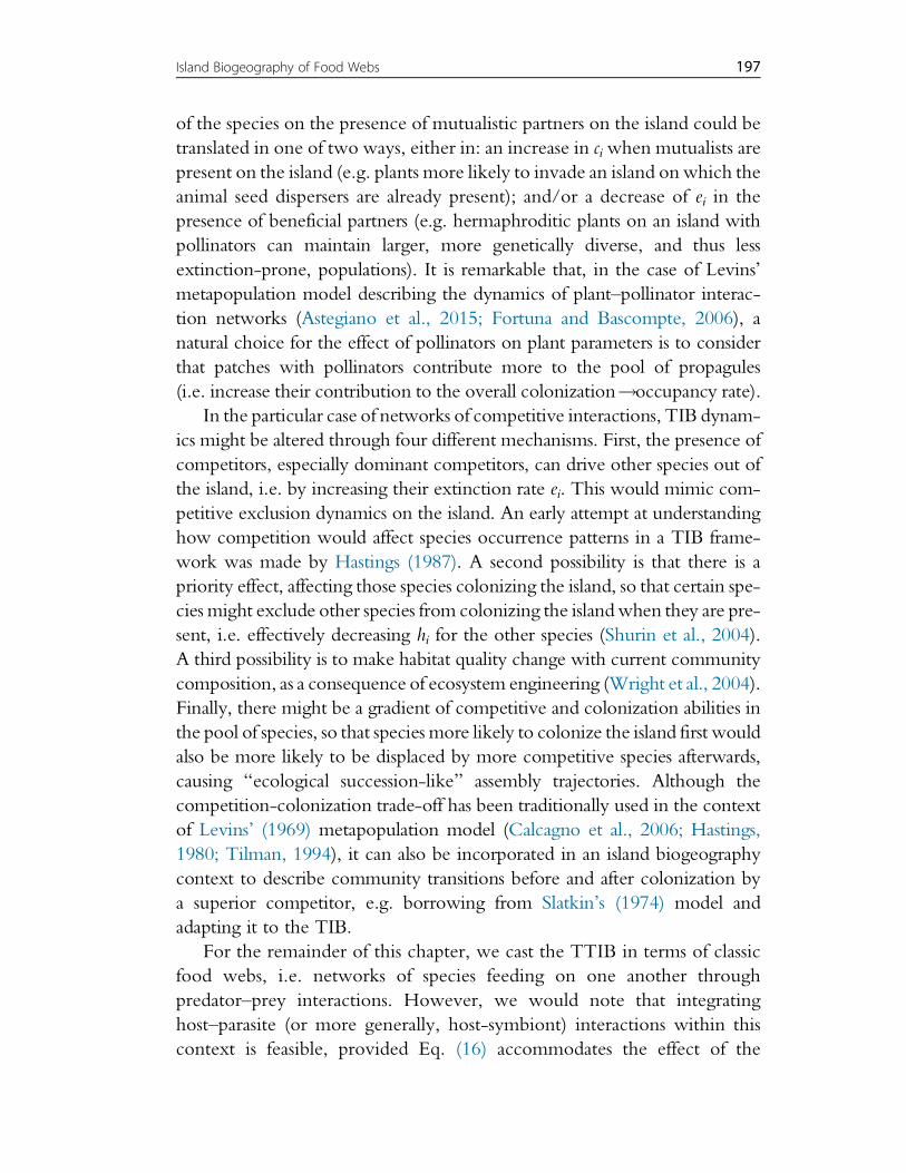
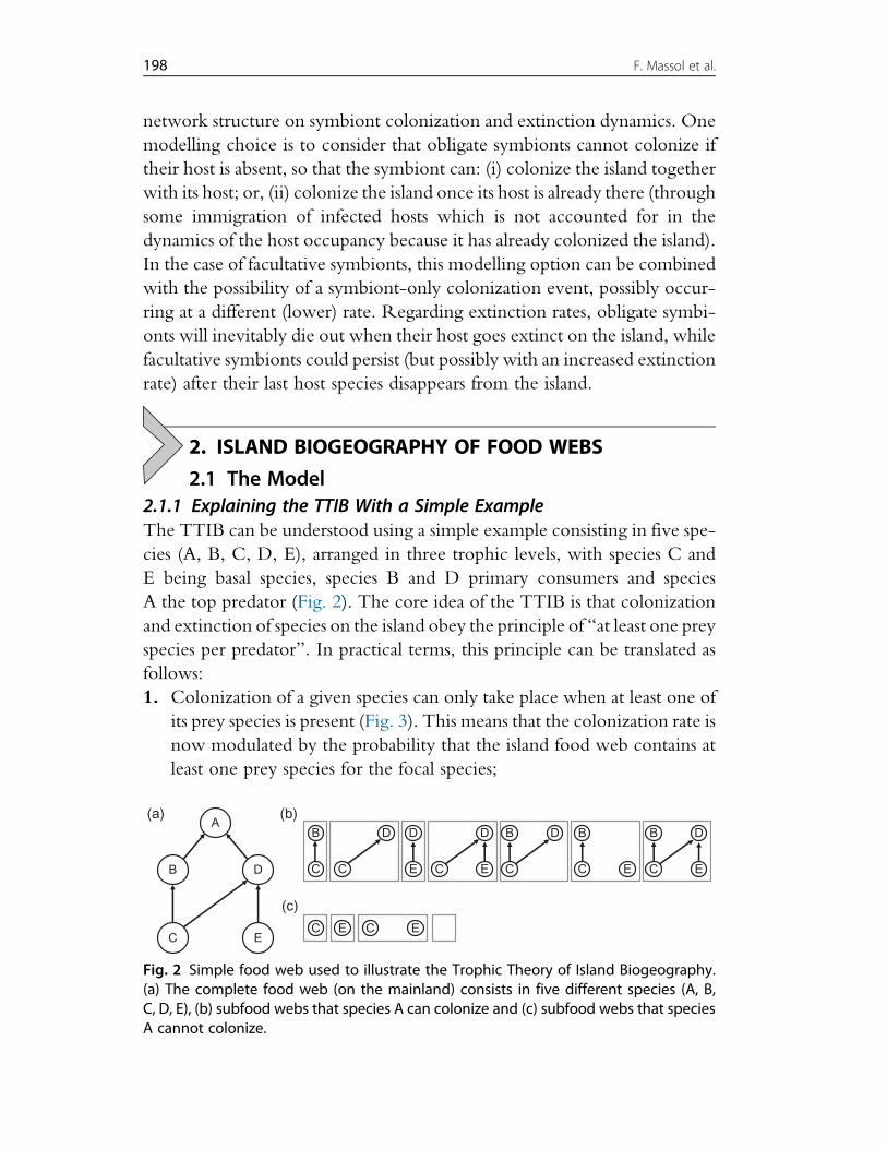
2.1.1 Explaining the TTIB With a Simple ExampleThe TTIB can be understood using a simple example consisting in five spe-

cies (A, B, C, D, E), arranged in three trophic levels, with species C and

E being basal species, species B and D primary consumers and species

A the top predator (Fig. 2). The core idea of the TTIB is that colonization

and extinction of species on the island obey the principle of “at least one prey

species per predator”. In practical terms, this principle can be translated as

follows:

1. Colonization of a given species can only take place when at least one of

its prey species is present (Fig. 3). This means that the colonization rate is

now modulated by the probability that the island food web contains at

least one prey species for the focal species;

A(b)

(c)

(a)

B D

C E

B

C

D

C

D

E

D

C E

B D

C

B

C E

C E C E

B D

C E

Fig. 2 Simple food web used to illustrate the Trophic Theory of Island Biogeography.(a) The complete food web (on the mainland) consists in five different species (A, B,C, D, E), (b) subfood webs that species A can colonize and (c) subfood webs that speciesA cannot colonize.


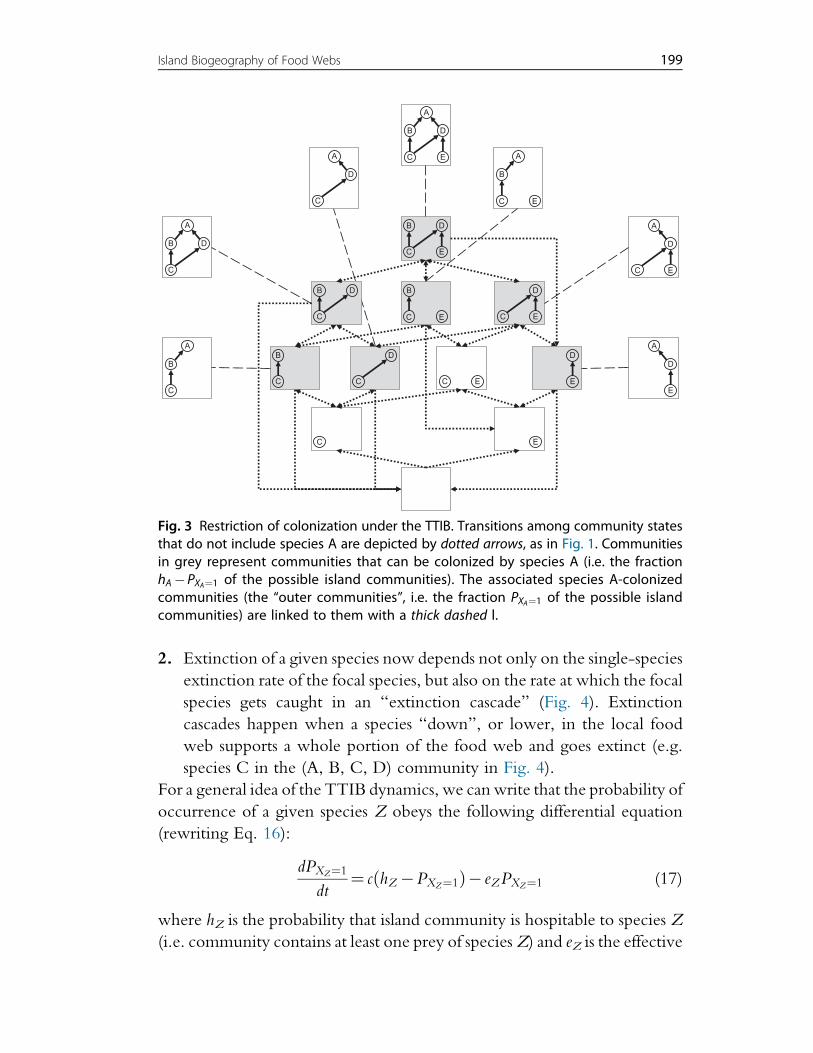
2. Extinction of a given species now depends not only on the single-species

extinction rate of the focal species, but also on the rate at which the focal

species gets caught in an “extinction cascade” (Fig. 4). Extinction

cascades happen when a species “down”, or lower, in the local food

web supports a whole portion of the food web and goes extinct (e.g.

species C in the (A, B, C, D) community in Fig. 4).

For a general idea of the TTIB dynamics, we can write that the probability of

occurrence of a given species Z obeys the following differential equation

(rewriting Eq. 16):

dPXZ¼1

dt¼ c hZ "PXZ¼1ð Þ" eZPXZ¼1 (17)

where hZ is the probability that island community is hospitable to species Z

(i.e. community contains at least one prey of speciesZ) and eZ is the effective

B D

C E

C E

C E

B

C

D

C

D

C E

B D

C

D

E

B

C E

A

B D

C E

A

B D

C

A

B

C

A

D

C E

A

D

C

A

D

E

A

B

C E

Fig. 3 Restriction of colonization under the TTIB. Transitions among community statesthat do not include species A are depicted by dotted arrows, as in Fig. 1. Communitiesin grey represent communities that can be colonized by species A (i.e. the fractionhA"PXA¼1 of the possible island communities). The associated species A-colonizedcommunities (the “outer communities”, i.e. the fraction PXA¼1 of the possible islandcommunities) are linked to them with a thick dashed l.


extinction rate of species Z computed using e, the number of ways it can go

extinct through a single-species extinction in the island food web and the

weights associated with these extinction events (which are computed from

the occurrence probabilities of species “down” the food web).

Let us start this example using the mainland food web given in Fig. 2a.

Species A can only colonize a restricted set of island food webs (Figs 2b and 3).

In other island food webs, it simply cannot settle because there is neither

prey species B nor D (Fig. 2c). Once species A is on the island, the

community must be in one of the “outer community” states of Fig. 3.

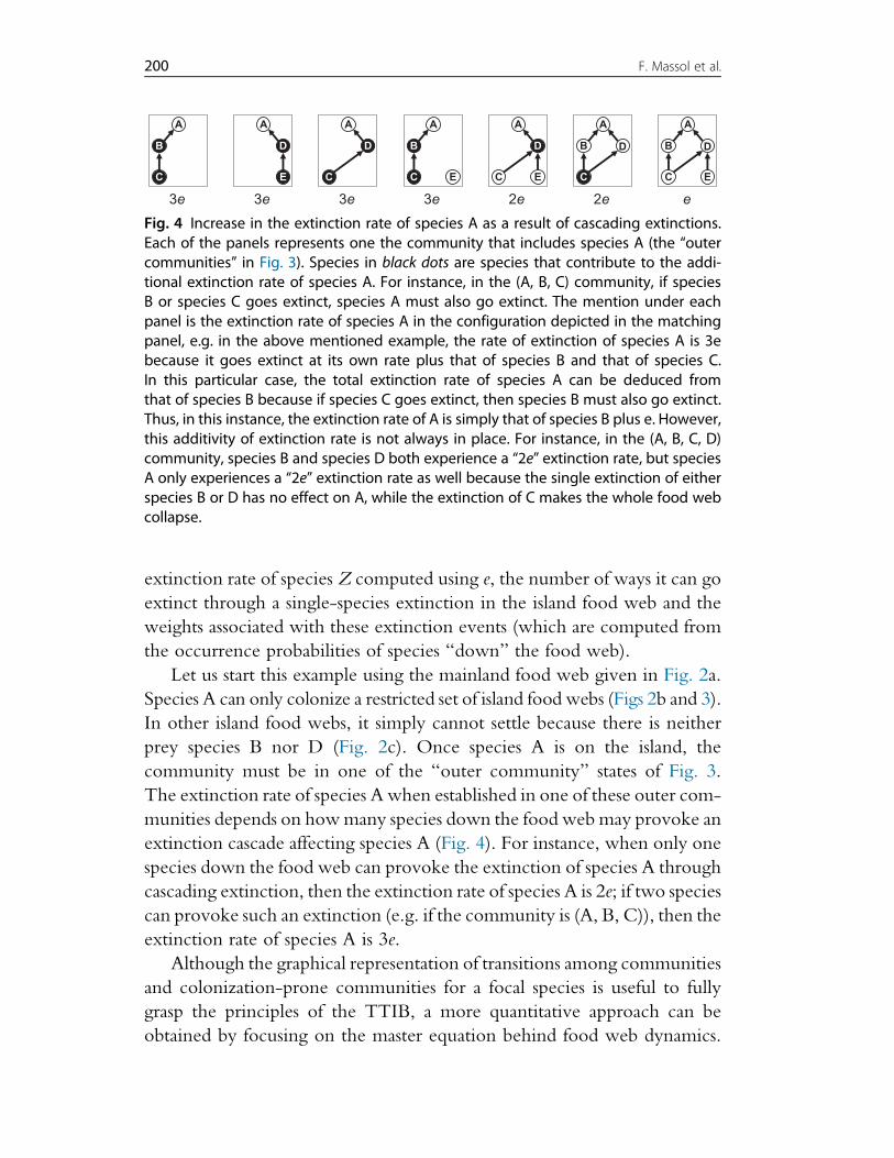
The extinction rate of species A when established in one of these outer com-

munities depends on howmany species down the food web may provoke an

extinction cascade affecting species A (Fig. 4). For instance, when only one

species down the food web can provoke the extinction of species A through

cascading extinction, then the extinction rate of species A is 2e; if two species

can provoke such an extinction (e.g. if the community is (A, B, C)), then the

extinction rate of species A is 3e.

Although the graphical representation of transitions among communities

and colonization-prone communities for a focal species is useful to fully

grasp the principles of the TTIB, a more quantitative approach can be

obtained by focusing on the master equation behind food web dynamics.

A

B D

C E

A

B D

C

A

B

C

A

D

C E

A

D

C

A

D

E

A

B

C E

3e 3e 3e 3e 2e 2e e

Fig. 4 Increase in the extinction rate of species A as a result of cascading extinctions.Each of the panels represents one the community that includes species A (the “outercommunities” in Fig. 3). Species in black dots are species that contribute to the addi-tional extinction rate of species A. For instance, in the (A, B, C) community, if speciesB or species C goes extinct, species A must also go extinct. The mention under eachpanel is the extinction rate of species A in the configuration depicted in the matchingpanel, e.g. in the above mentioned example, the rate of extinction of species A is 3ebecause it goes extinct at its own rate plus that of species B and that of species C.In this particular case, the total extinction rate of species A can be deduced fromthat of species B because if species C goes extinct, then species B must also go extinct.Thus, in this instance, the extinction rate of A is simply that of species B plus e. However,this additivity of extinction rate is not always in place. For instance, in the (A, B, C, D)community, species B and species D both experience a “2e” extinction rate, but speciesA only experiences a “2e” extinction rate as well because the single extinction of eitherspecies B or D has no effect on A, while the extinction of C makes the whole food webcollapse.


The following explanation starts with the corresponding master equation

in the TIB and then introduces an equivalent formulation in the case

of the TTIB.

The TIB model, as expressed using Eqs (1) and (2), does not distinguish

species based on any feature. However, the underlying random variable

describing the number of species present on the island, S, can be decomposed

as a sum of indicator variables Xi which describe the presence/absence of

species i, so that at all times:

S tð Þ¼X

i

Xi tð Þ (18)

Under the TIB, each of the Xi(t) is a random variable the value of which

changes from 1 to 0 with rate e and from 0 to 1 with rate c. The

corresponding master equation for a single species is thus given by two

coupled differential equations (indices i are omitted for the sake of clarity):

dPX¼0

dt¼ ePX¼1$ cPX¼0 (19a)

dPX¼1

dt¼ cPX¼0$ ePX¼1 (19b)

Noting PX¼1¼ p and PX¼0¼ 1$ p, we obtain the well-known equation for

the occupancy of islands by a single species under MacArthur and Wilson’s

framework:

dp

dt¼ c 1$ pð Þ$ ep (20)

When compared with the framework set by Eqs (16) or (17), Eq. (20) means

that: (i) there are no effects of network structure on any one of the three

parameters of Eq. (16); and (ii) the probability that an island is hospitable

to colonization is always 1 (i.e. there is no restriction to species colonization

potential).

The stationary distribution of X following Eq. (19) is a Bernoulli distri-

bution of parameter c= c + eð Þ, associated with the eigenvalue 0 of the matrix

defining the process defined in Eq. (19). In other words, solving for the equi-

librium of Eq. (19) is equivalent to finding the eigenvalues and eigenvectors

of a 2%2 matrix, and the equilibrium is given by the eigenvector associated

with the eigenvalue 0. The other eigenvalue,$ c + eð Þ, is associated with theeigenvector $1,1ð Þ (i.e. any discrepancy in the probability of occurrence of


the species from the stationary distribution of X), so that an initially absent

species at time t¼0 has a probability of occurrence at time t equal to:

PX tð Þ¼1jX 0ð Þ¼0¼c

c + e1$ e$ c + eð Þt

! "(21a)

while an initially present species at time t¼0 has occurrence probability:

PX tð Þ¼1jX 0ð Þ¼1¼c

c + e+

e

c + ee$ c + eð Þt (21b)

Now let us proceed with the simple four species community (B, C, D, E)

given in Fig. 1 under the TIB, i.e. without using the principle of “at least one

prey species per predator species” on the island. Each of the PX, where X

now represents a community, obeys a differential equation similar to

Eq. (19b), with losses due to both extinction of local species and colonization

by new species, and gains due to “upwards” transitions from species-poor

communities and “downwards” transitions from species-rich ones. For

instance, the equation for the community (D, E) is:

dPDE

dt¼ c PD +PEð Þ+ e PBDE +PCDEð Þ$2 c + eð ÞPDE (22)

More generally, noting P the vector of all PX, the master equation can be

written as:

dP

dt¼G %P (23)

where G is a matrix describing all the coefficients of the master equation.

In the case of the TIB acting on the food web described in Fig. 1a, matrix

G is given in Table 1.

Solving the equation G %P¼ 0 (i.e. finding a vector of sum equal to 1

associated with the eigenvalue 0 of matrix G) yields the probability of find-

ing the food web in the different states. In the case of the TIB, the result is

somehow easy to find without having to resort to the study of matrix eigen-

values and eigenvectors; Eq. (11) already gives the probability of finding a

community with exactly S species present. Dividing this expression by

the number of combinations of S species among T yields the following

general formula:

PX ¼ c

c + e

! " Xj j e

c + e

! "T$ Xj j(24)


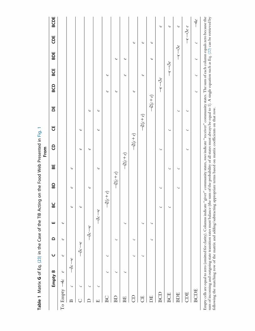
Table1

Matrix

Gof

Eq.(23

)intheCa

seof

theTIBActingon

theFo

odWeb

Presen

tedin

Fig.

1From

EmptyB

CD

EBC

BDBE

CDCE

DE

BCD

BCE

BDE

CDE

BCDE

ToEmpty

!4c

ee

ee

Bc

!3c!e

ee

e

Cc

!3c!

ee

ee

Dc

!3c!

ee

ee

Ec

!3c!e

ee

e

BC

cc

!2(c+

e)e

e

BD

cc

!2(c+

e)e

e

BE

cc

!2(c+

e)e

e

CD

cc

!2(c+

e)e

e

CE

cc

!2(c+

e)e

e

DE

cc

!2(c+

e)e

e

BCD

cc

c!c!

3e

e

BCE

cc

c!c!

3ee

BDE

cc

c!c!

3ee

CDE

cc

c!c!

3ee

BCDE

cc

cc

!4e

Emptycellsareequalto

zero

(omittedforclarity).C

olumnsindicate“giver”communitystates,rowsindicate“receiver”

communitystates.T

hesumofeachcolumnequalszero

becausethe

sum

ofincomingandoutgoingstatetransitionratesmustbalance

(thesum

oftheprobabilityofallstatesmustalwaysbeequalto

1).Asingleequationsuch

asEq.(22)

canberetrievedby

followingthematchingrow

ofthematrixandadding/subtractingappropriateterm

sbased

onmatrixcoefficientsonthatrow.

where jXj is the cardinality of community X (i.e. its species richness). The

probability that a single species, say C, is present on the island can be

obtained by summing Eq. (24) over all communities that include species C:

PXC¼1¼X

C2XPX ¼

XT

k¼0

X

C 2XXj j¼ k

c

c + e

! "k e

c + e

! "T"k

¼XT

k¼1

T "1k"1

# $c

c + e

! "k e

c + e

! "T"k

¼ c

c + e(25)

We now shift to the case of the TTIB, using the example given in

Fig. 1b, i.e. the same food web as the one used above, but with an intrinsic

dependency between species occurrences due to the underlying TTIB prin-

ciple. In this context, certain communities cannot exist, i.e. (B), (D), (B, D),

(B, E), (B, D, E) (grey communities in Fig. 1b). The associated G matrix is

given in Table 2.

SolvingG #P¼ 0 using theGmatrix given in Table 2 yields complicated

expressions. However, the same type of computations as the ones used to go

from Eq. (24) to Eq. (25) can be applied to this stable distribution of com-

munity states to obtain the stable distribution of each species occurrence

probability. For instance, one obtains that the probability of observing

species B is given by:

PXB¼1¼c2

c + eð Þ c +2eð Þ(26)

The food chain (B, C) being particularly simple (see also Section 2.2.1), this

result is easy to interpret: the probability of occurrence of species B relies

on species C being present (with probability c= c + eð Þ as species C is a basal

species), and species B having colonized (rate c), and the whole food chain

not collapsing (rate of species B extinction 2e).

2.1.2 A More General Presentation of the TTIBA simple consequence of the rules governing the dynamics of the TTIB is

that the two variables needed to compute the dynamics of a given species Z,

hZ and eZ (Eq. (17)) can be obtained based only on the probability of occur-

rence of species “down” the food web. In other words, looking “up” the

food web (i.e. at species that depend on Z for colonization) or “laterally”

(i.e. at species that have no dependence relation withZ for their colonization

or for species Z colonization) is not needed when assessing hZ and eZ. This


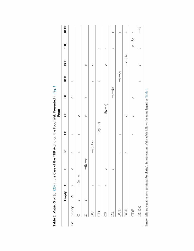
Table2

Matrix

Gof

Eq.(23

)intheCa

seof

theTTIB

Actingon

theFo

odWeb

Presen

tedin

Fig.

1From

Empty

CE

BCCD

CEDE

BCD

BCE

CDE

BCDE

To

Empty

!2c

ee

ee

ee

Cc

!3c!e

ee

e

Ec

!2c!

ee

ee

BC

c!2(c+

e)e

e

CD

c!2(c+

e)e

e

CE

cc

!2(c+

e)e

e

DE

c!c!

2ee

e

BCD

cc

!c!

3e

e

BCE

cc

!c!

3ee

CDE

cc

c!c!

3ee

BCDE

cc

c!4e

Empty

cells

areequalto

zero

(omittedforclarity).InterpretationofthistablefollowsthesamelegendasTable1.

means that, when focusing on species Z, we can focus on species Z and the

species it depends on to colonize (the ones “down” the food web), and thus

describe the dynamics of community states forgetting about the occurrence

of all the other species in the mainland food web. For instance, following the

example given above (Fig. 3), if we were to focus on species B, the only

community states to focus on would be the empty community, the one with

species C and the one with species (B, C). When forgetting about the rest of

the food web, the “empty state” refers to any state in which both species

B and C are absent, the “C community” refers to all states in which species

C is present but not species B, and the “(B, C) community” refers to all states

in which both species are present. In this instance, the (B, C, D) community

would “count” under the (B, C) modeled community state. In the follow-

ing, we present a new analytical derivation of the expressions for hZ and

eZ under the assumptions of the TTIB, which was not provided by

Gravel et al. (2011b).

This can be formalized more rigorously using notations that will help us

navigate the set of possible communities:

• Species Y is a foundation species for species Z if Y is part of at least one

path linking a basal species to species Z. The set of all foundation species

for species Z is noted FZ.

• Among foundation species for speciesZ, we noteGZ the set of prey spe-

cies of speciesZ. For convenience, we also noteHZ ¼FZ [ Zf g, i.e. theset of foundation species and the focal species itself. The intuitive notion

of species being “up” or “down” the food web can be understood

through the following statement: species Y is in HZ if and only if HY

is included in HZ.

• We will call a community, K, TTIB-compatible when all species in

the community are connected to at least one basal species in the com-

munity by at least one path of species present in the community.

• The trimmed community, bKc, is obtained by removing the minimal

number of species from community K so that the community obtained

is TTIB-compatible.

• We noteΩ the set of all TTIB-compatible communities containing

from 0 to T species of the mainland food web.

• We note ΩZ the set all TTIB-compatible communities that include

species Z.

• ForTTIB-compatible communityK,wenoteΦK itsTTIB-compatible

combination set, i.e. the set of all TTIB-compatible communities

consisting only of combinations of species in K. Naturally, K 2ΦK .


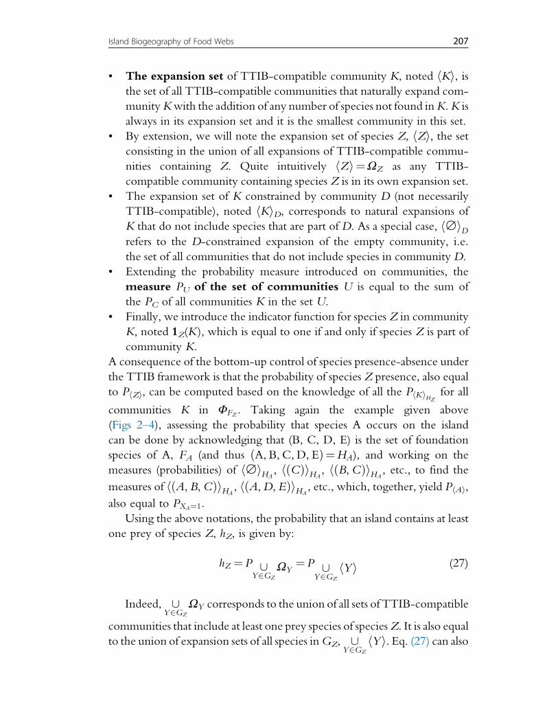
• The expansion set of TTIB-compatible community K, noted hKi, isthe set of all TTIB-compatible communities that naturally expand com-

munityKwith the addition of any number of species not found inK.K is

always in its expansion set and it is the smallest community in this set.

• By extension, we will note the expansion set of species Z, hZi, the setconsisting in the union of all expansions of TTIB-compatible commu-

nities containing Z. Quite intuitively Zh i¼ΩZ as any TTIB-

compatible community containing species Z is in its own expansion set.

• The expansion set of K constrained by community D (not necessarily

TTIB-compatible), noted hKiD, corresponds to natural expansions of

K that do not include species that are part of D. As a special case, ∅h iDrefers to the D-constrained expansion of the empty community, i.e.

the set of all communities that do not include species in community D.

• Extending the probability measure introduced on communities, the

measure PU of the set of communities U is equal to the sum of

the PC of all communities K in the set U.

• Finally, we introduce the indicator function for species Z in community

K, noted 1Z(K), which is equal to one if and only if species Z is part of

community K.

A consequence of the bottom-up control of species presence-absence under

the TTIB framework is that the probability of species Z presence, also equal

to PhZi, can be computed based on the knowledge of all the P Kh iHZfor all

communities K in ΦFZ . Taking again the example given above

(Figs 2–4), assessing the probability that species A occurs on the island

can be done by acknowledging that (B, C, D, E) is the set of foundation

species of A, FA (and thus A, B, C, D, Eð Þ¼HA), and working on the

measures (probabilities) of ∅h iHA, Cð Þh iHA

, B,Cð Þh iHA, etc., to find the

measures of A, B,Cð Þh iHA, A,D, Eð Þh iHA

, etc., which, together, yield PhAi,

also equal to PXA¼1.

Using the above notations, the probability that an island contains at least

one prey of species Z, hZ, is given by:

hZ ¼P [Y2GZ

ΩY¼P [

Y2GZ

Yh i (27)

Indeed, [Y2GZ

ΩY corresponds to the union of all sets of TTIB-compatible

communities that include at least one prey species of speciesZ. It is also equal

to the union of expansion sets of all species inGZ, [Y2GZ

Yh i. Eq. (27) can also


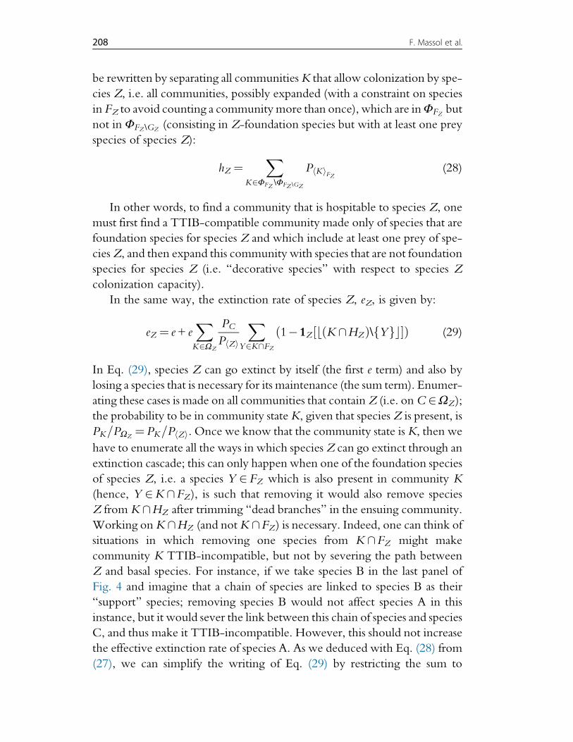
be rewritten by separating all communitiesK that allow colonization by spe-

cies Z, i.e. all communities, possibly expanded (with a constraint on species

in FZ to avoid counting a community more than once), which are inΦFZ but

not in ΦFZ \GZ(consisting in Z-foundation species but with at least one prey

species of species Z):

hZ ¼X

K2ΦFZ \ΦFZ \GZ

P Kh iFZ(28)

In other words, to find a community that is hospitable to species Z, one

must first find a TTIB-compatible community made only of species that are

foundation species for species Z and which include at least one prey of spe-

ciesZ, and then expand this community with species that are not foundation

species for species Z (i.e. “decorative species” with respect to species Z

colonization capacity).

In the same way, the extinction rate of species Z, eZ, is given by:

eZ ¼ e+ eX

K2ΩZ

PCP Zh i

X

Y2K\FZ1"1Z K \HZð Þ\ Yf gb c½ &ð Þ (29)

In Eq. (29), species Z can go extinct by itself (the first e term) and also by

losing a species that is necessary for its maintenance (the sum term). Enumer-

ating these cases is made on all communities that containZ (i.e. onC 2ΩZ);

the probability to be in community stateK, given that speciesZ is present, is

PK=PΩZ¼PK=P Zh i. Once we know that the community state is K, then we

have to enumerate all the ways in which speciesZ can go extinct through an

extinction cascade; this can only happen when one of the foundation species

of species Z, i.e. a species Y 2FZ which is also present in community K

(hence, Y 2K \FZ), is such that removing it would also remove species

Z from K \HZ after trimming “dead branches” in the ensuing community.

Working onK \HZ (and notK \FZ) is necessary. Indeed, one can think ofsituations in which removing one species from K \FZ might make

community K TTIB-incompatible, but not by severing the path between

Z and basal species. For instance, if we take species B in the last panel of

Fig. 4 and imagine that a chain of species are linked to species B as their

“support” species; removing species B would not affect species A in this

instance, but it would sever the link between this chain of species and species

C, and thus make it TTIB-incompatible. However, this should not increase

the effective extinction rate of species A. As we deduced with Eq. (28) from

(27), we can simplify the writing of Eq. (29) by restricting the sum to


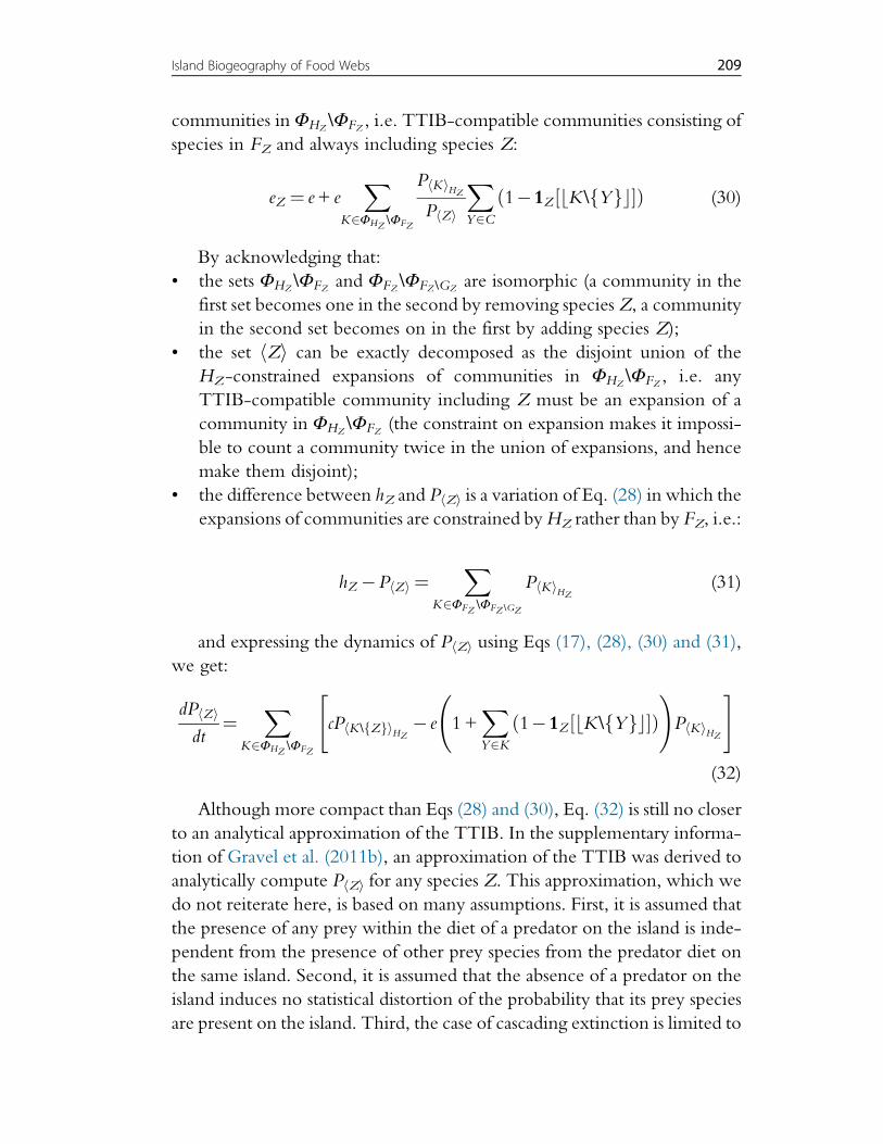
communities in ΦHZ\ΦFZ , i.e. TTIB-compatible communities consisting of

species in FZ and always including species Z:

eZ ¼ e+ eX

K2ΦHZ \ΦFZ

P Kh iHZ

P Zh i

X

Y2C1"1Z K \ Yf gb c½ $ð Þ (30)

By acknowledging that:

• the sets ΦHZ\ΦFZ and ΦFZ \ΦFZ \GZ

are isomorphic (a community in the

first set becomes one in the second by removing species Z, a community

in the second set becomes on in the first by adding species Z);

• the set hZi can be exactly decomposed as the disjoint union of the

HZ-constrained expansions of communities in ΦHZ\ΦFZ , i.e. any

TTIB-compatible community including Z must be an expansion of a

community in ΦHZ\ΦFZ (the constraint on expansion makes it impossi-

ble to count a community twice in the union of expansions, and hence

make them disjoint);

• the difference between hZ and PhZi is a variation of Eq. (28) in which the

expansions of communities are constrained byHZ rather than by FZ, i.e.:

hZ "P Zh i¼X

K2ΦFZ \ΦFZ \GZ

P Kh iHZ(31)

and expressing the dynamics of PhZi using Eqs (17), (28), (30) and (31),

we get:

dP Zh i

dt¼

X

K2ΦHZ \ΦFZ

cP K \ Zf gh iHZ" e 1+

X

Y2K1"1Z K \ Yf gb c½ $ð Þ

!P Kh iHZ

" #

(32)

Although more compact than Eqs (28) and (30), Eq. (32) is still no closer

to an analytical approximation of the TTIB. In the supplementary informa-

tion of Gravel et al. (2011b), an approximation of the TTIB was derived to

analytically compute PhZi for any species Z. This approximation, which we

do not reiterate here, is based on many assumptions. First, it is assumed that

the presence of any prey within the diet of a predator on the island is inde-

pendent from the presence of other prey species from the predator diet on

the same island. Second, it is assumed that the absence of a predator on the

island induces no statistical distortion of the probability that its prey species

are present on the island. Third, the case of cascading extinction is limited to


the extinction of species within the immediate diet of the focal predator,

i.e. the extra extinction rate incurred by species A in the case of community

(A, B, C, D) in Fig. 4 is ignored. Overall, all these assumptions can be trans-

lated as follows: for any speciesZ, the identity FZ ¼ [Y2GZ

HY is considered as

a union over disjoint sets, with empty intersections between any two HY’s

among the predator’s prey species.

2.2 Simple InsightsIn this section, we apply the rationale of the TTIB to very simple food web

topologies in order to gain insight into the interaction of colonization/

extinction dynamics with the position of species within foodwebs on species

occurrence.

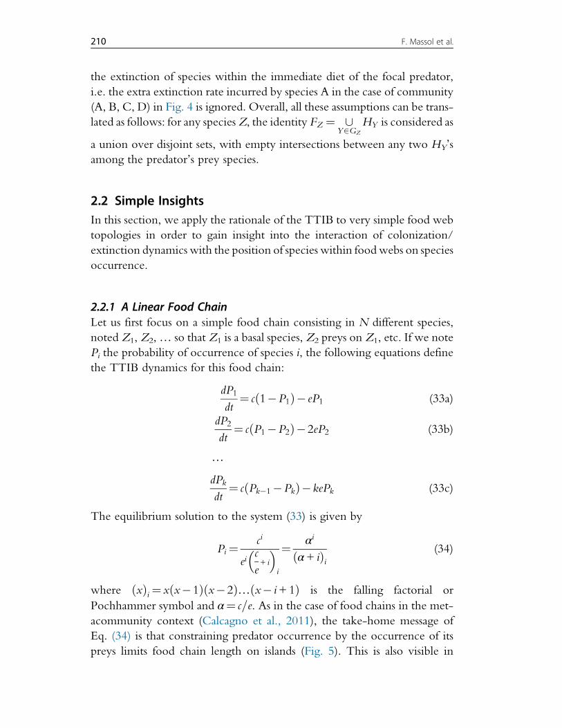
2.2.1 A Linear Food ChainLet us first focus on a simple food chain consisting in N different species,

noted Z1, Z2,… so that Z1 is a basal species, Z2 preys on Z1, etc. If we note

Pi the probability of occurrence of species i, the following equations define

the TTIB dynamics for this food chain:

dP1

dt¼ c 1"P1ð Þ" eP1 (33a)

dP2dt

¼ c P1"P2ð Þ"2eP2 (33b)

…

dPkdt

¼ c Pk"1"Pkð Þ"kePk (33c)

The equilibrium solution to the system (33) is given by

Pi¼ci

eic

e+ i

! "

i

¼ αi

α+ ið Þi(34)

where xð Þi¼ x x"1ð Þ x"2ð Þ… x" i+1ð Þ is the falling factorial or

Pochhammer symbol and α¼ c=e. As in the case of food chains in the met-

acommunity context (Calcagno et al., 2011), the take-home message of

Eq. (34) is that constraining predator occurrence by the occurrence of its

preys limits food chain length on islands (Fig. 5). This is also visible in


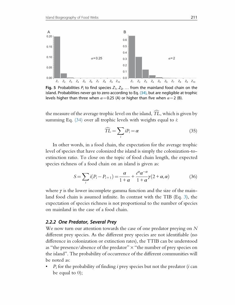
the measure of the average trophic level on the island, cTL , which is given bysumming Eq. (34) over all trophic levels with weights equal to i:

cTL ¼X

i

iPi¼ α (35)

In other words, in a food chain, the expectation for the average trophic

level of species that have colonized the island is simply the colonization-to-

extinction ratio. To close on the topic of food chain length, the expected

species richness of a food chain on an island is given as:

S¼X

i

i Pi"Pi+1ð Þ¼ α1+ α

+eαα"α

1+ αγ 2+ α,αð Þ (36)

where γ is the lower incomplete gamma function and the size of the main-

land food chain is assumed infinite. In contrast with the TIB (Eq. 3), the

expectation of species richness is not proportional to the number of species

on mainland in the case of a food chain.

2.2.2 One Predator, Several PreyWe now turn our attention towards the case of one predator preying on N

different prey species. As the different prey species are not identifiable (no

difference in colonization or extinction rates), the TTIB can be understood

as “the presence/absence of the predator”%“the number of prey species on

the island”. The probability of occurrence of the different communities will

be noted as:

• Pi for the probability of finding i prey species but not the predator (i can

be equal to 0);

BA

a= 0.25 a= 2

0.00

0.05

0.10

0.15

0.20

Z1 Z2 Z3 Z4 Z5 Z6 Z7 Z8 Z9 Z10 Z1 Z2 Z3 Z4 Z5 Z6 Z7 Z8 Z9 Z10

0.0

0.1

0.2

0.3

0.4

0.5

0.6

Fig. 5 Probabilities Pi to find species Z1, Z2, … from the mainland food chain on theisland. Probabilities never go to zero according to Eq. (34), but are negligible at trophiclevels higher than three when α¼0.25 (A) or higher than five when α¼2 (B).


• Qi for the probability of finding i prey species and the predator (i! 1).

The equations defining the TTIB in such a case are:

dP0dt

¼ e P1 +Q1ð Þ% cNP0 (37a)

dPidt

¼ c N % i+1ð ÞPi%1 + e i+1ð ÞPi+1% c N % ið Þ+ ei½ 'Pi% cPi + eQi (37b)

dQi

dt¼ c N % i+1ð ÞQi%1 + e i+1ð ÞQi+1% c N % ið Þ+ ei½ 'Qi + cPi% eQi

(37c)

Solving system (37) in the general case is quite complicated. The path to a

complete (but difficult to express) solution lies in rewriting system (37) for

quantities Fi ¼Pi +Qi and Di¼Pi%Qi, identifying the dynamics of Fi as

those of the TIB (and hence its probabilities are known and given by

Eq. 11), simplifying the recursions on Di and finally expressing Di in terms

of the Fi’s.We found no general form for this solution, but an interesting rela-

tionship between the expected number of prey species present to support a

predator and the probability of predator occurrence emerges at equilibrium:

X

k!1

kQk¼Nα2

2+Nα4

X

k!1

Qk (38)

where α¼ c=e. Eq. (38) always holds exactly for this system (i.e. it is not an

approximation).

To obtain a general formula for the probability of predator occurrence,

i.e.X

k!1

Qk, we can assume that α≪1. As the colonization by the predator

species entails a colonization event on top of the ones already needed for the

prey species to occur, we assume that the quantities Fk¼Pk +Qk are asym-

metrically separated, i.e. we assume that the Qk’s can be written as:

Qk¼ akαFk (39)

Developing Eq. (37c) in powers of α, we find that:

a1¼N

2(40a)

ai¼1+ iai%1

1 + i(40b)


Solving recursion (40b), we finally have the following expression for the ai’s:

ai ¼i"1+N

1+ i(41)

Plugged into Eq. (39) and summed over all k’s, Eq. (41), take at the first

available order in α, yields:

X

k#1

Qk$N 2α2

2(42)

Plugged into Eq. (38), Eq. (42) implies:X

k#1

kQk

X

k#1

Qk

$ 1

N+Nα4

(43)

What Eqs (42) and (43) mean is that: (i) the probability of occurrence of

the predator at low α is proportional to the square of its degree (i.e. the num-

ber of preys it can feed on); and, (ii) the expected number of prey species

occurring with the predator, conditionally on its occurrence, is proportional

to its degree when it is not too low. Eq. (42) can also be reinterpreted given

that, when α is low,X

k#1

Fk$Nα:

X

k#1

Qk$Nα2

X

k#1

Fk (44)

Hence, a predator only occupies a “fraction”, Nα/2, of the probabilityspace given by its preys.

2.2.3 Multipartite Network as a Food WebWe now extend Eqs (42)–(44), i.e. assuming that α¼ c=e is small and con-

sider a multipartite food web in which each and every species can be assigned

a precise trophic level and only prey on species at the immediate trophic

level down the web.We will noteDk the random variable giving the degree

(as a predator, i.e. the in-degree) of species at trophic level k in the mainland

food web. We assume that there are many species at each trophic level

and we note Nk the number of species at trophic level k in the mainland

food web. We will also note Sk the number of species at trophic level k

on the island.


Following the TIB, we know that the expected number of basal species

on the island is:

E S1½ " #N1α (45)

Using relation (42), we find that the expected number of species of the

second trophic level occurring on the island is given by:

E S2½ " #N2α2

2E D2

2

! "(46)

Generalizing approximation (46) to the next trophic levels, we finally get:

E Sk½ " #Nkαk

2k$1

Yk

i¼1

E D2i

! "(47)

When the distribution of degrees is the same across trophic levels (i.e.

E D2i

! "¼E D2

! "for all i), noting T ¼

XNk the total number of species

on the mainland and S¼X

Sk the equivalent on the island, we can trans-

form Eq. (47) using β¼ αE D2! "

=2:

E S½ " # αTX

k&1

βk$1Nk

T(48)

Eq. (48) expresses the relationship between E S½ " and T as a function

of α (as in the classic TIB) and the distribution of degrees across the

food web (through β) and the distribution of trophic levels in the food

web (through Nk/T). The approximation remains valid as long as E D2! "

¼Var D½ "+E D½ "2 remains small compared to 1/α, ensuring a relatively lowdegree of dependence between species occurrence within the same

trophic level.

2.3 Interpretation in Terms of Food Web Transitions2.3.1 Reformulation in Terms of Transitions Between Community StatesAs suggested in Section 2.1.2, an analytical alternative for the study of the

TTIB is to derive a master equation for community states rather than indi-

vidual species. The mathematical object is then the random process Ct>0¼[Ti¼1Xi which is a vector of 0 and 1 describing the presence and absence of

all species at any time t. For T species, there are 2T community states.

Table 3 provides an example for species B, C, D and E presented in Fig. 2.


Deriving the equation associated to a given community state Sk requires

study of the transition probabilities between community states between t and

t + dt (dt is assumed to be short enough to permit only one transition). As all

community states are included in the set Sk,k2 1, 2,…, 2T! "

, following the

law of total probability, for any community state:

PCt + dt¼Sk ¼X2T"1

l¼0

PCt + dt¼SkjCt¼SlPCt¼Sl (49)

The transition probabilities PCt+ dt¼SkjCt¼Sl are assumed to be linear func-

tions of dt, when dt is small enough. For k 6¼ l, the transitionmatrixG, similar

to the one presented in Eq. (23), is defined by:

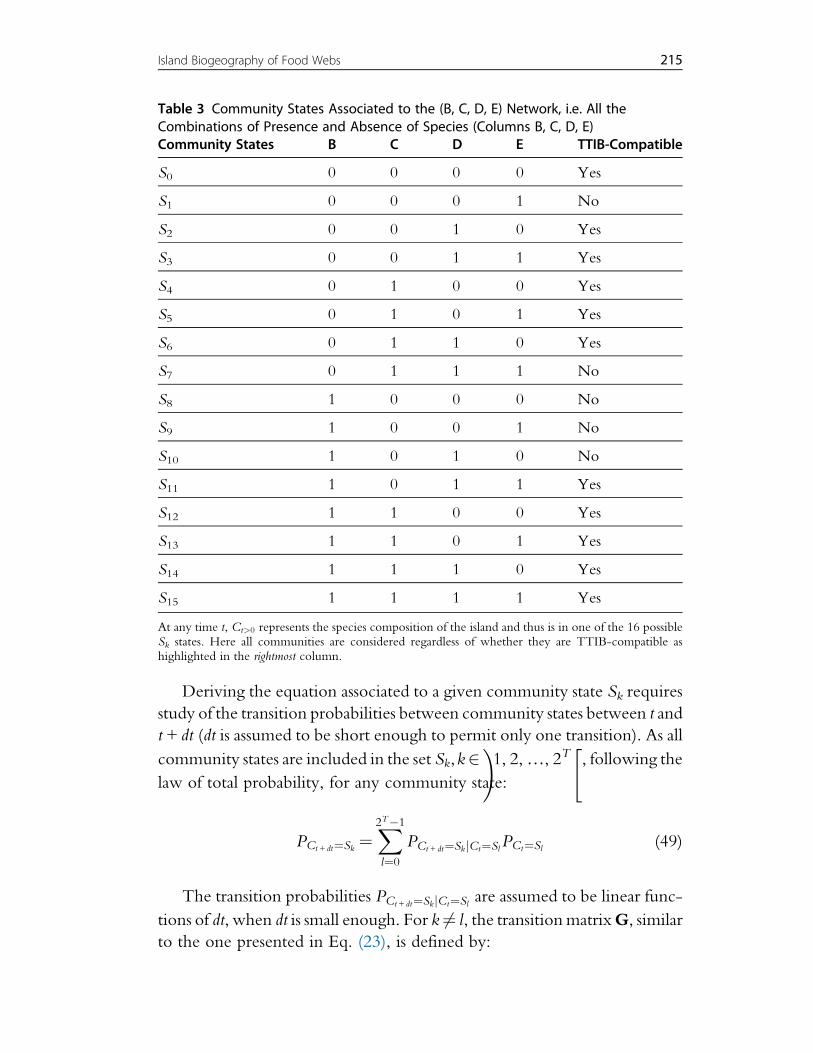
Table 3 Community States Associated to the (B, C, D, E) Network, i.e. All theCombinations of Presence and Absence of Species (Columns B, C, D, E)Community States B C D E TTIB-Compatible

S0 0 0 0 0 Yes

S1 0 0 0 1 No

S2 0 0 1 0 Yes

S3 0 0 1 1 Yes

S4 0 1 0 0 Yes

S5 0 1 0 1 Yes

S6 0 1 1 0 Yes

S7 0 1 1 1 No

S8 1 0 0 0 No

S9 1 0 0 1 No

S10 1 0 1 0 No

S11 1 0 1 1 Yes

S12 1 1 0 0 Yes

S13 1 1 0 1 Yes

S14 1 1 1 0 Yes

S15 1 1 1 1 Yes

At any time t, Ct>0 represents the species composition of the island and thus is in one of the 16 possibleSk states. Here all communities are considered regardless of whether they are TTIB-compatible ashighlighted in the rightmost column.


PCt+ dt¼SkjCt¼Sl ¼ gkldt (50)

and, asX

l

PCt + dt¼Sl jCt¼Sk ¼ 1:

PCt + dt¼SkjCt¼Sk ¼ 1"X

l 6¼k

glkdt (51)

gklreflects the rate at which community state switches from state Sl to

state Sk, and it can be greater than one as long as gkldt< 1. The TTIB

acknowledges the existence of trophic interactions by assuming:

1. gkl¼ 0, when the transition from Sl to Sk involves the colonization of a

predator without any prey,

2. gkl¼ e, when removing a species from Sl and then successively removing

all predators not sustained by any prey species transforms the community

into state Sk.

Plugging Eqs (50) and (51) in Eq. (49), we obtain:

PCt+ dt¼Sk "PCt¼Sk

dt¼"

X

l 6¼k

glk

!

PCt¼Sk +X

l 6¼k

gklPCt¼Sl (52)

When dt! 0, this approach provides the master equation than can be writ-

ten in vector format to integrate the dynamics of all community states

P¼ PS1 , PS2 ,…, PS2T! "

:

dP

dt¼G #P (53)

This equation is the same as Eq. (23); P includes all community states and

the coefficients of the matrix G generally depend on the community. Nev-

ertheless, the form of the solution remains equivalent:

P tð Þ¼ etGP0 (54)

This approach describes a continuous-time Markov chain. When all the

community states communicate (i.e. the Markov chain is irreducible), their

probabilities reach an equilibrium P* given by the vector in the kernel ofGthe elements of which sum to one.

2.3.2 Reasonable ApproximationsThe formulation above allows the study of nonindependence between

species occurrences, but suffers from its generality: for T species, the matrix


G must be filled with 2T !1! "

" 2T !1! "

coefficients (the “!1” acknowl-

edges that at any time t the elements of P(t) sum to one). Even if the knowl-

edge of a particular network may help find these coefficients, reasonable

assumptions can be made to decrease the complexity of G.

• First, community compositions between t and t+dt cannot differ in

more than one species, i.e. gkl¼ 0 when Skj j! Slj jj j> 1. This turns G

into a sparse matrix: at most T " 2T !1! "

of its coefficients are not equal

to zero. This assumption is not possible under the TTIB as the extinction

of a prey can lead to multiple extinctions. However, this issue is easy to

circumvent by allowing the predator to survive a (very) short period

alone on the island. This can be done using large value for gklthat

measures the transition of a community with a predator to the same com-

munity without it.

• A second assumption is that colonization processes may be independent

of interactions. That is, a predator can actually colonize an island without

any prey. This is reasonable if the extinction probability of this predator

on such an island is high, as is recommended to comply with the first

assumption. Therefore, we can assume gkl¼ c when Skj j! Slj j¼ 1. This

assumption is also useful to integrate variability in dispersal capacities

among species (Cazelles et al., 2015b).

Table 4 presents matrixG for species C, D and E of the example presented in

Figs 2–4, i.e. community states from S0 to S8. Once the colonization prob-

ability is determined, the remaining T " 2T !2! "

coefficients can be found

based on the biological knowledge of species studies, e.g. the nature and the

strength of interactions.

2.3.3 Deriving Species RichnessThe solution P* contains the probabilities of all community states at equi-

librium. This information is actually more than the knowledge of individual

species presence and species richness. Indeed the probabilities of species

occurrence are particular unions of community states; therefore, P* is

sufficient to derive them at equilibrium. The probability of a species being

present at equilibrium is given by:

PXi¼1¼X

kjSk, i¼1

P*k (55)

where Sk, i ¼ 1means that species i is in community state Sk andPk* is the kthcomponent of P*. Similarly, the species richness is given by the sum of P*weighted by the cardinality of the community states it refers to:


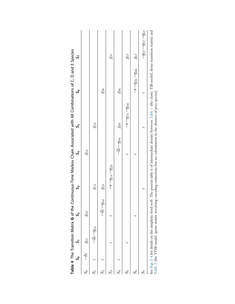
Table4

TheTran

sitio

nMatrix

Gof

theCo

ntinuo

us-Tim

eMarko

vCh

ainAssociatedwith

AllCo

mbina

tions

ofC,

Dan

dESp

ecies

S 0S 1

S 2S 3

S 4S 5

S 6S 7

S0

!3c

g 01

g 02

g 04

S1

c!2c!g 01

g 13

g 15

S2

c!2c!g 02

g 23

g 26

S3

cc

!c!

g 13!g 23

g 37

S4

c!2c!g 04

g 45

g 46

S5

cc

!c!

g 15!g 45

g 57

S6

cc

!c!

g 26!g 46

g 67

S7

cc

c!g 37!g 57!g 67

SeeFigs2–4

fordetailsonthissimplisticfoodweb.Thepresenttableisofinterm

ediate

density

betweenTable1(theclassicTIB

model,dense

transitionmatrix)

and

Table2(theTTIB

model,sparse

matrixinvolvingcascadingextinctionsbutnocolonizationin

theabsence

ofpreyspecies).

S¼X2T"1

k¼0

jSkjP*k (56)

In a similar fashion, many probabilities can be derived regarding either a

particular set of species or a particular property of the community. For

instance, this framework allows deriving the probability of finding a given

set of predators but also the mean trophic level expected and even the prob-

ability of having a trophic chain of at least p levels. In all these situations,

computation of probabilities requires the identification of the community

states to be summed.

3. EFFECTS OF MAINLAND FOOD WEB PROPERTIESON COMMUNITY ASSEMBLY

In this section, our aim is to explore how the structural properties of

mainland food webs affect the colonization/extinction dynamics and the

resulting structural properties of island food webs. We first assess the effects

of the degree distribution, the network size, the network connectance and

the proportion of primary producers on island food web structural proper-

ties. In a second stage, we assess the effects of modularity in the mainland

food web on island food web properties.

The degree distribution (i.e. the distribution of the number of links per

node) is known to be a fundamental property of real-world, complex net-

works (Barabasi and Albert, 1999; Newman et al., 2001) and will have

important implications for their stability (Allesina et al., 2015; May,

1972). Food web models classically used in ecology—the niche model

(Williams and Martinez, 2000), the cascade model (Cohen and Newman,

1985), etc.—are able to reproduce some properties of real food webs. How-

ever, they do not constrain the degree distribution, and typically display dis-

tributions of links that follow an exponential law for which there is mixed

evidence in empirical data (Camacho et al., 2002; Dunne et al., 2002a).

Moreover, those models do not control for the connectance or the propor-

tion of basal species, contrary to the model used by Th!ebault and Fontaine

(2010), for example. In the same vein, classic network generation models

used in network science—the Erdos-R!enyi model (Erdos and R!enyi,1959), the preferential attachment algorithm (Barabasi and Albert, 1999;

De Solla Price, 1976), etc.—are able to generate different degree distribu-

tions but in a stochastic way. Furthermore, one version of the Erdos–R!enyi


model allows the number of links to be fixed, but this is not the case for the

Barabasi–Albert algorithm in which network topology arises through a

growth process (i.e. preferential or random attachment) and in which each

vertex is added with a certain number of links. Finally, the growth process of

the Barabasi–Albert algorithm could lead to particular features in the

resulting networks other than just the degree distribution (Newman,

2005; Stumpf and Porter, 2012). We therefore use a network generation

algorithm based on degree sequence (Bollobas et al., 2001; Chung et al.,

2003; Kim et al., 2009; Miklos et al., 2013).

3.1 Simulating the Model3.1.1 Generating Directed Networks With Given Structural PropertiesBecause we want to assess the effects of different structural properties of the

mainland food web on the colonization/extinction dynamics of island food

webs, we need a network generation model that is able to be constrained by

different properties. In particular, we want to fix the size of the network, the

number of edges, the proportion of primary producers and the degree dis-

tribution. The typical size of food webs and other ecological networks is at

least several orders of magnitude below that of network datasets from physics

or computer science. For this reason, we want to use a network-building

algorithm that yields a food web with properties (size, connectance, degree

distribution, etc.) set at exact values, in order to remove the noise that could

result from working with food webs that only obey “expected” constraints.

The sequence of degrees, which lists the total number of links of each

node, allows the simultaneous fixing of three different metrics: the degree

distribution, the network connectance and the size of the network. Thus,

we generated the sequences of degrees in a deterministic way, using the pro-

cedure of Astegiano et al. (2015), adapted for unipartite networks, which

was based on the algorithm of Chung et al. (2003).

3.1.1.1 Generating the Sequence of Degrees for a Given Degree DistributionWe want a degree sequence w¼ w1, w2,…, wnf g representing the number

of undirected links per node in a decreasing order, i.e. such that wi "wi+1

for all i, with n the total number of vertices, and such that the sequence of

degrees follows a given probability density function f. One way of deriving

such a sequence can be found by solving for wi:

i

n# 1$F wið Þ (57a)


or equivalently

wi!F"1 1" i

n

! "(57b)

where F is the cumulative distribution function associated with the proba-

bility density function f. Given a fixed connectanceC, the parameters of the

probability density function have to be selected such that:

2C! 1

n n"1ð ÞX

i

wi (58a)

with C the desired directed connectance;

C¼L=n n"1ð Þ (58b)

and L the number of directed links in the network. The denominator in

Eq. (58) is n n"1ð Þ, because we consider that there is no self-loop (i.e. can-

nibalism) to avoid species that would stay on an island without any prey

except itself. One can adjust the degree distribution (i.e. through f ) to obey

this constraint by setting the average undirected degree to be exactly

2C(n"1). We target twice the desired connectance (2C) because the algo-

rithm for directed links leads to a loss of half of the links (due to the passage

from undirected to directed links). Finally, this sequence has to be feasible

(i.e. the sequence has to be graphic) for a simple connected graph (with no

cannibalism, i.e. self-reference, or multiple edges, and with a unique com-

ponent). In other words, at least one simple connected graph must exist

which satisfies the degree sequence (Berger, 2014; Brualdi and Ryser,

1991; Ryser, 1957).

We use truncated degree distributions, and so do not allow node degrees

to be below or over certain predetermined limits. Indeed, the maximal

degree of a vertex within a community of n species is n"1, in the absence

of cannibalism, and the minimal degree is one because we target simply

connected graph (i.e. without disconnected species). When high values of

network connectance are targeted with a Power law for the degree distri-

bution, obtained degree sequences are generally not graphic. In those cases,

distributions are left-truncated in order to obtain graphic sequences that

maintain a heavy tail. We also round degrees obtained for exponential dis-

tribution, because this law is continuous. This is not needed for Poisson and

Power law (Zipf law) distributions, which are discrete. It should be noted

that Power law distributions have been included mostly for the sake of


comparison, even though it is very difficult to evidence the existence of such

distributions in data unless the distribution of degrees spans at least three

orders of magnitude (e.g. with degrees spanning the whole 1–1000 interval;Clauset et al., 2009; Stumpf and Porter, 2012).

3.1.1.2 Generating a Graph With a Prescribed Degree SequenceIf the sequence is graphic, the second step is to generate random undirected

connected simple graphs that satisfy the sequence of degrees (and therefore

the other desired properties as well), drawn uniformly from all the possible

sets of graphs. To do so, we use the procedure described in Viger and Latapy

(2005), which improves the MCMC algorithm fromGkantsidis et al. (2003)

and is implemented in the R package igraph (Csardi and Nepusz, 2006).

3.1.1.3 Directing the LinksFinally, the generated networks have to be directed in order to be construed

as food webs. There is, to our knowledge, no method currently available to

direct a graph such that it has a fixed number of primary producers and to

ensure that all vertices can be reached from a basal species (there are of course

methods to generate directed graphs from undirected ones obeying certain

constraints, e.g. Stanley, 1973, but these algorithms were not designed to

keep certain nodes as incoming or outgoing ends of the graph, as is needed

in the case of food webs with controlled number of basal species).

To do this, we first randomly selected the desired number of basal ver-

tices. These vertices have to be disconnected. Indeed, if two vertices are

connected, necessarily one of them cannot be a primary producer. Because

of constraints on connectance and degree distribution, some proportions of

basal species seem to be unreachable. To confirm that there is no solution in

those instances, we use a graph colouring algorithm (Bl€ochliger and

Zufferey, 2008). This algorithm tries to find the minimal number of colours

necessary to colour each vertex such that two adjacent vertices have a dif-

ferent colour. Thus, a set of disconnected vertices is associated to each col-

our. If this algorithm finds not a single colour-associated set containing at

least the desired number of primary producers, then we consider that our

basal species assignment problem has no solution. In fact, all parameter sets

are not possible, especially for degree distributions following a Poisson law

(see later), or when connectance reaches relatively high values (!0.1). Then,

the network is directed by an algorithm inspired from breadth-first search on

graphs (see Appendix). The basic idea is that, at each time step, one proceeds

from the current “trophic level” to the next up the food chain by exploring


the graph from each of the node of the current trophic level, taking all nodes

that can be reached in one step from all the nodes in the current trophic

level. The next trophic level consists of all nodes thus explored that were

not explored earlier; all links between the current level and the next are

directed “upwards” (i.e. from current to the next), while links between

nodes in the next trophic level are randomly directed. The next step of

the algorithm then takes place after taking the next trophic level as the

current one.

3.1.2 Generating Modular NetworksModularity, i.e. the propensity of nodes to form densely connected clusters

with few links between them, has been suggested as a potential explanation

for properties such as ecological network stability (Th!ebault and Fontaine,

2010), persistence (Stouffer and Bascompte, 2011) and feasibility (Rozdilsky

and Stone, 2001). In the context of the TTIB, our objective is to assess

whether the modular structure of a mainland food web affects expectation

on islands and, if so, how?

Modular networks are generated with a stochastic block model (SBM;

Govaert and Nadif, 2008). Vertices are grouped into groups, and edges

are added following the Erdos–R!enyi model (Erdos and R!enyi, 1959), witha probability qw of finding an edge between two vertices in the same group,

and a probability qb between two vertices in different groups. If all modules

have the same size, the expected network connectance is:

E 2C½ " ¼ 1

m$ 1

n$11$ 1

m

! "# $qw$ qbð Þ+ qb (59)

with m is the number of modules. Note that when n (number of vertices/

species) is large enough, the expected connectance can be approximated by

the following equation:

E 2C½ " ' qw$ qbm

+ qb (60)

As described in Section 3.1.4.4, modularity is computed with the

walktrap algorithm (Pons and Latapy, 2006), and with the flow-based

infomap algorithm (Rosvall and Bergstrom, 2008). Modularity cannot be

controlled exactly, but can be approximated through generations of net-

works with different qw and qb such that the connectance stays constant.


An approximate log-linear relation can be found between the logarithm of

modularity and the ratio β¼ qb=qw < 1 (at a constant connectance C):

log Qð Þ$ aCβ+ bC (61)

Using a linear regression, a and b values can be computed. Based on

approximations (60) and (61), we can approximately control both the

expectation of the connectance and the modularity of the network.

3.1.3 Defining a Null ModelWhen we compare the properties of local food webs on islands relative to

their mainland counterpart, there can possibly be two confounding effects.

On the one hand, observed differences could be due to the sequential

dependence of colonization/extinction events. On the other hand, differ-

ences could arise just because local food webs are limited subsets of the main-

land food webs. In particular, some network properties could vary in a

systematic way with the size of local networks (Poisot and Gravel, 2014).

In order to disentangle these two confounding effects, we use a null

model, which is simply MacArthur and Wilson’s TIB model, i.e. without

any interaction. For each of the 50 replicates of each parameter set, and

for each value of the colonization-to-extinction ratio (α¼ c=e), we ran-

domly draw a sample of species on the mainland. It is noteworthy that to

get a broad range of local web sizes, we had to use a wider range of α values

for the null model than for the simulations with interactions. The size of the

sample is a proportion of the total number of species on mainland, whose

value is determined by the value predicted by MacArthur and Wilson’s

model (i.e. Eq. 3). In this case, all species have the same colonization and

extinction rates and are thus considered sampled with the same probability.

We do not add any constraint on this random sample, which can thus lead

to unrealistic local food webs (e.g. an intermediate species in the mainland

food web could appear as a “basal” species in the island network generated

by the null model, or a large proportion of species could end up being

completely disconnected from the island network, especially for small α,weak connectance and small size of the mainland food web).

3.1.4 Network Properties of Interest3.1.4.1 ConnectanceWe consider the directed connectance, which is the number of directed

links found in the network relative to the maximal number of directed links

possible, given by Eq. (58b).


We have to note that connectance for the null model is computed con-

sidering all species on the island, be they connected or not. When α is small

(i.e. c<< e), the proportion of disconnected species (i.e. species with no

link) increases and thus, the connectance rapidly decreases.

3.1.4.2 Trophic LevelsWe use the notion of the shortest trophic level (Williams et al., 2002), which

is, the shortest path from a species i to any basal species. This metric is com-

puted using the adjacency matrix (A, with aij ¼ 1 when there is a link going

from species j to species i) of the food web in the following way; for a species

i, its trophic level is one plus the smallest τ such that:

xTi "Aτ "b 6¼ 0 (62)

where b is the vector of basal species (i.e. if species j is a basal species, then

bj ¼ 1, else bj ¼ 0) and xi is a vector of zeroes with a single “1” at position i.

Noting τi the shortest path from a species i to basal species, the mean shortest

trophic level over the whole island food web is:

cTL ¼ 1

n

X

i

1+ τið Þ (63)

where n is the number of species in the food web. The maximal trophic level

in the same food web is:

TLmax ¼ maxi

1+ τið Þ (64)

3.1.4.3 Degree DistributionIdentification of degree distribution is done by fitting several models

(Uniform, Poisson, Exponential and Power law) and retaining the one with

the lowest Akaike Information Criterion (AIC). Likelihood and parameter

estimates are computed with theR package fitdistrplus.When this is done

on mainland webs, in which the degree distribution is imposed, the best-fit

distribution does not always correspond to the desired distribution. For

example, relatively small networks with a weak connectance tend to be

characterized by uniform or Poisson distributions. Similarly, Power law-

constructed networks can appear as following an exponential distribution

of degrees when there are not enough well-connected nodes (Newman,

2005; Stumpf and Porter, 2012). For results about degree distributions,

we consider the distribution given by the best-fit model rather than the


distribution used to create the input networks so as to better relate our

findings to the type of information empiricists have access to.

3.1.4.4 ModularityAs previously noted, modules can be defined as a set of nodes that interact

significantly more with each other than with nodes in the rest of the network

(Newman, 2004, 2006a,b; Newman and Girvan, 2004). The identification

of modules relies on partitioning the nodes of a given network in different

modules such that this partition maximizes a property named modularity. In

ecology, the definition commonly used is the one of Newman and Girvan

(2004). With this definition, directed links (i.e. arrow from one species to

another) in ecological networks are generally considered as undirected

(but see Arenas et al., 2007; Leicht and Newman, 2008, for ways to extend

classic modularity to directed networks). As food webs present directed links

that represent energy or matter fluxes, this information could be important

for constructing modules. Thus, we also use a flow-based approach, the

infomap algorithm (Rosvall and Bergstrom, 2008) to partition food webs.

With this approach, the network is decomposed into modules by optimally

compressing a description of a randomwalk (representing information, mat-

ter or energy) on the network. This method could be more capable of

detecting modules associated with energy channels (as in Rooney et al.,

2006) than the classic optimization of modularity. A value of modularity

can be obtained with the partition of the food web obtained by the infomap

algorithm. However, we instead use the compression rate, i.e. oneminus the

ratio of description length after/before compression, the description lengths

being given in bits necessary to describe typical random walks on the

network, as a proxy for modularity.

3.1.5 Running SimulationsAs many properties are susceptible to scale with the complexity of the net-

work (Wood et al., 2015), simulations are done with mainland food webs of

different sizes (100, 250, 500 nodes/species) and connectance values (0.01,

0.025, 0.05 and 0.1) as well as for different proportions of basal species

(5%, 10%, 20%, 40%), since this could alter the outcome of the process

by forming a more or less solid foundation for food chain construction.

Three different degree distributions are used: Zipf (Power law), Poisson

and Exponential (geometric) distributions. Thirty-two combinations of

parameter sets are not feasible because they either lead to food webs that

do not consist of a single component (disconnected webs) or are unable


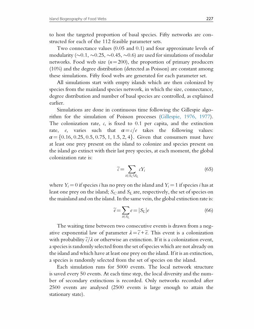
to host the targeted proportion of basal species. Fifty networks are con-

structed for each of the 112 feasible parameter sets.

Two connectance values (0.05 and 0.1) and four approximate levels of

modularity (!0.1,!0.25,!0.45,!0.6) are used for simulations of modular

networks. Food web size (n¼200), the proportion of primary producers

(10%) and the degree distribution (detected as Poisson) are constant among

these simulations. Fifty food webs are generated for each parameter set.

All simulations start with empty islands which are then colonized by

species from the mainland species network, in which the size, connectance,

degree distribution and number of basal species are controlled, as explained

earlier.

Simulations are done in continuous time following the Gillespie algo-

rithm for the simulation of Poisson processes (Gillespie, 1976, 1977).

The colonization rate, c, is fixed to 0.1 per capita, and the extinction

rate, e, varies such that α¼ c=e takes the following values:

α¼ 0:16, 0:25, 0:5, 0:75, 1, 1:5, 2, 4f g. Given that consumers must have

at least one prey present on the island to colonize and species present on

the island go extinct with their last prey species, at each moment, the global

colonization rate is:

ec¼X

i2SC \SLcYi (65)

where Yi¼ 0 if species i has no prey on the island and Yi ¼ 1 if species i has at

least one prey on the island; SC and SL are, respectively, the set of species on

themainland and on the island. In the same vein, the global extinction rate is:

ee¼X

i2SLe¼ SLj je (66)

The waiting time between two consecutive events is drawn from a neg-

ative exponential law of parameter λ¼ec +ee. This event is a colonization

with probabilityec=λ or otherwise an extinction. If it is a colonization event,

a species is randomly selected from the set of species which are not already on

the island and which have at least one prey on the island. If it is an extinction,

a species is randomly selected from the set of species on the island.

Each simulation runs for 5000 events. The local network structure

is saved every 50 events. At each time step, the local diversity and the num-

ber of secondary extinctions is recorded. Only networks recorded after

2500 events are analysed (2500 events is large enough to attain the

stationary state).


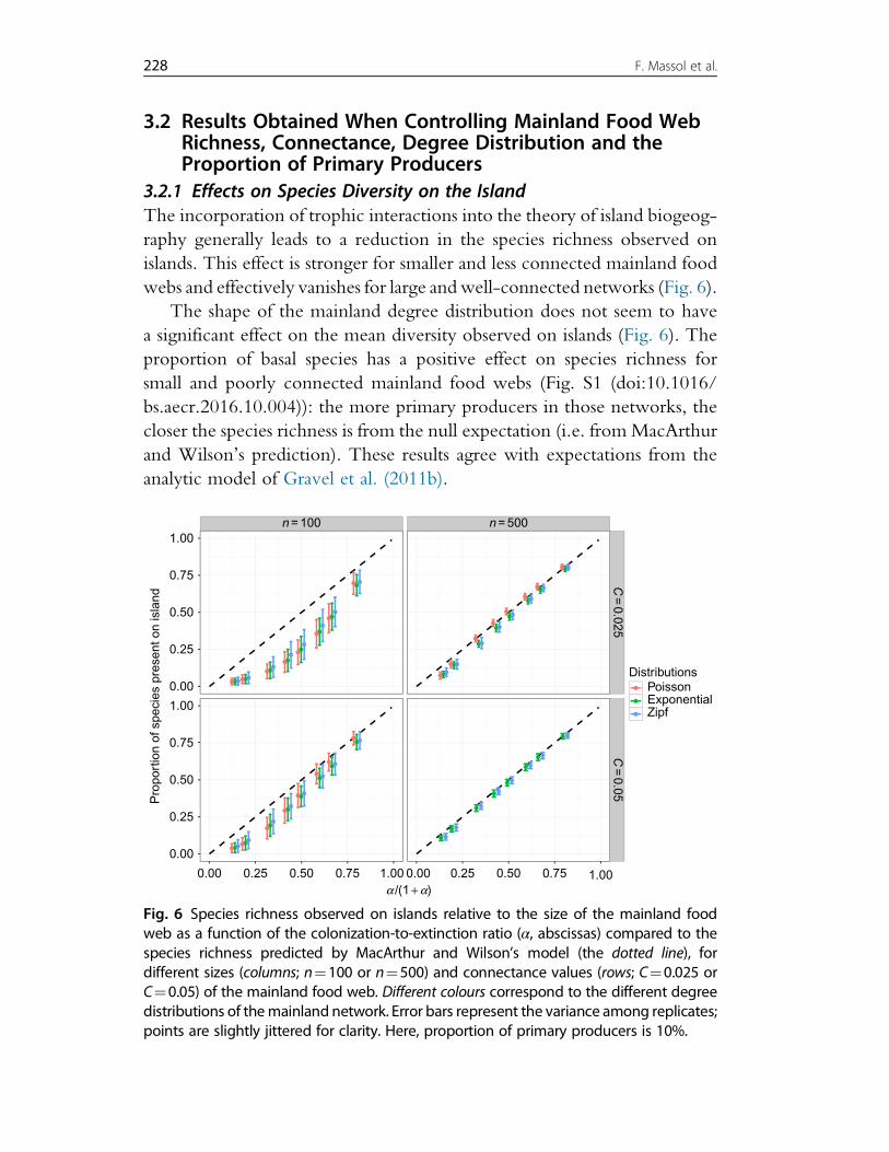
3.2 Results Obtained When Controlling Mainland Food WebRichness, Connectance, Degree Distribution and theProportion of Primary Producers

3.2.1 Effects on Species Diversity on the IslandThe incorporation of trophic interactions into the theory of island biogeog-

raphy generally leads to a reduction in the species richness observed on

islands. This effect is stronger for smaller and less connected mainland food

webs and effectively vanishes for large andwell-connected networks (Fig. 6).

The shape of the mainland degree distribution does not seem to have

a significant effect on the mean diversity observed on islands (Fig. 6). The

proportion of basal species has a positive effect on species richness for

small and poorly connected mainland food webs (Fig. S1 (doi:10.1016/

bs.aecr.2016.10.004)): the more primary producers in those networks, the

closer the species richness is from the null expectation (i.e. from MacArthur

and Wilson’s prediction). These results agree with expectations from the

analytic model of Gravel et al. (2011b).

DistributionsPoissonExponentialZipf

n = 100 n = 500

0.25

0.50

0.75

1.00

0.00

0.25

0.50

0.75

0.00

1.00

Pro

port

ion

of s

peci

es p

rese

nt o

n is

land

0.00 0.25 0.50 0.75 1.00 0.00 0.25 0.50 0.75 1.00

C=

0.025C

=0.05

a /(1 +a)

Fig. 6 Species richness observed on islands relative to the size of the mainland foodweb as a function of the colonization-to-extinction ratio (α, abscissas) compared to thespecies richness predicted by MacArthur and Wilson’s model (the dotted line), fordifferent sizes (columns; n¼100 or n¼500) and connectance values (rows; C¼0.025 orC¼0.05) of the mainland food web. Different colours correspond to the different degreedistributions of themainland network. Error bars represent the variance among replicates;points are slightly jittered for clarity. Here, proportion of primary producers is 10%.


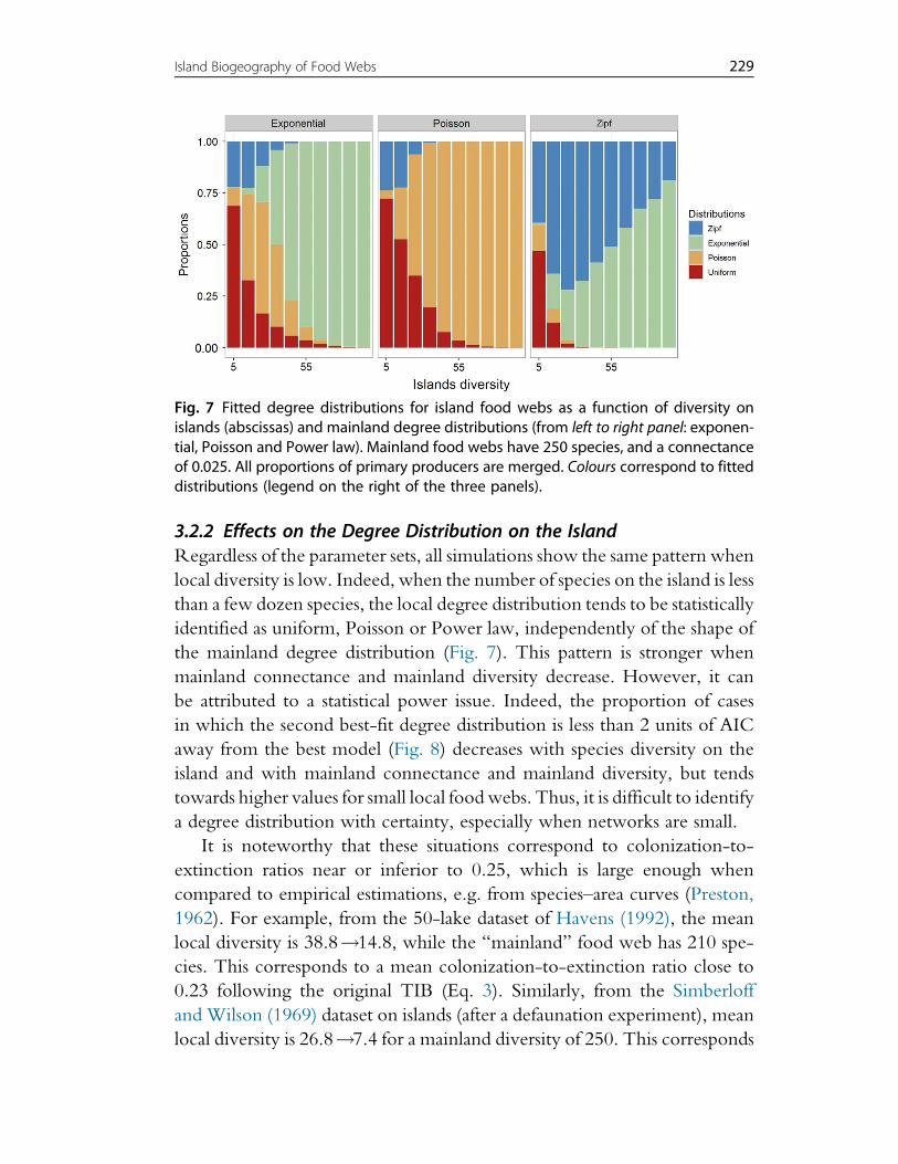
3.2.2 Effects on the Degree Distribution on the IslandRegardless of the parameter sets, all simulations show the same pattern when

local diversity is low. Indeed, when the number of species on the island is less

than a few dozen species, the local degree distribution tends to be statistically

identified as uniform, Poisson or Power law, independently of the shape of

the mainland degree distribution (Fig. 7). This pattern is stronger when

mainland connectance and mainland diversity decrease. However, it can

be attributed to a statistical power issue. Indeed, the proportion of cases

in which the second best-fit degree distribution is less than 2 units of AIC

away from the best model (Fig. 8) decreases with species diversity on the

island and with mainland connectance and mainland diversity, but tends

towards higher values for small local foodwebs. Thus, it is difficult to identify

a degree distribution with certainty, especially when networks are small.

It is noteworthy that these situations correspond to colonization-to-

extinction ratios near or inferior to 0.25, which is large enough when

compared to empirical estimations, e.g. from species–area curves (Preston,1962). For example, from the 50-lake dataset of Havens (1992), the mean

local diversity is 38.8!14.8, while the “mainland” food web has 210 spe-

cies. This corresponds to a mean colonization-to-extinction ratio close to

0.23 following the original TIB (Eq. 3). Similarly, from the Simberloff

andWilson (1969) dataset on islands (after a defaunation experiment), mean

local diversity is 26.8!7.4 for a mainland diversity of 250. This corresponds

Fig. 7 Fitted degree distributions for island food webs as a function of diversity onislands (abscissas) and mainland degree distributions (from left to right panel: exponen-tial, Poisson and Power law). Mainland food webs have 250 species, and a connectanceof 0.025. All proportions of primary producers are merged. Colours correspond to fitteddistributions (legend on the right of the three panels).


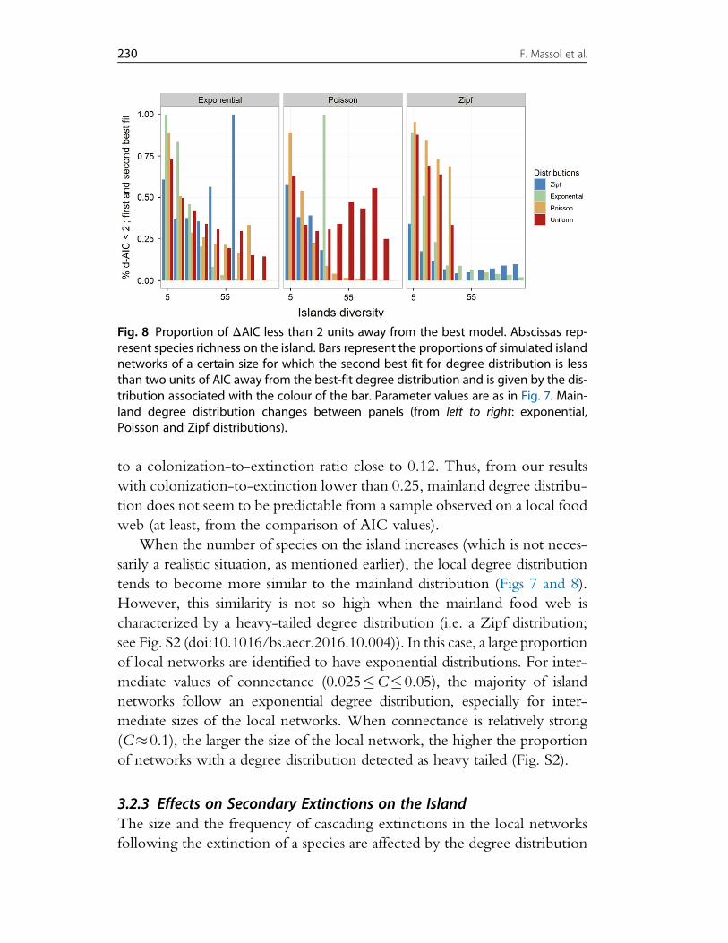
to a colonization-to-extinction ratio close to 0.12. Thus, from our results

with colonization-to-extinction lower than 0.25, mainland degree distribu-

tion does not seem to be predictable from a sample observed on a local food

web (at least, from the comparison of AIC values).

When the number of species on the island increases (which is not neces-

sarily a realistic situation, as mentioned earlier), the local degree distribution

tends to become more similar to the mainland distribution (Figs 7 and 8).

However, this similarity is not so high when the mainland food web is

characterized by a heavy-tailed degree distribution (i.e. a Zipf distribution;

see Fig. S2 (doi:10.1016/bs.aecr.2016.10.004)). In this case, a large proportion

of local networks are identified to have exponential distributions. For inter-

mediate values of connectance (0.025!C!0.05), the majority of island

networks follow an exponential degree distribution, especially for inter-

mediate sizes of the local networks. When connectance is relatively strong

(C"0.1), the larger the size of the local network, the higher the proportion

of networks with a degree distribution detected as heavy tailed (Fig. S2).

3.2.3 Effects on Secondary Extinctions on the IslandThe size and the frequency of cascading extinctions in the local networks

following the extinction of a species are affected by the degree distribution

Fig. 8 Proportion of ΔAIC less than 2 units away from the best model. Abscissas rep-resent species richness on the island. Bars represent the proportions of simulated islandnetworks of a certain size for which the second best fit for degree distribution is lessthan two units of AIC away from the best-fit degree distribution and is given by the dis-tribution associated with the colour of the bar. Parameter values are as in Fig. 7. Main-land degree distribution changes between panels (from left to right: exponential,Poisson and Zipf distributions).


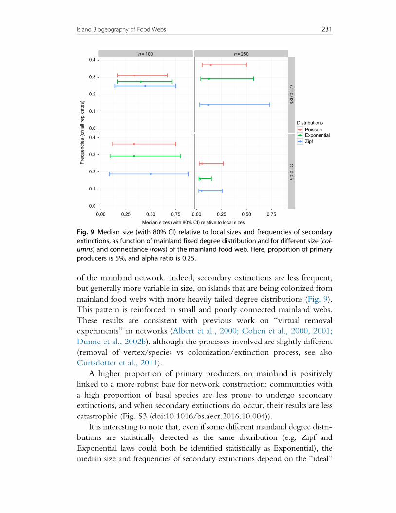
of the mainland network. Indeed, secondary extinctions are less frequent,

but generally more variable in size, on islands that are being colonized from

mainland food webs with more heavily tailed degree distributions (Fig. 9).

This pattern is reinforced in small and poorly connected mainland webs.

These results are consistent with previous work on “virtual removal

experiments” in networks (Albert et al., 2000; Cohen et al., 2000, 2001;

Dunne et al., 2002b), although the processes involved are slightly different

(removal of vertex/species vs colonization/extinction process, see also

Curtsdotter et al., 2011).

A higher proportion of primary producers on mainland is positively

linked to a more robust base for network construction: communities with

a high proportion of basal species are less prone to undergo secondary

extinctions, and when secondary extinctions do occur, their results are less

catastrophic (Fig. S3 (doi:10.1016/bs.aecr.2016.10.004)).

It is interesting to note that, even if some different mainland degree distri-

butions are statistically detected as the same distribution (e.g. Zipf and

Exponential laws could both be identified statistically as Exponential), the

median size and frequencies of secondary extinctions depend on the “ideal”

n = 100 n = 250

0.0

0.1

0.2

0.3

0.4

0.0

0.1

0.2

0.3

0.4

C=

0.025C

=0.05

0.00 0.25 0.50 0.75 0.00 0.25 0.50 0.75

Median sizes (with 80% CI) relative to local sizes

Fre

quen

cies

(on

all

repl

icat

es)


Fig. 9 Median size (with 80% CI) relative to local sizes and frequencies of secondaryextinctions, as function of mainland fixed degree distribution and for different size (col-umns) and connectance (rows) of the mainland food web. Here, proportion of primaryproducers is 5%, and alpha ratio is 0.25.


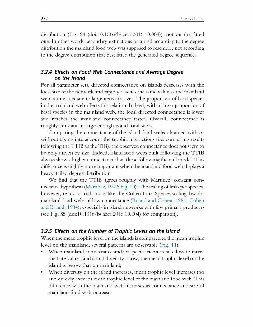
distribution (Fig. S4 (doi:10.1016/bs.aecr.2016.10.004)), not on the fitted

one. In other words, secondary extinctions occurred according to the degree

distribution the mainland food web was supposed to resemble, not according

to the degree distribution that best fitted the generated degree sequence.

3.2.4 Effects on Food Web Connectance and Average Degreeon the Island

For all parameter sets, directed connectance on islands decreases with the

local size of the network and rapidly reaches the same value as the mainland

web at intermediate to large network sizes. The proportion of basal species

in the mainland web affects this relation. Indeed, with a larger proportion of

basal species in the mainland web, the local directed connectance is lower

and reaches the mainland connectance faster. Overall, connectance is

roughly constant in large enough island food webs.

Comparing the connectance of the island food webs obtained with or

without taking into account the trophic interactions (i.e. comparing results

following the TTIB vs the TIB), the observed connectance does not seem to

be only driven by size. Indeed, island food webs built following the TTIB

always show a higher connectance than those following the null model. This

difference is slightly more important when the mainland food web displays a

heavy-tailed degree distribution.

We find that the TTIB agrees roughly with Martinez’ constant con-

nectance hypothesis (Martinez, 1992; Fig. 10). The scaling of links per species,

however, tends to look more like the Cohen Link-Species scaling law for

mainland food webs of low connectance (Briand and Cohen, 1984; Cohen

and Briand, 1984), especially in island networks with few primary producers

(see Fig. S5 (doi:10.1016/bs.aecr.2016.10.004) for comparison).

3.2.5 Effects on the Number of Trophic Levels on the IslandWhen the mean trophic level on the islands is compared to the mean trophic

level on the mainland, several patterns are observable (Fig. 11):

• When mainland connectance and/or species richness take low to inter-

mediate values, and island diversity is low, the mean trophic level on the

island is below that on mainland;

• When diversity on the island increases, mean trophic level increases too

and quickly exceeds mean trophic level of the mainland food web. This

difference with the mainland web increases as connectance and size of

mainland food web increase;


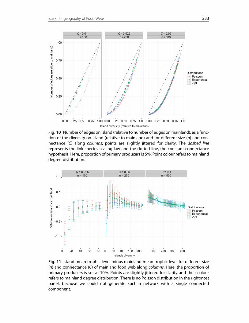
C = 0.01n = 100

C = 0.025n = 250

C = 0.05n = 500

0.00

0.25

0.50

0.75

1.00

0.00 0.25 0.50 0.75 1.00 0.00 0.25 0.50 0.75 1.00 0.00 0.25 0.50 0.75 1.00

Island diversity (relative to mainland)

Num

ber

of e

dges

(re

lativ

e to

mai

nlan

d)


Fig. 10 Number of edges on island (relative to number of edges onmainland), as a func-tion of the diversity on island (relative to mainland) and for different size (n) and con-nectance (C) along columns; points are slightly jittered for clarity. The dashed linerepresents the link-species scaling law and the dotted line, the constant connectancehypothesis. Here, proportion of primary producers is 5%. Point colour refers to mainlanddegree distribution.

C = 0.025

−1.0

−0.5

0.0

0.5

1.0

Diff

eren

ces

isla

nd v

s m

ainl

and

0 20 40 60 80 0 50 100 150 200 100 200 300 400Islands diversity

C = 0.1n = 500

C = 0.05n = 250n = 100


Fig. 11 Island mean trophic level minus mainland mean trophic level for different size(n) and connectance (C) of mainland food web along columns. Here, the proportion ofprimary producers is set at 10%. Points are slightly jittered for clarity and their colourrefers to mainland degree distribution. There is no Poisson distribution in the rightmostpanel, because we could not generate such a network with a single connectedcomponent.


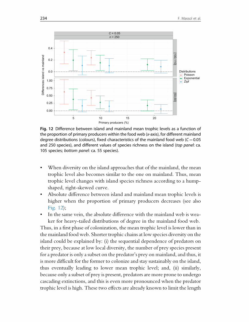
• When diversity on the island approaches that of the mainland, the mean

trophic level also becomes similar to the one on mainland. Thus, mean

trophic level changes with island species richness according to a hump-

shaped, right-skewed curve.

• Absolute difference between island and mainland mean trophic levels is

higher when the proportion of primary producers decreases (see also

Fig. 12);

• In the same vein, the absolute difference with the mainland web is wea-

ker for heavy-tailed distributions of degree in the mainland food web.

Thus, in a first phase of colonization, the mean trophic level is lower than in

the mainland foodweb. Shorter trophic chains at low species diversity on the

island could be explained by: (i) the sequential dependence of predators on

their prey, because at low local diversity, the number of prey species present

for a predator is only a subset on the predator’s prey on mainland, and thus, it

is more difficult for the former to colonize and stay sustainably on the island,

thus eventually leading to lower mean trophic level; and, (ii) similarly,

because only a subset of prey is present, predators are more prone to undergo

cascading extinctions, and this is even more pronounced when the predator

trophic level is high. These two effects are already known to limit the length

C = 0.05n = 250

0.0

0.2

0.4

0.00

0.25

0.50

0.75

1.00

[100,110][50,60]

5 10 15 20

Primary producers (%)

Diff

eren

ces

isla

nd v

s m

ainl

and


Fig. 12 Difference between island and mainland mean trophic levels as a function ofthe proportion of primary producers within the food web (x-axis), for different mainlanddegree distributions (colours), fixed characteristics of the mainland food web (C¼0.05and 250 species), and different values of species richness on the island (top panel: ca.105 species; bottom panel: ca. 55 species).


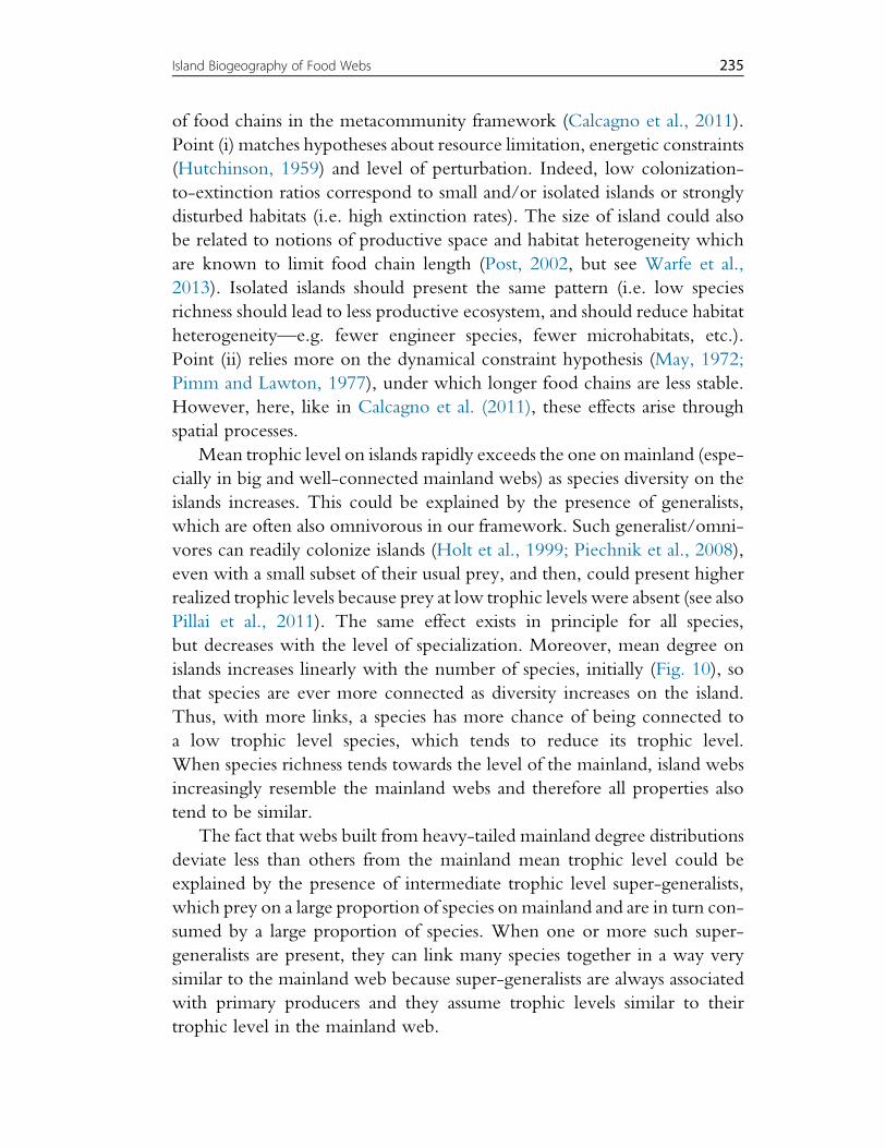
of food chains in the metacommunity framework (Calcagno et al., 2011).

Point (i) matches hypotheses about resource limitation, energetic constraints

(Hutchinson, 1959) and level of perturbation. Indeed, low colonization-

to-extinction ratios correspond to small and/or isolated islands or strongly

disturbed habitats (i.e. high extinction rates). The size of island could also

be related to notions of productive space and habitat heterogeneity which

are known to limit food chain length (Post, 2002, but see Warfe et al.,

2013). Isolated islands should present the same pattern (i.e. low species

richness should lead to less productive ecosystem, and should reduce habitat

heterogeneity—e.g. fewer engineer species, fewer microhabitats, etc.).

Point (ii) relies more on the dynamical constraint hypothesis (May, 1972;

Pimm and Lawton, 1977), under which longer food chains are less stable.

However, here, like in Calcagno et al. (2011), these effects arise through

spatial processes.

Mean trophic level on islands rapidly exceeds the one onmainland (espe-

cially in big and well-connected mainland webs) as species diversity on the

islands increases. This could be explained by the presence of generalists,

which are often also omnivorous in our framework. Such generalist/omni-

vores can readily colonize islands (Holt et al., 1999; Piechnik et al., 2008),

even with a small subset of their usual prey, and then, could present higher

realized trophic levels because prey at low trophic levels were absent (see also

Pillai et al., 2011). The same effect exists in principle for all species,

but decreases with the level of specialization. Moreover, mean degree on

islands increases linearly with the number of species, initially (Fig. 10), so

that species are ever more connected as diversity increases on the island.

Thus, with more links, a species has more chance of being connected to

a low trophic level species, which tends to reduce its trophic level.

When species richness tends towards the level of the mainland, island webs

increasingly resemble the mainland webs and therefore all properties also

tend to be similar.

The fact that webs built from heavy-tailed mainland degree distributions

deviate less than others from the mainland mean trophic level could be

explained by the presence of intermediate trophic level super-generalists,

which prey on a large proportion of species on mainland and are in turn con-

sumed by a large proportion of species. When one or more such super-

generalists are present, they can link many species together in a way very

similar to the mainland web because super-generalists are always associated

with primary producers and they assume trophic levels similar to their

trophic level in the mainland web.


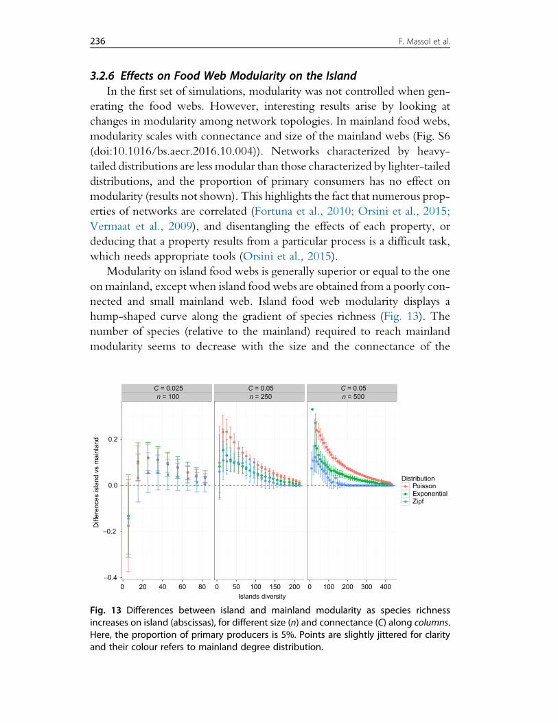
3.2.6 Effects on Food Web Modularity on the IslandIn the first set of simulations, modularity was not controlled when gen-

erating the food webs. However, interesting results arise by looking at

changes in modularity among network topologies. In mainland food webs,

modularity scales with connectance and size of the mainland webs (Fig. S6

(doi:10.1016/bs.aecr.2016.10.004)). Networks characterized by heavy-

tailed distributions are less modular than those characterized by lighter-tailed

distributions, and the proportion of primary consumers has no effect on

modularity (results not shown). This highlights the fact that numerous prop-

erties of networks are correlated (Fortuna et al., 2010; Orsini et al., 2015;

Vermaat et al., 2009), and disentangling the effects of each property, or

deducing that a property results from a particular process is a difficult task,

which needs appropriate tools (Orsini et al., 2015).

Modularity on island food webs is generally superior or equal to the one

on mainland, except when island food webs are obtained from a poorly con-

nected and small mainland web. Island food web modularity displays a

hump-shaped curve along the gradient of species richness (Fig. 13). The

number of species (relative to the mainland) required to reach mainland

modularity seems to decrease with the size and the connectance of the

C = 0.025n = 100

C = 0.05n = 250

C = 0.05n = 500

−0.4

−0.2

0.0

0.2

0 20 40 60 80 0 50 100 150 200 0 100 200 300 400Islands diversity

Diff

eren

ces

isla

nd v

s m

ainl

and

DistributionPoissonExponentialZipf

Fig. 13 Differences between island and mainland modularity as species richnessincreases on island (abscissas), for different size (n) and connectance (C) along columns.Here, the proportion of primary producers is 5%. Points are slightly jittered for clarityand their colour refers to mainland degree distribution.


mainland web, especially with Power law degree distributions. Food webs

constructed from complex mainland webs (C¼0.05) with heavy-tailed

degree distributions deviate less and reach the mainland web modularity

faster. Again, this is only true when the mainland web is large and well

connected. A large proportion of primary producers increases the difference

in modularity between mainland and island, but only for small and poorly

connected mainland webs (Fig. S7 (doi:10.1016/bs.aecr.2016.10.004)).

It should be noted that modularity is always lower under the TTIB than

under the classic TIB (results not shown). Indeed, species samples obtained

through the classic TIB are not necessarily simply connected; every con-

nected component of the food web then automatically amounts to another

module, hence increasing modularity. However, as empirical measures of

modularity are always obtained on simply connected networks (i.e. a single

connected component with no disconnected species), results obtained with

the null model are not at all comparable with empirical measures on island

food webs.

It is remarkable that modularity has more or less the same response to

island diversity as mean trophic level. In the first stages, only a few numbers

of primary producers are present, and then, trophic chains are constructed

independently from each basal vertex by adding new species with higher

trophic levels. This leads to several compartments based on different primary

producers (different “channels”) and could be seen as a niche-based con-

struction of food webs, assimilating each channel as a different niche. When

the diversity on the island increases, with higher colonization-to-extinction

ratio, the different trophic “chains” tend to progressively merge together,

thus finally leading to a unique component.

Food webs built from heavily tailed mainland degree distributions devi-

ate less and reach the mainland modularity faster, as noted earlier. This could

be a consequence of the presence of super-generalist species, which tend

to merge the different compartments faster than expected under a more

homogeneous degree distribution.

3.3 Results Obtained Using the SBM to Generate MainlandFood Web

3.3.1 Effects of Modularity on Species RichnessModularity is often considered as a property that enhances the stability

and robustness of trophic networks by limiting the diffusion of perturbations

through the web (Th!ebault and Fontaine, 2010) and is often found in empir-

ical data (e.g. Krause et al., 2003). Here, we investigated its effects on food


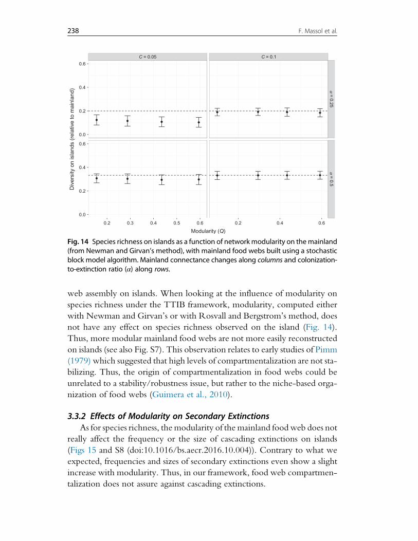
web assembly on islands. When looking at the influence of modularity on

species richness under the TTIB framework, modularity, computed either

with Newman and Girvan’s or with Rosvall and Bergstrom’s method, does

not have any effect on species richness observed on the island (Fig. 14).

Thus, more modular mainland food webs are not more easily reconstructed

on islands (see also Fig. S7). This observation relates to early studies of Pimm

(1979) which suggested that high levels of compartmentalization are not sta-

bilizing. Thus, the origin of compartmentalization in food webs could be

unrelated to a stability/robustness issue, but rather to the niche-based orga-

nization of food webs (Guimera et al., 2010).

3.3.2 Effects of Modularity on Secondary ExtinctionsAs for species richness, themodularity of themainland foodweb does not

really affect the frequency or the size of cascading extinctions on islands

(Figs 15 and S8 (doi:10.1016/bs.aecr.2016.10.004)). Contrary to what we

expected, frequencies and sizes of secondary extinctions even show a slight

increase with modularity. Thus, in our framework, food web compartmen-

talization does not assure against cascading extinctions.

C = 0.05

Modularity (Q)

C = 0.1

a = 0.25a = 0.5

Fig. 14 Species richness on islands as a function of networkmodularity on themainland(from Newman and Girvan’s method), with mainland food webs built using a stochasticblock model algorithm. Mainland connectance changes along columns and colonization-to-extinction ratio (α) along rows.


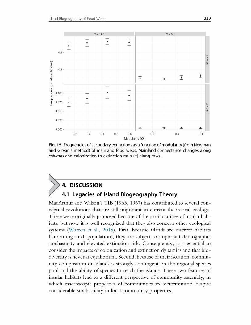
4. DISCUSSION4.1 Legacies of Island Biogeography Theory

MacArthur and Wilson’s TIB (1963, 1967) has contributed to several con-

ceptual revolutions that are still important in current theoretical ecology.

These were originally proposed because of the particularities of insular hab-

itats, but now it is well recognized that they also concern other ecological

systems (Warren et al., 2015). First, because islands are discrete habitats

harbouring small populations, they are subject to important demographic

stochasticity and elevated extinction risk. Consequently, it is essential to

consider the impacts of colonization and extinction dynamics and that bio-

diversity is never at equilibrium. Second, because of their isolation, commu-

nity composition on islands is strongly contingent on the regional species

pool and the ability of species to reach the islands. These two features of

insular habitats lead to a different perspective of community assembly, in

which macroscopic properties of communities are deterministic, despite

considerable stochasticity in local community properties.

C = 0.05

Modularity (Q)

C = 0.1

a = 0.25a = 0.5

Fig. 15 Frequencies of secondary extinctions as a function ofmodularity (fromNewmanand Girvan’s method) of mainland food webs. Mainland connectance changes alongcolumns and colonization-to-extinction ratio (α) along rows.


The neutral theory of biodiversity (Bell, 2000, 2001; Etienne andAlonso,

2005;Hubbell, 2001;Volkov et al., 2003) is perhaps the best example to illus-

trate the legacy of the TIB on today’s theoretical ecology. As with the TIB,

the neutral theory of biodiversity assumes that some meaningful predictions

about community organization can be made without detailed knowledge of

the natural history (Wennekes et al., 2012). The neutral theory integrates the

dynamical balance between colonization and extinction dynamics and then

adds competitive interactions.While it maintains the main predictions of the

TIB (species abundance–rank curves and species turnover), it also expands therange of predictions owing to its individual-based formulation (e.g. species

abundance distributions, range–abundance relationship). Neutral theory is,

however, not the endpoint of the story, as we have argued in this chapter

in which we developed theory for nonneutral interactions. While the TIB

and neutral theory were originally concerned with competitive interactions,

recent developments have also paved the way to a network theory of bioge-

ography.Extending theTIB to several trophic levels also reveals different spe-

cies–area relationships for prey and predators (Holt et al., 1999) and the

reciprocal feedback between insular dynamics and network structure

(Gravel et al., 2011b).We discuss here how the TIB can be used as a template

to add complexity in species interactions and contribute to the integration of

community ecology and biogeography.

4.2 The Future of Island Biogeography Theory4.2.1 A General Theory for Sampling the Regional Species PoolThe TIB establishes the principle that a local community is a sample of the

regional species pool. The size (i.e. species richness) and the composition of

this sample depend on the probability of each species to be sampled from the

regional pool. In the TIB, and incidentally in neutral theory as well, this

probability is only influenced by two abiotic variables, that is island size

and isolation. The model supposes that all species are functionally equivalent

and have the same probability to compose the regional pool. All species are

treated as equal and consequently they all have the same occupancy. At any

time, a local community of a random sample of S species drawn from the

regional pool can be described using the following general stochastic model:

P Ri,Xi¼ 1ð Þ¼P Rið ÞP Xi¼ 1jRið Þ (67)

where P Ri,Xi ¼ 1ð Þ is the probability of observing a species i with charac-

teristicsRi on an island, P(Ri) represents the probability of sampling a species


with such characteristics and P Xi¼ 1jRið Þ is the occupancy function for

such a species, conditional on its characteristics. The classic TIB assumes

that P Xi ¼ 1jRið Þ is independent of Ri and consequently the distribution

of species characteristics on an island is only driven by their distribution

in the regional species pool.

The trophic extension of the TIB introduced the idea that the sampling

could be biased by trophic interactions, and indirectly by the traits driving

these interactions (Gravel et al., 2016). Here, we derived a model in which

diet breadth and trophic position with respect to primary resources deter-

mine species-specific occurrence probabilities. In this model, generalist spe-

cies located at low trophic levels are more likely to find prey species at

colonization and thereafter persist. Compared to the mainland species pool,

local community composition is biased towards more generalist species, as

described by:

P Xi¼ 1jRið Þ¼ c Rið Þc Rið Þ+ e Rið Þ

(68)

where c and e are colonization and extinction functions based on the char-

acteristics of the species, Ri. In addition, we have shown that these charac-

teristics are not stationary. In other words, the diet of a species on an island,

and so its colonization and extinction probabilities, is a function not only of

its position in the mainland food web, but also of the local community com-

position (see e.g. Fig. 11 on trophic levels). The inclusion of species-specific

equilibrium occurrence probabilities, developed in the TTIB, therefore

paves the way to the integration of functional ecology, community ecology

and biogeography. This approach could indeed be extended to further sets of

biogeographical models that incorporate biotic variables related to species

dispersal capacities (e.g. symbionts, see Amsellem et al., 2017) and extinction

probabilities.

Such an example is provided by the investigation of body mass distri-

bution on islands. Body mass appears to be a fundamental trait that per-

colates through all aspects of community dynamics and ecosystem

processes, from productivity to energy flows (Brown et al., 2004;

Cohen et al., 2003; Etienne and Olff, 2004; Otto et al., 2007; Peters,

1986; Woodward et al., 2005). Body mass has also been successfully used

to parameterize models of food web topology (Allesina et al., 2008; Ekl€ofet al., 2013; Gravel et al., 2013; Petchey et al., 2008; Rohr et al., 2010;

Williams et al., 2010). At the biogeographical scale, body mass is likely to


influence both colonization and extinction rates (Bradbury et al., 2008;

Soininen, 2016). The scaling of colonization and extinction rates with

body mass could be easily integrated into the TIB and the TTIB, leading

to an allometric theory of island biogeography with species-specific and

mass-dependent occurrence probabilities. Owing to the negative rela-

tionship between abundance and body mass (Blackburn and Gaston,

1999; Cohen et al., 2003; Damuth, 1981; Nee et al., 1991; White

et al., 2007), we would expect extinction rate to correlate positively with

body mass (Gotelli and Taylor, 1999; Petchey et al., 2004). However,

empirical evidence for this assumption is weak (Gaston, 2000), while

the supposed higher abundance of small-bodied species might be bal-

anced by other factors that make them more prone to extinction, like

their higher dependence on habitat complexity (Graham et al., 2011).

In contrast, the scaling of colonization rate, dispersal and space use with

body size is supported by many empirical studies, in particular in marine

systems (Jetz et al., 2004; Peters and Wassenberg, 1983; Wieters et al.,

2008). All life-history traits increasing the rate of colonization, such as

fecundity, home range, mobility or diet generality are indeed positively

correlated to fish body size (Kulbicki et al., 2015; Luiz et al., 2013; Mora

et al., 2003; Nash et al., 2015). The scaling of colonization rate with body

size is, however, less straightforward in taxonomic groups in which these

traits scale differently. For example, fecundity decreases with body size for

birds and mammals while mobility increases (Marquet et al., 2005). In

terrestrial and semiterrestrial animals, a positive relationship between dis-

persal and body size is generally supported by existing data (Stevens et al.,

2014), although exceptions do exist. Even if single large individuals might

disperse further away than small ones, the larger number of offspring pro-

duced by populations of smaller organisms could also lead to inverse scal-

ing relationships. Allee effects might also affect the establishment success

of immigrants, and we do not have clear expectations of how it might

scale with body size. While intuitive at first, the integration of allometric

constraints into the TIB and the TTIB will require direct empirical inves-

tigation of colonization and extinction rates.

4.2.2 Abundance and EnergyIn the TTIB, the consequences of ecological interactions are only percep-

tible when a predator cannot find any prey. However, the consequences of

interactions may actually be perceptible for any change in the composition


of the community when analysing species abundances. Thus, extinction rate

should vary more smoothly with community composition (i.e. not sharply

increase when the underlying food web is weakened by extinction of a key-

stone species) because of the role of trophic regulation on population size

(Hairston et al., 1960; Oksanen et al., 1981; Persson et al., 1992). Moreover,

fluctuations of individual species numbers due to interactions may further

influence extinction rates when driving populations to very low densities.

It is also the rationale on which the results pertaining to the stability of eco-

logical networks are based (Allesina and Tang, 2012; May, 1972, 1973).

Hence, introducing species abundance in the TTIB, and their link to

dynamical stability, is a promising avenue towards a more mechanistic

and integrated TIB.

Species abundances are also key to introduce energetic constraints in a

mechanistic framework (Trebilco et al., 2013). In the TIB, the existence

of such limits lies in considering the extinction rate as a decreasing function

of the island area. In the TTIB, energetic constraints actually restrict the

diversity of primary producers which in turn reduces species richness at

higher trophic levels. Therefore, as in the TIB, rich communities are pre-

cluded, but in the TTIB, species are not equally affected: the higher their

trophic level, the more affected they are. Furthermore, the energetic con-

sumption of an entire island community at equilibrium can be computed

based on the relationships between the body mass and the metabolic rates.

This measurement can then be used to determine if the community may

persist on the island or if imminent extinctions are expected due to the lack

of available energy. Integrating species abundances and energetic constraints

in the TTIB may provide new insights into the abundance–body mass

relationship that remains poorly understood (Blackburn and Gaston,

1999; Blackburn et al., 1993; Damuth, 2007; Trebilco et al., 2013). It also

promises the investigation of biodiversity distribution over large tempera-

ture gradient and might prove useful at explaining the widely documented

relationship between energy and species richness (Currie, 1991; Currie

et al., 2004; Hurlbert, 2004). Also, taken from an evolutionary perspective,

these considerations might possibly come up with new explanations of

gigantism and dwarfism on islands.

4.2.3 Environmental HeterogeneityKadmon and Allouche (2007) proposed a model unifying niche and

metapopulation theories under the area-heterogeneity trade-off hypothesis


(see also Allouche et al., 2012). The niche theory proposes that species coex-

istence occurs because a differentiated response to the environment reduces

the interspecific competition below intraspecific competition (Chesson,

2000). Assuming species packing along niche axes, species richness should

be proportional to the range of these axes and inversely proportional to

the niche width of individual species. The TIB, on the other hand, proposes

that species richness in a locality is a dynamical equilibrium between stochas-

tic colonization and extinction events. The TIB predicts a positive relation-

ship between area and species richness because larger islands will have lower

extinction rates. Kadmon and Allouche (2007) proposed to unification of

these concepts with a single assumption: for a given region, the average area

of favourable habitats should decrease with increasing environmental het-

erogeneity because each extra portion of a novel habitat reduces the surface

occupied by other ones. There are, therefore, two contrasting forces acting

on species richness with increasing environmental heterogeneity: a positive

effect of niche diversity and a negative effect of increased extinction rate

(Allouche et al., 2012). The theory consequently predicts a hump–shaperelationship between environmental heterogeneity and equilibrium species

richness, which has been partly supported by empirical data (Hurlbert, 2004;

Tews et al., 2004). The last missing piece of information is the scaling of

environmental heterogeneity with area. A positive relationship, which is

generally expected, would further strengthen the scaling relationship

between area and species richness.

It could be feasible to extend this theory further to account for species-

specific colonization and extinction probabilities, contingent on the envi-

ronmental heterogeneity. With such an approach, results might differ as

some species could benefit from increasing environmental heterogeneity

because they are more likely to find their niche, or alternatively they could

be increasingly maladapted with more environmental heterogeneity (Farkas

et al., 2015). Overall, it is likely that a large portion of model deviations from

the classic TIB would be linked to the variance of environmental conditions,

and the average conditions relative to the average niches of the mainland

species pool. With such extensions, we could find flat, positive, negative

and hump-shaped relationships between average conditions and species

richness.

The TIB has been established and tested for islands, but the vision pro-

vided in the early sixties goes beyond the scope of islands. The TIB can

indeed be regarded as the simplest metacommunity model with two patches.


The first patch has an infinite area (the continent) and contains all the species.

The second patch has a finite area (the island) and contains a sample of species

present in the first patch. The TIB describes the occupancy dynamics of the

latter given colonization of species from the former. Although this vision is

applicable in many situations, regardless of the insular nature of patches

considered, it has often been restricted to islands and fragmentation studies

(Losos and Ricklefs, 2009). Among the limitations hampering the applica-

tion of the TIB to other contexts, there is the paucity of predictions regard-

ing abiotic conditions, such as temperature and precipitation, which are at

the core of the theory of biogeography (Peterson et al., 2011). This apparent

gap in the TIB is not surprising given that on many islands, abiotic condi-

tions can reasonably be assumed similar between islands and the continent,

i.e. the latitudinal range of colonization from the continent is restricted.

However, this assumption prevents the TIB from being used to study species

richness along environmental gradients.

Recently, Cazelles et al. (2015b) have developed a framework inspired

from the TTIB that integrates abiotic constraints. According to their work,

introducing an environmental gradient in the TTIB requires an explicit

statement for how the local conditions prevailing on the island affect species

differently, i.e. modulating the extinction rate, the colonization rate or both

according to the values of the environmental gradient. The authors highlight

the potential of such an integration for examining the interplay between

biotic and abiotic constraints, which is often neglected in models used to

predict species distributions (Thuiller et al., 2013). For instance, they hinted

at the importance of positive covariation in the response to the environment

between interacting species. Independent environmental requirements

between interacting species might result in a dislocation of local networks.

Broadly speaking, such an extension of the TIB corresponds to the introduc-

tion of the abiotic niche in the TTIB and the possibility of studying the rela-

tionship between the fundamental niche and the realized one (Cazelles

et al., 2015a).

4.2.4 Network MacroevolutionThe isolation of oceanic islands provides an ideal setting to investigate diver-

sification dynamics in a context of limited immigration and gene flow

(Gillespie, 2004; Losos et al., 1998; Warren et al., 2015). Island biogeogra-

phy theory has been influential to the study of macroevolution and commu-

nity phylogenetics (Warren et al., 2015). Fairly simple extensions to the


modelling approach described in this study might allow investigation of

the macroevolution of network structure. The model of colonization-

extinction dynamics is analogous to speciation-extinction models of macro-

evolution, with the distinction that in macroevolutionary models the

regional pools emerges from the dynamics and is not fixed in time.

There is currently an intense debate about the effect of ecological inter-

actions on diversification rates (Harmon and Harrison, 2015; Rabosky and

Hurlbert, 2015), and it is possible that an evolutionary extension of trophic

island biogeography could perhaps address these issues. Except for a few

mechanistic endeavours (e.g. Hubert et al., 2015), the bulk of current quan-

titative approaches considers a phenomenological model to represent the

effect of species diversity on diversification, under which the net

diversification rate (speciation and extinction) slowly decays with diversity,

in a manner similar to a logistic growth model (Ricklefs, 2007). Following

the dynamics of the TTIB, one could consider that a successful speciation

event will occur provided that a mutant finds at least one prey species, and

accordingly it goes extinct on losing its last prey (see also Quince et al.,

2002). Such a model would predict an exponentially increasing diversification

rate in absence of top-down control because the more species there are, the

more successful mutants will be and the lower the extinction rate. On the

other hand, diversification is expected to saturate at a stable equilibrium spe-

cies richness in the presence of negative effects of predators on the extinction

rate of the preys since higher species richness will result in stronger top-down

control (Rabosky and Hurlbert, 2015). Such a model could be used to inves-

tigate a much larger range of predictions than typical birth-death models do

(Ricklefs, 2007), with predictions on diversification rates as well as phyloge-

netic structure of trophic interactions (Peralta, in press).

4.2.5 Biological InvasionsA recurring question in the field of biological invasions is to understand

the determinants of invasion success and impacts (David et al., 2017;

Mollot et al., 2017; Pantel et al., 2017). Historically, approaches to

solve this question have first relied on species-centred, static attributes

(i.e. not variable among populations of the same species and/or considered

absolute measures of species “invasiveness”) such as fecundity, generation

time, growth and development trajectories, etc. (Van Kleunen et al., 2010,

2015) and include “classic laws” e.g. Baker’s law (Baker, 1955, 1967)—self-

compatible plants should have an edge as invaders of areas disconnected from


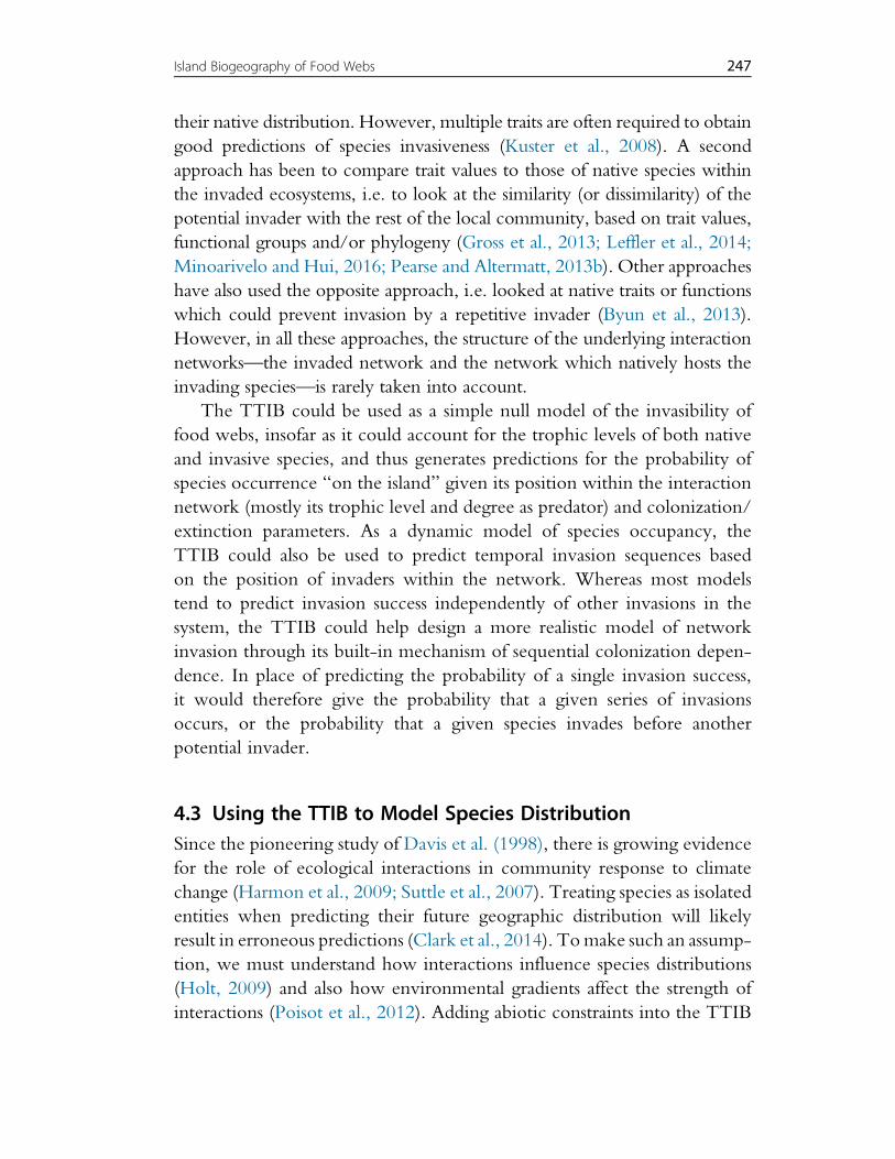
their native distribution. However, multiple traits are often required to obtain

good predictions of species invasiveness (Kuster et al., 2008). A second

approach has been to compare trait values to those of native species within

the invaded ecosystems, i.e. to look at the similarity (or dissimilarity) of the

potential invader with the rest of the local community, based on trait values,

functional groups and/or phylogeny (Gross et al., 2013; Leffler et al., 2014;

Minoarivelo and Hui, 2016; Pearse and Altermatt, 2013b). Other approaches

have also used the opposite approach, i.e. looked at native traits or functions

which could prevent invasion by a repetitive invader (Byun et al., 2013).

However, in all these approaches, the structure of the underlying interaction

networks—the invaded network and the network which natively hosts the

invading species—is rarely taken into account.

The TTIB could be used as a simple null model of the invasibility of

food webs, insofar as it could account for the trophic levels of both native

and invasive species, and thus generates predictions for the probability of

species occurrence “on the island” given its position within the interaction

network (mostly its trophic level and degree as predator) and colonization/

extinction parameters. As a dynamic model of species occupancy, the

TTIB could also be used to predict temporal invasion sequences based

on the position of invaders within the network. Whereas most models

tend to predict invasion success independently of other invasions in the

system, the TTIB could help design a more realistic model of network

invasion through its built-in mechanism of sequential colonization depen-

dence. In place of predicting the probability of a single invasion success,

it would therefore give the probability that a given series of invasions

occurs, or the probability that a given species invades before another

potential invader.

4.3 Using the TTIB to Model Species DistributionSince the pioneering study of Davis et al. (1998), there is growing evidence

for the role of ecological interactions in community response to climate

change (Harmon et al., 2009; Suttle et al., 2007). Treating species as isolated

entities when predicting their future geographic distribution will likely

result in erroneous predictions (Clark et al., 2014). Tomake such an assump-

tion, we must understand how interactions influence species distributions

(Holt, 2009) and also how environmental gradients affect the strength of

interactions (Poisot et al., 2012). Adding abiotic constraints into the TTIB


yields an adequate theoretical model to scrutinize the relative contribution

of trophic interactions and individuals response in the context of climate

change (Cazelles et al., 2015b). In this framework, a species colonizes a patch

according to its abiotic requirements and survives only if it becomes embed-

ded in a network that is assumed to be feasible. Hence, a predator whose

prey cannot survive during the warming up will go extinct. This provides

a simple model that reflects observed extinctions under climate changes

mainly caused by changes in network structure (Cahill et al., 2013; Pearse

and Altermatt, 2013a; S€aterberg et al., 2013). This application of an

extended TTIB could be the key to renewal of the theoretical foundations

of species distribution models, but it will demand significant effort to turn

this theoretical model into a statistical tool (see Gravel et al., 2011b).

4.4 From Theory to DataExtensions of the TIB, such as the incorporation of trophic interactions,

not only introduce more realism but also considerably enrich the range of

predictions and our ability to test theory with empirical observations.

The species–area relationship is one of the best-documented observations

in ecology (Preston, 1962), but it also has several competing explanations

for which there is currently no agreement (Lomolino, 2000). In such a case

of conflicting theories with common predictions, distinguishing them does

require testing them from different perspectives (Chave et al., 2002; McGill,

2003). It is of course a challenge to increase model complexity without fac-

ing a trade-off with the number of parameters to evaluate. But, the devel-

opment and evaluation of the TTIB with empirical data has shown it is

possible to keep a model relatively simple, without the addition of extra

parameters, owing to some realistic assumptions (Gravel et al., 2011b). As

presented earlier, the biggest advantage of the approach developed in this

chapter is to derive species-level predictions, in comparison to the commu-

nity aggregated predictions of the classic TIB. It is possible to fit the occu-

pancy functions using maximum likelihood methods (Gravel et al., 2011b).

The next step is perhaps to evaluate the capacity of the theory to predict finer

aspects of network structure, such as the distribution of motifs (Stouffer

et al., 2007). The frequency distribution of the motifs could be derived using

approximate Bayesian computing (Beaumont, 2010) or exponential random

graph models (Snijders et al., 2006), and compared to empirical data. Unfor-

tunately, we still lack appropriate data to go beyond what has been done so


far. Doing so will require specific data on realized interactions at different

locations and, for now, there are only few candidate datasets with replicated

network sampling that could allow it.

Surprisingly, despite the simplicity of the approach, we are not aware

of any attempt to directly measure colonization and extinction processes,

and then comparing quantitative predictions of expected species richness

to observations. Doing so would require time-series data, such as the one

collected by Simberloff and Wilson (1969) in their classic experiment,

measuring the colonization and extinction probabilities for different

islands and then relating them to island area and isolation. One would

simply seek to evaluate the probability of a colonization (and extinction)

event occurring between time step t and step t+dt. The model could

be rendered more complex, with detailed investigation of the species-

specific colonization and extinction rates, trying to relate them to their

position in the food web and other functional traits. This is indeed what

Cirtwill and Stouffer (2016) performed for colonization. They found that

in Simberloff’s experiment, the variability of colonization rates among

arthropods was best understood from species diet. Time-series data for

entire communities combined with knowledge of trophic interactions

are hard to gather but would have immense value for the advancement

of island biogeography theory specifically, and for community assembly

theory and ecology more generally.

ACKNOWLEDGEMENTSWe thank D.A. Bohan for organizing this issue and for editing this manuscript, the EEP unitand particularly S. Gallina for access to computational resources, the French ANR for funding

(AFFAIRS project in the BIOADAPT program—P.I.: Dr P. David—grant no.12-ADAP-005; ARSENIC project—P.I.: Dr F. Massol—grant no. 14-CE02-0012), theCESAB working group COREIDS for opportunities to develop this work and TOTALand the FRB for funding COREIDS. We thank N. Loeuille and an anonymous referee

for making insightful suggestions on the first version of the manuscript.

APPENDIX. BREADTH-FIRST DIRECTING OF THE LINKSIN THE GENERATED NETWORK

For a undirected connected simple graph G¼ V, Eð Þ, with V the set ofvertices and E the edges set. VB (withVB$V) represent the basal species set,drawn from the colouring algorithm. Capital letters are vertices set, upper-

case letters represent one vertex. Finally, double arrow ($) represents an


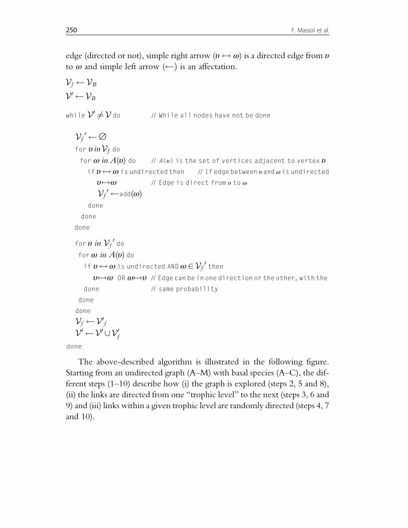
edge (directed or not), simple right arrow (υ 7! ω) is a directed edge from υto ω and simple left arrow ( Þ is an affectation.

V f VBV0 VB

while V0 6¼V do // While all nodes have not be done

V f 0 ∅for υ inV f dofor ω in A(υ) do // A(υ) is the set of vertices adjacent to vertex υ

if υ$ω is undirected then // If edge between υ andω is undirected

υ 7!ω // Edge is direct from υ to ω

V f 0 add(ω)done

done

done

for υ in V f 0 doforω in A(υ) doif υ$ω is undirected ANDω2V f 0 then

υ 7!ω OR ω 7!υ // Edge can be in one direction or the other, with the

done // same probability

done

done

V f V0fV0 V0 [V0f

done

The above-described algorithm is illustrated in the following figure.

Starting from an undirected graph (A–M) with basal species (A–C), the dif-ferent steps (1–10) describe how (i) the graph is explored (steps 2, 5 and 8),

(ii) the links are directed from one “trophic level” to the next (steps 3, 6 and

9) and (iii) links within a given trophic level are randomly directed (steps 4, 7

and 10).


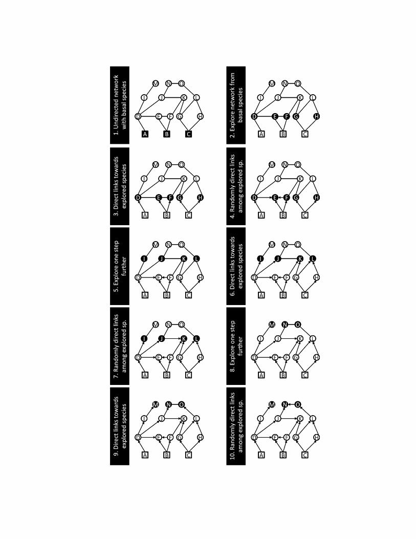
REFERENCESAlbert, R., Jeong, H., Barabasi, A.-L., 2000. Error and attack tolerance of complex networks.

Nature 406, 378–382.Allesina, S., Tang, S., 2012. Stability criteria for complex ecosystems. Nature 483, 205–208.Allesina, S., Alonso, D., Pascual, M., 2008. A general model for food web structure. Science

320, 658–661.Allesina, S., Grilli, J., Barabas, G., Tang, S., Aljadeff, J., Maritan, A., 2015. Predicting the

stability of large structured food webs. Nat. Commun. 6, http://dx.doi.org/10.1038/ncomms8842 (online journal).

Allhoff, K.T., Ritterskamp, D., Rall, B.C., Drossel, B., Guill, C., 2015. Evolutionary foodweb model based on body masses gives realistic networks with permanent speciesturnover. Sci. Rep. 5, http://dx.doi.org/10.1038/srep10955 (online journal).

Allouche, O., Kalyuzhny, M., Moreno-Rueda, G., Pizarro, M., Kadmon, R., 2012. Area–heterogeneity tradeoff and the diversity of ecological communities. Proc. Natl. Acad.Sci. U.S.A. 109, 17495–17500.

Amsellem, L., Brouat, C., Duron, O., Porter, S.S., Vilcinskas, A., Facon, B., 2017. Impor-tance of microorganisms tomacroorganisms invasions: is the essential invisible to the eye?(The little prince, A. de Saint-Exupery, 1943) Adv. Ecol. Res. 57, 99–146.

Arenas, A., Duch, J., Fernandez, A., Gomez, S., 2007. Size reduction of complex networkspreserving modularity. New J. Phys. 9, 176.

Astegiano, J., Guimaraes Jr., P.R., Cheptou, P.-O., Vidal, M.M., Mandai, C.Y.,Ashworth, L., Massol, F., 2015. Persistence of plants and pollinators in the face of habitatloss: Insights from trait-based metacommunity models. Adv. Ecol. Res. 53, 201–257.Academic Press.

Baker, H.G., 1955. Self compatibility and establishment after “long-distance” dispersal.Evolution 9, 347–349.

Baker, H.G., 1967. Support for Baker’s law as a rule. Evolution 21, 853–856.Barabasi, A.L., Albert, R., 1999. Emergence of scaling in random networks. Science

286, 509–512.Beaumont, M.A., 2010. Approximate Bayesian computation in evolution and ecology.

Annu. Rev. Ecol. Evol. Syst. 41, 379–406.Bell, G., 2000. The distribution of abundance in neutral communities. Am. Nat.

155, 606–617.Bell, G., 2001. Neutral macroecology. Science 293, 2413–2418.Berger, A., 2014. A note on the characterization of digraphic sequences. Discret. Math.

314, 38–41.Blackburn, T.M., Gaston, K.J., 1999. The relationship between animal abundance and body

size: a review of the mechanisms. Adv. Ecol. Res. 28, 181–210. Academic Press.Blackburn, T.M., Lawton, J.H., Pimm, S.L., 1993. Non-metabolic explanations for the

relationship between body size and animal abundance. J. Anim. Ecol. 62, 694–702.Bl€ochliger, I., Zufferey, N., 2008. A graph coloring heuristic using partial solutions and a

reactive tabu scheme. Comput. Oper. Res. 35, 960–975.Bollobas, B., Riordan, O., Spencer, J., Tusnady, G., 2001. The degree sequence of a scale-

free random graph process. Random Struct. Algorithm 18, 279–290.Bonsall, M.B., Jansen, V.A.A., Hassell, M.P., 2004. Life history trade-offs assemble ecological

guilds. Science 306, 111–114.Boots, M., White, A., Best, A., Bowers, R., 2014. How specificity and epidemiology drive

the coevolution of static trait diversity in hosts and parasites. Evolution 68, 1594–1606.Bradbury, I.R., Laurel, B., Snelgrove, P.V.R., Bentzen, P., Campana, S.E., 2008. Global

patterns in marine dispersal estimates: the influence of geography, taxonomic categoryand life history. Proc. R. Soc. Lond. B Biol. Sci. 275, 1803–1809.


Br€annstr€om, A., Johansson, J., Loeuille, N., Kristensen, N., Troost, T.A., Lambers, R.H.R.,Dieckmann, U., 2012.Modelling the ecology and evolution of communities: a review ofpast achievements, current efforts, and future promises. Evol. Ecol. Res. 14, 601–625.

Briand, F., Cohen, J.E., 1984. Community food webs have scale-invariant structure. Nature307, 264–267.

Brown, J.H., Gillooly, J.F., Allen, A.P., Savage, V.M.,West, G.B., 2004. Toward ametabolictheory of ecology. Ecology 85, 1771–1789.

Brualdi, R.A., Ryser, H.J., 1991. Combinatorial Matrix Theory. Cambridge University Press,Cambridge, UK.

Byun, C., de Blois, S., Brisson, J., 2013. Plant functional group identity and diversitydetermine biotic resistance to invasion by an exotic grass. J. Ecol. 101, 128–139.

Cahill, A.E., Aiello-Lammens, M.E., Fisher-Reid, M.C., Hua, X., Karanewsky, C.J., YeongRyu, H., Sbeglia, G.C., Spagnolo, F., Waldron, J.B., Warsi, O., Wiens, J.J., 2013.How does climate change cause extinction? Proc. R. Soc. B Biol. Sci. 280, 20121890.

Calcagno, V., Mouquet, N., Jarne, P., David, P., 2006. Coexistence in a metacommunity:the competition-colonization trade-off is not dead. Ecol. Lett. 9, 897–907.

Calcagno, V., Massol, F., Mouquet, N., Jarne, P., David, P., 2011. Constraints on food chainlength arising from regional metacommunity dynamics. Proc. R. Soc. Lond. B Biol. Sci.278, 3042–3049.

Camacho, J., Guimera, R., Nunes Amaral, L.A., 2002. Robust patterns in food webstructure. Phys. Rev. Lett. 88, 228102.

Cameron, R.A.D., Triantis, K.A., Parent, C.E., Guilhaumon, F., Alonso, M.R., Ibanez, M.,de Frias Martins, A.M., Ladle, R.J., Whittaker, R.J., 2013. Snails on oceanic islands: test-ing the general dynamic model of oceanic island biogeography using linear mixed effectmodels. J. Biogeogr. 40, 117–130.

Cazelles, K., Araujo, M.B., Mouquet, N., Gravel, D., 2015a. A theory for speciesco-occurrence in interaction networks. Theor. Ecol. 9, 39–48.

Cazelles, K., Mouquet, N., Mouillot, D., Gravel, D., 2015b. On the integration of bioticinteraction and environmental constraints at the biogeographical scale. Ecography39, 921–931.

Chase, J.M., Leibold, M.A., Downing, A.L., Shurin, J.B., 2000. The effects of productivity,herbivory, and plant species turnover in grassland food webs. Ecology 81, 2485–2497.

Chave, J., Muller-Landau, H.C., Levin, S.A., 2002. Comparing classical community models:theoretical consequences for patterns of diversity. Am. Nat. 159, 1–23.

Chesson, P., 2000. Mechanisms of maintenance of species diversity. Annu. Rev. Ecol. Syst.31, 343–366.

Chung, F., Lu, L., Vu, V., 2003. Spectra of random graphs with given expected degrees.Proc. Natl. Acad. Sci. U.S.A. 100, 6313–6318.

Cirtwill, A.R., Stouffer, D.B., 2016. Knowledge of predator–prey interactions improvespredictions of immigration and extinction in island biogeography. Glob. Ecol. Biogeogr.25, 900–911.

Clark, J.S., Gelfand, A.E., Woodall, C.W., Zhu, K., 2014. More than the sum of the parts:forest climate response from joint species distribution models. Ecol. Appl. 24, 990–999.

Clauset, A., Shalizi, C.R., Newman, M.E.J., 2009. Power-law distributions in empiricaldata. SIAM Rev. 51, 661–703.

Cohen, J.E., Briand, F., 1984. Trophic links of community food webs. Proc. Natl. Acad. Sci.U.S.A. 81, 4105–4109.

Cohen, J., Łuczak, T., 1992. Trophic levels in community food webs. Evol. Ecol. 6, 73–89.Cohen, J.E., Newman, C.M., 1985. A stochastic theory of community food webs: I. Models

and aggregated data. Proc. R. Soc. B Biol. Sci. 224, 421–448.Cohen, R., Erez, K., ben-Avraham, D., Havlin, S., 2000. Resilience of the internet to

random breakdowns. Phys. Rev. Lett. 85, 4626–4628.


Cohen, R., Erez, K., ben-Avraham, D., Havlin, S., 2001. Breakdown of the internet underintentional attack. Phys. Rev. Lett. 86, 3682–3685.

Cohen, J.E., Jonsson, T., Carpenter, S.R., 2003. Ecological community description usingthe food web, species abundance, and body size. Proc. Natl. Acad. Sci. U.S.A.100, 1781–1786.

Condit, R., Pitman, N., Leigh, E.G., Chave, J., Terborgh, J., Foster, R.B., Nunez, P.,Aguilar, S., Valencia, R., Villa, G., Muller-Landau, H.C., Losos, E., Hubbell, S.P.,2002. Beta-diversity in tropical forest trees. Science 295, 666–669.

Csardi, G., Nepusz, T., 2006. The igraph software package for complex network research.InterJournal Complex Syst. 1695, 1–9.

Currie, D.J., 1991. Energy and large-scale patterns of animal- and plant-species richness. Am.Nat. 137, 27–49.

Currie, D.J., Mittelbach, G.G., Cornell, H.V., Field, R., Gu!egan, J.-F., Hawkins, B.A.,Kaufman, D.M., Kerr, J.T., Oberdorff, T., O’Brien, E., Turner, J.R.G., 2004.Predictions and tests of climate-based hypotheses of broad-scale variation in taxonomicrichness. Ecol. Lett. 7, 1121–1134.

Curtsdotter, A., Binzer, A., Brose, U., de Castro, F., Ebenman, B., Ekl€of, A., Riede, J.O.,Thierry, A., Rall, B.C., 2011. Robustness to secondary extinctions: comparing trait-basedsequential deletions in static and dynamic food webs. Basic Appl. Ecol. 12, 571–580.

Damuth, J., 1981. Population density and body size in mammals. Nature 290, 699–700.Damuth, J., Associate Editor: Claire de, M., Editor: Donald, L.D., 2007. AMacroevolution-

ary Explanation for Energy Equivalence in the Scaling of Body Size and PopulationDensity. The American Naturalist, 169, 621–631.

Daufresne, T., Hedin, L.O., 2005. Plant coexistence depends on ecosystem nutrient cycles:extension of the resource-ratio theory. Proc. Natl. Acad. Sci. U.S.A. 102, 9212–9217.

David, P., Thebault, E., Anneville, O., Duyck, P.-F., Chapuis, E., Loeuille, N., 2017.Impacts of invasive species on food webs: a review of empirical data. Adv. Ecol. Res.56, 1–60.

Davis, A.J., Jenkinson, L.S., Lawton, J.H., Shorrocks, B., Wood, S., 1998. Making mistakeswhen predicting shifts in species range in response to global warming. Nature391, 783–786.

De Solla Price, D., 1976. A general theory of bibliometric and other cumulative advantageprocesses. J. Am. Soc. Inf. Sci. 27, 292–306.

Dieckmann, U., Marrow, P., Law, R., 1995. Evolutionary cycling in predator-prey inter-actions: population dynamics and the red queen. J. Theor. Biol. 176, 91–102.

Doebeli, M., Dieckmann, U., 2000. Evolutionary branching and sympatric speciation causedby different types of ecological interactions. Am. Nat. 156, S77–S101.

Downing, A.L., Leibold, M.A., 2002. Ecosystem consequences of species richness and com-position in pond food webs. Nature 416, 837–841.

Drossel, B., McKane, A.J., Quince, C., 2004. The impact of nonlinear functional responseson the long-term evolution of food web structure. J. Theor. Biol. 229, 539–548.

Duggins, D.O., Simenstad, C.A., Estes, J.A., 1989. Magnification of secondary productionby kelp detritus in coastal marine ecosystems. Science 245, 170–173.

Dunne, J.A., Williams, R.J., Martinez, N.D., 2002a. Food-web structure and network the-ory: the role of connectance and size. Proc. Natl. Acad. Sci. U.S.A. 99, 12917–12922.

Dunne, J.A., Williams, R.J., Martinez, N.D., 2002b. Network structure and biodiversity lossin food webs: robustness increases with connectance. Ecol. Lett. 5, 558–567.

Dunne, J.A., Williams, R.J., Martinez, N.D., 2004. Network structure and robustness ofmarine food webs. Mar. Ecol. Prog. Ser. 273, 291–302.

Ekl€of, A., Jacob, U., Kopp, J., Bosch, J., Castro-Urgal, R., Chacoff, N.P., Dalsgaard, B., deSassi, C., Galetti, M., Guimaraes, P.R., Lomascolo, S.B., Martın Gonzalez, A.M.,


Pizo, M.A., Rader, R., Rodrigo, A., Tylianakis, J.M., Vazquez, D.P., Allesina, S., 2013.The dimensionality of ecological networks. Ecol. Lett. 16, 577–583.

Erdos, P., R!enyi, A., 1959. On random graphs I. Publ. Math. Debr. 6, 290–297.Estes, J.A., Duggins, D.O., 1995. Sea otters and Kelp forests in Alaska: generality and var-

iation in a community ecological paradigm. Ecol. Monogr. 65, 75–100.Estes, J.A., Tinker, M.T., Williams, T.M., Doak, D.F., 1998. Killer whale predation on sea

otters linking oceanic and nearshore ecosystems. Science 282, 473–476.Etienne, R.S., Alonso, D., 2005. A dispersal-limited sampling theory for species and alleles.

Ecol. Lett. 8, 1147–1156.Etienne, R.S., Olff, H., 2004. How dispersal limitation shapes species-body size distributions

in local communities. Am. Nat. 163, 69–83.Farkas, T.E., Hendry, A.P., Nosil, P., Beckerman, A.P., 2015. How maladaptation can

structure biodiversity: eco-evolutionary island biogeography. Trends Ecol. Evol. 30,154–160.

Fortuna, M.A., Bascompte, J., 2006. Habitat loss and the structure of plant-animal mutualisticnetworks. Ecol. Lett. 9, 278–283.

Fortuna, M.A., Stouffer, D.B., Olesen, J.M., Jordano, P., Mouillot, D., Krasnov, B.R.,Poulin, R., Bascompte, J., 2010. Nestedness versus modularity in ecological networks:two sides of the same coin? J. Anim. Ecol. 79, 811–817.

Fortuna, M.A., Krishna, A., Bascompte, J., 2013. Habitat loss and the disassembly ofmutalistic networks. Oikos 122, 938–942.

Gandon, S., Buckling, A., Decaestecker, E., Day, T., 2008. Host–parasite coevolution andpatterns of adaptation across time and space. J. Evol. Biol. 21, 1861–1866.

Gaston, K.J., 2000. Global patterns in biodiversity. Nature 405, 220–227.Gillespie, D.T., 1976. A general method for numerically simulating the stochastic time evo-

lution of coupled chemical reactions. J. Comput. Phys. 22, 403–434.Gillespie, D.T., 1977. Exact stochastic simulation of coupled chemical reactions. J. Phys.

Chem. 81, 2340–2361.Gillespie, R., 2004. Community assembly through adaptive radiation in Hawaiian spiders.

Science 303, 356–359.Gkantsidis, C., Mihail, M., Zegura, E., 2003. The markov chain simulation method for gen-

erating connected Power law random graphs. In: Proceedings of the Fifth Workshop onAlgorithm Engineering and Experiments. SIAM, pp. 16–25.

Gotelli, N.J., Taylor, C.M., 1999. Testing macroecology models with stream-fish assem-blages. Evol. Ecol. Res. 1, 847–858.

Govaert, G., Nadif, M., 2008. Block clustering with Bernoulli mixture models: comparisonof different approaches. Comput. Stat. Data Anal. 52, 3233–3245.

Graham, N.A.J., Chabanet, P., Evans, R.D., Jennings, S., Letourneur, Y., Aaron MacNeil,

M., McClanahan, T.R., €Ohman, M.C., Polunin, N.V.C., Wilson, S.K., 2011. Extinc-tion vulnerability of coral reef fishes. Ecol. Lett. 14, 341–348.

Gravel, D., Guichard, F., Loreau, M., Mouquet, N., 2010. Source and sink dynamics inmeta-ecosystems. Ecology 91, 2172–2184.

Gravel, D., Canard, E., Guichard, F., Mouquet, N., 2011a. Persistence increases with diver-sity and connectance in trophic metacommunities. PLoS One 6. e19374. http://dx.doi.org/10.1371/journal.pone.0019374.

Gravel, D., Massol, F., Canard, E., Mouillot, D., Mouquet, N., 2011b. Trophic theory ofisland biogeography. Ecol. Lett. 14, 1010–1016.

Gravel, D., Poisot, T., Albouy, C., Velez, L., Mouillot, D., 2013. Inferring food web struc-ture from predator–prey body size relationships. Methods Ecol. Evol. 4, 1083–1090.

Gravel, D., Albouy, C., Thuiller, W., 2016. The meaning of functional trait compositionof food webs for ecosystem functioning. Philos. Trans. R. Soc. B 371, 20150268.


Gross, N., B€orger, L., Duncan, R.P., Hulme, P.E., 2013. Functional differences betweenalien and native species: do biotic interactions determine the functional structure ofhighly invaded grasslands? Funct. Ecol. 27, 1262–1272.

Guilhaumon, F., Gimenez, O., Gaston, K.J., Mouillot, D., 2008. Taxonomic and regionaluncertainty in species-area relationships and the identification of richness hotspots. Proc.Natl. Acad. Sci. U.S.A. 105, 15458–15463.

Guimera, R., Stouffer, D.B., Sales-Pardo, M., Leicht, E.A., Newman, M.E.J.,Amaral, L.A.N., 2010. Origin of compartmentalization in food webs. Ecology91, 2941–2951.

Haegeman, B., Loreau, M., 2014. General relationships between consumer dispersal,resource dispersal and metacommunity diversity. Ecol. Lett. 17, 175–184.

Hairston, N.G., Smith, F.E., Slobodkin, L.B., 1960. Community structure, populationcontrol, and competition. Am. Nat. 44, 421–425.

Hannan, L.B., Roth, J.D., Ehrhart, L.M., Weishampel, J.F., 2007. Dune vegetation fertili-zation by nesting sea turtles. Ecology 88, 1053–1058.

Hanski, I., 1999. Metapopulation Ecology. Oxford University Press, Oxford.Harmon, L.J., Harrison, S., 2015. Species diversity is dynamic and unbounded at local and

continental scales. Am. Nat. 185, 584–593.Harmon, J.P., Moran, N.A., Ives, A.R., 2009. Species response to environmental change:

impacts of food web interactions and evolution. Science 323, 1347–1350.Hastings, A., 1980. Disturbance, coexistence, history, and competition for space. Theor.

Popul. Biol. 18, 363–373.Hastings, A., 1987. Can competition be detected using species co-occurrence data? Ecology

68, 117–123.Havens, K., 1992. Scale and structure in natural food webs. Science 257, 1107–1109.Helfield, J.M., Naiman, R.J., 2002. Salmon and alder as nitrogen sources to riparian forests in

a boreal Alaskan watershed. Oecologia 133, 573–582.HilleRisLambers, J., Adler, P.B., Harpole, W.S., Levine, J.M., Mayfield, M.M., 2012.

Rethinking community assembly through the lens of coexistence theory. Annu. Rev.Ecol. Evol. Syst. 43, 227.

Holt, R.D., 1977. Predation, apparent competition, and structure of prey communities.Theor. Popul. Biol. 12, 197–229.

Holt, R.D., 2002. Food webs in space: on the interplay of dynamic instability and spatialprocesses. Ecol. Res. 17, 261–273.

Holt, R.D., 2009. Bringing the Hutchinsonian niche into the 21st century: ecological andevolutionary perspectives. Proc. Natl. Acad. Sci. 106, 19659–19665.

Holt, R.D., Lawton, J.H., Polis, G.A., Martinez, N.D., 1999. Trophic rank and the species-area relationship. Ecology 80, 1495–1504.

Holt, R.D., Gomulkiewicz, R., Barfield, M., 2003. The phenomology of niche evolutionvia quantitive traits in a “black-hole” sink. Proc. R. Soc. Lond. Ser. B 270, 215–224.

Hubbell, S.P., 2001. The Unified Neutral Theory of Biodiversity and Biogeography.Princeton University Press, Princeton.

Hubert, N., Calcagno, V., Etienne, R.S., Mouquet, N., 2015. Metacommunity speciationmodels and their implications for diversification theory. Ecol. Lett. 18, 864–881.

Huffaker, C.B., 1958. Experimental studies on predation: dispersion factors and predator-prey oscillations. Hilgardia 27, 343–383.

Huffaker, C.B., Shea, K.P., Herman, S.G., 1963. Experimental studies on predation: com-plex dispersion and levels of food in an acarine predator-prey interaction. Hilgardia34, 305–329.

Hurlbert, A.H., 2004. Species–energy relationships and habitat complexity in bird commu-nities. Ecol. Lett. 7, 714–720.


Hutchinson, G.E., 1959. Homage to Santa Rosalia, or why are there so many kinds ofanimals? Am. Nat. 93, 145–159.

Jefferies, R.L., Rockwell, R.F., Abraham, K.F., 2004. Agricultural food subsidies, migratoryconnectivity and large-scale disturbance in Arctic coastal systems: a case study. Integr.Comp. Biol. 44, 130.

Jetz, W., Carbone, C., Fulford, J., Brown, J.H., 2004. The scaling of animal space use.Science 306, 266–268.

Kadmon, R., Allouche, O., 2007. Integrating the effects of area, isolation, and habitat het-erogeneity on species diversity: a unification of island biogeography and niche theory.Am. Nat. 170, 443–454.

Kawecki, T.J., 2004. Ecological and evolutionary consequences of source-sink populationdynamics. In: Hanski, I., Gaggiotti, O.E. (Eds.), Ecology, Genetics, and Evolution ofMetapopulations. Elsevier Academic Press, Burlington, pp. 387–414.

K!efi, S., Berlow, E.L., Wieters, E.A., Navarrete, S.A., Petchey, O.L., Wood, S.A., Boit, A.,Joppa, L.N., Lafferty, K.D., Williams, R.J., Martinez, N.D., Menge, B.A.,Blanchette, C.A., Iles, A.C., Brose, U., 2012. More than a meal … integratingnon-feeding interactions into food webs. Ecol. Lett. 15, 291–300.

Kim, H., Toroczkai, Z., Erdos, P.L., Miklos, I., Sz!ekely, L.A., 2009. Degree-based graphconstruction. J. Phys. A Math. Theor. 42, 392001.

Krause, A.E., Frank, K.A., Mason, D.M., Ulanowicz, R.E., Taylor, W.W., 2003. Compart-ments revealed in food-web structure. Nature 426, 282–285.

Kulbicki, M., Parravicini, V.,Mouillot, D., 2015. Patterns and processes in reef fish body size.In: Mora, C. (Ed.), Ecology of Fishes on Coral Reefs. Cambridge University Press,Cambridge, UK, pp. 104–115.

Kuster, E.C., Kuhn, I., Bruelheide, H., Klotz, S., 2008. Trait interactions help explain plantinvasion success in the German flora. J. Ecol. 96, 860–868.

Leffler, A.J., James, J.J., Monaco, T.A., Sheley, R.L., 2014. A new perspective on traitdifferences between native and invasive exotic plants. Ecology 95, 298–305.

Leibold, M.A., 1996. A graphical model of keystone predators in food webs: trophicregulation of abundance, incidence, and diversity patterns in communities. Am. Nat.147, 784–812.

Leibold, M.A., Holyoak, M., Mouquet, N., Amarasekare, P., Chase, J.M., Hoopes, M.F.,Holt, R.D., Shurin, J.B., Law, R., Tilman, D., Loreau, M., Gonzalez, A., 2004. Themetacommunity concept: a framework for multi-scale community ecology. Ecol. Lett.7, 601–613.

Leicht, E.A., Newman, M.E.J., 2008. Community structure in directed networks. Phys.Rev. Lett. 100, 118703.

Levins, R., 1969. Some demographic and genetic consequences of environmental heteroge-neity for biological control. Bull. Entomol. Soc. Am. 15, 237–240.

Levins, R., Heatwole, H., 1963. On the distribution of organisms on islands. Caribb. J. Sci.3, 173–177.

Loeuille, N., Leibold, M.A., 2008. Ecological consequences of evolution in plant defenses ina metacommunity. Theor. Popul. Biol. 74, 34–45.

Loeuille, N., Leibold, M.A., 2014. Effects of local negative feedbacks on the evolution ofspecies within metacommunities. Ecol. Lett. 17, 563–573.

Loeuille, N., Loreau, M., 2005. Evolutionary emergence of size-structured food webs. Proc.Natl. Acad. Sci. U.S.A. 102, 5761–5766.

Lomolino, M.V., 1985. Body size of mammals on islands: the island rule reexamined. Am.Nat. 125, 310–316.

Lomolino, M.V., 2000. Ecology’s most general, yet protean pattern: the species-arearelationship. J. Biogeogr. 27, 17–26.


Loreau, M., Holt, R.D., 2004. Spatial flows and the regulation of ecosystems. Am. Nat.163, 606–615.

Loreau, M., Daufresne, T., Gonzalez, A., Gravel, D., Guichard, F., Leroux, S.J.,Loeuille, N., Massol, F., Mouquet, N., 2013. Unifying sources and sinks in ecologyand Earth sciences. Biol. Rev. 88, 365–379.

Losos, J.B., Ricklefs, R.E., 2009. The Theory of Island Biogeography Revisited. PrincetonUniversity Press, Princeton, NJ.

Losos, J.B., Jackman, T.R., Larson, A., de Queiroz, K., Rodriguez-Schettino, L., 1998.Contingency and determinism in replicated adaptive radiations of island lizards.Science 279, 2115–2118.

Luiz,O.J., Allen, A.P., Robertson, D.R., Floeter, S.R., Kulbicki,M., Vigliola, L., Becheler,R.,Madin, J.S., 2013. Adult and larval traits as determinants of geographic range size amongtropical reef fishes. Proc. Natl. Acad. Sci. U.S.A. 110, 16498–16502.

MacArthur, R.H., Wilson, E.O., 1963. An equilibrium theory of insular zoogeography.Evolution 17, 373–387.

MacArthur, R.H., Wilson, E.O., 1967. The Theory of Island Biogeography. PrincetonUniversity Press, Princeton.

Marquet, P.A., Quinones, R.A., Abades, S., Labra, F., Tognelli, M., Arim, M.,Rivadeneira, M., 2005. Scaling and Power-laws in ecological systems. J. Exp. Biol.208, 1749–1769.

Martinez, N.D., 1992. Constant connectance in community food webs. Am. Nat.139, 1208–1218.

Massol, F., Cheptou, P.O., 2011. When should we expect the evolutionary association ofself-fertilization and dispersal? Evolution 65, 1217–1220.

Massol, F., Petit, S., 2013. Interaction networks in agricultural landscape mosaics. Adv. Ecol.Res. 49, 291–338.

Massol, F., Gravel, D., Mouquet, N., Cadotte, M.W., Fukami, T., Leibold, M.A., 2011.Linking ecosystem and community dynamics through spatial ecology. Ecol. Lett.14, 313–323.

May, R.M., 1972. Will a large complex system be stable? Nature 238, 413–414.May, R.M., 1973. Qualitative stability in model ecosystems. Ecology 54, 638–641.McCann, K.S., Rasmussen, J.B., Umbanhowar, J., 2005. The dynamics of spatially coupled

food webs. Ecol. Lett. 8, 513–523.McGill, B.J., 2003. A test of the unified neutral theory of biodiversity. Nature 422, 881–885.Miklos, I., Erdos, P.L., Soukup, L., 2013. Towards random uniform sampling of bipartite

graphs with given degree sequence. Electron. J. Comb. 20. P16.Minoarivelo, H.O., Hui, C., 2016. Invading a mutualistic network: to be or not to be similar.

Ecol. Evol. 6, 4981–4996.Mollot, G., Pantel, J.H., Romanuk, T.N., 2017. The effects of invasive species on the

decline in species richness: a global meta-analysis. Adv. Ecol. Res. 56, 61–83.Mora, C., Chittaro, P.M., Sale, P.F., Kritzer, J.P., Ludsin, S.A., 2003. Patterns and processes

in reef fish diversity. Nature 421, 933–936.Morton, R.D., Law, R., 1997. Regional species pools and the assembly of local ecological

communities. J. Theor. Biol. 187, 321–331.Nakano, S., Murakami, M., 2001. Reciprocal subsidies: dynamic interdependence between

terrestrial and aquatic food webs. Proc. Natl. Acad. Sci. U.S.A. 98, 166–170.Nash, K.L., Welsh, J.Q., Graham, N.A.J., Bellwood, D.R., 2015. Home-range allometry in

coral reef fishes: comparison to other vertebrates, methodological issues and managementimplications. Oecologia 177, 73–83.

Nee, S., May, R.M., 1992. Dynamics of metapopulations: habitat destruction and compet-itive coexistence. J. Anim. Ecol. 61, 37–40.


Nee, S., Read, A.F., Greenwood, J.J.D., Harvey, P.H., 1991. The relationship betweenabundance and body size in British birds. Nature 351, 312–313.

Newman, M.E.J., 2004. Detecting community structure in networks. Eur. Phys. J. B.38, 321–330.

Newman, M.E.J., 2005. Power laws, Pareto distributions and Zipf’s law. Contemp. Phys.46, 323–351.

Newman,M.E.J., 2006a. Finding community structure in networks using the eigenvectors ofmatrices. Phys. Rev. E 74, 036104.

Newman, M.E.J., 2006b. Modularity and community structure in networks. Proc. Natl.Acad. Sci. U.S.A. 103, 8577–8582.

Newman, M.E.J., Girvan, M., 2004. Finding and evaluating community structure innetworks. Phys. Rev. E 69, 026113.

Newman, M.E.J., Strogatz, S.H., Watts, D.J., 2001. Random graphs with arbitrary degreedistributions and their applications. Phys. Rev. E 64, 026118.

Nordbotten, J.M., Stenseth, N.C., 2016. Asymmetric ecological conditions favor Red-Queen type of continued evolution over stasis. Proc. Natl. Acad. Sci. U.S.A.113, 1847–1852.

Nuismer, S.L., Jordano, P., Bascompte, J., 2013. Coevolution and the architecture ofmutualistic networks. Evolution 67, 338–354.

Ojanen, S.P., Nieminen, M., Meyke, E., P€oyry, J., Hanski, I., 2013. Long-termmetapopulation study of the Glanville fritillary butterfly (Melitaea cinxia): surveymethods, data management, and long-term population trends. Ecol. Evol. 3, 3713–3737.

Oksanen, L., Fretwell, S.D., Arruda, J., Niemel€a, P., 1981. Exploitation ecosystems ingradients of primary productivity. Am. Nat. 118, 240–261.

Orsini, C., Dankulov, M.M., Colomer-de-Simon, P., Jamakovic, A., Mahadevan, P.,Vahdat, A., Bassler, K.E., Toroczkai, Z., Boguna, M., Caldarelli, G., Fortunato, S.,Krioukov, D., 2015. Quantifying randomness in real networks. Nat. Commun. 6,http://dx.doi.org/10.1038/ncomms9627.

Otto, S.B., Rall, B.C., Brose, U., 2007. Allometric degree distributions facilitate food-webstability. Nature 450, 1226–1229.

Pantel, J.H., Bohan, D.A., Calcagno, V., David, P., Duyck, P.-F., Kamenova, S., Loeuille,N., Mollot, G., Romanuk, T.N., Thebault, E., Tixier, P., Massol, F., 2017. 14 questionsfor invasion in ecological networks. Adv. Ecol. Res. 56, 293–340.

Pearse, I.S., Altermatt, F., 2013a. Extinction cascades partially estimate herbivore losses in acomplete Lepidoptera-plant food web. Ecology 94, 1785–1794.

Pearse, I.S., Altermatt, F., 2013b. Predicting novel trophic interactions in a non-nativeworld. Ecol. Lett. 16, 1088–1094.

Peralta, G., in press. Merging evolutionary history into species interaction networks.Funct. Ecol. http://dx.doi.org/10.1111/1365-2435.12669.

Persson, L., Diehl, S., Johansson, L., Andersson, G., Hamrin, S.F., 1992. Trophicinteractions in temperate lake ecosystems: a test of food chain theory. Am. Nat.140, 59–84.

Petchey, O.L., Downing, A.L., Mittelbach, G.G., Persson, L., Steiner, C.F., Warren, P.H.,Woodward, G., 2004. Species loss and the structure and functioning of multitrophicaquatic systems. Oikos 104, 467–478.

Petchey, O.L., Beckerman, A.P., Riede, J.O., Warren, P.H., 2008. Size, foraging, and foodweb structure. Proc. Natl. Acad. Sci. U.S.A. 105, 4191–4196.

Peters, R.H., 1986. The Ecological Implications of Body Size. Cambridge University Press,Cambridge, UK.

Peters, R.H.,Wassenberg, K., 1983. The effect of body size on animal abundance. Oecologia60, 89–96.


Peterson, A.T., Soberon, J., Pearson, R.G., Anderson, R.P., Martınez-Meyer, E.,Nakamura, M., Araujo, M.B., 2011. Ecological Niches and Geographic Distributions.Princeton University Press, Princeton, NJ.

Piechnik, D.A., Lawler, S.P., Martinez, N.D., 2008. Food-web assembly during a classic bio-geographic study: species’ “trophic breadth” corresponds to colonization order. Oikos117, 665–674.

Pillai, P., Guichard, F., 2012. Competition-colonization trade-offs, competitive uncertainty,and the evolutionary assembly of species. PLoS One 7. e33566.

Pillai, P., Loreau, M., Gonzalez, A., 2010. A patch-dynamic framework for food webmetacommunities. Theor. Ecol. 3, 223–237.

Pillai, P., Gonzalez, A., Loreau,M., 2011.Metacommunity theory explains the emergence offood web complexity. Proc. Natl. Acad. Sci. U.S.A. 108, 19293–19298.

Pimm, S.L., 1979. The structure of food webs. Theor. Popul. Biol. 16, 144–158.Pimm, S.L., Lawton, J.H., 1977. Number of trophic levels in ecological communities.

Nature 268, 329–331.Pimm, S.L., Lawton, J.H., Cohen, J.E., 1991. Food web patterns and their consequences.

Nature 350, 669–674.Poisot, T., Gravel, D., 2014. When is an ecological network complex? Connectance drives

degree distribution and emerging network properties. PeerJ 2. e251.Poisot, T., Canard, E., Mouillot, D., Mouquet, N., Gravel, D., 2012. The dissimilarity of

species interaction networks. Ecol. Lett. 15, 1353–1361.Polis, G.A., Hurd, S.D., 1995. Extraordinarily high spider densities on islands: flow of energy

from the marine to terrestrial food webs and the absence of predation. Proc. Natl. Acad.Sci. U.S.A. 92, 4382–4386.

Polis, G.A., Power, M.E., Huxel, G.R., 2004. FoodWebs at the Landscape Level. Universityof Chicago Press, Chicago and London.

Pons, P., Latapy, M., 2006. Computing communities in large networks using random walks.J. Graph Algorithms Appl. 10, 191–218.

Post, D.M., 2002. The long and short of food-chain length. Trends Ecol. Evol. 17, 269–277.Post, D.M., Conners, M.E., Goldberg, D.S., 2000. Prey preference by a top predator and the

stability of linked food chains. Ecology 81, 8–14.Preston, F.W., 1962. The canonical distribution of commonness and rarity: part I. Ecology

43, 185–215.Quince, C., Higgs, P.G., McKane, A.J., 2002. Food web structure and the evolution of

ecological communities. In: L€assig, M., Valleriani, A. (Eds.), Biological Evolution andStatistical Physics. Springer-Verlag, Berlin, pp. 281–298.

Rabosky, D.L., Hurlbert, A.H., 2015. Species richness at continental scales is dominated byecological limits. Am. Nat. 185, 572–583.

Ricklefs, R.E., 2007. Estimating diversification rates from phylogenetic information. TrendsEcol. Evol. 22, 601–610.

Ricklefs, R.E., Renner, S.S., 2012. Global correlations in tropical tree species richness andabundance reject neutrality. Science 335, 464–467.

Rohr, R.P., Scherer, H., Kehrli, P., Mazza, C., Bersier, L.F., 2010. Modeling food webs:exploring unexplained structure using latent traits. Am. Nat. 176, 170–177.

Romanuk, T.N., Zhou, Y., Valdovinos, F.S., Martinez, N.D., 2017. Robustness trade-offs in model food webs: invasion probability decreases while invasion consequencesincrease with connectance. Adv. Ecol. Res. 56, 263–291.

Rooney, N., McCann, K., Gellner, G., Moore, J.C., 2006. Structural asymmetry and thestability of diverse food webs. Nature 442, 265–269.

Rossberg, A.G., Matsuda, H., Amemiya, T., Itoh, K., 2006. Food webs: experts consumingfamilies of experts. J. Theor. Biol. 241, 552–563.

Rosvall, M., Bergstrom, C.T., 2008. Maps of random walks on complex networks revealcommunity structure. Proc. Natl. Acad. Sci. U.S.A. 105, 1118.


Rousset, F., 1999. Reproductive value vs sources and sinks. Oikos 86, 591–596.Rozdilsky, I.D., Stone, L., 2001. Complexity can enhance stability in competitive systems.

Ecol. Lett. 4, 397–400.Rummel, J.D., Roughgarden, J., 1985. A theory of faunal buildup for competition commu-

nities. Evolution 39, 1009–1033.Ryser, H.J., 1957. Combinatorial properties of matrices of zeros and ones. Can. J. Math.

9, 371–377.Salath!e, M., Kouyos, R.D., Bonhoeffer, S., 2008. The state of affairs in the kingdom of the

Red Queen. Trends Ecol. Evol. 23, 439–445.S€aterberg, T., Sellman, S., Ebenman, B., 2013. High frequency of functional extinctions in

ecological networks. Nature 499, 468–470.Shurin, J.B., Amarasekare, P., Chase, J.M., Holt, R.D., Hoopes, M.F., Leibold, M.A., 2004.

Alternative stable states and regional community structure. J. Theor. Biol. 227, 359–368.Simberloff, D., 1976. Experimental zoogeography of islands: effects of island size. Ecology

57, 629–648.Simberloff, D.S., Abele, L.G., 1976. Island biogeography theory and conservation practice.

Science 191, 285–286.Simberloff, D.S., Wilson, E.O., 1969. Experimental zoogeography of islands: the coloniza-

tion of empty islands. Ecology 50, 278–296.Slatkin, M., 1974. Competition and regional coexistence. Ecology 55, 128–134.Snijders, T.A.B., Pattison, P.E., Robins, G.L., Handcock,M.S., 2006. New specifications for

exponential random graph models. Sociol. Methodol. 36, 99–153.Soininen, J., 2016. Spatial structure in ecological communities—a quantitative analysis.

Oikos 125, 160–166.Stanley, R.P., 1973. Acyclic orientations of graphs. Discret. Math. 5, 171–178.Stevens, V.M., Whitmee, S., Le Galliard, J.-F., Clobert, J., B€ohning-Gaese, K., Bonte, D.,

Br€andle, M., Matthias Dehling, D., Hof, C., Trochet, A., Baguette, M., 2014.A comparative analysis of dispersal syndromes in terrestrial and semi-terrestrial animals.Ecol. Lett. 17, 1039–1052.

Stouffer, D.B., Bascompte, J., 2011. Compartmentalization increases food-web persistence.Proc. Natl. Acad. Sci. U.S.A. 108, 3648–3652.

Stouffer, D.B., Camacho, J., Jiang, W., Amaral, L.A.N., 2007. Evidence for the existenceof a robust pattern of prey selection in food webs. Proc. R. Soc. B Biol. Sci.274, 1931–1940.

Stumpf, M.P.H., Porter, M.A., 2012. Critical truths about Power laws. Science335, 665–666.

Suttle, K.B., Thomsen, M.A., Power, M.E., 2007. Species interactions reverse grasslandresponses to changing climate. Science 315, 640–642.

Takimoto, G., Post, D.M., Spiller, D.A., Holt, R.D., 2012. Effects of productivity, distur-bance, and ecosystem size on food-chain length: insights from a metacommunity modelof intraguild predation. Ecol. Res. 27, 481–493.

Tews, J., Brose, U., Grimm, V., Tielb€orger, K.,Wichmann,M.C., Schwager, M., Jeltsch, F.,2004. Animal species diversity driven by habitat heterogeneity/diversity: the importanceof keystone structures. J. Biogeogr. 31, 79–92.

Th!ebault, E., Fontaine, C., 2010. Stability of ecological communities and the architecture ofmutualistic and trophic networks. Science 329, 853–856.

Thuiller, W., M€unkem€uller, T., Lavergne, S., Mouillot, D., Mouquet, N., Schiffers, K.,Gravel, D., 2013. A road map for integrating eco-evolutionary processes into biodiver-sity models. Ecol. Lett. 16, 94–105.

Tilman, D., 1994. Competition and biodiversity in spatially structured habitats. Ecology75, 2–16.

Tokita, K., Yasutomi, A., 2003. Emergence of a complex and stable network in a modelecosystem with extinction and mutation. Theor. Popul. Biol. 63, 131–146.


Trebilco, R., Baum, J.K., Salomon, A.K., Dulvy, N.K., 2013. Ecosystem ecology: size-basedconstraints on the pyramids of life. Trends Ecol. Evol. 28, 423–431.

Triantis, K.A., Guilhaumon, F., Whittaker, R.J., 2012. The island species–area relationship:biology and statistics. J. Biogeogr. 39, 215–231.

Ulanowicz, R.E., 1997. Ecology, the Ascendent Perspective. Columbia University Press,New York, NY.

Van Kleunen, M., Weber, E., Fischer, M., 2010. A meta-analysis of trait differences betweeninvasive and non-invasive plant species. Ecol. Lett. 13, 235–245.

Van Kleunen, M., Dawson, W., Maurel, N., 2015. Characteristics of successful alien plants.Mol. Ecol. 24, 1954–1968.

Vanoverbeke, J., Urban, M.C., De Meester, L., 2016. Community assembly is a racebetween immigration and adaptation: eco-evolutionary interactions across spatial scales.Ecography 39, 858–870.

Vermaat, J.E., Dunne, J.A., Gilbert, A.J., 2009. Major dimensions in food-web structureproperties. Ecology 90, 278–282.

Viger, F., Latapy, M., 2005. Random generation of large connected simple graphs withprescribed degree distribution. In: 11th International Conference on Computing andCombinatorics, Kunming, Yunnan, Chine.

Volkov, I., Banavar, J.R., Hubbell, S.P., Maritan, A., 2003. Neutral theory and relativespecies abundance in ecology. Nature 424, 1035–1037.

Warfe, D.M., Jardine, T.D., Pettit, N.E., Hamilton, S.K., Pusey, B.J., Bunn, S.E.,Davies, P.M., Douglas, M.M., 2013. Productivity, disturbance and ecosystem size haveno influence on food chain length in seasonally connected rivers. PLoS One 8, e66240.

Warren, B.H., Simberloff, D., Ricklefs, R.E., Aguil!ee, R., Condamine, F.L., Gravel, D.,Morlon, H., Mouquet, N., Rosindell, J., Casquet, J., Conti, E., Cornuault, J.,Fernandez-Palacios, J.M., Hengl, T., Norder, S.J., Rijsdijk, K.F., Sanmartın, I.,Strasberg, D., Triantis, K.A., Valente, L.M., Whittaker, R.J., Gillespie, R.G.,Emerson, B.C., Th!ebaud, C., 2015. Islands as model systems in ecology and evolution:prospects fifty years after MacArthur-Wilson. Ecol. Lett. 18, 200–217.

Wennekes, P.L., Rosindell, J., Etienne, R.S., 2012. The neutral-niche debate: a philosoph-ical perspective. Acta Biotheor. 60, 257–271.

White, E.P., Ernest, S.K.M., Kerkhoff, A.J., Enquist, B.J., 2007. Relationships betweenbody size and abundance in ecology. Trends Ecol. Evol. 22, 323–330.

Whittaker, R.J., Fernandez-Palacios, J.M., 2007. Island Biogeography: Ecology, Evolution,and Conservation. Oxford University Press, Oxford, UK.

Wieters, E.A., Gaines, S.D., Navarrete, S.A., Blanchette, C.A., Menge, B.A., 2008. Scalesof dispersal and the biogeography of marine predator-prey interactions. Am. Nat. 171,405–417.

Williams, R.J., Martinez, N.D., 2000. Simple rules yield complex food webs. Nature404, 180–183.

Williams, R.J., Berlow, E.L., Dunne, J.A., Barabasi, A.L., Martinez, N.D., 2002. Two degreesof separation in complex food webs. Proc. Natl. Acad. Sci. U.S.A. 99, 12913–12916.

Williams, R.J., Anandanadesan, A., Purves, D., 2010. The probabilistic niche model revealsthe niche structure and role of body size in a complex food web. PLoS One 5. e12092.

Wilson, E.O., Simberloff, D.S., 1969. Experimental zoogeography of islands: defaunationand monitoring techniques. Ecology 50, 267–278.

Wood, S.A., Russell, R., Hanson, D., Williams, R.J., Dunne, J.A., 2015. Effects of spatialscale of sampling on food web structure. Ecol. Evol. 5, 3769–3782.

Woodward, G., Ebenman, B., Ernmerson, M., Montoya, J.M., Olesen, J.M., Valido, A.,Warren, P.H., 2005. Body size in ecological networks. Trends Ecol. Evol. 20, 402–409.

Wright, J.P., Gurney, W.S.C., Jones, C.G., 2004. Patch dynamics in a landscape modified byecosystem engineers. Oikos 105, 336–348.


View publication statsView publication stats

Documents

Island Biogeography of Food Webs - Claire Jacquet