Embed Size (px)
Citation preview

arX
iv:h
ep-t
h/01
0111
4v3
30
Jan
2001
Preprint typeset in JHEP style. - PAPER VERSION CLNS-00/1704
String Webs from Field Theory
Philip C. Argyres and K. Narayan
Newman Laboratory, Cornell University, Ithaca NY 14853
E-mail: [email protected], [email protected]
Abstract: The spectrum of stable electrically and magnetically charged supersym-
metric particles can change discontinuously as one changes the vacuum on the Coulomb
branch of gauge theories with extended supersymmetry in four dimensions. We show
that this decay process can be understood and is well described by semiclassical field
configurations purely in terms of the low energy effective action on the Coulomb branch
even when it occurs at strong coupling. The resulting picture of the stable supersym-
metric spectrum is a generalization of the “string web” picture of these states found in
string constructions for certain theories.
Contents
1. Introduction 1
2. BPS states near CMS 5
3. A U(1) toy example 7
3.1 Boundary conditions and BPS bounds 9
3.2 Spike and prong solutions 13
3.3 Recovery of a string junction picture 18
4. BPS states in N=4 SU(N) theories 19
4.1 BPS states as webs on the moduli space 20
4.1.1 Moduli space and boundary conditions 21
4.1.2 BPS bound 23
4.1.3 BPS solutions 25
4.1.4 Spike solutions (1/2 BPS states) 26
4.1.5 Prong solutions (1/4 BPS states) 28
4.1.6 Webs on moduli space 30
4.2 Projecting BPS prongs to string webs 33
5. BPS states in N=2 theories 35
6. Open questions and future directions 43
A. Appendix 45
1. Introduction
Four dimensional gauge theories with at least eight supersymmetries have a Coulomb
branch of inequivalent vacua in which the low energy effective theory generically has
an unbroken U(1)n gauge invariance. These theories also have a spectrum of massive
charged particles with various electric and magnetic charges under the U(1)’s, lying
in supersymmetry multiplets. Those lying in short multiplets of the supersymmetry
1

algebra (the BPS states) leave some fraction of the supercharges unbroken, and their
masses are related to their charges by the supersymmetry algebra [1]. The spectrum of
the possible BPS masses can then be determined using supersymmetry selections rules
[2, 3]. This, however, leaves open the question of the existence and multiplicity of these
states. Furthermore, even if such a state exists in some region of the Coulomb branch
(for some values of the vevs), they may be unstable to decay at curves of marginal
stability (CMS) on the Coulomb branch [4, 2]. In this paper we propose a solution to
the question of the multiplicity of BPS states for N=2 and 4 theories in four dimensions
just in terms of the low energy effective U(1)n action on the Coulomb branch.
The form of the answer we get coincides with the “string web” picture of BPS states
[5, 6, 7, 8, 9, 10, 11, 12, 13, 14] developed in the context of the D3-brane construction
of N=4 SU(n) superYang-Mills (SYM) theory [15], and the F theory solution to N=2
SU(2) gauge theory with fundamental matter [16, 17]. (In general, it is possible to
realize certain classes of gauge theories as worldvolume field theories on probe D3-
branes in specific string theory backgrounds in the limit of vanishing string length,
ℓs → 0—see [18] for a review of these constructions.) BPS states carrying electric and
magnetic charges (p, q) in the low energy theory (which is the effective action on the
brane probe) are realized in these constructions as webs of (p, q) strings meeting at
3-string junctions and ending on the probe D3-brane as well as various “sources” in the
string theory background space time.
Our solution coincides with the string web constructions in the cases mentioned
above, and generalizes these constructions to arbitrary field theory data (gauge groups,
matter representations, couplings and masses). The resulting picture is quite simple:
BPS states are represented by string webs on the Coulomb branch of the theory with
one end at the point corresponding to the vacuum in question (the analog of the 3-brane
probe in the F theory picture) and the other ends lying on the complex codimension
1 singularities on the Coulomb branch (the analogs of the (p, q) 7-branes of the F
theory picture). The strands of the string web lie along geodesics in the Coulomb
branch metric. Each strand carries electric and magnetic charges under the U(1)n low
energy gauge group: the total charge flowing into the vacuum point determines the
total charge of the BPS state, while only multiples of the charges determined by the
Sp(2n, Z) monodromies around the codimension 1 singularities are allowed to flow into
those ends of the web; see figure 1. Finally, three string junctions obey a tension-
balancing constraint, where the tension of the strings is given by the usual formula in
terms of the electric and magnetic charges they carry.
Perhaps the most surprising thing about our solution is that it describes the stabil-
ity of the monopole and dyon BPS spectrum wholly in terms of the U(1)n low energy
2

effective action.1 This is possible because the distance ∆X from a given vacuum on
the Coulomb branch to a CMS acts as a new low energy scale which can be made ar-
bitrarily small compared to the strong coupling scale Λ of the nonabelian gauge theory
as we approach the CMS. In particular, we will show that, as we approach the CMS,
the classical low energy field configuration describing a state which decays across the
CMS will develop two or more widely separated charge centers (which appear as singu-
larities in the low energy solution); the distance between these centers varies inversely
with ∆X. Thus, in this limit the details of the microscopic physics become irrelevant
for the decay of a BPS state across a CMS, which is described by a low energy field
configuration with charge centers becoming infinitely separated.
In general, classical BPS field configura-
Figure 1: A slice of the Coulomb
branch of SU(3) N=2 SYM showing
some complex co-dimension one curves
of singularities (dark lines), and a BPS
state represented as a string web (dashed
lines) joining a given vacuum (the open
circle).
tions in the low energy effective field theory
can be interpreted as a static deformation of a
3-brane worldvolume known as a brane spike
[20], or as a “brane prong” in the case where
the field configuration has multiple sources. In
the limit that the cutoff scale is removed (e.g.,
Λ → ∞ or ℓs → 0) such a brane spike or prong
approaches a (p, q) string or string web ending
on the 3-brane. Thus, in the limit that we ap-
proach the CMS this picture becomes arbitrar-
ily accurate in the U(1)n effective theory; it can
then be extended to the rest of the Coulomb
branch essentially by analyticity.
The brane prong picture arises from think-
ing of the classical BPS field configuration of
the scalar fields in the low energy supersym-
metric U(1)n gauge theory on the Coulomb branch
as maps from space-time (the worldvolume of the 3-brane) to the Coulomb branch (the
background geometry that the 3-branes live in). Such a field configuration will have
one or more singularities or sources where scalar field gradients and U(1) field strengths
diverge. Near these points the low energy description breaks down and should be cut
off by boundary conditions reflecting the matching onto the microscopic physics of the
nonabelian gauge theory. We will show that these boundary conditions are essentially
determined by the BPS condition: all other details of the choice of boundary conditions
do not affect the behavior of the prong solution in the limit that the cut off length scale
vanishes relative to the low energy length scale. In particular, since the ratio of the
cut off length scale to the relevant low energy length scale (the distance between the1Note, however, that the original four dimensional studies [19] of the BPS stability question already
used the low energy effective action—in particular the global structure of the Coulomb branch—to
determine the stable BPS spectrum in SU(2) gauge theories.3

separating sources) vanishes at the CMS, the way the BPS spectrum jumps across the
CMS is independent of the the details of the way the BPS charges are regularized.
This paper is organized as follows. In the next section we present a simple physical
argument for why BPS states near a CMS develop widely separated charge centers and
therefore have a good semiclassical description in the low energy theory. In section 3 we
solve for the semiclassical field configurations and show the decay of the relevant BPS
states in a simple U(1) toy model. In particular, the separation of the charge centers
near the CMS can be simply and explicitly demonstrated in this example. In section 4
we generalize our analysis to the U(1)n low energy theory of N=4 SYM, and show
how the string web picture of 1/2 and 1/4 BPS states is recovered in the SU(N) case.
Section 5 discusses the generalization to N=2 theories. Section 6 closes with some
open questions and directions for future research: the most pressing open question has
to do with the derivation of the “s-rule” [21, 9, 11, 12] in N=2 theories, which is not
apparent in our solutions; interesting extensions of the arguments of this paper apply
to similar phenomena in other dimensions and in gravitational theories.
The work in this paper overlaps that of a number of other papers which have
appeared in the last few years. The main new contribution of this paper is the under-
standing that a string web picture of decaying BPS states follows directly from the low
energy effective theory in the vicinity of a CMS and relies on approximate boundary
conditions which become exact in the limit of approaching the CMS. More specifically,
the semiclassical description of BPS states in low energy U(1)n effective theories has
been explored in many contexts, especially [22] whose discussion of brane prong solu-
tions was a starting point for this paper, and [23] whose discussion of how brane prong
solutions approximate string webs near the CMS overlaps with our discussion in sec-
tion 3. A related discussion of brane spikes in an N=2 F theory background appears in
[24]. Our discussion of brane spike and prong solutions differs mainly in our treatment
of the boundary conditions at the charge sources as well as in our generalization of these
solutions to arbitrary N=4 or N=2 supersymmetric field theory data. Also, the basic
phenomenon of separating charge centers (or at least the growth in overall size) of BPS
states near CMS has been noted repeatedly in the context of semiclassical dyon solu-
tions in SYM theories [25, 26, 27, 28, 29, 30, 31, 32]. In particular the general picture
of loosely bound composite BPS states in [33] overlaps with our discussion in section 2;
we add to it the observation that the separation of the charge centers is generic and
persists in strong coupling regions of the Coulomb branch. Finally, the discussion in
the last section of [34] amounts to a gravitational version of our discussion in section 5;
in addition to our different treatment of the boundary conditions following from the
regime of validity of the low energy effective theory, we add the observation that the
image of the low energy solution in moduli space more and more closely approximates
4

a string web configuration as we approach the CMS.
2. BPS states near CMS
Since the total electric and magnetic charges (QiE, QBi) with respect to the unbroken
U(1)n gauge group on the Coulomb branch are conserved, we can restrict our attention
to a single charge sector of the theory. Our question is whether at a given vacuum
there is or is not a one-particle BPS state in that charge sector. The mass of a BPS
state is determined by the superalgebra to be the absolute value of the central charge,
and the central charge is the sum of terms proportional to the charges
Z = QiEai + QBia
iD (2.1)
where the coefficients ai and aiD depend only on the vacuum in question and not on the
charges. This mass, |Z|, is the minimum mass of any state (BPS or not, single particle
or not) in this charge sector and so, in particular, the spectrum in this charge sector is
gapped.
A single BPS particle in this charge sector A
B
2
CMS
M , M stable
1M, M ,M stable2
1
Figure 2: A generic decay across a
CMS. The dotted line denotes a path on
the Coulomb branch.
would have a mass M = |Z|. It is stable or at
worst marginally stable against decay into two
(or any number of) constituent particles, since
by charge conservation Z = Z1 + Z2, so by the
triangle inequality
M ≤ M1 + M2. (2.2)
The CMS are submanifolds of the Coulomb
branch where the inequality in (2.2) is satu-
rated. As one adiabatically changes the order
parameter on the Coulomb branch from a vac-
uum A on one side of a CMS to a vacuum B on the other, the one particle state M in
our charge sector will become more and more nearly degenerate with the two particle
state M1 + M2. Supposing M does decay across the CMS, then only the two particle
state M1 + M2 will remain in the spectrum once we have crossed the CMS. This is il-
lustrated in figure 2. By assumption M1 and M2 are in the stable spectrum everywhere
on the B side of the CMS. It follows from the BPS mass formula that they are also
generically stable on the A side, since possible decays like M1 → M + (−M2) (where
−M2 is the charge conjugate of M2) are not allowed since M1 < M + M2 on the CMS.
Also, it follows from (2.2) that the two particle state M1 + M2 is not BPS, even for
zero relative momentum, except precisely at the CMS.
5

In terms of the density of states, on the A side of the CMS where M is stable, we
have a discrete one particle state lying below the threshold to the M1 +M2 two particle
state continuum. Right at the CMS the one particle state just coincides with the two
particle threshold. On the B side of the CMS, where M is no longer in the spectrum,
there is just the two particle continuum; see figure 3.
Since the transition takes place right at threshold, M will “decay” into the two
particle state with zero relative momentum. Now, it follows from (2.2) that the two
particle state M1+M2 is not BPS, even for zero relative momentum, except precisely at
the CMS. Thus there will generically be no BPS force cancelation between particles M1
and M2, so the zero relative momentum two particle state is classically approximated
by two spatially infinitely separated one particle states (to have a static configuration).
The transition across the CMS of a one particle
E
M
E
p
p
A vacuum
B vacuum
M +M1 2
M +M1 2
Figure 3: Generic density of
states in the charge sector of
M at the A and B vacua.
state to a widely separated, zero momentum, two par-
ticle state should go by way of field configurations with
large spatial overlap, as follows heuristically from local-
ity and the adiabatic theorem. In particular, this im-
plies that a state decaying just where its mass reaches
the two-particle threshold of its decay products (zero
“phase space”) should have a diverging spatial extent
as it approaches the transition. This is despite the fact
that precisely at the CMS the two particle state is BPS
and so may be spatially small: the relevant field configu-
rations are the ones with widely separated centers which
have large overlap with the two particle decay state away
from the CMS.
The large spatial extent of a state decaying at a CMS
means that the decay of such a state should be visible
semiclassically in the low energy effective action. We
will show in a simple U(1) example in the next section
that this is, indeed, the case. This argument gives the
basic physics underlying our approach to decays across
CMS: if a BPS state does decay across a CMS, that decay
will be visible semiclassically in the low energy effective
action even if it takes place at strong coupling from a
microscopic point of view.
We can analyze this picture further to predict in more detail what we should see
in the classical BPS field configurations of the low energy U(1)n effective action on
the Coulomb branch. Since the two particle zero momentum state is classically given
6
by two static charges at very large spatial separation, its corresponding classical low
energy field configuration is just the long-range response of the massless fields to the
charge sources. Thus we expect the decaying one particle state to be a static dumbbell-
like configuration of the massless fields, i.e. one with two charge centers whose relative
separation |~x1 − ~x2| ∼ 1/∆X diverges as we approach the CMS: ∆X → 0. Here X
represents the vevs of the scalar fields parameterizing the Coulomb branch.
The charge centers themselves are singularities in the low energy description. They
should be regularized at an appropriate microscopic length scale, 1/Λ, where Λ is
some strong coupling scale of the underlying gauge theory. This cut off scale and the
boundary conditions for the massless fields near the charge cores will be discussed in
detail in the next section. Since the mass gap between the two particle threshold and
the one particle state decreases as we approach the CMS, the two charge cores must be
more and more loosely bound in this limit. Indeed, the low lying field theory spectrum
in the given charge sector should be approximated by the spectrum of excitations
around our static “soliton” configuration. Quantizing the collective motions of the
soliton will reproduce the diminishing mass gap and the two particle continuum in the
limit as we approach the CMS: the extra three (non-relativistic) degrees of freedom of
the two particle continuum come from the two rotational and one vibrational mode of
the dumbbell configuration. The increasing separation of the charge (and mass) centers
and the weakening of their binding implies that the energy level spacing and gap of
this rotator and oscillator indeed vanishes at the CMS.2
The resulting picture is quite intuitive: a BPS state decaying across a CMS does
so by becoming an ever larger, more loosely bound state of its eventual decay products.
Once the CMS is crossed, the bound state ceases to exist, and so, in particular, there
will be no static BPS solutions to the low energy equations of motion and boundary
conditions in this region of the Coulomb branch.
3. A U(1) toy example
In this section we will consider the low energy U(1) effective action with two real scalars
Xr, r = 1, 2:
S = −∫
d4x
(1
4FµνF
µν +1
2∂µX1∂
µX1 +1
2∂µX2∂
µX2
)(3.1)
This can be thought of either as the bosonic sector of a U(1) N=4 SYM theory with
four of the six (real) scalars suppressed, or as that of a U(1) N=2 SYM theory with
2This point is made more concretely (and supersymmetrically) in [33] in semiclassical computations
at weak coupling.
7
a flat Coulomb branch. The gauge coupling has been set to unity for simplicity and
a theta angle term does not affect the energy functional which is really all we will be
working with, so it has not been included in this expression. We will be looking for
static solutions to this theory, and will denote spatial vectors by arrows, e.g. ~x, and
vectors on the X1–X2 plane by boldface letters, e.g. X. The static sourceless equations
of motion are ~∇· ~E = ~∇× ~E = ~∇ · ~B = ~∇× ~B = 0 and ∇2X = 0, where the electric ~E
and magnetic ~B fields have been defined in the usual way. If a region contains a charge
core with electric and magnetic charges (QE , QB), then by Gauss’ law we have∮
S2Λ
~E · d~a = QE ,
∮
S2Λ
~B · d~a = QB, (3.2)
where the integral is over a sphere S2Λ of radius rΛ enclosing the charged core.
The toy theory (3.1) by itself is too simple to be interesting, but all we need
to add to it to capture the essential physics of the decay of BPS states across CMS
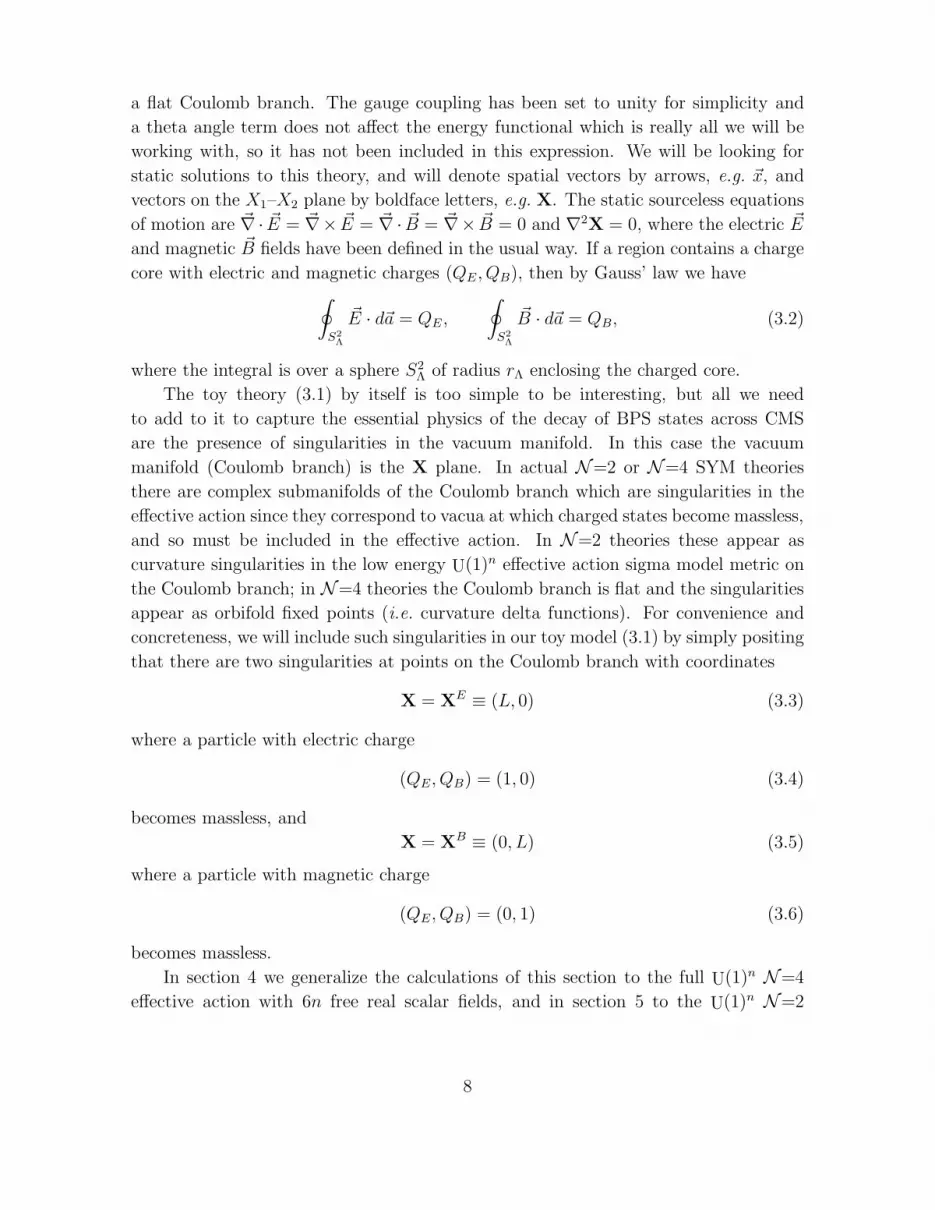
are the presence of singularities in the vacuum manifold. In this case the vacuum
manifold (Coulomb branch) is the X plane. In actual N=2 or N=4 SYM theories
there are complex submanifolds of the Coulomb branch which are singularities in the
effective action since they correspond to vacua at which charged states become massless,
and so must be included in the effective action. In N=2 theories these appear as
curvature singularities in the low energy U(1)n effective action sigma model metric on
the Coulomb branch; in N=4 theories the Coulomb branch is flat and the singularities
appear as orbifold fixed points (i.e. curvature delta functions). For convenience and
concreteness, we will include such singularities in our toy model (3.1) by simply positing
that there are two singularities at points on the Coulomb branch with coordinates
X = XE ≡ (L, 0) (3.3)
where a particle with electric charge
(QE, QB) = (1, 0) (3.4)
becomes massless, and
X = XB ≡ (0, L) (3.5)
where a particle with magnetic charge
(QE, QB) = (0, 1) (3.6)
becomes massless.
In section 4 we generalize the calculations of this section to the full U(1)n N=4
effective action with 6n free real scalar fields, and in section 5 to the U(1)n N=2
8

effective action with 2n real scalar fields with curved sigma model metric. In both
cases the core of the physics will be seen to be the same as that of the toy model of
eqns. (3.1) and (3.3–3.6), though the combinatorics and some details of the analysis
will be more complicated.
3.1 Boundary conditions and BPS bounds
As a low energy effective action, (3.1) should be considered as the first terms in a
derivative expansion. Suppressing all the higher derivative terms is a good approxima-
tion as long as we do not probe the physics describing the core of the BPS state. Near
such a core the U(1) field strength and, by supersymmetry, the values of the scalar
fields X will grow large. Indeed, in the presence of a static source at spatial position
~x0 the electric and magnetic fields and the scalar fields diverge as
| ~E|, | ~B|, |~∇X| ∼ 1
r2, (3.7)
where r = |~x − ~x0|. With an ultraviolet scale Λ suppressing derivative corrections
to the U(1) effective action by powers of Λ, for example Λ−2|∂X|4, we see that when
|~∇X| ∼ Λ2, or at a typical distance
r ∼ rΛ ≡ 1
Λ(3.8)
from the core, the low energy U(1) solution ceases to be valid. Also, when expanding
about a given vacuum X0 on the Coulomb branch there will also be irrelevant terms
with polynomial coefficients, e.g. Λ−6|X − X0|2|∂X|4, implying the breakdown of the
low energy solution when |X−X0| & Λ3r2 where r is the spatial distance from a charge
core. Such terms imply that the value X(~x) of the scalars at any given spatial position
~x is itself reliable only up to some accuracy
|δX(~x)| ≃ Λ. (3.9)
This fuzziness in the solution Λ is not easy to estimate directly from the action, for it
varies with ~x as well as with the choice of vacuum X0 and charges (QE , QB). We will
see below how it can be determined self-consistently from static solutions.
Our strategy will be to use the low energy U(1) solution away from the cores
(r > rΛ) and impose appropriate boundary conditions in the vicinity of the charge
cores (r ∼ rΛ). The qualitative features of these boundary conditions are easy to
deduce, as we will discuss momentarily; we will see in the course of this section that
only these qualitative features are important for the physics in the vicinity of a CMS—
other details of the boundary conditions do not affect the results.
9
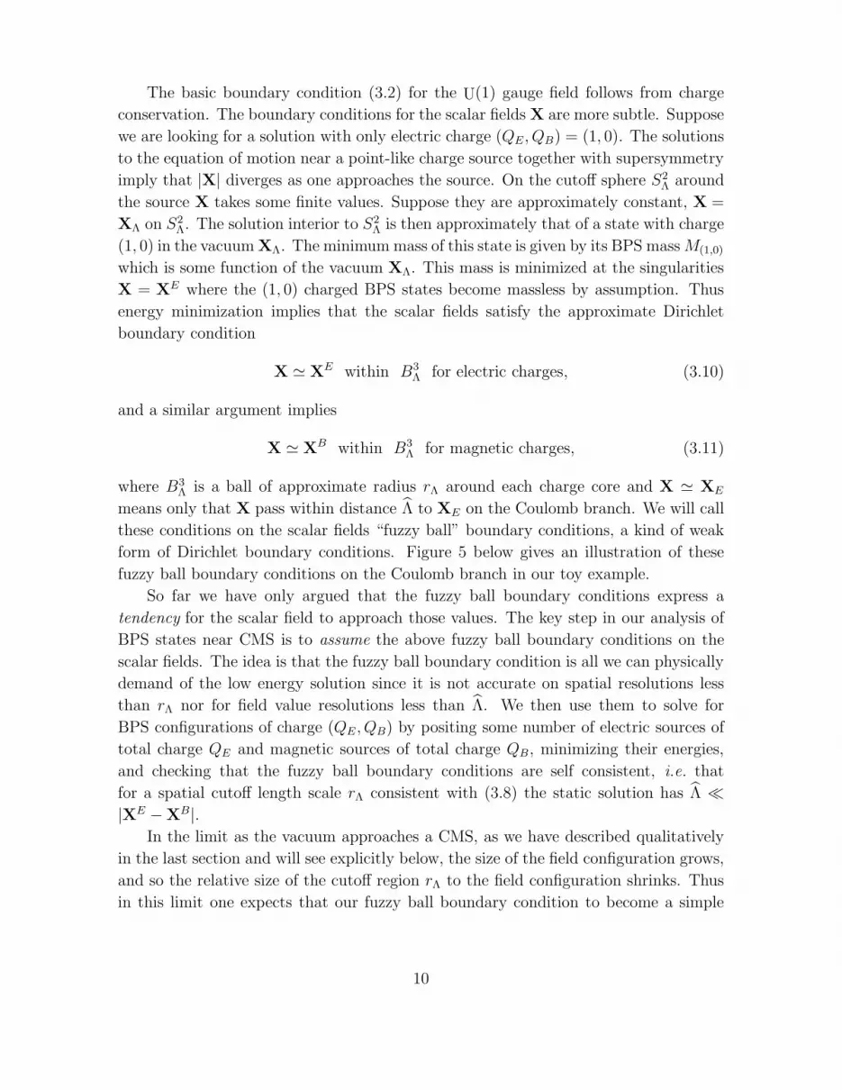
The basic boundary condition (3.2) for the U(1) gauge field follows from charge
conservation. The boundary conditions for the scalar fields X are more subtle. Suppose
we are looking for a solution with only electric charge (QE , QB) = (1, 0). The solutions
to the equation of motion near a point-like charge source together with supersymmetry
imply that |X| diverges as one approaches the source. On the cutoff sphere S2Λ around
the source X takes some finite values. Suppose they are approximately constant, X =
XΛ on S2Λ. The solution interior to S2
Λ is then approximately that of a state with charge
(1, 0) in the vacuum XΛ. The minimum mass of this state is given by its BPS mass M(1,0)
which is some function of the vacuum XΛ. This mass is minimized at the singularities
X = XE where the (1, 0) charged BPS states become massless by assumption. Thus
energy minimization implies that the scalar fields satisfy the approximate Dirichlet
boundary condition
X ≃ XE within B3Λ for electric charges, (3.10)
and a similar argument implies
X ≃ XB within B3Λ for magnetic charges, (3.11)
where B3Λ is a ball of approximate radius rΛ around each charge core and X ≃ XE
means only that X pass within distance Λ to XE on the Coulomb branch. We will call
these conditions on the scalar fields “fuzzy ball” boundary conditions, a kind of weak
form of Dirichlet boundary conditions. Figure 5 below gives an illustration of these
fuzzy ball boundary conditions on the Coulomb branch in our toy example.
So far we have only argued that the fuzzy ball boundary conditions express a
tendency for the scalar field to approach those values. The key step in our analysis of
BPS states near CMS is to assume the above fuzzy ball boundary conditions on the
scalar fields. The idea is that the fuzzy ball boundary condition is all we can physically
demand of the low energy solution since it is not accurate on spatial resolutions less
than rΛ nor for field value resolutions less than Λ. We then use them to solve for
BPS configurations of charge (QE , QB) by positing some number of electric sources of
total charge QE and magnetic sources of total charge QB, minimizing their energies,
and checking that the fuzzy ball boundary conditions are self consistent, i.e. that
for a spatial cutoff length scale rΛ consistent with (3.8) the static solution has Λ ≪|XE − XB|.
In the limit as the vacuum approaches a CMS, as we have described qualitatively
in the last section and will see explicitly below, the size of the field configuration grows,
and so the relative size of the cutoff region rΛ to the field configuration shrinks. Thus
in this limit one expects that our fuzzy ball boundary condition to become a simple
10

Dirichlet boundary condition, i.e. Λ → 0. Indeed, as shown in [22] for spherically
symmetric 1/2 BPS states in N=4 SYM theory, a simple (spherical) Dirichlet boundary
condition exactly reproduces the BPS bound; near the CMS a decaying 1/4 BPS state
will become to arbitrary accuracy a very loosely bound state of two 1/2 BPS states, and
so the fuzzy ball boundary conditions should approach Dirichlet boundary conditions
to the same accuracy.
Furthermore, far enough away from the CMS (at distances greater than or on the
order of Λ on the Coulomb branch) the boundary conditions (3.10) and (3.11) will
break down entirely, and cannot be satisfied even approximately. Thus, far out on the
Coulomb branch, where monopole states are well-described by semiclassical nonabelian
field configurations, our low energy U(1) description breaks down entirely.3 In this sense
our description of BPS states is complementary to the semiclassical one.
Now let us use these boundary conditions to derive the low energy field equations
satisfied by our static BPS solutions. We do this by the familiar method of minimiz-
ing the energy of the field configurations. From the action (3.1), an energy density
functional for static configurations can be constructed by the usual canonical methods
E =1
2
[~E2 + ~B2 + (~∇X)2
]. (3.12)
This can be rewritten in the following fashion
E =1
2
[( ~E − cos α~∇X1 + sin α~∇X2)
2 + ( ~B − sin α~∇X1 − cos α~∇X2)2]
+ cos α( ~E · ~∇X1 + ~B · ~∇X2) + sin α( ~B · ~∇X1 − ~E · ~∇X2). (3.13)
Integrating this expression over three dimensional space gives the mass of the configu-
ration as
M =
∫d3~x
1
2
[( ~E − cos α~∇X1 + sin α~∇X2)
2 + ( ~B − sin α~∇X1 − cos α~∇X2)2]
+
n∑
I=0
{
cos α
∮
S2I
(X1~E + X2
~B) · d~a + sin α
∮
S2I
(X1~B − X2
~E) · d~a}
(3.14)
where the boundaries S2I are spheres around each charge source and one sphere at
infinity. We have used the divergence-free equation of motion for the electric and
magnetic fields ~∇ · ~E = ~∇ · ~B = 0 away from the sources. If we label the boundaries so
that the I = 0 boundary is the one at infinity and the I = i 6= 0 are the ones around the
3More precisely, it becomes equivalent to the Dirac monopole solution which carries no information
about the structure of the state.
11

charge sources, then our approximate Dirichlet boundary conditions (3.10) and (3.11)
imply that at the ith boundary the scalars X take the constant values Xi = XE or XB
while at infinity they take their asymptotic values X0, the Coulomb branch coordinates
of the vacuum. Since these are constants they can be taken outside the surface integrals
which then give by (3.2) the charges (QIE , QI
B) enclosed by each sphere, so that
M =
∫d3~x
1
2
[( ~E − cos α~∇X1 + sin α~∇X2)
2 + ( ~B − sin α~∇X1 − cos α~∇X2)2]
+
n∑
I=0
[cos α(XI
1QIE + XI
2QIB) + sin α(XI
1QIB − XI
2QIE)]. (3.15)
Here (Q0E , Q0
B) = (QE , QB) is the total charge of the configuration. By charge conser-
vation
(QE , QB) = −n∑
i=1
(QiE, Qi
B) (3.16)
so, defining the position vectors of the singularities on the Coulomb branch relative to
the vacuum by
ξi ≡ Xi − X0, (3.17)
and since the first line in (3.15) is positive definite we get the bound
M ≥ cos α(ξi1Q
iE + ξi
2QiB) + sin α(ξi
1QiB − ξi
2QiE), (3.18)
where the sum on i over the charge sources is implied. The tightest bound on M comes
from maximizing the right hand side with respect to α, giving the BPS bound
M ≥√
(ξi1Q
iE + ξi
2QiB)2 + (ξi
1QiB − ξi
2QiE)2. (3.19)
Thus the minimal energy configurations saturating the inequality are solutions of the
BPS equations
~E = cos α~∇X1 − sin α~∇X2,
~B = sin α~∇X1 + cos α~∇X2 (3.20)
where
tan α =ξi1Q
iB − ξi
2QiE
ξi1Q
iE + ξi
2QiB
. (3.21)
The rest of this section is devoted to analyzing the solutions to (3.20) subject to our
boundary conditions (3.10) and (3.11) minimizing the BPS mass (3.19).
12

In finding the solutions to the BPS equa-
X
ξB
XE=(0,L)
XB=(L,0)
X2
X 1
ξ
0
E
β
β
Figure 4: Coordinates on the Coulomb
branch of the U(1) toy model. X = X0
denotes the vacuum, while ξE and ξB are
vectors from the vacuum to the electric
and magnetic singularities, respectively.
The dashed line is the CMS.
tions (3.20) we have the discrete choice of charges
at the sources, i.e. the set of integer charges
(QiE , Qi
B), which are constrained by charge con-
servation (3.16). In our simple example, though,
since only electric charges can flow into the
XE = (L, 0) singularity and magnetic into the
XB = (0, L) one, we see that there are only
two possible values for the ξi:
ξE ≡ XE − X0 (3.22)
for sources with only electric charges (QiB = 0),
or
ξB ≡ XB − X0 (3.23)
for sources with only magnetic charges (QiE =
0); see figure 4.
This leads to a simplification of the BPS
mass formula (3.19) to
M(QE , QB) =
√(QE)2ξE · ξE + (QB)2ξB · ξB + 2QEQBξE × ξB. (3.24)
In the case of purely electric or purely magnetic total charges, the bound further sim-
plifies to
M(QE , 0) = |QE||ξE|,M(0, QB) = |QB||ξB|, (3.25)
i.e. the charge times the distance to relevant singularity on the Coulomb branch.
The CMS for the decay of a (QE, QB) state to a (QE , 0) plus a (0, QB) state is
then given by the curve on the Coulomb branch for which M(QE , QB) = M(QE , 0) +
M(0, QB). From (3.24) and (3.25) this implies that |ξE||ξB| = |ξE × ξB|, or that ξE
be perpendicular to ξB. This describes a circle on the Coulomb branch, shown as the
dashed curve in figure 4.
3.2 Spike and prong solutions
We will now illustrate some simple solutions to the BPS equations and boundary con-
ditions in our toy model. To simplify the algebra and make the basic points clear we
13

choose the vacuum to be symmetrically placed at the point X0 = (X0, X0) on the
Coulomb branch.
The simplest case is where there is a single charge source of purely electric or
magnetic charge. For example, suppose QB = 0. By (3.20) and since ~B = 0 (because
all the magnetic charges in the problem vanish) and tanα = −ξE2 /ξE
1 , the component of
X perpendicular to ξE on the Coulomb branch must be constant, while its component
parallel to ξE satisfies Laplace’s equation with a source of total charge QE. The solution
is thus simply
X1 − X0 =QE cos β
4π|~x − ~xE|, X2 − X0 =
QE sin β
4π|~x − ~xE|, (3.26)
which implies electric and magnetic fields
~E =QE
4π
~x − ~x0
|~x − ~x0|3, ~B = 0. (3.27)
Here β is the angle on the Coulomb branch shown in figure 4, and ~xE is the spatial
location of the electric charge source. Since both α and α + π satisfy (3.21) the sign of
QE in (3.26) is undetermined; we will determine it below.
Following the brane picture of [20] we will call this a “spike” solution. In the brane
picture, the space-time coordinates are identified with the worldvolume coordinates of a
D3-brane, and the X scalars take values in the dimensions transverse to the brane. Thus
the solution (3.26) can be thought of as describing a semi-infinite spike-like deformation
of the brane in this enlarged space. As described in [20] such a solution can be identified
with a fundamental string ending on the D3-brane. Likewise, the solution for a purely
magnetically charged BPS state is given by
X1 − X0 =QB sin β
4π|~x − ~xB|, X2 − X0 =
QB cos β
4π|~x − ~xB|, (3.28)
which can be interpreted as a spike with mass per unit length equal to that of a D-string
attached to the D3-brane.
We still need to apply our fuzzy ball boundary conditions (3.10) and (3.11) to
these solutions. These boundary conditions fix the undetermined signs of QE and QB
in (3.26) and (3.28). The signs of these solutions are appropriate for
X0 ≤ L/2 (3.29)
or, equivalently, for β > −π/4, which we will assume from now on. The boundary
conditions also determine the radii of the cutoff spheres S2Λ to be
rΛ =|QE|4πℓ
(3.30)
14

implying a cutoff energy scale of Λ ∼ ℓ, where ℓ = |ξE| = |ξB| is the distance from the
vacuum to either Coulomb branch singularity. This is indeed the appropriate cutoff
scale for the low energy effective theory since there are new light charged particles with
masses (3.25) proportional to this Coulomb branch distance.
The simple spike solutions found above do not have any interesting structure on
the Coulomb branch: they exist for any vacuum and obey exactly Dirichlet boundary
conditions with spherical boundaries which we expected to be only approximately sat-
isfied in general. The situation becomes more interesting when we turn to states with
two or more charge sources.
First consider a purely electrically charged two center solution with QE = Q1E +Q2
E .
It is easy to find solutions with the fuzzy ball boundary conditions (3.10) and (3.11).
Indeed,
X1 − X0 =Q1
E cos β
4π|~x − ~xE,1|+
Q2E cos β
4π|~x− ~xE,2|,
X2 − X0 =Q1
E sin β
4π|~x − ~xE,1|+
Q2E sin β
4π|~x− ~xE,2|, (3.31)
does the job as long as the distance
r12 = |~xE,1 − ~xE,2| (3.32)
between the two sources satisfies
r12 >1
4πℓ. (3.33)
That is to say, as long as sources are sufficiently far apart one can enclose the sources in
disjoint spheres within which X take the value (L, 0). This behavior is sensible: since
a static configuration of two charged BPS states with commensurate charge vectors is
itself BPS, there should exist a static low energy configuration for any separation of
the sources. The restriction (3.33) that they not be too close just reflects the fact that
the low energy description of their interaction breaks down on scales r . ℓ−1.
Now focus on a dyonic state with both electric and magnetic charges. For simplicity
we take (QE , QB) = (1, 1). By (3.21) we see that α = π/2, so the BPS equations (3.20)
reduce to~E = ~∇X1, ~B = ~∇X2. (3.34)
From the linearity of the BPS equations and since X are harmonic functions, we expect
the solution to be given at least approximately by a solution of the form
X1 − X0 =cos γ
4π|~x − ~xE|+
sin δ
4π|~x − ~xB|,
X2 − X0 =sin γ
4π|~x − ~xE|+
cos δ
4π|~x − ~xB|. (3.35)
15

Compatibility with Gauss’ law and the BPS equations then imply that γ = δ = 0 so
X1 − X0 =1
4π|~x − ~xE|,
X2 − X0 =1
4π|~x − ~xB |. (3.36)
We want to check whether there are values of the electric and magnetic charge source
centers, ~xE and ~xB, for which this solution satisfies our fuzzy ball boundary conditions
(3.10) and (3.11). What this asks is that the X values taken by this solution enter
(and go through) a small ball around XE = (L, 0) as ~x → ~xE and a small ball around
XB = (0, L) as ~x → ~xB. As ~x → ~xE the above solution approaches
X1 − X0 =1
4πrΛ,
X2 − X0 ≃ 1
4πrEB
, (3.37)
where
rΛ = |~x − ~xE|, rEB = |~xE − ~xB|. (3.38)
The X1 = L fuzzy boundary condition is achieved if the spatial cutoff length scale
around the electric source is taken to be
rΛ =1
4π(L − X0), (3.39)
while the X2 = 0 boundary condition fixes the separation of the electric and magnetic
charge sources to be [23]
rEB =1
4π(−X0). (3.40)
Furthermore, on the sphere of radius rΛ around the electric source at ~xE , by (3.36) X2
takes values in a range |X2| < Λ with
Λ =(X0)2L
1 − 2(X0/L). (3.41)
The boundary conditions at the magnetic source give the same results.
The conditions for our solution to be consistent are thus that
X0 < 0 (3.42)
since the distance rEB is necessarily positive, and that Λ is less than the distance ∼ L
between the electric and magnetic singularities on the Coulomb branch, which implies
|X0| . L. (3.43)
16

These conditions illustrate the qualitative picture of(a)
0X
0X
(b)
Figure 5: The shaded regions are
the images of the low energy dyon
solution in the Coulomb branch for
various values of the vacuum X0.
They are only valid outside the
lighter circles about the singulari-
ties which denote the Λ fuzzy ball
boundary conditions.
decaying BPS states that we have argued for in the
previous section. Referring to figure 4 we see that
X0 = 0 is the location of the CMS. So (3.42) implies
that a solution exists on one side of the CMS, and
ceases to exist once one crosses it. Furthermore, the
region of self-consistency of the fuzzy ball boundary
conditions includes the CMS; indeed, the fuzzy ball
boundary conditions become more and more accu-
rately simple Dirichlet boundary conditions as one
approaches the CMS since (3.41) implies that
Λ ∼ (X0)2/L (3.44)
vanishes as X0 → 0. Finally, (3.40) shows that the
spatial distance between the charge cores diverges
as we approach the CMS. Figure 5 illustrates the
qualitative behavior of these solutions for different
values of X0. These figures show the projection of
our low energy solutions on the Coulomb branch.
Note that this projection suppresses the spatial ex-
tent of the field configuration; in particular note
that as the vacuum approaches the CMS, though
the projection on the Coulomb branch degenerates
to a string web configuration, in space-time it ex-
pands as the positions of the charge centers diverge.
Figure 5(a) shows how the fuzzy ball boundary con-
ditions break down too far from the CMS, while fig-
ure 5(b) illustrates how the image of the solution in
the Coulomb branch more closely approximates a
string web configuration (shown as heavy lines) in
the limit as the vacuum approaches the CMS.
We will refer to these multi-center solutions as brane prongs, again in analogy to
the brane picture where the Coulomb branch is realized as additional transverse spatial
dimensions. The breakdown of the low energy solution when X0 is large compared to L
so that (3.43) is not satisfied simply reflects the fact that in this case the uncertainties
in the locations of ~xE and ~xB are of the order of the separation rEB itself, so now one
cannot really tell if there are two centers of charge in the low energy theory or one.
Thus this configuration effectively looks like one brane spike from a (1, 1) dyon.
17

Finally, it is straightforward to generalize the calculations of this section to the
case of arbitrary position of the X0 of the vacuum, arbitrary (QE , QB) charge sector,
and arbitrary value for the low energy U(1) coupling g. The result is a static solution
for the (QE , QB) dyon outside the CMS for any relatively prime QE and QB, which
decays into QE charge (1, 0) plus QB charge (0, 1) particles inside the CMS. A two
particle state with mutually local charges (i.e. commensurate charge vectors) is BPS
and so a static solution exists for any spatial separation. Thus our low energy method
is not able to determine whether there is a one particle bound state at threshold for
electric and magnetic charges which are not mutually prime.
3.3 Recovery of a string junction picture
We have thus explicitly verified all the qualitative features expected of a BPS state
decaying across a CMS. The last thing to show is how this information extracted from
the low energy effective action on the Coulomb branch is equivalent to a string web
picture of the BPS states.
The string web picture is recovered in two stages. First, in the limit as the vacuum
approaches the CMS, the image of the low energy field configuration in the Coulomb
branch degenerates to a collection of curves on that space. These curves are the images
of brane spike solutions which carry precisely the energy per unit length of the corre-
sponding (p, q) string [20]. This is easy to see in our example by taking X0 → 0 in (3.36)
and comparing to our electric and magnetic spike solutions (3.26) and (3.28) (with
β = 0). Thus arbitrarily close to the CMS the projection onto the Coulomb branch of
all the (QE , QB) charged states look like strings of appropriate tension stretched across
the Coulomb branch.
In string theory, 3-pronged string states that stretch between D-branes satisfy
charge conservation and tension balance. For example, the above configuration corre-
sponds to a (1, 0) (fundamental string), a (0, 1) (D-string)and a (1, 1) string stretched
between three D3-branes. The three prongs or string legs meet at a common point,
the junction, which remains point-like even arbitrarily close to the CMS. In the field
theory picture discussed in this section, we have seen that the leg corresponding to
the decaying (1, 1) dyon grows in spatial size (i.e., along the D3-brane worldvolume)
near the CMS. Arbitrarily close to the CMS, the configuration resembles two separate
strings that end on the D3-brane corresponding to the decaying U(1). Thus there does
not appear to be a point-like junction as the decaying configuration approaches the
CMS in the field theory picture.
The difference between the two perspectives is the result of different orders of
limits. Consider the Dirac-Born-Infeld action for the D3-brane corresponding to the
decaying dyon, treating it as a probe in a background of other D3-branes. The brane
18
prong corresponding to the decaying (1, 1) dyon then ends on other D3-branes that are
treated as a fixed background. Looking at the quadratic terms and comparing with
the low energy effective action we have used above, we can see that the scalars X in
the field theory with mass dimension unity and the coordinates in the brane transverse
space, x, are related by X = x/α′, where α′ is the string length squared. The separation
between the charge centers in the D-brane worldvolume is
rEB ∼ 1/(−X0) = α′/(−x0). (3.45)
The low energy field theory is a good approximation in the α′ → 0 limit holding the
scalar vevs, including X0, fixed. On the other hand, in the string junction/geodesic
picture in string theory, the coordinates x0 are what are held fixed: taking α′ → 0 to
suppress higher stringy corrections gives a vanishing separation rEB between the charge
centers, i.e. a pointlike junction. For x0 = 0, the separation is indeterminate, which
corresponds to the two strings ending anywhere on the D-brane. This recovers the
string theory result and it further illustrates that the point-like junction is not visible
within the field theory approximation.
The second stage is to extend this picture to the rest of the Coulomb branch by
continuity and matching to the BPS mass formula. This can be done uniquely since the
given tension of a (QE , QB) string (namely T (QE , QB) =√
Q2E + Q2
B in our example
where we have set the coupling g = 1) fixes the path away from the CMS it must be
extended in in order to give the contribution to the state’s mass required to match its
BPS mass. That this path is a geodesic on the Coulomb branch follows from the form
of the BPS mass formula [35]. In the case of our toy example, the Coulomb branch is
flat so the geodesics are straight lines and it is clear that the string web picture of the
BPS states extends without obstruction over the whole Coulomb branch.
The result is therefore the prediction in our toy model that outside the CMS the
spectrum consists of all (QE , QB)-charged dyons with QE and QB relatively prime,
while inside the CMS only the (±1, 0) and (0,±1) states are in the spectrum. Of
course, this is only a toy example. We will perform essentially the same analysis in the
next section for the N=4 SYM theories.
4. BPS states in N=4 SU(N) theories
In this section we turn to an analysis of the static BPS field configurations of given
total electric and magnetic charges in the low energy U(1)N−1 theory on the moduli
space of an N=4 SU(N) SYM theory. The N=4 superalgebra allows both 1/2 and 1/4
BPS particle states. From the expression for the BPS mass, there are no CMS for 1/2
BPS states, but there are CMS for 1/4 BPS states to decay.
19

In section 4.1 below we will effectively rederive the N=4 BPS mass formula, as
well as the BPS equations in the low energy theory. We then find solutions to the BPS
equations subject to our fuzzy ball boundary conditions and show how they reproduce
a string web picture on the moduli space of the N=4 theory.
However this is not the usual string web picture of BPS states in N=4 theories
derived from string theory. In this picture [15] the U(N) SYM theory is realized
by open strings and D1-branes ending on a set of N parallel D3-branes in a flat 10-
dimensional IIB string theory background. The relative positions of the N D3-branes in
the transverse 6-dimensional space form the 6N -dimensional moduli space of the N=4
theory. BPS states are described by webs of (p, q) strings stretching between the D3-
branes [6]; a web has charge (QE, QB) with respect to a given low energy U(1) factor if
it ends on the associated D3-brane with a (QE, QB) string. These string webs thus live
in a 6-dimensional space stretched between N point sources, which is different from the
picture we derive below as string webs stretched in the 6N -dimensional moduli space
and ending on 6(N − 1)-dimensional singular submanifolds. In section 4.2 below we
show how the 6-dimensional string theory webs are obtained from our 6N -dimensional
webs by a simple mapping. The basic reason this works is that the 6N -dimensional
moduli space M of the U(N) theory is M = (R6)N/SN where the permutation group
SN interchanging the R6 factors is the Weyl group of U(N). Because of this simple
relation between the transverse R6 of the D3-branes and M, webs on M can be uniquely
mapped onto webs in R6, recovering the string picture.
A similar construction presumably also works for the SO and Sp N=4 SYM the-
ories, since their Weyl groups are also fairly simple, differing from the action of the
SU Weyl group by the addition of Z2 identifications on each R6. This will fold webs
on M down to webs on R6/Z2, thus realizing the string web picture of BPS states for
these theories which are found by placing D3-branes in the background of an appro-
priate orientifold O3-plane. The action of the Weyl groups of the exceptional groups
is more complicated, and it is not clear whether any folding of our webs on M to a
6-dimensional space can be performed. This may “explain” why there are no D3 brane
constructions of the N=4 SYM theories with exceptional gauge groups.
4.1 BPS states as webs on the moduli space
The generic point on the moduli space of an N=4 SYM theory with gauge group SU(N)
is described by a low energy U(1)N−1 N=4 theory. A convenient trick to simplify the
algebra will be look at the U(N) theory instead, which has a U(1)N effective description,
but restrict ourselves to states which are neutral under the extra U(1).
Now, each U(1) N=4 multiplet has six real scalar fields, so the moduli space is
locally coordinatized by the values of the 6N scalars Xra where r = 1, . . . , N and
20

a = 1, . . . , 6. The other bosonic massless fields are the electric and magnetic fields ~Er
and ~Br for each U(1) factor. We are interested in static low energy solutions carrying
electric and magnetic charges (QEr, QBr) with respect to these fields. We normalize
the fields so that the low energy effective action for the bosonic fields is
S =
∫d4x
N∑
r=1
(1
4g2Fr µνF
µνr +
ϑ
64π2ǫµνρσF µν
r F ρσr +
1
4g2
6∑
a=1
∂µXra∂µXra
)
, (4.1)
with the ~Er and ~Br related to F µνr in the usual way. The fact that all the U(1)’s have
the same coupling and no cross-couplings reflects the specific basis of U(1)N we have
chosen. The fact that the coupling is independent of the Xra reflects the flatness of the
metric on M for N=4 theories. We normalize the charges so that
∮
S2
~Er · d~a = g2QEr,∮
S2
~Br · d~a = g2QBr. (4.2)
Thus, the Dirac quantization condition plus the effect of the theta angle imply that the
charges are quantized as
QEr = nEr +ϑ
2πnBr and QBr =
4π
g2nBr (4.3)
for some integers nEr and nBr.
4.1.1 Moduli space and boundary conditions
Globally, the moduli space is
M = R6N/SN (4.4)
where SN acts by permuting the N R6 factors. Suppose we have some ordering of
points in R6 (say “alphabetical” ordering on their six coordinates in some given basis)
denoted by X1a ≥ X2a where X1 and X2 are two points in R6. Then we can take as a
fundamental domain of SN on R6N the set of all N 6-vectors satisfying
X1a ≥ X2a ≥ · · · ≥ XNa. (4.5)
The boundaries of this wedge-like convex domain are identified by the SN action.
The locus of fixed points of the action of SN are orbifold singularities of M where
BPS states of certain charges become massless. The typical such singularity is the
fixed line under interchange of, say, X1a with X2a. The result is a 6(N −1)-dimensional
21

manifold of Z2 singularities at X1a = X2a, with all the other Xra arbitrary for r > 2. At
this singularity states with charges QE1 = −QE2 and QB1 = −QB2 arbitrary and QEr =
QBr = 0 for r > 2 become massless. Actually all such 6(N − 1)-dimensional manifolds
of Z2 singularities are identified by the SN orbifolding. However, which charged states
become massless there depends on the direction the singularity is approached from.
Thus it is convenient to treat M as the wedge (4.5) with different charge images of the
Z2 singularity on its boundary.
In addition, these images of the Z2 singularities may intersect one another along
submanifolds of smaller dimension where states charged under three or more U(1)
factors become massless. In fact, on the 6-dimensional submanifold of M where all the
Xra, r = 1, . . . , N are equal, BPS states of arbitrary charge become massless. Since
we are only considering states which are neutral with respect to the diagonal U(1)
factor (to decouple the extra U(1) of the U(N) gauge group), all configurations will be
invariant under translations in M by any such vector of equal Xr’s.
With this description of the moduli space and its singularities in hand, we are ready
to solve for static low energy field configurations in a given charge sector subject to
our fuzzy ball boundary conditions. Since we are looking for BPS configurations which
preserve at least 1/4 of the supersymmetries, we can restrict ourselves to configurations
which lie in some fixed two-dimensional subspace of each R6 factor, which we will
take to be that given by the Xra with a = 1, 2. Furthermore, the residual (N = 1)
supersymmetry implies that the BPS configurations must depend holomorphically on
the Xr1 + iXr2 complex coordinates. It will thus be convenient to introduce a notation
in which all quantities are assembled into N component complex vectors defined by
Xr ≡ Xr1 + iXr2,
~Fr ≡ ~Er + i ~Br,
Qr ≡ QEr + iQBr. (4.6)
Denote the total charge of our configuration by Q0r . Suppose our configuration has
M charge centers with (approximate) spatial positions ~x = ~xi, with charges labeled
by Qir, i = 1, . . . , M . (We will mainly concentrate on the case of prong solutions with
M = 2 below.) Then charge conservation implies
M∑
I=0
QIr = 0. (4.7)
Label the boundaries of space by the spheres S2I where S2
0 refers to the sphere at infinity,
while the S2i for i = 1, . . . , M are small spheres around the M charge sources at ~x = ~xi.
22

The Gauss’ law implies ∮
S2I
d~a · ~Fr = g2QIr . (4.8)
The scalars approach
Xr = X0r on S2
0 , (4.9)
where X0r are the moduli space coordinates of the vacuum. Our fuzzy ball boundary
conditions imply that the Xr will approach (at least approximately) constant values on
the S2i boundaries, which we will denote
Xr ≃ X ir on S2
i . (4.10)
Furthermore, the X ir are constrained to lie in only those singular submanifolds of M
where states of charge Qir become massless. From the above description of M the X i
r
must live on the appropriate singular submanifold where a BPS state with its associated
charges becomes massless.
4.1.2 BPS bound
The mass of our configuration is computed by integrating the field energy density (with
an implicit sum over repeated indices)
M =1
2g2
∫d3~x (~F ∗
r · ~Fr + ~∇X∗r · ~∇Xr). (4.11)
This can be rewritten as
M =1
2g2
∫d3~x |~Fr − Ars
~∇Xs|2 +1
2g2Re
∫d3~xArs
~F ∗r · ~∇Xs (4.12)
if Ars is an U(N) matrix
A∗rsArt = δst. (4.13)
Using ~∇ · ~Fr = 0 away from the sources, the second term in (4.12) becomes a surface
term which can be evaluated using (4.8)–(4.10) to
M =1
2g2
∫d3~x |~Fr − Ars
~∇Xs|2 + Re∑
I
QI∗r ArsX
Is . (4.14)
Since the first term on the right hand side is positive definite, we get the bound
M ≥ Re{QI∗r ArsX
Is}. (4.15)
23

The BPS bound arises from maximizing the right hand side of this expression subject
to (4.13)
MBPS = maxA∈U(N)
Re{QI∗r ArsX
Is }. (4.16)
Finally, this BPS bound is saturated when the BPS equations
~Fr = Ars~∇Xs, ∇2Xs = 0, (4.17)
are satisfied for the Ars which maximizes (4.16), where the last equation is a result of
the divergence free property of ~Fr.
The expression for MBPS can be simplified slightly using charge conservation. De-
fine by
ξis ≡ X i
s − X0s (4.18)
the vector pointing from the vacuum X0s to the source (singularity) at X i
s. Then, by
(4.7),
QI∗r ArsX
Is = Qi∗
r Arsξis, (4.19)
and the BPS bound becomes
MBPS = maxA∈U(N)
Re{Qi∗r Arsξ
is}. (4.20)
Now, as described above, the singularities of M are whole submanifolds, not iso-
lated points, so the vectors ξis pointing to the singularities can vary continuously. We
must therefore vary our boundary conditions to find the lightest (potentially) BPS
state in the given charge sector. This has two consequences. First, this implies that
generically the charge sources will lie along the the Z2 singularities in M, i.e. that only
with some special fine tuning will a source charged under three or more U(1)’s not split
into several sources each with (opposite) charges under only two U(1)’s. This follows
simply because the multi-charged sources are constrained to lie in submanifolds at the
intersection of the higher-dimensional Z2 singularities. The second consequence is that
the true BPS bound is given by the the minimization of (4.20) with respect to the set
of vectors ξir ending on the Z2 singularities
MBPS = minξ∈sings.
maxA∈U(N)
Re{Qi∗r Arsξ
is}. (4.21)
It is important to note that the maximization with respect to the rotation Ars be
done for each ξir before the minimizing with respect to ξi
r. If the space of singularities
over which the ξi can vary were compact and smooth, then (since the space of A’s
is compact) there would be no issue over the order in which the extremizations were
24

performed. But the space of singularities over which the ξi can vary themselves have
singularities, and so some care must be taken in case the solution lies not at a saddle
point of ReQ∗i · A · ξi, but at one of these singularities. We have found, however, that
for generic Qi’s and X0 this does not happen so the order of extremization can be
reversed. This greatly simplifies the problem of finding MBPS in N=4 theories because
the singularities lie along linear subspaces of the flat moduli space. Thus minimization
with respect to the ξi by itself gives M independent complex conditions on A, essentially
fixing it and MBPS entirely in the cases of one or two charge sources (M = 1 or 2) each
charged under only two U(1) factors. This minimization is carried out in the Appendix
for two charge sources.
Even in this case one must still do the maximization with respect the A to determine
the values of the ξi in terms of given source charges Qis and vacuum X0
s . Solving this
minimization and maximization problem for the ξi and MBPS with an arbitrary number
of given charge sources Qir is difficult in general. However, as we will explain below, it
is sufficient to solve it for just two sources each charged under only two U(1) factors.
This is also done explicitly in the Appendix for two charge sources. We see there that
the ξi are not completely determined by the extremization of the BPS bound, but are
ambiguous up to a single undetermined real parameter. The final condition needed to
fix the boundary conditions (the ξi) comes from demanding that solutions to the BPS
equations exist.
4.1.3 BPS solutions
So, suppose we fix the ξi, and thus the boundary values of the scalars. We will now solve
the low energy BPS equations (4.17) subject to the charge boundary conditions (4.8),
the boundary conditions at infinity (4.9), as well as our fuzzy ball boundary conditions
centered around the above determined boundary values. In doing so we will determine
necessary conditions for a solution to exist given these boundary conditions. These
conditions can phrased as the conditions that a certain matrix αij be real, symmetric,
and have only positive entries. The reality and symmetry condition will provide the
extra condition needed to determine the ξi for two or more charge sources. Finally, the
positivity condition is satisfied only on one side of the CMS, and so it is this condition
which determines the stability of BPS states.
The BPS equations can be solved as in the toy model of section 3 by a superposition
of single source solutions:
ξs(~x) =M∑
i=1
QirA
∗rs
4π|~x − ~xi|, (4.22)
25

where we have defined
ξs(~x) ≡ Xs(~x) − X0s . (4.23)
The numerators on the right hand side are determined by (4.17) and (4.8). Now, the
fuzzy ball boundary conditions are that ξs goes through a small ball around ξis as
~x → ~xi. In this limit ξ(~x) approaches
lim~x→~xi
ξs ≃A∗
rsQir
ǫ+
M∑
j 6=i
A∗rsQ
js
rij
→ ∞ (4.24)
where
ǫ ≡ 4π|~x − ~xj |, and rij ≡ 4π|~xi − ~xj |. (4.25)
Thus as ~x → ~xj our solutions go to infinity asymptoting a line along the A∗rsQ
js direc-
tion and with intercept δir =
∑j 6=i
A∗
rsQjs
rij. So a necessary condition for the fuzzy ball
boundary conditions to be satisfied is that the approximate boundary value ξi at the
ith source lies on this asymptote:
ξir = αA∗
rsQis +∑
j 6=i
A∗rsQ
js
rij
, for some α > 0. (4.26)
In particular, the fact that rij > 0 means that the condition (4.26) has the form
ξi =∑
j
αijA∗rsQ
js (4.27)
for αij a real symmetric matrix of positive numbers. Multiplying this equation on both
sides by the unitary matrix Art implies therefore that a necessary condition for there to
exist a solution to the BPS equations with our fuzzy ball boundary conditions is that
the Arsξis must be in the real, symmetric, and positive span of the Qk
r :
Arsξis =
∑
k
αijQjr, αij = αji ≥ 0. (4.28)
4.1.4 Spike solutions (1/2 BPS states)
It is straightforward to find single source brane spike solutions representing 1/2 BPS
states in the low energy theory. These correspond to solutions with a single charge
source charged under one pair of U(1) factors (recall that the total charge under the
diagonal U(1) is assumed zero to decouple it). Thus, without loss of generality, we can
restrict ourselves to just two U(1) factors, with everything neutral under the diagonal
U(1). We will take the associated complex charge vector to be
Q =
(q
−q
). (4.29)
26
We also choose the vacuum to be at the complex scalar vevs
X0 =
(a
−a
). (4.30)
From our earlier discussion, the singular submanifold of the (relevant one-complex-
dimensional submanifold of) moduli space where states of charge Q can end is only the
origin
Xsing =
(0
0
). (4.31)
This follows because the singular manifolds are those points with equal complex coor-
dinates under the two U(1)’s; but the decoupling of the diagonal U(1) restricts us to
the submanifold where the two coordinates sum to zero, as in (4.30).
Since we are effectively restricted to a one-complex-dimensional space, it is conve-
nient to change basis on the moduli space by means of a simple unitary transformation(
a
−a
)→ 1√
2
(1 −1
1 1
)(a
−a
)=
(√2a
0
). (4.32)
In this basis, where we can ignore the last component which will always vanish by the
tracelessness condition, the charge and vacuum are simply the complex numbers
Q =√
2q, X0 =√
2a. (4.33)
Our general expression derived above for the BPS mass (4.21) simplifies to
MBPS = maxφ
Re{Q∗eiφ(−X0)} = maxφ
Re{−2q∗aeiφ} = 2|q| |a|. (4.34)
Here we have written the U(1) “matrix” A as the phase eiφ. The maximization deter-
mines φ to be the phase of −qa∗.
The solution to the BPS equations (4.22) also simplifies to
X(~x) − a =qe−iφ
4π|~x − ~x0|(4.35)
where, ~x0 is the arbitrary spatial location of the charge source. This solution clearly
exists everywhere on the moduli space (i.e. for all a): it has no structure and satisfies
Dirichlet boundary conditions X = 0 on the sphere around ~x0:
|~x − ~x0| = −qe−iφ
4πa=
|q|4π|a| , (4.36)
where the last equality follows from the solution for φ in (4.34). These properties are
just as in the spike solutions in our toy example of section 3.
27
4.1.5 Prong solutions (1/4 BPS states)
Now let us specialize to the case M = 2, that is, two sources, each charged under one
pair of U(1) factors (recall that the total charge under the diagonal U(1) is assumed
zero to decouple it). Thus, without loss of generality, we can restrict ourselves to just
three U(1) factors, with everything neutral under the diagonal U(1). We will take the
associated complex charge vectors to be
Q1 =
q1
−q1
0
, Q2 =
0
q2
−q2
. (4.37)
We also choose the vacuum to be at the complex scalar vevs
X0 =
a
b
c
, a + b + c = 0. (4.38)
From our earlier discussion, the singular submanifold of the moduli space where states
of charge Q1 and Q2 can end can have coordinates
X1 =
x
x
−2x
, X2 =
−2y
y
y
, (4.39)
respectively, for arbitrary complex x and y.
In the Appendix we analyze the conditions on x and y that result from extremizing
the BPS bound and demanding reality and symmetry of the αij. These conditions fix
x and y completely.
The result can be expressed as follows. First we set up a convenient notation.
Define θ1 and θ2 to be the phases of q1 and q2:
qj = |qj|eiθj . (4.40)
Then decompose each of the complex numbers a, b, c, x, y in the (non-orthogonal)
basis {e1, e2} defined by
ej ≡ ei(θj−φ), (4.41)
where φ is a phase to be defined below. Thus, for example, we write
a = a1e1 + a2e2 (4.42)
for unique real numbers aj ; define similarly the real numbers bj , cj , xj ,and yj , for
j = 1, 2.
28

Finally, φ is defined by
q1(b∗ − a∗) + q2(c
∗ − b∗) = MBPSeiφ. (4.43)
In other words, φ is the phase of the left hand side, and MBPS, the BPS mass, is the
norm:
MBPS = |q∗1(a − b) + q∗2(b − c)|. (4.44)
Then the result for x and y is given by
x = −1
2c1e1 + a2e2,
y = c1e1 −1
2a2e2. (4.45)
The final condition for the existence of a prong type solution in the N=4 effective
action with our boundary conditions is that
αij ≥ 0, (4.46)
where the αij are defined in (4.27). From the expressions for the αij derived in the
Appendix it is easy to see that (4.46) is equivalent to the four conditions
b1 ≥ a1, b1 ≥ c1,
c2 ≥ b2, a2 ≥ b2. (4.47)
Note that (since a + b + c = 0) the only way both conditions in either line can be
saturated is if aj = bj = cj = 0, a singular vacuum. Thus the non-singular way these
conditions can be saturated is if only one inequality in each line of (4.47) is saturated,
e.g.,
b1 > a1, b1 = c1,
c2 > b2, a2 = b2. (4.48)
A check of our picture is that this boundary at which prong solutions cease to exist
corresponds to being on a CMS.
We can check that this is indeed the case as follows. Now, (4.43) and (4.44) imply
that the BPS mass can be written as
MBPS = Re{eiφ [q∗1(b − a) + q∗2(c − b)]
}, (4.49)
which when expanded in the ei basis gives
MBPS = |q1| [(b1 − a1) + (b2 − a2) cos(θ1 − θ2)]+ |q2| [(c2 − b2) + (c1 − b1) cos(θ1 − θ2)] .
(4.50)
29

If, on the other hand, there is just one charge source of charge Q1 then its BPS mass
is given by (4.44) with q2 = 0, implying
M1 = |q1| |b − a| = |q1|√
(b1 − a1)2 + (b2 − a2)2 + 2(b1 − a1)(b2 − a2) cos(θ1 − θ2).
(4.51)
Similarly, the BPS mass for the charge Q2 one-source state
M2 = |q2|√
(c1 − b1)2 + (c2 − b2)2 + 2(c1 − b1)(c2 − b2) cos(θ1 − θ2). (4.52)
The condition to be on a CMS is, by definition,
MBPS = M1 + M2, (4.53)
which by (4.50), (4.51), and (4.52), precisely corresponds to (4.48) as required.
Note that if the phases of the charge vectors are identical, i.e. θ1 = θ2, then the
vector space spanned by the ei basis degenerates and there are no 1/4 BPS states, only
1/2 BPS states, as expected.
It will be useful to note that in the vicinity of the CMS and on the side where
prong solutions exist, i.e. where (4.47) is satisfied, the following inequalities hold:
b1 > c1 > 0 > a1, and c2 > 0 > a2 > b2. (4.54)
These follow from a + b + c = 0, (4.47), and the condition that we are near the CMS,
i.e. b1 ≃ c1 and a2 ≃ b2.
Putting all the pieces of this calculation together we have thus shown that in the
N=4 low energy effective theory, two source “prong” solutions (4.22) always exist on
one side of the relevant CMS. Furthermore, the CMS condition (4.48) is equivalent to
α12 = α21 = 0 in (4.27), which, comparing to (4.26), implies r12 = ∞ where r12 is the
spatial source separation (4.25). Thus we learn that in the prong solutions the sources
have definite spatial separation which diverges as we approach the CMS, in accord with
the qualitative picture described in section 2.
Finally, in the limit as we approach the CMS the prong solutions obey Dirichlet
boundary conditions (as opposed to the more general fuzzy ball boundary conditions)
to ever-greater accuracy, just as in the discussion in the toy example in section 3. Hence
there will always be some distance from the CMS on the moduli space within which
our low energy fuzzy ball boundary conditions are self-consistent.
4.1.6 Webs on moduli space
The final step in deriving a string web picture of BPS states on the moduli space of the
N=4 theory is to project the solutions we have constructed above onto that moduli
space.
30

We start with the spike (or single source) solutions given in (4.35). Since the spatial
dependence only enters in the positive factor |~x−~x0|−1, the image of X(~x) on the moduli
space is simply a straight line segment, starting at X0 =√
2a (at ~x = ∞) and ending
at the origin X = 0 on the sphere of (4.36). This, together with its mass (4.34), is thus
consistent with its interpretation as a string of tension |Q| = |√
2q| stretched a length
|√
2a| on the moduli space.
A similar picture applies to the brane prong (or two source) solutions as well. As
the vacuum approaches the CMS, the image of the solution (4.22) in the moduli space
approaches that of a web of line segments, just as discussed of section 3. One segment
leads from the vacuum to the CMS, where two more segments emanate, leading to
the singularities Xj. From the form of the solution (4.22), the two segments leading
towards the singularities point along the direction
QjrA
∗rs = e−iφQj
s (4.55)
in the moduli space. Recalling our definitions (4.37) of the complex charge vectors Qj ,
it follows that the directions of the line segments going to X1 and X2 can be written
as
|q1|
e1
−e1
0
, and |q2|
0
e2
−e2
, (4.56)
respectively. Then from our solution for the Xj it follows immediately that the three
line segments that the prong solution degenerates to are given by
X0 → CMS : X(t) =
a
b
c
+ t
(b1 − c1)e1
(c1 − b1)e1 + (a2 − b2)e2
(b2 − a2)e2
,
X1 → CMS : X(t) =
−1
2c1e1 + a2e2
−12c1e1 + a2e2
+c1e1 − 2a2e2
+ t
−3
2c1e1
+32c1e1
0
, (4.57)
X2 → CMS : X(t) =
−2c1e1 + a2e2
+c1e1 − 12a2e2
+c1e1 − 12a2e2
+ t
0
+32a2e2
−32a2e2
,
where in all cases t ∈ [0, 1]. Notice that the common t = 1 endpoint of each of these
segments,
−2c1e1 + a2e2
+c1e1 + a2e2
+c1e1 − 2a2e2
, (4.58)
satisfies (4.48) so is indeed on the CMS.
31

Finally, we check that this three-string junction on the moduli space of the N=4
theory indeed gives the correct BPS mass just by adding the lengths of its segments
weighted by the tension of each string (which is the norm of its charge vector in our
conventions). Showing this shows that this string-junction picture can be continued to
all vacua, and not just those close to the CMS.
The charges for the Xj → CMS segments are Qj , j = 1, 2 respectively, thus the
tension of these strings are |Qj | =√
2|qj |. The multiplied by the lengths of their
respective segments gives their masses as
M(X1 → CMS) = 3|q1|c1,
M(X2 → CMS) = −3|q1|a2, (4.59)
where we have used the fact that c1 is positive and a2 negative from (4.54). The charge
of the X0 → CMS segment is the total charge which can be written
Q1 + Q2 = eiφ
+|q1|e1
−|q1|e1 + |q2|e2
−|q2|e2
. (4.60)
Now, as shown in the Appendix the condition determining φ implies eq. (A.19) which
can be written as
(a2 − b2) = β|q2|, (b1 − c1) = β|q1|, for some real β > 0, (4.61)
where we have again used the fact that a2 − b2 and b1 − c1 are positive from (4.54).
This implies that e−iφ times the charge vector and the vector on moduli space for the
X0 → CMS line segment are proportional with positive real proportionality factor β.
Thus the product of the lengths of these two vectors is the same as their inner product,
giving the mass of this string segment as
M(X0 → CMS) = (b1−c1) [2|q1| − |q2| cos(θ1 − θ2)]+(a2−b2) [2|q2| − |q1| cos(θ1 − θ2)] .
(4.62)
Adding the masses of the segments (4.59), (4.62), indeed gives the BPS mass (4.50).
This completes our construction of our representation of BPS states as three-string
junctions on the moduli space of N=4 theories.
So far we have only dealt with one and two source solutions. The general BPS
state will be charged under more than just three U(1) factors, and so will generically
break up into more that just two charge sources. However, our low energy method can
deal with such cases only in an indirect manner. The reason is that our approximate
boundary conditions are only valid when the vacuum is close to a CMS. But a generic
32

solution with three or more charge sources generically has two or more distinct CMS
corresponding in the string web picture to two or more separate three-string junctions.
Thus, except for exceptional states (represented by a single n-string junction in the
string picture), we can generically only tune the vacuum close to one CMS. Thus our
approximate boundary conditions will generically not be valid for the whole low energy
solution since the other junctions need not be close to their CMS.
However, having deduced the 3-string junction picture of the two source states
allows us to bootstrap our way to the string web picture of a general n-source state.
To do this, group the n sources in pairs (in all possible ways). Then solve for all 3-
string junction states for each of those pairs of charges to find the manifold of possible
“vacua” where such 3-string junctions could originate. We can then use these manifolds
of 3-string junction vacua as the values for a new set of fuzzy ball boundary conditions,
and thus determine the existence of a new 3-string junction connecting pairs of the
previously calculated 3-string junctions, and so on, thereby building up many-branched
trees of 3-string junctions. This procedure thus constructs a picture of the general BPS
state as a string web on the moduli space of N=4 theories.
4.2 Projecting BPS prongs to string webs
So far we have developed a picture of N=4 BPS states as string webs on the
moduli space of vacua. However, the actual string web construction of BPS states in
string theory does not in general involve strings on the moduli space of the theory. For
example, the SU(N) N=4 theory can be realized as open string and D1-brane degrees
of freedom propagating on a stack of parallel D3-branes in IIB string theory. BPS
states are then represented as webs of these (p, q) strings ending on the D3-branes and
extending in the transverse R6 spatial dimensions. This R6 is not the moduli space of
the N=4 theory, which is a 6N -dimensional space M = R6N/SN .
However, there is a simple map relating points in the full moduli space to arrange-
ments of branes in the transverse R6. We will now show how this map can be used to
map our string webs on the moduli space of N=4 theories to the string webs in the
R6 transverse to D3-branes in IIB theory. First, just as for our low energy solutions
we could restrict ourselves to a CN/SN subspace of M, the condition that 1/4 of the
supersymmetry be left unbroken in the IIB string construction allows one to confine
oneself to string webs living in a one-complex-dimensional subspace C of the transverse
R6 space. A general point X0 in C
N/SN is given as a complex vector with N unordered
components, e.g. X0 = (a, b, c) in the case of N = 3. This is mapped to a configura-
tion of N D3-branes at positions in the complex transverse plane corresponding to the
complex coordinates, e.g. for N = 3, X0 corresponds to three D3-branes at positions
a, b, and c in C. (Our freedom to set a + b + c = 0 upon decoupling the diagonal U(1)
33

gauge factor corresponds in the brane picture to the freedom to shift the center of mass
position of the D3-branes to the origin.)
This map can also be used to map string webs on
��������
����
����
��������
������
������
��������
��������
C
A
B
Figure 6: Image of a 3-string
junction on moduli space in
a transverse plane to three
D3-branes in IIB string the-
ory. The images of the X0 →CMS segment are solid lines,
while those of X1 → CMS are
dashed, and those of X2 →CMS are dotted. The seg-
ments traced out by the A
brane are shown in red, the
B brane in green, and the C
brane in blue.
the moduli space to paths on the transverse C. As each
point in moduli space translates to an arrangement of
D3-branes in C, the image of a path in moduli space will
be a set of N paths in C of each D3-brane. Thus, in the
case of our 3-string junction (4.57) on moduli space, each
segment will translate into three segments in C traced
out by the corresponding D3-branes. Since there are a
total of three straight segments on the moduli space,
generically the image in C will consist of nine segments.
We will now show that our BPS solution is just such that
these nine segments line up to form a 3-string junction
on C, thus recovering the usual IIB string web.
To see this, simply trace out the path of each D3-
brane. Starting at the vacuum, X0 = (a, b, c), we label
the three D3-branes corresponding to the points a, b,
and c ∈ C, as “A”, “B”, and “C”, respectively. Let us
first follow the image of the B D3-brane in C. Since
along the X0 → CMS segment the second coordinate on
the moduli space traverses b → c1e1 + a2e2, so therefore
does the B brane in C. We can similarly trace out its
image path in C of the other segments. Doing this for
the A and C branes as well we get the nine segments
X0 → CMS CMS → X1 CMS → X2
A a → −2c1e1 + a2e2 −2c1e1 + a2e2 → −12c1e1 + a2e2 −2c1e1 + a2e2 → −2c1e1 + a2e2
B b → +c1e1 + a2e2 +c1e1 + a2e2 → −12c1e1 + a2e2 +c1e1 + a2e2 → +c1e1 − 1
2a2e2
C c → +c1e1 − 2a2e2 +c1e1 − 2a2e2 → +c1e1 − 2a2e2 +c1e1 − 2a2e2 → +c1e1 − 12a2e2
(4.63)
Notice first that the A: CMS → X2 segment and the C: CMS → X1 segment are both
just points in C. Second, notice that the A: X0 → CMS segment plus the A: CMS →X1 segment plus the B: X1 → CMS segment form a straight line a → c1e1 + a2e2.
(Recall from (4.54) and the fact that a1 + b1 + c1 = 0 that c1 > −12c1 > −2c1 > a1,
so the segments are traced out consecutively.) Similarly, the C: X0 → CMS segment
plus the C: CMS → X2 segment plus the B: X2 → CMS segment form a straight
line c → c1e1 + a2e2. Finally, the B: X0 → CMS segment forms a third line to the
34

same point. Thus the image in C of the 3-string junction on moduli space is again a
three string junction leading from the vacuum positions a, b, c, of the D3-branes to a
common central point; see figure 6.
We have thus recovered the IIB string web picture of 1/4 BPS states of the N=4
SU(N) superYang-Mills theory.
5. BPS states in N=2 theories
A similar picture of 1/2 BPS states as string webs on the Coulomb branch of N=2
theories can be derived in close analogy to our discussion of N=4 theories in the last
section. The generic point on the Coulomb branch of an N=2 gauge theory with
gauge group G is described by a low energy U(1)N N=2 theory where N = rankG.
The theory may have Nf “matter” hypermultiplets in various representations; they are
massive at the generic Coulomb branch vacuum. Each U(1) N=2 multiplet has one
complex scalar field, φr r = 1, . . . , N , whose vevs parameterize the Coulomb branch.
The other bosonic massless fields are the electric and magnetic fields ~Er and ~Br for
each U(1) factor. We are interested in static low energy solutions carrying electric and
magnetic charges (nrE , nBr) with respect to these fields. We normalize the fields so that
the low energy effective action for the bosonic fields is4
S =
∫d4x
{Im τ rs
16πFr µνF
µνs +
Re τ rs
32πǫµνρσF µν
r F ρσs +
Im τ rs
16π∂µφr∂
µφ∗s
}, (5.1)
with an implicit sum over repeated indices, and where ~Er and ~Br are related to F µνr in
the usual way, and
τ rs(φ) ≡ ϑrs(φ)
2π+ i
4π
g2rs(φ)
(5.2)
is the matrix of effective U(1) couplings and theta angles which depend holomorphically
on the φr. Thus the metric on the Coulomb branch is given by the line element
ds2 = Im τ rs(φ) dφrdφ∗s. (5.3)
Note that τ rs is a symmetric matrix by definition, and that Im τ rs is positive definite
by unitarity. The rigid special Kahler geometry of the N=2 Coulomb branch implies
that
τ rs(φ) =∂2F(φ)
∂φr∂φs
(5.4)
4We have chosen the normalization of the scalars φr to differ from their canonical normalization
by a factor of√
2 to simplify later formulas.
35

for some prepotential F .
It is useful to introduce the “dual scalars”
φrD ≡ ∂F
∂φr
, (5.5)
the complex field strength~Fr ≡ ~Br + i ~Er (5.6)
which appears in the same supermultiplet as φr, as well as its dual
~F rD ≡ τ rs ~Fs, (5.7)
which is in the same multiplet as φrD.
The Bianchi identities as well as the static equations of motion in vacuum (without
sources) for the electric and magnetic fields that follow from (5.1) are
0 = ~∇ · Re ~F rD,
0 = ~∇ · Re ~Fr,
0 = ~∇× Im ~F rD,
0 = ~∇× Im ~Fr, (5.8)
implying, together with the Dirac quantization condition, that the electric and magnetic
charges are quantized as∮
S2
Re ~F rD · d~a = −4πnr
E ,∮
S2
Re ~Fr · d~a = +4πnBr, (5.9)
for some integers nrE and nBr. (The magnetic field contribution in the first line includes
the effect of the theta angle on electric charge quantization.)
Just as in our discussion in section 3 the scalar fields should obey fuzzy ball bound-
ary conditions at the charge sources, i.e. their values in the vicinity of a charge source
approaches those of the coordinates of a singularity on the Coulomb branch where a
state of that charge becomes massless. The generic singularities on an N=2 Coulomb
branch are complex codimension one submanifolds, which we denote S(i), at which
a state of given charges (n(i)rE , n
(i)Br) becomes massless. In a solution with M charge
sources, we denote by (n(i)rE , n
(i)Br) the charges of each source, i = 1, . . . , M , and by
(n(0)rE , n
(0)Br) the total charge, so that
(n(0)rE , n
(0)Br) +
M∑
i=1
(n(i)rE , n
(i)Br) = 0. (5.10)
36

The relation between the charges of the states which become massless at S(i) and the
coordinate values of the φr on S(i) follows from the monodromies that the φr experience
upon traversing a path encircling S(i). To see this, recall [3] that the monodromy in the
U(1)N effective theory is an element of Sp(2n, Z) ⋉ ZNf which acts on the scalar fields
and their duals, as well as the electric, magnetic, and hypermultiplet number charges.
The latter are the integer charges npQ, p = 1, . . . , Nf , under the U(1)Nf global flavor
symmetry group. If the (bare) masses of the hypermultiplets are denoted by mp, then
the monodromy acts on the scalar fields as
(φr
D
φr
)→ S
(φr
D
φr
)+ T
m1...
mNf
, (5.11)
where S ∈ Sp(2N, Z) and T is a 2N × Nf integer matrix. The monodromy matrices
around a submanifold S where a state of charges (nrE, nBr, n
pQ) is massless is then [37]
S =
(δrs + nr
EnBs nrEns
E
−nBrnBs δsr − nBrn
sE
),
T =
(np
QnrE
−npQnBr
). (5.12)
The coordinates φr or φrD of the singularity S are characterized by the condition that
they be invariant under this monodromy. This condition together with (5.11) and (5.12)
then imply that
nrEφr + nBrφ
rD + np
Qmp = 0. (5.13)
This one complex equation (locally) determines the complex-codimension one singular
manifold S, and will play an important role in what follows.
(There is a global issue concerning the identification of the charges of the state
which becomes massless. As we have discussed extensively in earlier sections, the static
low energy BPS solutions can be thought of as a map from three-space into the Coulomb
branch interpolating between the vacuum (at ~x = ∞) and various singularities S(i) (at
points ~x = ~xi). Since τ rs can undergo Sp(2N, Z) monodromies upon traversing paths
which loop around singularities in the Coulomb branch, the charges of the state which
becomes massless at S(i) must be redefined by the monodromy corresponding to the
path on the Coulomb branch traced out by the low energy solution as it interpolates
between ~x = ∞ and ~xi. Thus the integers (n(i)rE , n
(i)Br) will refer to the charges referred
back in this way to ~x = ∞.)
With this description of the moduli space and its singularities in hand, we are
ready to solve for static low energy field configurations in a given charge sector subject
37

to our fuzzy ball boundary conditions. The mass of our configuration is computed by
integrating the field energy density (with an implicit sum over repeated indices)
M =1
8π
∫d3~x Im(τ rs)(~Fr · ~F ∗
s + ~∇φr · ~∇φ∗s). (5.14)
This can be rewritten [36] by the usual trick of completing the square with surface
terms:
M =1
8π
∫d3~x Im(τ rs)(~Fr + eiα~∇φr) · (~F ∗
s + e−iα~∇φ∗s)
− 1
4π
∫d3~x Im(τ rs)
{~Br · Re(eiα~∇φs) + ~Er · Im(eiα~∇φs)
}
≥ − 1
4π
∫d3~x
{Re(~Fr) · Im(eiα~∇φr
D) − Re(~F rD) · Im(eiα~∇φr)
}
= Im
M∑
I=0
eiα{
n(I)Brφ
(I)rD + n
(I)rE φ(I)
r
}. (5.15)
Here α is a constant phase to be determined below. The third line comes from inte-
grating by parts and using (5.9). The inequality arises because the first term in the
first line is positive, so that the inequality is saturated only if the BPS equations
~Fr + eiα~∇φr = 0 (5.16)
are satisfied. It is useful to note, using (5.5) and (5.7) that this can be rewritten as
~F rD + eiα ~∇φr
D = 0. (5.17)
It follows from these equations and (5.8) that away from the sources
∇2 Re(eiαφr) = ∇2 Re(eiαφrD) = 0. (5.18)
The BPS bound arises from maximizing the right hand side of (5.15). Define
Z(I) ≡ n(I)Brφ
(I)rD + n
(I)rE φ(I)
r , (5.19)
the central charge associated with the Ith source, and denote by
Z ≡M∑
I=0
Z(I) (5.20)
their sum. Then
MBPS = maxα
Im{eiαZ} = |Z|, (5.21)
38

implying that
eiα = iZ∗/|Z|. (5.22)
This expression for the BPS mass should coincide with the usual N=2 BPS mass
formula [3]
MBPS = |n(0)rE φ(0)
r + n(0)Brφ
(0)rD + n
(0)pQ mp|, (5.23)
where n(0)pQ are the total “quark” numbers of the state in question. For (5.23) and
(5.21) to be the same requires that
npQmp =
M∑
i=1
Z(i). (5.24)
But this follows automatically from the condition (5.13) characterizing the singularities
on the Coulomb branch, which reads
Z(i) = −n(i)pQ mp (5.25)
where n(i)pQ are the “quark” quantum numbers of the ith charge source. Conservation
of quark number impliesM∑
I=0
n(I)pQ = 0, (5.26)
which, together with (5.25) implies (5.24).
Now, as described above, the singularities of the Coulomb branch are whole complex
codimension one submanifolds S(i), not isolated points, so the coordinates φ(i)r of the
singularities can vary continuously. We have just demonstrated that the BPS mass
bound is independent of the precise values of the φ(i)r . Therefore, unlike the N=4 case,
no minimization of the BPS bound over the S(i) needs to be performed. But, as in the
N=4 case, the extra conditions needed to fix the boundary conditions (the φ(i)) come
from demanding that solutions to the BPS equations exist.
So, suppose we fix the φ(i), and thus the boundary values of the scalars. We will
now solve the low energy BPS equations (5.18) subject to the charge and fuzzy ball
boundary conditions. In doing so we will determine necessary conditions for a solution
to exist given these boundary conditions. As in the N=4 case it is sufficient to solve
the equations with just one or two charge sources, as solutions with more sources can
be built up from these simpler ones. Also just as in the N=4 case we will show below
that the condition that these solutions exist can be phrased as the conditions that a
certain matrix αij be real, symmetric, and have only positive entries. The reality and
symmetry conditions will provide the extra conditions needed to determine the φ(i)r for
39

one or two charge sources. Finally, the positivity condition is satisfied only on one side
of the CMS, and so it is this condition which determines the stability of BPS states.
The harmonic BPS equations (5.18) can be solved as in the toy model of section 3
by a superposition of single source solutions:
Re(eiαφr(~x)
)=
M∑
i=1
n(i)Br
|~x − ~xi|+ Re
(eiαφ(0)
r (~x)),
Re(eiαφr
D(~x))
= −M∑
i=1
n(i)rE
|~x − ~xi|+ Re
(eiαφ
(0)rD (~x)
). (5.27)
The numerators on the right hand side are determined by (5.16) and (5.9). Now, the
fuzzy ball boundary conditions are that φr goes through a small ball around φ(i)r as
~x → ~xi. In this limit we have
lim~x→~xi
Re(eiαφr(~x)
)≃ n
(i)Br
ǫi
+M∑
j 6=i
n(j)Br
rij
+ Re(eiαφ(0)
r
),
lim~x→~xi
Re(eiαφr
D(~x))≃ −n
(i)rE
ǫi
−M∑
j 6=i
n(j)rE
rij
+ Re(eiαφ
(0)rD
), (5.28)
where
ǫi ≡ |~x − ~xi|, and rij ≡ |~xi − ~xj |. (5.29)
Thus as ~x → ~xi our solutions go to infinity asymptoting a line in the Re eiαφr–Re eiαφrD
plane along the (n(i)Br, n
(i)rE ) direction and with some intercept. So a necessary condition
for the fuzzy ball boundary conditions to be satisfied is that the approximate boundary
value φ(i)r at the ith source lies on this asymptote:
Re(eiαφ(i)
r
)=∑
j
αijn(j)Br + Re
(eiαφ(0)
r
),
Re(eiαφ
(i)rD
)= −
∑
j
αijn(j)rE + Re
(eiαφ
(0)rD
), (5.30)
for some αij a real symmetric matrix of positive numbers,
αij = αji > 0, (5.31)
which follows because αij = 1/rij for i 6= j are the spatial source separations, while
αii = 1/ǫi is the spatial cutoff around the ith source.
The conditions (5.30) subject to (5.31) are 2MN real equations for 2MN −M(3−M)/2 real unknowns. (There are M(M + 1)/2 αij ’s and 2N − 2 real components of
40

φ(i)r in each of the M S(i) singular submanifolds.) In particular, for the one source
M = 1 (“spike”) and two source M = 2 (“prong”) solutions in which we are interested,
we have one more equation than unknown, which would imply that generically there
are no solutions to the BPS equations and our boundary conditions. However, there
is one combination of these equations which is automatically satisfied by virtue of the
condition (5.13) defining the singular manifolds S(i). In particular, the sum over i and
r of n(i)rE times the first equation in (5.30) plus that of n
(i)Br times the second gives an
identity using (5.13) as well as charge conservation (5.10), (5.26), and the definition
(5.22) of the phase eiα. Therefore there is generically a unique spike or prong solution
to the BPS equations and our boundary conditions which uniquely fixes the boundary
values of the φ(i)r . Just as in the N=4 case the positivity condition on the αij will
prevent some solutions from existing; places where a solution ceases to exist because
one of the αij changes sign will correspond to the decay of a state across a CMS.
It now only remains to show that the projection of these spike and prong solutions
onto the Coulomb branch leads to a string junction picture of the states, as least in the
limit as the vacuum approaches the appropriate CMS. But this follows with almost no
work from what we have done so far.
In particular, a one source (spike) solution is rotationally invariant about its spatial
center ~x1; therefore the projection of the solution (5.27) on the Coulomb branch is just
a one real dimensional path leading from the vacuum to the singular submanifold. In
the case of a one complex dimensional Coulomb branch (N = 1), taking the sum of nE
times the first equation in (5.27) plus nB times the second gives the condition (satisfied
everywhere along the solution)
Re(eiα[nEφ + nBφD + nQ · m]
)= 0. (5.32)
But this is precisely the condition determining the path of an (nE , nB) string stretched
on the SU(2) Coulomb branch found in its F-theory representation [5, 9, 12], and im-
plies in particular that they lie along geodesics in the Coulomb branch metric. We
thus recover the string picture for the spike solutions in the case of a one complex
dimensional Coulomb branch. Furthermore, in the cases where F theory describes a
higher-dimensional Coulomb branch (i.e. with multiple D3-brane probes of a 7-brane
background corresponding to the Sp(2N) theory with four fundamental and one mass-
less antisymmetric hypermultiplet [38, 39] and the higher rank generalizations of the
exceptional theories with En global symmetry groups [40, 41]), the Coulomb branch is
just the tensor product of one complex dimensional Coulomb branches (modulo per-
mutations) just as with the N=4 moduli space. In these cases the F theory string
picture is found by a similar mapping of the “string” found by projecting the spike
solution onto the multi-dimensional Coulomb branch onto the one dimensional space.
41

Note, however, that our string picture persists in theories with higher-rank Coulomb
branches even when they do not have a direct product geometry.
Finally, it remains to show that the projection of the brane prong (two source)
solutions onto the Coulomb branch recovers the string junction picture of these states in
the vicinity of the CMS. We will illustrate this in a simple example below, but the main
point follows from our general discussion so far: the diverging spatial separation of the
charge centers as we approach the CMS implies that any prong state will more and more
accurately approach the sum of two spike solutions, whose Coulomb branch projections
we have just seen are (nE , nB) strings lying along geodesics. Furthermore, in the limit
as the vacuum approaches the CMS, the analysis of the solution in a neighborhood
of the vacuum point will reproduce precisely the string junction conditions with the
junction lying on the CMS. This follows because in this limit we can ignore the curvature
of the Coulomb branch metric in a small enough neighborhood of the vacuum point,
thus taking τ rs to be locally constant, so that φrD ∼ τ rsφs. Then the N=2 solutions
(5.27) become formally the same as the N=4 solutions (4.22), and so inherit their local
properties.
This can also be checked explicitly using some detailed properties of a given
Coulomb branch geometry. We will illustrate this in the simplest example, namely
the decay of the W boson in SU(2) N=2 superYang-Mills across its CMS. We follow
the conventions of [8] (our φ and φD correspond to their a and aD). The massive W bo-
son is a BPS state with charges (n(0)E , n
(0)B ) = (2, 0) and so in a vacuum with coordinates
φ or φD, has central charge
Z = 2φ, (5.33)
implying that
eiα = iφ∗
|φ| . (5.34)
(We have dropped the (0) superscripts on the φ and φD coordinates for the vacuum.)
The CMS is given by a curve satisfying the real condition
Im
(φD
φ
)= 0. (5.35)
The Coulomb branch has two singularities, a “magnetic” one with coordinates
φ(1) =2
π, φ
(1)D = 0 (5.36)
where a state of charge
(n(1)E , n
(1)B ) = (0, 1) (5.37)
42

becomes massless; and a “dyonic” one with coordinates
φ(2) =2i
π, φ
(2)D = −4i
π(5.38)
where a state of charge
(n(2)E , n
(2)B ) = (−2,−1) (5.39)
becomes massless. Plugging all this into the conditions (5.30) gives three independent
equations for the αij which can be solved to give
α12 =|φ|2
Im
(φD
φ
),
α11 =|φ|2
Im
(φD
φ
)+
2
π
Im φ
|φ| ,
α22 =|φ|2
Im
(φD
φ
)+
2
π
Re φ
|φ| . (5.40)
The positivity condition for α12 then implies
Im
(φD
φ
)> 0, (5.41)
which is precisely the condition to be outside the CMS. Furthermore, as we approach
the CMS, α12 → 0, which, since α12 = 1/r12, implies that the charge sources are
becoming infinitely spatially separated in the limit.
We have thus seen how to recover the string web picture of N=2 BPS states from
the low energy U(1)N effective action on the Coulomb branch. We have checked that
it matches precisely with the string webs found in the F theory realization of certain
N=2 theories as D3-brane probes of 7-brane backgrounds. But we emphasize that our
string web picture has much greater generality: we have shown that BPS states can
be represented by string webs on the Coulomb branch of an arbitrary N=2 theory,
irrespective of whether a string construction of that theory is known.
6. Open questions and future directions
In this paper we have shown that a string junction picture of decaying BPS states
follows directly from the low energy effective theory in the vicinity of a CMS and relies
on approximate boundary conditions which become exact in the limit of approaching
the CMS. Furthermore this construction works for arbitrary field theory data (gauge
group, matter representations, couplings and masses).
43

There are, however, a number of questions arising in this framework which we have
not addressed. The most pressing of these is the “s-rule” [21, 9, 11, 12] in N=2 theories,
which is not apparent in our solutions. The s-rule is a selection rule on string junction
configurations in 7-brane backgrounds which rules out some string junctions as not
being supersymmetric even though they satisfy the charge conservation and tension-
balancing constraints. Our generalized string webs reproduce these constraints but not
the s-rule constraints. The s-rule presumably arises from the low energy point of view
as an extra condition on our N=2 solutions (5.27) to be BPS. In fact, such an extra
condition may already be present in our discussion of the N=2 BPS states, for we really
solved only the harmonic equations (5.18) following from the BPS equations (5.16) and
the Gauss constraints (5.9). To rederive the BPS equations from the harmonic equations
requires an extra condition, namely that φr and φrD be related by the special geometry
relation (5.5).5 Perhaps this extra condition gives rise to the s-rule for our low energy
configurations. A low energy understanding of the s-rule is also needed to examine
proposed stable non-BPS states in N=2 theories [42].
There are also a number of other issues which can be examined in our framework.
One is to use our string web picture to compute the spectrum of stable BPS states
at strong coupling and conformal points in higher rank N=2 theories; in some cases
such spectra have been proposed using other methods [43, 44, 45]. Another open ques-
tion which should be addressable in our framework is the question of the multiplicity
of stable BPS states, for which only partial information is known from semiclassical
techniques [46, 10, 47, 48].
It is an open question whether the string T-dual version of the string web picture of
BPS states—namely BPS states as curves on the Seiberg-Witten Riemann surface with
a certain metric [49, 50, 51, 52, 43, 44, 45]—has a low energy field theory explanation,
and if so, what its relation is to the string web picture we have derived here.
Finally, our string web picture can be generalized in a number of directions. Our
basic physical picture for the existence of a string web picture of BPS states near a
CMS was very general and did not depend on the dimension of space-time. It would be
interesting to apply these arguments to CMS in two dimensional [4], three dimensional
[21], and five dimensional [53, 54] theories, especially as string constructions in the
latter two cases already provide a string web picture of BPS states in certain cases.
Another interesting generalization is to effective gravitational theories [34] and the
associated question of the connection to formulations of BPS stability in string theory
compactifications [55, 56].
5We thank A. Shapere for discussions on this point.
44

Acknowledgments
It is a pleasure to thank A. Buchel, J. Hein, R. Maimon, J. Maldacena, M. Moriconi,
S. Pelland, M. Rangamani, V. Sahakian and A. Shapere for helpful comments and
discussions. This work was supported in part by NSF grant PHY95-13717.
A. Appendix
This appendix solves the conditions coming from the extremization of the BPS bound,
(4.21), and the reality and symmetry of the αij in (4.27) in the case of two charge
sources. The setup is as described in section 4.1.5, so points on the SU(3) moduli
space are parameterized by complex 3-vectors (a, b, c) satisfying a+ b+ c = 0. The low
energy U(1)2 charges are also described by complex 3-vectors whose components sum
to zero. Vectors of this form can be transformed into complex 2-component vectors by
a convenient unitary transformation
1√3
√2 − 1√
2− 1√
2
0√
32
−√
32
1 1 1
a
b
c
=1√2
√3a
b − c
0
(A.1)
which rotates the third component to zero. Then the charges become
Q1 =1√2q1
(√3
−1
), Q2 =
1√2q2
(0
2
), (A.2)
the manifolds of singularities become
X1 =1√2x
(√3
3
), X2 =
1√2y
(−2√
3
0
), (A.3)
and the vacuum becomes
X0 =1√2
( √3a
b − c
). (A.4)
The vectors pointing from the vacuum to the singularities are thus
ξ1 =1√2
(√3x −
√3a
3x + c − b
), ξ2 =
1√2
(−2√
3y −√
3a
c − b
). (A.5)
The BPS bound to be extremized is
M = Re{ξ1 · A · Q∗1 + ξ2 · A · Q∗
2} (A.6)
=1
2Re{
q∗1
[x(3A11 −
√3A12 + 3
√3A21 − 3A22) − 3aA11 +
√3aA12
+(c − b)(√
3A21 − A22)]− q∗2
[4√
3yA12 + 2√
3aA12 + 2(b − c)A22
]}
45

where Aij is a general U(2) matrix. Extremizing with respect to x and y first implies
that A12 = A21 = 0 and A11 = A22 = eiφ with φ undetermined. Maximizing with
respect to φ gives the BPS mass as
MBPS = maxφ
Re{eiφ[q∗1(b − a) + q∗2(c − b)]
}
= |q∗1(b − a) + q∗2(c − b)|. (A.7)
The maximization in the first line implies that φ is the phase of q1(b∗−a∗)+q2(c
∗−b∗),
or equivalently, that
0 = Im{eiφ[q∗1(b − a) + q∗2(c − b)]
}. (A.8)
To determine x and y we must perform the extremization with respect to the U(2)
matrix A before doing the x, y extremization. Expand A about its extremal value as
A = eiφ
(1 + iA iB − C
iB + C 1 + iD
)(A.9)
for small real A, B, C and D. Inserting this in the BPS bound (A.6) and extremizing
with respect to A, B, C and D gives the four conditions
0 = Im{eiφq∗1(x − a)
},
0 = Im{eiφ[q∗1(3x + c − b) + 2q∗2(b − c)]
},
0 = Im{eiφ[q∗1(x − b) − q∗2(2y + a)]
},
0 = Re{eiφ[q∗1(2x + c) + q∗2(2y + a)]
}. (A.10)
Subtracting three times the first equation from the second gives back the condition
(A.8) which determines φ. Thus a convenient set of independent conditions on x and
y can be taken to be
0 = Im{eiφq∗1(x − a)
},
0 = Im{eiφq∗2(y − c)
},
0 = Re{eiφ[q∗1(2x + c) + q∗2(2y + a)]
}, (A.11)
where the second condition is a linear combination of the first three equations of (A.10).
These are three real equations for the two complex variables x and y.
The extra condition needed to determine x and y completely comes from the reality
and symmetry of the αij coefficients defined in (4.28). Inserting our two-component
vector values for the ξi and Qi gives the equations
eiφ
(√3x −
√3a
3x + c − b
)= α11q1
(√3
−1
)+ α12q2
(0
2
),
eiφ
(−2√
3y −√
3a
c − b
)= α21q1
(√3
−1
)+ α22q2
(0
2
), (A.12)
46

which can be inverted to give
α11 = eiφ(x − a)/q1,
α21 = eiφ(−2y − a)/q1,
α12 = eiφ(2x + c)/q2,
α22 = eiφ(−y + c)/q2. (A.13)
The reality and symmetry conditions on the αij give five more conditions: Im αij = 0
and Re(α12 −α21) = 0. In fact only one of these conditions is independent of the three
conditions in (A.11) and the condition (A.8) determining φ.
To see this and to solve these conditions, it is convenient to choose a non-orthogonal
basis {e1, e2} for the complex numbers defined by
ej ≡ ei(θj−φ), (A.14)
where θ1 and θ2 are defined to be the phases of q1 and q2:
qj = |qj|eiθj . (A.15)
We then write, for example,
a = a1e1 + a2e2 (A.16)
for unique real numbers aj ; define similarly the real numbers bj , cj , xj ,and yj , for
j = 1, 2.
In this basis the conditions (A.11) become
0 = x2 − a2,
0 = y1 − c1, (A.17)
and
0 = [2x1 +c1+(2x2+c2) cos(θ1−θ2)]|q1|+[2y2+a2 +(2y1+a1) cos(θ1−θ2)]|q2|, (A.18)
and
(a2 − b2)|q1| = (b1 − c1)|q2|, (A.19)
where this last condition is the translation into this basis of the condition (A.8) deter-
mining φ. The conditions that Im α11 = Im α22 = 0 are easily seen to give the first
two conditions in (A.17) again, and so are not independent. The other two αij reality
conditions give
Im α12 = 0 = 2y2 + a2,
Im α21 = 0 = 2x1 + c1. (A.20)
47

These two conditions, together with (A.17) and (A.19), imply (A.18). Thus (A.17) and
(A.20) are an independent set of conditions determining x and y to be
x = −1
2c1e1 + a2e2,
y = +c1e1 −1
2a2e2. (A.21)
Finally, we must show that the symmetry condition on the αij , namely Re(α12 −α21) = 0, is not an independent condition. This condition reads in our basis
0 = |q1|[2x2 +c2+(2x1 +c1) cos(θ1−θ2)]+ |q2|[2y1+a1 +(2y2+a2) cos(θ1−θ2)]; (A.22)
plugging in the values for x and y then gives precisely (A.19), which shows that it is
indeed not an independent condition.
References
[1] E. Witten and D. Olive, Supersymmetry algebras that include topological charges, Phys.
Lett. B 78 (1978) 97.
[2] N. Seiberg and E. Witten, Electric-magnetic duality, monopole condensation, and con-
finement in N=2 supersymmetric Yang-Mills theory, Nucl. Phys. B 426 (1994) 19
[hep-th/9407087].
[3] N. Seiberg and E. Witten, Monopoles, duality and chiral symmetry breaking in N=2
supersymmetric QCD, Nucl. Phys. B 431 (1994) 484 [hep-th/9408099].
[4] S. Cecotti and C. Vafa, On the classification of N=2 supersymmetric theories, Comm.
Math. Phys. 158 (1993) 569 [hep-th/9211097].
[5] A. Fayyazuddin, Results in supersymmetric field theory from 3-brane probe in F-theory,
Nucl. Phys. B 497 (1997) 101 [hep-th/9701185].
[6] O. Bergman, Three-pronged strings and 1/4 BPS states in N=4 super-Yang-Mills theory,
Nucl. Phys. B 525 (1998) 104 [hep-th/9712211].
[7] M. Gaberdiel, T. Hauer and B. Zwiebach, Open string–string junction transitions, Nucl.
Phys. B 525 (1998) 117 [hep-th/9801205].
[8] O. Bergman and A. Fayyazuddin, String junctions and BPS states in Seiberg-Witten
theory, Nucl. Phys. B 531 (1998) 108 [hep-th/9802033].
[9] A. Mikhailov, N. Nekrasov and S. Sethi, Geometric realization of BPS states in N=2
theories, Nucl. Phys. B 531 (1998) 345 [hep-th/9803142].
48

[10] O. Bergman and B. Kol, String webs and 1/4 BPS monopoles, Nucl. Phys. B 536 (1998)
149 [hep-th/9804160].
[11] O. DeWolfe, T. Hauer, A. Iqbal and B. Zwiebach, Constraints on the BPS spectrum
of N=2, D=4 theories with A-D-E flavor symmetries, Nucl. Phys. B 534 (1998) 261
[hep-th/9805220].
[12] O. Bergman and A. Fayyazuddin, String junction transitions in the moduli space of N=2
SYM, Nucl. Phys. B 535 (1998) 139 hep-th/9806011].
[13] D. Bak, K. Hashimoto, B. Lee, H. Min and N. Sasakura, Moduli space dimensions of
multi-pronged strings, Phys. Rev. D 60 (1999) 046005 [hep-th/9901107].
[14] D. Tong, A note on 1/4-BPS states, Phys. Lett. B 460 (1999) 295 [hep-th/9902005].
[15] E. Witten, Bound states of strings and p-branes, Nucl. Phys. B 460 (1996) 335
[hep-th/9510135].
[16] A. Sen, F-theory and orientifolds, Nucl. Phys. B 475 (1996) 562 [hep-th/9605150].
[17] T. Banks, M. Douglas and N. Seiberg, Probing F-theory with branes, Phys. Lett. B 387
(1996) 278 [hep-th/9605199].
[18] A. Giveon and D. Kutasov, Brane Dynamics and Gauge Theory, Rev. Mod. Phys. 71
(1999) 983 [hep-th/9802067].
[19] F. Ferrari and A. Bilal, The strong coupling spectrum of the Seiberg-Witten theory, Nucl.
Phys. B 469 (1996) 387 [hep-th/9602082];
A. Bilal and F. Ferrari, Curves of marginal stability and weak and strong-coupling BPS
spectra in N=2 supersymmetric QCD, Nucl. Phys. B 480 (1996) 589 [hep-th/9605101];
F. Ferrari, The dyon spectra of finite gauge theories, Nucl. Phys. B 501 (1997) 53
[hep-th/9702166];
A. Bilal and F. Ferrari, The BPS spectra and superconformal points in massive N=2
supersymmetric QCD, Nucl. Phys. B 516 (1998) 175 [hep-th/9706145].
[20] C. Callan and J. Maldacena, Brane dynamics from the Born-Infeld action, Nucl. Phys.
B 513 (1998) 198 [hep-th/9708147].
[21] A. Hanany and E. Witten, Type IIB superstrings, BPS monopoles, and three-dimensional
gauge dynamics, Nucl. Phys. B 492 (1997) 152 [hep-th/9611230].
[22] J. Gauntlett, C. Koehl, D. Mateos, P. Townsend and M. Zamaklar, Finite energy
Dirac-Born-Infeld monopoles and string junctions, Phys. Rev. D 60 (1999) 045004
[hep-th/9903156].
[23] B. Kol and M. Kroyter, On the spatial structure of monopoles, [hep-th/0002118].
49

[24] R. Koch, A. Paulin-Campbell and J. Rodrigues, Monopole dynamics in N=2 super Yang-
Mills theory from a threebrane probe, Nucl. Phys. B 559 (1999) 143 [hep-th/9903207].
[25] K. Hashimoto, H. Hata and N. Sasakura, 3-string junction and BPS saturated so-
lutions in SU(3) supersymmetric Yang-Mills theory, Phys. Lett. B 431 (1998) 303
[hep-th/9803127]; Multi-pronged strings and BPS saturated solutions in SU(N) super-
symmetric Yang-Mills theory, Nucl. Phys. B 535 (1998) 83 [hep-th/9804164].
[26] T. Kawano and K. Okuyama, String network and 1/4 BPS states in N=4 SU(n) super-
symmetric Yang-Mills theory, Phys. Lett. B 432 (1998) 338 [hep-th/9804139].
[27] K. Lee and P. Yi, Dyons in N = 4 supersymmetric theories and three-pronged strings,
Phys. Rev. D 58 (1998) 066005 [hep-th/9804174].
[28] D. Bak, C. Lee, K. Lee and P. Yi, Low energy dynamics for 1/4 BPS dyons, Phys. Rev.
D 61 (2000) 025001, [hep-th/9906119].
[29] D. Bak, K. Lee and P. Yi, Quantum 1/4 BPS dyons, Phys. Rev. D 61 (2000) 045003
[hep-th/9907090].
[30] D. Bak and K. Lee, Comments on the moduli dynamics of 1/4 BPS dyons, Phys. Lett.
B 468 (1999) 76 [hep-th/9909035].
[31] J. P. Gauntlett, N. Kim, J. Park and P. Yi, Monopole dynamics and BPS dyons N = 2
super-Yang-Mills theories, Phys. Rev. D 61 (2000) 125012 [hep-th/9912082].
[32] J. P. Gauntlett, N. Kim, K. Lee and P. Yi, General low energy dynamics of supersym-
metric monopoles, [hep-th/0008031].
[33] A. Ritz, M. Shifman, A. Vainshtein and M. Voloshin, Marginal stability and the meta-
morphosis of BPS states, [hep-th/0006028].
[34] F. Denef, Supergravity flows and D-brane stability, J. High Energy Phys. 0008 (2000)
050 [hep-th/0005049].
[35] A. Sen, BPS states on a three-brane probe, Phys. Rev. D 55 (1997) 2501
[hep-th/9608005].
[36] G. Chalmers, M. Rocek and R. von Unge, Monopoles in quantum corrected N=2 super
Yang-Mills theory, [hep-th/9612195].
[37] P. Argyres, M. Plesser and A. Shapere, The Coulomb phase of N=2 supersymmetric
QCD, Phys. Rev. Lett. 75 (1995) 1699 [hep-th/9505100].
[38] O. Aharony, J. Sonnenschein, S. Yankielowicz and S. Theisen, Field theory questions for
string theory answers, Nucl. Phys. B 493 (1997) 177 [hep-th/9611222].
50

[39] M. Douglas, D. Lowe and J. Schwarz, Probing F theory with multiple branes, Phys. Lett.
B 394 (1997) 297 [hep-th/9612062].
[40] A. Fayyazuddin and M. Spalinski, Large N superconformal gauge theories and supergrav-
ity orientifolds, Nucl. Phys. B 535 (1998) 219 [hep-th/9805096].
[41] O. Aharony, A. Fayyazuddin and J. Maldacena, The large N limit of N=2,1 field theories
from threebranes in F theory, J. High Energy Phys. 9807 (1998) 013 [hep-th/9806159].
[42] O. Bergman, Stable non-BPS dyons in N=2 SYM, J. High Energy Phys. 9905 (1999)
004 [hep-th/9811064].
[43] A. Gustavsson and M. Henningson, The light spectrum near the Argyres-Douglas point,
Phys. Lett. B 463 (1999) 201 [hep-th/9906053].
[44] A. Shapere and C. Vafa, The structure of Argyres-Douglas superconformal theories,
[hep-th/9910182].
[45] W. Lerche, On a boundary CFT description of nonperturbative N=2 Yang-Mills theory,
[hep-th/0006100].
[46] M. Henningson, Discontinuous BPS spectra in N=2 gauge theory, Nucl. Phys. B 461
(1996) 101 [hep-th/9510138].
[47] B. Kol, Thermal monopoles, J. High Energy Phys. 0007 (2000) 026 [hep-th/9812021].
[48] M. Stern and P. Yi, Counting Yang-Mills dyons with index theorems, Phys. Rev. D 62
(2000) 125006 [hep-th/0005275].
[49] A. Klemm, W. Lerche, P. Mayr, C. Vafa and N. Warner, Selfdual strings and N=2
supersymmetric field theory, Nucl. Phys. B 477 (1996) 746 [hep-th/9604034].
[50] E. Witten, Solutions of four-dimensional field theories via M theory, Nucl. Phys. B 500
(1997) 3 [hep-th/9703166].
[51] M. Henningson and P. Yi, Four-dimensional BPS spectra via M theory, Phys. Rev. D
57 (1998) 1291 [hep-th/9707251].
[52] A. Mikhailov, BPS states and minimal surfaces, Nucl. Phys. B 533 (1998) 243
[hep-th/9708068].
[53] O. Aharony and A. Hanany Branes, superpotentials and superconformal fixed points,
Nucl. Phys. B 504 (1997) 239 [hep-th/9704170].
[54] O. Aharony, A. Hanany and B. Kol, Webs of (p,q) 5-branes, five dimensional field theories
and grid diagrams, J. High Energy Phys. 9801 (1998) 002 [hep-th/9710116].
51

[55] S. Kachru and J. McGreevy, Supersymmetric three-cycles and (super)symmetry breaking,
Phys. Rev. D 61 (2000) 026001 [hep-th/9908135].
[56] M. Douglas, B. Fiol and C. Romelsberger, Stability and BPS branes, [hep-th/0002037].
52


