Embed Size (px)
Citation preview
AAMJAF Vol. 14, No. 2, 1–23, 2018
© Asian Academy of Management and Penerbit Universiti Sains Malaysia, 2018. This work is licensed under the terms of the Creative Commons Attribution (CC BY) (http://creativecommons.org/licenses/by/4.0/).
Asian Academy of Management Journal
of Accounting and Finance
RETENTION RATIO, LOCK-UP PERIOD AND PRESTIGE SIGNALS AND THEIR RELATIONSHIP WITH INITIAL
PUBLIC OFFERING (IPO) INITIAL RETURN: MALAYSIAN EVIDENCE
Ali Albada1*, Othman Yong1, Mohd. Ezani Mat Hassan1 and Ruzita Abdul-Rahim2
1Graduate School of Business, Universiti Kebangsaan Malaysia, 43600 UKM Bangi, Selangor, Malaysia
2Faculty of Economics and Management, Universiti Kebangsaan Malaysia, 43600 UKM Bangi, Selangor, Malaysia
*Corresponding author: [email protected]
ABSTRACT
High-quality issuing firms with encouraging inside information regarding their prospect will use signalling to differentiate their issues from low-quality issuing firms and convince prospective investors regarding the value of their firm. Hence, the present study investigates the dominant signals in explaining the initial return in the Malaysian IPO market. The study investigates the following signalling variables: Lock-up period, shareholder retention ratio, underwriter reputation, auditor reputation and board reputation. Moreover, the current study also uses the stepwise regression analysis to know the order of contribution of the signalling variables to the overall model. The results of the regression analysis show that three signals out of five have a significant relationship with the initial return. Furthermore, the stepwise regression shows their order of contribution, where shareholder retention ratio is ranked first, followed by auditor reputation and board reputation. The outcomes of the present study offer new evidence regarding the kind of information that investors should be concerned with when evaluating IPOs and making decisions concerning investment in the Malaysian IPO market.
Keywords: prestige signals, lock-up period, shareholder retention ratio, initial return, Malaysian IPO market
Published date: 31 December 2018
To cite this article: Albada, A., Yong, O., Mat Hassan, M. E., & Abdul-Rahim, R. (2018). Retention ration, lock-up period and prestige signals and their relationship with Initial Public Offering (IPO) initial return: Malaysian evidence. Asian Academy of Management Journal of Accounting and Finance, 14(2), 1–23. https://doi.org/10.21315/aamjaf2018.14.2.1
To link to this article: https://doi.org/10.21315/aamjaf2018.14.2.1
Ali Albada et al.
2
INTRODUCTION
The signalling hypothesis is built on the essence that higher-valued firms use signalling as a strategy to reflect their quality to prospective investors and discourage lower-valued firms from competing against them in the Initial Public Offering (IPO) market. Welch (1989) was among the first to propose a signalling model in which issuers use under-pricing as a method to signal the quality and the value of their firm to prospective investors. Also, this signal helps listing firms to acquire either a higher offer price or a better price when the firm offers subsequent seasoned offering (Allen & Faulhaber, 1989). However, under-pricing is not the only signal that can be used by IPO firms. Bhabra and Pettway (2003) argued that public companies before listing are considered privately owned (unlisted companies), and the information regarding them is not easily accessible by investors before listing, so the investors’ decision regarding investing in IPOs must rely mainly on signals provided by the prospectus. For example, the firm size, offer size, venture capital (VC) backing and underwriter prestige. In other words, investors can make use of the available information in the prospectus to look for signals that able to reduce their hesitation about the prospect of the listing firm they are aiming to invest in (Spence, 1973).
The focal objective of this study is to investigate the order of contribution of the five signals that investors could obtain from the prospectus to explain the initial return within the Malaysian IPO market. The main five signals of the study are the lock-up period, shareholder retention ratio, underwriter reputation, auditor reputation, and board reputation. The current study, in particular, had selected each of the signalling variables because each one of them is able to contribute to the Malaysian literature. Shareholder retention has received a very little attention, even in developed markets (Bradley & Jordan, 2002; Wong, Ong, & Ooi, 2013; Zheng, Ogden, & Jen, 2005). Due to this lack of research in this field, the validity of the relationship in a developing market, such as Malaysia, remains relatively unexplored in the existing body of literature. On the other hand, the lock-up period in the Malaysian IPO market is heavily regulated, where the new issuing firms do not have the pleasure of choosing the period of the lock-up period—one year period before 2009 and six months period after 2009—or even the choice of implementing the lock-up period or not. For that reason, the current study wants to investigate if the lock-up period still holds any relationship with the initial return due to the mandatory regulations put forth by the Securities Commission (SC) in the Malaysian market.
Signalling and Malaysian IPO Initial Return
3
The present study extends the work of Jelic, Saadouni and Briston (2001), through extending the period they covered in their study from 1980 to 1995. Furthermore, the present study investigates the relationship between auditor reputation and initial return to fulfil the request made by Yong (2007a), who suggested that the relationship between the reputation of auditing firms and IPO initial return lacks in the Asian region. Finally, the current study extends Yatim’s (2011) work through narrowing the definition of board reputation by indicating that independent non-executive directors (INEDs) can convey the quality of the issuing firms, which leads to a reduction in IPO under-pricing because prospective investors believe that prestigious INEDs are well informed about the future of the issuing firm.
The other objective from examining the five signals in the same model is to find out if the current results of the present study using the Malaysian IPO market can provide consistent results with the literature that investigated the individual relationship of the study signalling variables with the initial return. For example, shareholder retention (Clarkson, Dontoh, Richardson, & Sefcik, 1991; Habib & Ljungqvist, 2001; Leland & Pyle, 1977), underwriter reputation (Dimovski, Philavanh, & Brooks, 2011; Kenourgios, Papathanasiou, & Melas, 2007), lock-up period (Michaely & Shaw, 1994; Mohd Rashid, Abdul-Rahim, & Yong, 2014), auditor reputation (Michaely & Shaw, 1995) and board reputation (Certo, Daily, & Dalton, 2001; Yatim, 2011). The majority of the studies considered examining the individual relationship of each signalling variable with the initial return, ignoring their overall coherence in the IPO market. Seemingly, the approach of only considering the relationship of the individual signal has the potential to not take into consideration the multidimensionality of the signalling environment, which causes the results to suffer from absent variable bias (Keasey & Short, 1997).
Finally, the present study focuses on the Malaysian IPO market because it suffers from a high level of information asymmetry due to weak institutional development (Hemmer & Bardhan, 2000),1 and weak investor protections (La Porta, Lopez-de-Silanes, Shleifer, & Vishny, 2000).2 Furthermore, another reason for the high information asymmetry in the Malaysian IPO market is caused by the fixed-priced offer mechanism of pricing the IPOs, where the fixed-priced offer mechanism set the offer price before the allocation of IPOs in the market (Yong, 2011).3 According to Mohd Rashid et al. (2014), this high level of information asymmetry makes Malaysia as one of the best candidates to examine the relationship between the study signals and initial return.
Ali Albada et al.
4
LITERATURE REVIEW AND HYPOTHESES
The main implication behind information asymmetry is that the issuing firms’ insiders know the real value of their business, but they are unable to credibly communicate their value to the market, especially to future investors. According to Bessembinder, Hao and Zheng (2015), a market failure occurs in particular to firms like these or at times when the mixture of confidence regarding asset value is low, and the possibility of information asymmetry is high. However, the signalling theory has provided a solution to the information asymmetry dilemma, by communicating the superior quality of new issuing firms to potential investors. For example, a prestigious underwriter could signal the magnitude of risk of the issuing firm to prospective investors (Logue, 1973; Rumokoy, Neupane, Chung, & Vithanage, 2017). Besides that, the lock-up period is an appropriate signal to represent the issuing firm’s quality (Mohd Rashid et al., 2014). Shareholder retention ratio is also considered by investors to be a good signal to reflect the quality of issuing firm because the insiders of the issuing firm have a much clearer knowledge of their firm’s future cash flows than the outside investors (Leland & Pyle, 1977; Kang, Kang, Kim, & Kim, 2015). Issues with reputable auditing firms (the Big 5) are presented as a moderate risk because prestigious auditors normally screen issuing firms and undertake the ones with less riskto protect their reputation (Michaely & Shaw, 1995; Boulton, Smart, & Zutter, 2017). Board prestige is used to signal the issuing firm’s quality to investors, which may increase IPO performance (Certo, 2003; Handa & Singh, 2017).
Another important characteristic that any signal must have is the ability to be naturally available in advance (i.e. available before stock offering) to prospective investors. The availability of such information will allow the market participants to utilise the signal effectively. The signalling variables of the current study (i.e. lock-up period, shareholder retention ratio, underwriter reputation, auditor reputation, and board reputation) are available to investors through the prospectus and can be investigated freely before the IPO offer date. According to Butler, Connor and Kieschnick (2014), prior IPO information is necessary and does influence IPO initial return. They reported that many of the variations in IPO initial return could be clarified via the publicly available information known before the IPO offer date.
The third characteristic—according to the signalling theory—that is as equally important as the other characteristics, is that a signal must be costly. This will make it difficult for low-quality firms to imitate such a signal. According to Michaely and Shaw (1994), issuing firms use signalling as a tool to reduce agency costs by conveying the message that they are too costly for low-quality firms to
Signalling and Malaysian IPO Initial Return
5
imitate. In the case of shareholder retention ratio, the higher the percentage of shares retained by pre-IPO shareholders, the higher the cost they would have to bear regarding the additional non-diversifiable risk that they must shoulder (Leland & Pyle, 1977). Neuberger and Chapelle (1983) divided underwriters into two groups depending on their level of prestige in the market. They concluded that prestigious underwriters reduce information asymmetry in the IPO market and charge larger fees. The lock-up period imposes an enormous cost on insiders. This is because insiders hold undiversified portfolios that consist mainly of their firm’s issue, and the longer the period is, the higher the price will become (Courteau, 1995). Furthermore, Sundarasen, Khan and Rajangam (2017) indicated that high-quality issuing firms in Malaysian select costly reputable underwriters as a platform to market their credibility. "Good" reputable auditors charge higher auditing fees for higher-quality reporting (Michaely & Shaw, 1995; Khurana, Ni, & Shi, 2017). Finally, board reputation is considered to be costly and very problematic for low-quality firms to imitate (Certo et al., 2001; Yatim, 2011; Xu, Wang, & Long, 2017).
Another reason for choosing these signals is due to their significant relationship with the initial return. There have been mixed findings in the literature regarding some of the study signalling variables. For instance, shareholder retention ratio is reported to have a positive (Clarkson et al., 1991; Leland & Pyle, 1977; Kang et al., 2015) and negative (Espenlaub & Tonks, 1998) relationship with the initial return. Underwriter reputation is reported to have a positive (Dimovski & Brooks, 2008; Kenourgios et al., 2007; Ammer & Ahmad-Zaluki, 2016) and negative (Jelic et al., 2001; Neuberger & Chapelle, 1983; Tong & Ahmad, 2015; Sundarasen et al., 2017) relationship with the initial return. Furthermore, studies on the lock-up period have reported a positive relationship with the initial return (Mohan & Chen, 2002; Mohd Rashid et al., 2014), while studies on auditor reputation have reported a negative relationship with the initial return (Michaely & Shaw, 1995; Khurana et al., 2017) and positive relationship with initial return (Sundarasen et al., 2017). Finally, Certo et al. (2001) documented hat board reputation has a negative relationship with the initial return. However, Yatim (2011) reported that board reputation has a positive relationship with the initial return in the Malaysian market.
Building on the previous discussion, the IPO market consists of various signals that can be used by the issuing firm. However, the majority of the studies considered examining the individual relationship of each signalling variable with the initial return, ignoring their overall coherence in the IPO market. Seemingly, considering such an approach has the potential to cause the results to suffer from omitted variable bias (Keasey & Short, 1997). Furthermore, drawing on the mixed
Ali Albada et al.
6
findings of the past studies it can be inferred that each signalling variable may not fully explain the information conveyed by the issuing firms. Furthermore, the information conveyed by each signal could be incomplete. Thus, it is conjectured that the various signals play complementary roles in reducing information asymmetry around their issues through reflecting the quality of the new issuing firms and all of the selected signals can co-exist with one another. Thus, the present study hypothesises the following:
H1: Shareholder retention ratio has a positive relationship with the initial return.
H2: Lock-up period has a positive relationship with the initial return.
H3: Underwriter reputation has a negative relationship with the initial return.
H4: Auditor reputation has a negative relationship with the initial return.
H5: Board reputation has a negative relationship with the initial return.
The Malaysian IPO literature consists of various studies that have managed to pinpoint significant factors that influence the initial return. Paudyal, Saadouni and Briston (1998) documented that certain variables (volatility of the market, oversubscription, risk, underwriter reputation, and sector dummy) have a significant relationship with the initial return. Meanwhile, Yong and Isa (2003) showed that only the variable oversubscription ratio (OSR) has a significant relationship with IPO initial return. Wan-Hussin (2005), on the other hand, found that owner participation ratio is negatively associated with under-pricing and the fractions of directors’ shares that were locked-up were positively related with under-pricing. Furthermore, Wan-Hussin (2005) reported that demand (oversubscription ratio), offer size, and the lock-up period is significantly related to under-pricing. Meanwhile, Jelic et al. (2001) found that over-subscription, the market condition of three months before issue, demand, and book-to-market value ratio to have a significant relationship with the market adjusted initial return.
How, Jelic, Saadouni and Verhoeven (2007) found that users, multiple, technology and regulation were the significant factors in explaining IPO initial return. Abdul-Rahim and Yong (2010) used a sample of regular IPOs and Shari’a-compliant IPOs from the Malaysian market to study under-pricing. They found that the oversubscription ratio and size of the offer were significant in explaining the initial return. Yong (2011) found that larger percentage of private placement
Signalling and Malaysian IPO Initial Return
7
could lead to a higher initial return, which points out the bandwagon effect due to the involvement of the bigger group of informed (institutional) investors in the issue. Mohd Rashid et al. (2014) extracted two variables from the information provided by the prospectors regarding the lock-up, which are lock-up period and lock-up ratio. They concluded that the relationship with the initial return was more pronounced in the case of the lock-up period rather than a lock-upratio, and the lock-up period was more appropriate for signalling the quality of the firm.
Control Variables
The Malaysian literature has managed to identify some variables that are unique to the Malaysian IPO market, which has helped in explaining initial return. Thus, to measure the full effect of the study signalling variables, there is a need to control the influencing effect of such variables. The current study, therefore, selected the following four control variables due to their ability to explain the initial return in the Malaysian IPO market, according to the literature. These control variables are the institutional investor involvement, the demand for IPOs, the supply of IPOs, and market condition.
The Malaysian literature has reported a negative relationship between the supply of IPOs and initial return. This negative correlationis fueled by the smaller supply of shares, which has led to greater pressure on initial return (Abdul-Rahim & Yong, 2010; Yong 2007b). Meanwhile, the demand side of IPOs is determined by the over-subscription ratio, which has a positive relationship with the initial return (Abdul-Rahim & Yong 2010). The demand side is considered unique to the Malaysian IPO market due to the use of the fixed-price mechanism in setting the offer price of the issues (Yong 2007b).
In the case of Malaysia, Yong (2011) hypothesised that the level of under-pricing would become higher for issues subscribed by a larger proportion of institutional investors (informed investors). Finally, the current study controls market condition using the EMAS Index since it provides a wider coverage of the market than the commonly used FTSE KLCI index. Ritter (1984) concluded that during the bullish market, initial return tends to increase due to higher market return and market volume.
DATA AND METHODOLOGY
The lock-up period was made mandatory on 3 May 1999, for specific issues in the Malaysian IPO market. For any new regulation, time is needed to take action as well as for investors to realise the regulatory change. This study accounts for
Ali Albada et al.
8
all issues that went for listing on Bursa Malaysia from January 2000 to December 2015, leaving a 6-month lapse according to Mohd Rashid et al. (2014). The data concerning the IPOs is gathered from the websites of Bursa Malaysia, annual reports of Bursa Malaysia, Star online, and DataStream database.
During the present study period, a total of 544 IPOs were reviewed. The sample of the study consists of the IPOs that fall under any of the following forms: public issue, private placement, and offer-for-sale, or a hybrid of any of these forms. This selection of IPOs is based on Abdul-Rahim and Yong (2010), Yong (2007b), and Mohd Rashid et al. (2014). The Malaysian IPOs consist of unique types of issues.4 The final sample excludes those unique types of issues because they are not available for subscription by the general public. Furthermore, according to Abdul-Rahim and Yong (2010) and Yong (2007b), these unique types of offers can be excluded from the sample to avoid less meaningful outcomes.
The present study also omits the Real Estate Investment Trust (REIT) category, because according to Mohd Rashid et al. (2014), this type consists of a different presentation format of financial statements. Finally, the current study also dismisses offers including institutional offering, because these types of offers are rare and cause massive spikes in the total units provided and the amount of market capitalisation for each year. These huge spikes could have an influence in selecting the top 5 and top 10 reputable underwriters and auditors. The final sample of the current study, therefore, consists of 420 IPOs.
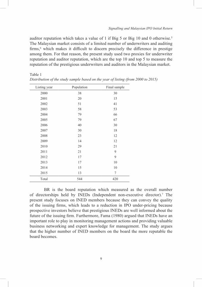
Table 1 summarises the distribution of both the IPOs collected for this study (population) as well as the IPOs used in the final sample. The distribution of the population and the final sample are established based on the year of listing.
A cross-sectional regression model is applied to assess the impact of the five signalling variables on initial return, in the following form:
IR = α + β1SHRTNi + β2LPi + β3URi + β4ARi + β5BRi + β6OFFSZi + β7OSRi + β8PRIVi + β9MKTCONi + εi
(1)
where IR is the primary initial return, which is calculated by finding the percentage change in the issue price from the offer price to the opening price of the first day, SHRTN is the shareholder retention ratio which represents the percentage of shares that the insiders of the firm remain to hold after the firm went public, LP is the lock-up period that is calculated by taking the natural log of lockup length for every IPO firm (in days), UR is the dummy variable for underwriter reputation takes a value of 1 if Big 5 or Big 10 and 0 otherwise, is the dummy variable of
Signalling and Malaysian IPO Initial Return
9
auditor reputation which takes a value of 1 if Big 5 or Big 10 and 0 otherwise.5 The Malaysian market consists of a limited number of underwriters and auditing firms,6 which makes it difficult to discern precisely the difference in prestige among them. For that reason, the present study used two proxies for underwriter reputation and auditor reputation, which are the top 10 and top 5 to measure the reputation of the prestigious underwriters and auditors in the Malaysian market.
Table 1Distribution of the study sample based on the year of listing (from 2000 to 2015)
Listing year Population Final sample
2000 38 302001 20 152002 51 412003 58 532004 79 662005 79 672006 40 302007 30 182008 23 122009 14 122010 29 212011 21 92012 17 92013 17 102014 15 102015 13 7
Total 544 420
BR is the board reputation which measured as the overall number of directorships held by INEDs (Independent non-executive director).7 The present study focuses on INED members because they can convey the quality of the issuing firms, which leads to a reduction in IPO under-pricing because prospective investors believe that prestigious INEDs are well informed about the future of the issuing firm. Furthermore, Fama (1980) argued that INEDs have an important role to play in monitoring management actions and providing valuable business networking and expert knowledge for management. The study argues that the higher number of INED members on the board the more reputable the board becomes.
Ali Albada et al.
10
The present study has four control variables, which are OFFSZ is the natural log of offer-size which indicates the supply of IPOs, OSR can be used as a measure of investors’ demand on IPOs because it can indicate the amount of times the IPO is oversubscribed, PRIV is the institutional investor involvement that takes a value of 1 to represent firms with private placement and zero otherwise, and MKTCON is the market condition that takes EMAS Index as a proxy for listed firms on the Main Market and ACE as well since it provides a wider coverage of the Malaysian market.8
The present study is also interested in knowing the dominant signals in explaining the initial return. For that reason, the stepwise regression is implemented by the current study because of its ability to identify the contribution order of the independent variables to the overall model. Furthermore, the stepwise regression method can develop a regression model with the least number of statistically significant independent variables that also have the highest predictive accuracy (Yong, 2015).
RESULTS
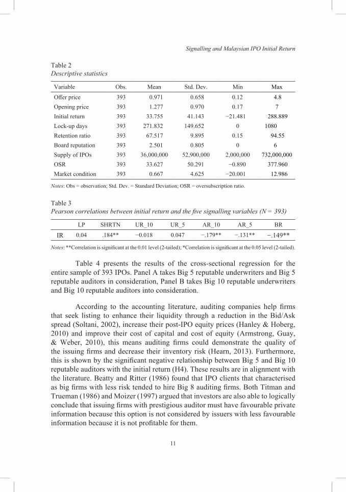
The descriptive statistics in Table 2 are based on the final sample of 393 IPOs.9 The average initial return is about 33.7% this value is slightly higher than the 26.34% average offer-to-open initial return covering the period from 2001 to 2009 in Yong (2011) and 29% average initial return for the period of 2000 to 2012 in Mohd Rashid et al. (2014); but very close to 30% average initial return covering the period from 2003 to 2008 in Abdul-Rahim, Sapian, Yong and Auzairy (2013) and 30.83% average initial return for the period from 2000 to 2007 in Low and Yong (2011).
Table 3 presents the correlation between the initial return and the five signalling variables. The correlation table can provide a prediction of what to be expected from the regression analysis. Starting with the independent variable shareholder retention ratio is expected to have a significant positive relationship with the initial return. Furthermore, the Big 5 reputable auditors, Big 10 reputable auditors and board reputation are expected to have a significant negative relationship with the initial return. However, the lock-up period is not expected to have a significant relationship with the initial return. Finally, the Big 5 reputable underwriters and Big 10 reputable underwriters are not expected to have a significant relationship with the initial return.
Signalling and Malaysian IPO Initial Return
11
Table 2Descriptive statistics
Variable Obs. Mean Std. Dev. Min Max
Offer price 393 0.971 0.658 0.12 4.8Opening price 393 1.277 0.970 0.17 7Initial return 393 33.755 41.143 −21.481 288.889Lock-up days 393 271.832 149.652 0 1080Retention ratio 393 67.517 9.895 0.15 94.55Board reputation 393 2.501 0.805 0 6Supply of IPOs 393 36,000,000 52,900,000 2,000,000 732,000,000OSR 393 33.627 50.291 −0.890 377.960Market condition 393 0.667 4.625 −20.001 12.986
Notes: Obs = observation; Std. Dev. = Standard Deviation; OSR = oversubscription ratio.
Table 3Pearson correlations between initial return and the five signalling variables (N = 393)
LP SHRTN UR_10 UR_5 AR_10 AR_5 BR
IR 0.04 .184** −0.018 0.047 −.179** −.131** −.149**
Notes: **Correlation is significant at the 0.01 level (2-tailed); *Correlation is significant at the 0.05 level (2-tailed).
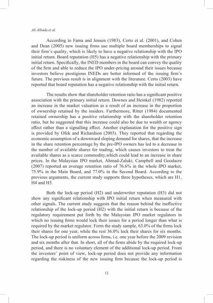
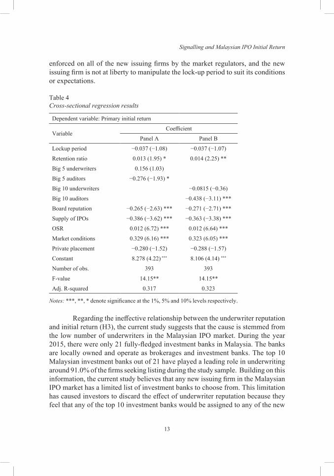
Table 4 presents the results of the cross-sectional regression for the entire sample of 393 IPOs. Panel A takes Big 5 reputable underwriters and Big 5 reputable auditors in consideration, Panel B takes Big 10 reputable underwriters and Big 10 reputable auditors into consideration.
According to the accounting literature, auditing companies help firms that seek listing to enhance their liquidity through a reduction in the Bid/Ask spread (Soltani, 2002), increase their post-IPO equity prices (Hanley & Hoberg, 2010) and improve their cost of capital and cost of equity (Armstrong, Guay, & Weber, 2010), this means auditing firms could demonstrate the quality of the issuing firms and decrease their inventory risk (Hearn, 2013). Furthermore, this is shown by the significant negative relationship between Big 5 and Big 10 reputable auditors with the initial return (H4). These results are in alignment with the literature. Beatty and Ritter (1986) found that IPO clients that characterised as big firms with less risk tended to hire Big 8 auditing firms. Both Titman and Trueman (1986) and Moizer (1997) argued that investors are also able to logically conclude that issuing firms with prestigious auditor must have favourable private information because this option is not considered by issuers with less favourable information because it is not profitable for them.
Ali Albada et al.
12
According to Fama and Jensen (1983), Certo et al. (2001), and Cohen and Dean (2005) new issuing firms use multiple board memberships to signal their firm’s quality, which is likely to have a negative relationship with the IPO initial return. Board reputation (H5) has a negative relationship with the primary initial return. Specifically, the INED members in the board can convey the quality of the firm and able to reduce the IPO under-pricing around their issues because investors believe prestigious INEDs are better informed of the issuing firm’s future. The previous result is in alignment with the literature. Certo (2003) have reported that board reputation has a negative relationship with the initial return.
The results show that shareholder retention ratio has a significant positive association with the primary initial return. Downes and Heinkel (1982) reported an increase in the market valuation as a result of an increase in the proportion of ownership retained by the insiders. Furthermore, Ritter (1984) documented retained ownership has a positive relationship with the shareholder retention ratio, but he suggested that this increase could also be due to wealth or agency effect rather than a signalling effect. Another explanation for the positive sign is provided by Ofek and Richardson (2003). They reported that regarding the economic assumption of a downward sloping demand for shares, that the increase in the share retention percentage by the pre-IPO owners has led to a decrease in the number of available shares for trading, which causes investors to treat the available shares as a scarce commodity,which could lead to an increase in share prices. In the Malaysian IPO market, Ahmad-Zaluki, Campbell and Goodacre (2007) reported an average retention ratio of 76.6% in the whole IPO market, 75.9% in the Main Board, and 77.0% in the Second Board. According to the previous arguments, the current study supports three hypotheses, which are H1, H4 and H5.
Both the lock-up period (H2) and underwriter reputation (H3) did not show any significant relationship with IPO initial return when measured with other signals. The current study suggests that the reason behind the ineffective relationship of the lock-up period (H2) with the initial return is because of the regulatory requirement put forth by the Malaysian IPO market regulators in which no issuing firms would lock their issues for a period longer than what is required by the market regulator. Form the study sample, 63.0% of the firms lock their shares for one year, while the rest 36.0% lock their shares for six months. The lock-up period is uniform across firms, i.e. one year before the 2009 revision and six months after that. In short, all of the firms abide by the required lock-up period, and there is no voluntary element of the additional lock-up period. From the investors’ point of view, lock-up period does not provide any information regarding the riskiness of the new issuing firm because the lock-up period is
Signalling and Malaysian IPO Initial Return
13
enforced on all of the new issuing firms by the market regulators, and the new issuing firm is not at liberty to manipulate the lock-up period to suit its conditions or expectations.
Table 4Cross-sectional regression results
Dependent variable: Primary initial return
VariableCoefficient
Panel A Panel B
Lockup period −0.037 (−1.08) −0.037 (−1.07)
Retention ratio 0.013 (1.95) * 0.014 (2.25) **
Big 5 underwriters 0.156 (1.03)
Big 5 auditors −0.276 (−1.93) *
Big 10 underwriters −0.0815 (−0.36)
Big 10 auditors −0.438 (−3.11) ***
Board reputation −0.265 (−2.63) *** −0.271 (−2.71) ***
Supply of IPOs −0.386 (−3.62) *** −0.363 (−3.38) ***
OSR 0.012 (6.72) *** 0.012 (6.64) ***
Market conditions 0.329 (6.16) *** 0.323 (6.05) ***
Private placement −0.280 (−1.52) −0.288 (−1.57)
Constant 8.278 (4.22) *** 8.106 (4.14) ***
Number of obs. 393 393
F-value 14.15** 14.15**
Adj. R-squared 0.317 0.323
Notes: ***, **, * denote significance at the 1%, 5% and 10% levels respectively.
Regarding the ineffective relationship between the underwriter reputation and initial return (H3), the current study suggests that the cause is stemmed from the low number of underwriters in the Malaysian IPO market. During the year 2015, there were only 21 fully-fledged investment banks in Malaysia. The banks are locally owned and operate as brokerages and investment banks. The top 10 Malaysian investment banks out of 21 have played a leading role in underwriting around 91.0% of the firms seeking listing during the study sample. Building on this information, the current study believes that any new issuing firm in the Malaysian IPO market has a limited list of investment banks to choose from. This limitation has caused investors to discard the effect of underwriter reputation because they feel that any of the top 10 investment banks would be assigned to any of the new
Ali Albada et al.
14
issues. Furthermore, the lack of international investment banks in the Malaysian market has led to an absence of competition between the investment banks, since all of the investments banks in the Malaysian IPO market are locally owned. Moreover, Jelic et al. (2001) suggested that the absence of statistical significance may also point toward a lack of competitive pressure between underwriters in the Malaysian market.
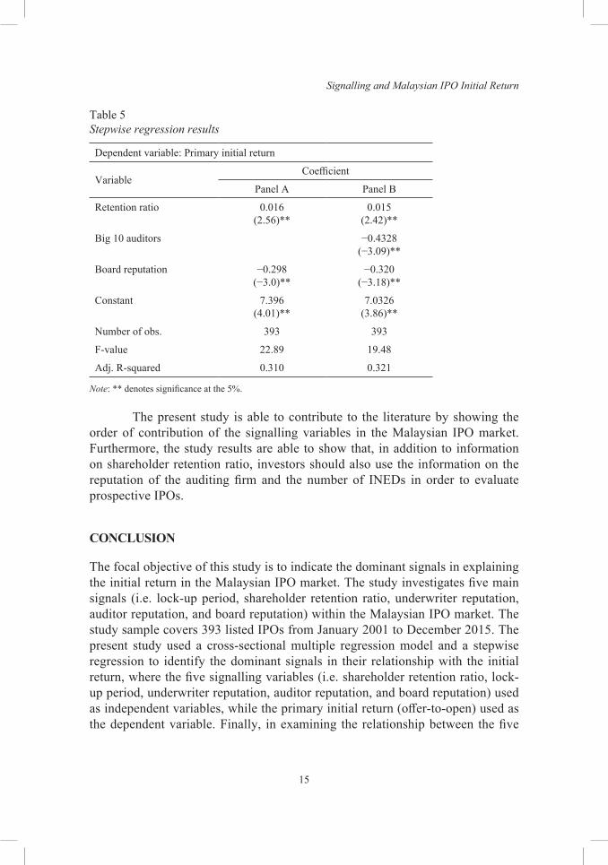
The current study uses the stepwise regression to know the order of contribution of the signalling variables to the initial return. Table 5 shows the results of the stepwise regression, where Panel A shows the results of taking Big 5 reputable underwriters and Big 5 reputable auditors in consideration and Panel B takes Big 10 reputable underwriters and Big10 reputable auditors into consideration. The present study employs the stepwise regression due to its ability to develop a regression model that includes only the statistically significant independent variables. Furthermore, the stepwise regression is able to introduce the independent variables in the model in the order of their statistical significance, from the highest predictability accuracy to the lowest, which will be helpful in achieving the objective of the current study of determining the order of contribution of the study signalling variables.
Table 5 shows that the stepwise regression is able to produce the same results obtained by the cross-sectional regression in Table 4, plus the stepwise regression is also able to drop the independent variables that do not have a statistical significance with the dependent variable, which are underwriter reputation, lock-up period. The results in Table 5 shows that both reputable auditors and board reputation still have a negative relationship with the initial return, while shareholder retention ratio still has a positive relationship with the initial return. The extra information that the stepwise regression is able to introduce is the order of contribution of the study signalling variables, where shareholder retention ratio has the highest statistical significance in its relationship with the initial return. This means that prospective investors should keep a vigilant eye on the percentage retained by the original owners of the listing firm because higher percentage can be construed as: (1) the original owners have faith in the future of the company and its quality; and (2) the listed company will have high the initial return during the first-day of listing. Moreover, the results in Table 5 shows that the second place goes to the reputation of the auditing firm followed by the reputation of the board which is represented by the number of INEDs in the board.
Signalling and Malaysian IPO Initial Return
15
Table 5Stepwise regression results
Dependent variable: Primary initial return
VariableCoefficient
Panel A Panel B
Retention ratio 0.016 (2.56)**
0.015 (2.42)**
Big 10 auditors −0.4328 (−3.09)**
Board reputation −0.298 (−3.0)**
−0.320 (−3.18)**
Constant 7.396 (4.01)**
7.0326 (3.86)**
Number of obs. 393 393
F-value 22.89 19.48
Adj. R-squared 0.310 0.321
Note: ** denotes significance at the 5%.
The present study is able to contribute to the literature by showing the order of contribution of the signalling variables in the Malaysian IPO market. Furthermore, the study results are able to show that, in addition to information on shareholder retention ratio, investors should also use the information on the reputation of the auditing firm and the number of INEDs in order to evaluate prospective IPOs.
CONCLUSION
The focal objective of this study is to indicate the dominant signals in explaining the initial return in the Malaysian IPO market. The study investigates five main signals (i.e. lock-up period, shareholder retention ratio, underwriter reputation, auditor reputation, and board reputation) within the Malaysian IPO market. The study sample covers 393 listed IPOs from January 2001 to December 2015. The present study used a cross-sectional multiple regression model and a stepwise regression to identify the dominant signals in their relationship with the initial return, where the five signalling variables (i.e. shareholder retention ratio, lock-up period, underwriter reputation, auditor reputation, and board reputation) used as independent variables, while the primary initial return (offer-to-open) used as the dependent variable. Finally, in examining the relationship between the five
Ali Albada et al.
16
signals and initial return, the present study took into account four control variables (i.e. private placement, offer size, demand [OSR], and market conditions) due to their significant relationship with initial return as empirically documented by the Malaysian literature (Abdul-Rahim, Che Embi, & Yong, 2012; Abdul-Rahim & Yong, 2010; Agarwal, Liu, & Rhee, 2008).
The statistical analysis shows that the average initial return is about 33.7% for primary initial return. The result is in alignment with the average initial return calculated by recent scholars such as Abdul-Rahim et al. (2013) and Low and Yong (2011). On the other hand, the regression analysis shows that three out of five signals reported a statistically significant relationship with the initial return; the signals are shareholder retention ratio, auditor reputation, and board reputation. This significant association indicates that these signals contain certain information to investors and have an important impact on the initial return. Moreover, the current study is also interested in knowing the ranking of those signals in explaining the initial return. For that reason, the stepwise regression is implemented by the current study because of its ability to identify the order of contribution of the signalling variables to the initial return. The results of the stepwise regression show that shareholder retention ratio is ranked first followed by auditor reputation and board reputation.
Issuing firms are obligated to release their information through the prospectus, which is used by prospective investors to evaluate IPOs and help them in their decision-making process. However, the investor’s judgment can be easily clouded by the amount of information available to them through the prospectus. Therefore, the investor needs to be selective in choosing the information that relevant in explaining the initial return. The present study is based upon the argument that some of the information disclosed by prospectuses is important in helping prospective investors in evaluating IPOs. Therefore, such information should be given a higher prioritisation by prospective investors who are seeking an investment in the IPO market.
The results of the present study show that shareholder retention ratio, auditor reputation, and board reputation are significant in explaining the initial return. The findings imply that such information is important in determining the initial return in the Malaysian IPO market. Therefore, it is reasonable to suggest that information regarding these signals must be clearly disclosed to the investors because current disclosure practice in Malaysia only embeds information concerning these variables in bits and pieces of other seemingly standard information.
Signalling and Malaysian IPO Initial Return
17
The results of the present study show that the lock-up period has no relationship with the initial return. The study suggests that the reason behind this it is due to the mandatory regulations enforced on the new issuing firms regarding the lock-up period, where the new issuing firms are mandated to have a lock-up period of one year or six months after the amendments of 2009. According to Brav and Gompers (2003) and Mohan and Chen (2002), the lock-up period is used by the issuing firm to signal its risk to the market, because investors interpreted the lock-up period as a commitment by major shareholders who believes in the future of the listing firm; and subsequently, such listing firm is expected to have higher initial return for a firm with a longer lock-up period. The present study suggests that for the lock-up period to be able to implement such functionality in the market, the regulatory body in the Malaysian market should relax the regulations around the lock-up period, by providing the new issuing firm with the opportunity to express themselves to future investors through implementing the lock-up period that reflects their quality. The current study suggests that relaxing the regulations regarding the lock-up period could help investors to make better investment decisions regarding the new issuing firms they want to invest in.
The study results also show that underwriter reputation is not significant in explaining the initial return. The lack of statistical significance is caused by the lack of competitive pressure between underwriters in the Malaysian market (Jelic et al. 2001). The study results have shown that the Big 10 reputable underwriters have underwritten more than 90.0% of the study sample. Furthermore, the Malaysian market consists of only 21 investment banks and all of them are locally owned. The current study suggests that the regulatory body in the Malaysian market should open the door for new underwriters to enter the Malaysian IPO market, especially foreign underwriters. Such changes can increase the competitive pressure in the Malaysian underwriting market and turn back underwriter reputation for being a useful signal for investors to determine potential investment decisions.
Overall, the results of the present study provide a new insight for investors regarding the importance of the information in the prospectus when making informed investment decisions about IPOs. Although the initial return is getting lower in the recent years, shying away from the IPO market may present a great opportunity cost to the investors, as documented in the present study. The Malaysian IPOs are still providing a much higher return than secondary stocks in general. In short, as long as investors know which information about the firms and the market is important, they should continue to participate in the IPO market and not behave irrationally.
Ali Albada et al.
18
NOTES
1. Hemmer and Bardhan (2000) argued that the low levels of institutional development in the Asian countries are caused by the following: (1) the traditional institutions of exchange in developing countries often did not evolve into more complex (impersonal, open, legal rational) rules or institutions of enforcement as in early modern Europe; (2) the institutional arrangements of a society are often the outcome of strategic distributive conflicts among different social groups, and inequality in the distribution of power and resources can sometimes block the rearrangement of these institutions in ways that are conducive to over-all development.
2. La Porta et al. (2000) refered to investor protections: as the ability of the legal system, meaning both laws and their enforcement, to protect outside investors – whether shareholders or creditors from insiders. Moreover, they showed the effect of investor protections on expanding the financial markets, on facilitating external financing of new firms, on moving away from concentrated ownership, and on improving the efficiency of investment allocation.
3. Rock (1986) argued that the uninformed investors are always faced with the winner’s curse, which allows uninformed investors to always get the shares they ask for because these shares are ignored (not wanted) by the informed investors (institutional investors). Thus, uninformed investors are faced with adverse selection problem due to the bias in the allocation of IPOs (Yong, 2011), which could help in increasing the levels of information asymmetry in the Malaysian IPOs market.
4. Such as restricted offer-for-sale, restricted public issue, restricted offer-for-sale to eligible employees, restricted offer-for-sale to Bumiputra (Malays and indigenous people) investors, special and restricted issues to Bumiputra investors, tender offers, and special issues.
5. The study measures underwriter and auditor reputation through the proportion of the number of issues an investment bank (auditing firm) have underwritten (audited) as lead manager (lead auditor), and this method has been used by Jelic et al. (2001), Dimovski et al. (2011) to measure underwriter reputation, by Megginson and Weiss (1991) to measure auditor reputation.
6. Big 10 underwriter covered 91% of IPOs, Big 5 underwriters covered 90% of IPOs, Big 10 auditors 72% of IPOs, and Big 5 auditors covered 62% of IPOs.
7. The board of a public-listed company (PLC) consists of different types of directors. The non-executive directors (NED) have the role of critical oversight and can also be considered as the last line of defence against decisions that go against the best interest of the company. The NED consists of two groups, which are independent NED (INED) and the non-independent NED (NINED) groups. The main focus of the study is INED because the Bursa Malaysia Securities Berhad has a set of criteria that define INED, which outlined in its listing requirements. The purpose of such criteria is to guard against relationships and transactions that may impair the director’s independence.
8. The EMAS Index is a capitalisation weighted index. The index comprises the large and mid cap constituents of the FTSE Bursa Malaysia 100 Index and the FTSE Bursa Malaysia Small Cap Index. The index was developed with a base value of 6,000 as of 31 March, 2006.
Signalling and Malaysian IPO Initial Return
19
9. The present study removes extreme outliers using studentised residuals (Ruppert, 2004), DFITS and Cooks (Rahman, Sathik, & Kannan, 2012). As suggested by Ryan (2008), DFITS and Cooks allow for the simultaneous detection of both extreme outliers and influential observations. The rule of thumb is to remove outliers only if the outliers are also influential because the outliers will be able to influence the regression model only in such cases. The current study deletes 27 IPO extreme outliers, reducing the sample from 420 to 393 new issues.
REFERENCES
Abdul-Rahim, R., & Yong, O. (2010). Initial returns of Malaysian IPOs and Shari’a compliant status. Journal of Islamic Accounting and Business Research, 1(1), 60–74. https://doi.org/10.1108/17590811011033415
Abdul-Rahim, R., Che Embi, N. A., & Yong, O. (2012). Winner’s curse and IPO initial performance: New evidence from Malaysia. International Journal of Business and Management Studies, 4(2), 151–159.
Abdul-Rahim, R., Sapian, R. Z. Z., Yong, O., & Auzairy, N. A. (2013). Flipping activity and subsequent after-market trading in Malaysian initial public offerings (IPOs). Asian Academy of Management Journal of Accounting and Finance, 9(1), 113–128.
Agarwal, S., Liu, C., & Rhee, S. G. (2008). Investor demand for IPOs and after-market performance: Evidence from the Hong Kong stock market. Journal of International Financial Markets Institutions and Money, 18(2), 176–190. https://doi.org/10.1016/j.intfin.2006.09.001
Ahmad-Zaluki, N. A., Campbell, K., & Goodacre, A. (2007). The long-run share price performance of Malaysian initial public offerings (IPOs). Journal of Business Finance and Accounting, 34(1–2), 78–110. https://doi.org/10.1111/j.1468-5957.2006.00655.x
Allen, F., & Faulhaber, G. R. (1989). Signalling by under-pricing in the IPO market. Journal of Financial Economics, 23(2), 303–323. https://doi.org/10.1016/0304-405X(89)90060-3
Ammer, M. A., & Ahmad-Zaluki, N. A. (2016). The effect of underwriter's market share, spread and management earnings forecasts bias and accuracy on under-pricing of Malaysian IPOs. International Journal of Managerial Finance, 12(3), 351–371. https://doi.org/10.1108/IJMF-12-2014-0187
Armstrong, C. S., Guay, W. R., & Weber, J. P. (2010). The role of information and financial reporting in corporate governance and debt contracting. Journal of Accounting and Economics, 50(2–3), 179–234. https://doi.org/10.1016/j.jacceco.2010.10.001
Beatty, R. P., & Ritter, J. R. (1986). Investment banking, reputation, and the under-pricing of initial public offerings. Journal of Financial Economics, 15(1–2), 213–232. https://doi.org/10.1016/0304-405X(86)90055-3
Bessembinder, H., Hao, J. I. A., & Zheng, K. (2015). Market making contracts, firm value, and the IPO decision. Journal of Finance, 70(5), 1997–2028. https://doi.org/10.1111/jofi.12285
Ali Albada et al.
20
Bhabra, H. S., & Pettway, R. H. (2003). IPO prospectus information and subsequent performance. Financial Review, 38(3), 369–397. https://doi.org/10.1111/1540-6288.00051
Boulton, T. J., Smart, S. B., & Zutter, C. J. (2017). Conservatism and international IPO under- pricing. Journal of International Business Studies, 48(6), 763–785. https://doi.org/10.1057/s41267-016-0054-8
Bradley, D. J., & Jordan, B. D. (2002). Partial adjustment to public information and IPO under-pricing. Journal of Financial and Quantitative Analysis, 37(4), 595–616. https://doi.org/10.2307/3595013
Brav, A., & Gompers, P. A. (2003). The role of lock-ups in initial public offerings. Review of Financial Studies, 16(1), 1–29. https://doi.org/10.1093/rfs/16.1.0001
Butler, A. W., Connor, M. O., & Kieschnick, R. (2014). Robust determinants of IPO under-pricing and their implications for IPO research. Journal of Corporate Finance, 27(1), 367–383. https://doi.org/10.1016/j.jcorpfin.2014.06.002
Certo, S. T. (2003). Influencing initial public offering investors with prestige: Signalling with board structures. Academy of Management Review, 28(3), 432–446. https://doi.org/10.5465/amr.2003.10196754
Certo, S. T., Daily, C. M., & Dalton, D. R. (2001). Signalling firm value through board structure: An investigation of initial public offerings. Entrepreneurship: Theory and Practice, 26(2), 33– 50.
Clarkson, P. M., Dontoh, A., Richardson, G., & Sefcik, S. E. (1991). Retained ownership and the valuation of initial public offerings: Canadian evidence. Contemporary Accounting Research, 8(1), 115–131. https://doi.org/10.1111/j.1911-3846.1991.tb00838.x
Cohen, B. D., & Dean, T. J. (2005). Information asymmetry and investor valuation of IPOs: Top management team legitimacy as a capital market signal. Strategic Management Journal, 26(7), 683–690. https://doi.org/10.1002/smj.463
Courteau, L. (1995). Under-diversification and retention commitments in IPOs. Journal of Financial and Quantitative Analysis, 30(4), 487–517. https://doi.org/10. 2307/2331274
Dimovski, W., & Brooks, R. (2008). The under-pricing of gold mining initial public offerings. Research in International Business and Finance, 22(1), 1–16. https://doi.org/10.1016/j.ribaf.2006.11.002
Dimovski, W., Philavanh, S., & Brooks, R. (2011). Underwriter reputation and under-pricing: Evidence from the Australian IPO market. Review of Quantitative Finance and Accounting, 37(4), 409–426. https://doi.org/10.1007/s11156-010-0211-2
Downes, D. H., & Heinkel, R. (1982). Signalling and the valuation of unseasoned new issues: A comment. Journal of Finance, 37(1), 1–10. https://doi.org/10. 1111/j.1540-6261.1982.tb01091.x
Espenlaub, S., & Tonks, I. (1998). Post-IPO directors’ sales and reissuing activity: An empirical test of IPO signalling models. Journal of Business Finance and Accounting, 25(9–10), 1037–1079.
Fama, E. F. (1980). Agency problems and the theory of the firm. Journal of Political Economy, 88(2), 288–307. https://doi.org/10.1086/260866
Signalling and Malaysian IPO Initial Return
21
Fama, E. F., & Jensen, M. C. (1983). Separation of ownership and control. Journal of Law and Economics, 26(2), 301–325. https://doi.org/10.1086/467037
Habib, M. A., & Ljungqvist, A. P. (2001). Under-pricing and entrepreneurial wealth losses in IPOs: Theory and evidence. Review of Financial Studies, 14(2), 433–458. https://doi.org/10.1093/rfs/14.2.433
Handa, R., & Singh, B. (2017). Performance of Indian IPOs: An empirical analysis. Global Business Review, 18(3), 734–749.
Hanley, K. W., & Hoberg, G. (2010). The information content of IPO prospectuses. Review of Financial Studies, 23(7), 2821–2864. https://doi.org/10.1093/rfs/hhq024
Hearn, B. (2013). The determinants of IPO firm prospectus length in Africa. Review of Development Finance, 3(2), 84–98. https://doi.org/10.1016/j.rdf.2013.04.002
Hemmer, H. R., & Bardhan, P. (2000). Understanding under-development: Challenges for institutional economics from the point of view of poor countries. Journal of Institutional and Theoretical Economics-Zeitschrift Fur Die Gesamte Staatswissenschaft, 156(1), 216– 235.
How, J., Jelic, R., Saadouni, B., & Verhoeven, P. (2007). Share allocations and performance of KLSE second board IPOs. Pacific-Basin Finance Journal, 15(3), 292–314. https://doi.org/10.1016/j.pacfin.2006.09.002
Jelic, R., Saadouni, B., & Briston, R. (2001). Performance of Malaysian IPOs: Underwriters reputation and management earnings forecasts. Pacific-Basin Finance Journal, 9(5), 457– 486. https://doi.org/10.1016/S0927-538X(01)00013-0
Kang, S. K., Kang, H. C., Kim, J., & Kim, N. (2015). Insiders’ pre-IPO ownership, under-pricing, and share-selling behaviour: Evidence from Korean IPOs. Emerging Markets Finance and Trade, 51(3), 66–84. https://doi.org/10.1080/1540496X.2015.1039902
Keasey, K., & Short, H. (1997). Equity retention and initial public offerings: The influence of signalling and entrenchment effects. Applied Financial Economics, 7(1), 75–85. https://doi.org/10.1080/096031097333862
Kenourgios, D. F., Papathanasiou, S., & Melas, E. R. (2007). Initial performance of Greek IPOs, underwriter’s reputation and oversubscription. Managerial Finance, 33(5), 332–343. https://doi.org/10.1108/03074350710739614
Khurana, I., Ni, C., & Shi, C. (2017). The role of big 4 auditors in the global primary market: Does audit quality matter most when investors are protected least? Paper presented at The Asian Bureau of Finance and Economic Research (ABFER) 5th Annual Conference, Shangri-La Hotel, Singapore, 22–25 May.
La Porta, R., Lopez-de-Silanes, F., Shleifer, A., & Vishny, R. (2000). Investor protection and corporate governance. Journal of Financial Economics, 58(1–2), 3–27. https://doi.org/10.1016/S0304-405X(00)00065-9
Leland, H. E., & Pyle, D. H. (1977). Informational asymmetries, financial structure, and financial intermediation. Journal of Finance, 32(2), 371–387. https://doi.org/10.2307/2326770
Logue, D. E. (1973). On the pricing of unseasoned equity issues: 1965–1969. Journal of Financial and Quantitative Analysis, 8(1), 91–103. https://doi.org/10. 2307/2329751
Ali Albada et al.
22
Low, S. W., & Yong, O. (2011). Explaining over-subscription in fixed-price IPOs: Evidence from the Malaysian stock market. Emerging Markets Review, 12(3), 205–216. https://doi.org/10.1016/j.ememar.2011.03.003
Megginson, L., & Weiss, A. (1991). Venture capitalist certification in initial public offerings. Journal of Finance, 46(3), 879–903. https://doi.org/10.1111/j.1540-6261.1991.tb03770.x
Michaely, R., & Shaw, W. H. (1994). The pricing of initial public offerings: Tests of adverse-selection and signalling theories. Review of Financial Studies, 7(2), 279–319. https://doi.org/10.1093/rfs/7.2.279
Michaely, R., & Shaw, W. H. (1995). Does the choice of auditor convey quality in an initial public offering? Journal of the Financial Management Association, 24(4), 15–30. https://doi.org/10.2307/3665948
Mohan, N. J., & Chen, C. R. (2002). Information content of lock-up provisions in initial public offerings. International Review of Economics and Finance, 10(1), 41–59. https://doi.org/10.1016/S1059-0560(00)00070-8
Mohd Rashid, R., Abdul-Rahim, R., & Yong, O. (2014). The influence of lock-up provisions on IPO initial returns: Evidence from an emerging market. Economic Systems, 38(4), 487–501. https://doi.org/10.1016/j.ecosys.2014.03.003
Moizer, P. (1997). Auditor reputation: The international empirical evidence. International Journal of Auditing, 1(1), 61–74.
Neuberger, B. M., & Chapelle, C. A. L. (1983). Unseasoned new issue price performance on three tiers: 1975–1980. Financial Management, 12(3), 23–28. https://doi.org/10.2307/3665513
Ofek, E., & Richardson, M. (2003). Dotcom mania: The rise and fall of Internet stock prices. Journal of Finance, 58(3), 1113–1137. https://doi.org/10.1111/1540-6261.00560
Paudyal, K., Saadouni, B., & Briston, R. J. (1998). Privatisation initial public offerings in Malaysia: Initial premium and long-term performance. Pacific-Basin Finance Journal, 6(5), 427– 451. https://doi.org/10.1016/S0927-538X(98)00018-3
Rahman, S. M. A. K., Sathik, M. M., & Kannan, K. S. (2012). Multiple linear regression models in outlier detection. International Journal of Research in Computer Science, 2(2), 23–28. https://doi.org/10.7815/ijorcs.22.2012.018
Ritter, J. R. (1984). Signalling and the valuation of unseasoned new issues: A comment. Journal of Finance, 39(4), 1231–1237. https://doi.org/10.1111/j.1540-6261.1984.tb03907.x
Rock, K. (1986). Why new issues are under-priced. Journal of Financial Economics, 15(1–2), 187– 212. https://doi.org/10.1016/0304-405X(86)90054-1
Rumokoy, L. J., Neupane, S., Chung, R. Y., & Vithanage, K. (2017). Underwriter network structure and political connections in the Chinese IPO market. Pacific-Basin Finance Journal. Available online 7 November 2017. https://www.sciencedirect.com/science/article/pii/S0927538X16302451
Ruppert, D. (2004). Statistics and finance an introduction. New York: Springer.Ryan, T. P. (2009). Modern regression methods. (2nd ed.). Hoboken, NJ: Wiley.
Signalling and Malaysian IPO Initial Return
23
Soltani, B. (2002). Timeliness of corporate and audit reports: Some empirical evidence in the French context. International Journal of Accounting, 37(1), 215–246. https://doi.org/10.1016/S0020-7063(02)00152-8
Spence, M. (1973). Job market signalling. Quarterly Journal of Economics, 87(3), 355–374. https://doi.org/10.2307/1882010
Sundarasen, S. D., Khan, A., & Rajangam, N. (2017). Signalling roles of prestigious auditors and underwriters in an emerging IPO market. Global Business Review, 19(1), 69–84. https://doi.org/10.1177/0972150917713367
Titman, S., & Trueman, B. (1986). Information quality and the valuation of new issues. Journal of Accounting and Economics, 8(2), 159–172. https://doi.org/ 10.1016/0165-4101(86)90016-9
Tong L. Y., & Ahmad, R. (2015). The signalling power of the investment banks’ reputation on the performance of IPOs on Bursa Malaysia. Jurnal Pengurusan, 45(1), 1–16.
Wan-Hussin, W. N. (2005). The effects of owners’ participation and lock-up on IPO under- pricing in Malaysia. Asian Academy of Management Journal, 10(1), 19–36.
Welch, I. (1989). Seasoned offerings, imitation costs, and the under-pricing of initial public offerings. Journal of Finance, 44(2), 421–449. https://doi.org/ 10.1111/j.1540-6261.1989.tb05064.x
Wong, W. C., Ong, S. E., & Ooi, J. T. L. (2013). Sponsor backing in Asian REIT IPOs. Journal of Real Estate Finance and Economics, 46(2), 299–320. https://doi.org/ 10.1007/s11146-011-9336-x
Xu, Z. Wang, L. and Long, J. (2017). The impact of directors' heterogeneity on IPO under- pricing. Chinese Management Studies, 11(2), 230–247. https://doi.org/10.1108/CMS-05-2016-0095
Yatim, P. (2011). Under-pricing and board structures: An investigation of Malaysian initial public offerings (IPOs). Asian Academy of Management Journal of Accounting and Finance, 7(1), 73–93.
Yong, O. (2007a). A review of IPO research in Asia: What’s next? Pacific-Basin Finance Journal, 15(3), 253–275. https://doi.org/10.1016/j.pacfin.2006.09.001
Yong, O. (2007b). Investor demand, size effect and performance of Malaysian initial public offerings: Evidence from post-1997 financial crisis. Journal Pengurusan, 26(1), 25–47.
Yong, O. (2011). Winner’s curse and bandwagon effect in Malaysian IPOs: Evidence from 2001–2009. Journal Pengurusan, 32(1), 21–26.
Yong, O. (2015). What is the “true” value of an initial public offering? Journal of Scientific Research and Development, 2(10), 78–85.
Yong, O., & Isa, Z. (2003). Initial performance of new issues of shares in Malaysia. Applied Economics, 35(8), 919–930. https://doi.org/10.1080/0003684022000020869
Zheng, S. X., Ogden, J. P., & Jen, F. C. (2005). Pursuing value through liquidity in IPOs: Under-pricing, share retention, lock-up, and trading volume relationships. Review of Quantitative Finance and Accounting, 25(3), 293–312. https://doi.org/10.1007/s11156-005-4769-z
AAMJAF Vol. 14, No. 2, 25–44, 2018
© Asian Academy of Management and Penerbit Universiti Sains Malaysia, 2018. This work is licensed under the terms of the Creative Commons Attribution (CC BY) (http://creativecommons.org/licenses/by/4.0/).
Asian Academy of Management Journal
of Accounting and Finance
IMPACT OF CHINA ON MALAYSIAN ECONOMY: EMPIRICAL EVIDENCE OF SIGN-RESTRICTED
STRuCTuRAL VECTOR AuTOREGRESSION (SVAR) MODEL
Mohd Azlan Shah Zaidi1, Zulkefly Abdul Karim1* and Zurina Kefeli @ Zulkefli2
1Center of Sustainable and Inclusive Development (SID), Faculty of Economics and Management, Universiti Kebangsaan Malaysia (UKM),
43600 Bangi, Selangor, Malaysia2Faculty of Economics and Muamalat, Universiti Sains Islam Malaysia (USIM),
Bandar Baru Nilai, 71800 Nilai, Negeri sembilan, Malaysia
*Corresponding author: [email protected]
ABSTRACT
China has been developing aggressively since its accession into the World Trade Organisation. Consequently, China has become one of the major trading partners to many countries in the world including Malaysia. To what extent China has affected Malaysian economy has been a hot issue facing the economists and practitioners. This paper examines the influence of China on Malaysian economic performances. Using structural vector autoregression (SVAR) methodology that takes into account the effect of other major trading partner countries such as the U.S., Japan and Singapore, the results indicate that different utilisation of foreign country variables to represent external sector in the model brings about different impact on domestic variables. It is shown that the U.S. is particularly important to affect domestic output while China is more important in influencing domestic inflation and the exchange rate, especially with regards to their respective income shocks. In addition, Singapore plays more dominant role in affecting domestic sector when foreign monetary policy shocks are considered. Japan is however more influential in affecting the exchange rate in some other shocks. While China is showing their dominance in the world economy, the study implies that knowing which country exactly affects which domestic
Published date: 31 December 2018
To cite this article: Zaidi, M. A. S., Karim, Z. A., & Kefeli, Z. (2018). Impact of China on Malaysian economy: Empirical evidence of sign-restricted structural vector autoregression (SVAR) model. Asian Academy of Management Journal of Accounting and Finance, 14(2), 25–44. https://doi.org/10.21315/aamjaf2018.14.2.2
To link to this article: https://doi.org/10.21315/aamjaf2018.14.2.2
Mohd Azlan Shah Zaidi et al.
26
variables is very crucial in mitigating the adverse impact of foreign policy change or shocks in the process of transforming Malaysia’s economy toward high income nation in the near future.
Keywords: foreign shocks, China, monetary policy, SVAR, sign restrictions
INTRODuCTION
Since its accession into the World Trade Organisation (WTO), China has been an important trading partner country to most of the developed and developing economies. For Malaysia, apart from the U.S., Japan and Singapore, the importance of China has become more apparent since the middle of 2000. China only accounted for 6% of the total trade of the four largest trading partner countries of Malaysia (U.S., Japan, Singapore and China) while U.S., Japan and Singapore contributed about 30% respectively at the end of 2000. The contribution of China increased significantly to 27% while the shares of Japan and Singapore decreased to 25% and 27% respectively at the end of 2010. The share of U.S., decreased significantly to 22% in the same period. At the end of 2016, the share of China increased to 35% and was the highest among the four countries. The Japan share of the total trade, nevertheless decreased significantly to around 18%. This indicates that China has increasingly and relatively become more important to Malaysia.
As a small and highly trade-dependent economy, it is undeniable that Malaysia’s economy would be vulnerable to a variety of external shocks such as world oil price, and foreign income and monetary policy shocks, especially from these four countries. To what extent China and others have influenced the Malaysia’s economy has been a major concern to investors, policy makers as well as the academicians. To maintain economic stability, understanding how the economy is affected by external shocks is crucial for Malaysia’s policy makers in making better policy formulation.
Most previous studies on the effect of foreign shocks on Malaysia mainly take into account the influence of the U.S. and Japan (see Ibrahim, 2005; Tang, 2006; Maćkowiak, 2006; and Zaidi, Karim, & Azman-Saini, 2013). As China has become more important to Malaysia’s economy, exclusion of the country in the Malaysian macro model might have made the impact of China shock on the Malaysian economy under estimated. Thus, the true consequences of the shock can only be verified by empirical research.
In view of this crucial matter, this paper investigates the effect of China on Malaysian economic performance. This is done by investigating the relative importance of China as well as other major trading partner countries, namely
Impact of China on Malaysian Economy
27
Singapore, U.S. and Japan, on Malaysian income and inflation. A structural autoregressive (SVAR) model with sign restrictions approach is utilised in evaluating the relative response of Malaysian income and inflation to China and other countries’ shocks. Furthermore, a sign restriction approach is employed in the identification strategy, as proposed by Uhlig (2005), whereby some impulse responses are constrained to follow economic theory while others are left unrestricted. Thus, some of the puzzles that normally appear in macroeconomic modeling can largely be avoided.
The results of the study indicate that different utilisation of foreign country variables to represent external sector in the model would bring about different impact on domestic variables. For example, the U.S. is particularly important to affect domestic output while China is more important in influencing domestic inflation. In addition, Singapore plays more dominant role in affecting domestic sector when foreign monetary policy shocks are considered. Japan is however more influential in affecting the exchange rate.
LITERATuRE REVIEW
Studies on foreign shock effect on a small open economics are numerous (see for example, Cushman & Zha, 1997; Dungey & Pagan, 2000; Dungey & Fry, 2003; Buckle, Kim, Kirkham & Sharma, 2007; Kim & Roubini, 2000; Kim, 2001; Canova, 2005; Maćkowiak, 2007; Zaidi et al., 2013; Zaidi & Karim, 2014; Othman, Yusop, Zaidi & Karim, 2015). Most of the studies find that foreign factors (foreign income and foreign monetary policy) play significant roles in influencing the domestic economy. Cushman and Zha (1997), for instance uncover that external shocks (U.S. income, U.S. inflation, U.S. federal fund rate, and world total commodity export prices) have become significant sources of domestic output fluctuations in Canada, whereas, domestic monetary policy shock (an increase in interest rates) has only a small contribution on output. Similarly, Dungey and Pagan (2000) find that international factors are generally a substantial contributor to Australian economy while domestic monetary policy contributes to stabilise economic activity, but the effect is not large. In New Zealand, Buckle et al. (2007) find that international business cycles and export and import prices fluctuations have been dominant influences to the New Zealand business cycle than international or domestic financial shocks.
Kim and Roubini (2000) study for G-7 countries conclude that foreign shocks (oil price shocks and the U.S. monetary policy) have contributed more to output fluctuations while in the most countries, domestic monetary policy is not the major contributor to output fluctuations. Similarly, Kim (2001) finds
Mohd Azlan Shah Zaidi et al.
28
that a U.S. monetary policy expansion has a positive spillover effect on the non-U.S. G-6 countries’ output. Applying a structural VAR model as in Kim (2001), Canova (2005) also finds that U.S. monetary policy shocks significantly affect the interest rates in Latin America. In addition, such external shocks are an important source of macroeconomic fluctuations in Latin America. For emerging market countries, Maćkowiak (2007) also unveils that external shocks have an important impact on their macroeconomic fluctuations. The U.S. monetary policy shocks, in particular, have strong and immediate effects upon emerging market interest rates and exchange rates.
Besides looking at the U.S. as the foreign factors, some studies take into account the effect of Japanese economy. Callen and McKibbin (2001), for example, analyse the effect of Japanese economy on Asia Pacific region. Their findings imply that Japanese monetary policy shocks will not have significant effect on the rest of the region. Coenen and Wieland (2003) on the other hand, examine the effect Japanese monetary policy shocks on the country’s main trading partners. Their findings reveal the Japanese monetary policy shocks have negative effect on its trading partner economies. Looking at the effect of Japanese monetary policy shock on the East Asia countries, Maćkowiak (2006) finds relatively modest effect of Japan’s monetary policy shock on real output, trade balances and exchange rates in East Asia.
Studies on the impact of China on other countries are relatively limited. Of particular interest are the Koźluk and Mehrotra (2009) and Johansson (2012) studies. Koźluk and Mehrotra (2009) examine the effect of China monetary policy on East and Southeast Asia and find that China monetary policy has importance consequence on real output in other countries in the region. Johansson (2012) on the other hand, looks at the potential transmission of China’s monetary policy shocks to equity markets in five Southeast Asian countries namely, Indonesia, Malaysia, Philippines, Singapore and Thailand. His results show some evidence of China’s growing influence in financial markets of the Southeast Asia.
As for Malaysia, study that looks specifically on China’s effect is rather limited. Besides Johansson (2012), most of the studies take into account U.S. or Japan or both as the foreign variables in the models (see Azali & Matthews, 1999; Ibrahim, 2005; Tang, 2006; Zaidi & Fisher, 2010; and Zaidi et al., 2013). Zaidi and Karim (2014) and Othman et al. (2015) add Singapore, other than U.S. and Japan economies as foreign factors to investigate the relative importance of U.S., Japan and Singapore on Malaysian economy and on Malaysians electronic and electrical (E & E) export demand respectively. Both studies find that Singapore is relative more important in influencing Malaysia’s economy. As China becomes more involved in Malaysia’s economy, investigating its impact is of important.
Impact of China on Malaysian Economy
29
A study by Dizioli, Guajardo, Klyuev, Mano and Raissi (2016) indicates that China’s growth slowdown would affect the countries with closer trade linkages with China (Malaysia, Singapore and Thailand) and net commodity exporters (Indonesia and Malaysia) the most.
Thus, based on this backdrop, this study adds to the existing literature especially for Malaysia case by employing a sign restricted SVAR technique to investigate further the impact of China effect on domestic economy. Unlike other previous studies, this study looks at relative importance of China and other important trading partner’s countries namely the U.S., Japan and Singapore in influencing Malaysian economy.
METHODOLOGY
This section describes the variables used in the model and the estimation procedures. Basically, there are four models to be estimated and each model consists of three foreign country variables and three domestic variables. The first model takes into account the U.S. variables to represent an external sector while the other three models take Japan, Singapore and China respectively to represent the foreign sector.
The variables in each model are divided into two blocks, namely the foreign and domestic blocks. The foreign block consists of oil price, foreign output, inflation and an interest rate, while the domestic block comprises real output, inflation, the interest rate and the real exchange rate. The foreign block is assumed to be block-exogenous to each of the domestic macroeconomic variable (see Cushman & Zha, 1997; and Zha, 1999). Thus, there are no contemporaneous or lagged effects from the domestic variables to the international variables.
For foreign output (Y*), industrial production index is used as a proxy, while foreign inflation (π*) is calculated by month-on-month change in consumer price index. Meanwhile, the foreign interest rates (i*) are measured by the Federal Funds rate for the U.S., the call money rate for Japan, the three month interbank rate for Singapore and the bank rate for China.1 For the internal block, the variables are industrial production index for aggregate output (Y), month-on-month percentage change in Consumer Index Price (CPI) for inflation (π), the interbank overnight money rate for the interest rate (i) and the real exchange rate of Malaysia, Singapore, U.S. and Japan for the exchange rate variable (e).
All variables are transformed into natural logs except for foreign and domestic inflation and both foreign and domestic policy interest rates.2 Data are taken from International Financial Statistics (IFS) database and various

Mohd Azlan Shah Zaidi et al.
30
publications of Monthly Statistical Bulletin of Bank Negara Malaysia (BNM). The sample period runs from 2000:1 until 2016:12, covering one global economic crisis of 2008/2009. Thus to capture the effect of the global economic recession, one dummy is used, Dummy for Global Crisis (DGC). DGC is set to equal to one from 2008:9 to 2009:12 and zero otherwise.
SVAR Models
Dynamic relationships for the selected economic variables in a SVAR approach are given by the following equation;
BY C L L L Y1 1
2
t kk
t tf fC C C= + + + + +` j (1)
where B is a square matrix that captures the structural contemporaneous relationships among the economic variables, Yt is n × 1 vector of macroeconomics variables, C is a vector of deterministic variables, Γ(L) is a kth order matrix polynomial in lag operator, L and tf is a vector of structural innovations that satisfies the conditions that 0E tf =_ i , E t s
'f f R= f` j for all t = s and 0E t s'f f =` j
otherwise.
Pre-multiplying Equation (1) with B−1, produces a reduced form VAR equation:
Y B C B L L L Y B1 1
1 1
2 1
t kk
t tf fC C C= + + + + +- - -` j (2)
where e B 1t tf= - is a reduced form VAR residual which satisfies the conditions
that e 0E t =_ i , e eE t s e' R=` j . Σe is a (n × n) symmetric, positive definite matrix
which can be estimated from the data. The relationship between the variance-covariance matrix of the estimated residuals, Σe and the variance-covariance matrix of the structural innovations, Σe is such that
E t t'f fR =f ` j
Be e e eE B BE BB B
t t t t
eR
= =
=
l l l l
l
_ _i i (3)
Sufficient restrictions must be imposed in order for the system to be identified, so as to recover all structural innovations from the reduced form VAR residuals, et. Thus, for (n × n) symmetric matrix Σe, there are (n2 + n)/2 unknowns and hence (n2 + n)/2 additional restrictions need to be imposed to exactly identify the system.
Impact of China on Malaysian Economy
31
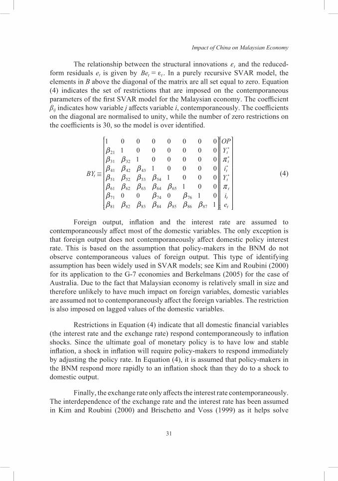
The relationship between the structural innovations tf and the reduced-form residuals et is given by Bet tf= . In a purely recursive SVAR model, the elements in B above the diagonal of the matrix are all set equal to zero. Equation (4) indicates the set of restrictions that are imposed on the contemporaneous parameters of the first SVAR model for the Malaysian economy. The coefficient βij indicates how variable j affects variable i, contemporaneously. The coefficients on the diagonal are normalised to unity, while the number of zero restrictions on the coefficients is 30, so the model is over identified.
0 0 0
1 0
1
0
0
1
0
0
0
1
0
0
0
0
1
0
0
0
0
0
1
0
0
0
0
0
0
1
0
0
0
0
0
0
0
1
BY
OPY
iY
ie
21
31
41
51
61
71
81
32
42
52
62
82
43
53
63
83
54
64
74
84
65
85
76
86 87
t
t
t
t
t
t
t
t
/
b
b
b
b
b
b
b
b
b
b
b
b
b
b
b
b
b
b
b
b
b
b
b
b b
r
r
)
)
)
)
R
T
SSSSSSSSSSSSSSSSSSSSSSSS
R
T
SSSSSSSSSSSSSSSSSSSSSSSS
V
X
WWWWWWWWWWWWWWWWWWWWWWWW
V
X
WWWWWWWWWWWWWWWWWWWWWWWW
(4)
Foreign output, inflation and the interest rate are assumed to contemporaneously affect most of the domestic variables. The only exception is that foreign output does not contemporaneously affect domestic policy interest rate. This is based on the assumption that policy-makers in the BNM do not observe contemporaneous values of foreign output. This type of identifying assumption has been widely used in SVAR models; see Kim and Roubini (2000) for its application to the G-7 economies and Berkelmans (2005) for the case of Australia. Due to the fact that Malaysian economy is relatively small in size and therefore unlikely to have much impact on foreign variables, domestic variables are assumed not to contemporaneously affect the foreign variables. The restriction is also imposed on lagged values of the domestic variables.
Restrictions in Equation (4) indicate that all domestic financial variables (the interest rate and the exchange rate) respond contemporaneously to inflation shocks. Since the ultimate goal of monetary policy is to have low and stable inflation, a shock in inflation will require policy-makers to respond immediately by adjusting the policy rate. In Equation (4), it is assumed that policy-makers in the BNM respond more rapidly to an inflation shock than they do to a shock to domestic output.
Finally, the exchange rate only affects the interest rate contemporaneously. The interdependence of the exchange rate and the interest rate has been assumed in Kim and Roubini (2000) and Brischetto and Voss (1999) as it helps solve
Mohd Azlan Shah Zaidi et al.
32
the exchange rate puzzle. As in other VAR studies, the exchange rate responds contemporaneously to all variables in the model. Even though some variables do not affect the others contemporaneously, lagged effects among variables are unrestricted, except that the foreign and domestic sectors are assumed to be block exogenous.
Technically SVAR model is estimated in its reduced VAR form. In order to estimate the SVAR parameters, this study follows a two-step procedure suggested by Bernanke (1986). First, from the reduced form VAR estimates, the residuals, et and the variance-covariance matrix, Σe are calculated. Second, through the sample estimates of Σe the contemporaneous matrix B is estimated. In this study, B is estimated using maximum likelihood.3 The log likelihood function is
2 2
1ln
T B B e B Be1 1 1
1
t tt
T
R R- -=
f f- - -
l l lt t^ `h j/ (5)
If there are more than (n2 + n)/2 additional restrictions, the system is over-identified. In this case the χ2 test statistic:
2eR
e| R R= - (6)
with R number of restrictions exceeding (n2 + n)/2 degrees of freedom can be used to test the restricted system. e
RR is the restricted variance-covariance matrix while Σe is the unrestricted variance-covariance matrix.
In choosing an appropriate lag length for the VAR model, information criteria for the full system of equations are considered, viz. Akaike’s (1973) Information Criterion (AIC) and Schwarz (1978) Bayesian Criterion (SBC). As a simple indicator of model stability test, the eigenvalues of the companion matrix of the VAR model are calculated. If all the eigenvalues are inside the unit circle, the model is stable (see Lutkepohl, 1993).
From the SVAR model, impulse response functions are produced to describe the direction of response of a variable of interest (e.g. the Malaysian output) to an exogenous shock (e.g. foreign interest rate shock). Recently, new development in empirical studies using VAR/SVAR model focuses on sign restrictions approach as one of the identification strategies. Proposed by Faust (1998), Canova and De Nicolo (2002) and Uhlig (2005), the strategy accepts all the impulses that are in accordance with sign restrictions on impact while others are rejected. Since then a number of researchers have applied this strategy to examine the effect of fiscal, monetary policy as well as the demand and supply shocks (see among others Mountford & Uhlig, 2009; Lippi & Nobili, 2012; Peersman & Straub, 2009; Canova & Pappa, 2007).
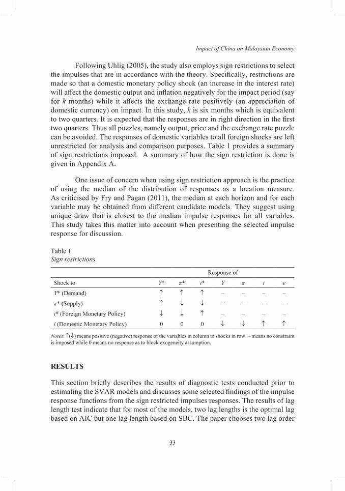
Impact of China on Malaysian Economy
33
Following Uhlig (2005), the study also employs sign restrictions to select the impulses that are in accordance with the theory. Specifically, restrictions are made so that a domestic monetary policy shock (an increase in the interest rate) will affect the domestic output and inflation negatively for the impact period (say for k months) while it affects the exchange rate positively (an appreciation of domestic currency) on impact. In this study, k is six months which is equivalent to two quarters. It is expected that the responses are in right direction in the first two quarters. Thus all puzzles, namely output, price and the exchange rate puzzle can be avoided. The responses of domestic variables to all foreign shocks are left unrestricted for analysis and comparison purposes. Table 1 provides a summary of sign restrictions imposed. A summary of how the sign restriction is done is given in Appendix A.
One issue of concern when using sign restriction approach is the practice of using the median of the distribution of responses as a location measure. As criticised by Fry and Pagan (2011), the median at each horizon and for each variable may be obtained from different candidate models. They suggest using unique draw that is closest to the median impulse responses for all variables. This study takes this matter into account when presenting the selected impulse response for discussion.
Table 1 Sign restrictions
Response of
Shock to Y* π* i* Y π i e
Y* (Demand) ↑ ↑ ↑ – – – –
π* (Supply) ↑ ↓ ↓ – – – –
i* (Foreign Monetary Policy) ↓ ↓ ↑ – – – –
i (Domestic Monetary Policy) 0 0 0 ↓ ↓ ↑ ↑
Notes: ↑(↓) means positive (negative) response of the variables in column to shocks in row. – means no constraint is imposed while 0 means no response as to block exogeneity assumption.
RESuLTS
This section briefly describes the results of diagnostic tests conducted prior to estimating the SVAR models and discusses some selected findings of the impulse response functions from the sign restricted impulses responses. The results of lag length test indicate that for most of the models, two lag lengths is the optimal lag based on AIC but one lag length based on SBC. The paper chooses two lag order
Mohd Azlan Shah Zaidi et al.
34
since it is sufficient to capture the dynamics of the variables and do not involve the loss of too many degrees of freedom. Furthermore, for stability indicator, all the eigenvalues for the baseline model in absolute value are less than one, indicating that the model is stable.4
Figure 1 shows the responses of domestic macroeconomic variables to domestic monetary policy shock. As depicted, the directions of all responses are in accordance with the theory. The responses of domestic output and inflation are negative for at least the impact period of six months, while the response of the exchange rate is positive. Due to the application of the sign restrictions method, all the price puzzles do not appear. There are four responses in each graph. Each indicates which foreign factors are under investigation. A shock in domestic monetary policy brings about greatest negative impact on domestic output when the Japanese factors are used in the model. On the other hand, negative impact of the shock on domestic inflation is more pronounced if Singapore factors are considered. However, when the Singapore variables are used as the only external sectors, its impact is more realised in the response of the exchange rate. Even though the initial response is not as big as the others, its impact takes longer time to diminish. The whole pictures indicate that different utilisation of foreign country variables to represent external sector in the model would bring about different impact of domestic variables.
Figure 2 shows the impact of shocks to foreign monetary policy on domestic variables. It seems that, the monetary policy shocks from Singapore and the U.S. (after 9 months) have positive effects on Malaysian output, whereas the monetary policy shocks from Japan and China (until 27 months) have negative effects on Malaysian output. While the U.S. monetary policy shock has positive and greater impact on Malaysian interest rates, the monetary policy shocks from Singapore, Japan and China (after 13 months) have negative effects on Malaysian domestic interest rates. In the meantime, each foreign monetary policy shock affects Malaysian inflation negatively. The effect of Singapore monetary policy shock is nevertheless more pronounced. When it comes to the exchange rate, the effect of each foreign monetary policy shock on the exchange rate is quite distinctive. The monetary policy shock from Singapore has greater and positive effect on Malaysian exchange rate, whereas the U.S. monetary policy shock has negative effect on the exchange rate. In the meantime, China monetary policy shock has positive effect on the exchange rate within 10 months only, whereas Japanese monetary policy shock has positive effect on the exchange rate after 3 months and stays positive until 24 months.
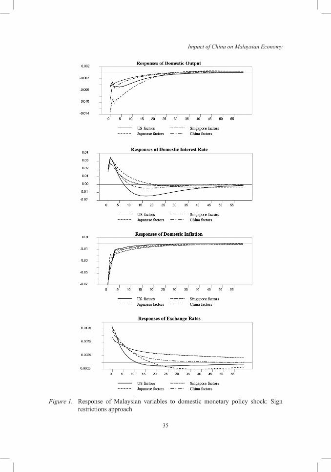
Impact of China on Malaysian Economy
35
Figure 1. Response of Malaysian variables to domestic monetary policy shock: Sign restrictions approach
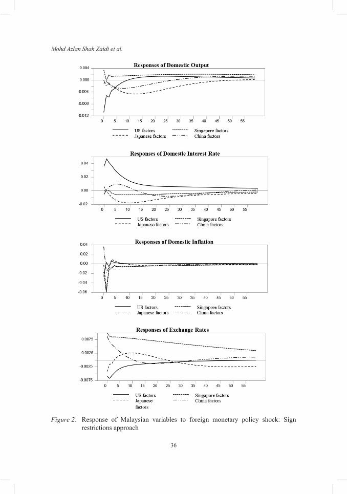
Mohd Azlan Shah Zaidi et al.
36
Figure 2. Response of Malaysian variables to foreign monetary policy shock: Sign restrictions approach
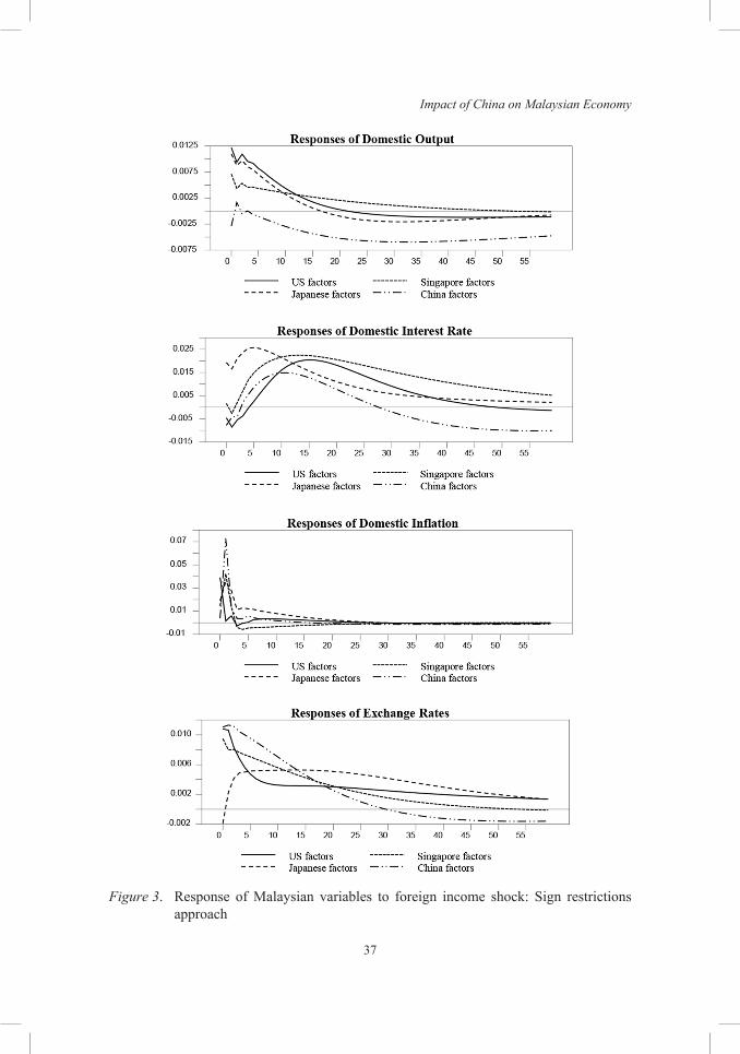
Impact of China on Malaysian Economy
37
Figure 3. Response of Malaysian variables to foreign income shock: Sign restrictions approach
Mohd Azlan Shah Zaidi et al.
38
Figure 3 depicts the responses of Malaysian domestic variables to foreign output shocks. As can be seen, within 13 months, the income shock from the U.S. has the greatest influence on Malaysian output. However after 13 months, income shock from Singapore has more pronounced effect on Malaysian output. Interestingly, income shock from China has negative effect on Malaysian output throughout the time horizon. This indicates that there is a beggar-thy-neighbour effect (negative spillover) from an economic expansion in China to Malaysian output. China factors are also more dominant in terms of its income shock’s effect on Malaysian inflation. This indicates that an economic expansion in China has triggered greater inflationary pressure in Malaysia than that of the economic expansion from the other countries. In addition, the China factors have also dominant effect on the exchange rate within 13 months, which after that is taken over by the Japanese factors. Furthermore, it seems that Malaysian interest rate has responded positively to all foreign income shocks, in which the shock from Japan is more dominant within 10 months, and then this role is taken over by Singapore after 10 months.
Figure 4 summaries the responses of domestic variables to foreign inflation shocks. As can be seen, China factors become more dominant than the others, after 20 months, in affecting Malaysian output. In general, Malaysian output has responded positively to inflation shocks from all countries. This indicates that inflationary pressures from foreign countries have positive effects on the Malaysian output. The responses of domestic interest rate upon foreign inflation shocks are heterogeneous across countries in terms of magnitudes and signs. The inflation shocks from China and Singapore have negative effects on Malaysian interest rate until 25 months. In contrast, the U.S. and Japanese factors have positive effects on Malaysian interest rate in the short run. For example, inflation shock from the U.S. has positive effect on Malaysian interest rate until 5 months, whereas inflation shock from Japan has positive impact on the interest rate until 17 months. Furthermore, the inflation shocks from all countries have negative effects on Malaysian inflation. In particular, an inflation shock in Singapore has caused the greatest negative response in Malaysian inflation. With regards to the exchange rate, shocks to inflation in all foreign countries have positive impacts on the variable at least in the short run.
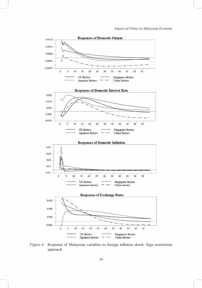
Impact of China on Malaysian Economy
39
Figure 4. Response of Malaysian variables to foreign inflation shock: Sign restrictions approach
Mohd Azlan Shah Zaidi et al.
40
CONCLuSIONS
This paper provides new empirical evidence on the impact of foreign shocks (foreign income and foreign monetary policy) of Malaysia’s major trading partners, namely the U.S., Japan, Singapore and China on the domestic macroeconomic variables. A special attention is given on the effect of China since China has increasingly become more influential in the world economy. The paper employs anon-recursive SVAR identification scheme in examining the relative importance of the foreign shocks. There are four SVAR models estimated to deal with various measures of foreign factors that have often been ignored in previous studies, in particular the China factor. Block exogeneity assumption is mainly emphasised in building and estimating the structural VAR models. In order to identify the structural parameters, the paper utilises short-run restriction as well as sign restriction technique. The sign-restricted impulse responses are generated in accordance with the suggestion of Uhlig (2005) and Fry and Pagan (2011).
Overall, the results show that applying the sign restriction approach helps in overcoming the price puzzles. Since not all impulses are sign-restricted, the procedure manages to indicate the true responses of domestic variables to foreign factor shocks. The results indicate, in particular, that the U.S. is more dominant in affecting domestic output, while China plays prominent role in influencing domestic inflation and the exchange rate, especially with regards to their respective income shocks. As for foreign monetary policy shock, the effect of Singapore in influencing Malaysian inflation and the exchange rate is more pronounced. This is in line with the findings of Zaidi and Karim (2014) when quarterly data are used in their models.
The findings suggest that in order to model the impact of foreign sector on Malaysian economy, one has to look at which specific country the external shock comes from. Generalising one country, for example the U.S. to represent the world economy might have detrimental effect on the policy making since significant impact of other country might have been ignored. The study might have some benefits to policy makers especially in tackling issues pertaining to the impact of specific foreign country to domestic sector. This is particularly important for Malaysia in formulating policy to mitigate adverse impact of foreign policy change or shocks in the process of transforming its economy toward high income nation in the near future.
Impact of China on Malaysian Economy
41
ACKNOWLEDGEMENTS
The authors thankfully acknowledge financial support from the Universiti Kebangsaan Malaysia research grant (Grant number: UKM-GGPM-PLW-016-2011).
NOTES
1. Singapore uses the exchange rate while China uses monetary aggregate as their monetary policy variable respectively. The inclusion of the interest rate as monetary policy variable for Singapore and China is for comparison purpose.
2. All unadjusted data at source are seasonally adjusted using X11 command in RATS.3. In RATS, B is estimated using the Broyden, Fletcher, Goldfarb and Shanno (BFGS)
algorithm. The initial starting values for B are found using the genetic method.4. The values are not shown in this paper.
REFERENCES
Akaike, H. (1973). Information theory and an extension of the maximum likelihood principle. In B. N. Petrov, & F. Csaki (Eds.), Second international symposium on information theory (pp. 267–281). Budapest: AkademiaiKiado.
Azali, M., & Matthews, K. (1999). Money-income and credit-income relationships during the pre-and the post-liberalization periods: Evidence from Malaysia. Applied Economics, 31(10), 1161–1170. https://doi.org/10.1080/000368499323382
Berkelmans, L. (2005). Credit and monetary policy: An Australian SVAR. Research Discussion Paper No. 2005–06, Reserve Bank of Australia.
Bernanke, B. S. (1986). Alternative explanations of the money-income correlation. Carnegie-Rochester Conference Series on Public Policy, 25(1), 49–100.
Brischetto, A., & Voss, G. (1999). A structural vector auto regression model of monetary policy in Australia. Research Discussion Paper 1999–11, Reserve Bank of Australia.
Buckle, R. A., Kim, K., Kirkham, H., H., M., & Sharma, J. (2007). A structural VAR business cycle model for a volatile small open economy. Economic Modeling, 24(6), 990–1017. https://doi.org/10.1016/j.econmod.2007.04.003
Callen T., & McKibbin, W. (2001). Policies and prospects in Japan and the implications for the Asia Pacific Region. IMF Working Paper WP/01/131, International Monetary Fund. https://doi.org/10.5089/9781451855289.001
Canova, F., & De Nicolo, G. (2002). Monetary disturbances matter for business fluctuations in the G-7. Journal of Monetary Economics, 49(6), 1131–1159.
Canova, F., & Pappa, E. (2007). Price differentials in monetary unions: The role of fiscal shocks. Economic Journal, 117(520), 713–734. https://doi.org/10.1111/j.1468-0297.2007.02047.x
Mohd Azlan Shah Zaidi et al.
42
Canova, F. (2005). The transmission of US shocks to Latin America. Journal of Applied Econometrics, 20(2), 229–251. https://doi.org/10.1002/jae.837
Coenen, G., & Wieland, V. (2003). The zero-interest-rate bound and the role of the exchange rate for monetary policy in Japan. Journal of Monetary Economics, 50(5), 1071–1101.
Cushman, D. O., & Zha, T. (1997). Identifying monetary policy in a small open economy under flexible exchange rates. Journal of Monetary Economics, 39(3), 433–448.
Dizioli, A., Guajardo, J., Klyuev, V., Mano, R., & Raissi, M. (2016). Spillovers from China’s growth slowdown and rebalancing to the ASEAN-5 economies, IMF Working Paper, August 2016, International Monetary Fund.
Doan, T. A. (2010). RATS handbook for vector autoregressions. Retrieved from https://hhstokes.people.uic.edu/ftp/e538/VAR_Material/VAR%20Workbook.pdf
Dungey, M., & Fry, R. (2003). International shocks on Australia: The Japanese effect. Australian Economic Papers, 42(2), 158–182. https://doi.org/10.1111/1467-8454.00193
Dungey, M., & Pagan, A. (2000). A structural VAR model of the Australian economy. The Economic Record, 76(235), 321–342. https://doi.org/10.1111/j.1475-4932.2000.tb00030.x
Faust, J. (1998). The robustness of identified VAR conclusions about money. Carnegie-Rochester Conference Series in Public Policy, 49, 207–204.
Fry, R., & Pagan, A. (2011). Sign restrictions in structural vector autoregressions: A critical review. Journal of Economic Literature, 49(4), 938–960. https://doi.org/10.1257/jel.49.4.938
Ibrahim, M. (2005). Sectoral effect of monetary policy: Evidence from Malaysia. Asian Economic Journal, 19(1), 83–102. https://doi.org/10.1111/j.1467-8381. 2005.00205.x
Johansson, A. C. (2012). China’s growing influence in Southeast Asia: Monetary policy and equity markets. The World Economy, 35(7), 816–837.
Kim, S., & Roubini, N. (2000). Exchange rate anomalies in the industrial countries: A solution with a structural VAR approach. Journal of Monetary Economics, 45(3), 561–586.
Kim, S. (2001). International transmission of U.S. monetary policy shocks: Evidence from VAR’s. Journal of Monetary Economics, 48(2), 339–372.
Koźluk, T., & Mehrotra, A. (2009). The impact of Chinese monetary policy shocks: Evidence from VAR’s. Journal of Monetary Economics, 48, 339–372.
Lippi, F., & Nobili, A. (2012). Oil and the macroeconomy: A quantitative structural analysis. Journal of the European Economic Association, 10(5), 1059–1083. https://doi.org/10.1111/j.1542-4774.2012.01079.x
Lutkepohl, H. (1993). Introduction to multiple time series analysis (2nd ed.). Berlin: Springer-Verlag. https://doi.org/10.1007/978-3-642-61695-2
Maćkowiak, B. (2006). What does the bank of Japan do to East Asia? Journal of International Economics, 70(1), 253–270. https://doi.org/10.1016/j.jinteco.2005.10.001
Maćkowiak, B. (2007). External shocks, U.S monetary policy and macroeconomics fluctuations in emerging markets. Journal of Monetary Economics, 54(8), 2512–2520. https://doi.org/10.1016/j.jmoneco.2007.06.021
Impact of China on Malaysian Economy
43
Mountford, A., & Uhlig, H. (2009). What are the effects of fiscal policy shocks? Journal of Applied Econometrics, 24(6), 960–992. https://doi.org/10.1002/jae.1079
Othman, N., Yusop Z., Zaidi M. A. S., & Karim, Z. A. (2015). Impact of external and domestic shocks on Malaysia’s electronic and electrical (E & E) export demand. International Journal of Economics and Management, 9(S), 1–20.
Peersman, G., & Straub, R. (2009). Technology shocks and robust sign restrictions in a euro area SVAR. International Economic Review, 50(3), 727–750. https://doi.org/10.1111/j.1468-2354.2009.00546.x
Schwarz, G. (1978). Estimating the dimension of a model. Annals of Statistics, 6(2), 461–464. https://doi.org/10.1214/aos/1176344136
Tang, H. C. (2006). The relative important of monetary policy transmission channels in Malaysia. CAMA Working Paper Series. The Australian National University.
Uhlig, H. (2005). What are the effects of monetary policy on output? Results from an agnostic identification procedure. Journal of Monetary Economics, 52(2), 381–419. https://doi.org/10.1016/j.jmoneco.2004.05.007
Zaidi, M. A. S., Karim Z. A., & Azman-Saini, W. N. W. (2013). Foreign and domestic shocks: Macroeconomic responses of ASEAN-3 countries. Global Economic Review: Perspectives on East Asian Economies and Industries, 42(3), 215–237. https://doi.org/10.1080/1226508X.2013.835900
Zaidi, M. A. S., & Karim, Z. A. (2014). Impact of Singapore, US and Japanese macroeconomics shocks on Malaysian economy: A sign-restricted SVAR analysis. Jurnal Pengurusan, 41, 113–122. https://doi.org/10.17576/pengurusan- 2014-41-10
Zaidi. M. A. S., & Fisher, L. A. (2010). Monetary policy and foreign shocks: An SVAR analysis for Malaysia. Korea and the World Economy, 11(3), 527–550.
Zha, T. (1999). Block recursion and structural autoregressions. Journal of Econometrics, 90(2), 291–316.

Mohd Azlan Shah Zaidi et al.
44
APPENDIX A
Summary of Sign Restriction Approach (Taken from Doan (2010))
This is a summary of sign restriction approach as suggested by Uhlig (2005) and Canova and De Nicolo (2002). This is with the assumption that the full reduced form VAR is estimated.
1. Generate a draw for the VAR coefficients and covariance matrix using standard methods.
2. Compute a Choleski factor and the responses to it.3. Generate a random unit vector (α) in m-space (dimensional unit sphere).
This is the start of a “subdraw”.4. Weight the impulse responses from step 2 by α to get the responses to the
chosen impulse vector.5. If the impulse responses meet the restrictions, save them.6. Repeat steps 3–5 a certain number of times for each main draw.7. Repeat steps 1–6 until the desired number of draws have been accepted.
AAMJAF Vol. 14, No. 2, 45–64, 2018
© Asian Academy of Management and Penerbit Universiti Sains Malaysia, 2018. This work is licensed under the terms of the Creative Commons Attribution (CC BY) (http://creativecommons.org/licenses/by/4.0/).
Asian Academy of Management Journal
of Accounting and Finance
Financial Sector and aggregate import demand: a general equilibrium perSpective
with Japan data
tuck cheong tang
Department of Economics, Faculty of Economics and Administration, University of Malaya, 50603 Kuala Lumpur, Malaysia
E-mail: [email protected]
abStract
This study explores the role of financial sector on import demand behaviour (the real sector) from general equilibrium perspective, which is based on the portfolio balance approach to capture financial market. Japan’s data support partially this hypothesis given non-cointegration finding, while foreign interest rate is significant i.e. reduces Japan’s imports. Growth in foreign income is the most influential factor, and domestic economic growth both make more imports. However, the relative price of domestic goods, and domestic interest rate are insignificant. Japan’s monetary policy (interest rate) is inappropriate in altering the behaviour of imports in Japan, but fiscal policy that influences Japan’s economic growth.
Keywords: aggregate import demand, financial sector, general equilibrium perspective, Japan, portfolio balance approach
introduction
This study proposes a structural framework for analysing long-run aggregate import demand that is derived from a general equilibrium perspective. This framework differs from the partial equilibrium approach by incorporating both real factors and financial factors of the economy. In general, partial equilibrium
Publication date: 31 December 2018
To cite this article: Tang, T. C. (2018). Financial sector and aggregate import demand: A general equilibrium perspective with Japan data. Asian Academy of Management Journal of Accounting and Finance, 14(2), 45–64. https://doi.org/10.21315/aamjaf2018.14.2.3
To link to this article: https://doi.org/10.21315/aamjaf2018.14.2.3
Tuck Cheong Tang
46
analysis focuses on one market at a time under the strict proviso of ceteris paribus. This approach has been applied to import demand analysis with a focus on the real sector of the economy. The influence of the financial sector in the import demand decision is essentially ignored on the grounds of the classical homogeneity or neutrality postulate that financial forces are essentially accommodating. Some existing studies have considered the role of select financial variables such as bank credit, money supply, or interest rates as additional explanatory variables of import demand (Athens, 1985; Ceglowski, 1991; Craigwell, 1994; Tang, 2004). But these specifications have been generally of an ad hoc nature rather than being embedded in a formal general equilibrium framework.
In an open economy, the real resource flows also involve cross-border transactions, exports and imports of goods and services. Firms import real resources such as raw materials and final products that cannot be provided domestically, while they export those goods and services that are in excess of domestic requirements. The cross-border real resource flow is typically regarded as the swapping of some real resources for other real resources. In formal analysis it is treated as if it were a barter system with balanced exchanges where financial considerations have no independent role to play. In a monetised economy, as distinct from a barter system, any transaction or exchange has by definition a monetary or financial side. This is captured in Clower’s (1967) memorable phrase that “money buys goods and goods buy money.” This implies that the goods market flow is necessarily associated with an equivalent financial flow. The circular flow relationship merely depicts the fundamental simultaneity between the real sector and the financial sector. This relationship has received extensive attention in closed (autarky) economy analysis but has traditionally been ignored in the analysis of international trade flows. The systemic simultaneity implies that adjustment behaviour in the financial sector may be one of the forces that drive adjustment flows in the goods and services market. And, vice versa, imbalances in goods markets may be one of the factors that determine adjustment behaviour in the financial sector.
This interdependence raises interesting questions about the relative importance of financial and real factors in influencing the demand for imports. In the absence of money illusion non-monetary factors, that is the “real” factors of tastes, resources, and technology, are the ultimate determinants of production, consumption, trade and relative prices in economic equilibrium. The goods and services which each sector absorbs must be paid for with financial assets, money or bonds (Mundell, 1963, p. 476–477). It follows from the fundamental simultaneity property that financial disturbances may well affects the gross and net flows of cross-border exchanges of goods and services.
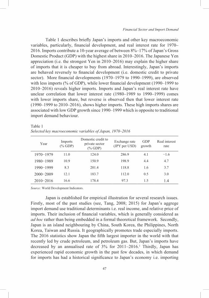
Financial Sector and Import Demand
47
Table 1 describes briefly Japan’s imports and other key macroeconomic variables, particularly, financial development, and real interest rate for 1970–2016. Imports contribute a 10-year average of between 8%–17% of Japan’s Gross Domestic Product (GDP) with the highest share in 2010–2016. The Japanese Yen appreciation (i.e. the strongest Yen in 2010–2016) may explain the higher share of imports that it is cheaper to buy from abroad. Interestingly, Japan’s imports are behaved reversely to financial development (i.e. domestic credit to private sector). More financial developments (1970–1979 to 1990–1999), are observed with less imports (% of GDP), while lower financial development (1990–1999 to 2010–2016) reveals higher imports. Imports and Japan’s real interest rate have unclear correlation that lower interest rate (1980–1989 to 1990–1999) comes with lower imports share, but reverse is observed then that lower interest rate (1990–1999 to 2010–2016), shows higher imports. These high imports shares are associated with low GDP growth since 1990–1999 which is opposite to traditional import demand behaviour.
Table 1Selected key macroeconomic variables of Japan, 1970–2016
Year Imports (% GDP)
Domestic credit to private sector
(% GDP)
Exchange rate (JPY per USD)
GDP growth
Real interest rate
1970−1979 11.0 124.0 286.9 4.1 −1.6
1980−1989 10.9 150.9 198.9 4.4 4.7
1990−1999 8.3 201.4 118.8 1.6 3.7
2000−2009 12.1 183.7 112.0 0.5 3.0
2010−2016 16.6 178.4 97.3 1.5 1.4
Source: World Development Indicators.
Japan is established for empirical illustration for several research issues. Firstly, most of the past studies (see, Tang, 2008; 2015) for Japan’s aggrege import demand use traditional determinants i.e. real income, and relative price of imports. Their inclusion of financial variables, which is generally considered as ad hoc rather than being embedded in a formal theoretical framework. Secondly, Japan is an island neighbouring by China, South Korea, the Philippines, North Korea, Taiwan and Russia. It geographically promotes trade especially imports. The 2016 statistics show Japan the fifth largest importer in the world with that recently led by crude petroleum, and petroleum gas. But, Japan’s imports have decreased by an annualised rate of 3% for 2011–2016.1 Thirdly, Japan has experienced rapid economic growth in the past few decades, in which demand for imports has had a historical significance to Japan’s economy i.e. importing
Tuck Cheong Tang
48
raw materials and by processing (adding value to) them before exporting in the export-led policy. Finally, Japan plays a competitive role in international trade as a member of multiple international trade organisations (Asia Pacific Economic Cooperation [APEC], World Trade Organisation [WTO], Organisation for Economic Co-operation and Development [OECD], Group of Eight [G8] and Group of Twenty [G20]). Indeed, Japan still maintains protectionist policies in numerous industries, particularly in agriculture.2 These stylised facts motivate this study to Japan’s import demand behaviour especially, the role of financial sector.
This study shows that financial sector partially supports the demand for imports with Japan’s data. No long-run (cointegration) import demand for the specification proposed, but its ‘financial sector’ determinants, [change in] foreign interest rate is negatively significant, and foreign income is the most influential factor for more imports. The domestic interest rate is insignificant.
literature review
There has been rich amount of studies that have attempted to examine the aggregate demand behaviour for imports (i.e. goods and services), empirically for both the developed and developing nations. They (Chang, 1945–1946; Houthakker & Magee, 1969; Khan, 1974; Gafar, 1988; and Senhadji, 1998, for examples), have basically employed the traditional or conventional specification of import demand function that relating the volume of imports to two fundamental factors (real income, and relative price of imports). It is assumed that the demand behaviour is determined by one market of the economy; the partial equilibrium approach that the goods and services market or real sector under the strict proviso of ceteris paribus. However, this approach ignores the influence of the financial sector.
Some studies examined the aggregate import demand behaviour with financial variables such as money supply, interest rates, remittance, financial development, and bank credit, including volume of tools used in financing trade, and trade credits (see, Table 2). They concluded that ‘finance’ is important and has significant effects on imports. However, they do not provide any systematic theoretical derivation of their import demand specifications. Recent work by Ziramba and Mumangeni (2017) consider bank credit in explaining imports in South Africa as the previous studies did. For examples, Athens (1985) examines the role of the money market in import demand behaviour for the U.S. and the U.K. Accordingly, if there is an excess supply of money, the foreign sector will provide the means for restoring the private sector’s stock equilibrium through

Financial Sector and Import Demand
49
Tabl
e 2
Sum
mar
y of
exi
stin
g st
udie
s tha
t rec
ogni
se fi
nanc
ial d
eter
min
ants
of i
mpo
rt d
eman
d
Stud
yC
ount
ry sa
mpl
e pe
riod
Fina
ncia
l var
iabl
e(s)
Just
ifica
tion(
s)Fi
ndin
gs
Ath
ens (
1985
)U
.S. &
U.K
.[1
960q
1–19
79q4
]M
oney
supp
lyO
mis
sion
of m
oney
mar
ket v
aria
ble.
Mon
etar
y ap
proa
ch fo
r lon
g-ru
n ba
lanc
e of
pay
men
t flow
s.
A d
irect
link
(pos
itive
) bet
wee
n m
oney
su
pply
and
impo
rt de
man
d.
Ceg
low
ski (
1991
)U
.S.
[196
8q1–
1988
q4]
Rea
l int
eres
t rat
eC
onsu
mpt
ion
theo
ry-w
ith in
terte
mpo
ral
optim
isat
ion
that
impo
rt de
man
d va
ries
posi
tivel
y w
ith th
e ex
pect
ed re
al in
tere
st ra
te.
Rea
l int
eres
t rat
e is
sign
ifica
nt.
Cra
igw
ell (
1994
)B
arba
dos
[196
0–19
93]
Priv
ate
sect
or c
redi
tC
redi
t is a
read
y an
d ne
cess
ary
sour
ce o
f fin
anci
ng in
crea
ses i
n sp
endi
ng.
All
varia
bles
are
coi
nteg
rate
d. C
redi
t is
posi
tivel
y re
late
d to
impo
rts.
Tang
(200
4)Ja
pan
[197
3q1–
2000
q2]
Ban
k cr
edit,
lend
ing
rate
, de
posi
t rat
e, g
over
nmen
t bo
nd y
ield
, & sh
are
pric
es
TB =
S–I
, the
var
iabl
es a
ffect
ing
savi
ngs (
S)
and
inve
stm
ents
(I) m
ay a
lso
influ
ence
impo
rts.
All
varia
bles
are
coi
nteg
rate
d. T
he fi
nanc
ial
varia
bles
hav
e po
sitiv
e si
gn.
Tang
(200
6)M
alay
sia,
Indo
nesi
a, T
haila
nd,
the
Phili
ppin
es [1
960–
2000
] &
Sing
apor
e [1
974–
2000
]
Ban
d cr
edit
As C
raig
wel
l (19
94)
All
varia
bles
are
coi
nteg
rate
d.
Cre
dit h
as p
ositi
ve si
gn.
Muk
tadi
r-A
l-Muk
it
et a
l. (2
013)
Ban
glad
esh
[200
5m1–
2011
m12
]R
emitt
ance
Rem
ittan
ces i
ncre
ases
dem
and
on g
oods
and
se
rvic
es, t
hen
dom
estic
pric
e, w
hich
resu
lt m
ore
impo
rts.
Rem
ittan
ces i
ncre
ase
fore
ign
curr
ency
supp
ly-
appr
ecia
te lo
cal c
urre
ncy,
che
aper
impo
rts.
Rem
ittan
ces a
nd im
ports
are
coi
nteg
rate
d.
Rem
ittan
ce h
as p
ositi
ve si
gn (l
ong-
run)
, but
, in
sign
ifica
nt in
the
shor
t-run
. No
caus
atio
n fr
om re
mitt
ance
to im
ports
, but
oth
erw
ise.
Aub
oin
&
Enge
man
n (2
014)
Pane
l dat
a of
91
coun
tries
[2
005q
1–20
11q4
]Sh
ort-t
erm
insu
red
trade
cr
edits
Trad
e cr
edit
-wor
king
cap
ital fi
nanc
ing
in
stan
dard
equ
atio
n fo
r im
ports
.Tr
ade
cred
it ha
s pos
itive
effe
ct o
n re
al
impo
rts.
Alta
n (2
016)
Turk
ey[1
990–
2015
]V
olum
e of
the
tool
s use
d in
fina
ncin
g fo
reig
n tra
deV
ario
us p
aym
ent m
etho
ds p
rom
ote
fore
ign
trade
via
fina
ncin
g.Pa
ymen
t met
hods
are
impo
rtant
to im
ports
.
Aha
d et
al.
(201
7)Pa
kist
an [1
972q
1–20
12q4
]Fi
nanc
ial d
evel
opm
ent
(dom
estic
cre
dit t
o pr
ivat
e se
ctor
)
Paki
stan
impl
emen
ted
refo
rms t
o im
prov
e tra
de a
nd fi
nanc
ial d
evel
opm
ent.
All
varia
bles
are
coi
nteg
rate
d. F
inan
cial
de
velo
pmen
t has
pos
itive
sign
. Fee
dbac
k eff
ect b
etw
een
finan
cial
dev
elop
men
t and
im
ports
.
Zira
mba
&
Mum
ange
ni (2
017)
Sout
h A
fric
a[1
965
to 2
014]
Ban
k cr
edit
Follo
w p
ast s
tudi
esA
ll va
riabl
es a
re c
oint
egra
ted.
Ban
k cr
edit
is
sign
ifica
nt in
the
shor
t-run
.
Tuck Cheong Tang
50
increases in imports or net capital outflows. Therefore, monetary disequilibrium will have an impact on the demand for imports (Athens 1985, p. 93). The results show that imports are positively influenced by money supply (M3). Also, Ceglowski (1991) commented that conventional import demand specifications do not consider intertemporal choice which would emphasize the importance of real interest rates for import determination; changes in the expected real interest rate alter the price of current consumption relative to future consumption and may affect the intertemporal allocation of consumption. Therefore, an increase in expected real interest rates should induce households to substitute future consumption for current consumption.
In the open economy context, this intertemporal substitution implies a reduced demand for imports in the present and increased future import demand. Based on quarterly U.S. data 1968–1988, the study identifies a positive elasticity of intertemporal substitution for imports. This suggests a role for the real interest rate in influencing the demand for imports. The intertemporal aspects of import demand suggest real interest rates provide a second channel through which macroeconomic policy can alter the level of imports and the trade balance (Ceglowski, 1991, p. 119). Craigwell (1994) viewed on the influence of bank credit on aggregate import demand as a “ready and necessary source to finance increases in spending”. The empirical results show a positive influence of bank credit for Barbados’s import demand, and the underlying variables (with bank credit) are cointegrated. But, it is not for the conventional specification. Craigwell argues that this finding suggests misspecification in conventional import demand specifications. Croix and Urbain (1998) pointed out that most of the conventionally specified import demand models are derived from a pure empirical exercise and that either pseudo-reduced form models or dynamic specifications usually have ‘naïve’ theoretical foundations.
general equilibrium perSpective: aggregate import demand relation
This section explores a simple general equilibrium structure for an aggregate import demand relation with assumptions of fixed exchange rates, and that capital moves freely between national economies. The general equilibrium perspective covers two fundamental approaches: (1) Income-expenditure equilibrium, which is de facto still partial because it looks only at one market, the goods and services market; it ignores the role of the financial sector (money market and bonds market); and (2) Portfolio balance approach that captures the financial market. This section focuses on the second one.3
Financial Sector and Import Demand
51
Financial market: portfolio balance
Financial sector considers money market and bond market. Money market equilibrium requires that the stock of money is willingly held by the public. It requires that the money stock supplied by the central bank and the banking system is equivalent to the private sector demand for money. The stock supply of money is backed by central bank assets, domestic credit (DC) which represents central bank lending to the private sector, prominently the banking system, and to the government, and by international reserves (IR). The stock and flow clearing conditions in the money market fulfil that M d = M s = DC + IR, and ∆M d =∆M s = ∆DC + ∆IR. In open economies, the money supply is influenced by international reserve flows. The response of money supply to domestic credit and international reserves depends on transactors’ behaviour to demand cash balances. Portfolio balance behaviour suggests that transactors desire an optimum amount of money and other assets. If that is not provided by the monetary authority they try to secure it through other means by building up cash balances through reduced spending. In an open economy, the reduction in spending improves the trade balance and draws in reserves. Hence, any excess stock demand for money that is not accommodated by domestic monetary expansion will draw international reserves into the domestic monetary system to expand the money stock endogenously.
Similarly, stock equilibrium in the bond market requires that transactors willingly hold the existing stock of income-bearing financial assets. The bond market clearing condition is that the stock demand for bond holdings must equal the net stock supply of bonds (Bd = Bs). In an open economy characterised by capital mobility, domestic residents are not restricted to domestically issued bonds but they can also hold bonds that are issued abroad. Since central banks do not hold privately issued securities all bonds issued in the private sector are held by private wealth owners. The net stock supply consists of bonds issued by the domestic government (Bg) and by foreign agents, private and public (F). Hence, stock and flow clearing conditions in the bonds market are Bd = Bs ≡ Bg + F, and ∆Bd =∆Bs ≡ ∆Bg + ∆F. Since the stock of government bonds is determined exogenously, flow equilibrium implies that an excess demand for bonds must be satisfied by additional foreign bond holdings, and conversely.
The basic premise of the monetary approach is that in a monetised economy the money demand function and the money supply process should play a central role in balance of payments (BoP, hence after) analysis and, hence, in the determination of its flow components, particularly in the long-run (Mussa, 1974). The monetary approach to the BoP challenges pre-modern understanding of money in a manner similar to David Hume.4 Paganelli (2006, p. 537) argues that
Tuck Cheong Tang
52
money is not the cause of trade in general but excess money supply can change the trade pattern through changes in the price level which make domestic goods less attractive compared to foreign goods. A deterioration of the trade balance with domestic inflation implies, ceteris paribus, that the domestic supply of money decreases. The BoP is an accounting record that is reckoned in monetary terms by the principles of double-entry bookkeeping. Any imbalance in its component accounts (current or trade account and capital account) represents a discrepancy between money receipts and money payments. This suggests that the BoP is governed by monetary forces and monetary policy rather than by real factors such as real incomes and relative prices operating through spending propensities and price elasticities of demand for exports and imports (Johnson, 1972).
According to Mussa (1974), the monetary approach to the balance of payment does not attempt to provide a theory of the individual component accounts such as goods, services, transfers, short-and long-term capital. Instead, the monetary approach attempts to provide only a theory of the overall BoP outcome in the sense of the balance of autonomous transactions between residents of one country and the rest of the world. To the extent that monetary forces influence the overall outcome they must affect (at least some of) the individual component accounts of the BoP. Imports and exports are traded in exchange for some quid pro quo. These are typically financial instruments – money or bonds. Hence, net imports must be matched by corresponding “accommodating” financial flows (International Monetary Fund, 1993, p. 159). The same logic applies to cross-border capital flows. Domestic and foreign bonds are also traded in exchange for some quid pro quo so that net purchases are reflected in corresponding cross-border “accommodating” financial flows. These “accommodating” financial flows affect the portfolio balance of domestic wealth owners which leads to adjustments that may impact on their spending plans, including expenditure on traded goods.
external balance
The BoP accounts record each cross-border transaction and its settlement (quid pro quo). From this principle of double-entry book-keeping it follows that, ex post, the sum of all international transactions (on current and capital or financial account) and their settlements (flows of reserve assets) must be equal to zero. Analogously, ex ante it captures a requirement for general flow equilibrium in the three markets of the economy. In terms of BoP accounting categories this means that net cross-border resource flows, i.e. net exports of goods and services (CA), must be financed by an equivalent net cross-border flows of money and bonds. Thus, the BoP constraint is CAt + [KAt + ∆IRt] = 05 where CA is the current account balance, KA is the capital account balance and ∆IR denotes the balance
Financial Sector and Import Demand
53
of official monetary movements. Rearranging this identity yields an equation for the demand for imports which explicitly recognises the potential influence of the financial sector working through net capital movements and cross-border reserve flows:
CAt = Xt – IMt = –(KAt + ∆IRt)
IMt = Xt + (KAt + ∆IRt) (1)
Equation (1) shows that import demand is influenced by portfolio balance behaviour in assets markets. Specifically, it recognises that the planned flow of imports can be “funded” by planned exports obviating the need for any net financial settlement flows. Alternatively, any excess import demand must be financed by disposals of domestic holdings of financial assets (either by sales of foreign bond holdings or by foreign borrowing or by a reduction of international reserve holdings). Conventional monetary analysis provides the behavioural determinants that drive adjustment behaviour. The demand for real money is positively related to a scale variable (Y) that captures the volume of transactions to be effected and negatively related to interest rates (r) which determine the opportunity cost of holding money. Accordingly, the demand for nominal balances is given by M d = P.L(Y, r). The stock supply of nominal money is determined by the volume of domestic credit (DC) extended by the central bank and the holdings of international reserves (IR), M s = DC + IR.
With the assumption of purchasing power parity, P = EPw, favoured by the monetary approach, where E denotes the nominal exchange rate and Pw the world price level, the demand function for money in stock and flow terms can be rewritten as M d = EPw.L (Y (+), r (−)), and ∆M d = ∆E + ∆Pw L (Y (+), r (−)). Combining the flow equilibrium condition for the money market, and the BoP constraint, substituting the demand for money (∆M d) and rearranging yields a general import demand relation that captures money and bond market developments, IMt = Xt + KAt + [∆E + ∆Pw.L (Y,r)]t − ∆DCt
0. With fixed exchange rates, ∆E = 0, so that this equation simplifies to IMt = Xt + KAt + [∆Pw.L (Y,r)]t − ∆DCt
0. For flexible exchange rates, ∆IR = ∆M d − ∆DC = 0, and the import demand relation becomes IMt = Xt + KAt. This derivation supports the inclusion of bank credit and money supply variables in import demand analysis by Craigwell (1994) and Athens (1985) from different conceptual frameworks. By way of placing the bond market into more direct focus we can replace the capital account variable in the equation by the change in net foreign bond holdings. ∆F > 0, the net acquisition of foreign bonds, constitutes a capital outflow or negative capital account balance (KA < 0).
Tuck Cheong Tang
54
Functional relationS, aggregate import demand equationS and empirical illuStration
Interpreting Equation (1) and its underlying building blocks as behavioural relationships yields:
IMt(.) = Xt(.) + KAt(.) − ∆IRt(.)6
orIMt(.) = Xt(.) + KAt(.) − [∆Pw.L(Y, r)]t + ∆DCt
0 (2)
where each term is written in functional notation in order to emphasise the behavioural nature of the variables reflecting planned magnitudes. Equation (2) is derived not from partial equilibrium considerations but from the market clearing requirements in the goods market. Equation (2) states that an increase in imports is associated with an increase in exports, capital inflows or reserve losses, or some combination of these changes. It brings into clear focus that import demand is determined not only by relative price considerations and spending propensities but also by the overall resource requirements of the home economy.
These associations are captured by Equation (2) which relates the demand for imports to the overall macroeconomic balance of the domestic economy. An open economy permits market imbalances provided they are mutually consistent.7 That consistency requirement is captured in the BoP constraint. In a one-period equilibrium,8 an economy may well ‘spend beyond its means’ if the excess spending (net imports from abroad) is funded by equivalent net financial inflows. But those financial inflows or reductions in net claims on the rest of the world, must be consistent with the equilibrium requirements in the domestic assets markets. Equation (4) thus captures both the real sector (exports and imports) and the financial sector (bond and international reserve flows). When exchange rates are not perfectly flexible international reserve flows create disturbances in the domestic money market (∆IR ≠ 0) which are likely to feed into the goods and bond markets as wealth owners react to the disturbance of their portfolios. Conversely, when exchange rates are flexible changes in real exchange rate alter the value of real money balances and create price disturbances in the markets for domestic goods which will have further repercussions in the remaining sectors of the economy.
The determinants of the right-hand side behavioural variables can be derived from conventional assumptions of economic behaviour or economic structure. The demand function for exports Xt(.) relates the quantity of exports to world/foreign income, Y *, and relative price of domestic goods, Pdt /Pwt
Financial Sector and Import Demand
55
(where Pd represents domestic prices; Pw is the world price). This relative price variable has a negative impact on exports as an increase in relative domestic prices decreases exports. The aggregate demand for exports is positively related to world income through import propensities. The capital account balance (KA) is the difference between the change in foreign ownership of domestic assets and the change in domestic ownership of foreign assets. Changes in income, the world interest rate, exchange-rate expectations and in monetary policy instruments have strong effects on the capital account (Kouri & Porter, 1974). For simplicity, it is assumed that the capital account balance is dominated by the cross-border yield differential which is captured by the difference between the interest rates at home (r) and abroad (r*). An increase in domestic interest rates attracts inflows of capital that re-establish interest rate parity by easing credit conditions in domestic financial markets. The foreign interest rate has the reverse influence on the capital account as improved profitability of foreign assets encourages their purchase by domestic residents (and repatriation of cross-border investments by foreign residents), lowering the capital account balance. However, exchange rate expectations and inflation expectations may attenuate or even reverse these effects. If increases in domestic interest rates are associated with higher expectations of depreciation then the expected capital losses reduce the attraction of domestic assets. Households will tend to reduce cash balances and other domestic asset holdings to buy foreign bonds (capital outflow). Similarly, with strong inflation expectations real interest rates are expected to fall, once again reducing the attractiveness of domestic assets. The domestic credit (DC) variable is assumed to be exogenous. The behavioural variables in import demand relation (2) can be presented as follows.
IMt = Xt (Y *t(+), Pdt /Pwt
(−)) + KAt (rt(+), r*
t(−)) − [∆Pw.L (Y (+), r (−))]t + ∆DCt
0 (3)
where r and r* are domestic and foreign real interest rates, Y and Y *are domestic and foreign income, Pd is domestic price and Pw is the world price. The superscripted symbols (.) note the direction of adjustment of the right-hand side behavioural variables.
Equation (3) represent the general equilibrium demand functions for imports derived from the market clearing conditions in the financial market. It emphasises the potential influence of financial factors on import demand. An increase in domestic interest rates (r)9 or foreign income (Y *) raises the demand for imports, while domestic activity (Y ), the relative price of domestic goods (Pd /Pw) and foreign interest rates (r*) return negative effects on imports. As interest rates reflect the opportunity cost of holding money, an increase in interest rates leads to an excess supply of real money balances which would
Tuck Cheong Tang
56
tend to stimulate imports (as well as capital inflows). An increase in domestic activity (Y ) increases the demand for cash balances. If this demand is not satisfied through monetary expansion, transactors will need to reduce their spending including purchases of imported goods and services to build up their cash balance holdings. The effect of foreign activity (Y *) and relative price of domestic goods (Pd /Pw) are driven by their direct effects on exports as discussed in the income-expenditure approach. Domestic inflation and income expansion also initiate portfolio substitutions as they increase the demand for nominal balances. In the absence of accommodating monetary expansion this requires that households reduce spending including spending on imports. Lastly, the demand for imports is expected to be negatively associated with foreign interest rates (r*). An increase in foreign interest rates reduces the interest rate differential in favour of the domestic country and attracts capital outflows. In the absence of official financing, deteriorations of the capital account balance require improvements on current account.
Given full employment, increases in exports must be “funded” by resources that are imported from abroad in the absence of any accommodating drop in domestic absorption. In the absence of reserve movements an improvement on capital account can occur only if there is a corresponding deterioration on current account. Failing such a deterioration, any attempt to obtain domestic bonds can be accommodated only through portfolio substitutions that will leave the net foreign asset position unchanged.
For empirical implementation, the equation modelling import demand can be estimated by the structural import demand equations in reduced form (4). This equation captures the minimalist functional form of the behavioural structure of import demand that is informed by the equilibrium requirements in the financial market. The domestic credit (DC0) is assumed to be exogenous to import demand.
IMt =∆DCt0 + IMt (Yt
(−), Pdt /Pwt(−), Yt
*(+), rt(+), rt
*(−)) (4)
Equation (4) has been proposed for the case of Japan since the past studies have substantially considered this country (see, Tang, 2008; 2015). Some of them are with financial variables as omitted determinants for import demand, but, their specifications are ad hoc. Therefore, it adds the existing literature with new findings. An empirical illustration with the Japan’s data is documented. Double-log linear form10 of data-driven import demand regressions of Equation (4) is being presented as follow.
lnIMt = β0 − β1lnyYt − β2ln(Pdt/Pwt) + β3lnY*t + β4rt − β5r*
t+ ut (5)
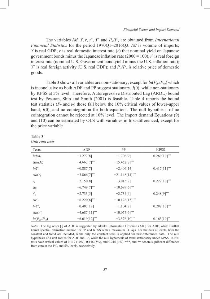
Financial Sector and Import Demand
57
The variables IM, Y, r, r*, Y * and Pd/Pw are obtained from International Financial Statistics for the period 1970Q1–2016Q3. IM is volume of imports; Y is real GDP; r is real domestic interest rate (r) that nominal yield on Japanese government bonds minus the Japanese inflation rate (2000 = 100); r* is real foreign interest rate (nominal U.S. Government bond yield minus the U.S. inflation rate); Y * is real foreign activity (U.S. real GDP); and Pd/Pw is relative price of domestic goods.
Table 3 shows all variables are non-stationary, except for ln(Pdt /Pwt) which is inconclusive as both ADF and PP suggest stationary, I(0), while non-stationary by KPSS at 5% level. Therefore, Autoregressive Distributed Lag (ARDL) bound test by Pesaran, Shin and Smith (2001) is feasible. Table 4 reports the bound test statistics (F- and t-) those fall below the 10% critical values of lower-upper band, I(0), and no cointegration for both equations. The null hypothesis of no cointegration cannot be rejected at 10% level. The import demand Equations (9) and (10) can be estimated by OLS with variables in first-differenced, except for the price variable.
Table 3 Unit root tests
Tests ADF PP KPSS
lnIMt −1.277[8] −1.706[9] 0.269[10]***
ΔlnIMt −4.663[7]*** −15.452[8]***
lnYt −0.887[7] −2.406[14] 0.417[11]***
ΔlnYt −3.866[7]*** −21.148[14]***
rt −2.150[8] −3.015[2] 0.222[10]***
Δrt −6.749[7]*** −10.699[6]***
r*t −2.733[5] −2.734[4] 0.248[9]***
Δr*t −6.220[6]*** −10.176[13]***
lnY *t −0.487[12] −1.104[7] 0.282[10]***
ΔlnY *t −4.687[11]*** −10.057[6]***
ln(Pdt /Pwt) −6.619[12]*** −3.576[10]** 0.163[10]**
Notes: The lag order [.] of ADF is suggested by Akaike Information Criterion (AIC) for ADF, while Bartlett kernel spectral estimation method for PP and KPSS with a maximum 14 lags. For the data at levels, both the constant and trend are included, while only the constant term is applied for first-differenced data. The null hypothesis of a unit root is for ADF and PP, while the null hypothesis of trend stationarity under KPSS. KPSS tests have critical values of 0.119 (10%), 0.146 (5%), and 0.216 (1%). ***, and ** denote significant difference from zero at the 1%, and 5% levels, respectively.
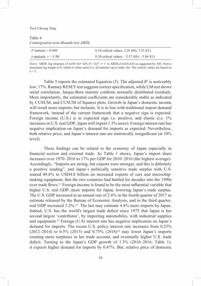
Tuck Cheong Tang
58
Table 4 Cointegration tests-Bounds test ARDL
F-statistic = 0.949 0.10 critical values: 2.26 I(0); 3.35 I(1)
t-statistic = −1.50 0.10 critical values: −2.57 I(0); −3.86 I(1)
Notes: ARDL lag structure of lnIM−lnY−lnPd/Pw−lnY*−r−r* is ARDL(5,6,0,8,4,0) as suggested by AIC from a maximum lag length of 8, which is white noise (i.e. Q-statistics up to order 36). The critical values are based on k = 5.
Table 5 reports the estimated Equation (5). The adjusted R2 is noticeably low, 17%. Ramsey RESET test suggests correct specification, while LM test shows serial correlation. Jarque-Bera statistic confirms normally distributed residuals. More importantly, the estimated coefficients are considerably stable as indicated by CUSUM, and CUSUM of Squares plots. Growth in Japan’s domestic income will result more imports, but inelastic. It is in line with traditional import demand framework, instead of the current framework that a negative sign is expected. Foreign income (U.S.) is in expected sign i.e. positive, and elastic (i.e. 1% increases in U.S. real GDP, Japan will import 1.5% more). Foreign interest rate has negative implication on Japan’s demand for imports as expected. Nevertheless, both relative price, and Japan’s interest rate are statistically insignificant (at 10% level).
These findings can be related to the economy of Japan especially in financial section and external trade. As Table 1 shows, Japan’s import share increases over 1970–2016 to 17% per GDP for 2010–2016 (the highest average). Accordingly, “Imports are strong, but exports were stronger, and this is definitely a positive reading”, and Japan’s politically sensitive trade surplus with U.S. soared 49.6% to USD4.8 billion on increased exports of cars and microchip-making equipment, that the two countries had battled for decades into the 1990s over trade flows.11 Foreign income is found to be the most influential variable that higher U.S. real GDP, more imports for Japan, lowering Japan’s trade surplus. The U.S. GDP increased at an annual rate of 2.6% in the fourth quarter of 2017 as estimate released by the Bureau of Economic Analysis, and in the third quarter, real GDP increased 3.2%.12 The last may estimate 4.8% more imports by Japan. Indeed, U.S. has the world's largest trade deficit since 1975 that Japan is her second largest ‘contributor’, by importing automobiles, with industrial supplies and equipment.13 Foreign (U.S) interest rate has negative implication on Japan’s demand for imports. The recent U.S. policy interest rate increases from 0.25% (2012–2014) to 0.5% (2015) and 0.75% (2016)14 may lower Japan’s imports creating more surpluses in her trade account, and eventually higher U.S. trade deficit. Turning to the Japan’s GDP growth of 1.5% (2010–2016, Table 1), it expects higher demand for imports by 0.47%. But, relative price of domestic
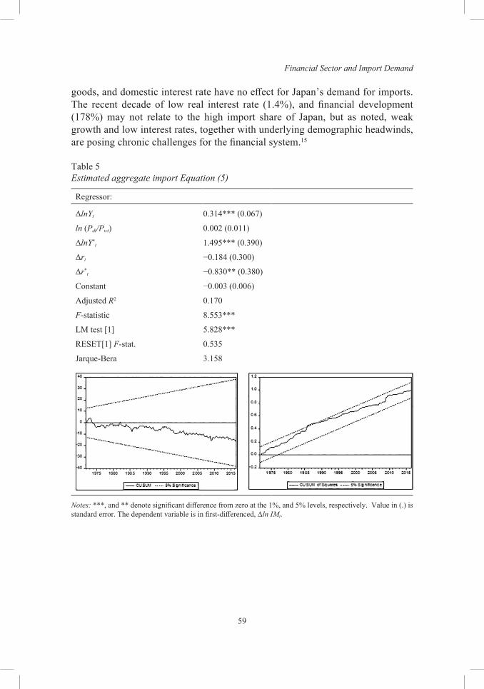
Financial Sector and Import Demand
59
goods, and domestic interest rate have no effect for Japan’s demand for imports. The recent decade of low real interest rate (1.4%), and financial development (178%) may not relate to the high import share of Japan, but as noted, weak growth and low interest rates, together with underlying demographic headwinds, are posing chronic challenges for the financial system.15
Table 5Estimated aggregate import Equation (5)
Regressor:
ΔlnYt 0.314*** (0.067)
ln (Pdt/Pwt) 0.002 (0.011)
ΔlnY*t 1.495*** (0.390)
Δrt −0.184 (0.300)
Δr*t −0.830** (0.380)
Constant −0.003 (0.006)
Adjusted R2 0.170
F-statistic 8.553***
LM test [1] 5.828***
RESET[1] F-stat. 0.535
Jarque-Bera 3.158
Notes: ***, and ** denote significant difference from zero at the 1%, and 5% levels, respectively. Value in (.) is standard error. The dependent variable is in first-differenced, Δln IMt.
Tuck Cheong Tang
60
concluding remarKS
This study derives a structural import demand equation that account for both real sector and financial sector influences. It is based on the portfolio balance approach emphasises adjustment processes in financial markets. This model recognises also forces operating in the financial markets, such as foreign interest rates, and different adjustment mechanisms such as the real balance effect and portfolio adjustment and their impact on goods market. The empirical results presented of using Japan’s data, partially recognise the proposed aggregate import demand modelling framework by their statistically significant estimated coefficient, but no long-run relation. The non-traditional determinants such as foreign interest rates, and foreign income have significant impacts on Japan’s aggregate demand for imports. Domestic GDP is consistent with traditional import demand function. But, relative price of domestic goods, and Japan’s interest rate are insignificant.
The important policy can be suggested from the findings for Japan. Fiscal policy such as government spending, and/or tax plays a favorable outcome than of monetary policy in altering Japan’s demand behavior for imports –lower the trade surplus by stimulating higher growth which makes more imports. Japan relies heavily on primary imports (energy imports), is inevitable that associates with economic growth. Indeed, higher tax revenue via. tariff as strong imports because of higher Japan’s income, that to further finance budget deficit, as in 2015, the state deficit of Japan was at about 3.51% per GDP.16 Growth is estimated to have picked up to 1.5% in 2017, aided by stronger international trade and fiscal stimulus.17 Meanwhile, Japan’s monetary policy, especially the interest rate channel, has no effect on imports, while Bank of Japan’s negative short-term interest rate target at −0.01%, should go for financing more imports. Accordingly, Bank of Japan should maintain its expansionary monetary policy until the 2% inflation target is achieved,18 as the relative price of domestic goods does not affect imports. The recently macroprudential policy that assure the financial system stability that promote growth (i.e. finance led growth) should be formulated, which may indirectly result more imports.
Such a conclusion, however, is dryly generated from a single country’s experiences: Japan. Perhaps, it can be further strengthened by future research which considers a wider range of countries. It is worth to note that this study does not intend to replace the existing aggregate import demand function(s), but the two newly proposed equations do provide a new direction for the future research topics in international trade involving import demand function.
Financial Sector and Import Demand
61
noteS
1. https://atlas.media.mit.edu/en/profile/country/jpn/#Imports2. http://www.economywatch.com/world_economy/japan/export-import.html3. See, the seminal version in Tang (2013). For the first approach (i.e. income-
expenditure equilibrium), in the goods and services market, planned expenditure (E ) equals planned output (Y) per period. An equilibrium relation with the imports variable into left-hand side yields IMt = −(Sp
t − It) − (Tt − Gt) + Xt which can be rewritten as IMt = It − Sp
t + BDt + Xt given a budget deficit (BD). The behavioural structure of this relation is IMt(.) = It(.) − S p
t(.) + BDt(.) + Xt(.) or more precisely, IMt(.) = It(rt
(−)) − Spt(Yt
(+),rt(+)) + BDt
0 + Xt(Y*t(+),Pdt /Pwt
(−)). A reduced form of import demand function can be derived for empirical analysis with IMt = BDt
0 + IMt(Yt(−),
Pdt /Pwt(−),Yt
*(+),rt(−)). Similar finding of non-cointegration (by bounds test) is found
as to the portfolio balance approach, and both approaches give identical regression estimates. The results are available upon request from the author.
4. Fausten (1979) examined the alleged Humean origin of the contemporary monetary approach to the BoP, and he noted that the monetary approach differs in some respect from the Humean approach, “[money] is none of the wheels of trade: It is the oil which renders the motion of the wheels more smooth and easy” (Fausten, 1979, p. 670).
5. Note that in BoP accounting ΔIR > 0 represents a loss of reserves, and conversely.6. In order to make the notation consistent between the BoP relation and the money
supply, redefine (ΔIR > 0) as a gain in reserves. That means inverting the sign in front of the ΔIR variable in the BoP relation.
7. These imbalances are reflected in cross-border flows and, hence, strictly confined to flow equilibria. Full equilibrium, in the sense of stock and flow equilibrium, obviously precludes any such adjustment flows.
8. The sustainability over time of such imbalances is not of immediate concern in the present context. An extensive literature deals with the dynamic adjustment paths in open economies.
9. In this case the interest rate effect works through portfolio substitutions initiated by changes in the demand for money. The net effect on the demand for imports will be positive as long as the interest elasticity of the demand for bonds is smaller than the interest elasticity of the demand for money balances.
10. This form is usually used for import demand equations because of its convenience and ease of interepretation (Carone, 1996, p. 5). It is the most appropriate functional form because the estimated coefficients give directly the relevant elasticity coefficients (Thursby & Thursby, 1984). This functional form has the added advantage of avoiding estimation problems such as multicollinearity (Gafar, 1988).
11. https://www.japantimes.co.jp/news/2017/09/20/business/economy-business/japan-trade-balance-returns-surplus-strength-auto-electronics-exports/#.WnPNOKiWbIU
12. https://www.bea.gov/newsreleases/glance.htm13. https://www.thebalance.com/trade-deficit-by-county-330626414. https://www.focus-economics.com/country-indicator/united-states/interest-rate
Tuck Cheong Tang
62
15. Financial System Stability Assessment Paper on Japan was prepared by the International Monetary Fund as background documentation for the periodic consultation with Japan, that was completed on 12 July 2017. https://www.imf.org/~/media/Files/Publications/CR/2017/cr17244.ashx
16. https://www.statista.com/statistics/270118/budget-balance-in-japan-in-relation-to-gross-domestic-product-gdp/
17. http://www.oecd.org/eco/outlook/japan-economic-forecast-summary.htm18. As footnote 17.
reFerenceS
Ahad, M., Afza, T., & Shahbaz, M. (2017). Financial development and estimation of import demand function in Pakistan: Evidence from combined cointegration and causality tests. Global Business Review, 18(1), 118–131. https://doi.org/10.1177/0972150916666909
Altan, M. (2016). The role of banks funding and promoting the foreign trade: Case of Turkey. International Journal of Economics and Management Engineering, 10(7), 2438–2441. Retrieved from http://waset.org/publications/10005005/the-role-of-banks-funding-and-promoting-the-foreign-trade-case-of-turkey
Auboin, M., & Engemann, M. (2014). Testing the trade credit and trade link: Evidence from data on export credit insurance. Review of World Economics, 150(4), 715–743. https://doi.org/10.1007/s10290-014-0195-4
Athens, E. P. (1985). The aggregate import equation: price homogeneity and monetary effects. Empirical Economics, 10(2), 91–101. https://doi.org/10.1007/BF01973543
Carone, G. (1996). Modeling the U.S. demand for imports through cointegration and error correction. Journal of Policy Modeling, 18(1), 1–48.
Ceglowski, J. (1991). Intertemporal substitution in import demand. Journal of International Money and Finance, 10(1), 118–130. https://doi.org/10.1016/0261-5606(91)90030-N
Chang, T. C. (1945–1946). International comparison of demand for imports. Review of Economic Studies, 13(2), 53–67. https://doi.org/10.2307/2296036
Clower, R. W. (1967). A reconsideration of the microfoundation of monetary theory. Western Economic Journal, 6(1), 1–9. https://doi.org/10.1111/j.1465-7295.1967.tb01171.x
Craigwell, R. (1994). Modelling aggregae import demand in Barbados, Central Bank of Barbados. Retrieved from http://www.centralbank.org.bb/Portals/0/Files/WP1994-11.PDF
Croix, D. D., & Urbain, J. P. (1998). Intertemporal substitution in import demand and habit formation. Journal of Applied Econometrics, 13(6), 589–612. https://doi.org/10.1002/(SICI)1099-1255(199811/12)13:6<589::AID-JAE489>3.0.CO;2-2
Fausten, D. K. (1979). The Humean origin of the contemporary monetary approach to the balance of payments. Quarterly Journal of Economics, 93(4), 655–673. https://doi.org/10.2307/1884474
Financial Sector and Import Demand
63
Gafar, J. S. (1988). The determinants of import demand in Trinidad and Tobago: 1967–1984. Applied Economics, 20(3), 303–313. https://doi.org/10.1080/ 00036848800000044
Houthakker, H., & Magee, S. (1969). Income and price elasticities in world trade. Review of Economics and Statistics, 51(2), 111–125. https://doi.org/10.2307/1926720
International Monetary Fund. (1993). Balance of payments manual (5th ed.). Retrieved from http://www.imf.org/external/np/sta/bop/BOPmain.pdf
Johnson, H. G. (1972). Further essays in monetary economics. London: George Allen and Unwin.
Khan, M. S. (1974). Import and export demand in developing countries. IMF Staff Paper, 21(3), 678–693. https://doi.org/10.2307/3866553
Kouri, P. J., & Porter, M. G. (1974). International capital flows and portfolio equilibrium. Journal of Political Economy, 82(3), 443–467. Retrieved from http://www.journals.uchicago.edu/doi/pdfplus/10.1086/260207
Miller, S. M., & Russek, F. S. (1989). Are the twin deficits really related? Contemporary Policy Issues, 7(4), 91–115. https://doi.org/10.1111/j.1465-7287.1992.tb00218.x
Muktadir-Al-Mukit, D., Shafiullah, A. Z. M., & Sajib, A. H. (2013). Determination of causality between remittance and import: Evidence from Bangladesh. International Journal of Business and Social Research, 3(3), 55–62. https://doi.org/10.18533/ijbsr.v3i3.56
Mundell, R. A. (1963). Capital mobility and stabilization policy under fixed and flexible exchange rates. Canadian Journal of Economics and Political Science, 29(4), 475–485. https://doi.org/10.2307/139336
Mussa, M. (1974). A monetary approach to balance-of-payments analysis. Journal of Money, Credit and Banking, 6(3), 333–351. https://doi.org/10.2307/1991173
Paganelli, M. P. (2006) Hume and endogenous money. Eastern Economic Journal, 32(3), 533–547. Retrieved from http://www.jstor.org/stable/40326294
Pesaran, M., Shin, Y., & Smith R. (2001). Bounds testing approaches to the analysis of level relationships. Journal of Applied Econometrics, 16(3), 289–326. https://doi.org/10.1002/jae.616
Senhadji, A. (1998). Time-series estimation of structural import demand equations: A cross-country analysis. IMF Staff Papers, 45(2), 236–268. https://doi.org/ 10.2307/3867390
Tang, T. C. (2004). Does financial variable(s) explain the Japanese aggregate import demand? A cointegration analysis. Applied Economics Letters, 11(12), 775–780. https://doi.org/10.1080/1350485042000236584
Tang, T. C. (2006). Aggregate import demand and bank credit in Southeast Asia: An empirical study. International Journal of Economics and Management, 1(1), 117–139. Retrieved from http://www.ijem.upm.edu.my/vol1no1/6.pdf
Tang, T. C. (2008). The demand for imports in Japan: A review article. International Journal of Business and Society, 9(1), 53–76. Retrieved from http://www.ijbs.unimas.my/repository/pdf/VOL9NO1(abs4).pdf
Tuck Cheong Tang
64
Tang, T. C. (2013). A general equilibrium perspective of aggregate import demand, Department of Economics Discussion Paper 06/13, Monash University, 1–23. https://www.monash.edu/__data/assets/pdf_file/0008/925721/a_general_equilibrium_perspective_of_aggregate_import_demand.pdf
Tang, T. C. (2015). “Common factors”, cointegration, and Japan’s aggregate import demand function. International Journal of Economics and Management, 9(2), 34–53. Retrieved from http://www.myjurnal.my/public/article-view.php?id= 90191
Thursby, J. G., & Thursby, M. C. (1984). How reliable are simple, single equation specifications of import demand? The Review of Economics and Statistics, 66(1), 120–128.
Ziramba, E., & Mumangeni, J. (2017). Bank credit and aggregate import demand in South Africa: An autoregressive distributed lag approach. European Scientific Journal, 13(16), 71–83. https://doi.org/10.19044/esj.2017.v13n16p71
AAMJAF Vol. 14, No. 2, 65–102, 2018
© Asian Academy of Management and Penerbit Universiti Sains Malaysia, 2018. This work is licensed under the terms of the Creative Commons Attribution (CC BY) (http://creativecommons.org/licenses/by/4.0/).
Asian Academy of Management Journal
of Accounting and Finance
GOVERNANCE OF BEHAVIOURAL BIASES IN ASSET MANAGEMENT INDUSTRY: INSIGHTS FROM FUND
MANAGERS IN MALAYSIA
Zamri Ahmad1*, Haslindar Ibrahim1 and Jasman Tuyon2
1School of Management, Universiti Sains Malaysia, 11800 USM Pulau Pinang, Malaysia
2Faculty of Business and Management, Universiti Teknologi MARA, 88997, Kota Kinabalu, Sabah, Malaysia
*Corresponding author: [email protected]
ABSTRACT
Institutional investors’ behavioural biases have been growingly observed in global financial markets but the governance policy initiatives to mitigate these biases have been long overdue. Taking Malaysia as the case, this paper examines the possibility of behavioural biases among professional investors and discusses the importance of behavioural biases governance in asset management industry. Combination of survey and Delphi methods are used for data collection (survey) and validation of opinions (Delphi). The survey shows the possibility of behavioural biases impacting the thought, decision, and investing strategies of the fund manager. Of great concern, the need to govern behavioural biases in the fund management governance framework has been neglected. This brings challenges to the performance and sustainability of fund management industry. This paper provides behavioural finance insights to inform researchers, practitioners and regulators on the needs and ways to govern behavioural biases through behavioural governance.
Keywords: behavioural analysis, behavioural biases, behavioural finance, behavioural governance, institutional investors
Publication date: 31 December 2018
To cite this article: Ahmad, Z., Ibrahim, H., & Tuyon, J. (2018). Governance of behavioural biases in asset management industry: Insights from fund managers in Malaysia. Asian Academy of Management Journal of Accounting and Finance, 14(2), 65–102. https://doi.org/10.21315/aamjaf2018.14.2.4
To link to this article: https://doi.org/10.21315/aamjaf2018.14.2.4
Zamri Ahmad et al.
66
INTRODUCTION
Behavioural biases among institutional investors are real, permanent, and crucially impacting Malaysia asset management industry performance and sustainability as well as financial market efficiency. Behavioural finance postulates that normal investor behaviour, despite mostly intelligent, often deviates from logic and display many behavioural biases in their investment decision-making processes (Baker & Ricciardi, 2014; Statman, 2014). Behavioural biases can be grouped into two categories namely cognitive and affective biases, both yield irrational behaviour and decision in financial markets. In investment practices, behavioural biases could cause prices to deviate from fundamental value in the long term (Shefrin, 2000). This systematic mispricing causes substantial resource misallocation (Daniel, Hirshleifer, & Teoh, 2002) and directly affects financial market efficiency stability. Noting these facts, it is important for fund management institutions and regulators to understand this issue.
To date, mounting evidence of irrational behaviour in financial institutions and repetitive financial market crises are sufficient to warrant attention on the need to govern the benavioral biases. In has been acknowledged in finance literature that fund managers are portrayed as herds that exacerbate volatility, destabilise markets, increase the fragility of the financial system, and consequently impair financial market efficiency (Bikhchandani & Sharma, 2001; Allen & Wood, 2006). In fact, the 2008 global financial crisis is largely due behavioural biases and this pointed to the failure of traditional governance framework (Arsalidou, 2016). Arising from these crises, a number of developments in recent years have combined to put the issue of financial stability as the top agenda which include a focus on costly crises in national financial systems, and several high-profile mishaps at individual institutions (Crockett, 1997). To mitigate continuous damage in financial markets due to investor irrationality, governance of behavioural biases are needed to be incorporated into the existing governance framework (Cuthbertson, Nitzsche, & O’Sullivan, 2016).
Despite long appearance of behavioural biases in global financial market practice, governance of these biases have been neglected in the current governance framework of financial institutions and markets. This is because the current financial laws and policies have been influenced and formed based on modern finance core ideology (i.e. human rationality and market efficiency) which dominates financial practice and policy (Cunningham, 2002). This result to the ignorance of the issue of biases in human behaviour in general corporate governance framework (Marnet, 2005) by the policy makers. Equally important, the same issue has been less attended and insufficiently tackled in the governance literature (Marnet, 2005; Bodolica & Spraggon, 2011).
Governance of Behavioural Biases in Asset Management Industry
67
Research in behavioural governance is still new with limited evidence. However, it draws notable growing interest from the interdisciplinary science. Key theoretical perspectives could be referred from the nudge theory (Thaler & Sunstein, 2008), the behavioural theory of the firm (Gavetti, Greve, Levinthal, & Ocasio, 2012), behavioural governance (Huse, 2005; Morck, 2008; Van Ees, Gabrielsson, & Huse, 2009; Bodolica & Spraggon, 2011; Virgina & Martin, 2011; Westphal & Zajac, 2013), Islamic governance (Lewis, 2005; Choudhury & Alam, 2013), and the newly emerging neuroethics research (Evers, 2007; Levy, 2008; Northoff, 2009). All of these interdisciplinary research are generally looking at the ethical concepts and practices of human in organisation, markets and society levels.
The aims of this study are to examine evidence proving the presence of behavioural biases among fund managers in Malaysia and to discuss ways to govern behavioural biases through behavioural governance. Noting that behavioural biases are argued to be higher in Asian markets (Kim & Nofsinger, 2008), Malaysia is conveniently chosen as a case to study behavioural biases. A single country investigation is preferred to control for homogeneity of the behaviour. In addition, Malaysian financial market is an important market for global fund managers for geographical portfolio diversification. Recent evidence on the presence of various behavioural biases among instutional investors in Malaysia have been documented by many studies (see: Lai, Low, & Lai, 2001; Lai, Tan, & Chong, 2013; Mohamad & Perry, 2015; Khan, Tan, & Chong, 2016; Ahmad, Ibrahim, & Tuyon; 2017b; Khan, Naz, Qureshi, & Ghafoor, 2017; Khan, Tan, & Chong, 2017; Jaiyeoba, Adewale, Haron, & Che Ismail, 2018). In addition, some studies provide evidence on the presence of behavioural biases on general market perspective (Brahmana, Hooy, & Ahmad, 2012; Tuyon, Ahmad, & Matahir, 2016; Anusakumar, Ali, & Hooy, 2017).
This research extends the above enquiries by investigating how behavioural biases could be governed by reference to Malaysia case. The study of behavioural biases governance in the Malaysian financial market is crucial given the following grounds. Fund management firms are the largest players in the Malaysian financial market and several fund management firms are considering behavioural elements in their fund management strategies as summarised in Table 1. Noted that some are going against the behavioural biases and others are exploiting them. Yet, the behavioural finance courses conducted in Malaysia are still limited. List of behavioural finance courses (past and on-going) in Malaysia is as tabulated in Table 2. Of particular important, misconduct cases in Malaysian financial markets are largely due to human errors. Based on the Securities Commission’s annual report (2017), the top issues are related to possible market misconduct involving
Zamri Ahmad et al.
68
insider trading (56%), corporate governance (17%), securities fraud (9%), and market manipulation (6%). On a positive note, acknowledging the limitations of traditional regulatory policies that are designed on the assumption of rational human behaviour, and the potential regulatory benefits offered by behavioural insights, Securities commission have established the behavioural analysis unit in 2017 to undertake behavioural studies and to design better policies that have more effective outcomes (Securities Commission of Malaysia, 2017). However, the behavioural initiative is still in early stage and no specific behavioural governance policy has been executed yet.
THEORY AND EVIDENCE ON INSTITUTIONAL INVESTOR BEHAVIOURAL BIASES
Theoretical Underpinning
In behavioural finance, vital to effective financial market and institution policy design is the recognition that the financial world is organised by bounded rational agents and that the financial markets are imperfect. This research briefly introduce the following behavioural theories that shed lights on an imperfection in human behaviour and behavioural governance.
Bounded rational theory (Simon, 1955) offers the behavioural model of individual choice, which does not assume full rational of market players. The bounded rationality theory postulates that individual decisions and behaviours contain both rational and irrational elements. Thus, decisions are normally goal oriented and adaptive (Jones, 1999). The bounded rationality of human decision has been conceptualised by Kahneman (2003) into the dual system of human mind; intuition (System I) and reasoning (System II). The operational processes of System I is categorised as fast, automatic, effortless, associative and emotional. While the operational processes of System II are slower, serial, effortful, deliberately controlled and rule-governed.
Gene-culture coevolutionary theory brings to behavioural finance attention the gene-culture coevolution (Rushton, Littlefield, & Lumsden, 1986; Gintis, 2011) that embraces the importance of culture and complex social organisation to the evolutionary success of Homo sapiens, whereby, individual fitness in humans depends on the structure of social life. This theory postulated that culture is both constrained and promoted by the human genome, human cognitive, affective and moral capacities are the product of an evolutionary dynamic involving the interaction of genes and culture.
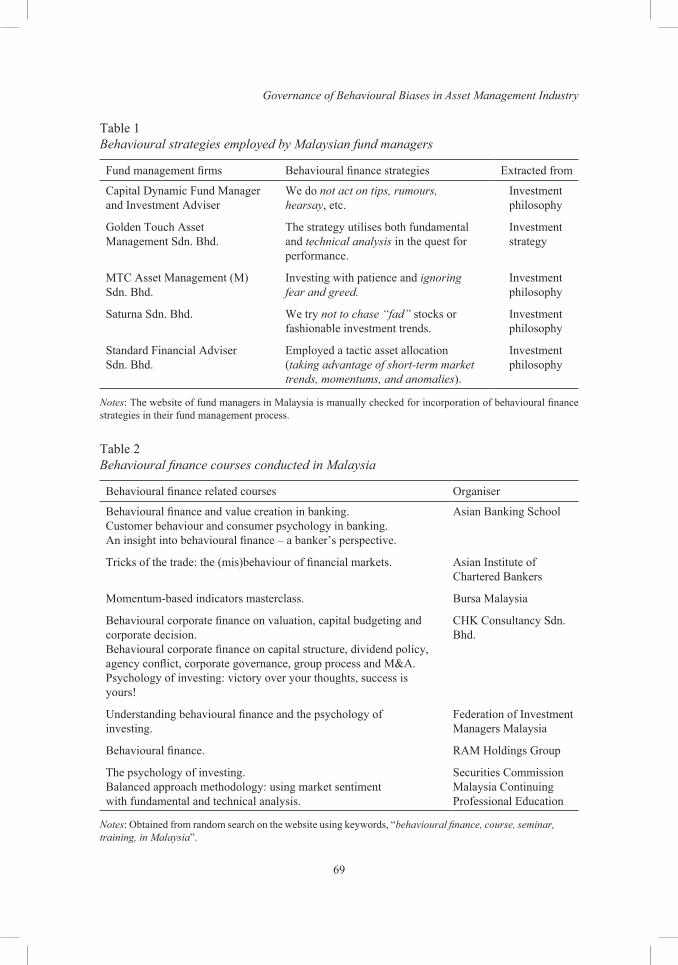
Governance of Behavioural Biases in Asset Management Industry
69
Table 1Behavioural strategies employed by Malaysian fund managers
Fund management firms Behavioural finance strategies Extracted from
Capital Dynamic Fund Manager and Investment Adviser
We do not act on tips, rumours, hearsay, etc.
Investment philosophy
Golden Touch Asset Management Sdn. Bhd.
The strategy utilises both fundamental and technical analysis in the quest for performance.
Investment strategy
MTC Asset Management (M) Sdn. Bhd.
Investing with patience and ignoring fear and greed.
Investment philosophy
Saturna Sdn. Bhd. We try not to chase “fad” stocks or fashionable investment trends.
Investment philosophy
Standard Financial Adviser Sdn. Bhd.
Employed a tactic asset allocation (taking advantage of short-term market trends, momentums, and anomalies).
Investment philosophy
Notes: The website of fund managers in Malaysia is manually checked for incorporation of behavioural finance strategies in their fund management process.
Table 2Behavioural finance courses conducted in Malaysia
Behavioural finance related courses Organiser
Behavioural finance and value creation in banking.Customer behaviour and consumer psychology in banking.An insight into behavioural finance – a banker’s perspective.
Asian Banking School
Tricks of the trade: the (mis)behaviour of financial markets. Asian Institute of Chartered Bankers
Momentum-based indicators masterclass. Bursa Malaysia
Behavioural corporate finance on valuation, capital budgeting and corporate decision.Behavioural corporate finance on capital structure, dividend policy, agency conflict, corporate governance, group process and M&A.Psychology of investing: victory over your thoughts, success is yours!
CHK Consultancy Sdn. Bhd.
Understanding behavioural finance and the psychology of investing.
Federation of Investment Managers Malaysia
Behavioural finance. RAM Holdings Group
The psychology of investing.Balanced approach methodology: using market sentiment with fundamental and technical analysis.
Securities Commission Malaysia Continuing Professional Education
Notes: Obtained from random search on the website using keywords, “behavioural finance, course, seminar, training, in Malaysia”.

Zamri Ahmad et al.
70
Prospect theory is an alternative model of decision making under risk that acknowledge human imperfection idealised by Kahneman and Tversky (1979). Prospect theory distinguishes two phases in individual choice process namely framing and valuation. In the framing stage the individual constructs a representation of the acts, contingency and outcomes relevant to the decision. In the evaluation stage, individual assess each of the prospects available and choose accordingly. Prospect theory offers valuable behavioural insights on firm and individual level risk taking behaviour (Holmes, Bromiley, Devers, Holcomb, & McGuire, 2011). In the context of governance of financial institution, prospect theory are significant in understanding managers’ tendancy to be risk-seeking in situation of possible loss and risk averse in a situation of a certain gain is likely (Arsalidou, 2016).
Nudge theory of Thaler and Sunstein (2008) acknowledged the bounded rational of individuals and suggested the behavioural ways to mitigate possible biases arising our of individual bounded rationality. In particular, the theory suggested that if the irrational behavioural or decision making is the result of cognitive boundaries, biases, or habits, this behaviour may be “nudged” toward a better option by integrating insights about the boundaries, biases, and habits into the “choice architecture” surrounding the behaviour i.e. the physical, social, and psychological aspects of the contexts in ways that promote a more preferred behaviour. Nudges could change behaviour through various intervention mechanism that is more effective and costless (Sunstein, 2014). For instance, through a financial incentives, providing relevant information, actively blocking an inappropriate choice, and other possible behavioural intervention mechanisms (Kosters & der Heijden, 2015).
Empirical Evidence on Institutional Investor Behavioural Biases
Selected global survey-based evidences of fund managers’ behavioural biases covering 19 countries as summarised in Table 3 is adapted from Ahmad, Ibrahim and Tuyon (2017a). These behavioural biases are inducing irrational investment decisions. We extend this literature perspective by reviewing empirical evidences from interdisciplinary inquiries which provide insights that different individual or group of individual has different degree of behavioural biases. This non-homogeneous behavioural biases are due to differences in individual, cultural, and institutional forces as discussed in the following.
Individual traits
Individual traits refers to demographic and personality type. Behavioural aspects of demographic and personality type possible influence on decision making and

Governance of Behavioural Biases in Asset Management Industry
71
financial risk taking behaviour have been well documented in finance and economics literature since Siegal and Hoban (1982). Demographic forces as important determinants for individual risk taking decision have been well established in behavioural finance literature. The first factor is gender difference. In psychology research, men have been acknowledged as more risk tolerant compared to women in many risks taking decisions (Byrnes, Miller, & Schafer, 1999) partly because they are more exposed to overconfidence bias (Montier, 2002). This hypothesis has also been supported in behavioural finance research (de Venter & Michayluk, 2008; Halko, Kaustia, & Alanko, 2012). The second factor is age difference. Positive relationship between investor ages and level of risk tolerance has been empirically supported in finance research. Riley and Chow (1992) documented that investor level of risk aversion decreases with their ages. However, evidence from Halko et al. (2012) showed that age effect on risk aversion is reduced when controlling for financial knowledge. The third factor is experience differences. Empirical evidences showed that more experienced and expert investors are more prone to overreaction and overconfidence biases (Chen, Kim, & Nofsinger, 2004; Griffin & Tversky, 1992) and more risk takers (Corter & Chen, 2006). An education difference is the fourth factor. Previous research suggests that education is important in predicting preferences and behaviour. In finance research, finance education that is expected to increase financial literacy has been associated with choices for investment (Schooley & Worden, 1999; Bernheim & Garrett, 2003) risk taking behaviour (Wang, 2009; Sjöberg & Engelberg, 2009) and encourages wealth-creating investment (McCannon, 2014). Nikiforow (2010) shows that training on behavioural finance does increase awareness and reduce the fund managers’ behavioural biases. Personality types are psychological characteristics of individual. Many have examined the connection between personality type and risk tolerance level. There are many personality tests available but the popularly used psychology-based personality tests are the Myers-Briggs Type Indicator,1 Big Five personality taxanomy,2 Zuckerman’s Sensation Seeking Scale (Zuckerman, 1994), Domain-Specific Risk Taking Scale3 (Weber, Blais, & Betz, 2002; Blais & Weber, 2006) and Risk Tollerance Questionnaire (Corter & Chen, 2006). Using the Myers-Briggs Type Indicator test in behavioural finance research provides insights that higher score for extraversion, intuition, thinking and perceiving are positively related to higher level of risk tolerance (Filbeck, Hatfield, & Horvath, 2005). In Mayfield, Perdue and Wooten (2008), using big five personality test, they provide evidence that extraverted individual intend to engage in short-term investing and neuroticism individuals shows that they are more risk averse and do not engage in short-term investing. Meanwhile, individual with openness to experience are inclined to engage in long-term investing.
Zamri Ahmad et al.
72
Cultural traits
Based on sociology perspective, culture is partly important in understanding individual behaviour. Cultural factor has a great determinant role in investment decision-making because investors personally and collectively adhere to conserve personal relationship within the organisation or society they belong to (Ellison & Fudenberg, 1993). Discussions on cultural important in behavioural finance theory is important. Growing evidences from behavioural finance research and other sociology research indicated that investors’ behaviours are related to the cultural origin of the individual. This perspective suggests that individual investment behaviour could be predicted based on their cultural characteristics. We synthesize these survey-based evidences based on Hofstede’s cultural index4 as graphically presented in the following self-explanatory Figure 1. Summary of the survey-based evidences provides further evidence on this issue that the relation between culture and finance is complex. As shown in this figure, regardless of cultural dimension, all countries experienced behavioural biases as documented in the 31 articles reviewed. The theoretical link between culture and finance is shown by the Hofstede’s cultural dimension (Hofstede, 1980) which has been recently referred in behavioural finance research to explain the behaviour of investors across different cultural context. Nguyen and Truong (2013) provides worldwide evidences that information content of stock markets is higher in more individualistic countries and in low uncertainty avoidance countries. Beracha, Fedenia, and Skiba (2014) provide evidence those institutional investors from different cultural background trades differently. In addition, they provide evidence that institutional investors trade at higher frequency in their home countries and in countries with similar cultural background. This finding can be corroborated to earlier findings by Anderson, Fedenia, Hirschey and Skiba (2011), which provide evidence that home bias and international diversification by institutional investors are influenced by cultural bias. Bialkowiski, Bohl, Kaufmann and Wisniewski (2013) confirmed that fund managers exploit the Ramadhan anomaly in their trading strategy which is related to cultural-holiday induced bias in finance literature.
Institutional traits
Two important institutional traits namely governance and ethical concerns. Current corporate governance policy and practice, which are based on the rational model of decision making, may be insufficient to mitigate future corporate failure (Marnet, 2005; 2007). Lack of corporate governance in curving the behavioural biases and information asymmetry has been pointed out as one of the reasons for failure in addressing behavioural induced risks in financial markets. Marnet (2005)

Governance of Behavioural Biases in Asset Management Industry
73
argued that to gamble imprudently seems inherent in human nature. Stocks returns in emerging markets tend to be more positively skewed which can be attributed to managers having more discretion to release good information immediately and bad information slowly (Claessens & Yurtoglu, 2013). To complement this limited evidence, we review the empirical evidences on institutional investor’s behavioural biases against the rank of governance index5 of their respective countries to gauge whether higher corporate governance revealed lower incidences of behavioural biases by institutional investors. This surprising summary portrays that both countries with high and low governance index experiencing behavioural biases. This is probably due to the fact that the current practice of corporate governance does not take into account the need to curve behavioural biases. Some scholars have voiced the needs for corporate governance to include a new mission for corporate governance to control behavioural biases in firms and in financial markets in general (Suto & Toshino, 2005). Being ethical can help to reduce bounded rationality as discussed in Zhang, Fletcher, Gino and Bazerman (2015). Ethical concerns have also been reported to have important roles in mitigating behavioural biases in fund management. In this perspective, Marco, Munoz and Vargas (2011) provide evidences of differences in risk taking behaviour between ethical and conventional mutual fund managers noting that the former is less aggressive in risk taking. This evidence can be corroborated with the findings drawn in Wins and Zwergel (2015) which noted that ethical funds are less risky despite perform lower in comparison with conventional funds.
Figure 1. Hofstede’s cultural dimension for surveyed countriesNotes: This figure plotted the cultural profile of the surveyed countries in the referred 31 articles (as listed in Table 1). Generally, this figure points to the ideas that Asia countries are more on collectivism society, having lower uncertainty avoidance, and lower long term orientation.
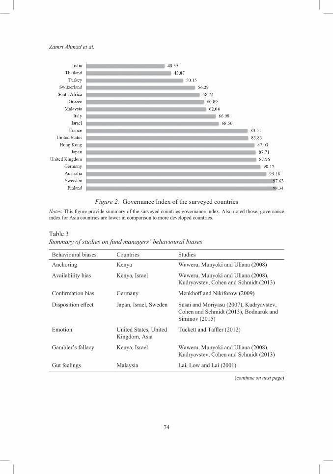
Zamri Ahmad et al.
74
Figure 2. Governance Index of the surveyed countriesNotes: This figure provide summary of the surveyed countries governance index. Also noted those, governance index for Asia countries are lower in comparison to more developed countries.
Table 3Summary of studies on fund managers’ behavioural biases
Behavioural biases Countries Studies
Anchoring Kenya Waweru, Munyoki and Uliana (2008)
Availability bias Kenya, Israel Waweru, Munyoki and Uliana (2008), Kudryavstev, Cohen and Schmidt (2013)
Confirmation bias Germany Menkhoff and Nikiforow (2009)
Disposition effect Japan, Israel, Sweden Susai and Moriyasu (2007), Kudryavstev, Cohen and Schmidt (2013), Bodnaruk and Siminov (2015)
Emotion United States, United Kingdom, Asia
Tuckett and Taffler (2012)
Gambler’s fallacy Kenya, Israel Waweru, Munyoki and Uliana (2008), Kudryavstev, Cohen and Schmidt (2013)
Gut feelings Malaysia Lai, Low and Lai (2001)
(continue on next page)
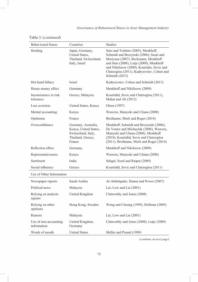
Governance of Behavioural Biases in Asset Management Industry
75
Behavioural biases Countries Studies
Herding Japan, Germany, United States, Thailand, Switzerland, Italy, Israel
Suto and Toshino (2005), Menkhoff, Schmidt and Brozynski (2006), Susai and Moriyasu (2007), Beckmann, Menkhoff and Suto (2008), Lutje (2009), Menkhoff and Nikiforow (2009), Kourtidis, Sevic and Chatzoglou (2011), Kudryavstev, Cohen and Schmidt (2013)
Hot hand fallacy Israel Kudryavstev, Cohen and Schmidt (2013)
House money effect Germany Menkhoff and Nikiforow (2009)
Inconsistence in risk tolerance
Greece, Malaysia Kourtidid, Sevic and Chatzoglou (2011), Mahat and Ali (2012)
Loss aversion United States, Kenya Olsen (1997)
Mental accounting Kenya Waweru, Munyoki and Uliana (2008)
Optimism France Broihanne, Merli and Roger (2014)
Overconfidence Germany, Australia, Kenya, United States, Switzerland, Italy, Thailand, Greece, France
Menkhoff, Schmidt and Brozynski (2006), De Venter and Michayluk (2008), Waweru, Munyoki and Uliana (2008), Menkhoff (2010), Kourtidid, Sevic and Chatzoglou (2011), Broihanne, Merli and Roger (2014)
Reflection effect Germany Menkhoff and Nikiforow (2009)
Representativeness Kenya Waweru, Munyoki and Uliana (2008)
Sentiment India Sehgal, Sood and Raiput (2009)
Social influence Greece Kourtidid, Sevic and Chatzoglou (2011)
Use of Other Information
Newspaper reports Saudi Arabia Al-Abdulqader, Hanna and Power (2007)
Political news Malaysia Lai, Low and Lai (2001)
Relying on analysts reports
United Kingdom Clatworthy and Jones (2008)
Relying on other opinions
Hong Kong, Sweden Wong and Cheung (1999), Hellman (2005)
Rumors Malaysia Lai, Low and Lai (2001)
Use of non-accounting information
United Kingdom, Germany
Clatworthy and Jones (2008), Lutje (2009)
Words of mouth United States Shiller and Pound (1989)
(continue on next page)
Table 3: (continued)

Zamri Ahmad et al.
76
Behavioural biases Countries Studies
Irrational Investment Behaviour
Excessive portfolio turnover
Sweden Bodnaruk and Siminov (2015)
Home bias Germany Menkhoff and Nikiforow (2009)
Momentum trading United States, United Kingdom
Richardson, Tuna and Wysocki (2010)
Winner and spotlight stocks
Germany Arnswald (2001)
Self-marketing Japan Suto and Toshino (2005)
Self-monitoring Greece Kourtidid, Sevic and Chatzoglou (2011)
Short-termism Japan, Germany, United States, Switzerland, Italy, Thailand
Suto and Toshino (2005), Lutje (2009), Menkhoff (2010)
Use of technical analysis
Hong Kong, Malaysia, Saudi Arabia, Germany, Switzerland, United States, Italy, Thailand, United Kingdom
Wong and Cheung (1999), Lai, Low and Lai (2001), Al-Abdulqader, Hanna and Power (2007), Kourtidis, Sevic and Chatzoglou (2011), Menkhoff (2010), Richardson, Tuna and Wysocki (2010)
Source: Adopted from Ahmad et al. (2017a)Notes: This table provides summary of the behavioural biases among institutional investors reflected in the above-mentioned 31 referred studies based on survey methods.
Issues on Governance of Behavioural Biases in Asset Management Industry
Governance of behavioural biases is a serious problem to the fund management institutions and policy makers. Mounting evidence have highlighted the sources and repercussion of behavioural biases in financial markets globally (Chui, Titman, & Wei, 2010; Anderson et al., 2011; Kumar & Goyal, 2015). These behavioural biases bring serious repercussion to the efficiency and sustainability of financial systems in general. In specific context of the study, behavioural biases challenge the performance and sustainability of fund performance. Earlier evidence highlighted the facts that the mutual fund late trading scandal of 2003 brought the failure of mutual fund governance to the public’s attention. Calls for stronger shareholder protections following the 2003 mutual fund scandal, fund boards have become increasingly independent and transparent. Despite this transition, poor governance persists (Calluzzo & Dong, 2014). Further, Hellman (2005) and Cuthberston, Nitzsche and O’Sullivan (2016), highlighted the behavioural effects on fund performance and the needs for governance of these biases.
Table 3: (continued)
Governance of Behavioural Biases in Asset Management Industry
77
The idea to govern behavioural issues in corporate governance is to induce greater rationality and more considered ethics in corporate governance (Morck, 2008). In this regards, Kurniawan, How and Verhoeven (2016) provides evidence on the effectiveness of fund governance in containing investment style drift in the mutual fund industry. Shefrin (2000) advices practitioners to recognize their own and others mistakes, to understand the reasons for these mistakes, and to avoid mistakes. In investment analysis and fund management practices, Fromlet (2001) argued that behavioural finance theories suggest ways to avoid serious mistakes in investment analysis and find profitable investment strategies. As such, institutional investors need to be aware of the growing importance of behavioural finance perspectives (Montier, 2002). Strategies and checklist to overcome behavioural errors are discussed in Kahneman and Riepe (1998), Fromlet (2001), and Baker and Ricciardi (2014).
In Malaysia fund management governance framework, so far, the behavioural biases are not recognised in the policies documents. We qualitatively review two governance policy documents. First is the Malaysia Code for Institutional Investors6 which was first drafted in 2014. This governance policy contains six principles of the code namely; disclosing policies on stewardship, monitoring investee companies, engaging investee companies, managing conflict of interest, incorporating sustainability considerations, and publishing voting policy. Second is the Guidelines on Compliance Function for Fund Management Companies7 which has been available since in 2011. This policy document requires fund management firm to comply with nine core principles namely; integrity; skill, care and diligence; acting in clients’ interests; supervision and control; adequate resources; business conduct; client asset protection; communication with investors and clients; and conflict of interest. Both of these governance policy documents contain no discussion about behavioural biases governance. In fact, the Malaysian Code for Institutional is not mandatory but voluntary.
METHODOLOGY AND DATA
This research uses a triangulation of survey and Delphi methods to understand the fund managers investment practices and opinions on the need and ways to govern behavioural biases. To theoretically understand investor behaviour, the best approach is to focus on individual decision making as suggested in Warneryd (2001). The data from this study has been collected using two methods. First, a post-based survey8 has been conducted in 2016 involving 30 fund managers working with asset management firm in Malaysia as summarised in Table 4 Panel A. In this survey, a set of questionnaire has been prepared to
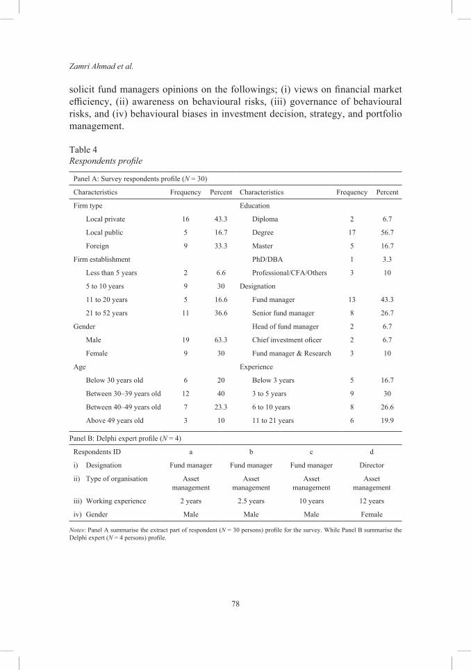
Zamri Ahmad et al.
78
solicit fund managers opinions on the followings; (i) views on financial market efficiency, (ii) awareness on behavioural risks, (iii) governance of behavioural risks, and (iv) behavioural biases in investment decision, strategy, and portfolio management.
Table 4Respondents profile
Panel A: Survey respondents profile (N = 30)
Characteristics Frequency Percent Characteristics Frequency Percent
Firm type Education
Local private 16 43.3 Diploma 2 6.7
Local public 5 16.7 Degree 17 56.7
Foreign 9 33.3 Master 5 16.7
Firm establishment PhD/DBA 1 3.3
Less than 5 years 2 6.6 Professional/CFA/Others 3 10
5 to 10 years 9 30 Designation
11 to 20 years 5 16.6 Fund manager 13 43.3
21 to 52 years 11 36.6 Senior fund manager 8 26.7
Gender Head of fund manager 2 6.7
Male 19 63.3 Chief investment oficer 2 6.7
Female 9 30 Fund manager & Research 3 10
Age Experience
Below 30 years old 6 20 Below 3 years 5 16.7
Between 30–39 years old 12 40 3 to 5 years 9 30
Between 40–49 years old 7 23.3 6 to 10 years 8 26.6
Above 49 years old 3 10 11 to 21 years 6 19.9
Panel B: Delphi expert profile (N = 4)
Respondents ID a b c d
i) Designation Fund manager Fund manager Fund manager Director
ii) Type of organisation Asset management
Asset management
Asset management
Asset management
iii) Working experience 2 years 2.5 years 10 years 12 years
iv) Gender Male Male Male Female
Notes: Panel A summarise the extract part of respondent (N = 30 persons) profile for the survey. While Panel B summarise the Delphi expert (N = 4 persons) profile.
Governance of Behavioural Biases in Asset Management Industry
79
Second, the Delphi method which is the judgement of experts (which can involve a number of less than ten) by means of successive iterations of a given questionnaire, to show possible convergence of opinions obtained in the first survey (Huan-Niemi, Rikkonen, Niemi, Wuori, & Niemi, 2016). In this research, an online Delphi method9 is used to verify the current governance practice and the need to incorporate behavioural risks in the existing fund management governance framework. We have randomly invited a number of Chartered Financial Analysts (CFA) charterholders who are currently working as fund managers in Malaysia. The information is obtained from CFA members’ directory10. We managed to get four respondents to be the Delphi expert for this study as summarised in Table 4 Panel B. Three of them are a fund manager and one is a director with experience from 2 to 12 years. This justifies the knowledge and experience of the Delphi experts employed in this study. In the survey and Delphi method, we solicit the opinions of respondents on issues of research interest (i.e. bounded rational of investors, market imperfect efficiency, and the relevant of behavioural risk governance). These opinions can be represented as a proxy for true behaviour. This is in line with the concepts of opinions and beliefs are acquired behavioural dispositions which refer to tendencies toward particular acts, such as evaluating, or acting toward a particular object or a particular process (Bergman, 1998).
FINDINGS
Survey of Fund Managers Opinions
Views on financial market efficiency
In the first section of the survey questionnaire, we seek fund managers opinions on the state of Malaysia market efficiency. As noted in Table 5, the fund manager’s opinions can be summarised as follows: (i) They agreed that it is possible to predict future returns to Malaysian stocks using various source of information including past returns, private and publicly available information; (ii) They believe that the market is offering arbitrage opportunities, and (iii) They confirmed that fund managers can beat the market performance without taking above-average risk. These opinions are reflected by a high percentage of respondents who agree to five items asked in the questionnaire. Collectively, these opinions is suggesting the presence of possible bounded rationality and inefficiency in the market.

Zamri Ahmad et al.
80
Awareness on behavioural biases and opinion on governance of behavioural biases
The current research also solicits funds managers’ awareness on behavioural finance theory and behavioural risks as well as governance of these behavioural risks in investment practices. The results are presented in Table 6. As for the awareness on behavioural risks, majority of the respondents were not aware of any behavioural finance theory and did not undertake any courses or training related to behavioural finance. However, majority indicated that they are aware of some behavioural risks associated with investment. In addition, majority of them also indicated that some behavioural finance strategies have been incorporated in investment practices and believe that behavioural risks matter in the short term only (Panel A). As for governance of behavioural risks, it is interesting to note that majority of the respondents indicated that mitigating behavioural risks have been incorporated in; investment policy, governance mechanism, audit of trading process, and audit of portfolio management record (Panel B). Nonetheless, the specific governance mechanisms used to mitigate these behavioural risks have not been solicited from the respondents.
Behavioural biases in investment management practice
Investment analysis and source of information used are summarised in Table 7. Fund managers are using a combination of fundamental, technical, and behavioural investment appraisal approaches in their practices (Panel A). These managers rank fundamental method as a priority, rank technical into second and behavioural into third in terms of importance. The mix investment appraisal approaches are also consistent with the important sources of information referred by fund managers (Panel B). The fund managers made reference to both rational sources (i.e. company visits, annual reports, analysts’ recommendations, investor relation reports, broker recommendations, and management financial reports) and information sources with possible irrational elements (i.e. Television and newspapers, internet and investment blogs, friends, and rumors). In Panel C, list of popularly referred fundamental, technical, and behavioural information have been provided by the fund managers.
Table 8 Panel A summarise the strategies used in investment decision and fund portfolio management. The results indicate the followings. First, investment decision is a collective group-based decision among designated fund managers and subjected to pre-specified investment policy of the firm. This evidence highlighted the importance of group decision making and institutional characteristics in fund portfolio management. Second, there is higher evidence of
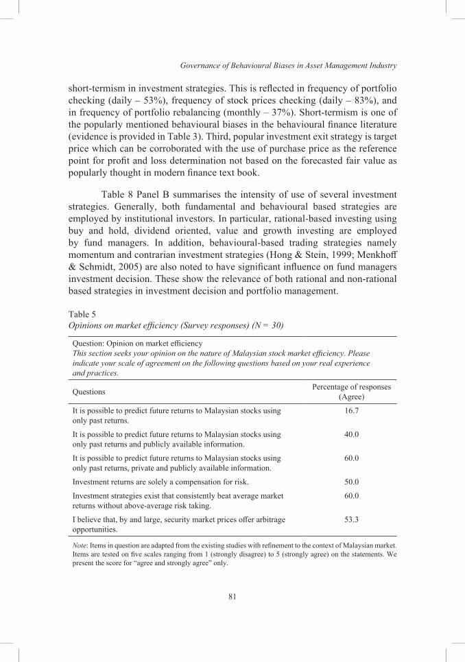
Governance of Behavioural Biases in Asset Management Industry
81
short-termism in investment strategies. This is reflected in frequency of portfolio checking (daily – 53%), frequency of stock prices checking (daily – 83%), and in frequency of portfolio rebalancing (monthly – 37%). Short-termism is one of the popularly mentioned behavioural biases in the behavioural finance literature (evidence is provided in Table 3). Third, popular investment exit strategy is target price which can be corroborated with the use of purchase price as the reference point for profit and loss determination not based on the forecasted fair value as popularly thought in modern finance text book.
Table 8 Panel B summarises the intensity of use of several investment strategies. Generally, both fundamental and behavioural based strategies are employed by institutional investors. In particular, rational-based investing using buy and hold, dividend oriented, value and growth investing are employed by fund managers. In addition, behavioural-based trading strategies namely momentum and contrarian investment strategies (Hong & Stein, 1999; Menkhoff & Schmidt, 2005) are also noted to have significant influence on fund managers investment decision. These show the relevance of both rational and non-rational based strategies in investment decision and portfolio management.
Table 5Opinions on market efficiency (Survey responses) (N = 30)
Question: Opinion on market efficiencyThis section seeks your opinion on the nature of Malaysian stock market efficiency. Please indicate your scale of agreement on the following questions based on your real experience and practices.
Questions Percentage of responses (Agree)
It is possible to predict future returns to Malaysian stocks using only past returns.
16.7
It is possible to predict future returns to Malaysian stocks using only past returns and publicly available information.
40.0
It is possible to predict future returns to Malaysian stocks using only past returns, private and publicly available information.
60.0
Investment returns are solely a compensation for risk. 50.0
Investment strategies exist that consistently beat average market returns without above-average risk taking.
60.0
I believe that, by and large, security market prices offer arbitrage opportunities.
53.3
Note: Items in question are adapted from the existing studies with refinement to the context of Malaysian market. Items are tested on five scales ranging from 1 (strongly disagree) to 5 (strongly agree) on the statements. We present the score for “agree and strongly agree” only.

Zamri Ahmad et al.
82
Table 6Awareness on behavioural risks and opinion on governance of behavioural risks (Survey responses)(N = 30)
Question: Awareness on behavioural risks and opinion on governance of behavioural risksThis section seeks your awareness and your firm governance on behavioural risks. Please answer either Yes or No on the following questions based on your current knowledge, experience, and practice.
Panel A: Awareness on behavioural risks
Question Percentage of responses (Yes)
Are you aware of any behavioural finance theory? 36.7
Have you taken any behavioural finance courses during your undergraduate or postgraduate studies?
36.7
Have you ever attended any training or workshop related to behavioural finance during your employment?
43.3
Are you aware of behavioural factors and investment risk associated with them?
86.7
Behavioural finance approaches are already integrated in our investment strategies.
60.0
Do you think behavioural factors influence your trading behaviour? 83.3
Do you think behavioural factors influence your fund portfolio performance in the short term?
83.3
Do you think behavioural factors influence your fund portfolio performance in the long term?
46.7
Panel B: Governance of behavioural risksDoes your firm currently have an investment policy to mitigate behavioural risks?
63.3
Does your firm currently have a governance mechanism to mitigate behavioural risks?
63.3
Is your trading process regularly audited to mitigate behavioural risks? 66.7
Is your portfolio management record regularly audited to mitigate behavioural risks?
63.3
Note: Items in Panel A and B are self-constructed since no existing reference is available. Items are tested based on YES and NO answer options.
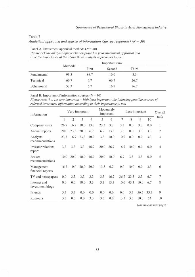
Governance of Behavioural Biases in Asset Management Industry
83
Table 7Analytical approach and source of information (Survey responses) (N = 30)
Panel A: Investment appraisal methods (N = 30)Please tick the analysis approaches employed in your investment appraisal and rank the importance of the above three analysis approaches to you.
MethodsImportant rank
First Second Third
Fundamental 93.3 86.7 10.0 3.3
Technical 66.7 6.7 66.7 26.7
Behavioural 53.3 6.7 16.7 76.7
Panel B: Important of information sources (N = 30)Please rank (i.e. 1st very important – 10th least important) the following possible sources of referred investment information according to their importance to you
InformationVery important Moderately
important Less important Overall rank
1 2 3 4 5 6 7 8 9 10
Company visits 26.7 16.7 10.0 13.3 23.3 3.3 3.3 0.0 3.3 0.0 1
Annual reports 20.0 23.3 20.0 6.7 6.7 13.3 3.3 0.0 3.3 3.3 2
Analysts’ recommendations
23.3 16.7 23.3 10.0 3.3 10.0 10.0 0.0 0.0 3.3 3
Investor relations report
3.3 3.3 3.3 16.7 20.0 26.7 16.7 10.0 0.0 0.0 4
Broker recommendations
10.0 20.0 10.0 16.0 20.0 10.0 6.7 3.3 3.3 0.0 5
Management financial reports
16.7 10.0 20.0 20.0 13.3 6.7 0.0 10.0 0.0 3.3 6
TV and newspapers 0.0 3.3 3.3 3.3 3.3 16.7 36.7 23.3 3.3 6.7 7
Internet and investment blogs
0.0 0.0 10.0 3.3 3.3 13.3 10.0 43.3 10.0 6.7 8
Friends 3.3 3.3 0.0 0.0 0.0 0.0 0.0 3.3 56.7 33.3 9
Rumours 3.3 0.0 0.0 3.3 3.3 0.0 13.3 3.3 10.0 63 10
(continue on next page)
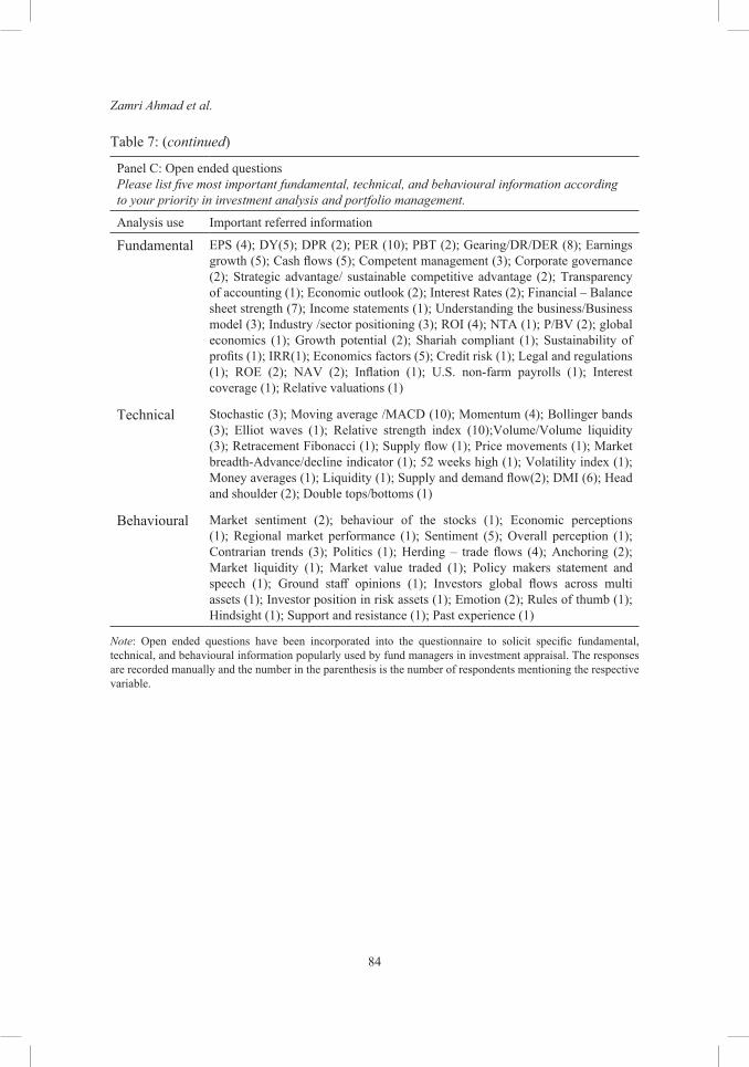
Zamri Ahmad et al.
84
Panel C: Open ended questionsPlease list five most important fundamental, technical, and behavioural information according to your priority in investment analysis and portfolio management.
Analysis use Important referred information
Fundamental EPS (4); DY(5); DPR (2); PER (10); PBT (2); Gearing/DR/DER (8); Earnings growth (5); Cash flows (5); Competent management (3); Corporate governance (2); Strategic advantage/ sustainable competitive advantage (2); Transparency of accounting (1); Economic outlook (2); Interest Rates (2); Financial – Balance sheet strength (7); Income statements (1); Understanding the business/Business model (3); Industry /sector positioning (3); ROI (4); NTA (1); P/BV (2); global economics (1); Growth potential (2); Shariah compliant (1); Sustainability of profits (1); IRR(1); Economics factors (5); Credit risk (1); Legal and regulations (1); ROE (2); NAV (2); Inflation (1); U.S. non-farm payrolls (1); Interest coverage (1); Relative valuations (1)
Technical Stochastic (3); Moving average /MACD (10); Momentum (4); Bollinger bands (3); Elliot waves (1); Relative strength index (10);Volume/Volume liquidity (3); Retracement Fibonacci (1); Supply flow (1); Price movements (1); Market breadth-Advance/decline indicator (1); 52 weeks high (1); Volatility index (1); Money averages (1); Liquidity (1); Supply and demand flow(2); DMI (6); Head and shoulder (2); Double tops/bottoms (1)
Behavioural Market sentiment (2); behaviour of the stocks (1); Economic perceptions (1); Regional market performance (1); Sentiment (5); Overall perception (1); Contrarian trends (3); Politics (1); Herding – trade flows (4); Anchoring (2); Market liquidity (1); Market value traded (1); Policy makers statement and speech (1); Ground staff opinions (1); Investors global flows across multi assets (1); Investor position in risk assets (1); Emotion (2); Rules of thumb (1); Hindsight (1); Support and resistance (1); Past experience (1)
Note: Open ended questions have been incorporated into the questionnaire to solicit specific fundamental, technical, and behavioural information popularly used by fund managers in investment appraisal. The responses are recorded manually and the number in the parenthesis is the number of respondents mentioning the respective variable.
Table 7: (continued)
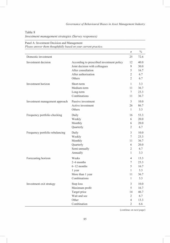
Governance of Behavioural Biases in Asset Management Industry
85
Table 8Investment management strategies (Survey responses)
Panel A: Investment Decision and ManagementPlease answer them thoughtfully based on your current practice.
n %
Domestic investment 25 72.6
Investment decision According to prescribed investment policy 12 40.0Joint decision with colleagues 9 30.0After consultation 5 16.7After authorisation 2 6.7Others 2 6.7
Investment horizon Short-term 1 3.3Medium-term 11 36.7Long-term 7 23.3Combinations 11 36.7
Investment management approach Passive investment 3 10.0Active investment 26 86.7Others 1 3.3
Frequency portfolio checking Daily 16 53.3Weekly 6 20.0Monthly 6 20.0Quarterly 2 6.7
Frequency portfolio rebalancing Daily 3 10.0Weekly 7 23.3Monthly 11 36.7Quarterly 6 20.0Semi-annually 2 6.7Annually 1 3.3
Forecasting horizon Weeks 4 13.32–6 months 7 23.36–12 months 5 16.71 year 1 3.3More than 1 year 11 36.7Combinations 1 3.3
Investment exit strategy Stop loss 3 10.0Maximum profit 5 16.7Target price 14 46.7Wait and see 2 6.7Other 4 13.3Combination 2 6.6
(continue on next page)
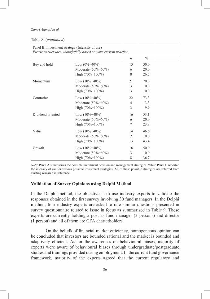
Zamri Ahmad et al.
86
Panel B: Investment strategy (Intensity of use)Please answer them thoughtfully based on your current practice
n %
Buy and hold Low (0%−40%) 15 50.0Moderate (50%−60%) 6 20.0High (70%−100%) 8 26.7
Momentum Low (10%−40%) 21 70.0Moderate (50%−60%) 3 10.0High (70%−100%) 3 10.0
Contrarian Low (10%−40%) 22 73.3Moderate (50%−60%) 4 13.3High (70%−100%) 3 9.9
Dividend oriented Low (10%−40%) 16 53.1Moderate (50%−60%) 6 20.0High (70%−100%) 7 23.3
Value Low (10%−40%) 14 46.6Moderate (50%−60%) 2 10.0High (70%−100%) 13 43.4
Growth Low (10%−40%) 16 50.0Moderate (50%−60%) 3 10.0High (70%−100%) 8 36.7
Note: Panel A summarises the possible investment decision and management strategies. While Panel B reported the intensity of use for various possible investment strategies. All of these possible strategies are referred from existing research in reference.
Validation of Survey Opinions using Delphi Method
In the Delphi method, the objective is to use industry experts to validate the responses obtained in the first survey involving 30 fund managers. In the Delphi method, four industry experts are asked to rate similar questions presented in survey questionnaire related to issue in focus as summarised in Table 9. These experts are currently holding a post as fund manager (3 persons) and director (1 person) and all of them are CFA charterholders.
On the beliefs of financial market efficiency, homogeneous opinion can be concluded that investors are bounded rational and the market is bounded and adaptively efficient. As for the awareness on behavioural biases, majority of experts were aware of behavioural biases through undergraduate/postgraduate studies and trainings provided during employment. In the current fund governance framework, majority of the experts agreed that the current regulatory and
Table 8: (continued)
Governance of Behavioural Biases in Asset Management Industry
87
governance framework does not take into account the need to govern behavioural biases. In addition, they did not agree on the fact that these behavioural biases have to be governed. The other opinion provides supports to this stand. One opined that behavioural risk cannot be regulated due to subjective elements involved and another one was not sure about what are behavioural biases and how could they be governed. General conclusion can be drawn that the Delphi experts and the survey respondents are homogeneous in opinions with regards to the issues of; the state of adaptive market efficiency in Malaysia, awareness and commitment to learn on behavioural finance and behavioural biases, and the need to regulate and govern the behavioural biases in financial institutions practice and financial market policy.
The analysis on findings from the Delphi method is expanded by performing behavioural analysis on the expert responses for behavioural governance framework building as discussed herein. Believe on bounded rationality of institutional investor can be captured from majority of expert endorsement of the opinions that the market offers arbitrage opportunities that could be exploited by investors using various information as well as the repetitive waves of financial crises and market inefficiency are due to the irrational behaviour of market players. In contrast to the survey findings, the Delphi experts’ education background in behavioural finance have helped them to enhance their awareness of behavioural finance theory, and behavioural biases as well as its implications for trading behaviour and portfolio performance. This can be supported with the fact that all of these experts are CFA charterholders in which behavioural finance are covered in the CFA program curriculum. The absence of in-house training related to behavioural finance provided or to be conducted in the near future is an indication of the ignorance of the importance of behavioural finance training by the management. Training related to behavioural finance is required by fund managers to increase awareness and correcting actions on the behavioural biases as noted by one of the experts. The Delphi experts provide fair opinions that the current regulatory and governance framework in the fund management industry does not take into account the behavioural biases. However, they do not agree for regulation and governance of behavioural biases in fund management and financial markets. This could indicate ignorance of the individual fund managers. Their ignorance is due to lack of present knowledge and information on behavioural governance. In particular, these fund managers are not clearly informed on the followings; What behavioural biases to be governed? How to regulate and govern those behavioural biases? Can behavioural governance effectively regulate behavioural biases? and, How to distinguish between agency risk and behavioural biases? In this regards, they demand the fund management industry and its regulators to increase the awareness of, and espouse the benefits of behavioural finance and behavioural governance to them as practitioners.

Zamri Ahmad et al.
88
Table 9Responses from Delphi experts
Question 1: Opinion on the State of Market Efficiency
Agree Disagree
i) It is possible to predict future returns to Malaysian stocks using only past returns.
2 2
ii) It is possible to predict future returns to Malaysian stocks using only past returns and publicly available information.
3 1
iii) It is possible to predict future returns to Malaysian stocks using only past returns, publicly available information, and private information.
3 1
iv) Investment strategies exist that consistently beat average market returns without taking above-average risk.
2 2
v) I believe that, by and large, security market prices offer arbitrage opportunities.
3 1
vi) The adaptive market efficiency hypothesis suggests that market is sometimes efficient, other times not.
3 1
vii) Empirical evidence provides testimony that the repetitive waves of financial crises and market inefficiency are due to irrational behaviour of market players.
3 1
Question 2: Awareness and Commitment to Learn on Behavioural Finance and Behavioural Bias
Yes No
i) Are you aware of any behavioural finance theory? 4
ii) Have you taken any behavioural finance courses during your undergraduate or postgraduate studies?
3 1
iii) Have you ever attended any training or workshop related to behavioural finance during your employment?
4
iv) Are you aware of behavioural bias and investment risk associated with them?
4
v) Do you think behavioural factors influence the trading behaviour of market players?
4
vi) Do you think behavioural factors influence investment portfolio performance in the short term?
4
vii) Do you think behavioural factors influence investment portfolio performance in the long term?
3 1
viii) Did you organisation conducted any in-house training related to understanding of behavioural finance or behavioural bias in investing?
4
ix) Is your organisation planning to conduct any in-house training related to understanding of behavioural finance or behavioural bias in investing?
1 3
(continue on next page)
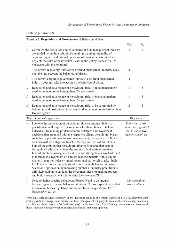
Governance of Behavioural Biases in Asset Management Industry
89
Table 9: (continued)
Question 3: Regulation and Governance of Behavioural Bias
Yes No
i) Currently, the regulation and governance of fund management industry are guided by modern school of thought (assuming rationality of economic agents and rational operation of financial markets) which neglects the roles of behavioural biases in the policy framework. Do you agree with this opinion?
2 2
ii) The current regulatory framework for fund management industry does not take into account the behavioural biases.
4
iii) The current corporate governance framework for fund management industry does not take into account the behavioural biases.
4
iv) Regulation and governance of behavioural risks in fund management need to be incorporated/strengthen. Do you agree?
1 3
v) Regulation and governance of behavioural risks in financial markets need to be incorporated/strengthen. Do you agree?
1 3
vi) Regulation and governance of behavioural risks to be committed by both retail and institutional investors need to be incorporated/strengthen. Do you agree?
2 2
Other Opinions/Suggestions Key ideas
i) I believe the application of behavioural finance amongst industry practitioners will improve the outcomes for their clients (retail and individual) by making prudent recommendations and investment decisions that are tuned with the respective clients behavioural biases. As industry practitioners in asset management, we operate in a fiduciary capacity with an obligation to act in the best interests of our clients. I am of the opinion that behavioural finance is an area that cannot be regulated effectively given the amount of subjectivity involved. Instead, the fund management industry and its regulators would do well to increase the awareness of, and espouse the benefits of this subject matter. It requires industry practitioners such as myself to take “high level” course correcting actions when observing behavioural finance. Successful application by increasing number of industry practitioners will likely add more value to the investment decision making process and build stronger client relationships [Respondent ID: b].
Behavioural risk cannot be regulated
due to subjective elements involved.
ii) Need to define specific behavioural biases. Need to distinguish between agency risk and behavioural biases. Not sure specifically what behavioural biases regulation are needed from the questions above [Respondent ID: c].
Not sure about what and how.
Note: This table provides summary of the questions asked to the Delphi experts (i.e. 4 CFA charterholders working as fund managers and directors of fund management company) to validate the fund managers opinion (i.e. obtained from survey of 30 fund managers) on the state of market efficiency, awareness on behavioural biases, regulation and governance of behavioural risks, and other opinions.
Zamri Ahmad et al.
90
DISCUSSIONS
Collectively, the finding drawn in this research is in contrast to the general beliefs that institutional investors will always act rationally because they are knowledgeable and professionally trained. The discussions focused on syntheses of current research findings to the referred theories and evidences based on behavioural finance theoretical lenses as discussed below. The research use survey and Delphi methods to gauge attitudes, beliefs, and opinions which are behavioural disposition of human real behaviour on the following issues.
Belief on financial market efficiency: The financial markets activities are organised by normal human who are bounded rational as postulated in general behavioural choice theory of bounded rational theory (Simon, 1955). This perspective is also similar with the quasi rational theory (Russel and Thaler, 1985) applied in financial market context. This research draw contrast evidence to the modern finance assumption that market will be efficient due to the presence of rational institutional investors which will always off-set the presence of arbitrage opportunities. This evidence is in confirmation to the behavioural finance views that market is bounded and adaptively efficient. This conclusion is justified with the fact that in rational perspective, asset prices are unpredictable (moves in random) given any informations and the market offers no arbitrage opportunity to be exploited by the investors. Similar argument for Malaysian market has been presented in Tuyon and Ahmad (2016) and Ahmad et al. (2017a, b). Awareness of behavioural risks: Behavioural risks could be mitigated internally and externally. Internally, human behaviours including behavioural biases are products of human minds which are rooted from the brain activities (Barrett, 2009). Being aware is an indication that fund managers realise what these behavioural biases are, how they happen, and what their consequences are. Despite no knowledge on behavioural finance theory, majority of the fund managers are aware of the cause and effects of behavioural biases committed by them. Their knowledge on behavioural finance strategies have been possibly acquired through experience being a fund manager. Bounded rationality of institutional investors: Institutional investors (in this case, fund managers) being a normal human beings are naturally influenced by rational and irrational forces of human mind. This research provides confirming evidence to this ideology in the context of fund managers in Malaysia. Similar earlier evidence is discussed in Ahmad et al. (2017a, b). Governance of behavioural biases: Learning from theory and evidence of higher behavioural biases in Asian financial markets, the need for behavioural biases governance is important particularly for these markets. In the context of Malaysian market
Governance of Behavioural Biases in Asset Management Industry
91
as a focus of the current study, the need to govern behavioural risks in the fund management practice has been neglected. These claims can be substantiated by opinion from fund managers in this survey and absence of the same in the current scope of the Malaysian Code for Institutional Investors.
We extend the discussion on the survey and Delphi expert opinions concerning the possibility of Dunning-Kruger effect.12 The Dunning-Kruger effect states that people unexperienced in a certain field or subject generally perceived themselves as having greater aptitude then in reality they do (Kruger and Dunning, 1999). The presence of such effect will cause bias to the survey results. The present survey is unlikely affected by such bias given the following justifications. In reference to Table 4, the respondents are the real fund managers/chief investment officer/director with working experience ranging from 2 to 21 years. Many of them having postgraduate qualifications (Master/PhD/DBA/CFA/other professional qualifications). These characteristics support the respondents’ knowledge on the subject and quality of opinions given in the survey.
The needs to regulate behavioural biases have been stressed in Daniel et al. (2002) to mitigate the effects of irrational behaviour and imperfect markets. In this regards, they suggested two important issues for public policy. The first one is to help investors avoid mistakes (through education mechanism), while the second is to promote the efficiency of the markets (through policy mechanism). The same argument has been presented in Cunningham (2002) who suggested that investor governance could include investor education and market regulation. The need to incorporate behavioural finance ideology to corporate governance has also been promoted in Cunningham (2002) and Morck (2008) in line with emerging behavioural corporate governance theory (Westphal & Zajac, 2013). Some behavioural approach and cognitive mapping technique is suggested in Garoui and Jarboui (2014). The following conceptual framework (Figure 3) summarises the research findings and the proposal for the need to govern behavioural risks to protect fund performance and sustainability against negative impacts of behavioural biases. The basic premise of this behavioural biases governance framework is that behavioural biases could be governed through internal and external control mechanisms. Internal mechanisms include institutional investor’s education and regulation related to behavioural biases. External mechanisms, meanwhile, are related to financial markets laws and policies to govern behavioural risks. The idea is referred from Daniel et al. s(2002), Cunningham (2002), Suto and Toshino (2005), Li (2008), Morck (2008), Spindler (2011), and Kurniawan, How and Verhoeven (2016).
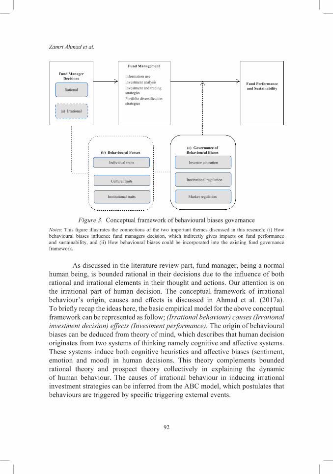
Zamri Ahmad et al.
92
Fund Manager Decisions
Rational
Cultural traits
Institutional traits Market regulation
Investor education
Institutional regulation
Individual traits
Information useInvestment analysisInvestment and trading strategiesPortfolio diversification strategies
(a) Irrational
(b) Behavioural Forces(c) Governance of Behavioural Biases
Fund Management
Fund Performance and Sustainability
Figure 3. Conceptual framework of behavioural biases governanceNotes: This figure illustrates the connections of the two important themes discussed in this research; (i) How behavioural biases influence fund managers decision, which indirectly gives impacts on fund performance and sustainability, and (ii) How behavioural biases could be incorporated into the existing fund governance framework.
As discussed in the literature review part, fund manager, being a normal human being, is bounded rational in their decisions due to the influence of both rational and irrational elements in their thought and actions. Our attention is on the irrational part of human decision. The conceptual framework of irrational behaviour’s origin, causes and effects is discussed in Ahmad et al. (2017a). To briefly recap the ideas here, the basic empirical model for the above conceptual framework can be represented as follow; (Irrational behaviour) causes (Irrational investment decision) effects (Investment performance). The origin of behavioural biases can be deduced from theory of mind, which describes that human decision originates from two systems of thinking namely cognitive and affective systems. These systems induce both cognitive heuristics and affective biases (sentiment, emotion and mood) in human decisions. This theory complements bounded rational theory and prospect theory collectively in explaining the dynamic of human behaviour. The causes of irrational behaviour in inducing irrational investment strategies can be inferred from the ABC model, which postulates that behaviours are triggered by specific triggering external events.
Governance of Behavioural Biases in Asset Management Industry
93
In addition, the conceptual framework also acknowledges that human irrational behaviour differ from one individual to another. The heterogeneity of behavioural biases among individuals are induced by differences in individual, institutional, and cultural traits. The current research extends Ahmad et al. (2017a) work with the ideas that behavioural biases could be mitigated and they can be incorporated in the existing institutional fund governance framework. The suggestions on the governance of behavioural biases through investor education, institutional regulation, and market regulation are in line with the ideas advised by earlier scholars mentioned previously. Different with the existing research, we extend the ideas by providing linkages to (a) irrational behaviour, is due to (b) behavioural forces, and these provide theoretical and empirical supports to behavioural governance elements (c) governance of behavioural biases. This framework shed lights on the behavioural governance curiosity arise from the survey and Delphi opinions. Theoretical ideas on behavioural governance can be learn from the nudge theory. This theory stressed the need to govern choice architecture (physical, social, and psychological aspects of the contexts) that influences the individual behaviours. Similar to this ideology, the proposed conceptual framework also emphasize the behavioural forces (individual traits, cultural traits, and institutional traits) that determine individual behaviours. Accordingly behavioural governance intervention mechanisms could be initiated in these areas covering three aspects namely; investor education, institutional regulations, and market regulations). In investor education, the ideas is to educate the investors (institutional and retail) on various behavioural biases that are coming from the cognitive and affective biases of human minds. In institutional regulations, the institutional culture and the standard investment management operating procedures need to incorporate mechanisms to mitigate commitment of behavioural biases by fund managers. In market regulation, the existing financial market governance needs to be complemented with intervention mechanisms to mitigate excessive behavioural biases that could negatively impact the financial markets.
The practical value of the nudge theory to financial market governance has been acknowledged by the CFA UK’s market integrity and professionalism committee (Radia, 2011). So far, the theory is just providing a descriptive perspective and no complete behavioural governance framework has been crafted. Complementary perspectives on behavioural governance intervention mechanisms could also be learned from the behavioural agency model (Wiseman & Gomez-Mejia, 1998), behavioural theory of the fund management firm (Holland, 2016), Islamic governance, and neuroethics research that collectively offer an interdisciplinary perspectives on the origin of behavioural biases in human decision and possible ways to govern behavioural biases in the financial institutions and markets.
Zamri Ahmad et al.
94
CONCLUSION
This paper provides insights to the field of behavioural finance and aims to inform researchers, practitioners and regulators on the needs and ways to govern behavioural biases in fund management industry taking Malaysia as the case. The findings from this research suggest that behavioural biases are committed by fund managers with awareness on the source and repercussion. To date the profession and the policy makers have neglected the need to govern behavioural biases in the fund governance framework. This claim is supported by the current survey findings and expert endorsement in the Delphi method. In addition, this opinion can also be substantiated with the absence of behavioural risks consideration in the current institutional investor’s governance framework. The research raises important questions about the needs to govern behavioural biases in fund management industry to protect the fund performance and sustainability against the negative effects of behavioural biases. Since the impact of behavioural biases in fund management industry is crucial to the investor’s wealth, fund management institutions performance and sustainability, and the nation financial markets efficiency, we propose that it would be fruitful to pursue further research on how to incorporate governance of behavioural biases in the existing fund governance framework.
ACKNOWLEDGEMENTS
We greatly acknowledged the financial assistance provided by the Universiti Sains Malaysia (USM) through USM-RUI account no. 1001/PMGT/816276. We would like to thank the fund managers’ participation in the survey and those being the Delphi experts. The earlier version of this article was presented in the 12th Asian Academy of Management International Conference 2017 held in Pulau Pinang, Malaysia from 6–9 October 2017. We are grateful to the journal’s management and two anonymous reviewers for their dedication.
NOTES
1. See Filbeck et al. (2005) for detail descriptions.2. See Mayfield et al. (2008) for detail descriptions.3. See Blais and Weber (2006) for detail of questions.4. Hofsteede’s cultural indexes for the respective countries are obtained from
http://geert-hofstede.com/countries.html. We obtained the relevant Hofsteede’s cultural index (i.e. individualism, uncertainty avoidance, and long-term orientation) for all countries covered in the 31 papers reviewed and clustered them on high and low points based on cut point index of 50 (i.e. <50 is low and >50 is high).
Governance of Behavioural Biases in Asset Management Industry
95
5. Governance Index is represented by the Worldwide Governance Indicators of the World Bank, obtained from http://info.worldbank.org/governance/wgi/index.aspx#home. The aggregate governance index is based on six broad dimensions of governance: Voice and Accountability, Political Stability and Absence of Violence/Terrorism, Government Effectiveness, Regulatory Quality, Rule of Law, and Control of Corruption. We obtained the Governance index (i.e. for 2013) for all countries covered in the 31 papers reviewed and clustered them on high and low points based on cut point index of 75 (i.e. <75 is low and >75 in line with World Bank definition).
6. The Malaysian Code for Institutional Investors is retrieved from https://www.sc.com.my/wp-content/uploads/eng/html/cg/mcii_140627.pdf
7. The Guidelines on Compliance Function for Fund Management Companies is retrieved from: https://www.sc.com.my/wp-content/uploads/eng/html/resources/guidelines/FundManagers/ GuidelinesFundManager_170509.pdf
8. Details information and partial analysis of the survey is presented in Ahmad et al. (2017b).
9. The online questionnaire for Delphi experts is available at; https://docs.google.com/forms/d/1Z77CK_2ETrBbUkSAFFZQoInBknY3G_uHyFffYWlTCbI/edit
10. https://www.cfainstitute.org/community/membership/directory/Pages/index.aspx#section-1
11. https://plato.stanford.edu/entries/mental-representation/#Representational12. We thank the reviewer for highlighting this possibility.
REFERENCES
Ahmad, Z., Ibrahim, H., & Tuyon, J. (2017a). Institutional investor behavioral biases: Syntheses of theory and evidence. Management Research Review, 40(5), 578–603. https://doi.org/10.1108/MRR-04-2016-0091
Ahmad, Z., Ibrahim, H., & Tuyon, J. (2017b). Behavior of fund managers in Malaysian investment management industry. Qualitative Research in Financial Markets, 9(3), 205–239. https://doi.org/10.1108/QRFM-08-2016-0024
Allen, W. A., & Wood, G. (2006). Defining and achieving financial stability. Journal of Financial Stability, 2(2), 152–172. https://doi.org/10.1016/j.jfs.2005.10.001
Anderson, C. W., Fedenia, M., Hirschey, M., & Skiba, H. (2011). Cultural influences on home bias and international diversification by institutional investors. Journal of Banking & Finance, 35(4), 916–934. https://doi.org/10.1016/j.jbankfin.2010.09.006
Anusakumar, S. V., Ali, R., & Hooy, C. W. (2017). The effect of investor sentiment on stock returns: Insight from emerging Asian markets. Asian Academy of Management Journal of Accounting and Finance, 13(1), 159–178. https://doi.org/10.21315/aamjaf2017.13.1.7
Arsalidou, D. (2016). Rethinking corporate governance in financial institutions. New York, NY: Rutledge.
Baker, H. K., & Nofsinger, J. R. (2002). Psychological biases of investors. Financial Services Review, 11(2), 97–116. https://doi.org/10.1002/cb.1644
Zamri Ahmad et al.
96
Baker, H. K., & Ricciardi, V. (2014). How biases affect investor behavior. European Financial Review, (February-March), 7–10.
Barrett, L. F. (2009). The future of psychology: Connecting mind to brain. Perspectives on psychological science, 4(4), 326–339. https://doi.org/10.1111/j.1745-6924.2009.01134.x
Beracha, E., Fedenia, M., & Skiba, H. (2014). Culture’s impact on institutional investors’ trading frequency. International Review of Financial Analysis, 31, 34–47. https://doi.org/10.1016/j.irfa.2013.10.002
Bergman, M. M. (1998). A theoretical note on the differences between attitudes, opinions, and values. Swiss Political Science Review, 4(2), 81–93. https://doi.org/10.1002/j.1662-6370.1998.tb00239.x
Bernheim, B. D., & Garrett, D. M. (2003). The effects of financial education in the workplace: Evidence from a survey of households. Journal of Public Economics, 87(1-2), 1487–1519. https://doi.org/10.1016/S0047-2727(01)00184-0
Białkowski, J., Bohl, M. T., Kaufmann, P., & Wisniewski, T. P. (2013). Do mutual fund managers exploit the Ramadan anomaly? Evidence from Turkey. Emerging Markets Review, 15(C), 211–232. https://doi.org/10.1016/j.ememar.2013.02.003
Bikhchandani S, & Sharma, S. (2001). Herd behavior in financial markets. IMF Staff Papers, 47(3), 279–310.
Blais, A. R., & Weber, E. U. (2006). A domain-specific risk-taking (DOSPERT) scale for adult populations. Judgement and Decision Making, 1(1), 33–47. https://doi.org/10.1037/t13084-000
Bodolica, V., & Spraggon, M. (2011). Behavioral governance and self-conscious emotions: Unveiling governance implications of authentic and hubric pride. Journal of Business Ethics, 100, 535–550. https://doi.org/10.1007/s10551-010-0695-7
Brahmana, R., Hooy, W. W., & Ahmad, Z. (2012). The role of herd behaviour in determining the investor’s monday irrationality. Asian Academy of Management Journal of Accounting and Finance, 8(2), 1–20.
Byrnes, J. P., Miller, D. C., & Schafer, W. D. (1999). Gender differences in risk taking: A meta-analysis. Psychological Bulletin, 125(3), 367–383. http://doi.org/ 10.1037/0033-2909.125.3.367
Calluzzo, P., & Dong, G. N. (2014). Fund governance contagion: New evidence on the mutual fund governance paradox. Journal of Corporate Finance, 28, 83–101. https://doi.org/10.1016/j.jcorpfin.2013.11.007
Chen, G., Kim, K., & Nofsinger, J. (2004). Behavior and performance of emerging market investors: Evidence from China. Working paper, Polytechnic University, Kowloon, Hong Kong.
Choudhury, M. A., & Alam, M. N. (2013). Corporate governance in Islamic perspective. International Journal of Islamic and Middle Eastern Finance and Management, 6(3), 180–199. https://doi.org/10.1108/IMEFM-10-2012-0101
Chui, A. C., Titman, S., & Wei, K. J. (2010). Individualism and momentum around the world. Journal of Finance, 65(1), 361–392. https://doi.org/10.1111/j.1540-6261.2009.01532.x
Governance of Behavioural Biases in Asset Management Industry
97
Claessens, S., & Yurtoglu, B. B. (2013). Corporate governance in emerging markets. Emerging Markets Review, 15, 1–33. https://doi.org/10.1016/j.ememar.2012.03.002
Corter, J. E., & Chen Y. J. (2006). Do investment risk tolerance attitudes predict portfolio risk? Journal of Business and Psychology, 20(3), 369–381. https://doi.org/10.1007/s10869-005-9010-5
Crockett, A. (1997). Why is financial stability a goal of public policy? Economic Review-Federal Reserve Bank of Kansas City, 82(4), 5–22.
Cunningham, L. A. (2002). Behavioral finance and investor governance. Washington and Lee Law Review, 59(3), 767–837.
Cuthbertson, K., Nitzsche, D., & O’Sullivan, N. (2016). A review of behavioral and management effects in mutual fund performance. International Review of Financial Analysis, 44, 162–176. https://doi.org/10.1016/j.irfa.2016.01.016
Daniel, K., Hirshleifer, D., & Teoh, S. H. (2002). Investor psychology in capital markets: Evidence and policy implications. Journal of Monetary Economics, 49(1), 139–209. https://doi.org/10.1016/S0304-3932(01)00091-5
de Venter, G. V., & Michayluk, D. (2008). An insight into overconfidence in the forecasting abilities of financial advisors. Australian Journal of Management, 32(3), 545–557. https://doi.org/10.1177/031289620803200309
Ellison, G., & Fudenberg, D. (1993). Rules of thumb for social learning. Journal of Political Economy, 101(4), 612–643. https://doi/abs/10.1086/261890
Evers, K. (2007). Towards a philosophy for neuroethics. EMBO Reports, 8(1S), S48–S51. https://doi.org/10.1038/sj.embor.7401014
Filbeck, G., Hatfield, P., & Horvath, P. (2005). Risk aversion and personality type. Journal of Behavioral Finance, 6, 170–180. https://doi.org/10.1207/s15427579jpfm0604_1
Fromlet, H. (2001). Behavioral finance: Theory and practical application. Business Economics, 36(3), 63–69.
Garling, T., Kirchler, E., Lewis, A., & Raaij, F. V. (2009). Psychology, financial decision making, and financial crises. Psychological Science in the Public Interest, 10(1), 1–47. https://doi.org/ 10.1177/1529100610378437
Garoui, N., & Jarboui, A. (2014). Corporate governance: Behavioral approach and cognitive mapping technique. Contemporary Economics, 8(2), 229–242. https://doi.org/10.5709/ce.1897-9254.143
Gavetti, G., Greve, H. R., Levinthal, D. A., & Ocasio, W. (2012). The behavioral theory of the firm: Assessment and prospects. Academy of Management Annals, 6(1), 1–40. https://doi.org/ 10.1080/19416520.2012.656841
Gintis, H. (2011). Gene–culture coevolution and the nature of human sociality. Philosophical Transactions of the Royal Society of London B: Biological Sciences, 366(1566), 878–888. https://doi.org/10.1098/rstb.2010.0310
Griffin, D., & Tversky, A. (1992). The weighting of evidence and the determinants of confidence. Cognitive Psychology, 3, 430–454. https://doi.org/10.1016/0010-0285(92)90013-R
Halko, M. L., Kaustia, M., & Alanko, E. (2012). The gender effect in risky asset holdings. Journal of Economic Behavior & Organization, 83, 66–81. https://doi.org/10.1016/j.jebo.2011.06.011
Zamri Ahmad et al.
98
Hellman, K. (2005). Strategy‐driven B2B promotions. Journal of Business & Industrial Marketing, 20(1), 4–11. https://doi.org/10.1108/08858620510576748
Hofstede. G. (1980). Cultural consequences: International differences in work related values. Beverly Hills, CA.: Sage Publication
Holland, J. (2016). A behavioral theory of the fund management firm. European Journal of Finance, 22(11), 1004–1039. https://doi.org/ 10.1080/1351847X. 2014.924078
Holmes, R. M., Jr., Bromiley, P., Devers, C. E., Holcomb, T. R., & McGuire, J. B. (2011). Management theory applications of prospect theory: Accomplishments, challenges, and opportunities. Journal of Management, 37, 1069–1107. https://doi.org/ 10.1177/0149206310394863
Hong, H., & Stein, J. C. (1999). A unified theory of underreaction, momentum trading, and overreaction in asset markets. Journal of Finance, 54(6), 2143–2184. https://doi.org/10.1111/0022-1082.00184
Huan-Niemi, E., Rikkonen, P., Niemi, J., Wuori, O., & Niemi, J. (2016). Combining quantitative and qualitative research methods to foresee the changes in the Finnish agri-food sector. Futures, 83, 88–99. https://doi.org/10.1016/j.futures. 2016.03.007
Huse, M. (2005). Accountability and creating accountability: A framework for exploring behavioral perspectives of corporate governance. British Journal of Management, 16(1), S65–S79. https://doi.org/10.1111/j.1467-8551.2005.00448.x
Jaiyeoba, H. B., Adewale, A. A., Haron, R., & Che Ismail, C. M. H. (2018). Investment decision behavior of the Malaysian retail investors and fund managers: A qualitative inquiry. Qualitative Research in Financial Markets, 10(2), 134–151. https://doi.org/10.1108/QRFM-07-2017-0062
Jones, B. D. (1999). Bounded rationality. Annual Review of Political Science, 2, 297–321. https://doi.org/10.1146/annurev.polisci.2.1.297
Kahneman, D. (2003). Maps of bounded rationality: Psychology of behavioral economics. American Economic Review, 93(5), 1449–1475. https://doi.org/ 10. 1257/000282803322655392
Kahneman, D., & Riepe, M. W. (1998). Aspects of investor psychology. Journal of Portfolio Management, 24(4), 52–65. https://doi.org/10.3905/jpm.1998.409643
Kahneman, D., & Tversky, A. (1979). Prospect theory: An analysis of decision under risk. Econometrica, 47(2), 263–291. https://doi.org/10.1142/9789814417358_0006
Khan, H. H., Naz, I., Qureshi, F., & Ghafoor, A. (2017). Heuristics and stock buying decision: Evidence from Malaysian and Pakistani stock markets. Borsa Istanbul Review, 17(2), 97–110. https://doi.org/10.1016/j.bir.2016.12.002
Khan, M. T. I., Tan, S. H., & Chong, L. L. (2016). Perception of past portfolio returns, optimism and financial decisions. Review of Behavioral Finance, 9(1), 79–98. https://doi.org/10.1108/RBF-02-2016-0005
Khan, M. T. I., Tan, S. H., & Chong, L. L. (2017). Information sources and investing decisions: A path modeling approach. Managerial Finance, 43(8), 928–946. https://doi.org/10.1108/MF-08-2016-0232
Kim, K. A., & Nofsinger, J. R. (2008). Behavioral finance in Asia. Pacific-Basin Finance Journal, 16(1), 1–7. https://doi.org/10.1016/j.pacfin.2007.04.001
Governance of Behavioural Biases in Asset Management Industry
99
Kosters, M., & der Heijeden, J. V. (2015). From mechanism to virtue: Evaluating nudge theory. Evaluation, 21(3), 276–291. https://doi.org/ 10.1177/1356389015590218
Kruger, J., & Dunning, D. (1999). Unskilled and unaware of it: How difficulties in recognizing one’s own incompetence lead to inflated self-assessments. Journal of Personality and Social Psychology, 77(6), 1121–1134. https://doi.org/10. 1037/0022-3514.77.6.1121
Kumar, S., & Goyal, N. (2015). Behavioral biases in investment decision making: A systematic literature review. Qualitative Research in Financial Markets, 7(1), 88–108. https://doi.org/10.1108/QRFM-07-2014-0022
Kurniawan, M., How, J., & Verhoeven, P. (2016). Fund governance and style drift. Pacific-Basin Finance Journal, 40, 59–72. https://doi.org/10.1016/j.pacfin.2016. 08.006
Lai, M. M., Low, K. L., & Lai, M. M. (2001). Are Malaysian investors rational? Journal of Psychology and Financial Markets, 2(4), 210–215. https://doi.org/10.1207/S15327760JPFM0204_5
Lai, M. M., Tan, S. H., & Chong, L. L. (2013). The behavior of institutional and retail investors in bursa Malaysia during the bulls and bears. Journal of Behavioral Finance, 14(2), 104–115. https://doi.org/10.1080/15427560.2013.790822
Levy, N. (2008). Introducing neuroethics. Neuroethics, 1(1), 1–8. https://doi.org/10.1007/s12152-008-9007-7
Lewis, M. K. (2005). Islamic corporate governance. Review of Islamic Economics, 9(1), 5–29.
Li, G. (2008). China’s stock market: Inefficiencies and institutional implications. China & World Economy, 16(6), 81–96. https://doi.org/10.1111/j.1749-124X. 2008.00139.x
Lowenstein, G., & Chater, N. (2017). Putting nudges in perspective. Behavioural Public Policy, 1(1), 26–53. https://doi.org/10.1017/bpp.2016.7
Marco, I., Munoz, F., & Vargas, M. (2011). Do ethical and conventional mutual fund managers show different risk-taking behavior? Spanish Review of Financial Economics, 9, 11–19. https://doi.org/10.1016/j.srfe.2010.03.001
Marnet, O. (2005). Behavior and rationality in corporate governance. Journal of Economic Issues, 39(3), 613–632. https://doi.org/10.1080/00213624.2005.11506837
Marnet, O. (2007). History repeats itself: The failure of rational choice models in corporate governance. Critical Perspectives on Accounting, 18(2), 191–210. https://doi.org/10.1016/j.cpa.2005.11.010
Mayfield, C., Perdue, G., & Wooten, K. (2008). Investment management and personality type. Financial Services Review, 17, 219–236.
McCannon, B. C. (2014). Finance education and social preferences: Experimental evidence. Journal of Behavioral and Experimental Finance, 4, 57–62. https://doi.org/10.1016/j.jbef.2014.10.001
Menkhoff, L., & Schmidt, U. (2005). The use of trading strategies by fund managers: Some first survey evidence. Applied Economics, 37(15), 1719–1730. https://doi.org/10.1080/00036840500217606
Zamri Ahmad et al.
100
Menkhoff, L., Schmeling, M., & Schmidt, U. (2013). Overconfidence, experience, and professionalism: An experimental study. Journal of Economic Behavior & Organization, 86, 92–101. https://doi.org/10.1016/j.jebo.2012.12.022
Mohamad, S. G., & Perry, C. (2015). How fund managers in Malaysia make decisions. Qualitative Research in Financial Markets, 7(1), 72–87. https://doi.org/10.1108/QRFM-08-2016-0024
Montier, J. (2002). Behavioral finance: Insights into irrational minds and markets. England: John Wiley & Sons Ltd.
Morck, R. (2008). Behavioral finance in corporate governance: Economics and ethics of the devil’s advocate. Journal of Management & Governance, 12(2), 179–200. https://doi.org/10.1007/s10997-008-9059-4
Nguyen, N. H., & Truong, C. (2013). The information content of stock markets around the world: A cultural explanation. International Financial Markets, Institutions & Money, 26, 1–29. https://doi.org/10.1515/rebs-2018-0067
Nikiforow, M. (2010). Does training on behavioral finance influence fund managers’ perception and behavior? Applied Financial Economics, 20, 515–528. https://doi.org/10.1080/09603100903459832
Northoff, G. (2009). What is neuroethics? empirical and theoretical neuroethics. Current Opinion in Psychiatry, 22(6), 565–569. https://doi.org/10.1097/YCO. 0b013e32832e088b
Olsen, R. A. (1997). Prospect theory as an explanation of risky choice by professional investors: some evidence. Review of Financial Economics, 6(2), 225–232. https://doi.org/10.1016/S1058-3300(97)90008-2
Radia, S. (2011). Effective regulation. CFA Society United Kingdom. Retrieved from https://secure.cfauk.org/assets/3769/CFA1192_Effective_Regs_Position_paper.pdf
Riley, W., & Chow, K. V. (1992). Asset allocation and individual risk aversion. Financial Analysts Journal, 48, 32–37. https://doi.org/10.2469/faj.v48.n6.32
Rushton, J. P., Littlefield, C. H., & Lumsden, C. J. (1986). Gene-culture coevolution of complex social behavior: human altruism and mate choice. Proceedings of the National Academy of Sciences, 83(19), 7340–7343. https://doi.org/10.1073/pnas. 83.19.7340
Russell, T., & Thaler, R. (1985). The relevance of quasi rationality in competitive markets. American Economic Review, 75(5), 1071–1082.
Schooley, D., & Worden, D. (1999). Investors’ asset allocations versus life cycle funds. Financial Analysts Journal, 55, 37–43. https://doi.org/10.2469/faj.v55.n5.2297
Scott, J., Stumpp, M., & Xu, P. (1999). Behavioral biase, valuation, and active management. Financial Analysts Journal, 55(4), 49–57. https://doi.org/10.2469/faj.v55.n4.2284
Secutities Commission of Malaysia. (2017). Annual report. Retrieved from https://www.sc.com.my/post_archive/2017-annual-report/
Shefrin, H. (2000). Beyond greed and fear: Understanding behavioral finance and the psychology of investing. United States: Harvard Business School Press.
Siegal, F., & Hoban, J. (1982). Relative risk aversion revisited. Review of Economics and Statistics, 64, 481–487. https://doi.org/10.2307/1925947
Governance of Behavioural Biases in Asset Management Industry
101
Simon, C., & Tagliabue, M. (2018). Feeding the behavioral revolution: contributions of behavior analysis to nudging and vice versa. Journal of Behavioral Economics for Policy, 2(1), 97–97.
Simon, H. (1955). A behavioral model of rational choice. Quarterly Journal of Economics, 69(1), 99–118. https://doi.org/10.2307/1884852
Sjöberg, L., & Engelberg, E. (2009). Attitudes to economic risk taking, sensation seeking and values of business students specializing in finance. Journal of Behavioral Finance, 10(1), 33–43. https://doi.org/10.1080/15427560902728712
Spindler, G. (2011). Behavioral finance and investor protection regulations. Journal of Consumer Policy, 34(3), 315. https://doi.org/10.1007/s10603-011-9165-6
Statman, M. (2014). Behavioral finance: finance with normal people. Borsa Istanbul Review, 14(2), 65–73. https://doi.org/10.1016/j.bir.2014.03.001
Sunstein, C. R. (2014). Nudging: a very short guide. Journal of Consumer Policy, 37(4), 583–588. https://doi.org/10.1007/s10603-014-9273-1
Suto, M., & Toshino, M. (2005). Behavioural biases of Japanese institutional investors: Fund management and corporate governance. Corporate Governance, 13(4), 466–477. https://doi.org/10.1111/j.1467-8683.2005.00442.x
Thaler, R. H., & Sunstein, C. R. (2008). Nudge – Improving decision about health, wealth, and happiness. United States of America, USA: Yale University Press.
Tuyon, J., & Ahmad, Z. (2016). Behavioral finance perspectives on Malaysian stock market efficiency. Borsa Istanbul Review, 16(1), 43–61. https://doi.org/10.1016/j.bir.2016.01.001
Tuyon, J., Ahmad, Z., & Matahir, H. (2016). The roles of investor sentiment in Malaysian stock market. Asian Academy of Management Journal of Accounting and Finance, 12(Suppl. 1), 43–75. https://doi.org/10.21315/aamjaf2016.11.S1.3
Van Ees, H., Gabrielsson, J., & Huse, M. (2009). Toward a behavioral theory of boards and corporate governance. Corporate Governance: An International Review, 17(3), 307–319. https://doi.org/10.1111/j.1467-8683.2009.00741.x
Virgina, B. & Martin, S. (2011). Behavioral governance and self-conscious emotions: Unveiling governance implications of authentic and hubristic pride. Journal of Business Ethics, 100(3), 535–550. https://doi.org/10.1007/s10551-010-0695-7
Wang, A. (2009). Interplay of investors financial knowledge and risk taking. Journal of Behavioral Finance, 10(4), 304–213. https://doi.org/10.1080/ 15427560903369292
Warneryd, K. E. (2001). Stock-market psychology: How people value and trade stocks. UK: Edward Elgar Publishing Limited.
Weber, E. U., Blais, A. R., & Betz, N. E. (2002). A domain-specific risk-attitude scale: Measuring risk perceptions and risk behaviors. Journal of Behavioral Decision Making, 15(4), 263–290. https://doi.org/10.1002/bdm.414
Westphal, J. D., & Zajac, E. J. (2013). A behavioral theory of corporate governance: Explicating the mechanisms of socially situated and socially constituted agency. Academy of Management Annals, 7(1), 607–661. https://doi.org/10.1080/19416520.2013.783669
Zamri Ahmad et al.
102
Wins, A., & Zwergel, B. (2015). Private ethical fund investors across countries and time: A survey-based review. Qualitative Research in Financial Markets, 7(4), 379–411. https://doi.org/10.1108/QRFM-10-2014-0030
Wiseman, R. M., & Gomez-Mejia, L. R. (1998). A behavioral agency model of managerial risk taking. Academy of Management Review, 23(1), 133–153. https://doi.org/ 10.2307/259103
Wood, A. S. (2006). Behavioral finance and investment committee decision making. CFA Institute Conference Proceedings, 23(4), 29–37. https://doi.org/ 10.2469/cp.v23.n4.4369
Zhang, T., Fletcher, P. O., Gino, F., & Bazerman, M. H. (2015). Reducing bounded ethicality: How to help individuals notice and avoid unethical behavior. Organizational Dynamics, 44(4), 310–317. https://doi.org/10.1016/j.orgdyn. 2015.09.009
Zuckerman, M. (1994). Behavioral expressions and biosocial bases of sensation seeking. Cambridge: Cambridge University Press.
AAMJAF Vol. 14, No. 2, 103–135, 2018
© Asian Academy of Management and Penerbit Universiti Sains Malaysia, 2018. This work is licensed under the terms of the Creative Commons Attribution (CC BY) (http://creativecommons.org/licenses/by/4.0/).
Asian Academy of Management Journal
of Accounting and Finance
DO INSIDERS TRADING BEFORE OPEN MARKET SHARE REPURCHASE ANNOUNCEMENT GIVE AN ADDITIONAL
SIGNALING? A STUDY IN THE INDIAN CONTEXT
Sarthak Kumar Jena*, Chandra Sekhar Mishra and Prabina Rajib
Vinod Gupta School of Management, Indian Institute of Technology Kharagpur, India-721302
*Corresponding author: [email protected]
ABSTRACT
This paper aims to derive an undervaluation signal from the insider trading of Indian companies, where the ownership is complex and concentrated, investors’ protection is weak, and the insider rules and regulations are not stringent like a developed country. It also examines the relationship between insider trading and the actual share repurchase by the firm. A sample of 78 companies spanning from 2008–09 to 2014–15 is analysed in this study because of the unavailability of insider data in the Indian context. The paper finds that insider trading of sample firms are more than matching firms before buyback announcement. Insider buying before share repurchase announcement positively influences share repurchase decisions. We observed that insider buying has a positive and significant relationship, whereas insider selling has a negative and significant relationship with announcement return. We also found that insider buying has a positive and significant relationship with actual share repurchase and program completion. The study is constrained by the small sample size, so the results must be viewed by keeping this limitation in mind. The paper is the first study in the Indian context wherein the insider trading literature is extended to share repurchase to find out undervaluation signal associated with it.
Keywords: insider trading, signaling hypothesis, share repurchase, buy hold return
Publication date: 31 December 2018
To cite this article: Jena, S. K., Mishra, C. S., & Rajib, P. (2018). Do insiders trading before open market share repurchase accouncement give an additional signaling? A study in the Indian context. Asian Academy of Management Journal of Accounting and Finance, 14(2), 103–135. https://doi.org/ 10.21315/aamjaf2018.14.2.5
To link to this article: https://doi.org/10.21315/aamjaf2018.14.2.5
Sarthak Kumar Jena et al.
104
INTRODUCTION
Undervaluation as a primary motive for share repurchase is well accepted in throughout the world, and vast literature is available in its support (Vermaelen, 1981; Dann, 1981; Comment & Jarrel, 1991; Bartov, 1991; Ikenberry, Lakonishok, &Vermaelen, 1995; Dittmar, 2000; Yarram, 2014). It is further reported that tender offer gives more credible and strong signal of undervaluation than open market share repurchase (Comment & Jarrel, 1991). However, investors may not think share repurchase announcement as a tool indicating undervaluation because of the growing popularity of share repurchase as a mechanism of the excess cash distribution to the investors instead of paying a dividend (Grullon & Michaely, 2002; Skinner, 2008).
The key argument of the paper is about investors’ way of understanding the credibility of the undervaluation signal conveyed by the open market share repurchase announcement and their reaction to it. Management stock ownership and insiders action provide credibility to the undervaluation signaling because insider will lose money if the share to be bought is over valued. So, investors keep a close watch on the insider buying and selling before buyback announcement to evaluate the signaling content of the announcement. Seyhun (1986) reported that if insiders are active traders, then they will buy before a good news and sell definitely before a bad news. Similarly, insiders buy shares before repurchase announcement by perceiving that shares are undervalued and do exactly the opposite when they perceive the shares to be overvalued. In the long run, insiders gain profit through purchase of undervalued share before share repurchase announcement and prevent loss by selling overvalued share before an announcement.
Insider activities are debatable regarding the advantage and disadvantage associated with the investors. Insiders have superior price sensitive information than the investors, so they are in a position to take the benefit of this information asymmetry and make windfall gain. In contrast, Carlton and Fischel (1983) suggested that insiders are the most informed trader in the market. Therefore, they communicate the most sensitive information to the market through their trading and make the stock price more informative and promote optimal allocation of resources. So, by following the second philosophy, this paper examines the insider trading before share repurchase announcement for extracting the information within it. To put our argument more formally, we present the managerial behaviour model based on the signaling literature (John & Mishra, 1990; Oded, 2005; Leland & Pyle, 1977). These studies suggest that insiders purchase more shares before share repurchase announcement because the announcement is tended
Do Insiders Trading Before Open Market Share
105
to be made during undervaluation of the stock. Intuitively, insider buying before share repurchase announcement serves as a strong signal for undervaluation and helps the investors to understand the motive of share repurchase.
Insider trading is extensively studied in the finance literature. However, the major chunk of the studies is focused on developed market settings like the U.S. The evidence of insider trading has been documented on the basis of the U.S. stock market over 40 years. The studies on insider trading in emerging countries depict that the regulatory intervention in these countries is not as tight as in the developed countries. Therefore, the study of insider trading in emerging countries gives a new perspective to the existing literature and specifically addresses the issue (Fernandes & Ferreira, 2009). The variation of a developing market setting in developed countries like U.S. and an emerging country like India can be seen from the 2009 ranking of investor protection as reported by the Doing Business project of the World Bank. According to this ranking, India occupies the 44th position, whereas the U.S. occupies the 5th position. Furthermore, accounting disclosure transparency, reported by the World Economic Forum Global Competitiveness Report 2010–2011, is stronger for U.S. firms compared to the Indian firms (Chauhan, Kumar, & Chaturvedula, 2016).
Cheuk, Fan and So (2006) claimed that the result of the studies conducted in the developed market might not apply to the Asian or emerging market because of the difference between the two markets regarding rules and regulation, market transparency, and the ownership structure. Bhattacharya and Daouk (2002) reported that shareholder’s right is weaker in India as compared to the developed market. Beny (2005) reported that insider trading regulations in India are not stringent as in the developed market. Therefore, it can be argued that insiders are more motivated to trade on private information because of the concentrated ownership in the hands of promoters and family, weaker investor protection, and lack of stringent insider rules. Thus, the unique capital market condition for insider trading along with complex ownership structure and poor investor protection provides us strong motivation to study the signaling content of insider trading before share repurchase in India.
Based on the above discussion, this study aims to validate the signaling hypothesis through insider trading in the Indian context. The broad objective of this study is to test whether insider trading in India complements or mitigates the signaling hypothesis conveyed by share repurchase. This study is further divided into four sub-objectives. First, both net insider selling and buying as a motivation behind share repurchase decisions are examined. Second, the impact of insider trading on the three days (−1, +1) announcement return is investigated. Third,
Sarthak Kumar Jena et al.
106
actual share repurchase and program completion are tested as a derived indicator of signaling through insider trading. And finally, the association between one-year long-term return after buyback announcement with insider trading are examined.
INSIDER TRADING REGULATION IN INDIA
In India, Security Exchange Board of India (SEBI) first time introduced insider trading law by passing a resolution and prior approval of the Government of India named as “Prohibition of insider trading regulation, 1992.” However, this regulation suffers from many loopholes and limitations. Therefore, to tighten the gaps and to cope with the changing business equation, SEBI introduced a new insider trading law “Prohibition of insider trading regulation, 2015,” on 15 May 2015 that repeals the existing law in insider trading. The new law in insider trading is more pragmatic and encouraging to the investors and is in synchronisation with the global standard. It also has the provisions for better compliance and enforcement. First, the most important change in the new insider act is the introduction of a compliance officer, who will be the sole person in-charge of compliance with policies, procedures, and maintenance of records. He is also the person in-charge of the preservation of unpublished price sensitive information and monitoring of insider trades in the company. Second, the scope of connected person and deemed to be connected person is widened. Third, the definition of price sensitive information includes both the company and its securities; whereas earlier it only addressed the company information. Fourth, insiders, who are liable to possess price sensitive information throughout the year including chief executive officer (CEO), chief financial officer (CFO), and senior management, have the option of trading by formulating pre-scheduled trading plans and getting the plan approved by the compliance officer and trade accordingly. Fifth, the penalty and punishment for insider trading remains the same as the old law. The person accused of violating insider trading rules is liable to imprisonment for up to 10 years or pay a fine of Rs. 25 crores or pay thrice the amount of profit made out of the trading activity. Sixth, the new rules specifically define insider trading and prescribe a more structured disclosure policy. And finally, the new law not only restricts trading while in possession of unpublished price sensitive information but also refrains from communicating or procuring the information without any legitimate purpose.
From the above discussion, it is very much clear that before Prohibition of insider trading regulation 2015, insiders are free to trade prior to the announcement of price-sensitive information. SEBI (Buy back of securities) regulations, 1998, allow promoters to tender their share for a tender method of the buyback. However, the offer document must publish the information regarding
Do Insiders Trading Before Open Market Share
107
the quantum of shares tendered by the promoters and detail of their transactions of last six months before passing the resolution, such as shares acquired, price, and date of acquisition. However, in open market, share repurchase promoters and persons in control of the company are prohibited from offering their share for sale. Hence, they are not required to disclose their trading activity in the offer document.
Irrespective of the background of insiders’ rules, regulations, and buyback environment, it is imperative to study the insider trading pattern before the announcement of open market buyback to validate the signaling of undervaluation in India. In emerging countries like India, the ownership pattern of companies is different from that of the developed countries. In India, major corporate houses are family owned, and the concept of widely held ownership is a rarity unlike the developed countries (Shleifer & Vishny, 1986; Holderness & Sheehan, 1988; Anderson & Reeb, 2003). The average promoters holding of the sample company in our study is 50.26%. In developed countries, insiders mainly consist of a CEO, a CFO, and the directors of the company, whereas in the case of India, the majority shareholding lies with promoters and substantial shareholders. The directors in India are required to hold qualifications shares as per the law; however, they may hold more shares, as there is no restriction on it. Another problem of emerging countries like India is the interlocked board of the firm. In this case, one executive or director of one company is the director of another company. As a consequence, the board loses its independence, and it helps insiders in exploiting private information through insider trading.
REVIEW OF LITERATURE AND HYPOTHESIS DEVELOPMENT
Share repurchase activity has been widely studied in the finance literature, after it gained popularity in the 1980s. Previous studies identify many theories and incentives that influence the share repurchase decisions of the firms. In the literature, share repurchase has been tested on the basis of substitution hypothesis (Grullon & Michaely, 2002; Jagannathan, Stephens, & Weisbach, 2000; Skinner, 2008), signaling hypothesis (Vermaelen, 1981; Dann, 1981; Comment & Jarrel, 1991; Bartov, 1991; Ikenberry et al., 1995; Dittmar, 2000; Yarram, 2014), free cash flow hypothesis (Jensen, 1986; Vafeas & Joy,1995; Nohel & Tarhan, 1998; Stephens & Weisbach, 1998; Dittmar, 2000; Boudry, Kallberg, & Liu, 2013), leverage hypothesis (Bagwell & Shoven, 1988; Hovakimian, Opler, & Titman, 2001; Hovakimian, 2004; Oded, 2005; Bonaimé, Öztekin, & Warr, 2014), stock option hypothesis (Fenn & Liang, 2001; Kahle, 2002; Bens, Nagar, Skinner, & Wong, 2003), takeover hypothesis (Sinha, 1991; Bagwell, 1991; Billet & Xue, 2007), and liquidity hypothesis (Brockman, Howe, & Mortal, 2008).
Sarthak Kumar Jena et al.
108
The theories of share repurchase discussed in the above paragraph are validated by different studies in different countries depending on their share buyback environment. However, theory related to signaling hypothesis is common and relevant in all countries, so it holds the center stage for further research. Signaling hypothesis argues that share repurchase announcement of the company is an indication to the investors about the undervaluation of shares. So, it is believed that firms are more likely to buy their shares when it is perceived that their shares are undervalued. The credibility of this hypothesis is questioned on the ground of earnings management before share repurchase. Sometimes managers deliberately manage their earnings down to give false signals of undervaluation, which entices the investors to sell their shares at a less price (Gong, Louis, & Sun, 2008). For this reason, investors need a concrete proof about the credibility and trustworthiness of the signal, as it will encourage investors to believe on the signal and act accordingly. So, insider trading on their account is studied to give an additional proof of undervaluation as both share repurchase and insider trading decisions emanate from the same set of persons. Investors will only find the signal to be more credible if the share repurchase and insider trading convey the same signal of undervaluation, and this is only possible when the insiders trading is in harmony with the undervaluation principle.
As both share repurchase and insider trading can convey undervaluation signal to the market, it is necessary to study both these aspects simultaneously for evaluating the intensity of the signal conveyed. There may be two types of a situation such as firm and insiders trade in the same direction or firms and insiders trade in the opposite direction. Lee, Mikkelson and Partch (1992) examined the insider trading pattern before the announcement of the tender offer in the U.S. market and observed that managers buy more shares and sell fewer shares before the tender offer, and insider trading returns to the normal level after the tender offer is over. Louis, Sun and White (2010) observed that insiders sell more just after the announcement of fixed price and Dutch-auction tender offer. Babenko, Tserlukevich and Vedrashko (2012) found that more insider buying than selling takes place prior to the one year of open market share repurchase announcement. They also found a positive relationship between actual share repurchase and program completion and net insider buying. Chan, Ikenberry, Lee and Wang (2012) examined the interaction of insider trading and share repurchase through focus on the firm value, when market price deviates from fair value. They even observed that insider trading provides a strong complement to the repurchase signal where perceived mispricing is an important factor. Bonaime and Ryngaert (2013) reported an abnormal relationship between insider trading and share repurchase and observed that share repurchase follows net insider selling rather than net insider buying. They provided a plausible argument that firms do share
Do Insiders Trading Before Open Market Share
109
repurchase to support the share price and avoid dilution and are less likely to give undervaluation signal. They also found that insider trading either validates or mitigates the undervaluation signal.
Based on the above literature review, two types of thoughts regarding the signaling content of insider trading are perceived. One argues that insider buying complements the undervaluation signal conveyed by share repurchase; and the other argues that share repurchase follows insider selling to support the share price. Both the thoughts are contradictory. So, to validate any of the above thoughts in the Indian context, the following hypotheses are developed. First, insider trading is an incentive or motive for share repurchase decisions in India. Second, if insider trading confirms the undervaluation signal proclaiming the share repurchase announcement, then insiders must buy more stocks before share repurchase announcement. Third, the correlation between the announcement return and insider buying increases if the firm announces share repurchase to signal undervaluation and vice versa. The presence of information asymmetry between insiders and investors gives rise to abnormal announcement return. The more the information asymmetry, the higher the return and vice versa. Fourth, it is assumed that firms are likely to repurchase more shares and the probability of program completion increases, if insiders buy more shares before share repurchase announcement. Last, a positive relationship exists between insider buying and long-term abnormal return, if insider buying confirms the same undervaluation signal like share repurchase.
DATA AND SAMPLE SELECTION
Studies related to emerging market are constrained by the availability of data. In this study, we are limited by the availability of insider data of all companies that have undertaken buyback earlier. We have used two main sources for data. First, insider data is collected from Bloomberg database. Insider data on the Indian context is available in the Bloomberg database from 2007; however, as we require insider data for the year prior to share repurchase, we have taken the samples from 2008 onwards. Therefore, our study period is restricted to the period from 2008–2009 to 2014–2015. Second, firm-specific parameters are collected from ProwessIQ, a database maintained by the Center for Monitoring Indian Economy (CMIE).
The sample consists of companies that undertook buyback from 2008–2009 to 2014–2015 and were listed in either Bombay Stock Exchange (BSE) or National Stock Exchange (NSE) in India. The period is considered owing to the unavailability of insider data before 2007. During this time, 95 Indian companies
Sarthak Kumar Jena et al.
110
announced buybacks. However, we have excluded five buybacks of the financial industry, as they are regulated by a different set of rules and regulation. For this study, we have ignored multiple buybacks by the same company over the year to avoid data overlapping problem. This study only considers open market share repurchase, so the sample set is restricted to 78 companies after deducting 12 tender offers.
By following Babenko et al. (2012), we have selected the best matching firms for our 78 buybacks. Non-repurchasing samples from the same population are selected by two phases of filtering procedure, i.e., industry wise, market value, and market to book ratio. First, we segregated companies into different industry groups based on a two-digit National Industrial Classification (NIC) code of industry categorisation as given by the Ministry of Statistics and Programme Implementation. Subsequently, we matched the firms as a reference to market value and market to book ratio. Finally, a firm is selected as a control firm if the firm falls into the same industry category and market value and market to book ratio are within ±10% of the sample firm. If no firm fits the criteria, then one-digit NIC code is followed. Another important criterion is to choose those firms within the group that have the smallest sum of absolute deviation from the market value and market to book ratio of the sample firms.
UNIVARIATE ANALYSIS
According to the availability of insiders trading data, we segregate the data into four different catogories such as insider trading by directors, officers, promoters, and substantial shareholders. The shareholdings of these four catogories are mutually eclusive because of the Insider trading regulation Act of India which clearly distinguishes the four catogories of insiders of a company. Companies Act 2013, cleary defines director, officer, promoters and substantial shareholders and Secrities and Exchange Board of India (Prohibition of insider trading) reguations,1992 take these definitions from Companies Act. The summary statistics of insiders buying and selling are reported in Table 1.
The mean of insider buying and insider selling is 0.02. The mean insider buying and selling by directors is close to zero; this means that in India, director trade very less prior to the open market share repurchase announcement. Another insight from the table is that promoters and substantial share holders trade more before the open market share repurchase announcement. For better understanding of the trading pattern of the insiders, we need to compare it with the control firms as well as with the repurchase announcement of the subsequent year.
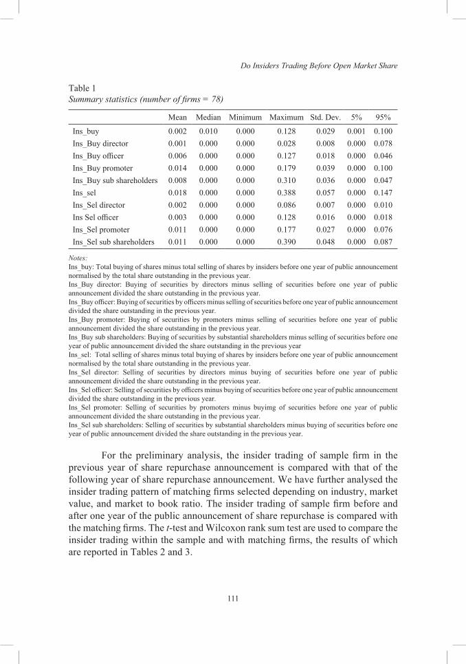
Do Insiders Trading Before Open Market Share
111
Table 1Summary statistics (number of firms = 78)
Mean Median Minimum Maximum Std. Dev. 5% 95%
Ins_buy 0.002 0.010 0.000 0.128 0.029 0.001 0.100Ins_Buy director 0.001 0.000 0.000 0.028 0.008 0.000 0.078Ins_Buy officer 0.006 0.000 0.000 0.127 0.018 0.000 0.046Ins_Buy promoter 0.014 0.000 0.000 0.179 0.039 0.000 0.100Ins_Buy sub shareholders 0.008 0.000 0.000 0.310 0.036 0.000 0.047Ins_sel 0.018 0.000 0.000 0.388 0.057 0.000 0.147Ins_Sel director 0.002 0.000 0.000 0.086 0.007 0.000 0.010Ins Sel officer 0.003 0.000 0.000 0.128 0.016 0.000 0.018Ins_Sel promoter 0.011 0.000 0.000 0.177 0.027 0.000 0.076Ins_Sel sub shareholders 0.011 0.000 0.000 0.390 0.048 0.000 0.087
Notes: Ins_buy: Total buying of shares minus total selling of shares by insiders before one year of public announcement normalised by the total share outstanding in the previous year. Ins_Buy director: Buying of securities by directors minus selling of securities before one year of public announcement divided the share outstanding in the previous year.Ins_Buy officer: Buying of securities by officers minus selling of securities before one year of public announcement divided the share outstanding in the previous year.Ins_Buy promoter: Buying of securities by promoters minus selling of securities before one year of public announcement divided the share outstanding in the previous year.Ins_Buy sub shareholders: Buying of securities by substantial shareholders minus selling of securities before one year of public announcement divided the share outstanding in the previous year Ins_sel: Total selling of shares minus total buying of shares by insiders before one year of public announcement normalised by the total share outstanding in the previous year. Ins_Sel director: Selling of securities by directors minus buying of securities before one year of public announcement divided the share outstanding in the previous year.Ins_Sel officer: Selling of securities by officers minus buying of securities before one year of public announcement divided the share outstanding in the previous year.Ins_Sel promoter: Selling of securities by promoters minus buyimg of securities before one year of public announcement divided the share outstanding in the previous year.Ins_Sel sub shareholders: Selling of securities by substantial shareholders minus buying of securities before one year of public announcement divided the share outstanding in the previous year.
For the preliminary analysis, the insider trading of sample firm in the previous year of share repurchase announcement is compared with that of the following year of share repurchase announcement. We have further analysed the insider trading pattern of matching firms selected depending on industry, market value, and market to book ratio. The insider trading of sample firm before and after one year of the public announcement of share repurchase is compared with the matching firms. The t-test and Wilcoxon rank sum test are used to compare the insider trading within the sample and with matching firms, the results of which are reported in Tables 2 and 3.
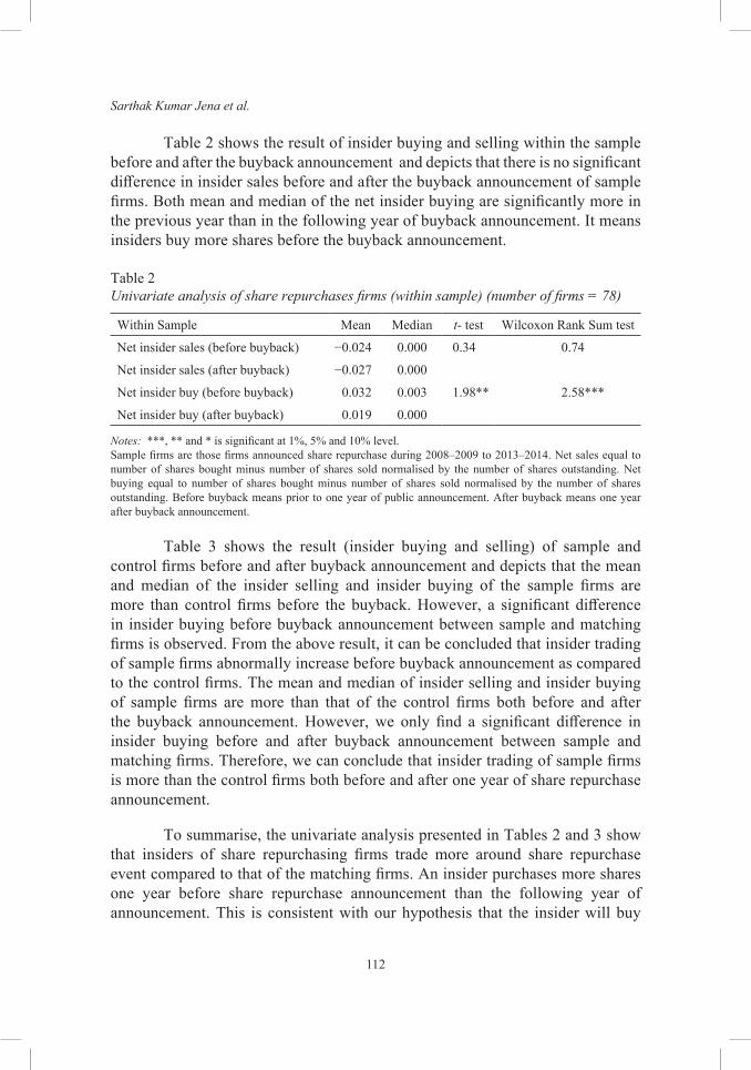
Sarthak Kumar Jena et al.
112
Table 2 shows the result of insider buying and selling within the sample before and after the buyback announcement and depicts that there is no significant difference in insider sales before and after the buyback announcement of sample firms. Both mean and median of the net insider buying are significantly more in the previous year than in the following year of buyback announcement. It means insiders buy more shares before the buyback announcement.
Table 2Univariate analysis of share repurchases firms (within sample) (number of firms = 78)
Within Sample Mean Median t- test Wilcoxon Rank Sum test
Net insider sales (before buyback) −0.024 0.000 0.34 0.74
Net insider sales (after buyback) −0.027 0.000
Net insider buy (before buyback) 0.032 0.003 1.98** 2.58***
Net insider buy (after buyback) 0.019 0.000
Notes: ***, ** and * is significant at 1%, 5% and 10% level. Sample firms are those firms announced share repurchase during 2008–2009 to 2013–2014. Net sales equal to number of shares bought minus number of shares sold normalised by the number of shares outstanding. Net buying equal to number of shares bought minus number of shares sold normalised by the number of shares outstanding. Before buyback means prior to one year of public announcement. After buyback means one year after buyback announcement.
Table 3 shows the result (insider buying and selling) of sample and control firms before and after buyback announcement and depicts that the mean and median of the insider selling and insider buying of the sample firms are more than control firms before the buyback. However, a significant difference in insider buying before buyback announcement between sample and matching firms is observed. From the above result, it can be concluded that insider trading of sample firms abnormally increase before buyback announcement as compared to the control firms. The mean and median of insider selling and insider buying of sample firms are more than that of the control firms both before and after the buyback announcement. However, we only find a significant difference in insider buying before and after buyback announcement between sample and matching firms. Therefore, we can conclude that insider trading of sample firms is more than the control firms both before and after one year of share repurchase announcement.
To summarise, the univariate analysis presented in Tables 2 and 3 show that insiders of share repurchasing firms trade more around share repurchase event compared to that of the matching firms. An insider purchases more shares one year before share repurchase announcement than the following year of announcement. This is consistent with our hypothesis that the insider will buy
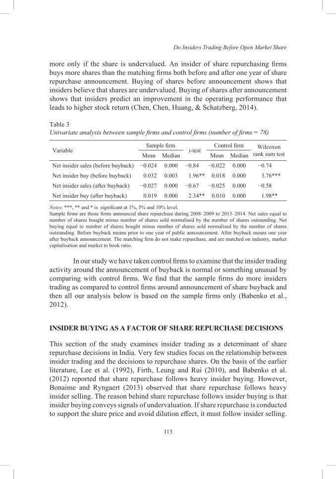
Do Insiders Trading Before Open Market Share
113
more only if the share is undervalued. An insider of share repurchasing firms buys more shares than the matching firms both before and after one year of share repurchase announcement. Buying of shares before announcement shows that insiders believe that shares are undervalued. Buying of shares after announcement shows that insiders predict an improvement in the operating performance that leads to higher stock return (Chen, Chen, Huang, & Schatzberg, 2014).
Table 3Univariate analysis between sample firms and control firms (number of firms = 78)
VariableSample firm
t-testControl firm Wilcoxon
rank sum testMean Median Mean Median
Net insider sales (before buyback) −0.024 0.000 −0.84 −0.022 0.000 −0.74
Net insider buy (before buyback) 0.032 0.003 1.96** 0.018 0.000 3.76***
Net insider sales (after buyback) −0.027 0.000 −0.67 −0.025 0.000 −0.58
Net insider buy (after buyback) 0.019 0.000 2.34** 0.010 0.000 1.98**
Notes: ***, ** and * is significant at 1%, 5% and 10% level. Sample firms are those firms announced share repurchase during 2008–2009 to 2013–2014. Net sales equal to number of shares bought minus number of shares sold normalised by the number of shares outstanding. Net buying equal to number of shares bought minus number of shares sold normalised by the number of shares outstanding. Before buyback means prior to one year of public announcement. After buyback means one year after buyback announcement. The matching firm do not make repurchase, and are matched on industry, market capitalisation and market to book ratio.
In our study we have taken control firms to examine that the insider trading activity around the announcement of buyback is normal or something unusual by comparing with control firms. We find that the sample firms do more insiders trading as compared to control firms around announcement of share buyback and then all our analysis below is based on the sample firms only (Babenko et al., 2012).
INSIDER BUYING AS A FACTOR OF SHARE REPURCHASE DECISIONS
This section of the study examines insider trading as a determinant of share repurchase decisions in India. Very few studies focus on the relationship between insider trading and the decisions to repurchase shares. On the basis of the earlier literature, Lee et al. (1992), Firth, Leung and Rui (2010), and Babenko et al. (2012) reported that share repurchase follows heavy insider buying. However, Bonaime and Ryngaert (2013) observed that share repurchase follows heavy insider selling. The reason behind share repurchase follows insider buying is that insider buying conveys signals of undervaluation. If share repurchase is conducted to support the share price and avoid dilution effect, it must follow insider selling.
Sarthak Kumar Jena et al.
114
In India, no study examines this kind of relationship between insider trading and share repurchase decision. Therefore, we have tried to examine the potential of insider trading for influencing share repurchase decisions.We have used the Tobit model in this study to know the influence of insiders trading on share repurchase decisions. The positive relation between insider buying and share repurchase will prove that insider buying confirms the undervaluation signal conveyed by share repurchase announcement. The positive relationship between insider selling and share repurchase states that instead of signalling undervaluation, firms announce share repurchase to support the share price and avoid dilution effect. In case, there is no relationship between insider trading and share repurchase, then it will be clear that in the Indian context, insider activity does not convey any information to the investors. By following the studies by Dittmar (2000) and Firth et al. (2010), we have used the Tobit model, and the only additional factor added to the model is insider activity. The hypotheses considered in the Tobit model are explained below.
Excess Cash Flow Hypothesis
A firm with more cash than investment opportunities can either retain or distribute the excess cash to the shareholders (Easterbrook, 1984; Jensen, 1986). Dittmar (2000), Mitchell and Dharmawan (2007), Boudry et al. (2013), and Lee and Suh (2011) found a positive relationship between excess cash holding and the incentive to the repurchase of shares. In India, the Companies Act (2013) prescribes that repurchase must be done either from the reserves or from undistributed profit. Therefore, companies before repurchase must have ample cash reserves on their balance sheet. In India, no share repurchase can be made out of the borrowed fund. We have measured cash by considering total available cash of the previous year in the balance sheet of share repurchase to the total assets (Cash).
Leverage Hypothesis
Leverage hypothesis posits that companies are more likely to do repurchase if their actual debt equity ratio (D/E ratio) is less than the target ratio (Bagwell & Shoven, 1988; Dittmar, 2000; Mitchell & Dharmawan, 2007). Hovakimian et al. (2001) documented that firms adjust their capital structure by moving toward an optimum capital structure by doing a share repurchase. The gap between the actual and the target D/E ratio plays a major role in repurchase decisions. In India, buyback regulation specifies that the debt should not be more than two times of the paid-up capital and free reserves after the execution of buyback, so in India the standard debt to paid-up capital and free reserve is 2:1. Unlike other developed countries, Indian companies are not permitted to use borrowed fund to
Do Insiders Trading Before Open Market Share
115
buyback shares. We have taken the gap between the standard (2) and actual DE ratio as a control variable. The actual D/E ratio is calculated as total debt divided by paid-up capital and free reserves.
Substitution Hypothesis
Substitution hypothesis refers to the preference for share buyback as a payout method to shareholders over the dividend. The primary cause for substitution hypothesis is the taxable nature of income from the dividend paid and buyback in the hands of shareholders. The income from buyback is taxed as capital gain, and the dividend income is charged as normal income. As capital gain tax is much lower than the dividend, share repurchase is more tax efficient and valuable to shareholders (Grullon & Michaely, 2000). In India, from 2003, the dividend paid by the Indian companies has been tax-free in the hands of investors. However, the profit arising out of buyback receipt is taxed as long term and short term capital gain in the hands of shareholders depending on the duration of the holding of the securities before tendering these as part of the buyback. In India, if the holding period exceeds 12 months, then it is taxed as a long-term capital gain, and if it is less than 12 months, then it is considered as a short-term capital gain. The positive and negative relationships between share repurchase and dividend paid determine the complement and substitution effect, respectively. The amount of dividend paid is measured by taking dividend payout (DP) ratio. DP is calculated as the total dividend paid to profit after paying tax.
Signaling of Undervaluation
Undervaluation hypothesis is based on the premise that owing to information asymmetry between insider and outside investors, the share price is misvalued. The signaling hypothesis assigns an informative role to share buyback and posits that firms will repurchase their shares while passing private information to the investors and maintaining information symmetry in the market. Under-pricing signaling hypothesis suggests that the firm is motivated to repurchase their shares as a self-investment technique through undervaluation of the shares (Liang, Chan, Lai, & Wang, 2013). Therefore, the company undertakes share repurchase at a higher price than the market price (Asquith & Mullins, 1986). Dittmar (2000) used firm size as a proxy for information asymmetry and stated that information asymmetry is low for large firms compared to small firms because many analysts monitor the performance of large firms. He also considered market value to book value (MB) as an indicator of undervaluation. Market to book value is calculated as the market value of equity plus debt to total book value of the asset. The same proxy is used for holding investment proxy constant.
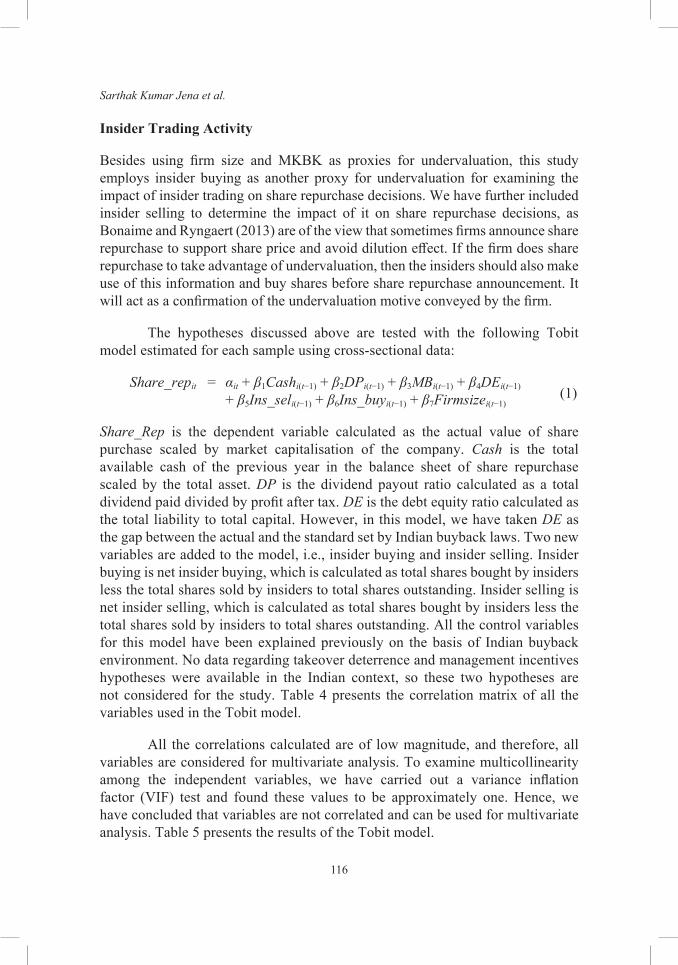
Sarthak Kumar Jena et al.
116
Insider Trading Activity
Besides using firm size and MKBK as proxies for undervaluation, this study employs insider buying as another proxy for undervaluation for examining the impact of insider trading on share repurchase decisions. We have further included insider selling to determine the impact of it on share repurchase decisions, as Bonaime and Ryngaert (2013) are of the view that sometimes firms announce share repurchase to support share price and avoid dilution effect. If the firm does share repurchase to take advantage of undervaluation, then the insiders should also make use of this information and buy shares before share repurchase announcement. It will act as a confirmation of the undervaluation motive conveyed by the firm.
The hypotheses discussed above are tested with the following Tobit model estimated for each sample using cross-sectional data:
Share_repit = αit + β1Cashi(t−1) + β2DPi(t−1) + β3MBi(t−1) + β4DEi(t−1) + β5Ins_seli(t−1) + β6Ins_buyi(t−1) + β7Firmsizei(t−1)
(1)
Share_Rep is the dependent variable calculated as the actual value of share purchase scaled by market capitalisation of the company. Cash is the total available cash of the previous year in the balance sheet of share repurchase scaled by the total asset. DP is the dividend payout ratio calculated as a total dividend paid divided by profit after tax. DE is the debt equity ratio calculated as the total liability to total capital. However, in this model, we have taken DE as the gap between the actual and the standard set by Indian buyback laws. Two new variables are added to the model, i.e., insider buying and insider selling. Insider buying is net insider buying, which is calculated as total shares bought by insiders less the total shares sold by insiders to total shares outstanding. Insider selling is net insider selling, which is calculated as total shares bought by insiders less the total shares sold by insiders to total shares outstanding. All the control variables for this model have been explained previously on the basis of Indian buyback environment. No data regarding takeover deterrence and management incentives hypotheses were available in the Indian context, so these two hypotheses are not considered for the study. Table 4 presents the correlation matrix of all the variables used in the Tobit model.
All the correlations calculated are of low magnitude, and therefore, all variables are considered for multivariate analysis. To examine multicollinearity among the independent variables, we have carried out a variance inflation factor (VIF) test and found these values to be approximately one. Hence, we have concluded that variables are not correlated and can be used for multivariate analysis. Table 5 presents the results of the Tobit model.
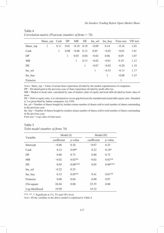
Do Insiders Trading Before Open Market Share
117
Table 4Correlation matrix (Pearson) (number of firms = 78)
Share_rep Cash DP MB DE Ins_sel Ins_buy Firm size VIF test
Share_rep 1 0.11 0.01 −0.18 0.19 −0.09 0.14 −0.16 1.03
Cash 1 0.08 −0.06 0.13 0.05 −0.03 −0.01 1.01
DP 1 0.03 0.04 −0.02 0.06 0.05 1.07
MB 1 0.13 −0.02 −0.01 0.19 1.12
DE 1 −0.07 −0.02 −0.20 1.19
Ins_sel 1 −0.35 −0.13 1.17
Ins_buy 1 −0.08 1.15
Firmsize 1
Notes: Share_rep = Value of actual share repurchase divided by the market capitalisation of companies.DP = Dividend paid in the previous year of share repurchase divided by profit after tax.MB = Market to book ratio, calculated by sum of market value of equity and total debt divided by book value of asset.DE = Debt to equity ratio, it is calculated as excess gap between the standard and actual debt equity ratio. Standard is 2 as prescribed by Indian companies Act 1956.Ins_sel = Number of shares bought by insiders minus number of shares sold to total number of shares outstanding in the previous year.Ins_buy = Number of shares bought by insiders minus number of shares sold to total number of shares outstanding in the previous year.Firm size = Log value of total asset.
Table 5Tobit model (number of firms 78)
Variable Model (I) Model (II)
coefficient p-value coefficient p-value
Intercept −0.06 0.36 −0.07 0.25
Cash 0.23 0.09* 0.22 0.10*
DP 0.00 0.75 0.00 0.75
MB −0.02 0.02** −0.02 0.02**
DE 0.05 0.00*** 0.05 0.00***
Ins_sel −0.22 0.25
Ins_buy 0.33 0.05** 0.41 0.01**
Firmsize 0.00 0.84 0.00 0.97
Chi-square 26.84 0.00 25.55 0.00
Log-likelihood 19.99 19.32
***, **, *: Significant at 1%, 5% and 10% level. Note: All the variables in the above model is explained in Table 4.
Sarthak Kumar Jena et al.
118
The result shows that MB is significant, but the coefficient is negative. It means firms repurchase their share when they are potentially undervalued. Insider buying is also considered as a proxy for undervaluation, which is found to be positive and significant in the presence of insider selling. It means the higher the insider buying before share repurchase, the higher the probability of doing a share repurchase. Insider buying confirms the undervaluation signal conveyed by the share repurchase announcement. There is a negative and insignificant relationship of insider selling with share repurchase. By eliminating insider selling from the model, it is seen that insider buying has a positive and significant relationship with share repurchase decisions. Cash/TA is positive and significant in both the models; it shows that cash is a prerequisite for share repurchase. DE ratio is significant in both the models at 1% significant level. It means the more the gap between the standard and actual D/E ratio, it is more likely for the firms to do share repurchase in India.
ANNOUNCEMENT RETURNS AND INSIDER TRADING
The signaling power of share repurchase is tested by finding abnormal announcement return around share repurchase decision (Dann, 1981; Vermaelen, 1981; Comment & Jarrel, 1991; Ikenberry et al., 1995; Li & McNally, 2007; Reddy, Nangia, & Agrawal, 2013). So, in this section, we have tested our second hypothesis, which states that whether market considers insider trading at the time of repurchase announcement. This hypothesis holds true in the Indian context if positive and significant announcement return around share repurchase is related to insider buying and negative announcement return is related to insider selling.
Following the study by Babenko et al. (2012), we have regressed three days buy hold abnormal return (BHAR) around an announcement on past insider trading and controlling of important determinants. In India, share repurchase is announced in three parts. First, it is declared in the Board of Directors meeting. Second, a public announcement about share repurchase is made along with declaration of an offer document, which contains detailed information about the offer. Third, with the initiation of actual share repurchase, three days BHAR has been calculated around all the three phases of the announcement of share repurchase. We have regressed the BHAR around Board of Directors approval and BHAR around the opening of buyback with insider trading; however, no significant result is obtained. During Board approval, there is no surety that the firm will undertake buyback in future, so investors could not react to such decisions. Again during the opening of the buyback, the information is already absorbed the market at the time of the public announcement. Public announcement of share
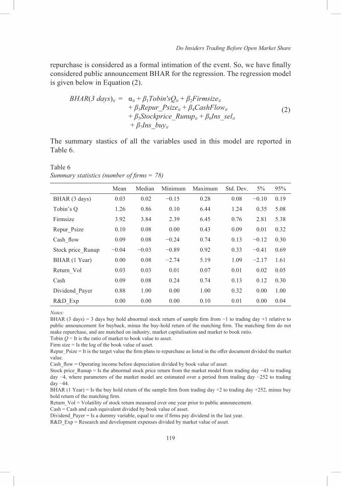
Do Insiders Trading Before Open Market Share
119
repurchase is considered as a formal intimation of the event. So, we have finally considered public announcement BHAR for the regression. The regression model is given below in Equation (2).
BHAR(3 days)it = αit + β1Tobin'sQit + β2Firmsizeit + β3Repur_Psizeit + β4CashFlowit
+ β5Stockprice_Runupit + β6Ins_selit
+ β7Ins_buyit
(2)
The summary stastics of all the variables used in this model are reported in Table 6.
Table 6Summary statistics (number of firms = 78)
Mean Median Minimum Maximum Std. Dev. 5% 95%
BHAR (3 days) 0.03 0.02 −0.15 0.28 0.08 −0.10 0.19
Tobin’s Q 1.26 0.86 0.10 6.44 1.24 0.35 5.08
Firmsize 3.92 3.84 2.39 6.45 0.76 2.81 5.38
Repur_Psize 0.10 0.08 0.00 0.43 0.09 0.01 0.32
Cash_flow 0.09 0.08 −0.24 0.74 0.13 −0.12 0.30
Stock price_Runup −0.04 −0.03 −0.89 0.92 0.33 −0.41 0.69
BHAR (1 Year) 0.00 0.08 −2.74 5.19 1.09 −2.17 1.61
Return_Vol 0.03 0.03 0.01 0.07 0.01 0.02 0.05
Cash 0.09 0.08 0.24 0.74 0.13 0.12 0.30
Dividend_Payer 0.88 1.00 0.00 1.00 0.32 0.00 1.00
R&D_Exp 0.00 0.00 0.00 0.10 0.01 0.00 0.04
Notes:BHAR (3 days) = 3 days buy hold abnormal stock return of sample firm from −1 to trading day +1 relative to public announcement for buyback, minus the buy-hold return of the matching firm. The matching firm do not make repurchase, and are matched on industry, market capitalisation and market to book ratio.Tobin Q = It is the ratio of market to book value to asset.Firm size = Is the log of the book value of asset.Repur_Psize = It is the target value the firm plans to repurchase as listed in the offer document divided the market value.Cash_flow = Operating income before depreciation divided by book value of asset.Stock price_Runup = Is the abnormal stock price return from the market model from trading day −43 to trading day −4, where parameters of the market model are estimated over a period from trading day −252 to trading day −44.BHAR (1 Year) = Is the buy hold return of the sample firm from trading day +2 to trading day +252, minus buy hold return of the matching firm.Return_Vol = Volatility of stock return measured over one year prior to public announcement.Cash = Cash and cash equivalent divided by book value of asset.Dividend_Payer = Is a dummy variable, equal to one if firms pay dividend in the last year.R&D_Exp = Research and development expenses divided by market value of asset.
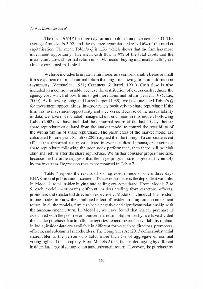
Sarthak Kumar Jena et al.
120
The mean BHAR for three days around public announcement is 0.03. The average firm size is 3.92, and the average repurchase size is 10% of the market capitalisation. The mean Tobin’s Q is 1.26, which shows that the firm has more investment opportunity. The mean cash flow is 9% of the total assets and the mean cumulative abnormal return is −0.04. Insider buying and insider selling are already explained in Table 1.
We have included firm size in this model as a control variable because small firms experience more abnormal return than big firms owing to more information asymmetry (Vermaelen, 1981; Comment & Jarrel, 1991). Cash flow is also included as a control variable because the distribution of excess cash reduces the agency cost, which allows firms to get more abnormal return (Jensen, 1986; Lie, 2000). By following Lang and Litzenberger (1989), we have included Tobin’s Q for investment opportunities; investor reacts positively to share repurchase if the firm has no investment opportunity and vice versa. Because of the unavailability of data, we have not included managerial entrenchment in this model. Following Kahle (2002), we have included the abnormal return of the last 40 days before share repurchase calculated from the market model to control the possibility of the wrong timing of share repurchase. The parameters of the market model are calculated for one year. Schultz (2003) argued that the timing of a corporate event affects the abnormal return calculated in event studies. If manager announces share repurchase following the poor stock performance, then there will be high abnormal return after the share repurchase. We further consider programme size, because the literature suggests that the large program size is greeted favourably by the investors. Regression results are reported in Table 7.
Table 7 reports the results of six regression models, where three days BHAR around public announcement of share repurchase is the dependent variable. In Model 1, total insider buying and selling are considered. From Models 2 to 5, each model incorporates different insiders trading from directors, officers, promoters and substantial directors, respectively. Model 6 includes all the insiders in one model to know the combined effect of insiders trading on announcement return. In all the models, firm size has a negative and significant relationship with the announcement return. In Model 1, we have found that insider purchase is associated with the positive announcement return. Subsequently, we have divided the insider purchase data into four categories depending on the availability of data. In India, insider data are available in different forms such as directors, promoters, officers, and substantial shareholders. The Companies Act 2013 defines substantial shareholder as the person who holds more than 5% of aggregate or nominal voting rights of the company. From Models 2 to 5, the insider buying by different insiders has a positive impact on announcement return. However, the purchase by
Do Insiders Trading Before Open Market Share
121
Tabl
e 7
Anno
unce
men
t ret
urn
and
insi
ders
pur
chas
e (n
umbe
r of fi
rms =
78)
Var
iabl
e M
odel
(I)
Mod
el (I
I)M
odel
(III
)M
odel
(IV
)M
odel
(V)
Mod
el (V
I)
Coe
ff.t-s
tat
Coe
ff.t-s
tat
Coe
ff.t-s
tat
Coe
ff.t-s
tat
Coe
ff.t-s
tat
Coe
ff.t-s
tat
Inte
rcep
t0.
101.
74*
0.12
2.22
**0.
142.
46**
0.11
2.00
**0.
122.
14**
0.14
2.60
***
Tobi
n’s Q
−0.0
1−0
.89
−0.0
1−0
.78
−0.0
1−0
.66
−0.0
0−0
.52
−0.0
1−0
.66
−0.0
1−0
.64
Firm
size
−0.0
2−1
.78*
−0.0
2−2
.04*
*−0
.03
−2.1
0**
−0.0
2−1
.76*
*−0
.02
−1.8
7*−0
.03
−2.3
4**
Rep
ur_P
size
0.10
0.89
0.05
0.49
0.09
0.80
0.12
1.00
0.11
0.95
0.03
0.27
Cas
h_Fl
ow−0
.03
−0.4
3−0
.02
−0.3
2−0
.06
−0.8
4−0
.04
−0.5
0−0
.04
−0.6
2−0
.04
−0.5
3
Stoc
k pr
ice_
Run
up−0
.02
−0.6
8−0
.01
−0.4
4−0
.01
−0.3
8−0
.01
−0.2
8−0
.01
−0.2
2−0
.01
−0.4
5
Ins_
sel
−0.3
6−2
.50*
*−0
.32
−2.3
1**
−0.3
4−2
.33*
*−0
.37
−2.3
8**
−0.3
1−2
.05*
*−0
.31
−2.0
5**
Ins_
buy
0.65
2.18
**
Ins_
Buy
dire
ctor
5.44
1.35
0.02
0.09
Ins_
Buy
offi
cer
0.77
1.49
5.39
1.45
Ins_
Buy
pro
mot
er0.
212.
01**
0.77
1.96
**
Ins_
Buy
sub
shar
ehol
ders
0.12
2.47
**0.
141.
98**
R-s
quar
ed0.
210.
280.
190.
170.
160.
31
Not
es: *
**, *
*, *
: Sig
nific
ant a
t 1%
, 5%
and
10%
leve
l. B
HA
R (−
1, +
1) a
roun
d sh
are
repu
rcha
se a
nnou
ncem
ent i
s the
dep
ende
nt v
aria
ble.
All
the
varia
bles
in th
e ab
ove
mod
el is
exp
lain
ed in
Tab
le 1
.
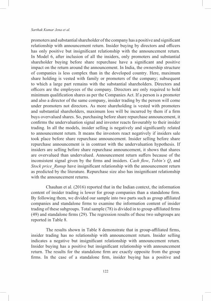
Sarthak Kumar Jena et al.
122
promoters and substantial shareholder of the company has a positive and significant relationship with announcement return. Insider buying by directors and officers has only positive but insignificant relationship with the announcement return. In Model 6, after inclusion of all the insiders, only promoters and substantial shareholder buying before share repurchase have a significant and positive impact on the return around the announcement. In India, the ownership structure of companies is less complex than in the developed country. Here, maximum share holding is vested with family or promoters of the company; subsequent to which a large part remains with the substantial shareholders. Directors and officers are the employees of the company. Directors are only required to hold minimum qualification shares as per the Companies Act. If a person is a promoter and also a director of the same company, insider trading by the person will come under promoters not directors. As more shareholding is vested with promoters and substantial shareholders, maximum loss will be incurred by them if a firm buys overvalued shares. So, purchasing before share repurchase announcement, it confirms the undervaluation signal and investor reacts favourably to their insider trading. In all the models, insider selling is negatively and significantly related to announcement return. It means the investors react negatively if insiders sale took place before share repurchase announcement. Insider selling before share repurchase announcement is in contrast with the undervaluation hypothesis. If insiders are selling before share repurchase announcement, it shows that shares are overvalued than undervalued. Announcement return suffers because of the inconsistent signal given by the firms and insiders. Cash flow, Tobin’s Q, and Stock price_Runup have insignificant relationship with the announcement return as predicted by the literature. Repurchase size also has insignificant relationship with the announcement returns.
Chauhan et al. (2016) reported that in the Indian context, the information content of insider trading is lower for group companies than a standalone firm. By following them, we divided our sample into two parts such as group affiliated companies and standalone firms to examine the information content of insider trading of these subgroups. Total sample (78) is divided in to group-affiliated firms (49) and standalone firms (29). The regression results of these two subgroups are reported in Table 8.
The results shown in Table 8 demonstrate that in group-affiliated firms, insider trading has no relationship with announcement return. Insider selling indicates a negative but insignificant relationship with announcement return. Insider buying has a positive but insignificant relationship with announcement return. The results for the standalone firm are exactly opposite from the group firms. In the case of a standalone firm, insider buying has a positive and
Do Insiders Trading Before Open Market Share
123
significant relationship with announcement return. It further communicates the same undervaluation signal conveyed by share repurchase. Insider selling has a negative and significant relationship with announcement return. Selling of the insiders’ share before share repurchase announcement, it sends a contrasting signal other than undervaluation.
Table 8Announcement return and insiders purchase (business group firm vs. standalone firm) (number of firms = 78)
Variable Business Group Standalone
coefficient t-stat coefficient t-stat
Intercept 0.12 1.48 0.13 1.33
Tobin’s Q −0.01 −1.17 −0.01 −0.46
Firmsize −0.03 −1.61 −0.03 −1.02
Repur_Psize 0.24 1.56 0.04 0.22
Cash Flow −0.14 −1.46 −0.14 −1.28
Stock price_Runup −0.00 −0.06 −0.01 −0.22
Ins_sel −0.18 −1.02 −0.97 −3.10***
Ins_buy 0.11 0.31 0.81 1.98**
R-squared 0.22 0.46
Notes: ***, **, *: Significant at 1%, 5% and 10% level. BHAR (−1, +1) around share repurchase announcement is the dependent variable. All the variables in the above model is explained in Table 1.
PROGRAM COMPLETION RATES AND INSIDER TRADING
Share repurchase gained momentum during the 1990s in the U.S., and for the first time in 1998, the total value of share repurchases exceeded the value of dividends (Grullon & Michaely, 2002). Stephens and Weisbach (1998) reported that in the U.S. market, at least 57% of the firms purchase the number of shares originally announced over three years, 10% of the firms purchase less than 5% of the shares announced, and a significant number of firms repurchase very few or no shares. They also suggested that the actual repurchase depends on the perceived degree of undervaluation.
The announcement of open market repurchase program is just an intention to do repurchase without any obligation, and firms are not liable to buy even a single share after the announcement. Sometimes, share repurchase announcement is used for a small adjustment in the share price with no intention of actually buying
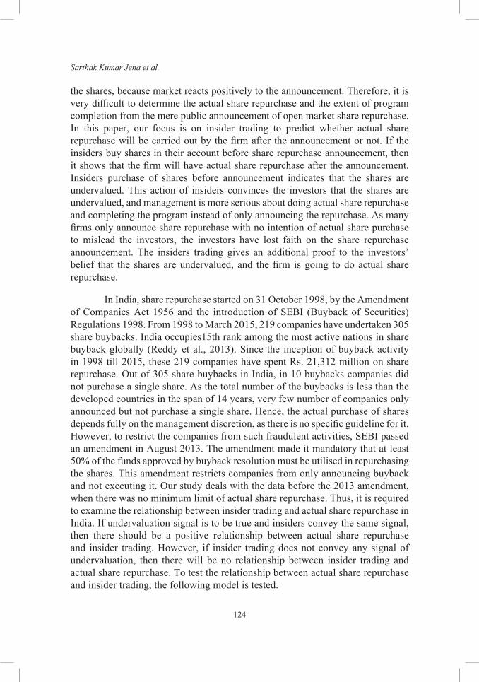
Sarthak Kumar Jena et al.
124
the shares, because market reacts positively to the announcement. Therefore, it is very difficult to determine the actual share repurchase and the extent of program completion from the mere public announcement of open market share repurchase. In this paper, our focus is on insider trading to predict whether actual share repurchase will be carried out by the firm after the announcement or not. If the insiders buy shares in their account before share repurchase announcement, then it shows that the firm will have actual share repurchase after the announcement. Insiders purchase of shares before announcement indicates that the shares are undervalued. This action of insiders convinces the investors that the shares are undervalued, and management is more serious about doing actual share repurchase and completing the program instead of only announcing the repurchase. As many firms only announce share repurchase with no intention of actual share purchase to mislead the investors, the investors have lost faith on the share repurchase announcement. The insiders trading gives an additional proof to the investors’ belief that the shares are undervalued, and the firm is going to do actual share repurchase.
In India, share repurchase started on 31 October 1998, by the Amendment of Companies Act 1956 and the introduction of SEBI (Buyback of Securities) Regulations 1998. From 1998 to March 2015, 219 companies have undertaken 305 share buybacks. India occupies15th rank among the most active nations in share buyback globally (Reddy et al., 2013). Since the inception of buyback activity in 1998 till 2015, these 219 companies have spent Rs. 21,312 million on share repurchase. Out of 305 share buybacks in India, in 10 buybacks companies did not purchase a single share. As the total number of the buybacks is less than the developed countries in the span of 14 years, very few number of companies only announced but not purchase a single share. Hence, the actual purchase of shares depends fully on the management discretion, as there is no specific guideline for it. However, to restrict the companies from such fraudulent activities, SEBI passed an amendment in August 2013. The amendment made it mandatory that at least 50% of the funds approved by buyback resolution must be utilised in repurchasing the shares. This amendment restricts companies from only announcing buyback and not executing it. Our study deals with the data before the 2013 amendment, when there was no minimum limit of actual share repurchase. Thus, it is required to examine the relationship between insider trading and actual share repurchase in India. If undervaluation signal is to be true and insiders convey the same signal, then there should be a positive relationship between actual share repurchase and insider trading. However, if insider trading does not convey any signal of undervaluation, then there will be no relationship between insider trading and actual share repurchase. To test the relationship between actual share repurchase and insider trading, the following model is tested.
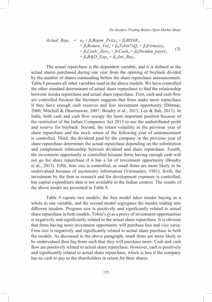
Do Insiders Trading Before Open Market Share
125
Actual_Repit = αit + β1Repur_Psizeit + β2BHARit + β3Return_Volit + β4Tobin"sQit + β5Firmsizeit
+ β6Cash_ flowit + β7Cashit + β8Dividen_payerit
+ β9R&D_Expit + β10Ins_Buyit
(3)
The actual repurchase is the dependent variable, and it is defined as the actual shares purchased during one year from the opening of buyback divided by the number of shares outstanding before the share repurchase announcement. Table 6 presents all other variables used in the above models. We have controlled the other standard determinant of actual share repurchase to find the relationship between insider repurchase and actual share repurchase. First, cash and cash flow are controlled because the literature suggests that firms make more repurchase if they have enough cash reserves and less investment opportunity (Dittmar, 2000; Mitchell & Dharmawan, 2007; Boudry et al., 2013; Lee & Suh, 2011). In India, both cash and cash flow occupy the most important position because of the restriction of the Indian Companies Act 2013 to use the undistributed profit and reserve for buyback. Second, the return volatility in the previous year of share repurchase and the stock return of the following year of announcement is controlled. Third, the dividend paid by the company in the previous year of share repurchase determines the actual repurchase depending on the substitution and complement relationship between dividend and share repurchase. Fourth, the investment opportunity is controlled because firms having enough cash will not go for share repurchase if it has a lot of investment opportunity (Boudry et al., 2013). Fifth, firm size is controlled, as small firms are more likely to be undervalued because of asymmetry information (Vermaelen, 1981). Sixth, the investment by the firm in research and for development expenses is controlled, but capital expenditure data is not available in the Indian context. The results of the above model are presented in Table 9.
Table 9 reports two models; the first model takes insider buying as a whole in one variable, and the second model segregates the insider trading into different insiders. Program size is positively and significantly related to actual share repurchase in both models. Tobin’s Q as a proxy of investment opportunities is negatively and significantly related to the actual share repurchase. It is obvious that firms having more investment opportunity will purchase less and vice versa. Firm size is negatively and significantly related to actual share purchase in both the models. As discussed in the above paragraph, small firms are more likely to be undervalued than big firms such that they will purchase more. Cash and cash flow are positively related to actual share repurchase. However, cash is positively and significantly related to actual share repurchase, which is less if the company has no cash to pay to the shareholders in return for their shares.
Sarthak Kumar Jena et al.
126
Table 9Actual share repurchases and insiders trading (number of firms = 78)
Variable Model (I) Model (II)
coefficient t-stat coefficient t-stat
Intercept 0.10 3.24*** 0.09 2.95***
Repur_Psize 0.10 2.00** 0.14 2.77***
Bhar 0.00 0.13 0.00 0.48
Return_Vol −0.61 −1.63* −0.28 −0.75
Tobin’s Q −0.01 −2.05** −0.00 −2.42**
Firmsize −0.01 −2.40** −0.01 −2.72***
Cash_flow 0.00 0.14 0.01 0.45
Cash 0.14 3.03*** 0.14 3.06***
Dividend_Payer 0.00 0.32 0.01 0.72
R&D_Exp −0.18 −0.67 −0.06 −0.23
Ins_buy 0.10 2.06**
Ins_Buy director 1.73 2.47**
Ins_Buy officer 0.11 0.22
Ins_Buy promoter 0.25 2.27**
Ins_Buy sub shareholders 0.04 0.41
R-squared 0.40 0.47
***, **, *: Significant at 1%, 5% and 10% level. Note: Actual share repurchase is defined as the number of shares purchased over one year divided by the number of shares outstanding. Rest all the variables in the above model is explained in Table 1.
Apart from the control variables discussed in the above paragraph, Table 9 also indicates the relationship between insider trading and actual share repurchase. The results are consistent with our hypothesis, which states that insider trading conveys the signal of undervaluation more firmly. Hence, actual share purchase depends on the transaction made by insider in their account before the share repurchase announcement. In the first model, insider buying is positively and significantly related to actual share repurchase. It means that the more the insider buys shares before the announcement of share repurchase; it is more likely that the firms purchase more shares. In the second model, insider buying is segregated into different insiders as per the availability of data in the Indian context, and the results show that insider buying by directors and promoters has a positive and significant relationship with actual share repurchase. In India, 95% of the big corporate houses are family owned (Sir Adrian Committee report), where the average promoters holding of our sample companies is more than 50.26%.
Do Insiders Trading Before Open Market Share
127
Therefore, promoters purchase of share before share repurchase announcement demonstrates that the shares are undervalued.
The relationship between program completion and insiders trading is tested in the following model explained as below.
Program_Completionit = αit + β1BHARit + β2Return_Volit
+ β3Tobin'sQit + β4Firmsizeit
+ β5Cash_Flowit + β6Cashit + β7Dividen_Payerit + β8R&D_Expit
+ β9Ins_buyit
(4)
Program completion is a dependent variable, and it is defined as the actual shares purchased during one year from the opening of buyback, which is divided by the number of shares announce to be purchased in the offer document. All the other variables used in the model are already explained in Equation (3).
Table 10Program completion and insiders trading (number of firms = 78)
Variable Model (I) Model (II)
coefficient t-stat coefficient t-stat
Intercept 1.49 3.19*** 1.54 3.24***Bhar −0.01 −0.19 −0.00 −0.09Return_Vol −7.13 −1.24 −8.17 −1.39Tobin’s Q −0.01 2.45** −0.00 −1.96**Firmsize −0.10 −1.19 −0.11 −1.32Cash_flow 0.09 0.20 0.09 0.20Cash 0.41 2.69*** 0.57 2.76***Dividend_Payer 0.15 0.84 0.13 0.70R&D_Exp −0.15 −0.04 0.55 0.13Ins_buy 1.81 2.84***Ins_Buy director 9.11 0.86Ins_Buy officer 0.74 0.26Ins_Buy promoter 2.97 2.96***Ins_Buy sub shareholders 0.89 0.61R-squared 0.10 0.13
Notes: ***, **, *: Significant at 1%, 5% and 10% level. Program completion rate is defined as the number of shares purchased over one year divided by the number of shares to be purchased prescribed by the offer document in India. Rest all the variables in the above model is explained in Table 1.
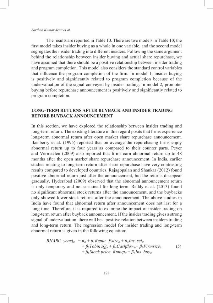
Sarthak Kumar Jena et al.
128
The results are reported in Table 10. There are two models in Table 10; the first model takes insider buying as a whole in one variable, and the second model segregates the insider trading into different insiders. Following the same argument behind the relationship between insider buying and actual share repurchase, we have assumed that there should be a positive relationship between insider trading and program completion. This model also considers the standard control variables that influence the program completion of the firm. In model 1, insider buying is positively and significantly related to program completion because of the undervaluation of the signal conveyed by insider trading. In model 2, promoter buying before repurchase announcement is positively and significantly related to program completion.
LONG-TERM RETURNS AFTER BUYBACK AND INSIDER TRADING BEFORE BUYBACK ANNOUNCEMENT
In this section, we have explored the relationship between insider trading and long-term return. The existing literature in this regard posits that firms experience long-term abnormal return after open market share repurchase announcement. Ikenberry et al. (1995) reported that on average the repurchasing firms enjoy abnormal return up to four years as compared to their counter parts. Peyer and Vermaelen (2009) also reported that firms earn abnormal return up to 48 months after the open market share repurchase announcement. In India, earlier studies relating to long-term return after share repurchase have very contrasting results compared to developed countries. Rajagopalan and Shankar (2012) found positive abnormal return just after the announcement, but the returns disappear gradually. Hyderabad (2009) observed that the abnormal announcement return is only temporary and not sustained for long term. Reddy et al. (2013) found no significant abnormal stock returns after the announcement, and the buybacks only showed lower stock returns after the announcement. The above studies in India have found that abnormal return after announcement does not last for a long time. Therefore, it is required to examine the impact of insider trading on long-term return after buyback announcement. If the insider trading gives a strong signal of undervaluation, there will be a positive relation between insiders trading and long-term return. The regression model for insider trading and long-term abnormal return is given in the following equation:
BHAR(1 year)it = αit + β1Repur_Psizeit + β2Ins_selit + β3Tobin'sQit + β4Cashflowit+ β5Firmsizeit + β6Stock price_Runupit + β7Ins_buyit
(5)
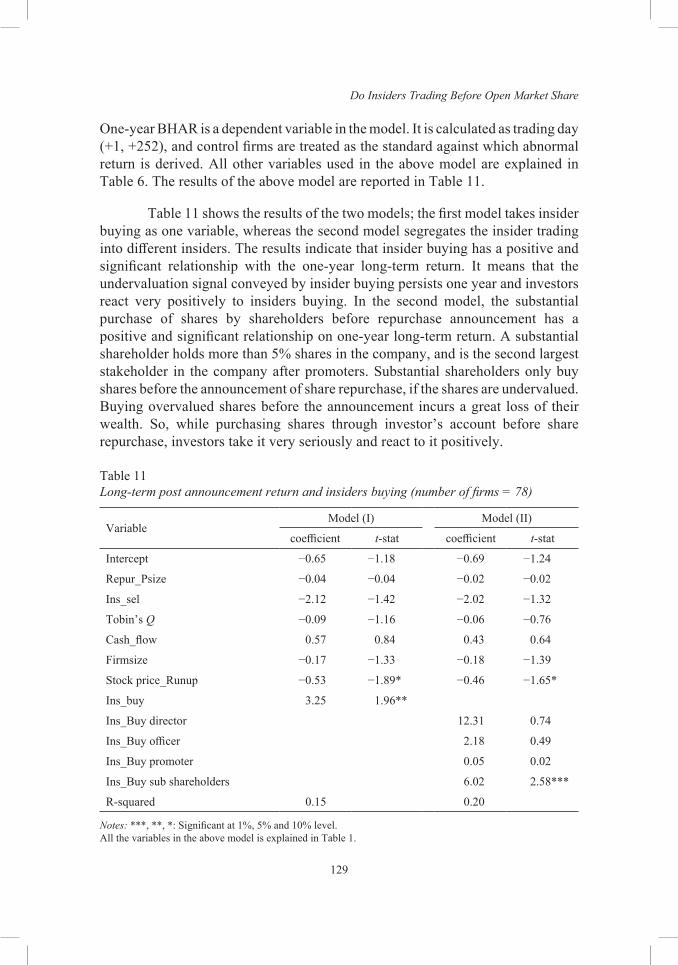
Do Insiders Trading Before Open Market Share
129
One-year BHAR is a dependent variable in the model. It is calculated as trading day (+1, +252), and control firms are treated as the standard against which abnormal return is derived. All other variables used in the above model are explained in Table 6. The results of the above model are reported in Table 11.
Table 11 shows the results of the two models; the first model takes insider buying as one variable, whereas the second model segregates the insider trading into different insiders. The results indicate that insider buying has a positive and significant relationship with the one-year long-term return. It means that the undervaluation signal conveyed by insider buying persists one year and investors react very positively to insiders buying. In the second model, the substantial purchase of shares by shareholders before repurchase announcement has a positive and significant relationship on one-year long-term return. A substantial shareholder holds more than 5% shares in the company, and is the second largest stakeholder in the company after promoters. Substantial shareholders only buy shares before the announcement of share repurchase, if the shares are undervalued. Buying overvalued shares before the announcement incurs a great loss of their wealth. So, while purchasing shares through investor’s account before share repurchase, investors take it very seriously and react to it positively.
Table 11Long-term post announcement return and insiders buying (number of firms = 78)
Variable Model (I) Model (II)
coefficient t-stat coefficient t-stat
Intercept −0.65 −1.18 −0.69 −1.24
Repur_Psize −0.04 −0.04 −0.02 −0.02
Ins_sel −2.12 −1.42 −2.02 −1.32
Tobin’s Q −0.09 −1.16 −0.06 −0.76
Cash_flow 0.57 0.84 0.43 0.64
Firmsize −0.17 −1.33 −0.18 −1.39
Stock price_Runup −0.53 −1.89* −0.46 −1.65*
Ins_buy 3.25 1.96**
Ins_Buy director 12.31 0.74
Ins_Buy officer 2.18 0.49
Ins_Buy promoter 0.05 0.02
Ins_Buy sub shareholders 6.02 2.58***
R-squared 0.15 0.20
Notes: ***, **, *: Significant at 1%, 5% and 10% level. All the variables in the above model is explained in Table 1.
Sarthak Kumar Jena et al.
130
CONCLUSION
In this paper, we have extended insiders trading literature by examining insider data around the share repurchase period to find the informational content in the context of India. This paper investigates the private information conveyed by insider trading with regard to share repurchase and undervaluation. Our empirical results support that insider trading in India conveys an undervaluation signal to the investors, who act accordingly. A detailed analysis of insider trading around share repurchase event is performed to investigate its intensity within the sample firm in the previous year as well as the subsequent year of share repurchase. We have observed that insider trading (buying and selling) of sample firms is more around share repurchase compared to matching firms. Sample firms buy more shares in the previous year of share repurchase than the following year of share repurchase. However, Tobit’s model shows that insider buying before share repurchase announcement has a positive influence on share repurchase decisions. The higher the insider buying, the higher is the undervaluation, and the firms are more likely to do repurchase.
We found that insider buying has a positive and significant relationship with announcement return, whereas insider selling has a negative and significant relationship with announcement return. The result is consistent with Babenko et al. (2012) and Firth et al. (2010). The paper also segregates the total sample into two; one is group-affiliated firms and the other is standalone firms to examine the information content on the ground of different ownerships. We have found that in India insider trading of standalone firms conveys more private information than group-affiliated firms and this finding is consistent with Chauhan et al. (2016).
We found that insider buying has a positive and significant relationship with actual share repurchase and program completion. The more the insider purchase before the announcement, the more likely the firm is to do actual share repurchase and complete the program. We also found that insider trading has a positive and significant relationship with long-term return, which means that the firms enjoy the benefit of the undervaluation signal conveyed by insider trading up to one year.
Our results support the view that insider trading conveys the undervaluation signal in an emerging country like India, where insider rules and regulation are not stringent as in a developed country. We further supported the view that ownership structure influences the information content of insider trading in India and extended the literature of insider trading to share repurchase in India for the first time to know the undervaluation signal associated with it. The future work
Do Insiders Trading Before Open Market Share
131
can be extended to analyse the profit accrued to the insiders by possessing the price-sensitive information before share repurchase. Insider trading after share repurchase announcement can be linked to firm performance in India, although it has been studied in the context of a developed country.
ACKNOWLEDGEMENTS
We are grateful to the anonymous referees of the journal for their valuable suggestions to improve the quality of the paper and University Grant Commission of India to provide financial help for this research.
REFERENCES
Anderson, R. C., & Reeb, D. M. (2003). Founding-family ownership and firm performance: evidence from the S&P 500. The Journal of Finance, 58(3), 1301–1328. https://doi.org/10.1111/1540-6261.00567
Asquith, P., & Mullins Jr, D. W. (1986). Signalling with dividends, stock repurchases, and equity issues. Financial Management, 15(3), 27–44. https://doi.org/10.2307/ 3664842
Babenko, I., Tserlukevich, Y., & Vedrashko, A. (2012). The credibility of open market share repurchase signaling. Journal of Financial and Quantitative Analysis, 47(05), 1059–1088. https://doi.org/10.1017/S0022109012000312
Bagwell, L. S. (1991). Share repurchase and takeover deterrence. The RAND Journal of Economics, 22(1), 72–88. https://doi.org/10.2307/2601008
Bagwell, L. S., & Shoven, J. B. (1988). Share repurchases and acquisitions: An analysis of which firms participate. In Corporate takeovers: Causes and consequences (pp. 191–220). Chicago: University of Chicago Press.
Bartov, E. (1991). Open-market stock repurchases as signals for earnings and risk changes. Journal of Accounting and Economics, 14(3), 275–294. https://doi.org/ 10.1016/0165-4101(91)90015-G
Beny, L. N. (2005). Do insider trading laws matter? Some preliminary comparative evidence. American Law and Economics Review, 7(1), 144–183. https://doi.org/ 10.1093/aler/ahi002
Bens, D. A., Nagar, V., Skinner, D. J., & Wong, M. F. (2003). Employee stock options, EPS dilution, and stock repurchases. Journal of Accounting and Economics, 36(1), 51–90. https://doi.org/10.1016/j.jacceco.2003.10.006
Bhattacharya, U., & Daouk, H. (2002). The world price of insider trading. The Journal of Finance, 57(1), 75–108. https://doi.org/10.1111/1540-6261.00416
Billett, M. T., & Xue, H. (2007). The takeover deterrent effect of open market share repurchases. The Journal of Finance, 62(4), 1827–1850. https://doi.org/10.1111/j.1540-6261.2007.01258.x
Sarthak Kumar Jena et al.
132
Bonaime, A. A., & Ryngaert, M. D. (2013). Insider trading and share repurchases: Do insiders and firms trade in the same direction? Journal of Corporate Finance, 22, 35–53. https://doi.org/10.1016/j.jcorpfin.2013.03.003
Bonaimé, A. A., Öztekin, Ö., & Warr, R. S. (2014). Capital structure, equity mispricing, and stock repurchases. Journal of Corporate Finance, 26, 182–200. https://doi.org/10.1016/j.jcorpfin.2014.03.007
Boudry, W. I., Kallberg, J. G., & Liu, C. H. (2013). Investment opportunities and share repurchases. Journal of Corporate Finance, 23, 23–38. https://doi.org/10.1016/j.jcorpfin.2013.07.006
Brockman, P., Howe, J. S., & Mortal, S. (2008). Stock market liquidity and the decision to repurchase. Journal of Corporate Finance, 14(4), 446–459. https://doi.org/ 10.1016/j.jcorpfin.2008.06.001
Carlton, D. W., & Fischel, D. R. (1983). The regulation of insider trading. Stanford Law Review, 857–895. https://doi.org/10.2307/1228706
Chan, K., Ikenberry, D. L., Lee, I., & Wang, Y. A. (2012). Informed traders: Linking legal insider trading and share repurchases. Financial Analysts Journal, 68(1), 60. https://doi.org/10.2469/faj.v68.n1.3
Chauhan, Y., Kumar, K. K., & Chaturvedula, C. (2016). Information asymmetry and the information content of insider trades: Evidence from the Indian stock market. Journal of Multinational Financial Management, 34, 65–79. https://doi.org/10. 1016/j.mulfin.2015.12.003
Chen, H. C., Chen, S. S., Huang, C. W., & Schatzberg, J. D. (2014). Insider trading and firm performance following open market share repurchase announcements. Journal of Business Finance & Accounting, 41(1–2), 156–184. https://doi.org/ 10.1111/jbfa.12059
Cheuk, M. Y., Fan, D. K., & So, R. W. (2006). Insider trading in Hong Kong: Some stylized facts. Pacific-Basin Finance Journal, 14(1), 73–90. https://doi.org/ 10.1016/j.pacfin.2005.06.002
Comment, R., & Jarrell, G. A. (1991). The relative signalling power of Dutch-auction and fixed-price self-tender offers and open-market share repurchases. The Journal of Finance, 46(4), 1243–1271. https://doi.org/10.1111/j.1540-6261.1991.tb04617.x
Dann, L. Y. (1981). Common stock repurchases: An analysis of returns to bondholders and stockholders. Journal of Financial Economics, 9(2), 113–138. https://doi.org/10.1016/0304-405X(81)90010-6
Dittmar, A. K. (2000). Why do firms repurchase stock. The Journal of Business, 73(3), 331–355. https://doi.org/10.1086/209646
Easterbrook, F. H. (1984). Two agency-cost explanations of dividends. The American Economic Review, 74(4), 650–659.
Fenn, G. W., & Liang, N. (2001). Corporate payout policy and managerial stock incentives. Journal of Financial Economics, 60(1), 45–72. https://doi.org/10.1016/S0304-405X(01)00039-3
Fernandes, N., & Ferreira, M. A. (2009). Insider trading laws and stock price informativeness. Review of Financial Studies, 22(5), 1845–1887. https://doi.org/10.1093/rfs/hhn066
Do Insiders Trading Before Open Market Share
133
Firth, M., Leung, T. Y., & Rui, O. M. (2010). Double signals or single signal? An investigation of insider trading around share repurchases. Journal of International Financial Markets, Institutions and Money, 20(4), 376–388. https://doi.org/10.1016/j.intfin.2010.05.002
Gong, G., Louis, H., & Sun, A. X. (2008). Earnings management and firm performance following open-market repurchases. The Journal of Finance, 63(2), 947–986. https://doi.org/10.1111/j.1540-6261.2008.01336.x
Grullon, G., & Michaely, R. (2002). Dividends, share repurchases, and the substitution hypothesis. The Journal of Finance, 57(4), 1649–1684. https://doi.org/10. 1111/1540-6261.00474
Holderness, C. G., & Sheehan, D. P. (1988). The role of majority shareholders in publicly held corporations: An exploratory analysis. Journal of Financial Economics, 20, 317–346. https://doi.org/10.1016/0304-405X(88)90049-9
Hovakimian, A. (2004). The role of target leverage in security issues and repurchases. The Journal of Business, 77(4), 1041–1072. https://doi.org/10.1086/422442
Hovakimian, A., Opler, T., & Titman, S. (2001). The debt-equity choice. Journal of Financial and Quantitative Analysis, 36(1), 1–24.
Hyderabad, R. L. (2009). Price performance following share buyback announcement in India. Vision, 13(1), 59–78. https://doi.org/10.1177/097226290901300105
Ikenberry, D., Lakonishok, J., &Vermaelen, T. (1995). Market underreaction to open market share repurchases. Journal of Financial Economics, 39(2), 181–208. https://doi.org/10.1016/0304-405X(95)00826-Z
Jagannathan, M., Stephens, C. P., & Weisbach, M. S. (2000). Financial flexibility and the choice between dividends and stock repurchases. Journal of Financial Economics, 57(3), 355–384. https://doi.org/10.1016/S0304-405X(00)00061-1
Jensen, M. C. (1986). Agency cost of free cash flow, corporate finance, and takeovers. Corporate Finance and Takeovers. American Economic Review, 76(2), 323–329.
John, K., & Mishra, B. (1990). Information content of insider trading around corporate announcements: The case of capital expenditures. The Journal of Finance, 45(3), 835–855. https://doi.org/10.1111/j.1540-6261.1990.tb05108.x
Kahle, K. M. (2002). When a buyback isn’t a buyback: Open market repurchases and employee options. Journal of Financial Economics, 63(2), 235–261. https://doi.org/10.1016/S0304-405X(01)00095-2
Lang, L. H., & Litzenberger, R. H. (1989). Dividend announcements: Cash flow signalling vs. free cash flow hypothesis? Journal of Financial Economics, 24(1), 181–191.
Lee, B. S., & Suh, J. (2011). Cash holdings and share repurchases: International evidence. Journal of Corporate Finance, 17(5), 1306–1329. https://doi.org/10.1016/j.jcorpfin.2011.06.006
Lee, D. S., Mikkelson, W. H., & Partch, M. M. (1992). Managers’ trading around stock repurchases. The Journal of Finance, 47(5), 1947–1962. https://doi.org/ 10.1111/j.1540-6261.1992.tb04690.x
Leland, H. E., & Pyle, D. H. (1977). Informational asymmetries, financial structure, and financial intermediation. The journal of Finance, 32(2), 371–387. https://doi.org/10.2307/2326770
Sarthak Kumar Jena et al.
134
Li, K., & McNally, W. (2007). The information content of Canadian open market repurchase announcements. Managerial Finance, 33(1), 65–80. https://doi.org/ 10.1108/03074350710715818
Liang, W. L., Chan, K., Lai, W. H., & Wang, Y. (2013). Motivation for repurchases: A life cycle explanation. Journal of Financial Services Research, 43(2), 221–242. https://doi.org/10.1007/s10693-011-0126-7
Lie, E. (2000). Excess funds and agency problems: An empirical study of incremental cash disbursements. Review of Financial Studies, 13(1), 219–248. https://doi.org/10.1093/rfs/13.1.219
Louis, H., Sun, A. X., & White, H. (2010). Insider trading after repurchase tender offer announcements: Timing versus informed trading. Financial Management, 39(1), 301–322. https://doi.org/10.1111/j.1755-053X.2010.01074.x
Mitchell, J. D., & Dharmawan, G. V. (2007). Incentives for on-market buy-backs: Evidence from a transparent buy-back regime. Journal of Corporate Finance, 13(1), 146–169. https://doi.org/10.1016/j.jcorpfin.2006.12.002
Nohel, T., & Tarhan, V. (1998). Share repurchases and firm performance: New evidence on the agency costs of free cash flow. Journal of Financial Economics, 49(2), 187–222. https://doi.org/10.1016/S0304-405X(98)00022-1
Oded, J. (2005). Why do firms announce open-market repurchase programs? Review of Financial Studies, 18(1), 271–300. https://doi.org/10.1093/rfs/hhh004
Peyer, U., & Vermaelen, T. (2009). The nature and persistence of buyback anomalies. Review of Financial Studies, 22(4), 1693–1745. https://doi.org/10.1093/rfs/hhn024
Rajagopalan, N. V. R., & Shankar, H. (2012). Stock market behaviour around buyback announcements in India: An empirical justification for preferring the open market repurchase mode. Indian Journal of Finance, 6, 43–52. https://doi.org/10.17010/ijf/2012/v6i12/72364
Reddy, K. S., Nangia, V. K., & Agrawal, R. (2013). Share repurchases, signalling effect and implications for corporate governance: Evidence from India. Asia-Pacific Journal of Management Research and Innovation, 9(1), 107–124. https://doi.org/10.1177/2319510X13483518
Schultz, P. (2003). Pseudo market timing and the long-run underperformance of IPOs. The Journal of Finance, 58(2), 483–518. https://doi.org/10.1111/1540-6261. 00535
Seyhun, H. N. (1986). Insiders’ profits, costs of trading, and market efficiency. Journal of Financial Economics, 16(2), 189–212. https://doi.org/10.1016/0304-405X (86)90060-7
Shleifer, A., & Vishny, R. W. (1986). Large shareholders and corporate control. Journal of Political Economy, 94(3, Part 1), 461–488. https://doi.org/10.1086/261385
Sinha, S. (1991). Share repurchase as a takeover defense. Journal of Financial and Quantitative Analysis, 26(02), 233–244. https://doi.org/10.2307/2331267
Skinner, D. J. (2008). The evolving relation between earnings, dividends, and stock repurchases. Journal of Financial Economics, 87(3), 582–609. https://doi.org/ 10.1016/j.jfineco.2007.05.003

Do Insiders Trading Before Open Market Share
135
Stephens, C. P., &Weisbach, M. S. (1998). Actual share reacquisitions in open-market repurchase programs. The Journal of Finance, 53(1), 313–333. https://doi.org/ 10.1111/0022-1082.115194
Vafeas, N., & Joy, O. M. (1995). Open market share repurchases and the free cash flow hypothesis G35. Economics Letters, 48(3), 405–410. https://doi.org/10. 1016/0165-1765(94)00631-B
Vermaelen, T. (1981). Common stock repurchases and market signalling: An empirical study. Journal of Financial Economics, 9(2), 139–183. https://doi.org/10.1016/ 0304-405X(81)90011-8
Yarram, S. R. (2014). Factors influencing on-market share repurchase decisions in Australia. Studies in Economics and Finance, 31(3), 255–271. https://doi.org/10.1108/SEF-02-2013-0021
AAMJAF Vol. 14, No. 2, 137–156, 2018
© Asian Academy of Management and Penerbit Universiti Sains Malaysia, 2018. This work is licensed under the terms of the Creative Commons Attribution (CC BY) (http://creativecommons.org/licenses/by/4.0/).
Asian Academy of Management Journal
of Accounting and Finance
MONETARY POLICY, BANK COMPETITIVENESS AND BANK RISK-TAKING: EMPIRICAL EVIDENCE FROM
VIETNAM
Nguyen Tran Thai Ha1* and Phan Gia Quyen2
1Finance and Accounting Faculty, Saigon University 28 Nguyen Thong Street, Ward 7, Dist. 3, Ho Chi Minh City, Vietnam
2Saigon Thuong Tin Commercial Joint Stock Bank, Vietnam 266 – 268 Nam Ki Khoi Nghia Street, Ward 6, Dist. 3,
Ho Chi Minh City, Vietnam
*Corresponding author: [email protected]
ABSTRACT
This study assesses the impact(s) of monetary policy and further influence of competitiveness on bank risk-taking of the Vietnamese commercial banks over the period of 2007–2016, an unstable period of the domestic monetary policy. The monetary policy is captured by a set of different variables including money supply, refinancing interest rate and treasury bill interest rate. Using the GMM methodology, the study finds that the monetary policy of Vietnam has a significant impact on bank risk-taking level, as measured by Z-score index. The empirical findings also indicate that bank risk-taking increases in the context of a loose monetary policy. In addition, the competitiveness of banks, presented by the Lerner index, is found as a determinant of bank risk-taking levels. By using interacting variables, the findings indicate that the impact of the competitiveness of banks outweighs that of monetary policy on bank risk-taking behaviour. It implies that the banks with high market power demonstrate less risk-taking behaviour even in a loose monetary policy environment. Besides that, liquidity, credit level and cost inefficiency could increase risk-taking behaviour of banks while bank size poses restrictions on bank risk-taking.
Keywords: bank, risk-taking, monetary policy, competitiveness, GMM, Vietnam
Publication date: 31 December 2018
To cite this article: Ha, N. T. T., & Quyen, P. G. (2018). Monetary policy, bank competitiveness and bank risk-taking: Empirical evidence from Vietnam. Asian Academy of management Journal of Accounting and Finance, 14(2), 137–156. https://doi.org/10.21315/aamjaf2018.14.2.6
To link to this article: https://doi.org/10.21315/aamjaf2018.14.2.6
Nguyen Tran Thai Ha and Phan Gia Quyen
138
INTRODUCTION
The stability of the banking sector plays an important role in ensuring that the country’s economic goals are met, especially in developing countries. Therefore, the government generally steps in to consolidate the stability and improve the efficiency of the banking system through policies, in particular monetary policy. Similar to other developing countries, Vietnam has its banking sector working as the backbone of its economic system. Nevertheless, the erratic monetary policy, from loose policy to tight policy during the 2006–2012 period, had implications on the operation of the banking system in Vietnam. The expansionary monetary policy, which took effect during 2006–2007 and 2008–2009, significantly pushed domestic credit growth from about 25% to over 50%. The loose monetary policy, normally presented by an increase in money supply or decrease in interest rate, not only facilitated a boom in credit growth and non-controlling investments but also contributed to asset bubbles and bad debts. From 2007, bad debts soared as a consequence of high credit growth, while the risk management ability of banks was still weak. Bad debt rising rate reached over 51% during 2008–2011, twice the average credit growth rate in the same period. As a result, the government had to tighten the monetary policy, which in turn led to the fall of the financial market and the banking system in the following period (Refer to Appendix A).
Fundamentally, monetary policy affects the money and asset markets through the transmission mechanism, which involves influences on monetary and credit aggregation, market interest rates, asset prices and exchange rate. As a consequence, banks’ operations are impacted and they respond to adapt to changes in monetary policy. In this mechanism, the respondency of financial institutions, which could be presented by commercial banks, receives a lot of attention both in theoretical and empirical research. Previous studies estimated that bank risk-taking is likely to be considerably affected by monetary policy (Gambacorta, 2009; Delis & Staikouras, 2011) in three ways: (1) Low interest rate is a motive for banks to seek more new investment products/projects; (2) Interest rate directly affects on the pricing evaluation process and the cash flows of projects, thus it can impact on the risk perception of banks’ managers; and (3) banks usually set up financial targets in their balance sheet in order to balance with the interest’s variation. Banks, therefore, could increase their risk-taking appetite to achieve the financial objectives on their balance sheets. Besides that, the competitiveness of banks is also considered a contributing factor in the transmission mechanism of monetary policy (Brissimis, Iosifidi, & Delis, 2014). A number of previous studies claimed that if the competitiveness of the banks is high, it could lead to lower risk-taking behaviour as compared to others with lower competitiveness irrespective of a loose monetary policy environment (Beck, De Jonghe, & Schepens, 2013;
Monetary Policy, Bank Competitiveness and Bank Risk-Taking
139
Fu, Lin, & Molyneux, 2014). This difference reflects the ability to access other financial resources when the interest rate changes. Highly competitive banks, in this regard, do not need to search for and resort to risky investment projects.
Although the combined impact of monetary policy and competitiveness on bank risk-taking has been prolifically studied, this area has not been given sufficient focus and research in Vietnam. In addition, statistical results in Appendix A show that the expansionary monetary policy had been done by government, bad debt had an increasing trend in the following years. It gives a question whether or not the relationship between monetary policy and bank risk-taking behaviours. Some scarce prior studies mostly analysed only the impact of the competition on the sustainability of the banks and the relationship among competitiveness, monetary policy, and the credit growth of banks. Hence, this study aims to shed some light on the effect of monetary policy on bank risk-taking in Vietnam and to examine the additional role of competition in the relationship between monetary policy and bank risk-taking through the use and analysis of the database of 26 commercial banks in Vietnam from 2007 to 2016. In the context of continuous changes of monetary policy and apparent instability of banks in Vietnam, this study has specific implications. Firstly, few prior research, to our knowledge, has addressed the complex interaction between monetary policy, competition and risk-taking level of banks in the specific context of developing countries. Secondly, this study investigates the inter-relatedness between key variables of competition – market power, monetary policy and bank risk-taking to lend more support to the analysis. Thirdly, there are recommendations drawn from the results of the study which could be of use to policymakers as well as bank managers. As this study is conducted in a period of changeable monetary policies; it could be referred to when considering the impact of the Vietnamese government’s policies in the future.
The findings indicate that loose monetary policy could push the risk-taking level of commercial banks. However, the banks with high market power are not willing to trade-off their stability, even in the loose monetary policy environment. In other words, banks with greater market power often focus more on general stability than on taking risks to gain profits. Bank characteristics have also been found to make significant impacts on bank risk-taking.
LITERATURE REVIEW
In prior studies on the transmission mechanism of monetary policy, the risk-taking channel is assumed to closely correlate with the credit growth channel (Keeley, 1990; Dell’Ariccia & Marquez, 2006). Through the credit channel, the monetary
Nguyen Tran Thai Ha and Phan Gia Quyen
140
policy could affect the credit approval process (the lending channel) and the needs of the customers (the balance sheet channel). The risk-taking channel can be seen as the combination between the lending channel and the balance sheet channel of the banks (Alpanda & Aysun, 2012). This channel provides a new outlook of the transmission mechanism of monetary policy; it also takes into consideration the relationship between the changes in the monetary policy represented by the interest rate and the risk-taking ability of individuals in the economy (Borio & Zhu, 2012).
Firstly, interest can affect the risk-awareness of individuals in the economy and the risk level of the adverse selection of customers (Gambacorta, 2009). Particularly, the risk-taking behaviour will increase as the interest rate goes down, and this leads to the changes in the behaviour of the lending bank (Borio & Zhu, 2012). Therefore, low-interest rate results in an increase in not only banks’ debt but also the risk-taking level of the bank's managers. Low-interest rate is liable to motivate bank’s managers to search for more investment projects in order to get more profits. This, however, can pose challenges to ensuring the financial stability of banks. Moreover, these potential projects may not be promising due to the psychological1 and the institutional problems (Gambacorta, 2009). When a high nominal profit seems to be hard to capture in a low-interest rate environment, many bank managers could venture into risky projects to gain more profits. The monetary illusion could push bank’s managers to try to find highest nominal profits that they used to achieve in the blossomed economy in the past. As such, bank’s managers are willing to trade-off bank risks, in another word, they are willing to accept risk-taking incentives. Secondly, borrower’s financial situation is based on borrower’s net worth, which is defined as the sum of the value of liquid and marketable assets. Interest rate affects the pricing evaluation and the cash flow of the projects or assets. Therefore, it will also have an impact on the risk awareness of bank managers about borrower’s balance sheet (Borio & Zhu, 2012). For instance, low interest will increase the net present value of projects’ cash flow when discount rate decreases. Risk projects with negative net present value will become feasible; and firms will easily access financial resources thanks to the low cost of capital. Therefore, low interest rate could lead to the change(s) in risk-awareness of individuals. Estimates regarding project risk will also change as a consequence of low-interest rate, and they will actually be riskier in bank’s portfolio. Thirdly, banks often set up financial goals, such as a targeted level of financial leverage or a capital adequacy ratio. When asset prices increase as a result of the expansionary monetary policy environment, the balance sheet of the banks will be better, and their market value will be improved. It implies that the leverage of banks – determined by the ratio of equity and total assets – will decrease. If the total assets increase while the banks do not adjust their equity
Monetary Policy, Bank Competitiveness and Bank Risk-Taking
141
in a timely manner, the leverage will be negatively correlated with the total assets, and their liquidity will become better. However, banks usually want to minimise the excess high-cost capital to acquire their financial targets as well as their performance improving through accelerate financial leverage (Adrian & Shin, 2010). It implies that the banks will be able to expand their balance sheets after the monetary policy is loosened. Adrian and Shin (2008) found a strong correlation between loose monetary policy and the expansion of banks’ balance sheets. In this study, the authors will give evidence to show that banks managed their leverage actively and aimed to keep a reasonable and appropriate financial leverage at a particular interest rate.
It can be seen that the transmission mechanism of monetary policy through the risk-taking channel and balance sheet channel can increase bank risk-taking when interest rate environment is relatively low; in comparison with current potential macroeconomic conditions. This phenomenon was found and confirmed by many previous studies (e.g. Keeley, 1990; Rajan, 2006). Therefore, this study expects that the monetary policy will have a significant impact on the bank risk-taking; for instance, when interest rate declines, risk-taking tendency of banks will be higher.
H1: The monetary policy has a significant positive impact on the bank risk-taking.
Empirical evidence with respect to whether competition enhances or reduces bank risk-taking is somewhat mixed and inconclusive. Previous studies have considered that the competitiveness of banks has exerted a considerable impact on their risk acceptance in addition to and amid the transmission mechanism of monetary policy (Brissimis et al., 2014). Some studies have implied that banks with stronger market power (higher competitive ability) could demonstrate more risk-taking tendency. Banks with high competitiveness easily get more future lending opportunities. Therefore, they are willing to venture to get more profits by offering customers with promoted interest rates on deposits. Thus, even in the context of decreasing interest rate in a loose monetary policy environment, market power can have still a significant effect on risk-taking behaviour of banks.
However, other studies on bank competition and risk-taking are sceptical about this conclusion. They suggested that banks with stronger market power often get more earnings than others. The premise is that high market power leads to a “quiet life”,2 a situation where these banks will not have the motivation to seek investment opportunities and forgo cost savings because they have already achieved high profits from the advantages of their superior market power. They will not exchange their existing prestige and stability for more risk profits, even in
Nguyen Tran Thai Ha and Phan Gia Quyen
142
a low-interest rate environment. Furthermore, Brissimis et al. (2014) determined that market power is an internal factor influencing banks’ reaction in terms of lending and risk-taking to monetary policy impulses. The marginal cost of loan activities is considerably affected by changes in domestic monetary policy, which determines the interest rate banks must pay to access sources of finance. Thus, a change in interest rates can change the marginal cost and lending interest rate of the credit activities. As a result, in more competitive environments, there is greater pressure on maintaining profits, which makes banks take on more risks, resulting in higher fragility (Sanjukta & Rudra, 2016). However, in the non-competitive market, the lending interest rate is considered less sensitive to the changes in the marginal cost of the loan activities (Khan, Scheule, & Wu, 2017). Since banks with market power have easier access to alternative sources of finance, and they are inclined to hold their current situations and be willing with their “quiet life”; a change in central bank rates will cause less impact on their marginal cost (Brissimis et al., 2014). Thus, this study assumes that banks with high market power will have less risk-taking acceptance, even in a low-interest rate environment; or in other words, competitiveness has a negative and adverse impact on the relationship between the monetary policy and the risk-taking behaviour of banks.
H2: The competitiveness of banks has a negative and adverse impact on the relationship between the monetary policy and the bank risk-taking.
METHODOLOGY
To examine the impact of monetary policy, competitiveness on the bank risk-taking, this study uses the database from Vietnamese commercial banks from 2007 to 2016, which is collected by FiinPro.3 It should be noted that this study excludes the commercial banks which do not disclose sufficient data on bank financial statements during the period of research. Moreover, this study excludes the banks which are acquired or controlled under special terms by the State Bank of Vietnam, and banks which were merged and consolidated in the past. The final sample consists of 26 commercial banks, including one commercial bank with 100% state capital, three state-owned commercial banks and 22 private commercial banks. After the data selection process, the sample comprises 238 entries for 26 banks.
This study uses the model previously applied by Baselga-Pascual, Trujillo-Ponce and Cardone-Riportella (2015), Lapteacru (2017), and Paligorova and Santos (2017). The relationship between the competitiveness of banks, the
Monetary Policy, Bank Competitiveness and Bank Risk-Taking
143
existing monetary policy and the banks’ risk-taking level is illustrated by the following equation:
Riskit = β0 + β1 * Riskit–1 + β2 * Liquidit + β3 * Loansit
+ β4 * Depositit + β5 * Sizeit + β6 * Costit + β7 * Lernerit + β8 * Monetarypolicyit + β9 * Lernerit * Monetarypolicyit + εit
(1)
In this Equation (1), Risk represents the bank risk-taking, calculated by Z-score, according to Turk Ariss (2010) and Beck et al. (2013). The justification for using Z-score is to highlight the relationship between a bank’s capital and the volatility of its returns, which reflects how much variability in returns could be absorbed by a bank’s capital without putting the bank into insolvency. Z-score is the natural logarithm of the index which is calculated by the following equation:
Z-score ROAROA E
TA= v+
ROA is the after-tax profit on the total assets; E/TA reflects the leverage of the banks calculated by the ratio of equity to total assets of the bank; and is the standard deviation of ROA. From the above Z-score formula, it can be seen that an increase in Z-score value may result from an increase in ROA or bank capital, or a decrease in the volatility of standard deviation of ROA. The assumption is that in the scenario where bank’s capital level falls to zero, it becomes insolvent. It could therefore be implied that bank risk will be lower when the Z-score value increases and vice versa (Berger, Klapper, & Turk-Ariss, 2009; Beck et al., 2013).
From Equation (1), monetary policy is presented by a set of variables such as the refinancing interest rate (rate), the M2 money supply (m2), the treasury bill interest rate (tbill). Normally, a loose monetary policy is presented by an increase in money supply or a decrease in interest rate (e.g. refinancing interest rate or treasury bill interest rate); and conversely, a tight policy is signified by a decrease in money supply or an increase in interest rate. These variables have been used extensively in many prior studies on monetary policy. The loose monetary policy, as used in the study’s hypothesis, can trigger banks to implement the inherently risky investment projects to increase their profits, so banks will be more willing to accept risks.
In Equation (1), the competitiveness is captured by the Lerner index. The Lerner index (commonly-known as the price-cost margin) is a popular measure of market power in the banking market. It is defined as the difference between output prices and marginal costs (relative to prices), and higher values of
Nguyen Tran Thai Ha and Phan Gia Quyen
144
the Lerner index implies greater market power of bank. According to Demirgüç-Kunt and Huizinga (2010), the Lerner index is calculated based on the difference between the output price (P), calculated by the ratio of total revenue to total assets, and the marginal cost (MC); a subtraction which is then divided by the output price.
Lerner PP MC=-
With reference to Berger et al. (2009) and Turk Ariss (2010), this study estimates marginal cost through the following translog cost function:
2Cost lnQ lnQ k W
lnQ W W W
Trend Trend Trend lnQ
Trend W e
0 1
2 2
1
2
2
1
2
1
1
2
1
2
2
2
3
1
2
it kk
k kk
k jjk
k kk
) ) )
) ) )
) ) ) )
) )
i
b bb
c
d
d d
{
= + + +
+ + +
+ +
+ +
=
= ==
=
/
/ //
/
(2)
As presented in the above formula, bank cost (Cost) is a function of output. The physical capital, the human capital and financial capital are three input prices, in which financial capital is calculated by the interest expenses on the total deposits (w1), the physical capital is denoted by operating expenses on the total assets (w2), and the human capital is calculated by staff salaries on the total assets (w3). The output products (lnQ) is presented by the total assets of the bank. Trend shows movements in the cost function over time (technical changes). The study scales the cost of input (w1) and (w2) by (w3) to control heteroskedasticity. After estimating the Equation (2) by the OLS estimation method, the marginal costs (MC) are then computed as:
lnMC QCost Q W Trend1 2 3
1
2
k kk
) ) ) )ib b d= + +=
f p/
Besides that, the study considers that risk-taking level is also affected by the characteristics of a bank. Thus, a set of control variables is added to account for bank risk-taking. These features, including liquidity of bank (Liquid), outstanding loan rate (Loans), bank deposit proportion (Deposit), bank size (Size), Operating expenses (Cost), are used in a large number of previous studies (Refer to Appendix B). We emphasize that equity-to-asset ratio (Equity) and net profit on total assets (ROA) are not considered as control variables in our model because the (Z-score) (dependent variable) is calculated based on these two indices. They, therefore, cause spurious regression.
Monetary Policy, Bank Competitiveness and Bank Risk-Taking
145
Liquidity of bank (Liquid) is measured by the ratio of a liquid asset to total asset. An improvement in a bank’s liquidity implies the adequacy of capital to cover the banks’ operations (Borio & Zhu, 2012). As regards the relationship between a bank’s liquidity and its risk-taking, it is argued that the excess holding of liquid assets will generate a considerable expense to the banks. This may drive banks to seek more high-profit investments with high risks, and therefore shows that banks are accepting more risk-taking behaviour (Acharya & Naqvi, 2012). Bank deposit (Deposit) is presented by a deposit which is measured by the ratio of total customer deposits to total assets. According to Acharya and Naqvi (2012), excess deposits will make bank managers more tolerant to risk.
Bank size (Size), which is measured by the natural logarithm of total assets, is one of the critical factors to determine bank risk-taking. However, the impact of bank size on risk-taking behaviour has not been confirmed. Supporting views point to the “too big to fail” theory to stipulate that bank size has a positive relationship on bank risk-taking. According to “too big to fail” theory, these banks have acknowledged that they will get government support if they have any potential bankruptcy risk. Hence, they become more adventurous in their activities. By contrast, many researchers have based on a view of diversification to emphasise that bank size could negatively influence risk-taking behaviour of banks. In other words, large banks will diversify their portfolio, incomes and loans; so they will have less risk than smaller banks. This study assumes that bank size has a negative relationship with bank risk-taking.
Loans, measured by the ratio of the total loans to the total assets, could be seen as an important factor in generating more profits for the bank. However, the correlation between loans and bank risk-taking is not consistent; and it also largely depends on the level of risk involving in the investments or projects which a bank finances. Besides that, operating cost (Cost), captured by operating cost and total assets, reflects the efficiency of bank operation. Banks demonstrating high operating cost imply low profitability; hence their bank managers will be pushed to seek more investments or projects with higher risk. In other words, high operating costs will probably lead banks to hazardous situations (Boyd & Prescott, 1986; Agoraki, Delis, & Pasiouras, 2011).
To examine the model, the study uses a GMM-sys method (Generalise Momentum Method) for two main reasons: (1) The GMM can overcome endogenous, heteroskedasticity and autocorrection problems. As mentioned above, Z-score and independent variables, such as liquidity, loans or bank size, may have correlations; and it could cause endogenous problems or heteroskedasticity. GMM is a suitable method to deal with these problems. (2) The two-step system GMM estimation method gives better results than the other separate two-step
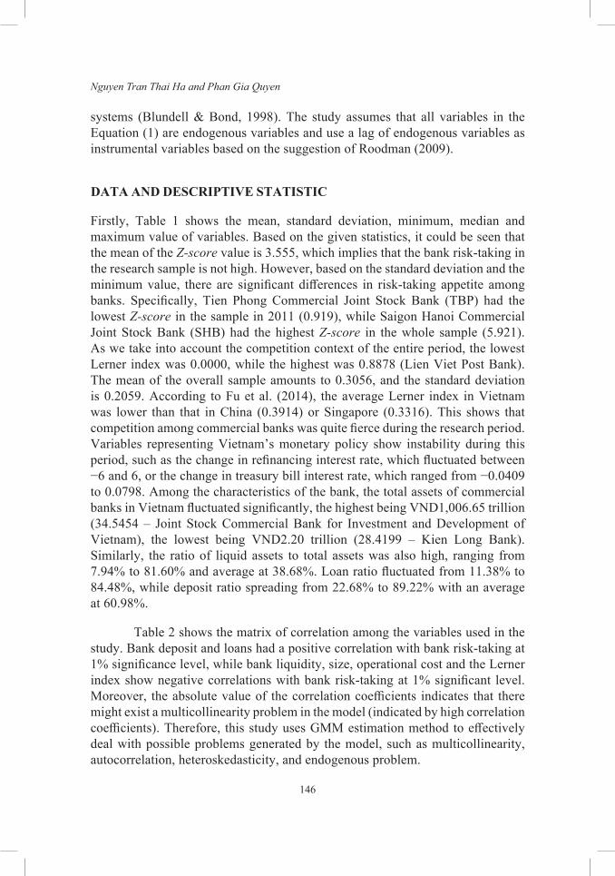
Nguyen Tran Thai Ha and Phan Gia Quyen
146
systems (Blundell & Bond, 1998). The study assumes that all variables in the Equation (1) are endogenous variables and use a lag of endogenous variables as instrumental variables based on the suggestion of Roodman (2009).
DATA AND DESCRIPTIVE STATISTIC
Firstly, Table 1 shows the mean, standard deviation, minimum, median and maximum value of variables. Based on the given statistics, it could be seen that the mean of the Z-score value is 3.555, which implies that the bank risk-taking in the research sample is not high. However, based on the standard deviation and the minimum value, there are significant differences in risk-taking appetite among banks. Specifically, Tien Phong Commercial Joint Stock Bank (TBP) had the lowest Z-score in the sample in 2011 (0.919), while Saigon Hanoi Commercial Joint Stock Bank (SHB) had the highest Z-score in the whole sample (5.921). As we take into account the competition context of the entire period, the lowest Lerner index was 0.0000, while the highest was 0.8878 (Lien Viet Post Bank). The mean of the overall sample amounts to 0.3056, and the standard deviation is 0.2059. According to Fu et al. (2014), the average Lerner index in Vietnam was lower than that in China (0.3914) or Singapore (0.3316). This shows that competition among commercial banks was quite fierce during the research period. Variables representing Vietnam’s monetary policy show instability during this period, such as the change in refinancing interest rate, which fluctuated between −6 and 6, or the change in treasury bill interest rate, which ranged from −0.0409 to 0.0798. Among the characteristics of the bank, the total assets of commercial banks in Vietnam fluctuated significantly, the highest being VND1,006.65 trillion (34.5454 – Joint Stock Commercial Bank for Investment and Development of Vietnam), the lowest being VND2.20 trillion (28.4199 – Kien Long Bank). Similarly, the ratio of liquid assets to total assets was also high, ranging from 7.94% to 81.60% and average at 38.68%. Loan ratio fluctuated from 11.38% to 84.48%, while deposit ratio spreading from 22.68% to 89.22% with an average at 60.98%.
Table 2 shows the matrix of correlation among the variables used in the study. Bank deposit and loans had a positive correlation with bank risk-taking at 1% significance level, while bank liquidity, size, operational cost and the Lerner index show negative correlations with bank risk-taking at 1% significant level. Moreover, the absolute value of the correlation coefficients indicates that there might exist a multicollinearity problem in the model (indicated by high correlation coefficients). Therefore, this study uses GMM estimation method to effectively deal with possible problems generated by the model, such as multicollinearity, autocorrelation, heteroskedasticity, and endogenous problem.
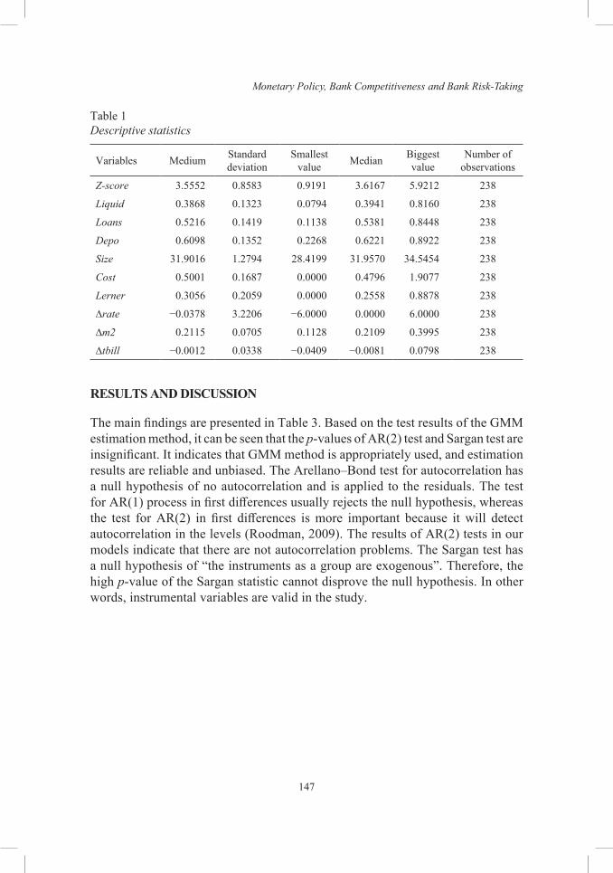
Monetary Policy, Bank Competitiveness and Bank Risk-Taking
147
Table 1Descriptive statistics
Variables Medium Standard deviation
Smallest value Median Biggest
valueNumber of
observations
Z-score 3.5552 0.8583 0.9191 3.6167 5.9212 238
Liquid 0.3868 0.1323 0.0794 0.3941 0.8160 238
Loans 0.5216 0.1419 0.1138 0.5381 0.8448 238
Depo 0.6098 0.1352 0.2268 0.6221 0.8922 238
Size 31.9016 1.2794 28.4199 31.9570 34.5454 238
Cost 0.5001 0.1687 0.0000 0.4796 1.9077 238
Lerner 0.3056 0.2059 0.0000 0.2558 0.8878 238
∆rate −0.0378 3.2206 −6.0000 0.0000 6.0000 238
∆m2 0.2115 0.0705 0.1128 0.2109 0.3995 238
∆tbill −0.0012 0.0338 −0.0409 −0.0081 0.0798 238
RESULTS AND DISCUSSION
The main findings are presented in Table 3. Based on the test results of the GMM estimation method, it can be seen that the p-values of AR(2) test and Sargan test are insignificant. It indicates that GMM method is appropriately used, and estimation results are reliable and unbiased. The Arellano–Bond test for autocorrelation has a null hypothesis of no autocorrelation and is applied to the residuals. The test for AR(1) process in first differences usually rejects the null hypothesis, whereas the test for AR(2) in first differences is more important because it will detect autocorrelation in the levels (Roodman, 2009). The results of AR(2) tests in our models indicate that there are not autocorrelation problems. The Sargan test has a null hypothesis of “the instruments as a group are exogenous”. Therefore, the high p-value of the Sargan statistic cannot disprove the null hypothesis. In other words, instrumental variables are valid in the study.
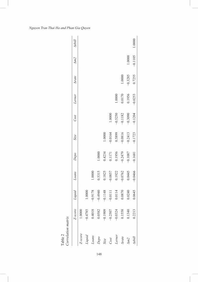
Nguyen Tran Thai Ha and Phan Gia Quyen
148
Tabl
e 2
Cor
rela
tion
mat
rix Z-sc
ore
Liqu
idLo
ans
Dep
oSi
zeC
ost
Lern
er∆r
ate
∆m2
∆tbi
ll
Z-sc
ore
1.00
00
Liqu
id−0
.478
51.
0000
Loan
s0.
4018
−0.9
178
1.00
00
Dep
o0.
0582
−0.4
940
0.53
151.
0000
Size
−0.1
909
−0.1
148
0.18
250.
4234
1.00
00
Cos
t−0
.250
7−0
.011
1−0
.085
70.
1171
−0.0
164
1.00
00
Lern
er−0
.032
40.
0114
0.19
220.
1956
0.58
99−0
.525
01.
0000
∆rat
e0.
1558
0.08
70−0
.076
2−0
.247
9−0
.081
6−0
.118
20.
0170
1.00
00
∆m2
0.13
400.
0240
0.04
45−0
.108
7−0
.241
3−0
.309
00.
1956
−0.3
285
1.00
00
∆tbi
ll0.
2213
0.06
45−0
.046
6−0
.168
1−0
.172
3−0
.120
4−0
.025
30.
7255
−0.1
105
1.00
00
Monetary Policy, Bank Competitiveness and Bank Risk-Taking
149
Table 3Estimated results of Equation (1)
Z-score Model (1) Model (2) Model (3) Model (4) Model (5) Model (6)
Z-score (−1) 0.6063***(14.04)
0.6200***(16.42)
0.6659***(10.27)
0.6927***(22.57)
0.7513***(24.83)
0.6868***(28.35)
Liquid −3.6735***(−4.00)
−2.9739***(−4.24)
−4.0306***(−3.22)
−2.8761***(−3.49)
−2.9431***(−4.23)
−2.3354***(−3.62)
Loans −2.4967***(−3.34)
−2.2045***(−2.67)
−2.4712**(−1.98)
−1.8947***(−2.59)
−1.6517**(−1.97)
−1.5605**(−2.33)
Depo 0.5516(1.48)
0.6389(1.34)
−0.2319(−0.78)
−0.0334(−0.20)
0.0046(0.02)
0.2605(1.16)
Size 0.0468*(1.72)
0.1005**(2.14)
0.1072*(1.74)
0.0732**(2.31)
0.1059***(2.64)
0.1259***(3.66)
Cost −1.6331***(−8.24)
−1.4775***(−5.12)
−1.1439***(−8.93)
−1.2276***(−6.79)
−0.9197***(−10.60)
−1.1458***(−6.51)
Lerner −0.6043***(−3.56)
−0.8747***(−2.76)
−0.8997**(−2.19)
−1.4975*(−1.87)
−0.8113***(−2.74)
−0.8056***(−2.90)
∆rate 0.0292***(5.79)
0.0488***(8.07)
∆m2 −1.1770***(−2.95)
−4.2596***(−4.52)
∆tbill 4.0780***(11.17)
10.1017***(14.87)
∆rate*Lerner −0.0735**(−2.46)
∆m2*Lerner 6.9929**(2.23)
∆tbill*Lerner −19.9441***(−7.41)
Coefficient 3.2041**(2.30)
0.9746(0.58)
1.7547(0.61)
2.1519 (1.62)
0.1083(0.06)
−0.6209(−0.5)
AR(1) 0.0090 0.0110 0.002 0.007 0.003 0.0030
AR(2) 0.3910 0.8220 0.415 0.805 0.606 0.5350
Sargan 0.4890 0.5140 0.137 0.145 0.581 0.7720
Notes: Model (1) to (6) estimates the relationship between monetary policy, bank competitiveness and interaction of them on bank risk-taking. *, ** and *** indicates significance level at 10%, 5% and 1% respectively.
Nguyen Tran Thai Ha and Phan Gia Quyen
150
Firstly, monetary policy, represented by a quantitative change in refinancing interest rates, monetary supply or treasury bill interest rates, has impacts on bank risk-taking at a statistically significant rate of 1% in all equations. In particular, the sensitivity of the refinancing interest rates as well as treasury bill interest rates has a positive relationship with the Z-score index. In other words, the increase in refinancing or treasury bill interest rates, generally known as typical consequences of a tight monetary policy, will lead to a corresponding increase in Z-score value, with the coefficients of 0.0292 and 4.0780 respectively. Meanwhile, the expansion of M2 monetary supply, which can be understood as an indicator of a loose monetary policy, has a negative impact on the Z-score index of −1.1770 at significant 1%. These findings arrive at the same implication: the government loosening monetary policy will increase bank risk-taking (and conversely, tightening monetary policy will decrease risk-taking) . The findings bear a similarity to those in prior empirical studies such as Gambacorta (2009) and Delis and Staikouras (2011).
Secondly, the Lerner index shows an adverse effect on the Z-score at statistically significant 1% or 10% in all equations. In other words, a decrease in Lerner index will increase the Z-score value. As a representation of bank competitiveness, the result shows that banks with high competitive power will not venture into potential risks. This finding is consistent with previous results from Uhde and Heimeshoff (2009) and Schaeck and Cihák (2013). However, specific figures on the interactions between monetary policy and competitiveness of banks show surprising elements. The ∆rate and ∆tbill coefficients are 0.0488 and 10.1017, while ∆rate*Lerner and ∆tbill*Lerner coefficients are −0.0735 and −19.9441 respectively at 1% significant level. It suggests that the competitiveness of banks can override the impact of the monetary policy on bank risk-taking. The results are robust when further estimations with monetary supply variable (∆m2) are conducted. The ∆m2 coefficient is −4.2596, while ∆m2*Lerner coefficients are 6.9929 at 1% significant level. Since negative changes in refinancing interest rate or treasury bill interest rate as well as positive changes in money supply are also synonymous with loose monetary policy, such changes will lead to an increase in the Z-score value with a sufficiently high Lerner index (it is found to range from 0.5 to 0.6 in our sample, and it is higher than median Lerner index at 0.25). It means that the banks with high market power are not willing to increase their risk-taking levels when the government loosens the monetary policy. In these cases, the impact of competitiveness outweighs the impact of monetary policy on bank risk-taking. The banks with high competitiveness may impose the higher price (deposit interest rate or lending interest rate) than average marginal
Monetary Policy, Bank Competitiveness and Bank Risk-Taking
151
cost (Demirgüç-Kunt & Huizinga, 2010). Such banks, therefore, will not have the motivation to engage in any high-risk investment projects, even in a low-interest rate environment (Beck et al., 2013; Fu et al., 2014).
Thirdly, bank characteristics have been found to be determinants towards bank risk-taking. In more details, the liquidity of banks has a negative impact on the Z-score of 1% in all equations. A possible explanation is that holding many liquid assets will lead to a situation in which banks must accept a lower profit margin than lending (Delis & Staikouras, 2011). Those banks, therefore, have to seek other investment opportunities with higher potential risks to achieve their target profits. As a consequence, the banks will undertake more risk-taking behaviour. Similarly, loan also shows a negative relationship with Z-score at 1% statistical significance in all equations. When the credit level goes up, it reduces the Z-score value; in other words, bank risk-taking will increase. It is relevant to the no-good situation, in which banks will have to face more bad debts as well as payback ability in the long term when they raise lending activities (Trujillo-Ponce, 2012). Operating cost has been found to have a negative relation with Z-score at 1% significance level. This result indicates that a considerable increase in operating costs implies inefficiency in cost management. Bank executives, under the pressure of delivering results and attaining goals, will compensate the losses caused by the rising operating expenses through seeking high-profit investments with potential risk. To some extent, efficiency in cost management also reflects the quality of credit activities as well as risk level of the bank (Louzis, Vouldis, & Metaxas, 2012; Baselga-Pascual et al., 2015). Therefore, the banks with high operating expenses are considered high risk. This result supports the findings of Uhde and Heimeshoff (2009), Delis and Staikouras (2011) and Baselga-Pascual et al. (2015).
By contrast, bank size has been found to make a positive effect on the Z-score at 10% significant level. Larger banks often have fewer activities of taking risks than smaller banks. This is probably related to the ability/capability of diversification in their activities (Salas & Saurina, 2002). In addition, it can be seen that large banks are in a better position to access financial resources, and can deal with liquidity shortage better (Konishi & Yasuda, 2004). Meanwhile, there is no proof to show that deposit has an impact on bank risk-taking in all empirical equations. Finally, bank risk-taking depends on the prior risk-taking behaviour of banks in earlier periods because the coefficient of the lagged of Z-score is a positive relationship with Z-score at 1% significant.
Nguyen Tran Thai Ha and Phan Gia Quyen
152
CONCLUSION
This study assesses the impact of monetary policy on bank risk-taking and the influence of competitive ability within this relationship of the Vietnamese commercial banks from 2007 to 2016. With the GMM methodology, the study found that the monetary policy has a significant impact on the bank risk-taking, captured by Z-score. The empirical findings show that bank risk-taking increases when the government conducts loose monetary policy and the converse way is also true. Besides that, the competitiveness of banks is found as a key factor in bank risk-taking levels. Banks with high market power, presented by the Lerner index, have less risk-taking behaviour, even in a loose monetary policy environment. Using interacting variables, the findings indicate that the impact of bank competitiveness outweighs the impact of monetary policy on bank risk-taking. In addition, bank characteristics have an influence on bank risk-taking in different ways. While liquidity, credit level and cost inefficiency could increase risk-taking behaviour of banks, bank size has a negative impact on bank risk-taking.
The study is conducted in a period of changing monetary policies from 2007 to 2016; hence it has certain implications for bank managers and policymakers. Firstly, managers could control their bank’s risks through controlling vulnerable bank characteristics mentioned in the study. Secondly, the government should consider how a change in monetary policy could alleviate or aggravate the vulnerability of the banking system, as well as consequently increasing bad debts in the future.
ACKNOWLEDGEMENTS
The author would like to thank Mr. Bui Van Huy, Market Strategies Manager of Ho Chi minh City Securities Corporation (HSC) who provided the necessary support and help. We also thank the Editor and independent reviewers of AAMJAF for their thoughtful comments and suggestions.
NOTES
1. For example, investors may ignore the fact that nominal interest rates may decline to compensate for lower inflation (Gambacorta, 2009).
2. A term is given by Hicks (1935).3. An associate company of Nikkei Inc. and QUICK Corp., is known a leading financial
and business information corporation in Vietnam, website: http://stoxplus.com
Monetary Policy, Bank Competitiveness and Bank Risk-Taking
153
REFERENCES
Acharya, V., & Naqvi, H. (2012). The seeds of a crisis: A theory of bank liquidity and risk taking over the business cycle. Journal of Financial Economics, 106(2), 349–366. https://doi.org/10.1016/j.jfineco.2012.05.014
Adrian, T., & Shin, H. S. (2008). Financial intermediaries, financial stability, and monetary policy. New York: Federal Reserve Bank of New York.
Adrian, T., & Shin, H. S. (2010). Liquidity and leverage. Journal of Financial Intermediation, 19(3), 418–437. https://doi.org/10.1016/j.jfi.2008.12.002
Agoraki, M.-E. K., Delis, M. D., & Pasiouras, F. (2011). Regulations, competition and bank risk-taking in transition countries. Journal of Financial Stability, 7(1), 38–48. https://doi.org/10.1016/j.jfs.2009.08.002
Alpanda, S., & Aysun, U. (2012). Global banking and the balance sheet channel of monetary transmission. International Journal of Central Banking, 8(3), 141–175.
Baselga-Pascual, L., Trujillo-Ponce, A., & Cardone-Riportella, C. (2015). Factors influencing bank risk in Europe: Evidence from the financial crisis. The North American Journal of Economics and Finance, 34, 138–166. https://doi.org/10. 1016/j.najef.2015.08.004
Beck, T., De Jonghe, O., & Schepens, G. (2013). Bank competition and stability: Cross-country heterogeneity. Journal of Financial Intermediation, 22(2), 218–244. https://doi.org/10.1016/j.jfi.2012.07.001
Berger, A., Klapper, L., & Turk-Ariss, R. (2009). Bank competition and financial stability. Journal of Financial Services Research, 35, 99–118.
Blundell, R., & Bond, S. (1998). Initial conditions and moment restrictions in dynamic panel data models. Journal of Econometrics, 87(1), 115–143.
Borio, C., & Zhu, H. (2012). Capital regulation, risk-taking and monetary policy: A missing link in the transmission mechanism? Journal of Financial Stability, 8(4), 236–251. https://doi.org/10.1016/j.jfs.2011.12.003
Boyd, J. H., & Prescott, E. C. (1986). Financial intermediary-coalitions. Journal of Economic Theory, 38(2), 211–232. https://doi.org/10.1016/0022-0531(86)90115-8
Brissimis, S. N., Iosifidi, M., & Delis, M. D. (2014). Bank market power and monetary policy transmission. SSRN Electronic Journal. https://doi.org/10.2139/ssrn.2858468
Delis, M. D., & Staikouras, P. K. (2011). Supervisory effectiveness and bank risk. Review of Finance, 15(3), 511–543. https://doi.org/10.1093/rof/rfq035
Dell’Ariccia, G., & Marquez, R. (2006). Competition among regulators and credit market integration. Journal of Financial Economics, 79(2), 401–430.
Demirgüç-Kunt, A., & Huizinga, H. (2010). Bank activity and funding strategies: The impact on risk and returns. Journal of Financial Economics, 98(3), 626–650. https://doi.org/10.1016/j.jfineco.2010.06.004
Fu, X. M., Lin, Y. R., & Molyneux, P. (2014). Bank competition and financial stability in Asia Pacific. Journal of Banking & Finance, 38, 64–77.
Gambacorta, L. (2009). Monetary policy and the risk-taking channel. BIS Quarterly Review, December, 43–33.
Hicks, J. (1935). Annual survey of economic theory: The theory of monopoly. Econometrica, 3, 1–20.
Nguyen Tran Thai Ha and Phan Gia Quyen
154
Keeley, M. (1990). Deposit insurance, risk, and market power in banking. American Economic Review, 80, 1183–1200.
Khan, M. S., Scheule, H., & Wu, E. (2017). Funding liquidity and bank risk taking. Journal of Banking & Finance, 82, 203–216. https://doi.org/10.1016/j.jbankfin. 2016.09.005
Konishi, M., & Yasuda, Y. (2004). Factors affecting bank risk taking: Evidence from Japan. Journal of Banking & Finance, 28(1), 215–232. https://doi.org/10.1016/s0378-4266(02)00405-3
Lapteacru, I. (2017). Market Power and risk of central and Eastern European Banks: Does more powerful mean safer? Economic Modelling, 63, 46–59. https://doi.org/10.1016/j.econmod.2017.01.022
Louzis, D. P., Vouldis, A. T., & Metaxas, V. L. (2012). Macroeconomic and bank-specific determinants of non-performing loans in Greece: A comparative study of mortgage, business and consumer loan portfolios. Journal of Banking & Finance, 36(4), 1012–1027. https://doi.org/10.1016/j.jbankfin.2011.10
Paligorova, T., & Santos, J. A. C. (2017). Monetary policy and bank risk-taking: Evidence from the corporate loan market. Journal of Financial Intermediation, 30, 35–49. https://doi.org/10.1016/j.jfi.2016.11.003
Rajan, R. G. (2006). Has finance made the world riskier? European Financial Management, 12(4), 499–533. https://doi.org/10.1111/j.1468-036x.2006.00330.x
Roodman, D. (2009). How to do Xtabond2: An introduction to difference and system GMM in stata. The Stata Journal, 9, 86–136.
Salas, V., & Saurina, J. (2002). Credit risk in two institutional regimes: Spanish commercial and savings banks. Journal of Financial Services Research, 22(3), 203–224. https://doi.org/10.1023/a:1019781109676
Sanjukta, S., & Rudra, S. (2016). The relationship between competition and risk-taking behaviour of Indian banks. Journal of Financial Economic Policy, 8(1), 95–119. https://doi.org/10.1108/JFEP-05-2015-0030
Schaeck, K., & Cihák, M. (2013). Competition, efficiency, and stability in banking. Financial Management, 43(1), 215–241. https://doi.org/10.1111/fima.12010
Trujillo-Ponce, A. (2012). What determines the profitability of banks? Evidence from Spain. Accounting & Finance, 53(2), 561–586. https://doi.org/10.1111/j.1467-629x.2011.00466.x
Turk Ariss, R. (2010). On the implications of market power in banking: evidence from developing countries. Journal of Banking & Finance, 34(4), 765–775. https://doi.org/10.1016/j.jbankfin.2009.09.004
Uhde, A., & Heimeshoff, U. (2009). Consolidation in banking and financial stability in Europe: Empirical evidence. Journal of Banking & Finance, 33(7), 1299–1311. https://doi.org/10.1016/j.jbankfin.2009.01.006
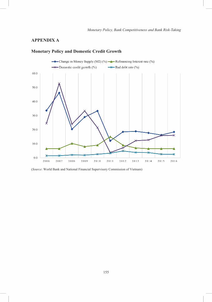
Monetary Policy, Bank Competitiveness and Bank Risk-Taking
155
APPENDIX A
Monetary Policy and Domestic Credit Growth
(Source: World Bank and National Financial Supervisory Commission of Vietnam)
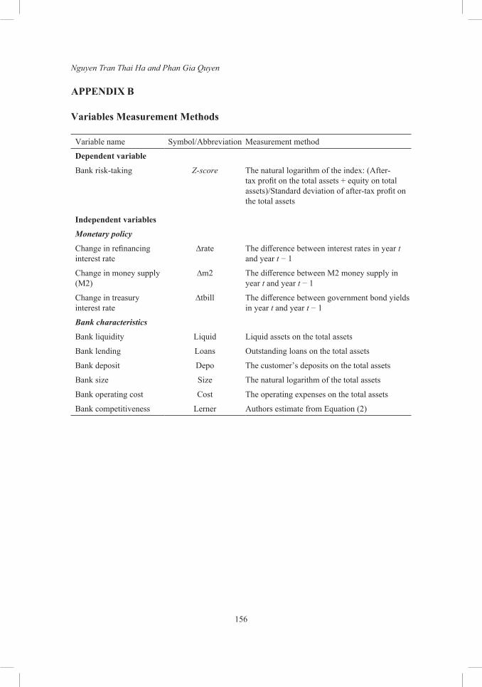
Nguyen Tran Thai Ha and Phan Gia Quyen
156
APPENDIX B
Variables Measurement Methods
Variable name Symbol/Abbreviation Measurement method
Dependent variable
Bank risk-taking Z-score The natural logarithm of the index: (After-tax profit on the total assets + equity on total assets)/Standard deviation of after-tax profit on the total assets
Independent variables
Monetary policy
Change in refinancing interest rate
∆rate The difference between interest rates in year t and year t − 1
Change in money supply (M2)
∆m2 The difference between M2 money supply in year t and year t − 1
Change in treasury interest rate
∆tbill The difference between government bond yields in year t and year t − 1
Bank characteristics
Bank liquidity Liquid Liquid assets on the total assets
Bank lending Loans Outstanding loans on the total assets
Bank deposit Depo The customer’s deposits on the total assets
Bank size Size The natural logarithm of the total assets
Bank operating cost Cost The operating expenses on the total assets
Bank competitiveness Lerner Authors estimate from Equation (2)
AAMJAF Vol. 14, No. 2, 157–184, 2018
© Asian Academy of Management and Penerbit Universiti Sains Malaysia, 2018. This work is licensed under the terms of the Creative Commons Attribution (CC BY) (http://creativecommons.org/licenses/by/4.0/).
Asian Academy of Management Journal
of Accounting and Finance
EXCHANGE RATE EXPOSURE AND CRUDE OIL PRICE: THE CASE OF AN EMERGING MARKET
Meen Chee Hong1, Ei Yet Chu1* and Saw Imm Song2
1Graduate School of Business, Universiti Sains Malaysia, 11800 USM Pulau Pinang, Malaysia
2Faculty of Business Management, Universiti Teknologi MARA, 13500 Pulau Pinang, Malaysia
*Corresponding author: [email protected]
ABSTRACT
The purpose of this study is to examine the depreciation of USD and crude oil price on exchange rate exposure in Malaysia. Based on the argument that domestic and foreign markets could affect foreign exchange exposure, the study examined 993 public listed firms that involved in domestic business, foreign sales, and assets, respectively. The sample period of 2014 to 2016 illustrates different time-varying conditions when the depreciation of Ringgit Malaysia and crude oil price were the most severe for the last decades. The findings show that firms with foreign sales face the most significant negative exposure of foreign exchange, followed by domestic firms and firms with foreign assets. The study shows that many Malaysia export firms are not effective in hedging, hence, they did not benefit from the depreciation of Ringgit Malaysia and crude oil price. The study concludes that there is an influence of domestic and foreign market effects on foreign currency exposure in the economy.
Keywords: foreign exchange exposure, oil price, USD, Ringgit Malaysia, emerging market
Publication date: 31 December 2018
To cite this article: Hong, M. C., Chu, E. Y., & Song, S. I. (2018). Exchange rate exposure and crude oil price: The case of an emerging market. Asian Academy of Management Journal of Accounting and Finance, 14(2), 157–184. https://doi.org/10.21315/aamjaf2018.14.2.7
To link to this article: https://doi.org/10.21315/aamjaf2018.14.2.7
Meen Chee Hong et al.
158
INTRODUCTION
Uncertainty in the US Dollar (USD) has brought exchange-rate risk to many companies in the emerging market, especially Malaysia which have seen Malaysian Ringgit depreciated significantly as compared to other emerging market counterparts. Firms with foreign exchange exposures need to adjust its costs and benefits in operations to avoid an adverse effect on firms’ cash flows, and value (Akay & Cifter, 2014). The exposures cause challenges to macroeconomic management in emerging economies and affect the profit and loss of firms. In the global financial stability report, International Monetary Fund (IMF) highlights that the issue of the foreign currency exposure is significant especially in the perspective of risks, spillovers, and crisis prevention, given the volatility of US Dollar (International Monetary Fund, 2014). IMF further emphasises the need for improvement in the study related to the foreign exchange exposure, especially in emerging markets (International Monetary Fund, 2015). Moreover, the volatility of domestic exchange rate, especially in emerging markets where domestic currencies are not the trading currencies, could have a serious impact on firms’ operation risks and values and deplete a country’s foreign reserve significantly (Muller & Verschoor, 2006).
Firms, irrespective of whether they involve in foreign operations or have no foreign currency assets, liabilities or transaction are exposed to foreign currency risk (Adler & Dumas, 1984). The domestic firms’ exposure will be influenced indirectly by their suppliers and buyers who are importing or exporting firms. On the same notes, domestic firms may face local competitors whose buyers and suppliers may engage in foreign borrowing and investment, and therefore indirectly exposed firms to changes in exchange rates (Aggarwal & Harper, 2010). There are accounting and economic approaches to address foreign currency exposure. The economic approach, use the sensitivity changes between stock returns and the exchange rate as the measurement of foreign exchange exposure (see survey study in Muller and Verschoor, 2006). The method provides a direct measurement of the impact of foreign exchange exposure on firms’ value, by taking into consideration of firms’ and economic factors.
Generally, firms in advanced countries have advantages over emerging countries over foreign currency exposure. The U.S. companies are found to have less economics exposure to exchange-rate movement (e.g. Jorion, 1990; Choi & Prasad, 1995). Unlike advanced countries, foreign exchange exposure is higher in emerging markets (e.g. Kiymaz, 2003). The exposure varies according to time-
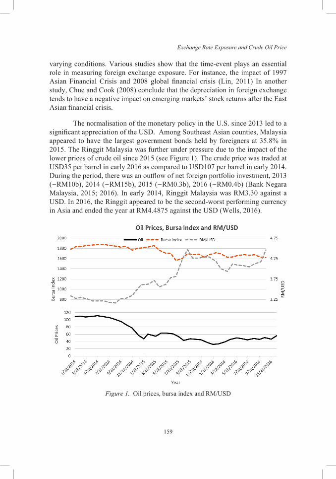
Exchange Rate Exposure and Crude Oil Price
159
varying conditions. Various studies show that the time-event plays an essential role in measuring foreign exchange exposure. For instance, the impact of 1997 Asian Financial Crisis and 2008 global financial crisis (Lin, 2011) In another study, Chue and Cook (2008) conclude that the depreciation in foreign exchange tends to have a negative impact on emerging markets’ stock returns after the East Asian financial crisis.
The normalisation of the monetary policy in the U.S. since 2013 led to a significant appreciation of the USD. Among Southeast Asian counties, Malaysia appeared to have the largest government bonds held by foreigners at 35.8% in 2015. The Ringgit Malaysia was further under pressure due to the impact of the lower prices of crude oil since 2015 (see Figure 1). The crude price was traded at USD35 per barrel in early 2016 as compared to USD107 per barrel in early 2014. During the period, there was an outflow of net foreign portfolio investment, 2013 (−RM10b), 2014 (−RM15b), 2015 (−RM0.3b), 2016 (−RM0.4b) (Bank Negara Malaysia, 2015; 2016). In early 2014, Ringgit Malaysia was RM3.30 against a USD. In 2016, the Ringgit appeared to be the second-worst performing currency in Asia and ended the year at RM4.4875 against the USD (Wells, 2016).
Figure 1. Oil prices, bursa index and RM/USD
Meen Chee Hong et al.
160
Generally, Malaysia’s international trade comprises 136% of Gross Domestic Product (GDP) in 2017 (World Bank, 2017). The country is a net exporter of the crude oil, with 0.3% of GDP (Bank Negara Malaysia, 2016). The descent of oil price and normalisation of the USD, affecting the oil revenue and adversely lead to a significant appreciation of the USD against the Ringgit Malaysia from mid-2014 to end of 2017 (Figure 1). The Bursa Index declined significantly from 1800 points in 2014 and moved around 1600 and 1700 points in 2015 and 2016 (Figure 1). Despite these, the country’s GDP’s grow at the average of 5% from 2014 to 2016. Therefore, it is essential to understand the Malaysian firms’ exposure to the depreciation of currency movements.
Generally, Malaysia economy is consumption based which contribute to 53% of GDP (Bank Negara Malaysia, 2016). The depreciation of the domestic currency will reduce the domestic demand. Besides, Malaysia is part of the global manufacturing network; firms import inputs and produce intermediate and final goods for exporting (Bank Negara Malaysia, 2010). Hence, there is an uncertainty of the net off when there is a depreciation of the domestic currency.
The study addresses the issues of foreign currency exposure at the time when the U.S. rationalised its monetary policy and crude oil price was low. First, we address whether domestic firms, firms with foreign sales and foreign assets could influence on the currency exposure. There is a dual effect of domestic and foreign markets for firms’ exposure. A depreciation of the domestic currency may lead to inflation and hence reduce domestic demand, and offset the revenue for exporting firms. Second, previous studies focused on the relationship of crude oil price on USD (e.g. Basher, Haug & Sadorsky, 2015; Bams, Blanchard, Honarvar, & Lehnert, 2017), but the studies did not address firms’ foreign currency exposure and movement of oil price. Hence, this study focuses on the emerging market, which faces depreciation of the local currency and crude oil price and moves a step forward by examining the impact of oil price on foreign currency exposure.
LITERATURE REVIEW
Empirical papers that investigate exchange rate exposure from the economic perspective normally take the Adler and Dumas’ (1984) approach. The approach defines foreign exchange exposure as a regression of an equity return on the exchange rate. Finance theory predicts that foreign exchange exposure can influence firms’ value due to firms’ foreign currency cash flows which originating from firms’ involvement in international business. The estimated exposure is net of any activities that management might have undertaken to hedge the exchange rate risk (see Bartram and Bodnar, 2007). Nonetheless, the empirical works
Exchange Rate Exposure and Crude Oil Price
161
show that only a small number of firms illustrate a significant impact of foreign exchange rate risk on firms’ value, a finding which literature concludes as the “exposure puzzle” (Bartram, 2007).
The “exposure puzzle” stems from the studies where USD is the home currency and the primary traded currency around the world. In a country where the financial market is more developed, especially the U.S. firms where USD is the dominant currency for trading, the foreign exchange exposure of firms’ is found to be less significant. Research studies find that only about 5% of firms significantly exposed in the United States (eg. Jorion, 1990; Bartov & Bodnar, 1994), and about 10% from 18 European countries, the United States and Japan with the introduction of the Euro (Bartram & Karolyi, 2006).
In non-Eurozone European; e.g. Norway, Sweden, Switzerland and U.K. show a higher exchange rate exposure since the introduction of the Euro, while Germany has the lowest count exposure of foreign currencies (Hutson & O’Driscoll, 2010). For France, the introduction of Euro has reduced firms’ foreign exchange exposure (Nguyen, Faff, & Marshall, 2007). Clearly, the Euro members have lesser currency exposure. In another study, there are 14.93% of U.K. firms expose directly and 30.50% indirectly to the fluctuations in USD, the Euro and the Japanese Yen (Agyei-Ampomah, Mazouz, & Yin, 2012). In a study on the smaller economy like Sweden, there are 26% of the 47 firms significantly exposed to exchange rate changes (Nydahl, 1999). While a study in Australia illustrates that firms exposure increases from 14.43% to 45.36% from 2007 to 2008 in response to the global financial crisis (Yip & Nguyen, 2012). Besides, 26.3% of 171 Japanese multinationals show a significant exchange rate exposure during different time periods from 1979 to 1993 (He & Ng, 1998). Moreover, Japanese stock returns consist of significant exchange rate risk premium, particularly in multinational and exporting firms (Doukas, Hall, & Lang, 1999).
In contrast, in countries where the currencies are weak face a higher foreign exchange as compared to the trading currencies’ home countries (Kiymaz, 2003; Chue & Cook, 2008). However, the study of exchange-rate exposure on emerging country is rather limited. Also, it is found to have time-varying conditions on the findings. Studies generally focus on firms, industrial and cross-countries, which based on aggregate macroeconomic data (Lin, 2011).
Domestic and Firms with Foreign Sales and Assets
Economic theory and finance literature suggest that the depreciation of home currency has a positive relationship between firms’ value and firms’ international sales. However, firms are affected by dual effect of domestic and foreign markets.
Meen Chee Hong et al.
162
A depreciation of the domestic currency may lead to inflation and hence reduce domestic demand. These adversely affect stock return and offset additional revenue of currency conversion which benefits exporting firms (Pritamani, Shome, & Singal, 2004). Therefore, the impact on depreciation of local currencies on exporting firms is ambiguous. Aggarwal and Harper (2010) showed that domestic firms have significant exposure to foreign currency. Moreover, they illustrated that in the foreign exchange exposure is no different in between domestic corporations and multinational corporations in the U.S. Pritamani et al. (2004) argued that insignificant of the findings are due to the “total” exposure for firms, which incorporated firm-specific and macroeconomic effects. These dual-effects of the domestic economy and foreign markets lead to insignificant total exposures for exporters.
In the European countries, it is the domestic firm which is more vulnerable to foreign exchange changes than the exporting firm (Parlapiano, Alexeev, & Dungey, 2012). The finding is similar in the Baltic States which use Euro as a mean of exchange. There is a significant foreign exchange exposure in local domestic firms that lead to significant losses (Rupeika-Apoga & Nedovis, 2016). It is a straightforward effect on importing firms. A depreciation of domestic currencies will make import items more expensive and reduce domestic demand and stock returns. Therefore, the firms’ value will be affected directly and vice-versa.
In contrast, an appreciation of the domestic currency strengthens the domestic demand, and offset the reduced global demand for a firm with foreign sales due to higher export priced. Pertaining to this, the European firms illustrate those firms’ economic exposure increase correspondingly to their international business involvement (Parlapiano et al., 2012). In a study on U.K.’s non-financial firms, El-Masry, Abdel-Salam and Alatraby (2007) showed a high proportion of positive exposure coefficients, which benefiting firms from an appreciation of the pound. He and Ng (1998) concluded that there is a positive relationship between a firm’s export ratio and foreign exchange exposures in Japanese multinational companies. While Ito, Koibuchi, Sato and Shimizu’s (2016) focused on exporting firms and reported a higher foreign currency exposure when USD is the invoiced currency as compared to Yen. In Germany, firms with higher sales abroad illustrate systematically higher exposures than domestic-oriented firms (Bartram, 2004).
Lin’s (2011) showed that net exporters’ firms or firms with dollar assets show a higher exposure in six Asian emerging countries, India, Indonesia, Korea, the Philippines, Taiwan and Thailand despite being subjected to the managed float exchange rate regime. Moreover, the benefits of currency depreciation disappear after adjusting for the inflation. In a study in China, despite pegging of RMB, suggesting a 34% of the sample display a significance exposure (Schena, 2007).
Exchange Rate Exposure and Crude Oil Price
163
The domestic market effects could cause adverse effects on firms’ with foreign sales for a poorer stock return, and offset additional revenue of currency conversion which benefits exporting firms (Pritamani et al., 2004). While foreign sales cause operation exposure, firms with substantial foreign sales may also engage in foreign assets to reduce total operation exposure. The existing foreign assets in firms could cause positive translation exposure and therefore offset overall foreign exchange exposure in firms (Eiteman, Stonehill, & Moffett, 2010). Therefore, if firms use hedging effectively, there will be indifferent between domestic firms and foreign sales firms on foreign exchange exposures, because of the effects of domestic and foreign market exposure.
The study on the currency exposure on Malaysia market is limited. An earlier study was offered by Bacha, Mohamad, Zain and Rasid (2012) that 71% of 158 Malaysia firms are significantly exposed due to foreign currency volatility. However, the study did not address the dual effect of the domestic and foreign market on foreign currency exposure in the country. Given the fact that Malaysia is an export-oriented country, with high international exposure, the depreciation of Ringgit Malaysia will bring in benefits to exporting firms. However, there will be importing inflation due to the appreciation of the USD. The impacts of domestic and foreign effects are uncertain, a priori, the study proposes the alternative hypothesis as:
H1: there is a difference in foreign exchange exposure between domestic firms and firms with foreign sales and assets.
Oil Prices and Foreign Exchange Exposure
The significant decline in global oil price and changes in the direction of the U.S. monetary policy has caused uneven growth and flow of capital. As oil price is contracted in the USD, the influence in crude oil price is significant (Zhang, 2013). The scenarios exert significant pressure on local currencies, especially for oil exporting countries. Generally, there is a co-movement relationship between oil price and USD in the long run (Donahue, 2016). The appreciation of USD, and the oversupply of the crude oil, further exert pressure on the price and cause depreciation of currencies of oil exporting countries comparing to USD. On the other hand, a depreciation of the USD will cause a higher demand for oil and subsequently increase crude oil price. Subsequently, the currencies of net importing countries will appreciate relatively to the USD (Lizardo & Mollick, 2010).
Meen Chee Hong et al.
164
Similar to the foreign currency exchange, the stock returns of the Gulf’s stock markets comprise of oil price risk (Demirer, Jategaonkar, & Khalifa, 2015). There is an impact of oil shocks on exchange rates movements. A lower oil price naturally could cause lower interest rates and inflation, and at the same time increase equity prices in the U.S. economy (e.g. Basher et al., 2015). However, for the net oil exporting countries, the effects of oil prices differ widely as oil producers try to increase production to compensate for the decline of the oil revenue (Mohaddes & Pesaran, 2017).
Further, the impacts of oil price volatility are sector-specific. Bams et al. (2017) conclude that the impacts of oil price and the exchange rate are only essential for oil-relevant industries. Despite the sector-specific factor, there is no direct study on oil price on the exchange rate exposure. A closer study on Turkey’s energy sector looks at the impact of the exchange rate exposure on energy firms, but the study did not address the impact of oil price on the currency exposure (Kandir, Erismis, & Ozturk, 2015). Hence, there is a dearth of studies offered in respect to crude oil price and foreign currency exposure.
Despite the exchange rate exposure puzzle (Bartram & Bodnar, 2007), the issue of country origin, especially on an individual emerging country, is limited. Moreover, the issue is more complex in an economy such as Malaysia where the export items are import (input) oriented, and Malaysia is also a net oil export country. The recent depreciation of crude oil price and an appreciation of USD is expected to increase firms’ exposure to foreign currencies in this economy, which however is subjected to the dual effect-domestic and foreign markets. Time-varying conditions to cater the differences in macroeconomics scenarios are necessary. Malaysia, therefore provides a unique platform to look at the influences of oil price on currency exposure as compared to other emerging economies. In view of this, the study proposes that subject to time-varying conditions:
H2: There is a positive relationship between foreign currency exposure and crude oil price.
Industry Factors
Bodnar and Gentry (1993) used data from the U.S., Canada and Japan also find industry differences in foreign currency exposure. Griffin and Stulz (2001) found the effect of exchange rate shocks is minimal in explaining U.S.’ industry performance. Marston (2001) showed that foreign exchange exposure is dependent on the competitive structure of an industry. In a study on Turkey’s Firms, Akay and Cifter (2014) conclude that the degree of industrial openness could influence foreign exchange exposures in firms.
Exchange Rate Exposure and Crude Oil Price
165
In terms of operation and transaction exposure, the changes in foreign exchange influence firms’ cash flow directly. The impact is particularly on operational cash flows rather than financing, and investment cash flows for the U.K. non-financial firms (Bartram, 2007). However, the impact on cash flos may subject to industry-specific factors. For instance, it has a negative impact on the cash flow in the textile industry in the Istanbul market (Akay & Cifter, 2014). In another study, using quick ratio rather than cash flow, the measurement is insignificant to explain foreign exchange exposure in emerging markets (Ye, Hutson, & Muckley, 2014).
Lastly, concerning firms’ characteristics, total debt has also been employed to measure firms’ probability of distress. A higher debt ratio towards higher foreign exchange exposure in firms with international business implies a higher possibility that firms use hedging instrument (Geczy, Minton, & Schrand, 1997; He & Ng, 1998; Ye et al., 2014). Therefore, there is a negative relationship between debt ratio and foreign currency exposure (Akay & Cifter, 2014). Other firms’ characteristics with higher growth opportunities (market to book ratio) and tight financial constraints are prompt to use hedging tools to reduce cash flow variation (Geczy et al., 1997). The risk of a country, such as chances of default, the potential of financial crisis add to increased risk premiums and increase foreign exchange exposure of a country (Parlapiano et al., 2012).
METHODOLOGY
Equation 1 refers to single factor model of Adler and Dumas (1984) whereby economic exposure as the coefficient β1,t between the firm value, Ri,t, the dependent variable and the exchange rate f (XR) as the independent variable. The sole coefficient β1,t f (XR) is the total exposure that captures the exchange rate and macroeconomic effects. Jorion (1991) initiated two factors, a market index, in addition to the exchange rate in estimating exchange-rate exposure. The two-factor model (Equation 2) attempts to isolate firms’ cash flow exposure from the macroeconomic factors.
R f XR, , ,i t j i t j t!v b= + +^ h (1)
R f XR R, 1, 2, , ,i t j t t m t j t!v b b= + + +^ h (2)
Where Ri,t and Rm,t are the returns on a stock i, and an equity market or portfolio, respectively. Ri,t represents the percentage change in the value of an asset in domestic currency, σ is a constant that varies across firms, β1,t estimates the total foreign exchange (XR) exposure, β2,t is the estimate of the market portfolio return.
Meen Chee Hong et al.
166
DDomestic Fsales Fassets
Oil Cash Firms
Dind DT DT
, 1 , 2 , 3 ,
4 5 , 6 ,
7 , 8 1 9 2 ,
i t j i t i t i t
t i t i tkn
i tkn
i t
b a c c c
c c c
c c c f
= + + +
+ + + +
+ + + +
` j/
/ (3)
where E(β1,t | negative exposure) = f (negative exposure)
The above two-factor model has been used in various studies of foreign exchange exposure and incorporated with firms and macroeconomics’ variables (eg. Bodnar & Gentry, 1993; Bartov & Bodnar, 1994; He & Ng, 1998; Griffin & Stulz, 2001). The dependent variable- foreign exchange exposure βi,t for each firm in Equation 3 is the value estimated from coefficient β1,t from the Equation 2. The study focuses on the period when Ringgit Malaysia face worst depreciation due to U.S. normalisation of monetary policy and the plunge of crude oil price. The sample covers the period from January 2014 to December 2016. As in other studies on foreign exchange exposure, (e.g. Akay & Cifter, 2014), the study used ordinary least square regression on panel dataset consists of 989 firms listed on Bursa Malaysia. The study applies a full population of 989 firms which has a constant variance and therefore heteroscedasticity in the study can be disregarded.
The scenario creates adverse impacts rather than positive impacts. Hence, the study will focus on firms with negative foreign exchange exposure. The focus on negative exposure will divulge useful information to the study. The measurements of firms doing domestic business (dummy 1 for domestic [DDomestic]) and foreign sales ([Fsales] in percentage) and foreign assets ([Fassets] in percentage) are used to examine their contributions to exchange-rate exposure in firms.
Moreover, the equation includes crude oil price (Oil) to examine the magnitude of the crude oil price for foreign exchange exposure. The cash (Cash) is to reflect the impact of exchange rate exposure. Firms’ characteristic Firms ,i tk
na k/ such as firm value (Tobin’s Q – measured as market value/ book value) and debt (debt over asset) reflect higher chances of employing hedging strategies in firms .
A few sectors which have the highest number of firms in our sample are used as control variables for industries. In particular, the summation of dummy industries (Dind) reflects automotive and parts (Dauto), construction materials (Dconsm), food industry (Dfood), travelling (Dtravel), and industrial transportation (Dinttrans). These industries reflect domestic markets, while semiconductor industry – electronic and electrical (Dene), industrial engineering (Dindeng), oil and gas (Doilgas) industries are used to reflect foreign market and
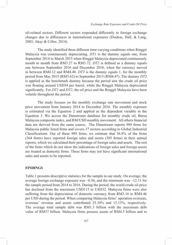
Exchange Rate Exposure and Crude Oil Price
167
oil-related sectors. Different sectors responded differently to foreign exchange changes due to differences in international exposures (Doukas, Hall, & Lang, 2003; Akay & Cifter, 2014).
The study identified three different time-varying conditions when Ringgit Malaysia was continuously depreciating. DT1 is the dummy equals one, from September 2014 to March 2015 when Ringgit Malaysia depreciated continuously month to month from RM3.27 to RM3.72. DT2 is defined as a dummy equals one between September 2016 and December 2016, when the currency moved in between RM4.12 and RM4.48. DT3 is the dummy equals 1, for the monthly period from May 2015 (RM3.62) to September 2015 (RM4.47). The dummy DT3 is applied as the benchmark dummy because the period saw the crude oil price was floating around USD54 per barrel, while the Ringgit Malaysia depreciated significantly. For DT1 and DT2, the oil price and the Ringgit Malaysia have been volatile throughout the period.
The study focuses on the monthly exchange rate movement and stock price movement from January 2014 to December 2016. The monthly exposure is estimated via the Equation 2 and applied as the dependent variable in the Equation 3. We access the Datastream database for monthly crude oil, Bursa Malaysia composite index, and RM/USD monthly movement. All others financial data are derived from the same source. The Datastream reports 989 firms for Malaysia public listed firms and covers 37 sectors according to Global Industrial Classifications. Out of these 989 firms, we estimate that 36.8% of the firms (364 firms) have reported foreign sales and assets (305 firms) in their annual reports, which we calculated their percentage of foreign sales and assets. The rest of the firms which do not show the indications of foreign sales and foreign assets are treated as domestic firms. These firms may not have significant international sales and assets to be reported.
FINDINGS
Table 1 presents descriptive statistics for the sample in our study. On average, the average foreign exchange exposure was −0.56, and the minimum was −12.31 for the sample period from 2014 to 2016. During the period, the world crude oil price has declined from the maximum USD115 to USD32. Malaysia firms were also suffering from the depreciation of domestic currency from RM3.16 to RM4.46 per USD during the period. When comparing Malaysia firms’ operation overseas, overseas’ revenue and assets contributed 25.34% and 12.13%, respectively. The average total sample debt was RM1.3 billion with the maximum debt value of RM37 billion. Malaysia firms possess assets of RM4.5 billion and to
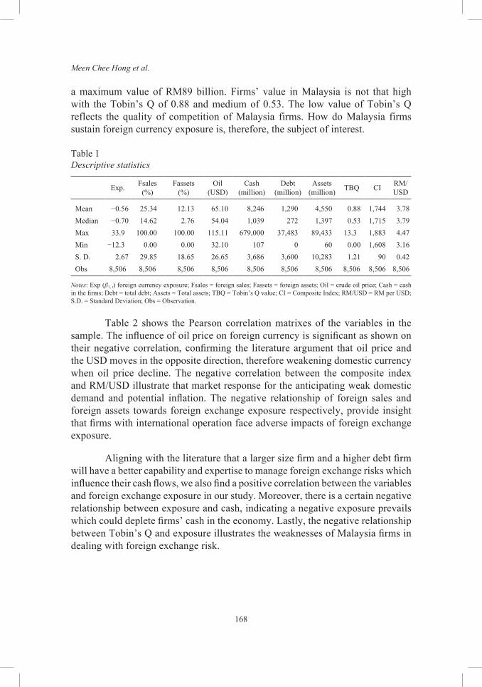
Meen Chee Hong et al.
168
a maximum value of RM89 billion. Firms’ value in Malaysia is not that high with the Tobin’s Q of 0.88 and medium of 0.53. The low value of Tobin’s Q reflects the quality of competition of Malaysia firms. How do Malaysia firms sustain foreign currency exposure is, therefore, the subject of interest.
Table 1Descriptive statistics
Exp. Fsales (%)
Fassets (%)
Oil (USD)
Cash (million)
Debt (million)
Assets (million) TBQ CI RM/
USD
Mean −0.56 25.34 12.13 65.10 8,246 1,290 4,550 0.88 1,744 3.78Median −0.70 14.62 2.76 54.04 1,039 272 1,397 0.53 1,715 3.79Max 33.9 100.00 100.00 115.11 679,000 37,483 89,433 13.3 1,883 4.47Min −12.3 0.00 0.00 32.10 107 0 60 0.00 1,608 3.16S. D. 2.67 29.85 18.65 26.65 3,686 3,600 10,283 1.21 90 0.42Obs 8,506 8,506 8,506 8,506 8,506 8,506 8,506 8,506 8,506 8,506
Notes: Exp (β1, t) foreign currency exposure; Fsales = foreign sales; Fassets = foreign assets; Oil = crude oil price; Cash = cash in the firms; Debt = total debt; Assets = Total assets; TBQ = Tobin’s Q value; CI = Composite Index; RM/USD = RM per USD; S.D. = Standard Deviation; Obs = Observation.
Table 2 shows the Pearson correlation matrixes of the variables in the sample. The influence of oil price on foreign currency is significant as shown on their negative correlation, confirming the literature argument that oil price and the USD moves in the opposite direction, therefore weakening domestic currency when oil price decline. The negative correlation between the composite index and RM/USD illustrate that market response for the anticipating weak domestic demand and potential inflation. The negative relationship of foreign sales and foreign assets towards foreign exchange exposure respectively, provide insight that firms with international operation face adverse impacts of foreign exchange exposure.
Aligning with the literature that a larger size firm and a higher debt firm will have a better capability and expertise to manage foreign exchange risks which influence their cash flows, we also find a positive correlation between the variables and foreign exchange exposure in our study. Moreover, there is a certain negative relationship between exposure and cash, indicating a negative exposure prevails which could deplete firms’ cash in the economy. Lastly, the negative relationship between Tobin’s Q and exposure illustrates the weaknesses of Malaysia firms in dealing with foreign exchange risk.
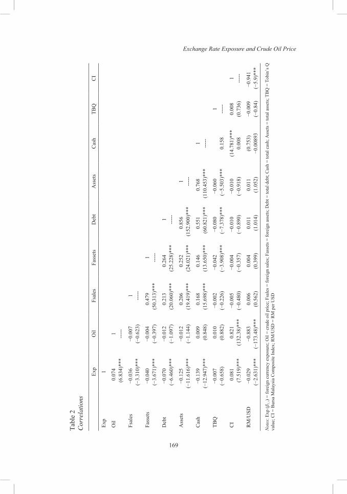
Exchange Rate Exposure and Crude Oil Price
169
Tabl
e 2
Cor
rela
tions
Ex
pO
ilFs
ales
Fass
ets
Deb
tA
sset
sC
ash
TBQ
CI
Exp
1
Oil
0.07
41
(6.8
34)*
**--
---
Fsal
es
−0.0
36−0
.007
1(−
3.31
0)**
*(−
0.62
3)--
---
Fass
ets
−0.0
40−0
.004
0.47
91
(−3.
671)
***
(−0.
397)
(50.
313)
***
----
-
Deb
t −0
.070
−0.0
120.
213
0.26
41
(−6.
460)
***
(−1.
097)
(20.
060)
***
(25.
228)
***
----
-
Ass
ets
−0.1
25−0
.012
0.20
60.
252
0.85
61
(−11
.616
)***
(−1.
144)
(19.
419)
***
(24.
021)
***
(152
.900
)***
----
-
Cas
h−0
.139
0.00
90.
168
0.14
60.
551
0.76
81
(−12
.947
)***
(0.8
48)
(15.
698)
***
(13.
650)
***
(60.
821)
***
(110
.453
)***
----
-
TBQ
−0
.007
0.01
0−0
.002
−0.0
42−0
.080
−0.0
601
(−0.
658)
(0.8
82)
(−0.
226)
(−3.
908)
***
(−7.
378)
***
(−5.
503)
***
0.15
8--
---
CI
0.08
10.
821
−0.0
05−0
.004
−0.0
10−0
.010
(14.
781)
***
0.00
81
(7.5
19)*
**(1
32.3
8)**
*(−
0.48
0)(−
0.35
7)(−
0.89
0)(−
0.91
8)0.
008
(0.7
36)
----
-
RM
/USD
−0
.029
−0.8
830.
006
0.00
40.
011
0.01
1(0
.753
)−0
.009
−0.9
41
(−2.
631)
***
(−17
3.48
)***
(0.5
62)
(0.3
99)
(1.0
14)
(1.0
52)
−0.0
0893
(−0.
84)
(−5.
9)**
*
Not
es: E
xp (β
1, t)
= fo
reig
n cu
rren
cy e
xpos
ure;
Oil
= cr
ude
oil p
rice;
Fsa
les =
fore
ign
sale
s; F
asse
ts =
fore
ign
asse
ts; D
ebt =
tota
l deb
t; C
ash
= to
tal c
ash;
Ass
ets =
tota
l ass
ets;
TB
Q =
Tob
in’s
Q
valu
e; C
I = B
ursa
Mal
aysi
a C
ompo
site
Inde
x; R
M/U
SD =
RM
per
USD
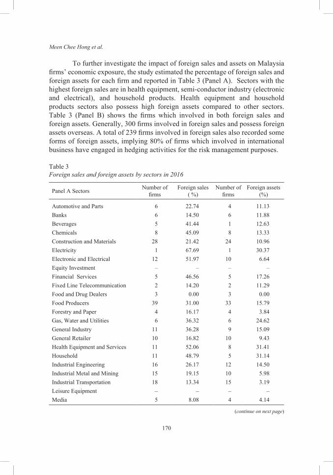
Meen Chee Hong et al.
170
To further investigate the impact of foreign sales and assets on Malaysia firms’ economic exposure, the study estimated the percentage of foreign sales and foreign assets for each firm and reported in Table 3 (Panel A). Sectors with the highest foreign sales are in health equipment, semi-conductor industry (electronic and electrical), and household products. Health equipment and household products sectors also possess high foreign assets compared to other sectors. Table 3 (Panel B) shows the firms which involved in both foreign sales and foreign assets. Generally, 300 firms involved in foreign sales and possess foreign assets overseas. A total of 239 firms involved in foreign sales also recorded some forms of foreign assets, implying 80% of firms which involved in international business have engaged in hedging activities for the risk management purposes.
Table 3Foreign sales and foreign assets by sectors in 2016
Panel A Sectors Number of firms
Foreign sales ( %)
Number of firms
Foreign assets (%)
Automotive and Parts 6 22.74 4 11.13Banks 6 14.50 6 11.88Beverages 5 41.44 1 12.63Chemicals 8 45.09 8 13.33Construction and Materials 28 21.42 24 10.96Electricity 1 67.69 1 30.37Electronic and Electrical 12 51.97 10 6.64Equity Investment – – – –Financial Services 5 46.56 5 17.26Fixed Line Telecommunication 2 14.20 2 11.29Food and Drug Dealers 3 0.00 3 0.00Food Producers 39 31.00 33 15.79Forestry and Paper 4 16.17 4 3.84Gas, Water and Utilities 6 36.32 6 24.62General Industry 11 36.28 9 15.09General Retailer 10 16.82 10 9.43Health Equipment and Services 11 52.06 8 31.41Household 11 48.79 5 31.14Industrial Engineering 16 26.17 12 14.50Industrial Metal and Mining 15 19.15 10 5.98Industrial Transportation 18 13.34 15 3.19Leisure Equipment – – – –Media 5 8.08 4 4.14
(continue on next page)
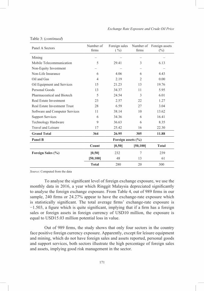
Exchange Rate Exposure and Crude Oil Price
171
Panel A Sectors Number of firms
Foreign sales ( %)
Number of firms
Foreign assets (%)
Mining – – – –Mobile Telecommunication 5 29.41 3 6.13Non-Equity Investment – – – –Non-Life Insurance 6 4.06 6 4.43Oil and Gas 4 2.19 2 0.00Oil Equipment and Services 15 21.23 13 19.76Personal Goods 13 34.37 11 5.95Pharmaceutical and Biotech 5 24.54 3 6.01Real Estate Investment 23 2.57 22 1.27Real Estate Investment Trust 28 6.59 27 3.04Software and Computer Services 11 38.14 10 13.62Support Services 6 34.36 6 16.41Technology Hardware 9 36.63 6 8.35Travel and Leisure 17 25.42 16 22.30
Grand Total 364 26.95 305 11.88
Panel B Foreign assets (%)
Count [0,50] [50,100] Total
Foreign Sales (%) [0,50] 232 7 239[50,100] 48 13 61
Total 280 20 300
Source: Computed from the data
To analyse the significant level of foreign exchange exposure, we use the monthly data in 2016, a year which Ringgit Malaysia depreciated significantly to analyse the foreign exchange exposure. From Table 4, out of 989 firms in our sample, 240 firms or 24.27% appear to have the exchange-rate exposure which is statistically significant. The total average firms’ exchange-rate exposure is −1.503, a figure which is quite significant, implying that if a firm has a foreign sales or foreign assets in foreign currency of USD10 million, the exposure is equal to USD15.03 million potential loss in value.
Out of 989 firms, the study shows that only four sectors in the country face positive foreign currency exposure. Apparently, except for leisure equipment and mining, which do not have foreign sales and assets reported, personal goods and support services, both sectors illustrate the high percentage of foreign sales and assets, implying good risk management in the sector.
Table 3: (continued)
Meen Chee Hong et al.
172
Approximately 164 (16.6%) of the firms show the significant negative exposure as compared to 67 (7.0%) firms which benefit from significant positive foreign currency exposure. A total of 14 firms from food produce sectors suffering the blow of negative exposure at the average of −2.35, despite the sector has a significant amount of foreign sales and foreign assets. Construction and materials suffer the most number of foreign exchanges exposure. However, the coefficient is relatively low at −0.410. Semi-conductor sector (electronic and electrical) despite showing a high foreign sales, the exposure is moderate at −0.53 illustrated their experience in facing international economic changes.
Similarly, health equipment sector, like in the semiconductor sector shows negative exposure of −1.036. However, industrial transportation, 30.55% of negative foreign exchange exposure (−1.29) illustrate the direct effects of the increasing crude oil price and depreciation of foreign currency on the sector. Banks, however, show a high negative foreign exchange exposure at −2.869, despite the low foreign sales and foreign assets, which indicates the necessity to improve their asset-risk management.
Table 5 show the results of the overall firms which have negative foreign exchange exposure. The Model 1 illustrates that domestic firms are positive and significant and firms with foreign sales (Fsales) are not significant relates to foreign currency exposure. The Model 2 includes the effects of domestic and foreign markets when Fsales and foreign assets (Fassets) are included in the study. The Fassets is a natural hedging instrument for a firm’s internationalisation.
The dummy for domestic firms has continued to show a positive result, indicate that foreign exchange exposure is lesser in domestic firms. Because the regression only includes firms with negative foreign exchange exposure, the positive coefficient implies that the magnitude of negative exposure is smaller for domestic firms. On the other hand, firms with Fsales show a negative coefficient of −0.55%, and a positive Fassets of 0.24%. Thus, the findings indicate that there is a difference in foreign exchange exposure between domestic firms and firms with foreign sales and assets, as suggested in H1. In summary, firms with foreign sales has the most significant negative exposure as compared to domestic firms and Fassets firms.
The Model 2 includes debt and Tobin’s Q (TBQ). Higher debt is a good proxy for hedging due to firms with high debt is likely to use a hedge instrument. A firm with high TBQ illustrates that better growth opportunities and prompt the firm to use hedging tools to reduce cash flow variation. The inclusion of the variables will influence the findings on domestic and foreign sales.
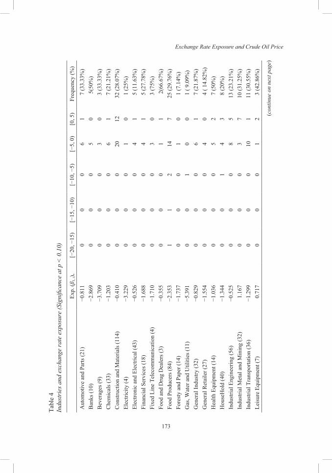
Exchange Rate Exposure and Crude Oil Price
173
Tabl
e 4
Indu
stri
es a
nd e
xcha
nge
rate
exp
osur
e (S
igni
fican
ce a
t p <
0.1
0)
Ex
p. (β
1, t),
[−20
, −15
)[−
15, −
10)
[−10
, −5)
[−5,
0)
[0, 5
)Fr
eque
ncy
(%)
Aut
omot
ive
and
Parts
(21)
−0.8
110
00
61
7 (3
3.33
%)
Ban
ks (1
0)−2
.869
00
05
05(
50%
)B
ever
ages
(9)
−3.7
090
00
30
3 (3
3.33
%)
Che
mic
als (
33)
−1.2
030
00
61
7 (2
1.21
%)
Con
stru
ctio
n an
d M
ater
ials
(114
)−0
.410
00
020
1232
(28.
07%
)El
ectri
city
(4)
−3.2
290
00
10
1 (2
5%)
Elec
troni
c an
d El
ectri
cal (
43)
−0.5
260
00
41
5 (1
1.63
%)
Fina
ncia
l Ser
vice
s (18
)−1
.688
00
04
15
(27.
78%
)Fi
xed
Line
Tel
ecom
mun
icat
ion
(4)
−1.7
100
00
30
3 (7
5%)
Food
and
Dru
g D
eale
rs (3
)−0
.355
00
01
12(
66.6
7%)
Food
Pro
duce
rs (8
4)−2
.353
11
214
725
(29.
76%
)Fo
rest
y an
d Pa
per (
14)
−1.7
370
00
10
1 (7
.14%
)G
as, W
ater
and
Util
ities
(11)
−5.3
910
01
00
1 ( 9
.09%
)G
ener
al In
dust
ry (3
2)−0
.829
00
06
17
(21.
87%
)G
ener
al R
etai
ler (
27)
−1.5
540
00
40
4 ( 1
4.82
%)
Hea
lth E
quip
men
t (14
)−1
.036
00
05
27
(50%
)H
ouse
Hol
d (4
0)−1
.344
00
14
38
(20%
)In
dust
rial E
ngin
eerin
g (5
6)−0
.525
00
08
513
(23.
21%
)In
dust
rial M
etal
and
Min
ing
(32)
1.16
70
00
37
10 (3
1.25
%)
Indu
stria
l Tra
nspo
rtatio
n (3
6)−1
.299
00
010
111
(30.
55%
)Le
isur
e Eq
uipm
ent (
7)0.
717
00
01
23
(42.
86%
)
(con
tinue
on
next
pag
e)
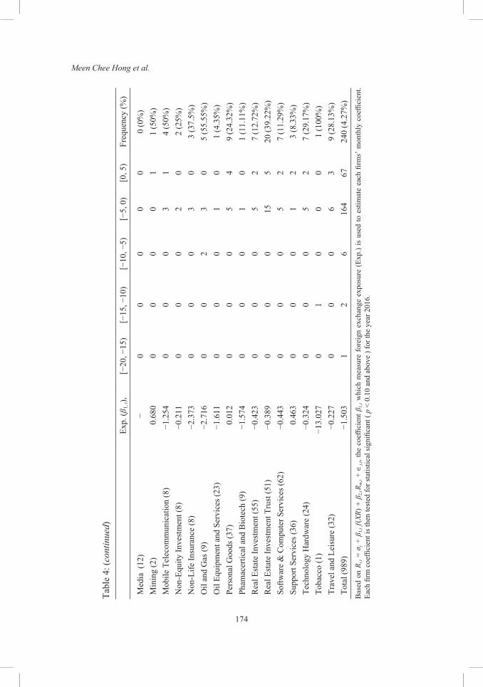
Meen Chee Hong et al.
174
Tabl
e 4:
(con
tinue
d)
Ex
p. (β
1, t),
[−20
, −15
)[−
15, −
10)
[−10
, −5)
[−5,
0)
[0, 5
)Fr
eque
ncy
(%)
Med
ia (
12)
−0
00
00
0 (0
%)
Min
ing
(2)
0.68
00
00
01
1 (5
0%)
Mob
ile T
elec
omm
unic
atio
n (8
)−1
.254
00
03
14
(50%
)N
on-E
quity
Inve
stm
ent (
8)−0
.211
00
02
02
(25%
)N
on-L
ife In
sura
nce
(8)
−2.3
730
00
30
3 (3
7.5%
)O
il an
d G
as (9
)−2
.716
00
23
05
(55.
55%
)O
il Eq
uipm
ent a
nd S
ervi
ces (
23)
−1.6
110
00
10
1 (4
.35%
)Pe
rson
al G
oods
(37)
0.01
20
00
54
9 (2
4.32
%)
Pham
acer
tical
and
Bio
tech
(9)
−1.5
740
00
10
1 (1
1.11
%)
Rea
l Est
ate
Inve
stm
ent (
55)
−0.4
230
00
52
7 (1
2.72
%)
Rea
l Est
ate
Inve
stm
ent T
rust
(51)
−0.3
890
00
155
20 (3
9.22
%)
Softw
are
& C
ompu
ter S
ervi
ces (
62)
−0.4
430
00
52
7 (1
1.29
%)
Supp
ort S
ervi
ces (
36)
0.46
30
00
12
3 (8
.33%
)Te
chno
logy
Har
dwar
e (2
4)−0
.324
00
05
27
(29.
17%
)To
bacc
o (1
)−1
3.02
70
10
00
1 (1
00%
)Tr
avel
and
Lei
sure
(32)
−0.2
270
00
63
9 (2
8.13
%)
Tota
l (98
9)−1
.503
12
616
467
240
(4.2
7%)
Bas
ed o
n R i
,t = σ
j + β
1,t f
(XR)
+ β
2,tR
m,t +
∈j,t, t
he c
oeffi
cien
t β1,
t whi
ch m
easu
re fo
reig
n ex
chan
ge e
xpos
ure
(Exp
.) is
use
d to
est
imat
e ea
ch fi
rms’
mon
thly
coe
ffici
ent.
Each
firm
coe
ffici
ent i
s the
n te
sted
for s
tatis
tical
sign
ifica
nt (
p <
0.10
and
abo
ve )
for t
he y
ear 2
016.
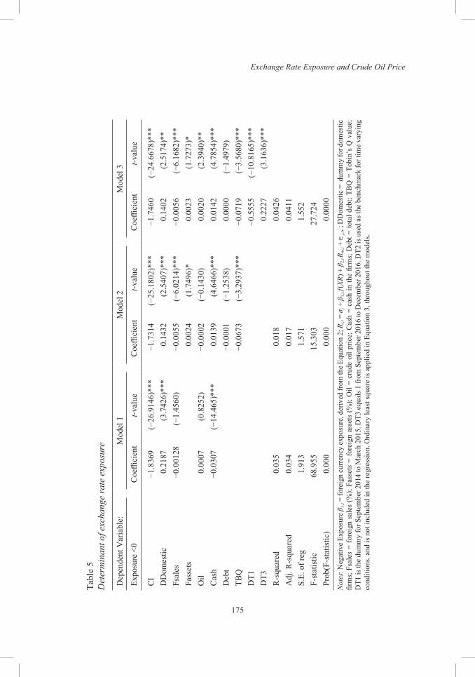
Exchange Rate Exposure and Crude Oil Price
175
Tabl
e 5
Det
erm
inan
t of e
xcha
nge
rate
exp
osur
e
Dep
ende
nt V
aria
ble:
Mod
el 1
Mod
el 2
Mod
el 3
Expo
sure
<0
Coe
ffici
ent
t-val
ueC
oeffi
cien
tt-v
alue
Coe
ffici
ent
t-val
ue
CI
−1.8
369
(−26
.914
6)**
*−1
.731
4(−
25.1
802)
***
−1.7
460
(−24
.667
8)**
*D
Dom
estic
0.21
87(3
.742
6)**
*0.
1432
(2.5
407)
***
0.14
02(2
.517
4)**
Fsal
es−0
.001
28(−
1.45
60)
−0.0
055
(−6.
0214
)***
−0.0
056
(−6.
1682
)***
Fass
ets
0.00
24(1
.749
6)*
0.00
23(1
.727
3)*
Oil
0.00
07(0
.825
2)−0
.000
2(−
0.14
30)
0.00
20(2
.394
0)**
Cas
h−0
.030
7(−
14.4
65)*
**0.
0139
(4.6
466)
***
0.01
42(4
.785
4)**
*D
ebt
−0.0
001
(−1.
2538
)0.
0000
(−1.
4979
)TB
Q−0
.067
3(−
3.29
37)*
**−0
.071
9(−
3.56
80)*
**D
T1−0
.555
5(−
10.8
165)
***
DT3
0.22
27(3
.163
6)**
*R
-squ
ared
0.03
50.
018
0.04
26A
dj. R
-squ
ared
0.03
40.
017
0.04
11S.
E. o
f reg
1.91
31.
571
1.55
2F-
stat
istic
68.9
5515
.303
27.7
24Pr
ob(F
-sta
tistic
)0.
000
0.00
00.
0000
Not
es: N
egat
ive E
xpos
ure β
1,t =
fore
ign
curr
ency
expo
sure
, der
ived
from
the E
quat
ion
2; R
i,t =
σj +
β1,
t f(X
R) +
β2,
tRm
,t + ∈
j,t, ;
DD
omes
tic =
dum
my
for d
omes
tic
firm
s; F
sale
s =
fore
ign
sale
s (%
); Fa
sset
s =
fore
ign
asse
ts (%
); O
il =
crud
e oi
l pric
e; C
ash
= ca
sh in
the
firm
s; D
ebt =
tota
l deb
t; TB
Q =
Tob
in’s
Q v
alue
; D
T1 is
the
dum
my
for S
epte
mbe
r 201
4 to
Mar
ch 2
015.
DT3
equ
als 1
from
Sep
tem
ber 2
016
to D
ecem
ber 2
016.
DT2
is u
sed
as th
e be
nchm
ark
for t
ime
vary
ing
cond
ition
s, an
d is
not
incl
uded
in th
e re
gres
sion
. Ord
inar
y le
ast s
quar
e is
app
lied
in E
quat
ion
3, th
roug
hout
the
mod
els.

Meen Chee Hong et al.
176
The variable crude oil price is not significant in the Model 1 and Model 2. These could be due to the effects had been reflected in the Equation 2 by the overall Bursa Index Return Rm,t. Moreover, the counter effects of lower crude oil price put less pressure on the domestic market, but the appreciation of the USD reduces domestic demand.
When we consider the factors of time-varying conditions (DT1 and DT3), Ringgit Malaysia depreciate continuously for a few months, the oil price has become positively influenced the exposure. DT2 is not included in the regression as it is applied as the benchmark for the time-varying conditions. DT1 occurs when Ringgit Malaysia depreciate significantly from RM3.27 to RM3.72, back to back with the movement of crude oil price which dropped significantly from USD94.72 to USD54.56 per barrel. While during the time-varying condition of DT3, the crude oil price reached the point of USD45 per barrel and the pressure of the US presidential election at the end of 2016, are significant to make crude oil price a significant factor to explain currency exposure. Therefore, we accept the H2.
In Table 6, Model 1, the study includes dummies for electronic and electrical (Dene), industrial engineering (Dindeng), and oil and gas (Doilgas) as the sectors which are relevant to the foreign market and oil-related sectors. While in the Model 2, the study includes automotive and parts (Dauto), construction materials (Dconsm), food industry (Dfood), travel (Dtravel) and industrial transportation (Dinttrans) to reflect domestic markets. The findings of the main variables-domestic, foreign sales and foreign assets are consistent as in Table 5, which again gives support to the H1.
In the Model 1, electronic and electrical which have a high percentage of foreign sales and assets have a significantly higher value of foreign exchange exposure, but not so for industrial engineering where foreign sales are relatively lower. For the oil and gas sector which is closely related to crude oil price, the positive relationship but a significantly low level towards exposure reflects the challenges the sector is facing for the period.
In the Model 2, Table 6, there is a mixed result for the sectors which are dominant in the domestic market. Given that the exposure in our sample is limited to negative exposure, the negative relationship of exposure for auto and part, food and industrial transportation sectors imply that the sectors face a negative impact when there is a depreciation of domestic currency. The dual effect of the domestic market and foreign market prevail in these industries. The depreciation of the currency and crude oil price benefits the local travelling companies.
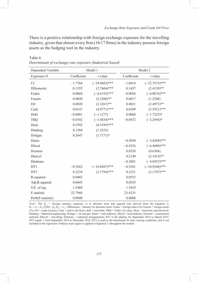
Exchange Rate Exposure and Crude Oil Price
177
There is a positive relationship with foreign exchange exposure for the travelling industry, given that almost every firm (16/17 firms) in the industry possess foreign assets as the hedging tool in the industry.
Table 6Determinant of exchange rate exposure (Industrial based)
Dependent Variable Model 1 Model 2
Exposure<0 Coefficient t-value Coefficient t-value
CI −1.7764 (−24.9603)*** −1.6816 (−22.7673)***DDomestic 0.1555 (2.7604)*** 0.1437 (2.4159)**Fsales −0.0060 (−6.6192)*** −0.0056 (−6.0676)***Fassets 0.0030 (2.2200)** 0.0017 (1.2548)Oil 0.0020 (2.3267)** 0.0021 (2.4973)**Cash 0.0147 (4.9771)*** 0.0109 (3.5931)***Debt −0.0001 (−1.1277) 0.0000 (−1.7225)*TBQ −0.0702 (−3.4834)*** −0.0472 (−2.2956)*Dene 0.5592 (4.3545)***Dindeng 0.1384 (1.3255)Doilgas 0.3647 (1.7171)*Dauto −0.5850 (−3.4269)***Dfood −0.4326 (−6.4689)***Dconsm 0.0528 (0.6364)Dtravel 0.2149 (2.1914)**Dinttrans −0.3601 (−4.0567)***DT1 −0.5562 (−10.8497)*** −0.5581 (−10.9348)***DT3 0.2234 (3.1794)*** 0.2221 (3.1747)***R-squared 0.0465 0.0553Adj.R-squared 0.0445 0.0529S.E. of reg 1.5488 1.5419F-statistic 22.7968 23.4335Prob(F-statistic) 0.0000 0.0000
Notes: The β1,t = foreign currency exposure, is in absolute term and squared root derived from the Equation 2; Ri,t = σj + β1,t f (XR) + β2,t Rm,t + ∈j,t; DDomestic = dummy for domestic firms, Fsales = foreign sales-(%); Fassets = foreign assets (%); Oil = crude oil price, Cash = cash in the firms; debt = total debt; TBQ = Tobin’s Q value; Dene = electronic and electrical; Dindeng = Industrial engineering; Doilgas = oil and gas; Dauto = auto industry; Dfood = food industry; Dconsm = construction material; Dtravel = travelling; Dinttrans = industrial transportation; DT1 is the dummy for September 2014 to March 2015; DT3 equals 1 from September 2016 to December 2016; DT2 is used as the benchmark for time varying conditions, and is not included in the regression. Ordinary least square is applied in Equation 3, throughout the models.
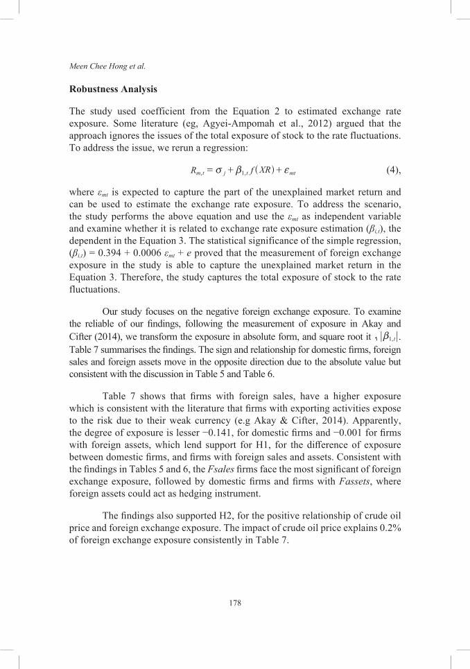
Meen Chee Hong et al.
178
Robustness Analysis
The study used coefficient from the Equation 2 to estimated exchange rate exposure. Some literature (eg, Agyei-Ampomah et al., 2012) argued that the approach ignores the issues of the total exposure of stock to the rate fluctuations. To address the issue, we rerun a regression:
R f XR, 1,m t j t mtv b f= + +^ h (4),
where εmt is expected to capture the part of the unexplained market return and can be used to estimate the exchange rate exposure. To address the scenario, the study performs the above equation and use the εmt as independent variable and examine whether it is related to exchange rate exposure estimation (βi,t), the dependent in the Equation 3. The statistical significance of the simple regression, (βi,t) = 0.394 + 0.0006 εmt + e proved that the measurement of foreign exchange exposure in the study is able to capture the unexplained market return in the Equation 3. Therefore, the study captures the total exposure of stock to the rate fluctuations.
Our study focuses on the negative foreign exchange exposure. To examine the reliable of our findings, following the measurement of exposure in Akay and Cifter (2014), we transform the exposure in absolute form, and square root it 1,tb . Table 7 summarises the findings. The sign and relationship for domestic firms, foreign sales and foreign assets move in the opposite direction due to the absolute value but consistent with the discussion in Table 5 and Table 6.
Table 7 shows that firms with foreign sales, have a higher exposure which is consistent with the literature that firms with exporting activities expose to the risk due to their weak currency (e.g Akay & Cifter, 2014). Apparently, the degree of exposure is lesser −0.141, for domestic firms and −0.001 for firms with foreign assets, which lend support for H1, for the difference of exposure between domestic firms, and firms with foreign sales and assets. Consistent with the findings in Tables 5 and 6, the Fsales firms face the most significant of foreign exchange exposure, followed by domestic firms and firms with Fassets, where foreign assets could act as hedging instrument.
The findings also supported H2, for the positive relationship of crude oil price and foreign exchange exposure. The impact of crude oil price explains 0.2% of foreign exchange exposure consistently in Table 7.
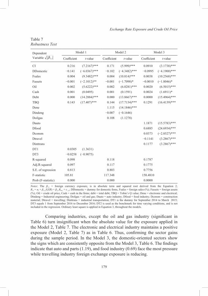
Exchange Rate Exposure and Crude Oil Price
179
Table 7Robustness Test
Dependent Variable 1,tb
Model 1 Model 2 Model 3
Coefficient t-value Coefficient t-value Coefficient t-value
CI 0.216 (7.2167)*** 0.171 (5.999)*** 0.0910 (3.1738)***DDomestic −0.141 (−6.0367)*** −0.102 (−4.3482)*** −0.0995 (−4.1900)***Fsales 0.004 (9.3482)*** 0.004 (10.814)*** 0.0038 (10.2568)***Fassets −0.001 (−2.1012)** −0.001 (−1.7098)* −0.0010 (−1.8046)*Oil 0.002 (5.6222)*** 0.002 (6.0281)*** 0.0020 (6.5015)***Cash 0.001 (0.0495) 0.001 (0.1591) 0.0024 (1.6911)*Debt 0.000 (14.2884)*** 0.000 (13.8667)*** 0.0000 (15.4964)***TBQ 0.143 (17.407)*** 0.144 (17.7134)*** 0.1291 (16.4139)***Dene 1.115 (14.1846)***Dindeng −0.007 (−0.1646)Doilgas 0.108 (1.1278)Dauto 1.1871 (15.5783)***Dfood 0.6885 (24.6934)***Dconsm 0.0373 (−2.8527)***Dtravel −0.1141 (3.2867)***Dinttrans 0.1177 (3.2867)***DT1 0.0305 (1.3631)DT3 −0.0258 (−0.9075)R-squared 0.098 0.118 0.1787Adj.R-squared 0.097 0.117 0.1775S.E. of regression 0.813 0.803 0.7756F-statistic 105.81 117.348 158.4810Prob (F-statistic) 0.000 0.000 0.0000
Notes: The β1,t = foreign currency exposure, is in absolute term and squared root derived from the Equation 2; Ri,t = σj + β1,t f (XR) + β2,t Rm,t + ∈j,t; DDomestic = dummy for domestic firms, Fsales = foreign sales-(%); Fassets = foreign assets (%); Oil = crude oil price, Cash = cash in the firms; debt = total debt; TBQ = Tobin’s Q value; Dene = electronic and electrical; Dindeng = Industrial engineering; Doilgas = oil and gas; Dauto = auto industry; Dfood = food industry; Dconsm = construction material; Dtravel = travelling; Dinttrans = industrial transportation; DT1 is the dummy for September 2014 to March 2015; DT3 equals 1 from September 2016 to December 2016; DT2 is used as the benchmark for time varying conditions, and is not included in the regression. Ordinary least square is applied in Equation 3, throughout the models.
Comparing industries, except the oil and gas industry (significant in Table 6) turn insignificant when the absolute value for the exposure applied in the Model 2, Table 7. The electronic and electrical industry maintains a positive exposure (Model 2, Table 7) as in Table 6. Thus, confirming the sector gains during the sample period. In the Model 3, the domestic-oriented sectors show the signs which are consistently opposite from the Model 3, Table 6. The findings indicate that auto and parts (1.19), and food industry (0.69) face the most pressure while travelling industry foreign exchange exposure is reducing.
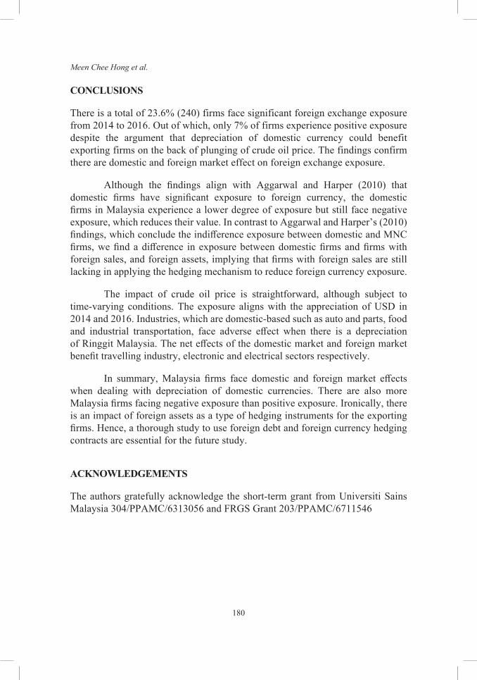
Meen Chee Hong et al.
180
CONCLUSIONS
There is a total of 23.6% (240) firms face significant foreign exchange exposure from 2014 to 2016. Out of which, only 7% of firms experience positive exposure despite the argument that depreciation of domestic currency could benefit exporting firms on the back of plunging of crude oil price. The findings confirm there are domestic and foreign market effect on foreign exchange exposure.
Although the findings align with Aggarwal and Harper (2010) that domestic firms have significant exposure to foreign currency, the domestic firms in Malaysia experience a lower degree of exposure but still face negative exposure, which reduces their value. In contrast to Aggarwal and Harper’s (2010) findings, which conclude the indifference exposure between domestic and MNC firms, we find a difference in exposure between domestic firms and firms with foreign sales, and foreign assets, implying that firms with foreign sales are still lacking in applying the hedging mechanism to reduce foreign currency exposure.
The impact of crude oil price is straightforward, although subject to time-varying conditions. The exposure aligns with the appreciation of USD in 2014 and 2016. Industries, which are domestic-based such as auto and parts, food and industrial transportation, face adverse effect when there is a depreciation of Ringgit Malaysia. The net effects of the domestic market and foreign market benefit travelling industry, electronic and electrical sectors respectively.
In summary, Malaysia firms face domestic and foreign market effects when dealing with depreciation of domestic currencies. There are also more Malaysia firms facing negative exposure than positive exposure. Ironically, there is an impact of foreign assets as a type of hedging instruments for the exporting firms. Hence, a thorough study to use foreign debt and foreign currency hedging contracts are essential for the future study.
ACKNOWLEDGEMENTS
The authors gratefully acknowledge the short-term grant from Universiti Sains Malaysia 304/PPAMC/6313056 and FRGS Grant 203/PPAMC/6711546
Exchange Rate Exposure and Crude Oil Price
181
REFERENCES
Adler, M., & Dumas, B. (1984). Exposure to currency risks: definition and management. Financial Management, 13(2), 41–50. https://doi.org/10.2307/3665446
Aggarwal, R., & Harper, J. (2010). Foreign exchange exposure of “domestic” corporations. Journal of International Money and Finance, 29(8), 1619–1636. https://doi.org/10.1016/j.jimonfin.2010.05.003
Agyei-Ampomah, S., Mazouz, K., & Yin, S (2012). The foreign exchange exposure of UK non-financial firms: A comparison of market based methodologies. International Review of Financial Analysis, 29, 251–260. https://doi.org/10.1016/j.irfa.2012. 05.006
Akay, G., & Cifter, A. (2014). Exchange rate exposure at the firm and industry levels: Evidence from Turkey. Economic Modelling, 43, 426-434. https://doi.org/ 10.1016/j.econmod.2014.09.003
Bank Negara Malaysia. (2010). Bank Negara Malaysia Annual Report 2010. Kuala Lumpur: Bank Negara Malaysia.
Bank Negara Malaysia. (2015). Bank Negara Malaysia Annual Report 2015. Kuala Lumpur: Bank Negara Malaysia.
Bank Negara Malaysia. (2016). Bank Negara Malaysia Annual Report 2016. Kuala Lumpur: Bank Negara Malaysia.
Bacha, O., Mohamad, A., Zain, S, & Rasid, M. (2012). Foreign exchange exposure and impact of policy switch-the case of Malaysian listed firms. Applied Economics, 45(20), 2974–2984. https://doi.org/10.1080/00036846.2012.684790
Bams, D., Blanchard, G., Honarvar, I., & Lehnert, T (2017). Does oil and gold price uncertainty matter for the stock market? Journal of Empirical Finance, 44, 270–285. https://doi.org/10.1016/j.jempfin.2017.07.003
Bartov, E., & Bodnar, G. (1994). Firm valuation, earnings expectations and the exchange rate effect. Journal of Finance, 49(5), 1755–1785. https://doi.org/ 10.1111/j.1540-6261.1994.tb04780.x
Bartram, S. (2004). Linear and non-linear foreign exchange exposure of Germany non-financial companies. Journal of International Money and Finance, 23(4), 673-699. https://doi.org/10.1016/j.jimonfin.2004.03.002
Bartram, S. (2007). Corporate cash flow and stock price exposures to foreign exchange rate risk. Journal of Corporate Finance, 13(5), 981–994. https://doi.org/10.1016/j.jcorpfin.2007.05.002
Bartram, S., & Bodnar, G. (2007). The exchange rate exposure puzzle. Managerial Finance, 33(9), 642–666. https://doi.org/10.1108/03074350710776226
Bartram, S., & Karolyi, G. (2006). The impact of the introduction of the Euro on foreign exchange rate risk exposures. Journal of Empirical Finance, 13(4–5), 519–549. https://doi.org/10.1016/j.jempfin.2006.01.002
Basher S., Haug, A., & Sadorsky, P (2015). The impact of oil shocks on exchange rates: A Markov-switching approach. Energy Economics, 54, 11–23. https://doi.org/ 10.1016/j.eneco.2015.12.004
Meen Chee Hong et al.
182
Bodnar, G., & Gentry, W. (1993). Exchange rate exposure and industry characteristics: Evidence from Canada, Japan, and the USA. Journal of International Money and Finance, 12(1), 201–215. https://doi.org/10.1016/0261-5606(93)90008-Y
Choi, J., & Prasad, M. (1995). Exchange rate sensitivity and its determinants: a firm and industry analysis of U.S. multinationals. Financial Management, 24(3), 77–88. https://doi.org/10.2307/3665559
Chue, T., & Cook, D. (2008). Emerging market exchange rate exposure. Journal of Banking and Finance, 32(7), 1349–1362. https://doi.org/10.1016/j.jbankfin.2007.11.005
Demirer, R., Jategaonkar, S., & Khalifa, A. (2015). Oil price risk exposure and the cross-section of stock returns: The case of net exporting countries. Energy Economics, 49, 132–140. https://doi.org/10.1016/j.eneco.2015.02.010
Donahue, C. (2016). Oil prices and a stronger dollar: Causation or correlation? Honors Program Capstone Projects (Paper 2), Merrimack College.
Doukas, J., Hall, P., & Lang, L. (1999). The pricing of currency risk in Japan. Journal of Banking and Finance, 23(1), 1–20. https://doi.org/10.1016/S0378-4266(98) 00112-5
Doukas, J., Hall, P., & Lang, L. (2003). Exchange rate exposure at the firm and industry level. Financial Market, Institutions and Instruments, 12, 291–346. https://doi.org/10.1046/j.0963-8008.2003.00001.x
Eiteman, D., Stonehill, A., & Moffett, M. (2010). Multinational business finance. Singapore: Pearson Publisher.
El-Masry, A., Abdel-Salam, O., & Alatraby, M. (2007). The exchange rate exposure of UK non-financial companies. Managerial Finance, 33(9), 620–641. https://doi.org/10.1108/03074350710776217
Geczy, C., Minton, B., & Schrand, C. (1997). Why firms use currency derivatives. The Journal of Finance, 52(4), 1323–1354. https://doi.org/10.1111/j.1540-6261.1997.tb01112.x
Griffin, J., & Stulz, R. (2001). International competition and exchange rate shocks: A cross‐country industry analysis of stock returns. Review of Financial Studies, 14(1), 215–241. https://doi.org/10.1093/rfs/14.1.215
He, J., & Ng, L. (1998). The foreign exchange exposure of Japanese multinational corporations. Journal of Finance, 53(2), 733–753. https://doi.org/10.1111/0022-1082.295575
Hutson, E., & O’Driscoll, A. (2010). Firm-level exchange rate exposure in the Eurozone. International Business Review, 19(5), 468–478. https://doi.org/10.1016/j.ibusrev.2009.02.007
International Monetary Fund. (2014). Foreign currencies exposures. Twenty-seventh Meeting of the IMF Committee on Balance of Payment Statistics. Washington, 27–29 October 2014.
International Monetary Fund. (2015). Global financial stability report: Vulnerabilities, legacies, and policy challenges: Risks rotating to emerging markets. New York: IMF.
Ito, T., Koibuichi, S., Sato, K., & Shimizu, J. (2016). Exchange rate exposure and risk management: The case of Japanese exporting firms. Journal of the Japanese and International Economies, 41, 17–29. https://doi.org/10.1016/j.jjie.2016.05.001
Exchange Rate Exposure and Crude Oil Price
183
Jorion, P. (1990). The exchange-rate exposure of U.S. multinationals. The Journal of Business, 63(3), 331–345. https://doi.org/10.1086/296510
Kandir, S.Y, Erismis, A., & Ozturk, I. (2015). Investigating exchange rate exposure of energy firms: Evidence from Turkey. Prague Economic Papers, 24(6), 729–743. https://doi.org/10.18267/j.pep.532
Kiymaz, H. (2003). Estimation of foreign exchange exposure: an emerging market application. Journal of Multinational Financial Management, 13(1), 71–84. https://doi.org/10.1016/S1042-444X(02)00034-8
Lin, C. (2011). Exchange-rate exposure in the Asian emerging markets. Journal of Multinational Financial Management, 21(4), 224–238. https://doi.org/10.1016/j.mulfin.2011.04.002
Lizardo, R., & Mollick, A. (2010). Oil price fluctuations and US dollar exchange rates. Energy Econonomics, 32(2), 399–408. https://doi.org/10.1016/j.eneco. 2009.10.005
Marston, R. (2001). The effects of industry structure on economic exposure. Journal of International Money and Finance, 20(2), 149–164. https://doi.org/10.1016/S0261-5606(00)00052-8
Mohaddes, K., & Pesaran, M. (2017). Oil prices and the global economy: Is it different this time around? Energy Economics, 65, 315–325. https://doi.org/10.1016/j.eneco.2017.05.011
Muller, A., & Verschoor, W. (2006). Foreign exchange risk exposure: Survey and suggestions. Journal of Multinational Financial Management, 16(4), 385–410. https://doi.org/10.1016/j.mulfin.2005.09.001
Nguyen, H., Faff, R., & Marshall, A. (2007). Exchange rate exposure, foreign currency derivatives and the introduction of the Euro: French evidence. International Review of Economics and Finance, 16(4), 563–577. https://doi.org/10.1016/j.iref.2006.01.002
Nydahl, S. (1999). Exchange rate exposure, foreign involvement and currency hedging of firms: Some Swedish evidence. European Financial Management, 5, 241–257. https://doi.org/10.1111/1468-036X.00091
Parlapiano, F., Alexeev, V., & Dungey, M. (2012). Exchange rate risk exposure and the value of European firms. The European Journal of Finance, 23(2), 111–129. https://doi.org/10.1080/1351847X.2015.1072570
Pritamani, M. D., Shome, D. K., & Singal, V. (2004). Foreign exchange exposure of exporting and importing firms. Journal of Banking and Finance, 28(7), 1697–1710. https://doi.org/10.1016/j.jbankfin.2003.06.002
Rupeika-Apoga, R., & Nedovis, R. (2016). The foreign exchange exposure of domestic companies in Eurozone: Case of the Baltic States. European Research Studies Journal, 1(1), 165–178.
Schena, P. (2007). Value creation in multinational enterprise. International Finance Review, 7, 285–306. https://doi.org/10.1016/S1569-3767(06)07012-9
Ye, M., Hutson, E., & Muckley, C. (2014). Exchange rate regime and foreign exchange exposure: The case of emerging market firms. Emerging Market Review, 21, 156–182. https://doi.org/10.1016/j.ememar.2014.09.001

Meen Chee Hong et al.
184
Yip, W., & Nguyen, H. (2012). Exchange rate exposure and the use of foreign currency derivatives in the Australian resources sector. Journal of Multinational Financial Management, 22(4), 151–167. https://doi.org/10.1016/j.mulfin.2012. 06.003
Wells, P. (2016). Ringgit knocked to weakest level since Asian financial crisis. Financial Times. 24 November.
World Bank. (2017). World Bank data. Retrieved from https://data.worldbank.org/indicator/
Zhang, Y. (2013). The links between the price of oil and the value of US Dollar. International Journal of Energy Economics and Policy, 3, 341–351.


