Embed Size (px)
Citation preview

REGISTRANTS, VOTERS, AND TURNOUTVARIABILITY ACROSS NEIGHBORHOODS
James G. Gimpel, Joshua J. Dyck, and Daron R. Shaw
Although political participation has received wide-ranging scholarly attention, little isknown for certain about the effects of social and political context on turnout. A scat-tered set of analyses—well-known by both political scientists and campaign consul-tants—suggests that one’s neighborhood has a relatively minor impact on the decisionto vote. These analyses, however, typically rely upon data from a single location.Drawing on official lists of registered voters from sixteen major counties across sevenstates (including Florida) from the 2000 presidential election, we use geographic/mapping information and hierarchical models to obtain a more accurate picture of howneighborhood characteristics affect participation, especially among partisans. Ourresearch shows that neighborhoods influence voting by interacting with partisanaffiliation to dampen turnout among voters we might otherwise expect to participate.Most notably, we find Republican partisans in enemy territory tend to vote less thanexpected, even after accounting for socioeconomic status. Our findings have implica-tions for campaign strategy, and lead us to suggest that campaign targeting effortscould be improved by an integration of aggregate- and individual-level informationabout voters.
Key words: voting; voter turnout; political participation; context effects; presidentialelections; partisanship; hierarchical generalized linear models; mixed models.
Based on the extraordinarily close elections of 2000 and 2004, the newconventional wisdom among students of American campaigns is that resultsincreasingly hinge on turnout efforts (Citrin, Schickler, and Sides, 2003;DeNardo, 1980, 1986). This insight has led the parties to invest a much higherproportion of their resources into personal contacting and mobilizationefforts.1 In light of recent studies from political science suggesting that these
James G. Gimpel, University of Maryland, Department of Government, 3140 Tydings Hall,College Park, MD 20742 ([email protected]). Joshua J. Dyck, University of Maryland, MD,Daron R. Shaw, University of Texas, Austin, TX, USA
Political Behavior, Vol. 26, No. 4, December 2004 (� 2004)
343
0190-9320/04/1200-0343 � 2004 Springer Science+Business Media, Inc. 2004
investments can bear fruit, this shift in allocation appears sensible (see Gerberand Green, 2000b; Imai, 2004). But neither campaign professionals norpolitical scientists have a strong sense of precisely who should be contactedbecause we do not know how local context affects the propensity of individualsto vote. For example, we know that campaigns and parties are strategic inidentifying whom they want to mobilize (Herrnson, 2004; Shea and Burton,2001; Wielhouwer, 2003), commonly drawing upon both individual-level andecological data to estimate turnout probabilities for all registered voters inrelevant jurisdictions (Malchow, 2003; pp. 151–159). In spite of their politicaland methodological sophistication, however, these political elites use fairlysimplistic assumptions to generate their estimates and typically ignore theeffects of context on individual-level behavior. Furthermore, there is littleconsensus among professionals about exactly how to use these estimatedturnout probabilities when targeting direct mail and phone calls.
To be fair, the failure to reckon with context is hardly unique to politicalconsultants and operatives. In political science, a long history of participationresearch—based primarily on self-reported survey data—points to a consensuallist of individual level factors that influence the propensity to vote (Campbell,Converse, Miller, and Stokes, 1960; Rosenstone and Hansen, 1993; Rosenstoneand Wolfinger, 1980; Stoker and Jennings, 1995; Verba and Nie, 1972; Verba,Schlozman, and Brady, 1995; Zipp and Smith, 1979). By contrast, we are far lessconfident about how neighborhood characteristics condition the importance ofthese traditional factors, although we have strong reasons to believe that con-textual characteristics do matter (Huckfeldt, 1986; Huckfeldt and Sprague,1987, 1991; Huckfeldt, Plutzer, and Sprague, 1993; Johnston et al., 2004). Inthis study, we take aim at this issue and examine geocoded voter list data fromsixteen counties to estimate how the social and residential context of neigh-borhoods affects the likelihood that someone voted in the 2000 general election.
Our broader theoretical claim is simple: geographic context affects voterturnout when it limits the acquisition of political information among voterswho are normally resource rich. Conversely, we posit that certain contextsboost turnout among those who are otherwise resource poor. This perspectiveleads to several more specific hypotheses. In particular, we hypothesize thatparty composition (and, by extension, racial/ethnic composition) should sup-press turnout among out-numbered partisans because minority status in acommunity can interfere with the acquisition of political information thatfacilitates voting. In addition to partisan and demographic factors, we alsoexpect that residential mobility contributes to individual turnout probabilities.New voters can register, but may face significant costs learning about theunfamiliar names on the long ballot, the relevant issues facing their commu-nity, and where they must go to cast their vote.
It would be easy to misconstrue the causal mechanism we are claiming here,so let us be clear. It is not that voting is such a highly public or demanding act
344 GIMPEL ET AL.
that social pressure comes directly into play, but rather that many key ante-cedents of the act of voting are influenced by the peculiar and variable opiniondistributions of local areas. Where citizens live at least partly determines whatthey learn and know.
At the same time, we are open to the possibility that politically stimulatingenvironments can enhance the participatory impulses of those who mightotherwise abstain. A politically diverse context can maximize the amount ofpolitical knowledge and discussion in a locale, generating information flowsthat produce greater efficacy than in more homogeneous areas (Gimpel, Lay,Schuknecht, 2003). In summary, then, similar people may wind up with verydifferent voting histories because of where they live. Political participation hasa geography, as well as a psychology.
HOW NEIGHBORHOODS AFFECT TURNOUT
How is a citizen’s probability of voting affected by context—that is, by thesocial characteristics and predispositions of those around her? As stated ear-lier, our principal theoretical claim is that context adversely affects voterturnout when it limits information acquisition among otherwise resource richvoters. It can also promote turnout under circumstances where it maximizesinformation acquisition. We are certainly not the first to advance this idea. TheColumbia scholars identified social context as perhaps the most importantfactor in the activation of partisan predispositions (Berelson and Gaudet, 1994;Lazarsfeld and Mcphee, 1954). They also posited that citizens subjected to‘‘cross pressures’’—conflicting political signals from group and opinion lead-ers—tended to abstain from voting. This notion was picked up by the Mich-igan scholars, who pointed out that a heterogeneous social context is one of anumber of key explanations for attitude conflict and even demobilization(Campbell et al., 1960; pp. 80–81).
Even more germane to our work, however, are more recent studies dem-onstrating the relevance of neighborhood effects to turnout and opinion(Baybeck and McClurg, 2004; Beck, Dalton, Green, and Huckfeldt, 2002;Cohen and Dawson, 1993; Eulau and Rothenberg, 1986; Giles and Dantico,1982; Huckfeldt, 1979; Huckfeldt and Sprague, 1997; Huckfeldt, Plutzer, andSprague, 1993; Kenny, 1992; Krassa, 1988; Rolfe, 2004; Straits, 1990). Herethe data indicate that neighborhoods and local context seem to matter less forcertain kinds of participation (Huckfeldt, 1979), with voter turnout lessaffected by context than more involved acts such as posting a sign in one’s yard,attending a rally, giving money, or working for a campaign (Kenny, 1992).
Our expectation is that the requisite information necessary to vote isavailable to citizens, even those who are predisposed to favor candidates atodds with the prevailing preferences of the neighborhood. This information
345REGISTRANTS, VOTERS, AND TURNOUT

can be acquired via the mainstream news media, family, and perhaps friendsand co-workers from outside the neighborhood. But we also believe thatpolitical information from more localized sources can still influence turnoutrates for those whose predispositions run contrary to local majority views. It isimportant to point out that while we assume people acquire a sense of thelocal opinion distribution, we do not necessarily assume voters have a greatdeal of contact with their neighbors. Baybeck and McClurg (2004) have shownthat even citizens who seldom interact with neighbors or read a local news-paper are still able to perceive accurately their political and economic envi-ronments.
The reasons for this demobilization are deceptively simple. Perceiving thatone is at odds with one’s neighborhood may (a) reduce the perceived utility ofsupporting the preferred party’s candidate, and (b) increase the incentive toavoid cognitive dissonance, and perhaps interpersonal conflict, by withdrawingfrom politics. Avoidance of dissonance is not necessarily a direct cause ofabstention, but can indirectly cause abstention by producing an aversion toacquiring the kind of political information that generates higher turnout. Wealso presume that party mobilization efforts—which provide voting cues alongwith substantive political information—may be less aggressive in neighbor-hoods dominated by the other party. In short, we suspect citizens who wouldotherwise be expected to vote might not do so in neighborhoods dominated bytheir non-preferred party.
As for which aspects of social context matter, and how they matter, theextant literature provides some intriguing clues. As suggested above, someresearch indicates that partisan context is likely to influence participation in asmuch as it shapes the flow and content of information that drives turnout. Thelogic of this argument is that partisans avoid discussions of politics in areasdominated by the other side. Avoidance of discussion, in turn, leads to adearth of information among minority partisans (Huckfeldt and Sprague,1995; Noelle-Neumann, 1993). Moreover, if they have no other sources ofinformation, they may participate less simply because their neighborhoodmakes engagement in political activity a potentially conflictual act. This notionis backed by empirical studies demonstrating that citizens functioning underconditions where their policy interests are consistently defeated or shouted-down feel less efficacious than citizens whose interests dominate (Iyengar,1980; Weissberg, 1975). Conversely, a more evenly divided macro environ-ment stimulates participation because it increases information flow and oftenattracts the attention of political candidates and parties looking to find andpersuade swing voters.
Aside from the partisan complexion of the neighborhood, local educationand income profiles may also affect individual voters. According to theresource theory of turnout, participation is driven by skills, money, and status,all of which abound in wealthier and better-educated environments (Leighley,
346 GIMPEL ET AL.
1995, p. 183).2 Although our registered voter lists do not provide data onindividual income and education levels, we can evaluate the effects ofneighborhood SES, which we measure by the percentage of residents with a4-year college degree.3 Of course it is likely that the neighborhood variablesmeasuring socioeconomic status significantly correlate with the wealth andeducation of individual voters sampled from the lists. More to the point, weexpect partisan identifiers living in areas with lower levels of education willshow less of a propensity to participate than those living in better-educatedsettings.
We also evaluate the effects of a neighborhood’s racial and ethnic compo-sition on the participation of Republican and Democratic registrants.Undoubtedly, neighborhood characteristics correspond to the individualethnic and racial identities of individuals residing there. Furthermore, withoutrace or ethnicity data on individuals in the voter file, it is impossible to eval-uate the interplay of individual and neighborhood racial characteristics. Still, itis informative to know whether the participation of Republicans and Demo-crats varies with the racial composition of their neighborhoods. We mightexpect, for example, that Republican registrants living in Black and Latinoneighborhoods—where GOP adherents would typically be a decided minor-ity—will vote less frequently than Democrats who would ordinarily findthemselves safely in the majority in these same places. On the other side of theledger, Democrats in Black and Latino neighborhoods may show a higherpropensity to vote than they would in homogeneously white areas becausethese neighborhoods tend to have heavily Democratic (and, hence, more like-minded) populations.
Beyond party, status, and race/ethnicity, previous research shows that polit-ical participation rates are much lower among recent residents than amongthe well-established (Gimpel, 1999; Highton and Wolfinger, 2001; Squire,Wolfinger, and Glass, 1987; Timpone, 1998). Unless highly motivated, newresidents may not even be on the registration rolls in places with burdensomeregistration requirements. Nevertheless, even among those who are registeredto vote, the habit of voting in a new location is acquired slowly. We anticipatethat neighborhoods with higher turnover will also be locations of low infor-mation exchange, where politics are not widely discussed. Partisans living insuch neighborhoods thus suffer the consequences of living around otheruninformed voters—it is more difficult and costly to navigate an unfamiliarpolitical landscape.
Although we are somewhat limited by the individual-level information onthe voter lists, we are able to gauge how gender, age, and previous vote historyaffect turnout in 2000 across a variety of neighborhood contexts. Our expec-tations for each of these control variables are straight-forward, though notobvious. Knowing that many recent studies have found little or no gendergap in political participation or engagement (Sapiro and Conover, 1997;
347REGISTRANTS, VOTERS, AND TURNOUT

Schlozman, Burns, and Verba, 1994; Verba, Burns, and Schlozman, 1997), webelieve one may exist once we control for both previous participation and con-text. Specifically, we hypothesize that among irregular voters, women will bemore likely to turn out than men, primarily because both parties and interestgroups more deliberately target women for campaign-related contacts.4
In addition to the multi-level relationships between neighborhood andpartisanship, we also control for two individual level variables that could haveindependent effects on turnout: age and vote history. For age, a considerablebody of work has shown that younger voters often do not develop participatoryhabits and are much less likely to turn out than middle-aged voters. The dataalso show that participation rates drop off again in old age (Rosenstone andHansen, 1993).
For vote history, we posit that current participation levels are likely to beexplained by previous voting behavior (Plutzer, 2002). In fact, one importantstudy found that the effect of past voting far surpasses the effects of age andeducation reported in prior research (Gerber, Green, and Shachar, 2003). Tomeasure vote history, we rely on actual turnout records from the 2000 presi-dential primary and the off-year general election in 1998. We expect that thosewho participated in these elections are far more likely to have voted in the 2000general election than those who did not. Furthermore, given that campaignscustomarily spend an inordinate amount of time and money contacting citizenswho are already reliable participants, including vote history measures allows usto explain participation patterns as a habit. To be sure, this inclusion mayweaken the effect of traditional explanatory variables on participation, but it willalso help us to understand the powerful impact of habit on political behavior.
DATA AND RESEARCH DESIGN
For all the impressive research on participation in the U.S., we have notadvanced far in our understanding of how neighborhoods condition the par-ticipation of voters because we often lack the appropriate data and analyticaltools. Traditional ecological data sets measure voter characteristics at too grossa level (states, standard metropolitan statistical areas, or even counties) tofacilitate definitive inference. Surveys, on the other hand, typically rely onrespondent descriptions of where they live and what local conditions are like.Over-reporting is also a problem with the survey approach, as more respon-dents say they voted than actually did. For this study, we utilize individual-level data supplemented by block-level information from the 2000 U.S.Census. More specifically, we employ lists of all registered voters in 16counties: Brevard (FL), Broward (FL), Hillsborough (FL), Orange (FL), PalmBeach (FL), Pinellas (FL), Dallas (IA), Polk (IA), Story (IA), Chester (PA),Delaware (PA), Montgomery (PA), Bernalillo (NM), Clark (NV), Jefferson(KY), and Mecklenburg (NC).
348 GIMPEL ET AL.

The Florida, Iowa, New Mexico, and Pennsylvania counties were selectedbecause they were key locations in battleground states in 2000. The Kentucky,Nevada, and North Carolina counties were added to increase variation in thesample, most notably with respect to competitiveness and campaign out-reach.5 The availability of party enrollment data was a factor, as manystates—including Colorado, Missouri, Wisconsin, Minnesota, Michigan,Washington, and Ohio—do not record party affiliation when registering vot-ers. Our goal in selecting states and counties was to take advantage of theavailability of voter lists while simultaneously maximizing variance across all ofour contextual and explanatory factors.
In each county, registered voters’ addresses were geocoded onto precinctsand census tracts using a Geographic Information System (GIS). The geo-coding process involves matching the addresses for voters on each list to streetranges contained in a GIS database for each county. In our case, we used theDynamap 2000TM street range database and found that we were easily able topinpoint the residences of over 90% of registered voters across the 16 coun-ties.6 To purge the voter lists of dead wood resulting from address changes,each list was checked prior to geocoding by running all names and addressesthrough the U.S. Postal Service’s National Change of Address (NCOA) reg-istry, a database established in 1986 containing 150 million change-of addressrecords. The NCOA process effectively highlights addresses that are no longervalid for registered voters who have moved within the previous 48 months.7
Once each residential address is geocoded onto the map, it is easy to link therecord from the voter list to the relevant neighborhood information on pre-cincts and census tracts. From there, our goal is to model the pattern ofparticipation and abstention by reference to individual and neighborhoodcharacteristics.
To assess the effect of neighborhood context and other factors on turnout,we rely upon a method that is uniquely suited to provide unbiased estimates ofmulti-level effects. Hierarchical Linear Modeling (HLM) is a procedure forinvestigating data occurring at two levels of analysis (Humphries, 2001; Leeand Bryk, 1989; Raudenbush and Bryk, 1986, 2002; Steenbergen and Jones,2002). Level one variables are observed at the individual level. In our case,these include the items contained in the voter list file: the participation history,party registration, age, and sex of the voter. Since we hypothesize that turnoutis a function not merely of individual characteristics, but also characteristics ofneighborhoods, we have a second level of data: observations occurring at theneighborhood level, for which we use either census tract information, orindividual data aggregated to the tract or precinct level.
Because our observations at level one are clustered into neighborhoods,traditional regression approaches, which assume that the observations areindependent, are inappropriate. Citizens living within a particular neighbor-hood share certain background characteristics and look more like each other,
349REGISTRANTS, VOTERS, AND TURNOUT
on average, than they do someone many miles away. And because Republicansand Democrats, for example, are present to varying degrees across neigh-borhoods, a failure to represent this unevenness could bias the coefficients ofa traditional prediction equation, distorting voter-level effect estimates(Raudenbush and Bryk, 2002, pp. 137–138). We confine remaining details ofthe estimation procedure to the appendix.
As suggested above, using geocoded voter lists for participation research hastwo impressive advantages over traditional approaches. First, the turnoutfigures are not self-reports, as in survey research, but the actual participationrecords of registered voters. Second, extraordinarily large samples can bedrawn from the lists, providing us with the capacity to truly represent and testneighborhood contexts. In particular, a data set must include sufficient caseswithin neighborhoods so that these cases can be aggregated to produce acontext-specific estimate of neighborhood effects (Huckfeldt and Sprague,1995, p. 35); the voter lists easily meet this condition.
By contrast, the major limitation of using voter lists to study political par-ticipation is the absence of detailed individual level data.8 While almost all listscontain some information on the vote history, age, sex, and party registrationof each registrant,9 desirable items such as income, education level, politicalinterest, issue opinions, and candidate evaluations are lacking. Still, politicalinterest, education level and income are likely to be highly correlated withvote history, suggesting that the inclusion of previous decisions about partic-ipation in primary and off-year elections may capture some variation thatmight otherwise be explained by these missing bits of individual information.To thoroughly consider the limitations to our approach, we also validate thevoter list analysis by examining survey data that contain individual-levelcovariates as well as neighborhood level information (see analysis accompa-nying Table 4). More specifically, we examine the political behavior anddemographic characteristics of individuals from Brevard, Broward, Hillsbor-ough, Palm Beach, and Pinellas Counties using tracking polls conducted bythe Bush-Cheney campaign in Florida between September 24 and October25, 2000.10 The 2,000 cases from these counties allow us to investigate theeffects of neighborhood context in the presence of relevant individual levelcovariates not available on the voter file itself.
RESULTS
Our analysis of the voter list data underscores several key findings. First,Republicans across a variety of contexts tended to vote at higher rates thanDemocrats in 2000—no great surprise. Second, neighborhoods can and docondition the effects of several of the more predictable individual influenceson the vote. In particular, partisans were often less likely to vote in neigh-borhoods where they were surrounded by supporters of the other party in
350 GIMPEL ET AL.

2000. Furthermore—and perhaps surprisingly, given the aforementionedGOP turnout advantage—the neighborhood effects appear to have been moreconsistently powerful for Republicans facing Democratic majorities than vice-versa. It is also apparent that Republicans and Democrats (but especiallyRepublicans) were less likely to turn out in areas of high in-migration. Theseresults are considered in greater detail across several settings. Initially, weexamine several Florida locations. We then proceed to compare the lessonslearned in the Sunshine State to results from other states.
Florida
In Table 1, we present a panel of results for our six Florida counties. As forpartisan differences, we find Republican turnout to be higher than Demo-cratic turnout in all of the counties, except heavily Democratic Broward.While the expected odds that a Republican would turn out to vote in BrowardCounty are 1.19 times the odds of an ‘‘independent,’’11 the odds of a Dem-ocrat going to the polls in Broward County are slightly higher, or 1.25 timesthe odds of a similar independent showing up. What makes the Browardresults so remarkable is that in all other Florida locations, Democratic turnoutruns considerably lower than Republican participation, with the widest gapoccurring in the Orlando area (Orange County).
But how do the average partisan effects on turnout we have just highlightedvary across neighborhoods? To determine that, we examine the magnitudeand significance of the level-two effects included in the model. Is there atendency for Republicans and Democrats to stay home in areas where they area decided minority? Yes, but the depressive effect is consistently greater forRepublicans. Republicans are significantly less likely to turn out as theDemocratic edge grows across neighborhoods in every single Florida location.In Palm Beach County, for instance, moving from low to high levels ofDemocratic concentration in neighborhoods drops Republican turnout byabout 8%. Democrats lose ground as Republican strength edges upwardacross neighborhoods only in Broward County, where Republicans are adecided minority countywide.
Aside from this partisan effect, one of our most noteworthy findings is thatRepublican turnout declines in areas with significant in-migration. In eachFlorida county, neighborhoods with high proportions of movers show lowerGOP turnout. The effect is less evident for the Democrats, but it does appearin Brevard, Broward and Hillsborough counties.
Individual characteristics also interact with other neighborhood contexts,but not as significantly. We find some tendency for participation to moveupward in Florida neighborhoods with better educated residents. Republi-can participation rises in neighborhoods with higher educational attainmentin Broward, Orange and Pinellas Counties. Democratic participation rises
351REGISTRANTS, VOTERS, AND TURNOUT

TA
BL
E1.
Tw
oL
eve
lM
od
el
of
Vote
rT
urn
ou
t,co
ntr
oll
ing
for
ind
ivid
ual
Ch
arac
teri
stic
san
dN
eig
hb
orh
ood
Con
text
ual
Eff
ect
s
Fix
edE
ffec
tsE
xpla
nat
ory
Var
iab
leB
reva
rdC
oun
ty,
FL
Bro
war
dC
oun
ty,
FL
Hill
sbor
ough
Cou
nty
,F
LO
ran
geC
oun
tyF
LP
alm
Bea
chC
oun
ty,
FL
Pin
ella
sC
oun
ty,
FL
Ove
rall
Mea
ns
(b0)
Inte
rcep
t)
.941
9***
)1.
3523***
)1.
1789***
)1.
0352
***
).9
558***
).8
317*
**
(.06
69)
(.03
82)
(.05
23)
(.05
92)
(.05
04)
(.04
92)
.389
9.2
586
.307
6.3
551
.384
5.4
353
Rep
ub
lican
Iden
tifi
ers
(b1)
Inte
rcep
t.9
391*
**
.176
4*.8
253***
.882
2***
.389
3***
.644
0***
(.21
50)
(.10
28)
(.12
97)
(.14
17)
(.13
63)
(.13
68)
2.55
761.
1929
2.28
252.
4161
1.47
601.
9041
Per
cen
tB
lack
).0
028
).0
035***
).0
036***
).0
012
).0
058***
).0
011
(.00
31)
(.00
10)
(.00
18)
(.00
20)
(.00
16)
(.00
18)
Per
cen
tC
olle
geE
du
cate
d-.
0001
.006
0***
.001
8.0
050*
*.0
033
.004
5**
(.00
31)
(.00
16)
(.00
14)
(.00
20)
(.00
22)
(.00
20)
Per
cen
tage
Mig
ran
ts(l
ast
5ye
ars)
).0
082*
).0
118***
).0
086***
).0
081*
*)
.009
9**
).0
119*
**
(.00
43)
(.00
38)
(.00
33)
(.00
35)
(.00
43)
(.00
34)
Per
cen
tH
isp
anic
).0
093
.004
3***
).0
022
).0
013
).0
006
).0
010
(.01
27)
(.00
16)
(.00
17)
(.00
23)
(.00
23)
(.00
60)
Per
cen
tD
emoc
rati
c)
.010
3**
).0
033**
).0
080***
).0
133*
**
).0
063***
).0
124*
**
(.00
42)
(.00
16)
(.00
27)
(.00
27)
(.00
20)
(.00
28)
Dem
ocra
tic
Iden
tifi
ers
(b2)
Inte
rcep
t)
.182
7.2
270***
.173
2.0
414
.152
3.2
707*
*(.
1837
)(.
0704
)(.
1102
)(.
1530
)(.
1006
)(.
1112
).8
330
1.25
491.
1892
1.04
231.
1646
.762
8P
erce
nt
Bla
ck.0
026
).0
003
).0
015
).0
018
).0
032***
.002
7**
(.00
25)
(.00
07)
(.00
12)
(.00
16)
(.00
11)
(.00
12)
Per
cen
tC
olle
geE
du
cate
d.0
000
.009
2***
.005
1***
.006
3***
.002
3.0
061*
**
(.00
30)
(.00
14)
(.00
14)
(.00
23)
(.00
20)
(.00
20)
Per
cen
tM
igra
nts
(las
t5
year
s)
-.00
75*
(.0043)
-.00
83**
(.0033)
-.01
27***
(.0032)
-.00
34(.
0039
).0
008
(.00
40-.
0054
(.00
34)
352 GIMPEL ET AL.

TA
BL
E1.
Con
tin
ued
.
Fix
edE
ffec
tsE
xpla
nat
ory
Var
iab
leB
reva
rdC
oun
ty,
FL
Bro
war
dC
oun
ty,
FL
Hill
sbor
ough
Cou
nty
,F
LO
ran
geC
oun
tyF
LP
alm
Bea
chC
oun
ty,
FL
Pin
ella
sC
oun
ty,
FL
Per
cen
tH
isp
anic
.016
2.0
043*
**
.000
3.0
009
-.00
43**
-.00
96*
(.01
17)
(.00
14)
(.00
15)
(.00
24)
(.00
19)
(.00
55)
Per
cen
tR
epu
blic
an.0
109*
**
).0
070*
**
.005
0***
.003
1)
.001
1.0
085*
**
(.00
34)
(.00
15)
(.00
23)
(.00
24)
(.00
19)
(.00
25)
Gen
der
(b3)
Inte
rcep
t.2
154*
**
.231
3***
.202
5***
.176
3***
.188
4***
.187
5***
(.02
42)
(.01
31)
(.01
90)
(.02
18)
(.01
74)
(.01
68)
1.24
031.
2602
1.22
441.
1928
1.20
731.
2063
Age
18–2
9(b
4)
Inte
rcep
t)
.478
8***
).0
191
).0
551
).0
169
).2
651*
**
).3
190*
**
(.05
97)
(.03
41)
(.04
28)
(.04
94)
(.04
18)
(.04
13)
.619
5.9
811
.946
4.9
833
.767
2.7
269
Age
20–3
9(b
5)
Inte
rcep
t-.
0173
.350
2***
.411
9***
.434
4***
.188
1***
.091
0**
(.05
51)
(.03
35)
(.04
39)
(.05
05)
(.04
20)
(.04
04)
.982
81.
4194
1.50
971.
5440
1.20
701.
0952
Age
40–4
9(b
6)
Inte
rcep
t.2
343*
**
.551
7***
.624
7***
.644
0***
.452
2***
.291
5***
(.05
67)
(.03
48)
(.04
60)
(.04
96)
(.04
14)
(.03
96)
1.26
401.
7362
1.86
781.
9040
1.57
181.
3384
Age
50–5
9(b
7)
Inte
rcep
t.3
726*
**
.638
6***
.680
2***
.723
9***
.497
5***
.367
4***
(.05
50)
(.03
56)
(.04
80)
(.05
27)
(.04
05)
(.03
95)
1.45
161.
8938
1.97
442.
0625
1.64
461.
4439
Age
65an
du
p(b
8)
Inte
rcep
t.2
603*
**
.293
8***
.411
4***
.555
7.1
789*
**
.099
7***
(.05
40)
(.03
22)
(.04
68)
(.05
39)
(.04
01)
(.03
86)
1.29
741.
3416
1.50
901.
7431
1.19
591.
1049
1998
Gen
eral
Vot
er(b
9)
Inte
rcep
t2.
7794
***
2.75
94***
2.79
08***
2.49
25***
2.89
30***
2.87
71***
(.03
81)
(.02
27)
(.03
16)
(.03
73)
(.02
77)
(.02
85)
16.1
099
15.7
907
16.2
943
12.0
909
18.0
465
17.7
624
353REGISTRANTS, VOTERS, AND TURNOUT

TA
BL
E1.
Con
tin
ued
.
Fix
edE
ffec
tsE
xpla
nat
ory
Var
iab
leB
reva
rdC
oun
ty,
FL
Bro
war
dC
oun
ty,
FL
Hill
sbor
ough
Cou
nty
,F
LO
ran
geC
oun
tyF
LP
alm
Bea
chC
oun
ty,
FL
Pin
ella
sC
oun
ty,
FL
2000
Pri
mar
yV
oter
(b1
0)
Inte
rcep
t2.
3038
***
2.27
93***
2.07
78***
2.05
35***
2.33
99***
2.21
86***
(.10
24)
(.04
10)
(.07
61)
(.05
92)
(.05
63)
(.06
44)
10.0
121
9.76
947.
9870
7.79
5510
.380
29.
1948
No.
ofL
evel
1U
nit
s47
,645
155,
643
82,6
9458
,995
100,
675
101,
681
No.
ofL
evel
2U
nit
s15
756
930
531
651
133
5
Hie
rarc
hic
alG
ener
aliz
edL
inea
rM
odel
;S
lop
esan
dIn
terc
epts
Est
imat
ion
cell
entr
ies
are
logi
stic
regr
essi
onco
effi
cien
ts,
(sta
nd
ard
erro
rs),
and
odd
sra
tios
.R
esu
lts
fro
relia
bili
tyes
tim
ates
and
vari
ance
com
pon
ents
do
not
app
ear
inth
eta
ble
,b
ut
are
avai
lab
lefr
omth
eau
thor
su
pon
req
ues
t.*p
<10
;**p£
.05;
***p£
.01.
354 GIMPEL ET AL.

education levels increase in Broward, Hillsborough, Orange and Pinellascounties.
Among the other results, our estimates consistently indicate that womenturned out in higher proportions than men. Note, though, that these modelscontrol for vote history, suggesting that the gender variable is picking up theeffect of women who are irregular voters (e.g., those who do not participateregularly in off-year and primary elections). In other words, it would appearthat women who may be peripheral (or ‘‘floating’’) voters were mobilized in2000.
Consistent with previous research, younger voters (18–29) are less likely tovote just about everywhere, but especially in Brevard, Palm Beach andPinellas Counties, where older voters are particularly likely to vote, exacer-bating the contrast between the generations. In Pinellas, for every 100 oldervoters going to the polls, only an estimated 73 young voters showed up. InBrevard, the deficit is even worse, with only 62 young voters turning out forevery 100 older voters. The elderly, for their part, are most active in theOrlando area, where they outvote younger voters by a factor of 1.74, accordingto the odds ratio in Table 1.
As expected, turnout is unquestionably influenced by previous votingbehavior. The odds ratios are enormous, indicating that the impact of habit faroutweighs any other force in these models, consistent with the findings ofprevious research (Gerber et al., 2003). If we could use only one previousvote, turnout in the 1998 midterm (not the 2000 primary) would be the bestpredictor of voting in the 2000 presidential contest.
Locations in Other States
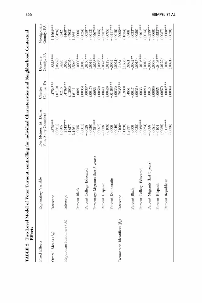
How unique are the Florida results? By taking the same analyticalapproach in other areas, we seek more consistent and general patterns.Tables 2 and 3 present results for Des Moines, Louisville, Las Vegas,Albuquerque, Charlotte, and the collar counties that constitute suburbanPhiladelphia. On the GOP side of the equation, a few things stand out. First,Republicans exhibit lower turnout in areas of high in-migration. In thisimportant respect, the results are the same as those from Florida. Repub-licans do especially poorly in high migration areas of Montgomery County,Pennsylvania, where GOP registrants in the most highly migratory neigh-borhoods participate 14% less than those in the most residentially stableneighborhoods.
Second, Republicans commonly turn out at lower rates in the heavilyDemocratic neighborhoods (Chester, Charlotte, Clark, and Montgomery). Forinstance, in Albuquerque, New Mexico, if we compare two Republican voterswho are similar in other ways, but differ by 10% in the extent of Democraticdominance in their neighborhood, we can expect the voter in the more
355REGISTRANTS, VOTERS, AND TURNOUT
TA
BL
E2.
Tw
oL
eve
lM
od
el
of
Vote
rT
urn
ou
t,co
ntr
oll
ing
for
ind
ivid
ual
Ch
arac
teri
stic
san
dN
eig
hb
orh
ood
Con
text
ual
Eff
ect
s
Fix
edE
ffec
tsE
xpla
nat
ory
Var
iab
leD
esM
oin
es,
IA(D
alla
s,P
olk,
Sto
ryC
oun
ties
)C
hes
ter
Cou
nty
,P
AD
elaw
are
Cou
nty
,P
AM
ontg
omer
yC
oun
ty,
PA
Ove
rall
Mea
ns
(b0)
Inte
rcep
t.4
578*
**
).4
754***
).8
615***
)1.
1264
***
(.06
81)
(.07
10)
(.06
62)
(.04
26)
1.58
05.6
216
.422
5.3
242
Rep
ub
lican
Iden
tifi
ers
(b1)
Inte
rcep
t.7
543*
**
.476
9***
.052
6.4
460***
(.18
27)
(.13
93)
(.07
05)
(.07
63)
2.12
611.
6111
1.50
401.
5621
Per
cen
tB
lack
).0
055
).0
021
).0
039***
).0
006
(.00
61)
(.00
35)
(.00
13)
(.00
24)
Per
cen
tC
olle
geE
du
cate
d)
.002
8.0
038**
.015
0***
.005
9***
(.00
26)
(.00
17)
(.00
14)
(.00
13)
Per
cen
tage
Mig
ran
ts(l
ast
5ye
ars)
).0
251*
**
).0
086
).0
268***
).0
207***
(.00
97)
(.00
52)
(.00
56)
(.00
55)
Per
cen
tH
isp
anic
).0
038
).0
040
).0
325***
).0
237**
(.01
08)
(.00
48)
(.01
19)
(.00
95)
Per
cen
tD
emoc
rati
c.0
006
).0
168***
).0
034
).0
111***
(.00
40)
(.00
33)
(.00
21)
(.00
19)
Dem
ocra
tic
Iden
tifi
ers
(b2)
Inte
rcep
t.2
100*
).7
235***
).1
484
).3
995***
(.11
20)
(.19
30)
(.16
36)
(.13
34)
1.23
37.4
851
.862
1.6
706
Per
cen
tB
lack
.000
0)
.001
7)
.003
2**
.005
3***
(.00
38)
(.00
31)
(.00
13)
(.00
20)
Per
cen
tC
olle
geE
du
cate
d)
.006
8***
.003
3.0
108***
.010
1***
(.00
24)
(.00
21)
(.00
18)
(.00
14)
Per
cen
tM
igra
nts
(las
t5
year
s))
.008
8.0
016
).0
088
).0
238***
(.00
81)
(.00
68)
(.00
68)
(.00
60)
Per
cen
tH
isp
anic
).0
104
).0
085
).0
403***
).0
253***
(.00
82)
(.00
57)
(.01
22)
(.00
87)
Per
cen
tR
epu
blic
an.0
112*
**
.009
2***
.001
3.0
060***
(.00
36)
(.00
34)
(.00
21)
(.00
20)
356 GIMPEL ET AL.

TA
BL
E2.
Con
tin
ued
.
Fix
edE
ffec
tsE
xpla
nat
ory
Var
iab
leD
esM
oin
es,
IA(D
alla
s,P
olk,
Sto
ryC
oun
ties
)C
hes
ter
Cou
nty
,P
AD
elaw
are
Cou
nty
,P
AM
ontg
omer
yC
oun
ty,
PA
Gen
der
(b3)
Inte
rcep
t.1
234***
.096
1***
.292
2***
.150
3***
(.02
41)
(.02
48)
(.02
05)
(.01
79)
1.13
141.
1009
1.33
931.
1621
Age
18–2
9(b
4)
Inte
rcep
t)
.534
1***
).2
905***
).0
140
.285
2***
(.06
78)
(.06
33)
(.05
28)
(.03
43)
.586
2.7
479
.986
11.
3300
Age
30–3
9(b
5)
Inte
rcep
t)
.481
3***
.176
4***
.345
3***
.573
6***
(.06
84)
(.06
38)
(.05
26)
(.03
28)
.618
01.
1929
1.41
251.
7746
Age
40–4
9(b
6)
Inte
rcep
t)
.157
1.5
370***
.640
7***
.951
6***
(.06
90)
(.06
46)
(.05
41)
(.03
56)
.854
61.
7108
1.89
782.
5898
Age
50–5
9(b
7)
Inte
rcep
t.0
422
.502
1***
.761
1***
1.00
58***
(.07
22)
(.06
37)
(.05
80)
(.03
55)
1.04
521.
6521
2.14
072.
7341
Age
65an
du
p(b
8)
Inte
rcep
t)
.232
5***
).0
902
.174
9***
.393
6***
(.07
46)
(.06
51)
(.05
72)
(.03
60)
.792
5.9
137
1.19
111.
4823
1998
Gen
eral
Vot
er(b
9)
Inte
rcep
t1.
9098***
2.02
04***
2.57
10***
2.62
24***
(.03
91)
(.03
49)
(.03
62)
(.03
04)
6.75
187.
5413
13.0
794
13.7
687
2000
Pri
mar
yV
oter
(b10)
Inte
rcep
t.7
272***
2.57
23***
2.21
25***
2.14
78***
(.04
26)
(.09
91)
(.07
37)
(.06
92)
2.06
9413
.095
69.
1390
8.56
59N
o.of
Lev
el1
Un
its
55,2
4742
,200
58,7
9180
,334
No.
ofL
evel
2U
nit
s22
821
740
740
4
Hie
rarc
hic
alG
ener
aliz
edL
inea
rM
odel
;S
lop
esan
dIn
terc
epts
Est
imat
ion
cell
entr
ies
are
logi
stic
regr
essi
onco
effi
cien
ts(s
tan
dar
der
rors
),an
dod
ds
rati
os.
Res
ult
sfo
rre
liab
ility
esti
mat
esan
dva
rian
ceco
mp
onen
tsd
on
otap
pea
rin
the
tab
le,
bu
tar
eav
aila
ble
from
the
auth
ors
up
onre
qu
est.
*p£
10;**p£
.05;
***p£
.01.
357REGISTRANTS, VOTERS, AND TURNOUT
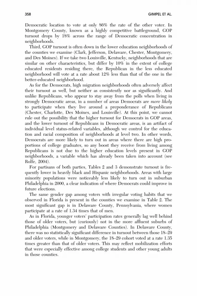
Democratic location to vote at only 86% the rate of the other voter. InMontgomery County, known as a highly competitive battleground, GOPturnout drops by 18% across the range of Democratic concentration inneighborhoods.
Third, GOP turnout is often down in the lower education neighborhoods ofthe counties we examine (Clark, Jefferson, Delaware, Chester, Montgomery,and Des Moines). If we take two Louisville, Kentucky, neighborhoods that aresimilar on other characteristics, but differ by 10% in the extent of collegeeducated residents residing there, the Republican in the less educatedneighborhood will vote at a rate about 12% less than that of the one in thebetter-educated neighborhood.
As for the Democrats, high migration neighborhoods often adversely affecttheir turnout as well, but neither as consistently nor as significantly. Andunlike Republicans, who appear to stay away from the polls when living instrongly Democratic areas, in a number of areas Democrats are more likelyto participate when they live around a preponderance of Republicans(Chester, Charlotte, Des Moines, and Louisville). At this point, we cannotrule out the possibility that the higher turnout for Democrats in GOP areas,and the lower turnout of Republicans in Democratic areas, is an artifact ofindividual level status-related variables, although we control for the educa-tion and racial composition of neighborhoods at level two. In other words,Democrats are more likely to turn out in areas where there are high pro-portions of college graduates, so any boost they receive from living amongRepublicans is not due to the higher education levels present in GOPneighborhoods, a variable which has already been taken into account (seeRolfe, 2004).
For partisans of both parties, Tables 2 and 3 demonstrate turnout is fre-quently lower in heavily black and Hispanic neighborhoods. Areas with largeminority populations were noticeably less likely to turn out in suburbanPhiladelphia in 2000, a clear indication of where Democrats could improve infuture elections.
The same gender gap among voters with irregular voting habits that weobserved in Florida is present in the counties we examine in Table 2. Themost significant gap is in Delaware County, Pennsylvania, where womenparticipate at a rate of 1.34 times that of men.
As in Florida, younger voters’ participation rates generally lag well behindthose of older voters, but (curiously) not in the more affluent suburbs ofPhiladelphia (Montgomery and Delaware Counties). In Delaware County,there was no statistically significant difference in turnout between those 18–29and older voters, while in Montgomery, the 18–29 cohort voted at a rate 1.35times greater than that of older voters. This may reflect mobilization effortsthat were especially effective among college students and other young adultsin those counties.
358 GIMPEL ET AL.

TA
BL
E3.
Tw
oL
eve
lM
od
el
of
Vote
rT
urn
ou
t,C
on
troll
ing
for
Ind
ivid
ual
Ch
arac
teri
stic
san
dN
eig
hb
orh
ood
Con
text
ual
Eff
ect
s
Fix
edE
ffec
tsE
xpla
nat
ory
Var
iab
leB
ern
alill
oC
oun
ty,
NM
Cla
rkC
oun
ty,
NV
Jeff
erso
nC
oun
ty,
KY
Mec
klen
bu
rgC
oun
ty,
NC
Ove
rall
Mea
ns
(b0)
Inte
rcep
t)
.662
5***
).6
846***
)1.
2961
***
)1.
0947***
(.07
64)
(.05
21)
(.06
16)
(.06
33)
.515
5.5
043
.273
6.3
646
Rep
ub
lican
Iden
tifi
ers
(b1)
Inte
rcep
t1.
0882
***
.985
5***
.655
6***
.927
2***
(.21
97)
(.15
82)
(.18
81)
(.17
47)
2.96
892.
6792
1.92
622.
5274
Per
cen
tB
lack
).0
212
).0
004
).0
053*
**
).0
002
(.01
78)
(.00
31)
(.00
15)
(.00
26)
Per
cen
tC
olle
geE
du
cate
d.0
011
.005
9**
.012
3***
.002
0(.
0031
)(.
0028
)(.
0018
)(.
0024
)P
erce
nta
geM
igra
nts
(las
t5
year
s))
.007
1)
.004
1**
).0
157*
*)
.004
1(.
0045
)(.
0018
)(.
0068
)(.
0035
)P
erce
nt
His
pan
ic.0
014
).0
057***
.023
0)
0.00
89(.
0028
)(.
0019
)(.
0153
)(.
0051
)P
erce
nt
Dem
ocra
tic
).0
152*
**
).0
134***
).0
074*
*)
.014
8***
(.00
31)
(.00
29)
(.00
30)
(.00
31)
Dem
ocra
tic
Iden
tifi
ers
(b2)
Inte
rcep
t)
.428
5**
.124
7)
.099
0)
.168
8(.
2151
)(.
1323
)(.
0849
)(.
1760
).6
515
1.13
28.9
058
.844
7P
erce
nt
Bla
ck)
.009
4)
.000
7.0
015
.001
3(.
0139
)(.
0019
)(.
0009
)(.
0019
)P
erce
nt
Col
lege
Ed
uca
ted
.007
7***
.006
1**
.010
8***
).0
027
(.00
26)
(.00
27)
(.00
15)
(.00
22)
Per
cen
tM
igra
nts
(las
t5
year
s))
.006
3)
.002
7)
.024
9***
).0
014
(.00
43)
(.00
17)
(.00
56)
(.00
33)
359REGISTRANTS, VOTERS, AND TURNOUT

TA
BL
E3.
Con
tin
ued
.
Fix
edE
ffec
tsE
xpla
nat
ory
Var
iab
leB
ern
alill
oC
oun
ty,
NM
Cla
rkC
oun
ty,
NV
Jeff
erso
nC
oun
ty,
KY
Mec
klen
bu
rgC
oun
ty,
NC
Per
cen
tH
isp
anic
).0
002
).0
066*
**
).0
062
.000
2(.
0021
)(.
0015
)(.
0118
)(.
0041
)P
erce
nt
Rep
ub
lican
.011
4***
.005
5**
.011
5***
.013
0***
(.00
22)
(.00
27)
(.00
24)
(.00
29)
Gen
der
(b3)
Inte
rcep
t.0
542
.190
7***
.165
9***
.209
9***
(.02
77)
(.01
73)
(.02
11)
(.02
14)
1.05
571.
2101
1.18
041.
2336
Age
18–2
9(b
4)
Inte
rcep
t)
.008
0)
.848
2***
.615
2***
).0
116
(.06
27)
(.04
45)
(.05
02)
(.05
11)
.881
1.4
282
1.85
00.9
885
Age
30–3
9(b
5)
Inte
rcep
t.1
468*
**
).4
364*
**
.703
2***
.224
5***
(.06
18)
(.04
40)
(.05
09)
(.05
68)
1.15
81.6
464
2.02
011.
2516
Age
40–4
9(b
6)
Inte
rcep
t.3
720*
**
).2
765*
**
.817
9***
.382
7***
(.06
12)
(.04
41)
(.05
09)
(.05
65)
1.45
06.7
585
2.26
561.
4662
Age
50–5
9(b
7)
Inte
rcep
t.5
183*
**
).1
817*
**
.883
7***
.508
6***
(.06
41)
(.04
29)
(.05
40)
(.05
68)
1.67
92.8
338
2.41
981.
6629
Age
65an
du
p(b
8)
Inte
rcep
t.2
045*
**
).1
216*
**
.417
7***
.063
7(.
0663
)(.
0450
)(.
0516
)(.
0592
)1.
2269
.885
51.
5184
1.06
5819
98G
ener
alV
oter
(b9)
Inte
rcep
t2.
1619
***
2.52
01***
3.02
67***
2.68
74***
(.03
23)
(.02
57)
(.03
61)
(.03
92)
8.68
7612
.430
220
.628
614
.693
4
360 GIMPEL ET AL.
TA
BL
E3.
Con
tin
ued
.
Fix
edE
ffec
tsE
xpla
nat
ory
Var
iab
leB
ern
alill
oC
oun
ty,
NM
Cla
rkC
oun
ty,
NV
Jeff
erso
nC
oun
ty,
KY
Mec
klen
bu
rgC
oun
ty,
NC
2000
Pri
mar
yV
oter
(b1
0)
Inte
rcep
t2.
1632
***
2.83
72***
2.71
50***
2.11
16***
(.07
419)
(.05
94)
(.09
13)
(.08
06)
8.70
0617
.067
815
.105
28.
2614
No.
ofL
evel
1U
nit
s41
,719
89,6
0669
,242
63,4
54N
o.of
Lev
el2
Un
its
379
615
488
187
Hie
rarc
hic
alG
ener
aliz
edL
inea
rM
odel
;S
lop
esan
dIn
terc
epts
Est
imat
ion
cell
entr
ies
are
logi
stic
regr
essi
onco
effi
cien
ts(s
tan
dar
der
rors
),an
dod
ds
rati
os.
Res
ult
sfo
rre
liab
ility
esti
mat
esan
dva
rian
ceco
mp
onen
tsd
on
otap
pea
rin
the
tab
le,
bu
tar
eav
aila
ble
from
the
auth
ors
up
onre
qu
est.
*p£
10;**p£
.05;
***p£
.01.
361REGISTRANTS, VOTERS, AND TURNOUT
Further Analysis: Validation with Survey Data
Our data indicate that in the locations we are studying Republicans weredemobilized by living among Democrats, but the converse was less true. Thisraises a question about whether the effect of partisan context in Tables 1–3 isactually a function of the higher education levels of those Democrats who liveamong Republicans, or the lower education levels of Republicans who areliving in predominantly Democratic neighborhoods. While our models so farhave controlled for the education level of neighborhoods, perhaps a control forthe education level of individual voters would confirm (or disconfirm) theseresults, helping us to evaluate whether the suggested neighborhood effectsassociated with partisan context are real, or simply an artifact of missingindividual level covariates.
Surveys containing data that can be georeferenced to the neighborhoodlevel are extremely difficult to find due to the understandable confidentialityprotections associated with research on human subjects. As briefly discussedin the design section above, we were able to obtain a cumulative data file withall of the Bush campaign’s tracking poll interviews from the state of Florida forthe 2000 election. This file contains the phone numbers and related identi-fying information of approximately 2,000 citizens surveyed in September andOctober of that year. We proceeded to match these respondents to the 2000Florida registered voter file, thereby obtaining a validated measure of turnout,which we then modeled with a set of demographic and political variables,including education level, race and ethnicity.12 In total, we were able to matchapproximately 1,100 of the surveyed respondents to the voter file. Those whocould not be matched were most likely unregistered to vote, although a fewrefused to provide information that would permit a match.
While a vast majority of those we were able to match to the voter file didturn out to vote (88%),13 we have sufficient variation to use the turnout ofthese survey respondents as a dependent variable in order to evaluate theresults of the models presented in Tables 1–3. As a check, we also used self-rated likelihood of participation in the November election as an alternativedependent variable.14 Once again, most of those surveyed said they intendedto participate, but there is enough variation to suggest that hypothesis testingcan bear fruit.
To be sure, the limited number of cases makes it likely that multicollinearityamong the variables will inflate the standard errors of regression coefficients.In spite of this limitation, however, we control for most of the same explan-atory variables that can be found in the hierarchical models—including votehistory—only here they are measured at the individual level. Perhaps mostimportantly, partisan composition of the neighborhood is derived frommatching the individual survey respondents to the appropriate precinct andentering the percentage of registered Democrats (Republicans) as an
362 GIMPEL ET AL.
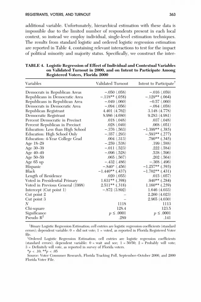
additional variable. Unfortunately, hierarchical estimation with these data isimpossible due to the limited number of respondents present in each localcontext, so instead we employ individual, single-level estimation techniques.The results from standard logistic and ordered logistic regression estimationare reported in Table 4, containing relevant interactions to test for the impactof political minority and majority status. Specifically, we construct the inter-
TABLE 4. Logistic Regression of Effect of Individual and Contextual Variableson Validated Turnout in 2000, and on Intent to Participate AmongRegistered Voters, Florida 2000
Variables Validated Turnout Intent to Participate�
Democrats in Republican Areas ).050 (.058) ).016 (.059)Republicans in Democratic Area ).118** (.058) ).129** (.064)Republicans in Republican Area ).049 (.060) )0.57 (.060)Democrats in Democratic Area ).094 (.056) ).084 (.058)Republican Registrant 4.401 (4.762) 3.148 (4.778)Democratic Registrant 8.986 (4.680) 9.283 (4.981)Percent Democratic in Precinct .018 (.048) .037 (.048)Percent Republican in Precinct .028 (.049) .068 (.051)Education: Less than High School ).376 (.563) )1.399** (.385)Education: High School Only ).357 (.293) ).593** (.277)Education: 4-Year College Grad .004 (.313) .790** (.345)Age 18–29 ).259 (.538) .199 (.588)Age 30–39 ).011 (.523) .222 (.584)Age 40–49 ).096 (.528) .538 (.596)Age 50–59 .065 (.567) .202 (.564)Age 65 up ).432 (.486) ).368 (.496)Hispanic ).840* (.456) )1.257** (.593)Black )1.440** (.437) )1.702** (.431)Length of Residence .020 (.055) .015 (.057)Voted in Presidential Primary 1.631** (.398) .940** (.284)Voted in Previous General (1998) 2.511** (.318) 1.160** (.259)Intercept (Cut point 1) ).872 (3.892) 1.646 (4.033)Cut point 2 – 2.260 (4.023)Cut point 3 – 2.965 (4.030)N 1118 1113Chi-square 128.4 123.5Significance p £ .0001 p £ .0001Pseudo R2 .289 .141
zBinary Logistic Regression Estimation; cell entries are logistic regression coefficients (standarderrors); dependent variable: 0 = did not vote; 1 = voted, as reported in Florida Registered Voterfile.yOrdered Logistic Regression Estimation; cell entries are logistic regression coefficients
(standard errors); dependent variable: 0 = wait and see; 1 = 50/50; 2 = Probably will vote;3 = Definitely will vote, as reported in survey of Florida voters.*p < .10; **p < .05Source: Voter Consumer Research, Florida Tracking Poll, September–October 2000, and 2000
Florida Voter File.
363REGISTRANTS, VOTERS, AND TURNOUT

actions by multiplying individual Republican (Democratic) party identificationby both the Democratic and Republican percentage of registered voters in theprecinct. Independents are the excluded baseline for comparison. Fourinteractions are evaluated in the models presented in Table 4: Republicans inRepublican settings, Republicans in Democratic settings, Democrats inRepublican settings, and Democrats in Democratic settings.
In spite of the limited variation offered by our dependent variable, we findthat one principal neighborhood effect remains statistically significant andsubstantively strong. The relevant probability calculations from the coeffi-cients in Table 4 reveal that—controlling for individual education lev-els—Republicans are 24% less likely to vote if they live in neighborhoods thatare one standard deviation above the mean level of Democratic composition,compared to the turnout of those at the mean. That the interaction of GOPparty registration and Democratic neighborhood dominance remains statisti-cally significant in spite of controls for education and age suggests that theresults from the hierarchical estimation are not spurious. And perhaps weshould not be so surprised because a recent study aimed at understandingcontextual effects in British elections found that neighborhood effects wereamong the strongest influences on party choice, controlling for individualcharacteristics including educational attainment, personal financial situationand household income (Johnston, et al., 2004; see also: Rolfe, 2004). Themoral of the story is a geographic one: otherwise similar people vote differ-ently in dissimilar places.
The other indicators of partisan context are statistically insignificant,although one could easily argue they are also substantively noteworthy. We donot detail these substantive effects here, but our calculations based on theprobability of voting at various high and low values of these variables indicate avast gulf in the tendency to vote resulting from the partisan character ofneighborhoods in combination with the partisanship of individuals. Becauseall four of the interactions capturing partisan context and party registration arenegatively signed, it strongly suggests that two kinds of neighborhoods mightpotentially damage turnout: (1) those where partisans find themselves in anoverwhelming majority, and (2) those where partisans find themselves in asimilarly lopsided minority. These results square with recent evidence thatevenly divided partisan environments produce higher levels of politicalknowledge and efficacy than one-sided ones (Gimpel et al., 2003).
The results using respondents’ self-reported likelihood of participationexhibit the same pattern (see the second column of Table 4), though withgreater statistical significance due to the enhanced variation of the dependentvariable. Among the interactions for context and partisanship, Republicansliving in heavily Democratic neighborhoods are least likely to say they intendto vote. In this model, the education variables are statistically significant and inthe expected direction, with those having a college degree exhibiting much
364 GIMPEL ET AL.

greater certainty that they will vote than those with less than a high schooleducation. The vote history variables are by far the most important explana-tions of participation here, as they are in Tables 1–3. Their presenceundoubtedly produces a conservative estimate of the statistical significance oftraditional factors such as education, and even context, in explaining validatedturnout.
DISCUSSION
These investigations yield a number of intriguing insights. Some of therelationships identified here we can expect to see repeated across a variety oflocations. Others need to be evaluated on a case-by-case basis. Either way,there are valuable lessons here for both political scientists and strategists whothink about how to get out the vote.
On the Republican side of the ledger, two findings seem generally appli-cable. First, the results from Tables 1–3 indicate that Republicans wouldgreatly benefit if they were to target voters living in neighborhoods of highresidential mobility. Second, Republicans also appear to have serious turnoutproblems in many Democratically-inclined neighborhoods, even after wecontrol for the education level of these neighborhoods. Perhaps surprisingly,GOP losses in lopsided Democratic areas are not necessarily offset by poorDemocratic performance in Republican locations. Bolstering the impressionthat Republicans have problems turning out their own registrants on enemyturf is the finding that Republicans are especially unlikely to vote when theylive in neighborhoods reporting lower education levels (this occurred in eightof the fourteen locations we examined in Tables 1–3). Presumably, thesevoters include ‘‘hard-hats,’’ ‘‘NASCAR-dads,’’ and white ethnics—workingclass Republicans who do not live and breathe politics, and may not voteunless reminded.
Why is GOP turnout depressed in heavily Democratic areas, but Demo-cratic turnout is not as affected by Republican dominance? A couple ofexplanations come to mind. First, many of our locations are in cities ormetropolitan areas where Democrats are the dominant party. Given thatindividuals are part of more than one context, Democrats may be in theminority in their immediate neighborhood, but realize that they are part of ameaningful local majority. Republicans, conversely, might be more sensitive toneighborhood context because they realize they are a decided minority in boththeir neighborhood and the broader metropolitan area or city. In this manner,our results parallel those of Ada Finifter’s (1974) famous study of Detroitfactory workers, in which adherents of the minority party were sensitive to thepartisan orientation of their closest associates, whereas majority partisans werenot (see also Gimpel et al., 2003).
365REGISTRANTS, VOTERS, AND TURNOUT

A second explanation is that Republicans are more widely scattered acrossthe metropolitan landscape, landing them in places with more widely varyingpolitical distributions. In particular, we notice that lopsided Republicanneighborhoods are considerably less lopsided than the most lopsided Demo-cratic neighborhoods. It is not uncommon to find Democratic neighborhoodsthat are over 95% Democratic, whereas Republican neighborhoods usually topout in the 65–75% range. Even in Chester County, Pennsylvania—probablythe most Republican location we studied—only one precinct showed as muchas 76% GOP registration. Generally, Democrats are more geographicallyconcentrated and are therefore less likely to be found living among Repub-lican majorities. And when they do live among Republicans, these GOPmajorities are not as one-sided as the Democratic majorities in whichRepublicans are sometimes situated. Along these lines, higher Democraticturnout in the midst of Republican majorities may signal that these Democratsare really living in areas that remain substantially diverse (and competitive)because their Republican tendencies are not overwhelming. A study of ruraland suburban locations where local Republican majorities are more lopsidedwould undoubtedly round out the research we have begun here.
A third possibility is that low turnout among local partisan minorities (espe-cially Republicans) is because party organizations did not reach out to like-minded partisans residing in enemy territory. If the parties (especially theRepublicans) did contact them, and these voters did not show up at the polls, weneed to revise our thinking. Bear in mind that this would not change our argu-ment that context affects turnout. Rather, it would cause us to re-think thenature of this relationship. Initially, we would have to alter our political infor-mation flow argument to exclude the idea that this reduced information flowincludes diminished party contacting. We would also reverse our position thatcandidates and parties ought to target their partisans in opposition strongholds.Based on our examination of contacting information from the voter files, how-ever, we see little reason to believe that campaign contacting was extensive orconsistent for partisans in politically hostile neighborhoods in 2000. Thisimpression is augmented by personal interviews with Donnie Fowler of theDemocratic National Committee and Matthew Dowd of the Bush-Cheneycampaign, both of whom indicated that many partisans residing in voting pre-cincts dominated by partisans from the other side were not contacted in 2000.15
From the Democratic perspective, there is the over-riding problem of theturnout gap. Democrats mobilize fewer of their registrants than Republicansin nearly every battleground location. Aside from that familiar finding, theDemocratic turnout picture is a mixed bag. In heavily African Americanneighborhoods, where they have an impressive base of voters, Democratsshow no inclination toward high turnout. In fact, they have lower turnout ratesin places such as suburban Philadelphia. The same is true in heavily Hispanicneighborhoods. Democrats did especially poorly in Latino neighborhoods in
366 GIMPEL ET AL.

the Philadelphia suburbs and in Las Vegas. Similarly, while Democratsmanage to avoid the consistent losses that Republicans face in areas of highin-migration, this may well be due to the fact that most new migrants areRepublicans (Gimpel, 1999; Gimpel and Schuknecht, 2001), not becauseDemocrats are adept at mobilizing the new arrivals. More generally, the resultsshown in Tables 1–3 demonstrate that Democrats do experience more turnoutvariability across locations, which makes it difficult to build a general modelupon which the party could base strategic decisions. The upshot is that Dem-ocratic strategists would be wise to work on a case-by-case (or list-by-list) basisas they identify neighborhoods and partisan subgroups requiring attention.
Of course, one might reasonably consider explanations of the partisanresults and prescriptions for strategists premature given the possibility that wehave the causal arrow backwards. In other words, is it possible that onlypolitically inactive partisans move to hostile political environments? Mightthere be politically motivated ‘‘selection effects’’ with respect to where citizenschoose to live? This possibility would, in fact, lead us to be skeptical aboutreaching out to individuals who choose to reside among the enemy. Thisalternative explanation, however, makes little theoretical sense. People do notgo out of their way to choose neighbors or networks of associates on the basisof turnout or partisanship because these facts about a person or neighborhoodare almost never apprehended in advance (Mutz, 2002, p. 845). It is possiblethat some unmeasured third factor is causing both the demobilization of theseminority partisans and their residence in hostile political environments, butrelated research has ruled out many of the most obvious, plausible explana-tions (Mutz, 2002, p. 845). In Table 4, for example, we provide evidence thatindividual-level education is not producing the results shown in Tables 1–3.
Setting aside the broader question of causality and the aforementionedparty-centered findings, a handful of other results seem to hold across mostlocations. Young people remain one of the most consistent turnout weaknessesfor both parties. There were, however, at least a couple of locations where theirparticipation was unusually high in 2000: Montgomery County, Pennsylvania,and Louisville, Kentucky. These areas may be worth further examination todetermine what went right. Perhaps particularly vigorous mobilization effortssucceeded in targeting youth at these locations. Generally, though, it might bewise for candidates and parties to focus much more attention on socializingyoung voters into the habits of citizenship (Plutzer, 2002).
We take penultimate note of the impressive explanatory power of the votehistory items from the voter lists. The vote history available in the voter files iscritical because it allows us to focus our attention not on the most regularvoters (who are highly likely to turn out in a presidential election), but ratheron the least reliable voters. The failure to make such basic distinctionsbetween regular and occasional voters condemns campaign strategies tospending time and money on voters who, at best, may appreciate the phone
367REGISTRANTS, VOTERS, AND TURNOUT
call or extra piece of mail, but will not be influenced to vote by either. Byincluding the vote history items in our models, we can learn more about whatmotivates the legions of irregular voters to participate or abstain on ElectionDay. Perhaps the centralization of political party activity that has occurredover the last 75 years has been detrimental to mobilization precisely because ithas stripped mobilization efforts of the local knowledge they required to trulysucceed. At least some of that local knowledge can be recovered throughcareful study of the voter lists as we have outlined here.
Practical lessons, however, should not obscure the broader implication ofour research for the study of voting. For starters, we examine the impact ofindividual characteristics on participation, controlling for recent vote history(a measure of habitual voting), something not always accounted for in previouswork. Treating the habitual aspect of voting as an independent variable isvaluable because our estimates indicate that the impact of individual char-acteristics may be exaggerated, or misunderstood. We also acknowledge thatpartisan differences, derived from the parties’ coalitional bases, may manifestthemselves in unique residential patterns and, as a result, turnout dynamics.More generally, our research aims at advancing an understanding of politicalbehavior anchored in the study of individuals in their social environments.Although it is pedagogically easier to gloss over local nuances in politicalbehavior, even the most basic political decisions remain expressive of localcontextual circumstances, even in elections where national offices are at stake.Since local contexts do matter, it can be risky for political scientists or cam-paign strategists to base their understanding of a local electorate upon studiescarried out at a different location or based on overly general national polls.
APPENDIX
A traditional HLM, where the expected outcome is modeled as a linearfunction of the regression coefficients and random effects at each level, isinappropriate for our application given that our dependent variable is binary(1 ¼ voted, 0 ¼ did not vote).16 In the HLM framework, the regressionparameters (intercepts and slopes) may vary across neighborhoods (dependingupon theoretical expectations) and the level two variables can be used topredict this variation in both the intercept and the regression coefficients. Thelevel-one model17 can be written as:
Turn outij ¼ b0j þ b1jðDemocratÞij þ b2jðRepublicanÞij þ b3jðFemaleÞijþ b4jðAge 18 � 29Þij þ b5jðAge 30 � 39Þij þ b6jðAge 40 � 49Þijþ b7jð Age 50 � 59Þij þ b8jðAge 65upÞijþ b9jð2000 Primary VoterÞij þ b10jð1998 General VoterÞij þ rij
ð1Þ
368 GIMPEL ET AL.

Where i is the individual and j is the neighborhood and rij represents theresidual for individual i within neighborhood j. The subscript j permits eachneighborhood to have a unique slope for each independent variable’s effect onturnout, contingent upon the predictors and stochastic error at level two. Notebelow that we do not estimate the variability of the intercept, age, and votehistory variables across neighborhoods with level two predictors, although wedo evaluate their variability across contexts.
At level two, we model three of the logistic regression coefficients from thewithin-unit model in equation 1 as dependent variables. We examine variationacross these level one coefficients as follows:
b1jðDemocratÞij ¼ c10 þ c11ð% EducationÞj þ c12ð% RepublicanÞjþ c13ð% MigrationÞj þ c14ð% BlackÞj þ c15ð% HispanicÞjþ u1j ð2Þ
TABLE A. 1. Level One and Two Variables in the Hierarchical Analysis
Variables Measure
Level oneVoted in 2000 GeneralElection
0 = did not vote, 1 = voted
Republican Registrant 0 = Other (Non-Republican), 1 = RepublicanDemocratic Registrant 0 = Other (Non-Democrat), 1 = DemocratSex of Registrant 0 = male, 1 = femaleAge 18–29 0 = older than 18–29, 1 = in Age 18–29 groupAge 30–39 0 = other than 30–39, 1 = in Age 30–39 groupAge 40–49 0 = other than 40–49, 1 = in Age 40–49 groupAge 50–59 0 = other than 50–59, 1 = in Age 50–59 groupAge 65 up 0 = younger than age 65, 1 = Age 65 or olderPrimary Voter 0 = did not vote in primary, 1 = did vote in 2000
primaryGeneral Election 98 Voter 0 = did not vote in 1998, 1 = did vote in 1998 general
Level TwoPercent Republicany Percentage of Republican Registrants Aggregated
to PrecinctPercent Democraticz Percentage of Democrats Aggregated to PrecinctMedian Income Median Income of Census TractPercent College Percent of Residents with 4-Year Degree or More
in Census TractPercent Black Percent of African American in Census TractPercent Hispanic Percent Hispanic/Latinos in Census TractPercent Migrants Percent Migrants from Other States in Last Five
Years in Tract?
Level one variables come from the voter list files from each county.y Level two variables are from U.S. Census 2000 except as noted.z These level two variables were formulated by aggregating level one information to voterprecinct boundaries.
369REGISTRANTS, VOTERS, AND TURNOUT
b2jRepublicanij ¼ c20 þ c21ð% EducationÞj þ c22ð% DemocraticÞjþ c23ð% MigrationÞj þ c24ð% BlackÞj þ c25ð% HispanicÞjþ u2j: ð3Þ
The remaining coefficients for age cohorts and vote history in the level onemodel are treated as randomly variable, including an intercept, but withoutspecifying additional level two predictor variables:
b3j...b10j ¼ c30...100 þ u3j...10j ð4Þ
Equation 2 assesses the extent to which these various neighborhood char-acteristics ðc10 � c16Þ moderate the relationship between Democratic iden-tification and turnout. b1j represents the difference in the log-odds of votingbetween Democrats and non-Democrats. Equation 3 does the same for therelationship between Republican identification and turnout, with b2j esti-mating the difference in the log-odds of voting between Republicans andnon-Republicans. Finally, Equation 4 estimates the mean values for thegender, age cohort, and vote history variables across all neighborhoods,allowing us to examine the heterogeneity of variance in these coefficients.The great advantage of HGLM over traditional regression estimation is thatthe error at both the individual and contextual levels is accounted for and wetherefore avoid the problem with single level estimation of neighborhoodeffects—an underestimation of the standard errors and likely biasing of thecoefficients.
As indicated earlier, because of the intense computational resourcesrequired for estimating models based on the entire voter list for each county,we drew random samples from each list. All told, we selected 20% of availablenames from the counties, leaving sample cases to permit highly confidentgeneralization within and across neighborhoods. Missing data were treatedwith pairwise deletion at the voter level and listwise deletion at the aggregatelevel.
Estimates were generated for all of the models using quasi-likelihood esti-mation, also described as penalized quasi-likelihood (PQL), in the relevant lit-erature (Raudenbush and Bryk, 2002, pp. 457–459), and are presented inTables 1–3. We present unit-specific results that emphasize how the effects ofneighborhood characteristics influence the level one relationships. We do notpresent population average results, which provide no indication of thedistribution of outcomes across level two units (Bryk and Raudenbush, 2002, pp.303–304).
370 GIMPEL ET AL.

NOTES
1. See Stephen Dinan, ‘‘GOP ‘Ground Game’ is Getting Out Vote,’’ Washington Times, January5, 2003; Staff writers, ‘‘Close Election Turns on Voter Turnout,’’ Washington Post. November1, 2002.
2. Generally, the effect of education level on participation is greater than the effect ofincome.
3. As is discussed later, education and income are so highly correlated that it did not make sensefor us to include both among the level-2 indicators.
4. Based on the authors’ email exchanges (June 2001) with Donnie Fowler, National Field Chairfor Gore-Lieberman, and in person interview (February 2001) with Matthew Dowd, seniorstrategist for Bush-Cheney.
5. Although Kentucky, Nevada, and North Carolina were reasonably competitive in 2000, nonereceived the attention lavished on true battleground states, such as Florida. It is also the casethat Voter list data were much less rich in one-sided states, such as Massachusetts andUtah.
6. The 10% deficit is due mainly to P.O. Box addresses and Rural Route addresses that could notbe assigned to a specific street range.
7. For businesses that engage in mass mailing, the NCOA service helps reduce undeliverable-as-addressed mail by correcting input addresses prior to mailing, or by returning a ‘‘nixie’’ codefor those addresses that are no longer valid. For our purposes, it serves to eliminate thosevoters who have moved out of a jurisdiction and are no longer eligible to vote in the locationwhere they were once registered.
8. Another limitation of voter lists is that we can only analyze neighborhood and contextual effectsamong registered voters. We assume the dynamics uncovered here should also apply to themobilization of unregistered voters. The main difference, of course, is that party-basedmobilization of non-registrants requires both registering them and turning them out on ElectionDay.
9. A few Southern states also identify the race of the registrant, although we do not examineindividual-level racial information in this paper.
10. The interviews were conducted by Voter Consumer Research and Market Strategies, Inc. onbehalf of Bush-Cheney 2000. The survey dates were September 24–28, October 1–5, 8–12,15–19, and 22–25. Approximately 150 registered voters were interviewed every evening. Thetrial ballot result for the cumulative file is 41.0% Bush, 41.1% Gore.
11. ‘‘independent’’ is defined here in the broad sense of a non-Republican or non-Democrat, someof these registrants could be third-party identifiers as well as those who registered as inde-pendents.
12. Income was not available on the survey, but we did not include it in Tables 1–3 either. Ourgoal with the survey is to validate the effect of partisan context, using substantially similarmodels, controlling for the individual level education of respondents.
13. This is a higher percentage than among registered voters on the voter files, which usually ran inthe 67–80% range for the Florida locations we studied. This high level of response by thosesurveyed raises the intriguing possibility that the survey itself had the impact of mobilizingthose who responded.
14. The models of participation likelihood are estimated using an ordered logit procedure on thefour-fold scale offered in the survey. See Table 4 for details.
15. Admittedly, the data on party outreach efforts available in the voter files is sketchy. Emailexchange with Donnie Fowler, June 2001. In-person interview with Matthew Dowd, February2001.
16. This model is discussed in Chapter 10 of Raudenbush and Bryk (2002).17. All level-one predictors are dichotomously coded dummy variables.
371REGISTRANTS, VOTERS, AND TURNOUT

REFERENCES
Adams, William C., and Smith, Dennis J. (1980). Effects of telephone canvassingon turnout and Preferences: a field experiment. Public Opinion Quarterly 44:389–395.
Baybeck, Brady, and McClurg, Scott D (2004). What do they know and how do theyknow it? An examination of citizen awareness of context. University of Missouri, St.Louis, Unpublished ms.
Beck, Paul Allen, Dalton, Russell J., Greene, Steven, and Huckfeldt, Robert. (2002).The social calculus of voting: interpersonal, media and organizational influences onpresidential choices. American Political Science Review 96: 75–90.
Berelson, Bernard R., Lazarsfeld, Paul F., and McPhee, William N. (1954). Voting: AStudy of Opinion Formation in a Presidential Campaign. Chicago: University ofChicago Press.
Bobo, Lawrence, and Gilliam, Franklin D. Jr. (1990). Race, sociopolitical participationand black empowerment. American Political Science Review 84: 377–393.
Bullock, Charles S. III, and Shafer, David J. (1997). Party targeting and electoralsuccess. Legislative Studies Quarterly 22: 573–584.
Campbell, Angus (1960). Surge and Decline: a study of electoral change. PublicOpinion Quarterly 24: 397–418
Campbell, Angus, Converse, Phillip E., Miller, Warren E., and Stokes, Donald E.(1960). The American Voter. New York: John Wiley and Sons.
Campbell, James E. (1993). Congressional Elections: The Presidential Pulse. Lexington:The University Press of Kentucky.
Citrin, Jack, Shickler, Eric, and Sides, John (2003). What if everyone voted? Simulatingthe impact of increased turnout in senate elections. American Journal of PoliticalScience 47: 75–90.
Cohen, Cathy, and Dawson, Michael (1993). Neighborhood poverty and AfricanAmerican politics American Political Science Review 87: 286–302.
DeNardo, James (1980). Turnout and the vote: The Joke’s on the democrats. AmericanPolitical Science Review 74: 406–420.
DeNardo, James (1986). Does Heavy turnout help democrats in presidential elections?American Political Science Review 80: 1298–1304.
Eulau, Heniz, and Rothenburg, Lawrence (1986). Life space and social networks aspolitical contexts. Political Behavior 8: 130–157.
Finifter, Ada (1974). The friendship group as a protective environment for politicaldeviants. American Political Science Review 68: 607–625.
Freedman, Paul, and Goldstein, Kenneth M. (1999). Measuring media exposure and theeffects of negative campaign ads. American journal of political Science 43: 1189–1208.
Goldstein Kenneth M., and Freedman, Paul (2002). Campaign advertising and voterturnout: new evidence for a stimulation effect. Journal of Politics 64: 721–740.
Gerber, Alan S., and Green, Donald P. (2000a). The effect of a nonpartisan get-out-the-vote drive: an experimental study of leafletting. Journal of Politics 62: 846–857.
Gerber, Alan S., and Green. Donald P. (2000b). The effects of canvassing, direct mailand telephone contact on voter turnout: A field experiment. American PoliticalScience Review 94: 653–663.
Gerber, Alan S., and Green, Donald P. (2001). Do phone calls increase voter turnout?A field experiment. Public Opinion Quarterly 65: 75–85.
Gerber, Alan S., Green, Donald P. and Ron Shachar (2003). Voting may be habitforming: evidence from a randomized field experiment. American Journal of PoliticalScience 47: 540–580.
372 GIMPEL ET AL.

Gilles Michael, and Dantico, Marilyn K. (1982). Political participation and neighbor-hood Social Context Revisited. American Journal of Political Science 26: 144–150.
Gimpel, James G. (1999). Separate Destinations: Migration, Immigration and thePolitics of Places. Ann Arbor: University of Michigan Press.
Gimpel, James G., and Schuknecht, Jason E. (2001). Interstate migration and electoralpolitics. Journal of Politics 63: 207–231.
Gimpel, James G., Lay, J. Celeste, and Schuknecht, Jason E. (2003). CultivatingDemocracy: Civic Environments and Political Socialization in America. Washington,DC: Brookings Institution Press.
Green, Donald P., Gerber, Alan S., and Nickerson, David W. (2003). Getting out thevote in local elections: results from six door-to-door canvassing experiments. Journalof Politics 65: 1083–1096.
Green, Donald P., and Smith, Jennifer K. (2003). Professionalization of campaigns andthe secret history of collective action problems. Journal of Theoretical Politics 15: 321–339.
Herrnson, Paul S. (2004). Congressional Elections, 5th edn. Washington, D.C.: Con-gressional Quarterly Press.
Highton, Benjamin (1997). Easy registration and voter turnout. Journal of Politics 59:565–575.
Highton, Benjamin, and Wolfinger, Raymond (2001). The first seven years of thepolitical lifecycle. American Journal of Political Science 45: 202–209.
Huckfeldt, R. Robert (1979). Political participation and the neighborhood social con-text. American Journal of Political Science 23: 579–592.
Huckfeldt, R. Robert (1986). Politics in Context: Assimilation and Conflict in UrbanNeighborhoods. New York: Agathon.
Huckfeldt, Robert, Plutzer, Eric, and Sprague, John (1993). Alternative contexts ofpolitical behavior: churches, neighborhoods and individuals. Journal of Politics 55:365–381.
Huckfeldt, Robert, and Sprague, John (1987). Networks in context: The social flow ofpolitical information. American Political Science Review 81: 1197–1216.
Huckfeldt, Robert, and Sprague, John (1995) Citizens, Politics and Social Communi-cation. New York: Cambridge University Press.
Humphries, Stan (2001). Who’s afraid of the big, bad firm: The impact of economicscale on political participation. American Journal of Political Science 45: 678–699.
Imai, Kosuke (2004). Do get-out-the vote calls reduce turnout? The importance ofstatistical methods for field experiments. American Political Science Review (forth-coming).
Iyengar, Shanto (1980). Subjective political efficacy as a measure of diffuse support.Public Opinion Quarterly 44: 249–256.
Jackson, Robert A. (1996). The mobilization of congressional electorates. LegislativeStudies Quarterly 21: 425–445.
Johnston, Ron, Jones, Kelvyn, Sarker, Rebecca, Propper, Carol, Burgess, Simon,and Bolster, Anne (2004). Party support and the neighborhood effect: spatialpolarisation of the British Electorate, 1991–2001. Political Geography 23(5):367–402.
Joslyn, Mark R. (1997). The public nature of personal opinion: The impact of collective.sentiment on individual appraisal. Political Behavior 19: 337–363.
Kenny, Christopher B. (1992). Political participation and effects from the socialenvironment. American Journal of Political Science 36: 259–267.
Krassa, Michael A. (1988). Context and the canvass: the mechanisms of interaction.Political Behavior 10: 233–246.
373REGISTRANTS, VOTERS, AND TURNOUT
Lazarsfeld, Paul F., Berelson, Bernard R., and Gaudet, Hazel (1944). The People’sChoice. New York: Duell, Sloan and Pearce.
Lee, Valerie, and Bryk, Anthony S. (1989). A multilevel model of the social distributionof high school achievement. Sociology of Education 63: 172–192.
Leighley, Jan E. (1995). Attitudes, opportunities and incentives: a field essay onpolitical participation. Political Research Quarterly 48: 181–209.
Malchow, Hal (2003). The New Political Targeting. Washington, DC: Campaigns &Elections Magazine.
Mutz, Diana (2002). The consequences of cross-cutting networks for political partici-pation. American Journal of Political Science 46: 838–855.
Noelle-Neumann, Elisabeth (1993). The Spiral of Silence: Public Opinion – Our SocialSkin. Chicago: University of Chicago Press.
Plutzer, Eric (2002). Becoming a habitual voter: inertia, resources and growth in youngadulthood. American Political Science Review 96: 41–56.
Powell, G. Bingham (l986). American voter turnout in comparative perspective.American Political Science Review 80: 17–43.
Raudenbush, Stephen W., and Bhumirat, Chinnapat (1992). The distribution ofresources for primary education and its consequences for education achievement inThailand. International Journal of Educational Research 143–164.
Raudenbush, Stephen W., and Bryk, Anthony S. (1986). A hierarchical model forstudying school effects. Sociology of Education 59: 1–17.
Raudenbush, Stephen W., and Bryk, Anthony S. (2002). Hierarchical Linear Models:Applications and Data Analysis Methods. Thousand Oaks, CA: Sage.
Rolfe Meredith (2004). Taking social structure seriously: education and voter turnout.Paper presented at the annual meeting of the Midwest Political Science Association,Chicago, IL, April 14–16.
Rosenstone, Steven J., and Hansen, John Mark (1993). Mobilization, Participation andDemocracy in America. New York: Macmillan.
Salmore, Barbara G., and Salmore, Stephen A. (1989). Candidates, Parties, andCampaigns: Electoral Politics in America, 2nd edn. Washington, DC CongressionalQuarterly Press.
Sapiro, Virginia, and Conover, Pamela Johnston (1997). The variable gender bias ofelectoral politics: Gender and Context in the 1992 U.S. Election. British Journal ofPolitical Science 27: 497–523.
Schlozman, Kay Lehman, Burns, Nancy, and Verba, Sidney (1994) Gender and thepathways to participation: the role of resources. Journal of Politics 56: 963–990.
Shaw, Catherine M., and Holstein, Michael E. (1999). The Campaign Manager:Running and Winning Local Elections, 2nd edn. Boulder: Westview Press.
Shaw, Daron R., de la Garza, Rodolfo, and Lee, Jongho (2000). Estimating latinoturnout in 1996: a three-State, validated survey approach. American Journal ofPolitical Science 44: 338–346.
Shea, Daniel M., and Burton, John (2001). Campaign Craft: The Strategies, Tactics andArt of Political Campaign Management. Westport, CT: Praeger.
Simpson, Dick. (1996). Winning Elections: A Handbook of Modern Participatory Pol-itics. New York: HarperCollins.
Squire, Pervill, Wolfinger, Raymond E., and Glass, David P. (1987). Residentialmobility and voter turnout. American Political Science Review 81: 45–65.
Straits, Bruce C. (1990). The social context of voter turnout. Public Opinion Quarterly54: 64–73.
Steenbergen, Marco R., and Jones, Bradford S. (2002). Modeling multilevel datastructures. American Journal of Political Science 46: 218–237.
374 GIMPEL ET AL.
Stoker, Laura and Jennings, M. Kent (1995). Life-cycle transitions and political par-ticipation: the case of marriage. The American Political Science Review 89: 421–433.
Timpone, Richard J. (1998). Structure, behavior and vote turnout in the United States.American Political Science Review 92: 145–158.
Traugott, Michael W., and Goldenberg, Edie N. (1984). Campaigning for Congress.Washington, DC: Congressional Quarterly.
Verba, Sidney, and Norman Nie H. (1972). Participation in America: PoliticalDemocracy and, Social Equalty. New York: Harper & Row.
Verba, Sidney, Burns, Nancy, and Schlozman, Kay Lehman (1997). Knowing and caringabout politics: gender and political engagement. Journal of Politics 59: 1051–1072.
Wielhouwer, Peter W. (2003). In search of Lincoln’s perfect list: targeting in grassrootscampaigns. American Politics Research 31: 632–669.
Weissberg, Robert (1975). Political efficacy and political illusion. Journal of Politics 37:469–487.
Wolfinger, Raymond E. and Steven J. Rosentone (1980). Who Votes? New Haven: YaleUniversity Press.
Zipp, John F., and Smith, Joel (1979). The structure of electoral political participation.American Journal of Sociology 85: 167–177.
375REGISTRANTS, VOTERS, AND TURNOUT