DECEMBER 2009 #3 Properties of Weighted Least Squares Regression for Cutoff Sampling in Establishment Surveys by James R. Knaub, Jr.

file:////eianas01/...ression%20for%20Cutoff%20Sampling%20in%20Establishment%20Surveys%20by%20James%20R.%20Knaub,%20Jr..htm[4/9/2014 5:42:35 PM]

Properties of Weighted Least Squares Regression for Cutoff Sampling inEstablishment Surveys

by James R. Knaub, Jr.

Abstract:Ordinary least squares (OLS) regression gets most of the attention in the statistical literature, but for cases ofregression through the origin, say for use with skewed establishment survey data, weighted least squares (WLS)regression is needed. Here will be gathered some information on properties of weighted least squares regression,particularly with regard to regression through the origin for establishment survey data, for use in periodic publications.

Key Words: classical ratio estimator; coefficient of heteroscedasticity; model-based estimation; regression through theorigin; regression weights; sample; survey

Author:James R. Knaub, Jr., James.Knaub@eia.doe.gov

Editor:Richard G. Graf, rgraf@sunstroke.sdsu.edu

NOTE: This article was revised on November 25, 2013.

READING THE ARTICLE: You can read the article in portable document (.pdf) format (345515 bytes.)

NOTE: The content of this article is the intellectual property of the authors, who retains all rights to futurepublication.

This page has been accessed 2842 times since December 22, 2009.

Return to the Home Page.

Corrections made on 5/19/2016 to Section 4 title: "Confidence Limits about y-values" changed to "Prediction Intervals about predicted y-values"- and "confidence" changed to "prediction"elsewhere as well.

Properties of Weighted Least Squares Regression for Cutoff Sampling in Establishment Surveys James R. Knaub, Jr., Energy Information Administration1

Abstract: Ordinary least squares (OLS) regression gets most of the attention in the statistical literature, but for cases of regression through the origin, say for use with skewed establishment survey data, weighted least squares (WLS) regression is needed. Here will be gathered some information on properties of weighted least squares regression, particularly with regard to regression through the origin for establishment survey data, for use in periodic publications.

Key words: classical ratio estimator; coefficient of heteroscedasticity; model-based estimation; regression through the origin; regression weights; sample; survey

1. Introduction:From Knaub(2007a) we see that homoscedasticity refers to a constant variance regardlessas to placement of a point on a scatterplot graph. Generally, however, the variance for y,given y as a function of one or more regressors in a matrix x, increases for any increasingregressor xji, especially for regression through the origin, for nonnegative numbers. Thisshould apply to regressions through the collected data points (xi,y=f(xi)+ei), for any regressor j, for a one-regressor ratio model, or even through (xj,y=f(x)+e). For multiple regression in many establishment survey applications, we may use heteroscedastic ratio estimators to study residuals through the points (f(x),y).

For an example of an intuitive ratio estimate, consider the classical ratio estimator (CRE) which is found for one regressor, for (x,y), by summing the y-values and dividing by the sum of the x-values to obtain a factor to be multiplied by other x-values to estimate unknown y-values. When x and y are from a past census and a current sample, correspondingly, for the same data element, say sales of electricity, then the relating “factor” could be considered a “growth factor.” This inherently assumes a given degree of heteroscedasticity in which the variance of y increases proportionately with increased values of x. For regression through the origin, this degree of heteroscedasticity or more should always be the case, but data quality concerns for the smaller respondents can make this problematic. (See Knaub(2002, 2008).) For more on the CRE, see Knaub(2005).

For regression through the origin with one regressor, we have ,

where the estimated residual, , or written as the product of a random and

a systematic or nonrandom factor . Brewer(2002) notes the importance of

2/1/0 iiii webxy

2/1/0 iii wee

0 iii wee 5.0

1 Disclaimer: The views expressed are those of the author, and are not official US Energy Information Administration positions unless claimed to be in an official US Government document.

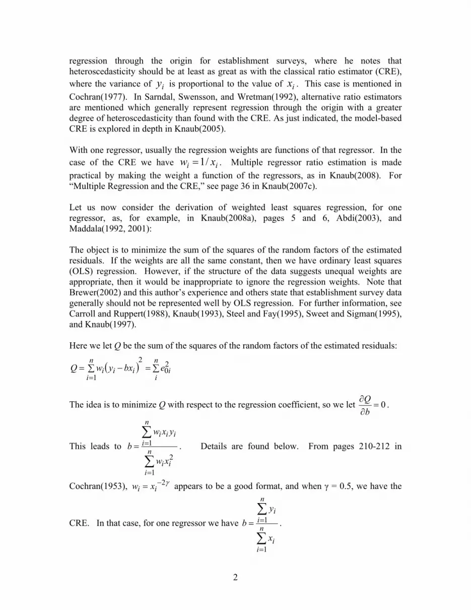
regression through the origin for establishment surveys, where he notes that heteroscedasticity should be at least as great as with the classical ratio estimator (CRE), where the variance of is proportional to the value of . This case is mentioned in

Cochran(1977). In Sarndal, Swensson, and Wretman(1992), alternative ratio estimators are mentioned which generally represent regression through the origin with a greater degree of heteroscedasticity than found with the CRE. As just indicated, the model-based CRE is explored in depth in Knaub(2005).

iy ix

With one regressor, usually the regression weights are functions of that regressor. In the case of the CRE we have ii xw /1 . Multiple regressor ratio estimation is made

practical by making the weight a function of the regressors, as in Knaub(2008). For “Multiple Regression and the CRE,” see page 36 in Knaub(2007c).

Let us now consider the derivation of weighted least squares regression, for one regressor, as, for example, in Knaub(2008a), pages 5 and 6, Abdi(2003), and Maddala(1992, 2001):

The object is to minimize the sum of the squares of the random factors of the estimated residuals. If the weights are all the same constant, then we have ordinary least squares (OLS) regression. However, if the structure of the data suggests unequal weights are appropriate, then it would be inappropriate to ignore the regression weights. Note that Brewer(2002) and this author’s experience and others state that establishment survey data generally should not be represented well by OLS regression. For further information, see Carroll and Ruppert(1988), Knaub(1993), Steel and Fay(1995), Sweet and Sigman(1995), and Knaub(1997).

Here we let Q be the sum of the squares of the random factors of the estimated residuals:

in

iiii bxywQ

2

1n

ie20

The idea is to minimize Q with respect to the regression coefficient, so we let 0

bQ

.

This leads to

n

iii

ii

xw

xw

12

ix

n

iiy

b2

1 . Details are found below. From pages 210-212 in

Cochran(1953), appears to be a good format, and when γ = 0.5, we have the

CRE. In that case, for one regressor we have

iw

n

ii

n

ii

x

yb

1

1 .

2

The sections to follow are arranged in an attempt at a logical progression. Section 2 is a basic derivation of a coefficient for a model-based ratio estimate, available many places, but included here as a way of further introducing the topics to follow. Section 3 is a comment on the philosophy of using WLS regression. In section 4 the reader will find remarks on scatterplots for the data used in a regression model and the nature of prediction bands about regression lines through those points. Section 5 contains notes on variance leading to the estimation of variance for estimated totals from a finite population, and section 6 is an aside on estimating those variances when only a lump sum is available for regressor data not corresponding to the sample units. In sections 7 and 8, alternatives are given for the derivation of the variance of prediction errors and for regression weight formats, respectively. Section 9 is with regard to the estimation of variance of total for a finite population, when incorrectly assuming OLS or other some other incorrect degree of heteroscedasticity. Section 10 provides a final comment, and an extensive reference list and bibliography are provided.

2. Derivation of coefficient for single regressor for WLS with zero intercept:

This covers a broad class of ratio estimates, as shown in Sarndal, Swensson, and Wretman(1992), pages 255 through 258, section 7.3.4, which includes the CRE. This is shown in Knaub(2008), and given here for completeness and convenience as a reference. Also see Abdi(2003) and elsewhere.

Let Q be the sum of squares of the weighted residuals, as shown above.

n

ii

n

iiii ebxywQ 2

0

2

1 and set 0

bQ

If then we have 2

1

50 .

n

iiii bxywQ

50

1

50 .)(.20 ii

n

iiii wxbxyw

bQ

Then so , and therefore, 0)(1

n

iiiii bxywx i

n

ii

n

iiii wxbywx

1

2

1

3

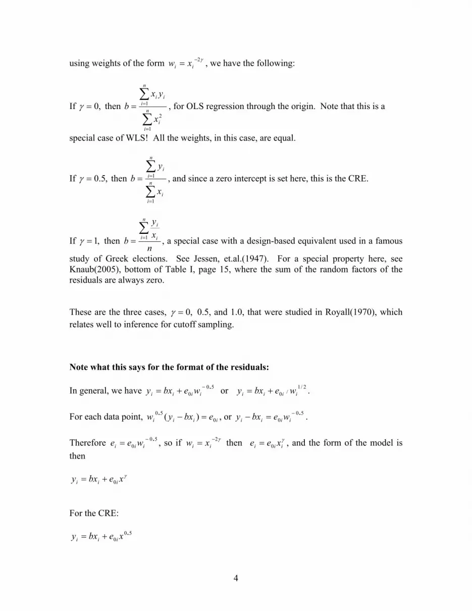
using weights of the form , we have the following: 2 ii xw

,0If then

n

ii

n

iii

x

yxb

1

2

1 , for OLS regression through the origin. Note that this is a

special case of WLS! All the weights, in this case, are equal.

If ,5.0 then

n

ii

n

ii

x

yb

1

1 , and since a zero intercept is set here, this is the CRE.

If ,1 then nxy

b

n

i i

i 1 , a special case with a design-based equivalent used in a famous

study of Greek elections. See Jessen, et.al.(1947). For a special property here, see Knaub(2005), bottom of Table I, page 15, where the sum of the random factors of the residuals are always zero.

These are the three cases, ,0 0.5, and 1.0, that were studied in Royall(1970), which relates well to inference for cutoff sampling.

Note what this says for the format of the residuals:

In general, we have or . 500

. iiii webxy 2/1/0 iiii webxy

For each data point, , or . iiii ebxyw 050 )(. 50

0. iiii webxy

Therefore , so if then , and the form of the model is

then

500

. iii wee 2 ii xw iii xee 0

xebxy iii 0

For the CRE:

500

.xebxy iii

4

3. The Nature of Weighted Least Squares (WLS) Regression:

“All horses are animals, but not all animals are horses.” (Socrates) - Analogously, all ordinary least squares (OLS) regressions are weighted least squares (WLS) regressions, but not all WLS regressions are OLS. That is, OLS regression is a special case of WLS regression. Many may use OLS as a default, and in some applications that might be good enough, but just because we do not know what weights are appropriate, it does not mean that one avoids assigning weights by using OLS, because we are de facto claiming that the weights are equal. That, in fact, is a very decisive assignment of weights. For establishment surveys, that is not a good assumption. See Brewer(2002). When we use regression through the origin, the strong weight assumption implicit in OLS regression is likely to be a highly faulty assumption.

An example of this confusion, from NIST(2009), a generally very nice handbook, is as follows: “The biggest disadvantage of weighted least squares, which many people are not aware of, is probably the fact that the theory behind this method is based on the assumption that the weights are known exactly. … It is important to remain aware of this potential problem, and to only use weighted least squares when the weights can be estimated precisely relative to one another.” This is very misleading because it says that if one cannot estimate regression weights “precisely relative to one another” then one should always assume that they are equal. This may sometimes be true enough, but not for regression through the origin. Some information regarding the regression weights should be gleaned in any case. To use OLS actually does assume one knows the regression weights “precisely relative to one another.”

Weights can be estimated from the data. (See Knaub(1993, 1997), Carroll and Ruppert(1988), Sweet and Sigman(1995), Steel and Fay(1995), and Brewer(1963), for example.) If the estimated weights cause an increase in estimated variance, it is not OK to pick another weight solely to lower the variance estimate. Such an estimate would not be justified unless there was a functional reason for it. The object is to give less weight to the more uncertain data points, and those are generally the largest, but data near the origin can have disproportionately large measurement error in many practical situations. A good reason for using cutoff sampling is to avoid collecting data that are not reliable. Often with design-based sampling, the smallest observations are imputed by some model since they are either nonrespondents or their responses do not ‘pass the laugh test’ (badly fail reasonable edits). However, from Knaub(2008a), one may find a modified weight to be better for reasons of robustness.

In regression through the origin we may use 0.5<γ<1 (see Brewer(2002)), but near the origin, data quality problems can cause gamma to appear to be smaller (see Knaub(2002)). If one were to use WLS with those data, then one may overestimate

5

variance. A prediction band about such a regression line may make this point, as it may be quite obviously too wide. As in Knaub(2008a), a modified weight that avoids giving too much weight to the smallest observations may be in order. According to Brewer(2002), γ=0.5 is very low for what should be expected, and many practical data sets with electric power data at the EIA have agreed, typically with estimated γ>0.7. The largest observed data points should have less weight, but to avoid giving the smallest observations too much weight, let us considered, as in Knaub(2008a), another modified weight. Consider this:

p

ppxixforixxixforx

wi /1

/1

iw

where p is a percentile, say the 25th percentile (the quartile), so

that is a constant (OLS) for the first p percent of the data points (by ranked x-values,

starting with the smallest), and resembles the CRE after that. The comparative weights between data with the smallest x-values and those with the largest would not vary even as much as with γ=0.5, but may be more realistic for such “badly behaved” data in some extreme cases.

Perhaps the most common WLS estimate to be found, however, is the model-based CRE, and as indicated above, the CRE may be robust enough against smaller heteroscedasticity near the origin. The model-based CRE is the intuitive ratio, as opposed to alternative ratios in Sarndal Swensson and Wretman(1992), section 7.3.4, that Pierre-Simon Laplace used in 1820, to estimate the population of France. See Knaub(2005). He used an

estimate of the form

i

i

xy

, which means that in every case. This also means

that incomplete regressor data still allow us to estimate VL (see Knaub(1991)).

01

n

iie

In the case of multiple regression one can use a ratio-related weight. See Knaub(2003), pages 3 to 5. Perhaps the best measure of size to be used in such a regression weight is a preliminary estimate of y. For a scatterplot of y vs y*, slope is 1, but any subset of data with slope other than 1 is estimated to be biased accordingly.

Before proceeding to look at properties in detail, there is one more oddity in the literature that will be noted here: When one uses the term mean square error (MSE), for OLS, this does have an intuitive meaning. It is the estimated mean of the squares of the residuals. However, for WLS, what seems to generally be meant is the estimated mean of the squares of the random factors of the residuals. In the special WLS case called OLS, there is no distinction. However, for WLS in general, the estimated mean of the squares of the random factors of the residuals is the estimate of a constant, but it has little meaning by itself, re a finite population, except as a tool in looking at overall variance. The estimated mean of the squares of the residuals has more meaning to a given finite data set, although it is dependent upon the entire population. A cutoff sample would not have the same mean of the squares of the residuals using WLS regression as the population would.

6

So, makes sense for OLS, but the WLS equivalent could be

Instead we see written , or at best

, see Kutner, Nachtsheim, and Neter(2004), Chapter 11, page

424, to indicate this is only the estimated mean square of the random factor of the residuals. We want to minimize this, but it does not represent the mean square of the

residuals. Note that later in this article, we write

2

1

2 ../

fdeMSEn

ii

../1

1

20 fdwe i

n

i i

../1

20 fde

n

iiw

MSE

MSE

../1

20 fdeMSE

n

ii

../1

20 fde

n

ii

2*e

4. Scatterplots and Prediction Intervals about Predicted y-values for WLSRegression through the Origin (re Establishment Surveys and other uses):

This section may be of interest in imagining the influences on prediction bands about a regression line through the origin, with heteroscedasticity. (For a definition of heteroscedasticity, see Knaub(2007a).)

For a one-regressor model with a fixed zero-intercept, using WLS, 2/1

0 iiii webxy

or here,

iiii xebxy 0 ,

the variance of the prediction error (see Knaub (1996) and Maddala (2001), p. 85) in this case is

)()( *22*

** bVxw

yyV ii

eiiL

, where ../

2*

1

20 fdee

n

ii

For the classical ratio estimator (CRE) (see Knaub (2005)), which appears robust for use with cutoff sampling (see Knaub (2007c)), this becomes

7

)()()( 2*22***

iiiiiieiiL cxaxcxaxbVxxyyV

Alternatively, from Knaub (1996), page 7, and page 259 of Maddala(1977), we have

)1()()( 2*22*2**22***iieieieiieiiL dxxxdxbVxxyyV ,

where, based on Maddala(1977), for the CRE, 1

1

n

iixd is a constant based on a

given sample.

adding to each (for the upper bound) or subtracting from it (for the lower bound) the

an amount

Starting with the yi*-values on the regression line, prediction bounds are found by

*( iy

*iy

*L 2/1

)iyVz

Therefore, for the upper bound on , , and applying equally well to the lower

bound, one has

*iy *

iUy

*iUy = = 2/1

*** )( iiLi yyVzy 2/12** )1( iiei dxxzy

or

*iUy = 2/1

2* )1( iiei dxxzbx

We know that the estimated regression line, , is a straight line because b, from

, is a constant. However, is a constant too? If not, then the points

ii bxy *

ix/ii xyb /* iUy*

that are the upper (or lower) prediction limits for the y* are not on a straight line. i

iiU xy /* = 2/112* )1( iie dxxzb

This leaves a generally nonlinear term: 2/112*

ie xz , since is a constant. 2*

ed

8

This term, , diminishes as 2/112*

ie xz ix , so the curves formed by these

prediction limits approach straight lines as one moves further from the origin (i.e., straight lines asymptotically approach these prediction bounds). Thus the slopes of these

prediction bound curves approach constant values of . From above, 2/1*dzb e

2*e

* )(bVd . Therefore, as ix , the prediction bound slopes approach

)b(*Vzb .

Now let us look at the term : 2/112*

ie xz

The random and nonrandom factors of residuals are, respectively: andie01

iw .

Usually we let 2 ii xw , where 2/1 for the classical ratio estimator (CRE), so

. 500

.iii xee

If the variance of the random factor of the residuals, , is zero, as in the artificial data

in Knaub (1997), then the term

2*e

2/112*

ie xz disappears. That is why the artificial data

there followed straight lines. This means that if is a relatively small part of ,

then the prediction bounds form straight lines ‘faster.’ In the case of larger relative

, the curvature of these prediction bounds is greater. Also, in the case of

disproportionately large nonsampling error, this will cause greater error near the origin. This temporarily alters or even reverses the pattern assigned to the nonrandom factor of the estimated residuals. Regression weights are based on the nonrandom factor of these residuals. If we alter these weights to account for an increase in the residuals near the origin, then the prediction bounds for these scatterplots should become closer to straight lines. (Note that Sweet and Sigman (1995), and Steel and Fay (1995) mention other modifications of the standard weights. However, it seems that it is often impossible to do better than the standard format (Cochran (1953), Knaub (1995)),

2*e

2*

2*e

2 ii xw . (Also see

Karmel and Jain (1987).) More will be said regarding alternative regression weights later.

9

Note - 5/19/2016 - This format, with gamma as the coefficient of heteroscedasticity, is traced further in Knaub(2011):https://www.researchgate.net/publication/261596397_Ken_Brewer_and_the_coefficient_of_heteroscedasticity_as_used_in_sample_survey_inference

5. Notes on variances:

Here, we use or sometimes for . Keep

in mind that is actually an estimate because we have an estimated regression line, and

is an estimated residual (i.e., an estimate of

2/1/0 iiii webxy

iy

xebxy iii 0

i

iii ebxy

ie ). Also, we are not considering the to

have variance (an area that could be explored is “errors-in-variables,” Fuller(1987)), which will become apparent below, even though the are generally measured with

error. By not specifically modeling for that, we are simplifying, but perhaps oversimplifying at times.

ix

ix

Here we use an asterisk to represent a WLS estimate (consistent with notation used in Maddala(1977) pages 259 - 261). So, . ii bxy *

The variance of the residuals is if we use to be the estimated variance

of , That is,

12*2* iei w 2*e

ie0 ../2*

1

20 fdee

n

ii

i

e

w

2*iw 2/1

/ ) iii ee 02* ( .

So, the standard linear regression variance estimate, , of , for each that we

predict is LV*

LV iy

i

eiiiiLiiL w

bVxwexbbVyyV2*

*22/1/0

****)()()(

, or )(*2

2*

bVxw i

i

e

as found in

the previous section of this article. One could say )()( *22*

** bVxw

yV ii

eiL

as only the

predicted values are considered to have uncertainty here, even though they have an ‘exact’ calculation. This notation corresponds to Maddala (2001) in that the variance of the is considered in the development by Maddala to be the variance of the error in

estimating (“predicting”) , which is to say the variance of . Here we are

considering each to have no variance (although we might want to consider errors-in-

variables models), but the coefficient, b, does have variance greater than zero, which is written as in Knaub(1999) to indicate this is what Maddala means by the

variance of the prediction error, or in SAS PROC REG, the square of the STDI. (Disclaimer: This is not an endorsement of SAS over any other software. It is just a statement that the commonly found “STDI” in SAS, or its equivalent in any other software system, is the positive square root of the variance of the prediction error for a given . In Knaub(1999), “S1” is used in place of “STDI.” S2 in that article is the

positive square root of the weighted mean square error of the random factors of the

iy

iy ii yy *

ix

y )( **iiL yV

iy

10

residuals, i

eiiii w

wee2*

2/1/0

2* )(

. It seems that SAS refers to as the (estimated)

MSE, even though it is only for the random factors of the residuals. For OLS, this distinction is no longer present, but for WLS, it is important as discussed above.

2*e

So, this variance estimator for the error in each is written in Knaub (1999) to indicate

Maddala’s variance of the prediction error, and if now we only consider one regressor, we use

iy

)()( *22*

** bVxw

yyV ii

eiiL

(Compare this to mid-page 85 in Maddala (2001). The

differences are that here we are not considering an intercept term – so the intercept is set at zero – and here we do consider heteroscedasticity.)

So, for an estimated total, *T , is used in Knaub (1999), but here we will

derive it as : )( **

iiL TTV

)( **iL TV

N

nii

n

ii yyT

1

*

1

*

()( ***iiLi yyVyV

. Noting from above that although , one still has

, because the variance for the estimated y-values is

dependent upon the estimated regression coefficient (slope) and the estimated residual. So,

iiy* bx

)() ii ebxV

)()()(*)(1

2/1/0

11

*

N

niiii

N

niii

N

nii webxVebxVyVTV

= = =

N

nii

N

nii ebxV

11

N

niii

N

nii webxV

1

2/1/0

1

ii

N

nii webxV 2/1

/01

N

ni 1

=

N

ni i

eN

nii w

bVx1

2**

1

)(2

This is found in Knaub (1999) as

)(2

/)( *

11

2*** bVxwTTVN

nii

N

niieL

So,

N

niiiLL yyVTTV

1

**** )()(

11

because

N

nii

i

eN

niiiL bVx

wyyV

1

*22*

1

**)()(

,

and . 2

)()(1

*

1

2*

N

nii

N

nii xbVxbV

In general, . 2

)()(1

*

1

2*

N

nii

N

nii xbVxbV

This was explored in Knaub (1999) to find a way to estimate , i.e., estimate

, from information found in , as that is what a software package such as

SAS PROC REG, for example provides. (Disclaimer: This is not an endorsement of any particular software vendor.) It turned out to provide a quick way to change the number of regressors, which was the original point, and therefore reduced data processing burden, but also made small area applications easier, and it makes results more portable for possible later repackaging, say to different geographic. The storage of S1 and S2 values (Knaub (1999)) makes archiving information for such repackaging potentially very efficient.

)( ** TTVL *

LV )( **

iiL yyV

6. Use of incomplete information for a given regressor data, for estimation ofvariance (see Knaub (1991)):

When we use in , we have

. So, we have two summations multiplied by

estimated variances. The second summation does not require that we know the individual values, just their sum. When

2 ii xw

1

2

N

nii Vx

)(2

/)( *

11

2*** bVxwTTVN

nii

N

niieL

2

1

N

niix

,5.0

)()( *2***

eL bTTV

ix or ,0 this is also true of the first

summation. For our establishment survey purposes, recall that Brewer(2002) argues that normally 0.15.0 . Because the author’s experience with electric power data appears to indicate that using ,5.0 with a zero intercept, that is, using the CRE, is quite robust for inference from cutoff samples, it is being used at the EIA in the Electric Power Division (EPD). See Knaub (2005) for more information on the CRE. Multiple

12

regressor versions of the CRE are also used in the EPD. See page 36 in Knaub(2007c) regarding this. One possible use might be for a sample taken from demand-side (customer) data for some commodity, and if a census of supply side data corresponding to this was available for regressor data. The regressor data and sample data would only need to be matched for the members of the sample. A lump sum for the remainder of each regressor dataset would still be sufficient to calculate variance. 7. Alternative format for derivation of the variance of the prediction error for weighted least squares (WLS) regression This comes directly from a set of notes referenced in Knaub(2005) as follows: Knaub, J.R., Jr. (circa 1994), “A formulation for the variance of the prediction error for weighted least squares simple regression,” unpublished manuscript extending this from the ordinary least squares found in Maddala, G.S. (1992), Introduction to Econometrics, (2nd ed., Macmillan Pub. Co.). It may be more meaningful to some to derive this using the operator, . At the least,

for many, the approach Maddala uses may be of interest. icw

Here the model will be yi = α+βxi+ui, . where ui = eoiw

-½i The variance of the prediction

error for the ordinary least squares (OLS) case (wi= c, a constant, for all i) is well known.

The weighted least squares (WLS) case for simple linear regression is shown here. The intercept term is included here as Maddala did, but for most cutoff sampling applications, this article considers fixed zero intercepts (no intercept term). 7.1 Derivation: Using Maddala (1992), pages 115-117 (OLS case) as a guide:

)(2)(

))((*β

____

____

________

wyiyicw

wxixiw

wxixwyiyiw

, where

2)(

)(____

____

wxixiw

wxixiwicw

and , iwixiwwx /____

iwiyiwwy /____

22)(2)(

)(22)*β( ____

____

____

____

iiw

wxjxjw

wxix

wxjxjw

wxixiwiicwV

, and since

13

22eiiw which is estimated by )2/(

1

2 nn

iioe , and is a constant,

.

2e

2)(____

wxjxjw /2)*β( eV

Now,

α* = yw -β* xw = 1Σwi

Σwiyi- xw

Σwi(yi- yw )(xi- xw )

Σwj(xj- xw )2

= 1Σwi

Σwiyi - xw

Σwiyi(xi- xw )

Σwj(xj- xw )2 + xw

Σwi yw (xi- xw )

Σwj(xj- xw )2.

So α* = Σ

wiyi

1

Σwj - xw

(xi- xw )

Σwj(xj- xw )2 + xw

Σwi yw (xi- xw )

Σwj(xj- xw )2

= Σ

wiyi

1

Σwj - xw

(xi- xw )

Σwj(xj- xw )2 + xw

Σwj(xj- xw )

Σwj Σwj(xj- xw )2.

Therefore, α* = Σwdiyi, wherewdi = wiΣwj

+ wig - xw wi(xi- xw )

Σwj(xj- xw )2 and

g = xw Σwj(xj- xw )

Σwj Σwj(xj- xw )2 = 0

V(α*) = Σwd2i σ

2i = Σσ

2i

wi

Σwj -

xw wi(xi- xw )

Σwj(xj- xw )22

=Σσ2i wi

1

Σwj -

xw (xi- xw )

Σwj(xj- xw )2

wi

Σwj -

xw wi(xi- xw )

Σwj(xj- xw )2.

(Note that after some manipulation, the cross terms reduce to

a constant Σwi(xi- xw ) = 0.)

14

Therefore, V(α*) = σ2e

Σ

1

Σwj2wi +

xw2

Σwj(xj- xw )2.

COV(α*,β*)=Σ[wcwi diσ

2i ] = Σ

wi(xi- xw )

Σwj(xj- xw )2

wi

Σwj -

xw wi(xi- xw )

Σwj(xj- xw )2σ

2i

= -σ2e

xw

Σwj(xj- xw )2.

From Maddala (1992), page 86, "The variance of the prediction error is..."

V(y*

)o-yo) = V(α*-α) + x2oV(β*-β) + 2xoCOV(α*-α,β*-β) + V(uo

V(y*

) o-yo) = V(α*) + x2oV(β*) + 2xoCOV(α*,β*) + V(uo

=σ2e

Σ

1

Σwj2wi +

(xo- xw )2

Σwj(xj- xw )2 + w

-1o ,

where σ2e is estimated by

nΣe

2oi(n-2), e

2oi

= u2i wi, yi = α + βxi + ui, e

*oi

= (yi-α*-β*xi)w

½i ,

and here one could let wi = x-2γi if 'model failure' is not a problem.

Note that eoi is used to denote the random factor of error; but wo, xo, and yo are made

consistent with xo and yo in Maddala (1992), where for a given value of x (xo), one predicts

a value for y (yo .)

7.2 Application methodology

To estimate γ, the procedure described in Knaub (1993), or perhaps the Iterated

Reweighted Least Squares method (see Carroll and Ruppert(1988), for example) or some

other method, could be used. Since here it is generally not practical to use a different

data set to estimate a parameter or parameters than is used for the end product estimation,

one must be careful not to overspecify the model. Also, it is sometimes found that in

15

establishment surveys, when the intercept is zero, the estimate for γ may vary greatly

with the range of x-values included in the calculation. It seems that γ = ½ often performs

well, under such circumstances, even when the estimate for γ overall may be substantially

larger.

When the intercept is not zero, it would seem that γ = ½ may still often be useful, for

purposes of comparison at the very least. Note that if a constant is added into the zero-

intercept cases that led to using γ = ½, the sensitivity analysis results for γ above often

still apply. Therefore, note that for the case of γ = ½, which implies wi = x-1

i , prediction

error will be estimated by

n

Σi[ ](yi-α

*-β*xi)2xi

n-2

nΣi

1

nΣj

x-1

j

2x-1

i +

xo-

n

nΣi

x-1

i

2

nΣi

xi-

n

nΣj

x-1

j

2xi

+xo .

8. Alternative regression weight formats:

It may be important to consider weights of a format other than that found in Cochran(1953). (Again, note those found in Sweet and Sigman(1995) and Steel and Fay(1995), for example.) However, simplicity is important. Overspecifying a model may mean good perceived performance for a given set of data, but the model may be less applicable in general, which is an especially important consideration in a production environment, where a statistical agency is in the business of publishing periodic information. The very general form of the CRE has often been found useful. However, we may sometimes want to investigate alternative weights in analyses of our data, to perhaps learn more about the nature of our data, given enough information is available.

16

Weights of the form 22ixixiw or even 22

ihxigxiw

may seem of

interest, but the author has not appeared to have had much success with them. It may

appear obvious from some graphs that 2ixiw could likely be useful, but the

value of would vary greatly from graph to graph. It is difficult to impossible to identify a practical way to apply this to a number of sets of data in a frequent

production/publication environment. One solution may be to use 2*2ei xiw ,

where the value of *e2 would vary in such a way that a practical value or values for

might be found experimentally.

Because the CRE has worked so well, with the exception of cases with a relatively great deal of nonsampling error (probably measurement error) near the origin, primarily impacting variance estimates of estimated totals, one could try 5.0 , such that

2*2eixiw becomes *1

eixiw .

To study this, one could use tables and/or graphics to show z-values, as in Knaub(2001), and to use variance as in Knaub(2007d) for estimates of relative standard error (RSE), and relative standard error under a superpopulation (RSESP), as functions of . (If one could obtain such information and look for the value(s) of that minimize(s) one or more of these measures, one could make progress, as long as such a value is somewhat ‘portable’ [i.e., useable in the next similar situation, Knaub(1995)].)

The problem with adjusting regression weights to account for low data quality near the origin (the “thermometer effect” in Knaub(2002)), however, especially for a production/data publication environment, is still that a number that is large for one data set may not be large for another. This problem may be partially solved by considering percentiles, rather than absolute numbers, when judging what is “small” or “large.” Section 7 on Knaub(2008a) showed such a development for alternative weights. Graphical representations are found there. The idea is to comply with the usual case of regression through the origin for establishment survey data in many cases, such that the largest responses have the most uncertainty, but still account for the data quality problems of the smallest observations, which may still be present even in a cutoff sample. Because there generally are multiple attributes, that is, multiple variables of interest (data elements) that are collected using an establishment survey, a “cutoff” sample is not as straightforward as it would be with the case where there is only one attribute for which estimation is needed. A respondent may report a relatively small number for what it would consider to be a secondary data element, when it is in the sample primarily to report on another data element. Hopefully the larger respondents would report all their data well, as they often have a division for collecting this information, but some of the

17

smallest observations may still have disproportionately large measurement errors or other practical considerations that make them unique.

A simplified version of these weights graphed in Knaub(2008a) would be

where p is a percentile,

p

ppxixforixxixforx

wi /1

/1

As noted in Section 3.

9. How does assuming OLS impact the variance calculation for an estimated totalunder cutoff sampling for establishment surveys?

Considering the prevalence of OLS regression in the statistical literature, and especially the fact that it may often be the only regression with which many people are familiar, what might be the consequence of assuming OLS for regression through the origin?

Further, is there an “optimum” value for that would yield the lowest calculated value

for the estimation of , regardless of correctness? Might that value be

*TTVL 0 ?

Here we explore some possibilities.

Often ordinary least squares (OLS) regression is assumed as a default, even when it is clearly not a good approximation. (See Brewer(2002) regarding establishment surveys.) So, to restate, does the OLS assumed variance calculation yield the lowest

value, or the highest, regardless as to whether or not γ really is zero, or

are there other factors present? That is, will the OLS calculation for

underestimate or overestimate when actually γ > 0? How does this relate to inference from cutoff sampling?

)( ** TTVL )( ** TTVL

For a one-regressor model with a fixed zero-intercept, using WLS, we might use

2/10

iiii webxy

or here one might just use

iiii xebxy 0 ,

the variance of the prediction error (see Knaub (1996) and Maddala (2001), p. 85) in this case is

18

)()( *22*

** bVxw

yyV ii

eiiL

.

This article largely has application to multiple regression, but here let us consider just one regressor for regression through the origin, which is often useful with establishment surveys. (Note that in Knaub(2003) it is suggested that for multiple regression, the weight in the residual could be based on a linear combination of the regressor coefficients, preferably a preliminary estimate of y.)

Now please note that in Knaub(1997), page 2, it is obvious that if data follow the format iiii xebxy 0 closely enough, then the data themselves will provide the appropriate

value for . A calculation for )( ** TTVL that uses any other value of is technically

not appropriate. However, models are never followed exactly (consider data near the origin mentioned above), and as noted in Knaub(2005) and Knaub(2008), = 0.5 seems to provide some protection from “model failure” (Cochran(1977), page ) that may occur with regression through the origin.

When we use in , we have 2 ii xw )(2

/)( *

11

2*** bVxwTTVN

nii

N

niieL

2)()(

1

*

1

22***

N

nii

N

niieL xbVxTTV , and .

12*2* iei w

If and r=1, because r is the number of regressors, and the

intercept is fixed at zero here, then we have

)/(1

20

2* rne

n

iie

)1/(1

20

2*

ne

n

iie

From Maddala(1977), pages 259 and 260, and the above,

n

iie xbV

1

222

**

/

19

(Note that on page 261, Maddala(1977), it says “…the WLS estimator is just the ratio of the means.” Actually, that is “a” particular WLS estimator, the classical ratio estimator, CRE.)

9.1 Minimum V*L(T*-T) re the Coefficient of Heteroscedasticity:

So for one regressor and the intercept set to zero, and with , we have 2 ii xw

21)(

11

22

1

22***N

nii

n

ii

N

niieL xxxTTV

To find the γ, the coefficient of heteroscedasticity (Brewer(2002)) that minimizes

, solve for γ in the following:)( ** TTVL

0**

TTVL

and see if

**

2

2

TTVL is positive.

To do this, consider that

21)(

11

22

1

22***N

nii

n

ii

N

niieL xxxTTV A2*

e is a rather

complicated function of γ, because 2*e is a function of residuals, which are a function

of the and b, the estimated regression coefficient, which in turn is a function of .

To show this, consider the following:

iiii xebxy 0 → 22

02 iiii xbxye

)1/(1

20

2*

ne

n

iie → )1/(

1

222

*

nxbxyn

iiiie

Further,

i

n

ii

n

iiii wxbywx

1

2

1

and therefore, using weights of the form , 2 ii xw

20

n

jj

n

jjj

x

yxb

1

22

1

21

21

)1/()(11

22

1

2

1

2

2

1

22

1

21

**N

nii

n

ii

N

nii

n

iiin

jj

n

jjj

iL xxxnxxx

yxyTTV

9.2 The partial derivative of the variance of the prediction error for an estimated total:

To obtain

**

TTVL and

**

2

2

TTVL requires a lot of algebra. (And this is

for just one regressor with regression through the origin! Yikes!) Basic formulae for derivatives are available on the internet. The author found Math2.org(2009) to be in an easily recognized format that proved useful, but Caglar(2009) contained more formulas

needed. Results found in steps toward solving

**

TTVL=0 quickly became very

messy functions of y , and x , . A simulation for studying seems feasible,

but a closed form solution for even the first derivative is not very appealing.

**TTVL

9.3 The partial derivative of the variance of the regression coefficient:

So, let us just look at 0

b to at least see if there is a value for γ that will

minimize the impact of a change in γ on the coefficient that determines the regression line used for the relevant predictions.

21

From above, if we use

n

jj

n

jjj

x

yxb

1

22

1

21

, we can set , and

, then from Caglar(2009) for example, we have

j

jj yxf1

n

21

n

jjxg

1

22

0

2

g

gffg

gfb

Using Math2.org(2009), or Caglar(2009), or any appropriate table, we can show that

21

1

ln2

jj

n

jj xxyf

and

n

jjj xxg

1

22ln2

so

0

2

ln2ln2

1

22

1

22

1

21

1

2221

1

n

jj

n

jjj

n

jjj

n

jjjj

n

jj

x

xxyxxxxy

gfb

Clearly this happens when .

This happens at least in the case where

n

jjjj

n

jj

n

jjj

n

jjj xxxyxxyx

1

2221

11

22

1

21 lnln

ii yx for all . This does not appear to be very

helpful. Perhaps certain distributional forms, or more importantly here, error structures, could show one gamma to be better than another. This could make the estimated gamma always yield the least variance in b or not, it appears difficult to say. (Even here, for b only, a simulation may be most practical.)

i

Let us evaluate

b for 0 , 0.5, and 1:

22

2

lnln2|1

2

1

2

11

2

10 /

n

jj

n

jj

n

jjjj

n

jjj

n

jjj xxxxyxxyxb

Note that as , we have ii bxy 0| 0

b .

This is because if we say , then ii bxy

0lnln2

2|

1

2

1

2

1

2

1

2

0

n

jjj

n

jjj

n

jj

n

jj

xxxxx

x

bb

Similarly, if 5.0 and , then ii bxy

0lnln2

2|

111

1

2

1

n

jjj

n

jjj

n

jj

n

jj

xxxxx

x

bb

For 1 and , ii bxy

0lnln2

|11

1

n

jj

n

jj xx

nbb

Under what conditions is it then, that each of the above values for

b

approaches 0

fastest? This does not appear to be obvious here. Computer simulations could be of use.

23

9.4 The partial derivative of the variance of the prediction error for an individual data point:

)( **

iiL yyV , the variance of the prediction error, as found in Maddala(1977) and

Maddala(2001), is a building block for ) , the variance for the estimated total, as indicated in Knaub(1999).

( ** TTVL

Consider cutoff sampling, often useful for establishment surveys. In that case, it matters that the missing data points are generally where is smallest. We will keep that in mind

below. ix

From Knaub(1999), pages 4 and 5, we see the relationship between and

, and at the top of page 5 there, we have

)( **

iiL yyV

)( ** TTVL

...)()( 1

*21

*

0

2***

bVxbVw

yyV ii

eiiL

For one regressor, with regression through the origin, with , and

, we consequently have

2 ii xw

n

iie xbV

1

222

**

/

n

iieiiei

i

eiiL xxxbVx

wyyV

1

222

*222**22*

**/)()(

so,

1

)(1

221

2222*** n

iiiieiiL xxxyyV

Therefore, for the smallest we have , and for the largest , we

have

ix

2ix

22***)( ieiiL xyyV

22*

1

22 21

ie

n

ii xx

ix

22*1

221

222***2)( ieiieiiL xxxyyV

24

Therefore, with larger , with weighted least squares (WLS) regression, not only does

the residual become larger, but also the variance of the prediction error of becomes

larger at a faster pace, due to the variance of the regression coefficient .

ix

iyb

For cutoff sampling, there may be imputation for nonresponse, which lacking any additional information may be treated as out-of-sample, though this author has tried using different values of depending upon whether missing data are nonrespondents or the smaller out-of-sample cases. (See Knaub(1999).) Here we will consider all of these cases out-of-sample, for which we predict. Recall, Knaub(2002) and above, that although typical estimates from the data may yield something approximately like 9.07.0 , that the classical ratio estimator (CRE, Knaub(2005)), where =0.5, often appears robust against disproportionately large nonsampling error for the smallest respondents. Note that Holmberg and Swensson(2001) also found it better to underestimate than to overestimate it. Brewer(2002) put practical limits for for establishment surveys at

0.15.0 .

This brings us back to the central question: “How does assuming OLS impact the variance calculation for a model-based estimated total, for a finite population, with regression through the origin, for establishment survey data?” When using cutoff sampling and predicting for the data out-of-sample, that is, those with the smallest , the

. If calculating by assuming OLS, where

ix 22***

)( ieiiL xyyV )( **

iiL yyV =0, then

these prediction error variances are roughly equal, based greatly on the assumed constant variance of the residuals, and increasing only slowly with x. Therefore, the OLS-based

calculations for the very smallest cases would overestimate , tending to start

with a prediction band that is too wide and ending with one that is too small. Up to a point, then, for cutoff sampling, the variance of the prediction errors, if calculated as if OLS applies, would overestimate the actual variance of the prediction error. That would be reversed for a larger missing value. (Consider that if OLS is used when

)( **

iiL yyV

is substantially larger than zero, the largest observations are getting more weight than they should.)

Similarly, if we assume 5.0 when it is really greater than 0.5, often close to 1, then for predicting for “cutoff” values, by underestimating , we overestimate the

used in relative standard error (RSE) estimates, because variance is still

based on overall data more variable than the portion of the data not-in-sample that contribute to the estimated total and estimated variance.

)( **

iiL yyV

As suggested then by comments above regarding 0**

TTVL

, and the subjective

analysis just given, the impact of using an OLS assumption when calculating an estimate

25

of , when for establishment surveys it is generally not good to assume OLS, is

highly dependent upon and . However, for cutoff sampling with no ‘large’ (large

) nonrespondents for , we might reasonably expect to overestimate . Of

course, nonsampling error and bias will generally dilute or overwhelm this impact in the analysis of ‘real-world’ data.

**TTVL

ix

iy

iy

ix

**TTVL

Let us consider other ways we might overestimate : Consider data near the

origin, but still above the ‘cutoff,’ with disproportionately large nonsampling error (violating the model form). A weighted least square error (WLS) regression model would then interpret that the larger data would have larger variance than would actually

be the case. That could cause us to overestimate . In that case, the

overestimation might be mitigated by choosing a relatively low choice for

*TTVL

*TVL

T

, say 0.5. Another way we might overestimate variance might be if collinearity is a problem for multiple regression. This could inflate variance for the regression coefficients. These are influences that would seem to collectively threaten substantial overestimation

of . However, this has not generally seemed to be the case. From test and real

data, RSE estimates are usually very good. See Knaub(2001). However, it does seem in this author’s experience that many cases of inflated variance estimations have been found when data quality has been a particular problem for smaller observations (but still above the cutoff thresholds). This may tend to happen more when a survey is first established, and respondents are unaccustomed to responding to that survey or its format. This is then essentially a problem with nonsampling error, as it interacts with sampling error. Sometimes an increased sample size, to include smaller and less reliable responses, may result in less accurate estimates, not more accurate, as noticed by more than one person at the EIA.

**TTVL

0.15

9.5 Conclusion regarding use of values for gamma that may not be indicated: If a model is followed exactly, then for establishment surveys, we should have

.0 according to Brewer(2002). Brewer refers to as the coefficient of heteroscedasticity. Holmberg and Swensson(2001) argue it is better to underestimate

26

than overestimate . (Note that here we use as defined by Brewer(2002), but that in the references Holmberg and Swensson(2001) and Sarndal, Swensson, and Wretman(1992), differs by a factor of 2 due to the way the model is formulated.) Knaub(1991), Knaub(1993), Knaub(2005), and Knaub(2008) note the usefulness of setting 5.0 . There are other formats for regression weights, as noted in Sweet and Sigman(1995), but the format used here is very helpful, and likely never consistently bettered, and in particular, the classical ratio estimator, Knaub(2005), 5.0 , is, as stated in Cochran(1977), “hard to beat.” It does seem like a robust choice. If we were to use ordinary least squares (OLS), however, we assume that .0 It seems logical, as noted in Brewer(2002) and Cochran(1977), that for establishment surveys we often consider regression through the origin. That is because there are many applications for one regressor where it is expected that if x is 0, then y is 0. If we let

0 , however, then for cutoff sampling, barring large nonrespondents, from above, this will likely overestimate variance, unless there are a lot of smaller x-value data points with disproportionately large nonsampling error in y. This could happen, for example, when the x-values are from a previous annual census, and the y-values are from a monthly sample, where some y-values collected are not actually strictly observed each month, as in the case of a meter that is only read every three months. However, the point of cutoff sampling can be to eliminate data that cannot be accurately collected on a frequent basis. If data above the threshold for data collection are still unreliable to the point that using OLS is advisable, then all results may be very questionable. So, it seems that in almost any useful situation, for inference for cutoff sampling without

large nonrespondents, using OLS will likely inflate the estimation of . A

more general statement is elusive, as

*TTVL

0**

VL

TT

appears intractable. One

should pick a value of to use that is either indicated by the data, as shown, for example, on page 2 of Knaub(1997), or one that seems more robust, but using the value

of gamma that yields the lowest estimate of would seem irrelevant.

Fortunately it turns out that there does not appear to be an “optimum” value for

*TTVL

that

would yield the lowest calculated value for the estimation of , regardless of

correctness, as it would be quite tempting to use it. Suppose, however, that the value for

*TTVL

that would yield the lowest estimate of V actually were the correct value of T

*T L

to use, at least in the case of data that ‘exactly’ followed a model. That would be nice, but it is not obvious that this is the case.

27

Note also, that a distinction has been made here for inference from cutoff sampling, between the ‘best’ value of for predicting for data out of sample, and imputing for nonresponse. However, this would appear to strengthen the argument for use of the classical ratio estimator, to avoid complications during production of periodic data publications. 10. Final Comment: The collection of analyses here with regard to WLS regression show that even for the relatively simple case of regression through the origin, and even with only one regressor, and no complicated error structures or involved lag terms as in econometrics, there is still much to consider. Acknowledgments: This document represents a number of techniques developed, which have been discussed for many years with various statisticians, up to and including conversations with current EIA Federal and contractor staff. The ASA Energy Committee has also contributed to discussions. The author thanks all for comments, stimulating conversations, and references, most recently, in particular, with Joel Douglas (EIA), and Lisa Dooley (formerly with EIA), and Sundar Thapa (SAIC). Other support included retrieval of an old document file that the author assumed likely lost for years and was grateful to see again, and other processing help. Note that the use of online tables of derivatives helped in background investigation for section 9 of this article. References: Abdi, H. (2003). Least-squares. In M. Lewis-Beck, A. Bryman, T. Futing (Eds): Encyclopedia for research methods for the social sciences. Thousand Oaks (CA): Sage. pp. 559-561.

28

Brewer, K.R.W. (1963), "Ratio Estimation in Finite Populations: Some Results Deducible from the Assumption of an Underlying Stochastic Process," Australian Journal of Statistics, 5, pp. 93-105. Brewer, KRW (2002), Combined survey sampling inference: Weighing Basu's elephants, Arnold: London and Oxford University Press. Caglar, A.(2009), downloaded Nov 6, 2009 from http://www.uwgb.edu/caglara/notesfor%20calculusstudents/formulae.pdf Carroll, R.J., and Ruppert, D. (1988), Transformation and Weighting in Regression, Chapman &Hall. Cochran, W.G.(1953), Sampling Techniques, 1st ed., John Wiley & Sons, pages 210 – 212. Cochran, W.G.(1977), Sampling Techniques, 3rd ed., John Wiley & Sons. Fuller, Wayne A.(1987), Measurement Error Models, John Wiley & Sons, Inc. Holmberg, A., and Swensson, B. (2001), “On Pareto πps Sampling: Reflections on Unequal Probability Sampling Strategies,” Theory of Stochastic Processes, Vol. 7, pp. 142-155. Jessen, Raymond J., et.al. (1947), “On a Population Sample for Greece,” Journal of the Statistical Association, Vol. 42, September, 1947. Karmel, T.S., and Jain, M. (1987), "Comparison of Purposive and Random Sampling Schemes for Estimating Capital Expenditure," Journal of the American Statistical Association, Vol.82, pages 52-57. Knaub, J.R., Jr. (1991), “Some Applications of Model Sampling to Electric Power Data,” Proceedings of the Section on Survey Research Methods, American Statistical Association, pp. 773-778. http://www.amstat.org/sections/srms/proceedings/

Knaub, J.R., Jr. (1993), "Alternative to the Iterated Reweighted Least Squares Method: Apparent Heteroscedasticity and Linear Regression Model Sampling," Proceedings of the International Conference on Establishment Surveys (Buffalo, NY, USA), American Statistical Association, pp. 520-525. Knaub, J.R., Jr. (circa 1994), “A formulation for the variance of the prediction error for weighted least squares simple regression,” unpublished manuscript extending this from the ordinary least squares found in Maddala, G.S. (1992), Introduction to Econometrics, (2nd ed., Macmillan Pub. Co.).

29

Knaub (1995), “A New Look at 'Portability' for Survey Model Sampling and Imputation,” ASA Survey Research Methods Section Proceedings, 1995, Appendix 1, pages 704-705. http://www.amstat.org/sections/SRMS/Proceedings/ Knaub, J.R., Jr. (1996), “Weighted Multiple Regression Estimation for Survey Model Sampling,” InterStat, May 1996, http://interstat.statjournals.net/. (Note that there is a shorter, more recent version in the ASA Survey Research Methods Section Proceedings, 1996.) Knaub, J.R., Jr. (1997), "Weighting in Regression for Use in Survey Methodology," InterStat, April 1997, http://interstat.statjournals.net/. (Note shorter, but improved version in the 1997 Proceedings of the Section on Survey Research Methods, American Statistical Association, pp. 153-157.) Knaub, J.R., Jr. (1999), “Using Prediction-Oriented Software for Survey Estimation,” InterStat, August 1999, http://interstat.statjournals.net/, partially covered in "Using Prediction-Oriented Software for Model-Based and Small Area Estimation," in ASA Survey Research Methods Section proceedings, 1999, and partially covered in "Using Prediction-Oriented Software for Estimation in the Presence of Nonresponse,” presented at the International Conference on Survey Nonresponse, 1999. Knaub, J.R., Jr. (2001), “Using Prediction-Oriented Software for Survey Estimation - Part III: Full-Scale Study of Variance and Bias,” InterStat, June 2001, http://interstat.statjournals.net/. (Note another version in ASA Survey Research Methods Section proceedings, 2001.) Knaub, J.R., Jr. (2002), “Practical Methods for Electric Power Survey Data,” InterStat, July 2002, http://interstat.statjournals.net/. (Note another version in ASA Survey Research Methods Section proceedings, 2002.) Knaub, J.R., Jr. (2003), “Applied Multiple Regression for Surveys with Regressors of Changing Relevance: Fuel Switching by Electric Power Producers,” InterStat, May 2003, http://interstat.statjournals.net/. (Note another version in ASA Survey Research Methods Section proceedings, 2003.) Knaub, J.R., Jr. (2005), “Classical Ratio Estimator,” InterStat, October 2005, http://interstat.statjournals.net/. Knaub, J.R., Jr. (2007a), “Heteroscedasticity and Homoscedasticity” in Encyclopedia of Measurement and Statistics, Editor: Neil J. Salkind, Sage, Vol. 2, pp. 431-432. Knaub, J.R., Jr. (2007c), “Cutoff Sampling and Inference,” InterStat, April 2007, http://interstat.statjournals.net/.

30

Knaub, J.R., Jr. (2007d), "Model and Survey Performance Measurement by the RSE and RSESP," Proceedings of the Section on Survey Research Methods, American Statistical Association, pp. 2730-2736. http://www.amstat.org/sections/srms/proceedings/ Knaub, J.R., Jr. (2008a), “Cutoff vs. Design-Based Sampling and Inference For Establishment Surveys,” InterStat, June 2008, http://interstat.statjournals.net/. Kutner, M., Nachtsheim, C., and Neter, J.(2004), Applied Linear Regression Models, 4th ed., McGraw-Hill/Irwin. Maddala, G.S. (1977), Econometrics, McGraw-Hill. Maddala, G.S. (1992), Introduction to Econometrics, 2nd ed., Macmillan Pub. Co. Maddala, G.S. (2001), Introduction to Econometrics, 3rd ed., Wiley. Math2.org(2009), downloaded Nov 6, 2009 from http://math2.org/math/derivatives/tableof.htm NIST(2009), National Institute of Standards and Technology Engineering Statistics Handbook, with SEMATECH contractor: NIST/SEMATECH Engineering Statistics Internet Handbook, downloaded on November 24, 2009, from URL http://www.itl.nist.gov/div898/handbook/pmd/section1/pmd143.htm. Royall, R.M. (1970), "On Finite Population Sampling Theory Under Certain Linear Regression Models," Biometrika, 57, pp. 377-387. Särndal, C.-E., and Lundström, S., (2005), Estimation in Surveys with Nonresponse, Wiley, pages 34, 35, and 42 (showing how survey weights and regression weights can be used together). Särndal, C.-E., Swensson, B. and Wretman, J. (1992), Model Assisted Survey Sampling, Springer-Verlag. Steel. P. and Fay, R.E. (1995), “Variance Estimation for Finite Populations with Imputed Data,” ASA Survey Research Methods Section Proceedings, 1995, pages 374-379. http://www.amstat.org/sections/SRMS/Proceedings/ Sweet, E.M., and Sigman, R.S. (1995). “Evaluation of Model-Assisted Procedures for Stratifying Skewed Populations Using Auxiliary Data,” ASA Survey Research Methods Section Proceedings, 1995, pages 491-496. http://www.amstat.org/sections/SRMS/Proceedings/

31

Bibliography/Additional related resources: Ahmed, Y.Z., and Kirkendall, N.J. (1981), “Results of Model-Based Approach to Sampling,” Proceedings of the Survey Research Methods Section, ASA, pp. 674-679, http://www.amstat.org/sections/srms/proceedings/papers/1981_144.pdf Assaf, Sima(2005), Voorburg Group on Service Statistics, Service Price Index for Investigation and Security Services, Central Bureau of Statistics, Israel, August 2005 http://www.stat.fi/voorburg2005/assaf.pdf Bailar, B.A. (1984), “The Quality of Survey Data,” Proceedings of the Survey Research Methods Section, ASA, pp. 43-52, http://www.amstat.org/sections/srms/proceedings/papers/1984_009.pdf Bailar, B.A., Isaki, C.T., Wolter, K.M. (1983), “A Survey Practitioner’s Viewpoint,” Proceedings of the Survey Research Methods Section, ASA, pp. 16-25, http://www.amstat.org/sections/SRMS/proceedings/papers/1983_004.pdf Brewer, K.R.W. (1995), “Combining Design-Based and Model-Based Inference,” Business Survey Methods, ed. by B.G. Cox, D.A. Binder, B.N. Chinnappa, A. Christianson, M.J. Colledge, and P.S. Kott, John Wiley & Sons, pp. 589-606. Butani, S., Stamas, G., and Brick, M. (1997), “Sample Redesign for the Current Employment Statistics Survey,” Proceedings of the Survey Research Methods Section, ASA, pp. 517-522, http://www.amstat.org/sections/srms/proceedings/ Chaudhuri, A. and Stenger, H. (1992), Survey Sampling: Theory and Methods, Marcel Dekker, Inc. Cumberland, W.G., and Royall, R.M. (1982), “Does SRS Provide Adequate Balance?,” Proceedings of the Survey Research Methods Section, ASA, pp. 226-229, http://www.amstat.org/sections/srms/proceedings/ Dalén, J. (2005), “Sampling Issues in Business Surveys,” Pilot Project 1 of the European Community's Phare 2002 Multi Beneficiary Statistics Programme, Quality in Statistics, http://epp.eurostat.ec.europa.eu/pls/portal/docs/PAGE/PGP_DS_QUALITY/TAB47143266/QIS_PHARE2002_SAMPLING_ISSUES.PDF Dorfman, A., and Valliant, R. (1993), “Quantile Variance Estimators in Complex Surveys,” Proceedings of the Survey Research Methods Section, ASA, pp. 866-871, http://www.amstat.org/sections/srms/proceedings/ Elisson, H, and Elvers, E (2001), “Cut-off sampling and estimation,” Statistics Canada International Symposium Series – Proceedings. http://www.statcan.ca/english/freepub/11-522-XIE/2001001/session10/s10a.pdf

32

Eurostat (2006), Eurostat, “Handbook on methodological aspects related to sampling designs and weights estimations,” Version 1.0, July 2006 http://forum.europa.eu.int/irc/dsis/nacecpacon/info/data/en/handbook%20part3%20-%20sampling%20and%20estimation.pdf from http://forum.europa.eu.int/irc/dsis/nacecpacon/info/data/en/index.htm FCSM (1988), Federal Committee on Statistical Methodology, Statistical Policy Working Paper 15 - Measurement of Quality in Establishment Surveys, 1988, http://www.fcsm.gov/working-papers/wp15.html Federal Committee on Statistical Methodology (2001). Measuring and Reporting Sources of Errors in Surveys. Washington, DC: U.S. Office of Management and Budget (Statistical Policy Working Paper 31). http://www.fcsm.gov/01papers/SPWP31_final.pdf Griffiths, W.E., Hill, R.C., Judge, G.G. (1993), Learning and Practicing Econometrics, Wiley. Haan, J. De, E. Opperdoes, and C.M. Schut (1999). “Item Selection in the Consumer Price Index: Cut-off Versus Probability Sampling”, Survey methodology, 25, pp. 31-41. Hansen, M.H., Hurwitz, W.N., and Madow, W.G. (1953). Sample Survey Methods and Theory, Volume I. Wiley. Hansen, M.H., Madow, W.G., and Tepping, B.J. (1978), “On Inference and Estimation from Sample Surveys,” Proceedings of the Survey Research Methods Section, ASA, pp. 82-107. http://www.amstat.org/sections/srms/proceedings/ Hansen, M.H., Madow, W.G., and Tepping, B.J. (1983), “An Evaluation of Model-Dependent and Probability-Sampling Inferences in Sample Surveys: Rejoinder,” Journal of the American Statistical Association, Vol. 78, No. 384 (Dec., 1983), pp. 805-807. Harding, K. and Berger, A. (1971), United States Department of the Interior, Bureau of Mines Information Circular,. IC 8516, “A Practical Approach to Cutoff Sampling for Repetitive Surveys,” June 1971. Helfand, S.D., Impett, L.R., and Trager, M.L. (1978), “Annual Sample Update of the Census Bureau’s Monthly Business Surveys,” Proceedings of the Survey Research Methods Section, ASA, pp. 128-133. http://www.amstat.org/sections/srms/proceedings/ Heppner, T.G., and French, C.L. (1995), “Accuracy of Petroleum Supply Data,” Petroleum Supply Monthly, Energy Information Administration, July 1995.

33

Hidiroglou, M.A. (1979), “On the Inclusion of Large Units in Simple Random Sampling,” Proceedings of the Survey Research Methods Section, ASA, Proceedings of the Survey Research Methods Section, ASA, pp. 305-308. http://www.amstat.org/sections/srms/proceedings/ Holmberg, Anders (2003), Essays on Model Assisted Survey Planning, Uppsala. http://www.diva-portal.org/diva/getDocument?urn_nbn_se_uu_diva-3417-1__fulltext.pdf ILO (1999), International Labour Organization, Joint UN/ECE/ILO Meeting on Consumer price Indices (3-5 November 1999, Geneva), Summary of Discussion, http://www.ilo.org/public/english/bureau/stat/guides/cpi/summary.htm IMF (2004a), International Monetary Fund, “Manual on Export and Import Price Indices,” Chapter 5, 2004: http://www.imf.org/external/np/sta/tegeipi/ch5.pdf IMF (2004b), International Monetary Fund, “Manual on the Producer Price Index,” Chapter 5, 2004: http://www.imf.org/external/np/sta/tegppi/ch5.pdf IMF (2004c), International Monetary Fund, “Manual on the Consumer Price Index,” Chapter 5, 2004: http://www.ilo.org/public/english/bureau/stat/download/cpi/ch5.pdf Kadilar, C., and Cingi, H. (2006), “New Ratio Estimators Using Correlation Coefficient,” InterStat, http://interstat.statjournals.net/, March 2006. Kirkendall, et.al. (1990), “Sampling and Estimation: Making Best Use of Available Data,” seminar at the EIA, September 1990. Kirkendall, N.J. (1992), “When Is Model-Based Sampling Appropriate for EIA Surveys?” http://www.amstat.org/sections/srms/proceedings/ 1992, pp. 637-642. Knaub, J.R., Jr. (1987), "Practical Interpretation of Hypothesis Tests," Vol. 41, No. 3 (August), letter, The American Statistician, American Statistical Association, pp. 246-247. Knaub, J.R., Jr. (1989a), "Fellegi-Sunter Record Linkage Theory as Compared to Hypothesis Testing," Computing Science and Statistics, Proceedings of the 21st Symposium on the Interface, pages 524-527. Knaub, J.R., Jr. (1989b), "Ratio Estimation and Approximate Optimum Stratification in Electric Power Surveys," Proceedings of the Section on Survey Research Methods, American Statistical Association, pp. 848-853. http://www.amstat.org/sections/srms/proceedings/

34

Knaub, J.R., Jr. (1990), “Some Theoretical and Applied Investigations of Model and Unequal Probability Sampling for Electric Power Generation and Cost,” Proceedings of the Section on Survey Research Methods, American Statistical Association, pp. 748-753. http://www.amstat.org/sections/srms/proceedings/ Knaub, J.R., Jr. (1991a), position statement, The Future of Statistical Software: Proceedings of a Forum, National Research Council, National Academy Press, p.82. Knaub, J.R., Jr. (1991b), “Some Applications of Model Sampling to Electric Power Data,” Proceedings of the Section on Survey Research Methods, American Statistical Association, pp. 773-778. http://www.amstat.org/sections/srms/proceedings/ Knaub, J.R., Jr. (1992), "More Model Sampling and Analyses Applied to Electric Power Data," Proceedings of the Section on Survey Research Methods, American Statistical Association, pp. 876-881. http://www.amstat.org/sections/srms/proceedings/ Knaub, J.R., Jr. (1993), "Alternative to the Iterated Reweighted Least Squares Method: Apparent Heteroscedasticity and Linear Regression Model Sampling," Proceedings of the International Conference on Establishment Surveys, American Statistical Association, pp. 520-525. Knaub, J.R., Jr. (1994), "Relative Standard Error for a Ratio of Variables at an Aggregate Level Under Model Sampling," Proceedings of the Section on Survey Research Methods, American Statistical Association, pp. 310-312. http://www.amstat.org/sections/srms/proceedings/ Knaub, J.R., Jr. (1995a), "Planning Monthly Sampling of Electric Power Data for a Restructured Electric Power Industry," Data Quality, Vol. 1, No.1, March 1995, pp. 13-20. Knaub, J.R., Jr. (1995b), "A New Look at 'Portability' for Survey Model Sampling and Imputation," Proceedings of the Section on Survey Research Methods, Vol. II, American Statistical Association, pp. 701-705. http://www.amstat.org/sections/srms/proceedings/ Knaub. J.R., Jr. (1996), “Weighted Multiple Regression Estimation for Survey Model Sampling,” InterStat, May 1996, http://interstat.statjournals.net/. (Note that there is a shorter version in the ASA Survey Research Methods Section proceedings, 1996.) Knaub, J.R., Jr. (1998a), “Filling in the Gaps for A Partially Discontinued Data Series,” InterStat, October 1998, http://interstat.statjournals.net/. (Note shorter, more recent version in ASA Business and Economic Statistics Section proceedings, 1998.)

35

Knaub, J.R., Jr. (circa 1998b), "Model-Based Sampling, Inference and Imputation," found on the EIA web site under http://www.eia.doe.gov/cneaf/electricity/page/forms.html. Knaub, J.R., Jr. (1999a), “Using Prediction-Oriented Software for Survey Estimation,” InterStat, August 1999, http://interstat.statjournals.net/, partially covered in "Using Prediction-Oriented Software for Model-Based and Small Area Estimation," in ASA Survey Research Methods Section proceedings, 1999, and partially covered in "Using Prediction-Oriented Software for Estimation in the Presence of Nonresponse,” presented at the International Conference on Survey Nonresponse, 1999. Knaub, J.R. Jr. (1999b), “Model-Based Sampling, Inference and Imputation,” EIA web site: http://www.eia.doe.gov/cneaf/electricity/forms/eiawebme.pdf Knaub, J.R., Jr. (2000), “Using Prediction-Oriented Software for Survey Estimation - Part II: Ratios of Totals,” InterStat, June 2000, http://interstat.statjournals.net/. (Note shorter, more recent version in ASA Survey Research Methods Section proceedings, 2000.) Knaub, J.R., Jr. (2004), “Modeling Superpopulation Variance: Its Relationship to Total Survey Error,” InterStat, August 2004, http://interstat.statjournals.net/. (Note another version in ASA Survey Research Methods Section proceedings, 2004.) Knaub, J.R., Jr. (2006), Book Review, Journal of Official Statistics, Vol. 22, No. 2, 2006, pp. 351–355, http://www.jos.nu/Articles/article.asp Knaub, J.R., Jr. (2007b), “Survey Weights” in Encyclopedia of Measurement and Statistics, Editor: Neil J. Salkind, Sage, Vol. 3, p. 981. Knaub, J.R., Jr. (2008b), “Cutoff Sampling.” In Encyclopedia of Survey Research Methods, Editor: Paul J. Lavrakas, Sage. Lee, H., Rancourt, E., and Särndal, C.-E. (1999), “Variance Estimation from Survey Data Under Single Value Imputation,” presented at the International Conference on Survey Nonresponse, Oct. 1999, published in Survey Nonresponse, ed by Groves, Dillman, Eltinge and Little, 2002, John Wiley & Sons, Inc., pp 315-328. Madow, L.H., and Madow, W.G. (1978), “On Link Relative Estimators,” Proceedings of the Survey Research Methods Section, ASA, pp. 534-539. http://www.amstat.org/sections/srms/proceedings/ Madow, L.H., and Madow, W.G. (1979), “On Link Relative Estimators II,” Proceedings of the Survey Research Methods Section, ASA, pp. 336-339. http://www.amstat.org/sections/srms/proceedings/

36

Model Quality Report (1999), Model Quality Report in Business Statistics, Volume I, Theory and Methods for Quality Evaluation, and Volume IV, Guidelines for Implementation of Model Quality Reports, General Editors: Pam Davies, Paul Smith at http://www.ams.ucsc.edu/~draper/bergdahl-etal-1999-v1.pdf NAS (1992), “Behind the Numbers: U.S. Trade in the World Economy,” The National Academy of Sciences, http://books.nap.edu/openbook.php?record_id=1865&page=R1 OECD (2004), Organisation for Economic Co-operation and Development, The “Short-Term Economic Statistics (STES) Timeliness Framework,” URL http://www.oecd.org/, search on “cutoff sampling” to find the link to “STES Timeliness Framework: Efficient Sample Designs,” March 13, 2004. OECD (2006), Organisation for Economic Co-operation and Development, Glossary of Statistical Terms, downloaded Nov 4, 2006 from http://stats.oecd.org/glossary/detail.asp?ID=5713. OTS (1995), Examination Handbook 209.B, Office of Thrift Supervision, US Dept. of the Treasury, http://www.ots.treas.gov/docs/4/422030.pdf Plewes, T.J. (1988), “Focusing on Quality in Establishment Surveys,” Proceedings of the Section on Survey Research Methods, American Statistical Association, pp. 71-74. http://www.amstat.org/sections/srms/proceedings/ Rao, Poduri, S.R.S. (1992), unpublished correspondence, Aug. - Oct. 1992, on covariances associated with three Royall and Cumberland model sampling variance estimators. Referenced in Knaub (1994). Royall, R.M. (1978), Discussion of some papers presented, Proceedings of the Survey Research Methods Section, ASA, p. 102. http://www.amstat.org/sections/srms/proceedings/ Samaniego, F.J., and Watnik, M.R. (1997), “The Separation Principle in Linear Regression,” Journal of Statistics Education, Vol. 5, No. 3, http://www.amstat.org/publications/jse/v5n3/samaniego.html. Schonlau, M., Fricker, R.D., and Elliott, M.N. (2002), Conducting Research Surveys via E-mail and the Web, RAND Corporation, pp. 33-34. http://www.rand.org/pubs/monograph_reports/MR1480/ Statistics Sweden (2001), “The Swedish Consumer Price Index, A handbook of methods,” http://www.scb.se/statistik/PR/PR0101/handbok.pdf

37

38

Steel, P. and Fay, R.E. (1995), “Variance Estimation for Finite Populations with Imputed Data,” Proceedings of the Section on Survey Research Methods, Vol. I, American Statistical Association, pp. 374-379. http://www.amstat.org/sections/srms/proceedings/ Sweet, E.M. and Sigman, R.S. (1995), “Evaluation of Model-Assisted Procedures for Stratifying Skewed Populations Using Auxiliary Data,” Proceedings of the Section on Survey Research Methods, Vol. I, American Statistical Association, pp. 491-496. http://www.amstat.org/sections/srms/proceedings/ Tupek, A.R., Copeland, K.R. and Waite, P.J. (1988), "Sample Design and Estimation Practices in Federal Establishment Surveys,” in the American Statistical Association Proceedings on the Section on Survey Research Methods, pp. 298-303. http://www.amstat.org/sections/srms/proceedings/ Valliant, R., Dorfman, A.H., and Royall, R.M. (2000), Finite Population Sampling and Inference, A Predictive Approach, John Wiley & Sons. Waugh, S., Norman, K. and Knaub, J. (2003) “Proposed EIA Guidance on Relative Standard Errors (RSEs),” Presentation to the ASA Committee on Energy Statistics, October 17, 2003, http://www.eia.doe.gov/smg/asa_meeting_2003/fall/files/rseguidance.pdf Willett, J.B. and Singer, J.D. (1988), “Another Cautionary Note about R-square: Its Use in Weighted Least-Squares Regression Analysis,” The American Statistician, Vol. 42, pages 236-238. World Bank (retrieved Dec 2009), Chapter 6, “Sampling and Price Collection,” http://siteresources.worldbank.org/ICPINT/Resources/ch6_Sampling_Apr06.doc