Embed Size (px)
Citation preview
ORIGINAL PAPER - PRODUCTION ENGINEERING
Production performance analysis of fractured horizontal wellin tight oil reservoir
Hongwen Luo1• Haitao Li1 • Jianfeng Zhang1
• Junchao Wang2•
Ke Wang1• Tao Xia1
• Xiaoping Zhu3
Received: 26 August 2016 / Accepted: 12 March 2017 / Published online: 23 March 2017
� The Author(s) 2017. This article is an open access publication
Abstract As unconventional tight oil reservoirs are cur-
rently a superior focus on exploration and exploitation
throughout the world, studies on production performance
analysis of tight oil reservoirs appear to be meaningful. In
this paper, on the basis of modern production analysis, a
method to estimate dynamic reserve (OOIPSRV) for an
individual multistage fractured horizontal well (MFHW) in
tight oil reservoir has been proposed. A model using
microseismic data has been developed to calculate frac-
turing network parameters: storativity (x) and transmis-
sivity ratio (k). There main focuses of this study are in two
aspects: (1) find out effective methods to estimate
OOIPSRV for an individual MFHW in tight oil reservoir
when there is only production data available and (2) study
the relationship between productivity and fracturing net-
work parameters (x and k) so as to estimate the produc-
tivity for individual MFHW from microseismic data. In
order to demonstrate and verify the feasibility of developed
methods and models, 5 filed wells and 2 simulated wells
have been analyzed. The proposed method to calculate
OOIPSRV proves to be applicable for MFHW in tight oil
reservoirs. From the calculated results of x and k for
example wells, it has been found that there exists linear
relationship between the value of x/k and average
production (Qave) for an individual MFHW completed in
this actual tight oil reservoir. On the basis of derived linear
relationship between x/k and Qave, the productivity for
more individual MFHWs can be directly estimated
according to microseismic interpretation.
Keywords Tight oil reservoir � Production performance �Storativity � Transmissivity ratio � Advanced production
decline analysis
List of symbols
Ac Total contacted matrix surface area of
hydraulic fracture (m2)
Ac1 Contacted matrix surface area of hydraulic
fractures of a single side (m2)
a; b Relationship factor
b0 Relationship parameters of square root time
plot
Bo Oil volume factor (m3/m3)
Boi Original oil volume factor (m3/m3)
ct Total compressibility (MPa-1)
d Fracture spacing (m)
h Thickness of pay zone layers (m)
HFO Average height of every hydraulic fracturing
stages (m)
HFOi Height of an particular individual fracturing
stage (m)
kSRV Effective permeability of SRV zone (mD)
kf,in Inherent permeability of natural fracture (mD)
kf Permeability of hydraulic fracture (mD)
le Eeffective length of the horizontal well (m)
LFO Average length of every hydraulic fracturing
stages (m)
LFOi Length of an particular individual fracturing
stage (m)
& Hongwen Luo
1 State Key Laboratory of Oil & Gas Reservoir Geology and
Exploitation, Southwest Petroleum University, Chengdu
610500, China
2 Xinjiang Oilfield Company of Petro China, Karamay 834000,
China
3 The First Primary School of Xi Yong, Chongqing 401132,
China
123
J Petrol Explor Prod Technol (2018) 8:229–247
https://doi.org/10.1007/s13202-017-0339-x
m Slope of square root time plot [MPa/
(m3/day day0.5)]
nf Numbers of artificial fractures
NP Cumulative production (m3)
OOIPSRV Dynamic reserve in SRV (m3)
Pi Initial reservoir pressure (MPa)
Pwf Bottom hole pressure (MPa)
Dp Drawdown pressure (MPa)
q Production rate (m3/day)
Qave Average production of an individual MFHW
(m3/day)
qi Original production rate (m3/day)
qD Dimensionless rate
qDd Dimensionless pseudo-rate
re Drainage radius (m)
reD Dimensionless drainage radius
Rf Volume factor of natural fracture
rw Wellbore radius (m)
rwa Effective wellbore radius (m)
s Skin factor
Soi Original oil saturation (%)
Swi Original water saturation (%)
t Production time (day)
T Reservoir temperature (�C)tca Material balance time
tcDd Dimensionless material balance pseudo-time
tD Dimensionless time
Telf End time of linear flow (day)
V Volume of fracture fluid (104 m3)
VF Total volume of hydraulic fractures (104 m3)
Vf Total volume of natural fracture system
(104 m3)
VSRV Total volume of SRV zone (104 m3)
WFO Average width of every hydraulic fracture (m)
WFOi Width of an particular individual hydraulic
fracture (m)
x SRV of single fracture (106 m3)
Xe Reservoir width (m)
Xf Fracture half length (m)
y x or kYe Reservoir length (m)
/ Total porosity of reservoir (%)
um Porosity of matrix (%)
l Viscosity (mPa s)
g Average efficiency of fracturing fluid (%)
gi Efficiency of fracture fluid for a particular
individual fracturing stage (%)
x Storativity
k Transmissivity ratio
Abbreviations
A–G Agarwal–Gardner
APDA Advanced production decline analysis approach
DSRV Detected SRV from microseismic 104 m3
ESRV Effective SRV from advanced production
decline analysis 104 m3
MFHW Multistage fractured horizontal well
MPA Modern production analysis method
NPI Normalized pressure integrative
SRV Stimulated reservoir volume 104 m3
TCM Type curve matching
Subscripts
d Derivative
D Dimensionless
f Fracture
i Integration
id Integral derivative
m Matrix
Introduction
In order to achieve economical exploration, hydraulic
fracturing stimulation has been widely used to enhance the
production performance of tight reservoirs because of its
low or ultra-low permeability (Bello and Wattenbarger
2010). A successful fracturing stimulation can directly
improve the deliverability and productivity of an individual
well. The significance of production performance analysis
is that dynamic reserves and reservoir parameters can be
determined.
Often, linear flow is the dominant flow regime in tight
reservoirs and production takes place at high drawdowns
because of the low permeability. On the basis of linear flow
characteristic for MFHW in unconventional reservoirs,
modern production analysis method (MPA) has been
developed obtain reservoir parameters and perform flow
regime identification (Cheng 2011; Song and Ehlig-
Economides 2011; Clarkson 2013). Log–log normalized
rate versus time plot and square root time plot are two
useful tools of MPA to identify flow regime change and
obtain characteristic parameters which are available for the
estimation of reservoir permeability and effective fracture
half length (Clarkson and Beierle 2010; Poe et al. 2012).
Ibrahim et al. (2006) derived Ac
ffiffiffiffiffiffiffiffiffi
kSRVp
and OOIPSRVaccording to the slope of square root time plot and the end
of the linear flow (Telf). A correction factor which corrects
the slope of the square root time plot and improves the
accuracy of Ac
ffiffiffiffiffiffiffiffiffi
kSRVp
was presented (Clarkson et al. 2012).
OOIPSRV and reservoir parameters could also be calculated
from advanced production decline analysis methods
(APDA) which is based on the boundary dominated flow
regime (Tang et al. 2013). The Arps-Fetkovich-type curves
were used to identify the transient versus depleting stages
and to estimate the reservoir parameters and future decline
230 J Petrol Explor Prod Technol (2018) 8:229–247
123
paths (Abdelhafidh and Djebbar 2001). A comprehensive
presentation of all the methods available for analyzing
production data, highlighting the strengths and limitations
of each method has been finished (Mattar and Anderson
2003). These methods include Arps, Fetkovich, Blas-
ingame and Agarwal–Gardner (A–G), normalized pressure
integrative (NPI) as well as a new method called the
Flowing Material Balance. Li et al. (2009) and Qin et al.
(2012) performed the production analysis on unconven-
tional gas reservoirs and presented the limitations and the
range of application of different curves. As the indexes of
fracturing stimulation effectiveness, fracturing network
parameters (x and k) are widely studied by many scholars.
Moghadam et al. (2010) generated dual-porosity-type
curves for various Lambda and Omega values, and con-
verted them to a single curve that is equivalent to Wat-
tenbarger’s linear flow-type curve. Al-Ajmi et al. (2003)
presented a practical method to estimate the storativity of a
layered reservoir with cross-flow from pressure transient
data. An estimate of the transmissivity ratio may be
obtained from production logs. The storativity on the other
hand needs to be determined from the pressure transient
data or by independent means (Brown et al. 2011). Lian
et al. (2011) derived the collaborative relationship between
storativity and transmissivity ratio during the decrease in
reservoir pressure. Few works have been done to study the
direct relationship between fracturing network parameters
(x and k) and productivity. However, Sander (1986) pro-
posed a method to estimate the ratio of transmissivity (k)and storativity (x) from decline analysis using streamflow
data that provides a useful reference when researchers are
seeking for the relationship between productivity and
fracturing network parameters.
Modern production analysis (MPA) and advanced pro-
duction decline analysis (APDA) methods are commonly
used to evaluate shale gas reservoirs in the previous stud-
ies. In this work, we demonstrate the availability of these
two approaches in tight oil reservoirs, and we have intro-
duced a solution to estimate OOIPSRV directly on the basis
of MPA. As a validation of our introduced method, three
APDA techniques (Blasingame A–G and NPI) have been
used to calculate OOIPSRV as well. For the purpose of
finding out the inside relationship between productivity and
fracturing network parameters, a model has been developed
to calculate x and k for an individual fracturing stage or forthe whole MFHW in tight oil reservoir on the basis of
microseismic data. Once x and k are figured out for an
individual MFHW, it becomes easy to find the relationship
between productivity and fracturing network parameters. In
order to demonstrate the feasibility and applicability of
developed methods and models, 5 filed wells and 2 simu-
lated wells have been analyzed. It has been found that there
exists linear relationship between x/k (the ratio of
storativity and transmissivity ratio) and average production
of a single MFHW(Qave) for target tight oil reservoir. On
the basis of derived linear relationship, the productivity for
more individual MFHW can be directly estimated accord-
ing to microseismic interpretation. The results of analysis
and calculation for actual cases have validated the appli-
cability of proposed solution for OOIPSRV estimation and
verified the convenience of developed models for fractur-
ing network parameters calculation. From this study, it
provides a method to estimate productivity directly from
macroseismic data which is meaningful to be applied to
more tight oil reservoirs.
Methodology
MPA is one of the most commonly used methods to con-
duct production performance for multistage fractured hor-
izontal well (MFHW) completed in unconventional
reservoirs. Reservoir parameters and fracture properties
can be obtained from production performance analysis
using linear flow plot and square root time plot (Clarkson
and Beierle 2010; Anderson et al. 2010; Clarkson 2013).
Log–log normalized rate vs time plot is use to perform flow
regime identification for MFHW in this paper, and a
method based on square root time plot analysis to estimate
OOIPSRV has been introduced. As modern production
performance analysis technique, advanced production
decline analysis (APDA) expands the range of application
of decline analysis methods. APDA has been applied to
carry out reservoir parameters calculation and OOIPSRVevaluation in this study. What’s more, methods to calculate
fracturing network parameters (x and k) for MFHW
according to microseismic interpretation have been devel-
oped. With the knowledge of relationship between frac-
turing network parameters and productivity, it is
convenient to estimate the productivity for a new MFHW
on the basis of microseismic data.
Modern production analysis method (MPA)
Oil/gas reservoir performance describing methods are
based on the high-accuracy pressure data from transient
well tests. MPA and well test are the basic facilities which
were utilized to evaluate the characteristics and perfor-
mances of unconventional reservoirs. As for tight oil
reservoirs, well test needs very accurate pressure data from
transient pressure tests which is time-consuming due to the
very low pressure conductivity in tight layers. MPA has
been widely adopted to accomplish production perfor-
mance analysis to obtain useful reservoir parameters and
OOIPSRV.
J Petrol Explor Prod Technol (2018) 8:229–247 231
123
Log–log normalized rate versus time plot analysis
As for MFHW completed in tight oil reservoirs, two
dominant flow regimes, transient linear flow regime which
may last for several months or years, even several decades
and boundary dominated flow, are widely agreed on in this
industry. According to previous researches (Clarkson and
Beierle 2010) or case studies (Clarkson and Williams-
Kovacs 2013; Anderson et al. 2012) for tight oil or shale
gas wells, the flow regime identification is performed to
determine which model (corresponding to specific flow
regime) to be used for reservoir parameters estimation.
Many theories and methods have been set up to capture the
flow regime changes. In this paper, log–log normalized oil
rate versus time plot has been used to identify flow regime.
This plot has proven to be useful to perform flow regime
identification for fractured horizontal wells completed in
tight oil reservoirs (Clarkson 2013; Pinillos and Rong
2015).
During linear flow period, the slope of Log q/(Pi - Pwf)
vs log time plot is equal to -0.5. During the boundary
dominated flow, it equals to -1. The most significant
contribution of Log–log normalized rate versus time plot in
this paper is to identify the linear flow regime and find out
the end time of linear flow (Telf) directly. In order to
decrease the production data fluctuation led by the change
of production systems, the dimensionless rate and dimen-
sionless time have been brought into use in this work,
which are defined as follow (Bello and Wattenbarger
2010):
qD ¼ 1
2pffiffiffiffiffiffiffi
ptDp ð1Þ
qD ¼ 1:842� 10�3Bql
kffiffiffi
Ap
Dpð2Þ
tD ¼ 86:4kt
/lctAð3Þ
Generate Eqs. (2) and (3) into Eq. (1) (derivation refers
to ‘‘Appendix 1’’):
Dpq
¼ 0:19Blffiffiffiffiffiffiffiffiffiffi
/lctp
Affiffiffi
kp
ffiffi
tp
ð4Þ
Equation (4) indicates that there exists linear
relationship between normalized pressure and square root
time (Dpqversus
ffiffi
tp
).
Square root time plot analysis
Considering the characteristics of linear flow regimes, we
can draw the normalized pressure versus square root of
material time plot to figure out the slope (m) of
characteristic straight line. Once Telf and m have been
determined, the effective permeability (kSRV) and effective
fracture half length (Xf) of SRV zone can be estimated
from Eqs. (5) and (6) (Qin et al. 2012; Chu et al. 2012; Ye
et al. 2013).
kSRV ¼ 79:014
4
d2/lctTelf
ð5Þ
Xf ¼4:972B
ffiffiffiffiffiffiffi
Telfp
mleh/ctð6Þ
Linear flow that may last for a long time (several months
or years) is the most common flow regime in tight oil
reservoirs (Clarkson and Beierle 2010). In order to conform
the linear flow, a clear half-slope trend should be observed
on the log–log normalized rate and time plot, or a straight
line appears on the square root time plot. Note that half-
slope trend may not appear on the log–log normalized rates
(Anderson et al. 2010), because the skin damage may cover
it.
Based on the straight-line behavior of linear flow on the
square root time plot, the simplest form of the linear flow
equation is (Clarkson et al. 2012):
1
q¼ m
ffiffi
tp
þ b0 ð7Þ
Considering the interference of adjacent wells, skin
factor and finite conductivity, the slope of plot is defined as
Eq. (8).
m ¼ 31:3B
hXf
ffiffiffiffiffiffiffiffiffi
kSRVp
ffiffiffiffiffiffiffi
l/ct
r
� 1
Pi � Pwf
ð8Þ
The equations presented above are based on the
assumption of a constant flowing pressure. While the
flowing pressure of oil well is variable, the slope of square
root time plot was given by Anderson et al. (2010):
m ¼ 19:927B
hXf
ffiffiffiffiffiffiffiffiffi
kSRVp
ffiffiffiffiffiffiffi
l/ct
r
ð9Þ
The product of effective permeability and fracturing half
length is as follows:
Xf
ffiffiffiffiffiffiffiffiffi
kSRVp
¼ 19:927B
mh
ffiffiffiffiffiffiffi
l/ct
r
ð10Þ
The slope of characteristic straight line on square root
time plot is determined by production performance in
substance, and it can be figured out directly from the square
root time plot. With the combination of Telf, reservoir
parameters (kSRV and Xf) and OOIPSRV can be estimated.
It is assumed that a multistage fractured horizontal well
(MFHW) is made up of a series of individual fracture stage,
every stages of a MFHW are identical and the number of
hydraulic fractures equals the number of fracture stage
232 J Petrol Explor Prod Technol (2018) 8:229–247
123
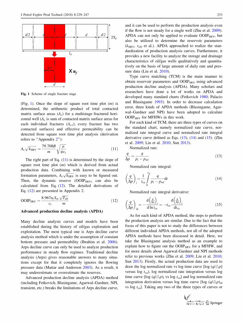
(Fig. 1). Once the slope of square root time plot (m) is
determined, the arithmetic product of total contacted
matrix surface areas (Ac) for a multistage fractured hori-
zontal well (Ac is sum of contacted matrix surface areas for
each individual fractures (Ac1); every fracture has two
contacted surfaces) and effective permeability can be
detected from square root time plot analysis (derivation
refers to ‘‘Appendix 2’’):
Ac
ffiffiffiffiffiffiffiffiffi
kSRVp
¼ 79:708B
m
ffiffiffiffiffiffiffi
l/ct
r
ð11Þ
The right part of Eq. (11) is determined by the slope of
square root time plot (m) which is derived from actual
production data. Combining with known or measured
formation parameters, Ac
ffiffiffiffiffiffiffiffiffi
kSRVp
is easy to be figured out.
Then, the dynamic reserve (OOIPSRV) can also be
calculated from Eq. (12). The detailed derivations of
Eq. (12) are presented in Appendix 2.
OOIPSRV ¼ 8:967nf Soict
ffiffiffiffiffiffiffi
Telfp
mð12Þ
Advanced production decline analysis (APDA)
Many decline analysis curves and models have been
established during the history of oil/gas exploration and
exploitation. The most typical one is Arps decline curve
analysis method which is under the assumption of constant
bottom pressure and permeability (Ibrahim et al. 2006).
Arps decline curve can only be used to analyze production
performance in steady flow regimes. Traditional decline
analysis (Arps) gives reasonable answers to many situa-
tions except for that it completely ignores the flowing
pressure data (Mattar and Anderson 2003). As a result, it
may underestimate or overestimate the reserves.
Advanced production decline analysis (APDA) method
(including Fetkovich, Blasingame, Agarwal–Gardner, NPI,
transient, etc.) breaks the limitations of Arps decline curve,
and it can be used to perform the production analysis even
if the flow is not steady for a single well (Zhu et al. 2009).
APDA can not only be applied to evaluate OOIPSRV, but
also be utilized to determine the reservoir parameters
(kSRV, reD et al.). APDA approached to realize the stan-
dardization of production analysis curves. Furthermore, it
provides a new facility to analyze the storage and drainage
characteristics of oil/gas wells qualitatively and quantita-
tively on the basis of large amount of daily rate and pres-
sure data (Liu et al. 2010).
Type curve matching (TCM) is the main manner to
obtain reservoir parameters and OOIPSRV using advanced
production decline analysis (APDA). Many scholars and
researchers have done a lot of works on APDA and
developed many standard charts (Fetkovich 1980; Palacio
and Blasingame 1993). In order to decrease calculation
error, three kinds of APDA methods (Blasingame, Agar-
wal–Gardner and NPI) have been adopted to calculate
OOIPSRV for MFHWs in this work.
For each kind of TCM, there are three types of curves on
the standard chart, namely normalized rate curve, nor-
malized rate integral curve and normalized rate integral
derivative curve defined as Eqs. (13), (14) and (15). (Zhu
et al. 2009; Liu et al. 2010; Sun 2013).
Normalized rate:
q
Dp¼ q
pi � pwfð13Þ
Normalized rate integral:
q
Dp
� �
i
¼ 1
tca
Z
tca
0
q
pi � pwfdt ð14Þ
Normalized rate integral derivative:
q
Dp
� �
id
¼ �d q
Dp
� �
i
d ln tca¼ �tca
d qDp
� �
i
dtcað15Þ
As for each kind of APDA method, the steps to perform
the production analysis are similar. Due to the fact that the
focus of this paper is not to study the differences between
different individual APDA methods, not all of the adopted
APDA methods have been discussed in detail. Here, we
take the Blasingame analysis method as an example to
explain how to figure out the OOIPSRV for a MFHW, and
for more details about Agarwal-Gardner and NPI methods
refer to previous works (Zhu et al. 2009; Liu et al. 2010;
Sun 2013). Firstly, the actual production data are used to
draw the log normalized rate vs log time curve [log (q/4p]
versus log tca), log normalized rate integration versus log
time curve [log (q/4p)i vs log tca] and log normalized rate
integration derivation versus log time curve [log (q/4p)idvs log tca]. Taking any two of the three types of curves or
Fig. 1 Scheme of single fracture stage
J Petrol Explor Prod Technol (2018) 8:229–247 233
123
all of the three curves, a TCM log–log chart is established.
Subsequently, the actual TCM log–log chart for target well
is applied to fit the developed standard chart to determine
the dimensionless borehole radius (reD). The detailed steps
to obtain reD are presented in ‘‘Appendix 3’’; once reD have
been figured out, the OOIPSRV and more relevant reservoir
parameters can be estimated.
Effective permeability of SRV zone:
kSRV ¼ ðq=DpÞmatch
ðqDdÞmatch
lB2ph
ln reD � 1
2
� �
ð16Þ
Effective wellbore radius (rwa):
rwa ¼ffiffiffiffiffiffiffiffiffiffiffiffiffiffiffiffiffiffiffiffiffiffiffiffiffiffiffiffiffiffiffiffiffiffiffiffiffiffiffiffiffiffiffiffiffiffiffiffiffiffiffiffiffiffiffiffi
2K=/lctðr2eD � 1Þ ln reD � 1
2
� �
tca
tcDd
� �
s
ð17Þ
The drainage radius (re) could be calculated from
Eq. (16) as reD and rwa have been obtained:
re ¼ reDrwa ð18Þ
As shown in ‘‘Appendix 3’’, we have introduced how to
determine the variables which are used to calculate
dynamic reserve (OOIPSRV):
OOIPSRV ¼ 1
ct
tca
tcDd
� �
match
q=DpqDd
� �
match
ð1� SwiÞ ð19Þ
Fracturing network parameters calculation
Network fracturing technique is an important method to
improve the production for tight oil reservoirs. Fracturing
network parameters (x and k) are the indexes of fracturingstimulation effectiveness.
Storativity (x) is defined as the ratio of elastic storage
ability of fracture system to the total storage ability of the
pay zone. It indicates the relative size of elastic storage
ability of fracture system and matrix system (Lian et al.
2011). Resources exchanged between fractures and matrix
blocks can be characterized by transmissivity ratio (k)which reflects how easy or difficult the fluid medium flows
into fracture from matrix (Wang 2015).
Due to the fact that the main purpose of fracturing
stimulation for tight oil reservoir is to develop larger
stimulated reservoir volume (SRV), the focus of network
fracturing is to connect as many natural fractures as pos-
sible based on the shear slide of secondary fracture system.
Most proppants are used to support hydraulic fractures, and
very few proppants (even if there is some, the proppant size
is very small and the volume of those proppants can be
ignored comparing the total volume of secondary fractural
system in SRV) can be brought into natural fractures. Then,
the volume of secondary fracture system can be estimated
from the volume of fracturing fluid injected into reservoir
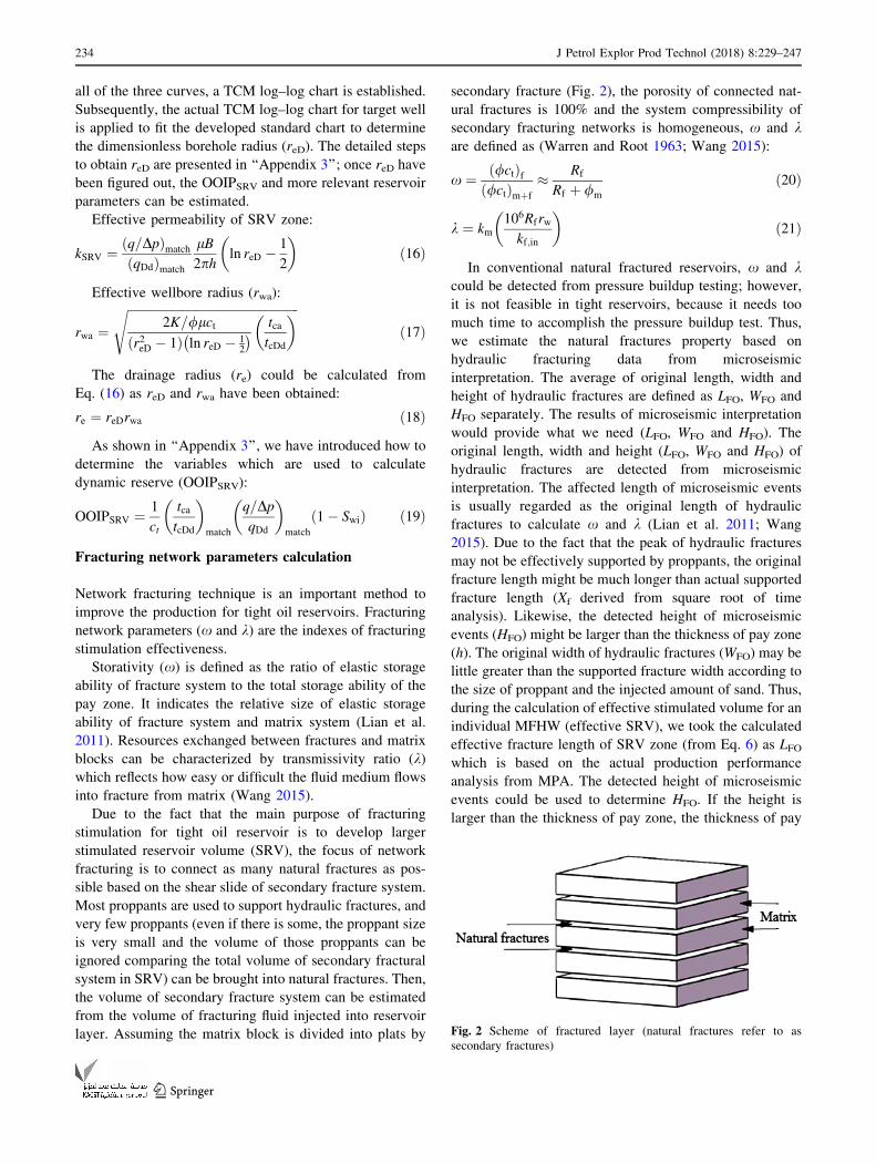
layer. Assuming the matrix block is divided into plats by
secondary fracture (Fig. 2), the porosity of connected nat-
ural fractures is 100% and the system compressibility of
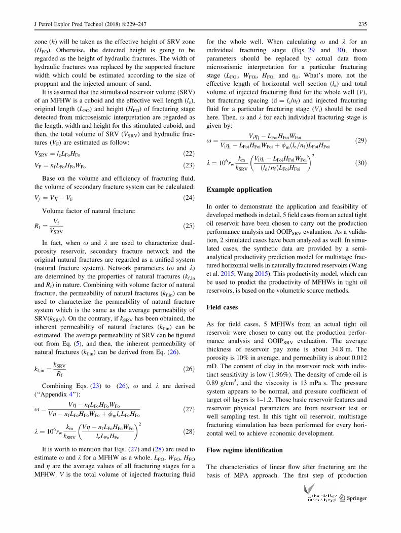
secondary fracturing networks is homogeneous, x and kare defined as (Warren and Root 1963; Wang 2015):
x ¼ /ctð Þf/ctð Þmþf
� Rf
Rf þ /m
ð20Þ
k ¼ km106Rfrw
kf;in
� �
ð21Þ
In conventional natural fractured reservoirs, x and kcould be detected from pressure buildup testing; however,
it is not feasible in tight reservoirs, because it needs too
much time to accomplish the pressure buildup test. Thus,
we estimate the natural fractures property based on
hydraulic fracturing data from microseismic
interpretation. The average of original length, width and
height of hydraulic fractures are defined as LFO, WFO and
HFO separately. The results of microseismic interpretation
would provide what we need (LFO, WFO and HFO). The
original length, width and height (LFO, WFO and HFO) of
hydraulic fractures are detected from microseismic
interpretation. The affected length of microseismic events
is usually regarded as the original length of hydraulic
fractures to calculate x and k (Lian et al. 2011; Wang
2015). Due to the fact that the peak of hydraulic fractures
may not be effectively supported by proppants, the original
fracture length might be much longer than actual supported
fracture length (Xf derived from square root of time
analysis). Likewise, the detected height of microseismic
events (HFO) might be larger than the thickness of pay zone
(h). The original width of hydraulic fractures (WFO) may be
little greater than the supported fracture width according to
the size of proppant and the injected amount of sand. Thus,
during the calculation of effective stimulated volume for an
individual MFHW (effective SRV), we took the calculated
effective fracture length of SRV zone (from Eq. 6) as LFOwhich is based on the actual production performance
analysis from MPA. The detected height of microseismic
events could be used to determine HFO. If the height is
larger than the thickness of pay zone, the thickness of pay
Fig. 2 Scheme of fractured layer (natural fractures refer to as
secondary fractures)
234 J Petrol Explor Prod Technol (2018) 8:229–247
123
zone (h) will be taken as the effective height of SRV zone
(HFO). Otherwise, the detected height is going to be
regarded as the height of hydraulic fractures. The width of
hydraulic fractures was replaced by the supported fracture
width which could be estimated according to the size of
proppant and the injected amount of sand.
It is assumed that the stimulated reservoir volume (SRV)
of an MFHW is a cuboid and the effective well length (le),
original length (LFO) and height (HFO) of fracturing stage
detected from microseismic interpretation are regarded as
the length, width and height for this stimulated cuboid, and
then, the total volume of SRV (VSRV) and hydraulic frac-
tures (VF) are estimated as follow:
VSRV ¼ leLFoHFo ð22ÞVF ¼ nfLFoHFoWFo ð23Þ
Base on the volume and efficiency of fracturing fluid,
the volume of secondary fracture system can be calculated:
Vf ¼ Vg� VF ð24Þ
Volume factor of natural fracture:
Rf ¼Vf
VSRV
ð25Þ
In fact, when x and k are used to characterize dual-
porosity reservoir, secondary fracture network and the
original natural fractures are regarded as a unified system
(natural fracture system). Network parameters (x and k)are determined by the properties of natural fractures (kf,inand Rf) in nature. Combining with volume factor of natural
fracture, the permeability of natural fractures (kf,in) can be
used to characterize the permeability of natural fracture
system which is the same as the average permeability of
SRV(kSRV). On the contrary, if kSRV has been obtained, the
inherent permeability of natural fractures (kf,in) can be
estimated. The average permeability of SRV can be figured
out from Eq. (5), and then, the inherent permeability of
natural fractures (kf,in) can be derived from Eq. (26).
kf;in ¼kSRV
Rf
ð26Þ
Combining Eqs. (23) to (26), x and k are derived
(‘‘Appendix 4’’):
x ¼ Vg� nfLFoHFoWFo
Vg� nfLFoHFoWFo þ /mleLFoHFo
ð27Þ
k ¼ 106rwkm
kSRV
Vg� nfLFoHFoWFo
leLFoHFo
� �2
ð28Þ
It is worth to mention that Eqs. (27) and (28) are used to
estimate x and k for a MFHW as a whole. LFO, WFO, HFO
and g are the average values of all fracturing stages for a
MFHW. V is the total volume of injected fracturing fluid
for the whole well. When calculating x and k for an
individual fracturing stage (Eqs. 29 and 30), those
parameters should be replaced by actual data from
microseismic interpretation for a particular fracturing
stage (LFOi, WFOi, HFOi and gi). What’s more, not the
effective length of horizontal well section (le) and total
volume of injected fracturing fluid for the whole well (V),
but fracturing spacing (d = le/nf) and injected fracturing
fluid for a particular fracturing stage (Vi) should be used
here. Then, x and k for each individual fracturing stage is
given by:
x ¼ Vigi � LFoiHFoiWFoi
Vigi � LFoiHFoiWFoi þ /mðle=nfÞLFoiHFoi
ð29Þ
k ¼ 106rwkm
kSRV
Vigi � LFoiHFoiWFoi
ðle=nfÞLFoiHFoi
� �2
ð30Þ
Example application
In order to demonstrate the application and feasibility of
developed methods in detail, 5 field cases from an actual tight
oil reservoir have been chosen to carry out the production
performance analysis and OOIPSRV evaluation. As a valida-
tion, 2 simulated cases have been analyzed as well. In simu-
lated cases, the synthetic data are provided by a semi-
analytical productivity prediction model for multistage frac-
tured horizontal wells in naturally fractured reservoirs (Wang
et al. 2015; Wang 2015). This productivity model, which can
be used to predict the productivity of MFHWs in tight oil
reservoirs, is based on the volumetric source methods.
Field cases
As for field cases, 5 MFHWs from an actual tight oil
reservoir were chosen to carry out the production perfor-
mance analysis and OOIPSRV evaluation. The average
thickness of reservoir pay zone is about 34.8 m. The
porosity is 10% in average, and permeability is about 0.012
mD. The content of clay in the reservoir rock with indis-
tinct sensitivity is low (1.96%). The density of crude oil is
0.89 g/cm3, and the viscosity is 13 mPa s. The pressure
system appears to be normal, and pressure coefficient of
target oil layers is 1–1.2. Those basic reservoir features and
reservoir physical parameters are from reservoir test or
well sampling test. In this tight oil reservoir, multistage
fracturing stimulation has been performed for every hori-
zontal well to achieve economic development.
Flow regime identification
The characteristics of linear flow after fracturing are the
basis of MPA approach. The first step of production
J Petrol Explor Prod Technol (2018) 8:229–247 235
123
performance analysis is to figure out two key parameters
(Telf and m) which are essential to the calculation of
reservoir parameters and OOIPSRV. Taking Well 1 as an
example, we have demonstrated how to identify the flow
regimes for a fractured horizontal well completed in tight
oil reservoir.
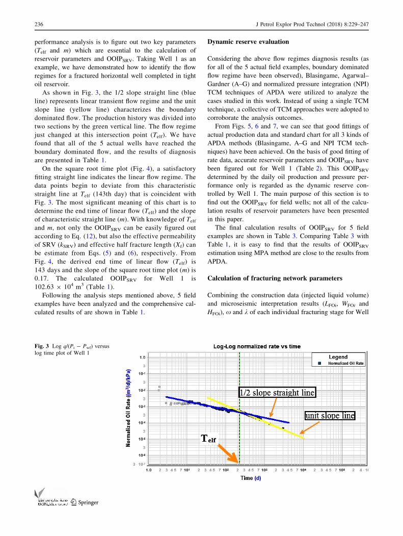
As shown in Fig. 3, the 1/2 slope straight line (blue
line) represents linear transient flow regime and the unit
slope line (yellow line) characterizes the boundary
dominated flow. The production history was divided into
two sections by the green vertical line. The flow regime
just changed at this intersection point (Telf). We have
found that all of the 5 actual wells have reached the
boundary dominated flow, and the results of diagnosis
are presented in Table 1.
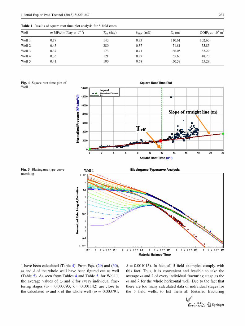
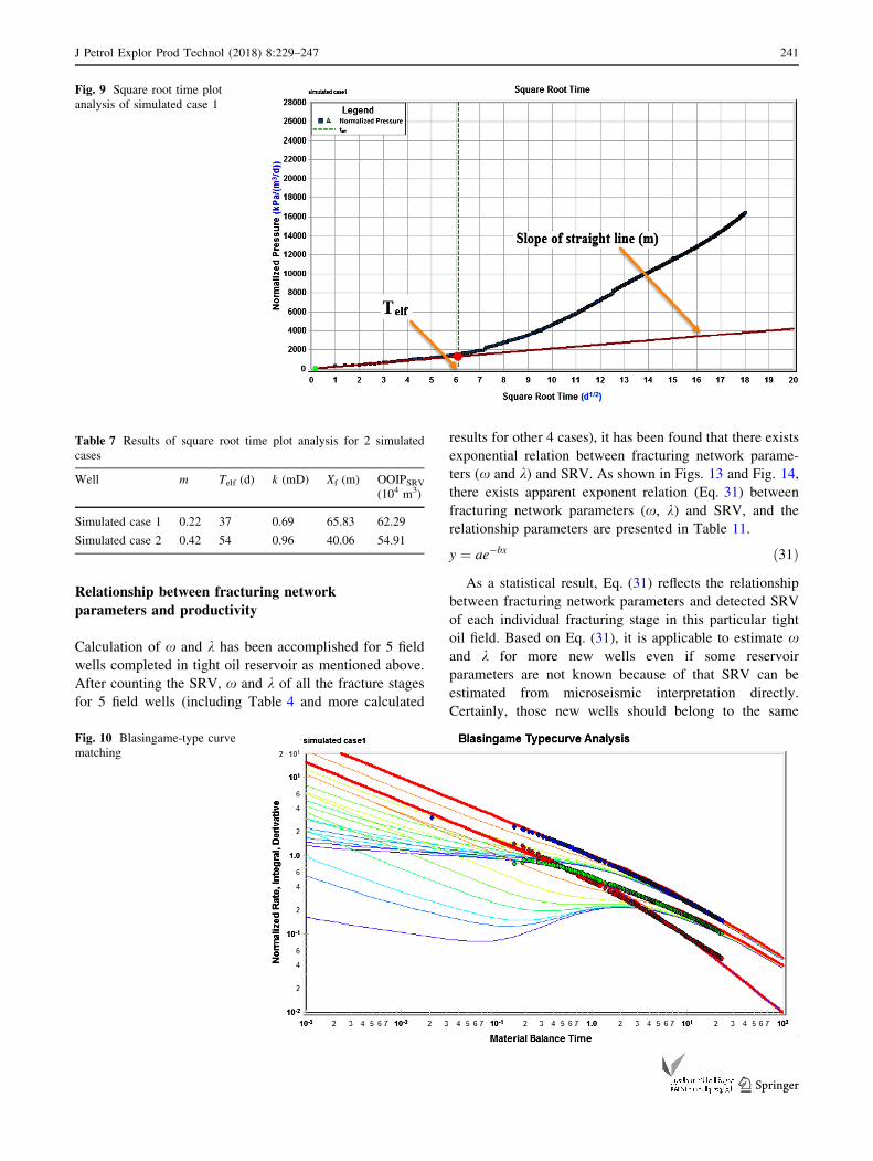
On the square root time plot (Fig. 4), a satisfactory
fitting straight line indicates the linear flow regime. The
data points begin to deviate from this characteristic
straight line at Telf (143th day) that is coincident with
Fig. 3. The most significant meaning of this chart is to
determine the end time of linear flow (Telf) and the slope
of characteristic straight line (m). With knowledge of Telfand m, not only the OOIPSRV can be easily figured out
according to Eq. (12), but also the effective permeability
of SRV (kSRV) and effective half fracture length (Xf) can
be estimate from Eqs. (5) and (6), respectively. From
Fig. 4, the derived end time of linear flow (Telf) is
143 days and the slope of the square root time plot (m) is
0.17. The calculated OOIPSRV for Well 1 is
102.63 9 104 m3 (Table 1).
Following the analysis steps mentioned above, 5 field
examples have been analyzed and the comprehensive cal-
culated results of are shown in Table 1.
Dynamic reserve evaluation
Considering the above flow regimes diagnosis results (as
for all of the 5 actual field examples, boundary dominated
flow regime have been observed), Blasingame, Agarwal–
Gardner (A–G) and normalized pressure integration (NPI)
TCM techniques of APDA were utilized to analyze the
cases studied in this work. Instead of using a single TCM
technique, a collective of TCM approaches were adopted to
corroborate the analysis outcomes.
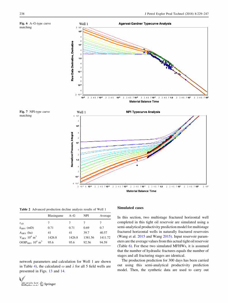
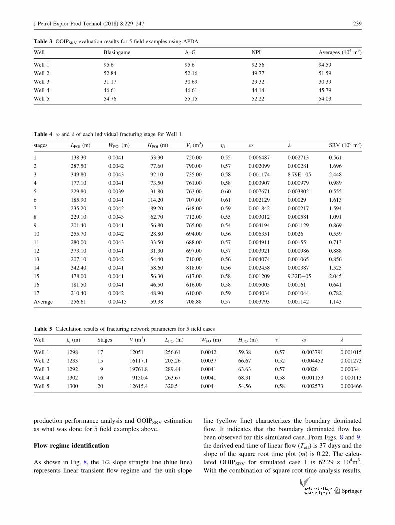
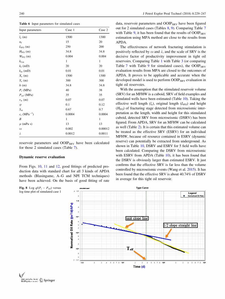
From Figs. 5, 6 and 7, we can see that good fittings of
actual production data and standard chart for all 3 kinds of
APDA methods (Blasingame, A–G and NPI TCM tech-
niques) have been achieved. On the basis of good fitting of
rate data, accurate reservoir parameters and OOIPSRV have
been figured out for Well 1 (Table 2). This OOIPSRVdetermined by the daily oil production and pressure per-
formance only is regarded as the dynamic reserve con-
trolled by Well 1. The main purpose of this section is to
find out the OOIPSRV for field wells; not all of the calcu-
lation results of reservoir parameters have been presented
in this paper.
The final calculation results of OOIPSRV for 5 field
examples are shown in Table 3. Comparing Table 3 with
Table 1, it is easy to find that the results of OOIPSRVestimation using MPA method are close to the results from
APDA.
Calculation of fracturing network parameters
Combining the construction data (injected liquid volume)
and microseismic interpretation results (LFOi, WFOi and
HFOi), x and k of each individual fracturing stage for Well
Fig. 3 Log q/(Pi - Pwf) versus
log time plot of Well 1
236 J Petrol Explor Prod Technol (2018) 8:229–247
123
1 have been calculated (Table 4). From Eqs. (29) and (30),
x and k of the whole well have been figured out as well
(Table 5). As seen from Tables 4 and Table 5, for Well 1,
the average values of x and k for every individual frac-
turing stages (x = 0.003793, k = 0.001142) are close to
the calculated x and k of the whole well (x = 0.003791,
k = 0.001015). In fact, all 5 field examples comply with
this fact. Thus, it is convenient and feasible to take the
average x and k of every individual fracturing stage as the
x and k for the whole horizontal well. Due to the fact that
there are too many calculated data of individual stages for
the 5 field wells, to list them all (detailed fracturing
Table 1 Results of square root time plot analysis for 5 field cases
Well m MPa/(m3/day 9 d0.5) Telf (day) kSRV (mD) Xf (m) OOIPSRV 104 m3
Well 1 0.17 143 0.73 110.61 102.63
Well 2 0.45 280 0.37 71.81 55.85
Well 3 0.37 173 0.41 66.05 32.29
Well 4 0.35 121 0.87 55.63 48.73
Well 5 0.41 100 0.58 50.58 55.29
Fig. 4 Square root time plot of
Well 1
Fig. 5 Blasingame-type curve
matching
J Petrol Explor Prod Technol (2018) 8:229–247 237
123
network parameters and calculation for Well 1 are shown
in Table 4), the calculated x and k for all 5 field wells are
presented in Figs. 13 and 14.
Simulated cases
In this section, two multistage fractured horizontal well
completed in this tight oil reservoir are simulated using a
semi-analytical productivity predictionmodel for multistage
fractured horizontal wells in naturally fractured reservoirs
(Wang et al. 2015 and Wang 2015). Input reservoir param-
eters are the average values from this actual tight oil reservoir
(Table 6). For these two simulated MFHWs, it is assumed
that the number of hydraulic fractures equals the number of
stages and all fracturing stages are identical.
The production prediction for 300 days has been carried
out using this semi-analytical productivity prediction
model. Then, the synthetic data are used to carry out
Fig. 6 A–G-type curve
matching
Fig. 7 NPI-type curve
matching
Table 2 Advanced production decline analysis results of Well 1
Blasingame A–G NPI Average
reD 7 7 7 7
kSRV (mD) 0.71 0.71 0.69 0.7
ASRV (ha) 41 41 39.7 40.57
VSRV 104 m3 1426.8 1426.8 1381.56 1411.72
OOIPSRV 104 m3 95.6 95.6 92.56 94.59
238 J Petrol Explor Prod Technol (2018) 8:229–247
123
production performance analysis and OOIPSRV estimation
as what was done for 5 field examples above.
Flow regime identification
As shown in Fig. 8, the 1/2 slope straight line (blue line)
represents linear transient flow regime and the unit slope
line (yellow line) characterizes the boundary dominated
flow. It indicates that the boundary dominated flow has
been observed for this simulated case. From Figs. 8 and 9,
the derived end time of linear flow (Telf) is 37 days and the
slope of the square root time plot (m) is 0.22. The calcu-
lated OOIPSRV for simulated case 1 is 62.29 9 104m3.
With the combination of square root time analysis results,
Table 3 OOIPSRV evaluation results for 5 field examples using APDA
Well Blasingame A–G NPI Averages (104 m3)
Well 1 95.6 95.6 92.56 94.59
Well 2 52.84 52.16 49.77 51.59
Well 3 31.17 30.69 29.32 30.39
Well 4 46.61 46.61 44.14 45.79
Well 5 54.76 55.15 52.22 54.03
Table 4 x and k of each individual fracturing stage for Well 1
stages LFOi (m) WFOi (m) HFOi (m) Vi (m3) gi x k SRV (106 m3)
1 138.30 0.0041 53.30 720.00 0.55 0.006487 0.002713 0.561
2 287.50 0.0042 77.60 790.00 0.57 0.002099 0.000281 1.696
3 349.80 0.0043 92.10 735.00 0.58 0.001174 8.79E-05 2.448
4 177.10 0.0041 73.50 761.00 0.58 0.003907 0.000979 0.989
5 229.80 0.0039 31.80 763.00 0.60 0.007671 0.003802 0.555
6 185.90 0.0041 114.20 707.00 0.61 0.002129 0.00029 1.613
7 235.20 0.0042 89.20 648.00 0.59 0.001842 0.000217 1.594
8 229.10 0.0043 62.70 712.00 0.55 0.003012 0.000581 1.091
9 201.40 0.0041 56.80 765.00 0.54 0.004194 0.001129 0.869
10 255.70 0.0042 28.80 694.00 0.56 0.006351 0.0026 0.559
11 280.00 0.0043 33.50 688.00 0.57 0.004911 0.00155 0.713
12 373.10 0.0041 31.30 697.00 0.57 0.003921 0.000986 0.888
13 207.10 0.0042 54.40 710.00 0.56 0.004074 0.001065 0.856
14 342.40 0.0041 58.60 818.00 0.56 0.002458 0.000387 1.525
15 478.00 0.0041 56.30 617.00 0.58 0.001209 9.32E-05 2.045
16 181.50 0.0041 46.50 616.00 0.58 0.005005 0.00161 0.641
17 210.40 0.0042 48.90 610.00 0.59 0.004034 0.001044 0.782
Average 256.61 0.00415 59.38 708.88 0.57 0.003793 0.001142 1.143
Table 5 Calculation results of fracturing network parameters for 5 field cases
Well le (m) Stages V (m3) LFO (m) WFO (m) HFO (m) g x k
Well 1 1298 17 12051 256.61 0.0042 59.38 0.57 0.003791 0.001015
Well 2 1233 15 16117.1 205.26 0.0037 66.67 0.52 0.004452 0.001273
Well 3 1292 9 19761.8 289.44 0.0041 63.63 0.57 0.0026 0.00034
Well 4 1302 16 9150.4 263.67 0.0041 68.31 0.58 0.001153 0.000113
Well 5 1300 20 12615.4 320.5 0.004 54.56 0.58 0.002573 0.000466
J Petrol Explor Prod Technol (2018) 8:229–247 239
123
reservoir parameters and OOIPSRV have been calculated
for those 2 simulated cases (Table 7).
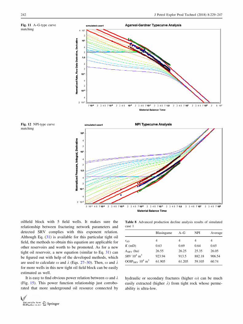
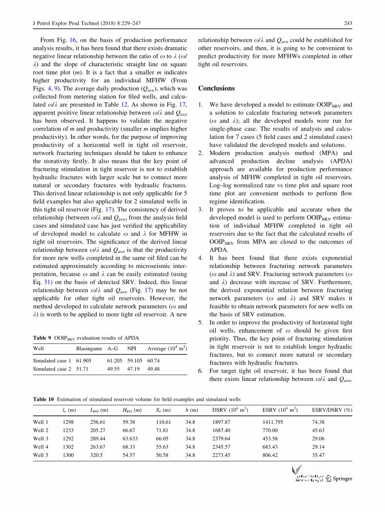
Dynamic reserve evaluation
From Figs. 10, 11 and 12, good fittings of predicted pro-
duction data with standard chart for all 3 kinds of APDA
methods (Blasingame, A–G and NPI TCM techniques)
have been achieved. On the basis of good fitting of rate
data, reservoir parameters and OOIPSRV have been figured
out for 2 simulated cases (Tables 8, 9). Comparing Table 7
with Table 9, it has been found that the results of OOIPSRVestimation using MPA method are close to the results from
APDA.
The effectiveness of network fracturing stimulation is
positively reflected by x and k, and the scale of SRV is the
decisive factor of productivity improvement in tight oil
reservoirs. Comparing Table 1 with Table 3 (or comparing
Table 7 with Table 9 for simulated cases), the OOIPSRVevaluation results from MPA are closed to the outcomes of
APDA. It proves to be applicable and accurate when the
developed model is used to perform OOIPSRV evaluation in
tight oil reservoirs.
With the assumption that the stimulated reservoir volume
(SRV) for an MFHW is a cuboid, SRV of field examples and
simulated wells have been estimated (Table 10). Taking the
effective well length (le), original length (LFO) and height
(HFO) of fracturing stage detected from microseismic inter-
pretation as the length, width and height for this stimulated
cuboid, detected SRV from microseismic (DSRV) has been
figured. From APDA, SRV for an MFHW can be calculated
as well (Table 2). It is certain that this estimated volume can
be treated as the effective SRV (ESRV) for an individual
MFHW, because oil resource contained in ESRV (dynamic
reserve) can potentially be extracted from underground. As
shown in Table 10, DSRV and ESRV for 5 field wells have
been calculated. Comparing the DSRV from microseismic
with ESRV from APDA (Table 10), it has been found that
the DSRV is obviously larger than estimated ESRV. It just
confirms that the effective SRV is far less than the volume
controlled by microseismic events (Wang et al. 2015). It has
been found that the effective SRV is about 40.74% of DSRV
in average for this tight oil reservoir.
Table 6 Input parameters for simulated cases
Input parameters Case 1 Case 2
le (m) 1500 1300
nf 15 20
LFO (m) 250 200
HFO (m) 34.8 34.8
WFO (m) 0.004 0.004
kf,in 1 1
kf (mD) 20 20
km (mD) 0.01 0.01
Xe (m) 1500 1300
Ye (m) 300 300
h (m) 34.8 34.8
Pi (MPa) 40 38
Pwf (MPa) 35 35
rw (m) 0.07 0.07
u 0.1 0.12
Soi 0.67 0.7
ct (MPa-1) 0.0004 0.0004
B 1 1
l (mPa s) 13 13
x 0.002 0.00012
k 0.0012 0.0011
Fig. 8 Log q/(Pi - Pwf) versus
log time plot of simulated case 1
240 J Petrol Explor Prod Technol (2018) 8:229–247
123
Relationship between fracturing network
parameters and productivity
Calculation of x and k has been accomplished for 5 field
wells completed in tight oil reservoir as mentioned above.
After counting the SRV, x and k of all the fracture stages
for 5 field wells (including Table 4 and more calculated
results for other 4 cases), it has been found that there exists
exponential relation between fracturing network parame-
ters (x and k) and SRV. As shown in Figs. 13 and Fig. 14,
there exists apparent exponent relation (Eq. 31) between
fracturing network parameters (x, k) and SRV, and the
relationship parameters are presented in Table 11.
y ¼ ae�bx ð31Þ
As a statistical result, Eq. (31) reflects the relationship
between fracturing network parameters and detected SRV
of each individual fracturing stage in this particular tight
oil field. Based on Eq. (31), it is applicable to estimate xand k for more new wells even if some reservoir
parameters are not known because of that SRV can be
estimated from microseismic interpretation directly.
Certainly, those new wells should belong to the same
Fig. 9 Square root time plot
analysis of simulated case 1
Table 7 Results of square root time plot analysis for 2 simulated
cases
Well m Telf (d) k (mD) Xf (m) OOIPSRV(104 m3)
Simulated case 1 0.22 37 0.69 65.83 62.29
Simulated case 2 0.42 54 0.96 40.06 54.91
Fig. 10 Blasingame-type curve
matching
J Petrol Explor Prod Technol (2018) 8:229–247 241
123
oilfield block with 5 field wells. It makes sure the
relationship between fracturing network parameters and
detected SRV complies with this exponent relation.
Although Eq. (31) is available for this particular tight oil
field, the methods to obtain this equation are applicable for
other reservoirs and worth to be promoted. As for a new
tight oil reservoir, a new equation (similar to Eq. 31) can
be figured out with help of the developed methods, which
are used to calculate x and k (Eqs. 27–30). Then, x and kfor more wells in this new tight oil field block can be easily
estimated as well.
It is easy to find obvious power relation between x and k(Fig. 15). This power function relationship just corrobo-
rated that more underground oil resource connected by
hydraulic or secondary fractures (higher x) can be much
easily extracted (higher k) from tight rock whose perme-
ability is ultra-low.
Fig. 11 A–G-type curve
matching
Fig. 12 NPI-type curve
matching
Table 8 Advanced production decline analysis results of simulated
case 1
Blasingame A–G NPI Average
reD 4 4 4 4
K (mD) 0.63 0.69 0.64 0.65
ASRV (ha) 26.55 26.25 25.35 26.05
SRV 104 m3 923.94 913.5 882.18 906.54
OOIPSRV 104 m3 61.905 61.205 59.105 60.74
242 J Petrol Explor Prod Technol (2018) 8:229–247
123
From Fig. 16, on the basis of production performance
analysis results, it has been found that there exists dramatic
negative linear relationship between the ratio of x to k (x/k) and the slope of characteristic straight line on square
root time plot (m). It is a fact that a smaller m indicates
higher productivity for an individual MFHW (From
Figs. 4, 9). The average daily production (Qave), which was
collected from metering station for filed wells, and calcu-
lated x/k are presented in Table 12. As shown in Fig. 17,
apparent positive linear relationship between x/k and Qave
has been observed. It happens to validate the negative
correlation of m and productivity (smaller m implies higher
productivity). In other words, for the purpose of improving
productivity of a horizontal well in tight oil reservoir,
network fracturing techniques should be taken to enhance
the storativity firstly. It also means that the key point of
fracturing stimulation in tight reservoir is not to establish
hydraulic fractures with larger scale but to connect more
natural or secondary fractures with hydraulic fractures.
This derived linear relationship is not only applicable for 5
field examples but also applicable for 2 simulated wells in
this tight oil reservoir (Fig. 17). The consistency of derived
relationship (between x/k and Qave) from the analysis field
cases and simulated case has just verified the applicability
of developed model to calculate x and k for MFHW in
tight oil reservoirs. The significance of the derived linear
relationship between x/k and Qave is that the productivity
for more new wells completed in the same oil filed can be
estimated approximately according to microseismic inter-
pretation, because x and k can be easily estimated (using
Eq. 31) on the basis of detected SRV. Indeed, this linear
relationship between x/k and Qave (Fig. 17) may be not
applicable for other tight oil reservoirs. However, the
method developed to calculate network parameters (x and
k) is worth to be applied to more tight oil reservoir. A new
relationship between x/k and Qave could be established for
other reservoirs, and then, it is going to be convenient to
predict productivity for more MFHWs completed in other
tight oil reservoirs.
Conclusions
1. We have developed a model to estimate OOIPSRV and
a solution to calculate fracturing network parameters
(x and k); all the developed models were run for
single-phase case. The results of analysis and calcu-
lation for 7 cases (5 field cases and 2 simulated cases)
have validated the developed models and solutions.
2. Modern production analysis method (MPA) and
advanced production decline analysis (APDA)
approach are available for production performance
analysis of MFHW completed in tight oil reservoirs.
Log–log normalized rate vs time plot and square root
time plot are convenient methods to perform flow
regime identification.
3. It proves to be applicable and accurate when the
developed model is used to perform OOIPSRV estima-
tion of individual MFHW completed in tight oil
reservoirs due to the fact that the calculated results of
OOIPSRV from MPA are closed to the outcomes of
APDA.
4. It has been found that there exists exponential
relationship between fracturing network parameters
(x and k) and SRV. Fracturing network parameters (xand k) decrease with increase of SRV. Furthermore,
the derived exponential relation between fracturing
network parameters (x and k) and SRV makes it
feasible to obtain network parameters for new wells on
the basis of SRV estimation.
5. In order to improve the productivity of horizontal tight
oil wells, enhancement of x should be given first
priority. Thus, the key point of fracturing stimulation
in tight reservoir is not to establish longer hydraulic
fractures, but to connect more natural or secondary
fractures with hydraulic fractures.
6. For target tight oil reservoir, it has been found that
there exists linear relationship between x/k and Qave.
Table 9 OOIPSRV evaluation results of APDA
Well Blasingame A–G NPI Average (104 m3)
Simulated case 1 61.905 61.205 59.105 60.74
Simulated case 2 51.71 49.55 47.19 49.48
Table 10 Estimation of stimulated reservoir volume for field examples and simulated wells
le (m) LFO (m) HFO (m) Xf (m) h (m) DSRV (104 m3) ESRV (104 m3) ESRV/DSRV (%)
Well 1 1298 256.61 59.38 110.61 34.8 1897.87 1411.795 74.38
Well 2 1233 205.27 66.67 71.81 34.8 1687.40 770.00 45.63
Well 3 1292 289.44 63.633 66.05 34.8 2379.64 453.58 29.06
Well 4 1302 263.67 68.33 55.63 34.8 2345.57 683.43 29.14
Well 5 1300 320.5 54.57 50.58 34.8 2273.45 806.42 35.47
J Petrol Explor Prod Technol (2018) 8:229–247 243
123
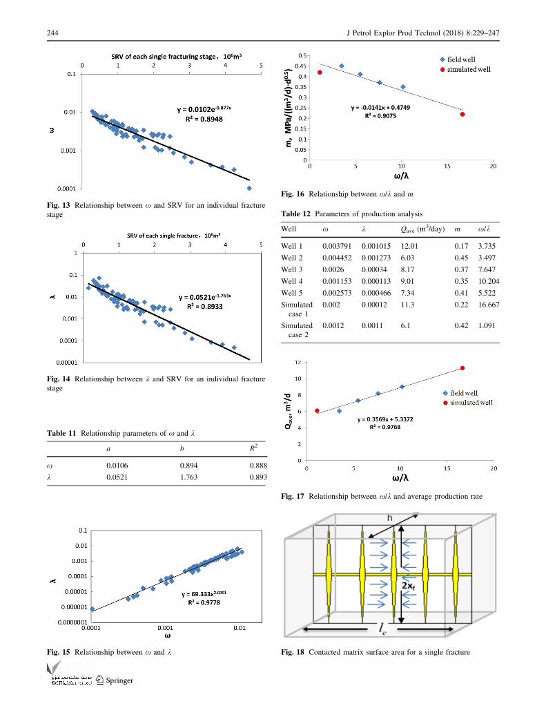
Fig. 13 Relationship between x and SRV for an individual fracture
stage
Fig. 14 Relationship between k and SRV for an individual fracture
stage
Table 11 Relationship parameters of x and k
a b R2
x 0.0106 0.894 0.888
k 0.0521 1.763 0.893
Fig. 15 Relationship between x and k
Fig. 16 Relationship between x/k and m
Table 12 Parameters of production analysis
Well x k Qave (m3/day) m x/k
Well 1 0.003791 0.001015 12.01 0.17 3.735
Well 2 0.004452 0.001273 6.03 0.45 3.497
Well 3 0.0026 0.00034 8.17 0.37 7.647
Well 4 0.001153 0.000113 9.01 0.35 10.204
Well 5 0.002573 0.000466 7.34 0.41 5.522
Simulated
case 1
0.002 0.00012 11.3 0.22 16.667
Simulated
case 2
0.0012 0.0011 6.1 0.42 1.091
Fig. 17 Relationship between x/k and average production rate
Fig. 18 Contacted matrix surface area for a single fracture
244 J Petrol Explor Prod Technol (2018) 8:229–247
123
On the basis of derived linear relationship between x/kand Qave, the productivity for more individual MFHW
can be directly estimated according to microseismic
interpretation.
Acknowledgements The authors wish to thank State Key Laboratory
of Oil and Gas Reservoir Geology and Exploitation, Chengdu for the
technical support of this study.
Open Access This article is distributed under the terms of the Crea-
tive Commons Attribution 4.0 International License (http://
creativecommons.org/licenses/by/4.0/), which permits unrestricted
use, distribution, and reproduction in any medium, provided you give
appropriate credit to the original author(s) and the source, provide a link
to the Creative Commons license, and indicate if changes were made.
Appendix 1: Equations of MPA plot
Dimensionless rate and dimensionless are defined as
follow:
qD ¼ 1
2pffiffiffiffiffiffiffi
ptDp ð32Þ
qD ¼ 1:842� 10�3Bql
kffiffiffi
Ap
Dpð33Þ
tD ¼ 86:4kt
/lctAð34Þ
Generate Eqs. (34) and (33) into Eq. (32):
1:842� 10�3Bql
kffiffiffi
Ap
Dp¼ 1
2pffiffiffiffiffiffiffiffiffiffiffiffiffi
p 86:4kt/lctA
q ð35Þ
Square Eq. (35):
1:8422 � 10�6B2q2l2
k2ADp2¼ /lctA
4� 86:4p3ktð36Þ
Simplify and inverse Eq. (36)
Dp2
q2¼ 4� 86:4p3 � 1:8422 � 10�6B2l2t
/lctAkð37Þ
Take p as 3.14, and take the square root of equation
Eq. (37):
Dpq
¼ 0:19Blffiffiffiffiffiffiffiffiffiffi
/lctp
Affiffiffi
kp
ffiffi
tp
ð38Þ
Appendix 2: Equations of square root time analysismethod
As shown in Fig. 18, there are two sides for an individual
hydraulic fracture. The total matrix surface area contacted
by a hydraulic fracture (Ac) is defined as (Clarkson and
Beierle 2010; Clarkson 2013):
Ac ¼ 4nfhXf ð39Þ
Transform Eq. (10) in the body text:
4hXf
ffiffiffiffiffiffiffiffiffi
kSRVp
¼ 4� 19:927Bo
m
ffiffiffiffiffiffiffi
luct
r
ð40Þ
Generate Eq. (39) into Eq. (40):
Ac
ffiffiffiffiffiffiffiffiffi
kSRVp
¼ 79:708nfBo
m
ffiffiffiffiffiffiffi
l/ct
r
ð41Þ
The total contacted matrix surface area:
Ac ¼79:708nfBo
mffiffiffiffiffiffiffiffiffi
kSRVp
ffiffiffiffiffiffiffi
l/ct
r
ð42Þ
There are two sides of an individual fracture. With the
assumption that hydraulic fractures of a MFHW are
identical and the number of hydraulic fractures equals the
number of stage, the contacted matrix surface area for a
single side of fracture is (Ac1):
Ac1 ¼Ac
2nfð43Þ
Ac1 ¼79:708Bo
2mffiffiffiffiffiffiffiffiffi
kSRVp
ffiffiffiffiffiffiffi
l/ct
r
ð44Þ
From Fig. (12), the volume of SRV for a fractured
horizontal well could be calculated approximately:
VSRV ¼ Ac1le ð45Þ
Put Eq. (44) into Eq. (45):
VSRV ¼ 79:708Bole
2mffiffiffiffiffiffiffiffiffi
kSRVp
ffiffiffiffiffiffiffi
l/ct
r
ð46Þ
Combining with Eq. (5):
VSRV ¼ 79:708Bole
2m
ffiffiffiffiffiffiffi
l/ct
r
2ffiffiffiffiffiffiffiffiffiffiffiffiffiffi
79:014p
ffiffiffiffiffiffiffi
Telfp
dffiffiffiffiffiffiffiffiffiffi
/lctp
¼ 79:708ffiffiffiffiffiffiffiffiffiffiffiffiffiffi
79:014p Bole
d/ct
ffiffiffiffiffiffiffi
Telfp
m
¼ 8:967Bonf
/ct
ffiffiffiffiffiffiffi
Telfp
m
ð47Þ
The oil resource in SRV:
OOIPSRV ¼ VSRV/SoiBoi
ð48Þ
Generate Eq. (47) into (48), the dynamic reserve could
be estimated:
OOIPSRV ¼ 8:967Bonf
/ct
ffiffiffiffiffiffiffi
Telfp
m
/SoiBoi
¼ 8:967nfBoSoi
ctBoi
ffiffiffiffiffiffiffi
Telfp
m
ð49Þ
Usually, taking the volume factor of oil as a constant,
OOIPSRV is estimated as:
J Petrol Explor Prod Technol (2018) 8:229–247 245
123
OOIPSRV ¼ 8:967nfSoict
ffiffiffiffiffiffiffi
Telfp
mð50Þ
Appendix 3: Equations of APDA analysis method
Material balance time, dimensionless material balance
time, dimensionless material balance pseudo-time, dimen-
sionless borehole radius and dimensionless pseudo-rate are
defined as follow (Palacio and Blasingame 1993; Sun
2013):
tca ¼Np
qð51Þ
tcD ¼ K
lA/cttca ð52Þ
tcDd ¼ tcD1
12ðr2eD � 1Þ ln reD � 1
2
� � ð53Þ
reD ¼ re
rwað54Þ
qDd ¼1
1þ tcDdð55Þ
The dimensionless borehole radius (reD) is determined
from the fit of production data on standard
chart (Fetkovich 1980; Palacio and Blasingame 1993).
In standard chart, there are a series of standard curves and
each standard curve corresponds to a reD. On the basis of
best fit of production data, the particular standard cure can
be detected for a single well, and then, reD is figured out.
It is assumed that all the hydraulic fractures contribute to
flow and the individual fractured horizontal well is
located in a circular reservoir zone; with the best fit of
production data and the knowledge of reD, reservoir
parameters and reserve can be estimated (Liu et al. 2010;
Sun 2013).
Selecting an actual data point (tca, q/4p) arbitrarily from
actual production data points, the selected actual produc-
tion data point (tca, q/4p) corresponds to a theoretical fit-
ting point on standard chart (tcDa, qDd). With the
combination of detected reD, the effective permeability
(kSRV) and effective borehole radius (rwa) can be
calculated:
kSRV ¼ ðq=DpÞmatch
ðqDdÞmatch
lB2ph
ln reD � 1
2
� �
ð56Þ
rwa ¼ffiffiffiffiffiffiffiffiffiffiffiffiffiffiffiffiffiffiffiffiffiffiffiffiffiffiffiffiffiffiffiffiffiffiffiffiffiffiffiffiffiffiffiffiffiffiffiffiffiffiffiffiffiffiffiffiffiffiffiffiffiffiffiffi
2kSRV=/lctðr2eD � 1Þðln reD � 1
2Þ
tca
tcDd
� �
match
s
ð57Þ
According to Eq. (54), the controlled radius for a
horizontal is:
re ¼ reDrwa ð58Þ
The total pore volume can be estimated as:
Vp ¼ pr2eh/ ð59Þ
Dynamic reserve in SRV (OOIPSRV):
OOIPSRV ¼ Vpð1� SwiÞBoi
ð60Þ
From previous studies (Liu et al. 2010; Sun 2013), the
total pore volume can also be directly estimated from the
fitting of production data using arbitrary matched data
points:
Vp ¼B
ct
tca
tcDd
� �
match
q=DpqDd
� �
match
ð61Þ
Then, generate Eq. (61) into Eq. (60), OOIPSRV is:
OOIPSRV ¼ 1
ct
tca
tcDd
� �
match
q=DpqDd
� �
match
ð1� SwiÞ ð62Þ
Appendix 4: Equations of fracturing networkparameters
With the combination of Eqs. (20) to (26), the storativity
(x) can be calculated:
x ¼ Rf
Rf þ /m
¼Vf
VSRV
Vf
VSRVþ /m
¼Vg�nfLFoHFoWFo
leLFoHFo
Vg�nfLFoHFoWFo
leLFoHFoþ /m
¼ Vg� nfLFoHFoWFo
Vg� nfLFoHFoWFo þ /mleLFoHFo
ð63Þ
And transmissivity ratio (k):
k ¼ km106Rfrw
kf;in
� �
¼ 106kmrwR2f
kSRV
¼ 106rwkm
kSRV
Vf
VSRV
� �2
¼ 106rwkm
kSRV
Vg� nfLFoHFoWFo
leLFoHFo
� �2
ð64Þ
References
Abdelhafidh F, Djebbar T (2001) Application of Decline-Curve
Analysis technique in oil reservoir using a universal fitting
equation. In: SPE permian basin oil and gas recovery conference.
Society of Petroleum Engineers
246 J Petrol Explor Prod Technol (2018) 8:229–247
123
Al-Ajmi NM, Kazemi H, Ozkan E (2003) Estimation of storativity
ratio in a layered reservoir with crossflow. In: SPE annual
technical conference and exhibition. Society of Petroleum
Engineers
Anderson DM, Nobakht M, Moghadam S, Mattar L (2010) Analysis
of production data from fractured shale gas wells. In: SPE
unconventional gas conference. Society of Petroleum Engineers
Anderson DM, Lian P, Okouma V (2012) Probabilistic for recasting
of unconventional resources using rate transient analysis: case
studies. In: SPE Americas unconventional resources conference.
Society of Petroleum Engineers
Bello RO and Wattenbarger RA (2010) Modelling and analysis of
shale gas production with a skin effect. In: SPE annual technical
meeting of the petroleum society. Society of Petroleum
Engineers
Brown M, Ozkan E, Raghavan R, Kazemi H (2011) Practical
solutions for pressure-transient responses of fractured horizontal
wells in unconventional shale reservoirs. In: SPE annual
technical conference and exhibition. Society of Petroleum
Engineers
Cheng YM (2011) Pressure transient characteristics of hydraulically
fractured horizontal shale gas wells. In: SPE eastern regional
meeting. Society of Petroleum Engineers
Chu L, Ye P, Harmawan I (2012) Characterizing and Simulating the
non-stationariness and non-linearity in unconventional oil reser-
voirs: bakken application. In: SPE Canadian unconventional
resources conference. Alberta Society of Petroleum Engineers
Clarkson CR (2013) Production data analysis of unconventional gas
wells: Review of theory and best practices. Int J Coal Geo
109–110:101–146
Clarkson CR, Beierle JJ (2010) Integration of microseismic and other
post-fracture surveillance with production analysis: a tight gas
study. In: SPE unconventional gas conference. Society of
Petroleum Engineers
Clarkson CR and Williams-Kovacs (2013) A new method for
modeling multi-phase flowback of multi-Fractured horizontal
tight oil wells to determine hydraulic fracture properties. In: SPE
annual technical conference and exhibition. Society of Petroleum
Engineers
Clarkson CR, Qanbari F, Nobakht M, Heffner L (2012) Incorporating
geomechanical and dynamic hydraulic fracture property changes
into rate-transient analysis: example from the Haynesville Shale.
In: Canadian unconventional resources conference. Society of
Petroleum Engineers
Fetkovich MJ (1980) Decline curve analysis using type curves.
J Petrol Technol 32(6):1065–1077
Ibrahim M., Suez CU, Wattenbarger RA (2006) Analysis of rate
dependence in transient linear flow in tight gas wells. In: Abu
Dhabi international petroleum exhibition and conference. Soci-
ety of Petroleum Engineers
Li Y, Li BZ, Hu YL, Tang ML, Xiao XJ, Zhang FE (2009)
Application of modern production decline analysis in the
performance analysis of gas condensate reservoirs. Nat Gas
Geo 20(2):305–307
Lian PQ, Cheng LS, Li LL, Li Z (2011) The variation law of
storativity ratio and interporosity transfer coefficient in fractured
reservoirs. Eng Mech 9(28):240–243
Liu XH, Zhou CM, Jiang YD, Yang XF (2010) Theory and
application of modern production decline analysis. Gas Ind
30(5):50–54
Mattar L, Anderson DM (2003) A systematic and comprehensive
methodology for advanced analysis of production data. In: SPE
annual technical conference and exhibition. Society of Petroleum
Engineers
Moghadam S, Mattarand LM, Pooladi-Darvish (2010) Dual Porosity
type curves for shale gas reservoirs. In: The Canadian uncon-
ventional resources and international petroleum conference.
Society of Petroleum Engineers
Palacio JC, Blasingame TA (1993) Decline-curve analysis using type
curves: analysis of gas production data. In: SPE joint rocky
mountain regional and low permeability reservoirs symposium.
Society of Petroleum Engineers
Pinillos C, Rong YC (2015) Integration of pressure transient analysis
in reservoir characterization: a case study. In: SPE Asia Pacific
oil and gas conference and exhibition. Society of Petroleum
Engineers
Poe BD, Vacca H, Benjamin A (2012) Production decline analysis of
horizontal well intersecting multiple transverse vertical hydrau-
lic fractures in low-permeability shale reservoirs. In: SPE annual
technical conference and exhibition. Society of Petroleum
Engineers
Qin H, Yin L, Chen GR (2012) The application of advanced
production decline method analysis in fractured low permeable
gas well. Nat Gas Technol Eco 6(3):37–38
Sander JE (1986) The ration, transmissivity/storativity from electric
analog values of streamflow. Ground Water 24(2):152–156
Song B, Ehlig-Economides CA (2011) Rate-normalized pressure
analysis for determination of shale gas well performance. In:
North American unconventional gas conference and exhibition.
Society of Petroleum Engineers
Sun HD (2013) Advanced production decline analysis and applica-
tion. CNKI, Beijinig
Tang R, Li JH, Tao SZ (2013) A brief analysis of several common
methods of oil-gas well production decline analysis. Guang
Dong Chem Ind 40(264):15–16
Wang JC (2015) Volumetric source model of binary system and its
application. Dissertation, Southwest Petroleum University
Wang JC, Li HT, Wang YQ (2015) A new model to predict
productivity of multiple-fractured horizontal well in naturally
fractured reservoirs. Math Probl Eng 2015:1–9
Warren JE, Root PJ (1963) The behavior of naturally fractured
reservoirs. SPE J 3(3):245–255
Ye P, Chu LL, Williams M (2013) Beyond linear analysis in an
unconventional oil reservoir. In: Unconventional resources
conference-USA. Society of Petroleum Engineers
Zhu YC, Liu JY, Zhang GD, Zhu DL, Li J (2009) Correlation of
production decline for gas wells. Nat Gas Exp Dev 32(1):28–31
J Petrol Explor Prod Technol (2018) 8:229–247 247
123


