Embed Size (px)
Citation preview
Proceedings of the Eighth
ESSLLI Student Session
August 2003, Vienna, Austria
Balder ten Cate (Ed.)

Preface
Ever since its 1996 edition, the annual European Summer School on LogicLanguage and Information has been accompanied by a separate studentsession. This student session performs an important role, by providing aforum where students can present their own work and get feedback fromfellow students and experienced researchers. It welcomes submissions relatedto the familiar ESSLLI subject areas, from students at any level (graduateas well as undergraduate).
The popularity of the student session has been growing throughout theyears, and this is reflected by the high number of submissions. This year,we received a total number of 69 papers, of which 18 were accepted for oralpresentation and 14 as a poster. Of these 32 papers, 29 are included in thisvolume.
I’m very grateful to the program committee for all their contributionsto the organization. I’d like to thank the co-chairs in particular for theirefforts in coordinating the reviewing process, and the area experts for theircontinuous presence and helpful advice. Also, my gratitude goes to all thereviewers, whose detailed comments have not only proved invaluable duringthe selection procedure, but also provide useful feedback to the authors. Asin previous years, Kluwer Academic Publishers have generously offered tosupport the ESSLLI student session with special awards for the Best paperpresentation and Best poster. I’m very grateful for their support. Finally,there are a number of people who I would like to thank in particular, sincethey were always ready to give help and advice: Raffaella Bernardi, PaulDekker, Darrin Hindsill, Ivana Kruijff-Korbayova, Malvina Nissim, MarieSafarova, Kristina Striegnitz and Willemijn Vermaat.
I’m very much looking forward to this year’s ESSLLI summer school,which will take place August 18–29, 2003 in Vienna, Austria. Hopefully, itsstudent session will provide the stimulating and fruitful atmosphere that itdid in the past.
Balder ten Cate Stanford, June 2003Chair of the ESSLLI 2003 Student Session
i
Program Committee
Logic & Language
Christian Retore, INRIA Futurs, FranceRoberto Bonato, University of Verona, Italy; University of Bordeaux I, FrancePaul Egre, University of Paris I, France
Logic & Computation
Sergio Tessaris, University of Bolzano, ItalyJakob Kellner, Vienna University of Technology, AustriaFavio Miranda-Perea, LMU Munchen, Germany
Language & Computation
Dan Flickinger, Stanford University, USALaura Alonso i Alemany, University of Barcelona, SpainMaria Fuentes Fort, University of Girona, SpainGabriel Infante Lopez, University of Amsterdam, The Netherlands
Reviewers
Marco Aiello, Natasha Alechina, Alex Alsina, Thorsten Altenkirch, J.Gabriel Amores, Carlos Areces, Pablo Ariel Duboue, Victoria ArranzCorzana, Nicholas Asher, Sergio Balari, Denis Bechet, Claire Beyssade,Nick Bezhanishvili, Patrick Blackburn, Eerke Boiten, Patrick Brezillon,Hans J. Briegel, Daniel Buring, Alastair Butler, Miriam Butt, Xavier Car-reras Perez, Robyn Carston, Montserrat Civit, Francis Corblin, Alexan-der Dekhtyar, Paul Dekker, Stephane Demri, Alexandre Dikovsky, My-roslava Dzikovska, Jason Eisner, Noemie Elhadad, Martin Everaert, AnnieForet, Bernd Gartner, Kim Gerdes, Jonathan Ginzburg, Radu Gramatovici,Phillippe de Groote, Kenneth Harris, Peter Harvey, James Henderson,Jan Johannsen, Makoto Kanazawa, Tracy Holloway King, Felix Klaedtke,Alexander Koller, Angelika Kratzer, Geert-Jan Kruijff, Alexander Kurz,Martin Lange, Mirella Lapata, Michael L. Littman, Lluıs Marquez, Car-los Martın-Vide, Louise McNally, Stephan Merz, Paola Monachesi, RichardMoot, Karin Muller, David Nicolas, Richard Oehrle Antoni Oliver, LluısPadro, Rohit Parikh, Gerald Penn, Ahti-Veikko Pietarinen, Anna Pilatova,David Poole, Detlef Prescher, Maurizio Proietti, Alessandro Provetti, JosepQuer, Owen Rambow, Francesco Ricca, German Rigau, Horacio Rodriguez,Soyoung Roger-Yun, Robert van Rooy, Joana Rossello, Jon Rowe, MarieSafarova, Gabriel Sandu, Katsumi Sasaki, Ulrike Sattler, Uli Sauerland,Philippe Schlenker, Renate Schmidt, Chung-chieh Shan, Khalil Sima’an,Christoph Simon, Viorica Sofronie-Stokkermans, Martin Stokhof, KristinaStriegnitz, Vitezslav Svejdar, Kriszta Szendroi, Annette ten Teije, Hans-JorgTiede, Leon van der Torre, Angela Weiss, Dag Westerstahl, Stefan Woltran,Paul Wong, Alden Wright, Hi-Yon Yoo, Patrick Zabalbeascoa, Henk Zeevat
ii
Contents
The Proper Treatment of Your Ass in English . . . . . . . . . . . . . . . . . . . . 1John Beavers and Andrew Koontz-Garboden
Algorithms for Combinatorial Optimization and GamesAdapted from Linear Programming . . . . . . . . . . . . . . . . . . . . . . . . . . . . . . . 13Henrik Bjorklund and Sven Sandberg
Building Sub-corpora Suitable for Extraction of Lexico-Syntactic Information . . . . . . . . . . . . . . . . . . . . . . . . . . . . . . . . . . . . . . . . . . . . . . . 25Ondrej Bojar
Formalizing determination and typicality with LDO . . . . . . . . . . . . . 35Jerome Cardot
Non-Redundant Scope Disambiguation in UnderspecifiedSemantics . . . . . . . . . . . . . . . . . . . . . . . . . . . . . . . . . . . . . . . . . . . . . . . . . . . . . . . . . . . . .47Rui Pedro Chaves
The Beth Property for the Modal Logic of Graded Modalities,with an Application to the Description Logic ALCQ . . . . . . . . . . . . . 59Willem Conradie
Alternations, monotonicity and the lexicon: an application tofactorising information in a Tree Adjoining Grammar . . . . . . . . . . . 69Benoit Crabbe
On a Unified Semantic Treatment of Donkey Sentences in aDynamic Framework . . . . . . . . . . . . . . . . . . . . . . . . . . . . . . . . . . . . . . . . . . . . . . . . 81Fabio Del Prete
On the Categorization via Rank-Distance . . . . . . . . . . . . . . . . . . . . . . . . 95Anca Dinu and Liviu P. Dinu
Resumptive Elements: Pronouns or Traces?. . . . . . . . . . . . . . . . . . . . .103Judit Gervain
iii
Formalized Interpretability in Primitive RecursiveArithmetic . . . . . . . . . . . . . . . . . . . . . . . . . . . . . . . . . . . . . . . . . . . . . . . . . . . . . . . . . . 117Joost J. Joosten
A Simple Semantics for Destructive Updates . . . . . . . . . . . . . . . . . . . 127Jan Kluka
A New Proof of Decidability for the Modal Logic of SubsetSpaces . . . . . . . . . . . . . . . . . . . . . . . . . . . . . . . . . . . . . . . . . . . . . . . . . . . . . . . . . . . . . . . 137Gisela Krommes
An application of Sahlqvist Theory to Bisorted Modal Logic . . 149Wouter Kuijper and Jorge Petrucio Viana
Contextual Grammars and Go Through Automata . . . . . . . . . . . . . 159Florin Manea
Coreferential Definite and Demonstrative Descriptions inFrench: A Corpus Study for Text Generation . . . . . . . . . . . . . . . . . . . 169Helene Manuelian
Formalizing a Constituency Based Dynamic Grammar . . . . . . . . . 181Alessandro Mazzei
Exploiting Sequent Structure in Membership Algorithms forthe Lambek Calculus . . . . . . . . . . . . . . . . . . . . . . . . . . . . . . . . . . . . . . . . . . . . . . . 191Ryan T. McDonald
Comparing Evolutionary Computation Techniques . . . . . . . . . . . . . 203Boris Mitavskiy
Properties of Translations for Logic Programs . . . . . . . . . . . . . . . . . . 213Juan Antonio Navarro Perez
Worst-case upper bounds for SAT: automated proof . . . . . . . . . . . 225Sergey Nikolenko and Alexander Sirotkin
A Logic Approach to Supporting Collaboration in LearningEnvironments . . . . . . . . . . . . . . . . . . . . . . . . . . . . . . . . . . . . . . . . . . . . . . . . . . . . . . . 233M. Magdalena Ortiz de la Fuente
LTL Hierarchies and Model Checking . . . . . . . . . . . . . . . . . . . . . . . . . . . . 245Radek Pelanek
Model Checking Epistemic Properties of Interpreted Systems 255Franco Raimondi
iv
A Formal Representation of Korean Temporal Markerdongan . . . . . . . . . . . . . . . . . . . . . . . . . . . . . . . . . . . . . . . . . . . . . . . . . . . . . . . . . . . . . . 265Hyunjung Son
Scalar Implicatures: Exhaustivity and Gricean Reasoning . . . . . 277Benjamin Spector
Formalization of Morphosyntactic Features of flectivelanguage as exemplified by Croatian . . . . . . . . . . . . . . . . . . . . . . . . . . . . . 289Tomislav Stojanov
In Search of Theme and Rheme Pitch Accents in Estonian . . . . 303Maarika Traat
Formal Representation of Property Grammars . . . . . . . . . . . . . . . . . .315Tristan VanRullen, Marie-Laure Guenot and Emmanuel
Bellengier
v

The Proper Treatment of Your Ass in
English
John Beavers and Andrew Koontz-GarbodenStanford University
jbeavers,[email protected]
Abstract. Reflexives (e.g. himself ) and pronouns (e.g. him) are usually distin-guished by categorical conditions on their binding domains. However, there is aclass of English expressions of the form Possessive Pronoun+ass (e.g. your ass)which we demonstrate to have pronominal properties but which appear to haveunrestricted binding domains. We explore the problems such expressions pose fordifferent types of binding theories and how an appeal to the unique meaning ofass-pronouns can resolve potential domain specificity conflicts.
1 Introduction
In many colloquial dialects of English, there exist pronominal expressionsof the form Possessive Pronoun+ass, which we collectively refer to as yourass. Examples of this pronominal expression are given in (1).1,2
(1) (a) Rundgren’s shit is only fuckin’ good when his ass singspop....You and I see shit the fuckin’ same way. I can digpartying with your ass. [rec.music.progressive, 03-12-98] (=hesings pop, I can dig partying with you)
(b) The poster claimed that HE paid for gas. In reality, every timehis ass drives his car where he doesn’t need to go, WE pay forit... [alt.fan.rush-limbaugh, 07-02-1997] (=He drives his car)
1We would like to thank David Beaver, Emily Bender, Lev Blumenfeld, Cleo Con-doravdi, Ivan Garcıa, Andrea Kortenhoven, Jacques Lafleur, John Rickford, Peter Sells,John Singler, and Arnold Zwicky for their useful comments and suggestions, and we’despecially like to thank Paul Kiparsky and Tom Wasow for their support and lively dis-cussions. We’d also like to thank James Isaacs for first pointing out to us that your asshas binding properties. The ideas and discussion in this paper are as always our own re-sponsibility. We really, really mean that. Both authors contributed equally to this paper;the order of authors is entirely alphabetical by last name.
2Although we both have native intuitions about your ass, we use naturally occurringexamples wherever possible. These were collected via searches with Google of newsgroupsand web text, and are listed with their original reference.
Proceedings of the Eighth ESSLLI Student SessionBalder ten Cate (editor)Chapter 1, Copyright c© 2003, John Beavers and Andrew Koontz-Garboden
1
The Proper Treatment of Your Ass in English
(c) their asses sure know how to fuckin’ jam. kick ass guitar,whaling keys, and fuckin’ screetching ass voices! dig it. fuckin’a. after the fuckin’ jam was over my ass handed the old chickher ten fuckin’ bucks....his ass claimed that his old lady gavehim the fuckin’ bucks to fuckin’ buy an ice cream sandwich....itold his ass i needed the fuckin’ money in order to fuckin’ buysome beer. shit. my ass ain’t ready to rip off texaco quite yet.[alt.music.yes, 04-01-2000] (=They know, I handed, I told him,I’m not ready)
The expression is not simply a combination of possessive pronoun + ass;it is semantically non-compositional, since your ass can do things that anass cannot do. This can be seen most clearly in examples such as (1c).It’s not literally their asses that know how to jam, but rather the peoplein question. Likewise, the speaker did not literally hand ten dollars to thewoman with his buttocks; the speaker merely means that he handed her themoney, presumably with his hands. The non-compositionality of your ass,in addition to other data we consider below, leads us to conclude that yourass is not a simple possessive pronoun+NP expression (PossNP). Rather,we argue, it is a pronoun, of a somewhat peculiar type, since it appears inboth reflexive and pronominal binding domains, contrary to the predictionsof many binding theories, as shown in (2).
(2) (a) But most people do believe OJi bought his assi/himselfi/*himi
out of jailtime. [soc.culture.china, 01-28-2002](b) First Newton, Alexander, and Moore make an ass out of
Pangborni. The more hei whined about it, the more they nailedhis assi/himi/*himselfi. [soc.men, 04-23-99]
(c) his ass/he/*himself claimed that his old lady gave him thefuckin’ bucks to fuckin’ buy an ice cream sandwich....[alt.music.yes, 04-01-2000]
In what follows, we first argue that your ass is a pronoun rather thansimply a PossNP. We then consider its binding properties from the perspec-tive of Kiparsky’s (2002) binding theory, which actually predicts some of itspeculiar properties, though also potentially causing problems for this theoryas well. We examine further data showing both that your ass is not easilyaccommodated in alternative theories (particularly Reinhart and Reuland(1993)), and that it can be accommodated within Kiparsky’s theory, oncesemantic factors are taken into account.
2 The Pronominality of Your Ass
In this section we present evidence that your ass is indeed pronominal ratherthan a PossNP. Unfortunately, there appears to be no standard non-theory-
2
John Beavers and Andrew Koontz-Garboden
internal definition for a pronoun; rather pronominals tend to be identifiedby clusters of distributional properties and then defined in theoretical terms(e.g. as referential entities that obey certain principles). We shall not at-tempt to offer any autonomous definition of a pronominal, but instead showthat your ass patterns more like complex reflexives than PossNPs by a va-riety of syntactic and semantic criteria. We start by differentiating tworeadings: the non-literal (referring to a person) from the literal (referring tosomeone’s backside). Focusing on the non-literal your ass, the main distinc-tion between it and PossNPs is compositionality: your ass shares referencewith its possessive determiner, unlike all other PossNPs, e.g. your ear, yourcar, your preferred syntactic theory, and your mother refer to ears, cars,theories, and mothers rather than the hearer. This can be seen in exampleslike (3) and (4):
(3) (a) Johni bought [hisi ear/mother/neck]j=i a car.
(b) Johni bought [himself/hisi ass]i a car.
In (3a) the recipient is the ear, mother, or neck, and never John, while itis only John in (3b) on the intended non-literal reading. If your ass werea PossNP this would be surprising since in no other PossNP does a verbpredicate of the possessor rather than the possessed (i.e. assign a θ-role tothe pronoun in [Spec,DP] rather than the DP itself).
Furthermore, your ass has unique properties when serving as the an-tecedent of other pronouns:
(4) (a) Johni, his assi upset himselfi/*himi.
(b) Johni, hisi grade/mother/broken back upset himi/*himselfi.
If his ass in (4a) were a PossNP then the purported possessive pronounwould be licensing the reflexive, something possessors in other PossNPs can-not do, as shown in (4b). This referential behavior is identical to reflexives,which are also non-compositional.
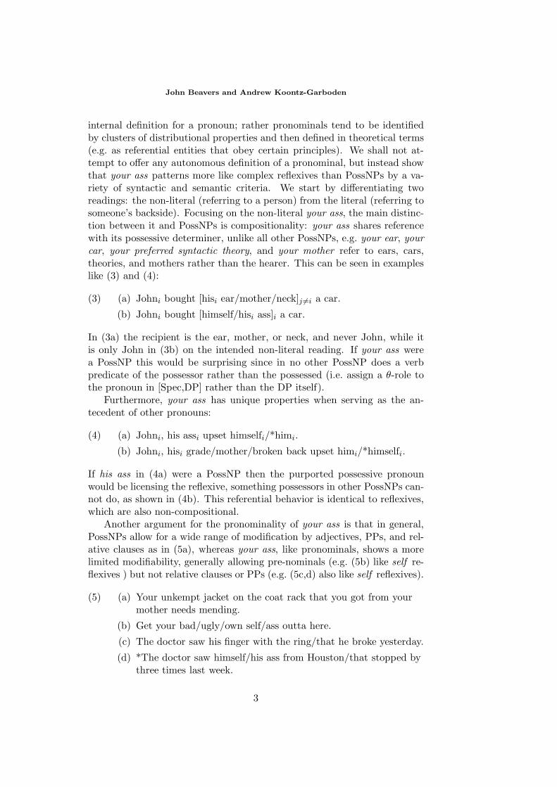
Another argument for the pronominality of your ass is that in general,PossNPs allow for a wide range of modification by adjectives, PPs, and rel-ative clauses as in (5a), whereas your ass, like pronominals, shows a morelimited modifiability, generally allowing pre-nominals (e.g. (5b) like self re-flexives ) but not relative clauses or PPs (e.g. (5c,d) also like self reflexives).
(5) (a) Your unkempt jacket on the coat rack that you got from yourmother needs mending.
(b) Get your bad/ugly/own self/ass outta here.
(c) The doctor saw his finger with the ring/that he broke yesterday.
(d) *The doctor saw himself/his ass from Houston/that stopped bythree times last week.
3
The Proper Treatment of Your Ass in English
Finally, PossNPs can license N -ellipsis whereas reflexives and your asscannot (coindexation is intended to indicate “sense” coreference and notstrict coreference):
(6) (a) Mary had her [car/house/office painted]i, and Jane had hers ei
entirely remodeled.
(b) *Mary had herselfi/her assi committed, and Jane had hers ei
released.
Given the evidence presented here, it is clear that your ass is a pronom-inal, not a regular PossNP. The superficial similarity between your ass anda PossNP is not surprising, however, since complex pronominals in a varietyof languages (including English himself ) are often grammaticalized PossNPsformed from a possessive pronoun+some body part (Faltz, 1985, Schladt,2000). Typically these grammaticalize to reflexives as the PossNP type con-struction serves as a way of placing the pronominal (as a possessive) ina non-argument position and thus exempting it from binding constraints.In this sense it might also be best to view your ass as being on a clineof pronominal grammaticalization, patterning closer to pronominals thanPossNPs.3
3 Pronoun Typology and the Elsewhere Principle
Kiparsky (2002, p.200ff) proposes a hierarchy of binding domains basedon four increasingly specific criteria. The broadest criterion is referentialdependence, wherein referentially dependent pronouns require the presenceof a discourse antecedent, and referentially independent pronouns do not(cf. (7a)). Referentially dependent pronominals, in turn, are either non-reflexive, allowing for a syntactic or discourse-based antecedent, or reflexive,requiring a syntactic antecedent (cf. (7b)). Reflexive pronouns may be eitherfinite-bound, requiring an antecedent in the same finite clause, or not finite-bound, allowing for the possibility of being bound by an antecedent outsideof the finite clause (cf. (7c)). Finally, finite-bound pronominals may beeither locally-bound, requiring an antecedent in the “first accessible subjectdomain”, or not (cf. (7d,e)).
(7) (a) We need to talk about himi/*himselfi, himj/*himselfj , andherk/*herselfk. [pointing] (Referential independence)
(b) Johni is here. I saw himi/*himselfi. (Referentially dependent,non-reflexive)
3Interestingly, according to Holm (2000, 226) the word for “buttocks” in several creolelanguages also shows at least reflexive uses, if not pronominal ones as well (Holm notesonly a reflexive use).
4
John Beavers and Andrew Koontz-Garboden
(c) Johni thought that I would criticize himi/*himselfi. (Reflexive,non-finite-bound)
(d) Johni asked me to criticize himi/*himselfi. (Finite-bound,non-local)
(e) Johni criticized himselfi/*himi. (Local) (Kiparsky, 2002, p.201)
Each domain is cross-classified for the property of ‘obviation’:
(8) ObviationCoarguments have disjoint reference (Kiparsky, 2002, p.2)).
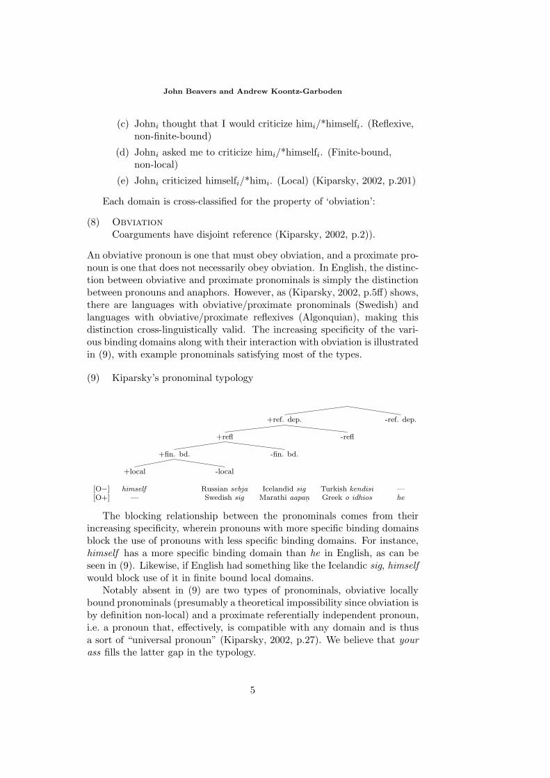
An obviative pronoun is one that must obey obviation, and a proximate pro-noun is one that does not necessarily obey obviation. In English, the distinc-tion between obviative and proximate pronominals is simply the distinctionbetween pronouns and anaphors. However, as (Kiparsky, 2002, p.5ff) shows,there are languages with obviative/proximate pronominals (Swedish) andlanguages with obviative/proximate reflexives (Algonquian), making thisdistinction cross-linguistically valid. The increasing specificity of the vari-ous binding domains along with their interaction with obviation is illustratedin (9), with example pronominals satisfying most of the types.
(9) Kiparsky’s pronominal typology
+ref. dep. -ref. dep.
+refl -refl
+fin. bd. -fin. bd.
+local -local
[O−] himself Russian sebja Icelandid sig Turkish kendisi —[O+] — Swedish sig Marathi aapan. Greek o idhios he
The blocking relationship between the pronominals comes from theirincreasing specificity, wherein pronouns with more specific binding domainsblock the use of pronouns with less specific binding domains. For instance,himself has a more specific binding domain than he in English, as can beseen in (9). Likewise, if English had something like the Icelandic sig, himselfwould block use of it in finite bound local domains.
Notably absent in (9) are two types of pronominals, obviative locallybound pronominals (presumably a theoretical impossibility since obviation isby definition non-local) and a proximate referentially independent pronoun,i.e. a pronoun that, effectively, is compatible with any domain and is thusa sort of “universal pronoun” (Kiparsky, 2002, p.27). We believe that yourass fills the latter gap in the typology.
5
The Proper Treatment of Your Ass in English
4 Your Ass and the Pronominal Typology
Of interest in the present context is the fact that your ass can apparentlybe used in all of the binding domains in (7), as shown in (10)-(14).
(10) Referential independence
(a) On the agenda for today is to talk about his assi, his assj , andher assk. [pointing]
(b) I mean her ass, over there.
(11) Referentially dependent, non-reflexive
(a) Please explain to me is Bobby Vi a good coach or not....Hisi
team has less infield errors than anyone else, give his assi somecredit. [alt.sports.baseball.ny-mets, 08-25-99]
(b) I think if Mike and Buzz had their way, he’di be outta there.Mike hates his assi and Don knows it. The only think (sic)worse than listening to Dennisi is listening to Bart and Freida.[alt.fan.don-n-mike, 06-16-2000]
(12) Reflexive, non-finite-bound
(a) I had one guy tell me the change was for gas, the box, and Ibought his assi a coke while he waited in a long line....[alt.toys.gi-joe, 05-11-02]
(b) First Newton, Alexander, and Moore make an ass out ofPangborni. The more hei whined about it, the more they nailedhis assi. [soc.men, 04-23-99]
(13) Finite-bound, non-local
(a) Johni asked me not to criticize his assi.
(b) Maryi told me to buy her assi a diamond ring.
(14) Local
(a) Youi bought your assi a lap-dance? [alt.angst, 08-31-00]
(b) Don’t give up! I am 30 and was ag. for a little over a year untilIi got my assi some help... [alt.support.agoraphobia, 06-15-99]
The fact that your ass can occur in contexts such as (14) shows thatyour ass is a proximate, and the fact that it can occur in contexts such as(10), with no linguistic antecedent, shows that it is referentially independent.Prima facie, these data appear to show that your ass is in fact a universal
6
John Beavers and Andrew Koontz-Garboden
pronoun, i.e. a referentially independent proximate. This type of pronomi-nal, while theoretically possible, is otherwise unattested in Kiparsky’s exten-sive survey, and proof of the existence of such a pronominal further validatesthis typology by filling in the final logically possible gap in the paradigm.However, your ass poses a serious problem for the theory in general since itseems to contradict the blocking principle, which incorrectly predicts thatreflexives should block your ass in local binding domains (cf. (14)).
5 Semantics of Your Ass and Blocking
We argue, however, that examination of the meaning of your ass can accountfor its anomalous behavior. Specifically, it seems that your ass has twoelements of meaning not found in other pronominals: (a) it can be usedonly in the proper social setting (acting as a marker of that setting), and(b) it carries additional semantics about relationships between participantsand referents in the discourse.
5.1 On the social meaning of your ass
Although it may seem obvious, your ass can be used only in certain socialsettings; there are many social settings in which it is simply not appropriate,e.g. in a nice restaurant, at church, in a reputable conference proceedings,etc. This same point is made by Spears (1998, p.236) who argues that themeaning of your ass is “social and abstract” and that it “marks a discourse asbeing in U[ncensored] M[ode]”, i.e. in a social context where expressions thatwould be inappropriate elsewhere (i.e. censored contexts) are neutral withrespect to appropriateness (Spears, 1998, p.232).4 Thus, your ass marks adiscourse as being in a particular mode/social setting in a way that standardpronominals do not. This fact alone shows that there are more differencesbetween your ass and other pronominals than simply domain specificity.
5.2 On The Non-Social Meaning of Your Ass
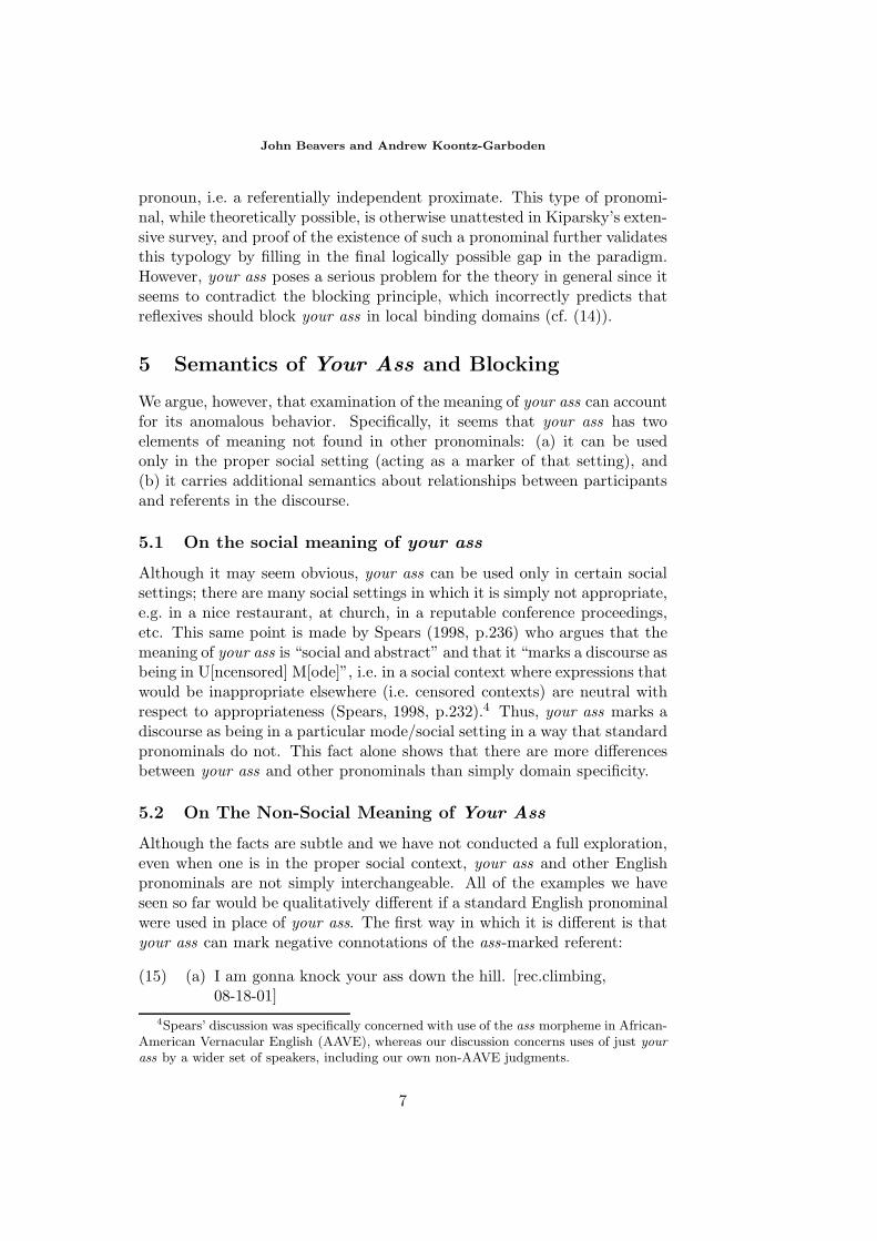
Although the facts are subtle and we have not conducted a full exploration,even when one is in the proper social context, your ass and other Englishpronominals are not simply interchangeable. All of the examples we haveseen so far would be qualitatively different if a standard English pronominalwere used in place of your ass. The first way in which it is different is thatyour ass can mark negative connotations of the ass-marked referent:
(15) (a) I am gonna knock your ass down the hill. [rec.climbing,08-18-01]
4Spears’ discussion was specifically concerned with use of the ass morpheme in African-American Vernacular English (AAVE), whereas our discussion concerns uses of just yourass by a wider set of speakers, including our own non-AAVE judgments.
7
The Proper Treatment of Your Ass in English
(b) I am gonna knock you down the hill.
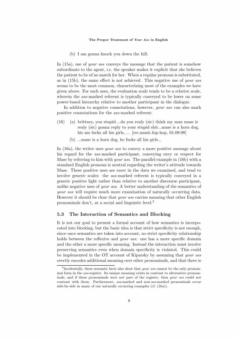
In (15a), use of your ass conveys the message that the patient is somehowsubordinate to the agent, i.e. the speaker makes it explicit that she believesthe patient to be of no match for her. When a regular pronoun is substituted,as in (15b), the same effect is not achieved. This negative use of your assseems to be the most common, characterizing most of the examples we havegiven above. For such uses, the evaluation scale tends to be a relative scale,wherein the ass-marked referent is typically conveyed to be lower on somepower-based hierarchy relative to another participant in the dialogue.
In addition to negative connotations, however, your ass can also markpositive connotations for the ass-marked referent:
(16) (a) brittney, you stupid....do you realy (sic) think my man mase isrealy (sic) gonna reply to your stupid shit...mase is a horn dog,his ass fucks all his girls, ... [rec.music.hip-hop, 01-09-98]
(b) ...mase is a horn dog, he fucks all his girls...
In (16a), the writer uses your ass to convey a more positive message abouthis regard for the ass-marked participant, conveying envy or respect forMase by referring to him with your ass. The parallel example in (16b) with astandard English pronoun is neutral regarding the writer’s attitude towardsMase. These positive uses are rarer in the data we examined, and tend toinvolve generic scales: the ass-marked referent is typically conveyed in ageneric positive light rather than relative to another discourse participant,unlike negative uses of your ass. A better understanding of the semantics ofyour ass will require much more examination of naturally occurring data.However it should be clear that your ass carries meaning that other Englishpronominals don’t, at a social and linguistic level.5
5.3 The Interaction of Semantics and Blocking
It is not our goal to present a formal account of how semantics is incorpo-rated into blocking, but the basic idea is that strict specificity is not enough,since once semantics are taken into account, no strict specificity relationshipholds between the reflexive and your ass: one has a more specific domainand the other a more specific meaning. Instead the interaction must involvepreserving semantics even when domain specificity is violated. This couldbe implemented in the OT account of Kiparsky by assuming that your assovertly encodes additional meaning over other pronominals, and that there is
5Incidentally, these semantic facts also show that your ass cannot be the only pronom-inal form in the ass-register. Its unique meaning exists in contrast to alternative pronom-inals, and if these pronominals were not part of the register, then your ass could notcontrast with them. Furthermore, ass-marked and non-ass-marked pronominals occurside-by-side in many of our naturally occurring examples (cf. (16a)).
8
John Beavers and Andrew Koontz-Garboden
a very highly ranked constraint, a sort of “semantic faithfulness” constraint,requiring this meaning to be overtly realized in the output if present in theinput. With such a constraint, himself always loses on semantic groundsregardless of domain specificity since it never carries the more specific se-mantics. Presumably other approaches might accomplish the same thing,but the main point is that blocking must be sensitive to more than justbinding domains and in a more complicated way than just specificity.
6 Non-Blocking Theories of Binding
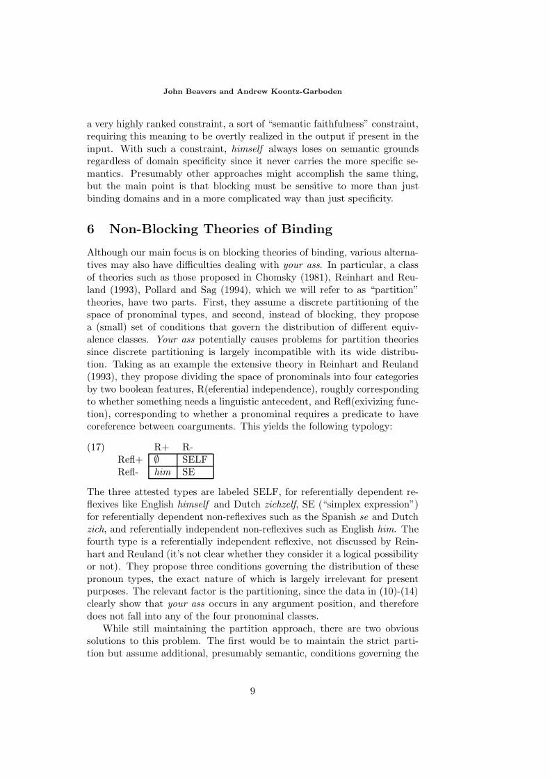
Although our main focus is on blocking theories of binding, various alterna-tives may also have difficulties dealing with your ass. In particular, a classof theories such as those proposed in Chomsky (1981), Reinhart and Reu-land (1993), Pollard and Sag (1994), which we will refer to as “partition”theories, have two parts. First, they assume a discrete partitioning of thespace of pronominal types, and second, instead of blocking, they proposea (small) set of conditions that govern the distribution of different equiv-alence classes. Your ass potentially causes problems for partition theoriessince discrete partitioning is largely incompatible with its wide distribu-tion. Taking as an example the extensive theory in Reinhart and Reuland(1993), they propose dividing the space of pronominals into four categoriesby two boolean features, R(eferential independence), roughly correspondingto whether something needs a linguistic antecedent, and Refl(exivizing func-tion), corresponding to whether a pronominal requires a predicate to havecoreference between coarguments. This yields the following typology:
(17) R+ R-Refl+ ∅ SELFRefl- him SE
The three attested types are labeled SELF, for referentially dependent re-flexives like English himself and Dutch zichzelf, SE (“simplex expression”)for referentially dependent non-reflexives such as the Spanish se and Dutchzich, and referentially independent non-reflexives such as English him. Thefourth type is a referentially independent reflexive, not discussed by Rein-hart and Reuland (it’s not clear whether they consider it a logical possibilityor not). They propose three conditions governing the distribution of thesepronoun types, the exact nature of which is largely irrelevant for presentpurposes. The relevant factor is the partitioning, since the data in (10)-(14)clearly show that your ass occurs in any argument position, and thereforedoes not fall into any of the four pronominal classes.
While still maintaining the partition approach, there are two obvioussolutions to this problem. The first would be to maintain the strict parti-tion but assume additional, presumably semantic, conditions governing the
9
The Proper Treatment of Your Ass in English
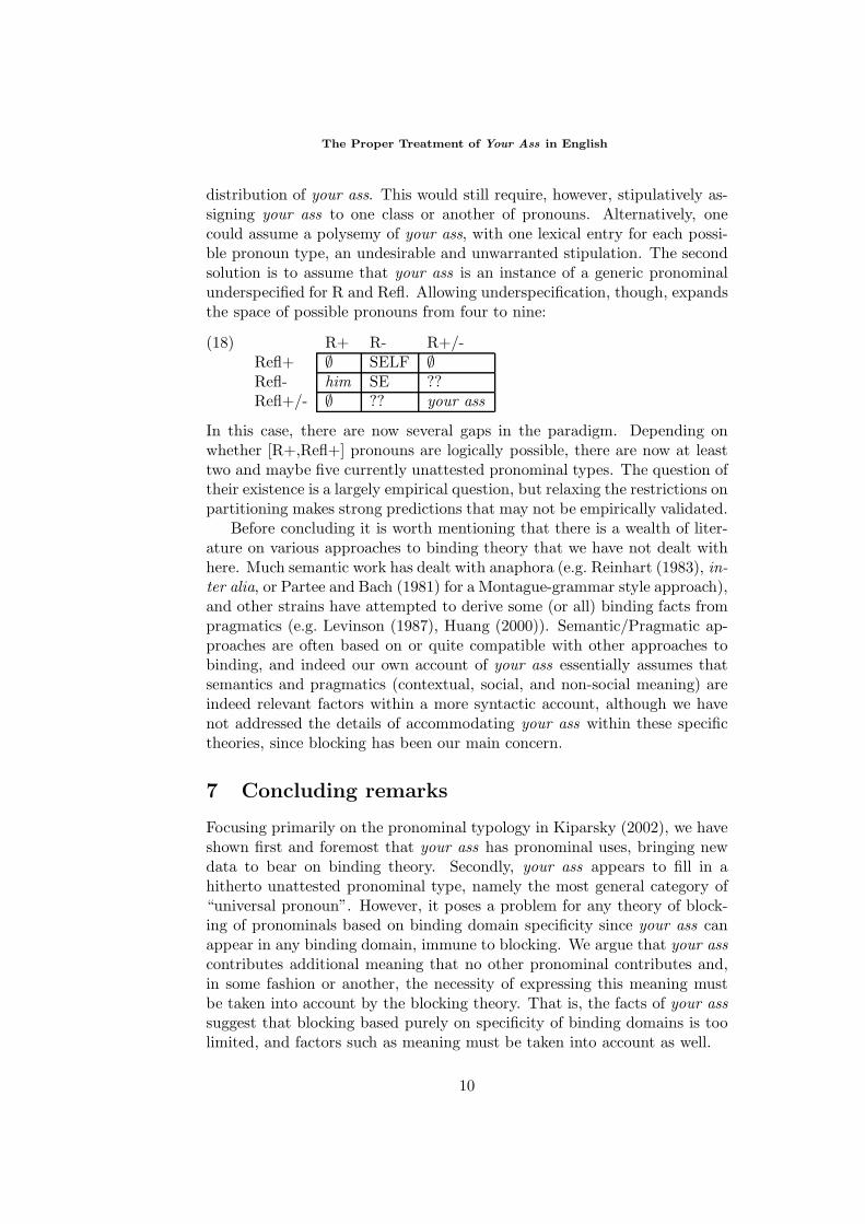
distribution of your ass. This would still require, however, stipulatively as-signing your ass to one class or another of pronouns. Alternatively, onecould assume a polysemy of your ass, with one lexical entry for each possi-ble pronoun type, an undesirable and unwarranted stipulation. The secondsolution is to assume that your ass is an instance of a generic pronominalunderspecified for R and Refl. Allowing underspecification, though, expandsthe space of possible pronouns from four to nine:
(18) R+ R- R+/-Refl+ ∅ SELF ∅Refl- him SE ??Refl+/- ∅ ?? your ass
In this case, there are now several gaps in the paradigm. Depending onwhether [R+,Refl+] pronouns are logically possible, there are now at leasttwo and maybe five currently unattested pronominal types. The question oftheir existence is a largely empirical question, but relaxing the restrictions onpartitioning makes strong predictions that may not be empirically validated.
Before concluding it is worth mentioning that there is a wealth of liter-ature on various approaches to binding theory that we have not dealt withhere. Much semantic work has dealt with anaphora (e.g. Reinhart (1983), in-ter alia, or Partee and Bach (1981) for a Montague-grammar style approach),and other strains have attempted to derive some (or all) binding facts frompragmatics (e.g. Levinson (1987), Huang (2000)). Semantic/Pragmatic ap-proaches are often based on or quite compatible with other approaches tobinding, and indeed our own account of your ass essentially assumes thatsemantics and pragmatics (contextual, social, and non-social meaning) areindeed relevant factors within a more syntactic account, although we havenot addressed the details of accommodating your ass within these specifictheories, since blocking has been our main concern.
7 Concluding remarks
Focusing primarily on the pronominal typology in Kiparsky (2002), we haveshown first and foremost that your ass has pronominal uses, bringing newdata to bear on binding theory. Secondly, your ass appears to fill in ahitherto unattested pronominal type, namely the most general category of“universal pronoun”. However, it poses a problem for any theory of block-ing of pronominals based on binding domain specificity since your ass canappear in any binding domain, immune to blocking. We argue that your asscontributes additional meaning that no other pronominal contributes and,in some fashion or another, the necessity of expressing this meaning mustbe taken into account by the blocking theory. That is, the facts of your asssuggest that blocking based purely on specificity of binding domains is toolimited, and factors such as meaning must be taken into account as well.
10
John Beavers and Andrew Koontz-Garboden
References
Chomsky, N. (1981). Lectures on Government and Binding. Dordrecht: Foris.
Faltz, L. M. (1985). Reflexivization: A Study in Universal Syntax. New York:Garland Publishing, Inc.
Holm, J. (2000). An Introduction to Pidgins and Creoles. Cambridge, UK: Cam-bridge University Press.
Huang, Y. (2000). Anaphora: a cross-linguistic approach. New York: OxfordUniversity Press.
Kiparsky, P. (2002). Disjoint reference and the typology of pronouns. In I. Kauf-mann and B. Stiebels (Eds.), More Than Words. Berlin: Acadamie Verlag.
Levinson, S. C. (1987). Pragmatics and the grammar of anaphora: a partial prag-matic reduction of binding and control phenomena. Journal of Linguistics (23),379–434.
Partee, B. and E. Bach (1981). Quantification, pronouns, and VP anaphora. InJ. Groenendijk, T. Janssen, and M. Stokhof (Eds.), Formal Methods in the Studyof Language, pp. 445–481. Amsterdam: Mathematisch Centrum.
Pollard, C. and I. A. Sag (1994). Head-Driven Phrase Structure Grammar.Chicago, IL: The University of Chicago.
Reinhart, T. (1983). Anaphora and Semantic Interpretation. London: CroomHelm.
Reinhart, T. and E. Reuland (1993). Reflexivity. Linguistic Inquiry 28.
Schladt, M. (2000). The typology and grammaticalization of reflexives. In Z. Fra-jzyngier and T. S. Curl (Eds.), Reflexives: Forms and Functions. Amsterdam:John Benjamins.
Spears, A. (1998). African-American language use: ideology and so-called obscen-ity. In S. Mufwene, J. Rickford, G. Bailey, and J. Baugh (Eds.), African-AmericanEnglish: Structure, History, and Use. New York: Routledge.
11

12
Algorithms for Combinatorial Optimization andGames Adapted from Linear Programming
HENRIK BJORKLUND
Uppsala University
SVEN SANDBERG
Uppsala University
ABSTRACT. The problem of maximizing functionsf : 0, 1d → R from the booleanhypercube to real numbers arises naturally in a wide range of applications. This paper studiesan even more general setting, in which the function to maximize is defined on what we call ahyperstructure. A hyperstructure is a Cartesian product of finite sets with possibly more than twoelements. We also relax the codomain to any partially ordered set. Well-behaved such functionsarise in game theoretic contexts, in particular from parity games (equivalent to the modalµ-calculus model checking) and simple stochastic games (Bj¨orklund, Sandberg, and Vorobyov2003b). We show how several subexponential algorithms for linear programming (Kalai 1992;Matousek, Sharir, and Welzl 1992) can be adapted to hyperstructures and give a reduction to theabstract optimization problems introduced in (G¨artner 1995).
1 Introduction
We investigate the problem of optimizing certain well-behaved functions definedon combinatorial hyperstructures, generalizations of the boolean hypercube0, 1d.Such functions arise naturally in game-theoretic contexts. Their local maxima canbe found with the following general local improvement scheme. Start at a vertexv of the hyperstructure. Ifv has a value greater or equal to all its neighbors, thenreturnv; otherwise restart from one of the better neighbors. Generally, this algo-rithm can take exponential time (Tovey1997). Since the result is a local maximum,it is natural to require every local maximum to be global. This condition, calledlocal-global or LG (Tovey 1986), holds in the game-theoretic setting. Addition-ally, games satisfy the important property that local maxima are globalon everysubstructure. We call such functionsrecursively local-global or RLG for short. Aswe will show, the extra structure of RLG-functions allows us to optimize them insubexponential time, roughly2O(
√d), whered is the dimension.
Proceedings of the Eighth ESSLLI Student SessionBalder ten Cate (editor)Chapter 2, Copyrightc© 2003, Henrik Bjorklund and Sven Sandberg
13
Algorithms for Combinatorial Optimization and Games Adapted from Linear Programming
The main motivation for our study is the application to parity and simplestochastic games. Parity games are two-player games played by moving a pebblealong edges of a directed graph. The associated computational problem consists infinding the optimal strategies of both players. It is interesting from a complexityviewpoint as one of the few natural problems in NP∩ CONP not known to be poly-nomial, especially after PRIMES was shown to be polynomial (Agrawal, Kayal,and Saxena 2002). It is practically significant, being polynomial time equivalentto model-checking for the modalµ-calculus (Emerson, Jutla, and Sistla 1993), oneof the most expressive temporal logics of programs, subsuming logics like LTL,CTL, CTL*, etc. It is also polynomial time equivalent to Rabin chain tree automatanonemptiness (Emerson, Jutla, and Sistla 1993).
In a binary parity game, where the players have at most two choices in eachmove, a strategy of one player can be viewed as a corner of a hypercube. A strategyimprovement algorithm finds the winner of a parity game by assigning values toeach strategy of one player and then moving to better and better strategies until thebest one is reached. The strategy evaluation has to be carefully chosen so that theresulting function is LG with any maximum corresponding to an optimal strategyof the game. This guarantees that the algorithm is correct. This was first donein (Voge and Jurdzi´nski 2000) and we later showed how to compress the valuespace to allow for a better upper bound on the number of iterations (Bj¨orklund,Sandberg, and Vorobyov 2003a). These functions are automatically also RLG,since any subgame is also a game. The same value functions also work for non-binary games, but the domain now becomes a more generalhyperstructure.
A hyperstructure is a Cartesian product of finite sets with possibly more thantwo elements. Although non-binary parity games can be transformed to binarygames, keeping them non-binary allows for better upper bounds because the trans-formation increases the number of vertices. Simple stochastic games is a relatedclass of games where iterative improvement algorithms are easier to understandand have been known for a longer time; see, e.g., (Condon 1993). The values ofstrategies are real numbers and the resulting functions are also RLG.
Linear programming (LP) is the problem of finding the maximum of a lin-ear functional on a convex polyhedron inRd. Although the problem statementlooks very different from that of optimizing an RLG-function on a hyperstructure,we show how to adapt several LP algorithms to RLG optimization. These algo-rithms aresubexponential in the dimension of the polyhedron. Translated to ourterms, they are subexponential in the dimension of the hyperstructure (defined asthe number of sets in the Cartesian product), and in terms of parity games theyare subexponential in the number of vertices that the first player owns. The firstalgorithm shown to be subexponential was (Kalai 1992), adapted by us to paritygames in (Bj¨orklund, Sandberg, and Vorobyov 2003a). The algorithm in (Sharirand Welzl 1992) was invented before Kalai’s, but they proved it subexponentiallater (Matousek, Sharir, and Welzl 1992); see also (Matouˇsek, Sharir, and Welzl1996). It is easier to understand than Kalai’s and the upper bound is similar. For asurvey of these and other related algorithms, see (Goldwasser 1995). Ludwig was
14
Henrik Bj orklund and Sven Sandberg
first to adapt these algorithms to games; he shows how Matouˇsek–Sharir–Welzl’salgorithm works on binary simple stochastic games (Ludwig 1995).
The success of transforming linear programming algorithms to hyperstructuresand games can be understood through problem reductions. First, the strategy eval-uation functions for parity games and simple stochastic games are RLG, as alreadydiscussed. Second, RLG-functions can be directly reduced to theLP-type problemsintroduced in (Sharir and Welzl 1992). LP-type problems is an abstract frameworkcapturing the combinatorial structure of linear programming and numerous otherproblems in computational geometry (Matouˇsek, Sharir, and Welzl 1996). Thealgorithms discussed here and several others work on such problems. The reduc-tion from RLG-functions to LP-type problems was shown for the more restrictedclass of CLG-functions in (Bj¨orklund, Sandberg, and Vorobyov 2003b), but workswithout modification on RLG-functions. The games actually have more structure,captured by CLG-functions, which allows for optimization algorithms that are in-tuitively ‘more aggressive’ (can take longer steps in the hyperstructure) but the bestknown upper bounds remain exponential.
The paper is organized as follows. In Section 2 we define the functions weoptimize and the structures they are defined on. As an introduction to the conceptsunderlying later sections, we present a Ludwig-style optimization algorithm forhypercubes in Section 3. Sections 4 and 5 adapt the linear programming algorithmsfrom (Matousek, Sharir, and Welzl 1996) and (Kalai 1992), respectively. Finally,we show in Section 6 how our problem can be reduced to what (G¨artner 1995) callsan abstract optimization problem (AOP).
2 Hyperstructures
The set of all positional strategies in a parity game is isomorphic to a product offinite sets, each representing the choices in a vertex. Functions from strategies tovalues in such games motivate our study of functions on thehyperstructures definedhere. They are generalizations of the boolean hypercube0, 1d. Optimization ofwell-behaved functions on hypercubes has been extensively studied in, e.g., (Ham-mer, Simeone, Liebling, and De Werra 1988; Wiedemann 1985; Williamson Hoke1988; Tovey1997; Bjorklund, Sandberg, and Vorobyov 2002).
Definition 2.1 (Hyperstructure) For each j ∈ 1, . . . , d let Pj = ej,1, . . . ,
ej,δj be a finite nonempty set. Call P =
∏dj=1Pj a d-dimensional hyperstructure,
or structurefor short.
A substructure of P is a productP′ =∏d
j=1P ′j, where∅ = P ′
j ⊆ Pj forall j. A facet of P is a substructure obtained by fixing the choice in exactly onecoordinate. ThusP′ is a facet ofP if there is aj ∈ 1, . . . , d such that|P′j | = 1andP′
k = Pk for all k = j. We will sometimes identify a facet with its definingelementej,i ∈ Pj, assuming all setsPk to be disjoint. If|P′
j | ≤ 2 for all j, thenP ′ is called asubcube since it is isomorphic to a boolean hypercube. We will
15
Algorithms for Combinatorial Optimization and Games Adapted from Linear Programming
consistently use the letterd for the dimension andn :=∑d
j=1 |Pj | for the numberof facets. If |Pj | = 1 for somej, this coordinate can be disregarded since it isconstant, and we will consider such structures as having smaller dimension.
An element ofP is called avertex. Two verticesx, y ∈ P areneighbors if theydiffer in only one coordinate. The neighbor relation induces a graph with elementsof P as nodes, and allows us to talk about paths and distances inP.
For a setE ⊆ ⋃dj=1Pj, definestruct(E) to be the substructureP′ =
∏dj=1(Pj∩
E). Thus, if E does not have elements from eachPj , thenstruct(E) = ∅. Fora setF of facets, we usestruct(F) for struct(E) whereE is the set of definingelements of the facets inF .
Throughout this paper, letD be some partially ordered set. We are interestedin finding optima of functions that mapP toD, such that any two neighbors havecomparable values. Alocal maximum of a functionf : P → D is a vertexvsuch thatf(v) ≥ f(u) for all neighborsu of v. If f(v) ≥ f(u) for all verticesu ∈ P, thenv is aglobal maximum of f onP. Local and globalminima are definedsymmetrically.
Arbitrary functions onP cannot be efficiently optimized; see, e.g., Corollary19 of (Tovey1997), but the prospects are better for some nontrivial and very in-teresting subclasses. The class ofcompletely unimodal (CU) functions on hyper-cubesH = 0, 1d has been studied in, e.g, (Hammer, Simeone, Liebling, andDe Werra 1988; Williamson Hoke 1988; Wiedemann 1985; Bj¨orklund, Sandberg,and Vorobyov 2002), and can be optimized in subexponential time (Bj¨orklund,Sandberg, and Vorobyov 2002). In (Bj¨orklund, Sandberg, and Vorobyov 2003b)we defined the class ofcompletely local-global (CLG) functions, a generalizationof CU-functions, defined on hyperstructures and capturing the properties of value-functions obtained from parity games. To demonstrate the full applicability of thealgorithms in later sections, we here define the even wider class ofrecursivelylocal-global (RLG) functions. The inclusions CU⊂ CLG⊂ RLG follow from thedefinitions. The strictness of these inclusions is easy to establish.
Definition 2.2 (Recursively Local-Global) A function f : P → D for which allneighbors have comparable values is called recursively local-global(RLG) if forevery substructure P′ of P, all local maxima of the restriction of f to P′ are alsoglobal.
In the sequel, we discuss algorithms for maximizing RLG-functions. Such al-gorithms can also be used to maximize CLG-functions and CU-functions. We useRLG-structure to denote an RLG-function together with its underlying hyperstruc-ture, and we useRLG-cube if the hyperstructure is a hypercube. An RLG-structurecan be thought of as a hyperstructure with its vertices labeled by function values.Given an RLG-functionf : P → D, and a substructureP′ of P, let wf (P ′) be themaximum value off onP′.
16
Henrik Bj orklund and Sven Sandberg
3 Ludwig-Style Algorithm for Hypercubes
The first subexponential randomized algorithm for solving simple stochastic gameswas presented in (Ludwig 1995). It uses the ideas of the linear programming algo-rithms in (Matousek, Sharir, and Welzl 1992; Matouˇsek, Sharir, and Welzl 1996)and (Kalai 1992), which we will discuss in later sections. Unfortunately, the al-gorithm only applies to binary games (with vertex outdegree at most two), andreduction to such games may increase the number of vertices, undermining thesubexponential analysis. Binary games give rise to RLG-cubes (Bj¨orklund, Sand-berg, and Vorobyov 2003b).
As an introduction to the ideas underlying the algorithms presented later, andtheir adaptations to RLG-functions, the Ludwig-style Algorithm 1 maximizes anyRLG-function f : H → D, whereH = 0, 1d.
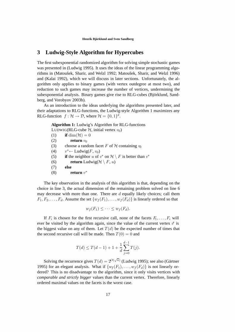
Algorithm 1: Ludwig’s Algorithm for RLG-functionsLUDWIG(RLG-cubeH, initial vertexv0)(1) if dim(H) = 0(2) return v0
(3) choose a random facetF of H containingv0(4) v∗← Ludwig(F , v0)(5) if the neighboru of v∗ onH \ F is better thanv∗
(6) return Ludwig(H \ F , u)(7) else(8) return v∗
The key observation in the analysis of this algorithm is that, depending on thechoice in line 3, the actual dimension of the remaining problem solved on line 6may decrease with more than one. There ared equally likely choices; call themF1, F2, . . . , Fd. Assume the setwf (F1), . . . , wf (Fd) is linearly ordered so that
wf (F1) ≤ · · · ≤ wf (Fd).
If Fi is chosen for the first recursive call, none of the facetsF1, . . . , Fi willever be visited by the algorithm again, since the value of the current vertexv∗ isthe biggest value on any of them. LetT (d) be the expected number of times thatthe second recursive call will be made. ThenT (0) = 0 and
T (d) ≤ T (d− 1) + 1 +1d
d−1∑j=0
T (j).
Solving the recurrence givesT (d) = 2O(√
n) (Ludwig 1995); see also (G¨artner1995) for an elegant analysis. What ifwf (F1), . . . , wf (Fd) is not linearly or-dered? This is no disadvantage to the algorithm, since it only visits vertices withcomparable and strictly bigger values than the current vertex. Therefore, linearlyordered maximal values on the facets is the worst case.
17
Algorithms for Combinatorial Optimization and Games Adapted from Linear Programming
4 Matousek–Sharir–Welzl-Style Algorithm
In this section, we show how the LP-algorithm in (Matouˇsek, Sharir, and Welzl1992; Matousek, Sharir, and Welzl 1996) can be modified for RLG-functions,yielding a simple subexponential randomized algorithm for the problem (and thusalso for parity games; see also (Bj¨orklund, Sandberg, and Vorobyov 2003b)). It has
expected running time at most2O(√
d log(n/√
d)+log n), wheren =∑d
j=1 |Pj | is thenumber of facets ofP.
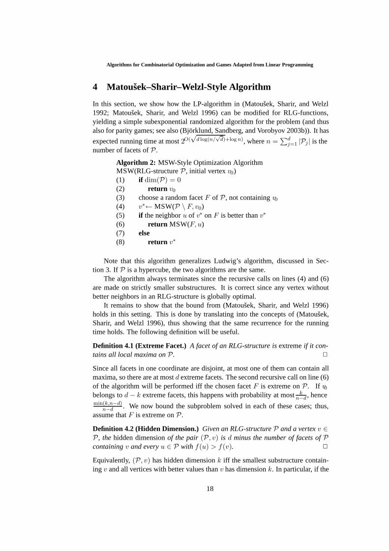
Algorithm 2: MSW-Style Optimization AlgorithmMSW(RLG-structureP, initial vertexv0)(1) if dim(P) = 0(2) return v0
(3) choose a random facetF of P, not containingv0(4) v∗← MSW(P \ F, v0)(5) if the neighboru of v∗ onF is better thanv∗
(6) return MSW(F, u)(7) else(8) return v∗
Note that this algorithm generalizes Ludwig’s algorithm, discussed in Sec-tion 3. If P is a hypercube, the two algorithms are the same.
The algorithm always terminates since the recursive calls on lines (4) and (6)are made on strictly smaller substructures. It is correct since any vertex withoutbetter neighbors in an RLG-structure is globally optimal.
It remains to show that the bound from (Matouˇsek, Sharir, and Welzl 1996)holds in this setting. This is done by translating into the concepts of (Matouˇsek,Sharir, and Welzl 1996), thus showing that the same recurrence for the runningtime holds. The following definition will be useful.
Definition 4.1 (Extreme Facet.) A facet of an RLG-structure is extremeif it con-tains all local maxima on P.
Since all facets in one coordinate are disjoint, at most one of them can contain allmaxima, so there are at mostd extreme facets. The second recursive call on line (6)of the algorithm will be performed iff the chosen facetF is extreme onP. If v0belongs tod− k extreme facets, this happens with probability at mostk
n−d , hencemin(k,n−d)
n−d . We now bound the subproblem solved in each of these cases; thus,assume thatF is extreme onP.
Definition 4.2 (Hidden Dimension.) Given an RLG-structure P and a vertex v ∈P, the hidden dimensionof the pair (P, v) is d minus the number of facets of Pcontaining v and every u ∈ P with f(u) > f(v).
Equivalently,(P, v) has hidden dimensionk iff the smallest substructure contain-ing v and all vertices with better values thanv has dimensionk. In particular, if the
18
Henrik Bj orklund and Sven Sandberg
hidden dimension is0, thenv is a maximum onP. Let k be the hidden dimensionandP′ the corresponding substructure. The algorithm will only visit vertices thatbelong toP′. There ared − k facets,F1, . . . , Fd−k, that containP′; all these areextreme. In the worst case there arek more extreme facets,Fd−k+1, . . . , Fd. Foreach such facet, consider the best value that does not belong to it. Assume first thatthese values are totally ordered. Enumerate the facets so that
wf (P \Fd−k+1) ≤ · · · ≤ wf (P \Fd−k+i) ≤ · · · ≤ wf (P \Fd). (1)
Suppose the algorithm chooses facetFd−k+i. Thenf(v∗) = wf (P \ Fd−k+i) <f(u). Every vertex with a better value thanv∗ that belongs toFd−k+i must alsobelong toFd−k+j for all 1 ≤ j < i; the opposite would contradict (1). Thusubelongs to(d − k + i) facets that contain all vertices with better values, and thehidden dimension of the pair(Fd−k+i, u) for the second call is at most(k − i).
If the best values outside the remaining extreme facets are not totally ordered,this only benefits the algorithm. The values are partially ordered, and if facetFd−k+i is chosen,u will belong to all facets that do not have a strictly biggervalue forwf (P \Fj), and they will all contain all vertices with better values. Thisis because ifwf (P \ Fd−k+i) andwf (P \ Fj) are incomparable, then any valuebetter thanwf (P \ Fd−k+i) will be better than or incomparable towf (P \ Fj),since the order onD is transitive.
This discussion gives the same recurrences for the numbers of tests on line (5)and jumps tou on line (6) as (Matouˇsek, Sharir, and Welzl 1996) gets for thenumbers of violation tests and basis computations, respectively, in the linear pro-gramming setting. They are both bounded by the recurrencetk(d) = 0 (where0 ≤ k ≤ d) and
tk(n) ≤ tk(n− 1) + 1 +1
n− d
min(k,n−d)∑i=1
tk−i(n), for n > d.
The recurrence is solved in (Matouˇsek, Sharir, and Welzl 1996), and from thesolution it is easy to infer that the expected running time of the algorithm on RLG-
structures is at most2O(√
d log(n/√
d)+log n), as long as function evaluation and com-parison of function values can be performed in polynomial time. As soon asncan be assumed to be polynomially bounded byd, this bound is subexponentialin d. The reduction from parity games withd vertices to RLG-functions givesn = O(d2), so we can solve parity games in expected time2O(
√d log d).
5 Kalai-Style Algorithm
We now describe another algorithm for optimizing RLG-structures, originally in-vented for linear programming by Kalai (Kalai 1992; Goldwasser 1995) and lateradapted by us to parity games (Bj¨orklund, Sandberg, and Vorobyov 2003a). It is
19
Algorithms for Combinatorial Optimization and Games Adapted from Linear Programming
also subexponential with complexity similar to the MSW-style algorithm of theprevious section (but it is slightly more complicated).
Let P(d, n) denote the class of RLG-structures with dimensiond and n =∑dj=1 |Pj |. If v is a vertex inP then a facetF is v-improving if some witness
vertex v′ ∈ F has a better value thanv.
The Algorithm takes an RLG-structureP ∈ P(d, n) and an initial vertexv0 asinputs and returns the optimal vertex onP. It uses the subroutine COLLECT-IMPROVING-FACETS, described later, that collects a set of pairs(F, v) of v0-improving facetsF and corresponding witness verticesv ∈ F .
Algorithm 3: Kalai-Style Optimization AlgorithmKALAI (RLG-structureP, initial vertexv0)(1) if dim(P) = 0(2) return v0
(3) M← COLLECT-IMPROVING-FACETS(P, v0 )(4) choose a random pair(F, v1) ∈M(5) v∗ ← KALAI (F, v1)(6) if some neighboru of v∗ onP \ F is better thanv∗
(7) return KALAI (P, u)(8) else(9) return v∗
How to Find Many Improving Facets. Now we describe the subroutine COLLECT-IMPROVING-FACETS. The goal is to findr v0-improving facets, wherer is a pa-rameter (Kalai usesr = max(d, n/2) to get the best complexity analysis). Tothis end we construct a sequence(P0,P1, . . . ,Pr−d) of substructures ofP, withPi ∈ P(d, d + i) andPi ⊂ Pi+1. All the d + i facets ofPi arev0-improving;we simultaneously determine the corresponding witness verticesvj optimal inPj .The subroutine returnsr facets ofP, each one obtained by fixing one of therchoices inPr−d ∈ P(d, r). All these arev0-improving by construction.
Let v0 be a better neighbor ofv0 onP. (If no better neighbor exists thenv0 isoptimal inP and we are done.) SetP0 to the RLG-structure containing onlyv0.Fixing any of thed coordinates ofP as inv0 defines av0-improving facet ofPwith v0 as a witness.
To constructPi+1 from Pi, let v′ be a better neighbor ofvi. (Note thatvi isoptimal inPi but not necessarily in the full structureP. If it is, we terminate.)Let Pi+1 be the smallest substructure ofP containingv′ and all vertices inPi.Recursively apply the algorithm to find the optimalvi+1 in Pi+1. Note that fixinga coordinate inP to any of thed + i choices inPi defines av0-improving facet.Therefore, the finalPr−d hasr v0-improving facets.
Analysis. First note that we can pick the random number before line 3, pass it toCOLLECT-IMPROVING-FACETS, and only find that many facets. Now each solvedsubproblem starts from a strictly better vertex, so the algorithm clearly terminates.
20
Henrik Bj orklund and Sven Sandberg
It is correct because it can only terminate by returning an optimal vertex.This algorithm yields a recurrence similar to those in previous sections. Kalai
solves it and gets the subexponential running time2O((log n)√
d/ log d).It is interesting to note the similarities of Ludwig’s, Matouˇsek–Sharir–Welzl’s,
and Kalai’s subexponential algorithms. They all take a structureP and a vertexv0as parameters and recursively find the optimumv∗ on a substructureP′ of P. Thechoice ofP′ is random, but it is guaranteed to contain vertices at least as good asv0, and the recursive call starts from a witness of this fact. If the result is not anoptimum on the entire structure, then we optimize the rest of the structure, startingfrom a better neighbor ofv∗. Intuitively, the subexponential upper bound relies onthe substructure being taken randomly from some set. Thus it is expected that theoptima of many structures in the set are no better thanv∗, and those structures willbe ignored in the remainder of the algorithm.
6 Abstract Optimization Problems
The class ofabstract optimization problems (AOPs) was introduced in (G¨artner1995). He uses this generalization to show how the ideas from (Matouˇsek, Sharir,and Welzl 1996; Kalai 1992) can be used to obtain a subexponential randomizedalgorithm for a wider class of optimization problems. In this section we showthat optimizing an RLG-function with totally ordered codomain can be reduced tosolving an AOP.
Definition 6.1 (AOP (Gartner 1995)) An AOP is a triple (A,<,Φ), where A is afinite set, < is a total order on 2A, and Φ : (C,B)|C ⊆ B ⊆ A → 2A satisfies
Φ(C,B) =
C, iff C = max<C ′|C ′ ⊆ B;C ′, for some C′ s.t. C < C ′ ⊆ B, otherwise.
For B ⊆ A, let opt(B) denote max<C|C ⊆ B. Solving an AOP means findingopt(A).
Intuitively, solving an AOP corresponds to maximizing some function on a booleanhypercube. The function may be unstructured, but there is an oracle capable offinding some better vertex than the current one on any subcube containing the ori-gin. The algorithm in (G¨artner 1995) solves any AOP with|A| = n using expectede2
√n+O( 4
√n ln n) calls toΦ. Maximizing an RLG-functionf with n facets can be
reduced to solving an AOP with|A| = n, if its codomain is totally ordered. Thisrestriction is often satisfied, as for, e.g., parity games (Bj¨orklund, Sandberg, andVorobyov 2003b).
Let P be ad-dimensional hyperstructure withn facets, and letf : P → Dbe an RLG-function with totally ordered codomain. Define an AOP(F , <,Ψ) asfollows. Let−∞ be an artificial value, smaller than all values of vertices ofP. Let
21
Algorithms for Combinatorial Optimization and Games Adapted from Linear Programming
F be the set of all facets ofp, and defineval : 2F → D ∪ −∞ by
val(F ) =
wf (struct(F )), iff struct(F ) = ∅;−∞, otherwise.
Take≺ to be any total order on2F such thatF ≺ F ′ whenever|F | > |F ′|.For F,F ′ ∈ F let F < F ′ iff 1) val(F ) < val(F ′), or 2)val(F ) = val(F ′) andF ≺ F ′. Now defineΦ(F,G) as follows.
• Supposeval(F ) = −∞ andstruct(F ) contains only one vertexv. If v is alocal maximum onstruct(G), thenΦ(F,G) = F . OtherwiseΦ(F,G) is aset defining a 0-dimensional substructure containing only a better neighborof v on struct(G).• If val(F ) = −∞ but |F | > d then Φ(F,G) = F ′ whereF ′ defines a
substructure containing only one vertex with maximal value onstruct(F ).• If val(F ) = −∞ andstruct(G) = ∅ thenΦ(F,G) = ∅.• If val(F ) = −∞ andstruct(G) = ∅ thenΦ(F,G) = F ′ for someF ′ ∈
struct(G).
Now (F , <,Φ) defines an AOP, and applying G¨artner’s algorithm will yield a solu-tion from which a maximal vertex of the original RLG-structure can be recovered.
Unfortunately, the bound this gives for maximizing RLG-functions is not verygood. The previously discussed algorithms give bounds subexponential ind as longasn is polynomial ind, which is not the case here. If, for example,n = Θ(d2),which is the worst case when reducing games to RLG-functions, we only get a2O(d) bound on the expected calls toΦ. The reason seems to be that the originaldimension is lost in the reduction, and all facets are treated as independent.
Gartner’s algorithm, called with the appropriate parameters, will never callΦwith any set of size bigger thand as the first parameter. For such sets,Φ can becomputed in polynomial time.
7 Conclusions
In (Bjorklund, Sandberg, and Vorobyov 2003a; Bj¨orklund, Sandberg, and Vorobyov2003b) we showed how the well-known linear programming algorithms from (Kalai1992; Matousek, Sharir, and Welzl 1996) can be adapted to solving parity games.In this paper we showed that these algorithms work for maximizing recursivelylocal-global functions on hyperstructures. Together with the reductions from gamesto RLG-functions from (Bj¨orklund, Sandberg, and Vorobyov 2003b), this stressesthe combinatorial similarities between linear programming and solving games. Italso provides a simple setting, stripped of cumbersome details, convenient for in-vestigation of such similarities and for developing new algorithms for parity andsimple stochastic games.
AcknowledgementsWe thank anonymous referees for valuable remarks, improve-ments and references.
22
Henrik Bj orklund and Sven Sandberg
References
Agrawal, M., N. Kayal, and N. Saxena (2002, August). Primes is in P. Unpublishedmanuscript,http://www.cse.iitk.ac.in/news/primality.html.
Bjorklund, H., S. Sandberg, and S. Vorobyov (2002, May). Optimization on completelyunimodal hypercubes. Technical Report 018, Uppsala University / Information Technol-ogy. http://www.it.uu.se/research/reports/.
Bjorklund, H., S. Sandberg, and S. Vorobyov (2003a). A discrete subexponential algo-rithm for parity games. In H. Alt and M. Habib (Eds.),20th International Symposium onTheoretical Aspects of Computer Science, STACS’2003, Volume 2607 ofLecture Notes inComputer Science, Berlin, pp. 663–674. Springer-Verlag. Full preliminary version: TR-2002-026, Department of Information Technology, Uppsala University, September 2002,http://www.it.uu.se/research/reports/.
Bjorklund, H., S. Sandberg, and S. Vorobyov (2003b, January). Oncombinatorial structure and algorithms for parity games. Technical Re-port 2003-002, Department of Information Technology, Uppsala University.http://www.it.uu.se/research/reports/.
Condon, A. (1993). On algorithms for simple stochastic games.DIMACS Series inDiscrete Mathematics and Theoretical Computer Science 13, 51–71.
Emerson, E. A., C. Jutla, and A. P. Sistla (1993). On model-checking for fragments ofµ-calculus. InComputer Aided Verification, Proc. 5th Int. Conference, Volume 697, pp.385–396. Lect. Notes Comput. Sci.
Gartner, B. (1995). A subexponential algorithm for abstract optimization problems.SIAMJournal on Computing 24, 1018–1035.
Goldwasser (1995). A survey of linear programming in randomized subexponential time.SIGACTN: SIGACT News (ACM Special Interest Group on Automata and ComputabilityTheory) 26, 96–104.
Hammer, P. L., B. Simeone, T. M. Liebling, and D. De Werra (1988). From linear separa-bility to unimodality: a hierarchy of pseudo-boolean functions.SIAM J. Disc. Math. 1(2),174–184.
Kalai, G. (1992). A subexponential randomized simplex algorithm. In24th ACM STOC,pp. 475–482.
Ludwig, W. (1995). A subexponential randomized algorithm for the simple stochasticgame problem.Information and Computation 117, 151–155.
Matousek, J., M. Sharir, and M. Welzl (1992). A subexponential bound for linear pro-gramming. In8th ACM Symp. on Computational Geometry, pp. 1–8.
Matousek, J., M. Sharir, and M. Welzl (1996). A subexponential bound for linear pro-gramming.Algorithmica 16, 498–516.
Sharir, M. and E. Welzl (1992). A combinatorial bound for linear programming and re-lated problems. In9th Symposium on Theoretical Aspects of Computer Science (STACS),Volume 577 ofLecture Notes in Computer Science, Berlin, pp. 569–579. Springer-Verlag.
Tovey, C. A.(1986). Low order polynomial bounds on the expected performance of localimprovement algorithms.Mathematical Programming 35, 193–224.
23
Algorithms for Combinatorial Optimization and Games Adapted from Linear Programming
Tovey, C. A.(1997). Local improvement on discrete structures. In E. Aarts and L. J. K.(Eds.),Local Search in Combinatorial Optimization, pp. 57–89. John Wiley & Sons.
Voge, J. and M. Jurdzi´nski (2000). A discrete strategy improvement algorithm for solvingparity games. InCAV’00: Computer-Aided Verification, Volume 1855 ofLect. NotesComput. Sci., pp. 202–215. Springer-Verlag.
Wiedemann, D. (1985). Unimodal set-functions.Congressus Numerantium 50, 165–169.
Williamson Hoke, K. (1988). Completely unimodal numberings of a simple polytope.Discrete Applied Mathematics 20, 69–81.
24
Building Sub-corpora Suitable for
Extraction of Lexico-Syntactic
Information
Ondrej BojarInstitute of Formal and Applied Linguistics, UFAL MFF UK, Malostranske namestı 25, CZ-11800
Praha, Czech Republic
Abstract.
Accuracy of automatic syntactic analysis of natural languages with relatively freeword order (such as Czech) can be hardly improved without building large andprecise lexicons of syntactic behavior of individual words (e.g. lexicons of verb va-lency frames). The current treebanks available do not cover enough words. Largercorpora lack the syntactic annotation and many sentences contained in them aretoo complex to extract the information easily or even automatically. The systemAX (automatic extraction) was developed to perform selection of morphologicallyanalyzed sentences by means of custom hand-written rules. The rules can be eas-ily formulated to perform linguistic-motivated filtration. The system AX allows toperform partial syntactic analysis in order to check the occurrence of more complexlinguistic phenomena.
1 Motivation
At the current stage of the development, the accuracy of automatic syntac-tic analyzers of natural languages (in particular Czech) is limited due to thelack of large and precise lexicons of syntactic behavior of individual words(verb valency frames are the most important example). Building such lex-icons by hand is rather a time-consuming task and any kind of automaticpreprocessing would help.
The available data sources include corpora annotated on different levelsof linguistic description. Syntactic information can be easily extracted fromcorpora annotated on the syntactic level (such as the Prague DependencyTreebank, PDT1, Bohmova et al. (2001)) and some attempts to extractfor example verb subcategorization frames from treebanks were already per-formed2. However the number of occurrences of individual lexical items in
1http://ufal.mff.cuni.cz/pdt/2Such as (Sarkar and Zeman, 2000).
Proceedings of the Eighth ESSLLI Student SessionBalder ten Cate (editor)Chapter 3, Copyright c© 2003, Ondrej Bojar
25
Building Sub-corpora Suitable for Extraction of Lexico-Syntactic Information
such corpora is usually not sufficient. Bojar (2002) shows that only a fewhundreds of verbs have enough occurrences in PDT and that more than 60%of 26,000 verbs found in the Czech National Corpus (CNC3) are not cov-ered in PDT at all. Therefore, it is necessary to extract the lexico-syntacticinformation from larger corpora (such as the CNC) or any texts available.
However, not all sentences containing a given lexeme can serve as a goodexample to extract the syntactic information (for instance, if two verbs arepresent in one clause, their complements and adjuncts can be arbitrarilyintermixed). And moreover, as the syntactic annotation in these corpora ismissing, the sentences can often be too complex to be analyzed by any ofthe available parsers at a reasonable level of accuracy.
I developed the system AX to simplify the task of selecting feasibleexamples of sentences for extracting a specific lexico-syntactic information(not just the verb valency frames). The sentences can be easily selectedon linguistically based criteria. Partial syntactic analysis of sentences ispossible, in order to be able to answer more complex linguistic questionsabout the sentence.
In section 2 I describe the overall architecture of the system AX. Section3 gives a brief description of the basic data structure, variant feature struc-ture. Sections 4 and 5 describe the core of the scripting language AX: filtersto reject sentences and rules to perform (partial) syntactic analysis. In thelast section, I illustrate the use of the system to select sentences suitable forextracting valency frames of Czech verbs and document the improvement ofaccuracy of Czech parsers when applied only to the selected sentences.
2 The Architecture of AX
The system AX combines the idea of regular expressions and replacements(see (Karttunen et al., 1996; Aıt-Mokhtar and Chanod, 1997) and others)with the idea of feature structures (see below) known from unification-basedparsers. This combination leads to a formalism that is both, strong todescribe complex linguistic properties of sentences of natural language andefficient in the process of parsing.
The user prepares a script of filters and rules to select sentences suitablefor a specific purpose. The system AX loads the script and then expectssentences augmented with their morphological annotation (in format of thePDT4) on the standard input. The input sentences may or may be not mor-phologically disambiguated. For every input sentence, the system runs thescript and checks, if the sentence passed all the filters or has been rejected.For sentences that pass (referred to with the term “selected sentences”), theoutput of the final phase (see below) is printed out. This output is for some
3http://ucnk.ff.cuni.cz/4See http://shadow.ms.mff.cuni.cz/pdt/Corpora/PDT 1.0/Doc/morph.html
26
Ondrej Bojar
purposes already suitable for collecting the lexico-syntactic information sothat no other parser to process the sentences is needed.
In the following, I describe the overall running scheme of AX. The inputsentence is internally stored as a sequence of feature structures that corre-spond one to one to input word forms. (See section 3 for details.) The inputsentence is then processed through a pipe of consecutive blocks (phases) ofoperation. Each of the blocks is either a filter, or a set of rules.
The input for each block is a set of sequences of feature structures (re-ferred to with the term the set of “input readings” of the sentence). If theblock is a filter, it checks all the input readings and possibly rejects someof them. If the block is a set of rules, it updates every input reading withall applicable rules and returns a larger set of new readings (it “generates”new readings).
Consecutive blocks are connected, so that the output set of readings fromthe former block is used as the input set of readings for the latter block. Thefirst of the blocks receives as input the input sentence, the output from thelast block is printed out. The order and type of the blocks is up to theauthor of the script. All the input sentences that were not rejected by anyof the filters are accepted and the output produced for each of them can alsobe used to extract the lexico-syntactic information, if appropriate.
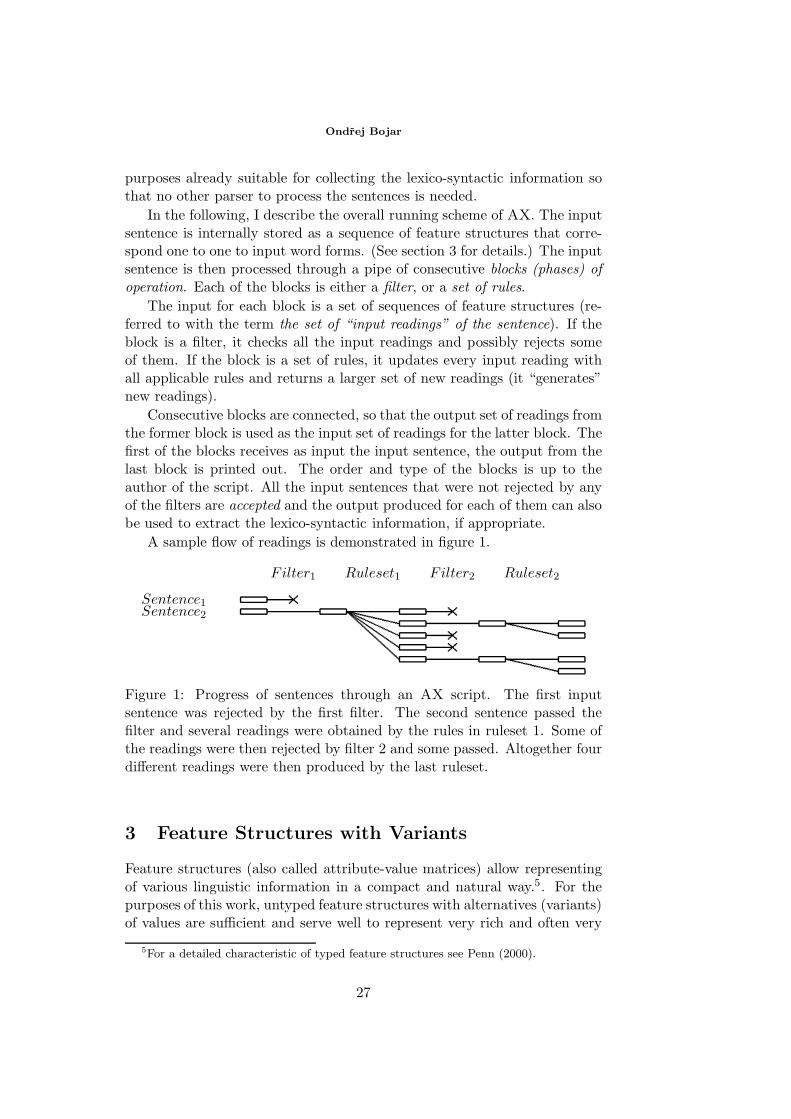
A sample flow of readings is demonstrated in figure 1.
Filter1 Ruleset1 Filter2 Ruleset2
Sentence1Sentence2
Figure 1: Progress of sentences through an AX script. The first inputsentence was rejected by the first filter. The second sentence passed thefilter and several readings were obtained by the rules in ruleset 1. Some ofthe readings were then rejected by filter 2 and some passed. Altogether fourdifferent readings were then produced by the last ruleset.
3 Feature Structures with Variants
Feature structures (also called attribute-value matrices) allow representingof various linguistic information in a compact and natural way.5. For thepurposes of this work, untyped feature structures with alternatives (variants)of values are sufficient and serve well to represent very rich and often very
5For a detailed characteristic of typed feature structures see Penn (2000).
27
Building Sub-corpora Suitable for Extraction of Lexico-Syntactic Information
ambiguous morphological information6 as well as arbitrary user flags usefulin the process of filtering and generating new readings by rules.
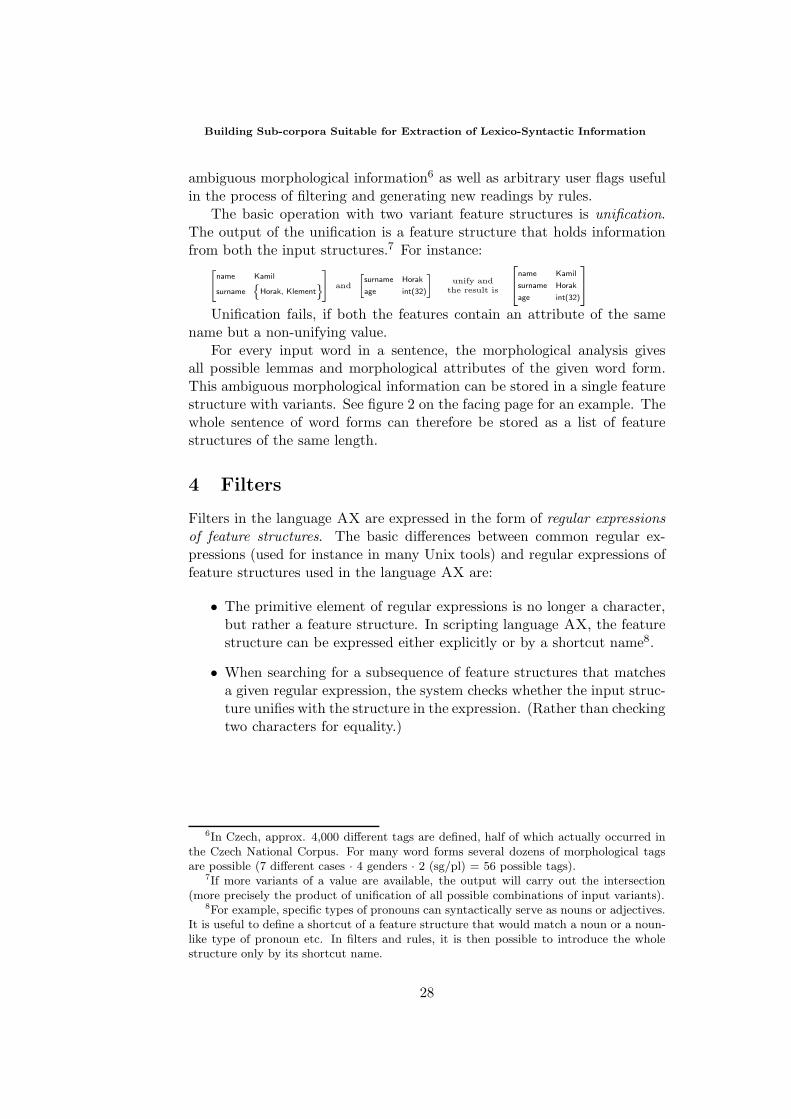
The basic operation with two variant feature structures is unification.The output of the unification is a feature structure that holds informationfrom both the input structures.7 For instance:[
name Kamil
surname
Horak, Klement] and
[surname Horak
age int(32)
]unify and
the result is
[name Kamil
surname Horak
age int(32)
]
Unification fails, if both the features contain an attribute of the samename but a non-unifying value.
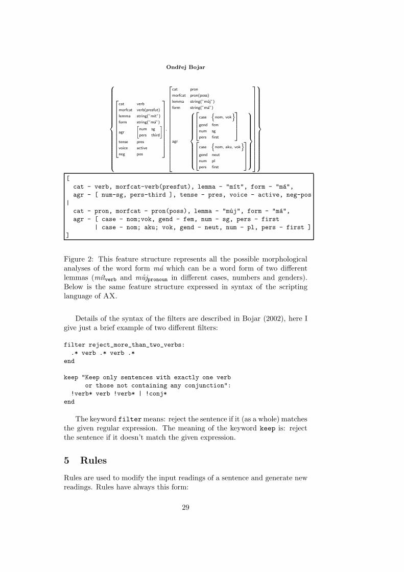
For every input word in a sentence, the morphological analysis givesall possible lemmas and morphological attributes of the given word form.This ambiguous morphological information can be stored in a single featurestructure with variants. See figure 2 on the facing page for an example. Thewhole sentence of word forms can therefore be stored as a list of featurestructures of the same length.
4 Filters
Filters in the language AX are expressed in the form of regular expressionsof feature structures. The basic differences between common regular ex-pressions (used for instance in many Unix tools) and regular expressions offeature structures used in the language AX are:
• The primitive element of regular expressions is no longer a character,but rather a feature structure. In scripting language AX, the featurestructure can be expressed either explicitly or by a shortcut name8.
• When searching for a subsequence of feature structures that matchesa given regular expression, the system checks whether the input struc-ture unifies with the structure in the expression. (Rather than checkingtwo characters for equality.)
6In Czech, approx. 4,000 different tags are defined, half of which actually occurred inthe Czech National Corpus. For many word forms several dozens of morphological tagsare possible (7 different cases · 4 genders · 2 (sg/pl) = 56 possible tags).
7If more variants of a value are available, the output will carry out the intersection(more precisely the product of unification of all possible combinations of input variants).
8For example, specific types of pronouns can syntactically serve as nouns or adjectives.It is useful to define a shortcut of a feature structure that would match a noun or a noun-like type of pronoun etc. In filters and rules, it is then possible to introduce the wholestructure only by its shortcut name.
28
Ondrej Bojar
cat verb
morfcat verb(presfut)
lemma string(”mıt”)
form string(”ma”)
agr
[num sg
pers third
]tense pres
voice active
neg pos
,
cat pron
morfcat pron(poss)
lemma string(”muj”)
form string(”ma”)
agr
case
nom, vok
gend fem
num sg
pers first
case
nom, aku, vok
gend neut
num pl
pers first
[cat - verb, morfcat-verb(presfut), lemma - "mıt", form - "ma",agr - [ num-sg, pers-third ], tense - pres, voice - active, neg-pos
|cat - pron, morfcat - pron(poss), lemma - "muj", form - "ma",agr - [ case - nom;vok, gend - fem, num - sg, pers - first
| case - nom; aku; vok, gend - neut, num - pl, pers - first ]]
Figure 2: This feature structure represents all the possible morphologicalanalyses of the word form ma which can be a word form of two differentlemmas (mıtverb and mujpronoun in different cases, numbers and genders).Below is the same feature structure expressed in syntax of the scriptinglanguage of AX.
Details of the syntax of the filters are described in Bojar (2002), here Igive just a brief example of two different filters:
filter reject_more_than_two_verbs:.* verb .* verb .*
end
keep "Keep only sentences with exactly one verbor those not containing any conjunction":
!verb* verb !verb* | !conj*end
The keyword filtermeans: reject the sentence if it (as a whole) matchesthe given regular expression. The meaning of the keyword keep is: rejectthe sentence if it doesn’t match the given expression.
5 Rules
Rules are used to modify the input readings of a sentence and generate newreadings. Rules have always this form:
29
Building Sub-corpora Suitable for Extraction of Lexico-Syntactic Information
rule <rule name> :<replacement> ---> <input regular expression> ::<constraints>end
The rule is applied as follows:
• The input sequence of feature structures is searched in order to finda subsequence that matches the <input regular expression> and the<constraints>.
• The obtained subsequence of feature structures is replaced with the<replacement>.
By default, the input sequence is searched for all possible subsequencesmatching the regular expression and constraints, therefore the rule can pro-duce for one input reading several output readings. In many situations, thisnondeterministic approach leads to more output readings than the user actu-ally wants. For such cases, the user can write special keywords in the arrowin the rule to make the rule substitute for instance only the first matchingsubsequence of feature structures.
By default, the output of one rule within a ruleset is used as input foranother rule in the same ruleset (possibly reusing the rule itself). All possiblecombinations of applying rules are attempted and all the possible outcomesare collected to build the final output set of possible readings for this block(phase) of operation. This nondeterministic behavior can be restricted inseveral ways: rules can be limited in number of allowed applications9, anoutput from one rule can be included in the final set only if no other rulewas able to change it, and others. A detailed description of all the optionsis out of the scope of this paper.
In order to “compute” the <replacement> from the subsequence foundin the input, one can use variables. The variables can be used in all partsof rules: from the <input regular expression> they get their initial value.The value is then restricted or updated by the <constraints> and their finalvalue is given to the output in the <replacement>.
All the variables can hold a feature structure. The scope of the variablesis limited for one application of one rule, that is all the variables are localfor the rule and within one application.
The <constraints> are expressed as an unordered list of requirements onvariables values. All the requirements must be fulfilled for the rule to be ap-plicable. The constraints can only require certain feature (sub)structures to
9In fact, the system AX will not start unless all non-shortening rules, i.e. the rules thatare able to produce output not shorter than the input reading, have this maximum numberof applications explicitly expressed as a function of the number of input structures. Thiseffectively blocks out the possibility to loop ad infinitum.
30
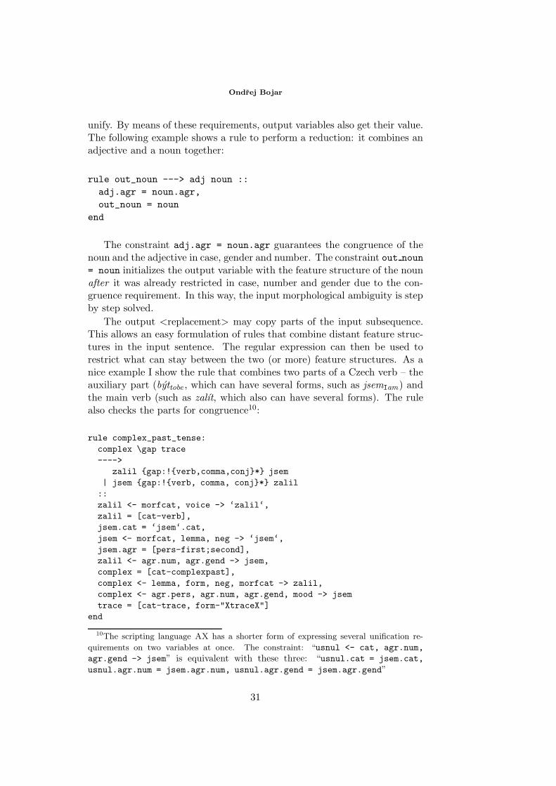
Ondrej Bojar
unify. By means of these requirements, output variables also get their value.The following example shows a rule to perform a reduction: it combines anadjective and a noun together:
rule out_noun ---> adj noun ::adj.agr = noun.agr,out_noun = noun
end
The constraint adj.agr = noun.agr guarantees the congruence of thenoun and the adjective in case, gender and number. The constraint out noun= noun initializes the output variable with the feature structure of the nounafter it was already restricted in case, number and gender due to the con-gruence requirement. In this way, the input morphological ambiguity is stepby step solved.
The output <replacement> may copy parts of the input subsequence.This allows an easy formulation of rules that combine distant feature struc-tures in the input sentence. The regular expression can then be used torestrict what can stay between the two (or more) feature structures. As anice example I show the rule that combines two parts of a Czech verb – theauxiliary part (byttobe , which can have several forms, such as jsemIam ) andthe main verb (such as zalıt, which also can have several forms). The rulealso checks the parts for congruence10:
rule complex_past_tense:complex \gap trace---->
zalil gap:!verb,comma,conj* jsem| jsem gap:!verb, comma, conj* zalil::zalil <- morfcat, voice -> ‘zalil‘,zalil = [cat-verb],jsem.cat = ‘jsem‘.cat,jsem <- morfcat, lemma, neg -> ‘jsem‘,jsem.agr = [pers-first;second],zalil <- agr.num, agr.gend -> jsem,complex = [cat-complexpast],complex <- lemma, form, neg, morfcat -> zalil,complex <- agr.pers, agr.num, agr.gend, mood -> jsemtrace = [cat-trace, form-"XtraceX"]
end
10The scripting language AX has a shorter form of expressing several unification re-
quirements on two variables at once. The constraint: “usnul <- cat, agr.num,agr.gend -> jsem” is equivalent with these three: “usnul.cat = jsem.cat,usnul.agr.num = jsem.agr.num, usnul.agr.gend = jsem.agr.gend”
31
Building Sub-corpora Suitable for Extraction of Lexico-Syntactic Information
The rules find such a subsequence of feature structures that begins withthe auxiliary verb and ends with the main verb (or vice versa). The gapbetween the parts of verb must not contain any other verb, comma or con-junction (introduced by means of shortcuts, see above). The gap gets a label“gap”, so that it can be copied to the output replacement. As the output,the rule produces a single feature structure representing the complex verbfollowed a copy of the gap section and an auxiliary trace at the place wherethe other part of the verb was found. Naturally, the trace can be omitted ifnot needed by any other rules of filters.
6 A Sample AX Usage and Results
The system AX was used to select sentences suitable for extracting typicalcomplements of verbs, namely verb valency frames. The script for thispurpose contained 15 filters and 21 rules and selected sentences where thecomplements of verbs would be easy to observe and excluded sentences thatare too difficult to parse. Approximately 15 to 20% of sentences from theCzech National Corpus are selected by this script. I call them “very simplesentences”.11
So far, the task of actually extracting verb valency frames from the se-lected sentences was not performed, neither manually nor automatically.12
Anyway, the utility of the described sentence preselection can be illus-trated by measuring the improvement of accuracy of parsers available forCzech (Collins et al. (1999), Zeman (1997, 2002) and a parser by ZdenekZabokrtsky (unpublished)). All the parsers were tested on all the sentencesin the evaluation part of the Prague Dependency Treebank and separatelyon the selected “very simple sentences” only.
The results show that the best parser available for Czech, the Collinsparser, is able to correctly observe 55% of verb frames13. When used onvery simple sentences only, this measure increases by 10%. A similar resultcan be achieved by using the parser on short sentences only: in sentenceswith at most ten words, the Collins parser correctly observes 68% of verbframes. A combination of both filters, short and “very simple” sentences, ishowever still 5% better, exceeding 73% of correctly observed verb frames.
11Optionally, sentences containing “suspicious word order patterns” (WOP) were alsorejected. Stranakova-Lopatkova (2001) cautiously analyzes the risks of syntactic ambi-guity of noun and prepositional phrases in Czech. She defines those WOPs, where thereit is not possible to decide whether a noun phrase depends on another noun phrase oron the verb itself. These examples would spoil the observation of verb frames, but it iseasy to filter them out using the AX. Full description of the linguistically motivated filtersexceeds the scope of this paper, see (Bojar, 2002) for details.
12In (Bojar, 2002) I propose an algorithm to extract surface verb frames and describeseveral open problems of the task of inferring verb valency frames from the surface ones.
13That is to correctly identify all immediate daughters of a verb in the dependency treeand not mark any extra nodes as daughters of the verb.
32
Ondrej Bojar
Also quite interesting is the improvement of the traditional accuracymeasure, namely the number of correctly assigned dependencies. If used onvery simple sentences, the parsers achieve an accuracy of 5 to 10 percentbetter, up to 88% for Collins. On short and “very simple” sentences, 91.4%for Collins is achieved.
7 Conclusions
In this paper I described a system to perform selection of sentences fromcorpora based on linguistically motivated criteria. The system allows aneasy formulation of filters and also rules for partial syntactic analysis of sen-tences, if needed to check for more complex phenomena. The sentences canbe selected for many purposes: as an automated preprocessing to supplylexicographers with more relevant examples of sentences as well as a firststep in a fully automatic extraction of lexico-syntactic information. If thescript of filters and rules is cautiously designed, already the output producedfrom the system AX can serve as raw input to build a lexicon. The expres-sive power of filters and rules of AX is better than any corpus searchingtool known to me. The system was used to select sentences suitable to ex-tract verb valency frames and the utility of this selection was illustrated byimprovement of three parsers’ accuracy.
In future work, I will use the described system in a large scale to extractvalency frames of verbs from the whole Czech National Corpus. I will alsotry to design an AX script to select sentences suitable for extraction ofvalency frames of nouns.
8 Acknowledgments
The scripting language presented in this article was developed as a part ofmy master thesis, Bojar (2002). I would like thank to the supervisor ofthe thesis, RNDr. Vladislav Kubon, Ph.D., as well as to all the researchersand staff at the Center for Computational Linguistics, Charles University,Prague. This work was partially supported by the grant GACR 201/02/1456and GAUK 300/2002/A INF-MFF.
References
Aıt-Mokhtar, Salah and Jean-Pierre Chanod. 1997. Incremental finite-stateparsing. In Proceedings of ANLP’97, pages 72–79, Washington, March31st to April 3rd.
Bohmova, Alena, Jan Hajic, Eva Hajicova, and Barbora Hladka. 2001.The Prague Dependency Treebank: Three-Level Annotation Scenario.
33
References
In Anne Abeille, editor, Treebanks: Building and Using SyntacticallyAnnotated Corpora. Kluwer Academic Publishers.
Bojar, Ondrej. 2002. Automaticka extrakce lexikalne-syntaktickych udajuz korpusu (Automatic extraction of lexico-syntactic information fromcorpora). Master’s thesis, UFAL, MFF UK, Prague, Czech Republic. InCzech.
Collins, Michael, Jan Hajic, Eric Brill, Lance Ramshaw, and Christoph Till-mann. 1999. A Statistical Parser of Czech. In Proceedings of 37th ACLConference, pages 505–512, University of Maryland, College Park, USA.
Karttunen, Lauri, Jean-Pierre Chanod, Gregory Grefenstette, and AnneSchiller. 1996. Regular expressions for language engineering. NaturalLanguage Engineering, 2(4):305–328.
Penn, Gerald. 2000. The Algebraic Structure of Attributed Type Signatures.Ph.D. thesis, School of Computer Science, Carnegie Mellon University.
Sarkar, Anoop and Daniel Zeman. 2000. Automatic Extraction of Subcat-egorization Frames for Czech. In Proceedings of the 18th InternationalConference on Computational Linguistics (Coling 2000), Saarbrucken,Germany. Universitat des Saarlandes.
Stranakova-Lopatkova, Marketa. 2001. Homonymie predlozkovych skupinv cestine a moznost jejich automatickeho zpracovanı (Ambiguity ofprepositional phrases in Czech and possibilities for automatic treatment).Technical Report TR-2001-11, UFAL/CKL, Prague, Czech Republic. InCzech.
Zeman, Daniel. 1997. A Statistical Parser of Czech. Master’s thesis, UFAL,MFF UK, Prague, Czech Republic. In Czech.
Zeman, Daniel. 2002. Can Subcategorization Help a Statistical Parser?In Proceedings of the 19th International Conference on ComputationalLinguistics (Coling 2002), Taibei, Tchaj-wan. Zhongyang Yanjiuyuan(Academia Sinica).
34
Formalizing determination and typicality
with LDO
Jerome Cardot
Equipe LaLICC: Langages, Logiques, Informatique, Cognition, Communication
UMR 8139 - CNRS - Universite Paris IV Sorbonne
http://www.lalic.paris4.sorbonne.fr
Abstract. Determination is a fundamental operation in language, by which ob-jects are built intensionally, more and more specified along the utterance. Thispaper presents LDO, a formalism in which objects are built upon concepts. Con-cepts are involved in incompatibility relations, used by LDO to give a representa-tion of essence and intension of concepts. LDO allows inference on typicality, andrepresentation of objects of language.
When we use a common noun to introduce a new object in discourse, thisobject is at first time unspecified, indeterminate. Then the utterance givesdeterminations to it, through different ways: determiners, quantifiers, mod-ifiers such as adjectives, noun complements, relatives.
In this article, we present LDO1, a logic to represent how objects aredeterminated. We show how the fundamental operation of determinationhelps in analyzing quantification and typicality, and in structuring conceptswith intensional relations. We give a formalization and some theorems forLDO, then we point how this logic can represent objects, joining ability tostructure the lexicon and ability to describe objects along utterances.
1 Overview of LDO
1.1 Sources of LDO
The main choice in LDO is to construct objects by their intension, that is,by ideas (or concepts) related with terms. This was already pointed out by(Arnauld and Nicole 1662)2:
1LDO: Logique de la Determination d’Objets; the basic idea was originally presentedin (Descles 1986).
2Usually called Logique de Port-Royal.
Proceedings of the Eighth ESSLLI Student SessionBalder ten Cate (editor)Chapter 4, Copyright c© 2003, Jerome Cardot
35
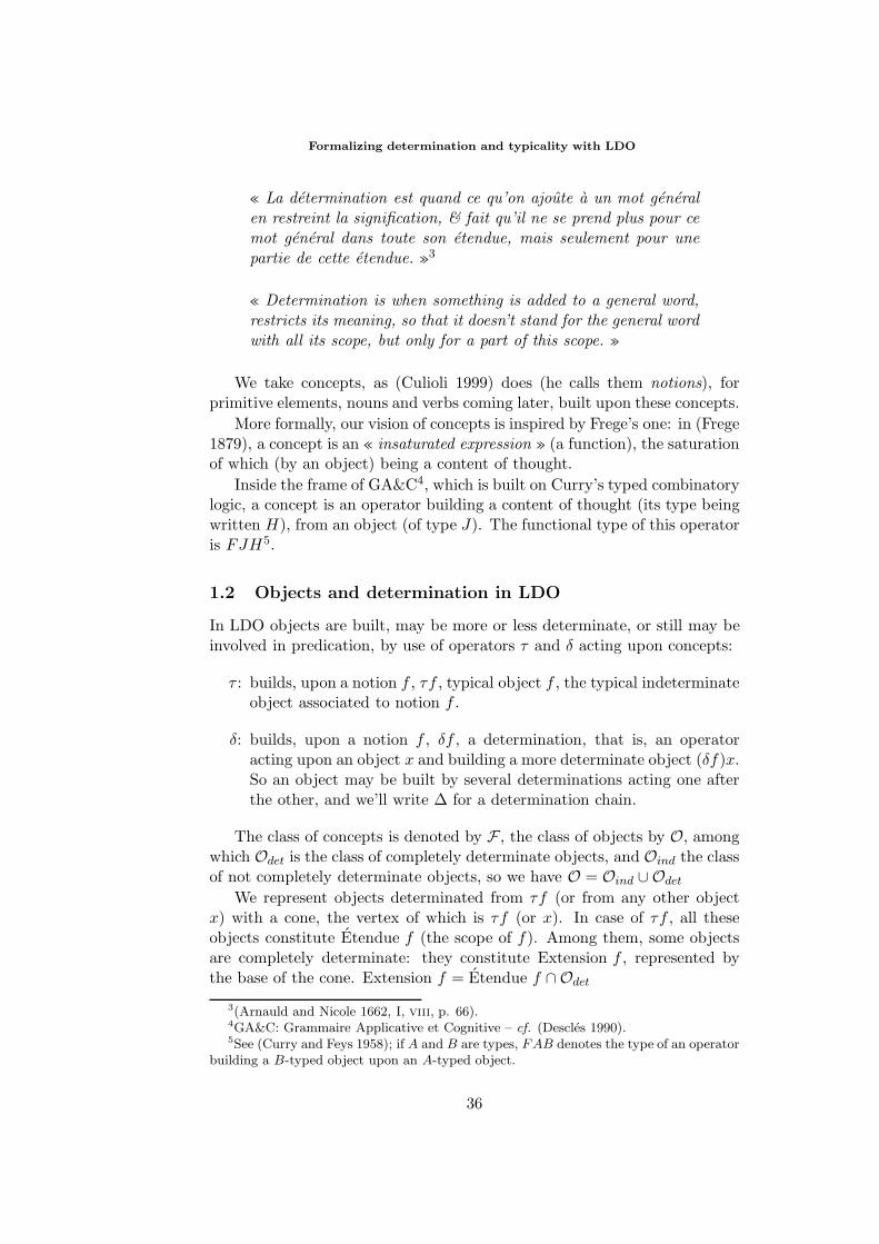
Formalizing determination and typicality with LDO
« La determination est quand ce qu’on ajoute a un mot generalen restreint la signification, & fait qu’il ne se prend plus pour cemot general dans toute son etendue, mais seulement pour unepartie de cette etendue. »3
« Determination is when something is added to a general word,restricts its meaning, so that it doesn’t stand for the general wordwith all its scope, but only for a part of this scope. »
We take concepts, as (Culioli 1999) does (he calls them notions), forprimitive elements, nouns and verbs coming later, built upon these concepts.
More formally, our vision of concepts is inspired by Frege’s one: in (Frege1879), a concept is an « insaturated expression » (a function), the saturationof which (by an object) being a content of thought.
Inside the frame of GA&C4, which is built on Curry’s typed combinatorylogic, a concept is an operator building a content of thought (its type beingwritten H), from an object (of type J). The functional type of this operatoris FJH5.
1.2 Objects and determination in LDO
In LDO objects are built, may be more or less determinate, or still may beinvolved in predication, by use of operators τ and δ acting upon concepts:
τ : builds, upon a notion f , τf , typical object f , the typical indeterminateobject associated to notion f .
δ: builds, upon a notion f , δf , a determination, that is, an operatoracting upon an object x and building a more determinate object (δf)x.So an object may be built by several determinations acting one afterthe other, and we’ll write ∆ for a determination chain.
The class of concepts is denoted by F , the class of objects by O, amongwhich Odet is the class of completely determinate objects, and Oind the classof not completely determinate objects, so we have O = Oind ∪ Odet
We represent objects determinated from τf (or from any other objectx) with a cone, the vertex of which is τf (or x). In case of τf , all theseobjects constitute Etendue f (the scope of f). Among them, some objectsare completely determinate: they constitute Extension f , represented bythe base of the cone. Extension f = Etendue f ∩ Odet
3(Arnauld and Nicole 1662, I, viii, p. 66).4GA&C: Grammaire Applicative et Cognitive – cf. (Descles 1990).5See (Curry and Feys 1958); if A and B are types, FAB denotes the type of an operator
building a B-typed object upon an A-typed object.
36
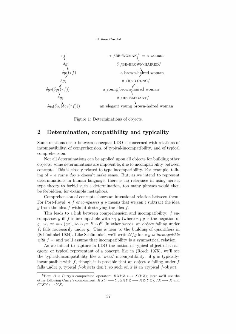
Jerome Cardot
τ /be-woman/ = a woman
a brown-haired woman
a young brown-haired woman
an elegant young brown-haired woman
δ /be-brown-haired/
δ /be-young/
δ /be-elegant/
τf
δg1(τf)
δg2(δg1(τf))
δg3(δg2(δg1(τf)))
δg1
δg2
δg3
Figure 1: Determinations of objects.
2 Determination, compatibility and typicality
Some relations occur between concepts: LDO is concerned with relations ofincompatibility, of comprehension, of typical-incompatibility, and of typicalcomprehension.
Not all determinations can be applied upon all objects for building otherobjects: some determinations are impossible, due to incompatibility betweenconcepts. This is closely related to type incompatibility. For example, talk-ing of « a rainy dog » doesn’t make sense. But, as we intend to representdeterminations in human language, there is no relevance in using here atype theory to forbid such a determination, too many phrases would thenbe forbidden, for example metaphors.
Comprehension of concepts shows an intensional relation between them.For Port-Royal, « f encompasses g » means that we can’t subtract the ideag from the idea f without destroying the idea f .
This leads to a link between comprehension and incompatibility: f en-compasses g iff f is incompatible with ∼1 g (where ∼1 g is the negation ofg: ∼1 gx =∼ (gx), so ∼1≡ B ∼)6. In other words, an object falling underf , falls necessarily under g. This is near to the building of quantifiers in(Schonfinkel 1924). Like Schonfinkel, we’ll write Ufg for « g is incompatiblewith f », and we’ll assume that incompatibility is a symmetrical relation.
As we intend to capture in LDO the notion of typical object of a cat-egory, or typical representant of a concept, like in (Rosch 1975), we’ll seethe typical-incompatibility like a ‘weak’ incompatibility: if g is typically-incompatible with f , though it is possible that an object x falling under ffalls under g, typical f -objects don’t, so such an x is an atypical f -object.
6Here B is Curry’s composition operator: BXY Z −→ X(Y Z); later we’ll use theother following Curry’s combinators: KXY −→ Y , SXY Z −→ XZ(Y Z), IX −→ X andC∗XY −→ Y X.
37
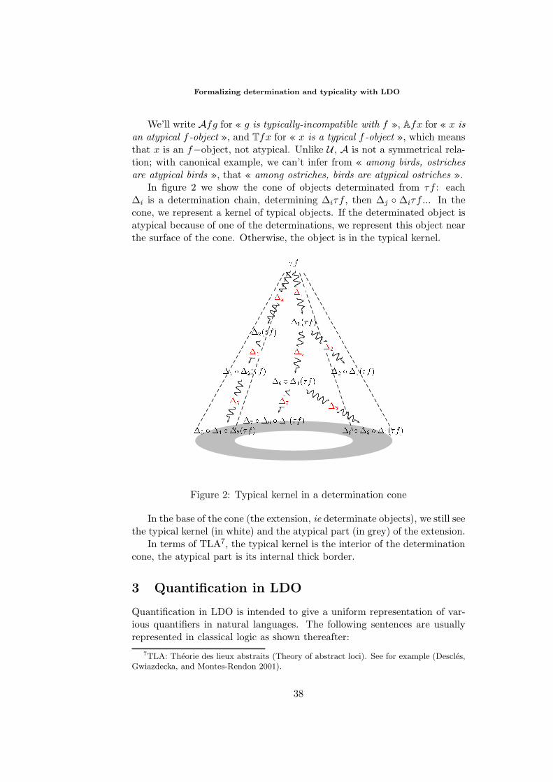
Formalizing determination and typicality with LDO
We’ll write Afg for « g is typically-incompatible with f », Afx for « x isan atypical f -object », and Tfx for « x is a typical f -object », which meansthat x is an f−object, not atypical. Unlike U , A is not a symmetrical rela-tion; with canonical example, we can’t infer from « among birds, ostrichesare atypical birds », that « among ostriches, birds are atypical ostriches ».
In figure 2 we show the cone of objects determinated from τf : each∆i is a determination chain, determining ∆iτf , then ∆j ∆iτf ... In thecone, we represent a kernel of typical objects. If the determinated object isatypical because of one of the determinations, we represent this object nearthe surface of the cone. Otherwise, the object is in the typical kernel.
Æ
Æ
Æ Æ
Æ
Æ Æ Æ Æ
Figure 2: Typical kernel in a determination cone
In the base of the cone (the extension, ie determinate objects), we still seethe typical kernel (in white) and the atypical part (in grey) of the extension.
In terms of TLA7, the typical kernel is the interior of the determinationcone, the atypical part is its internal thick border.
3 Quantification in LDO
Quantification in LDO is intended to give a uniform representation of var-ious quantifiers in natural languages. The following sentences are usuallyrepresented in classical logic as shown thereafter:
7TLA: Theorie des lieux abstraits (Theory of abstract loci). See for example (Descles,Gwiazdecka, and Montes-Rendon 2001).
38
Jerome Cardot
1. « Jean is mortal » /be-mortal/ (Jean)
2. « A man is mortal » ∃x(/be-man/ (x) ∧ /be-mortal/ (x))
3. « Every man is mortal » ∀x(/be-man/ (x) ⊃ /be-mortal/ (x))
LDO gives for them the following forms:
1. /be-mortal/ (Jean)
2. /be-mortal/ (Σ∗/be-man/ )
3. /be-mortal/ (Π∗/be-man/ )
Σ∗ and Π∗ are linked to Curry’s illative quantifiers Σ2 and Π2 through:
Σ2 ≡ BC∗Σ∗ and Π2 ≡ BC∗Π∗.
In (1), we could even write ∆(τ/be-man/ ) for Jean, to show that Jeanis determinated from the typical man through a determination chain ∆.
In each case, the LDO expression shows a determinated subject fallingunder a predicate, and meets the traditional medieval analysis, which ismuch closer to the language than the analysis of classical logic, or otherformalisms like the so-called intensional logic.
Otherwise, from Curry’s logic, LDO inheritates the ability of expressingquantification directly as a relation between concepts, without using boundvariables (which don’t appear in natural languages).
Here is to be noticed that quantification has the same effect than deter-mination: it restricts the scope of a term. So quantification is to be analyzedlike a particular determination, whereas other formalisms paraphrase deter-mination with help of quantification.
4 Essence, intension
The class of concepts encompassed by f is called « essence of f », denotedby Ess f and characterized by: g ∈ Ess f iff U(∼1 g)f , or Uf(∼1 g) (dueto symmetry). We’ll write f → g for « f encompasses g ». → is a partialorder on F .
But essence is not enough to capture all the meaning of a concept, es-pecially when we consider typicality: though some birds don’t fly, /be-able-to-fly/ is an important part of the concept /be-bird/ ; we’ll say« /be-able-to-fly/ is in the intension of /be-bird/ ».
As essence is related to quantification by g ∈ Ess f ⊃ Πfg (or g(Π∗f)),we define « intension of f », denoted by Intension f , based on the weakenedcomprehension relation (typical comprehension):
39
Formalizing determination and typicality with LDO
fT→ g iff. Π(Tf)g iff. g(Π∗(Tf)).
So: Intension f = g ∈ F ; f T→ g and Ess f = g ∈ F ; f → g.f → g ⊃ f
T→ g. Hence: Ess f ⊂ Intension f .Like → w.r.t. U , T→ can be expressed with A, so:Intension f = g ∈ F ;Af(∼1 g)f−objects share all properties of Ess f , typical f−objects share all prop-
erties of Intension f ; atypical f−objects are atypical because they lack of (atleast) one property of the intension, but they still may have other propertiesof the intension.
This allows inference with inconsistent inheritance networks, like Nixon’sdiamond, as will be detailed in section 6.1.
One trouble is that, unlike →, T→ is not a partial order on F . If we readf
T→ g as « typical f−objects fall under g », obviously fT→ g doesn’t imply
that typical f−objects are typical g−objects. For example, /be-bird/ isin the intension (and even in the essence) of /be-ostrich/ , but an ostrich,even a typical one, is not a typical bird.
Of course we could have given Ess f and Intension f as primitives, ratherthan relations between concepts, but structure among concepts and coher-ence of the system wouldn’t have appeared so clearly. Here essence andintension of different concepts are coherent because they are inferred fromU and A.
5 Formalization
In this section we give axioms for τ and δ operators, inference rules for LDO,and some theorems. As the formalism is based on functional calculus, wedevelop an applicative point of view and show results as fixed-point of someoperator, when possible.
5.1 Axioms
Aτδ1: For each concept f , there are an object τf and an operator δf .
Axiom Aτδ1 shows clearly that in LDO an object exists as object inthought. It doesn’t matter here whether a real object can be com-pletely determinated from τf or not. The point is that τf exists inthe logical system.
Aτδ2: (∀f ∈ F)[(δf(τf)) = (τf)]
τf is a fixed-point of δf ; written in terms of Curry’s combinators:Sδτf = τf so Sδτ = τ ; τ is a fixed-point of Sδ.
Aτδ3: (∀f, g ∈ F)(∀x ∈ O)[[(fx) = ∧ g ∈ Ess f ] ⇒ ((δg)x) = x]
40
Jerome Cardot
An object falling under f is a fixed-point of δg, for all g in the essenceof f .
Aτδ4: (∀f ∈ F)[δf δf = δf ]
Determination by a concept is idempotent. With applicational pointof view, WB(δf) = δf , which leads to recognize δ as a fixed-point ofBBWB.
Aτδ5: (∀f ∈ F)(f(τf)) = With applicational point of view: f(τf) = SIτf , and the axiom con-sists in identifying SIτ to K , the constant-true function.
With this last axiom, τ is connected to the ε−function of Hilbert8; butHilbert thought about extensional existence, whereas we think about inten-sional existence; former works on LDO had made here other choices, forexample (Pascu 2001) identifies f(τf) with Extension τf = ∅ which means:∃x, x determinate and f−typical, such that (fx) = (with extensionalsense to existence).
5.2 Rules
LDO includes rules of Curry’s combinatory logic and rules of inference forconnectors of classical logic (as presented in (Gentzen 1955)). Here arespecific rules for LDO:
Atypicality and inheritance
x = δg y y = ∆(τf) Afg
Afx
x = δg y Afy
Afx
These rules show the two ways for building an atypical f−object: byapplying an f−typically-incompatible determination upon an f−object, orby determining an atypical f−object. Atypicality is inherited, and can’t belost through determination.
Typicality
Tf(τf)fx ∼ (Afx)
Tfx
τf is called « typical f−object », so at least we have to recognize it astypical! Besides, if we know that an f−object is not atypical, then it istypical.
8Cf. (Bernays 1935).
41
Formalizing determination and typicality with LDO
5.3 Some theorems
Axioms, rules (including rules of natural logic) and previous definitions allowto prove the following theorems; the next section will give a proof of theorems(3) and (4).
1.h ∈ Ess f (f x)
(h x)An object falling under f falls under the con-cepts in the essence of f .
2. A ≡ BUTBoth of these operators characterize thetypical-incompatibility.
3.fx ∼ (Tfx)
Afx
If we know that an f−object is not typical,then it is atypical; this is a lemma to provethe next theorem.
4.g(Π(Tf)) ∼1 gx f x
Afx
If typical f−objects fall under g, and x is an f−object which doesn’tfall under g, then x is atypical (as an f−object).
5. Etendue f is the smallest class including τf and stable through allf−compatible determinations. This stability means, it is a fixed-pointfor X −→
⋃
x∈X,g∈Fδg x
5.4 Consistency
The main result about consistency in LDO, is that no contradiction mayoccur through deduction rules about typicality.
Such a contradiction would appear as: Tfx ∧ Afx. But none of thetwo rules introducing Tfx may lead to this: one supposes that ∼ Afx, theother one supposes that x = τf , so that no determination has made x bean atypical f−object.
Another point to be stressed is that incoherent data about U would notlead to contradictions but would prevent the existence of some objects.
6 Applications
LDO is intended to study determinations in a logical point of view and innatural languages. We show in this section some inferences, with the proofof two theorems listed above, and with inference on typicality. Then weexplain how LDO is helpful for representing language.
42
Jerome Cardot
6.1 Inferences
Proof of theorems 3 and 4.
Here are proof-trees of theorems 3 (at left) and 4 (at right) from the previoussection.
fx ∼ (Tfx)
fx ∼ (Afx)
Tfx ∼ (Tfx)
⊥fx;∼ (Tfx);∼ (Afx) ⊥
Afx
g(Π(Tf))
Π2(Tf)g
(Tfx) ⊃ (gx)
∼1 gx
∼ (gx)
∼ (Tfx) f x
Afx
Inferring on typicality
The canonical example of atypicality: « typical birds fly, ostriches are birdsbut an ostrich doesn’t fly » is solved by theorem 4, with f = /be-bird/ ,g = /be-able-to-fly/ , and x = τ/be-ostrich/ . So the theorem tells:A/be-bird/ (τ/be-ostrich/ ), which is to be read « An ostrich is an atyp-ical bird ».
Let’s go on with a transparent adaptation of Nixon’s diamond: « (a)Bush is methodist – (b) methodists are pacifist – (c) Bush is republican –(d) republicans are not pacifist. » From (a) and (b), Bush is pacifist, from(c) and (d) he isn’t. To solve the inconsistence, we have to formalize at leastone of (b) or (d) with T→ rather than with →.
For example, /be-methodist/ T→/be-pacifist/ , which could also havebeen written /be-pacifist/ (Π∗(T/be-methodist/ )): typical methodistsare pacifist; so, if Bush is not pacifist (doesn’t matter here whether all oronly typical republicans are not pacifist), he is an atypical methodist. Andif Bush were pacifist, we would conclude that he is an atypical republican.
6.2 LDO and language
Lexicon can be structured with use of determination: for example a defi-nition such as « a manor is a big luxurious house » could be representedby:
τ/be-manor/ := δ/be-big/ (δ/be-luxurious/ (τ/be-house/ ))U and A relations (or their complement) allow to represent compatibility
and typicality between concepts. A structured lexicon using LDO shouldgive these relations.
Words refer to objects, and by saying « a car », we’re speaking aboutan object, even if we don’t know which one, but we’re not speaking aboutthe class of cars. Natural language deals with more or less determinatedobjects, and determinates them along the discourse. LDO gives a way torepresent that part of semantics.
43
Formalizing determination and typicality with LDO
In (Cardot 2003), we showed how determination is involved in semanticrepresentation of verbs, mainly for state clauses and event clauses. Ouraim in forthcoming development is to represent how new determinations aregiven to an object along a text.
Moreover, LDO allows to represent identification of an object to another.For example, in « John is (like) a lion », the speaker selects in Intension /be-lion/ the part he thinks relevant, and asserts this part about John.
Conclusion
Determination is a fundamental operation in language, by which objects arebuilt intensionally, more and more specified along the utterance.
LDO, built with an intensional point of view, deals with this operation,by which objects, rather than classes, are specified. Formalization, based onU and A relations of (typical-)incompatibility, allows inference on typicalityand representation of objects along the discourse. These incompatibilityrelations give access to essence and intension of concepts.
LDO contributes to the study of categorization, and can be included ina general formalism for representing language, such as GA&C.
References
Arnauld, A. and P. Nicole (1662). La logique ou l’art de penser (1993 ed.). Paris:Vrin.
Bernays, P. (1935). Hilberts Untersuchungen uber die Grundlagen der Arithmetik,pp. 196–216. dans (Hilbert 1935).
Cardot, J. (2003). Logique de la determination d’objets: un formalisme pour larepresentation des objets du discours. In Actas del VIIIvo symposio internacionalde comunicacion social, Santiago de Cuba, pp. 115–120.
Culioli, A. (1999). Pour une linguistique de l’enonciation – Tome 3: Domainenotionnel. Paris: Ophrys.
Curry, H. B. and R. Feys (1958). Combinatory Logic, Volume I. North Holland.
Descles, J.-P. (1986). Implication entre concepts: la notion de typicalite. Travauxde linguistique et de litterature (XXIV).
Descles, J.-P. (1990). Langages applicatifs, Langues naturelles et Cognition. Paris:Hermes.
Descles, J.-P., E. Gwiazdecka, and A. Montes-Rendon (2001). Towards invari-ant meanings of spatial preposition and preverbs. In Workshop on Spatial andTemporal Information Processing, ACL-2001, Toulouse.
Frege, G. (1879). Begriffsschrift, eine der arithmetischen nachgebildete Formel-sprache des reinen Denkens. Halle. Version francaise par Corine Besson,l’Ideographie, Vrin, Paris, 1999.
44
Jerome Cardot
Gentzen, G. (1955). Recherches sur la deduction logique - Untersuchungen uberdas logische Schließen. Paris: Presses Universitaires de France.
Hilbert, D. (1935). Gesammelte Abhandlungen – tome 3 (1970 ed.). Berlin:Springer Verlag.
Pascu, A. (2001). Logique de Determination d’Objets: concepts de base etmathematisation en vue d’une modelisation objet. Ph. D. thesis, Universite ParisIV.
Rosch, E. (1975). Cognitive representations of semantic categories. Journal ofExprimental Psychology (104), 192–233.
Schonfinkel, M. (1924). Uber die Bausteine der mathematischen Logik. Mathe-matische Analen 92, 305–315.
45

46
Non-Redundant Scope Disambiguation in
Underspecified Semantics
Rui Pedro Chaves
Centro de Linguıstica da Universidade de Lisboa (CLUL), Av. Gama Pinto, n2, Lisboa, Portugal
Abstract. This paper presents a strategy that aims to efficiently avoid thegeneration of logically equivalent formulas that arise in scope processing applica-tions. Constraint based semantic underspecification formalisms may be extendedto include an additional scoping restriction that constrains the set of possible dis-ambiguations, straightforwardly avoiding the generation of redundant quantifierscopings. Such a restriction, in principle valid to any logic, is formalized withinHole Semantics (Bos 1996), a general semantic underspecification framework.
1 Introduction
Semantic Underspecification frameworks (such as QLF (Alshawi and Crouch1992), UDRSs (Reyle 1993), UMRS (Egg and Lebeth 1995), Hole Seman-tics (Bos 1996) and CLLS (Egg et al. 1998)) are able to cope efficientlywith the combinatorial explosion of highly ambiguous Natural Languagephenomena such as scope ambiguity.
Classic approaches to scope processing (such as Cooper (1983), Hobbsand Shieber (1987) and Keller (1988)) are inefficient in the sense that anexponential number of formulas is always generated (worse case entailsgenerating n! formulas, for n quantifiers). In underspecified semantics,the set of possible readings is described via a unique, compact partial rep-resentation which may be reduced in a straightforward fashion, simply bythe incremental specification of additional constraints (e.g. from prosody,discourse context or world knowledge). Furthermore, underspecification isable to deal with other scope bearing constituents other than quantification.
However, the existing methods of scope processing typically overgeneratein the sense that some or even all generated formulas may be logicallyequivalent. We present a new scoping restriction capable of reducing theset of scopal disambiguations in underspecified semantics, avoiding the gen-eration of logical redundancies that result from quantifier scope (a subset offormulas with the same prenex normal form) and therefore greatly reducing
Proceedings of the Eighth ESSLLI Student SessionBalder ten Cate (editor)Chapter 5, Copyright c© 2003, Rui Pedro Chaves
47
Non-Redundant Scope Disambiguation in Underspecified Semantics
the need for theorem provers. Section 2 briefly reviews the existing methodsfor the elimination of redundant formulas. Section 3 formalizes a scope dis-ambiguation restriction within Hole Semantics and applies it to DiscourseRepresentation Theory (Kamp and Reyle 1993) formulas. Finally, practicalimplementation results and some extensions are discussed.
2 Logical Overgeneration: Redundant Scopings
It is well known that the relative orderings of identical first order quantifiersdo not result in distinct truth conditions. For instance, sentence (1) onlyhas a single reading, yet two equivalent formulas are typically generated:
(1) Every boy saw every girl.(1a) (∀x)(boy(x) → (∀y)(girl(y) → saw(x, y)))(1b) (∀y)(girl(y) → (∀x)(boy(x) → saw(x, y)))
A more complex case is visible in sentence (2), which typically receivesup to 60 equivalent formulas1 but only has a single reading:
(2) A boy that sings in a choir gave a flower with a velvet lace to a girl.
The formulas generated for each of the examples above have the sameprenex normal form2 and hence are equivalent. We are presently con-cerned with equivalences that result from the Laws of Quantifier Movement(pulling nested quantifiers out of formulas: (ϕ → (∀x)ψ(x)) ⇔ (∀x)(ψ →ψ(x)) and (ϕ → (∀x)ψ(x)) ⇔ (∀x)(ψ → ψ(x)) where x is not free in ϕand from the Laws of Quantifier Independence (interchanging quantifiers:(∀x)(∀y)ϕ(x, y) ⇔ (∀y)(∀x)ϕ(x, y) and (∃x)(∃y)ϕ(x, y) ⇔ (∃y)(∃x)ϕ(x, y)).
Much more subtle cases involve (possibly many) different sets of logi-cally redundant scopings, as sentence (3) below illustrates. Here, a distinctscopal operator (negation) induces partial non-redundancy: 6 possible per-mutations but only 4 logically distinct readings.
(3) A cat doesn’t like a dog.(3a) (∃y)(dog(y) ∧ (∃x)(cat(x) ∧ ¬like(x, y)))(3b) (∃y)(dog(y) ∧ ¬(∃x)(cat(x) ∧ like(x, y)))(3c) ¬(∃y)(dog(y) ∧ (∃x)(cat(x) ∧ like(x, y)))(3d) (∃x)(cat(x) ∧ (∃y)(dog(y) ∧ ¬like(x, y)))(3e) (∃x)(cat(x) ∧ ¬(∃y)(dog(y) ∧ like(x, y)))(3f) ¬(∃x)(cat(x) ∧ (∃y)(dog(y) ∧ like(x, y)))
1The total number of scopings is not factorial (i.e. 5! = 120) because nested NPscannot have arbitrary semantic scope beyond their syntactical local domain, e.g. ‘a choir ’may not simultaneously outscope ‘a velvet lace’ and be outscoped by ‘a flower ’.
2(Q0 x0) . . . (Qn−1 xn−1)ψ where Qi (0 < i < n) is a quantifier and ψ is quantifier-free.
48
Rui Pedro Chaves
Clearly, formula (3a) is equivalent to (3d) and formula (3c) is equivalentto (3f). One solution to this problem is to use a theorem prover with asearch time limit to help decide the equivalence of each pair of formulasgenerated: formulas P and Q are equivalent iff (P⇔Q) is provable. For ngenerated formulas a theorem prover requires n(n − 1) proofs in the worsecase (i.e. equivalent formulas do not exist), for pairwise choices of P and Q.
Vestre (1991) presents a method that avoids quantifier scope redun-dancy by limiting the selection of determiners in an enumerative algorithmfor scope processing that exhaustively generates and evaluates all possi-ble scopings for a given quantifier. In contrast, we present a method thatdoes not search an exponential number of scopings. Rather, the proposedstrategy strictly generates irredundant quantifier scopings by keeping trackof the scope-bearing constituent undergoing disambiguation and prohibitingcertain disambiguation patterns. Because this method is formalized withina semantic underspecification framework it is able to consider partially dis-ambiguated structures and the interaction of other scope-bearing structuresbesides quantification, such as negation, modality and indirect discourse.
Gabsdil and Striegnitz (1999) proposes and implements a general methodthat orders all the formulas outputted by a scoping algorithm into a graphstructure in which logically equivalent readings are collapsed into a singlestructure. This strategy requires the exhaustive enumeration of possibleformulas, the very problem that underspecification originally aimed to solve.The next section formalizes a method, independent from the logic of choice,that aborts (sets of) disambiguations that describe redundant scopings.
3 Non-Redundant Scopings in Hole Semantics
Hole Semantics (Bos 1996) is a general underspecification framework wherethere is a clear distinction between the underspecification metalanguage andthe object language. In this framework, scopal ambiguity is represented viapartial subordination constraints in an upper-semilattice. What follows is abrief excursion to Hole Semantics.
An Underspecified Representation (UR) is a triple 〈H,L,C〉 where H isa set of metavariables (holes) over formulas; L is a set of labelled formulas;and C is a set of subordination constraints expressed via a relation “≤ ” thatestablishes a partial order (i.e. is reflexive, transitive and antisymmetric)over labels and metavariables. This partial order is also an upper-semilatticegiven that a special element, the supremum, subsumes any pair of elementsin the structure. An admissible disambiguation (henceforth a plugging) isa bijection from holes to labelled formulas that does not violate the set ofconstraints, operating recursively from a special top hole h0. When a hole isplugged (i.e. P(h)=l), the hole variable is substituted by the formula iden-tified by the correspondent label (e.g. “l :ϕ”). Bos (1996) shows that both
49
Non-Redundant Scope Disambiguation in Underspecified Semantics
Dynamic Predicate Logic and Discourse Representation Structures (DRSs(Kamp and Reyle 1993)) can be used as object language in Hole Semantics.
We now formalize a general method within Hole Semantics that con-sists in a restriction that acts to constrain the set of possible pluggings (i.e.disambiguations that do not violate any subordination constraints), and istherefore in principle applicable to any logic of choice. In essence, pluggingsshall be associated to a special unrestricted scope operator, initialised as“”, and as the disambiguation proceeds this operator may be updated, per-colated or forced to abort (“⊥”) the plugging (in the latter case, plugging agiven hole with a given formula would result in a non-empty set of formulaswith logically equivalent scopings, if disambiguation is completed).
It must be expressly noted that we assume the numerical indexes asso-ciated to each label are unique and lexically attributed according to surfaceorder. The Distinct Scope restriction will be endowed with a ‘short-termmemory’ of the disambiguation process and shall impose decreasing orderon the label indexes between formulas that may induce logical redundancy.More generally, scope disambiguation in constraint based underspecifica-tion formalisms can be further restricted in order to efficiently avoid thesymmetric scoping counterpart between specific operators capable of induc-ing logical redundancy.
3.1 Metalanguage Definitions
Firstly, we shall define the set of metalanguage formula schemata that canresult in redundant disambiguations. Secondly, we provide a basis for de-tecting formulas with identical outermost scopal operators and finally, weformalize a general Distinct Scope function and the restrictions therein.
Definition 1: Scopal SchemataLet S be the set of formula schemata Op(ψ): Op(ψ) ∈ U, defined in agiven metalanguage U, under the scope of an operator Op that can poten-tially induce redundant disambiguations. For instance, in an underspecifiedaccount of predicate logic such as Bos (1996), one would have S = (∃x)(k),(∀y)(k); where k is either a metavariable or a metalanguage formula.
Definition 2: Scopal Operator EquivalenceFormulas ϕ and ψ have an equivalent syntactical scope (ϕ ≡ ψ) iff ϕ andψ are of the form Opi(ϕ’) and Opj(ψ’) respectively, where Opi and Opj areidentical scope-bearing operators. E.g. : ‘(∃x)(α)’ ≡ ‘(∃y)(β)’ ≡ ‘(∀z)(τ)’.
Definition 3: Distinct Scope RestrictionLet D be the function which is defined as follows D : Γ × Γ → Γ, where Γis a set of φ::= (l : ϕ)||⊥. This function establishes a mapping between aordered pair of main scope operators (either some labelled metaformula ‘l :ϕ’,
50
Rui Pedro Chaves
or the special symbols “” (verum) and “⊥” (falsum)) and a new mainscope operator. For n equivalent readings, the ordering constraints enforcedby D are able to interrupt pluggings linearly, at most n times (i.e. dependingon the plugging strategy). Below, ϕ and ψ are metalanguage formulas:
D(, (li : ϕ)) = (li : ϕ) (initial scope domain update)
D((li : ϕ), (lj : ψ)) =
(li : ϕ) if ψ ∈ S (percolate)(lj : ψ) if ψ ∈ S ∧ ϕ ≡ ψ (update)(lj : ψ) if ϕ, ψ ∈ S ∧ ϕ ≡ ψ ∧ i > j (update)
⊥ otherwise (abort)
The crucial step takes place when both syntactically equivalent formulasare in set S and have decreasing labelling indexes. Function D aborts thisspecific plug, not allowing orderings where the numerical indexes increase,thus eliminating the full permutation of logically identical quantificationaloperators. For instance “every1 student2 read3 every4 poem5 to6 every7
girl8” would only have the disambiguation with the scoping order: 7>4>1.Next, the main scope operator slot and D must be embedded into
the plugging procedure itself. To illustrate this we shall adopt unpluggedDRSs (Bos 1996) as a description language, extended in order to explicitlyconsider duplex conditions and a basic account of indirect discourse.
3.2 Extended Plugging Procedure for DRTU
Typical disambiguation algorithms for DRT formulas will also be able toovergenerate by building identical DRSs, given different scoping choices:
Syntax of DRTU formulas (adapted from Bos (1996))
1. If hi and hj are holes, p is a propositional discourse marker and Q is ageneralized quantifier, then 〈,hi ⇒ hj〉, 〈,¬hi〉, 〈,hi ∨hj〉,and 〈p,p : h〉 are DRTU formulas.
2. If h is a hole, x is a discourse marker and k1 . . . kn are holes or DRTUformulas then ⊗k1, . . . , kn and 〈,Qx(k, h)〉 are DRTU formulas.
3. If x1 . . . xn are discourse markers and P is a symbol for an n-placepredicate, then 〈x,〉 and 〈,P (x1, . . . , xn)〉 are DRTU formulas.
4. Nothing else is a DRTU formula.
The merge operator “⊗” denotes the union of DRSs (Universes andConditions), e.g. ⊗〈U1, C1〉, . . . , 〈Un, Cn〉=〈U1 ∪ . . . ∪ Un, C1 ∪ . . . ∪ Cn〉.By definition, the label of the formula subordinates every hole variable in-troduced by that same formula. In these terms, a single underspecifiedrepresentation is assigned to an ambiguous sentence such as (4):
51
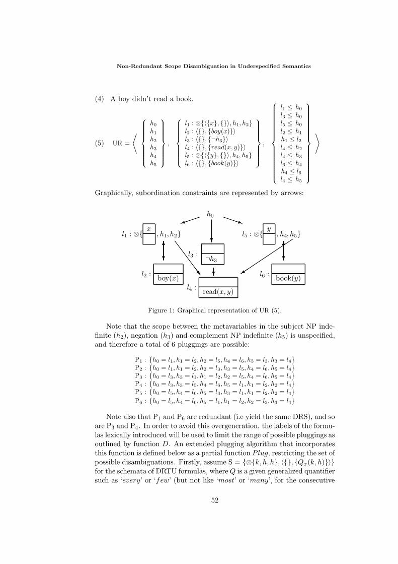
Non-Redundant Scope Disambiguation in Underspecified Semantics
(4) A boy didn’t read a book.
(5) UR =
⟨
h0
h1
h2
h3
h4
h5
,
l1 : ⊗〈x, 〉, h1, h2l2 : 〈, boy(x)〉l3 : 〈, ¬h3〉l4 : 〈, read(x, y)〉l5 : ⊗〈y, 〉, h4, h5l6 : 〈, book(y)〉
,
l1 ≤ h0
l3 ≤ h0
l5 ≤ h0
l2 ≤ h1
h1 ≤ l2l4 ≤ h2
l4 ≤ h3
l6 ≤ h4
h4 ≤ l6l4 ≤ h5
⟩
Graphically, subordination constraints are represented by arrows:
h0
l1 : ⊗ x, , h1 h2 h4 h5l5 : ⊗ y
, ,
l3 : ¬h3
l2 : boy(x)l4 : read(x, y)
l6 : book(y)
Figure 1: Graphical representation of UR (5).
Note that the scope between the metavariables in the subject NP inde-finite (h2), negation (h3) and complement NP indefinite (h5) is unspecified,and therefore a total of 6 pluggings are possible:
P1 : h0 = l1, h1 = l2, h2 = l5, h4 = l6, h5 = l3, h3 = l4P2 : h0 = l1, h1 = l2, h2 = l3, h3 = l5, h4 = l6, h5 = l4P3 : h0 = l3, h3 = l1, h1 = l2, h2 = l5, h4 = l6, h5 = l4P4 : h0 = l3, h3 = l5, h4 = l6, h5 = l1, h1 = l2, h2 = l4P5 : h0 = l5, h4 = l6, h5 = l3, h3 = l1, h1 = l2, h2 = l4P6 : h0 = l5, h4 = l6, h5 = l1, h1 = l2, h2 = l3, h3 = l4
Note also that P1 and P6 are redundant (i.e yield the same DRS), and soare P3 and P4. In order to avoid this overgeneration, the labels of the formu-las lexically introduced will be used to limit the range of possible pluggings asoutlined by function D. An extended plugging algorithm that incorporatesthis function is defined below as a partial function Plug, restricting the set ofpossible disambiguations. Firstly, assume S = ⊗k, h, h, 〈, Qx(k, h)〉for the schemata of DRTU formulas, whereQ is a given generalized quantifiersuch as ‘every’ or ‘few’ (but not like ‘most’ or ‘many’, for the consecutive
52
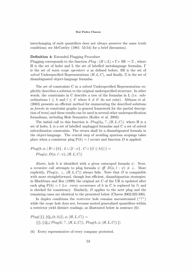
Rui Pedro Chaves
interchanging of such quantifiers does not always preserve the same truthconditions; see McCawley (1981: 53-54) for a brief discussion).
Definition 4: Extended Plugging ProcedurePlugging corresponds to the function Plug : (H ∪L)× Γ× SR → Σ , whereH is the set of holes and L the set of labelled metalanguage formulas, Γis the set of main scope operators φ as defined before, SR is the set ofsolved Underspecified Representations 〈H,L,C〉, and finally, Σ is the set ofdisambiguated object-language formulas.
The set of constraints C in a solved Underspecified Representation ex-plicitly describes a solution to the original underspecified structure. In otherwords, the constraints in C describe a tree of the formulas in L (i.e. sub-ordinations l ≤ h and l ≤ h′ where h = h′ do not exist). Althaus et al.(2003) presents an efficient method for enumerating the described solutionsas forests in constraint graphs (a general framework for the partial descrip-tion of trees) and these results can be used in several other underspecificationformalisms, including Hole Semantics (Koller et al. 2003).
The initial call to this function is Plug(h0,, 〈H,L,C〉) where H is aset of holes, L is a set of labelled unplugged formulas and C a set of solvedsubordination constraints. The return shall be a disambiguated formula inthe object-language. The crucial step of avoiding spurious scopings takesplace when a consistent plug P(h) = l occurs and function D is applied:
Plug(h, φ, 〈H ∪ h , L ∪ l : ψ , C ∪ (l ≤ h) 〉) =
Plug(ψ,D(φ, l : ψ), 〈H,L,C〉)
Above, hole h is identified with a given outscoped formula ψ. Next,a recursive call attempts to plug formula ψ iff D(φ, l : ψ) = ⊥. Moreexplicitly, Plug(ψ, ⊥, 〈H,L,C〉) always fails. Note that D is compatiblewith more straightforward, though less efficient, disambiguation strategies:in Blackburn and Bos (1999) the original set C of the UR is updated aftereach plug P(h) = l (i.e. every occurrence of h in C is replaced by l) andis checked for consistency. Similarly, D applies to the next plug and theremaining cases are identical to the presented below (Chaves 2002:325-330).
In duplex conditions the restrictor hole remains unconstrained (“”)while the scope hole does not, because nested generalized quantifiers withina restrictor yield distinct readings, as illustrated below in sentence (6):
Plug(〈, Qx(k, h)〉, φ, 〈H,L,C〉) =
〈, Qx(Plug(k,, 〈H,L,C〉), P lug(h, φ, 〈H,L,C〉) 〉
(6) Every representative of every company protested.
53
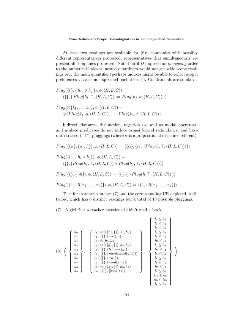
Non-Redundant Scope Disambiguation in Underspecified Semantics
At least two readings are available for (6): companies with possiblydifferent representatives protested; representatives that simultaneously re-present all companies protested. Note that if D imposed an increasing orderto the numerical indexes, nested quantifiers would not get wide scope read-ings over the main quantifier (perhaps indexes might be able to reflect scopalpreferences via an underspecified partial order). Conditionals are similar:
Plug(〈, hi ⇒ hj 〉, φ, 〈H,L,C〉) =〈, Plug(hi ,, 〈H,L,C〉) ⇒ Plug(hj , φ, 〈H,L,C〉) 〉
Plug(⊗k1, . . . , kn, φ, 〈H,L,C〉) =⊗Plug(k1, φ, 〈H,L,C〉), . . . , P lug(kn, φ, 〈H,L,C〉)
Indirect discourse, disjunction, negation (as well as modal operators)and n-place predicates do not induce scopal logical redundancy, and haveunrestricted (“”) pluggings (where α is a propositional discourse referent):
Plug(〈α, α : h〉, φ, 〈H,L,C〉) = 〈α, α : (Plug(h,, 〈H,L,C〉))〉
Plug(〈, hi ∨ hj〉 , φ, 〈H,L,C〉) =〈, Plug(hi ,, 〈H,L,C〉) ∨ Plug(hj ,, 〈H,L,C〉)〉
Plug(〈, ¬h〉, φ, 〈H,L,C〉) = 〈, ¬Plug(h,, 〈H,L,C〉) 〉
Plug(〈, R(x1 , . . . , xn)〉, φ, 〈H,L,C〉) = 〈, R(x1, . . . , xn)〉Take for instance sentence (7) and the corresponding UR depicted in (8)
below, which has 6 distinct readings but a total of 18 possible pluggings:
(7) A girl that a teacher mentioned didn’t read a book.
(8)
⟨
h0
h1
h2
h3
h4
h5
h6
h7
h8
h9
,
l1 : ⊗〈x, 〉, h1, h2l2 : 〈, girl(x)〉l3 : ⊗h3, h4l4 : ⊗〈y, 〉, h5, h6l5 : 〈, teacher(y)〉l6 : 〈, mentioned(y, x)〉l7 : 〈, ¬h7〉l8 : 〈, read(x, z)〉l9 : ⊗〈z, 〉, h8, h9l10 : 〈, book(z)〉
,
l1 ≤ h0
l4 ≤ h0
l7 ≤ h0
l9 ≤ h0
l3 ≤ h1
h1 ≤ l3l2 ≤ h3
h3 ≤ l2l6 ≤ h4
l8 ≤ h2
l5 ≤ h5
h5 ≤ l5l6 ≤ h6
l10 ≤ h8
h8 ≤ l10l8 ≤ h9
⟩
54
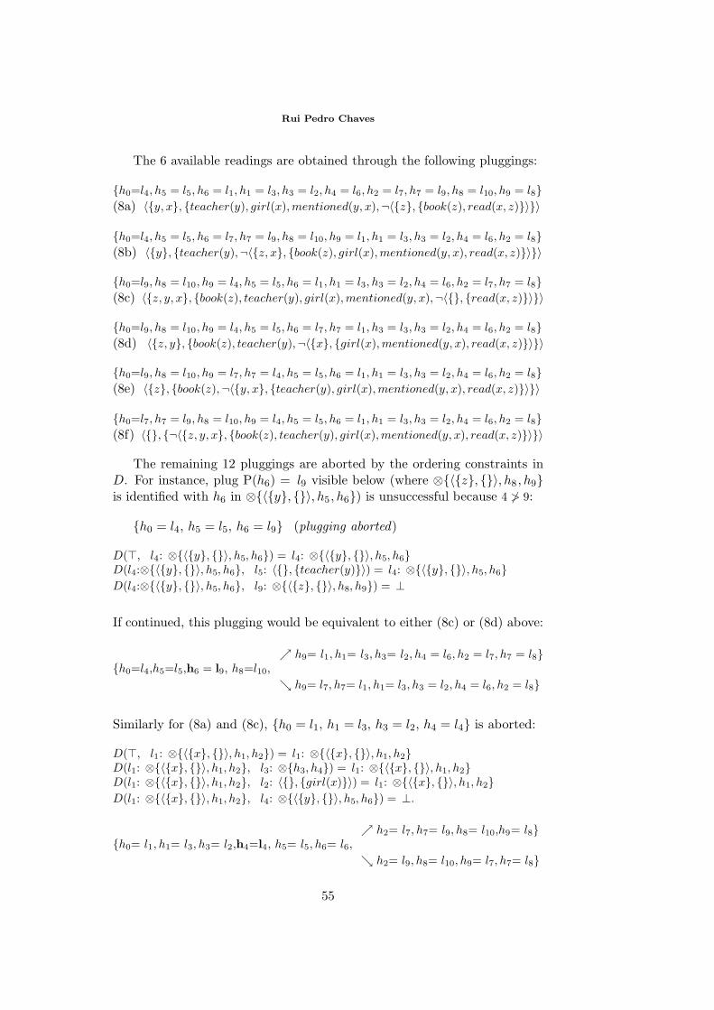
Rui Pedro Chaves
The 6 available readings are obtained through the following pluggings:
h0=l4, h5 = l5, h6 = l1, h1 = l3, h3 = l2, h4 = l6, h2 = l7, h7 = l9, h8 = l10, h9 = l8(8a) 〈y, x, teacher(y), girl(x),mentioned(y, x),¬〈z, book(z), read(x, z)〉〉
h0=l4, h5 = l5, h6 = l7, h7 = l9, h8 = l10, h9 = l1, h1 = l3, h3 = l2, h4 = l6, h2 = l8(8b) 〈y, teacher(y),¬〈z, x, book(z), girl(x),mentioned(y, x), read(x, z)〉〉
h0=l9, h8 = l10, h9 = l4, h5 = l5, h6 = l1, h1 = l3, h3 = l2, h4 = l6, h2 = l7, h7 = l8(8c) 〈z, y, x, book(z), teacher(y), girl(x),mentioned(y, x),¬〈, read(x, z)〉〉
h0=l9, h8 = l10, h9 = l4, h5 = l5, h6 = l7, h7 = l1, h3 = l3, h3 = l2, h4 = l6, h2 = l8(8d) 〈z, y, book(z), teacher(y),¬〈x, girl(x),mentioned(y, x), read(x, z)〉〉
h0=l9, h8 = l10, h9 = l7, h7 = l4, h5 = l5, h6 = l1, h1 = l3, h3 = l2, h4 = l6, h2 = l8(8e) 〈z, book(z),¬〈y, x, teacher(y), girl(x),mentioned(y, x), read(x, z)〉〉
h0=l7, h7 = l9, h8 = l10, h9 = l4, h5 = l5, h6 = l1, h1 = l3, h3 = l2, h4 = l6, h2 = l8(8f) 〈, ¬〈z, y, x, book(z), teacher(y), girl(x),mentioned(y, x), read(x, z)〉〉
The remaining 12 pluggings are aborted by the ordering constraints inD. For instance, plug P(h6) = l9 visible below (where ⊗〈z, 〉, h8 , h9is identified with h6 in ⊗〈y, 〉, h5 , h6) is unsuccessful because 4 > 9:
h0 = l4, h5 = l5, h6 = l9 (plugging aborted)
D(, l4: ⊗〈y, 〉, h5, h6) = l4: ⊗〈y, 〉, h5, h6D(l4:⊗〈y, 〉, h5, h6, l5: 〈, teacher(y)〉) = l4: ⊗〈y, 〉, h5, h6D(l4:⊗〈y, 〉, h5, h6, l9: ⊗〈z, 〉, h8, h9) = ⊥
If continued, this plugging would be equivalent to either (8c) or (8d) above:
h9= l1, h1= l3, h3= l2, h4 = l6, h2 = l7, h7 = l8h0=l4,h5=l5,h6 = l9, h8=l10,
h9= l7, h7= l1, h1= l3, h3 = l2, h4 = l6, h2 = l8
Similarly for (8a) and (8c), h0 = l1, h1 = l3, h3 = l2, h4 = l4 is aborted:
D(, l1: ⊗〈x, 〉, h1, h2) = l1: ⊗〈x, 〉, h1, h2D(l1: ⊗〈x, 〉, h1, h2, l3: ⊗h3, h4) = l1: ⊗〈x, 〉, h1, h2D(l1: ⊗〈x, 〉, h1, h2, l2: 〈, girl(x)〉) = l1: ⊗〈x, 〉, h1, h2D(l1: ⊗〈x, 〉, h1, h2, l4: ⊗〈y, 〉, h5, h6) = ⊥.
h2= l7, h7= l9, h8= l10,h9= l8h0= l1, h1= l3, h3= l2,h4=l4, h5= l5, h6= l6,
h2= l9, h8= l10, h9= l7, h7= l8
55
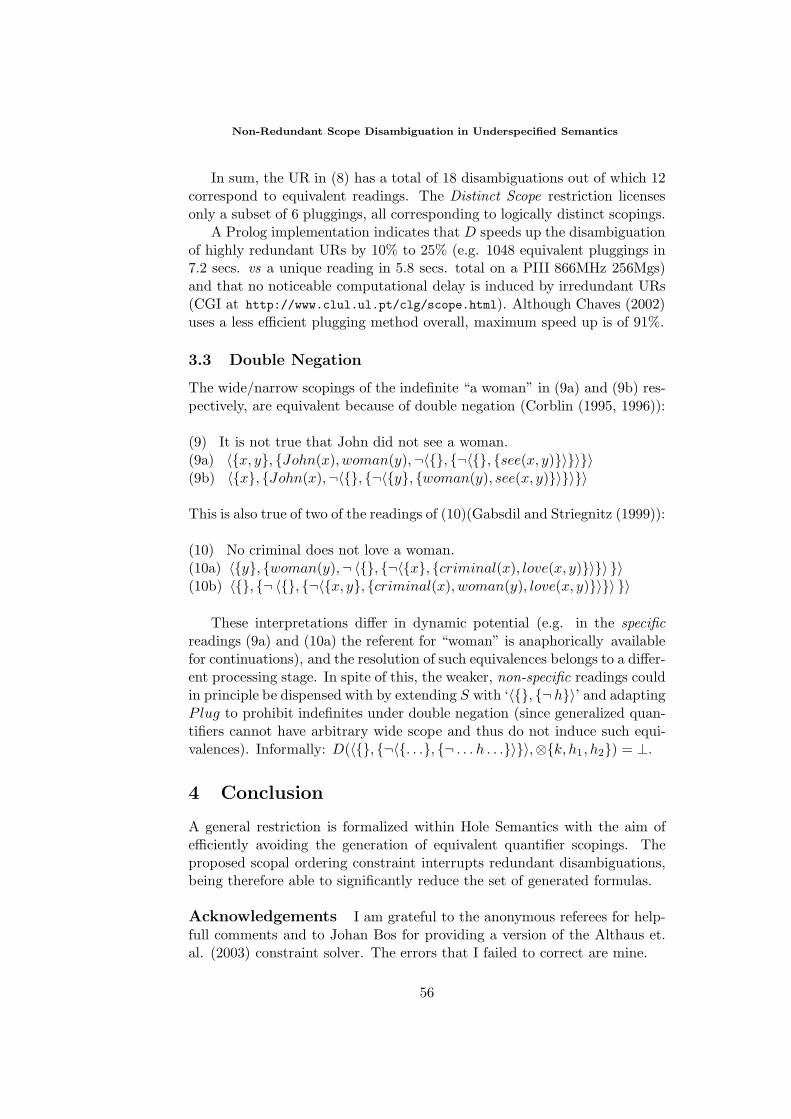
Non-Redundant Scope Disambiguation in Underspecified Semantics
In sum, the UR in (8) has a total of 18 disambiguations out of which 12correspond to equivalent readings. The Distinct Scope restriction licensesonly a subset of 6 pluggings, all corresponding to logically distinct scopings.
A Prolog implementation indicates that D speeds up the disambiguationof highly redundant URs by 10% to 25% (e.g. 1048 equivalent pluggings in7.2 secs. vs a unique reading in 5.8 secs. total on a PIII 866MHz 256Mgs)and that no noticeable computational delay is induced by irredundant URs(CGI at http://www.clul.ul.pt/clg/scope.html). Although Chaves (2002)uses a less efficient plugging method overall, maximum speed up is of 91%.
3.3 Double Negation
The wide/narrow scopings of the indefinite “a woman” in (9a) and (9b) res-pectively, are equivalent because of double negation (Corblin (1995, 1996)):
(9) It is not true that John did not see a woman.(9a) 〈x, y, John(x), woman(y),¬〈, ¬〈, see(x, y)〉〉〉(9b) 〈x, John(x),¬〈, ¬〈y, woman(y), see(x, y)〉〉〉
This is also true of two of the readings of (10)(Gabsdil and Striegnitz (1999)):
(10) No criminal does not love a woman.(10a) 〈y, woman(y),¬ 〈, ¬〈x, criminal(x), love(x, y)〉〉 〉(10b) 〈, ¬ 〈, ¬〈x, y, criminal(x), woman(y), love(x, y)〉〉 〉
These interpretations differ in dynamic potential (e.g. in the specificreadings (9a) and (10a) the referent for “woman” is anaphorically availablefor continuations), and the resolution of such equivalences belongs to a differ-ent processing stage. In spite of this, the weaker, non-specific readings couldin principle be dispensed with by extending S with ‘〈, ¬h〉’ and adaptingPlug to prohibit indefinites under double negation (since generalized quan-tifiers cannot have arbitrary wide scope and thus do not induce such equi-valences). Informally: D(〈, ¬〈. . ., ¬ . . . h . . .〉〉,⊗k, h1, h2) = ⊥.
4 Conclusion
A general restriction is formalized within Hole Semantics with the aim ofefficiently avoiding the generation of equivalent quantifier scopings. Theproposed scopal ordering constraint interrupts redundant disambiguations,being therefore able to significantly reduce the set of generated formulas.
Acknowledgements I am grateful to the anonymous referees for help-full comments and to Johan Bos for providing a version of the Althaus et.al. (2003) constraint solver. The errors that I failed to correct are mine.
56
Rui Pedro Chaves
References
Alshawi, H. and R. Crouch (1992). Monotonic semantic interpretation. In Pro-ceedings of the 30th ACL, pp. 32–39. Newark, Delaware.
Althaus, E., D. Duchier, A. Koller, K. Mehlhorn, J. Niehren, and S. Thiel (2003).An efficient graph algorithm for dominance constraints. Journal of Algorithms,To appear.
Blackburn, P. and J. Bos (1999). Representation and Inference forNatural Language - A First Course in Computational Semantics.http://www.coli.uni-sb.de/~bos/comsem.
Bos, J. (1996). Predicate logic unplugged. In Proceedings of the 10th Amster-dam Colloquium, pp. 133–142. ILLC / Department of Philosophy, University ofAmsterdam, The Netherlands.
Chaves, R. P. (2002). Fundamentos para uma Gramatica Computacional doPortugues – Uma abordagem lexicalista. Master’s dissertation, University of Lis-bon, Lisbon.
Cooper, R. (1983). Quantification and Syntactic Theory. Reidel Publications,Dordrecht.
Corblin, F. (1995). Compositionality and complexity in multiple negation. IGPLBulletin 3, 3-2, 449–473.
Corblin, F. (1996). Multiple negation processing in Natural Language. In Theoria,pp. 214–260.
Egg, M. and K. Lebeth (1995). Semantic underspecification and modifier attach-ment ambiguities. In J. Kilbury and R. Wiese (Eds.), Integrative Ansatze in dercomputer linguistik, pp. 19–24. Dusseldorf, Seminar fur Allgemeine Sprachwis-senschaft.
Egg, M., J. Niehren, P. Ruhrberg, and F. Xu (1998). Constraints over lambda-structures in semantic underspecification. In Joint COLING/ACL, pp. 353–359.Montreal, Canada.
Gabsdil, M. and K. Striegnitz (1999). Classifying scope ambiguities. In C. Montzand M. de Rijke (Eds.), ICOS-1, Institute for Logic, Language and Computation(ILLC), Amsterdam, pp. 125–131.
Hobbs, J. R. and S. M. Shieber (1987). An algorithm for generating quantifierscopings. Computational Linguistics 13(1-2), 47–55.
Kamp, H. and U. Reyle (1993). From Discourse to Logic: An Introduction to Mod-eltheoretic Semantics of Natural Language, Formal Logic and DRT. Dordrecht,Holland: Kluwer.
Keller, W. R. (1988). Nested Cooper storage: The proper treatment of quantifica-tion in ordinary noun phrases. In U. Reyle and C. Roher (Eds.), Natural LanguageParsing and Linguistic Theories, Dordrecht: Reidel, pp. 432–447.
Koller, A., J. Niehren, and S. Thater (2003). Bridging the gap between under-specification formalisms: Hole semantics as dominance constraints. In Proceedingsof the 11th EACL, Budapest.
57
Non-Redundant Scope Disambiguation in Underspecified Semantics
McCawley, J. D. (1981). Everything that Linguists always wanted to know aboutlogic. . . but were ashamed to ask. Chicago: The University of Chicago Press.
Reyle, U. (1993). Dealing with Ambiguities by Underspecification: Construction,Representation and Deduction. Journal of Semantics 102, 123–179.
Vestre, E. J. (1991). An algorithm for generating non-redundant quantifier scop-ings. In Fifth Conference of the European Chapter of the ACL, pp. 251–256. Berlin,Germany.
58
The Beth Property for the Modal Logic of
Graded Modalities, with an Application
to the Description Logic ALCQ.
Willem ConradieDepartment of Mathematics and Statistics,
Rand Afrikaans University,
P O Box 524, Auckland Park, 2006, South [email protected]
Abstract. Abstract: We prove the Beth definability-property for a modal logicwith graded (or “counting”) modalities. The result has an important consequencefor the description logic known as ALCQ, as it implies that every definitorial ALCQ-terminology is equivalent to an acyclic ALCQ-terminology. It is shown that theBeth property fails for the logics obtained by adding the difference operator to thelogic of graded modalities or to basic modal logic.
1 Introduction
In section 1.1 we introduce the Beth property - a property standardly in-vestigated for logics, which also happens to have a nice intuitive applicationto description logics. These are introduced in section 1.2. In section 2 weextend modal logic by adding to it the difference operator and graded modal-ities. Certain combinations of these operators give rise to logics in whichthe Beth property fails - two of these are illustrated is section 4, makinguse of a characterization of the Beth property given in section 3. Section 5centers around the proof of our main result - the Beth property for the logicof graded modalities, and also makes use of the characterization provided insection 3.
We assume basic knowledge of the syntax and semantics of modal logic,as well the notions of bisimulation, generated submodel, the unravelling of amodel and the standard translation of a modal formula. A state of the artreference here is [Blackburn et al., 2001]. From first-order model theory weassume the notions of (countably) saturated model, type and ultraproductsas well as related theorems such as that of Los (see [Hodges, 1993]). Allwork will be purely semantical, languages will always be interpreted overthe class of all possible models. With this in mind we will mostly identify
Proceedings of the Eighth ESSLLI Student SessionBalder ten Cate (editor)Chapter 6, Copyright c© 2003, Willem Conradie
59
The Beth Property for the Modal Logic of Graded Modalities
logics with their languages for the sake of brevity. We shall work with aglobal consequence relation .
1.1 The Beth-Property
We parameterize a language L with a set of proposition letters Π, as followsL(Π) is we want to be explicit about the proposition letters used in thelanguage. Similarly for sets of formulas: Γ(Π). When Π = q1, q2, . . . , qi, pwe shall write Γ(q, p).
Suppose that we are working in a logic S in a language L. Before in-troducing the Beth-property for propositional (modal) logics, we need thenotions of explicit- and implicit definitions:
Definition 1.1 Let Γ(q, p) be a set of formulas in L and p′ a propositionletter not occurring in any formula in Γ(q, p). Let Γ(q, p′) be the resultof uniformly substituting p′ for every occurrence of p in Γ. Γ is called animplicit definition of p, if Γ(q, p),Γ(q, p′) S p↔ p′.
The intuitive meaning of this rather technical-looking definition is the fol-lowing: Given an interpretation of the symbols in Γ except p, the interpre-tation of p is fixed. Or stated another way, given any model for the languageL(Γ) − p, this model can be extended in at most one way to a model ofΓ, by giving a valuation for p. Showing that a set of formulas Γ is not animplicit definition of p then boils down to demonstrating the existence oftwo models of Γ, based on the same frame and having the same q-valuation,but differing on their p-valuation. This was first observed by Padoa in 1900in the context of first order logic, and the method has become known asPadoa’s method.
Definition 1.2 Let p be a proposition letter and Γ(q, p) a set of formulas inL. A formula φ ∈ L(q) is called an explicit definition of p relative to Γ(q, p)if Γ(q, p) S p↔ φ.
Definition 1.3 A logic S is said to have the Beth-property if for any implicitdefinition Γ, of a proposition letter p, there exists an explicit definition φ ofp relative to Γ.
The Beth-property has been established for quite a number of (proposi-tional) modal logics, including the logic K. One particularly interestingresult here is due to [Maksimova, 1993]. This states that all normal exten-sions of the logic K4 have the Beth-property. One should also mention therelationship between interpolation and the Beth property. Stated simply,interpolation implies the Beth-property. For a detailed discussion of thesematters the reader is referred to [Hoogland, 2001].
60
Willem Conradie
1.2 Description Logic
An extensive hierarchy of knowledge representation formalisms, known asdescription logics, exists in the literature (see [Baader et al., 2003]). Manyof these logics turn out to be syntactic variants of (extended) multi-modallogics. For example, the description language ALC corresponds to a propo-sitional modal language with (possibly) multiple diamonds. ALCQ, a muchmore expressive description logic, corresponds to the modal logic with count-ing modalities L≤, which we define below, but possibly with many unarymodalities. For an introduction to description logics the reader is referredto [Baader and Nutt, 2003].
Certain sets of formulas in description logics are known as terminologies.In such a terminology concepts (corresponding to our proposition letters)are defined in terms of other base concepts (corresponding to a designatedsubset of the proposition letters in the language). The definition of a conceptmay also (directly or indirectly) make use of the concept itself. A terminol-ogy in which this happens is said to by cyclic, and acyclic otherwise.
A terminology, T , is said to be definitorial if any interpretation of the baseconcepts completely determines the interpretation of the defined conceptson any model for T . This is clearly the same as saying that T is an im-plicit definition of the defined concepts. The Beth property for a descriptionlogic then says that on any model for a definitorial terminology, for everydefined concept there is a formulas equivalent to it, only making use of baseconcepts. This implies that every definitorial terminology in the logic isequivalent to a acyclic terminology. From a computational viewpoint this isvery important, as reasoning with acyclic terminologies is much easier thatdoing so with cyclic ones.
2 The Difference Operator and Graded Modalities
We work on Kripke models with one binary relation (as for the basic modallanguage). Let M = (W,R, V ) be such a model and m ∈W . The differenceoperator, D, has the following semantics
M,m Dφ iff there exists a point n ∈M such that n= m and M, n φ.
Note that the difference operator allows us to define the universal modality(cf. [Blackburn et al., 2001], p. 415 )
Eφ ≡ φ ∨ Dφ
andAφ ≡ ¬(E¬φ).
61
The Beth Property for the Modal Logic of Graded Modalities
We are also able to count states in a limited way. Define
E!φ ≡ E(φ ∧ ¬Dφ)
which holds on a model precisely when exactly one state where φ holds.
Taking the idea of counting (successor) states more seriously leads us tothe idea of graded modalities: For each n ∈ ω we add the modality ≤n toour language, with the following interpretation
M,m ≤nφ if and only if |y ∈M : Rmy and M, y φ| ≤ n.
One can now define
>nφ ≡ ¬≤nφ, ≥nφ ≡ >n−1φ, =nφ ≡ (≤nφ∧≥nφ), ♦φ ≡ ≥1φ
We shall be considering the languages L♦,D defined as
φ ::= p | | ¬φ | φ ∨ ψ | ♦φ | Dφ
and L≤ given byφ ::= p | | ¬φ | φ ∨ ψ | ≤n φ
Note that, even though it does not contain the ♦-operator, L≤ subsumesthe basic modal language in terms of expressivity.
We extend the notion of a modal bisimulation to accommodate the dif-ference operator and graded modalities respectively, obtaining the notionsof difference bisimulation and counting bisimulation. If w is a point in amodel we write R[w] for the set its R-successors in that model.
Definition 2.1 Let M = (M,R, V ) and M′ = (M ′, R′, V ′) be models. Arelation Z ⊆ M ×M ′ is called a difference bisimulation if it satisfies thefollowing.
bisimulation Z is a bisimulation
difference forth if uZu′, v ∈ M and v = u, then there exists a pointv′ ∈M ′ such that v′ = u′ and vZv′
difference back if uZu′, v′ ∈ M and v′ = u′, then there exists a pointv ∈M such that v = u and vZv′
We write M,m ↔L♦,DM′,m′ to indicate that there exists a difference
bisimulation between m and m′, or M,m ↔L♦,D(Π) M′,m′ if Π is the setof proposition letters with respect to which the local harmony clause of thebisimulation is taken, i.e. the clause specifying that bisimilar states satisfythe same proposition letters.
62
Willem Conradie
The proof of the next proposition is standard.
Proposition 2.2 Let M = (M,R, V ) and M′ = (M ′, R′, V ′) be models,m ∈M and m′ ∈M ′. If M,m ↔ L♦,DM′,m′ then M,m L♦,DM′,m′.
Definition 2.3 Let M = (M,R, V ) and M′ = (M ′, R′, V ′) be models.A relation Z ⊆ M ×M ′ is called a counting bisimulation if the followingconditions are satisfied
local harmony if uZu′ then u and u′ satisfy the same proposition letters
counting forth if uZu′ and S ⊆ R[u] is a finite or countably infinite set,then there exists a set S′ ⊆ R′[u′] such that (i) for each s ∈ S thereexists an s′ ∈ S′ such that sZs′, (ii) for each s′ ∈ S′ there exists ans ∈ S such that sZs′ and (iii) |S| = |S′|.
counting back A similar condition for points in M′ and sets of their suc-cessors.
We write M,m ↔L≤ M′,m′ to indicate that there exists a counting bisim-ulation linking m and m′, or M,m ↔L≤(Π) M′,m′ if Π is the set of propo-sition letters with respect to which the local harmony clause is taken.
Proposition 2.4 Let M = (M,R, V ) and M′ = (M ′, R′, V ′) be two (notnecessarily distinct) models, m ∈ M , m′ ∈ M ′, and Z : M,m ↔L≤(Π)
M′,m′ a counting bisimulation linking m and m′. Then m L≤(Π) m′.
The logic L≤,D is obtained by adding the difference operator to L≤. Thenotion of a difference counting bisimulation is obtained by adding differenceclauses to a counting bisimulation. The corresponding preservation result iseasily proved.
3 The Beth Property as the Extendability of Equiv-alences
In this section we formulate and prove a necessary and sufficient conditionfor a logic with Kripkean semantics to have the Beth property. This will beused in the proof of our main result, theorem 5.5.
If m1 and m2 are points from (not necessarily distinct) Kripke modelsM1 and M2 respectively, we write M1,m1 L(Π) M2,m2 if m1 and m2
satisfy exactly the same formulas from the language L(Π). We say m1 andm2 are equivalent with respect to L(Π).
63
The Beth Property for the Modal Logic of Graded Modalities
Theorem 3.1 Let S be a compact logic in a language L, and Γ(q, p) a(possibly empty) set of formulas. There exists an explicit definition of p inthe language L(q) relative to Γ(q, p) if and only if for any models M1 andM2 of Γ and points m1 ∈ M1 and m2 ∈ M2,
m1 L(q) m2 only if m1 L(q,p) m2.
Proof: Suppose there exists an explicit definition of p relative toΓ(q, p), say φ ∈ L(q). Specifically Γ p ↔ φ, hence if ψ ∈ L(q, p) andψ[p/φ] is the result of uniformly replacing p with φ in ψ, we have thatΓ ψ ↔ ψ[p/φ]. Let M = (W,R, V ) be any model of Γ and m1,m2 ∈ W .Suppose m1 L(q) m2. If ψ ∈ L(q, p) then M,m1 ψ iff M,m1 ψ[p/φ]iff M,m2 ψ[p/φ] iff M,m2 ψ. Hence m1 L(q,p) m2.
To prove the right-to-left direction we proceed by contraposition. Sup-pose that there exists no explicit definition of p relative to Γ(q, p). Letψ0, ψ1, ψ2, . . . be an enumeration of the formulas in L(q). For each ψi letψ1
i = ψi and ψ0i = ¬ψi.
Claim 1: For each n ∈ ω there exists a function χ : 0, 1, . . . , n → 0, 1such that both p ∧
∧ni=1 ψ
χ(i)i and ¬p ∧
∧ni=1 ψ
χ(i)i are satisfiable on models
of Γ.
Proof of Claim 1: Let n ∈ ω. Note that there are 2n functions χ :0, 1, . . . , n → 0, 1, call them χ1, χ2, . . . , χ2n . Suppose to the contrarythat for no function χ : 0, 1, . . . , n → 0, 1 both p ∧
∧ni=1 ψ
χ(i)i and
¬p∧∧n
i=1 ψχ(i)i are Γ-satisfiable. Hence for each χ, either Γ
∧ni=1 ψ
χ(i)i → p
or Γ ∧n
i=1 ψχ(i)i → ¬p. Let Ψj =
∧ni=1 ψ
χj(i)i for each 1 ≤ j ≤ 2n. Note
that ∨2n
j=1 Ψj ↔ . Let J1 = j : Γ Ψj → p and J2 = j : Γ Ψj → ¬p. Then clearly Γ
∨j∈J1
Ψj → p and Γ ∨
j∈J2Ψj → ¬p, and
J1 ∪ J2 = 1, 2, . . . , 2n. Hence Γ ∨
j∈J1Ψj ↔ p, yielding an explicit
definition and a contradiction.
Claim 2: There exists a chain of functions ρ1 ⊆ ρ2 ⊆ ρ3 ⊆ · · · wherefor each i, ρi : 1, 2, . . . , i → 0, 1, such that if Φi =
∧ij=1 ψ
ρi(j)j then both
Φi ∧ p and Φi ∧ ¬p are Γ-satisfiable.
Proof of Claim 2: To see that this is the case, let as represent theset of functions F = χ : 0, 1, . . . , n → 0, 1 : n ∈ ω as a binary tree.We call this tree T . More precisely, a function χ : 0, 1, . . . , n → 0, 1 isrepresented by a path from the root to level n+ 1, where, if the left branchis taken at level i, it means that χ(i) = 0, and if the right is taken that
64
Willem Conradie
χ(i) = 1. Clearly there is a one-to-one correspondence between functions inF and finite paths in T .
We call a function f ∈ F acceptable for n ∈ ω if f : 0, 1, . . . ,m →0, 1 for some m ≥ n, and both p ∧
∧ni=1 ψ
f(i)i and ¬p ∧
∧ni=1 ψ
f(i)i are sat-
isfiable on models of Γ. Clearly, if f is acceptable for n, then f is acceptablefor all j ≤ n. We call a path of length n acceptable, if it corresponds tosome function in F which is acceptable for n.
By claim 1 there are arbitrarily long acceptable paths from the root ofT . Thus by Konig’s Lemma there must be an infinitely long path from theroot of T , call it P , such that every finite sub-path of P , starting at the rootis acceptable. The desired chain of functions is then the chain correspondingto the finite sub-paths of P , starting at the root.
Let U = p ∪ Φi : i ∈ ω and T = ¬p ∪ Φi : i ∈ ω. Every finitesubset of U is Γ-satisfiable, as is every finite subset of T , hence U and T areboth Γ-satisfiable, hence by compactness (recall that by assumption we aredealing with a compact modal logic) both U and T are satisfiable on modelsof Γ. Moreover U and T are maximal satisfiable sets in the language L(q),as for each ψi either ψi or ¬ψi is a conjunct of Φi. This means there aremodels of Γ, M = (W,R, V ) and M′ = (W ′, R′, V ′) say, and points w ∈Wand w′ ∈W ′ such that every formula in U is satisfied at w and every formulain T is satisfied at w′. As U and T are maximal in L(q), w and w′ agree onall formulas in L(q), but differ on their valuation of p, i.e w L(q) w
′ butw L(q,p) w
′.
4 Two Negative Beth Results
Theorem 4.1 L♦,D and L≤,D do not have the Beth property.
Proof: Let p, q and r be proposition letters and let
Γ(q, r, p) = E!(p ∧ q)),¬q → p,Er, r → ♦, r → (p ∧ q)
The intuitive content of this proof is the following. On any model of Γ allthe ¬q-points are p-points, and further there is precisely one (p ∧ q)-point.But at which q-point must p hold? This is pointed out by some r-point: theunique point which is the successor of all the r-points. The death-blow toany aspiring explicit definition however, is the fact that a p-point might notbe able to “see” if it is being pointed at by an r-point. It is not difficult toprove that if M = (M,R, V ) and M Γ, then
[[p]]M = [[¬q]]M ∪ m ∈M : M,m q andthere is a w ∈M such that M, w r and Rwm
65
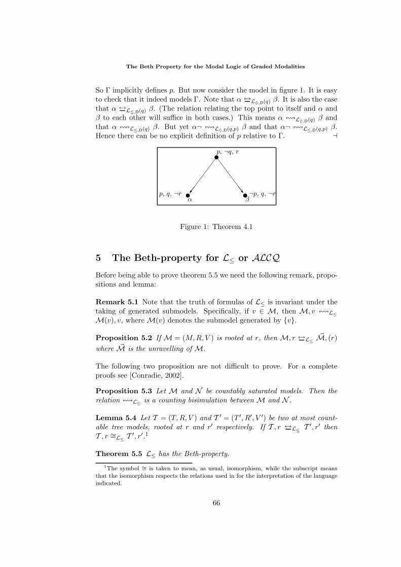
The Beth Property for the Modal Logic of Graded Modalities
So Γ implicitly defines p. But now consider the model in figure 1. It is easyto check that it indeed models Γ. Note that α ↔L♦,D(q) β. It is also the casethat α ↔L≤,D(q) β. (The relation relating the top point to itself and α andβ to each other will suffice in both cases.) This means α L♦,D(q) β andthat α L≤,D(q) β. But yet α¬ L♦,D(q,p) β and that α¬ L≤,D(q,p) β.Hence there can be no explicit definition of p relative to Γ.
p, ¬q, r
p, q, ¬r ¬p, q, ¬rα β
Figure 1: Theorem 4.1
5 The Beth-property for L≤ or ALCQBefore being able to prove theorem 5.5 we need the following remark, propo-sitions and lemma:
Remark 5.1 Note that the truth of formulas of L≤ is invariant under thetaking of generated submodels. Specifically, if v ∈ M, then M, v L≤M(v), v, where M(v) denotes the submodel generated by v.
Proposition 5.2 If M = (M,R, V ) is rooted at r, then M, r ↔L≤M, (r)
where M is the unravelling of M.
The following two proposition are not difficult to prove. For a completeproofs see [Conradie, 2002].
Proposition 5.3 Let M and N be countably saturated models. Then therelation L≤ is a counting bisimulation between M and N .
Lemma 5.4 Let T = (T,R, V ) and T ′ = (T ′, R′, V ′) be two at most count-able tree models, rooted at r and r′ respectively. If T , r ↔L≤ T ′, r′ thenT , r ∼=L≤ T ′, r′.1
Theorem 5.5 L≤ has the Beth-property.
1The symbol ∼= is taken to mean, as usual, isomorphism, while the subscript meansthat the isomorphism respects the relations used in for the interpretation of the languageindicated.
66
Willem Conradie
Proof: Suppose as set of formulas Γ(q, p) implicitly defines p. Let M andM′ be any models of Γ(q, p) of of at most countable cardinality. Let m andm′ be points in M and M′ respectively such that M,m L≤(q) M′,m′.By theorem 3.1 it is sufficient to show that M,m L≤(q,p) M′,m′. This iswhat we now proceed to do.
Let UM and UM′ be ultrapowers of M and M′ respectively over somecountably incomplete ultrafilter U . Let idm and idm′ be the points a/Uand a′/U in UM and UM′ respectively where a(i) = m and a′(i) = m′
for all i. Note that these models are still at most countable. By Los’stheorem (and the fact that L≤-formulas may be translated into first-orderformulas preserving equivalence on the level of models) it is the case thatM,m L≤(q,p) UM, idm and M′,m′ L≤(q,p) UM′, idm′ and, further,that UM and UM′ are models of Γ(q, p). Hence we have UM, idm L≤(q)
UM′, idm′ . But since UM and UM′ are countably saturated it follows fromlemma 5.3 that in fact UM, idm ↔L≤(q) UM′, idm′ .
Now, unravel UM and UM′, around idm and idm′ respectively (by re-mark 5.1 we may assume that the they are rooted at idm and idm′) to obtaintwo tree models T and T ′ rooted at (idm) and (idm′) respectively. Note thatthe tree models are at most countable and models of Γ(q, p). By proposition5.2 we have UM, idm ↔L≤(q,p) T , (idm) and UM′, idm′ ↔L≤(q,p) T ′, (idm′)and hence T , (idm) ↔L≤(q) T ′, (idm′). But it then follows from lemma 5.4that T , (idm) ∼=L≤(q) T ′, (idm′). It must be the case that T , (idm) ∼=L≤(q,p)
T ′, (idm′), for otherwise, by Padoa’s method it would follow that Γ(q, p) didnot implicitly define p - a contradiction. But this implies that T , (idm) ↔L≤(q,p)
T ′, (idm′), hence that T , (idm) L≤(q,p) T ′, (idm′). Now we have
m L≤(q,p) idm L≤(q,p) (idm) L≤(q,p) (idm′) L≤(q,p) idm′ L≤(q,p) m′
i.e. m L≤(q,p) m′ as desired.
This proves the Beth property for the logic over the class of all models ofat most countable cardinality. We may now apply the Lowenheim-Skolemtheorem upwards, to obtain the result for the logic over the class of allmodels.
6 Concluding Remarks
To conclude we mention some recent results and some open questions.[Ten Cate, 2003] has recently proven that the smallest extension of the L♦,D
that has the interpolation property is the first order correspondence lan-guage. It would be interesting to find a similar result for the smallest ex-tensions of L♦,D and L≤,D that have the Beth-property. As far as ALCQ-terminologies are concerned, it would be interesting to find an upper boundon the size of the acyclic terminology corresponding to a cyclic terminology,the existence of which is guaranteed by our result. Lastly, techniques for
67
The Beth Property for the Modal Logic of Graded Modalities
finding such an acyclic terminology constructively (analogous to those de-veloped in [Blackburn and Marx, 2002] for finding interpolants) do not seemto exist as yet.
References
[Baader and Nutt, 2003] F. Baader, W.Nutt. Basic Description Logics. In F.Baader, D. Calvanese, D. McGuinness, D. Nardi and P. Patel-Schneider (edi-tors). The Description Logic Handbook: Theory, Implementation and Appli-cations, Cambridge University Press, 2003.
[Baader et al., 2003] F. Baader, D. Calvanese, D. McGuinness, D. Nardi and P.Patel-Schneider (editors). The Description Logic Handbook: Theory, Imple-mentation and Applications, Cambridge University Press, 2003.
[Beth, 1953] E. W. Beth. On Padoa’s method in the theory of definition. IndagionesMath., 15:330-339, 1953.
[Blackburn et al., 2001] P. Blackburn, M. de Rijke, and Y. Venema. Modal Logic.Cambridge University Press, 2001.
[Blackburn and Marx, 2002] P. Blackburn and M. Marx. Constructive interpolantsfor every bounded fragment definable hybrid logic. To appear in Journal ofSymbolic Logic.
[Conradie, 2002] W. E. Conradie. Definability and Changing Perspectives - TheBeth Property for Three extensions of Modal Logic. MOL Thesis, Institutefor Logic, Language and Computation, Universiteit van Amsterdam, 2002.
[D’Agostino, 1998] G. D’Agostino. Modal Logic and non-well-founded Set Theory:translation, bimsimulation, interpolation. PhD Thesis, Institute for Logic,Language and Computation, Universiteit van Amsterdam, 1998.
[Fine, 1972] K. Fine. In so many possible worlds. Notre Dame Journal of FormalLogic, 13(4):516-520, 1972.
[Hodges, 1993] W. Hodges. Model Theory. Cambridge University Press, 1993.
[Hoogland, 2001] E. Hoogland. Definability and Interpolation. PhD Thesis, Insti-tute for Logic, Language and Computation, Universiteit van Amsterdam,2001.
[Kurtonina and de Rijke, 1999] N. Kurtonina and M. de Rijke. Expressiveness ofconcept expressions in first-order description logics. Artificial Intelligence,107:303-333, 1999.
[Maksimova, 1993] L. L. Maksimova. An analogue of Beth’s theorem in normalextensions of the modal logic K4. Siberian Mathematical Journal, 33(6):1052-1065.
[Ten Cate, 2003] Ten Cate, B. Personal communication.
[Van der Hoek and de Rijke, 1995] W. van der Hoek and M. de Rijke. CountingObjects. Journal of Logic and Computation, 5(3):325-345, 1995.
68
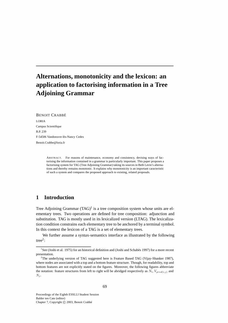
Alternations, monotonicity and the lexicon: anapplication to factorising information in a TreeAdjoining Grammar
BENOIT CRABBÉ
LORIA
Campus Scientifique
B.P. 239
F-54506 Vandoeuvre-lès-Nancy Cedex
ABSTRACT. For reasons of maintenance, economy and consistency, devising ways of fac-torising the information contained in a grammar is particularly important. This paper proposes afactorising system for TAG (Tree Adjoining Grammar) taking its sources in Beth Levin’s alterna-tions and thereby remains monotonic. It explains why monotonicity is an important caracteristicof such a system and compares the proposed approach to existing, related proposals.
1 Introduction
Tree Adjoining Grammar (TAG)1 is a tree composition system whose units are el-ementary trees. Two operations are defined for tree composition: adjunction andsubstitution. TAG is mostly used in its lexicalized version (LTAG). The lexicaliza-tion condition constrains each elementary tree to be anchored by a terminal symbol.In this context the lexicon of a TAG is a set of elementary trees.
We further assume a syntax-semantics interface as illustrated by the followingtree2:
1See (Joshi et al. 1975) for an historical definition and (Joshi and Schabès 1997) for a more recentpresentation.
2The underlying version of TAG suggested here is Feature Based TAG (Vijay-Shanker 1987),where nodes are associated with a top and a bottom feature structure. Though, for readability, top andbottom features are not explicitly stated on the figures. Moreover, the following figures abbreviatethe notation: feature structures from left to right will be abridged respectively asNi, Vpred(i,j) andNj .
Proceedings of the Eighth ESSLLI Student SessionBalder ten Cate (editor)Chapter 7, Copyrightc© 2003, Benoit Crabbé
69
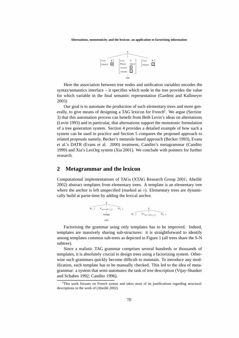
Alternations, monotonicity and the lexicon: an application to factorising information
S
[CAT N
INDEX i
]
CAT VPRED PRED
AGENT i
THEME j
[CAT N
INDEX j
]
eats
Here the association between tree nodes and unification variables encodes thesyntax/semantics interface – it specifies which node in the tree provides the valuefor which variable in the final semantic representation (Gardent and Kallmeyer2003)
Our goal is to automate the production of such elementary trees and more gen-erally, to give means of designing a TAG lexicon for French3. We argue (Section3) that this automation process can benefit from Beth Levin’s ideas on alternations(Levin 1993) and in particular, that alternations support the monotonic formulationof a tree generation system. Section 4 provides a detailed example of how such asystem can be used in practice and Section 5 compares the proposed approach torelated proposals namely, Becker’s metarule based approach (Becker 1993), Evanset al.’s DATR (Evans et al. 2000) treatment, Candito’s metagrammar (Candito1999) and Xia’s LexOrg system (Xia 2001). We conclude with pointers for furtherresearch.
2 Metagrammar and the lexicon
Computational implementations of TAGs (XTAG Research Group 2001; Abeillé2002) abstract templates from elementary trees. A template is an elementary treewhere the anchor is left unspecified (marked as). Elementary trees are dynami-cally build at parse-time by adding the lexical anchor.
S
Ni ↓ Vpred(i,j) Nj ↓
mange
eats
S
Ni ↓ Vpred(i,j) Nj ↓
Factorising the grammar using only templates has to be improved. Indeed,templates are massively sharing sub-structures: it is straightforward to identifyamong templates common sub-trees as depicted in Figure 1 (all trees share the S-Nsubtree).
Since a realistic TAG grammar comprises several hundreds or thousands oftemplates, it is absolutely crucial to design trees using a factorizing system. Other-wise such grammars quickly become difficult to maintain. To introduce any mod-ification, each template has to be manually checked. This led to the idea of meta-grammar: a system that semi-automates the task of tree description (Vijay-Shankerand Schabes 1992; Candito 1996).
3This work focuses on French syntax and takes most of its justifications regarding structuraldescriptions in the work of (Abeillé 2002).
70
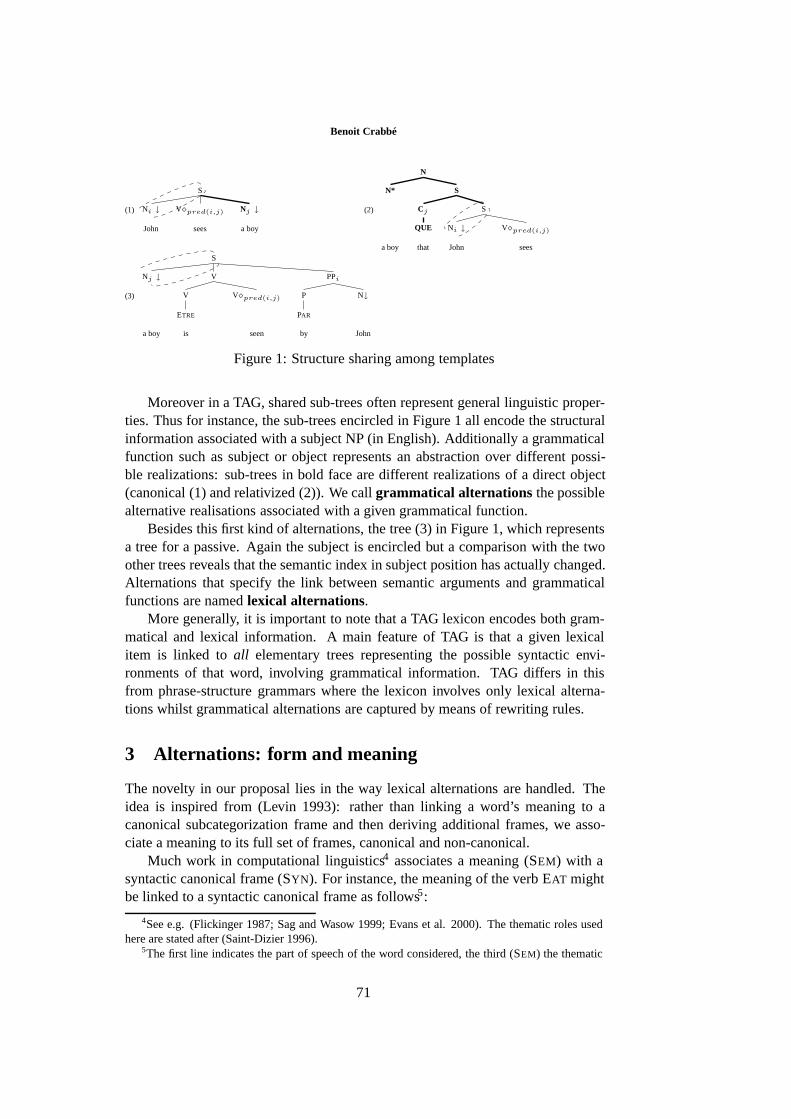
Benoit Crabbé
(1)
S
Ni ↓ Vpred(i,j) Nj ↓
John sees a boy
(2)
N
N* S
Cj S
QUE Ni ↓ Vpred(i,j)
a boy that John sees
(3)
S
Nj ↓ V PPi
V Vpred(i,j) P N↓
ETRE PAR
a boy is seen by John
Figure 1: Structure sharing among templates
Moreover in a TAG, shared sub-trees often represent general linguistic proper-ties. Thus for instance, the sub-trees encircled in Figure 1 all encode the structuralinformation associated with a subject NP (in English). Additionally a grammaticalfunction such as subject or object represents an abstraction over different possi-ble realizations: sub-trees in bold face are different realizations of a direct object(canonical (1) and relativized (2)). We callgrammatical alternations the possiblealternative realisations associated with a given grammatical function.
Besides this first kind of alternations, the tree (3) in Figure 1, which representsa tree for a passive. Again the subject is encircled but a comparison with the twoother trees reveals that the semantic index in subject position has actually changed.Alternations that specify the link between semantic arguments and grammaticalfunctions are namedlexical alternations.
More generally, it is important to note that a TAG lexicon encodes both gram-matical and lexical information. A main feature of TAG is that a given lexicalitem is linked toall elementary trees representing the possible syntactic envi-ronments of that word, involving grammatical information. TAG differs in thisfrom phrase-structure grammars where the lexicon involves only lexical alterna-tions whilst grammatical alternations are captured by means of rewriting rules.
3 Alternations: form and meaning
The novelty in our proposal lies in the way lexical alternations are handled. Theidea is inspired from (Levin 1993): rather than linking a word’s meaning to acanonical subcategorization frame and then deriving additional frames, we asso-ciate a meaning to its full set of frames, canonical and non-canonical.
Much work in computational linguistics4 associates a meaning (SEM) with asyntactic canonical frame (SYN). For instance, the meaning of the verb EAT mightbe linked to a syntactic canonical frame as follows5:
4See e.g. (Flickinger 1987; Sag and Wasow 1999; Evans et al. 2000). The thematic roles usedhere are stated after (Saint-Dizier 1996).
5The first line indicates the part of speech of the word considered, the third (SEM) the thematic
71
Alternations, monotonicity and the lexicon: an application to factorising information
(1)CAT VSYN 〈SUBJ(NP)i, OBJ(NP)j〉SEM 〈AGENTi, THEMEj〉
In a second step, syntactic variants of this canonical frame are derived by theapplication of lexical rules6. For instance, the application to frame (1) of a lexicalrule mapping active to passive might yields the following additional frame:
(2)CAT VSYN 〈SUBJ(NP)j, BY-OBJ(PP)i〉SEM 〈AGENTi, THEMEj〉
However, it is well known that lexical rules encounter many exceptions. Con-sider for instance, the following examples:
(a) Peter broke the window(b) The window broke(c) Peter ate an apple(d) *An apple ate
Whereasbreakallows the ergative rule application,eat doesn’t. This kind ofobservation leads to a Bloomfield like conclusion: lexical rules encounter arbitraryexceptions.
In other words, classical work associates a meaning only with its canonicalframe and then mechanically derives additional frames using lexical rules, whichrequires in practice to specify many exceptions.
Here we want to identify a meaning with its full set of syntactic frames, canon-ical as non-canonical, that is with its full set of alternations. Thus we deny anystatus to lexical rules.
Indeed, that approach reflects lexical idiosyncrasy and removes the need tospecify exceptions. But, an obvious drawback of such an approach is the loss ofmajor syntactic generalisations expressed by lexical rules.
An alternation class is a set of alternations which are common to a significantnumber of verbs: according to the syntactic point of view, these verbs behave ex-actly the same way. Furthermore, it appears that verbs belonging to a given classshare the same kind of meaning: for English, B. Levin identifies classes such asVERBS OFPUTTING, VERBS OFCOLOURING, VERBS OFPERCEPTION. . . Asfor a given language, the set of classes is finite, it follows that establishing a lexi-con using this approach only requires to identify a given lexeme with its alternationclass.
To sum up, we get a different degree of generality: instead of expressing gen-erality through the use of lexical rules, it is done through the use of alternationclasses. It seems to be a better generalization in that it does not require to state anyexceptions.
roles realised by the syntactic arguments of this word, and the second (SYN) the grammatical functionand the category of the arguments. The linking between syntactic arguments and thematic roles isgiven by the shared indices (herei andj). Thus frame (1) indicates that EAT is a verb that can takea subject and an object NP as arguments, whereby the subject provides the agent and the object thetheme index.
6Such an application can be expressed as a proceduralif . . . then statement, as in early LFG, oras an inheritance relation, see e.g. (Bouma et al. 1998; Sag and Wasow 1999).
72
Benoit Crabbé
3.1 A formal corollary: monotonicity
We have just seen the linguistic interest of alternations, but a further interest lieson the formal side: using alternations permits us to express lexical knowledge in amonotonic (hence declarative) way.
Systems for lexical representation are usually non-monotonic (Flickinger 1987;Sag and Wasow 1999; Evans et al. 2000). A major source of non-monotonicitycomes from the use of lexical rules that erase arguments. A striking example comesfrom a rule such asagentless passive. Given the two place subcategorization frameof the canonical frame (1), this rule outputs a one place subcategorization frame:
CAT VSYN 〈SUBJ(NP)j〉SEM 〈AGENTi, THEMEj〉
Using erasing rules licenses the removal of information, here the subject ex-pressed in the canonical frame has been removed. Erasing is related to sequencing:allowing to remove information requires defining different states in the system.Hence the resulting system is procedural .
In contrast, using alternations does not require to apply erasing rules since theserules are not considered anymore. To handle agentless passive, we simply associatewith a given verb the agentless passive alternation as well as any other alternationthat is possible for that verb.
Besides erasing, there are cases were multiple lexical rules may be applied (ina given order) to a canonical structure. Here is an example taken from French:
Marie lave MarieMary washes MaryMary washes Mary (canonical)Marie se laveMary herself washMary washes herself (+ reflexive)Jean fait se laver MarieJohn causes herself wash MaryJohn causes Mary to wash herself (+ causative)
To account for this, we must ensure that the set of possible alternations also in-clude these alternations that corresponds to each possible sequence of rules. How-ever these cases are, in French, quite limited. Indeed, (Candito 1999) identifiesonly ten such sequences, all involving the causative rule.
4 Formalization
This section concentrates on the use of alternations to factorise a TAG lexiconand automate its production. The basic idea is to describe a TAG by means of a(very big) disjunctive tree description. The TAG described is then the set of treessatisfying this description.
We proceed in three steps. First, we show how to describe a single TAG tree.Then, we show how the approach can be generalized to describing the full set
73
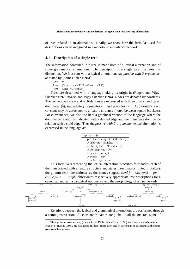
Alternations, monotonicity and the lexicon: an application to factorising information
of trees related to an alternation. Finally, we show how the formulas used fordescriptions can be integrated in a monotonic inheritance network.
4.1 Description of a single tree
The information contained in a tree is made both of a lexical alternation and ofsome grammatical alternations. The description of a single tree illustrates thisdistinction. We first start with a lexical alternation, saypassive-with-2-arguments,as stated by (Saint-Dizier 1996)7.
CAT VSYN 〈SUBJECTj(NP),BY-OBJECTi(PP)〉SEM 〈AGENTi, THEMEj〉
Trees are described with a language taking its origin in (Rogers and Vijay-Shanker 1992; Rogers and Vijay-Shanker 1994). Nodes are denoted by constants.The connectives are∧ and∨. Relations are expressed with three binary predicates:
dominates (), immediately dominates () and precedes (≺). Additionally, each
constant may be associated to a feature structure (noted between square brackets).For convenience, we also use here a graphical version of the language where thedominance relation is indicated with a dashed edge and the immediate dominancerelation with a solid edge. Thus thepassive-with-2-argumentslexical alternation isexpressed in the language as:
φpass − alt
pred [cat = V; agent = i; theme = j]∧ subj [cat = N; index = j]∧ obl-obj [cat = PP; index = i]∧ obl-prep [cat = by]∧ φpass− morph∧ φsubj − can∧ φobl − pp − can
This formula representing the lexical alternation describes four nodes, each ofthem associated with a feature structure and states three macros (noted in italics),the grammatical alternations: as the names suggestφsubj − can, φobl − pp −can, φpass − morph, abbreviates respectively appropriate tree descriptions for acanonical subject, a canonical oblique PP and the morphology of a passive verb.
φsubj − can φobl − pp − can φpass − morph
s[cat = S]
subj[cat = Ntype =↓
] ≺ v[cat = V]
s[cat = S]
v[cat = V]) ≺ obl-obj[cat = PP]
prep[cat = P] ≺ obl-head[cat = Ntype =↓
]
obl-prep
s[cat = S]
v[cat = V]
syn-head[cat = V] ≺ pred[cat = Vtype =
]
infl[cat = ETRE]
Relations between the lexical and grammatical alternations are performed througha naming convention. As constants’s names are global to all the macros, some of
7Though to a lesser extent, (Saint-Dizier 1996; Saint-Dizier 1999) aims to be an adaptation toFrench of (Levin 1993). He has added further information and in particular he associates a thematicrole to each argument.
74
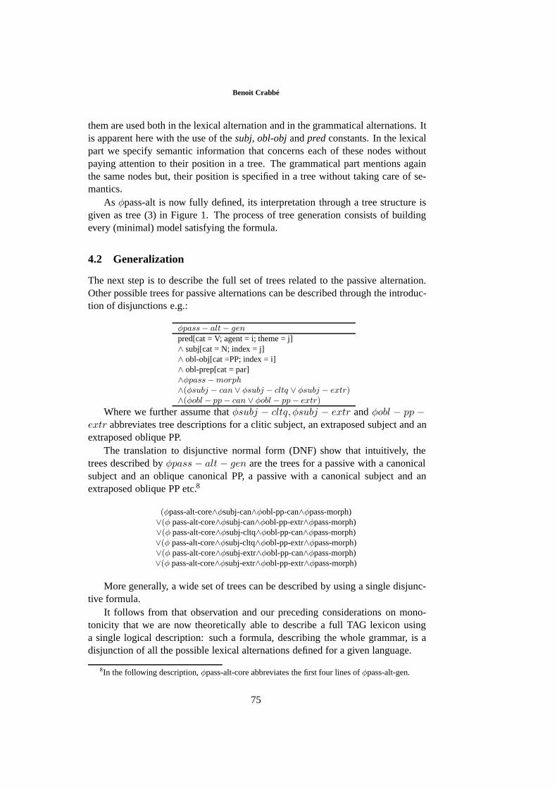
Benoit Crabbé
them are used both in the lexical alternation and in the grammatical alternations. Itis apparent here with the use of thesubj, obl-objandpredconstants. In the lexicalpart we specify semantic information that concerns each of these nodes withoutpaying attention to their position in a tree. The grammatical part mentions againthe same nodes but, their position is specified in a tree without taking care of se-mantics.
As φpass-alt is now fully defined, its interpretation through a tree structure isgiven as tree (3) in Figure 1. The process of tree generation consists of buildingevery (minimal) model satisfying the formula.
4.2 Generalization
The next step is to describe the full set of trees related to the passive alternation.Other possible trees for passive alternations can be described through the introduc-tion of disjunctions e.g.:
φpass− alt − gen
pred[cat = V; agent = i; theme = j]∧ subj[cat = N; index = j]∧ obl-obj[cat =PP; index = i]∧ obl-prep[cat = par]∧φpass− morph∧(φsubj − can ∨ φsubj − cltq ∨ φsubj − extr)∧(φobl − pp − can ∨ φobl − pp − extr)
Where we further assume thatφsubj − cltq, φsubj − extr andφobl − pp −extr abbreviates tree descriptions for a clitic subject, an extraposed subject and anextraposed oblique PP.
The translation to disjunctive normal form (DNF) show that intuitively, thetrees described byφpass − alt − gen are the trees for a passive with a canonicalsubject and an oblique canonical PP, a passive with a canonical subject and anextraposed oblique PP etc.8
(φpass-alt-core∧φsubj-can∧φobl-pp-can∧φpass-morph)∨(φ pass-alt-core∧φsubj-can∧φobl-pp-extr∧φpass-morph)∨(φ pass-alt-core∧φsubj-cltq∧φobl-pp-can∧φpass-morph)∨(φ pass-alt-core∧φsubj-cltq∧φobl-pp-extr∧φpass-morph)∨(φ pass-alt-core∧φsubj-extr∧φobl-pp-can∧φpass-morph)∨(φ pass-alt-core∧φsubj-extr∧φobl-pp-extr∧φpass-morph)
More generally, a wide set of trees can be described by using a single disjunc-tive formula.
It follows from that observation and our preceding considerations on mono-tonicity that we are now theoretically able to describe a full TAG lexicon usinga single logical description: such a formula, describing the whole grammar, is adisjunction of all the possible lexical alternations defined for a given language.
8In the following description,φpass-alt-core abbreviates the first four lines ofφpass-alt-gen.
75
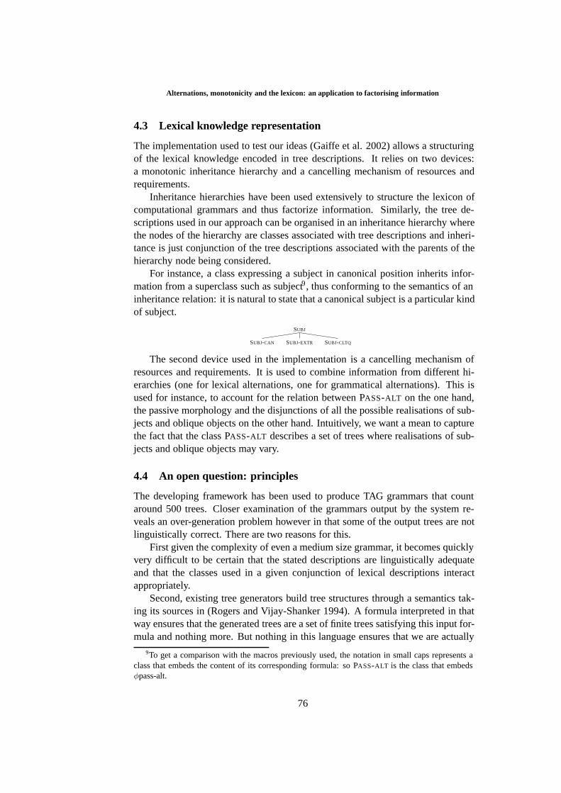
Alternations, monotonicity and the lexicon: an application to factorising information
4.3 Lexical knowledge representation
The implementation used to test our ideas (Gaiffe et al. 2002) allows a structuringof the lexical knowledge encoded in tree descriptions. It relies on two devices:a monotonic inheritance hierarchy and a cancelling mechanism of resources andrequirements.
Inheritance hierarchies have been used extensively to structure the lexicon ofcomputational grammars and thus factorize information. Similarly, the tree de-scriptions used in our approach can be organised in an inheritance hierarchy wherethe nodes of the hierarchy are classes associated with tree descriptions and inheri-tance is just conjunction of the tree descriptions associated with the parents of thehierarchy node being considered.
For instance, a class expressing a subject in canonical position inherits infor-mation from a superclass such as subject9, thus conforming to the semantics of aninheritance relation: it is natural to state that a canonical subject is a particular kindof subject.
SUBJ
SUBJ-CAN SUBJ-EXTR SUBJ-CLTQ
The second device used in the implementation is a cancelling mechanism ofresources and requirements. It is used to combine information from different hi-erarchies (one for lexical alternations, one for grammatical alternations). This isused for instance, to account for the relation between PASS-ALT on the one hand,the passive morphology and the disjunctions of all the possible realisations of sub-jects and oblique objects on the other hand. Intuitively, we want a mean to capturethe fact that the class PASS-ALT describes a set of trees where realisations of sub-jects and oblique objects may vary.
4.4 An open question: principles
The developing framework has been used to produce TAG grammars that countaround 500 trees. Closer examination of the grammars output by the system re-veals an over-generation problem however in that some of the output trees are notlinguistically correct. There are two reasons for this.
First given the complexity of even a medium size grammar, it becomes quicklyvery difficult to be certain that the stated descriptions are linguistically adequateand that the classes used in a given conjunction of lexical descriptions interactappropriately.
Second, existing tree generators build tree structures through a semantics tak-ing its sources in (Rogers and Vijay-Shanker 1994). A formula interpreted in thatway ensures that the generated trees are a set of finite trees satisfying this input for-mula and nothing more. But nothing in this language ensures that we are actually
9To get a comparison with the macros previously used, the notation in small caps represents aclass that embeds the content of its corresponding formula: so PASS-ALT is the class that embedsφpass-alt.
76
Benoit Crabbé
describing elementary trees. To do this we should indeed state more constrainedmodels, expressing additional interpretative conditions. Such models would giveus insurance that a tree contains at least one anchor (lexicalization), that a root andfoot node share the same label. . .
One way to overcome this over-generation problem is to use general linguisticprinciples to filter out linguistically illegitimate trees. Recall that in TAG, gram-mar rules are very empoverished (Indeed tree composition is done with only twooperations: adjunction and substitution) and that subsequently, most of the linguis-tic content is described within elementary trees. From a theoretical perspective, itwould thus be of major interest to define principles of well formation of trees thatgo far beyond the sole guarantee of describing finite trees. Target principles are,for instance, LFG’s completeness-unicity, or a Predicate Argument CoocurrencyPrinciple (PACP).
Besides universal constraints such as completeness-unicity, a TAG lexicon hasto verify additional constraints that are language specific. For French, (Candito1999) identifies constraints that are TAG counterparts to (Ross 1985) constraintson transformations or to (Perlmutter 1970) surface constraints on clitic orderingin Romance languages. These constraints are related to the interaction betweenindependently described phenomenons. Such a constraint is for instance:if thereis an extracted argument and if there is a sentential argument then the latter has tobe represented as a substitution node, which is a standard manner to account forwh-islands constraints in TAG (Abeillé 2002; Frank 2002).
5 Comparison with related work
The idea of automating tree generation for TAG is not new. We review briefly thefour existing systems.
The first two systems are built upon an non monotonic inheritance networkto express structure sharing, patterned after the work of D. Flickinger (Flickinger1987)10 for phrase structure grammar. Metarules (Becker 1993; Becker 2000) are away of emulating transformations over elementary trees. A set of base elementarytrees is manually defined and a set of metarules is applied to them in order to out-put an extended set of elementary trees11. In the same register, (Evans et al. 2000)show that the problem of compact lexical representation in TAG can be handledusing DATR, that is using a non-monotonic system designed for lexical represen-tation. This proposal has lead to the compact encoding of a DTG lexicon (Smetsand Evans 1998). Both approaches differ from ours in that they take their founda-tions in the use of lexical rules allowing to express non-monotonicity (erasing, ruleordering. . . ), thus reflecting the usual structuring of the lexicon.
10See also (Sag and Wasow 1999; Bouma et al. 1998) for an up to date presentation in HPSG.11The reader is reported to (Prolo 2002) for an extensive evaluation with XTAG. See also (Kinyon
and Prolo 2002) for a more detailed comparison between metarules and metagrammar.
77
Alternations, monotonicity and the lexicon: an application to factorising information
The two remaining systems are based on a tree description language. How-ever both systems include extra layers of representation allowing to express non-monotonicity. Candito’s metagrammar is the closest work to ours (Candito 1996;Candito 1999). First thought to be monotonic (Candito 1996), it eventually turnedout not to be (Candito 1999), for above mentioned reasons reflecting the use oferasing rules. Her algorithm is procedural: first describing argument structure,then diathesis lexical rules and finally grammatical alternations. She catches manyprinciples, but unfortunately they are partly mixed with her algorithm. This sys-tem has been proven to generate wide coverage grammars but add-ons that adjustthe initial intuition make a formal system with unknown properties. Xia’s LexOrg(Xia 2001) is two sided: a lexical side where lexical rules are applied on subcate-gorization frames and a grammatical side responsible for describing sub-trees. Thetwo parts are linked by a translation module. For a classical, lexical-rule basedapproach, her system seems to be a good compromise. But she has underestimatedthe importance of language specific well-formation principles. As for Candito’ssystem, her algorithm directly allows her to account for some constraints such asthere cannot be two extracted arguments in an elementary tree. Unfortunately,there exists counter-examples to such a principle. (Abeillé 2002) mentions casesof double extraction in French.
6 Conclusion and Perspectives
Our proposal aims to specify a system of lexical knowledge representation forTAG. We have seen that alternations enable to state the lexicon using a monotonicframework.
Technically, monotonicity allows to use only a logical language dedicated totree description for describing a TAG lexicon. For practical purposes, we add aninheritance hierarchy, defined as a macro layer, allowing to structure the organisa-tion of the lexicon.
On the linguistical side, monotonicity casts a different perspective on lexicalorganisation. It specifically favours an in-depth exploration of Levin’s alternationsthrough its integration in syntax.
Subsequent work demands to define a formal system specifically crafted fortree generation where the goal is to give a satisfactory account for the representa-tion of principles.
7 Acknowledgements
The author would like to thank Claire Gardent and two anonymous reviewers.Their support and their comments contribute to clarify and improve this work.
78
Benoit Crabbé
References
Abeillé, A. (2002). Une grammaire d’arbres adjoints pour le français. Paris: Editionsdu CNRS.
Becker, T. (1993).HyTAG : A new Type of Tree Adjoining Grammars for Hybrid SyntacticRepresentation of Free Word Order Language. Ph. D. thesis, Universität des Saarlandes.
Becker, T. (2000). Patterns in metarules for tag. In A. Abeillé and O. Rambow (Eds.),Tree Adjoining Grammars. Formalisms, Linguistic Analysis and Processing. Stanford:CSLI.
Bouma, G., F. van Eynde, and D. Flickinger (1998). Constraint-based lexicons. In F. vanEynde, D. Gibbon, and I. Schuurman (Eds.),Lexicon Development for Speech and Lan-guage Processing, Dordrecht. Kluwer. 1999.
Candito, M.-H. (1996). A principle based hierarchical representation of LTAGs.Pro-ceedings of COLING 96.
Candito, M.-H. (1999).Organisation Modulaire et Paramétrable de Grammaires Elec-troniques Lexicalisées. Ph. D. thesis, Université de Paris 7.
Evans, R., G. Gazdar, and D. Weir (2000). ’lexical rules’ are just lexical rules. InA. Abeillé and O. Rambow (Eds.),Tree Adjoining Grammars. Formalisms, LinguisticAnalysis and Processing. Stanford: CSLI.
Flickinger, D. (1987).Lexical Rules in the Hierachical Lexicon. Ph. D. thesis, StanfordUniversity.
Frank, R. (2002).Phrase Structure Composition and Syntactic Dependencies. Boston:MIT Press.
Gaiffe, B., B. Crabbé, and A. Roussanaly (2002). A new metagrammar compiler.Pro-ceedings of TAG+6.
Gardent, C. and L. Kallmeyer (2003). Semantic construction in feature-based tree ad-joining grammar. Proceedings of the 10th conference of the European Chapter of theAssociation for Computational Linguistics.
Joshi, A. K., L. S. Levy, and M. Takahashi (1975). Tree adjunct grammars.Journal ofthe Computer and System Sciences 10, 136–163.
Joshi, A. K. and Y. Schabès (1997). Tree adjoining grammars. In G. Rozenberg andA. Salomaa (Eds.),Handbook of Formal Languages. Berlin: Springer Verlag.
Kinyon, A. and C. Prolo (2002). A classification of grammar development strategies.Proc. GEE 2002.
Levin, B. (1993). English Verb Classes and Alternations. The University of ChicagoPress.
Perlmutter, D. (1970). Surface structure constraints in syntax.Linguistic Inquiry 1, 187–255.
Prolo, C. (2002). Systematic grammar development int the XTAG project.Proceedingsof COLING’02.
Rogers, J. and K. Vijay-Shanker (1992). Reasoning with descriptions of trees.Proceed-ings of ACL 92.
79
Alternations, monotonicity and the lexicon: an application to factorising information
Rogers, J. and K. Vijay-Shanker (1994). Obtaining trees from their descriptions: anapplication to tree-adjoining grammars.Computational Intelligence 10, 401–421.
Ross, J. (1985).Infinite Syntax !Dordrecht: Reidel.
Sag, I. and T. Wasow (1999).Syntactic Theory. A Formal Introduction. Stanford: CSLIPublications.
Saint-Dizier, P. (1996). Verb semantic classes in french. version 2. Technical report, IRIT– CNRS, Toulouse.
Saint-Dizier, P. (1999). Alternations and verb semantic classes for french : Analysis andclass formation. In P. Saint-Dizier (Ed.),Predicative Forms in Natural Language andLexical Knowledge Bases. Dordrecht: Kluwer.
Smets, M. and R. Evans (1998). A compact encoding of a dtg grammar.Proc. TAG+4.
Vijay-Shanker, K. (1987).A study of Tree Adjoining Grammar. Ph. D. thesis, Department.of computer and information science, University of Pennsylvania.
Vijay-Shanker, K. and Y. Schabes (1992). Structure sharing in lexicalized tree-adjoininggrammars.COLING 92.
Xia, F. (2001).Automatic Grammar Generation from two Different Perspectives. Ph. D.thesis, University of Pennsylvania.
XTAG Research Group (2001). A lexicalized tree adjoining grammar for english. Tech-nical Report IRCS-01-03, IRCS, University of Pennsylvania.
80
81
On a Unified Semantic Treatment of Donkey Sentences in a Dynamic Framework FABIO DEL PRETE University of Milan [email protected]
ABSTRACT. In this paper I take into account some irregularities concerning the distribution of so called ∀-readings and ∃-readings on the set of relative clause donkey-sentences. Dynamic semantics is assumed to provide the correct analysis of donkey dependencies. I defend a theory of the distributional facts based on a notion of dynamic monotonicity, and introduce for this end an algorithmic form of quantifier domain restriction, whose representation at LF provides a key to explain away counter-examples. No ambiguity is introduced in the semantics either of pronouns, or of quantificational determiners.
1 The problem Commonly held semantic judgments concerning truth-conditions of some
donkey-sentences pose a serious challenge to any theory of donkey-anaphora in which uniform semantic representations are construed for such sentences. Take the following representative pair:
(1) Every person who has a credit card pays a heavy charge for it. (1') ∀x[(person(x)∧∃y(c-card(y)∧have(x,y))) → ∀y((c-card(y)∧have(x,y)) →
pay-charge-for(x,y))]
(2) Every person who has a credit card pays the bill with it. (2') ∀x[(person(x)∧∃y(c-card(y)∧have(x,y)))→∃y(c-card(y)∧have(x,y)∧pay-
with(x,y))]
According to intuition, (1) shows a preference for a ∀-reading, formally expressed in (1'), whereas (2) seems to require an ∃-reading construal, given in (2'). The latter sentence is problematic for every classical approach to donkey-anaphora: Kamp’s DRT (1981) and Groenendijk&Stokhof’s DPL (1991), on the dynamic side, as well as the variants of the e-type approach proposed by Heim (1990) and Neale (1990), on the static side, would all indeed converge in predicting a ∀-reading for both (1) and (2). All these approaches lack a formally
Proceedings of the Eighth ESSLLI Student Session. Balder ten Cate (editor) Chapter 8, Copyright © 2003, Fabio Del Prete
On a Unified Semantic Treatment of Donkey Sentences in a Dynamic Framework
82
implemented explanation of how ∃-readings of sentences with ‘every’ come about.1
In the case at hand, the logical formulas hypothetically assumed as adequate semantic representations are not isomorphic, in spite of the structural similarity between the two sentences. The question thus arises, whether a uniform semantic representation of (1) and (2) is conceivable, which has the potentiality of accommodating both readings (1') and (2'). More generally, we are faced with the question whether a principled explanation of how the two readings are distributed can be provided. Hereafter, I will speak of ‘distribution’ simpliciter, meaning the distribution of ∀/∃-readings on the set of donkey-sentences.
2 A monotonicity-based theory of distribution I assume here that dynamic semantics provides the correct approach to the
analysis of donkey sentences; I stick further to a theory of distribution based on extension of monotonicity to dynamic contexts2. According to Kanazawa (1994), the distributional phenomena should be expected to correlate with monotonicity patterns of determiners. In general, whether a donkey-sentence [detδ][N'γ][VPχ] has a ∀-reading or an ∃-reading is relevant for the quantifier which interprets [detδ] to preserve the usual monotonicity behaviour of the determiner itself. Take for instance (3), which has intuitively a ∀-reading. If one accepts Kanazawa’s theory, one has principled reasons to expect that (3) should have such a reading. Roughly, his argument runs as follows: suppose (3) had the ∃-reading; as a consequence, the downward monotonicity inference from (3) to (3c), which is intuitively felt to hold, could not be valid:
(3) Every man who has a son loves him. (3b) Every man who has a teen-age son is a man who has a son. (3c) Every man who has a teen-age son loves him.
Suppose that in the discourse domain there be a man x who has just two sons y, z : y is a teen-ager, z is six years old, and x loves only z. In a situation so characterized, fixed an ∃-reading construal for both (3) and (3c), (3) could be true, but (3c) could not; but if we assume that the base generated reading for a sentence with ‘every’ is the universal one, we are in a position to explain the validity of a monotonicity inference like the one exemplified by (3)-(3c): under such an assumption, we could not have anymore the premiss true and the conclusion false, since x would be a counter-instance for (3) too. 1 The extended e-type approach put forward by Lappin&Francez (1994) can indeed cope with these data; but it seems to me that it gains empirical adequacy at the price of positing a semantic ambiguity in donkey-pronouns, whose representations at LF happen to involve semantically different types of functions (maximal functions vs. choice functions). 2 See Kanazawa (1993, 1994).
Fabio Del Prete
83
The simple example I have thus given shows that there are important reasons for expecting that sentences with ‘every’ have the ∀-reading, and more generally that the distributional phenomena be not random, but conform to an ideal pattern correlating with the exact distribution of monotonicity properties on the set of quantificational determiners. These reasons concern preservation of a particular semantic structure in the transition from simple (non-donkey) quantificational contexts to quantified sentences with donkey-anaphora. The interesting point is that semantic properties of quantifiers such as monotonicity have been assuming a central role in contemporary semantic theory, so that the requirement that these properties hold of quantifiers even when they occur in donkey-contexts appears as perfectly natural and coherent with current assumptions concerning the role of so-called semantic universals. However, an objection against the possibility of extending the concept of monotonicity to donkey-sentences (hence to a concept of dynamic monotonicity) may come from consideration of the following invalid syllogism3:
(A) Every man who has a house is a man who has a garden. (B) Every man who has a garden sprinkles it on Sundays. (C) So(???), every man who has a house sprinkles it on Sundays.
Dynamic semantics allows one to explain the inferential failure in (A)-(C) in a natural, non-ad hoc way, without giving up the idea that determiners maintain their usual monotonicity behaviour in donkey-contexts. The reason of the failure is that the premiss (A) expresses a simple inclusion between the set of house-owners and the set of garden-owners, the latter being the static denotation of (B)’s N'-restriction ‘man who owns a garden’, whereas a proper semantic analysis of (B) would require to take into account the anaphoric potential of such constituent, hence its dynamic denotation. To put it in an informal way, one can say that in (B) the N'-restriction on ‘every’ sets up pairs of referents <x, y>, such that x is a man and y is a garden that x has, whereas each of such pairs is relevant for the evaluation of the VP. Hence, for the purpose of drawing (left) monotonicity inferences from donkey-sentences, one should consider inclusions between given sets of pairs of this kind. In what follows, I will provide a formalization of left dynamic monotonicity principles, hence a more precise characterization of the condition thus informally expressed.
3 The Monotonicity Principle in a dynamic setting Following Kanazawa (1994), I assume a meta-semantic principle whose
function is that of regulating the distribution of the two readings on the pure semantic ground represented by monotonicity of quantificational determiners. To formulate the principle in a semi-formal manner, we need firstly to introduce
3 This syllogism is due to van Benthem.
On a Unified Semantic Treatment of Donkey Sentences in a Dynamic Framework
84
some logical notation. In our language we want symbols for both static and dynamic generalized quantifiers. We will use dynamic generalized quantifiers to model donkey-sentences, so as to represent donkey-dependencies as binding relations. The main characteristics of a DGQ is indeed that of allowing variables occurring free in its right argument to be bound to existential quantifiers in its left argument. For each SGQ Q, our dynamic logic has a corresponding DGQ Q; to say that Q corresponds to Q as its dynamic counterpart means that QxΦΨ and QxΦΨ get the same truth-conditions when Ψ does not contain free occurrences of a variable which is accessible to existential quantifiers in Φ. Logical signs comprehend static and dynamic connectives: on the static side, we have the usual connectives ¬, ∧, →,…, with their usual interpretations; amongst dynamic connectives we have ; and ⇒ for dynamic conjunction and dynamic implication respectively. Dynamic existential quantifier is symbolized as E. Definitions of ; , ⇒ and E are as in Groenendijk&Stokhof (1991); given the relevance of these logical operators in modeling donkey sentences, I report below their semantic clauses, besides the one for the meta-connective ≤, which is put for dynamic meaning inclusion and play a crucial role in the formalization of left dynamic monotonicity:
(a) [[Exϕ]] = <g,h>: ∃k k[x]g & <k,h>∈[[ϕ]] (b) [[ϕ;ψ]] = <g,h>: ∃k <g,k>∈[[ϕ]] & <k,h>∈[[ψ]] (c) [[ϕ⇒ψ]] = <g,h>: h=g & ∀k <g,k>∈[[ϕ]] → ∃m<k,m>∈[[ψ]] (d) [[ϕ≤ψ]]=<g,h>: g=h & ∀s <g,s>∈[[ϕ]] ⇒ <g,s>∈[[ψ]]
The combined effect of (a)-(c) is that the following (static) equivalences hold:
(Exϕ)⇒ψ ≡ ∀x(ϕ⇒ψ) whether x doesn’t occur free in ψ or not (Exϕ);ψ ≡ Ex(ϕ;ψ)
As a purely language-internal matter, one finds the question of how to define the semantics of a DGQ Q so as to create the possibility of indirect binding relations between its two arguments. There are a lot of definitional options from a technical point of view, but having to express either ∀-readings or ∃-readings, we can restrict ourselves to two possibilities:
(Def.1) QxΦΨ =def QxΦΦ⇒Ψ (Def.2) QxΦΨ =def QxΦΦ;Ψ
Assuming definition (Def.1) for DGQs, we are able to represent the ∀-reading of (1) by means of the following logical structure:
(1°) EVERY x person(x) ; Ey c-card(y) ; have(x,y)pay-charge-for(x,y) ≡ EVERY x person(x) ∧ ∃y(c-card(y) ∧ have(x,y)) ∀y((c-card(y) ∧
have(x,y)) → pay-charge-for(x,y))
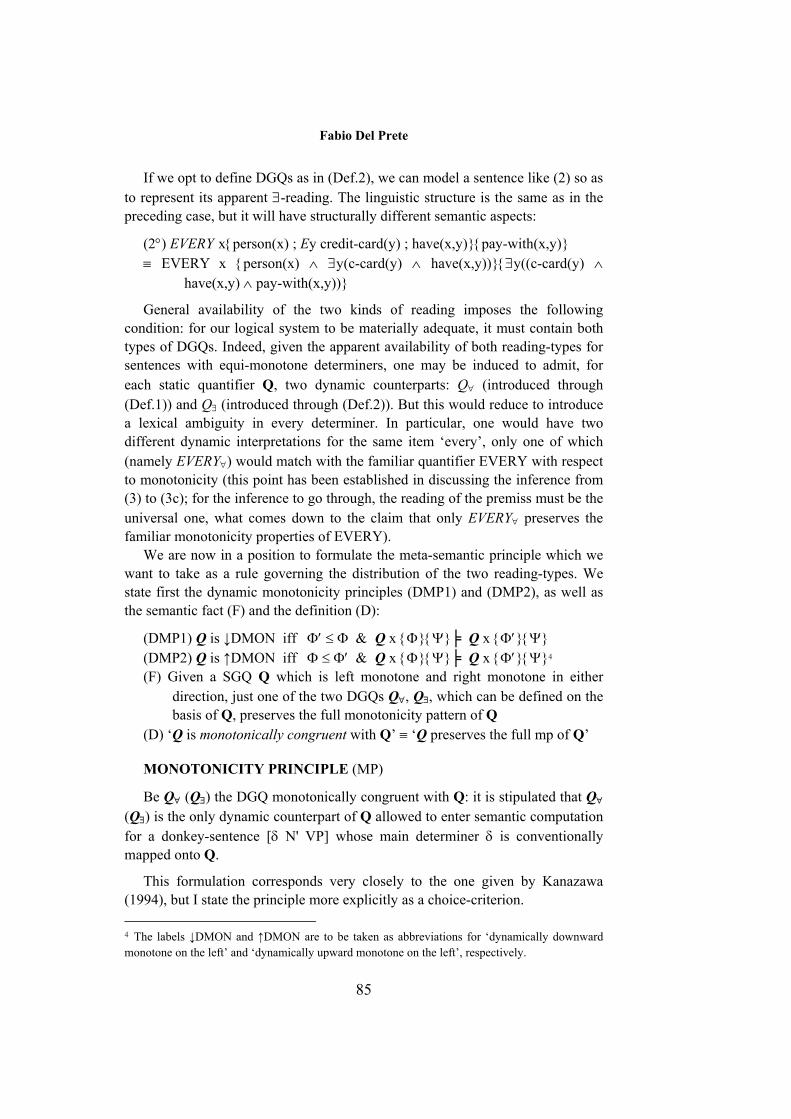
Fabio Del Prete
85
If we opt to define DGQs as in (Def.2), we can model a sentence like (2) so as to represent its apparent ∃-reading. The linguistic structure is the same as in the preceding case, but it will have structurally different semantic aspects:
(2°) EVERY xperson(x) ; Ey credit-card(y) ; have(x,y)pay-with(x,y) ≡ EVERY x person(x) ∧ ∃y(c-card(y) ∧ have(x,y))∃y((c-card(y) ∧
have(x,y) ∧ pay-with(x,y))
General availability of the two kinds of reading imposes the following condition: for our logical system to be materially adequate, it must contain both types of DGQs. Indeed, given the apparent availability of both reading-types for sentences with equi-monotone determiners, one may be induced to admit, for each static quantifier Q, two dynamic counterparts: Q∀ (introduced through (Def.1)) and Q∃ (introduced through (Def.2)). But this would reduce to introduce a lexical ambiguity in every determiner. In particular, one would have two different dynamic interpretations for the same item ‘every’, only one of which (namely EVERY∀) would match with the familiar quantifier EVERY with respect to monotonicity (this point has been established in discussing the inference from (3) to (3c); for the inference to go through, the reading of the premiss must be the universal one, what comes down to the claim that only EVERY∀ preserves the familiar monotonicity properties of EVERY).
We are now in a position to formulate the meta-semantic principle which we want to take as a rule governing the distribution of the two reading-types. We state first the dynamic monotonicity principles (DMP1) and (DMP2), as well as the semantic fact (F) and the definition (D):
(DMP1) Q is ↓DMON iff Φ′ ≤ Φ & Q x ΦΨ Q x Φ′Ψ (DMP2) Q is ↑DMON iff Φ ≤ Φ′ & Q x ΦΨ Q x Φ′Ψ4 (F) Given a SGQ Q which is left monotone and right monotone in either
direction, just one of the two DGQs Q∀, Q∃, which can be defined on the basis of Q, preserves the full monotonicity pattern of Q
(D) ‘Q is monotonically congruent with Q’ ≡ ‘Q preserves the full mp of Q’
MONOTONICITY PRINCIPLE (MP)
Be Q∀ (Q∃) the DGQ monotonically congruent with Q: it is stipulated that Q∀ (Q∃) is the only dynamic counterpart of Q allowed to enter semantic computation for a donkey-sentence [δ N' VP] whose main determiner δ is conventionally mapped onto Q.
This formulation corresponds very closely to the one given by Kanazawa (1994), but I state the principle more explicitly as a choice-criterion. 4 The labels ↓DMON and ↑DMON are to be taken as abbreviations for ‘dynamically downward monotone on the left’ and ‘dynamically upward monotone on the left’, respectively.
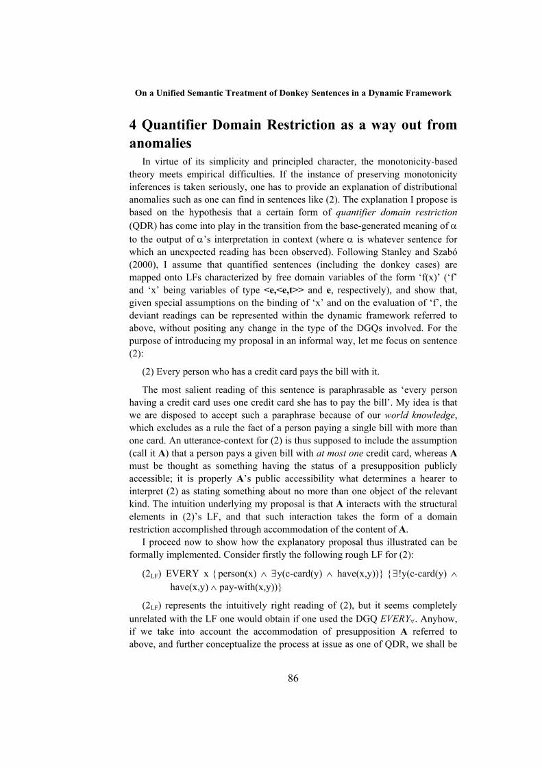
On a Unified Semantic Treatment of Donkey Sentences in a Dynamic Framework
86
4 Quantifier Domain Restriction as a way out from anomalies
In virtue of its simplicity and principled character, the monotonicity-based theory meets empirical difficulties. If the instance of preserving monotonicity inferences is taken seriously, one has to provide an explanation of distributional anomalies such as one can find in sentences like (2). The explanation I propose is based on the hypothesis that a certain form of quantifier domain restriction (QDR) has come into play in the transition from the base-generated meaning of α to the output of α’s interpretation in context (where α is whatever sentence for which an unexpected reading has been observed). Following Stanley and Szabó (2000), I assume that quantified sentences (including the donkey cases) are mapped onto LFs characterized by free domain variables of the form ‘f(x)’ (‘f’ and ‘x’ being variables of type <e,<e,t>> and e, respectively), and show that, given special assumptions on the binding of ‘x’ and on the evaluation of ‘f’, the deviant readings can be represented within the dynamic framework referred to above, without positing any change in the type of the DGQs involved. For the purpose of introducing my proposal in an informal way, let me focus on sentence (2):
(2) Every person who has a credit card pays the bill with it.
The most salient reading of this sentence is paraphrasable as ‘every person having a credit card uses one credit card she has to pay the bill’. My idea is that we are disposed to accept such a paraphrase because of our world knowledge, which excludes as a rule the fact of a person paying a single bill with more than one card. An utterance-context for (2) is thus supposed to include the assumption (call it A) that a person pays a given bill with at most one credit card, whereas A must be thought as something having the status of a presupposition publicly accessible; it is properly A’s public accessibility what determines a hearer to interpret (2) as stating something about no more than one object of the relevant kind. The intuition underlying my proposal is that A interacts with the structural elements in (2)’s LF, and that such interaction takes the form of a domain restriction accomplished through accommodation of the content of A.
I proceed now to show how the explanatory proposal thus illustrated can be formally implemented. Consider firstly the following rough LF for (2):
(2LF) EVERY x person(x) ∧ ∃y(c-card(y) ∧ have(x,y)) ∃!y(c-card(y) ∧ have(x,y) ∧ pay-with(x,y))
(2LF) represents the intuitively right reading of (2), but it seems completely unrelated with the LF one would obtain if one used the DGQ EVERY∀. Anyhow, if we take into account the accommodation of presupposition A referred to above, and further conceptualize the process at issue as one of QDR, we shall be
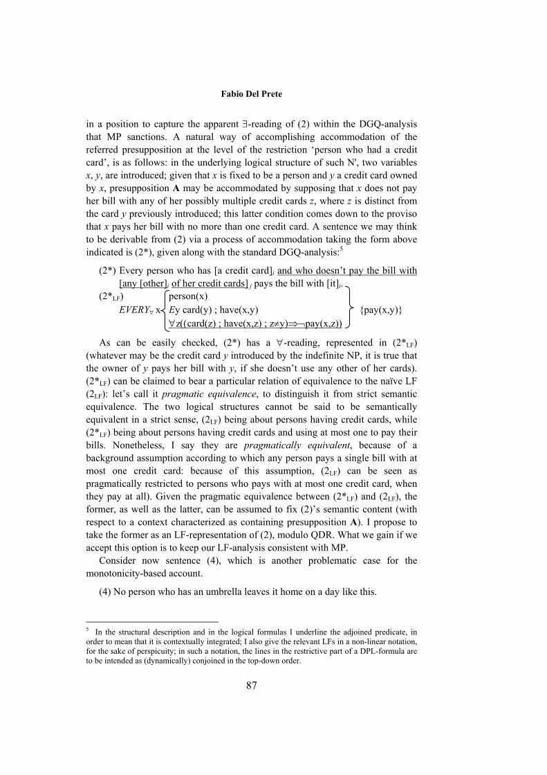
Fabio Del Prete
87
in a position to capture the apparent ∃-reading of (2) within the DGQ-analysis that MP sanctions. A natural way of accomplishing accommodation of the referred presupposition at the level of the restriction ‘person who had a credit card’, is as follows: in the underlying logical structure of such N', two variables x, y, are introduced; given that x is fixed to be a person and y a credit card owned by x, presupposition A may be accommodated by supposing that x does not pay her bill with any of her possibly multiple credit cards z, where z is distinct from the card y previously introduced; this latter condition comes down to the proviso that x pays her bill with no more than one credit card. A sentence we may think to be derivable from (2) via a process of accommodation taking the form above indicated is (2*), given along with the standard DGQ-analysis:5
(2*) Every person who has [a credit card]i and who doesn’t pay the bill with [any [other]i of her credit cards] j pays the bill with [it]i.
(2*LF) person(x) EVERY∀ x Ey card(y) ; have(x,y) pay(x,y)
∀z((card(z) ; have(x,z) ; z≠y)⇒¬pay(x,z))
As can be easily checked, (2*) has a ∀-reading, represented in (2*LF) (whatever may be the credit card y introduced by the indefinite NP, it is true that the owner of y pays her bill with y, if she doesn’t use any other of her cards). (2*LF) can be claimed to bear a particular relation of equivalence to the naïve LF (2LF): let’s call it pragmatic equivalence, to distinguish it from strict semantic equivalence. The two logical structures cannot be said to be semantically equivalent in a strict sense, (2LF) being about persons having credit cards, while (2*LF) being about persons having credit cards and using at most one to pay their bills. Nonetheless, I say they are pragmatically equivalent, because of a background assumption according to which any person pays a single bill with at most one credit card: because of this assumption, (2LF) can be seen as pragmatically restricted to persons who pays with at most one credit card, when they pay at all). Given the pragmatic equivalence between (2*LF) and (2LF), the former, as well as the latter, can be assumed to fix (2)’s semantic content (with respect to a context characterized as containing presupposition A). I propose to take the former as an LF-representation of (2), modulo QDR. What we gain if we accept this option is to keep our LF-analysis consistent with MP.
Consider now sentence (4), which is another problematic case for the monotonicity-based account.
(4) No person who has an umbrella leaves it home on a day like this.
5 In the structural description and in the logical formulas I underline the adjoined predicate, in order to mean that it is contextually integrated; I also give the relevant LFs in a non-linear notation, for the sake of perspicuity; in such a notation, the lines in the restrictive part of a DPL-formula are to be intended as (dynamically) conjoined in the top-down order.
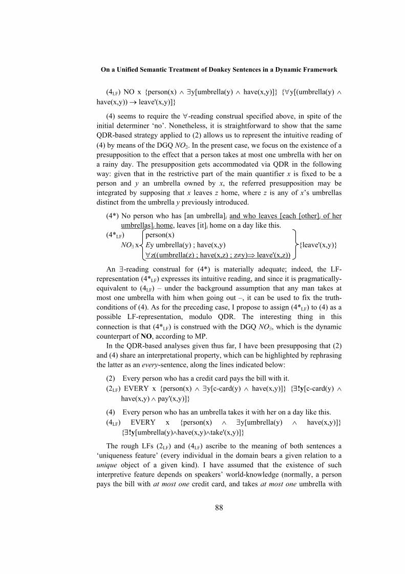
On a Unified Semantic Treatment of Donkey Sentences in a Dynamic Framework
88
(4LF) NO x person(x) ∧ ∃y[umbrella(y) ∧ have(x,y)] ∀y[(umbrella(y) ∧ have(x,y)) → leave'(x,y)]
(4) seems to require the ∀-reading construal specified above, in spite of the initial determiner ‘no’. Nonetheless, it is straightforward to show that the same QDR-based strategy applied to (2) allows us to represent the intuitive reading of (4) by means of the DGQ NO∃. In the present case, we focus on the existence of a presupposition to the effect that a person takes at most one umbrella with her on a rainy day. The presupposition gets accommodated via QDR in the following way: given that in the restrictive part of the main quantifier x is fixed to be a person and y an umbrella owned by x, the referred presupposition may be integrated by supposing that x leaves z home, where z is any of x’s umbrellas distinct from the umbrella y previously introduced.
(4*) No person who has [an umbrella]i and who leaves [each [other]i of her umbrellas]j home, leaves [it]i home on a day like this.
(4*LF) person(x) NO∃ x Ey umbrella(y) ; have(x,y) leave'(x,y)
∀z((umbrella(z) ; have(x,z) ; z≠y)⇒ leave'(x,z))
An ∃-reading construal for (4*) is materially adequate; indeed, the LF-representation (4*LF) expresses its intuitive reading, and since it is pragmatically-equivalent to (4LF) – under the background assumption that any man takes at most one umbrella with him when going out –, it can be used to fix the truth-conditions of (4). As for the preceding case, I propose to assign (4*LF) to (4) as a possible LF-representation, modulo QDR. The interesting thing in this connection is that (4*LF) is construed with the DGQ NO∃, which is the dynamic counterpart of NO, according to MP.
In the QDR-based analyses given thus far, I have been presupposing that (2) and (4) share an interpretational property, which can be highlighted by rephrasing the latter as an every-sentence, along the lines indicated below:
(2) Every person who has a credit card pays the bill with it. (2LF) EVERY x person(x) ∧ ∃y[c-card(y) ∧ have(x,y)] ∃!y[c-card(y) ∧
have(x,y) ∧ pay'(x,y)]
(4) Every person who has an umbrella takes it with her on a day like this. (4LF) EVERY x person(x) ∧ ∃y[umbrella(y) ∧ have(x,y)]
∃!y[umbrella(y)∧have(x,y)∧take'(x,y)]
The rough LFs (2LF) and (4LF) ascribe to the meaning of both sentences a ‘uniqueness feature’ (every individual in the domain bears a given relation to a unique object of a given kind). I have assumed that the existence of such interpretive feature depends on speakers’ world-knowledge (normally, a person pays the bill with at most one credit card, and takes at most one umbrella with
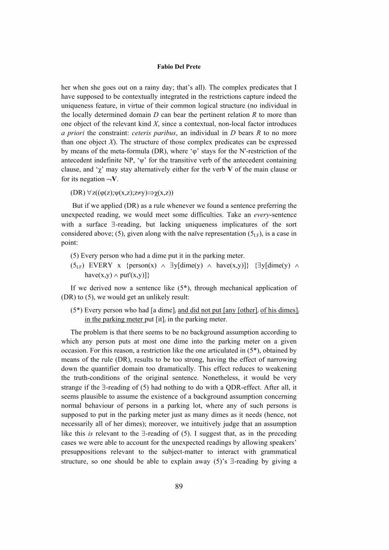
Fabio Del Prete
89
her when she goes out on a rainy day; that’s all). The complex predicates that I have supposed to be contextually integrated in the restrictions capture indeed the uniqueness feature, in virtue of their common logical structure (no individual in the locally determined domain D can bear the pertinent relation R to more than one object of the relevant kind X, since a contextual, non-local factor introduces a priori the constraint: ceteris paribus, an individual in D bears R to no more than one object X). The structure of those complex predicates can be expressed by means of the meta-formula (DR), where ‘φ’ stays for the N'-restriction of the antecedent indefinite NP, ‘ψ’ for the transitive verb of the antecedent containing clause, and ‘χ’ may stay alternatively either for the verb V of the main clause or for its negation ¬V.
(DR) ∀z((φ(z);ψ(x,z);z≠y)⇒χ(x,z))
But if we applied (DR) as a rule whenever we found a sentence preferring the unexpected reading, we would meet some difficulties. Take an every-sentence with a surface ∃-reading, but lacking uniqueness implicatures of the sort considered above; (5), given along with the naïve representation (5LF), is a case in point:
(5) Every person who had a dime put it in the parking meter. (5LF) EVERY x person(x) ∧ ∃y[dime(y) ∧ have(x,y)] ∃y[dime(y) ∧
have(x,y) ∧ put'(x,y)]
If we derived now a sentence like (5*), through mechanical application of (DR) to (5), we would get an unlikely result:
(5*) Every person who had [a dime]i and did not put [any [other]i of his dimes]j in the parking meter put [it]i in the parking meter.
The problem is that there seems to be no background assumption according to which any person puts at most one dime into the parking meter on a given occasion. For this reason, a restriction like the one articulated in (5*), obtained by means of the rule (DR), results to be too strong, having the effect of narrowing down the quantifier domain too dramatically. This effect reduces to weakening the truth-conditions of the original sentence. Nonetheless, it would be very strange if the ∃-reading of (5) had nothing to do with a QDR-effect. After all, it seems plausible to assume the existence of a background assumption concerning normal behaviour of persons in a parking lot, where any of such persons is supposed to put in the parking meter just as many dimes as it needs (hence, not necessarily all of her dimes); moreover, we intuitively judge that an assumption like this is relevant to the ∃-reading of (5). I suggest that, as in the preceding cases we were able to account for the unexpected readings by allowing speakers’ presuppositions relevant to the subject-matter to interact with grammatical structure, so one should be able to explain away (5)’s ∃-reading by giving a
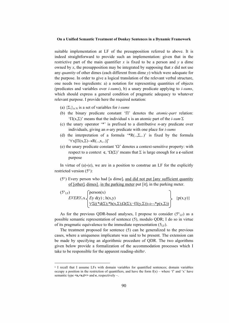
On a Unified Semantic Treatment of Donkey Sentences in a Dynamic Framework
90
suitable implementation at LF of the presupposition referred to above. It is indeed straightforward to provide such an implementation: given that in the restrictive part of the main quantifier x is fixed to be a person and y a dime owned by x, the presupposition may be integrated by supposing that x did not use any quantity of other dimes (each different from dime y) which were adequate for the purpose. In order to give a logical translation of the relevant verbal structure, one needs two ingredients: a) a notation for representing quantities of objects (predicates and variables over i-sums), b) a unary predicate applying to i-sums, which should express a general condition of pragmatic adequacy to whatever relevant purpose. I provide here the required notation:
(a) Σii∈N is a set of variables for i-sums (b) the binary predicate constant ‘Π’ denotes the atomic-part relation:
‘Π(x,Σ)’ means that the individual x is an atomic part of the i-sum Σ (c) the unary operator ‘*’ is prefixed to a distributive n-ary predicate over
individuals, giving an n-ary predicate with one place for i-sums (d) the interpretation of a formula ‘*R(..,Σ,..)’ is fixed by the formula
‘∀x[Π(x,Σ)→R(..,x,..)]’ (e) the unary predicate constant ‘Ω’ denotes a context-sensitive property: with
respect to a context c, ‘Ω(Σ)’ means that Σ is large enough for a c-salient purpose
In virtue of (a)-(e), we are in a position to construe an LF for the explicitly restricted version (5°):
(5°) Every person who had [a dime]i and did not put [any sufficient quantity of [other]i dimes] j in the parking meter put [it]i in the parking meter.
(5°LF) person(x) EVERY∀x Ey d(y) ; h(x,y) p(x,y)
∀Σ((*d(Σ);*h(x,Σ);Ω(Σ);¬Π(y,Σ))⇒¬*p(x,Σ))
As for the previous QDR-based analyses, I propose to consider (5°LF) as a possible semantic representation of sentence (5), modulo QDR; I do so in virtue of its pragmatic equivalence to the immediate representation (5LF).
The treatment proposed for sentence (5) can be generalized to the previous cases, where a uniqueness implicature was said to be present. The extension can be made by specifying an algorithmic procedure of QDR. The two algorithms given below provide a formalization of the accommodation processes which I take to be responsible for the apparent reading-shifts6.
6 I recall that I assume LFs with domain variables for quantified sentences; domain variables occupy a position in the restriction of quantifiers, and have the form f(x) – where ‘f’ and ‘x’ have semantic type <e,<e,t>> and e, respectively –.
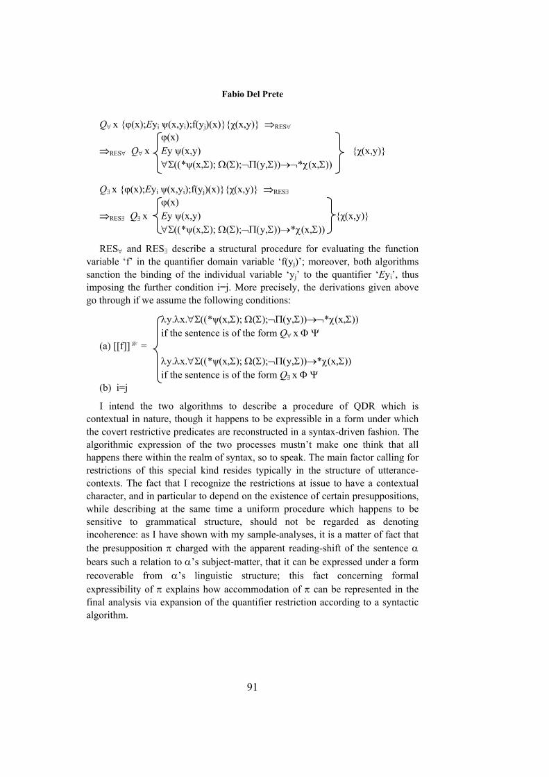
Fabio Del Prete
91
Q∀ x φ(x);Eyi ψ(x,yi);f(yj)(x)χ(x,y) ⇒RES∀
φ(x) ⇒RES∀ Q∀ x Ey ψ(x,y) χ(x,y)
∀Σ((*ψ(x,Σ); Ω(Σ);¬Π(y,Σ))→¬*χ(x,Σ))
Q∃ x φ(x);Eyi ψ(x,yi);f(yj)(x)χ(x,y) ⇒RES∃
φ(x) ⇒RES∃ Q∃ x Ey ψ(x,y) χ(x,y)
∀Σ((*ψ(x,Σ); Ω(Σ);¬Π(y,Σ))→*χ(x,Σ))
RES∀ and RES∃ describe a structural procedure for evaluating the function variable ‘f’ in the quantifier domain variable ‘f(yj)’; moreover, both algorithms sanction the binding of the individual variable ‘yj’ to the quantifier ‘Eyi’, thus imposing the further condition i=j. More precisely, the derivations given above go through if we assume the following conditions:
λy.λx.∀Σ((*ψ(x,Σ); Ω(Σ);¬Π(y,Σ))→¬*χ(x,Σ)) if the sentence is of the form Q∀ x Φ Ψ (a) [[f]] cg = λy.λx.∀Σ((*ψ(x,Σ); Ω(Σ);¬Π(y,Σ))→*χ(x,Σ)) if the sentence is of the form Q∃ x Φ Ψ (b) i=j
I intend the two algorithms to describe a procedure of QDR which is contextual in nature, though it happens to be expressible in a form under which the covert restrictive predicates are reconstructed in a syntax-driven fashion. The algorithmic expression of the two processes mustn’t make one think that all happens there within the realm of syntax, so to speak. The main factor calling for restrictions of this special kind resides typically in the structure of utterance-contexts. The fact that I recognize the restrictions at issue to have a contextual character, and in particular to depend on the existence of certain presuppositions, while describing at the same time a uniform procedure which happens to be sensitive to grammatical structure, should not be regarded as denoting incoherence: as I have shown with my sample-analyses, it is a matter of fact that the presupposition π charged with the apparent reading-shift of the sentence α bears such a relation to α’s subject-matter, that it can be expressed under a form recoverable from α’s linguistic structure; this fact concerning formal expressibility of π explains how accommodation of π can be represented in the final analysis via expansion of the quantifier restriction according to a syntactic algorithm.
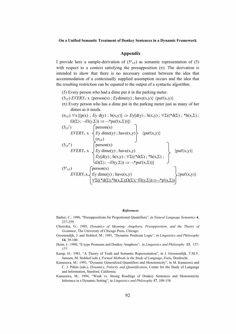
On a Unified Semantic Treatment of Donkey Sentences in a Dynamic Framework
92
Appendix
I provide here a sample-derivation of (5°LF) as semantic representation of (5) with respect to a context satisfying the presupposition (π). The derivation is intended to show that there is no necessary contrast between the idea that accommodation of a contextually supplied assumption occurs and the idea that the resulting restriction can be equated to the output of a syntactic algorithm.
(5) Every person who had a dime put it in the parking meter. (5LF) EVERY∀ x person(x) ; Eydime(y) ; have(x,y) put'(x,y) (π) Every person who has a dime put in the parking meter just as many of her
dimes as it needs. (πLF) ∀x[p(x) ; Ey d(y) ; h(x,y)] ⇒ Ey[d(y) ; h(x,y) ; ∀Σ((*d(Σ) ; *h(x,Σ) ;
Ω(Σ) ; ¬Π(y,Σ)) ⇒ ¬*put'(x,Σ))] (5LF′) person(x)
EVERY∀ x Ey dime(y) ; have(x,y) put'(x,y) (πLF)
(5LF″) person(x) EVERY∀ x Ey dime(y) ; have(x,y) put'(x,y)
Ey[d(y) ; h(x,y) ; ∀Σ((*d(Σ) ; *h(x,Σ) ; Ω(Σ) ; ¬Π(y,Σ)) ⇒ ¬*put'(x,Σ))]
(5°LF) person(x) EVERY∀x Ey dime(y) ; have(x,y) put'(x,y)
∀Σ((*d(Σ);*h(x,Σ);Ω(Σ);¬Π(y,Σ))⇒¬*p'(x,Σ))
References
Barker, C.: 1996, “Presuppositions for Proportional Quantifiers”, in Natural Language Semantics 4, 237-259.
Chierchia, G.: 1995, Dynamics of Meaning: Anaphora, Presupposition, and the Theory of Grammar, The University of Chicago Press, Chicago.
Groenendijk, J. and Stokhof, M.: 1991, “Dynamic Predicate Logic”, in Linguistics and Philosophy 14, 39-100.
Heim, I.: 1990, “E-type Pronouns and Donkey Anaphora”, in Linguistics and Philosophy 13, 137-177
Kamp, H.: 1981, “A Theory of Truth and Semantic Representation”, in J. Groenendijk, T.M.V. Janssen, M. Stokhof (eds.), Formal Methods in the Study of Language, Foris, Dordrecht.
Kanazawa, M.: 1993, “Dynamic Generalized Quantifiers and Monotonicity”, in M. Kanazawa and C. J. Piñón (eds.), Dynamics, Polarity and Quantification, Center for the Study of Language and Information, Stanford, California.
Kanazawa, M.: 1994, “Weak vs. Strong Readings of Donkey Sentences and Monotonicity Inference in a Dynamic Setting”, in Linguistics and Philosophy 17, 109-158.

Fabio Del Prete
93
Lappin, S. and Francez, N.: 1994, “E-type Pronouns, I-sums, and Donkey Anaphora”, in Linguistics and Philosophy 17, 391-428.
Neale, S.: 1990, Descriptions, Cambridge, Mass.: MIT Press. Stanley, J. and Szabó, Z. G.: 2000, “On Quantifier Domain Restriction”, in Mind and Language 15,
219-261.

94
On the Categorization via Rank-Distance
Anca Dinu
Bucharest University, Faculty of Mathematics
anca [email protected]
Liviu P. Dinu
Bucharest University, Faculty of Mathematics
Abstract. In this paper we present an unsupervised categorization method. Themethod uses the rank distance (Dinu, 2003a), a metric which measures the similar-ity between two classifications based on the ranks of objects. In the framework ofnatural language, the most important information is carried by the first part of theunit. By analogy, the difference on the first positions between two classificationsis more important than the difference on the last positions. This was the startingpoint in the construction of the rank distance.
1 Introduction
When dealing with categorization and/or aggregation problems, there arethree important decisions to make: choosing the metric, the aggregationmethod and the classifiers.
The long series of papers (Finch, 1993; Herdan, 1966; Kashyap and Oom-men, 1983; Manning and Schutze, 1999; Marcus and others, 1971; Marcus,1974; Mitchell, 1997; Paun, 1983; Schutze and others, 1995; Tin Kam Ho andothers, 1994) and their references dedicated to this topic proves the theoret-ical and practical relevance of the problem. We mention here some metricsas Euclidean metric, Manhattan metric, Spearman rank correlation coeffi-cient, divergence, Hamming distance, Leuvenstein distance, etc. and someclassification and aggregation methods as decision trees, k nearest neighborclassification, Bayesian classification, maximum entropy modeling, decisioninference, logistic regression, neural networks based method, Borda aggrega-tion method, etc. encountered in the above works.
The classifications may differ not only by the position of the elements,but also by the elements themselves: some element in a classification maybe absent in another classification. In this paper we present an unsupervised
Proceedings of the Eighth ESSLLI Student SessionBalder ten Cate (editor)Chapter 9, Copyright c© 2003, A. Dinu and L. Dinu
95
On the Categorization via Rank-Distance
categorization method. The method uses the rank distance (Dinu, 2003a),a metric which measures the similarity between two classifications basedon the ranks of objects. We define the aggregation of n classifications asthe classification for which the sum of distances from it to each of the nclassifications is minimal.
2 Rank distance
In this section we shortly present the rank distance (Dinu, L.P., 2003a,2003b).
Any classification can be regarded as a word of finite length, obtainedfrom concatenation of the elements of the classification, in their appearanceorder, from the first to the last one. By analogy with natural languagewhere the most important information is carried by the first part of thelexical unit (Marcus, 1971), the difference on the first positions between twoclassifications is more important than the difference on the last positions.This was the starting point in the construction of the rank distance. Thus,if the differences between two classifications are at the top (i.e., in essentialpoints), the distance has a bigger value then when the differences are at thebottom of the classifications.
Let L = (x1, x2, · · · , xn) be a classification of length n, such that xi isin ith position (1 ≤ i ≤ n) in classification L. In this classification xi
means the element itself, not the classification criterion (for example, if wechose the frequency as classification criterion, xi would not represent thefrequency, but the element xi which is in position i). We assume that theelements of the classification are mutually different. We shall attribute to thefirst element of the classification the highest rank, i.e., n, to the second one(n−1), and so on, to the final element the lowest rank, i.e., 1 (a classificationin Borda sense). It is possible that some elements require the same place(e.g., some elements have the same frequency). In this case we adopt thesame strategy as in Spearman rank correlation coefficient method (Herdan,1966; Finch, 1993): the rank of elements will be the mean of ranks theyshould receive.
Notation 1 We denote the position of the element x in classification L withord(x|L).
Notation 2 We denote the vocabulary of the classification L with V(L),i.e., V (L) = x1, x2, . . . , xn−1, xn.
Let L1 and L2 be two classifications of lengths n, m respectively. Wemay presume m ≥ n.
96
A. Dinu and L. Dinu
Definition 1 The rank distance between L1 and L2 is given by:
∆(L1, L2) =∑
x∈V (L1)∩V (L2)
|ord(x | V (L1)) − ord(x | V (L2))|
+∑
x∈V (L1)\V (L2)
ord(x | V (L1)) +∑
x∈V (L2)\V (L1)
ord(x | V (L2)).
Example 1 Set L1 = (a, b, c, d) and L2 = (x, a, b), V (L1) = a, b, c, d,V (L2) = a, b, x. According to Definition 1, we have:∆(L1, L2) = |ord(a|L1)− ord(a|L2)|+ |ord(b|L1)− ord(b|L2)|+ ord(c|L1) +ord(d|L1) + ord(x|L2) = |4 − 2| + |3 − 1| + 2 + 1 + 3 = 10.
Theorem 1 ∆ is a distance.
Proposition 1 The rank-distance between L1 and L2 is minimal when V (L1) ⊆V (L2) and ord(xi|L1) + m − n = ord(xi|L2) for all i = 1, 2, . . . , n, and it ismaximal when V (L1)
⋂V (L2) = Ø. In former case ∆(L1, L2) = n(m−n)+
m−n∑i=1
i = 12 (m−n)(m+n+1) and in later ∆(L1, L2) = 1
2n(n+1)+ 12m(m+1).
Marcus (1974) has used a similar idea to measure the distance betweentwo codons (sixty-four triplets of nucleotide). He has modified the Hammingdistance (Hamming, 1950) by giving a different weight to each position ofthe three possible position in a codon, in the decreasing order from left toright, p1 > p2 > p3. The distance between two codons differing on the first(second, third) position will be equal to p1 (p2, p3 respectively);the distancebetween two codons differing on the first and the second (the first and thethird, the second and the third) positions will be equal to p1 + p2 (p1 + p3,p2 + p3 respectively); the distance between two codons differing on each oftheir positions will be equal to p1 + p2 + p3.
We must say that the existing distances are not appropriate yet forgenomics. In (Karp, 2002) it is shown that ”the distance between genomesshould be measured not only by counting mutations, but also by determiningthe number of large-scale rearrangements needed to transform one genometo another.
3 An aggregation method based on rank distance
The aggregation of classifications means to obtain a classification of givenobjects that appear in the set of initial classifications. Categorization is thetask of assigning objects from a universe to two or more classes or categories(Manning and Schutze, 1999).
In this section we present an aggregation method (Dinu, 2003b) basedon rank distance which can aggregate classifications having different vocab-ularies. A particularity of this method is the non-determinist feature.
97
On the Categorization via Rank-Distance
3.1 Rank-distance aggregation method
Definition 2 Let A be a set with n elements. A classification L is of lengthm over A if it contains m elements (|V (L)| = m) and V (L) ⊆ A. We writeL ∈ Am.
Definition 3 Let T = L1, L2, . . . , Ln be a sequence of n initial classifi-cations. The vocabulary of the sequence T is the set V (T ):
V (T ) =n⋃
i=1V (Li).
Definition 4 Let T = L1, L2, . . . , Ln be a sequence of n initial classifi-cations having the same length m and let L be a classification of length m.We denote the distance between L and T with ∆(T , L):
∆(T , L) =n∑
i=1∆(Li, L).
Definition 5 Consider T = L1, L2, . . . , Ln as in Definition 4. The rank-distance aggregation (RDA) is the classification L ∈ V m(T ) for which oneobtain the minimum of the following expression:
minX∈V m(T )
1n
n∑i=1
∆(Li,X),
i.e., ∆(T , L) = minX∈V m(T )
∆(T ,X).
Remark 1 The aggregate classification is not unique. Thus, we introduce anew set of classifications, containing all aggregate classifications that satisfythe minimum condition from Definition 5.
Notation 3 Consider T as in Definition 4. We denote the set of RDAclassifications with agr(T ).
Remark 2 The set agr(T ) is not empty. It contains at least one element.
3.2 On the aggregation algorithm
We have introduced a new method for the aggregation of classifications.One of the problems is the computational aspect. Some constructions thatproduce a subset of agr (T ) were developed, but we have not obtained yetan efficient algorithm (i.e. polynomial) that produces all the RDA classifi-cations for a given sequence T .
98
A. Dinu and L. Dinu
3.3 The equivalence of elements
In a given classification, two or more elements are said to be equivalentif they have the same position. The RDA method cannot aggregate clas-sifications that have equivalent elements. To overcome this problem weshall decompose each classification L that contains n equivalent elementsai+1, . . . , ai+n into n! classifications. Each of this classifications will containone of the n! possible permutations of the elements ai+1, . . . , ai+n.
3.4 Example
Example 2 Set the following sequence of 5 initial classifications: T =(a1 > a2 > a3), (a1 > a2 > a3), (a3 > a1 > a2), (a2 > a3 > a1), (a2 >a3 > a1).The vocabulary of this sequence is: V (T ) = a1, a2, a3.The set of classifications over V 3(T ) contains 6 elements (permutations of3 elements). We shall evaluate the distance between each classification toT . We shall choose the classifications having the minimal distance.
1. L = (a1 > a2 > a3); ∆(L,T ) = 125
2. L = (a1 > a3 > a2); ∆(L,T ) = 145
3. L = (a2 > a1 > a3); ∆(L,T ) = 125
4. L = (a2 > a3 > a1); ∆(L,T ) = 125
5. L = (a3 > a2 > a1); ∆(L,T ) = 145
6. L = (a3 > a1 > a2); ∆(L,T ) = 165
minX∈V 3(T )
∆(X,T ) = 125 ,
agr(T ) = (a1 > a2 > a3), (a2 > a1 > a3), (a2 > a3 > a1).
We observe in Example 2 that agr(T ) can have the cardinal bigger then 1and that a RDA classification is not necessary an initial classification((a2 >a1 > a3) is not in T ).
4 A categorization method based on the RDA method
As most of the products of human mind, the aggregation and categoriza-tion methods should have the characteristic of being rational. Arrow (1973)proved that not any rationality conditions can be satisfied simultaneously:thereis no aggregation method that simultaneously satisfies the relevance, Paretooptimality, independence and the absence of the dictator conditions, for all
99
On the Categorization via Rank-Distance
problems with at least 3 objects and at least 2 initial classifications, suppos-ing any classification of those elements is admissible (can appear as initialclassification).
Paun (1987, 1983) mentions 17 conditions of rationality that should befulfilled by an aggregation method. Based on some subsets of this conditions,he proposes some variants of the impossibility theorem of aggregation (Paun,1983, 1987).
4.1 Properties of RDA
Definition 6 Pareto optimality. If ai is preferred to aj in all the initialclassifications, then ai is preferred to aj in the aggregated classification aswell.
Proposition 2 The rank-distance aggregation method satisfies the Paretooptimality conditions.
Definition 7 Reasonability. An aggregation method is reasonable if, whenapplied only for two elements, gives the same results as the simple majoritymethod.
Proposition 3 The rank-distance aggregation method satisfies the reason-ability condition.
Definition 8 Independence The final order of any two objects ai and aj
only depends on ai and aj and it never depends on the presence of anotherelement ak.
Proposition 4 The rank-distance aggregation method does not satisfy theindependence condition.
4.2 Rank distance categorization method
An essential problem in text categorization is to choose the classifiers. Dif-ferent classifiers may assign different classes to the same object. Decisionmethods based on the inference of classifiers can be used to predict the classof the object.
A method of inference of classifiers based on logistic regression is pre-sented in (Ho et al., 1994). Each classifier receives a weight using a trainingset.
In the following we propose an unsupervised method of categorizationbased on rank-distance aggregation (called rank-distance categorization -RDC).
Consider C=(C1, C2, . . . , Cn) a set of n classifiers and S=s1, s2, . . . , smthe possible classes of an object.
100
A. Dinu and L. Dinu
Each classifier gives a classification of classes; let T =L1, L2, . . . , Ln bethe set of this classifications.
Let agr(T )=A1, A2, . . . , Ak be the aggregation of the set T .The class of the object predicted by the RDC method is the one that
occupies most frequently the first position in the classifications A1, .., Ak.Due to the Proposition 2, if all classifiers predict a class s on the first
place, then the RDC method will predict the same s class on first place.We tested the RDC method on the data base World Now. The method
Naıve Bayes was used to choose four classifiers. The RDC method improvedthe mean of individual performance of classifiers with fifteen-twenty percent.
5 Final remarks and further investigations
We have presented the rank distance aggregation (RDA) method, that de-fines the aggregation of a sequence T of classifications as those classificationsL for which
∑∆(T , L) has the minimum value, where ∆ is the rank distance
(Dinu, 2003a). The classification obtained by RDA method is not necessar-ily unique. Based on RDA, we have defined the rank distance categorizationmethod (RDC).
As we have shown in section 3.2, the construction of an efficient algo-rithm to compute agr(T ), for a given sequence T , remains an open problem.The investigation of rank distance in genome analysis applications and therelationship of the RDC with other existing technique (e.g. Crammer andSinger, 2003, 2001) are some future work which are in our attention.
Acknowledgements
We thank the anonymous referees for remarks permitting the improvementof the text and for suggestions regarding future works.
References
[1] Borelli, M. and A. Sgarro. A Possibilistic Distance for Sequences of Equal andUnequal Length. In Finite VS Infinite: Contributions to an Eternal Dilemma,C. Calude and Gh. Paun eds., Springer-Verlag, London, 2000
[2] Crammer, K. and Y. Singer. Pranking with ranking. In Advances in Neuralinformation Processing Systems 14, 2001
[3] Crammer, K. and Y. Singer. A family of additive algorithms for categoryranking. Journal of Machine Learning Research, 3, 1025-1058, 2003
[4] Dinu, L. On the similarity of the classifications (submitted), 2003a
[5] Dinu, L. On the Aggregation of Hierarchies with Different Constitutive Ele-ments, Fundamenta Informaticae, 55, (1), 39-50, 2003b
[6] Finch, S.P. Finding stucture in language. PhD thesis, Univ. of Edinburgh, 1993
101
On the Categorization via Rank-Distance
[7] Hamming, R.W. Error detecting and error correcting codes. Bell System Tech-nical Journal, 29, 146-160, 1950
[8] Herdan, G. The advanced theory of language as choice and chance. Springer,New York, 1966
[9] Karp, R. Mathematical Challenges from Genomics and Molecular Biology.Notices of the AMS, 49, 544-553, 2002
[10] Kashyap, R.L. and B.J. OOmmen. Similarity Measure for Sets of Stringst.Intern. J. Computer Math. 13, 95-104, 1983
[11] Manning, C. and H. Schutze. Foundations of statistical natural language pro-cessing, MIT Press, 1999
[12] Marcus, S., E. Nicolau and S. Stati. Introduzione alle linguistica matematica.Casa editrice Riccardo Patron, Bologna, 1971
[13] Marcus, S. Linguistic structures and generative devices in molecular genetics.Cahiers Ling. Theor. Appl., 11, 77-104, 1974
[14] Marcus, S. An emergent triangle: semiotics-genomics-computation. In Pro-ceedings of the Congress of the German Semiotic Society, Kassel, July 2002(to appear)
[15] Mitchell, T.M. Machine Learning. McGraw-Hill, New York, 1997
[16] Paun, Gh. An imposibility theorem for social indicators aggregation, FuzzySets and Systems, 9, pp. 205-210, 1983
[17] Sgarro, A. A Fuzzy Hamming Distance, Bull. Math. de la Soc. Sci. Math dela Roumanie, Tome 21 (69), no. 1-2, 1977
[18] Schutze, H., D.A. Hull and J.O. Pedersen. A comparison of classifiers anddocument representations for the routing problem. In SIGIR ’95, pp. 229-237,1995
[19] Tin Kam Ho, J. Hull and S. Srihari. Decision Combination in Multiple Clas-sifier Systems, IEEE Transactions on Pattern Analysis and Machine Intelli-gence, vol. 16, no 1, pp. 66-75, 1994.
102
103
Resumptive Elements: Pronouns or Traces?
JUDIT GERVAIN University of Szeged and Scuola Internazionale di Studi Avanzati (SISSA) [email protected]
ABSTRACT. Resumptives have been characterized in the literature both as resembling pronouns and traces. The aim of the present paper is to confront the two theories on the basis of their empirical predictions. A small-scale experimental survey was carried out to test speakers judgments with respect to several diagnostic constructions as they apply to focus-raising via resumption in Hungarian. It is concluded that resumptives have a dual nature, their syntactic behavior is ambiguous between pronouns and traces. This ambiguity is theoretically captured by an analysis in terms of vehicle change (Fiengo and May 1994; Safir 1999).
1 Resumptives in Hungarian Focus-Raising
Previous work (Gervain forthcoming) has found that focus-raising (FR) constructions ((1b) vs. (1a), an expletive construction ), traditionally analyzed as instances of A’-movement (É.Kiss 1987; Kenesei 1994; Lipták 1998), are construed via resumption (focus-raising via resumption, FRR), at least for certain speakers of Hungarian (1c)1.
(1) a Azt mondtad, (hogy) GÁBOR síel jól. expl.acc said.2s that Gábor.nom ski.3s well “You said Gábor can ski well.”
b (*Azt) GÁBORTi mondtad, hogy ei jól síel. expl.acc Gábor.acc said.2s that well ski.3s
c [CP GÁBORTi mondtad, [CP hogy proi jól síel]]. The empirical evidence for this assumption comes from an experimental
survey (for the methods and the statistical analyses, see Gervain 2002), where speakers of Hungarian were shown to cluster into three groups (“dialects”2 or microvariants) with respect to their grammaticality judgment patterns for focus-raising sentences. Besides the irrelevant group of informants who rejected FR altogether, the other two dialects exhibited opposite patterns for subject focus-
1 Small capitals indicate focus. 2 No implication of a geographical or sociological distinction is intended here.
Proceedings of the Eighth ESSLLI Student Session. Balder ten Cate (editor) Chapter 10, Copyright © 2003, Judit Gervain
Resumptive Elements: Pronouns or Variables?
104
raising along two factors, namely the case of the focused DP and number agreement on the embedded verb (of which the focused DP is the subject).
Before the experimental findings are discussed, a peculiarity of Hungarian number morphology has to be introduced. Plurality is not marked on a noun that is preceded by a numeral or a (plural) quantifier (2a). Moreover, the whole DP agrees with its verb in the singular (2b), but it still clearly refers to plural entities, as cross-sentential anaphora illustrates (2c). So [Num/Quantpl [Nsg]]sg, pl type DPs3 act as morphologically/syntactically singular, but semantically plural entities.
(2) a [DP [NumP két [NP fiú ]]] two boy.sg “two boys”
b Két fiú jött/ *jöttek. two boy.sg.nom come.past.3s/ come.past.3p “Two boys came.”
c Két fiú jött. Leültettem *őt/ őket. two boy.sg.nom come.past.3s seat.past.1s him/ them “Two boys came. I offered them seats.”
The results of Gervain (2002) show that when such a DP is in the matrix focus position, one dialect (3) tolerates both nominative and accusative case on the DP, but strictly rejects plural embedded verbs, whereas the other dialect (4) accepts only one of the cases, accusative, but both agreements.
(3) a ???AZ ÖSSZES LÁNY mondtad, hogy jön. the all girl.sg.nom said.2s that come.3s
“You said that all the girls were coming.” b *AZ ÖSSZES LÁNY mondtad, hogy jönnek.
the all girl.sg.nom said.2s that come.3p c ?AZ ÖSSZES LÁNYT mondtad, hogy jön.
the all girl.sg.acc said.2s that come.3s d AZ ÖSSZES LÁNYT mondtad, hogy jönnek.
the all girl.sg.acc said.2s that come.3p (4) a ??Az ÖSSZES LÁNY mondtad, hogy jön.
the all girl.sg.nom said.2s that come.3s “You said that all the girls were coming.”
b ???AZ ÖSSZES LÁNY mondtad, hogy jönnek. the all girl.sg.nom said.2s that come.3p
c ?AZ ÖSSZES LÁNYT mondtad, hogy jön. the all girl.sg.acc said.2s that come.3s
d ??AZ ÖSSZES LÁNYT mondtad, hogy jönnek. the all girl.sg.acc said.2s that come.3p
3 Indices in italics refer to semantic, non italicized ones to syntactic properties.
Judit Gervain
105
These empirical generalizations were analyzed as reflecting two underlying strategies for FR. Speakers of the first dialect (3) display a pattern that is readily describable as resulting from movement. The raised DP is base-generated as the subject of the embedded verb, thus it agrees with it in the singular and receives nominative case. When it undergoes raising, it optionally takes up the accusative case of the matrix verb, which is normally assigned to the expletive in the non-raising expletive constructions (1a). Consequently, it can surface in either of the two cases (for the technical details of how double case is licensed and derived for chains, see Bejar and Massam 1999; Español-Echevarría and Ralli 2000).
The second dialect (4), however, doesn’t lend itself to this account, since the embedded verb is in the plural, which is excluded under regular subject-verb agreement in simple clauses (2b). Rather, Gervain (forthcoming) proposes a resumptive strategy to account for this dialect. Under this view, the DP is base-generated directly in the matrix clause, in the position occupied by the expletive in the non-raising counterpart. Here, it receives accusative as its only case, in which it obligatorily surfaces. As for the embedded subject position, it is filled by a phonologically null4 resumptive pronoun, which establishes a dependency with the antecedent DP. Through this dependency, the resumptive inherits among others the number feature of the DP. Just how this is done exactly will constitute the subject of this paper, but even without going into the details, it can be argued that because of the number ambiguity of the DP, the resumptive may inherit either of the number features. Depending on the value of the transmitted feature then, the resumptive can trigger singular or plural agreement on the embedded verb.
Gervain (2002) presents further empirical and theoretical evidence to ground the above distinction between a movement and a resumptive strategy of FR. Most of them are not discussed here in detail, however one is worth mentioning at this point and some others will also be evoked in later discussions. The most common diagnostic tool to tell apart movement and resumption is movement constraint violations, e.g. islands, as suggested by Chomsky (1981, 1982) and exemplified in (5).
(5) a I wonder whoi Mary marries (*himi). b I wonder [whoi they think [that [if Mary marries *(himi) ] then
everybody will be happy]] Speakers of the two different FR dialects are expected to behave differently
with respect to such diagnostics. Judgments on FR sentences containing complex NPs were measured and compared. Informants in the two dialects answer statistically differently both as a group and individually. Movement speakers
4 That the resumptive pronoun is phonologically null comes as no surprise, since Hungarian is a pro-drop and an Avoid Pronoun language. Languages of this kind typically exhibit null resumptives (Engdahl 1985; Suñer 1998). A formal account of these observations is given by Montalbetti’s (1984) Overt Pronoun Constraint.
Resumptive Elements: Pronouns or Variables?
106
fully reject, while resumptive speakers accept sentences like (6). This further confirms the movement-resumption dissociation.
(6) b AZ ÖSSZES VENDÉGET mondtad, hogy hallottad the all guest.sg.acc say.past.2s that hear.past.2s “You said that you heard the news that all the guests had arrived.” a hírt, hogy megérkeztek. the news that arrive.past.3p
In light of the above considerations, the two strategies are well established. However, Gervain (2002) and Gervain (forthcoming) leave the issue about the nature of the resumptive dependency unresolved. Two alternatives are proposed, but theoretical considerations and empirical data are not conclusive. The first possibility outlined assumes that the dependency is entirely syntactic, i.e. operator-variable binding and coindexation between the antecedent and the resumptive. In such a scenario, the optionality of number results from the fact that the DP is transparent for coindexation, à la Longobardi (2001), so the resumptive may target either the plural Num/QuantP or the singular NP. The second option consists of positing a mixed type dependency, one that can be either syntactic or semantic. In the former case, the resumptive will inherit the feature of the whole DP, i.e. singular. In the latter, coreference obtains, which, as (2c) showed, is plural. Notice that the ultimate difference between the two possibilities hinges on the nature of the resumptive element. If resumptives are like variables, they always have to be bound, whereas if they resemble pronouns, they may be bound, but may also corefer.
The nature of resumptives appears to vary considerably across languages, and no theoretical consensus has been reached in the literature either. The present paper attempts to contribute to the debate by introducing experimental evidence, as well as by offering a theoretical account of Hungarian resumptives in FR constructions.
2 Theories of resumption
Resumptive elements come in various shapes and sizes in the world’s languages. Their theoretical analyses are equally heterogeneous. In the following, I will give a brief overview of the resumptive landscape.
As referred to above, one of the first detailed theoretical treatments of resumptive pronouns was given in Chomsky (1981, 1982). The main assumption, based mostly on English data of the type (5), was that resumptives appear in positions from where gaps/traces are excluded by constraints on movement (e.g. in island contexts). The resumptive pronoun is base-generated in its surface position and is A’-bound at LF by its antecedent, with which it is coindexed. On this view, resumptive pronouns are expected to be in complementary distribution with traces, and they come as a kind of last resort device to save otherwise
Judit Gervain
107
disallowed movement configurations. Overall, they were thought of as a rare and marked strategy, with no specific UG constraints required to account for them. Rather their distribution was believed to fall out from independent UG principles.
This approach was later challenged on several grounds. Resumptive strategies turned out to be subject to considerable cross-linguistic variation, which led to the introduction of different typologies (Engdahl 1985; Demirdache 1991; Suñer 1998; Aoun et al. 2001). The last resort nature of resumption has also been questioned (see e.g. Shlonsky 1992 and Aoun et al. 2001 for strong last resort views; but Suñer 1998 and Willis 2000 for challenges).
In addition to the above cited works, some analyses specifically address the question whether resumptives are pronouns or traces. These will be presented in somewhat more detail.
Discussing relative clauses in Hebrew, Sharvit (1999) points out that some of the syntactically free and optional alternations between traces and resumptives actually produce interpretational differences. Pair-list/multiple individual readings are not available for resumpives, while they are possible with traces in non-equative relative clauses, while this asymmetry disappears in equative clauses. In his account, resumptives are licensed under two conditions: (i) they need a contextually salient (e.g. D-linked) antecedent, and (ii) they can only be assigned values that the given pronoun can take when it is A/A’-free. Pair-list readings generally violate the first condition, but this impairment is amended in equative clauses, where a highly salient antecedent is available. Sharvit further claims that resumptives have a dual nature. Like traces, they are A’-bound and are interpreted as bound variables, while their distribution (e.g. within islands) resembles that of ordinary pronouns.
Falk (2002) offers an LFG account of resumptives. He introduces the pronoun vs. variable debate, and summarizes some of the empirical evidence. As arguments for the trace hypothesis, he enumerates the following observations: (i) resumptives, just like gaps, are linked to some discourse function or operator (cf. also Erteschik-Shir 1992; Sharvit 1999), (ii) anaphora between a possessive reflexive in a fronted whP and its antecedent DP in an embedded subject position is allowed when the extraction site of the whP contains a trace or a resumptive (cf. Zaenen et al. 1981), (iii) like traces, resumptives are able to license parasitic gaps (cf. Engdahl 1985; Shlonsky 1992), (iv) both traces and resumptives show crossover effects (cf. Shlonsky 1992), and (v) they can be coordinated. On the other hand, as Falk underlines, resumptives are exempt in most (but not all) languages from the island constraints traces/movement obey (Chomsky 1981, 1982). Also, resumptives are associated with special morphology on the verb or the complementizer in some languages (cf. McCloskey 2001, Vailette 2002). In Falk’s own analysis, which is cast in LFG terms, resumptives receive the same treatment as gaps, except for their licensing. Interestingly, on the basis of the same empirical evidence as Sharvit, Falk makes the additional claim that
Resumptive Elements: Pronouns or Variables?
108
resumptives are referential and cannot be bound variables. Rather, they are D-linked, and besides syntactic constraints, they also respect the principle of Sufficiency of Expression, which claims that syntactic elements providing clues for parsing are exceptions to (syntactic) considerations of economy.
As it is apparent from the above argumentations, the debate between the pronoun and the trace hypotheses is far from being resolved. In the following, I will examine resumptives in Hungarian FR, by applying some of the aforementioned empirical tests.
3 The experiment
Focus-raising in itself is not a good testing ground to distinguish between the trace and the pronoun hypotheses. Therefore, some of the diagnostics had to be applied to allow a better comparison between the predictions of the two approaches.
If resumptives behave like traces, i.e. bound variables, they are expected not to be able to corefer. They are supposed to license parasitic gaps and show crossover effects. Moreover, their coordination with another trace should be grammatical. If, on the other hand, they resemble ordinary pronouns, they can corefer, they don’t license parasitic gaps or show crossover effects and it is impossible to coordinate them with traces.
To test these predictions, a paper-and-pencil survey was carried out, comprising the following diagnostics: i, parasitic gap licensing; ii, coordination with traces/pronouns; iii, crossover effects. Responses were given statistical treatment5.
Material. Sentences were constructed to test the following structures: (i) FR from embedded subject position: acceptable/ unacceptable (ii) FR from embedded object position: acceptable/ unacceptable (iii) coreference: acceptable/unacceptable (iv) overt resumptive pronoun in FR of embedded subject:
acceptable/unacceptable (v) overt resumptive pronoun in FR of embedded object:
acceptable/unacceptable (vi) parasitic gaps in FR: licensed/not licensed (vii) strong crossover effects: present/absent
5 The use and interpretation of statistics carried out on grammaticality scales is not
without its difficulties. Lack of space precludes any serious discussion here, but Schütze (1996), Cowart (1997), Keller (2000) and Gervain (2002) give ample treatment to the subject. One consideration is noteworthy here. The use of parametric statistics means that judgments are interpreted not only as absolute values, which is the general practice in (non-experimental) syntactic research, but also as relative ones.
Judit Gervain
109
(viii) weak crossover effects: present/absent (ix) coordination of resumptive pronoun: with null pronoun/with overt
pronoun Factor (i) served as the criterion for inclusion; all subjects rejecting subject FR
via resumption were automatically excluded from all further analysis. As discussed above, parasitic gap licensing and crossover phenomena have been proposed as diagnostics to distinguish between gaps and pronouns. As crossover phenomena are more readily testable with wh-movement than with other types of displacement, wh-raising (whR) constructions, rather than FR, were used in crossover sentences. This should introduce no confound in the test, given the fact that whR and FR are both instantiations of the more general phenomenon of operator-raising6. However, to exclude all potential biases, additional sentence types were constructed to serve as controls for (vii)-(viii) above.
(viic) whR from embedded subject position: acceptable/ unacceptable (viiic) anaphor binding between raised subject and reflexive pronoun in the
embedded object position: acceptable/ unacceptable To avoid lexical biases and to enable the statistical treatment of judgments,
each sentence type was instantiated by three sentence tokens. Thus, for example, (i) is represented by (7a-c).
(7) a KÉT FIÚT mondtál, hogy jönnek. two boy.sg.acc say.past.2s that come.3p “You said that two boys were coming.”
b NÉGY LÁNYT mondtál, hogy táncoltak. four girl.sg.acc say.past.2s that dance.past.3p “You said that four girls had danced.”
c HÁROM DIÁKOT hiszel, hogy feleltek. three student.sg.acc believe.2s that reply.past.3p “You believed that three students were interrogated.”
Since plural verbal agreement with két fiút type NPs is a telltale sign of FR via resumption, sentences with raised subjects were construed with plural embedded verbs. In addition, for sentence types (vii), (viii), (viic) and (viiic), singular variants were also included. This adds up to 48 test and control sentences. Furthermore, habituation and repetition effects were counterbalanced by the insertion of 15 grammatical and ungrammatical filler sentences. These were
6 In early treatments (e.g. Marácz 1987, É. Kiss 1987), the two kinds of opertaror-
raising receive identical treatment. Moreover, Bródy (1995) argues for an essential underlying similarity between focus and questions in Hungarian. Recently, however the similarity between whR and FR has been challenged by Lipták (1998). Nevertheless, even if Lipták (1998) is right, the differences are very subtle and do not concern the properties under investigation in this study. For empirical confirmation of the similarity, see the current results.
Resumptive Elements: Pronouns or Variables?
110
never included in the data used for the statistical analyses. The complete survey thus contained 63 sentences.
Subjects. Twenty-two informants participated in the survey. Four of them rejected FRR completely (i.e. assigned a grammaticality value lower than 0 to at least two of the test sentences used as inclusion criteria (7), therefore they were excluded from the statistical analyses.
Procedure. A paper-and-pencil questionnaire was administered to informants through electronic mail or physically. Informants were given detailed instructions and examples. Subjects were asked to evaluate the sentences on a five-grade scale (from –2 to +2), ranging from totally unacceptable (-2) through three intermediate levels (-1, 0, 1) to fully acceptable (+2). The five-grade scale was adopted in order to allow comparison, as it is one of the most commonly used ratings and was also employed in Gervain (2002).
Results. First a baseline of comparison had to be established, i.e. the grammaticality of pure FRR had to be calculated. The mean grammaticality values of subject FRR were 1.167, 1.278 and –.5567, their average being .630. Object FRR (values 1.056, –.222, 1.611) had an average of .815. A t-test showed no statistical difference between the two means (t(17)=.777, ns.), absolute grammaticality values were also very similar. Secondly, the availability of overt resumptive pronouns had to be evaluated. The means for overt subject resumptives were –1.056, 0.000 and –.278 for the individual sentences, with an overall average of –.444. Overt object resumptives obtained mean grammaticality values –1.056, –1.389 and –1.556, the overall average was –1.333. A repeated measures analysis of variance (ANOVA) was carried out with the factors Overtness (null vs. overt pronoun) and Constituent Type (subject vs. object). Constituent Type, just like in the previous t-test, had no significant main effect (F(1, 17)=3.610, ns.), whereas Overtness did (F(1,17)=78.555, p< .0001). In addition, the Constituent Type × Overtness interaction was also very significant (F(1,68)=16.980, p<.001). Results thus show that FRR resists overt resumptives.
Secondly, diagnostic sentences were examined in comparison to the established baselines. Test sentences combining parasitic gaps with object FR obtained sentence means of .167, -.556 and .444, with an average of .019. This was compared to object FRR in a t-test, which revealed a significant difference (t(17)=–3.690, p<.05). Nevertheless, note that the average grammaticailty of parasitic gap + object FRR sentences is still within the positive range of the –2 to +2 scale. Parasitic gaps do worsen grammaticality, but do not induce severe violations. These results are not decisive. Further evidence could be gained from
7 The grammaticality of sentence 11 is considerably lower than that of the other two subject FRR sentences. A possible explanation, also suggested by previous data (Gervain 2002) is that the verb hisz „to believe” is not clearly a bridge verb in Hungarian. This case nicely shows the advantages of the experimental procedure. A lexical bias is compensated for by other, non-biased lexicalisations.
Judit Gervain
111
a comparison with simple parasitic gap constructions, i.e. those not containing an additional resumptive dependency.
Co-ordination with traces was designed as a second diagnostic tool. This measure, however, crucially depends on the availability of overt resumptives, which turned out not to be the case in Hungarian. Therefore, the analysis of this diagnostic test will not be further pursued.
Several instanciations of cross-over effects were also tested8. Strong cross-over (SCO) was lexicalized both with singular and plural embedded verbs (the latter being an overt sign of the presence of resumptives). The means of the singular sentences were –1.500, –1.500 and –1.500, those of the plurals were –1.722, –1.333 and –1.000 respectively. The overall means were –1.500 for singular, –1.352 for plural sentences. There was no significant difference between the grammaticality of the two types (t(17)=–1.512, ns.). The absolute values were very low, implying that SCO sentences are quite marginal, as expected. Weak-cross over (WCO) effects, on the other hand, appear to be finer diagnostic tools (Bissell 1999; Ruys 2000). Like SCO, these constructions were also lexicalized both with singular and plural morphology, but the relevant site of agreement is not the embedded verb, but the possessive suffix of the embedded subject DP9. The means of the sentences were .560, .278, .556 and –.500, –.333, –.167, with averages .296 and –.333. Controls for WCO were whR sentences in which the wh-constituent was in the subject, rather than the object position of the embedded clause, hence no crossover could obtain. Both singular and plural were tested. The means for the individual sentences were 1.222, 1.500, 1.444 and 1.000, 1.333, 1.222. The overall averages are 1.315 and 1.185. A t-test showed no difference between the two types (t(17)=1.236, ns.). To compare WCO sentences to their controls, a repeated measures ANOVA was performed with factors Crossover (WCO vs. control) and Number (singular vs. plural). The factor Crossover had a highly significant main effect (F(1,17)=47.361, p<.0001), indicating that WCO sentences are less grammatical than controls. The main effect of Number was also significant (F(1,17)=8.286, p<.05). There was no two-way interaction between the factors (F(1,17)=3.180, ns.).
8 Several types of controls were introduced for cross-over sentences. Space
considerations prevent me from giving an appropriate description of these, but some statistics will be mentioned where necessary.
9 An example sentence is: (i) ???Hány férfiti gondolsz, hogy a feleség-ei/
how.many man.acc think.2s that the wife.poss3g “How many men do you think his/their wife loves?” feleség-üki szeret ti? wife.poss3p love.3s
Resumptive Elements: Pronouns or Variables?
112
To sum up new results, the presence of crossover effects shows a variable-like behavior, while the marginality of the parasitic gap test points in the other direction.
Discussion. The present results attest to an ambiguity in the syntactic behavior of resumptives. Some previous evidence is worth evoking here that also shows the same ambiguity. Empirical results in Gervain (2002) suggest that the resumptive dependency is grammatical with a quantified DP antecedent, even through islands. This is indicative of a variable-like nature, at least at LF. On the other hand, reciprocals in the embedded object position improve or even force plural agreement (which is not the case in simple clauses, where agreement is strictly singular). This property goes in the direction of the pronoun hypothesis. An antecedent that is made contextually more salient is easier to establish coreference with. The most general conclusion on the basis of these results is that resumptives have both trace-like properties, for instance crossover effects and (possibly) parasitic gaps licensing, while they also exhibit traits characteristic of pronouns, e.g. they appear in islands and are sensitive to contextual salience. Therefore, I conclude, in accordance with Sharvit (1999) and Falk (2002), that resumptives are ambiguous in nature between traces and pronouns.
4 Towards a syntactic analysis
Some previous accounts, such as Sharvit (1999) and Falk (2002) do acknowledge the two-faceted nature of resumptives. However, they propose solutions, in which the ambiguity results from a tension between syntactic constraints and other considerations, e.g. semantic or processings (e.g. Falk 2002). Without denying the need for a complex, multilevel account (for some discussion, see section 5), I argue that the ambiguity of resumptives has to be captured on a syntactic level, as well. I propose that resumptives, at least in the examined FR context, are best analyzed as instances of vehicle change.
Vehicle change, as defined by Fiengo and May (1994) and Safir (1999), is a mechanism that allows copies/traces of names to be treated as pronouns by interpretive principles. It was originally proposed to explain the lack of Principle C effects in certain elliptic constructions (8).
(8) a ???Lara loves Soli and hei thinks that Sally loves Soli too. b Lara loves Soli and hei thinks that Sally does too.
Sentence (8a) violates Principle C on the reading that the indices define, because the second occurrence of Sol is not free. However, the same does not hold for the elliptic counterpart (8b). Fiengo and May (1994) argue that the first instance of Sol is not copied identically into its trace in the second VP. Rather, the trace changes into identically into its trace in the second VP. Rather, the trace changes into a pronominal element for purposes (and mechanisms) of interpretation, e.g. binding.
Judit Gervain
113
I claim that the same mechanism applies to FR in Hungarian. The resumptive pronoun behaves like a variable in many respects, e.g. crossover or parasitic gaps, but it can be treated as a pronoun for interpretive purposes, for instance when there is a contextually salient antecedent that facilitates coreference. A clear objection that can be made at this point is that vehicle change was proposed for names, i.e. non-quantificational DPs, while Hungarian FR is grammatical with quantified DPs as antecedents. The reason for this, I believe, has to do with the fact that resumptives in FR are linked with quantified DPs that are focused. Focus obviously comes with strong discursive/contextual relevance, and creates a set of possible interpretations. Thus I claim that focused quantifiers lose their real quantificational force, and behave like ordinary, non-quantified DPs. This is illustrated in (9).
(9) a *MINDEN LÁNY jött el. every girl.sg.nom come.past.3s PART “It was every girl that came.”
b SOK LÁNY jött el, many girl.sg.nom come.past.3s PART “It was many girls that came (not a few/a few boys).” (nem KEVÉS/ KEVÉS FIÚ) not few/ few boy
As (9a) shows, when there is nothing to contrast with the focused quantifier, the result is ungrammatical. When some contrastive interpretation is possible, the sentences is ruled in. Without a more elaborate theory of the semantics of focus, strong conclusions might appear far-fetched, but (9) suggests that when in focus, quantifiers suspend their usual function of quantifying over NPs, rather they denote contrastable elements with a set, for instance many girls as opposed to just a few girls, no girls or some boys (within the contextually relevant group of boys and girls). In this situation, quantified DPs are not different from ordinary ones, thus vehicle change is allowed to apply. Note how this approach parallels Sharvit’s (1999) two constraints on resumptives, but offers a syntactic account at the same time. Focus provides a contextually salient antecedent, which can be further reinforced by other coreferent pronouns, e.g. a reciprocal. When in focus, quantified DPs act like ordinary ones, which makes them possible referents for the free counterpart of the pronoun, in other words, the difference between két fiú and az összes fiú is minimized.
Safir (1999) also raises the possibility that vehicle change is responsible for resumptives, and hypothesizes that restrictions on the type of the antecedent might be relaxed in resumptive contexts, as opposed to ellipsis and reconstructions. However, in the absence of empirical evidence, he elaborates the claim no further. I assume that the Hungarian data presented in this work offers exactly this evidence. Furthermore, restrictions do not need to be relaxed in an ad
Resumptive Elements: Pronouns or Variables?
114
hoc, thus unattractive way. The interaction of quantifiers and focus takes care of this issue.
A prediction of my proposal is that resumptives should not be able to link to their antecedents when those are quantified and nothing intervenes to modify their interpretation. This prediction seems to be borne out, for instance in Lebanese Arabic, where resumptives cannot be construed with QPs in certain contexts (see Aoun et al. 2001 for the data, although the account they give is different; see also Sharvit (1999) and Falk (2002) on some relevant Hebrew data).
In sum, it has been proposed that the syntactic duality of resumptives can be explained if we assume that they are mediated by vehicle change. The otherwise variable-like resumptives are seen as pronouns by interpretive mechanisms. To answer the original question left open in Gervain (2002), the two options that were put forward to describe the resumptive dependency do not represent an either/or choice. Rather, the mixed kind of chain (coindexation and coreference) is „seen” by interpretive mechanisms, while the „coindexation only” chain applied in the rest of the syntax.
5 Conclusion and perspectives
A proposal has been put forth claiming that the syntactic ambiguity of resumptives is best explained as a case of vehicle change. This account makes special reference to interpretive mechanisms. As mentioned earlier, this is not the only analysis of resumptives that links their syntactic properties to semantic (Sharvit 1999), pragmatic (Erteschik-Shir 1992) or even parsing (Falk 2002) considerations.
The questions that need to be addressed on these levels of description are somewhat similar to the one formulated in syntax above. What is the semantic type of resumptives? Are they bound variables or rather pronouns that refer to individuals (e-type entities)? If resumptives play a role in parsing, as some experimental results suggest (Alexopoulou and Keller 2002), what is the interaction between their syntax, semantics and psychology? In more general terms, what level of language is responsible for resumptives: is it possible that they constitute an „intrusion” into the autonomy of syntax?
Judit Gervain
115
References Alexopoulou, T. and F. Keller. 2002. Resumption and locality. Papers from
the 38th Meeting of the Chicago Linguistic Society, Vol. 1: The Main Session. Chicago.
Aoun, J., L. Chouieri, N. Hornstein. 2001. Resumption, Movement, and Derivational Economy. Linguistic Inquiry 32: 3.
Bissell, T. 1999. Further Evidence for Null Pronominal Variables. Unpublished MA Thesis. University of California at Santa Cruz. Downloadable at http://www.mit.edu/~bissell/NullPro.pdf
Bródy, M. 1995. Focus and checking theory. In Levels and Structures (Approaches to Hungarian 5.) edited by I. Kenesei. Szeged: JATEPress.
Chomsky, N. 1981. Lectures on Government and Binding. Dordrecht: Foris. Chomsky, N. 1982. Some Concepts and Consequences of the Theory of
Government and Binding. (Linguistic Inquiry Monographs 6.) Cambridge, MA.: The MIT Press.
Cowart, W. 1997. Experimental Syntax: Applying Objective Methods to Sentence Judgments. Thousand Oaks: Sage Publications.
Demirdache, H. 1991. Resumptive chains in restrictive relatives, appositives and dislocation structures. Doctoral dissertation. MIT.
É. Kiss, K. 1987. Configurationality in Hungarian. Budapest: Akadémiai Kiadó.
Engdahl, E. 1985. Parasitic gaps, resumptive pronouns, and subject extractions. Linguistics 23: 3-44.
Erteschik-Shir, N. 1992. Resumptive Pronouns in Islands. In Island Constraints edited by H. Goodluck. and M. Rochemont, 89-108. Dordrecht: Kluwer.
Español-Echevarría, M., A. Ralli. 2000. Case mismatches in Greek: Evidence for the autonomy of Morphology. Acta Linguistica Hungarica 47(1-4): 179-203.
Falk, Y. 2002. Resumptive Pronouns in LFG. In Proceedings of the LFG 02 Conference edited by M. Butt and T. Holloway King, 154-173. On-line publication at http://.cslipublications.standord.edu/LFG/7/lfg02.html
Gervain, J. forthcoming. Syntactic microvariation and methodology. Acta Linguistica Hungarica.
Gervain, J. 2002. Linguistic Methodology and Microvariation in Language. MAThesis. University of Szeged.
Horvath, J. 1995. Partial Wh-Movement and Wh ‘Scope-Markers’. In Levels and Structures (Approaches to Hungarian 5.) edited by I. Kenesei, 89-124. Szeged: JATEPress.
Resumptive Elements: Pronouns or Variables?
116
Horvath, J. 1998. Multiple wh-pharses and the wh-scope-marker strategy in Hungarian Interrogatives. Acta Linguistica Hungarica 45(1-2): 31-60.
Keller, F. 2000. Gradience in Grammar. Ph.D. dissertation. University of Edinburgh, Edinburgh.
Kenesei, I. 1994. Subordinate Clause. In The Syntactic Structure of Hungarian. Syntax and Semantics 27, edited by F. Kiefer and K. E. Kiss, 275-354. New York: Academic Press.
Lipták, A. 1998. A magyar fókuszemelések egy minimalista elemzése. In Proceedings of “A mai magyar nyelv leírásának újabb módszerei III.” L. Büky, M. Maleczki M., 93-115. Szeged: JATEPress.
Longobardi, G. 2001. NP structure. In The Handbook of Current Syntactic Theory edited by Ch. Collins and M. Baltin. Cambridge, Mass.: MIT Press.
Marácz, L. 1987. Wh-strategies in Hungarian: data and theory. In Logic and Language edited by I. Ruzsa and A. Szabolcsi. Budapest: ELTE.
McCloskey, J. 2001. The morphosyntax of wh-extraction in Irish. Journal of Linguistics 37: 67-100.
McDaniel, D., W. Cowart. 1999. Experimental evidence for a minimalist account of English resumptive pronouns. Cognition 70: B15-B24.
Montalbetti, M. 1984. After binding. Doctoral Dissertation. MIT. Ruys, E.G. 2000. Weak Crossover as a Scope Phenomenon. Linguistic Inquiry
31(3): 513-539. Safir, K. 1999. Vehicle Change and Reconstruction in A’-Chains. Linguistic
Inquiry 30(4): 587-620. Schütze, C. 1996. The empirical base of linguistics. Grammaticality
judgments and linguistic methodology. Chicago: Chicago University Press.
Sharvit, Y. 1999. Resumptive Pronouns in Relative Clauses. Natural Language and Linguistic Theory 17: 587-612.
Shlonsky, U. 1992. Resumptive Pronouns as a Last Resort. Linguistic Inquiry 23(3): 443-468.
Suñer, M. 1998. Resumptive restrictive relatives: A cross-linguistic perspective. Language 74(2): 335-364.
Vailette, N. 2002. Irish gaps and resumptive pronouns in HPSG. In Proceedings of the 8th International HPSG Conference edited by F. van Eynde et al., 284-299. On-line publication: http://cslipublications.stanford.edu
Willis, D. 2000. On the distribution of resumptive pronouns and wh-traces in Welsh. Journal of Linguistics 36: 531-573.
Zaenen, A., E. Engdahl, J. Maling. 1981. Resumptive Pronouns can be syntactically bound. Linguistic Inquiry 12(4): 679-682.
Formalized Interpretability in Primitive
Recursive Arithmetic
Joost J. JoostenDepartment of Philosophy, University of Utrecht,
Heidelberglaan 8, 3584CS Utrecht, The Netherlands
http://www.phil.uu.nl/∼jjoosten/
Abstract. Interpretations are a natural tool in comparing the strength of twotheories. In this paper we give a brief introduction to the topic of interpretabilityand interpretability logics. We will focus on the, so far, unknown interpretabilitylogic of PRA. One research technique will be treated. This technique can be bestdescribed as restricting the realizations in the arithmetical semantics.
1 What are interpretations and why study them?
How to interpret “Eli, Eli, lama sabachtani”? Let us consider the conceptof interpretation in the previous phrase1. What does it actually mean tointerpret something. Or more specifically, what do we mean when we saythat T interprets some utterance ϕ of S? Well, in this case T can firsttranslate ϕ to its own language, then place it in an adequate context andthen somehow make sense of it.
The mathematical notion of interpretation is somewhat similar. Wesay that a theory T interprets another theory S whenever there is sometranslation such that all translated theorems of S become provable in T .We give a precise definition. Throughout this paper we will stay in therealm of first-order logic.
Definition 1 K is a relative interpretation of a theory S into a theory T ,we write K : T S, whenever the following holds. K is a pair 〈δ, F 〉. Thefirst component, δ, is a formula in the language of T with a single freevariable. This formula is used to specify the domain of our interpretationin a sense that we will see right now. The second component, F , is an
1“Eli, Eli, lama sabachtani” were Jesus’ last words. Some scholars translate this to“My God, my God, why hast thou forsaken me?”. Others read it as “My God, my God,how thou dost glorify me!”.
Proceedings of the Eighth ESSLLI Student SessionBalder ten Cate (editor)Chapter 11, Copyright c© 2003, Joost J. Joosten
117
Formalized Interpretability in Primitive Recursive Arithmetic
easy (primitive recursive) map that sends formulas ψ in the language ofS, to formulas F (ψ) in the language of T . We demand for all ψ that thefree variables of ψ and F (ψ) are the same. The map F should commutewith the boolean connectives, like F (α ∧ β) = F (α) ∧ F (β). Moreover Fshould relativize the quantifiers to our domain specifier δ. Thus, for exampleF (∀x α) = ∀x (δ(x) → F (α)).
We think this notion of interpretation is a natural one and comes closeto our every day use of the concept of interpretation. And indeed it is anatural tool in comparing the the proof strength of two theories.
A first guess to say what it means that some theory T is at least asstrong as some other theory S could be the following. Whenever S sees thetruth of a formula ψ, T should also be able to see the truth of ψ. But, S andT might speak different languages. This is where the idea of a translationcomes in.
Of course the translation should preserve some structure. Also it seemsunreasonable that T should have the same domain of discourse as S. Tak-ing these considerations into account it comes quite natural to say that Tis at least as strong as S whenever T interprets S in the sense of Definition 1.
In the mathematical and metamathematical literature the here definednotion of interpretation turns up time and again. Perhaps the most famousexample is in the proof of the consistency of non-euclidean geometry. Inthis proof (see for example [Gre96]) a model for non-euclidean geometry isbuilt in a uniform way inside a model for euclidean geometry. Of coursewe somehow “know” that euclidean geometry is consistent. This uniformmodel construction is really nothing but an interpretation.
Tarski, Mostowski and Robinson first studied interpretations as a (meta)mathematical tool in a systematic way in [TMR53]. They also used inter-pretations to determine the undecidability of certain theories. It is not hardto convince oneself that some consistent theory T is undecidable wheneverT interprets some essentially undecidable theory S. We say that S is essen-tially undecidable if S is undecidable and every consistent extension of T inthe same language is also undecidable.
2 Formalized interpretability
In the previous section we have introduced the mathematical notion of inter-pretability. We have given some arguments to plea that it is a natural andinteresting notion to consider. In this section we will add one more argu-ment to our list. We will see that theories can in a certain way speak aboutinterpretations. This insight will provide us with a simple yet expressive for-malism in which large parts of metamathematical practise are expressible.
118
Joost J. Joosten
Amongst these are the Model Existence lemma as used in Godel’s Complete-ness theorem, Godel’s Second Incompleteness theorem, but also the methodof relative consistency using interpretations.
Ever since Godel we know that in theories of some minimal strength wecan code syntax and syntactical notions like provability. We write Tϕ forthe very long statement that codes the fact that the sentence ϕ is provablein the theory T . As usual we denote ¬¬ϕ by ϕ. Once we realize thatthe notion of provability can be coded in a theory, it does not come as asurprise that we can do the same for interpretability.
For, what does it mean that S is interpretable in T ? This means thatthere is a primitive recursive translation such that all translated theorems ofS are provable in T . With some sloppy notation this can be written down as∃j ∀x (Sx→ Tx
j). Indeed, it turns out that the notion of interpretabilitycan be expressed by a Σ3-sentence.2 We will denote the formalized statementof T interprets S by T S.
In this paper we will, for reasons that will become clear below, be mainlyinterested in interpretability relations between theories that are both finiteextensions of some base theory T . Thus, we are interested in statements ofthe form (T +α) (T +β) which we will abbreviate with αT β. When thebase theory T is clear from the context we will even omit sometimes the Tin T and in T .
After having introduced this notation we see that many interesting prop-erties can be expressed. For example (i) : αβ → (α→ β). The formula(i) expresses that T + β is consistent whenever it is interpretable in a con-sistent theory T + α. We would like to say that (i) actually holds for anychoice of α and β. One way of doing so is by working with arithmeticalrealizations and modal logics.
Definition 2 By FormIL we denote the set of formulas in the modal lan-guage of interpretability logic. This is the smallest set containing ⊥, , acountable infinite set of propositional variables and being closed under theboolean connectives, a unary modal operator and a binary modal operator. The will be an abbreviation for ¬¬.
Definition 3 An arithmetical realization (relative to a theory T ) is a map(·)∗ that sends any propositional variable p to some arithmetical sentencep∗. This map is extended to FormIL by stipulating that it commutes withthe boolean connectives and demanding that (A)∗ = TA
∗ and that (A
B)∗ = A∗ T B∗. An interpretability principle of a theory T is a formula
in FormIL that is provable in T under any arithmetical realization. By theinterpretability logic of T we mean the set of all interpretability principlesof T or some system generating this set. We write IL(T).
2A Σ3-sentence is one that starts with a sequence of an existential- then universal- andthen again existential quantifier to be followed by some formula only containing boundedquantification.
119
Formalized Interpretability in Primitive Recursive Arithmetic
Note that by we might now denote either the modal operator or theformalized notion of interpretability. We are confident however that thiswill not cause any confusion. Also note that the interpretability logic of atheory is the interpretability behaviour of that theory as seen by itself.
The modal language we have just introduced is rather expressive. Godel’sSecond Incompleteness theorem can be written down as → ¬.Some reflection learns us that → ¬() can be seen as a generalizedversion of Godel’s Second Incompleteness theorem; Under the assumptionof the consistency, the consistency itself is not only just not provable, butnot even interpretable!
An interpretation of S in T provides in an obvious way a uniform pro-cedure to define a model of S within any model of T . Thus, the formulaAA expresses in a certain sense the Model Existence lemma; wheneverA is consistent in T , we can make a model of T +A.
Now consider a theory T . What is the modal characterization of itsinterpretability logic? For two classes of theories the answer to this questionis known. If T is finitely axiomatizable IL(T) is known to be ILP as definedbelow. If T is essentially reflexive3 IL(T) is also known. It is ILM, which isdefined below. (See for an overview of these results [Vis97].)
We now present a logic IL that generates interpretability formulas thatare interpretability principles for any reasonable theory. The logic IL is thesmallest set of formulas in FormIL that is closed under the necessitation ruleA/A and under Modus Ponens that contains all propositional tautologiesand all instantiations of the following axiom schemata.
L1 : (C → D) → (C → D)L2 : A→ AL3 : (A→ A) → AJ1 : (C → D) → C DJ2 : (C D) ∧ (D E) → C EJ3 : (C E) ∧ (D E) → C ∨D EJ4 : C D → (C → D)J5 : AA
The logic that arises from only the provability schemes L1-L3 is oftencalled GL after Godel and Lob. In this logic we have only formulas whichare built up using the modality. We call this class of formulas FormGL.
Two other prominent principles are M : A B → A ∧ C B ∧ Cand P : A B → (A B). The logic that arises by adding more axiomschemes to IL is denoted by IL with the names of the principles postfixedto it.
3A theory is reflexive if it proves the consistence of any finitely axiomatized subtheory.It is essentially reflexive if all its finite extensions are reflexive.
120
Joost J. Joosten
For no theory T that is neither finitely axiomatizable nor essentiallyreflexive, IL(T) is known. PRA is such a theory.
3 What is PRA?
Primitive Recursive Arithmetic, we will write PRA, is a theory that has beenstudied extensively in the literature. We can think of PRA as the theorywith minimal strength that can do basic reasoning about primitive recursion.In a rudimentary form PRA was first introduced by Skolem in 1923. (Seefor a translation [Sko67].) The emergence of PRA is best understood in thelight of Hilbert’s programme and finitism (see [Tai81]).
The precise formulation is not very much to our interest in this paperbut the reader may think of it as I∆0 (see for example [HP93]) together withthe Σ1 induction rule. The latter allows one to conclude ∀x σ(x) from σ(0)and ∀x (σ(x) → σ(x+ 1)) whenever σ is a Σ1-formula.
It is well known that PRA is a reflexive theory but not essentially re-flexive. However, any extension of PRA by Σ2-sentences is reflexive (see[Bek97]). This important feature of PRA is reflected in our treatise of alowerbound of IL(PRA). It is worth noting that we use no specific proper-ties of PRA in providing an upperbound for IL(PRA) and indeed our resultshold for a large class of theories.
4 A specific research tool: restricting the possible
arithmetical realizations.
As we mentioned before, it is unknown what is IL(PRA). In this situationlower and upper bounds are already quite informative. This section makessome comments on these bounds. Also we shall reflect a bit on one techniquethat is used in determining upperbounds.
A lowerbound PRA certainly is a reasonable theory according to [JV00].From [JV00] we thus get for free that ILM0P0W ⊆ IL(PRA). With theseletters we refer to the corresponding schemata:
M0 : AB → A ∧ C B ∧ CP0 : A B → (AB)W : AB → AB ∧ ¬A
In [Joo03] two more interpretability principles of PRA are formulated.
B : AB → A ∧ C B ∧ CZ : (AB) ∧ (B A) → AA ∧B
121
Formalized Interpretability in Primitive Recursive Arithmetic
In B we require that A be an ES2 (essentially Σ2) formula. In Z we requirethat both A and B be ED2 (essentially ∆2) formulas. These two classes offormulas are defined as follows.
ES2 := FormIL | ¬FormIL | ES2 ∧ ES2 | ES2 ∨ ES2 | ¬(ES2 FormIL)ED2 := FormIL | ¬ED2 | ED2 ∧ ED2 | ED2 ∨ ED2
Consequently ILBM0P0WZ is also a lowerbound for IL(PRA).
An upperbound In our Definition 3 we defined IL(T) to be the set of allinterpretability principles of T . An interpretability principle of T is a modalformula in FormIL that is provable in T under any arithmetical realization.
Let Sub(Γ) be the set of realizations that take their values in Γ. Wedefine the Γ-interpretability logic of T to be set of all formulas in FormIL
that are provable in T under any realization in Sub(Γ). We denote this logicby ILΓ(T). Clearly we have that IL∆(T) ⊆ ILΓ(T) whenever Γ ⊆ ∆. Thisobservation can be used to obtain a rough upperbound for IL(PRA). Inorder to do so, we first calculate the Γ-provability logic of PRA for a specificΓ. This is defined completely analogously to its interpretability variant andis denoted by PLΓ(PRA).
First we define the set B of arithmetical sentences as follows.
B := ⊥ | | (B) | (B) | B → B | B ∨ B | B ∧ B
Definition 4 The logic RGL is obtained by adding the linearity axiomschema (A → B) ∨ (B → A) to GL. Here B is an abbreviation ofB ∧ B.
The logic RGL (the R stands for restricted) has been considered beforein the literature. It is the system J in Chapter 13 of Boolos’ book [Boo93].Ever since Solovay (see [Sol76]) we know that GL is the provability logic ofany strong enough theory and certainly for PRA.
In the proof below we will make use of the standard modal semanticsfor GL. A GL-frame F is a pair 〈W,R〉 where W is a finite non-emptyset of worlds and R is a transitive conversely well-founded relation on it. AGL-model is a triple 〈W,R,〉. Here is a relation on W×FormGL suchthat for all m∈M the set A∈FormGL | m A is a maximal GL-consistentone. Moreover we demand m A ⇔ ∀n (mRn → n A). We writeM |= A and say that A holds on M if for all m∈M we have m A. For F aframe we write F |= A if A holds on any model that has F as its underlyingframe. It is well known that GL A if and only if A holds on all finitetransitive and conversely well-founded models.
Theorem 5 PLB(PRA) = RGL
122
Joost J. Joosten
Proof of Theorem 5. Let Ln be the linear frame with n elements. Forconvenience we call the bottom world n−1 and the top world 0. It is wellknown that RGL A ⇔ ∀n (Ln |= A). Our proof will thus consist ofshowing that ∀ ∗ ∈Sub(B) PRA A∗ ⇔ ∀n (Ln |= A).
For the ⇐ direction we assume that ∃ ∗ ∈Sub(B) PRA A∗ and showthat for some m∈ω, Lm |= A. So, fix a ∗ for which PRA A∗. Thearithmetical formula A∗ can be seen as a formula in the closed fragmentof GL. By the completeness of GL we can find a GL model such thatM,x ¬A∗. By ρ(y) we denote the rank of y, that is, the length of thelongest R-chain that starts in y. Let ρ(x) = n. As the valuation of ¬A∗ at xsolely depends on the rank of x (see for example [Boo93], Chapter 7, Lemma3), we see that Ln+1, n ¬A∗ for every possible valuation on Ln+1 (we alsodenote this by Ln+1, n |= ¬A∗). We define Ln+1,m p⇔ Ln+1,m |= p∗. Itis clear that Ln+1, n ¬A.
For the ⇒ direction we fix some n∈ω such that Ln |= A and construct a∗ in Sub(B) such that PRA A∗. Let Ln be a model with domain Ln suchthat Ln, n−1 ¬A. Instead of applying the Solovay construction we canassign to each world m the arithmetical sentence
ϕm := m+1PRA⊥ ∧ m
PRA.
(We define 0PRA⊥:=⊥ and n+1
PRA⊥:=PRA(nPRA⊥). From now on we will
omit the subscript PRA.) It is easy to see that
1. PRA ϕl → ¬ϕm if l = m,
2. PRA ϕl → (∨∨
m<l ϕm),
3. PRA ϕl →∧∧
m<l ϕm.
We set p∗ :=∨∨
Ln,mp ϕm. Notice that ∗ is in Sub(B). Using 1, 2 and 3 wecan prove a truth lemma, that is, for all m
Ln,m C ⇒ PRA ϕm → C∗ andLn,m C ⇒ PRA ϕm → ¬C∗.
By this truth-lemma, Ln, n − 1 ¬A ⇒ PRA ϕn−1 → (¬A)∗ and conse-quently PRA ϕn−1 → ¬A∗. Thus N |= ϕn−1 → ¬A∗. As ϕn−1 isconsistent with PRA we see that N |= ϕn−1 whence N |= ¬A∗ and thusPRA A∗. qed
Definition 6 The logic RIL is obtained by adding the linearity axiom schema(A→ B) ∨ (B → A) to ILW.
Theorem 7 RIL = ILB(PRA)
123
Formalized Interpretability in Primitive Recursive Arithmetic
Proof of Theorem 7. We will expose a translation from formulas ϕ inFormIL to formulas ϕtr in FormGL such that
RIL ϕ⇔ RGL ϕtr (∗)and
RIL ϕ↔ ϕtr. (∗∗)
If we moreover know (∗∗∗) : RIL ϕ⇒ ∀ ∗ ∈Sub(B) PRA ϕ∗ we wouldbe done. For then we have by (∗∗) and (∗∗∗) that
∀ ∗ ∈Sub(B) PRA ϕ∗ ↔ (ϕtr)∗
and consequently
∀ ∗ ∈Sub(B) PRA ϕ∗ ⇔∀ ∗ ∈Sub(B) PRA (ϕtr)∗ ⇔RGL ϕtr ⇔RIL ϕ.
We first see that (∗∗∗) holds. From our remarks concerning a lowerboundof IL(PRA) we know that ILW ⊆ ILB(PRA). Thus it remains to showthat PRA (A∗ → B∗) ∨ (B∗ → A∗) for any formulas A and B inFormIL and any ∗∈Sub(B). As any formula in the closed fragment of ILW isequivalent to a formula in the closed fragment of GL (see [HS91]), Theorem5 gives us that indeed the linearity axiom holds for the closed fragment ofGL.
Our translation will be the identity translation except for . In thatcase we define
(AB)tr := (Atr → (Btr ∨ Btr)).
We first see that we have (∗∗). It is sufficient to show that RIL pq →(p→ (q∨q)). We reason in RIL. An instantiation of the linearity axiomgives us (¬q → (¬p∨q))∨((¬p∨q)∧(¬p∨q) → ¬q). The first disjunctimmediately yields (p → (q ∨ q)).
In case of the second disjunct we get by propositional logic (q → (p∧¬q)) and thus also (q → p). Now we assume p q. By W we getp q ∧ ¬p. Together with (q → p), this gives us p ⊥, that is ¬p.Consequently we have (p→ (q ∨ q)).
We now prove (∗). By induction on RIL ϕ we see that RGL ϕtr.All the specific interpretability axioms turn out to be provable under ourtranslation in GL. The only axioms where the A → A axiom schemeis really used is in J2 and J4. To prove the translation of W we also need L3.
If RGL ϕtr then certainly RIL ϕtr and by (∗∗), RIL ϕ.qed
124
Joost J. Joosten
We thus see that RIL is an upperbound for IL(PRA). Using the trans-lation from the proof of Theorem 7, it is not hard to see that both theprinciples P and M are provable in RIL. Choosing larger Γ will generallyyield a smaller ILΓ(PRA) and thus a sharper upperbound.
Finally we remark that if RGL ϕ, then ϕ is certainly not a provabilityprinciple. But in this case we can find a counterexample with a “clear(meta)mathematical” content.
I would like to thank Lev Beklemishev for many enligthening discussionsand for pointing out an error in an earlier version of this paper. Also I wouldlike to thank an anonymous reviewer who helped improving the readabilityof this paper.
References
[Bek97] L.D. Beklemishev. Induction rules, reflection principles, and provablyrecursive functions. Annals of Pure and Applied Logic, 85:193–242, 1997.
[Boo93] G. Boolos. The Logic of Provability. Cambridge University Press, Cam-bridge, 1993.
[Gre96] M.J. Greenberg. Euclidean and Non-Euclidean Geometries, 3rd edition.Freeman, 1996.
[HP93] P. Hajek and P. Pudlak. Metamathematics of First Order Arithmetic.Springer-Verlag, Berlin, Heidelberg, New York, 1993.
[HS91] P. Hajek and V. Svejdar. A note on the normal form of closed formulasof interpretability logic. Studia Logica, 50:25–38, 1991.
[Joo03] J.J. Joosten. The closed fragment of the interpretability logic of PRAwith a constant for IΣ1. Logic Group Preprint Series 128, University ofUtrecht, February 2003.
[JV00] J.J. Joosten and A. Visser. The interpretability logic of all reasonablearithmetical theories. Erkenntnis, 53(1–2):3–26, 2000.
[Sko67] T. Skolem. The foundations of elementary arithmetic established bymeans of the recursive mode of thought, without the use of apparentvariables ranging over infinite domains. In J. van Heijenoort, editor,From Frege to Godel, pages 302–333. iUniverse, Harvard, 1967.
[Sol76] R.M. Solovay. Provability interpretations of modal logic. Israel Journalof Mathematics, 28:33–71, 1976.
[Tai81] W. Tait. Finitism. Journal of Philosophy, 78:524–546, 1981.
[TMR53] A. Tarski, A. Mostowski, and R. Robinson. Undecidable theories. North–Holland, Amsterdam, 1953.
[Vis97] A. Visser. An overview of interpretability logic. In M. Kracht, M. deRijke, and H. Wansing, editors, Advances in modal logic ’96, pages 307–359. CSLI Publications, Stanford, CA, 1997.
125

126
A Simple Semantics for Destructive
Updates
Jan KlukaInstitute of Informatics, Comenius University, Mlynska dolina, 842 48 Bratislava, Slovakia
Abstract. Many algorithms intended to destructively update arrays can beimplemented in declarative programming languages by programs operating on lists.These programs are easy to understand and prove, but possibly inefficient. Wesketch a semantic method ensuring that a suitably annotated program operatingon lists can be correctly transformed into an efficient program that destructivelyupdates arrays.
1 Introduction
Many algorithms on arrays can be presented in declarative languages interms of list constructions and concatenations. Such declarative programsoperating on lists are often simpler to understand and easier to prove thannaive translations of array algorithms to declarative programs that use arrayindexing and updates. On the other hand, programs that use indexing areeasy to compile to a lower level code that actually indexes and destructivelyupdates arrays.
The note [Vod02] has suggested how to transform a declarative programthat operates on lists into one that uses array indexing and updates. In thispaper, we describe how a programmer should control the transformationby annotating the program that operates on lists. Moreover, we outline amethod for ensuring correctness of the program resulting from the trans-formation. The method is based on checking certain semantic propertiesof an intermediate form of the original program. We use the algorithm ofquicksort partitioning as an example.
Various approaches to the problem of destructive updates in declara-tive languages have been proposed. Static analysis enables the compilerto turn some updates into destructive. It is based either on specializednonstandard semantics [Hud87, Blo94], or on purely syntactic properties ofprograms [Sha99]. In other approaches, the programmer marks some up-dates as destructive, and the program is then checked by typing [Wad90], or
Proceedings of the Eighth ESSLLI Student SessionBalder ten Cate (editor)Chapter 12, Copyright c© 2003, Jan Kluka
127
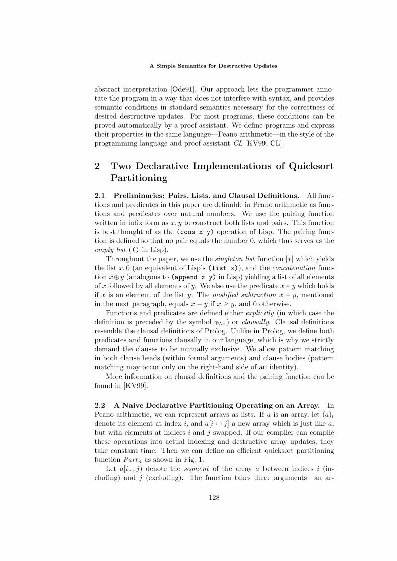
A Simple Semantics for Destructive Updates
abstract interpretation [Ode91]. Our approach lets the programmer anno-tate the program in a way that does not interfere with syntax, and providessemantic conditions in standard semantics necessary for the correctness ofdesired destructive updates. For most programs, these conditions can beproved automatically by a proof assistant. We define programs and expresstheir properties in the same language—Peano arithmetic—in the style of theprogramming language and proof assistant CL [KV99, CL].
2 Two Declarative Implementations of QuicksortPartitioning
2.1 Preliminaries: Pairs, Lists, and Clausal Definitions. All func-tions and predicates in this paper are definable in Peano arithmetic as func-tions and predicates over natural numbers. We use the pairing functionwritten in infix form as x, y to construct both lists and pairs. This functionis best thought of as the (cons x y) operation of Lisp. The pairing func-tion is defined so that no pair equals the number 0, which thus serves as theempty list (() in Lisp).
Throughout the paper, we use the singleton list function [x] which yieldsthe list x, 0 (an equivalent of Lisp’s (list x)), and the concatenation func-tion x⊕y (analogous to (append x y) in Lisp) yielding a list of all elementsof x followed by all elements of y. We also use the predicate x ε y which holdsif x is an element of the list y. The modified subtraction x .− y, mentionedin the next paragraph, equals x− y if x ≥ y, and 0 otherwise.
Functions and predicates are defined either explicitly (in which case thedefinition is preceded by the symbol PAx ) or clausally. Clausal definitionsresemble the clausal definitions of Prolog. Unlike in Prolog, we define bothpredicates and functions clausally in our language, which is why we strictlydemand the clauses to be mutually exclusive. We allow pattern matchingin both clause heads (within formal arguments) and clause bodies (patternmatching may occur only on the right-hand side of an identity).
More information on clausal definitions and the pairing function can befound in [KV99].
2.2 A Naive Declarative Partitioning Operating on an Array. InPeano arithmetic, we can represent arrays as lists. If a is an array, let (a)idenote its element at index i, and a[i↔ j] a new array which is just like a,but with elements at indices i and j swapped. If our compiler can compilethese operations into actual indexing and destructive array updates, theytake constant time. Then we can define an efficient quicksort partitioningfunction Partn as shown in Fig. 1.
Let a[i . . j) denote the segment of the array a between indices i (in-cluding) and j (excluding). The function takes three arguments—an ar-
128
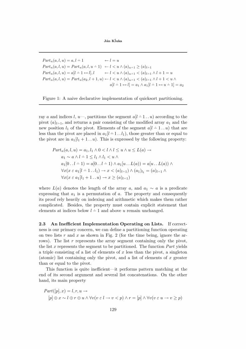
Jan Kluka
Partn(a, l, u) = a, l .− 1 ← l = u
Partn(a, l, u) = Partn(a, l, u .− 1) ← l < u ∧ (a)u .−1 ≥ (a)l .−1
Partn(a, l, u) = a[l .− 1↔ l], l ← l < u ∧ (a)u .−1 < (a)l .−1 ∧ l + 1 = u
Partn(a, l, u) = Partn(a2, l + 1, u)← l < u ∧ (a)u .−1 < (a)l .−1 ∧ l + 1 < u ∧a[l .− 1↔ l] = a1 ∧ a1[l .− 1↔ u .− 1] = a2
Figure 1: A naive declarative implementation of quicksort partitioning.
ray a and indices l, u—, partitions the segment a[l .− 1 . . u) according to thepivot (a)l .−1, and returns a pair consisting of the modified array a1 and thenew position l1 of the pivot. Elements of the segment a[l .− 1 . . u) that areless than the pivot are placed in a1[l .−1 . . l1), those greater than or equal tothe pivot are in a1[l1 + 1 . . u). This is expressed by the following property:
Partn(a, l, u) = a1, l1 ∧ 0 < l ∧ l ≤ u ∧ u ≤ L(a)→a1 ∼ a ∧ l .− 1 ≤ l1 ∧ l1 < u ∧a1[0 . . l .− 1) = a[0 . . l .− 1) ∧ a1[u . . L(a)) = a[u . . L(a)) ∧∀x(x ε a1[l .− 1 . . l1)→ x < (a)l .−1) ∧ (a1)l1 = (a)l .−1 ∧∀x(x ε a1[l1 + 1 . . u)→ x ≥ (a)l .−1)
where L(a) denotes the length of the array a, and a1 ∼ a is a predicateexpressing that a1 is a permutation of a. The property and consequentlyits proof rely heavily on indexing and arithmetic which makes them rathercomplicated. Besides, the property must contain explicit statement thatelements at indices below l .− 1 and above u remain unchanged.
2.3 An Inefficient Implementation Operating on Lists. If correct-ness is our primary concern, we can define a partitioning function operatingon two lists r and x as shown in Fig. 2 (for the time being, ignore the ar-rows). The list r represents the array segment containing only the pivot,the list x represents the segment to be partitioned. The function Part yieldsa triple consisting of a list of elements of x less than the pivot, a singleton(atomic) list containing only the pivot, and a list of elements of x greaterthan or equal to the pivot.
This function is quite inefficient—it performs pattern matching at theend of its second argument and several list concatenations. On the otherhand, its main property
Part([p], x) = l, r, u→[p]⊕ x ∼ l ⊕ r ⊕ u ∧ ∀v(v ε l→ v < p) ∧ r = [p] ∧ ∀v(v ε u→ v ≥ p)
129
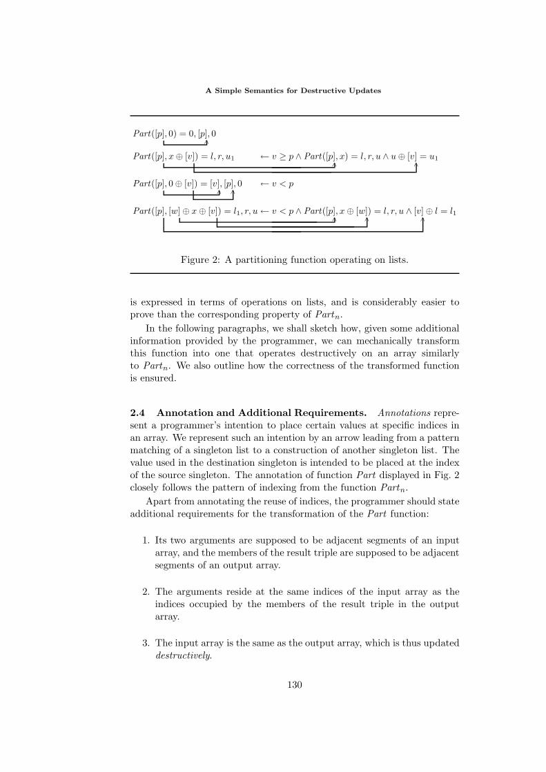
A Simple Semantics for Destructive Updates
Part([p], 0) = 0, [p], 0∧
Part([p], x⊕ [v]) = l, r, u1 ← v ≥ p ∧ Part([p], x) = l, r, u ∧ u⊕ [v] = u1∧ ∧
Part([p], 0⊕ [v]) = [v], [p], 0 ← v < p∧ ∧
Part([p], [w]⊕ x⊕ [v]) = l1, r, u← v < p ∧ Part([p], x⊕ [w]) = l, r, u ∧ [v]⊕ l = l1∧ ∧ ∧
Figure 2: A partitioning function operating on lists.
is expressed in terms of operations on lists, and is considerably easier toprove than the corresponding property of Partn.
In the following paragraphs, we shall sketch how, given some additionalinformation provided by the programmer, we can mechanically transformthis function into one that operates destructively on an array similarlyto Partn. We also outline how the correctness of the transformed functionis ensured.
2.4 Annotation and Additional Requirements. Annotations repre-sent a programmer’s intention to place certain values at specific indices inan array. We represent such an intention by an arrow leading from a patternmatching of a singleton list to a construction of another singleton list. Thevalue used in the destination singleton is intended to be placed at the indexof the source singleton. The annotation of function Part displayed in Fig. 2closely follows the pattern of indexing from the function Partn.
Apart from annotating the reuse of indices, the programmer should stateadditional requirements for the transformation of the Part function:
1. Its two arguments are supposed to be adjacent segments of an inputarray, and the members of the result triple are supposed to be adjacentsegments of an output array.
2. The arguments reside at the same indices of the input array as theindices occupied by the members of the result triple in the outputarray.
3. The input array is the same as the output array, which is thus updateddestructively.
130
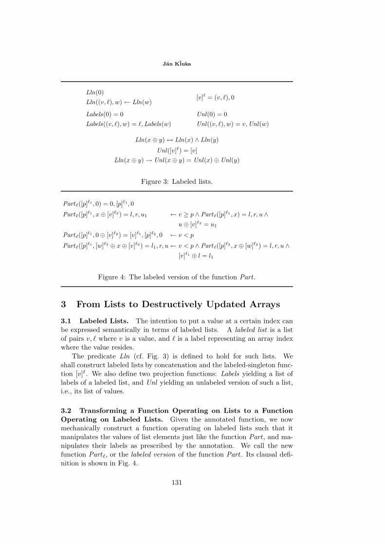
Jan Kluka
Lln(0)Lln((v, ), w)← Lln(w)
[v] = (v, ), 0
Labels(0) = 0Labels((v, ), w) = ,Labels(w)
Unl(0) = 0Unl((v, ), w) = v,Unl(w)
Lln(x ⊕ y)↔ Lln(x) ∧ Lln(y)
Unl([v]) = [v]Lln(x⊕ y)→ Unl(x ⊕ y) = Unl(x)⊕Unl(y)
Figure 3: Labeled lists.
Part([p]1 , 0) = 0, [p]1, 0
Part([p]1 , x⊕ [v]2) = l, r, u1 ← v ≥ p ∧ Part([p]1 , x) = l, r, u ∧u⊕ [v]2 = u1
Part([p]1 , 0⊕ [v]2) = [v]1 , [p]2 , 0 ← v < p
Part([p]1 , [w]3 ⊕ x⊕ [v]2) = l1, r, u← v < p ∧ Part([p]3 , x⊕ [w]2) = l, r, u ∧[v]1 ⊕ l = l1
Figure 4: The labeled version of the function Part .
3 From Lists to Destructively Updated Arrays
3.1 Labeled Lists. The intention to put a value at a certain index canbe expressed semantically in terms of labeled lists. A labeled list is a listof pairs v, where v is a value, and is a label representing an array indexwhere the value resides.
The predicate Lln (cf. Fig. 3) is defined to hold for such lists. Weshall construct labeled lists by concatenation and the labeled-singleton func-tion [v]. We also define two projection functions: Labels yielding a list oflabels of a labeled list, and Unl yielding an unlabeled version of such a list,i.e., its list of values.
3.2 Transforming a Function Operating on Lists to a FunctionOperating on Labeled Lists. Given the annotated function, we nowmechanically construct a function operating on labeled lists such that itmanipulates the values of list elements just like the function Part , and ma-nipulates their labels as prescribed by the annotation. We call the newfunction Part , or the labeled version of the function Part . Its clausal defi-nition is shown in Fig. 4.
131
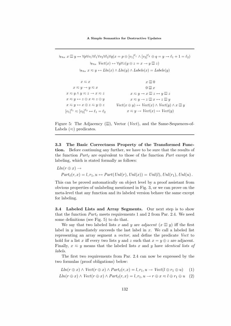
A Simple Semantics for Destructive Updates
PAx x ⊥ y ↔ ∀p∀v1∀1∀v2∀2∀q(x = p⊕ [v1]1 ∧ [v2]2 ⊕ q = y → 1 + 1 = 2)
PAx Vect(x)↔ ∀y∀z(y ⊕ z = x→ y ⊥ z)PAx x y ↔ Lln(x) ∧ Lln(y) ∧ Labels(x) = Labels(y)
x x
x y → y x
x y ∧ y z → x z
x y ↔ z ⊕ x z ⊕ yx y ↔ x⊕ z y ⊕ z[v1]1 [v2]2 ↔ 1 = 2
x ⊥ 00 ⊥ x
x y → x ⊥ z ↔ y ⊥ zx y → z ⊥ x↔ z ⊥ y
Vect(x⊕ y)↔ Vect(x) ∧ Vect(y) ∧ x ⊥ yx y → Vect(x)↔ Vect(y)
Figure 5: The Adjacency (⊥), Vector (Vect), and the Same-Sequences-of-Labels () predicates.
3.3 The Basic Correctness Property of the Transformed Func-tion. Before continuing any further, we have to be sure that the results ofthe function Part are equivalent to those of the function Part except forlabeling, which is stated formally as follows:
Lln(r ⊕ x)→Part (r, x) = l, r1, u↔ Part(Unl(r),Unl(x)) = Unl(l),Unl(r1),Unl(u) .
This can be proved automatically on object level by a proof assistant fromobvious properties of unlabeling mentioned in Fig. 3, or we can prove on themeta-level that any function and its labeled version behave the same exceptfor labeling.
3.4 Labeled Lists and Array Segments. Our next step is to showthat the function Part meets requirements 1 and 2 from Par. 2.4. We needsome definitions (see Fig. 5) to do that.
We say that two labeled lists x and y are adjacent (x ⊥ y) iff the firstlabel in y immediately succeeds the last label in x. We call a labeled listrepresenting an array segment a vector, and define the predicate Vect tohold for a list x iff every two lists y and z such that x = y ⊕ z are adjacent.Finally, x y means that the labeled lists x and y have identical lists oflabels.
The first two requirements from Par. 2.4 can now be expressed by thetwo formulas (proof obligations) below:
Lln(r ⊕ x) ∧ Vect(r ⊕ x) ∧ Part (r, x) = l, r1, u→ Vect(l ⊕ r1 ⊕ u) (1)Lln(r ⊕ x) ∧Vect(r ⊕ x) ∧ Part (r, x) = l, r1, u→ r ⊕ x l ⊕ r1 ⊕ u (2)
132
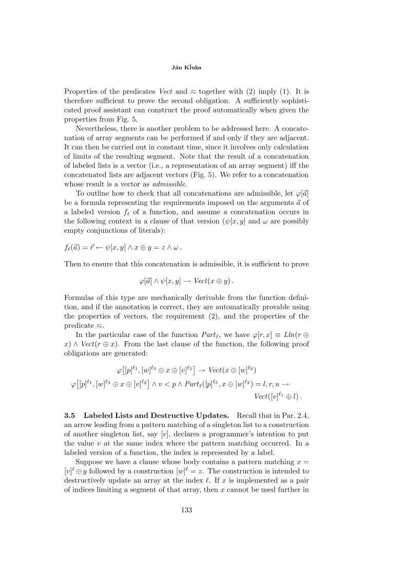
Jan Kluka
Properties of the predicates Vect and together with (2) imply (1). It istherefore sufficient to prove the second obligation. A sufficiently sophisti-cated proof assistant can construct the proof automatically when given theproperties from Fig. 5.
Nevertheless, there is another problem to be addressed here. A concate-nation of array segments can be performed if and only if they are adjacent.It can then be carried out in constant time, since it involves only calculationof limits of the resulting segment. Note that the result of a concatenationof labeled lists is a vector (i.e., a representation of an array segment) iff theconcatenated lists are adjacent vectors (Fig. 5). We refer to a concatenationwhose result is a vector as admissible.
To outline how to check that all concatenations are admissible, let ϕ[a]be a formula representing the requirements imposed on the arguments a ofa labeled version f of a function, and assume a concatenation occurs inthe following context in a clause of that version (ψ[x, y] and ω are possiblyempty conjunctions of literals):
f(a) = r ← ψ[x, y] ∧ x⊕ y = z ∧ ω .
Then to ensure that this concatenation is admissible, it is sufficient to prove
ϕ[a] ∧ ψ[x, y]→ Vect(x⊕ y) .
Formulas of this type are mechanically derivable from the function defini-tion, and if the annotation is correct, they are automatically provable usingthe properties of vectors, the requirement (2), and the properties of thepredicate .
In the particular case of the function Part , we have ϕ[r, x] ≡ Lln(r ⊕x) ∧ Vect(r ⊕ x). From the last clause of the function, the following proofobligations are generated:
ϕ[[p]1 , [w]3 ⊕ x⊕ [v]2
]→ Vect(x⊕ [w]2)
ϕ[[p]1, [w]3 ⊕ x⊕ [v]2
] ∧ v < p ∧ Part ([p]3 , x⊕ [w]2) = l, r, u→Vect([v]1 ⊕ l) .
3.5 Labeled Lists and Destructive Updates. Recall that in Par. 2.4,an arrow leading from a pattern matching of a singleton list to a constructionof another singleton list, say [v], declares a programmer’s intention to putthe value v at the same index where the pattern matching occurred. In alabeled version of a function, the index is represented by a label.
Suppose we have a clause whose body contains a pattern matching x =[v]⊕ y followed by a construction [w] = z. The construction is intended todestructively update an array at the index . If x is implemented as a pairof indices limiting a segment of that array, then x cannot be used further in
133
A Simple Semantics for Destructive Updates
PAx x # y ↔ ∀∀v1∀v2(v1, /ε x ∨ v2, /ε y)
PAx x y ↔ ∀∀v1∀v2(v1, ε x ∧ v2, ε y → v1 = v2)
x # 0Lln(x)→ x # x↔ x = 0
x # y → y # x
x # [v] ↔ ∀v(v, /ε x)x # y ⊕ z ↔ x # y ∧ x # z
x y → x # z ↔ y # z
Lln(x⊕ y) ∧Vect(x ⊕ y)→ x # y
x 0x y → y x
x y ⊕ z ↔ x y ∧ x zx # y → x y
Lln(x⊕ y) ∧Vect(x⊕ y)→ x⊕ y xLln(x⊕ y) ∧ Vect(x⊕ y)→ x⊕ y y
Figure 6: Definitions and selected properties of the Disjoint-Labels predicate#, and the Correctly-Aliased predicate .
the clause since the list of values of x may be no longer actually present inthe corresponding array segment.
A simple solution to this problem is to allow each list variable to beused only once after it is given a value. Although the function Part (andconsequently Part ) complies with this constraint, it is too restrictive—inthe above example, using the variable x between the pattern matching andthe construction would do no harm.
To deal with this problem in a more permissive semantic manner, wedefine the predicates shown in Fig. 6. Formula x # y expresses the fact thatthe sets of labels of two labeled lists x and y are disjoint. We shall call twolists x and y correctly aliased and write x y iff for every label shared bythese lists, the value that occurs at label in the list x is the same as thevalue occurring at that label in the list y. If these lists are vectors, and theyactually share a label, they represent two overlapping array segments.
Let ϕ[a] stand for the requirements imposed on the arguments of a la-beled version f of a function (as in Par. 3.4). Furthermore, assume thatlabeled-list variables x and y occur in a clause of f in the following con-text (ξ, ψ, and ω[x] are possibly empty conjunctions of literals, τ and ρ areterms):
f(a) = r← ξ ∧ τ = x ∧ ψ ∧ ρ = y ∧ ω[x] .
The identity τ = x gives a value to the variable x, ρ = y gives a value to y.After that, x is used in the rest ω[x] of the clause.
We claim, that if a property of the form
ϕ[a] ∧ ξ ∧ τ = x ∧ ψ ∧ ρ = y → y x
134
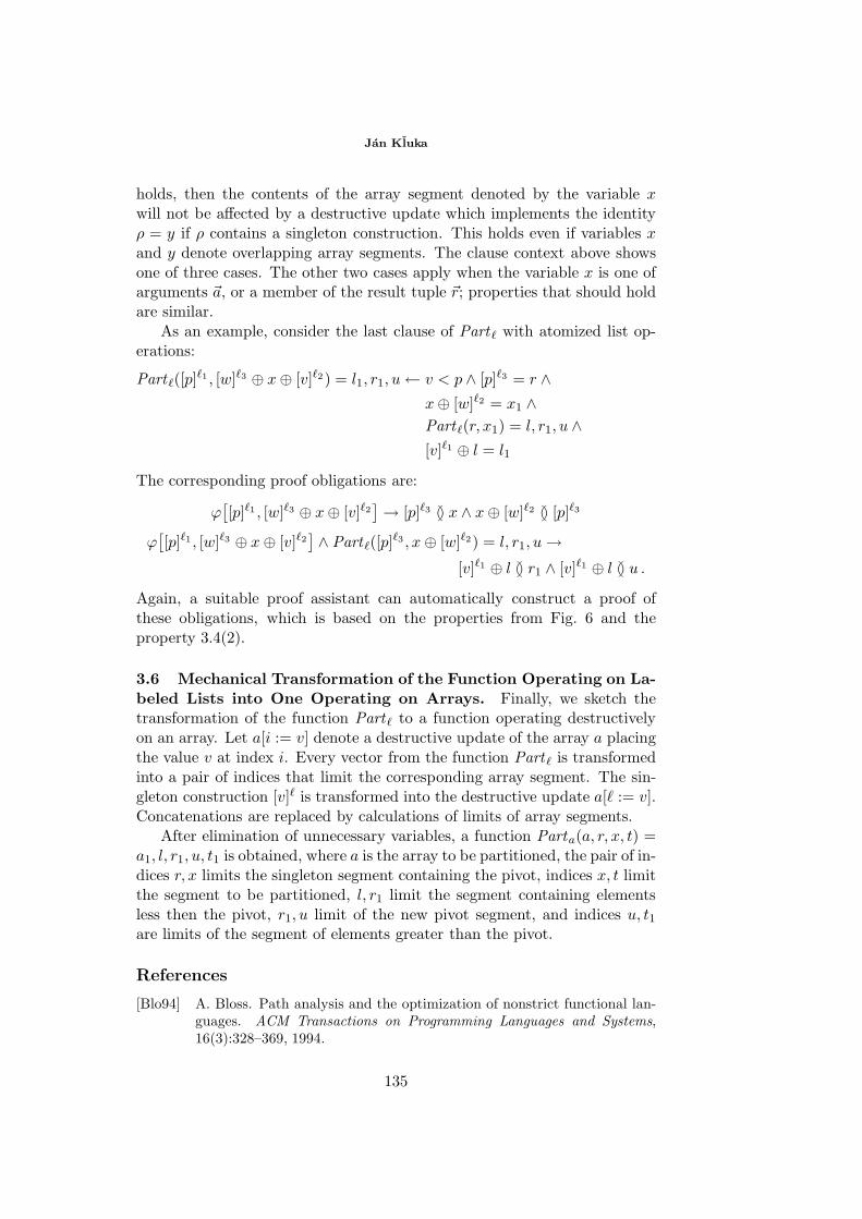
Jan Kluka
holds, then the contents of the array segment denoted by the variable xwill not be affected by a destructive update which implements the identityρ = y if ρ contains a singleton construction. This holds even if variables xand y denote overlapping array segments. The clause context above showsone of three cases. The other two cases apply when the variable x is one ofarguments a, or a member of the result tuple r; properties that should holdare similar.
As an example, consider the last clause of Part with atomized list op-erations:
Part ([p]1 , [w]3 ⊕ x⊕ [v]2) = l1, r1, u← v < p ∧ [p]3 = r ∧x⊕ [w]2 = x1 ∧Part (r, x1) = l, r1, u ∧[v]1 ⊕ l = l1
The corresponding proof obligations are:
ϕ[[p]1 , [w]3 ⊕ x⊕ [v]2
]→ [p]3 x ∧ x⊕ [w]2 [p]3
ϕ[[p]1, [w]3 ⊕ x⊕ [v]2
] ∧ Part ([p]3 , x⊕ [w]2) = l, r1, u→[v]1 ⊕ l r1 ∧ [v]1 ⊕ l u .
Again, a suitable proof assistant can automatically construct a proof ofthese obligations, which is based on the properties from Fig. 6 and theproperty 3.4(2).
3.6 Mechanical Transformation of the Function Operating on La-beled Lists into One Operating on Arrays. Finally, we sketch thetransformation of the function Part to a function operating destructivelyon an array. Let a[i := v] denote a destructive update of the array a placingthe value v at index i. Every vector from the function Part is transformedinto a pair of indices that limit the corresponding array segment. The sin-gleton construction [v] is transformed into the destructive update a[ := v].Concatenations are replaced by calculations of limits of array segments.
After elimination of unnecessary variables, a function Parta(a, r, x, t) =a1, l, r1, u, t1 is obtained, where a is the array to be partitioned, the pair of in-dices r, x limits the singleton segment containing the pivot, indices x, t limitthe segment to be partitioned, l, r1 limit the segment containing elementsless then the pivot, r1, u limit of the new pivot segment, and indices u, t1are limits of the segment of elements greater than the pivot.
References
[Blo94] A. Bloss. Path analysis and the optimization of nonstrict functional lan-guages. ACM Transactions on Programming Languages and Systems,16(3):328–369, 1994.
135
A Simple Semantics for Destructive Updates
[CL] The CL homepage. http://www.ii.fmph.uniba.sk/cl .
[Hud87] P. Hudak. A semantic model for reference counting and its abstraction. InS. Abramsky and C. Hankin, editors, Abstract Interpretation of Declara-tive Languages. Ellis Horwood Ltd., 1987.
[KV99] J. Komara and P. Voda. Theorems of Peter and Parsons in computer pro-gramming. In G. Gottlob, E. Grandjean, and K. Seyr, editors, Proceedingsof CSL’98, number 1584 in LNCS, pages 204–223. Springer Verlag, 1999.
[Ode91] M. Odersky. How to make destructive updates less destructive. In Con-ference Record of the Eighteenth Annual ACM Symposium on Principlesof Programming Languages, Orlando, Florida, pages 25–26. ACM Press,1991.
[Sha99] N. Shankar. Efficiently Executing PVS. Technical report, SRI In-ternational, Menlo Park, CA, 1999. Available through WWW fromhttp://www.csl.sri.com/users/shankar/shankar-drafts.html.
[Vod02] P. Voda. On modification of declarative arrays, 2002. Available throughWWW from http://www.diku.dk/undervisning/2002e/213/segm.ps.
[Wad90] P. Wadler. Linear types can change the world! In M. Broy and C. Jones,editors, IFIP TC 2 Working Conference on Programming Concepts andMethods, Sea of Galilee, Israel, pages 347–359. North Holland, 1990.
136
137
A New Proof of Decidability for the Modal Logicof Subset Spaces
GISELA KROMMESFernUniversität [email protected]
ABSTRACT. We present a simplified proof of decidability for the bimodal logic ofsubset spaces, introduced by Moss and Parikh, and discuss some difficulties in deter-mining the complexity of the decision problem. Basically designed for elementary rea-soning about points and sets in general topology, this logic gives basis to suitable for-malisms for reasoning about various subjects, especially topology or the acquisition ofknowledge.
1 Introduction
The logic of subset spaces of Moss and Parikh [MP92], let us call it LSS,combines the two well-known modal systems S4 and S5. As the name alreadyindicates, the most natural interpretation of LSS is not in usual Kripke structuresbut in subset spaces ( , )X , where the S5-operator K quantifies 'horizontally'
across points from a given set X and the S4-operator quantifies 'vertically'across the elements of a distinguished set of non-empty subsets of X. The in-teraction of both modalities is basically described by the cross axiom
K Kϕ ϕ→ .
This interpretation leads to an interesting application of LSS as a topologicallogic of knowledge. McKinsey [McK41] first investigated the close connectionbetween S4 and topology. He pointed out that the interior operator on a topologi-cal space has S4-like properties and although is not necessarily closed underfinite union and intersection, it gives a good intuition to think about ( , )X as a
kind of topological space. Moreover, the S5 component of LSS can be taken asthe widely used tool for the logical treatment of an agent's knowledge,cf. [FHMV96], i.e. Kϕ can be read as 'the agent knows ϕ '. In this way LSS con-nects the notion of knowledge with elementary topological reasoning.
What is the benefit of this connection? LSS provides a formalism to describeknowledge acquisition. In subset spaces, formulae are evaluated at neighborhood
Proceedings of the Eighth ESSLLI Student Session.Balder ten Cate (editor)Chapter 13, Copyright © 2003, Gisela Krommes
A New Proof of Decidability for the Modal Logic of Subset Spaces
138
situations (p,U) ∈ (q,V) ∈ X × | q∈V, consisting of a point (or state) p and aneighborhood U thereof.The basic LSS deals only with the knowledge of one agent: U consists of allstates the agent considers alternative to his actual state p and the knowledge op-erator K quantifies across all the states in U. Hence the agent's knowledge de-pends crucially upon the actual neighborhood of its state p.
If in the actual situation ( p,U ) the agent doesn’t know whether ϕ holds ornot, he considers both as possibilities, so we have
p,U ² Lϕ ∧ L¬ϕ(as usual we use Lϕ as an abbreviation of ¬K¬ϕ and ◊ϕ as an abbreviation of¬ ¬ϕ). But the more the agent knows, the smaller number of alternatives hetakes into account, thus acquisition of knowledge corresponds to shrinking the setof possible alternatives or, in the notion of topology, to shrinking p's neighbor-hood U. At this point the S4- comes into play: forced by the cross axiom, itquantifies across all neighborhoods of p that are subsets of U.
But since points and sets are general tools for formalization, LSS can also beuseful for the treatment of quite different subjects as the description of decisionor selection processes, where step-by-step additional constraints are satisfied.Moreover the underlying ideas gave rise to the development of special variants,which differ in the class of subset spaces, cf. [DMP96] (here is additionally thecase treated where ∪ ∅ is in fact a topology on X), [Geo97] (treelike spaces),[Hei98a] (spaces satisfying finite chain conditions), [WP02] (directed spaces,which are related to bases of neighborhood filters of topological spaces) or themodalities in use, cf. [Hei98b] (S4 weakened to a partial function to obtain a"next-time" operator), [DG00] (two S4 systems). The last paper is motivated bythe application domain of continuous and hybrid dynamic systems with practicaluse in several engineering tasks.
Syntax, semantics and a list of axioms for LSS are introduced in the next Sec-tion. Section 3 is dedicated to the decision problem. For this section, we assumesome familiarity with canonical models and filtration methods. (For a very acces-sible introduction see e.g. [BdRV01]). The proof of decidability given in[DMP96] is based on the finite model property (f.m.p.) of LSS w.r.t. a specialclass of models. The f.m.p. is established via filtration of the canonical modelusing the minimal filtration for both modalities. But proving that the so obtainedquotient structure belongs to the relevant class of models turns out to be hard todo. Pursuing a suggestion by Heinemann, we replace the minimal filtration forthe modality by its transitive closure, thus having transitivity by definition andcutting away the main difficulties of the original proof. We also use a bigger fil-ter set with better closure properties and for the resulting quotient structure, wecan state a nice property which is as easy to imagine as to prove. With this prop-erty at hand, the proof is quickly done.
Gisela Krommes
139
Up to now we could only establish PSPACE as a lower bound for the com-plexity of the decision problem. We discuss this result and the difficulties in de-termining the exact complexity briefly in Section 4. We will finish with someconcluding remarks in Section 5.
The work presented in this paper is part of our forthcoming diploma thesis.
2 The Logic LSS
We start with the definition of the logical language for LSS.
Definition 2.1 (Syntax of LSS) Let PV be a recursive1 and countable set ofatomic propositions. The set of LSS-formulae is recursively generated by:
1 2 :: | | | |A Kϕ ϕ ϕ ϕ ϕ ϕ= ¬ ∧
with A∈PV, an atomic proposition.
The other Boolean connectives, logical constants and dual modalities are de-finable in the standard way. The semantical domains of LSS are subset modelsand defined as follows:
Definition 2.2 (Subset Models) A subset space is a pair( , )X
where X is a non-empty set of points (or states) and is a set of non-empty sub-sets of X, called opens.A subset model is a triple
( ), ,X σ=where ( , )X is a subset space and σ is a mapping : ( )PV Xσ → , called
valuation.
Although formulae are evaluated at neighborhood situations the valuation σ isdefined with respect only to points and this fact gives reason to the persistenceaxiom introduced later on. For a given subset model we now define the satis-faction relation ² between neighborhood situations of the underlying modeland formulae in .
Definition 2.3 (Satisfaction relation) Let ( ), ,X σ= be a subset model. For
p U∈ ∈ and ϕ ∈ the satisfaction relation ² is defined by recursion
on ϕ :(p,U ) ² A iff p∈σ (A)
(p,U ) ² ¬ϕ iff (p,U ) ϕ
1 Since we focus on the decidability of LSS we stress that PV is a decidable set and there-fore the set of valid LSS-formulae is decidable as well.
A New Proof of Decidability for the Modal Logic of Subset Spaces
140
(p,U ) ² ϕ ∧ ψ iff (p,U ) ² ϕ and p,U ² ψ(p,U ) ² Kϕ iff (q,U ) ² ϕ for all q∈U
(p,U ) ² ϕ iff (p,V ) ² ϕ for all V ∈ such that p ∈ V ⊆ U
In other words, we are considering a Kripke structure whose worlds are thepairs (p,U) and with two accessibility relations corresponding to shrinking an open( ) while maintaining a reference point, or to moving a reference point insidethe given open (K).
The following schemata of formulae are suitable for the axiomatization of theset of LSS-validities:
(1) All -instances of propositional tautologies
(2) K(ϕ → ψ) → (Kϕ → Kψ)
(3) (ϕ → ψ) → ( ϕ → ψ)
(4) ϕ → ϕ (reflexivity)
(5) ϕ → ϕ (transitivity)
(6) Kϕ → ϕ (reflexivity)
(7) Kϕ → KKϕ (transitivity)
(8) Lϕ → KLϕ (Euclidean property)
(9) (A → A) ∧ (¬A → ¬A) for atomic A (persistence axiom)
(10) K ϕ → Kϕ (cross axiom)
The deductive system LSS is established by adding rules of inference:
( ),modus ponens
ϕ ψ ϕψ
→ ( )-necessitationK
K
ϕϕ
( )-necessitationϕϕ
The cross axiom is the typical one for the logic of subset spaces. In the notionof knowledge, this so-called cross property demands that the agent under consid-eration does not forget. The axioms are often used in their dual form, e.g. thecross axiom K ϕ → Kϕ ≡ ◊Lϕ → L ◊ϕ. Note that because of the persistenceaxiom, LSS is not closed under substitution.
We conclude the introduction of LSS by stating its soundness and complete-ness w.r.t. subset frames and turn to the proof of decidability in the next section.
Theorem 2.4 (Soundness and Completeness of LSS) Let ϕ ∈ be a formula.Then ϕ is LSS-derivable iff it is valid in every model based on a subset frame.
The soundness part of theorem 2.4 is obvious, completeness is much harder toshow. See [DMP96] for a proof using a rather complicated step-by-step con-struction.
S4-axioms
S5-axioms
Gisela Krommes
141
3 Decidability of LSS
It is folklore that the above given axiomatization together with the f.m.p. wouldimmediately yield the decidability of the satisfaction problem. But we have badnews: the logic of subset spaces lacks the f.m.p. To see this, consider the follow-ing scheme of infinity axioms:
( ):ψ ϕ ϕ= ◊ ∧ ◊¬ .
No sentence of this form can have a finite subset model. For suppose thatwere a finite model containing p and U such that ,p U ψ . We may assume that
U is a ⊆-minimal open about p with this property. But the minimality implies
( ),p U ϕ ϕ∧ ¬ , and this is absurd.
However, substitute ϕ by ( )( )L B KB LC∧ ∨ and see [DMP96] for an infinite
subset model of the resulting formula ψ '.
The problem that ψ ' has only infinite subset models, stems from the fact thatin subset spaces the accessibility relation corresponding to the -operator is an-tisymmetric, as according to the ⊆-relation, although this property is not de-manded by the axioms. But there is a class of models avoiding this difficulty, theclass of cross axiom models, to which LSS is also sound and complete and satis-fies the f.m.p. as shown below.
Definition 3.1 (Cross Axiom Model) A cross axiom frame is a tuple
( ), , LJ ◊→ →
such that J is a non-empty set, L→ is an equivalence relation on J, ◊
→ is a
preorder on J, and the following property holds: If i ◊→ j
L→ k, then there is
some l such that i L→ l
◊→ k.
A cross axiom model is a cross axiom frame together with an interpretation σ ofthe atomic propositions of ;. σ must satisfy the condition that
if i ◊→ j, then i ∈ σ (A) iff j ∈ σ (A).
A cross axiom model is simply a bimodal Kripke structure such that the ac-cessibility relations satisfy the corresponding axioms and also the cross axiomholds. In addition, the valuation σ satisfies the persistence axiom. Hence, LSS isobviously sound w.r.t. the class of cross axiom models (not frames, because ofthe persistence axiom). Moreover, every subset model ( ), ,X σ= gives rise to
a cross axiom model
( ), , , 'LJ σ◊→ →=as follows:
J := <p,U> ∈ X × | p ∈ U (<p,U> denotes a single point of J )
A New Proof of Decidability for the Modal Logic of Subset Spaces
142
<p,U> L→ <q,V> iff U = V
<p,U> ◊→ <q,V> iff p = q and V ⊆ U
σ ' (A) := <p,U> | p ∈ σ (A) ∩ U for all atomic propositions A
A simple induction shows that
( p,U ) ² ϕ ⇔ <p,U> ² ϕ for all formulae ϕ ∈ , thus we can state:
Lemma 3.2 (Completeness w.r.t. Cross Axiom Models) LSS is sound andcomplete w.r.t. the class of cross axiom models.
Hence, for any formula ϕ ∈ it suffices to look for a finite cross axiom model.
Since the canonical model of LSS satisfies every LSS-consistent ϕ and the fil-
tration method constructs a finite quotient structure out of , also a model of ϕ,
the remaining problem is to choose a filtration method such that is a cross axiommodel.
The canonical model
( ) : , , , L σ◊→ →=
is formed in the usual way, i.e. consists of all maximal LSS-consistent sets offormulae and the accessibility relations induced by the modal operators K and are for all S, T∈ defined by
: |LS T K S Tψ ψ→ ⇔ ∈ ∈ ⊆ and
: | S T S Tψ ψ◊→ ⇔ ∈ ∈ ⊆ .
Finally, the valuation σ is defined by
( ) : A T A Tσ∈ ⇔ ∈ for all A∈PV and T ∈ .
Let us now fix a formula ϕ ∈ and gather together the notions needed to define
: Corresponding to ϕ, we build the filter set Σ ⊆ in several steps. Starting
with the set sf (ϕ ) of subformulae of ϕ we define:
Σ¬ := sf (ϕ ) ∪¬ψ ∈ | ψ ∈ sf (ϕ )
Σ' := Σ¬ ∪ψ | ψ is a conjunction or disjunction of pairwise distinct x∈Σ¬
Σ" := Σ' ∪ ψ | ψ is a conjunction or disjunction of pairwise distinct x∈Σ'
Σ := Σ" ∪ Lψ | ψ ∈ Σ" ∪ Kψ | ψ ∈ Σ" .
Note that all sets are finite and subformula closed and that Σ" is a kind of Boo-lean closure of sf (ϕ ).
For T∈ let [T] denote the set S∈ | T ∩ Σ = S ∩ Σ which is the equiva-lence class of T w.r.t. Σ . The minimal filtration [ ]L→ of L→ is defined by
Gisela Krommes
143
[S] [ ]L→ [T] : ⇔ ∃ S' ∈ [S], T' ∈ [T] : S L→ T for all S, T ∈and the minimal filtration of ◊→ is defined accordingly. With these notionsavailable, we can define
:= ([ ], [ ]L→ , [ ◊ ]→ , σ ),
where [ ] := [T] | T ∈ , [ ]L→ is the minimal filtration of L→ , [ ◊ ]→ is the
transitive closure of the minimal filtration of ◊→ , and for all atomic A we have
σ (A) := [T] ∈ [ ] | A ∈ T ∩ Σ.
The following proposition guaranties that is indeed a model of ϕ.
Lemma 3.3 Let ( ) , , , L σ◊→ →= be the canonical model of LSS and
= ([ ], [ ]L→ , [ ◊ ]→ , σ ) the quotient structure described above. Then is a
filtration of .
Proof. We have to show that [ ]L→ and [ ◊ ]→ are filtrations of L→ and ◊→ ,
respectively. For [ ]L→ , the common minimal filtration, this is clear. Concerning [ ◊ ]
→ this is an easy consequence of the definition of the minimal filtration andits transitive closure; for the complete proof we refer to [CZ97], p. 141 ff.
To prepare the proof that is a cross axiom model, we first state a very use-
ful property of the filter set Σ.
Lemma 3.4 Let :T Tγγ γ
∈ ∩Σ= ∧ be the identifying formula for the above defined
equivalence class [T] of T w.r.t. Σ. Then
TLγ ∈ S' for some S' ∈ [S] ⇒ TLγ ∈ S" for all S"∈ [S].
Proof. Let TLγ ∈ S' ∈ [S]. By definition of L→ , there is some T' ∈ such that
S' L→ T ' and Tγ ∈ T'. By the same argument, we get Lψ | ψ ∈ T' ∩ Σ−Σ" ⊆ S'.
We now make use of the S5 property that every formula Oψ ∈ with a prefix
O ∈K, L2 is equivalent to some O'ψ, where O' ∈K, L1. So with the definitionof Σ−Σ" we also get Lψ | ψ ∈ T' ∩ Σ−Σ" ⊆ S" for arbitrary S"∈ [S].Since all formulae in Σ−Σ" are K or L sentences we obtain with the S5 laws
( )' "' :T T
K Kγ
γ γ∈ ∩Σ−Σ
= ∧ ∈ S". *
Clearly TLγ ∈ S' ⇒ "TLγ ∈ S', where "
" :T Tγγ γ
∈ ∩Σ= ∧ , and since "TLγ ∈ Σ by
construction of Σ, we also have
"TLγ ∈ S". **
A New Proof of Decidability for the Modal Logic of Subset Spaces
144
Putting * and ** together we get 'TKγ , "TLγ ⊆ S". Hence there exists some
U ∈ such that S" L→ U and 'Tγ , "Tγ ⊆ U. Since 'Tγ ∧ "Tγ ≡ Tγ ∈ U
we finally get TLγ ∈ S".
Now let us turn to the question of how to show that has the cross property.
Whenever [S] [ ◊ ]→ [T] [ ]L→ [U], we need some [V] ∈ [ ] such that
[S] [ ]L→ [V] [ ◊ ]→ [U].
By definition of [ ◊ ]→ and [ ]L→ , there are S' ∈ [S], T' and T" ∈ [T], U' ∈ [U]
such that S' ◊→ T' and T" L→ U'. If T' = T", the cross property of supplies the
desired V' ∈ [V] such that S L→ V' ◊→ U and hence, [S] [ ]L→ [V] [ ◊ ]
→ [U]. Butpossibly T'≠T". However, Lemma 3.4 gives a solution: According to T' we can
always find some U"∈[U] such that T' L→ U", i.e. we have S' ◊→ T' L→ U" andtherefore, the set V' we are looking for must exist. This is the announced nice
property of .
Lemma 3.5 Let := ([ ], [ ]L→ , [ ◊ ]→ , σ ) be defined as above. Then for all
[S], [T]∈ [ ] the following holds:
[S] [ ]L→ [T] ⇒ for all S' ∈ [S] there exists some T' ∈ [T]
such that S' L→ T '.
Proof. This is a direct consequence of Lemma 3.3, observing that [S] [ ]L→ [T]
implies the existence of some S' ∈ [S] such that Lγ T ∈ S'.
We are now well prepared to show that is a cross axiom model and in thisway prove that LSS has the f.m.p. with respect to cross axiom models.
Theorem 3.6 (Finite Model Property) Every satisfiable ϕ ∈ has a finite crossaxiom model.
Proof. Let ϕ be satisfiable and the model described above. Obviously [ ◊ ]→
is reflexive and transitive and σ satisfies the required property. Reflexivity and
symmetry of [ ]L→ are direct consequences of the fact that this is the minimal
filtration of L→ . Finally, we get transitivity of [ ]L→ and the cross property by
iterated application of Lemma 3.4. Hence is a finite cross axiom model of ϕ.
Since satisfiability and validity are dual problems, this leads to the following:
Corollary 3.7 (Decidability) The set of satisfiable ϕ ∈ and the set of LSS-theorems are both decidable.
Gisela Krommes
145
4 Complexity
There are few variants of the basic LSS with reasonable computational behavior,cf. [Hei98c], where linear subset spaces and binary computation structures areinvestigated, both of them NP-complete.
But not surprisingly, the basic LSS turned out to be at least PSPACE-hard.Using techniques introduced by Ladner [Lad77] and very comprehensively ap-plied in [HM92], we proved this result by reducing the problem of decidingwhether an element of the quantified Boolean formulae (QBF) is true to that ofdeciding whether a formula is LSS satisfiable2. The first problem is known to bePSPACE-hard.
However, this result gives us only one lower bound and says nothing aboutthe exact complexity of LSS since up to now we could not establish PSPACE asan upper bound. Obviously, LSS lacks the tree model property, cf. [Grä99a] defi-nition 3.5, so the commonly used tableau method to get a PSPACE decision algo-rithm may not work.
Possibly, the complexity of the decision problem is worse, thus we tried toprove EXTIME as a lower bound. One may take it as a good sign that we did notget along with it. The methods we know to show EXTIME-hardness are based ontiling problems, cf. [vEm96], or on formulae that force any satisfying model tohave a path of exponential length, cf. [HM92]. In any case, these methods requirethe encoding of an n-bit binary counter, but LSS seems to be too weak for thispurpose.
There is still another possibility to show EXTIME-hardness: The criterionEdith Hemaspaandra provides in [Spa93]. This criterion looks for a formula ca-pable to simulate full irreflexive, asymmetric, intransitive binary trees of arbi-trary but finite height. To this end we would have to translate a formula ϕ out ofsome logical language having such a tree as model into a satisfiable formula
ψ ∈ , simulating this tree. The problem is that in LSS both accessibility rela-tions are transitive. To overcome this we could add special atomic propositionsH0 , H1 ,…,Hn , each one true at exactly one level of the tree, to encode the heightof a node. But since we do not know a bound for the height of the tree model forϕ we do not know how to choose n. Hence this does not seem to work either.
So until now the facts we can state about the complexity of the decisionproblem for LSS are: PSPACE as a lower bound and NEXTIME as an upperbound, supplied by the original proof of decidability. The filter set we used in ourproof leads to N2EXTIME as an upper bound, that is the price we have to pay forthe simplification of the proof.
2 This proof is also part of our diploma thesis.
A New Proof of Decidability for the Modal Logic of Subset Spaces
146
5 Conclusions and Future Work
We introduced the bimodal logic of subset spaces invented by Moss and Parikh andexplained its interpretation as a topological logic of knowledge. For decidability asimplified proof was presented and finally we discussed the difficulties in determin-ing the complexity of the decision problem. To overcome these difficulties and findout what the complexity of the decision problem really is seems to us a task worthyof further research. We didn't yet give up the hope that LSS may be PSPACE-complete − and if so, this would be a reason for a party!3
Furthermore, we think it is a good idea to follow the referee's suggestion and try tofind other applications for LSS or related systems. This seems indeed another inter-esting and important task and we appreciate this hint very much.
Acknowledgement
We would like to thank Bernhard Heinemann and the anonymous referees for severalvaluable suggestions and helpful comments.
References
[BdRV01] P. Blackburn, M. de Rijke, Y. Venema. 2001. Modal Logic, volume 53 ofCambridge Tracts in Theoretical Computer Science. Cambridge UniversityPress, Cambridge, 2001.
[CZ97] A. Chagrov, M. Zakharyaschev. 1997. Modal Logic, volume 35 of OxfordLogic Guides. Clarendon Press, Oxford, 1997.
[DG00] J.M. Davoren, R.P. Goré. 2000. Bimodal logics for reasoning aboutcontinuous dynamics. In Proceedings of Advances in Modal Logic. Leipzig,to appear.
[DMP96] A. Dabrowski, L.S. Moss, R. Parikh. 1996. Topological reasoning and thelogic of knowledge. Ann. Pure Appl. Logic, 78 (1996) 73-110.
[FHMV96] R. Fagin, J.Y. Halpern, Y. Moses, M.Y. Vardi. 1995. Reasoning aboutKnowledge. MIT Press, Cambridge, MA.
[Geo97] K. Georgatos. 1997. Knowledge on Treelike Spaces. Studia Logica,59:271-301.
[Grä99a] E. Grädel. 1999. On the restraining power of guards. Journal of SymbolicLogic, 64(4): 1719–1742, 1999.
3 This remark about logics with a decision problem solvable with a PSPACE-algorithm is
said to stem from Vardi, cf. [Grä99b].
Gisela Krommes
147
[Gra99b] E. Graedel. 1999. Why are modal logics so robustly decidable?. Bulletin ofthe European Association for Theoretical Computer Science, vol 68,pp 90-103.
[Hei98a] B. Heinemann. 1998. Topological Modal Logics Satisfying Finite ChainConditions. Notre Dame Journal of Formal Logic, 39(3):406-421.
[Hei98b] B. Heinemann. 1998. Topological nexttime logic. In M. Kracht et al., editor,Advances in Modal Logic, Volume 1, pages 99-113. CSLI.
[Hei98c] B. Heinemann. 1998. Subset pace logics of knowledge and time. HabilitationThesis, Fachbereich Informatik, FernUniversität Hagen.
[Spa93] E. Spaan. 1993. Complexity of modal logics. PhD thesis, University ofAmsterdam, Institute for Logic, Language and Computation.
[HM92] J.Y. Halpern, Y. Moses. 1992. A Guide to Completeness and Complexity forModal Logics of Knowledge and Belief. Artificial Intelligence 54:319-379.
[Lad77] R.E. Ladner. 1977. The Computational Complexity of Provability in Systemsof Modal Propositional Logic. SIAM Journal of Computing 6:467-480.
[McK41] J.C.C. McKinsey. 1941. A solution to the decision problem for the Lewissystems S2 and S4, with an application to topology. J. SymbolicLogic 6 (3) 117-141.
[MP92] L.S. Moss, R. Parikh. 1992. Topological reasoning and the logic ofknowledge. Theoretical Aspects of Reasoning about Knowledge, TARK1992, ed. Y. Moses, 95-105. Morgan Kaufmann.
[vEm96] P. van Emde Boas. 1996. The convenience of tilings. TechnicalReport CT-96-01, Institute for Logic, Language and Computation, Universityof Amsterdam
[WP02] A. Weiss, R. Parikh. 2002. Completeness of Certain Bimodal Logics forSubset Spaces. Studia Logica, 71:1-30.

148
An application of Sahlqvist Theory to
Bisorted Modal Logic
Wouter KuijperILLC/University of Amsterdam, the Netherlands.
Jorge Petrucio VianaInstitute of Mathematics/Federal Fluminense University and COPPE/Federal University of Rio
de Janeiro, Brazil. Visiting ILLC/University of Amsterdam, the Netherlands. Supported by
CAPES, Proc. n. BEX0493/02-3.
Abstract. We axiomatize two bisorted modal logics: basic hybrid logic and sub-set modal logic. The systems are presented as normal multimodal logics allowingus to freely apply Sahlqvist Theory. The proposed axiomatizations are clearer andmore concise than existing axiomatizations of the same theories. In particular, theaxioms have better motivations because each corresponds in a very direct senseto a frame condition. Proving completeness becomes a straightforward exerciseby appealing to canonicity directly avoiding the usual canonical model construc-tion. Moreover the resulting systems are automatically complete to all Sahlqvistextensions, even those containing nominals.
1 Introduction
It is a well established fact that modal logic over models can be seen asa fragment of first order logic whereas over frames it is a fragment ofmonadic second order logic . The study of the connections in the expressivityhierarchy of these three languages — or language families — is what iscommonly called Correspondence Theory [10]. Comparing different systemswith regard to expressivity, in some sense, presupposes a common, adequatesemantics. Although for a lot of modal logics that interest us relationalstructures do the job nicely, not every logic is sound and complete withrespect to some frame class [5, 9]. A huge amount of research has goneinto uncovering which logics are. In all generality we could call this fieldCompleteness Theory [3].
At the intersection of both these well explored paths we find a nice set ofresults generally referred to as Sahlqvist Theory. In essence Sahlqvist Theory
Proceedings of the Eighth ESSLLI Student SessionBalder ten Cate (editor)Chapter 14, Copyright c© 2003, Wouter Kuijper and Jorge Petrucio Viana
149
An application of Sahlqvist Theory to Bisorted Modal Logic
seeks to identify large classes of modal formulas that are both canonical andthat correspond to an elementary frame condition which can be effectivelycomputed from the formula. The landmark result in this research is thetheorem below. (All terminological and conceptual pre–requisites can befound in [3].)
Definition 1.1 (Sahlqvist Formulas). Positive and negative formulasare defined as usual. A Sahlqvist antecedent is a formula built up fromformulas that are either negative or of the form np, using only ∧ , ∨ and♦. A Sahlqvist implication is any implication that has a Sahlqvist antecedentand a positive consequent. A Sahlqvist formula is built up from Sahlqvistimplications using and ∧ freely, and ∨ only to disjuncts that do not shareproposition symbols.
Theorem 1.1 (Sahlqvist 1974). For every Sahlqvist formula A it holds
(i) A is canonical,
(ii) A has a local first order frame correspondent AFO that can be effec-tively computed from A.
It is not decidable in general whether an arbitrary formula has a firstorder correspondent [4]. The Sahlqvist fragment can be seen as a good com-promise between simplicity and generality in picking out a large portion offormulas for which this is decidable. Of course this leaves room for gener-alization of the result [6, 8]. Here we will use a version that in addition tounary modalities allows nullary modalities (or modal constants) to occur inSahlqvist formulas [3].
Sorting was proposed by P. Blackburn [2] and V. Goranko [7] as a gen-eral strategy to improve the expressive power of modal languages. A basicexample of a bisorted logic is basic hybrid logic (BHL), obtained from basicmodal logic by introducing nominals, a second type of proposition symbolsthat serve as unique names for states, also added are satisfaction opera-tors to jump to these named states and continue evaluation there [1]. As afirst step in establishing a general theory of sorted modal logics, Gorankostarted to investigate Subset Modal Logic (SML), inspired on BHL, SML isobtained by relieving the restriction of nominals to be interpreted strictlyas singletons [7].
In relation to the traditional logical issues, such as expressiveness, axiom-atization, decidability, and complexity, a lot of results to BHL have alreadybeen established (cf. [2] and the bibliography therein).
In this paper we study versions of these systems. We consider theproblem of the transfer of results from the basic (unisorted) modal settingto this more general context. In particular, we investigate Sahlqvist theoryand its use to obtain simpler sets of axioms and simpler completeness proofsto our versions of BHL and SML.
150
Wouter Kuijper and Jorge Petrucio Viana
This paper contains three main contributions in the line of researchsketched above. Firstly, we provide new axiomatizations to two bisortedmodal logics: basic hybrid logic and subset modal logic. Secondly, we ex-emplify how to treat sorted modal logics as normal multimodal logics usinginfinite axiomatizations. Lastly we show that it is possible, as a consequenceof this approach, to easily apply Sahlqvist Theory to sorted modal logics.
The paper is structured as follows. In Section 2 we review the syntaxand semantics of the basic hybrid logic in its common form. In Section 3we present the basic subset modal logic as a normal multimodal logic withnullary modalities. In Section 4 we axiomatize the minimal subset modallogic. Next, we proceed to show, in Section 5, how by extending the minimalsubset modal logic with two very simple axioms we obtain the minimal basichybrid logic. We conclude with some more comments, discussion andsuggestions for further research.
2 Basic Hybrid Logic
In this section we review syntax and semantics of basic hybrid logic [1].BHL is usually presented as a two sorted modal logic, viewing nominalsas proposition symbols whose interpretation on models is restricted. InSection 3, we present BHL as a multimodal logic, viewing nominals as specialkinds of modal constants, interpreted on frames. As will be shown, thischange in approach allows us transfer existing results for orthodox modallogics, in particular the multimodal version of Theorem 1.1 to BHL.
The basic hybrid language has countably many distinct nominals i andassociated satisfaction operators @i to identify, respectively refer to, po-tentially countably many named states. The idea is that by using thesenominals we can identify a unique state in our model. Basic modal logic, asit is bisimulation invariant, cannot express this [3]. Hence we have improvedthe expressive power of BML getting it closer to first–order logic, hopefullywithout losing its modal flavor [2].
Definition 2.1 (Basic Hybrid Language). The basic hybrid language isproduced by
φ := ⊥ | p | i | φ1 ∨ φ2 | ¬φ | ♦φ | @iφ, where i ∈ Ω.
Basic hybrid logic is interpreted with respect to exactly the same frameclass as the basic modal logic. This means that at the level of frames there isno interpretation for nominals nor for their associated satisfaction operators.The following definitions make clear exactly how this information arises atthe level of models.
Definition 2.2 (Hybrid Models). A hybrid model is a pair (F, V ) whereF = (W,R) is a basic modal frame and V is a hybrid valuation, i.e., a function
151
An application of Sahlqvist Theory to Bisorted Modal Logic
[K@] @i(p → q) → (@ip → @iq)
[self-dual] @ip ↔ ¬@i¬p
[introduction] i ∧ p → @ip
[ref] @ii
[sym] @ij ↔ @ji
[nom] @ij ∧ @jp → @ip
[agree] @j@ip ↔ @ip
[back] ♦@ip → @ip
Table 1: The axioms to the minimal Hybrid Logic given in [3].
that maps proposition symbols to subsets of W and nominals to singletonsof W .
Definition 2.3 (Hybrid Satisfaction). A hybrid formula φ being satisfiedin the hybrid model M at state w, notation:
M, w φ,
is inductively defined as follows
M, w p iff w ∈ V (p),M, w i iff w = V (i),
M, w ♦φ iff there exists v ∈ W such that Rwv and M, v φ,
M, w @iφ iff M, v φ where v = V (i).
with the boolean cases in the obvious way. Validity in a frame is defined asusual.
For some examples of hybrid validities cf. Table 1.Note that here nominals have same status as proposition symbols. This
is in fact inconvenient when we want to define the class of hybrid frames,i.e. frames with interpretation for nominals and their associated satisfactionoperators.
3 Subset Modal Logic
Subset modal logic was introduced by V. Goranko [7] — in connection withwhat he calls “vanilla set sorts” — as a step in extending the basic hy-brid mechanisms to sorted modal languages. In [7], Goranko advocates the
152
Wouter Kuijper and Jorge Petrucio Viana
study of sorted modal formalisms and provides examples from the litera-ture, showing that this kind of strategy can improve the expressive powerof modal logics. One of the basic ideas of Goranko’s approach, also presentin [2], is that sorted modal logics can be seen as a more general type ofhybrid logics. Goranko starts the extension of hybrid ideas to sorted modallogics, presenting SML and proposing an axiomatization to it. As a problemhe left to prove his axioms are complete.
For some intuition about SML observe that in the basic hybrid casea frame can be seen as a general frame in which the family of admissiblesubsets, for nominals, is exactly the set generated from all singletons. Thehybrid language has the power to denote these unique states. In SML, inthe basic case, this restriction to singletons is dropped. Nominals —in SMLwe call them subset constants— can be interpreted on any subset again, justlike ordinary proposition symbols. This in turn establishes the duality ofour @ operators now written as @∃ and @∀. In terms of satisfaction thiswill work out in the following way
M, w @∃i φ iff there exists v ∈ W such that M, v i ∧ φ, (3.1)
and dually,
M, w @∀i φ iff for all v ∈ W it holds M, v i → φ. (3.2)
Goranko specifies the SML syntax and semantics in an informal way.We choose to formulate SML as a “regular” normal modal logic [3], in thisway, trying to avoid the difficulties we pointed out in the last paragraph ofSection 2.
Definition 3.1 (SML Similarity Type). The similarity type for SMLexpands the similarity type for basic modal logic with a countable set Ω ofnullary modalities called subset constants and an associated countable set@∀
i i∈Ω of unary modalities called subset accessibility operators.
In the frame correspondence language the unary predicate associated tothe subset constant i is denoted Si and the binary predicate associated tothe the subset accessibility operator @∃
i is denoted Ri.The definitions of satisfaction and validity are the same as in modal logic.
To ensure condition (3.1) and (3.2) we define the appropriate semantics forSML.
Definition 3.2 (SML Frame). An SML frame
F =(W,R, (Ri)i∈Ω , (Si)i∈Ω
)
is a frame for the SML similarity type that satisfies for each i ∈ Ω the follow-ing defining condition on the interplay between subsets and their associated
153
An application of Sahlqvist Theory to Bisorted Modal Logic
accessibility relations:
∀xy(Rixy ↔ Siy). (3.3)
A hybrid SML frame is an SML frame where all Si are singleton.
Observation 3.1 (Hybrid SML Frames and Hybrid Models). Whenwe identify the @∀ and @∃ operators in the SML language over the class ofall hybrid SML frames, we end up with the same theory as the basic hybridlanguage over the class of all hybrid models.
4 Axiomatizing the Minimal SML
In this section we present an infinite axiomatization to minimal SML andprove completeness.
Recall that a normal modal logic is a set of modal formulas closed un-der generalization, uniform substitution and modus ponens; containing allpropositional tautologies plus special axioms saying how each modality re-lates to its dual and how it distributes over implication.
We denote by K the minimal modal logic, i.e. the normal modal logicthat is sound and complete with respect to the class of all frames.
Definition 4.1 (Logic KS). Let S be the countable collection of Sahlqvistaxioms given in Table 2. Define KS as the normal modal logic for the SMLsimilarity type with the additional axioms in S.
[trans] @∃j @
∃i p → @∃
i p ∀xyz(Rjxy ∧ Riyz → Rixz)
[trans♦] ♦@∃i p → @∃
i p ∀xyz(Rxy ∧ Riyz → Rixz)
[eucl] @∃i p → @∀
j @∃i p ∀xyz(Rixy ∧ Rjxz → Rizy)
[eucl♦] @∃i p → @∃
i p ∀xyz(Rixy ∧ Rxz → Rizy)
[label] @∀i i ∀xy(Rixy → Siy)
[ref] i ∧ p → @∃i p ∀x(Six → Rixx)
Table 2: Sahlqvist axioms to minimal SML with their First–Order corre-spondents; i, j ∈ Ω.
The following lemma motivates our choice of axioms. It shows that wehave defined a broader class of frames that has the same modal theory asthe intended frame class of all SML frames.
First we recall the definition of a rooted or point generated subframe Fw
which is the restriction of F to all nodes that are reachable from w by a
154
Wouter Kuijper and Jorge Petrucio Viana
path consisting of R and Ri steps. Taking generated subframes is a frameconstruction that preserves truth of modal formulas.
Lemma 4.1. The following holds
(i) S is valid on SML frames.
(ii) If a rooted frame validates S then it is an SML frame.
Proof. Note that by the correspondence part of Sahlqvist’s theorem to mul-timodal logic we can actually confuse our axioms with the first order prop-erties they define.
For (i), it suffices to check that all first–order correspondents in Table 2are consequences of (3.3). For [label] and [ref] this is immediate. For [trans],observe that by (3.3) Riyz implies Siz which warrants Rixz. The other casesare similar.
For (ii), let Fw be a point generated subframe that satisfies S. We show(3.3) holds on Fw. Take arbitrary x, y ∈ Fw. For the left to right direction,assume Rixy then by [label] we have Siy. For the right to left direction,assume Siy then by [ref] we have Riyy. Because y is in Fw there is a pathleading from w up to y. By induction on the length of this path, using[trans] and [trans♦], we get Riwy. Since x is in Fw, again, there is a pathleading from w up to x. By induction on the length of this path, using [eucl]and [eucl♦], we get Rixy.
Theorem 4.1. KS is the minimal subset modal logic.
Proof. Let S be the class of all SML frames. With S′ we denote the class offrames defined by S. Note that by Sahlqvist’s theorem we have automaticsoundness and completeness with respect to S′
KS = Th(S′),
hence it suffices to show that
Th(S′) = Th(S).
By Lemma 4.1(i), S ⊆ S′ and we have Th(S′) ⊆ Th(S). This correspondsto soundness of our axiom system.
For the other direction Th(S) ⊆ Th(S′), we will show that every non–validity of Th(S′) has a counterexample in S. This corresponds to complete-ness.
Let φ /∈ Th(S′) then there exists a counterexample F, w φ. Clearlyby modal invariance under taking generated subframes Fw φ. Then byLemma 4.1(ii), we have Fw ∈ S is the required counterexample.
155
An application of Sahlqvist Theory to Bisorted Modal Logic
5 Back to Hybrid Logic
We adapt SML to obtain the minimal hybrid logic. To this end we add thetwo new axiom schemes in Table 3.
The known axiomatizations of the minimal hybrid logic require us toreplace the uniform substitution rule in the normal modal logic Hilbert–style proof system by a new rule called sorted substitution that allows usto uniformly substitute proposition symbols by formulas and nominals bynominals [3]. Our logic is equipped with plain old uniform substitution, butthis does not present a problem because nominals are now treated as nullarymodalities and not as proposition symbols anymore. To simulate the powerof sorted substitution we have axioms to all (permutations of) nominals.
The next proposition shows the strength of the two new axioms [ser] and[func] in relation to the axioms to minimal SML.
Proposition 5.1. [trans], [trans♦], [ser], [func] [eucl], [eucl♦], [self-dual],[label].
Proof. We prove only [eucl] and [label].To prove [eucl] assume Rixy and Rjxz. By [ser] there is a w such that
Rizw and Siw. By [trans] we get Rixw and this, together with Rixy, gives,by [func], y = w. So, we obtain Rizy.
To prove [label] assume Rixy. By [ser] there is a z such that Rixz andSiz. Hence y = z, by [func], and we get Siy.
Definition 5.1 (Logic KH). Let H be the countable collection of Sahlqvistaxioms given by [trans], [trans♦], [ref], [ser], and [func]. Define KH as thenormal modal logic for the SML similarity type with the additional axiomsin H.
[ser] @∃i i ∀x∃y(Rixy ∧ Siy)
[func] @∃i p → @∀
i p ∀xyz(Rixy ∧ Rixz → y = z)
Table 3: Additional Sahlqvist axioms for minimal Hybrid Logic; i ∈ Ω.
Lemma 5.1. The following holds
(i) Every axiom in Table 3 is valid in a hybrid SML frame.
(ii) Every point generated subframe satisfying H is a hybrid SML frame.
Proof. The first part is left to the reader.Let Fw be a point generated subframe that satisfies H. By Proposi-
tion 5.1 Fw is an SML frame.
156
Wouter Kuijper and Jorge Petrucio Viana
We show that Fw is hybrid, i.e. each Si is singleton.Take arbitrary x, y ∈ Fw. By [ser] we have x′, y′ ∈ Fw such that Rixx′
and Riyy′. By [trans] and [trans♦] we have Riwx′ and Riwy′. Finally by[func] x′ = y′. Hence Ri is a constant total function. By condition (3.3) itfollows Si is singleton.
Theorem 5.1. KH is the minimal Hybrid Modal Logic.
Proof. Analogous to the proof of Theorem 4.1 now using Lemma 5.1 to carryover the counterexample.
6 Perspectives
The hybrid logic literature tends to stress the analogies between hybridlogic and first-order logic, and to emphasize the first order aspects of hybridlogic. But, as we showed in this paper, hybrid logic is genuinely modal too.An important aspect of our approach, that brings out the modal aspect ofhybrid logic very well, is that our results give automatic completeness forall Sahlqvist formulas. In fact, the following result is immediate.
Corollary 6.1. Let Σ be a set of Sahlqvist formulas in the SML similaritytype, possibly containing nominals. Then, the logics obtained by extending,KS and KH to, respectively KSΣ and KHΣ are sound and complete for,respectively, the subclass of all SML frames and the subclass of all hybridSML frames they define.
To see this, note that the proofs of Theorems 4.1 and 5.1 do not dependin any way on the properties we want to impose on the generated subframes.In fact both proofs are completely analogous. For any Sahlqvist formula thatlocally corresponds to a first order canonical property the proof is still valid.
There are some obvious directions for future research. Firstly, in relationto subset modal logic, we have only touched the obvious aspect of complete-ness. We can ask what can be said about other properties of SML, e.g.expressivity, filtrations, finite model property, decidability, and complexity.
Secondly, one of the main motivations of this work was to exemplify thealternative technique to prove completeness presented. We can ask what arethe merits of the new technique and if it really leads to more general results.
For HL it is known that by adding stronger deductive capabilities to theproof system, allowing introduction of new names while reasoning, we canobtain a strong automatic completeness result for all pure extensions withrespect to the class of all named models. Where a named model is simplya hybrid model where every state has at least one name (makes at leastone nominal true) and a pure extension is any axiom that doesn’t containproposition symbols, only nominals.
157
An application of Sahlqvist Theory to Bisorted Modal Logic
In a way these extensions can be viewed as hybrid extensions since theymust obviously use the added hybrid expressivity to define meaningful prop-erties. In contrast, Sahlqvist axioms can be viewed as intrinsically modal.
As we noted in Corollary 6.1 our systems are trivially complete to allpure extensions. However they are complete with respect to the class of allhybrid models which contains among all the names ones also models withunnamed states. This reduces significantly the expressivity of pure axiomssince, obviously, a pure axiom can only define meaningful properties on acountable subset of the universe: the named part of the model. Hence thequestion remains in what way we can obtain automatic correspondence andcompleteness of bisorted Sahlqvist formulas to the class of all named models.
Acknowledgments
We are much indebted to Patrick Blackburn, Balder ten Cate, ValentinGoranko, Maarten Marx and the two anonymous referees.
References
[1] P. Blackburn. Internalizing labelled deduction. Journal of Logic and Compu-tation, 10:137–168, 2000.
[2] P. Blackburn. Representation, reasoning, and relational structures: a hybridlogic manifesto. Logic Journal of the IGPL, 8:339–365, 2000.
[3] P. Blackburn, M. de Rijke, and Y. Venema. Modal Logic. Cambridge UniversityPress, Cambridge, 2002.
[4] L.A. Chagrova. An undecidable problem in correspondence theory. Journal ofSymbolic Logic, 56:1261–1272, 1991.
[5] K. Fine. An incomplete logic containing S4. Theoria, 40:23–29, 1974.
[6] M. Gehrke, H. Nagahashi, and Y. Venema. A Sahlqvist theorem for distributivemodal logic. ILLC Prepublications, PP-2002-9, 2002.
[7] V. Goranko. Sorting and hybrid logics. Unpublished manuscript, 2000.
[8] V. Goranko and D. Vakarelov. Sahlqvist formulas in hybrid polyadic modallogics. Journal of Logic and Computation, 11:737–754, 2001.
[9] S.K. Thomason. An incompleteness theorem in modal logic. Theoria, 40:150–158, 1974.
[10] J. van Benthem. Correspondence theory. In Handbook of Philosophical Logic,volume 2, pages 167–247. Kluwer, Dordrecht, 1974.
158
Contextual Grammars and Go Through
Automata
Florin Manea
Faculty of Mathematics, Bucharest University
Abstract. In this paper we apply different variants of go through automatafor the recognition of languages generated by internal contextual grammars (withor without choice) and shuffled contextual grammars. Go through automata aregeneralizations of the push-down automata in the area of context-sensitivity.
1 Introduction
Contextual grammars were introduced in 1969 by Solomon Marcus [3] asan attempt to transform in generative devices some procedures developedwithin the framework of analytical models (see [4] for a comprehensive dis-cussion on the linguistic motivations of contextual grammars).
Contextual grammars are alternatives to Chomsky-like generative de-vices. Main aspects that individualize contextual grammars are the integrityof the derivation sequence and the global derivation, at the sentence level.
Classes of languages generated by contextual grammars are usually in-comparable with the classical classes of languages from the Chomsky hier-archy. Usual automata, like finite or push-down automata do not apply forany class of contextual grammars. With a notable exception (see [5]), thereis a lack of automata for the recognition of contextual languages.
In this paper, we propose the recognition of threes classes of contextualgrammars (shuffled, internal without choice and internal with choice) bymeans of various go through automata. Go through automata were intro-duced in [1], as a generalization of push-down automata.
The following general definitions and notations will be used throughoutthe paper. Let V be finite alphabet. By V + we denote the set of non emptywords over V, by λ the empty word, and by V ∗ = V + ∪ λ. We denoteby |w| the length of the word w. For a set A, Pf (A) is the set of all finitesubsets of A. The shuffle operation between sentences,denoted ⊥ , is definedrecursively by av ⊥ bw = a(v ⊥ bw)∪b(av ⊥ w) and w ⊥ λ = w, λ ⊥ w = w
Proceedings of the Eighth ESSLLI Student SessionBalder ten Cate (editor)Chapter 15, Copyright c© 2003, Florin Manea
159
Contextual Grammars and Go Through Automata
where a, b ∈ V and v,w ∈ V ∗ (where singleton sets are denoted by theirunique element).
2 Basic Definitions
We will present the definitions of contextual grammars that will be usedlater in this paper. For further details, the reader is referred to [6].
An internal contextual grammar without choice is a constructG = (V,A,C) where V is an alphabet, A is a finite language over V (i.e.A ⊂ V ∗ and A is finite), and C is a finite subset of V ∗×V ∗. The derivationstyle is defined as x ⇒in y ⇐⇒ x = x1x2x3 and y = x1ux2vx3 where(u, v) ∈ C. By ∗⇒in we denote the reflexive and transitive closure of ⇒in.Then Lin(G) = x ∈ V ∗| w
∗⇒in x,w ∈ A is the language generated by G.An internal contextual grammar with choice is a construct G =
(V,A,C.φ) where V is an alphabet, A is a finite language over V (i.e. A ⊂ V ∗
and A is finite), C is a finite subset of V ∗ × V ∗, and φ : V ∗ →P(C). Thederivation style is defined as x ⇒in y ⇐⇒ x = x1x2x3 and y = x1ux2vx3
where (u, v) ∈ φ(x2). By ∗⇒in we denote the reflexive and transitive closureof ⇒in. Then Lin(G) = x ∈ V ∗| w
∗⇒in x,w ∈ A is the internal languagegenerated by G. G is called an internal contextual grammar with finitechoice if φ−1(c) is a finite set, for any c ∈ C.
A shuffled contextual grammar is a construct G = (V,A,C) whereV is an alphabet, A is a finite language over V, and C is a finite subset ofV ∗. The language generated by G is the smallest subset L of V ∗ such that:A ⊆ L and if x ∈ L and c ∈ C then x ⊥ c ⊆ L.
We will present the definitions of go through automata that will be usedlater in this paper.
A go through automaton (gta) is a construct M =(Q,V,W, q0, Z, F, δ)where: Q,V and W are non-empty sets (called the set of states, the inputalphabet and the stack alphabet, respectively); q0 is the initial state; Zis the initial symbol of the stack; F ⊆ Q is the set of final states; δ :Q × (V ∪ λ) × W → Pf (Q × W ∗ × ↓, ↑) is the transition function,satisfying the condition:
[q2, η, ↓] ∈ δ(q1, a, b) ⇐⇒ a = λ,
[q2, η, ↑] ∈ δ(q1, a, b) ⇐⇒ a = λ.
↑ and ↓ are denotations for the movement of the head in the stack.
Remark 2.1 A gta with the constraint [q2, η, x] ∈ δ(q1, a, b) ⇒ x =↑ is a(real-time) push-down automaton (pda).
An instant configuration of a gta M is a triple (q, α, β.γ) where q ∈ Qis the current sate of M, α ∈ V ∗ is the input tape and β, γ ∈ W ∗; βγ is the
160
Florin Manea
stack of the automaton (with the top of the stack to the left), and . indicatesthe position of the head in the stack. The behavior of a gta is describedby the transitions between instant configurations. We extend the transitionfunctions to instant configurations in the following way:
(q1, aα, β.bγ) (q2, α, .βηγ) ⇐⇒ [q2, η, ↑] ∈ δ(q1, a, b),(q1, aα, β.bγ) (q2, aα, βη.γ) ⇐⇒ [q2, η, ↓] ∈ δ(q1, λ, b)
for any q1, q2 ∈ Q, a ∈ V, α ∈ V ∗, b ∈ W,β, γ, η ∈ W ∗. An initial con-figuration of the automaton M is an instant configuration (q0, α, Z). We
denote by∗ the reflexive and transitive closure of . For the rest of this
paper, we will consider the empty stack as the acceptance method. Conse-quently, we will take every time an empty set of final states, F = ∅. Thelanguage recognized by the go through automaton M (with the empty stack)
is: Lλ(M) = w ∈ V ∗|(q0, w, Z)∗ (q, λ, .).
A go through automaton M is non-expansive iff: [q2, λ, x] ∈ δ(q1, a, b) ⇒a = λ. A go through automaton M is weak iff: [q2, η, ↓] ∈ δ(q1, a, b) ⇒ η =b. A go through automaton M is simple iff: [q2, η, ↓] ∈ δ(q1, a, b) ⇒ q2 =q1 & η = b.
3 Implementations
Theorem 3.1 For any shuffled contextual grammar G there exists a simplego through automaton M such that L(M) = L(G).
Proof: Let G = (V,A,C) be a shuffled contextual grammar. Let M =(Q,V,W, q0, Z, ∅, δ) be a simple gta defined by: Q = q0, q1, W = Z ∪(c, k) ∈ (C ∪ A) × IN | k < |c| where by [c : k] we highlight that we havefound the first k symbols of c. The function δ is defined by the followingtransitions:
1. (q, yx, ↑) ∈ δ(q, a, x) iff q ∈ Q is an arbitrary state, c ∈ C is a contextand a ∈ V is its first symbol, x ∈ W is an arbitrary stack symbol andy = [c, 1] if |c| > 1, otherwise y = λ
2. (q1, y, ↑) ∈ δ(q0, a, Z) iff c ∈ A is an axiom and a is its first symboland y = [c, 1] if |c| > 1, otherwise y = λ
3. (q, x, ↓) ∈ δ(q, λ, x) iff q ∈ Q is an arbitrary state and x ∈ W is anarbitrary stack symbol
4. (q, y, ↑) ∈ δ(q, a, [c, k]) iff q ∈ Q is an arbitrary state, c ∈ C ∪ A is acontext or an axiom and a is the (k+1)th symbol of c and y = [c, k+1]if k < |c| − 1, otherwise y = λ
161
Contextual Grammars and Go Through Automata
The algorithm implemented by M is mainly the following: for every inputsymbol a we try to match it to a context in the stack(we can go through thestack to find that context) or we put into the stack a new context startingwith a. It is necessary to have in the stack a word from A or we will notempty the stack (the state q1 appears only when a word from A was put intothe stack, replacing the initial symbol Z, and also guarantees that we willnot put another word from A in the stack). After a context is completed(every symbol of the context was matched) it will be erased from the stack.We have L(M) = L(G).
Example 3.1 Let G = (V,A,C) be a shuffle contextual grammar, withV = a, b, c, A = abc and C = abc. Then L(G) = w ∈ V + ||w|a = |w|b = |w|c and for any x such that w = xy, |x|a ≥ |x|b ≥ |x|c. LetM = (q0, q1, a, b, c, Z, [abc : 0], [abc : 1], [abc : 2], ∅, δ) be a simple gtafor L(G), where δ is defined by:
(q, [abc : 1]x, ↑) ∈ δ(q, a, x) iff q ∈ Q, x ∈ W ;(q, [abc : 1], ↑) ∈ δ(q, a, Z) iff q ∈ Q;(q1, [abc : 1]x, ↑) ∈ δ(q0, a, x) iff x ∈ W ;(q1, [abc : 1], ↑) ∈ δ(q0, a, Z)(q, x, ↓) ∈ δ(q, λ, x) iff q ∈ Q, x ∈ W ;(q, [abc : 2], ↑) ∈ δ(q, b, [abc : 1]) iff q ∈ Q;(q, λ, ↑) ∈ δ(q, c, [abc : 3]) iff q ∈ Q.
Let w = aaabbcbcc. We will show how the automaton works on this example:(q0, aaabbcbcc, .Z) (q1, aabbcbcc, .[abc : 1]) (q1, abbcbcc, .[abc : 1][abc : 1]) (q1, bbcbcc, .[abc : 1][abc : 1][abc : 1]) (q1, bcbcc, .[abc : 2][abc : 1][abc : 1]) (q1, bcbcc, [abc : 2].[abc : 1][abc : 1]) (q1, bcbcc, [abc : 2][abc : 1].[abc : 1]) (q1, cbcc, .[abc : 2][abc : 1][abc : 2]) (q1, bcc, .[abc : 1][abc : 2]) (q1, cc, .[abc : 2][abc : 2]) (q1, c, .[abc : 2]) (q1, λ, .λ)
Note that it does not matter the order of the insertion of contexts in theinitial axiom, so it is useless to try to keep a track of this order of insertion.In the next we will need such a technique, and for this we will use the orderof insertion in the stack.
In the following we will work with grammars G = (V,A,C, φ), such thatC contains only contexts with their sides not empty, and also λ /∈ A. Theserestrictions are due to the fact that any insertion and deletion in the stackof the gta should be made without λ transitions.
Theorem 3.2 For any internal contextual grammar without choice G, hav-ing any (u, v) ∈ C ⇒ u ∈ V +, v ∈ V + and λ /∈ A, there exists a weak gothrough automaton M such that L(M) = L(G).
Proof: Let G = (V,A,C) an internal contextual grammar without choice.For this grammar we define a gta M = (Q,V,W, q, Z, F, δ) where: Q = q,
162
Florin Manea
W = Z ∪ [u : k, v : l]|(u, v) ∈ C, k, l ∈ IN, k < |u| + 1, l < |v| + 1∪[w : k]|w ∈ A, k ∈ IN, k < |w| + 1. Here by [u : k, v : l] we highlight thatwe have found the first k symbols of u and the first l from v, where (u, v) is acontext. For axioms the same interpretation of [w : k] holds. The transitionfunction δ is defined by the following relations:
1. (q, [u : 1, v : 0]Z, ↑) ∈ δ(q, a, Z) iff (u, v) ∈ C and the first symbol of uis a
2. (q, [w : 1], ↑) ∈ δ(q, a, Z) iff w ∈ A and the first symbol of w is a
3. (q, [u : 1, v : 0]x, ↑) ∈ δ(q, a, x) iff (u, v) ∈ C and the first symbol of uis a and x ∈ W
4. (q, [u : 0, v : 0], ↑) ∈ δ(q, a, [w : |w| − 1]) iff (u, v) ∈ C and the lastsymbol of w is a;
5. (q, [u∗ : 0, v∗ : 0], ↑) ∈ δ(q, a, [u : |u|, v : |v| − 1]) iff (u∗, v∗) ∈ C andthe first symbol of v is a
6. (q, [u : k + 1, v : 0], ↑) ∈ δ(q, a, [u : k, v : 0]) iff (u, v) ∈ C, k < |u| andthe (k + 1)th symbol of u is a
7. (q, [w : k + 1], ↑) ∈ δ(q, a, [w : k]) iff w ∈ A, (k + 1) < |w| and the(k + 1)th symbol of w is a
8. (q, [u : |u|, v : 0], ↓) ∈ δ(q, λ, [u : |u|, v : 0]) iff (u, v) ∈ C
9. (q, [w : 1], ↑) ∈ δ(q, a, Z) iff w ∈ A and a is the first symbol of w
10. (q, [u : |u|, v : k + 1], ↑) ∈ δ(q, a, [u : |u|, v : k]) iff (u, v) ∈ C, (k + 1) <|v| and the (k + 1)th symbol of v is a
11. (q, λ, ↑) ∈ δ(q, a, [u : |u|, v : |v| − 1]) iff (u, v) ∈ C and the last symbolof v is a
12. (q, λ, ↑) ∈ δ(q, a, [w : |w| − 1]) iff w ∈ A and the last symbol of w is a
We will prove that L(M) = L(G).First we will prove that L(M) ⊆ L(G). For this let w be a word from
L(M). Let C1 be the set of all the contexts (u, v) such that [u : k, v : l]was inserted in the stack during the computation for w.If the context (u, v)was inserted more than once we will consider each apparition as a distinctone. In this set we will consider the relation > defined by (u, v) > (x, y) forsome (u, v), (x, y) ∈ C1 iff [u : k, v : l] appeared above [x : s, y : t]. Let bethe transitive closure of >. We will say that (x, y) is in relation with (u, v)iff any of (u, v) (x, y) or (x, y) (u, v) holds. We will define inductively(Ak)k∈IN by:
163
Contextual Grammars and Go Through Automata
A0 = (u, v) ∈ C1|(x, y) in relation with (u, v) ⇒ (u, v) (x, y)Ak = (u, v) ∈ C1|(x, y) in relation with (u, v) ⇒ (u, v) (x, y) if (x, y) /∈ Ai
for i < k for k > 0.Let max = argmax(Ak|Ak = ∅). A0 is the set of contexts that have beenon the top of the stack and no other contexts have been above them untilthey were completed. Ak is the set of contexts that have had above them inthe stack only contexts from Ai, i < k. Ak can be seen as the set of contextsthat could have been on the top only if the contexts from Ai, i < k were notpresent. From the condition that we can go over one context in the stackonly if it has its left side completed it results that the contexts from Ai wereinserted in the word after the contexts Ai+1. Let α be the word from Afound on the stack. If we insert into α the contexts from Ak, k > 0 startingfrom Amax and we continue descending, according to the indexes, it is easyto see that we obtain w.
We will prove now that L(G) ⊆ L(M). For this let w be a word fromL(G) such that it was obtained from α ∈ A by inserting contexts (ci)i>0
in increasing order, according to the indexes. The acceptance of w followsthe next algorithm. A context ci is inserted (in the stack) such that everycontext inserted above has bigger index and every context below him (inthe stack) has lower index. This can be done because when ci is inserted,if we have the context ck = (uk, vk), where k > i, present in the stack thenwe have read uk entirely from the input tape, or we have read the wholeck from the input tape. In this way we will have on the top of the stackthe most recent inserted context. It is easy to see that an acceptance canbe done only when we have deleted the initial symbol of the stack Z, i.e.when a word from A was inserted in the stack. So, we have proven thatL(M) = L(G).
Remark 3.1 The restriction that we cannot go over contexts in stack ifthey do not have their left side completed, and their right side is not in theprocess of completion, is natural if we remember that in this grammars thecontexts are not shuffled in the word, but they are inserted as a right wordand a left word, with the property that inside this two words we will not findsymbols inserted before them.
Remark 3.2 The way gtas are used in acceptance of internal contextualgrammars without choice can be now summarized: for every symbol of theinput tape we will try to match it into an existing context or axiom (and thisis done by going through the stack following the rules stated in remark 3.1)or by inserting in the stack a new context having its first symbol the symbolof the input tape that was just read. The transitions of the automaton fromTheorem 3.2 implement this strategy, taking into account all the differentcases that could occur.
164
Florin Manea
Remark 3.3 Note that the sets Ak produced during the acceptance of someword w can be used as a description of the strucutre of a derivation of w. Ifwe associate with every context c from Ak the string that was read from theinput tape before c was inserted in the stack, then c will be inserted in thesentential form after every context from Ak−1 was inserted, and right after(as position) the string associated with it. We will start the derivation withthe axiom found in the stack.
Theorem 3.3 For any internal contextual grammar with finite choice G,having any (u, v) ∈ C ⇒ u ∈ V +, v ∈ V + and λ /∈ A, there exists a non-expansive go through automaton M such that L(M) = L(G).
Proof: Let G = (V,A,C, φ) be an internal contextual grammar with finitechoice. We define a non-expansive gta M = (Q,V,W, q, Z, F, δ) by the fol-lowing: Q = q ∪ ql|l ∈ V , W = [u : k, x : p, v : t]|(u, v) ∈ φ(x), k, p, t ∈IN, k < |u|+ 1, p < |x|+ 1, t < |v|+ 1 ∪ [w : k]|w ∈ A, k ∈ IN, k < |w|+ 1(where we will interpret [u : k, x : p, v : t] and [w : k] as we have done inTheorem 3.2) and δ is defined using the same principles as in the precedenttheorem:
1. (q, [w : 1], ↑) ∈ δ(q, a, Z) iff a is the first symbol of w ∈ A
2. (q, [u : 1, x : 0, v : 0]Z, ↑) ∈ δ(q, a, Z) iff a is the first symbol of u where(u, v) ∈ φ(x), x ∈ V ∗
3. (q, [u : 0, 0 : 0, v : 0], ↑) ∈ δ(q, a, [w : |w| − 1]) iff a is the last symbol ofw and (u, v) ∈ φ(λ)
4. (q, [u∗ : 0, 0 : 0, v∗ : 0], ↑) ∈ δ(q, a, [u : |u|, x : |x|, v : |v| − 1]) iff a is thelast symbol of v and (u∗, v∗) ∈ φ(λ)
5. (q, [u : 1, x : 0, v : 0]M, ↑) ∈ δ(q, a,M) iff (u, v) ∈ φ(x), the first symbolof u is a and M ∈ W
6. (q, [u : k + 1, x : 0, v : 0], ↑) ∈ δ(q, a, [u : k, x : 0, v : 0]) iff (u, v) ∈ φ(x),k < |u| and the (k + 1)th symbol of u is a
7. (q, [w : k + 1], ↑) ∈ δ(q, a, [w : k]) iff w ∈ A, (k + 1) < |w| and the(k + 1)th symbol of w is a
8. (q, [u : k + 1, x : 0, v : 0], ↑) ∈ δ(ql, l, [u : k, x : 0, v : 0]) iff (u, v) ∈ φ(x),k < |u| and the (k + 1)th symbol of u is l
9. (q, [w : k + 1], ↑) ∈ δ(ql, l, [w : k]) iff w ∈ A, (k + 1) < |w| and the(k + 1)th symbol of w is l
10. (q, [u : |u|, x : |x|, v : k + 1], ↑) ∈ δ(ql, l, [u : |u|, x : |x|, v : k]) iff(u, v) ∈ φ(x), (k + 1) < |v| and the (k + 1)th symbol of v is l
165
Contextual Grammars and Go Through Automata
11. (q, [u : 1, x : 0, v : 0]M, ↑) ∈ δ(ql, l,M) iff (u, v) ∈ φ(x), the first symbolof u is l and M ∈ W
12. (q, [u : 0, 0 : 0, v : 0], ↑) ∈ δ(ql, a, [w : |w| − 1]) iff a is the last symbolof w and (u, v) ∈ φ(λ)
13. (q, [u∗ : 0, 0 : 0, v∗ : 0], ↑) ∈ δ(ql, a, [u : |u|, x : |x|, v : |v|− 1]) iff a is thelast symbol of v and (u∗, v∗) ∈ φ(λ)
14. (q, λ, ↑) ∈ δ(ql, l, [w : |w| − 1]) iff w ∈ A and the last symbol of w is l
15. (ql, [u : |u|, x : k + 1, v : 0], ↓) ∈ δ(q , λ, [u : |u|, x : k, v : 0]) iff(u, v) ∈ φ(x) and l is the k + 1th symbol of x
16. (ql, [u : |u|, x : k + 1, v : 0], ↓) ∈ δ(ql, λ, [u : |u|, x : k, v : 0]) iff(u, v) ∈ φ(x) and l is the k + 1th symbol of x
17. (q, [u : |u|, x : |x|, v : k + 1], ↑) ∈ δ(q, a, [u : |u|, x : |x|, v : k]) iff(u, v) ∈ φ(x), (k + 1) < |v| and the (k + 1)th symbol of v is a
18. (q, λ, ↑) ∈ δ(q, a, [u : |u|, x : |x|, v : |v| − 1]) iff (u, v) ∈ φ(x) and thelast symbol of v is a
19. (q, λ, ↑) ∈ δ(q, a, [w : |w| − 1]) iff w ∈ A and the last symbol of w is a
To prove that L(G) = L(M), we can take the same strategy used inTheorem 3.2
First we prove that L(M) ⊆ L(G). Let w be a word from L(M). Wecan construct, as we have already seen, an ordered set C1 as being the setof all triples (u, v, p) such that (u, v) ∈ φ(p) and [|u| : k, |p| : l, |v| : t] waspresent during the computation in the stack. In this set we will considerthe relation > defined by (u, v, p) > (x, y, r) for some (u, v, p), (x, y, r) ∈ C1
iff [|u| : k, |p| : t, |v| : l] appeared above [|x| : s, |r| : j, |y| : t].Let be thetransitive closure of >. We will say that (x, y, r) is in relation with (u, v, p)iff any of (u, v, p) (x, y, r) or (x, y, r) (u, v, p) holds. It is easy to seethat the relation is not contradictory. We will define inductively (Ak)k∈IN
by:A0 = (u, v, p) ∈ C1|(x, y, r) in relation with (u, v, p) ⇒ (u, v, p) (x, y, r)Ak = (u, v, p) ∈ C1|(x, y, r) in relation with (u, v, p) ⇒ (u, v, p) (x, y, r)if (x, y, r) /∈ Ai for i < k for k > 0.Let max = argmax(Ak|Ak = ∅). We observe that between any two symbolsa, b of w such that a, b are symbols of the left side of a context from Ai
there are no symbols from any context in Ak, k > i. The same affirmationholds for right sides. A0 is the set of contexts that have been on the topof the stack and no other contexts have been above them until they werecompleted. Ak is the set of contexts that have had above them in the stackonly contexts from Ai, i < k. Ak can be seen as the set of contexts that
166
Florin Manea
could have been on the top of the stack only if the contexts from Ai, i < kwere not present. From the condition that we can go over one context in thestack only if it has its left side completed it results that the contexts from Ai
were inserted in the word after the contexts Ai+1. Let α be the word fromA found on the stack. We insert into α the contexts from Ak, k > 0 startingfrom Amax, and every context (u, v) is inserted in α around x (if there ismore than one we could try all possiblities, or we can keep, together withthe contexts, the words that were read from the input tape before certaincontext was inserted using the same strategy stated in Remark 3.3), where(u, v, x) ∈ Ak (x is in α, otherwise the computation will not be completed).It is easy to see that, in the end, we will obtain w.
Now we will prove the reverse implication L(G) ⊆ L(M). Let w bea word from L(G) obtained from α ∈ A by inserting contexts (ci)i>0 inincreasing order. The acceptance of w will follow the next algorithm (alsosimillar with the one in theorem 3.2). An context ci is inserted such thatevery context inserted above it in the stack has bigger index and everycontext below him (in the stack) has lower index. This can be done becausewhen ci is inserted, any ck = (uk, vk), where k > i, which is present in thestack will have its left side uk already found on the input tape, or the wholeck was already found; anyways the selector xk of ck will be necessarily foundwhen we try to complete vk. In this way we will have on the top of the stackthe most recent inserted context (the last context inserted in the sententialform), and, when we will descend in the stack, for every context that willbe passed by, we will complete its selector with one symbol (this symbol ismemorized in the state of the automaton). This algorithm will lead to theacceptance of w. Note that an acceptance can be done only when we are instate q, i.e. when a word from A was inserted in the stack, and consequentlyZ was deleted from the stack.
We now have that L(M) = L(G).
Remark 3.4 The way gtas are used in acceptance of internal contextualgrammars with finite choice is quite simillar with what we have done inthe case of internal contextual grammars without choice. We go through thestack to find the right position of a symbol (in what context it fits), keeping inmind the conditions from Remark 3.1. We will point out the main differencesthat occur in the design of an automaton for internal contextual grammarswith finite choice. An important condition is raised by the usage of selectors:now when we descend in the stack we must change every context that wemeet, by highlighting that a symbol from its selector was found (this is doneby increasing the number associated with the selector). We can only go pastcontexts that have uncompleted selectors. Since gta can descend in the stackonly using λ transitions we suppose before we start descending that we willfind the symbol a on the input tape, we find its place in the stack followingthe restrictions already stated, and then we check if the first not-consummed
167
Contextual Grammars and Go Through Automata
symbol of the input tape is really a. If it is so we continue the computation,otherwise the gta is blocked.
Remark 3.5 The sets Ak produced during the acceptance of some word wcan be used as a description of the strucutre of a derivation of w in the sameway they were used in derivation in internal grammars without choice.
4 Conclusions
The results presented above point out the main idea in using go throughautomata in recognition of different languages: for every input symbol wego through the stack trying to match it exactly where is its place. Of coursea tool that can permit the search of that place unrestricted is too powerful.So the constraint that for each symbol we can go only once through the stackis meant to restrict the power of the device. Further, we intend to apply gothrough automata for the recognition of other non-context free languages.
References
[1] R. Gramatovici, Bounded Deterministic Go-Through Automata, Third Interna-tional Conference on Discrete Mathematics and Theoretical Computer Science- DMTCS’01, Constanta, Romania, 2001, to appear, 2003.
[2] R. Gramatovici, On the Recognizing Power of Go Through Automata, to ap-pear, 2002
[3] S. Marcus, Contextual grammars, Rev. Roum. Math. Pures Appl., 14 (10), 1969,69-74.
[4] S. Marcus, Contextual grammars and natural languages, in The Handbook ofFormal Languages, G. Rozenberg, A. Salomaa, eds., Springer-Verlag, Berlin,Heidelberg, New-York, vol. 2, 215-235, 1997.
[5] F. Mraz, M. Platek, M. Prochazcha, Restarting automata, deleting and Marcusgrammars, in Recent Topics in Mathematical and Computational Linguistics,C. Martin-Vide, Gh. Paun, eds., Romanian Academy Publishing House, 2000,218-233.
[6] Gh. Paun, Marcus Contextual Grammars, Kluwer, Dordrecht, Boston, London,1997.
168
Coreferential Definite and Demonstrative
Descriptions in French: A Corpus Study
for Text Generation
Helene ManuelianLORIA, Nancy, France
Abstract. This paper presents a new classification for the use of definite anddemonstrative descriptions, its application in a corpus analysis and the resultsof this analysis. The proposed classification is based on existing literature andextended to support the generation of definite and demonstrative NPs. The corpusanalysis shows in particular, that subsequent mentions of a referent can perform twofunctions (repeating given information and/or introducing new information). Thecomparison between definite and demonstrative determiners leads to preliminarydata for generation algorithms.
1 Introduction
Algorithms for the generation of referring expressions [Dale et Reiter, 1995,Van Deemter, 2001, Van Deemter, 2000, Krahmer et al., 2001] essentially gen-erate definite descriptions. The purpose of these algorithms is to producegiven a referent that is already present in the context a referring expressionthat is informative enough for the identification of the intended referent bythe listener. In a different perspective, [Gardent, Striegnitz, 2000] presentan algorithm for the generation of bridging descriptions based on a struc-tured model of the context and a tight interleaving between inference andgeneration. All these algorithms generate definite descriptions referring toobjects already present in the context and sometimes handle the definite /pronoun opposition. However, they never handle the distinction betweendefinite and demonstrative descriptions. A good way to extend these algo-rithms could be to introduce the distinction between the definite and thedemonstrative. Both determine anaphoric noun phrases, so we need to knowhow to choose between them [Kleiber, 1986, Kleiber, 1988, Corblin, 1987].
This paper is a first step in this direction: we propose to explore this dis-tinction through a corpus study of the anaphoric uses of definite and demon-strative. We show that the literature about French definite and demonstra-
Proceedings of the Eighth ESSLLI Student SessionBalder ten Cate (editor)Chapter 16, Copyright c© 2003, Helene Manuelian
169
Coreferential Definite and Demonstrative Descriptions in French
tive is not precise enough to handle the generation of coreferential expres-sions. We further present a corpus study based on this literature from whichwe derived a new classification of determiner use, taking into account im-portant data for generation which is not mentioned in the literature namely,the global content of the noun phrase. We give in conclusion some directionsfor the generation of referring expressions.
2 A First Corpus Study
The corpus studied is a part of the PAROLE corpus1 which contains 65 000words, 8777 definite noun phrases and 555 demonstrative noun phrases. Thecorpus is composed of articles from the French newspaper Le Monde whichare taken from every section (national and international politics, economics,culture, sports, and leisure). It is annotated at the morphosyntactic levelaccording to the Multext / Multitag annotation scheme [Lecomte, 1997,Beaumont et al. 1998].
Our goal was to maximally automatize the corpus processing, so we ap-plied much preprocessing before performing the annotation described in thissection. We used the G-search tool [Corley et al., 2001] to identify the nounphrases in the corpus and we wrote several filters to adapt the resulting out-put to the format used by our annotation tool, MMAX [Muller, Strube, 2001].The annotation with MMAX is completely manual.
2.1 Annotation Scheme
The first distinction between demonstrative and definite is linked with theprocess of referent identification. The definite determines an expressionwhose referent is unique in the context with respect to the description con-tained in the noun phrase. The demonstrative NP denotes a referent whichis highly focused, and the semantic content of the description is not used toidentify the intended referent [Kleiber, 1986, Kleiber, 1988, Corblin, 1987].The literature identifies three main uses for both determiners: first mention,anaphoric mention or bridging. Our annotation identifies all these uses forboth determiners.
First mention This is the case when the referent has not been mentionedbefore in the context and cannot be inferred from any antecedent. Withthe definite, the referent must be uniquely identifiable in the context. Thedemonstrative must be used with a gesture (”deictic use” of the demonstra-tive).
1This corpus is shared with the ATILF research unit (Analyse et Traitement Infor-matique de la Langue Francaise) in the context of the regional collaboration ”CPERIntelligence Logicielle”.
170
Helene Manuelian
Anaphoric Noun Phrases Both determiners can be used in coreference.The difference is explained by the process of referent identification. Thedemonstrative requires the referent to be highly focused whereas it is notthe case with the definite. Three types of anaphoric uses are found andannotated in our corpus. For each anaphoric use, an antecedent has to beidentified in the previous text.Direct Coreference Both determiners can be used in direct coreferencesituations. This is the case when the phrase head noun is the same in theantecedent and in the anaphor.Indirect Coreference This is the case when the head noun of the anaphoricphrase is different from the head noun of the antecedent. The indirectcoreference is also found with both determiners. Several ways of realisingcoreference are found and subtyped in the annotation, but this is out of thescope of this paper (for more details, see [Manuelian, 2003]).Bridging This category of referring expression is essentially used with thedefinite [Clark, 1977]. This is the case when the antecedent and the anaphordo not corefer, but the anaphor is interpreted as a part of the antecedent oras an object linked to the antecedent by the world knowledge. We can findcases of demonstrative in bridging descriptions but these are rather rare.
Attributes and appositions We classified in a separated category def-inite noun phrases which corefer to another noun phrase in apposition, orattributes coreferring with the subject of the verb to be, considering that itwas a particular case of coreference, expressed explicitly, and using differentmechanism from classical coreference.
2.2 Results and Analysis
The table (1) shows the annotation results for both determiners. They con-firm the results of previous theoretic and empirical studies [Corblin, 1987,Kleiber, 1986, Kleiber, 1988, Poesio, Vieira 1998, Vieira et al. 2002].
We can see clearly that the definite can be used in first mention cases,which is less the case for demonstrative. The proportion of first men-tion for the definite is very high compared with other empirical studies[Poesio, Vieira 1998], because it also contains the ”containing inferrable”which are usually distinguished from other first mention uses (cases as thelight of the Sun, that are uniquely identifiable in their first mention). Indeed,we can see that the most important use for demonstrative is the anaphoricuse, which is not the case for definite (about 75% of the uses of the demon-strative are - directly or indirectly - coreferential against 16% for the defi-nite).We can also find an illustration of the reclassification power of the demon-strative if we look at only the coreferential uses: 312 cases of coreferential
171
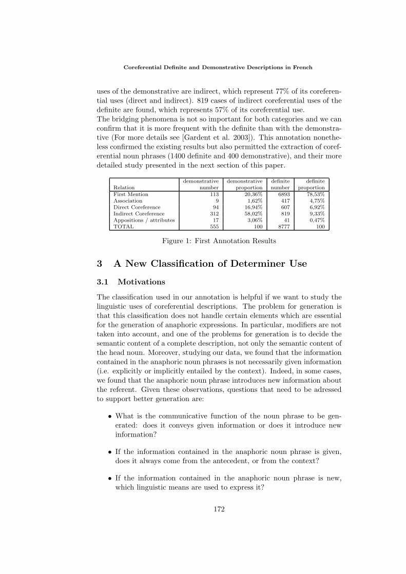
Coreferential Definite and Demonstrative Descriptions in French
uses of the demonstrative are indirect, which represent 77% of its coreferen-tial uses (direct and indirect). 819 cases of indirect coreferential uses of thedefinite are found, which represents 57% of its coreferential use.The bridging phenomena is not so important for both categories and we canconfirm that it is more frequent with the definite than with the demonstra-tive (For more details see [Gardent et al. 2003]). This annotation nonethe-less confirmed the existing results but also permitted the extraction of coref-erential noun phrases (1400 definite and 400 demonstrative), and their moredetailed study presented in the next section of this paper.
demonstrative demonstrative definite definiteRelation number proportion number proportionFirst Mention 113 20,36% 6893 78,53%Association 9 1,62% 417 4,75%Direct Coreference 94 16,94% 607 6,92%Indirect Coreference 312 58,02% 819 9,33%Appositions / attributes 17 3,06% 41 0,47%TOTAL 555 100 8777 100
Figure 1: First Annotation Results
3 A New Classification of Determiner Use
3.1 Motivations
The classification used in our annotation is helpful if we want to study thelinguistic uses of coreferential descriptions. The problem for generation isthat this classification does not handle certain elements which are essentialfor the generation of anaphoric expressions. In particular, modifiers are nottaken into account, and one of the problems for generation is to decide thesemantic content of a complete description, not only the semantic content ofthe head noun. Moreover, studying our data, we found that the informationcontained in the anaphoric noun phrases is not necessarily given information(i.e. explicitly or implicitly entailed by the context). Indeed, in some cases,we found that the anaphoric noun phrase introduces new information aboutthe referent. Given these observations, questions that need to be adressedto support better generation are:
• What is the communicative function of the noun phrase to be gen-erated: does it conveys given information or does it introduce newinformation?
• If the information contained in the anaphoric noun phrase is given,does it always come from the antecedent, or from the context?
• If the information contained in the anaphoric noun phrase is new,which linguistic means are used to express it?
172
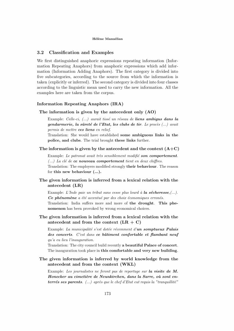
Helene Manuelian
3.2 Classification and Examples
We first distinguished anaphoric expressions repeating information (Infor-mation Repeating Anaphors) from anaphoric expressions which add infor-mation (Information Adding Anaphors). The first category is divided intofive subcategories, according to the source from which the information istaken (explicitly or inferred). The second category is divided into four classesaccording to the linguistic mean used to carry the new information. All theexamples here are taken from the corpus.
Information Repeating Anaphors (IRA)
The information is given by the antecedent only (AO)
Example: Celle-ci, (...) aurait tisse un reseau de liens ambigus dans la
gendarmerie, la surete de l’Etat, les clubs de tir. Le proces (...) avaitpermis de mettre ces liens en relief.Translation: She would have established some ambiguous links in thepolice, and clubs. The trial brought these links further.
The information is given by the antecedent and the context (A+C)
Example: Le patronat avait tres sensiblement modifie son comportement.(...) La cle de ce nouveau comportement tient en deux chiffres.Translation: The employers modified strongly their behaviour. The reasonfor this new behaviour (...).
The given information is inferred from a lexical relation with theantecedent (LR)
Example: L’Inde paie un tribut sans cesse plus lourd a la secheresse,(...).Ce phenomene a ete accentue par des choix economiques errones.Translation: India suffers more and more of the drought. This phe-nomenon has been provoked by wrong economical choices.
The given information is inferred from a lexical relation with theantecedent and from the context (LR + C)
Example: La municipalite s’est dotee recemment d’un somptueux Palais
des concerts. C’est dans ce batiment confortable et flambant neuf
qu’a eu lieu l’inauguration.Translation: The city council build recently a beautiful Palace of concert.The inauguration took place in this comfortable and very new building.
The given information is inferred by world knowledge from theantecedent and from the context (WKL)
Example: Les journalistes ne feront pas de reportage sur la visite de M.
Honecker au cimetiere de Neunkirchen, dans la Sarre, ou sont en-
terres ses parents. (...) apres que le chef d’Etat eut requis la ”tranquillite”
173
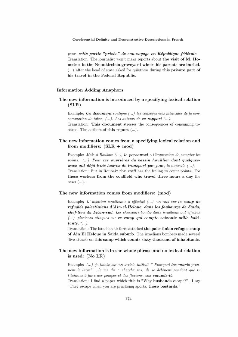
Coreferential Definite and Demonstrative Descriptions in French
pour cette partie ”privee” de son voyage en Republique federale.Translation: The journalist won’t make reports about the visit of M. Ho-necker in the Neunkirchen graveyard where his parents are buried.(...) after the head of state asked for quietness during this private part ofhis travel in the Federal Republic.
Information Adding Anaphors
The new information is introduced by a specifying lexical relation(SLR)
Example: Ce document souligne (...) les consequences medicales de la con-sommation de tabac, (...). Les auteurs de ce rapport (...).Translation: This document stresses the consequences of consuming to-bacco. The authors of this report (...).
The new information comes from a specifying lexical relation andfrom modifiers: (SLR + mod)
Example: Mais a Roubaix (...), le personnel a l’impression de compter lespoints. (...) Pour ces ouvrieres du bassin houillier dont quelques-
unes ont deja trois heures de transport par jour, la nouvelle (...).Translation: But in Roubaix the staff has the feeling to count points. Forthese workers from the coalfield who travel three hours a day thenews (...).
The new information comes from modifiers: (mod)
Example: L’ aviation israelienne a effectue (...) un raid sur le camp de
refugies palestiniens d’Ain-el-Heloue, dans les faubourgs de Saida,
chef-lieu du Liban-sud. Les chasseurs-bombardiers israeliens ont effectue(...) plusieurs attaques sur ce camp qui compte soixante-mille habi-
tants, (...).Translation: The Israelian air force attacked the palestinian refugee campof Ain El Heloue in Saida suburb. The israelians bombers made severaldive attacks on this camp which counts sixty thousand of inhabitants.
The new information is in the whole phrase and no lexical relationis used: (No LR)
Example: (...) je tombe sur un article intitule ” Pourquoi les maris pren-nent le large”. Je me dis : cherche pas, ils se debinent pendant que tut’echines a faire des pompes et des flexions, ces salauds-la.Translation: I find a paper which title is ”Why husbands escape?”. I say”They escape when you are practising sports, these bastards.”
174
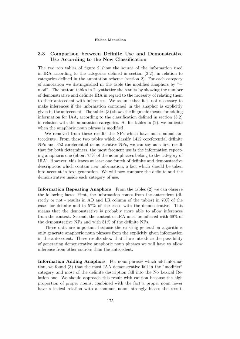
Helene Manuelian
3.3 Comparison between Definite Use and DemonstrativeUse According to the New Classification
The two top tables of figure 2 show the source of the information usedin IRA according to the categories defined in section (3.2), in relation tocategories defined in the annotation scheme (section 2). For each categoryof annotation we distinguished in the table the modified anaphors by ”+mod”. The bottom tables in 2 synthetize the results by showing the numberof demonstrative and definite IRA in regard to the necessity of relating themto their antecedent with inferences. We assume that it is not necessary tomake inferences if the information contained in the anaphor is explicitlygiven in the antecedent. The tables (3) shows the linguistic means for addinginformation for IAA, according to the classification defined in section (3.2)in relation with the annotation categories. As for tables in (2), we indicatewhen the anaphoric noun phrase is modified.
We removed from these results the NPs which have non-nominal an-tecedents. From these two tables which classify 1412 coreferential definiteNPs and 352 coreferential demonstrative NPs, we can say as a first resultthat for both determiners, the most frequent use is the information repeat-ing anaphoric one (about 75% of the noun phrases belong to the category ofIRA). However, this leaves at least one fourth of definite and demonstrativedescriptions which contain new information, a fact which should be takeninto account in text generation. We will now compare the definite and thedemonstrative inside each category of use.
Information Repeating Anaphors From the tables (2) we can observethe following facts: First, the information comes from the antecedent (di-rectly or not - results in AO and LR column of the tables) in 70% of thecases for definite and in 57% of the cases with the demonstrative. Thismeans that the demonstrative is probably more able to allow inferencesfrom the context. Second, the content of IRA must be inferred with 69% ofthe demonstrative NPs and with 51% of the definite NPs.
These data are important because the existing generation algorithmsonly generate anaphoric noun phrases from the explicitly given informationin the antecedent. These results show that if we introduce the possibilityof generating demonstrative anaphoric noun phrases we will have to allowinference from other sources than the antecedent.
Information Adding Anaphors For noun phrases which add informa-tion, we found (3) that the most IAA demonstrative fall in the ”modifier”category and most of the definite description fall into the No Lexical Re-lation one. We should approach this result with caution because the highproportion of proper nouns, combined with the fact a proper noun neverhave a lexical relation with a common noun, strongly biases the result,
175
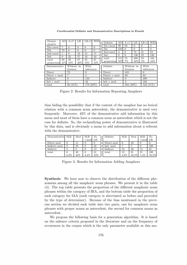
Coreferential Definite and Demonstrative Descriptions in French
Demon-strative
AO A+C LR LR+C WKL
Dir+mod 7 4 0 0 0Dir 72 0 0 0 0Ind+mod 1 0 10 15 17Ind 0 22 57 10 44total 80 26 67 25 61proportion 21% 10% 26% 10% 23%
Definite AO A+C LR LR+C WKLDir+mod 90 59 0 0 4Dir 410 0 0 0 0Ind+mod 4 6 72 31 53Ind 0 9 136 22 126total 511 73 208 53 183proportion 50% 7% 20% 5% 18%
Demonstrative Without in-ferences
Withinferences
Direct 72 0Direct + mod 7 4Indirect 0 133Ind + mod 1 42total 80 (21%) 179 (69%)
Definite Without in-ferences
Withinferences
Direct 410 0Direct + mod 90 63Indirect 0 299Ind + mod 4 162total 504 (49%) 524 (51%)
Figure 2: Results for Information Repeating Anaphors
thus hiding the possibility that if the content of the anaphor has no lexicalrelation with a common noun antecedent, the demonstrative is used veryfrequently. Moreover, 43% of the demonstrative add information by thismean and most of them have a common noun as antecedent which is not thecase for definite. So, the reclassifying power of demonstrative is illustratedby this data, and is obviously a mean to add information about a referentwith the demonstrative.
Demonstrative SLR Mod SLR+mod
NoLR
Direct mod 0 11 0 0Indirect mod 2 33 8 22Indirect 4 0 0 13total 6
6,3%4042%
88,4%
4143%
Definite SLR Mod SLR+mod
NoLR
Direct mod 0 43 0 0Ind. mod 1 7 0 108Indirect 12 38 14 61total 13
4,6%8128,5%
217,4%
16959,5%
Figure 3: Results for Information Adding Anaphors
Synthesis We have now to observe the distribution of the different phe-nomena among all the anaphoric noun phrases. We present it in the table(4). The top table presents the proportion of the different anaphoric nounphrases within the category of IRA, and the bottom table the proportion ofeach category for IAA (each category is abreviated as before and precededby the type of determiner). Because of the bias mentioned in the previ-ous section we divided each table into two parts, one for anaphoric nounphrases with proper nouns as antecedent, the second for common nouns asantecedent.
We propose the following basis for a generation algorithm. It is basedon the salience criteria proposed in the literature and on the frequency ofoccurences in the corpus which is the only parameter available at this mo-
176
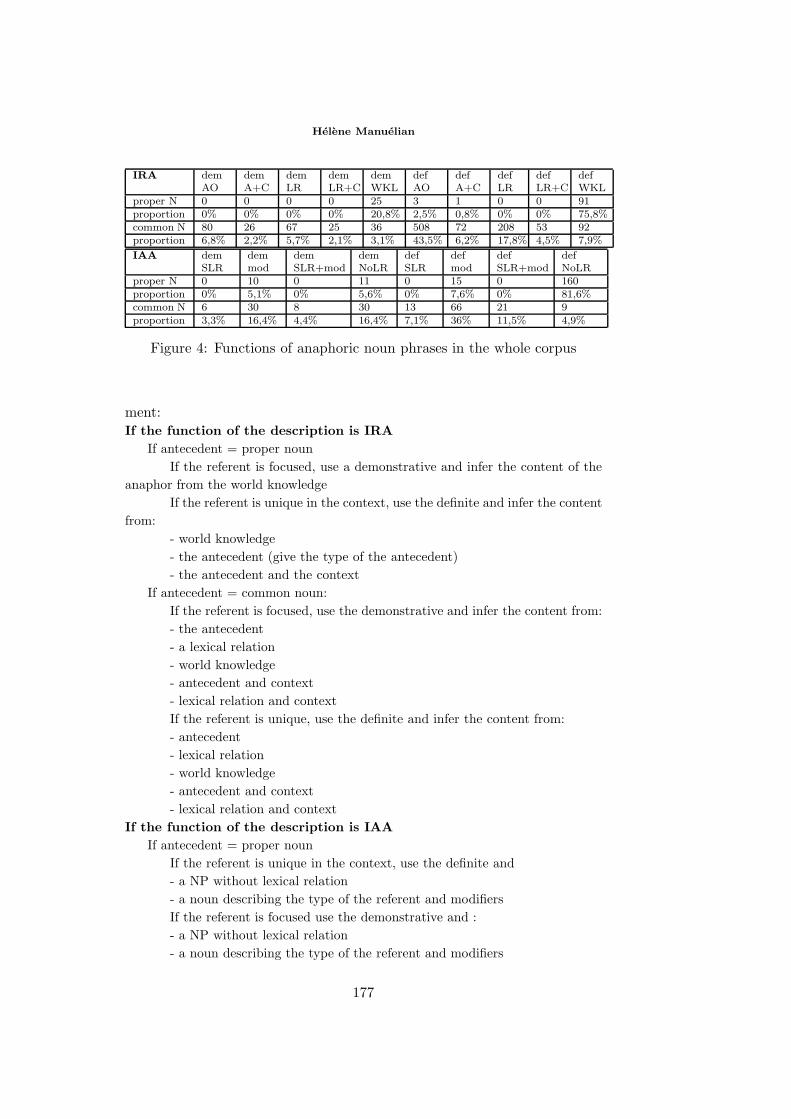
Helene Manuelian
IRA demAO
demA+C
demLR
demLR+C
demWKL
defAO
defA+C
defLR
defLR+C
defWKL
proper N 0 0 0 0 25 3 1 0 0 91proportion 0% 0% 0% 0% 20,8% 2,5% 0,8% 0% 0% 75,8%common N 80 26 67 25 36 508 72 208 53 92proportion 6,8% 2,2% 5,7% 2,1% 3,1% 43,5% 6,2% 17,8% 4,5% 7,9%
IAA demSLR
demmod
demSLR+mod
demNoLR
defSLR
defmod
defSLR+mod
defNoLR
proper N 0 10 0 11 0 15 0 160proportion 0% 5,1% 0% 5,6% 0% 7,6% 0% 81,6%common N 6 30 8 30 13 66 21 9proportion 3,3% 16,4% 4,4% 16,4% 7,1% 36% 11,5% 4,9%
Figure 4: Functions of anaphoric noun phrases in the whole corpus
ment:If the function of the description is IRA
If antecedent = proper nounIf the referent is focused, use a demonstrative and infer the content of the
anaphor from the world knowledgeIf the referent is unique in the context, use the definite and infer the content
from:- world knowledge- the antecedent (give the type of the antecedent)- the antecedent and the context
If antecedent = common noun:If the referent is focused, use the demonstrative and infer the content from:- the antecedent- a lexical relation- world knowledge- antecedent and context- lexical relation and contextIf the referent is unique, use the definite and infer the content from:- antecedent- lexical relation- world knowledge- antecedent and context- lexical relation and context
If the function of the description is IAAIf antecedent = proper noun
If the referent is unique in the context, use the definite and- a NP without lexical relation- a noun describing the type of the referent and modifiersIf the referent is focused use the demonstrative and :- a NP without lexical relation- a noun describing the type of the referent and modifiers
177
Coreferential Definite and Demonstrative Descriptions in French
If antecedent = common nounIf the referent is unique in the context, use the definite and :- modifiers- specifying lexical relation and modifiers,- specifying lexical relation- a NP without lexical relation
If antecedent = common noun and if focused, use the demonstrative and- equally use modifiers or a NP without lexical relation- a specifying lexical relation and modifiers- lexical relation
4 Conclusion and Future Work
In this paper we laid the ground for an extension of the existing genera-tion algorithms for referring expressions which would encompass not onlyanaphoric definite descriptions but also anaphoric demonstrative descrip-tions. Based on the classification proposed in the literature, we describedthe results of a first corpus analysis. We then proposed a more detailed clas-sification whose classes are arguably needed for a better specification of thedifferent uses of definite and demonstrative. We applied this classificationto the corpus thereby extracting from the resulting analysis interesting factsabout both definite and demonstrative. We ended by sketching the basis ofan algorithm supporting the choice between the two determiners. This studymust be completed by adding parameters to lead to a real algorithm. Theseparameters could be discourse-linked restrictions (position in the anaphoricchain for example) or syntactic restrictions (distance from the antecedent,grammatical functions of the antecedent...).
5 Acknowledgements
I would like to thank Claire Gardent for her precious help and support,and Eric Kow for all the scripts and programmes he wrote for the corpusexploitation.
References
[Beaumont et al. 1998] Beaumont C., Lecomte J., et Hatout N., (1998) Etiquetagemorpho-syntaxique du corpus ”Le Monde” pour les besoins du projet PAROLE,Technical Report, INALF, Nancy.
[Clark, 1977] Clark H.H., Bridging Thinking: Readings in Cognitive Science,Johnson-Laird P.N., Wason P.C. (eds), Cambridge, Cambridge UniversityPress.
178
Helene Manuelian
[Corblin, 1987] Corblin F. (1987), Indefini, Defini et Demonstratif, Geneve, Paris,Droz.
[Corblin, 1999] Corblin F. (1999), Les references mentionnelles : le premier, ledernier, celui-ci. In La reference (2) Statut et processus, Mettouch A. andQuinyin H. (eds.), Travaux linguistiques du CERLICO, Rennes, PUF.
[Corley et al., 2001] Corley S., Corley M., Keller F., Crocker M.W., et Trewin S.,(2001) Finding Syntactic Structure in Unparsed Corpora : The Gsearch corpusquery system, Computer and Humanities, 35(2), pp81-94.
[Dale et Reiter, 1995] Dale R. Reiter E., (1995), Computational Interprerationsof the Gricean Maxims in the Generation of Referring Expressions CognitiveSciences 19(2), pp233-263.
[Gardent, Striegnitz, 2000] Gardent C., Striegnitz K., (2000), Generating IndirectAnaphora, proceedings of IWCS’00 (International Workshop on Computa-tional Semantics).
[Gardent et al. 2003] Gardent C., Manuelian H., Kow E., (2003), Which Bridgesfor Bridging Descriptions, in EACL Workshop on Linguistically InterpretedCorpora proceedings.
[Kleiber, 1986] Kleiber G., (1986), Pour une explication du paradoxe de la repriseimmediate un N - le N / un N - Ce N Langue Francaise, 72, pp 54-79.
[Kleiber, 1988] Kleiber G., (1988), Reprise immediate et theorie des contrastes,Studia Romanica Posnaniensa, 13, pp 67-83.
[Krahmer et al., 2001] Krahmer E., van Erk S., Verleg A., (2001), A Meta-Algorithm for the Generation of Referring Expressions, proceedings of 8thEuropean Workshop on Natural Language Generation pp 29-39.
[Lecomte, 1997] Lecomte J., (1997) Codage Multext - GRACE pour l’actionGRACE / Multitag, Technical Report, INALF, Nancy.
[Manuelian, 2002] Manuelian H., (2002), Annotation des descriptions definies : lecas des reprises par les roles thematiques, proceedings of RECITAL 2002,Nancy, France, pp455-467.
[Manuelian, 2003] Manuelian H., (2003), Une analyse du demonstratif en corpus,proceedings of TALN 2003, Batz sur Mer, France.
[Muller, Strube, 2001] Muller C., Strube M., (2001) Annotating Anaphoric andBridging Relations with MMAX, proceedings of 2nd SIGDial Workshop onDiscourse and Dialogue, pp90-95.
[Poesio, Vieira 1998] Poesio M., Vieira R., (1998), A Corpus Based Investigationof Definite Description Use, Computational Linguistics, 24-2 pp183-216.
[Vieira et al. 2002] Vieira R., Salmon-Alt S., Gasperin C., Schang E., Othero G.,(2002), Coreference and Anaphoric Relations of Demonstrative Noun Phrasesin a Multilingual Corpus, proceedings of DAARC.
[Van Deemter, 2000] Van Deemter K., (2000), Generating Vague Descriptions, pro-ceedings of First International Conference on Natural Language Generation,pp 179-186.
179

Coreferential Definite and Demonstrative Descriptions in French
[Van Deemter, 2001] Van Deemter K., (2001), Logical Form Equivalence : the Caseof Referring Expressions Generation, proceedings of 8th European Workshopon Natural Language Generation 21-29.
180
Formalizing a Constituency Based DynamicGrammar
ALESSANDRO MAZZEI
Dip. Informatica, Universita di Torino
ABSTRACT. Dynamic grammars are a grammatical formalism that describes the derivationand recognition processes via dynamics: a string is derived and parsed as a consequence of atransition between states. This paper formalizes tree adjoining based dynamic grammar (DV-TAG). In particular, we show that DV-TAG is adequate to describe some linguistic phenomena,and that we can also generate languages beyond the context-free power.
1 Introduction
Incrementality is a property of natural language understanding: humans build uppartial analyses of the sentences as soon as the words are heard or seen ([MW73]).This property has important effects at syntactic and semantic analysis level: thelanguage processor interprets syntactic structures, word by word, and incremen-tally produces semantic representation.
In two ways a syntactic theory can satisfy incrementality: working at perfor-mance level, it can respect the constraints in parsing and derivation strategies. Orworking at competence level, it can modify the grammatical formalism, thus thegrammar derives only structures that respect incremental constraints. In the lattercase we fulfill the transparency hypothesis ([BW84]): a syntactic theory must re-flect the behaviour of the human syntactic processor in its formal operations.Stabler (cf. [Sta94]) formalized a stronger property (that we call strong incre-mentality): people incorporate each word into a single, totally connected syntacticstructure before any further words follow. Incremental interpretation is achievedinterpreting this single connected syntactic structure.
Dynamic grammars1 can satisfy the strong incrementality and transparency hy-pothesis both: the time evolution of a single fully connected syntactic structure isgoverned by the appearance of lexical items. The syntactic process in a dynamicgrammar is a sequence of transitions between adjacent states Si−1 and Si movingfrom left to right in the input string.
1cf. [Gel98] for an overview of the dynamic paradigm in cognitive science.
Proceedings of the Eighth ESSLLI Student SessionBalder ten Cate (editor)Chapter 17, Copyright c© 2003, Alessandro Mazzei
181
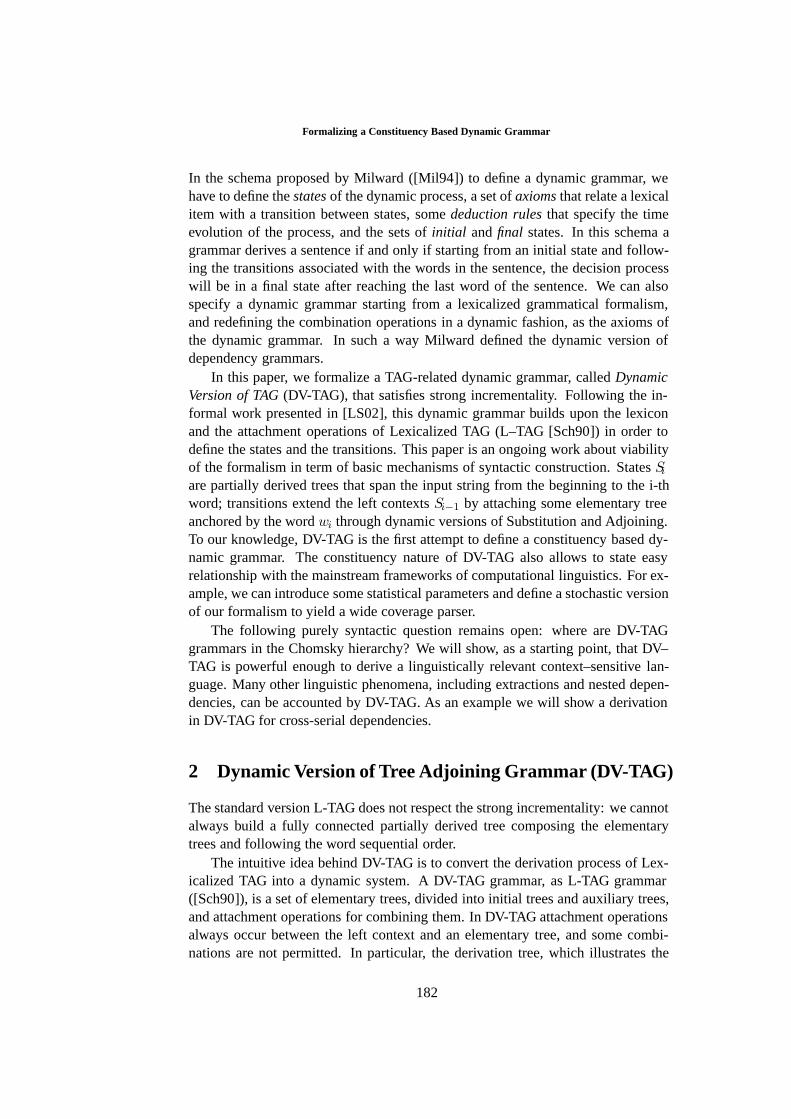
Formalizing a Constituency Based Dynamic Grammar
In the schema proposed by Milward ([Mil94]) to define a dynamic grammar, wehave to define the states of the dynamic process, a set of axioms that relate a lexicalitem with a transition between states, some deduction rules that specify the timeevolution of the process, and the sets of initial and final states. In this schema agrammar derives a sentence if and only if starting from an initial state and follow-ing the transitions associated with the words in the sentence, the decision processwill be in a final state after reaching the last word of the sentence. We can alsospecify a dynamic grammar starting from a lexicalized grammatical formalism,and redefining the combination operations in a dynamic fashion, as the axioms ofthe dynamic grammar. In such a way Milward defined the dynamic version ofdependency grammars.
In this paper, we formalize a TAG-related dynamic grammar, called DynamicVersion of TAG (DV-TAG), that satisfies strong incrementality. Following the in-formal work presented in [LS02], this dynamic grammar builds upon the lexiconand the attachment operations of Lexicalized TAG (L–TAG [Sch90]) in order todefine the states and the transitions. This paper is an ongoing work about viabilityof the formalism in term of basic mechanisms of syntactic construction. States Si
are partially derived trees that span the input string from the beginning to the i-thword; transitions extend the left contexts Si−1 by attaching some elementary treeanchored by the word wi through dynamic versions of Substitution and Adjoining.To our knowledge, DV-TAG is the first attempt to define a constituency based dy-namic grammar. The constituency nature of DV-TAG also allows to state easyrelationship with the mainstream frameworks of computational linguistics. For ex-ample, we can introduce some statistical parameters and define a stochastic versionof our formalism to yield a wide coverage parser.
The following purely syntactic question remains open: where are DV-TAGgrammars in the Chomsky hierarchy? We will show, as a starting point, that DV–TAG is powerful enough to derive a linguistically relevant context–sensitive lan-guage. Many other linguistic phenomena, including extractions and nested depen-dencies, can be accounted by DV-TAG. As an example we will show a derivationin DV-TAG for cross-serial dependencies.
2 Dynamic Version of Tree Adjoining Grammar (DV-TAG)
The standard version L-TAG does not respect the strong incrementality: we cannotalways build a fully connected partially derived tree composing the elementarytrees and following the word sequential order.
The intuitive idea behind DV-TAG is to convert the derivation process of Lex-icalized TAG into a dynamic system. A DV-TAG grammar, as L-TAG grammar([Sch90]), is a set of elementary trees, divided into initial trees and auxiliary trees,and attachment operations for combining them. In DV-TAG attachment operationsalways occur between the left context and an elementary tree, and some combi-nations are not permitted. In particular, the derivation tree, which illustrates the
182
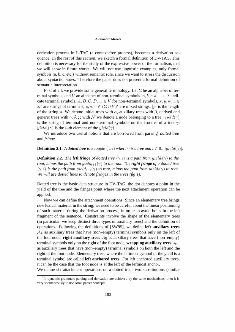
Alessandro Mazzei
derivation process in L-TAG (a context-free process), becomes a derivation se-quence. In the rest of this section, we sketch a formal definition of DV-TAG. Thisdefinition is necessary for the study of the expressive power of the formalism, thatwe will show in future works. We will not use linguistic examples, only formalsymbols (a, b, c, etc.) without semantic role, since we want to stress the discussionabout syntactic issues. Therefore the paper does not present a formal definition ofsemantic interpretation.
First of all, we provide some general terminology. Let Σ be an alphabet of ter-minal symbols, and V an alphabet of non–terminal symbols. a, b, c, d, ... ∈ Σ indi-cate terminal symbols, A,B,C,D, ... ∈ V for non–terminal symbols, x, y,w, z ∈Σ∗ are strings of terminals, ρ, σ, τ ∈ (Σ ∪ V )∗ are mixed strings; |ρ| is the lengthof the string ρ. We denote initial trees with α, auxiliary trees with β, derived andgeneric trees with γ, δ, ζ; with N we denote a node belonging to a tree. yield(γ)is the string of terminal and non–terminal symbols on the frontier of a tree γ;yieldi(γ) is the i–th element of the yield(γ).
We introduce two useful notions that are borrowed from parsing2 dotted treeand fringe.
Definition 2.1. A dotted tree is a couple 〈γ, i〉where γ is a tree and i ∈ 0...|yield(γ)|.
Definition 2.2. The left fringe of dotted tree 〈γ, i〉 is a path from yieldi(γ) to theroot, minus the path from yieldi+1(γ) to the root. The right fringe of a dotted tree〈γ, i〉 is the path from yieldi+1(γ) to root, minus the path from yieldi(γ) to root.We will use dotted lines to denote fringes in the trees (fig 1).
Dotted tree is the basic data structure in DV–TAG: the dot denotes a point in theyield of the tree and the fringes point where the next attachment operation can beapplied.
Now we can define the attachment operations. Since an elementary tree bringsnew lexical material in the string, we need to be careful about the linear positioningof such material during the derivation process, in order to avoid holes in the leftfragment of the sentence. Constraints involve the shape of the elementary trees(in particular, we keep distinct three types of auxiliary trees) and the definition ofoperations. Following the definitions of [SW95], we define left auxiliary treesAL as auxiliary trees that have (non–empty) terminal symbols only on the left ofthe foot node, right auxiliary trees AR as auxiliary trees that have (non–empty)terminal symbols only on the right of the foot node, wrapping auxiliary trees AW
as auxiliary trees that have (non–empty) terminal symbols on both the left and theright of the foot node. Elementary trees where the leftmost symbol of the yield is aterminal symbol are called left anchored trees. For left anchored auxiliary trees,it can be the case that the foot node is at the left of the leftmost anchor.We define six attachment operations on a dotted tree: two substitutions (similar
2In dynamic grammars parsing and derivation are achieved by the same mechanisms, then it isvery spontaneously to use some parser concepts.
183
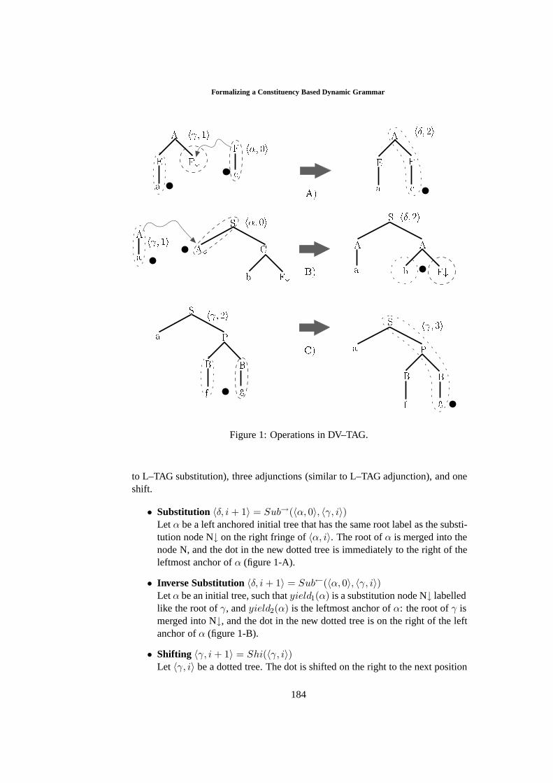
Formalizing a Constituency Based Dynamic Grammar
Æ
Æ
Figure 1: Operations in DV–TAG.
to L–TAG substitution), three adjunctions (similar to L–TAG adjunction), and oneshift.
• Substitution 〈δ, i + 1〉 = Sub→(〈α, 0〉, 〈γ, i〉)Let α be a left anchored initial tree that has the same root label as the substi-tution node N↓ on the right fringe of 〈α, i〉. The root of α is merged into thenode N, and the dot in the new dotted tree is immediately to the right of theleftmost anchor of α (figure 1-A).
• Inverse Substitution 〈δ, i + 1〉 = Sub←(〈α, 0〉, 〈γ, i〉)Let α be an initial tree, such that yield1(α) is a substitution node N↓ labelledlike the root of γ, and yield2(α) is the leftmost anchor of α: the root of γ ismerged into N↓, and the dot in the new dotted tree is on the right of the leftanchor of α (figure 1-B).
• Shifting 〈γ, i + 1〉 = Shi(〈γ, i〉)Let 〈γ, i〉 be a dotted tree. The dot is shifted on the right to the next position
184
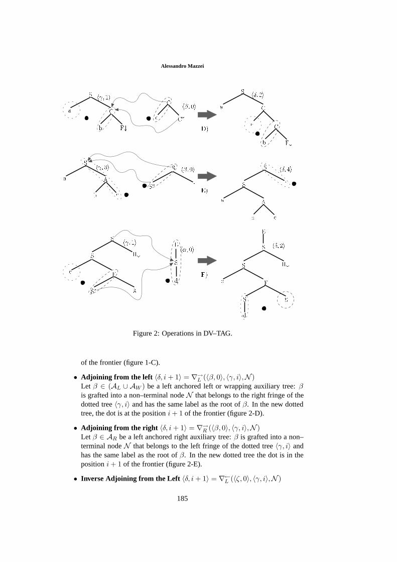
Alessandro Mazzei
Æ
Æ
Æ
Figure 2: Operations in DV–TAG.
of the frontier (figure 1-C).
• Adjoining from the left 〈δ, i + 1〉 = ∇→L (〈β, 0〉, 〈γ, i〉,N )Let β ∈ (AL ∪ AW ) be a left anchored left or wrapping auxiliary tree: βis grafted into a non–terminal node N that belongs to the right fringe of thedotted tree 〈γ, i〉 and has the same label as the root of β. In the new dottedtree, the dot is at the position i + 1 of the frontier (figure 2-D).
• Adjoining from the right 〈δ, i + 1〉 = ∇→R (〈β, 0〉, 〈γ, i〉,N )Let β ∈ AR be a left anchored right auxiliary tree: β is grafted into a non–terminal node N that belongs to the left fringe of the dotted tree 〈γ, i〉 andhas the same label as the root of β. In the new dotted tree the dot is in theposition i + 1 of the frontier (figure 2-E).
• Inverse Adjoining from the Left 〈δ, i + 1〉 = ∇←L (〈ζ, 0〉, 〈γ, i〉,N )
185
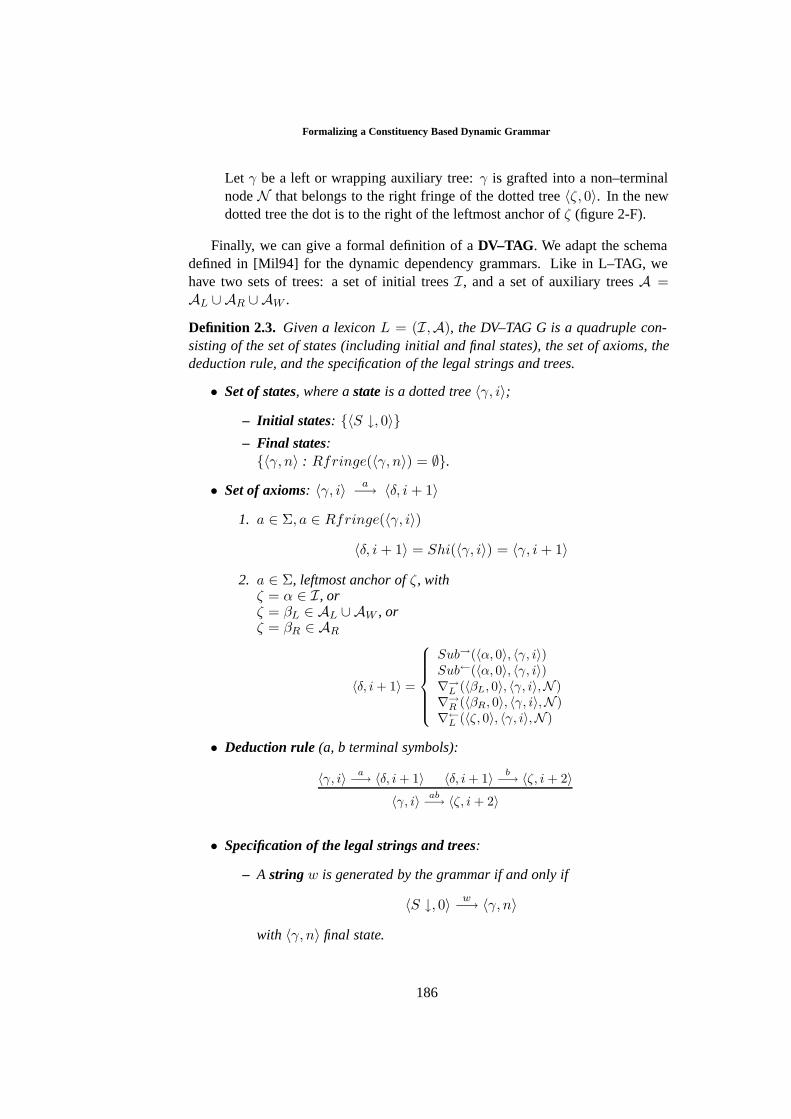
Formalizing a Constituency Based Dynamic Grammar
Let γ be a left or wrapping auxiliary tree: γ is grafted into a non–terminalnode N that belongs to the right fringe of the dotted tree 〈ζ, 0〉. In the newdotted tree the dot is to the right of the leftmost anchor of ζ (figure 2-F).
Finally, we can give a formal definition of a DV–TAG. We adapt the schemadefined in [Mil94] for the dynamic dependency grammars. Like in L–TAG, wehave two sets of trees: a set of initial trees I , and a set of auxiliary trees A =AL ∪ AR ∪ AW .
Definition 2.3. Given a lexicon L = (I,A), the DV–TAG G is a quadruple con-sisting of the set of states (including initial and final states), the set of axioms, thededuction rule, and the specification of the legal strings and trees.
• Set of states, where a state is a dotted tree 〈γ, i〉;– Initial states: 〈S ↓, 0〉– Final states:〈γ, n〉 : Rfringe(〈γ, n〉) = ∅.
• Set of axioms: 〈γ, i〉 a−→ 〈δ, i + 1〉1. a ∈ Σ, a ∈ Rfringe(〈γ, i〉)
〈δ, i + 1〉 = Shi(〈γ, i〉) = 〈γ, i + 1〉2. a ∈ Σ, leftmost anchor of ζ , with
ζ = α ∈ I , orζ = βL ∈ AL ∪ AW , orζ = βR ∈ AR
〈δ, i + 1〉 =
Sub→(〈α, 0〉, 〈γ, i〉)Sub←(〈α, 0〉, 〈γ, i〉)∇→L (〈βL, 0〉, 〈γ, i〉,N )∇→R (〈βR, 0〉, 〈γ, i〉,N )∇←L (〈ζ, 0〉, 〈γ, i〉,N )
• Deduction rule (a, b terminal symbols):
〈γ, i〉 a−→ 〈δ, i + 1〉 〈δ, i + 1〉 b−→ 〈ζ, i + 2〉〈γ, i〉 ab−→ 〈ζ, i + 2〉
• Specification of the legal strings and trees:
– A string w is generated by the grammar if and only if
〈S ↓, 0〉 w−→ 〈γ, n〉with 〈γ, n〉 final state.
186
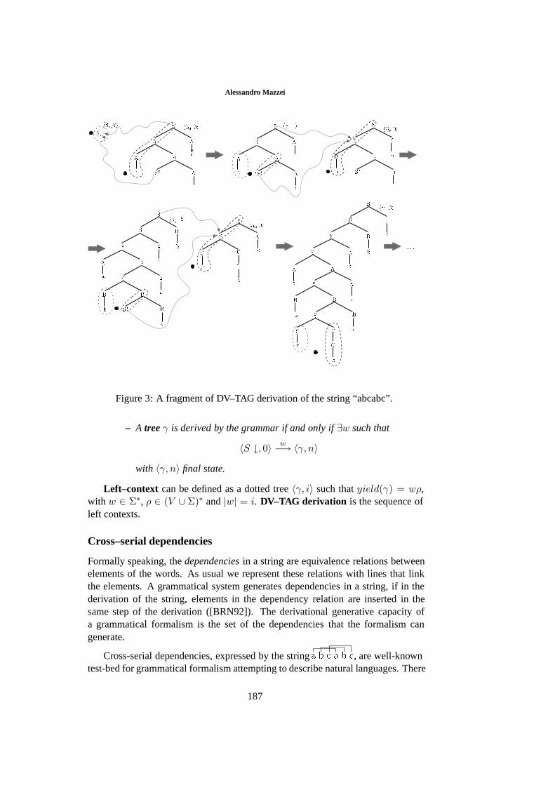
Alessandro Mazzei
Figure 3: A fragment of DV–TAG derivation of the string “abcabc”.
– A tree γ is derived by the grammar if and only if ∃w such that
〈S ↓, 0〉 w−→ 〈γ, n〉with 〈γ, n〉 final state.
Left–context can be defined as a dotted tree 〈γ, i〉 such that yield(γ) = wρ,with w ∈ Σ∗, ρ ∈ (V ∪ Σ)∗ and |w| = i. DV–TAG derivation is the sequence ofleft contexts.
Cross–serial dependencies
Formally speaking, the dependencies in a string are equivalence relations betweenelements of the words. As usual we represent these relations with lines that linkthe elements. A grammatical system generates dependencies in a string, if in thederivation of the string, elements in the dependency relation are inserted in thesame step of the derivation ([BRN92]). The derivational generative capacity ofa grammatical formalism is the set of the dependencies that the formalism cangenerate.
Cross-serial dependencies, expressed by the string , are well-knowntest-bed for grammatical formalism attempting to describe natural languages. There
187
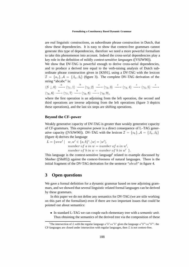
Formalizing a Constituency Based Dynamic Grammar
are real linguistic constructions, as subordinate phrase construction in Dutch, thatshow these dependencies. It is easy to show that context-free grammars cannotgenerate this type of dependencies, therefore we need a more powerful formalismto take this phenomenon into account. Indeed the cross-serial dependencies play akey role in the definition of mildly context-sensitive languages ([VSJW90]).We show that DV-TAG is powerful enough to derive cross-serial dependencies,and to produce a derived tree equal to the verb-raising analysis of Dutch sub-ordinate phrase construction given in [KS91], using a DV-TAG with the lexiconI = αc,A = βa, βb (figure 3). The complete DV–TAG derivation of thestring “abcabc” is:
〈S ↓, 0〉 a−−−→ 〈γ1, 1〉b−−−→ 〈γ2, 2〉
c−−−→ 〈γ3, 3〉ε−−−→ 〈γ4, 4〉
ε−−−→ 〈γ5, 5〉ε−−−→
〈γ6, 6〉a−−−→ 〈γ7, 7〉
b−−−→ 〈γ8, 8〉c−−−→ 〈γ9, 9〉,
where the first operation is an adjoining from the left operation, the second andthird operations are inverse adjoining from the left operations (figure 3 depictsthese operations), and the last six steps are shifting operations.
Beyond the CF–power
Weakly generative capacity of DV-TAG is greater than weakly generative capacityof CF-grammars. This expressive power is a direct consequence of L–TAG gener-ative capacity ([VSJW90]). DV–TAG with the lexicon I = αe,A = βa, βb(figure 4) derives the language
L = wew′ | w,w′ ∈ a, b∗, |w| = |w′|,number of a in w = number of a in w′,number of b in w = number of b in w′ .
This language is the context-sensitive language3 related to example discussed byShieber ([Shi85]) against the context-freeness of natural languages. There is theinitial fragment of the DV-TAG derivation for the sentence “abeab” in figure 4.
3 Open questions
We gave a formal definition for a dynamic grammar based on tree adjoining gram-mars, and we showed that several linguistic related formal languages can be derivedby these grammars.
In this paper we do not define any semantics for DV-TAG (we are stile workingon this part of the formalism) even if there are two important issues that could bepointed out about semantics:
• In standard L-TAG we can couple each elementary tree with a semantic unit.Thus obtaining the semantics of the derived tree via the composition of these
3The intersection of L with the regular language a∗b∗ea∗b∗ gives the language anbmeanbm: theCF-languages are closed under intersection with regular languages, then L is not context-free.
188

Alessandro Mazzei
Figure 4: A DV–TAG deriving a context–sensitive language
units. We have to distinguish adjoining and substitution through differentrules of semantic composition. We can say that “the derivation trees repre-sent predicate-argument structures” ([AR00]).
In DV-TAG, in order to satisfy the strong incrementality, and then to allowincremental construction of a derivation tree, we have to “augment” the el-ementary structures with nodes that are not projected by the lexical anchorof the tree4. To respect the semantic compositionality we have to define an“unification-substitution” operation to check which nodes of the elementarytree are yet in the partially derived tree ([LS02]). In this paper, we did notformalize this unification operation, because it does not change the expres-sive power of the formalism, even if it is necessary for linguistic reasons.
• In the standard TAG, the derivation tree plays a key role in the definition ofsemantic interpretation but, the way the derivation tree is built is irrelevant.In DV-TAG we have a more powerful structure, called derivation sequence,describing the derivation tree and also how it is built. In our opinion, seman-tics for DV-TAG could be better defined using this structure.
In the future work we will first draw the exact position of DV–TAG in Chomskyhierarchy, answering the question whether DV–TAGs are mildly context-sensitive
4This procedure resembles the type-raising procedure of CCG formalism ([Ste00])
189
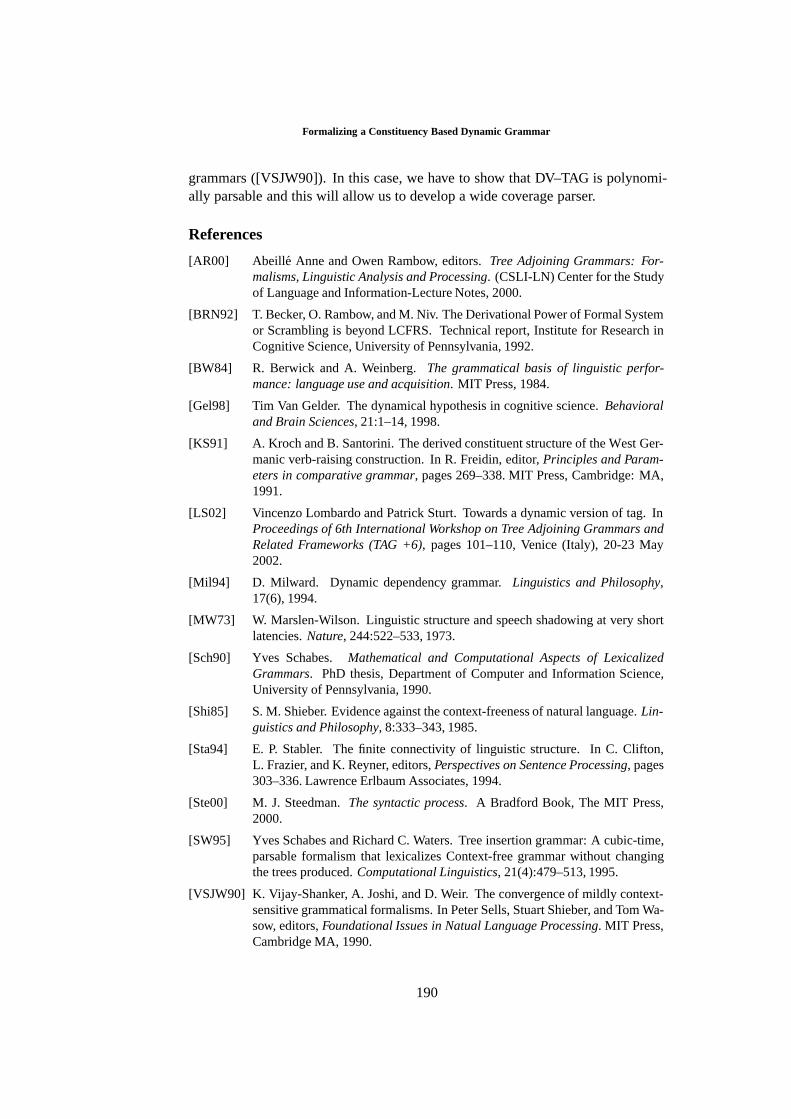
Formalizing a Constituency Based Dynamic Grammar
grammars ([VSJW90]). In this case, we have to show that DV–TAG is polynomi-ally parsable and this will allow us to develop a wide coverage parser.
References
[AR00] Abeille Anne and Owen Rambow, editors. Tree Adjoining Grammars: For-malisms, Linguistic Analysis and Processing. (CSLI-LN) Center for the Studyof Language and Information-Lecture Notes, 2000.
[BRN92] T. Becker, O. Rambow, and M. Niv. The Derivational Power of Formal Systemor Scrambling is beyond LCFRS. Technical report, Institute for Research inCognitive Science, University of Pennsylvania, 1992.
[BW84] R. Berwick and A. Weinberg. The grammatical basis of linguistic perfor-mance: language use and acquisition. MIT Press, 1984.
[Gel98] Tim Van Gelder. The dynamical hypothesis in cognitive science. Behavioraland Brain Sciences, 21:1–14, 1998.
[KS91] A. Kroch and B. Santorini. The derived constituent structure of the West Ger-manic verb-raising construction. In R. Freidin, editor, Principles and Param-eters in comparative grammar, pages 269–338. MIT Press, Cambridge: MA,1991.
[LS02] Vincenzo Lombardo and Patrick Sturt. Towards a dynamic version of tag. InProceedings of 6th International Workshop on Tree Adjoining Grammars andRelated Frameworks (TAG +6), pages 101–110, Venice (Italy), 20-23 May2002.
[Mil94] D. Milward. Dynamic dependency grammar. Linguistics and Philosophy,17(6), 1994.
[MW73] W. Marslen-Wilson. Linguistic structure and speech shadowing at very shortlatencies. Nature, 244:522–533, 1973.
[Sch90] Yves Schabes. Mathematical and Computational Aspects of LexicalizedGrammars. PhD thesis, Department of Computer and Information Science,University of Pennsylvania, 1990.
[Shi85] S. M. Shieber. Evidence against the context-freeness of natural language. Lin-guistics and Philosophy, 8:333–343, 1985.
[Sta94] E. P. Stabler. The finite connectivity of linguistic structure. In C. Clifton,L. Frazier, and K. Reyner, editors, Perspectives on Sentence Processing, pages303–336. Lawrence Erlbaum Associates, 1994.
[Ste00] M. J. Steedman. The syntactic process. A Bradford Book, The MIT Press,2000.
[SW95] Yves Schabes and Richard C. Waters. Tree insertion grammar: A cubic-time,parsable formalism that lexicalizes Context-free grammar without changingthe trees produced. Computational Linguistics, 21(4):479–513, 1995.
[VSJW90] K. Vijay-Shanker, A. Joshi, and D. Weir. The convergence of mildly context-sensitive grammatical formalisms. In Peter Sells, Stuart Shieber, and Tom Wa-sow, editors, Foundational Issues in Natual Language Processing. MIT Press,Cambridge MA, 1990.
190
Exploiting Sequent Structure in
Membership Algorithms for the Lambek
Calculus
Ryan T. McDonaldDepartment of Computer and Information Science
University of Pennsylvania
Abstract. This paper will examine the open problem of whether or not a se-quent is derivable in the Lambek Calculus (L) in polynomial-time. This will bedone through an investigation of Lambek Calculus Graphs (LC-Graphs), whichwere introduced by Penn[7] to represent the well-formedness constraints of a se-quent’s derivation in L. Presented here is a simplified version of LC-Graphs andtheir integrity criteria. We also show that storing a small amount of structuralinformation about a sequent during parsing can reduce the number of integritycriteria for LC-Graphs from four to two. To this effect, a polynomial-time mem-bership algorithm is presented that recognizes all derivable sequents and falselyrecognizes an identifiable class of underivable sequents.
1 Introduction
Substructural logics are a group of logics whose proof systems only use asubset of the structural rules of classical proof systems. The most wellknown substructural logics include Relevance Logic, which does not employweakening, and Girard’s[3] Linear Logic, which uses neither weakening norcontraction. The complexity of membership algorithms for these logics iswell studied with results often proving their intractability [4, 5].
Also in the class of substructural logics is the Lambek Calculus (L),which has the following structural rules:
(/L) Γ′B Γ,A,Γ′′SΓ,A/B,Γ′,Γ′′S
(/R) Γ,BAΓA/B
(∗)(\L) Γ′B Γ,A,Γ′′S
Γ,Γ′,B\A,Γ′′S(\R) B,ΓA
ΓB\A
(∗)
(•L) Γ,A,B,Γ′SΓ,A•B,Γ′S
(•R) ΓA Γ′BΓ,Γ′A•B
* if Γ is non-empty.
These operators are known as left-implication (\), right-implication (/) andproduct (•), where A/B means looking for premise B on the right to imply A
Proceedings of the Eighth ESSLLI Student SessionBalder ten Cate (editor)Chapter 18, Copyright c© 2003, Ryan T. McDonald
191
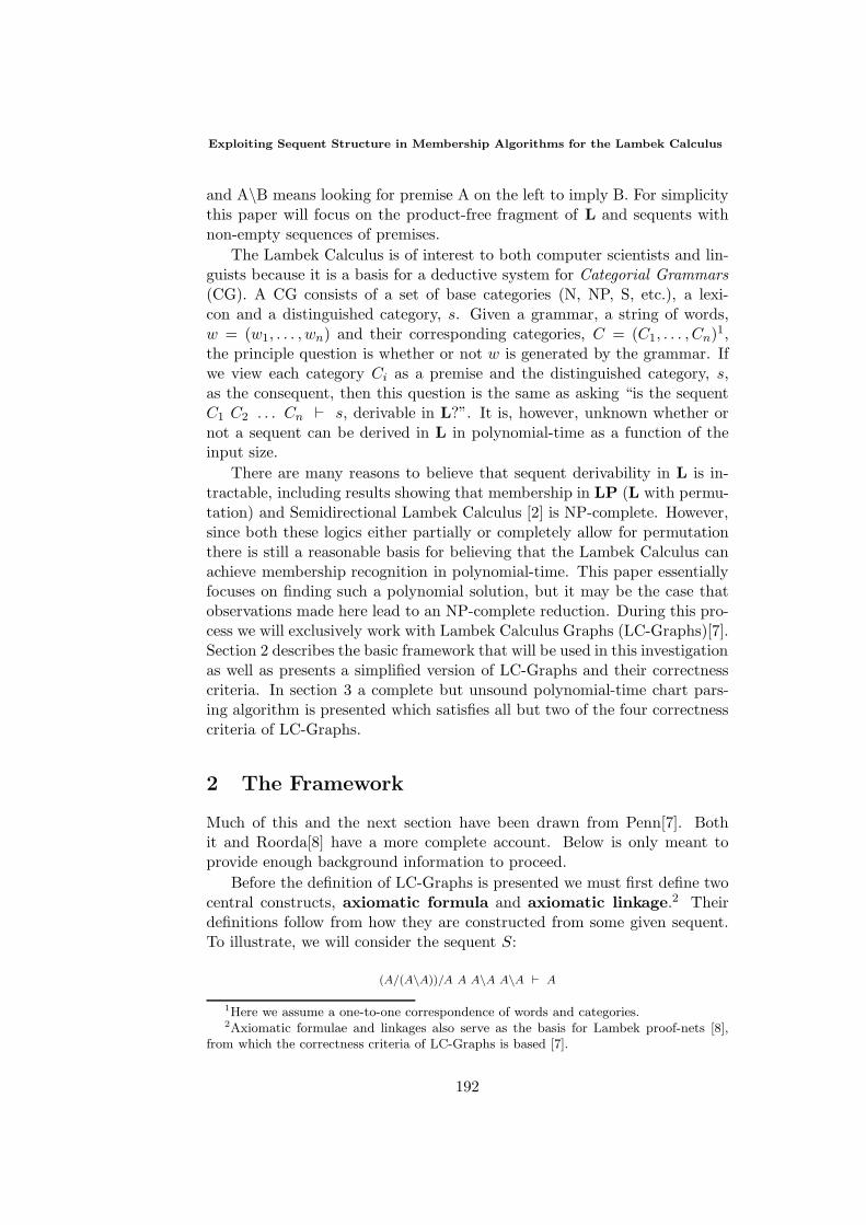
Exploiting Sequent Structure in Membership Algorithms for the Lambek Calculus
and A\B means looking for premise A on the left to imply B. For simplicitythis paper will focus on the product-free fragment of L and sequents withnon-empty sequences of premises.
The Lambek Calculus is of interest to both computer scientists and lin-guists because it is a basis for a deductive system for Categorial Grammars(CG). A CG consists of a set of base categories (N, NP, S, etc.), a lexi-con and a distinguished category, s. Given a grammar, a string of words,w = (w1, . . . , wn) and their corresponding categories, C = (C1, . . . , Cn)1,the principle question is whether or not w is generated by the grammar. Ifwe view each category Ci as a premise and the distinguished category, s,as the consequent, then this question is the same as asking “is the sequentC1 C2 . . . Cn s, derivable in L?”. It is, however, unknown whether ornot a sequent can be derived in L in polynomial-time as a function of theinput size.
There are many reasons to believe that sequent derivability in L is in-tractable, including results showing that membership in LP (L with permu-tation) and Semidirectional Lambek Calculus [2] is NP-complete. However,since both these logics either partially or completely allow for permutationthere is still a reasonable basis for believing that the Lambek Calculus canachieve membership recognition in polynomial-time. This paper essentiallyfocuses on finding such a polynomial solution, but it may be the case thatobservations made here lead to an NP-complete reduction. During this pro-cess we will exclusively work with Lambek Calculus Graphs (LC-Graphs)[7].Section 2 describes the basic framework that will be used in this investigationas well as presents a simplified version of LC-Graphs and their correctnesscriteria. In section 3 a complete but unsound polynomial-time chart pars-ing algorithm is presented which satisfies all but two of the four correctnesscriteria of LC-Graphs.
2 The Framework
Much of this and the next section have been drawn from Penn[7]. Bothit and Roorda[8] have a more complete account. Below is only meant toprovide enough background information to proceed.
Before the definition of LC-Graphs is presented we must first define twocentral constructs, axiomatic formula and axiomatic linkage.2 Theirdefinitions follow from how they are constructed from some given sequent.To illustrate, we will consider the sequent S:
(A/(A\A))/A A A\A A\A A
1Here we assume a one-to-one correspondence of words and categories.2Axiomatic formulae and linkages also serve as the basis for Lambek proof-nets [8],
from which the correctness criteria of LC-Graphs is based [7].
192
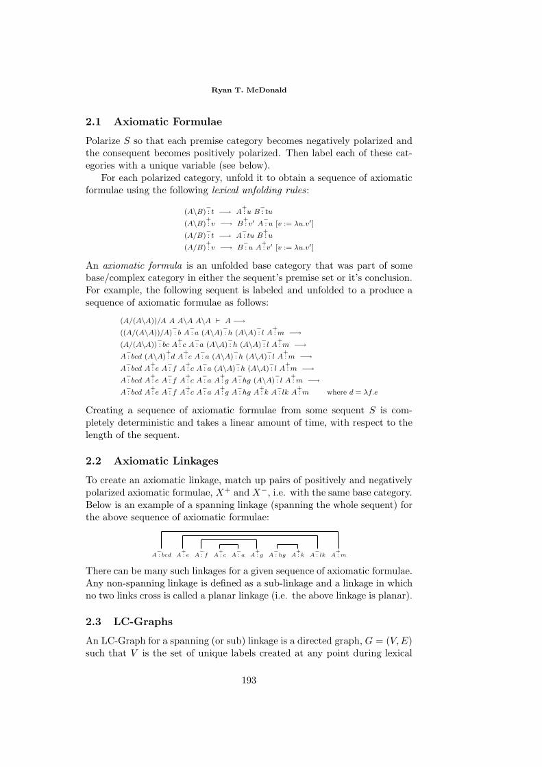
Ryan T. McDonald
2.1 Axiomatic Formulae
Polarize S so that each premise category becomes negatively polarized andthe consequent becomes positively polarized. Then label each of these cat-egories with a unique variable (see below).
For each polarized category, unfold it to obtain a sequence of axiomaticformulae using the following lexical unfolding rules:
(A\B)−: t −→ A
+: u B
−: tu
(A\B)+: v −→ B
+: v′ A
−: u [v := λu.v′]
(A/B)−: t −→ A
−: tu B
+: u
(A/B)+: v −→ B
−: u A
+: v′ [v := λu.v′]
An axiomatic formula is an unfolded base category that was part of somebase/complex category in either the sequent’s premise set or it’s conclusion.For example, the following sequent is labeled and unfolded to a produce asequence of axiomatic formulae as follows:
(A/(A\A))/A A A\A A\A A −→((A/(A\A))/A)
−: b A
−: a (A\A)
−: h (A\A)
−: l A
+: m −→
(A/(A\A))−: bc A
+: c A
−: a (A\A)
−: h (A\A)
−: l A
+: m −→
A−: bcd (A\A)
+: d A
+: c A
−: a (A\A)
−: h (A\A)
−: l A
+: m −→
A−: bcd A
+: e A
−: f A
+: c A
−: a (A\A)
−: h (A\A)
−: l A
+: m −→
A−: bcd A
+: e A
−: f A
+: c A
−: a A
+: g A
−: hg (A\A)
−: l A
+: m −→
A−: bcd A
+: e A
−: f A
+: c A
−: a A
+: g A
−: hg A
+: k A
−: lk A
+: m where d = λf.e
Creating a sequence of axiomatic formulae from some sequent S is com-pletely deterministic and takes a linear amount of time, with respect to thelength of the sequent.
2.2 Axiomatic Linkages
To create an axiomatic linkage, match up pairs of positively and negativelypolarized axiomatic formulae, X+ and X−, i.e. with the same base category.Below is an example of a spanning linkage (spanning the whole sequent) forthe above sequence of axiomatic formulae:
A−: bcd A
+: e A
−: f A
+: c A
−: a A
+: g A
−: hg A
+: k A
−: lk A
+: m
There can be many such linkages for a given sequence of axiomatic formulae.Any non-spanning linkage is defined as a sub-linkage and a linkage in whichno two links cross is called a planar linkage (i.e. the above linkage is planar).
2.3 LC-Graphs
An LC-Graph for a spanning (or sub) linkage is a directed graph, G = (V,E)such that V is the set of unique labels created at any point during lexical
193
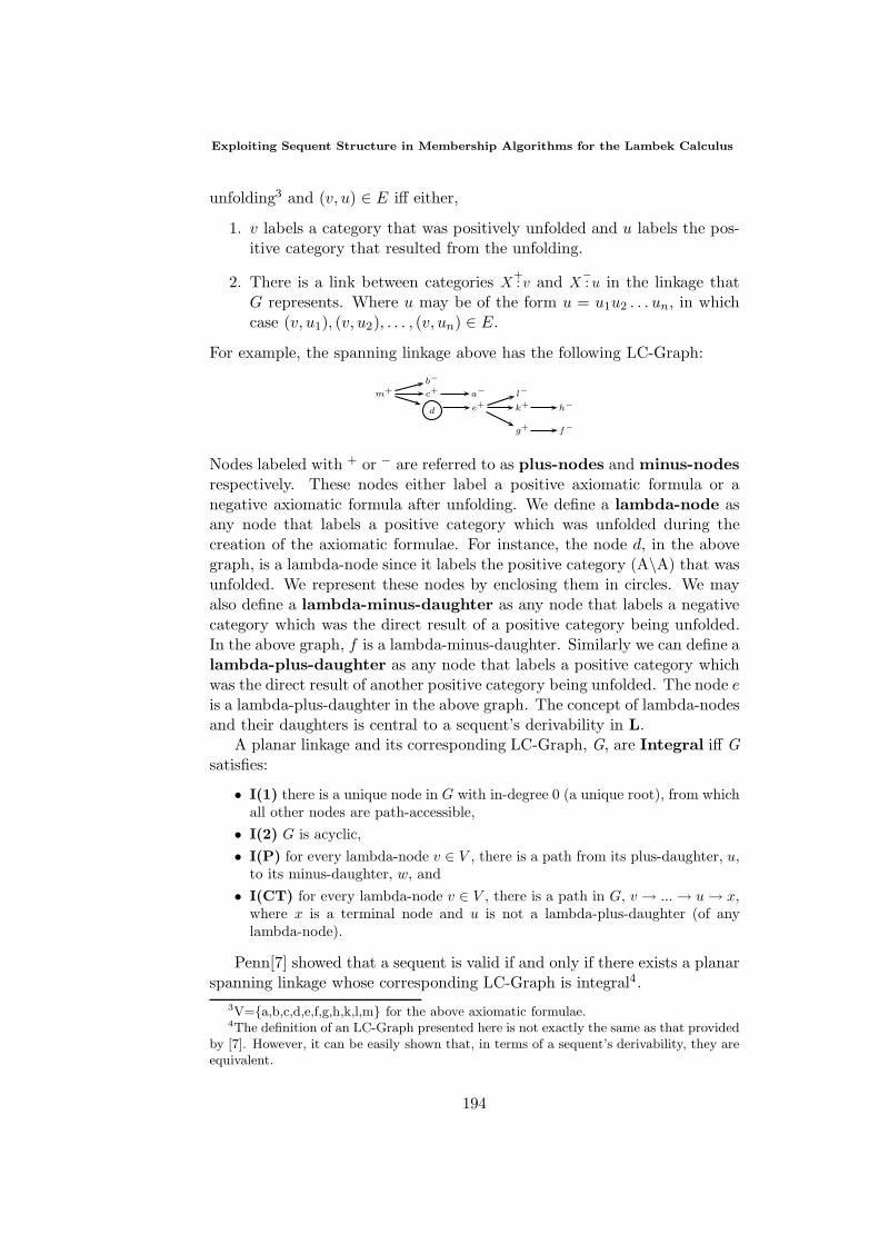
Exploiting Sequent Structure in Membership Algorithms for the Lambek Calculus
unfolding3 and (v, u) ∈ E iff either,
1. v labels a category that was positively unfolded and u labels the pos-itive category that resulted from the unfolding.
2. There is a link between categories X+: v and X
−: u in the linkage that
G represents. Where u may be of the form u = u1u2 . . . un, in whichcase (v, u1), (v, u2), . . . , (v, un) ∈ E.
For example, the spanning linkage above has the following LC-Graph:
b−
m+ c+ a− l−
d e+ k+ h−
g+ f−
Nodes labeled with + or − are referred to as plus-nodes and minus-nodesrespectively. These nodes either label a positive axiomatic formula or anegative axiomatic formula after unfolding. We define a lambda-node asany node that labels a positive category which was unfolded during thecreation of the axiomatic formulae. For instance, the node d, in the abovegraph, is a lambda-node since it labels the positive category (A\A) that wasunfolded. We represent these nodes by enclosing them in circles. We mayalso define a lambda-minus-daughter as any node that labels a negativecategory which was the direct result of a positive category being unfolded.In the above graph, f is a lambda-minus-daughter. Similarly we can define alambda-plus-daughter as any node that labels a positive category whichwas the direct result of another positive category being unfolded. The node eis a lambda-plus-daughter in the above graph. The concept of lambda-nodesand their daughters is central to a sequent’s derivability in L.
A planar linkage and its corresponding LC-Graph, G, are Integral iff Gsatisfies:
• I(1) there is a unique node in G with in-degree 0 (a unique root), from whichall other nodes are path-accessible,
• I(2) G is acyclic,• I(P) for every lambda-node v ∈ V , there is a path from its plus-daughter, u,
to its minus-daughter, w, and• I(CT) for every lambda-node v ∈ V , there is a path in G, v → ... → u → x,
where x is a terminal node and u is not a lambda-plus-daughter (of anylambda-node).
Penn[7] showed that a sequent is valid if and only if there exists a planarspanning linkage whose corresponding LC-Graph is integral4.
3V=a,b,c,d,e,f,g,h,k,l,m for the above axiomatic formulae.4The definition of an LC-Graph presented here is not exactly the same as that provided
by [7]. However, it can be easily shown that, in terms of a sequent’s derivability, they areequivalent.
194
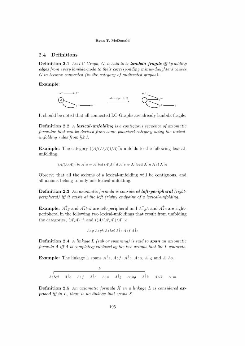
Ryan T. McDonald
2.4 Definitions
Definition 2.1 An LC-Graph, G, is said to be lambda-fragile iff by addingedges from every lambda-node to their corresponding minus-daughters causesG to become connected (in the category of undirected graphs).
Example:
m+ f−
d
e+ b−
add edge (d, f)
m+
d f−
e+ b−
It should be noted that all connected LC-Graphs are already lambda-fragile.
Definition 2.2 A lexical-unfolding is a contiguous sequence of axiomaticformulae that can be derived from some polarized category using the lexical-unfolding rules from §2.1.
Example: The category ((A/(A\A))/A)−: b unfolds to the following lexical-
unfolding,
(A/(A\A))−: bc A
+: c ⇒ A
−: bcd (A\A)
+: d A
+: c ⇒ A
−: bcd A
+: e A
−: f A
+: c
Observe that all the axioms of a lexical-unfolding will be contiguous, andall axioms belong to only one lexical-unfolding.
Definition 2.3 An axiomatic formula is considered left-peripheral (right-peripheral) iff it exists at the left (right) endpoint of a lexical-unfolding.
Example: A+: g and A
−: bcd are left-peripheral and A
−: gh and A
+: c are right-
peripheral in the following two lexical-unfoldings that result from unfoldingthe categories, (A\A)
−: h and ((A/(A\A))/A)
−: b
A+: g A
−: gh A
−: bcd A
+: e A
−: f A
+: c
Definition 2.4 A linkage L (sub or spanning) is said to span an axiomaticformula A iff A is completely enclosed by the two axioms that the L connects.
Example: The linkage L spans A+: e, A
−: f , A
+: c, A
−: a, A
+: g and A
−: hg.
A−: bcd A
+: e A
−: f A
+: c A
−: a A
+: g A
−: hg A
+: k A
−: lk A
+: m
L
Definition 2.5 An axiomatic formula X in a linkage L is considered ex-posed iff in L, there is no linkage that spans X.
195
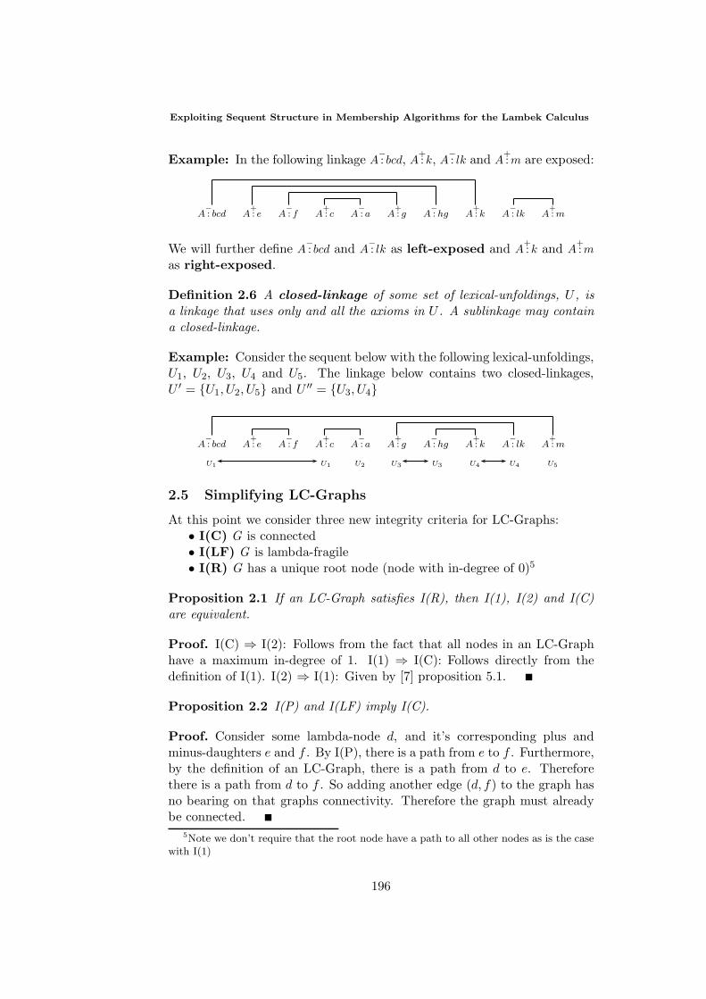
Exploiting Sequent Structure in Membership Algorithms for the Lambek Calculus
Example: In the following linkage A−: bcd, A
+: k, A
−: lk and A
+: m are exposed:
A−: bcd A
+: e A
−: f A
+: c A
−: a A
+: g A
−: hg A
+: k A
−: lk A
+: m
We will further define A−: bcd and A
−: lk as left-exposed and A
+: k and A
+: m
as right-exposed.
Definition 2.6 A closed-linkage of some set of lexical-unfoldings, U , isa linkage that uses only and all the axioms in U . A sublinkage may containa closed-linkage.
Example: Consider the sequent below with the following lexical-unfoldings,U1, U2, U3, U4 and U5. The linkage below contains two closed-linkages,U ′ = U1, U2, U5 and U ′′ = U3, U4
A−: bcd A
+: e A
−: f A
+: c A
−: a A
+: g A
−: hg A
+: k A
−: lk A
+: m
U1 U1 U2 U3 U3 U4 U4 U5
2.5 Simplifying LC-Graphs
At this point we consider three new integrity criteria for LC-Graphs:• I(C) G is connected• I(LF) G is lambda-fragile• I(R) G has a unique root node (node with in-degree of 0)5
Proposition 2.1 If an LC-Graph satisfies I(R), then I(1), I(2) and I(C)are equivalent.
Proof. I(C) ⇒ I(2): Follows from the fact that all nodes in an LC-Graphhave a maximum in-degree of 1. I(1) ⇒ I(C): Follows directly from thedefinition of I(1). I(2) ⇒ I(1): Given by [7] proposition 5.1.
Proposition 2.2 I(P) and I(LF) imply I(C).
Proof. Consider some lambda-node d, and it’s corresponding plus andminus-daughters e and f . By I(P), there is a path from e to f . Furthermore,by the definition of an LC-Graph, there is a path from d to e. Thereforethere is a path from d to f . So adding another edge (d, f) to the graph hasno bearing on that graphs connectivity. Therefore the graph must alreadybe connected.
5Note we don’t require that the root node have a path to all other nodes as is the casewith I(1)
196
Ryan T. McDonald
Proposition 2.3 A sequent S is derivable in L iff there exists a planarspanning linkage, whose corresponding LC-Graph satisfies I(R), I(LF), I(P)and I(CT).
Proof. Consequence of propositions 2.1 and 2.2
Where I(R) can be easily checked during lexical unfolding by ensuringthe existence of exactly one consequent in the sequent, leaving only I(LF),I(P) and I(CT) needing to be enforced.
3 Enforcing Lambda-Fragility
Penn[7] displayed an algorithm that used a chart parser to incrementallycreate all the possible planar spanning linkages for a given sequent. Chartparsers were designed for CFGs, in which the use of non-terminals on RHSsis invariant over their specific LHS derivations. Therefore each edge in thechart could correspond to possibly many different sublinkages. Penn alsoshowed how to store LC-Graphs on each edge so that each graph correspondsto some linkage represented by that edge. A sequent’s derivability maythen be determined by ensuring that at least one of the LC-Graphs onthe spanning edge is integral. However, because an edge may representan exponential number of linkages, it must then also store an exponentialnumber of LC-Graphs.6
Here an extension to this algorithm is presented that enforces lambda-fragility. In other words it forces each LC-Graph associated with the span-ning edge in the chart to be lambda-fragile.
Proposition 3.1 All nodes a1, . . . , an that represent labels in the same lex-ical unfolding will exist in the same connected component (in the undirectedsense) for any spanning lambda-fragile LC-Graph.
Proof. By induction on the number of unfoldings to create the lexical-unfolding (see lexical unfolding rules in §2.1). A single unfolding will eitherresult in two axiomatic formula with a common label (negative unfolding)or two axiomatic formula that are the positive and negative daughters ofsome lambda node (positive unfolding). In the former case, the commonlabel will ensure that all the labels are in the same connected componentand in the latter case, the edges from the lambda-node to its plus and minusdaughters will force all labels to be in the same component.
Inductively assume after n unfolding steps a lexical unfolding consitsof m different unfolded categories (possibly not axiomatic). The n + 1st
unfolding step must be on only one of these categories. By a similar analysis6This approach is similar to the parsing algorithm presented by Morrill[6]. Where Penn
stores possible LC-Graphs over spans, Morrill stores possible unifications over spans.
197
Exploiting Sequent Structure in Membership Algorithms for the Lambek Calculus
to the base case all the labels of the two new categories created will be inthe same connected component. Hence by induction, all of the labels for thelexical-unfolding will be in the same component.
Proposition 3.2 A spanning LC-Graph, G, for spanning linkage L is notlambda-fragile iff L contains a closed-linkage.
Proof. Assume some LC-Graph G is not lambda-fragile. By proposition 3.1all the labels in a single lexical-unfolding are in the same connected compo-nent. So if G is not lambda-fragile, then there are at least two connectedcomponents and each will consist of all and only a set of labels for somesubset of lexical unfoldings. This component can only have been created bya closed-linkage (since links correspond to edges in LC-Graphs).
Conversely assume that L contains a closed-linkage over some subsetof lexical-unfoldings U and that G is lambda-fragile. By proposition 3.1we know that all the labels of some unfolding in U will be in the sameconnected component. Also, since each link creates an edge in the LC-Graph, it must be the case that all the labels of all the axioms in U will bein the same connected component. And, since there are no other links tolexical-unfoldings outside of U , then it also must be the case that there areno edges from any node in the component of the labels of U to nodes outsideof it. Hence, this component is disconnected from the rest of the graph andG cannot be lambda-fragile since adding an edge from a lambda-node to aminus-daughter can only connect two nodes in the same lexical-unfolding.
With proposition 3.2 in mind we would like each edge to store some kindof periphery information such that it forces the parser to never add an edgeto the chart that can only be created using a sub-linkage that contains aclosed-linkage.
To do this the chart parser will use the following six rules7:
1) L → B L2) B → X− L X+, for every basic category X3) B → X+ L X−, for every basic category X4) B → X− X+, for every basic category X5) B → X+ X−, for every basic category X6) L → B
Using these six rules and by following the procedures outlined by Penn[7,sec. 7] it is possible to store LC-Graphs on each edge in the chart thatcorrespond to the different sublinkages that that edge represents. However,as stated earlier, this may result in an exponential number of LC-Graphs.In order to keep the amount of information polynomial in size, we will drop
7These are the rules Penn[7] uses in his algorithm.
198
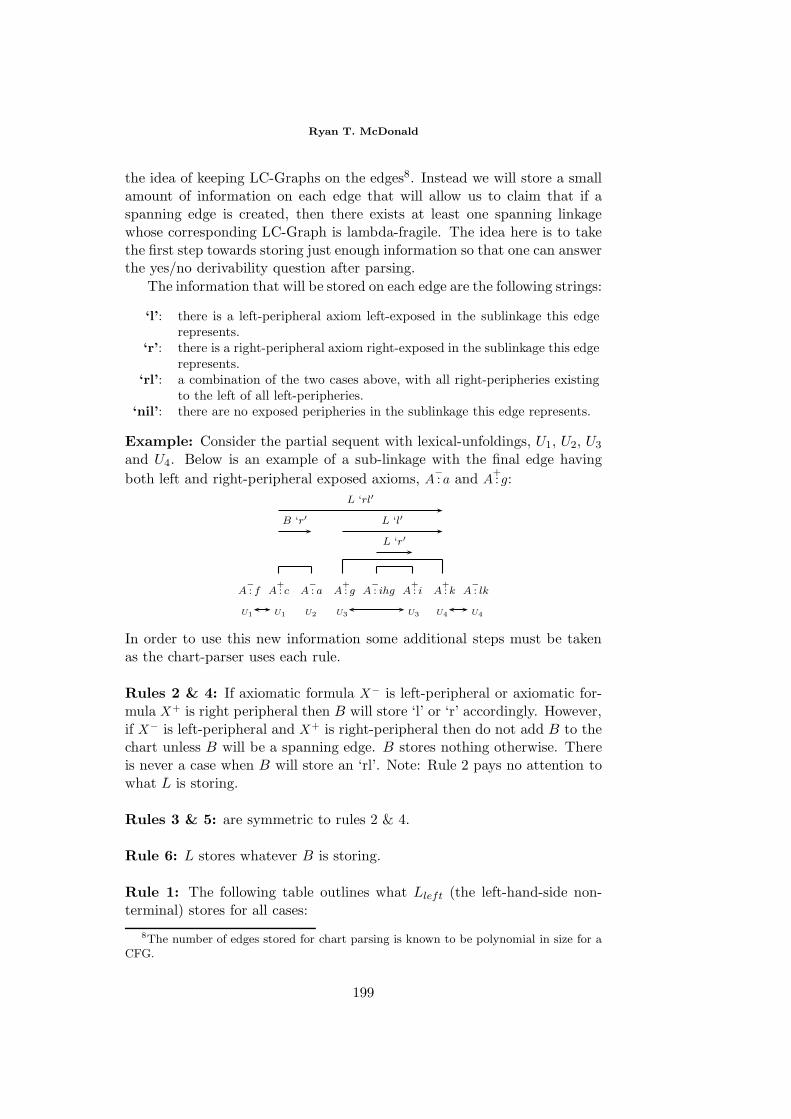
Ryan T. McDonald
the idea of keeping LC-Graphs on the edges8. Instead we will store a smallamount of information on each edge that will allow us to claim that if aspanning edge is created, then there exists at least one spanning linkagewhose corresponding LC-Graph is lambda-fragile. The idea here is to takethe first step towards storing just enough information so that one can answerthe yes/no derivability question after parsing.
The information that will be stored on each edge are the following strings:
‘l’: there is a left-peripheral axiom left-exposed in the sublinkage this edgerepresents.
‘r’: there is a right-peripheral axiom right-exposed in the sublinkage this edgerepresents.
‘rl’: a combination of the two cases above, with all right-peripheries existingto the left of all left-peripheries.
‘nil’: there are no exposed peripheries in the sublinkage this edge represents.
Example: Consider the partial sequent with lexical-unfoldings, U1, U2, U3
and U4. Below is an example of a sub-linkage with the final edge havingboth left and right-peripheral exposed axioms, A
−: a and A
+: g:
A−: f A
+: c A
−: a A
+: g A
−: ihg A
+: i A
+: k A
−: lk
U1 U1 U2 U3 U3 U4 U4
L ‘r′
B ‘r′ L ‘l′
L ‘rl′
In order to use this new information some additional steps must be takenas the chart-parser uses each rule.
Rules 2 & 4: If axiomatic formula X− is left-peripheral or axiomatic for-mula X+ is right peripheral then B will store ‘l’ or ‘r’ accordingly. However,if X− is left-peripheral and X+ is right-peripheral then do not add B to thechart unless B will be a spanning edge. B stores nothing otherwise. Thereis never a case when B will store an ‘rl’. Note: Rule 2 pays no attention towhat L is storing.
Rules 3 & 5: are symmetric to rules 2 & 4.
Rule 6: L stores whatever B is storing.
Rule 1: The following table outlines what Lleft (the left-hand-side non-terminal) stores for all cases:
8The number of edges stored for chart parsing is known to be polynomial in size for aCFG.
199
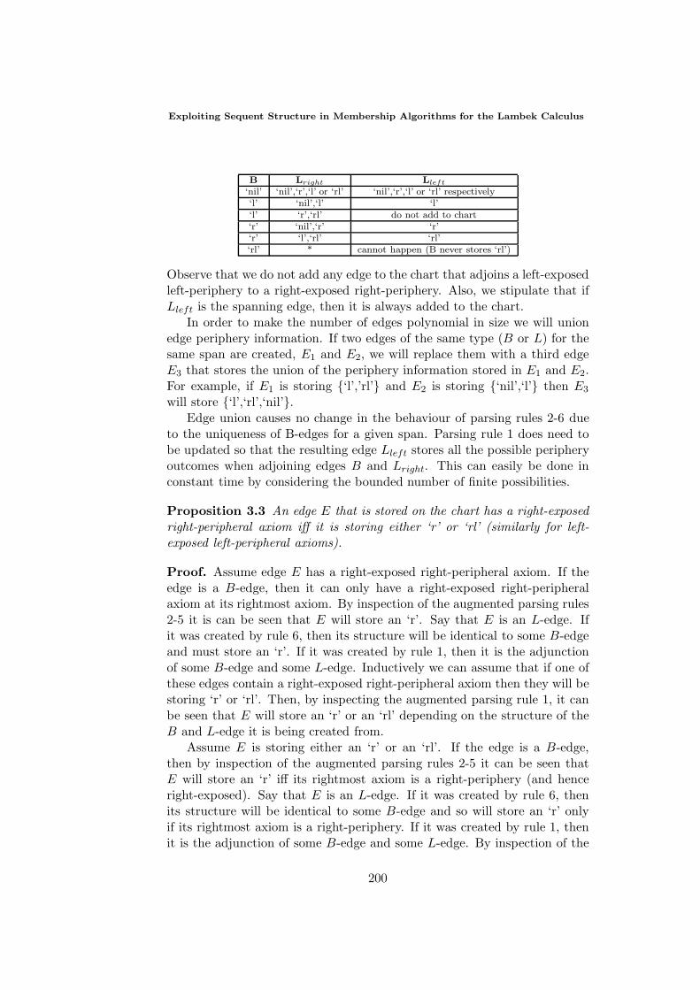
Exploiting Sequent Structure in Membership Algorithms for the Lambek Calculus
B Lright Lleft
‘nil’ ‘nil’,‘r’,‘l’ or ‘rl’ ‘nil’,‘r’,‘l’ or ‘rl’ respectively‘l’ ‘nil’,‘l’ ‘l’‘l’ ‘r’,‘rl’ do not add to chart‘r’ ‘nil’,‘r’ ‘r’‘r’ ‘l’,‘rl’ ‘rl’‘rl’ * cannot happen (B never stores ‘rl’)
Observe that we do not add any edge to the chart that adjoins a left-exposedleft-periphery to a right-exposed right-periphery. Also, we stipulate that ifLleft is the spanning edge, then it is always added to the chart.
In order to make the number of edges polynomial in size we will unionedge periphery information. If two edges of the same type (B or L) for thesame span are created, E1 and E2, we will replace them with a third edgeE3 that stores the union of the periphery information stored in E1 and E2.For example, if E1 is storing ‘l’,’rl’ and E2 is storing ‘nil’,‘l’ then E3
will store ‘l’,‘rl’,‘nil’.Edge union causes no change in the behaviour of parsing rules 2-6 due
to the uniqueness of B-edges for a given span. Parsing rule 1 does need tobe updated so that the resulting edge Lleft stores all the possible peripheryoutcomes when adjoining edges B and Lright. This can easily be done inconstant time by considering the bounded number of finite possibilities.
Proposition 3.3 An edge E that is stored on the chart has a right-exposedright-peripheral axiom iff it is storing either ‘r’ or ‘rl’ (similarly for left-exposed left-peripheral axioms).
Proof. Assume edge E has a right-exposed right-peripheral axiom. If theedge is a B-edge, then it can only have a right-exposed right-peripheralaxiom at its rightmost axiom. By inspection of the augmented parsing rules2-5 it is can be seen that E will store an ‘r’. Say that E is an L-edge. Ifit was created by rule 6, then its structure will be identical to some B-edgeand must store an ‘r’. If it was created by rule 1, then it is the adjunctionof some B-edge and some L-edge. Inductively we can assume that if one ofthese edges contain a right-exposed right-peripheral axiom then they will bestoring ‘r’ or ‘rl’. Then, by inspecting the augmented parsing rule 1, it canbe seen that E will store an ‘r’ or an ‘rl’ depending on the structure of theB and L-edge it is being created from.
Assume E is storing either an ‘r’ or an ‘rl’. If the edge is a B-edge,then by inspection of the augmented parsing rules 2-5 it can be seen thatE will store an ‘r’ iff its rightmost axiom is a right-periphery (and henceright-exposed). Say that E is an L-edge. If it was created by rule 6, thenits structure will be identical to some B-edge and so will store an ‘r’ onlyif its rightmost axiom is a right-periphery. If it was created by rule 1, thenit is the adjunction of some B-edge and some L-edge. By inspection of the
200
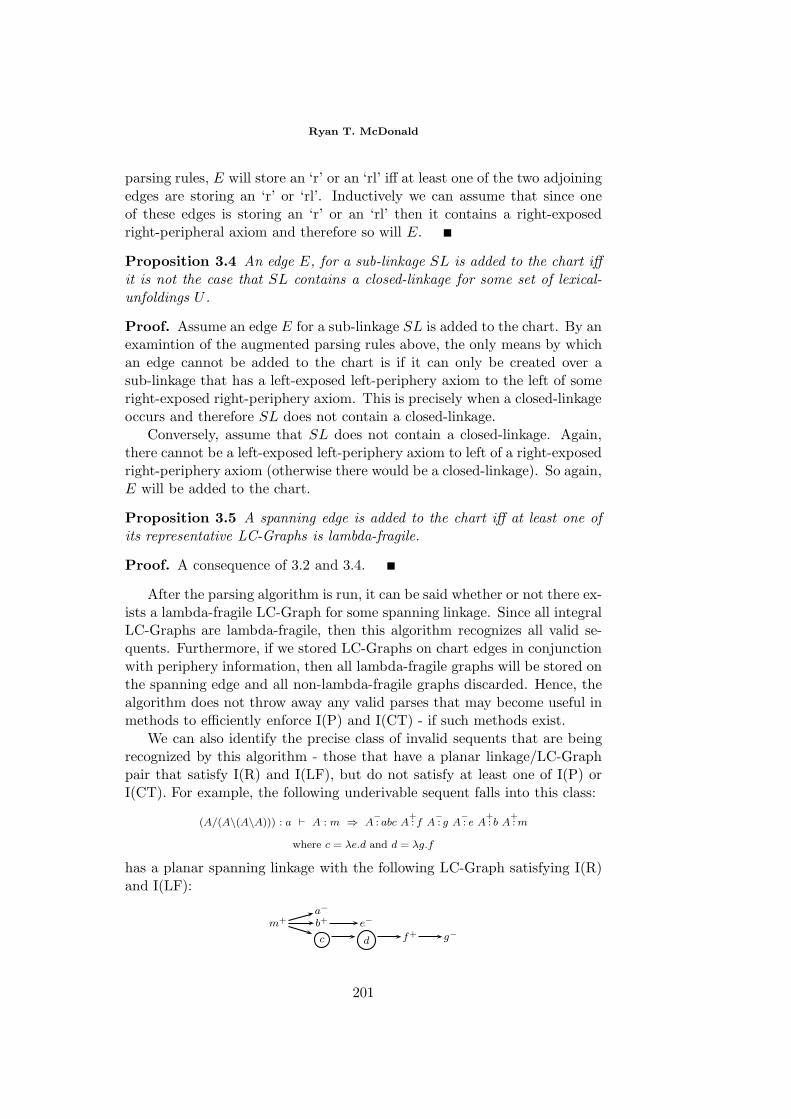
Ryan T. McDonald
parsing rules, E will store an ‘r’ or an ‘rl’ iff at least one of the two adjoiningedges are storing an ‘r’ or ‘rl’. Inductively we can assume that since oneof these edges is storing an ‘r’ or an ‘rl’ then it contains a right-exposedright-peripheral axiom and therefore so will E.
Proposition 3.4 An edge E, for a sub-linkage SL is added to the chart iffit is not the case that SL contains a closed-linkage for some set of lexical-unfoldings U .
Proof. Assume an edge E for a sub-linkage SL is added to the chart. By anexamintion of the augmented parsing rules above, the only means by whichan edge cannot be added to the chart is if it can only be created over asub-linkage that has a left-exposed left-periphery axiom to the left of someright-exposed right-periphery axiom. This is precisely when a closed-linkageoccurs and therefore SL does not contain a closed-linkage.
Conversely, assume that SL does not contain a closed-linkage. Again,there cannot be a left-exposed left-periphery axiom to left of a right-exposedright-periphery axiom (otherwise there would be a closed-linkage). So again,E will be added to the chart.
Proposition 3.5 A spanning edge is added to the chart iff at least one ofits representative LC-Graphs is lambda-fragile.
Proof. A consequence of 3.2 and 3.4.
After the parsing algorithm is run, it can be said whether or not there ex-ists a lambda-fragile LC-Graph for some spanning linkage. Since all integralLC-Graphs are lambda-fragile, then this algorithm recognizes all valid se-quents. Furthermore, if we stored LC-Graphs on chart edges in conjunctionwith periphery information, then all lambda-fragile graphs will be stored onthe spanning edge and all non-lambda-fragile graphs discarded. Hence, thealgorithm does not throw away any valid parses that may become useful inmethods to efficiently enforce I(P) and I(CT) - if such methods exist.
We can also identify the precise class of invalid sequents that are beingrecognized by this algorithm - those that have a planar linkage/LC-Graphpair that satisfy I(R) and I(LF), but do not satisfy at least one of I(P) orI(CT). For example, the following underivable sequent falls into this class:
(A/(A\(A\A))) : a A : m ⇒ A−: abc A
+: f A
−: g A
−: e A
+: b A
+: m
where c = λe.d and d = λg.f
has a planar spanning linkage with the following LC-Graph satisfying I(R)and I(LF):
a−m+ b+ e−
c d f+ g−
201
Exploiting Sequent Structure in Membership Algorithms for the Lambek Calculus
4 Discussion
By storing a small amount of bounded information on each edge ina chart parser, it was shown that we could force certain properties of theLC-Graphs that are associated with those edges - namely that they are alllambda-fragile. Of course the only problem is that not all lambda-fragileLC-Graphs are integral, which means the algorithm presented here is notsound.
Future studies should focus on finding a similar method that uses sequentstructure to force all LC-Graphs on the spanning edge to satisfy I(P). If thiscan be done in conjunction with the above algorithm, then it would be likelythat I(CT) could be satisfied as well, since both integrity criteria involveensuring the existence of particular paths.
References
[1] Carpenter, Bob. Type-Logical Semantics. Cambridge, MA: The MIT Press(1997).
[2] Dorre, Jochen. Parsing for semidirectional lambek calculus is NP-Complete,Proceedings of the Thirty-Fourth Annual Meeting of the Association for Com-putational Linguistics (1996), pp. 95-100.
[3] Girard, J.-Y. Linear Logic, Theoretical Computer Science 56 (1987), pp. 1-102.
[4] Kanovich, M. The multiplicative fragment of linear logic is NP-complete, Tech-nical Report X-91-13, Institute for Language, Logic and Information (1991).
[5] Lincoln, P., Mitchell, A., Scedrov, A. and Shankar, N. Decision problems forpropositional linear logic, In Proceedings 31st Annual IEEE Symposium onFoundations of Computer Science (1990).
[6] Morrill G. Memoisation of categorial proof nets: parallelism in categorial pro-cessing, Technical Report LSI-96-24-R, Dept. de Llenguatges i Sistemes In-formatics, Universitat Politecnica de Datlunya (1996).
[7] Penn, Gerald. A Graph theoretic approach to sequent derivability in the lambekcalculus, Electronic Notes in Theoretical Computer Science 53 (2001).
[8] Roorda, Dirk. “Resource Logics: Proof Theoretic Investigations” Ph.D. Thesis,Universiteit van Amsterdam (1991).
[9] Urquhart, A. The undecidability of entailment and relevant implication, Jour-nal of Symbolic Logic, 49 (1990), pp. 1059-1073.
Acknowledgments
The author would like to thank Gerald Penn for donating much of his valu-able time to provide many useful discussions and insights on the presentedwork. This work was supported by a grant from the Natural Sciences andEngineering Reasearch Council of Canada.
202
A Category Theoretic Method for
Comparing Evolutionary Computation
Techniques via Their Representation
Boris Mitavskiy
Department of Mathematics
University of Michigan
Ann Arbor, MI, 48109
Abstract. In the current paper we use category theory to build a rigorousfoundation for comparing various evolutionary computation techniques via theirrepresentation. Moreover, the best possible coarse graining of a given search algo-rithm to make it embeddable into a binary semi-genetic and/or a binary geneticalgorithm is constructed in terms of the left adjoint to the corresponding forgetfulfunctor.
1 Introduction
Over the past 25 years evolutionary algorithms have been widely exploitedto solve various optimization problems. The aim of this paper is to develop arigorous mathematical foundation to compare the representations of variousevolutionary computation techniques. The importance of this problem isemphasized in the introduction to chapter 17 of [9] in [10] and in [8]. Toaccomplish this task we exploit the language of Category Theory (see [3] fora detailed exposition). In the current section we describe the notation andintroduce the actual notion of what a representation is. In the next sectionwe introduce a few special evolutionary algorithm which play an importantrole in this paper. In section 3 we introduce rigorous definitions and list anumber of results (the proofs are omitted due to space limitations). Many ofthese results (proposition 3.1, Theorem 3.2, corollary 3.3 and corollary 3.4 aswell as a very special case of theorem 3.7) are available with proofs in [5]. Theuse of universal constructions (or, equivalently, adjunctions) in connectionwith coarse graining issues (see definition 3.8, theorem 3.6, definition 3.10and theorem 3.7) appears for the first time in the current paper. The proofsare available upon request from the author. Theorem 3.7 (a special case
Proceedings of the Eighth ESSLLI Student SessionBalder ten Cate (editor)Chapter 19, Copyright c© 2003, Boris Mitavskiy
203
Comparing Evolutionary Computation Techniques
of this theorem, namely theorem 20 of [5] is sufficient) implies that everyGenetic Programming algorithm which uses either one-point or the uniformhomologous crossover operators can be embedded into the classical binarygenetic algorithm.
In order to apply an evolutionary algorithm to attack a specific opti-mization problem, one needs to model the problem in a suitable manner.That is, one needs to construct a search space Ω (the set whose elementsare all possible solutions to the problem) together with a computable pos-itive valued fitness function f : Ω → (0, ∞) and an appropriate family of“mating” and “mutation” transformations. One can say, therefore, that arepresentation of a given problem by an evolutionary algorithm is an ordered4-tuple (Ω, F , M, f) where Ω is the search space, F is a family of binaryoperations on Ω and M is the family of unary transformations on Ω, that is,M is just a family of functions from Ω to itself. Intuitively F is the familyof mating transformations: every element of F takes two elements of Ω (theparents) and produces one element of Ω (the child).1 while M is the familyof mutations (or asexual reproductions) on Ω. For theoretical purposes itis usually assumed that M is ergodic in the sense that the only invariantsubsets under M are the ∅ and the entire search space Ω. (The ergodicityassumption ensures that the Markov process modelling the algorithm is ir-reducible ( see, for instance, [1] ). A typical evolutionary algorithm worksas follows: A population P = (x1, x2, . . . , x2m)T where xi ∈ Ω is selectedrandomly 2. The algorithm cycles through the following stages:
Evaluation:Individuals of P are evaluated:
x1
x2...
x2m
→ f(x1)→ f(x2)...
...→ f(x2m)
Selection:A new population P ′ = (y1, y2, . . . , y2m)T is obtained where yi = xj with
probability f(xj)
Σ2ml=1f(xl)
.
In other words, all of the individuals of P ′ are these of P , and theexpectation of the number of occurrences of any individual of P in P ′ isproportional to the number of occurrences of that individual in P times theindividual’s fitness value. In particular, the fitter the individual is, the morecopies of that individual are likely to be present in P ′. On the other hand,
1In general there is no reason to assume that a child has exactly two parents. All of theresults in this paper are valid for the families of m-ary operations on Ω. The only reasonF is assumed to be the family of binary transformations is to simplify the notation.
2Here we exploit the transpose notation to convert a column vector into a row vectorto save space
204
Boris Mitavskiy
the individuals having relatively small fitness value are not likely to enterinto P ′ at all. This is designed to imitate the natural survival of the fittestprinciple.
Partition:The individuals of P ′ are partitioned into m pairwise disjoint couples for
mating according to some probabilistic rule: For instance the couples couldbe
Q1 = (yi11, yi12
)T , Q2 = (yi21, yi22
)T , . . . , Qj = (yij1
, yij2
)T , . . . , Qm = (yim1, yim2
)T
Reproduction:Replace every one of the selected couples Qj = (y
ij1, y
ij2)T with the
couples Q′ = (T1(yij1, y
ij2), T2(yij1
, yij2
))T for some couple of transformations
(T1, T2) ∈ F2. The couple (T1, T2) is selected according to a fixed probabil-ity distribution on F2. This gives us a new population P ′′ = (z1, z2, . . . , z2m)T
Mutation:Finally, with small probability we replace zi with F (zi) for some ran-
domly chosen F ∈ M. This, once again, gives us a new population
P ′′′ = (w1, w2, . . . , w2m)T
Upon completion of mutation start all over with the initial populationP ′′′. The cycle is repeated a certain number of times depending on theproblem. A more general and extensive description is given in [9]. A fewspecial evolutionary algorithms are introduced in the next section.
2 Special Evolutionary Algorithms
Classical Genetic Algorithm with Masked Crossover:Let Ω =
∏ni=1 Ai. For every subset M ⊆ 1, 2, . . . , n, define a binary
operation LM on Ω as follows:
LM(a,b) = (x1, x2, . . . , xi, . . . , xn)
where a = (a1, a2, . . . , an) and b = (b1, . . . , bn) ∈ Ω and xi =
ai if i ∈ M
bi otherwise.
The reader will recognize LM as a masked crossover operator with mask M .Let F = LM | M ⊆ 1, 2, . . . , n. That is, F in this example is simply
the family of masked crossover transformations. The probability distributionon the set F2 is concentrated on the pairs of the form (LM , LM ) where Mdenotes the complement of the set M in 1, 2, . . . , n. Most often the pairsare equally likely to be chosen from that diagonal-like subset.
The family of mutation transformations, M in this (and in all of thefollowing examples) consists of the transformations Ma : Ω → Ω where
205
Comparing Evolutionary Computation Techniques
a ∈ ⋃S⊆1, 2,...,n
∏i∈S Ai so that a = (ai1 , ai2 , . . . , aik) for i1 ≤ i2 ≤ . . . ≤
ik ∈ Sa ⊆ 1, 2, . . . , n defined as follows: ∀x = (x1, x2, . . . , xn) ∈ Ω we
have Ma(x) = y = (y1, y2 . . . , yn) where yq =
aq if q = ij for some j
xq otherwiseIn other words, Ma simply replaces the qth coordinate of its argument withaq ∈ Ai whenever q ∈ Sa.
Binary Genetic Algorithm with Masked Crossover:When every Ai = 0, 1 (which means that Ω = 0, 1n) in the example
above, one obtains the classical binary genetic algorithm.Binary Random Respectful RecombinationThe search space Ω and the family of mating transformations F and the
family of mutations M are exactly the same as these for the binary geneticalgorithm with masked crossover described above. The only difference isthat the probability distribution on F2 is now completely uniform (ratherthan being concentrated on the diagonal-like subset described in the classicalgenetic algorithm example). This particular family of transformations wasintroduced in [6]. For instance, if n = 5, M1 = 2, 3, 4, M2 = 1, 3, 5and the pair (TM1 , TM2) is selected for mating, we have, for instance,(
1 0 0 1 11 1 0 0 1
)−→
(TM1((1, 0, 0, 1, 1), (1, 1, 0, 0, 1))TM2((1, 0, 0, 1, 1), (1, 1, 0, 0, 1))
)=
(1 0 0 1 11 1 0 0 1
)
This type of a binary search algorithm can be classified by the followingproperty: If both parents have a 1 in the ith position then the offspring alsohas a 1 in the ith position. Likewise, if both parents have a 0 in the ith
position then the offspring also has a 0 in the ith position. If, on the otherhand, the alleles of the ith gene don’t coincide, then the ith allele could beeither a 0 or a 1.
The following type of algorithm may seem useless at first. Its importancewill become clear in the next section when we present the binary embed-ding theorem which shows that the binary semi-genetic algorithm (describedbelow) possesses an interesting universal property.
Binary Semi-Genetic Algorithm:The search space Ω = 0, 1n, just as in the case of the binary genetic
algorithm. The family of mating transformations F is defined as follows:Fix u = (u1, u2, . . . , un) ∈ Ω. Define a semi-crossover transformation Fu :Ω2 → Ω as follows: For any given pair (x, y) ∈ Ω2 with x = (x1, x2, . . . , xn)and y = (y1, y2, . . . , yn) we have Fu(x, y) = z = (z1, z2, . . . zn) ∈ Ω where
zi =
1 if xi = yi = 1ui otherwise
In other words, Fum preserves the ith gene if it is equal to 1 in all of therows of P , and replaces it with ui otherwise. Let F = Fu |u ∈ Ω be
206
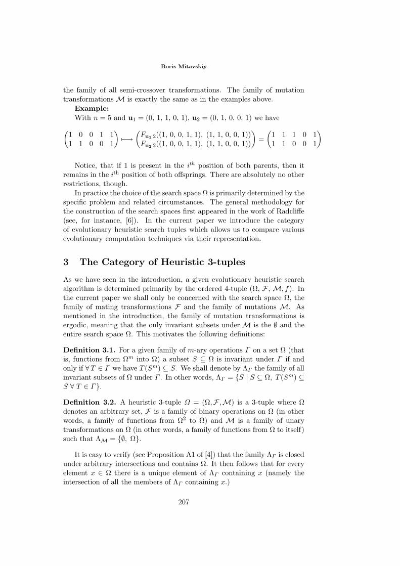
Boris Mitavskiy
the family of all semi-crossover transformations. The family of mutationtransformations M is exactly the same as in the examples above.
Example:With n = 5 and u1 = (0, 1, 1, 0, 1), u2 = (0, 1, 0, 0, 1) we have(
1 0 0 1 11 1 0 0 1
)−→
(Fu1 2((1, 0, 0, 1, 1), (1, 1, 0, 0, 1))Fu2 2((1, 0, 0, 1, 1), (1, 1, 0, 0, 1))
)=
(1 1 1 0 11 1 0 0 1
)
Notice, that if 1 is present in the ith position of both parents, then itremains in the ith position of both offsprings. There are absolutely no otherrestrictions, though.
In practice the choice of the search space Ω is primarily determined by thespecific problem and related circumstances. The general methodology forthe construction of the search spaces first appeared in the work of Radcliffe(see, for instance, [6]). In the current paper we introduce the categoryof evolutionary heuristic search tuples which allows us to compare variousevolutionary computation techniques via their representation.
3 The Category of Heuristic 3-tuples
As we have seen in the introduction, a given evolutionary heuristic searchalgorithm is determined primarily by the ordered 4-tuple (Ω, F , M, f). Inthe current paper we shall only be concerned with the search space Ω, thefamily of mating transformations F and the family of mutations M. Asmentioned in the introduction, the family of mutation transformations isergodic, meaning that the only invariant subsets under M is the ∅ and theentire search space Ω. This motivates the following definitions:
Definition 3.1. For a given family of m-ary operations Γ on a set Ω (thatis, functions from Ωm into Ω) a subset S ⊆ Ω is invariant under Γ if andonly if ∀T ∈ Γ we have T (Sm) ⊆ S. We shall denote by ΛΓ the family of allinvariant subsets of Ω under Γ . In other words, ΛΓ = S | S ⊆ Ω, T (Sm) ⊆S ∀ T ∈ Γ.Definition 3.2. A heuristic 3-tuple Ω = (Ω,F ,M) is a 3-tuple where Ωdenotes an arbitrary set, F is a family of binary operations on Ω (in otherwords, a family of functions from Ω2 to Ω) and M is a family of unarytransformations on Ω (in other words, a family of functions from Ω to itself)such that ΛM = ∅, Ω.
It is easy to verify (see Proposition A1 of [4]) that the family ΛΓ is closedunder arbitrary intersections and contains Ω. It then follows that for everyelement x ∈ Ω there is a unique element of ΛΓ containing x (namely theintersection of all the members of ΛΓ containing x.)
207
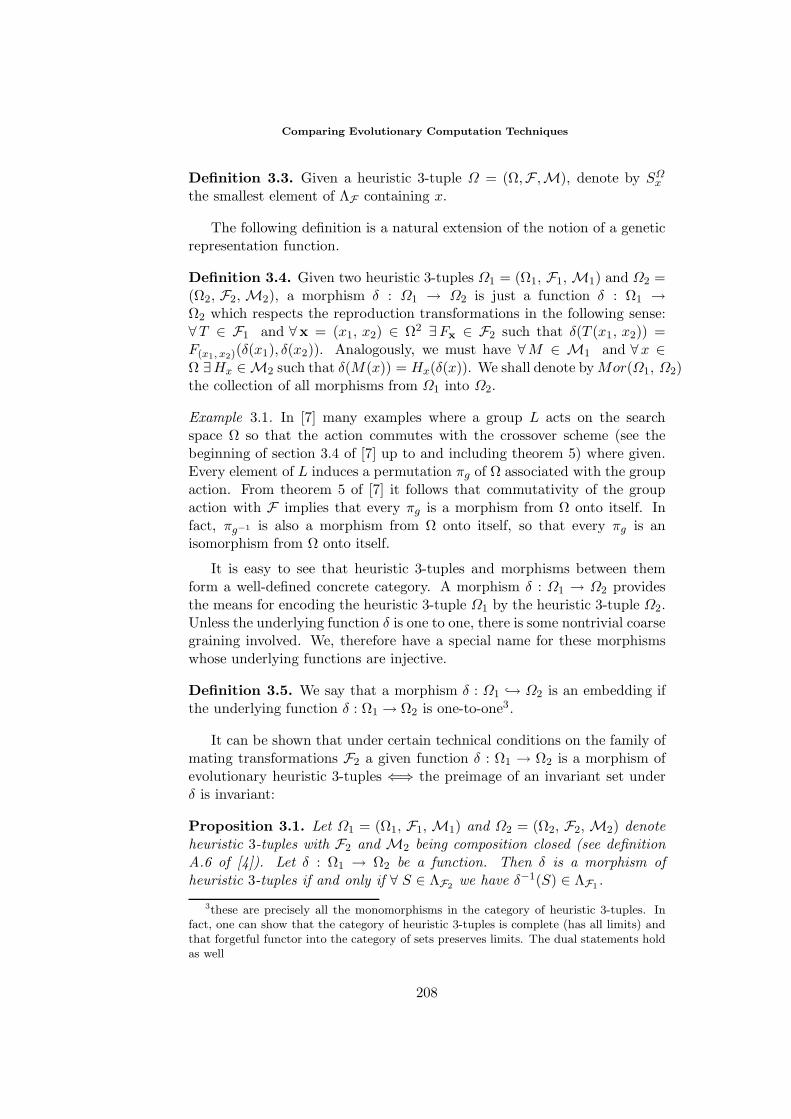
Comparing Evolutionary Computation Techniques
Definition 3.3. Given a heuristic 3-tuple Ω = (Ω,F ,M), denote by SΩx
the smallest element of ΛF containing x.
The following definition is a natural extension of the notion of a geneticrepresentation function.
Definition 3.4. Given two heuristic 3-tuples Ω1 = (Ω1, F1, M1) and Ω2 =(Ω2, F2, M2), a morphism δ : Ω1 → Ω2 is just a function δ : Ω1 →Ω2 which respects the reproduction transformations in the following sense:∀T ∈ F1 and ∀x = (x1, x2) ∈ Ω2 ∃Fx ∈ F2 such that δ(T (x1, x2)) =F(x1, x2)(δ(x1), δ(x2)). Analogously, we must have ∀M ∈ M1 and ∀x ∈Ω ∃Hx ∈ M2 such that δ(M(x)) = Hx(δ(x)). We shall denote by Mor(Ω1, Ω2)the collection of all morphisms from Ω1 into Ω2.
Example 3.1. In [7] many examples where a group L acts on the searchspace Ω so that the action commutes with the crossover scheme (see thebeginning of section 3.4 of [7] up to and including theorem 5) where given.Every element of L induces a permutation πg of Ω associated with the groupaction. From theorem 5 of [7] it follows that commutativity of the groupaction with F implies that every πg is a morphism from Ω onto itself. Infact, πg−1 is also a morphism from Ω onto itself, so that every πg is anisomorphism from Ω onto itself.
It is easy to see that heuristic 3-tuples and morphisms between themform a well-defined concrete category. A morphism δ : Ω1 → Ω2 providesthe means for encoding the heuristic 3-tuple Ω1 by the heuristic 3-tuple Ω2.Unless the underlying function δ is one to one, there is some nontrivial coarsegraining involved. We, therefore have a special name for these morphismswhose underlying functions are injective.
Definition 3.5. We say that a morphism δ : Ω1 → Ω2 is an embedding ifthe underlying function δ : Ω1 → Ω2 is one-to-one3.
It can be shown that under certain technical conditions on the family ofmating transformations F2 a given function δ : Ω1 → Ω2 is a morphism ofevolutionary heuristic 3-tuples ⇐⇒ the preimage of an invariant set underδ is invariant:
Proposition 3.1. Let Ω1 = (Ω1, F1, M1) and Ω2 = (Ω2, F2, M2) denoteheuristic 3-tuples with F2 and M2 being composition closed (see definitionA.6 of [4]). Let δ : Ω1 → Ω2 be a function. Then δ is a morphism ofheuristic 3-tuples if and only if ∀ S ∈ ΛF2 we have δ−1(S) ∈ ΛF1 .
3these are precisely all the monomorphisms in the category of heuristic 3-tuples. Infact, one can show that the category of heuristic 3-tuples is complete (has all limits) andthat forgetful functor into the category of sets preserves limits. The dual statements holdas well
208
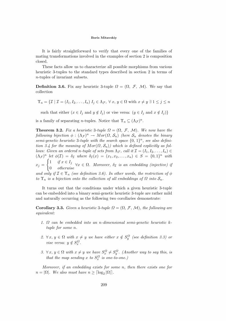
Boris Mitavskiy
It is fairly straightforward to verify that every one of the families ofmating transformations involved in the examples of section 2 is compositionclosed.
These facts allow us to characterize all possible morphisms from variousheuristic 3-tuples to the standard types described in section 2 in terms ofn-tuples of invariant subsets.
Definition 3.6. Fix any heuristic 3-tuple Ω = (Ω, F , M). We say thatcollection
Υn = I | I = (I1, I2, . . . , In) Ij ∈ ΛF , ∀ x, y ∈ Ω with x = y ∃ 1 ≤ j ≤ n
such that either (x ∈ Ij and y /∈ Ij) or vise versa: (y ∈ Ij and x /∈ Ij)is a family of separating n-tuples. Notice that Υn ⊆ (ΛF )n.
Theorem 3.2. Fix a heuristic 3-tuple Ω = (Ω, F , M). We now have thefollowing bijection φ : (ΛF )n → Mor(Ω, Sn) (here Sn denotes the binarysemi-genetic heuristic 3-tuple with the search space 0, 1n, see also defini-tion 3.4 for the meaning of Mor(Ω, Sn)) which is defined explicitly as fol-lows: Given an ordered n-tuple of sets from ΛF , call it I = (I1, I2, . . . , In) ∈(ΛF )n let φ(I) = δI where δI(x) = (x1, x2, . . . , xn) ∈ S = 0, 1n with
xj =
1 if x ∈ Ij
0 otherwise∀x ∈ Ω. Moreover, δI is an embedding (injective) if
and only if I ∈ Υn (see definition 3.6). In other words, the restriction of φto Υn is a bijection onto the collection of all embeddings of Ω into Sn.
It turns out that the conditions under which a given heuristic 3-tuplecan be embedded into a binary semi-genetic heuristic 3-tuple are rather mildand naturally occurring as the following two corollaries demonstrate:
Corollary 3.3. Given a heuristic 3-tuple Ω = (Ω, F , M), the following areequivalent:
1. Ω can be embedded into an n-dimensional semi-genetic heuristic k-tuple for some n.
2. ∀x, y ∈ Ω with x = y we have either x /∈ SΩy (see definition 3.3) or
vise versa: y /∈ SΩx .
3. ∀x, y ∈ Ω with x = y we have SΩx = SΩ
y . (Another way to say this, isthat the map sending x to SΩ
x is one-to-one.)
Moreover, if an embedding exists for some n, then there exists one forn = |Ω|. We also must have n ≥ log2 |Ω|.
209
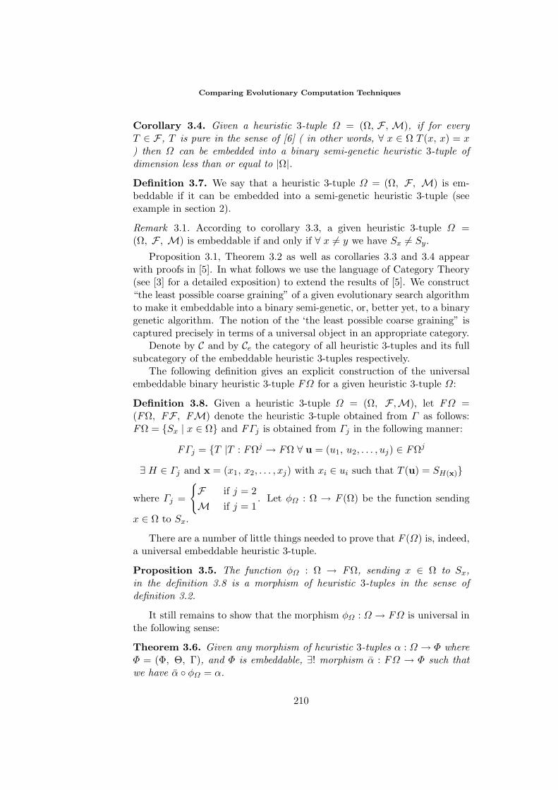
Comparing Evolutionary Computation Techniques
Corollary 3.4. Given a heuristic 3-tuple Ω = (Ω, F , M), if for everyT ∈ F , T is pure in the sense of [6] ( in other words, ∀ x ∈ Ω T (x, x) = x) then Ω can be embedded into a binary semi-genetic heuristic 3-tuple ofdimension less than or equal to |Ω|.Definition 3.7. We say that a heuristic 3-tuple Ω = (Ω, F , M) is em-beddable if it can be embedded into a semi-genetic heuristic 3-tuple (seeexample in section 2).
Remark 3.1. According to corollary 3.3, a given heuristic 3-tuple Ω =(Ω, F , M) is embeddable if and only if ∀ x = y we have Sx = Sy.
Proposition 3.1, Theorem 3.2 as well as corollaries 3.3 and 3.4 appearwith proofs in [5]. In what follows we use the language of Category Theory(see [3] for a detailed exposition) to extend the results of [5]. We construct“the least possible coarse graining” of a given evolutionary search algorithmto make it embeddable into a binary semi-genetic, or, better yet, to a binarygenetic algorithm. The notion of the ‘the least possible coarse graining” iscaptured precisely in terms of a universal object in an appropriate category.
Denote by C and by Ce the category of all heuristic 3-tuples and its fullsubcategory of the embeddable heuristic 3-tuples respectively.
The following definition gives an explicit construction of the universalembeddable binary heuristic 3-tuple FΩ for a given heuristic 3-tuple Ω:
Definition 3.8. Given a heuristic 3-tuple Ω = (Ω, F ,M), let FΩ =(FΩ, FF , FM) denote the heuristic 3-tuple obtained from Γ as follows:FΩ = Sx | x ∈ Ω and FΓj is obtained from Γj in the following manner:
FΓj = T |T : FΩj → FΩ ∀ u = (u1, u2, . . . , uj) ∈ FΩj
∃ H ∈ Γj and x = (x1, x2, . . . , xj) with xi ∈ ui such that T (u) = SH(x)
where Γj =
F if j = 2M if j = 1
. Let φΩ : Ω → F (Ω) be the function sending
x ∈ Ω to Sx.
There are a number of little things needed to prove that F (Ω) is, indeed,a universal embeddable heuristic 3-tuple.
Proposition 3.5. The function φΩ : Ω → FΩ, sending x ∈ Ω to Sx,in the definition 3.8 is a morphism of heuristic 3-tuples in the sense ofdefinition 3.2.
It still remains to show that the morphism φΩ : Ω → FΩ is universal inthe following sense:
Theorem 3.6. Given any morphism of heuristic 3-tuples α : Ω → Φ whereΦ = (Φ, Θ, Γ), and Φ is embeddable, ∃! morphism α : FΩ → Φ such thatwe have α φΩ = α.
210
Boris Mitavskiy
Notice that propositions 3.5 and 3.6 together say that the functor F :C → Ce is the left adjoint to the forgetful functor from Ce into C. A somewhatanalogous construction can be carried out for the full subcategory of theheuristic tuples which can be embedded into a binary genetic algorithm:
Definition 3.9. We say that a heuristic 3-tuple Ω = (Ω, F , M) is ge-netic if it can be embedded into a binary genetic algorithm (see example insection 2). Denote by Cg the full subcategory of all genetic 3-tuples.
Definition 3.10. Given a heuristic 3-tuple Ω = (Ω, F , M) let TΩ =(TΩ, TF , TM) be the heuristic 3-tuple obtained from Ω as follows: In-troduce the following equivalence relation ∼ on Ω: x ∼ y if and only if xand y can not be separated by a complementary pair of invariant subsets. Inother words, ∀A, B ∈ ΛF with A ∪ B = Ω and A ∩ B = ∅ we have either xand y ∈ A or x and y ∈ B. (∼ is an intersection of equivalence relations, soit is also an equivalence relation.) Let TΩ be the set of equivalence classesunder ∼. TF and TM are defined in the same way as in definition 3.8: justreplace F with T everywhere in the second part of definition 3.8.
Theorem 3.7. The functor T : C → Cg constructed in definition 3.10 isthe left adjoint to the forgetful functor Cg → C. The map ηΩ : Ω → TΩsending an element in Ω to its equivalence class under ∼ in TΩ is the unitof adjunction.
Theorem 3.7 implies, in particular, that a heuristic 3-tuple Ω = (Ω, F , M)can be embedded into a binary genetic algorithm if and only if any x, y ∈ Ωwith x = y can be separated by a disjoint pair of invariant subsets. (Ac-cording to definition 3.10 this is what it means to say that x y ∀ x = y sothat every SΩ
x = x and ηΩ is an isomorphism) It is easy to show (but thedetails are omitted due to space limitations) that the above scenario is satis-fied by the heuristic 3-tuples corresponding to various genetic programmingtechniques so that they can be regarded as “sub-algorithms” of the classicalbinary genetic algorithm introduced by John Holland.
4 conclusions
In the current paper we have developed a category theoretic frameworkfor comparing various evolutionary computation techniques via their rep-resentation. In particular, we have constructed the “most suitable” coarsegraining of a given heuristic search algorithm to make it imbeddable into abinary semi-genetic and/or by a binary genetic algorithm in terms of uni-versal properties (see theorems 3.6 and 3.7).
211
Comparing Evolutionary Computation Techniques
5 Acknowledgements
I want to thank my thesis advisor, Professor Andreas Blass for the numeroushelpful advisor meetings which have stimulated many ideas for this and formy future work. I also want to thank Professors John Holland and RickRiolo and the entire University of Michigan Complex Systems Group forhelpful discussions. Finally I want to thank the unanimous referees for theuseful comments and suggestions.
References
[1] Coffey, S. (1999) An Applied Probabilist’s Guide to Genetic Algorithms. AThesis Submitted to The University of Dublin for the degree of Master in Sci-ence.
[2] Liepins, G. and Vose, M. (1992). Characterizing Crossover in Genetic Algo-rithms. Annals of Mathematics and Artificial Intelligence, 5: 27 - 34.
[3] Mac Lane, S. (1971) Categories for the working mathematician. Graduate Textsin Mathematics 5, Springer-Verlag.
[4] Mitavskiy B. (Resubmitted). Crossover Invariant Subsets of theSearch Space for Evolutionary Algorithms. Evolutionary Computation.http://www.math.lsa.umich.edu/bmitavsk/
[5] Mitavskiy B. (2003). Comparing Evolutionary Computation Techniques viaTheir Representation. Proceedings of the Genetic and Evolutionary Computa-tion (GECCO) Conference, The Conference will be held July 12 - 16.
[6] Radcliffe, N. (1992). The algebra of genetic algorithms. Annals of Mathematicsand Artificial Intelligence, 10:339-384.
[7] Rowe, J., Vose, M., and Wright, A. (2002). Group properties of crossover andmutation. Evolutionary Computation, 10(2): 151-184.
[8] Stephens, C. (2001). Some exact results from a coarse grained formulation ofgenetic dynamics. Proceedings of the Genetic and Evolutionary Computation(GECCO) conference, pages 631-638, Morgan Kaufmann.
[9] Vose, M. (1999). The simple genetic algorithm: foundations and theory. MITPress, Cambridge, Massachusetts.
[10] Vose, M. and Wright, A. (2001). Form invariance and implicit parallelism.Evolutionary Computation, 9(3): 355-370.
[11] Wright, A., Rowe, J., Poli, R., and Stephens C. (2002). A fixed pointanalysis of a gene pool GA with mutation. Proceedings of the Geneticand Evolutionary Computation Conference (GECCO) Morgan Kaufmann.http://www.cs.umt.edu/u/wright/.
212
Properties of Translations for Logic
Programs
Juan Antonio Navarro Perez
Universidad de las Americas - Puebla
Abstract. We present a study of some properties of program translations inthe context of logic programming. In particular we provide, under the answer setsemantics, a translation for arbitrary propositional theories into the simple classof disjunctive programs. We also show how syntactic and semantic propertiesof translations can be related. The work follows a line of research that appliesmathematical logic to study notions and concepts in logic programming.
1 Introduction
Program translations are functions that map logic programs in a given classof programs to another class. Translations for logic programs can be veryinteresting for several different reasons: they can allow to simplify the struc-ture of programs (Osorio et al. 2001; Pearce et al. 2002; Sakama and Inoue1998), to derive correct programs from specifications (Pettorossi and Proietti1998), and even to perform program updates and belief revision for agentsystems (Alferes et al. 2002; Eiter et al. 2000).
We are interested in the study of the properties that translations shouldhave in order to preserve the semantical meaning of programs. In particularwe want to investigate this sort of properties in the context of Answer SetProgramming (ASP). This semantic, originally introduced by Gelfond andLifschitz (1988) and generalized later to include broader classes of programs(Lifschitz et al. 1999; Osorio et al. 2003), rapidly became a popular logicprogramming paradigm.
The great power of this semantic to express a wide variety of problems,and the existence of very efficient software to compute answer sets, allowedthe development of several real life applications based on ASP. The possi-bilities range from solving combinatorial problems, modeling logic agents,planning (Dimopoulos et al. 1997), knowledge representation (Baral 2003)and querying deductive databases (Eiter et al. 1997); just to mention a few.
Proceedings of the Eighth ESSLLI Student SessionBalder ten Cate (editor)Chapter 20, Copyright c© 2003, Juan Antonio Navarro Perez
213
Properties of Translations for Logic Programs
Previous work from Janhunen (2001) studies several syntactic and se-mantic properties of translations for arbitrary semantic operators. Thiskind of properties are relevant for several theoretical and practical reasons,as we will discus along this presentation. Pearce et al. (2002) shows, in par-ticular, a translation for programs containing nested expressions to the classof disjunctive programs that preserves the original semantics of programs.
In this paper we follow an approach, motivated from (Pearce 1999; Osorioet al. 2003), that tries to explain answer set programming in terms ofintermediate logics. We provide a translation, with nice syntactical andsemantical properties, that can reduce propositional theories to the class ofnested programs considered by Pearce et al. (2002).
We also show that, under certain simple assumptions, the syntactic prop-erties of a translation that preserves the answer set semantics can be enoughto be sure that the translation can also preserve the semantics for partiallytranslated programs. This sort of results show how the use of intuitionis-tic and other intermediate logics is an approach that can help us to betterunderstand the notion and concepts of answer sets.
Because of the lack of space, the proofs of some minor results were leftout from the main discussion of the paper. A complete version of the paper,including an appendix with all the omitted proofs, will be made available athttp://www.udlap.mx/~ma108907/papers.html.
2 Background
We review in this section the language of propositional logic used to describelogic programs. We briefly introduce intuitionistic and some multivalued-logics, state some notation and basic results. A more detailed presentationcan be found at (Mendelson 1987; Zakharyaschev et al. 2001). We alsodefine several concepts for logic programming: classes of logic programs,semantic operators and answer sets. Original definitions and related resultsare available in (Lloyd 1987; Lifschitz et al. 1999; Osorio et al. 2003).
Propositional Logic We consider a formal language built from an alpha-bet containing: a denumerable set L of elements called atoms, the 2-placeconnectives ∧, ∨, →, the 0-place connective ⊥, and auxiliary symbols (, ).Formulas are constructed as usual in logic. The formula is introduced asan abbreviation of ⊥ → ⊥, ¬A as an abbreviation of A → ⊥, and A ↔ Bto abbreviate of (A→ B) ∧ (B → A). The notation A← B is just anotherway of writing the formula B → A.
A theory is a set of formulas, we will restrict our attention, however,to finite theories. We use Prp to denote the set of all finite propositionaltheories. For a given theory T its signature is the set LT of atoms occurringin the theory T . A literal is either an atom a or a negated atom ¬a. Givena theory T we also define the negated theory ¬T = ¬A | A ∈ T and, for
214
Juan Antonio Navarro Perez
a set of atoms M , the closure of M (w.r.t. T ) as M = M ∪ ¬(LT \M).
Intermediate Logics Intuitionistic logic, denoted I, was developed as analternative to classical logic. It explains the meaning of the connectives interms of knowledge or provability, instead of absolute truths. We consider aformulation of intuitionistic logic where a juantheorem is a formula that canbe proved using the ten axioms that define I and modus ponens as inferencerule (van Dalen 1980).
Godel also defined the multivalued logics Gi, with i truth values, where amodel of a formula is a truth assignment to the atoms that, when propagatedover its connectives, evaluates to some designated true value. A formula isa tautology if it is true for every possible truth assignment. The two valuedlogic G2 corresponds to the classical logic, denoted C. (Mendelson 1987)
It was shown that the set of intuitionistic theorems is a proper subsetof the set of classical tautologies, and that the logics Gi lie in between. Sowe call intermediate logics to those logics whose set of provable formulas isbetween intuitionistic and classical logics (inclusive). A proper intermediatelogic is an intermediate logic that is not the classical one.
Notation and Basic Results We use the notation X F to denote thatthe formula F is provable (a theorem or tautology) in logic X. If T is atheory we use the symbol T X F to denote X (F1 ∧ · · · ∧ Fn) → F forsome formulas Fi ∈ T . We say that a theory T is consistent if it is not thecase that T C ⊥. It is easy to prove that the definition of a theory of beingconsistent does not depend on the logic chosen. The proof is given in theappendix at the end of the full version of this document.
We also introduce, if T and U are two theories, the symbol T X U todenote that T X F for all formulas F ∈ U . We will write T X U to denotethe fact that (i) T is consistent and (ii) T X U . Finally we say that twotheories T1 and T2 are equivalent (w.r.t. logic X), denoted T1 ≡X T2 if itholds that both T1 X T2 and T2 X T1.
Logic Programs In order to introduce the terminology of logic programs,using the propositional logic we have just presented, we define a clause as aformula H ← B where principal connective is implication. The formulas Hand B are known as the head and the body of the clause respectively.
The special case of a clause with the form ⊥ ← B is known as a con-straint, in this case the head is said to be empty. Each formula H that doesnot have implication as the principal connective can be associated with theclause H ← , this kind of clauses are known as facts. Then we can define alogic program as a finite set of clauses and a class of logic programs as someset of logic programs.
There are several kind of clauses defined in literature. The head and thebody of augmented clauses are constructed from the connectives ∧, ∨ and ¬arbitrarily nested. Note that the general case of implication is not allowed.The clause ¬(a ∧ ¬b) ← p ∨ (¬q ∧ r) is, for example, augmented while the
215
Properties of Translations for Logic Programs
clause a ← (b → c) is not. An augmented program is a set of augmentedclauses and Aug denotes the class of all augmented programs.
Another, more restricted, class is the disjunctive one. A disjunctiveclause allows only a (non-empty) disjunction of positive literals in the headand a conjunction of literals in the body, for example a ∨ b ← p ∧ q ∧ ¬r.Similarly, a disjunctive program is a set of disjunctive clauses and Dis is theclass of all disjunctive programs. Observe that we have Dis ⊂ Aug ⊂ Prp.Answer Sets Given a class of programs C, a semantic operator Sem is afunction that assigns to each program P ∈ C a set of sets of atoms M ⊆ LP .These sets of atoms are usually some “preferred” models of the program P .One popular semantic operator is the answer sets AS operator. We considerthe definition provided in (Osorio, Navarro, and Arrazola 2002) that extendsthe notion of an answer set to the whole set of propositional formulas.
Definition 1. If P ∈ Prp then AS(P ) =M ⊆ LP | P ∪ ¬¬M I M
.1
3 Conservative Transformations
Suppose that we have a logic program P and we want to compute AS(P ).We could simplify this task if we are able to construct some other simplerprogram P ′, such that the answer sets of P and P ′ are somehow related,compute AS(P ′) and recover the answer sets of the original P . It will beimportant that this “recovery” of the answer sets of P , knowing those of P ′,can be done trough a simple and efficient method. A conservative transfor-mation is a relation between logic programs with this kind of properties.
Definition 2. Let Sem be a semantic operator defined for a class of pro-grams C and let P,P ′ ∈ C. We say P ′ is a conservative transformation ofP , denoted P
Sem−−−→ P ′, if LP ⊆ LP ′ and
Sem(P ) =M ∩ LP |M ∈ Sem(P ′)
.
A conservative extension, as presented in (Baral 2003), is a conservativetransformation where the programs also satisfy P ⊆ P ′. Our definition ismore general since it allows the program to be modified or “transformed”and not only extended. As far as we know this definition is new, and so theresults presented in this section are all original.
A conservative transformation of a logic program P can, possibly, intro-duce new atoms (those in LP ′ \LP ) in order to achieve simplifications. But,if we ignore this newly introduced atoms, we obtain exactly the answer setsof P . We refer to this new atoms in LP ′ \ LP as the reserved atoms of thetransformation.
1The original definition uses the notation ¬M ∪¬¬M , where M = LP \ M , instead ofthe set ¬¬M , where M = M ∪¬(LP \M). It is easy to verify that the two conditions areequivalent since I ¬a ↔ ¬¬¬a.
216
Juan Antonio Navarro Perez
It is easy to verify that conservative transformations define a transitiverelation, a formal proof is included in the appendix. Much more surprisingis that arrows in the notation of conservative extensions can sometimes betraveled backwards. If a logic program Q is a conservative extension of twoprograms P and R then, under the premise that LP ⊆ LR, we can alsorelate the answer sets of P and R by a conservative transformation.
Proposition 1. If PSem−−−→ Q, R
Sem−−−→ Q, and LP ⊆ LR then PSem−−−→ R.
Proof. Take M ∈ Sem(R), since RSem−−−→ Q there must be N ∈ Sem(Q) such
that M = N ∩ LR. But, since PSem−−−→ Q, we have that N ∩ LP ∈ Sem(P ).
Observe, since LP ⊆ LR, that M ∩ LP = (N ∩ LR) ∩ LP = N ∩ LP . Thuswe obtain M ∩ LP ∈ Sem(P ).
Now take M ∈ Sem(P ), since PSem−−−→ Q there must be N ∈ Sem(Q) such
that M = N ∩ LP . But, since RSem−−−→ Q, we have that N ∩ LR ∈ Sem(R).
Observe, since LP ⊆ LR, that (N ∩ LR) ∩ LP = N ∩ LP = M . ThenN ∩ LR ∈ Sem(R) is the model such that (N ∩ LR) ∩ LP ∈ Sem(P ).
The following proposition allows us to construct a very simple conserva-tive translation for the semantic of answer sets. It can be used to extendthe language of a given program without modifying its answer sets. Thisresult will be used later in the proof of Theorem 3.
Proposition 2. Given a set of atoms A, let L = a← a | a ∈ A. For anyprogram P ∈ Prp, P
AS−−→ P ∪ L.
Another particular case of a conservative transformation, which is pre-sented in the following proposition, stands that is possible to introduce newatoms as a definition of a formula that can be expressed using the atomsalready in the program.
Proposition 3. Let P ∈ Prp. Given a formula F such that LF ⊆ LP andan atom x /∈ LP , P
AS−−→ P ∪ x↔ F.
Conservative transformations may seem very effective in the context oflogic programming. But they dot not satisfy, in general, an important prop-erty for concrete programming applications. We would expect that makinga conservative transformation of one piece of a program would also result,“globally”, in a conservative transformation for the whole program.
This is not true for simple conservative transformations as just defined.Consider the two programs P1 = a← ¬b and P2 = a, b← b. Accord-ing to Definition 2, P2 is a conservative translation of P1 in the answer setsemantics since they both have AS(P1) = AS(P2) = a. However, re-placing P1 with P2 in the larger program P = a← ¬b, b, to obtain the
217
Properties of Translations for Logic Programs
program P ′ = a, b← b, b, will break this relation. Now P has only oneanswer set b, while P ′ has the answer set a, b.
In order to ensure that making local transformations of code inside logicprograms will preserve global equivalence, we introduce the notion of astrong conservative transformation.
Definition 3. Let Sem be a semantic operator for a class of programs C.Given two logic programs P,P ′ ∈ C, such that LP ⊆ LP ′ , we say that P ′
is a strong conservative translation of P , denoted PSem∗−−−−→ P ′, if for every
program Q, such that LQ ∩ (LP ′ \ LP ) = ∅, P ∪QSem−−−→ P ′ ∪Q.
The condition LQ ∩ (LP ′ \ LP ) = ∅ states that the programs Q, used toextend P , may not contain any of this reserved atoms of the transformation.In an actual implementation we could ensure this condition by defininga special set of atoms reserved for internal translations and not availableto the user for writing programs. As we may expect, strong conservativetranslations also define a transitive relation.
In the particular case when L′P = LP , when there are no reserved atoms,this relation is known as a strong equivalence between programs. This notionwas originally introduced in (Lifschitz, Pearce, and Valverde 2001) where theauthors provide a characterization of strong equivalence for augmented pro-grams, using the answer set semantics, in terms of the logic HT equivalent tothe 3 valued logic G3. These relations between answer sets and intermediatelogics are also studied in (Navarro 2002) where the characterization of strongequivalence is revised and extended to arbitrary propositional theories.
Theorem 1. (Lifschitz et al. 2001; Navarro 2002) Let P,P ′ ∈ Prp, suchthat LP = LP ′. P
AS∗−−−→ P ′ if and only if P ≡G3 P ′.
4 Program Translations
A translation is a function Tr: C → C ′, where C and C ′ are two classes oflogic programs. Janhunen (2001) discusses important properties of programtranslations, relevant to logic programming, for arbitrary semantic opera-tors. Particular applications for the answer set semantics are also given in(Pearce et al. 2002).
Definition 4. (Janhunen 2001; Pearce et al. 2002) Let Sem be a semanticoperator for a class of programs D, a translation Tr: C → C ′, where theclasses C,C ′ ⊆ D are closed under unions2, is said to be:
polynomial if the time required to compute Tr(P ) is polynomial with re-spect to the number of symbols in P .
2A class of programs C is closed under unions if P1, P2 ∈ C implies that P1 ∪ P2 ∈ C.
218
Juan Antonio Navarro Perez
faithful if, for all programs P ∈ C, PSem−−−→ Tr(P ).
strongly faithful if, for all programs P ∈ C, PSem∗−−−−→ Tr(P ).
modular if, for all programs P1, P2 ∈ C, Tr(P1 ∪ P2) = Tr(P1) ∪ Tr(P2).
reductive if C ′ ⊆ C and Tr(P ′) = P ′ for all programs P ′ ∈ C ′.3
The property of a translation being polynomial (P) is related with theorder of complexity that an actual computer implementation of the trans-lation should have. A faithful (F) translation can be applied to a programpreserving the semantics, while a strongly faithful (S) translation can alsobe applied locally to some section of the program without altering the se-mantics.
The last two properties deal with the form of the translation, not withits particular semantics. If a translation is modular (M) we could split aprogram into several pieces and then perform the translation piece by piece.A reductive (R) translation maps one class of programs into some givensubclass, and the programs that are already in the subclass will not beenmodified by the translation.
As a form of notation we say that a translation is PFM if it is simultane-ously polynomial, faithful and modular. Analogously, a PSMR translationis polynomial, strongly faithful, modular and reductive. We can drop anyof the letters from the notation if we are just interested in some properties.
Proposition 4. (Pearce et al. 2002) There is a PSM translation, for thethe semantic of answer sets, AugDis : Aug→ Dis.
Using the machinery of logic, based on Definition 1 and results like Theo-rem 1, it is also possible to provide a translation of logic programs, containingarbitrary propositional formulas, into augmented programs.
Definition 5. If a formula F contains a proper subformula A→ B, whereA and B contain no more implications, we say that A → B is a simpleembedded implication of the formula F . We define recursively the translationPrpAug: Prp→ Aug for every P ∈ Prp, as follows:
(i) P contains no clause with embedded implications. Then P is alreadyan augmented program and PrpAug(P ) = P .
(ii) P contains a clause F with some embedded implications. Take onesimple embedded implication, A→ B, from the formula F ; and take anew atom x ∈ L\LP not already in P . Let F ′ be the formula obtained
3The definition of a modular translation we introduce here corresponds to the one givenin (Pearce et al. 2002). Janhunen (2001) presents a different definition which correspondsto modular + reductive (when C′ ⊆ C is satisfied).
219
Properties of Translations for Logic Programs
by replacing the occurrence of A→ B in F with the new atom x, andlet P ′ be the program obtained by replacing F with F ′ in P . Alsolet ∆ = x ∧A→ B, ¬A ∨B → x, x ∨A ∨ ¬B. We finally definePrpAug(P ) = PrpAug(P ′ ∪∆).
The recursive definition of PrpAug is well-founded since, on each recur-sion step, the program P ′ ∪∆ has one implication less than P .
Proposition 5. The translation PrpAug: Prp→ Aug is PSMR.
Proof. The number of recursion steps required to complete the translationis exactly the number of embedded implications in the program, thereforethe translation is polynomial. It is also clear, since PrpAug acts on oneclause at a time and does not modify programs already in the augmentedclass, that the translation is modular and reductive.
To justify that the recursion step is a strong conservative transformationobserve that, from Proposition 3, P
AS−−→ P∪x↔ (A→ B). The key pointis that x↔ (A→ B) ≡G3 ∆ and, therefore, we also have the equivalenceP ∪x↔ (A→ B) ≡G3 P ′∪∆. Using Theorem 1, and transitivity, we endup with P
AS−−→ P ′ ∪∆.
Current implementations of the answer set programming paradigm res-trict the syntax of formulas to the class of disjunctive programs where, inparticular, implication in the body is not allowed. A common work aroundto this limitation was to use the intuitive equivalence (A→ B)↔ (¬A∨B).This practice, however, caused sometimes the appearance of unexpectedmodels (or the miss of expected ones) when computing answer sets.
The first rule x∧A→ B in our equivalence is used to model the behaviorof the implication symbol in the head. The second rule ¬A ∨B → x comesfrom the classical intuitive meaning of the implication connective. This tworules, however, are not enough to provide the required equivalence in thelogic G3. This could possibly explain the unexpected results obtained fromthe erroneous work around. The less intuitive third rule x∨A∨¬B requiredwas discovered, in fact, by an examination of the G3 models of the originalformula x ↔ (A → B). This points out the importance of results likeTheorem 1 that allows us to better understand the notion of answer sets,proposing the logic G3 as a more correct guide for our intuition.
5 Properties of Translations
In the previous section we provided a translation for the class of propo-sitional theories into the class of augmented programs and, together withother translations (Pearce et al. 2002), it is possible to reduce them to theclass of disjunctive programs. Using any of the popular answer set finders for
220
Juan Antonio Navarro Perez
disjunctive programs, dlv4 or smodels5, it is possible to provide an efficientmethod to compute answer sets for propositional theories. The followingtheorem is a direct consequence from Propositions 4 and 5.
Theorem 2. There is a translation PrpDis: Prp → Dis, which is PSM forthe semantic of answer sets.
Observe that the properties of strongly faithful and modular are some-how related. Both notions can be interpreted in terms of a program thathas been split into several pieces. A strongly faithful translation can beapplied to one of these pieces preserving the semantics of the program. Onthe other hand, a modular translation can also be applied “piece by piece”to the program but we do have to complete the translation for each one ofthe pieces. It is possible, indeed, to construct a FM translation which is notstrongly faithful.
Example 1. Let C be the class of disjunctive programs that have exactlyone atom in the head and zero or one atoms in the body. Also let C ′ bethe class of disjunctive programs that have exactly two atoms in the headand zero or two atoms in the body. Clearly both C and C ′ are closed underunions. For each atom a in the user language let a′ be a new reserved atom.The translation Hide: C → C ′ is defined mapping each clause, a or a ← b,as follows:
Hide(a) = a′ ∨ a′, a ∨ a← a′ ∧ a′Hide(a← b) = a′ ∨ a′ ← b′ ∧ b′, a ∨ a← a′ ∧ a′, b ∨ b← b′ ∧ b′
It is clear, by construction, that the translation is modular. The translationis also faithful since it rewrites the original program, with new reservedatoms, and appending a set of rules, equivalent to a ← a′, in order torecover answer sets in the original signature.
Consider the program P = a← b, b ∈ C. Both P and Hide(P ) havethe same answer sets. If we apply the translation, however, just to the firstclause the program Hide(a← b) ∪ b will have different semantics. Therule a← b is now “hidden” and the existence of the fact b can not be usedanymore to infer a. The translation is not strongly faithful.
We will see, however, that there is a wide class of interesting and usefultranslations where the syntactic properties of being modular and reductiveare enough to be strongly faithful. The following theorem shows how, in thecontext of the answer sets semantics, this can be possible.
Theorem 3. Given two classes of logic programs C and C ′, closed underunions and such that Dis ⊆ C ′ ⊆ C ⊆ Prp. If the translation Tr: C → C ′ isFMR in the answer set semantics then it is also strongly faithful.
4http://www.dbai.tuwien.ac.at/proj/dlv/5http://www.tcs.hut.fi/Software/smodels/
221
Properties of Translations for Logic Programs
Proof. Let Q ∈ Prp be a program containing no atoms from LTr(P ) \LP andlet L =
a← a | a ∈ LTr(P )
, so that the signatures are LP ⊆ LTr(P ) = LL.
Construct then the disjunctive program D = PrpDis(Q ∪ L) and, sinceTheorem 2 states that the translation is strongly faithful, Q ∪ L
AS∗−−−→ D.Neither P nor Tr(P ) contain reserved atoms from LD \ LQ∪L. Using
the result from Proposition 2 and from the definition of strongly faithfulwe obtain that P ∪ Q
AS−−→ P ∪ (Q ∪ L) AS−−→ P ∪ D and, similarly for thetranslated program, Tr(P ) ∪Q
AS−−→ Tr(P ) ∪ (Q ∪ L) AS−−→ Tr(P ) ∪D.
Now, since the translation Tr is faithful, we have P ∪DAS−−→ Tr(P ∪D).
Also, from the modular and reductive properties, we obtain Tr(P ∪ D) =Tr(P )∪Tr(D) = Tr(P )∪D. Thus we get P ∪Q
AS−−→ P ∪DAS−−→ Tr(P )∪D
and, by Proposition 1, we can finally conclude P ∪QAS−−→ Tr(P ) ∪Q.
6 Conclusions
We have presented in this paper a translation that can be used to map ar-bitrary propositional theories into the class of simple disjunctive programs.Moreover, the translation is strongly faithful and has good syntactical prop-erties. Previous work, from Pearce et al. (2002), presented a similar trans-lation but only for programs in the augmented class. Using results fromLifschitz et al. (2001) and Osorio et al. (2003) we could show how to extendthis translation for any propositional theory.
The existence of such translation has some theoretical significance. Itshows, in particular, that the class of disjunctive programs is as expressive asthe class of propositional theories. Also an important practical consequenceof the result is that it allows the development of software tools to computeanswer sets for logic programs containing arbitrary propositional formulas.
We also exhibit how, for a wide range of program translations, the con-ditions of being faithful, modular and reductive are sufficient to state thatthe translation is also strongly faithful. The main assumption required forthis result to hold is that the translation takes programs from a class of logicprograms to some, more simple in principle, subclass.
It is important to stress out the fact that this results were obtainedthrough the “Logic Programming via Logic” approach initiated by Pearce(1999) and developed later by Osorio et al. (2003). Thus showing how theuse of intermediate logics in the study of answer sets can be useful to developthe theory and applications of answer sets. This could open a new line ofresearch and provide a lot of feedback between this two areas.
Acknowledgments This research is sponsored by the Mexican NationalCouncil of Science and Technology, CONACyT (project 37837-A).
222
Juan Antonio Navarro Perez
References
Alferes, J. J., L. M. Pereira, H. Pryzmusinska, and T. Prymusinski (2002). LUPS—a language for updating logic programs. Artificial Intelligence 138, 87–116.
Baral, C. (2003). Knowledge Representation, reasoning and declarative problemsolving with Answer Sets. Cambridge: Cambridge University Press.
Dimopoulos, Y., B. Nebel, and J. Koehler (1997). Encoding planning problems innon-monotonic logic programs. In Proceedings of the Fourth European Conferenceon Planning, pp. 169–181. Springer-Verlag.
Eiter, T., M. Fink, G. Sabbatini, and H. Tompits (2000). On updates of logicprograms: Semantics and properties. Research Report 1843-00-08, INFSYS. Ashortened version of this paper appears in Theory and Practice of Logic Program-ming, 2002.
Eiter, T., N. Leone, C. Mateis, G. Pfeifer, and F. Scarcello (1997, June). The ar-chitecture of a disjunctive deductive database system. In M. Falaschi, M. Navarro,and A. Policriti (Eds.), Proceedings Joint Conference on Declarative Programming(APPIA-GULP-PRODE ’97), pp. 141–151.
Gelfond, M. and V. Lifschitz (1988). The stable model semantics for logic program-ming. In R. Kowalski and K. Bowen (Eds.), 5th Conference on Logic Programming,pp. 1070–1080. MIT Press.
Janhunen, T. (2001, September). On the effect of default negation on the expres-siveness of disjunctive rules. In T. Eiter, W. Faber, and M. Truszczynski (Eds.),Logic Programming and Nonmonotonic Reasoning, 6th International Conference,Number 2173 in Lecture Notes in Computer Science, Vienna, Austria, pp. 93–106.Springer.
Lifschitz, V., D. Pearce, and A. Valverde (2001). Strongly equivalent logic pro-grams. ACM Transactions on Computational Logic 2, 526–541.
Lifschitz, V., L. R. Tang, and H. Turner (1999). Nested expressions in logicprograms. Annals of Mathematics and Artificial Intelligence 25, 369–389.
Lloyd, J. W. (1987). Foundations of Logic Programming (Second ed.). Berlin:Springer.
Mendelson, E. (1987). Introduction to Mathematical Logic (Third ed.). Belmont,CA: Wadsworth.
Navarro, J. A. (2002, August). Answer set programming through G3 logic. InM. Nissim (Ed.), Seventh ESSLLI Student Session, European Summer School inLogic, Language and Information, Trento, Italy.
Osorio, M., J. A. Navarro, and J. Arrazola (2001, November). Equivalence inanswer set programming. In A. Pettorossi (Ed.), Logic Based Program Synthesisand Transformation. 11th International Workshop, LOPSTR 2001, Number 2372in LNCS, Paphos, Cyprus, pp. 57–75. Springer.
Osorio, M., J. A. Navarro, and J. Arrazola (2002). A logical approach for A-Prolog. In R. de Queiroz, L. C. Pereira, and E. H. Haeusler (Eds.), 9th Workshopon Logic, Language, Information and Computation (WoLLIC), Volume 67 of Elec-tronic Notes in Theoretical Computer Science, Rio de Janeiro, Brazil, pp. 265–275.Elsevier Science Publishers.
223
Properties of Translations for Logic Programs
Osorio, M., J. A. Navarro, and J. Arrazola (2003). Applications of intuitionisticlogic in answer set programming. Accepted to appear at the TPLP journal.
Pearce, D. (1999). Stable inference as intuitionistic validity. Logic Program-ming 38, 79–91.
Pearce, D., V. Sarsakov, T. Schaub, H. Tompits, and S. Woltran (2002, August). Apolynomial translation of logic programs with nested expressions into disjunctivelogic programs: Preliminary report. In P. J. Stuckey (Ed.), Logic Programming.18th International Conference, ICLP 2002, Number 2401 in LNCS, Copenhagen,Denmark, pp. 405–420. Springer.
Pettorossi, A. and M. Proietti (1998). Transformation of logic programs. InC. J. H. D. M. Gabbay and J. A. Robinson (Eds.), Handbook of Logic in ArtificialIntelligence and Logic Programming, Volume 5, Chapter D, pp. 697–787. OxfordUniversity Press.
Sakama, C. and K. Inoue (1998). Negation as failure in the head. Journal of LogicProgramming 35(1), 39–78.
van Dalen, D. (1980). Logic and Structure (Second ed.). Berlin: Springer.
Zakharyaschev, M., F. Wolter, and A. Chagrov (2001, December). Advancedmodal logic. In D. M. Gabbay and F. Guenthner (Eds.), Handbook of Philo-sophical Logic (Second ed.), Volume 3, pp. 83–266. Dordrecht: Kluwer AcademicPublishers.
224
Worst-case upper bounds for SAT:
automated proof
Sergey Nikolenko
St.-Petersburg State University
Alexander Sirotkin
St.-Petersburg State University
Abstract. Propositional satisfiability (SAT), an NP-hard problem, can certainlybe solved in less than 2K steps, where K denotes the number of clauses in theinput formula, for instance, with the help of DPLL-type SAT solvers. In this paper,describing a work in progress, we deal with automated proofs of upper bounds onthe running time of DPLL-type algorithms for SAT.
For a class of algorithms working with the pure literal elimination, we prove apreviously unknown upper bound w.r.t. the number of clauses in the input formula.We also note that the employed line of reasoning cannot lead to better results.
1 Introduction
The problem of propositional satisfiability is known to be NP-complete, and,therefore, it is highly unlikely that a polynomial-time algorithm for SAT willbe discovered. Therefore, the need in “good” exponential-time algorithmsarose. The naive algorithm would in the general case take at least poly(N)2N
steps to find a satisfying assignment, where N is a complexity measure suchas number of variables, clauses or length of the input formula. Therefore,it has for quite a long time been a challenging problem to prove betterand better worst-case upper bounds for various SAT solvers. The currentrecord holder is due to Edward A. Hirsch. He proved in [6] that his (rathercomplex) algorithm works for the time 20.30897...K , where K is the numberof clauses in the input formula. We prove a weaker bound, but for a muchsimpler algorithm.
One of the two main approaches to obtaining less-than-2N bounds is thelocal search approach, when an algorithm starts from a random assignment
Proceedings of the Eighth ESSLLI Student SessionBalder ten Cate (editor)Chapter 21, Copyright c© 2003, Sergey Nikolenko and Alexander Sirotkin
225
Worst-case upper bounds for SAT: automated proof
and modifies it to get closer to a satisfying assignment (for references see,for example, [1]).
Algorithms of the other are called DPLL-type, due to the works of Davis,Putnam, Logemann and Loveland ([3], [2]). The DPLL-type algorithmsbuild a tree, the so-called branching tree, whose nodes are partial assign-ments to the variables of the input formula. On each step, a DPLL-typealgorithm first tries to simplify the input formula, employing a number ofsimplification rules. Then, if the result is not obvious yet, it makes a split-ting, that is, it chooses a literal l in the input formula, constructs two for-mulae, one corresponding to l := true and the other to l := false, andrecursively calls itself for these two formulas. If any of the calls returns theanswer “Satisfiable”, the algorithm also returns this answer. Otherwise, itreturns “Unsatisfiable”.
During the past decade the proofs of worst-case upper bounds for DPLL-type SAT solvers have become quite similar. The point of such proofs is toconstruct the branching tree, described in Section 2, and prove that in anypossible case of the literals’ mutual arrangement in the input formula thealgorithm in question will be able to pick a literal, the splitting by whichwould provide the necessary branching vector with respect to the necessarycomplexity measure.
The proofs have become less elegant and more technical. Simple combi-natorial properties of all the possible cases usually comprise the whole proof(probably [6] is the best example of such a proof). The only “creative”element of these proofs are the elimination rules.
In the sequel we present a successful attempt to automate the proofs ofworst-case upper bounds for DPLL-type algorithms. Attempts to prove suchbounds usually employ the Kullmann-Luckhardt’s lemma, to which Section2 is devoted. Sections 3 describes the ideology of automating these proofs,Section 4 provides a hard instance for this line of reasoning that matcheswith the upper bound presented, and Section 5 presents a new bound provenwith the help of a computer, the complete output of whose work is presentedin the appendix.
2 Basic definitions and Kullmann-Luckhardt’s lemma
We denote by X a set of boolean variables. The negation of a variable x isdenoted by x. If U ⊆ X, then U = x | x ∈ U. Literals are members of theset X ∪X. A clause is a set of literals that does not contain simultaneouslyany variable together with its negation. A formula in CNF is a finite set ofclauses. A clause is called unit if it consists of one literal.
We count the number of appearances of a chosen literal in the formula.We call l an (i, j)-literal with respect to a formula F , if F contains i appear-ances of l and j appearances of l. We call l an (i, j+)-literal with respect to
226
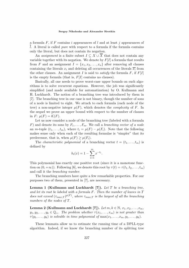
Sergey Nikolenko and Alexander Sirotkin
a formula F , if F contains i appearances of l and at least j appearances ofl. A literal is called pure with respect to a formula if the formula containsonly the literal, but does not contain its negation.
An assignment is a finite subset I ⊆ X ∪ X that does not contain anyvariable together with its negation. We denote by F [I] a formula that resultsfrom F and an assignment I = x1, x2, . . . , xn after removing all clausescontaining the literals xi and deleting all occurrences of the literals xi fromthe other clauses. An assignment I is said to satisfy the formula F , if F [I]is the empty formula (that is, F [I] contains no clauses).
Basically, all one needs to prove worst-case upper bounds on such algo-rithms is to solve recurrent equations. However, the job was significantlysimplified (and made available for automatization) by O. Kullmann andH. Luckhardt. The notion of a branching tree was introduced by them in[7]. The branching tree in our case is not binary, though the number of sonsof a node is limited to eight. We attach to each formula (each node of thetree) a non-negative integer µ(F ), which denotes the complexity of F . Inthe sequel we prove an upper bound with respect to the number of clausesin F : µ(F ) = K(F ).
Let us now consider a node of the branching tree (labeled with a formulaF ) and denote its sons by F1, . . . , Fm. We call a branching vector of a nodean m-tuple (t1, . . . , tm), where ti = µ(F ) − µ(Fi). Note that the followingmakes sense only when each of the resulting formulae is “simpler” that itspredecessor, that is, when µ(F ) ≥ µ(Fi).
The characteristic polynomial of a branching vector t = (t1, . . . , tm) isdefined by
ht(x) = 1 −m∑
i=1
x−ti .
This polymonial has exactly one positive root (since it is a monotone func-tion on (0,+∞)). Following [6], we denote this root by τ(t) = τ(t1, t2, . . . , tm)and call it the branching number.
The branching numbers have quite a few remarkable properties. For ourpurposes two of them, presented in [7], are necessary.
Lemma 1 (Kullmann and Luckhardt [7]). Let T be a branching tree,and let its root be labeled with a formula F . Then the number of leaves in Tdoes not exceed (τmax,T )µ(F ), where τmax,T is the largest of all the branchingnumbers of the nodes of T .
Lemma 2 (Kullmann and Luckhardt [7]). Let m,k ∈ N, x1, x2, . . . , xm,y1, y2, . . . , yk ∈ Q+. The problem whether τ(x1, . . . , xm) is not greater thanτ(y1, . . . , yk) is solvable in time polynomial of max(x1, . . . , xm, y1, . . . , yk).
These lemmata allow us to estimate the running time of a DPLL-typealgorithm. Indeed, if we know the branching number of its splitting tree
227
Worst-case upper bounds for SAT: automated proof
0
8
8Figure 1: Branching numbers (i, j) ∈ N × N such that τ(i, j) ≥ τ(3, 4)
(τmax,T ) and provided it processes each of its leaves in polynomial time,Lemma 1 gives a worst-case upper bound on its running time as poly(µ(F ))τµ(F )
max,T ,where F is its input formula and µ an arbitrary complexity measure, strictlydecreasing with each splitting.
Besides, Lemma 2 allows the algorithm to estimate the branching num-bers in polynomial time and choose the next literal according to the suitablebranching number.
3 Programming issues
The main idea of the program was to introduce in it the notion of an unknownliteral. The program actually looks at a rather small piece of formula, justbig enough to hold all the occurrences of several literals. The rest of theliterals is supposed unknown; they are not subject to elimination rules.
The program receives as input the target branching number τ . First ofall, let us note that if a formula contains an (i, j)-literal such that τ(i, j) ≤ τ ,making a split on this literal would achieve the purpose of the current step.Therefore, it is possible to reduce the possibilities for positive and negativeoccurrences of the literals to a certain finite subset of Z × Z, depending onthe target branching number (see an example on Fig. ??).
Then the program initializes a literal and marks all other literals asunknown (if the first considered literal is an (i, j)-literal, then there wouldbe i + j clauses in the formula after its initialization – the rest are unknownand therefore irrelevant for reducing). After initializing, it tries to reducethe resulting formula using the current rules. If succeeded, it means that
228
Sergey Nikolenko and Alexander Sirotkin
this formula cannot be obtained as an input for the splitting and, therefore,we may proceed to other cases.
Then the program tries to find an acceptable split, that is, literalsl1, . . . , lk such that the corresponding branching number is less than τ . Ifsucceeded, it goes on through all the remaining possibilities of the literals’mutual arrangement. If it does not succeed, it initializes another literal andtries to split or reduce the resulting formula, looking for the target branchingnumber.
4 Lower bounds for this type of reasoning
Of course, this kind of reasoning has its limitations. We present here anexample of a formula that is very simple for any solver by itself. However,it constitutes an unavoidable obstacle for the line of reasoning based onKullmann-Luckhardt’s lemma.
Consider the following formula:
G(x1, x2, x3) = (x1 ∨ x2 ∨ x3) ∧ (x1 ∨ x2 ∨ x3) ∧ (x1 ∨ x2 ∨ x3).
Note that in the terms of Kullmann-Luckhardt’s lemma, whichever literalwe split on first, we produce a (1, 3)-split (that is, one clause is eliminatedwhen xi is set to false and all three clauses disappear when xi := true).The second splitting (we have to consider it only in one case, since in theother the whole formula disappears) would inevitably reduce the formula toan empty one.
Now let us consider the formula
F (x1, . . . , xn) = G(x1, x2, x3) ∧ G(x4, x5, x6) ∧ . . . ∧ G(xn−2, xn−1, xn).
Due to the symmetry of the formula and the independence of subformulaswith three variables, we can rearrange the splittings made by the pure literalselimination algorithm in any suitable order (provided we preserve the orderof every pair of splittings made in any independent subformula). Let usrearrange them in such a way that splittings made by variables occuring ineach subformula appear one after another. Then it is easy to see that everysequence of two splittings result in a branching vector with a branchingnumber of τ(3, 3, 3) = 1.442250 . . ..
Note that the formula itself is remarkably simple, because the majorityof all the assignments are satisfiable, and it may not be considered a hardinstance for any SAT solver. However, the line of reasoning along which theautomated search is going would inevitably fail at this point.
229
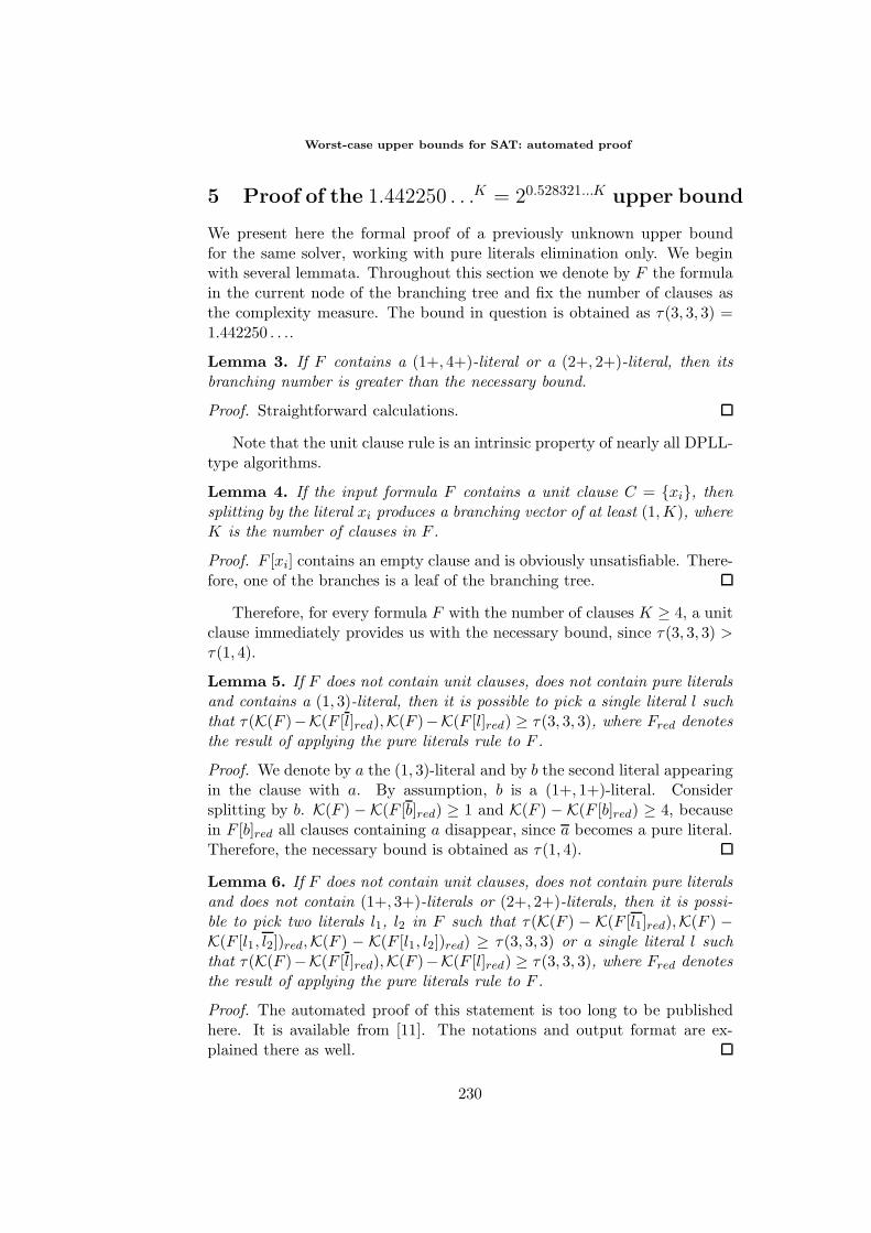
Worst-case upper bounds for SAT: automated proof
5 Proof of the 1.442250 . . .K = 20.528321...K upper bound
We present here the formal proof of a previously unknown upper boundfor the same solver, working with pure literals elimination only. We beginwith several lemmata. Throughout this section we denote by F the formulain the current node of the branching tree and fix the number of clauses asthe complexity measure. The bound in question is obtained as τ(3, 3, 3) =1.442250 . . ..
Lemma 3. If F contains a (1+, 4+)-literal or a (2+, 2+)-literal, then itsbranching number is greater than the necessary bound.
Proof. Straightforward calculations.
Note that the unit clause rule is an intrinsic property of nearly all DPLL-type algorithms.
Lemma 4. If the input formula F contains a unit clause C = xi, thensplitting by the literal xi produces a branching vector of at least (1,K), whereK is the number of clauses in F .
Proof. F [xi] contains an empty clause and is obviously unsatisfiable. There-fore, one of the branches is a leaf of the branching tree.
Therefore, for every formula F with the number of clauses K ≥ 4, a unitclause immediately provides us with the necessary bound, since τ(3, 3, 3) >τ(1, 4).
Lemma 5. If F does not contain unit clauses, does not contain pure literalsand contains a (1, 3)-literal, then it is possible to pick a single literal l suchthat τ(K(F )−K(F [l]red),K(F )−K(F [l]red) ≥ τ(3, 3, 3), where Fred denotesthe result of applying the pure literals rule to F .
Proof. We denote by a the (1, 3)-literal and by b the second literal appearingin the clause with a. By assumption, b is a (1+, 1+)-literal. Considersplitting by b. K(F ) − K(F [b]red) ≥ 1 and K(F ) − K(F [b]red) ≥ 4, becausein F [b]red all clauses containing a disappear, since a becomes a pure literal.Therefore, the necessary bound is obtained as τ(1, 4).
Lemma 6. If F does not contain unit clauses, does not contain pure literalsand does not contain (1+, 3+)-literals or (2+, 2+)-literals, then it is possi-ble to pick two literals l1, l2 in F such that τ(K(F ) − K(F [l1]red),K(F ) −K(F [l1, l2])red,K(F ) − K(F [l1, l2])red) ≥ τ(3, 3, 3) or a single literal l suchthat τ(K(F )−K(F [l]red),K(F )−K(F [l]red) ≥ τ(3, 3, 3), where Fred denotesthe result of applying the pure literals rule to F .
Proof. The automated proof of this statement is too long to be publishedhere. It is available from [11]. The notations and output format are ex-plained there as well.
230
Sergey Nikolenko and Alexander Sirotkin
All of the above, after applying Lemmata 1 and 2, proves the following.
Theorem 1. The described DPLL-type algorithm with pure literals elimi-nation as the only simplification rule gives the correct answer in the timenot exceeding poly(K)20.64743...K , where K is the number of clauses in theinput formula.
6 Further work
One direction for further work in this field is obvious: we will implementother elimination rules and obtain better bounds. Other known elimina-tion rules include elimination by resolution, unit clause elimination, blockedclauses elimination and the black-and-white literals rule (for an examplewhere all of them are used, see [6]). It would be also interesting to try toprove bounds w.r.t. other complexity measures, the most interesting beingthe number of variables. We are currently working on it, and on this waywe expect some new results and, possibly, records.
Another direction is to extend these methods to other NP-complete prob-lems. There exist algorithms for other problems that employ similar split-ting methods and bounds on which also have been achieved with the help ofKullmann-Luckhardt’s lemma. An example of such algorithms for MAX-2-SAT and MAX-CUT can be found in [5], and the current record holder forMAX-CUT ([4]) also uses such techniques.
And, last but not least, it has been an equally challenging problem toobtain exponential lower bounds for such algorithms. Previous attemptsusually employed graph-theoretical techniques ([9],[10],[8]). The automatedsearch for upper bounds may yield explicit formulae that are hard for DPLL-type algorithms: after all, it does not succeed every time, and analysis of itsoutput when a bound cannot be proven might turn out to be very useful.For example, this output may provide the so-called “bottleneck cases”, i.e.explicit formulae where the algorithm performs with complexity close to itsproven worst-case upper bound.
Acknowledgements
The authors would like to express gratitude to Edward A. Hirsch, who posedthe problem and supervised our work.
References
[1] E.Y. Dantsin, E.A. Hirsch, S.V. Ivanov, M.A. Vsemirnov. Algorithms forSAT and upper bounds on their complexity (in Russian: Algoritmy dljapropozitsional’noj vypolnimosti i verhnie otsenki ih slozhnosti). Zapiski nauch-nyh seminarov POMI, 277:14-46, 2001. English version appears in Elec-
231
Worst-case upper bounds for SAT: automated proof
tronic Colloquium on Computational Complexity, Technical Report 01-012,ftp://ftp.eccc.uni-trier.de/pub/eccc/reports/2001/TR01-012/Paper.ps
[2] M. Davis, G. Logemann, D. Loveland. A machine program for theorem-proving. Communications of the ACM 5(7) (1962), 394-397.
[3] M. Davis, H. Putnam. A computing procedure for quantification theory. Jour-nal of the ACM 7(3) (1960), 201-215.
[4] S. Fedin, A. Kulikov. A 2|E|/4-time algorithm for MAX-CUT. Zapiski nauch-nyh seminarov POMI, 293:129-138, 2002.
[5] J. Gramm, E.A. Hirsch, R. Niedermeier, P. Rossmanith. New worst-case upperbounds for MAX-2-SAT with application to MAX-CUT. Electronic Colloquiumon Computational Complexity, Report No. 37(2000).
[6] E.A. Hirsch. New worst-case upper bounds for SAT. Journal of AutomatedReasoning, 24:397-420, 2000.
[7] O. Kullmann, H. Luckhardt. Algorithms for SAT/TAUT decision based onvarious measures. Informatics and Computation, 1998.
[8] S.I. Nikolenko. Hard satisfiable instances for DPLL-type algorithms. Zapiskinauchnyh seminarov POMI, 293:139-148, 2002.
[9] G.S. Tseitin. On the complexity of derivation in propositional calculus. Stud-ies in Constructive Mathematics and Matematical Logic, Part II. ConsultantsBureau, New York – London, 1968, 115-125.
[10] A. Urquhart. Hard Examples for Resolution. The Bulletin of Symbolic Logic,vol. 1, num. 4, Dec. 1995.
[11] http://logic.pdmi.ras.ru/˜sergey/
232
233
A Logic Approach to Supporting Collaboration in Learning Environments M. MAGDALENA ORTIZ DE LA FUENTE Universidad de las Américas – Puebla. Mexico [email protected]
ABSTRACT. We introduce a new application of extended disjunctive logic programs in the area of CSCL environments. A logic representation of the learner model is proposed as a set of beliefs that an agent holds about the interests and capabilities of its user. Based on these beliefs, the agent assures awareness and assists the collaboration among the learners in the community. It is an application of ASP, a formalism for non-monotonic reasoning, which has proved to be suitable since it allows simple and clear modeling and the behavior of the system is appropriate. Here we present the main aspects of the formalized model and some general properties of it.
1 Introduction
Due to the need of adding certain features to traditional logic programming
(two types of negation, disjunction in the head of rules) many researchers have focused on the development of new semantics that support these extensions [12, 16, 29, 31]. Result of this effort is the Stable Models Semantics introduced in the late 80s by Gelfond and Lifschitz [17], also known as Answer Sets Programming (ASP). It is an alternative logic programming paradigm for disjunctive deductive databases (function free logic programs that allow the use of negation in the body of rules and disjunctions in the heads). Unlike most of the other semantics for extended logic programs (Well Founded Semantics [31], Perfect Models [29], etc.) the stable models semantics does not restrict logic programs to a single intended model, but they allow the existence of sets of various intended models (stable models or answer sets) [22]. ASP is now widely accepted as one of the best semantics for non-monotonic reasoning and disjunctive deductive databases.
With all these new semantics, we are able to develop more adequate reasoning models for applications in many fields. In the areas of computer assisted learning and tutoring systems, logic programming has been widely used, usually for knowledge representation [7, 9]. However, the development of logic-based applications for collaboration in learning communities is very scarce. In this paper, we address the problem from the perspective of ASP. There is some work on learner modeling for collaborative learning environments based on
Proceedings of the Eighth ESSLLI Student Session. Balder ten Cate (editor) Chapter 22, Copyright © 2003, M. Magdalena Ortiz de la Fuente
A Logic Approach to Supporting Collaboration in Learning Environments
234
probabilistic approaches, which provided good results [26]. In our previous work [23], we proposed ASP as a suitable basis for learner modeling in Computer Supported Collaborative Learning (CSCL) environments. Now we use ASP to model how the agents in this kind of learning environments can effectively support collaboration in the community according to their learner models.
In agent based CSCL environments [4, 5, 6, 30], the agents hold a set of beliefs about the learners, which they use to infer the best learning and collaboration opportunities for them within the community. These beliefs are usually incomplete or insufficient, and thus sometimes, when there is a lack of evidence, we need to reach non-monotonic conclusions. That’s why we find that Answer Set Programming (ASP) is an appropriate logical framework [16]. Another reason to prefer ASP above other programming paradigms, is that in this context, there is usually not such thing as a single “right answer”. We only want to suggest the learner possible learning tasks and workgroups. The multiple models given by the ASP semantics fit perfectly this need, since they allow us to have more than one adequate proposal for the learner [22].
Since we are using extended programs with two types of negation (classical negation and default negation), we can deal with different levels of reliability without needing a wider truth value lattice. Having both negations proved very useful for our purpose, since it makes modeling natural and direct, allowing us to weaken rules by the normally construct [16]. For more on negation see [18, 21]. There are also extensions of ASP that give us useful additional features like strong and weak constraints and the possibility of dealing with preferences [8, 12]. As we will discuss later, this can also be enriching since it allows more natural and accurate modeling.
The organization of the paper is as follows: First, in section 2, we present some preliminary concepts, focusing on CSCL. Sections 3 and 4 give an overview of the system, presenting the formalization of the domain and the learner model. In Section 5 we explain how the agents can promote collaboration based on a reasoning model formalized in ASP. Finally our conclusions and perspectives for future work are given in section 6.
2 Preliminaries Computer Supported Collaborative Learning (CSCL) environments consist on
the establishment of learner groups where the users learn as they collaborate in common tasks [6]. In a CSCL environment, learning is a collaborative process that is made possible with the active participation and the interaction among its members, who share and construct knowledge [5]. For the learning process in this kind of environments, collaboration is the most relevant issue [4]. In agent-based CSCL environments, each learner interacts with an agent that holds a set of beliefs about him/her known as Learner Model (LM) [30]. The agent uses its
M. Magdalena Ortiz de la Fuente
235
own learner model and the beliefs of the other agents in the community to reach decisions that will give its learner the best collaboration and learning opportunities within the community. Our work consists of a logic formalization of this learner model and the way it can be used to promote better collaboration.
In our approach, we consider that the knowledge repository is possessed by the learners, instead of stored in the system. However, it is necessary that the agents are able to identify certain relations between the domain elements in order to understand its learner’s development. For this reason, our model includes a representation schema for the knowledge domain. We also present a formalization of the learner model (agent’s beliefs), based on the approach presented in [23]. According to these domain and learner models, we are going to propose a way in which the agents can help the learners establish an adequate learning plan and configure workgroups.
We suppose that the reader is familiar with the main aspects of logic programming as well as with the essential features of ASP. For a deeper reading or unexplained concepts see [16, 17, 21, 24]. Here we will refer more to the features of ASP that make it a suitable formalism for the application that we are modeling. For most of the formal details, we will simply refer to the literature on the subject. Throughout this paper, we are going to use the standard A-Prolog [16] notation, with slight differences that will be pointed out.
3 Domain In a CSCL environment, the learning process implies the learners’
participation in solving common tasks. In our approach, the tasks are related to one or more areas of interest (topics). To every task, there is a set of situations. Note that theses situations1 are understood as small parts of a task where a particular knowledge element can be applied. We also relate support material to different situations and tasks which we call learning resources. Based on the approach of Goldstein [19], we are going to represent the relations between the knowledge elements in a genetic graph. This is a way of representing knowledge which consists of individual knowledge elements connected by genetic relations, which are specification/generalization, refinement/simplification and analogy. Based on this definition of the domain, we formalize it as follows:
D = < DM, GG > is the pair representing the domain, where DM is the domain map and GG the genetic graph.
1 The term situation is taken from the theory of situated cognition [10], and is not related with situation calculus or action languages in the context of ASP.
A Logic Approach to Supporting Collaboration in Learning Environments
236
The domain map DM is represented as a 5-tuple: DM = < A, T, S, R, K, Rel >, being A, T, S, R and K the sets of areas, tasks, situations, resources and knowledge elements respectively. In the set Rel there are three types of relations: • similarity relations between areas:
similar ⊆ A x A • association relations between tasks and areas, situations and tasks,
resources and situations or resources and tasks: associated1 ⊆ T x A associated3 ⊆ S x T associated2 ⊆ R x S associated4 ⊆ R x T When we use the term associated we refer to any of these four. • applicability relations between knowledge elements and situations:
applicable ⊆ K x S The genetic graph GG is the pair GG = < K, Rk >; where K is the set of knowledge elements and Rk ⊆ K x K is the set of genetic relations between them.
For example, in our German grammar domain, we represent different tasks where the users have to write a conversation applying different grammar rules (knowledge elements). Here we present a part of this domain, including only one area and two tasks. For the moment, we leave out the associated learning resources. The DM would be as follows:
A = a1:[Services] T = t1:[Eating in a restaurant], t2: [Shopping in the market]
S = s1:[Request an article], s2:[Ask about the availability of an article],
s3:[Ask the price of an article], s4:[Request the bill]
K = k1:[request_obj+bitte], k2:[request_möchte/hätte (+gern) + obj], k3:[request_(bill)+bitte], k4:[question_verb], k5:[question_QW], …
Both task are related to the only area we are dealing with. Situations s1, s2 and
s4 are related to task t1, and situations s1, s2 and s3 are related to t2. The knowledge elements k1 and k2 can be applied in situations s1 and s4, while k3 can only be applied in situation s4, and so on. This way the applicability relations are defined for all elements in K x S. In the genetic graph, k1 holds a refinement relation with k2, as k3 does with k4. At the same time, k2 holds an specification relation with k4. The inverse relation from refinement is simplification, and from specification is generalization. There are also analogy relations, which are symmetric, as between k4 and k5 for example.
To represent our domain as an ASP program, we use the following predicates. area/1 task/1 situation/1
resource/1 knowledgeElement/1
similar/2 associated/2 applicable/2
M. Magdalena Ortiz de la Fuente
237
analogy/2 generalization/2
refinement/2 simplification/2
specification/2 geneticRelation/2
As an example, here we present a part of our German grammar example already coded in DLV2, an implementation of ASP [20]. The complete program, as well as a full description of the example, is available online3.
task(restaurant). situation(req_art). knowledgeElement(request_bitte). knowledgeElement(request_moechtehaette). refinement(request_bitte, request_moechtehaette). associated(req_art, restaurant). applicable(request_bitte, req_art). analogy(X, Y) :- analogy(Y, X). simplification(X, Y) :- refinement(Y, X). generalization(X, Y) :- specification(Y, X). geneticRelation(X , Y) :- analogy(X, Y). geneticRelation(X , Y) :- refinement(X, Y).
4 Learner model A Learner Model (LM) is a particular case of an user model consisting of a
set of beliefs about the learner’s interests and capabilities [6, 30]. The LM is what the agent believes about its learner. All the decisions made by the agent concerning the learner’s learning proposal, configuration of groups, etc. are based on the beliefs contained in the LM.
The beliefs in the LM are represented by instances of the predicates interested/2 and capable/2. For example, the LM of learner would be defined by facts like the following: interested (learner, a). learner is interested in the (area/task/situation/resource) a. capable (learner b). learner is capable of applying correctly knowledge element b.
This type of facts are called basic beliefs. However, they are often not enough to allow the agent to find the best learning opportunities for its learner. On the basis of its basic beliefs, the agent can derive more beliefs about him/her.
First of all, there are two derived capability relations that can be expressed through the following rules: • a learner is capable of handling a situation correctly, when he/she is capable
of apply a suitable knowledge element. capable(Learner, Situation) ←
applicable(KnowElem, Situation), capable(Learner, KnowElem) • a learner is capable of fulfilling a task, when he/she is capable of handling all
the situations associated to the task. capable(Learner, Task) ←
(∀Situation: associated(Situation, Task)→ capable(Learner, Situation))
2 http://www.dbai.tuwien.ac.at/proj/dlv/ 3 http://mailweb.udlap.mx/~is103378/tesis
A Logic Approach to Supporting Collaboration in Learning Environments
238
Note that we use universal quantifiers for abbreviation reasons, as well as implication the body of rules. They do not belong to the strict ASP syntax, however rules of the form r←∀ x: (p(x)→q(x)) are used due to their usefulness in the modeling process. Certain intuitions are clearly and naturally expressed through this construction. Theses rules can be expressed in ASP through simple transformations. The quantifier can expressed in terms of conjunctions of elements (the Herbrand universe is finite), and the implication can be re-written in terms of negation and disjunction, as we would do in classical logic. This alternative can be questioned in ASP, but it is possible under certain considerations. For a deeper reading on the subject, go to [24, 25, 28].
4.1 Belief derivation rules
There are many ways in which an agent can derive beliefs about its learner.
We propose a set of rules that allow the agent to do this derivation on the basis of its basic beliefs, the structure of the domain and the beliefs of other agents. We call them Belief Derivation Rules. The extension and improvement of these rules is an open area of research, as we mentioned in [23], where we also suggest some approaches that we believe could suitable for this purpose. Here we present some of the rules that we have been working with. They are believed to de adequate in most cases, however, they can be adapted to suit the needs of different learning communities.
4.1.1 Structural derivation of interests
According to the structural relations between the domain elements, the agent can infer new beliefs about the learner. For example, when the agent believes that a learner is interested in an area, it will also believe that he/she is normally interested in similar areas. Associated domain elements will be treated in a similar way.
interested(Learner, Area1) ←
similar(Area1, Area2), interested(Learner, Area1) , not ~interested(Learner, Area2)
interested(Learner, Element2) ←
associated(Element1,Element2), interested(Learner, Element1) , not ~interested(Learner, Element2)
4.1.2 Social derivation of interests The agent can also suppose that the user could or should be interested in
certain resources because they are very popular in the community, or because
M. Magdalena Ortiz de la Fuente
239
they appear frequently related to other users with similar interests. The agent will believe, for example, that an user is normally interested in the domain elements (areas, tasks, situations, resources) that are a part of the interests of all the people in his workgroup.
interested(Learner, Element) ←
(∀ Learner1: ( Learner1≠Learner, taskgroup(Learner, Task), taskgroup(Learner1, Task)) → interested(Learner1, Element) ), not ~interested(Learner, Element)
4.1.3 Derivation of capabilities Finally, the following rules are an example of the ones we have used for
deriving beliefs about the capabilities of the learner. capable(Learner, KnowElem2) ←
simplification(KnowElem1, KnowElem2), capable(Learner, KnowElem1), not ~capable(Learner, KnowElem2)
capable(Learner, Ke1) ←
(∀Ke: specialization(Ke1,Ke) → capable(Learner, Ke)), not ~capable(Learner, Ke1)
The set of all basic beliefs and all derived beliefs are the agent’s learner model. We will use the term InterestsLearner to name the set of all the domain elements (areas / tasks / situations / resources) that the agent believes that Learner is interested in. On the other hand, Interests~
Learner will contain all elements that the agent believes Learner is not interested in. Analogously, we define CapabilitiesLearner and Capabilities~
Learner as the corresponding sets of knowledge elements.
For example, according to the domain example presented in section 3, the basic beliefs of the of a learner named John, could be coded as follows:
interested(john, market). interested(john, request_article). capable (john, request_bitte). capable(john, request_moechtehaette).
In this case, since John is capable of applying the knowledge element k4:[request_moechtehaette], which is applicable in situation s4:[Request the bill], the agent will believe that John is also capable of handling s4. In this way, the agent will derive John’s learner model, which will be the answer sets of the logic program that contains the basic beliefs of the agent as well as the belief derivation rules.
A Logic Approach to Supporting Collaboration in Learning Environments
240
5 Supporting collaboration As mentioned above, collaboration is the key issue in CSCL environments.
The agents are going to support it by assuring the social and concept awareness [4] of all the learners in the community, carrying out two main tasks:
a) Proposing the learner an appropriate set of tasks in order to help him/her to establish a learning plan.
b) Assisting group configuration according to the interests and capabilities of the members of the community.
5.1 Learning proposal In this section, we explain briefly how the agent can propose the learner the tasks that it considers appropriate for him/her, so that the learner can maintain his/her own learning plan. We are going to do it based on the proposal of Ayala and Yano [6], which is inspired on the theory of social learning [32] and consists on the creation of zones of proximal development. A more detailed description of this approach and of our formalization of it are available in [6, 23]. We will call the rules presented in this section Learning Proposal Rules. 5.1.1 Knowledge frontier (KF) We define the Knowledge Frontier of a learner as the set of knowledge elements that the agent does not believe to be in the learner’s capabilities, and which are related via genetic relation to those knowledge elements that the agent believes that he/she is already capable of applying. Under ASP, we can define the knowledge frontier through the following rule:
memberOfKF(Learner, KnowElem2) ← geneticRelation (KnowElem1, KnowElem2), capable(Learner, KnowElem1) , not capable(Learner, KnowElem2)
5.1.2 Zone of proximal development (ZPD) The ZPD is the set of knowledge elements that are in the learners KF and that have already been internalized by other mebers of the community. They are the knowledge elements that are believed to have the best opportunities of being internalized by collaborating in the community. We can derive the learner’s ZPD in ASP with the following rule:
memeberOfZPD(KnowElem) ←
memberOfKF(Learner, KnowElem), capable(Learner1, KnowElem), Learner1 ≠ Learner
M. Magdalena Ortiz de la Fuente
241
5.1.3 Learning Proposal (LP) The LP will be the set of tasks where the knowledge elements in the learner’s ZPD are applied and that are related to the learners’ interests. These are the tasks that the agent will propose to the learner. This can be expressed in ASP through the following rule:
memberOfLP(Learner, Task) ← memberOfZPD(Learner, KnowElem), applicable(KnowElem, Situation), associated(Situation, Task), interested(Learner, Task)
5.1.4 Establishment of a learning plan
We will call P the logic program which contains the learner model (basic beliefs and belief derivation rules) as well as the learning proposal rules. The semantics of P under ASP are a set of stable models (answer sets). We will refer to this set as S(P)=s1(P), s2(P), …, sn(P). All the answer sets s1(P), s2(P), … give us valid learning proposals for the learner, which the agent will propose to him/her. In the presence of multiple models, we can sort the possible proposals in meta-language. Further considerations about this issue were presented in [23]. For the time being, we present only one simple criteria that allows us to select those tasks that the agent believes are more likely to be appropriate for the leaner when we have multiple learning proposals,
For this purpose, we define the first choice and second choice of LP. During the interaction with the learner, the agent proposes those tasks that are part of the learning proposal in every answer set (cautious entailment [16]) as a first choice for the students learning plan. In case that the learner request more tasks, or does not accept the firsts one proposed, the agent proposes the second choice, which includes those tasks that are part of the learning proposal in only some of the answer sets (brave entailment [16]).
5.2 Group proposal
Assisting the configuration of groups is the next relevant task for the agent. All the groups are formed for an specific task on which the group members will work together. To define a group, we need the following conditions:
1. There must be more than one member. 2. The task must be a part of the learning plan of all members
With this two conditions, we can make a task group. However, it would also be desirable to fulfill some additional conditions:
3. All the learners in the community should have a group. 4. Every member can make an effective contribution in the task (apply a
knowledge element of which he/she is already capable).
A Logic Approach to Supporting Collaboration in Learning Environments
242
5. For every situation in the task, there is a member of the group that is capable of applying a suitable knowledge element.
Conditions 1 and 2 can be expressed in ASP through the following rule: groupProposal(Learner,Task) ← memberOfLp(Learner,Task), memberOfLp(Learner1,Task), Learner ≠ Learner1
However, it would be good if conditions 3, 4 and 5 could also be satisfied. This can be easily solved using an extension of Disjunctive Datalog enhanced with weak constraints [12, 13]. The traditional (integrity) constraints :-α must always be satisfied (α must be false). Weak constraints, on the other side, are only satisfied if possible. They are usually written :~α and the semantics of programs with this type of constraints give the best models of a program, i.e., the answer sets where the true instances of α are minimized. Weak constraints are a very useful extension for representing common sense reasoning. They allow us to enhance our model by rules similar to the following one: :~ groupProposal (Learner, Task), not capableOfAssociatedSituation(Learner, Task).
capableOfAssociatedSituation(Learner, Task) ←
associated(Situation, Task),capable(Learner, Situation).
In the full model more of these constraints are given. They are implemented using different priority levels and weight, an useful feature of DLV.
6 Conclusions Applying and implementing the theoretical results obtained has always been a
challenge for the Logic Programming community. Here we have tried to do it in a different type of application. ASP turned out to be well suitable, since it allows easy and natural modeling, and model behaves as expected. Collaborative learning is a suitable field for applications of disjunctive programming, since it deals naturally with changing beliefs and incomplete information. Some examples have already been implemented in DLV with satisfactory results.
We are currently working on dynamic issues of the model using well known semantics for updating knowledge bases under the ASP framework, like Dynamic Logic Programming [2, 3] and Update Programs [14, 15]. There are still many research projects in the framework of ASP that can lead to interesting extensions of the model [1, 8, 11, 27].
Aknowledgements: This project was partially supported by CONACYT, Mexico. Projects: 37837-A and W8056.
M. Magdalena Ortiz de la Fuente
243
References [1] Acosta, J. C., Arrazola, J. and Osorio M.. Making belief revision with LUPS. In Juan
Humberto Sossa Azuela and Gustavo Arroyo Figueroa, editors, XI International Conference on Computing, PO Box 75-476 Col. Nueva Industrial Vallejo 07738, México, D.F., November 2002. CICIPN.
[2] Alferes, J. J.; Pereira, L. M.; Przymusinska, H. and Przymusinski, T. C. LUPS - a language for updating logic programs. Artificial Intelligence 138(1-2), 2002.
[3] Alferes J. J.; Leite J. A.; Pereira L. M.; Przymusinska H., and Przymusinski, T. Dynamic logic programming. In A. Cohn and L. Schubert, editors, KR'98. Morgan Kaufmann, 1998. http://citeseer.nj.nec.com/article/alferes98dynamic.html
[4] Ayala, G. Towards Lifelong Learning Environments: agents supporting the collaborative construction of knowledge in virtual communities, Computer Support for Collaborative Learning CSCL2003, Bergen, Norway, June (aceptado).
[5] Ayala, G. Intelligent Agents Supporting the Social Construction of Knowledge in a Lifelong Learning Enviroment, Proceedings of the International Workshop on New Technologies for Collaborative Learning NTCL 2000, November, Hyogo, Japan, 79-88, 2000.
[6] Ayala, G. and Yano, Y. Learner Models for Supporting Awareness and Collaboration in a CSCL Environment. Intelligent Tutoring Systems, Claude Frasson, Gilles Gauthier and Alan Lesgold (Eds.), Lecture Notes in Computer Science 1086, Springer Verlag 1996, pp: 158-167.
[7] Baral, C. and Gelfond, M. Logic Programming and Knowledge Representation. Journal of Logic Programming 19, 20: 1994. pp. 73-148.
[8] Brewka, G. and Eiter, T. Preferred answer sets for extended logic programs. Artificial Intelligence, 109(1-2):297-356, 1999.
[9] Brna, P. Logic Programming in Education: a Perspective on the State of the Art. 1994. http://citeseer.nj.nec.com/brna94logic.html
[10] Brown, J. S., Collins, A. and Duguid, P. Situated cognition and the culture of learning. Education Researcher 18 (1) 32 - 42. 1989.
[11] Buccafurri, F.; Faber, W. and Leone, N. Disjunctive logic programs with inheritance. In D. De Schreye, editor, ICLP'99. MIT Press, 1999. http://citeseer.nj.nec.com/buccafurri99disjunctive.html
[12] Buccafurri, F.; Leone, N. and Rullo, P. Adding Weak Constraints to Disjunctive Datalog. In Proceedings of the 1997 Joint Conference on Declarative Programming APPIA-GULP-PRODE'97, Grado, Italy, June 1997.
[13] Dix, J. Semantics of Logic Programs: Their Intuitions and Formal Properties. An Overview. In Andre Fuhrmann and Hans Rott, editors, Logic, Action and Information -- Essays on Logic in Philosophy and Artificial Intelligence, pages 241--327. DeGruyter, 1995
[14] Eiter, T.; Fink, M.; Sabbatini, G. and Tompits, H. On Updates of Logic Programs: Semantics and Properties, 2002
[15] Eiter, T.; Fink, M.; Sabbatini, G. and Tompits, Hans. An Update Front-End for Extended Logic Programs. Logic Programming and Non.Monotonic Reasoning. LPNMR 2001: 397-401
[16] Gelfond, M. Representing Knowledge in A-Prolog, volume 2408 of Computational Logic: Logic Programming and Beyond, Essays in Honour of Robert A. Kowalski, Part II, pages 413-451. Springer-Verlag, Berlin, 2002.
[17] Gelfond, M. and Lifschitz, V.. The stable model semantics for logic programming. In R. Kowalski and K. Bowen, editors, Logic Programming: Proc. of the Fifth Int'l Conf. and Symp., pages 1070-1080, 1988.
[18] Gelfond, M. and Lifschitz, V., Classical Negation in Logic Programs and Disjunctive Databases, New Generation Computing 9(3,4):365--385 (1991). http://citeseer.nj.nec.com/gelfond91classical.html
[19] Goldstein, I. P. The genetic graph: A representation for the evolution of procedural knowledge. International Journal of Man-Machine Studies, 11, pp. 51-77. 1979.
[20] Leone, N.; Pfeifer, G.; Faber, W.; Calimeri, F.; Dell'Armi, T.; Eiter, T.; Gottlob, G.; Ianni, G.; Ielpa, G.; Koch, C.; Perri, S. and Polleres, A. The DLV System. In Giovambattista Ianni and Sergio Flesca, editors, Proceedings of the 8th European Conference on Artificial Intelligence (JELIA), number 2424 in Lecture Notes in Computer Science, September 2002.
A Logic Approach to Supporting Collaboration in Learning Environments
244
[21] Lifschitz, V. Foundations of logic programming. in Principles of Knowledge Representation, CSLI Publications, 1996, pp. 69-127.
[22] Marek, W. and Truszczynski, M. Stable models and an alternative logic programming paradigm. In The Logic Programming Paradigm: a 25-Year Perspective, pages 375-398. Springer-Verlag, 1999. http://citeseer.nj.nec.com/article/marek99stable.html
[23] Ortiz M., Ayala G. and Osorio M. Formalizing the Learner model for CSCL Enviroments, Fourth Mexican International Conference in Computer Science. (ENC' 03) Tlaxcala, Mexico, September 2003 (accepted).
[24] Osorio, M.; Navarro, J. A. ; Arrazola, J. Applications of Intuitionistic Logic in Answer Set Programming. Journal of Theory and Practice of Logic Programming (Accepted in 2003).
[25] Osorio, M. Navarro, J. A., Arrazola J. A logical approach to A-Prolog . Electronic notes in theoretical computer science, 67. Elsevier Science. 2002. http://www.elsevier.nl/locate/entcs/volume67.html
[26] Paredes, R. G. and Ayala, G. An user model server for the personalization of digital services and collections, proceedings of the XII Congreso Internacional de Ingeniería Electrónica, Comunicaciones y Computadoras, IEEE Puebla y UDLA, Acapulco, Mexico, pp.84- 88. 2002
[27] Pearce, D., Sarsakov V., Schaub, T.; Tompits, H. and Woltran, S.: A Polynomial Translation of Logic Programs with Nested Expressions into Disjunctive Logic Programs: Preliminary Report. ICLP 2002: 405-420
[28] Pearce, D. From Here to There: Stable Negation in Logic Programming. In D. Gabbay and H. Wansing, editors, What is Negation? Kluwer, 1999.
[29] Przymusinski, T. On the declarative semantics of deductive databases and logic programs. In J. Minker, editor, Foundations of Deductive Databases and Logic Programming, pages 193-216. Morgan Kaufmann, San Mateo, CA., 1988.
[30] Self, J. The role of learner models in learning environments. Transactions of the Institute of Electronics, Information and Communication Engineers, E77-D(1), 1994. pp. http://citeseer.nj.nec.com/self94role.html
[31] Van Gelder, A.; Ross, K. and Schlipf, J. The well-founded semantics for general logic programs. Journal of ACM, 38(3):620-650, 1991.
[32] Vygotsky, L. Mind in Society: The development of higher psychological processes. M.Cole, V. John-Steiner, S. Scribner & E. Souberman, Eds. Cambridge MA: Harvard University Press. 1978
LTL Hierarchies and Model Checking
Radek PelanekDepartment of Computer Science, Faculty of Informatics
Masaryk University Brno, Czech Republic
Abstract. We propose a new hierarchy of LTL formulas based on alternationsof Until and Release operators and show that it is more relevant to model checkingthen previously studied hierarchies. Moreover, we study practically used formulasand conclude that in most cases it is possible to use specialized algorithms whichare more efficient then general algorithm for LTL model checking.
1 Introduction
Linear Temporal Logic (LTL) is a popular formalism used in formal verifica-tion, particularly in model checking. Despite the high theoretical complexitybound, LTL model checking is well-known to be PSPACE-complete, LTL issuccessfully used in practice.
This contrast led Demri and Schonoebelen [6] to ask: ”What makesLTL model checking feasible in practice?”. They tried to answer this ques-tion by the study of natural hierarchies of LTL formulas and complexity ofmodel checking of their restricted classes. Unfortunately, they found thatthe PSPACE lower bound hold even for classes at the bottom of the hierar-chies.
Notwithstanding this negative result, LTL hierarchies are a very activeresearch area [27, 15, 25, 11, 21]. However, the recent works address mainlyexpressivity problems. In this work we overview most hierarchies studied inthe literature with the following question in mind: ”Have these hierarchiesany relation to model checking?” We find out that most of the previouslystudied hierarchies do not have much connection to model checking.
Our main contribution is the introduction of a new hierarchy of LTLformulas based on the alternation depth of Until and Release operators. Weprovide the relation of this hierarchy with previously studied safety-progresshierarchy [22, 4] and show that it is possible to use more efficient algorithmsfor verification of formulas from lower classes of the Until/Release hierarchy.
Proceedings of the Eighth ESSLLI Student SessionBalder ten Cate (editor)Chapter 23, Copyright c© 2003, Radek Pelanek
245
Thus we claim that this hierarchy is more relevant to model checking thanthe previously studied hierarchies.
Finally, we study practically used formulas from ”Specification PatternsSystem” [7]. We find out that many practically used formulas lie in thelower classes of the Until/Release hierarchy.
Due to the space limitations we do not go into technical details andprovide only general overview of our research.
2 Preliminaries
Linear Temporal Logic. The set of LTL formulas is defined inductively start-ing from a countable set AP of atomic propositions, Boolean operators, andthe temporal operators X (Next) and U (Until):
Ψ := a | ¬Ψ | Ψ ∨ Ψ | Ψ ∧ Ψ | XΨ | Ψ UΨ
LTL formulas are interpreted in the standard way [9] on infinite words overthe alphabet 2AP . We adopt standard abbreviations R, F, G for temporal op-erators Release (α Rβ ≡ ¬(¬α U¬β)), Future (Fα ≡ trueUα), and Globally(Gα ≡ false Rα) respectively.Automata. A Buchi automaton is a tuple A = 〈Σ, Q, q0, δ, F 〉, where Σis a finite alphabet, Q is a finite set of states, q0 ∈ Q is an initial state,δ : Q×Σ → 2Q is a nondeterministic transition function, and F ⊆ Q is a setof accepting states. We differentiate general, weak, and terminal automataaccording to the following restrictions posed on their transition functions:
- general : none restriction
- weak : there exists a partition of the set Q into components Qi and anordering ≤ on these sets, such that for each q ∈ Qi, p ∈ Qj, if ∃a ∈Σ : q ∈ δ(p, a) then Qi ≤ Qj. Moreover for each Qi, Qi ∩ F = ∅ orQi ⊆ F .
- terminal : for each q ∈ F, a ∈ Σ it holds δ(q, a) = ∅ and δ(q, a) ⊆ F .
Terminal and weak automata are jointly called specialized automata.Model Checking. The LTL model checking problem is to decide for a givensystem S and an LTL formula ϕ whether S |= ϕ, i.e. whether each run ofS satisfy ϕ. The standard approach to LTL model checking is to constructan automaton A¬ϕ which accepts exactly words which are not models of ϕand then test the product automaton S ×A¬ϕ for non-emptiness.
3 LTL Hierarchies
The most classical classes of LTL formulas are obtained by restricting theuse of temporal operators. Following the usual notation ([9, 24]) we let
246
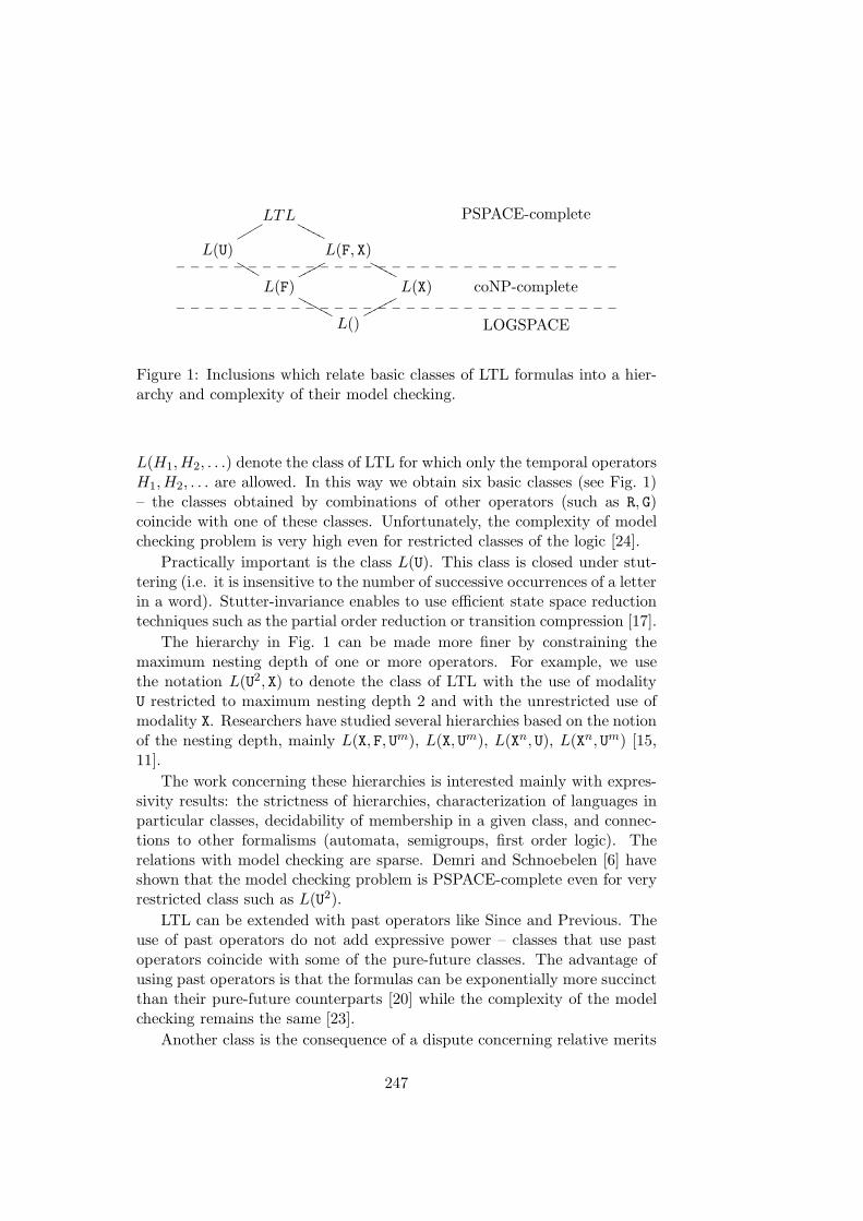
LTL
PSPACE-complete
L(U)
L(F, X)
L(F)
L(X)
coNP-complete
L() LOGSPACE
Figure 1: Inclusions which relate basic classes of LTL formulas into a hier-archy and complexity of their model checking.
L(H1,H2, . . .) denote the class of LTL for which only the temporal operatorsH1,H2, . . . are allowed. In this way we obtain six basic classes (see Fig. 1)– the classes obtained by combinations of other operators (such as R, G)coincide with one of these classes. Unfortunately, the complexity of modelchecking problem is very high even for restricted classes of the logic [24].
Practically important is the class L(U). This class is closed under stut-tering (i.e. it is insensitive to the number of successive occurrences of a letterin a word). Stutter-invariance enables to use efficient state space reductiontechniques such as the partial order reduction or transition compression [17].
The hierarchy in Fig. 1 can be made more finer by constraining themaximum nesting depth of one or more operators. For example, we usethe notation L(U2, X) to denote the class of LTL with the use of modalityU restricted to maximum nesting depth 2 and with the unrestricted use ofmodality X. Researchers have studied several hierarchies based on the notionof the nesting depth, mainly L(X, F, Um), L(X, Um), L(Xn, U), L(Xn, Um) [15,11].
The work concerning these hierarchies is interested mainly with expres-sivity results: the strictness of hierarchies, characterization of languages inparticular classes, decidability of membership in a given class, and connec-tions to other formalisms (automata, semigroups, first order logic). Therelations with model checking are sparse. Demri and Schnoebelen [6] haveshown that the model checking problem is PSPACE-complete even for veryrestricted class such as L(U2).
LTL can be extended with past operators like Since and Previous. Theuse of past operators do not add expressive power – classes that use pastoperators coincide with some of the pure-future classes. The advantage ofusing past operators is that the formulas can be exponentially more succinctthan their pure-future counterparts [20] while the complexity of the modelchecking remains the same [23].
Another class is the consequence of a dispute concerning relative merits
247
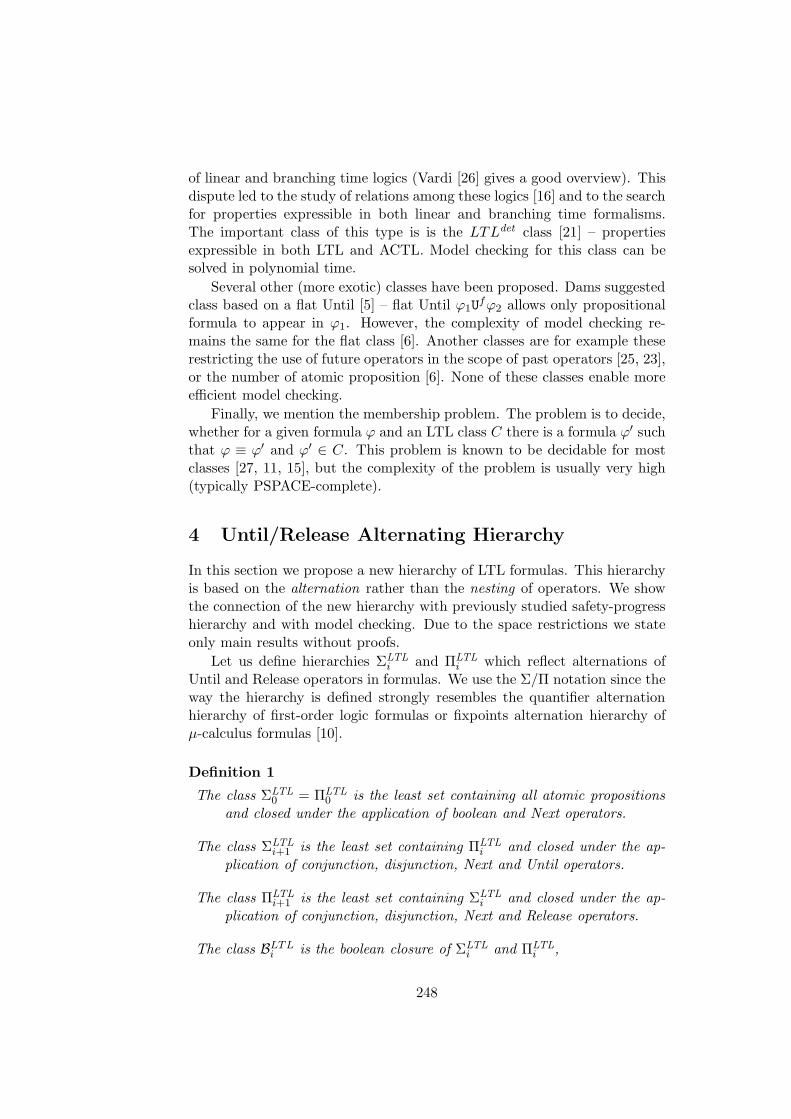
of linear and branching time logics (Vardi [26] gives a good overview). Thisdispute led to the study of relations among these logics [16] and to the searchfor properties expressible in both linear and branching time formalisms.The important class of this type is is the LTLdet class [21] – propertiesexpressible in both LTL and ACTL. Model checking for this class can besolved in polynomial time.
Several other (more exotic) classes have been proposed. Dams suggestedclass based on a flat Until [5] – flat Until ϕ1Ufϕ2 allows only propositionalformula to appear in ϕ1. However, the complexity of model checking re-mains the same for the flat class [6]. Another classes are for example theserestricting the use of future operators in the scope of past operators [25, 23],or the number of atomic proposition [6]. None of these classes enable moreefficient model checking.
Finally, we mention the membership problem. The problem is to decide,whether for a given formula ϕ and an LTL class C there is a formula ϕ′ suchthat ϕ ≡ ϕ′ and ϕ′ ∈ C. This problem is known to be decidable for mostclasses [27, 11, 15], but the complexity of the problem is usually very high(typically PSPACE-complete).
4 Until/Release Alternating Hierarchy
In this section we propose a new hierarchy of LTL formulas. This hierarchyis based on the alternation rather than the nesting of operators. We showthe connection of the new hierarchy with previously studied safety-progresshierarchy and with model checking. Due to the space restrictions we stateonly main results without proofs.
Let us define hierarchies ΣLTLi and ΠLTL
i which reflect alternations ofUntil and Release operators in formulas. We use the Σ/Π notation since theway the hierarchy is defined strongly resembles the quantifier alternationhierarchy of first-order logic formulas or fixpoints alternation hierarchy ofµ-calculus formulas [10].
Definition 1
The class ΣLTL0 = ΠLTL
0 is the least set containing all atomic propositionsand closed under the application of boolean and Next operators.
The class ΣLTLi+1 is the least set containing ΠLTL
i and closed under the ap-plication of conjunction, disjunction, Next and Until operators.
The class ΠLTLi+1 is the least set containing ΣLTL
i and closed under the ap-plication of conjunction, disjunction, Next and Release operators.
The class BLTLi is the boolean closure of ΣLTLi and ΠLTL
i ,
248
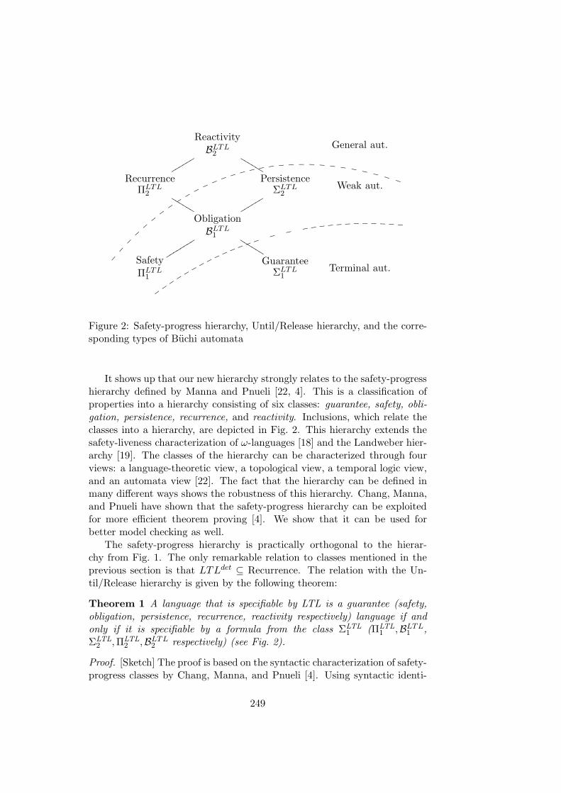
ReactivityBLTL2
General aut.
RecurrenceΠLTL
2
PersistenceΣLTL
2
Weak aut.
ObligationBLTL1
! "
SafetyΠLTL
1
GuaranteeΣLTL
1Terminal aut.
#$ % & ' (
) * +
Figure 2: Safety-progress hierarchy, Until/Release hierarchy, and the corre-sponding types of Buchi automata
It shows up that our new hierarchy strongly relates to the safety-progresshierarchy defined by Manna and Pnueli [22, 4]. This is a classification ofproperties into a hierarchy consisting of six classes: guarantee, safety, obli-gation, persistence, recurrence, and reactivity. Inclusions, which relate theclasses into a hierarchy, are depicted in Fig. 2. This hierarchy extends thesafety-liveness characterization of ω-languages [18] and the Landweber hier-archy [19]. The classes of the hierarchy can be characterized through fourviews: a language-theoretic view, a topological view, a temporal logic view,and an automata view [22]. The fact that the hierarchy can be defined inmany different ways shows the robustness of this hierarchy. Chang, Manna,and Pnueli have shown that the safety-progress hierarchy can be exploitedfor more efficient theorem proving [4]. We show that it can be used forbetter model checking as well.
The safety-progress hierarchy is practically orthogonal to the hierar-chy from Fig. 1. The only remarkable relation to classes mentioned in theprevious section is that LTLdet ⊆ Recurrence. The relation with the Un-til/Release hierarchy is given by the following theorem:
Theorem 1 A language that is specifiable by LTL is a guarantee (safety,obligation, persistence, recurrence, reactivity respectively) language if andonly if it is specifiable by a formula from the class ΣLTL
1 (ΠLTL1 ,BLTL1 ,
ΣLTL2 ,ΠLTL
2 ,BLTL2 respectively) (see Fig. 2).
Proof. [Sketch] The proof is based on the syntactic characterization of safety-progress classes by Chang, Manna, and Pnueli [4]. Using syntactic identi-
249
ties we are able to transform their characterization into the correspondingΣLTL/ΠLTL characterization.
As a consequence of the relation with safety-progress hierarchy we ob-tain the following, quite surprising fact (note that the previously mentionedhierarchies of first-order and µ-calculus formulas are infinite):
Theorem 2 Both ΣLTLi and ΠLTL
i hierarchies semantically collapse – everyLTL specifiable formula is specifiable by a BLTL2 formula.
The complexity of model checking is still PSPACE-complete even forlower classes of the hierarchy. Nevertheless, it is possible to employ thishierarchy for model checking. Formulas from lower classes of the hierarchycan be translated into specialized automata and the non-emptiness checkfor the product automaton can be performed more efficiently.
Theorem 3 For every ΣLTL1 (ΣLTL
2 ) formula ϕ one can construct a termi-nal (weak) automaton accepting the language defined by ϕ.
Proof. [Sketch] The basic idea of the construction is the same as for classicalalgorithm for transformation of LTL formula into automaton [13]. Statesof the automaton are sets of subformulas of the formula ϕ. The transitionfunction is constructed in such a way that the following invariant is valid: ifthe automaton is in a state S then the remaining suffix of the word shouldsatisfy all formulas in S. The main difference is in the way the acceptancecondition is defined. For ΣLTL
1 and ΣLTL2 formulas the acceptance condition
can be simplified thanks to the special structure of alternation of Until andRelease operators in the formula.
The non-emptiness of general automata is usually checked by nesteddepth-first search with explicit representation of the state space [14] or bynested fixpoint computation with quadratic number of symbolic steps withsymbolic representation [12]. The non-emptiness of weak automata can besolved by single depth-first search [8] or by simple fixpoint computationwith linear number of steps [2] respectively. The non-emptiness of terminalautomata can be solved by classical reachability.
With the symbolic representation there is even asymptotic difference be-tween the non-emptiness algorithms for general and specialized automata.All explicit algorithms have the same complexity, but the use of special-ized algorithms still brings several benefits. Time and space optimiza-tion, “Guided search” heuristics [8], and the partial order reduction [14]can be employed more directly for specialized algorithms. Algorithms forspecialized automata can be performed in distributed environment moreeasily [3]. Many of these benefits have been already demonstrated experi-mentally [2, 8, 3].
250
Since for ΣLTL1 and ΣLTL
2 formulas we can use more efficient algorithmsthen for general formulas, the membership problem for these classes is of par-ticular interest. This problem is decidable. Unfortunately, as for previouslyconsidered classes, the complexity of the problem is very high (the directdecision procedure goes via deterministic Streett automata and is doublyexponential). However, as we will see in the next section, practically usedformulas are very short (thus it is feasible to perform expensive algorithmsfor them) and many of them even lie in ΣLTL
1 and ΣLTL2 classes.
5 Practically Used Formulas
In order to find in which LTL classes practically used formulas lie, we havestudied properties from the ”Specification Patterns System” [7]. This systemis a collection of the most often used model checking properties. The systemprovides properties in several different formalisms, LTL being one of them,together with their frequency (i.e. how often they are used) of each of them.We have observed following characteristics of these properties:
• The next operator is not used in these patterns, i.e. practically usedproperties are stutter-invariant.
• The most often used formulas are very short (three or less temporaloperators).
• The nesting depth of until operator is in most cases one or two. Thenesting depth is greater than three only in very rare cases.
• Most properties are either from safety class (41%) or from recurrenceclass (54%). This means that in most cases the resulting automatonis specialized1.
The last observation is supported by Kupferman and Vardi [16] whoclaim that: ”... most of the LTL formulas ψ used in practice are such thatA¬ψ is a 1-weak automaton” (1-weak automata are strict subclass of weakautomata).
6 Conclusions and Future Work
The worst case complexity is not much useful with respect to the practi-cal model checking. In practice, the computational complexity caused byLTL formula is ”shadowed” by the size of a verified system. Thus it is im-portant to use algorithms efficient with respect to a system. We conclude
1Please remember that in the verification process the negation of the formula is trans-lated into an automaton. Therefore recurrence and safety formulas are translated intoweak and terminal automata respectively.
251
that important classes of LTL are these which enable the use of such effi-cient algorithms — stutter-invariant class L(U), which enable partial orderreduction, and newly identified classes ΣLTL
1 (safety properties) and ΣLTL2
(recurrence properties), which enable the use of specialized algorithms fornon-emptiness check.
Our intended future works is to try to find out some new connectionsamong other hierarchies and model checking. Particularly, we would like tostudy the connections with bounded model checking [1].
Acknowledgment
I thank Ivana Cerna, my supervisor, for many valuable discussions and JanStrejcek for reading a draft of the paper.The work on this paper has been partially supported by GA CR grantnumber 201/03/0509.
References
[1] A. Biere, A. Cimatti, E. Clarke, and Y. Zhu. Symbolic model checking with-out BDDs. In W. R. Cleaveland, editor, Proc. Tools and Algorithms for theConstruction and Analysis of Systems, volume 1579 of LNCS, pages 193–207.Springer, 1999.
[2] R. Bloem, K. Ravi, and F. Somenzi. Efficient decision procedures for modelchecking of linear time logic properties. In Proc. Computer Aided Verification,volume 1633 of LNCS, pages 222–235. Springer, 1999.
[3] I. Cerna and R. Pelanek. Distributed explicit fair cycle detection. In Proc.SPIN workshop, number 2648 in LNCS. Springer, 2003.
[4] E. Y. Chang, Z. Manna, and A. Pnueli. Characterization of temporal propertyclasses. In Proc. Automata, Languages and Programming, volume 623 of LNCS,pages 474–486. Springer, 1992.
[5] D.R. Dams. Flat fragments of CTL and CTL∗: Separating the expressive anddistinguishing powers. Logic Journal of the IGPL, 7(1):55–78, 1999.
[6] S. Demri and Ph. Schnoebelen. The complexity of propositional linear tem-poral logics in simple cases (extended abstract). In Proc. 15th Ann. Symp.Theoretical Aspects of Computer Science, volume 1373, pages 61–72. Springer,1998.
[7] M. B. Dwyer, G. S. Avrunin, and J. C. Corbett. Property specification patternsfor finite-state verification. In Proc. Workshop on Formal Methods in SoftwarePractice, pages 7–15. ACM Press, 1998.
[8] S. Edelkamp, A. L. Lafuente, and S. Leue. Directed explicit model checkingwith HSF-SPIN. In Proc. SPIN workshop, volume 2057 of LNCS, pages 57–79.Springer, 2001.
252
[9] E. A. Emerson. Temporal and modal logic. In J. Van Leeuwen, editor, Hand-book of Theoretical Computer Science: Volume B, Formal Models and Seman-tics, pages 995–1072. North-Holland Publishing Company, 1990.
[10] E. A. Emerson and C. L. Lei. Efficient model checking in fragments of thepropositional mu-calculus. In Proc. IEEE Symposium on Logic in ComuterScience, pages 267 – 278. Computer Society Press, 1986.
[11] K. Etessami and T. Wilke. An Until hierarchy for temporal logic. In Proc.IEEE Symposium on Logic in Computer Science, pages 108–117. ComputerSociety Press, 1996.
[12] K. Fisler, R. Fraer, G. Kamhi Y. Vardi, and Z. Yang. Is there a best symboliccycle-detection algorithm? In Proc. Tools and Algorithms for Construction andAnalysis of Systems, volume 2031 of LNCS, pages 420–434. Springer, 2001.
[13] R. Gerth, D. Peled, M. Y. Vardi, and P. Wolper. Simple on-the-fly automaticverification of linear temporal logic. In Proc. Protocol Specification Testingand Verification, pages 3–18. Chapman & Hall, 1995.
[14] G. J. Holzmann, D. Peled, and M. Yannakakis. On nested depth first search.In Proc. SPIN Workshop, pages 23–32. American Mathematical Society, 1996.
[15] A. Kucera and J. Strejcek. The stuttering principle revisited: On the expres-siveness of nested X and U operators in the logic LTL. In Proc. ComputerScience Logic, volume 2471 of LNCS, pages 276–291. Springer, 2002.
[16] O. Kupferman and M. Y. Vardi. Relating linear and branching model checking.In Proc. Programming Concepts and Method, pages 304–326. Chapman & Hall,1998.
[17] R. P. Kurshan, V. Levin, and H. Yenigun. Compressing transitions for modelchecking. In Computer Aided Verification (CAV’02), volume 2404 of LNCS,pages 569–581, 2002.
[18] L. Lamport. Proving correctness of multiprocess programs. IEEE TransactionsSoftware Engineering, (3):125–143, 1977.
[19] L. H. Landweber. Decision problems for omega-automata. Mathematical Sys-tems Theory, 3(4):376–384, 1969.
[20] F. Laroussinie, N. Markey, and Ph. Schnoebelen. Temporal logic with for-gettable past. In Proc. Logic in Computer Science (LICS). IEEE ComputerSociety, 2002.
[21] M. Maidl. The common fragment of CTL and LTL. In Proc. 41th AnnualSymposium on Foundations of Computer Science, pages 643–652, 2000.
[22] Z. Manna and A. Pnueli. A hierarchy of temporal properties. In Proc. ACMSymposium on Principles of Distributed Computing, pages 377–410. ACMPress, 1990.
[23] N. Markey. Past is for free: on the complexity of verifying linear temporalproperties with past. In Proc. EXPRESS, volume 68. Elsevier, 2002.
[24] A. P. Sistla and E. M. Clarke. The complexity of propositional linear temporallogics. Journal of the ACM (JACM), 32(3):733–749, 1985.
253
[25] D. Therien and T. Wilke. Nesting Until and Since in linear temporal logic. InProc. Symposium on Theoretical Aspects of Computer Science, volume 2285 ofLNCS, pages 455–464. Springer, 2002.
[26] M. Y. Vardi. Branching vs. linear time: Final showdown. In Proc. Tools andAlgorithms for Construction and Analysis of Systems, volume 2031 of LNCS,pages 1–22. Springer, 2001.
[27] T. Wilke. Classifying discrete temporal properties. In Symposium on Theoret-ical Aspects of Computer Science, pages 32–46, 1999.
254
Model Checking Epistemic Properties of
Interpreted Systems
Franco RaimondiDepartment of Computer Science - King’s College
Strand, London WC2R 2LS
Abstract. Multi-agent systems are often taken as a paradigm in the specificationof complex systems because of their ability to abstract away from implementationdetails. Different kinds of modal logics have been used to model agents’ knowl-edge/beliefs/desires and their evolution with time. In this paper we investigatehow model checking techniques can be applied to some problems of verification inmulti-agent systems. We present results achieved in the verification of static epis-temic properties of two examples encoded in the formalism of Interpreted Systems:the bit transmission problem and the protocol of the dining cryptographers.
1 IntroductionRational agents in computer science [28] can be seen as the abstractionof any piece of hardware or software enjoying autonomy, social ability, re-activity, and pro-activity. The use of multi-agent systems (MAS) in thedesign of complex systems, where implementations details are unnecessaryor unknown [17], has been proven an appealing and successful paradigm: ex-amples include information retrieval using software agents, online auctions,protocols for communication, etc.
In the past twenty years, various logical theories have been developed toformalise knowledge, beliefs, desires, intentions and other intentional atti-tudes (in the sense of [9]) of MAS. Such logics include Cohen and Levesque’stheory of intention [8], Rao and Georgeff BDI architecture [21], Wooldridge’sLogic for Rational Agents (LORA, [26]), and Interpreted Systems by Fagin,Halpern, Moses and Vardi [10].
Comparatively, less effort has been put in the verification of MAS. Assuggested in [11], model checking techniques can be applied in the verifica-tion of MAS. Various results along these lines have been achieved recentlyby Benerecetti, Wooldrige, Bordini, van der Meyden and others [1, 14, 23,27, 2, 22, 13, 19]. In this paper we employ Interpreted Systems [10] to spec-ify MAS because they provide a computationally grounded theory of agency.
Proceedings of the Eighth ESSLLI Student SessionBalder ten Cate (editor)Chapter 24, Copyright c© 2003, Franco Raimondi
255
Model Checking Epistemic Properties of Interpreted Systems
The notion of computationally grounded theory of agency was introduced byM. Wooldridge in [25] to denote a theory that can be interpreted in termsof some concrete computational model.
By means of two well-known examples from the AI arena (the bit trans-mission problem [10] and the protocol of the dining cryptographers [5]), wepresent different methodologies that can be employed in the verification ofepistemic, temporal and deontic operators in Interpreted Systems.
The rest of the paper is organised as follows: in the next section we in-troduce the formalism of Interpreted Systems and model checking. Section 3presents the main results in model checking “static” formulae. We concludein Section 4 by suggesting future development and by comparing our workto the state of the art in this field.
2 PreliminariesDue to space considerations, we refer to [10, 15] for details on InterpretedSystems extended with deontic operators. Model checking is explored fullyin [7].
2.1 Interpreted Systems
Consider n agents in a system and n non-empty sets L1, . . . , Ln of localstates, one for every agent of the system. Elements of Li will be denoted byl1, l
′1, l2, l
′2, . . .. For every agent of the system there is a set Acti of actions
that the agent can perform. Actions are not executed randomly, but follow-ing particular specifications called protocols. A protocol Pi for agent i is afunction from the set Li of local states to a non-empty set of actions Acti
Pi : Li → 2Acti .
A system of global states for n agents S is a non-empty subset of the cartesianproduct L1 × . . .×Ln. A global state g of a system S is a tuple of the formg = (l1, . . . , ln). li(g) denotes the local state of agent i in global state g.
The evolution of the system can be modelled by means of a transitionfunction π from global states and joint actions to global states:
π : S × Act → S
where Act = Act1 × . . . × Actn is the set of joint actions for the system.This defines temporal flows on the set of global states. A run r is a functionfrom time to global states: r : N → S. Hence, a run is a sequence ofglobal states obtained by applying the function π to global states and jointactions. Notice that, in the definition of π, all the local states are updatedsynchronously at each temporal step.
Given a set of propositional variables P , an Interpreted System of globalstates is a pair IS = (S, h) where S is a system of global states and
256
Franco Raimondi
h : S → 2P is an interpretation function; intuitively, h returns the proposi-tional variables true in a global state. Interpreted systems can then be usedto model time and knowledge. The logic CTLK (Computation Tree Logicof Knowledge [13]) is an extensions of CTL to include epistemic operators.For instance, epistemic modalities Ki (one for each agent) are interpretedas follows:
(IS , g) |= Ki ϕ if for all g′ li(g) = li(g′)implies (IS , g′) |= ϕ.
(intuitively, Ki ϕ captures the idea that agent i knows ϕ, i.e. ϕ holds inevery state that i considers possible).
The notion of interpreted systems can be extended to incorporate theidea of correct functioning behaviour of some or all of the components [16].Given n agents and n non-empty sets G1, . . . , Gn, a deontic system of globalstates is any system of global states defined on L1 ⊇ G1, . . . , Ln ⊇ Gn. Gi
is called the set of green states for agent i. The complement of Gi withrespect to Li, denoted with Ri, is called the set of red states for agent i.Deontic systems of global states are used to interpret other modalities ontop of CTLK, such as the following one:
(IS , g) |= Oi ϕ if for all g′ we have that li(g′) ∈ Gi implies(IS , g′) |= ϕ.
Oi ϕ is used to represent that ϕ holds in all (global) states in which agent iis functioning correctly. Another concept of particular interest is the knowl-edge that an agent i has on the assumption that the system (the environment,agent j, group of agents X) is functioning correctly. We employ the (dou-bly relativised) modal operator Kj
i for this notion, which is interpreted asfollows:
(IS , g) |= Kji ϕ if for all g′ such that li(g) = li(g′) and
lj(g′) ∈ Gj we have that (IS , g′) |= ϕ.
The resulting logic for modalities Ki is S5n; this models agents with com-plete introspection capabilities and veridical knowledge. Completeness re-sults can be shown for the Oi as well (see [15]).
2.2 Model Checking and SMV
Given a program P and a property that can be represented as a logicalformula ϕ in some (temporal) logic, model checking techniques allow forthe automatic verification of whether or not a model MP , representing theprogram P , satisfies the formula ϕ.
In the last two decades there have been great advances in the effective-ness of this approach thanks to sophisticated data manipulation techniques.Techniques based on Binary Decision Diagrams (BDDs, [3]) have been used
257
Model Checking Epistemic Properties of Interpreted Systems
to develop model checkers that are able to check large number of states [4].Alternative approaches using automata have also been developed [24].
Software tools originated from these lines of research. SPIN (see [12])exploits automata theory and related algorithms, while SMV [18] uses BDDsto represent states and transitions. In this paper we will use NuSMV, a novelimplementation of SMV [6].
By means of these softwares a large number of systems ranging fromcommunication protocols to hardware components have been verified. Theseare not agent systems, but standard distributed processes.
3 Static model checking of Interpreted SystemsIn this section we present a methodology to check epistemic formulae ex-pressing properties of an Interpreted System. We are interested in the ver-ification of formulae involving epistemic modalities only, and we do notconsider temporal operators in the formulae we want to check. We call thismethodology static model checking.
Given an Interpreted System IS , it is possible to build an SMV programPIS such that the set of states in the temporal model generated by PIS hasa one-to-one correspondence with global states of the Interpreted System.The SMV program is constructed as follows1:
1. We declare a variable for each agent, where the values of local statesare stored.
2. We declare an array of actions for each agent. Intuitively, this arraycontains the actions “enabled” in a local state, with respect to theprotocol for each agent.
3. Actions are synchronised with local states, for each agent and in eachstate.
4. The conditions for the evolution of the SMV model are obtained fromthe evolution function of the Interpreted System.
5. Propositions are defined using the function h of the Interpreted Sys-tem.
The translation into SMV is manual when deontic operators have to bechecked, as in Section 3.1. In Section 3.2 the SMV code is generated au-tomatically. In both cases, there is a one-to-one correspondence betweenglobal states of the Interpreted System and SMV states.
NuSMV provides an operator to compute the set of “reachable states”;this set is needed to build epistemic and deontic relations between states toevaluate formulae involving epistemic and deontic operators. Specifically,we have built a parser that takes the set of reachable states as input andproduces a model with epistemic and deontic relations in the format ofAkka, a Kripke model editor2. We chose to use Akka because the Kripke
1The methodology presented here is a revised version of the one in [14].2http://turing.wins.uva.nl/∼lhendrik/
258
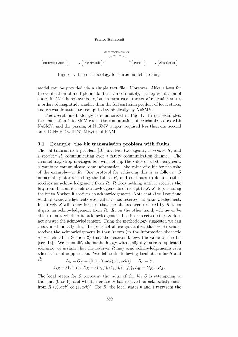
Franco Raimondi
Akka checkerInterpreted System NuSMV code Parser
Set of reachable states
Figure 1: The methodology for static model checking.
model can be provided via a simple text file. Moreover, Akka allows forthe verification of multiple modalities. Unfortunately, the representation ofstates in Akka is not symbolic, but in most cases the set of reachable statesis orders of magnitude smaller than the full cartesian product of local states,and reachable states are computed symbolically by NuSMV.
The overall methodology is summarised in Fig. 1. In our examples,the translation into SMV code, the computation of reachable states withNuSMV, and the parsing of NuSMV output required less than one secondon a 1GHz PC with 256MBytes of RAM.
3.1 Example: the bit transmission problem with faults
The bit-transmission problem [10] involves two agents, a sender S, anda receiver R, communicating over a faulty communication channel. Thechannel may drop messages but will not flip the value of a bit being sent.S wants to communicate some information—the value of a bit for the sakeof the example—to R. One protocol for achieving this is as follows. Simmediately starts sending the bit to R, and continues to do so until itreceives an acknowledgement from R. R does nothing until it receives thebit; from then on it sends acknowledgements of receipt to S. S stops sendingthe bit to R when it receives an acknowledgement. Note that R will continuesending acknowledgements even after S has received its acknowledgement.Intuitively S will know for sure that the bit has been received by R whenit gets an acknowledgement from R. R, on the other hand, will never beable to know whether its acknowledgement has been received since S doesnot answer the acknowledgement. Using the methodology suggested we cancheck mechanically that the protocol above guarantees that when senderreceives the acknowledgement it then knows (in the information-theoreticsense defined in Section 2) that the receiver knows the value of the bit(see [14]). We exemplify the methodology with a slightly more complicatedscenario: we assume that the receiver R may send acknowledgements evenwhen it is not supposed to. We define the following local states for S andR: LS = GS = 0, 1, (0, ack), (1, ack), RS = ∅.
GR = 0, 1, ε, RR = (0, f), (1, f), (ε, f), LR = GR ∪ RR.
The local states for S represent the value of the bit S is attempting totransmit (0 or 1), and whether or not S has received an acknowledgementfrom R ((0, ack) or (1, ack)). For R, the local states 0 and 1 represent the
259
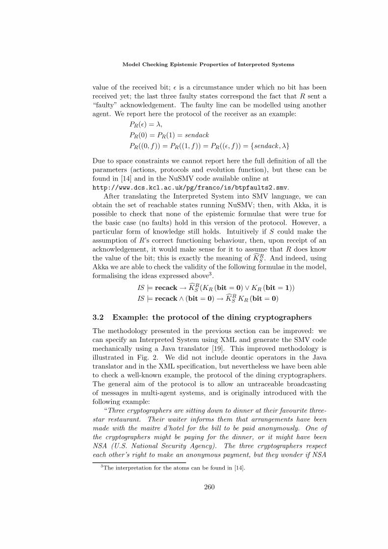
Model Checking Epistemic Properties of Interpreted Systems
value of the received bit; ε is a circumstance under which no bit has beenreceived yet; the last three faulty states correspond the fact that R sent a“faulty” acknowledgement. The faulty line can be modelled using anotheragent. We report here the protocol of the receiver as an example:
PR(ε) = λ,
PR(0) = PR(1) = sendackPR((0, f)) = PR((1, f)) = PR((ε, f)) = sendack , λ
Due to space constraints we cannot report here the full definition of all theparameters (actions, protocols and evolution function), but these can befound in [14] and in the NuSMV code available online athttp://www.dcs.kcl.ac.uk/pg/franco/is/btpfaults2.smv.
After translating the Interpreted System into SMV language, we canobtain the set of reachable states running NuSMV; then, with Akka, it ispossible to check that none of the epistemic formulae that were true forthe basic case (no faults) hold in this version of the protocol. However, aparticular form of knowledge still holds. Intuitively if S could make theassumption of R’s correct functioning behaviour, then, upon receipt of anacknowledgement, it would make sense for it to assume that R does knowthe value of the bit; this is exactly the meaning of KR
S . And indeed, usingAkka we are able to check the validity of the following formulae in the model,formalising the ideas expressed above3.
IS |= recack → KRS (KR (bit = 0) ∨ KR (bit = 1))
IS |= recack ∧ (bit = 0) → KRS KR (bit = 0)
3.2 Example: the protocol of the dining cryptographers
The methodology presented in the previous section can be improved: wecan specify an Interpreted System using XML and generate the SMV codemechanically using a Java translator [19]. This improved methodology isillustrated in Fig. 2. We did not include deontic operators in the Javatranslator and in the XML specification, but nevertheless we have been ableto check a well-known example, the protocol of the dining cryptographers.The general aim of the protocol is to allow an untraceable broadcastingof messages in multi-agent systems, and is originally introduced with thefollowing example:
“Three cryptographers are sitting down to dinner at their favourite three-star restaurant. Their waiter informs them that arrangements have beenmade with the maitre d’hotel for the bill to be paid anonymously. One ofthe cryptographers might be paying for the dinner, or it might have beenNSA (U.S. National Security Agency). The three cryptographers respecteach other’s right to make an anonymous payment, but they wonder if NSA
3The interpretation for the atoms can be found in [14].
260
Franco Raimondi
Specify interpreted system
Translate specification into NuSMV program
Model check epistemic formulae
Build an epistemic model
Use NuSMV to compute reachable states
XML editor
Parser
Akka
NuSMV
Software toolsProcedures
Java compiler
Figure 2: An improved methodology for static model checking.
is paying. They resolve their uncertainty fairly by carrying out the followingprotocol: Each cryptographer flips an unbiased coin behind his menu, betweenhim and the cryptographer on his right, so that only the two of them can seethe outcome. Each cryptographer then states aloud whether the two coins hecan see – the one he flipped and the one his left-hand neighbour flipped – fellon the same side or on different sides. If one of the cryptographers is thepayer, he states the opposite of what he sees. An odd number of differencesuttered at the table indicates that a cryptographer is paying; an even numberindicates that NSA is paying (assuming that the dinner was paid for onlyonce). Yet if a cryptographer is paying, neither of the other two learnsanything from the utterances about which cryptographer it is.”[5]
As with the example of the bit transmission problem, we can model theprotocol with Interpreted Systems. We introduce three agents Ci, i = 1, 2, 3,to model the three cryptographers, and one agent E for the Environment.By running the Java translator, NuSMV, and Akka, we can formally checkthat the following propositions hold in the Interpreted System of the diningcryptographers (details can be found in [19]):
IS |= odd → (¬paid1 → (KC1(paid2 ∨ paid3)∧
¬KC1(paid2) ∧ ¬KC1(paid2))))
IS |= even → KC1(¬paid1 ∧ ¬paid2 ∧ ¬paid3)
These two formulae confirm the correctness of the statement: if the firstcryptographer did not pay for the dinner and there is an odd number ofdifferences in the utterances, then the first cryptographer knows that eitherthe second or the third cryptographer paid for the dinner; moreover, inthis case, the first cryptographer does not know which one of the remainingcryptographers is the payer. Conversely, if the number of differences in the
261
Model Checking Epistemic Properties of Interpreted Systems
utterances is odd, then the first cryptographer knows that nobody paid forthe dinner.
4 ConclusionsIn this paper we have presented results on model checking knowledge inmulti-agent systems with two examples. Though the methodology applies to“static” formulae only, we think that these results are particularly interestingbecause we have been able to model check knowledge in a system that hasa clear correspondence with computational states of agents, and is logicallycomplete.
We have explored the issue of verification in MAS. Recently, differentworks have tackled this subject. In [27], M. Wooldridge et al. present theMABLE language for the specification of MAS. Modalities are modelled asnested data structures, in the spirit of [1]. Bordini et al [2] use a modifiedversion of the AgentSpeak(L) language [20] to specify agents and to exploitexisting model checkers.
The works of van der Meyden and Shilov [22], and van der Meydenand Su [23], are probably more related to this paper. They consider theverification of a particular class of Interpreted Systems, namely the classof synchronous distributed systems with perfect recall. An algorithm formodel checking is introduced in the first paper, but the algorithm is notimplemented and specification is not considered. In [23] verification islimited to a specific class of temporal specifications.
We have obtained preliminary results in the verification of a richer lan-guage involving temporal operators and epistemic operators, along differentextensions of the methodology presented here. In parallel, we are currentlyinvestigating theoretical aspects of the Kj
i operator, extending the workof [15].
References
[1] M. Benerecetti, F. Giunchiglia, and L. Serafini. Model checking multiagentsystems. Journal of Logic and Computation, 8(3):401–423, June 1998.
[2] R. H. Bordini, M. Fisher, C. Pardavila, and M. Wooldridge. Model checkingagentspeak. In Proceedings of the Second International Joint Conference onAutonomous Agents and Multiagent Systems (AAMAS’03), July 2003.
[3] R. E. Bryant. Graph-based algorithms for boolean function manipulation.IEEE Transaction on Computers, pages 677–691, Aug. 1986.
[4] J. R. Burch, E. M. Clarke, K. L. McMillan, D. L. Dill, and L. J. Hwang. Sym-bolic model checking: 1020 states and beyond. Information and Computation,98(2):142–170, June 1992.
[5] D. Chaum. The dining cryptographers problem: Unconditional sender andrecipient untraceability. Journal of Cryptology, 1:65–75, 1988.
262
Franco Raimondi
[6] A. Cimatti, E. Clarke, F. Giunchiglia, and M. Roveri. NuSMV: A new sym-bolic model verifier. In N. Halbwachs and D. Peled, editors, Computer AidedVerification, volume 1633 of Lecture Notes in Computer Science, pages 495–??,1999.
[7] E. M. Clarke, O. Grumberg, and D. A. Peled. Model Checking. The MITPress, Cambridge, Massachusetts, 1999.
[8] P. R. Cohen and H. J. Levesque. Intention is choice with commitment. Arti-ficial Intelligence, AI, 42(2–3):213–261, Mar. 1990.
[9] D. C. Dennett. The intentional stance. The MIT Press, Massachusetts, 1987.388 pages, 1987.
[10] R. Fagin, J. Y. Halpern, Y. Moses, and M. Y. Vardi. Reasoning about Knowl-edge. The MIT Press, Cambridge, Massachusetts, 1995.
[11] J. Halpern and M. Vardi. Model checking vs. theorem proving: a manifesto,pages 151–176. Artificial Intelligence and Mathematical Theory of Computa-tion. Academic Press, Inc, 1991.
[12] G. J. Holzmann. The model checker spin. IEEE transaction on softwareengineering, 23(5), May 1997.
[13] A. Lomuscio and W. Penczek. Bounded model checking for interpreted sys-tems. Technical report, Institute of Computer Science of the Polish Academyof Sciences, 2002.
[14] A. Lomuscio, F. Raimondi, and M. Sergot. Towards model checking interpretedsystems. In Proceedings of MoChArt, Lyon, France, August 2002.
[15] A. Lomuscio and M. Sergot. Investigations in grounded semantics for multi-agent systems specifications via deontic logic. Technical report, Imperial Col-lege, London, UK, 2000.
[16] A. Lomuscio and M. Sergot. On multi-agent systems specification via deonticlogic. In J.-J. Meyer, editor, Proceedings of ATAL 2001. Springer Verlag, July2001. To Appear.
[17] J. McCarthy. Ascribing mental qualities to machines. In M. Ringle, editor,Philosophical Perspectives in Artificial Intelligence. Harvester Press, 1979.
[18] K. McMillan. Symbolic model checking: An approach to the state explosionproblem. Kluwer Academic Publishers, 1993.
[19] F. Raimondi and A. Lomuscio. A tool for specification and verification ofepistemic and temporal properties of multi-agent system. Submitted, 2003.
[20] A. S. Rao. AgentSpeak(L): BDI agents speak out in a logical computablelanguage. Lecture Notes in Computer Science, 1038:42–??, 1996.
[21] A. S. Rao and M. P. Georgeff. Modeling rational agents within a BDI-architecture. In J. Allen, R. Fikes, and E. Sandewall, editors, Proceedings ofthe 2nd International Conference on Principles of Knowledge Representationand Reasoning, pages 473–484. Morgan Kaufmann Publishers, Apr. 1991.
263
Model Checking Epistemic Properties of Interpreted Systems
[22] R. van der Meyden and N. V. Shilov. Model checking knowledge and timein systems with perfect recall. FSTTCS: Foundations of Software Technologyand Theoretical Computer Science, 19, 1999.
[23] R. van der Meyden and K. Su. Symbolic model checking the knowledge of thedining cryptographers. Submitted, 2002.
[24] M. Y. Vardi and P. Wolper. An automata-theoretic approach to automaticprogram verification. In Symposium on Logic in Computer Science (LICS’86),pages 332–345, Washington, D.C., USA, June 1986. IEEE Computer SocietyPress.
[25] M. Wooldridge. Computationally grounded theories of agency. In E. Dur-fee, editor, Proceedings of the Fourth International Conference on Multi-AgentSystems (ICMAS 2000). IEEE Press, July 2000.
[26] M. Wooldridge. Reasoning about rational agents. MIT Press, July 2000.
[27] M. Wooldridge, M. Fisher, M.-P. Huget, and S. Parsons. Model checking multi-agent systems with MABLE. In M. Gini, T. Ishida, C. Castelfranchi, and W. L.Johnson, editors, Proceedings of the First International Joint Conference onAutonomous Agents and Multiagent Systems (AAMAS’02), pages 952–959.ACM Press, July 2002.
[28] M. Wooldridge and N. Jennings. Intelligent agents: Theory and practice.Knowledge Engineering Review, 10(2), 1995.
264
A Formal Representation of Korean
Temporal Marker dongan
Hyunjung SonEHESS Paris,
hyunjung [email protected]
Abstract. This paper has two objectives. The first is to account for the semanticfunctions of Korean temporal marker dongan in comparison with English markerfor. The second objective is to represent these functions in terms of type theory,which allows us to establish semantic representations in a coherent and explicitway.
1 Introduction
Comparing cross-lingual semantics contributes to the understanding of thenature of linguistic meaning in two different ways; first, it discovers andverifies the principles representing the universal phenomena across naturallanguages, and second, it provides evidence to support the claim of languagespecificity. In this paper, we attempt to describe the semantic characteris-tics of Korean temporal marker dongan, in comparison to English temporalmarker for. The formal representation of the observed temporal propertiesis based on type theory of Andrews (1986), Hindley et al.(1986) and Renaud(1996).
2 Semantic Representation
Our semantic representation of temporal marker dongan is based on thefollowing assumptions. First, we regard the event described by a sentence asa primitive entity like individuals and denote it by a variable ‘e’ in line withDavidson (1967). Second, we assume that the linguistic time is ordered,discrete, infinite and consisting of instants corresponding to the naturalnumbers. Thus, the linguistic time can be expressed with one of thesethree notions: instant, extended interval and duration. Instants are unitaryconstituents of linguistic time and noted by a quintuplet of natural numbers[x1,x2,x3,x4,x5] of which x1 stands for year, x2 for month, x3 for day, x4 forhour and x5 for minute.
Proceedings of the Eighth ESSLLI Student SessionBalder ten Cate (editor)Chapter 25, Copyright c© 2003, Hyunjung Son
265
A Formal Representation of Korean Temporal Marker dongan
(ex) at 3 o’clock on April 5th, 2003: instant [2003,4,5,3,0]
An extended interval is a set of consecutive instants determined by abeginning instant and an ending instant.
(ex) on April 5th, 2003: interval [[2003,4,5,0,0], [2003,4,5,23,59]]
Duration refers to a temporal distance between two distinct instants.
(ex) for 5 years: duration [5, , , , ]
For the purpose of temporal description of a sentential event, we definedthe following types and functional terms on the basis of type theory. Thesymbol λ stands for abstraction and • stands for application.
2.1 Definitions of Types
i : type symbol denoting the type of individuals
p : type symbol denoting the type of propositions
e : type symbol denoting the type of events
ent : type symbol denoting the type of natural numbers
inst : type symbol denoting the type of instants
inter : type symbol denoting the type of extended intervals
dur : type symbol denoting the type of durations
Type symbols may be omitted when no ambiguity is introduced.
2.2 Definitions of Functional Terms
(λe. moment•e): e→inst
Applying this function to any argument of type e, we obtain the mo-ment of e of type inst.
(λe. interv•e): e→inter
Applying this function to any argument of type e, we obtain the in-terval of e of type inter.
(λx. beginning•x): e→inst / (λx. ending•x): e→inst
Applying these functions to any argument x of type e, we obtain thebeginning/ending instant of x of type inst.
266
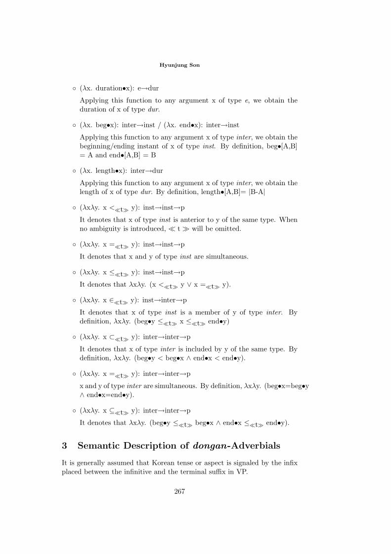
Hyunjung Son
(λx. duration•x): e→dur
Applying this function to any argument x of type e, we obtain theduration of x of type dur.
(λx. beg•x): inter→inst / (λx. end•x): inter→inst
Applying this function to any argument x of type inter, we obtain thebeginning/ending instant of x of type inst. By definition, beg•[A,B]= A and end•[A,B] = B
(λx. length•x): inter→dur
Applying this function to any argument x of type inter, we obtain thelength of x of type dur. By definition, length•[A,B]= |B-A|
(λxλy. x <t y): inst→inst→p
It denotes that x of type inst is anterior to y of the same type. Whenno ambiguity is introduced, t will be omitted.
(λxλy. x =t y): inst→inst→p
It denotes that x and y of type inst are simultaneous.
(λxλy. x ≤t y): inst→inst→p
It denotes that λxλy. (x <t y ∨ x =t y).
(λxλy. x ∈t y): inst→inter→p
It denotes that x of type inst is a member of y of type inter. Bydefinition, λxλy. (beg•y ≤t x ≤t end•y)
(λxλy. x ⊂t y): inter→inter→p
It denotes that x of type inter is included by y of the same type. Bydefinition, λxλy. (beg•y < beg•x ∧ end•x < end•y).
(λxλy. x =t y): inter→inter→p
x and y of type inter are simultaneous. By definition, λxλy. (beg•x=beg•y∧ end•x=end•y).
(λxλy. x ⊆t y): inter→inter→p
It denotes that λxλy. (beg•y ≤t beg•x ∧ end•x ≤t end•y).
3 Semantic Description of dongan-Adverbials
It is generally assumed that Korean tense or aspect is signaled by the infixplaced between the infinitive and the terminal suffix in VP.
267
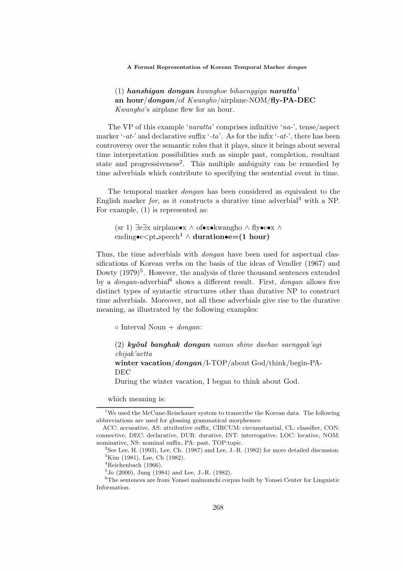
A Formal Representation of Korean Temporal Marker dongan
(1) hanshigan dongan kwanghoe bihaenggiga naratta1
an hour/dongan/of Kwangho/airplane-NOM/fly-PA-DECKwangho’s airplane flew for an hour.
The VP of this example ‘naratta’ comprises infinitive ‘na-’, tense/aspectmarker ‘-at-’ and declarative suffix ‘-ta’. As for the infix ‘-at-’, there has beencontroversy over the semantic roles that it plays, since it brings about severaltime interpretation possibilities such as simple past, completion, resultantstate and progressiveness2. This multiple ambiguity can be remedied bytime adverbials which contribute to specifying the sentential event in time.
The temporal marker dongan has been considered as equivalent to theEnglish marker for, as it constructs a durative time adverbial3 with a NP.For example, (1) is represented as:
(sr 1) ∃e∃x airplane•x ∧ of•x•kwangho ∧ fly•e•x ∧ending•e<pt speech4 ∧ duration•e=(1 hour)
Thus, the time adverbials with dongan have been used for aspectual clas-sifications of Korean verbs on the basis of the ideas of Vendler (1967) andDowty (1979)5. However, the analysis of three thousand sentences extendedby a dongan-adverbial6 shows a different result. First, dongan allows fivedistinct types of syntactic structures other than durative NP to constructtime adverbials. Moreover, not all these adverbials give rise to the durativemeaning, as illustrated by the following examples:
Interval Noun + dongan:
(2) kyoul banghak dongan nanun shine daehae saenggak’agichijak’aettawinter vacation/dongan/I-TOP/about God/think/begin-PA-DECDuring the winter vacation, I began to think about God.
which meaning is:1We used the McCune-Reischauer system to transcribe the Korean data. The following
abbreviations are used for glossing grammatical morphemes:ACC: accusative, AS: attributive suffix, CIRCUM: circumstantial, CL: classifier, CON:
connective, DEC: declarative, DUR: durative, INT: interrogative, LOC: locative, NOM:nominative, NS: nominal suffix, PA: past, TOP:topic.
2See Lee, H. (1993), Lee, Ch. (1987) and Lee, J.-R. (1982) for more detailed discussion.3Kim (1981), Lee, Ch (1982).4Reichenbach (1966).5Jo (2000), Jung (1984) and Lee, J.-R. (1982).6The sentences are from Yonsei malmunchi corpus built by Yonsei Center for Linguistic
Information.
268
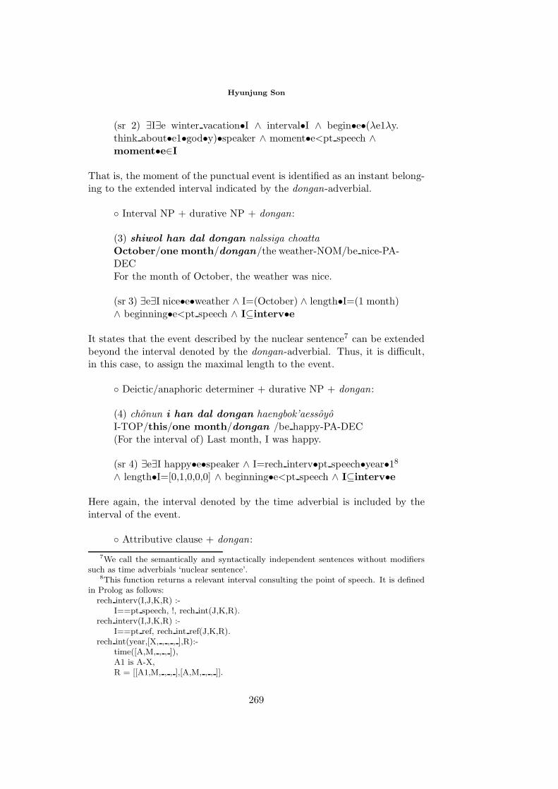
Hyunjung Son
(sr 2) ∃I∃e winter vacation•I ∧ interval•I ∧ begin•e•(λe1λy.think about•e1•god•y)•speaker ∧ moment•e<pt speech ∧moment•e∈I
That is, the moment of the punctual event is identified as an instant belong-ing to the extended interval indicated by the dongan-adverbial.
Interval NP + durative NP + dongan:
(3) shiwol han dal dongan nalssiga choattaOctober/one month/dongan/the weather-NOM/be nice-PA-DECFor the month of October, the weather was nice.
(sr 3) ∃e∃I nice•e•weather ∧ I=(October) ∧ length•I=(1 month)∧ beginning•e<pt speech ∧ I⊆interv•e
It states that the event described by the nuclear sentence7 can be extendedbeyond the interval denoted by the dongan-adverbial. Thus, it is difficult,in this case, to assign the maximal length to the event.
Deictic/anaphoric determiner + durative NP + dongan:
(4) chonun i han dal dongan haengbok’aessoyoI-TOP/this/one month/dongan /be happy-PA-DEC(For the interval of) Last month, I was happy.
(sr 4) ∃e∃I happy•e•speaker ∧ I=rech interv•pt speech•year•18
∧ length•I=[0,1,0,0,0] ∧ beginning•e<pt speech ∧ I⊆interv•e
Here again, the interval denoted by the time adverbial is included by theinterval of the event.
Attributive clause + dongan:
7We call the semantically and syntactically independent sentences without modifierssuch as time adverbials ‘nuclear sentence’.
8This function returns a relevant interval consulting the point of speech. It is definedin Prolog as follows:
rech interv(I,J,K,R) :-I==pt speech, !, rech int(J,K,R).
rech interv(I,J,K,R) :-I==pt ref, rech int ref(J,K,R).
rech int(year,[X, , , , ],R):-time([A,M, , , ]),A1 is A-X,R = [[A1,M, , , ],[A,M, , , ]].
269
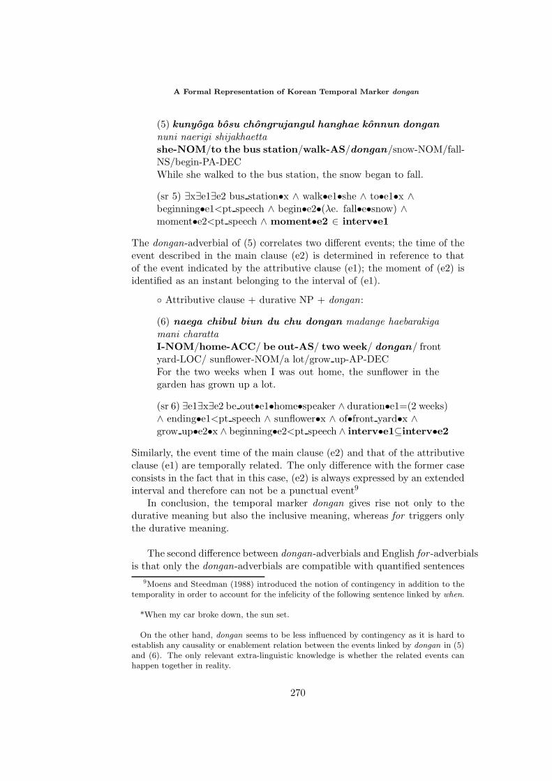
A Formal Representation of Korean Temporal Marker dongan
(5) kunyoga bosu chongrujangul hanghae konnun dongannuni naerigi shijakhaettashe-NOM/to the bus station/walk-AS/dongan/snow-NOM/fall-NS/begin-PA-DECWhile she walked to the bus station, the snow began to fall.
(sr 5) ∃x∃e1∃e2 bus station•x ∧ walk•e1•she ∧ to•e1•x ∧beginning•e1<pt speech ∧ begin•e2•(λe. fall•e•snow) ∧moment•e2<pt speech ∧ moment•e2 ∈ interv•e1
The dongan-adverbial of (5) correlates two different events; the time of theevent described in the main clause (e2) is determined in reference to thatof the event indicated by the attributive clause (e1); the moment of (e2) isidentified as an instant belonging to the interval of (e1).
Attributive clause + durative NP + dongan:
(6) naega chibul biun du chu dongan madange haebarakigamani charattaI-NOM/home-ACC/ be out-AS/ two week/ dongan/ frontyard-LOC/ sunflower-NOM/a lot/grow up-AP-DECFor the two weeks when I was out home, the sunflower in thegarden has grown up a lot.
(sr 6) ∃e1∃x∃e2 be out•e1•home•speaker ∧ duration•e1=(2 weeks)∧ ending•e1<pt speech ∧ sunflower•x ∧ of•front yard•x ∧grow up•e2•x ∧ beginning•e2<pt speech ∧ interv•e1⊆interv•e2
Similarly, the event time of the main clause (e2) and that of the attributiveclause (e1) are temporally related. The only difference with the former caseconsists in the fact that in this case, (e2) is always expressed by an extendedinterval and therefore can not be a punctual event9
In conclusion, the temporal marker dongan gives rise not only to thedurative meaning but also the inclusive meaning, whereas for triggers onlythe durative meaning.
The second difference between dongan-adverbials and English for -adverbialsis that only the dongan-adverbials are compatible with quantified sentences
9Moens and Steedman (1988) introduced the notion of contingency in addition to thetemporality in order to account for the infelicity of the following sentence linked by when.
*When my car broke down, the sun set.
On the other hand, dongan seems to be less influenced by contingency as it is hard toestablish any causality or enablement relation between the events linked by dongan in (5)and (6). The only relevant extra-linguistic knowledge is whether the related events canhappen together in reality.
270
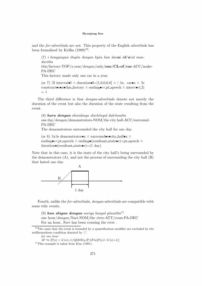
Hyunjung Son
and the for -adverbials are not. This property of the English adverbials hasbeen formalized by Krifka (1989)10.
(7) i kongjangun ilnyon dongan kyou han daeui ch’arul man-durottathis/factory-TOP/a year/dongan/only/one/CL-of/car-ACC/make-PA-DECThis factory made only one car in a year.
(sr 7) ∃I interval•I ∧ duration•I=[1,0,0,0,0] ∧ | λx. car•x ∧ ∃econstruct•e•x•this factory ∧ ending•e<pt speech ∧ interv•e⊆I|= 1
The third difference is that dongan-adverbials denote not merely theduration of the event but also the duration of the state resulting from theevent.
(8) haru dongan shiwidaega shichongul dulrossattaone day/dongan/demonstrators-NOM/the city hall-ACC/surround-PA-DECThe demonstrators surrounded the city hall for one day.
(sr 8) ∃x∃e demonstrator•x ∧ surround•e•city hall•x ∧ending•e<pt speech ∧ ending•(resultant state•e)<pt speech ∧duration•(resultant state•e)=(1 day)
Note that in this case, it is the state of the city hall’s being surrounded bythe demonstrators (A), and not the process of surrounding the city hall (B)that lasted one day.
A
B
1 day
Fourth, unlike the for -adverbials, dongan-adverbials are compatible withsome telic events.
(9) han shigan dongan nariga kangul gonnotta11
one hour/dongan/Nari-NOM/the river-ATT/cross-PA-DECFor an hour, Nari has been crossing the river .
10The cases that the event is bounded by a quantification modifier are excluded by thewellformedness condition denoted by ‘/’.
for one hourλP ∀e [P(e) ∧ h′(e)=1/QMODE(P,λPλe[P(e)∧ h′(e)=1)]
11This example is taken from Kim (1981).
271
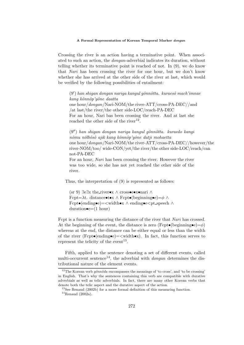
A Formal Representation of Korean Temporal Marker dongan
Crossing the river is an action having a terminative point. When associ-ated to such an action, the dongan-adverbial indicates its duration, withouttelling whether its terminative point is reached of not. In (9), we do knowthat Nari has been crossing the river for one hour, but we don’t knowwhether she has arrived at the other side of the river at last, which wouldbe verified by the following possibilities of entailment:
(9′) han shigan dongan nariga kangul gonnotta. kuraeso mach’imnaekang konnop’yone daattaone hour/dongan/Nari-NOM/the river-ATT/cross-PA-DEC//and/at last/the river/the other side-LOC/reach-PA-DECFor an hour, Nari bas been crossing the river. And at last shereached the other side of the river12.
(9′′) han shigan dongan nariga kangul gonnotta. kuraedo kanginomu nolboso ajik kang konnop’yone datji mohaettaone hour/dongan/Nari-NOM/the river-ATT/cross-PA-DEC//however/theriver-NOM/too/ wide-CON/yet/the river/the other side-LOC/reach/cannot-PA-DECFor an hour, Nari has been crossing the river. However the riverwas too wide, so she has not yet reached the other side of theriver.
Thus, the interpretation of (9) is represented as follows:
(sr 9) ∃e∃x the river•x ∧ cross•e•x•nari ∧Fcpt=λt. distance•t•x ∧ Fcpt•(beginning•e)=φ ∧Fcpt•(ending•e)=<width•x ∧ ending•e<pt speech ∧duration•e=(1 hour)
Fcpt is a function measuring the distance of the river that Nari has crossed.At the beginning of the event, the distance is zero (Fcpt•(beginning•e)=φ)whereas at the end, the distance can be either equal or less than the widthof the river (Fcpt•(ending•e)=<width•x). In fact, this function serves torepresent the telicity of the event13.
Fifth, applied to the sentence denoting a set of different events, calledmulti-occurrent sentence14, the adverbial with dongan determines the dis-tributional nature of the element events.
12The Korean verb gonnoda encompasses the meanings of ‘to cross’, and ‘to be crossing’in English. That’s why the sentences containing this verb are compatible with durativeadverbials as well as telic adverbials. In fact, there are many other Korean verbs thatdenote both the telic aspect and the durative aspect of the action.
13See Renaud (2002b) for a more formal definition of this measuring function.14Renaud (2002a).
272
Hyunjung Son
(10) shimnyon dongan yunsokun mon badaeso kogijabirul haetta10 years/dongan/Yunsok-TOP/far ocean-LOC/fishing-ACC/do-PA-DECFor ten years, Yunsok fished far in the ocean.
That is, the ten years is the maximal length of the interval in which Yunsok ’sfishing has been repeated in a consistent way15.
interval of reference (intref )
10 years
• •• • •• • • •• • •• • • • •
This interpretation is represented as follows 16 :
(sr 10) λD. ∃P equi-partition•D•P•intref ∧∃I I=(λJ. P•J ∧ ∃e fish•e•yunsok ∧ in•e•the far ocean ∧ending•e<pt speech ∧ interv•e⊆J) ∧∃M (max•(λN. N⊆(∪•I) ∧ [inferior•(∪•N), superior•(∪•N)] ∩intref = ∪•N)•M ∧ duration•M = (10 years))
where the function equi-partition•D•P•L denotes that the element eventsoccurred regularly during the period.
But when the sentence is modified by quantification, the time adver-bial no longer imposes the distributional constraint and merely signals thetemporal scope of the quantification.
(10′) shimnyon dongan yunsokun mon badaeso se bon kogi-jabirul haetta10 years/dongan/Yunsok-TOP/far ocean-LOC/three times/fishing-ACC/do-PA-DECFor ten years, Yunsok fished three times far in the ocean.
(sr 10′) ∃I interv•I ∧ duration•I=[10,0,0,0,0] ∧ | λe. fish•e•yunsok∧ in•e•the far ocean ∧ ending•e<pt speech ∧ interval•e⊆I|=3
Finally, the facts that we observed concerning the temporal adverbialswith dongan can be summarized as follows:
15The occurrences of Yunsok ’s fishing are noted by ‘•’ in the figure.16Renaud (2002a) defines the functions used in this formula as :
equi-partition•D•P•N ≡ (N=(∪ • P ) ∧ | P |>2 ∧∀K1 K2 ((P•K1 ∧ P•K2 ∧ K1=K2)→ (duration•K1=duration•K2=D ∧ K1∩K2=φ)))∪ •R ≡ λx. ∃R (R•P ∧ P•x) [A, B] ≡ an interval with the limits A and Bmax•E•M ≡ (E•M ∧ ¬∃N(M⊂N ∧ E•N))
273
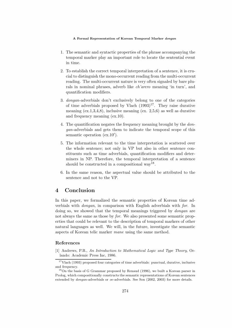
A Formal Representation of Korean Temporal Marker dongan
1. The semantic and syntactic properties of the phrase accompanying thetemporal marker play an important role to locate the sentential eventin time.
2. To establish the correct temporal interpretation of a sentence, it is cru-cial to distinguish the mono-occurrent reading from the multi-occurrentreading. The multi-occurrent nature is very often signaled by bare plu-rals in nominal phrases, adverb like ch’arero meaning ‘in turn’, andquantification modifiers.
3. dongan-adverbials don’t exclusively belong to one of the categoriesof time adverbials proposed by Vlach (1993)17. They raise durativemeaning (ex.1,3,4,8), inclusive meaning (ex. 2,5,6) as well as durativeand frequency meaning (ex.10).
4. The quantification negates the frequency meaning brought by the don-gan-adverbials and gets them to indicate the temporal scope of thissemantic operation (ex.10′).
5. The information relevant to the time interpretation is scattered overthe whole sentence; not only in VP but also in other sentence con-stituents such as time adverbials, quantification modifiers and deter-miners in NP. Therefore, the temporal interpretation of a sentenceshould be constructed in a compositional way18.
6. In the same reason, the aspectual value should be attributed to thesentence and not to the VP.
4 Conclusion
In this paper, we formalized the semantic properties of Korean time ad-verbials with dongan, in comparison with English adverbials with for. Indoing so, we showed that the temporal meanings triggered by dongan arenot always the same as those by for. We also presented some semantic prop-erties that could be relevant to the description of temporal markers of othernatural languages as well. We will, in the future, investigate the semanticaspects of Korean telic marker mane using the same method.
References
[1] Andrews, P.B., An Introduction to Mathematical Logic and Type Theory, Or-lando: Academic Press Inc, 1986.17Vlach (1993) proposed four categories of time adverbials: punctual, durative, inclusive
and frequency.18On the basis of G Grammar proposed by Renaud (1996), we built a Korean parser in
Prolog, which compositionally constructs the semantic representations of Korean sentencesextended by dongan-adverbials or oe-adverbials. See Son (2002, 2003) for more details.
274
Hyunjung Son
[2] Davidson, D., The logical Form of Action Sentences, in Essays on Actions andEvents, Oxford: Clarendon Press, 1967 [1980].
[3] Dowty, D.R., Word Meaning and Montague Grammar, Dordrecht: Reidel, 1979.
[4] Hindley, J. and Seldin, J.P., Introduction to Combinators and λ-Calculus, Cam-bridge: Cambridge Univ. Press, 1986.
[5] Jo, M.-J., A Study on the Aspect of Korean (in Korean), Yonsei Univ. Disser-tation, 2000.
[6] Jung, M., “Classification of Korean Verbs with Aspectual Properties” (in Ko-rean), Study of Grammar 5 (1984), Seoul: Society of Korean Grammar.
[7] Kim, S.-D., “Aspect of Korean”(in Korean), Aesan Hakbo 1 (1981): 25-70,Seoul: Aesan Hakhoe.
[8] Krifka, M., “Nominal Reference, Temporal Constitution and Quantification inEvent”, in Bartsch, R. et al.(eds.), Dordrecht: Foris Publications, 1989.
[9] Moens, M. and Steedman, M., “Temporal Ontology and Temporal Reference”,Computational Linguistics 14 (1988): 15-28.
[10] Lee, Ch., “Aspects of Aspect in Korean”, Language 7 (1982): 570-582, Seoul:Korean Linguistic Society.
[11] Lee, H. S., “Tense or aspect : The speaker’s communicative goals and con-cerns as determinant, with reference to the Anterior -oss- in Korean”, Journalof Pragmatics 20 (1993): 327-358.
[12] Lee, J.-R., “A Study of Aspectual Forms of Modern Korean”(in Korean), Ko-rean Linguistic Research 51 (1982), Seoul: Society of Korean Studies.
[13] Reichenbach, H., The Elements of Symbolic Logic, New York: The Free Press,1966.
[14] Renaud, F., Semantique du temps et lambda-calculus, Paris: puf, 1996.
[15] Renaud, F., “Durativite et negation”, ms, 2002a.
[16] Renaud, F., “Telicite et quantification”, ms, 2002b.
[17] Son, H., “Formal Description of NP+OE with Lambda-Calculus andUnification Mechanism”(in Korean), Annual Meeting of Korean Society for Lan-guage and Information (2002), 77-86.
[18] Son, H., “A Computational Treatment of Korean Temporal Markers, OE andDONGAN ”, submitted to Student Research Workshop of ACL (2003).
[19] Vendler, Z., Linguistics in Philosophy, Ithaca: Cornell Univ. Press, 1967.
[20] Vlach, F., 1993, “Temporal Adverbials, Tense and the Perfect”, Linguisticsand Philosophy 16 (1989), 231-283.
275
277
Scalar Implicatures: Exhaustivity and Gricean Reasoning
BENJAMIN SPECTOR Laboratoire de Linguistique Formelle - Paris VII / Institut Jean-Nicod [email protected] ABSTRACT. This paper shows that both scalar implicatures and exhaustification of answers can
be understood as the outcome of a pragmatic reasoning based on gricean maxims. I offer a formalization of the gricean reasoning that solves the problems (cf. Chierchia 2001) faced by standard neo-gricean accounts. I further show that positive and non-positive answers pattern very differently, in a way that can be predicted by stating carefully, for a given question-answer pair, what counts as an "alternative answer" - this notion plays the same role as that of “scalar alternative” in previous approaches.
I. Imperfections of Standard Neo-gricean Accounts According to neo-gricean accounts, scalar implicatures are computed as
follows: given a sentence S containing a scalar term t, S is to be compared to all sentences which can be obtained from S by replacing t with a term belonging to t’s scale. For any such scalar alternative S’ such that S’ asymmetrically entails S, the hearer infers that S’ is not part of the speaker’s beliefs. (hereafter, rule R1; this derives the so-called epistemic implicatures). The underlying principle motivating this inference is Grice’s first maxim of Quantity. Assuming further that the speaker is maximally informed, the hearer infers that S’ is in fact false according to the speaker (hereafter, rule R2).
(1) A or B (2) A and B Suppose the speaker utters a sentence of the form of (1). Its unique scalar
alternative is (2). Since (2) is logically stronger than (1), (2) is not part of the speaker’s belief. Moreover, if the speaker is maximally informed, (2) is false, so that or in (1) is interpreted as exclusive, even though its literal linguistic meaning is that of inclusive disjunction.
Whatever the merits of this approach (in particular, the fact that it predicts that the exclusive reading of or should disappear in monotone decreasing contexts, due to the reversal of entailment patterns), it has been shown to be inaccurate in many cases, especially when a scalar term is interpreted under the scope of some operators. For instance, Chierchia (2001) points out that the neo-gricean procedure yields too weak results for a sentence like (3):
(3) Each of the students read Othello or King Lear
Proceedings of the Eighth ESSLLI Student Session. Balder ten Cate (editor) Chapter 26, Copyright © 2003, Benjamin Spector
Scalar Implicatures: Exhaustivity and Gricean Reasoning
278
(3) (sometimes) implicates (4)1: (4) Each of the students read Othello or King Lear and not both. The neo-gricean account predicts a much weaker implicature, namely (5): (5) It is not the case that each of the students read Othello and King Lear. Another problem is that the neo-gricean account can also lead to too strong
predictions. Take a sentence of the following form: (6) (A or B) or C Salar alternatives of (6): a. (A and B) or C b. (A or B) and C c. (A and B) and C All these alternatives are stronger than (6), so that (6) should implicate that
they are all false (by rule R2). In particular, a. should be false, in which case C is. But (6) certainly does not implicate that C is false. Let me call this problem, which is actually very general, that of unwanted negations. If, on the other hand, we find a way of blocking this inference, we remain unable to predict that (6) normally implicates that only one of the three disjuncts is true.
I. 1 Chierchia’s localist solution Chierchia (2001) presents a solution based on a recursive interpretation
function which computes “strengthened meanings” in tandem with the interpretation function that computes “literal meanings”. For him, scalar implicatures are simply an additional dimension of meaning, and the link between scalar implicatures and general principles of conversational rationality becomes less clear, even though some basic aspects of the neo-gricean approaches are retained.
Hereafter, I will defend a “globalist” approach to scalar implicatures, in the sense that it relies on the natural hypothesis that pragmatic processes operate at least at the sentential level.
I. 2. Sauerland (2001) Sauerland (2001) modifies the neo-gricean procedure by changing what
counts as a scalar alternative for a given sentence. If a certain sentence S is of the form "P or Q", then P and Q count as alternative sentences, and so do P and Q's own scalar alternatives. But this move, as such, can only lead to a strengthening of what the ‘standard’ account derives, i.e. cannot remove the unwanted negations. Sauerland shows that this problem can be solved if one adopts more plausible inference rules. His proposal is quite similar to mine in this respect2.
I. 3. Is exhaustification the solution ? Van Rooy (2002) proposes to derive scalar implicatures from the fact that, if a
certain question Q is under discussion and a certain sentence S is given as an answer to Q, S is generally interpreted as "exhaustive".
1 In section III.3.3, I account for the fact that this inference is not systematic. 2 I am grateful to an anonymous reviewer for pointing out a version of
Sauerland’s paper that is more recent than the one I had read and bears more similarity to my own proposal.
Benjamin Spector
279
The exhaustivity operator (Groenendijk & Stokhof 1984) operates on answers of the form 'GQ P', where GQ stands for a generalized quantifier and P for a predicate. The question under discussion is understood as "for which objects is P true of these objects ?".
The exhaustivity (exh) operator works as follows3: [[exh (GQ P)]] = 1 iff [[P]] ∈ (Min [[GQ]] ), where (Min [[GQ]] ) is the set that
includes only the minimal members of [[GQ]] , i.e: Min [[GQ]] = x x ∈ [[GQ]] and there is no x' in [[GQ]] such that x' ⊂ x (⊂ = “is a proper subset of”) Example: (7) a. Among John, Mary and Peter, who came? b. John or Mary came [[John or Mary]] = J, M, P, J, M, J, P, J, M, P, M (Min [[John or Mary]] ) = J, M [[exh (John or Mary came)]] = 1 iff [[came]] ∈ J, M i.e. iff only John
came or only Mary came. Van Rooy shows that when exhaustification is applied to monotone increasing
contexts, it can solve some of Chierchia's puzzles. I. 4. When exactly do we exhaustify answers ? However, if exhaustification is applied to a sentence 'GQ P' where GQ is
decreasing, exhaustification as defined above leads to unrealistic implicatures: "less than two chemists came" should implicate that nobody came! So Van Rooy uses a second exhaustivity operator (exh’) in these cases, following Stechow & Zimmermann (1984):
[[exh' (GQ P)]] = 1 iff [[P]] ∈ (Max [[GQ]] ), where (Max [[GQ]] ) is the set that includes only the maximal members of [[GQ]]
There are several problems with this account. First, the second rule of exhaustification makes wrong predictions: (8) a. Among the chemists and the philosophers, who came? b. Less than two of the chemists Exhaustification leads to b': b' . Exactly one chemist and all the philosophers came. But b. does not seem to implicate b'; b. actually does indeed suggest that some
chemist came, but does not implicate anything regarding non-chemists. It rather suggests that the speaker does not know much about them.
Second, these two rules are unable to account for cases where the speaker combines increasing and decreasing quantifiers, thus creating a non-monotone GQ, as in (9)b:
(9) a. Among the chemists, the philosophers and the linguists, who came?
3 I reformulate Groenendijk & Stockhof’s exhaustivity operator in more
simple terms, but the difference is immaterial.
Scalar Implicatures: Exhaustivity and Gricean Reasoning
280
b. Less than two chemists but one philosopher came If we apply the first exhaustivity operator, what we get is that b. implicates
that no chemist and no linguist came, while exactly one philosopher came. If we apply the second exhaustivity operator, what we get is that exactly one
chemist, all the philosophers and all the linguists came. None of these predictions is in fact borne out. Rather, it seems that (9)
implicates that at least one chemist came, exactly one philosopher came, and that the speaker does not know much about linguists.
I. 5. Goal of this paper: deriving exhaustivity In the next sections, I show that both scalar implicatures and exhaustification
of answers can be understood as the outcome of a pragmatic reasoning that is based on the gricean maxims. I will first offer a precise formalization of the gricean reasoning, meant to replace the two rules R1 and R2. I will then show that it is possible to predict the facts reviewed above by defining carefully what counts as an "alternative answer" for a given answer to a certain question under discussion.
II. Formalizing the gricean reasoning I now assume that a certain sentence A is uttered as an answer to a (maybe
implicit) question Q, and I adopt a partition semantics for questions (Groenendijk & Stockhof 1984): Q induces an equivalence relation RQ, over the set of worlds.
Notation: - w RQ w’ w and w’ belongs to the same « cell» - RQ (v) = w w RQ v (= the set of worlds equivalent to v, or v’s cell) - α (w) α is true in w (alternatively: w ∈ α) - α ⊆ β α is a subset of β; α entails β - α ⊂ β α is a proper subset of β; α asymmetrically entails β The proposition α expressed by A is supposed to meet the condition of strong
relevance. Def 1 (strong relevance): A proposition α (= set of worlds) is strongly
relevant with respect to a question Q if a) ∃ w, (RQ(w) ∩ α) = Ø (i.e.: α excludes at least one cell) and b) ∀w, (α(w) ↔ (RQ(w) ⊆ á)) (α does not distinguish between
two worlds that belong to the same cell, i.e. provides no irrelevant information) The speaker’s information state is modeled as a set of worlds, i.e. a
proposition. As an agent believes a lot of things that are irrelevant in the context of a given question, it is useful to define what counts as the relevant information contained in a certain information state:
Benjamin Spector
281
Def 2 (relevant information): Let i be an information state and Q a question. Then we define i relativized to Q, written as i/Q, as follows:
i/Q = w ∃ w', (w' RQ w and w'∈ i) ( = ∪w∈ i RQ(w)). The gricean reasoning is based on the idea that α (the proposition given as an
answer) must be compared to a certain set of alternative propositions4 which the speaker could have chosen instead of α. This alternative set, call it S, must contain α itself, and be such that all its members are relevant5. The hearer's task when interpreting the speaker's utterance is to address the following question: given that the speaker has preferred α to all the other members of S, what does this entail regarding his information state i0? First, the speaker must believe α to be true (Grice’s maxim of quality), i.e. i0 must entail α. Second, α must be optimal in the sense that there must be no more informative proposition in S entailed by the speaker’s beliefs (Grice’s maxim of quantity), i.e. there must be no proposition α’ such that i0 entails α’ and α’ asymmetrically entails α. Put differently, i0 must belong to the following set I(S,α,Q):
Def 3: I(S,α,Q) = i i ⊆ α and ∀ α' (α' ∈ S and i ⊆ α’) → ¬ (α' ⊂ α) So if a certain proposition β is entailed by no member of I(S,α,Q), the hearer
can conclude that β is not part of the speaker’s belief. This reasoning plays the role of rule R1. It is immediately predicted that if the speaker utters a sentence P of the form “A or B” and if the propositions expressed by A and by B belong to the alternative set S, as I will assume (so does Sauerland (2001)), then the speaker cannot know A to be either true or false: if A were true, then A would have been a better answer than P; if A were false, B would be true (since P is), and B would have been a better answer than P6. Now, let the hearer assume that the speaker is as informed as possible given the answer he made. This means that his information state i0 is maximal in I(S,α,Q) in the following sense: there is no i’ in I(S,α,Q) such that i’ (relativized to Q) asymmetrically entails i0 (relativized to Q). In other words, i0 belongs to Max(S,α,Q), defined as follows:
Def 4: Max(S,α,Q)=ii ∈ I(S,α,Q) and∀i' (i'∈I(S,α,Q))→ ¬ (i'/Q⊂ i/Q ) From this the hearer can conclude that if a proposition β is entailed by all the
members of Max(S,α,Q), then β is believed by the speaker. This reasoning plays the role of R2, but is not equivalent to it: there is no way of deriving an “unwanted negation”. In the case of a disjunctive statement in which the disjuncts are logically independent, the disjuncts and their negations are entailed by no member of I(S,α,Q), as shown above, so that they cannot be entailed by any member of Max(S,α,Q) either, since Max(S,α,Q) is included in I(S,α,Q).
4 As my formulation makes clear, I am now adopting the simplifying view
that what the hearer compares are propositions. 5 The exact definition of alternative sets is the topic of section III. 6 Assuming that A and B are logically independent.
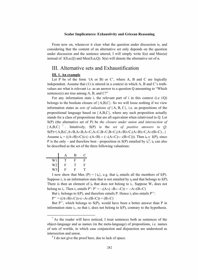
Scalar Implicatures: Exhaustivity and Gricean Reasoning
282
From now on, whenever it clear what the question under discussion is, and considering that the content of an alternative set only depends on the question under discussion and the sentence uttered, I will simply write I(α) and Max(α) instead of I(S,α,Q) and Max(S,α,Q). S(α) will denote the alternative set of α.
III. Alternative sets and Exhaustification III. 1. An example Let P be of the form ‘(A or B) or C’, where A, B and C are logically
independent. Assume that (1) is uttered in a context in which A, B and C’s truth-values are what is relevant i.e. as an answer to a question Q amounting to “Which sentence(s) are true among A, B, and C?”
For any information state i, the relevant part of i in this context (i.e i/Q) belongs to the boolean closure of A,B,C. So we will loose nothing if we view information states as sets of valuations of A, B, C, i.e. as propositions of the propositional language based on A,B,C, where any such proposition actually stands for a class of propositions that are all equivalent when relativized to Q. Let S(P) (the alternative set of P) be the closure under union and intersection of A,B,C 7 . Intuitively, S(P) is the set of positive answers to Q: S(P)=A,B,C,A∨B,A∧B,A∨C,A∧C,B∨C,B∧C,(A∨B)∨C,(A∧B)∨C,A∨(B∧C)...Assume i0 = ((A∨B)∨C))∧(¬(A∧B) ∧ (¬(A∧C)∧¬(B∧C))). Then i0 ∈ I(P), since P is the only – and therefore best - proposition in S(P) entailed by i0
8; i0 can also be described as the set of the three following valuations:
A B CW1 T F FW2 F T FW3 F F TI now show that Max (P) = i0, e.g. that i0 entails all the members of I(P).
Suppose i1 is an information state that is not entailed by i0 and that belongs to I(P). There is then an element of i0 that does not belong to i1. Suppose W1 does not belong to i1. Then i1 entails P’: P’ = ¬(A∧(¬B∧¬C)) = ¬A∨(B∨C)
But i1 belongs to I(P), and therefore entails P. Hence i1 also entails P’’: P’’ = ((A∨B)∨C))∧(¬A∨(B∨C)) = (B∨C) But P’’, which belongs to S(P), would have been a better answer than P in
information state i1, so that i1 does not belong to I(P), contrary to the hypothesis.
7 As the reader will have noticed, I treat sentences both as sentences of the
object-language and as names (in the meta-language) of propositions, i.e. names of sets of worlds, in which case conjunction and disjunction are understood as intersection and union.
8 I do not give the proof here, due to lack of space.
Benjamin Spector
283
Things are similar if W2 or W3 does not belong to i1 (by symmetry). Hence Max(P) = i0, and P implicates i0.
This proof can be generalized to all formulas whose only logical operators are disjunctions.
III. 2. Background concepts As shown in section I. 4, answers lead to different kinds of implicatures,
especially regarding exhausitivity, depending on whether they are, intuitively speaking, positive or negative. But this cannot make sense so far, as I have not said precisely what it is for an answer to be “positive”. This is the goal of the present section.
I now assume that questions are all equivalent to something like: Q: “For which x is P(x) true?”, where x is of any semantic type, and P is a
certain predicate (simple or complex) that can be built in a natural language. I further assume that the domain of quantification is fixed and finite, and known to all participants. Thus any relevant answer to Q can be translated into the following propositional language LQ: let (ci)0< i < n+1 be an enumeration of names for each of the individuals of the domain. Then LQ is the propositional language with disjunction and conjunction as its only binary connectors and based on the atomic sentences (Pi)0< i < n+1, where Pi translates P(ci).
Now, relevant answers to Q can be seen as sets of valuations of (Pi) 0< i < n+1. And the relevant part of any information state can also be seen as a set of valuations. So we can assimilate information states to sets of valuations, without loosing anything.
Definitions: 1. Literal: a literal is an atomic sentence or the negation of an atomic
sentence. A literal is positive if it is an atomic sentence, negative otherwise 2. Sentence P favours literal L: a sentence or a proposition P favours a
literal L iff there is a valuation V such that V(P) = V(L) = 1 and V-L(P) = 0, where V-L is defined as the valuation which is identical to V except for the value it assigns to L.
3. Sentence P essentially mentions literal L: A sentence P essentially mentions a literal L iff L occurs without a negation preceding it in every P' equivalent to P and such that the scope of all negations occurring in P' is an atomic sentence.
4. positive sentence/positive proposition: a sentence or a proposition is positive (resp. negative) iff it favours at least one positive (resp. negative) literal and no negative (resp. positive) literal.
We can then prove the following theorems (Egré, Gliozzi & Spector): Theorem 1: For any sentence P and any literal L, P favours L iff P
essentially mentions L
Scalar Implicatures: Exhaustivity and Gricean Reasoning
284
Theorem 2: A sentence P is positive (resp. negative) iff P is equivalent to a sentence which belongs to the closure of positive (resp. negative) literals under conjunction and disjunction
Corollary: A sentence P is positive iff it is equivalent to a sentence P' which contains no negation.
We therefore have two characterizations of positive answers: an answer is positive if it is equivalent to a sentence which contains no negation, or, equivalently, if it favors at least one positive literal and no negative literal. This equivalence will prove helpful.
III. 3. The case of positive propositions: predicting exhaustification The alternative set of any positive proposition is defined as the set of all
positive propositions9. III. 3.1. An Example Consider the following dialogue: (10) – Among John, Peter, Mary and Sue, who will come? - Well, John will come, or Peter and Mary will come I translate the answer into a propositional language containing four atomic
sentences A, B, C and D: P = A∨( B∧C) P quite clearly implicates Q : Q = (A∧¬B∧¬C∧¬D)∨(B∧C ∧¬A ∧¬D) i.e.
“either only John will come, or only Peter and Mary will”, which is exactly what exhaustification in Groenendijk & Stokhof’s sense would yield.
What I will now prove is that Max(P) = Q, from which it indeed follows that P implicates Q.
First, I show that Q ∈ I(P), i.e. P is an optimal answer in S(P) in information state Q. Suppose the speaker’s information state is Q. Q can be represented as the following set of valuations, where a valuation is itself represented the set of atomic sentences that this valuation makes true: Q = A,B, C.
By hypothesis, the speaker has to choose a proposition that belongs to the alternative set. This proposition must be entailed by Q and be such that there is no better proposition in the alternative set. Let Q’ be a positive sentence entailed by Q. Necessarily the valuation represented by A is in Q’. But then, the valuation A,B must be in Q’ too: if A,B were not in Q’, indeed, ¬B would be favoured by Q’, since there would be a valuation v making ¬B true in Q’ (namely v = A) and such that the valuation v’ identical to v except over B (v’=A, B) would not be in Q’; so Q’ would favour a negative literal and not be positive, contrary to the hypothesis. By the same reasoning, A,C, A,D
9 It should be clear that the alternative set is dependent on the question under discussion, since “positivity” is defined in terms of the propositional language derived from the question under discussion via the translation procedure defined above.
Benjamin Spector
285
A,B,C, A,B,D, A,C,D and A,B,C,D must belong to Q’, and so does B,C,D (since B,C is in Q and therefore in Q’). So any positive proposition entailed by Q must include the following proposition, i.e. be entailed by it:
A, A,B, A,C,A,D, A,B,C,A,B,D, A,C,D,A,B,C,D, B,C, B,C,D (= P)
But this set, which turns out to represent P, is a positive proposition which is entailed by Q and which entails all other positive propositions that are entailed by Q (as I have just shown). So P is the strongest positive proposition entailed by Q, i.e. Q ∈ I(P) (recall that I(P) is the set of all information states which make P an optimal answer among positive answers ).
Second, I show that Max(P) = Q. This amounts to proving that Q entails all the members of I(P). Assume there is an information state i which belongs to I(P) and is not entailed by Q. Since i is not entailed by Q, then either A or B, C does not belong to i. Suppose A does not belong to i. On the other hand, i belongs to I(P) and therefore entails P. From which it follows that i entails P-A, i.e. i is included in the following set of valuations:
P - A = A,B, A,C, A,D, A,B,C, A,B,D, A,C,D, A,B,C,D, B,C, B,C,D. But this set is itself a positive proposition, since it can be checked that P-A favours no negative proposition. In fact, P-A can be written as: (A∧(B∨C∨D))∨(B∧C). So i entails a positive proposition that is stronger than P, namely P-A, which contradicts the hypothesis that i belongs to I(P). Things work similarly if B,C does not belong to i. Therefore there is no such i. From which it follows that Q entails all the members of I(P). Q.E.D
III. 3. 2. Predicting exhaustification In the general case, positive answers are predicted to be interpreted as
exhaustive. Definitions: 1. Exhaustification: Let P be any non-negative proposition, then the function Exhaust is defined as
follows: Exhaust(P) = V V∈ P and there is no valuation V' in P such that V' ⊂ V This operator is the propositional counterpart of Groenendijk & Stockhof’s
exhaustivity operator. 2. Positive extension of a proposition P: for any non negative proposition P,
there is a unique positive proposition Q such that P entails Q and Q entails all the other positive propositions that P entails (i.e. Q is the strongest positive proposition that P entails). This can be shown by using the same reasoning as in the previous section: namely, you get Q by adding to P all the valuations that are needed in order not to favour any negative literal. The result of this operation I call the Positive Extension of P, or Pos (P).
Scalar Implicatures: Exhaustivity and Gricean Reasoning
286
For any P, Pos(P) = V there is a valuation V' in P such that V' ⊆ V (recall that a valuation is seen as a set of atomic sentences)
Facts: for any non negative proposition P, 1. If P is positive, Pos(P) = P 2. Exhaust (P) ⊆ P 3. Exhaust (P) = Exhaust (Pos (P)) 4. Pos (Exhaust (P)) = Pos (P) From these facts, I prove the following theorem: Theorem: if P is a positive proposition, then Max(P) = Exhaust(P), and
therefore P implicates Exhaust(P). Proof: let P be a positive proposition. Suppose i ∈ I(P), i.e. i is such that a
speaker who is in information state i would choose P among the set of positive sentences. Then P must be the strongest positive proposition that i entails, e.g. P = Pos(i) and I(P) = iPos(i)=P. Since Pos(Exhaust(P))=Pos(P)=P, Exhaust(P) ∈ I(P). Let i1 be a member of I(P) such that Exhaust(P) does not entail i1. Then there is a valuation V1 in Exhaust(P) which does not belong to i1.
Therefore V1 does not belong to Exhaust(i1), and Exhaust(P) ≠ Exhaust(i1). But Exhaust(i1)=Exhaust(Pos(i1))=Exhaust (P), which is contradictory. Hence there is no such i1 and Exhaust(P) entails all the members of I(P), from which it follows that: Max(P) = Exhaust(P). Q.E.D
III. 3. 3. Pair-list questions Consider sentence (3) again (“Each of the students read Othello or
King Lear”). If (3) is understood as an answer to a pair-list question like “Which students read which plays by Shakespeare?”, exhaustification predicts an exclusive reading for or. Note that the translation of a certain natural language sentence into a sentence of propositional logic will yield different results for different underlying questions (see section III. 2.). In the case of the above pair-list question, but not in other cases, atomic sentences represent elementary answers of the type ‘x read y’, and (3) will be translated as something like (3’):
(3’) (A∨B)∧(C∨D) ∧(E∨F)∧……… ∧(G∨H) Exhaustification of (3’) yields the desired result (exclusive reading for all the
disjunctions). This context-dependency explains why judgments are not uniform. III. 4. Non-positive propositions We have seen in I. 4. that negative answers are not exhaustified, but
nevertheless trigger some implicatures. This is straightforwardly predicted if the alternative set of a negative proposition P consists in the closure under disjunction and conjunction of all the literals that P favours. The asymmetry between negative and positive answers then boils down to the fact that positive answers are compared to all positive answers, while negative answers are compared only to a proper subset of the negative answers.
Regarding answers that are neither positive nor negative, the data are quite complex, and judgments are not very robust. A good strategy is to look at the
Benjamin Spector
287
clearest cases, find which principles could account for them and then let these principles decide for the other cases:
(11) a. Among Peter, Mary and Jack, who came ? b. Peter, but not Mary >> No exhaustivity effect: we infer nothing regarding Jack (12) a. Among the philosophers, the linguists and the chemists, who came? b. Between two and five linguists >> Exhaustivity effect : we infer that no chemist and no philosopher came. One difference between (11) and (12) is that, even though both are neither
positive nor negative, (12) is quasi-positive in the following sense: Def 1: A proposition P strongly favours a literal L if P favours L and P does
not favour the negation of L Def 2: A proposition P is quasi-positive if P does not strongly favour any
negative literal. If we want to predict that only quasi-positive sentences lead to
exhaustification, we may adopt the two following rules, which cover all the cases: If P is quasi-positive, P's alternative set consists in the union of the set of
positive propositions and P itself. If P is not quasi-positive, then P's alternative set consists in the closure
under union and intersection of all the literals that P favours. These rules make the following predictions (assuming the question under
discussion is the same as in (12)): (13) Between two and five linguists and no philosopher came. >> no exhaustivity effect: nothing should be implicated regarding linguists (14) Between two and five linguists and three philosophers came >>Exhaustivity effect: suggests no linguist came (15) Three philosophers but less than two chemists came >>No-exhaustivity effect: nothing should be inferred regarding linguists. Though judgments are not so clear, an informal inquiry seems to indicate that
most people have the expected intuitions. More work needs to be done in order to understand what is really going on here10.
Conclusion I have offered a precise formalization of the gricean reasoning that underlies
scalar implicatures, and exhaustification of answers. I have shown that the facts regarding exhaustification can be directly derived from the gricean reasoning11.
10 I do not give the proof that my two rules achieve the results I claim they do, due to lack of space.
11 As an anonymous reviewer noticed, I have not addressed all the cases that Chierchia pointed out as problematic for the standard neo-gricean procedure. Once again, limitation of space prevents me from doing so. Let me mention that a
Scalar Implicatures: Exhaustivity and Gricean Reasoning
288
The only stipulations that were needed concern the rules according to which alternative sets are built. Yet the original notion of "scalar alternatives" is also stipulative. It remains to be seen whether the role played by polarity (namely, the distinction between positive and non-positive answers) can be derived in a more principled way. I suspect that introducing a notion of utility in our model of information processing, as Nilsenova & Van Rooy (2002) do in order to account for the pragmatic effects of polar questions, could help explain why "positive" and "negative" answers pattern asymmetrically. Another topic that must be investigated is the following one: a sentence like "John will come or John and Mary will" expresses the same proposition as "John will come", but is not interpreted in the same way. This shows the limitations of any procedure that only takes into account the literal semantic values of sentences, and not their actual phonological and syntactic form. I will explore some possible solutions to this problem.
Finally, let me point out that while the procedure I have defined is context-dependent (since implicature computation depends on what the question under discussion is), it is possible to devise a very similar procedure that would not be context-dependent. These two procedures, taken together, can provide us with an analytic tool for investigating to what extent scalar implicatures are generalized rather than extremely sensitive to context.
Selected references Chierchia, G., 2001, "Scalar Implicatures, polarity phenomena, and the
syntax/pragmatics interface", University of Milan, Ms. Egré, P., Gliozzi, V. & Spector, B., “Mentioning, Involving and Favouring”,
Ms., IJN, forthcoming. Groenendijk, J. & Stokhof, M., 1984, Studies in the Semantics of Questions
and the Pragmatics of Answers, PhD Thesis, University of Amsterdam Nilsenova, M. & Van Rooy, R., 2002, “No’s no good alternatives”, Stuttgart
Workshop on Information Structure, Ms. Sauerland, U., 2001, "Scalar Implicatures in Complex Sentences”, university
of Tübingen, Ms. Van Rooy, R., 2002, "Relevance Implicatures", ILLC, Amsterdam, Ms. Stechow, A. von & Zimmermann T. E., 1984, “term answers and contextual
change”, Linguistics, 22, 3-40 Zeevat, H., 1994, “Questions and Exhaustivity in update Semantics”, in Bunt
& al., Proceedings of the International Workshop in Computational Semantics, Institute for Language technology and Artificial Intelligence, Tilburg.
more sophisticated version of my proposal is able to predict the phenomenon of conditional strengthening (inference from“if A, then B”to“B if and only if A”).
289
Formalization of Morphosyntactic Features of flective language as exemplified by Croatian
TOMISLAV STÒJANOV Faculty of Philosophy, Zagreb [email protected]
ABSTRACT. The article is about a morphosyntactic model of Croatian language with
which help the formal processing is being approached. It presents grammatical basis of the project ‘Machine Understanding of Croatian Language’ (MZT-RH-130440) in tagger developing for Croatian language which is based on morphologic generator included in Microsoft Word’s Spelling Checker (Silić, 1996). Besides the researches on the removal of ambiguity in formal processing of natural languages, based in the first place on qualitative (grammatical) criteria, classes of morphosyntactic units obtained by formal analysis can also serve as a theoretical approach to the typology of word classes.
There are 15 classes of lexical units in Croatian language, divided according to 31 morphosyntactic features of 9 formal categories.
The work is divided in two parts: the first one contains a summary of formal features, their structure and methodology applied for the division into classes of units or parts of speech. The second part provides a concise explanation of each unit class, and points out problematic situations with the modes applied for their solving.
It is emphasized that (i) the introduction of the full morphosyntactic constraints in the classification of units into classes and types is possible, (ii) formal procession of natural language could use features that traditional linguistics does not find descriptive, (iii) due to the morphosyntactic predetermination of syntax, parsing should start from the morphosyntactic features seen as the minimal units, (iv) every formal analysis which takes into consideration the grammatical categorial features is marked by language-specific approach.
1 Introduction In morphosyntactic and syntactic sentence analysis, the acceptance of
methodology that will by its results be able to satisfy the functional coherence, mathematical explicitness and computational efficiency is being demanded of contemporary linguistic science more than ever. 1 Satisfying these aspirations caused a splitting into ‘traditional’ and ‘formal’ linguistics.
1 “Fulfilling these requirements will take hard, systematic, goal-oriented work, but it will be worth the effort.” Hausser (1999: 3)
Proceedings of the Eighth ESSLLI Student Session. Balder ten Cate (editor) Chapter 27, Copyright © 2003, Tomislav Stòjanov
The Formalization of Morphosyntactic Features of Flective Language
290
Applying the exact principles, grammar had to be redefined in order to solve the same questions that were occupying the first antique grammarians – parts of speech. Plato, Aristotle and Stoics were the first grammarians who considered the language as the logical form of Logos [Gr. λόγος] that was resulted in parts-of-speech dividing. (cf. Dionizije Tračanin [Dionysius the Thrax], 1995)
Computational linguistics demands as prerequisite condition well-defined grammatical units, which is a particular problem because many linguistic terms are not only polysemantic and imprecise, but also non-exact and non-empirical.
It is paradoxical to talk about computational linguistics without previously defined unit of natural language – word (word form, morphosyntactic word [Spencer 1991:45; Trask 1999:343], morphosyntactic unit, morphosyntacteme).2
The initial presumption is that it is possible to create a consistent model that will in the first place use morphosyntactic and syntactic features in parsing, and that will also tend towards descriptive adequacy of describing a specific language.
2 Survey of formal features
2.1 Formal features in relation to the traditional ones Formal processing requires complete defining of values for each lexical unit by
its category features. Categorial features can be: a) morphosyntactic (besides syntactic and other grammatical features that are not
an issue of interest here), and b) formal.
Regarding terminology, it is worth mentioning that formal linguistics use the
terms feature and value for terms category and feature used by traditional linguistics. Thus the feature [NUMBER] has the values [SINGULAR] and [PLURAL], unlike traditional nomenclature in which number category is divided into features of singular and plural.
Formal features and values are written in capital letters and in angle brackets, in order to be distinguished from morphosyntactic categories and features.
Corbett (2000:4) says the following regarding these terminological differences: “In many theoretical frameworks number, like comparable categories such as
2 After numerous explained theories and approaches, Spencer (1991: 453) at the end of his book as the answer to the question “Where’s morphology?” concludes: “I conclude this discussion with a rephrasing of this question, which will serve as the background to my own answer to it. At various times I’ve suggested that one of the key unresolved questions in morphology is ‘what is a word?”. According to his suggestion, we could assume that every method unfailingly implies theory about minimal units, and that grammarians, before their elaborating, should answer to the basic question: what are, and which are the minimal units of their approach?
Tomislav Stòjanov
291
gender, case and person, is treated as a ‘feature’. This feature is said to have certain ‘values’ (for number, these include singular and plural, and we have already come across others too). (...) An alternative terminology has number as a ‘category’ and singular as a ‘property’ or ‘feature’ (...). We retain ‘category of number’ as a wider term, to include all manifestation of number, including number words (...), as opposed to the category of gender, tense and so on.” Corbett does not state that terminological difference is determined by the different methodology.
The difference between certain formal and morphosyntactic feature (gender,
for instance) is in the following: 1. formal gender can have three features: [+GENDER], [–GENDER],
[±GENDER], while morphosyntactic gender can have only one; 2. formal gender has values ([MASCULINE], [FEMININE], [NEUTER]) and
valency, while morphosyntactic gender has features (masculine, feminine, neuter);
3. formal gender is expressed in capital letters and in angle brackets, while morphosyntactic gender in small letters without brackets.
2.2 Structure of the formal features Formal feature is made of two pieces of information: (i) valency and (ii) title of
the feature or value, and it is written as [xTITLE] where x represents valency or valency feature, and TITLE the name of valency feature or valency value. There are four possible ways to annotate formal feature:
[FEATURE], e.g. [NUMBER]; [xFEATURE], e.g. [–NUMBER]; [VALUE], e.g. [SINGULAR]; [xVALUE], e.g. [–SINGULAR]. Valency feature is the common name for univalent, bivalent, polyvalent and
extravalent features. Bivalent features have opposite, binary, or-or value. They have a label [+] or 2v.
These are, for instance, affirmation category (affirmative and negative) and number (singular and plural): bivalent feature [+NUMBER] has the values [+SINGULAR] [+PLURAL].
Graphically representing, bivalent feature [+NUMBER] means (1):
Bivalency indicates that unit can have any one of the two values in the feature.
+SINGULAR +PLURAL
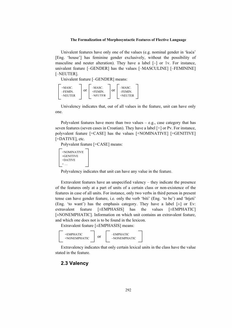
The Formalization of Morphosyntactic Features of Flective Language
292
Univalent features have only one of the values (e.g. nominal gender in ‘kuća’ [Eng. ‘house’] has feminine gender exclusively, without the possibility of masculine and neuter alteration). They have a label [–] or 1v. For instance, univalent feature [–GENDER] has the values [–MASCULINE] [–FEMININE] [–NEUTER].
Univalent feature [–GENDER] means: or or Univalency indicates that, out of all values in the feature, unit can have only
one. Polyvalent features have more than two values – e.g., case category that has
seven features (seven cases in Croatian). They have a label [+] or Pv. For instance, polyvalent feature [+CASE] has the values [+NOMINATIVE] [+GENITIVE] [+DATIVE], etc.
Polyvalent feature [+CASE] means: Polyvalency indicates that unit can have any value in the feature. Extravalent features have an unspecified valency – they indicate the presence
of the features only at a part of units of a certain class or non-existence of the features in case of all units. For instance, only two verbs in third person in present tense can have gender feature, i.e. only the verb ‘biti’ (Eng. ‘to be’) and ‘htjeti’ (Eng. ‘to want’) has the emphasis category. They have a label [±] or Ev: extravalent feature [±EMPHASIS] has the values [±EMPHATIC] [±NONEMPHATIC]. Information on which unit contains an extravalent feature, and which one does not is to be found in the lexicon.
Extravalent feature [±EMPHASIS] means: or Extravalency indicates that only certain lexical units in the class have the value
stated in the feature.
2.3 Valency
+NOMINATIVE +GENITIVE +DATIVE + …
+EMPHATIC +NONEMPHATIC
–EMPHATIC –NONEMPHATIC
+MASC. –FEMIN. –NEUTER
–MASC. +FEMIN. –NEUTER
–MASC. –FEMIN. +NEUTER
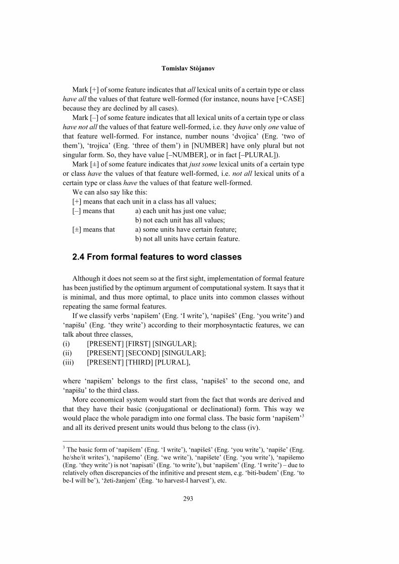
Tomislav Stòjanov
293
Mark [+] of some feature indicates that all lexical units of a certain type or class have all the values of that feature well-formed (for instance, nouns have [+CASE] because they are declined by all cases).
Mark [–] of some feature indicates that all lexical units of a certain type or class have not all the values of that feature well-formed, i.e. they have only one value of that feature well-formed. For instance, number nouns ‘dvojica’ (Eng. ‘two of them’), ‘trojica’ (Eng. ‘three of them’) in [NUMBER] have only plural but not singular form. So, they have value [–NUMBER], or in fact [–PLURAL]).
Mark [±] of some feature indicates that just some lexical units of a certain type or class have the values of that feature well-formed, i.e. not all lexical units of a certain type or class have the values of that feature well-formed.
We can also say like this: [+] means that each unit in a class has all values; [–] means that a) each unit has just one value; b) not each unit has all values; [±] means that a) some units have certain feature; b) not all units have certain feature.
2.4 From formal features to word classes Although it does not seem so at the first sight, implementation of formal feature
has been justified by the optimum argument of computational system. It says that it is minimal, and thus more optimal, to place units into common classes without repeating the same formal features.
If we classify verbs ‘napišem’ (Eng. ‘I write’), ‘napišeš’ (Eng. ‘you write’) and ‘napišu’ (Eng. ‘they write’) according to their morphosyntactic features, we can talk about three classes, (i) [PRESENT] [FIRST] [SINGULAR]; (ii) [PRESENT] [SECOND] [SINGULAR]; (iii) [PRESENT] [THIRD] [PLURAL],
where ‘napišem’ belongs to the first class, ‘napišeš’ to the second one, and ‘napišu’ to the third class.
More economical system would start from the fact that words are derived and that they have their basic (conjugational or declinational) form. This way we would place the whole paradigm into one formal class. The basic form ‘napišem’3 and all its derived present units would thus belong to the class (iv).
3 The basic form of ‘napišem’ (Eng. ‘I write’), ‘napišeš’ (Eng. ‘you write’), ‘napiše’ (Eng. he/she/it writes’), ‘napišemo’ (Eng. ‘we write’), ‘napišete’ (Eng. ‘you write’), ‘napišemo (Eng. ‘they write’) is not ‘napisati’ (Eng. ‘to write’), but ‘napišem’ (Eng. ‘I write’) – due to relatively often discrepancies of the infinitive and present stem, e.g. ‘biti-budem’ (Eng. ‘to be-I will be’), ‘žeti-žanjem’ (Eng. ‘to harvest-I harvest’), etc.
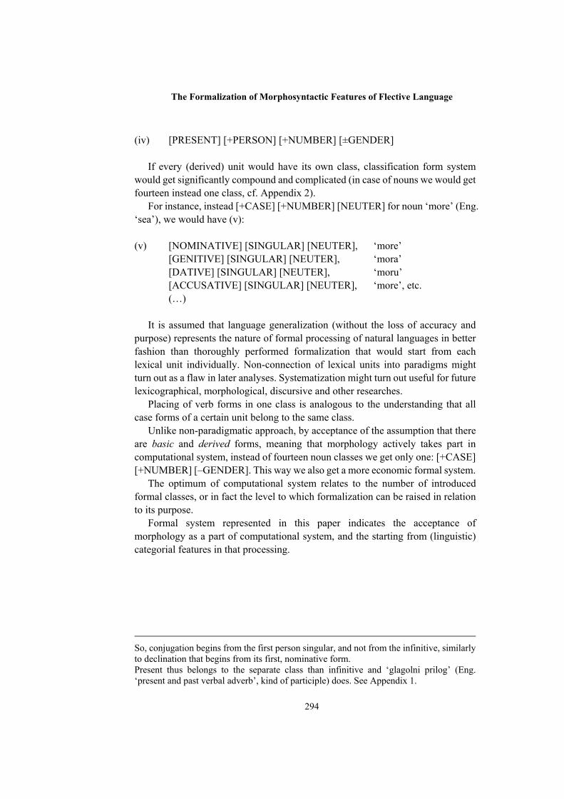
The Formalization of Morphosyntactic Features of Flective Language
294
(iv) [PRESENT] [+PERSON] [+NUMBER] [±GENDER]
If every (derived) unit would have its own class, classification form system
would get significantly compound and complicated (in case of nouns we would get fourteen instead one class, cf. Appendix 2).
For instance, instead [+CASE] [+NUMBER] [NEUTER] for noun ‘more’ (Eng. ‘sea’), we would have (v):
(v) [NOMINATIVE] [SINGULAR] [NEUTER], ‘more’
[GENITIVE] [SINGULAR] [NEUTER], ‘mora’ [DATIVE] [SINGULAR] [NEUTER], ‘moru’ [ACCUSATIVE] [SINGULAR] [NEUTER], ‘more’, etc.
(…) It is assumed that language generalization (without the loss of accuracy and
purpose) represents the nature of formal processing of natural languages in better fashion than thoroughly performed formalization that would start from each lexical unit individually. Non-connection of lexical units into paradigms might turn out as a flaw in later analyses. Systematization might turn out useful for future lexicographical, morphological, discursive and other researches.
Placing of verb forms in one class is analogous to the understanding that all case forms of a certain unit belong to the same class.
Unlike non-paradigmatic approach, by acceptance of the assumption that there are basic and derived forms, meaning that morphology actively takes part in computational system, instead of fourteen noun classes we get only one: [+CASE] [+NUMBER] [–GENDER]. This way we also get a more economic formal system.
The optimum of computational system relates to the number of introduced formal classes, or in fact the level to which formalization can be raised in relation to its purpose.
Formal system represented in this paper indicates the acceptance of morphology as a part of computational system, and the starting from (linguistic) categorial features in that processing.
So, conjugation begins from the first person singular, and not from the infinitive, similarly to declination that begins from its first, nominative form. Present thus belongs to the separate class than infinitive and ‘glagolni prilog’ (Eng. ‘present and past verbal adverb’, kind of participle) does. See Appendix 1.
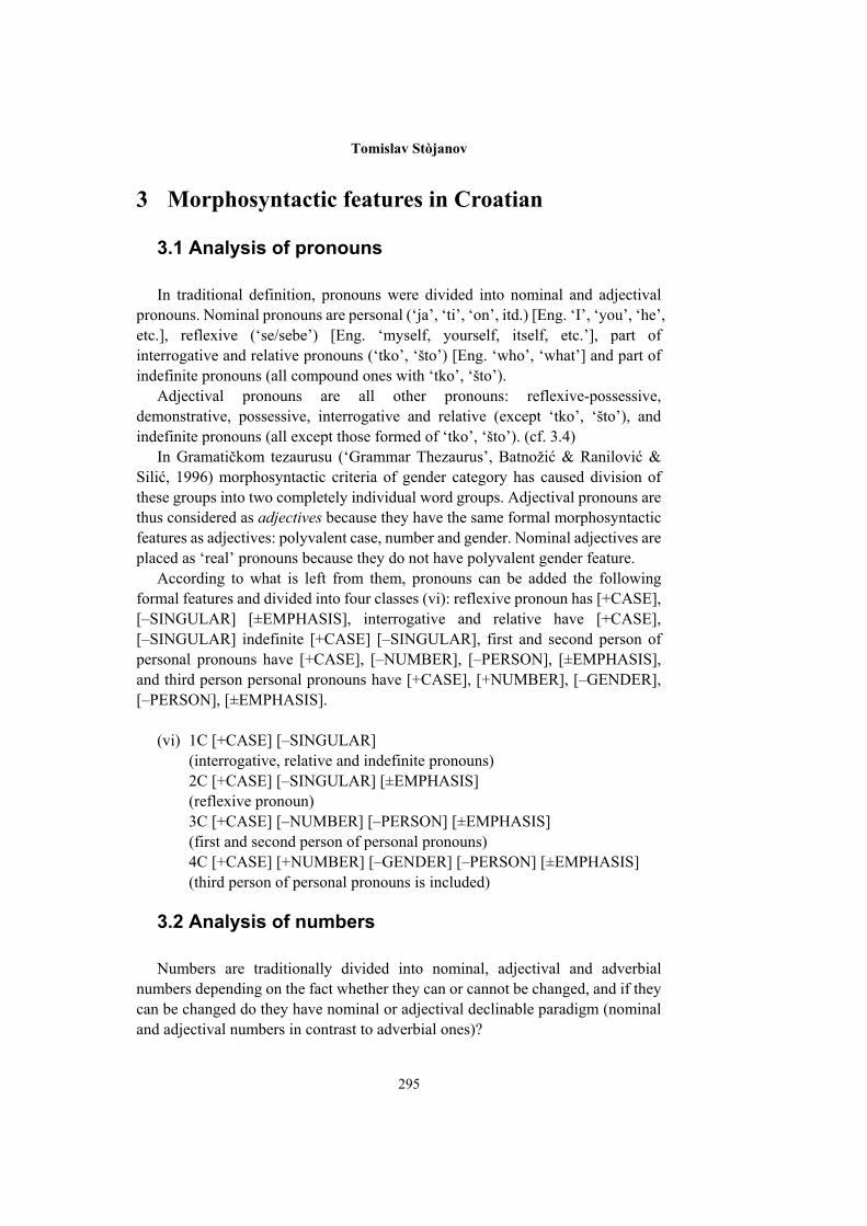
Tomislav Stòjanov
295
3 Morphosyntactic features in Croatian
3.1 Analysis of pronouns In traditional definition, pronouns were divided into nominal and adjectival
pronouns. Nominal pronouns are personal (‘ja’, ‘ti’, ‘on’, itd.) [Eng. ‘I’, ‘you’, ‘he’, etc.], reflexive (‘se/sebe’) [Eng. ‘myself, yourself, itself, etc.’], part of interrogative and relative pronouns (‘tko’, ‘što’) [Eng. ‘who’, ‘what’] and part of indefinite pronouns (all compound ones with ‘tko’, ‘što’).
Adjectival pronouns are all other pronouns: reflexive-possessive, demonstrative, possessive, interrogative and relative (except ‘tko’, ‘što’), and indefinite pronouns (all except those formed of ‘tko’, ‘što’). (cf. 3.4)
In Gramatičkom tezaurusu (‘Grammar Thezaurus’, Batnožić & Ranilović & Silić, 1996) morphosyntactic criteria of gender category has caused division of these groups into two completely individual word groups. Adjectival pronouns are thus considered as adjectives because they have the same formal morphosyntactic features as adjectives: polyvalent case, number and gender. Nominal adjectives are placed as ‘real’ pronouns because they do not have polyvalent gender feature.
According to what is left from them, pronouns can be added the following formal features and divided into four classes (vi): reflexive pronoun has [+CASE], [–SINGULAR] [±EMPHASIS], interrogative and relative have [+CASE], [–SINGULAR] indefinite [+CASE] [–SINGULAR], first and second person of personal pronouns have [+CASE], [–NUMBER], [–PERSON], [±EMPHASIS], and third person personal pronouns have [+CASE], [+NUMBER], [–GENDER], [–PERSON], [±EMPHASIS].
(vi) 1C [+CASE] [–SINGULAR] (interrogative, relative and indefinite pronouns) 2C [+CASE] [–SINGULAR] [±EMPHASIS] (reflexive pronoun) 3C [+CASE] [–NUMBER] [–PERSON] [±EMPHASIS] (first and second person of personal pronouns) 4C [+CASE] [+NUMBER] [–GENDER] [–PERSON] [±EMPHASIS] (third person of personal pronouns is included)
3.2 Analysis of numbers Numbers are traditionally divided into nominal, adjectival and adverbial
numbers depending on the fact whether they can or cannot be changed, and if they can be changed do they have nominal or adjectival declinable paradigm (nominal and adjectival numbers in contrast to adverbial ones)?
The Formalization of Morphosyntactic Features of Flective Language
296
The difference between nominal and adjectival paradigm is in gender category: nominal numbers have univalent [–GENDER] (e.g. ‘dva’, ‘oba’, ‘dvije’, ‘petero’) [Eng. ‘two’-nom.pl., ‘both of them’-nom.pl.m., ‘two of them’-nom.pl.f., ‘five of them’-nom.sg.n.]), and adjective ones polyvalent feature of gender [+GENDER] (e.g. ‘dvoji/dvoja/dvoje’ [Eng. ‘two’-nom.pl.m./f./n.), ‘prvi/prva/prvo’, [Eng. ‘first’-nom.sg.m./f./n.], etc.).
Since adverbial numbers do not have morphosyntactic categories, they are excluded from numbers, so that only nominal and adjectival numbers are considered as numeral type.
Therefore, numbers have two classes: [+CASE], [–NUMBER] [–GENDER] (so called nominal numbers, first class numbers, or 1C numbers) and 2C [+CASE] [–NUMBER] [+GENDER] or adjectival numbers.
3.3 Analysis of nouns Nouns are also various in their formal features. There are nouns (i) that have
only singular (singularia tantum) – e.g., personal names like ‘Ilija’, ‘Ines’, ‘Marko’, nouns like ‘tele’, ‘prase’ (Eng. ‘calf’, ‘piglet’), or nouns (ii) that have only plural (pluralia tantum) – e.g., ‘gaće’, ‘grablje’, ‘ljestve’, ‘naočale’, etc. (Eng. ‘underpants’, ‘rake’, ‘ladder’, ‘glasses’), and (iii) numeral nouns like ‘dvojica’, ‘trojica’ (Eng. ‘two of them’-nom.pl.n., ‘three of them’-nom.pl.n.).
[–NUMBER] is common to all of them. Indeclinable nouns belong to the separate class (female name ‘Ines’, for
instance). Thus, nouns are formally divided into three classes: the first one with features
[+CASE], [+NUMBER], [–GENDER] (first class nouns or 1C nouns), the second one with [+CASE], [–NUMBER], [–GENDER] (second class nouns or 2C nouns), and the third one with [–NOMINATIVE] [–SINGULAR] [–GENDER] (third class nouns or 3C nouns).
3.4 Analysis of adjectives Adjectives are divided into four classes; they all have common features of case,
number and gender. Except the indeclinable adjectives (e.g. ‘braun’ [Eng. ‘brown’]), all other
adjectives have difference only in comparison and aspect. At division of adjectives into formal classes the difference between traditional
and computational linguistics is what is the most noticeable. It is most visible in differentiation of form and meaning of adjectival aspect category (definite and indefinite aspect). As contrary to the expectations, formal approach determines
Tomislav Stòjanov
297
adjectival aspect as a semantic category and in dealing with it acts accordingly4, because it was not possible to establish formal classes by observing forms. Besides, adjectives do not have different paradigms for aspect category for all their forms – they differ in only five masculine singular cases and in three neuter singular cases, whereas all feminine forms are equalized. Compromise was impossible since the observation of relation between form and meaning did not bring us to the conclusion – for instance, adjectives with definite form, e.g. ‘dalmatinski’ [Eng. ‘Dalmatian’-nom.m.sg.], ‘šivaći’ [Eng. ‘sewing’-nom.m.sg.] can be both definite and indefinite in their meanings, whereas indefinite ‘sinov’ [Eng. son’s-nom.m.sg.] is definite in meaning.
Abolishing of adjectival aspect as a formal category would not solve the problem. Therefore, the following methodology was applied: definiteness and indefiniteness are viewed as semantically determined categories that have their own forms but cannot change them (in such a way that is a case of gender in adjectives, for instance). Determining which adjective is definite, and which one indefinite was done indirectly with the help of comparison category, like in Silić’ Grammar Thesaurus. Semantic analysis of Croatian language indeed prove that only indefinite adjectives can have comparison category (since only quality is compared, and not substance), whereby a conclusion that all comparable adjectives are indefinite can be drawn.
It is also worth emphasizing that established formal classes could not encompass an example of superlative in definite use5, which is explained by semantic transformation of higher order, like even clearer example of possessive (definite) adjectives (‘majčino mlijeko’ [Eng. mother’s milk] or ‘Ivanov auto’ [Eng. Ivan’s car]) that can be indefinite only with a special explanation of the context.
All comparable adjectives that are therefore indefinite go into the first class. All
incomparable (definite) and possessive adjectives go into the second class. The third class encompasses all pronominal adjectives: possessive pronominal adjectives (e.g., ‘moj’, ‘tvoj’ [Eng. ‘my’, ‘your’]), possessive-reflexive pronominal adjective ‘svoj’ [Eng. one’s own], interrogative and relative pronominal adjectives (e.g., ‘tko’, ‘čiji’ [Eng. ‘which one’, ‘whose’]), demonstrative pronominal adjectives (e.g., ‘taj’ [Eng. ‘that one’]), and indefinite pronominal adjectives (e.g., ‘ikoji’ [Eng. ‘any one’]). Their formal features are: 1C [+CASE] [+NUMBER] [+GENDER] [+COMPARISON] [–INDEFINITE]
4 Unlike traditional grammars that place the form on the first place although the issue of aspect is in fact completely a semantic one. 5 ‘najpametniji neka odu’ (koji? a ne kakvi?) the smartest-nom.m. let-particle leave-3.pl.pres. (which? not what like?) ‘the smartest ones may leave’ (who may leave? not what like may leave?)
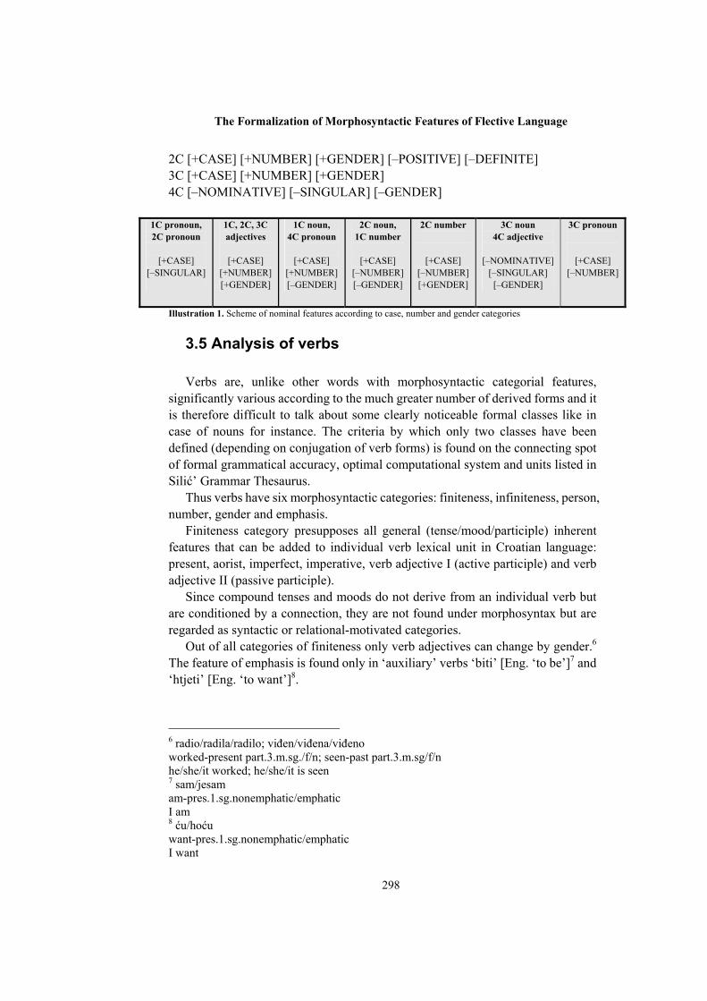
The Formalization of Morphosyntactic Features of Flective Language
298
2C [+CASE] [+NUMBER] [+GENDER] [–POSITIVE] [–DEFINITE] 3C [+CASE] [+NUMBER] [+GENDER] 4C [–NOMINATIVE] [–SINGULAR] [–GENDER]
1C pronoun, 2C pronoun
[+CASE]
[–SINGULAR]
1C, 2C, 3C adjectives
[+CASE]
[+NUMBER] [+GENDER]
1C noun, 4C pronoun
[+CASE]
[+NUMBER] [–GENDER]
2C noun, 1C number
[+CASE]
[–NUMBER] [–GENDER]
2C number
[+CASE] [–NUMBER] [+GENDER]
3C noun 4C adjective
[–NOMINATIVE]
[–SINGULAR] [–GENDER]
3C pronoun
[+CASE] [–NUMBER]
Illustration 1. Scheme of nominal features according to case, number and gender categories
3.5 Analysis of verbs Verbs are, unlike other words with morphosyntactic categorial features,
significantly various according to the much greater number of derived forms and it is therefore difficult to talk about some clearly noticeable formal classes like in case of nouns for instance. The criteria by which only two classes have been defined (depending on conjugation of verb forms) is found on the connecting spot of formal grammatical accuracy, optimal computational system and units listed in Silić’ Grammar Thesaurus.
Thus verbs have six morphosyntactic categories: finiteness, infiniteness, person, number, gender and emphasis.
Finiteness category presupposes all general (tense/mood/participle) inherent features that can be added to individual verb lexical unit in Croatian language: present, aorist, imperfect, imperative, verb adjective I (active participle) and verb adjective II (passive participle).
Since compound tenses and moods do not derive from an individual verb but are conditioned by a connection, they are not found under morphosyntax but are regarded as syntactic or relational-motivated categories.
Out of all categories of finiteness only verb adjectives can change by gender.6 The feature of emphasis is found only in ‘auxiliary’ verbs ‘biti’ [Eng. ‘to be’]7 and ‘htjeti’ [Eng. ‘to want’]8.
6 radio/radila/radilo; viđen/viđena/viđeno worked-present part.3.m.sg./f/n; seen-past part.3.m.sg/f/n he/she/it worked; he/she/it is seen 7 sam/jesam am-pres.1.sg.nonemphatic/emphatic I am 8 ću/hoću want-pres.1.sg.nonemphatic/emphatic I want
Tomislav Stòjanov
299
Infinitive, verb adverb I (present) (e.g., ‘kopajući’ [Eng. ‘digging’]) and verb adverb II (past) (e.g., ‘kopavši’ [Eng. ‘having dug’]) go into conjugatable verb class. 1C v. [–FINITENESS] [+PERSON] [+NUMBER] [±GENDER] [±EMPHASIS]; 2C verbs [–INFINITENESS].
4 Conclusion Formal morphosyntactic analysis deals with the formalization of
morphosyntactic features of Croatian language. The aim of this paper is to work on the frame for description of morphosyntax, i.e. inflective morphology, for the needs of tagging and parsing.9
Unlike the traditional approach where description significantly included semantic component, here morphosyntactic valencies have been used for grammatical and conceptual-forming categorial features in defining of lexical units.10
Thus instead of classical definition, adjectives are here defined as well-formed lexical units that have categories of case (Pv), gender (Pv), number (2v), comparison (ø/1v/Pv) and aspect (ø/1v).
Formally speaking, there are no nouns, numbers, pronouns, adjectives and verbs in morphosyntax, but formal features that define classes. However, although the criteria for division of types and classes is of formal nature, we still use the marks from traditional terminology (nouns, verbs, etc.; Van Valin, 2000: 13) which directs us to the need for further studying of syntactic as well as semantic categorial features.
This is the basis on which it was spotted that basic division of changeable and non-changeable forms should be replaced by division of units with and without morphosyntactic categories. Lexical units without morphosyntactic features have to be able to be determined with the help of syntactic categorial features.
In Croatian language, inflective forms are divided into 5 types and 16 classes. Morphosyntactic analysis of Croatian language encompasses 46 features in 10 morphosyntactic categories
9 For more on computational application of inflective morphology see Daille, Fabre & Sebillot (2002: 210-234) 10 “In traditional grammar, lexical categories are given notional definitions, i.e. they are characterized in terms of their semantic content. For example, ‘noun’ is defined as ‘the name are of a person, place or thing’, ‘verb’ is defined as an ‘action word’, and ‘adjective’ is defined as a ‘word expressing a property or attribute’. In modern linguistics, however, they are defined morphosyntactically in terms of their grammatical properties.”, Van Valin, Jr (2000: 6)
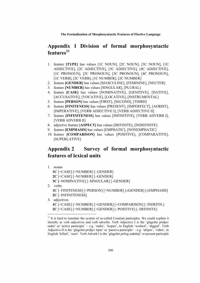
The Formalization of Morphosyntactic Features of Flective Language
300
Appendix 1 Division of formal morphosyntactic features11
1. feature [TYPE] has values [1C NOUN], [2C NOUN], [3C NOUN], [1C
ADJECTIVE], [2C ADJECTIVE], [3C ADJECTIVE], [4C ADJECTIVE], [1C PRONOUN], [2C PRONOUN], [3C PRONOUN], [4C PRONOUN], [1C VERB], [2C VERB], [1C NUMBER], [2C NUMBER]
2. feature [GENDER] has values [MASCULINE], [FEMININE], [NEUTER] 3. feature [NUMBER] has values [SINGULAR], [PLURAL] 4. feature [CASE] has values [NOMINATIVE], [GENITIVE], [DATIVE],
[ACCUSATIVE], [VOCATIVE], [LOCATIVE], [INSTRUMENTAL] 5. feature [PERSON] has values [FIRST], [SECOND], [THIRD] 6. feature [FINITENESS] has values [PRESENT], [IMPERFECT], [AORIST],
[IMPERATIVE], [VERB ADJECTIVE I], [VERB ADJECTIVE II] 7. feature [INFINITENESS] has values [INFINITIVE], [VERB ADVERB I],
[VERB ADVERB II] 8. adjective feature [ASPECT] has values [DEFINITE], [INDEFINITE] 9. feature [EMPHASIS] has values [EMPHATIC], [NONEMPHATIC] 10. feature [COMPARISON] has values [POSITIVE], [COMPARATIVE],
[SUPERLATIVE]
Appendix 2 Survey of formal morphosyntactic features of lexical units
1. nouns
1C [+CASE] [+NUMBER] [–GENDER] 2C [+CASE] [–NUMBER] [–GENDER] 3C [–NOMINATIVE] [–SINGULAR] [–GENDER]
2. verbs 1C [–FINITENESS] [+PERSON] [+NUMBER] [±GENDER] [±EMPHASIS] 2C [–INFINITENESS]
3. adjectives 1C [+CASE] [+NUMBER] [+GENDER] [+COMPARISON] [–INDEFIN.] 2C [+CASE] [+NUMBER] [+GENDER] [–POSITIVE] [–DEFINITE]
11 It is hard to translate the system of so-called Croatian participles. We could explain it literally as verb adjectives and verb adverbs. Verb Adjective I is the ‘glagolni pridjev radni’ or ‘active participle’ – e.g. ‘radio’, ‘kopao’, in English ‘worked’, ‘digged’. Verb Adjective II is the ‘glagolni pridjev trpni’ or ‘passive participle’ – e.g. ‘ubijen’, ‘viđen’, in English ‘killed’, ‘seen’. Verb Adverb I is the ‘glagolni prilog sadašnji’ or present participle
Tomislav Stòjanov
301
3C [+CASE] [+NUMBER] [+GENDER] 4C [–NOMINATIVE] [–SINGULAR] [–GENDER]
4. pronouns 1C [+CASE] [–SINGULAR] 2C [+CASE] [–SINGULAR] [±EMPHASIS] 3C [+CASE] [–NUMBER] [–PERSON] [±EMPHASIS] 4C [+CASE] [+NUMBER] [–GENDER] [–PERSON] [±EMPHASIS]
5. numbers 1C [+CASE] [–NUMBER] [–GENDER] 2C [+CASE] [–NUMBER] [+GENDER]
References Batnožić & Ranilović & Silić (1996) Hrvatski računalni pravopis, MH, SYS,
Zagreb Corbet (2000) Number, Cambridge Daille, Fabre & Sébillot (2002) Applications of Computational Morphology. In
Many Morphologies, ed. Paul Boucher, 210-234, Somerville, MA: Cascadilla Press
Dionizije Tračanin [Dionysius the Thrax] (1995) Gramatičko umijeće, edition and translation by Dubravko Škiljan, biblioteka Latina et graeca, book XXXVIII, Zagreb
Franks (1995) Parameters of Slavic Morphosyntax, Oxford Hausser (1999) Foundations of Computational Linguistics, Man-Machine
Communication in Natural Language, Springer Silić (1996), cf. Batnožić & Ranilović & Silić Silić (2001) Hrvatski jezik 2, udžbenik za II. razred gimnazije, ŠK, Zagreb Spencer (1991) Morphological Theory, An Introduction to Word Structure in
Generative Grammar, Blackwell Tadić (1994) Računalna obrada morfologije hrvatskoga književnog jezika,
unpublished Ph.D. thesis, Zagreb Trask (1999) Key Concepts in Language and Linguistics, Routledge Van Valin, Jr (2001) An introduction to Syntax, Cambridge Key words: natural language processing, computational linguistics, flective
languages, Croatian language, morphosyntax, formal features, valency features, morphosyntactic features, word classes, tagging.
– e.g. ‘kopajući’, ‘radeći’, in English ‘digging’, ‘working’. Verb Adverb II is the ‘glagolni prilog prošli’ – e.g. ‘kopavši’, ‘radivši’, in English ‘having dug’, ‘having worked’.

302
In Search of Theme and Rheme Pitch
Accents in Estonian
Maarika TraatThe University of Edinburgh
Abstract. It has been proposed that certain pitch accents in English alwaysgo with theme, while others always accompany rheme (Steedman 2000a), wheretheme and rheme are defined in terms of contextual ”alternative sets”. The goal ofthe present pilot study was exploring whether any regularities of this sort could befound in the Estonian language, which being a ”free word-order” language, differsconsiderably from English. On the basis of the data studied the shapes of thetheme and rheme pitch accents in Estonian do not seem to be remarkably different,but the rheme accents always reach a higher maximum pitch than the theme pitchaccents in the same sentence.
1 Introduction
The present paper was motivated by the claim ((Steedman 2000a), (Steed-man 2000b), (Steedman 2002)) that in the English language certain pitchaccents always accompany theme, while others always go with rheme. Theabove raised the question whether anything of the kind could be detectedin the Estonian language.
The present paper analyses several prosodically annotated Estonian ex-amples from information structural point of view, the principal goal beingfinding out whether there are any regularities regarding the use of pitchaccents in connection with theme and rheme linguistic material.
Very little work has been done on both Estonian intonation and the infor-mation structure of Estonian sentences. Nobody has explored the possibleconnection between the pitch accents used and the information structure ofthe sentence.
Word order in Estonian being considerably freer than that in English,there is a good chance that some effects in meaning achieved by means of in-tonation in English may be achieved by variation in word order in Estonian.The above claim is supported by (Asu 2002) analysis of Estonian questionsaccording to which the intonation of the questions which use very straight-forward morpho-syntactic marking does not differ from that of statements,
Proceedings of the Eighth ESSLLI Student SessionBalder ten Cate (editor)Chapter 28, Copyright c© 2003, Maarika Traat
303
In Search of Theme and Rheme Pitch Accents in Estonian
while the intonation of the morpho-syntactically unmarked ones does.
1.1 Motivations behind the study of intonation
The study of intonation is interesting firstly from cognitive point of view, be-cause the findings shed light to how people process and present information.Secondly, the knowledge about intonation is important in speech technology— both speech recognition and synthesis applications benefit from it. Inspeech recognition intonation can make available additional information tobe retrieved from the spoken text; in speech synthesis knowing how peopleuse intonation helps to make the speech output more natural, and also, evenmore importantly, helps to convey the intended meaning.
2 About the ”meaning” of intonation
It turns out that people use intonation in a systematic way. The intonationcontour used depends on the context and on the intended meaning of theutterance. The same string of words uttered with a different intonationcontour can be appropriate in certain contexts while not in others. Thefollowing example illustrates the point (the words carrying the main pitchaccent of the sentence are printed in capital letters):
(1) Q: Who taught Alexander the Great?A1: ARISTOTLE taught Alexander the Great.A2: *Aristotle taught ALEXANDER THE GREAT.A3: *Aristotle TAUGHT Alexander the Great.
Even though the three answer candidates to the question in the aboveexample contain exactly the same string of words, only the first answer isappropriate. The second and third answer candidate, even though convey-ing the same propositional meaning, are not appropriate answers to thequestion above. But each of them would be an appropriate answer to adifferent question. Thus, intonation seems to carry some kind of ”pragmaticmeaning”.
2.1 The relationship between information structure and in-tonation
Information structure refers to the way information is packaged in an ut-terance. There are several proposals about the constituents of informationstructure. According to (Vallduvı and Engdahl 1996) in spite of the bigvariety of proposed constituent names, there are two main bipartite infor-mational articulations:
304
Maarika Traat
• ground/focus division
• topic/comment division
(Vallduvı 1992) defines a tripartite hierarchical articulation, according towhich a sentence is composed of focus and ground, the latter being furtherdivided into link and tail.
The present paper uses Steedman’s (Steedman 2000a) theme/rheme, aninstance of ground/focus division according to (Vallduvı and Engdahl 1996),to describe the information structure. The terms theme and rheme havepreviously been used in (Mathesius 1929), (Firbas 1964), (Firbas 1966),(Halliday 1967), (Halliday 1970).
The theme is a known, expected, or noninformative part of the sentence.It is the link that is presupposed to the preceding discourse, or as Hallidayput it ”the peg on which the message is to hang” and the element in which”the speaker announces his intentions” (Halliday 1970). The remaining partof the utterance is what moves the discourse onward — the rheme — anewsy, informative, or dominant part of the sentence. The following exampleillustrates the notions of theme (th) and rheme (rh).
(2) Q1: Who taught Alexander the Great?A1: (ARISTOTLE)rh (taught Alexander the Great.)th
(3) Q2: Who did Aristotle teach?A2: (Aristotle taught)th (ALEXANDER THE GREAT.)rh
Intonation appears to be closely related to the information structure.As proposed in (Steedman 2000a), (Steedman 2000b), (Steedman 2002) thespecific pitch accent or the subset of the pitch accents that can be usedin a certain position in an utterance is determined by the ”themeness” or”rhemeness” of the part of the utterance.
Besides the choice of intonation contour, information structure can alsoplay an important role in determining the appropriate word order, especiallyin free word order languages.
3 Some comments on related research
The works most directly related to the present study are (Steedman 2000a),(Steedman 2000b), (Steedman 2002), where Steedman discusses his compo-sitional approach to the information structural meaning of intonation. Heestablishes there being two principal types of intonational tunes - themetunes and rheme tunes. According to him the most common intonationpattern for a marked theme1 is L+H* LH% and the most common tune for
1Themes can be divided into marked themes and unmarked themes. The intonation ofan unmarked theme is ambiguous as far as information structure is concerned, and it does
305
In Search of Theme and Rheme Pitch Accents in Estonian
the rheme is H* LL%2. He also proposes that the choice of pitch accentsused conveys whether the theme/rheme is mutually agreed or not, and theboundary tones indicate whether the speaker or the hearer is ”responsiblefor” the corresponding information unit.
A practical implementation of Steedman’s information structural theoryin a speech generation application was provided by Prevost (Prevost 1995).Prevost also examines the issue of contrastive stress, and how it influencesthe choice of the word to carry the principal pitch accent in an intonationalphrase. He develops an algorithm for making this choice using alternativeset semantics.
Similarly to Steedman, Pierrehumbert and Hirschberg (Pierrehumbertand Hirschberg 1990) pursue a compositional approach towards the meaningof intonation. In addition they claim that:
/- - -/ a speaker (S) chooses a particular tune to convey a particu-lar relationship between an utterance, currently perceived beliefs of ahearer (H), and anticipated contributions of subsequent utterances.
As for the study of the intonation of Estonian language not much hasbeen done. Asu ((Asu 2001),(Asu 2002)) has been working out the inven-tory of Estonian pitch accents using the approach of autosegmental-metricaltheory. But nobody has examined the relationship between intonation andinformation structure.
4 A quick quide to the Estonian language
The Estonian language belongs to the Finnic branch of the Finno-Ugric lan-guage family. It is characterised by a relatively free word order, a ratherelaborate declinational and conjugational system — nouns, adjectives, pro-nouns, numerals have as many as fourteen cases, the verbs are used in fourdifferent tenses, and the ending of the verb depends on the tense, person andnumber. The stems of words tend to change in declination and conjugation.Estonian has no prepositions, but there are several postpositions. Estonianuses no articles and no gender. Word stress is always on the first syllable,except in the case of some relatively recent loan words. Another peculiar-ity of the Estonian language is that it makes lexical distinctions based onquantity - the meaning of the word depends on the length of the vowel inits stressed syllable. The vowel can have three different lengths: short, long,very long.
(4) koli (short)junk(nom.sing.)
kooli (long)school(gen.sing.)
kooli (very long)school(part.sing.)
not contrast with any previous theme. A marked theme is ”marked” by one of the specifictheme intonational tunes, and stands in contrast with a theme from previous discourse.See (Steedman 2000a).
2This notation is taken from autosegmental-metrical theory (Pierrehumbert 1980).
306
Maarika Traat
vala (short)pour(2ndpers.sing.imperative)
vaala (long)whale(gen.sing.)
vaala (very long)whale(part.sing.)
Word order in Estonian being considerably freer than that in English,there is a good chance that some effects in meaning achieved by meansof intonation in English may be achieved by variation in word order inEstonian.
5 Experiment
When studying intonation two approaches are possible:
• to make subjects read handcrafted examples,• to analyse spontaneous speech data.
The positive side of the first approach is that it allows the experimenterto have control over her data; spontaneous speech data is difficult to han-dle because of its enormous variety and complexity. However, the in-labapproach also has downsides - the subjects are put into an artificial envi-ronment, and the sentences to be read are set in artificial context. This canshed doubt to the naturalness of the results.
For the present preliminary study of the Estonian theme and rheme pitchaccents the approach using handcrafted examples was chosen. The mainreason for the choice was the desire to be able to draw conclusions fromthe study of a limited amount of controlled data. Altogether 80 examplesread by a single speaker were studied. In order to put the sentences of theexperiment into context, they were presented as answers to questions. Bothmarked (a clearly distinguishable change in pitch in intonation contour) andunmarked themes were viewed. The examples contained both utteranceswith theme at the sentence initial position, and those with rheme precedingtheme. Also as in Estonian both SVO and OVS word orders are possible,examples with both word orders were studied.
The shape of the intonation contour on the stressed syllable of the wordcarrying the pitch accent depends on the quantity of the vowel in the syllable.Therefore, to be able to draw any sound conclusions, great care was takenabout having words with the same stressed syllable vowel length in themeand rheme positions in the examples.
The following two examples illustrate the kinds of examples that wereused in the study.
(5) Q: MinaInom
muunsell
maasikaid.strawberriesacc.
AgaBut
keswhonom
vaarikaidraspberriesacc
muub?sells?
I sell strawberries. But who sells raspberries?
A1: (VaarikaidRaspberriesacc
muub)th
sells(Maarika.)rh
Maarikanom.(OVS)
307
In Search of Theme and Rheme Pitch Accents in Estonian
(Maarika)rh (sells raspberries.)th
A2: (Maarika)rh
Maarikanom
(muubsells
vaarikaid.)th
raspberriesacc.(SVO)
(Maarika)rh (sells raspberries.)th
A3: (Maarika.)rh
Maarikanom.(S)
(Maarika does.)rh
(6) Q: MinaInom
muunsell
maasikaid.strawberriesacc.
AgaBut
midawhatacc
MaarikaMaarikanom
muub?sells?
I sell strawberries. But what does Maarika sell?
A1: (MaarikaMaarikanom
muub)th
sells(vaarikaid.)rh
raspberriesacc.(SVO)
(Maarika sells)th (raspberries.)rh
A2:* (Vaarikaid)rh
Raspberriesnom
(muubsells
Maarika.)th
Maarikaacc.(OVS)
A3: (Vaarikaid.)rh
Raspberriesacc.(O)
(Raspberries.)rh
The examples studied seem to indicate that in Estonian an object cannotbe placed sentence initially if it is a rheme (see 6:A2). However, an answerto a question containing just a rheme fragment (it is the only element in theanswer, hence it is initial) is perfectly acceptable (see 6:A3).
6 Intonation contours and results
Figures (1)–(3) along with Examples (7)–(9) illustrate some of the examplesanalysed. All these examples contain a marked theme — the stressed syllableof the ”marked” word is accompanied by a rise in the intonation contour.However, in Figure 2 the pitch rise on theme is much smaller than in theother two figures presented. Since the tendency was the same whenever amarked theme followed a rheme, it is probable that this rise in pitch mayhave been caused by a concious effort made by the subject to always producemarked themes as well as unmarked ones, and in reality a marked themecan never follow the rheme (supported by the native speaker’s intuitionof the author). In order to mark the theme with intonation, it may benecessary that it be placed also syntactically in a more prominent position,i.e. sentence initially.
(7) (Meie(Our
MAArikaMaarikanom
muub)th
sells)th(magusaid(sweet
VAArikaid)rh.raspberriesacc)rh.
308
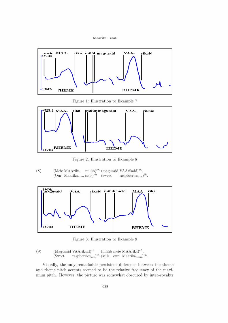
Maarika Traat
Figure 1: Illustration to Example 7
Figure 2: Illustration to Example 8
(8) (Meie(Our
MAArikaMaarikanom
muub)rh
sells)rh(magusaid(sweet
VAArikaid)th.raspberriesacc)th.
Figure 3: Illustration to Example 9
(9) (Magusaid(Sweet
VAArikaid)th
raspberriesacc)th(muub(sells
meieour
MAArika)rh.Maarikanom)rh.
Visually, the only remarkable persistent difference between the themeand rheme pitch accents seemed to be the relative frequency of the maxi-mum pitch. However, the picture was somewhat obscured by intra-speaker
309
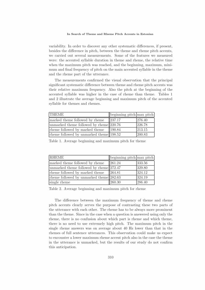
In Search of Theme and Rheme Pitch Accents in Estonian
variability. In order to discover any other systematic differences, if present,besides the difference in pitch, between the theme and rheme pitch accents,we carried out several measurements. Some of the features we measuredwere: the accented syllable duration in theme and rheme, the relative timewhen the maximum pitch was reached, and the beginning, maximum, mini-mum and final frequency of pitch on the main accented syllable in the themeand the rheme part of the utterance.
The measurements confirmed the visual observation that the principalsignificant systematic difference between theme and rheme pitch accents wastheir relative maximum frequency. Also the pitch at the beginning of theaccented syllable was higher in the case of rheme than theme. Tables 1and 2 illustrate the average beginning and maximum pitch of the accentedsyllable for themes and rhemes.
THEME beginning pitch max pitchmarked theme followed by rheme 237.17 276.40unmarked theme followed by rheme 220.76 226.78rheme followed by marked theme 190.84 213.15rheme followed by unmarked theme 198.52 200.83
Table 1. Average beginning and maximum pitch for theme
RHEME beginning pitch max pitchmarked theme followed by rheme 261.24 333.56unmarked theme followed by rheme 272.47 329.80rheme followed by marked theme 264.81 324.12rheme followed by unmarked theme 282.63 324.19single rheme 260.30 286.40
Table 2. Average beginning and maximum pitch for rheme
The difference between the maximum frequency of theme and rhemepitch accents clearly serves the purpose of contrasting these two parts ofthe utterance with each other. The rheme has to be always more prominentthan the theme. Since in the case when a question is answered using only therheme, there is no confusion about which part is rheme and which theme,there is no need to use extremely high pitch. The maximum pitch in thesingle rheme answers was on average about 40 Hz lower than that in therhemes of full sentence utterances. This observation could make us expectto encounter a lower maximum rheme accent pitch also in the case the themein the utterance is unmarked, but the results of our study do not confirmthis anticipation.
310
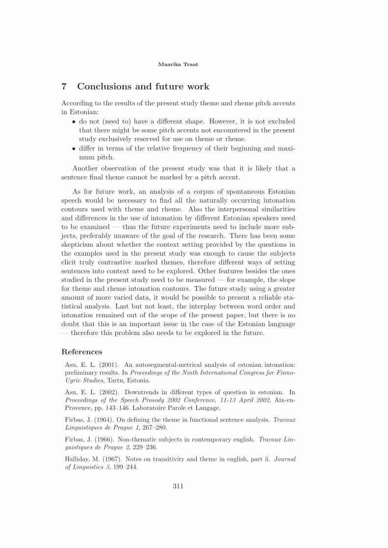
Maarika Traat
7 Conclusions and future work
According to the results of the present study theme and rheme pitch accentsin Estonian:
• do not (need to) have a different shape. However, it is not excludedthat there might be some pitch accents not encountered in the presentstudy exclusively reserved for use on theme or rheme.
• differ in terms of the relative frequency of their beginning and maxi-mum pitch.
Another observation of the present study was that it is likely that asentence final theme cannot be marked by a pitch accent.
As for future work, an analysis of a corpus of spontaneous Estonianspeech would be necessary to find all the naturally occurring intonationcontours used with theme and rheme. Also the interpersonal similaritiesand differences in the use of intonation by different Estonian speakers needto be examined — thus the future experiments need to include more sub-jects, preferably unaware of the goal of the research. There has been someskepticism about whether the context setting provided by the questions inthe examples used in the present study was enough to cause the subjectselicit truly contrastive marked themes, therefore different ways of settingsentences into context need to be explored. Other features besides the onesstudied in the present study need to be measured — for example, the slopefor theme and rheme intonation contours. The future study using a greateramount of more varied data, it would be possible to present a reliable sta-tistical analysis. Last but not least, the interplay between word order andintonation remained out of the scope of the present paper, but there is nodoubt that this is an important issue in the case of the Estonian language— therefore this problem also needs to be explored in the future.
References
Asu, E. L. (2001). An autosegmental-metrical analysis of estonian intonation:preliminary results. In Proceedings of the Ninth International Congress for Finno-Ugric Studies, Tartu, Estonia.
Asu, E. L. (2002). Downtrends in different types of question in estonian. InProceedings of the Speech Prosody 2002 Conference, 11-13 April 2002, Aix-en-Provence, pp. 143–146. Laboratoire Parole et Langage.
Firbas, J. (1964). On defining the theme in functional sentence analysis. TravauxLinguistiques de Prague 1, 267–280.
Firbas, J. (1966). Non-thematic subjects in contemporary english. Travaux Lin-guistiques de Prague 2, 229–236.
Halliday, M. (1967). Notes on transitivity and theme in english, part ii. Journalof Linguistics 3, 199–244.
311
In Search of Theme and Rheme Pitch Accents in Estonian
Halliday, M. (1970). Language structure and language function. In J. Lyons (Ed.),New Horizons in Linguistics, pp. 140–165. Harmondsworth: Penguin.
Mathesius, V. (1929). Functional lingusitics. In J. Vachek (Ed.), Praguiana: SomeBasic and Less Well-known Aspects of the Prague Linguistics School, pp. 121–142.Amsterdam: John Benjamins, 1983.
Pierrehumbert, J. (1980). The Phonology and Phonetics of English Intonation.Ph. D. thesis, Massachusetts Institute of Technology. Published 1988 by IndianaUniversity Linguistics Club, Bloomington, IN.
Pierrehumbert, J. and J. Hirschberg (1990). The meaning of intonational contoursin the interpretation of discourse. In P. Cohen, J. Morgan, and M. Pollack (Eds.),Intentions in Communication, pp. 271–312. Cambridge, MA: MIT Press.
Prevost, S. A. (1995). A Semantics of Contrast and Information Structure forSpecifying Intonation in Spoken Language Generation. Ph. D. thesis, Universityof Pennsylvania.
Steedman, M. (2000a, July). Information structure and the syntax-phonologyinterface. Linguistic Inquiry 31.
Steedman, M. (2000b). The Syntactic Process. Cambridge, Massachusetts: TheMIT Press.
Steedman, M. (2002, June). Information structural semantics of english intona-tion. Draft.
Vallduvı, E. (1992). The informational component. New York: Garland.
Vallduvı, E. and E. Engdahl (1996). The linguistic realization of informationpackaging. Linguistics 34, 459–519.
312
Formal Representation of Property
Grammars
Tristan VanRullenLaboratoire Parole et Langage, CNRS - Universite de Provence, Aix-en-Provence - France
Marie-Laure GuenotLaboratoire Parole et Langage, CNRS - Universite de Provence, Aix-en-Provence - France
Emmanuel BellengierLPL, CNRS - Universite de Provence, Aix-en-Provence - France, and Semantia, ADER-PACA
Abstract. A problem for the development of constraint-based formalisms con-cerns (i) the maintainability of the grammars (ii) the modification of the programsaccording to this maintenance operations. We propose a solution to these dif-ficulties by formally describing the global behaviour of the constraint satisfactionprocess and by expressing mathematically the locale functioning of each constraint.The proposed solution allows modifying the grammar without modifying the codeof the program.
1 Introduction
In this paper, we propose a formal representation of a constraint-based for-malism called Property Grammars (presented in [Bla01]). This formalismis totally based on constraints (also called properties): they represent alllinguistic information, which allows parsing to be only conceived as a con-straint satisfaction problem. The aim of this article is to show that wecan provide a sufficiently well-defined logical representation of the formal-ism. This logical representation permits to modify the grammar withoutmodifying programs.
We first present the role of properties in the Property Grammars formal-ism (hereafter PG). Then we describe and build the logical representation ofPG. Finally we show a set of properties defined in the ground of a currentlydeveloped French grammar.
Proceedings of the Eighth ESSLLI Student SessionBalder ten Cate (editor)Chapter 29, Copyright c© 2003, VanRullen, Guenot and Bellengier
313
Formal Representation of Property Grammars
2 Constraint-based formalisms
Almost all linguistic formalism make use of the notion of constraint1 whichindicates, in its broadest meaning, a property, relying two or more objects,that has to be satisfied. Constraints are extremely useful (and then ex-tremely usual), both to describe linguistic information, and to control itsparsing process. Nevertheless, the room given to these constraints may dif-fer substantially from one approach to another: in certain cases they onlyform an auxiliary mechanism, though in other ones the entire theory revolvesaround them.
In this section, after having explained the reasons why a totally constraint-based approach is so valuable for natural language representation and pro-cessing, we will illustrate some of the problems it states through the case ofcurrent linguistic formalisms and indicate how the PG formalism allows toresolve some of these problems.
2.1 The role of constraints in current linguistic theories
From an implementation point of view, constraints present several restric-tions of use. More precisely, if parsing can easily be considered as a con-straint satisfaction problem, it is obviously much more complicated to con-cretely implement this idea. Most of contemporary approaches claim toreally implement their parsing algorithm as a constraint satisfaction prob-lem. Their way to represent it is (roughly) to specify a set of variables, theirdomain and a constraint system; the satisfaction mechanism consists thenin constantly verifying the consistency of this system. Although, the mainoutcoming problem comes from the specification of the constraint variables,that usually defines high-level structures and/or partially constructed ob-jects, and thus prohibits an immediate access to their values. More precisely,one can distinguish sequential methods on the one hand, which makes use ofrules systems and constructs separately different representation levels (likein [PS93]), and incremental methods on the other hand, in which parsingis considered as a parallel process (like in HPSG: see [PS94]). In the for-mer, one has to select, among the convergent (well-formed) derivations, theoptimal one; in this approach, constraint satisfaction is necessary but notsufficient to evaluate grammaticality. In the latter, typically a constraint-based one, one has to replace the set of rules by an interactive constraintsystem (see [Pol96]), which allows a more direct connection between thegrammar theory and its implementation.
1For example, see [SW99] concerning HPSG, [PS93] or [AL97] concerning OptimalityTheory, and [DT99] or [Mar98] concerning Constraint Dependency Grammars.
314
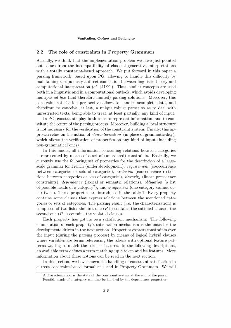
VanRullen, Guenot and Bellengier
2.2 The role of constraints in Property Grammars
Actually, we think that the implementation problem we have just pointedout comes from the incompatibility of classical generative interpretationswith a totally constraint-based approach. We put forward in this paper aparsing framework, based upon PG, allowing to handle this difficulty bymaintaining scrupulously a direct connection between linguistic theory andcomputational interpretation (cf. [JL99]). Thus, similar concepts are usedboth in a linguistic and in a computational outlook, which avoids developingmultiple ad hoc (and therefore limited) parsing solutions. Moreover, thisconstraint satisfaction perspective allows to handle incomplete data, andtherefrom to conceive, at last, a unique robust parser so as to deal withunrestricted texts, being able to treat, at least partially, any kind of input.
In PG, constraints play both roles to represent information, and to con-stitute the centre of the parsing process. Moreover, building a local structureis not necessary for the verification of the constraint system. Finally, this ap-proach relies on the notion of characterization1(in place of grammaticality),which allows the verification of properties on any kind of input (includingnon-grammatical ones).
In this model, all information concerning relations between categoriesis represented by means of a set of (unordered) constraints. Basically, wecurrently use the following set of properties for the description of a large-scale grammar for French (under development): requirement (cooccurrencebetween categories or sets of categories), exclusion (cooccurrence restric-tions between categories or sets of categories), linearity (linear precedenceconstraints), dependency (lexical or semantic relations), obligation (a listof possible heads of a category2), and uniqueness (one category cannot oc-cur twice). These properties are introduced in the table 1. Every propertycontains some clauses that express relations between the mentioned cate-gories or sets of categories. The parsing result (i.e. the characterization) iscomposed of two lists: the first one (P+) contains the satisfied clauses, thesecond one (P−) contains the violated clauses.
Each property has got its own satisfaction mechanism. The followingenumeration of each property’s satisfaction mechanism is the basis for thedevelopments driven in the next section. Properties express constraints overthe input (during the parsing process) by means of logical hybrid clauseswhere variables are terms referencing the tokens with optional feature pat-terns waiting to match the tokens’ features. In the following descriptions,an available term defines a term matching up a token and its features. Moreinformation about these notions can be read in the next section.
In this section, we have shown the handling of constraint satisfaction incurrent constraint-based formalisms, and in Property Grammars. We will
1A characterization is the state of the constraint system at the end of the parse.2Possible heads of a category can also be handled by the dependency properties.
315
Formal Representation of Property Grammars
see in details below how the difficulties we have seen can be solved with PG.
Property Semantics of the Property’s clauses Sample clauses
Requirementterm1 ⇒ term2
if term1 is not available thenthe clause is not available;
elseif term2 is not available then
put the clause in Pi− (violated);else
put the clause in Pi+ (satisfied);end if
end if
For the category “Adj”(adjective or adjectival phrase):
Adj ⇒ Adj or Adv or Coord ∗
(i.e. in an adjectival phrase, an adjectiverequires the presence of another adjectiveor an adverb, or a coordonner)
*: Such a clause is not a tautology becauseleft and right “Adj” are two different variables
Exclusionterm1 = term2
if term1 is not available thenthe clause is not available;
elseif term2 is available then
put the clause in Pi− (violated);else
put the clause in Pi+ (satisfied);end if
end if
For the category “Adj”(adjective or adjectival phrase):
Coord = Adv or Vparticiple
(i.e. in an adjectival phrase, a coordonnercannot co-occur with an adverbor a participle verb)
Linearityterm1 term2
if term1 is not available or term2 is notavailable then
the clause is not available;else
if term1.rank ≥ term2.rank thenput the clause in Pi− (violated);
elseput the clause in Pi+ (satisfied);
end ifend if
For the category “NP” (noun phrase)
Det or Num Noun or Adj or Adv
(i.e. in a noun phrase, a determiner or anumeral must occur before a noun, anadjective or an adverb)
Dependencyterm1 ≈ term2
if term1 is not available or term2 is notavailable then
the clause is not available;else
if term1.feature = term2.featurethen
put the clause in Pi− (violated);else
put the clause in Pi+ (satisfied);end if
end if
For the category “NP” (noun phrase):
Noungender ≈ DetgenderNounnumber ≈ Detnumber
(i.e. in a noun phrase, a noun and adeterminer must agree in gender andnumber)
Table 1: Formal description of the properties’ satisfaction mechanism
3 Logical and mathematical background
3.1 Parsing with constraints
Before exploring the main point of this section, an overview of former workson parsing with PG should demonstrate the advantages of retrieving a logi-cal frame in their mechanisms. Parsers programmed in the paradigm of PGhave in fact been built with different goals and for different uses: some topermit speech synthesis (see [BH01]), others to parse large corpora or toextract rich information (see [BGV03]), and some to test the PG formalismand to compare it with other ones (see [BV02]). We can distinguish themin terms of determinism, deepness, dynamism, as well as in terms of pro-gramming language, heuristics and complexity. This is the way we usuallycompare parsers. In the current consideration, the only comparison will be
316
VanRullen, Guenot and Bellengier
done in terms of genericity. From shallow parsers to deep ones, many makeuse of logico-mathematical fundaments and each program offers its own in-terpretation (see for different examples [BM01] and [BBV02]). With CHRor PROLOG rules, with graphs, trees or tables, heuristics are intimatelylinked to data structures and generally to the formalism’s implicit semanticfundings.
The observation of how the already built parsers deal with constraintsand with the evolution of the formalism itself allows to catalogue their sim-ilarities and principles. Such an inventory can lead to find neither generalnor universal rules, but a formal system of constraint mechanisms, homo-morphic with other potential systems. The following points characterize theparsing processes with PG, whatever the program and its heuristics:
• Parsers use bottom-up, tree walking strategies with a pattern matchingstep for constraint satisfaction.
• It is possible to enumerate different kinds of patterns to match:
– constants, such as feature values, to recognize in the inputs,
– variables referencing linguistic tokens,
– variables referencing tokens’ features (even domains of these fea-tures),
– second order typed calculus functions expressing relations andconstraints over patterns.
• Several common points in the mechanism of the properties allowing ageneralization of their writing.
Writing a generic parser based on these points can now be imagined.This is what we explain hereafter.
3.2 Computational perspective
Many constraints interfere simultaneously for the choice of the grammar’sconstraints representation. The problematic governing these constraintsshould be given in epistemological terms (so that a large overview of re-lations between linguistic models and theories is kept), as in mathematicalterms (by choosing a model, totally representative of its set of objects with-out implicit knowledge, and canonical for the treatments it allows). Asshown on figure 1, different representations of a grammar lead to differentoutputs, which can differ in their organisation, but which should contain thesame (or similar) information. Choosing one kind of representation is thusa procedure driven by a need of genericity.
Another question in the choice of a representation is given by the com-putational perspective: a program that would have to be changed (partially
317
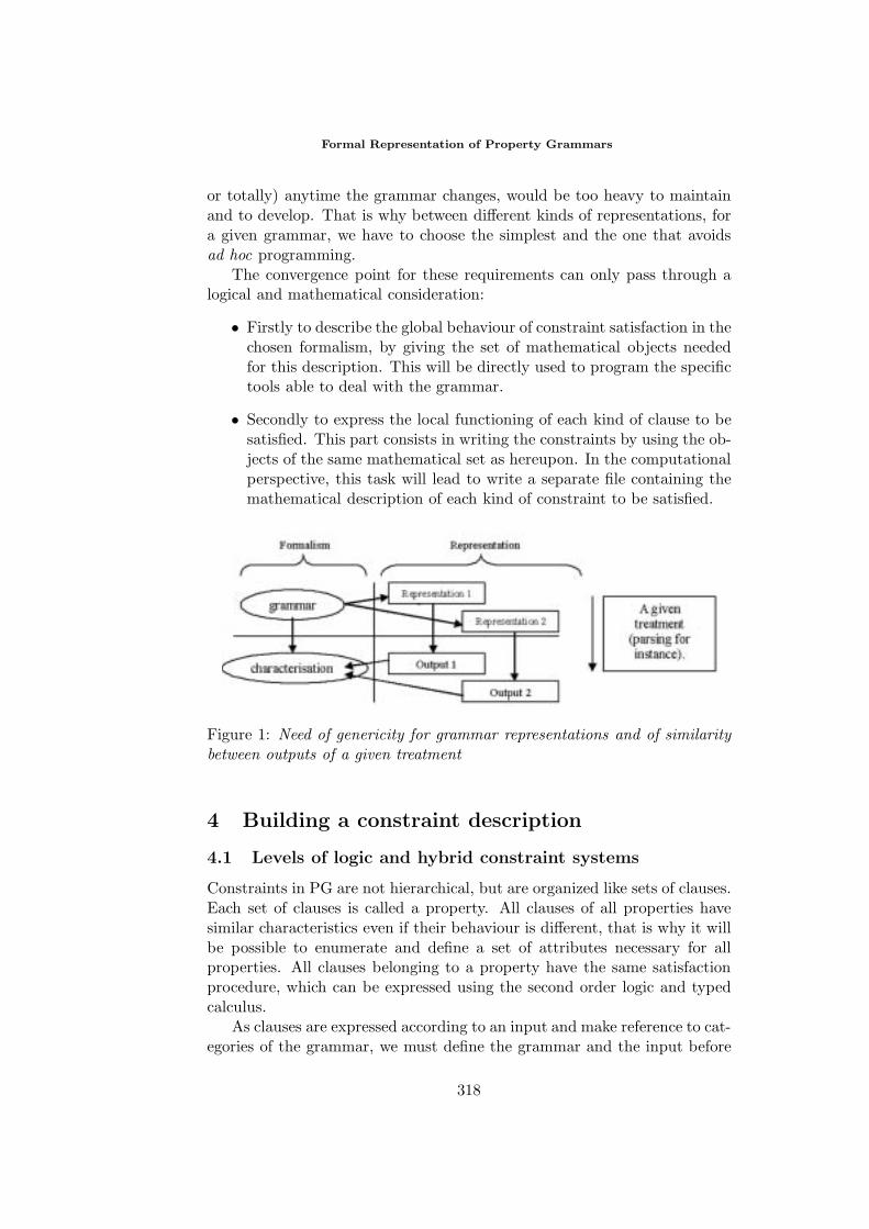
Formal Representation of Property Grammars
or totally) anytime the grammar changes, would be too heavy to maintainand to develop. That is why between different kinds of representations, fora given grammar, we have to choose the simplest and the one that avoidsad hoc programming.
The convergence point for these requirements can only pass through alogical and mathematical consideration:
• Firstly to describe the global behaviour of constraint satisfaction in thechosen formalism, by giving the set of mathematical objects neededfor this description. This will be directly used to program the specifictools able to deal with the grammar.
• Secondly to express the local functioning of each kind of clause to besatisfied. This part consists in writing the constraints by using the ob-jects of the same mathematical set as hereupon. In the computationalperspective, this task will lead to write a separate file containing themathematical description of each kind of constraint to be satisfied.
Figure 1: Need of genericity for grammar representations and of similaritybetween outputs of a given treatment
4 Building a constraint description
4.1 Levels of logic and hybrid constraint systems
Constraints in PG are not hierarchical, but are organized like sets of clauses.Each set of clauses is called a property. All clauses of all properties havesimilar characteristics even if their behaviour is different, that is why it willbe possible to enumerate and define a set of attributes necessary for allproperties. All clauses belonging to a property have the same satisfactionprocedure, which can be expressed using the second order logic and typedcalculus.
As clauses are expressed according to an input and make reference to cat-egories of the grammar, we must define the grammar and the input before
318
VanRullen, Guenot and Bellengier
expressing the clauses, which can be done in an extended Backus-Naur Form.
- Grammar G ::=[[set C of Categories],[set D of property definitions]]
Let card(C) be the cardinality of C, let ci (i∈ [0. . . card(C)]) be the ith
category of C,
- Category ci ::=[name of the category (label),[set of Properties Pci ],[set Mci of features]]
Grammatical categories can be lexical categories (like noun, verb, etc.)as well as syntagmatic categories (NP , V P , PP , . . . ). The sets of featuresare not described here, because their importance is minimal for the logicalrepresentation of properties. An input for the grammar is a vector of het-erogeneous information, supposed to describe enough each parsed token:
- Input Ir ::=[a word (label),r (rank order, position in the sentence)∈ [0. . .∞[,a disambiguated category cr belonging to C,[a set Mcr of features]]
Each property given for each category in the grammar is a set of prop-erty clauses (called clauses because of their satisfying procedure, but we candefine them as truth functions over hybrid second order arguments). We canseparate the enumeration of the clauses of a property from the definition ofa property’s behaviour (which does not depend on the category).
- Property Pc ::=[Name of the property (label),[a set Kpc of clauses]]
A given clause kpc in a given property p of a given category c can bedefined like a set of terms:
- Clause kpc ::=[ordered set T of ap terms]](ap, the arity of a clause is defined hereunder)
- Term t ::=[Reference or Logical expression]
319
Formal Representation of Property Grammars
- Reference ρ ::=[Name of the referenced category (label)∈ C,[a pattern of features Mρ (optional)]]
- Logical Expression E ::=[Logical operator O,[a set of term (its cardinality agrees with O’s arity)]]
A property definition furnishes the symbol (name) of its clauses (e.g.the symbol for a clause of linearity is ) and describes the context of theirsatisfiability with a mathematical expression. The cardinality of the set ofclauses can be fixed or variable, and an order relation between the clausesof a property may have to be observed (see table 1).
With the definitions given here, we can now write the main definition (forthis article), dealing with the goal of mathematical and logical genericity.- Property definition dp ::=
[Name of the property (label),Symbol for its clauses (label),(ap (arity of the clauses)∈ (0, 1, 2 . . . ) (finite integer),Expression of satisfiability Ep for the clauses,cardinality of the set of clauses (fixed or not) ∈ (0, 1, 2 . . .∞),a boolean Ordered ∈ (true, false)]
The expression Ep describes how a clause can be satisfied in a propertyp by using second order logic and typed calculus (see below). Consider-ing a grammar description as a preliminary for a parsing process, we candefine some characteristics of the references and the logical expressions, inaccordance with a supposed input characteristics:
Definition 1. availability of a reference: A reference has to be inter-preted as a variable declaration; a variable has a name and refers to anexisting category of the grammar. It can also be sub-defined by describinga pattern of features referring to the category’s set of potential lexical orsemantic features. During the parse, an input will be presented to eachvariable referring to it. If the input features match the variable pattern, thereference is then declared available.
Definition 2. availability of a logical expression: A logical expressionis available when all of its terms are available.
Notation:Let t1, t2, ti, . . . tap be the terms of a clause in Kp verifying i ∈ [1. . . ap].
Definition 3. availability of a term: We define a truth value ωi ( avail-ability of a term i) which is true when the term ti, is available and falsewhen not available (a term can be a logical expression or a single reference).
320
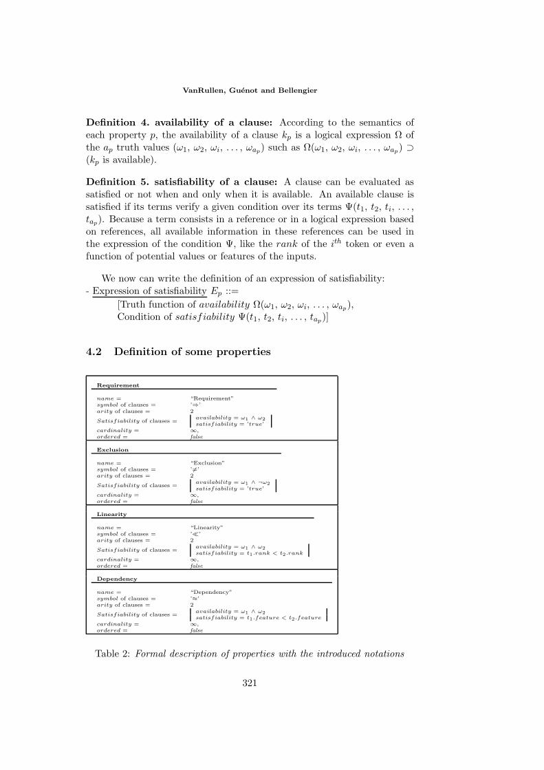
VanRullen, Guenot and Bellengier
Definition 4. availability of a clause: According to the semantics ofeach property p, the availability of a clause kp is a logical expression Ω ofthe ap truth values (ω1, ω2, ωi, . . . , ωap) such as Ω(ω1, ω2, ωi, . . . , ωap) ⊃(kp is available).
Definition 5. satisfiability of a clause: A clause can be evaluated assatisfied or not when and only when it is available. An available clause issatisfied if its terms verify a given condition over its terms Ψ(t1, t2, ti, . . . ,tap). Because a term consists in a reference or in a logical expression basedon references, all available information in these references can be used inthe expression of the condition Ψ, like the rank of the ith token or even afunction of potential values or features of the inputs.
We now can write the definition of an expression of satisfiability:- Expression of satisfiability Ep ::=
[Truth function of availability Ω(ω1, ω2, ωi, . . . , ωap),Condition of satisfiability Ψ(t1, t2, ti, . . . , tap)]
4.2 Definition of some properties
Requirement
name = “Requirement”symbol of clauses = ’⇒’arity of clauses = 2
Satisfiability of clauses =availability = ω1 ∧ ω2satisfiability = ’true’
cardinality = ∞,ordered = false
Exclusion
name = “Exclusion”symbol of clauses = ’=’arity of clauses = 2
Satisfiability of clauses =availability = ω1 ∧ ¬ω2satisfiability = ’true’
cardinality = ∞,ordered = false
Linearity
name = “Linearity”symbol of clauses = ’’arity of clauses = 2
Satisfiability of clauses =availability = ω1 ∧ ω2satisfiability = t1.rank < t2.rank
cardinality = ∞,ordered = false
Dependency
name = “Dependency”symbol of clauses = ’≈’arity of clauses = 2
Satisfiability of clauses =availability = ω1 ∧ ω2satisfiability = t1.feature < t2.feature
cardinality = ∞,ordered = false
Table 2: Formal description of properties with the introduced notations
321
Formal Representation of Property Grammars
The table 2 expresses the semantics of properties in the grammar, corre-sponding to the table 1. It presents the advantage of being extensible. Withthe introduced notions, it will be possible to describe semantic or prosodicphenomena without building new parsers. With the fundaments describedhere, the pattern matching step still has to be defined in a compatible formu-lation, which will be possible by designing data structures like graphs wherenodes and edges carry dynamic semantic objects. In this direction, severalcomputational paradigms propose realizable solutions, like classical CSPs,parallel processing, reactive machine and hybrid models or graph walking.Our current work is based on the third one. It should lead to a deep parserwith variable granularity (see [BBV02] and [OCC+00]).
5 Conclusion
Constraints offer several advantages, both for linguistics and computationalreasons. We have seen that a Property Grammar representation can expressconstraints directly over categories and use constraints at any level of theparsing process.
We have shown that a well defined logical representation of the proper-ties allows the modification of the grammar without any modification of theprogram (in a parsing strategy). Property Grammars seem to be a satisfyingtool for the representation of linguistics information and for a computationalimplementation. The perspective of working with hybrid constraints withinthe formalism added to the possibility of relaxing violated constraints with-out giving up the parsing process will be decisive in the future of symbolicparsing paradigm.
322
VanRullen, Guenot and Bellengier
References
[AL97] Diana Archangeli and Douglass Terence Langendoen, Optimality theory,Blackwell, 1997.
[BBV02] Jean-Marie Balfourier, Philippe Blache, and Tristan VanRullen, Fromshallow to deep parsing using constraint satisfaction, Proceedings ofthe 27th International Conference on Computational Linguistics (COL-ING’02), 2002, pp. 36–42.
[BGV03] Philippe Blache, Marie-Laure Guenot, and Tristan VanRullen, Corpus-based grammar development, Proceedings of Corpus Linguistics 2003,2003, pp. 124–131.
[BH01] Philippe Blache and Daniel Hirst, Aligning prosody and syntax in prop-erty grammars, Proceedings of EuroSpeech 2001, 2001.
[Bla01] Philippe Blache, Les grammaires de proprietes : des contraintes pour letraitement automatique des langues naturelles, Hermes Science, 2001.
[BM01] Philippe Blache and Franz Morawietz, A non-generative constraint-based formalism, Travaux Interdisciplinaires du Laboratoire Parole etLangage d’Aix-en-Provence 19 (2001), 11–26.
[BV02] Philippe Blache and Tristan VanRullen, An evaluation of different shal-low parsing techniques, Proceedings of LREC-2002, 2002.
[DT99] Denys Duchier and Stefan Thater, Parsing with tree descriptions: aconstraint-based approach, Proceedings of Sixth International Work-shop on Natural Language Understanding and Logic Program-ming(NLULP’99), 1999.
[JL99] David Johnson and Shalom Lappin, Local constraints vs. economy,CSLI, 1999.
[Mar98] Hiroshi Maruyama, Structural disambiguation with constraint propaga-tion, COLINGACL’98, 1998.
[OCC+00] Stephan Oepen, Ulrich Callmeier, Ann Copestake, Dan Flickinger, andRobin Malouf, Scalable grammar software for computational linguists,Proceedings of the 38th Annual Meeting of the Association for Compu-tational Linguistics (ACL’00), 2000.
[Pol96] Karl Pollard, The nature of constraint-based grammar, Proceedings ofthe 10th Pacific Asia Conference on Language, Information and Com-putation (PACLING’96), 1996.
[PS93] Alan Prince and Peter Smolensky, Optimality theory: Constraint inter-action in generative grammar, Rutgers University Centre for CognitiveScience, 1993.
[PS94] Karl Pollard and Ivan Sag, Head-driven phrase structure grammars,CSLI, Chicago University Press, 1994.
[SW99] Ivan Sag and Tom Wasow, Syntactic theory. a formal introduction,CSLI, 1999.
323


