Embed Size (px)
Citation preview
arX
iv:1
104.
1580
v3 [
astr
o-ph
.IM
] 2
7 Ju
n 20
11
Proceedings of the 2011
New York Workshop on
Computer, Earth and Space Science
February 2011
Goddard Institute for Space Studies
http://www.giss.nasa.gov/meetings/cess2011
Editors
M.J. Way and C. Naud
Sponsored by the Goddard Institute for Space Studies
1
Contents
ForewordMichael Way & Catherine Naud 4
IntroductionMichael Way 5
On a new approach for estimating threshold crossing timeswith an application to global warming
Victor H. de la Pena 8
Cosmology through the large-scale structure of the UniverseEyal Kazin 13
On the Shoulders of Gauss, Bessel, and Poisson: Links,Chunks, Spheres, and Conditional Models
William Heavlin 21
Mining Citizen Science Data: Machine Learning ChallengesKirk Borne 24
Tracking Climate ModelsClaire Monteleoni 28
Spectral Analysis Methods for Complex Source MixturesKevin Knuth 31
Beyond Objects: Using Machines to Understand the DiffuseUniverse
J.E.G. Peek 35
Viewpoints: A high-performance high-dimensional exploratorydata analysis tool
Michael J. Way 44
Clustering Approach for Partitioning Directional Data inEarth and Space Sciences
Christian Klose 46
Planetary Detection: The Kepler MissionJon Jenkins 52
2
Understanding the possible influence of the solar activityon the terrestrial climate: a times series analysis approach
Elizabeth Martınez-Gomez 54
Optimal Scheduling of Exoplanet Observations Using BayesianAdaptive Exploration
Thomas J. Loredo 61
Beyond Photometric Redshifts using Bayesian InferenceTamas Budavari 65
Long-Range Climate Forecasts Using Data Clustering andInformation Theory
Dimitris Giannakis 68
Comparison of Information-Theoretic Methods to estimatethe information flow in a dynamical system
Deniz Gencaga 72
Reconstructing the Galactic halos accretion history: A finitemixture model approach
Duane Lee & Will Jessop 77
Program 78
Participants 79
Talk Video Links 82
3
Foreword
Michael WayNASA/Goddard Institute for Space Studies2880 BroadwayNew York, New York, USA
Catherine NaudDepartment of Applied Physics and Applied MathematicsColumbia University, New York, New York, USAandNASA/Goddard Institute for Space Studies2880 BroadwayNew York, New York, USA
The purpose of the New York Workshop on Computer, Earth and SpaceSciences is to bring together the New York area’s finest Astronomers, Statis-ticians, Computer Scientists, Space and Earth Scientists to explore potentialsynergies between their respective fields. The 2011 edition (CESS2011) wasa great success, and we would like to thank all of the presenters and partici-pants for attending.
This year was also special as it included authors from the upcomingbook titled “Advances in Machine Learning and Data Mining for Astron-omy.” Over two days, the latest advanced techniques used to analyze thevast amounts of information now available for the understanding of our uni-verse and our planet were presented. These proceedings attempt to providea small window into what the current state of research is in this vast inter-disciplinary field and we’d like to thank the speakers who spent the time tocontribute to this volume.
This year all of the presentations were video taped and those presentationshave all been uploaded to YouTube for easy access. As well, the slides from allof the presentations are available and can be downloaded from the workshopwebsite1.
We would also like to thank the local NASA/GISS staff for their assistancein organizing the workshop; in particular Carl Codan and Patricia Formosa.Thanks also goes to Drs. Jim Hansen and Larry Travis for supporting theworkshop and allowing us to host it at The Goddard Institute for SpaceStudies again.
1http://www.giss.nasa/gov/meetings/cess2011
4
Introduction
Michael WayNASA/Goddard Institute for Space Studies2880 BroadwayNew York, New York, USA
This is the 2nd time I’ve co-hosted the New York Workshop on Com-puter, Earth, and Space Sciences (CESS). My reason for continuing to do sois that, like many at this workshop, I’m a strong advocate of interdisciplinaryresearch. My own research institute (GISS2) has traditionally contained peo-ple in the fields of Planetary Science, Astronomy, Earth Science, Mathematicsand Physics. We believe this has been a recipe for success and hence we alsocontinue partnerships with the Applied Mathematics and Statistics Depart-ments at Columbia University and New York Unversity. Our goal with theseon-going workshops is to find new partnerships between people/groups inthe entire New York area who otherwise would never have the opportunityto meet and share ideas for solving problems of mutual interest.
My own science has greatly benefitted over the years via collaborationswith people I would have never imagined working with 10 years ago. Forexample, we have managed to find new ways of using Gaussian Process Re-gression (a non-linear regression technique) (Way et al. 2009) by workingwith linear algebra specialists at the San Jose State University departmentof Mathematics and Computer Science. This has led to novel methods for in-verting relatively large (∼100,000×100,000) non-sparse matrices for use withGaussian Process Regression (Foster et al. 2009).
As we are all aware, many scientific fields are also dealing with a datadeluge which is often approached by different disciplines in different ways.A recent issue of Science Magazine3 has discussed this in some detail (e.g.Baranuik 2011). It has also been discussed in the recent book “The FourthParadigm” Hey et al. (2009). What the Science articles made me the mostaware of is my own continued narrow focus. For example, there is a greatdeal that could be shared between the people at this workshop and the fieldsof Biology, Bio-Chemistry, Genomics and Ecologists to name a few from theScience article. This is particularly embarrassing for myself since in 2004 Iattended a two-day seminar in Silicon Valley that discussed several chapters
2Goddard Institute for Space Studies3http://www.sciencemag.org/site/special/data
5
in the book “The Elements of Statistical Learning” (Hastie, Tibshirani, &Friedman 2003). Over 90% of the audience were Bio-Chemists, while I wasonly one of two Astronomers.
Another area which I think we can all agree most fields can benefit fromis better (and cheaper) methods for displaying and hence interrogating ourdata. Later today I will discuss a program called viewpoints (Gazis, Levit, &Way 2010) which can be used to look at modest sized multivariate data setson an individual desktop/laptop. Another of the Science Magazine articles(Fox & Hendler 2011) discusses a number of ways to look at data in lessexpensive way.
In fact several of the speakers at the CESS workshop this year are alsocontributors to a book in progress (Way et al. 2011) that has chapters writtenby a number of people in the fields of Astronomy, Machine Learning and DataMining who have themselves engaged in interdisciplinary research – this beingone of the rationales for inviting them to contribute to this volume.
Finally, although I’ve restricted myself to the “hard sciences” we shouldnot forget that interdisciplinary research is taking place in areas that per-haps only a few of us are familiar with. For example, I can highly recom-mend a recent book (Morris 2010) that discusses possible theories for thecurrent western lead in technological innovation. The author (Ian Morris)uses data and methodologies from the fields of History, Sociology, Anthro-pology/Archaeology, Geology, Geography and Genetics to support the thesisin the short title of his book: “Why The West Rules – For Now”.
Regardless, I would like to thank all of the speakers for coming to NewYork and also for contributing to the workshop proceedings.
References
Baranuik, R.G. 2011, More Is Less: Signal Processing and the Data Deluge,Science, 331, 6018, 717
Foster, L., Waagen, A., Aijaz, N., Hurley, M., Luis, A., Rinsky, J. Satyavolu,C., Way, M., Gazis, P., Srivastava, A. 2009, Stable and Efficient GaussianProcess Calculations, Journal of Machine Learning Research, 10, 857
Fox, P. & Hendler, J. 2011, Changing the Equation on Scientific Data Visu-alization, Science, 331, 6018, 705
Gazis, P.R., Levit, C. & Way, M.J. 2010, Viewpoints: A High-PerformanceHigh-Dimensional Exploratory Data Analysis Tool, Publications of the As-tronomical Society of the Pacific, 122, 1518
6
Hastie, T., Tibshirani, R. & Friedman, J.H. 2003, The Elements of StatisticalLearning, Springer 2003, ISBN-10: 0387952845
Hey, T., Tansley, S. & Tolle, K. 2009, The Fourth Paradigm: Data-IntensiveScientific Discovery, Microsoft Research, ISBN-10: 0982544200
Morris, I. 2010, Why the West Rules–for Now: The Patterns of History, andWhat They Reveal About the Future, Farrar, Straus and Giroux, ISBN-10:0374290024
Way, M.J., Foster, L.V., Gazis, P.R. & Srivastava, A.N. 2009, New Ap-proaches To Photometric Redshift Prediction Via Gaussian Process Re-gression In The Sloan Digital Sky Survey, The Astrophysical Journal, 706,623
Way, M.J., Scargle, J., Ali, K & Srivastava, A.N. 2011, Advances in MachineLearning and Data Mining for Astronomy, in preparation, Chapman andHall
7
On a new approach for estimating thresholdcrossing times with an application to global
warming
Victor J. de la Pena4
Columbia UniversityDepartment of StatisticsNew York, New York, USA
Abstract
Given a range of future projected climate trajectories taken from a multi-tude of models or scenarios, we attempt to find the best way to determine thethreshold crossing time. In particular, we compare the proposed estimatorsto the more commonly used method of calculating the crossing time fromthe average of all trajectories (the mean path) and show that the former aresuperior in different situations. Moreover, using one of the former approachesalso allows us to provide a measure of uncertainty as well as other propertiesof the crossing times distribution. In the cases with infinite first-hitting time,we also provide a new approach for estimating the cross time and show thatour methods perform better than the common forecast. As a demonstrationof our method, we look at the projected reduction in rainfall in two subtrop-ical regions: the US Southwest and the Mediterranean.
KEYWORDS: Climate change; First-hitting time; Threshold-crossing; Prob-ability bounds; Decoupling.
Introduction: Data and Methods
The data used to carry out the demonstration of the proposed method aretime series of Southwest (U.S.) and Mediterranean region precipitation, cal-culated from IPCC Fourth Assessment (AR4) model simulations of the twen-tieth and twenty-first centuries (Randall et al. 2007). To demonstrate theapplication of our methods, simulated annual mean precipitation time series,area averaged over the US West (125◦W to 95◦W and 25◦N to 40◦N) and
4Joint work with Brown, M., Kushnir, Y., Ravindarath, A. and Sit, T
8
the Mediterranean (30◦N to 45◦N and 10◦W to 50◦E), were assembled fromnineteen models. Refer to Seager et al. (2007) and the references therein fordetails.
Optimality of an unbiased estimator
An unbiased estimator
Before discussing the two possible estimators, we defineX(t) = {X1(t), . . . , Xn(t)}be the outcomes of n models (stochastic processes in the same probabilityspace). The first hitting time of the ith simulated path Xi with T boundedis defined as
Tr,i := inf {t ∈ [0, τ ] : Xi(t) ≥ r} where Xi(t) ≥ 0 , i = 1, . . . , n(= 19).
Unless otherwise known, we assume that the paths are equally likely to beclose to the “true” path. Therefore, we let
Tr = Tj with probability1
n, j = 1, . . . , n(= 19), (1)
where Tr denotes the true path. There are two possible ways to estimate thefirst-hitting time of the true path, namely
1. Mean of the first-hitting time:
T (UF )r :=
1
n
n∑
i=1
Tr,i,
2. First-hitting time of the mean path:
T (CF )r := inf
{
t ∈ [0, τ ] : Xn(t) :=1
n
n∑
i=1
Xi(t) ≥ r
}
.
Proposition 0.1. The unbiased estimator T(UF )b outperforms the traditional
estimator T(CF )b in terms of (i) mean-squared error and (ii) Brier skill score.
a−1(n)(r), to be specified in Theorem 3.1, is preferred in cases where T
(UF )r = ∞.
Remark: By considering the crossing times of individual paths, we can ob-tain an empirical CDF for Tr, which is useful for modeling various statisticalproperties of Tr.
9
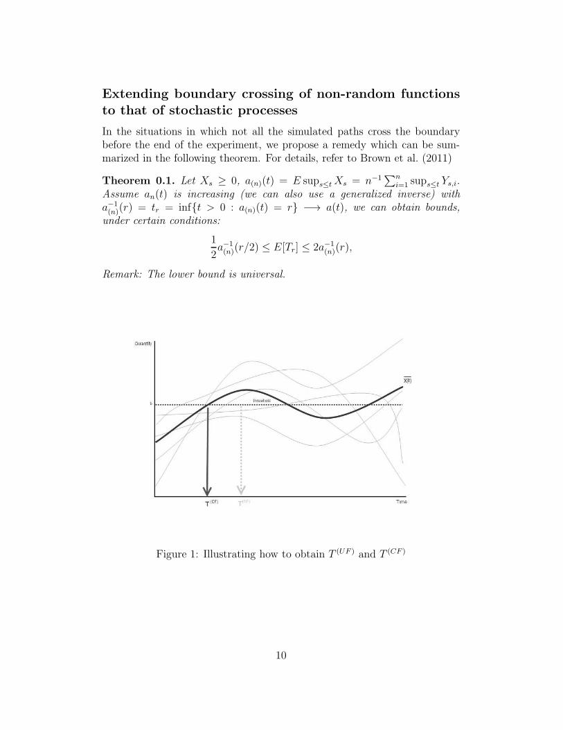
Extending boundary crossing of non-random functionsto that of stochastic processes
In the situations in which not all the simulated paths cross the boundarybefore the end of the experiment, we propose a remedy which can be sum-marized in the following theorem. For details, refer to Brown et al. (2011)
Theorem 0.1. Let Xs ≥ 0, a(n)(t) = E sups≤tXs = n−1∑n
i=1 sups≤t Ys,i.Assume an(t) is increasing (we can also use a generalized inverse) witha−1(n)(r) = tr = inf{t > 0 : a(n)(t) = r} −→ a(t), we can obtain bounds,
under certain conditions:
1
2a−1(n)(r/2) ≤ E[Tr] ≤ 2a−1
(n)(r),
Remark: The lower bound is universal.
Figure 1: Illustrating how to obtain T (UF ) and T (CF )
10
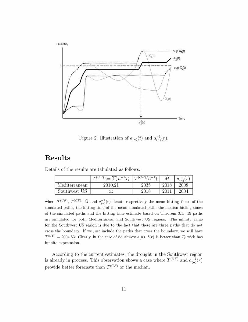
Figure 2: Illustration of a(n)(t) and a−1(n)(r).
Results
Details of the results are tabulated as follows:
T (UF ) :=∑
n−1Ti T (CF )(n−1) M a−1(n)(r)
Mediterranean 2010.21 2035 2018 2008Southwest US ∞ 2018 2011 2004
where T(UF ), T (CF ), M and a
−1(n)(r) denote respectively the mean hitting times of the
simulated paths, the hitting time of the mean simulated path, the median hitting times
of the simulated paths and the hitting time estimate based on Theorem 3.1. 19 paths
are simulated for both Mediterranean and Southwest US regions. The infinity value
for the Southwest US region is due to the fact that there are three paths that do not
cross the boundary. If we just include the paths that cross the boundary, we will have
T(UF ) = 2004.63. Clearly, in the case of Southwest,a(n)
−1(r) is better than Tr wich has
infinite expectation.
According to the current estimates, the drought in the Southwest regionis already in process. This observation shows a case where T (UF ) and a−1
(n)(r)
provide better forecasts than T (CF ) or the median.
11
References
Brown M, de la Pena, V.H., Kushnir, Y & Sit, T 2011, “On EstimatingThreshold Crossing Times,” submitted.
Seager, R., Ting, M. F., Held, I., Kushnir, Y., Lu, J., Vecchi, G., Huang, H.P., Harnik, N., Leetmaa, A., Lau, N. C., Li, C. H., Velez, J. & Naik, N.2007, “Model projections of an imminent transition to a more arid climatein southwestern North America,” Science, May 25, Volume 316, Issue 5828,p.1181-1184.
Randall D.A., Wood R.A., Bony S., Colman R., Fichefet T., Fyfe J., KattsovV., Pitman A., Shukla J., Srinivasan J., Stouffer R.J., Sumi A. & TaylorK.E. 2007, “Climate Models and Their Evaluation.” in: Climate Change2007: The Physical Science Basis. Contribution of Working Group I tothe Fourth Assessment Report of the Intergovernmental Panel on ClimateChange, Solomon, S, Qin D, Manning M, Chen Z, Marquis M, Averyt KB,Tignor M, Miller HL, editors. Cambridge University Press, Cambridge,United Kingdom and New York, NY, USA.
12
Cosmology through the large-scale structureof the Universe
Eyal A. Kazin5
Center for Cosmology and Particle PhysicsNew York University, 4 Washington PlaceNew York, NY 10003, USA
Abstract
The distribution of matter contains a lot of cosmological information. Ap-plying N-point statistics one can measure the geometry and expansion ofthe cosmos as well as test General Relativity at scales of millions to billionsof light years. In particular, I will discuss an exciting recent measurementdubbed the “baryonic acoustic feature”, which has recently been detected inthe Sloan Digital Sky Survey galaxy sample. It is the largest known “stan-dard ruler” (half a billion light years across), and is being used to investigatethe nature of the acceleration of the Universe.
The questions posed by ΛCDM
The Cosmic Microwave Background (CMB) shows us a picture of the earlyUniverse which was very uniform (Penzias & Wilson 1965), yet with enoughinhomogeneities (Smoot et al. 1992) to seed the structure we see today inthe form of galaxies and the cosmic-web. Ongoing sky surveys are measuringdeeper into the Universe with high edge technology transforming cosmologyinto a precision science.
The leading “Big Bang” model today is dubbed ΛCDM. While shownto be superbly consistent with many independent astronomical probes, itindicates that the “regular” material (atoms, radiation) comprise of only 5%of the energy budget, hence challenging our current understanding of physics.
The Λ is a reintroduction of Einstein’s so-called cosmological constant.He originally introduced it to stabilize a Universe that could expand or con-tract, according to General Relativity. At present, it is considered a mys-terious energy with a repulsive force that explains the acceleration of theobserved Universe. This acceleration was first noticed through super-novae
13
distance-redshift relationships (Riess et al. 1998, Perlmutter et al. 1999). Of-ten called dark energy, it has no clear explanation, and most cosmologistswould happily do away with it, once a better intuitive explanation emerges.One stream of thought is modifying General Relativity on very large scales,e.g, by generalizing to higher dimensions.
Cold dark matter (CDM), on the other hand, has gained its “street-cred”throughout recent decades, as an invisible substance (meaning not interactingwith radiation), but seen time and time again as the dominant gravitationalsource. Dark matter is required to explain various measurements as thevirial motions of galaxies within clusters (Zwicky 1933), the rotation curvesof galaxies (Rubin & Ford 1970), the gravitational lensing of backgroundgalaxies, and collisions of galaxy clusters (Clowe et al. 2004). We have yet todetect dark matter on Earth, although there already have been false positives.Physicists hope to see convincing evidence emerge from the Large HadronCollider which is bashing protons at near the speed of light.
One of the most convincing pieces of evidence for dark matter is thegrowth of the large-scale structure of the Universe, the subject of this essay.The CMB gives us a picture of the Universe when it was one thousand timesmaller than present. Early Universe inhomogeneities seen through tempera-ture fluctuations in the CMB are of the order one part in 105. By measuringthe distribution of galaxies, the structure in the recent Universe is probedto percent level at scales of hundreds of millions of light-year scales and itcan also be probed at the unity level and higher at “smaller” cosmic scales ofthousands of light-years. These tantalizing differences in structure can not beexplained by the gravitational attraction of regular material alone (atoms,molecules, stars, galaxies etc.), but can be explained with non-relativisticdark matter. Similar arguments show that the dark matter consists of ∼ 20%of the energy budget, and dark energy ∼ 75%.
The distribution of matter, hence, is a vital test for any cosmologicalmodel.
Acoustic oscillations as a cosmic ruler
Recently an important feature dubbed the baryonic acoustic feature hasbeen detected in galaxy clustering (Eisenstein et al. 2005, Percival et al.2010, Kazin et al. 2010). The feature has been detected significantly in theanisotropies of the CMB by various Earth and space based missions (e.g.Torbet et al. 1999, Komatsu et al. 2009). Hence, cosmologists have made animportant connection between the early and late Universe.
When the Universe was much smaller than today, energetic radiation
14
dominated and did not enable the formation of atoms. Photon pressure onthe free electrons and protons (collectively called baryons), caused them topropagate as a fluid in acoustic wave fashion. A useful analogy to have inmind is a pebble dropped in water perturbing it and forming a wave.
As the Universe expanded it cooled down and the first atoms formedfreeing the radiation, which we now measure as the CMB. Imagine the pondfreezing, including the wave. As the atoms are no longer being pushed theyslow down, and are now gravitationally bound to dark matter.
This means that around every over density, where the plasma-photonwaves (or pebble) originated, we expect an excess of material at a character-istic radius of the wave when it froze, dubbed the sound horizon.
In practice, this does not happen in a unique place, but throughoutthe whole Universe (think of throwing many pebbles into the pond). Thismeans that we expect to measure a characteristic correlation length in theanisotropies of the CMB, as well as in the clustering of matter in a statisticalmanner. Figure 1 demonstrates the detection of the feature in the CMB tem-perature anisotropies (Larson et al. 2011) and in the clustering of luminousred galaxies (Eisenstein et al. 2001).
As mentioned before, the ∼ 105 increase in the amplitude of the inhomo-geneities between early (CMB) and late Universe (galaxies) is explained verywell with dark matter. The height of the baryonic acoustic feature also servesas a firm prediction of the CDM paradigm. If there was no dark matter, therelative amplitude of the feature would be much higher. An interesting anec-dote is that we happen to live in an era when the feature is still detectablein galaxy clustering. Billions of years from now, it will be washed away, dueto gravitational interplay between dark matter and galaxies.
In a practical sense, as the feature spans a characteristic scale, it canbe used as a cosmic ruler. The signature in the anisotropies of the CMB(Figure 1a), calibrates this ruler by measuring the sound-horizon currentlyto an accuracy of ∼ 1.5% (Komatsu et al. 2009).
By measuring the feature in galaxy clustering transverse to the line-of-sight, you can think of it as the base of a triangle, for which we know theobserved angle, and hence can infer the distance to the galaxy sample. Clus-tering along the line-of-sight is an even more powerful measurement, as itis sensitive to the expansion of the Universe. By measuring expansion ratesone can test effects of dark energy. Current measurements show that thebaryonic acoustic feature in Figure 1b, can be used to measure the distanceto ∼ 3.5 billion light-years to an accuracy of ∼ 4% (Percival et al. 2010,Kazin et al. 2010).
15
Clustering- the technical details
As dark matter can not be seen directly, luminous objects, as galaxies, canserve as tracers, like the tips of icebergs. Galaxies are thought to form inregions of high dark matter density. An effective way to measure galaxyclustering (and hence inferring the matter distribution) is through two-pointcorrelations of over-densities.
An over-density at point ~x is defined as the contrast to the mean densityρ:
δ(~x) ≡ρ(~x)
ρ− 1. (2)
The auto-correlation function, defined as the joint probability of measuringan excess of density at a given separation r is defined as:
ξ(r) ≡ 〈δ(~x)δ(~x+ ~r)〉, (3)
where the average is over the volume, and the cosmological principle assumesstatistical isotropy. This is related to the Fourier complementary power spec-trum P(k).
For P(k), it is common to smooth out the galaxies into density fields,Fourier transforming δ and convolving with a “window function” that de-scribes the actual geometry of the survey.
The estimated ξ, in practice, is calculated by counting galaxy pairs:
ξ(r) =DD(r)
RR(r)− 1, (4)
where DD(r) is the normalized number of galaxy pairs within a sphericalshells of radius r ± 1
2∆r. This is compared to random points distributed ac-
cording to the survey geometry, where RR is the random-random normalizedpair count. By normalized I refer to the fact that one uses many more ran-dom points than data points to reduce Poisson shot noise. Landy & Szalay(1993) show that an estimator that minimizes the variance is:
ξ(r) =DD(r) +RR(r)− 2DR(r)
RR(r), (5)
where DR are the normalized data-random pairs.
The Sloan Digital Sky Survey
Using a dedicated 2.5 meter telescope, the SDSS has industrialized (in apositive way!) astronomy. In January 2011, they publicly released an image
16
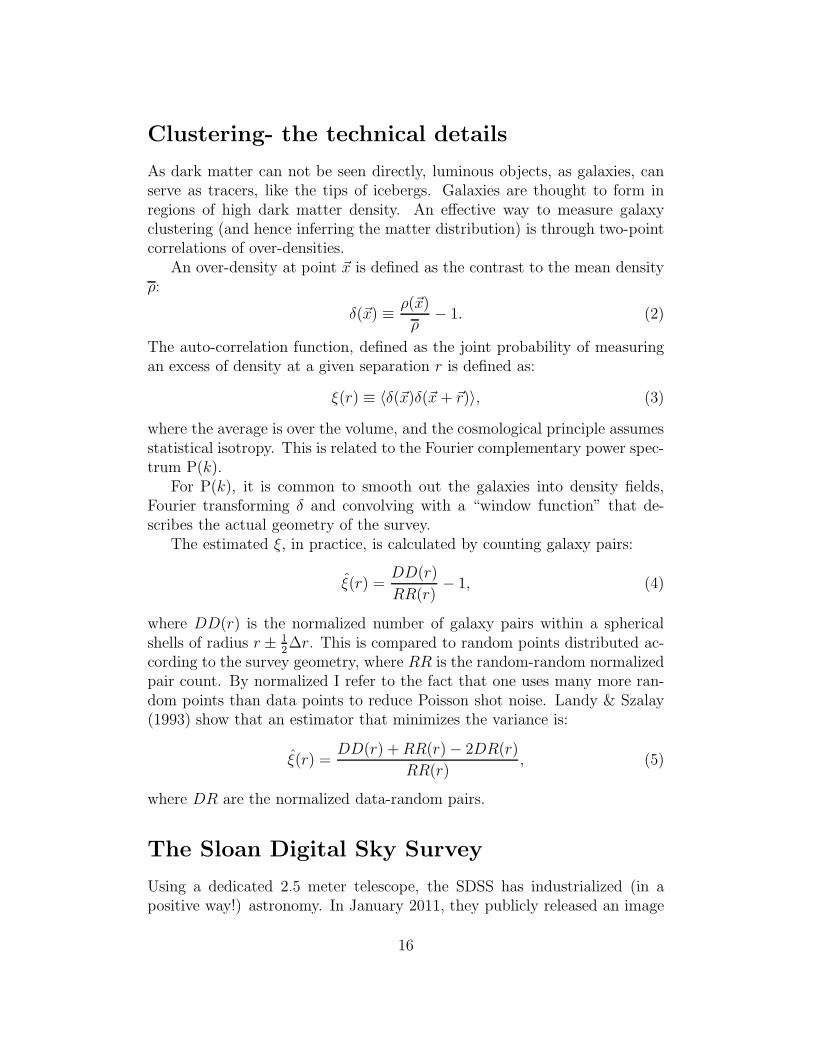
Figure 1: The baryonic acoustic feature in the large-scale structure of theUniverse. The solid lines are ΛCDM predictions. (a) Temperature fluctu-ations in the CMB (2D projected k-space), measured by WMAP, ACBARand QUaD. The feature is the form of peaks and troughs, and is detected tovery high significance. These anisotropies are at the level of 10−5, and reflectthe Universe as it was 1000-fold smaller than today (∼ 13.3 billion year ago).(b) SDSS luminous galaxy 3D clustering ξ at very large scales (100h−1Mpccorresponds to ∼ 0.5 billion light years). The feature is detected consistentwith predictions. Notice ξ is of order 1% at the feature, showing a pictureof the Universe ∼ 3 billion years ago. The gray regions indicate 68, 95% CLregions of simulated mock galaxy catalogs, reflecting cosmic variance. Thesewill be substantially reduced in the future with larger volume surveys. (ABBmeans time “after big bang”)
17
of one third of the sky, and detected 469 million objects from astroids togalaxies6 (SDSS-III collaboration: Hiroaki Aihara et al. 2011).
These images give a 2D projected image of the Universe. This is followedup by targeting objects of interest, obtaining their spectroscopy. The spectracontains information about the composition of the objects. As galaxies andquasars have signature spectra, these can be used as a templates to measurethe Doppler-shift. The expanding Universe causes these to be redshifted.The redshift z can be simply related to the distance d through the Hubbleequation at low z:
cz = Hd, (6)
where c is the speed of light and the Hubble parameter H [1/time] is theexpansion rate of the Universe. Hence, by measuring z, observers obtain a 3Dpicture of the Universe, which can be used to measure clustering. Dark energyeffects Equation 6 through H(z), when generalizing for larger distances.
The SDSS team has obtained spectroscopic redshifts of over a millionobjects in the largest volume to date. It is now in its third phase, obtainingmore spectra for various missions including: improving measurements of thebaryonic acoustic feature (and hence measuring dark energy) by measuringa larger and deeper volume, learning the structure of the Milky Way, anddetection of exoplanets (Eisenstein et al. 2011).
Summary
Cosmologists are showing that there is much more than meets the eye. Itis just a matter of time until dark matter will be understood, and might Ibe bold enough to say harnessed? The acceleration of the Universe, is stilla profound mystery, but equipped with tools such as the baryonic acousticfeature, cosmologists will be able to provide rigorous tests.
E.K was partially supported by a Google Research Award and NASAAward NNX09AC85G.
References
Clowe, D., Gonzalez, A., & Markevitch, M. 2004, The Astrophysical Journal,604, 596
6http://www.sdss3.org/dr8/
18
Eisenstein, D. J., Weinberg, D. H., Agol, E., Aihara, H., Allende Prieto, C.,Anderson, S. F., Arns, J. A., Aubourg, E., Bailey, S., Balbinot, E., et al.2011, arXiv:1101.1529v1
Eisenstein, D. J. et al. 2001, The Astronomical Journal, 122, 2267
Eisenstein, D. J. et al. 2005, The Astrophysical Journal, 633, 560
Kazin, E. A., Blanton, M. R., Scoccimarro, R., McBride, C. K., Berlind,A. A., Bahcall, N. A., Brinkmann, J., Czarapata, P., Frieman, J. A., Kent,S. M., Schneider, D. P., & Szalay, A. S. 2010, The Astrophysical Journal,710, 1444
Komatsu, E., Dunkley, J., Nolta, M. R., Bennett, C. L., Gold, B., Hinshaw,G., Jarosik, N., Larson, D., Limon, M., Page, L., Spergel, D. N., Halpern,M., Hill, R. S., Kogut, A., Meyer, S. S., Tucker, G. S., Weiland, J. L.,Wollack, E., & Wright, E. L. 2009, The Astrophysical Journal SupplementSeries, 180, 330
Landy, S. D. & Szalay, A. S. 1993, The Astrophysical Journal, 412, 64
Larson, D., Dunkley, J., Hinshaw, G., Komatsu, E., Nolta, M. R., Bennett,C. L., Gold, B., Halpern, M., Hill, R. S., Jarosik, N., Kogut, A., Limon,M., Meyer, S. S., Odegard, N., Page, L., Smith, K. M., Spergel, D. N.,Tucker, G. S., Weiland, J. L., Wollack, E., & Wright, E. L. 2011, TheAstrophysical Journal Supplement Series, 192, 16
Penzias, A. A. & Wilson, R. W. 1965, The Astrophysical Journal, 142, 419
Percival, W. J., Reid, B. A., Eisenstein, D. J., Bahcall, N. A., Budavari, T.,Fukugita, M., Gunn, J. E., Ivezic, Z., Knapp, G. R., Kron, R. G., Loveday,J., Lupton, R. H., McKay, T. A., Meiksin, A., Nichol, R. C., Pope, A. C.,Schlegel, D. J., Schneider, D. P., Spergel, D. N., Stoughton, C., Strauss,M. A., Szalay, A. S., Tegmark, M., Weinberg, D. H., York, D. G., & Zehavi,I. 2010, Monthly Notices of the Royal Astronomical Society, 401, 2148
Perlmutter, S. et al. 1999, The Astrophysical Journal, 517, 565
Riess, A. G., Filippenko, A. V., Challis, P., Clocchiatti, A., Diercks, A.,Garnavich, P. M., Gilliland, R. L., Hogan, C. J., Jha, S., Kirshner, R. P.,Leibundgut, B., Phillips, M. M., Reiss, D., Schmidt, B. P., Schommer,R. A., Smith, R. C., Spyromilio, J., Stubbs, C., Suntzeff, N. B., & Tonry,J. 1998, The Astronomical Journal, 116, 1009
19

Rubin, V. C. & Ford, Jr., W. K. 1970, The Astrophysical Journal, 159, 379
SDSS-III collaboration: Hiroaki Aihara, Allende Prieto, C., An, D., et al.2011, arXiv:1101.1559v2
Smoot, G. F., Bennett, C. L., Kogut, A., Wright, E. L., Aymon, J., Boggess,N. W., Cheng, E. S., de Amici, G., Gulkis, S., Hauser, M. G., Hin-shaw, G., Jackson, P. D., Janssen, M., Kaita, E., Kelsall, T., Keegstra,P., Lineweaver, C., Loewenstein, K., Lubin, P., Mather, J., Meyer, S. S.,Moseley, S. H., Murdock, T., Rokke, L., Silverberg, R. F., Tenorio, L.,Weiss, R., & Wilkinson, D. T. 1992, The Astrophysical Journal Letters,396, L1
Torbet, E., Devlin, M. J., Dorwart, W. B., Herbig, T., Miller, A. D., Nolta,M. R., Page, L., Puchalla, J., & Tran, H. T. 1999, The AstrophysicalJournal Letters, 521, L79
Zwicky, F. 1933, Helvetica Physica Acta, 6, 110
20
On the Shoulders of Gauss, Bessel, andPoisson: Links, Chunks, Spheres, and
Conditional Models
William D HeavlinGoogle, Inc.Mountain View, California, USA
Abstract
We consider generalized linear models (GLMs) and the associated exponen-tial family (“links”). Our data structure partitions the data into mutuallyexclusively subsets (“chunks”). The conditional likelihood is defined as con-ditional on the within-chunk histogram of the response. These likelihoodshave combinatorial complexity. To compute such likelihoods efficiently, wereplace a sum over permutations with an integration over the orthogonalor rotation group (“spheres”). The resulting approximate likelihood givesrise to estimates that are highly linearized, therefore computationally attrac-tive. Further, this approach refines our understanding of GLMs in severaldirections.
Notation and Model
Our observations are chunked into subsets indexed by g : (ygi,xgi : g =1, 2, . . . , G; i = 1, . . . , ng). The g-th chunk’s responses are denoted by yg =(yg1, yg2, . . . , ygng
) and its feature matrix by Xg; its i -th row is xTgi. Our
framework is that of the generalized linear model (McCullough & Nelder1999):
Pr{ygi|xTgiβ} = exp{ygix
Tgiβ) + h1(ygi) + h2(x
Tgiβ)}. (7)
The Spherical Approximation
Motivated by the risk of attenuation, we condition ultimately on the varianceof yg. The resulting likelihood consists of these terms, indexed by g :
21
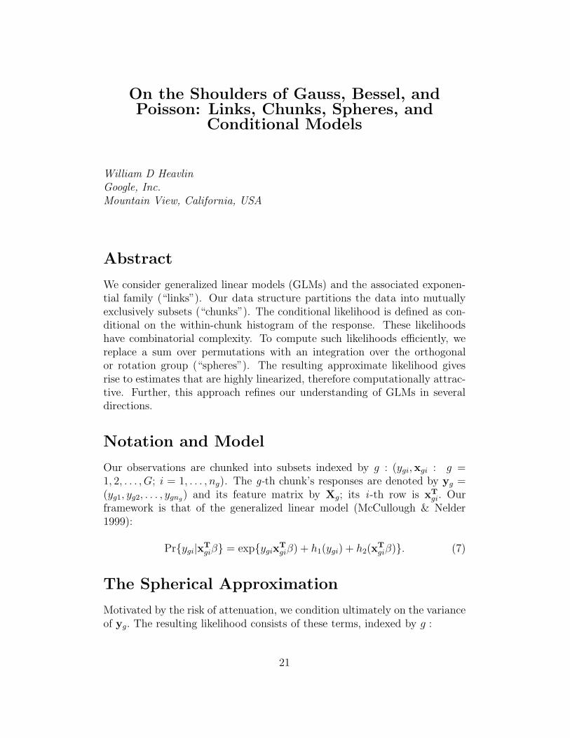
Figure 1: Numerically calculated values of ∂∂κ
logQ as a function of radius κ.
exp{Lcg(β)} ≈exp{yT
g Xgβ}
ave{exp{yTg P
Tτ Xgβ}|τ ∈ orthogonal}
(8)
Free of intercept terms, this likelihood resists attenuation. The rightmostterm of (8) reduces to the von Mises-Fisher distribution (Mardia & Jupp2000, Watson & Williams 1956) and is computationally attractive (Plis et al.2010).
Figure 1 assesses the spherical approximation. The x-axis is the radiusκ = ||yg|| × ||Xgβ||, the y-axis the differential effect of equation (8)’s twodenominators. Panel (c) illustrates how larger chunk sizes ng improve thespherical approximation. Panel (a) and (b) illustrates how the approximationfor ng = 2 can be improved by a continuity correction.
Some Normal Equations
From (8) these maximum likelihood equations follow:
[∑
g
ρgrgXT
g Xg]β = XTg yg, (9)
which are nearly the same as those of Gauss. Added is the ratio ρg/rg, whichthrottles chunks with less information; to first order, it equals the within-chunk variance.
The dependence of ρg/rg on β is weak, so the convergence of (9) is rapid.Equation (9) resembles iteratively reweighted least squares (Jorgensen 2006),but is more attractive computationally. To estimate many more features, weinvestigate marginal regression (Fan & Lv 2008) and boosting (Schapire &Singer 1999).
22
Conditional models like those in (8) do not furnish estimates of inter-cepts. The theory of conditional models therefore establishes a frameworkfor multiple-stage modeling.
References
Fan, J. & Lv, J. 2008, “Sure independence screening for ultra-high dimen-sional feature space (with discussion).” Journal of the Royal StatisticalSociety, series B vol. 70, pp. 849-911.
Jorgensen, M. (2006). “Iteratively reweighted least squares,” Encyclopedia ofEnvironmetrics. John Wiley & Sons.
McCullough, P. & Nelder, J.A. 1999, Generalized Linear Models, 2nd edition,John Wiley & Sons.
Mardia, K.V. & Jupp, P.E. 2000, Directional Statistics, 2nd edition, JohnWiley & Sons.
Plis, S.M., Lane, T., Calhoun, V.D. 2010, “Permutations as angular data:efficient inference in factorial spaces,” IEEE International Conference onData Mining, pp.403-410.
Schapire, R.E. & Singer, Y. 1999, “Improved Boosting Algorithms UsingConfidence-Rated Predictors.” Machine Learning, vol. 37, pp. 297-336.
Watson, G.S. & Williams, E.J. 1956, “On the construction of significancetests on the circle and the sphere.” Biometrika, vol. 43. pp. 344-352.
23
Mining Citizen Science Data: MachineLearning Challenges
Kirk BorneSchool of Physics, Astronomy & Computational ScienceGeorge Mason University Fairfax, Virginia, USA
Large sky surveys in astronomy, with their open data policies (“data forall”) and their uniformly calibrated scientific databases, are key cyberinfras-tructure for astronomical research. These sky survey databases are also amajor content provider for educators and the general public. Depending onthe audience, we recognize three broad modes of interaction with sky sur-vey data (including the image archives and the science database catalogs).These modes of interaction span the progression from information-gatheringto active engagement to discovery. They are:
a.) Data Discovery – What was observed, when, and by whom? Retrieveobservation parameters from an sky survey catalog database. Retrieveparameters for interesting objects.
b.) Data Browse – Retrieve images from a sky survey image archive. Viewthumbnails. Select data format (JPEG, Google Sky KML, FITS). Panthe sky and examine catalog-provided tags (Google Sky, World WideTelescope).
c.) Data Immersion – Perform data analysis, mining, and visualization.Report discoveries. Comment on observations. Contribute followupobservations. Engage in social networking, annotation, and tagging.Provide classifications of complex images, data correlations, data clus-ters, or novel (outlying, anomalous) detections.
In the latter category are Citizen Science research experiences. The worldof Citizen Science is blossoming in many ways, including century-old pro-grams such as the Audubon Society bird counts and the American Associa-tion of Variable Star Observers (at aavso.org) continuous monitoring, mea-surement, collation, and dissemination of brightness variations of thousandsof variable stars, but now including numerous projects in modern astron-omy, climate science, biodiversity, watershed monitoring, space science, andmore. The most famous and successful of these is the Galaxy Zoo project (at
24
galaxyzoo.org), which is “staffed” by approximately 400,000 volunteer con-tributors. Modern Citizen Science experiences are naturally online, takingadvantage of Web 2.0 technologies, for database-image-tagging mash-ups. Ittakes the form of crowd-sourcing the various stages of the scientific process.Citizen Scientists assist scientists’ research efforts by collecting, organizing,characterizing, annotating, and/or analyzing data. Citizen Science is oneapproach to engaging the public in authentic scientific research experienceswith large astronomical sky survey databases and image archives.
Citizen Science is a term used for scientific research projects in which indi-vidual (non-scientist) volunteers (with little or no scientific training) performor manage research-related tasks such as observation, measurement, or com-putation. In the Galaxy Zoo project, volunteers are asked to click on variouspre-defined tags that describe the observable features in galaxy images –nearly one million such images from the SDSS (Sloan Digital Sky Survey, atsdss.org). Every one of these million galaxies has now been classified by Zoovolunteers approximately 200 times each. These tag data are a rich source ofinformation about the galaxies, about human-computer interactions, aboutcognitive science, and about the Universe. The galaxy classifications arebeing used by astronomers to understand the dynamics, structure, and evo-lution of galaxies through cosmic time, and thereby used to understand theorigin, state, and ultimate fate of our Universe. This illustrates some of theprimary characteristics (and required features) of Citizen Science: that theexperience must be engaging, must work with real scientific data, must notbe busy-work, must address authentic science research questions that are be-yond the capacity of science teams and computational processing pipelines,and must involve the scientists. The latter two points are demonstrated (andproven) by: (a) the sheer enormous number of galaxies to be classified is be-yond the scope of the scientist teams, plus the complexity of the classificationproblem is beyond the capabilities of computational algorithms, primarily be-cause the classification process is strongly based upon human recognition ofcomplex patterns in the images, thereby requiring “eyes on the data”; and (b)approximately 20 peer- reviewed journal articles have already been producedfrom the Galaxy Zoo results – many of these papers contain Zoo volunteersas co-authors, and at least one of the papers includes no professional scien-tists as authors. The next major step in astronomical Citizen Science (butalso including other scientific disciplines) is the Zooniverse project (at zooni-verse.org). The Zooniverse is a framework for new Citizen Science projects,thereby enabling any science team to make use of the framework for theirown projects with minimal effort and development activity. Currently activeZooniverse projects include Galaxy Zoo II, Galaxy Merger Zoo, the MilkyWay Project, Supernova Search, Planet Hunters, Solar Storm Watch, Moon
25
Zoo, and Old Weather. All of these depend on the power of human cognition(i.e., human computation), which is superb at finding patterns in data, atdescribing (characterizing) the data, and at finding anomalies (i.e., unusualfeatures) in data. The most exciting example of this was the discovery ofHanny’s Voorwerp (Figure 1). A key component of the Zooniverse researchprogram is the mining of the volunteer tags. These tag databases themselvesrepresent a major source of data for knowledge discovery, pattern detection,and trend analysis. We are developing and applying machine learning algo-rithms to the scientific discovery process with these tag databases. Specifi-cally, we are addressing the question: how do the volunteer-contributed tags,labels, and annotations correlate with the scientist-measured science param-eters (generated by automated pipelines and stored in project databases)?The ultimate goal will be to train the automated data pipelines in future skysurveys with improved classification algorithms, for better identification ofanomalies, and with fewer classification errors. These improvements will bebased upon millions of training examples provided by the Citizen Scientists.These improvements will be absolutely essential for projects like the futureLSST (Large Synoptic Survey Telescope, at lsst.org), since LSST will mea-sure properties for at least 100 times more galaxies and 100 times more starsthan SDSS. Also, LSST will do repeated imaging of the sky over its 10-yearproject duration, so that each of the roughly 50 billion objects observed byLSST will have approximately 1000 separate observations. These 50 trilliontime series data points will provide an enormous opportunity for Citizen Sci-entists to explore time series (i.e., object light curves) to discover all typesof rare phenomena, rare objects, rare classes, and new objects, classes, andsub-classes. The contributions of human participants may include: character-ization of countless light curves; human-assisted search for best-fit models ofrotating asteroids (including shapes, spin periods, and varying surface reflec-tion properties); discovery of sub-patterns of variability in known variablestars; discovery of interesting objects in the environments around variableobjects; discovery of associations among multiple variable and/or movingobjects in a field; and more.
As an example of machine learning the tag data, a preliminary study by(Baehr 2010) of the galaxy mergers found in the Galaxy Zoo I project wascarried out. We found specific parameters in the SDSS science database thatcorrelate best with “mergerness” versus “non-mergerness”. These databaseparameters are therefore useful in distinguishing normal (undisturbed) galax-ies from abnormal (merging, colliding, interacting, disturbed) galaxies. Suchresults may consequently be applied to future sky surveys (e.g., LSST), toimprove the automatic (machine-based) classification algorithms for collid-ing and merging galaxies. All of this was made possible by the fact that
26
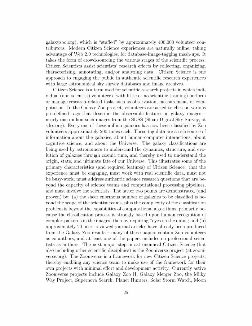
Figure 1: Hanny’s Voorwerp (Hanny’s Object) – The green gas cloud seenbelow the spiral galaxy in these images was first recognized as somethingunusual and “out of the ordinary” by Galaxy Zoo volunteer Hanny van Arkel,a Dutch school teacher, who was initially focused on classifying the dominantspiral galaxy above the green blob. This object is an illuminated gas cloud,glowing in the emission of ionized oxygen. It is probably the light echo froma dead quasar that was luminous at the center of the spiral galaxy about100,000 years ago. These images are approximately true color. The leftimage was taken with a ground- based telescope, and the right image wasobtained by the Hubble Space Telescope (courtesy W. Keel, the Galaxy Zooteam, NASA, and ESA).
the galaxy classifications provided by Galaxy Zoo I participants led to thecreation of the largest pure set of colliding and merging galaxies yet to becompiled for use by astronomers.
References
Baehr, S., Vedachalam, A., Borne, K., & Sponseller, D., ”Data Mining theGalaxy Zoo Mergers,” NASA Conference on Intelligent Data Understand-ing, https://c3.ndc.nasa.gov/dashlink/resources/220/, pp. 133-144 (2010).
27
Tracking Climate Models7
Claire Monteleoni 8
Center for Computational Learning Systems, Columbia UniversityNew York, New York, USA
Gavin A. SchmidtNASA Goddard Institute for Space Studies, 2880 BroadwayandCenter for Climate Systems Research, Columbia UniversityNew York, New York, USA
Shailesh SarohaDepartment of Computer ScienceColumbia UniversityNew York, New York, USA
Eva AsplundDepartment of Computer Science, Columbia UniversityandBarnard CollegeNew York, New York, USA
Climate models are complex mathematical models designed by meteorol-ogists, geophysicists, and climate scientists, and run as computer simulations,to predict climate. There is currently high variance among the predictionsof 20 global climate models, from various laboratories around the world,that inform the Intergovernmental Panel on Climate Change (IPCC). Giventemperature predictions from 20 IPCC global climate models, and over 100years of historical temperature data, we track the changing sequence of whichmodel currently predicts best. We use an algorithm due to Monteleoni &Jaakkola (2003), that models the sequence of observations using a hierarchi-cal learner, based on a set of generalized Hidden Markov Models, where theidentity of the current best climate model is the hidden variable. The tran-sition probabilities between climate models are learned online, simultaneousto tracking the temperature predictions.
7This is an excerpt from a journal paper currently under review. The conference versionappeared at the NASA Conference on Intelligent Data Understanding, 2010 (Monteleoni,Schmidt & Saroha 2010)
28
20 40 60 80 100 120 140 160 1800
1
2
3
4
5
Time in years (1900−2098)
Squ
ared
loss
Worst expertBest expertAverage prediction over 19 modelsLearn−alpha algorithm
20 40 60 80 100 120 140 160 1800
0.05
0.1
0.15
0.2
0.25
0.3
0.35
0.4
0.45
Time in years (1900−2098)
Squ
ared
loss
Best expertAverage prediction over 19 modelsLearn−alpha algorithm
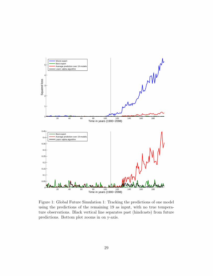
Figure 1: Global Future Simulation 1: Tracking the predictions of one modelusing the predictions of the remaining 19 as input, with no true tempera-ture observations. Black vertical line separates past (hindcasts) from futurepredictions. Bottom plot zooms in on y-axis.
29
On historical global mean temperature data, our online learning algo-rithm’s average prediction loss nearly matches that of the best performingclimate model in hindsight. Moreover its performance surpasses that of theaverage model prediction, which is the default practice in climate science,the median prediction, and least squares linear regression. We also exper-imented on climate model predictions through the year 2098. Simulatinglabels with the predictions of any one climate model, we found significantlyimproved performance using our online learning algorithm with respect tothe other climate models, and techniques (see e.g. Figure 1). To complementour global results, we also ran experiments on IPCC global climate modeltemperature predictions for the specific geographic regions of Africa, Europe,and North America. On historical data, at both annual and monthly time-scales, and in future simulations, our algorithm typically outperformed boththe best climate model per region, and linear regression. Notably, our al-gorithm consistently outperformed the average prediction over models, thecurrent benchmark.
References
Monteleoni, C. & Jaakkola, T. 2003 “Online learning of non-stationary se-quences”, In NIPS ’03: Advances in Neural Information Processing Sys-tems 16, 2003
Monteleoni, C., Schmidt, G & Saroha, S. 2010 “Tracking Climate Models”,in NASA Conference on Intelligent Data Understanding, 2010
30
Spectral Analysis Methods for ComplexSource Mixtures
Kevin H. KnuthDepartments of Physics and InformaticsUniversity at AlbanyAlbany, New York, USA
Abstract
Spectral analysis in real problems must contend with the fact that theremay be a large number of interesting sources some of which have knowncharacteristics and others which have unknown characteristics. In addition,one must also contend with the presence of uninteresting or backgroundsources, again with potentially known and unknown characteristics. In thistalk I will discuss some of these challenges and describe some of the usefulsolutions we have developed, such as sampling methods to fit large numbersof sources and spline methods to fit unknown background signals.
Introduction
The infrared spectrum of star-forming regions is dominated by emission froma class of benzene-based molecules known as Polycyclic Aromatic Hydrocar-bons (PAHs). The observed emission appears to arise from the combinedemission of numerous PAH molecular species, both neutral and ionized, eachwith its unique spectrum. Unraveling these variations is crucial to a deeperunderstanding of star-forming regions in the universe. However, efforts tofit these data have been defeated by the complexity of the observed PAHspectra and the very large number of potential PAH emitters. Linear su-perposition of the various PAH species accompanied by additional sourcesidentifies this problem as a source separation problem. It is, however, ofa formidable class of source separation problems given that different PAHsources are potentially in the hundreds, even thousands, and there is onlyone measured spectral signal for a given astrophysical site. In collabora-tion with Duane Carbon (NASA Advanced Supercomputing Center, NASAAmes), we have focused on developing informed Bayesian source separation
31
techniques (Knuth 2005) to identify and characterize the contribution of alarge number of PAH species to infrared spectra recorded from the InfraredSpace Observatory (ISO). To accomplish this we take advantage of a largedatabase of over 500 atomic and molecular PAH spectra in various statesof ionization that has been constructed by the NASA Ames PAH team (Al-lamandola, Bauschlicher, Cami and Peeters). To isolate the PAH spectra,much effort has gone into developing background estimation algorithms thatmodel the spectral background so that it can be removed to reveal PAH, aswell as atomic and ionic, emission lines.
The Spectrum Model
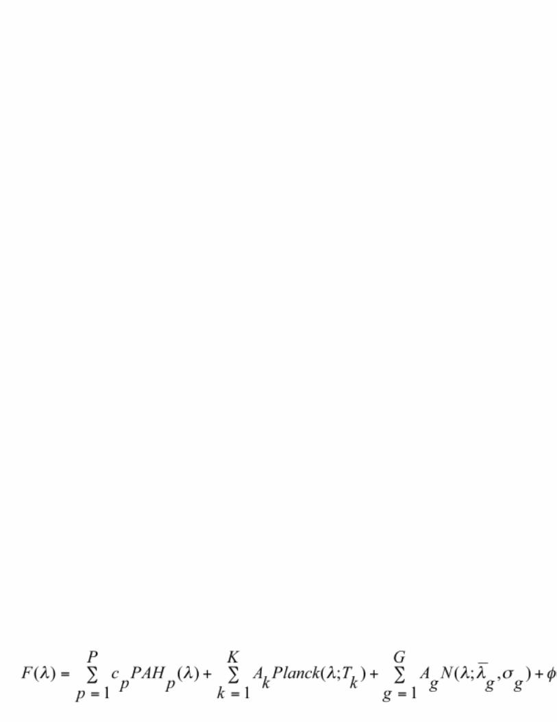
Blind techniques are not always useful in complex situations like these wheremuch is known about the physics of the source signal generation and prop-agation. Higher-order models relying on physically-motivated parameter-ized functions are required, and by adopting such models, one can introducemore sophisticated likelihood and prior probabilities. We call this approachInformed Source Separation (Knuth et al. 2007). In this problem, we havelinear mixing of P PAH spectra, K Planck blackbodies, a mixture of G Gaus-sians to describe unknown sources and additive noise:
F (λ) =
P∑
p=1
cpPAHp(λ) +
K∑
k=1
AkP lanck(λ;Tk) +
G∑
g=1
AgN(λ; λg, σg) + φ(λ)
(10)where PAHp is a p-indexed PAH spectrum from the dictionary, N is a
Gaussian. The function Planck is
P lanck(λ;Tk) =
√
λmax
λ
exp(hc/λmaxkT )− 1
exp(hc/λkT )− 1(11)
where h is Planck’s constant, c is the speed of light, k is Boltzmann’sconstant, T is the temperature of the cloud, and λmax is the wavelengthwhere the blackbody spectral energy peaks λmax = hc/4.965kT .
Source Separation using Sampling Methods
The sum over Planck blackbodies in the modeled spectrum (1) takes into ac-count the fact that we are recording spectra from potentially several sourcesarranged along the line-of-sight. Applying this model in conjunction with a
32
nested sampling algorithm to data recorded from ISO of the Orion Bar wewere able to obtain reasonable background fits, which often showed the pres-ence of multiple blackbodies. The results indicate that there is one blackbodyradiator at a temperature of 61.043 ± 0.004 K, and possibly a second (36.3%chance), at a temperature around 18.8 K. Despite these successes, this algo-rithm did not provide adequate results for background removal since the es-timated background was not constrained to lie below the recorded spectrum.Upon background subtraction, this led to unphysical negative spectral power.This result encouraged us to develop an alternative background estimationalgorithm. Estimation of PAHs was demonstrated to be feasible in syntheticmixtures with low noise using sampling methods, such as Metropolis-HastingsMarkov chain Monte Carlo (MCMC) and Nested Sampling. Estimation us-ing gradient climbing techniques, such as the Nelder-Mead simplex method,too often were trapped in local solutions. In real data, PAH estimation wasconfounded by spectral background.
Background Removal Algorithm
Our most advanced background removal algorithm was developed to avoidthe problem of negative spectral power by employing a spline-based modelcoupled with a likelihood function that favors background models that liebelow the recorded spectrum. This is accomplished by using a likelihoodfunction based on the Gaussian where the standard deviation on the neg-ative side is 10 times smaller than on the positive side. The algorithm isdesigned with the option to include a second derivative smoothing prior.Users choose the number of spline knots and set their positions along thex-axis. This provides the option of fitting a spectral feature or estimatinga smooth background underlying it. Our preliminary work shows that thebackground estimation algorithm works very well with both synthetic andreal data (Nathan 2010). The use of this algorithm illustrates that PAHestimates are extremely sensitive to background, and that PAH characteri-zation is extremely difficult in cases where the background spectra are poorlyunderstood.
Kevin Knuth would like to acknowledge Duane Carbon, Joshua Choinsky,Deniz Gencaga, Haley Maunu, Brian Nathan and ManKit Tse for all of theirhard work on this project.
33
References
Knuth, K.H. 2005. “Informed source separation: A Bayesian tutorial” (In-vited paper) B. Sankur , E. Cetin, M. Tekalp , E. Kuruoglu (ed.), Pro-ceedings of the 13th European Signal Processing Conference (EUSIPCO2005), Antalya, Turkey.
Knuth, K.H., Tse M.K., Choinsky J., Maunu H.A, Carbon D.F. 2007,“Bayesian source separation applied to identifying complex organicmolecules in space”, Proceedings of the IEEE Statistical Signal ProcessingWorkshop, Madison WI, August 2007.
Nathan, B. 2010. “Spectral analysis methods for characterizing organicmolecules in space”. M.S. Thesis, University at Albany, K.H. Knuth, Ad-visor.
34
Beyond Objects: Using Machines toUnderstand the Diffuse Universe
J. E. G. PeekDepartment of AstronomyColumbia UniversityNew York, New York, USA
In this contribution I argue that our understanding of the universe hasbeen shaped by an intrinsically “object-oriented” perspective, and that tobetter understand our diffuse universe we need to develop new ways of think-ing and new algorithms to do this thinking for us.
Envisioning our universe in the context of objects is natural both observa-tionally and physically. When our ancestors looked up into the the starry sky,they noticed something very different from the daytime sky. The nighttimesky has specific objects, and we gave them names: Rigel, Procyon, Fomal-haut, Saturn, Venus, Mars. These objects were both very distinct from theblackness of space, but they were also persistent night to night. The samecould not be said of the daytime sky, with its amorphous, drifting clouds,never to be seen again, with no particular identity. Clouds could sometimesbe distinguished from the background sky, but often were a complex, in-teracting blend. From this point forward astronomy has been a science ofobjects. And we have been rewarded for this assumption: stars in space canbe thought of very well as discrete things. They have huge density contrastscompared to the rest of space, and they are incredibly rare and compact.They rarely contact each other, and are typically easy to distinguish. Thesame can be said (to a lesser extent) of planets and galaxies, as well as allmanner of astronomical objects.
I argue, though, that we have gotten to a stage of understanding of ouruniverse that we need to be able to better consider the diffuse universe.We now know that the material universe is largely made out of the verydiffuse dark matter, which, while clumpy, is not well approximated as discreteobjects. Even the baryonic matter is largely diffuse: of the 4% of the mass-energy budget of the universe devoted to baryons, 3.5% is diffuse hot gaspermeating the universe, and collecting around groups of galaxies. Besidesthe simple accounting argument, it is important to realize that the interestsof astronomers are now oriented more and more toward origins: origins ofplanets, origins of stars, origins of galaxies. This is manifest in the fact thatNASA devotes a plurality of its astrophysics budget to the “cosmic origins”
35
program. And what do we mean by origins? The entire history of anythingin the universe can be roughly summed up as “it started diffuse and then,under the force of gravity, it became more dense”. If we are serious aboutunderstanding the origins of things in the universe, we must do better atunderstanding not just the objects, but the diffuse material whence theycame.
We have, as investigators of the universe, enlisted machines to do a lotof our understanding for us. And, as machines inherit our intuition throughthe codes and algorithms we write, we have given them a keen sense ofobjects. A modern and powerful example is the Sloan Digital Sky Survey(SDSS; York et al. 2000). SDSS makes huge maps of the sky with veryhigh fidelity, but these maps are rarely used for anything beyond wall decor.The real power of the SDSS experiment depends on the photometric pipeline(Lupton et al. 2001), which interprets that sky into tens of millions of objects,each with precise photometric information. With these lists in hand wecan better take a census of the stars and galaxies in our universe. It issometimes interesting to understand the limits of these methodologies; thephoto pipeline can find distant galaxies easily, but large, nearby galaxies are achallenge, as the photo pipeline cannot easily interpret these huge diaphanousshapes (West et al. 2010; Fig 1). The Virtual Astronomical Observatory(VAO; e.g. Hanisch 2010) is another example of a collection of algorithms thatenables our object-oriented mindset. VAO has developed a huge set of toolsthat allow astronomers to collect a vast array of information from differentsources, and combine them elegantly together. These tools, however, almostalways use the “object” as the smallest element of information, and are muchless useful in interpreting the diffuse universe. Finally, astrometry.net isan example of how cutting edge algorithms combined with excellent datacan yield new tools for interpreting astronomical data (Lang et al. 2010).By accessing giant catalogs of objects, the software can, in seconds, giveprecise astrometric information about any image containing stars. Again, weleverage our object-oriented understanding, both both psychologically andcomputationally, to decode our data.
As a case study, we examine at a truly object-less data space: the Galacticneutral hydrogen (H i) interstellar medium (ISM). Through the 21-cm hyper-fine transition of H i, we can study the neutral ISM of our Galaxy and othersboth angularly and in the velocity domain (e.g. Kulkarni & Heiles 1988).H i images of other galaxies, while sometimes diffuse, do typically have clearedges. In our own Galaxy we are afforded no such luxury. The GalacticH i ISM is sky-filling, and can represent gas on a huge range of distancesand physical conditions. As our technology increases, we are able to buildlarger and larger, and more and more detailed images of the H i ISM. What
36
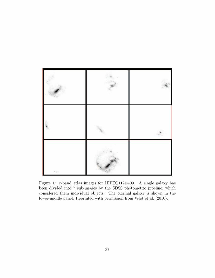
Figure 1: r -band atlas images for HIPEQ1124+03. A single galaxy hasbeen divided into 7 sub-images by the SDSS photometric pipeline, whichconsidered them individual objects. The original galaxy is shown in thelower-middle panel. Reprinted with permission from West et al. (2010).
37
we see in these multi-spectral images is an incredible cacophony of shapesand structures, overlapping, intermingling, with a variety of size, shape, andintensity that cannot be easily described. Indeed, it is this lack of languagethat is at the crux of the problem. These data are affected by a huge num-ber of processes; the accretion of material onto the Galaxy (e.g. Begum etal. 2010), the impact of shockwaves and explosions (e.g. Heiles 1979), theformation of stars (e.g. Kim et al. 1998), the effect of magnetization (e.g.McClure-Griffiths et al. 2006). And yet, we have very few tools that capturethis information.
As yet, there are two “flavors” of mechanisms we as a community haveused to try to interpret this kind of diffuse data. The first is the observer’smethod. In the observer’s method the data cubes are inspected by eye,and visually interesting shapes have been picked out (e.g. Ford et al. 2010).These shapes are then cataloged and described, usually qualitatively andwithout statistical rigor. The problems with these methods are self-evident:impossible statistics, unquantifiable biases, and an inability to compare tophysical models. The second method is the theorist’s method. In the the-orist’s method, some equation is applied to the data set wholesale, and anumber comes out (e.g. Chepurnov et al. 2010). This method is powerful inthat it can be compared directly to simulation, but typically cannot inter-pret any shape information at all. Given that the ISM is not a homogeneous,isotropic system, and various physical effects may influence the gas in differ-ent directions or at different velocities, this method seems a poor match forthe data. It also cuts out any intuition as to what data may be carrying themost interesting information.
We are in the process of developing a “third way”, which I will explainin two examples. Of the two projects, our more completed one is a searchfor compact, low-velocity clouds in the Galaxy (e.g. Saul et al. 2011). Theseclouds are inherently interesting as they likely probe the surface of the Galaxyas it interacts with the Galactic halo, a very active area of astronomicalresearch. To do this our group, led by Destry Saul, wrote a wavelet-style codeto search through the data cubes for isolated clouds that matched our searchcriteria. These clouds once found could then be “objectified”, quantifiedand studied as a population. In some sense, through this objectification,we are trying to shoehorn an intrinsically diffuse problem into the object-oriented style thinking we are trying to escape. This gives us the advantagethat we can use well known tools for analysis (e.g. scatter plots), but wegive up a perhaps deeper understanding of these structures from consideringthem in their context. The harder, and far less developed, project is to tryto understand the meaning of very straight and narrow diffuse structuresin the HI ISM at very low velocity. The HI ISM is suffused with “blobby
38
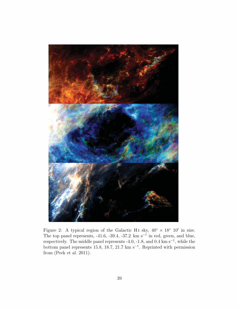
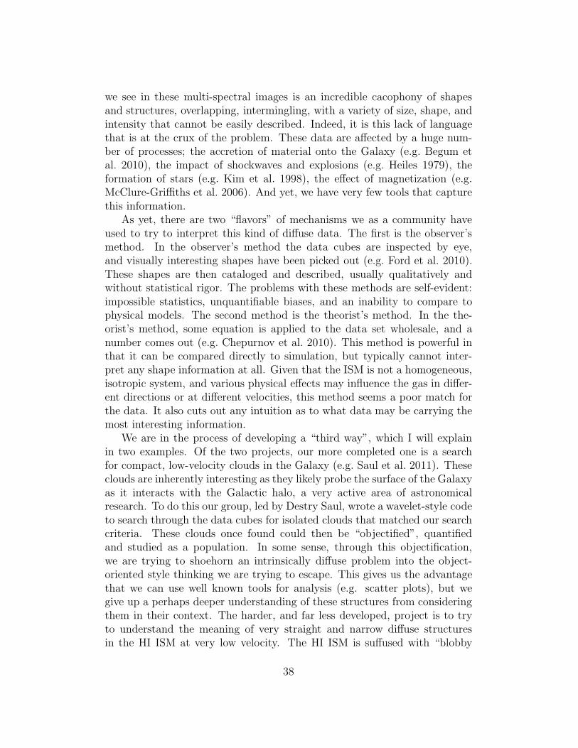
Figure 2: A typical region of the Galactic H i sky, 40◦ × 18◦ 10′ in size.The top panel represents, -41.6, -39.4, -37.2 km s−1 in red, green, and blue,respectively. The middle panel represents -4.0, -1.8, and 0.4 km s−1, while thebottom panel represents 15.8, 18.7, 21.7 km s−1. Reprinted with permissionfrom (Peek et al. 2011).
39
Figure 3: An H i image of the Riegel-Crutcher cloud from McClure-Griffithset al. (2006) at 4.95 km s−1 vLSR. The polarization vectors from backgroundstarlight indicate that the structure of the ISM reflects the structure of theintrinsic magnetization. Reprinted with permission from McClure-Griffithset al. (2006).
40
filaments”, but these particular structures seem to stand out, looking likea handful of dry fettuccine dropped on the kitchen floor. We know thatthese kinds of structures can give us insight into the physics of the ISM: indenser environments it has been shown that more discrete versions of thesefeatures are qualitatively correlated with dust polarizations and the magneticunderpinning of the ISM (McClure-Griffiths et al. 2006). We would like toinvestigate these features more quantitatively, but we have not developedmechanisms to answer even the simplest questions. In a given directionhow much of this feature is there? In which way is it pointing? What areits qualities? Does there exist a continuum of these features, or are theytruly discrete? The “object-oriented” astronomer mindset is not equippedto address these sophisticated questions.
We are just beginning to investigate machine vision techniques for under-standing these unexplored data spaces. Machine vision technologies are beingdeveloped to better parse our very confusing visual world using computers,such as in the context of object identification and the 3D reconstruction of2D images (Sonka et al. 2008). Up until now, most astronomical machinevision problems have been embarrassingly easy; points in space are relativelysimple to parse for machines. Perhaps the diffuse universe will be a newchallenge for computer vision specialists and be a focal point for communi-cation between the two fields. Machine learning methods, and human-aideddata interpretation on large scales may also prove crucial to cracking thesecomplex problems. How exactly we employ these new technologies in parsingour diffuse universe is very much up to us.
References
Begum, A., Stanimirovic, S., Peek, J. E., Ballering, N. P., Heiles, C., Douglas,K. A., Putman, M., Gibson, S. J., Grcevich, J., Korpela, E. J., Lee, M.-Y.,Saul, D., & Gallagher, J. S. 2010, eprint arXiv, 1008, 1364
Chepurnov, A., Lazarian, A., Stanimirovic, S., Heiles, C., & Peek, J. E. G.2010, The Astrophysical Journal, 714, 1398
Ford, H. A., Lockman, F. J., & McClure-Griffiths, N. M. 2010, The Astro-physical Journal, 722, 367
Hanisch, R. 2010, Astronomical Data Analysis Software and Systems XIX,434, 65
Heiles, C. 1979, Astrophysical Journal, 229, 533
41

Kim, S., Staveley-Smith, L., Dopita, M. A., Freeman, K. C., Sault, R. J.,Kesteven, M. J., & Mcconnell, D. 1998, Astrophysical Journal v.503, 503,674
Kulkarni, S. R. & Heiles, C. 1988, Neutral hydrogen and the diffuse inter-stellar medium, 95–153
Lang, D., Hogg, D. W., Mierle, K., Blanton, M., & Roweis, S. 2010, TheAstronomical Journal, 139, 1782
Lupton, R., Gunn, J. E., Ivezic, Z., Knapp, G. R., Kent, S., & Yasuda, N.2001, arXiv, astro-ph
McClure-Griffiths, N. M., Dickey, J. M., Gaensler, B. M., Green, A. J., &Haverkorn, M. 2006, The Astrophysical Journal, 652, 1339
Peek, J. E. G., Heiles, C., Douglas, K. A., Lee, M.-Y., Grcevich, J., Stan-imirovic, S., Putman, M. E., Korpela, E. J., Gibson, S. J., Begum, A., &Saul, D. 2011, The Astrophysical Journal Supplement, 1
Saul, D., Peek, J. E. G., Grcevich, J., & Putman, M. E. 2011, in prep, 1
Sonka, M., Hlavac, V., & Boyle, R. 2008, 829
West, A. A., Garcia-Appadoo, D. A., Dalcanton, J. J., Disney, M. J., Rockosi,C. M., Ivezic, Z., Bentz, M. C., & Brinkmann, J. 2010, The AstronomicalJournal, 139, 315
York, D. G., Adelman, J., Anderson, J., Anderson, S. F., Annis, J., Bahcall,N. A., Bakken, J. A., Barkhouser, R., Bastian, S., Berman, E., Boroski,W. N., Bracker, S., Briegel, C., Briggs, J. W., Brinkmann, J., Brunner, R.,Burles, S., Carey, L., Carr, M. A., Castander, F. J., Chen, B., Colestock,P. L., Connolly, A. J., Crocker, J. H., Csabai, I., Czarapata, P. C., Davis,J. E., Doi, M., Dombeck, T., Eisenstein, D., Ellman, N., Elms, B. R.,Evans, M. L., Fan, X., Federwitz, G. R., Fiscelli, L., Friedman, S., Frieman,J. A., Fukugita, M., Gillespie, B., Gunn, J. E., Gurbani, V. K., de Haas,E., Haldeman, M., Harris, F. H., Hayes, J., Heckman, T. M., Hennessy,G. S., Hindsley, R. B., Holm, S., Holmgren, D. J., h Huang, C., Hull,C., Husby, D., Ichikawa, S.-I., Ichikawa, T., Ivezic, Z., Kent, S., Kim,R. S. J., Kinney, E., Klaene, M., Kleinman, A. N., Kleinman, S., Knapp,G. R., Korienek, J., Kron, R. G., Kunszt, P. Z., Lamb, D. Q., Lee, B.,Leger, R. F., Limmongkol, S., Lindenmeyer, C., Long, D. C., Loomis,C., Loveday, J., Lucinio, R., Lupton, R. H., MacKinnon, B., Mannery,E. J., Mantsch, P. M., Margon, B., McGehee, P., McKay, T. A., Meiksin,
42

A., Merelli, A., Monet, D. G., Munn, J. A., Narayanan, V. K., Nash,T., Neilsen, E., Neswold, R., Newberg, H. J., Nichol, R. C., Nicinski, T.,Nonino, M., Okada, N., Okamura, S., Ostriker, J. P., Owen, R., Pauls,A. G., Peoples, J., Peterson, R. L., Petravick, D., Pier, J. R., Pope, A.,Pordes, R., Prosapio, A., Rechenmacher, R., Quinn, T. R., Richards, G. T.,Richmond, M. W., Rivetta, C. H., Rockosi, C. M., Ruthmansdorfer, K.,Sandford, D., Schlegel, D. J., Schneider, D. P., Sekiguchi, M., Sergey,G., Shimasaku, K., Siegmund, W. A., Smee, S., Smith, J. A., Snedden,S., Stone, R., Stoughton, C., Strauss, M. A., Stubbs, C., SubbaRao, M.,Szalay, A. S., Szapudi, I., Szokoly, G. P., Thakar, A. R., Tremonti, C.,Tucker, D. L., Uomoto, A., Berk, D. V., Vogeley, M. S., Waddell, P.,i Wang, S., Watanabe, M., Weinberg, D. H., Yanny, B., & Yasuda, N.2000, The Astronomical Journal, 120, 1579
43
Viewpoints: A high-performancehigh-dimensional exploratory data analysis
tool
Michael WayNASA/Goddard Institute for Space Studies2880 BroadwayNew York, New York, USA
Creon Levit & Paul GazisNASA/Ames Research CenterMoffett Field, California, USA
Viewpoints (Gazis et al. 2010) is a high-performance visualization andanalysis tool for large, complex, multidimensional data sets. It allows inter-active exploration of data in 100 or more dimensions with sample counts,or the number of points, exceeding 106 (up to 108 depending on availableRAM). Viewpoints was originally created for use with the extremely largedata sets produced by current and future NASA space science missions, butit has been used for a wide variety of diverse applications ranging from aero-nautical engineering, quantum chemistry, and computational fluid dynamicsto virology, computational finance, and aviation safety. One of it’s main fea-tures is the ability to look at the correlation of variables in multivariate datastreams (see Figure 1).
Viewpoints can be considered a kind of “mini” version of the NASA AmesHyperwall (Sandstrom et al. 2003) which has been used for examining multi-variate data of much larger sizes (see Figure 2). Viewpoints has been usedextensively as a pre-processor to the Hyperwall in that one can look at sub-selections of the full dataset (if the full data set cannot be run) prior toviewing it with the Hyperwall (which is a highly leveraged resource). Cur-rently viewpoints runs on Mac OS, Windows and Linux platforms, and onlyrequires a moderately new (less than 6 years old) graphics card supportingOpenGL.
More information can be found here:http://astrophysics.arc.nasa.gov/viewpointsYou can download the software from here:http://www.assembla.com/wiki/show/viewpoints/downloads
44
Figure 1: Viewpoints as a collaboration tool: Here one workstation withmultiple screens is looking at the same multi-variate data on a laptop. Screenlayout and setup can be saved to an xml file which allows one to retraceprevious investigations.
Figure 2: Left: The back of the original (7×7 display) hyperwall atNASA/Ames. Right: The front of the hyperwall. One can see the obvi-ous similarities between the Hyperwall and viewpoints.
References
Gazis, P.R., Levit, C. & Way, M.J. 2010, Publications of the AstronomicalSociety of the Pacific, 122, 1518, “Viewpoints: A High-Performance High-Dimensional Exploratory Data Analysis Tool”
Sandstrom, T. A., Henze, C. & Levit, C. 2003, Coordinated & Multiple Viewsin Exploratory Visualization, (Piscataway: IEEE), 124
45
Clustering Approach for PartitioningDirectional Data in Earth and Space Sciences
C. D. KloseThink GeoHazardsNew York, New York, USA
K. ObermayerElectrical Engineering and Computer ScienceTechnical University of BerlinBerlin, Germany
Abstract
A simple clustering approach, based on vector quantization (VQ) is presentedfor partitioning directional data in Earth and Space Sciences. Directionaldata are grouped into a certain number of disjoint isotropic clusters, and atthe same time the average direction is calculated for each group. The algo-rithm is fast, and thus can be easily utilized for large data sets. It shows goodclustering results compared to other benchmark counting methods for direc-tional data. No heuristics is being used, because the grouping of data points,the binary assignment of new data points to clusters, and the calculation ofthe average cluster values are based on the same cost function.
Keywords: clustering, directional data, discontinuities, fracture grouping
Introduction
Clustering problems of directional data are fundamental problems in earthand space sciences. Several methods have been proposed to help to findgroups within directional data. Here, we give short overview on existingclustering methods of directional data and outline a new clustering methodwhich is based on vector quantization (Gray 1984). The new method im-proves on several issues of clustering directional data and is published byKlose (2004).
46
Counting methods for visually partitioning the orientation data in stereo-graphic plots were introduced by Schmidt (1925). Shanley & Mahtab (1976)and Wallbrecher (1978) developed counting techniques to identify clusters oforientation data. The parameters of Shanley & Mahtab’s counting methodhave to be optimized by minimizing an objective function. Wallbrecher’smethod is optimized by comparing the clustering result with a given proba-bility distribution on the sphere in order to obtain good partitioning results.However, counting methods depend on the density of data points and theirresults are prone to sampling bias (e.g., 1-D or 2-D sampling to describe a 3-Dspace). Counting methods are time-consuming, can lead to incorrect resultsfor clusters with small dip angles, and can lead to solutions which an expertwould rate sub-optimal. Pecher (1989) developed a supervised method forgrouping of directional data distributions. A contour density plot is calcu-lated and an observer picks initial values for the average dip directions anddip angles of one to a maximum of seven clusters. The method has a con-ceptual disadvantage. It uses two different distance measures; one measurefor the assignment of data points to clusters and another measure defined bythe orientation matrix to calculate the refined values for dip direction anddip angle. Thus, average values and cluster assignments are not determinedin a self-consistent way.
Dershowitz et al. (1996) developed a partitioning method that is based onan iterative, stochastic reassignment of orientation vectors to clusters. Prob-ability assignments are calculated using selected probability distributions onthe sphere, which are centered on the average orientation vector that charac-terizes the cluster. The average orientation vector is then re-estimated usingprincipal component analysis (PCA) of the orientation matrices. Probabil-ity distributions on the sphere were developed by several authors and aresummarized in Fisher et al. (1987).
Hammah & Curran (1998) described a related approach based on fuzzysets and on a similarity measure d2(~x, ~w) = 1 − (~xT ~w)2, where ~x is theorientation vector of a data point and ~w is the average orientation vectorof the cluster. This measure is normally used for the analysis of orientationdata (Anderberg 1973, Fisher et al. 1987).
Directional Data
Dip direction α and the dip angle θ of linear or planar structures are measuredin degrees (◦), where 0◦ ≤ α ≤ 360◦ and 0◦ ≤ θ ≤ 90◦. By convention, linear
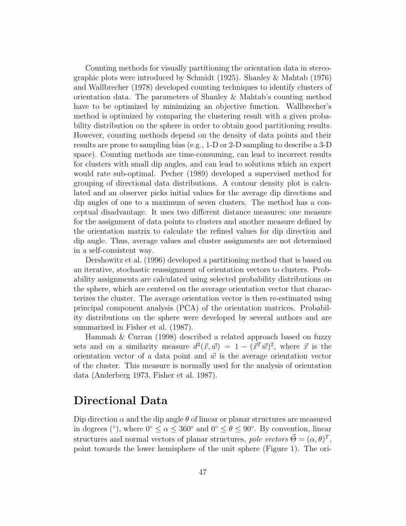
structures and normal vectors of planar structures, pole vectors ~Θ = (α, θ)T ,point towards the lower hemisphere of the unit sphere (Figure 1). The ori-
47
entation ~ΘA = (αA, θA)T of a pole vector A can be described by Cartesiancoordinates ~xA = (x1, x2, x3)
T (Figure 1), where
x1 = cos(α) cos(θ) North direction
x2 = sin(α) cos(θ) East direction
x3 = sin(θ) downward.
(12)
The projection A′ of the endpoint A of all given pole vectors onto thex1-x2 plane is called a stereographic plot (Figure 1) and is commonly usedfor visualisation purposes.
A) B)
North
Figure 1: A) Construction of a stereographic plot.B) Stereographic plot with kernel density distribution.
The Clustering Method
Given are a set of N pole vectors ~xk, k = 1, . . . , N, (eq. 12). The vectors cor-respond to N noisy measurements taken from M orientation discontinuitieswhose spatial orientations are described by their (yet unknown) average polevectors ~wl, l = 1, . . . ,M . For every partition l of the orientation data, thereexists one average pole vector ~wl. The dissimilarity between a data point ~xk
and an average pole vector ~wl is denoted by d(~xk, ~wl).We now describe the assignment of pole vectors ~xk to a partition by the
binary assignment variables
mlk =
{
1, if data point k belongs to cluster l0, otherwise.
(13)
One data point ~xk belongs to only one orientation discontinuity ~wl. Here,the arc-length between the pole vectors on the unit sphere is proposed as the
48
distance measure, i.e.
d(~x, ~w) = arccos ( | ~xT ~w | ), (14)
where |.| denotes the absolute value.The average dissimilarity between the data points and the pole vectors
of the directional data they belong to is given by
E =1
N
N∑
k=1
M∑
l=1
mlk d(~xk, ~wl), (15)
from which we calculate the optimal partition by minimizing the cost functionE, i.e.
E!= min
{mlk},{~wl}. (16)
Minimization is performed iteratively in two steps. In the first step, thecost function E is minimized with respect to the assignment variables {mlk}using
mlk =
{
1, if l = argminq d(~xk, ~wq)0, else.
(17)
In the second step, cost E is minimized with respect to the angles ~Θl =(αl, θl)
T which describe the average pole vectors ~wl (see eq. (12)). This isdone by evaluating the expression
∂E
∂~Θl
= ~0, (18)
where ~0 is a zero vector with respect to ~Θ1 = (αl, θl)T . This iterative proce-
dure is called batch learning and converges to a minimum of the cost, becauseE can never increase and is bounded from below. In most cases, however,a stochastic learning procedure called on-line learning is used which is morerobust:
BEGIN LoopSelect a data point ~xk.Assign data point ~xk to cluster l by:
l = argminq
d(~xk, ~wq) (19)
Change the average pole vector of this cluster by:
∆~Θl = −γ∂d(~xk , ~wl(~Θl))
∂~Θl
(20)
END Loop
49
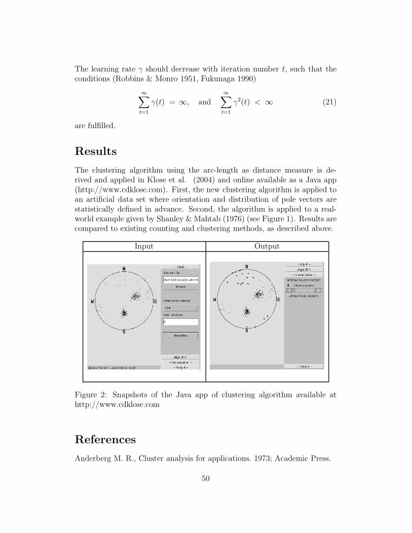
The learning rate γ should decrease with iteration number t, such that theconditions (Robbins & Monro 1951, Fukunaga 1990)
∞∑
t=1
γ(t) = ∞, and
∞∑
t=1
γ2(t) < ∞ (21)
are fulfilled.
Results
The clustering algorithm using the arc-length as distance measure is de-rived and applied in Klose et al. (2004) and online available as a Java app(http://www.cdklose.com). First, the new clustering algorithm is applied toan artificial data set where orientation and distribution of pole vectors arestatistically defined in advance. Second, the algorithm is applied to a real-world example given by Shanley & Mahtab (1976) (see Figure 1). Results arecompared to existing counting and clustering methods, as described above.
Input Output
Figure 2: Snapshots of the Java app of clustering algorithm available athttp://www.cdklose.com
References
Anderberg M. R., Cluster analysis for applications. 1973; Academic Press.
50
Dershowitz W. Busse R. Geier J. and Uchida M., A stochastic approach forfracture set definition, In: Aubertin M. Hassani F. and Mitri H., eds.,Proc., 2nd NARMS, Rock Mechanics Tools and Techniques, Montreal.1996; 1809-1813.
Fisher, N. I. Lewis, T. and Embleton B. J., Statistical analysis of sphericaldata. 1987; Cambridge University Press.
Fukunaga K., Introduction to statistical pattern recognition. 1990; AcademicPress.
Gray R.M., Vector Quantization, IEEE ASSP. 1984; 1 (2): 4-29.
Hammah R. E. and Curran J. H., Fuzzy cluster algorithm for the automaticdelineation of joint sets, Int. J. Rock Mech. Min. Sci. 1998; 35 (7): 889-905.
Klose R.M., A New Clustering Approach for Partiontioning Directional Data,IJRMMS. 2004; (42): 315-321.
Pecher A., SchmidtMac - A program to display and analyze directionaldata, Computers & Geosciences. 1989; 15 (8): 1315-1326.
Robbins H. and Monro S., A stochastic approximation method, Ann. Math.Stat. 1951; 22: 400-407.
Schmidt W., Gefugestatistik, Tschermaks Mineral. Petrol. Mitt. 1925; 38:392-423.
Shanley R. J. and Mahtab M. A., Delineation and analysis of clusters inorientation data, Mathematical Geology. 1976; 8 (1): 9-23.
Wallbrecher E., Ein Cluster-Verfahren zur richungsstatistischen Analyse tek-tonischer Daten, Geologische Rundschau. 1978; 67 (3): 840-857.
51
Planetary Detection: The Kepler Mission
Jon JenkinsNASA/Ames Research CenterMoffett Field, California, USA
The Kepler telescope was launched into orbit in March 2009 to determinethe frequency of Earth-sized planets transiting their Sun-like host stars inthe habitable zone – that range of orbital distances for which liquid waterwould pool on the surface of a terrestrial planet such as Earth or Mars. Thisdaunting task demands an instrument capable of measuring the light outputfrom each of over 150,000 stars over a 115 square degree field of view simul-taneously at an unprecedented photometric precision of 20 parts per million(ppm) on 6.5-hour intervals. Kepler is opening up a new vista in astronomyand astrophysics and is operating in a new regime where the instrumentalsignatures compete with the miniscule signatures of terrestrial planets tran-siting their host stars. The dynamic range of the intrinsic stellar variabilityobserved in the light curves is breathtaking: RR Lyrae stars explosively os-cillate with periods of approximately 0.5 days, doubling their brightness overa few hours. Some flare stars double their brightness on much shorter timescales at unpredictable intervals. At the same time, some stars exhibit quasi-coherent oscillations with amplitudes of 50 ppm that can be seen by eye inthe raw flux time series. The richness of Kepler’s data lies in the huge dy-namic range for the variations in intensity >104 and the large dynamic rangeof time scales probed by the data, from a few minutes to weeks, months, andultimately, to years.
Kepler is an audacious mission that places rigorous demands on the sci-ence pipeline used to process the ever-accumulating, large amount of dataand to identify and characterize the minute planetary signatures hiding inthe data haystack. We give an overview of the Science pipeline that reducesthe pixel data to obtain flux time series and detect and characterize planetarytransit signatures. In particular, we detail the adaptive, wavelet-based tran-sit detector that performs the automated search through each light curve fortransit signatures of Earth-sized planets. We describe a Bayesian MaximumA Posteriori (MAP) estimation approach under development to improve ourability to identify and remove instrumental signatures from the light curvesthat minimizes any distortion of astrophysical signals in the data and pre-vents the introduction of additional noise that may mask small, transit fea-tures, as indicated in the Figure 1. This approach leverages the availabilityof thousands of stellar targets on each CCD detector in order to construct
52
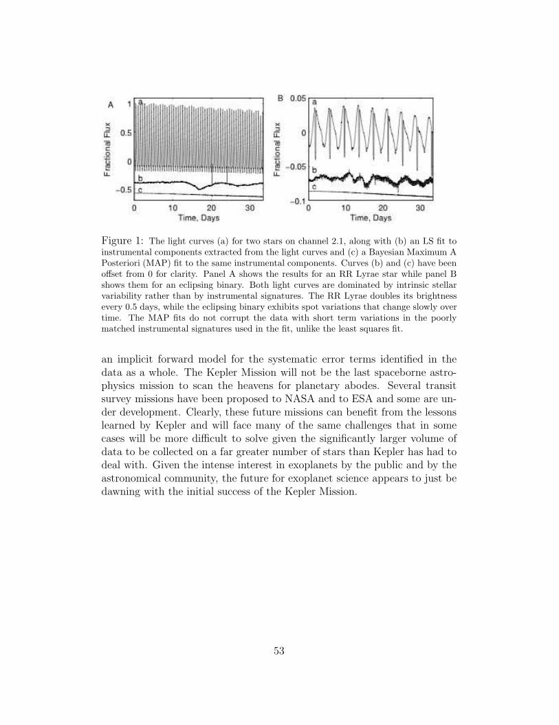
Figure 1: The light curves (a) for two stars on channel 2.1, along with (b) an LS fit toinstrumental components extracted from the light curves and (c) a Bayesian Maximum APosteriori (MAP) fit to the same instrumental components. Curves (b) and (c) have beenoffset from 0 for clarity. Panel A shows the results for an RR Lyrae star while panel Bshows them for an eclipsing binary. Both light curves are dominated by intrinsic stellarvariability rather than by instrumental signatures. The RR Lyrae doubles its brightnessevery 0.5 days, while the eclipsing binary exhibits spot variations that change slowly overtime. The MAP fits do not corrupt the data with short term variations in the poorlymatched instrumental signatures used in the fit, unlike the least squares fit.
an implicit forward model for the systematic error terms identified in thedata as a whole. The Kepler Mission will not be the last spaceborne astro-physics mission to scan the heavens for planetary abodes. Several transitsurvey missions have been proposed to NASA and to ESA and some are un-der development. Clearly, these future missions can benefit from the lessonslearned by Kepler and will face many of the same challenges that in somecases will be more difficult to solve given the significantly larger volume ofdata to be collected on a far greater number of stars than Kepler has had todeal with. Given the intense interest in exoplanets by the public and by theastronomical community, the future for exoplanet science appears to just bedawning with the initial success of the Kepler Mission.
53
Understanding the possible influence of thesolar activity on the terrestrial climate: a
times series analysis approach
Elizabeth Martınez-GomezCenter for Astrostatistics326 Thomas BuildingThe Pennsylvania State UniversityUniversity Park, PA, USA
Vıctor M. GuerreroDepartmento de EstadısticaInstituto Tecnologico Autonomo de Mexico01080, Alvaro Obregon, Mexico
Francisco EstradaCentro de Ciencias de la AtmosferaUniversidad Nacional Autonoma de MexicoCiudad Universitaria, 04510, Coyoacan, Mexico
Abstract
Until the beginning of the 1980s, the relation between the Sun and climatechange was still viewed with suspicion by the wider climate community andoften remained a “taboo” subject in the solar astrophysics community. Themain reason for this fact was a lack of knowledge about the causal link be-tween the solar activity and its irradiance, that is, the amount of energyreceived at the average distance between the Earth and the Sun. For manyyears, some authors doubted about the invariability of the solar radiativeoutput due to the apparent, but poorly explained, correlations between fluc-tuations of solar activity and atmospheric phenomena. Research on the mech-anisms of solar effects on climate and their magnitude is currently benefitingfrom tremendous renewal of interest. A large amount of high resolution datais now available; however, the matter remains controversial because most ofthese records are influenced by other factors in addition to solar activity.In many works, the association between solar and terrestrial environmentalparameters is found through some type of correlation based on multivariate
54
statistics or applying the wavelet analysis on the corresponding time seriesdata. The talk is divided in three parts. In the first I will review the solar-terrestrial climate problem. Later, I will focus on the time series analysisused in our study and finally, I will summarize our preliminary findings andcomment further ideas to improve our model.
Review of the solar terrestrial problem
It is well-known that the Sun has an effect on terrestrial climate since its elec-tromagnetic radiation is the main energy for the outer envelopes of Earth.This is one of the so called solar-terrestrial physics problems. This problemhas been the subject of speculation and research by scientists for many years.Understanding the behavior of natural fluctuations in the climate is especiallyimportant because of the possibility of man-induced climate changes (Din-gel & Landberg 1971, Schneider 1979, Tett et al. 1999). Many studies havebeen conducted to show correlations between the solar activity and variousmeteorological parameters but historical observations of solar activity wererestricted to sunspot numbers and it was not clear how these could be phys-ically related to meteorological factors. In this section we briefly describesome of the most remarkable characteristics of the solar activity and theterrestrial climate, emphasizing their possible connection.
a) Solar Activity The term solar activity comprises photospheric and chro-mospheric phenomena such as sunspots, prominences and coronal dis-turbances. It has been measured via satellites during recent decades(for the Total Solar Irradiance, TSI) and through other “proxy” vari-ables in prior times (for example, the daily observed number of sunspots,and the concentration of some cosmogenic isotopes in ice cores as 14Cand 10Be).
The phenomena mentioned above are related to the variations of thesolar magnetic field and the amount of received energy. Those arecyclic variations like the 11-year (sunspots), and 22-year (magneticfield reversion), among others.
b) Terrestrial climate The Intergovernmental Panel on Climate Change(IPCC) glossary defines the climate as the “average weather,” or morerigorously, as the statistical description in terms of the mean and vari-ability of relevant quantities (for example, temperature, precipitation,and wind) over a period of time ranging from months to thousands ormillions of years.
55
Table 1: Description of the time series for the variables associated to thesolar activity and the terrestrial climate.
Description Variable Timescale Stationarity Available periodPeriod
of Study
SolarActivity
Number of sunspots(SP)
dailymonthlyyearly
No 1700–20081700–1985
Total Solar Irradia-tion (TSI)
yearly No
1750–1978 (recon-structed time seriesby Lean et al.(1995) 1978–2008(satellites)
10BE concentrationin ice cores
geological No 1424–1985
Terrestrialclimate
Global temperaturein both hemispheres(TN, TS)
monthlyBreakpoint(1977)
Jan 1850–May 2009Jan 1950 –May2008Mulivariate ENSO
Index (MEI)monthly
Breakpoint(1977)
Jan 1950–June2009
North Atlantic Oscil-lation(NAO)
monthly Yes Jul 1821–May 2008
Pacific Decadal Oscil-lation(PDO)
monthlyBreakpoints(1977,1990)
Jan 1900–Jan 2009
c) Is there a connection between solar activity & terrestrial climate?There are several hypotheses for how solar variations may affect Earth.Some variations, such as changes in Earth’s orbit (Milankovitch cycles)are only of interest in astronomy. The correlation between cosmic rayfluxes and clouds (Laken et al. 2010), as well as, the correlation betweenthe number of sunspots and changes in the wind patterns (Willett 1949)have also been reported. Studies about the solar and climate relation-ship have not been conclusive since the actual changes are not enoughto account for the majority of the warming observed in the atmosphereover the last half of the 20th century.
Multivariate Time Series Analysis: VARmethod-
ology
A common assumption in many time series techniques (e.g. VAR methodol-ogy) is that the data are stationary. A stationary process has the propertythat the mean, variance and autocorrelation structure do not change overtime (in other words, a flat looking series without trend, constant varianceover time, a constant autocorrelation structure over time and no periodicfluctuations). If the time series, Yt, is not stationary, we can often transform
56
it with one of the following techniques: 1) apply a Box-Cox transformation(logarithm is the simplest), and/or 2) differentiate the data Yt to create anew series Xt (Xt = ∇Yt = Yt–Yt−1 ; Xt =∇2Yt = Yt – 2Yt−1 + Yt−2).
VAR methodology: description
The Vector AutoRegression (VAR) model is one of the most successful, flex-ible, and easy to use models for the analysis of multivariate time series. It isa natural extension of the univariate autoregressive model to dynamic mul-tivariate time series (Sims 1972; 1980; 1982). It describes the evolution of aset of k variables (called endogenous variables) over the same sample period(t = 1, ..., T) as a linear function of only their past evolution:
yt = c+ α1yt−1 + α2yt−2 + ...+ αpyt−p + ǫt (22)
where c is a k × 1 vector of constants (intercept) , αi is a k × k matrix (forevery i=1,.., p), p is the number of lags (that is, the number of periods back),and ǫt is a k×1 vector of error terms. There are some additional assumptionsabout the error terms: 1) the expected value is zero, that is, E[ǫit]=0 witht=1,..., T, and 2) the errors are not autocorrelated, E[ǫit ǫjt]=0 with t 6= τ .
The determination of the number of lags p is a trade-off between thedimensionality and abbreviate models. To find the optimal lag length wecan apply a Log-Likelihood Ratio test (LR) test or an information criterion(Lutkepohl 1993).
Once the estimation of the parameters in the VAR(p) model shown in Eq.(1) through Ordinary Least Squares (OLS), we need to interpret the dynamicrelationship between the indicated variables using the Granger causality.
Application of the VAR methodology to model the solaractivity and terrestrial climate connection
Our purpose is to investigate the relationship between the solar activity andthe major climate phenomena by means of time series analysis. The dataare taken from the National Geophysical Data Center (NGDC) and the Na-tional Climatic Data Center (NCDC). In Table 1 we summarize the selectedvariables for each physical system.
a) VAR model for the solar-terrestrial climate connection We esti-mate a VAR(p) model using the variables shown in Table 1 where thenon-stationary time series have been differentiated once. The exoge-nous variables are: a) number of sunspots, b) TSI, c) d76 (dummy vari-able for 1976), d) d77 (dummy variable for 1977) and e) d90 (dummyvariable for 1990).
57
Table 2: Description of the time series for the variables associated to thesolar activity and the terrestrial climate.VAR(p)characteristic
ModelSolar-terrestrial climateconnection
Solar activity
Lag length (p) 4 8
Significance of the coef-ficients
All (except equation forNAO)
All
Stability Yes Yes
Homoskedasticity of theresiduals
No No
Normality of the residu-als
Yes (except equation forTN)
No
Granger causalityTSI does not affect MEI,NAO and PDO
10BE does not affectSP and TSI
The optimal lag length is 4 and the VAR(4) is formed by 5 equations(TN, TS, MEI, NAO, and PDO). The statistical validation is shown inTable 2.
b) VAR model for the solar activity We estimate a VAR(p) model us-ing the variables shown in Table 1 where the non-stationary time serieshave been differentiated once.
The optimal lag length is 8 and the VAR(8) is formed by 3 equations(SP, TSI, and 10BE). The statistical validation is shown in Table 2.
Summary and ideas for future work
The possible relation between the solar activity and the terrestrial climatehas been addressed in many works. Most of them search for periodicities orcorrelations among the set of variables that characterize the solar activity andthe main climate parameters. For example, the “wavelet analysis” cannotbe the most adequate to analyze multivariate time series. In this work wehave proposed and estimated a VAR model to explain such a connection.For this model we have analyzed the time series for the most remarkablecharacteristics of both the solar activity and climate. Our main results andsome ideas for future work are listed below.
58
• The solar activity is modeled by a VAR(8) in which we find that the10Be concentration does not play a fundamental role.
• The solar activity and terrestrial climate connection is modeled by aVAR(4) where the solar variables are taken as exogenous. It seems thatthe sun (described only for the number of sunspots and the TSI) has aweak connection to Earth, at least for the major climate phenomena.
• It is convenient to include a term related to the cloudiness to verify theprevious findings.
• Analyzing certain cycles in the solar activity could help us to determinethe epochs in which the connection with the terrestrial climate wasstronger.
• We need to search for other proxy variables that describe the solar ac-tivity and introduce variables related to regional climate (for example:precipitation, pressure, local temperature).
Acknowledgements
E. Martınez-Gomez thanks to the Faculty For The Future Program andCONACyT-Mexico postdoctoral fellowship for their financial support to thisresearch. V. M. Guerrero acknowledges support from Asociacion Mexicanade Cultura, A. C.
References
Dingle, A. N. & H. E. Landsberg 1971, Science, 173(3995), 461-462.
Laken, B. A., D. R. Kniveton and M. R. Frogley 2010, Atmos. Chem. Phys.,10, 1094110948.
Lean, J., J. Beer and R. Bradley (1995), Geophys. Res. Lett., 22(23), 3195-3198.
Lutkepohl, H. 1993, Introduction to multiple time series analysis, SpringerVerlag, Germany.
Schneider, S. H. (1979), The effect of mans activities on climatic changes inEvolution of Planetary and Climatology of the Earth. Proceedings of theInternational Conference, Nice, France, 16-20 October 1978, pp. 527.
59

Sims, C. A. 1972, American Economic Review 62, 540-552.
Sims, C. A. 1980, Econometrica 48, 1-48.
Sims, C. A. 1982, Brooking Papers on Economic Activity 1, 107-152.
Tett, F. B. S., P. A. Stott, M. R. Allen, W. J. Ingram & J. F. B. Mitchell1999, Nature, 399, 569-572.
Willett, H. C. 1949, J. Atm. Sciences, 6(1), 34-50.
60
Optimal Scheduling of ExoplanetObservations Using Bayesian Adaptive
Exploration
Thomas J. LoredoDepartment of AstronomyCornell UniversityCornell, New York, USA
This presentation describes ongoing work by a collaboration of astronomersand statisticians developing a suite of Bayesian tools for analysis and adaptivescheduling of exoplanet host star reflex motion observations. In this presen-tation I focus on the most unique aspect of our work: adaptive schedulingof observations using the principles of Bayesian experimental design in a se-quential data analysis setting. I introduce the core ideas and highlight someof the computational challenges that arise when implementing Bayesian de-sign with nonlinear models. Specializing to parameter estimation cases (e.g.,measuring the orbit of planet known to be present), there is an importantsimplification that enables relatively straightforward calculation of greedydesigns via maximum entropy (MaxEnt) sampling. We implement MaxEntsampling using population-based MCMC to provide samples used in a nestedMonte Carlo integration algorithm. I demonstrate the approach with a toyproblem, and with a re-analysis of existing exoplanet data supplemented bysimulated optimal data points.
Bayesian adaptive exploration (BAE) proceeds by iterating a three-stagecycle: Observation–Inference–Design. Figure 1 depicts the flow of informa-tion through one such cycle. In the observation stage, new data are obtainedbased on an observing strategy produced by the previous cycle of explo-ration. The inference stage synthesizes the information provided by previousand new observations to produce interim results such as signal detections,parameter estimates, or object classifications. In the design stage the interiminferences are used to predict future data for a variety of possible observingstrategies; the strategy that offers the greatest expected improvement in in-ferences, quantified with information-theoretic measures, is passed on to thenext Observation–Inference–Design cycle.
Figures 2 and 3 show highlights of application of BAE to radial velocity(RV) observations of the single-planet system HD 222582. Vogt et al. (2000)reported 24 observations obtained over a 683 d time span with instrumen-tation at the Keck observatory; Butler et al. (2006) reported 13 subsequent
61
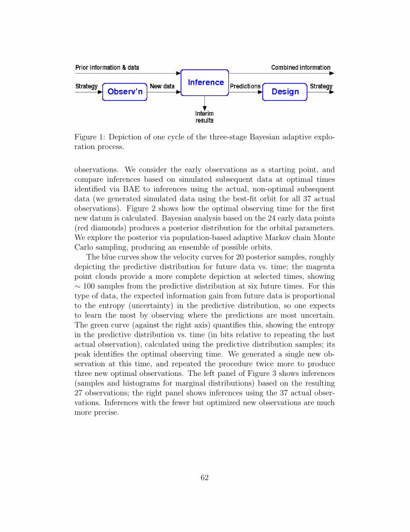
Figure 1: Depiction of one cycle of the three-stage Bayesian adaptive explo-ration process.
observations. We consider the early observations as a starting point, andcompare inferences based on simulated subsequent data at optimal timesidentified via BAE to inferences using the actual, non-optimal subsequentdata (we generated simulated data using the best-fit orbit for all 37 actualobservations). Figure 2 shows how the optimal observing time for the firstnew datum is calculated. Bayesian analysis based on the 24 early data points(red diamonds) produces a posterior distribution for the orbital parameters.We explore the posterior via population-based adaptive Markov chain MonteCarlo sampling, producing an ensemble of possible orbits.
The blue curves show the velocity curves for 20 posterior samples, roughlydepicting the predictive distribution for future data vs. time; the magentapoint clouds provide a more complete depiction at selected times, showing∼ 100 samples from the predictive distribution at six future times. For thistype of data, the expected information gain from future data is proportionalto the entropy (uncertainty) in the predictive distribution, so one expectsto learn the most by observing where the predictions are most uncertain.The green curve (against the right axis) quantifies this, showing the entropyin the predictive distribution vs. time (in bits relative to repeating the lastactual observation), calculated using the predictive distribution samples; itspeak identifies the optimal observing time. We generated a single new ob-servation at this time, and repeated the procedure twice more to producethree new optimal observations. The left panel of Figure 3 shows inferences(samples and histograms for marginal distributions) based on the resulting27 observations; the right panel shows inferences using the 37 actual obser-vations. Inferences with the fewer but optimized new observations are muchmore precise.
62
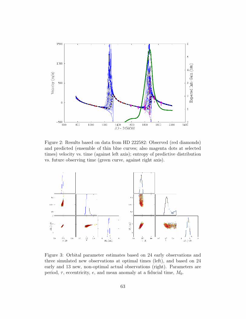
Figure 2: Results based on data from HD 222582: Observed (red diamonds)and predicted (ensemble of thin blue curves; also magenta dots at selectedtimes) velocity vs. time (against left axis); entropy of predictive distributionvs. future observing time (green curve, against right axis).
Figure 3: Orbital parameter estimates based on 24 early observations andthree simulated new observations at optimal times (left), and based on 24early and 13 new, non-optimal actual observations (right). Parameters areperiod, τ , eccentricity, e, and mean anomaly at a fiducial time, M0.
63

References
Vogt, S.S., Marcy, G.W., Butler, R.P. & Apps, K. 2000, Six New Planetsfrom the Keck Precision Velocity Survey, Astrophysical Journal, 536, 902
Butler, R. P., Wright, J. T., Marcy, G. W., Fischer, D. A., Vogt, S. S., Tinney,C. G., Jones, H. R. A., Carter, B. D., Johnson, J. A., McCarthy, C. &Penny, A. J. 2006, Catalog of Nearby Exoplanets, Astrophysical Journal,646, 505
64
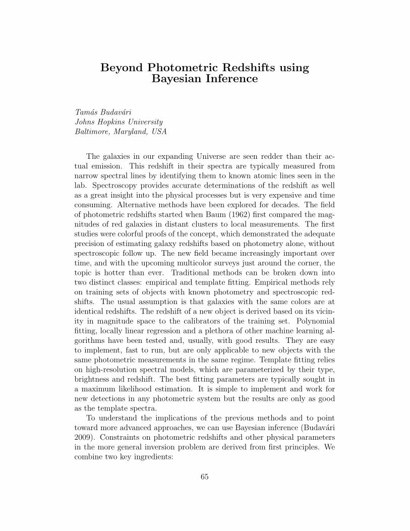
Beyond Photometric Redshifts usingBayesian Inference
Tamas BudavariJohns Hopkins UniversityBaltimore, Maryland, USA
The galaxies in our expanding Universe are seen redder than their ac-tual emission. This redshift in their spectra are typically measured fromnarrow spectral lines by identifying them to known atomic lines seen in thelab. Spectroscopy provides accurate determinations of the redshift as wellas a great insight into the physical processes but is very expensive and timeconsuming. Alternative methods have been explored for decades. The fieldof photometric redshifts started when Baum (1962) first compared the mag-nitudes of red galaxies in distant clusters to local measurements. The firststudies were colorful proofs of the concept, which demonstrated the adequateprecision of estimating galaxy redshifts based on photometry alone, withoutspectroscopic follow up. The new field became increasingly important overtime, and with the upcoming multicolor surveys just around the corner, thetopic is hotter than ever. Traditional methods can be broken down intotwo distinct classes: empirical and template fitting. Empirical methods relyon training sets of objects with known photometry and spectroscopic red-shifts. The usual assumption is that galaxies with the same colors are atidentical redshifts. The redshift of a new object is derived based on its vicin-ity in magnitude space to the calibrators of the training set. Polynomialfitting, locally linear regression and a plethora of other machine learning al-gorithms have been tested and, usually, with good results. They are easyto implement, fast to run, but are only applicable to new objects with thesame photometric measurements in the same regime. Template fitting relieson high-resolution spectral models, which are parameterized by their type,brightness and redshift. The best fitting parameters are typically sought ina maximum likelihood estimation. It is simple to implement and work fornew detections in any photometric system but the results are only as goodas the template spectra.
To understand the implications of the previous methods and to pointtoward more advanced approaches, we can use Bayesian inference (Budavari2009). Constraints on photometric redshifts and other physical parametersin the more general inversion problem are derived from first principles. Wecombine two key ingredients:
65
Figure 1: The presented slide illustrates the minimalist model to incorporatethe photometric uncertainties of the new galaxy. Using KDE the relation isestimated (blue dotted line), which is averaged with the uncertainty for thefinal result (red solid line).
(1) Relation to physics — The redshift (z) is not simply a function ofthe observables. Considering that they cannot possibly capture all the in-formation, one expects a spread. Regression is only a good model, when thewidth is very narrow. Otherwise one should estimate the conditional densityof p(z|m). While not easy in practice, this is conceptually straightforward todo on a given set of calibrators.
(2) Mapping of the observables — If we would like to perform the esti-mation of a new object with colors in a separate photometric system, its m′
magnitudes need to be mapped on to the passbands of the training set (m).This might be as simple as an empirical conversion formula or as sophisti-cated as spectral synthesis. In general, a model is needed, which can alsopropagate the uncertainties, p(m|m′). The final density is the convolution ofthese two functions.
After 50 years of pragmatism, photometric redshift estimation is nowplaced on a firm statistical foundation. We can put the traditional methodsin context; they are special cases of a unified framework. Their conceptualweaknesses become visible from this aspect. The new approach points ustoward more advanced methods that combine the advantages of the earliertechniques. In addition we can formally learn about selecting calibration sets
66

for specific studies. These advancements are going to be vital for analyzingthe observations of the next-generation survey telescopes.
67
Long-Range Climate Forecasts Using DataClustering and Information Theory
Dimitris GiannakisNew York UniversityNew York, New York, USA
Even though forecasting the weather beyond about two weeks is not pos-sible, certain climate processes (involving, e.g., the large-scale circulation inthe Earth’s oceans) are predictable up to a decade in advance. These so-called climate regimes can influence regions as large as the West Coast ofNorth America over several years, and therefore developing models to pre-dict them is a problem of wide practical impact. An additional central issueis to quantify objectively the errors and biases that are invariably associatedwith these models.
In classical studies on decadal prediction (Boer 2000; 2004, Collins 2002),ensemble experiments are performed using one or more climate models ini-tialized by perturbed initial conditions relative to a reference state, and pre-dictive skill is measured by comparing the root mean square difference ofensemble trajectories to its equilibrium value. However, skill metrics of thistype have the drawback of not being invariant under invertible transforma-tions of the prediction variables, and not taking into account the importantissue of model error. Further challenges concern the choice of initial con-ditions of the ensemble members (Hurrell et al. 2009, Meehl et al. 2009,Solomon et al. 2009).
In this talk, we present recent work (Giannakis and Majda 2011a;b) onmethods based on data clustering and information theory to build and assessprobabilistic models for long-range climate forecasts that address several ofthe above issues. The fundamental perspective adopted here is that predic-tions in climate models correspond to transfer of information; specificallytransfer of information between the initial conditions (which in general arenot known completely) and the state of the climate system at some futuretime. This opens up the possibility of using the mathematical framework ofinformation theory to characterize both dynamical prediction skill and modelerror with metrics that are invariant under invertible nonlinear transforma-tions of observables (Kleeman 2002, Roulston and Smith 2002, Majda et al.2002; 2005, DelSole and Tippet 2007, Majda and Gershgorin 2010).
The key points of our discussion are that (i) the long-range predictive skillof climate models can be revealed through a suitable coarse-grained partition
68
of the set of initial data available to a model (which are generally incomplete);(ii) long-range predictive skill with imperfect models depends simultaneouslyon the fidelity of these models at asymptotic times, their fidelity during dy-namical relaxation to equilibrium, and the discrepancy from equilibrium offorecast probabilities at finite lead times. Here, the coarse-grained partitionof the initial data is constructed by data-clustering equilibrium realizationsof ergodic dynamical systems without having to carry out ensemble initial-izations. Moreover, prediction probabilities conditioned on the clusters canbe evaluated empirically without having to invoke additional assumptions(e.g., Gaussianity), since detailed initial conditions are not needed to samplethese distributions.
In this framework, predictive skill corresponds to the additional infor-mation content beyond equilibrium of the cluster-conditional distributions.The natural information-theoretic functional to measure this additional in-formation is relative entropy, which induces a notion of distance between thecluster-conditional and equilibrium distributions. A related analysis leadsto measures of model error that correspond to the lack of information (orignorance) of an imperfect model relative to the true model. The techniquesdeveloped here have potential applications across several disciplines involvingdynamical system predictions.
As a concrete application of our approach, we study long-range pre-dictability in the equivalent barotropic, double-gyre model of McCalpin andHaidvogel (1996) (frequently called the “1.5-layer model”). This simplemodel of ocean circulation has non-trivial low-frequency dynamics, charac-terized by infrequent transitions between meandering, moderate-energy, andextensional configurations of the eastward jet (analogous to the Gulf Streamin the North Atlantic). The algorithm employed here for phase-space parti-tioning involves building a multi-time family of clusters, computed for differ-ent temporal intervals of coarse graining; a recipe similar to kernel densityestimation methods. We demonstrate that knowledge of cluster affiliation inthe computed partitions carries significant information beyond equilibriumabout the total energy and the leading two principal components (PCs) ofthe streamfunction (which are natural variables for the low-frequency dy-namics of this system) for five- to seven-year forecast lead times, i.e., for atimescale about a factor of five longer than the maximum decorrelation timeof the PCs.
As an application involving imperfect models, we discuss the error inMarkov models of the switching process between the ocean circulation regimes.Imposing Markovianity on the transition process is a familiar approximationin this context (Franzke et al. 2008; 2009), though the validity of this as-sumption typically remains moot. Our analysis exposes starkly the falseness
69
of predictive skill that one might attribute to a Markovian description of theregime transitions in the 1.5-layer model model by relying on an (internal)assessment based solely on the deviation of the time-dependent predictionprobabilities of the Markov model from its biased equilibrium. In particular,we find that a Markov model associated with a seven-state partition appearsto outperform a three-state model, both in its discriminating power and itspersistence (measured respectively by the deviation from equilibrium andrate of approach to equilibrium), when actually the skill of the seven-statemodel is false because its equilibrium statistics are biased. Here, the mainconclusion is that evaluating simultaneously model errors in both the cli-matology and the dynamical relaxation to equilibrium should be an integralpart of assessments of long-range forecasting skill.
Acknowledgment The material presented in this talk is joint work with An-drew Majda of New York University. This research is partially supportedby NSF grant DMS-0456713, from ONR DRI grants N25-74200-F6607 andN00014-10-1-0554, and from DARPA grants N00014-07-10750 and N00014-08-1-1080.
References
G. J. Boer. A study of atmosphere-ocean predictability on long time scales.Climate Dyn., 16(6):469–477, 2000. doi: 10.1007/s003820050340.
G. J. Boer. Long time-scale potential predictability in an ensemble of coupledclimate models. Climate Dyn., 23(1):29–44, 2004. doi: 10.1007/s00382-004-0419-8.
M. Collins. Climate predictability on interannual to decadal time scales:The initial value problem. Climate Dyn., 19:671–692, 2002. doi:10.1007/s00382-002-0254-8.
T. DelSole and M. K. Tippet. Predictability: Recent insights from informa-tion theory. Rev. Geophys., 45:RG4002, 2007. doi: 10.1029/2006rg000202.
C. Franzke, D. Crommelin, A. Fischer, and A. J. Majda. A hidden Markovmodel perspective on regimes and metastability in atmospheric flows. J.Climate, 21(8):1740–1757, 2008. doi: 10.1175/2007jcli1751.1.
C. Franzke, I. Horenko, A. J. Majda, and R. Klein. Systematic metastableregime identification in an AGCM. J. Atmos. Sci., 66(9):1997–2012, 2009.doi: 10.1175/2009jas2939.1.
70
D. Giannakis and A. J. Majda. Quantifying the predictive skill in long-rangeforecasting. Part I: Coarse-grained predictions in a simple ocean model. J.Climate, 2011a. submitted.
D. Giannakis and A. J. Majda. Quantifying the predictive skill in long-rangeforecasting. Part II: Model error in coarse-grained Markov models withapplication to ocean-circulation regimes. J. Climate, 2011b. submitted.
J. W. Hurrell et al. Decadal climate prediction: Opportunities and challenges.In Proceedings of the OceanObs09 Conference: Sustained Ocean Observa-tions and Information for Society, pages 21–25, Venice, Italy, 2009.
R. Kleeman. Measuring dynamical prediction utility using relative entropy.J. Atmos. Sci., 59(13):2057–2072, 2002.
A. J. Majda and B. Gershgorin. Quantifying uncertainty in climage changescience through empirical information theory. Proc. Natl. Acad. Sci., 107(34):14958–14963, 2010. doi: 10.1073/pnas.1007009107.
A. J. Majda, R. Kleeman, and D. Cai. A mathematical framework for pre-dictability through relative entropy. Methods Appl. Anal., 9(3):425–444,2002.
A. J. Majda, R. V. Abramov, and M. J. Grote. Information Theory andStochastics for Multiscale Nonlinear Systems, volume 25 of CRM Mono-graph Series. Americal Mathematical Society, Providence, 2005.
J. D. McCalpin and D. B. Haidvogel. Phenomenology of the low-frequencyvariability in a reduced-gravity quasigeostrophic double-gyre model. J.Phys. Oceanogr., 26(5):739–752, 1996.
G. A. Meehl et al. Decadal prediction. can it be skillful? Bull. Amer. Meteor.Soc., 90(10):1467–1485, 2009. doi: 10.1175/2009bams2778.1.
M.S. Roulston and L.A. Smith. Evaluating probabilistic forecasts using in-formation theory. Mon. Weather Rev., 130(6):1653–1660, 2002.
A. Solomon et al. Distinguishing the roles of natural and anthropogenicallyforced decadal climate variability: Implications for prediction. Bull. Amer.Meteor. Soc., 2009. Submitted.
71
Comparison of Information-TheoreticMethods to estimate the information flow in
a dynamical system
Deniz GencagaNOAA CrestNew York, New York, USA
Abstract
In order to quantify the amount of information about a variable, or to quan-tify the information shared between two variables, we utilize information-theoretic quantities like entropy and mutual information (MI), respectively.If these variables constitute a coupled, dynamical system, they share the in-formation along a direction, i.e. we have an information flow in time. In thiscase, the direction of the information flow also needs to be estimated. How-ever, MI does not provide directionality. Transfer entropy (TE) has beenproposed in the literature to estimate the direction of information flow inaddition to its magnitude. Here, our goal is to estimate the transfer entropyfrom observed data accurately. For this purpose, we compare most frequentlyused methods in the literature and propose our own technique. Unfortu-nately, every method has its own free tuning parameter(s) so that there isnot a consensus on an optimal way of estimating TE from a dataset. In thiswork, we compare several methods along with a method that we propose, ona Lorenz model. Here, our goal is to develop the required appropriate andreliable mathematical tool synthesizing from all of these disjoint methodsused in fields ranging from biomedicine to telecommunications and apply theresulting technique on tropical data sets to better understand events such asthe Madden Julian Oscillation in the future.
Introduction and problem statement
Nonlinear coupling between complex dynamical systems is very common inmany fields (Wallace et al. 2006, Gourvitch & Eggermont 2007). In orderto study the relationships between such coupled subsystems, we must utilizehigher-order statistics. Thus, using linear techniques based on correlation
72
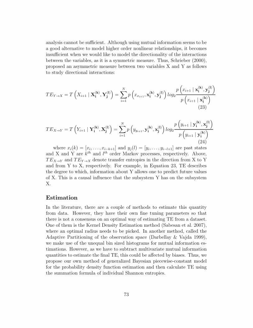
analysis cannot be sufficient. Although using mutual information seems to bea good alternative to model higher order nonlinear relationships, it becomesinsufficient when we would like to model the directionality of the interactionsbetween the variables, as it is a symmetric measure. Thus, Schrieber (2000),proposed an asymmetric measure between two variables X and Y as followsto study directional interactions:
TEY→X = T(
Xi+1 | X(k)i ,Y
(l)j
)
=N∑
i=1
p(
xxi+1,x
(k)i ,y
(l)j
)
log2p(
xi+1 | x(k)i ,y
(l)j
)
p(
xi+1 | x(k)i
)
(23)
TEX→Y = T(
Yi+1 | Y(k)i ,X
(l)j
)
=N∑
i=1
p(
yyi+1,y
(k)i ,x
(l)j
)
log2p(
yi+1 | y(k)i ,x
(l)j
)
p(
yi+1 | y(k)i
)
(24)where xi(k) = [xi, . . . , xi−k+1] and yj(l) = [yi, . . . , yi−l+1] are past states
and X and Y are kth and lth order Markov processes, respectively. Above,TEX→Y and TEY→X denote transfer entropies in the direction from X to Yand from Y to X, respectively. For example, in Equation 23, TE describesthe degree to which, information about Y allows one to predict future valuesof X. This is a causal influence that the subsystem Y has on the subsystemX.
Estimation
In the literature, there are a couple of methods to estimate this quantityfrom data. However, they have their own fine tuning parameters so thatthere is not a consensus on an optimal way of estimating TE from a dataset.One of them is the Kernel Density Estimation method (Sabesan et al. 2007),where an optimal radius needs to be picked. In another method, called theAdaptive Partitioning of the observation space (Darbellay & Vajda 1999),we make use of the unequal bin sized histograms for mutual information es-timations. However, as we have to subtract multivariate mutual informationquantities to estimate the final TE, this could be affected by biases. Thus, wepropose our own method of generalized Bayesian piecewise-constant modelfor the probability density function estimation and then calculate TE usingthe summation formula of individual Shannon entropies.
73
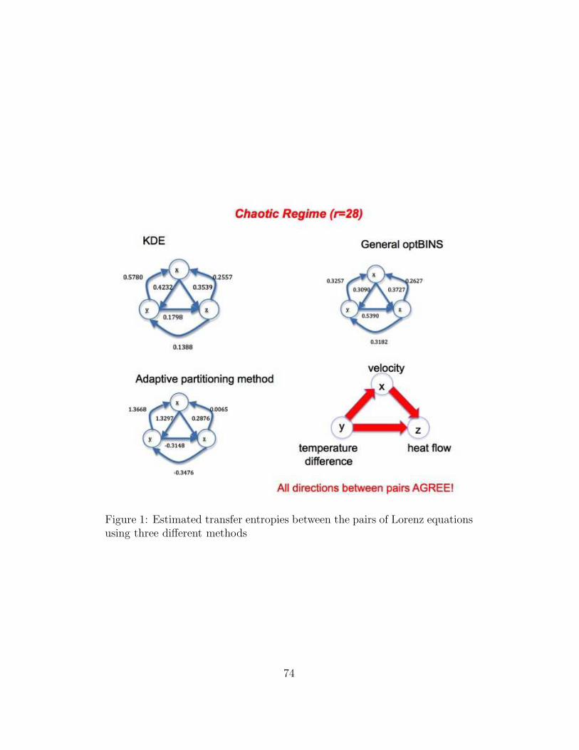
Figure 1: Estimated transfer entropies between the pairs of Lorenz equationsusing three different methods
74
EXPERIMENT AND CONCLUSION
We tested three methods on the nonlinear coupled Lorenz equations givenbelow. In climatology, they represent a model of an atmospheric convectionroll where x, y, z denote convective velocity, vertical temperature differenceand mean convective heat flow, respectively. Using the three methods, weobtained the TE estimates illustrated in Figure 1.
dx
dt= σ (y − x) (25)
dy
dt= −xz + rx− y
dz
dt= xy − bz
where σ = 10, b = 83, r: Rayleigh number and r = 28 in a chaotic regime.
In conclusion, computer simulations demonstrate that we can find a re-liable parameter regime for all methods at the same time and estimate TEdirection from data so that we can identify the information flow between thevariables reliably, as all methods agree both mathematically and physically.Currently, we are working on the magnitude differences between the meth-ods so that we can apply TE to identify the information flow between therelevant climate variables of the tropical disturbance, called Madden JulianOscillation (MJO). Later, this technique will be developed for us to betterunderstand the highly nonlinear nature of atmospheric dynamics.
References
J. Wallace, P. Hobbs, Atmospheric Science, Second Edition: An IntroductorySurvey, 2006
B. Gourvitch and J. Eggermont, “Evaluating Information Transfer BetweenAuditory Cortical Neurons”, J. Neurophysiology, vol. 97, no.3, pp. 2533-2543.
T. Schreiber, “Measuring information transfer”, Phys. Rev. Let., Vol. 85, No.2, pp.461-464, 2000
S. Sabesan, K. Narayanan, A. Prasad, L. Iasemidis, A. Spanias and K.Tsakalis, “Information Flow in Coupled Nonlinear Systems: Applicationto the Epileptic Human Brain”, Data Mining in Biomedicine, Data Miningin Biomedicine, 2007
75

G. Darbellay and I. Vajda, “Estimation of the Information by an adaptivepartitioning of the observation space”, IEEE Trans. On Information The-ory, Vol. 45, No.4, 1999
76
Reconstructing the Galactic halo’s accretionhistory: A finite mixture model approach
Duane LeeDepartment of AstronomyColumbia UniversityNew York, New York, USA
Will JessopDepartment of StatisticsColumbia UniversityNew York, New York, USA
Abstract
The stellar halo that surrounds our Milky Way Galaxy is thought to havebeen built, at least in part, from the agglomeration of stars from manysmaller galaxies. This talk outlines an approach to reconstructing the historyof Galactic accretion events by looking at the distribution of the chemicalabundances of halo stars. The full distribution is assumed to result from thesuperpositionof stellar populations accreted at different times from progenitorgalaxies of different sizes. Our approach uses the Expectation-Maximization(EM) algorithm to find the maximum-likelihood estimators that assess thecontribution of each of these progenitors in forming the Galaxy.
77

Scientific Program
Thursday, February 24, 2011
10:00 Welcome Michael Way (GISS)Catherine Naud (GISS)
10:20 How long will it take. A historical approachto boundary crossing.
Victor de la Pena (Columbia)
10:45 Cosmology through the Large-Scale Struc-ture of the Universe
Eyal Kazin (NYU)
11:30 On the shoulders of Gauss, Bessel, and Pois-son: links, chunks, spheres, and conditionalmodels
William Heavlin (Google)
12:15 Mining Citizen Science Data: MachineLearning Challenges
Kirk Borne (GMU)
13:00 Lunch Break
14:30 Tracking Climate Models: Advances in Cli-mate Informatics
Claire Monteleoni (Columbia)
15:15 Spectral Analysis Methods for ComplexSource Mixtures
Kevin Knuth (SUNY/Albany)
16:00 Beyond Objects: Using machines to under-stand the diffuse universe
Joshua Peek (Columbia)
16:45 Viewpoints: A high-performance visualiza-tion and analysis tool
Michael Way (GISS)
Friday, February 25, 2011
10:00 Clustering Approach for Partitioning Direc-tional Data in Earth and Space Sciences
Christian Klose (Think Geohazards)
10:45 Planetary Detection: The Kepler Mission Jon Jenkins (NASA/Ames)11:30 Understanding the possible influence of the
solar activity on the terrestrial climate: Atimes series analysis approach
Elizabeth Martınez-Gomez (Penn State)
12:15 Bayesian adaptive exploration applied to op-timal scheduling of exoplanet Radial Velocityobservations
Tom Loredo (Cornell)
13:00 Lunch Break
14:30 Bayesian Inference from Photometric Surveys Tamas Budavari (JHU)15:15 Long-Range Forecasts Using Data Clustering
and Information TheoryDimitris Giannakis (NYU)
16:00 Comparison of Information-Theoretic Meth-ods to estimate the information flow in a dy-namical system
Deniz Gencaga (CCNY)
16:45 Reconstructing the Galactic halo’s accretionhistory: A finite mixture model approach
Duane Lee and Will Jessop (Columbia)
78

Participants
Ryan Abrahams CUNY Graduate CenterHannah Aizenman CCNY/Computer ScienceArif Albayrak NASA GES DISCKehinde-Paul Alabi CCNY/Computer Science
Vivienne Baldassare CUNY/Hunter College/PhysicsImre Bartos Columbia/PhysicsMike Bauer Columbia-NASA/GISSRohit Bhardwaj Columbia/Computer ScienceAmitai Bin-Nun University of Pennsylvania/AstronomyJames Booth NASA/GISSKirk Borne George Mason University speakerAndreas Breiler IdeLaboratorietDouglas Brenner American Museum of Natural HistoryTamas Budavari Johns Hopkins University speaker
Samantha Chan Lamont-Doherty Earth Observatory,Columbia University
Milena C. Cuellar BCC. CUNYVictor de al Pena Columbia/Statistics speaker
Danielle Dowling CUNY Graduate CenterTarek El-Gaaly Rutgers/Computer ScienceDaniel Feldman CUNY/College of Staten IslandStephanie Fiorenza CUNY/College of Staten Island/PhysicsCarl Friedberg NYC/Comets.com
Deniz Gencaga CCNY/EE, NOAA-CREST speakerDimitrios Giannakis Center for Atmosphere Ocean Science,
Courant Institute of Mathematical Sciencesspeaker
Irina Gladkova CCNY/Computer ScienceElizabeth Gomez Penn State University/Statistics speakerJoshua Gordon Columbia/Computer ScienceSam Gordon ColumbiaMichael Grossberg CCNY/Computer Science
79

Participants cont’
Michael Haken NASA/GSFC, Science Systems & Applica-tions, Inc.
Zachary Haberman SUNY at Albany/PhysicsNaveed Hasan Columbia/Computer ScienceNicholas Hatzopou-los
CUNY Gradate Center
William D Heavlin Google, Inc speakerKay Hiranaka CUNY Graduate CenterHao Huang Stony Brook University/Computer ScienceDarryl Hutchinson CUNY Graduate Center
Ilknur Icke CUNY Graduate Center/Computer ScienceGeetha Jagannathan Columbia/Computer ScienceJon Jenkins SETI Institute/NASA Ames Research Center speakerWill Jessop Columbia/Statistics speakerEd Kaita SSAI@GSFC/NASAEyal Kazin New York University speakerLee Case Klippel Columbia UniversityChristian D. Klose Think GeoHazards speakerKirk Knobelspiesse ORAU-NASA/GISSKevin Knuth SUNY at Albany speakerIoannis Kostopoulos CUNY Graduate Center
Duane Lee Columbia/Astronomy speakerErbo Li Columbia/Computer ScienceCharles Liu CUNY at CSIThomas Loredo Cornell/Astronomy speakerChris Malone SUNY at Stony Brook/Physics and Astron-
omySzabolcs Marka Columbia/PhysicsZsuzsa Marka Columbia Astrophysics LaboratoryHaley Maunu SUNY at Albany/PhysicsVinod Mohan ColumbiaClaire Monteleoni Columbia/Computer Science speaker
80

Participants cont’
Catherine Naud NASA/GISSAlejandro Nunez CUNY Graduate CenterIndrani Pal IRI, The Earth InstituteVladimir Pavlovic Rutgers/Computer ScienceJoshua Peek Columbia/Astronomy speaker
Fergie Ramos Student/College of New RochelleKhary Richardson CUNY Graduate CenterWilliam Rossow CCNY/NOAA-CRESTSyamantak Saha NYU SternDestry Saul Columbia/AstronomyJoshua Schlieder SUNY at Stony BrookFrank Scalzo NASA/GISSBodhisattva Sen Columbia/StatisticsMonika Sikand Stevens Institute of Tech/PhysicsMichal Simon SUNY at Stony Brook/Physics and Astron-
omyIshan Singh ColumbiaDamain Sowinski CUNY Graduate Center
Ilya Tsinis NYU/CourantMaria Tzortziou GSFC/NASA - University of MarylandMichael Way NASA/GISSAdrian Weller Columbia/Computer ScienceLaird Whitehill Cornell/AstronomyAlexander Wong JP Morgan ChaseNettie Wong American Museum of Natural HistoryEmmi Yonekura Columbia UniversityShinjae Yoo Brookhaven National Lab/Computer Science
CenterSejong Yoon Rutgers/Computer ScienceDantong Yu Brookhaven National Lab
81

Video Links
Introduction Michael Wayhttp://www.youtube.com/watch?v=CHEoya e2Do (NASA/GISS)How long will it take. A historical approach to boundary crossing Victor de la Penahttp://www.youtube.com/watch?v=3gfHeerVqHs (Columbia U)Cosmology through the Large-Scale Structure of the Universe Eyal Kazinhttp://www.youtube.com/watch?v=es4dH0jBJYw (NYU)On the shoulders of Gauss, Bessel, and Poisson: links, chunks,spheres, and conditional models
William Heavlin
http://www.youtube.com/watch?v=FzFAxaXTkUQ (Google Inc.)Mining Citizen Science Data: Machine Learning Challenges Kirk Bornehttp://www.youtube.com/watch?v=XoS 4axsb5A (GMU)Tracking Climate Models: Advances in Climate Informatics Claire Monteleonihttp://www.youtube.com/watch?v=78IeffwV6bU (Columbia U)Spectral Analysis Methods for Complex Source Mixtures Kevin Knuthhttp://www.youtube.com/watch?v=t9mCoff5YZo (Suny/Albany)Beyond Objects: Using machines to understand the diffuse uni-verse
Joshua Peek
http://www.youtube.com/watch?v=hgp8CeR43So (Columbia U)Viewpoints: A high-performance visualization and analysis tool Michael Wayhttp://www.youtube.com/watch?v=FsW64idYw6c (NASA/GISS)Clustering Approach for Partitioning Directional Data in Earthand Space Sciences
Christian Klose
http://www.youtube.com/watch?v=5Ak6 rvayqg (Think Geohazards)Planetary Detection: The Kepler Mission Jon Jenkinshttp://www.youtube.com/watch?v=2dnA95smRE0 (NASA/Ames)Understanding the possible influence of the solar activity on theterrestrial climate: A times series analysis approach
Elizabeth Martınez-Gomez
http://www.youtube.com/watch?v=CXmC1dh9Wdg (Penn State)Bayesian adaptive exploration applied to optimal scheduling ofexoplanet Radial Velocity observations
Tom Loredo
http://www.youtube.com/watch?v=B1pVtHmu9E0 (Cornell U)Bayesian Inference from Photometric Surveys Tamas Budavarihttp://www.youtube.com/watch?v=xCzUl0HtWGM (JHU)Long-Range Forecasts Using Data Clustering and InformationTheory
Dimitris Giannakis
http://www.youtube.com/watch?v=pFDqP94btCg (NYU)Comparison of Information-Theoretic Methods to estimate theinformation flow in a dynamical system
Deniz Gencaga
http://www.youtube.com/watch?v=ejX MWImP6A (CCNY)Reconstructing the Galactic halo’s accretion history: Duane Lee &A finite mixture model approach Will Jessophttp://www.youtube.com/watch?v=moehYYsIOFw (Columbia U)
82